This problem aims to study the peculiar physics of galaxies, such as their dynamics and structure. In particular, we explain how to measure the mass distribution of our galaxy from the inside. For this we will focus on hydrogen, its main constituent.

Throughout this problem we will only use \(\hbar\), defined as \(\hbar=h/2\pi\).

Part A - Introduction

Bohr model

We assume that the hydrogen atom consists of a non-relativistic electron, with mass \(m_e\), orbiting a fixed proton. Throughout this part, we assume its motion is on a circular orbit.

A.1 — 0.2pt

Determine the electron's velocity \(v\) in a circular orbit of radius \(r\).

In the Bohr model, we assume the magnitude of the electron's angular momentum \(L\) is quantized, \(L=n\hbar\) where \(n>0\) is an integer. We define \(\alpha=\dfrac{e^2}{4\pi\varepsilon_0\hbar c}\approx7.27\times10^{-3}\).

A.2 — 0.5pt

Show that the radius of each orbit is given by \(r_n=n^2r_1\), where \(r_1\) is called the Bohr radius. Express \(r_1\) in terms of \(\alpha\), \(m_e\), \(c\) and \(\hbar\) and calculate its numerical value with 3 digits. Express \(v_1\), the velocity on the orbit of radius \(r_1\), in terms of \(\alpha\) and \(c\).

A.3 — 0.5pt

Determine the electron's mechanical energy \(E_n\) on an orbit of radius \(r_n\) in terms of \(e\), \(\varepsilon_0\), \(r_1\) and \(n\). Determine \(E_1\) in the ground state in terms of \(\alpha\), \(m_e\) and \(c\). Compute its numerical value in eV.

Hydrogen fine and hyperfine structures

The rare spontaneous inversion of the electron's spin causes a photon to be emitted on average once per 10 million years per hydrogen atom. This emission serves as a hydrogen tracer in the universe and is thus fundamental in astrophysics. We will study the transition responsible for this emission in two steps.

First, consider the interaction between the electron spin and the relative motion of the electron and the proton. Working in the electron's frame of reference, the proton orbits the electron at a distance \(r_1\). This produces a magnetic field \(\vec B_1\).

A.4 — 0.5pt

Determine the magnitude \(B_1\) of \(\vec B_1\) at the position of the electron in terms of \(\mu_0\), \(e\), \(\alpha\), \(c\) and \(r_1\).

Second, the electron spin creates a magnetic moment \(\vec{\mathcal M}_s\). Its magnitude is roughly \(\mathcal M_s=\dfrac{e}{m_e}\hbar\). The fine (F) structure is related to the energy difference \(\Delta E_{\mathrm F}\) between an electron with a magnetic moment \(\vec{\mathcal M}_s\) parallel to \(\vec B_1\) and that of an electron with \(\vec{\mathcal M}_s\) anti-parallel to \(\vec B_1\). Similarly, the hyperfine (HF) structure is related to the energy difference \(\Delta E_{\mathrm{HF}}\), due to the interaction between parallel and anti-parallel magnetic moments of the electron and the proton. It is known to be approximately \(\Delta E_{\mathrm{HF}}\simeq3.72\dfrac{m_e}{m_p}\Delta E_{\mathrm F}\) where \(m_p\) is the proton mass.

A.5 — 0.5pt

Express \(\Delta E_{\mathrm F}\) as a function of \(\alpha\) and \(E_1\).

Express the wavelength \(\lambda_{\mathrm{HF}}\) of a photon emitted during a transition between the two states of the hyperfine structure and give its numerical value with two digits.

Part B - Rotation curves of galaxies

Data

• Kiloparsec: \(1\,\mathrm{kpc}=3.09\times10^{19}\,\mathrm m\)
• Solar mass : \(1\,M_\odot=1.99\times10^{30}\,\mathrm{kg}\)

We consider a spherical galaxy centered around a fixed point \(O\). At any point \(P\), let \(\rho=\rho(P)\) be the volumetric mass density and \(\varphi=\varphi(P)\) the associated gravitational potential (i.e. potential energy per unit mass). Both \(\rho\) and \(\varphi\) depend only on \(r=\|\overrightarrow{OP}\|\). The motion of a mass \(m\) located at \(P\), due to the field \(\varphi\), is restricted to a plane containing \(O\).

B.1 — 0.2pt

In the case of a circular orbit, determine the velocity \(v_c\) of an object on a circular orbit passing through \(P\) in terms of \(r\) and \(\dfrac{d\varphi}{dr}\).

Fig. 1(A) is a picture of the spiral galaxy NGC 6946 in the visible band (from the 0.8m Schulman Telescope at the Mount Lemmon Sky Center in Arizona). The little ellipses in Fig. 1(B) show experimental measurements of \(v_c\) for this galaxy. The central region (\(r<1\,\mathrm{kpc}\)) is named the bulge. In this region, the mass distribution is roughly homogeneous. The red curve is a prediction for \(v_c\) if the system were homogeneous in the bulge and keplerian (\(\varphi(r)=-\beta/r\) with \(\beta>0\)) outside it, i.e. considering that the total mass of the galaxy is concentrated in the bulge.

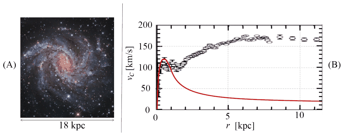
Fig. 1: NGC 6946 galaxy: Picture (A) and rotation curve (B).

B.2 — 0.5pt

Deduce the mass \(M_b\) of the bulge of NGC 6946 from the red rotation curve in Fig. 1(B), in solar mass units.

Comparing the keplerian model and the experimental data makes astronomers confident that part of the mass is invisible in the picture. They thus suppose that the galaxy's actual mass density is given by

\[ \rho_m(r)=\frac{C_m}{r_m^2+r^2} \tag{1} \]

where \(C_m>0\) and \(r_m>0\) are constants.

B.3 — 1.8pt

Show that the velocity profile \(v_{c,m}(r)\), corresponding to the mass density in Eq. 1, can be written \[ v_{c,m}(r)=\sqrt{k_1-\frac{k_2\cdot\arctan\!\left(\frac r{r_m}\right)}r}. \] Express \(k_1\) and \(k_2\) in terms of \(C_m\), \(r_m\) and \(G\).

(Hints: \(\displaystyle\int_0^r\frac{x^2}{a^2+x^2}\,dx=r-a\arctan(r/a)\), and: \(\arctan(x)\simeq x-x^3/3\) for \(x\ll1\).)

Simplify \(v_{c,m}(r)\) when \(r\ll r_m\) and when \(r\gg r_m\).

Show that if \(r\gg r_m\), the mass \(M_m(r)\) embedded in a sphere of radius \(r\) with the mass density given by Eq. 1 simplifies and depends only on \(C_m\) and \(r\).

Estimate the mass of the galaxy NGC 6946 actually present in the picture in Fig. 1(A).

Part C - Mass distribution in our galaxy

For a spiral galaxy, the model for Eq. 1 is modified and one usually considers the gravitational potential is given by \[ \varphi_G(r,z)=\varphi_0\ln\!\left(\frac r{r_0}\right) \exp\!\left[-\left(\frac z{z_0}\right)^2\right], \] where \(z\) is the distance to the galactic plane (defined by \(z=0\)), and \(r<r_0\) is now the axial radius and \(\varphi_0>0\) a constant to be determined. \(r_0\) and \(z_0\) are constant values.

C.1 — 0.5pt

Find the equation of motion on \(z\) for the vertical motion of a point mass \(m\) in such a potential, assuming \(r\) is constant. Show that, if \(r<r_0\) the galactic plane is a stable equilibrium state by giving the angular frequency \(\omega_0\) of small oscillations around it.

From here on, we set \(z=0\).

C.2 — 0.6pt

Identify the regime, either \(r\gg r_m\) or \(r\ll r_m\), in which the model of Eq. 1 recovers a potential of the form \(\varphi_G(r,0)\) with a suitable definition of \(\varphi_0\).

Under this condition \(v_c(r)\) no longer depends on \(r\). Express it in terms of \(\varphi_0\).

Therefore, outside the bulge the velocity modulus \(v_c\) does not depend on the distance to the galactic center. We will use this fact, as astronomers do, to measure the galaxy's mass distribution from the inside.

All galactic objects considered here for astronomical observations, such as stars or nebulae, are primarily composed of hydrogen. Outside the bulge, we assume that they rotate on circular orbits around the galactic center \(C\). \(S\) is the sun's position and \(E\) that of a given galactic object emitting in the hydrogen spectrum. In the galactic plane, we consider a line of sight \(SE\) corresponding to the orientation of an observation, on the unit vector \(\hat u_v\) (see Fig. 2).

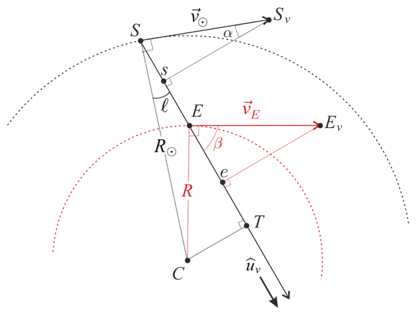
Fig. 2: Geometry of the measurement

Let \(\ell\) be the galactic longitude, measuring the angle between \(SC\) and the \(SE\). The sun's velocity on its circular orbit of radius \(R_\odot=8.00\,\mathrm{kpc}\) is denoted \(\vec v_\odot\). A galactic object in \(E\) orbits on another circle of radius \(R\) at velocity \(\vec v_E\). Using a Doppler effect on the previously studied 21cm line, one can obtain the relative radial velocity \(v_{rE/S}\) of the emitter \(E\) with respect to the sun \(S\): it is the projection of \(\vec v_E-\vec v_\odot\) on the line of sight.

C.3 — 0.7pt

Determine \(v_{rE/S}\) in terms of \(\ell\), \(R\), \(R_\odot\) and \(v_\odot\). Then, express \(R\) in terms of \(R_\odot\), \(v_\odot\), \(\ell\) and \(v_{rE/S}\).

Using a radio telescope, we make observations in the plane of our galaxy toward a longitude \(\ell=30^\circ\). The frequency band used contains the 21cm line, whose frequency is \(f_0=1.42\,\mathrm{GHz}\). The results are reported in Fig. 3.

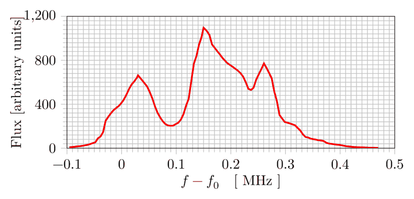
Fig. 3: Electromagnetic signal as a function of the frequency shift, measured in the radio frequency band at \(\ell=30^\circ\) using EU-HOU RadioAstronomy

C.4 — 0.6pt

In our galaxy, \(v_\odot=220\,\mathrm{km\cdot s^{-1}}\). Determine the values of the relative radial velocity (with 3 significant digits) and the distance from the galactic center (with 2 significant digits) of the 3 sources observed in Fig. 3. Distances should be expressed as multiples of \(R_\odot\).

C.5 — 0.6pt

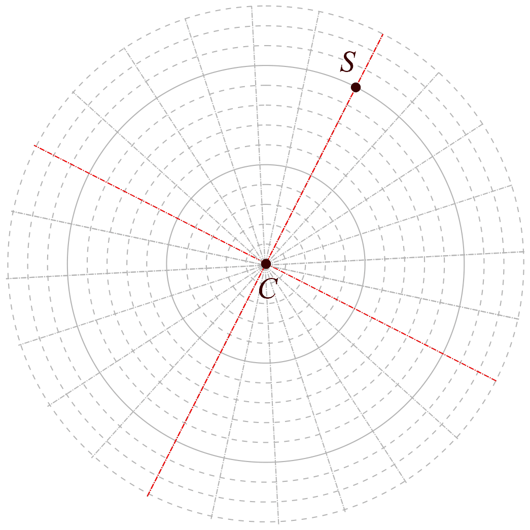
On the top view of our galaxy (in the answer box), indicate the positions of the sources observed in Fig. 3.

What could be deduced from repeated measurements changing \(\ell\)?

Part D - Tully-Fisher relation and MOND theory

The flat external velocity curve of NGC 6946 in Fig. 1 is a common property of spiral galaxies, as can be seen in Fig. 4 (left). Plotting the external constant velocity value \(v_{c,\infty}\) as a function of the measured total mass \(M_{\mathrm{tot}}\) of each galaxy gives an interesting correlation called the Tully-Fischer relation, see Fig. 4 (right).

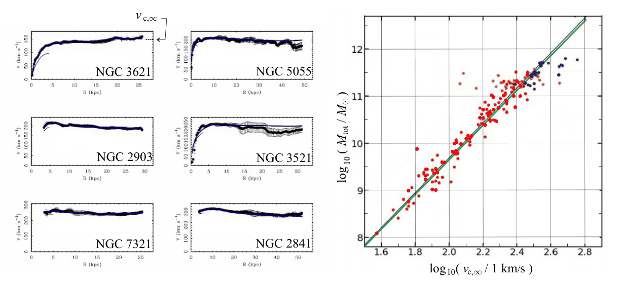
Fig. 4. Left: Rotation curves for typical spiral galaxies - Right: \(\log_{10}(M_{\mathrm{tot}})\) as a function of \(\log_{10}(v_{c,\infty})\) on linear scales. Colored dots correspond to different galaxies and different surveys. The green line is the Tully-Fischer relation which is in very good agreement with the best fit line of the data (in black).

D.1 — 0.4pt

Assuming that the radius \(R\) of a galaxy doesn't depend on its mass, show that the model of Eq. 1 (part B) gives a relation of the form \(M_{\mathrm{tot}}=\eta v_{c,\infty}^{\gamma}\) where \(\gamma\) and \(\eta\) should be specified.

Compare this expression to the Tully-Fischer relation by computing \(\gamma_{TF}\).

In the extremely low acceleration regime, of the order of \(a_0=10^{-10}\,\mathrm{m\cdot s^{-2}}\), the MOdified Newtonian Dynamics (MOND) theory suggests that one can modify Newton's second law using \[ \vec F=m\mu\!\left(\frac a{a_0}\right)\vec a \] where \(a=\|\vec a\|\) is the modulus of the acceleration and the \(\mu\) function is defined by \(\mu(x)=\dfrac{x}{1+x}\).

D.2 — 0.2pt

Using data for NGC 6946 in Fig. 1, estimate, within Newton's theory, the modulus of the acceleration \(a_m\) of a mass in the outer regions of NGC 6946.

D.3 — 0.8pt

Let \(m\) be a mass on a circular orbit of radius \(r\) with velocity \(v_{c,\infty}\) in the gravity field of a fixed mass \(M\).

Within the MOND theory, with \(a\ll a_0\), determine the Tully-Fischer exponent.

Using data for NGC 6946 and/or Tully-Fischer law, calculate \(a_0\) to show that MOND operates in the correct regime.

D.4 — 0.9pt

Considering relevant cases, determine \(v_c(r)\) for all values of \(r\) in the MOND theory in the case of a gravitational field due to a homogeneously distributed mass \(M\) with radius \(R_b\).

General Data Sheet

Constant	Notation	Value	Unit
Speed of light in vacuum	\(c\)	\(2.997\,924\,58\times10^8\)	\(\mathrm{m\cdot s^{-1}}\)
Planck constant	\(h\)	\(6.626\,070\,15\times10^{-34}\)	\(\mathrm{kg\cdot m^2\cdot s^{-1}}\)
Reduced Planck constant	\(\hbar=\dfrac h{2\pi}\)	\(1.054\,571\,818\times10^{-34}\)	\(\mathrm{kg\cdot m^2\cdot s^{-1}}\)
Boltzmann constant	\(k_{\mathrm B}\)	\(1.380\,649\times10^{-23}\)	\(\mathrm{kg\cdot m^2\cdot s^{-2}\cdot K^{-1}}\)
Avogadro constant	\(N_{\mathrm A}\)	\(6.022\,140\,76\times10^{23}\)	\(\mathrm{mol^{-1}}\)
Molar gas constant	\(R\)	\(8.314\,462\,618\,153\,24\)	\(\mathrm{kg\cdot m^2\cdot s^{-2}\cdot mol^{-1}\cdot K^{-1}}\)
Elementary charge	\(e\)	\(1.602\,176\,634\times10^{-19}\)	\(\mathrm{A\cdot s}\)
Universal constant of gravitation	\(G\)	\(6.674\,30(15)\times10^{-11}\)	\(\mathrm{m^3\cdot kg^{-1}\cdot s^{-2}}\)
Standard acceleration due to gravity	\(g\)	\(9.806\,65\)	\(\mathrm{m\cdot s^{-2}}\)
Stefan Boltzmann constant	\(\sigma\)	\(5.670\,374\,419\times10^{-8}\)	\(\mathrm{kg\cdot s^{-3}\cdot K^{-4}}\)
Vacuum permeability (magnetic constant)	\(\mu_0\)	\(1.256\,637\,061\,27(20)\times10^{-6}\)	\(\mathrm{kg\cdot m\cdot A^{-2}\cdot s^{-2}}\)
Vacuum permittivity (electrical constant)	\(\epsilon_0\)	\(8.854\,187\,818\,8(14)\times10^{-12}\)	\(\mathrm{A^2\cdot s^4\cdot kg^{-1}\cdot m^{-3}}\)
Rydberg constant	\(R_\infty\)	\(1.097\,373\,156\,815\,7(12)\times10^7\)	\(\mathrm{m^{-1}}\)
Mass of the electron	\(m_e\)	\(9.109\,383\,713\,9(28)\times10^{-31}\)	\(\mathrm{kg}\)
Mass of the proton	\(m_p\)	\(1.672\,621\,925\,95(52)\times10^{-27}\)	\(\mathrm{kg}\)
Mass of the neutron	\(m_n\)	\(1.674\,927\,500\,56(85)\times10^{-27}\)	\(\mathrm{kg}\)
Atomic mass constant	\(m_u\)	\(1.660\,539\,068\,92(52)\times10^{-27}\)	\(\mathrm{kg}\)
Electronvolt	\(\mathrm{eV}\)	\(1.602\,176\,634\times10^{-19}\)	\(\mathrm{kg\cdot m^2\cdot s^{-2}}\)

Official English text of the problem.

In 1765, British clockmaker James Cox invented a clock whose only source of energy is the fluctuations in atmospheric pressure. Cox's clock used two vessels containing mercury. Changes in atmospheric pressure caused mercury to move between the vessels, and the two vessels to move relative to each other. This movement acted as an energy source for the actual clock.

We propose an analysis of this device. Throughout, we assume that

• the Earth's gravitational field \(\vec g=-g\vec u_z\) is uniform with \(g=9.8\,\mathrm{m\cdot s^{-2}}\) and \(\vec u_z\) a unit vector;
• all liquids are incompressible and their density is denoted \(\rho\);
• no surface tension effects will be considered;
• the variations of atmospheric pressure with altitude are neglected;
• the surrounding temperature \(T_a\) is uniform and all transformations are isothermal.

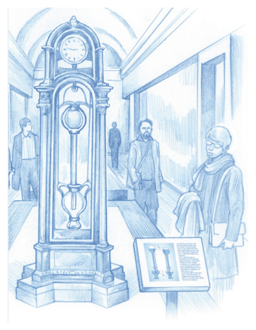
Fig. 1. Artistic view of Cox's clock \({}^{1}\)

Part A - Pulling on a submerged tube

We first consider a bath of water that occupies the semi-infinite space \(z\leq0\). The air above it is at a pressure \(P_a=P_0\). A cylindrical vertical tube of length \(H=1\,\mathrm m\), cross-sectional area \(S=10\,\mathrm{cm^2}\) and mass \(m=0.5\,\mathrm{kg}\) is dipped into the bath. The bottom end of the tube is open, and the top end of the tube is closed. We denote \(h\) the altitude of the top of the tube and \(z_\ell\) that of the water inside the tube. The thickness of the tube walls is neglected.

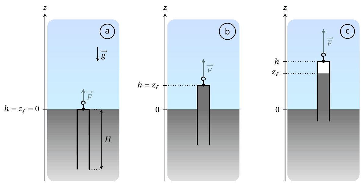
Fig. 2. Sketch of the tube in different configurations

We start from the situation where the tube in Fig. 2 contains no gas and its top is at the bath level: in other words, \(h=0\) and \(z_\ell=0\) (case a). The tube is then slowly lifted until its bottom end reaches the bath level. The pulling force exerted on the tube is denoted \(\vec F=F\vec u_z\).

A.1 — 0.2pt

For the configuration shown in Fig. 2 (case b), express the pressure \(P_w\) in the water at the top of the tube. Also express the force \(\vec F\) necessary to maintain the tube at this position. Expressions must be written in terms of \(P_0,\rho,m,S,h,g\) and \(\vec u_z\).

Three experiments are performed. In each, the tube is lifted from the initial state shown in Fig. 2(a) under the conditions specified in Table 1.

Experiment	Liquid	\(T_a\) (°C)	\(\rho\) (\(\mathrm{kg\cdot m^{-3}}\))	\(P_{\mathrm{sat}}\) (Pa)
1	Water	20	\(1.00\times10^3\)	\(2.34\times10^3\)
2	Water	80	\(0.97\times10^3\)	\(47.4\times10^3\)
3	Water	99	\(0.96\times10^3\)	\(99.8\times10^3\)

Table 1. Experimental conditions and numerical values of physical quantities for each experiment

(\(P_{\mathrm{sat}}\) designates the saturated vapour pressure of the pure fluid)

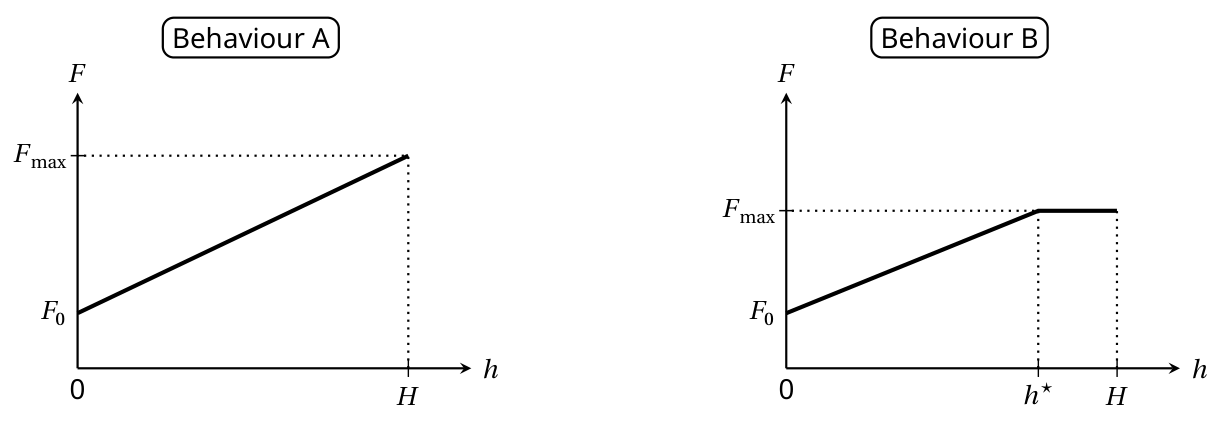
In each case, we study the evolution of the force \(F\) that must be applied in order to maintain the tube in equilibrium at an altitude \(h\), the external pressure being fixed at \(P_a=P_0=1.000\times10^5\,\mathrm{Pa}\). Two different behaviours are possible

A.2 — 0.8pt

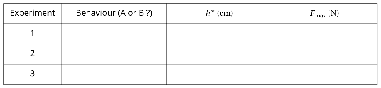
For each experiment, complete the table in the answer sheet to indicate the expected behaviour and the numerical values for \(F_{\max}\) and for \(h^\star\) (when pertinent), where \(F_{\max}\) and \(h^\star\) are defined in the figures illustrating the two behaviours.

When we replace the water with liquid mercury (whose properties are given below), behaviour B is observed.

Liquid	\(T_a\) (°C)	\(\rho\) (\(\mathrm{kg\cdot m^{-3}}\))	\(P_{\mathrm{sat}}\) (Pa)
Mercury	20	\(13.5\times10^3\)	\(0.163\)

A.3 — 0.3pt

Express the relative error, denoted \(\varepsilon\), committed when we evaluate the maximal force \(F_{\max}\) neglecting \(P_{\mathrm{sat}}\) compared to \(P_0\). Give the numerical value of \(\varepsilon\).

Part B - Two-part barometric tube

From now on, we work with mercury (density \(\rho=13.5\times10^3\,\mathrm{kg\cdot m^{-3}}\)) at the ambient temperature \(T_a=20^\circ\mathrm C\) and we take \(P_{\mathrm{sat}}=0\).

Let us consider a tube with a reservoir on top, modeled as two superposed cylinders of different dimensions, as shown in Fig. 3.

• the bottom part (still called the tube) has cross-sectional area \(S_t\) and height \(H_t=80\,\mathrm{cm}\);
• the top part (called the bulb) has cross-sectional area \(S_b>S_t\) and height \(H_b=20\,\mathrm{cm}\).

This two-part tube is dipped into a semi-infinite liquid bath.

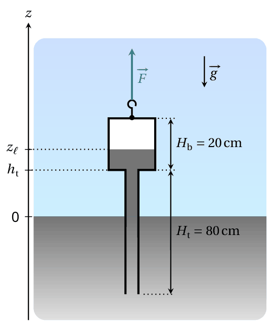
Fig. 3. Sketch of the two-part barometric tube

As in Part A, the system is prepared such that the tube contains no air. We identify the vertical position of the tube by the altitude \(h_t\) of the junction between the tube and the bulb. The height of the column of mercury is again denoted \(z_\ell\). The force \(\vec F\) that must be exerted to maintain the tube in equilibrium in the configuration shown in Fig. 3 can now be written as

\[ \vec F=(m_{\mathrm{tb}}+m_{\mathrm{add}})g\vec u_z \tag{1} \]

where \(m_{\mathrm{tb}}\) is the total mass of the two-part tube (when empty of mercury).

B.1 — 0.3pt

On the answer sheet, color the area corresponding to the volume of liquid mercury that is responsible for the term \(m_{\mathrm{add}}\) appearing in equation (1).

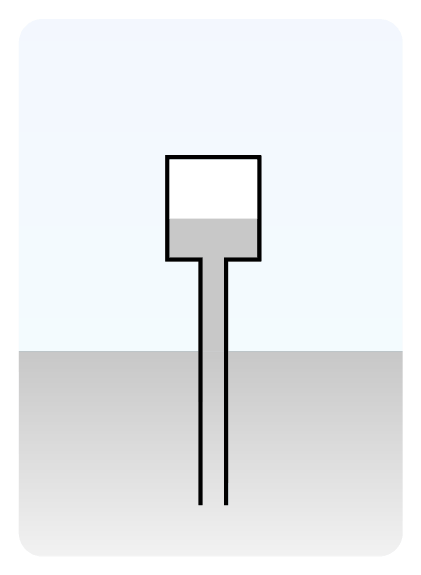
The mass \(m_{\mathrm{add}}\) depends both on the height \(h_t\) and the atmospheric pressure \(P_a\). For the next question, assume that the atmospheric pressure is fixed at \(P_a=P_0=1.000\times10^5\,\mathrm{Pa}\). Starting from the situation where the system is completely submerged, the tube is slowly lifted until its base is flush with the liquid bath.

B.2 — 1.4pt

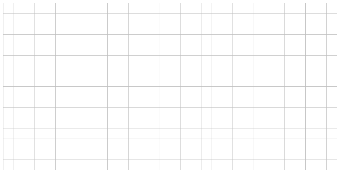
Sketch the evolution of the mass \(m_{\mathrm{add}}\) as a function of \(h_t\) for \(h_t\in[-H_b,H_t]\). On the graph, provide the expression for the slopes of the different segments, as well as the \(h_t\) analytical value of any angular points, in terms of \(P_0,\rho,g,S_b,S_t,H_b\) and \(H_t\).

As the system is lifted while \(P_a=P_0=10^5\,\mathrm{Pa}\), we stop when the free surface of the liquid is in the middle of the bulb. The value of \(h_t\) is fixed and then we observe variations in the mass \(m_{\mathrm{add}}\) due to variations in the atmospheric pressure described by

\[ P_a(t)=P_0+P_1(t) \tag{2} \]

where \(P_0\) designates the average value and \(P_1\) is a perturbative term. We model \(P_1\) by a periodic triangular function of amplitude \(A=5\times10^2\,\mathrm{Pa}\) and period \(\tau_1\) of 1 week.

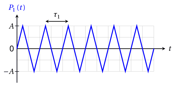
Fig. 4. Simplified model of the perturbative term \(P_1(t)\)

B.3 — 0.3pt

Given that \(S_t=5\,\mathrm{cm^2}\) and \(S_b=200\,\mathrm{cm^2}\), express the amplitude \(\Delta m_{\mathrm{add}}\) of the variations of the mass \(m_{\mathrm{add}}\) over time, then give its numerical value. Assume that the liquid surface always stays in the bulb.

Part C - Cox's timepiece

The real mechanism developed by Cox is complex (Fig. 5). We study a simplified version, depicted in Fig. 6, and described below

• a cylindrical bottom cistern containing a mercury bath;
• a two-part barometric tube identical to that studied in part B, which is still completely emptied of any air, is dipped into the bath;
• the cistern and the two-part tube are each suspended by a cable. Both cables (assumed to be inextensible and of negligible mass) pass through a system of ideal pullies and finish attached to either side of the same mass \(M\), which can slide on a horizontal surface;
• the total volume of liquid mercury contained in the system is \(V_\ell=5\,\mathrm L\).

The height, cross-section and masses of each part are given in Table 2. The position of mass \(M\) is referenced by the coordinate \(x\) of its center of mass. We consider solid friction between the horizontal support and the mass \(M\), without distinction between static and dynamic coefficients; the magnitude of this force when sliding occurs is denoted \(F_s\).

Two stops limit the displacement of the mass \(M\) such that \(-X\leq x\leq X\) (with \(X>0\)). Assume that the value of \(X\) guarantees that

• the bottom of the two-part tube never touches the bottom of the cistern nor comes out of the liquid bath;
• the altitude \(z_\ell\) of the mercury column is always in the upper bulb.

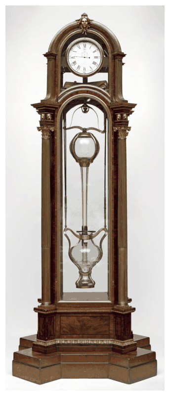
Fig. 5. Real Cox's timepiece \({}^{2}\) (without mercury)

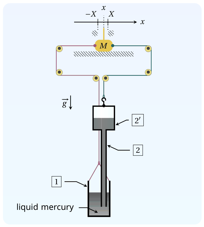
Fig. 6. Sketch of the system modeling the timepiece

Reference	Name	Height	Cross section area	Empty mass
\(\boxed{1}\)	cistern	\(H_c=30\,\mathrm{cm}\)	\(S_c=210\,\mathrm{cm^2}\)	\(m_c\)
\(\boxed{2}\)	tubular part of the barometric tube	\(H_t=80\,\mathrm{cm}\)	\(S_t=5\,\mathrm{cm^2}\)	total mass of the barometric tube: \(m_{\mathrm{tb}}\)
\(\boxed{2'}\)	bulb of the barometric tube	\(H_b=20\,\mathrm{cm}\)	\(S_b=200\,\mathrm{cm^2}\)

Table 2. Dimensions and notations for the model system

The system evolves in contact with the atmosphere, whose pressure fluctuates as in Fig. 4 (still with amplitude \(A=5\times10^2\,\mathrm{Pa}\) and period \(\tau_1=1\) week). At the start \(t=0\), the mass \(M\) is at rest at \(x=0\) and the tensions exerted by the two cables on either side of the mass \(M\) are in balance while \(P_1(0)=0\). We define

\[ \xi= \frac{S_b+S_c-S_t}{S_bS_c}\frac{F_s}{A} \simeq \frac{S_b+S_c}{S_bS_c}\frac{F_s}{A} \tag{3} \]

where the last expression uses that \(S_t\ll S_b,S_c\) (which we will assume is valid until the end of the problem).

C.1 — 1pt

Determine the threshold \(\xi^\star\) such that \(M\) remains indefinitely at rest when \(\xi>\xi^\star\).

For the next question only, suppose that the mass \(M\) is temporarily blocked at \(x=X\).

C.2 — 1pt

Give an expression for the total tension force \(\vec T=T\vec u_x\) acting on the mass \(M\) due to the tension in two cables at this position, when \(P_1=0\), in terms of \(\rho,g,X\) and pertinent cross-sections.

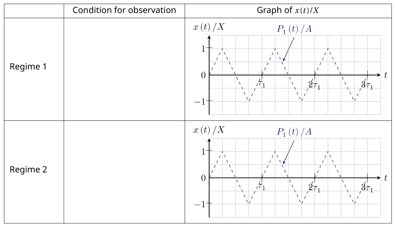
When \(\xi<\xi^\star\), starting again from \(x=0\) and \(P_1=0\), two different behaviours can be observed for \(t\geq0\). To distinguish them, we need to introduce another parameter

\[ \lambda= \frac{2(S_b-S_t)}{S_b}\frac{\rho gX}{A} \simeq \frac{2\rho gX}{A} \tag{4} \]

C.3 — 2pt

Complete the table in the answer sheet to indicate the condition under which each regime is obtained. Conditions must be expressed as inequalities on \(\xi\) and/or \(\lambda\). In addition, sketch the variations of \(x(t)/X\) for \(t\in[0,3\tau_1]\) that are consistent with the variations of \(P_1(t)/A\) already present. Specification of remarkable points coordinates is not required.

In the real Cox's timepiece, energy provided by the mechanism is stored using a system of ratchets and used to raise a counterweight, like in a traditional clock. In the simplified model studied here, the energy recovered by the clock corresponds to the energy dissipated by the friction force exerted by the horizontal surface on the mass \(M\). From now on, we assume that the system is dimensioned such that to work in the regime that allows the clock to recuperate energy. We also assume that the permanent regime is established. We denote \(W\) the energy dissipated by the solid friction force during a period \(\tau_1\), which can be expressed only in terms of \(F_s\) and \(X\).

All else equal, \(F_s\) and \(X\) can be adjusted to maximize the energy \(W\); we denote \(F_s^\star\) and \(X^\star\) their respective values in the optimal situation.

C.4 — 1pt

Considering \(S_b\simeq S_c\) and \(S_t\ll S_b\), determine the expressions for \(F_s^\star\) and \(X^\star\) as functions of \(\rho,g,S_c\) and \(A\). Express the corresponding maximum energy \(W^\star\), then calculate its numerical value with \(A=5\times10^2\,\mathrm{Pa}\).

We denote \(W_{\mathrm{pr}}^\star\) the work of atmospheric pressure forces received by the system in the optimal situation during a period \(\tau_1\).

C.5 — 1.7pt

Express \(W_{\mathrm{pr}}^\star\), then calculate the ratio \(W^\star/W_{\mathrm{pr}}^\star\). It could be useful to represent the evolution of the system in a \((P,V)\) diagram, where \(V\) is the system's volume.

Credits:

[1]: Bruno Vacaro;
[2]: Victoria and Albert Museum, London.

Official English text of the problem.

Warning: Excessive alcohol consumption is harmful to health and drinking alcohol below legal age is prohibited.

Champagne is a French sparkling wine. Fermentation of sugars produces carbon dioxide (\(\mathrm{CO}_2\)) in the bottle. The molar concentration of \(\mathrm{CO}_2\) in the liquid phase \(c_\ell\) and the partial pressure \(P_{\mathrm{CO}_2}\) in the gas phase are related by \(c_\ell=k_{\mathrm H}P_{\mathrm{CO}_2}\), known as Henry's law and where \(k_{\mathrm H}\) is called Henry's constant.

Data

• Surface tension of champagne \(\sigma=47\times10^{-3}\,\mathrm{J\cdot m^{-2}}\)
• Density of the liquid \(\rho_\ell=1.0\times10^3\,\mathrm{kg\cdot m^{-3}}\)
• Henry's constant at \(T_0=20^\circ\mathrm C\), \(k_{\mathrm H}(20^\circ\mathrm C)=3.3\times10^{-4}\,\mathrm{mol\cdot m^{-3}\cdot Pa^{-1}}\)
• Henry's constant at \(T_0=6^\circ\mathrm C\), \(k_{\mathrm H}(6^\circ\mathrm C)=5.4\times10^{-4}\,\mathrm{mol\cdot m^{-3}\cdot Pa^{-1}}\)
• Atmospheric pressure \(P_0=1\,\mathrm{bar}=1.0\times10^5\,\mathrm{Pa}\)
• Gases are ideal with an adiabatic coefficient \(\gamma=1.3\)

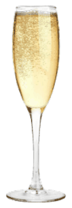
Fig. 1. A glass filled with champagne.

Part A. Nucleation, growth and rise of bubbles

Immediately after opening a bottle of champagne at temperature \(T_0=20^\circ\mathrm C\), we fill a glass. The pressure in the liquid is \(P_0\) and its temperature stays constant at \(T_0\). The concentration \(c_\ell\) of dissolved \(\mathrm{CO}_2\) exceeds the equilibrium concentration and we study the nucleation of a \(\mathrm{CO}_2\) bubble. We note \(a\) its radius and \(P_{\mathrm b}\) its inner pressure.

A.1 — 0.2pt

Express the pressure \(P_{\mathrm b}\) in terms of \(P_0\), \(a\) and \(\sigma\).

In the liquid, the concentration of dissolved \(\mathrm{CO}_2\) depends on the distance to the bubble. At long distance we recover the value \(c_\ell\) and we note \(c_{\mathrm b}\) the concentration close to the bubble surface. According to Henry's law, \(c_{\mathrm b}=k_{\mathrm H}P_{\mathrm b}\). We furthermore assume in all the problem that bubbles contain only \(\mathrm{CO}_2\).

Since \(c_\ell\ne c_{\mathrm b}\), \(\mathrm{CO}_2\) molecules diffuse from areas of high to low concentration. We assume also that any molecule from the liquid phase reaching the bubble surface is transferred to the vapour.

A.2 — 0.5pt

Express the critical radius \(a_{\mathrm c}\) above which a bubble is expected to grow in terms of \(P_0,\sigma,c_\ell\) and \(c_0\) where \(c_0=k_{\mathrm H}P_0\). Calculate numerically \(a_{\mathrm c}\) for \(c_\ell=4c_0\).

In practice, bubbles mainly grow from pre-existing gas cavities. Consider then a bubble with initial radius \(a_0\approx40\,\mu\mathrm m\). The number of moles of \(\mathrm{CO}_2\) transferred at the bubble's surface per unit area and time is noted \(j\). Two models are possible for \(j\).

• model (1) \(j=\dfrac{D}{a}(c_\ell-c_{\mathrm b})\) where \(D\) is the diffusion coefficient of \(\mathrm{CO}_2\) in the liquid.
• model (2) \(j=K(c_\ell-c_{\mathrm b})\) where \(K\) is a constant here.

Experimentally, the bubble radius \(a(t)\) is found to depend on time as shown in Fig. 2. Here \(c_\ell\approx4c_0\), and since bubbles are large enough to be visible, the excess pressure due to surface tension can be neglected and \(P_{\mathrm b}\approx P_0\).

A.3 — 1.2pt

Express the number of \(\mathrm{CO}_2\) moles in the bubble \(n_{\mathrm c}\) in terms of \(a,P_0,T_0\) and ideal gas constant \(R\). Find \(a(t)\) for both models. Indicate which model explains the experimental results in Fig. 2. Depending on your answer, calculate numerically \(K\) or \(D\).

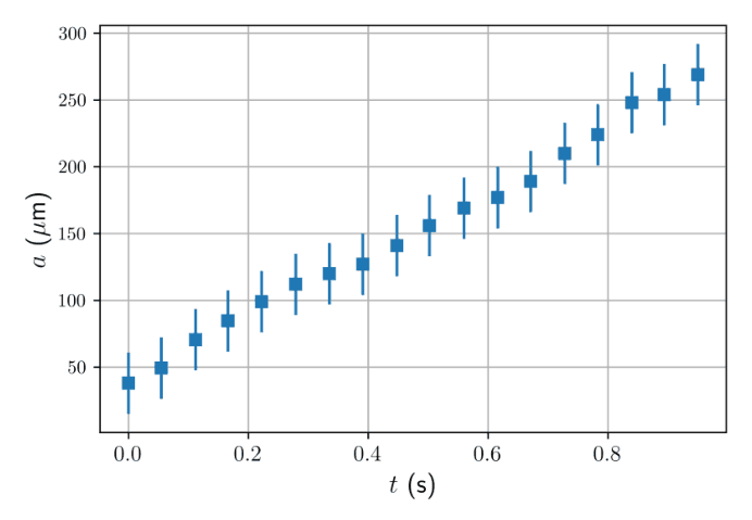
Fig. 2. Time evolution of \(\mathrm{CO}_2\) bubble radius in a glass of champagne (adapted from [1]).

Eventually bubbles detach from the bottom of the glass and continue to grow while rising. Fig. 3. shows a train of bubbles. The bubbles of the train have the same initial radius and are emitted at a constant frequency \(f_{\mathrm b}=20\,\mathrm{Hz}\).

Fig. 3. A train of bubbles. The photo is rotated horizontally for the page layout (adapted from [1]).

For the range of velocities studied here, the drag force \(F\) on a bubble of radius \(a\) moving at velocity \(v\) in a liquid of dynamic viscosity \(\eta\) is given by Stokes' law \(F=6\pi\eta av\). Measurements show that at any moment in time, the bubble can be assumed to be travelling at its terminal velocity.

A.4 — 0.8pt

Give the expression of the main forces exerted on a vertically rising bubble. Obtain the expression of \(v(a)\). Give a numerical estimate of \(\eta\) using \(\rho_\ell\), \(g_0\) and quantities measured on Fig. 3.

The quasi-stationary growth of bubbles with rate \(q_a=\dfrac{\mathrm da}{\mathrm dt}\) still applies during bubble rise.

A.5 — 0.5pt

Express the radius \(a_{H_\ell}\) of a bubble reaching the free surface in terms of height travelled \(H_\ell\), growth rate \(q_a=\dfrac{\mathrm da}{\mathrm dt}\), and any constants you may need. Assume \(a_{H_\ell}\gg a_0\) and \(q_a\) constant, and give the numerical value of \(a_{H_\ell}\) with \(H_\ell=10\,\mathrm{cm}\) and \(q_a\) corresponding to Fig. 2.

There are \(N_{\mathrm b}\) nucleation sites of bubbles. Assume that the bubbles are nucleated at a constant frequency \(f_{\mathrm b}\) at the bottom of a glass of champagne (height \(H_\ell\) for a volume \(V_\ell\)), with \(a_0\) still negligible. Neglect diffusion of \(\mathrm{CO}_2\) at the free surface.

A.6 — 1.1pt

Write the differential equation for \(c_\ell(t)\). Obtain from this equation the characteristic time \(\tau\) for the decay of the concentration of dissolved \(\mathrm{CO}_2\) in the liquid.

Part B. Acoustic emission of a bursting bubble

Small bubbles are nearly spherical as they reach the free surface. Once the liquid film separating the bubble from the air thins out sufficiently, a circular hole of radius \(r\) forms in the film and, driven by surface tension, opens very quickly (Fig. 4. left). The hole opens at constant speed \(v_{\mathrm f}\) (Fig. 4. right). The film outside the rim remains still, with constant thickness \(h\).

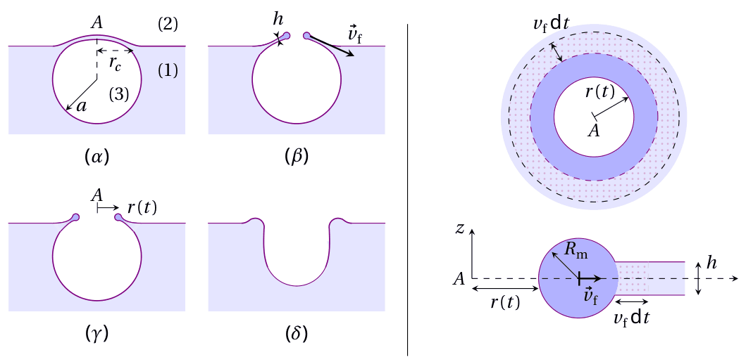
Fig. 4. (Left) \((\alpha)\) Bubble at the surface: (1) liquid, (2) air at pressure \(P_0\) and (3), \(\mathrm{CO}_2\) at pressure \(P_{\mathrm b}\), \((\beta)\) and \((\gamma)\) retraction of the liquid film, where the rim is in dark blue, \((\delta)\) bubble collapse. (Right) Retraction of the liquid film at time \(t\). Top: sketch of the pierced film seen from above. Bottom: cross-section of the rim and the retracting film. During \(\mathrm dt\) the rim accumulates nearby liquid (dotted).

Due to dissipative processes, only half of the difference of the surface energy between \(t\) and \(t+\mathrm dt\) of the rim and the accumulated liquid is transformed into kinetic energy. We further assume that the variation of the surface of the rim is negligible compared to that of the film.

B.1 — 1.1pt

Express \(v_{\mathrm f}\) in terms of \(\rho_\ell,\sigma\) and \(h\).

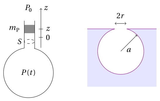
Fig. 5. (Left) a Helmholtz resonator. (Right) a bubble as an oscillator.

When the film bursts, it releases internal pressure and emits a sound. We model this acoustic emission by a Helmholtz resonator: a cavity open to the atmosphere at \(P_0\) through a bottleneck aperture of area \(S\) (Fig. 5. left). In the neck, a mass \(m_{\mathrm p}\) makes small amplitude position oscillations due to the pressure forces it experiences as the gas in the cavity expands or compresses adiabatically. The gravity force on \(m_{\mathrm p}\) is negligible compared to pressure forces. Let \(V_0\) be the volume of gas under the mass \(m_{\mathrm p}\) for \(P=P_0\) as \(z=0\).

B.2 — 1.1pt

Express the frequency of oscillation \(f_0\) of \(m_{\mathrm p}\). Hint: for \(\varepsilon\ll1\), \((1+\varepsilon)^\alpha\approx1+\alpha\varepsilon\).

The Helmholtz model may be used for a bubble of radius \(a\). \(V_0\) is the volume of the closed bubble. From litterature, the mass of the equivalent of the piston is \(m_{\mathrm p}=8\rho_{\mathrm g}r^3/3\) where \(r\) is the radius of the circular aperture and \(\rho_{\mathrm g}=1.8\,\mathrm{kg\cdot m^{-3}}\) is the density of the gas (Fig. 5. right). During the bursting process, \(r\) goes from \(0\) to \(r_{\mathrm c}\), given by \[ r_{\mathrm c}=\frac{2}{\sqrt3}a^2\sqrt{\frac{\rho_\ell g_0}{\sigma}}. \] At the same time, the frequency of emitted sound increases until a maximum value of \(40\,\mathrm{kHz}\) and the bursting time is \(t_{\mathrm b}=3\times10^{-2}\,\mathrm{ms}\).

B.3 — 1.1pt

Find the radius \(a\) and the thickness \(h\) of the champagne film separating the bubble from the atmosphere.

Part C. Popping champagne

In a bottle, the total quantity of \(\mathrm{CO}_2\) is \(n_{\mathrm T}=0.2\,\mathrm{mol}\), either dissolved in the volume \(V_{\mathrm L}=750\,\mathrm{mL}\) of liquid champagne, or as a gas in the volume \(V_{\mathrm G}=25\,\mathrm{mL}\) under the cork (Fig. 6. left). \(V_{\mathrm G}\) contains only \(\mathrm{CO}_2\). The equilibrium between both \(\mathrm{CO}_2\) phases follows Henry's Law. We suppose that the fast gaseous \(\mathrm{CO}_2\) expansion when the bottle is opened, is adiabatic and reversible. Ambient temperature \(T_0\) and pressure \(P_0=1\,\mathrm{bar}\) are constant.

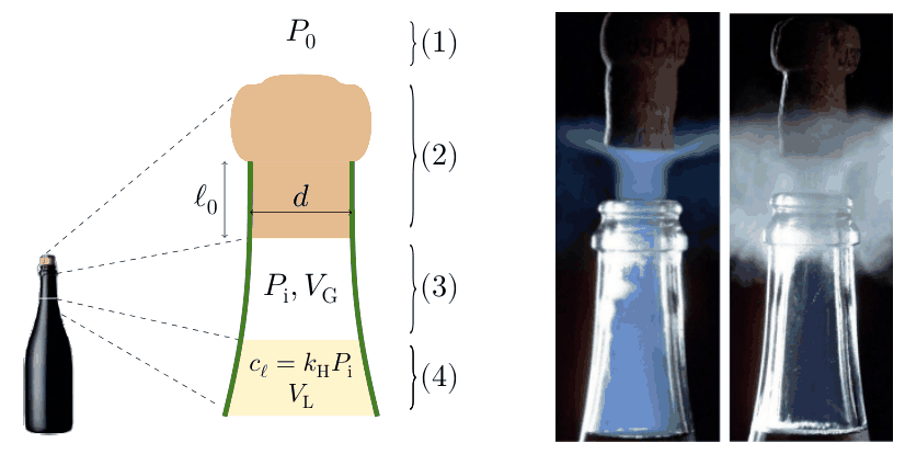
Fig. 6. Left: traditional bottleneck: (1) surrounding air, (2) cork stopper, (3) headspace, (4) liquid champagne. Right: Two phenomena observed while opening the bottle at two different temperatures (adapted from [2]).

C.1 — 0.4pt

Give the numerical value of the pressure \(P_{\mathrm i}\) of gaseous \(\mathrm{CO}_2\) in the bottle for \(T_0=6^\circ\mathrm C\) and \(T_0=20^\circ\mathrm C\).

Another step of champagne production (not described here) leads to the following values of \(P_{\mathrm i}\) that we will use for the next questions: \(P_{\mathrm i}=4.69\,\mathrm{bar}\) at \(T_0=6^\circ\mathrm C\) and \(P_{\mathrm i}=7.45\,\mathrm{bar}\) at \(T_0=20^\circ\mathrm C\).

During bottle opening, two different phenomena can be observed, depending on \(T_0\) (Fig. 6. right).

• either a blue fog appears, due to the formation of solid \(\mathrm{CO}_2\) crystals (but water condensation is inhibited);
• or a grey-white fog appears, due to water vapor condensation in the air surrounding the bottleneck. In this latter case, there is no formation of \(\mathrm{CO}_2\) solid crystals.

The saturated vapor pressure \(P_{\mathrm{sat}}^{\mathrm{CO}_2}\) for the \(\mathrm{CO}_2\) solid/gas transition follows: \[ \log_{10}\left(\frac{P_{\mathrm{sat}}^{\mathrm{CO}_2}}{P_0}\right) =A-\frac{B}{T+C} \] with \(T\) in \(\mathrm K\), \(A=6.81\), \(B=1.30\times10^3\,\mathrm K\) and \(C=-3.49\,\mathrm K\).

C.2 — 0.7pt

Give the numerical value \(T_{\mathrm f}\) of the \(\mathrm{CO}_2\) gas at the end of the expansion, after opening a bottle, if \(T_0=6^\circ\mathrm C\) and if \(T_0=20^\circ\mathrm C\), if no phase transition occured.

Choose which statements are true (several statements possible):

1. At \(T_0=6^\circ\mathrm C\) a grey-white fog appears while opening the bottle.
2. At \(T_0=6^\circ\mathrm C\) a blue fog appears while opening the bottle.
3. At \(T_0=20^\circ\mathrm C\) a grey-white fog appears while opening the bottle.
4. At \(T_0=20^\circ\mathrm C\) a blue fog appears while opening the bottle.

During bottle opening, the cork stopper pops out. We now determine the maximum height \(H_{\mathrm c}\) it reaches. Assume that the friction force \(F\) due to the bottleneck on the cork stopper is \(F=\alpha A\) where \(A\) is the area of contact and \(\alpha\) is a constant to determine. Initially, the pressure force slightly overcomes the friction force. The cork's mass is \(m=10\,\mathrm g\), its diameter \(d=1.8\,\mathrm{cm}\) and the length of the cylindrical part initially stuck in the bottleneck is \(\ell_0=2.5\,\mathrm{cm}\). Once the cork has left the bottleneck, you can neglect the net pressure force.

C.3 — 1.3pt

Give the numerical value of \(H_{\mathrm c}\) if the external temperature is \(T_0=6^\circ\mathrm C\).

[1] Liger-Belair et al, Am. J. Enol. Vitic., Vol. 50, No. 3 (1999).

[2] Liger-Belair et al., Sc. Reports 7, 10938 (2017).

General Data Sheet

Constant	Notation	Value	Unit
Speed of light in vacuum	\(c\)	\(2.997\,924\,58\times10^8\)	\(\mathrm{m\cdot s^{-1}}\)
Planck constant	\(h\)	\(6.626\,070\,15\times10^{-34}\)	\(\mathrm{kg\cdot m^2\cdot s^{-1}}\)
Reduced Planck constant	\(\hbar=\dfrac{h}{2\pi}\)	\(1.054\,571\,818\times10^{-34}\)	\(\mathrm{kg\cdot m^2\cdot s^{-1}}\)
Boltzmann constant	\(k_{\mathrm B}\)	\(1.380\,649\times10^{-23}\)	\(\mathrm{kg\cdot m^2\cdot s^{-2}\cdot K^{-1}}\)
Avogadro constant	\(N_{\mathrm A}\)	\(6.022\,140\,76\times10^{23}\)	\(\mathrm{mol^{-1}}\)
Molar gas constant	\(R\)	\(8.314\,462\,618\,153\,24\)	\(\mathrm{kg\cdot m^2\cdot s^{-2}\cdot mol^{-1}\cdot K^{-1}}\)
Elementary charge	\(e\)	\(1.602\,176\,634\times10^{-19}\)	\(\mathrm{A\cdot s}\)
Universal constant of gravitation	\(G\)	\(6.674\,30(15)\times10^{-11}\)	\(\mathrm{m^3\cdot kg^{-1}\cdot s^{-2}}\)
Standard acceleration due to gravity	\(g\)	\(9.806\,65\)	\(\mathrm{m\cdot s^{-2}}\)
Stefan Boltzmann constant	\(\sigma\)	\(5.670\,374\,419\times10^{-8}\)	\(\mathrm{kg\cdot s^{-3}\cdot K^{-4}}\)
Vacuum permeability (magnetic constant)	\(\mu_0\)	\(1.256\,637\,061\,27(20)\times10^{-6}\)	\(\mathrm{kg\cdot m\cdot A^{-2}\cdot s^{-2}}\)
Vacuum permittivity (electrical constant)	\(\epsilon_0\)	\(8.854\,187\,818\,8(14)\times10^{-12}\)	\(\mathrm{A^2\cdot s^4\cdot kg^{-1}\cdot m^{-3}}\)
Rydberg constant	\(R_\infty\)	\(1.097\,373\,156\,815\,7(12)\times10^7\)	\(\mathrm{m^{-1}}\)
Mass of the electron	\(m_{\mathrm e}\)	\(9.109\,383\,713\,9(28)\times10^{-31}\)	\(\mathrm{kg}\)
Mass of the proton	\(m_{\mathrm p}\)	\(1.672\,621\,925\,95(52)\times10^{-27}\)	\(\mathrm{kg}\)
Mass of the neutron	\(m_{\mathrm n}\)	\(1.674\,927\,500\,56(85)\times10^{-27}\)	\(\mathrm{kg}\)
Atomic mass constant	\(m_{\mathrm u}\)	\(1.660\,539\,068\,92(52)\times10^{-27}\)	\(\mathrm{kg}\)
Electronvolt	\(\mathrm{eV}\)	\(1.602\,176\,634\times10^{-19}\)	\(\mathrm{kg\cdot m^2\cdot s^{-2}}\)

Official English text of the problem.

Diese Aufgabe untersucht die besonderen physikalischen Eigenschaften von Galaxien, etwa ihre Dynamik und Struktur. Insbesondere erläutern wir, wie sich die Massenverteilung unserer Galaxie von innen heraus messen lässt. Dazu konzentrieren wir uns auf Wasserstoff, ihren Hauptbestandteil.

In dieser gesamten Aufgabe verwenden wir ausschließlich \(\hbar\), definiert durch \(\hbar=h/2\pi\).

Teil A - Einführung

Bohrsches Atommodell

Wir nehmen an, dass das Wasserstoffatom aus einem nichtrelativistischen Elektron der Masse \(m_e\) besteht, das ein ortsfestes Proton umkreist. In diesem gesamten Teil nehmen wir an, dass es sich auf einer Kreisbahn bewegt.

A.1 — 0.2 Punkte

Bestimmen Sie die Geschwindigkeit \(v\) des Elektrons auf einer Kreisbahn mit Radius \(r\).

Im Bohrschen Atommodell nehmen wir an, dass der Betrag des Drehimpulses \(L\) des Elektrons quantisiert ist: \(L=n\hbar\), wobei \(n>0\) eine ganze Zahl ist. Wir definieren \(\alpha=\dfrac{e^2}{4\pi\varepsilon_0\hbar c}\approx7.27\times10^{-3}\).

A.2 — 0.5 Punkte

Zeigen Sie, dass der Radius jeder Bahn durch \(r_n=n^2r_1\) gegeben ist, wobei \(r_1\) als Bohrscher Radius bezeichnet wird. Drücken Sie \(r_1\) durch \(\alpha\), \(m_e\), \(c\) und \(\hbar\) aus und berechnen Sie seinen Zahlenwert mit 3 signifikanten Stellen. Drücken Sie \(v_1\), die Geschwindigkeit auf der Bahn mit Radius \(r_1\), durch \(\alpha\) und \(c\) aus.

A.3 — 0.5 Punkte

Bestimmen Sie die mechanische Energie \(E_n\) des Elektrons auf einer Bahn mit Radius \(r_n\) in Abhängigkeit von \(e\), \(\varepsilon_0\), \(r_1\) und \(n\). Bestimmen Sie \(E_1\) im Grundzustand in Abhängigkeit von \(\alpha\), \(m_e\) und \(c\). Berechnen Sie ihren Zahlenwert in eV.

Fein- und Hyperfeinstruktur des Wasserstoffs

Die seltene spontane Umkehr des Elektronenspins führt dazu, dass pro Wasserstoffatom im Mittel einmal in 10 Millionen Jahren ein Photon emittiert wird. Diese Emission dient als Nachweis für Wasserstoff im Universum und ist daher von grundlegender Bedeutung für die Astrophysik. Wir untersuchen den für diese Emission verantwortlichen Übergang in zwei Schritten.

Betrachten Sie zunächst die Wechselwirkung zwischen dem Elektronenspin und der Relativbewegung von Elektron und Proton. Im Bezugssystem des Elektrons umkreist das Proton das Elektron im Abstand \(r_1\). Dadurch entsteht ein Magnetfeld \(\vec B_1\).

A.4 — 0.5 Punkte

Bestimmen Sie den Betrag \(B_1\) von \(\vec B_1\) am Ort des Elektrons in Abhängigkeit von \(\mu_0\), \(e\), \(\alpha\), \(c\) und \(r_1\).

Zweitens erzeugt der Elektronenspin ein magnetisches Moment \(\vec{\mathcal M}_s\). Sein Betrag ist näherungsweise \(\mathcal M_s=\dfrac{e}{m_e}\hbar\). Die Feinstruktur (F) hängt mit der Energiedifferenz \(\Delta E_{\mathrm F}\) zwischen einem Elektron, dessen magnetisches Moment \(\vec{\mathcal M}_s\) parallel zu \(\vec B_1\) ausgerichtet ist, und einem Elektron, dessen \(\vec{\mathcal M}_s\) antiparallel zu \(\vec B_1\) ausgerichtet ist, zusammen. Analog hängt die Hyperfeinstruktur (HF) mit der Energiedifferenz \(\Delta E_{\mathrm{HF}}\) zusammen, die sich aus der Wechselwirkung bei paralleler bzw. antiparalleler Ausrichtung der magnetischen Momente von Elektron und Proton ergibt. Es ist bekannt, dass näherungsweise \(\Delta E_{\mathrm{HF}}\simeq3.72\dfrac{m_e}{m_p}\Delta E_{\mathrm F}\) gilt, wobei \(m_p\) die Protonenmasse ist.

A.5 — 0.5 Punkte

Drücken Sie \(\Delta E_{\mathrm F}\) als Funktion von \(\alpha\) und \(E_1\) aus.

Geben Sie einen Ausdruck für die Wellenlänge \(\lambda_{\mathrm{HF}}\) eines Photons an, das bei einem Übergang zwischen den beiden Zuständen der Hyperfeinstruktur emittiert wird, und geben Sie ihren Zahlenwert mit zwei signifikanten Stellen an.

Teil B - Rotationskurven von Galaxien

Daten

• Kiloparsec: \(1\,\mathrm{kpc}=3.09\times10^{19}\,\mathrm m\)
• Sonnenmasse: \(1\,M_\odot=1.99\times10^{30}\,\mathrm{kg}\)

Wir betrachten eine kugelförmige Galaxie mit einem ortsfesten Punkt \(O\) als Zentrum. An einem beliebigen Punkt \(P\) sei \(\rho=\rho(P)\) die Massendichte und \(\varphi=\varphi(P)\) das zugehörige Gravitationspotential (d. h. die potentielle Energie pro Masseneinheit). Sowohl \(\rho\) als auch \(\varphi\) hängen nur von \(r=\|\overrightarrow{OP}\|\) ab. Die Bewegung einer am Punkt \(P\) befindlichen Masse \(m\) unter dem Einfluss des Feldes \(\varphi\) ist auf eine Ebene beschränkt, die \(O\) enthält.

B.1 — 0.2 Punkte

Bestimmen Sie für eine Kreisbahn die Geschwindigkeit \(v_c\) eines Objekts auf einer durch \(P\) verlaufenden Kreisbahn in Abhängigkeit von \(r\) und \(\dfrac{d\varphi}{dr}\).

Abb. 1(A) zeigt eine Aufnahme der Spiralgalaxie NGC 6946 im sichtbaren Spektralbereich (aufgenommen mit dem 0,8-m-Schulman-Teleskop am Mount Lemmon Sky Center in Arizona). Die kleinen Ellipsen in Abb. 1(B) zeigen experimentelle Messwerte von \(v_c\) für diese Galaxie. Der zentrale Bereich (\(r<1\,\mathrm{kpc}\)) wird als Bulge bezeichnet. In diesem Bereich ist die Massenverteilung näherungsweise homogen. Die rote Kurve ist eine Vorhersage für \(v_c\) unter der Annahme, dass das System im Bulge homogen und außerhalb keplersch (\(\varphi(r)=-\beta/r\) mit \(\beta>0\)) ist, d. h., dass die gesamte Masse der Galaxie im Bulge konzentriert ist.

Abb. 1: Galaxie NGC 6946: Aufnahme (A) und Rotationskurve (B).

B.2 — 0.5 Punkte

Leiten Sie aus der roten Rotationskurve in Abb. 1(B) die Masse \(M_b\) des Bulges von NGC 6946 in Einheiten der Sonnenmasse ab.

Der Vergleich des keplerschen Modells mit den experimentellen Daten überzeugt Astronomen davon, dass ein Teil der Masse auf dem Bild unsichtbar ist. Sie nehmen daher an, dass die tatsächliche Massendichte der Galaxie durch

\[ \rho_m(r)=\frac{C_m}{r_m^2+r^2} \tag{1} \]

gegeben ist, wobei \(C_m>0\) und \(r_m>0\) Konstanten sind.

B.3 — 1.8 Punkte

Zeigen Sie, dass das zur Massendichte aus Gl. 1 gehörende Geschwindigkeitsprofil \(v_{c,m}(r)\) in der Form \[ v_{c,m}(r)=\sqrt{k_1-\frac{k_2\cdot\arctan\!\left(\frac r{r_m}\right)}r}. \] geschrieben werden kann. Drücken Sie \(k_1\) und \(k_2\) durch \(C_m\), \(r_m\) und \(G\) aus.

(Hinweise: \(\displaystyle\int_0^r\frac{x^2}{a^2+x^2}\,dx=r-a\arctan(r/a)\), und: \(\arctan(x)\simeq x-x^3/3\) für \(x\ll1\).)

Vereinfachen Sie \(v_{c,m}(r)\) für \(r\ll r_m\) und für \(r\gg r_m\).

Zeigen Sie, dass sich für \(r\gg r_m\) die Masse \(M_m(r)\), die bei der Massendichte aus Gl. 1 in einer Kugel mit Radius \(r\) enthalten ist, vereinfacht und nur von \(C_m\) und \(r\) abhängt.

Schätzen Sie die tatsächlich im Bildausschnitt von Abb. 1(A) enthaltene Masse der Galaxie NGC 6946 ab.

Teil C - Massenverteilung in unserer Galaxie

Für eine Spiralgalaxie wird das Modell aus Gl. 1 abgeändert, und man nimmt üblicherweise an, dass das Gravitationspotential durch \[ \varphi_G(r,z)=\varphi_0\ln\!\left(\frac r{r_0}\right) \exp\!\left[-\left(\frac z{z_0}\right)^2\right], \] gegeben ist, wobei \(z\) der Abstand von der galaktischen Ebene (definiert durch \(z=0\)) ist, \(r<r_0\) nun den Abstand von der Achse bezeichnet und \(\varphi_0>0\) eine zu bestimmende Konstante ist. \(r_0\) und \(z_0\) sind konstante Größen.

C.1 — 0.5 Punkte

Bestimmen Sie die Bewegungsgleichung für \(z\) für die vertikale Bewegung einer Punktmasse \(m\) in einem solchen Potential unter der Annahme, dass \(r\) konstant ist. Zeigen Sie, dass die galaktische Ebene für \(r<r_0\) eine stabile Gleichgewichtslage ist, indem Sie die Kreisfrequenz \(\omega_0\) kleiner Schwingungen um diese Ebene angeben.

Von nun an setzen wir \(z=0\).

C.2 — 0.6 Punkte

Bestimmen Sie, in welchem Bereich, \(r\gg r_m\) oder \(r\ll r_m\), das Modell aus Gl. 1 bei geeigneter Definition von \(\varphi_0\) ein Potential der Form \(\varphi_G(r,0)\) ergibt.

Unter dieser Bedingung hängt \(v_c(r)\) nicht mehr von \(r\) ab. Drücken Sie es durch \(\varphi_0\) aus.

Außerhalb des Bulges hängt der Geschwindigkeitsbetrag \(v_c\) somit nicht vom Abstand zum galaktischen Zentrum ab. Wie Astronomen werden wir diese Tatsache nutzen, um die Massenverteilung der Galaxie von innen heraus zu messen.

Alle hier für astronomische Beobachtungen betrachteten galaktischen Objekte, etwa Sterne oder Nebel, bestehen hauptsächlich aus Wasserstoff. Außerhalb des Bulges nehmen wir an, dass sie sich auf Kreisbahnen um das galaktische Zentrum \(C\) bewegen. \(S\) ist der Ort der Sonne und \(E\) derjenige eines bestimmten galaktischen Objekts, das im Wasserstoffspektrum emittiert. In der galaktischen Ebene betrachten wir eine Sichtlinie \(SE\), die der Beobachtungsrichtung entspricht und entlang des Einheitsvektors \(\hat u_v\) verläuft (siehe Abb. 2).

Abb. 2: Geometrie der Messung

Sei \(\ell\) die galaktische Länge, die den Winkel zwischen \(SC\) und \(SE\) angibt. Die Geschwindigkeit der Sonne auf ihrer Kreisbahn mit Radius \(R_\odot=8.00\,\mathrm{kpc}\) wird mit \(\vec v_\odot\) bezeichnet. Ein galaktisches Objekt in \(E\) bewegt sich auf einer anderen Kreisbahn mit Radius \(R\) und Geschwindigkeit \(\vec v_E\). Mithilfe des Dopplereffekts an der zuvor untersuchten 21-cm-Linie lässt sich die relative Radialgeschwindigkeit \(v_{rE/S}\) des Emitters \(E\) bezüglich der Sonne \(S\) bestimmen: Sie ist die Projektion von \(\vec v_E-\vec v_\odot\) auf die Sichtlinie.

C.3 — 0.7 Punkte

Bestimmen Sie \(v_{rE/S}\) in Abhängigkeit von \(\ell\), \(R\), \(R_\odot\) und \(v_\odot\). Drücken Sie anschließend \(R\) durch \(R_\odot\), \(v_\odot\), \(\ell\) und \(v_{rE/S}\) aus.

Mit einem Radioteleskop führen wir Beobachtungen in der Ebene unserer Galaxie in Richtung der galaktischen Länge \(\ell=30^\circ\) durch. Das verwendete Frequenzband enthält die 21-cm-Linie mit der Frequenz \(f_0=1.42\,\mathrm{GHz}\). Die Ergebnisse sind in Abb. 3 dargestellt.

Abb. 3: Elektromagnetisches Signal als Funktion der Frequenzverschiebung, gemessen im Radiofrequenzbereich bei \(\ell=30^\circ\) mithilfe von EU-HOU RadioAstronomy

C.4 — 0.6 Punkte

In unserer Galaxie gilt \(v_\odot=220\,\mathrm{km\cdot s^{-1}}\). Bestimmen Sie für die 3 in Abb. 3 beobachteten Quellen die relative Radialgeschwindigkeit (mit 3 signifikanten Stellen) und den Abstand vom galaktischen Zentrum (mit 2 signifikanten Stellen). Die Abstände sind als Vielfache von \(R_\odot\) anzugeben.

C.5 — 0.6 Punkte

Markieren Sie in der Draufsicht unserer Galaxie (im Antwortfeld) die Positionen der in Abb. 3 beobachteten Quellen.

Was ließe sich aus wiederholten Messungen bei unterschiedlichen Werten von \(\ell\) ableiten?

Teil D - Tully-Fisher-Beziehung und MOND-Theorie

Die flache äußere Geschwindigkeitskurve von NGC 6946 in Abb. 1 ist eine gemeinsame Eigenschaft von Spiralgalaxien, wie in Abb. 4 (links) zu sehen ist. Trägt man den äußeren konstanten Geschwindigkeitswert \(v_{c,\infty}\) als Funktion der gemessenen Gesamtmasse \(M_{\mathrm{tot}}\) jeder Galaxie auf, ergibt sich eine interessante Korrelation, die als Tully-Fischer-Beziehung bezeichnet wird, siehe Abb. 4 (rechts).

Abb. 4. Links: Rotationskurven typischer Spiralgalaxien - Rechts: \(\log_{10}(M_{\mathrm{tot}})\) als Funktion von \(\log_{10}(v_{c,\infty})\) auf linearen Skalen. Die farbigen Punkte entsprechen verschiedenen Galaxien und verschiedenen Durchmusterungen. Die grüne Linie stellt die Tully-Fischer-Beziehung dar, die sehr gut mit der Ausgleichsgeraden der Daten (schwarz) übereinstimmt.

D.1 — 0.4 Punkte

Zeigen Sie unter der Annahme, dass der Radius \(R\) einer Galaxie nicht von ihrer Masse abhängt, dass das Modell aus Gl. 1 (Teil B) eine Beziehung der Form \(M_{\mathrm{tot}}=\eta v_{c,\infty}^{\gamma}\) ergibt, wobei \(\gamma\) und \(\eta\) anzugeben sind.

Vergleichen Sie diesen Ausdruck mit der Tully-Fischer-Beziehung, indem Sie \(\gamma_{TF}\) berechnen.

Im Bereich extrem kleiner Beschleunigungen in der Größenordnung von \(a_0=10^{-10}\,\mathrm{m\cdot s^{-2}}\) schlägt die Theorie der modifizierten Newtonschen Dynamik (MOND) vor, das zweite Newtonsche Gesetz durch \[ \vec F=m\mu\!\left(\frac a{a_0}\right)\vec a \] zu modifizieren, wobei \(a=\|\vec a\|\) der Betrag der Beschleunigung ist und die Funktion \(\mu\) durch \(\mu(x)=\dfrac{x}{1+x}\) definiert ist.

D.2 — 0.2 Punkte

Schätzen Sie anhand der Daten für NGC 6946 in Abb. 1 im Rahmen der Newtonschen Theorie den Betrag der Beschleunigung \(a_m\) einer Masse in den äußeren Bereichen von NGC 6946 ab.

D.3 — 0.8 Punkte

Eine Masse \(m\) bewege sich mit der Geschwindigkeit \(v_{c,\infty}\) auf einer Kreisbahn mit Radius \(r\) im Gravitationsfeld einer ortsfesten Masse \(M\).

Bestimmen Sie im Rahmen der MOND-Theorie für \(a\ll a_0\) den Tully-Fischer-Exponenten.

Berechnen Sie anhand der Daten für NGC 6946 und/oder des Tully-Fischer-Gesetzes \(a_0\), um zu zeigen, dass MOND im richtigen Bereich wirksam ist.

D.4 — 0.9 Punkte

Bestimmen Sie unter Berücksichtigung der relevanten Fälle \(v_c(r)\) für alle Werte von \(r\) in der MOND-Theorie für das Gravitationsfeld einer homogen verteilten Masse \(M\) mit Radius \(R_b\).

Allgemeines Datenblatt

Konstante	Symbol	Wert	Einheit
Lichtgeschwindigkeit im Vakuum	\(c\)	\(2.997\,924\,58\times10^8\)	\(\mathrm{m\cdot s^{-1}}\)
Planck-Konstante	\(h\)	\(6.626\,070\,15\times10^{-34}\)	\(\mathrm{kg\cdot m^2\cdot s^{-1}}\)
Reduzierte Planck-Konstante	\(\hbar=\dfrac h{2\pi}\)	\(1.054\,571\,818\times10^{-34}\)	\(\mathrm{kg\cdot m^2\cdot s^{-1}}\)
Boltzmann-Konstante	\(k_{\mathrm B}\)	\(1.380\,649\times10^{-23}\)	\(\mathrm{kg\cdot m^2\cdot s^{-2}\cdot K^{-1}}\)
Avogadro-Konstante	\(N_{\mathrm A}\)	\(6.022\,140\,76\times10^{23}\)	\(\mathrm{mol^{-1}}\)
Molare Gaskonstante	\(R\)	\(8.314\,462\,618\,153\,24\)	\(\mathrm{kg\cdot m^2\cdot s^{-2}\cdot mol^{-1}\cdot K^{-1}}\)
Elementarladung	\(e\)	\(1.602\,176\,634\times10^{-19}\)	\(\mathrm{A\cdot s}\)
Universelle Gravitationskonstante	\(G\)	\(6.674\,30(15)\times10^{-11}\)	\(\mathrm{m^3\cdot kg^{-1}\cdot s^{-2}}\)
Normfallbeschleunigung	\(g\)	\(9.806\,65\)	\(\mathrm{m\cdot s^{-2}}\)
Stefan-Boltzmann-Konstante	\(\sigma\)	\(5.670\,374\,419\times10^{-8}\)	\(\mathrm{kg\cdot s^{-3}\cdot K^{-4}}\)
Vakuumpermeabilität (magnetische Feldkonstante)	\(\mu_0\)	\(1.256\,637\,061\,27(20)\times10^{-6}\)	\(\mathrm{kg\cdot m\cdot A^{-2}\cdot s^{-2}}\)
Vakuumpermittivität (elektrische Feldkonstante)	\(\epsilon_0\)	\(8.854\,187\,818\,8(14)\times10^{-12}\)	\(\mathrm{A^2\cdot s^4\cdot kg^{-1}\cdot m^{-3}}\)
Rydberg-Konstante	\(R_\infty\)	\(1.097\,373\,156\,815\,7(12)\times10^7\)	\(\mathrm{m^{-1}}\)
Elektronenmasse	\(m_e\)	\(9.109\,383\,713\,9(28)\times10^{-31}\)	\(\mathrm{kg}\)
Protonenmasse	\(m_p\)	\(1.672\,621\,925\,95(52)\times10^{-27}\)	\(\mathrm{kg}\)
Neutronenmasse	\(m_n\)	\(1.674\,927\,500\,56(85)\times10^{-27}\)	\(\mathrm{kg}\)
Atomare Massenkonstante	\(m_u\)	\(1.660\,539\,068\,92(52)\times10^{-27}\)	\(\mathrm{kg}\)
Elektronenvolt	\(\mathrm{eV}\)	\(1.602\,176\,634\times10^{-19}\)	\(\mathrm{kg\cdot m^2\cdot s^{-2}}\)

Aufgabentext aus dem offiziellen englischen Text übersetzt.

Im Jahr 1765 erfand der britische Uhrmacher James Cox eine Uhr, deren einzige Energiequelle die Schwankungen des Luftdrucks sind. Cox' Uhr verwendete zwei Gefäße mit Quecksilber. Änderungen des Luftdrucks bewirkten, dass Quecksilber zwischen den Gefäßen strömte und sich die beiden Gefäße relativ zueinander bewegten. Diese Bewegung diente als Energiequelle für das eigentliche Uhrwerk.

Wir untersuchen diese Vorrichtung. Dabei nehmen wir durchgehend an, dass

• das Schwerefeld der Erde \(\vec g=-g\vec u_z\) homogen ist, mit \(g=9.8\,\mathrm{m\cdot s^{-2}}\) und dem Einheitsvektor \(\vec u_z\);
• alle Flüssigkeiten inkompressibel sind und ihre Dichte mit \(\rho\) bezeichnet wird;
• keine Effekte der Oberflächenspannung berücksichtigt werden;
• die Höhenabhängigkeit des Luftdrucks vernachlässigt wird;
• die Umgebungstemperatur \(T_a\) räumlich konstant ist und alle Zustandsänderungen isotherm verlaufen.

Abb. 1. Künstlerische Darstellung von Cox' Uhr \({}^{1}\)

Teil A - Ziehen an einem eingetauchten Rohr

Wir betrachten zunächst ein Wasserbad, das den Halbraum \(z\leq0\) einnimmt. Die Luft darüber steht unter dem Druck \(P_a=P_0\). Ein senkrechtes zylindrisches Rohr der Länge \(H=1\,\mathrm m\), der Querschnittsfläche \(S=10\,\mathrm{cm^2}\) und der Masse \(m=0.5\,\mathrm{kg}\) wird in das Bad eingetaucht. Das untere Ende des Rohrs ist offen, das obere Ende geschlossen. Mit \(h\) bezeichnen wir die Höhe des oberen Rohrendes und mit \(z_\ell\) die Höhe des Wassers im Rohr. Die Wanddicke des Rohrs wird vernachlässigt.

Abb. 2. Skizze des Rohrs in verschiedenen Anordnungen

Wir gehen von der Situation aus, in der das Rohr in Abb. 2 kein Gas enthält und sein oberes Ende auf Höhe der Badoberfläche liegt: Mit anderen Worten gilt \(h=0\) und \(z_\ell=0\) (Fall a). Anschließend wird das Rohr langsam angehoben, bis sein unteres Ende die Badoberfläche erreicht. Die auf das Rohr ausgeübte Zugkraft wird mit \(\vec F=F\vec u_z\) bezeichnet.

A.1 — 0.2 Punkte

Geben Sie für die in Abb. 2 gezeigte Anordnung (Fall b) den Druck \(P_w\) im Wasser am oberen Rohrende an. Geben Sie außerdem die Kraft \(\vec F\) an, die erforderlich ist, um das Rohr in dieser Position zu halten. Die Ausdrücke sind in Abhängigkeit von \(P_0,\rho,m,S,h,g\) und \(\vec u_z\) anzugeben.

Es werden drei Versuche durchgeführt. In jedem Versuch wird das Rohr ausgehend vom Anfangszustand in Abb. 2(a) unter den in Tabelle 1 angegebenen Bedingungen angehoben.

Versuch	Flüssigkeit	\(T_a\) (°C)	\(\rho\) (\(\mathrm{kg\cdot m^{-3}}\))	\(P_{\mathrm{sat}}\) (Pa)
1	Wasser	20	\(1.00\times10^3\)	\(2.34\times10^3\)
2	Wasser	80	\(0.97\times10^3\)	\(47.4\times10^3\)
3	Wasser	99	\(0.96\times10^3\)	\(99.8\times10^3\)

Tabelle 1. Versuchsbedingungen und Zahlenwerte der physikalischen Größen für die einzelnen Versuche

(\(P_{\mathrm{sat}}\) bezeichnet den Sättigungsdampfdruck des reinen Fluids)

In jedem Fall untersuchen wir den Verlauf der Kraft \(F\), die aufgebracht werden muss, um das Rohr in einer Höhe \(h\) im Gleichgewicht zu halten, wobei der Außendruck auf \(P_a=P_0=1.000\times10^5\,\mathrm{Pa}\) festgelegt ist. Zwei unterschiedliche Verhaltensweisen sind möglich

A.2 — 0.8 Punkte

Vervollständigen Sie für jeden Versuch die Tabelle auf dem Antwortblatt, indem Sie das erwartete Verhalten und die Zahlenwerte für \(F_{\max}\) und für \(h^\star\) (sofern zutreffend) angeben. Dabei sind \(F_{\max}\) und \(h^\star\) in den Abbildungen definiert, welche die beiden Verhaltensweisen veranschaulichen.

Wenn wir das Wasser durch flüssiges Quecksilber ersetzen (dessen Eigenschaften unten angegeben sind), wird Verhalten B beobachtet.

Flüssigkeit	\(T_a\) (°C)	\(\rho\) (\(\mathrm{kg\cdot m^{-3}}\))	\(P_{\mathrm{sat}}\) (Pa)
Quecksilber	20	\(13.5\times10^3\)	\(0.163\)

A.3 — 0.3 Punkte

Geben Sie den relativen Fehler \(\varepsilon\) an, der entsteht, wenn wir bei der Berechnung der maximalen Kraft \(F_{\max}\) den Druck \(P_{\mathrm{sat}}\) gegenüber \(P_0\) vernachlässigen. Geben Sie den Zahlenwert von \(\varepsilon\) an.

Teil B - Zweiteiliges Barometerrohr

Von nun an arbeiten wir mit Quecksilber (Dichte \(\rho=13.5\times10^3\,\mathrm{kg\cdot m^{-3}}\)) bei der Umgebungstemperatur \(T_a=20^\circ\mathrm C\) und setzen \(P_{\mathrm{sat}}=0\).

Wir betrachten ein Rohr mit einem Vorratsgefäß am oberen Ende, das als zwei übereinander angeordnete Zylinder unterschiedlicher Abmessungen modelliert wird, wie in Abb. 3 gezeigt.

• Der untere Teil (weiterhin als Rohr bezeichnet) hat die Querschnittsfläche \(S_t\) und die Höhe \(H_t=80\,\mathrm{cm}\);
• der obere Teil (als Erweiterung bezeichnet) hat die Querschnittsfläche \(S_b>S_t\) und die Höhe \(H_b=20\,\mathrm{cm}\).

Dieses zweiteilige Rohr wird in ein Flüssigkeitsbad eingetaucht, das einen Halbraum einnimmt.

Abb. 3. Skizze des zweiteiligen Barometerrohrs

Wie in Teil A wird das System so vorbereitet, dass das Rohr keine Luft enthält. Wir kennzeichnen die vertikale Position des Rohrs durch die Höhe \(h_t\) des Übergangs zwischen dem Rohr und der Erweiterung. Die Höhe der Quecksilbersäule wird wiederum mit \(z_\ell\) bezeichnet. Die Kraft \(\vec F\), die aufgebracht werden muss, um das Rohr in der in Abb. 3 gezeigten Anordnung im Gleichgewicht zu halten, lässt sich nun schreiben als

\[ \vec F=(m_{\mathrm{tb}}+m_{\mathrm{add}})g\vec u_z \tag{1} \]

wobei \(m_{\mathrm{tb}}\) die Gesamtmasse des zweiteiligen Rohrs (ohne Quecksilber) ist.

B.1 — 0.3 Punkte

Markieren Sie auf dem Antwortblatt die Fläche farbig, die dem Volumen des flüssigen Quecksilbers entspricht, das für den Term \(m_{\mathrm{add}}\) in Gleichung (1) verantwortlich ist.

Die Masse \(m_{\mathrm{add}}\) hängt sowohl von der Höhe \(h_t\) als auch vom Luftdruck \(P_a\) ab. Nehmen Sie für die nächste Frage an, dass der Luftdruck auf \(P_a=P_0=1.000\times10^5\,\mathrm{Pa}\) festgelegt ist. Ausgehend von einem vollständig eingetauchten System wird das Rohr langsam angehoben, bis sein unteres Ende bündig mit der Oberfläche des Flüssigkeitsbads liegt.

B.2 — 1.4 Punkte

Skizzieren Sie den Verlauf der Masse \(m_{\mathrm{add}}\) als Funktion von \(h_t\) für \(h_t\in[-H_b,H_t]\). Geben Sie im Diagramm die Ausdrücke für die Steigungen der einzelnen Abschnitte sowie die analytischen Werte von \(h_t\) an allen Knickpunkten in Abhängigkeit von \(P_0,\rho,g,S_b,S_t,H_b\) und \(H_t\) an.

Beim Anheben des Systems unter \(P_a=P_0=10^5\,\mathrm{Pa}\) halten wir an, sobald sich die freie Flüssigkeitsoberfläche in der Mitte der Erweiterung befindet. Der Wert von \(h_t\) wird festgehalten. Anschließend beobachten wir Änderungen der Masse \(m_{\mathrm{add}}\) infolge von Luftdruckschwankungen, die beschrieben werden durch

\[ P_a(t)=P_0+P_1(t) \tag{2} \]

wobei \(P_0\) den Mittelwert bezeichnet und \(P_1\) einen Störterm darstellt. Wir modellieren \(P_1\) durch eine periodische Dreiecksfunktion mit der Amplitude \(A=5\times10^2\,\mathrm{Pa}\) und der Periode \(\tau_1\) von 1 Woche.

Abb. 4. Vereinfachtes Modell des Störterms \(P_1(t)\)

B.3 — 0.3 Punkte

Geben Sie für \(S_t=5\,\mathrm{cm^2}\) und \(S_b=200\,\mathrm{cm^2}\) einen Ausdruck für die Amplitude \(\Delta m_{\mathrm{add}}\) der zeitlichen Schwankungen der Masse \(m_{\mathrm{add}}\) an und berechnen Sie anschließend ihren Zahlenwert. Nehmen Sie an, dass die Flüssigkeitsoberfläche stets in der Erweiterung bleibt.

Teil C - Cox' Uhr

Der von Cox entwickelte tatsächliche Mechanismus ist komplex (Abb. 5). Wir untersuchen eine vereinfachte Version, die in Abb. 6 dargestellt und nachfolgend beschrieben ist

• ein zylindrischer unterer Behälter mit einem Quecksilberbad;
• ein zweiteiliges Barometerrohr, das mit dem in Teil B untersuchten identisch und weiterhin vollständig luftleer ist, wird in das Bad eingetaucht;
• der Behälter und das zweiteilige Rohr hängen jeweils an einem Seil. Beide Seile (als undehnbar und von vernachlässigbarer Masse angenommen) laufen über ein System idealer Rollen und sind mit ihren Enden an gegenüberliegenden Seiten derselben Masse \(M\) befestigt, die auf einer horizontalen Fläche gleiten kann;
• das gesamte im System enthaltene Volumen an flüssigem Quecksilber beträgt \(V_\ell=5\,\mathrm L\).

Die Höhen, Querschnittsflächen und Massen der einzelnen Teile sind in Tabelle 2 angegeben. Die Position der Masse \(M\) wird durch die Koordinate \(x\) ihres Schwerpunkts beschrieben. Wir berücksichtigen Festkörperreibung zwischen der horizontalen Unterlage und der Masse \(M\), ohne zwischen Haft- und Gleitreibungskoeffizienten zu unterscheiden; der Betrag dieser Kraft beim Gleiten wird mit \(F_s\) bezeichnet.

Zwei Anschläge begrenzen die Verschiebung der Masse \(M\), sodass \(-X\leq x\leq X\) (mit \(X>0\)) gilt. Nehmen Sie an, dass der Wert von \(X\) gewährleistet, dass

• das untere Ende des zweiteiligen Rohrs weder den Boden des Behälters berührt noch aus dem Flüssigkeitsbad austritt;
• die Höhe \(z_\ell\) der Quecksilbersäule stets innerhalb der oberen Erweiterung liegt.

Abb. 5. Tatsächliche Uhr von Cox \({}^{2}\) (ohne Quecksilber)

Abb. 6. Skizze des Systems zur Modellierung der Uhr

Kennzeichnung	Bezeichnung	Höhe	Querschnittsfläche	Leermasse
\(\boxed{1}\)	Behälter	\(H_c=30\,\mathrm{cm}\)	\(S_c=210\,\mathrm{cm^2}\)	\(m_c\)
\(\boxed{2}\)	röhrenförmiger Teil des Barometerrohrs	\(H_t=80\,\mathrm{cm}\)	\(S_t=5\,\mathrm{cm^2}\)	Gesamtmasse des Barometerrohrs: \(m_{\mathrm{tb}}\)
\(\boxed{2'}\)	Erweiterung des Barometerrohrs	\(H_b=20\,\mathrm{cm}\)	\(S_b=200\,\mathrm{cm^2}\)

Tabelle 2. Abmessungen und Bezeichnungen des Modellsystems

Das System entwickelt sich im Kontakt mit der Atmosphäre, deren Druck wie in Abb. 4 schwankt (weiterhin mit der Amplitude \(A=5\times10^2\,\mathrm{Pa}\) und der Periode \(\tau_1=1\) Woche). Zu Beginn, bei \(t=0\), ruht die Masse \(M\) bei \(x=0\), und die von den beiden Seilen auf gegenüberliegenden Seiten der Masse \(M\) ausgeübten Zugkräfte gleichen sich aus, während \(P_1(0)=0\) gilt. Wir definieren

\[ \xi= \frac{S_b+S_c-S_t}{S_bS_c}\frac{F_s}{A} \simeq \frac{S_b+S_c}{S_bS_c}\frac{F_s}{A} \tag{3} \]

wobei im letzten Ausdruck \(S_t\ll S_b,S_c\) verwendet wird (was wir bis zum Ende der Aufgabe als gültig annehmen).

C.1 — 1 Punkt

Bestimmen Sie den Schwellenwert \(\xi^\star\), sodass \(M\) für \(\xi>\xi^\star\) unbegrenzt in Ruhe bleibt.

Nehmen Sie nur für die nächste Frage an, dass die Masse \(M\) vorübergehend bei \(x=X\) blockiert ist.

C.2 — 1 Punkt

Geben Sie für \(P_1=0\) einen Ausdruck für die resultierende Seilkraft \(\vec T=T\vec u_x\) an, die in dieser Position aufgrund der Zugkräfte in den beiden Seilen auf die Masse \(M\) wirkt, in Abhängigkeit von \(\rho,g,X\) und den relevanten Querschnittsflächen.

Für \(\xi<\xi^\star\) können, erneut ausgehend von \(x=0\) und \(P_1=0\), für \(t\geq0\) zwei unterschiedliche Verhaltensweisen beobachtet werden. Um sie zu unterscheiden, müssen wir einen weiteren Parameter einführen

\[ \lambda= \frac{2(S_b-S_t)}{S_b}\frac{\rho gX}{A} \simeq \frac{2\rho gX}{A} \tag{4} \]

C.3 — 2 Punkte

Vervollständigen Sie die Tabelle auf dem Antwortblatt, indem Sie die Bedingung angeben, unter der das jeweilige Regime auftritt. Die Bedingungen sind als Ungleichungen für \(\xi\) und/oder \(\lambda\) auszudrücken. Skizzieren Sie außerdem die Verläufe von \(x(t)/X\) für \(t\in[0,3\tau_1]\), die mit dem bereits eingezeichneten Verlauf von \(P_1(t)/A\) übereinstimmen. Die Koordinaten besonderer Punkte müssen nicht angegeben werden.

In der tatsächlichen Uhr von Cox wird die vom Mechanismus bereitgestellte Energie mithilfe eines Systems von Sperrklinken gespeichert und wie bei einer herkömmlichen Uhr zum Anheben eines Gegengewichts genutzt. Im hier untersuchten vereinfachten Modell entspricht die von der Uhr gewonnene Energie der Energie, die durch die von der horizontalen Fläche auf die Masse \(M\) ausgeübte Reibungskraft dissipiert wird. Von nun an nehmen wir an, dass das System so dimensioniert ist, dass es in dem Regime arbeitet, in dem die Uhr Energie gewinnen kann. Außerdem nehmen wir an, dass der eingeschwungene Zustand erreicht ist. Wir bezeichnen mit \(W\) die während einer Periode \(\tau_1\) durch die Festkörperreibung dissipierte Energie, die allein durch \(F_s\) und \(X\) ausgedrückt werden kann.

Bei ansonsten gleichen Bedingungen können \(F_s\) und \(X\) so eingestellt werden, dass die Energie \(W\) maximal wird; ihre jeweiligen Werte im optimalen Fall bezeichnen wir mit \(F_s^\star\) und \(X^\star\).

C.4 — 1 Punkt

Bestimmen Sie unter den Annahmen \(S_b\simeq S_c\) und \(S_t\ll S_b\) die Ausdrücke für \(F_s^\star\) und \(X^\star\) als Funktionen von \(\rho,g,S_c\) und \(A\). Geben Sie die entsprechende maximale Energie \(W^\star\) an und berechnen Sie anschließend ihren Zahlenwert für \(A=5\times10^2\,\mathrm{Pa}\).

Mit \(W_{\mathrm{pr}}^\star\) bezeichnen wir die Arbeit der Luftdruckkräfte, die dem System im optimalen Fall während einer Periode \(\tau_1\) zugeführt wird.

C.5 — 1.7 Punkte

Geben Sie \(W_{\mathrm{pr}}^\star\) an und berechnen Sie anschließend das Verhältnis \(W^\star/W_{\mathrm{pr}}^\star\). Es kann hilfreich sein, den Verlauf des Systems in einem \((P,V)\)-Diagramm darzustellen, wobei \(V\) das Volumen des Systems ist.

Bildnachweise:

[1]: Bruno Vacaro;
[2]: Victoria and Albert Museum, London.

Aufgabentext aus dem offiziellen englischen Text übersetzt.

Warnung: Übermäßiger Alkoholkonsum ist gesundheitsschädlich, und der Konsum von Alkohol unterhalb des gesetzlichen Mindestalters ist verboten.

Champagner ist ein französischer Schaumwein. Durch die Vergärung von Zucker entsteht Kohlendioxid (\(\mathrm{CO}_2\)) in der Flasche. Die Stoffmengenkonzentration von \(\mathrm{CO}_2\) in der flüssigen Phase \(c_\ell\) und der Partialdruck \(P_{\mathrm{CO}_2}\) in der Gasphase hängen über \(c_\ell=k_{\mathrm H}P_{\mathrm{CO}_2}\) zusammen. Dieser Zusammenhang ist als Henry-Gesetz bekannt; \(k_{\mathrm H}\) wird als Henry-Konstante bezeichnet.

Daten

• Oberflächenspannung von Champagner \(\sigma=47\times10^{-3}\,\mathrm{J\cdot m^{-2}}\)
• Dichte der Flüssigkeit \(\rho_\ell=1.0\times10^3\,\mathrm{kg\cdot m^{-3}}\)
• Henry-Konstante bei \(T_0=20^\circ\mathrm C\), \(k_{\mathrm H}(20^\circ\mathrm C)=3.3\times10^{-4}\,\mathrm{mol\cdot m^{-3}\cdot Pa^{-1}}\)
• Henry-Konstante bei \(T_0=6^\circ\mathrm C\), \(k_{\mathrm H}(6^\circ\mathrm C)=5.4\times10^{-4}\,\mathrm{mol\cdot m^{-3}\cdot Pa^{-1}}\)
• Atmosphärendruck \(P_0=1\,\mathrm{bar}=1.0\times10^5\,\mathrm{Pa}\)
• Die Gase sind ideal und haben einen Adiabatenexponenten \(\gamma=1.3\)

Abb. 1. Ein mit Champagner gefülltes Glas.

Teil A. Keimbildung, Wachstum und Aufstieg von Blasen

Unmittelbar nach dem Öffnen einer Champagnerflasche bei der Temperatur \(T_0=20^\circ\mathrm C\) füllen wir ein Glas. Der Druck in der Flüssigkeit beträgt \(P_0\), und ihre Temperatur bleibt konstant bei \(T_0\). Die Konzentration \(c_\ell\) des gelösten \(\mathrm{CO}_2\) übersteigt die Gleichgewichtskonzentration, und wir untersuchen die Keimbildung einer \(\mathrm{CO}_2\)-Blase. Ihren Radius bezeichnen wir mit \(a\) und ihren Innendruck mit \(P_{\mathrm b}\).

A.1 — 0.2 Punkte

Drücken Sie den Druck \(P_{\mathrm b}\) durch \(P_0\), \(a\) und \(\sigma\) aus.

In der Flüssigkeit hängt die Konzentration des gelösten \(\mathrm{CO}_2\) vom Abstand zur Blase ab. In großer Entfernung nimmt sie wieder den Wert \(c_\ell\) an; die Konzentration nahe der Blasenoberfläche bezeichnen wir mit \(c_{\mathrm b}\). Nach dem Henry-Gesetz gilt \(c_{\mathrm b}=k_{\mathrm H}P_{\mathrm b}\). Außerdem nehmen wir in der gesamten Aufgabe an, dass die Blasen ausschließlich \(\mathrm{CO}_2\) enthalten.

Da \(c_\ell\ne c_{\mathrm b}\), diffundieren \(\mathrm{CO}_2\)-Moleküle aus Bereichen hoher in Bereiche niedriger Konzentration. Wir nehmen zudem an, dass jedes Molekül aus der flüssigen Phase, das die Blasenoberfläche erreicht, in die Dampfphase übergeht.

A.2 — 0.5 Punkte

Drücken Sie den kritischen Radius \(a_{\mathrm c}\), oberhalb dessen eine Blase voraussichtlich wächst, durch \(P_0,\sigma,c_\ell\) und \(c_0\) aus, wobei \(c_0=k_{\mathrm H}P_0\) ist. Berechnen Sie den Zahlenwert von \(a_{\mathrm c}\) für \(c_\ell=4c_0\).

In der Praxis wachsen Blasen hauptsächlich aus bereits vorhandenen gasgefüllten Hohlräumen. Betrachten Sie daher eine Blase mit dem Anfangsradius \(a_0\approx40\,\mu\mathrm m\). Die Stoffmenge an \(\mathrm{CO}_2\), die pro Flächen- und Zeiteinheit an der Blasenoberfläche übertragen wird, wird mit \(j\) bezeichnet. Für \(j\) kommen zwei Modelle infrage.

• Modell (1) \(j=\dfrac{D}{a}(c_\ell-c_{\mathrm b})\), wobei \(D\) der Diffusionskoeffizient von \(\mathrm{CO}_2\) in der Flüssigkeit ist.
• Modell (2) \(j=K(c_\ell-c_{\mathrm b})\), wobei \(K\) hier eine Konstante ist.

Experimentell ergibt sich für den Blasenradius \(a(t)\) die in Abb. 2 dargestellte Zeitabhängigkeit. Hier gilt \(c_\ell\approx4c_0\), und da die Blasen groß genug sind, um sichtbar zu sein, kann der durch die Oberflächenspannung verursachte Überdruck vernachlässigt werden; somit gilt \(P_{\mathrm b}\approx P_0\).

A.3 — 1.2 Punkte

Drücken Sie die Stoffmenge \(n_{\mathrm c}\) des \(\mathrm{CO}_2\) in der Blase durch \(a,P_0,T_0\) und die universelle Gaskonstante \(R\) aus. Bestimmen Sie \(a(t)\) für beide Modelle. Geben Sie an, welches Modell die experimentellen Ergebnisse in Abb. 2 erklärt. Berechnen Sie je nach Ihrer Antwort den Zahlenwert von \(K\) oder \(D\).

Abb. 2. Zeitliche Entwicklung des Radius einer \(\mathrm{CO}_2\)-Blase in einem Glas Champagner (nach [1]).

Schließlich lösen sich die Blasen vom Glasboden und wachsen während ihres Aufstiegs weiter. Abb. 3. zeigt eine Blasenkette. Die Blasen dieser Kette haben denselben Anfangsradius und werden mit einer konstanten Frequenz \(f_{\mathrm b}=20\,\mathrm{Hz}\) freigesetzt.

Abb. 3. Eine Blasenkette. Für das Seitenlayout wurde das Foto in die Horizontale gedreht (nach [1]).

Im hier untersuchten Geschwindigkeitsbereich ist die Widerstandskraft \(F\) auf eine Blase mit dem Radius \(a\), die sich mit der Geschwindigkeit \(v\) in einer Flüssigkeit mit der dynamischen Viskosität \(\eta\) bewegt, durch das Stokes-Gesetz \(F=6\pi\eta av\) gegeben. Messungen zeigen, dass zu jedem Zeitpunkt angenommen werden kann, dass sich die Blase mit ihrer Endgeschwindigkeit bewegt.

A.4 — 0.8 Punkte

Geben Sie die Ausdrücke für die wesentlichen Kräfte an, die auf eine senkrecht aufsteigende Blase wirken. Leiten Sie den Ausdruck für \(v(a)\) her. Schätzen Sie den Zahlenwert von \(\eta\) mithilfe von \(\rho_\ell\), \(g_0\) und Größen ab, die Sie aus Abb. 3 abmessen.

Das quasistationäre Blasenwachstum mit der Rate \(q_a=\dfrac{\mathrm da}{\mathrm dt}\) gilt auch während des Blasenaufstiegs.

A.5 — 0.5 Punkte

Drücken Sie den Radius \(a_{H_\ell}\) einer Blase beim Erreichen der freien Oberfläche durch die zurückgelegte Höhe \(H_\ell\), die Wachstumsrate \(q_a=\dfrac{\mathrm da}{\mathrm dt}\) und gegebenenfalls benötigte Konstanten aus. Nehmen Sie \(a_{H_\ell}\gg a_0\) und ein konstantes \(q_a\) an und geben Sie den Zahlenwert von \(a_{H_\ell}\) für \(H_\ell=10\,\mathrm{cm}\) und das zu Abb. 2 gehörige \(q_a\) an.

Es gibt \(N_{\mathrm b}\) Keimbildungsstellen für Blasen. Nehmen Sie an, dass die Blasen mit einer konstanten Frequenz \(f_{\mathrm b}\) am Boden eines Champagnerglases entstehen (Höhe \(H_\ell\) bei einem Volumen \(V_\ell\)), wobei \(a_0\) weiterhin vernachlässigbar ist. Vernachlässigen Sie die Diffusion von \(\mathrm{CO}_2\) an der freien Oberfläche.

A.6 — 1.1 Punkte

Stellen Sie die Differentialgleichung für \(c_\ell(t)\) auf. Bestimmen Sie aus dieser Gleichung die charakteristische Zeit \(\tau\) für die Abnahme der Konzentration des gelösten \(\mathrm{CO}_2\) in der Flüssigkeit.

Teil B. Schallemission einer platzenden Blase

Kleine Blasen sind beim Erreichen der freien Oberfläche nahezu kugelförmig. Sobald der Flüssigkeitsfilm, der die Blase von der Luft trennt, ausreichend dünn geworden ist, bildet sich im Film ein kreisförmiges Loch mit dem Radius \(r\), das sich, angetrieben durch die Oberflächenspannung, sehr schnell öffnet (Abb. 4. links). Das Loch öffnet sich mit konstanter Geschwindigkeit \(v_{\mathrm f}\) (Abb. 4. rechts). Der Film außerhalb des Randwulstes bleibt in Ruhe und hat eine konstante Dicke \(h\).

Abb. 4. (Links) \((\alpha)\) Blase an der Oberfläche: (1) Flüssigkeit, (2) Luft beim Druck \(P_0\) und (3) \(\mathrm{CO}_2\) beim Druck \(P_{\mathrm b}\), \((\beta)\) und \((\gamma)\) Zurückziehen des Flüssigkeitsfilms, wobei der Randwulst dunkelblau dargestellt ist, \((\delta)\) Kollaps der Blase. (Rechts) Zurückziehen des Flüssigkeitsfilms zum Zeitpunkt \(t\). Oben: Skizze des durchlöcherten Films in der Draufsicht. Unten: Querschnitt durch den Randwulst und den sich zurückziehenden Film. Während \(\mathrm dt\) nimmt der Randwulst benachbarte Flüssigkeit auf (gepunktet).

Aufgrund dissipativer Prozesse wird nur die Hälfte der Differenz der Oberflächenenergie des Randwulstes und der aufgenommenen Flüssigkeit zwischen \(t\) und \(t+\mathrm dt\) in kinetische Energie umgewandelt. Wir nehmen außerdem an, dass die Änderung der Oberfläche des Randwulstes gegenüber derjenigen des Films vernachlässigbar ist.

B.1 — 1.1 Punkte

Drücken Sie \(v_{\mathrm f}\) durch \(\rho_\ell,\sigma\) und \(h\) aus.

Abb. 5. (Links) Ein Helmholtz-Resonator. (Rechts) Eine Blase als Oszillator.

Wenn der Film platzt, baut sich der Innendruck ab und es wird Schall emittiert. Wir modellieren diese Schallemission durch einen Helmholtz-Resonator: einen Hohlraum, der über eine enge Halsöffnung mit der Querschnittsfläche \(S\) mit der Atmosphäre beim Druck \(P_0\) verbunden ist (Abb. 5. links). Im Hals führt eine Masse \(m_{\mathrm p}\) aufgrund der auf sie wirkenden Druckkräfte Schwingungen kleiner Amplitude aus, während sich das Gas im Hohlraum adiabatisch ausdehnt oder zusammengezogen wird. Die Gewichtskraft auf \(m_{\mathrm p}\) ist gegenüber den Druckkräften vernachlässigbar. Sei \(V_0\) das Volumen des Gases unterhalb der Masse \(m_{\mathrm p}\) für \(P=P_0\) bei \(z=0\).

B.2 — 1.1 Punkte

Geben Sie einen Ausdruck für die Schwingungsfrequenz \(f_0\) von \(m_{\mathrm p}\) an. Hinweis: Für \(\varepsilon\ll1\) gilt \((1+\varepsilon)^\alpha\approx1+\alpha\varepsilon\).

Das Helmholtz-Modell lässt sich auf eine Blase mit dem Radius \(a\) anwenden. \(V_0\) ist das Volumen der geschlossenen Blase. Laut Literatur beträgt die Masse des äquivalenten Kolbens \(m_{\mathrm p}=8\rho_{\mathrm g}r^3/3\), wobei \(r\) der Radius der kreisförmigen Öffnung und \(\rho_{\mathrm g}=1.8\,\mathrm{kg\cdot m^{-3}}\) die Dichte des Gases ist (Abb. 5. rechts). Während des Platzens wächst \(r\) von \(0\) auf \(r_{\mathrm c}\), gegeben durch \[ r_{\mathrm c}=\frac{2}{\sqrt3}a^2\sqrt{\frac{\rho_\ell g_0}{\sigma}}. \] Gleichzeitig steigt die Frequenz des emittierten Schalls bis zu einem Maximalwert von \(40\,\mathrm{kHz}\), und die Dauer des Platzens beträgt \(t_{\mathrm b}=3\times10^{-2}\,\mathrm{ms}\).

B.3 — 1.1 Punkte

Bestimmen Sie den Radius \(a\) und die Dicke \(h\) des Champagnerfilms, der die Blase von der Atmosphäre trennt.

Teil C. Die Champagnerkorken knallen lassen

In einer Flasche beträgt die gesamte Stoffmenge an \(\mathrm{CO}_2\) \(n_{\mathrm T}=0.2\,\mathrm{mol}\). Es liegt entweder gelöst im Volumen \(V_{\mathrm L}=750\,\mathrm{mL}\) des flüssigen Champagners oder als Gas im Volumen \(V_{\mathrm G}=25\,\mathrm{mL}\) unter dem Korken vor (Abb. 6. links). \(V_{\mathrm G}\) enthält ausschließlich \(\mathrm{CO}_2\). Das Gleichgewicht zwischen den beiden \(\mathrm{CO}_2\)-Phasen folgt dem Henry-Gesetz. Wir nehmen an, dass die schnelle Expansion des gasförmigen \(\mathrm{CO}_2\) beim Öffnen der Flasche adiabatisch und reversibel verläuft. Die Umgebungstemperatur \(T_0\) und der Umgebungsdruck \(P_0=1\,\mathrm{bar}\) sind konstant.

Abb. 6. Links: herkömmlicher Flaschenhals: (1) Umgebungsluft, (2) Korken, (3) Kopfraum, (4) flüssiger Champagner. Rechts: Zwei Phänomene, die beim Öffnen der Flasche bei zwei verschiedenen Temperaturen beobachtet werden (nach [2]).

C.1 — 0.4 Punkte

Geben Sie den Zahlenwert des Drucks \(P_{\mathrm i}\) des gasförmigen \(\mathrm{CO}_2\) in der Flasche für \(T_0=6^\circ\mathrm C\) und \(T_0=20^\circ\mathrm C\) an.

Ein weiterer Schritt der Champagnerherstellung (hier nicht beschrieben) führt zu den folgenden Werten von \(P_{\mathrm i}\), die wir für die nächsten Fragen verwenden: \(P_{\mathrm i}=4.69\,\mathrm{bar}\) bei \(T_0=6^\circ\mathrm C\) und \(P_{\mathrm i}=7.45\,\mathrm{bar}\) bei \(T_0=20^\circ\mathrm C\).

Beim Öffnen der Flasche können abhängig von \(T_0\) zwei verschiedene Phänomene beobachtet werden (Abb. 6. rechts).

• Entweder erscheint ein blauer Nebel aufgrund der Bildung fester \(\mathrm{CO}_2\)-Kristalle (wobei die Kondensation von Wasser unterdrückt wird);
• oder es erscheint ein grauweißer Nebel aufgrund der Kondensation von Wasserdampf in der Luft um den Flaschenhals. In diesem letzteren Fall bilden sich keine festen \(\mathrm{CO}_2\)-Kristalle.

Für den Sättigungsdampfdruck \(P_{\mathrm{sat}}^{\mathrm{CO}_2}\) des Feststoff-Gas-Übergangs von \(\mathrm{CO}_2\) gilt: \[ \log_{10}\left(\frac{P_{\mathrm{sat}}^{\mathrm{CO}_2}}{P_0}\right) =A-\frac{B}{T+C} \] mit \(T\) in \(\mathrm K\), \(A=6.81\), \(B=1.30\times10^3\,\mathrm K\) und \(C=-3.49\,\mathrm K\).

C.2 — 0.7 Punkte

Geben Sie den Zahlenwert der Temperatur \(T_{\mathrm f}\) des \(\mathrm{CO}_2\)-Gases am Ende der Expansion nach dem Öffnen einer Flasche für \(T_0=6^\circ\mathrm C\) und für \(T_0=20^\circ\mathrm C\) an, falls kein Phasenübergang stattgefunden hätte.

Wählen Sie die zutreffenden Aussagen aus (mehrere Aussagen sind möglich):

1. Bei \(T_0=6^\circ\mathrm C\) erscheint beim Öffnen der Flasche ein grauweißer Nebel.
2. Bei \(T_0=6^\circ\mathrm C\) erscheint beim Öffnen der Flasche ein blauer Nebel.
3. Bei \(T_0=20^\circ\mathrm C\) erscheint beim Öffnen der Flasche ein grauweißer Nebel.
4. Bei \(T_0=20^\circ\mathrm C\) erscheint beim Öffnen der Flasche ein blauer Nebel.

Beim Öffnen der Flasche wird der Korken herausgeschleudert. Wir bestimmen nun die maximale Höhe \(H_{\mathrm c}\), die er erreicht. Nehmen Sie an, dass die vom Flaschenhals auf den Korken ausgeübte Reibungskraft \(F\) durch \(F=\alpha A\) gegeben ist, wobei \(A\) die Kontaktfläche und \(\alpha\) eine zu bestimmende Konstante ist. Anfangs übersteigt die Druckkraft die Reibungskraft geringfügig. Die Masse des Korkens beträgt \(m=10\,\mathrm g\), sein Durchmesser \(d=1.8\,\mathrm{cm}\) und die Länge des zylindrischen Teils, der anfangs im Flaschenhals steckt, \(\ell_0=2.5\,\mathrm{cm}\). Sobald der Korken den Flaschenhals verlassen hat, können Sie die resultierende Druckkraft vernachlässigen.

C.3 — 1.3 Punkte

Geben Sie den Zahlenwert von \(H_{\mathrm c}\) an, wenn die Außentemperatur \(T_0=6^\circ\mathrm C\) beträgt.

[1] Liger-Belair et al, Am. J. Enol. Vitic., Vol. 50, No. 3 (1999).

[2] Liger-Belair et al., Sc. Reports 7, 10938 (2017).

Allgemeines Datenblatt

Konstante	Symbol	Wert	Einheit
Lichtgeschwindigkeit im Vakuum	\(c\)	\(2.997\,924\,58\times10^8\)	\(\mathrm{m\cdot s^{-1}}\)
Planck-Konstante	\(h\)	\(6.626\,070\,15\times10^{-34}\)	\(\mathrm{kg\cdot m^2\cdot s^{-1}}\)
Reduzierte Planck-Konstante	\(\hbar=\dfrac{h}{2\pi}\)	\(1.054\,571\,818\times10^{-34}\)	\(\mathrm{kg\cdot m^2\cdot s^{-1}}\)
Boltzmann-Konstante	\(k_{\mathrm B}\)	\(1.380\,649\times10^{-23}\)	\(\mathrm{kg\cdot m^2\cdot s^{-2}\cdot K^{-1}}\)
Avogadro-Konstante	\(N_{\mathrm A}\)	\(6.022\,140\,76\times10^{23}\)	\(\mathrm{mol^{-1}}\)
Universelle Gaskonstante	\(R\)	\(8.314\,462\,618\,153\,24\)	\(\mathrm{kg\cdot m^2\cdot s^{-2}\cdot mol^{-1}\cdot K^{-1}}\)
Elementarladung	\(e\)	\(1.602\,176\,634\times10^{-19}\)	\(\mathrm{A\cdot s}\)
Universelle Gravitationskonstante	\(G\)	\(6.674\,30(15)\times10^{-11}\)	\(\mathrm{m^3\cdot kg^{-1}\cdot s^{-2}}\)
Normfallbeschleunigung	\(g\)	\(9.806\,65\)	\(\mathrm{m\cdot s^{-2}}\)
Stefan-Boltzmann-Konstante	\(\sigma\)	\(5.670\,374\,419\times10^{-8}\)	\(\mathrm{kg\cdot s^{-3}\cdot K^{-4}}\)
Vakuumpermeabilität (magnetische Feldkonstante)	\(\mu_0\)	\(1.256\,637\,061\,27(20)\times10^{-6}\)	\(\mathrm{kg\cdot m\cdot A^{-2}\cdot s^{-2}}\)
Vakuumpermittivität (elektrische Feldkonstante)	\(\epsilon_0\)	\(8.854\,187\,818\,8(14)\times10^{-12}\)	\(\mathrm{A^2\cdot s^4\cdot kg^{-1}\cdot m^{-3}}\)
Rydberg-Konstante	\(R_\infty\)	\(1.097\,373\,156\,815\,7(12)\times10^7\)	\(\mathrm{m^{-1}}\)
Masse des Elektrons	\(m_{\mathrm e}\)	\(9.109\,383\,713\,9(28)\times10^{-31}\)	\(\mathrm{kg}\)
Masse des Protons	\(m_{\mathrm p}\)	\(1.672\,621\,925\,95(52)\times10^{-27}\)	\(\mathrm{kg}\)
Masse des Neutrons	\(m_{\mathrm n}\)	\(1.674\,927\,500\,56(85)\times10^{-27}\)	\(\mathrm{kg}\)
Atomare Massenkonstante	\(m_{\mathrm u}\)	\(1.660\,539\,068\,92(52)\times10^{-27}\)	\(\mathrm{kg}\)
Elektronenvolt	\(\mathrm{eV}\)	\(1.602\,176\,634\times10^{-19}\)	\(\mathrm{kg\cdot m^2\cdot s^{-2}}\)

Aufgabentext aus dem offiziellen englischen Text übersetzt.

Bu soru, galaksilerin dinamikleri ve yapıları gibi kendilerine özgü fiziksel özelliklerini incelemeyi amaçlamaktadır. Özellikle, galaksimizin kütle dağılımının içeriden nasıl ölçüleceğini açıklıyoruz. Bunun için galaksimizin başlıca bileşeni olan hidrojene odaklanacağız.

Bu soru boyunca yalnızca \(\hbar=h/2\pi\) olarak tanımlanan \(\hbar\) kullanacağız.

Bölüm A - Giriş

Bohr modeli

Hidrojen atomunun, sabit bir protonun çevresinde dolanan, kütlesi \(m_e\) olan göreli olmayan bir elektrondan oluştuğunu varsayıyoruz. Bu bölüm boyunca elektronun dairesel bir yörüngede hareket ettiğini varsayıyoruz.

A.1 — 0.2 puan

Elektronun, yarıçapı \(r\) olan dairesel bir yörüngedeki \(v\) hızını belirleyiniz.

Bohr modelinde, elektronun açısal momentumunun büyüklüğü \(L\)'nin kuantumlandığını, yani \(n>0\) bir tam sayı olmak üzere \(L=n\hbar\) olduğunu varsayıyoruz. \(\alpha=\dfrac{e^2}{4\pi\varepsilon_0\hbar c}\approx7.27\times10^{-3}\) tanımını yapıyoruz.

A.2 — 0.5 puan

Her bir yörüngenin yarıçapının, \(r_1\) Bohr yarıçapı olarak adlandırılmak üzere, \(r_n=n^2r_1\) ile verildiğini gösteriniz. \(r_1\)'i \(\alpha\), \(m_e\), \(c\) ve \(\hbar\) cinsinden ifade ediniz ve sayısal değerini 3 basamakla hesaplayınız. Yarıçapı \(r_1\) olan yörüngedeki hız \(v_1\)'i, \(\alpha\) ve \(c\) cinsinden ifade ediniz.

A.3 — 0.5 puan

Elektronun, yarıçapı \(r_n\) olan bir yörüngedeki mekanik enerjisi \(E_n\)'yi \(e\), \(\varepsilon_0\), \(r_1\) ve \(n\) cinsinden belirleyiniz. Temel durumdaki \(E_1\)'i \(\alpha\), \(m_e\) ve \(c\) cinsinden belirleyiniz. Sayısal değerini eV cinsinden hesaplayınız.

Hidrojenin ince ve aşırı ince yapıları

Elektron spininin nadiren gerçekleşen kendiliğinden ters dönmesi, hidrojen atomu başına ortalama 10 milyon yılda bir foton yayılmasına neden olur. Bu ışıma, evrendeki hidrojenin izini sürmeye yarar ve dolayısıyla astrofizikte temel bir öneme sahiptir. Bu ışımanın kaynağı olan geçişi iki adımda inceleyeceğiz.

İlk olarak, elektron spini ile elektron ve protonun bağıl hareketi arasındaki etkileşimi ele alalım. Elektronun referans çerçevesinde proton, elektrondan \(r_1\) uzaklıkta onun çevresinde dolanır. Bu, bir \(\vec B_1\) manyetik alanı oluşturur.

A.4 — 0.5 puan

Elektronun bulunduğu konumda \(\vec B_1\)'in büyüklüğü \(B_1\)'i \(\mu_0\), \(e\), \(\alpha\), \(c\) ve \(r_1\) cinsinden belirleyiniz.

İkinci olarak, elektron spini bir \(\vec{\mathcal M}_s\) manyetik momenti oluşturur. Bunun büyüklüğü yaklaşık olarak \(\mathcal M_s=\dfrac{e}{m_e}\hbar\)'tır. İnce (F) yapı, manyetik momenti \(\vec{\mathcal M}_s\), \(\vec B_1\)'e paralel olan bir elektron ile \(\vec{\mathcal M}_s\)'si \(\vec B_1\)'e antiparalel olan bir elektron arasındaki \(\Delta E_{\mathrm F}\) enerji farkıyla ilişkilidir. Benzer şekilde, aşırı ince (HF) yapı, elektron ve protonun paralel ve antiparalel manyetik momentleri arasındaki etkileşimden kaynaklanan \(\Delta E_{\mathrm{HF}}\) enerji farkıyla ilişkilidir. Bu farkın, \(m_p\) protonun kütlesi olmak üzere, yaklaşık olarak \(\Delta E_{\mathrm{HF}}\simeq3.72\dfrac{m_e}{m_p}\Delta E_{\mathrm F}\) olduğu bilinmektedir.

A.5 — 0.5 puan

\(\Delta E_{\mathrm F}\)'yi \(\alpha\) ve \(E_1\)'in bir fonksiyonu olarak ifade ediniz.

Aşırı ince yapının iki durumu arasındaki geçiş sırasında yayılan bir fotonun dalga boyu \(\lambda_{\mathrm{HF}}\)'yi ifade ediniz ve sayısal değerini iki basamakla veriniz.

Bölüm B - Galaksilerin dönme eğrileri

Veriler

• Kiloparsek: \(1\,\mathrm{kpc}=3.09\times10^{19}\,\mathrm m\)
• Güneş kütlesi: \(1\,M_\odot=1.99\times10^{30}\,\mathrm{kg}\)

Merkezi sabit bir \(O\) noktası olan küresel bir galaksiyi ele alıyoruz. Herhangi bir \(P\) noktasında hacimsel kütle yoğunluğu \(\rho=\rho(P)\), buna karşılık gelen kütleçekim potansiyeli (yani birim kütle başına potansiyel enerji) ise \(\varphi=\varphi(P)\) olsun. Hem \(\rho\) hem de \(\varphi\) yalnızca \(r=\|\overrightarrow{OP}\|\)'ye bağlıdır. \(P\)'de bulunan \(m\) kütlesinin \(\varphi\) alanından kaynaklanan hareketi, \(O\)'yu içeren bir düzlemle sınırlıdır.

B.1 — 0.2 puan

Dairesel bir yörünge durumunda, \(P\)'den geçen dairesel bir yörüngedeki cismin \(v_c\) hızını \(r\) ve \(\dfrac{d\varphi}{dr}\) cinsinden belirleyiniz.

Şekil 1(A), sarmal galaksi NGC 6946'nın görünür banttaki bir görüntüsüdür (Arizona'daki Mount Lemmon Sky Center'da bulunan 0.8 m'lik Schulman Teleskobu ile alınmıştır). Şekil 1(B)'deki küçük elipsler, bu galaksi için \(v_c\)'nin deneysel ölçümlerini göstermektedir. Merkezdeki bölge (\(r<1\,\mathrm{kpc}\)) şişkinlik olarak adlandırılır. Bu bölgede kütle dağılımı yaklaşık olarak homojendir. Kırmızı eğri, sistemin şişkinlikte homojen, şişkinliğin dışında ise Kepler tipi (\(\beta>0\) olmak üzere \(\varphi(r)=-\beta/r\)) olduğu, yani galaksinin toplam kütlesinin şişkinlikte toplandığı kabul edilirse \(v_c\) için elde edilen bir öngörüdür.

Şekil 1: NGC 6946 galaksisi: Görüntü (A) ve dönme eğrisi (B).

B.2 — 0.5 puan

Şekil 1(B)'deki kırmızı dönme eğrisinden NGC 6946'nın şişkinliğinin \(M_b\) kütlesini Güneş kütlesi biriminde çıkarınız.

Kepler tipi model ile deneysel verilerin karşılaştırılması, gökbilimcileri kütlenin bir kısmının görüntüde görünmez olduğuna ikna etmektedir. Bu nedenle galaksinin gerçek kütle yoğunluğunun

\[ \rho_m(r)=\frac{C_m}{r_m^2+r^2} \tag{1} \]

ile verildiğini varsayarlar; burada \(C_m>0\) ve \(r_m>0\) sabitlerdir.

B.3 — 1.8 puan

Denklem 1'deki kütle yoğunluğuna karşılık gelen \(v_{c,m}(r)\) hız profilinin \[ v_{c,m}(r)=\sqrt{k_1-\frac{k_2\cdot\arctan\!\left(\frac r{r_m}\right)}r} \] biçiminde yazılabileceğini gösteriniz. \(k_1\) ve \(k_2\)'yi \(C_m\), \(r_m\) ve \(G\) cinsinden ifade ediniz.

(İpuçları: \(\displaystyle\int_0^r\frac{x^2}{a^2+x^2}\,dx=r-a\arctan(r/a)\) ve \(x\ll1\) için \(\arctan(x)\simeq x-x^3/3\).)

\(r\ll r_m\) ve \(r\gg r_m\) durumlarında \(v_{c,m}(r)\)'yi sadeleştiriniz.

\(r\gg r_m\) ise, kütle yoğunluğu Denklem 1 ile verilen, yarıçapı \(r\) olan bir kürenin içerdiği \(M_m(r)\) kütlesinin ifadesinin sadeleştiğini ve yalnızca \(C_m\) ile \(r\)'ye bağlı olduğunu gösteriniz.

NGC 6946 galaksisinin Şekil 1(A)'daki görüntünün kapsadığı bölgede gerçekte bulunan kütlesini tahmin ediniz.

Bölüm C - Galaksimizdeki kütle dağılımı

Sarmal bir galaksi için Denklem 1'deki model değiştirilir ve genellikle kütleçekim potansiyelinin \[ \varphi_G(r,z)=\varphi_0\ln\!\left(\frac r{r_0}\right) \exp\!\left[-\left(\frac z{z_0}\right)^2\right], \] ile verildiği kabul edilir; burada \(z\), (\(z=0\) ile tanımlanan) galaksi düzlemine olan uzaklıktır, \(r<r_0\) artık eksene olan uzaklığı belirten yarıçaptır ve \(\varphi_0>0\) belirlenecek bir sabittir. \(r_0\) ve \(z_0\) sabit değerlerdir.

C.1 — 0.5 puan

\(r\)'nin sabit olduğunu varsayarak, böyle bir potansiyelde \(m\) noktasal kütlesinin düşey hareketi için \(z\)'ye ilişkin hareket denklemini bulunuz. \(r<r_0\) ise, galaksi düzlemi çevresindeki küçük salınımların \(\omega_0\) açısal frekansını vererek bu düzlemin kararlı bir denge durumu olduğunu gösteriniz.

Bundan sonra \(z=0\) alıyoruz.

C.2 — 0.6 puan

\(\varphi_0\)'ın uygun bir tanımıyla, Denklem 1'deki modelin \(\varphi_G(r,0)\) biçiminde bir potansiyel verdiği rejimin \(r\gg r_m\) mi yoksa \(r\ll r_m\) mi olduğunu belirleyiniz.

Bu koşul altında \(v_c(r)\) artık \(r\)'ye bağlı değildir. Bunu \(\varphi_0\) cinsinden ifade ediniz.

Dolayısıyla, şişkinliğin dışında hızın büyüklüğü \(v_c\), galaksi merkezine olan uzaklığa bağlı değildir. Gökbilimcilerin yaptığı gibi, bu olguyu galaksinin kütle dağılımını içeriden ölçmek için kullanacağız.

Burada astronomik gözlemler için ele alınan yıldızlar veya bulutsular gibi tüm galaktik cisimler, başlıca hidrojenden oluşur. Şişkinliğin dışında bunların galaksi merkezi \(C\) çevresinde dairesel yörüngelerde döndüklerini varsayıyoruz. \(S\), Güneş'in; \(E\) ise hidrojen tayfında ışıma yapan belirli bir galaktik cismin konumudur. Galaksi düzleminde, bir gözlemin yönüne karşılık gelen ve \(\hat u_v\) birim vektörü doğrultusundaki \(SE\) görüş hattını ele alıyoruz (bkz. Şekil 2).

Şekil 2: Ölçümün geometrisi

\(\ell\), \(SC\) ile \(SE\) arasındaki açıyı ölçen galaktik boylam olsun. Güneş'in, yarıçapı \(R_\odot=8.00\,\mathrm{kpc}\) olan dairesel yörüngesindeki hızı \(\vec v_\odot\) ile gösterilir. \(E\)'deki bir galaktik cisim, yarıçapı \(R\) olan başka bir çember üzerinde \(\vec v_E\) hızıyla dolanır. Daha önce incelenen 21 cm çizgisindeki Doppler etkisi kullanılarak, ışımayı yapan \(E\)'nin Güneş \(S\)'ye göre bağıl radyal hızı \(v_{rE/S}\) elde edilebilir: bu, \(\vec v_E-\vec v_\odot\)'nin görüş hattı üzerindeki izdüşümüdür.

C.3 — 0.7 puan

\(v_{rE/S}\)'yi \(\ell\), \(R\), \(R_\odot\) ve \(v_\odot\) cinsinden belirleyiniz. Ardından \(R\)'yi \(R_\odot\), \(v_\odot\), \(\ell\) ve \(v_{rE/S}\) cinsinden ifade ediniz.

Bir radyo teleskop kullanarak galaksimizin düzleminde \(\ell=30^\circ\) boylamına doğru gözlemler yapıyoruz. Kullanılan frekans bandı, frekansı \(f_0=1.42\,\mathrm{GHz}\) olan 21 cm çizgisini içermektedir. Sonuçlar Şekil 3'te verilmiştir.

Şekil 3: EU-HOU RadioAstronomy kullanılarak \(\ell=30^\circ\)'de radyo frekansı bandında ölçülen, frekans kaymasının fonksiyonu olarak elektromanyetik sinyal

C.4 — 0.6 puan

Galaksimizde \(v_\odot=220\,\mathrm{km\cdot s^{-1}}\)'dir. Şekil 3'te gözlenen 3 kaynağın bağıl radyal hızlarını (3 anlamlı basamakla) ve galaksi merkezine uzaklıklarını (2 anlamlı basamakla) belirleyiniz. Uzaklıklar \(R_\odot\)'in katları olarak ifade edilmelidir.

C.5 — 0.6 puan

Galaksimizin üstten görünümü üzerinde (cevap kutusunda), Şekil 3'te gözlenen kaynakların konumlarını belirtiniz.

\(\ell\) değiştirilerek tekrarlanan ölçümlerden ne çıkarılabilir?

Bölüm D - Tully-Fisher bağıntısı ve MOND kuramı

NGC 6946'nın Şekil 1'deki dış bölgelerde yatay seyreden hız eğrisi, Şekil 4'te (solda) görülebileceği gibi, sarmal galaksilerin ortak bir özelliğidir. Her galaksinin dış bölgelerindeki sabit hız değeri \(v_{c,\infty}\)'nin, ölçülen toplam kütlesi \(M_{\mathrm{tot}}\)'un bir fonksiyonu olarak grafiğe geçirilmesi, Tully-Fischer bağıntısı adı verilen ilginç bir korelasyon verir; bkz. Şekil 4 (sağ).

Şekil 4. Sol: Tipik sarmal galaksilerin dönme eğrileri - Sağ: Doğrusal ölçeklerde \(\log_{10}(v_{c,\infty})\)'nin fonksiyonu olarak \(\log_{10}(M_{\mathrm{tot}})\). Renkli noktalar farklı galaksilere ve farklı gökyüzü taramalarına karşılık gelir. Yeşil doğru, verilere en iyi uyan doğruyla (siyah) çok iyi bir uyum gösteren Tully-Fischer bağıntısıdır.

D.1 — 0.4 puan

Bir galaksinin \(R\) yarıçapının kütlesine bağlı olmadığını varsayarak, Denklem 1'deki modelin (bölüm B) \(M_{\mathrm{tot}}=\eta v_{c,\infty}^{\gamma}\) biçiminde bir bağıntı verdiğini gösteriniz; \(\gamma\) ve \(\eta\) belirlenmelidir.

\(\gamma_{TF}\)'yi hesaplayarak bu ifadeyi Tully-Fischer bağıntısıyla karşılaştırınız.

\(a_0=10^{-10}\,\mathrm{m\cdot s^{-2}}\) mertebesindeki son derece düşük ivme rejiminde, Değiştirilmiş Newton Dinamiği (MOND) kuramı, Newton'un ikinci yasasının \[ \vec F=m\mu\!\left(\frac a{a_0}\right)\vec a \] kullanılarak değiştirilebileceğini öne sürer; burada \(a=\|\vec a\|\) ivmenin büyüklüğüdür ve \(\mu\) fonksiyonu \(\mu(x)=\dfrac{x}{1+x}\) ile tanımlanır.

D.2 — 0.2 puan

Şekil 1'deki NGC 6946 verilerini kullanarak, Newton kuramı çerçevesinde, NGC 6946'nın dış bölgelerindeki bir kütlenin ivmesinin \(a_m\) büyüklüğünü tahmin ediniz.

D.3 — 0.8 puan

\(m\), sabit bir \(M\) kütlesinin kütleçekim alanında, yarıçapı \(r\) olan dairesel bir yörüngede \(v_{c,\infty}\) hızıyla hareket eden bir kütle olsun.

MOND kuramı çerçevesinde, \(a\ll a_0\) iken Tully-Fischer üssünü belirleyiniz.

NGC 6946 verilerini ve/veya Tully-Fischer yasasını kullanarak, MOND'un doğru rejimde işlediğini göstermek için \(a_0\)'ı hesaplayınız.

D.4 — 0.9 puan

İlgili durumları ele alarak, yarıçapı \(R_b\) olan ve homojen olarak dağılmış \(M\) kütlesinin oluşturduğu kütleçekim alanı için MOND kuramında tüm \(r\) değerlerinde \(v_c(r)\)'yi belirleyiniz.

Genel Veri Tablosu

Sabit	Gösterim	Değer	Birim
Işığın boşluktaki hızı	\(c\)	\(2.997\,924\,58\times10^8\)	\(\mathrm{m\cdot s^{-1}}\)
Planck sabiti	\(h\)	\(6.626\,070\,15\times10^{-34}\)	\(\mathrm{kg\cdot m^2\cdot s^{-1}}\)
İndirgenmiş Planck sabiti	\(\hbar=\dfrac h{2\pi}\)	\(1.054\,571\,818\times10^{-34}\)	\(\mathrm{kg\cdot m^2\cdot s^{-1}}\)
Boltzmann sabiti	\(k_{\mathrm B}\)	\(1.380\,649\times10^{-23}\)	\(\mathrm{kg\cdot m^2\cdot s^{-2}\cdot K^{-1}}\)
Avogadro sabiti	\(N_{\mathrm A}\)	\(6.022\,140\,76\times10^{23}\)	\(\mathrm{mol^{-1}}\)
Molar gaz sabiti	\(R\)	\(8.314\,462\,618\,153\,24\)	\(\mathrm{kg\cdot m^2\cdot s^{-2}\cdot mol^{-1}\cdot K^{-1}}\)
Temel yük	\(e\)	\(1.602\,176\,634\times10^{-19}\)	\(\mathrm{A\cdot s}\)
Evrensel kütleçekim sabiti	\(G\)	\(6.674\,30(15)\times10^{-11}\)	\(\mathrm{m^3\cdot kg^{-1}\cdot s^{-2}}\)
Standart yerçekimi ivmesi	\(g\)	\(9.806\,65\)	\(\mathrm{m\cdot s^{-2}}\)
Stefan Boltzmann sabiti	\(\sigma\)	\(5.670\,374\,419\times10^{-8}\)	\(\mathrm{kg\cdot s^{-3}\cdot K^{-4}}\)
Boşluğun manyetik geçirgenliği (manyetik sabit)	\(\mu_0\)	\(1.256\,637\,061\,27(20)\times10^{-6}\)	\(\mathrm{kg\cdot m\cdot A^{-2}\cdot s^{-2}}\)
Boşluğun elektriksel geçirgenliği (elektriksel sabit)	\(\epsilon_0\)	\(8.854\,187\,818\,8(14)\times10^{-12}\)	\(\mathrm{A^2\cdot s^4\cdot kg^{-1}\cdot m^{-3}}\)
Rydberg sabiti	\(R_\infty\)	\(1.097\,373\,156\,815\,7(12)\times10^7\)	\(\mathrm{m^{-1}}\)
Elektronun kütlesi	\(m_e\)	\(9.109\,383\,713\,9(28)\times10^{-31}\)	\(\mathrm{kg}\)
Protonun kütlesi	\(m_p\)	\(1.672\,621\,925\,95(52)\times10^{-27}\)	\(\mathrm{kg}\)
Nötronun kütlesi	\(m_n\)	\(1.674\,927\,500\,56(85)\times10^{-27}\)	\(\mathrm{kg}\)
Atomik kütle sabiti	\(m_u\)	\(1.660\,539\,068\,92(52)\times10^{-27}\)	\(\mathrm{kg}\)
Elektronvolt	\(\mathrm{eV}\)	\(1.602\,176\,634\times10^{-19}\)	\(\mathrm{kg\cdot m^2\cdot s^{-2}}\)

Soru metni resmi İngilizce metinden çevrilmiştir.

1765 yılında İngiliz saat ustası James Cox, tek enerji kaynağı atmosfer basıncındaki dalgalanmalar olan bir saat icat etti. Cox'un saatinde cıva içeren iki kap kullanılıyordu. Atmosfer basıncındaki değişimler, cıvanın kaplar arasında hareket etmesine ve iki kabın birbirine göre yer değiştirmesine neden oluyordu. Bu hareket, saatin kendisi için bir enerji kaynağı görevi görüyordu.

Bu düzeneğin bir analizini yapmayı öneriyoruz. Problem boyunca şu varsayımları kullanacağız:

• Dünya'nın yer çekimi alanı \(\vec g=-g\vec u_z\) düzgündür; burada \(g=9.8\,\mathrm{m\cdot s^{-2}}\) ve \(\vec u_z\) birim vektördür;
• tüm sıvılar sıkıştırılamazdır ve yoğunlukları \(\rho\) ile gösterilir;
• yüzey gerilimi etkileri dikkate alınmayacaktır;
• atmosfer basıncının yükseklikle değişimi ihmal edilir;
• çevre sıcaklığı \(T_a\) düzgündür ve tüm dönüşümler izotermaldir.

Şekil 1. Cox'un saatinin sanatsal bir tasviri \({}^{1}\)

Bölüm A - Sıvıya batırılmış bir boruyu çekmek

Önce \(z\leq0\) yarı sonsuz uzayını kaplayan bir su banyosunu ele alalım. Üzerindeki havanın basıncı \(P_a=P_0\)'dır. Uzunluğu \(H=1\,\mathrm m\), kesit alanı \(S=10\,\mathrm{cm^2}\) ve kütlesi \(m=0.5\,\mathrm{kg}\) olan düşey, silindirik bir boru banyoya daldırılır. Borunun alt ucu açık, üst ucu kapalıdır. Borunun üst ucunun yüksekliğini \(h\), borunun içindeki suyun yüksekliğini ise \(z_\ell\) ile gösteriyoruz. Boru duvarlarının kalınlığı ihmal edilir.

Şekil 2. Borunun farklı durumlarının şematik gösterimi

Şekil 2'deki borunun hiç gaz içermediği ve üst ucunun banyo seviyesinde olduğu durumdan başlıyoruz: başka bir deyişle, \(h=0\) ve \(z_\ell=0\) (a durumu). Ardından boru, alt ucu banyo seviyesine ulaşıncaya kadar yavaşça kaldırılır. Boruya uygulanan çekme kuvveti \(\vec F=F\vec u_z\) ile gösterilir.

A.1 — 0.2 puan

Şekil 2'de gösterilen durum (b durumu) için, borunun üst ucundaki suyun basıncı \(P_w\)'yi ifade ediniz. Ayrıca boruyu bu konumda tutmak için gerekli \(\vec F\) kuvvetini ifade ediniz. İfadeler \(P_0,\rho,m,S,h,g\) ve \(\vec u_z\) cinsinden yazılmalıdır.

Üç deney yapılır. Her birinde boru, Tablo 1'de belirtilen koşullar altında, Şekil 2(a)'da gösterilen başlangıç durumundan itibaren kaldırılır.

Deney	Sıvı	\(T_a\) (°C)	\(\rho\) (\(\mathrm{kg\cdot m^{-3}}\))	\(P_{\mathrm{sat}}\) (Pa)
1	Su	20	\(1.00\times10^3\)	\(2.34\times10^3\)
2	Su	80	\(0.97\times10^3\)	\(47.4\times10^3\)
3	Su	99	\(0.96\times10^3\)	\(99.8\times10^3\)

Tablo 1. Her deney için deney koşulları ve fiziksel niceliklerin sayısal değerleri

(\(P_{\mathrm{sat}}\), saf akışkanın doymuş buhar basıncını gösterir)

Her durumda, dış basınç \(P_a=P_0=1.000\times10^5\,\mathrm{Pa}\) değerinde sabit tutulurken, boruyu \(h\) yüksekliğinde dengede tutmak için uygulanması gereken \(F\) kuvvetinin değişimini inceliyoruz. İki farklı davranış mümkündür

A.2 — 0.8 puan

Her deney için cevap kâğıdındaki tabloyu doldurarak beklenen davranışı ve \(F_{\max}\) ile (uygun olduğunda) \(h^\star\)'ın sayısal değerlerini belirtiniz; burada \(F_{\max}\) ve \(h^\star\), iki davranışı gösteren şekillerde tanımlanmıştır.

Suyun yerine (özellikleri aşağıda verilen) sıvı cıva koyduğumuzda B davranışı gözlenir.

Sıvı	\(T_a\) (°C)	\(\rho\) (\(\mathrm{kg\cdot m^{-3}}\))	\(P_{\mathrm{sat}}\) (Pa)
Cıva	20	\(13.5\times10^3\)	\(0.163\)

A.3 — 0.3 puan

\(P_{\mathrm{sat}}\)'ı \(P_0\)'a kıyasla ihmal ederek en büyük kuvvet \(F_{\max}\)'ı hesaplarken yapılan ve \(\varepsilon\) ile gösterilen bağıl hatayı ifade ediniz. \(\varepsilon\)'un sayısal değerini veriniz.

Bölüm B - İki parçalı barometre borusu

Bundan sonra, \(T_a=20^\circ\mathrm C\) ortam sıcaklığındaki cıva (yoğunluğu \(\rho=13.5\times10^3\,\mathrm{kg\cdot m^{-3}}\)) ile çalışıyoruz ve \(P_{\mathrm{sat}}=0\) alıyoruz.

Üst kısmında bir hazne bulunan ve Şekil 3'te gösterildiği gibi, farklı boyutlarda üst üste yerleştirilmiş iki silindir olarak modellenen bir boruyu ele alalım.

• alt kısmın (yine boru olarak adlandırılır) kesit alanı \(S_t\), yüksekliği \(H_t=80\,\mathrm{cm}\)'dir;
• üst kısmın (hazne olarak adlandırılır) kesit alanı \(S_b>S_t\), yüksekliği \(H_b=20\,\mathrm{cm}\)'dir.

Bu iki parçalı boru, yarı sonsuz bir sıvı banyosuna daldırılır.

Şekil 3. İki parçalı barometre borusunun şematik gösterimi

Bölüm A'da olduğu gibi, sistem borunun içinde hiç hava bulunmayacak şekilde hazırlanır. Borunun düşey konumunu, boru ile haznenin birleşim yerinin \(h_t\) yüksekliğiyle belirtiyoruz. Cıva sütununun yüksekliği yine \(z_\ell\) ile gösterilir. Boruyu Şekil 3'te gösterilen durumda dengede tutmak için uygulanması gereken \(\vec F\) kuvveti artık şöyle yazılabilir:

\[ \vec F=(m_{\mathrm{tb}}+m_{\mathrm{add}})g\vec u_z \tag{1} \]

Burada \(m_{\mathrm{tb}}\), iki parçalı borunun (içinde cıva yokken) toplam kütlesidir.

B.1 — 0.3 puan

Cevap kâğıdında, (1) denkleminde yer alan \(m_{\mathrm{add}}\) terimine karşılık gelen sıvı cıva hacminin bulunduğu bölgeyi boyayınız.

\(m_{\mathrm{add}}\) kütlesi hem \(h_t\) yüksekliğine hem de \(P_a\) atmosfer basıncına bağlıdır. Sonraki soru için atmosfer basıncının \(P_a=P_0=1.000\times10^5\,\mathrm{Pa}\) değerinde sabit olduğunu varsayınız. Sistemin tamamen sıvıya batırılmış olduğu durumdan başlanarak boru, tabanı sıvı banyosuyla aynı seviyeye gelinceye kadar yavaşça kaldırılır.

B.2 — 1.4 puan

\(h_t\in[-H_b,H_t]\) için \(m_{\mathrm{add}}\) kütlesinin \(h_t\)'ye bağlı değişiminin grafiğini çiziniz. Grafikte, farklı doğru parçalarının eğimlerinin ifadelerini ve tüm köşe noktalarının \(h_t\) koordinatlarının analitik değerlerini \(P_0,\rho,g,S_b,S_t,H_b\) ve \(H_t\) cinsinden veriniz.

Sistem \(P_a=P_0=10^5\,\mathrm{Pa}\) iken kaldırılırken, sıvının serbest yüzeyi haznenin ortasına geldiğinde duruyoruz. \(h_t\) değeri sabit tutulur ve ardından atmosfer basıncının

\[ P_a(t)=P_0+P_1(t) \tag{2} \]

ile tanımlanan değişimlerinden kaynaklanan \(m_{\mathrm{add}}\) kütlesindeki değişimler gözlenir. Burada \(P_0\) ortalama değeri, \(P_1\) ise bir pertürbasyon terimini gösterir. \(P_1\)'i, genliği \(A=5\times10^2\,\mathrm{Pa}\) ve periyodu \(\tau_1\) 1 hafta olan periyodik bir üçgen fonksiyonla modelliyoruz.

Şekil 4. \(P_1(t)\) pertürbasyon teriminin basitleştirilmiş modeli

B.3 — 0.3 puan

\(S_t=5\,\mathrm{cm^2}\) ve \(S_b=200\,\mathrm{cm^2}\) verildiğine göre, \(m_{\mathrm{add}}\) kütlesinin zaman içindeki değişimlerinin genliği \(\Delta m_{\mathrm{add}}\)'i ifade ediniz, ardından sayısal değerini veriniz. Sıvı yüzeyinin daima haznenin içinde kaldığını varsayınız.

Bölüm C - Cox'un saati

Cox'un geliştirdiği gerçek mekanizma karmaşıktır (Şekil 5). Şekil 6'da gösterilen ve aşağıda açıklanan basitleştirilmiş bir modeli inceliyoruz:

• cıva banyosu içeren silindirik bir alt kap;
• Bölüm B'de incelenenle özdeş ve içindeki hava yine tamamen boşaltılmış olan iki parçalı bir barometre borusu banyoya daldırılmıştır;
• kap ve iki parçalı boru, ayrı ayrı birer kabloyla asılmıştır. Her iki kablo da (uzamaz ve kütleleri ihmal edilebilir kabul edilir) ideal makaralardan oluşan bir sistemden geçer ve uçları yatay bir yüzey üzerinde kayabilen aynı \(M\) kütlesinin iki yanına bağlanır;
• sistemde bulunan toplam sıvı cıva hacmi \(V_\ell=5\,\mathrm L\)'dir.

Her parçanın yüksekliği, kesit alanı ve kütlesi Tablo 2'de verilmiştir. \(M\) kütlesinin konumu, kütle merkezinin \(x\) koordinatıyla belirtilir. Yatay destek ile \(M\) kütlesi arasındaki kuru sürtünmeyi, statik ve kinetik sürtünme katsayıları arasında ayrım yapmadan ele alıyoruz; kayma sırasında bu kuvvetin büyüklüğü \(F_s\) ile gösterilir.

İki durdurucu, \(M\) kütlesinin yer değiştirmesini \(-X\leq x\leq X\) olacak şekilde sınırlar (\(X>0\)). \(X\) değerinin şu koşulları sağladığını varsayınız:

• iki parçalı borunun alt ucu hiçbir zaman kabın tabanına değmez ve sıvı banyosunun dışına çıkmaz;
• cıva sütununun \(z_\ell\) yüksekliği daima üst haznenin içindedir.

Şekil 5. Gerçek Cox saati \({}^{2}\) (cıva olmadan)

Şekil 6. Saati modelleyen sistemin şematik gösterimi

Referans	Adı	Yükseklik	Kesit alanı	Boş kütle
\(\boxed{1}\)	kap	\(H_c=30\,\mathrm{cm}\)	\(S_c=210\,\mathrm{cm^2}\)	\(m_c\)
\(\boxed{2}\)	barometre borusunun boru kısmı	\(H_t=80\,\mathrm{cm}\)	\(S_t=5\,\mathrm{cm^2}\)	barometre borusunun toplam kütlesi: \(m_{\mathrm{tb}}\)
\(\boxed{2'}\)	barometre borusunun haznesi	\(H_b=20\,\mathrm{cm}\)	\(S_b=200\,\mathrm{cm^2}\)

Tablo 2. Model sistemin boyutları ve kullanılan gösterimler

Sistem, basıncı Şekil 4'teki gibi dalgalanan atmosferle temas hâlinde değişim geçirir (genlik yine \(A=5\times10^2\,\mathrm{Pa}\), periyot ise \(\tau_1=1\) haftadır). Başlangıçta, \(t=0\) anında, \(M\) kütlesi \(x=0\) konumunda durmaktadır ve \(P_1(0)=0\) iken iki kablonun \(M\) kütlesinin iki yanına uyguladığı gerilme kuvvetleri dengededir. Şu tanımı yapıyoruz:

\[ \xi= \frac{S_b+S_c-S_t}{S_bS_c}\frac{F_s}{A} \simeq \frac{S_b+S_c}{S_bS_c}\frac{F_s}{A} \tag{3} \]

Burada son ifadede \(S_t\ll S_b,S_c\) olduğu kullanılmıştır (bu varsayımın problemin sonuna kadar geçerli olduğunu kabul edeceğiz).

C.1 — 1 puan

\(\xi>\xi^\star\) olduğunda \(M\)'nin süresiz olarak hareketsiz kalmasını sağlayan \(\xi^\star\) eşik değerini belirleyiniz.

Yalnızca sonraki soru için, \(M\) kütlesinin geçici olarak \(x=X\) konumunda sabitlendiğini varsayınız.

C.2 — 1 puan

Bu konumda, \(P_1=0\) iken iki kablonun gerilmesinden dolayı \(M\) kütlesine etki eden toplam gerilme kuvveti \(\vec T=T\vec u_x\) için \(\rho,g,X\) ve ilgili kesit alanları cinsinden bir ifade veriniz.

\(\xi<\xi^\star\) olduğunda, yine \(x=0\) ve \(P_1=0\) durumundan başlanırsa \(t\geq0\) için iki farklı davranış gözlenebilir. Bunları ayırt etmek için başka bir parametre tanımlamamız gerekir:

\[ \lambda= \frac{2(S_b-S_t)}{S_b}\frac{\rho gX}{A} \simeq \frac{2\rho gX}{A} \tag{4} \]

C.3 — 2 puan

Cevap kâğıdındaki tabloyu doldurarak her rejimin hangi koşul altında ortaya çıktığını belirtiniz. Koşullar, \(\xi\) ve/veya \(\lambda\) için eşitsizlikler olarak ifade edilmelidir. Ayrıca \(t\in[0,3\tau_1]\) için \(x(t)/X\)'in değişimini, önceden verilmiş olan \(P_1(t)/A\) değişimleriyle uyumlu olacak şekilde çiziniz. Önemli noktaların koordinatlarının belirtilmesi gerekli değildir.

Gerçek Cox saatinde, mekanizmanın sağladığı enerji bir mandal sistemi kullanılarak depolanır ve geleneksel bir saatte olduğu gibi bir karşı ağırlığı kaldırmak için kullanılır. Burada incelenen basitleştirilmiş modelde, saatin elde ettiği enerji, yatay yüzeyin \(M\) kütlesine uyguladığı sürtünme kuvvetiyle harcanan enerjiye karşılık gelir. Bundan sonra, sistemin saatin enerji elde etmesini sağlayan rejimde çalışacak şekilde boyutlandırıldığını varsayıyoruz. Ayrıca kalıcı rejimin oluştuğunu da varsayıyoruz. Bir \(\tau_1\) periyodu boyunca kuru sürtünme kuvvetiyle harcanan enerjiyi \(W\) ile gösteriyoruz; bu enerji yalnızca \(F_s\) ve \(X\) cinsinden ifade edilebilir.

Diğer her şey aynı kalmak üzere, \(W\) enerjisini en büyük yapmak için \(F_s\) ve \(X\) ayarlanabilir; optimum durumdaki değerlerini sırasıyla \(F_s^\star\) ve \(X^\star\) ile gösteriyoruz.

C.4 — 1 puan

\(S_b\simeq S_c\) ve \(S_t\ll S_b\) olduğunu dikkate alarak, \(F_s^\star\) ve \(X^\star\) ifadelerini \(\rho,g,S_c\) ve \(A\)'nın fonksiyonları olarak belirleyiniz. Buna karşılık gelen en büyük enerji \(W^\star\)'ı ifade ediniz, ardından \(A=5\times10^2\,\mathrm{Pa}\) için sayısal değerini hesaplayınız.

Optimum durumda, bir \(\tau_1\) periyodu boyunca atmosfer basıncı kuvvetlerinin sistem üzerinde yaptığı işi \(W_{\mathrm{pr}}^\star\) ile gösteriyoruz.

C.5 — 1.7 puan

\(W_{\mathrm{pr}}^\star\)'ı ifade ediniz, ardından \(W^\star/W_{\mathrm{pr}}^\star\) oranını hesaplayınız. Sistemin değişimini, \(V\)'nin sistemin hacmi olduğu bir \((P,V)\) diyagramında göstermek yararlı olabilir.

Görsel kaynakları:

[1]: Bruno Vacaro;
[2]: Victoria and Albert Museum, Londra.

Soru metni resmi İngilizce metinden çevrilmiştir.

Uyarı: Aşırı alkol tüketimi sağlığa zararlıdır ve yasal yaş sınırının altında alkol tüketmek yasaktır.

Şampanya, bir Fransız köpüklü şarabıdır. Şekerlerin fermantasyonu şişede karbondioksit (\(\mathrm{CO}_2\)) üretir. Sıvı fazdaki \(\mathrm{CO}_2\)'nin molar derişimi \(c_\ell\) ile gaz fazındaki kısmi basıncı \(P_{\mathrm{CO}_2}\) arasında, Henry yasası olarak bilinen \(c_\ell=k_{\mathrm H}P_{\mathrm{CO}_2}\) bağıntısı vardır; burada \(k_{\mathrm H}\), Henry sabiti olarak adlandırılır.

Veriler

• Şampanyanın yüzey gerilimi \(\sigma=47\times10^{-3}\,\mathrm{J\cdot m^{-2}}\)
• Sıvının yoğunluğu \(\rho_\ell=1.0\times10^3\,\mathrm{kg\cdot m^{-3}}\)
• \(T_0=20^\circ\mathrm C\) sıcaklığında Henry sabiti, \(k_{\mathrm H}(20^\circ\mathrm C)=3.3\times10^{-4}\,\mathrm{mol\cdot m^{-3}\cdot Pa^{-1}}\)
• \(T_0=6^\circ\mathrm C\) sıcaklığında Henry sabiti, \(k_{\mathrm H}(6^\circ\mathrm C)=5.4\times10^{-4}\,\mathrm{mol\cdot m^{-3}\cdot Pa^{-1}}\)
• Atmosfer basıncı \(P_0=1\,\mathrm{bar}=1.0\times10^5\,\mathrm{Pa}\)
• Gazlar idealdir ve adyabatik katsayıları \(\gamma=1.3\)'tür.

Şekil 1. Şampanya dolu bir kadeh.

Bölüm A. Kabarcıkların çekirdeklenmesi, büyümesi ve yükselmesi

\(T_0=20^\circ\mathrm C\) sıcaklığındaki bir şampanya şişesini açtıktan hemen sonra bir kadehi dolduruyoruz. Sıvının basıncı \(P_0\)'dır ve sıcaklığı \(T_0\)'da sabit kalır. Çözünmüş \(\mathrm{CO}_2\)'nin \(c_\ell\) derişimi denge derişimini aşmaktadır ve bir \(\mathrm{CO}_2\) kabarcığının çekirdeklenmesini inceliyoruz. Kabarcığın yarıçapını \(a\), iç basıncını ise \(P_{\mathrm b}\) ile gösteriyoruz.

A.1 — 0.2 puan

\(P_{\mathrm b}\) basıncını \(P_0\), \(a\) ve \(\sigma\) cinsinden ifade ediniz.

Sıvı içinde çözünmüş \(\mathrm{CO}_2\)'nin derişimi, kabarcığa olan uzaklığa bağlıdır. Uzak mesafelerde yeniden \(c_\ell\) değerine ulaşılır; kabarcık yüzeyinin yakınındaki derişimi \(c_{\mathrm b}\) ile gösteriyoruz. Henry yasasına göre \(c_{\mathrm b}=k_{\mathrm H}P_{\mathrm b}\)'dir. Ayrıca sorunun tamamında kabarcıkların yalnızca \(\mathrm{CO}_2\) içerdiğini varsayıyoruz.

\(c_\ell\ne c_{\mathrm b}\) olduğundan, \(\mathrm{CO}_2\) molekülleri yüksek derişimli bölgelerden düşük derişimli bölgelere difüzyonla geçer. Ayrıca sıvı fazdan kabarcık yüzeyine ulaşan her molekülün buhar fazına geçtiğini varsayıyoruz.

A.2 — 0.5 puan

Üzerinde bir kabarcığın büyümesinin beklendiği kritik yarıçap \(a_{\mathrm c}\)'yi \(P_0,\sigma,c_\ell\) ve \(c_0\) cinsinden ifade ediniz; burada \(c_0=k_{\mathrm H}P_0\)'dır. \(c_\ell=4c_0\) için \(a_{\mathrm c}\)'yi sayısal olarak hesaplayınız.

Pratikte kabarcıklar çoğunlukla önceden var olan gaz boşluklarından büyür. Bu nedenle başlangıç yarıçapı \(a_0\approx40\,\mu\mathrm m\) olan bir kabarcık ele alınız. Kabarcık yüzeyinde birim alan ve birim zamanda aktarılan \(\mathrm{CO}_2\)'nin mol sayısı \(j\) ile gösterilir. \(j\) için iki model mümkündür.

• model (1) \(j=\dfrac{D}{a}(c_\ell-c_{\mathrm b})\); burada \(D\), \(\mathrm{CO}_2\)'nin sıvı içindeki difüzyon katsayısıdır.
• model (2) \(j=K(c_\ell-c_{\mathrm b})\); burada \(K\) bir sabittir.

Deneysel olarak kabarcık yarıçapının \(a(t)\), zamana Şekil 2'de gösterildiği gibi bağlı olduğu bulunmuştur. Burada \(c_\ell\approx4c_0\)'dır ve kabarcıklar görülebilecek kadar büyük olduğundan, yüzey geriliminin yol açtığı ek basınç ihmal edilebilir ve \(P_{\mathrm b}\approx P_0\) alınabilir.

A.3 — 1.2 puan

Kabarcıktaki \(\mathrm{CO}_2\)'nin mol sayısı \(n_{\mathrm c}\)'yi \(a,P_0,T_0\) ve ideal gaz sabiti \(R\) cinsinden ifade ediniz. Her iki model için \(a(t)\)'yi bulunuz. Şekil 2'deki deneysel sonuçları hangi modelin açıkladığını belirtiniz. Cevabınıza bağlı olarak \(K\) veya \(D\)'yi sayısal olarak hesaplayınız.

Şekil 2. Bir kadeh şampanyadaki \(\mathrm{CO}_2\) kabarcığının yarıçapının zamanla değişimi ([1]'den uyarlanmıştır).

Sonunda kabarcıklar kadehin tabanından ayrılır ve yükselirken büyümeye devam eder. Şekil 3, bir kabarcık dizisini göstermektedir. Dizideki kabarcıklar aynı başlangıç yarıçapına sahiptir ve sabit \(f_{\mathrm b}=20\,\mathrm{Hz}\) frekansıyla salınırlar.

Şekil 3. Bir kabarcık dizisi. Fotoğraf, sayfa düzeni için yatay olacak şekilde döndürülmüştür ([1]'den uyarlanmıştır).

Burada incelenen hız aralığında, dinamik viskozitesi \(\eta\) olan bir sıvıda \(v\) hızıyla hareket eden \(a\) yarıçaplı bir kabarcığa etki eden sürükleme kuvveti \(F\), Stokes yasası \(F=6\pi\eta av\) ile verilir. Ölçümler, kabarcığın her an limit hızıyla hareket ettiğinin varsayılabileceğini göstermektedir.

A.4 — 0.8 puan

Düşey olarak yükselen bir kabarcığa etki eden başlıca kuvvetlerin ifadelerini veriniz. \(v(a)\) ifadesini elde ediniz. \(\rho_\ell\), \(g_0\) ve Şekil 3 üzerinden ölçülen büyüklükleri kullanarak \(\eta\) için sayısal bir tahminde bulununuz.

Kabarcıkların \(q_a=\dfrac{\mathrm da}{\mathrm dt}\) hızıyla yarı durağan büyümesi, kabarcıkların yükselmesi sırasında da geçerlidir.

A.5 — 0.5 puan

Serbest yüzeye ulaşan bir kabarcığın yarıçapı \(a_{H_\ell}\)'yi, katettiği yükseklik \(H_\ell\), büyüme hızı \(q_a=\dfrac{\mathrm da}{\mathrm dt}\) ve gerek duyduğunuz sabitler cinsinden ifade ediniz. \(a_{H_\ell}\gg a_0\) olduğunu ve \(q_a\)'nın sabit kaldığını varsayınız; \(H_\ell=10\,\mathrm{cm}\) ve Şekil 2'ye karşılık gelen \(q_a\) için \(a_{H_\ell}\)'nin sayısal değerini veriniz.

Kabarcıkların çekirdeklendiği \(N_{\mathrm b}\) adet yer vardır. Kabarcıkların, bir şampanya kadehinin (\(V_\ell\) hacmi için yüksekliği \(H_\ell\)) tabanında sabit \(f_{\mathrm b}\) frekansıyla çekirdeklendiğini ve \(a_0\)'ın hâlâ ihmal edilebilir olduğunu varsayınız. Serbest yüzeyde \(\mathrm{CO}_2\) difüzyonunu ihmal ediniz.

A.6 — 1.1 puan

\(c_\ell(t)\) için diferansiyel denklemi yazınız. Bu denklemden, sıvıda çözünmüş \(\mathrm{CO}_2\) derişiminin azalmasının karakteristik süresi \(\tau\)'yu elde ediniz.

Bölüm B. Patlayan bir kabarcığın ses yayması

Küçük kabarcıklar serbest yüzeye ulaştıklarında neredeyse küreseldir. Kabarcığı havadan ayıran sıvı film yeterince inceldiğinde, filmde \(r\) yarıçaplı dairesel bir delik oluşur ve yüzey geriliminin etkisiyle çok hızlı bir şekilde açılır (Şekil 4, sol). Delik sabit \(v_{\mathrm f}\) hızıyla açılır (Şekil 4, sağ). Kenar halkasının dışındaki film, sabit \(h\) kalınlığında ve hareketsiz kalır.

Şekil 4. (Sol) \((\alpha)\) Yüzeydeki kabarcık: (1) sıvı, (2) \(P_0\) basıncındaki hava ve (3) \(P_{\mathrm b}\) basıncındaki \(\mathrm{CO}_2\); \((\beta)\) ve \((\gamma)\) sıvı filmin geri çekilmesi, kenar halkası koyu maviyle gösterilmiştir; \((\delta)\) kabarcığın çökmesi. (Sağ) \(t\) anında sıvı filmin geri çekilmesi. Üst: delinmiş filmin üstten görünümünün çizimi. Alt: kenar halkasının ve geri çekilen filmin kesiti. \(\mathrm dt\) süresince kenar halkası yakınındaki sıvıyı toplar (noktalı çizgi).

Enerji kaybına yol açan süreçler nedeniyle, kenar halkası ve toplanan sıvının \(t\) ile \(t+\mathrm dt\) anları arasındaki yüzey enerjisi farkının yalnızca yarısı kinetik enerjiye dönüşür. Ayrıca kenar halkasının yüzey alanındaki değişimin, filminkine göre ihmal edilebilir olduğunu varsayıyoruz.

B.1 — 1.1 puan

\(v_{\mathrm f}\)'yi \(\rho_\ell,\sigma\) ve \(h\) cinsinden ifade ediniz.

Şekil 5. (Sol) Bir Helmholtz rezonatörü. (Sağ) Bir osilatör olarak kabarcık.

Film patladığında iç basıncı serbest bırakır ve bir ses yayar. Bu ses yayımını bir Helmholtz rezonatörüyle modelliyoruz: \(S\) alanlı dar bir boyun açıklığı üzerinden \(P_0\) basıncındaki atmosfere açılan bir boşluk (Şekil 5, sol). Boyunda bulunan \(m_{\mathrm p}\) kütlesi, boşluktaki gaz adyabatik olarak genleşirken veya sıkışırken maruz kaldığı basınç kuvvetleri nedeniyle küçük genlikli konum salınımları yapar. \(m_{\mathrm p}\)'ye etki eden yer çekimi kuvveti, basınç kuvvetlerine göre ihmal edilebilir. \(z=0\) iken \(P=P_0\) için \(m_{\mathrm p}\) kütlesinin altındaki gazın hacmi \(V_0\) olsun.

B.2 — 1.1 puan

\(m_{\mathrm p}\)'nin salınım frekansı \(f_0\)'ı ifade ediniz. İpucu: \(\varepsilon\ll1\) için \((1+\varepsilon)^\alpha\approx1+\alpha\varepsilon\).

Helmholtz modeli, \(a\) yarıçaplı bir kabarcık için kullanılabilir. \(V_0\), kapalı kabarcığın hacmidir. Literatüre göre eşdeğer pistonun kütlesi \(m_{\mathrm p}=8\rho_{\mathrm g}r^3/3\)'tür; burada \(r\), dairesel açıklığın yarıçapı ve \(\rho_{\mathrm g}=1.8\,\mathrm{kg\cdot m^{-3}}\) gazın yoğunluğudur (Şekil 5, sağ). Patlama sürecinde \(r\), \(0\)'dan aşağıda verilen \(r_{\mathrm c}\) değerine kadar değişir: \[ r_{\mathrm c}=\frac{2}{\sqrt3}a^2\sqrt{\frac{\rho_\ell g_0}{\sigma}}. \] Aynı zamanda yayılan sesin frekansı en büyük değeri olan \(40\,\mathrm{kHz}\)'e kadar artar ve patlama süresi \(t_{\mathrm b}=3\times10^{-2}\,\mathrm{ms}\)'dir.

B.3 — 1.1 puan

Kabarcığın yarıçapı \(a\)'yı ve kabarcığı atmosferden ayıran şampanya filminin kalınlığı \(h\)'yi bulunuz.

Bölüm C. Şampanya şişesinin açılması

Bir şişedeki toplam \(\mathrm{CO}_2\) miktarı \(n_{\mathrm T}=0.2\,\mathrm{mol}\)'dür; bu miktar ya \(V_{\mathrm L}=750\,\mathrm{mL}\) hacmindeki sıvı şampanyada çözünmüş hâlde ya da mantarın altındaki \(V_{\mathrm G}=25\,\mathrm{mL}\) hacminde gaz hâlinde bulunur (Şekil 6, sol). \(V_{\mathrm G}\) yalnızca \(\mathrm{CO}_2\) içerir. İki \(\mathrm{CO}_2\) fazı arasındaki denge Henry yasasına uyar. Şişe açıldığında gaz hâlindeki \(\mathrm{CO}_2\)'nin hızlı genleşmesinin adyabatik ve tersinir olduğunu varsayıyoruz. Ortam sıcaklığı \(T_0\) ve basıncı \(P_0=1\,\mathrm{bar}\) sabittir.

Şekil 6. Sol: geleneksel şişe boynu: (1) çevredeki hava, (2) mantar tıpa, (3) üst boşluk, (4) sıvı şampanya. Sağ: Şişe iki farklı sıcaklıkta açılırken gözlenen iki olay ([2]'den uyarlanmıştır).

C.1 — 0.4 puan

\(T_0=6^\circ\mathrm C\) ve \(T_0=20^\circ\mathrm C\) için şişedeki gaz hâlindeki \(\mathrm{CO}_2\)'nin basıncı \(P_{\mathrm i}\)'nin sayısal değerini veriniz.

Şampanya üretiminin başka bir aşaması (burada açıklanmamıştır), sonraki sorularda kullanacağımız şu \(P_{\mathrm i}\) değerlerine yol açar: \(T_0=6^\circ\mathrm C\) için \(P_{\mathrm i}=4.69\,\mathrm{bar}\) ve \(T_0=20^\circ\mathrm C\) için \(P_{\mathrm i}=7.45\,\mathrm{bar}\).

Şişe açılırken \(T_0\)'a bağlı olarak iki farklı olay gözlenebilir (Şekil 6, sağ).

• ya katı \(\mathrm{CO}_2\) kristallerinin oluşması nedeniyle mavi bir sis ortaya çıkar (ancak suyun yoğuşması engellenir);
• ya da şişe boynunu çevreleyen havadaki su buharının yoğuşması nedeniyle gri-beyaz bir sis ortaya çıkar. Bu ikinci durumda katı \(\mathrm{CO}_2\) kristalleri oluşmaz.

\(\mathrm{CO}_2\)'nin katı/gaz geçişi için doymuş buhar basıncı \(P_{\mathrm{sat}}^{\mathrm{CO}_2}\) şu bağıntıya uyar: \[ \log_{10}\left(\frac{P_{\mathrm{sat}}^{\mathrm{CO}_2}}{P_0}\right) =A-\frac{B}{T+C} \] burada \(T\), \(\mathrm K\) cinsindendir; \(A=6.81\), \(B=1.30\times10^3\,\mathrm K\) ve \(C=-3.49\,\mathrm K\)'dir.

C.2 — 0.7 puan

Hiçbir faz geçişi gerçekleşmediği durumda, \(T_0=6^\circ\mathrm C\) ve \(T_0=20^\circ\mathrm C\) için şişe açıldıktan sonra genleşmenin sonunda \(\mathrm{CO}_2\) gazının sıcaklığı \(T_{\mathrm f}\)'nin sayısal değerini veriniz.

Doğru olan ifadeleri seçiniz (birden fazla ifade doğru olabilir):

1. \(T_0=6^\circ\mathrm C\) iken şişe açılırken gri-beyaz bir sis ortaya çıkar.
2. \(T_0=6^\circ\mathrm C\) iken şişe açılırken mavi bir sis ortaya çıkar.
3. \(T_0=20^\circ\mathrm C\) iken şişe açılırken gri-beyaz bir sis ortaya çıkar.
4. \(T_0=20^\circ\mathrm C\) iken şişe açılırken mavi bir sis ortaya çıkar.

Şişe açılırken mantar tıpa dışarı fırlar. Şimdi ulaştığı en büyük yükseklik \(H_{\mathrm c}\)'yi belirleyeceğiz. Şişe boynunun mantar tıpaya uyguladığı sürtünme kuvveti \(F\)'nin \(F=\alpha A\) olduğunu varsayınız; burada \(A\) temas alanı, \(\alpha\) ise belirlenecek bir sabittir. Başlangıçta basınç kuvveti sürtünme kuvvetini az miktarda aşar. Mantarın kütlesi \(m=10\,\mathrm g\), çapı \(d=1.8\,\mathrm{cm}\) ve başlangıçta şişe boynuna sıkışmış olan silindirik kısmının uzunluğu \(\ell_0=2.5\,\mathrm{cm}\)'dir. Mantar şişe boynundan çıktıktan sonra net basınç kuvvetini ihmal edebilirsiniz.

C.3 — 1.3 puan

Dış ortam sıcaklığı \(T_0=6^\circ\mathrm C\) ise \(H_{\mathrm c}\)'nin sayısal değerini veriniz.

[1] Liger-Belair ve diğerleri, Am. J. Enol. Vitic., Cilt 50, Sayı 3 (1999).

[2] Liger-Belair ve diğerleri, Sc. Reports 7, 10938 (2017).

Genel Veri Tablosu

Sabit	Gösterim	Değer	Birim
Işığın boşluktaki hızı	\(c\)	\(2.997\,924\,58\times10^8\)	\(\mathrm{m\cdot s^{-1}}\)
Planck sabiti	\(h\)	\(6.626\,070\,15\times10^{-34}\)	\(\mathrm{kg\cdot m^2\cdot s^{-1}}\)
İndirgenmiş Planck sabiti	\(\hbar=\dfrac{h}{2\pi}\)	\(1.054\,571\,818\times10^{-34}\)	\(\mathrm{kg\cdot m^2\cdot s^{-1}}\)
Boltzmann sabiti	\(k_{\mathrm B}\)	\(1.380\,649\times10^{-23}\)	\(\mathrm{kg\cdot m^2\cdot s^{-2}\cdot K^{-1}}\)
Avogadro sabiti	\(N_{\mathrm A}\)	\(6.022\,140\,76\times10^{23}\)	\(\mathrm{mol^{-1}}\)
Molar gaz sabiti	\(R\)	\(8.314\,462\,618\,153\,24\)	\(\mathrm{kg\cdot m^2\cdot s^{-2}\cdot mol^{-1}\cdot K^{-1}}\)
Temel yük	\(e\)	\(1.602\,176\,634\times10^{-19}\)	\(\mathrm{A\cdot s}\)
Evrensel kütle çekim sabiti	\(G\)	\(6.674\,30(15)\times10^{-11}\)	\(\mathrm{m^3\cdot kg^{-1}\cdot s^{-2}}\)
Standart yer çekimi ivmesi	\(g\)	\(9.806\,65\)	\(\mathrm{m\cdot s^{-2}}\)
Stefan–Boltzmann sabiti	\(\sigma\)	\(5.670\,374\,419\times10^{-8}\)	\(\mathrm{kg\cdot s^{-3}\cdot K^{-4}}\)
Boşluğun manyetik geçirgenliği (manyetik sabit)	\(\mu_0\)	\(1.256\,637\,061\,27(20)\times10^{-6}\)	\(\mathrm{kg\cdot m\cdot A^{-2}\cdot s^{-2}}\)
Boşluğun elektriksel geçirgenliği (elektrik sabiti)	\(\epsilon_0\)	\(8.854\,187\,818\,8(14)\times10^{-12}\)	\(\mathrm{A^2\cdot s^4\cdot kg^{-1}\cdot m^{-3}}\)
Rydberg sabiti	\(R_\infty\)	\(1.097\,373\,156\,815\,7(12)\times10^7\)	\(\mathrm{m^{-1}}\)
Elektronun kütlesi	\(m_{\mathrm e}\)	\(9.109\,383\,713\,9(28)\times10^{-31}\)	\(\mathrm{kg}\)
Protonun kütlesi	\(m_{\mathrm p}\)	\(1.672\,621\,925\,95(52)\times10^{-27}\)	\(\mathrm{kg}\)
Nötronun kütlesi	\(m_{\mathrm n}\)	\(1.674\,927\,500\,56(85)\times10^{-27}\)	\(\mathrm{kg}\)
Atomik kütle sabiti	\(m_{\mathrm u}\)	\(1.660\,539\,068\,92(52)\times10^{-27}\)	\(\mathrm{kg}\)
Elektronvolt	\(\mathrm{eV}\)	\(1.602\,176\,634\times10^{-19}\)	\(\mathrm{kg\cdot m^2\cdot s^{-2}}\)

Soru metni resmi İngilizce metinden çevrilmiştir.

Este problema tiene como objetivo estudiar la peculiar física de las galaxias, como su dinámica y estructura. En particular, explicamos cómo medir la distribución de masa de nuestra galaxia desde su interior. Para ello nos centraremos en el hidrógeno, su principal constituyente.

A lo largo de este problema utilizaremos únicamente \(\hbar\), definida como \(\hbar=h/2\pi\).

Parte A - Introducción

Modelo de Bohr

Suponemos que el átomo de hidrógeno consta de un electrón no relativista, de masa \(m_e\), que orbita alrededor de un protón fijo. A lo largo de esta parte, suponemos que su movimiento describe una órbita circular.

A.1 — 0.2pt

Determine la velocidad \(v\) del electrón en una órbita circular de radio \(r\).

En el modelo de Bohr, suponemos que el módulo del momento angular \(L\) del electrón está cuantizado, \(L=n\hbar\), donde \(n>0\) es un entero. Definimos \(\alpha=\dfrac{e^2}{4\pi\varepsilon_0\hbar c}\approx7.27\times10^{-3}\).

A.2 — 0.5pt

Demuestre que el radio de cada órbita viene dado por \(r_n=n^2r_1\), donde \(r_1\) se denomina radio de Bohr. Exprese \(r_1\) en función de \(\alpha\), \(m_e\), \(c\) y \(\hbar\) y calcule su valor numérico con 3 cifras. Exprese \(v_1\), la velocidad en la órbita de radio \(r_1\), en función de \(\alpha\) y \(c\).

A.3 — 0.5pt

Determine la energía mecánica \(E_n\) del electrón en una órbita de radio \(r_n\) en función de \(e\), \(\varepsilon_0\), \(r_1\) y \(n\). Determine \(E_1\) en el estado fundamental en función de \(\alpha\), \(m_e\) y \(c\). Calcule su valor numérico en eV.

Estructuras fina e hiperfina del hidrógeno

La infrecuente inversión espontánea del espín del electrón provoca la emisión de un fotón, en promedio, una vez cada 10 millones de años por átomo de hidrógeno. Esta emisión sirve como trazador del hidrógeno en el universo y, por tanto, es fundamental en astrofísica. Estudiaremos en dos pasos la transición responsable de esta emisión.

En primer lugar, considere la interacción entre el espín del electrón y el movimiento relativo del electrón y el protón. En el sistema de referencia del electrón, el protón orbita alrededor del electrón a una distancia \(r_1\). Esto produce un campo magnético \(\vec B_1\).

A.4 — 0.5pt

Determine el módulo \(B_1\) de \(\vec B_1\) en la posición del electrón en función de \(\mu_0\), \(e\), \(\alpha\), \(c\) y \(r_1\).

En segundo lugar, el espín del electrón crea un momento magnético \(\vec{\mathcal M}_s\). Su módulo es aproximadamente \(\mathcal M_s=\dfrac{e}{m_e}\hbar\). La estructura fina (F) está relacionada con la diferencia de energía \(\Delta E_{\mathrm F}\) entre un electrón con un momento magnético \(\vec{\mathcal M}_s\) paralelo a \(\vec B_1\) y un electrón con \(\vec{\mathcal M}_s\) antiparalelo a \(\vec B_1\). De manera similar, la estructura hiperfina (HF) está relacionada con la diferencia de energía \(\Delta E_{\mathrm{HF}}\), debida a la interacción entre los momentos magnéticos paralelos y antiparalelos del electrón y del protón. Se sabe que es aproximadamente \(\Delta E_{\mathrm{HF}}\simeq3.72\dfrac{m_e}{m_p}\Delta E_{\mathrm F}\), donde \(m_p\) es la masa del protón.

A.5 — 0.5pt

Exprese \(\Delta E_{\mathrm F}\) en función de \(\alpha\) y \(E_1\).

Exprese la longitud de onda \(\lambda_{\mathrm{HF}}\) de un fotón emitido durante una transición entre los dos estados de la estructura hiperfina y dé su valor numérico con dos cifras.

Parte B - Curvas de rotación de galaxias

Datos

• Kilopársec: \(1\,\mathrm{kpc}=3.09\times10^{19}\,\mathrm m\)
• Masa solar: \(1\,M_\odot=1.99\times10^{30}\,\mathrm{kg}\)

Consideramos una galaxia esférica centrada en un punto fijo \(O\). En cualquier punto \(P\), sean \(\rho=\rho(P)\) la densidad volumétrica de masa y \(\varphi=\varphi(P)\) el potencial gravitatorio asociado (es decir, la energía potencial por unidad de masa). Tanto \(\rho\) como \(\varphi\) dependen únicamente de \(r=\|\overrightarrow{OP}\|\). El movimiento de una masa \(m\) situada en \(P\), debido al campo \(\varphi\), está restringido a un plano que contiene a \(O\).

B.1 — 0.2pt

En el caso de una órbita circular, determine la velocidad \(v_c\) de un objeto en una órbita circular que pasa por \(P\) en función de \(r\) y \(\dfrac{d\varphi}{dr}\).

La Fig. 1(A) es una imagen de la galaxia espiral NGC 6946 en la banda visible (obtenida con el telescopio Schulman de 0.8 m del Mount Lemmon Sky Center, en Arizona). Las pequeñas elipses de la Fig. 1(B) muestran medidas experimentales de \(v_c\) para esta galaxia. La región central (\(r<1\,\mathrm{kpc}\)) se denomina bulbo. En esta región, la distribución de masa es aproximadamente homogénea. La curva roja es una predicción de \(v_c\) si el sistema fuera homogéneo en el bulbo y kepleriano (\(\varphi(r)=-\beta/r\), con \(\beta>0\)) fuera de él, es decir, considerando que la masa total de la galaxia está concentrada en el bulbo.

Fig. 1: Galaxia NGC 6946: imagen (A) y curva de rotación (B).

B.2 — 0.5pt

Deduzca la masa \(M_b\) del bulbo de NGC 6946 a partir de la curva de rotación roja de la Fig. 1(B), en unidades de masa solar.

La comparación del modelo kepleriano con los datos experimentales lleva a los astrónomos a concluir que parte de la masa es invisible en la imagen. Por ello, suponen que la densidad de masa real de la galaxia viene dada por

\[ \rho_m(r)=\frac{C_m}{r_m^2+r^2} \tag{1} \]

donde \(C_m>0\) y \(r_m>0\) son constantes.

B.3 — 1.8pt

Demuestre que el perfil de velocidades \(v_{c,m}(r)\), correspondiente a la densidad de masa de la Ec. 1, puede escribirse como \[ v_{c,m}(r)=\sqrt{k_1-\frac{k_2\cdot\arctan\!\left(\frac r{r_m}\right)}r}. \] Exprese \(k_1\) y \(k_2\) en función de \(C_m\), \(r_m\) y \(G\).

(Pistas: \(\displaystyle\int_0^r\frac{x^2}{a^2+x^2}\,dx=r-a\arctan(r/a)\), y: \(\arctan(x)\simeq x-x^3/3\) para \(x\ll1\).)

Simplifique \(v_{c,m}(r)\) cuando \(r\ll r_m\) y cuando \(r\gg r_m\).

Demuestre que, si \(r\gg r_m\), la masa \(M_m(r)\) contenida en una esfera de radio \(r\) con la densidad de masa dada por la Ec. 1 se simplifica y depende únicamente de \(C_m\) y \(r\).

Estime la masa de la galaxia NGC 6946 que está realmente presente en la imagen de la Fig. 1(A).

Parte C - Distribución de masa en nuestra galaxia

Para una galaxia espiral, el modelo de la Ec. 1 se modifica y habitualmente se considera que el potencial gravitatorio viene dado por \[ \varphi_G(r,z)=\varphi_0\ln\!\left(\frac r{r_0}\right) \exp\!\left[-\left(\frac z{z_0}\right)^2\right], \] donde \(z\) es la distancia al plano galáctico (definido por \(z=0\)), y \(r<r_0\) es ahora el radio respecto al eje y \(\varphi_0>0\) una constante que debe determinarse. \(r_0\) y \(z_0\) son valores constantes.

C.1 — 0.5pt

Halle la ecuación de movimiento para \(z\) correspondiente al movimiento vertical de una masa puntual \(m\) en este potencial, suponiendo que \(r\) es constante. Demuestre que, si \(r<r_0\), el plano galáctico es un estado de equilibrio estable, dando la frecuencia angular \(\omega_0\) de las pequeñas oscilaciones a su alrededor.

A partir de aquí, fijamos \(z=0\).

C.2 — 0.6pt

Identifique el régimen, ya sea \(r\gg r_m\) o \(r\ll r_m\), en el que el modelo de la Ec. 1 recupera un potencial de la forma \(\varphi_G(r,0)\) con una definición adecuada de \(\varphi_0\).

En esta condición, \(v_c(r)\) deja de depender de \(r\). Exprésela en función de \(\varphi_0\).

Por tanto, fuera del bulbo, el módulo de la velocidad \(v_c\) no depende de la distancia al centro galáctico. Utilizaremos este hecho, como hacen los astrónomos, para medir la distribución de masa de la galaxia desde su interior.

Todos los objetos galácticos considerados aquí para las observaciones astronómicas, como estrellas o nebulosas, están compuestos principalmente de hidrógeno. Fuera del bulbo, suponemos que giran en órbitas circulares alrededor del centro galáctico \(C\). \(S\) es la posición del Sol y \(E\) la de un objeto galáctico dado que emite en el espectro del hidrógeno. En el plano galáctico, consideramos una línea de visión \(SE\) correspondiente a la orientación de una observación, en la dirección del vector unitario \(\hat u_v\) (véase la Fig. 2).

Fig. 2: Geometría de la medida

Sea \(\ell\) la longitud galáctica, que mide el ángulo entre \(SC\) y \(SE\). La velocidad del Sol en su órbita circular de radio \(R_\odot=8.00\,\mathrm{kpc}\) se denota por \(\vec v_\odot\). Un objeto galáctico en \(E\) orbita en otra circunferencia de radio \(R\) con velocidad \(\vec v_E\). Mediante el efecto Doppler en la línea de 21 cm estudiada anteriormente, se puede obtener la velocidad radial relativa \(v_{rE/S}\) del emisor \(E\) respecto al Sol \(S\): es la proyección de \(\vec v_E-\vec v_\odot\) sobre la línea de visión.

C.3 — 0.7pt

Determine \(v_{rE/S}\) en función de \(\ell\), \(R\), \(R_\odot\) y \(v_\odot\). A continuación, exprese \(R\) en función de \(R_\odot\), \(v_\odot\), \(\ell\) y \(v_{rE/S}\).

Con un radiotelescopio, realizamos observaciones en el plano de nuestra galaxia hacia una longitud \(\ell=30^\circ\). La banda de frecuencias utilizada contiene la línea de 21 cm, cuya frecuencia es \(f_0=1.42\,\mathrm{GHz}\). Los resultados se presentan en la Fig. 3.

Fig. 3: Señal electromagnética en función del desplazamiento de frecuencia, medida en la banda de radiofrecuencias a \(\ell=30^\circ\) utilizando EU-HOU RadioAstronomy

C.4 — 0.6pt

En nuestra galaxia, \(v_\odot=220\,\mathrm{km\cdot s^{-1}}\). Determine los valores de la velocidad radial relativa (con 3 cifras significativas) y de la distancia al centro galáctico (con 2 cifras significativas) de las 3 fuentes observadas en la Fig. 3. Las distancias deben expresarse como múltiplos de \(R_\odot\).

C.5 — 0.6pt

En la vista superior de nuestra galaxia (en el recuadro de respuesta), indique las posiciones de las fuentes observadas en la Fig. 3.

¿Qué podría deducirse al repetir las medidas variando \(\ell\)?

Parte D - Relación de Tully-Fisher y teoría MOND

La curva plana de velocidad en las regiones externas de NGC 6946 en la Fig. 1 es una propiedad común de las galaxias espirales, como puede verse en la Fig. 4 (izquierda). Al representar el valor constante de la velocidad externa \(v_{c,\infty}\) en función de la masa total medida \(M_{\mathrm{tot}}\) de cada galaxia, se obtiene una interesante correlación denominada relación de Tully-Fischer; véase la Fig. 4 (derecha).

Fig. 4. Izquierda: curvas de rotación de galaxias espirales típicas. Derecha: \(\log_{10}(M_{\mathrm{tot}})\) en función de \(\log_{10}(v_{c,\infty})\) en escalas lineales. Los puntos de colores corresponden a distintas galaxias y a distintos sondeos. La línea verde es la relación de Tully-Fischer, que concuerda muy bien con la recta de mejor ajuste a los datos (en negro).

D.1 — 0.4pt

Suponiendo que el radio \(R\) de una galaxia no depende de su masa, demuestre que el modelo de la Ec. 1 (parte B) da una relación de la forma \(M_{\mathrm{tot}}=\eta v_{c,\infty}^{\gamma}\), donde deben especificarse \(\gamma\) y \(\eta\).

Compare esta expresión con la relación de Tully-Fischer calculando \(\gamma_{TF}\).

En el régimen de aceleraciones extremadamente bajas, del orden de \(a_0=10^{-10}\,\mathrm{m\cdot s^{-2}}\), la teoría de la dinámica newtoniana modificada (MOND) propone modificar la segunda ley de Newton mediante \[ \vec F=m\mu\!\left(\frac a{a_0}\right)\vec a \] donde \(a=\|\vec a\|\) es el módulo de la aceleración y la función \(\mu\) se define como \(\mu(x)=\dfrac{x}{1+x}\).

D.2 — 0.2pt

Utilizando los datos de NGC 6946 de la Fig. 1, estime, en el marco de la teoría de Newton, el módulo de la aceleración \(a_m\) de una masa en las regiones externas de NGC 6946.

D.3 — 0.8pt

Sea \(m\) una masa en una órbita circular de radio \(r\) con velocidad \(v_{c,\infty}\) en el campo gravitatorio de una masa fija \(M\).

En el marco de la teoría MOND, con \(a\ll a_0\), determine el exponente de Tully-Fischer.

Utilizando los datos de NGC 6946 y/o la ley de Tully-Fischer, calcule \(a_0\) para demostrar que MOND opera en el régimen correcto.

D.4 — 0.9pt

Considerando los casos pertinentes, determine \(v_c(r)\) para todos los valores de \(r\) en la teoría MOND en el caso de un campo gravitatorio debido a una masa \(M\) distribuida homogéneamente con radio \(R_b\).

Hoja de datos generales

Constante	Notación	Valor	Unidad
Velocidad de la luz en el vacío	\(c\)	\(2.997\,924\,58\times10^8\)	\(\mathrm{m\cdot s^{-1}}\)
Constante de Planck	\(h\)	\(6.626\,070\,15\times10^{-34}\)	\(\mathrm{kg\cdot m^2\cdot s^{-1}}\)
Constante de Planck reducida	\(\hbar=\dfrac h{2\pi}\)	\(1.054\,571\,818\times10^{-34}\)	\(\mathrm{kg\cdot m^2\cdot s^{-1}}\)
Constante de Boltzmann	\(k_{\mathrm B}\)	\(1.380\,649\times10^{-23}\)	\(\mathrm{kg\cdot m^2\cdot s^{-2}\cdot K^{-1}}\)
Constante de Avogadro	\(N_{\mathrm A}\)	\(6.022\,140\,76\times10^{23}\)	\(\mathrm{mol^{-1}}\)
Constante molar de los gases	\(R\)	\(8.314\,462\,618\,153\,24\)	\(\mathrm{kg\cdot m^2\cdot s^{-2}\cdot mol^{-1}\cdot K^{-1}}\)
Carga elemental	\(e\)	\(1.602\,176\,634\times10^{-19}\)	\(\mathrm{A\cdot s}\)
Constante de gravitación universal	\(G\)	\(6.674\,30(15)\times10^{-11}\)	\(\mathrm{m^3\cdot kg^{-1}\cdot s^{-2}}\)
Aceleración normal de la gravedad	\(g\)	\(9.806\,65\)	\(\mathrm{m\cdot s^{-2}}\)
Constante de Stefan-Boltzmann	\(\sigma\)	\(5.670\,374\,419\times10^{-8}\)	\(\mathrm{kg\cdot s^{-3}\cdot K^{-4}}\)
Permeabilidad del vacío (constante magnética)	\(\mu_0\)	\(1.256\,637\,061\,27(20)\times10^{-6}\)	\(\mathrm{kg\cdot m\cdot A^{-2}\cdot s^{-2}}\)
Permitividad del vacío (constante eléctrica)	\(\epsilon_0\)	\(8.854\,187\,818\,8(14)\times10^{-12}\)	\(\mathrm{A^2\cdot s^4\cdot kg^{-1}\cdot m^{-3}}\)
Constante de Rydberg	\(R_\infty\)	\(1.097\,373\,156\,815\,7(12)\times10^7\)	\(\mathrm{m^{-1}}\)
Masa del electrón	\(m_e\)	\(9.109\,383\,713\,9(28)\times10^{-31}\)	\(\mathrm{kg}\)
Masa del protón	\(m_p\)	\(1.672\,621\,925\,95(52)\times10^{-27}\)	\(\mathrm{kg}\)
Masa del neutrón	\(m_n\)	\(1.674\,927\,500\,56(85)\times10^{-27}\)	\(\mathrm{kg}\)
Constante de masa atómica	\(m_u\)	\(1.660\,539\,068\,92(52)\times10^{-27}\)	\(\mathrm{kg}\)
Electronvoltio	\(\mathrm{eV}\)	\(1.602\,176\,634\times10^{-19}\)	\(\mathrm{kg\cdot m^2\cdot s^{-2}}\)

Enunciado traducido del texto oficial en inglés.

En 1765, el relojero británico James Cox inventó un reloj cuya única fuente de energía son las fluctuaciones de la presión atmosférica. El reloj de Cox utilizaba dos recipientes que contenían mercurio. Los cambios de presión atmosférica hacían que el mercurio se desplazara entre los recipientes y que estos se movieran uno respecto al otro. Este movimiento servía como fuente de energía para el reloj propiamente dicho.

Proponemos un análisis de este dispositivo. En todo el problema, suponemos que

• el campo gravitatorio terrestre \(\vec g=-g\vec u_z\) es uniforme, con \(g=9.8\,\mathrm{m\cdot s^{-2}}\) y \(\vec u_z\) un vector unitario;
• todos los líquidos son incompresibles y su densidad se denota por \(\rho\);
• no se considerarán los efectos de la tensión superficial;
• se desprecian las variaciones de la presión atmosférica con la altitud;
• la temperatura del entorno \(T_a\) es uniforme y todas las transformaciones son isotérmicas.

Fig. 1. Representación artística del reloj de Cox \({}^{1}\)

Parte A - Tracción sobre un tubo sumergido

Consideramos primero un baño de agua que ocupa el semiespacio \(z\leq0\). El aire situado encima está a una presión \(P_a=P_0\). Se introduce en el baño un tubo cilíndrico vertical de longitud \(H=1\,\mathrm m\), área de sección transversal \(S=10\,\mathrm{cm^2}\) y masa \(m=0.5\,\mathrm{kg}\). El extremo inferior del tubo está abierto y el superior está cerrado. Denotamos por \(h\) la altitud de la parte superior del tubo y por \(z_\ell\) la del agua dentro del tubo. Se desprecia el espesor de las paredes del tubo.

Fig. 2. Esquema del tubo en distintas configuraciones

Partimos de la situación en la que el tubo de la Fig. 2 no contiene gas y su parte superior se encuentra al nivel del baño: es decir, \(h=0\) y \(z_\ell=0\) (caso a). A continuación, se eleva lentamente el tubo hasta que su extremo inferior alcanza el nivel del baño. La fuerza de tracción ejercida sobre el tubo se denota por \(\vec F=F\vec u_z\).

A.1 — 0.2pt

Para la configuración mostrada en la Fig. 2 (caso b), exprese la presión \(P_w\) en el agua en la parte superior del tubo. Exprese también la fuerza \(\vec F\) necesaria para mantener el tubo en esta posición. Las expresiones deben escribirse en función de \(P_0,\rho,m,S,h,g\) y \(\vec u_z\).

Se realizan tres experimentos. En cada uno, se eleva el tubo desde el estado inicial mostrado en la Fig. 2(a), en las condiciones especificadas en la Tabla 1.

Experimento	Líquido	\(T_a\) (°C)	\(\rho\) (\(\mathrm{kg\cdot m^{-3}}\))	\(P_{\mathrm{sat}}\) (Pa)
1	Agua	20	\(1.00\times10^3\)	\(2.34\times10^3\)
2	Agua	80	\(0.97\times10^3\)	\(47.4\times10^3\)
3	Agua	99	\(0.96\times10^3\)	\(99.8\times10^3\)

Tabla 1. Condiciones experimentales y valores numéricos de las magnitudes físicas para cada experimento

(\(P_{\mathrm{sat}}\) designa la presión de vapor saturado del fluido puro)

En cada caso, estudiamos la evolución de la fuerza \(F\) que debe aplicarse para mantener el tubo en equilibrio a una altitud \(h\), con la presión exterior fijada en \(P_a=P_0=1.000\times10^5\,\mathrm{Pa}\). Son posibles dos comportamientos diferentes

A.2 — 0.8pt

Para cada experimento, complete la tabla de la hoja de respuestas indicando el comportamiento esperado y los valores numéricos de \(F_{\max}\) y de \(h^\star\) (cuando corresponda), donde \(F_{\max}\) y \(h^\star\) se definen en las figuras que ilustran los dos comportamientos.

Cuando sustituimos el agua por mercurio líquido (cuyas propiedades se indican a continuación), se observa el comportamiento B.

Líquido	\(T_a\) (°C)	\(\rho\) (\(\mathrm{kg\cdot m^{-3}}\))	\(P_{\mathrm{sat}}\) (Pa)
Mercurio	20	\(13.5\times10^3\)	\(0.163\)

A.3 — 0.3pt

Exprese el error relativo, denotado por \(\varepsilon\), que se comete al evaluar la fuerza máxima \(F_{\max}\) despreciando \(P_{\mathrm{sat}}\) frente a \(P_0\). Dé el valor numérico de \(\varepsilon\).

Parte B - Tubo barométrico de dos partes

A partir de ahora, trabajamos con mercurio (densidad \(\rho=13.5\times10^3\,\mathrm{kg\cdot m^{-3}}\)) a la temperatura ambiente \(T_a=20^\circ\mathrm C\) y tomamos \(P_{\mathrm{sat}}=0\).

Consideremos un tubo con un depósito en su parte superior, modelado como dos cilindros superpuestos de dimensiones diferentes, como se muestra en la Fig. 3.

• la parte inferior (que seguimos llamando tubo) tiene un área de sección transversal \(S_t\) y una altura \(H_t=80\,\mathrm{cm}\);
• la parte superior (llamada bulbo) tiene un área de sección transversal \(S_b>S_t\) y una altura \(H_b=20\,\mathrm{cm}\).

Este tubo de dos partes se introduce en un baño líquido semiinfinito.

Fig. 3. Esquema del tubo barométrico de dos partes

Como en la Parte A, el sistema se prepara de modo que el tubo no contenga aire. Identificamos la posición vertical del tubo mediante la altitud \(h_t\) de la unión entre el tubo y el bulbo. La altura de la columna de mercurio se denota de nuevo por \(z_\ell\). La fuerza \(\vec F\) que debe ejercerse para mantener el tubo en equilibrio en la configuración mostrada en la Fig. 3 puede escribirse ahora como

\[ \vec F=(m_{\mathrm{tb}}+m_{\mathrm{add}})g\vec u_z \tag{1} \]

donde \(m_{\mathrm{tb}}\) es la masa total del tubo de dos partes (cuando no contiene mercurio).

B.1 — 0.3pt

En la hoja de respuestas, coloree la zona correspondiente al volumen de mercurio líquido responsable del término \(m_{\mathrm{add}}\) que aparece en la ecuación (1).

La masa \(m_{\mathrm{add}}\) depende tanto de la altura \(h_t\) como de la presión atmosférica \(P_a\). Para la siguiente pregunta, suponga que la presión atmosférica está fijada en \(P_a=P_0=1.000\times10^5\,\mathrm{Pa}\). Partiendo de la situación en la que el sistema está completamente sumergido, se eleva lentamente el tubo hasta que su base queda al nivel de la superficie del baño líquido.

B.2 — 1.4pt

Esboce la evolución de la masa \(m_{\mathrm{add}}\) en función de \(h_t\) para \(h_t\in[-H_b,H_t]\). En la gráfica, indique la expresión de las pendientes de los distintos segmentos, así como el valor analítico de \(h_t\) de todos los puntos angulosos, en función de \(P_0,\rho,g,S_b,S_t,H_b\) y \(H_t\).

Mientras se eleva el sistema con \(P_a=P_0=10^5\,\mathrm{Pa}\), nos detenemos cuando la superficie libre del líquido se encuentra en el centro del bulbo. Se fija el valor de \(h_t\) y, a continuación, observamos variaciones de la masa \(m_{\mathrm{add}}\) debidas a variaciones de la presión atmosférica descritas por

\[ P_a(t)=P_0+P_1(t) \tag{2} \]

donde \(P_0\) designa el valor medio y \(P_1\) es un término perturbativo. Modelamos \(P_1\) mediante una función triangular periódica de amplitud \(A=5\times10^2\,\mathrm{Pa}\) y período \(\tau_1\) de 1 semana.

Fig. 4. Modelo simplificado del término perturbativo \(P_1(t)\)

B.3 — 0.3pt

Dado que \(S_t=5\,\mathrm{cm^2}\) y \(S_b=200\,\mathrm{cm^2}\), exprese la amplitud \(\Delta m_{\mathrm{add}}\) de las variaciones de la masa \(m_{\mathrm{add}}\) a lo largo del tiempo y dé su valor numérico. Suponga que la superficie del líquido permanece siempre en el bulbo.

Parte C - El reloj de Cox

El mecanismo real desarrollado por Cox es complejo (Fig. 5). Estudiamos una versión simplificada, representada en la Fig. 6 y descrita a continuación

• una cubeta inferior cilíndrica que contiene un baño de mercurio;
• un tubo barométrico de dos partes idéntico al estudiado en la parte B, del que se ha extraído por completo todo el aire, se introduce en el baño;
• la cubeta y el tubo de dos partes están suspendidos, cada uno, de un cable. Ambos cables (supuestos inextensibles y de masa despreciable) pasan por un sistema de poleas ideales y sus extremos se unen a lados opuestos de una misma masa \(M\), que puede deslizarse sobre una superficie horizontal;
• el volumen total de mercurio líquido contenido en el sistema es \(V_\ell=5\,\mathrm L\).

La altura, la sección transversal y las masas de cada parte se indican en la Tabla 2. La posición de la masa \(M\) se determina mediante la coordenada \(x\) de su centro de masas. Consideramos rozamiento seco entre el soporte horizontal y la masa \(M\), sin distinguir entre los coeficientes estático y dinámico; el módulo de esta fuerza cuando se produce deslizamiento se denota por \(F_s\).

Dos topes limitan el desplazamiento de la masa \(M\) de modo que \(-X\leq x\leq X\) (con \(X>0\)). Suponga que el valor de \(X\) garantiza que

• el extremo inferior del tubo de dos partes nunca toca el fondo de la cubeta ni sale del baño líquido;
• la altitud \(z_\ell\) de la columna de mercurio se encuentra siempre en el bulbo superior.

Fig. 5. Reloj real de Cox \({}^{2}\) (sin mercurio)

Fig. 6. Esquema del sistema que modela el reloj

Referencia	Nombre	Altura	Área de sección transversal	Masa en vacío
\(\boxed{1}\)	cubeta	\(H_c=30\,\mathrm{cm}\)	\(S_c=210\,\mathrm{cm^2}\)	\(m_c\)
\(\boxed{2}\)	parte tubular del tubo barométrico	\(H_t=80\,\mathrm{cm}\)	\(S_t=5\,\mathrm{cm^2}\)	masa total del tubo barométrico: \(m_{\mathrm{tb}}\)
\(\boxed{2'}\)	bulbo del tubo barométrico	\(H_b=20\,\mathrm{cm}\)	\(S_b=200\,\mathrm{cm^2}\)

Tabla 2. Dimensiones y notación del sistema modelo

El sistema evoluciona en contacto con la atmósfera, cuya presión fluctúa como en la Fig. 4 (también con amplitud \(A=5\times10^2\,\mathrm{Pa}\) y período \(\tau_1=1\) semana). Al inicio, \(t=0\), la masa \(M\) está en reposo en \(x=0\) y las tensiones ejercidas por los dos cables a ambos lados de la masa \(M\) se equilibran, mientras que \(P_1(0)=0\). Definimos

\[ \xi= \frac{S_b+S_c-S_t}{S_bS_c}\frac{F_s}{A} \simeq \frac{S_b+S_c}{S_bS_c}\frac{F_s}{A} \tag{3} \]

donde la última expresión utiliza que \(S_t\ll S_b,S_c\) (lo cual supondremos válido hasta el final del problema).

C.1 — 1pt

Determine el umbral \(\xi^\star\) tal que \(M\) permanece indefinidamente en reposo cuando \(\xi>\xi^\star\).

Solo para la siguiente pregunta, suponga que la masa \(M\) está bloqueada temporalmente en \(x=X\).

C.2 — 1pt

Dé una expresión de la fuerza de tensión total \(\vec T=T\vec u_x\) que actúa sobre la masa \(M\) debida a la tensión de los dos cables en esta posición, cuando \(P_1=0\), en función de \(\rho,g,X\) y de las secciones transversales pertinentes.

Cuando \(\xi<\xi^\star\), partiendo de nuevo de \(x=0\) y \(P_1=0\), pueden observarse dos comportamientos diferentes para \(t\geq0\). Para distinguirlos, debemos introducir otro parámetro

\[ \lambda= \frac{2(S_b-S_t)}{S_b}\frac{\rho gX}{A} \simeq \frac{2\rho gX}{A} \tag{4} \]

C.3 — 2pt

Complete la tabla de la hoja de respuestas indicando la condición en la que se obtiene cada régimen. Las condiciones deben expresarse como desigualdades para \(\xi\) y/o \(\lambda\). Además, esboce las variaciones de \(x(t)/X\) para \(t\in[0,3\tau_1]\) que sean coherentes con las variaciones de \(P_1(t)/A\) ya representadas. No es necesario especificar las coordenadas de los puntos notables.

En el reloj real de Cox, la energía proporcionada por el mecanismo se almacena mediante un sistema de trinquetes y se utiliza para elevar un contrapeso, como en un reloj tradicional. En el modelo simplificado que estudiamos aquí, la energía recuperada por el reloj corresponde a la energía disipada por la fuerza de rozamiento que ejerce la superficie horizontal sobre la masa \(M\). A partir de ahora, suponemos que el sistema está dimensionado para funcionar en el régimen que permite al reloj recuperar energía. Suponemos también que se ha establecido el régimen permanente. Denotamos por \(W\) la energía disipada por la fuerza de rozamiento seco durante un período \(\tau_1\), que puede expresarse únicamente en función de \(F_s\) y \(X\).

Manteniendo todo lo demás constante, \(F_s\) y \(X\) pueden ajustarse para maximizar la energía \(W\); denotamos por \(F_s^\star\) y \(X^\star\) sus respectivos valores en la situación óptima.

C.4 — 1pt

Considerando \(S_b\simeq S_c\) y \(S_t\ll S_b\), determine las expresiones de \(F_s^\star\) y \(X^\star\) en función de \(\rho,g,S_c\) y \(A\). Exprese la energía máxima correspondiente \(W^\star\) y calcule su valor numérico con \(A=5\times10^2\,\mathrm{Pa}\).

Denotamos por \(W_{\mathrm{pr}}^\star\) el trabajo de las fuerzas de presión atmosférica recibido por el sistema en la situación óptima durante un período \(\tau_1\).

C.5 — 1.7pt

Exprese \(W_{\mathrm{pr}}^\star\) y calcule el cociente \(W^\star/W_{\mathrm{pr}}^\star\). Puede resultar útil representar la evolución del sistema en un diagrama \((P,V)\), donde \(V\) es el volumen del sistema.

Créditos:

[1]: Bruno Vacaro;
[2]: Victoria and Albert Museum, Londres.

Enunciado traducido del texto oficial en inglés.

Advertencia: El consumo excesivo de alcohol es perjudicial para la salud y está prohibido consumir alcohol antes de alcanzar la edad legal.

El champán es un vino espumoso francés. La fermentación de los azúcares produce dióxido de carbono (\(\mathrm{CO}_2\)) en la botella. La concentración molar de \(\mathrm{CO}_2\) en la fase líquida \(c_\ell\) y la presión parcial \(P_{\mathrm{CO}_2}\) en la fase gaseosa están relacionadas mediante \(c_\ell=k_{\mathrm H}P_{\mathrm{CO}_2}\), relación conocida como ley de Henry, donde \(k_{\mathrm H}\) se denomina constante de Henry.

Datos

• Tensión superficial del champán \(\sigma=47\times10^{-3}\,\mathrm{J\cdot m^{-2}}\)
• Densidad del líquido \(\rho_\ell=1.0\times10^3\,\mathrm{kg\cdot m^{-3}}\)
• Constante de Henry a \(T_0=20^\circ\mathrm C\), \(k_{\mathrm H}(20^\circ\mathrm C)=3.3\times10^{-4}\,\mathrm{mol\cdot m^{-3}\cdot Pa^{-1}}\)
• Constante de Henry a \(T_0=6^\circ\mathrm C\), \(k_{\mathrm H}(6^\circ\mathrm C)=5.4\times10^{-4}\,\mathrm{mol\cdot m^{-3}\cdot Pa^{-1}}\)
• Presión atmosférica \(P_0=1\,\mathrm{bar}=1.0\times10^5\,\mathrm{Pa}\)
• Los gases son ideales, con un coeficiente adiabático \(\gamma=1.3\)

Fig. 1. Una copa llena de champán.

Parte A. Nucleación, crecimiento y ascenso de las burbujas

Inmediatamente después de abrir una botella de champán a una temperatura \(T_0=20^\circ\mathrm C\), llenamos una copa. La presión en el líquido es \(P_0\) y su temperatura se mantiene constante en \(T_0\). La concentración \(c_\ell\) de \(\mathrm{CO}_2\) disuelto supera la concentración de equilibrio y estudiamos la nucleación de una burbuja de \(\mathrm{CO}_2\). Denotamos por \(a\) su radio y por \(P_{\mathrm b}\) su presión interna.

A.1 — 0.2pt

Exprese la presión \(P_{\mathrm b}\) en función de \(P_0\), \(a\) y \(\sigma\).

En el líquido, la concentración de \(\mathrm{CO}_2\) disuelto depende de la distancia a la burbuja. A gran distancia se recupera el valor \(c_\ell\), y denotamos por \(c_{\mathrm b}\) la concentración cerca de la superficie de la burbuja. Según la ley de Henry, \(c_{\mathrm b}=k_{\mathrm H}P_{\mathrm b}\). Además, suponemos en todo el problema que las burbujas contienen únicamente \(\mathrm{CO}_2\).

Como \(c_\ell\ne c_{\mathrm b}\), las moléculas de \(\mathrm{CO}_2\) se difunden desde las zonas de mayor concentración hacia las de menor concentración. Suponemos también que toda molécula de la fase líquida que alcanza la superficie de la burbuja pasa al vapor.

A.2 — 0.5pt

Exprese el radio crítico \(a_{\mathrm c}\), por encima del cual se espera que una burbuja crezca, en función de \(P_0,\sigma,c_\ell\) y \(c_0\), donde \(c_0=k_{\mathrm H}P_0\). Calcule numéricamente \(a_{\mathrm c}\) para \(c_\ell=4c_0\).

En la práctica, las burbujas crecen principalmente a partir de cavidades gaseosas preexistentes. Consideremos entonces una burbuja de radio inicial \(a_0\approx40\,\mu\mathrm m\). El número de moles de \(\mathrm{CO}_2\) transferidos a través de la superficie de la burbuja por unidad de área y de tiempo se denota por \(j\). Se proponen dos modelos para \(j\).

• modelo (1) \(j=\dfrac{D}{a}(c_\ell-c_{\mathrm b})\), donde \(D\) es el coeficiente de difusión del \(\mathrm{CO}_2\) en el líquido.
• modelo (2) \(j=K(c_\ell-c_{\mathrm b})\), donde \(K\) es una constante en este caso.

Experimentalmente, se observa que el radio de la burbuja \(a(t)\) depende del tiempo como se muestra en la Fig. 2. Aquí \(c_\ell\approx4c_0\) y, puesto que las burbujas son lo suficientemente grandes como para ser visibles, puede despreciarse el exceso de presión debido a la tensión superficial y \(P_{\mathrm b}\approx P_0\).

A.3 — 1.2pt

Exprese el número de moles de \(\mathrm{CO}_2\) en la burbuja \(n_{\mathrm c}\) en función de \(a,P_0,T_0\) y de la constante de los gases ideales \(R\). Halle \(a(t)\) para ambos modelos. Indique qué modelo explica los resultados experimentales de la Fig. 2. Según su respuesta, calcule numéricamente \(K\) o \(D\).

Fig. 2. Evolución temporal del radio de una burbuja de \(\mathrm{CO}_2\) en una copa de champán (adaptado de [1]).

Finalmente, las burbujas se desprenden del fondo de la copa y siguen creciendo mientras ascienden. La Fig. 3. muestra un tren de burbujas. Las burbujas del tren tienen el mismo radio inicial y se emiten con una frecuencia constante \(f_{\mathrm b}=20\,\mathrm{Hz}\).

Fig. 3. Un tren de burbujas. La fotografía se ha girado hasta quedar horizontal para adaptarla a la maquetación de la página (adaptado de [1]).

Para el intervalo de velocidades estudiado aquí, la fuerza de resistencia \(F\) sobre una burbuja de radio \(a\) que se mueve con velocidad \(v\) en un líquido de viscosidad dinámica \(\eta\) viene dada por la ley de Stokes \(F=6\pi\eta av\). Las mediciones muestran que, en cualquier instante, puede suponerse que la burbuja se desplaza a su velocidad límite.

A.4 — 0.8pt

Dé la expresión de las principales fuerzas que actúan sobre una burbuja que asciende verticalmente. Obtenga la expresión de \(v(a)\). Dé una estimación numérica de \(\eta\) utilizando \(\rho_\ell\), \(g_0\) y magnitudes medidas en la Fig. 3.

El crecimiento cuasiestacionario de las burbujas con una tasa \(q_a=\dfrac{\mathrm da}{\mathrm dt}\) sigue siendo válido durante su ascenso.

A.5 — 0.5pt

Exprese el radio \(a_{H_\ell}\) de una burbuja que alcanza la superficie libre en función de la altura recorrida \(H_\ell\), de la tasa de crecimiento \(q_a=\dfrac{\mathrm da}{\mathrm dt}\) y de las constantes que necesite. Suponga que \(a_{H_\ell}\gg a_0\) y que \(q_a\) es constante, y dé el valor numérico de \(a_{H_\ell}\) para \(H_\ell=10\,\mathrm{cm}\) y el valor de \(q_a\) correspondiente a la Fig. 2.

Hay \(N_{\mathrm b}\) sitios de nucleación de burbujas. Suponga que las burbujas se nuclean con una frecuencia constante \(f_{\mathrm b}\) en el fondo de una copa de champán (de altura \(H_\ell\) para un volumen \(V_\ell\)), y que \(a_0\) sigue siendo despreciable. Desprecie la difusión de \(\mathrm{CO}_2\) en la superficie libre.

A.6 — 1.1pt

Escriba la ecuación diferencial para \(c_\ell(t)\). Obtenga a partir de esta ecuación el tiempo característico \(\tau\) de disminución de la concentración de \(\mathrm{CO}_2\) disuelto en el líquido.

Parte B. Emisión acústica de una burbuja al estallar

Las burbujas pequeñas son casi esféricas cuando alcanzan la superficie libre. Una vez que la película líquida que separa la burbuja del aire se adelgaza lo suficiente, se forma en ella un orificio circular de radio \(r\) que, impulsado por la tensión superficial, se abre muy rápidamente (Fig. 4., izquierda). El orificio se abre a una velocidad constante \(v_{\mathrm f}\) (Fig. 4., derecha). La película situada fuera del borde permanece en reposo, con un espesor constante \(h\).

Fig. 4. (Izquierda) \((\alpha)\) Burbuja en la superficie: (1) líquido, (2) aire a presión \(P_0\) y (3), \(\mathrm{CO}_2\) a presión \(P_{\mathrm b}\), \((\beta)\) y \((\gamma)\) retracción de la película líquida, cuyo borde se muestra en azul oscuro, \((\delta)\) colapso de la burbuja. (Derecha) Retracción de la película líquida en el instante \(t\). Arriba: esquema de la película perforada vista desde arriba. Abajo: sección transversal del borde y de la película en retracción. Durante \(\mathrm dt\), el borde acumula el líquido próximo (punteado).

Debido a los procesos disipativos, solo la mitad de la diferencia de energía superficial entre \(t\) y \(t+\mathrm dt\) del borde y del líquido acumulado se transforma en energía cinética. Suponemos además que la variación de la superficie del borde es despreciable frente a la de la película.

B.1 — 1.1pt

Exprese \(v_{\mathrm f}\) en función de \(\rho_\ell,\sigma\) y \(h\).

Fig. 5. (Izquierda) Un resonador de Helmholtz. (Derecha) Una burbuja como oscilador.

Cuando la película se rompe, libera la presión interna y emite un sonido. Modelizamos esta emisión acústica mediante un resonador de Helmholtz: una cavidad abierta a la atmósfera a \(P_0\) a través de una abertura de área \(S\) en un cuello estrecho (Fig. 5., izquierda). En el cuello, una masa \(m_{\mathrm p}\) realiza oscilaciones de posición de pequeña amplitud debido a las fuerzas de presión que experimenta cuando el gas de la cavidad se expande o se comprime adiabáticamente. La fuerza gravitatoria sobre \(m_{\mathrm p}\) es despreciable frente a las fuerzas de presión. Sea \(V_0\) el volumen de gas bajo la masa \(m_{\mathrm p}\) para \(P=P_0\) cuando \(z=0\).

B.2 — 1.1pt

Exprese la frecuencia de oscilación \(f_0\) de \(m_{\mathrm p}\). Indicación: para \(\varepsilon\ll1\), \((1+\varepsilon)^\alpha\approx1+\alpha\varepsilon\).

El modelo de Helmholtz puede utilizarse para una burbuja de radio \(a\). \(V_0\) es el volumen de la burbuja cerrada. Según la bibliografía, la masa del equivalente del pistón es \(m_{\mathrm p}=8\rho_{\mathrm g}r^3/3\), donde \(r\) es el radio de la abertura circular y \(\rho_{\mathrm g}=1.8\,\mathrm{kg\cdot m^{-3}}\) es la densidad del gas (Fig. 5., derecha). Durante el estallido, \(r\) pasa de \(0\) a \(r_{\mathrm c}\), dado por \[ r_{\mathrm c}=\frac{2}{\sqrt3}a^2\sqrt{\frac{\rho_\ell g_0}{\sigma}}. \] Al mismo tiempo, la frecuencia del sonido emitido aumenta hasta un valor máximo de \(40\,\mathrm{kHz}\), y el tiempo de estallido es \(t_{\mathrm b}=3\times10^{-2}\,\mathrm{ms}\).

B.3 — 1.1pt

Halle el radio \(a\) y el espesor \(h\) de la película de champán que separa la burbuja de la atmósfera.

Parte C. El descorche del champán

En una botella, la cantidad total de \(\mathrm{CO}_2\) es \(n_{\mathrm T}=0.2\,\mathrm{mol}\), ya sea disuelto en el volumen \(V_{\mathrm L}=750\,\mathrm{mL}\) de champán líquido o en forma de gas en el volumen \(V_{\mathrm G}=25\,\mathrm{mL}\) bajo el corcho (Fig. 6., izquierda). \(V_{\mathrm G}\) contiene únicamente \(\mathrm{CO}_2\). El equilibrio entre ambas fases del \(\mathrm{CO}_2\) obedece a la ley de Henry. Suponemos que la rápida expansión del \(\mathrm{CO}_2\) gaseoso al abrir la botella es adiabática y reversible. La temperatura ambiente \(T_0\) y la presión \(P_0=1\,\mathrm{bar}\) son constantes.

Fig. 6. Izquierda: cuello de botella tradicional: (1) aire circundante, (2) tapón de corcho, (3) espacio de cabeza, (4) champán líquido. Derecha: dos fenómenos observados al abrir la botella a dos temperaturas distintas (adaptado de [2]).

C.1 — 0.4pt

Dé el valor numérico de la presión \(P_{\mathrm i}\) del \(\mathrm{CO}_2\) gaseoso en la botella para \(T_0=6^\circ\mathrm C\) y \(T_0=20^\circ\mathrm C\).

Otra etapa de la producción de champán (no descrita aquí) conduce a los siguientes valores de \(P_{\mathrm i}\), que utilizaremos en las preguntas siguientes: \(P_{\mathrm i}=4.69\,\mathrm{bar}\) a \(T_0=6^\circ\mathrm C\) y \(P_{\mathrm i}=7.45\,\mathrm{bar}\) a \(T_0=20^\circ\mathrm C\).

Durante la apertura de la botella pueden observarse dos fenómenos distintos, según \(T_0\) (Fig. 6., derecha).

• o bien aparece una niebla azul, debida a la formación de cristales de \(\mathrm{CO}_2\) sólido (pero se inhibe la condensación del agua);
• o bien aparece una niebla blanca grisácea, debida a la condensación del vapor de agua en el aire que rodea el cuello de la botella. En este último caso, no se forman cristales de \(\mathrm{CO}_2\) sólido.

La presión de vapor de saturación \(P_{\mathrm{sat}}^{\mathrm{CO}_2}\) para la transición sólido/gas del \(\mathrm{CO}_2\) obedece a: \[ \log_{10}\left(\frac{P_{\mathrm{sat}}^{\mathrm{CO}_2}}{P_0}\right) =A-\frac{B}{T+C} \] con \(T\) en \(\mathrm K\), \(A=6.81\), \(B=1.30\times10^3\,\mathrm K\) y \(C=-3.49\,\mathrm K\).

C.2 — 0.7pt

Dé el valor numérico de la temperatura \(T_{\mathrm f}\) del gas \(\mathrm{CO}_2\) al final de la expansión, tras abrir una botella, para \(T_0=6^\circ\mathrm C\) y para \(T_0=20^\circ\mathrm C\), si no se produjera ninguna transición de fase.

Seleccione las afirmaciones verdaderas (puede haber varias):

1. A \(T_0=6^\circ\mathrm C\) aparece una niebla blanca grisácea al abrir la botella.
2. A \(T_0=6^\circ\mathrm C\) aparece una niebla azul al abrir la botella.
3. A \(T_0=20^\circ\mathrm C\) aparece una niebla blanca grisácea al abrir la botella.
4. A \(T_0=20^\circ\mathrm C\) aparece una niebla azul al abrir la botella.

Durante la apertura de la botella, el tapón de corcho sale disparado. Determinaremos ahora la altura máxima \(H_{\mathrm c}\) que alcanza. Suponga que la fuerza de rozamiento \(F\) que ejerce el cuello de la botella sobre el tapón de corcho es \(F=\alpha A\), donde \(A\) es el área de contacto y \(\alpha\) es una constante que debe determinarse. Inicialmente, la fuerza de presión supera ligeramente la fuerza de rozamiento. La masa del corcho es \(m=10\,\mathrm g\), su diámetro es \(d=1.8\,\mathrm{cm}\) y la longitud de la parte cilíndrica inicialmente encajada en el cuello de la botella es \(\ell_0=2.5\,\mathrm{cm}\). Una vez que el corcho ha salido del cuello de la botella, puede despreciarse la fuerza neta de presión.

C.3 — 1.3pt

Dé el valor numérico de \(H_{\mathrm c}\) si la temperatura exterior es \(T_0=6^\circ\mathrm C\).

[1] Liger-Belair et al, Am. J. Enol. Vitic., Vol. 50, n.º 3 (1999).

[2] Liger-Belair et al., Sc. Reports 7, 10938 (2017).

Hoja de datos generales

Constante	Notación	Valor	Unidad
Velocidad de la luz en el vacío	\(c\)	\(2.997\,924\,58\times10^8\)	\(\mathrm{m\cdot s^{-1}}\)
Constante de Planck	\(h\)	\(6.626\,070\,15\times10^{-34}\)	\(\mathrm{kg\cdot m^2\cdot s^{-1}}\)
Constante reducida de Planck	\(\hbar=\dfrac{h}{2\pi}\)	\(1.054\,571\,818\times10^{-34}\)	\(\mathrm{kg\cdot m^2\cdot s^{-1}}\)
Constante de Boltzmann	\(k_{\mathrm B}\)	\(1.380\,649\times10^{-23}\)	\(\mathrm{kg\cdot m^2\cdot s^{-2}\cdot K^{-1}}\)
Constante de Avogadro	\(N_{\mathrm A}\)	\(6.022\,140\,76\times10^{23}\)	\(\mathrm{mol^{-1}}\)
Constante molar de los gases	\(R\)	\(8.314\,462\,618\,153\,24\)	\(\mathrm{kg\cdot m^2\cdot s^{-2}\cdot mol^{-1}\cdot K^{-1}}\)
Carga elemental	\(e\)	\(1.602\,176\,634\times10^{-19}\)	\(\mathrm{A\cdot s}\)
Constante de gravitación universal	\(G\)	\(6.674\,30(15)\times10^{-11}\)	\(\mathrm{m^3\cdot kg^{-1}\cdot s^{-2}}\)
Aceleración normal de la gravedad	\(g\)	\(9.806\,65\)	\(\mathrm{m\cdot s^{-2}}\)
Constante de Stefan-Boltzmann	\(\sigma\)	\(5.670\,374\,419\times10^{-8}\)	\(\mathrm{kg\cdot s^{-3}\cdot K^{-4}}\)
Permeabilidad del vacío (constante magnética)	\(\mu_0\)	\(1.256\,637\,061\,27(20)\times10^{-6}\)	\(\mathrm{kg\cdot m\cdot A^{-2}\cdot s^{-2}}\)
Permitividad del vacío (constante eléctrica)	\(\epsilon_0\)	\(8.854\,187\,818\,8(14)\times10^{-12}\)	\(\mathrm{A^2\cdot s^4\cdot kg^{-1}\cdot m^{-3}}\)
Constante de Rydberg	\(R_\infty\)	\(1.097\,373\,156\,815\,7(12)\times10^7\)	\(\mathrm{m^{-1}}\)
Masa del electrón	\(m_{\mathrm e}\)	\(9.109\,383\,713\,9(28)\times10^{-31}\)	\(\mathrm{kg}\)
Masa del protón	\(m_{\mathrm p}\)	\(1.672\,621\,925\,95(52)\times10^{-27}\)	\(\mathrm{kg}\)
Masa del neutrón	\(m_{\mathrm n}\)	\(1.674\,927\,500\,56(85)\times10^{-27}\)	\(\mathrm{kg}\)
Constante de masa atómica	\(m_{\mathrm u}\)	\(1.660\,539\,068\,92(52)\times10^{-27}\)	\(\mathrm{kg}\)
Electronvoltio	\(\mathrm{eV}\)	\(1.602\,176\,634\times10^{-19}\)	\(\mathrm{kg\cdot m^2\cdot s^{-2}}\)

Enunciado traducido del texto oficial en inglés.

本题旨在研究星系独特的物理性质，例如其动力学和结构。具体而言，我们将说明如何从银河系内部测量其质量分布。为此，我们将着重研究银河系的主要组成成分——氢。

本题始终只使用 \(\hbar\)，其定义为 \(\hbar=h/2\pi\)。

部分 A - 引言

玻尔模型

我们假设氢原子由一个质量为 \(m_e\) 的非相对论性电子绕一个固定的质子运动而构成。在本部分中，我们始终假设电子沿圆形轨道运动。

A.1 — 0.2 分

求电子在半径为 \(r\) 的圆形轨道上的速率 \(v\)。

在玻尔模型中，我们假设电子角动量 \(L\) 的大小是量子化的，即 \(L=n\hbar\)，其中 \(n>0\) 为整数。定义 \(\alpha=\dfrac{e^2}{4\pi\varepsilon_0\hbar c}\approx7.27\times10^{-3}\)。

A.2 — 0.5 分

证明各轨道的半径为 \(r_n=n^2r_1\)，其中 \(r_1\) 称为玻尔半径。用 \(\alpha\)、\(m_e\)、\(c\) 和 \(\hbar\) 表示 \(r_1\)，并计算其数值，保留 3 位有效数字。用 \(\alpha\) 和 \(c\) 表示半径为 \(r_1\) 的轨道上的速率 \(v_1\)。

A.3 — 0.5 分

用 \(e\)、\(\varepsilon_0\)、\(r_1\) 和 \(n\) 表示电子在半径为 \(r_n\) 的轨道上的机械能 \(E_n\)。用 \(\alpha\)、\(m_e\) 和 \(c\) 表示基态能量 \(E_1\)。计算其数值，以 eV 为单位。

氢的精细结构和超精细结构

电子自旋罕见的自发翻转会导致光子发射，平均每个氢原子每 1000 万年发生一次。这种辐射可用于示踪宇宙中的氢，因此在天体物理学中具有根本性的重要意义。我们将分两步研究产生这种辐射的跃迁。

首先，考虑电子自旋与电子和质子相对运动之间的相互作用。在电子参考系中，质子在距电子 \(r_1\) 处绕电子运动。这会产生磁场 \(\vec B_1\)。

A.4 — 0.5 分

用 \(\mu_0\)、\(e\)、\(\alpha\)、\(c\) 和 \(r_1\) 表示电子所在位置处 \(\vec B_1\) 的大小 \(B_1\)。

其次，电子自旋产生磁矩 \(\vec{\mathcal M}_s\)。其大小约为 \(\mathcal M_s=\dfrac{e}{m_e}\hbar\)。精细（F）结构与电子磁矩 \(\vec{\mathcal M}_s\) 平行于 \(\vec B_1\) 和反平行于 \(\vec B_1\) 时的能量差 \(\Delta E_{\mathrm F}\) 有关。类似地，超精细（HF）结构与能量差 \(\Delta E_{\mathrm{HF}}\) 有关，这一能量差源于电子和质子的磁矩在平行与反平行两种取向下的相互作用。已知其近似为 \(\Delta E_{\mathrm{HF}}\simeq3.72\dfrac{m_e}{m_p}\Delta E_{\mathrm F}\)，其中 \(m_p\) 为质子质量。

A.5 — 0.5 分

将 \(\Delta E_{\mathrm F}\) 表示为 \(\alpha\) 和 \(E_1\) 的函数。

写出超精细结构的两个状态之间发生跃迁时所发射光子的波长 \(\lambda_{\mathrm{HF}}\)，并给出其数值，保留两位有效数字。

部分 B - 星系的旋转曲线

数据

• 千秒差距：\(1\,\mathrm{kpc}=3.09\times10^{19}\,\mathrm m\)
• 太阳质量：\(1\,M_\odot=1.99\times10^{30}\,\mathrm{kg}\)

考虑一个以固定点 \(O\) 为中心的球对称星系。在任意点 \(P\) 处，设 \(\rho=\rho(P)\) 为体积质量密度，\(\varphi=\varphi(P)\) 为相应的引力势（即单位质量的势能）。\(\rho\) 和 \(\varphi\) 都仅依赖于 \(r=\|\overrightarrow{OP}\|\)。位于 \(P\) 处、质量为 \(m\) 的物体在势场 \(\varphi\) 中的运动局限于一个包含 \(O\) 的平面内。

B.1 — 0.2 分

对于圆形轨道，用 \(r\) 和 \(\dfrac{d\varphi}{dr}\) 表示沿经过 \(P\) 点的圆形轨道运动的物体的速率 \(v_c\)。

图 1(A) 是旋涡星系 NGC 6946 的可见光图像（由亚利桑那州莱蒙山天空中心的 0.8m 舒尔曼望远镜拍摄）。图 1(B) 中的小椭圆表示该星系 \(v_c\) 的实验测量结果。中心区域（\(r<1\,\mathrm{kpc}\)）称为核球。在这一区域内，质量分布近似均匀。红色曲线表示假设系统在核球内均匀分布、在核球外遵循开普勒模型（\(\varphi(r)=-\beta/r\)，其中 \(\beta>0\)）时对 \(v_c\) 的预测，即认为星系的全部质量都集中在核球中。

图 1：NGC 6946 星系：图像 (A) 和旋转曲线 (B)。

B.2 — 0.5 分

根据图 1(B) 中的红色旋转曲线，推算 NGC 6946 核球的质量 \(M_b\)，以太阳质量为单位。

对比开普勒模型和实验数据，使天文学家确信有一部分质量在图像中不可见。因此，他们假设星系的实际质量密度为

\[ \rho_m(r)=\frac{C_m}{r_m^2+r^2} \tag{1} \]

其中 \(C_m>0\) 和 \(r_m>0\) 为常量。

B.3 — 1.8 分

证明，与式 1 中的质量密度对应的速率分布 \(v_{c,m}(r)\) 可写为 \[ v_{c,m}(r)=\sqrt{k_1-\frac{k_2\cdot\arctan\!\left(\frac r{r_m}\right)}r}. \] 用 \(C_m\)、\(r_m\) 和 \(G\) 表示 \(k_1\) 和 \(k_2\)。

（提示：\(\displaystyle\int_0^r\frac{x^2}{a^2+x^2}\,dx=r-a\arctan(r/a)\)，以及：当 \(x\ll1\) 时，\(\arctan(x)\simeq x-x^3/3\)。）

分别在 \(r\ll r_m\) 和 \(r\gg r_m\) 时化简 \(v_{c,m}(r)\)。

证明，当 \(r\gg r_m\) 时，质量密度由式 1 给出的半径为 \(r\) 的球内所包含的质量 \(M_m(r)\) 可化简为仅依赖于 \(C_m\) 和 \(r\) 的表达式。

估算图 1(A) 所示范围内 NGC 6946 星系实际包含的质量。

部分 C - 银河系中的质量分布

对于旋涡星系，需要修正式 1 所对应的模型，通常认为引力势为 \[ \varphi_G(r,z)=\varphi_0\ln\!\left(\frac r{r_0}\right) \exp\!\left[-\left(\frac z{z_0}\right)^2\right], \] 其中 \(z\) 为到银道面（定义为 \(z=0\)）的距离，\(r<r_0\) 现在表示到对称轴的径向距离，\(\varphi_0>0\) 为待确定的常量。\(r_0\) 和 \(z_0\) 为常量。

C.1 — 0.5 分

假设 \(r\) 保持不变，求质量为 \(m\) 的质点在此势场中沿竖直方向运动时关于 \(z\) 的运动方程。给出质点在银道面附近小振动的角频率 \(\omega_0\)，从而证明当 \(r<r_0\) 时，银道面对应稳定平衡状态。

从此处起，令 \(z=0\)。

C.2 — 0.6 分

判断在 \(r\gg r_m\) 和 \(r\ll r_m\) 这两种情形中的哪一种下，通过适当定义 \(\varphi_0\)，式 1 的模型可得到形式为 \(\varphi_G(r,0)\) 的势。

在此条件下，\(v_c(r)\) 不再依赖于 \(r\)。用 \(\varphi_0\) 表示它。

因此，在核球以外，速率 \(v_c\) 与到银心的距离无关。我们将像天文学家那样，利用这一事实从银河系内部测量其质量分布。

这里用于天文观测的所有银河系天体，例如恒星或星云，都主要由氢构成。在核球以外，我们假设它们沿圆形轨道绕银心 \(C\) 运动。\(S\) 为太阳的位置，\(E\) 为某个发射氢光谱辐射的银河系天体的位置。在银道面内，考虑一条与观测方向对应的视线 \(SE\)，其方向沿单位矢量 \(\hat u_v\)（见图 2）。

图 2：测量的几何关系

设 \(\ell\) 为银经，即 \(SC\) 与 \(SE\) 之间的夹角。太阳在半径为 \(R_\odot=8.00\,\mathrm{kpc}\) 的圆形轨道上的速度记为 \(\vec v_\odot\)。位于 \(E\) 的银河系天体以速度 \(\vec v_E\) 沿另一个半径为 \(R\) 的圆形轨道运动。利用前面研究的 21cm 谱线的多普勒效应，可以获得辐射源 \(E\) 相对于太阳 \(S\) 的相对径向速度 \(v_{rE/S}\)：它是 \(\vec v_E-\vec v_\odot\) 在视线方向上的投影。

C.3 — 0.7 分

用 \(\ell\)、\(R\)、\(R_\odot\) 和 \(v_\odot\) 表示 \(v_{rE/S}\)。然后，用 \(R_\odot\)、\(v_\odot\)、\(\ell\) 和 \(v_{rE/S}\) 表示 \(R\)。

使用射电望远镜，在银道面内朝银经 \(\ell=30^\circ\) 的方向进行观测。所用频段包含 21cm 谱线，其频率为 \(f_0=1.42\,\mathrm{GHz}\)。结果如图 3 所示。

图 3：使用 EU-HOU RadioAstronomy 在 \(\ell=30^\circ\) 方向的射电频段测得的电磁信号随频移的变化

C.4 — 0.6 分

在银河系中，\(v_\odot=220\,\mathrm{km\cdot s^{-1}}\)。求图 3 中观测到的 3 个辐射源的相对径向速度（保留 3 位有效数字）和到银心的距离（保留 2 位有效数字）。距离应表示为 \(R_\odot\) 的倍数。

C.5 — 0.6 分

在银河系俯视图（答题框内）上标出图 3 中观测到的辐射源的位置。

改变 \(\ell\) 并重复测量，可以推断出什么？

部分 D - 塔利–费舍尔关系与 MOND 理论

图 1 中 NGC 6946 的外部速度曲线呈平坦形态，这是旋涡星系的共同性质，如图 4（左）所示。将各星系外部的恒定速率值 \(v_{c,\infty}\) 作为测得的总质量 \(M_{\mathrm{tot}}\) 的函数作图，可得到一个有趣的相关关系，称为塔利–费舍尔关系，见图 4（右）。

图 4。左：典型旋涡星系的旋转曲线；右：在线性坐标轴上绘制的 \(\log_{10}(M_{\mathrm{tot}})\) 随 \(\log_{10}(v_{c,\infty})\) 的变化。彩色点对应不同的星系和不同的巡天观测。绿色直线表示塔利–费舍尔关系，与数据的最佳拟合直线（黑色）非常吻合。

D.1 — 0.4 分

假设星系半径 \(R\) 与其质量无关，证明式 1 的模型（部分 B）给出形如 \(M_{\mathrm{tot}}=\eta v_{c,\infty}^{\gamma}\) 的关系，并确定 \(\gamma\) 和 \(\eta\)。

通过计算 \(\gamma_{TF}\)，将此表达式与塔利–费舍尔关系进行比较。

在加速度极低、量级为 \(a_0=10^{-10}\,\mathrm{m\cdot s^{-2}}\) 的情形下，修正牛顿动力学（MOND）理论提出，可以将牛顿第二定律修正为 \[ \vec F=m\mu\!\left(\frac a{a_0}\right)\vec a \] 其中 \(a=\|\vec a\|\) 为加速度的大小，函数 \(\mu\) 定义为 \(\mu(x)=\dfrac{x}{1+x}\)。

D.2 — 0.2 分

利用图 1 中 NGC 6946 的数据，在牛顿理论框架内估算 NGC 6946 外部区域中一个物体的加速度大小 \(a_m\)。

D.3 — 0.8 分

设质量为 \(m\) 的物体在一个固定质量 \(M\) 的引力场中，以速率 \(v_{c,\infty}\) 沿半径为 \(r\) 的圆形轨道运动。

在 MOND 理论中，当 \(a\ll a_0\) 时，求塔利–费舍尔关系的指数。

利用 NGC 6946 的数据和/或塔利–费舍尔定律，计算 \(a_0\)，以说明 MOND 适用于恰当的加速度范围。

D.4 — 0.9 分

考虑相关的不同情形，在 MOND 理论中，求由半径为 \(R_b\)、总质量为 \(M\) 的均匀质量分布产生的引力场中，对所有 \(r\) 值均适用的 \(v_c(r)\)。

通用数据表

常量	符号	数值	单位
真空光速	\(c\)	\(2.997\,924\,58\times10^8\)	\(\mathrm{m\cdot s^{-1}}\)
普朗克常量	\(h\)	\(6.626\,070\,15\times10^{-34}\)	\(\mathrm{kg\cdot m^2\cdot s^{-1}}\)
约化普朗克常量	\(\hbar=\dfrac h{2\pi}\)	\(1.054\,571\,818\times10^{-34}\)	\(\mathrm{kg\cdot m^2\cdot s^{-1}}\)
玻尔兹曼常量	\(k_{\mathrm B}\)	\(1.380\,649\times10^{-23}\)	\(\mathrm{kg\cdot m^2\cdot s^{-2}\cdot K^{-1}}\)
阿伏伽德罗常量	\(N_{\mathrm A}\)	\(6.022\,140\,76\times10^{23}\)	\(\mathrm{mol^{-1}}\)
摩尔气体常量	\(R\)	\(8.314\,462\,618\,153\,24\)	\(\mathrm{kg\cdot m^2\cdot s^{-2}\cdot mol^{-1}\cdot K^{-1}}\)
元电荷	\(e\)	\(1.602\,176\,634\times10^{-19}\)	\(\mathrm{A\cdot s}\)
万有引力常量	\(G\)	\(6.674\,30(15)\times10^{-11}\)	\(\mathrm{m^3\cdot kg^{-1}\cdot s^{-2}}\)
标准重力加速度	\(g\)	\(9.806\,65\)	\(\mathrm{m\cdot s^{-2}}\)
斯特藩–玻尔兹曼常量	\(\sigma\)	\(5.670\,374\,419\times10^{-8}\)	\(\mathrm{kg\cdot s^{-3}\cdot K^{-4}}\)
真空磁导率（磁学常量）	\(\mu_0\)	\(1.256\,637\,061\,27(20)\times10^{-6}\)	\(\mathrm{kg\cdot m\cdot A^{-2}\cdot s^{-2}}\)
真空介电常数（电学常量）	\(\epsilon_0\)	\(8.854\,187\,818\,8(14)\times10^{-12}\)	\(\mathrm{A^2\cdot s^4\cdot kg^{-1}\cdot m^{-3}}\)
里德伯常量	\(R_\infty\)	\(1.097\,373\,156\,815\,7(12)\times10^7\)	\(\mathrm{m^{-1}}\)
电子质量	\(m_e\)	\(9.109\,383\,713\,9(28)\times10^{-31}\)	\(\mathrm{kg}\)
质子质量	\(m_p\)	\(1.672\,621\,925\,95(52)\times10^{-27}\)	\(\mathrm{kg}\)
中子质量	\(m_n\)	\(1.674\,927\,500\,56(85)\times10^{-27}\)	\(\mathrm{kg}\)
原子质量常量	\(m_u\)	\(1.660\,539\,068\,92(52)\times10^{-27}\)	\(\mathrm{kg}\)
电子伏特	\(\mathrm{eV}\)	\(1.602\,176\,634\times10^{-19}\)	\(\mathrm{kg\cdot m^2\cdot s^{-2}}\)

题目译自官方英文原文。

1765 年，英国钟表匠詹姆斯·考克斯发明了一种仅以大气压波动为能源的时钟。考克斯的时钟使用两个装有汞的容器。大气压的变化使汞在两个容器之间流动，并使两个容器发生相对运动。这种运动为时钟本身提供能量。

我们将对这一装置进行分析。在整个问题中，假设

• 地球重力场 \(\vec g=-g\vec u_z\) 是均匀的，其中 \(g=9.8\,\mathrm{m\cdot s^{-2}}\)，\(\vec u_z\) 为单位矢量；
• 所有液体均不可压缩，其密度记为 \(\rho\)；
• 不考虑表面张力效应；
• 忽略大气压随高度的变化；
• 周围环境温度 \(T_a\) 均匀，所有过程均为等温过程。

图 1. 考克斯时钟的艺术示意图 \({}^{1}\)

部分 A - 拉起浸没的管子

首先考虑占据半无限空间 \(z\leq0\) 的水浴。其上方空气的压强为 \(P_a=P_0\)。将一根长度为 \(H=1\,\mathrm m\)、横截面积为 \(S=10\,\mathrm{cm^2}\)、质量为 \(m=0.5\,\mathrm{kg}\) 的竖直圆柱形管浸入水浴。管子下端开口，上端封闭。管子顶端的高度记为 \(h\)，管内水面的高度记为 \(z_\ell\)。忽略管壁厚度。

图 2. 管子在不同状态下的示意图

初始时，图 2 中的管子内没有气体，且管子顶端与水浴液面齐平：换言之，\(h=0\) 且 \(z_\ell=0\)（情形 a）。随后缓慢提起管子，直到其下端到达水浴液面。施加在管子上的拉力记为 \(\vec F=F\vec u_z\)。

A.1 — 0.2 分

对于图 2（情形 b）所示的状态，写出管子顶端处水的压强 \(P_w\) 的表达式。再写出使管子保持在该位置所需的力 \(\vec F\) 的表达式。表达式须用 \(P_0,\rho,m,S,h,g\) 和 \(\vec u_z\) 表示。

进行三次实验。每次实验均在表 1 指定的条件下，从图 2(a) 所示的初始状态开始提起管子。

实验	液体	\(T_a\) (°C)	\(\rho\) (\(\mathrm{kg\cdot m^{-3}}\))	\(P_{\mathrm{sat}}\) (Pa)
1	水	20	\(1.00\times10^3\)	\(2.34\times10^3\)
2	水	80	\(0.97\times10^3\)	\(47.4\times10^3\)
3	水	99	\(0.96\times10^3\)	\(99.8\times10^3\)

表 1. 各次实验的实验条件及物理量数值

（\(P_{\mathrm{sat}}\) 表示纯流体的饱和蒸气压）

在每种情况下，研究为使管子在高度 \(h\) 处保持平衡而必须施加的力 \(F\) 的变化，外界压强固定为 \(P_a=P_0=1.000\times10^5\,\mathrm{Pa}\)。可能出现两种不同的变化情况

A.2 — 0.8 分

对于每次实验，填写答题纸上的表格，指出预期出现的变化情况，并给出 \(F_{\max}\) 和 \(h^\star\)（适用时）的数值，其中 \(F_{\max}\) 和 \(h^\star\) 的定义见展示这两种变化情况的图。

当用液态汞（其性质如下表所示）替代水时，观察到变化情况 B。

液体	\(T_a\) (°C)	\(\rho\) (\(\mathrm{kg\cdot m^{-3}}\))	\(P_{\mathrm{sat}}\) (Pa)
汞	20	\(13.5\times10^3\)	\(0.163\)

A.3 — 0.3 分

在计算最大力 \(F_{\max}\) 时，若相对于 \(P_0\) 忽略 \(P_{\mathrm{sat}}\)，写出由此产生的相对误差 \(\varepsilon\) 的表达式。给出 \(\varepsilon\) 的数值。

部分 B - 两段式气压管

从现在起，使用环境温度 \(T_a=20^\circ\mathrm C\) 下的汞（密度 \(\rho=13.5\times10^3\,\mathrm{kg\cdot m^{-3}}\)），并取 \(P_{\mathrm{sat}}=0\)。

考虑一根顶部带有储液室的管子，将其建模为上下叠置的两个尺寸不同的圆柱体，如图 3 所示。

• 下部（仍称为管子）的横截面积为 \(S_t\)，高度为 \(H_t=80\,\mathrm{cm}\)；
• 上部（称为膨大部）的横截面积为 \(S_b>S_t\)，高度为 \(H_b=20\,\mathrm{cm}\)。

将这根两段式管浸入半无限的液浴中。

图 3. 两段式气压管示意图

与部分 A 一样，制备系统，使管内不含空气。用管子与膨大部连接处的高度 \(h_t\) 表示管子的竖直位置。汞柱的高度仍记为 \(z_\ell\)。为使管子在图 3 所示状态下保持平衡而必须施加的力 \(\vec F\)，现在可以写成

\[ \vec F=(m_{\mathrm{tb}}+m_{\mathrm{add}})g\vec u_z \tag{1} \]

其中 \(m_{\mathrm{tb}}\) 是两段式管（未装汞时）的总质量。

B.1 — 0.3 分

在答题纸上，将与方程 (1) 中 \(m_{\mathrm{add}}\) 项对应的液态汞所占区域涂色。

质量 \(m_{\mathrm{add}}\) 同时取决于高度 \(h_t\) 和大气压 \(P_a\)。在下一问中，假设大气压固定为 \(P_a=P_0=1.000\times10^5\,\mathrm{Pa}\)。从系统完全浸没的状态开始，缓慢提起管子，直到其底端与液浴液面齐平。

B.2 — 1.4 分

在 \(h_t\in[-H_b,H_t]\) 范围内，画出质量 \(m_{\mathrm{add}}\) 随 \(h_t\) 变化的示意图。在图上给出各线段斜率的表达式，以及所有折点的 \(h_t\) 解析值，用 \(P_0,\rho,g,S_b,S_t,H_b\) 和 \(H_t\) 表示。

在 \(P_a=P_0=10^5\,\mathrm{Pa}\) 时提起系统，当液体自由表面位于膨大部中部时停止。固定 \(h_t\) 的值，然后观察大气压变化引起的质量 \(m_{\mathrm{add}}\) 的变化，其中大气压的变化描述为

\[ P_a(t)=P_0+P_1(t) \tag{2} \]

其中 \(P_0\) 表示平均值，\(P_1\) 为扰动项。将 \(P_1\) 建模为振幅为 \(A=5\times10^2\,\mathrm{Pa}\)、周期 \(\tau_1\) 为 1 周的周期性三角波函数。

图 4. 扰动项 \(P_1(t)\) 的简化模型

B.3 — 0.3 分

已知 \(S_t=5\,\mathrm{cm^2}\) 且 \(S_b=200\,\mathrm{cm^2}\)，写出质量 \(m_{\mathrm{add}}\) 随时间变化的振幅 \(\Delta m_{\mathrm{add}}\) 的表达式，并给出其数值。假设液面始终位于膨大部内。

部分 C - 考克斯的时钟

考克斯设计的实际机构很复杂（图 5）。我们研究图 6 所示的简化版本，其构成如下

• 下方一个圆柱形储液槽，内装汞浴；
• 一根与部分 B 中所研究的相同的两段式气压管，管内仍完全排尽空气，浸入汞浴中；
• 储液槽和两段式管各由一根绳索悬挂。两根绳索（假设不可伸长且质量可忽略）均穿过一个理想滑轮系统，末端分别连接在同一质量为 \(M\) 的物块两侧，物块可在水平面上滑动；
• 系统内液态汞的总体积为 \(V_\ell=5\,\mathrm L\)。

各部分的高度、横截面积和质量见表 2。质量为 \(M\) 的物块的位置由其质心坐标 \(x\) 表示。考虑水平支承面与物块 \(M\) 之间的干摩擦，不区分静摩擦系数和动摩擦系数；滑动时该摩擦力的大小记为 \(F_s\)。

两个限位挡块限制物块 \(M\) 的位移，使其满足 \(-X\leq x\leq X\)（其中 \(X>0\)）。假设 \(X\) 的取值保证

• 两段式管的底端既不会接触储液槽底部，也不会露出液浴；
• 汞柱液面的高度 \(z_\ell\) 始终位于上方的膨大部内。

图 5. 实际的考克斯时钟 \({}^{2}\)（未装汞）

图 6. 时钟模型系统示意图

标号	名称	高度	横截面积	空载质量
\(\boxed{1}\)	储液槽	\(H_c=30\,\mathrm{cm}\)	\(S_c=210\,\mathrm{cm^2}\)	\(m_c\)
\(\boxed{2}\)	气压管的细管部分	\(H_t=80\,\mathrm{cm}\)	\(S_t=5\,\mathrm{cm^2}\)	气压管的总质量：\(m_{\mathrm{tb}}\)
\(\boxed{2'}\)	气压管的膨大部	\(H_b=20\,\mathrm{cm}\)	\(S_b=200\,\mathrm{cm^2}\)

表 2. 模型系统的尺寸与符号

系统在与大气接触的条件下演化，大气压如图 4 所示波动（振幅仍为 \(A=5\times10^2\,\mathrm{Pa}\)，周期 \(\tau_1=1\) 周）。初始时刻 \(t=0\)，物块 \(M\) 静止于 \(x=0\)，两根绳索在物块 \(M\) 两侧施加的张力平衡，此时 \(P_1(0)=0\)。定义

\[ \xi= \frac{S_b+S_c-S_t}{S_bS_c}\frac{F_s}{A} \simeq \frac{S_b+S_c}{S_bS_c}\frac{F_s}{A} \tag{3} \]

其中最后一个表达式利用了 \(S_t\ll S_b,S_c\)（在本题余下部分均假设此条件成立）。

C.1 — 1 分

求阈值 \(\xi^\star\)，使得当 \(\xi>\xi^\star\) 时，\(M\) 始终保持静止。

仅在下一问中，假设物块 \(M\) 暂时被固定在 \(x=X\) 处。

C.2 — 1 分

当 \(P_1=0\) 时，写出物块 \(M\) 在该位置受到的两根绳索张力的合力 \(\vec T=T\vec u_x\) 的表达式，用 \(\rho,g,X\) 和相关横截面积表示。

当 \(\xi<\xi^\star\) 时，再次从 \(x=0\) 且 \(P_1=0\) 出发，对于 \(t\geq0\) 可以观察到两种不同的运动状态。为区分这两种状态，需要引入另一个参数

\[ \lambda= \frac{2(S_b-S_t)}{S_b}\frac{\rho gX}{A} \simeq \frac{2\rho gX}{A} \tag{4} \]

C.3 — 2 分

填写答题纸上的表格，指出出现每种运动状态的条件。条件须表示为关于 \(\xi\) 和/或 \(\lambda\) 的不等式。此外，根据已给出的 \(P_1(t)/A\) 的变化，在 \(t\in[0,3\tau_1]\) 范围内画出相应的 \(x(t)/X\) 变化示意图。不要求标明特殊点的坐标。

在实际的考克斯时钟中，机构提供的能量通过棘轮系统储存起来，并像传统时钟那样用于提升重锤。在这里研究的简化模型中，时钟回收的能量对应于水平面施加在物块 \(M\) 上的摩擦力所耗散的能量。从现在起，假设系统的尺寸参数使其工作在能够让时钟回收能量的运动状态下。同时假设系统已进入稳定运行状态。用 \(W\) 表示干摩擦力在一个周期 \(\tau_1\) 内耗散的能量，它可以仅用 \(F_s\) 和 \(X\) 表示。

在其他条件相同的情况下，可以调节 \(F_s\) 和 \(X\)，使能量 \(W\) 最大；将最优情况下二者的值分别记为 \(F_s^\star\) 和 \(X^\star\)。

C.4 — 1 分

考虑 \(S_b\simeq S_c\) 且 \(S_t\ll S_b\)，求 \(F_s^\star\) 和 \(X^\star\) 关于 \(\rho,g,S_c\) 和 \(A\) 的表达式。写出相应的最大能量 \(W^\star\)，然后取 \(A=5\times10^2\,\mathrm{Pa}\) 计算其数值。

用 \(W_{\mathrm{pr}}^\star\) 表示在最优情况下，大气压力在一个周期 \(\tau_1\) 内对系统所做的功。

C.5 — 1.7 分

写出 \(W_{\mathrm{pr}}^\star\) 的表达式，然后计算比值 \(W^\star/W_{\mathrm{pr}}^\star\)。在 \((P,V)\) 图上表示系统的演化过程可能有所帮助，其中 \(V\) 为系统体积。

图片来源：

[1]: Bruno Vacaro;
[2]: 伦敦维多利亚与艾伯特博物馆。

题目译自官方英文原文。

警告： 过量饮酒有害健康，未达到法定饮酒年龄者禁止饮酒。

香槟是一种法国起泡葡萄酒。糖的发酵在瓶中产生二氧化碳（\(\mathrm{CO}_2\)）。液相中 \(\mathrm{CO}_2\) 的摩尔浓度 \(c_\ell\) 与气相中的分压 \(P_{\mathrm{CO}_2}\) 满足关系 \(c_\ell=k_{\mathrm H}P_{\mathrm{CO}_2}\)，这称为亨利定律，其中 \(k_{\mathrm H}\) 称为亨利常数。

数据

• 香槟的表面张力 \(\sigma=47\times10^{-3}\,\mathrm{J\cdot m^{-2}}\)
• 液体密度 \(\rho_\ell=1.0\times10^3\,\mathrm{kg\cdot m^{-3}}\)
• \(T_0=20^\circ\mathrm C\) 时的亨利常数，\(k_{\mathrm H}(20^\circ\mathrm C)=3.3\times10^{-4}\,\mathrm{mol\cdot m^{-3}\cdot Pa^{-1}}\)
• \(T_0=6^\circ\mathrm C\) 时的亨利常数，\(k_{\mathrm H}(6^\circ\mathrm C)=5.4\times10^{-4}\,\mathrm{mol\cdot m^{-3}\cdot Pa^{-1}}\)
• 大气压 \(P_0=1\,\mathrm{bar}=1.0\times10^5\,\mathrm{Pa}\)
• 气体均为理想气体，绝热指数为 \(\gamma=1.3\)

图 1. 一杯香槟。

部分 A. 气泡的成核、生长和上升

打开一瓶温度为 \(T_0=20^\circ\mathrm C\) 的香槟后，立即将其倒入杯中。液体中的压强为 \(P_0\)，温度保持为 \(T_0\) 不变。溶解的 \(\mathrm{CO}_2\) 的浓度 \(c_\ell\) 超过平衡浓度，我们研究一个 \(\mathrm{CO}_2\) 气泡的成核过程。记其半径为 \(a\)，内部压强为 \(P_{\mathrm b}\)。

A.1 — 0.2 分

用 \(P_0\)、\(a\) 和 \(\sigma\) 表示压强 \(P_{\mathrm b}\)。

在液体中，溶解的 \(\mathrm{CO}_2\) 的浓度随到气泡的距离而变化。在远离气泡处，浓度恢复为 \(c_\ell\)，记气泡表面附近的浓度为 \(c_{\mathrm b}\)。根据亨利定律，\(c_{\mathrm b}=k_{\mathrm H}P_{\mathrm b}\)。此外，在整道题中均假设气泡只含有 \(\mathrm{CO}_2\)。

由于 \(c_\ell\ne c_{\mathrm b}\)，\(\mathrm{CO}_2\) 分子从高浓度区域向低浓度区域扩散。我们还假设，液相中任何到达气泡表面的分子都会转移到气相中。

A.2 — 0.5 分

用 \(P_0,\sigma,c_\ell\) 和 \(c_0\) 表示临界半径 \(a_{\mathrm c}\)，半径超过该值的气泡预期会生长，其中 \(c_0=k_{\mathrm H}P_0\)。计算 \(c_\ell=4c_0\) 时 \(a_{\mathrm c}\) 的数值。

实际上，气泡主要从预先存在的气穴生长而来。因此，考虑一个初始半径为 \(a_0\approx40\,\mu\mathrm m\) 的气泡。记单位时间、单位面积内通过气泡表面转移的 \(\mathrm{CO}_2\) 的物质的量为 \(j\)。对于 \(j\)，有两种可能的模型。

• 模型 (1) \(j=\dfrac{D}{a}(c_\ell-c_{\mathrm b})\)，其中 \(D\) 是 \(\mathrm{CO}_2\) 在液体中的扩散系数。
• 模型 (2) \(j=K(c_\ell-c_{\mathrm b})\)，其中 \(K\) 在此为常数。

实验发现，气泡半径 \(a(t)\) 随时间的变化如图 2 所示。这里 \(c_\ell\approx4c_0\)，且由于气泡足够大，已经肉眼可见，表面张力引起的附加压强可以忽略，因而 \(P_{\mathrm b}\approx P_0\)。

A.3 — 1.2 分

用 \(a,P_0,T_0\) 和理想气体常数 \(R\) 表示气泡中 \(\mathrm{CO}_2\) 的物质的量 \(n_{\mathrm c}\)。分别求出两种模型下的 \(a(t)\)。指出哪种模型能够解释图 2 中的实验结果。根据你的回答，计算 \(K\) 或 \(D\) 的数值。

图 2. 一杯香槟中 \(\mathrm{CO}_2\) 气泡半径随时间的变化（改编自 [1]）。

最终，气泡脱离杯底，并在上升过程中继续生长。图 3 展示了一列气泡。这列气泡具有相同的初始半径，并以恒定频率 \(f_{\mathrm b}=20\,\mathrm{Hz}\) 产生。

图 3. 一列气泡。为适应页面布局，照片已旋转至水平方向（改编自 [1]）。

在此处研究的速度范围内，半径为 \(a\) 的气泡以速度 \(v\) 在动力黏度为 \(\eta\) 的液体中运动时，所受的阻力 \(F\) 由斯托克斯定律 \(F=6\pi\eta av\) 给出。测量表明，在任意时刻，都可以认为气泡以其终端速度运动。

A.4 — 0.8 分

写出竖直上升的气泡所受主要力的表达式。求出 \(v(a)\) 的表达式。利用 \(\rho_\ell\)、\(g_0\) 以及从图 3 中测得的量，估算 \(\eta\) 的数值。

气泡以速率 \(q_a=\dfrac{\mathrm da}{\mathrm dt}\) 准稳态生长的规律在上升过程中仍然适用。

A.5 — 0.5 分

用上升高度 \(H_\ell\)、生长速率 \(q_a=\dfrac{\mathrm da}{\mathrm dt}\) 以及所需的任何常数，表示气泡到达自由液面时的半径 \(a_{H_\ell}\)。假设 \(a_{H_\ell}\gg a_0\) 且 \(q_a\) 为常数，给出 \(H_\ell=10\,\mathrm{cm}\)、\(q_a\) 取图 2 所对应值时 \(a_{H_\ell}\) 的数值。

气泡的成核位点共有 \(N_{\mathrm b}\) 个。假设气泡以恒定频率 \(f_{\mathrm b}\) 在一杯香槟的杯底成核（液体高度为 \(H_\ell\)，体积为 \(V_\ell\)），且 \(a_0\) 仍可忽略。忽略 \(\mathrm{CO}_2\) 在自由液面处的扩散。

A.6 — 1.1 分

写出 \(c_\ell(t)\) 的微分方程。由此方程求出液体中溶解的 \(\mathrm{CO}_2\) 浓度衰减的特征时间 \(\tau\)。

部分 B. 气泡破裂时的声发射

小气泡到达自由液面时近似为球形。当隔开气泡与空气的液膜变得足够薄时，液膜上形成一个半径为 \(r\) 的圆孔，并在表面张力驱动下迅速扩大（图 4 左）。圆孔以恒定速率 \(v_{\mathrm f}\) 扩大（图 4 右）。孔缘外侧的液膜保持静止，厚度 \(h\) 恒定。

图 4. （左）\((\alpha)\) 液面处的气泡：(1) 液体，(2) 压强为 \(P_0\) 的空气，(3) 压强为 \(P_{\mathrm b}\) 的 \(\mathrm{CO}_2\)；\((\beta)\) 和 \((\gamma)\) 液膜回缩，其中孔缘用深蓝色表示；\((\delta)\) 气泡塌陷。（右）\(t\) 时刻液膜的回缩。上：从上方观察已穿孔液膜的示意图。下：孔缘及回缩液膜的截面。在 \(\mathrm dt\) 内，孔缘收集附近的液体（虚线所示）。

由于耗散过程，孔缘及被收集液体在 \(t\) 与 \(t+\mathrm dt\) 之间的表面能之差仅有一半转化为动能。我们进一步假设，与液膜表面积的变化相比，孔缘表面积的变化可以忽略。

B.1 — 1.1 分

用 \(\rho_\ell,\sigma\) 和 \(h\) 表示 \(v_{\mathrm f}\)。

图 5. （左）亥姆霍兹共振器。（右）作为振子的气泡。

液膜破裂时，气泡释放内部压力并发出声音。我们用亥姆霍兹共振器来模拟这一声发射过程：一个空腔通过截面积为 \(S\) 的颈部开口与压强为 \(P_0\) 的大气相通（图 5 左）。颈部中有一个质量为 \(m_{\mathrm p}\) 的物体，空腔内的气体绝热膨胀或压缩时产生的压力使其做小振幅的位移振荡。与压力相比，作用在 \(m_{\mathrm p}\) 上的重力可以忽略。设 \(z=0\)、\(P=P_0\) 时，质量为 \(m_{\mathrm p}\) 的物体下方气体的体积为 \(V_0\)。

B.2 — 1.1 分

写出 \(m_{\mathrm p}\) 的振动频率 \(f_0\) 的表达式。提示：当 \(\varepsilon\ll1\) 时，\((1+\varepsilon)^\alpha\approx1+\alpha\varepsilon\)。

亥姆霍兹模型可用于半径为 \(a\) 的气泡。\(V_0\) 为封闭气泡的体积。根据文献，等效活塞的质量为 \(m_{\mathrm p}=8\rho_{\mathrm g}r^3/3\)，其中 \(r\) 为圆形开口的半径，\(\rho_{\mathrm g}=1.8\,\mathrm{kg\cdot m^{-3}}\) 为气体密度（图 5 右）。在破裂过程中，\(r\) 从 \(0\) 增大到 \(r_{\mathrm c}\)，其中 \[ r_{\mathrm c}=\frac{2}{\sqrt3}a^2\sqrt{\frac{\rho_\ell g_0}{\sigma}}. \] 与此同时，发出的声音的频率不断增大，直至最大值 \(40\,\mathrm{kHz}\)，破裂时间为 \(t_{\mathrm b}=3\times10^{-2}\,\mathrm{ms}\)。

B.3 — 1.1 分

求气泡半径 \(a\) 以及将气泡与大气隔开的香槟液膜厚度 \(h\)。

部分 C. 开启香槟

一瓶香槟中，\(\mathrm{CO}_2\) 的总物质的量为 \(n_{\mathrm T}=0.2\,\mathrm{mol}\)，其中一部分溶解在体积为 \(V_{\mathrm L}=750\,\mathrm{mL}\) 的香槟液体中，另一部分以气体形式存在于瓶塞下方体积为 \(V_{\mathrm G}=25\,\mathrm{mL}\) 的空间内（图 6 左）。\(V_{\mathrm G}\) 中只含有 \(\mathrm{CO}_2\)。\(\mathrm{CO}_2\) 两相之间的平衡遵循亨利定律。假设开瓶时气态 \(\mathrm{CO}_2\) 的快速膨胀是绝热可逆的。环境温度 \(T_0\) 和压强 \(P_0=1\,\mathrm{bar}\) 保持不变。

图 6. 左：传统瓶颈：(1) 周围空气，(2) 软木塞，(3) 顶部气相空间，(4) 香槟液体。右：在两种不同温度下开瓶时观察到的两种现象（改编自 [2]）。

C.1 — 0.4 分

给出 \(T_0=6^\circ\mathrm C\) 和 \(T_0=20^\circ\mathrm C\) 时瓶内气态 \(\mathrm{CO}_2\) 压强 \(P_{\mathrm i}\) 的数值。

香槟生产中的另一个步骤（此处未作描述）使 \(P_{\mathrm i}\) 取下列数值，后续问题中将使用这些数值：在 \(T_0=6^\circ\mathrm C\) 时，\(P_{\mathrm i}=4.69\,\mathrm{bar}\)；在 \(T_0=20^\circ\mathrm C\) 时，\(P_{\mathrm i}=7.45\,\mathrm{bar}\)。

开瓶时，根据 \(T_0\) 的不同，可以观察到两种不同的现象（图 6 右）。

• 或者出现蓝色雾，这是由于形成了固态 \(\mathrm{CO}_2\) 晶体（但水的凝结受到抑制）；
• 或者出现灰白色雾，这是由于瓶颈周围空气中的水蒸气凝结。在后一种情况下，不形成 \(\mathrm{CO}_2\) 固体晶体。

\(\mathrm{CO}_2\) 固气相变的饱和蒸气压 \(P_{\mathrm{sat}}^{\mathrm{CO}_2}\) 满足： \[ \log_{10}\left(\frac{P_{\mathrm{sat}}^{\mathrm{CO}_2}}{P_0}\right) =A-\frac{B}{T+C} \] 其中 \(T\) 的单位为 \(\mathrm K\)，\(A=6.81\)、\(B=1.30\times10^3\,\mathrm K\)、\(C=-3.49\,\mathrm K\)。

C.2 — 0.7 分

假设没有发生相变，分别给出 \(T_0=6^\circ\mathrm C\) 和 \(T_0=20^\circ\mathrm C\) 时，开瓶后膨胀结束时 \(\mathrm{CO}_2\) 气体温度 \(T_{\mathrm f}\) 的数值。

选出正确的陈述（可多选）：

1. 在 \(T_0=6^\circ\mathrm C\) 时，开瓶会出现灰白色雾。
2. 在 \(T_0=6^\circ\mathrm C\) 时，开瓶会出现蓝色雾。
3. 在 \(T_0=20^\circ\mathrm C\) 时，开瓶会出现灰白色雾。
4. 在 \(T_0=20^\circ\mathrm C\) 时，开瓶会出现蓝色雾。

开瓶时，软木塞弹出。现在确定它所能达到的最大高度 \(H_{\mathrm c}\)。假设瓶颈对软木塞的摩擦力 \(F\) 为 \(F=\alpha A\)，其中 \(A\) 为接触面积，\(\alpha\) 为待定常数。初始时，压力略大于摩擦力。软木塞的质量为 \(m=10\,\mathrm g\)，直径为 \(d=1.8\,\mathrm{cm}\)，最初嵌在瓶颈中的圆柱部分长度为 \(\ell_0=2.5\,\mathrm{cm}\)。软木塞离开瓶颈后，可以忽略压力的合力。

C.3 — 1.3 分

给出外界温度为 \(T_0=6^\circ\mathrm C\) 时 \(H_{\mathrm c}\) 的数值。

[1] Liger-Belair 等，Am. J. Enol. Vitic.，第 50 卷，第 3 期（1999）。

[2] Liger-Belair 等，Sc. Reports 7，10938（2017）。

通用数据表

常数	符号	数值	单位
真空中的光速	\(c\)	\(2.997\,924\,58\times10^8\)	\(\mathrm{m\cdot s^{-1}}\)
普朗克常数	\(h\)	\(6.626\,070\,15\times10^{-34}\)	\(\mathrm{kg\cdot m^2\cdot s^{-1}}\)
约化普朗克常数	\(\hbar=\dfrac{h}{2\pi}\)	\(1.054\,571\,818\times10^{-34}\)	\(\mathrm{kg\cdot m^2\cdot s^{-1}}\)
玻尔兹曼常数	\(k_{\mathrm B}\)	\(1.380\,649\times10^{-23}\)	\(\mathrm{kg\cdot m^2\cdot s^{-2}\cdot K^{-1}}\)
阿伏伽德罗常数	\(N_{\mathrm A}\)	\(6.022\,140\,76\times10^{23}\)	\(\mathrm{mol^{-1}}\)
摩尔气体常数	\(R\)	\(8.314\,462\,618\,153\,24\)	\(\mathrm{kg\cdot m^2\cdot s^{-2}\cdot mol^{-1}\cdot K^{-1}}\)
元电荷	\(e\)	\(1.602\,176\,634\times10^{-19}\)	\(\mathrm{A\cdot s}\)
万有引力常数	\(G\)	\(6.674\,30(15)\times10^{-11}\)	\(\mathrm{m^3\cdot kg^{-1}\cdot s^{-2}}\)
标准重力加速度	\(g\)	\(9.806\,65\)	\(\mathrm{m\cdot s^{-2}}\)
斯特藩–玻尔兹曼常数	\(\sigma\)	\(5.670\,374\,419\times10^{-8}\)	\(\mathrm{kg\cdot s^{-3}\cdot K^{-4}}\)
真空磁导率（磁常数）	\(\mu_0\)	\(1.256\,637\,061\,27(20)\times10^{-6}\)	\(\mathrm{kg\cdot m\cdot A^{-2}\cdot s^{-2}}\)
真空介电常数（电常数）	\(\epsilon_0\)	\(8.854\,187\,818\,8(14)\times10^{-12}\)	\(\mathrm{A^2\cdot s^4\cdot kg^{-1}\cdot m^{-3}}\)
里德伯常数	\(R_\infty\)	\(1.097\,373\,156\,815\,7(12)\times10^7\)	\(\mathrm{m^{-1}}\)
电子质量	\(m_{\mathrm e}\)	\(9.109\,383\,713\,9(28)\times10^{-31}\)	\(\mathrm{kg}\)
质子质量	\(m_{\mathrm p}\)	\(1.672\,621\,925\,95(52)\times10^{-27}\)	\(\mathrm{kg}\)
中子质量	\(m_{\mathrm n}\)	\(1.674\,927\,500\,56(85)\times10^{-27}\)	\(\mathrm{kg}\)
原子质量常数	\(m_{\mathrm u}\)	\(1.660\,539\,068\,92(52)\times10^{-27}\)	\(\mathrm{kg}\)
电子伏特	\(\mathrm{eV}\)	\(1.602\,176\,634\times10^{-19}\)	\(\mathrm{kg\cdot m^2\cdot s^{-2}}\)

题目译自官方英文原文。

Цель этой задачи — изучить особенности физики галактик, в частности их динамику и структуру. Мы выясним, как можно измерить распределение массы нашей Галактики, находясь внутри неё. Для этого мы сосредоточимся на водороде — её основном компоненте.

Во всей задаче мы будем использовать только \(\hbar\), определяемую как \(\hbar=h/2\pi\).

Часть A - Введение

Модель Бора

Будем считать, что атом водорода состоит из нерелятивистского электрона массой \(m_e\), обращающегося вокруг неподвижного протона. Во всей этой части будем предполагать, что электрон движется по круговой орбите.

A.1 — 0.2 балла

Определите скорость электрона \(v\) на круговой орбите радиуса \(r\).

В модели Бора предполагается, что модуль момента импульса электрона \(L\) квантован: \(L=n\hbar\), где \(n>0\) — целое число. Введём \(\alpha=\dfrac{e^2}{4\pi\varepsilon_0\hbar c}\approx7.27\times10^{-3}\).

A.2 — 0.5 балла

Покажите, что радиус каждой орбиты задаётся выражением \(r_n=n^2r_1\), где \(r_1\) называется боровским радиусом. Выразите \(r_1\) через \(\alpha\), \(m_e\), \(c\) и \(\hbar\) и вычислите его численное значение с 3 значащими цифрами. Выразите \(v_1\), скорость на орбите радиуса \(r_1\), через \(\alpha\) и \(c\).

A.3 — 0.5 балла

Определите механическую энергию электрона \(E_n\) на орбите радиуса \(r_n\) через \(e\), \(\varepsilon_0\), \(r_1\) и \(n\). Определите \(E_1\) в основном состоянии через \(\alpha\), \(m_e\) и \(c\). Вычислите её численное значение в эВ.

Тонкая и сверхтонкая структура водорода

Редкое спонтанное изменение направления спина электрона приводит к испусканию фотона, которое происходит в среднем один раз в 10 миллионов лет на атом водорода. Это излучение служит индикатором водорода во Вселенной и потому имеет фундаментальное значение в астрофизике. Мы изучим переход, ответственный за это излучение, в два этапа.

Сначала рассмотрим взаимодействие спина электрона с относительным движением электрона и протона. В системе отсчёта электрона протон обращается вокруг него на расстоянии \(r_1\). При этом возникает магнитное поле \(\vec B_1\).

A.4 — 0.5 балла

Определите модуль \(B_1\) поля \(\vec B_1\) в точке нахождения электрона через \(\mu_0\), \(e\), \(\alpha\), \(c\) и \(r_1\).

Далее, спин электрона создаёт магнитный момент \(\vec{\mathcal M}_s\). Его модуль приближённо равен \(\mathcal M_s=\dfrac{e}{m_e}\hbar\). Тонкая (F) структура связана с разностью энергий \(\Delta E_{\mathrm F}\) электрона с магнитным моментом \(\vec{\mathcal M}_s\), параллельным \(\vec B_1\), и электрона с \(\vec{\mathcal M}_s\), антипараллельным \(\vec B_1\). Аналогично, сверхтонкая (HF) структура связана с разностью энергий \(\Delta E_{\mathrm{HF}}\), обусловленной взаимодействием параллельных и антипараллельных магнитных моментов электрона и протона. Известно, что приближённо \(\Delta E_{\mathrm{HF}}\simeq3.72\dfrac{m_e}{m_p}\Delta E_{\mathrm F}\), где \(m_p\) — масса протона.

A.5 — 0.5 балла

Выразите \(\Delta E_{\mathrm F}\) как функцию \(\alpha\) и \(E_1\).

Выразите длину волны \(\lambda_{\mathrm{HF}}\) фотона, испускаемого при переходе между двумя состояниями сверхтонкой структуры, и приведите её численное значение с двумя значащими цифрами.

Часть B - Кривые вращения галактик

Данные

• Килопарсек: \(1\,\mathrm{kpc}=3.09\times10^{19}\,\mathrm m\)
• Масса Солнца: \(1\,M_\odot=1.99\times10^{30}\,\mathrm{kg}\)

Рассмотрим сферическую галактику с центром в неподвижной точке \(O\). В произвольной точке \(P\) обозначим через \(\rho=\rho(P)\) объёмную плотность массы, а через \(\varphi=\varphi(P)\) — соответствующий гравитационный потенциал (то есть потенциальную энергию на единицу массы). И \(\rho\), и \(\varphi\) зависят только от \(r=\|\overrightarrow{OP}\|\). Движение тела массой \(m\), находящегося в \(P\), под действием поля \(\varphi\) происходит в плоскости, содержащей \(O\).

B.1 — 0.2 балла

Для круговой орбиты определите скорость \(v_c\) объекта на круговой орбите, проходящей через \(P\), через \(r\) и \(\dfrac{d\varphi}{dr}\).

На рис. 1(A) показано изображение спиральной галактики NGC 6946 в видимом диапазоне (полученное с помощью 0.8-метрового телескопа Шульмана в обсерватории Маунт-Леммон в Аризоне). Маленькие эллипсы на рис. 1(B) показывают экспериментальные измерения \(v_c\) для этой галактики. Центральная область (\(r<1\,\mathrm{kpc}\)) называется балджем. В этой области распределение массы приблизительно однородно. Красная кривая показывает предсказание для \(v_c\), если система однородна в балдже, а за его пределами является кеплеровской (\(\varphi(r)=-\beta/r\) при \(\beta>0\)), то есть если считать, что вся масса галактики сосредоточена в балдже.

Рис. 1: Галактика NGC 6946: изображение (A) и кривая вращения (B).

B.2 — 0.5 балла

Определите массу \(M_b\) балджа NGC 6946 по красной кривой вращения на рис. 1(B) в единицах массы Солнца.

Сравнение кеплеровской модели с экспериментальными данными убеждает астрономов в том, что часть массы не видна на изображении. Поэтому они предполагают, что фактическая плотность массы галактики задаётся выражением

\[ \rho_m(r)=\frac{C_m}{r_m^2+r^2} \tag{1} \]

где \(C_m>0\) и \(r_m>0\) — постоянные.

B.3 — 1.8 балла

Покажите, что профиль скорости \(v_{c,m}(r)\), соответствующий плотности массы из уравнения 1, можно записать в виде \[ v_{c,m}(r)=\sqrt{k_1-\frac{k_2\cdot\arctan\!\left(\frac r{r_m}\right)}r}. \] Выразите \(k_1\) и \(k_2\) через \(C_m\), \(r_m\) и \(G\).

(Подсказки: \(\displaystyle\int_0^r\frac{x^2}{a^2+x^2}\,dx=r-a\arctan(r/a)\), а также: \(\arctan(x)\simeq x-x^3/3\) при \(x\ll1\).)

Упростите \(v_{c,m}(r)\) при \(r\ll r_m\) и при \(r\gg r_m\).

Покажите, что при \(r\gg r_m\) выражение для массы \(M_m(r)\), заключённой в сфере радиуса \(r\) с плотностью массы, задаваемой уравнением 1, упрощается и зависит только от \(C_m\) и \(r\).

Оцените массу галактики NGC 6946, фактически заключённую в области, показанной на рис. 1(A).

Часть C - Распределение массы в нашей Галактике

Для спиральной галактики модель, описываемую уравнением 1, модифицируют и обычно считают, что гравитационный потенциал задаётся выражением \[ \varphi_G(r,z)=\varphi_0\ln\!\left(\frac r{r_0}\right) \exp\!\left[-\left(\frac z{z_0}\right)^2\right], \] где \(z\) — расстояние до галактической плоскости (определяемой условием \(z=0\)), \(r<r_0\) теперь обозначает расстояние до оси, а \(\varphi_0>0\) — постоянная, которую нужно определить. Величины \(r_0\) и \(z_0\) постоянны.

C.1 — 0.5 балла

Найдите уравнение движения по координате \(z\) для вертикального движения материальной точки массой \(m\) в таком потенциале, предполагая, что \(r\) постоянно. Покажите, что при \(r<r_0\) галактическая плоскость является положением устойчивого равновесия, и найдите угловую частоту \(\omega_0\) малых колебаний около неё.

Далее полагаем \(z=0\).

C.2 — 0.6 балла

Определите режим, \(r\gg r_m\) или \(r\ll r_m\), в котором модель уравнения 1 даёт потенциал вида \(\varphi_G(r,0)\) при подходящем определении \(\varphi_0\).

При этом условии \(v_c(r)\) больше не зависит от \(r\). Выразите её через \(\varphi_0\).

Таким образом, вне балджа модуль скорости \(v_c\) не зависит от расстояния до галактического центра. Мы воспользуемся этим фактом, как это делают астрономы, чтобы измерить распределение массы Галактики изнутри.

Все галактические объекты, рассматриваемые здесь в астрономических наблюдениях, такие как звёзды или туманности, состоят преимущественно из водорода. Предположим, что вне балджа они обращаются по круговым орбитам вокруг галактического центра \(C\). Точка \(S\) обозначает положение Солнца, а \(E\) — положение некоторого галактического объекта, излучающего в спектре водорода. В галактической плоскости рассмотрим луч зрения \(SE\), соответствующий направлению наблюдения, вдоль единичного вектора \(\hat u_v\) (см. рис. 2).

Рис. 2: Геометрия измерения

Пусть \(\ell\) — галактическая долгота, равная углу между \(SC\) и \(SE\). Скорость Солнца на его круговой орбите радиуса \(R_\odot=8.00\,\mathrm{kpc}\) обозначим \(\vec v_\odot\). Галактический объект в \(E\) обращается по другой окружности радиуса \(R\) со скоростью \(\vec v_E\). Используя эффект Доплера для рассмотренной ранее линии 21 см, можно получить относительную лучевую скорость \(v_{rE/S}\) излучателя \(E\) относительно Солнца \(S\): это проекция \(\vec v_E-\vec v_\odot\) на луч зрения.

C.3 — 0.7 балла

Определите \(v_{rE/S}\) через \(\ell\), \(R\), \(R_\odot\) и \(v_\odot\). Затем выразите \(R\) через \(R_\odot\), \(v_\odot\), \(\ell\) и \(v_{rE/S}\).

С помощью радиотелескопа проведём наблюдения в плоскости нашей Галактики в направлении с долготой \(\ell=30^\circ\). Используемый частотный диапазон содержит линию 21 см, частота которой равна \(f_0=1.42\,\mathrm{GHz}\). Результаты представлены на рис. 3.

Рис. 3: Электромагнитный сигнал в зависимости от сдвига частоты, измеренный в радиочастотном диапазоне при \(\ell=30^\circ\) с помощью EU-HOU RadioAstronomy

C.4 — 0.6 балла

В нашей Галактике \(v_\odot=220\,\mathrm{km\cdot s^{-1}}\). Определите значения относительной лучевой скорости (с 3 значащими цифрами) и расстояния от галактического центра (с 2 значащими цифрами) для 3 источников, наблюдаемых на рис. 3. Расстояния следует выразить в единицах \(R_\odot\).

C.5 — 0.6 балла

На виде нашей Галактики сверху (в поле для ответа) укажите положения источников, наблюдаемых на рис. 3.

Что можно было бы установить, повторяя измерения при различных \(\ell\)?

Часть D - Соотношение Талли — Фишера и теория MOND

Плоский внешний участок кривой вращения NGC 6946 на рис. 1 — общее свойство спиральных галактик, как видно на рис. 4 (слева). Если построить зависимость постоянной скорости во внешней области \(v_{c,\infty}\) от измеренной полной массы \(M_{\mathrm{tot}}\) каждой галактики, обнаруживается интересная корреляция, называемая соотношением Талли — Фишера, см. рис. 4 (справа).

Рис. 4. Слева: кривые вращения типичных спиральных галактик. Справа: \(\log_{10}(M_{\mathrm{tot}})\) в зависимости от \(\log_{10}(v_{c,\infty})\) в линейных масштабах. Цветные точки соответствуют различным галактикам и различным обзорам. Зелёная линия — соотношение Талли — Фишера, очень хорошо согласующееся с линией наилучшей аппроксимации данных (чёрной).

D.1 — 0.4 балла

Предполагая, что радиус \(R\) галактики не зависит от её массы, покажите, что модель уравнения 1 (часть B) даёт соотношение вида \(M_{\mathrm{tot}}=\eta v_{c,\infty}^{\gamma}\), и определите \(\gamma\) и \(\eta\).

Сравните это выражение с соотношением Талли — Фишера, вычислив \(\gamma_{TF}\).

В режиме чрезвычайно малых ускорений, порядка \(a_0=10^{-10}\,\mathrm{m\cdot s^{-2}}\), теория модифицированной ньютоновской динамики (MOND) предлагает изменить второй закон Ньютона следующим образом: \[ \vec F=m\mu\!\left(\frac a{a_0}\right)\vec a \] где \(a=\|\vec a\|\) — модуль ускорения, а функция \(\mu\) определяется как \(\mu(x)=\dfrac{x}{1+x}\).

D.2 — 0.2 балла

Используя данные для NGC 6946 на рис. 1, оцените в рамках теории Ньютона модуль ускорения \(a_m\) тела во внешних областях NGC 6946.

D.3 — 0.8 балла

Пусть тело массой \(m\) движется по круговой орбите радиуса \(r\) со скоростью \(v_{c,\infty}\) в гравитационном поле неподвижной массы \(M\).

В рамках теории MOND при \(a\ll a_0\) определите показатель степени в соотношении Талли — Фишера.

Используя данные для NGC 6946 и/или закон Талли — Фишера, вычислите \(a_0\), чтобы показать, что MOND применяется в соответствующем режиме.

D.4 — 0.9 балла

Рассмотрев соответствующие случаи, определите \(v_c(r)\) для всех значений \(r\) в теории MOND для гравитационного поля, создаваемого однородно распределённой массой \(M\) радиуса \(R_b\).

Общие справочные данные

Постоянная	Обозначение	Значение	Единица измерения
Скорость света в вакууме	\(c\)	\(2.997\,924\,58\times10^8\)	\(\mathrm{m\cdot s^{-1}}\)
Постоянная Планка	\(h\)	\(6.626\,070\,15\times10^{-34}\)	\(\mathrm{kg\cdot m^2\cdot s^{-1}}\)
Приведённая постоянная Планка	\(\hbar=\dfrac h{2\pi}\)	\(1.054\,571\,818\times10^{-34}\)	\(\mathrm{kg\cdot m^2\cdot s^{-1}}\)
Постоянная Больцмана	\(k_{\mathrm B}\)	\(1.380\,649\times10^{-23}\)	\(\mathrm{kg\cdot m^2\cdot s^{-2}\cdot K^{-1}}\)
Постоянная Авогадро	\(N_{\mathrm A}\)	\(6.022\,140\,76\times10^{23}\)	\(\mathrm{mol^{-1}}\)
Универсальная газовая постоянная	\(R\)	\(8.314\,462\,618\,153\,24\)	\(\mathrm{kg\cdot m^2\cdot s^{-2}\cdot mol^{-1}\cdot K^{-1}}\)
Элементарный заряд	\(e\)	\(1.602\,176\,634\times10^{-19}\)	\(\mathrm{A\cdot s}\)
Гравитационная постоянная	\(G\)	\(6.674\,30(15)\times10^{-11}\)	\(\mathrm{m^3\cdot kg^{-1}\cdot s^{-2}}\)
Стандартное ускорение свободного падения	\(g\)	\(9.806\,65\)	\(\mathrm{m\cdot s^{-2}}\)
Постоянная Стефана — Больцмана	\(\sigma\)	\(5.670\,374\,419\times10^{-8}\)	\(\mathrm{kg\cdot s^{-3}\cdot K^{-4}}\)
Магнитная проницаемость вакуума (магнитная постоянная)	\(\mu_0\)	\(1.256\,637\,061\,27(20)\times10^{-6}\)	\(\mathrm{kg\cdot m\cdot A^{-2}\cdot s^{-2}}\)
Диэлектрическая проницаемость вакуума (электрическая постоянная)	\(\epsilon_0\)	\(8.854\,187\,818\,8(14)\times10^{-12}\)	\(\mathrm{A^2\cdot s^4\cdot kg^{-1}\cdot m^{-3}}\)
Постоянная Ридберга	\(R_\infty\)	\(1.097\,373\,156\,815\,7(12)\times10^7\)	\(\mathrm{m^{-1}}\)
Масса электрона	\(m_e\)	\(9.109\,383\,713\,9(28)\times10^{-31}\)	\(\mathrm{kg}\)
Масса протона	\(m_p\)	\(1.672\,621\,925\,95(52)\times10^{-27}\)	\(\mathrm{kg}\)
Масса нейтрона	\(m_n\)	\(1.674\,927\,500\,56(85)\times10^{-27}\)	\(\mathrm{kg}\)
Атомная единица массы	\(m_u\)	\(1.660\,539\,068\,92(52)\times10^{-27}\)	\(\mathrm{kg}\)
Электронвольт	\(\mathrm{eV}\)	\(1.602\,176\,634\times10^{-19}\)	\(\mathrm{kg\cdot m^2\cdot s^{-2}}\)

Условие переведено с официального английского текста.

В 1765 году британский часовщик Джеймс Кокс изобрёл часы, единственным источником энергии для которых служат колебания атмосферного давления. В часах Кокса использовались два сосуда с ртутью. Изменения атмосферного давления заставляли ртуть перетекать между сосудами, а сами сосуды — перемещаться друг относительно друга. Это движение служило источником энергии для часового механизма.

Предлагаем проанализировать это устройство. На протяжении всей задачи будем считать, что

• поле тяжести Земли \(\vec g=-g\vec u_z\) однородно, причём \(g=9.8\,\mathrm{m\cdot s^{-2}}\), а \(\vec u_z\) — единичный вектор;
• все жидкости несжимаемы, а их плотность обозначается \(\rho\);
• эффекты поверхностного натяжения не учитываются;
• изменением атмосферного давления с высотой можно пренебречь;
• температура окружающей среды \(T_a\) всюду одинакова, а все процессы изотермические.

Рис. 1. Художественное изображение часов Кокса \({}^{1}\)

Часть A - Вытягивание погружённой трубки

Сначала рассмотрим резервуар с водой, занимающей полубесконечное пространство \(z\leq0\). Давление воздуха над водой равно \(P_a=P_0\). В воду погружена вертикальная цилиндрическая трубка длиной \(H=1\,\mathrm m\), площадью поперечного сечения \(S=10\,\mathrm{cm^2}\) и массой \(m=0.5\,\mathrm{kg}\). Нижний конец трубки открыт, а верхний закрыт. Обозначим через \(h\) высоту верхнего конца трубки, а через \(z_\ell\) — уровень воды внутри трубки. Толщиной стенок трубки пренебрегаем.

Рис. 2. Схематическое изображение трубки в различных состояниях

Начнём с ситуации, когда трубка на рис. 2 не содержит газа, а её верхний конец находится на уровне поверхности воды в резервуаре: иными словами, \(h=0\) и \(z_\ell=0\) (случай a). Затем трубку медленно поднимают до тех пор, пока её нижний конец не достигнет уровня поверхности воды в резервуаре. Силу, с которой тянут трубку, обозначим \(\vec F=F\vec u_z\).

A.1 — 0.2 балла

Для конфигурации, показанной на рис. 2 (случай b), выразите давление \(P_w\) в воде у верхнего конца трубки. Также выразите силу \(\vec F\), необходимую для удержания трубки в этом положении. Выражения должны быть записаны через \(P_0,\rho,m,S,h,g\) и \(\vec u_z\).

Проводят три опыта. В каждом из них трубку поднимают из начального состояния, показанного на рис. 2(a), при условиях, указанных в таблице 1.

Опыт	Жидкость	\(T_a\) (°C)	\(\rho\) (\(\mathrm{kg\cdot m^{-3}}\))	\(P_{\mathrm{sat}}\) (Pa)
1	Вода	20	\(1.00\times10^3\)	\(2.34\times10^3\)
2	Вода	80	\(0.97\times10^3\)	\(47.4\times10^3\)
3	Вода	99	\(0.96\times10^3\)	\(99.8\times10^3\)

Таблица 1. Условия проведения опытов и численные значения физических величин для каждого опыта

(\(P_{\mathrm{sat}}\) обозначает давление насыщенного пара чистой жидкости)

В каждом случае исследуется изменение силы \(F\), которую необходимо приложить для удержания трубки в равновесии на высоте \(h\), при постоянном внешнем давлении \(P_a=P_0=1.000\times10^5\,\mathrm{Pa}\). Возможны два различных типа поведения

A.2 — 0.8 балла

Для каждого опыта заполните таблицу в бланке ответов, указав ожидаемый тип поведения и численные значения \(F_{\max}\) и \(h^\star\) (когда это применимо), где \(F_{\max}\) и \(h^\star\) определены на рисунках, иллюстрирующих два типа поведения.

Если заменить воду жидкой ртутью (свойства которой приведены ниже), наблюдается поведение B.

Жидкость	\(T_a\) (°C)	\(\rho\) (\(\mathrm{kg\cdot m^{-3}}\))	\(P_{\mathrm{sat}}\) (Pa)
Ртуть	20	\(13.5\times10^3\)	\(0.163\)

A.3 — 0.3 балла

Выразите относительную погрешность, обозначаемую \(\varepsilon\), возникающую при вычислении максимальной силы \(F_{\max}\), если пренебречь \(P_{\mathrm{sat}}\) по сравнению с \(P_0\). Приведите численное значение \(\varepsilon\).

Часть B - Барометрическая трубка из двух частей

Далее будем работать с ртутью (плотность \(\rho=13.5\times10^3\,\mathrm{kg\cdot m^{-3}}\)) при температуре окружающей среды \(T_a=20^\circ\mathrm C\) и считать \(P_{\mathrm{sat}}=0\).

Рассмотрим трубку с расширением в верхней части, которую моделируем двумя цилиндрами разных размеров, расположенными один над другим, как показано на рис. 3.

• нижняя часть (по-прежнему называемая трубкой) имеет площадь поперечного сечения \(S_t\) и высоту \(H_t=80\,\mathrm{cm}\);
• верхняя часть (называемая колбой) имеет площадь поперечного сечения \(S_b>S_t\) и высоту \(H_b=20\,\mathrm{cm}\).

Эта двухчастная трубка погружена в полубесконечный резервуар с жидкостью.

Рис. 3. Схема барометрической трубки из двух частей

Как и в части A, систему подготавливают так, чтобы в трубке не было воздуха. Вертикальное положение трубки зададим высотой \(h_t\) границы между трубкой и колбой. Высоту столба ртути вновь обозначим \(z_\ell\). Силу \(\vec F\), которую необходимо приложить для удержания трубки в равновесии в конфигурации, показанной на рис. 3, теперь можно записать в виде

\[ \vec F=(m_{\mathrm{tb}}+m_{\mathrm{add}})g\vec u_z \tag{1} \]

где \(m_{\mathrm{tb}}\) — полная масса двухчастной трубки (без ртути).

B.1 — 0.3 балла

В бланке ответов закрасьте область, соответствующую объёму жидкой ртути, который обусловливает слагаемое \(m_{\mathrm{add}}\) в уравнении (1).

Масса \(m_{\mathrm{add}}\) зависит как от высоты \(h_t\), так и от атмосферного давления \(P_a\). В следующем вопросе считайте, что атмосферное давление постоянно и равно \(P_a=P_0=1.000\times10^5\,\mathrm{Pa}\). Начиная с полностью погружённого состояния системы, трубку медленно поднимают до тех пор, пока её основание не окажется вровень с поверхностью жидкости в резервуаре.

B.2 — 1.4 балла

Изобразите качественный график зависимости массы \(m_{\mathrm{add}}\) от \(h_t\) при \(h_t\in[-H_b,H_t]\). Укажите на графике выражения для угловых коэффициентов различных участков, а также аналитические значения \(h_t\) всех точек излома через \(P_0,\rho,g,S_b,S_t,H_b\) и \(H_t\).

При подъёме системы при \(P_a=P_0=10^5\,\mathrm{Pa}\) остановимся, когда свободная поверхность жидкости окажется посередине колбы. Значение \(h_t\) фиксируется, после чего наблюдают изменения массы \(m_{\mathrm{add}}\), вызванные изменениями атмосферного давления, описываемыми выражением

\[ P_a(t)=P_0+P_1(t) \tag{2} \]

где \(P_0\) обозначает среднее значение, а \(P_1\) — малое возмущение. Моделируем \(P_1\) периодической треугольной функцией с амплитудой \(A=5\times10^2\,\mathrm{Pa}\) и периодом \(\tau_1\), равным 1 неделе.

Рис. 4. Упрощённая модель возмущения \(P_1(t)\)

B.3 — 0.3 балла

При \(S_t=5\,\mathrm{cm^2}\) и \(S_b=200\,\mathrm{cm^2}\) выразите амплитуду \(\Delta m_{\mathrm{add}}\) изменений массы \(m_{\mathrm{add}}\) со временем, затем приведите её численное значение. Считайте, что поверхность жидкости всегда остаётся внутри колбы.

Часть C - Часы Кокса

Реальный механизм, разработанный Коксом, сложен (рис. 5). Мы исследуем упрощённую версию, изображённую на рис. 6 и описанную ниже

• нижний цилиндрический резервуар содержит ртуть;
• в ртуть погружена двухчастная барометрическая трубка, идентичная рассмотренной в части B, из которой по-прежнему полностью удалён воздух;
• резервуар и двухчастная трубка подвешены каждый на своём тросе. Оба троса (которые считаются нерастяжимыми и имеют пренебрежимо малую массу) проходят через систему идеальных блоков и прикреплены к противоположным сторонам одного и того же груза массой \(M\), способного скользить по горизонтальной поверхности;
• общий объём жидкой ртути в системе равен \(V_\ell=5\,\mathrm L\).

Высота, площадь поперечного сечения и масса каждой части приведены в таблице 2. Положение груза \(M\) задаётся координатой \(x\) его центра масс. Учитывается сухое трение между горизонтальной опорой и грузом \(M\), причём коэффициенты трения покоя и скольжения считаются одинаковыми; модуль этой силы при скольжении обозначим \(F_s\).

Два упора ограничивают перемещение груза \(M\) так, что \(-X\leq x\leq X\) (где \(X>0\)). Считайте, что значение \(X\) гарантирует выполнение следующих условий:

• нижний конец двухчастной трубки никогда не касается дна резервуара и не выходит из жидкости;
• уровень \(z_\ell\) столба ртути всегда находится внутри верхней колбы.

Рис. 5. Настоящие часы Кокса \({}^{2}\) (без ртути)

Рис. 6. Схема системы, моделирующей часы

Обозначение	Название	Высота	Площадь поперечного сечения	Масса без ртути
\(\boxed{1}\)	резервуар	\(H_c=30\,\mathrm{cm}\)	\(S_c=210\,\mathrm{cm^2}\)	\(m_c\)
\(\boxed{2}\)	трубчатая часть барометрической трубки	\(H_t=80\,\mathrm{cm}\)	\(S_t=5\,\mathrm{cm^2}\)	полная масса барометрической трубки: \(m_{\mathrm{tb}}\)
\(\boxed{2'}\)	колба барометрической трубки	\(H_b=20\,\mathrm{cm}\)	\(S_b=200\,\mathrm{cm^2}\)

Таблица 2. Размеры и обозначения для модельной системы

Система взаимодействует с атмосферой, давление которой колеблется, как на рис. 4 (по-прежнему с амплитудой \(A=5\times10^2\,\mathrm{Pa}\) и периодом \(\tau_1=1\) неделя). В начальный момент \(t=0\) груз \(M\) покоится при \(x=0\), а силы натяжения двух тросов, действующие на груз \(M\) с противоположных сторон, уравновешивают друг друга при \(P_1(0)=0\). Введём

\[ \xi= \frac{S_b+S_c-S_t}{S_bS_c}\frac{F_s}{A} \simeq \frac{S_b+S_c}{S_bS_c}\frac{F_s}{A} \tag{3} \]

где в последнем выражении использовано условие \(S_t\ll S_b,S_c\) (которое будем считать выполненным до конца задачи).

C.1 — 1 балл

Определите пороговое значение \(\xi^\star\), такое, что при \(\xi>\xi^\star\) груз \(M\) остаётся в покое неограниченно долго.

Только в следующем вопросе предположим, что груз \(M\) временно зафиксирован при \(x=X\).

C.2 — 1 балл

Запишите выражение для суммарной силы натяжения \(\vec T=T\vec u_x\), действующей на груз \(M\) со стороны двух тросов в этом положении при \(P_1=0\), через \(\rho,g,X\) и соответствующие площади поперечных сечений.

При \(\xi<\xi^\star\), если вновь начать с \(x=0\) и \(P_1=0\), при \(t\geq0\) могут наблюдаться два различных типа поведения. Чтобы различить их, необходимо ввести ещё один параметр

\[ \lambda= \frac{2(S_b-S_t)}{S_b}\frac{\rho gX}{A} \simeq \frac{2\rho gX}{A} \tag{4} \]

C.3 — 2 балла

Заполните таблицу в бланке ответов, указав условие реализации каждого режима. Условия должны быть выражены в виде неравенств для \(\xi\) и/или \(\lambda\). Кроме того, изобразите качественные графики зависимости \(x(t)/X\) для \(t\in[0,3\tau_1]\), согласующиеся с уже изображёнными изменениями \(P_1(t)/A\). Указывать координаты характерных точек не требуется.

В настоящих часах Кокса энергия, вырабатываемая механизмом, запасается с помощью системы храповых механизмов и используется для подъёма противовеса, как в обычных часах. В рассматриваемой упрощённой модели энергия, получаемая часами, соответствует энергии, рассеиваемой силой трения, действующей на груз \(M\) со стороны горизонтальной поверхности. Далее будем считать, что параметры системы выбраны так, чтобы она работала в режиме, позволяющем часам получать энергию. Также будем считать, что установившийся режим уже достигнут. Обозначим через \(W\) энергию, рассеиваемую силой сухого трения за период \(\tau_1\); её можно выразить только через \(F_s\) и \(X\).

При прочих равных \(F_s\) и \(X\) можно изменять так, чтобы максимизировать энергию \(W\); обозначим их значения в оптимальном случае через \(F_s^\star\) и \(X^\star\) соответственно.

C.4 — 1 балл

Считая \(S_b\simeq S_c\) и \(S_t\ll S_b\), определите выражения для \(F_s^\star\) и \(X^\star\) как функций \(\rho,g,S_c\) и \(A\). Выразите соответствующую максимальную энергию \(W^\star\), затем вычислите её численное значение при \(A=5\times10^2\,\mathrm{Pa}\).

Обозначим через \(W_{\mathrm{pr}}^\star\) работу сил атмосферного давления, полученную системой в оптимальном случае за период \(\tau_1\).

C.5 — 1.7 балла

Выразите \(W_{\mathrm{pr}}^\star\), затем вычислите отношение \(W^\star/W_{\mathrm{pr}}^\star\). Может оказаться полезным изобразить эволюцию системы на диаграмме \((P,V)\), где \(V\) — объём системы.

Источники изображений:

[1]: Бруно Вакаро;
[2]: Музей Виктории и Альберта, Лондон.

Условие переведено с официального английского текста.

Предупреждение: Чрезмерное употребление алкоголя вредит здоровью, а употребление алкоголя лицами, не достигшими установленного законом возраста, запрещено.

Шампанское — французское игристое вино. При брожении сахаров в бутылке образуется углекислый газ (\(\mathrm{CO}_2\)). Молярная концентрация \(\mathrm{CO}_2\) в жидкой фазе \(c_\ell\) и парциальное давление \(P_{\mathrm{CO}_2}\) в газовой фазе связаны соотношением \(c_\ell=k_{\mathrm H}P_{\mathrm{CO}_2}\), известным как закон Генри, где \(k_{\mathrm H}\) называется постоянной Генри.

Данные

• Поверхностное натяжение шампанского \(\sigma=47\times10^{-3}\,\mathrm{J\cdot m^{-2}}\)
• Плотность жидкости \(\rho_\ell=1.0\times10^3\,\mathrm{kg\cdot m^{-3}}\)
• Постоянная Генри при \(T_0=20^\circ\mathrm C\), \(k_{\mathrm H}(20^\circ\mathrm C)=3.3\times10^{-4}\,\mathrm{mol\cdot m^{-3}\cdot Pa^{-1}}\)
• Постоянная Генри при \(T_0=6^\circ\mathrm C\), \(k_{\mathrm H}(6^\circ\mathrm C)=5.4\times10^{-4}\,\mathrm{mol\cdot m^{-3}\cdot Pa^{-1}}\)
• Атмосферное давление \(P_0=1\,\mathrm{bar}=1.0\times10^5\,\mathrm{Pa}\)
• Газы идеальны, показатель адиабаты \(\gamma=1.3\)

Рис. 1. Бокал, наполненный шампанским.

Часть A. Зарождение, рост и всплытие пузырьков

Сразу после открывания бутылки шампанского при температуре \(T_0=20^\circ\mathrm C\) наполним бокал. Давление в жидкости равно \(P_0\), а её температура остаётся постоянной и равной \(T_0\). Концентрация \(c_\ell\) растворённого \(\mathrm{CO}_2\) превышает равновесную концентрацию; исследуем зарождение пузырька \(\mathrm{CO}_2\). Обозначим его радиус через \(a\), а давление внутри него — через \(P_{\mathrm b}\).

A.1 — 0.2 балла

Выразите давление \(P_{\mathrm b}\) через \(P_0\), \(a\) и \(\sigma\).

Концентрация растворённого \(\mathrm{CO}_2\) в жидкости зависит от расстояния до пузырька. На большом расстоянии она принимает значение \(c_\ell\); концентрацию вблизи поверхности пузырька обозначим через \(c_{\mathrm b}\). Согласно закону Генри, \(c_{\mathrm b}=k_{\mathrm H}P_{\mathrm b}\). Кроме того, во всей задаче будем считать, что пузырьки содержат только \(\mathrm{CO}_2\).

Поскольку \(c_\ell\ne c_{\mathrm b}\), молекулы \(\mathrm{CO}_2\) диффундируют из областей с высокой концентрацией в области с низкой концентрацией. Также будем считать, что любая молекула из жидкой фазы, достигшая поверхности пузырька, переходит в пар.

A.2 — 0.5 балла

Выразите критический радиус \(a_{\mathrm c}\), при превышении которого пузырёк должен расти, через \(P_0,\sigma,c_\ell\) и \(c_0\), где \(c_0=k_{\mathrm H}P_0\). Вычислите численное значение \(a_{\mathrm c}\) при \(c_\ell=4c_0\).

На практике пузырьки растут преимущественно из уже существующих газовых полостей. Рассмотрим поэтому пузырёк с начальным радиусом \(a_0\approx40\,\mu\mathrm m\). Число молей \(\mathrm{CO}_2\), переносимых через единицу площади поверхности пузырька за единицу времени, обозначим через \(j\). Для \(j\) возможны две модели.

• модель (1) \(j=\dfrac{D}{a}(c_\ell-c_{\mathrm b})\), где \(D\) — коэффициент диффузии \(\mathrm{CO}_2\) в жидкости.
• модель (2) \(j=K(c_\ell-c_{\mathrm b})\), где \(K\) здесь является постоянной.

Экспериментально установлено, что радиус пузырька \(a(t)\) зависит от времени так, как показано на рис. 2. Здесь \(c_\ell\approx4c_0\), и, поскольку пузырьки достаточно велики, чтобы быть видимыми, избыточным давлением, обусловленным поверхностным натяжением, можно пренебречь: \(P_{\mathrm b}\approx P_0\).

A.3 — 1.2 балла

Выразите число молей \(\mathrm{CO}_2\) в пузырьке \(n_{\mathrm c}\) через \(a,P_0,T_0\) и универсальную газовую постоянную \(R\). Найдите \(a(t)\) для обеих моделей. Укажите, какая модель объясняет экспериментальные результаты на рис. 2. В зависимости от ответа вычислите численное значение \(K\) или \(D\).

Рис. 2. Зависимость радиуса пузырька \(\mathrm{CO}_2\) в бокале шампанского от времени (адаптировано из [1]).

В конце концов пузырьки отрываются от дна бокала и продолжают расти при всплытии. На рис. 3 показана цепочка пузырьков. Пузырьки в цепочке имеют одинаковый начальный радиус и образуются с постоянной частотой \(f_{\mathrm b}=20\,\mathrm{Hz}\).

Рис. 3. Цепочка пузырьков. Для размещения на странице фотография повёрнута в горизонтальное положение (адаптировано из [1]).

В рассматриваемом диапазоне скоростей сила сопротивления \(F\), действующая на пузырёк радиуса \(a\), движущийся со скоростью \(v\) в жидкости с динамической вязкостью \(\eta\), определяется законом Стокса \(F=6\pi\eta av\). Измерения показывают, что в любой момент времени можно считать, что пузырёк движется с установившейся скоростью.

A.4 — 0.8 балла

Запишите выражения для основных сил, действующих на вертикально всплывающий пузырёк. Получите выражение для \(v(a)\). Дайте численную оценку \(\eta\), используя \(\rho_\ell\), \(g_0\) и величины, измеренные по рис. 3.

При всплытии пузырьков по-прежнему применимо квазистационарное описание их роста со скоростью \(q_a=\dfrac{\mathrm da}{\mathrm dt}\).

A.5 — 0.5 балла

Выразите радиус \(a_{H_\ell}\) пузырька, достигающего свободной поверхности, через высоту подъёма \(H_\ell\), скорость роста \(q_a=\dfrac{\mathrm da}{\mathrm dt}\) и любые необходимые постоянные. Считая, что \(a_{H_\ell}\gg a_0\) и \(q_a\) постоянна, найдите численное значение \(a_{H_\ell}\) при \(H_\ell=10\,\mathrm{cm}\) и \(q_a\), соответствующей рис. 2.

Имеется \(N_{\mathrm b}\) центров зарождения пузырьков. Предположим, что пузырьки зарождаются с постоянной частотой \(f_{\mathrm b}\) на дне бокала шампанского (высота жидкости \(H_\ell\), её объём \(V_\ell\)), причём \(a_0\) по-прежнему пренебрежимо мал. Пренебрегите диффузией \(\mathrm{CO}_2\) через свободную поверхность.

A.6 — 1.1 балла

Запишите дифференциальное уравнение для \(c_\ell(t)\). Получите из этого уравнения характерное время \(\tau\) убывания концентрации растворённого \(\mathrm{CO}_2\) в жидкости.

Часть B. Акустическое излучение лопающегося пузырька

Малые пузырьки при достижении свободной поверхности имеют почти сферическую форму. Когда жидкая плёнка, отделяющая пузырёк от воздуха, становится достаточно тонкой, в ней образуется круглое отверстие радиуса \(r\), которое под действием поверхностного натяжения очень быстро расширяется (рис. 4, слева). Отверстие расширяется с постоянной скоростью \(v_{\mathrm f}\) (рис. 4, справа). Плёнка за пределами ободка остаётся неподвижной и имеет постоянную толщину \(h\).

Рис. 4. (Слева) \((\alpha)\) Пузырёк на поверхности: (1) жидкость, (2) воздух при давлении \(P_0\) и (3) \(\mathrm{CO}_2\) при давлении \(P_{\mathrm b}\); \((\beta)\) и \((\gamma)\) стягивание жидкой плёнки, ободок показан тёмно-синим цветом; \((\delta)\) схлопывание пузырька. (Справа) Стягивание жидкой плёнки в момент времени \(t\). Вверху: схема плёнки с отверстием, вид сверху. Внизу: поперечное сечение ободка и стягивающейся плёнки. За время \(\mathrm dt\) ободок захватывает прилегающую жидкость (показана пунктиром).

Из-за диссипативных процессов лишь половина разности поверхностных энергий ободка и захватываемой жидкости в моменты \(t\) и \(t+\mathrm dt\) превращается в кинетическую энергию. Кроме того, будем считать, что изменением площади поверхности ободка можно пренебречь по сравнению с изменением площади поверхности плёнки.

B.1 — 1.1 балла

Выразите \(v_{\mathrm f}\) через \(\rho_\ell,\sigma\) и \(h\).

Рис. 5. (Слева) Резонатор Гельмгольца. (Справа) Пузырёк как осциллятор.

При разрыве плёнки избыточное внутреннее давление сбрасывается и излучается звук. Будем моделировать это акустическое излучение резонатором Гельмгольца: полостью, сообщающейся с атмосферой при давлении \(P_0\) через отверстие горлышка площадью \(S\) (рис. 5, слева). В горлышке тело массой \(m_{\mathrm p}\) совершает колебания положения с малой амплитудой под действием сил давления, возникающих при адиабатическом расширении или сжатии газа в полости. Сила тяжести, действующая на \(m_{\mathrm p}\), пренебрежимо мала по сравнению с силами давления. Пусть \(V_0\) — объём газа под телом массой \(m_{\mathrm p}\) при \(P=P_0\) и \(z=0\).

B.2 — 1.1 балла

Выразите частоту колебаний \(f_0\) тела массой \(m_{\mathrm p}\). Подсказка: при \(\varepsilon\ll1\) справедливо \((1+\varepsilon)^\alpha\approx1+\alpha\varepsilon\).

Модель Гельмгольца можно применить к пузырьку радиуса \(a\). \(V_0\) — объём замкнутого пузырька. Согласно литературным данным, масса эквивалентного поршня равна \(m_{\mathrm p}=8\rho_{\mathrm g}r^3/3\), где \(r\) — радиус круглого отверстия, а \(\rho_{\mathrm g}=1.8\,\mathrm{kg\cdot m^{-3}}\) — плотность газа (рис. 5, справа). В процессе разрыва \(r\) изменяется от \(0\) до \(r_{\mathrm c}\), определяемого выражением \[ r_{\mathrm c}=\frac{2}{\sqrt3}a^2\sqrt{\frac{\rho_\ell g_0}{\sigma}}. \] При этом частота излучаемого звука возрастает до максимального значения \(40\,\mathrm{kHz}\), а время разрыва составляет \(t_{\mathrm b}=3\times10^{-2}\,\mathrm{ms}\).

B.3 — 1.1 балла

Найдите радиус \(a\) и толщину \(h\) плёнки шампанского, отделяющей пузырёк от атмосферы.

Часть C. Откупоривание шампанского

В бутылке общее количество \(\mathrm{CO}_2\) равно \(n_{\mathrm T}=0.2\,\mathrm{mol}\); он находится либо в растворённом виде в объёме \(V_{\mathrm L}=750\,\mathrm{mL}\) жидкого шампанского, либо в газообразном виде в объёме \(V_{\mathrm G}=25\,\mathrm{mL}\) под пробкой (рис. 6, слева). Объём \(V_{\mathrm G}\) содержит только \(\mathrm{CO}_2\). Равновесие между обеими фазами \(\mathrm{CO}_2\) подчиняется закону Генри. Будем считать, что быстрое расширение газообразного \(\mathrm{CO}_2\) при открывании бутылки адиабатическое и обратимое. Температура окружающей среды \(T_0\) и давление \(P_0=1\,\mathrm{bar}\) постоянны.

Рис. 6. Слева: обычное горлышко бутылки: (1) окружающий воздух, (2) пробка, (3) газовое пространство под пробкой, (4) жидкое шампанское. Справа: два явления, наблюдаемые при открывании бутылки при двух различных температурах (адаптировано из [2]).

C.1 — 0.4 балла

Найдите численное значение давления \(P_{\mathrm i}\) газообразного \(\mathrm{CO}_2\) в бутылке при \(T_0=6^\circ\mathrm C\) и \(T_0=20^\circ\mathrm C\).

Другой этап производства шампанского (здесь не описанный) приводит к следующим значениям \(P_{\mathrm i}\), которые мы будем использовать в последующих вопросах: \(P_{\mathrm i}=4.69\,\mathrm{bar}\) при \(T_0=6^\circ\mathrm C\) и \(P_{\mathrm i}=7.45\,\mathrm{bar}\) при \(T_0=20^\circ\mathrm C\).

При открывании бутылки в зависимости от \(T_0\) можно наблюдать два различных явления (рис. 6, справа).

• либо появляется голубой туман, обусловленный образованием кристаллов твёрдого \(\mathrm{CO}_2\) (при этом конденсация воды подавлена);
• либо появляется серо-белый туман, обусловленный конденсацией водяного пара в воздухе, окружающем горлышко бутылки. В этом случае кристаллы твёрдого \(\mathrm{CO}_2\) не образуются.

Давление насыщенного пара \(P_{\mathrm{sat}}^{\mathrm{CO}_2}\) для перехода \(\mathrm{CO}_2\) между твёрдой и газообразной фазами подчиняется соотношению: \[ \log_{10}\left(\frac{P_{\mathrm{sat}}^{\mathrm{CO}_2}}{P_0}\right) =A-\frac{B}{T+C} \] где \(T\) выражена в \(\mathrm K\), \(A=6.81\), \(B=1.30\times10^3\,\mathrm K\) и \(C=-3.49\,\mathrm K\).

C.2 — 0.7 балла

Найдите численное значение температуры \(T_{\mathrm f}\) газообразного \(\mathrm{CO}_2\) в конце расширения после открывания бутылки при \(T_0=6^\circ\mathrm C\) и при \(T_0=20^\circ\mathrm C\), если фазового перехода не произошло.

Выберите верные утверждения (верных утверждений может быть несколько):

1. При \(T_0=6^\circ\mathrm C\) во время открывания бутылки появляется серо-белый туман.
2. При \(T_0=6^\circ\mathrm C\) во время открывания бутылки появляется голубой туман.
3. При \(T_0=20^\circ\mathrm C\) во время открывания бутылки появляется серо-белый туман.
4. При \(T_0=20^\circ\mathrm C\) во время открывания бутылки появляется голубой туман.

При открывании бутылки пробка вылетает. Теперь определим максимальную высоту \(H_{\mathrm c}\), которой она достигает. Будем считать, что сила трения \(F\), действующая на пробку со стороны горлышка бутылки, равна \(F=\alpha A\), где \(A\) — площадь контакта, а \(\alpha\) — постоянная, которую требуется определить. Вначале сила давления немного превышает силу трения. Масса пробки \(m=10\,\mathrm g\), её диаметр \(d=1.8\,\mathrm{cm}\), а длина цилиндрической части, первоначально находящейся в горлышке, равна \(\ell_0=2.5\,\mathrm{cm}\). После того как пробка покинет горлышко, равнодействующей сил давления можно пренебречь.

C.3 — 1.3 балла

Найдите численное значение \(H_{\mathrm c}\), если температура окружающей среды \(T_0=6^\circ\mathrm C\).

[1] Liger-Belair и др., Am. J. Enol. Vitic., том 50, № 3 (1999).

[2] Liger-Belair и др., Sc. Reports 7, 10938 (2017).

Таблица физических постоянных

Постоянная	Обозначение	Значение	Единица
Скорость света в вакууме	\(c\)	\(2.997\,924\,58\times10^8\)	\(\mathrm{m\cdot s^{-1}}\)
Постоянная Планка	\(h\)	\(6.626\,070\,15\times10^{-34}\)	\(\mathrm{kg\cdot m^2\cdot s^{-1}}\)
Приведённая постоянная Планка	\(\hbar=\dfrac{h}{2\pi}\)	\(1.054\,571\,818\times10^{-34}\)	\(\mathrm{kg\cdot m^2\cdot s^{-1}}\)
Постоянная Больцмана	\(k_{\mathrm B}\)	\(1.380\,649\times10^{-23}\)	\(\mathrm{kg\cdot m^2\cdot s^{-2}\cdot K^{-1}}\)
Постоянная Авогадро	\(N_{\mathrm A}\)	\(6.022\,140\,76\times10^{23}\)	\(\mathrm{mol^{-1}}\)
Универсальная газовая постоянная	\(R\)	\(8.314\,462\,618\,153\,24\)	\(\mathrm{kg\cdot m^2\cdot s^{-2}\cdot mol^{-1}\cdot K^{-1}}\)
Элементарный заряд	\(e\)	\(1.602\,176\,634\times10^{-19}\)	\(\mathrm{A\cdot s}\)
Гравитационная постоянная	\(G\)	\(6.674\,30(15)\times10^{-11}\)	\(\mathrm{m^3\cdot kg^{-1}\cdot s^{-2}}\)
Стандартное ускорение свободного падения	\(g\)	\(9.806\,65\)	\(\mathrm{m\cdot s^{-2}}\)
Постоянная Стефана — Больцмана	\(\sigma\)	\(5.670\,374\,419\times10^{-8}\)	\(\mathrm{kg\cdot s^{-3}\cdot K^{-4}}\)
Магнитная постоянная	\(\mu_0\)	\(1.256\,637\,061\,27(20)\times10^{-6}\)	\(\mathrm{kg\cdot m\cdot A^{-2}\cdot s^{-2}}\)
Электрическая постоянная	\(\epsilon_0\)	\(8.854\,187\,818\,8(14)\times10^{-12}\)	\(\mathrm{A^2\cdot s^4\cdot kg^{-1}\cdot m^{-3}}\)
Постоянная Ридберга	\(R_\infty\)	\(1.097\,373\,156\,815\,7(12)\times10^7\)	\(\mathrm{m^{-1}}\)
Масса электрона	\(m_{\mathrm e}\)	\(9.109\,383\,713\,9(28)\times10^{-31}\)	\(\mathrm{kg}\)
Масса протона	\(m_{\mathrm p}\)	\(1.672\,621\,925\,95(52)\times10^{-27}\)	\(\mathrm{kg}\)
Масса нейтрона	\(m_{\mathrm n}\)	\(1.674\,927\,500\,56(85)\times10^{-27}\)	\(\mathrm{kg}\)
Атомная единица массы	\(m_{\mathrm u}\)	\(1.660\,539\,068\,92(52)\times10^{-27}\)	\(\mathrm{kg}\)
Электронвольт	\(\mathrm{eV}\)	\(1.602\,176\,634\times10^{-19}\)	\(\mathrm{kg\cdot m^2\cdot s^{-2}}\)

Условие переведено с официального английского текста.

تهدف هذه المسألة إلى دراسة الخصائص الفيزيائية المميزة للمجرات، مثل ديناميكيتها وبنيتها. وعلى وجه الخصوص، نوضح كيفية قياس توزيع الكتلة في مجرتنا من داخلها. ولهذا سنركز على الهيدروجين، وهو مكوّنها الرئيسي.

سنستخدم في هذه المسألة كلها \(\hbar\) فقط، وهو معرّف بالعلاقة \(\hbar=h/2\pi\).

الجزء A - مقدمة

نموذج بور

نفترض أن ذرة الهيدروجين تتكون من إلكترون غير نسبي، كتلته \(m_e\)، يدور حول بروتون ثابت. ونفترض طوال هذا الجزء أن حركته تجري في مدار دائري.

A.1 — 0.2 نقطة

حدّد سرعة الإلكترون \(v\) في مدار دائري نصف قطره \(r\).

في نموذج بور، نفترض أن مقدار الزخم الزاوي للإلكترون \(L\) مكمّم، بحيث \(L=n\hbar\)، حيث \(n>0\) عدد صحيح. ونعرّف \(\alpha=\dfrac{e^2}{4\pi\varepsilon_0\hbar c}\approx7.27\times10^{-3}\).

A.2 — 0.5 نقطة

بيّن أن نصف قطر كل مدار يُعطى بالعلاقة \(r_n=n^2r_1\)، حيث يُسمّى \(r_1\) نصف قطر بور. عبّر عن \(r_1\) بدلالة \(\alpha\) و\(m_e\) و\(c\) و\(\hbar\)، واحسب قيمته العددية بثلاثة أرقام معنوية. عبّر عن \(v_1\)، وهي السرعة في المدار ذي نصف القطر \(r_1\)، بدلالة \(\alpha\) و\(c\).

A.3 — 0.5 نقطة

حدّد الطاقة الميكانيكية للإلكترون \(E_n\) في مدار نصف قطره \(r_n\) بدلالة \(e\) و\(\varepsilon_0\) و\(r_1\) و\(n\). حدّد \(E_1\) في الحالة القاعية بدلالة \(\alpha\) و\(m_e\) و\(c\). احسب قيمتها العددية بوحدة eV.

البنيتان الدقيقة وفائقة الدقة للهيدروجين

يؤدي الانقلاب التلقائي النادر للفّ المغزلي للإلكترون إلى انبعاث فوتون، بمعدل مرة واحدة كل 10 ملايين سنة لكل ذرة هيدروجين. ويُستخدم هذا الانبعاث لتتبّع الهيدروجين في الكون، ولذلك فهو أساسي في الفيزياء الفلكية. سندرس الانتقال المسؤول عن هذا الانبعاث على خطوتين.

أولًا، لننظر في التآثر بين اللفّ المغزلي للإلكترون والحركة النسبية للإلكترون والبروتون. في الإطار المرجعي للإلكترون، يدور البروتون حول الإلكترون على مسافة \(r_1\). وينشأ عن ذلك مجال مغناطيسي \(\vec B_1\).

A.4 — 0.5 نقطة

حدّد مقدار المجال \(\vec B_1\)، أي \(B_1\)، عند موضع الإلكترون، بدلالة \(\mu_0\) و\(e\) و\(\alpha\) و\(c\) و\(r_1\).

ثانيًا، يولّد اللفّ المغزلي للإلكترون عزمًا مغناطيسيًا \(\vec{\mathcal M}_s\). ويبلغ مقداره تقريبًا \(\mathcal M_s=\dfrac{e}{m_e}\hbar\). ترتبط البنية الدقيقة (F) بفرق الطاقة \(\Delta E_{\mathrm F}\) بين إلكترون عزمه المغناطيسي \(\vec{\mathcal M}_s\) موازٍ للمجال \(\vec B_1\)، وإلكترون عزمه \(\vec{\mathcal M}_s\) معاكس لاتجاه \(\vec B_1\). وبالمثل، ترتبط البنية فائقة الدقة (HF) بفرق الطاقة \(\Delta E_{\mathrm{HF}}\)، الناتج عن التآثر بين العزمين المغناطيسيين للإلكترون والبروتون في حالتي توازيهما وتعاكس اتجاهيهما. ومن المعلوم أنه يُعطى تقريبًا بالعلاقة \(\Delta E_{\mathrm{HF}}\simeq3.72\dfrac{m_e}{m_p}\Delta E_{\mathrm F}\)، حيث \(m_p\) كتلة البروتون.

A.5 — 0.5 نقطة

عبّر عن \(\Delta E_{\mathrm F}\) بدلالة \(\alpha\) و\(E_1\).

أوجد تعبيرًا للطول الموجي \(\lambda_{\mathrm{HF}}\) لفوتون ينبعث أثناء انتقال بين حالتي البنية فائقة الدقة، وأعطِ قيمته العددية برقمين معنويين.

الجزء B - منحنيات دوران المجرات

المعطيات

• الكيلوفرسخ الفلكي: \(1\,\mathrm{kpc}=3.09\times10^{19}\,\mathrm m\)
• الكتلة الشمسية: \(1\,M_\odot=1.99\times10^{30}\,\mathrm{kg}\)

نعتبر مجرة كروية مركزها نقطة ثابتة \(O\). عند أي نقطة \(P\)، لتكن \(\rho=\rho(P)\) كثافة الكتلة الحجمية، و\(\varphi=\varphi(P)\) جهد الجاذبية المرتبط بها (أي طاقة الوضع لكل وحدة كتلة). يعتمد كلٌّ من \(\rho\) و\(\varphi\) على \(r=\|\overrightarrow{OP}\|\) فقط. وتقتصر حركة كتلة \(m\) تقع عند \(P\)، بفعل المجال \(\varphi\)، على مستوى يحتوي على \(O\).

B.1 — 0.2 نقطة

في حالة المدار الدائري، حدّد سرعة جسم \(v_c\) في مدار دائري يمرّ بالنقطة \(P\)، بدلالة \(r\) و\(\dfrac{d\varphi}{dr}\).

الشكل 1(A) صورة للمجرة الحلزونية NGC 6946 في النطاق المرئي (التُقطت بتلسكوب شولمان ذي القطر 0.8m في مركز ماونت ليمون لرصد السماء في أريزونا). وتمثّل الأشكال البيضاوية الصغيرة في الشكل 1(B) القياسات التجريبية للسرعة \(v_c\) في هذه المجرة. تُسمّى المنطقة المركزية (\(r<1\,\mathrm{kpc}\)) الانتفاخ المركزي. وفي هذه المنطقة، يكون توزيع الكتلة متجانسًا تقريبًا. يمثّل المنحنى الأحمر تنبؤًا بالسرعة \(v_c\) إذا كان النظام متجانسًا في الانتفاخ المركزي وكبلريًا (\(\varphi(r)=-\beta/r\) مع \(\beta>0\)) خارجه، أي بافتراض أن الكتلة الكلية للمجرة متركزة في الانتفاخ المركزي.

الشكل 1: المجرة NGC 6946: الصورة (A) ومنحنى الدوران (B).

B.2 — 0.5 نقطة

استنتج كتلة الانتفاخ المركزي \(M_b\) للمجرة NGC 6946 من منحنى الدوران الأحمر في الشكل 1(B)، بوحدات الكتلة الشمسية.

إن مقارنة النموذج الكبلري بالبيانات التجريبية تجعل الفلكيين واثقين من أن جزءًا من الكتلة غير مرئي في الصورة. لذا يفترضون أن كثافة الكتلة الفعلية للمجرة تُعطى بالعلاقة

\[ \rho_m(r)=\frac{C_m}{r_m^2+r^2} \tag{1} \]

حيث \(C_m>0\) و\(r_m>0\) ثابتان.

B.3 — 1.8 نقطة

بيّن أن توزيع السرعة \(v_{c,m}(r)\)، الموافق لكثافة الكتلة في المعادلة 1، يمكن كتابته على الصورة \[ v_{c,m}(r)=\sqrt{k_1-\frac{k_2\cdot\arctan\!\left(\frac r{r_m}\right)}r}. \] عبّر عن \(k_1\) و\(k_2\) بدلالة \(C_m\) و\(r_m\) و\(G\).

(تلميحان: \(\displaystyle\int_0^r\frac{x^2}{a^2+x^2}\,dx=r-a\arctan(r/a)\)، وكذلك: \(\arctan(x)\simeq x-x^3/3\) عندما \(x\ll1\).)

بسّط \(v_{c,m}(r)\) عندما \(r\ll r_m\) وعندما \(r\gg r_m\).

بيّن أنه إذا كان \(r\gg r_m\)، فإن الكتلة \(M_m(r)\) المحتواة داخل كرة نصف قطرها \(r\)، ذات كثافة الكتلة المعطاة بالمعادلة 1، تأخذ صورة مبسطة لا تعتمد إلا على \(C_m\) و\(r\).

قدّر كتلة المجرة NGC 6946 الموجودة فعليًا ضمن الصورة في الشكل 1(A).

الجزء C - توزيع الكتلة في مجرتنا

في حالة المجرة الحلزونية، يُعدَّل نموذج المعادلة 1، ويُفترض عادةً أن جهد الجاذبية يُعطى بالعلاقة \[ \varphi_G(r,z)=\varphi_0\ln\!\left(\frac r{r_0}\right) \exp\!\left[-\left(\frac z{z_0}\right)^2\right], \] حيث \(z\) هو البعد عن المستوى المجري (المعرّف بالعلاقة \(z=0\))، وأصبح \(r<r_0\) الآن نصف القطر المحوري، و\(\varphi_0>0\) ثابت مطلوب تحديده. أما \(r_0\) و\(z_0\) فقيمتان ثابتتان.

C.1 — 0.5 نقطة

أوجد معادلة الحركة بالنسبة إلى \(z\) للحركة الرأسية لكتلة نقطية \(m\) في هذا الجهد، بافتراض ثبات \(r\). بيّن أنه إذا كان \(r<r_0\)، فإن المستوى المجري يمثّل حالة اتزان مستقر، وذلك بإعطاء التردد الزاوي \(\omega_0\) للاهتزازات الصغيرة حوله.

من الآن فصاعدًا، نضع \(z=0\).

C.2 — 0.6 نقطة

حدّد النظام، إما \(r\gg r_m\) أو \(r\ll r_m\)، الذي يستعيد فيه نموذج المعادلة 1 جهدًا من الشكل \(\varphi_G(r,0)\)، مع تعريف مناسب للثابت \(\varphi_0\).

في ظل هذا الشرط، لا تعود \(v_c(r)\) معتمدة على \(r\). عبّر عنها بدلالة \(\varphi_0\).

إذن، خارج الانتفاخ المركزي، لا يعتمد مقدار السرعة \(v_c\) على البعد عن مركز المجرة. وسنستخدم هذه الحقيقة، كما يفعل الفلكيون، لقياس توزيع الكتلة في المجرة من داخلها.

تتكون جميع الأجرام المجرية التي نعتبرها هنا لأغراض الرصد الفلكي، مثل النجوم أو السدم، أساسًا من الهيدروجين. ونفترض أنها تدور خارج الانتفاخ المركزي في مدارات دائرية حول مركز المجرة \(C\). تمثّل \(S\) موضع الشمس، وتمثّل \(E\) موضع جرم مجري معيّن يصدر إشعاعًا في طيف الهيدروجين. في المستوى المجري، نعتبر خط نظر \(SE\) يوافق اتجاه الرصد، على متجه الوحدة \(\hat u_v\) (انظر الشكل 2).

الشكل 2: هندسة القياس

ليكن \(\ell\) خط الطول المجري، الذي يقيس الزاوية بين \(SC\) و\(SE\). نرمز لسرعة الشمس في مدارها الدائري ذي نصف القطر \(R_\odot=8.00\,\mathrm{kpc}\) بالرمز \(\vec v_\odot\). ويدور جرم مجري عند \(E\) على دائرة أخرى نصف قطرها \(R\) بسرعة \(\vec v_E\). باستخدام تأثير دوبلر على خط 21cm الذي درسناه سابقًا، يمكن الحصول على السرعة الشعاعية النسبية \(v_{rE/S}\) للمصدر \(E\) بالنسبة إلى الشمس \(S\): وهي إسقاط \(\vec v_E-\vec v_\odot\) على خط النظر.

C.3 — 0.7 نقطة

حدّد \(v_{rE/S}\) بدلالة \(\ell\) و\(R\) و\(R_\odot\) و\(v_\odot\). ثم عبّر عن \(R\) بدلالة \(R_\odot\) و\(v_\odot\) و\(\ell\) و\(v_{rE/S}\).

باستخدام تلسكوب راديوي، نجري أرصادًا في مستوى مجرتنا باتجاه خط الطول \(\ell=30^\circ\). يحتوي نطاق التردد المستخدم على خط 21cm، الذي يبلغ تردده \(f_0=1.42\,\mathrm{GHz}\). وتُعرض النتائج في الشكل 3.

الشكل 3: الإشارة الكهرومغناطيسية بدلالة انزياح التردد، مقيسة في نطاق الترددات الراديوية عند \(\ell=30^\circ\) باستخدام EU-HOU RadioAstronomy

C.4 — 0.6 نقطة

في مجرتنا، \(v_\odot=220\,\mathrm{km\cdot s^{-1}}\). حدّد قيم السرعة الشعاعية النسبية (بثلاثة أرقام معنوية) والبعد عن مركز المجرة (برقمين معنويين) للمصادر الثلاثة المرصودة في الشكل 3. ينبغي التعبير عن المسافات بمضاعفات \(R_\odot\).

C.5 — 0.6 نقطة

على المنظر العلوي لمجرتنا (في مربع الإجابة)، حدّد مواضع المصادر المرصودة في الشكل 3.

ما الذي يمكن استنتاجه من تكرار القياسات مع تغيير \(\ell\)؟

الجزء D - علاقة تولي–فيشر ونظرية MOND

يُعدّ استواء منحنى السرعة في المناطق الخارجية للمجرة NGC 6946 في الشكل 1 خاصية شائعة للمجرات الحلزونية، كما يُرى في الشكل 4 (يسارًا). إن رسم قيمة السرعة الخارجية الثابتة \(v_{c,\infty}\) بدلالة الكتلة الكلية المقيسة \(M_{\mathrm{tot}}\) لكل مجرة يكشف عن ارتباط مثير للاهتمام يُسمّى علاقة تولي–فيشر، انظر الشكل 4 (يمينًا).

الشكل 4. يسارًا: منحنيات دوران لمجرات حلزونية نموذجية - يمينًا: \(\log_{10}(M_{\mathrm{tot}})\) بدلالة \(\log_{10}(v_{c,\infty})\) على مقياسين خطيين. تقابل النقاط الملونة مجرات مختلفة ومسوحًا مختلفة. ويمثّل الخط الأخضر علاقة تولي–فيشر، وهي تتفق اتفاقًا جيدًا جدًا مع خط أفضل ملاءمة للبيانات (بالأسود).

D.1 — 0.4 نقطة

بافتراض أن نصف قطر المجرة \(R\) لا يعتمد على كتلتها، بيّن أن نموذج المعادلة 1 (الجزء B) يعطي علاقة من الشكل \(M_{\mathrm{tot}}=\eta v_{c,\infty}^{\gamma}\)، حيث ينبغي تحديد \(\gamma\) و\(\eta\).

قارن هذا التعبير بعلاقة تولي–فيشر بحساب \(\gamma_{TF}\).

في نظام التسارع المنخفض للغاية، من رتبة \(a_0=10^{-10}\,\mathrm{m\cdot s^{-2}}\)، تقترح نظرية الديناميكا النيوتونية المعدّلة (MOND) إمكانية تعديل قانون نيوتن الثاني باستخدام \[ \vec F=m\mu\!\left(\frac a{a_0}\right)\vec a \] حيث \(a=\|\vec a\|\) هو مقدار التسارع، والدالة \(\mu\) معرّفة بالعلاقة \(\mu(x)=\dfrac{x}{1+x}\).

D.2 — 0.2 نقطة

باستخدام بيانات المجرة NGC 6946 في الشكل 1، قدّر، ضمن نظرية نيوتن، مقدار التسارع \(a_m\) لكتلة في المناطق الخارجية للمجرة NGC 6946.

D.3 — 0.8 نقطة

لتكن \(m\) كتلة تتحرك في مدار دائري نصف قطره \(r\) بسرعة \(v_{c,\infty}\) في مجال جاذبية كتلة ثابتة \(M\).

ضمن نظرية MOND، مع \(a\ll a_0\)، حدّد أسّ علاقة تولي–فيشر.

باستخدام بيانات المجرة NGC 6946 و/أو قانون تولي–فيشر، احسب \(a_0\) لتبيّن أن MOND تعمل في النظام الصحيح.

D.4 — 0.9 نقطة

بالنظر في الحالات ذات الصلة، حدّد \(v_c(r)\) لجميع قيم \(r\) في نظرية MOND، في حالة مجال جاذبية ناشئ عن كتلة \(M\) موزعة توزيعًا متجانسًا ضمن نصف قطر \(R_b\).

ورقة المعطيات العامة

الثابت	الرمز	القيمة	الوحدة
سرعة الضوء في الفراغ	\(c\)	\(2.997\,924\,58\times10^8\)	\(\mathrm{m\cdot s^{-1}}\)
ثابت بلانك	\(h\)	\(6.626\,070\,15\times10^{-34}\)	\(\mathrm{kg\cdot m^2\cdot s^{-1}}\)
ثابت بلانك المختزل	\(\hbar=\dfrac h{2\pi}\)	\(1.054\,571\,818\times10^{-34}\)	\(\mathrm{kg\cdot m^2\cdot s^{-1}}\)
ثابت بولتزمان	\(k_{\mathrm B}\)	\(1.380\,649\times10^{-23}\)	\(\mathrm{kg\cdot m^2\cdot s^{-2}\cdot K^{-1}}\)
ثابت أفوغادرو	\(N_{\mathrm A}\)	\(6.022\,140\,76\times10^{23}\)	\(\mathrm{mol^{-1}}\)
ثابت الغاز المولي	\(R\)	\(8.314\,462\,618\,153\,24\)	\(\mathrm{kg\cdot m^2\cdot s^{-2}\cdot mol^{-1}\cdot K^{-1}}\)
الشحنة الأولية	\(e\)	\(1.602\,176\,634\times10^{-19}\)	\(\mathrm{A\cdot s}\)
ثابت الجذب العام	\(G\)	\(6.674\,30(15)\times10^{-11}\)	\(\mathrm{m^3\cdot kg^{-1}\cdot s^{-2}}\)
التسارع القياسي للجاذبية	\(g\)	\(9.806\,65\)	\(\mathrm{m\cdot s^{-2}}\)
ثابت ستيفان–بولتزمان	\(\sigma\)	\(5.670\,374\,419\times10^{-8}\)	\(\mathrm{kg\cdot s^{-3}\cdot K^{-4}}\)
نفاذية الفراغ (الثابت المغناطيسي)	\(\mu_0\)	\(1.256\,637\,061\,27(20)\times10^{-6}\)	\(\mathrm{kg\cdot m\cdot A^{-2}\cdot s^{-2}}\)
سماحية الفراغ (الثابت الكهربائي)	\(\epsilon_0\)	\(8.854\,187\,818\,8(14)\times10^{-12}\)	\(\mathrm{A^2\cdot s^4\cdot kg^{-1}\cdot m^{-3}}\)
ثابت ريدبرغ	\(R_\infty\)	\(1.097\,373\,156\,815\,7(12)\times10^7\)	\(\mathrm{m^{-1}}\)
كتلة الإلكترون	\(m_e\)	\(9.109\,383\,713\,9(28)\times10^{-31}\)	\(\mathrm{kg}\)
كتلة البروتون	\(m_p\)	\(1.672\,621\,925\,95(52)\times10^{-27}\)	\(\mathrm{kg}\)
كتلة النيوترون	\(m_n\)	\(1.674\,927\,500\,56(85)\times10^{-27}\)	\(\mathrm{kg}\)
ثابت الكتلة الذرية	\(m_u\)	\(1.660\,539\,068\,92(52)\times10^{-27}\)	\(\mathrm{kg}\)
الإلكترون فولت	\(\mathrm{eV}\)	\(1.602\,176\,634\times10^{-19}\)	\(\mathrm{kg\cdot m^2\cdot s^{-2}}\)

نص المسألة مترجم عن النص الإنجليزي الرسمي.

في عام 1765، اخترع صانع الساعات البريطاني جيمس كوكس ساعةً مصدر طاقتها الوحيد هو تقلبات الضغط الجوي. استخدمت ساعة كوكس وعاءين يحتويان على الزئبق. وكانت تغيرات الضغط الجوي تتسبب في انتقال الزئبق بين الوعاءين، وفي حركة الوعاءين أحدهما بالنسبة إلى الآخر. وقد مثّلت هذه الحركة مصدرًا للطاقة اللازمة لتشغيل الساعة نفسها.

نقترح تحليل هذا الجهاز. ونفترض في جميع ما يلي أن

• مجال الجاذبية الأرضية \(\vec g=-g\vec u_z\) منتظم، حيث \(g=9.8\,\mathrm{m\cdot s^{-2}}\) و\(\vec u_z\) متجه وحدة؛
• جميع السوائل غير قابلة للانضغاط، ويُرمز إلى كثافتها بـ\(\rho\)؛
• لن تؤخذ تأثيرات التوتر السطحي في الحسبان؛
• تُهمل تغيرات الضغط الجوي مع الارتفاع؛
• درجة حرارة الوسط المحيط \(T_a\) منتظمة، وجميع التحولات متساوية الحرارة.

الشكل 1. تصور فني لساعة كوكس \({}^{1}\)

الجزء A - سحب أنبوب مغمور

ننظر أولًا في حوض ماء يشغل الحيز نصف اللانهائي \(z\leq0\). ويكون الهواء فوقه عند ضغط \(P_a=P_0\). يُغمر في الحوض أنبوب أسطواني رأسي طوله \(H=1\,\mathrm m\)، ومساحة مقطعه \(S=10\,\mathrm{cm^2}\)، وكتلته \(m=0.5\,\mathrm{kg}\). الطرف السفلي للأنبوب مفتوح، وطرفه العلوي مغلق. نرمز بـ\(h\) إلى منسوب قمة الأنبوب، وبـ\(z_\ell\) إلى منسوب الماء داخل الأنبوب. ويُهمل سمك جدران الأنبوب.

الشكل 2. رسم تخطيطي للأنبوب في أوضاع مختلفة

نبدأ من الحالة التي لا يحتوي فيها الأنبوب في الشكل 2 على أي غاز، وتكون قمته عند مستوى سطح الحوض: أي إن \(h=0\) و\(z_\ell=0\) (الحالة a). ثم يُرفع الأنبوب ببطء حتى يصل طرفه السفلي إلى مستوى سطح الحوض. ويُرمز إلى قوة السحب المؤثرة في الأنبوب بـ\(\vec F=F\vec u_z\).

A.1 — 0.2 نقطة

للوضع المبين في الشكل 2 (الحالة b)، عبّر عن الضغط \(P_w\) في الماء عند قمة الأنبوب. وعبّر أيضًا عن القوة \(\vec F\) اللازمة لإبقاء الأنبوب في هذا الموضع. يجب كتابة التعابير بدلالة \(P_0,\rho,m,S,h,g\) و\(\vec u_z\).

تُجرى ثلاث تجارب. وفي كل منها، يُرفع الأنبوب من الحالة الابتدائية المبينة في الشكل 2(a)، وفق الشروط المحددة في الجدول 1.

التجربة	السائل	\(T_a\) (°C)	\(\rho\) (\(\mathrm{kg\cdot m^{-3}}\))	\(P_{\mathrm{sat}}\) (Pa)
1	الماء	20	\(1.00\times10^3\)	\(2.34\times10^3\)
2	الماء	80	\(0.97\times10^3\)	\(47.4\times10^3\)
3	الماء	99	\(0.96\times10^3\)	\(99.8\times10^3\)

الجدول 1. الشروط التجريبية والقيم العددية للكميات الفيزيائية في كل تجربة

(يشير \(P_{\mathrm{sat}}\) إلى ضغط البخار المشبع للمائع النقي)

في كل حالة، ندرس تغير القوة \(F\) التي يجب تطبيقها لإبقاء الأنبوب في حالة اتزان عند منسوب \(h\)، مع تثبيت الضغط الخارجي عند \(P_a=P_0=1.000\times10^5\,\mathrm{Pa}\). ويمكن أن يظهر سلوكان مختلفان

A.2 — 0.8 نقطة

لكل تجربة، أكمل الجدول في ورقة الإجابة لتبيين السلوك المتوقع والقيم العددية لكل من \(F_{\max}\) و\(h^\star\) (عندما يكون ذلك ذا صلة)، حيث يُعرَّف \(F_{\max}\) و\(h^\star\) في الشكلين اللذين يوضحان السلوكين.

عندما نستبدل الماء بالزئبق السائل (الذي ترد خواصه أدناه)، يُلاحظ السلوك B.

السائل	\(T_a\) (°C)	\(\rho\) (\(\mathrm{kg\cdot m^{-3}}\))	\(P_{\mathrm{sat}}\) (Pa)
الزئبق	20	\(13.5\times10^3\)	\(0.163\)

A.3 — 0.3 نقطة

عبّر عن الخطأ النسبي، الذي يُرمز إليه بـ\(\varepsilon\)، المرتكب عند حساب القوة العظمى \(F_{\max}\) بإهمال \(P_{\mathrm{sat}}\) مقارنةً بـ\(P_0\). أعطِ القيمة العددية لـ\(\varepsilon\).

الجزء B - أنبوب بارومتري ذو جزأين

من الآن فصاعدًا، نستخدم الزئبق (كثافته \(\rho=13.5\times10^3\,\mathrm{kg\cdot m^{-3}}\)) عند درجة حرارة الوسط المحيط \(T_a=20^\circ\mathrm C\)، ونأخذ \(P_{\mathrm{sat}}=0\).

لننظر في أنبوب يعلوه خزان، نمثله بأسطوانتين موضوعتين إحداهما فوق الأخرى ولهما أبعاد مختلفة، كما هو مبين في الشكل 3.

• الجزء السفلي (الذي سنظل نسميه الأنبوب) مساحة مقطعه \(S_t\) وارتفاعه \(H_t=80\,\mathrm{cm}\)؛
• الجزء العلوي (المسمى الانتفاخ) مساحة مقطعه \(S_b>S_t\) وارتفاعه \(H_b=20\,\mathrm{cm}\).

يُغمر هذا الأنبوب ذو الجزأين في حوض سائل نصف لانهائي.

الشكل 3. رسم تخطيطي للأنبوب البارومتري ذي الجزأين

كما في الجزء A، يُحضَّر النظام بحيث لا يحتوي الأنبوب على أي هواء. ونحدد الموضع الرأسي للأنبوب بمنسوب \(h_t\) لنقطة اتصال الأنبوب بالانتفاخ. ونرمز مجددًا إلى ارتفاع عمود الزئبق بـ\(z_\ell\). ويمكن الآن كتابة القوة \(\vec F\) التي يجب بذلها لإبقاء الأنبوب في حالة اتزان في الوضع المبين في الشكل 3 على الصورة

\[ \vec F=(m_{\mathrm{tb}}+m_{\mathrm{add}})g\vec u_z \tag{1} \]

حيث \(m_{\mathrm{tb}}\) هي الكتلة الكلية للأنبوب ذي الجزأين (عندما يكون خاليًا من الزئبق).

B.1 — 0.3 نقطة

لوّن في ورقة الإجابة المنطقة التي تقابل حجم الزئبق السائل المسؤول عن الحد \(m_{\mathrm{add}}\) الوارد في المعادلة (1).

تعتمد الكتلة \(m_{\mathrm{add}}\) على كل من الارتفاع \(h_t\) والضغط الجوي \(P_a\). في السؤال التالي، افترض أن الضغط الجوي ثابت عند \(P_a=P_0=1.000\times10^5\,\mathrm{Pa}\). انطلاقًا من الحالة التي يكون فيها النظام مغمورًا بالكامل، يُرفع الأنبوب ببطء حتى تصبح قاعدته بمحاذاة سطح حوض السائل.

B.2 — 1.4 نقطة

ارسم رسمًا تخطيطيًا لتغير الكتلة \(m_{\mathrm{add}}\) بدلالة \(h_t\)، من أجل \(h_t\in[-H_b,H_t]\). بيّن على الرسم تعابير ميول القطع المختلفة، وكذلك القيمة التحليلية لـ\(h_t\) عند كل نقطة زاوية، بدلالة \(P_0,\rho,g,S_b,S_t,H_b\) و\(H_t\).

أثناء رفع النظام مع بقاء \(P_a=P_0=10^5\,\mathrm{Pa}\)، نتوقف عندما يكون السطح الحر للسائل في منتصف الانتفاخ. نثبت قيمة \(h_t\)، ثم نلاحظ تغيرات الكتلة \(m_{\mathrm{add}}\) الناتجة عن تغيرات الضغط الجوي الموصوفة بالعلاقة

\[ P_a(t)=P_0+P_1(t) \tag{2} \]

حيث يشير \(P_0\) إلى القيمة المتوسطة، و\(P_1\) حد اضطرابي. نمثل \(P_1\) بدالة مثلثية دورية سعتها \(A=5\times10^2\,\mathrm{Pa}\) ودورها \(\tau_1\) أسبوع واحد.

الشكل 4. نموذج مبسط للحد الاضطرابي \(P_1(t)\)

B.3 — 0.3 نقطة

علمًا بأن \(S_t=5\,\mathrm{cm^2}\) و\(S_b=200\,\mathrm{cm^2}\)، عبّر عن سعة \(\Delta m_{\mathrm{add}}\) تغيرات الكتلة \(m_{\mathrm{add}}\) مع الزمن، ثم أعطِ قيمتها العددية. افترض أن سطح السائل يبقى دائمًا داخل الانتفاخ.

الجزء C - ساعة كوكس

الآلية الفعلية التي طوّرها كوكس معقدة (الشكل 5). ندرس نسخة مبسطة، مبينة في الشكل 6 وموصوفة أدناه

• حوض سفلي أسطواني يحتوي على حمام من الزئبق؛
• أنبوب بارومتري ذو جزأين مماثل لذلك المدروس في الجزء B، ما يزال مفرغًا تمامًا من أي هواء، ومغمور في الحمام؛
• يُعلَّق كل من الحوض والأنبوب ذي الجزأين بكبل. يمر الكبلان (المفترض أنهما غير قابلين للاستطالة وكتلتهما مهملة) عبر منظومة بكرات مثالية، وينتهيان مثبتين على جانبي الكتلة نفسها \(M\)، التي يمكنها الانزلاق على سطح أفقي؛
• الحجم الكلي للزئبق السائل الموجود في النظام هو \(V_\ell=5\,\mathrm L\).

ترد ارتفاعات الأجزاء ومساحات مقاطعها وكتلها في الجدول 2. يُحدد موضع الكتلة \(M\) بالإحداثي \(x\) لمركز كتلتها. نأخذ في الحسبان الاحتكاك الجاف بين المسند الأفقي والكتلة \(M\)، دون تمييز بين معاملي الاحتكاك السكوني والحركي؛ ويُرمز إلى مقدار هذه القوة عند حدوث الانزلاق بـ\(F_s\).

يحدّ مصدّان من إزاحة الكتلة \(M\) بحيث \(-X\leq x\leq X\) (مع \(X>0\)). افترض أن قيمة \(X\) تضمن أن

• قاع الأنبوب ذي الجزأين لا يلامس قاع الحوض أبدًا، ولا يخرج من حمام السائل؛
• منسوب \(z_\ell\) عمود الزئبق يقع دائمًا داخل الانتفاخ العلوي.

الشكل 5. ساعة كوكس الفعلية \({}^{2}\) (من دون زئبق)

الشكل 6. رسم تخطيطي للنظام الذي يمثل الساعة

الرمز المرجعي	الاسم	الارتفاع	مساحة المقطع	الكتلة عند الفراغ
\(\boxed{1}\)	الحوض	\(H_c=30\,\mathrm{cm}\)	\(S_c=210\,\mathrm{cm^2}\)	\(m_c\)
\(\boxed{2}\)	الجزء الأنبوبي من الأنبوب البارومتري	\(H_t=80\,\mathrm{cm}\)	\(S_t=5\,\mathrm{cm^2}\)	الكتلة الكلية للأنبوب البارومتري: \(m_{\mathrm{tb}}\)
\(\boxed{2'}\)	انتفاخ الأنبوب البارومتري	\(H_b=20\,\mathrm{cm}\)	\(S_b=200\,\mathrm{cm^2}\)

الجدول 2. أبعاد النظام النموذجي ورموزه

يتطور النظام وهو على تماس مع الغلاف الجوي، الذي يتقلب ضغطه كما في الشكل 4 (مع بقاء السعة \(A=5\times10^2\,\mathrm{Pa}\) والدور \(\tau_1=1\) أسبوع). في البداية \(t=0\)، تكون الكتلة \(M\) ساكنة عند \(x=0\)، وتكون قوتا الشد اللتان يبذلهما الكبلان على جانبي الكتلة \(M\) متوازنتين، مع \(P_1(0)=0\). نعرّف

\[ \xi= \frac{S_b+S_c-S_t}{S_bS_c}\frac{F_s}{A} \simeq \frac{S_b+S_c}{S_bS_c}\frac{F_s}{A} \tag{3} \]

حيث يستخدم التعبير الأخير العلاقة \(S_t\ll S_b,S_c\) (التي سنفترض صحتها حتى نهاية المسألة).

C.1 — 1 نقطة

حدد العتبة \(\xi^\star\) التي تبقى الكتلة \(M\) عند تجاوزها ساكنة إلى أجل غير مسمى، أي عندما \(\xi>\xi^\star\).

للسؤال التالي فقط، افترض أن الكتلة \(M\) مثبتة مؤقتًا عند \(x=X\).

C.2 — 1 نقطة

أعطِ تعبيرًا لقوة الشد الكلية \(\vec T=T\vec u_x\) المؤثرة في الكتلة \(M\) بفعل شد الكبلين عند هذا الموضع، عندما \(P_1=0\)، بدلالة \(\rho,g,X\) ومساحات المقاطع ذات الصلة.

عندما \(\xi<\xi^\star\)، وبالبدء مجددًا من \(x=0\) و\(P_1=0\)، يمكن ملاحظة سلوكين مختلفين من أجل \(t\geq0\). وللتمييز بينهما، نحتاج إلى إدخال معامل آخر

\[ \lambda= \frac{2(S_b-S_t)}{S_b}\frac{\rho gX}{A} \simeq \frac{2\rho gX}{A} \tag{4} \]

C.3 — 2 نقطة

أكمل الجدول في ورقة الإجابة لتبيين الشرط الذي يتحقق في ظله كل نمط. يجب التعبير عن الشروط بمتباينات تتعلق بـ\(\xi\) و/أو \(\lambda\). وارسم أيضًا رسمًا تخطيطيًا لتغيرات \(x(t)/X\) من أجل \(t\in[0,3\tau_1]\)، بحيث تتوافق مع تغيرات \(P_1(t)/A\) المبينة مسبقًا. لا يلزم تحديد إحداثيات النقاط المميزة.

في ساعة كوكس الفعلية، تُخزَّن الطاقة التي توفرها الآلية باستخدام منظومة مسننات ذات سقّاطات، وتُستخدم لرفع ثقل موازن، كما في الساعة التقليدية. وفي النموذج المبسط المدروس هنا، تقابل الطاقة التي تستخلصها الساعة الطاقة المبددة بفعل قوة الاحتكاك التي يبذلها السطح الأفقي على الكتلة \(M\). من الآن فصاعدًا، نفترض أن أبعاد النظام مختارة بحيث يعمل في النمط الذي يتيح للساعة استخلاص الطاقة. ونفترض أيضًا أن النظام قد بلغ الحالة الدائمة. نرمز بـ\(W\) إلى الطاقة المبددة بفعل قوة الاحتكاك الجاف خلال دور \(\tau_1\)، والتي يمكن التعبير عنها بدلالة \(F_s\) و\(X\) فقط.

مع ثبات سائر العوامل، يمكن ضبط \(F_s\) و\(X\) لتعظيم الطاقة \(W\)؛ ونرمز بـ\(F_s^\star\) و\(X^\star\) إلى قيمتيهما، على الترتيب، في الحالة المثلى.

C.4 — 1 نقطة

باعتبار \(S_b\simeq S_c\) و\(S_t\ll S_b\)، حدد تعبيري \(F_s^\star\) و\(X^\star\) بدلالة \(\rho,g,S_c\) و\(A\). عبّر عن الطاقة العظمى الموافقة \(W^\star\)، ثم احسب قيمتها العددية مع \(A=5\times10^2\,\mathrm{Pa}\).

نرمز بـ\(W_{\mathrm{pr}}^\star\) إلى شغل قوى الضغط الجوي الذي يتلقاه النظام في الحالة المثلى خلال دور \(\tau_1\).

C.5 — 1.7 نقطة

عبّر عن \(W_{\mathrm{pr}}^\star\)، ثم احسب النسبة \(W^\star/W_{\mathrm{pr}}^\star\). قد يكون من المفيد تمثيل تطور النظام في مخطط \((P,V)\)، حيث \(V\) حجم النظام.

نَسب الصور:

[1]: Bruno Vacaro;
[2]: متحف فيكتوريا وألبرت، لندن.

نص المسألة مترجم عن النص الإنجليزي الرسمي.

تحذير: الإفراط في استهلاك الكحول مضر بالصحة، ويُحظر شرب الكحول دون السن القانونية.

الشمبانيا نبيذ فرنسي فوّار. ينتج عن تخمّر السكريات ثاني أكسيد الكربون (\(\mathrm{CO}_2\)) داخل الزجاجة. يرتبط التركيز المولي لغاز \(\mathrm{CO}_2\) في الطور السائل \(c_\ell\) بضغطه الجزئي \(P_{\mathrm{CO}_2}\) في الطور الغازي بالعلاقة \(c_\ell=k_{\mathrm H}P_{\mathrm{CO}_2}\)، المعروفة بقانون هنري، حيث يُسمّى \(k_{\mathrm H}\) ثابت هنري.

المعطيات

• التوتر السطحي للشمبانيا \(\sigma=47\times10^{-3}\,\mathrm{J\cdot m^{-2}}\)
• كثافة السائل \(\rho_\ell=1.0\times10^3\,\mathrm{kg\cdot m^{-3}}\)
• ثابت هنري عند \(T_0=20^\circ\mathrm C\)، \(k_{\mathrm H}(20^\circ\mathrm C)=3.3\times10^{-4}\,\mathrm{mol\cdot m^{-3}\cdot Pa^{-1}}\)
• ثابت هنري عند \(T_0=6^\circ\mathrm C\)، \(k_{\mathrm H}(6^\circ\mathrm C)=5.4\times10^{-4}\,\mathrm{mol\cdot m^{-3}\cdot Pa^{-1}}\)
• الضغط الجوي \(P_0=1\,\mathrm{bar}=1.0\times10^5\,\mathrm{Pa}\)
• الغازات مثالية، ومعاملها الأديباتي \(\gamma=1.3\)

الشكل 1. كأس مملوءة بالشمبانيا.

الجزء A. تنوّي الفقاعات ونموّها وصعودها

نملأ كأسًا مباشرة بعد فتح زجاجة شمبانيا عند درجة الحرارة \(T_0=20^\circ\mathrm C\). يبلغ الضغط في السائل \(P_0\)، وتبقى درجة حرارته ثابتة عند \(T_0\). يتجاوز تركيز \(\mathrm{CO}_2\) المذاب، \(c_\ell\)، تركيز الاتزان، وندرس تنوّي فقاعة من \(\mathrm{CO}_2\). نرمز إلى نصف قطرها بالرمز \(a\)، وإلى ضغطها الداخلي بالرمز \(P_{\mathrm b}\).

A.1 — 0.2 نقطة

عبّر عن الضغط \(P_{\mathrm b}\) بدلالة \(P_0\) و\(a\) و\(\sigma\).

يعتمد تركيز \(\mathrm{CO}_2\) المذاب في السائل على المسافة من الفقاعة. وعلى مسافة بعيدة، يستعيد التركيز القيمة \(c_\ell\)، ونرمز بالرمز \(c_{\mathrm b}\) إلى التركيز بالقرب من سطح الفقاعة. وفقًا لقانون هنري، \(c_{\mathrm b}=k_{\mathrm H}P_{\mathrm b}\). ونفترض كذلك، في جميع أجزاء المسألة، أن الفقاعات لا تحتوي إلا على \(\mathrm{CO}_2\).

بما أن \(c_\ell\ne c_{\mathrm b}\)، تنتشر جزيئات \(\mathrm{CO}_2\) من المناطق ذات التركيز المرتفع إلى المناطق ذات التركيز المنخفض. ونفترض أيضًا أن أي جزيء من الطور السائل يصل إلى سطح الفقاعة ينتقل إلى البخار.

A.2 — 0.5 نقطة

عبّر عن نصف القطر الحرج \(a_{\mathrm c}\)، الذي يُتوقع أن تنمو الفقاعة إذا تجاوز نصف قطرها قيمته، بدلالة \(P_0,\sigma,c_\ell\) و\(c_0\)، حيث \(c_0=k_{\mathrm H}P_0\). احسب عدديًا \(a_{\mathrm c}\) عندما \(c_\ell=4c_0\).

عمليًا، تنمو الفقاعات أساسًا انطلاقًا من تجاويف غازية موجودة مسبقًا. لذا، لنعتبر فقاعة نصف قطرها الابتدائي \(a_0\approx40\,\mu\mathrm m\). نرمز بالرمز \(j\) إلى عدد مولات \(\mathrm{CO}_2\) المنتقلة عبر سطح الفقاعة لكل وحدة مساحة ووحدة زمن. يمكن اعتماد نموذجين لوصف \(j\).

• النموذج (1) \(j=\dfrac{D}{a}(c_\ell-c_{\mathrm b})\)، حيث \(D\) هو معامل انتشار \(\mathrm{CO}_2\) في السائل.
• النموذج (2) \(j=K(c_\ell-c_{\mathrm b})\)، حيث \(K\) ثابت هنا.

تُظهر التجربة أن نصف قطر الفقاعة \(a(t)\) يعتمد على الزمن كما هو موضح في الشكل 2. هنا \(c_\ell\approx4c_0\)، وبما أن الفقاعات كبيرة بما يكفي لتكون مرئية، يمكن إهمال الضغط الزائد الناجم عن التوتر السطحي، ويكون \(P_{\mathrm b}\approx P_0\).

A.3 — 1.2 نقطة

عبّر عن عدد مولات \(\mathrm{CO}_2\) داخل الفقاعة، \(n_{\mathrm c}\)، بدلالة \(a,P_0,T_0\) وثابت الغاز المثالي \(R\). أوجد \(a(t)\) لكلا النموذجين. حدّد النموذج الذي يفسّر النتائج التجريبية في الشكل 2. وبناءً على إجابتك، احسب عدديًا \(K\) أو \(D\).

الشكل 2. التطور الزمني لنصف قطر فقاعة \(\mathrm{CO}_2\) في كأس شمبانيا (مقتبس بتصرّف من [1]).

تنفصل الفقاعات في نهاية المطاف عن قاع الكأس، وتواصل النمو أثناء صعودها. يُظهر الشكل 3. قطارًا من الفقاعات. لفقاعات القطار نصف القطر الابتدائي نفسه، وتنبعث بتردد ثابت \(f_{\mathrm b}=20\,\mathrm{Hz}\).

الشكل 3. قطار من الفقاعات. أُديرت الصورة إلى الوضع الأفقي لتناسب تنسيق الصفحة (مقتبس بتصرّف من [1]).

في مجال السرعات المدروس هنا، تُعطى قوة مقاومة المائع \(F\) المؤثرة في فقاعة نصف قطرها \(a\)، تتحرك بسرعة \(v\) في سائل لزوجته الديناميكية \(\eta\)، بقانون ستوكس \(F=6\pi\eta av\). تُظهر القياسات أنه يمكن افتراض أن الفقاعة تتحرك بسرعتها الحدّية في كل لحظة.

A.4 — 0.8 نقطة

أعطِ تعبيرات القوى الرئيسية المؤثرة في فقاعة تصعد رأسيًا. استنتج تعبير \(v(a)\). أعطِ تقديرًا عدديًا للزوجة \(\eta\) باستخدام \(\rho_\ell\) و\(g_0\) وكميات مقيسة من الشكل 3.

يظل وصف النمو شبه المستقر للفقاعات بمعدل \(q_a=\dfrac{\mathrm da}{\mathrm dt}\) ساريًا أثناء صعودها.

A.5 — 0.5 نقطة

عبّر عن نصف قطر فقاعة تصل إلى السطح الحر، \(a_{H_\ell}\)، بدلالة الارتفاع المقطوع \(H_\ell\)، ومعدل النمو \(q_a=\dfrac{\mathrm da}{\mathrm dt}\)، وأي ثوابت قد تحتاج إليها. افترض أن \(a_{H_\ell}\gg a_0\) وأن \(q_a\) ثابت، وأعطِ القيمة العددية لـ\(a_{H_\ell}\) عند \(H_\ell=10\,\mathrm{cm}\)، وباستخدام \(q_a\) الموافق لـالشكل 2.

يوجد \(N_{\mathrm b}\) من مواقع تنوّي الفقاعات. افترض أن الفقاعات تتنوّى بتردد ثابت \(f_{\mathrm b}\) عند قاع كأس شمبانيا (ارتفاع السائل فيها \(H_\ell\) وحجمه \(V_\ell\))، مع استمرار إهمال \(a_0\). أهمل انتشار \(\mathrm{CO}_2\) عبر السطح الحر.

A.6 — 1.1 نقطة

اكتب المعادلة التفاضلية التي تحققها \(c_\ell(t)\). استنتج من هذه المعادلة الزمن المميّز \(\tau\) لتناقص تركيز \(\mathrm{CO}_2\) المذاب في السائل.

الجزء B. الانبعاث الصوتي لفقاعة تنفجر

تكون الفقاعات الصغيرة شبه كروية عند وصولها إلى السطح الحر. وما إن يرقّ الغشاء السائل الفاصل بين الفقاعة والهواء بما يكفي، حتى تتشكل فيه فتحة دائرية نصف قطرها \(r\)، وتتسع بسرعة كبيرة بفعل التوتر السطحي (الشكل 4. يسارًا). تتسع الفتحة بسرعة ثابتة \(v_{\mathrm f}\) (الشكل 4. يمينًا). ويظل الغشاء خارج الحافة ساكنًا، بسماكة ثابتة \(h\).

الشكل 4. (يسارًا) \((\alpha)\) فقاعة عند السطح: (1) السائل، و(2) الهواء عند الضغط \(P_0\)، و(3) \(\mathrm{CO}_2\) عند الضغط \(P_{\mathrm b}\)؛ \((\beta)\) و\((\gamma)\) تراجع الغشاء السائل، حيث تظهر الحافة باللون الأزرق الداكن؛ \((\delta)\) انهيار الفقاعة. (يمينًا) تراجع الغشاء السائل عند الزمن \(t\). في الأعلى: رسم تخطيطي للغشاء المثقوب كما يُرى من أعلى. في الأسفل: مقطع عرضي للحافة والغشاء المتراجع. خلال \(\mathrm dt\)، تضم الحافة إليها السائل المجاور (المنقّط).

بسبب العمليات التبدّدية، لا يتحول إلى طاقة حركية إلا نصف الفرق بين طاقتي السطح عند \(t\) و\(t+\mathrm dt\) للحافة والسائل المتراكم. ونفترض كذلك أن تغيّر مساحة سطح الحافة مهمل مقارنة بتغيّر مساحة سطح الغشاء.

B.1 — 1.1 نقطة

عبّر عن \(v_{\mathrm f}\) بدلالة \(\rho_\ell,\sigma\) و\(h\).

الشكل 5. (يسارًا) مرنان هلمهولتز. (يمينًا) فقاعة بوصفها مهتزًا.

عندما ينفجر الغشاء، يتحرر الضغط الداخلي وينبعث صوت. نمثّل هذا الانبعاث الصوتي بمرنان هلمهولتز: تجويف مفتوح على الجو عند الضغط \(P_0\) عبر فتحة عنق مساحتها \(S\) (الشكل 5. يسارًا). في العنق، تتذبذب كتلة \(m_{\mathrm p}\) حول موضعها بسعة صغيرة بفعل قوى الضغط المؤثرة فيها، عندما يتمدد الغاز داخل التجويف أو ينضغط أديباتيًا. قوة الثقل المؤثرة في \(m_{\mathrm p}\) مهملة مقارنة بقوى الضغط. ليكن \(V_0\) حجم الغاز أسفل الكتلة \(m_{\mathrm p}\) عند \(P=P_0\)، حين يكون \(z=0\).

B.2 — 1.1 نقطة

عبّر عن تردد تذبذب \(m_{\mathrm p}\)، وهو \(f_0\). تلميح: عندما \(\varepsilon\ll1\)، فإن \((1+\varepsilon)^\alpha\approx1+\alpha\varepsilon\).

يمكن استخدام نموذج هلمهولتز لفقاعة نصف قطرها \(a\). ويكون \(V_0\) حجم الفقاعة المغلقة. وفقًا للمراجع العلمية، تبلغ كتلة المكبس المكافئ \(m_{\mathrm p}=8\rho_{\mathrm g}r^3/3\)، حيث \(r\) نصف قطر الفتحة الدائرية، و\(\rho_{\mathrm g}=1.8\,\mathrm{kg\cdot m^{-3}}\) كثافة الغاز (الشكل 5. يمينًا). أثناء عملية الانفجار، يتغير \(r\) من \(0\) إلى \(r_{\mathrm c}\)، المعطى بالعلاقة \[ r_{\mathrm c}=\frac{2}{\sqrt3}a^2\sqrt{\frac{\rho_\ell g_0}{\sigma}}. \] وفي الوقت نفسه، يزداد تردد الصوت المنبعث حتى قيمة عظمى تبلغ \(40\,\mathrm{kHz}\)، وتبلغ مدة الانفجار \(t_{\mathrm b}=3\times10^{-2}\,\mathrm{ms}\).

B.3 — 1.1 نقطة

أوجد نصف القطر \(a\) وسماكة غشاء الشمبانيا \(h\) الفاصل بين الفقاعة والجو.

الجزء C. فرقعة الشمبانيا

تبلغ الكمية الكلية من \(\mathrm{CO}_2\) في زجاجة \(n_{\mathrm T}=0.2\,\mathrm{mol}\)، وهي إما مذابة في حجم \(V_{\mathrm L}=750\,\mathrm{mL}\) من الشمبانيا السائلة، أو غازية في الحجم \(V_{\mathrm G}=25\,\mathrm{mL}\) أسفل السدادة الفلينية (الشكل 6. يسارًا). لا يحتوي \(V_{\mathrm G}\) إلا على \(\mathrm{CO}_2\). يخضع الاتزان بين طوري \(\mathrm{CO}_2\) لقانون هنري. نفترض أن التمدد السريع لغاز \(\mathrm{CO}_2\) عند فتح الزجاجة أديباتي وعكوس. وتبقى درجة حرارة الوسط المحيط \(T_0\) وضغطه \(P_0=1\,\mathrm{bar}\) ثابتين.

الشكل 6. يسارًا: عنق زجاجة تقليدي: (1) الهواء المحيط، (2) السدادة الفلينية، (3) الحيّز الغازي العلوي، (4) الشمبانيا السائلة. يمينًا: ظاهرتان تُلاحظان عند فتح الزجاجة عند درجتي حرارة مختلفتين (مقتبس بتصرّف من [2]).

C.1 — 0.4 نقطة

أعطِ القيمة العددية لضغط \(\mathrm{CO}_2\) الغازي في الزجاجة، \(P_{\mathrm i}\)، عند \(T_0=6^\circ\mathrm C\) وعند \(T_0=20^\circ\mathrm C\).

تؤدي خطوة أخرى من إنتاج الشمبانيا (غير موصوفة هنا) إلى القيم الآتية لـ\(P_{\mathrm i}\)، التي سنستخدمها في الأسئلة التالية: \(P_{\mathrm i}=4.69\,\mathrm{bar}\) عند \(T_0=6^\circ\mathrm C\)، و\(P_{\mathrm i}=7.45\,\mathrm{bar}\) عند \(T_0=20^\circ\mathrm C\).

عند فتح الزجاجة، يمكن ملاحظة ظاهرتين مختلفتين تبعًا لـ\(T_0\) (الشكل 6. يمينًا).

• إما أن يظهر ضباب أزرق، بسبب تشكّل بلورات \(\mathrm{CO}_2\) الصلبة (مع تثبيط تكاثف الماء)؛
• أو أن يظهر ضباب أبيض مائل إلى الرمادي، بسبب تكاثف بخار الماء في الهواء المحيط بعنق الزجاجة. وفي هذه الحالة الأخيرة، لا تتشكل بلورات \(\mathrm{CO}_2\) الصلبة.

يتبع ضغط البخار المشبع \(P_{\mathrm{sat}}^{\mathrm{CO}_2}\) لانتقال \(\mathrm{CO}_2\) بين الطورين الصلب والغازي العلاقة: \[ \log_{10}\left(\frac{P_{\mathrm{sat}}^{\mathrm{CO}_2}}{P_0}\right) =A-\frac{B}{T+C} \] حيث \(T\) بوحدة \(\mathrm K\)، و\(A=6.81\)، و\(B=1.30\times10^3\,\mathrm K\)، و\(C=-3.49\,\mathrm K\).

C.2 — 0.7 نقطة

أعطِ القيمة العددية لدرجة حرارة غاز \(\mathrm{CO}_2\)، \(T_{\mathrm f}\)، في نهاية التمدد بعد فتح الزجاجة، عند \(T_0=6^\circ\mathrm C\) وعند \(T_0=20^\circ\mathrm C\)، إذا لم يحدث أي انتقال طوري.

اختر العبارات الصحيحة (قد تكون عدة عبارات صحيحة):

1. عند \(T_0=6^\circ\mathrm C\)، يظهر ضباب أبيض مائل إلى الرمادي أثناء فتح الزجاجة.
2. عند \(T_0=6^\circ\mathrm C\)، يظهر ضباب أزرق أثناء فتح الزجاجة.
3. عند \(T_0=20^\circ\mathrm C\)، يظهر ضباب أبيض مائل إلى الرمادي أثناء فتح الزجاجة.
4. عند \(T_0=20^\circ\mathrm C\)، يظهر ضباب أزرق أثناء فتح الزجاجة.

أثناء فتح الزجاجة، تندفع السدادة الفلينية إلى الخارج. نحدّد الآن أقصى ارتفاع \(H_{\mathrm c}\) تصل إليه. افترض أن قوة الاحتكاك \(F\) التي يؤثر بها عنق الزجاجة في السدادة الفلينية هي \(F=\alpha A\)، حيث \(A\) مساحة التلامس، و\(\alpha\) ثابت يجب تحديده. في البداية، تتجاوز قوة الضغط قوة الاحتكاك بقليل. تبلغ كتلة السدادة \(m=10\,\mathrm g\)، وقطرها \(d=1.8\,\mathrm{cm}\)، وطول الجزء الأسطواني المنحشر ابتداءً في عنق الزجاجة \(\ell_0=2.5\,\mathrm{cm}\). ما إن تغادر السدادة عنق الزجاجة، يمكن إهمال محصلة قوى الضغط.

C.3 — 1.3 نقطة

أعطِ القيمة العددية لـ\(H_{\mathrm c}\) إذا كانت درجة الحرارة الخارجية \(T_0=6^\circ\mathrm C\).

[1] Liger-Belair وآخرون، Am. J. Enol. Vitic.، المجلد 50، العدد 3 (1999).

[2] Liger-Belair وآخرون، Sc. Reports 7، 10938 (2017).

جدول المعطيات العامة

الثابت	الرمز	القيمة	الوحدة
سرعة الضوء في الفراغ	\(c\)	\(2.997\,924\,58\times10^8\)	\(\mathrm{m\cdot s^{-1}}\)
ثابت بلانك	\(h\)	\(6.626\,070\,15\times10^{-34}\)	\(\mathrm{kg\cdot m^2\cdot s^{-1}}\)
ثابت بلانك المختزل	\(\hbar=\dfrac{h}{2\pi}\)	\(1.054\,571\,818\times10^{-34}\)	\(\mathrm{kg\cdot m^2\cdot s^{-1}}\)
ثابت بولتزمان	\(k_{\mathrm B}\)	\(1.380\,649\times10^{-23}\)	\(\mathrm{kg\cdot m^2\cdot s^{-2}\cdot K^{-1}}\)
ثابت أفوغادرو	\(N_{\mathrm A}\)	\(6.022\,140\,76\times10^{23}\)	\(\mathrm{mol^{-1}}\)
ثابت الغاز المولي	\(R\)	\(8.314\,462\,618\,153\,24\)	\(\mathrm{kg\cdot m^2\cdot s^{-2}\cdot mol^{-1}\cdot K^{-1}}\)
الشحنة الأولية	\(e\)	\(1.602\,176\,634\times10^{-19}\)	\(\mathrm{A\cdot s}\)
ثابت الجذب العام	\(G\)	\(6.674\,30(15)\times10^{-11}\)	\(\mathrm{m^3\cdot kg^{-1}\cdot s^{-2}}\)
تسارع الجاذبية القياسي	\(g\)	\(9.806\,65\)	\(\mathrm{m\cdot s^{-2}}\)
ثابت ستيفان–بولتزمان	\(\sigma\)	\(5.670\,374\,419\times10^{-8}\)	\(\mathrm{kg\cdot s^{-3}\cdot K^{-4}}\)
نفاذية الفراغ (الثابت المغناطيسي)	\(\mu_0\)	\(1.256\,637\,061\,27(20)\times10^{-6}\)	\(\mathrm{kg\cdot m\cdot A^{-2}\cdot s^{-2}}\)
سماحية الفراغ (الثابت الكهربائي)	\(\epsilon_0\)	\(8.854\,187\,818\,8(14)\times10^{-12}\)	\(\mathrm{A^2\cdot s^4\cdot kg^{-1}\cdot m^{-3}}\)
ثابت ريدبرغ	\(R_\infty\)	\(1.097\,373\,156\,815\,7(12)\times10^7\)	\(\mathrm{m^{-1}}\)
كتلة الإلكترون	\(m_{\mathrm e}\)	\(9.109\,383\,713\,9(28)\times10^{-31}\)	\(\mathrm{kg}\)
كتلة البروتون	\(m_{\mathrm p}\)	\(1.672\,621\,925\,95(52)\times10^{-27}\)	\(\mathrm{kg}\)
كتلة النيوترون	\(m_{\mathrm n}\)	\(1.674\,927\,500\,56(85)\times10^{-27}\)	\(\mathrm{kg}\)
ثابت الكتلة الذرية	\(m_{\mathrm u}\)	\(1.660\,539\,068\,92(52)\times10^{-27}\)	\(\mathrm{kg}\)
الإلكترون فولت	\(\mathrm{eV}\)	\(1.602\,176\,634\times10^{-19}\)	\(\mathrm{kg\cdot m^2\cdot s^{-2}}\)

نص المسألة مترجم عن النص الإنجليزي الرسمي.