In 2021, Syukuro Manabe and Klaus Hasselmann were awarded half of the Nobel Prize in Physics for their work in modeling Earth's climate and accurately predicting the global warming caused by human industrial activities. In this problem, we will examine a simple model of global warming due to the greenhouse effect. The greenhouse gases alter the optical properties of the Earth's atmosphere in transmitting or absorbing Earth's infrared radiation, resulting in a rise in the average temperature of the planet.

All objects, at different temperatures, emit thermal radiation. The quantity \(u(\lambda,T)d\lambda\) indicates the thermal radiative power per unit area of an object at temperature \(T\) between the wavelengths \(\lambda\) and \(\lambda+d\lambda\). According to Planck’s theory of blackbody radiation, we have

\[ u(\lambda,T)=\frac{2\pi hc^2}{\lambda^5} \frac{1}{\exp\!\left(\frac{hc}{\lambda k_{\mathrm B}T}\right)-1}, \tag{1} \]

in which \(hc=1.24\times10^3\ \mathrm{eV\cdot nm}\) and \(k_{\mathrm B}=8.62\times10^{-5}\ \mathrm{eV/K}\). The wavelength corresponding to the maximum of \(u(\lambda,T)\) comes from the relation \(\lambda_{\max}T=b\) (Wien’s displacement law). Indeed, using equation (1), it can be shown that \(b=\frac{hc}{x_mk_{\mathrm B}}\), where the dimensionless quantity \(x_m\) is the non-trivial root of an equation of the form \(f(x)=0\); you are asked to find the function \(f(x)\) in one of the following tasks. Total radiative power per unit area of a blackbody in all wavelengths is given by the Stephan-Boltzmann law as \(U(T)=\sigma T^4\) where \(\sigma=5.67\times10^{-8}\ \mathrm{W/m^2K^4}\). Moreover, according to Kirchhoff’s law of radiation, at thermal equilibrium a body absorbing a certain fraction of the incident radiation at a specific wavelength, will radiate the same fraction of the blackbody radiation at that same wavelength.

Throughout this problem assume that the Sun is a blackbody at its average surface temperature of \(T_{\mathrm S}=5.77\times10^3\ \mathrm K\). The Sun’s radius is \(R_{\mathrm S}=6.96\times10^8\ \mathrm m\) and the average distance between the Earth and the Sun is \(d=1.50\times10^{11}\ \mathrm m\). We denote by \(\tilde{u}_{\mathrm S}(\lambda)\), the spectral solar power radiated into a unit area of the Earth normal to the direction of radiation. The integral of this quantity over all wavelengths, i.e. \(S_0=\int\tilde{u}_{\mathrm S}(\lambda)d\lambda\), is called the solar constant.

In this problem assume that the Earth is in thermal equilibrium and has the same temperature at all points on its surface. In all parts of the problem, express the desired quantity in parametric form in terms of the data given in the problem and then find its numerical value accurate to three significant figures. The required units are indicated on the answer sheet.

A. Earth as a Blackbody

In this part, consider the Earth’s surface as a blackbody and neglect the Earth's atmosphere.

Part	Task	Points
A-1	Find the solar constant, \(S_0\).	0.6 pt
A-2	Find the Earth’s temperature, \(T_{\mathrm E}\).	0.6 pt
A-3	Find the function \(f(x)\).	0.4 pt
A-4	Calculate the numerical value of \(x_m\), and from this value \(x_m\), find the value of \(b\).	0.4 pt
A-5	Find \(\lambda_{\max}\) for the Sun and the Earth.	0.2 pt

In figure 1 the functions \(\gamma\tilde{u}_{\mathrm S}(\lambda)\) and \(u(\lambda,T_{\mathrm E})\) are plotted versus \(\lambda\), where \(\gamma\) is a dimensionless coefficient to rescale \(\tilde{u}_{\mathrm S}(\lambda)\) such that the values of the two peaks coincide.

Part	Task	Points
A-6	Determine \(\gamma\).	0.8 pt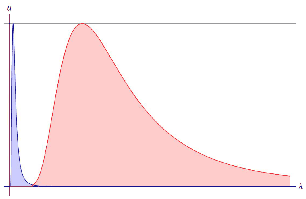

Figure 1 - The plot of \(u(\lambda,T_{\mathrm E})\) (red) and \(\gamma\tilde{u}_{\mathrm S}(\lambda)\) (blue) versus \(\lambda\)

B. The Greenhouse Effect

In this part, we introduce a simple model in which the Earth’s atmosphere is modeled as a thin layer at a small distance above the Earth’s surface so that the difference between the area of the atmosphere’s layer and the area of the Earth's surface can be neglected (see figure 2). In what follows assume that the major part of the thermal radiation from the Earth and the Sun are emitted at wavelengths near the \(\lambda_{\max}\) for each one. Also assume that the “atmosphere layer” reflects a fraction \(r_{\mathrm A}=0.255\) of the visible-ultraviolet radiation incident from above or below, and completely transmits the rest. Assume that the atmosphere does not reflect any part of the infrared radiation, however, it absorbs a fraction \(\varepsilon\) of the infrared radiation and transmits the rest. This behavior, known as the greenhouse effect, changes the average temperature of the Earth. The Earth’s surface, on the other hand, reflects a fraction \(r_{\mathrm E}\) of the visible-ultraviolet radiation and absorbs the rest of this radiation and all the infrared radiation.

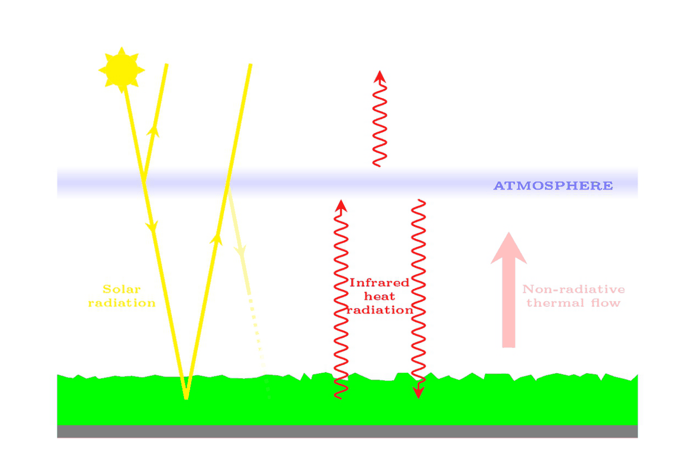
Figure 2 - Thermal flows between the Earth and the atmosphere

Part	Task	Points
B-1	Assume that \(\varepsilon=1\) and \(r_{\mathrm E}=0\), and calculate the Earth’s temperature \(T_{\mathrm E}\) and the atmosphere’s temperature \(T_{\mathrm A}\).	1.0 pt

Now assume that \(r_{\mathrm E}\ne0\). In this case, the combined system of “Earth + atmosphere” reflects a different fraction of the solar radiation, called “albedo” and denoted by \(\alpha\).

Part	Task	Points
B-2	Determine the albedo, \(\alpha\), in terms of \(r_{\mathrm E}\) and \(r_{\mathrm A}\). Then calculate its numerical value assuming \(r_{\mathrm E}=0.102\) (and \(r_{\mathrm A}=0.255\)).	1.6 pt
B-3	a) Express the Earth’s temperature in terms of \(\sigma\), \(\alpha\), \(S_0\), and \(\varepsilon\). b) Using the given data and the calculated albedo, find the numerical value of \(\varepsilon\) which leads to the current average temperature of \(T_{\mathrm E}=288\ \mathrm K\) for the Earth.	1.0 pt
B-4	Find \(\frac{dT_{\mathrm E}}{d\varepsilon}\) and determine by how much the Earth’s temperature increases if \(\varepsilon\) increases by one percent.	0.8 pt

Assume \(T_{\mathrm A}=245\ \mathrm K\) and \(T_{\mathrm E}=288\ \mathrm K\). These values come from real data and may differ from the results which you have obtained in the previous tasks. Now suppose that a non-radiative (e. g. convective) thermal flow \(J_{\mathrm{NR}}=k(T_{\mathrm E}-T_{\mathrm A})\) is maintained from the Earth to the atmosphere, where \(k\) is a constant. The quantity, \(J_{\mathrm{NR}}\), is the transmitted power per unit area.

Part	Task	Points
B-5	Calculate \(\varepsilon\) and \(k\) in terms of \(T_{\mathrm E}\), \(T_{\mathrm A}\), \(\sigma\), \(\alpha\), and \(S_0\).	1.6 pt
B-6	a) Differentiating the equations obtained in part B-5 with respect to \(\varepsilon\), find the two algebraic equations satisfied by \(\frac{dT_{\mathrm A}}{d\varepsilon}\) and \(\frac{dT_{\mathrm E}}{d\varepsilon}\). b) Use these equations to find the numerical value of change in the Earth’s temperature as a result of a one percent increase in the value of \(\varepsilon\).	1.0 pt

Official English text of the problem.

In recent decades, trapping and cooling atoms and ions has been a fascinating topic for physicists, with several Nobel prizes awarded for work in this area. In the first part of this question, we will explore a technique for trapping ions, known as the "Paul trap". Wolfgang Paul and Hans Dehmelt received one half of the 1989 Nobel Prize in Physics for this work. Next, we investigate the Doppler cooling technique, one of the works cited in the press release for the 1997 Nobel Prize in Physics awarded to Steven Chu, Claude Cohen-Tannoudji, and William Daniel Phillips "for developments of methods to cool and trap atoms with laser light".

A. The Paul Trap

It is known that with electrostatic fields, it is not possible to create a stable equilibrium for a charged particle. Therefore, creating a stable equilibrium point for ions requires more sophisticated techniques. The Paul trap is one of these techniques.

Consider a ring of charge with a radius \(R\) and a uniform positive linear charge density \(\lambda\). A positive point charge \(Q\) with mass \(m\) is placed at the center of the ring.

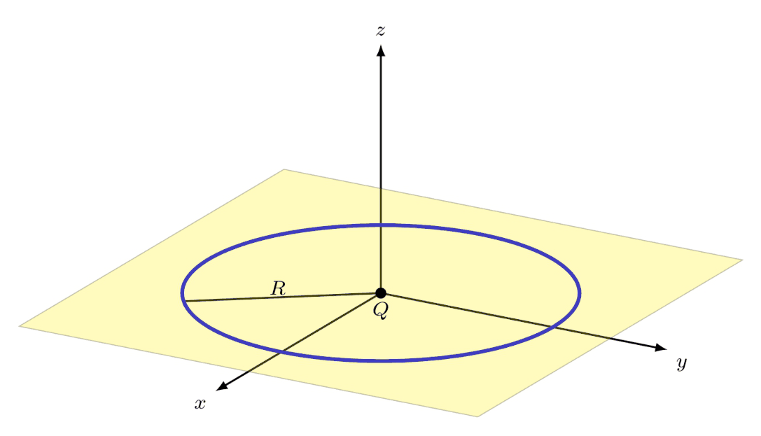
Figure 1 - A positively charged ring with a uniform linear charge density \(\lambda\) and radius \(R\): the origin of the coordinate system is at the center of the ring.

A-1

a) In cartesian coordinates \((x,y,z)\), obtain the electric field due to the charged ring in the vicinity of the ring’s center to the first order in \(x/R\), \(y/R\), and \(z/R\). b) Find the angular frequency of small oscillations of the charged particle around the center of the ring in the directions for which a stable equilibrium exists.

1.5 pt

In order to trap the charge \(Q\) fully, we would like to apply alternating fields to produce a dynamic equilibrium. Assume that the charge density is \(\lambda=\lambda_0+u\cos\Omega t\) in which \(\lambda_0\), \(u\), and \(\Omega\) are adjustable. We shall ignore radiative effects. Then the equation of motion for small displacements from the center of the ring, along the direction perpendicular to the plane of the ring will turn out to be:

\[ \ddot z=(+k^2+a\Omega^2\cos\Omega t)z \tag{1} \]

A-2

Write \(a\) and \(k\) in terms of the known parameters.

0.4 pt

We would like to obtain an approximate solution to Equation (1) by making the following simplifying assumptions: \(a\ll1\), \(\Omega\gg k\), and \(a\Omega^2\gg k^2\). With these assumptions, it can be shown that the solution of this equation can be split into two parts: \(z(t)=p(t)+q(t)\), where \(p(t)\) is a slowly varying component and \(q(t)\) is a small-amplitude rapidly-varying component with a mean value of zero. In other words, \(p(t)\) may be assumed constant over a few oscillations of \(q(t)\) (see Figure 2).

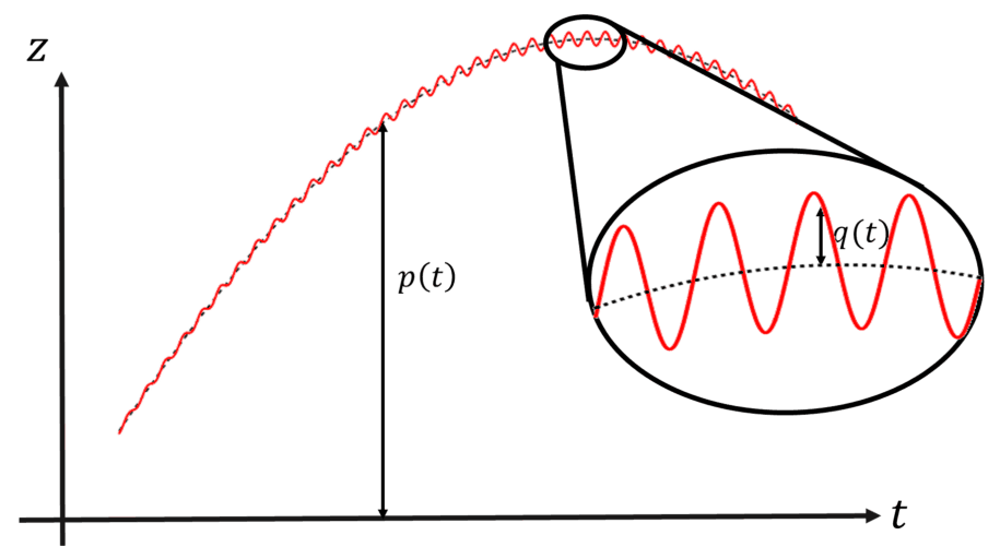
Figure 2 - A typical solution for the equation of motion of the charged particle: \(p(t)\) gives the overall motion, and \(q(t)\) represents small oscillations around this trajectory. The ellipse on the right is a magnification of a part of this trajectory.

A-3	a) Using the approximations stated above, find the equation of motion for \(q(t)\) in terms of \(a\), \(\Omega\), and \(p\). b) Find the solution of this equation by considering appropriate initial conditions corresponding to the required properties of this function.	1.8 pt
A-4	a) Using the mean effect of the rapidly varying component and obtain an effective equation of motion for \(p(t)\). b) Investigate the stability of the equilibrium point and find the condition for a stable equilibrium.	1.5 pt

Assume that \(\lambda_0=8\times10^{-9}\ \mathrm{C/m}\) and \(R=10\ \mathrm{cm}\). We would like to use this device to trap a singly ionized atom 100 times heavier than a hydrogen atom.

A-5

Calculate \(k\). Assume \(a=0.04\) and estimate the smallest frequency required to stabilize the motion of this ion. Use the data given at the end of the question.

0.4 pt

B. Doppler Cooling

It may be necessary to cool a trapped atom or ion. Assume that a trapped atom of mass \(m\), has two energy levels with an energy difference of \(E_0=\hbar\omega_{\mathrm A}\). Electrons in the lower level may absorb a photon and jump to the higher level, but after a period \(\tau\) they will return to the lower level and emit a photon with a frequency predominantly within \([\omega_{\mathrm A}-\Gamma,\omega_{\mathrm A}+\Gamma]\).

B-1

Use the Heisenberg’s uncertainty principle to find \(\Gamma\).

0.5 pt

With a similar reasoning, when we shine a laser light on the trapped atom, if the angular frequency of the laser, \(\omega_{\mathrm L}\), falls in the interval \([\omega_{\mathrm A}-\Gamma,\omega_{\mathrm A}+\Gamma]\), the atom may absorb the photon. Assume that the frequency \(\omega_{\mathrm L}\) of the laser light is slightly lower than \(\omega_{\mathrm A}\). For a particular device, the rate of photon absorption by an atom in the reference frame of the atom is given in Figure 3. The absorbed photon is then re-emitted in a random direction. To make things simple, we consider the problem in one dimension, i.e. we assume that the atoms can only move in the \(x\)-direction and the laser light shines on them both from the left and from the right. In the atom’s reference frame, the light has a higher or lower frequency due to the motion of the atoms. Since the velocity \(v\) of the atoms is very small, we only include terms of order \(v/c\) and ignore all the higher-order terms. Moreover, we have \(m\gg\hbar\omega_{\mathrm A}/c^2\) so that the velocity of the atom nearly does not change after absorbing the photon. Also, the change in frequency due to the Doppler effect is so small compared to \(\omega_{\mathrm A}-\omega_{\mathrm L}\), that the function for \(s\) in the diagram of Figure 3 may be approximated by the following linear function:

\[ s(\omega)=s_{\mathrm L}+\alpha(\omega-\omega_{\mathrm L}) \]

where \(s\) is the number of absorbed photons per unit of time, \(s_{\mathrm L}\) is the value of \(s\) for \(\omega=\omega_{\mathrm L}\), and \(\alpha\) is the slope of the line tangent to the curve at \(\omega_{\mathrm L}\). The frequency of the re-emitted photon is almost equal to the frequency of the incident photon, but it is emitted with equal probability in the positive or negative \(x\)-direction. In fact, up to the order considered here the two frequencies are identical. Note that we are considering the whole process in the atom’s reference frame.

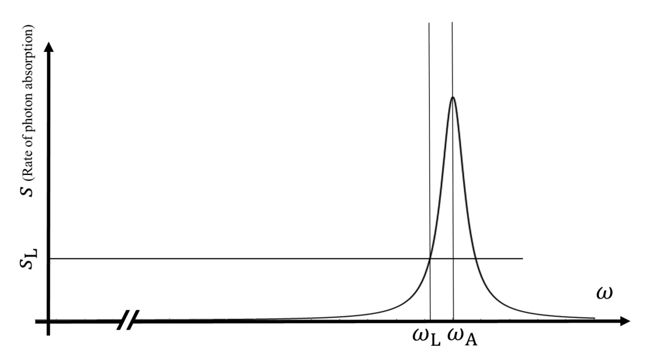
Figure 3 - The rate of photon absorption as a function of the frequency for a particular trap: the frequency corresponding to the energy difference between the two atomic levels is indicated by \(\omega_{\mathrm A}\) and the slighlty smaller frequency of the laser is indicated by \(\omega_{\mathrm L}\).

B-2

a) Assume that the trapped atom is moving with a velocity, \(v=v_x\) in the lab frame. In the frame of reference of the atom, calculate the collision rate of the photons, incident from each of the two directions, with the atoms (denoted by \(s_+\) and \(s_-\)) and the rate of absorption of momentum in each direction (denoted by \(\pi_+\) and \(\pi_-\)). b) Determine the effective force on the atom as a function of \(v\), \(k_{\mathrm L}=\omega_{\mathrm L}/c\), \(\hbar\), and \(\alpha\), in the reference frame of the laboratory. Assume \(s_{\mathrm L}\ll\alpha\omega_{\mathrm L}\),

1.7 pt

We would like to find the lowest temperature that can be achieved using this technique. Assume that the velocity of a particular atom has been reduced to zero exactly, and at this very moment it absorbs a photon (incident from any of the two directions), and re-emits the photon randomly in any of the two directions, with almost the same frequency. Assume that this process happens once every \(\tau\) units of time.

B-3	Considering the momentum of the atom after such a process for the two possible outcomes, calculate the average power absorbed by the atom.	1.0 pt
B-4	Consider the force calculated in Task B-2 and calculate the output power. Then, calculate the average value of \(v^2\) at equilibrium. Using your knowledge of the kinetic theory of gases estimate the temperature of the atoms.	0.8 pt
B-5	Estimate this temperature, for an atom 100 times heavier than a hydrogen atom. Assume that \(\omega_{\mathrm L}=2\times10^{16}\ \mathrm{rad/s}\), \(\tau=5\times10^{-9}\ \mathrm s\), and \(\alpha=4\).	0.4 pt

mass of hydrogen atom:	\(m_{\mathrm H}=1.674\times10^{-27}\ \mathrm{kg}\)
charge of an electron:	\(e=1.602\times10^{-19}\ \mathrm C\)
permittivity of free space:	\(\varepsilon_0=8.854\times10^{-12}\ \mathrm{F/m}\)
Boltzmann constant:	\(k_{\mathrm B}=1.381\times10^{-23}\ \mathrm{J/K}\)
Planck constant:	\(\hbar=1.055\times10^{-34}\ \mathrm{J\cdot s}\)

Official English text of the problem.

A significant number of the observed stars are binaries. One or both of the stars may be neutron stars rotating with a high angular velocity and emitting electromagnetic waves; such stars are called pulsars. Sometimes a companion star is an expansive mass of gas that gradually falls down onto the neutron star and causes its mass to increase (Figure 1-a). In this way, a neutron star gradually swallows up a portion of the mass of its companion star. For this reason, the neutron star has been compared to a black widow (or redback spider), a female spider which eats its mate after mating. The heating of the gas falling down onto the black widow generates radiation which can be observed. The heaviest neutron stars often are black widows and they serve as natural laboratories for testing fundamental physics. Figure 1-b shows the picture of the companion of the neutron star PSR J2215+5135, taken by the 3.4-meter optical telescope of the Iranian National Observatory. No neutron star can be seen in this image and the observed light is due to its companion.

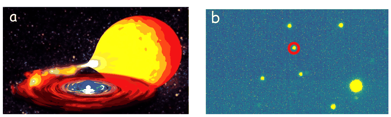
Figure 1 - (a) The falling gases of the companion star onto the neutron star - (b) The companion of the neutron star PSR J2215+5135

A. A Binary System

Consider a simple model in which the black widow and its companion star, are represented by two point masses \(M_1\) and \(M_2\) moving on a circular orbit around their center of mass. To investigate the dynamics of this system, consider a rotating coordinate system in which the two bodies are stationary. Take the center of mass to be the origin of the coordinate system. Assume that the two point masses lie on the \(x\)-axis on both sides of the origin at a distance \(a\) from each other, and that \(M_1\) lies on the negative \(x\)-axis. At an arbitrary point \((x,y)\) in the plane of motion, the effective potential \(\varphi(x,y)\) for a unit test mass is the sum of the gravitational potentials of the two point masses plus the centrifugal potential.

A-1	Write \(\varphi(x,y)\) in terms of \(M_1\), \(M_2\), \(G\), and \(a\).	1.0 pt
A-2	Assuming \(M_1>M_2\), plot the function \(\varphi(x,0)\) qualitatively.	0.7 pt

Suppose (just for task A-3) \(M_2=M_1/3\) and assume that \(M_2\) is surrounded by a rarefied gas of very low density. The mass of this gas is insignificant and we ignore its gravitational effects. If the size of this gas envelope becomes greater than a specific limit, the gas will overflow onto \(M_1\). Suppose the overflow occurs through \(x=x_0\) on the \(x\)-axis.

A-3

Find the numerical value of \(\dfrac{x_0}{a}\), up to two significant figures. You may use the calculator.

0.5 pt

Take the rotational period of the stars around their center of mass to be \(P\). Assume that mass flows from \(M_2\) to \(M_1\) at a very small rate of \(dM_1/dt=\beta\). This rate is so small that in each period of rotation, the distance between the two stars can be assumed to be constant. However, after a long period of time, the distance between the two stars changes, while the motion remains circular.

A-4

Calculate the rate of change of \(a\) and \(P\) in terms of \(\beta\), \(M_1\), \(M_2\), \(G\), and \(a\).

0.6 pt

The gas separated from \(M_2\) forms a disk rotating around \(M_1\) and heats up due to friction (Figure 1-a). As the gas loses energy, it spirals inward toward \(M_1\) and finally falls onto it. In the steady state, the mass flows at the constant rate of \(\beta\), from \(M_2\) to the disc and from the disc onto \(M_1\). At the same time, the heated disk emits thermal radiation as a blackbody. This disk forms very close to the neutron star so the gravitational pull of the \(M_2\) star can be ignored for the analysis of the disk’s motion. Also, ignore the heat capacity of the gas.

A-5

Determine the temperature of the disc at distance \(r\) from the center of the star \(M_1\) in terms of \(\beta\), \(M_1\), \(G\), and \(\sigma\) (Stefan-Boltzmann constant).

1.0 pt

In the binary system PSR J2215+5135, the mass of the neutron star is \(M_{\mathrm{NS}}=2.27\,M_\odot\) and the mass of its companion star is \(M_{\mathrm{S}}=0.33\,M_\odot\), where \(M_\odot=1.98\times10^{30}\ \mathrm{kg}\) is the mass of the Sun. The rotational period is \(P=4.14\ \mathrm{hr}\), and the Stefan-Boltzmann constant is \(\sigma=5.67\times10^{-8}\ \mathrm{W/m^2K^4}\), and the gravitational constant is \(G=6.67\times10^{-11}\ \mathrm{m^3/kg\,s^2}\).

Assume that the mass flow rate to the neutron star is \(\beta=\dot M_{\mathrm{NS}}=9\times10^{-10}\,M_\odot\,\mathrm{yr}^{-1}\).

A-6

Calculate the temperature of the disc at the radius \(r=\dfrac{a}{10}\) in kelvins.

0.5 pt

Assume that after a sudden explosion, the \(M_1\) star ejects a part of its mass out of the binary system at a very high speed, and its mass becomes \(M_1'\). Take the magnitude of the velocity of \(M_1'\) relative to \(M_2\) to be \(v'\) after the explosion.

A-7

Determine the maximum value of \(v'\), in terms of \(M_1'\), \(M_2\), \(G\), and \(a\), that allows the new binary system to stay bounded. Assuming that the explosion is isotropic, what is the minimum value of \(M_1'\) for the binary system to remain bounded?

0.7 pt

B. Analysis of the Stability of a Star

In this part we study the stability of a single star. Consider a star containing a specific kind of matter with the equation of state \(p=K\rho^\gamma\) where \(K\) and \(\gamma\) are constants. Let \(p(r)\) and \(\rho(r)\) be the pressure and density at a distance \(r\) from the center of the star, respectively. The pressure and density at the center of the star are \(p_c\) and \(\rho_c\), respectively. In all tasks of the part B, take all outward vectors to be positive.

B-1	Determine the gravitational acceleration \(g(r)\) near the center of the star in terms of \(r\) and the constants \(G\) and \(\rho_c\).	0.2 pt
B-2	Derive a (differential) equation for determining \(\rho(r)\) at equilibrium, and write it in the following form: \(\dfrac{d}{dr}\left[h_1(\rho,r)\dfrac{d\rho}{dr}\right]+h_2(r)\rho=0\). Find the functions \(h_1\) and \(h_2\).	0.6 pt
B-3	Construct a quantity \(r_0\) of the form \(r_0=G^l p_c^m\rho_c^n\) with the dimension of length.	0.4 pt
B-4	Rewrite the (differential) equation of task B-2 in the following form: \(\dfrac{d}{dx}\left[A_1(u,x)\dfrac{du}{dx}\right]+A_2(x)u(x)=0,\) where \(x=\dfrac{r}{r_0}\) and \(u=\dfrac{\rho}{\rho_c}\). Find the functions \(A_1(u,x)\) and \(A_2(x)\).	0.3 pt
B-5	For \(\gamma=2\) one finds \(u(x)=\dfrac{f(x)}{x}\). Determine \(f(x)\).	0.6 pt

Assume that for a particular star \(\dfrac{du}{dx}\), as a function of \(x\), is given by the curve given in Figure 2.

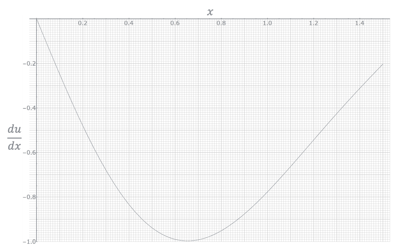
Figure 2 - The plot of \(\dfrac{du}{dx}\)

B-6

Use the behavior of the curve in Figure 2, in the vicinity of the point \(x=0\), to find \(\gamma\) up to 3 significant figures. Use the given ruler if necessary.

0.8 pt

To analyze the stability of the system, we assume that the star deviates slightly from its equilibrium state: we assume that the spherical shell, which was in equilibrium at radius \(r\), now has a radius \(\tilde r\), similarly the parameters \(g\), \(p\), and \(\rho\) have changed to \(\tilde g\), \(\tilde p\), and \(\tilde\rho\) respectively. For convenience, we shall only consider small \(r\)’s near the center of the star, for which we can assume that \(\tilde r=r(1+\varepsilon(t))\), where \(\varepsilon(t)\ll1\).

B-7	Find \(\tilde\rho\) and \(\tilde g\) in terms of \(\rho\) and \(g\) to the first order in \(\varepsilon\).	0.9 pt
B-8	Using Newton's equation of motion for the spherical layer with the equilibrium radius of \(r\) find \(\dfrac{d^2\tilde r}{dt^2}\) in terms of \(\tilde g\), \(\tilde\rho\), \(K\), \(\gamma\), and \(\dfrac{\partial\tilde\rho}{\partial\tilde r}\) (By \(\dfrac{\partial\tilde\rho}{\partial\tilde r}\) we mean derivative of \(\tilde\rho\) with respect to \(\tilde r\) at constant \(t\).)	0.6 pt
B-9	Obtain \(\dfrac{d^2\varepsilon}{dt^2}\) in terms of \(\varepsilon\) and the constants given in the problem. Find the minimum value of \(\gamma\) for a stable equilibrium, and find the oscillation's angular frequency of the star.	0.6 pt

Official English text of the problem.

Im Jahr 2021 wurde Syukuro Manabe und Klaus Hasselmann die Hälfte des Nobelpreises für Physik für ihre Arbeiten zur Modellierung des Erdklimas und zur zuverlässigen Vorhersage der durch menschliche Industrieaktivitäten verursachten globalen Erwärmung verliehen. In dieser Aufgabe untersuchen wir ein einfaches Modell der globalen Erwärmung durch den Treibhauseffekt. Die Treibhausgase verändern die optischen Eigenschaften der Erdatmosphäre hinsichtlich der Transmission und Absorption der Infrarotstrahlung der Erde, wodurch die mittlere Temperatur des Planeten ansteigt.

Alle Körper emittieren bei unterschiedlichen Temperaturen Wärmestrahlung. Die Größe \(u(\lambda,T)d\lambda\) gibt die thermische Strahlungsleistung pro Flächeneinheit eines Körpers bei der Temperatur \(T\) im Wellenlängenintervall zwischen \(\lambda\) und \(\lambda+d\lambda\) an. Nach der Planckschen Theorie der Schwarzkörperstrahlung gilt

\[ u(\lambda,T)=\frac{2\pi hc^2}{\lambda^5} \frac{1}{\exp\!\left(\frac{hc}{\lambda k_{\mathrm B}T}\right)-1}, \tag{1} \]

wobei \(hc=1.24\times10^3\ \mathrm{eV\cdot nm}\) und \(k_{\mathrm B}=8.62\times10^{-5}\ \mathrm{eV/K}\) sind. Die Wellenlänge, bei der \(u(\lambda,T)\) maximal ist, ergibt sich aus der Beziehung \(\lambda_{\max}T=b\) (Wiensches Verschiebungsgesetz). Mithilfe von Gleichung (1) lässt sich zeigen, dass \(b=\frac{hc}{x_mk_{\mathrm B}}\) gilt, wobei die dimensionslose Größe \(x_m\) die nichttriviale Lösung einer Gleichung der Form \(f(x)=0\) ist; in einer der folgenden Teilaufgaben sollen Sie die Funktion \(f(x)\) bestimmen. Die gesamte Strahlungsleistung pro Flächeneinheit eines schwarzen Körpers über alle Wellenlängen ist nach dem Stefan-Boltzmann-Gesetz durch \(U(T)=\sigma T^4\) gegeben, wobei \(\sigma=5.67\times10^{-8}\ \mathrm{W/m^2K^4}\) ist. Darüber hinaus gilt nach dem Kirchhoffschen Strahlungsgesetz: Ein Körper, der im thermischen Gleichgewicht bei einer bestimmten Wellenlänge einen bestimmten Anteil der einfallenden Strahlung absorbiert, emittiert bei derselben Wellenlänge denselben Anteil der Schwarzkörperstrahlung.

Nehmen Sie in dieser gesamten Aufgabe an, dass die Sonne ein schwarzer Körper mit ihrer mittleren Oberflächentemperatur von \(T_{\mathrm S}=5.77\times10^3\ \mathrm K\) ist. Der Sonnenradius beträgt \(R_{\mathrm S}=6.96\times10^8\ \mathrm m\), und der mittlere Abstand zwischen Erde und Sonne beträgt \(d=1.50\times10^{11}\ \mathrm m\). Mit \(\tilde{u}_{\mathrm S}(\lambda)\) bezeichnen wir die spektrale Sonnenstrahlungsleistung, die auf eine zur Strahlungsrichtung senkrechte Einheitsfläche an der Erde fällt. Das Integral dieser Größe über alle Wellenlängen, also \(S_0=\int\tilde{u}_{\mathrm S}(\lambda)d\lambda\), wird Solarkonstante genannt.

Nehmen Sie in dieser Aufgabe an, dass sich die Erde im thermischen Gleichgewicht befindet und an allen Punkten ihrer Oberfläche dieselbe Temperatur hat. Geben Sie in allen Teilaufgaben die gesuchte Größe zunächst als Formel in Abhängigkeit von den in der Aufgabe gegebenen Größen an und bestimmen Sie anschließend ihren Zahlenwert auf drei signifikante Stellen genau. Die erforderlichen Einheiten sind auf dem Antwortblatt angegeben.

A. Die Erde als schwarzer Körper

Betrachten Sie in diesem Teil die Erdoberfläche als schwarzen Körper und vernachlässigen Sie die Erdatmosphäre.

Teil	Aufgabe	Punkte
A-1	Bestimmen Sie die Solarkonstante \(S_0\).	0.6 Pkt.
A-2	Bestimmen Sie die Temperatur der Erde \(T_{\mathrm E}\).	0.6 Pkt.
A-3	Bestimmen Sie die Funktion \(f(x)\).	0.4 Pkt.
A-4	Berechnen Sie den Zahlenwert von \(x_m\) und bestimmen Sie aus diesem Wert \(x_m\) den Wert von \(b\).	0.4 Pkt.
A-5	Bestimmen Sie \(\lambda_{\max}\) für die Sonne und die Erde.	0.2 Pkt.

In Abbildung 1 sind die Funktionen \(\gamma\tilde{u}_{\mathrm S}(\lambda)\) und \(u(\lambda,T_{\mathrm E})\) gegen \(\lambda\) aufgetragen. Dabei ist \(\gamma\) ein dimensionsloser Koeffizient, mit dem \(\tilde{u}_{\mathrm S}(\lambda)\) so skaliert wird, dass die Werte der beiden Maxima übereinstimmen.

Teil	Aufgabe	Punkte
A-6	Bestimmen Sie \(\gamma\).	0.8 Pkt.

Abbildung 1 - Darstellung von \(u(\lambda,T_{\mathrm E})\) (rot) und \(\gamma\tilde{u}_{\mathrm S}(\lambda)\) (blau) in Abhängigkeit von \(\lambda\)

B. Der Treibhauseffekt

In diesem Teil führen wir ein einfaches Modell ein, in dem die Erdatmosphäre als dünne Schicht in geringer Höhe über der Erdoberfläche modelliert wird, sodass der Unterschied zwischen der Fläche der Atmosphärenschicht und der Fläche der Erdoberfläche vernachlässigt werden kann (siehe Abbildung 2). Nehmen Sie im Folgenden an, dass der überwiegende Teil der Wärmestrahlung von Erde und Sonne bei Wellenlängen in der Nähe des jeweiligen \(\lambda_{\max}\) emittiert wird. Nehmen Sie außerdem an, dass die „Atmosphärenschicht“ einen Anteil \(r_{\mathrm A}=0.255\) der von oben oder unten einfallenden sichtbaren und ultravioletten Strahlung reflektiert und den Rest vollständig durchlässt. Nehmen Sie an, dass die Atmosphäre keinen Anteil der Infrarotstrahlung reflektiert, jedoch einen Anteil \(\varepsilon\) der Infrarotstrahlung absorbiert und den Rest durchlässt. Dieses als Treibhauseffekt bekannte Verhalten verändert die mittlere Temperatur der Erde. Die Erdoberfläche hingegen reflektiert einen Anteil \(r_{\mathrm E}\) der sichtbaren und ultravioletten Strahlung und absorbiert den Rest dieser Strahlung sowie die gesamte Infrarotstrahlung.

Abbildung 2 - Wärmeströme zwischen Erde und Atmosphäre

Teil	Aufgabe	Punkte
B-1	Nehmen Sie \(\varepsilon=1\) und \(r_{\mathrm E}=0\) an und berechnen Sie die Temperatur der Erde \(T_{\mathrm E}\) und die Temperatur der Atmosphäre \(T_{\mathrm A}\).	1.0 Pkt.

Nehmen Sie nun \(r_{\mathrm E}\ne0\) an. In diesem Fall reflektiert das Gesamtsystem „Erde + Atmosphäre“ einen anderen Anteil der Sonnenstrahlung, der „Albedo“ genannt und mit \(\alpha\) bezeichnet wird.

Teil	Aufgabe	Punkte
B-2	Bestimmen Sie die Albedo \(\alpha\) in Abhängigkeit von \(r_{\mathrm E}\) und \(r_{\mathrm A}\). Berechnen Sie anschließend ihren Zahlenwert unter der Annahme \(r_{\mathrm E}=0.102\) (und \(r_{\mathrm A}=0.255\)).	1.6 Pkt.
B-3	a) Drücken Sie die Temperatur der Erde durch \(\sigma\), \(\alpha\), \(S_0\) und \(\varepsilon\) aus. b) Bestimmen Sie mithilfe der gegebenen Daten und der berechneten Albedo den Zahlenwert von \(\varepsilon\), der zur gegenwärtigen mittleren Temperatur der Erde von \(T_{\mathrm E}=288\ \mathrm K\) führt.	1.0 Pkt.
B-4	Bestimmen Sie \(\frac{dT_{\mathrm E}}{d\varepsilon}\) und ermitteln Sie, um wie viel die Temperatur der Erde steigt, wenn \(\varepsilon\) um ein Prozent zunimmt.	0.8 Pkt.

Nehmen Sie \(T_{\mathrm A}=245\ \mathrm K\) und \(T_{\mathrm E}=288\ \mathrm K\) an. Diese Werte stammen aus realen Daten und können von den Ergebnissen abweichen, die Sie in den vorherigen Teilaufgaben erhalten haben. Nehmen Sie nun an, dass ein nichtstrahlungsbedingter (z. B. konvektiver) Wärmestrom \(J_{\mathrm{NR}}=k(T_{\mathrm E}-T_{\mathrm A})\) von der Erde zur Atmosphäre aufrechterhalten wird, wobei \(k\) eine Konstante ist. Die Größe \(J_{\mathrm{NR}}\) ist die übertragene Leistung pro Flächeneinheit.

Teil	Aufgabe	Punkte
B-5	Berechnen Sie \(\varepsilon\) und \(k\) in Abhängigkeit von \(T_{\mathrm E}\), \(T_{\mathrm A}\), \(\sigma\), \(\alpha\) und \(S_0\).	1.6 Pkt.
B-6	a) Leiten Sie die in Teil B-5 erhaltenen Gleichungen nach \(\varepsilon\) ab und bestimmen Sie die beiden algebraischen Gleichungen, die \(\frac{dT_{\mathrm A}}{d\varepsilon}\) und \(\frac{dT_{\mathrm E}}{d\varepsilon}\) erfüllen. b) Bestimmen Sie mithilfe dieser Gleichungen den Zahlenwert der Änderung der Erdtemperatur infolge einer Zunahme von \(\varepsilon\) um ein Prozent.	1.0 Pkt.

Aufgabentext aus dem offiziellen englischen Text übersetzt.

Das Einfangen und Kühlen von Atomen und Ionen war in den letzten Jahrzehnten ein faszinierendes Thema für Physiker; für Arbeiten auf diesem Gebiet wurden mehrere Nobelpreise verliehen. Im ersten Teil dieser Aufgabe untersuchen wir eine Technik zum Einfangen von Ionen, die als „Paul-Falle“ bekannt ist. Wolfgang Paul und Hans Dehmelt erhielten für diese Arbeit die Hälfte des Nobelpreises für Physik des Jahres 1989. Anschließend untersuchen wir die Dopplerkühlung, eine der Arbeiten, die in der Pressemitteilung zum Nobelpreis für Physik des Jahres 1997 genannt wurden. Dieser wurde Steven Chu, Claude Cohen-Tannoudji und William Daniel Phillips „für die Entwicklung von Methoden zum Kühlen und Einfangen von Atomen mit Laserlicht“ verliehen.

A. Die Paul-Falle

Bekanntlich lässt sich mit elektrostatischen Feldern kein stabiles Gleichgewicht für ein geladenes Teilchen erzeugen. Um einen stabilen Gleichgewichtspunkt für Ionen zu schaffen, sind daher ausgefeiltere Techniken erforderlich. Die Paul-Falle ist eine dieser Techniken.

Betrachten Sie einen geladenen Ring mit dem Radius \(R\) und einer gleichmäßigen positiven linearen Ladungsdichte \(\lambda\). Eine positive Punktladung \(Q\) mit der Masse \(m\) befindet sich im Mittelpunkt des Rings.

Abbildung 1 - Ein positiv geladener Ring mit einer gleichmäßigen linearen Ladungsdichte \(\lambda\) und dem Radius \(R\): Der Ursprung des Koordinatensystems liegt im Mittelpunkt des Rings.

A-1

a) Bestimmen Sie in kartesischen Koordinaten \((x,y,z)\) das elektrische Feld des geladenen Rings in der Nähe seines Mittelpunkts bis zur ersten Ordnung in \(x/R\), \(y/R\) und \(z/R\). b) Bestimmen Sie die Kreisfrequenz kleiner Schwingungen des geladenen Teilchens um den Mittelpunkt des Rings in den Richtungen, in denen ein stabiles Gleichgewicht besteht.

1.5 Pkt.

Um die Ladung \(Q\) vollständig einzufangen, wollen wir Wechselfelder anlegen, die ein dynamisches Gleichgewicht erzeugen. Nehmen Sie an, dass die Ladungsdichte \(\lambda=\lambda_0+u\cos\Omega t\) beträgt, wobei \(\lambda_0\), \(u\) und \(\Omega\) einstellbar sind. Strahlungseffekte werden vernachlässigt. Dann ergibt sich für kleine Auslenkungen aus dem Mittelpunkt des Rings senkrecht zur Ringebene die folgende Bewegungsgleichung:

\[ \ddot z=(+k^2+a\Omega^2\cos\Omega t)z \tag{1} \]

A-2

Drücken Sie \(a\) und \(k\) durch die bekannten Parameter aus.

0.4 Pkt.

Wir wollen eine Näherungslösung von Gleichung (1) erhalten, indem wir die folgenden vereinfachenden Annahmen treffen: \(a\ll1\), \(\Omega\gg k\) und \(a\Omega^2\gg k^2\). Unter diesen Annahmen lässt sich zeigen, dass die Lösung dieser Gleichung in zwei Anteile zerlegt werden kann: \(z(t)=p(t)+q(t)\), wobei \(p(t)\) ein langsam veränderlicher Anteil und \(q(t)\) ein schnell veränderlicher Anteil mit kleiner Amplitude und dem Mittelwert null ist. Mit anderen Worten kann \(p(t)\) über einige Schwingungen von \(q(t)\) hinweg als konstant angenommen werden (siehe Abbildung 2).

Abbildung 2 - Eine typische Lösung der Bewegungsgleichung des geladenen Teilchens: \(p(t)\) beschreibt die übergeordnete Bewegung, und \(q(t)\) stellt kleine Schwingungen um diese Bahn dar. Die Ellipse rechts zeigt eine Vergrößerung eines Teils dieser Bahn.

A-3	a) Bestimmen Sie mithilfe der oben angegebenen Näherungen die Bewegungsgleichung für \(q(t)\) in Abhängigkeit von \(a\), \(\Omega\) und \(p\). b) Bestimmen Sie die Lösung dieser Gleichung unter Berücksichtigung geeigneter Anfangsbedingungen, die den geforderten Eigenschaften dieser Funktion entsprechen.	1.8 Pkt.
A-4	a) Nutzen Sie die gemittelte Wirkung des schnell veränderlichen Anteils, um eine effektive Bewegungsgleichung für \(p(t)\) zu erhalten. b) Untersuchen Sie die Stabilität des Gleichgewichtspunkts und bestimmen Sie die Bedingung für ein stabiles Gleichgewicht.	1.5 Pkt.

Nehmen Sie an, dass \(\lambda_0=8\times10^{-9}\ \mathrm{C/m}\) und \(R=10\ \mathrm{cm}\) sind. Wir wollen mit dieser Vorrichtung ein einfach ionisiertes Atom einfangen, das 100-mal so schwer wie ein Wasserstoffatom ist.

A-5

Berechnen Sie \(k\). Nehmen Sie \(a=0.04\) an und schätzen Sie die kleinste Frequenz ab, die erforderlich ist, um die Bewegung dieses Ions zu stabilisieren. Verwenden Sie die am Ende der Aufgabe angegebenen Daten.

0.4 Pkt.

B. Dopplerkühlung

Es kann erforderlich sein, ein eingefangenes Atom oder Ion zu kühlen. Nehmen Sie an, dass ein eingefangenes Atom der Masse \(m\) zwei Energieniveaus mit einer Energiedifferenz von \(E_0=\hbar\omega_{\mathrm A}\) besitzt. Elektronen im unteren Niveau können ein Photon absorbieren und in das höhere Niveau übergehen; nach einer Zeit \(\tau\) kehren sie jedoch in das untere Niveau zurück und emittieren ein Photon, dessen Frequenz überwiegend innerhalb von \([\omega_{\mathrm A}-\Gamma,\omega_{\mathrm A}+\Gamma]\) liegt.

B-1

Bestimmen Sie \(\Gamma\) mithilfe der Heisenbergschen Unschärferelation.

0.5 Pkt.

Mit einer ähnlichen Überlegung folgt: Wenn wir das eingefangene Atom mit Laserlicht bestrahlen und die Kreisfrequenz des Lasers, \(\omega_{\mathrm L}\), im Intervall \([\omega_{\mathrm A}-\Gamma,\omega_{\mathrm A}+\Gamma]\) liegt, kann das Atom das Photon absorbieren. Nehmen Sie an, dass die Frequenz \(\omega_{\mathrm L}\) des Laserlichts etwas kleiner als \(\omega_{\mathrm A}\) ist. Für eine bestimmte Vorrichtung ist die Rate der Photonenabsorption durch ein Atom im Bezugssystem des Atoms in Abbildung 3 dargestellt. Das absorbierte Photon wird anschließend in einer zufälligen Richtung wieder emittiert. Zur Vereinfachung betrachten wir das Problem eindimensional, d. h., wir nehmen an, dass sich die Atome nur in \(x\)-Richtung bewegen können und das Laserlicht sowohl von links als auch von rechts auf sie trifft. Im Bezugssystem des Atoms hat das Licht aufgrund der Bewegung der Atome eine höhere oder niedrigere Frequenz. Da die Geschwindigkeit \(v\) der Atome sehr klein ist, berücksichtigen wir nur Terme der Ordnung \(v/c\) und vernachlässigen alle Terme höherer Ordnung. Außerdem gilt \(m\gg\hbar\omega_{\mathrm A}/c^2\), sodass sich die Geschwindigkeit des Atoms nach der Absorption des Photons nahezu nicht ändert. Die Frequenzänderung durch den Dopplereffekt ist zudem im Vergleich zu \(\omega_{\mathrm A}-\omega_{\mathrm L}\) so klein, dass die Funktion für \(s\) im Diagramm von Abbildung 3 durch die folgende lineare Funktion angenähert werden kann:

\[ s(\omega)=s_{\mathrm L}+\alpha(\omega-\omega_{\mathrm L}) \]

Dabei ist \(s\) die Anzahl der pro Zeiteinheit absorbierten Photonen, \(s_{\mathrm L}\) der Wert von \(s\) für \(\omega=\omega_{\mathrm L}\) und \(\alpha\) die Steigung der Tangente an die Kurve bei \(\omega_{\mathrm L}\). Die Frequenz des wieder emittierten Photons ist nahezu gleich der Frequenz des einfallenden Photons, es wird jedoch mit gleicher Wahrscheinlichkeit in positiver oder negativer \(x\)-Richtung emittiert. Tatsächlich sind die beiden Frequenzen bis zu der hier betrachteten Ordnung identisch. Beachten Sie, dass wir den gesamten Vorgang im Bezugssystem des Atoms betrachten.

Abbildung 3 - Die Rate der Photonenabsorption als Funktion der Frequenz für eine bestimmte Falle: Die Frequenz, die der Energiedifferenz zwischen den beiden atomaren Niveaus entspricht, ist mit \(\omega_{\mathrm A}\) bezeichnet, die etwas kleinere Frequenz des Lasers mit \(\omega_{\mathrm L}\).

B-2

a) Nehmen Sie an, dass sich das eingefangene Atom im Laborsystem mit der Geschwindigkeit \(v=v_x\) bewegt. Berechnen Sie im Bezugssystem des Atoms die Kollisionsrate der aus den beiden Richtungen einfallenden Photonen mit den Atomen (bezeichnet mit \(s_+\) und \(s_-\)) sowie die Rate der Impulsaufnahme aus jeder Richtung (bezeichnet mit \(\pi_+\) und \(\pi_-\)). b) Bestimmen Sie im Bezugssystem des Labors die effektive Kraft auf das Atom als Funktion von \(v\), \(k_{\mathrm L}=\omega_{\mathrm L}/c\), \(\hbar\) und \(\alpha\). Nehmen Sie \(s_{\mathrm L}\ll\alpha\omega_{\mathrm L}\) an.

1.7 Pkt.

Wir wollen die niedrigste Temperatur bestimmen, die mit dieser Technik erreicht werden kann. Nehmen Sie an, dass die Geschwindigkeit eines bestimmten Atoms genau auf null reduziert wurde und dass es genau in diesem Moment ein Photon absorbiert (das aus einer der beiden Richtungen einfällt) und das Photon mit nahezu derselben Frequenz zufällig in eine der beiden Richtungen wieder emittiert. Nehmen Sie an, dass dieser Vorgang einmal pro Zeitintervall \(\tau\) stattfindet.

B-3	Betrachten Sie den Impuls des Atoms nach einem solchen Vorgang für die beiden möglichen Ergebnisse und berechnen Sie die mittlere vom Atom aufgenommene Leistung.	1.0 Pkt.
B-4	Betrachten Sie die in Teilaufgabe B-2 berechnete Kraft und berechnen Sie die abgegebene Leistung. Berechnen Sie anschließend den Mittelwert von \(v^2\) im Gleichgewicht. Schätzen Sie mithilfe Ihrer Kenntnisse der kinetischen Gastheorie die Temperatur der Atome ab.	0.8 Pkt.
B-5	Schätzen Sie diese Temperatur für ein Atom ab, das 100-mal so schwer wie ein Wasserstoffatom ist. Nehmen Sie \(\omega_{\mathrm L}=2\times10^{16}\ \mathrm{rad/s}\), \(\tau=5\times10^{-9}\ \mathrm s\) und \(\alpha=4\) an.	0.4 Pkt.

Masse des Wasserstoffatoms:	\(m_{\mathrm H}=1.674\times10^{-27}\ \mathrm{kg}\)
Ladung eines Elektrons:	\(e=1.602\times10^{-19}\ \mathrm C\)
Elektrische Feldkonstante:	\(\varepsilon_0=8.854\times10^{-12}\ \mathrm{F/m}\)
Boltzmann-Konstante:	\(k_{\mathrm B}=1.381\times10^{-23}\ \mathrm{J/K}\)
Planck-Konstante:	\(\hbar=1.055\times10^{-34}\ \mathrm{J\cdot s}\)

Aufgabentext aus dem offiziellen englischen Text übersetzt.

Ein erheblicher Anteil der beobachteten Sterne sind Doppelsterne. Einer oder beide Sterne können Neutronensterne sein, die mit hoher Winkelgeschwindigkeit rotieren und elektromagnetische Wellen aussenden; solche Sterne werden Pulsare genannt. Manchmal ist ein Begleitstern eine ausgedehnte Gasmasse, die allmählich auf den Neutronenstern fällt und dadurch dessen Masse vergrößert (Abbildung 1-a). Auf diese Weise verschlingt ein Neutronenstern nach und nach einen Teil der Masse seines Begleitsterns. Deshalb wurde der Neutronenstern mit einer Schwarzen Witwe (oder Rotrückenspinne) verglichen, einer weiblichen Spinne, die ihren Partner nach der Paarung frisst. Die Erwärmung des auf die Schwarze Witwe fallenden Gases erzeugt beobachtbare Strahlung. Die schwersten Neutronensterne sind häufig Schwarze Witwen und dienen als natürliche Laboratorien zur Überprüfung grundlegender Physik. Abbildung 1-b zeigt eine Aufnahme des Begleiters des Neutronensterns PSR J2215+5135, die mit dem optischen 3,4-Meter-Teleskop des Iranischen Nationalobservatoriums aufgenommen wurde. Auf diesem Bild ist kein Neutronenstern zu sehen; das beobachtete Licht stammt von seinem Begleiter.

Abbildung 1 - (a) Das vom Begleitstern auf den Neutronenstern fallende Gas - (b) Der Begleiter des Neutronensterns PSR J2215+5135

A. Ein Doppelsternsystem

Betrachten Sie ein einfaches Modell, in dem die Schwarze Witwe und ihr Begleitstern durch zwei Punktmassen \(M_1\) und \(M_2\) dargestellt werden, die sich auf Kreisbahnen um ihren gemeinsamen Schwerpunkt bewegen. Um die Dynamik dieses Systems zu untersuchen, betrachten Sie ein rotierendes Koordinatensystem, in dem die beiden Körper ruhen. Wählen Sie den Schwerpunkt als Ursprung des Koordinatensystems. Nehmen Sie an, dass die beiden Punktmassen auf der \(x\)-Achse auf entgegengesetzten Seiten des Ursprungs im Abstand \(a\) voneinander liegen und dass \(M_1\) auf der negativen \(x\)-Achse liegt. An einem beliebigen Punkt \((x,y)\) in der Bewegungsebene ist das effektive Potential \(\varphi(x,y)\) für eine Testmasse der Größe eins die Summe der Gravitationspotentiale der beiden Punktmassen und des Zentrifugalpotentials.

A-1	Geben Sie \(\varphi(x,y)\) in Abhängigkeit von \(M_1\), \(M_2\), \(G\) und \(a\) an.	1.0 Pkt.
A-2	Skizzieren Sie unter der Annahme \(M_1>M_2\) den qualitativen Verlauf der Funktion \(\varphi(x,0)\).	0.7 Pkt.

Nehmen Sie (nur für Aufgabe A-3) an, dass \(M_2=M_1/3\) gilt und \(M_2\) von einem verdünnten Gas sehr geringer Dichte umgeben ist. Die Masse dieses Gases ist unbedeutend, und wir vernachlässigen seine Gravitationswirkung. Überschreitet die Größe dieser Gashülle einen bestimmten Grenzwert, strömt Gas auf \(M_1\) über. Nehmen Sie an, dass das Überströmen durch \(x=x_0\) auf der \(x\)-Achse erfolgt.

A-3

Bestimmen Sie den Zahlenwert von \(\dfrac{x_0}{a}\) auf zwei signifikante Stellen. Sie dürfen den Taschenrechner verwenden.

0.5 Pkt.

Die Umlaufdauer der Sterne um ihren gemeinsamen Schwerpunkt sei \(P\). Nehmen Sie an, dass Masse mit einer sehr geringen Rate von \(dM_1/dt=\beta\) von \(M_2\) zu \(M_1\) strömt. Diese Rate ist so gering, dass der Abstand zwischen den beiden Sternen während jeder Umlaufperiode als konstant angenommen werden kann. Über einen langen Zeitraum ändert sich jedoch der Abstand zwischen den beiden Sternen, während ihre Bahnen kreisförmig bleiben.

A-4

Berechnen Sie die Änderungsraten von \(a\) und \(P\) in Abhängigkeit von \(\beta\), \(M_1\), \(M_2\), \(G\) und \(a\).

0.6 Pkt.

Das von \(M_2\) abgelöste Gas bildet eine um \(M_1\) rotierende Scheibe und erwärmt sich durch Reibung (Abbildung 1-a). Während das Gas Energie verliert, bewegt es sich spiralförmig nach innen auf \(M_1\) zu und fällt schließlich auf den Stern. Im stationären Zustand strömt die Masse mit der konstanten Rate \(\beta\) von \(M_2\) zur Scheibe und von der Scheibe auf \(M_1\). Gleichzeitig emittiert die erhitzte Scheibe Wärmestrahlung wie ein schwarzer Körper. Diese Scheibe bildet sich sehr nahe am Neutronenstern, sodass die Gravitationskraft des Sterns \(M_2\) bei der Untersuchung der Scheibenbewegung vernachlässigt werden kann. Vernachlässigen Sie außerdem die Wärmekapazität des Gases.

A-5

Bestimmen Sie die Temperatur der Scheibe im Abstand \(r\) vom Zentrum des Sterns \(M_1\) in Abhängigkeit von \(\beta\), \(M_1\), \(G\) und \(\sigma\) (Stefan-Boltzmann-Konstante).

1.0 Pkt.

Im Doppelsternsystem PSR J2215+5135 beträgt die Masse des Neutronensterns \(M_{\mathrm{NS}}=2.27\,M_\odot\) und die Masse seines Begleitsterns \(M_{\mathrm{S}}=0.33\,M_\odot\), wobei \(M_\odot=1.98\times10^{30}\ \mathrm{kg}\) die Sonnenmasse ist. Die Umlaufdauer beträgt \(P=4.14\ \mathrm{hr}\), die Stefan-Boltzmann-Konstante ist \(\sigma=5.67\times10^{-8}\ \mathrm{W/m^2K^4}\), und die Gravitationskonstante ist \(G=6.67\times10^{-11}\ \mathrm{m^3/kg\,s^2}\).

Nehmen Sie an, dass die Massenstromrate zum Neutronenstern \(\beta=\dot M_{\mathrm{NS}}=9\times10^{-10}\,M_\odot\,\mathrm{yr}^{-1}\) beträgt.

A-6

Berechnen Sie die Temperatur der Scheibe beim Radius \(r=\dfrac{a}{10}\) in Kelvin.

0.5 Pkt.

Nehmen Sie an, dass der Stern \(M_1\) bei einer plötzlichen Explosion einen Teil seiner Masse mit sehr hoher Geschwindigkeit aus dem Doppelsternsystem ausstößt und seine Masse danach \(M_1'\) beträgt. Der Betrag der Geschwindigkeit von \(M_1'\) relativ zu \(M_2\) nach der Explosion sei \(v'\).

A-7

Bestimmen Sie den maximalen Wert von \(v'\) in Abhängigkeit von \(M_1'\), \(M_2\), \(G\) und \(a\), bei dem das neue Doppelsternsystem gebunden bleiben kann. Welchen minimalen Wert muss \(M_1'\) unter der Annahme einer isotropen Explosion haben, damit das Doppelsternsystem gebunden bleibt?

0.7 Pkt.

B. Untersuchung der Stabilität eines Sterns

In diesem Teil untersuchen wir die Stabilität eines einzelnen Sterns. Betrachten Sie einen Stern, der eine bestimmte Art von Materie mit der Zustandsgleichung \(p=K\rho^\gamma\) enthält, wobei \(K\) und \(\gamma\) Konstanten sind. Es seien \(p(r)\) und \(\rho(r)\) der Druck bzw. die Dichte im Abstand \(r\) vom Zentrum des Sterns. Der Druck und die Dichte im Zentrum des Sterns seien \(p_c\) bzw. \(\rho_c\). Wählen Sie in allen Aufgaben von Teil B für alle Vektoren die nach außen gerichtete Richtung als positiv.

B-1	Bestimmen Sie die Gravitationsbeschleunigung \(g(r)\) nahe dem Zentrum des Sterns in Abhängigkeit von \(r\) und den Konstanten \(G\) und \(\rho_c\).	0.2 Pkt.
B-2	Leiten Sie eine (Differential-)Gleichung zur Bestimmung von \(\rho(r)\) im Gleichgewicht her und schreiben Sie sie in der folgenden Form: \(\dfrac{d}{dr}\left[h_1(\rho,r)\dfrac{d\rho}{dr}\right]+h_2(r)\rho=0\). Bestimmen Sie die Funktionen \(h_1\) und \(h_2\).	0.6 Pkt.
B-3	Konstruieren Sie eine Größe \(r_0\) der Form \(r_0=G^l p_c^m\rho_c^n\) mit der Dimension einer Länge.	0.4 Pkt.
B-4	Schreiben Sie die (Differential-)Gleichung aus Aufgabe B-2 in der folgenden Form um: \(\dfrac{d}{dx}\left[A_1(u,x)\dfrac{du}{dx}\right]+A_2(x)u(x)=0,\) wobei \(x=\dfrac{r}{r_0}\) und \(u=\dfrac{\rho}{\rho_c}\) gelten. Bestimmen Sie die Funktionen \(A_1(u,x)\) und \(A_2(x)\).	0.3 Pkt.
B-5	Für \(\gamma=2\) erhält man \(u(x)=\dfrac{f(x)}{x}\). Bestimmen Sie \(f(x)\).	0.6 Pkt.

Nehmen Sie an, dass für einen bestimmten Stern \(\dfrac{du}{dx}\) als Funktion von \(x\) durch die Kurve in Abbildung 2 gegeben ist.

Abbildung 2 - Der Graph von \(\dfrac{du}{dx}\)

B-6

Nutzen Sie das Verhalten der Kurve in Abbildung 2 in der Nähe des Punktes \(x=0\), um \(\gamma\) auf 3 signifikante Stellen zu bestimmen. Verwenden Sie bei Bedarf das bereitgestellte Lineal.

0.8 Pkt.

Zur Untersuchung der Stabilität des Systems nehmen wir an, dass der Stern geringfügig von seinem Gleichgewichtszustand abweicht: Wir nehmen an, dass die Kugelschale, die sich beim Radius \(r\) im Gleichgewicht befand, nun den Radius \(\tilde r\) hat; entsprechend haben sich die Größen \(g\), \(p\) und \(\rho\) zu \(\tilde g\), \(\tilde p\) bzw. \(\tilde\rho\) geändert. Der Einfachheit halber betrachten wir nur kleine \(r\) nahe dem Zentrum des Sterns, für die wir \(\tilde r=r(1+\varepsilon(t))\) mit \(\varepsilon(t)\ll1\) annehmen können.

B-7	Bestimmen Sie \(\tilde\rho\) und \(\tilde g\) in Abhängigkeit von \(\rho\) und \(g\) bis zur ersten Ordnung in \(\varepsilon\).	0.9 Pkt.
B-8	Bestimmen Sie mithilfe der Newtonschen Bewegungsgleichung für die Kugelschale mit dem Gleichgewichtsradius \(r\) den Ausdruck \(\dfrac{d^2\tilde r}{dt^2}\) in Abhängigkeit von \(\tilde g\), \(\tilde\rho\), \(K\), \(\gamma\) und \(\dfrac{\partial\tilde\rho}{\partial\tilde r}\). (Mit \(\dfrac{\partial\tilde\rho}{\partial\tilde r}\) ist die Ableitung von \(\tilde\rho\) nach \(\tilde r\) bei konstantem \(t\) gemeint.)	0.6 Pkt.
B-9	Bestimmen Sie \(\dfrac{d^2\varepsilon}{dt^2}\) in Abhängigkeit von \(\varepsilon\) und den in der Aufgabe angegebenen Konstanten. Bestimmen Sie den minimalen Wert von \(\gamma\) für ein stabiles Gleichgewicht sowie die Kreisfrequenz der Schwingung des Sterns.	0.6 Pkt.

Aufgabentext aus dem offiziellen englischen Text übersetzt.

2021 yılında Syukuro Manabe ve Klaus Hasselmann, Dünya'nın iklimini modelleme ve insanların endüstriyel faaliyetlerinden kaynaklanan küresel ısınmayı doğru biçimde öngörme konusundaki çalışmaları nedeniyle Nobel Fizik Ödülü'nün yarısına layık görüldüler. Bu soruda, sera etkisine bağlı küresel ısınmanın basit bir modelini inceleyeceğiz. Sera gazları, Dünya atmosferinin Dünya'dan yayılan kızılötesi ışınımı geçirme veya soğurma ile ilgili optik özelliklerini değiştirerek gezegenin ortalama sıcaklığının yükselmesine neden olur.

Farklı sıcaklıklardaki tüm cisimler ısıl ışınım yayar. \(u(\lambda,T)d\lambda\) niceliği, \(T\) sıcaklığındaki bir cismin \(\lambda\) ile \(\lambda+d\lambda\) dalga boyları arasında birim alan başına yaydığı ısıl ışınım gücünü gösterir. Planck'ın kara cisim ışınımı kuramına göre

\[ u(\lambda,T)=\frac{2\pi hc^2}{\lambda^5} \frac{1}{\exp\!\left(\frac{hc}{\lambda k_{\mathrm B}T}\right)-1}, \tag{1} \]

burada \(hc=1.24\times10^3\ \mathrm{eV\cdot nm}\) ve \(k_{\mathrm B}=8.62\times10^{-5}\ \mathrm{eV/K}\) değerlerindedir. \(u(\lambda,T)\) fonksiyonunun maksimumuna karşılık gelen dalga boyu, \(\lambda_{\max}T=b\) bağıntısından (Wien kayma yasası) bulunur. Nitekim denklem (1) kullanılarak \(b=\frac{hc}{x_mk_{\mathrm B}}\) olduğu gösterilebilir; burada boyutsuz \(x_m\) niceliği, \(f(x)=0\) biçimindeki bir denklemin aşikâr olmayan köküdür; aşağıdaki görevlerden birinde \(f(x)\) fonksiyonunu bulmanız istenmektedir. Bir kara cismin tüm dalga boylarında birim alan başına yaydığı toplam ışınım gücü, Stefan–Boltzmann yasasıyla \(U(T)=\sigma T^4\) olarak verilir; burada \(\sigma=5.67\times10^{-8}\ \mathrm{W/m^2K^4}\) değerindedir. Ayrıca Kirchhoff'un ışınım yasasına göre, ısıl dengede belirli bir dalga boyunda üzerine gelen ışınımın belli bir oranını soğuran bir cisim, aynı dalga boyunda kara cisim ışınımının aynı oranı kadar ışınım yayar.

Bu soru boyunca Güneş'in, ortalama yüzey sıcaklığı olan \(T_{\mathrm S}=5.77\times10^3\ \mathrm K\) sıcaklığında bir kara cisim olduğunu varsayın. Güneş'in yarıçapı \(R_{\mathrm S}=6.96\times10^8\ \mathrm m\), Dünya ile Güneş arasındaki ortalama uzaklık ise \(d=1.50\times10^{11}\ \mathrm m\) değerindedir. Dünya üzerinde ışınım doğrultusuna dik birim alana gelen Güneş ışınımının spektral gücünü \(\tilde{u}_{\mathrm S}(\lambda)\) ile gösteriyoruz. Bu niceliğin tüm dalga boyları üzerinden integrali, yani \(S_0=\int\tilde{u}_{\mathrm S}(\lambda)d\lambda\), Güneş sabiti olarak adlandırılır.

Bu soruda Dünya'nın ısıl dengede olduğunu ve yüzeyinin tüm noktalarında aynı sıcaklığa sahip olduğunu varsayın. Sorunun tüm bölümlerinde, istenen niceliği önce soruda verilen veriler cinsinden parametrik biçimde ifade edin, ardından sayısal değerini üç anlamlı basamakla bulun. Gerekli birimler cevap kâğıdında belirtilmiştir.

A. Kara Cisim Olarak Dünya

Bu bölümde Dünya'nın yüzeyini bir kara cisim olarak ele alın ve Dünya'nın atmosferini ihmal edin.

Bölüm	Görev	Puan
A-1	Güneş sabiti \(S_0\)'ı bulun.	0.6 puan
A-2	Dünya'nın sıcaklığı \(T_{\mathrm E}\)'yi bulun.	0.6 puan
A-3	\(f(x)\) fonksiyonunu bulun.	0.4 puan
A-4	\(x_m\)'nin sayısal değerini hesaplayın ve bu \(x_m\) değerinden \(b\)'nin değerini bulun.	0.4 puan
A-5	Güneş ve Dünya için \(\lambda_{\max}\)'ı bulun.	0.2 puan

Şekil 1'de \(\gamma\tilde{u}_{\mathrm S}(\lambda)\) ve \(u(\lambda,T_{\mathrm E})\) fonksiyonları \(\lambda\)'ya bağlı olarak çizilmiştir; burada \(\gamma\), iki tepe değerinin eşit olmasını sağlayacak şekilde \(\tilde{u}_{\mathrm S}(\lambda)\)'yı yeniden ölçeklendiren boyutsuz bir katsayıdır.

Bölüm	Görev	Puan
A-6	\(\gamma\)'yı belirleyin.	0.8 puan

Şekil 1 - \(u(\lambda,T_{\mathrm E})\) (kırmızı) ve \(\gamma\tilde{u}_{\mathrm S}(\lambda)\) (mavi) fonksiyonlarının \(\lambda\)'ya bağlı grafiği

B. Sera Etkisi

Bu bölümde, Dünya atmosferinin Dünya yüzeyinin biraz üzerinde ince bir tabaka olarak modellendiği basit bir model sunuyoruz; böylece atmosfer tabakasının alanı ile Dünya yüzeyinin alanı arasındaki fark ihmal edilebilir (bkz. şekil 2). Bundan sonra, Dünya ve Güneş'ten yayılan ısıl ışınımın büyük kısmının, her birinin kendi \(\lambda_{\max}\) değerine yakın dalga boylarında yayıldığını varsayın. Ayrıca “atmosfer tabakasının” yukarıdan veya aşağıdan gelen görünür-morötesi ışınımın \(r_{\mathrm A}=0.255\) oranındaki kısmını yansıttığını ve geri kalanını tamamen geçirdiğini varsayın. Atmosferin kızılötesi ışınımın hiçbir kısmını yansıtmadığını, ancak kızılötesi ışınımın \(\varepsilon\) oranındaki kısmını soğurduğunu ve geri kalanını geçirdiğini varsayın. Sera etkisi olarak bilinen bu davranış, Dünya'nın ortalama sıcaklığını değiştirir. Dünya'nın yüzeyi ise görünür-morötesi ışınımın \(r_{\mathrm E}\) oranındaki kısmını yansıtır ve bu ışınımın geri kalanını ve kızılötesi ışınımın tamamını soğurur.

Şekil 2 - Dünya ile atmosfer arasındaki ısı akışları

Bölüm	Görev	Puan
B-1	\(\varepsilon=1\) ve \(r_{\mathrm E}=0\) olduğunu varsayarak Dünya'nın sıcaklığı \(T_{\mathrm E}\)'yi ve atmosferin sıcaklığı \(T_{\mathrm A}\)'yı hesaplayın.	1.0 puan

Şimdi \(r_{\mathrm E}\ne0\) olduğunu varsayın. Bu durumda “Dünya + atmosfer” birleşik sistemi, Güneş ışınımının “albedo” olarak adlandırılan ve \(\alpha\) ile gösterilen farklı bir oranını yansıtır.

Bölüm	Görev	Puan
B-2	Albedo \(\alpha\)'yı \(r_{\mathrm E}\) ve \(r_{\mathrm A}\) cinsinden belirleyin. Ardından \(r_{\mathrm E}=0.102\) (ve \(r_{\mathrm A}=0.255\)) olduğunu varsayarak sayısal değerini hesaplayın.	1.6 puan
B-3	a) Dünya'nın sıcaklığını \(\sigma\), \(\alpha\), \(S_0\) ve \(\varepsilon\) cinsinden ifade edin. b) Verilen verileri ve hesaplanan albedoyu kullanarak, Dünya'nın günümüzdeki ortalama sıcaklığı olan \(T_{\mathrm E}=288\ \mathrm K\) değerini veren \(\varepsilon\)'nun sayısal değerini bulun.	1.0 puan
B-4	\(\frac{dT_{\mathrm E}}{d\varepsilon}\)'nu bulun ve \(\varepsilon\) yüzde bir arttığında Dünya'nın sıcaklığının ne kadar artacağını belirleyin.	0.8 puan

\(T_{\mathrm A}=245\ \mathrm K\) ve \(T_{\mathrm E}=288\ \mathrm K\) olduğunu varsayın. Bu değerler gerçek verilerden elde edilmiştir ve önceki görevlerde bulduğunuz sonuçlardan farklı olabilir. Şimdi Dünya'dan atmosfere doğru \(J_{\mathrm{NR}}=k(T_{\mathrm E}-T_{\mathrm A})\) şeklinde ışınım dışı (örneğin taşınımla gerçekleşen) bir ısı akışının sürdüğünü varsayın; burada \(k\) bir sabittir. \(J_{\mathrm{NR}}\) niceliği, birim alan başına aktarılan güçtür.

Bölüm	Görev	Puan
B-5	\(\varepsilon\) ve \(k\)'yı \(T_{\mathrm E}\), \(T_{\mathrm A}\), \(\sigma\), \(\alpha\) ve \(S_0\) cinsinden hesaplayın.	1.6 puan
B-6	a) Bölüm B-5'te elde edilen denklemlerin \(\varepsilon\)'na göre türevini alarak, \(\frac{dT_{\mathrm A}}{d\varepsilon}\) ve \(\frac{dT_{\mathrm E}}{d\varepsilon}\)'nun sağladığı iki cebirsel denklemi bulun. b) Bu denklemleri kullanarak, \(\varepsilon\)'nun değerindeki yüzde birlik artış sonucunda Dünya'nın sıcaklığında meydana gelen değişimin sayısal değerini bulun.	1.0 puan

Soru metni resmi İngilizce metinden çevrilmiştir.

Son birkaç on yılda atomların ve iyonların tuzaklanması ve soğutulması, fizikçiler için ilgi çekici bir konu olmuş ve bu alandaki çalışmalar birçok Nobel ödülüne layık görülmüştür. Bu sorunun ilk bölümünde, iyonları tuzaklamak için kullanılan ve "Paul tuzağı" olarak bilinen bir tekniği inceleyeceğiz. Wolfgang Paul ve Hans Dehmelt, bu çalışmaları nedeniyle 1989 Nobel Fizik Ödülü'nün yarısını paylaşmıştır. Ardından, Steven Chu, Claude Cohen-Tannoudji ve William Daniel Phillips'e "atomları lazer ışığıyla soğutma ve tuzaklama yöntemlerini geliştirmelerinden dolayı" verilen 1997 Nobel Fizik Ödülü'nün basın açıklamasında anılan çalışmalardan biri olan Doppler soğutma tekniğini inceleyeceğiz.

A. Paul Tuzağı

Elektrostatik alanlarla yüklü bir parçacık için kararlı bir denge oluşturmanın mümkün olmadığı bilinmektedir. Bu nedenle, iyonlar için kararlı bir denge noktası oluşturmak daha gelişmiş teknikler gerektirir. Paul tuzağı bu tekniklerden biridir.

Yarıçapı \(R\) olan, düzgün dağılmış pozitif doğrusal yük yoğunluğu \(\lambda\) olan bir yük halkasını ele alalım. Kütlesi \(m\) olan pozitif bir \(Q\) noktasal yükü, halkanın merkezine yerleştirilmiştir.

Şekil 1 - Düzgün dağılmış doğrusal yük yoğunluğu \(\lambda\) ve yarıçapı \(R\) olan pozitif yüklü bir halka: koordinat sisteminin başlangıç noktası halkanın merkezindedir.

A-1

a) Kartezyen koordinatlarda \((x,y,z)\), yüklü halkanın merkezinin yakınında oluşturduğu elektrik alanı \(x/R\), \(y/R\) ve \(z/R\) cinsinden birinci mertebeye kadar elde ediniz. b) Kararlı dengenin bulunduğu doğrultularda, yüklü parçacığın halkanın merkezi çevresindeki küçük salınımlarının açısal frekansını bulunuz.

1.5 puan

\(Q\) yükünü tüm doğrultularda tuzaklamak için, değişken alanlar uygulayarak dinamik bir denge oluşturmak istiyoruz. Yük yoğunluğunun \(\lambda=\lambda_0+u\cos\Omega t\) olduğunu ve burada \(\lambda_0\), \(u\) ve \(\Omega\) değerlerinin ayarlanabildiğini varsayınız. Işınım etkilerini ihmal edeceğiz. Bu durumda, halkanın merkezinden halka düzlemine dik doğrultudaki küçük yer değiştirmeler için hareket denklemi şu biçimde olacaktır:

\[ \ddot z=(+k^2+a\Omega^2\cos\Omega t)z \tag{1} \]

A-2

\(a\) ve \(k\)'yı bilinen parametreler cinsinden yazınız.

0.4 puan

Şu basitleştirici varsayımları yaparak Denklem (1)'in yaklaşık bir çözümünü elde etmek istiyoruz: \(a\ll1\), \(\Omega\gg k\) ve \(a\Omega^2\gg k^2\). Bu varsayımlarla, bu denklemin çözümünün iki kısma ayrılabileceği gösterilebilir: \(z(t)=p(t)+q(t)\); burada \(p(t)\) yavaş değişen bir bileşen, \(q(t)\) ise ortalama değeri sıfır olan, küçük genlikli ve hızlı değişen bir bileşendir. Başka bir deyişle, \(q(t)\)'nin birkaç salınımı boyunca \(p(t)\) sabit kabul edilebilir (bkz. Şekil 2).

Şekil 2 - Yüklü parçacığın hareket denklemi için tipik bir çözüm: \(p(t)\) genel hareketi verirken \(q(t)\) bu yörüngenin çevresindeki küçük salınımları temsil eder. Sağdaki elips, bu yörüngenin bir kısmının büyütülmüş görünümüdür.

A-3	a) Yukarıda belirtilen yaklaşımları kullanarak \(q(t)\)'nin hareket denklemini \(a\), \(\Omega\) ve \(p\) cinsinden bulunuz. b) Bu fonksiyonun sahip olması gereken özelliklere karşılık gelen uygun başlangıç koşullarını dikkate alarak bu denklemin çözümünü bulunuz.	1.8 puan
A-4	a) Hızlı değişen bileşenin ortalama etkisini kullanarak \(p(t)\) için etkin bir hareket denklemi elde ediniz. b) Denge noktasının kararlılığını inceleyiniz ve kararlı denge koşulunu bulunuz.	1.5 puan

\(\lambda_0=8\times10^{-9}\ \mathrm{C/m}\) ve \(R=10\ \mathrm{cm}\) olduğunu varsayınız. Bu düzeneği, hidrojen atomundan 100 kat daha ağır, tek iyonlaşmış bir atomu tuzaklamak için kullanmak istiyoruz.

A-5

\(k\)'yı hesaplayınız. \(a=0.04\) olduğunu varsayarak bu iyonun hareketini kararlı hâle getirmek için gereken en küçük frekansı tahmin ediniz. Sorunun sonunda verilen verileri kullanınız.

0.4 puan

B. Doppler Soğutması

Tuzaklanmış bir atomu veya iyonu soğutmak gerekebilir. Kütlesi \(m\) olan tuzaklanmış bir atomun, aralarındaki enerji farkı \(E_0=\hbar\omega_{\mathrm A}\) olan iki enerji düzeyine sahip olduğunu varsayınız. Alt düzeydeki elektronlar bir foton soğurarak üst düzeye geçebilir; ancak \(\tau\) süresinin ardından alt düzeye döner ve frekansı ağırlıklı olarak \([\omega_{\mathrm A}-\Gamma,\omega_{\mathrm A}+\Gamma]\) aralığında olan bir foton yayarlar.

B-1

Heisenberg belirsizlik ilkesini kullanarak \(\Gamma\)'yı bulunuz.

0.5 puan

Benzer bir akıl yürütmeyle, tuzaklanmış atoma lazer ışığı gönderdiğimizde, lazerin açısal frekansı \(\omega_{\mathrm L}\), \([\omega_{\mathrm A}-\Gamma,\omega_{\mathrm A}+\Gamma]\) aralığındaysa atom fotonu soğurabilir. Lazer ışığının \(\omega_{\mathrm L}\) frekansının \(\omega_{\mathrm A}\)'dan biraz küçük olduğunu varsayınız. Belirli bir düzenek için, atomun referans sisteminde bir atomun foton soğurma hızı Şekil 3'te verilmiştir. Soğurulan foton daha sonra rastgele bir yönde yeniden yayılır. Basitlik için problemi bir boyutta ele alıyoruz; yani atomların yalnızca \(x\) doğrultusunda hareket edebildiğini ve lazer ışığının onlara hem soldan hem de sağdan geldiğini varsayıyoruz. Atomların hareketi nedeniyle, atomun referans sisteminde ışığın frekansı daha yüksek veya daha düşüktür. Atomların \(v\) hızı çok küçük olduğundan, yalnızca \(v/c\) mertebesindeki terimleri dikkate alıyor ve daha yüksek mertebeli tüm terimleri ihmal ediyoruz. Ayrıca \(m\gg\hbar\omega_{\mathrm A}/c^2\) olduğundan, atomun hızı fotonu soğurduktan sonra neredeyse değişmez. Bunun yanı sıra, Doppler etkisinden kaynaklanan frekans değişimi \(\omega_{\mathrm A}-\omega_{\mathrm L}\)'ye kıyasla o kadar küçüktür ki Şekil 3'teki grafikte \(s\)'yi veren fonksiyon aşağıdaki doğrusal fonksiyonla yaklaşık olarak ifade edilebilir:

\[ s(\omega)=s_{\mathrm L}+\alpha(\omega-\omega_{\mathrm L}) \]

Burada \(s\) birim zamanda soğurulan foton sayısı, \(s_{\mathrm L}\), \(\omega=\omega_{\mathrm L}\) için \(s\)'nin değeri ve \(\alpha\), eğriye \(\omega_{\mathrm L}\)'de teğet olan doğrunun eğimidir. Yeniden yayılan fotonun frekansı, gelen fotonun frekansına hemen hemen eşittir; ancak foton pozitif veya negatif \(x\) yönünde eşit olasılıkla yayılır. Aslında burada ele alınan mertebeye kadar bu iki frekans aynıdır. Tüm süreci atomun referans sisteminde ele aldığımıza dikkat ediniz.

Şekil 3 - Belirli bir tuzak için frekansın fonksiyonu olarak foton soğurma hızı: atomun iki enerji düzeyi arasındaki enerji farkına karşılık gelen frekans \(\omega_{\mathrm A}\) ile, lazerin bundan biraz daha küçük olan frekansı ise \(\omega_{\mathrm L}\) ile gösterilmiştir.

B-2

a) Tuzaklanmış atomun laboratuvar referans sisteminde \(v=v_x\) hızıyla hareket ettiğini varsayınız. Atomun referans sisteminde, iki yönden her birinden gelen fotonların atomlarla çarpışma hızını (\(s_+\) ve \(s_-\) ile gösterilen) ve her yöndeki momentum soğurma hızını (\(\pi_+\) ve \(\pi_-\) ile gösterilen) hesaplayınız. b) Laboratuvar referans sisteminde atoma etki eden etkin kuvveti \(v\), \(k_{\mathrm L}=\omega_{\mathrm L}/c\), \(\hbar\) ve \(\alpha\)'nın fonksiyonu olarak belirleyiniz. \(s_{\mathrm L}\ll\alpha\omega_{\mathrm L}\) olduğunu varsayınız.

1.7 puan

Bu teknikle ulaşılabilecek en düşük sıcaklığı bulmak istiyoruz. Belirli bir atomun hızının tam olarak sıfıra düşürüldüğünü ve tam o anda (iki yönden herhangi birinden gelen) bir fotonu soğurduğunu ve fotonu hemen hemen aynı frekansla, iki yönden herhangi birinde rastgele yeniden yaydığını varsayınız. Bu sürecin her \(\tau\) zaman aralığında bir kez gerçekleştiğini varsayınız.

B-3	Böyle bir sürecin ardından ortaya çıkabilecek iki sonuç için atomun momentumunu dikkate alarak, atom tarafından soğurulan ortalama gücü hesaplayınız.	1.0 puan
B-4	B-2 görevinde hesaplanan kuvveti dikkate alarak dışarı aktarılan gücü hesaplayınız. Ardından, dengede \(v^2\)'nin ortalama değerini hesaplayınız. Gazların kinetik teorisi hakkındaki bilgilerinizi kullanarak atomların sıcaklığını tahmin ediniz.	0.8 puan
B-5	Hidrojen atomundan 100 kat daha ağır bir atom için bu sıcaklığı tahmin ediniz. \(\omega_{\mathrm L}=2\times10^{16}\ \mathrm{rad/s}\), \(\tau=5\times10^{-9}\ \mathrm s\) ve \(\alpha=4\) olduğunu varsayınız.	0.4 puan

hidrojen atomunun kütlesi:	\(m_{\mathrm H}=1.674\times10^{-27}\ \mathrm{kg}\)
elektronun yükü:	\(e=1.602\times10^{-19}\ \mathrm C\)
boşluğun elektriksel geçirgenliği:	\(\varepsilon_0=8.854\times10^{-12}\ \mathrm{F/m}\)
Boltzmann sabiti:	\(k_{\mathrm B}=1.381\times10^{-23}\ \mathrm{J/K}\)
Planck sabiti:	\(\hbar=1.055\times10^{-34}\ \mathrm{J\cdot s}\)

Soru metni resmi İngilizce metinden çevrilmiştir.

Gözlenen yıldızların önemli bir bölümü çift yıldız sistemlerinde bulunur. Yıldızlardan biri ya da her ikisi, yüksek açısal hızla dönen ve elektromanyetik dalgalar yayan nötron yıldızları olabilir; bu tür yıldızlara pulsar denir. Bazen eş yıldız, nötron yıldızının üzerine yavaş yavaş düşerek onun kütlesini artıran geniş bir gaz kütlesidir (Şekil 1-a). Böylece bir nötron yıldızı, eş yıldızının kütlesinin bir bölümünü zamanla yutar. Bu nedenle nötron yıldızı, çiftleşmeden sonra eşini yiyen dişi bir örümcek olan karadula (ya da kırmızı sırtlı örümceğe) benzetilmiştir. Karadulun üzerine düşen gazın ısınması, gözlenebilen bir ışınım üretir. En ağır nötron yıldızları çoğunlukla karadullardır ve temel fiziğin sınanması için doğal laboratuvarlar olarak işlev görürler. Şekil 1-b, İran Ulusal Gözlemevi'nin 3.4 metrelik optik teleskobuyla çekilmiş, PSR J2215+5135 nötron yıldızının eşinin görüntüsünü göstermektedir. Bu görüntüde herhangi bir nötron yıldızı görülmemektedir ve gözlenen ışık onun eşinden kaynaklanmaktadır.

Şekil 1 - (a) Eş yıldızdan nötron yıldızının üzerine düşen gazlar - (b) PSR J2215+5135 nötron yıldızının eşi

A. Bir Çift Yıldız Sistemi

Karadulun ve eş yıldızının, kütle merkezleri çevresinde dairesel yörüngelerde hareket eden iki noktasal kütle \(M_1\) ve \(M_2\) ile temsil edildiği basit bir model ele alın. Bu sistemin dinamiğini incelemek için, iki cismin durgun olduğu dönen bir koordinat sistemi kullanın. Koordinat sisteminin başlangıç noktasını kütle merkezinde seçin. İki noktasal kütlenin, başlangıç noktasının iki yanında \(x\) ekseni üzerinde, birbirlerinden \(a\) uzaklıkta bulunduğunu ve \(M_1\)'in negatif \(x\) ekseninde yer aldığını varsayın. Hareket düzlemindeki herhangi bir \((x,y)\) noktasında, birim deneme kütlesi için etkin potansiyel \(\varphi(x,y)\), iki noktasal kütlenin kütleçekim potansiyelleri ile merkezkaç potansiyelinin toplamıdır.

A-1	\(\varphi(x,y)\)'yi \(M_1\), \(M_2\), \(G\) ve \(a\) cinsinden yazın.	1.0 puan
A-2	\(M_1>M_2\) olduğunu varsayarak \(\varphi(x,0)\) fonksiyonunun grafiğini nitel olarak çizin.	0.7 puan

Yalnızca A-3 sorusu için \(M_2=M_1/3\) olduğunu kabul edin ve \(M_2\)'nin çok düşük yoğunluklu, seyrek bir gazla çevrili olduğunu varsayın. Bu gazın kütlesi önemsizdir ve kütleçekim etkilerini ihmal ediyoruz. Bu gaz zarfının boyutu belirli bir sınırı aşarsa gaz, \(M_1\)'in üzerine taşar. Taşmanın \(x\) eksenindeki \(x=x_0\) noktasından gerçekleştiğini kabul edin.

A-3

\(\dfrac{x_0}{a}\)'nın sayısal değerini iki anlamlı basamakla bulun. Hesap makinesi kullanabilirsiniz.

0.5 puan

Yıldızların kütle merkezleri çevresindeki dolanım periyodu \(P\) olsun. Kütlenin \(M_2\)'den \(M_1\)'e, çok küçük bir \(dM_1/dt=\beta\) hızıyla aktığını varsayın. Bu hız o kadar küçüktür ki her bir dolanım periyodu boyunca iki yıldız arasındaki uzaklık sabit kabul edilebilir. Ancak uzun bir süre sonra, hareket dairesel kalırken iki yıldız arasındaki uzaklık değişir.

A-4

\(a\) ve \(P\)'nin değişim hızlarını \(\beta\), \(M_1\), \(M_2\), \(G\) ve \(a\) cinsinden hesaplayın.

0.6 puan

\(M_2\)'den ayrılan gaz, \(M_1\) çevresinde dönen bir disk oluşturur ve sürtünme nedeniyle ısınır (Şekil 1-a). Gaz enerji kaybettikçe \(M_1\)'e doğru içeriye sarmal çizerek ilerler ve sonunda onun üzerine düşer. Kararlı durumda kütle, \(M_2\)'den diske ve diskten \(M_1\)'in üzerine sabit \(\beta\) hızıyla akar. Aynı zamanda ısınan disk, bir kara cisim gibi ısıl ışınım yayar. Bu disk nötron yıldızına çok yakın oluştuğundan, diskin hareketinin analizinde \(M_2\) yıldızının kütleçekim etkisi ihmal edilebilir. Gazın ısı kapasitesini de ihmal edin.

A-5

Diskin, \(M_1\) yıldızının merkezinden \(r\) uzaklıktaki sıcaklığını \(\beta\), \(M_1\), \(G\) ve \(\sigma\) (Stefan-Boltzmann sabiti) cinsinden belirleyin.

1.0 puan

PSR J2215+5135 çift yıldız sisteminde nötron yıldızının kütlesi \(M_{\mathrm{NS}}=2.27\,M_\odot\) ve eş yıldızının kütlesi \(M_{\mathrm{S}}=0.33\,M_\odot\)'dır; burada \(M_\odot=1.98\times10^{30}\ \mathrm{kg}\), Güneş'in kütlesidir. Dolanım periyodu \(P=4.14\ \mathrm{hr}\), Stefan-Boltzmann sabiti \(\sigma=5.67\times10^{-8}\ \mathrm{W/m^2K^4}\) ve kütleçekim sabiti \(G=6.67\times10^{-11}\ \mathrm{m^3/kg\,s^2}\)'dir.

Nötron yıldızına kütle akış hızının \(\beta=\dot M_{\mathrm{NS}}=9\times10^{-10}\,M_\odot\,\mathrm{yr}^{-1}\) olduğunu varsayın.

A-6

Diskin \(r=\dfrac{a}{10}\) yarıçapındaki sıcaklığını kelvin cinsinden hesaplayın.

0.5 puan

Ani bir patlamadan sonra \(M_1\) yıldızının, kütlesinin bir bölümünü çok yüksek hızla çift yıldız sisteminin dışına fırlattığını ve kütlesinin \(M_1'\) olduğunu varsayın. Patlamadan sonra \(M_1'\)'in \(M_2\)'ye göre hızının büyüklüğü \(v'\) olsun.

A-7

Yeni çift yıldız sisteminin bağlı kalmasını sağlayan en büyük \(v'\) değerini \(M_1'\), \(M_2\), \(G\) ve \(a\) cinsinden belirleyin. Patlamanın izotropik olduğunu varsayarsanız, çift yıldız sisteminin bağlı kalması için \(M_1'\)'in en küçük değeri nedir?

0.7 puan

B. Bir Yıldızın Kararlılığının Analizi

Bu bölümde tek bir yıldızın kararlılığını inceliyoruz. \(K\) ve \(\gamma\) sabit olmak üzere, hal denklemi \(p=K\rho^\gamma\) olan belirli bir tür madde içeren bir yıldız ele alın. \(p(r)\) ve \(\rho(r)\), sırasıyla yıldızın merkezinden \(r\) uzaklıktaki basınç ve yoğunluk olsun. Yıldızın merkezindeki basınç ve yoğunluk sırasıyla \(p_c\) ve \(\rho_c\)'dir. B bölümünün tüm sorularında dışarı yönelen tüm vektörleri pozitif alın.

B-1	Yıldızın merkezine yakın yerlerde kütleçekim ivmesi \(g(r)\)'yi \(r\) ile \(G\) ve \(\rho_c\) sabitleri cinsinden belirleyin.	0.2 puan
B-2	Dengede \(\rho(r)\)'yi belirlemek için bir (diferansiyel) denklem türetin ve şu biçimde yazın: \(\dfrac{d}{dr}\left[h_1(\rho,r)\dfrac{d\rho}{dr}\right]+h_2(r)\rho=0\). \(h_1\) ve \(h_2\) fonksiyonlarını bulun.	0.6 puan
B-3	\(r_0=G^l p_c^m\rho_c^n\) biçiminde, uzunluk boyutuna sahip bir \(r_0\) niceliği oluşturun.	0.4 puan
B-4	B-2 sorusundaki (diferansiyel) denklemi şu biçimde yeniden yazın: \(\dfrac{d}{dx}\left[A_1(u,x)\dfrac{du}{dx}\right]+A_2(x)u(x)=0,\) burada \(x=\dfrac{r}{r_0}\) ve \(u=\dfrac{\rho}{\rho_c}\)'dir. \(A_1(u,x)\) ve \(A_2(x)\) fonksiyonlarını bulun.	0.3 puan
B-5	\(\gamma=2\) için \(u(x)=\dfrac{f(x)}{x}\) bulunur. \(f(x)\)'i belirleyin.	0.6 puan

Belirli bir yıldız için \(\dfrac{du}{dx}\)'in \(x\)'in fonksiyonu olarak Şekil 2'deki eğriyle verildiğini varsayın.

Şekil 2 - \(\dfrac{du}{dx}\)'in grafiği

B-6

Şekil 2'deki eğrinin \(x=0\) noktası yakınındaki davranışını kullanarak \(\gamma\)'yı 3 anlamlı basamakla bulun. Gerekirse verilen cetveli kullanın.

0.8 puan

Sistemin kararlılığını analiz etmek için yıldızın denge durumundan az miktarda saptığını varsayıyoruz: dengede yarıçapı \(r\) olan küresel kabuğun artık \(\tilde r\) yarıçapına sahip olduğunu, benzer biçimde \(g\), \(p\) ve \(\rho\) parametrelerinin de sırasıyla \(\tilde g\), \(\tilde p\) ve \(\tilde\rho\) değerlerine değiştiğini varsayıyoruz. Kolaylık olması için, yalnızca yıldızın merkezi yakınındaki küçük \(r\) değerlerini ele alacağız; bu bölgede \(\tilde r=r(1+\varepsilon(t))\) olduğunu varsayabiliriz; burada \(\varepsilon(t)\ll1\)'dir.

B-7	\(\tilde\rho\) ve \(\tilde g\)'yi \(\rho\) ve \(g\) cinsinden, \(\varepsilon\)'da birinci mertebeye kadar bulun.	0.9 puan
B-8	Denge yarıçapı \(r\) olan küresel tabaka için Newton'un hareket denklemini kullanarak \(\dfrac{d^2\tilde r}{dt^2}\)'yi \(\tilde g\), \(\tilde\rho\), \(K\), \(\gamma\) ve \(\dfrac{\partial\tilde\rho}{\partial\tilde r}\) cinsinden bulun (\(\dfrac{\partial\tilde\rho}{\partial\tilde r}\) ile, sabit \(t\)'de \(\tilde\rho\)'nun \(\tilde r\)'ye göre türevini kastediyoruz.)	0.6 puan
B-9	\(\dfrac{d^2\varepsilon}{dt^2}\)'yi \(\varepsilon\) ve soruda verilen sabitler cinsinden elde edin. Kararlı denge için \(\gamma\)'nın en küçük değerini ve yıldızın salınımının açısal frekansını bulun.	0.6 puan

Soru metni resmi İngilizce metinden çevrilmiştir.

En 2021, Syukuro Manabe y Klaus Hasselmann recibieron la mitad del Premio Nobel de Física por su trabajo en la modelización del clima terrestre y la predicción precisa del calentamiento global causado por las actividades industriales humanas. En este problema, examinaremos un modelo sencillo del calentamiento global debido al efecto invernadero. Los gases de efecto invernadero alteran las propiedades ópticas de la atmósfera terrestre en cuanto a la transmisión o absorción de la radiación infrarroja de la Tierra, lo que provoca un aumento de la temperatura media del planeta.

Todos los objetos, a distintas temperaturas, emiten radiación térmica. La cantidad \(u(\lambda,T)d\lambda\) indica la potencia de radiación térmica por unidad de área de un objeto a temperatura \(T\) entre las longitudes de onda \(\lambda\) y \(\lambda+d\lambda\). Según la teoría de Planck de la radiación del cuerpo negro, tenemos

\[ u(\lambda,T)=\frac{2\pi hc^2}{\lambda^5} \frac{1}{\exp\!\left(\frac{hc}{\lambda k_{\mathrm B}T}\right)-1}, \tag{1} \]

en la que \(hc=1.24\times10^3\ \mathrm{eV\cdot nm}\) y \(k_{\mathrm B}=8.62\times10^{-5}\ \mathrm{eV/K}\). La longitud de onda correspondiente al máximo de \(u(\lambda,T)\) se obtiene de la relación \(\lambda_{\max}T=b\) (ley de desplazamiento de Wien). En efecto, utilizando la ecuación (1), se puede demostrar que \(b=\frac{hc}{x_mk_{\mathrm B}}\), donde la cantidad adimensional \(x_m\) es la raíz no trivial de una ecuación de la forma \(f(x)=0\); en una de las siguientes tareas se pide hallar la función \(f(x)\). La potencia total radiada por unidad de área de un cuerpo negro en todas las longitudes de onda viene dada por la ley de Stefan–Boltzmann como \(U(T)=\sigma T^4\), donde \(\sigma=5.67\times10^{-8}\ \mathrm{W/m^2K^4}\). Además, según la ley de radiación de Kirchhoff, en equilibrio térmico, un cuerpo que absorbe una determinada fracción de la radiación incidente a una longitud de onda específica emite esa misma fracción de la radiación del cuerpo negro a esa misma longitud de onda.

A lo largo de este problema, suponga que el Sol es un cuerpo negro a su temperatura superficial media de \(T_{\mathrm S}=5.77\times10^3\ \mathrm K\). El radio del Sol es \(R_{\mathrm S}=6.96\times10^8\ \mathrm m\) y la distancia media entre la Tierra y el Sol es \(d=1.50\times10^{11}\ \mathrm m\). Denotamos por \(\tilde{u}_{\mathrm S}(\lambda)\) la potencia solar espectral que incide sobre una unidad de área en la Tierra perpendicular a la dirección de la radiación. La integral de esta cantidad sobre todas las longitudes de onda, es decir, \(S_0=\int\tilde{u}_{\mathrm S}(\lambda)d\lambda\), se denomina constante solar.

En este problema, suponga que la Tierra está en equilibrio térmico y tiene la misma temperatura en todos los puntos de su superficie. En todas las partes del problema, exprese la cantidad solicitada en forma paramétrica en función de los datos proporcionados en el problema y, a continuación, halle su valor numérico con tres cifras significativas. Las unidades requeridas se indican en la hoja de respuestas.

A. La Tierra como cuerpo negro

En esta parte, considere la superficie terrestre como un cuerpo negro y desprecie la atmósfera terrestre.

Parte	Tarea	Puntos
A-1	Halle la constante solar, \(S_0\).	0.6 pt
A-2	Halle la temperatura de la Tierra, \(T_{\mathrm E}\).	0.6 pt
A-3	Halle la función \(f(x)\).	0.4 pt
A-4	Calcule el valor numérico de \(x_m\) y, a partir de este valor \(x_m\), halle el valor de \(b\).	0.4 pt
A-5	Halle \(\lambda_{\max}\) para el Sol y la Tierra.	0.2 pt

En la figura 1 se representan las funciones \(\gamma\tilde{u}_{\mathrm S}(\lambda)\) y \(u(\lambda,T_{\mathrm E})\) en función de \(\lambda\), donde \(\gamma\) es un coeficiente adimensional que permite reescalar \(\tilde{u}_{\mathrm S}(\lambda)\) de modo que los valores de los dos máximos coincidan.

Parte	Tarea	Puntos
A-6	Determine \(\gamma\).	0.8 pt

Figura 1 - Gráfica de \(u(\lambda,T_{\mathrm E})\) (rojo) y \(\gamma\tilde{u}_{\mathrm S}(\lambda)\) (azul) en función de \(\lambda\)

B. El efecto invernadero

En esta parte, introducimos un modelo sencillo en el que la atmósfera terrestre se modeliza como una capa delgada situada a poca distancia por encima de la superficie terrestre, de modo que se puede despreciar la diferencia entre el área de la capa atmosférica y el área de la superficie terrestre (véase la figura 2). En lo que sigue, suponga que la mayor parte de la radiación térmica de la Tierra y del Sol se emite a longitudes de onda próximas a la \(\lambda_{\max}\) de cada uno. Suponga también que la «capa atmosférica» refleja una fracción \(r_{\mathrm A}=0.255\) de la radiación visible-ultravioleta incidente desde arriba o desde abajo, y transmite por completo el resto. Suponga que la atmósfera no refleja ninguna parte de la radiación infrarroja; sin embargo, absorbe una fracción \(\varepsilon\) de la radiación infrarroja y transmite el resto. Este comportamiento, conocido como efecto invernadero, modifica la temperatura media de la Tierra. La superficie terrestre, por su parte, refleja una fracción \(r_{\mathrm E}\) de la radiación visible-ultravioleta y absorbe el resto de esta radiación y toda la radiación infrarroja.

Figura 2 - Flujos térmicos entre la Tierra y la atmósfera

Parte	Tarea	Puntos
B-1	Suponga que \(\varepsilon=1\) y \(r_{\mathrm E}=0\), y calcule la temperatura de la Tierra \(T_{\mathrm E}\) y la temperatura de la atmósfera \(T_{\mathrm A}\).	1.0 pt

Suponga ahora que \(r_{\mathrm E}\ne0\). En este caso, el sistema conjunto «Tierra + atmósfera» refleja una fracción diferente de la radiación solar, denominada «albedo» y denotada por \(\alpha\).

Parte	Tarea	Puntos
B-2	Determine el albedo, \(\alpha\), en función de \(r_{\mathrm E}\) y \(r_{\mathrm A}\). A continuación, calcule su valor numérico suponiendo que \(r_{\mathrm E}=0.102\) (y \(r_{\mathrm A}=0.255\)).	1.6 pt
B-3	a) Exprese la temperatura de la Tierra en función de \(\sigma\), \(\alpha\), \(S_0\) y \(\varepsilon\). b) Utilizando los datos proporcionados y el albedo calculado, halle el valor numérico de \(\varepsilon\) que conduce a la temperatura media actual de \(T_{\mathrm E}=288\ \mathrm K\) de la Tierra.	1.0 pt
B-4	Halle \(\frac{dT_{\mathrm E}}{d\varepsilon}\) y determine cuánto aumenta la temperatura de la Tierra si \(\varepsilon\) aumenta un uno por ciento.	0.8 pt

Suponga que \(T_{\mathrm A}=245\ \mathrm K\) y \(T_{\mathrm E}=288\ \mathrm K\). Estos valores proceden de datos reales y pueden diferir de los resultados que haya obtenido en las tareas anteriores. Suponga ahora que se mantiene un flujo térmico no radiativo (por ejemplo, convectivo) \(J_{\mathrm{NR}}=k(T_{\mathrm E}-T_{\mathrm A})\) desde la Tierra hacia la atmósfera, donde \(k\) es una constante. La cantidad \(J_{\mathrm{NR}}\) es la potencia transmitida por unidad de área.

Parte	Tarea	Puntos
B-5	Calcule \(\varepsilon\) y \(k\) en función de \(T_{\mathrm E}\), \(T_{\mathrm A}\), \(\sigma\), \(\alpha\) y \(S_0\).	1.6 pt
B-6	a) Derivando las ecuaciones obtenidas en la parte B-5 con respecto a \(\varepsilon\), halle las dos ecuaciones algebraicas que satisfacen \(\frac{dT_{\mathrm A}}{d\varepsilon}\) y \(\frac{dT_{\mathrm E}}{d\varepsilon}\). b) Utilice estas ecuaciones para hallar el valor numérico del cambio de temperatura de la Tierra como resultado de un aumento del uno por ciento en el valor de \(\varepsilon\).	1.0 pt

Enunciado traducido del texto oficial en inglés.

En las últimas décadas, el atrapamiento y el enfriamiento de átomos e iones han sido un tema fascinante para los físicos, y se han concedido varios premios Nobel por trabajos en este campo. En la primera parte de este problema, exploraremos una técnica para atrapar iones conocida como «trampa de Paul». Wolfgang Paul y Hans Dehmelt recibieron la mitad del Premio Nobel de Física de 1989 por este trabajo. A continuación, investigaremos la técnica de enfriamiento Doppler, uno de los trabajos citados en el comunicado de prensa del Premio Nobel de Física de 1997, concedido a Steven Chu, Claude Cohen-Tannoudji y William Daniel Phillips «por el desarrollo de métodos para enfriar y atrapar átomos con luz láser».

A. La trampa de Paul

Se sabe que no es posible crear un equilibrio estable para una partícula cargada mediante campos electrostáticos. Por tanto, crear un punto de equilibrio estable para iones requiere técnicas más sofisticadas. La trampa de Paul es una de estas técnicas.

Consideremos un anillo de carga de radio \(R\) con una densidad lineal de carga positiva y uniforme \(\lambda\). En el centro del anillo se coloca una carga puntual positiva \(Q\) de masa \(m\).

Figura 1 - Un anillo cargado positivamente con una densidad lineal de carga uniforme \(\lambda\) y radio \(R\): el origen del sistema de coordenadas se encuentra en el centro del anillo.

A-1

a) En coordenadas cartesianas \((x,y,z)\), obtenga el campo eléctrico debido al anillo cargado en las proximidades de su centro, hasta primer orden en \(x/R\), \(y/R\) y \(z/R\). b) Halle la frecuencia angular de las pequeñas oscilaciones de la partícula cargada alrededor del centro del anillo en las direcciones en las que existe un equilibrio estable.

1.5 pt

Para atrapar completamente la carga \(Q\), queremos aplicar campos alternos que produzcan un equilibrio dinámico. Suponga que la densidad de carga es \(\lambda=\lambda_0+u\cos\Omega t\), donde \(\lambda_0\), \(u\) y \(\Omega\) son ajustables. Despreciaremos los efectos radiativos. Entonces, la ecuación de movimiento para pequeños desplazamientos respecto al centro del anillo, en la dirección perpendicular al plano del anillo, será:

\[ \ddot z=(+k^2+a\Omega^2\cos\Omega t)z \tag{1} \]

A-2

Exprese \(a\) y \(k\) en función de los parámetros conocidos.

0.4 pt

Queremos obtener una solución aproximada de la ecuación (1) utilizando las siguientes hipótesis simplificadoras: \(a\ll1\), \(\Omega\gg k\) y \(a\Omega^2\gg k^2\). Con estas hipótesis, se puede demostrar que la solución de esta ecuación puede separarse en dos partes: \(z(t)=p(t)+q(t)\), donde \(p(t)\) es una componente que varía lentamente y \(q(t)\) es una componente de pequeña amplitud que varía rápidamente y tiene un valor medio nulo. En otras palabras, se puede suponer que \(p(t)\) permanece constante durante unas pocas oscilaciones de \(q(t)\) (véase la figura 2).

Figura 2 - Una solución típica de la ecuación de movimiento de la partícula cargada: \(p(t)\) describe el movimiento global y \(q(t)\) representa pequeñas oscilaciones alrededor de esta trayectoria. La elipse de la derecha muestra una ampliación de una parte de esta trayectoria.

A-3	a) Utilizando las aproximaciones indicadas anteriormente, halle la ecuación de movimiento para \(q(t)\) en función de \(a\), \(\Omega\) y \(p\). b) Halle la solución de esta ecuación considerando condiciones iniciales apropiadas que correspondan a las propiedades requeridas de esta función.	1.8 pt
A-4	a) Utilice el efecto medio de la componente que varía rápidamente y obtenga una ecuación de movimiento efectiva para \(p(t)\). b) Investigue la estabilidad del punto de equilibrio y halle la condición para que el equilibrio sea estable.	1.5 pt

Suponga que \(\lambda_0=8\times10^{-9}\ \mathrm{C/m}\) y \(R=10\ \mathrm{cm}\). Queremos utilizar este dispositivo para atrapar un átomo ionizado una sola vez, cuya masa es 100 veces la de un átomo de hidrógeno.

A-5

Calcule \(k\). Suponga que \(a=0.04\) y estime la frecuencia mínima necesaria para estabilizar el movimiento de este ion. Utilice los datos proporcionados al final del problema.

0.4 pt

B. Enfriamiento Doppler

Puede ser necesario enfriar un átomo o ion atrapado. Suponga que un átomo atrapado de masa \(m\) tiene dos niveles de energía con una diferencia de energía \(E_0=\hbar\omega_{\mathrm A}\). Los electrones del nivel inferior pueden absorber un fotón y pasar al nivel superior, pero, después de un tiempo \(\tau\), volverán al nivel inferior y emitirán un fotón cuya frecuencia estará predominantemente dentro del intervalo \([\omega_{\mathrm A}-\Gamma,\omega_{\mathrm A}+\Gamma]\).

B-1

Utilice el principio de incertidumbre de Heisenberg para hallar \(\Gamma\).

0.5 pt

Mediante un razonamiento similar, cuando iluminamos el átomo atrapado con luz láser, si la frecuencia angular del láser, \(\omega_{\mathrm L}\), se encuentra en el intervalo \([\omega_{\mathrm A}-\Gamma,\omega_{\mathrm A}+\Gamma]\), el átomo puede absorber el fotón. Suponga que la frecuencia \(\omega_{\mathrm L}\) de la luz láser es ligeramente inferior a \(\omega_{\mathrm A}\). Para un dispositivo concreto, la tasa de absorción de fotones por un átomo en el sistema de referencia del átomo se muestra en la figura 3. El fotón absorbido se reemite después en una dirección aleatoria. Para simplificar, consideramos el problema en una dimensión, es decir, suponemos que los átomos solo pueden moverse en la dirección \(x\) y que la luz láser incide sobre ellos tanto desde la izquierda como desde la derecha. En el sistema de referencia del átomo, la luz tiene una frecuencia mayor o menor debido al movimiento de los átomos. Como la velocidad \(v\) de los átomos es muy pequeña, solo incluimos términos de orden \(v/c\) y despreciamos todos los términos de orden superior. Además, se cumple \(m\gg\hbar\omega_{\mathrm A}/c^2\), de modo que la velocidad del átomo apenas cambia tras absorber el fotón. Asimismo, el cambio de frecuencia debido al efecto Doppler es tan pequeño en comparación con \(\omega_{\mathrm A}-\omega_{\mathrm L}\) que la función de \(s\) en el diagrama de la figura 3 puede aproximarse mediante la siguiente función lineal:

\[ s(\omega)=s_{\mathrm L}+\alpha(\omega-\omega_{\mathrm L}) \]

donde \(s\) es el número de fotones absorbidos por unidad de tiempo, \(s_{\mathrm L}\) es el valor de \(s\) para \(\omega=\omega_{\mathrm L}\) y \(\alpha\) es la pendiente de la recta tangente a la curva en \(\omega_{\mathrm L}\). La frecuencia del fotón reemitido es casi igual a la del fotón incidente, pero se emite con igual probabilidad en el sentido positivo o negativo de la dirección \(x\). De hecho, hasta el orden considerado aquí, las dos frecuencias son idénticas. Observe que estamos considerando todo el proceso en el sistema de referencia del átomo.

Figura 3 - La tasa de absorción de fotones en función de la frecuencia para una trampa concreta: la frecuencia correspondiente a la diferencia de energía entre los dos niveles atómicos se indica mediante \(\omega_{\mathrm A}\), y la frecuencia ligeramente menor del láser se indica mediante \(\omega_{\mathrm L}\).

B-2

a) Suponga que el átomo atrapado se mueve con una velocidad \(v=v_x\) en el sistema del laboratorio. En el sistema de referencia del átomo, calcule la tasa de colisión de los fotones incidentes desde cada uno de los dos sentidos con los átomos (denotadas por \(s_+\) y \(s_-\)) y la tasa de absorción de cantidad de movimiento en cada sentido (denotadas por \(\pi_+\) y \(\pi_-\)). b) Determine la fuerza efectiva sobre el átomo en función de \(v\), \(k_{\mathrm L}=\omega_{\mathrm L}/c\), \(\hbar\) y \(\alpha\), en el sistema de referencia del laboratorio. Suponga que \(s_{\mathrm L}\ll\alpha\omega_{\mathrm L}\),

1.7 pt

Queremos hallar la temperatura más baja que puede alcanzarse mediante esta técnica. Suponga que la velocidad de un átomo concreto se ha reducido exactamente a cero y que, en ese mismo instante, absorbe un fotón (incidente desde cualquiera de los dos sentidos) y lo reemite aleatoriamente en cualquiera de los dos sentidos, con casi la misma frecuencia. Suponga que este proceso ocurre una vez cada \(\tau\) unidades de tiempo.

B-3	Considerando la cantidad de movimiento del átomo después de dicho proceso para los dos resultados posibles, calcule la potencia media absorbida por el átomo.	1.0 pt
B-4	Considere la fuerza calculada en la tarea B-2 y calcule la potencia de salida. A continuación, calcule el valor medio de \(v^2\) en el equilibrio. Utilizando sus conocimientos de la teoría cinética de los gases, estime la temperatura de los átomos.	0.8 pt
B-5	Estime esta temperatura para un átomo cuya masa es 100 veces la de un átomo de hidrógeno. Suponga que \(\omega_{\mathrm L}=2\times10^{16}\ \mathrm{rad/s}\), \(\tau=5\times10^{-9}\ \mathrm s\) y \(\alpha=4\).	0.4 pt

masa del átomo de hidrógeno:	\(m_{\mathrm H}=1.674\times10^{-27}\ \mathrm{kg}\)
carga de un electrón:	\(e=1.602\times10^{-19}\ \mathrm C\)
permitividad del vacío:	\(\varepsilon_0=8.854\times10^{-12}\ \mathrm{F/m}\)
constante de Boltzmann:	\(k_{\mathrm B}=1.381\times10^{-23}\ \mathrm{J/K}\)
constante de Planck:	\(\hbar=1.055\times10^{-34}\ \mathrm{J\cdot s}\)

Enunciado traducido del texto oficial en inglés.

Un número considerable de las estrellas observadas forman sistemas binarios. Una de las estrellas, o ambas, pueden ser estrellas de neutrones que giran con una elevada velocidad angular y emiten ondas electromagnéticas; estas estrellas se denominan púlsares. En ocasiones, una estrella compañera es una extensa masa de gas que cae gradualmente sobre la estrella de neutrones y provoca un aumento de su masa (Figura 1-a). De este modo, una estrella de neutrones engulle poco a poco una parte de la masa de su estrella compañera. Por esta razón, se ha comparado la estrella de neutrones con una viuda negra (o araña de espalda roja), una araña hembra que se come a su pareja después del apareamiento. El calentamiento del gas que cae sobre la viuda negra genera radiación que puede observarse. Las estrellas de neutrones más masivas suelen ser viudas negras y sirven como laboratorios naturales para poner a prueba la física fundamental. La Figura 1-b muestra una imagen de la compañera de la estrella de neutrones PSR J2215+5135, tomada con el telescopio óptico de 3.4 metros del Observatorio Nacional de Irán. En esta imagen no se puede ver ninguna estrella de neutrones, y la luz observada procede de su compañera.

Figura 1 - (a) Los gases de la estrella compañera que caen sobre la estrella de neutrones - (b) La compañera de la estrella de neutrones PSR J2215+5135

A. Un sistema binario

Considere un modelo sencillo en el que la viuda negra y su estrella compañera se representan mediante dos masas puntuales \(M_1\) y \(M_2\) que describen órbitas circulares alrededor de su centro de masas. Para estudiar la dinámica de este sistema, considere un sistema de coordenadas en rotación en el que los dos cuerpos estén en reposo. Tome el centro de masas como origen del sistema de coordenadas. Suponga que las dos masas puntuales se encuentran sobre el eje \(x\), a ambos lados del origen, separadas por una distancia \(a\), y que \(M_1\) se encuentra en el semieje \(x\) negativo. En un punto arbitrario \((x,y)\) del plano del movimiento, el potencial efectivo \(\varphi(x,y)\) para una masa de prueba unitaria es la suma de los potenciales gravitatorios de las dos masas puntuales más el potencial centrífugo.

A-1	Escriba \(\varphi(x,y)\) en función de \(M_1\), \(M_2\), \(G\) y \(a\).	1.0 pt
A-2	Suponiendo que \(M_1>M_2\), represente cualitativamente la función \(\varphi(x,0)\).	0.7 pt

Suponga (solo para el apartado A-3) que \(M_2=M_1/3\) y que \(M_2\) está rodeada por un gas enrarecido de muy baja densidad. La masa de este gas es insignificante y despreciamos sus efectos gravitatorios. Si el tamaño de esta envoltura gaseosa supera cierto límite, el gas se desbordará hacia \(M_1\). Suponga que el desbordamiento se produce a través de \(x=x_0\) sobre el eje \(x\).

A-3

Halle el valor numérico de \(\dfrac{x_0}{a}\), con dos cifras significativas. Puede utilizar la calculadora.

0.5 pt

Sea \(P\) el período de revolución de las estrellas alrededor de su centro de masas. Suponga que la masa fluye de \(M_2\) a \(M_1\) a una tasa muy pequeña de \(dM_1/dt=\beta\). Esta tasa es tan pequeña que, durante cada período de revolución, puede suponerse que la distancia entre las dos estrellas es constante. Sin embargo, al cabo de un tiempo prolongado, la distancia entre las dos estrellas cambia, mientras que el movimiento sigue siendo circular.

A-4

Calcule las tasas de variación de \(a\) y \(P\) en función de \(\beta\), \(M_1\), \(M_2\), \(G\) y \(a\).

0.6 pt

El gas que se separa de \(M_2\) forma un disco que gira alrededor de \(M_1\) y se calienta debido al rozamiento (Figura 1-a). A medida que el gas pierde energía, se desplaza en espiral hacia \(M_1\) y finalmente cae sobre ella. En régimen estacionario, la masa fluye a una tasa constante \(\beta\), de \(M_2\) al disco y del disco a \(M_1\). Al mismo tiempo, el disco caliente emite radiación térmica como un cuerpo negro. Este disco se forma muy cerca de la estrella de neutrones, por lo que puede despreciarse la atracción gravitatoria de la estrella \(M_2\) al analizar el movimiento del disco. Desprecie también la capacidad calorífica del gas.

A-5

Determine la temperatura del disco a una distancia \(r\) del centro de la estrella \(M_1\) en función de \(\beta\), \(M_1\), \(G\) y \(\sigma\) (constante de Stefan-Boltzmann).

1.0 pt

En el sistema binario PSR J2215+5135, la masa de la estrella de neutrones es \(M_{\mathrm{NS}}=2.27\,M_\odot\) y la masa de su estrella compañera es \(M_{\mathrm{S}}=0.33\,M_\odot\), donde \(M_\odot=1.98\times10^{30}\ \mathrm{kg}\) es la masa del Sol. El período de revolución es \(P=4.14\ \mathrm{hr}\), la constante de Stefan-Boltzmann es \(\sigma=5.67\times10^{-8}\ \mathrm{W/m^2K^4}\) y la constante de gravitación es \(G=6.67\times10^{-11}\ \mathrm{m^3/kg\,s^2}\).

Suponga que la tasa de flujo de masa hacia la estrella de neutrones es \(\beta=\dot M_{\mathrm{NS}}=9\times10^{-10}\,M_\odot\,\mathrm{yr}^{-1}\).

A-6

Calcule la temperatura del disco al radio \(r=\dfrac{a}{10}\) en kelvin.

0.5 pt

Suponga que, tras una explosión repentina, la estrella \(M_1\) expulsa parte de su masa fuera del sistema binario a una velocidad muy elevada, y su masa pasa a ser \(M_1'\). Sea \(v'\) el módulo de la velocidad de \(M_1'\) con respecto a \(M_2\) después de la explosión.

A-7

Determine el valor máximo de \(v'\), en función de \(M_1'\), \(M_2\), \(G\) y \(a\), que permite que el nuevo sistema binario permanezca ligado. Suponiendo que la explosión es isótropa, ¿cuál es el valor mínimo de \(M_1'\) para que el sistema binario permanezca ligado?

0.7 pt

B. Análisis de la estabilidad de una estrella

En esta parte estudiamos la estabilidad de una estrella aislada. Considere una estrella que contiene un tipo específico de materia con la ecuación de estado \(p=K\rho^\gamma\), donde \(K\) y \(\gamma\) son constantes. Sean \(p(r)\) y \(\rho(r)\) la presión y la densidad a una distancia \(r\) del centro de la estrella, respectivamente. La presión y la densidad en el centro de la estrella son \(p_c\) y \(\rho_c\), respectivamente. En todos los apartados de la parte B, tome como positivos todos los vectores dirigidos hacia fuera.

B-1	Determine la aceleración gravitatoria \(g(r)\) cerca del centro de la estrella en función de \(r\) y de las constantes \(G\) y \(\rho_c\).	0.2 pt
B-2	Deduzca una ecuación (diferencial) para determinar \(\rho(r)\) en el equilibrio y escríbala de la siguiente forma: \(\dfrac{d}{dr}\left[h_1(\rho,r)\dfrac{d\rho}{dr}\right]+h_2(r)\rho=0\). Halle las funciones \(h_1\) y \(h_2\).	0.6 pt
B-3	Construya una magnitud \(r_0\) de la forma \(r_0=G^l p_c^m\rho_c^n\) que tenga dimensiones de longitud.	0.4 pt
B-4	Reescriba la ecuación (diferencial) del apartado B-2 de la siguiente forma: \(\dfrac{d}{dx}\left[A_1(u,x)\dfrac{du}{dx}\right]+A_2(x)u(x)=0,\) donde \(x=\dfrac{r}{r_0}\) y \(u=\dfrac{\rho}{\rho_c}\). Halle las funciones \(A_1(u,x)\) y \(A_2(x)\).	0.3 pt
B-5	Para \(\gamma=2\) se obtiene \(u(x)=\dfrac{f(x)}{x}\). Determine \(f(x)\).	0.6 pt

Suponga que, para una estrella determinada, \(\dfrac{du}{dx}\), como función de \(x\), viene dada por la curva de la Figura 2.

Figura 2 - Gráfica de \(\dfrac{du}{dx}\)

B-6

Utilice el comportamiento de la curva de la Figura 2 en las proximidades del punto \(x=0\) para hallar \(\gamma\) con 3 cifras significativas. Utilice la regla proporcionada si es necesario.

0.8 pt

Para analizar la estabilidad del sistema, suponemos que la estrella se desvía ligeramente de su estado de equilibrio: suponemos que la capa esférica que estaba en equilibrio al radio \(r\) tiene ahora un radio \(\tilde r\); de manera análoga, los parámetros \(g\), \(p\) y \(\rho\) han cambiado a \(\tilde g\), \(\tilde p\) y \(\tilde\rho\), respectivamente. Por comodidad, solo consideraremos valores pequeños de \(r\), cerca del centro de la estrella, para los que podemos suponer que \(\tilde r=r(1+\varepsilon(t))\), donde \(\varepsilon(t)\ll1\).

B-7	Halle \(\tilde\rho\) y \(\tilde g\) en función de \(\rho\) y \(g\) a primer orden en \(\varepsilon\).	0.9 pt
B-8	Utilizando la ecuación de movimiento de Newton para la capa esférica cuyo radio de equilibrio es \(r\), halle \(\dfrac{d^2\tilde r}{dt^2}\) en función de \(\tilde g\), \(\tilde\rho\), \(K\), \(\gamma\) y \(\dfrac{\partial\tilde\rho}{\partial\tilde r}\) (Por \(\dfrac{\partial\tilde\rho}{\partial\tilde r}\) entendemos la derivada de \(\tilde\rho\) con respecto a \(\tilde r\) a \(t\) constante.)	0.6 pt
B-9	Obtenga \(\dfrac{d^2\varepsilon}{dt^2}\) en función de \(\varepsilon\) y de las constantes dadas en el problema. Halle el valor mínimo de \(\gamma\) para que el equilibrio sea estable y la frecuencia angular de oscilación de la estrella.	0.6 pt

Enunciado traducido del texto oficial en inglés.

2021 年，真锅淑郎和克劳斯·哈塞尔曼因在地球气候建模以及准确预测人类工业活动引起的全球变暖方面的工作，共同获得了当年诺贝尔物理学奖的一半。本题将考察一个由温室效应引起全球变暖的简单模型。温室气体改变了地球大气对地球红外辐射的透射或吸收等光学性质，导致地球平均温度升高。

处于不同温度的所有物体都会发出热辐射。量 \(u(\lambda,T)d\lambda\) 表示温度为 \(T\) 的物体在波长 \(\lambda\) 与 \(\lambda+d\lambda\) 之间单位面积的热辐射功率。根据普朗克黑体辐射理论，有

\[ u(\lambda,T)=\frac{2\pi hc^2}{\lambda^5} \frac{1}{\exp\!\left(\frac{hc}{\lambda k_{\mathrm B}T}\right)-1}, \tag{1} \]

其中，\(hc=1.24\times10^3\ \mathrm{eV\cdot nm}\)，\(k_{\mathrm B}=8.62\times10^{-5}\ \mathrm{eV/K}\)。\(u(\lambda,T)\) 取最大值时对应的波长由关系式 \(\lambda_{\max}T=b\)（维恩位移定律）给出。事实上，利用式 (1) 可以证明，\(b=\frac{hc}{x_mk_{\mathrm B}}\)，其中无量纲量 \(x_m\) 是形如 \(f(x)=0\) 的方程的非平凡根；在下面的一项任务中，你需要求出函数 \(f(x)\)。黑体在所有波长上单位面积的总辐射功率由斯特藩–玻尔兹曼定律给出，即 \(U(T)=\sigma T^4\)，其中 \(\sigma=5.67\times10^{-8}\ \mathrm{W/m^2K^4}\)。此外，根据基尔霍夫辐射定律，在热平衡时，若物体吸收某一特定波长入射辐射的一定比例，则该物体在同一波长发出的辐射也等于相应黑体辐射的同一比例。

本题始终假设太阳是温度等于其平均表面温度 \(T_{\mathrm S}=5.77\times10^3\ \mathrm K\) 的黑体。太阳半径为 \(R_{\mathrm S}=6.96\times10^8\ \mathrm m\)，地球与太阳之间的平均距离为 \(d=1.50\times10^{11}\ \mathrm m\)。用 \(\tilde{u}_{\mathrm S}(\lambda)\) 表示太阳辐射到地球处垂直于辐射方向的单位面积上的光谱功率。该量对所有波长的积分，即 \(S_0=\int\tilde{u}_{\mathrm S}(\lambda)d\lambda\)，称为太阳常数。

本题假设地球处于热平衡状态，且其表面各点温度相同。在本题所有部分中，请先用题目给定的数据，以参数表达式的形式表示所求物理量，再求出保留三位有效数字的数值。所需单位已在答题纸上注明。

A. 将地球视为黑体

在本部分中，将地球表面视为黑体，并忽略地球大气。

部分	任务	分值
A-1	求太阳常数 \(S_0\)。	0.6 分
A-2	求地球温度 \(T_{\mathrm E}\)。	0.6 分
A-3	求函数 \(f(x)\)。	0.4 分
A-4	计算 \(x_m\) 的数值，并由此 \(x_m\) 值求出 \(b\) 的值。	0.4 分
A-5	求太阳和地球的 \(\lambda_{\max}\)。	0.2 分

图 1 绘出了函数 \(\gamma\tilde{u}_{\mathrm S}(\lambda)\) 和 \(u(\lambda,T_{\mathrm E})\) 随 \(\lambda\) 的变化曲线，其中 \(\gamma\) 是一个无量纲系数，用于对 \(\tilde{u}_{\mathrm S}(\lambda)\) 进行缩放，使两个峰值相等。

部分	任务	分值
A-6	确定 \(\gamma\)。	0.8 分

图 1 - \(u(\lambda,T_{\mathrm E})\)（红色）和 \(\gamma\tilde{u}_{\mathrm S}(\lambda)\)（蓝色）随 \(\lambda\) 的变化曲线

B. 温室效应

在本部分中，我们引入一个简单模型，将地球大气视为地表上方距离很小的一层薄层，从而可以忽略大气层面积与地球表面积的差异（见图 2）。在下文中，假设地球和太阳的热辐射主要在各自的 \(\lambda_{\max}\) 附近的波长发出。还假设“大气层”对从上方或下方入射的可见光–紫外线辐射反射其中的 \(r_{\mathrm A}=0.255\)，其余部分全部透射。假设大气不反射任何红外辐射，但会吸收红外辐射中的 \(\varepsilon\)，并透射其余部分。这种行为称为温室效应，它会改变地球的平均温度。另一方面，地球表面对可见光–紫外线辐射反射其中的 \(r_{\mathrm E}\)，吸收其余部分以及全部红外辐射。

图 2 - 地球与大气之间的热流

部分	任务	分值
B-1	假设 \(\varepsilon=1\) 且 \(r_{\mathrm E}=0\)，计算地球温度 \(T_{\mathrm E}\) 和大气温度 \(T_{\mathrm A}\)。	1.0 分

现在假设 \(r_{\mathrm E}\ne0\)。在这种情况下，“地球 + 大气”组成的整体系统反射太阳辐射的比例有所不同，该比例称为“反照率”，用 \(\alpha\) 表示。

部分	任务	分值
B-2	用 \(r_{\mathrm E}\) 和 \(r_{\mathrm A}\) 表示反照率 \(\alpha\)。然后假设 \(r_{\mathrm E}=0.102\)（且 \(r_{\mathrm A}=0.255\)），计算其数值。	1.6 分
B-3	a) 用 \(\sigma\)、\(\alpha\)、\(S_0\) 和 \(\varepsilon\) 表示地球温度。 b) 利用给定数据和计算得到的反照率，求使地球达到当前平均温度 \(T_{\mathrm E}=288\ \mathrm K\) 所对应的 \(\varepsilon\) 的数值。	1.0 分
B-4	求 \(\frac{dT_{\mathrm E}}{d\varepsilon}\)，并确定当 \(\varepsilon\) 增加百分之一时，地球温度升高多少。	0.8 分

假设 \(T_{\mathrm A}=245\ \mathrm K\) 且 \(T_{\mathrm E}=288\ \mathrm K\)。这些数值来自实际数据，可能与你在前面各项任务中得到的结果不同。现在假设从地球向大气持续传递非辐射（例如对流）热流 \(J_{\mathrm{NR}}=k(T_{\mathrm E}-T_{\mathrm A})\)，其中 \(k\) 为常量。量 \(J_{\mathrm{NR}}\) 是单位面积的传热功率。

部分	任务	分值
B-5	用 \(T_{\mathrm E}\)、\(T_{\mathrm A}\)、\(\sigma\)、\(\alpha\) 和 \(S_0\) 计算 \(\varepsilon\) 和 \(k\)。	1.6 分
B-6	a) 将 B-5 部分中得到的方程对 \(\varepsilon\) 求导，求出 \(\frac{dT_{\mathrm A}}{d\varepsilon}\) 和 \(\frac{dT_{\mathrm E}}{d\varepsilon}\) 满足的两个代数方程。 b) 利用这些方程，求出 \(\varepsilon\) 的值增加百分之一所引起的地球温度变化的数值。	1.0 分

题目译自官方英文原文。

近几十年来，原子和离子的囚禁与冷却一直是令物理学家着迷的课题，这一领域的研究成果已多次获得诺贝尔奖。在本题的第一部分，我们将探讨一种称为“保罗阱”的离子囚禁技术。沃尔夫冈·保罗和汉斯·德默尔特因这项工作共同获得了 1989 年诺贝尔物理学奖的一半奖金。接下来，我们将研究多普勒冷却技术。1997 年诺贝尔物理学奖授予朱棣文、克洛德·科恩-塔努吉和威廉·丹尼尔·菲利普斯，以表彰他们“发展了利用激光冷却和囚禁原子的方法”，多普勒冷却技术正是该奖项新闻公报中提及的研究成果之一。

A. 保罗阱

众所周知，仅靠静电场无法使带电粒子处于稳定平衡。因此，要为离子建立稳定平衡点，需要采用更为精巧的技术。保罗阱就是其中一种。

考虑一个半径为 \(R\)、具有均匀正线电荷密度 \(\lambda\) 的带电圆环。在圆环中心放置一个质量为 \(m\) 的正点电荷 \(Q\)。

图 1 - 线电荷密度为 \(\lambda\)、半径为 \(R\) 的均匀带正电圆环：坐标原点位于圆环中心。

A-1

a) 在笛卡尔坐标系 \((x,y,z)\) 中，求带电圆环在其中心附近产生的电场，保留至 \(x/R\)、\(y/R\) 和 \(z/R\) 的一阶项。 b) 对于存在稳定平衡的方向，求带电粒子在圆环中心附近做小振动的角频率。

1.5 分

为了在所有方向上囚禁电荷 \(Q\)，我们希望施加交变电场，以产生动态平衡。设线电荷密度为 \(\lambda=\lambda_0+u\cos\Omega t\)，其中 \(\lambda_0\)、\(u\) 和 \(\Omega\) 均可调节。忽略辐射效应。这样，粒子在圆环中心附近沿垂直于圆环平面的方向发生小位移时，其运动方程为：

\[ \ddot z=(+k^2+a\Omega^2\cos\Omega t)z \tag{1} \]

A-2

用已知参数表示 \(a\) 和 \(k\)。

0.4 分

我们希望通过以下简化假设求出方程 (1) 的近似解：\(a\ll1\)、\(\Omega\gg k\) 和 \(a\Omega^2\gg k^2\)。在这些假设下，可以证明该方程的解可分为两部分：\(z(t)=p(t)+q(t)\)，其中 \(p(t)\) 是缓慢变化的分量，\(q(t)\) 是平均值为零、振幅很小的快速变化分量。换句话说，在 \(q(t)\) 振动几个周期的时间内，可以认为 \(p(t)\) 保持不变（见图 2）。

图 2 - 带电粒子运动方程的一个典型解：\(p(t)\) 描述整体运动，\(q(t)\) 表示围绕这一轨迹的小振动。右侧椭圆内为该轨迹局部的放大图。

A-3	a) 利用上述近似，求出 \(q(t)\) 的运动方程，用 \(a\)、\(\Omega\) 和 \(p\) 表示。 b) 根据该函数应具有的性质选取适当的初始条件，求解此方程。	1.8 分
A-4	a) 利用快速变化分量的平均效应，求出 \(p(t)\) 的有效运动方程。 b) 研究平衡点的稳定性，并求出稳定平衡的条件。	1.5 分

设 \(\lambda_0=8\times10^{-9}\ \mathrm{C/m}\)，\(R=10\ \mathrm{cm}\)。我们希望用这一装置囚禁一个质量为氢原子 100 倍的单电离原子。

A-5

计算 \(k\)。设 \(a=0.04\)，估算使该离子运动稳定所需的最低频率。使用题末给出的数据。

0.4 分

B. 多普勒冷却

有时需要冷却被囚禁的原子或离子。设一个质量为 \(m\) 的被囚禁原子具有两个能级，能级差为 \(E_0=\hbar\omega_{\mathrm A}\)。处于低能级的电子可以吸收一个光子并跃迁到高能级，但经过一段时间 \(\tau\) 后，它们会返回低能级，并发射一个频率主要位于 \([\omega_{\mathrm A}-\Gamma,\omega_{\mathrm A}+\Gamma]\) 范围内的光子。

B-1

利用海森堡不确定性原理求 \(\Gamma\)。

0.5 分

根据类似的推理，当我们用激光照射被囚禁的原子时，若激光的角频率 \(\omega_{\mathrm L}\) 位于区间 \([\omega_{\mathrm A}-\Gamma,\omega_{\mathrm A}+\Gamma]\) 内，原子就可能吸收光子。设激光频率 \(\omega_{\mathrm L}\) 略低于 \(\omega_{\mathrm A}\)。对于某一特定装置，在原子参考系中，原子吸收光子的速率如图 3 所示。被吸收的光子随后沿随机方向重新发射。为简化起见，我们只考虑一维问题，即假设原子只能沿 \(x\) 方向运动，激光同时从左、右两侧照射原子。在原子参考系中，由于原子的运动，光的频率会升高或降低。由于原子的速度 \(v\) 很小，我们只保留 \(v/c\) 的一阶项，忽略所有高阶项。此外，\(m\gg\hbar\omega_{\mathrm A}/c^2\)，因此原子吸收光子后速度几乎不变。同时，与 \(\omega_{\mathrm A}-\omega_{\mathrm L}\) 相比，多普勒效应引起的频率变化很小，因此图 3 中的 \(s\) 函数可以用下面的线性函数近似：

\[ s(\omega)=s_{\mathrm L}+\alpha(\omega-\omega_{\mathrm L}) \]

其中，\(s\) 是单位时间内吸收的光子数，\(s_{\mathrm L}\) 是 \(\omega=\omega_{\mathrm L}\) 时 \(s\) 的值，\(\alpha\) 是曲线在 \(\omega_{\mathrm L}\) 处切线的斜率。重新发射的光子的频率几乎等于入射光子的频率，但它沿 \(x\) 正方向或负方向发射的概率相等。实际上，在此处所保留的近似阶次内，这两个频率相同。注意，我们是在原子参考系中考虑整个过程的。

图 3 - 某一特定阱中光子吸收速率随频率的变化：与原子两个能级之差对应的频率用 \(\omega_{\mathrm A}\) 表示，略低于它的激光频率用 \(\omega_{\mathrm L}\) 表示。

B-2

a) 设被囚禁原子在实验室参考系中的速度为 \(v=v_x\)。在原子参考系中，计算分别从两个方向入射的光子与原子碰撞的速率（记为 \(s_+\) 和 \(s_-\)），以及各方向的动量吸收速率（记为 \(\pi_+\) 和 \(\pi_-\)）。 b) 求实验室参考系中原子受到的有效力，将其表示为 \(v\)、\(k_{\mathrm L}=\omega_{\mathrm L}/c\)、\(\hbar\) 和 \(\alpha\) 的函数。设 \(s_{\mathrm L}\ll\alpha\omega_{\mathrm L}\)，

1.7 分

我们希望求出利用这一技术能够达到的最低温度。假设某个原子的速度恰好降为零，就在此刻，它吸收一个光子（从任一方向入射），然后以几乎相同的频率，随机沿两个方向之一重新发射光子。设这一过程每隔 \(\tau\) 时间发生一次。

B-3	考虑这一过程的两种可能结果中原子的末动量，计算原子吸收的平均功率。	1.0 分
B-4	利用任务 B-2 中求得的力计算输出功率。然后，求平衡时 \(v^2\) 的平均值。利用气体动理论知识估算原子的温度。	0.8 分
B-5	对质量为氢原子 100 倍的原子，估算这一温度。设 \(\omega_{\mathrm L}=2\times10^{16}\ \mathrm{rad/s}\)、\(\tau=5\times10^{-9}\ \mathrm s\)，且 \(\alpha=4\)。	0.4 分

氢原子的质量：	\(m_{\mathrm H}=1.674\times10^{-27}\ \mathrm{kg}\)
电子的电荷量：	\(e=1.602\times10^{-19}\ \mathrm C\)
真空介电常数：	\(\varepsilon_0=8.854\times10^{-12}\ \mathrm{F/m}\)
玻尔兹曼常数：	\(k_{\mathrm B}=1.381\times10^{-23}\ \mathrm{J/K}\)
普朗克常数：	\(\hbar=1.055\times10^{-34}\ \mathrm{J\cdot s}\)

题目译自官方英文原文。

在已观测到的恒星中，双星占相当大的比例。其中一颗或两颗恒星可能是以很高的角速度自转并发射电磁波的中子星；这样的恒星称为脉冲星。有时，伴星是一团膨胀的气体，这些气体逐渐落到中子星上，使其质量增加（图 1-a）。这样，中子星逐渐吞噬其伴星的一部分质量。因此，人们将这种中子星比作黑寡妇蜘蛛（或红背蜘蛛），即交配后吃掉配偶的雌蜘蛛。落向黑寡妇的气体受热，产生可观测到的辐射。质量最大的中子星往往是黑寡妇，它们是检验基础物理的天然实验室。图 1-b 显示了伊朗国家天文台的 3.4 米光学望远镜拍摄的中子星 PSR J2215+5135 的伴星图像。在这幅图像中看不到中子星，所观测到的光来自它的伴星。

图 1 - (a) 从伴星落向中子星的气体 - (b) 中子星 PSR J2215+5135 的伴星

A. 双星系统

考虑一个简单模型，将黑寡妇及其伴星表示为两个质点，质量分别为 \(M_1\) 和 \(M_2\)，它们绕共同质心做圆周运动。为研究该系统的动力学，考虑一个旋转坐标系，在该坐标系中两个天体均静止。取质心为坐标原点。假设两个质点位于 \(x\) 轴上、分处原点两侧，相距 \(a\)，且 \(M_1\) 位于 \(x\) 轴负半轴上。在运动平面内的任意一点 \((x,y)\)，单位试探质量的有效势 \(\varphi(x,y)\) 为两个质点的引力势与离心势之和。

A-1	用 \(M_1\)、\(M_2\)、\(G\) 和 \(a\) 表示 \(\varphi(x,y)\)。	1.0 分
A-2	假设 \(M_1>M_2\)，定性画出函数 \(\varphi(x,0)\) 的图像。	0.7 分

假设（仅在 A-3 中）\(M_2=M_1/3\)，且 \(M_2\) 周围包裹着密度极低的稀薄气体。这些气体的质量微不足道，忽略其引力效应。如果气体包层的尺寸超过某一特定限度，气体就会溢流到 \(M_1\) 上。假设溢流发生在 \(x\) 轴上的 \(x=x_0\) 处。

A-3

求 \(\dfrac{x_0}{a}\) 的数值，保留两位有效数字。可以使用计算器。

0.5 分

设两颗恒星绕共同质心运动的周期为 \(P\)。假设物质以极小的速率 \(dM_1/dt=\beta\) 从 \(M_2\) 流向 \(M_1\)。这一速率如此之小，以至于在每个公转周期内，两颗恒星之间的距离可以视为不变。然而，经过很长一段时间后，两颗恒星之间的距离会发生变化，而运动仍保持为圆周运动。

A-4

用 \(\beta\)、\(M_1\)、\(M_2\)、\(G\) 和 \(a\) 表示 \(a\) 和 \(P\) 的变化率。

0.6 分

从 \(M_2\) 脱离的气体形成一个绕 \(M_1\) 旋转的盘，并因摩擦而升温（图 1-a）。随着气体损失能量，它沿螺旋轨迹向内靠近 \(M_1\)，最终落到其表面。在稳态下，物质以恒定速率 \(\beta\) 从 \(M_2\) 流入盘，再从盘落到 \(M_1\) 上。与此同时，受热的盘以黑体形式发出热辐射。该盘形成于非常靠近中子星的位置，因此在分析盘的运动时，可以忽略恒星 \(M_2\) 的引力。同时，忽略气体的热容。

A-5

用 \(\beta\)、\(M_1\)、\(G\) 和 \(\sigma\)（斯特藩–玻尔兹曼常量）表示盘在距恒星 \(M_1\) 中心 \(r\) 处的温度。

1.0 分

在双星系统 PSR J2215+5135 中，中子星的质量为 \(M_{\mathrm{NS}}=2.27\,M_\odot\)，伴星的质量为 \(M_{\mathrm{S}}=0.33\,M_\odot\)，其中 \(M_\odot=1.98\times10^{30}\ \mathrm{kg}\) 为太阳质量。公转周期为 \(P=4.14\ \mathrm{hr}\)，斯特藩–玻尔兹曼常量为 \(\sigma=5.67\times10^{-8}\ \mathrm{W/m^2K^4}\)，引力常量为 \(G=6.67\times10^{-11}\ \mathrm{m^3/kg\,s^2}\)。

假设流向中子星的质量流率为 \(\beta=\dot M_{\mathrm{NS}}=9\times10^{-10}\,M_\odot\,\mathrm{yr}^{-1}\)。

A-6

计算盘在半径 \(r=\dfrac{a}{10}\) 处的温度，以开尔文为单位。

0.5 分

假设在一次突然爆发后，恒星 \(M_1\) 将其一部分质量以极高速度抛出双星系统，其质量变为 \(M_1'\)。设爆发后 \(M_1'\) 相对于 \(M_2\) 的速度大小为 \(v'\)。

A-7

用 \(M_1'\)、\(M_2\)、\(G\) 和 \(a\) 表示使新双星系统保持束缚的 \(v'\) 的最大值。假设爆发是各向同性的，要使双星系统保持束缚，\(M_1'\) 的最小值是多少？

0.7 分

B. 恒星稳定性分析

本部分研究单颗恒星的稳定性。考虑一颗由某种特定物质构成的恒星，该物质的状态方程为 \(p=K\rho^\gamma\)，其中 \(K\) 和 \(\gamma\) 为常量。设 \(p(r)\) 和 \(\rho(r)\) 分别为距恒星中心 \(r\) 处的压强和密度。恒星中心的压强和密度分别为 \(p_c\) 和 \(\rho_c\)。在 B 部分的所有题目中，对所有矢量均取向外为正方向。

B-1	用 \(r\) 以及常量 \(G\) 和 \(\rho_c\) 表示恒星中心附近的引力加速度 \(g(r)\)。	0.2 分
B-2	推导确定平衡时 \(\rho(r)\) 的（微分）方程，并将其写成如下形式：\(\dfrac{d}{dr}\left[h_1(\rho,r)\dfrac{d\rho}{dr}\right]+h_2(r)\rho=0\)。求函数 \(h_1\) 和 \(h_2\)。	0.6 分
B-3	构造一个具有长度量纲、形式为 \(r_0=G^l p_c^m\rho_c^n\) 的量 \(r_0\)。	0.4 分
B-4	将 B-2 中的（微分）方程改写为如下形式：\(\dfrac{d}{dx}\left[A_1(u,x)\dfrac{du}{dx}\right]+A_2(x)u(x)=0,\) 其中 \(x=\dfrac{r}{r_0}\)，\(u=\dfrac{\rho}{\rho_c}\)。求函数 \(A_1(u,x)\) 和 \(A_2(x)\)。	0.3 分
B-5	对于 \(\gamma=2\)，可得 \(u(x)=\dfrac{f(x)}{x}\)。求 \(f(x)\)。	0.6 分

假设某颗恒星的 \(\dfrac{du}{dx}\) 随 \(x\) 变化的关系由图 2 中的曲线给出。

图 2 - \(\dfrac{du}{dx}\) 的图像

B-6

利用图 2 中曲线在 \(x=0\) 附近的行为，求 \(\gamma\)，保留 3 位有效数字。如有必要，可使用所提供的直尺。

0.8 分

为分析系统的稳定性，假设恒星略微偏离其平衡态：原先在半径 \(r\) 处处于平衡的球壳，现在的半径为 \(\tilde r\)；类似地，参数 \(g\)、\(p\) 和 \(\rho\) 分别变为 \(\tilde g\)、\(\tilde p\) 和 \(\tilde\rho\)。为方便起见，只考虑恒星中心附近较小的 \(r\)，此时可以假设 \(\tilde r=r(1+\varepsilon(t))\)，其中 \(\varepsilon(t)\ll1\)。

B-7	用 \(\rho\) 和 \(g\) 表示 \(\tilde\rho\) 和 \(\tilde g\)，保留到 \(\varepsilon\) 的一阶。	0.9 分
B-8	对平衡半径为 \(r\) 的球层应用牛顿运动方程，用 \(\tilde g\)、\(\tilde\rho\)、\(K\)、\(\gamma\) 和 \(\dfrac{\partial\tilde\rho}{\partial\tilde r}\) 表示 \(\dfrac{d^2\tilde r}{dt^2}\)（\(\dfrac{\partial\tilde\rho}{\partial\tilde r}\) 表示在 \(t\) 不变时，\(\tilde\rho\) 对 \(\tilde r\) 的导数）。	0.6 分
B-9	用 \(\varepsilon\) 和题目给出的常量表示 \(\dfrac{d^2\varepsilon}{dt^2}\)。求稳定平衡所需的 \(\gamma\) 的最小值，并求恒星振动的角频率。	0.6 分

题目译自官方英文原文。

В 2021 году Сюкуро Манабэ и Клаус Хассельман были удостоены половины Нобелевской премии по физике за работы по моделированию климата Земли и точному предсказанию глобального потепления, вызванного промышленной деятельностью человека. В этой задаче мы рассмотрим простую модель глобального потепления, обусловленного парниковым эффектом. Парниковые газы изменяют оптические свойства земной атмосферы, связанные с пропусканием и поглощением инфракрасного излучения Земли, что приводит к повышению средней температуры планеты.

Все тела при различных температурах испускают тепловое излучение. Величина \(u(\lambda,T)d\lambda\) представляет собой мощность теплового излучения с единицы площади тела при температуре \(T\) в интервале длин волн от \(\lambda\) до \(\lambda+d\lambda\). Согласно теории излучения абсолютно чёрного тела Планка,

\[ u(\lambda,T)=\frac{2\pi hc^2}{\lambda^5} \frac{1}{\exp\!\left(\frac{hc}{\lambda k_{\mathrm B}T}\right)-1}, \tag{1} \]

где \(hc=1.24\times10^3\ \mathrm{eV\cdot nm}\) и \(k_{\mathrm B}=8.62\times10^{-5}\ \mathrm{eV/K}\). Длина волны, соответствующая максимуму \(u(\lambda,T)\), определяется соотношением \(\lambda_{\max}T=b\) (закон смещения Вина). Действительно, используя уравнение (1), можно показать, что \(b=\frac{hc}{x_mk_{\mathrm B}}\), где безразмерная величина \(x_m\) — нетривиальный корень уравнения вида \(f(x)=0\); в одном из следующих заданий вам предстоит найти функцию \(f(x)\). Полная мощность излучения абсолютно чёрного тела с единицы площади во всём диапазоне длин волн определяется законом Стефана — Больцмана: \(U(T)=\sigma T^4\), где \(\sigma=5.67\times10^{-8}\ \mathrm{W/m^2K^4}\). Кроме того, согласно закону теплового излучения Кирхгофа, в состоянии теплового равновесия тело, поглощающее некоторую долю падающего излучения на определённой длине волны, испускает на той же длине волны такую же долю излучения абсолютно чёрного тела.

Во всей задаче считайте Солнце абсолютно чёрным телом со средней температурой поверхности \(T_{\mathrm S}=5.77\times10^3\ \mathrm K\). Радиус Солнца равен \(R_{\mathrm S}=6.96\times10^8\ \mathrm m\), а среднее расстояние между Землёй и Солнцем — \(d=1.50\times10^{11}\ \mathrm m\). Обозначим через \(\tilde{u}_{\mathrm S}(\lambda)\) спектральную плотность мощности солнечного излучения, падающего на единицу площади на Земле, перпендикулярную направлению излучения. Интеграл этой величины по всем длинам волн, то есть \(S_0=\int\tilde{u}_{\mathrm S}(\lambda)d\lambda\), называется солнечной постоянной.

В этой задаче считайте, что Земля находится в тепловом равновесии и имеет одинаковую температуру во всех точках поверхности. Во всех частях задачи выражайте искомую величину в общем виде через данные условия, а затем находите её численное значение с точностью до трёх значащих цифр. Требуемые единицы измерения указаны в бланке ответов.

A. Земля как абсолютно чёрное тело

В этой части считайте поверхность Земли абсолютно чёрным телом и пренебрегайте земной атмосферой.

Часть	Задание	Баллы
A-1	Найдите солнечную постоянную \(S_0\).	0.6 балла
A-2	Найдите температуру Земли \(T_{\mathrm E}\).	0.6 балла
A-3	Найдите функцию \(f(x)\).	0.4 балла
A-4	Вычислите численное значение \(x_m\) и по этому значению \(x_m\) найдите значение \(b\).	0.4 балла
A-5	Найдите \(\lambda_{\max}\) для Солнца и Земли.	0.2 балла

На рисунке 1 представлены графики функций \(\gamma\tilde{u}_{\mathrm S}(\lambda)\) и \(u(\lambda,T_{\mathrm E})\) в зависимости от \(\lambda\), где \(\gamma\) — безразмерный коэффициент, изменяющий масштаб \(\tilde{u}_{\mathrm S}(\lambda)\) так, чтобы значения обоих максимумов совпадали.

Часть	Задание	Баллы
A-6	Определите \(\gamma\).	0.8 балла

Рисунок 1 — Графики зависимостей \(u(\lambda,T_{\mathrm E})\) (красный) и \(\gamma\tilde{u}_{\mathrm S}(\lambda)\) (синий) от \(\lambda\)

B. Парниковый эффект

В этой части мы вводим простую модель, в которой земная атмосфера представлена тонким слоем на небольшой высоте над поверхностью Земли, так что разностью площадей атмосферного слоя и земной поверхности можно пренебречь (см. рисунок 2). Далее считайте, что основная часть теплового излучения Земли и Солнца приходится на длины волн, близкие к соответствующему значению \(\lambda_{\max}\). Также считайте, что «атмосферный слой» отражает долю \(r_{\mathrm A}=0.255\) видимого и ультрафиолетового излучения, падающего сверху или снизу, и полностью пропускает остальную его часть. Считайте, что атмосфера совсем не отражает инфракрасное излучение, однако поглощает долю \(\varepsilon\) инфракрасного излучения и пропускает остальное. Такое поведение, известное как парниковый эффект, изменяет среднюю температуру Земли. Поверхность Земли, в свою очередь, отражает долю \(r_{\mathrm E}\) видимого и ультрафиолетового излучения и поглощает оставшуюся часть этого излучения, а также всё инфракрасное излучение.

Рисунок 2 — Тепловые потоки между Землёй и атмосферой

Часть	Задание	Баллы
B-1	Считая, что \(\varepsilon=1\) и \(r_{\mathrm E}=0\), вычислите температуру Земли \(T_{\mathrm E}\) и температуру атмосферы \(T_{\mathrm A}\).	1.0 балла

Теперь предположим, что \(r_{\mathrm E}\ne0\). В этом случае система «Земля + атмосфера» отражает другую долю солнечного излучения, называемую «альбедо» и обозначаемую \(\alpha\).

Часть	Задание	Баллы
B-2	Выразите альбедо \(\alpha\) через \(r_{\mathrm E}\) и \(r_{\mathrm A}\). Затем вычислите его численное значение, считая \(r_{\mathrm E}=0.102\) (и \(r_{\mathrm A}=0.255\)).	1.6 балла
B-3	a) Выразите температуру Земли через \(\sigma\), \(\alpha\), \(S_0\) и \(\varepsilon\). b) Используя данные условия и вычисленное альбедо, найдите численное значение \(\varepsilon\), при котором средняя температура Земли равна современному значению \(T_{\mathrm E}=288\ \mathrm K\).	1.0 балла
B-4	Найдите \(\frac{dT_{\mathrm E}}{d\varepsilon}\) и определите, на сколько повысится температура Земли, если \(\varepsilon\) увеличится на один процент.	0.8 балла

Примите \(T_{\mathrm A}=245\ \mathrm K\) и \(T_{\mathrm E}=288\ \mathrm K\). Эти значения получены из реальных данных и могут отличаться от результатов, которые вы получили в предыдущих заданиях. Теперь предположим, что от Земли к атмосфере существует нерадиационный (например, конвективный) тепловой поток \(J_{\mathrm{NR}}=k(T_{\mathrm E}-T_{\mathrm A})\), где \(k\) — постоянная. Величина \(J_{\mathrm{NR}}\) представляет собой передаваемую мощность на единицу площади.

Часть	Задание	Баллы
B-5	Вычислите \(\varepsilon\) и \(k\), выразив их через \(T_{\mathrm E}\), \(T_{\mathrm A}\), \(\sigma\), \(\alpha\) и \(S_0\).	1.6 балла
B-6	a) Дифференцируя уравнения, полученные в части B-5, по \(\varepsilon\), найдите два алгебраических уравнения, которым удовлетворяют \(\frac{dT_{\mathrm A}}{d\varepsilon}\) и \(\frac{dT_{\mathrm E}}{d\varepsilon}\). b) Используя эти уравнения, найдите численное значение изменения температуры Земли при увеличении \(\varepsilon\) на один процент.	1.0 балла

Условие переведено с официального английского текста.

В последние десятилетия удержание и охлаждение атомов и ионов привлекают большой интерес физиков; за работы в этой области было присуждено несколько Нобелевских премий. В первой части этой задачи мы рассмотрим метод удержания ионов, известный как «ловушка Пауля». За эту работу Вольфганг Пауль и Ханс Демельт получили половину Нобелевской премии по физике за 1989 год. Затем мы исследуем метод доплеровского охлаждения — одну из работ, упомянутых в пресс-релизе о Нобелевской премии по физике за 1997 год, присуждённой Стивену Чу, Клоду Коэну-Таннуджи и Уильяму Дэниелу Филлипсу «за разработку методов охлаждения и удержания атомов лазерным светом».

A. Ловушка Пауля

Известно, что с помощью электростатических полей невозможно создать устойчивое равновесие для заряженной частицы. Поэтому для создания точки устойчивого равновесия для ионов требуются более сложные методы. Одним из них является ловушка Пауля.

Рассмотрим заряженное кольцо радиуса \(R\) с однородной положительной линейной плотностью заряда \(\lambda\). В центре кольца помещён положительный точечный заряд \(Q\) массой \(m\).

Рисунок 1 — Положительно заряженное кольцо с однородной линейной плотностью заряда \(\lambda\) и радиусом \(R\): начало системы координат находится в центре кольца.

A-1

a) В декартовых координатах \((x,y,z)\) найдите электрическое поле заряженного кольца вблизи его центра с точностью до первого порядка по \(x/R\), \(y/R\) и \(z/R\). b) Найдите угловую частоту малых колебаний заряженной частицы около центра кольца в тех направлениях, в которых существует устойчивое равновесие.

1.5 балла

Чтобы полностью удерживать заряд \(Q\), мы хотим приложить переменные поля для создания динамического равновесия. Предположим, что плотность заряда равна \(\lambda=\lambda_0+u\cos\Omega t\), где \(\lambda_0\), \(u\) и \(\Omega\) — регулируемые параметры. Излучением будем пренебрегать. Тогда уравнение движения при малых смещениях относительно центра кольца в направлении, перпендикулярном его плоскости, примет вид:

\[ \ddot z=(+k^2+a\Omega^2\cos\Omega t)z \tag{1} \]

A-2

Выразите \(a\) и \(k\) через известные параметры.

0.4 балла

Мы хотим получить приближённое решение уравнения (1), приняв следующие упрощающие предположения: \(a\ll1\), \(\Omega\gg k\) и \(a\Omega^2\gg k^2\). При этих предположениях можно показать, что решение этого уравнения можно разделить на две части: \(z(t)=p(t)+q(t)\), где \(p(t)\) — медленно меняющаяся составляющая, а \(q(t)\) — быстро меняющаяся составляющая малой амплитуды с нулевым средним значением. Иными словами, \(p(t)\) можно считать постоянной на протяжении нескольких колебаний \(q(t)\) (см. рисунок 2).

Рисунок 2 — Типичное решение уравнения движения заряженной частицы: \(p(t)\) описывает общее движение, а \(q(t)\) — малые колебания около этой траектории. В эллипсе справа увеличенно показан участок этой траектории.

A-3	a) Используя приведённые выше приближения, найдите уравнение движения для \(q(t)\) через \(a\), \(\Omega\) и \(p\). b) Найдите решение этого уравнения, выбрав подходящие начальные условия, соответствующие требуемым свойствам этой функции.	1.8 балла
A-4	a) Учитывая среднее воздействие быстро меняющейся составляющей, получите эффективное уравнение движения для \(p(t)\). b) Исследуйте устойчивость точки равновесия и найдите условие устойчивого равновесия.	1.5 балла

Предположим, что \(\lambda_0=8\times10^{-9}\ \mathrm{C/m}\) и \(R=10\ \mathrm{cm}\). Мы хотим использовать это устройство для удержания однократно ионизованного атома, масса которого в 100 раз больше массы атома водорода.

A-5

Вычислите \(k\). Примите \(a=0.04\) и оцените наименьшую частоту, необходимую для стабилизации движения этого иона. Используйте данные, приведённые в конце условия задачи.

0.4 балла

B. Доплеровское охлаждение

Может возникнуть необходимость охладить удерживаемый атом или ион. Предположим, что удерживаемый атом массой \(m\) имеет два энергетических уровня с разностью энергий \(E_0=\hbar\omega_{\mathrm A}\). Электроны на нижнем уровне могут поглотить фотон и перейти на верхний уровень, но через время \(\tau\) они вернутся на нижний уровень и испустят фотон, частота которого преимущественно лежит в интервале \([\omega_{\mathrm A}-\Gamma,\omega_{\mathrm A}+\Gamma]\).

B-1

Используя принцип неопределённости Гейзенберга, найдите \(\Gamma\).

0.5 балла

По аналогичным соображениям, если осветить удерживаемый атом лазерным светом и угловая частота лазера \(\omega_{\mathrm L}\) попадает в интервал \([\omega_{\mathrm A}-\Gamma,\omega_{\mathrm A}+\Gamma]\), атом может поглотить фотон. Предположим, что частота \(\omega_{\mathrm L}\) лазерного света немного ниже \(\omega_{\mathrm A}\). Для некоторого устройства скорость поглощения фотонов атомом в системе отсчёта атома показана на рисунке 3. Затем поглощённый фотон переизлучается в случайном направлении. Для упрощения рассмотрим одномерную задачу, то есть предположим, что атомы могут двигаться только в направлении \(x\), а лазерный свет падает на них как слева, так и справа. В системе отсчёта атома частота света выше или ниже из-за движения атомов. Поскольку скорость \(v\) атомов очень мала, мы учитываем только члены порядка \(v/c\) и пренебрегаем всеми членами более высоких порядков. Кроме того, \(m\gg\hbar\omega_{\mathrm A}/c^2\), так что скорость атома после поглощения фотона почти не меняется. Изменение частоты вследствие эффекта Доплера также настолько мало по сравнению с \(\omega_{\mathrm A}-\omega_{\mathrm L}\), что функцию \(s\) на графике рисунка 3 можно аппроксимировать следующей линейной функцией:

\[ s(\omega)=s_{\mathrm L}+\alpha(\omega-\omega_{\mathrm L}) \]

где \(s\) — число фотонов, поглощаемых в единицу времени, \(s_{\mathrm L}\) — значение \(s\) при \(\omega=\omega_{\mathrm L}\), а \(\alpha\) — угловой коэффициент касательной к кривой при \(\omega_{\mathrm L}\). Частота переизлучённого фотона почти равна частоте падающего фотона, но он испускается с равной вероятностью в положительном или отрицательном направлении оси \(x\). В действительности с точностью до рассматриваемого здесь порядка эти две частоты совпадают. Обратите внимание, что весь процесс рассматривается в системе отсчёта атома.

Рисунок 3 — Скорость поглощения фотонов в зависимости от частоты для некоторой ловушки: частота, соответствующая разности энергий двух атомных уровней, обозначена \(\omega_{\mathrm A}\), а немного меньшая частота лазера обозначена \(\omega_{\mathrm L}\).

B-2

a) Предположим, что удерживаемый атом движется в лабораторной системе отсчёта со скоростью \(v=v_x\). В системе отсчёта атома вычислите число столкновений фотонов с атомами в единицу времени для фотонов, падающих с каждого из двух направлений (обозначьте эти величины \(s_+\) и \(s_-\)), а также скорость поглощения импульса в каждом направлении (обозначьте эти величины \(\pi_+\) и \(\pi_-\)). b) Определите эффективную силу, действующую на атом в лабораторной системе отсчёта, как функцию \(v\), \(k_{\mathrm L}=\omega_{\mathrm L}/c\), \(\hbar\) и \(\alpha\). Считайте, что \(s_{\mathrm L}\ll\alpha\omega_{\mathrm L}\),

1.7 балла

Мы хотим найти наименьшую температуру, достижимую с помощью этого метода. Предположим, что скорость некоторого атома уменьшилась точно до нуля и в этот самый момент он поглощает фотон (падающий с любого из двух направлений), а затем переизлучает фотон случайным образом в одном из двух направлений с почти той же частотой. Предположим, что этот процесс происходит один раз за каждые \(\tau\) единиц времени.

B-3	Рассмотрев импульс атома после такого процесса для двух возможных исходов, вычислите среднюю мощность, поглощаемую атомом.	1.0 балла
B-4	Рассмотрите силу, вычисленную в задании B-2, и вычислите мощность отвода энергии. Затем вычислите среднее значение \(v^2\) в состоянии равновесия. Используя знания молекулярно-кинетической теории газов, оцените температуру атомов.	0.8 балла
B-5	Оцените эту температуру для атома, масса которого в 100 раз больше массы атома водорода. Примите \(\omega_{\mathrm L}=2\times10^{16}\ \mathrm{rad/s}\), \(\tau=5\times10^{-9}\ \mathrm s\) и \(\alpha=4\).	0.4 балла

масса атома водорода:	\(m_{\mathrm H}=1.674\times10^{-27}\ \mathrm{kg}\)
заряд электрона:	\(e=1.602\times10^{-19}\ \mathrm C\)
электрическая постоянная:	\(\varepsilon_0=8.854\times10^{-12}\ \mathrm{F/m}\)
постоянная Больцмана:	\(k_{\mathrm B}=1.381\times10^{-23}\ \mathrm{J/K}\)
постоянная Планка:	\(\hbar=1.055\times10^{-34}\ \mathrm{J\cdot s}\)

Условие переведено с официального английского текста.

Значительная часть наблюдаемых звёзд входит в состав двойных систем. Одна или обе звезды могут быть нейтронными звёздами, вращающимися с большой угловой скоростью и испускающими электромагнитные волны; такие звёзды называют пульсарами. Иногда звезда-компаньон представляет собой протяжённое газовое образование, вещество которого постепенно падает на нейтронную звезду и увеличивает её массу (рисунок 1-a). Таким образом, нейтронная звезда постепенно поглощает часть массы своего компаньона. По этой причине нейтронную звезду сравнивают с чёрной вдовой (или красноспинным пауком) — самкой паука, поедающей своего партнёра после спаривания. Нагрев газа, падающего на чёрную вдову, приводит к излучению, которое можно наблюдать. Самые массивные нейтронные звёзды часто являются чёрными вдовами и служат естественными лабораториями для проверки фундаментальных физических законов. На рисунке 1-b показано изображение компаньона нейтронной звезды PSR J2215+5135, полученное с помощью 3.4-метрового оптического телескопа Иранской национальной обсерватории. Нейтронная звезда на этом изображении не видна; наблюдаемый свет испускается её компаньоном.

Рисунок 1 - (a) Падение газа звезды-компаньона на нейтронную звезду - (b) Компаньон нейтронной звезды PSR J2215+5135

A. Двойная система

Рассмотрим простую модель, в которой чёрная вдова и её звезда-компаньон представлены двумя точечными массами \(M_1\) и \(M_2\), движущимися по круговым орбитам вокруг своего центра масс. Для исследования динамики этой системы рассмотрим вращающуюся систему координат, в которой оба тела неподвижны. Поместим начало координат в центр масс. Предположим, что обе точечные массы находятся на оси \(x\) по разные стороны от начала координат на расстоянии \(a\) друг от друга, причём \(M_1\) расположена на отрицательной полуоси \(x\). В произвольной точке \((x,y)\) плоскости движения эффективный потенциал \(\varphi(x,y)\) для единичной пробной массы равен сумме гравитационных потенциалов двух точечных масс и центробежного потенциала.

A-1	Запишите \(\varphi(x,y)\) через \(M_1\), \(M_2\), \(G\) и \(a\).	1.0 балла
A-2	Считая, что \(M_1>M_2\), качественно постройте график функции \(\varphi(x,0)\).	0.7 балла

Пусть (только в задании A-3) \(M_2=M_1/3\), и предположим, что \(M_2\) окружена разреженным газом с очень низкой плотностью. Масса этого газа незначительна, и его гравитационным воздействием можно пренебречь. Если размер этой газовой оболочки превысит определённый предел, газ начнёт перетекать на \(M_1\). Пусть перетекание происходит через точку \(x=x_0\) на оси \(x\).

A-3

Найдите численное значение \(\dfrac{x_0}{a}\) с точностью до двух значащих цифр. Можно воспользоваться калькулятором.

0.5 балла

Обозначим период обращения звёзд вокруг их центра масс через \(P\). Предположим, что вещество перетекает от \(M_2\) к \(M_1\) с очень малой скоростью \(dM_1/dt=\beta\). Эта скорость настолько мала, что в течение каждого периода обращения расстояние между звёздами можно считать постоянным. Однако за длительное время расстояние между звёздами меняется, а движение остаётся круговым.

A-4

Вычислите скорости изменения \(a\) и \(P\) через \(\beta\), \(M_1\), \(M_2\), \(G\) и \(a\).

0.6 балла

Газ, отделившийся от \(M_2\), образует диск, вращающийся вокруг \(M_1\), и нагревается за счёт трения (рисунок 1-a). По мере потери энергии газ движется по спирали к \(M_1\) и в конце концов падает на неё. В стационарном состоянии вещество перетекает с постоянной скоростью \(\beta\) от \(M_2\) в диск и из диска на \(M_1\). При этом нагретый диск испускает тепловое излучение как абсолютно чёрное тело. Этот диск образуется очень близко к нейтронной звезде, поэтому при анализе движения диска можно пренебречь гравитационным притяжением звезды \(M_2\). Также пренебрегите теплоёмкостью газа.

A-5

Определите температуру диска на расстоянии \(r\) от центра звезды \(M_1\) через \(\beta\), \(M_1\), \(G\) и \(\sigma\) (постоянную Стефана—Больцмана).

1.0 балла

В двойной системе PSR J2215+5135 масса нейтронной звезды равна \(M_{\mathrm{NS}}=2.27\,M_\odot\), а масса её звезды-компаньона равна \(M_{\mathrm{S}}=0.33\,M_\odot\), где \(M_\odot=1.98\times10^{30}\ \mathrm{kg}\) — масса Солнца. Период обращения равен \(P=4.14\ \mathrm{hr}\), постоянная Стефана—Больцмана равна \(\sigma=5.67\times10^{-8}\ \mathrm{W/m^2K^4}\), а гравитационная постоянная равна \(G=6.67\times10^{-11}\ \mathrm{m^3/kg\,s^2}\).

Предположим, что скорость поступления массы на нейтронную звезду составляет \(\beta=\dot M_{\mathrm{NS}}=9\times10^{-10}\,M_\odot\,\mathrm{yr}^{-1}\).

A-6

Вычислите температуру диска на радиусе \(r=\dfrac{a}{10}\) в кельвинах.

0.5 балла

Предположим, что при внезапном взрыве звезда \(M_1\) выбрасывает часть своей массы за пределы двойной системы с очень большой скоростью, и её масса становится равной \(M_1'\). Обозначим модуль скорости \(M_1'\) относительно \(M_2\) после взрыва через \(v'\).

A-7

Определите максимальное значение \(v'\) через \(M_1'\), \(M_2\), \(G\) и \(a\), при котором новая двойная система остаётся связанной. Считая взрыв изотропным, найдите минимальное значение \(M_1'\), при котором двойная система остаётся связанной.

0.7 балла

B. Анализ устойчивости звезды

В этой части мы исследуем устойчивость одиночной звезды. Рассмотрим звезду, состоящую из определённого вида вещества с уравнением состояния \(p=K\rho^\gamma\), где \(K\) и \(\gamma\) — постоянные. Пусть \(p(r)\) и \(\rho(r)\) — соответственно давление и плотность на расстоянии \(r\) от центра звезды. Давление и плотность в центре звезды равны соответственно \(p_c\) и \(\rho_c\). Во всех заданиях части B считайте направление наружу положительным для всех векторных величин.

B-1	Определите гравитационное ускорение \(g(r)\) вблизи центра звезды через \(r\) и постоянные \(G\) и \(\rho_c\).	0.2 балла
B-2	Выведите (дифференциальное) уравнение для определения \(\rho(r)\) в состоянии равновесия и запишите его в следующем виде: \(\dfrac{d}{dr}\left[h_1(\rho,r)\dfrac{d\rho}{dr}\right]+h_2(r)\rho=0\). Найдите функции \(h_1\) и \(h_2\).	0.6 балла
B-3	Составьте величину \(r_0\) вида \(r_0=G^l p_c^m\rho_c^n\), имеющую размерность длины.	0.4 балла
B-4	Перепишите (дифференциальное) уравнение из задания B-2 в следующем виде: \(\dfrac{d}{dx}\left[A_1(u,x)\dfrac{du}{dx}\right]+A_2(x)u(x)=0,\) где \(x=\dfrac{r}{r_0}\) и \(u=\dfrac{\rho}{\rho_c}\). Найдите функции \(A_1(u,x)\) и \(A_2(x)\).	0.3 балла
B-5	При \(\gamma=2\) получается \(u(x)=\dfrac{f(x)}{x}\). Определите \(f(x)\).	0.6 балла

Предположим, что для некоторой звезды зависимость \(\dfrac{du}{dx}\) от \(x\) задаётся кривой, приведённой на рисунке 2.

Рисунок 2 - График \(\dfrac{du}{dx}\)

B-6

Используя поведение кривой на рисунке 2 вблизи точки \(x=0\), найдите \(\gamma\) с точностью до 3 значащих цифр. При необходимости воспользуйтесь выданной линейкой.

0.8 балла

Для анализа устойчивости системы предположим, что звезда немного отклоняется от состояния равновесия: сферическая оболочка, имевшая в равновесии радиус \(r\), теперь имеет радиус \(\tilde r\); аналогично параметры \(g\), \(p\) и \(\rho\) изменились соответственно на \(\tilde g\), \(\tilde p\) и \(\tilde\rho\). Для удобства будем рассматривать только малые \(r\) вблизи центра звезды, для которых можно считать, что \(\tilde r=r(1+\varepsilon(t))\), где \(\varepsilon(t)\ll1\).

B-7	Найдите \(\tilde\rho\) и \(\tilde g\) через \(\rho\) и \(g\) в первом порядке по \(\varepsilon\).	0.9 балла
B-8	Используя уравнение движения Ньютона для сферического слоя с равновесным радиусом \(r\), найдите \(\dfrac{d^2\tilde r}{dt^2}\) через \(\tilde g\), \(\tilde\rho\), \(K\), \(\gamma\) и \(\dfrac{\partial\tilde\rho}{\partial\tilde r}\) (под \(\dfrac{\partial\tilde\rho}{\partial\tilde r}\) понимается производная \(\tilde\rho\) по \(\tilde r\) при постоянном \(t\)).	0.6 балла
B-9	Получите \(\dfrac{d^2\varepsilon}{dt^2}\) через \(\varepsilon\) и постоянные, заданные в условии. Найдите минимальное значение \(\gamma\) для устойчивого равновесия и угловую частоту колебаний звезды.	0.6 балла

Условие переведено с официального английского текста.

في عام 2021، مُنح سيوكورو مانابي وكلاوس هاسلمان نصف جائزة نوبل في الفيزياء عن عملهما في نمذجة مناخ الأرض والتنبؤ الدقيق بالاحترار العالمي الناجم عن الأنشطة الصناعية البشرية. في هذه المسألة، سندرس نموذجًا بسيطًا للاحترار العالمي الناتج عن تأثير الدفيئة. تغيّر غازات الدفيئة الخصائص البصرية للغلاف الجوي للأرض فيما يتعلق بنفاذ الأشعة تحت الحمراء الصادرة عن الأرض أو امتصاصها، مما يؤدي إلى ارتفاع متوسط درجة حرارة الكوكب.

تبعث جميع الأجسام، عند درجات حرارة مختلفة، إشعاعًا حراريًا. تشير الكمية \(u(\lambda,T)d\lambda\) إلى القدرة الإشعاعية الحرارية لكل وحدة مساحة من جسم درجة حرارته \(T\)، بين الطولين الموجيين \(\lambda\) و\(\lambda+d\lambda\). وفقًا لنظرية بلانك لإشعاع الجسم الأسود، لدينا

\[ u(\lambda,T)=\frac{2\pi hc^2}{\lambda^5} \frac{1}{\exp\!\left(\frac{hc}{\lambda k_{\mathrm B}T}\right)-1}, \tag{1} \]

حيث \(hc=1.24\times10^3\ \mathrm{eV\cdot nm}\) و\(k_{\mathrm B}=8.62\times10^{-5}\ \mathrm{eV/K}\). يُستخرج الطول الموجي الموافق للقيمة العظمى للدالة \(u(\lambda,T)\) من العلاقة \(\lambda_{\max}T=b\) (قانون فين للإزاحة). وبالفعل، يمكن باستخدام المعادلة (1) إثبات أن \(b=\frac{hc}{x_mk_{\mathrm B}}\)، حيث الكمية اللابُعدية \(x_m\) هي الجذر غير البديهي لمعادلة من الشكل \(f(x)=0\)؛ وسيُطلب منك إيجاد الدالة \(f(x)\) في إحدى المهام التالية. تُعطى القدرة الإشعاعية الكلية لكل وحدة مساحة من جسم أسود، على جميع الأطوال الموجية، بقانون ستيفان–بولتزمان على الصورة \(U(T)=\sigma T^4\)، حيث \(\sigma=5.67\times10^{-8}\ \mathrm{W/m^2K^4}\). وعلاوة على ذلك، وفقًا لقانون كيرشوف للإشعاع، فإن الجسم الذي يمتص، عند الاتزان الحراري، كسرًا معينًا من الإشعاع الساقط عند طول موجي محدد، يبعث الكسر نفسه من إشعاع الجسم الأسود عند الطول الموجي ذاته.

افترض في جميع أجزاء هذه المسألة أن الشمس جسم أسود عند متوسط درجة حرارة سطحها البالغ \(T_{\mathrm S}=5.77\times10^3\ \mathrm K\). نصف قطر الشمس هو \(R_{\mathrm S}=6.96\times10^8\ \mathrm m\)، ومتوسط المسافة بين الأرض والشمس هو \(d=1.50\times10^{11}\ \mathrm m\). نرمز بالرمز \(\tilde{u}_{\mathrm S}(\lambda)\) إلى القدرة الشمسية الطيفية الساقطة على وحدة مساحة من الأرض عمودية على اتجاه الإشعاع. ويُسمّى تكامل هذه الكمية على جميع الأطوال الموجية، أي \(S_0=\int\tilde{u}_{\mathrm S}(\lambda)d\lambda\)، الثابت الشمسي.

افترض في هذه المسألة أن الأرض في حالة اتزان حراري، وأن درجة الحرارة متساوية في جميع النقاط على سطحها. في جميع أجزاء المسألة، عبّر عن الكمية المطلوبة بصيغة رمزية بدلالة المعطيات الواردة في المسألة، ثم أوجد قيمتها العددية بدقة ثلاثة أرقام معنوية. الوحدات المطلوبة مبيّنة في ورقة الإجابة.

A. الأرض بوصفها جسمًا أسود

في هذا الجزء، اعتبر سطح الأرض جسمًا أسود وأهمل الغلاف الجوي للأرض.

الجزء	المهمة	الدرجات
A-1	أوجد الثابت الشمسي، \(S_0\).	0.6 درجة
A-2	أوجد درجة حرارة الأرض، \(T_{\mathrm E}\).	0.6 درجة
A-3	أوجد الدالة \(f(x)\).	0.4 درجة
A-4	احسب القيمة العددية لـ \(x_m\)، ومن هذه القيمة لـ \(x_m\)، أوجد قيمة \(b\).	0.4 درجة
A-5	أوجد \(\lambda_{\max}\) للشمس وللأرض.	0.2 درجة

في الشكل 1، رُسمت الدالتان \(\gamma\tilde{u}_{\mathrm S}(\lambda)\) و\(u(\lambda,T_{\mathrm E})\) بدلالة \(\lambda\)، حيث \(\gamma\) معامل لابُعدي لتغيير مقياس \(\tilde{u}_{\mathrm S}(\lambda)\) بحيث تتساوى قيمتا القمتين.

الجزء	المهمة	الدرجات
A-6	حدّد \(\gamma\).	0.8 درجة

الشكل 1 - منحنيَا \(u(\lambda,T_{\mathrm E})\) (بالأحمر) و\(\gamma\tilde{u}_{\mathrm S}(\lambda)\) (بالأزرق) بدلالة \(\lambda\)

B. تأثير الدفيئة

في هذا الجزء، نقدّم نموذجًا بسيطًا يُمثَّل فيه الغلاف الجوي للأرض بطبقة رقيقة على ارتفاع صغير فوق سطح الأرض، بحيث يمكن إهمال الفرق بين مساحة طبقة الغلاف الجوي ومساحة سطح الأرض (انظر الشكل 2). فيما يلي، افترض أن معظم الإشعاع الحراري الصادر عن الأرض والشمس ينبعث عند أطوال موجية قريبة من \(\lambda_{\max}\) لكل منهما. وافترض أيضًا أن «طبقة الغلاف الجوي» تعكس كسرًا \(r_{\mathrm A}=0.255\) من الإشعاع المرئي وفوق البنفسجي الساقط من أعلى أو من أسفل، وتسمح بنفاذ الباقي بالكامل. افترض أن الغلاف الجوي لا يعكس أي جزء من الأشعة تحت الحمراء، لكنه يمتص كسرًا \(\varepsilon\) من الأشعة تحت الحمراء ويسمح بنفاذ الباقي. يغيّر هذا السلوك، المعروف بتأثير الدفيئة، متوسط درجة حرارة الأرض. أما سطح الأرض، فيعكس كسرًا \(r_{\mathrm E}\) من الإشعاع المرئي وفوق البنفسجي، ويمتص بقية هذا الإشعاع وجميع الأشعة تحت الحمراء.

الشكل 2 - التدفقات الحرارية بين الأرض والغلاف الجوي

الجزء	المهمة	الدرجات
B-1	افترض أن \(\varepsilon=1\) و\(r_{\mathrm E}=0\)، واحسب درجة حرارة الأرض \(T_{\mathrm E}\) ودرجة حرارة الغلاف الجوي \(T_{\mathrm A}\).	1.0 درجة

افترض الآن أن \(r_{\mathrm E}\ne0\). في هذه الحالة، يعكس النظام المركّب «الأرض + الغلاف الجوي» كسرًا مختلفًا من الإشعاع الشمسي، يُسمّى «البياض» ويُرمز إليه بـ \(\alpha\).

الجزء	المهمة	الدرجات
B-2	حدّد البياض، \(\alpha\)، بدلالة \(r_{\mathrm E}\) و\(r_{\mathrm A}\). ثم احسب قيمته العددية بافتراض أن \(r_{\mathrm E}=0.102\) (و\(r_{\mathrm A}=0.255\)).	1.6 درجة
B-3	a) عبّر عن درجة حرارة الأرض بدلالة \(\sigma\)، و\(\alpha\)، و\(S_0\)، و\(\varepsilon\). b) باستخدام المعطيات والبياض المحسوب، أوجد القيمة العددية لـ \(\varepsilon\) التي تؤدي إلى متوسط درجة حرارة الأرض الحالي البالغ \(T_{\mathrm E}=288\ \mathrm K\).	1.0 درجة
B-4	أوجد \(\frac{dT_{\mathrm E}}{d\varepsilon}\)، وحدّد مقدار ارتفاع درجة حرارة الأرض إذا ازدادت \(\varepsilon\) بنسبة واحد في المئة.	0.8 درجة

افترض أن \(T_{\mathrm A}=245\ \mathrm K\) و\(T_{\mathrm E}=288\ \mathrm K\). تستند هاتان القيمتان إلى بيانات واقعية، وقد تختلفان عن النتائج التي حصلت عليها في المهام السابقة. افترض الآن وجود تدفق حراري غير إشعاعي مستمر (بالحمل الحراري مثلًا) من الأرض إلى الغلاف الجوي، مقداره \(J_{\mathrm{NR}}=k(T_{\mathrm E}-T_{\mathrm A})\)، حيث \(k\) ثابت. الكمية \(J_{\mathrm{NR}}\) هي القدرة المنتقلة لكل وحدة مساحة.

الجزء	المهمة	الدرجات
B-5	احسب \(\varepsilon\) و\(k\) بدلالة \(T_{\mathrm E}\)، و\(T_{\mathrm A}\)، و\(\sigma\)، و\(\alpha\)، و\(S_0\).	1.6 درجة
B-6	a) باشتقاق المعادلات التي حصلت عليها في الجزء B-5 بالنسبة إلى \(\varepsilon\)، أوجد المعادلتين الجبريتين اللتين تحققهما \(\frac{dT_{\mathrm A}}{d\varepsilon}\) و\(\frac{dT_{\mathrm E}}{d\varepsilon}\). b) استخدم هاتين المعادلتين لإيجاد القيمة العددية لتغيّر درجة حرارة الأرض نتيجة زيادة قيمة \(\varepsilon\) بنسبة واحد في المئة.	1.0 درجة

نص المسألة مترجم عن النص الإنجليزي الرسمي.

كان احتجاز الذرات والأيونات وتبريدها في العقود الأخيرة موضوعًا مثيرًا لاهتمام الفيزيائيين، وقد مُنحت عدة جوائز نوبل لأعمال في هذا المجال. في الجزء الأول من هذه المسألة، سنستكشف تقنية لاحتجاز الأيونات تُعرف باسم «مصيدة باول». وقد حصل فولفغانغ باول وهانس ديملت على نصف جائزة نوبل في الفيزياء لعام 1989 عن هذا العمل. ثم ندرس تقنية التبريد بدوبلر، وهي أحد الأعمال المذكورة في البيان الصحفي لجائزة نوبل في الفيزياء لعام 1997، التي مُنحت لستيفن تشو وكلود كوهين تانوجي وويليام دانيال فيليبس «لتطوير طرائق لتبريد الذرات واحتجازها باستخدام ضوء الليزر».

A. مصيدة باول

من المعروف أنه لا يمكن إنشاء اتزان مستقر لجسيم مشحون باستخدام مجالات كهروستاتيكية. ولذلك، يتطلب إنشاء نقطة اتزان مستقر للأيونات تقنيات أكثر تعقيدًا. ومصيدة باول إحدى هذه التقنيات.

لنعتبر حلقة مشحونة نصف قطرها \(R\) وكثافة شحنتها الخطية موجبة ومنتظمة وتساوي \(\lambda\). توضع شحنة نقطية موجبة \(Q\)، كتلتها \(m\)، في مركز الحلقة.

الشكل 1 - حلقة مشحونة بشحنة موجبة، ذات كثافة شحنة خطية منتظمة \(\lambda\) ونصف قطر \(R\): يقع مبدأ الإحداثيات في مركز الحلقة.

A-1

a) أوجد، بالإحداثيات الديكارتية \((x,y,z)\)، المجال الكهربائي الناتج عن الحلقة المشحونة بالقرب من مركزها، حتى الرتبة الأولى في \(x/R\) و\(y/R\) و\(z/R\). b) أوجد التردد الزاوي للاهتزازات الصغيرة للجسيم المشحون حول مركز الحلقة في الاتجاهات التي يوجد فيها اتزان مستقر.

1.5 درجة

لاحتجاز الشحنة \(Q\) احتجازًا تامًا، نريد تطبيق مجالات متناوبة لإحداث اتزان ديناميكي. افترض أن كثافة الشحنة هي \(\lambda=\lambda_0+u\cos\Omega t\)، حيث يمكن ضبط \(\lambda_0\) و\(u\) و\(\Omega\). سنهمل التأثيرات الإشعاعية. عندئذ تكون معادلة الحركة للإزاحات الصغيرة عن مركز الحلقة، في الاتجاه العمودي على مستواها، كما يلي:

\[ \ddot z=(+k^2+a\Omega^2\cos\Omega t)z \tag{1} \]

A-2

اكتب \(a\) و\(k\) بدلالة المعلمات المعروفة.

0.4 درجة

نريد الحصول على حل تقريبي للمعادلة (1) بوضع الافتراضات التبسيطية التالية: \(a\ll1\) و\(\Omega\gg k\) و\(a\Omega^2\gg k^2\). في ظل هذه الافتراضات، يمكن إظهار أن حل هذه المعادلة ينقسم إلى جزأين: \(z(t)=p(t)+q(t)\)، حيث \(p(t)\) مركبة بطيئة التغير، و\(q(t)\) مركبة سريعة التغير ذات سعة صغيرة ومتوسط يساوي صفرًا. بعبارة أخرى، يمكن افتراض ثبات \(p(t)\) خلال بضع اهتزازات من \(q(t)\) (انظر الشكل 2).

الشكل 2 - حل نموذجي لمعادلة حركة الجسيم المشحون: تعطي \(p(t)\) الحركة الإجمالية، وتمثل \(q(t)\) اهتزازات صغيرة حول هذا المسار. ويعرض الشكل البيضوي على اليمين تكبيرًا لجزء من هذا المسار.

A-3	a) باستخدام التقريبات المذكورة أعلاه، أوجد معادلة الحركة للمركبة \(q(t)\) بدلالة \(a\) و\(\Omega\) و\(p\). b) أوجد حل هذه المعادلة باختيار شروط ابتدائية مناسبة تتوافق مع الخصائص المطلوبة لهذه الدالة.	1.8 درجة
A-4	a) استخدم التأثير المتوسط للمركبة سريعة التغير للحصول على معادلة حركة فعالة للمركبة \(p(t)\). b) ادرس استقرار نقطة الاتزان وأوجد شرط الاتزان المستقر.	1.5 درجة

افترض أن \(\lambda_0=8\times10^{-9}\ \mathrm{C/m}\) وأن \(R=10\ \mathrm{cm}\). نريد استخدام هذا الجهاز لاحتجاز ذرة أحادية التأين كتلتها تساوي 100 ضعف كتلة ذرة الهيدروجين.

A-5

احسب \(k\). افترض أن \(a=0.04\)، وقدّر أصغر تردد لازم لجعل حركة هذا الأيون مستقرة. استخدم المعطيات الواردة في نهاية المسألة.

0.4 درجة

B. التبريد بدوبلر

قد يكون من الضروري تبريد ذرة أو أيون محتجز. افترض أن ذرة محتجزة كتلتها \(m\) لها مستويان للطاقة، والفرق بين طاقتيهما هو \(E_0=\hbar\omega_{\mathrm A}\). يمكن للإلكترونات في المستوى الأدنى أن تمتص فوتونًا وتنتقل إلى المستوى الأعلى، لكنها تعود بعد مدة \(\tau\) إلى المستوى الأدنى وتصدر فوتونًا يقع تردده في الغالب ضمن المجال \([\omega_{\mathrm A}-\Gamma,\omega_{\mathrm A}+\Gamma]\).

B-1

استخدم مبدأ عدم اليقين لهايزنبرغ لإيجاد \(\Gamma\).

0.5 درجة

باستدلال مماثل، عندما نسلّط ضوء ليزر على الذرة المحتجزة، يمكن للذرة أن تمتص الفوتون إذا وقع التردد الزاوي لليزر \(\omega_{\mathrm L}\) ضمن المجال \([\omega_{\mathrm A}-\Gamma,\omega_{\mathrm A}+\Gamma]\). افترض أن تردد ضوء الليزر \(\omega_{\mathrm L}\) أقل قليلًا من \(\omega_{\mathrm A}\). يبيّن الشكل 3، لجهاز معيّن، معدل امتصاص الذرة للفوتونات في إطارها المرجعي. ثم يُعاد إصدار الفوتون الممتص في اتجاه عشوائي. وللتبسيط، ندرس المسألة في بُعد واحد، أي نفترض أن الذرات لا تتحرك إلا في اتجاه \(x\)، وأن ضوء الليزر يسقط عليها من اليسار ومن اليمين. في الإطار المرجعي للذرة، يكون تردد الضوء أعلى أو أدنى بسبب حركة الذرات. ولأن سرعة الذرات \(v\) صغيرة جدًا، نحتفظ فقط بالحدود من رتبة \(v/c\) ونهمل جميع الحدود ذات الرتب الأعلى. ولدينا أيضًا \(m\gg\hbar\omega_{\mathrm A}/c^2\)، بحيث لا تكاد سرعة الذرة تتغير بعد امتصاص الفوتون. كذلك، فإن تغير التردد الناتج عن تأثير دوبلر صغير جدًا مقارنةً بـ \(\omega_{\mathrm A}-\omega_{\mathrm L}\)، ولذلك يمكن تقريب الدالة \(s\) في مخطط الشكل 3 بالدالة الخطية التالية:

\[ s(\omega)=s_{\mathrm L}+\alpha(\omega-\omega_{\mathrm L}) \]

حيث \(s\) عدد الفوتونات الممتصة في وحدة الزمن، و\(s_{\mathrm L}\) قيمة \(s\) عند \(\omega=\omega_{\mathrm L}\)، و\(\alpha\) ميل المستقيم المماس للمنحنى عند \(\omega_{\mathrm L}\). يكاد تردد الفوتون المعاد إصداره يساوي تردد الفوتون الساقط، لكنه يُصدر باحتمالين متساويين في اتجاه \(x\) الموجب أو السالب. وفي الواقع، يتطابق الترددان حتى الرتبة التي نأخذها في الحسبان هنا. لاحظ أننا ندرس العملية بأكملها في الإطار المرجعي للذرة.

الشكل 3 - معدل امتصاص الفوتونات بدلالة التردد لمصيدة معيّنة: يُرمز إلى التردد الموافق لفرق الطاقة بين المستويين الذريين بـ \(\omega_{\mathrm A}\)، وإلى تردد الليزر الأقل منه قليلًا بـ \(\omega_{\mathrm L}\).

B-2

a) افترض أن الذرة المحتجزة تتحرك بسرعة \(v=v_x\) في إطار المختبر. احسب، في الإطار المرجعي للذرة، معدل تصادم الفوتونات الساقطة من كل من الاتجاهين مع الذرات (ويُرمز إليهما بـ \(s_+\) و\(s_-\))، ومعدل امتصاص الزخم في كل اتجاه (ويُرمز إليهما بـ \(\pi_+\) و\(\pi_-\)). b) حدّد القوة الفعالة المؤثرة في الذرة بدلالة \(v\) و\(k_{\mathrm L}=\omega_{\mathrm L}/c\) و\(\hbar\) و\(\alpha\)، في الإطار المرجعي للمختبر. افترض أن \(s_{\mathrm L}\ll\alpha\omega_{\mathrm L}\)،

1.7 درجة

نريد إيجاد أدنى درجة حرارة يمكن بلوغها باستخدام هذه التقنية. افترض أن سرعة ذرة معيّنة قد انخفضت إلى الصفر تمامًا، وأنها تمتص في هذه اللحظة بالذات فوتونًا (ساقطًا من أيٍّ من الاتجاهين)، ثم تعيد إصداره عشوائيًا في أيٍّ من الاتجاهين، بالتردد نفسه تقريبًا. افترض أن هذه العملية تحدث مرة واحدة كل مدة زمنية \(\tau\).

B-3	بالنظر إلى زخم الذرة بعد هذه العملية في كل من النتيجتين الممكنتين، احسب متوسط القدرة التي تمتصها الذرة.	1.0 درجة
B-4	انظر إلى القوة المحسوبة في المهمة B-2 واحسب القدرة الخارجة. ثم احسب متوسط قيمة \(v^2\) عند الاتزان. استخدم معرفتك بالنظرية الحركية للغازات لتقدير درجة حرارة الذرات.	0.8 درجة
B-5	قدّر درجة الحرارة هذه لذرة كتلتها تساوي 100 ضعف كتلة ذرة الهيدروجين. افترض أن \(\omega_{\mathrm L}=2\times10^{16}\ \mathrm{rad/s}\) و\(\tau=5\times10^{-9}\ \mathrm s\) و\(\alpha=4\).	0.4 درجة

كتلة ذرة الهيدروجين:	\(m_{\mathrm H}=1.674\times10^{-27}\ \mathrm{kg}\)
شحنة الإلكترون:	\(e=1.602\times10^{-19}\ \mathrm C\)
سماحية الفراغ:	\(\varepsilon_0=8.854\times10^{-12}\ \mathrm{F/m}\)
ثابت بولتزمان:	\(k_{\mathrm B}=1.381\times10^{-23}\ \mathrm{J/K}\)
ثابت بلانك:	\(\hbar=1.055\times10^{-34}\ \mathrm{J\cdot s}\)

نص المسألة مترجم عن النص الإنجليزي الرسمي.

نسبة كبيرة من النجوم المرصودة هي نجوم ثنائية. وقد يكون أحد النجمين أو كلاهما نجمًا نيوترونيًا يدور بسرعة زاوية عالية ويصدر موجات كهرومغناطيسية؛ وتُسمّى هذه النجوم نجومًا نابضة. أحيانًا يكون النجم المرافق كتلة ممتدة من الغاز تسقط تدريجيًا على النجم النيوتروني فتؤدي إلى زيادة كتلته (الشكل 1-a). وبهذه الطريقة، يبتلع النجم النيوتروني تدريجيًا جزءًا من كتلة نجمه المرافق. ولهذا السبب، شُبّه النجم النيوتروني بالأرملة السوداء (أو العنكبوت ذي الظهر الأحمر)، وهي أنثى عنكبوت تأكل شريكها بعد التزاوج. ويولّد تسخين الغاز الساقط على الأرملة السوداء إشعاعًا يمكن رصده. وغالبًا ما تكون أثقل النجوم النيوترونية من الأرامل السوداء، وهي تُعدّ مختبرات طبيعية لاختبار الفيزياء الأساسية. يُظهر الشكل 1-b صورة مرافق النجم النيوتروني PSR J2215+5135، التقطها التلسكوب البصري ذو القطر 3.4 متر في المرصد الوطني الإيراني. ولا يمكن رؤية أي نجم نيوتروني في هذه الصورة، إذ يعود الضوء المرصود إلى نجمه المرافق.

الشكل 1 - (a) غازات النجم المرافق الساقطة على النجم النيوتروني - (b) مرافق النجم النيوتروني PSR J2215+5135

A. نظام ثنائي

اعتبر نموذجًا بسيطًا تُمثَّل فيه الأرملة السوداء ونجمها المرافق بكتلتين نقطيتين \(M_1\) و\(M_2\) تتحركان في مدار دائري حول مركز كتلتهما. ولدراسة ديناميكا هذا النظام، اعتبر نظام إحداثيات دوّارًا يكون فيه الجسمان ساكنين. اتخذ مركز الكتلة أصلًا لنظام الإحداثيات. افترض أن الكتلتين النقطيتين تقعان على المحور \(x\) على جانبي الأصل، وتفصل بينهما مسافة \(a\)، وأن \(M_1\) تقع على الجزء السالب من المحور \(x\). عند نقطة اعتباطية \((x,y)\) في مستوى الحركة، يكون الجهد الفعّال \(\varphi(x,y)\) لوحدة كتلة اختبار مساويًا لمجموع جهدي الجاذبية للكتلتين النقطيتين مضافًا إليه جهد الطرد المركزي.

A-1	اكتب \(\varphi(x,y)\) بدلالة \(M_1\) و\(M_2\) و\(G\) و\(a\).	1.0 نقطة
A-2	بافتراض أن \(M_1>M_2\)، ارسم الدالة \(\varphi(x,0)\) رسمًا نوعيًا.	0.7 نقطة

افترض (في المهمة A-3 فقط) أن \(M_2=M_1/3\)، وأن \(M_2\) محاطة بغاز مخلخل ذي كثافة منخفضة جدًا. كتلة هذا الغاز ضئيلة، ونهمل تأثيراته الثقالية. إذا تجاوز حجم هذا الغلاف الغازي حدًا معينًا، فسيفيض الغاز نحو \(M_1\). افترض أن الفيضان يحدث عبر \(x=x_0\) على المحور \(x\).

A-3

أوجد القيمة العددية للنسبة \(\dfrac{x_0}{a}\)، برقمين معنويين. يمكنك استخدام الآلة الحاسبة.

0.5 نقطة

لتكن دورة دوران النجمين حول مركز كتلتهما \(P\). افترض أن الكتلة تتدفق من \(M_2\) إلى \(M_1\) بمعدل صغير جدًا قدره \(dM_1/dt=\beta\). هذا المعدل صغير إلى حد يسمح بافتراض ثبات المسافة بين النجمين خلال كل دورة دوران. لكن المسافة بين النجمين تتغير بعد مرور زمن طويل، بينما تظل الحركة دائرية.

A-4

احسب معدل تغير كل من \(a\) و\(P\) بدلالة \(\beta\) و\(M_1\) و\(M_2\) و\(G\) و\(a\).

0.6 نقطة

يشكّل الغاز المنفصل عن \(M_2\) قرصًا يدور حول \(M_1\) ويسخن بفعل الاحتكاك (الشكل 1-a). ومع فقدان الغاز للطاقة، يتحرك لولبيًا إلى الداخل نحو \(M_1\) ويسقط عليها في النهاية. في الحالة المستقرة، تتدفق الكتلة بمعدل ثابت \(\beta\)، من \(M_2\) إلى القرص ومن القرص إلى \(M_1\). وفي الوقت نفسه، يصدر القرص الساخن إشعاعًا حراريًا بوصفه جسمًا أسود. يتشكل هذا القرص قريبًا جدًا من النجم النيوتروني، لذا يمكن إهمال جذب النجم \(M_2\) عند تحليل حركة القرص. أهمل أيضًا السعة الحرارية للغاز.

A-5

حدّد درجة حرارة القرص على بعد \(r\) من مركز النجم \(M_1\) بدلالة \(\beta\) و\(M_1\) و\(G\) و\(\sigma\) (ثابت ستيفان–بولتزمان).

1.0 نقطة

في النظام الثنائي PSR J2215+5135، تبلغ كتلة النجم النيوتروني \(M_{\mathrm{NS}}=2.27\,M_\odot\)، وتبلغ كتلة نجمه المرافق \(M_{\mathrm{S}}=0.33\,M_\odot\)، حيث \(M_\odot=1.98\times10^{30}\ \mathrm{kg}\) هي كتلة الشمس. زمن الدورة هو \(P=4.14\ \mathrm{hr}\)، وثابت ستيفان–بولتزمان هو \(\sigma=5.67\times10^{-8}\ \mathrm{W/m^2K^4}\)، وثابت الجاذبية هو \(G=6.67\times10^{-11}\ \mathrm{m^3/kg\,s^2}\).

افترض أن معدل تدفق الكتلة إلى النجم النيوتروني هو \(\beta=\dot M_{\mathrm{NS}}=9\times10^{-10}\,M_\odot\,\mathrm{yr}^{-1}\).

A-6

احسب درجة حرارة القرص عند نصف القطر \(r=\dfrac{a}{10}\) بالكلفن.

0.5 نقطة

افترض أن النجم \(M_1\)، إثر انفجار مفاجئ، يقذف جزءًا من كتلته خارج النظام الثنائي بسرعة عالية جدًا، فتصبح كتلته \(M_1'\). ليكن مقدار سرعة \(M_1'\) بالنسبة إلى \(M_2\) بعد الانفجار هو \(v'\).

A-7

حدّد القيمة العظمى لـ \(v'\)، بدلالة \(M_1'\) و\(M_2\) و\(G\) و\(a\)، التي تسمح للنظام الثنائي الجديد بأن يظل مرتبطًا. وبافتراض أن الانفجار متساوي الخواص، ما القيمة الدنيا لـ \(M_1'\) اللازمة لبقاء النظام الثنائي مرتبطًا؟

0.7 نقطة

B. تحليل استقرار نجم

ندرس في هذا الجزء استقرار نجم منفرد. اعتبر نجمًا يحتوي على نوع محدد من المادة معادلة حالته \(p=K\rho^\gamma\)، حيث \(K\) و\(\gamma\) ثابتان. لتكن \(p(r)\) و\(\rho(r)\) الضغط والكثافة، على الترتيب، على بعد \(r\) من مركز النجم. الضغط والكثافة عند مركز النجم هما \(p_c\) و\(\rho_c\)، على الترتيب. في جميع مهام الجزء B، اعتبر جميع المتجهات المتجهة إلى الخارج موجبة.

B-1	حدّد تسارع الجاذبية \(g(r)\) قرب مركز النجم بدلالة \(r\) والثابتين \(G\) و\(\rho_c\).	0.2 نقطة
B-2	اشتق معادلة (تفاضلية) لتحديد \(\rho(r)\) عند الاتزان، واكتبها بالشكل الآتي: \(\dfrac{d}{dr}\left[h_1(\rho,r)\dfrac{d\rho}{dr}\right]+h_2(r)\rho=0\). أوجد الدالتين \(h_1\) و\(h_2\).	0.6 نقطة
B-3	كوّن كمية \(r_0\) على الصورة \(r_0=G^l p_c^m\rho_c^n\) لها بُعد الطول.	0.4 نقطة
B-4	أعد كتابة المعادلة (التفاضلية) في المهمة B-2 بالشكل الآتي: \(\dfrac{d}{dx}\left[A_1(u,x)\dfrac{du}{dx}\right]+A_2(x)u(x)=0,\) حيث \(x=\dfrac{r}{r_0}\) و\(u=\dfrac{\rho}{\rho_c}\). أوجد الدالتين \(A_1(u,x)\) و\(A_2(x)\).	0.3 نقطة
B-5	عند \(\gamma=2\)، نجد أن \(u(x)=\dfrac{f(x)}{x}\). حدّد \(f(x)\).	0.6 نقطة

افترض أنه، لنجم معين، يُعطى \(\dfrac{du}{dx}\) بوصفه دالة في \(x\) بالمنحنى المبيّن في الشكل 2.

الشكل 2 - منحنى \(\dfrac{du}{dx}\)

B-6

استخدم سلوك المنحنى في الشكل 2، في جوار النقطة \(x=0\)، لإيجاد \(\gamma\) بثلاثة أرقام معنوية. استخدم المسطرة المعطاة عند الحاجة.

0.8 نقطة

لتحليل استقرار النظام، نفترض أن النجم ينحرف قليلًا عن حالة اتزانه: نفترض أن القشرة الكروية، التي كانت في حالة اتزان عند نصف القطر \(r\)، أصبح نصف قطرها الآن \(\tilde r\)، وبالمثل تغيّرت المعلمات \(g\) و\(p\) و\(\rho\) إلى \(\tilde g\) و\(\tilde p\) و\(\tilde\rho\)، على الترتيب. وللتيسير، سنقتصر على قيم \(r\) الصغيرة قرب مركز النجم، حيث يمكننا افتراض أن \(\tilde r=r(1+\varepsilon(t))\)، مع \(\varepsilon(t)\ll1\).

B-7	أوجد \(\tilde\rho\) و\(\tilde g\) بدلالة \(\rho\) و\(g\) إلى الرتبة الأولى في \(\varepsilon\).	0.9 نقطة
B-8	باستخدام معادلة نيوتن للحركة للطبقة الكروية التي نصف قطر اتزانها \(r\)، أوجد \(\dfrac{d^2\tilde r}{dt^2}\) بدلالة \(\tilde g\) و\(\tilde\rho\) و\(K\) و\(\gamma\) و\(\dfrac{\partial\tilde\rho}{\partial\tilde r}\) (نعني بـ \(\dfrac{\partial\tilde\rho}{\partial\tilde r}\) مشتقة \(\tilde\rho\) بالنسبة إلى \(\tilde r\) عند ثبات \(t\).)	0.6 نقطة
B-9	استنتج \(\dfrac{d^2\varepsilon}{dt^2}\) بدلالة \(\varepsilon\) والثوابت المعطاة في المسألة. أوجد القيمة الدنيا لـ \(\gamma\) اللازمة لاتزان مستقر، وأوجد التردد الزاوي لاهتزاز النجم.	0.6 نقطة

نص المسألة مترجم عن النص الإنجليزي الرسمي.