IPhO 2024 · Theory problem 2
Trapping Ions and Cooling Atoms
In recent decades, trapping and cooling atoms and ions has been a fascinating topic for physicists, with several Nobel prizes awarded for work in this area. In the first part of this question, we will explore a technique for trapping ions, known as the "Paul trap". Wolfgang Paul and Hans Dehmelt received one half of the 1989 Nobel Prize in Physics for this work. Next, we investigate the Doppler cooling technique, one of the works cited in the press release for the 1997 Nobel Prize in Physics awarded to Steven Chu, Claude Cohen-Tannoudji, and William Daniel Phillips "for developments of methods to cool and trap atoms with laser light".
A. The Paul Trap
It is known that with electrostatic fields, it is not possible to create a stable equilibrium for a charged particle. Therefore, creating a stable equilibrium point for ions requires more sophisticated techniques. The Paul trap is one of these techniques.
Consider a ring of charge with a radius \(R\) and a uniform positive linear charge density \(\lambda\). A positive point charge \(Q\) with mass \(m\) is placed at the center of the ring.
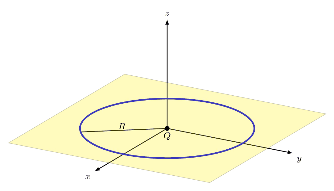
Figure 1 - A positively charged ring with a uniform linear charge density \(\lambda\) and radius \(R\): the origin of the coordinate system is at the center of the ring.
| A-1 | a) In cartesian coordinates \((x,y,z)\), obtain the electric field due to the charged ring in the vicinity of the ring’s center to the first order in \(x/R\), \(y/R\), and \(z/R\). b) Find the angular frequency of small oscillations of the charged particle around the center of the ring in the directions for which a stable equilibrium exists. |
1.5 pt |
In order to trap the charge \(Q\) fully, we would like to apply alternating fields to produce a dynamic equilibrium. Assume that the charge density is \(\lambda=\lambda_0+u\cos\Omega t\) in which \(\lambda_0\), \(u\), and \(\Omega\) are adjustable. We shall ignore radiative effects. Then the equation of motion for small displacements from the center of the ring, along the direction perpendicular to the plane of the ring will turn out to be:
\[ \ddot z=(+k^2+a\Omega^2\cos\Omega t)z \tag{1} \]
| A-2 | Write \(a\) and \(k\) in terms of the known parameters. | 0.4 pt |
We would like to obtain an approximate solution to Equation (1) by making the following simplifying assumptions: \(a\ll1\), \(\Omega\gg k\), and \(a\Omega^2\gg k^2\). With these assumptions, it can be shown that the solution of this equation can be split into two parts: \(z(t)=p(t)+q(t)\), where \(p(t)\) is a slowly varying component and \(q(t)\) is a small-amplitude rapidly-varying component with a mean value of zero. In other words, \(p(t)\) may be assumed constant over a few oscillations of \(q(t)\) (see Figure 2).
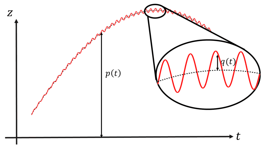
Figure 2 - A typical solution for the equation of motion of the charged particle: \(p(t)\) gives the overall motion, and \(q(t)\) represents small oscillations around this trajectory. The ellipse on the right is a magnification of a part of this trajectory.
| A-3 | a) Using the approximations stated above, find the equation of motion for \(q(t)\) in terms of \(a\), \(\Omega\), and \(p\). b) Find the solution of this equation by considering appropriate initial conditions corresponding to the required properties of this function. |
1.8 pt |
| A-4 | a) Using the mean effect of the rapidly varying component and obtain an effective equation of motion for \(p(t)\). b) Investigate the stability of the equilibrium point and find the condition for a stable equilibrium. |
1.5 pt |
Assume that \(\lambda_0=8\times10^{-9}\ \mathrm{C/m}\) and \(R=10\ \mathrm{cm}\). We would like to use this device to trap a singly ionized atom 100 times heavier than a hydrogen atom.
| A-5 | Calculate \(k\). Assume \(a=0.04\) and estimate the smallest frequency required to stabilize the motion of this ion. Use the data given at the end of the question. | 0.4 pt |
B. Doppler Cooling
It may be necessary to cool a trapped atom or ion. Assume that a trapped atom of mass \(m\), has two energy levels with an energy difference of \(E_0=\hbar\omega_{\mathrm A}\). Electrons in the lower level may absorb a photon and jump to the higher level, but after a period \(\tau\) they will return to the lower level and emit a photon with a frequency predominantly within \([\omega_{\mathrm A}-\Gamma,\omega_{\mathrm A}+\Gamma]\).
| B-1 | Use the Heisenberg’s uncertainty principle to find \(\Gamma\). | 0.5 pt |
With a similar reasoning, when we shine a laser light on the trapped atom, if the angular frequency of the laser, \(\omega_{\mathrm L}\), falls in the interval \([\omega_{\mathrm A}-\Gamma,\omega_{\mathrm A}+\Gamma]\), the atom may absorb the photon. Assume that the frequency \(\omega_{\mathrm L}\) of the laser light is slightly lower than \(\omega_{\mathrm A}\). For a particular device, the rate of photon absorption by an atom in the reference frame of the atom is given in Figure 3. The absorbed photon is then re-emitted in a random direction. To make things simple, we consider the problem in one dimension, i.e. we assume that the atoms can only move in the \(x\)-direction and the laser light shines on them both from the left and from the right. In the atom’s reference frame, the light has a higher or lower frequency due to the motion of the atoms. Since the velocity \(v\) of the atoms is very small, we only include terms of order \(v/c\) and ignore all the higher-order terms. Moreover, we have \(m\gg\hbar\omega_{\mathrm A}/c^2\) so that the velocity of the atom nearly does not change after absorbing the photon. Also, the change in frequency due to the Doppler effect is so small compared to \(\omega_{\mathrm A}-\omega_{\mathrm L}\), that the function for \(s\) in the diagram of Figure 3 may be approximated by the following linear function:
\[ s(\omega)=s_{\mathrm L}+\alpha(\omega-\omega_{\mathrm L}) \]
where \(s\) is the number of absorbed photons per unit of time, \(s_{\mathrm L}\) is the value of \(s\) for \(\omega=\omega_{\mathrm L}\), and \(\alpha\) is the slope of the line tangent to the curve at \(\omega_{\mathrm L}\). The frequency of the re-emitted photon is almost equal to the frequency of the incident photon, but it is emitted with equal probability in the positive or negative \(x\)-direction. In fact, up to the order considered here the two frequencies are identical. Note that we are considering the whole process in the atom’s reference frame.
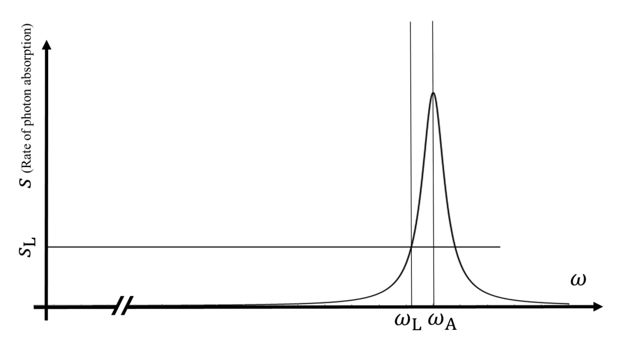
Figure 3 - The rate of photon absorption as a function of the frequency for a particular trap: the frequency corresponding to the energy difference between the two atomic levels is indicated by \(\omega_{\mathrm A}\) and the slighlty smaller frequency of the laser is indicated by \(\omega_{\mathrm L}\).
| B-2 | a) Assume that the trapped atom is moving with a velocity, \(v=v_x\) in the lab frame. In the frame of reference of the atom, calculate the collision rate of the photons, incident from each of the two directions, with the atoms (denoted by \(s_+\) and \(s_-\)) and the rate of absorption of momentum in each direction (denoted by \(\pi_+\) and \(\pi_-\)). b) Determine the effective force on the atom as a function of \(v\), \(k_{\mathrm L}=\omega_{\mathrm L}/c\), \(\hbar\), and \(\alpha\), in the reference frame of the laboratory. Assume \(s_{\mathrm L}\ll\alpha\omega_{\mathrm L}\), |
1.7 pt |
We would like to find the lowest temperature that can be achieved using this technique. Assume that the velocity of a particular atom has been reduced to zero exactly, and at this very moment it absorbs a photon (incident from any of the two directions), and re-emits the photon randomly in any of the two directions, with almost the same frequency. Assume that this process happens once every \(\tau\) units of time.
| B-3 | Considering the momentum of the atom after such a process for the two possible outcomes, calculate the average power absorbed by the atom. | 1.0 pt |
| B-4 | Consider the force calculated in Task B-2 and calculate the output power. Then, calculate the average value of \(v^2\) at equilibrium. Using your knowledge of the kinetic theory of gases estimate the temperature of the atoms. | 0.8 pt |
| B-5 | Estimate this temperature, for an atom 100 times heavier than a hydrogen atom. Assume that \(\omega_{\mathrm L}=2\times10^{16}\ \mathrm{rad/s}\), \(\tau=5\times10^{-9}\ \mathrm s\), and \(\alpha=4\). | 0.4 pt |
| mass of hydrogen atom: | \(m_{\mathrm H}=1.674\times10^{-27}\ \mathrm{kg}\) |
| charge of an electron: | \(e=1.602\times10^{-19}\ \mathrm C\) |
| permittivity of free space: | \(\varepsilon_0=8.854\times10^{-12}\ \mathrm{F/m}\) |
| Boltzmann constant: | \(k_{\mathrm B}=1.381\times10^{-23}\ \mathrm{J/K}\) |
| Planck constant: | \(\hbar=1.055\times10^{-34}\ \mathrm{J\cdot s}\) |
Official English text of the problem.
Answers
-
A-1(a): \[ \boxed{\mathbf E\simeq \frac{\lambda}{4\varepsilon_0R^2} \left(-x\,\hat{\mathbf x}-y\,\hat{\mathbf y}+2z\,\hat{\mathbf z}\right).} \]
-
A-1(b): All directions in the ring’s plane are stable, with \[ \boxed{\omega_x=\omega_y=\sqrt{\frac{Q\lambda}{4\varepsilon_0mR^2}}.} \] The \(z\)-direction is unstable.
-
A-2: \[ \boxed{a=\frac{Qu}{2\varepsilon_0mR^2\Omega^2}, \qquad k=\sqrt{\frac{Q\lambda_0}{2\varepsilon_0mR^2}}.} \]
-
A-3(a): \(\boxed{\ddot q\simeq a\Omega^2p\cos\Omega t}\).
-
A-3(b): \(\boxed{q(t)\simeq-ap(t)\cos\Omega t}\). For \(p\) treated as constant during a fast cycle, the appropriate initial conditions are \(q(0)=-ap\), \(\dot q(0)=0\).
-
A-4(a): \[ \boxed{\ddot p+\left(\frac{a^2\Omega^2}{2}-k^2\right)p=0.} \]
-
A-4(b): Stable trapping requires, within the stated approximation, \[ \boxed{a^2\Omega^2>2k^2.} \] The slow axial angular frequency is \(\sqrt{a^2\Omega^2/2-k^2}\).
-
A-5: \[ \boxed{k\simeq2.1\times10^5\ \mathrm{s^{-1}}.} \] The estimated threshold is \[ \boxed{\Omega_{\mathrm{th}}\simeq7.4\times10^6\ \mathrm{rad/s}, \qquad f_{\mathrm{th}}\simeq1.2\ \mathrm{MHz}.} \] Choose a frequency above this threshold.
-
B-1: The linewidth scale is \(\Gamma\sim1/\tau\); using the conventional lifetime half-width, \[ \boxed{\Gamma\simeq\frac{1}{2\tau}.} \]
-
B-2(a): Let \(+\) denote photons propagating along \(+x\), and let \(\pi_\pm\) be signed \(x\)-momentum transfer rates. Then \[ \boxed{s_\pm=s_{\mathrm L}\mp\alpha\omega_{\mathrm L}\frac vc,} \] \[ \boxed{\pi_\pm= \pm\hbar k_{\mathrm L} \left[s_{\mathrm L}\mp (s_{\mathrm L}+\alpha\omega_{\mathrm L})\frac vc\right].} \]
-
B-2(b): \[ \boxed{F_x=-2\alpha\hbar k_{\mathrm L}^{\,2}v.} \]
-
B-3: \[ \boxed{P_{\mathrm{in}}=\frac{\hbar^2k_{\mathrm L}^{\,2}}{m\tau}.} \]
-
B-4: The positive rate of energy removal is \[ \boxed{P_{\mathrm{out}}=2\alpha\hbar k_{\mathrm L}^{\,2}v^2.} \] At equilibrium, \[ \boxed{\langle v^2\rangle=\frac{\hbar}{2\alpha m\tau}, \qquad T=\frac{\hbar}{2\alpha k_{\mathrm B}\tau}.} \]
-
B-5: \[ \boxed{T\simeq1.9\times10^{-4}\ \mathrm K =0.19\ \mathrm{mK}.} \]
Solution
A-1(a)
The ring lies in the \(xy\)-plane and carries total charge \(2\pi R\lambda\). By Coulomb’s law, its electric field on the symmetry axis is
\[ E_z(0,0,z) =\frac{1}{4\pi\varepsilon_0} \frac{2\pi R\lambda\,z}{(R^2+z^2)^{3/2}}. \]
For \(|z|\ll R\),
\[ E_z(0,0,z)\simeq\frac{\lambda}{2\varepsilon_0R^2}z. \]
Reflection and rotational symmetry require the general linear field near the center to have the form
\[ E_x=Cx,\qquad E_y=Cy,\qquad E_z=Dz. \]
The axial result gives \(D=\lambda/(2\varepsilon_0R^2)\). There is no charge in the neighborhood of the center, so Gauss’s law gives
\[ \nabla\cdot\mathbf E=2C+D=0. \]
Consequently,
\[ \boxed{\mathbf E\simeq \frac{\lambda}{4\varepsilon_0R^2} \left(-x\,\hat{\mathbf x}-y\,\hat{\mathbf y}+2z\,\hat{\mathbf z}\right).} \]
A-1(b)
Newton’s second law in the plane gives
\[ m\ddot x=-\frac{Q\lambda}{4\varepsilon_0R^2}x, \qquad m\ddot y=-\frac{Q\lambda}{4\varepsilon_0R^2}y. \]
These are harmonic-oscillator equations. Thus every direction in the plane has the same angular frequency,
\[ \boxed{\omega_x=\omega_y= \sqrt{\frac{Q\lambda}{4\varepsilon_0mR^2}}.} \]
Along the axis,
\[ m\ddot z=\frac{Q\lambda}{2\varepsilon_0R^2}z. \]
For \(Q,\lambda>0\), this force points away from the center, so the axial equilibrium is unstable.
A-2
Substituting the time-dependent charge density into the axial equation gives
\[ \ddot z= \frac{Q}{2\varepsilon_0mR^2} \left(\lambda_0+u\cos\Omega t\right)z. \]
Comparison with Equation (1) yields
\[ \boxed{k^2=\frac{Q\lambda_0}{2\varepsilon_0mR^2}, \qquad a=\frac{Qu}{2\varepsilon_0mR^2\Omega^2}.} \]
Here \(a\) is dimensionless and \(k\) has units of inverse time.
A-3(a)
Insert \(z=p+q\) into the equation of motion:
\[ \ddot p+\ddot q =k^2p+k^2q+a\Omega^2p\cos\Omega t +a\Omega^2q\cos\Omega t. \]
Over a fast oscillation, \(p\) is approximately constant. Since \(q\) has small amplitude, \(a\ll1\), and \(a\Omega^2\gg k^2\), the leading rapidly varying equation is
\[ \boxed{\ddot q\simeq a\Omega^2p\cos\Omega t.} \]
A-3(b)
Holding \(p\) constant during the integration gives
\[ q(t)=-ap\cos\Omega t+C_1t+C_2. \]
A rapidly oscillating component cannot contain a secular drift, so \(C_1=0\). Its mean must vanish, which requires \(C_2=0\). Hence
\[ \boxed{q(t)\simeq-ap(t)\cos\Omega t.} \]
For frozen \(p\), the corresponding initial conditions are
\[ q(0)=-ap,\qquad \dot q(0)=0. \]
The amplitude of \(q\) is \(a\) times that of the local slow displacement, consistent with \(a\ll1\). Corrections involving the slow variation of \(p\) are neglected at this order.
A-4(a)
Average the full equation over a drive period, treating \(p\) as constant during that period. Since
\[ \langle q\rangle=0,\qquad \langle\cos\Omega t\rangle=0,\qquad \langle\cos^2\Omega t\rangle=\frac12, \]
we obtain
\[ \ddot p=k^2p+a\Omega^2\langle q\cos\Omega t\rangle. \]
Using \(q=-ap\cos\Omega t\),
\[ \langle q\cos\Omega t\rangle=-\frac{ap}{2}. \]
Therefore,
\[ \boxed{\ddot p= \left(k^2-\frac{a^2\Omega^2}{2}\right)p.} \]
Although \(k^2\) is small compared with \(a\Omega^2\), it must be retained here: the alternating field contributes to the mean motion only at order \(a^2\Omega^2\).
A-4(b)
Define
\[ \omega_{\mathrm s}^2=\frac{a^2\Omega^2}{2}-k^2. \]
If \(\omega_{\mathrm s}^2>0\), the slow displacement oscillates:
\[ p(t)=A\cos\omega_{\mathrm s}t+B\sin\omega_{\mathrm s}t, \]
and the complete approximate motion,
\[ z(t)\simeq p(t)\left(1-a\cos\Omega t\right), \]
remains bounded. Thus the axial stability condition is
\[ \boxed{a^2\Omega^2>2k^2.} \]
For \(a>0\), this is
\[ \boxed{\Omega>\frac{\sqrt2\,k}{a}.} \]
Below this threshold, the slow equation has an exponentially growing solution. At equality, \(\ddot p=0\), so a nonzero slow velocity produces unbounded drift; equality does not provide confinement.
For completeness, the transverse equation is
\[ \ddot x= -\left(\frac{k^2}{2} +\frac{a\Omega^2}{2}\cos\Omega t\right)x. \]
The same averaging procedure gives, for its slow component \(X\),
\[ \ddot X+ \left(\frac{k^2}{2}+\frac{a^2\Omega^2}{8}\right)X=0, \]
and identically for \(y\). These directions are stable within the approximation, so the axial condition supplies the requirement for trapping in all three directions.
A-5
The ion has
\[ Q=e,\qquad m=100m_{\mathrm H}=1.674\times10^{-25}\ \mathrm{kg}, \qquad R=0.10\ \mathrm m. \]
Thus
\[ k= \sqrt{ \frac{(1.602\times10^{-19})(8\times10^{-9})} {2(8.854\times10^{-12})(1.674\times10^{-25})(0.10)^2} } =2.079\times10^5\ \mathrm{s^{-1}}. \]
Therefore,
\[ \boxed{k\simeq2.1\times10^5\ \mathrm{s^{-1}}.} \]
For the specified \(a=0.04\), the estimated threshold angular frequency is
\[ \Omega_{\mathrm{th}} =\frac{\sqrt2\,k}{a} =7.351\times10^6\ \mathrm{rad/s}. \]
The corresponding ordinary frequency is
\[ f_{\mathrm{th}} =\frac{\Omega_{\mathrm{th}}}{2\pi} =1.170\times10^6\ \mathrm{Hz}. \]
Hence,
\[ \boxed{\Omega_{\mathrm{th}}\simeq7.4\times10^6\ \mathrm{rad/s}, \qquad f_{\mathrm{th}}\simeq1.2\ \mathrm{MHz}.} \]
A frequency above this estimated threshold is required. At the threshold,
\[ \frac{\Omega_{\mathrm{th}}}{k}\simeq35, \qquad \frac{a\Omega_{\mathrm{th}}^2}{k^2}=50, \]
consistent with the assumed separation of scales.
B-1
The excited state has a characteristic lifetime \(\tau\). The energy–time uncertainty estimate is
\[ \Delta E\,\tau\gtrsim\frac{\hbar}{2}. \]
Identifying the characteristic energy half-width as \(\Delta E\simeq\hbar\Gamma\) gives
\[ \Gamma\tau\gtrsim\frac12. \]
For a width set by the finite lifetime, the usual estimate is therefore
\[ \boxed{\Gamma\simeq\frac{1}{2\tau}.} \]
The robust conclusion from the uncertainty principle is the scale \(\Gamma\sim1/\tau\); the numerical factor depends on how the linewidth is defined.
B-2(a)
Let \(+\) label photons propagating along \(+x\), and \(-\) label photons propagating along \(-x\). For an atom moving at velocity \(v\), the first-order Doppler shifts give
\[ \omega'_+=\omega_{\mathrm L}\left(1-\frac vc\right), \qquad \omega'_-=\omega_{\mathrm L}\left(1+\frac vc\right). \]
A photon traveling in the same direction as the atom is redshifted; one traveling against it is blueshifted.
The supplied function \(s(\omega)\) already specifies the absorption rate in the atom’s frame. Evaluating it at these frequencies gives
\[ s_+=s_{\mathrm L}+\alpha(\omega'_+-\omega_{\mathrm L}) =s_{\mathrm L}-\alpha\omega_{\mathrm L}\frac vc, \]
\[ s_-=s_{\mathrm L}+\alpha(\omega'_--\omega_{\mathrm L}) =s_{\mathrm L}+\alpha\omega_{\mathrm L}\frac vc. \]
Thus,
\[ \boxed{s_\pm=s_{\mathrm L}\mp\alpha\omega_{\mathrm L}\frac vc.} \]
Each absorbed photon has signed momentum \(\pm\hbar\omega'_\pm/c\). Defining \(\pi_\pm\) as signed \(x\)-momentum transfer rates,
\[ \pi_+=\frac{\hbar\omega'_+}{c}s_+, \qquad \pi_-=-\frac{\hbar\omega'_-}{c}s_-. \]
Expanding and keeping only first-order terms in \(v/c\),
\[ \boxed{\pi_+=\hbar k_{\mathrm L} \left[s_{\mathrm L}-(s_{\mathrm L}+\alpha\omega_{\mathrm L})\frac vc\right],} \]
\[ \boxed{\pi_-=-\hbar k_{\mathrm L} \left[s_{\mathrm L}+(s_{\mathrm L}+\alpha\omega_{\mathrm L})\frac vc\right].} \]
B-2(b)
In the atom’s frame, re-emission has zero mean momentum because the two emission directions are equally probable. Therefore the mean force is
\[ F'_x=\pi_++\pi_- =-\frac{2\hbar\omega_{\mathrm L}}{c^2} (s_{\mathrm L}+\alpha\omega_{\mathrm L})v. \]
Within the approximation used here, the absorbed and emitted energies are equal in the atom’s frame. The completed cycle therefore has zero net energy transfer in that frame when recoil is neglected in calculating the mean force. Transforming to the laboratory leaves the longitudinal force unchanged to the retained order.
Using \(s_{\mathrm L}\ll\alpha\omega_{\mathrm L}\), we obtain
\[ \boxed{F_x\simeq -\frac{2\alpha\hbar\omega_{\mathrm L}^2}{c^2}v =-2\alpha\hbar k_{\mathrm L}^{\,2}v.} \]
The laser frequency lies on the rising side of the absorption curve, so \(\alpha>0\). The force therefore opposes the velocity and removes kinetic energy.
B-3
Let the incident photon propagate along \(+x\) and have momentum magnitude
\[ p_\gamma=\hbar k_{\mathrm L}. \]
The atom initially has zero momentum. Momentum conservation gives the two equally probable outcomes:
| Emission direction | Final atomic momentum | Final kinetic energy | Probability |
|---|---|---|---|
| Along \(+x\), the incident direction | \(0\) | \(0\) | \(1/2\) |
| Along \(-x\), opposite the incident direction | \(2p_\gamma\) | \(2p_\gamma^2/m\) | \(1/2\) |
Thus the mean kinetic-energy gain per absorption–emission cycle is
\[ \langle\Delta K\rangle =\frac12(0)+\frac12\frac{(2p_\gamma)^2}{2m} =\frac{p_\gamma^2}{m}. \]
An incident photon traveling along \(-x\) gives the same mean energy gain. Since there is one complete cycle every \(\tau\),
\[ \boxed{P_{\mathrm{in}} =\frac{\langle\Delta K\rangle}{\tau} =\frac{\hbar^2k_{\mathrm L}^{\,2}}{m\tau}.} \]
B-4
The rate at which the damping force changes the atom’s mechanical energy is
\[ F_xv=-2\alpha\hbar k_{\mathrm L}^{\,2}v^2. \]
Hence the positive output power, meaning the rate of energy removal, is
\[ \boxed{P_{\mathrm{out}} =2\alpha\hbar k_{\mathrm L}^{\,2}v^2.} \]
At thermal equilibrium, the mean cooling power balances recoil heating:
\[ 2\alpha\hbar k_{\mathrm L}^{\,2}\langle v^2\rangle =\frac{\hbar^2k_{\mathrm L}^{\,2}}{m\tau}. \]
Cancelling common factors gives
\[ \boxed{\langle v^2\rangle=\frac{\hbar}{2\alpha m\tau}.} \]
The problem restricts motion to one dimension, so equipartition gives
\[ \frac12m\langle v^2\rangle=\frac12k_{\mathrm B}T. \]
Consequently,
\[ \boxed{T=\frac{\hbar}{2\alpha k_{\mathrm B}\tau}.} \]
The atomic mass and laser wave number cancel from the equilibrium temperature in this model.
B-5
Using the given values,
\[ T= \frac{1.055\times10^{-34}} {2(4)(1.381\times10^{-23})(5\times10^{-9})} =1.9098\times10^{-4}\ \mathrm K. \]
Therefore,
\[ \boxed{T\simeq1.9\times10^{-4}\ \mathrm K =0.19\ \mathrm{mK}\simeq190\ \mu\mathrm K.} \]
For the specified mass \(m=1.674\times10^{-25}\ \mathrm{kg}\), the corresponding velocity variance is
\[ \langle v^2\rangle=1.58\times10^{-2}\ \mathrm{m^2/s^2}, \qquad v_{\mathrm{rms}}\simeq0.126\ \mathrm{m/s}. \]
The solution was checked against the official solution.
IPhO 2024 · Theorieaufgabe 2
Ionen einfangen und Atome kühlen
Das Einfangen und Kühlen von Atomen und Ionen war in den letzten Jahrzehnten ein faszinierendes Thema für Physiker; für Arbeiten auf diesem Gebiet wurden mehrere Nobelpreise verliehen. Im ersten Teil dieser Aufgabe untersuchen wir eine Technik zum Einfangen von Ionen, die als „Paul-Falle“ bekannt ist. Wolfgang Paul und Hans Dehmelt erhielten für diese Arbeit die Hälfte des Nobelpreises für Physik des Jahres 1989. Anschließend untersuchen wir die Dopplerkühlung, eine der Arbeiten, die in der Pressemitteilung zum Nobelpreis für Physik des Jahres 1997 genannt wurden. Dieser wurde Steven Chu, Claude Cohen-Tannoudji und William Daniel Phillips „für die Entwicklung von Methoden zum Kühlen und Einfangen von Atomen mit Laserlicht“ verliehen.
A. Die Paul-Falle
Bekanntlich lässt sich mit elektrostatischen Feldern kein stabiles Gleichgewicht für ein geladenes Teilchen erzeugen. Um einen stabilen Gleichgewichtspunkt für Ionen zu schaffen, sind daher ausgefeiltere Techniken erforderlich. Die Paul-Falle ist eine dieser Techniken.
Betrachten Sie einen geladenen Ring mit dem Radius \(R\) und einer gleichmäßigen positiven linearen Ladungsdichte \(\lambda\). Eine positive Punktladung \(Q\) mit der Masse \(m\) befindet sich im Mittelpunkt des Rings.
Abbildung 1 - Ein positiv geladener Ring mit einer gleichmäßigen linearen Ladungsdichte \(\lambda\) und dem Radius \(R\): Der Ursprung des Koordinatensystems liegt im Mittelpunkt des Rings.
| A-1 | a) Bestimmen Sie in kartesischen Koordinaten \((x,y,z)\) das elektrische Feld des geladenen Rings in der Nähe seines Mittelpunkts bis zur ersten Ordnung in \(x/R\), \(y/R\) und \(z/R\). b) Bestimmen Sie die Kreisfrequenz kleiner Schwingungen des geladenen Teilchens um den Mittelpunkt des Rings in den Richtungen, in denen ein stabiles Gleichgewicht besteht. |
1.5 Pkt. |
Um die Ladung \(Q\) vollständig einzufangen, wollen wir Wechselfelder anlegen, die ein dynamisches Gleichgewicht erzeugen. Nehmen Sie an, dass die Ladungsdichte \(\lambda=\lambda_0+u\cos\Omega t\) beträgt, wobei \(\lambda_0\), \(u\) und \(\Omega\) einstellbar sind. Strahlungseffekte werden vernachlässigt. Dann ergibt sich für kleine Auslenkungen aus dem Mittelpunkt des Rings senkrecht zur Ringebene die folgende Bewegungsgleichung:
\[ \ddot z=(+k^2+a\Omega^2\cos\Omega t)z \tag{1} \]
| A-2 | Drücken Sie \(a\) und \(k\) durch die bekannten Parameter aus. | 0.4 Pkt. |
Wir wollen eine Näherungslösung von Gleichung (1) erhalten, indem wir die folgenden vereinfachenden Annahmen treffen: \(a\ll1\), \(\Omega\gg k\) und \(a\Omega^2\gg k^2\). Unter diesen Annahmen lässt sich zeigen, dass die Lösung dieser Gleichung in zwei Anteile zerlegt werden kann: \(z(t)=p(t)+q(t)\), wobei \(p(t)\) ein langsam veränderlicher Anteil und \(q(t)\) ein schnell veränderlicher Anteil mit kleiner Amplitude und dem Mittelwert null ist. Mit anderen Worten kann \(p(t)\) über einige Schwingungen von \(q(t)\) hinweg als konstant angenommen werden (siehe Abbildung 2).
Abbildung 2 - Eine typische Lösung der Bewegungsgleichung des geladenen Teilchens: \(p(t)\) beschreibt die übergeordnete Bewegung, und \(q(t)\) stellt kleine Schwingungen um diese Bahn dar. Die Ellipse rechts zeigt eine Vergrößerung eines Teils dieser Bahn.
| A-3 | a) Bestimmen Sie mithilfe der oben angegebenen Näherungen die Bewegungsgleichung für \(q(t)\) in Abhängigkeit von \(a\), \(\Omega\) und \(p\). b) Bestimmen Sie die Lösung dieser Gleichung unter Berücksichtigung geeigneter Anfangsbedingungen, die den geforderten Eigenschaften dieser Funktion entsprechen. |
1.8 Pkt. |
| A-4 | a) Nutzen Sie die gemittelte Wirkung des schnell veränderlichen Anteils, um eine effektive Bewegungsgleichung für \(p(t)\) zu erhalten. b) Untersuchen Sie die Stabilität des Gleichgewichtspunkts und bestimmen Sie die Bedingung für ein stabiles Gleichgewicht. |
1.5 Pkt. |
Nehmen Sie an, dass \(\lambda_0=8\times10^{-9}\ \mathrm{C/m}\) und \(R=10\ \mathrm{cm}\) sind. Wir wollen mit dieser Vorrichtung ein einfach ionisiertes Atom einfangen, das 100-mal so schwer wie ein Wasserstoffatom ist.
| A-5 | Berechnen Sie \(k\). Nehmen Sie \(a=0.04\) an und schätzen Sie die kleinste Frequenz ab, die erforderlich ist, um die Bewegung dieses Ions zu stabilisieren. Verwenden Sie die am Ende der Aufgabe angegebenen Daten. | 0.4 Pkt. |
B. Dopplerkühlung
Es kann erforderlich sein, ein eingefangenes Atom oder Ion zu kühlen. Nehmen Sie an, dass ein eingefangenes Atom der Masse \(m\) zwei Energieniveaus mit einer Energiedifferenz von \(E_0=\hbar\omega_{\mathrm A}\) besitzt. Elektronen im unteren Niveau können ein Photon absorbieren und in das höhere Niveau übergehen; nach einer Zeit \(\tau\) kehren sie jedoch in das untere Niveau zurück und emittieren ein Photon, dessen Frequenz überwiegend innerhalb von \([\omega_{\mathrm A}-\Gamma,\omega_{\mathrm A}+\Gamma]\) liegt.
| B-1 | Bestimmen Sie \(\Gamma\) mithilfe der Heisenbergschen Unschärferelation. | 0.5 Pkt. |
Mit einer ähnlichen Überlegung folgt: Wenn wir das eingefangene Atom mit Laserlicht bestrahlen und die Kreisfrequenz des Lasers, \(\omega_{\mathrm L}\), im Intervall \([\omega_{\mathrm A}-\Gamma,\omega_{\mathrm A}+\Gamma]\) liegt, kann das Atom das Photon absorbieren. Nehmen Sie an, dass die Frequenz \(\omega_{\mathrm L}\) des Laserlichts etwas kleiner als \(\omega_{\mathrm A}\) ist. Für eine bestimmte Vorrichtung ist die Rate der Photonenabsorption durch ein Atom im Bezugssystem des Atoms in Abbildung 3 dargestellt. Das absorbierte Photon wird anschließend in einer zufälligen Richtung wieder emittiert. Zur Vereinfachung betrachten wir das Problem eindimensional, d. h., wir nehmen an, dass sich die Atome nur in \(x\)-Richtung bewegen können und das Laserlicht sowohl von links als auch von rechts auf sie trifft. Im Bezugssystem des Atoms hat das Licht aufgrund der Bewegung der Atome eine höhere oder niedrigere Frequenz. Da die Geschwindigkeit \(v\) der Atome sehr klein ist, berücksichtigen wir nur Terme der Ordnung \(v/c\) und vernachlässigen alle Terme höherer Ordnung. Außerdem gilt \(m\gg\hbar\omega_{\mathrm A}/c^2\), sodass sich die Geschwindigkeit des Atoms nach der Absorption des Photons nahezu nicht ändert. Die Frequenzänderung durch den Dopplereffekt ist zudem im Vergleich zu \(\omega_{\mathrm A}-\omega_{\mathrm L}\) so klein, dass die Funktion für \(s\) im Diagramm von Abbildung 3 durch die folgende lineare Funktion angenähert werden kann:
\[ s(\omega)=s_{\mathrm L}+\alpha(\omega-\omega_{\mathrm L}) \]
Dabei ist \(s\) die Anzahl der pro Zeiteinheit absorbierten Photonen, \(s_{\mathrm L}\) der Wert von \(s\) für \(\omega=\omega_{\mathrm L}\) und \(\alpha\) die Steigung der Tangente an die Kurve bei \(\omega_{\mathrm L}\). Die Frequenz des wieder emittierten Photons ist nahezu gleich der Frequenz des einfallenden Photons, es wird jedoch mit gleicher Wahrscheinlichkeit in positiver oder negativer \(x\)-Richtung emittiert. Tatsächlich sind die beiden Frequenzen bis zu der hier betrachteten Ordnung identisch. Beachten Sie, dass wir den gesamten Vorgang im Bezugssystem des Atoms betrachten.
Abbildung 3 - Die Rate der Photonenabsorption als Funktion der Frequenz für eine bestimmte Falle: Die Frequenz, die der Energiedifferenz zwischen den beiden atomaren Niveaus entspricht, ist mit \(\omega_{\mathrm A}\) bezeichnet, die etwas kleinere Frequenz des Lasers mit \(\omega_{\mathrm L}\).
| B-2 | a) Nehmen Sie an, dass sich das eingefangene Atom im Laborsystem mit der Geschwindigkeit \(v=v_x\) bewegt. Berechnen Sie im Bezugssystem des Atoms die Kollisionsrate der aus den beiden Richtungen einfallenden Photonen mit den Atomen (bezeichnet mit \(s_+\) und \(s_-\)) sowie die Rate der Impulsaufnahme aus jeder Richtung (bezeichnet mit \(\pi_+\) und \(\pi_-\)). b) Bestimmen Sie im Bezugssystem des Labors die effektive Kraft auf das Atom als Funktion von \(v\), \(k_{\mathrm L}=\omega_{\mathrm L}/c\), \(\hbar\) und \(\alpha\). Nehmen Sie \(s_{\mathrm L}\ll\alpha\omega_{\mathrm L}\) an. |
1.7 Pkt. |
Wir wollen die niedrigste Temperatur bestimmen, die mit dieser Technik erreicht werden kann. Nehmen Sie an, dass die Geschwindigkeit eines bestimmten Atoms genau auf null reduziert wurde und dass es genau in diesem Moment ein Photon absorbiert (das aus einer der beiden Richtungen einfällt) und das Photon mit nahezu derselben Frequenz zufällig in eine der beiden Richtungen wieder emittiert. Nehmen Sie an, dass dieser Vorgang einmal pro Zeitintervall \(\tau\) stattfindet.
| B-3 | Betrachten Sie den Impuls des Atoms nach einem solchen Vorgang für die beiden möglichen Ergebnisse und berechnen Sie die mittlere vom Atom aufgenommene Leistung. | 1.0 Pkt. |
| B-4 | Betrachten Sie die in Teilaufgabe B-2 berechnete Kraft und berechnen Sie die abgegebene Leistung. Berechnen Sie anschließend den Mittelwert von \(v^2\) im Gleichgewicht. Schätzen Sie mithilfe Ihrer Kenntnisse der kinetischen Gastheorie die Temperatur der Atome ab. | 0.8 Pkt. |
| B-5 | Schätzen Sie diese Temperatur für ein Atom ab, das 100-mal so schwer wie ein Wasserstoffatom ist. Nehmen Sie \(\omega_{\mathrm L}=2\times10^{16}\ \mathrm{rad/s}\), \(\tau=5\times10^{-9}\ \mathrm s\) und \(\alpha=4\) an. | 0.4 Pkt. |
| Masse des Wasserstoffatoms: | \(m_{\mathrm H}=1.674\times10^{-27}\ \mathrm{kg}\) |
| Ladung eines Elektrons: | \(e=1.602\times10^{-19}\ \mathrm C\) |
| Elektrische Feldkonstante: | \(\varepsilon_0=8.854\times10^{-12}\ \mathrm{F/m}\) |
| Boltzmann-Konstante: | \(k_{\mathrm B}=1.381\times10^{-23}\ \mathrm{J/K}\) |
| Planck-Konstante: | \(\hbar=1.055\times10^{-34}\ \mathrm{J\cdot s}\) |
Aufgabentext aus dem offiziellen englischen Text übersetzt.
Antworten
-
A-1(a): \[ \boxed{\mathbf E\simeq \frac{\lambda}{4\varepsilon_0R^2} \left(-x\,\hat{\mathbf x}-y\,\hat{\mathbf y}+2z\,\hat{\mathbf z}\right).} \]
-
A-1(b): Alle Richtungen in der Ringebene sind stabil, mit \[ \boxed{\omega_x=\omega_y=\sqrt{\frac{Q\lambda}{4\varepsilon_0mR^2}}.} \] Die \(z\)-Richtung ist instabil.
-
A-2: \[ \boxed{a=\frac{Qu}{2\varepsilon_0mR^2\Omega^2}, \qquad k=\sqrt{\frac{Q\lambda_0}{2\varepsilon_0mR^2}}.} \]
-
A-3(a): \(\boxed{\ddot q\simeq a\Omega^2p\cos\Omega t}\).
-
A-3(b): \(\boxed{q(t)\simeq-ap(t)\cos\Omega t}\). Wenn \(p\) während einer schnellen Schwingungsperiode als konstant behandelt wird, lauten die geeigneten Anfangsbedingungen \(q(0)=-ap\), \(\dot q(0)=0\).
-
A-4(a): \[ \boxed{\ddot p+\left(\frac{a^2\Omega^2}{2}-k^2\right)p=0.} \]
-
A-4(b): Ein stabiler Einschluss erfordert innerhalb der angegebenen Näherung \[ \boxed{a^2\Omega^2>2k^2.} \] Die langsame axiale Kreisfrequenz beträgt \(\sqrt{a^2\Omega^2/2-k^2}\).
-
A-5: \[ \boxed{k\simeq2.1\times10^5\ \mathrm{s^{-1}}.} \] Der geschätzte Schwellenwert beträgt \[ \boxed{\Omega_{\mathrm{th}}\simeq7.4\times10^6\ \mathrm{rad/s}, \qquad f_{\mathrm{th}}\simeq1.2\ \mathrm{MHz}.} \] Es ist eine Frequenz oberhalb dieses Schwellenwerts zu wählen.
-
B-1: Die Größenordnung der Linienbreite ist \(\Gamma\sim1/\tau\); mit der üblichen lebensdauerbedingten Halbbreite gilt \[ \boxed{\Gamma\simeq\frac{1}{2\tau}.} \]
-
B-2(a): Es bezeichne \(+\) Photonen, die sich entlang \(+x\) ausbreiten, und \(\pi_\pm\) seien die vorzeichenbehafteten Übertragungsraten des \(x\)-Impulses. Dann gilt \[ \boxed{s_\pm=s_{\mathrm L}\mp\alpha\omega_{\mathrm L}\frac vc,} \] \[ \boxed{\pi_\pm= \pm\hbar k_{\mathrm L} \left[s_{\mathrm L}\mp (s_{\mathrm L}+\alpha\omega_{\mathrm L})\frac vc\right].} \]
-
B-2(b): \[ \boxed{F_x=-2\alpha\hbar k_{\mathrm L}^{\,2}v.} \]
-
B-3: \[ \boxed{P_{\mathrm{in}}=\frac{\hbar^2k_{\mathrm L}^{\,2}}{m\tau}.} \]
-
B-4: Die positive Rate des Energieentzugs beträgt \[ \boxed{P_{\mathrm{out}}=2\alpha\hbar k_{\mathrm L}^{\,2}v^2.} \] Im Gleichgewicht gilt \[ \boxed{\langle v^2\rangle=\frac{\hbar}{2\alpha m\tau}, \qquad T=\frac{\hbar}{2\alpha k_{\mathrm B}\tau}.} \]
-
B-5: \[ \boxed{T\simeq1.9\times10^{-4}\ \mathrm K =0.19\ \mathrm{mK}.} \]
Lösung
A-1(a)
Der Ring liegt in der \(xy\)-Ebene und trägt die Gesamtladung \(2\pi R\lambda\). Nach dem Coulombschen Gesetz beträgt sein elektrisches Feld auf der Symmetrieachse
\[ E_z(0,0,z) =\frac{1}{4\pi\varepsilon_0} \frac{2\pi R\lambda\,z}{(R^2+z^2)^{3/2}}. \]
Für \(|z|\ll R\) gilt
\[ E_z(0,0,z)\simeq\frac{\lambda}{2\varepsilon_0R^2}z. \]
Spiegelungs- und Rotationssymmetrie erfordern, dass das allgemeine lineare Feld nahe dem Mittelpunkt die Form
\[ E_x=Cx,\qquad E_y=Cy,\qquad E_z=Dz. \]
hat. Aus dem Ergebnis auf der Achse folgt \(D=\lambda/(2\varepsilon_0R^2)\). In der Umgebung des Mittelpunkts befindet sich keine Ladung, sodass das Gaußsche Gesetz
\[ \nabla\cdot\mathbf E=2C+D=0. \]
liefert. Folglich gilt
\[ \boxed{\mathbf E\simeq \frac{\lambda}{4\varepsilon_0R^2} \left(-x\,\hat{\mathbf x}-y\,\hat{\mathbf y}+2z\,\hat{\mathbf z}\right).} \]
A-1(b)
Das zweite Newtonsche Gesetz liefert in der Ebene
\[ m\ddot x=-\frac{Q\lambda}{4\varepsilon_0R^2}x, \qquad m\ddot y=-\frac{Q\lambda}{4\varepsilon_0R^2}y. \]
Dies sind die Gleichungen harmonischer Oszillatoren. Somit ergibt sich für jede Richtung in der Ebene dieselbe Kreisfrequenz,
\[ \boxed{\omega_x=\omega_y= \sqrt{\frac{Q\lambda}{4\varepsilon_0mR^2}}.} \]
Entlang der Achse gilt
\[ m\ddot z=\frac{Q\lambda}{2\varepsilon_0R^2}z. \]
Für \(Q,\lambda>0\) ist diese Kraft vom Mittelpunkt weg gerichtet, sodass das axiale Gleichgewicht instabil ist.
A-2
Einsetzen der zeitabhängigen Ladungsdichte in die axiale Gleichung ergibt
\[ \ddot z= \frac{Q}{2\varepsilon_0mR^2} \left(\lambda_0+u\cos\Omega t\right)z. \]
Der Vergleich mit Gleichung (1) liefert
\[ \boxed{k^2=\frac{Q\lambda_0}{2\varepsilon_0mR^2}, \qquad a=\frac{Qu}{2\varepsilon_0mR^2\Omega^2}.} \]
Dabei ist \(a\) dimensionslos, und \(k\) hat die Einheit einer inversen Zeit.
A-3(a)
Wir setzen \(z=p+q\) in die Bewegungsgleichung ein:
\[ \ddot p+\ddot q =k^2p+k^2q+a\Omega^2p\cos\Omega t +a\Omega^2q\cos\Omega t. \]
Über eine schnelle Schwingung hinweg ist \(p\) näherungsweise konstant. Da \(q\) eine kleine Amplitude hat und \(a\ll1\) sowie \(a\Omega^2\gg k^2\) gelten, lautet die Gleichung für den schnell veränderlichen Anteil in führender Ordnung
\[ \boxed{\ddot q\simeq a\Omega^2p\cos\Omega t.} \]
A-3(b)
Wenn \(p\) während der Integration konstant gehalten wird, ergibt sich
\[ q(t)=-ap\cos\Omega t+C_1t+C_2. \]
Ein schnell schwingender Anteil kann keine säkulare Drift enthalten, daher ist \(C_1=0\). Sein Mittelwert muss verschwinden, was \(C_2=0\) erfordert. Somit gilt
\[ \boxed{q(t)\simeq-ap(t)\cos\Omega t.} \]
Für festgehaltenes \(p\) lauten die entsprechenden Anfangsbedingungen
\[ q(0)=-ap,\qquad \dot q(0)=0. \]
Die Amplitude von \(q\) beträgt das \(a\)-Fache der lokalen langsamen Auslenkung, im Einklang mit \(a\ll1\). Korrekturen, die mit der langsamen Änderung von \(p\) zusammenhängen, werden in dieser Ordnung vernachlässigt.
A-4(a)
Wir mitteln die vollständige Gleichung über eine Periode des Wechselfeldes und behandeln \(p\) während dieser Periode als konstant. Wegen
\[ \langle q\rangle=0,\qquad \langle\cos\Omega t\rangle=0,\qquad \langle\cos^2\Omega t\rangle=\frac12, \]
erhalten wir
\[ \ddot p=k^2p+a\Omega^2\langle q\cos\Omega t\rangle. \]
Mit \(q=-ap\cos\Omega t\) gilt
\[ \langle q\cos\Omega t\rangle=-\frac{ap}{2}. \]
Daher folgt
\[ \boxed{\ddot p= \left(k^2-\frac{a^2\Omega^2}{2}\right)p.} \]
Obwohl \(k^2\) im Vergleich zu \(a\Omega^2\) klein ist, muss es hier beibehalten werden: Das Wechselfeld trägt erst in der Ordnung \(a^2\Omega^2\) zur gemittelten Bewegung bei.
A-4(b)
Wir definieren
\[ \omega_{\mathrm s}^2=\frac{a^2\Omega^2}{2}-k^2. \]
Wenn \(\omega_{\mathrm s}^2>0\) ist, schwingt die langsame Auslenkung:
\[ p(t)=A\cos\omega_{\mathrm s}t+B\sin\omega_{\mathrm s}t, \]
und die vollständige näherungsweise Bewegung,
\[ z(t)\simeq p(t)\left(1-a\cos\Omega t\right), \]
bleibt beschränkt. Somit lautet die axiale Stabilitätsbedingung
\[ \boxed{a^2\Omega^2>2k^2.} \]
Für \(a>0\) ergibt sich daraus
\[ \boxed{\Omega>\frac{\sqrt2\,k}{a}.} \]
Unterhalb dieses Schwellenwerts hat die Gleichung für die langsame Bewegung eine exponentiell anwachsende Lösung. Bei Gleichheit gilt \(\ddot p=0\), sodass eine von null verschiedene langsame Geschwindigkeit eine unbeschränkte Drift erzeugt; Gleichheit gewährleistet keinen Einschluss.
Der Vollständigkeit halber lautet die transversale Gleichung
\[ \ddot x= -\left(\frac{k^2}{2} +\frac{a\Omega^2}{2}\cos\Omega t\right)x. \]
Dasselbe Mittelungsverfahren ergibt für ihren langsamen Anteil \(X\)
\[ \ddot X+ \left(\frac{k^2}{2}+\frac{a^2\Omega^2}{8}\right)X=0, \]
und entsprechend für \(y\). Diese Richtungen sind innerhalb der Näherung stabil, sodass die axiale Bedingung die Voraussetzung für den Einschluss in allen drei Richtungen liefert.
A-5
Für das Ion gilt
\[ Q=e,\qquad m=100m_{\mathrm H}=1.674\times10^{-25}\ \mathrm{kg}, \qquad R=0.10\ \mathrm m. \]
Damit ist
\[ k= \sqrt{ \frac{(1.602\times10^{-19})(8\times10^{-9})} {2(8.854\times10^{-12})(1.674\times10^{-25})(0.10)^2} } =2.079\times10^5\ \mathrm{s^{-1}}. \]
Also gilt
\[ \boxed{k\simeq2.1\times10^5\ \mathrm{s^{-1}}.} \]
Für den angegebenen Wert \(a=0.04\) beträgt die geschätzte Schwellenkreisfrequenz
\[ \Omega_{\mathrm{th}} =\frac{\sqrt2\,k}{a} =7.351\times10^6\ \mathrm{rad/s}. \]
Die entsprechende gewöhnliche Frequenz beträgt
\[ f_{\mathrm{th}} =\frac{\Omega_{\mathrm{th}}}{2\pi} =1.170\times10^6\ \mathrm{Hz}. \]
Somit ergibt sich
\[ \boxed{\Omega_{\mathrm{th}}\simeq7.4\times10^6\ \mathrm{rad/s}, \qquad f_{\mathrm{th}}\simeq1.2\ \mathrm{MHz}.} \]
Eine Frequenz oberhalb dieses geschätzten Schwellenwerts ist erforderlich. Am Schwellenwert gilt
\[ \frac{\Omega_{\mathrm{th}}}{k}\simeq35, \qquad \frac{a\Omega_{\mathrm{th}}^2}{k^2}=50, \]
im Einklang mit der angenommenen Trennung der Skalen.
B-1
Der angeregte Zustand hat eine charakteristische Lebensdauer \(\tau\). Die Abschätzung anhand der Energie-Zeit-Unschärferelation lautet
\[ \Delta E\,\tau\gtrsim\frac{\hbar}{2}. \]
Setzt man die charakteristische energetische Halbbreite als \(\Delta E\simeq\hbar\Gamma\) an, ergibt sich
\[ \Gamma\tau\gtrsim\frac12. \]
Für eine durch die endliche Lebensdauer bestimmte Breite lautet die übliche Abschätzung daher
\[ \boxed{\Gamma\simeq\frac{1}{2\tau}.} \]
Die belastbare Schlussfolgerung aus der Unschärferelation ist die Größenordnung \(\Gamma\sim1/\tau\); der Zahlenfaktor hängt davon ab, wie die Linienbreite definiert wird.
B-2(a)
Es kennzeichne \(+\) Photonen, die sich entlang \(+x\) ausbreiten, und \(-\) Photonen, die sich entlang \(-x\) ausbreiten. Für ein Atom, das sich mit der Geschwindigkeit \(v\) bewegt, ergeben die Dopplerverschiebungen in erster Ordnung
\[ \omega'_+=\omega_{\mathrm L}\left(1-\frac vc\right), \qquad \omega'_-=\omega_{\mathrm L}\left(1+\frac vc\right). \]
Ein Photon, das sich in derselben Richtung wie das Atom bewegt, ist rotverschoben; eines, das ihm entgegenläuft, ist blauverschoben.
Die angegebene Funktion \(s(\omega)\) beschreibt bereits die Absorptionsrate im Bezugssystem des Atoms. Ihre Auswertung bei diesen Frequenzen ergibt
\[ s_+=s_{\mathrm L}+\alpha(\omega'_+-\omega_{\mathrm L}) =s_{\mathrm L}-\alpha\omega_{\mathrm L}\frac vc, \]
\[ s_-=s_{\mathrm L}+\alpha(\omega'_--\omega_{\mathrm L}) =s_{\mathrm L}+\alpha\omega_{\mathrm L}\frac vc. \]
Somit gilt
\[ \boxed{s_\pm=s_{\mathrm L}\mp\alpha\omega_{\mathrm L}\frac vc.} \]
Jedes absorbierte Photon hat den vorzeichenbehafteten Impuls \(\pm\hbar\omega'_\pm/c\). Definieren wir \(\pi_\pm\) als die vorzeichenbehafteten Übertragungsraten des \(x\)-Impulses, so gilt
\[ \pi_+=\frac{\hbar\omega'_+}{c}s_+, \qquad \pi_-=-\frac{\hbar\omega'_-}{c}s_-. \]
Durch Ausmultiplizieren und Beibehalten nur der Terme erster Ordnung in \(v/c\) folgt
\[ \boxed{\pi_+=\hbar k_{\mathrm L} \left[s_{\mathrm L}-(s_{\mathrm L}+\alpha\omega_{\mathrm L})\frac vc\right],} \]
\[ \boxed{\pi_-=-\hbar k_{\mathrm L} \left[s_{\mathrm L}+(s_{\mathrm L}+\alpha\omega_{\mathrm L})\frac vc\right].} \]
B-2(b)
Im Bezugssystem des Atoms ist der mittlere Impuls bei der Wiederemission null, da die beiden Emissionsrichtungen gleich wahrscheinlich sind. Daher beträgt die mittlere Kraft
\[ F'_x=\pi_++\pi_- =-\frac{2\hbar\omega_{\mathrm L}}{c^2} (s_{\mathrm L}+\alpha\omega_{\mathrm L})v. \]
Innerhalb der hier verwendeten Näherung sind die absorbierte und die emittierte Energie im Bezugssystem des Atoms gleich. Über einen vollständigen Zyklus hinweg ist daher die Nettoenergieübertragung in diesem Bezugssystem null, wenn der Rückstoß bei der Berechnung der mittleren Kraft vernachlässigt wird. Bei der Transformation ins Laborsystem bleibt die longitudinale Kraft bis zur berücksichtigten Ordnung unverändert.
Mit \(s_{\mathrm L}\ll\alpha\omega_{\mathrm L}\) erhalten wir
\[ \boxed{F_x\simeq -\frac{2\alpha\hbar\omega_{\mathrm L}^2}{c^2}v =-2\alpha\hbar k_{\mathrm L}^{\,2}v.} \]
Die Laserfrequenz liegt auf der ansteigenden Flanke der Absorptionskurve, sodass \(\alpha>0\) ist. Die Kraft wirkt daher der Geschwindigkeit entgegen und entzieht kinetische Energie.
B-3
Das einfallende Photon breite sich entlang \(+x\) aus und habe den Impulsbetrag
\[ p_\gamma=\hbar k_{\mathrm L}. \]
Das Atom hat anfangs den Impuls null. Aus der Impulserhaltung ergeben sich die beiden gleich wahrscheinlichen Ergebnisse:
| Emissionsrichtung | Endimpuls des Atoms | Kinetische Endenergie | Wahrscheinlichkeit |
|---|---|---|---|
| Entlang \(+x\), in Einfallsrichtung | \(0\) | \(0\) | \(1/2\) |
| Entlang \(-x\), entgegen der Einfallsrichtung | \(2p_\gamma\) | \(2p_\gamma^2/m\) | \(1/2\) |
Damit beträgt der mittlere Zuwachs an kinetischer Energie pro Absorptions-Emissions-Zyklus
\[ \langle\Delta K\rangle =\frac12(0)+\frac12\frac{(2p_\gamma)^2}{2m} =\frac{p_\gamma^2}{m}. \]
Ein einfallendes Photon, das sich entlang \(-x\) bewegt, führt zum selben mittleren Energiezuwachs. Da alle \(\tau\) ein vollständiger Zyklus stattfindet, gilt
\[ \boxed{P_{\mathrm{in}} =\frac{\langle\Delta K\rangle}{\tau} =\frac{\hbar^2k_{\mathrm L}^{\,2}}{m\tau}.} \]
B-4
Die Rate, mit der die Dämpfungskraft die mechanische Energie des Atoms ändert, beträgt
\[ F_xv=-2\alpha\hbar k_{\mathrm L}^{\,2}v^2. \]
Daher ist die positive abgegebene Leistung, also die Rate des Energieentzugs,
\[ \boxed{P_{\mathrm{out}} =2\alpha\hbar k_{\mathrm L}^{\,2}v^2.} \]
Im thermischen Gleichgewicht gleicht die mittlere Kühlleistung die Rückstoßheizung aus:
\[ 2\alpha\hbar k_{\mathrm L}^{\,2}\langle v^2\rangle =\frac{\hbar^2k_{\mathrm L}^{\,2}}{m\tau}. \]
Kürzen der gemeinsamen Faktoren ergibt
\[ \boxed{\langle v^2\rangle=\frac{\hbar}{2\alpha m\tau}.} \]
Die Aufgabe beschränkt die Bewegung auf eine Dimension, sodass der Gleichverteilungssatz
\[ \frac12m\langle v^2\rangle=\frac12k_{\mathrm B}T. \]
liefert. Folglich gilt
\[ \boxed{T=\frac{\hbar}{2\alpha k_{\mathrm B}\tau}.} \]
Die Atommasse und die Wellenzahl des Lasers kürzen sich in diesem Modell aus der Gleichgewichtstemperatur heraus.
B-5
Mit den angegebenen Werten ergibt sich
\[ T= \frac{1.055\times10^{-34}} {2(4)(1.381\times10^{-23})(5\times10^{-9})} =1.9098\times10^{-4}\ \mathrm K. \]
Damit gilt
\[ \boxed{T\simeq1.9\times10^{-4}\ \mathrm K =0.19\ \mathrm{mK}\simeq190\ \mu\mathrm K.} \]
Für die angegebene Masse \(m=1.674\times10^{-25}\ \mathrm{kg}\) beträgt die entsprechende Geschwindigkeitsvarianz
\[ \langle v^2\rangle=1.58\times10^{-2}\ \mathrm{m^2/s^2}, \qquad v_{\mathrm{rms}}\simeq0.126\ \mathrm{m/s}. \]
Die Lösung wurde mit der offiziellen Lösung abgeglichen.
IPhO 2024 · Teori sorusu 2
İyonların Tuzaklanması ve Atomların Soğutulması
Son birkaç on yılda atomların ve iyonların tuzaklanması ve soğutulması, fizikçiler için ilgi çekici bir konu olmuş ve bu alandaki çalışmalar birçok Nobel ödülüne layık görülmüştür. Bu sorunun ilk bölümünde, iyonları tuzaklamak için kullanılan ve "Paul tuzağı" olarak bilinen bir tekniği inceleyeceğiz. Wolfgang Paul ve Hans Dehmelt, bu çalışmaları nedeniyle 1989 Nobel Fizik Ödülü'nün yarısını paylaşmıştır. Ardından, Steven Chu, Claude Cohen-Tannoudji ve William Daniel Phillips'e "atomları lazer ışığıyla soğutma ve tuzaklama yöntemlerini geliştirmelerinden dolayı" verilen 1997 Nobel Fizik Ödülü'nün basın açıklamasında anılan çalışmalardan biri olan Doppler soğutma tekniğini inceleyeceğiz.
A. Paul Tuzağı
Elektrostatik alanlarla yüklü bir parçacık için kararlı bir denge oluşturmanın mümkün olmadığı bilinmektedir. Bu nedenle, iyonlar için kararlı bir denge noktası oluşturmak daha gelişmiş teknikler gerektirir. Paul tuzağı bu tekniklerden biridir.
Yarıçapı \(R\) olan, düzgün dağılmış pozitif doğrusal yük yoğunluğu \(\lambda\) olan bir yük halkasını ele alalım. Kütlesi \(m\) olan pozitif bir \(Q\) noktasal yükü, halkanın merkezine yerleştirilmiştir.
Şekil 1 - Düzgün dağılmış doğrusal yük yoğunluğu \(\lambda\) ve yarıçapı \(R\) olan pozitif yüklü bir halka: koordinat sisteminin başlangıç noktası halkanın merkezindedir.
| A-1 | a) Kartezyen koordinatlarda \((x,y,z)\), yüklü halkanın merkezinin yakınında oluşturduğu elektrik alanı \(x/R\), \(y/R\) ve \(z/R\) cinsinden birinci mertebeye kadar elde ediniz. b) Kararlı dengenin bulunduğu doğrultularda, yüklü parçacığın halkanın merkezi çevresindeki küçük salınımlarının açısal frekansını bulunuz. |
1.5 puan |
\(Q\) yükünü tüm doğrultularda tuzaklamak için, değişken alanlar uygulayarak dinamik bir denge oluşturmak istiyoruz. Yük yoğunluğunun \(\lambda=\lambda_0+u\cos\Omega t\) olduğunu ve burada \(\lambda_0\), \(u\) ve \(\Omega\) değerlerinin ayarlanabildiğini varsayınız. Işınım etkilerini ihmal edeceğiz. Bu durumda, halkanın merkezinden halka düzlemine dik doğrultudaki küçük yer değiştirmeler için hareket denklemi şu biçimde olacaktır:
\[ \ddot z=(+k^2+a\Omega^2\cos\Omega t)z \tag{1} \]
| A-2 | \(a\) ve \(k\)'yı bilinen parametreler cinsinden yazınız. | 0.4 puan |
Şu basitleştirici varsayımları yaparak Denklem (1)'in yaklaşık bir çözümünü elde etmek istiyoruz: \(a\ll1\), \(\Omega\gg k\) ve \(a\Omega^2\gg k^2\). Bu varsayımlarla, bu denklemin çözümünün iki kısma ayrılabileceği gösterilebilir: \(z(t)=p(t)+q(t)\); burada \(p(t)\) yavaş değişen bir bileşen, \(q(t)\) ise ortalama değeri sıfır olan, küçük genlikli ve hızlı değişen bir bileşendir. Başka bir deyişle, \(q(t)\)'nin birkaç salınımı boyunca \(p(t)\) sabit kabul edilebilir (bkz. Şekil 2).
Şekil 2 - Yüklü parçacığın hareket denklemi için tipik bir çözüm: \(p(t)\) genel hareketi verirken \(q(t)\) bu yörüngenin çevresindeki küçük salınımları temsil eder. Sağdaki elips, bu yörüngenin bir kısmının büyütülmüş görünümüdür.
| A-3 | a) Yukarıda belirtilen yaklaşımları kullanarak \(q(t)\)'nin hareket denklemini \(a\), \(\Omega\) ve \(p\) cinsinden bulunuz. b) Bu fonksiyonun sahip olması gereken özelliklere karşılık gelen uygun başlangıç koşullarını dikkate alarak bu denklemin çözümünü bulunuz. |
1.8 puan |
| A-4 | a) Hızlı değişen bileşenin ortalama etkisini kullanarak \(p(t)\) için etkin bir hareket denklemi elde ediniz. b) Denge noktasının kararlılığını inceleyiniz ve kararlı denge koşulunu bulunuz. |
1.5 puan |
\(\lambda_0=8\times10^{-9}\ \mathrm{C/m}\) ve \(R=10\ \mathrm{cm}\) olduğunu varsayınız. Bu düzeneği, hidrojen atomundan 100 kat daha ağır, tek iyonlaşmış bir atomu tuzaklamak için kullanmak istiyoruz.
| A-5 | \(k\)'yı hesaplayınız. \(a=0.04\) olduğunu varsayarak bu iyonun hareketini kararlı hâle getirmek için gereken en küçük frekansı tahmin ediniz. Sorunun sonunda verilen verileri kullanınız. | 0.4 puan |
B. Doppler Soğutması
Tuzaklanmış bir atomu veya iyonu soğutmak gerekebilir. Kütlesi \(m\) olan tuzaklanmış bir atomun, aralarındaki enerji farkı \(E_0=\hbar\omega_{\mathrm A}\) olan iki enerji düzeyine sahip olduğunu varsayınız. Alt düzeydeki elektronlar bir foton soğurarak üst düzeye geçebilir; ancak \(\tau\) süresinin ardından alt düzeye döner ve frekansı ağırlıklı olarak \([\omega_{\mathrm A}-\Gamma,\omega_{\mathrm A}+\Gamma]\) aralığında olan bir foton yayarlar.
| B-1 | Heisenberg belirsizlik ilkesini kullanarak \(\Gamma\)'yı bulunuz. | 0.5 puan |
Benzer bir akıl yürütmeyle, tuzaklanmış atoma lazer ışığı gönderdiğimizde, lazerin açısal frekansı \(\omega_{\mathrm L}\), \([\omega_{\mathrm A}-\Gamma,\omega_{\mathrm A}+\Gamma]\) aralığındaysa atom fotonu soğurabilir. Lazer ışığının \(\omega_{\mathrm L}\) frekansının \(\omega_{\mathrm A}\)'dan biraz küçük olduğunu varsayınız. Belirli bir düzenek için, atomun referans sisteminde bir atomun foton soğurma hızı Şekil 3'te verilmiştir. Soğurulan foton daha sonra rastgele bir yönde yeniden yayılır. Basitlik için problemi bir boyutta ele alıyoruz; yani atomların yalnızca \(x\) doğrultusunda hareket edebildiğini ve lazer ışığının onlara hem soldan hem de sağdan geldiğini varsayıyoruz. Atomların hareketi nedeniyle, atomun referans sisteminde ışığın frekansı daha yüksek veya daha düşüktür. Atomların \(v\) hızı çok küçük olduğundan, yalnızca \(v/c\) mertebesindeki terimleri dikkate alıyor ve daha yüksek mertebeli tüm terimleri ihmal ediyoruz. Ayrıca \(m\gg\hbar\omega_{\mathrm A}/c^2\) olduğundan, atomun hızı fotonu soğurduktan sonra neredeyse değişmez. Bunun yanı sıra, Doppler etkisinden kaynaklanan frekans değişimi \(\omega_{\mathrm A}-\omega_{\mathrm L}\)'ye kıyasla o kadar küçüktür ki Şekil 3'teki grafikte \(s\)'yi veren fonksiyon aşağıdaki doğrusal fonksiyonla yaklaşık olarak ifade edilebilir:
\[ s(\omega)=s_{\mathrm L}+\alpha(\omega-\omega_{\mathrm L}) \]
Burada \(s\) birim zamanda soğurulan foton sayısı, \(s_{\mathrm L}\), \(\omega=\omega_{\mathrm L}\) için \(s\)'nin değeri ve \(\alpha\), eğriye \(\omega_{\mathrm L}\)'de teğet olan doğrunun eğimidir. Yeniden yayılan fotonun frekansı, gelen fotonun frekansına hemen hemen eşittir; ancak foton pozitif veya negatif \(x\) yönünde eşit olasılıkla yayılır. Aslında burada ele alınan mertebeye kadar bu iki frekans aynıdır. Tüm süreci atomun referans sisteminde ele aldığımıza dikkat ediniz.
Şekil 3 - Belirli bir tuzak için frekansın fonksiyonu olarak foton soğurma hızı: atomun iki enerji düzeyi arasındaki enerji farkına karşılık gelen frekans \(\omega_{\mathrm A}\) ile, lazerin bundan biraz daha küçük olan frekansı ise \(\omega_{\mathrm L}\) ile gösterilmiştir.
| B-2 | a) Tuzaklanmış atomun laboratuvar referans sisteminde \(v=v_x\) hızıyla hareket ettiğini varsayınız. Atomun referans sisteminde, iki yönden her birinden gelen fotonların atomlarla çarpışma hızını (\(s_+\) ve \(s_-\) ile gösterilen) ve her yöndeki momentum soğurma hızını (\(\pi_+\) ve \(\pi_-\) ile gösterilen) hesaplayınız. b) Laboratuvar referans sisteminde atoma etki eden etkin kuvveti \(v\), \(k_{\mathrm L}=\omega_{\mathrm L}/c\), \(\hbar\) ve \(\alpha\)'nın fonksiyonu olarak belirleyiniz. \(s_{\mathrm L}\ll\alpha\omega_{\mathrm L}\) olduğunu varsayınız. |
1.7 puan |
Bu teknikle ulaşılabilecek en düşük sıcaklığı bulmak istiyoruz. Belirli bir atomun hızının tam olarak sıfıra düşürüldüğünü ve tam o anda (iki yönden herhangi birinden gelen) bir fotonu soğurduğunu ve fotonu hemen hemen aynı frekansla, iki yönden herhangi birinde rastgele yeniden yaydığını varsayınız. Bu sürecin her \(\tau\) zaman aralığında bir kez gerçekleştiğini varsayınız.
| B-3 | Böyle bir sürecin ardından ortaya çıkabilecek iki sonuç için atomun momentumunu dikkate alarak, atom tarafından soğurulan ortalama gücü hesaplayınız. | 1.0 puan |
| B-4 | B-2 görevinde hesaplanan kuvveti dikkate alarak dışarı aktarılan gücü hesaplayınız. Ardından, dengede \(v^2\)'nin ortalama değerini hesaplayınız. Gazların kinetik teorisi hakkındaki bilgilerinizi kullanarak atomların sıcaklığını tahmin ediniz. | 0.8 puan |
| B-5 | Hidrojen atomundan 100 kat daha ağır bir atom için bu sıcaklığı tahmin ediniz. \(\omega_{\mathrm L}=2\times10^{16}\ \mathrm{rad/s}\), \(\tau=5\times10^{-9}\ \mathrm s\) ve \(\alpha=4\) olduğunu varsayınız. | 0.4 puan |
| hidrojen atomunun kütlesi: | \(m_{\mathrm H}=1.674\times10^{-27}\ \mathrm{kg}\) |
| elektronun yükü: | \(e=1.602\times10^{-19}\ \mathrm C\) |
| boşluğun elektriksel geçirgenliği: | \(\varepsilon_0=8.854\times10^{-12}\ \mathrm{F/m}\) |
| Boltzmann sabiti: | \(k_{\mathrm B}=1.381\times10^{-23}\ \mathrm{J/K}\) |
| Planck sabiti: | \(\hbar=1.055\times10^{-34}\ \mathrm{J\cdot s}\) |
Soru metni resmi İngilizce metinden çevrilmiştir.
Cevaplar
-
A-1(a): \[ \boxed{\mathbf E\simeq \frac{\lambda}{4\varepsilon_0R^2} \left(-x\,\hat{\mathbf x}-y\,\hat{\mathbf y}+2z\,\hat{\mathbf z}\right).} \]
-
A-1(b): Halkanın düzlemindeki tüm doğrultularda denge kararlıdır ve \[ \boxed{\omega_x=\omega_y=\sqrt{\frac{Q\lambda}{4\varepsilon_0mR^2}}.} \] \(z\) doğrultusunda denge kararsızdır.
-
A-2: \[ \boxed{a=\frac{Qu}{2\varepsilon_0mR^2\Omega^2}, \qquad k=\sqrt{\frac{Q\lambda_0}{2\varepsilon_0mR^2}}.} \]
-
A-3(a): \(\boxed{\ddot q\simeq a\Omega^2p\cos\Omega t}\).
-
A-3(b): \(\boxed{q(t)\simeq-ap(t)\cos\Omega t}\). Hızlı bir çevrim boyunca \(p\) sabit kabul edildiğinde, uygun başlangıç koşulları \(q(0)=-ap\), \(\dot q(0)=0\) olur.
-
A-4(a): \[ \boxed{\ddot p+\left(\frac{a^2\Omega^2}{2}-k^2\right)p=0.} \]
-
A-4(b): Belirtilen yaklaşım çerçevesinde kararlı tuzaklama için gereken koşul \[ \boxed{a^2\Omega^2>2k^2.} \] Yavaş eksenel hareketin açısal frekansı \(\sqrt{a^2\Omega^2/2-k^2}\) olur.
-
A-5: \[ \boxed{k\simeq2.1\times10^5\ \mathrm{s^{-1}}.} \] Tahmin edilen eşik değerleri \[ \boxed{\Omega_{\mathrm{th}}\simeq7.4\times10^6\ \mathrm{rad/s}, \qquad f_{\mathrm{th}}\simeq1.2\ \mathrm{MHz}.} \] Bu eşiğin üzerinde bir frekans seçiniz.
-
B-1: Çizgi genişliğinin ölçeği \(\Gamma\sim1/\tau\) olur; ömre bağlı yarı genişliğin geleneksel tanımı kullanıldığında, \[ \boxed{\Gamma\simeq\frac{1}{2\tau}.} \]
-
B-2(a): \(+\), \(+x\) yönünde ilerleyen fotonları göstersin ve \(\pi_\pm\), işaretli \(x\) momentumu aktarım hızları olsun. O hâlde \[ \boxed{s_\pm=s_{\mathrm L}\mp\alpha\omega_{\mathrm L}\frac vc,} \] \[ \boxed{\pi_\pm= \pm\hbar k_{\mathrm L} \left[s_{\mathrm L}\mp (s_{\mathrm L}+\alpha\omega_{\mathrm L})\frac vc\right].} \]
-
B-2(b): \[ \boxed{F_x=-2\alpha\hbar k_{\mathrm L}^{\,2}v.} \]
-
B-3: \[ \boxed{P_{\mathrm{in}}=\frac{\hbar^2k_{\mathrm L}^{\,2}}{m\tau}.} \]
-
B-4: Enerjinin dışarı aktarılma hızının pozitif değeri \[ \boxed{P_{\mathrm{out}}=2\alpha\hbar k_{\mathrm L}^{\,2}v^2.} \] Dengede, \[ \boxed{\langle v^2\rangle=\frac{\hbar}{2\alpha m\tau}, \qquad T=\frac{\hbar}{2\alpha k_{\mathrm B}\tau}.} \]
-
B-5: \[ \boxed{T\simeq1.9\times10^{-4}\ \mathrm K =0.19\ \mathrm{mK}.} \]
Çözüm
A-1(a)
Halka \(xy\) düzleminde bulunur ve toplam \(2\pi R\lambda\) yükünü taşır. Coulomb yasasına göre simetri ekseni üzerindeki elektrik alanı
\[ E_z(0,0,z) =\frac{1}{4\pi\varepsilon_0} \frac{2\pi R\lambda\,z}{(R^2+z^2)^{3/2}}. \]
\(|z|\ll R\) için,
\[ E_z(0,0,z)\simeq\frac{\lambda}{2\varepsilon_0R^2}z. \]
Yansıma ve dönme simetrileri, merkezin yakınındaki genel doğrusal alanın şu biçimde olmasını gerektirir:
\[ E_x=Cx,\qquad E_y=Cy,\qquad E_z=Dz. \]
Eksen üzerinde elde edilen sonuç \(D=\lambda/(2\varepsilon_0R^2)\) verir. Merkezin yakın çevresinde yük bulunmadığından Gauss yasası
\[ \nabla\cdot\mathbf E=2C+D=0. \]
sonucunu verir. Dolayısıyla,
\[ \boxed{\mathbf E\simeq \frac{\lambda}{4\varepsilon_0R^2} \left(-x\,\hat{\mathbf x}-y\,\hat{\mathbf y}+2z\,\hat{\mathbf z}\right).} \]
A-1(b)
Düzlemde Newton'un ikinci yasası
\[ m\ddot x=-\frac{Q\lambda}{4\varepsilon_0R^2}x, \qquad m\ddot y=-\frac{Q\lambda}{4\varepsilon_0R^2}y. \]
denklemlerini verir. Bunlar harmonik salınıcı denklemleridir. Dolayısıyla düzlemdeki her doğrultuda açısal frekans aynıdır:
\[ \boxed{\omega_x=\omega_y= \sqrt{\frac{Q\lambda}{4\varepsilon_0mR^2}}.} \]
Eksen boyunca,
\[ m\ddot z=\frac{Q\lambda}{2\varepsilon_0R^2}z. \]
\(Q,\lambda>0\) için bu kuvvet merkezden uzaklaşma yönündedir; dolayısıyla eksenel denge kararsızdır.
A-2
Zamana bağlı yük yoğunluğu eksenel hareket denkleminde yerine konulduğunda
\[ \ddot z= \frac{Q}{2\varepsilon_0mR^2} \left(\lambda_0+u\cos\Omega t\right)z. \]
elde edilir. Denklem (1) ile karşılaştırıldığında
\[ \boxed{k^2=\frac{Q\lambda_0}{2\varepsilon_0mR^2}, \qquad a=\frac{Qu}{2\varepsilon_0mR^2\Omega^2}.} \]
bulunur. Burada \(a\) boyutsuzdur ve \(k\)'nın birimi zamanın tersidir.
A-3(a)
Hareket denkleminde \(z=p+q\) yazalım:
\[ \ddot p+\ddot q =k^2p+k^2q+a\Omega^2p\cos\Omega t +a\Omega^2q\cos\Omega t. \]
Hızlı bir salınım boyunca \(p\) yaklaşık olarak sabittir. \(q\)'nun genliği küçük olduğundan, \(a\ll1\) ve \(a\Omega^2\gg k^2\) olduğundan, hızlı değişen hareketi başat mertebede veren denklem
\[ \boxed{\ddot q\simeq a\Omega^2p\cos\Omega t.} \]
A-3(b)
İntegrasyon sırasında \(p\) sabit tutulduğunda
\[ q(t)=-ap\cos\Omega t+C_1t+C_2. \]
elde edilir. Hızlı salınan bir bileşen, zamanla biriken bir sürüklenme içeremez; dolayısıyla \(C_1=0\) olur. Ortalaması sıfır olmalıdır; bu da \(C_2=0\) olmasını gerektirir. Böylece
\[ \boxed{q(t)\simeq-ap(t)\cos\Omega t.} \]
\(p\) sabit tutulduğunda, buna karşılık gelen başlangıç koşulları
\[ q(0)=-ap,\qquad \dot q(0)=0. \]
\(q\)'nun genliği, o andaki yavaş yer değiştirmenin \(a\) katıdır; bu, \(a\ll1\) ile tutarlıdır. \(p\)'nin yavaş değişimini içeren düzeltmeler bu mertebede ihmal edilir.
A-4(a)
Tam denklemin, sürücü alanın bir periyodu boyunca ortalamasını alalım ve bu periyot boyunca \(p\)'yi sabit kabul edelim.
\[ \langle q\rangle=0,\qquad \langle\cos\Omega t\rangle=0,\qquad \langle\cos^2\Omega t\rangle=\frac12, \]
olduğundan,
\[ \ddot p=k^2p+a\Omega^2\langle q\cos\Omega t\rangle. \]
elde edilir. \(q=-ap\cos\Omega t\) kullanıldığında,
\[ \langle q\cos\Omega t\rangle=-\frac{ap}{2}. \]
Dolayısıyla,
\[ \boxed{\ddot p= \left(k^2-\frac{a^2\Omega^2}{2}\right)p.} \]
\(k^2\), \(a\Omega^2\)'ye kıyasla küçük olsa da burada korunmalıdır: değişken alan, ortalama harekete yalnızca \(a^2\Omega^2\) mertebesinde katkıda bulunur.
A-4(b)
Şu tanımı yapalım:
\[ \omega_{\mathrm s}^2=\frac{a^2\Omega^2}{2}-k^2. \]
\(\omega_{\mathrm s}^2>0\) ise yavaş yer değiştirme salınım yapar:
\[ p(t)=A\cos\omega_{\mathrm s}t+B\sin\omega_{\mathrm s}t, \]
ve yaklaşık toplam hareket,
\[ z(t)\simeq p(t)\left(1-a\cos\Omega t\right), \]
sınırlı kalır. Dolayısıyla eksenel kararlılık koşulu
\[ \boxed{a^2\Omega^2>2k^2.} \]
\(a>0\) için bu koşul
\[ \boxed{\Omega>\frac{\sqrt2\,k}{a}.} \]
biçimindedir. Bu eşiğin altında, yavaş hareket denkleminin üstel olarak büyüyen bir çözümü vardır. Eşitlik durumunda \(\ddot p=0\) olur; dolayısıyla sıfırdan farklı bir yavaş hareket hızı, sınırsız sürüklenmeye yol açar; eşitlik, hapsedilme sağlamaz.
Tamlık açısından enine hareket denklemi
\[ \ddot x= -\left(\frac{k^2}{2} +\frac{a\Omega^2}{2}\cos\Omega t\right)x. \]
Aynı ortalama alma işlemi, bunun yavaş bileşeni \(X\) için
\[ \ddot X+ \left(\frac{k^2}{2}+\frac{a^2\Omega^2}{8}\right)X=0, \]
sonucunu verir ve \(y\) için de aynı sonuç geçerlidir. Bu doğrultular, kullanılan yaklaşım çerçevesinde kararlıdır; dolayısıyla eksenel koşul, üç doğrultunun tümünde tuzaklama için gereken koşulu sağlar.
A-5
İyon için
\[ Q=e,\qquad m=100m_{\mathrm H}=1.674\times10^{-25}\ \mathrm{kg}, \qquad R=0.10\ \mathrm m. \]
Böylece
\[ k= \sqrt{ \frac{(1.602\times10^{-19})(8\times10^{-9})} {2(8.854\times10^{-12})(1.674\times10^{-25})(0.10)^2} } =2.079\times10^5\ \mathrm{s^{-1}}. \]
Dolayısıyla,
\[ \boxed{k\simeq2.1\times10^5\ \mathrm{s^{-1}}.} \]
Verilen \(a=0.04\) için tahmin edilen eşik açısal frekansı
\[ \Omega_{\mathrm{th}} =\frac{\sqrt2\,k}{a} =7.351\times10^6\ \mathrm{rad/s}. \]
Buna karşılık gelen normal frekans
\[ f_{\mathrm{th}} =\frac{\Omega_{\mathrm{th}}}{2\pi} =1.170\times10^6\ \mathrm{Hz}. \]
Böylece,
\[ \boxed{\Omega_{\mathrm{th}}\simeq7.4\times10^6\ \mathrm{rad/s}, \qquad f_{\mathrm{th}}\simeq1.2\ \mathrm{MHz}.} \]
Tahmin edilen bu eşiğin üzerinde bir frekans gereklidir. Eşikte,
\[ \frac{\Omega_{\mathrm{th}}}{k}\simeq35, \qquad \frac{a\Omega_{\mathrm{th}}^2}{k^2}=50, \]
olur; bu da varsayılan ölçek ayrımıyla tutarlıdır.
B-1
Uyarılmış durumun karakteristik ömrü \(\tau\)'dur. Enerji–zaman belirsizliği tahmini
\[ \Delta E\,\tau\gtrsim\frac{\hbar}{2}. \]
Karakteristik enerji yarı genişliği \(\Delta E\simeq\hbar\Gamma\) olarak alındığında
\[ \Gamma\tau\gtrsim\frac12. \]
elde edilir. Sonlu ömür tarafından belirlenen bir genişlik için alışılmış tahmin bu nedenle
\[ \boxed{\Gamma\simeq\frac{1}{2\tau}.} \]
Belirsizlik ilkesinden çıkan sağlam sonuç, \(\Gamma\sim1/\tau\) ölçeğidir; sayısal çarpan, çizgi genişliğinin nasıl tanımlandığına bağlıdır.
B-2(a)
\(+\), \(+x\) yönünde ilerleyen fotonları; \(-\) ise \(-x\) yönünde ilerleyen fotonları göstersin. \(v\) hızıyla hareket eden bir atom için birinci mertebeden Doppler kaymaları
\[ \omega'_+=\omega_{\mathrm L}\left(1-\frac vc\right), \qquad \omega'_-=\omega_{\mathrm L}\left(1+\frac vc\right). \]
Atomla aynı yönde ilerleyen bir foton kırmızıya kayar; zıt yönde ilerleyen bir foton ise maviye kayar.
Verilen \(s(\omega)\) fonksiyonu, atomun referans sistemindeki soğurma hızını zaten belirtmektedir. Bu frekanslardaki değerleri hesaplandığında
\[ s_+=s_{\mathrm L}+\alpha(\omega'_+-\omega_{\mathrm L}) =s_{\mathrm L}-\alpha\omega_{\mathrm L}\frac vc, \]
\[ s_-=s_{\mathrm L}+\alpha(\omega'_--\omega_{\mathrm L}) =s_{\mathrm L}+\alpha\omega_{\mathrm L}\frac vc. \]
Böylece,
\[ \boxed{s_\pm=s_{\mathrm L}\mp\alpha\omega_{\mathrm L}\frac vc.} \]
Soğurulan her fotonun işaretli momentumu \(\pm\hbar\omega'_\pm/c\) olur. \(\pi_\pm\), işaretli \(x\) momentumu aktarım hızları olarak tanımlandığında,
\[ \pi_+=\frac{\hbar\omega'_+}{c}s_+, \qquad \pi_-=-\frac{\hbar\omega'_-}{c}s_-. \]
İfadeler açılıp yalnızca \(v/c\) cinsinden birinci mertebeli terimler korunduğunda,
\[ \boxed{\pi_+=\hbar k_{\mathrm L} \left[s_{\mathrm L}-(s_{\mathrm L}+\alpha\omega_{\mathrm L})\frac vc\right],} \]
\[ \boxed{\pi_-=-\hbar k_{\mathrm L} \left[s_{\mathrm L}+(s_{\mathrm L}+\alpha\omega_{\mathrm L})\frac vc\right].} \]
B-2(b)
Atomun referans sisteminde, iki yayılma yönü eşit olasılıklı olduğundan, yeniden yayılan fotonun ortalama momentumu sıfırdır. Bu nedenle ortalama kuvvet
\[ F'_x=\pi_++\pi_- =-\frac{2\hbar\omega_{\mathrm L}}{c^2} (s_{\mathrm L}+\alpha\omega_{\mathrm L})v. \]
Burada kullanılan yaklaşım çerçevesinde, atomun referans sisteminde soğurulan ve yayılan enerjiler eşittir. Dolayısıyla ortalama kuvvet hesaplanırken geri tepme ihmal edildiğinde, tamamlanan çevrimde bu referans sistemindeki net enerji aktarımı sıfırdır. Laboratuvar referans sistemine dönüşüm yapıldığında, korunan mertebeye kadar boyuna kuvvet değişmez.
\(s_{\mathrm L}\ll\alpha\omega_{\mathrm L}\) kullanılarak
\[ \boxed{F_x\simeq -\frac{2\alpha\hbar\omega_{\mathrm L}^2}{c^2}v =-2\alpha\hbar k_{\mathrm L}^{\,2}v.} \]
elde edilir. Lazer frekansı, soğurma eğrisinin yükselen tarafında yer alır; dolayısıyla \(\alpha>0\) olur. Bu nedenle kuvvet hıza zıt yöndedir ve kinetik enerjiyi azaltır.
B-3
Gelen foton \(+x\) yönünde ilerlesin ve momentumunun büyüklüğü
\[ p_\gamma=\hbar k_{\mathrm L}. \]
olsun. Atomun başlangıçtaki momentumu sıfırdır. Momentumun korunumu, eşit olasılıklı iki sonuç verir:
| Yayılma yönü | Atomun son momentumu | Son kinetik enerji | Olasılık |
|---|---|---|---|
| \(+x\) yönünde, gelen fotonla aynı yönde | \(0\) | \(0\) | \(1/2\) |
| \(-x\) yönünde, gelen fotona zıt yönde | \(2p_\gamma\) | \(2p_\gamma^2/m\) | \(1/2\) |
Böylece, her soğurma–yayılma çevrimindeki ortalama kinetik enerji kazanımı
\[ \langle\Delta K\rangle =\frac12(0)+\frac12\frac{(2p_\gamma)^2}{2m} =\frac{p_\gamma^2}{m}. \]
\(-x\) yönünde ilerleyen bir gelen foton da aynı ortalama enerji kazanımını sağlar. Her \(\tau\) süresinde bir tam çevrim gerçekleştiğinden,
\[ \boxed{P_{\mathrm{in}} =\frac{\langle\Delta K\rangle}{\tau} =\frac{\hbar^2k_{\mathrm L}^{\,2}}{m\tau}.} \]
B-4
Sönüm kuvvetinin atomun mekanik enerjisini değiştirme hızı
\[ F_xv=-2\alpha\hbar k_{\mathrm L}^{\,2}v^2. \]
Dolayısıyla, enerjinin dışarı aktarılma hızı anlamına gelen pozitif çıkış gücü
\[ \boxed{P_{\mathrm{out}} =2\alpha\hbar k_{\mathrm L}^{\,2}v^2.} \]
Isıl dengede, ortalama soğutma gücü geri tepmeden kaynaklanan ısınmayı dengeler:
\[ 2\alpha\hbar k_{\mathrm L}^{\,2}\langle v^2\rangle =\frac{\hbar^2k_{\mathrm L}^{\,2}}{m\tau}. \]
Ortak çarpanlar sadeleştirildiğinde
\[ \boxed{\langle v^2\rangle=\frac{\hbar}{2\alpha m\tau}.} \]
Problem, hareketi bir boyutla sınırlar; bu nedenle enerjinin eşit paylaşımı ilkesi
\[ \frac12m\langle v^2\rangle=\frac12k_{\mathrm B}T. \]
sonucunu verir. Dolayısıyla,
\[ \boxed{T=\frac{\hbar}{2\alpha k_{\mathrm B}\tau}.} \]
Bu modelde atom kütlesi ve lazerin dalga sayısı, denge sıcaklığı ifadesinde sadeleşir.
B-5
Verilen değerler kullanıldığında,
\[ T= \frac{1.055\times10^{-34}} {2(4)(1.381\times10^{-23})(5\times10^{-9})} =1.9098\times10^{-4}\ \mathrm K. \]
Dolayısıyla,
\[ \boxed{T\simeq1.9\times10^{-4}\ \mathrm K =0.19\ \mathrm{mK}\simeq190\ \mu\mathrm K.} \]
Belirtilen \(m=1.674\times10^{-25}\ \mathrm{kg}\) kütlesi için buna karşılık gelen hız varyansı
\[ \langle v^2\rangle=1.58\times10^{-2}\ \mathrm{m^2/s^2}, \qquad v_{\mathrm{rms}}\simeq0.126\ \mathrm{m/s}. \]
Çözüm, resmi çözümle karşılaştırılarak kontrol edildi.
IPhO 2024 · Problema teórico 2
Atrapamiento de iones y enfriamiento de átomos
En las últimas décadas, el atrapamiento y el enfriamiento de átomos e iones han sido un tema fascinante para los físicos, y se han concedido varios premios Nobel por trabajos en este campo. En la primera parte de este problema, exploraremos una técnica para atrapar iones conocida como «trampa de Paul». Wolfgang Paul y Hans Dehmelt recibieron la mitad del Premio Nobel de Física de 1989 por este trabajo. A continuación, investigaremos la técnica de enfriamiento Doppler, uno de los trabajos citados en el comunicado de prensa del Premio Nobel de Física de 1997, concedido a Steven Chu, Claude Cohen-Tannoudji y William Daniel Phillips «por el desarrollo de métodos para enfriar y atrapar átomos con luz láser».
A. La trampa de Paul
Se sabe que no es posible crear un equilibrio estable para una partícula cargada mediante campos electrostáticos. Por tanto, crear un punto de equilibrio estable para iones requiere técnicas más sofisticadas. La trampa de Paul es una de estas técnicas.
Consideremos un anillo de carga de radio \(R\) con una densidad lineal de carga positiva y uniforme \(\lambda\). En el centro del anillo se coloca una carga puntual positiva \(Q\) de masa \(m\).
Figura 1 - Un anillo cargado positivamente con una densidad lineal de carga uniforme \(\lambda\) y radio \(R\): el origen del sistema de coordenadas se encuentra en el centro del anillo.
| A-1 | a) En coordenadas cartesianas \((x,y,z)\), obtenga el campo eléctrico debido al anillo cargado en las proximidades de su centro, hasta primer orden en \(x/R\), \(y/R\) y \(z/R\). b) Halle la frecuencia angular de las pequeñas oscilaciones de la partícula cargada alrededor del centro del anillo en las direcciones en las que existe un equilibrio estable. |
1.5 pt |
Para atrapar completamente la carga \(Q\), queremos aplicar campos alternos que produzcan un equilibrio dinámico. Suponga que la densidad de carga es \(\lambda=\lambda_0+u\cos\Omega t\), donde \(\lambda_0\), \(u\) y \(\Omega\) son ajustables. Despreciaremos los efectos radiativos. Entonces, la ecuación de movimiento para pequeños desplazamientos respecto al centro del anillo, en la dirección perpendicular al plano del anillo, será:
\[ \ddot z=(+k^2+a\Omega^2\cos\Omega t)z \tag{1} \]
| A-2 | Exprese \(a\) y \(k\) en función de los parámetros conocidos. | 0.4 pt |
Queremos obtener una solución aproximada de la ecuación (1) utilizando las siguientes hipótesis simplificadoras: \(a\ll1\), \(\Omega\gg k\) y \(a\Omega^2\gg k^2\). Con estas hipótesis, se puede demostrar que la solución de esta ecuación puede separarse en dos partes: \(z(t)=p(t)+q(t)\), donde \(p(t)\) es una componente que varía lentamente y \(q(t)\) es una componente de pequeña amplitud que varía rápidamente y tiene un valor medio nulo. En otras palabras, se puede suponer que \(p(t)\) permanece constante durante unas pocas oscilaciones de \(q(t)\) (véase la figura 2).
Figura 2 - Una solución típica de la ecuación de movimiento de la partícula cargada: \(p(t)\) describe el movimiento global y \(q(t)\) representa pequeñas oscilaciones alrededor de esta trayectoria. La elipse de la derecha muestra una ampliación de una parte de esta trayectoria.
| A-3 | a) Utilizando las aproximaciones indicadas anteriormente, halle la ecuación de movimiento para \(q(t)\) en función de \(a\), \(\Omega\) y \(p\). b) Halle la solución de esta ecuación considerando condiciones iniciales apropiadas que correspondan a las propiedades requeridas de esta función. |
1.8 pt |
| A-4 | a) Utilice el efecto medio de la componente que varía rápidamente y obtenga una ecuación de movimiento efectiva para \(p(t)\). b) Investigue la estabilidad del punto de equilibrio y halle la condición para que el equilibrio sea estable. |
1.5 pt |
Suponga que \(\lambda_0=8\times10^{-9}\ \mathrm{C/m}\) y \(R=10\ \mathrm{cm}\). Queremos utilizar este dispositivo para atrapar un átomo ionizado una sola vez, cuya masa es 100 veces la de un átomo de hidrógeno.
| A-5 | Calcule \(k\). Suponga que \(a=0.04\) y estime la frecuencia mínima necesaria para estabilizar el movimiento de este ion. Utilice los datos proporcionados al final del problema. | 0.4 pt |
B. Enfriamiento Doppler
Puede ser necesario enfriar un átomo o ion atrapado. Suponga que un átomo atrapado de masa \(m\) tiene dos niveles de energía con una diferencia de energía \(E_0=\hbar\omega_{\mathrm A}\). Los electrones del nivel inferior pueden absorber un fotón y pasar al nivel superior, pero, después de un tiempo \(\tau\), volverán al nivel inferior y emitirán un fotón cuya frecuencia estará predominantemente dentro del intervalo \([\omega_{\mathrm A}-\Gamma,\omega_{\mathrm A}+\Gamma]\).
| B-1 | Utilice el principio de incertidumbre de Heisenberg para hallar \(\Gamma\). | 0.5 pt |
Mediante un razonamiento similar, cuando iluminamos el átomo atrapado con luz láser, si la frecuencia angular del láser, \(\omega_{\mathrm L}\), se encuentra en el intervalo \([\omega_{\mathrm A}-\Gamma,\omega_{\mathrm A}+\Gamma]\), el átomo puede absorber el fotón. Suponga que la frecuencia \(\omega_{\mathrm L}\) de la luz láser es ligeramente inferior a \(\omega_{\mathrm A}\). Para un dispositivo concreto, la tasa de absorción de fotones por un átomo en el sistema de referencia del átomo se muestra en la figura 3. El fotón absorbido se reemite después en una dirección aleatoria. Para simplificar, consideramos el problema en una dimensión, es decir, suponemos que los átomos solo pueden moverse en la dirección \(x\) y que la luz láser incide sobre ellos tanto desde la izquierda como desde la derecha. En el sistema de referencia del átomo, la luz tiene una frecuencia mayor o menor debido al movimiento de los átomos. Como la velocidad \(v\) de los átomos es muy pequeña, solo incluimos términos de orden \(v/c\) y despreciamos todos los términos de orden superior. Además, se cumple \(m\gg\hbar\omega_{\mathrm A}/c^2\), de modo que la velocidad del átomo apenas cambia tras absorber el fotón. Asimismo, el cambio de frecuencia debido al efecto Doppler es tan pequeño en comparación con \(\omega_{\mathrm A}-\omega_{\mathrm L}\) que la función de \(s\) en el diagrama de la figura 3 puede aproximarse mediante la siguiente función lineal:
\[ s(\omega)=s_{\mathrm L}+\alpha(\omega-\omega_{\mathrm L}) \]
donde \(s\) es el número de fotones absorbidos por unidad de tiempo, \(s_{\mathrm L}\) es el valor de \(s\) para \(\omega=\omega_{\mathrm L}\) y \(\alpha\) es la pendiente de la recta tangente a la curva en \(\omega_{\mathrm L}\). La frecuencia del fotón reemitido es casi igual a la del fotón incidente, pero se emite con igual probabilidad en el sentido positivo o negativo de la dirección \(x\). De hecho, hasta el orden considerado aquí, las dos frecuencias son idénticas. Observe que estamos considerando todo el proceso en el sistema de referencia del átomo.
Figura 3 - La tasa de absorción de fotones en función de la frecuencia para una trampa concreta: la frecuencia correspondiente a la diferencia de energía entre los dos niveles atómicos se indica mediante \(\omega_{\mathrm A}\), y la frecuencia ligeramente menor del láser se indica mediante \(\omega_{\mathrm L}\).
| B-2 | a) Suponga que el átomo atrapado se mueve con una velocidad \(v=v_x\) en el sistema del laboratorio. En el sistema de referencia del átomo, calcule la tasa de colisión de los fotones incidentes desde cada uno de los dos sentidos con los átomos (denotadas por \(s_+\) y \(s_-\)) y la tasa de absorción de cantidad de movimiento en cada sentido (denotadas por \(\pi_+\) y \(\pi_-\)). b) Determine la fuerza efectiva sobre el átomo en función de \(v\), \(k_{\mathrm L}=\omega_{\mathrm L}/c\), \(\hbar\) y \(\alpha\), en el sistema de referencia del laboratorio. Suponga que \(s_{\mathrm L}\ll\alpha\omega_{\mathrm L}\), |
1.7 pt |
Queremos hallar la temperatura más baja que puede alcanzarse mediante esta técnica. Suponga que la velocidad de un átomo concreto se ha reducido exactamente a cero y que, en ese mismo instante, absorbe un fotón (incidente desde cualquiera de los dos sentidos) y lo reemite aleatoriamente en cualquiera de los dos sentidos, con casi la misma frecuencia. Suponga que este proceso ocurre una vez cada \(\tau\) unidades de tiempo.
| B-3 | Considerando la cantidad de movimiento del átomo después de dicho proceso para los dos resultados posibles, calcule la potencia media absorbida por el átomo. | 1.0 pt |
| B-4 | Considere la fuerza calculada en la tarea B-2 y calcule la potencia de salida. A continuación, calcule el valor medio de \(v^2\) en el equilibrio. Utilizando sus conocimientos de la teoría cinética de los gases, estime la temperatura de los átomos. | 0.8 pt |
| B-5 | Estime esta temperatura para un átomo cuya masa es 100 veces la de un átomo de hidrógeno. Suponga que \(\omega_{\mathrm L}=2\times10^{16}\ \mathrm{rad/s}\), \(\tau=5\times10^{-9}\ \mathrm s\) y \(\alpha=4\). | 0.4 pt |
| masa del átomo de hidrógeno: | \(m_{\mathrm H}=1.674\times10^{-27}\ \mathrm{kg}\) |
| carga de un electrón: | \(e=1.602\times10^{-19}\ \mathrm C\) |
| permitividad del vacío: | \(\varepsilon_0=8.854\times10^{-12}\ \mathrm{F/m}\) |
| constante de Boltzmann: | \(k_{\mathrm B}=1.381\times10^{-23}\ \mathrm{J/K}\) |
| constante de Planck: | \(\hbar=1.055\times10^{-34}\ \mathrm{J\cdot s}\) |
Enunciado traducido del texto oficial en inglés.
Respuestas
-
A-1(a): \[ \boxed{\mathbf E\simeq \frac{\lambda}{4\varepsilon_0R^2} \left(-x\,\hat{\mathbf x}-y\,\hat{\mathbf y}+2z\,\hat{\mathbf z}\right).} \]
-
A-1(b): Todas las direcciones del plano del anillo son estables, con \[ \boxed{\omega_x=\omega_y=\sqrt{\frac{Q\lambda}{4\varepsilon_0mR^2}}.} \] La dirección \(z\) es inestable.
-
A-2: \[ \boxed{a=\frac{Qu}{2\varepsilon_0mR^2\Omega^2}, \qquad k=\sqrt{\frac{Q\lambda_0}{2\varepsilon_0mR^2}}.} \]
-
A-3(a): \(\boxed{\ddot q\simeq a\Omega^2p\cos\Omega t}\).
-
A-3(b): \(\boxed{q(t)\simeq-ap(t)\cos\Omega t}\). Si se considera \(p\) constante durante un ciclo rápido, las condiciones iniciales apropiadas son \(q(0)=-ap\), \(\dot q(0)=0\).
-
A-4(a): \[ \boxed{\ddot p+\left(\frac{a^2\Omega^2}{2}-k^2\right)p=0.} \]
-
A-4(b): El atrapamiento estable requiere, dentro de la aproximación indicada, \[ \boxed{a^2\Omega^2>2k^2.} \] La frecuencia angular axial lenta es \(\sqrt{a^2\Omega^2/2-k^2}\).
-
A-5: \[ \boxed{k\simeq2.1\times10^5\ \mathrm{s^{-1}}.} \] El umbral estimado es \[ \boxed{\Omega_{\mathrm{th}}\simeq7.4\times10^6\ \mathrm{rad/s}, \qquad f_{\mathrm{th}}\simeq1.2\ \mathrm{MHz}.} \] Elija una frecuencia superior a este umbral.
-
B-1: La escala de la anchura de línea es \(\Gamma\sim1/\tau\); utilizando la semianchura convencional debida al tiempo de vida, \[ \boxed{\Gamma\simeq\frac{1}{2\tau}.} \]
-
B-2(a): Sea \(+\) la etiqueta de los fotones que se propagan en el sentido \(+x\), y sean \(\pi_\pm\) las tasas de transferencia de cantidad de movimiento en \(x\), con signo. Entonces \[ \boxed{s_\pm=s_{\mathrm L}\mp\alpha\omega_{\mathrm L}\frac vc,} \] \[ \boxed{\pi_\pm= \pm\hbar k_{\mathrm L} \left[s_{\mathrm L}\mp (s_{\mathrm L}+\alpha\omega_{\mathrm L})\frac vc\right].} \]
-
B-2(b): \[ \boxed{F_x=-2\alpha\hbar k_{\mathrm L}^{\,2}v.} \]
-
B-3: \[ \boxed{P_{\mathrm{in}}=\frac{\hbar^2k_{\mathrm L}^{\,2}}{m\tau}.} \]
-
B-4: La tasa positiva de extracción de energía es \[ \boxed{P_{\mathrm{out}}=2\alpha\hbar k_{\mathrm L}^{\,2}v^2.} \] En el equilibrio, \[ \boxed{\langle v^2\rangle=\frac{\hbar}{2\alpha m\tau}, \qquad T=\frac{\hbar}{2\alpha k_{\mathrm B}\tau}.} \]
-
B-5: \[ \boxed{T\simeq1.9\times10^{-4}\ \mathrm K =0.19\ \mathrm{mK}.} \]
Solución
A-1(a)
El anillo se encuentra en el plano \(xy\) y tiene una carga total \(2\pi R\lambda\). Por la ley de Coulomb, su campo eléctrico sobre el eje de simetría es
\[ E_z(0,0,z) =\frac{1}{4\pi\varepsilon_0} \frac{2\pi R\lambda\,z}{(R^2+z^2)^{3/2}}. \]
Para \(|z|\ll R\),
\[ E_z(0,0,z)\simeq\frac{\lambda}{2\varepsilon_0R^2}z. \]
Las simetrías de reflexión y de rotación exigen que el campo lineal general cerca del centro tenga la forma
\[ E_x=Cx,\qquad E_y=Cy,\qquad E_z=Dz. \]
El resultado axial da \(D=\lambda/(2\varepsilon_0R^2)\). No hay carga en las proximidades del centro, por lo que la ley de Gauss da
\[ \nabla\cdot\mathbf E=2C+D=0. \]
Por consiguiente,
\[ \boxed{\mathbf E\simeq \frac{\lambda}{4\varepsilon_0R^2} \left(-x\,\hat{\mathbf x}-y\,\hat{\mathbf y}+2z\,\hat{\mathbf z}\right).} \]
A-1(b)
La segunda ley de Newton en el plano da
\[ m\ddot x=-\frac{Q\lambda}{4\varepsilon_0R^2}x, \qquad m\ddot y=-\frac{Q\lambda}{4\varepsilon_0R^2}y. \]
Estas son ecuaciones de un oscilador armónico. Por tanto, todas las direcciones del plano tienen la misma frecuencia angular,
\[ \boxed{\omega_x=\omega_y= \sqrt{\frac{Q\lambda}{4\varepsilon_0mR^2}}.} \]
A lo largo del eje,
\[ m\ddot z=\frac{Q\lambda}{2\varepsilon_0R^2}z. \]
Para \(Q,\lambda>0\), esta fuerza apunta alejándose del centro, de modo que el equilibrio axial es inestable.
A-2
Al sustituir la densidad de carga dependiente del tiempo en la ecuación axial, se obtiene
\[ \ddot z= \frac{Q}{2\varepsilon_0mR^2} \left(\lambda_0+u\cos\Omega t\right)z. \]
La comparación con la ecuación (1) da
\[ \boxed{k^2=\frac{Q\lambda_0}{2\varepsilon_0mR^2}, \qquad a=\frac{Qu}{2\varepsilon_0mR^2\Omega^2}.} \]
Aquí \(a\) es adimensional y \(k\) tiene unidades de inverso de tiempo.
A-3(a)
Sustituimos \(z=p+q\) en la ecuación de movimiento:
\[ \ddot p+\ddot q =k^2p+k^2q+a\Omega^2p\cos\Omega t +a\Omega^2q\cos\Omega t. \]
Durante una oscilación rápida, \(p\) es aproximadamente constante. Como \(q\) tiene una amplitud pequeña, \(a\ll1\) y \(a\Omega^2\gg k^2\), la ecuación dominante de la variación rápida es
\[ \boxed{\ddot q\simeq a\Omega^2p\cos\Omega t.} \]
A-3(b)
Manteniendo \(p\) constante durante la integración, se obtiene
\[ q(t)=-ap\cos\Omega t+C_1t+C_2. \]
Una componente que oscila rápidamente no puede contener una deriva secular, de modo que \(C_1=0\). Su valor medio debe ser nulo, lo que exige \(C_2=0\). Por tanto,
\[ \boxed{q(t)\simeq-ap(t)\cos\Omega t.} \]
Para \(p\) fija, las condiciones iniciales correspondientes son
\[ q(0)=-ap,\qquad \dot q(0)=0. \]
La amplitud de \(q\) es \(a\) veces la del desplazamiento lento local, en consonancia con \(a\ll1\). En este orden se desprecian las correcciones que implican la variación lenta de \(p\).
A-4(a)
Promediamos la ecuación completa a lo largo de un período de excitación, considerando \(p\) constante durante ese período. Puesto que
\[ \langle q\rangle=0,\qquad \langle\cos\Omega t\rangle=0,\qquad \langle\cos^2\Omega t\rangle=\frac12, \]
obtenemos
\[ \ddot p=k^2p+a\Omega^2\langle q\cos\Omega t\rangle. \]
Utilizando \(q=-ap\cos\Omega t\),
\[ \langle q\cos\Omega t\rangle=-\frac{ap}{2}. \]
Por tanto,
\[ \boxed{\ddot p= \left(k^2-\frac{a^2\Omega^2}{2}\right)p.} \]
Aunque \(k^2\) es pequeño en comparación con \(a\Omega^2\), debe conservarse aquí: el campo alterno solo contribuye al movimiento medio en el orden \(a^2\Omega^2\).
A-4(b)
Definimos
\[ \omega_{\mathrm s}^2=\frac{a^2\Omega^2}{2}-k^2. \]
Si \(\omega_{\mathrm s}^2>0\), el desplazamiento lento oscila:
\[ p(t)=A\cos\omega_{\mathrm s}t+B\sin\omega_{\mathrm s}t, \]
y el movimiento aproximado completo,
\[ z(t)\simeq p(t)\left(1-a\cos\Omega t\right), \]
permanece acotado. Por tanto, la condición de estabilidad axial es
\[ \boxed{a^2\Omega^2>2k^2.} \]
Para \(a>0\), esto equivale a
\[ \boxed{\Omega>\frac{\sqrt2\,k}{a}.} \]
Por debajo de este umbral, la ecuación lenta tiene una solución que crece exponencialmente. En el caso de igualdad, \(\ddot p=0\), de modo que una velocidad lenta no nula produce una deriva no acotada; la igualdad no proporciona confinamiento.
Para completar el análisis, la ecuación transversal es
\[ \ddot x= -\left(\frac{k^2}{2} +\frac{a\Omega^2}{2}\cos\Omega t\right)x. \]
El mismo procedimiento de promediado da, para su componente lenta \(X\),
\[ \ddot X+ \left(\frac{k^2}{2}+\frac{a^2\Omega^2}{8}\right)X=0, \]
y de manera idéntica para \(y\). Estas direcciones son estables dentro de la aproximación, de modo que la condición axial proporciona el requisito para el atrapamiento en las tres direcciones.
A-5
El ion tiene
\[ Q=e,\qquad m=100m_{\mathrm H}=1.674\times10^{-25}\ \mathrm{kg}, \qquad R=0.10\ \mathrm m. \]
Así,
\[ k= \sqrt{ \frac{(1.602\times10^{-19})(8\times10^{-9})} {2(8.854\times10^{-12})(1.674\times10^{-25})(0.10)^2} } =2.079\times10^5\ \mathrm{s^{-1}}. \]
Por tanto,
\[ \boxed{k\simeq2.1\times10^5\ \mathrm{s^{-1}}.} \]
Para el valor especificado \(a=0.04\), la frecuencia angular umbral estimada es
\[ \Omega_{\mathrm{th}} =\frac{\sqrt2\,k}{a} =7.351\times10^6\ \mathrm{rad/s}. \]
La frecuencia ordinaria correspondiente es
\[ f_{\mathrm{th}} =\frac{\Omega_{\mathrm{th}}}{2\pi} =1.170\times10^6\ \mathrm{Hz}. \]
Por tanto,
\[ \boxed{\Omega_{\mathrm{th}}\simeq7.4\times10^6\ \mathrm{rad/s}, \qquad f_{\mathrm{th}}\simeq1.2\ \mathrm{MHz}.} \]
Se requiere una frecuencia superior a este umbral estimado. En el umbral,
\[ \frac{\Omega_{\mathrm{th}}}{k}\simeq35, \qquad \frac{a\Omega_{\mathrm{th}}^2}{k^2}=50, \]
en consonancia con la separación de escalas supuesta.
B-1
El estado excitado tiene un tiempo de vida característico \(\tau\). La estimación basada en la incertidumbre energía-tiempo es
\[ \Delta E\,\tau\gtrsim\frac{\hbar}{2}. \]
Al identificar la semianchura energética característica como \(\Delta E\simeq\hbar\Gamma\), se obtiene
\[ \Gamma\tau\gtrsim\frac12. \]
Para una anchura determinada por el tiempo de vida finito, la estimación habitual es, por tanto,
\[ \boxed{\Gamma\simeq\frac{1}{2\tau}.} \]
La conclusión robusta del principio de incertidumbre es la escala \(\Gamma\sim1/\tau\); el factor numérico depende de cómo se defina la anchura de línea.
B-2(a)
Sea \(+\) la etiqueta de los fotones que se propagan en el sentido \(+x\), y \(-\) la de los fotones que se propagan en el sentido \(-x\). Para un átomo que se mueve con velocidad \(v\), los desplazamientos Doppler de primer orden dan
\[ \omega'_+=\omega_{\mathrm L}\left(1-\frac vc\right), \qquad \omega'_-=\omega_{\mathrm L}\left(1+\frac vc\right). \]
Un fotón que viaja en el mismo sentido que el átomo experimenta un desplazamiento al rojo; uno que viaja en sentido contrario experimenta un desplazamiento al azul.
La función proporcionada \(s(\omega)\) ya especifica la tasa de absorción en el sistema del átomo. Al evaluarla en estas frecuencias, se obtiene
\[ s_+=s_{\mathrm L}+\alpha(\omega'_+-\omega_{\mathrm L}) =s_{\mathrm L}-\alpha\omega_{\mathrm L}\frac vc, \]
\[ s_-=s_{\mathrm L}+\alpha(\omega'_--\omega_{\mathrm L}) =s_{\mathrm L}+\alpha\omega_{\mathrm L}\frac vc. \]
Así,
\[ \boxed{s_\pm=s_{\mathrm L}\mp\alpha\omega_{\mathrm L}\frac vc.} \]
Cada fotón absorbido tiene una cantidad de movimiento con signo \(\pm\hbar\omega'_\pm/c\). Definiendo \(\pi_\pm\) como las tasas de transferencia de cantidad de movimiento en \(x\), con signo,
\[ \pi_+=\frac{\hbar\omega'_+}{c}s_+, \qquad \pi_-=-\frac{\hbar\omega'_-}{c}s_-. \]
Al desarrollar y conservar únicamente los términos de primer orden en \(v/c\),
\[ \boxed{\pi_+=\hbar k_{\mathrm L} \left[s_{\mathrm L}-(s_{\mathrm L}+\alpha\omega_{\mathrm L})\frac vc\right],} \]
\[ \boxed{\pi_-=-\hbar k_{\mathrm L} \left[s_{\mathrm L}+(s_{\mathrm L}+\alpha\omega_{\mathrm L})\frac vc\right].} \]
B-2(b)
En el sistema del átomo, la reemisión tiene una cantidad de movimiento media nula porque los dos sentidos de emisión son igualmente probables. Por tanto, la fuerza media es
\[ F'_x=\pi_++\pi_- =-\frac{2\hbar\omega_{\mathrm L}}{c^2} (s_{\mathrm L}+\alpha\omega_{\mathrm L})v. \]
Dentro de la aproximación utilizada aquí, las energías absorbida y emitida son iguales en el sistema del átomo. Por tanto, el ciclo completo tiene una transferencia neta de energía nula en ese sistema cuando se desprecia el retroceso al calcular la fuerza media. La transformación al sistema del laboratorio deja la fuerza longitudinal inalterada hasta el orden conservado.
Utilizando \(s_{\mathrm L}\ll\alpha\omega_{\mathrm L}\), obtenemos
\[ \boxed{F_x\simeq -\frac{2\alpha\hbar\omega_{\mathrm L}^2}{c^2}v =-2\alpha\hbar k_{\mathrm L}^{\,2}v.} \]
La frecuencia del láser se encuentra en el flanco ascendente de la curva de absorción, de modo que \(\alpha>0\). Por tanto, la fuerza se opone a la velocidad y extrae energía cinética.
B-3
Supongamos que el fotón incidente se propaga en el sentido \(+x\) y que el módulo de su cantidad de movimiento es
\[ p_\gamma=\hbar k_{\mathrm L}. \]
El átomo tiene inicialmente una cantidad de movimiento nula. La conservación de la cantidad de movimiento da los dos resultados igualmente probables:
| Sentido de emisión | Cantidad de movimiento final del átomo | Energía cinética final | Probabilidad |
|---|---|---|---|
| En el sentido \(+x\), el sentido de incidencia | \(0\) | \(0\) | \(1/2\) |
| En el sentido \(-x\), opuesto al sentido de incidencia | \(2p_\gamma\) | \(2p_\gamma^2/m\) | \(1/2\) |
Así, la ganancia media de energía cinética por ciclo de absorción-emisión es
\[ \langle\Delta K\rangle =\frac12(0)+\frac12\frac{(2p_\gamma)^2}{2m} =\frac{p_\gamma^2}{m}. \]
Un fotón incidente que viaja en el sentido \(-x\) produce la misma ganancia media de energía. Como hay un ciclo completo cada \(\tau\),
\[ \boxed{P_{\mathrm{in}} =\frac{\langle\Delta K\rangle}{\tau} =\frac{\hbar^2k_{\mathrm L}^{\,2}}{m\tau}.} \]
B-4
La tasa a la que la fuerza de amortiguamiento modifica la energía mecánica del átomo es
\[ F_xv=-2\alpha\hbar k_{\mathrm L}^{\,2}v^2. \]
Por tanto, la potencia de salida positiva, entendida como la tasa de extracción de energía, es
\[ \boxed{P_{\mathrm{out}} =2\alpha\hbar k_{\mathrm L}^{\,2}v^2.} \]
En el equilibrio térmico, la potencia media de enfriamiento compensa el calentamiento por retroceso:
\[ 2\alpha\hbar k_{\mathrm L}^{\,2}\langle v^2\rangle =\frac{\hbar^2k_{\mathrm L}^{\,2}}{m\tau}. \]
Al cancelar los factores comunes, se obtiene
\[ \boxed{\langle v^2\rangle=\frac{\hbar}{2\alpha m\tau}.} \]
El problema restringe el movimiento a una dimensión, de modo que la equipartición da
\[ \frac12m\langle v^2\rangle=\frac12k_{\mathrm B}T. \]
Por consiguiente,
\[ \boxed{T=\frac{\hbar}{2\alpha k_{\mathrm B}\tau}.} \]
La masa atómica y el número de onda del láser se cancelan en la temperatura de equilibrio de este modelo.
B-5
Utilizando los valores dados,
\[ T= \frac{1.055\times10^{-34}} {2(4)(1.381\times10^{-23})(5\times10^{-9})} =1.9098\times10^{-4}\ \mathrm K. \]
Por tanto,
\[ \boxed{T\simeq1.9\times10^{-4}\ \mathrm K =0.19\ \mathrm{mK}\simeq190\ \mu\mathrm K.} \]
Para la masa especificada \(m=1.674\times10^{-25}\ \mathrm{kg}\), la varianza de la velocidad correspondiente es
\[ \langle v^2\rangle=1.58\times10^{-2}\ \mathrm{m^2/s^2}, \qquad v_{\mathrm{rms}}\simeq0.126\ \mathrm{m/s}. \]
La solución se comprobó con la solución oficial.
IPhO 2024 · 理论题 2
离子囚禁与原子冷却
近几十年来,原子和离子的囚禁与冷却一直是令物理学家着迷的课题,这一领域的研究成果已多次获得诺贝尔奖。在本题的第一部分,我们将探讨一种称为“保罗阱”的离子囚禁技术。沃尔夫冈·保罗和汉斯·德默尔特因这项工作共同获得了 1989 年诺贝尔物理学奖的一半奖金。接下来,我们将研究多普勒冷却技术。1997 年诺贝尔物理学奖授予朱棣文、克洛德·科恩-塔努吉和威廉·丹尼尔·菲利普斯,以表彰他们“发展了利用激光冷却和囚禁原子的方法”,多普勒冷却技术正是该奖项新闻公报中提及的研究成果之一。
A. 保罗阱
众所周知,仅靠静电场无法使带电粒子处于稳定平衡。因此,要为离子建立稳定平衡点,需要采用更为精巧的技术。保罗阱就是其中一种。
考虑一个半径为 \(R\)、具有均匀正线电荷密度 \(\lambda\) 的带电圆环。在圆环中心放置一个质量为 \(m\) 的正点电荷 \(Q\)。
图 1 - 线电荷密度为 \(\lambda\)、半径为 \(R\) 的均匀带正电圆环:坐标原点位于圆环中心。
| A-1 | a) 在笛卡尔坐标系 \((x,y,z)\) 中,求带电圆环在其中心附近产生的电场,保留至 \(x/R\)、\(y/R\) 和 \(z/R\) 的一阶项。 b) 对于存在稳定平衡的方向,求带电粒子在圆环中心附近做小振动的角频率。 |
1.5 分 |
为了在所有方向上囚禁电荷 \(Q\),我们希望施加交变电场,以产生动态平衡。设线电荷密度为 \(\lambda=\lambda_0+u\cos\Omega t\),其中 \(\lambda_0\)、\(u\) 和 \(\Omega\) 均可调节。忽略辐射效应。这样,粒子在圆环中心附近沿垂直于圆环平面的方向发生小位移时,其运动方程为:
\[ \ddot z=(+k^2+a\Omega^2\cos\Omega t)z \tag{1} \]
| A-2 | 用已知参数表示 \(a\) 和 \(k\)。 | 0.4 分 |
我们希望通过以下简化假设求出方程 (1) 的近似解:\(a\ll1\)、\(\Omega\gg k\) 和 \(a\Omega^2\gg k^2\)。在这些假设下,可以证明该方程的解可分为两部分:\(z(t)=p(t)+q(t)\),其中 \(p(t)\) 是缓慢变化的分量,\(q(t)\) 是平均值为零、振幅很小的快速变化分量。换句话说,在 \(q(t)\) 振动几个周期的时间内,可以认为 \(p(t)\) 保持不变(见图 2)。
图 2 - 带电粒子运动方程的一个典型解:\(p(t)\) 描述整体运动,\(q(t)\) 表示围绕这一轨迹的小振动。右侧椭圆内为该轨迹局部的放大图。
| A-3 | a) 利用上述近似,求出 \(q(t)\) 的运动方程,用 \(a\)、\(\Omega\) 和 \(p\) 表示。 b) 根据该函数应具有的性质选取适当的初始条件,求解此方程。 |
1.8 分 |
| A-4 | a) 利用快速变化分量的平均效应,求出 \(p(t)\) 的有效运动方程。 b) 研究平衡点的稳定性,并求出稳定平衡的条件。 |
1.5 分 |
设 \(\lambda_0=8\times10^{-9}\ \mathrm{C/m}\),\(R=10\ \mathrm{cm}\)。我们希望用这一装置囚禁一个质量为氢原子 100 倍的单电离原子。
| A-5 | 计算 \(k\)。设 \(a=0.04\),估算使该离子运动稳定所需的最低频率。使用题末给出的数据。 | 0.4 分 |
B. 多普勒冷却
有时需要冷却被囚禁的原子或离子。设一个质量为 \(m\) 的被囚禁原子具有两个能级,能级差为 \(E_0=\hbar\omega_{\mathrm A}\)。处于低能级的电子可以吸收一个光子并跃迁到高能级,但经过一段时间 \(\tau\) 后,它们会返回低能级,并发射一个频率主要位于 \([\omega_{\mathrm A}-\Gamma,\omega_{\mathrm A}+\Gamma]\) 范围内的光子。
| B-1 | 利用海森堡不确定性原理求 \(\Gamma\)。 | 0.5 分 |
根据类似的推理,当我们用激光照射被囚禁的原子时,若激光的角频率 \(\omega_{\mathrm L}\) 位于区间 \([\omega_{\mathrm A}-\Gamma,\omega_{\mathrm A}+\Gamma]\) 内,原子就可能吸收光子。设激光频率 \(\omega_{\mathrm L}\) 略低于 \(\omega_{\mathrm A}\)。对于某一特定装置,在原子参考系中,原子吸收光子的速率如图 3 所示。被吸收的光子随后沿随机方向重新发射。为简化起见,我们只考虑一维问题,即假设原子只能沿 \(x\) 方向运动,激光同时从左、右两侧照射原子。在原子参考系中,由于原子的运动,光的频率会升高或降低。由于原子的速度 \(v\) 很小,我们只保留 \(v/c\) 的一阶项,忽略所有高阶项。此外,\(m\gg\hbar\omega_{\mathrm A}/c^2\),因此原子吸收光子后速度几乎不变。同时,与 \(\omega_{\mathrm A}-\omega_{\mathrm L}\) 相比,多普勒效应引起的频率变化很小,因此图 3 中的 \(s\) 函数可以用下面的线性函数近似:
\[ s(\omega)=s_{\mathrm L}+\alpha(\omega-\omega_{\mathrm L}) \]
其中,\(s\) 是单位时间内吸收的光子数,\(s_{\mathrm L}\) 是 \(\omega=\omega_{\mathrm L}\) 时 \(s\) 的值,\(\alpha\) 是曲线在 \(\omega_{\mathrm L}\) 处切线的斜率。重新发射的光子的频率几乎等于入射光子的频率,但它沿 \(x\) 正方向或负方向发射的概率相等。实际上,在此处所保留的近似阶次内,这两个频率相同。注意,我们是在原子参考系中考虑整个过程的。
图 3 - 某一特定阱中光子吸收速率随频率的变化:与原子两个能级之差对应的频率用 \(\omega_{\mathrm A}\) 表示,略低于它的激光频率用 \(\omega_{\mathrm L}\) 表示。
| B-2 | a) 设被囚禁原子在实验室参考系中的速度为 \(v=v_x\)。在原子参考系中,计算分别从两个方向入射的光子与原子碰撞的速率(记为 \(s_+\) 和 \(s_-\)),以及各方向的动量吸收速率(记为 \(\pi_+\) 和 \(\pi_-\))。 b) 求实验室参考系中原子受到的有效力,将其表示为 \(v\)、\(k_{\mathrm L}=\omega_{\mathrm L}/c\)、\(\hbar\) 和 \(\alpha\) 的函数。设 \(s_{\mathrm L}\ll\alpha\omega_{\mathrm L}\), |
1.7 分 |
我们希望求出利用这一技术能够达到的最低温度。假设某个原子的速度恰好降为零,就在此刻,它吸收一个光子(从任一方向入射),然后以几乎相同的频率,随机沿两个方向之一重新发射光子。设这一过程每隔 \(\tau\) 时间发生一次。
| B-3 | 考虑这一过程的两种可能结果中原子的末动量,计算原子吸收的平均功率。 | 1.0 分 |
| B-4 | 利用任务 B-2 中求得的力计算输出功率。然后,求平衡时 \(v^2\) 的平均值。利用气体动理论知识估算原子的温度。 | 0.8 分 |
| B-5 | 对质量为氢原子 100 倍的原子,估算这一温度。设 \(\omega_{\mathrm L}=2\times10^{16}\ \mathrm{rad/s}\)、\(\tau=5\times10^{-9}\ \mathrm s\),且 \(\alpha=4\)。 | 0.4 分 |
| 氢原子的质量: | \(m_{\mathrm H}=1.674\times10^{-27}\ \mathrm{kg}\) |
| 电子的电荷量: | \(e=1.602\times10^{-19}\ \mathrm C\) |
| 真空介电常数: | \(\varepsilon_0=8.854\times10^{-12}\ \mathrm{F/m}\) |
| 玻尔兹曼常数: | \(k_{\mathrm B}=1.381\times10^{-23}\ \mathrm{J/K}\) |
| 普朗克常数: | \(\hbar=1.055\times10^{-34}\ \mathrm{J\cdot s}\) |
题目译自官方英文原文。
答案
-
A-1(a): \[ \boxed{\mathbf E\simeq \frac{\lambda}{4\varepsilon_0R^2} \left(-x\,\hat{\mathbf x}-y\,\hat{\mathbf y}+2z\,\hat{\mathbf z}\right).} \]
-
A-1(b): 圆环平面内的所有方向均稳定,其角频率为 \[ \boxed{\omega_x=\omega_y=\sqrt{\frac{Q\lambda}{4\varepsilon_0mR^2}}.} \] \(z\) 方向不稳定。
-
A-2: \[ \boxed{a=\frac{Qu}{2\varepsilon_0mR^2\Omega^2}, \qquad k=\sqrt{\frac{Q\lambda_0}{2\varepsilon_0mR^2}}.} \]
-
A-3(a): \(\boxed{\ddot q\simeq a\Omega^2p\cos\Omega t}\)。
-
A-3(b): \(\boxed{q(t)\simeq-ap(t)\cos\Omega t}\)。在一个快速振动周期内将 \(p\) 视为常量时,适当的初始条件为 \(q(0)=-ap\)、\(\dot q(0)=0\)。
-
A-4(a): \[ \boxed{\ddot p+\left(\frac{a^2\Omega^2}{2}-k^2\right)p=0.} \]
-
A-4(b): 在所述近似下,稳定囚禁要求 \[ \boxed{a^2\Omega^2>2k^2.} \] 轴向慢振动的角频率为 \(\sqrt{a^2\Omega^2/2-k^2}\)。
-
A-5: \[ \boxed{k\simeq2.1\times10^5\ \mathrm{s^{-1}}.} \] 估算的阈值为 \[ \boxed{\Omega_{\mathrm{th}}\simeq7.4\times10^6\ \mathrm{rad/s}, \qquad f_{\mathrm{th}}\simeq1.2\ \mathrm{MHz}.} \] 应选择高于此阈值的频率。
-
B-1: 线宽的量级为 \(\Gamma\sim1/\tau\);采用通常的寿命半宽定义, \[ \boxed{\Gamma\simeq\frac{1}{2\tau}.} \]
-
B-2(a): 用 \(+\) 表示沿 \(+x\) 方向传播的光子,并令 \(\pi_\pm\) 为带符号的 \(x\) 方向动量传递速率。则 \[ \boxed{s_\pm=s_{\mathrm L}\mp\alpha\omega_{\mathrm L}\frac vc,} \] \[ \boxed{\pi_\pm= \pm\hbar k_{\mathrm L} \left[s_{\mathrm L}\mp (s_{\mathrm L}+\alpha\omega_{\mathrm L})\frac vc\right].} \]
-
B-2(b): \[ \boxed{F_x=-2\alpha\hbar k_{\mathrm L}^{\,2}v.} \]
-
B-3: \[ \boxed{P_{\mathrm{in}}=\frac{\hbar^2k_{\mathrm L}^{\,2}}{m\tau}.} \]
-
B-4: 以正值表示的能量移除速率为 \[ \boxed{P_{\mathrm{out}}=2\alpha\hbar k_{\mathrm L}^{\,2}v^2.} \] 平衡时, \[ \boxed{\langle v^2\rangle=\frac{\hbar}{2\alpha m\tau}, \qquad T=\frac{\hbar}{2\alpha k_{\mathrm B}\tau}.} \]
-
B-5: \[ \boxed{T\simeq1.9\times10^{-4}\ \mathrm K =0.19\ \mathrm{mK}.} \]
解答
A-1(a)
圆环位于 \(xy\) 平面内,所带总电荷为 \(2\pi R\lambda\)。根据库仑定律,它在对称轴上产生的电场为
\[ E_z(0,0,z) =\frac{1}{4\pi\varepsilon_0} \frac{2\pi R\lambda\,z}{(R^2+z^2)^{3/2}}. \]
当 \(|z|\ll R\) 时,
\[ E_z(0,0,z)\simeq\frac{\lambda}{2\varepsilon_0R^2}z. \]
反射对称性和旋转对称性要求中心附近的一般线性电场具有以下形式:
\[ E_x=Cx,\qquad E_y=Cy,\qquad E_z=Dz. \]
轴向结果给出 \(D=\lambda/(2\varepsilon_0R^2)\)。中心附近没有电荷,因此由高斯定律可得
\[ \nabla\cdot\mathbf E=2C+D=0. \]
所以,
\[ \boxed{\mathbf E\simeq \frac{\lambda}{4\varepsilon_0R^2} \left(-x\,\hat{\mathbf x}-y\,\hat{\mathbf y}+2z\,\hat{\mathbf z}\right).} \]
A-1(b)
在圆环平面内,由牛顿第二定律可得
\[ m\ddot x=-\frac{Q\lambda}{4\varepsilon_0R^2}x, \qquad m\ddot y=-\frac{Q\lambda}{4\varepsilon_0R^2}y. \]
这些都是简谐振动方程。因此,平面内各个方向的振动角频率相同,均为
\[ \boxed{\omega_x=\omega_y= \sqrt{\frac{Q\lambda}{4\varepsilon_0mR^2}}.} \]
沿轴向,
\[ m\ddot z=\frac{Q\lambda}{2\varepsilon_0R^2}z. \]
当 \(Q,\lambda>0\) 时,此力指向远离中心的方向,因此轴向平衡不稳定。
A-2
将随时间变化的线电荷密度代入轴向运动方程,得
\[ \ddot z= \frac{Q}{2\varepsilon_0mR^2} \left(\lambda_0+u\cos\Omega t\right)z. \]
与方程 (1) 比较可得
\[ \boxed{k^2=\frac{Q\lambda_0}{2\varepsilon_0mR^2}, \qquad a=\frac{Qu}{2\varepsilon_0mR^2\Omega^2}.} \]
这里 \(a\) 是无量纲量,\(k\) 的单位为时间的倒数。
A-3(a)
将 \(z=p+q\) 代入运动方程:
\[ \ddot p+\ddot q =k^2p+k^2q+a\Omega^2p\cos\Omega t +a\Omega^2q\cos\Omega t. \]
在一次快速振动过程中,\(p\) 近似保持不变。由于 \(q\) 的振幅很小、\(a\ll1\),且 \(a\Omega^2\gg k^2\),快速变化分量的主导阶方程为
\[ \boxed{\ddot q\simeq a\Omega^2p\cos\Omega t.} \]
A-3(b)
积分时将 \(p\) 视为常量,得到
\[ q(t)=-ap\cos\Omega t+C_1t+C_2. \]
快速振动分量不能包含随时间持续增长的漂移项,因此 \(C_1=0\)。其平均值必须为零,这要求 \(C_2=0\)。所以
\[ \boxed{q(t)\simeq-ap(t)\cos\Omega t.} \]
将 \(p\) 固定时,对应的初始条件为
\[ q(0)=-ap,\qquad \dot q(0)=0. \]
\(q\) 的振幅为局部慢变位移的 \(a\) 倍,与 \(a\ll1\) 一致。在这一近似阶次下,忽略涉及 \(p\) 缓慢变化的修正。
A-4(a)
在一个驱动周期内对完整方程取平均,并在该周期内将 \(p\) 视为常量。由于
\[ \langle q\rangle=0,\qquad \langle\cos\Omega t\rangle=0,\qquad \langle\cos^2\Omega t\rangle=\frac12, \]
得到
\[ \ddot p=k^2p+a\Omega^2\langle q\cos\Omega t\rangle. \]
利用 \(q=-ap\cos\Omega t\),可得
\[ \langle q\cos\Omega t\rangle=-\frac{ap}{2}. \]
因此,
\[ \boxed{\ddot p= \left(k^2-\frac{a^2\Omega^2}{2}\right)p.} \]
尽管 \(k^2\) 与 \(a\Omega^2\) 相比很小,此处仍必须保留它:交变电场对平均运动的贡献仅为 \(a^2\Omega^2\) 阶。
A-4(b)
定义
\[ \omega_{\mathrm s}^2=\frac{a^2\Omega^2}{2}-k^2. \]
若 \(\omega_{\mathrm s}^2>0\),慢变位移将发生振动:
\[ p(t)=A\cos\omega_{\mathrm s}t+B\sin\omega_{\mathrm s}t, \]
而完整的近似运动
\[ z(t)\simeq p(t)\left(1-a\cos\Omega t\right), \]
保持有界。因此,轴向稳定性条件为
\[ \boxed{a^2\Omega^2>2k^2.} \]
对于 \(a>0\),该条件为
\[ \boxed{\Omega>\frac{\sqrt2\,k}{a}.} \]
低于这一阈值时,慢变运动方程具有指数增长的解。取等号时,\(\ddot p=0\),因此非零的慢变速度会导致无界漂移;等号情形不能实现囚禁。
为完整起见,横向运动方程为
\[ \ddot x= -\left(\frac{k^2}{2} +\frac{a\Omega^2}{2}\cos\Omega t\right)x. \]
采用相同的平均方法,对于其慢变分量 \(X\),得到
\[ \ddot X+ \left(\frac{k^2}{2}+\frac{a^2\Omega^2}{8}\right)X=0, \]
\(y\) 方向也完全相同。在此近似下,这些方向均稳定,因此轴向条件就给出了在三个方向上均实现囚禁所需的条件。
A-5
该离子的参数为
\[ Q=e,\qquad m=100m_{\mathrm H}=1.674\times10^{-25}\ \mathrm{kg}, \qquad R=0.10\ \mathrm m. \]
于是
\[ k= \sqrt{ \frac{(1.602\times10^{-19})(8\times10^{-9})} {2(8.854\times10^{-12})(1.674\times10^{-25})(0.10)^2} } =2.079\times10^5\ \mathrm{s^{-1}}. \]
因此,
\[ \boxed{k\simeq2.1\times10^5\ \mathrm{s^{-1}}.} \]
对于给定的 \(a=0.04\),估算的阈值角频率为
\[ \Omega_{\mathrm{th}} =\frac{\sqrt2\,k}{a} =7.351\times10^6\ \mathrm{rad/s}. \]
对应的普通频率为
\[ f_{\mathrm{th}} =\frac{\Omega_{\mathrm{th}}}{2\pi} =1.170\times10^6\ \mathrm{Hz}. \]
所以,
\[ \boxed{\Omega_{\mathrm{th}}\simeq7.4\times10^6\ \mathrm{rad/s}, \qquad f_{\mathrm{th}}\simeq1.2\ \mathrm{MHz}.} \]
所选频率必须高于这一估算阈值。在阈值处,
\[ \frac{\Omega_{\mathrm{th}}}{k}\simeq35, \qquad \frac{a\Omega_{\mathrm{th}}^2}{k^2}=50, \]
这与所假定的尺度分离一致。
B-1
激发态的特征寿命为 \(\tau\)。能量–时间不确定性关系给出的估算为
\[ \Delta E\,\tau\gtrsim\frac{\hbar}{2}. \]
将特征能量半宽取为 \(\Delta E\simeq\hbar\Gamma\),得到
\[ \Gamma\tau\gtrsim\frac12. \]
对于由有限寿命决定的线宽,通常的估算因而为
\[ \boxed{\Gamma\simeq\frac{1}{2\tau}.} \]
不确定性原理能够可靠给出的是量级关系 \(\Gamma\sim1/\tau\);数值因子取决于线宽的定义方式。
B-2(a)
用 \(+\) 标记沿 \(+x\) 方向传播的光子,用 \(-\) 标记沿 \(-x\) 方向传播的光子。对于以速度 \(v\) 运动的原子,一阶多普勒频移给出
\[ \omega'_+=\omega_{\mathrm L}\left(1-\frac vc\right), \qquad \omega'_-=\omega_{\mathrm L}\left(1+\frac vc\right). \]
与原子同向传播的光子发生红移;与原子反向传播的光子发生蓝移。
题目给出的函数 \(s(\omega)\) 已经规定了原子参考系中的吸收速率。将这些频率代入,得到
\[ s_+=s_{\mathrm L}+\alpha(\omega'_+-\omega_{\mathrm L}) =s_{\mathrm L}-\alpha\omega_{\mathrm L}\frac vc, \]
\[ s_-=s_{\mathrm L}+\alpha(\omega'_--\omega_{\mathrm L}) =s_{\mathrm L}+\alpha\omega_{\mathrm L}\frac vc. \]
于是,
\[ \boxed{s_\pm=s_{\mathrm L}\mp\alpha\omega_{\mathrm L}\frac vc.} \]
每个被吸收光子的带符号动量为 \(\pm\hbar\omega'_\pm/c\)。将 \(\pi_\pm\) 定义为带符号的 \(x\) 方向动量传递速率,则
\[ \pi_+=\frac{\hbar\omega'_+}{c}s_+, \qquad \pi_-=-\frac{\hbar\omega'_-}{c}s_-. \]
展开并仅保留 \(v/c\) 的一阶项,得到
\[ \boxed{\pi_+=\hbar k_{\mathrm L} \left[s_{\mathrm L}-(s_{\mathrm L}+\alpha\omega_{\mathrm L})\frac vc\right],} \]
\[ \boxed{\pi_-=-\hbar k_{\mathrm L} \left[s_{\mathrm L}+(s_{\mathrm L}+\alpha\omega_{\mathrm L})\frac vc\right].} \]
B-2(b)
在原子参考系中,由于两个发射方向等概率,重新发射的光子的平均动量为零。因此平均力为
\[ F'_x=\pi_++\pi_- =-\frac{2\hbar\omega_{\mathrm L}}{c^2} (s_{\mathrm L}+\alpha\omega_{\mathrm L})v. \]
在这里采用的近似下,原子参考系中吸收与发射的能量相等。因此,在计算平均力时忽略反冲,一个完整循环在该参考系中的净能量传递为零。变换到实验室参考系后,纵向力在所保留的近似阶次内不变。
利用 \(s_{\mathrm L}\ll\alpha\omega_{\mathrm L}\),得到
\[ \boxed{F_x\simeq -\frac{2\alpha\hbar\omega_{\mathrm L}^2}{c^2}v =-2\alpha\hbar k_{\mathrm L}^{\,2}v.} \]
激光频率位于吸收曲线的上升侧,因此 \(\alpha>0\)。所以该力与速度方向相反,使动能减小。
B-3
设入射光子沿 \(+x\) 方向传播,其动量大小为
\[ p_\gamma=\hbar k_{\mathrm L}. \]
原子的初始动量为零。由动量守恒可得以下两种等概率的结果:
| 发射方向 | 原子的末动量 | 末动能 | 概率 |
|---|---|---|---|
| 沿 \(+x\) 方向,与入射方向相同 | \(0\) | \(0\) | \(1/2\) |
| 沿 \(-x\) 方向,与入射方向相反 | \(2p_\gamma\) | \(2p_\gamma^2/m\) | \(1/2\) |
因此,每个吸收–发射循环中动能的平均增加量为
\[ \langle\Delta K\rangle =\frac12(0)+\frac12\frac{(2p_\gamma)^2}{2m} =\frac{p_\gamma^2}{m}. \]
沿 \(-x\) 方向传播的入射光子给出的平均能量增加量相同。由于每隔 \(\tau\) 完成一个循环,
\[ \boxed{P_{\mathrm{in}} =\frac{\langle\Delta K\rangle}{\tau} =\frac{\hbar^2k_{\mathrm L}^{\,2}}{m\tau}.} \]
B-4
阻尼力使原子机械能变化的速率为
\[ F_xv=-2\alpha\hbar k_{\mathrm L}^{\,2}v^2. \]
因此,以正值表示的输出功率,即能量移除速率,为
\[ \boxed{P_{\mathrm{out}} =2\alpha\hbar k_{\mathrm L}^{\,2}v^2.} \]
热平衡时,平均冷却功率与反冲加热功率相平衡:
\[ 2\alpha\hbar k_{\mathrm L}^{\,2}\langle v^2\rangle =\frac{\hbar^2k_{\mathrm L}^{\,2}}{m\tau}. \]
约去公因子,得到
\[ \boxed{\langle v^2\rangle=\frac{\hbar}{2\alpha m\tau}.} \]
本题将运动限制在一维,因此由能量均分定理可得
\[ \frac12m\langle v^2\rangle=\frac12k_{\mathrm B}T. \]
所以,
\[ \boxed{T=\frac{\hbar}{2\alpha k_{\mathrm B}\tau}.} \]
在这一模型中,原子质量和激光波数在平衡温度的表达式中相消。
B-5
代入给定数值,
\[ T= \frac{1.055\times10^{-34}} {2(4)(1.381\times10^{-23})(5\times10^{-9})} =1.9098\times10^{-4}\ \mathrm K. \]
因此,
\[ \boxed{T\simeq1.9\times10^{-4}\ \mathrm K =0.19\ \mathrm{mK}\simeq190\ \mu\mathrm K.} \]
对于给定的质量 \(m=1.674\times10^{-25}\ \mathrm{kg}\),相应的速度方差为
\[ \langle v^2\rangle=1.58\times10^{-2}\ \mathrm{m^2/s^2}, \qquad v_{\mathrm{rms}}\simeq0.126\ \mathrm{m/s}. \]
解答已与官方解答核对。
IPhO 2024 · Теоретическая задача 2
Удержание ионов и охлаждение атомов
В последние десятилетия удержание и охлаждение атомов и ионов привлекают большой интерес физиков; за работы в этой области было присуждено несколько Нобелевских премий. В первой части этой задачи мы рассмотрим метод удержания ионов, известный как «ловушка Пауля». За эту работу Вольфганг Пауль и Ханс Демельт получили половину Нобелевской премии по физике за 1989 год. Затем мы исследуем метод доплеровского охлаждения — одну из работ, упомянутых в пресс-релизе о Нобелевской премии по физике за 1997 год, присуждённой Стивену Чу, Клоду Коэну-Таннуджи и Уильяму Дэниелу Филлипсу «за разработку методов охлаждения и удержания атомов лазерным светом».
A. Ловушка Пауля
Известно, что с помощью электростатических полей невозможно создать устойчивое равновесие для заряженной частицы. Поэтому для создания точки устойчивого равновесия для ионов требуются более сложные методы. Одним из них является ловушка Пауля.
Рассмотрим заряженное кольцо радиуса \(R\) с однородной положительной линейной плотностью заряда \(\lambda\). В центре кольца помещён положительный точечный заряд \(Q\) массой \(m\).
Рисунок 1 — Положительно заряженное кольцо с однородной линейной плотностью заряда \(\lambda\) и радиусом \(R\): начало системы координат находится в центре кольца.
| A-1 | a) В декартовых координатах \((x,y,z)\) найдите электрическое поле заряженного кольца вблизи его центра с точностью до первого порядка по \(x/R\), \(y/R\) и \(z/R\). b) Найдите угловую частоту малых колебаний заряженной частицы около центра кольца в тех направлениях, в которых существует устойчивое равновесие. |
1.5 балла |
Чтобы полностью удерживать заряд \(Q\), мы хотим приложить переменные поля для создания динамического равновесия. Предположим, что плотность заряда равна \(\lambda=\lambda_0+u\cos\Omega t\), где \(\lambda_0\), \(u\) и \(\Omega\) — регулируемые параметры. Излучением будем пренебрегать. Тогда уравнение движения при малых смещениях относительно центра кольца в направлении, перпендикулярном его плоскости, примет вид:
\[ \ddot z=(+k^2+a\Omega^2\cos\Omega t)z \tag{1} \]
| A-2 | Выразите \(a\) и \(k\) через известные параметры. | 0.4 балла |
Мы хотим получить приближённое решение уравнения (1), приняв следующие упрощающие предположения: \(a\ll1\), \(\Omega\gg k\) и \(a\Omega^2\gg k^2\). При этих предположениях можно показать, что решение этого уравнения можно разделить на две части: \(z(t)=p(t)+q(t)\), где \(p(t)\) — медленно меняющаяся составляющая, а \(q(t)\) — быстро меняющаяся составляющая малой амплитуды с нулевым средним значением. Иными словами, \(p(t)\) можно считать постоянной на протяжении нескольких колебаний \(q(t)\) (см. рисунок 2).
Рисунок 2 — Типичное решение уравнения движения заряженной частицы: \(p(t)\) описывает общее движение, а \(q(t)\) — малые колебания около этой траектории. В эллипсе справа увеличенно показан участок этой траектории.
| A-3 | a) Используя приведённые выше приближения, найдите уравнение движения для \(q(t)\) через \(a\), \(\Omega\) и \(p\). b) Найдите решение этого уравнения, выбрав подходящие начальные условия, соответствующие требуемым свойствам этой функции. |
1.8 балла |
| A-4 | a) Учитывая среднее воздействие быстро меняющейся составляющей, получите эффективное уравнение движения для \(p(t)\). b) Исследуйте устойчивость точки равновесия и найдите условие устойчивого равновесия. |
1.5 балла |
Предположим, что \(\lambda_0=8\times10^{-9}\ \mathrm{C/m}\) и \(R=10\ \mathrm{cm}\). Мы хотим использовать это устройство для удержания однократно ионизованного атома, масса которого в 100 раз больше массы атома водорода.
| A-5 | Вычислите \(k\). Примите \(a=0.04\) и оцените наименьшую частоту, необходимую для стабилизации движения этого иона. Используйте данные, приведённые в конце условия задачи. | 0.4 балла |
B. Доплеровское охлаждение
Может возникнуть необходимость охладить удерживаемый атом или ион. Предположим, что удерживаемый атом массой \(m\) имеет два энергетических уровня с разностью энергий \(E_0=\hbar\omega_{\mathrm A}\). Электроны на нижнем уровне могут поглотить фотон и перейти на верхний уровень, но через время \(\tau\) они вернутся на нижний уровень и испустят фотон, частота которого преимущественно лежит в интервале \([\omega_{\mathrm A}-\Gamma,\omega_{\mathrm A}+\Gamma]\).
| B-1 | Используя принцип неопределённости Гейзенберга, найдите \(\Gamma\). | 0.5 балла |
По аналогичным соображениям, если осветить удерживаемый атом лазерным светом и угловая частота лазера \(\omega_{\mathrm L}\) попадает в интервал \([\omega_{\mathrm A}-\Gamma,\omega_{\mathrm A}+\Gamma]\), атом может поглотить фотон. Предположим, что частота \(\omega_{\mathrm L}\) лазерного света немного ниже \(\omega_{\mathrm A}\). Для некоторого устройства скорость поглощения фотонов атомом в системе отсчёта атома показана на рисунке 3. Затем поглощённый фотон переизлучается в случайном направлении. Для упрощения рассмотрим одномерную задачу, то есть предположим, что атомы могут двигаться только в направлении \(x\), а лазерный свет падает на них как слева, так и справа. В системе отсчёта атома частота света выше или ниже из-за движения атомов. Поскольку скорость \(v\) атомов очень мала, мы учитываем только члены порядка \(v/c\) и пренебрегаем всеми членами более высоких порядков. Кроме того, \(m\gg\hbar\omega_{\mathrm A}/c^2\), так что скорость атома после поглощения фотона почти не меняется. Изменение частоты вследствие эффекта Доплера также настолько мало по сравнению с \(\omega_{\mathrm A}-\omega_{\mathrm L}\), что функцию \(s\) на графике рисунка 3 можно аппроксимировать следующей линейной функцией:
\[ s(\omega)=s_{\mathrm L}+\alpha(\omega-\omega_{\mathrm L}) \]
где \(s\) — число фотонов, поглощаемых в единицу времени, \(s_{\mathrm L}\) — значение \(s\) при \(\omega=\omega_{\mathrm L}\), а \(\alpha\) — угловой коэффициент касательной к кривой при \(\omega_{\mathrm L}\). Частота переизлучённого фотона почти равна частоте падающего фотона, но он испускается с равной вероятностью в положительном или отрицательном направлении оси \(x\). В действительности с точностью до рассматриваемого здесь порядка эти две частоты совпадают. Обратите внимание, что весь процесс рассматривается в системе отсчёта атома.
Рисунок 3 — Скорость поглощения фотонов в зависимости от частоты для некоторой ловушки: частота, соответствующая разности энергий двух атомных уровней, обозначена \(\omega_{\mathrm A}\), а немного меньшая частота лазера обозначена \(\omega_{\mathrm L}\).
| B-2 | a) Предположим, что удерживаемый атом движется в лабораторной системе отсчёта со скоростью \(v=v_x\). В системе отсчёта атома вычислите число столкновений фотонов с атомами в единицу времени для фотонов, падающих с каждого из двух направлений (обозначьте эти величины \(s_+\) и \(s_-\)), а также скорость поглощения импульса в каждом направлении (обозначьте эти величины \(\pi_+\) и \(\pi_-\)). b) Определите эффективную силу, действующую на атом в лабораторной системе отсчёта, как функцию \(v\), \(k_{\mathrm L}=\omega_{\mathrm L}/c\), \(\hbar\) и \(\alpha\). Считайте, что \(s_{\mathrm L}\ll\alpha\omega_{\mathrm L}\), |
1.7 балла |
Мы хотим найти наименьшую температуру, достижимую с помощью этого метода. Предположим, что скорость некоторого атома уменьшилась точно до нуля и в этот самый момент он поглощает фотон (падающий с любого из двух направлений), а затем переизлучает фотон случайным образом в одном из двух направлений с почти той же частотой. Предположим, что этот процесс происходит один раз за каждые \(\tau\) единиц времени.
| B-3 | Рассмотрев импульс атома после такого процесса для двух возможных исходов, вычислите среднюю мощность, поглощаемую атомом. | 1.0 балла |
| B-4 | Рассмотрите силу, вычисленную в задании B-2, и вычислите мощность отвода энергии. Затем вычислите среднее значение \(v^2\) в состоянии равновесия. Используя знания молекулярно-кинетической теории газов, оцените температуру атомов. | 0.8 балла |
| B-5 | Оцените эту температуру для атома, масса которого в 100 раз больше массы атома водорода. Примите \(\omega_{\mathrm L}=2\times10^{16}\ \mathrm{rad/s}\), \(\tau=5\times10^{-9}\ \mathrm s\) и \(\alpha=4\). | 0.4 балла |
| масса атома водорода: | \(m_{\mathrm H}=1.674\times10^{-27}\ \mathrm{kg}\) |
| заряд электрона: | \(e=1.602\times10^{-19}\ \mathrm C\) |
| электрическая постоянная: | \(\varepsilon_0=8.854\times10^{-12}\ \mathrm{F/m}\) |
| постоянная Больцмана: | \(k_{\mathrm B}=1.381\times10^{-23}\ \mathrm{J/K}\) |
| постоянная Планка: | \(\hbar=1.055\times10^{-34}\ \mathrm{J\cdot s}\) |
Условие переведено с официального английского текста.
Ответы
-
A-1(a): \[ \boxed{\mathbf E\simeq \frac{\lambda}{4\varepsilon_0R^2} \left(-x\,\hat{\mathbf x}-y\,\hat{\mathbf y}+2z\,\hat{\mathbf z}\right).} \]
-
A-1(b): Равновесие устойчиво во всех направлениях в плоскости кольца, причём \[ \boxed{\omega_x=\omega_y=\sqrt{\frac{Q\lambda}{4\varepsilon_0mR^2}}.} \] В направлении \(z\) равновесие неустойчиво.
-
A-2: \[ \boxed{a=\frac{Qu}{2\varepsilon_0mR^2\Omega^2}, \qquad k=\sqrt{\frac{Q\lambda_0}{2\varepsilon_0mR^2}}.} \]
-
A-3(a): \(\boxed{\ddot q\simeq a\Omega^2p\cos\Omega t}\).
-
A-3(b): \(\boxed{q(t)\simeq-ap(t)\cos\Omega t}\). Если считать \(p\) постоянной в течение периода быстрого колебания, подходящие начальные условия имеют вид \(q(0)=-ap\), \(\dot q(0)=0\).
-
A-4(a): \[ \boxed{\ddot p+\left(\frac{a^2\Omega^2}{2}-k^2\right)p=0.} \]
-
A-4(b): В рамках указанного приближения для устойчивого удержания необходимо \[ \boxed{a^2\Omega^2>2k^2.} \] Угловая частота медленных осевых колебаний равна \(\sqrt{a^2\Omega^2/2-k^2}\).
-
A-5: \[ \boxed{k\simeq2.1\times10^5\ \mathrm{s^{-1}}.} \] Оценка пороговой частоты даёт \[ \boxed{\Omega_{\mathrm{th}}\simeq7.4\times10^6\ \mathrm{rad/s}, \qquad f_{\mathrm{th}}\simeq1.2\ \mathrm{MHz}.} \] Следует выбрать частоту выше этого порога.
-
B-1: Характерный масштаб ширины линии равен \(\Gamma\sim1/\tau\); при обычном определении естественной полуширины \[ \boxed{\Gamma\simeq\frac{1}{2\tau}.} \]
-
B-2(a): Пусть знак \(+\) обозначает фотоны, распространяющиеся вдоль \(+x\), а \(\pi_\pm\) — скорости передачи проекции импульса на ось \(x\) с учётом знака. Тогда \[ \boxed{s_\pm=s_{\mathrm L}\mp\alpha\omega_{\mathrm L}\frac vc,} \] \[ \boxed{\pi_\pm= \pm\hbar k_{\mathrm L} \left[s_{\mathrm L}\mp (s_{\mathrm L}+\alpha\omega_{\mathrm L})\frac vc\right].} \]
-
B-2(b): \[ \boxed{F_x=-2\alpha\hbar k_{\mathrm L}^{\,2}v.} \]
-
B-3: \[ \boxed{P_{\mathrm{in}}=\frac{\hbar^2k_{\mathrm L}^{\,2}}{m\tau}.} \]
-
B-4: Положительная величина мощности отвода энергии равна \[ \boxed{P_{\mathrm{out}}=2\alpha\hbar k_{\mathrm L}^{\,2}v^2.} \] В равновесии \[ \boxed{\langle v^2\rangle=\frac{\hbar}{2\alpha m\tau}, \qquad T=\frac{\hbar}{2\alpha k_{\mathrm B}\tau}.} \]
-
B-5: \[ \boxed{T\simeq1.9\times10^{-4}\ \mathrm K =0.19\ \mathrm{mK}.} \]
Решение
A-1(a)
Кольцо лежит в плоскости \(xy\) и несёт суммарный заряд \(2\pi R\lambda\). По закону Кулона его электрическое поле на оси симметрии равно
\[ E_z(0,0,z) =\frac{1}{4\pi\varepsilon_0} \frac{2\pi R\lambda\,z}{(R^2+z^2)^{3/2}}. \]
При \(|z|\ll R\)
\[ E_z(0,0,z)\simeq\frac{\lambda}{2\varepsilon_0R^2}z. \]
Зеркальная и вращательная симметрия требуют, чтобы общий вид линейного поля вблизи центра был следующим:
\[ E_x=Cx,\qquad E_y=Cy,\qquad E_z=Dz. \]
Из результата для оси получаем \(D=\lambda/(2\varepsilon_0R^2)\). В окрестности центра зарядов нет, поэтому по теореме Гаусса
\[ \nabla\cdot\mathbf E=2C+D=0. \]
Следовательно,
\[ \boxed{\mathbf E\simeq \frac{\lambda}{4\varepsilon_0R^2} \left(-x\,\hat{\mathbf x}-y\,\hat{\mathbf y}+2z\,\hat{\mathbf z}\right).} \]
A-1(b)
Второй закон Ньютона для движения в плоскости даёт
\[ m\ddot x=-\frac{Q\lambda}{4\varepsilon_0R^2}x, \qquad m\ddot y=-\frac{Q\lambda}{4\varepsilon_0R^2}y. \]
Это уравнения гармонического осциллятора. Следовательно, во всех направлениях в плоскости угловая частота одинакова:
\[ \boxed{\omega_x=\omega_y= \sqrt{\frac{Q\lambda}{4\varepsilon_0mR^2}}.} \]
Вдоль оси
\[ m\ddot z=\frac{Q\lambda}{2\varepsilon_0R^2}z. \]
При \(Q,\lambda>0\) эта сила направлена от центра, поэтому равновесие в осевом направлении неустойчиво.
A-2
Подставляя зависящую от времени плотность заряда в уравнение движения вдоль оси, получаем
\[ \ddot z= \frac{Q}{2\varepsilon_0mR^2} \left(\lambda_0+u\cos\Omega t\right)z. \]
Сравнение с уравнением (1) даёт
\[ \boxed{k^2=\frac{Q\lambda_0}{2\varepsilon_0mR^2}, \qquad a=\frac{Qu}{2\varepsilon_0mR^2\Omega^2}.} \]
Здесь \(a\) — безразмерная величина, а \(k\) имеет размерность обратного времени.
A-3(a)
Подставим \(z=p+q\) в уравнение движения:
\[ \ddot p+\ddot q =k^2p+k^2q+a\Omega^2p\cos\Omega t +a\Omega^2q\cos\Omega t. \]
В течение быстрого колебания \(p\) приблизительно постоянна. Поскольку амплитуда \(q\) мала, \(a\ll1\) и \(a\Omega^2\gg k^2\), уравнение для быстрой составляющей в главном порядке имеет вид
\[ \boxed{\ddot q\simeq a\Omega^2p\cos\Omega t.} \]
A-3(b)
Считая \(p\) постоянной при интегрировании, получаем
\[ q(t)=-ap\cos\Omega t+C_1t+C_2. \]
Быстро осциллирующая составляющая не может содержать векового дрейфа, поэтому \(C_1=0\). Её среднее значение должно быть равно нулю, что требует \(C_2=0\). Таким образом,
\[ \boxed{q(t)\simeq-ap(t)\cos\Omega t.} \]
При фиксированном \(p\) соответствующие начальные условия имеют вид
\[ q(0)=-ap,\qquad \dot q(0)=0. \]
Амплитуда \(q\) составляет долю \(a\) от величины медленного смещения в данный момент, что согласуется с \(a\ll1\). В этом порядке приближения поправками, связанными с медленным изменением \(p\), пренебрегаем.
A-4(a)
Усредним полное уравнение за период внешнего воздействия, считая \(p\) постоянной в течение этого периода. Поскольку
\[ \langle q\rangle=0,\qquad \langle\cos\Omega t\rangle=0,\qquad \langle\cos^2\Omega t\rangle=\frac12, \]
получаем
\[ \ddot p=k^2p+a\Omega^2\langle q\cos\Omega t\rangle. \]
Используя \(q=-ap\cos\Omega t\),
\[ \langle q\cos\Omega t\rangle=-\frac{ap}{2}. \]
Следовательно,
\[ \boxed{\ddot p= \left(k^2-\frac{a^2\Omega^2}{2}\right)p.} \]
Хотя \(k^2\) мало по сравнению с \(a\Omega^2\), здесь его необходимо сохранить: переменное поле вносит вклад в усреднённое движение лишь в порядке \(a^2\Omega^2\).
A-4(b)
Введём обозначение
\[ \omega_{\mathrm s}^2=\frac{a^2\Omega^2}{2}-k^2. \]
Если \(\omega_{\mathrm s}^2>0\), медленное смещение совершает колебания:
\[ p(t)=A\cos\omega_{\mathrm s}t+B\sin\omega_{\mathrm s}t, \]
а полное приближённое движение
\[ z(t)\simeq p(t)\left(1-a\cos\Omega t\right), \]
остаётся ограниченным. Таким образом, условие устойчивости в осевом направлении имеет вид
\[ \boxed{a^2\Omega^2>2k^2.} \]
При \(a>0\) это означает
\[ \boxed{\Omega>\frac{\sqrt2\,k}{a}.} \]
Ниже этого порога уравнение для медленного движения имеет экспоненциально растущее решение. При равенстве \(\ddot p=0\), поэтому ненулевая скорость медленного движения приводит к неограниченному дрейфу; равенство не обеспечивает удержания.
Для полноты рассмотрим уравнение поперечного движения:
\[ \ddot x= -\left(\frac{k^2}{2} +\frac{a\Omega^2}{2}\cos\Omega t\right)x. \]
Та же процедура усреднения даёт для его медленной составляющей \(X\)
\[ \ddot X+ \left(\frac{k^2}{2}+\frac{a^2\Omega^2}{8}\right)X=0, \]
и аналогично для \(y\). В рамках приближения равновесие в этих направлениях устойчиво, поэтому условие осевой устойчивости задаёт требование для удержания во всех трёх направлениях.
A-5
Для иона имеем
\[ Q=e,\qquad m=100m_{\mathrm H}=1.674\times10^{-25}\ \mathrm{kg}, \qquad R=0.10\ \mathrm m. \]
Тогда
\[ k= \sqrt{ \frac{(1.602\times10^{-19})(8\times10^{-9})} {2(8.854\times10^{-12})(1.674\times10^{-25})(0.10)^2} } =2.079\times10^5\ \mathrm{s^{-1}}. \]
Следовательно,
\[ \boxed{k\simeq2.1\times10^5\ \mathrm{s^{-1}}.} \]
Для заданного \(a=0.04\) оценка пороговой угловой частоты равна
\[ \Omega_{\mathrm{th}} =\frac{\sqrt2\,k}{a} =7.351\times10^6\ \mathrm{rad/s}. \]
Соответствующая обычная частота равна
\[ f_{\mathrm{th}} =\frac{\Omega_{\mathrm{th}}}{2\pi} =1.170\times10^6\ \mathrm{Hz}. \]
Таким образом,
\[ \boxed{\Omega_{\mathrm{th}}\simeq7.4\times10^6\ \mathrm{rad/s}, \qquad f_{\mathrm{th}}\simeq1.2\ \mathrm{MHz}.} \]
Требуется частота выше этого оценочного порога. На пороге
\[ \frac{\Omega_{\mathrm{th}}}{k}\simeq35, \qquad \frac{a\Omega_{\mathrm{th}}^2}{k^2}=50, \]
что согласуется с предполагаемым разделением масштабов.
B-1
Возбуждённое состояние имеет характерное время жизни \(\tau\). Оценка по соотношению неопределённостей для энергии и времени даёт
\[ \Delta E\,\tau\gtrsim\frac{\hbar}{2}. \]
Отождествляя характерную энергетическую полуширину с \(\Delta E\simeq\hbar\Gamma\), получаем
\[ \Gamma\tau\gtrsim\frac12. \]
Таким образом, для ширины, обусловленной конечным временем жизни, обычная оценка имеет вид
\[ \boxed{\Gamma\simeq\frac{1}{2\tau}.} \]
Надёжный вывод из принципа неопределённости — характерный масштаб \(\Gamma\sim1/\tau\); численный коэффициент зависит от определения ширины линии.
B-2(a)
Обозначим знаком \(+\) фотоны, распространяющиеся вдоль \(+x\), а знаком \(-\) — фотоны, распространяющиеся вдоль \(-x\). Для атома, движущегося со скоростью \(v\), доплеровские сдвиги в первом порядке дают
\[ \omega'_+=\omega_{\mathrm L}\left(1-\frac vc\right), \qquad \omega'_-=\omega_{\mathrm L}\left(1+\frac vc\right). \]
Фотон, движущийся в том же направлении, что и атом, испытывает красное смещение; фотон, движущийся навстречу атому, — синее смещение.
Заданная функция \(s(\omega)\) уже определяет скорость поглощения в системе отсчёта атома. Вычисляя её при этих частотах, получаем
\[ s_+=s_{\mathrm L}+\alpha(\omega'_+-\omega_{\mathrm L}) =s_{\mathrm L}-\alpha\omega_{\mathrm L}\frac vc, \]
\[ s_-=s_{\mathrm L}+\alpha(\omega'_--\omega_{\mathrm L}) =s_{\mathrm L}+\alpha\omega_{\mathrm L}\frac vc. \]
Таким образом,
\[ \boxed{s_\pm=s_{\mathrm L}\mp\alpha\omega_{\mathrm L}\frac vc.} \]
Каждый поглощённый фотон имеет проекцию импульса \(\pm\hbar\omega'_\pm/c\). Определяя \(\pi_\pm\) как скорости передачи проекции импульса на ось \(x\) с учётом знака, получаем
\[ \pi_+=\frac{\hbar\omega'_+}{c}s_+, \qquad \pi_-=-\frac{\hbar\omega'_-}{c}s_-. \]
Раскрывая скобки и сохраняя только члены первого порядка по \(v/c\), получаем
\[ \boxed{\pi_+=\hbar k_{\mathrm L} \left[s_{\mathrm L}-(s_{\mathrm L}+\alpha\omega_{\mathrm L})\frac vc\right],} \]
\[ \boxed{\pi_-=-\hbar k_{\mathrm L} \left[s_{\mathrm L}+(s_{\mathrm L}+\alpha\omega_{\mathrm L})\frac vc\right].} \]
B-2(b)
В системе отсчёта атома средний импульс переизлучения равен нулю, поскольку два направления испускания равновероятны. Поэтому средняя сила равна
\[ F'_x=\pi_++\pi_- =-\frac{2\hbar\omega_{\mathrm L}}{c^2} (s_{\mathrm L}+\alpha\omega_{\mathrm L})v. \]
В используемом здесь приближении поглощённая и испущенная энергии в системе отсчёта атома равны. Поэтому, если при вычислении средней силы пренебречь отдачей, суммарная передача энергии за полный цикл в этой системе отсчёта равна нулю. При переходе в лабораторную систему продольная сила остаётся неизменной с точностью до учитываемого порядка.
Используя \(s_{\mathrm L}\ll\alpha\omega_{\mathrm L}\), получаем
\[ \boxed{F_x\simeq -\frac{2\alpha\hbar\omega_{\mathrm L}^2}{c^2}v =-2\alpha\hbar k_{\mathrm L}^{\,2}v.} \]
Частота лазера находится на возрастающем участке кривой поглощения, поэтому \(\alpha>0\). Следовательно, сила направлена против скорости и уменьшает кинетическую энергию.
B-3
Пусть падающий фотон распространяется вдоль \(+x\) и имеет модуль импульса
\[ p_\gamma=\hbar k_{\mathrm L}. \]
Первоначально импульс атома равен нулю. Из закона сохранения импульса следуют два равновероятных исхода:
| Направление испускания | Конечный импульс атома | Конечная кинетическая энергия | Вероятность |
|---|---|---|---|
| Вдоль \(+x\), в направлении падающего фотона | \(0\) | \(0\) | \(1/2\) |
| Вдоль \(-x\), против направления падающего фотона | \(2p_\gamma\) | \(2p_\gamma^2/m\) | \(1/2\) |
Таким образом, средний прирост кинетической энергии за один цикл поглощения–испускания равен
\[ \langle\Delta K\rangle =\frac12(0)+\frac12\frac{(2p_\gamma)^2}{2m} =\frac{p_\gamma^2}{m}. \]
Падающий фотон, движущийся вдоль \(-x\), даёт такой же средний прирост энергии. Поскольку за время \(\tau\) происходит один полный цикл,
\[ \boxed{P_{\mathrm{in}} =\frac{\langle\Delta K\rangle}{\tau} =\frac{\hbar^2k_{\mathrm L}^{\,2}}{m\tau}.} \]
B-4
Скорость изменения механической энергии атома под действием тормозящей силы равна
\[ F_xv=-2\alpha\hbar k_{\mathrm L}^{\,2}v^2. \]
Следовательно, положительная мощность отвода энергии, то есть скорость её удаления, равна
\[ \boxed{P_{\mathrm{out}} =2\alpha\hbar k_{\mathrm L}^{\,2}v^2.} \]
В тепловом равновесии средняя мощность охлаждения компенсирует нагрев вследствие отдачи:
\[ 2\alpha\hbar k_{\mathrm L}^{\,2}\langle v^2\rangle =\frac{\hbar^2k_{\mathrm L}^{\,2}}{m\tau}. \]
Сокращая общие множители, получаем
\[ \boxed{\langle v^2\rangle=\frac{\hbar}{2\alpha m\tau}.} \]
В задаче движение ограничено одним измерением, поэтому теорема о равнораспределении энергии даёт
\[ \frac12m\langle v^2\rangle=\frac12k_{\mathrm B}T. \]
Следовательно,
\[ \boxed{T=\frac{\hbar}{2\alpha k_{\mathrm B}\tau}.} \]
В этой модели масса атома и волновое число лазерного излучения сокращаются в выражении для равновесной температуры.
B-5
Подставляя заданные значения, получаем
\[ T= \frac{1.055\times10^{-34}} {2(4)(1.381\times10^{-23})(5\times10^{-9})} =1.9098\times10^{-4}\ \mathrm K. \]
Следовательно,
\[ \boxed{T\simeq1.9\times10^{-4}\ \mathrm K =0.19\ \mathrm{mK}\simeq190\ \mu\mathrm K.} \]
Для заданной массы \(m=1.674\times10^{-25}\ \mathrm{kg}\) соответствующая дисперсия скорости равна
\[ \langle v^2\rangle=1.58\times10^{-2}\ \mathrm{m^2/s^2}, \qquad v_{\mathrm{rms}}\simeq0.126\ \mathrm{m/s}. \]
Решение проверено по официальному решению.
IPhO 2024 · مسألة نظرية 2
احتجاز الأيونات وتبريد الذرات
كان احتجاز الذرات والأيونات وتبريدها في العقود الأخيرة موضوعًا مثيرًا لاهتمام الفيزيائيين، وقد مُنحت عدة جوائز نوبل لأعمال في هذا المجال. في الجزء الأول من هذه المسألة، سنستكشف تقنية لاحتجاز الأيونات تُعرف باسم «مصيدة باول». وقد حصل فولفغانغ باول وهانس ديملت على نصف جائزة نوبل في الفيزياء لعام 1989 عن هذا العمل. ثم ندرس تقنية التبريد بدوبلر، وهي أحد الأعمال المذكورة في البيان الصحفي لجائزة نوبل في الفيزياء لعام 1997، التي مُنحت لستيفن تشو وكلود كوهين تانوجي وويليام دانيال فيليبس «لتطوير طرائق لتبريد الذرات واحتجازها باستخدام ضوء الليزر».
A. مصيدة باول
من المعروف أنه لا يمكن إنشاء اتزان مستقر لجسيم مشحون باستخدام مجالات كهروستاتيكية. ولذلك، يتطلب إنشاء نقطة اتزان مستقر للأيونات تقنيات أكثر تعقيدًا. ومصيدة باول إحدى هذه التقنيات.
لنعتبر حلقة مشحونة نصف قطرها \(R\) وكثافة شحنتها الخطية موجبة ومنتظمة وتساوي \(\lambda\). توضع شحنة نقطية موجبة \(Q\)، كتلتها \(m\)، في مركز الحلقة.
الشكل 1 - حلقة مشحونة بشحنة موجبة، ذات كثافة شحنة خطية منتظمة \(\lambda\) ونصف قطر \(R\): يقع مبدأ الإحداثيات في مركز الحلقة.
| A-1 | a) أوجد، بالإحداثيات الديكارتية \((x,y,z)\)، المجال الكهربائي الناتج عن الحلقة المشحونة بالقرب من مركزها، حتى الرتبة الأولى في \(x/R\) و\(y/R\) و\(z/R\). b) أوجد التردد الزاوي للاهتزازات الصغيرة للجسيم المشحون حول مركز الحلقة في الاتجاهات التي يوجد فيها اتزان مستقر. |
1.5 درجة |
لاحتجاز الشحنة \(Q\) احتجازًا تامًا، نريد تطبيق مجالات متناوبة لإحداث اتزان ديناميكي. افترض أن كثافة الشحنة هي \(\lambda=\lambda_0+u\cos\Omega t\)، حيث يمكن ضبط \(\lambda_0\) و\(u\) و\(\Omega\). سنهمل التأثيرات الإشعاعية. عندئذ تكون معادلة الحركة للإزاحات الصغيرة عن مركز الحلقة، في الاتجاه العمودي على مستواها، كما يلي:
\[ \ddot z=(+k^2+a\Omega^2\cos\Omega t)z \tag{1} \]
| A-2 | اكتب \(a\) و\(k\) بدلالة المعلمات المعروفة. | 0.4 درجة |
نريد الحصول على حل تقريبي للمعادلة (1) بوضع الافتراضات التبسيطية التالية: \(a\ll1\) و\(\Omega\gg k\) و\(a\Omega^2\gg k^2\). في ظل هذه الافتراضات، يمكن إظهار أن حل هذه المعادلة ينقسم إلى جزأين: \(z(t)=p(t)+q(t)\)، حيث \(p(t)\) مركبة بطيئة التغير، و\(q(t)\) مركبة سريعة التغير ذات سعة صغيرة ومتوسط يساوي صفرًا. بعبارة أخرى، يمكن افتراض ثبات \(p(t)\) خلال بضع اهتزازات من \(q(t)\) (انظر الشكل 2).
الشكل 2 - حل نموذجي لمعادلة حركة الجسيم المشحون: تعطي \(p(t)\) الحركة الإجمالية، وتمثل \(q(t)\) اهتزازات صغيرة حول هذا المسار. ويعرض الشكل البيضوي على اليمين تكبيرًا لجزء من هذا المسار.
| A-3 | a) باستخدام التقريبات المذكورة أعلاه، أوجد معادلة الحركة للمركبة \(q(t)\) بدلالة \(a\) و\(\Omega\) و\(p\). b) أوجد حل هذه المعادلة باختيار شروط ابتدائية مناسبة تتوافق مع الخصائص المطلوبة لهذه الدالة. |
1.8 درجة |
| A-4 | a) استخدم التأثير المتوسط للمركبة سريعة التغير للحصول على معادلة حركة فعالة للمركبة \(p(t)\). b) ادرس استقرار نقطة الاتزان وأوجد شرط الاتزان المستقر. |
1.5 درجة |
افترض أن \(\lambda_0=8\times10^{-9}\ \mathrm{C/m}\) وأن \(R=10\ \mathrm{cm}\). نريد استخدام هذا الجهاز لاحتجاز ذرة أحادية التأين كتلتها تساوي 100 ضعف كتلة ذرة الهيدروجين.
| A-5 | احسب \(k\). افترض أن \(a=0.04\)، وقدّر أصغر تردد لازم لجعل حركة هذا الأيون مستقرة. استخدم المعطيات الواردة في نهاية المسألة. | 0.4 درجة |
B. التبريد بدوبلر
قد يكون من الضروري تبريد ذرة أو أيون محتجز. افترض أن ذرة محتجزة كتلتها \(m\) لها مستويان للطاقة، والفرق بين طاقتيهما هو \(E_0=\hbar\omega_{\mathrm A}\). يمكن للإلكترونات في المستوى الأدنى أن تمتص فوتونًا وتنتقل إلى المستوى الأعلى، لكنها تعود بعد مدة \(\tau\) إلى المستوى الأدنى وتصدر فوتونًا يقع تردده في الغالب ضمن المجال \([\omega_{\mathrm A}-\Gamma,\omega_{\mathrm A}+\Gamma]\).
| B-1 | استخدم مبدأ عدم اليقين لهايزنبرغ لإيجاد \(\Gamma\). | 0.5 درجة |
باستدلال مماثل، عندما نسلّط ضوء ليزر على الذرة المحتجزة، يمكن للذرة أن تمتص الفوتون إذا وقع التردد الزاوي لليزر \(\omega_{\mathrm L}\) ضمن المجال \([\omega_{\mathrm A}-\Gamma,\omega_{\mathrm A}+\Gamma]\). افترض أن تردد ضوء الليزر \(\omega_{\mathrm L}\) أقل قليلًا من \(\omega_{\mathrm A}\). يبيّن الشكل 3، لجهاز معيّن، معدل امتصاص الذرة للفوتونات في إطارها المرجعي. ثم يُعاد إصدار الفوتون الممتص في اتجاه عشوائي. وللتبسيط، ندرس المسألة في بُعد واحد، أي نفترض أن الذرات لا تتحرك إلا في اتجاه \(x\)، وأن ضوء الليزر يسقط عليها من اليسار ومن اليمين. في الإطار المرجعي للذرة، يكون تردد الضوء أعلى أو أدنى بسبب حركة الذرات. ولأن سرعة الذرات \(v\) صغيرة جدًا، نحتفظ فقط بالحدود من رتبة \(v/c\) ونهمل جميع الحدود ذات الرتب الأعلى. ولدينا أيضًا \(m\gg\hbar\omega_{\mathrm A}/c^2\)، بحيث لا تكاد سرعة الذرة تتغير بعد امتصاص الفوتون. كذلك، فإن تغير التردد الناتج عن تأثير دوبلر صغير جدًا مقارنةً بـ \(\omega_{\mathrm A}-\omega_{\mathrm L}\)، ولذلك يمكن تقريب الدالة \(s\) في مخطط الشكل 3 بالدالة الخطية التالية:
\[ s(\omega)=s_{\mathrm L}+\alpha(\omega-\omega_{\mathrm L}) \]
حيث \(s\) عدد الفوتونات الممتصة في وحدة الزمن، و\(s_{\mathrm L}\) قيمة \(s\) عند \(\omega=\omega_{\mathrm L}\)، و\(\alpha\) ميل المستقيم المماس للمنحنى عند \(\omega_{\mathrm L}\). يكاد تردد الفوتون المعاد إصداره يساوي تردد الفوتون الساقط، لكنه يُصدر باحتمالين متساويين في اتجاه \(x\) الموجب أو السالب. وفي الواقع، يتطابق الترددان حتى الرتبة التي نأخذها في الحسبان هنا. لاحظ أننا ندرس العملية بأكملها في الإطار المرجعي للذرة.
الشكل 3 - معدل امتصاص الفوتونات بدلالة التردد لمصيدة معيّنة: يُرمز إلى التردد الموافق لفرق الطاقة بين المستويين الذريين بـ \(\omega_{\mathrm A}\)، وإلى تردد الليزر الأقل منه قليلًا بـ \(\omega_{\mathrm L}\).
| B-2 | a) افترض أن الذرة المحتجزة تتحرك بسرعة \(v=v_x\) في إطار المختبر. احسب، في الإطار المرجعي للذرة، معدل تصادم الفوتونات الساقطة من كل من الاتجاهين مع الذرات (ويُرمز إليهما بـ \(s_+\) و\(s_-\))، ومعدل امتصاص الزخم في كل اتجاه (ويُرمز إليهما بـ \(\pi_+\) و\(\pi_-\)). b) حدّد القوة الفعالة المؤثرة في الذرة بدلالة \(v\) و\(k_{\mathrm L}=\omega_{\mathrm L}/c\) و\(\hbar\) و\(\alpha\)، في الإطار المرجعي للمختبر. افترض أن \(s_{\mathrm L}\ll\alpha\omega_{\mathrm L}\)، |
1.7 درجة |
نريد إيجاد أدنى درجة حرارة يمكن بلوغها باستخدام هذه التقنية. افترض أن سرعة ذرة معيّنة قد انخفضت إلى الصفر تمامًا، وأنها تمتص في هذه اللحظة بالذات فوتونًا (ساقطًا من أيٍّ من الاتجاهين)، ثم تعيد إصداره عشوائيًا في أيٍّ من الاتجاهين، بالتردد نفسه تقريبًا. افترض أن هذه العملية تحدث مرة واحدة كل مدة زمنية \(\tau\).
| B-3 | بالنظر إلى زخم الذرة بعد هذه العملية في كل من النتيجتين الممكنتين، احسب متوسط القدرة التي تمتصها الذرة. | 1.0 درجة |
| B-4 | انظر إلى القوة المحسوبة في المهمة B-2 واحسب القدرة الخارجة. ثم احسب متوسط قيمة \(v^2\) عند الاتزان. استخدم معرفتك بالنظرية الحركية للغازات لتقدير درجة حرارة الذرات. | 0.8 درجة |
| B-5 | قدّر درجة الحرارة هذه لذرة كتلتها تساوي 100 ضعف كتلة ذرة الهيدروجين. افترض أن \(\omega_{\mathrm L}=2\times10^{16}\ \mathrm{rad/s}\) و\(\tau=5\times10^{-9}\ \mathrm s\) و\(\alpha=4\). | 0.4 درجة |
| كتلة ذرة الهيدروجين: | \(m_{\mathrm H}=1.674\times10^{-27}\ \mathrm{kg}\) |
| شحنة الإلكترون: | \(e=1.602\times10^{-19}\ \mathrm C\) |
| سماحية الفراغ: | \(\varepsilon_0=8.854\times10^{-12}\ \mathrm{F/m}\) |
| ثابت بولتزمان: | \(k_{\mathrm B}=1.381\times10^{-23}\ \mathrm{J/K}\) |
| ثابت بلانك: | \(\hbar=1.055\times10^{-34}\ \mathrm{J\cdot s}\) |
نص المسألة مترجم عن النص الإنجليزي الرسمي.
الإجابات
-
A-1(a): \[ \boxed{\mathbf E\simeq \frac{\lambda}{4\varepsilon_0R^2} \left(-x\,\hat{\mathbf x}-y\,\hat{\mathbf y}+2z\,\hat{\mathbf z}\right).} \]
-
A-1(b): جميع الاتجاهات في مستوى الحلقة مستقرة، حيث \[ \boxed{\omega_x=\omega_y=\sqrt{\frac{Q\lambda}{4\varepsilon_0mR^2}}.} \] أما اتجاه \(z\) فغير مستقر.
-
A-2: \[ \boxed{a=\frac{Qu}{2\varepsilon_0mR^2\Omega^2}, \qquad k=\sqrt{\frac{Q\lambda_0}{2\varepsilon_0mR^2}}.} \]
-
A-3(a): \(\boxed{\ddot q\simeq a\Omega^2p\cos\Omega t}\).
-
A-3(b): \(\boxed{q(t)\simeq-ap(t)\cos\Omega t}\). عند اعتبار \(p\) ثابتة خلال دورة سريعة، تكون الشروط الابتدائية المناسبة هي \(q(0)=-ap\) و\(\dot q(0)=0\).
-
A-4(a): \[ \boxed{\ddot p+\left(\frac{a^2\Omega^2}{2}-k^2\right)p=0.} \]
-
A-4(b): يتطلب الاحتجاز المستقر، ضمن التقريب المذكور، \[ \boxed{a^2\Omega^2>2k^2.} \] والتردد الزاوي المحوري البطيء هو \(\sqrt{a^2\Omega^2/2-k^2}\).
-
A-5: \[ \boxed{k\simeq2.1\times10^5\ \mathrm{s^{-1}}.} \] العتبة المقدّرة هي \[ \boxed{\Omega_{\mathrm{th}}\simeq7.4\times10^6\ \mathrm{rad/s}, \qquad f_{\mathrm{th}}\simeq1.2\ \mathrm{MHz}.} \] اختر ترددًا أعلى من هذه العتبة.
-
B-1: رتبة مقدار عرض الخط الطيفي هي \(\Gamma\sim1/\tau\)؛ وباستخدام نصف العرض المرتبط بالعمر وفق الاصطلاح المعتاد، \[ \boxed{\Gamma\simeq\frac{1}{2\tau}.} \]
-
B-2(a): ليكن الرمز \(+\) دالًا على الفوتونات المنتشرة في اتجاه \(+x\)، ولتكن \(\pi_\pm\) معدلات انتقال مركبة الزخم على محور \(x\) مع مراعاة الإشارة. عندئذ \[ \boxed{s_\pm=s_{\mathrm L}\mp\alpha\omega_{\mathrm L}\frac vc,} \] \[ \boxed{\pi_\pm= \pm\hbar k_{\mathrm L} \left[s_{\mathrm L}\mp (s_{\mathrm L}+\alpha\omega_{\mathrm L})\frac vc\right].} \]
-
B-2(b): \[ \boxed{F_x=-2\alpha\hbar k_{\mathrm L}^{\,2}v.} \]
-
B-3: \[ \boxed{P_{\mathrm{in}}=\frac{\hbar^2k_{\mathrm L}^{\,2}}{m\tau}.} \]
-
B-4: المعدل الموجب لسحب الطاقة هو \[ \boxed{P_{\mathrm{out}}=2\alpha\hbar k_{\mathrm L}^{\,2}v^2.} \] وعند الاتزان، \[ \boxed{\langle v^2\rangle=\frac{\hbar}{2\alpha m\tau}, \qquad T=\frac{\hbar}{2\alpha k_{\mathrm B}\tau}.} \]
-
B-5: \[ \boxed{T\simeq1.9\times10^{-4}\ \mathrm K =0.19\ \mathrm{mK}.} \]
الحل
A-1(a)
تقع الحلقة في المستوى \(xy\)، وتحمل شحنة كلية \(2\pi R\lambda\). وفق قانون كولوم، يكون مجالها الكهربائي على محور التناظر
\[ E_z(0,0,z) =\frac{1}{4\pi\varepsilon_0} \frac{2\pi R\lambda\,z}{(R^2+z^2)^{3/2}}. \]
عندما يكون \(|z|\ll R\)،
\[ E_z(0,0,z)\simeq\frac{\lambda}{2\varepsilon_0R^2}z. \]
يفرض تناظر الانعكاس والتناظر الدوراني أن يكون المجال الخطي العام بالقرب من المركز على الصورة
\[ E_x=Cx,\qquad E_y=Cy,\qquad E_z=Dz. \]
تعطي النتيجة المحورية \(D=\lambda/(2\varepsilon_0R^2)\). ولا توجد شحنة في جوار المركز، لذلك يعطي قانون غاوس
\[ \nabla\cdot\mathbf E=2C+D=0. \]
ومن ثم،
\[ \boxed{\mathbf E\simeq \frac{\lambda}{4\varepsilon_0R^2} \left(-x\,\hat{\mathbf x}-y\,\hat{\mathbf y}+2z\,\hat{\mathbf z}\right).} \]
A-1(b)
يعطي قانون نيوتن الثاني في المستوى
\[ m\ddot x=-\frac{Q\lambda}{4\varepsilon_0R^2}x, \qquad m\ddot y=-\frac{Q\lambda}{4\varepsilon_0R^2}y. \]
هاتان معادلتان لمهتز توافقي. ومن ثم يكون التردد الزاوي نفسه في كل اتجاه في المستوى،
\[ \boxed{\omega_x=\omega_y= \sqrt{\frac{Q\lambda}{4\varepsilon_0mR^2}}.} \]
وعلى امتداد المحور،
\[ m\ddot z=\frac{Q\lambda}{2\varepsilon_0R^2}z. \]
عندما يكون \(Q,\lambda>0\)، تتجه هذه القوة بعيدًا عن المركز، ولذلك يكون الاتزان المحوري غير مستقر.
A-2
بالتعويض بكثافة الشحنة المعتمدة على الزمن في المعادلة المحورية نحصل على
\[ \ddot z= \frac{Q}{2\varepsilon_0mR^2} \left(\lambda_0+u\cos\Omega t\right)z. \]
وبالمقارنة مع المعادلة (1) نجد
\[ \boxed{k^2=\frac{Q\lambda_0}{2\varepsilon_0mR^2}, \qquad a=\frac{Qu}{2\varepsilon_0mR^2\Omega^2}.} \]
هنا \(a\) كمية لا بُعدية، ووحدات \(k\) هي مقلوب الزمن.
A-3(a)
نعوّض بـ \(z=p+q\) في معادلة الحركة:
\[ \ddot p+\ddot q =k^2p+k^2q+a\Omega^2p\cos\Omega t +a\Omega^2q\cos\Omega t. \]
خلال اهتزازة سريعة، تكون \(p\) ثابتة تقريبًا. ولأن سعة \(q\) صغيرة، و\(a\ll1\)، و\(a\Omega^2\gg k^2\)، فإن معادلة التغير السريع في الرتبة السائدة هي
\[ \boxed{\ddot q\simeq a\Omega^2p\cos\Omega t.} \]
A-3(b)
بإبقاء \(p\) ثابتة أثناء التكامل نحصل على
\[ q(t)=-ap\cos\Omega t+C_1t+C_2. \]
لا يمكن أن تحتوي مركبة سريعة الاهتزاز على انجراف تراكمي، ولذلك \(C_1=0\). ويجب أن ينعدم متوسطها، مما يتطلب \(C_2=0\). ومن ثم
\[ \boxed{q(t)\simeq-ap(t)\cos\Omega t.} \]
عند تثبيت \(p\)، تكون الشروط الابتدائية الموافقة هي
\[ q(0)=-ap,\qquad \dot q(0)=0. \]
تساوي سعة \(q\) مقدار \(a\) مضروبًا في سعة الإزاحة البطيئة المحلية، بما يتفق مع \(a\ll1\). وتُهمل عند هذه الرتبة التصحيحات التي تتضمن التغير البطيء للمركبة \(p\).
A-4(a)
نأخذ متوسط المعادلة الكاملة على مدى دورة للقوة الدافعة، مع اعتبار \(p\) ثابتة خلال هذه الدورة. وبما أن
\[ \langle q\rangle=0,\qquad \langle\cos\Omega t\rangle=0,\qquad \langle\cos^2\Omega t\rangle=\frac12, \]
فإننا نحصل على
\[ \ddot p=k^2p+a\Omega^2\langle q\cos\Omega t\rangle. \]
وباستخدام \(q=-ap\cos\Omega t\)،
\[ \langle q\cos\Omega t\rangle=-\frac{ap}{2}. \]
إذن،
\[ \boxed{\ddot p= \left(k^2-\frac{a^2\Omega^2}{2}\right)p.} \]
على الرغم من أن \(k^2\) صغيرة مقارنةً بـ \(a\Omega^2\)، يجب الاحتفاظ بها هنا: إذ لا يسهم المجال المتناوب في الحركة المتوسطة إلا عند رتبة \(a^2\Omega^2\).
A-4(b)
نعرّف
\[ \omega_{\mathrm s}^2=\frac{a^2\Omega^2}{2}-k^2. \]
إذا كان \(\omega_{\mathrm s}^2>0\)، فإن الإزاحة البطيئة تهتز:
\[ p(t)=A\cos\omega_{\mathrm s}t+B\sin\omega_{\mathrm s}t, \]
وتظل الحركة التقريبية الكاملة،
\[ z(t)\simeq p(t)\left(1-a\cos\Omega t\right), \]
محدودة. ومن ثم يكون شرط الاستقرار المحوري
\[ \boxed{a^2\Omega^2>2k^2.} \]
وعندما يكون \(a>0\)، يصبح هذا الشرط
\[ \boxed{\Omega>\frac{\sqrt2\,k}{a}.} \]
تحت هذه العتبة، يكون للمعادلة البطيئة حل ينمو أُسّيًا. وعند المساواة، تكون \(\ddot p=0\)، ولذلك تؤدي سرعة بطيئة غير صفرية إلى انجراف غير محدود؛ فلا تحقق المساواة احتجازًا.
وللاستكمال، فإن المعادلة المستعرضة هي
\[ \ddot x= -\left(\frac{k^2}{2} +\frac{a\Omega^2}{2}\cos\Omega t\right)x. \]
وتعطي عملية أخذ المتوسط نفسها، للمركبة البطيئة \(X\)،
\[ \ddot X+ \left(\frac{k^2}{2}+\frac{a^2\Omega^2}{8}\right)X=0, \]
وكذلك تمامًا بالنسبة إلى \(y\). هذه الاتجاهات مستقرة ضمن التقريب، ولذلك يحدد الشرط المحوري متطلب الاحتجاز في الاتجاهات الثلاثة جميعًا.
A-5
للأيون المعطيات التالية:
\[ Q=e,\qquad m=100m_{\mathrm H}=1.674\times10^{-25}\ \mathrm{kg}, \qquad R=0.10\ \mathrm m. \]
ومن ثم
\[ k= \sqrt{ \frac{(1.602\times10^{-19})(8\times10^{-9})} {2(8.854\times10^{-12})(1.674\times10^{-25})(0.10)^2} } =2.079\times10^5\ \mathrm{s^{-1}}. \]
إذن،
\[ \boxed{k\simeq2.1\times10^5\ \mathrm{s^{-1}}.} \]
عند القيمة المحددة \(a=0.04\)، يكون التردد الزاوي المقدّر للعتبة
\[ \Omega_{\mathrm{th}} =\frac{\sqrt2\,k}{a} =7.351\times10^6\ \mathrm{rad/s}. \]
والتردد العادي الموافق هو
\[ f_{\mathrm{th}} =\frac{\Omega_{\mathrm{th}}}{2\pi} =1.170\times10^6\ \mathrm{Hz}. \]
ومن ثم،
\[ \boxed{\Omega_{\mathrm{th}}\simeq7.4\times10^6\ \mathrm{rad/s}, \qquad f_{\mathrm{th}}\simeq1.2\ \mathrm{MHz}.} \]
يلزم تردد أعلى من هذه العتبة المقدّرة. وعند العتبة،
\[ \frac{\Omega_{\mathrm{th}}}{k}\simeq35, \qquad \frac{a\Omega_{\mathrm{th}}^2}{k^2}=50, \]
وهو ما يتفق مع الفصل المفترض بين المقاييس.
B-1
للحالة المثارة عمر مميز \(\tau\). ويكون تقدير عدم اليقين بين الطاقة والزمن
\[ \Delta E\,\tau\gtrsim\frac{\hbar}{2}. \]
باعتبار نصف العرض المميز للطاقة هو \(\Delta E\simeq\hbar\Gamma\)، نحصل على
\[ \Gamma\tau\gtrsim\frac12. \]
ولعرض يحدده العمر المحدود، يكون التقدير المعتاد إذن
\[ \boxed{\Gamma\simeq\frac{1}{2\tau}.} \]
الاستنتاج الراسخ من مبدأ عدم اليقين هو رتبة المقدار \(\Gamma\sim1/\tau\)؛ أما العامل العددي فيعتمد على كيفية تعريف عرض الخط الطيفي.
B-2(a)
ليكن الرمز \(+\) دالًا على الفوتونات المنتشرة في اتجاه \(+x\)، والرمز \(-\) دالًا على الفوتونات المنتشرة في اتجاه \(-x\). لذرة تتحرك بسرعة \(v\)، تعطي إزاحتا دوبلر من الرتبة الأولى
\[ \omega'_+=\omega_{\mathrm L}\left(1-\frac vc\right), \qquad \omega'_-=\omega_{\mathrm L}\left(1+\frac vc\right). \]
ينزاح الفوتون الذي ينتشر في اتجاه حركة الذرة نفسه نحو الأحمر، أما الفوتون الذي ينتشر عكس حركتها فينزاح نحو الأزرق.
تحدد الدالة المعطاة \(s(\omega)\) أصلًا معدل الامتصاص في إطار الذرة. وبتقييمها عند هذين الترددين نحصل على
\[ s_+=s_{\mathrm L}+\alpha(\omega'_+-\omega_{\mathrm L}) =s_{\mathrm L}-\alpha\omega_{\mathrm L}\frac vc, \]
\[ s_-=s_{\mathrm L}+\alpha(\omega'_--\omega_{\mathrm L}) =s_{\mathrm L}+\alpha\omega_{\mathrm L}\frac vc. \]
إذن،
\[ \boxed{s_\pm=s_{\mathrm L}\mp\alpha\omega_{\mathrm L}\frac vc.} \]
لكل فوتون ممتص زخم ذو إشارة \(\pm\hbar\omega'_\pm/c\). وبتعريف \(\pi_\pm\) على أنهما معدلا انتقال مركبة الزخم على محور \(x\) مع مراعاة الإشارة،
\[ \pi_+=\frac{\hbar\omega'_+}{c}s_+, \qquad \pi_-=-\frac{\hbar\omega'_-}{c}s_-. \]
بالتوسيع والاحتفاظ فقط بحدود الرتبة الأولى في \(v/c\)،
\[ \boxed{\pi_+=\hbar k_{\mathrm L} \left[s_{\mathrm L}-(s_{\mathrm L}+\alpha\omega_{\mathrm L})\frac vc\right],} \]
\[ \boxed{\pi_-=-\hbar k_{\mathrm L} \left[s_{\mathrm L}+(s_{\mathrm L}+\alpha\omega_{\mathrm L})\frac vc\right].} \]
B-2(b)
في إطار الذرة، يكون متوسط زخم إعادة الإصدار صفرًا لأن اتجاهي الإصدار متساويا الاحتمال. ولذلك تكون القوة المتوسطة
\[ F'_x=\pi_++\pi_- =-\frac{2\hbar\omega_{\mathrm L}}{c^2} (s_{\mathrm L}+\alpha\omega_{\mathrm L})v. \]
ضمن التقريب المستخدم هنا، تتساوى الطاقتان الممتصة والصادرة في إطار الذرة. ولذلك يكون صافي انتقال الطاقة في الدورة الكاملة صفرًا في هذا الإطار عند إهمال الارتداد في حساب القوة المتوسطة. ويُبقي التحويل إلى إطار المختبر القوة الطولية دون تغيير حتى الرتبة المحتفظ بها.
وباستخدام \(s_{\mathrm L}\ll\alpha\omega_{\mathrm L}\)، نحصل على
\[ \boxed{F_x\simeq -\frac{2\alpha\hbar\omega_{\mathrm L}^2}{c^2}v =-2\alpha\hbar k_{\mathrm L}^{\,2}v.} \]
يقع تردد الليزر على الجانب الصاعد من منحنى الامتصاص، ولذلك \(\alpha>0\). ومن ثم تعاكس القوة السرعة وتسحب طاقة حركية.
B-3
لنفترض أن الفوتون الساقط ينتشر في اتجاه \(+x\)، وأن مقدار زخمه هو
\[ p_\gamma=\hbar k_{\mathrm L}. \]
يكون زخم الذرة في البداية صفرًا. ويعطي حفظ الزخم النتيجتين المتساويتين في الاحتمال التاليتين:
| اتجاه الإصدار | زخم الذرة النهائي | الطاقة الحركية النهائية | الاحتمال |
|---|---|---|---|
| في اتجاه \(+x\)، وهو اتجاه السقوط | \(0\) | \(0\) | \(1/2\) |
| في اتجاه \(-x\)، المعاكس لاتجاه السقوط | \(2p_\gamma\) | \(2p_\gamma^2/m\) | \(1/2\) |
ومن ثم يكون متوسط الزيادة في الطاقة الحركية لكل دورة امتصاص وإصدار
\[ \langle\Delta K\rangle =\frac12(0)+\frac12\frac{(2p_\gamma)^2}{2m} =\frac{p_\gamma^2}{m}. \]
ويعطي فوتون ساقط ينتشر في اتجاه \(-x\) متوسط الزيادة نفسه في الطاقة. وبما أن دورة كاملة واحدة تحدث كل مدة \(\tau\)،
\[ \boxed{P_{\mathrm{in}} =\frac{\langle\Delta K\rangle}{\tau} =\frac{\hbar^2k_{\mathrm L}^{\,2}}{m\tau}.} \]
B-4
المعدل الذي تغيّر به قوة التخميد الطاقة الميكانيكية للذرة هو
\[ F_xv=-2\alpha\hbar k_{\mathrm L}^{\,2}v^2. \]
ومن ثم فإن القدرة الخارجة الموجبة، أي معدل سحب الطاقة، هي
\[ \boxed{P_{\mathrm{out}} =2\alpha\hbar k_{\mathrm L}^{\,2}v^2.} \]
عند الاتزان الحراري، توازن قدرة التبريد المتوسطة التسخين الناتج عن الارتداد:
\[ 2\alpha\hbar k_{\mathrm L}^{\,2}\langle v^2\rangle =\frac{\hbar^2k_{\mathrm L}^{\,2}}{m\tau}. \]
وباختزال العوامل المشتركة نحصل على
\[ \boxed{\langle v^2\rangle=\frac{\hbar}{2\alpha m\tau}.} \]
تقصر المسألة الحركة على بُعد واحد، ولذلك يعطي مبدأ تساوي توزيع الطاقة
\[ \frac12m\langle v^2\rangle=\frac12k_{\mathrm B}T. \]
ومن ثم،
\[ \boxed{T=\frac{\hbar}{2\alpha k_{\mathrm B}\tau}.} \]
تُختزل كتلة الذرة والعدد الموجي لليزر من تعبير درجة حرارة الاتزان في هذا النموذج.
B-5
باستخدام القيم المعطاة،
\[ T= \frac{1.055\times10^{-34}} {2(4)(1.381\times10^{-23})(5\times10^{-9})} =1.9098\times10^{-4}\ \mathrm K. \]
إذن،
\[ \boxed{T\simeq1.9\times10^{-4}\ \mathrm K =0.19\ \mathrm{mK}\simeq190\ \mu\mathrm K.} \]
للكتلة المحددة \(m=1.674\times10^{-25}\ \mathrm{kg}\)، يكون تباين السرعة الموافق
\[ \langle v^2\rangle=1.58\times10^{-2}\ \mathrm{m^2/s^2}, \qquad v_{\mathrm{rms}}\simeq0.126\ \mathrm{m/s}. \]
تمت مراجعة الحل بمقارنته بالحل الرسمي.