IPhO 2024 · Theory problem 1
The Greenhouse Effect
In 2021, Syukuro Manabe and Klaus Hasselmann were awarded half of the Nobel Prize in Physics for their work in modeling Earth's climate and accurately predicting the global warming caused by human industrial activities. In this problem, we will examine a simple model of global warming due to the greenhouse effect. The greenhouse gases alter the optical properties of the Earth's atmosphere in transmitting or absorbing Earth's infrared radiation, resulting in a rise in the average temperature of the planet.
All objects, at different temperatures, emit thermal radiation. The quantity \(u(\lambda,T)d\lambda\) indicates the thermal radiative power per unit area of an object at temperature \(T\) between the wavelengths \(\lambda\) and \(\lambda+d\lambda\). According to Planck’s theory of blackbody radiation, we have
\[ u(\lambda,T)=\frac{2\pi hc^2}{\lambda^5} \frac{1}{\exp\!\left(\frac{hc}{\lambda k_{\mathrm B}T}\right)-1}, \tag{1} \]
in which \(hc=1.24\times10^3\ \mathrm{eV\cdot nm}\) and \(k_{\mathrm B}=8.62\times10^{-5}\ \mathrm{eV/K}\). The wavelength corresponding to the maximum of \(u(\lambda,T)\) comes from the relation \(\lambda_{\max}T=b\) (Wien’s displacement law). Indeed, using equation (1), it can be shown that \(b=\frac{hc}{x_mk_{\mathrm B}}\), where the dimensionless quantity \(x_m\) is the non-trivial root of an equation of the form \(f(x)=0\); you are asked to find the function \(f(x)\) in one of the following tasks. Total radiative power per unit area of a blackbody in all wavelengths is given by the Stephan-Boltzmann law as \(U(T)=\sigma T^4\) where \(\sigma=5.67\times10^{-8}\ \mathrm{W/m^2K^4}\). Moreover, according to Kirchhoff’s law of radiation, at thermal equilibrium a body absorbing a certain fraction of the incident radiation at a specific wavelength, will radiate the same fraction of the blackbody radiation at that same wavelength.
Throughout this problem assume that the Sun is a blackbody at its average surface temperature of \(T_{\mathrm S}=5.77\times10^3\ \mathrm K\). The Sun’s radius is \(R_{\mathrm S}=6.96\times10^8\ \mathrm m\) and the average distance between the Earth and the Sun is \(d=1.50\times10^{11}\ \mathrm m\). We denote by \(\tilde{u}_{\mathrm S}(\lambda)\), the spectral solar power radiated into a unit area of the Earth normal to the direction of radiation. The integral of this quantity over all wavelengths, i.e. \(S_0=\int\tilde{u}_{\mathrm S}(\lambda)d\lambda\), is called the solar constant.
In this problem assume that the Earth is in thermal equilibrium and has the same temperature at all points on its surface. In all parts of the problem, express the desired quantity in parametric form in terms of the data given in the problem and then find its numerical value accurate to three significant figures. The required units are indicated on the answer sheet.
A. Earth as a Blackbody
In this part, consider the Earth’s surface as a blackbody and neglect the Earth's atmosphere.
| Part | Task | Points |
|---|---|---|
| A-1 | Find the solar constant, \(S_0\). | 0.6 pt |
| A-2 | Find the Earth’s temperature, \(T_{\mathrm E}\). | 0.6 pt |
| A-3 | Find the function \(f(x)\). | 0.4 pt |
| A-4 | Calculate the numerical value of \(x_m\), and from this value \(x_m\), find the value of \(b\). | 0.4 pt |
| A-5 | Find \(\lambda_{\max}\) for the Sun and the Earth. | 0.2 pt |
In figure 1 the functions \(\gamma\tilde{u}_{\mathrm S}(\lambda)\) and \(u(\lambda,T_{\mathrm E})\) are plotted versus \(\lambda\), where \(\gamma\) is a dimensionless coefficient to rescale \(\tilde{u}_{\mathrm S}(\lambda)\) such that the values of the two peaks coincide.
| Part | Task | Points |
|---|---|---|
| A-6 | Determine \(\gamma\). | 0.8 pt |
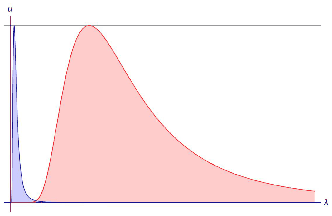
Figure 1 - The plot of \(u(\lambda,T_{\mathrm E})\) (red) and \(\gamma\tilde{u}_{\mathrm S}(\lambda)\) (blue) versus \(\lambda\)
B. The Greenhouse Effect
In this part, we introduce a simple model in which the Earth’s atmosphere is modeled as a thin layer at a small distance above the Earth’s surface so that the difference between the area of the atmosphere’s layer and the area of the Earth's surface can be neglected (see figure 2). In what follows assume that the major part of the thermal radiation from the Earth and the Sun are emitted at wavelengths near the \(\lambda_{\max}\) for each one. Also assume that the “atmosphere layer” reflects a fraction \(r_{\mathrm A}=0.255\) of the visible-ultraviolet radiation incident from above or below, and completely transmits the rest. Assume that the atmosphere does not reflect any part of the infrared radiation, however, it absorbs a fraction \(\varepsilon\) of the infrared radiation and transmits the rest. This behavior, known as the greenhouse effect, changes the average temperature of the Earth. The Earth’s surface, on the other hand, reflects a fraction \(r_{\mathrm E}\) of the visible-ultraviolet radiation and absorbs the rest of this radiation and all the infrared radiation.
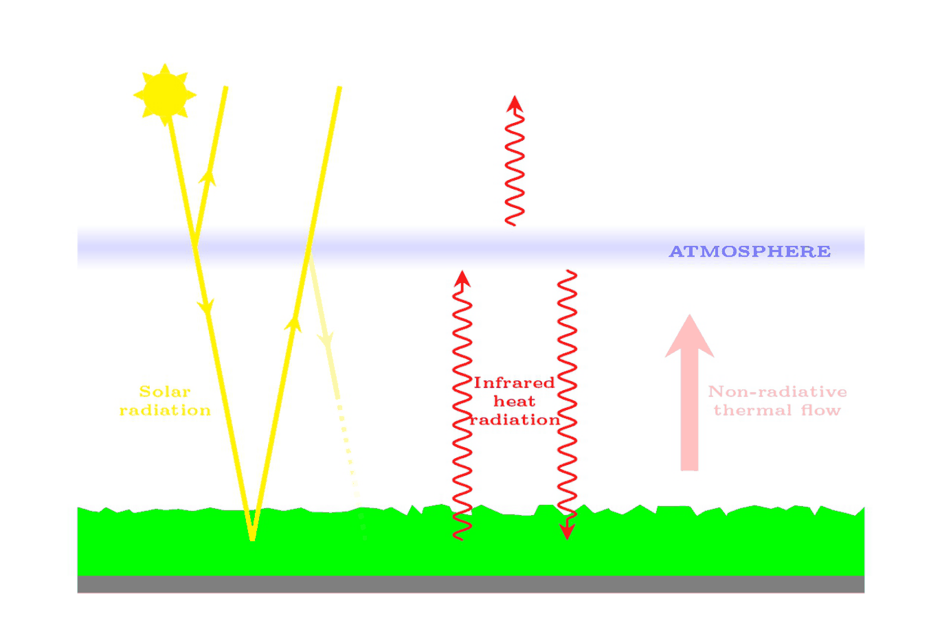
Figure 2 - Thermal flows between the Earth and the atmosphere
| Part | Task | Points |
|---|---|---|
| B-1 | Assume that \(\varepsilon=1\) and \(r_{\mathrm E}=0\), and calculate the Earth’s temperature \(T_{\mathrm E}\) and the atmosphere’s temperature \(T_{\mathrm A}\). | 1.0 pt |
Now assume that \(r_{\mathrm E}\ne0\). In this case, the combined system of “Earth + atmosphere” reflects a different fraction of the solar radiation, called “albedo” and denoted by \(\alpha\).
| Part | Task | Points |
|---|---|---|
| B-2 | Determine the albedo, \(\alpha\), in terms of \(r_{\mathrm E}\) and \(r_{\mathrm A}\). Then calculate its numerical value assuming \(r_{\mathrm E}=0.102\) (and \(r_{\mathrm A}=0.255\)). | 1.6 pt |
| B-3 | a) Express the Earth’s temperature in terms of \(\sigma\), \(\alpha\), \(S_0\), and \(\varepsilon\). b) Using the given data and the calculated albedo, find the numerical value of \(\varepsilon\) which leads to the current average temperature of \(T_{\mathrm E}=288\ \mathrm K\) for the Earth. |
1.0 pt |
| B-4 | Find \(\frac{dT_{\mathrm E}}{d\varepsilon}\) and determine by how much the Earth’s temperature increases if \(\varepsilon\) increases by one percent. | 0.8 pt |
Assume \(T_{\mathrm A}=245\ \mathrm K\) and \(T_{\mathrm E}=288\ \mathrm K\). These values come from real data and may differ from the results which you have obtained in the previous tasks. Now suppose that a non-radiative (e. g. convective) thermal flow \(J_{\mathrm{NR}}=k(T_{\mathrm E}-T_{\mathrm A})\) is maintained from the Earth to the atmosphere, where \(k\) is a constant. The quantity, \(J_{\mathrm{NR}}\), is the transmitted power per unit area.
| Part | Task | Points |
|---|---|---|
| B-5 | Calculate \(\varepsilon\) and \(k\) in terms of \(T_{\mathrm E}\), \(T_{\mathrm A}\), \(\sigma\), \(\alpha\), and \(S_0\). | 1.6 pt |
| B-6 | a) Differentiating the equations obtained in part B-5 with respect to \(\varepsilon\), find the two algebraic equations satisfied by \(\frac{dT_{\mathrm A}}{d\varepsilon}\) and \(\frac{dT_{\mathrm E}}{d\varepsilon}\). b) Use these equations to find the numerical value of change in the Earth’s temperature as a result of a one percent increase in the value of \(\varepsilon\). |
1.0 pt |
Official English text of the problem.
Answers
Define the globally averaged absorbed solar flux by \[ Q=\frac{(1-\alpha)S_0}{4}. \] A one-percent increase is taken to mean \(\Delta\varepsilon=0.01\varepsilon\). Numerical results use unrounded intermediate values.
-
A-1 \[ \boxed{S_0=\sigma T_{\mathrm S}^4\left(\frac{R_{\mathrm S}}d\right)^2 =1.35\times10^3\ \mathrm{W\,m^{-2}}.} \]
-
A-2 \[ \boxed{T_{\mathrm E}=\left(\frac{S_0}{4\sigma}\right)^{1/4} =T_{\mathrm S}\sqrt{\frac{R_{\mathrm S}}{2d}} =278\ \mathrm K.} \]
-
A-3 \[ \boxed{f(x)=5(1-e^{-x})-x.} \]
-
A-4 \[ \boxed{x_m=4.97,\qquad b=\frac{hc}{x_mk_{\mathrm B}}=2.90\times10^{-3}\ \mathrm{m\,K}.} \]
-
A-5 \[ \boxed{\lambda_{\max,\mathrm S}=\frac b{T_{\mathrm S}}=502\ \mathrm{nm}, \qquad \lambda_{\max,\mathrm E}=\frac b{T_{\mathrm E}}=10.4\ \mu\mathrm m.} \]
-
A-6 \[ \boxed{\gamma=\left(\frac d{R_{\mathrm S}}\right)^2 \left(\frac{T_{\mathrm E}}{T_{\mathrm S}}\right)^5 =\frac14\sqrt{\frac{R_{\mathrm S}}{2d}} =1.20\times10^{-2}.} \]
-
B-1 \[ \boxed{T_{\mathrm E}= \left[\frac{(1-r_{\mathrm A})S_0}{2\sigma}\right]^{1/4} =307\ \mathrm K,} \] \[ \boxed{T_{\mathrm A}= \left[\frac{(1-r_{\mathrm A})S_0}{4\sigma}\right]^{1/4} =258\ \mathrm K.} \]
-
B-2 \[ \boxed{\alpha=r_{\mathrm A}+ \frac{r_{\mathrm E}(1-r_{\mathrm A})^2}{1-r_{\mathrm A}r_{\mathrm E}} =0.313.} \]
-
B-3(a) \[ \boxed{T_{\mathrm E}= \left[\frac{(1-\alpha)S_0}{4\sigma(1-\varepsilon/2)}\right]^{1/4}.} \]
-
B-3(b) \[ \boxed{\varepsilon= 2-\frac{(1-\alpha)S_0}{2\sigma T_{\mathrm E}^4} =0.809.} \]
-
B-4 \[ \boxed{\frac{dT_{\mathrm E}}{d\varepsilon} =\frac{T_{\mathrm E}}{4(2-\varepsilon)} =60.4\ \mathrm K,} \qquad \boxed{\Delta T_{\mathrm E}\simeq0.489\ \mathrm K.} \] The temperature change is the first-order result; the exact finite change is \(0.491\ \mathrm K\).
-
B-5 \[ \boxed{\varepsilon= \frac{\sigma T_{\mathrm E}^4-Q} {\sigma(T_{\mathrm E}^4-T_{\mathrm A}^4)} =0.849,} \] \[ \boxed{k= \frac{(\sigma T_{\mathrm E}^4-Q)(2T_{\mathrm A}^4-T_{\mathrm E}^4)} {(T_{\mathrm E}^4-T_{\mathrm A}^4)(T_{\mathrm E}-T_{\mathrm A})} =0.365\ \mathrm{W\,m^{-2}\,K^{-1}}.} \]
-
B-6(a) With \(X=dT_{\mathrm E}/d\varepsilon\) and \(Y=dT_{\mathrm A}/d\varepsilon\), \[ \boxed{(4\sigma T_{\mathrm E}^3+k)X -(4\varepsilon\sigma T_{\mathrm A}^3+k)Y =\sigma T_{\mathrm A}^4,} \] \[ \boxed{-(4\varepsilon\sigma T_{\mathrm E}^3+k)X +(8\varepsilon\sigma T_{\mathrm A}^3+k)Y =\sigma(T_{\mathrm E}^4-2T_{\mathrm A}^4).} \]
-
B-6(b) \[ \boxed{X=61.7\ \mathrm K,\qquad Y=47.8\ \mathrm K,\qquad \Delta T_{\mathrm E}\simeq0.524\ \mathrm K.} \] The temperature change is the first-order result; the exact finite change is \(0.527\ \mathrm K\).
Solution
A-1
The Sun’s total radiated power follows from the Stefan–Boltzmann law: \[ L_{\mathrm S}=4\pi R_{\mathrm S}^2\sigma T_{\mathrm S}^4. \] Conservation of radiative power distributes this luminosity over a sphere of radius \(d\). Consequently, \[ S_0=\frac{L_{\mathrm S}}{4\pi d^2} =\sigma T_{\mathrm S}^4\left(\frac{R_{\mathrm S}}d\right)^2. \] Substitution gives \[ S_0=1353.076\ldots\ \mathrm{W\,m^{-2}} =\boxed{1.35\times10^3\ \mathrm{W\,m^{-2}}}. \]
The same geometrical dilution applies at every wavelength: \[ \tilde{u}_{\mathrm S}(\lambda) =\left(\frac{R_{\mathrm S}}d\right)^2u(\lambda,T_{\mathrm S}). \]
A-2
Let \(R_{\mathrm E}\) denote the Earth’s radius. The Earth intercepts sunlight over its projected area \(\pi R_{\mathrm E}^2\), while its entire surface \(4\pi R_{\mathrm E}^2\) emits thermal radiation.
For a blackbody Earth in equilibrium, \[ \pi R_{\mathrm E}^2S_0 =4\pi R_{\mathrm E}^2\sigma T_{\mathrm E}^4. \] Thus \[ T_{\mathrm E} =\left(\frac{S_0}{4\sigma}\right)^{1/4} =T_{\mathrm S}\sqrt{\frac{R_{\mathrm S}}{2d}} =277.920\ldots\ \mathrm K. \] Therefore, \[ \boxed{T_{\mathrm E}=278\ \mathrm K}. \]
A-3
At fixed \(T\), introduce \[ x=\frac{hc}{\lambda k_{\mathrm B}T}. \] Logarithmic differentiation of Planck’s law gives \[ \frac{1}{u}\frac{\partial u}{\partial\lambda} =\frac1\lambda\left[-5+\frac{x e^x}{e^x-1}\right]. \] At a finite-wavelength maximum this derivative vanishes, so \[ 5=\frac{x}{1-e^{-x}}. \] Hence a suitable function is \[ \boxed{f(x)=5(1-e^{-x})-x}. \]
The algebraic root \(x=0\) corresponds to \(\lambda\to\infty\), rather than a finite-wavelength maximum. The required root is positive and nonzero.
A-4
The nonzero root can be obtained, for example, using Newton’s method: \[ x_{n+1} =x_n-\frac{5(1-e^{-x_n})-x_n}{5e^{-x_n}-1}. \] Starting at \(x_0=5\) gives \[ x_m=4.965114\ldots. \] Since \(x_m=hc/(\lambda_{\max}k_{\mathrm B}T)\), \[ \lambda_{\max}T=\frac{hc}{x_mk_{\mathrm B}}=b. \] Using the supplied constants, \[ b= \frac{1.24\times10^3} {(4.965114\ldots)(8.62\times10^{-5})} \ \mathrm{nm\,K} =2.897244\ldots\times10^{-3}\ \mathrm{m\,K}. \] Therefore, \[ \boxed{x_m=4.97,\qquad b=2.90\times10^{-3}\ \mathrm{m\,K}}. \]
Planck’s function tends to zero at both wavelength endpoints, and this is its unique finite positive stationary point, so it is the maximum.
A-5
Applying Wien’s displacement law to each body, \[ \lambda_{\max,\mathrm S} =\frac b{T_{\mathrm S}} =502.122\ldots\ \mathrm{nm}, \] \[ \lambda_{\max,\mathrm E} =\frac b{T_{\mathrm E}} =10.4247\ldots\ \mu\mathrm m. \] Thus \[ \boxed{\lambda_{\max,\mathrm S}=502\ \mathrm{nm},\qquad \lambda_{\max,\mathrm E}=10.4\ \mu\mathrm m}. \]
The solar peak is in the visible range, while the Earth’s peak is in the infrared.
A-6
At the maximum, \(\lambda_{\max}=b/T\) and the exponential argument equals \(x_m\). Therefore, \[ u_{\max}(T) =\frac{2\pi hc^2}{b^5(e^{x_m}-1)}T^5. \] Thus the peak spectral power per unit wavelength scales as \(T^5\).
Equality of the two plotted peak heights requires \[ \gamma\left(\frac{R_{\mathrm S}}d\right)^2u_{\max}(T_{\mathrm S}) =u_{\max}(T_{\mathrm E}), \] which gives \[ \gamma=\left(\frac d{R_{\mathrm S}}\right)^2 \left(\frac{T_{\mathrm E}}{T_{\mathrm S}}\right)^5. \] From A-2, \[ \left(\frac{T_{\mathrm E}}{T_{\mathrm S}}\right)^4 =\frac14\left(\frac{R_{\mathrm S}}d\right)^2. \] Consequently, \[ \gamma=\frac{T_{\mathrm E}}{4T_{\mathrm S}} =\frac14\sqrt{\frac{R_{\mathrm S}}{2d}} =\boxed{1.20\times10^{-2}}. \]
B-1
In part B, the stated spectral approximation treats solar radiation as visible-ultraviolet and thermal emission from the Earth and atmosphere as infrared. The atmosphere absorbs no solar radiation. By Kirchhoff’s law, its infrared emissivity equals \(\varepsilon\), so each face emits a flux \(\varepsilon\sigma T_{\mathrm A}^4\). The Earth’s infrared emissivity is unity.
Here \(\varepsilon=1\) and \(r_{\mathrm E}=0\). The globally averaged solar flux absorbed at the surface is \[ Q_1=\frac{(1-r_{\mathrm A})S_0}{4}. \] Atmospheric equilibrium requires \[ \sigma T_{\mathrm E}^4=2\sigma T_{\mathrm A}^4, \] because the atmosphere absorbs the Earth’s upward emission and emits in both directions.
The surface balance is \[ Q_1+\sigma T_{\mathrm A}^4=\sigma T_{\mathrm E}^4. \] Combining the equations, \[ \sigma T_{\mathrm A}^4=Q_1,\qquad \sigma T_{\mathrm E}^4=2Q_1. \] Therefore, \[ T_{\mathrm A} =\left[\frac{(1-r_{\mathrm A})S_0}{4\sigma}\right]^{1/4} =\boxed{258\ \mathrm K}, \] \[ T_{\mathrm E} =\left[\frac{(1-r_{\mathrm A})S_0}{2\sigma}\right]^{1/4} =\boxed{307\ \mathrm K}. \]
B-2
Normalize the incoming solar power to unity. The atmosphere immediately reflects a fraction \(r_{\mathrm A}\). The fraction escaping to space after one reflection from the surface is \[ (1-r_{\mathrm A})r_{\mathrm E}(1-r_{\mathrm A}). \] Each additional round trip between the surface and atmosphere multiplies the remaining reflected power by \(r_{\mathrm A}r_{\mathrm E}\).
Summing all contributions, \[ \begin{aligned} \alpha &=r_{\mathrm A} +r_{\mathrm E}(1-r_{\mathrm A})^2 \sum_{n=0}^{\infty}(r_{\mathrm A}r_{\mathrm E})^n\\ &=r_{\mathrm A} +\frac{r_{\mathrm E}(1-r_{\mathrm A})^2} {1-r_{\mathrm A}r_{\mathrm E}}. \end{aligned} \] Equivalently, \[ 1-\alpha =\frac{(1-r_{\mathrm A})(1-r_{\mathrm E})} {1-r_{\mathrm A}r_{\mathrm E}}. \] With the given reflectivities, \[ \alpha=0.313124\ldots, \qquad \boxed{\alpha=0.313}. \]
All solar power that is not reflected is absorbed by the surface.
B-3
(a) Define \[ Q=\frac{(1-\alpha)S_0}{4}. \] Without non-radiative heat transport, the surface and atmospheric balances are \[ Q+\varepsilon\sigma T_{\mathrm A}^4=\sigma T_{\mathrm E}^4, \] \[ \varepsilon\sigma T_{\mathrm E}^4 =2\varepsilon\sigma T_{\mathrm A}^4. \] For \(\varepsilon>0\), the second equation gives \[ T_{\mathrm A}^4=\frac{T_{\mathrm E}^4}{2}. \] Substituting into the first equation, \[ Q=\sigma T_{\mathrm E}^4\left(1-\frac{\varepsilon}{2}\right). \] Hence \[ \boxed{ T_{\mathrm E} =\left[\frac{(1-\alpha)S_0} {4\sigma(1-\varepsilon/2)}\right]^{1/4}. } \] This expression also extends continuously to \(\varepsilon=0\).
(b) Rearranging for the absorptivity, \[ \varepsilon =2\left(1-\frac{Q}{\sigma T_{\mathrm E}^4}\right) =2-\frac{(1-\alpha)S_0}{2\sigma T_{\mathrm E}^4}. \] The unrounded fluxes are \[ Q=232.348778\ldots\ \mathrm{W\,m^{-2}}, \qquad \sigma(288\ \mathrm K)^4=390.079395\ldots\ \mathrm{W\,m^{-2}}. \] Thus \[ \varepsilon=0.808710\ldots, \qquad \boxed{\varepsilon=0.809}. \]
B-4
Hold \(S_0\) and \(\alpha\) fixed. Logarithmic differentiation of the B-3 result gives \[ \frac{1}{T_{\mathrm E}}\frac{dT_{\mathrm E}}{d\varepsilon} =\frac{1}{8(1-\varepsilon/2)} =\frac{1}{4(2-\varepsilon)}. \] Therefore, \[ \boxed{\frac{dT_{\mathrm E}}{d\varepsilon} =\frac{T_{\mathrm E}}{4(2-\varepsilon)}}. \] At the B-3 equilibrium, \[ \frac{dT_{\mathrm E}}{d\varepsilon} =60.4387\ldots\ \mathrm K =\boxed{60.4\ \mathrm K}. \]
For a relative one-percent increase, \[ \Delta\varepsilon=0.01\varepsilon. \] To first order, \[ \Delta T_{\mathrm E} \simeq\frac{dT_{\mathrm E}}{d\varepsilon}\Delta\varepsilon =\frac{0.01\varepsilon T_{\mathrm E}}{4(2-\varepsilon)} =\boxed{0.489\ \mathrm K}. \]
For comparison, evaluating the finite change directly gives \[ \Delta T_{\mathrm E}^{\mathrm{finite}} =T_{\mathrm E} \left[ \left(\frac{2-\varepsilon}{2-1.01\varepsilon}\right)^{1/4}-1 \right] =\boxed{0.491\ \mathrm K}. \]
B-5
Include the upward non-radiative flux \[ J_{\mathrm{NR}}=k(T_{\mathrm E}-T_{\mathrm A}). \] The surface loses this energy, while the atmosphere gains it. Their equilibrium equations become \[ Q+\varepsilon\sigma T_{\mathrm A}^4 =\sigma T_{\mathrm E}^4+k(T_{\mathrm E}-T_{\mathrm A}), \tag{2} \] \[ \varepsilon\sigma T_{\mathrm E}^4+k(T_{\mathrm E}-T_{\mathrm A}) =2\varepsilon\sigma T_{\mathrm A}^4. \tag{3} \]
For brevity, write \[ E=\sigma T_{\mathrm E}^4,\qquad A=\sigma T_{\mathrm A}^4. \] Adding the two energy balances eliminates the internal heat transfer: \[ Q=(1-\varepsilon)E+\varepsilon A. \] The right-hand side is the radiation escaping to space: transmitted surface radiation plus upward atmospheric emission. Solving, \[ \boxed{\varepsilon=\frac{E-Q}{E-A} =\frac{\sigma T_{\mathrm E}^4-Q} {\sigma(T_{\mathrm E}^4-T_{\mathrm A}^4)}}. \]
Equation (3) gives \[ k(T_{\mathrm E}-T_{\mathrm A})=\varepsilon(2A-E). \] Therefore, \[ \boxed{ k=\frac{\varepsilon\sigma(2T_{\mathrm A}^4-T_{\mathrm E}^4)} {T_{\mathrm E}-T_{\mathrm A}} =\frac{(\sigma T_{\mathrm E}^4-Q)(2T_{\mathrm A}^4-T_{\mathrm E}^4)} {(T_{\mathrm E}^4-T_{\mathrm A}^4)(T_{\mathrm E}-T_{\mathrm A})}. } \]
At \(T_{\mathrm E}=288\ \mathrm K\) and \(T_{\mathrm A}=245\ \mathrm K\), \[ E=390.079395\ldots\ \mathrm{W\,m^{-2}}, \qquad A=204.290135\ldots\ \mathrm{W\,m^{-2}}. \] Consequently, \[ \boxed{\varepsilon=0.849,\qquad k=0.365\ \mathrm{W\,m^{-2}\,K^{-1}}}. \] The resulting heat flux is \[ J_{\mathrm{NR}}=15.7\ \mathrm{W\,m^{-2}}, \] which is positive in the stipulated upward direction.
B-6
(a) When \(\varepsilon\) varies, hold \(S_0\), \(\alpha\), and \(k\) fixed, and allow both temperatures to change. Set \[ X=\frac{dT_{\mathrm E}}{d\varepsilon}, \qquad Y=\frac{dT_{\mathrm A}}{d\varepsilon}. \]
Differentiating equation (2) gives \[ \sigma T_{\mathrm A}^4 +4\varepsilon\sigma T_{\mathrm A}^3Y =4\sigma T_{\mathrm E}^3X+k(X-Y). \] Hence \[ \boxed{ (4\sigma T_{\mathrm E}^3+k)X -(4\varepsilon\sigma T_{\mathrm A}^3+k)Y =\sigma T_{\mathrm A}^4. } \]
Differentiating equation (3) gives \[ \sigma T_{\mathrm E}^4 +4\varepsilon\sigma T_{\mathrm E}^3X+k(X-Y) =2\sigma T_{\mathrm A}^4 +8\varepsilon\sigma T_{\mathrm A}^3Y. \] Thus \[ \boxed{ -(4\varepsilon\sigma T_{\mathrm E}^3+k)X +(8\varepsilon\sigma T_{\mathrm A}^3+k)Y =\sigma(T_{\mathrm E}^4-2T_{\mathrm A}^4). } \]
(b) To give an explicit parametric expression, define \[ p=4\sigma T_{\mathrm E}^3,\qquad q=4\sigma T_{\mathrm A}^3, \] and retain \(E=\sigma T_{\mathrm E}^4\), \(A=\sigma T_{\mathrm A}^4\). The determinant of the system is \[ D=(p+k)(2\varepsilon q+k)-(\varepsilon q+k)(\varepsilon p+k) =\varepsilon(2-\varepsilon)pq +k\bigl[(1-\varepsilon)p+\varepsilon q\bigr]. \] Eliminating \(Y\) gives \[ \boxed{ X=\frac{\varepsilon qE+k(E-A)}{D}. } \] Similarly, \[ Y=\frac{(p+k)(E-2A)+(\varepsilon p+k)A}{D}. \]
Using the equilibrium values from B-5, \[ X=61.7352\ldots\ \mathrm K, \qquad Y=47.7734\ldots\ \mathrm K. \] For \(\Delta\varepsilon=0.01\varepsilon\), \[ \Delta T_{\mathrm E} \simeq X\Delta\varepsilon =(61.7352\ldots)(0.01)(0.84897597\ldots)\ \mathrm K. \] Therefore, \[ \boxed{\Delta T_{\mathrm E}\simeq0.524\ \mathrm K}. \]
Solving the original nonlinear balances at \(\varepsilon_{\mathrm{new}}=1.01\varepsilon\), with the same \(k\), gives the finite change \[ \boxed{\Delta T_{\mathrm E}^{\mathrm{finite}}=0.527\ \mathrm K}. \]
The solution was checked against the official solution.
IPhO 2024 · Theorieaufgabe 1
Der Treibhauseffekt
Im Jahr 2021 wurde Syukuro Manabe und Klaus Hasselmann die Hälfte des Nobelpreises für Physik für ihre Arbeiten zur Modellierung des Erdklimas und zur zuverlässigen Vorhersage der durch menschliche Industrieaktivitäten verursachten globalen Erwärmung verliehen. In dieser Aufgabe untersuchen wir ein einfaches Modell der globalen Erwärmung durch den Treibhauseffekt. Die Treibhausgase verändern die optischen Eigenschaften der Erdatmosphäre hinsichtlich der Transmission und Absorption der Infrarotstrahlung der Erde, wodurch die mittlere Temperatur des Planeten ansteigt.
Alle Körper emittieren bei unterschiedlichen Temperaturen Wärmestrahlung. Die Größe \(u(\lambda,T)d\lambda\) gibt die thermische Strahlungsleistung pro Flächeneinheit eines Körpers bei der Temperatur \(T\) im Wellenlängenintervall zwischen \(\lambda\) und \(\lambda+d\lambda\) an. Nach der Planckschen Theorie der Schwarzkörperstrahlung gilt
\[ u(\lambda,T)=\frac{2\pi hc^2}{\lambda^5} \frac{1}{\exp\!\left(\frac{hc}{\lambda k_{\mathrm B}T}\right)-1}, \tag{1} \]
wobei \(hc=1.24\times10^3\ \mathrm{eV\cdot nm}\) und \(k_{\mathrm B}=8.62\times10^{-5}\ \mathrm{eV/K}\) sind. Die Wellenlänge, bei der \(u(\lambda,T)\) maximal ist, ergibt sich aus der Beziehung \(\lambda_{\max}T=b\) (Wiensches Verschiebungsgesetz). Mithilfe von Gleichung (1) lässt sich zeigen, dass \(b=\frac{hc}{x_mk_{\mathrm B}}\) gilt, wobei die dimensionslose Größe \(x_m\) die nichttriviale Lösung einer Gleichung der Form \(f(x)=0\) ist; in einer der folgenden Teilaufgaben sollen Sie die Funktion \(f(x)\) bestimmen. Die gesamte Strahlungsleistung pro Flächeneinheit eines schwarzen Körpers über alle Wellenlängen ist nach dem Stefan-Boltzmann-Gesetz durch \(U(T)=\sigma T^4\) gegeben, wobei \(\sigma=5.67\times10^{-8}\ \mathrm{W/m^2K^4}\) ist. Darüber hinaus gilt nach dem Kirchhoffschen Strahlungsgesetz: Ein Körper, der im thermischen Gleichgewicht bei einer bestimmten Wellenlänge einen bestimmten Anteil der einfallenden Strahlung absorbiert, emittiert bei derselben Wellenlänge denselben Anteil der Schwarzkörperstrahlung.
Nehmen Sie in dieser gesamten Aufgabe an, dass die Sonne ein schwarzer Körper mit ihrer mittleren Oberflächentemperatur von \(T_{\mathrm S}=5.77\times10^3\ \mathrm K\) ist. Der Sonnenradius beträgt \(R_{\mathrm S}=6.96\times10^8\ \mathrm m\), und der mittlere Abstand zwischen Erde und Sonne beträgt \(d=1.50\times10^{11}\ \mathrm m\). Mit \(\tilde{u}_{\mathrm S}(\lambda)\) bezeichnen wir die spektrale Sonnenstrahlungsleistung, die auf eine zur Strahlungsrichtung senkrechte Einheitsfläche an der Erde fällt. Das Integral dieser Größe über alle Wellenlängen, also \(S_0=\int\tilde{u}_{\mathrm S}(\lambda)d\lambda\), wird Solarkonstante genannt.
Nehmen Sie in dieser Aufgabe an, dass sich die Erde im thermischen Gleichgewicht befindet und an allen Punkten ihrer Oberfläche dieselbe Temperatur hat. Geben Sie in allen Teilaufgaben die gesuchte Größe zunächst als Formel in Abhängigkeit von den in der Aufgabe gegebenen Größen an und bestimmen Sie anschließend ihren Zahlenwert auf drei signifikante Stellen genau. Die erforderlichen Einheiten sind auf dem Antwortblatt angegeben.
A. Die Erde als schwarzer Körper
Betrachten Sie in diesem Teil die Erdoberfläche als schwarzen Körper und vernachlässigen Sie die Erdatmosphäre.
| Teil | Aufgabe | Punkte |
|---|---|---|
| A-1 | Bestimmen Sie die Solarkonstante \(S_0\). | 0.6 Pkt. |
| A-2 | Bestimmen Sie die Temperatur der Erde \(T_{\mathrm E}\). | 0.6 Pkt. |
| A-3 | Bestimmen Sie die Funktion \(f(x)\). | 0.4 Pkt. |
| A-4 | Berechnen Sie den Zahlenwert von \(x_m\) und bestimmen Sie aus diesem Wert \(x_m\) den Wert von \(b\). | 0.4 Pkt. |
| A-5 | Bestimmen Sie \(\lambda_{\max}\) für die Sonne und die Erde. | 0.2 Pkt. |
In Abbildung 1 sind die Funktionen \(\gamma\tilde{u}_{\mathrm S}(\lambda)\) und \(u(\lambda,T_{\mathrm E})\) gegen \(\lambda\) aufgetragen. Dabei ist \(\gamma\) ein dimensionsloser Koeffizient, mit dem \(\tilde{u}_{\mathrm S}(\lambda)\) so skaliert wird, dass die Werte der beiden Maxima übereinstimmen.
| Teil | Aufgabe | Punkte |
|---|---|---|
| A-6 | Bestimmen Sie \(\gamma\). | 0.8 Pkt. |
Abbildung 1 - Darstellung von \(u(\lambda,T_{\mathrm E})\) (rot) und \(\gamma\tilde{u}_{\mathrm S}(\lambda)\) (blau) in Abhängigkeit von \(\lambda\)
B. Der Treibhauseffekt
In diesem Teil führen wir ein einfaches Modell ein, in dem die Erdatmosphäre als dünne Schicht in geringer Höhe über der Erdoberfläche modelliert wird, sodass der Unterschied zwischen der Fläche der Atmosphärenschicht und der Fläche der Erdoberfläche vernachlässigt werden kann (siehe Abbildung 2). Nehmen Sie im Folgenden an, dass der überwiegende Teil der Wärmestrahlung von Erde und Sonne bei Wellenlängen in der Nähe des jeweiligen \(\lambda_{\max}\) emittiert wird. Nehmen Sie außerdem an, dass die „Atmosphärenschicht“ einen Anteil \(r_{\mathrm A}=0.255\) der von oben oder unten einfallenden sichtbaren und ultravioletten Strahlung reflektiert und den Rest vollständig durchlässt. Nehmen Sie an, dass die Atmosphäre keinen Anteil der Infrarotstrahlung reflektiert, jedoch einen Anteil \(\varepsilon\) der Infrarotstrahlung absorbiert und den Rest durchlässt. Dieses als Treibhauseffekt bekannte Verhalten verändert die mittlere Temperatur der Erde. Die Erdoberfläche hingegen reflektiert einen Anteil \(r_{\mathrm E}\) der sichtbaren und ultravioletten Strahlung und absorbiert den Rest dieser Strahlung sowie die gesamte Infrarotstrahlung.
Abbildung 2 - Wärmeströme zwischen Erde und Atmosphäre
| Teil | Aufgabe | Punkte |
|---|---|---|
| B-1 | Nehmen Sie \(\varepsilon=1\) und \(r_{\mathrm E}=0\) an und berechnen Sie die Temperatur der Erde \(T_{\mathrm E}\) und die Temperatur der Atmosphäre \(T_{\mathrm A}\). | 1.0 Pkt. |
Nehmen Sie nun \(r_{\mathrm E}\ne0\) an. In diesem Fall reflektiert das Gesamtsystem „Erde + Atmosphäre“ einen anderen Anteil der Sonnenstrahlung, der „Albedo“ genannt und mit \(\alpha\) bezeichnet wird.
| Teil | Aufgabe | Punkte |
|---|---|---|
| B-2 | Bestimmen Sie die Albedo \(\alpha\) in Abhängigkeit von \(r_{\mathrm E}\) und \(r_{\mathrm A}\). Berechnen Sie anschließend ihren Zahlenwert unter der Annahme \(r_{\mathrm E}=0.102\) (und \(r_{\mathrm A}=0.255\)). | 1.6 Pkt. |
| B-3 | a) Drücken Sie die Temperatur der Erde durch \(\sigma\), \(\alpha\), \(S_0\) und \(\varepsilon\) aus. b) Bestimmen Sie mithilfe der gegebenen Daten und der berechneten Albedo den Zahlenwert von \(\varepsilon\), der zur gegenwärtigen mittleren Temperatur der Erde von \(T_{\mathrm E}=288\ \mathrm K\) führt. |
1.0 Pkt. |
| B-4 | Bestimmen Sie \(\frac{dT_{\mathrm E}}{d\varepsilon}\) und ermitteln Sie, um wie viel die Temperatur der Erde steigt, wenn \(\varepsilon\) um ein Prozent zunimmt. | 0.8 Pkt. |
Nehmen Sie \(T_{\mathrm A}=245\ \mathrm K\) und \(T_{\mathrm E}=288\ \mathrm K\) an. Diese Werte stammen aus realen Daten und können von den Ergebnissen abweichen, die Sie in den vorherigen Teilaufgaben erhalten haben. Nehmen Sie nun an, dass ein nichtstrahlungsbedingter (z. B. konvektiver) Wärmestrom \(J_{\mathrm{NR}}=k(T_{\mathrm E}-T_{\mathrm A})\) von der Erde zur Atmosphäre aufrechterhalten wird, wobei \(k\) eine Konstante ist. Die Größe \(J_{\mathrm{NR}}\) ist die übertragene Leistung pro Flächeneinheit.
| Teil | Aufgabe | Punkte |
|---|---|---|
| B-5 | Berechnen Sie \(\varepsilon\) und \(k\) in Abhängigkeit von \(T_{\mathrm E}\), \(T_{\mathrm A}\), \(\sigma\), \(\alpha\) und \(S_0\). | 1.6 Pkt. |
| B-6 | a) Leiten Sie die in Teil B-5 erhaltenen Gleichungen nach \(\varepsilon\) ab und bestimmen Sie die beiden algebraischen Gleichungen, die \(\frac{dT_{\mathrm A}}{d\varepsilon}\) und \(\frac{dT_{\mathrm E}}{d\varepsilon}\) erfüllen. b) Bestimmen Sie mithilfe dieser Gleichungen den Zahlenwert der Änderung der Erdtemperatur infolge einer Zunahme von \(\varepsilon\) um ein Prozent. |
1.0 Pkt. |
Aufgabentext aus dem offiziellen englischen Text übersetzt.
Antworten
Die global gemittelte absorbierte solare Strahlungsflussdichte sei definiert durch \[ Q=\frac{(1-\alpha)S_0}{4}. \] Eine Zunahme um ein Prozent wird als \(\Delta\varepsilon=0.01\varepsilon\) verstanden. Für die numerischen Ergebnisse werden ungerundete Zwischenwerte verwendet.
-
A-1 \[ \boxed{S_0=\sigma T_{\mathrm S}^4\left(\frac{R_{\mathrm S}}d\right)^2 =1.35\times10^3\ \mathrm{W\,m^{-2}}.} \]
-
A-2 \[ \boxed{T_{\mathrm E}=\left(\frac{S_0}{4\sigma}\right)^{1/4} =T_{\mathrm S}\sqrt{\frac{R_{\mathrm S}}{2d}} =278\ \mathrm K.} \]
-
A-3 \[ \boxed{f(x)=5(1-e^{-x})-x.} \]
-
A-4 \[ \boxed{x_m=4.97,\qquad b=\frac{hc}{x_mk_{\mathrm B}}=2.90\times10^{-3}\ \mathrm{m\,K}.} \]
-
A-5 \[ \boxed{\lambda_{\max,\mathrm S}=\frac b{T_{\mathrm S}}=502\ \mathrm{nm}, \qquad \lambda_{\max,\mathrm E}=\frac b{T_{\mathrm E}}=10.4\ \mu\mathrm m.} \]
-
A-6 \[ \boxed{\gamma=\left(\frac d{R_{\mathrm S}}\right)^2 \left(\frac{T_{\mathrm E}}{T_{\mathrm S}}\right)^5 =\frac14\sqrt{\frac{R_{\mathrm S}}{2d}} =1.20\times10^{-2}.} \]
-
B-1 \[ \boxed{T_{\mathrm E}= \left[\frac{(1-r_{\mathrm A})S_0}{2\sigma}\right]^{1/4} =307\ \mathrm K,} \] \[ \boxed{T_{\mathrm A}= \left[\frac{(1-r_{\mathrm A})S_0}{4\sigma}\right]^{1/4} =258\ \mathrm K.} \]
-
B-2 \[ \boxed{\alpha=r_{\mathrm A}+ \frac{r_{\mathrm E}(1-r_{\mathrm A})^2}{1-r_{\mathrm A}r_{\mathrm E}} =0.313.} \]
-
B-3(a) \[ \boxed{T_{\mathrm E}= \left[\frac{(1-\alpha)S_0}{4\sigma(1-\varepsilon/2)}\right]^{1/4}.} \]
-
B-3(b) \[ \boxed{\varepsilon= 2-\frac{(1-\alpha)S_0}{2\sigma T_{\mathrm E}^4} =0.809.} \]
-
B-4 \[ \boxed{\frac{dT_{\mathrm E}}{d\varepsilon} =\frac{T_{\mathrm E}}{4(2-\varepsilon)} =60.4\ \mathrm K,} \qquad \boxed{\Delta T_{\mathrm E}\simeq0.489\ \mathrm K.} \] Die Temperaturänderung ist das Ergebnis erster Ordnung; die exakte endliche Änderung beträgt \(0.491\ \mathrm K\).
-
B-5 \[ \boxed{\varepsilon= \frac{\sigma T_{\mathrm E}^4-Q} {\sigma(T_{\mathrm E}^4-T_{\mathrm A}^4)} =0.849,} \] \[ \boxed{k= \frac{(\sigma T_{\mathrm E}^4-Q)(2T_{\mathrm A}^4-T_{\mathrm E}^4)} {(T_{\mathrm E}^4-T_{\mathrm A}^4)(T_{\mathrm E}-T_{\mathrm A})} =0.365\ \mathrm{W\,m^{-2}\,K^{-1}}.} \]
-
B-6(a) Mit \(X=dT_{\mathrm E}/d\varepsilon\) und \(Y=dT_{\mathrm A}/d\varepsilon\), \[ \boxed{(4\sigma T_{\mathrm E}^3+k)X -(4\varepsilon\sigma T_{\mathrm A}^3+k)Y =\sigma T_{\mathrm A}^4,} \] \[ \boxed{-(4\varepsilon\sigma T_{\mathrm E}^3+k)X +(8\varepsilon\sigma T_{\mathrm A}^3+k)Y =\sigma(T_{\mathrm E}^4-2T_{\mathrm A}^4).} \]
-
B-6(b) \[ \boxed{X=61.7\ \mathrm K,\qquad Y=47.8\ \mathrm K,\qquad \Delta T_{\mathrm E}\simeq0.524\ \mathrm K.} \] Die Temperaturänderung ist das Ergebnis erster Ordnung; die exakte endliche Änderung beträgt \(0.527\ \mathrm K\).
Lösung
A-1
Die gesamte Strahlungsleistung der Sonne ergibt sich aus dem Stefan-Boltzmann-Gesetz: \[ L_{\mathrm S}=4\pi R_{\mathrm S}^2\sigma T_{\mathrm S}^4. \] Aufgrund der Erhaltung der Strahlungsleistung verteilt sich diese Leuchtkraft auf eine Kugeloberfläche mit dem Radius \(d\). Folglich gilt \[ S_0=\frac{L_{\mathrm S}}{4\pi d^2} =\sigma T_{\mathrm S}^4\left(\frac{R_{\mathrm S}}d\right)^2. \] Einsetzen ergibt \[ S_0=1353.076\ldots\ \mathrm{W\,m^{-2}} =\boxed{1.35\times10^3\ \mathrm{W\,m^{-2}}}. \]
Dieselbe geometrische Abschwächung gilt bei jeder Wellenlänge: \[ \tilde{u}_{\mathrm S}(\lambda) =\left(\frac{R_{\mathrm S}}d\right)^2u(\lambda,T_{\mathrm S}). \]
A-2
Mit \(R_{\mathrm E}\) sei der Erdradius bezeichnet. Die Erde fängt Sonnenlicht über ihre projizierte Fläche \(\pi R_{\mathrm E}^2\) auf, während ihre gesamte Oberfläche \(4\pi R_{\mathrm E}^2\) Wärmestrahlung emittiert.
Für eine als schwarzer Körper betrachtete Erde im Gleichgewicht gilt \[ \pi R_{\mathrm E}^2S_0 =4\pi R_{\mathrm E}^2\sigma T_{\mathrm E}^4. \] Somit ist \[ T_{\mathrm E} =\left(\frac{S_0}{4\sigma}\right)^{1/4} =T_{\mathrm S}\sqrt{\frac{R_{\mathrm S}}{2d}} =277.920\ldots\ \mathrm K. \] Daher gilt \[ \boxed{T_{\mathrm E}=278\ \mathrm K}. \]
A-3
Bei festem \(T\) definieren wir \[ x=\frac{hc}{\lambda k_{\mathrm B}T}. \] Logarithmisches Differenzieren des Planckschen Strahlungsgesetzes ergibt \[ \frac{1}{u}\frac{\partial u}{\partial\lambda} =\frac1\lambda\left[-5+\frac{x e^x}{e^x-1}\right]. \] Bei einem Maximum mit endlicher Wellenlänge verschwindet diese Ableitung, sodass \[ 5=\frac{x}{1-e^{-x}}. \] Eine geeignete Funktion ist daher \[ \boxed{f(x)=5(1-e^{-x})-x}. \]
Die algebraische Nullstelle \(x=0\) entspricht \(\lambda\to\infty\) und keinem Maximum bei endlicher Wellenlänge. Die gesuchte Nullstelle ist positiv und von null verschieden.
A-4
Die von null verschiedene Nullstelle lässt sich beispielsweise mit dem Newton-Verfahren bestimmen: \[ x_{n+1} =x_n-\frac{5(1-e^{-x_n})-x_n}{5e^{-x_n}-1}. \] Mit dem Startwert \(x_0=5\) erhält man \[ x_m=4.965114\ldots. \] Da \(x_m=hc/(\lambda_{\max}k_{\mathrm B}T)\) gilt, folgt \[ \lambda_{\max}T=\frac{hc}{x_mk_{\mathrm B}}=b. \] Mit den angegebenen Konstanten ergibt sich \[ b= \frac{1.24\times10^3} {(4.965114\ldots)(8.62\times10^{-5})} \ \mathrm{nm\,K} =2.897244\ldots\times10^{-3}\ \mathrm{m\,K}. \] Daher gilt \[ \boxed{x_m=4.97,\qquad b=2.90\times10^{-3}\ \mathrm{m\,K}}. \]
Die Plancksche Funktion strebt an beiden Grenzen des Wellenlängenbereichs gegen null, und dies ist ihre einzige stationäre Stelle bei einer endlichen positiven Wellenlänge; folglich handelt es sich um das Maximum.
A-5
Die Anwendung des Wienschen Verschiebungsgesetzes auf die beiden Körper ergibt \[ \lambda_{\max,\mathrm S} =\frac b{T_{\mathrm S}} =502.122\ldots\ \mathrm{nm}, \] \[ \lambda_{\max,\mathrm E} =\frac b{T_{\mathrm E}} =10.4247\ldots\ \mu\mathrm m. \] Somit gilt \[ \boxed{\lambda_{\max,\mathrm S}=502\ \mathrm{nm},\qquad \lambda_{\max,\mathrm E}=10.4\ \mu\mathrm m}. \]
Das Maximum der Sonnenstrahlung liegt im sichtbaren Bereich, das der Erdstrahlung dagegen im Infrarotbereich.
A-6
Am Maximum gilt \(\lambda_{\max}=b/T\), und das Argument der Exponentialfunktion ist gleich \(x_m\). Daher ist \[ u_{\max}(T) =\frac{2\pi hc^2}{b^5(e^{x_m}-1)}T^5. \] Der Maximalwert der spektralen Strahlungsleistung pro Wellenlängeneinheit ist somit proportional zu \(T^5\).
Die Gleichheit der beiden dargestellten Maximalwerte erfordert \[ \gamma\left(\frac{R_{\mathrm S}}d\right)^2u_{\max}(T_{\mathrm S}) =u_{\max}(T_{\mathrm E}), \] Daraus folgt \[ \gamma=\left(\frac d{R_{\mathrm S}}\right)^2 \left(\frac{T_{\mathrm E}}{T_{\mathrm S}}\right)^5. \] Aus A-2 ergibt sich \[ \left(\frac{T_{\mathrm E}}{T_{\mathrm S}}\right)^4 =\frac14\left(\frac{R_{\mathrm S}}d\right)^2. \] Folglich gilt \[ \gamma=\frac{T_{\mathrm E}}{4T_{\mathrm S}} =\frac14\sqrt{\frac{R_{\mathrm S}}{2d}} =\boxed{1.20\times10^{-2}}. \]
B-1
In Teil B wird in der angegebenen spektralen Näherung die Sonnenstrahlung als sichtbare und ultraviolette Strahlung und die thermische Emission von Erde und Atmosphäre als Infrarotstrahlung behandelt. Die Atmosphäre absorbiert keine Sonnenstrahlung. Nach dem Kirchhoffschen Strahlungsgesetz ist ihr Emissionsgrad im Infrarotbereich gleich \(\varepsilon\), sodass jede Seite eine Strahlungsflussdichte von \(\varepsilon\sigma T_{\mathrm A}^4\) emittiert. Der Emissionsgrad der Erde im Infrarotbereich ist eins.
Hier sind \(\varepsilon=1\) und \(r_{\mathrm E}=0\). Die global gemittelte, an der Oberfläche absorbierte solare Strahlungsflussdichte beträgt \[ Q_1=\frac{(1-r_{\mathrm A})S_0}{4}. \] Das Gleichgewicht der Atmosphäre erfordert \[ \sigma T_{\mathrm E}^4=2\sigma T_{\mathrm A}^4, \] da die Atmosphäre die nach oben gerichtete Emission der Erde absorbiert und in beide Richtungen emittiert.
Die Bilanz an der Oberfläche lautet \[ Q_1+\sigma T_{\mathrm A}^4=\sigma T_{\mathrm E}^4. \] Kombinieren der Gleichungen ergibt \[ \sigma T_{\mathrm A}^4=Q_1,\qquad \sigma T_{\mathrm E}^4=2Q_1. \] Daher gilt \[ T_{\mathrm A} =\left[\frac{(1-r_{\mathrm A})S_0}{4\sigma}\right]^{1/4} =\boxed{258\ \mathrm K}, \] \[ T_{\mathrm E} =\left[\frac{(1-r_{\mathrm A})S_0}{2\sigma}\right]^{1/4} =\boxed{307\ \mathrm K}. \]
B-2
Wir normieren die einfallende Sonnenstrahlungsleistung auf eins. Die Atmosphäre reflektiert unmittelbar einen Anteil \(r_{\mathrm A}\). Der Anteil, der nach einer Reflexion an der Oberfläche in den Weltraum entweicht, beträgt \[ (1-r_{\mathrm A})r_{\mathrm E}(1-r_{\mathrm A}). \] Bei jedem weiteren Hin- und Rückweg zwischen Oberfläche und Atmosphäre wird die verbleibende reflektierte Leistung mit \(r_{\mathrm A}r_{\mathrm E}\) multipliziert.
Die Summe aller Beiträge ergibt \[ \begin{aligned} \alpha &=r_{\mathrm A} +r_{\mathrm E}(1-r_{\mathrm A})^2 \sum_{n=0}^{\infty}(r_{\mathrm A}r_{\mathrm E})^n\\ &=r_{\mathrm A} +\frac{r_{\mathrm E}(1-r_{\mathrm A})^2} {1-r_{\mathrm A}r_{\mathrm E}}. \end{aligned} \] Äquivalent dazu gilt \[ 1-\alpha =\frac{(1-r_{\mathrm A})(1-r_{\mathrm E})} {1-r_{\mathrm A}r_{\mathrm E}}. \] Mit den gegebenen Reflexionsgraden ergibt sich \[ \alpha=0.313124\ldots, \qquad \boxed{\alpha=0.313}. \]
Die gesamte nicht reflektierte Sonnenstrahlungsleistung wird von der Oberfläche absorbiert.
B-3
(a) Wir definieren \[ Q=\frac{(1-\alpha)S_0}{4}. \] Ohne nichtstrahlungsbedingten Wärmetransport lauten die Bilanzen für die Oberfläche und die Atmosphäre \[ Q+\varepsilon\sigma T_{\mathrm A}^4=\sigma T_{\mathrm E}^4, \] \[ \varepsilon\sigma T_{\mathrm E}^4 =2\varepsilon\sigma T_{\mathrm A}^4. \] Für \(\varepsilon>0\) liefert die zweite Gleichung \[ T_{\mathrm A}^4=\frac{T_{\mathrm E}^4}{2}. \] Einsetzen in die erste Gleichung ergibt \[ Q=\sigma T_{\mathrm E}^4\left(1-\frac{\varepsilon}{2}\right). \] Daraus folgt \[ \boxed{ T_{\mathrm E} =\left[\frac{(1-\alpha)S_0} {4\sigma(1-\varepsilon/2)}\right]^{1/4}. } \] Dieser Ausdruck lässt sich auch stetig auf \(\varepsilon=0\) fortsetzen.
(b) Umstellen nach dem Absorptionsgrad ergibt \[ \varepsilon =2\left(1-\frac{Q}{\sigma T_{\mathrm E}^4}\right) =2-\frac{(1-\alpha)S_0}{2\sigma T_{\mathrm E}^4}. \] Die ungerundeten Strahlungsflussdichten sind \[ Q=232.348778\ldots\ \mathrm{W\,m^{-2}}, \qquad \sigma(288\ \mathrm K)^4=390.079395\ldots\ \mathrm{W\,m^{-2}}. \] Somit gilt \[ \varepsilon=0.808710\ldots, \qquad \boxed{\varepsilon=0.809}. \]
B-4
Wir halten \(S_0\) und \(\alpha\) konstant. Logarithmisches Differenzieren des Ergebnisses aus B-3 liefert \[ \frac{1}{T_{\mathrm E}}\frac{dT_{\mathrm E}}{d\varepsilon} =\frac{1}{8(1-\varepsilon/2)} =\frac{1}{4(2-\varepsilon)}. \] Daher gilt \[ \boxed{\frac{dT_{\mathrm E}}{d\varepsilon} =\frac{T_{\mathrm E}}{4(2-\varepsilon)}}. \] Im Gleichgewichtszustand aus B-3 ist \[ \frac{dT_{\mathrm E}}{d\varepsilon} =60.4387\ldots\ \mathrm K =\boxed{60.4\ \mathrm K}. \]
Für eine relative Zunahme um ein Prozent gilt \[ \Delta\varepsilon=0.01\varepsilon. \] In erster Ordnung ist \[ \Delta T_{\mathrm E} \simeq\frac{dT_{\mathrm E}}{d\varepsilon}\Delta\varepsilon =\frac{0.01\varepsilon T_{\mathrm E}}{4(2-\varepsilon)} =\boxed{0.489\ \mathrm K}. \]
Zum Vergleich ergibt die direkte Berechnung der endlichen Änderung \[ \Delta T_{\mathrm E}^{\mathrm{finite}} =T_{\mathrm E} \left[ \left(\frac{2-\varepsilon}{2-1.01\varepsilon}\right)^{1/4}-1 \right] =\boxed{0.491\ \mathrm K}. \]
B-5
Wir berücksichtigen die nach oben gerichtete nichtstrahlungsbedingte Wärmestromdichte \[ J_{\mathrm{NR}}=k(T_{\mathrm E}-T_{\mathrm A}). \] Die Oberfläche gibt diese Energie ab, während die Atmosphäre sie aufnimmt. Ihre Gleichgewichtsbedingungen lauten nun \[ Q+\varepsilon\sigma T_{\mathrm A}^4 =\sigma T_{\mathrm E}^4+k(T_{\mathrm E}-T_{\mathrm A}), \tag{2} \] \[ \varepsilon\sigma T_{\mathrm E}^4+k(T_{\mathrm E}-T_{\mathrm A}) =2\varepsilon\sigma T_{\mathrm A}^4. \tag{3} \]
Zur Abkürzung schreiben wir \[ E=\sigma T_{\mathrm E}^4,\qquad A=\sigma T_{\mathrm A}^4. \] Durch Addition der beiden Energiebilanzen entfällt der interne Wärmetransport: \[ Q=(1-\varepsilon)E+\varepsilon A. \] Die rechte Seite beschreibt die in den Weltraum entweichende Strahlung: die durchgelassene Oberflächenstrahlung zuzüglich der nach oben gerichteten Emission der Atmosphäre. Auflösen ergibt \[ \boxed{\varepsilon=\frac{E-Q}{E-A} =\frac{\sigma T_{\mathrm E}^4-Q} {\sigma(T_{\mathrm E}^4-T_{\mathrm A}^4)}}. \]
Gleichung (3) liefert \[ k(T_{\mathrm E}-T_{\mathrm A})=\varepsilon(2A-E). \] Daher gilt \[ \boxed{ k=\frac{\varepsilon\sigma(2T_{\mathrm A}^4-T_{\mathrm E}^4)} {T_{\mathrm E}-T_{\mathrm A}} =\frac{(\sigma T_{\mathrm E}^4-Q)(2T_{\mathrm A}^4-T_{\mathrm E}^4)} {(T_{\mathrm E}^4-T_{\mathrm A}^4)(T_{\mathrm E}-T_{\mathrm A})}. } \]
Bei \(T_{\mathrm E}=288\ \mathrm K\) und \(T_{\mathrm A}=245\ \mathrm K\) gilt \[ E=390.079395\ldots\ \mathrm{W\,m^{-2}}, \qquad A=204.290135\ldots\ \mathrm{W\,m^{-2}}. \] Folglich ergibt sich \[ \boxed{\varepsilon=0.849,\qquad k=0.365\ \mathrm{W\,m^{-2}\,K^{-1}}}. \] Die resultierende Wärmestromdichte beträgt \[ J_{\mathrm{NR}}=15.7\ \mathrm{W\,m^{-2}}, \] und ist in der vorgegebenen Richtung nach oben positiv.
B-6
(a) Wenn \(\varepsilon\) variiert, halten wir \(S_0\), \(\alpha\) und \(k\) konstant und lassen Änderungen beider Temperaturen zu. Wir setzen \[ X=\frac{dT_{\mathrm E}}{d\varepsilon}, \qquad Y=\frac{dT_{\mathrm A}}{d\varepsilon}. \]
Differenzieren von Gleichung (2) ergibt \[ \sigma T_{\mathrm A}^4 +4\varepsilon\sigma T_{\mathrm A}^3Y =4\sigma T_{\mathrm E}^3X+k(X-Y). \] Daraus folgt \[ \boxed{ (4\sigma T_{\mathrm E}^3+k)X -(4\varepsilon\sigma T_{\mathrm A}^3+k)Y =\sigma T_{\mathrm A}^4. } \]
Differenzieren von Gleichung (3) ergibt \[ \sigma T_{\mathrm E}^4 +4\varepsilon\sigma T_{\mathrm E}^3X+k(X-Y) =2\sigma T_{\mathrm A}^4 +8\varepsilon\sigma T_{\mathrm A}^3Y. \] Somit gilt \[ \boxed{ -(4\varepsilon\sigma T_{\mathrm E}^3+k)X +(8\varepsilon\sigma T_{\mathrm A}^3+k)Y =\sigma(T_{\mathrm E}^4-2T_{\mathrm A}^4). } \]
(b) Um einen expliziten Ausdruck in Abhängigkeit von den Parametern anzugeben, definieren wir \[ p=4\sigma T_{\mathrm E}^3,\qquad q=4\sigma T_{\mathrm A}^3, \] und behalten \(E=\sigma T_{\mathrm E}^4\), \(A=\sigma T_{\mathrm A}^4\) bei. Die Determinante des Gleichungssystems ist \[ D=(p+k)(2\varepsilon q+k)-(\varepsilon q+k)(\varepsilon p+k) =\varepsilon(2-\varepsilon)pq +k\bigl[(1-\varepsilon)p+\varepsilon q\bigr]. \] Eliminieren von \(Y\) ergibt \[ \boxed{ X=\frac{\varepsilon qE+k(E-A)}{D}. } \] Analog gilt \[ Y=\frac{(p+k)(E-2A)+(\varepsilon p+k)A}{D}. \]
Mit den Gleichgewichtswerten aus B-5 ergibt sich \[ X=61.7352\ldots\ \mathrm K, \qquad Y=47.7734\ldots\ \mathrm K. \] Für \(\Delta\varepsilon=0.01\varepsilon\) gilt \[ \Delta T_{\mathrm E} \simeq X\Delta\varepsilon =(61.7352\ldots)(0.01)(0.84897597\ldots)\ \mathrm K. \] Daher ist \[ \boxed{\Delta T_{\mathrm E}\simeq0.524\ \mathrm K}. \]
Das Lösen der ursprünglichen nichtlinearen Bilanzgleichungen bei \(\varepsilon_{\mathrm{new}}=1.01\varepsilon\) mit demselben \(k\) ergibt die endliche Änderung \[ \boxed{\Delta T_{\mathrm E}^{\mathrm{finite}}=0.527\ \mathrm K}. \]
Die Lösung wurde mit der offiziellen Lösung abgeglichen.
IPhO 2024 · Teori sorusu 1
Sera Etkisi
2021 yılında Syukuro Manabe ve Klaus Hasselmann, Dünya'nın iklimini modelleme ve insanların endüstriyel faaliyetlerinden kaynaklanan küresel ısınmayı doğru biçimde öngörme konusundaki çalışmaları nedeniyle Nobel Fizik Ödülü'nün yarısına layık görüldüler. Bu soruda, sera etkisine bağlı küresel ısınmanın basit bir modelini inceleyeceğiz. Sera gazları, Dünya atmosferinin Dünya'dan yayılan kızılötesi ışınımı geçirme veya soğurma ile ilgili optik özelliklerini değiştirerek gezegenin ortalama sıcaklığının yükselmesine neden olur.
Farklı sıcaklıklardaki tüm cisimler ısıl ışınım yayar. \(u(\lambda,T)d\lambda\) niceliği, \(T\) sıcaklığındaki bir cismin \(\lambda\) ile \(\lambda+d\lambda\) dalga boyları arasında birim alan başına yaydığı ısıl ışınım gücünü gösterir. Planck'ın kara cisim ışınımı kuramına göre
\[ u(\lambda,T)=\frac{2\pi hc^2}{\lambda^5} \frac{1}{\exp\!\left(\frac{hc}{\lambda k_{\mathrm B}T}\right)-1}, \tag{1} \]
burada \(hc=1.24\times10^3\ \mathrm{eV\cdot nm}\) ve \(k_{\mathrm B}=8.62\times10^{-5}\ \mathrm{eV/K}\) değerlerindedir. \(u(\lambda,T)\) fonksiyonunun maksimumuna karşılık gelen dalga boyu, \(\lambda_{\max}T=b\) bağıntısından (Wien kayma yasası) bulunur. Nitekim denklem (1) kullanılarak \(b=\frac{hc}{x_mk_{\mathrm B}}\) olduğu gösterilebilir; burada boyutsuz \(x_m\) niceliği, \(f(x)=0\) biçimindeki bir denklemin aşikâr olmayan köküdür; aşağıdaki görevlerden birinde \(f(x)\) fonksiyonunu bulmanız istenmektedir. Bir kara cismin tüm dalga boylarında birim alan başına yaydığı toplam ışınım gücü, Stefan–Boltzmann yasasıyla \(U(T)=\sigma T^4\) olarak verilir; burada \(\sigma=5.67\times10^{-8}\ \mathrm{W/m^2K^4}\) değerindedir. Ayrıca Kirchhoff'un ışınım yasasına göre, ısıl dengede belirli bir dalga boyunda üzerine gelen ışınımın belli bir oranını soğuran bir cisim, aynı dalga boyunda kara cisim ışınımının aynı oranı kadar ışınım yayar.
Bu soru boyunca Güneş'in, ortalama yüzey sıcaklığı olan \(T_{\mathrm S}=5.77\times10^3\ \mathrm K\) sıcaklığında bir kara cisim olduğunu varsayın. Güneş'in yarıçapı \(R_{\mathrm S}=6.96\times10^8\ \mathrm m\), Dünya ile Güneş arasındaki ortalama uzaklık ise \(d=1.50\times10^{11}\ \mathrm m\) değerindedir. Dünya üzerinde ışınım doğrultusuna dik birim alana gelen Güneş ışınımının spektral gücünü \(\tilde{u}_{\mathrm S}(\lambda)\) ile gösteriyoruz. Bu niceliğin tüm dalga boyları üzerinden integrali, yani \(S_0=\int\tilde{u}_{\mathrm S}(\lambda)d\lambda\), Güneş sabiti olarak adlandırılır.
Bu soruda Dünya'nın ısıl dengede olduğunu ve yüzeyinin tüm noktalarında aynı sıcaklığa sahip olduğunu varsayın. Sorunun tüm bölümlerinde, istenen niceliği önce soruda verilen veriler cinsinden parametrik biçimde ifade edin, ardından sayısal değerini üç anlamlı basamakla bulun. Gerekli birimler cevap kâğıdında belirtilmiştir.
A. Kara Cisim Olarak Dünya
Bu bölümde Dünya'nın yüzeyini bir kara cisim olarak ele alın ve Dünya'nın atmosferini ihmal edin.
| Bölüm | Görev | Puan |
|---|---|---|
| A-1 | Güneş sabiti \(S_0\)'ı bulun. | 0.6 puan |
| A-2 | Dünya'nın sıcaklığı \(T_{\mathrm E}\)'yi bulun. | 0.6 puan |
| A-3 | \(f(x)\) fonksiyonunu bulun. | 0.4 puan |
| A-4 | \(x_m\)'nin sayısal değerini hesaplayın ve bu \(x_m\) değerinden \(b\)'nin değerini bulun. | 0.4 puan |
| A-5 | Güneş ve Dünya için \(\lambda_{\max}\)'ı bulun. | 0.2 puan |
Şekil 1'de \(\gamma\tilde{u}_{\mathrm S}(\lambda)\) ve \(u(\lambda,T_{\mathrm E})\) fonksiyonları \(\lambda\)'ya bağlı olarak çizilmiştir; burada \(\gamma\), iki tepe değerinin eşit olmasını sağlayacak şekilde \(\tilde{u}_{\mathrm S}(\lambda)\)'yı yeniden ölçeklendiren boyutsuz bir katsayıdır.
| Bölüm | Görev | Puan |
|---|---|---|
| A-6 | \(\gamma\)'yı belirleyin. | 0.8 puan |
Şekil 1 - \(u(\lambda,T_{\mathrm E})\) (kırmızı) ve \(\gamma\tilde{u}_{\mathrm S}(\lambda)\) (mavi) fonksiyonlarının \(\lambda\)'ya bağlı grafiği
B. Sera Etkisi
Bu bölümde, Dünya atmosferinin Dünya yüzeyinin biraz üzerinde ince bir tabaka olarak modellendiği basit bir model sunuyoruz; böylece atmosfer tabakasının alanı ile Dünya yüzeyinin alanı arasındaki fark ihmal edilebilir (bkz. şekil 2). Bundan sonra, Dünya ve Güneş'ten yayılan ısıl ışınımın büyük kısmının, her birinin kendi \(\lambda_{\max}\) değerine yakın dalga boylarında yayıldığını varsayın. Ayrıca “atmosfer tabakasının” yukarıdan veya aşağıdan gelen görünür-morötesi ışınımın \(r_{\mathrm A}=0.255\) oranındaki kısmını yansıttığını ve geri kalanını tamamen geçirdiğini varsayın. Atmosferin kızılötesi ışınımın hiçbir kısmını yansıtmadığını, ancak kızılötesi ışınımın \(\varepsilon\) oranındaki kısmını soğurduğunu ve geri kalanını geçirdiğini varsayın. Sera etkisi olarak bilinen bu davranış, Dünya'nın ortalama sıcaklığını değiştirir. Dünya'nın yüzeyi ise görünür-morötesi ışınımın \(r_{\mathrm E}\) oranındaki kısmını yansıtır ve bu ışınımın geri kalanını ve kızılötesi ışınımın tamamını soğurur.
Şekil 2 - Dünya ile atmosfer arasındaki ısı akışları
| Bölüm | Görev | Puan |
|---|---|---|
| B-1 | \(\varepsilon=1\) ve \(r_{\mathrm E}=0\) olduğunu varsayarak Dünya'nın sıcaklığı \(T_{\mathrm E}\)'yi ve atmosferin sıcaklığı \(T_{\mathrm A}\)'yı hesaplayın. | 1.0 puan |
Şimdi \(r_{\mathrm E}\ne0\) olduğunu varsayın. Bu durumda “Dünya + atmosfer” birleşik sistemi, Güneş ışınımının “albedo” olarak adlandırılan ve \(\alpha\) ile gösterilen farklı bir oranını yansıtır.
| Bölüm | Görev | Puan |
|---|---|---|
| B-2 | Albedo \(\alpha\)'yı \(r_{\mathrm E}\) ve \(r_{\mathrm A}\) cinsinden belirleyin. Ardından \(r_{\mathrm E}=0.102\) (ve \(r_{\mathrm A}=0.255\)) olduğunu varsayarak sayısal değerini hesaplayın. | 1.6 puan |
| B-3 | a) Dünya'nın sıcaklığını \(\sigma\), \(\alpha\), \(S_0\) ve \(\varepsilon\) cinsinden ifade edin. b) Verilen verileri ve hesaplanan albedoyu kullanarak, Dünya'nın günümüzdeki ortalama sıcaklığı olan \(T_{\mathrm E}=288\ \mathrm K\) değerini veren \(\varepsilon\)'nun sayısal değerini bulun. |
1.0 puan |
| B-4 | \(\frac{dT_{\mathrm E}}{d\varepsilon}\)'nu bulun ve \(\varepsilon\) yüzde bir arttığında Dünya'nın sıcaklığının ne kadar artacağını belirleyin. | 0.8 puan |
\(T_{\mathrm A}=245\ \mathrm K\) ve \(T_{\mathrm E}=288\ \mathrm K\) olduğunu varsayın. Bu değerler gerçek verilerden elde edilmiştir ve önceki görevlerde bulduğunuz sonuçlardan farklı olabilir. Şimdi Dünya'dan atmosfere doğru \(J_{\mathrm{NR}}=k(T_{\mathrm E}-T_{\mathrm A})\) şeklinde ışınım dışı (örneğin taşınımla gerçekleşen) bir ısı akışının sürdüğünü varsayın; burada \(k\) bir sabittir. \(J_{\mathrm{NR}}\) niceliği, birim alan başına aktarılan güçtür.
| Bölüm | Görev | Puan |
|---|---|---|
| B-5 | \(\varepsilon\) ve \(k\)'yı \(T_{\mathrm E}\), \(T_{\mathrm A}\), \(\sigma\), \(\alpha\) ve \(S_0\) cinsinden hesaplayın. | 1.6 puan |
| B-6 | a) Bölüm B-5'te elde edilen denklemlerin \(\varepsilon\)'na göre türevini alarak, \(\frac{dT_{\mathrm A}}{d\varepsilon}\) ve \(\frac{dT_{\mathrm E}}{d\varepsilon}\)'nun sağladığı iki cebirsel denklemi bulun. b) Bu denklemleri kullanarak, \(\varepsilon\)'nun değerindeki yüzde birlik artış sonucunda Dünya'nın sıcaklığında meydana gelen değişimin sayısal değerini bulun. |
1.0 puan |
Soru metni resmi İngilizce metinden çevrilmiştir.
Cevaplar
Küresel ortalaması alınmış soğurulan Güneş ışınımı akısını şöyle tanımlayalım: \[ Q=\frac{(1-\alpha)S_0}{4}. \] Yüzde birlik artış, \(\Delta\varepsilon=0.01\varepsilon\) olarak alınmıştır. Sayısal sonuçlarda yuvarlanmamış ara değerler kullanılmıştır.
-
A-1 \[ \boxed{S_0=\sigma T_{\mathrm S}^4\left(\frac{R_{\mathrm S}}d\right)^2 =1.35\times10^3\ \mathrm{W\,m^{-2}}.} \]
-
A-2 \[ \boxed{T_{\mathrm E}=\left(\frac{S_0}{4\sigma}\right)^{1/4} =T_{\mathrm S}\sqrt{\frac{R_{\mathrm S}}{2d}} =278\ \mathrm K.} \]
-
A-3 \[ \boxed{f(x)=5(1-e^{-x})-x.} \]
-
A-4 \[ \boxed{x_m=4.97,\qquad b=\frac{hc}{x_mk_{\mathrm B}}=2.90\times10^{-3}\ \mathrm{m\,K}.} \]
-
A-5 \[ \boxed{\lambda_{\max,\mathrm S}=\frac b{T_{\mathrm S}}=502\ \mathrm{nm}, \qquad \lambda_{\max,\mathrm E}=\frac b{T_{\mathrm E}}=10.4\ \mu\mathrm m.} \]
-
A-6 \[ \boxed{\gamma=\left(\frac d{R_{\mathrm S}}\right)^2 \left(\frac{T_{\mathrm E}}{T_{\mathrm S}}\right)^5 =\frac14\sqrt{\frac{R_{\mathrm S}}{2d}} =1.20\times10^{-2}.} \]
-
B-1 \[ \boxed{T_{\mathrm E}= \left[\frac{(1-r_{\mathrm A})S_0}{2\sigma}\right]^{1/4} =307\ \mathrm K,} \] \[ \boxed{T_{\mathrm A}= \left[\frac{(1-r_{\mathrm A})S_0}{4\sigma}\right]^{1/4} =258\ \mathrm K.} \]
-
B-2 \[ \boxed{\alpha=r_{\mathrm A}+ \frac{r_{\mathrm E}(1-r_{\mathrm A})^2}{1-r_{\mathrm A}r_{\mathrm E}} =0.313.} \]
-
B-3(a) \[ \boxed{T_{\mathrm E}= \left[\frac{(1-\alpha)S_0}{4\sigma(1-\varepsilon/2)}\right]^{1/4}.} \]
-
B-3(b) \[ \boxed{\varepsilon= 2-\frac{(1-\alpha)S_0}{2\sigma T_{\mathrm E}^4} =0.809.} \]
-
B-4 \[ \boxed{\frac{dT_{\mathrm E}}{d\varepsilon} =\frac{T_{\mathrm E}}{4(2-\varepsilon)} =60.4\ \mathrm K,} \qquad \boxed{\Delta T_{\mathrm E}\simeq0.489\ \mathrm K.} \] Sıcaklık değişimi birinci mertebeden elde edilen sonuçtur; tam sonlu değişim \(0.491\ \mathrm K\)'dir.
-
B-5 \[ \boxed{\varepsilon= \frac{\sigma T_{\mathrm E}^4-Q} {\sigma(T_{\mathrm E}^4-T_{\mathrm A}^4)} =0.849,} \] \[ \boxed{k= \frac{(\sigma T_{\mathrm E}^4-Q)(2T_{\mathrm A}^4-T_{\mathrm E}^4)} {(T_{\mathrm E}^4-T_{\mathrm A}^4)(T_{\mathrm E}-T_{\mathrm A})} =0.365\ \mathrm{W\,m^{-2}\,K^{-1}}.} \]
-
B-6(a) \(X=dT_{\mathrm E}/d\varepsilon\) ve \(Y=dT_{\mathrm A}/d\varepsilon\) olmak üzere, \[ \boxed{(4\sigma T_{\mathrm E}^3+k)X -(4\varepsilon\sigma T_{\mathrm A}^3+k)Y =\sigma T_{\mathrm A}^4,} \] \[ \boxed{-(4\varepsilon\sigma T_{\mathrm E}^3+k)X +(8\varepsilon\sigma T_{\mathrm A}^3+k)Y =\sigma(T_{\mathrm E}^4-2T_{\mathrm A}^4).} \]
-
B-6(b) \[ \boxed{X=61.7\ \mathrm K,\qquad Y=47.8\ \mathrm K,\qquad \Delta T_{\mathrm E}\simeq0.524\ \mathrm K.} \] Sıcaklık değişimi birinci mertebeden elde edilen sonuçtur; tam sonlu değişim \(0.527\ \mathrm K\)'dir.
Çözüm
A-1
Güneş'in yaydığı toplam güç Stefan–Boltzmann yasasından bulunur: \[ L_{\mathrm S}=4\pi R_{\mathrm S}^2\sigma T_{\mathrm S}^4. \] Işınım gücünün korunumu gereği, bu ışınım gücü \(d\) yarıçaplı bir kürenin yüzeyine dağılır. Dolayısıyla, \[ S_0=\frac{L_{\mathrm S}}{4\pi d^2} =\sigma T_{\mathrm S}^4\left(\frac{R_{\mathrm S}}d\right)^2. \] Değerler yerine konulduğunda \[ S_0=1353.076\ldots\ \mathrm{W\,m^{-2}} =\boxed{1.35\times10^3\ \mathrm{W\,m^{-2}}}. \]
Aynı geometrik seyrelme her dalga boyunda geçerlidir: \[ \tilde{u}_{\mathrm S}(\lambda) =\left(\frac{R_{\mathrm S}}d\right)^2u(\lambda,T_{\mathrm S}). \]
A-2
Dünya'nın yarıçapını \(R_{\mathrm E}\) ile gösterelim. Dünya, Güneş ışığını izdüşüm alanı \(\pi R_{\mathrm E}^2\) üzerinden alırken, \(4\pi R_{\mathrm E}^2\) alanlı yüzeyinin tamamı ısıl ışınım yayar.
Kara cisim olarak ele alınan Dünya dengedeyken, \[ \pi R_{\mathrm E}^2S_0 =4\pi R_{\mathrm E}^2\sigma T_{\mathrm E}^4. \] Böylece \[ T_{\mathrm E} =\left(\frac{S_0}{4\sigma}\right)^{1/4} =T_{\mathrm S}\sqrt{\frac{R_{\mathrm S}}{2d}} =277.920\ldots\ \mathrm K. \] Dolayısıyla, \[ \boxed{T_{\mathrm E}=278\ \mathrm K}. \]
A-3
Sabit \(T\) için şu değişkeni tanımlayalım: \[ x=\frac{hc}{\lambda k_{\mathrm B}T}. \] Planck yasasının logaritmik türevi alındığında \[ \frac{1}{u}\frac{\partial u}{\partial\lambda} =\frac1\lambda\left[-5+\frac{x e^x}{e^x-1}\right]. \] Sonlu bir dalga boyundaki maksimumda bu türev sıfır olur, dolayısıyla \[ 5=\frac{x}{1-e^{-x}}. \] Buna göre uygun bir fonksiyon \[ \boxed{f(x)=5(1-e^{-x})-x}. \]
\(x=0\) cebirsel kökü, sonlu bir dalga boyundaki maksimuma değil, \(\lambda\to\infty\) durumuna karşılık gelir. Aranan kök pozitif ve sıfırdan farklıdır.
A-4
Sıfırdan farklı kök, örneğin Newton yöntemiyle elde edilebilir: \[ x_{n+1} =x_n-\frac{5(1-e^{-x_n})-x_n}{5e^{-x_n}-1}. \] \(x_0=5\) ile başlanırsa \[ x_m=4.965114\ldots. \] \(x_m=hc/(\lambda_{\max}k_{\mathrm B}T)\) olduğundan, \[ \lambda_{\max}T=\frac{hc}{x_mk_{\mathrm B}}=b. \] Verilen sabitler kullanıldığında, \[ b= \frac{1.24\times10^3} {(4.965114\ldots)(8.62\times10^{-5})} \ \mathrm{nm\,K} =2.897244\ldots\times10^{-3}\ \mathrm{m\,K}. \] Dolayısıyla, \[ \boxed{x_m=4.97,\qquad b=2.90\times10^{-3}\ \mathrm{m\,K}}. \]
Planck fonksiyonu dalga boyu aralığının her iki ucunda sıfıra yaklaşır ve bu nokta onun sonlu, pozitif dalga boylarındaki tek durağan noktasıdır; dolayısıyla maksimumdur.
A-5
Wien kayma yasası her bir cisme uygulandığında, \[ \lambda_{\max,\mathrm S} =\frac b{T_{\mathrm S}} =502.122\ldots\ \mathrm{nm}, \] \[ \lambda_{\max,\mathrm E} =\frac b{T_{\mathrm E}} =10.4247\ldots\ \mu\mathrm m. \] Böylece \[ \boxed{\lambda_{\max,\mathrm S}=502\ \mathrm{nm},\qquad \lambda_{\max,\mathrm E}=10.4\ \mu\mathrm m}. \]
Güneş'in tepe noktası görünür bölgede, Dünya'nın tepe noktası ise kızılötesi bölgededir.
A-6
Maksimumda \(\lambda_{\max}=b/T\) olur ve üstel fonksiyonun argümanı \(x_m\)'ye eşittir. Dolayısıyla, \[ u_{\max}(T) =\frac{2\pi hc^2}{b^5(e^{x_m}-1)}T^5. \] Böylece birim dalga boyu başına spektral gücün tepe değeri \(T^5\) ile orantılıdır.
Çizilen iki tepenin yüksekliklerinin eşit olması için \[ \gamma\left(\frac{R_{\mathrm S}}d\right)^2u_{\max}(T_{\mathrm S}) =u_{\max}(T_{\mathrm E}), \] olmalıdır; buradan \[ \gamma=\left(\frac d{R_{\mathrm S}}\right)^2 \left(\frac{T_{\mathrm E}}{T_{\mathrm S}}\right)^5. \] A-2'den, \[ \left(\frac{T_{\mathrm E}}{T_{\mathrm S}}\right)^4 =\frac14\left(\frac{R_{\mathrm S}}d\right)^2. \] Dolayısıyla, \[ \gamma=\frac{T_{\mathrm E}}{4T_{\mathrm S}} =\frac14\sqrt{\frac{R_{\mathrm S}}{2d}} =\boxed{1.20\times10^{-2}}. \]
B-1
B bölümünde belirtilen spektral yaklaşım, Güneş ışınımını görünür-morötesi, Dünya ve atmosferden yayılan ısıl ışınımı ise kızılötesi olarak ele alır. Atmosfer, Güneş ışınımını soğurmaz. Kirchhoff yasasına göre atmosferin kızılötesi yayma katsayısı \(\varepsilon\)'na eşittir; dolayısıyla her bir yüzü \(\varepsilon\sigma T_{\mathrm A}^4\) akısı yayar. Dünya'nın kızılötesi yayma katsayısı birdir.
Burada \(\varepsilon=1\) ve \(r_{\mathrm E}=0\)'dır. Yüzeyde soğurulan Güneş ışınımı akısının küresel ortalaması \[ Q_1=\frac{(1-r_{\mathrm A})S_0}{4}. \] Atmosferin dengede olması için \[ \sigma T_{\mathrm E}^4=2\sigma T_{\mathrm A}^4, \] olmalıdır; çünkü atmosfer, Dünya'nın yukarı doğru yaydığı ışınımı soğurur ve her iki yönde ışınım yayar.
Yüzeyin enerji dengesi \[ Q_1+\sigma T_{\mathrm A}^4=\sigma T_{\mathrm E}^4. \] Denklemler birleştirildiğinde, \[ \sigma T_{\mathrm A}^4=Q_1,\qquad \sigma T_{\mathrm E}^4=2Q_1. \] Dolayısıyla, \[ T_{\mathrm A} =\left[\frac{(1-r_{\mathrm A})S_0}{4\sigma}\right]^{1/4} =\boxed{258\ \mathrm K}, \] \[ T_{\mathrm E} =\left[\frac{(1-r_{\mathrm A})S_0}{2\sigma}\right]^{1/4} =\boxed{307\ \mathrm K}. \]
B-2
Gelen Güneş ışınımı gücünü bire normalize edelim. Atmosfer bunun \(r_{\mathrm A}\) oranındaki kısmını doğrudan yansıtır. Yüzeyden bir kez yansıdıktan sonra uzaya kaçan kısım \[ (1-r_{\mathrm A})r_{\mathrm E}(1-r_{\mathrm A}). \] Yüzey ile atmosfer arasındaki her ek gidiş dönüşte, kalan yansımış güç \(r_{\mathrm A}r_{\mathrm E}\) çarpanı ile çarpılır.
Tüm katkılar toplandığında, \[ \begin{aligned} \alpha &=r_{\mathrm A} +r_{\mathrm E}(1-r_{\mathrm A})^2 \sum_{n=0}^{\infty}(r_{\mathrm A}r_{\mathrm E})^n\\ &=r_{\mathrm A} +\frac{r_{\mathrm E}(1-r_{\mathrm A})^2} {1-r_{\mathrm A}r_{\mathrm E}}. \end{aligned} \] Eşdeğer olarak, \[ 1-\alpha =\frac{(1-r_{\mathrm A})(1-r_{\mathrm E})} {1-r_{\mathrm A}r_{\mathrm E}}. \] Verilen yansıtma katsayılarıyla, \[ \alpha=0.313124\ldots, \qquad \boxed{\alpha=0.313}. \]
Yansıtılmayan Güneş ışınımı gücünün tamamı yüzey tarafından soğurulur.
B-3
(a) Şu tanımı yapalım: \[ Q=\frac{(1-\alpha)S_0}{4}. \] Işınım dışı ısı aktarımı olmadığında yüzeyin ve atmosferin enerji dengeleri \[ Q+\varepsilon\sigma T_{\mathrm A}^4=\sigma T_{\mathrm E}^4, \] \[ \varepsilon\sigma T_{\mathrm E}^4 =2\varepsilon\sigma T_{\mathrm A}^4. \] \(\varepsilon>0\) için ikinci denklemden \[ T_{\mathrm A}^4=\frac{T_{\mathrm E}^4}{2}. \] Birinci denklemde yerine konulduğunda, \[ Q=\sigma T_{\mathrm E}^4\left(1-\frac{\varepsilon}{2}\right). \] Böylece \[ \boxed{ T_{\mathrm E} =\left[\frac{(1-\alpha)S_0} {4\sigma(1-\varepsilon/2)}\right]^{1/4}. } \] Bu ifade, \(\varepsilon=0\) durumuna da sürekli biçimde uzanır.
(b) Soğurma katsayısı için yeniden düzenlendiğinde, \[ \varepsilon =2\left(1-\frac{Q}{\sigma T_{\mathrm E}^4}\right) =2-\frac{(1-\alpha)S_0}{2\sigma T_{\mathrm E}^4}. \] Yuvarlanmamış akılar \[ Q=232.348778\ldots\ \mathrm{W\,m^{-2}}, \qquad \sigma(288\ \mathrm K)^4=390.079395\ldots\ \mathrm{W\,m^{-2}}. \] Böylece \[ \varepsilon=0.808710\ldots, \qquad \boxed{\varepsilon=0.809}. \]
B-4
\(S_0\) ve \(\alpha\)'yı sabit tutalım. B-3'teki sonucun logaritmik türevi alındığında \[ \frac{1}{T_{\mathrm E}}\frac{dT_{\mathrm E}}{d\varepsilon} =\frac{1}{8(1-\varepsilon/2)} =\frac{1}{4(2-\varepsilon)}. \] Dolayısıyla, \[ \boxed{\frac{dT_{\mathrm E}}{d\varepsilon} =\frac{T_{\mathrm E}}{4(2-\varepsilon)}}. \] B-3'teki denge durumunda, \[ \frac{dT_{\mathrm E}}{d\varepsilon} =60.4387\ldots\ \mathrm K =\boxed{60.4\ \mathrm K}. \]
Yüzde birlik bağıl artış için, \[ \Delta\varepsilon=0.01\varepsilon. \] Birinci mertebede, \[ \Delta T_{\mathrm E} \simeq\frac{dT_{\mathrm E}}{d\varepsilon}\Delta\varepsilon =\frac{0.01\varepsilon T_{\mathrm E}}{4(2-\varepsilon)} =\boxed{0.489\ \mathrm K}. \]
Karşılaştırma için, sonlu değişim doğrudan hesaplandığında \[ \Delta T_{\mathrm E}^{\mathrm{finite}} =T_{\mathrm E} \left[ \left(\frac{2-\varepsilon}{2-1.01\varepsilon}\right)^{1/4}-1 \right] =\boxed{0.491\ \mathrm K}. \]
B-5
Yukarı yönlü ışınım dışı akıyı hesaba katalım: \[ J_{\mathrm{NR}}=k(T_{\mathrm E}-T_{\mathrm A}). \] Yüzey bu enerjiyi kaybederken atmosfer kazanır. Denge denklemleri şu hâle gelir: \[ Q+\varepsilon\sigma T_{\mathrm A}^4 =\sigma T_{\mathrm E}^4+k(T_{\mathrm E}-T_{\mathrm A}), \tag{2} \] \[ \varepsilon\sigma T_{\mathrm E}^4+k(T_{\mathrm E}-T_{\mathrm A}) =2\varepsilon\sigma T_{\mathrm A}^4. \tag{3} \]
Kısalık için şöyle yazalım: \[ E=\sigma T_{\mathrm E}^4,\qquad A=\sigma T_{\mathrm A}^4. \] İki enerji dengesi toplandığında sistem içindeki ısı aktarımı elenir: \[ Q=(1-\varepsilon)E+\varepsilon A. \] Sağ taraf, uzaya kaçan ışınımdır: atmosferden geçen yüzey ışınımı ile atmosferin yukarı doğru yaydığı ışınımın toplamı. Çözüldüğünde, \[ \boxed{\varepsilon=\frac{E-Q}{E-A} =\frac{\sigma T_{\mathrm E}^4-Q} {\sigma(T_{\mathrm E}^4-T_{\mathrm A}^4)}}. \]
Denklem (3)'ten \[ k(T_{\mathrm E}-T_{\mathrm A})=\varepsilon(2A-E). \] Dolayısıyla, \[ \boxed{ k=\frac{\varepsilon\sigma(2T_{\mathrm A}^4-T_{\mathrm E}^4)} {T_{\mathrm E}-T_{\mathrm A}} =\frac{(\sigma T_{\mathrm E}^4-Q)(2T_{\mathrm A}^4-T_{\mathrm E}^4)} {(T_{\mathrm E}^4-T_{\mathrm A}^4)(T_{\mathrm E}-T_{\mathrm A})}. } \]
\(T_{\mathrm E}=288\ \mathrm K\) ve \(T_{\mathrm A}=245\ \mathrm K\) için, \[ E=390.079395\ldots\ \mathrm{W\,m^{-2}}, \qquad A=204.290135\ldots\ \mathrm{W\,m^{-2}}. \] Dolayısıyla, \[ \boxed{\varepsilon=0.849,\qquad k=0.365\ \mathrm{W\,m^{-2}\,K^{-1}}}. \] Elde edilen ısı akısı \[ J_{\mathrm{NR}}=15.7\ \mathrm{W\,m^{-2}}, \] olup belirtilen yukarı yönde pozitiftir.
B-6
(a) \(\varepsilon\) değişirken \(S_0\), \(\alpha\) ve \(k\)'yı sabit tutalım ve her iki sıcaklığın da değişmesine izin verelim. Şu tanımları yapalım: \[ X=\frac{dT_{\mathrm E}}{d\varepsilon}, \qquad Y=\frac{dT_{\mathrm A}}{d\varepsilon}. \]
Denklem (2)'nin türevi alındığında \[ \sigma T_{\mathrm A}^4 +4\varepsilon\sigma T_{\mathrm A}^3Y =4\sigma T_{\mathrm E}^3X+k(X-Y). \] Böylece \[ \boxed{ (4\sigma T_{\mathrm E}^3+k)X -(4\varepsilon\sigma T_{\mathrm A}^3+k)Y =\sigma T_{\mathrm A}^4. } \]
Denklem (3)'ün türevi alındığında \[ \sigma T_{\mathrm E}^4 +4\varepsilon\sigma T_{\mathrm E}^3X+k(X-Y) =2\sigma T_{\mathrm A}^4 +8\varepsilon\sigma T_{\mathrm A}^3Y. \] Böylece \[ \boxed{ -(4\varepsilon\sigma T_{\mathrm E}^3+k)X +(8\varepsilon\sigma T_{\mathrm A}^3+k)Y =\sigma(T_{\mathrm E}^4-2T_{\mathrm A}^4). } \]
(b) Açık bir parametrik ifade vermek için \[ p=4\sigma T_{\mathrm E}^3,\qquad q=4\sigma T_{\mathrm A}^3, \] tanımlarını yapalım ve \(E=\sigma T_{\mathrm E}^4\), \(A=\sigma T_{\mathrm A}^4\) tanımlarını koruyalım. Sistemin determinantı \[ D=(p+k)(2\varepsilon q+k)-(\varepsilon q+k)(\varepsilon p+k) =\varepsilon(2-\varepsilon)pq +k\bigl[(1-\varepsilon)p+\varepsilon q\bigr]. \] \(Y\) elendiğinde \[ \boxed{ X=\frac{\varepsilon qE+k(E-A)}{D}. } \] Benzer şekilde, \[ Y=\frac{(p+k)(E-2A)+(\varepsilon p+k)A}{D}. \]
B-5'teki denge değerleri kullanıldığında, \[ X=61.7352\ldots\ \mathrm K, \qquad Y=47.7734\ldots\ \mathrm K. \] \(\Delta\varepsilon=0.01\varepsilon\) için, \[ \Delta T_{\mathrm E} \simeq X\Delta\varepsilon =(61.7352\ldots)(0.01)(0.84897597\ldots)\ \mathrm K. \] Dolayısıyla, \[ \boxed{\Delta T_{\mathrm E}\simeq0.524\ \mathrm K}. \]
Başlangıçtaki doğrusal olmayan denge denklemleri aynı \(k\) ile \(\varepsilon_{\mathrm{new}}=1.01\varepsilon\) için çözüldüğünde sonlu değişim elde edilir: \[ \boxed{\Delta T_{\mathrm E}^{\mathrm{finite}}=0.527\ \mathrm K}. \]
Çözüm, resmi çözümle karşılaştırılarak kontrol edildi.
IPhO 2024 · Problema teórico 1
El efecto invernadero
En 2021, Syukuro Manabe y Klaus Hasselmann recibieron la mitad del Premio Nobel de Física por su trabajo en la modelización del clima terrestre y la predicción precisa del calentamiento global causado por las actividades industriales humanas. En este problema, examinaremos un modelo sencillo del calentamiento global debido al efecto invernadero. Los gases de efecto invernadero alteran las propiedades ópticas de la atmósfera terrestre en cuanto a la transmisión o absorción de la radiación infrarroja de la Tierra, lo que provoca un aumento de la temperatura media del planeta.
Todos los objetos, a distintas temperaturas, emiten radiación térmica. La cantidad \(u(\lambda,T)d\lambda\) indica la potencia de radiación térmica por unidad de área de un objeto a temperatura \(T\) entre las longitudes de onda \(\lambda\) y \(\lambda+d\lambda\). Según la teoría de Planck de la radiación del cuerpo negro, tenemos
\[ u(\lambda,T)=\frac{2\pi hc^2}{\lambda^5} \frac{1}{\exp\!\left(\frac{hc}{\lambda k_{\mathrm B}T}\right)-1}, \tag{1} \]
en la que \(hc=1.24\times10^3\ \mathrm{eV\cdot nm}\) y \(k_{\mathrm B}=8.62\times10^{-5}\ \mathrm{eV/K}\). La longitud de onda correspondiente al máximo de \(u(\lambda,T)\) se obtiene de la relación \(\lambda_{\max}T=b\) (ley de desplazamiento de Wien). En efecto, utilizando la ecuación (1), se puede demostrar que \(b=\frac{hc}{x_mk_{\mathrm B}}\), donde la cantidad adimensional \(x_m\) es la raíz no trivial de una ecuación de la forma \(f(x)=0\); en una de las siguientes tareas se pide hallar la función \(f(x)\). La potencia total radiada por unidad de área de un cuerpo negro en todas las longitudes de onda viene dada por la ley de Stefan–Boltzmann como \(U(T)=\sigma T^4\), donde \(\sigma=5.67\times10^{-8}\ \mathrm{W/m^2K^4}\). Además, según la ley de radiación de Kirchhoff, en equilibrio térmico, un cuerpo que absorbe una determinada fracción de la radiación incidente a una longitud de onda específica emite esa misma fracción de la radiación del cuerpo negro a esa misma longitud de onda.
A lo largo de este problema, suponga que el Sol es un cuerpo negro a su temperatura superficial media de \(T_{\mathrm S}=5.77\times10^3\ \mathrm K\). El radio del Sol es \(R_{\mathrm S}=6.96\times10^8\ \mathrm m\) y la distancia media entre la Tierra y el Sol es \(d=1.50\times10^{11}\ \mathrm m\). Denotamos por \(\tilde{u}_{\mathrm S}(\lambda)\) la potencia solar espectral que incide sobre una unidad de área en la Tierra perpendicular a la dirección de la radiación. La integral de esta cantidad sobre todas las longitudes de onda, es decir, \(S_0=\int\tilde{u}_{\mathrm S}(\lambda)d\lambda\), se denomina constante solar.
En este problema, suponga que la Tierra está en equilibrio térmico y tiene la misma temperatura en todos los puntos de su superficie. En todas las partes del problema, exprese la cantidad solicitada en forma paramétrica en función de los datos proporcionados en el problema y, a continuación, halle su valor numérico con tres cifras significativas. Las unidades requeridas se indican en la hoja de respuestas.
A. La Tierra como cuerpo negro
En esta parte, considere la superficie terrestre como un cuerpo negro y desprecie la atmósfera terrestre.
| Parte | Tarea | Puntos |
|---|---|---|
| A-1 | Halle la constante solar, \(S_0\). | 0.6 pt |
| A-2 | Halle la temperatura de la Tierra, \(T_{\mathrm E}\). | 0.6 pt |
| A-3 | Halle la función \(f(x)\). | 0.4 pt |
| A-4 | Calcule el valor numérico de \(x_m\) y, a partir de este valor \(x_m\), halle el valor de \(b\). | 0.4 pt |
| A-5 | Halle \(\lambda_{\max}\) para el Sol y la Tierra. | 0.2 pt |
En la figura 1 se representan las funciones \(\gamma\tilde{u}_{\mathrm S}(\lambda)\) y \(u(\lambda,T_{\mathrm E})\) en función de \(\lambda\), donde \(\gamma\) es un coeficiente adimensional que permite reescalar \(\tilde{u}_{\mathrm S}(\lambda)\) de modo que los valores de los dos máximos coincidan.
| Parte | Tarea | Puntos |
|---|---|---|
| A-6 | Determine \(\gamma\). | 0.8 pt |
Figura 1 - Gráfica de \(u(\lambda,T_{\mathrm E})\) (rojo) y \(\gamma\tilde{u}_{\mathrm S}(\lambda)\) (azul) en función de \(\lambda\)
B. El efecto invernadero
En esta parte, introducimos un modelo sencillo en el que la atmósfera terrestre se modeliza como una capa delgada situada a poca distancia por encima de la superficie terrestre, de modo que se puede despreciar la diferencia entre el área de la capa atmosférica y el área de la superficie terrestre (véase la figura 2). En lo que sigue, suponga que la mayor parte de la radiación térmica de la Tierra y del Sol se emite a longitudes de onda próximas a la \(\lambda_{\max}\) de cada uno. Suponga también que la «capa atmosférica» refleja una fracción \(r_{\mathrm A}=0.255\) de la radiación visible-ultravioleta incidente desde arriba o desde abajo, y transmite por completo el resto. Suponga que la atmósfera no refleja ninguna parte de la radiación infrarroja; sin embargo, absorbe una fracción \(\varepsilon\) de la radiación infrarroja y transmite el resto. Este comportamiento, conocido como efecto invernadero, modifica la temperatura media de la Tierra. La superficie terrestre, por su parte, refleja una fracción \(r_{\mathrm E}\) de la radiación visible-ultravioleta y absorbe el resto de esta radiación y toda la radiación infrarroja.
Figura 2 - Flujos térmicos entre la Tierra y la atmósfera
| Parte | Tarea | Puntos |
|---|---|---|
| B-1 | Suponga que \(\varepsilon=1\) y \(r_{\mathrm E}=0\), y calcule la temperatura de la Tierra \(T_{\mathrm E}\) y la temperatura de la atmósfera \(T_{\mathrm A}\). | 1.0 pt |
Suponga ahora que \(r_{\mathrm E}\ne0\). En este caso, el sistema conjunto «Tierra + atmósfera» refleja una fracción diferente de la radiación solar, denominada «albedo» y denotada por \(\alpha\).
| Parte | Tarea | Puntos |
|---|---|---|
| B-2 | Determine el albedo, \(\alpha\), en función de \(r_{\mathrm E}\) y \(r_{\mathrm A}\). A continuación, calcule su valor numérico suponiendo que \(r_{\mathrm E}=0.102\) (y \(r_{\mathrm A}=0.255\)). | 1.6 pt |
| B-3 | a) Exprese la temperatura de la Tierra en función de \(\sigma\), \(\alpha\), \(S_0\) y \(\varepsilon\). b) Utilizando los datos proporcionados y el albedo calculado, halle el valor numérico de \(\varepsilon\) que conduce a la temperatura media actual de \(T_{\mathrm E}=288\ \mathrm K\) de la Tierra. |
1.0 pt |
| B-4 | Halle \(\frac{dT_{\mathrm E}}{d\varepsilon}\) y determine cuánto aumenta la temperatura de la Tierra si \(\varepsilon\) aumenta un uno por ciento. | 0.8 pt |
Suponga que \(T_{\mathrm A}=245\ \mathrm K\) y \(T_{\mathrm E}=288\ \mathrm K\). Estos valores proceden de datos reales y pueden diferir de los resultados que haya obtenido en las tareas anteriores. Suponga ahora que se mantiene un flujo térmico no radiativo (por ejemplo, convectivo) \(J_{\mathrm{NR}}=k(T_{\mathrm E}-T_{\mathrm A})\) desde la Tierra hacia la atmósfera, donde \(k\) es una constante. La cantidad \(J_{\mathrm{NR}}\) es la potencia transmitida por unidad de área.
| Parte | Tarea | Puntos |
|---|---|---|
| B-5 | Calcule \(\varepsilon\) y \(k\) en función de \(T_{\mathrm E}\), \(T_{\mathrm A}\), \(\sigma\), \(\alpha\) y \(S_0\). | 1.6 pt |
| B-6 | a) Derivando las ecuaciones obtenidas en la parte B-5 con respecto a \(\varepsilon\), halle las dos ecuaciones algebraicas que satisfacen \(\frac{dT_{\mathrm A}}{d\varepsilon}\) y \(\frac{dT_{\mathrm E}}{d\varepsilon}\). b) Utilice estas ecuaciones para hallar el valor numérico del cambio de temperatura de la Tierra como resultado de un aumento del uno por ciento en el valor de \(\varepsilon\). |
1.0 pt |
Enunciado traducido del texto oficial en inglés.
Respuestas
Definimos el flujo solar absorbido promediado sobre todo el planeta como \[ Q=\frac{(1-\alpha)S_0}{4}. \] Se interpreta un aumento del uno por ciento como \(\Delta\varepsilon=0.01\varepsilon\). Los resultados numéricos utilizan valores intermedios sin redondear.
-
A-1 \[ \boxed{S_0=\sigma T_{\mathrm S}^4\left(\frac{R_{\mathrm S}}d\right)^2 =1.35\times10^3\ \mathrm{W\,m^{-2}}.} \]
-
A-2 \[ \boxed{T_{\mathrm E}=\left(\frac{S_0}{4\sigma}\right)^{1/4} =T_{\mathrm S}\sqrt{\frac{R_{\mathrm S}}{2d}} =278\ \mathrm K.} \]
-
A-3 \[ \boxed{f(x)=5(1-e^{-x})-x.} \]
-
A-4 \[ \boxed{x_m=4.97,\qquad b=\frac{hc}{x_mk_{\mathrm B}}=2.90\times10^{-3}\ \mathrm{m\,K}.} \]
-
A-5 \[ \boxed{\lambda_{\max,\mathrm S}=\frac b{T_{\mathrm S}}=502\ \mathrm{nm}, \qquad \lambda_{\max,\mathrm E}=\frac b{T_{\mathrm E}}=10.4\ \mu\mathrm m.} \]
-
A-6 \[ \boxed{\gamma=\left(\frac d{R_{\mathrm S}}\right)^2 \left(\frac{T_{\mathrm E}}{T_{\mathrm S}}\right)^5 =\frac14\sqrt{\frac{R_{\mathrm S}}{2d}} =1.20\times10^{-2}.} \]
-
B-1 \[ \boxed{T_{\mathrm E}= \left[\frac{(1-r_{\mathrm A})S_0}{2\sigma}\right]^{1/4} =307\ \mathrm K,} \] \[ \boxed{T_{\mathrm A}= \left[\frac{(1-r_{\mathrm A})S_0}{4\sigma}\right]^{1/4} =258\ \mathrm K.} \]
-
B-2 \[ \boxed{\alpha=r_{\mathrm A}+ \frac{r_{\mathrm E}(1-r_{\mathrm A})^2}{1-r_{\mathrm A}r_{\mathrm E}} =0.313.} \]
-
B-3(a) \[ \boxed{T_{\mathrm E}= \left[\frac{(1-\alpha)S_0}{4\sigma(1-\varepsilon/2)}\right]^{1/4}.} \]
-
B-3(b) \[ \boxed{\varepsilon= 2-\frac{(1-\alpha)S_0}{2\sigma T_{\mathrm E}^4} =0.809.} \]
-
B-4 \[ \boxed{\frac{dT_{\mathrm E}}{d\varepsilon} =\frac{T_{\mathrm E}}{4(2-\varepsilon)} =60.4\ \mathrm K,} \qquad \boxed{\Delta T_{\mathrm E}\simeq0.489\ \mathrm K.} \] El cambio de temperatura es el resultado de primer orden; el cambio finito exacto es \(0.491\ \mathrm K\).
-
B-5 \[ \boxed{\varepsilon= \frac{\sigma T_{\mathrm E}^4-Q} {\sigma(T_{\mathrm E}^4-T_{\mathrm A}^4)} =0.849,} \] \[ \boxed{k= \frac{(\sigma T_{\mathrm E}^4-Q)(2T_{\mathrm A}^4-T_{\mathrm E}^4)} {(T_{\mathrm E}^4-T_{\mathrm A}^4)(T_{\mathrm E}-T_{\mathrm A})} =0.365\ \mathrm{W\,m^{-2}\,K^{-1}}.} \]
-
B-6(a) Con \(X=dT_{\mathrm E}/d\varepsilon\) e \(Y=dT_{\mathrm A}/d\varepsilon\), \[ \boxed{(4\sigma T_{\mathrm E}^3+k)X -(4\varepsilon\sigma T_{\mathrm A}^3+k)Y =\sigma T_{\mathrm A}^4,} \] \[ \boxed{-(4\varepsilon\sigma T_{\mathrm E}^3+k)X +(8\varepsilon\sigma T_{\mathrm A}^3+k)Y =\sigma(T_{\mathrm E}^4-2T_{\mathrm A}^4).} \]
-
B-6(b) \[ \boxed{X=61.7\ \mathrm K,\qquad Y=47.8\ \mathrm K,\qquad \Delta T_{\mathrm E}\simeq0.524\ \mathrm K.} \] El cambio de temperatura es el resultado de primer orden; el cambio finito exacto es \(0.527\ \mathrm K\).
Solución
A-1
La potencia total radiada por el Sol se obtiene de la ley de Stefan–Boltzmann: \[ L_{\mathrm S}=4\pi R_{\mathrm S}^2\sigma T_{\mathrm S}^4. \] La conservación de la potencia radiada distribuye esta luminosidad sobre una esfera de radio \(d\). Por consiguiente, \[ S_0=\frac{L_{\mathrm S}}{4\pi d^2} =\sigma T_{\mathrm S}^4\left(\frac{R_{\mathrm S}}d\right)^2. \] Al sustituir los valores se obtiene \[ S_0=1353.076\ldots\ \mathrm{W\,m^{-2}} =\boxed{1.35\times10^3\ \mathrm{W\,m^{-2}}}. \]
La misma dilución geométrica se aplica a cada longitud de onda: \[ \tilde{u}_{\mathrm S}(\lambda) =\left(\frac{R_{\mathrm S}}d\right)^2u(\lambda,T_{\mathrm S}). \]
A-2
Sea \(R_{\mathrm E}\) el radio de la Tierra. La Tierra intercepta la luz solar sobre su área proyectada \(\pi R_{\mathrm E}^2\), mientras que toda su superficie \(4\pi R_{\mathrm E}^2\) emite radiación térmica.
Para una Tierra considerada como un cuerpo negro en equilibrio, \[ \pi R_{\mathrm E}^2S_0 =4\pi R_{\mathrm E}^2\sigma T_{\mathrm E}^4. \] Así, \[ T_{\mathrm E} =\left(\frac{S_0}{4\sigma}\right)^{1/4} =T_{\mathrm S}\sqrt{\frac{R_{\mathrm S}}{2d}} =277.920\ldots\ \mathrm K. \] Por tanto, \[ \boxed{T_{\mathrm E}=278\ \mathrm K}. \]
A-3
Para un valor fijo de \(T\), introducimos \[ x=\frac{hc}{\lambda k_{\mathrm B}T}. \] La derivación logarítmica de la ley de Planck da \[ \frac{1}{u}\frac{\partial u}{\partial\lambda} =\frac1\lambda\left[-5+\frac{x e^x}{e^x-1}\right]. \] En un máximo a una longitud de onda finita, esta derivada se anula, de modo que \[ 5=\frac{x}{1-e^{-x}}. \] Por lo tanto, una función adecuada es \[ \boxed{f(x)=5(1-e^{-x})-x}. \]
La raíz algebraica \(x=0\) corresponde a \(\lambda\to\infty\), y no a un máximo a una longitud de onda finita. La raíz buscada es positiva y distinta de cero.
A-4
La raíz distinta de cero se puede obtener, por ejemplo, mediante el método de Newton: \[ x_{n+1} =x_n-\frac{5(1-e^{-x_n})-x_n}{5e^{-x_n}-1}. \] Partiendo de \(x_0=5\), se obtiene \[ x_m=4.965114\ldots. \] Como \(x_m=hc/(\lambda_{\max}k_{\mathrm B}T)\), \[ \lambda_{\max}T=\frac{hc}{x_mk_{\mathrm B}}=b. \] Utilizando las constantes proporcionadas, \[ b= \frac{1.24\times10^3} {(4.965114\ldots)(8.62\times10^{-5})} \ \mathrm{nm\,K} =2.897244\ldots\times10^{-3}\ \mathrm{m\,K}. \] Por tanto, \[ \boxed{x_m=4.97,\qquad b=2.90\times10^{-3}\ \mathrm{m\,K}}. \]
La función de Planck tiende a cero en ambos extremos del intervalo de longitudes de onda, y este es su único punto estacionario finito y positivo, por lo que es el máximo.
A-5
Aplicando la ley de desplazamiento de Wien a cada cuerpo, \[ \lambda_{\max,\mathrm S} =\frac b{T_{\mathrm S}} =502.122\ldots\ \mathrm{nm}, \] \[ \lambda_{\max,\mathrm E} =\frac b{T_{\mathrm E}} =10.4247\ldots\ \mu\mathrm m. \] Así, \[ \boxed{\lambda_{\max,\mathrm S}=502\ \mathrm{nm},\qquad \lambda_{\max,\mathrm E}=10.4\ \mu\mathrm m}. \]
El máximo solar se encuentra en el intervalo visible, mientras que el máximo terrestre se encuentra en el infrarrojo.
A-6
En el máximo, \(\lambda_{\max}=b/T\) y el argumento de la exponencial es igual a \(x_m\). Por tanto, \[ u_{\max}(T) =\frac{2\pi hc^2}{b^5(e^{x_m}-1)}T^5. \] Así, el máximo de la potencia espectral por unidad de longitud de onda es proporcional a \(T^5\).
La igualdad de las alturas de los dos máximos representados requiere \[ \gamma\left(\frac{R_{\mathrm S}}d\right)^2u_{\max}(T_{\mathrm S}) =u_{\max}(T_{\mathrm E}), \] lo que da \[ \gamma=\left(\frac d{R_{\mathrm S}}\right)^2 \left(\frac{T_{\mathrm E}}{T_{\mathrm S}}\right)^5. \] De A-2, \[ \left(\frac{T_{\mathrm E}}{T_{\mathrm S}}\right)^4 =\frac14\left(\frac{R_{\mathrm S}}d\right)^2. \] Por consiguiente, \[ \gamma=\frac{T_{\mathrm E}}{4T_{\mathrm S}} =\frac14\sqrt{\frac{R_{\mathrm S}}{2d}} =\boxed{1.20\times10^{-2}}. \]
B-1
En la parte B, la aproximación espectral indicada considera la radiación solar como visible-ultravioleta y la emisión térmica de la Tierra y de la atmósfera como infrarroja. La atmósfera no absorbe radiación solar. Según la ley de Kirchhoff, su emisividad infrarroja es igual a \(\varepsilon\), por lo que cada cara emite un flujo \(\varepsilon\sigma T_{\mathrm A}^4\). La emisividad infrarroja de la Tierra es igual a la unidad.
Aquí, \(\varepsilon=1\) y \(r_{\mathrm E}=0\). El flujo solar absorbido en la superficie, promediado sobre todo el planeta, es \[ Q_1=\frac{(1-r_{\mathrm A})S_0}{4}. \] El equilibrio atmosférico requiere \[ \sigma T_{\mathrm E}^4=2\sigma T_{\mathrm A}^4, \] porque la atmósfera absorbe la emisión ascendente de la Tierra y emite en ambas direcciones.
El balance en la superficie es \[ Q_1+\sigma T_{\mathrm A}^4=\sigma T_{\mathrm E}^4. \] Combinando las ecuaciones, \[ \sigma T_{\mathrm A}^4=Q_1,\qquad \sigma T_{\mathrm E}^4=2Q_1. \] Por tanto, \[ T_{\mathrm A} =\left[\frac{(1-r_{\mathrm A})S_0}{4\sigma}\right]^{1/4} =\boxed{258\ \mathrm K}, \] \[ T_{\mathrm E} =\left[\frac{(1-r_{\mathrm A})S_0}{2\sigma}\right]^{1/4} =\boxed{307\ \mathrm K}. \]
B-2
Normalizamos la potencia solar entrante a la unidad. La atmósfera refleja inmediatamente una fracción \(r_{\mathrm A}\). La fracción que escapa al espacio tras una reflexión en la superficie es \[ (1-r_{\mathrm A})r_{\mathrm E}(1-r_{\mathrm A}). \] Cada recorrido adicional de ida y vuelta entre la superficie y la atmósfera multiplica la potencia reflejada restante por \(r_{\mathrm A}r_{\mathrm E}\).
Sumando todas las contribuciones, \[ \begin{aligned} \alpha &=r_{\mathrm A} +r_{\mathrm E}(1-r_{\mathrm A})^2 \sum_{n=0}^{\infty}(r_{\mathrm A}r_{\mathrm E})^n\\ &=r_{\mathrm A} +\frac{r_{\mathrm E}(1-r_{\mathrm A})^2} {1-r_{\mathrm A}r_{\mathrm E}}. \end{aligned} \] De forma equivalente, \[ 1-\alpha =\frac{(1-r_{\mathrm A})(1-r_{\mathrm E})} {1-r_{\mathrm A}r_{\mathrm E}}. \] Con las reflectividades dadas, \[ \alpha=0.313124\ldots, \qquad \boxed{\alpha=0.313}. \]
Toda la potencia solar que no se refleja es absorbida por la superficie.
B-3
(a) Definimos \[ Q=\frac{(1-\alpha)S_0}{4}. \] Sin transporte de calor no radiativo, los balances de la superficie y de la atmósfera son \[ Q+\varepsilon\sigma T_{\mathrm A}^4=\sigma T_{\mathrm E}^4, \] \[ \varepsilon\sigma T_{\mathrm E}^4 =2\varepsilon\sigma T_{\mathrm A}^4. \] Para \(\varepsilon>0\), la segunda ecuación da \[ T_{\mathrm A}^4=\frac{T_{\mathrm E}^4}{2}. \] Sustituyendo en la primera ecuación, \[ Q=\sigma T_{\mathrm E}^4\left(1-\frac{\varepsilon}{2}\right). \] Por lo tanto, \[ \boxed{ T_{\mathrm E} =\left[\frac{(1-\alpha)S_0} {4\sigma(1-\varepsilon/2)}\right]^{1/4}. } \] Esta expresión también se extiende de forma continua a \(\varepsilon=0\).
(b) Despejando la absortividad, \[ \varepsilon =2\left(1-\frac{Q}{\sigma T_{\mathrm E}^4}\right) =2-\frac{(1-\alpha)S_0}{2\sigma T_{\mathrm E}^4}. \] Los flujos sin redondear son \[ Q=232.348778\ldots\ \mathrm{W\,m^{-2}}, \qquad \sigma(288\ \mathrm K)^4=390.079395\ldots\ \mathrm{W\,m^{-2}}. \] Así, \[ \varepsilon=0.808710\ldots, \qquad \boxed{\varepsilon=0.809}. \]
B-4
Mantenemos fijos \(S_0\) y \(\alpha\). La derivación logarítmica del resultado de B-3 da \[ \frac{1}{T_{\mathrm E}}\frac{dT_{\mathrm E}}{d\varepsilon} =\frac{1}{8(1-\varepsilon/2)} =\frac{1}{4(2-\varepsilon)}. \] Por tanto, \[ \boxed{\frac{dT_{\mathrm E}}{d\varepsilon} =\frac{T_{\mathrm E}}{4(2-\varepsilon)}}. \] En el equilibrio de B-3, \[ \frac{dT_{\mathrm E}}{d\varepsilon} =60.4387\ldots\ \mathrm K =\boxed{60.4\ \mathrm K}. \]
Para un aumento relativo del uno por ciento, \[ \Delta\varepsilon=0.01\varepsilon. \] A primer orden, \[ \Delta T_{\mathrm E} \simeq\frac{dT_{\mathrm E}}{d\varepsilon}\Delta\varepsilon =\frac{0.01\varepsilon T_{\mathrm E}}{4(2-\varepsilon)} =\boxed{0.489\ \mathrm K}. \]
A modo de comparación, la evaluación directa del cambio finito da \[ \Delta T_{\mathrm E}^{\mathrm{finite}} =T_{\mathrm E} \left[ \left(\frac{2-\varepsilon}{2-1.01\varepsilon}\right)^{1/4}-1 \right] =\boxed{0.491\ \mathrm K}. \]
B-5
Incluimos el flujo no radiativo ascendente \[ J_{\mathrm{NR}}=k(T_{\mathrm E}-T_{\mathrm A}). \] La superficie pierde esta energía, mientras que la atmósfera la gana. Sus ecuaciones de equilibrio pasan a ser \[ Q+\varepsilon\sigma T_{\mathrm A}^4 =\sigma T_{\mathrm E}^4+k(T_{\mathrm E}-T_{\mathrm A}), \tag{2} \] \[ \varepsilon\sigma T_{\mathrm E}^4+k(T_{\mathrm E}-T_{\mathrm A}) =2\varepsilon\sigma T_{\mathrm A}^4. \tag{3} \]
Por brevedad, escribimos \[ E=\sigma T_{\mathrm E}^4,\qquad A=\sigma T_{\mathrm A}^4. \] Al sumar los dos balances energéticos, se elimina la transferencia interna de calor: \[ Q=(1-\varepsilon)E+\varepsilon A. \] El miembro derecho es la radiación que escapa al espacio: la radiación de la superficie transmitida más la emisión atmosférica ascendente. Despejando, \[ \boxed{\varepsilon=\frac{E-Q}{E-A} =\frac{\sigma T_{\mathrm E}^4-Q} {\sigma(T_{\mathrm E}^4-T_{\mathrm A}^4)}}. \]
La ecuación (3) da \[ k(T_{\mathrm E}-T_{\mathrm A})=\varepsilon(2A-E). \] Por tanto, \[ \boxed{ k=\frac{\varepsilon\sigma(2T_{\mathrm A}^4-T_{\mathrm E}^4)} {T_{\mathrm E}-T_{\mathrm A}} =\frac{(\sigma T_{\mathrm E}^4-Q)(2T_{\mathrm A}^4-T_{\mathrm E}^4)} {(T_{\mathrm E}^4-T_{\mathrm A}^4)(T_{\mathrm E}-T_{\mathrm A})}. } \]
Para \(T_{\mathrm E}=288\ \mathrm K\) y \(T_{\mathrm A}=245\ \mathrm K\), \[ E=390.079395\ldots\ \mathrm{W\,m^{-2}}, \qquad A=204.290135\ldots\ \mathrm{W\,m^{-2}}. \] Por consiguiente, \[ \boxed{\varepsilon=0.849,\qquad k=0.365\ \mathrm{W\,m^{-2}\,K^{-1}}}. \] El flujo de calor resultante es \[ J_{\mathrm{NR}}=15.7\ \mathrm{W\,m^{-2}}, \] que es positivo en el sentido ascendente estipulado.
B-6
(a) Cuando varía \(\varepsilon\), mantenemos fijos \(S_0\), \(\alpha\) y \(k\), y permitimos que cambien ambas temperaturas. Definimos \[ X=\frac{dT_{\mathrm E}}{d\varepsilon}, \qquad Y=\frac{dT_{\mathrm A}}{d\varepsilon}. \]
Derivando la ecuación (2), se obtiene \[ \sigma T_{\mathrm A}^4 +4\varepsilon\sigma T_{\mathrm A}^3Y =4\sigma T_{\mathrm E}^3X+k(X-Y). \] Por lo tanto, \[ \boxed{ (4\sigma T_{\mathrm E}^3+k)X -(4\varepsilon\sigma T_{\mathrm A}^3+k)Y =\sigma T_{\mathrm A}^4. } \]
Derivando la ecuación (3), se obtiene \[ \sigma T_{\mathrm E}^4 +4\varepsilon\sigma T_{\mathrm E}^3X+k(X-Y) =2\sigma T_{\mathrm A}^4 +8\varepsilon\sigma T_{\mathrm A}^3Y. \] Así, \[ \boxed{ -(4\varepsilon\sigma T_{\mathrm E}^3+k)X +(8\varepsilon\sigma T_{\mathrm A}^3+k)Y =\sigma(T_{\mathrm E}^4-2T_{\mathrm A}^4). } \]
(b) Para dar una expresión paramétrica explícita, definimos \[ p=4\sigma T_{\mathrm E}^3,\qquad q=4\sigma T_{\mathrm A}^3, \] y conservamos \(E=\sigma T_{\mathrm E}^4\), \(A=\sigma T_{\mathrm A}^4\). El determinante del sistema es \[ D=(p+k)(2\varepsilon q+k)-(\varepsilon q+k)(\varepsilon p+k) =\varepsilon(2-\varepsilon)pq +k\bigl[(1-\varepsilon)p+\varepsilon q\bigr]. \] Al eliminar \(Y\), se obtiene \[ \boxed{ X=\frac{\varepsilon qE+k(E-A)}{D}. } \] De forma análoga, \[ Y=\frac{(p+k)(E-2A)+(\varepsilon p+k)A}{D}. \]
Utilizando los valores de equilibrio de B-5, \[ X=61.7352\ldots\ \mathrm K, \qquad Y=47.7734\ldots\ \mathrm K. \] Para \(\Delta\varepsilon=0.01\varepsilon\), \[ \Delta T_{\mathrm E} \simeq X\Delta\varepsilon =(61.7352\ldots)(0.01)(0.84897597\ldots)\ \mathrm K. \] Por tanto, \[ \boxed{\Delta T_{\mathrm E}\simeq0.524\ \mathrm K}. \]
Al resolver los balances no lineales originales para \(\varepsilon_{\mathrm{new}}=1.01\varepsilon\), con el mismo \(k\), se obtiene el cambio finito \[ \boxed{\Delta T_{\mathrm E}^{\mathrm{finite}}=0.527\ \mathrm K}. \]
La solución se comprobó con la solución oficial.
IPhO 2024 · 理论题 1
温室效应
2021 年,真锅淑郎和克劳斯·哈塞尔曼因在地球气候建模以及准确预测人类工业活动引起的全球变暖方面的工作,共同获得了当年诺贝尔物理学奖的一半。本题将考察一个由温室效应引起全球变暖的简单模型。温室气体改变了地球大气对地球红外辐射的透射或吸收等光学性质,导致地球平均温度升高。
处于不同温度的所有物体都会发出热辐射。量 \(u(\lambda,T)d\lambda\) 表示温度为 \(T\) 的物体在波长 \(\lambda\) 与 \(\lambda+d\lambda\) 之间单位面积的热辐射功率。根据普朗克黑体辐射理论,有
\[ u(\lambda,T)=\frac{2\pi hc^2}{\lambda^5} \frac{1}{\exp\!\left(\frac{hc}{\lambda k_{\mathrm B}T}\right)-1}, \tag{1} \]
其中,\(hc=1.24\times10^3\ \mathrm{eV\cdot nm}\),\(k_{\mathrm B}=8.62\times10^{-5}\ \mathrm{eV/K}\)。\(u(\lambda,T)\) 取最大值时对应的波长由关系式 \(\lambda_{\max}T=b\)(维恩位移定律)给出。事实上,利用式 (1) 可以证明,\(b=\frac{hc}{x_mk_{\mathrm B}}\),其中无量纲量 \(x_m\) 是形如 \(f(x)=0\) 的方程的非平凡根;在下面的一项任务中,你需要求出函数 \(f(x)\)。黑体在所有波长上单位面积的总辐射功率由斯特藩–玻尔兹曼定律给出,即 \(U(T)=\sigma T^4\),其中 \(\sigma=5.67\times10^{-8}\ \mathrm{W/m^2K^4}\)。此外,根据基尔霍夫辐射定律,在热平衡时,若物体吸收某一特定波长入射辐射的一定比例,则该物体在同一波长发出的辐射也等于相应黑体辐射的同一比例。
本题始终假设太阳是温度等于其平均表面温度 \(T_{\mathrm S}=5.77\times10^3\ \mathrm K\) 的黑体。太阳半径为 \(R_{\mathrm S}=6.96\times10^8\ \mathrm m\),地球与太阳之间的平均距离为 \(d=1.50\times10^{11}\ \mathrm m\)。用 \(\tilde{u}_{\mathrm S}(\lambda)\) 表示太阳辐射到地球处垂直于辐射方向的单位面积上的光谱功率。该量对所有波长的积分,即 \(S_0=\int\tilde{u}_{\mathrm S}(\lambda)d\lambda\),称为太阳常数。
本题假设地球处于热平衡状态,且其表面各点温度相同。在本题所有部分中,请先用题目给定的数据,以参数表达式的形式表示所求物理量,再求出保留三位有效数字的数值。所需单位已在答题纸上注明。
A. 将地球视为黑体
在本部分中,将地球表面视为黑体,并忽略地球大气。
| 部分 | 任务 | 分值 |
|---|---|---|
| A-1 | 求太阳常数 \(S_0\)。 | 0.6 分 |
| A-2 | 求地球温度 \(T_{\mathrm E}\)。 | 0.6 分 |
| A-3 | 求函数 \(f(x)\)。 | 0.4 分 |
| A-4 | 计算 \(x_m\) 的数值,并由此 \(x_m\) 值求出 \(b\) 的值。 | 0.4 分 |
| A-5 | 求太阳和地球的 \(\lambda_{\max}\)。 | 0.2 分 |
图 1 绘出了函数 \(\gamma\tilde{u}_{\mathrm S}(\lambda)\) 和 \(u(\lambda,T_{\mathrm E})\) 随 \(\lambda\) 的变化曲线,其中 \(\gamma\) 是一个无量纲系数,用于对 \(\tilde{u}_{\mathrm S}(\lambda)\) 进行缩放,使两个峰值相等。
| 部分 | 任务 | 分值 |
|---|---|---|
| A-6 | 确定 \(\gamma\)。 | 0.8 分 |
图 1 - \(u(\lambda,T_{\mathrm E})\)(红色)和 \(\gamma\tilde{u}_{\mathrm S}(\lambda)\)(蓝色)随 \(\lambda\) 的变化曲线
B. 温室效应
在本部分中,我们引入一个简单模型,将地球大气视为地表上方距离很小的一层薄层,从而可以忽略大气层面积与地球表面积的差异(见图 2)。在下文中,假设地球和太阳的热辐射主要在各自的 \(\lambda_{\max}\) 附近的波长发出。还假设“大气层”对从上方或下方入射的可见光–紫外线辐射反射其中的 \(r_{\mathrm A}=0.255\),其余部分全部透射。假设大气不反射任何红外辐射,但会吸收红外辐射中的 \(\varepsilon\),并透射其余部分。这种行为称为温室效应,它会改变地球的平均温度。另一方面,地球表面对可见光–紫外线辐射反射其中的 \(r_{\mathrm E}\),吸收其余部分以及全部红外辐射。
图 2 - 地球与大气之间的热流
| 部分 | 任务 | 分值 |
|---|---|---|
| B-1 | 假设 \(\varepsilon=1\) 且 \(r_{\mathrm E}=0\),计算地球温度 \(T_{\mathrm E}\) 和大气温度 \(T_{\mathrm A}\)。 | 1.0 分 |
现在假设 \(r_{\mathrm E}\ne0\)。在这种情况下,“地球 + 大气”组成的整体系统反射太阳辐射的比例有所不同,该比例称为“反照率”,用 \(\alpha\) 表示。
| 部分 | 任务 | 分值 |
|---|---|---|
| B-2 | 用 \(r_{\mathrm E}\) 和 \(r_{\mathrm A}\) 表示反照率 \(\alpha\)。然后假设 \(r_{\mathrm E}=0.102\)(且 \(r_{\mathrm A}=0.255\)),计算其数值。 | 1.6 分 |
| B-3 | a) 用 \(\sigma\)、\(\alpha\)、\(S_0\) 和 \(\varepsilon\) 表示地球温度。 b) 利用给定数据和计算得到的反照率,求使地球达到当前平均温度 \(T_{\mathrm E}=288\ \mathrm K\) 所对应的 \(\varepsilon\) 的数值。 |
1.0 分 |
| B-4 | 求 \(\frac{dT_{\mathrm E}}{d\varepsilon}\),并确定当 \(\varepsilon\) 增加百分之一时,地球温度升高多少。 | 0.8 分 |
假设 \(T_{\mathrm A}=245\ \mathrm K\) 且 \(T_{\mathrm E}=288\ \mathrm K\)。这些数值来自实际数据,可能与你在前面各项任务中得到的结果不同。现在假设从地球向大气持续传递非辐射(例如对流)热流 \(J_{\mathrm{NR}}=k(T_{\mathrm E}-T_{\mathrm A})\),其中 \(k\) 为常量。量 \(J_{\mathrm{NR}}\) 是单位面积的传热功率。
| 部分 | 任务 | 分值 |
|---|---|---|
| B-5 | 用 \(T_{\mathrm E}\)、\(T_{\mathrm A}\)、\(\sigma\)、\(\alpha\) 和 \(S_0\) 计算 \(\varepsilon\) 和 \(k\)。 | 1.6 分 |
| B-6 | a) 将 B-5 部分中得到的方程对 \(\varepsilon\) 求导,求出 \(\frac{dT_{\mathrm A}}{d\varepsilon}\) 和 \(\frac{dT_{\mathrm E}}{d\varepsilon}\) 满足的两个代数方程。 b) 利用这些方程,求出 \(\varepsilon\) 的值增加百分之一所引起的地球温度变化的数值。 |
1.0 分 |
题目译自官方英文原文。
答案
将全球平均吸收太阳辐射通量定义为 \[ Q=\frac{(1-\alpha)S_0}{4}. \] 增加百分之一按 \(\Delta\varepsilon=0.01\varepsilon\) 理解。数值结果均使用未舍入的中间值计算。
-
A-1 \[ \boxed{S_0=\sigma T_{\mathrm S}^4\left(\frac{R_{\mathrm S}}d\right)^2 =1.35\times10^3\ \mathrm{W\,m^{-2}}.} \]
-
A-2 \[ \boxed{T_{\mathrm E}=\left(\frac{S_0}{4\sigma}\right)^{1/4} =T_{\mathrm S}\sqrt{\frac{R_{\mathrm S}}{2d}} =278\ \mathrm K.} \]
-
A-3 \[ \boxed{f(x)=5(1-e^{-x})-x.} \]
-
A-4 \[ \boxed{x_m=4.97,\qquad b=\frac{hc}{x_mk_{\mathrm B}}=2.90\times10^{-3}\ \mathrm{m\,K}.} \]
-
A-5 \[ \boxed{\lambda_{\max,\mathrm S}=\frac b{T_{\mathrm S}}=502\ \mathrm{nm}, \qquad \lambda_{\max,\mathrm E}=\frac b{T_{\mathrm E}}=10.4\ \mu\mathrm m.} \]
-
A-6 \[ \boxed{\gamma=\left(\frac d{R_{\mathrm S}}\right)^2 \left(\frac{T_{\mathrm E}}{T_{\mathrm S}}\right)^5 =\frac14\sqrt{\frac{R_{\mathrm S}}{2d}} =1.20\times10^{-2}.} \]
-
B-1 \[ \boxed{T_{\mathrm E}= \left[\frac{(1-r_{\mathrm A})S_0}{2\sigma}\right]^{1/4} =307\ \mathrm K,} \] \[ \boxed{T_{\mathrm A}= \left[\frac{(1-r_{\mathrm A})S_0}{4\sigma}\right]^{1/4} =258\ \mathrm K.} \]
-
B-2 \[ \boxed{\alpha=r_{\mathrm A}+ \frac{r_{\mathrm E}(1-r_{\mathrm A})^2}{1-r_{\mathrm A}r_{\mathrm E}} =0.313.} \]
-
B-3(a) \[ \boxed{T_{\mathrm E}= \left[\frac{(1-\alpha)S_0}{4\sigma(1-\varepsilon/2)}\right]^{1/4}.} \]
-
B-3(b) \[ \boxed{\varepsilon= 2-\frac{(1-\alpha)S_0}{2\sigma T_{\mathrm E}^4} =0.809.} \]
-
B-4 \[ \boxed{\frac{dT_{\mathrm E}}{d\varepsilon} =\frac{T_{\mathrm E}}{4(2-\varepsilon)} =60.4\ \mathrm K,} \qquad \boxed{\Delta T_{\mathrm E}\simeq0.489\ \mathrm K.} \] 此温度变化为一阶近似结果;精确的有限变化量为 \(0.491\ \mathrm K\)。
-
B-5 \[ \boxed{\varepsilon= \frac{\sigma T_{\mathrm E}^4-Q} {\sigma(T_{\mathrm E}^4-T_{\mathrm A}^4)} =0.849,} \] \[ \boxed{k= \frac{(\sigma T_{\mathrm E}^4-Q)(2T_{\mathrm A}^4-T_{\mathrm E}^4)} {(T_{\mathrm E}^4-T_{\mathrm A}^4)(T_{\mathrm E}-T_{\mathrm A})} =0.365\ \mathrm{W\,m^{-2}\,K^{-1}}.} \]
-
B-6(a) 令 \(X=dT_{\mathrm E}/d\varepsilon\),\(Y=dT_{\mathrm A}/d\varepsilon\),则 \[ \boxed{(4\sigma T_{\mathrm E}^3+k)X -(4\varepsilon\sigma T_{\mathrm A}^3+k)Y =\sigma T_{\mathrm A}^4,} \] \[ \boxed{-(4\varepsilon\sigma T_{\mathrm E}^3+k)X +(8\varepsilon\sigma T_{\mathrm A}^3+k)Y =\sigma(T_{\mathrm E}^4-2T_{\mathrm A}^4).} \]
-
B-6(b) \[ \boxed{X=61.7\ \mathrm K,\qquad Y=47.8\ \mathrm K,\qquad \Delta T_{\mathrm E}\simeq0.524\ \mathrm K.} \] 此温度变化为一阶近似结果;精确的有限变化量为 \(0.527\ \mathrm K\)。
解答
A-1
由斯特藩–玻尔兹曼定律,太阳的总辐射功率为: \[ L_{\mathrm S}=4\pi R_{\mathrm S}^2\sigma T_{\mathrm S}^4. \] 根据辐射功率守恒,这一光度分布在半径为 \(d\) 的球面上。因此, \[ S_0=\frac{L_{\mathrm S}}{4\pi d^2} =\sigma T_{\mathrm S}^4\left(\frac{R_{\mathrm S}}d\right)^2. \] 代入数值得 \[ S_0=1353.076\ldots\ \mathrm{W\,m^{-2}} =\boxed{1.35\times10^3\ \mathrm{W\,m^{-2}}}. \]
同样的几何衰减关系适用于每个波长: \[ \tilde{u}_{\mathrm S}(\lambda) =\left(\frac{R_{\mathrm S}}d\right)^2u(\lambda,T_{\mathrm S}). \]
A-2
用 \(R_{\mathrm E}\) 表示地球半径。地球以其投影面积 \(\pi R_{\mathrm E}^2\) 截获太阳光,而其整个表面 \(4\pi R_{\mathrm E}^2\) 都发出热辐射。
对于处于平衡的黑体地球, \[ \pi R_{\mathrm E}^2S_0 =4\pi R_{\mathrm E}^2\sigma T_{\mathrm E}^4. \] 于是 \[ T_{\mathrm E} =\left(\frac{S_0}{4\sigma}\right)^{1/4} =T_{\mathrm S}\sqrt{\frac{R_{\mathrm S}}{2d}} =277.920\ldots\ \mathrm K. \] 因此, \[ \boxed{T_{\mathrm E}=278\ \mathrm K}. \]
A-3
在 \(T\) 固定时,引入 \[ x=\frac{hc}{\lambda k_{\mathrm B}T}. \] 对普朗克定律取对数后求导,得 \[ \frac{1}{u}\frac{\partial u}{\partial\lambda} =\frac1\lambda\left[-5+\frac{x e^x}{e^x-1}\right]. \] 在有限波长处的极大值点,该导数为零,因此 \[ 5=\frac{x}{1-e^{-x}}. \] 所以,一个合适的函数为 \[ \boxed{f(x)=5(1-e^{-x})-x}. \]
代数根 \(x=0\) 对应于 \(\lambda\to\infty\),而不是有限波长处的极大值。所需的根为非零正根。
A-4
例如,可以用牛顿法求出非零根: \[ x_{n+1} =x_n-\frac{5(1-e^{-x_n})-x_n}{5e^{-x_n}-1}. \] 从 \(x_0=5\) 开始迭代,得 \[ x_m=4.965114\ldots. \] 由于 \(x_m=hc/(\lambda_{\max}k_{\mathrm B}T)\), \[ \lambda_{\max}T=\frac{hc}{x_mk_{\mathrm B}}=b. \] 利用给定常量, \[ b= \frac{1.24\times10^3} {(4.965114\ldots)(8.62\times10^{-5})} \ \mathrm{nm\,K} =2.897244\ldots\times10^{-3}\ \mathrm{m\,K}. \] 因此, \[ \boxed{x_m=4.97,\qquad b=2.90\times10^{-3}\ \mathrm{m\,K}}. \]
普朗克函数在波长区间的两个端点均趋于零,而此点是其唯一的有限正波长驻点,因此该点为最大值点。
A-5
分别对两个天体应用维恩位移定律, \[ \lambda_{\max,\mathrm S} =\frac b{T_{\mathrm S}} =502.122\ldots\ \mathrm{nm}, \] \[ \lambda_{\max,\mathrm E} =\frac b{T_{\mathrm E}} =10.4247\ldots\ \mu\mathrm m. \] 于是 \[ \boxed{\lambda_{\max,\mathrm S}=502\ \mathrm{nm},\qquad \lambda_{\max,\mathrm E}=10.4\ \mu\mathrm m}. \]
太阳的辐射峰位于可见光波段,而地球的辐射峰位于红外波段。
A-6
在最大值处,\(\lambda_{\max}=b/T\),且指数函数的自变量等于 \(x_m\)。因此, \[ u_{\max}(T) =\frac{2\pi hc^2}{b^5(e^{x_m}-1)}T^5. \] 因此,按单位波长计的光谱功率峰值与 \(T^5\) 成正比。
图中两条曲线的峰高相等,要求 \[ \gamma\left(\frac{R_{\mathrm S}}d\right)^2u_{\max}(T_{\mathrm S}) =u_{\max}(T_{\mathrm E}), \] 由此得 \[ \gamma=\left(\frac d{R_{\mathrm S}}\right)^2 \left(\frac{T_{\mathrm E}}{T_{\mathrm S}}\right)^5. \] 由 A-2, \[ \left(\frac{T_{\mathrm E}}{T_{\mathrm S}}\right)^4 =\frac14\left(\frac{R_{\mathrm S}}d\right)^2. \] 因此, \[ \gamma=\frac{T_{\mathrm E}}{4T_{\mathrm S}} =\frac14\sqrt{\frac{R_{\mathrm S}}{2d}} =\boxed{1.20\times10^{-2}}. \]
B-1
在 B 部分中,题目给出的光谱近似将太阳辐射视为可见光–紫外线辐射,将地球和大气的热辐射视为红外辐射。大气不吸收太阳辐射。根据基尔霍夫定律,大气的红外发射率等于 \(\varepsilon\),因此大气层的每一面都发出通量为 \(\varepsilon\sigma T_{\mathrm A}^4\) 的辐射。地球的红外发射率为一。
此处 \(\varepsilon=1\),\(r_{\mathrm E}=0\)。地表吸收的全球平均太阳辐射通量为 \[ Q_1=\frac{(1-r_{\mathrm A})S_0}{4}. \] 大气平衡要求 \[ \sigma T_{\mathrm E}^4=2\sigma T_{\mathrm A}^4, \] 因为大气吸收地球向上发出的辐射,同时向两个方向发出辐射。
地表的平衡方程为 \[ Q_1+\sigma T_{\mathrm A}^4=\sigma T_{\mathrm E}^4. \] 联立上述方程,得 \[ \sigma T_{\mathrm A}^4=Q_1,\qquad \sigma T_{\mathrm E}^4=2Q_1. \] 因此, \[ T_{\mathrm A} =\left[\frac{(1-r_{\mathrm A})S_0}{4\sigma}\right]^{1/4} =\boxed{258\ \mathrm K}, \] \[ T_{\mathrm E} =\left[\frac{(1-r_{\mathrm A})S_0}{2\sigma}\right]^{1/4} =\boxed{307\ \mathrm K}. \]
B-2
将入射太阳辐射功率归一化为一。大气直接反射其中的 \(r_{\mathrm A}\)。经地表一次反射后逃逸到太空的比例为 \[ (1-r_{\mathrm A})r_{\mathrm E}(1-r_{\mathrm A}). \] 在地表与大气之间每多往返一次,剩余的反射功率就乘以 \(r_{\mathrm A}r_{\mathrm E}\)。
将所有贡献相加,得 \[ \begin{aligned} \alpha &=r_{\mathrm A} +r_{\mathrm E}(1-r_{\mathrm A})^2 \sum_{n=0}^{\infty}(r_{\mathrm A}r_{\mathrm E})^n\\ &=r_{\mathrm A} +\frac{r_{\mathrm E}(1-r_{\mathrm A})^2} {1-r_{\mathrm A}r_{\mathrm E}}. \end{aligned} \] 等价地, \[ 1-\alpha =\frac{(1-r_{\mathrm A})(1-r_{\mathrm E})} {1-r_{\mathrm A}r_{\mathrm E}}. \] 代入给定反射率,得 \[ \alpha=0.313124\ldots, \qquad \boxed{\alpha=0.313}. \]
所有未被反射的太阳辐射功率都由地表吸收。
B-3
(a) 定义 \[ Q=\frac{(1-\alpha)S_0}{4}. \] 在没有非辐射热输运时,地表和大气的平衡方程为 \[ Q+\varepsilon\sigma T_{\mathrm A}^4=\sigma T_{\mathrm E}^4, \] \[ \varepsilon\sigma T_{\mathrm E}^4 =2\varepsilon\sigma T_{\mathrm A}^4. \] 对于 \(\varepsilon>0\),第二个方程给出 \[ T_{\mathrm A}^4=\frac{T_{\mathrm E}^4}{2}. \] 代入第一个方程,得 \[ Q=\sigma T_{\mathrm E}^4\left(1-\frac{\varepsilon}{2}\right). \] 所以 \[ \boxed{ T_{\mathrm E} =\left[\frac{(1-\alpha)S_0} {4\sigma(1-\varepsilon/2)}\right]^{1/4}. } \] 此表达式还可连续延拓至 \(\varepsilon=0\)。
(b) 整理得到吸收率, \[ \varepsilon =2\left(1-\frac{Q}{\sigma T_{\mathrm E}^4}\right) =2-\frac{(1-\alpha)S_0}{2\sigma T_{\mathrm E}^4}. \] 未经舍入的通量为 \[ Q=232.348778\ldots\ \mathrm{W\,m^{-2}}, \qquad \sigma(288\ \mathrm K)^4=390.079395\ldots\ \mathrm{W\,m^{-2}}. \] 于是 \[ \varepsilon=0.808710\ldots, \qquad \boxed{\varepsilon=0.809}. \]
B-4
保持 \(S_0\) 和 \(\alpha\) 不变。对 B-3 的结果取对数后求导,得 \[ \frac{1}{T_{\mathrm E}}\frac{dT_{\mathrm E}}{d\varepsilon} =\frac{1}{8(1-\varepsilon/2)} =\frac{1}{4(2-\varepsilon)}. \] 因此, \[ \boxed{\frac{dT_{\mathrm E}}{d\varepsilon} =\frac{T_{\mathrm E}}{4(2-\varepsilon)}}. \] 在 B-3 的平衡状态下, \[ \frac{dT_{\mathrm E}}{d\varepsilon} =60.4387\ldots\ \mathrm K =\boxed{60.4\ \mathrm K}. \]
对于百分之一的相对增加, \[ \Delta\varepsilon=0.01\varepsilon. \] 在一阶近似下, \[ \Delta T_{\mathrm E} \simeq\frac{dT_{\mathrm E}}{d\varepsilon}\Delta\varepsilon =\frac{0.01\varepsilon T_{\mathrm E}}{4(2-\varepsilon)} =\boxed{0.489\ \mathrm K}. \]
作为比较,直接计算有限变化量得 \[ \Delta T_{\mathrm E}^{\mathrm{finite}} =T_{\mathrm E} \left[ \left(\frac{2-\varepsilon}{2-1.01\varepsilon}\right)^{1/4}-1 \right] =\boxed{0.491\ \mathrm K}. \]
B-5
计入向上的非辐射热通量 \[ J_{\mathrm{NR}}=k(T_{\mathrm E}-T_{\mathrm A}). \] 地表损失这部分能量,而大气获得这部分能量。两者的平衡方程变为 \[ Q+\varepsilon\sigma T_{\mathrm A}^4 =\sigma T_{\mathrm E}^4+k(T_{\mathrm E}-T_{\mathrm A}), \tag{2} \] \[ \varepsilon\sigma T_{\mathrm E}^4+k(T_{\mathrm E}-T_{\mathrm A}) =2\varepsilon\sigma T_{\mathrm A}^4. \tag{3} \]
为简洁起见,记 \[ E=\sigma T_{\mathrm E}^4,\qquad A=\sigma T_{\mathrm A}^4. \] 将两个能量平衡方程相加,可消去内部传热项: \[ Q=(1-\varepsilon)E+\varepsilon A. \] 右侧为逃逸到太空的辐射:透过大气的地表辐射与大气向上发出的辐射之和。解得 \[ \boxed{\varepsilon=\frac{E-Q}{E-A} =\frac{\sigma T_{\mathrm E}^4-Q} {\sigma(T_{\mathrm E}^4-T_{\mathrm A}^4)}}. \]
式 (3) 给出 \[ k(T_{\mathrm E}-T_{\mathrm A})=\varepsilon(2A-E). \] 因此, \[ \boxed{ k=\frac{\varepsilon\sigma(2T_{\mathrm A}^4-T_{\mathrm E}^4)} {T_{\mathrm E}-T_{\mathrm A}} =\frac{(\sigma T_{\mathrm E}^4-Q)(2T_{\mathrm A}^4-T_{\mathrm E}^4)} {(T_{\mathrm E}^4-T_{\mathrm A}^4)(T_{\mathrm E}-T_{\mathrm A})}. } \]
当 \(T_{\mathrm E}=288\ \mathrm K\),\(T_{\mathrm A}=245\ \mathrm K\) 时, \[ E=390.079395\ldots\ \mathrm{W\,m^{-2}}, \qquad A=204.290135\ldots\ \mathrm{W\,m^{-2}}. \] 因此, \[ \boxed{\varepsilon=0.849,\qquad k=0.365\ \mathrm{W\,m^{-2}\,K^{-1}}}. \] 由此得到的热通量为 \[ J_{\mathrm{NR}}=15.7\ \mathrm{W\,m^{-2}}, \] 在规定的向上方向上为正。
B-6
(a) 当 \(\varepsilon\) 改变时,保持 \(S_0\)、\(\alpha\) 和 \(k\) 不变,并允许两个温度均发生变化。令 \[ X=\frac{dT_{\mathrm E}}{d\varepsilon}, \qquad Y=\frac{dT_{\mathrm A}}{d\varepsilon}. \]
对式 (2) 求导,得 \[ \sigma T_{\mathrm A}^4 +4\varepsilon\sigma T_{\mathrm A}^3Y =4\sigma T_{\mathrm E}^3X+k(X-Y). \] 所以 \[ \boxed{ (4\sigma T_{\mathrm E}^3+k)X -(4\varepsilon\sigma T_{\mathrm A}^3+k)Y =\sigma T_{\mathrm A}^4. } \]
对式 (3) 求导,得 \[ \sigma T_{\mathrm E}^4 +4\varepsilon\sigma T_{\mathrm E}^3X+k(X-Y) =2\sigma T_{\mathrm A}^4 +8\varepsilon\sigma T_{\mathrm A}^3Y. \] 于是 \[ \boxed{ -(4\varepsilon\sigma T_{\mathrm E}^3+k)X +(8\varepsilon\sigma T_{\mathrm A}^3+k)Y =\sigma(T_{\mathrm E}^4-2T_{\mathrm A}^4). } \]
(b) 为给出显式的参数表达式,定义 \[ p=4\sigma T_{\mathrm E}^3,\qquad q=4\sigma T_{\mathrm A}^3, \] 并沿用 \(E=\sigma T_{\mathrm E}^4\)、\(A=\sigma T_{\mathrm A}^4\)。方程组的行列式为 \[ D=(p+k)(2\varepsilon q+k)-(\varepsilon q+k)(\varepsilon p+k) =\varepsilon(2-\varepsilon)pq +k\bigl[(1-\varepsilon)p+\varepsilon q\bigr]. \] 消去 \(Y\),得 \[ \boxed{ X=\frac{\varepsilon qE+k(E-A)}{D}. } \] 类似地, \[ Y=\frac{(p+k)(E-2A)+(\varepsilon p+k)A}{D}. \]
利用 B-5 中的平衡值, \[ X=61.7352\ldots\ \mathrm K, \qquad Y=47.7734\ldots\ \mathrm K. \] 对于 \(\Delta\varepsilon=0.01\varepsilon\), \[ \Delta T_{\mathrm E} \simeq X\Delta\varepsilon =(61.7352\ldots)(0.01)(0.84897597\ldots)\ \mathrm K. \] 因此, \[ \boxed{\Delta T_{\mathrm E}\simeq0.524\ \mathrm K}. \]
取 \(\varepsilon_{\mathrm{new}}=1.01\varepsilon\),保持 \(k\) 相同,求解原始非线性平衡方程,得到有限变化量 \[ \boxed{\Delta T_{\mathrm E}^{\mathrm{finite}}=0.527\ \mathrm K}. \]
解答已与官方解答核对。
IPhO 2024 · Теоретическая задача 1
Парниковый эффект
В 2021 году Сюкуро Манабэ и Клаус Хассельман были удостоены половины Нобелевской премии по физике за работы по моделированию климата Земли и точному предсказанию глобального потепления, вызванного промышленной деятельностью человека. В этой задаче мы рассмотрим простую модель глобального потепления, обусловленного парниковым эффектом. Парниковые газы изменяют оптические свойства земной атмосферы, связанные с пропусканием и поглощением инфракрасного излучения Земли, что приводит к повышению средней температуры планеты.
Все тела при различных температурах испускают тепловое излучение. Величина \(u(\lambda,T)d\lambda\) представляет собой мощность теплового излучения с единицы площади тела при температуре \(T\) в интервале длин волн от \(\lambda\) до \(\lambda+d\lambda\). Согласно теории излучения абсолютно чёрного тела Планка,
\[ u(\lambda,T)=\frac{2\pi hc^2}{\lambda^5} \frac{1}{\exp\!\left(\frac{hc}{\lambda k_{\mathrm B}T}\right)-1}, \tag{1} \]
где \(hc=1.24\times10^3\ \mathrm{eV\cdot nm}\) и \(k_{\mathrm B}=8.62\times10^{-5}\ \mathrm{eV/K}\). Длина волны, соответствующая максимуму \(u(\lambda,T)\), определяется соотношением \(\lambda_{\max}T=b\) (закон смещения Вина). Действительно, используя уравнение (1), можно показать, что \(b=\frac{hc}{x_mk_{\mathrm B}}\), где безразмерная величина \(x_m\) — нетривиальный корень уравнения вида \(f(x)=0\); в одном из следующих заданий вам предстоит найти функцию \(f(x)\). Полная мощность излучения абсолютно чёрного тела с единицы площади во всём диапазоне длин волн определяется законом Стефана — Больцмана: \(U(T)=\sigma T^4\), где \(\sigma=5.67\times10^{-8}\ \mathrm{W/m^2K^4}\). Кроме того, согласно закону теплового излучения Кирхгофа, в состоянии теплового равновесия тело, поглощающее некоторую долю падающего излучения на определённой длине волны, испускает на той же длине волны такую же долю излучения абсолютно чёрного тела.
Во всей задаче считайте Солнце абсолютно чёрным телом со средней температурой поверхности \(T_{\mathrm S}=5.77\times10^3\ \mathrm K\). Радиус Солнца равен \(R_{\mathrm S}=6.96\times10^8\ \mathrm m\), а среднее расстояние между Землёй и Солнцем — \(d=1.50\times10^{11}\ \mathrm m\). Обозначим через \(\tilde{u}_{\mathrm S}(\lambda)\) спектральную плотность мощности солнечного излучения, падающего на единицу площади на Земле, перпендикулярную направлению излучения. Интеграл этой величины по всем длинам волн, то есть \(S_0=\int\tilde{u}_{\mathrm S}(\lambda)d\lambda\), называется солнечной постоянной.
В этой задаче считайте, что Земля находится в тепловом равновесии и имеет одинаковую температуру во всех точках поверхности. Во всех частях задачи выражайте искомую величину в общем виде через данные условия, а затем находите её численное значение с точностью до трёх значащих цифр. Требуемые единицы измерения указаны в бланке ответов.
A. Земля как абсолютно чёрное тело
В этой части считайте поверхность Земли абсолютно чёрным телом и пренебрегайте земной атмосферой.
| Часть | Задание | Баллы |
|---|---|---|
| A-1 | Найдите солнечную постоянную \(S_0\). | 0.6 балла |
| A-2 | Найдите температуру Земли \(T_{\mathrm E}\). | 0.6 балла |
| A-3 | Найдите функцию \(f(x)\). | 0.4 балла |
| A-4 | Вычислите численное значение \(x_m\) и по этому значению \(x_m\) найдите значение \(b\). | 0.4 балла |
| A-5 | Найдите \(\lambda_{\max}\) для Солнца и Земли. | 0.2 балла |
На рисунке 1 представлены графики функций \(\gamma\tilde{u}_{\mathrm S}(\lambda)\) и \(u(\lambda,T_{\mathrm E})\) в зависимости от \(\lambda\), где \(\gamma\) — безразмерный коэффициент, изменяющий масштаб \(\tilde{u}_{\mathrm S}(\lambda)\) так, чтобы значения обоих максимумов совпадали.
| Часть | Задание | Баллы |
|---|---|---|
| A-6 | Определите \(\gamma\). | 0.8 балла |
Рисунок 1 — Графики зависимостей \(u(\lambda,T_{\mathrm E})\) (красный) и \(\gamma\tilde{u}_{\mathrm S}(\lambda)\) (синий) от \(\lambda\)
B. Парниковый эффект
В этой части мы вводим простую модель, в которой земная атмосфера представлена тонким слоем на небольшой высоте над поверхностью Земли, так что разностью площадей атмосферного слоя и земной поверхности можно пренебречь (см. рисунок 2). Далее считайте, что основная часть теплового излучения Земли и Солнца приходится на длины волн, близкие к соответствующему значению \(\lambda_{\max}\). Также считайте, что «атмосферный слой» отражает долю \(r_{\mathrm A}=0.255\) видимого и ультрафиолетового излучения, падающего сверху или снизу, и полностью пропускает остальную его часть. Считайте, что атмосфера совсем не отражает инфракрасное излучение, однако поглощает долю \(\varepsilon\) инфракрасного излучения и пропускает остальное. Такое поведение, известное как парниковый эффект, изменяет среднюю температуру Земли. Поверхность Земли, в свою очередь, отражает долю \(r_{\mathrm E}\) видимого и ультрафиолетового излучения и поглощает оставшуюся часть этого излучения, а также всё инфракрасное излучение.
Рисунок 2 — Тепловые потоки между Землёй и атмосферой
| Часть | Задание | Баллы |
|---|---|---|
| B-1 | Считая, что \(\varepsilon=1\) и \(r_{\mathrm E}=0\), вычислите температуру Земли \(T_{\mathrm E}\) и температуру атмосферы \(T_{\mathrm A}\). | 1.0 балла |
Теперь предположим, что \(r_{\mathrm E}\ne0\). В этом случае система «Земля + атмосфера» отражает другую долю солнечного излучения, называемую «альбедо» и обозначаемую \(\alpha\).
| Часть | Задание | Баллы |
|---|---|---|
| B-2 | Выразите альбедо \(\alpha\) через \(r_{\mathrm E}\) и \(r_{\mathrm A}\). Затем вычислите его численное значение, считая \(r_{\mathrm E}=0.102\) (и \(r_{\mathrm A}=0.255\)). | 1.6 балла |
| B-3 | a) Выразите температуру Земли через \(\sigma\), \(\alpha\), \(S_0\) и \(\varepsilon\). b) Используя данные условия и вычисленное альбедо, найдите численное значение \(\varepsilon\), при котором средняя температура Земли равна современному значению \(T_{\mathrm E}=288\ \mathrm K\). |
1.0 балла |
| B-4 | Найдите \(\frac{dT_{\mathrm E}}{d\varepsilon}\) и определите, на сколько повысится температура Земли, если \(\varepsilon\) увеличится на один процент. | 0.8 балла |
Примите \(T_{\mathrm A}=245\ \mathrm K\) и \(T_{\mathrm E}=288\ \mathrm K\). Эти значения получены из реальных данных и могут отличаться от результатов, которые вы получили в предыдущих заданиях. Теперь предположим, что от Земли к атмосфере существует нерадиационный (например, конвективный) тепловой поток \(J_{\mathrm{NR}}=k(T_{\mathrm E}-T_{\mathrm A})\), где \(k\) — постоянная. Величина \(J_{\mathrm{NR}}\) представляет собой передаваемую мощность на единицу площади.
| Часть | Задание | Баллы |
|---|---|---|
| B-5 | Вычислите \(\varepsilon\) и \(k\), выразив их через \(T_{\mathrm E}\), \(T_{\mathrm A}\), \(\sigma\), \(\alpha\) и \(S_0\). | 1.6 балла |
| B-6 | a) Дифференцируя уравнения, полученные в части B-5, по \(\varepsilon\), найдите два алгебраических уравнения, которым удовлетворяют \(\frac{dT_{\mathrm A}}{d\varepsilon}\) и \(\frac{dT_{\mathrm E}}{d\varepsilon}\). b) Используя эти уравнения, найдите численное значение изменения температуры Земли при увеличении \(\varepsilon\) на один процент. |
1.0 балла |
Условие переведено с официального английского текста.
Ответы
Определим усреднённый по всей поверхности Земли поглощённый поток солнечного излучения как \[ Q=\frac{(1-\alpha)S_0}{4}. \] Под увеличением на один процент понимается \(\Delta\varepsilon=0.01\varepsilon\). Численные результаты получены без округления промежуточных значений.
-
A-1 \[ \boxed{S_0=\sigma T_{\mathrm S}^4\left(\frac{R_{\mathrm S}}d\right)^2 =1.35\times10^3\ \mathrm{W\,m^{-2}}.} \]
-
A-2 \[ \boxed{T_{\mathrm E}=\left(\frac{S_0}{4\sigma}\right)^{1/4} =T_{\mathrm S}\sqrt{\frac{R_{\mathrm S}}{2d}} =278\ \mathrm K.} \]
-
A-3 \[ \boxed{f(x)=5(1-e^{-x})-x.} \]
-
A-4 \[ \boxed{x_m=4.97,\qquad b=\frac{hc}{x_mk_{\mathrm B}}=2.90\times10^{-3}\ \mathrm{m\,K}.} \]
-
A-5 \[ \boxed{\lambda_{\max,\mathrm S}=\frac b{T_{\mathrm S}}=502\ \mathrm{nm}, \qquad \lambda_{\max,\mathrm E}=\frac b{T_{\mathrm E}}=10.4\ \mu\mathrm m.} \]
-
A-6 \[ \boxed{\gamma=\left(\frac d{R_{\mathrm S}}\right)^2 \left(\frac{T_{\mathrm E}}{T_{\mathrm S}}\right)^5 =\frac14\sqrt{\frac{R_{\mathrm S}}{2d}} =1.20\times10^{-2}.} \]
-
B-1 \[ \boxed{T_{\mathrm E}= \left[\frac{(1-r_{\mathrm A})S_0}{2\sigma}\right]^{1/4} =307\ \mathrm K,} \] \[ \boxed{T_{\mathrm A}= \left[\frac{(1-r_{\mathrm A})S_0}{4\sigma}\right]^{1/4} =258\ \mathrm K.} \]
-
B-2 \[ \boxed{\alpha=r_{\mathrm A}+ \frac{r_{\mathrm E}(1-r_{\mathrm A})^2}{1-r_{\mathrm A}r_{\mathrm E}} =0.313.} \]
-
B-3(a) \[ \boxed{T_{\mathrm E}= \left[\frac{(1-\alpha)S_0}{4\sigma(1-\varepsilon/2)}\right]^{1/4}.} \]
-
B-3(b) \[ \boxed{\varepsilon= 2-\frac{(1-\alpha)S_0}{2\sigma T_{\mathrm E}^4} =0.809.} \]
-
B-4 \[ \boxed{\frac{dT_{\mathrm E}}{d\varepsilon} =\frac{T_{\mathrm E}}{4(2-\varepsilon)} =60.4\ \mathrm K,} \qquad \boxed{\Delta T_{\mathrm E}\simeq0.489\ \mathrm K.} \] Изменение температуры приведено в первом порядке приближения; точное конечное изменение равно \(0.491\ \mathrm K\).
-
B-5 \[ \boxed{\varepsilon= \frac{\sigma T_{\mathrm E}^4-Q} {\sigma(T_{\mathrm E}^4-T_{\mathrm A}^4)} =0.849,} \] \[ \boxed{k= \frac{(\sigma T_{\mathrm E}^4-Q)(2T_{\mathrm A}^4-T_{\mathrm E}^4)} {(T_{\mathrm E}^4-T_{\mathrm A}^4)(T_{\mathrm E}-T_{\mathrm A})} =0.365\ \mathrm{W\,m^{-2}\,K^{-1}}.} \]
-
B-6(a) При обозначениях \(X=dT_{\mathrm E}/d\varepsilon\) и \(Y=dT_{\mathrm A}/d\varepsilon\), \[ \boxed{(4\sigma T_{\mathrm E}^3+k)X -(4\varepsilon\sigma T_{\mathrm A}^3+k)Y =\sigma T_{\mathrm A}^4,} \] \[ \boxed{-(4\varepsilon\sigma T_{\mathrm E}^3+k)X +(8\varepsilon\sigma T_{\mathrm A}^3+k)Y =\sigma(T_{\mathrm E}^4-2T_{\mathrm A}^4).} \]
-
B-6(b) \[ \boxed{X=61.7\ \mathrm K,\qquad Y=47.8\ \mathrm K,\qquad \Delta T_{\mathrm E}\simeq0.524\ \mathrm K.} \] Изменение температуры приведено в первом порядке приближения; точное конечное изменение равно \(0.527\ \mathrm K\).
Решение
A-1
Полная мощность излучения Солнца определяется законом Стефана — Больцмана: \[ L_{\mathrm S}=4\pi R_{\mathrm S}^2\sigma T_{\mathrm S}^4. \] В силу сохранения мощности излучения эта светимость распределяется по сфере радиуса \(d\). Следовательно, \[ S_0=\frac{L_{\mathrm S}}{4\pi d^2} =\sigma T_{\mathrm S}^4\left(\frac{R_{\mathrm S}}d\right)^2. \] Подстановка даёт \[ S_0=1353.076\ldots\ \mathrm{W\,m^{-2}} =\boxed{1.35\times10^3\ \mathrm{W\,m^{-2}}}. \]
Тот же геометрический закон ослабления справедлив для каждой длины волны: \[ \tilde{u}_{\mathrm S}(\lambda) =\left(\frac{R_{\mathrm S}}d\right)^2u(\lambda,T_{\mathrm S}). \]
A-2
Обозначим радиус Земли через \(R_{\mathrm E}\). Земля перехватывает солнечное излучение площадью своей проекции \(\pi R_{\mathrm E}^2\), а тепловое излучение испускает всей поверхностью \(4\pi R_{\mathrm E}^2\).
Для Земли как абсолютно чёрного тела в равновесии \[ \pi R_{\mathrm E}^2S_0 =4\pi R_{\mathrm E}^2\sigma T_{\mathrm E}^4. \] Отсюда \[ T_{\mathrm E} =\left(\frac{S_0}{4\sigma}\right)^{1/4} =T_{\mathrm S}\sqrt{\frac{R_{\mathrm S}}{2d}} =277.920\ldots\ \mathrm K. \] Следовательно, \[ \boxed{T_{\mathrm E}=278\ \mathrm K}. \]
A-3
При фиксированной \(T\) введём \[ x=\frac{hc}{\lambda k_{\mathrm B}T}. \] Логарифмическое дифференцирование закона Планка даёт \[ \frac{1}{u}\frac{\partial u}{\partial\lambda} =\frac1\lambda\left[-5+\frac{x e^x}{e^x-1}\right]. \] В максимуме при конечной длине волны эта производная обращается в нуль, поэтому \[ 5=\frac{x}{1-e^{-x}}. \] Таким образом, подходящая функция имеет вид \[ \boxed{f(x)=5(1-e^{-x})-x}. \]
Алгебраический корень \(x=0\) соответствует \(\lambda\to\infty\), а не максимуму при конечной длине волны. Искомый корень положителен и отличен от нуля.
A-4
Ненулевой корень можно найти, например, методом Ньютона: \[ x_{n+1} =x_n-\frac{5(1-e^{-x_n})-x_n}{5e^{-x_n}-1}. \] При начальном значении \(x_0=5\) получаем \[ x_m=4.965114\ldots. \] Поскольку \(x_m=hc/(\lambda_{\max}k_{\mathrm B}T)\), \[ \lambda_{\max}T=\frac{hc}{x_mk_{\mathrm B}}=b. \] Используя приведённые в условии постоянные, получаем \[ b= \frac{1.24\times10^3} {(4.965114\ldots)(8.62\times10^{-5})} \ \mathrm{nm\,K} =2.897244\ldots\times10^{-3}\ \mathrm{m\,K}. \] Следовательно, \[ \boxed{x_m=4.97,\qquad b=2.90\times10^{-3}\ \mathrm{m\,K}}. \]
Функция Планка стремится к нулю на обоих концах диапазона длин волн, а найденная точка является её единственной стационарной точкой при конечной положительной длине волны, поэтому это максимум.
A-5
Применяя закон смещения Вина к каждому телу, получаем \[ \lambda_{\max,\mathrm S} =\frac b{T_{\mathrm S}} =502.122\ldots\ \mathrm{nm}, \] \[ \lambda_{\max,\mathrm E} =\frac b{T_{\mathrm E}} =10.4247\ldots\ \mu\mathrm m. \] Таким образом, \[ \boxed{\lambda_{\max,\mathrm S}=502\ \mathrm{nm},\qquad \lambda_{\max,\mathrm E}=10.4\ \mu\mathrm m}. \]
Максимум солнечного излучения находится в видимом диапазоне, а максимум излучения Земли — в инфракрасном.
A-6
В максимуме \(\lambda_{\max}=b/T\), а показатель экспоненты равен \(x_m\). Поэтому \[ u_{\max}(T) =\frac{2\pi hc^2}{b^5(e^{x_m}-1)}T^5. \] Таким образом, максимальная спектральная плотность мощности на единицу интервала длин волн пропорциональна \(T^5\).
Для равенства высот двух максимумов на графике необходимо \[ \gamma\left(\frac{R_{\mathrm S}}d\right)^2u_{\max}(T_{\mathrm S}) =u_{\max}(T_{\mathrm E}), \] откуда \[ \gamma=\left(\frac d{R_{\mathrm S}}\right)^2 \left(\frac{T_{\mathrm E}}{T_{\mathrm S}}\right)^5. \] Из A-2 следует \[ \left(\frac{T_{\mathrm E}}{T_{\mathrm S}}\right)^4 =\frac14\left(\frac{R_{\mathrm S}}d\right)^2. \] Следовательно, \[ \gamma=\frac{T_{\mathrm E}}{4T_{\mathrm S}} =\frac14\sqrt{\frac{R_{\mathrm S}}{2d}} =\boxed{1.20\times10^{-2}}. \]
B-1
В части B принятое спектральное приближение относит солнечное излучение к видимому и ультрафиолетовому диапазонам, а тепловое излучение Земли и атмосферы — к инфракрасному. Атмосфера не поглощает солнечное излучение. По закону Кирхгофа её коэффициент излучения в инфракрасном диапазоне равен \(\varepsilon\), поэтому каждая сторона слоя испускает поток \(\varepsilon\sigma T_{\mathrm A}^4\). Коэффициент излучения Земли в инфракрасном диапазоне равен единице.
Здесь \(\varepsilon=1\) и \(r_{\mathrm E}=0\). Усреднённый по всей поверхности Земли поток солнечного излучения, поглощаемый поверхностью, равен \[ Q_1=\frac{(1-r_{\mathrm A})S_0}{4}. \] Условие равновесия атмосферы имеет вид \[ \sigma T_{\mathrm E}^4=2\sigma T_{\mathrm A}^4, \] поскольку атмосфера поглощает направленное вверх излучение Земли и излучает в обоих направлениях.
Баланс энергии на поверхности имеет вид \[ Q_1+\sigma T_{\mathrm A}^4=\sigma T_{\mathrm E}^4. \] Объединяя уравнения, получаем \[ \sigma T_{\mathrm A}^4=Q_1,\qquad \sigma T_{\mathrm E}^4=2Q_1. \] Следовательно, \[ T_{\mathrm A} =\left[\frac{(1-r_{\mathrm A})S_0}{4\sigma}\right]^{1/4} =\boxed{258\ \mathrm K}, \] \[ T_{\mathrm E} =\left[\frac{(1-r_{\mathrm A})S_0}{2\sigma}\right]^{1/4} =\boxed{307\ \mathrm K}. \]
B-2
Примем мощность падающего солнечного излучения за единицу. Атмосфера сразу отражает долю \(r_{\mathrm A}\). Доля, уходящая в космос после одного отражения от поверхности, равна \[ (1-r_{\mathrm A})r_{\mathrm E}(1-r_{\mathrm A}). \] Каждый дополнительный проход от поверхности к атмосфере и обратно умножает оставшуюся отражённую мощность на \(r_{\mathrm A}r_{\mathrm E}\).
Суммируя все вклады, получаем \[ \begin{aligned} \alpha &=r_{\mathrm A} +r_{\mathrm E}(1-r_{\mathrm A})^2 \sum_{n=0}^{\infty}(r_{\mathrm A}r_{\mathrm E})^n\\ &=r_{\mathrm A} +\frac{r_{\mathrm E}(1-r_{\mathrm A})^2} {1-r_{\mathrm A}r_{\mathrm E}}. \end{aligned} \] Эквивалентная запись: \[ 1-\alpha =\frac{(1-r_{\mathrm A})(1-r_{\mathrm E})} {1-r_{\mathrm A}r_{\mathrm E}}. \] При заданных коэффициентах отражения \[ \alpha=0.313124\ldots, \qquad \boxed{\alpha=0.313}. \]
Всё солнечное излучение, которое не отражается, поглощается поверхностью.
B-3
(a) Определим \[ Q=\frac{(1-\alpha)S_0}{4}. \] В отсутствие нерадиационного переноса тепла уравнения баланса энергии для поверхности и атмосферы имеют вид \[ Q+\varepsilon\sigma T_{\mathrm A}^4=\sigma T_{\mathrm E}^4, \] \[ \varepsilon\sigma T_{\mathrm E}^4 =2\varepsilon\sigma T_{\mathrm A}^4. \] При \(\varepsilon>0\) второе уравнение даёт \[ T_{\mathrm A}^4=\frac{T_{\mathrm E}^4}{2}. \] Подставляя в первое уравнение, получаем \[ Q=\sigma T_{\mathrm E}^4\left(1-\frac{\varepsilon}{2}\right). \] Отсюда \[ \boxed{ T_{\mathrm E} =\left[\frac{(1-\alpha)S_0} {4\sigma(1-\varepsilon/2)}\right]^{1/4}. } \] Это выражение также непрерывно продолжается на случай \(\varepsilon=0\).
(b) Выражая коэффициент поглощения, получаем \[ \varepsilon =2\left(1-\frac{Q}{\sigma T_{\mathrm E}^4}\right) =2-\frac{(1-\alpha)S_0}{2\sigma T_{\mathrm E}^4}. \] Неокруглённые значения потоков равны \[ Q=232.348778\ldots\ \mathrm{W\,m^{-2}}, \qquad \sigma(288\ \mathrm K)^4=390.079395\ldots\ \mathrm{W\,m^{-2}}. \] Таким образом, \[ \varepsilon=0.808710\ldots, \qquad \boxed{\varepsilon=0.809}. \]
B-4
Считаем \(S_0\) и \(\alpha\) постоянными. Логарифмическое дифференцирование результата B-3 даёт \[ \frac{1}{T_{\mathrm E}}\frac{dT_{\mathrm E}}{d\varepsilon} =\frac{1}{8(1-\varepsilon/2)} =\frac{1}{4(2-\varepsilon)}. \] Следовательно, \[ \boxed{\frac{dT_{\mathrm E}}{d\varepsilon} =\frac{T_{\mathrm E}}{4(2-\varepsilon)}}. \] В состоянии равновесия из B-3 \[ \frac{dT_{\mathrm E}}{d\varepsilon} =60.4387\ldots\ \mathrm K =\boxed{60.4\ \mathrm K}. \]
При относительном увеличении на один процент \[ \Delta\varepsilon=0.01\varepsilon. \] В первом порядке приближения \[ \Delta T_{\mathrm E} \simeq\frac{dT_{\mathrm E}}{d\varepsilon}\Delta\varepsilon =\frac{0.01\varepsilon T_{\mathrm E}}{4(2-\varepsilon)} =\boxed{0.489\ \mathrm K}. \]
Для сравнения, непосредственное вычисление конечного изменения даёт \[ \Delta T_{\mathrm E}^{\mathrm{finite}} =T_{\mathrm E} \left[ \left(\frac{2-\varepsilon}{2-1.01\varepsilon}\right)^{1/4}-1 \right] =\boxed{0.491\ \mathrm K}. \]
B-5
Учтём направленный вверх нерадиационный поток \[ J_{\mathrm{NR}}=k(T_{\mathrm E}-T_{\mathrm A}). \] Поверхность теряет эту энергию, а атмосфера получает её. Уравнения их равновесия принимают вид \[ Q+\varepsilon\sigma T_{\mathrm A}^4 =\sigma T_{\mathrm E}^4+k(T_{\mathrm E}-T_{\mathrm A}), \tag{2} \] \[ \varepsilon\sigma T_{\mathrm E}^4+k(T_{\mathrm E}-T_{\mathrm A}) =2\varepsilon\sigma T_{\mathrm A}^4. \tag{3} \]
Для краткости обозначим \[ E=\sigma T_{\mathrm E}^4,\qquad A=\sigma T_{\mathrm A}^4. \] Сложение двух уравнений энергетического баланса исключает внутренний теплообмен: \[ Q=(1-\varepsilon)E+\varepsilon A. \] Правая часть представляет собой излучение, уходящее в космос: прошедшее через атмосферу излучение поверхности и направленное вверх излучение атмосферы. Решая уравнение, получаем \[ \boxed{\varepsilon=\frac{E-Q}{E-A} =\frac{\sigma T_{\mathrm E}^4-Q} {\sigma(T_{\mathrm E}^4-T_{\mathrm A}^4)}}. \]
Уравнение (3) даёт \[ k(T_{\mathrm E}-T_{\mathrm A})=\varepsilon(2A-E). \] Следовательно, \[ \boxed{ k=\frac{\varepsilon\sigma(2T_{\mathrm A}^4-T_{\mathrm E}^4)} {T_{\mathrm E}-T_{\mathrm A}} =\frac{(\sigma T_{\mathrm E}^4-Q)(2T_{\mathrm A}^4-T_{\mathrm E}^4)} {(T_{\mathrm E}^4-T_{\mathrm A}^4)(T_{\mathrm E}-T_{\mathrm A})}. } \]
При \(T_{\mathrm E}=288\ \mathrm K\) и \(T_{\mathrm A}=245\ \mathrm K\), \[ E=390.079395\ldots\ \mathrm{W\,m^{-2}}, \qquad A=204.290135\ldots\ \mathrm{W\,m^{-2}}. \] Следовательно, \[ \boxed{\varepsilon=0.849,\qquad k=0.365\ \mathrm{W\,m^{-2}\,K^{-1}}}. \] Получающийся тепловой поток равен \[ J_{\mathrm{NR}}=15.7\ \mathrm{W\,m^{-2}}, \] то есть положителен в заданном направлении вверх.
B-6
(a) При изменении \(\varepsilon\) считаем \(S_0\), \(\alpha\) и \(k\) постоянными, а обеим температурам позволяем изменяться. Положим \[ X=\frac{dT_{\mathrm E}}{d\varepsilon}, \qquad Y=\frac{dT_{\mathrm A}}{d\varepsilon}. \]
Дифференцирование уравнения (2) даёт \[ \sigma T_{\mathrm A}^4 +4\varepsilon\sigma T_{\mathrm A}^3Y =4\sigma T_{\mathrm E}^3X+k(X-Y). \] Отсюда \[ \boxed{ (4\sigma T_{\mathrm E}^3+k)X -(4\varepsilon\sigma T_{\mathrm A}^3+k)Y =\sigma T_{\mathrm A}^4. } \]
Дифференцирование уравнения (3) даёт \[ \sigma T_{\mathrm E}^4 +4\varepsilon\sigma T_{\mathrm E}^3X+k(X-Y) =2\sigma T_{\mathrm A}^4 +8\varepsilon\sigma T_{\mathrm A}^3Y. \] Таким образом, \[ \boxed{ -(4\varepsilon\sigma T_{\mathrm E}^3+k)X +(8\varepsilon\sigma T_{\mathrm A}^3+k)Y =\sigma(T_{\mathrm E}^4-2T_{\mathrm A}^4). } \]
(b) Чтобы получить явное выражение через параметры, определим \[ p=4\sigma T_{\mathrm E}^3,\qquad q=4\sigma T_{\mathrm A}^3, \] и сохраним обозначения \(E=\sigma T_{\mathrm E}^4\), \(A=\sigma T_{\mathrm A}^4\). Определитель системы равен \[ D=(p+k)(2\varepsilon q+k)-(\varepsilon q+k)(\varepsilon p+k) =\varepsilon(2-\varepsilon)pq +k\bigl[(1-\varepsilon)p+\varepsilon q\bigr]. \] Исключая \(Y\), получаем \[ \boxed{ X=\frac{\varepsilon qE+k(E-A)}{D}. } \] Аналогично, \[ Y=\frac{(p+k)(E-2A)+(\varepsilon p+k)A}{D}. \]
Используя равновесные значения из B-5, получаем \[ X=61.7352\ldots\ \mathrm K, \qquad Y=47.7734\ldots\ \mathrm K. \] При \(\Delta\varepsilon=0.01\varepsilon\), \[ \Delta T_{\mathrm E} \simeq X\Delta\varepsilon =(61.7352\ldots)(0.01)(0.84897597\ldots)\ \mathrm K. \] Следовательно, \[ \boxed{\Delta T_{\mathrm E}\simeq0.524\ \mathrm K}. \]
Решение исходных нелинейных уравнений баланса при \(\varepsilon_{\mathrm{new}}=1.01\varepsilon\) с тем же \(k\) даёт конечное изменение \[ \boxed{\Delta T_{\mathrm E}^{\mathrm{finite}}=0.527\ \mathrm K}. \]
Решение проверено по официальному решению.
IPhO 2024 · مسألة نظرية 1
تأثير الدفيئة
في عام 2021، مُنح سيوكورو مانابي وكلاوس هاسلمان نصف جائزة نوبل في الفيزياء عن عملهما في نمذجة مناخ الأرض والتنبؤ الدقيق بالاحترار العالمي الناجم عن الأنشطة الصناعية البشرية. في هذه المسألة، سندرس نموذجًا بسيطًا للاحترار العالمي الناتج عن تأثير الدفيئة. تغيّر غازات الدفيئة الخصائص البصرية للغلاف الجوي للأرض فيما يتعلق بنفاذ الأشعة تحت الحمراء الصادرة عن الأرض أو امتصاصها، مما يؤدي إلى ارتفاع متوسط درجة حرارة الكوكب.
تبعث جميع الأجسام، عند درجات حرارة مختلفة، إشعاعًا حراريًا. تشير الكمية \(u(\lambda,T)d\lambda\) إلى القدرة الإشعاعية الحرارية لكل وحدة مساحة من جسم درجة حرارته \(T\)، بين الطولين الموجيين \(\lambda\) و\(\lambda+d\lambda\). وفقًا لنظرية بلانك لإشعاع الجسم الأسود، لدينا
\[ u(\lambda,T)=\frac{2\pi hc^2}{\lambda^5} \frac{1}{\exp\!\left(\frac{hc}{\lambda k_{\mathrm B}T}\right)-1}, \tag{1} \]
حيث \(hc=1.24\times10^3\ \mathrm{eV\cdot nm}\) و\(k_{\mathrm B}=8.62\times10^{-5}\ \mathrm{eV/K}\). يُستخرج الطول الموجي الموافق للقيمة العظمى للدالة \(u(\lambda,T)\) من العلاقة \(\lambda_{\max}T=b\) (قانون فين للإزاحة). وبالفعل، يمكن باستخدام المعادلة (1) إثبات أن \(b=\frac{hc}{x_mk_{\mathrm B}}\)، حيث الكمية اللابُعدية \(x_m\) هي الجذر غير البديهي لمعادلة من الشكل \(f(x)=0\)؛ وسيُطلب منك إيجاد الدالة \(f(x)\) في إحدى المهام التالية. تُعطى القدرة الإشعاعية الكلية لكل وحدة مساحة من جسم أسود، على جميع الأطوال الموجية، بقانون ستيفان–بولتزمان على الصورة \(U(T)=\sigma T^4\)، حيث \(\sigma=5.67\times10^{-8}\ \mathrm{W/m^2K^4}\). وعلاوة على ذلك، وفقًا لقانون كيرشوف للإشعاع، فإن الجسم الذي يمتص، عند الاتزان الحراري، كسرًا معينًا من الإشعاع الساقط عند طول موجي محدد، يبعث الكسر نفسه من إشعاع الجسم الأسود عند الطول الموجي ذاته.
افترض في جميع أجزاء هذه المسألة أن الشمس جسم أسود عند متوسط درجة حرارة سطحها البالغ \(T_{\mathrm S}=5.77\times10^3\ \mathrm K\). نصف قطر الشمس هو \(R_{\mathrm S}=6.96\times10^8\ \mathrm m\)، ومتوسط المسافة بين الأرض والشمس هو \(d=1.50\times10^{11}\ \mathrm m\). نرمز بالرمز \(\tilde{u}_{\mathrm S}(\lambda)\) إلى القدرة الشمسية الطيفية الساقطة على وحدة مساحة من الأرض عمودية على اتجاه الإشعاع. ويُسمّى تكامل هذه الكمية على جميع الأطوال الموجية، أي \(S_0=\int\tilde{u}_{\mathrm S}(\lambda)d\lambda\)، الثابت الشمسي.
افترض في هذه المسألة أن الأرض في حالة اتزان حراري، وأن درجة الحرارة متساوية في جميع النقاط على سطحها. في جميع أجزاء المسألة، عبّر عن الكمية المطلوبة بصيغة رمزية بدلالة المعطيات الواردة في المسألة، ثم أوجد قيمتها العددية بدقة ثلاثة أرقام معنوية. الوحدات المطلوبة مبيّنة في ورقة الإجابة.
A. الأرض بوصفها جسمًا أسود
في هذا الجزء، اعتبر سطح الأرض جسمًا أسود وأهمل الغلاف الجوي للأرض.
| الجزء | المهمة | الدرجات |
|---|---|---|
| A-1 | أوجد الثابت الشمسي، \(S_0\). | 0.6 درجة |
| A-2 | أوجد درجة حرارة الأرض، \(T_{\mathrm E}\). | 0.6 درجة |
| A-3 | أوجد الدالة \(f(x)\). | 0.4 درجة |
| A-4 | احسب القيمة العددية لـ \(x_m\)، ومن هذه القيمة لـ \(x_m\)، أوجد قيمة \(b\). | 0.4 درجة |
| A-5 | أوجد \(\lambda_{\max}\) للشمس وللأرض. | 0.2 درجة |
في الشكل 1، رُسمت الدالتان \(\gamma\tilde{u}_{\mathrm S}(\lambda)\) و\(u(\lambda,T_{\mathrm E})\) بدلالة \(\lambda\)، حيث \(\gamma\) معامل لابُعدي لتغيير مقياس \(\tilde{u}_{\mathrm S}(\lambda)\) بحيث تتساوى قيمتا القمتين.
| الجزء | المهمة | الدرجات |
|---|---|---|
| A-6 | حدّد \(\gamma\). | 0.8 درجة |
الشكل 1 - منحنيَا \(u(\lambda,T_{\mathrm E})\) (بالأحمر) و\(\gamma\tilde{u}_{\mathrm S}(\lambda)\) (بالأزرق) بدلالة \(\lambda\)
B. تأثير الدفيئة
في هذا الجزء، نقدّم نموذجًا بسيطًا يُمثَّل فيه الغلاف الجوي للأرض بطبقة رقيقة على ارتفاع صغير فوق سطح الأرض، بحيث يمكن إهمال الفرق بين مساحة طبقة الغلاف الجوي ومساحة سطح الأرض (انظر الشكل 2). فيما يلي، افترض أن معظم الإشعاع الحراري الصادر عن الأرض والشمس ينبعث عند أطوال موجية قريبة من \(\lambda_{\max}\) لكل منهما. وافترض أيضًا أن «طبقة الغلاف الجوي» تعكس كسرًا \(r_{\mathrm A}=0.255\) من الإشعاع المرئي وفوق البنفسجي الساقط من أعلى أو من أسفل، وتسمح بنفاذ الباقي بالكامل. افترض أن الغلاف الجوي لا يعكس أي جزء من الأشعة تحت الحمراء، لكنه يمتص كسرًا \(\varepsilon\) من الأشعة تحت الحمراء ويسمح بنفاذ الباقي. يغيّر هذا السلوك، المعروف بتأثير الدفيئة، متوسط درجة حرارة الأرض. أما سطح الأرض، فيعكس كسرًا \(r_{\mathrm E}\) من الإشعاع المرئي وفوق البنفسجي، ويمتص بقية هذا الإشعاع وجميع الأشعة تحت الحمراء.
الشكل 2 - التدفقات الحرارية بين الأرض والغلاف الجوي
| الجزء | المهمة | الدرجات |
|---|---|---|
| B-1 | افترض أن \(\varepsilon=1\) و\(r_{\mathrm E}=0\)، واحسب درجة حرارة الأرض \(T_{\mathrm E}\) ودرجة حرارة الغلاف الجوي \(T_{\mathrm A}\). | 1.0 درجة |
افترض الآن أن \(r_{\mathrm E}\ne0\). في هذه الحالة، يعكس النظام المركّب «الأرض + الغلاف الجوي» كسرًا مختلفًا من الإشعاع الشمسي، يُسمّى «البياض» ويُرمز إليه بـ \(\alpha\).
| الجزء | المهمة | الدرجات |
|---|---|---|
| B-2 | حدّد البياض، \(\alpha\)، بدلالة \(r_{\mathrm E}\) و\(r_{\mathrm A}\). ثم احسب قيمته العددية بافتراض أن \(r_{\mathrm E}=0.102\) (و\(r_{\mathrm A}=0.255\)). | 1.6 درجة |
| B-3 | a) عبّر عن درجة حرارة الأرض بدلالة \(\sigma\)، و\(\alpha\)، و\(S_0\)، و\(\varepsilon\). b) باستخدام المعطيات والبياض المحسوب، أوجد القيمة العددية لـ \(\varepsilon\) التي تؤدي إلى متوسط درجة حرارة الأرض الحالي البالغ \(T_{\mathrm E}=288\ \mathrm K\). |
1.0 درجة |
| B-4 | أوجد \(\frac{dT_{\mathrm E}}{d\varepsilon}\)، وحدّد مقدار ارتفاع درجة حرارة الأرض إذا ازدادت \(\varepsilon\) بنسبة واحد في المئة. | 0.8 درجة |
افترض أن \(T_{\mathrm A}=245\ \mathrm K\) و\(T_{\mathrm E}=288\ \mathrm K\). تستند هاتان القيمتان إلى بيانات واقعية، وقد تختلفان عن النتائج التي حصلت عليها في المهام السابقة. افترض الآن وجود تدفق حراري غير إشعاعي مستمر (بالحمل الحراري مثلًا) من الأرض إلى الغلاف الجوي، مقداره \(J_{\mathrm{NR}}=k(T_{\mathrm E}-T_{\mathrm A})\)، حيث \(k\) ثابت. الكمية \(J_{\mathrm{NR}}\) هي القدرة المنتقلة لكل وحدة مساحة.
| الجزء | المهمة | الدرجات |
|---|---|---|
| B-5 | احسب \(\varepsilon\) و\(k\) بدلالة \(T_{\mathrm E}\)، و\(T_{\mathrm A}\)، و\(\sigma\)، و\(\alpha\)، و\(S_0\). | 1.6 درجة |
| B-6 | a) باشتقاق المعادلات التي حصلت عليها في الجزء B-5 بالنسبة إلى \(\varepsilon\)، أوجد المعادلتين الجبريتين اللتين تحققهما \(\frac{dT_{\mathrm A}}{d\varepsilon}\) و\(\frac{dT_{\mathrm E}}{d\varepsilon}\). b) استخدم هاتين المعادلتين لإيجاد القيمة العددية لتغيّر درجة حرارة الأرض نتيجة زيادة قيمة \(\varepsilon\) بنسبة واحد في المئة. |
1.0 درجة |
نص المسألة مترجم عن النص الإنجليزي الرسمي.
الإجابات
نعرّف متوسط الفيض الشمسي الممتص على مستوى الكرة الأرضية بالعلاقة \[ Q=\frac{(1-\alpha)S_0}{4}. \] تُفسَّر الزيادة بنسبة واحد في المئة على أنها \(\Delta\varepsilon=0.01\varepsilon\). تُستخدم قيم وسيطة غير مقرّبة في حساب النتائج العددية.
-
A-1 \[ \boxed{S_0=\sigma T_{\mathrm S}^4\left(\frac{R_{\mathrm S}}d\right)^2 =1.35\times10^3\ \mathrm{W\,m^{-2}}.} \]
-
A-2 \[ \boxed{T_{\mathrm E}=\left(\frac{S_0}{4\sigma}\right)^{1/4} =T_{\mathrm S}\sqrt{\frac{R_{\mathrm S}}{2d}} =278\ \mathrm K.} \]
-
A-3 \[ \boxed{f(x)=5(1-e^{-x})-x.} \]
-
A-4 \[ \boxed{x_m=4.97,\qquad b=\frac{hc}{x_mk_{\mathrm B}}=2.90\times10^{-3}\ \mathrm{m\,K}.} \]
-
A-5 \[ \boxed{\lambda_{\max,\mathrm S}=\frac b{T_{\mathrm S}}=502\ \mathrm{nm}, \qquad \lambda_{\max,\mathrm E}=\frac b{T_{\mathrm E}}=10.4\ \mu\mathrm m.} \]
-
A-6 \[ \boxed{\gamma=\left(\frac d{R_{\mathrm S}}\right)^2 \left(\frac{T_{\mathrm E}}{T_{\mathrm S}}\right)^5 =\frac14\sqrt{\frac{R_{\mathrm S}}{2d}} =1.20\times10^{-2}.} \]
-
B-1 \[ \boxed{T_{\mathrm E}= \left[\frac{(1-r_{\mathrm A})S_0}{2\sigma}\right]^{1/4} =307\ \mathrm K,} \] \[ \boxed{T_{\mathrm A}= \left[\frac{(1-r_{\mathrm A})S_0}{4\sigma}\right]^{1/4} =258\ \mathrm K.} \]
-
B-2 \[ \boxed{\alpha=r_{\mathrm A}+ \frac{r_{\mathrm E}(1-r_{\mathrm A})^2}{1-r_{\mathrm A}r_{\mathrm E}} =0.313.} \]
-
B-3(a) \[ \boxed{T_{\mathrm E}= \left[\frac{(1-\alpha)S_0}{4\sigma(1-\varepsilon/2)}\right]^{1/4}.} \]
-
B-3(b) \[ \boxed{\varepsilon= 2-\frac{(1-\alpha)S_0}{2\sigma T_{\mathrm E}^4} =0.809.} \]
-
B-4 \[ \boxed{\frac{dT_{\mathrm E}}{d\varepsilon} =\frac{T_{\mathrm E}}{4(2-\varepsilon)} =60.4\ \mathrm K,} \qquad \boxed{\Delta T_{\mathrm E}\simeq0.489\ \mathrm K.} \] تغيّر درجة الحرارة هو نتيجة التقريب من الرتبة الأولى؛ أما التغيّر المنتهي الدقيق فهو \(0.491\ \mathrm K\).
-
B-5 \[ \boxed{\varepsilon= \frac{\sigma T_{\mathrm E}^4-Q} {\sigma(T_{\mathrm E}^4-T_{\mathrm A}^4)} =0.849,} \] \[ \boxed{k= \frac{(\sigma T_{\mathrm E}^4-Q)(2T_{\mathrm A}^4-T_{\mathrm E}^4)} {(T_{\mathrm E}^4-T_{\mathrm A}^4)(T_{\mathrm E}-T_{\mathrm A})} =0.365\ \mathrm{W\,m^{-2}\,K^{-1}}.} \]
-
B-6(a) بوضع \(X=dT_{\mathrm E}/d\varepsilon\) و\(Y=dT_{\mathrm A}/d\varepsilon\)، \[ \boxed{(4\sigma T_{\mathrm E}^3+k)X -(4\varepsilon\sigma T_{\mathrm A}^3+k)Y =\sigma T_{\mathrm A}^4,} \] \[ \boxed{-(4\varepsilon\sigma T_{\mathrm E}^3+k)X +(8\varepsilon\sigma T_{\mathrm A}^3+k)Y =\sigma(T_{\mathrm E}^4-2T_{\mathrm A}^4).} \]
-
B-6(b) \[ \boxed{X=61.7\ \mathrm K,\qquad Y=47.8\ \mathrm K,\qquad \Delta T_{\mathrm E}\simeq0.524\ \mathrm K.} \] تغيّر درجة الحرارة هو نتيجة التقريب من الرتبة الأولى؛ أما التغيّر المنتهي الدقيق فهو \(0.527\ \mathrm K\).
الحل
A-1
تُستخرج القدرة الكلية التي تشعّها الشمس من قانون ستيفان–بولتزمان: \[ L_{\mathrm S}=4\pi R_{\mathrm S}^2\sigma T_{\mathrm S}^4. \] يقتضي انحفاظ القدرة الإشعاعية توزّع هذا اللمعان على كرة نصف قطرها \(d\). ومن ثم، \[ S_0=\frac{L_{\mathrm S}}{4\pi d^2} =\sigma T_{\mathrm S}^4\left(\frac{R_{\mathrm S}}d\right)^2. \] بالتعويض نحصل على \[ S_0=1353.076\ldots\ \mathrm{W\,m^{-2}} =\boxed{1.35\times10^3\ \mathrm{W\,m^{-2}}}. \]
ينطبق التناقص الهندسي نفسه عند كل طول موجي: \[ \tilde{u}_{\mathrm S}(\lambda) =\left(\frac{R_{\mathrm S}}d\right)^2u(\lambda,T_{\mathrm S}). \]
A-2
ليكن \(R_{\mathrm E}\) نصف قطر الأرض. تعترض الأرض ضوء الشمس على مساحة إسقاطها \(\pi R_{\mathrm E}^2\)، بينما يبعث سطحها بأكمله، ومساحته \(4\pi R_{\mathrm E}^2\)، إشعاعًا حراريًا.
عند اعتبار الأرض جسمًا أسود في حالة اتزان، \[ \pi R_{\mathrm E}^2S_0 =4\pi R_{\mathrm E}^2\sigma T_{\mathrm E}^4. \] إذن \[ T_{\mathrm E} =\left(\frac{S_0}{4\sigma}\right)^{1/4} =T_{\mathrm S}\sqrt{\frac{R_{\mathrm S}}{2d}} =277.920\ldots\ \mathrm K. \] وعليه، \[ \boxed{T_{\mathrm E}=278\ \mathrm K}. \]
A-3
عند ثبوت \(T\)، نعرّف \[ x=\frac{hc}{\lambda k_{\mathrm B}T}. \] يعطي الاشتقاق اللوغاريتمي لقانون بلانك \[ \frac{1}{u}\frac{\partial u}{\partial\lambda} =\frac1\lambda\left[-5+\frac{x e^x}{e^x-1}\right]. \] عند قيمة عظمى تقع عند طول موجي منتهٍ، تنعدم هذه المشتقة، ولذلك \[ 5=\frac{x}{1-e^{-x}}. \] ومن ثم فإن دالة مناسبة هي \[ \boxed{f(x)=5(1-e^{-x})-x}. \]
يقابل الجذر الجبري \(x=0\) الحالة \(\lambda\to\infty\)، ولا يقابل قيمة عظمى عند طول موجي منتهٍ. الجذر المطلوب موجب وغير صفري.
A-4
يمكن الحصول على الجذر غير الصفري باستخدام طريقة نيوتن مثلًا: \[ x_{n+1} =x_n-\frac{5(1-e^{-x_n})-x_n}{5e^{-x_n}-1}. \] بالبدء من \(x_0=5\) نحصل على \[ x_m=4.965114\ldots. \] وبما أن \(x_m=hc/(\lambda_{\max}k_{\mathrm B}T)\)، فإن \[ \lambda_{\max}T=\frac{hc}{x_mk_{\mathrm B}}=b. \] باستخدام الثوابت المعطاة، \[ b= \frac{1.24\times10^3} {(4.965114\ldots)(8.62\times10^{-5})} \ \mathrm{nm\,K} =2.897244\ldots\times10^{-3}\ \mathrm{m\,K}. \] وعليه، \[ \boxed{x_m=4.97,\qquad b=2.90\times10^{-3}\ \mathrm{m\,K}}. \]
تؤول دالة بلانك إلى الصفر عند طرفَي مجال الأطوال الموجية، وهذه هي نقطة سكونها الوحيدة عند طول موجي موجب ومنتهٍ، لذا فهي نقطة القيمة العظمى.
A-5
بتطبيق قانون فين للإزاحة على كل جسم، \[ \lambda_{\max,\mathrm S} =\frac b{T_{\mathrm S}} =502.122\ldots\ \mathrm{nm}, \] \[ \lambda_{\max,\mathrm E} =\frac b{T_{\mathrm E}} =10.4247\ldots\ \mu\mathrm m. \] إذن \[ \boxed{\lambda_{\max,\mathrm S}=502\ \mathrm{nm},\qquad \lambda_{\max,\mathrm E}=10.4\ \mu\mathrm m}. \]
تقع قمة الإشعاع الشمسي في النطاق المرئي، بينما تقع قمة إشعاع الأرض في نطاق الأشعة تحت الحمراء.
A-6
عند القيمة العظمى، يكون \(\lambda_{\max}=b/T\)، ويساوي أسّ الدالة الأسية \(x_m\). لذلك، \[ u_{\max}(T) =\frac{2\pi hc^2}{b^5(e^{x_m}-1)}T^5. \] إذن تتناسب قيمة الذروة للقدرة الطيفية لكل وحدة طول موجي مع \(T^5\).
يتطلب تساوي ارتفاعَي القمتين المرسومتين أن يكون \[ \gamma\left(\frac{R_{\mathrm S}}d\right)^2u_{\max}(T_{\mathrm S}) =u_{\max}(T_{\mathrm E}), \] مما يعطي \[ \gamma=\left(\frac d{R_{\mathrm S}}\right)^2 \left(\frac{T_{\mathrm E}}{T_{\mathrm S}}\right)^5. \] من A-2، \[ \left(\frac{T_{\mathrm E}}{T_{\mathrm S}}\right)^4 =\frac14\left(\frac{R_{\mathrm S}}d\right)^2. \] ومن ثم، \[ \gamma=\frac{T_{\mathrm E}}{4T_{\mathrm S}} =\frac14\sqrt{\frac{R_{\mathrm S}}{2d}} =\boxed{1.20\times10^{-2}}. \]
B-1
في الجزء B، يعامل التقريب الطيفي المذكور الإشعاع الشمسي بوصفه إشعاعًا مرئيًا وفوق بنفسجي، والانبعاث الحراري من الأرض والغلاف الجوي بوصفه إشعاعًا تحت أحمر. لا يمتص الغلاف الجوي أي إشعاع شمسي. ووفقًا لقانون كيرشوف، تساوي انبعاثيته في نطاق الأشعة تحت الحمراء \(\varepsilon\)، لذا يبعث كل وجه فيضًا \(\varepsilon\sigma T_{\mathrm A}^4\). انبعاثية الأرض في نطاق الأشعة تحت الحمراء تساوي الواحد.
هنا \(\varepsilon=1\) و\(r_{\mathrm E}=0\). متوسط الفيض الشمسي الممتص عند السطح على مستوى الكرة الأرضية هو \[ Q_1=\frac{(1-r_{\mathrm A})S_0}{4}. \] يتطلب اتزان الغلاف الجوي أن يكون \[ \sigma T_{\mathrm E}^4=2\sigma T_{\mathrm A}^4, \] لأن الغلاف الجوي يمتص انبعاث الأرض المتجه إلى أعلى، ويبعث إشعاعًا في كلا الاتجاهين.
معادلة توازن الطاقة عند السطح هي \[ Q_1+\sigma T_{\mathrm A}^4=\sigma T_{\mathrm E}^4. \] بدمج المعادلتين، \[ \sigma T_{\mathrm A}^4=Q_1,\qquad \sigma T_{\mathrm E}^4=2Q_1. \] وعليه، \[ T_{\mathrm A} =\left[\frac{(1-r_{\mathrm A})S_0}{4\sigma}\right]^{1/4} =\boxed{258\ \mathrm K}, \] \[ T_{\mathrm E} =\left[\frac{(1-r_{\mathrm A})S_0}{2\sigma}\right]^{1/4} =\boxed{307\ \mathrm K}. \]
B-2
نطبّع القدرة الشمسية الواردة إلى الواحد. يعكس الغلاف الجوي فورًا كسرًا \(r_{\mathrm A}\). والكسر الذي يفلت إلى الفضاء بعد انعكاس واحد عن السطح هو \[ (1-r_{\mathrm A})r_{\mathrm E}(1-r_{\mathrm A}). \] تضرب كل رحلة إضافية ذهابًا وإيابًا بين السطح والغلاف الجوي القدرة المنعكسة المتبقية في \(r_{\mathrm A}r_{\mathrm E}\).
بجمع جميع المساهمات، \[ \begin{aligned} \alpha &=r_{\mathrm A} +r_{\mathrm E}(1-r_{\mathrm A})^2 \sum_{n=0}^{\infty}(r_{\mathrm A}r_{\mathrm E})^n\\ &=r_{\mathrm A} +\frac{r_{\mathrm E}(1-r_{\mathrm A})^2} {1-r_{\mathrm A}r_{\mathrm E}}. \end{aligned} \] وبصورة مكافئة، \[ 1-\alpha =\frac{(1-r_{\mathrm A})(1-r_{\mathrm E})} {1-r_{\mathrm A}r_{\mathrm E}}. \] باستخدام الانعكاسيتين المعطاتين، \[ \alpha=0.313124\ldots, \qquad \boxed{\alpha=0.313}. \]
يمتص السطح كل القدرة الشمسية التي لا تنعكس.
B-3
(a) نعرّف \[ Q=\frac{(1-\alpha)S_0}{4}. \] في غياب انتقال الحرارة غير الإشعاعي، تكون معادلتا توازن الطاقة للسطح والغلاف الجوي \[ Q+\varepsilon\sigma T_{\mathrm A}^4=\sigma T_{\mathrm E}^4, \] \[ \varepsilon\sigma T_{\mathrm E}^4 =2\varepsilon\sigma T_{\mathrm A}^4. \] عندما تكون \(\varepsilon>0\)، تعطي المعادلة الثانية \[ T_{\mathrm A}^4=\frac{T_{\mathrm E}^4}{2}. \] بالتعويض في المعادلة الأولى، \[ Q=\sigma T_{\mathrm E}^4\left(1-\frac{\varepsilon}{2}\right). \] ومن ثم \[ \boxed{ T_{\mathrm E} =\left[\frac{(1-\alpha)S_0} {4\sigma(1-\varepsilon/2)}\right]^{1/4}. } \] يمتد هذا التعبير أيضًا بصورة متصلة إلى \(\varepsilon=0\).
(b) بإعادة الترتيب لإيجاد الامتصاصية، \[ \varepsilon =2\left(1-\frac{Q}{\sigma T_{\mathrm E}^4}\right) =2-\frac{(1-\alpha)S_0}{2\sigma T_{\mathrm E}^4}. \] قيم الفيض غير المقرّبة هي \[ Q=232.348778\ldots\ \mathrm{W\,m^{-2}}, \qquad \sigma(288\ \mathrm K)^4=390.079395\ldots\ \mathrm{W\,m^{-2}}. \] إذن \[ \varepsilon=0.808710\ldots, \qquad \boxed{\varepsilon=0.809}. \]
B-4
نُبقي \(S_0\) و\(\alpha\) ثابتين. يعطي الاشتقاق اللوغاريتمي لنتيجة B-3 \[ \frac{1}{T_{\mathrm E}}\frac{dT_{\mathrm E}}{d\varepsilon} =\frac{1}{8(1-\varepsilon/2)} =\frac{1}{4(2-\varepsilon)}. \] وعليه، \[ \boxed{\frac{dT_{\mathrm E}}{d\varepsilon} =\frac{T_{\mathrm E}}{4(2-\varepsilon)}}. \] عند حالة الاتزان في B-3، \[ \frac{dT_{\mathrm E}}{d\varepsilon} =60.4387\ldots\ \mathrm K =\boxed{60.4\ \mathrm K}. \]
لزيادة نسبية مقدارها واحد في المئة، \[ \Delta\varepsilon=0.01\varepsilon. \] بتقريب الرتبة الأولى، \[ \Delta T_{\mathrm E} \simeq\frac{dT_{\mathrm E}}{d\varepsilon}\Delta\varepsilon =\frac{0.01\varepsilon T_{\mathrm E}}{4(2-\varepsilon)} =\boxed{0.489\ \mathrm K}. \]
للمقارنة، يعطي حساب التغيّر المنتهي مباشرةً \[ \Delta T_{\mathrm E}^{\mathrm{finite}} =T_{\mathrm E} \left[ \left(\frac{2-\varepsilon}{2-1.01\varepsilon}\right)^{1/4}-1 \right] =\boxed{0.491\ \mathrm K}. \]
B-5
نُدرج الفيض غير الإشعاعي المتجه إلى أعلى \[ J_{\mathrm{NR}}=k(T_{\mathrm E}-T_{\mathrm A}). \] يفقد السطح هذه الطاقة، بينما يكتسبها الغلاف الجوي. وتصبح معادلتا اتزانهما \[ Q+\varepsilon\sigma T_{\mathrm A}^4 =\sigma T_{\mathrm E}^4+k(T_{\mathrm E}-T_{\mathrm A}), \tag{2} \] \[ \varepsilon\sigma T_{\mathrm E}^4+k(T_{\mathrm E}-T_{\mathrm A}) =2\varepsilon\sigma T_{\mathrm A}^4. \tag{3} \]
للاختصار، نكتب \[ E=\sigma T_{\mathrm E}^4,\qquad A=\sigma T_{\mathrm A}^4. \] يؤدي جمع معادلتَي توازن الطاقة إلى حذف انتقال الحرارة الداخلي: \[ Q=(1-\varepsilon)E+\varepsilon A. \] يمثّل الطرف الأيمن الإشعاع الذي يفلت إلى الفضاء: إشعاع السطح النافذ مضافًا إليه انبعاث الغلاف الجوي المتجه إلى أعلى. وبالحل، \[ \boxed{\varepsilon=\frac{E-Q}{E-A} =\frac{\sigma T_{\mathrm E}^4-Q} {\sigma(T_{\mathrm E}^4-T_{\mathrm A}^4)}}. \]
تعطي المعادلة (3) \[ k(T_{\mathrm E}-T_{\mathrm A})=\varepsilon(2A-E). \] وعليه، \[ \boxed{ k=\frac{\varepsilon\sigma(2T_{\mathrm A}^4-T_{\mathrm E}^4)} {T_{\mathrm E}-T_{\mathrm A}} =\frac{(\sigma T_{\mathrm E}^4-Q)(2T_{\mathrm A}^4-T_{\mathrm E}^4)} {(T_{\mathrm E}^4-T_{\mathrm A}^4)(T_{\mathrm E}-T_{\mathrm A})}. } \]
عند \(T_{\mathrm E}=288\ \mathrm K\) و\(T_{\mathrm A}=245\ \mathrm K\)، \[ E=390.079395\ldots\ \mathrm{W\,m^{-2}}, \qquad A=204.290135\ldots\ \mathrm{W\,m^{-2}}. \] ومن ثم، \[ \boxed{\varepsilon=0.849,\qquad k=0.365\ \mathrm{W\,m^{-2}\,K^{-1}}}. \] الفيض الحراري الناتج هو \[ J_{\mathrm{NR}}=15.7\ \mathrm{W\,m^{-2}}, \] وهو موجب في الاتجاه المفترض نحو الأعلى.
B-6
(a) عندما تتغير \(\varepsilon\)، نُبقي \(S_0\)، و\(\alpha\)، و\(k\) ثابتة، ونسمح بتغيّر درجتَي الحرارة. نضع \[ X=\frac{dT_{\mathrm E}}{d\varepsilon}, \qquad Y=\frac{dT_{\mathrm A}}{d\varepsilon}. \]
باشتقاق المعادلة (2) نحصل على \[ \sigma T_{\mathrm A}^4 +4\varepsilon\sigma T_{\mathrm A}^3Y =4\sigma T_{\mathrm E}^3X+k(X-Y). \] ومن ثم \[ \boxed{ (4\sigma T_{\mathrm E}^3+k)X -(4\varepsilon\sigma T_{\mathrm A}^3+k)Y =\sigma T_{\mathrm A}^4. } \]
باشتقاق المعادلة (3) نحصل على \[ \sigma T_{\mathrm E}^4 +4\varepsilon\sigma T_{\mathrm E}^3X+k(X-Y) =2\sigma T_{\mathrm A}^4 +8\varepsilon\sigma T_{\mathrm A}^3Y. \] إذن \[ \boxed{ -(4\varepsilon\sigma T_{\mathrm E}^3+k)X +(8\varepsilon\sigma T_{\mathrm A}^3+k)Y =\sigma(T_{\mathrm E}^4-2T_{\mathrm A}^4). } \]
(b) لإعطاء تعبير رمزي صريح، نعرّف \[ p=4\sigma T_{\mathrm E}^3,\qquad q=4\sigma T_{\mathrm A}^3, \] ونحتفظ بالتعريفين \(E=\sigma T_{\mathrm E}^4\)، و\(A=\sigma T_{\mathrm A}^4\). محدّد النظام هو \[ D=(p+k)(2\varepsilon q+k)-(\varepsilon q+k)(\varepsilon p+k) =\varepsilon(2-\varepsilon)pq +k\bigl[(1-\varepsilon)p+\varepsilon q\bigr]. \] بحذف \(Y\) نحصل على \[ \boxed{ X=\frac{\varepsilon qE+k(E-A)}{D}. } \] وبالمثل، \[ Y=\frac{(p+k)(E-2A)+(\varepsilon p+k)A}{D}. \]
باستخدام قيم الاتزان من B-5، \[ X=61.7352\ldots\ \mathrm K, \qquad Y=47.7734\ldots\ \mathrm K. \] عند \(\Delta\varepsilon=0.01\varepsilon\)، \[ \Delta T_{\mathrm E} \simeq X\Delta\varepsilon =(61.7352\ldots)(0.01)(0.84897597\ldots)\ \mathrm K. \] وعليه، \[ \boxed{\Delta T_{\mathrm E}\simeq0.524\ \mathrm K}. \]
يعطي حل معادلتَي التوازن الأصليتين غير الخطيتين عند \(\varepsilon_{\mathrm{new}}=1.01\varepsilon\)، مع الإبقاء على \(k\) نفسها، التغيّر المنتهي \[ \boxed{\Delta T_{\mathrm E}^{\mathrm{finite}}=0.527\ \mathrm K}. \]
تمت مراجعة الحل بمقارنته بالحل الرسمي.