Colloidal science is useful to characterize soil particles because many of them can be regarded as colloidal particles of micrometer size. For example, Brownian motion (random motion of colloidal particles) can be used to measure particle sizes.

Part A. Motions of colloidal particles (1.6 points)

We analyze the one-dimensional Brownian motion of a colloidal particle with mass \(M\). The equation of motion for its velocity \(v(t)\) reads:

\[ M\dot v=-\gamma v(t)+F(t)+F_{\mathrm{ext}}(t), \tag{1} \]

where \(\gamma\) is the friction coefficient, \(F(t)\) is a force due to random collisions with water molecules, and \(F_{\mathrm{ext}}(t)\) is an external force. In Part A, we assume \(F_{\mathrm{ext}}(t)=0\).

A.1 — 0.8pt

Consider that a water molecule collides with the particle at \(t=t_0\), giving impulse \(I_0\), and \(F(t)=0\) afterward. If \(v(t)=0\) before the collision, \(v(t)=v_0e^{-(t-t_0)/\tau}\) for \(t>t_0\). Determine \(v_0\) and \(\tau\), using \(I_0\) and necessary parameters in Eq.(1).

In the following, you may use \(\tau\) in your answers.

A.2 — 0.8pt

Actually, water molecules collide with the particle one after another. Suppose the \(i\)th collision gives the impulse \(I_i\) at time \(t_i\) and determine \(v(t)\) on condition that \(t>0\) and \(v(0)=0\). Also give the inequality specifying the range of \(t_i\) that needs to be considered for a given \(t\). In the answer sheet, it is not necessary to specify this range in the expression for \(v(t)\).

Part B. Effective equation of motion (1.8 points)

Results so far imply that particle velocities \(v(t)\) and \(v(t')\) may be regarded as uncorrelated random quantities if \(|t-t'|\gg\tau\). On this basis, we introduce a theoretical model to approximately describe the one-dimensional Brownian motion, where the velocity changes randomly at each time interval \(\delta\) \((\gg\tau)\), i.e.,

\[ v(t)=v_n\qquad(t_{n-1}<t\leq t_n), \tag{2} \]

with \(t_n=n\delta\) \((n=0,1,2,\cdots)\) and a random quantity \(v_n\). It satisfies

\[ \langle v_n\rangle=0,\qquad \langle v_nv_m\rangle= \begin{cases} C &(n=m),\\ 0 &(n\neq m), \end{cases} \tag{3} \]

with a parameter \(C\) depending on \(\delta\). Here \(\langle X\rangle\) indicates the expectation value of \(X\). That is, if you draw random numbers \(X\) infinite times, the mean will be \(\langle X\rangle\).

Now we consider the particle displacement \(\Delta x(t)=x(t)-x(0)\) for \(t=N\delta\) with an integer \(N\).

B.1 — 1.0pt

Determine \(\langle\Delta x(t)\rangle\) and \(\langle\Delta x(t)^2\rangle\) using \(C\), \(\delta\), and \(t\).

B.2 — 0.8pt

The quantity \(\langle\Delta x(t)^2\rangle\) is called the mean square displacement (MSD). It is a characteristic observable of the Brownian motion, which corresponds to the limiting case \(\delta\to0\). From this, we can show \(C\propto\delta^\alpha\) and \(\langle\Delta x(t)^2\rangle\propto t^\beta\). Determine the values of \(\alpha\) and \(\beta\).

Part C. Electrophoresis (2.7 points)

Here we discuss electrophoresis, i.e., transport of charged particles by an electric field. Suspension of colloidal particles with mass \(M\) and charge \(Q\) \((>0)\) is put in a narrow channel with a cross-section \(A\) (Fig.1(a)). We ignore the interaction between particles, effects of the wall, the fluid, the ions therein, and gravity.

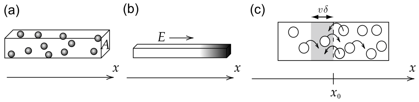
Fig.1: Setting for Part C.

By applying a uniform electric field \(E\) in the \(x\)-direction, particles are transported and their concentration \(n(x)\) (particle number per unit volume) becomes non-uniform (Fig.1(b)). When \(E\) is removed, this non-uniformity gradually disappears. This is due to Brownian motion of particles. If \(n(x)\) is not uniform, the numbers of right-going and left-going particles may differ (Fig.1(c)). This generates a particle flux \(J_D(x)\), the mean number of particles flowing at \(x\) along the \(x\)-axis per unit cross-sectional area and unit time. This flux is known to satisfy

\[ J_D(x)=-D\frac{dn}{dx}(x), \tag{4} \]

where \(D\) is called the diffusion coefficient.

Now let's assume, for simplicity, that half of the particles have velocity \(+v\) and the other half have velocity \(-v\). Let \(N_+(x_0)\) be the number of particles with velocity \(+v\) that cross \(x_0\) from left to right per unit cross-sectional area and unit time. For particles with velocity \(+v\) to cross \(x_0\) in the time interval \(\delta\), they should be in the shaded region of Fig.1(c). Since \(\delta\) is small, we have \(n(x)\simeq n(x_0)+(x-x_0)\frac{dn}{dx}(x_0)\) in this region.

C.1 — 0.5pt

Express \(N_+(x_0)\) using necessary quantities from \(v\), \(\delta\), \(n(x_0)\), and \(\frac{dn}{dx}(x_0)\).

We define \(N_-(x_0)\) as the counterpart of \(N_+(x_0)\) for the velocity \(-v\). With this, we have \(J_D(x_0)=\langle N_+(x_0)-N_-(x_0)\rangle\). According to Eq.(3), we have \(\langle v^2\rangle=C\).

C.2 — 0.7pt

Determine \(J_D(x_0)\) using necessary quantities from \(C\), \(\delta\), \(n(x_0)\), and \(\frac{dn}{dx}(x_0)\). Using this and Eq.(4), express \(D\) in terms of \(C\) and \(\delta\), and \(\langle\Delta x(t)^2\rangle\) in terms of \(D\) and \(t\).

Now we discuss the effect of osmotic pressure \(\Pi\). It is given by \(\Pi=\frac{n}{N_A}RT=nkT\) with the Avogadro constant \(N_A\), the gas constant \(R\), temperature \(T\), and the Boltzmann constant \(k=\frac{R}{N_A}\). Let us consider the non-uniform concentration formed under the electric field \(E\) (Fig.1(b)). Since \(n(x)\) depends on \(x\), so does \(\Pi(x)\). Then the forces due to \(\Pi(x)\) and \(\Pi(x+\Delta x)\) must be balanced with the total force from the field \(E\) acting on the particles (Fig.2). Here we consider small \(\Delta x\), so that \(n(x)\) can be regarded as constant over this range, while \(n(x+\Delta x)-n(x)\simeq\Delta x\frac{dn}{dx}(x)\).

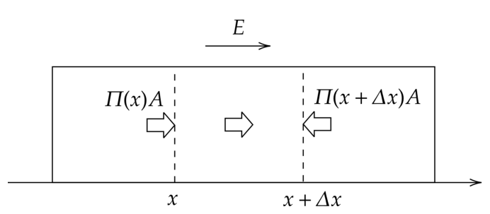
Fig.2: Force balance.

C.3 — 0.5pt

Express \(\frac{dn}{dx}(x)\) using \(n(x)\), \(T\), \(Q\), \(E\), and \(k\).

Let us discuss the balance of the flux now. Besides the flux \(J_D(x)\) due to the Brownian motion, there is also a flux due to the electric field, \(J_Q(x)\). It is given by

\[ J_Q(x)=n(x)u, \tag{5} \]

where \(u\) is the terminal velocity of particles driven by the field.

C.4 — 0.5pt

To determine \(u\), we use Eq.(1) with \(F_{\mathrm{ext}}(t)=QE\). Since \(v(t)\) is fluctuating, we consider \(\langle v(t)\rangle\). Assuming \(\langle v(0)\rangle=0\) and using \(\langle F(t)\rangle=0\), evaluate \(\langle v(t)\rangle\) and obtain \(u=\lim_{t\to\infty}\langle v(t)\rangle\).

C.5 — 0.5pt

The flux balance reads \(J_D(x)+J_Q(x)=0\). Express the diffusion coefficient \(D\) in terms of \(k\), \(\gamma\), and \(T\).

Part D. Mean square displacement (2.4 points)

Suppose we observed the Brownian motion of an isolated, spherical colloidal particle with radius \(a=5.0\,\mu\mathrm{m}\) in water. Figure 3 shows the histogram of displacements \(\Delta x\) measured in the \(x\)-direction at every interval \(\Delta t=60\,\mathrm{s}\). The friction coefficient is given by \(\gamma=6\pi a\eta\) with water viscosity \(\eta=8.9\times10^{-4}\,\mathrm{Pa\cdot s}\) and the temperature was \(T=25\,^\circ\mathrm{C}\).

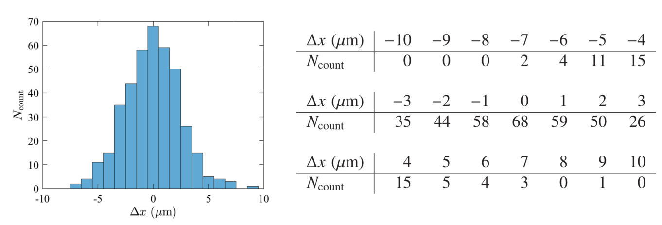
Fig.3: Histogram of displacements.

\(\Delta x\;(\mu\mathrm{m})\)	\(-10\)	\(-9\)	\(-8\)	\(-7\)	\(-6\)	\(-5\)	\(-4\)
\(N_{\mathrm{count}}\)	0	0	0	2	4	11	15

\(\Delta x\;(\mu\mathrm{m})\)	\(-3\)	\(-2\)	\(-1\)	\(0\)	\(1\)	\(2\)	\(3\)
\(N_{\mathrm{count}}\)	35	44	58	68	59	50	26

\(\Delta x\;(\mu\mathrm{m})\)	\(4\)	\(5\)	\(6\)	\(7\)	\(8\)	\(9\)	\(10\)
\(N_{\mathrm{count}}\)	15	5	4	3	0	1	0

D.1 — 1.0pt

Estimate the value of \(N_A\) without using the fact that it is the Avogadro constant, up to two significant digits from the data in Fig.3. The gas constant is \(R=8.31\,\mathrm{J/K\cdot mol}\). Do not use the value of the Boltzmann constant \(k\) given in General Instructions. As for the Avogadro constant, you might obtain a value different from that in General Instructions.

Now we extend the model in Part B to describe the motion of a particle with charge \(Q\) under an electric field \(E\). The particle velocity \(v(t)\) considered in Eq.(2) should be replaced by \(v(t)=u+v_n\) \((t_{n-1}<t\leq t_n)\) with \(v_n\) satisfying Eq. (3) and \(u\) being the terminal velocity considered in Eq.(5).

D.2 — 0.8pt

Express the MSD \(\langle\Delta x(t)^2\rangle\) in terms of \(u\), \(D\), and \(t\). Obtain approximate power laws for small \(t\) and large \(t\), as well as the characteristic time \(t_*\) where this change occurs. Draw a rough graph of MSD in a log-log plot, indicating the approximate location of \(t_*\).

Next, we consider swimming microbes (Fig.4(a)), in one dimension for simplicity (Fig.4(b)). These are spherical particles with radius \(a\). They swim at velocity either \(+u_0\) or \(-u_0\), the sign chosen randomly at every time interval \(\delta_0\) without correlation. The observed motion is a combination of displacements due to swimming and those due to the Brownian motion of a spherical particle.

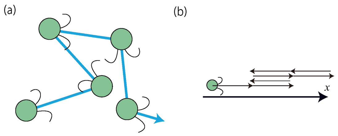
Fig.4: (a) Motion of microbes. (b) Its one-dimensional version.

D.3 — 0.6pt

Figure 5 displays the MSD \(\langle\Delta x(t)^2\rangle\) of those microbes, showing different power laws for small, large, and intermidiate \(t\), as indicated by dashed lines. Obtain the power law for each time range and express it using necessary quantities from \(D\), \(u_0\), \(\delta_0\), and \(t\).

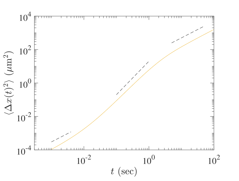
Fig.5: Mean square displacement of the microbes.

Part E. Water purification (1.5 points)

Here we discuss the purification of water including colloid-like soil particles, by adding electrolytes to coagulate them. Particles interact through van der Waals force and electrostatic force, the latter including effects of both surface charges and the surrounding layer of oppositely charged ions (such ions and their layer are called counter-ions and the electric double layer, respectively; see Fig.6(a)). As a result, the interaction potential for particle distance \(d\) (Fig.6(b)) is given by

\[ U(d)=-\frac{A}{d}+\frac{B\epsilon(kT)^2}{q^2}e^{-d/\lambda}, \tag{6} \]

where \(A\) and \(B\) are positive constants, \(\epsilon\) is the dielectric constant of water, and \(\lambda\) is the thickness of the electric double layer. Assuming that charges of ions are \(\pm q\), we have

\[ \lambda=\sqrt{\frac{\epsilon kT}{2N_Aq^2c}}, \tag{7} \]

where \(c\) is the molar concentration of ion.

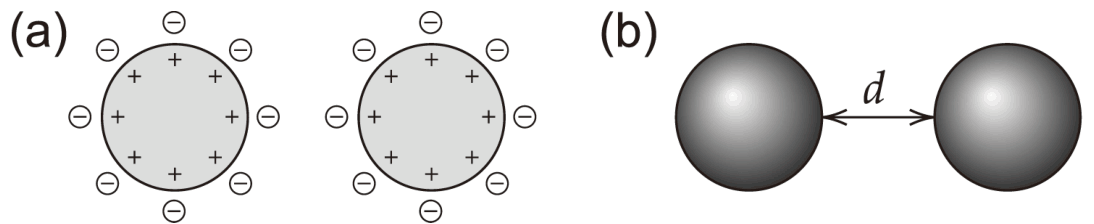
Fig.6: (a) Surface charges of colloidal particles and counter-ions. (b) Definition of the distance \(d\).

E.1 — 1.5pt

Addition of sodium chloride (NaCl) to the suspension causes colloidal particles to coagulate. Determine the lowest concentration \(c\) of NaCl necessary for coagulation. It is sufficient to consider two particles without thermal fluctuations, i.e., \(F(t)=0\) in Eq.(1), and assume that the terminal velocity for the given potential force is reached instantaneously.

Official English text of the problem.

We discuss the stability of large nuclei and estimate the mass of neutron stars theoretically and experimentally.

Part A. Mass and stability of nuclei (2.5 points)

The rest-energy of a nucleus \(m(Z,N)c^2\) consisting of \(Z\) protons and \(N\) neutrons is smaller than the sum of rest-energies of protons and neutrons, hereafter called nucleons, by the binding energy \(B(Z,N)\), where \(c\) is the speed of light in vacuum. Ignoring minor corrections, we can approximate the binding energy consisting of the volume term with \(a_V\), the surface term with \(a_S\), the Coulomb energy term with \(a_C\), and the symmetry energy term with \(a_{\mathrm{sym}}\) in the following way.

\[ m(Z,N)c^2=Am_Nc^2-B(Z,N),\qquad B(Z,N)=a_VA-a_SA^{2/3}-a_C\frac{Z^2}{A^{1/3}} -a_{\mathrm{sym}}\frac{(N-Z)^2}{A}, \tag{1} \]

where \(A=Z+N\) is the mass number and \(m_N\) is the nucleon mass. In the calculation, use \(a_V\approx15.8\ \mathrm{MeV}\), \(a_S\approx17.8\ \mathrm{MeV}\), \(a_C\approx0.711\ \mathrm{MeV}\), and \(a_{\mathrm{sym}}\approx23.7\ \mathrm{MeV}\) (\(\mathrm{MeV}=10^6\) electron volts).

A.1 — 0.9pt

Under the condition of \(Z=N\), determine \(A\) for maximizing the binding energy per nucleon, \(B/A\).

A.2 — 0.9pt

Under the condition of fixed \(A\), the atomic number of the most stable nucleus \(Z^*\) is determined by maximizing \(B(Z,A-Z)\). For \(A=197\), calculate \(Z^*\) using Eq. (1).

A.3 — 0.7pt

A nucleus having large \(A\) breaks up into lighter nuclei through fission in order to minimize the total rest-mass energy. For simplicity, we consider one of multiple ways to break a nucleus with \((Z,N)\) into two equal nuclei, which occurs when the following energy relation holds,

\[ m(Z,N)c^2>2m(Z/2,N/2)c^2. \]

When this relation is written as

\[ Z^2/A>C_{\mathrm{fission}}\frac{a_S}{a_C}, \]

obtain \(C_{\mathrm{fission}}\) up to two significant digits.

Part B. Neutron star as a gigantic nucleus (1.5 points)

For large nuclei with a large enough mass number \(A>A_c\) with a threshold \(A_c\), these nuclei stay stable against nuclear fission because of the sufficiently large binding energy due to gravity.

B.1 — 1.5pt

We assume that \(N=A\) and \(Z=0\) is realized for sufficiently large \(A\) and Eq. (1) continues to hold with the addition of the gravitational binding energy. The binding energy due to gravity is

\[ B_{\mathrm{grav}}=\frac35\frac{GM^2}{R}, \]

where \(M=m_NA\) and \(R=R_0A^{1/3}\) with \(R_0\simeq1.1\times10^{-15}\ \mathrm{m}=1.1\ \mathrm{fm}\) are the mass and the radius of the nucleus, respectively.

For \(B_{\mathrm{grav}}=a_{\mathrm{grav}}A^{5/3}\), obtain \(a_{\mathrm{grav}}\) in the MeV unit up to the first significant digit. Then, ignoring the surface term, estimate \(A_c\) up to the first significant digit. In the calculation, use \(m_Nc^2\simeq939\ \mathrm{MeV}\) and \(G=\hbar c/M_P^2\) where \(M_Pc^2\simeq1.22\times10^{22}\ \mathrm{MeV}\) and \(\hbar c\simeq197\ \mathrm{MeV}\cdot\mathrm{fm}\).

Part C. Neutron star in a binary system (6.0 points)

Some neutron stars are pulsars regularly emitting electromagnetic waves, which we call "light" for simplicity here, at a constant period. Neutron stars often make binary systems with a White Dwarf. Let us consider the star configuration shown in Fig. 1, where a light pulse from a neutron star N to the Earth E passes near a White Dwarf W of the binary system. Measuring these pulses influenced by the star's gravity leads to an accurate estimation of the mass of W as explained below, resulting in the estimation of the mass of N.

Fig. 1: Configurations with the \(x\)-axis along the line connecting N and E. (a) for \(x_N<0\) and (b) for \(x_N>0\).

C.1 — 1.0pt

As shown in the figure below, under the constant gravitational acceleration \(g\) we place two levels I and II with the height difference \(\Delta h(>0)\). Set the identical clocks at I, II, and \(F\), the free-falling system, denoted by clock-I, clock-II, and clock-\(F\), respectively.

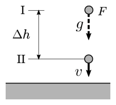
Set-up of the thought experiment.

We assume that an observer sits with clock-\(F\), and initially \(F\) is placed at the same height as that of clock-I and its velocity is zero. Since the clocks are identical, they register equal time intervals, \(\Delta\tau_F=\Delta\tau_{\mathrm{I}}\). Then, we let \(F\) fall freely, and work in the frame of \(F\), which is considered to be inertial. In this frame, clock-II passes by clock-\(F\) with velocity \(v\), so that the time dilation of clock-II can be determined by the Lorentz transformation. When time \(\Delta\tau_{\mathrm{I}}\) elapses on clock-\(F\), time \(\Delta\tau_{\mathrm{II}}\) elapses on clock-II.

Determine \(\Delta\tau_{\mathrm{II}}\) in terms of \(\Delta\tau_{\mathrm{I}}\) up to the first order in \(\Delta\phi/c^2\), where \(\Delta\phi=g\Delta h\) is a difference of the gravitational potential, i.e., the gravitational potential energy per unit mass.

C.2 — 1.8pt

Under the gravitational potential \(\phi\), time delays change the effective speed of light, \(c_{\mathrm{eff}}\), observed at the infinity, though the local speed of light is \(c\). When \(\phi(r=\infty)=0\), \(c_{\mathrm{eff}}\) can be given up to the first order in \(\phi/c^2\) as

\[ c_{\mathrm{eff}}\approx\left(1+\frac{2\phi}{c^2}\right)c \]

including the effect of space distortion, which was not featured in C.1. We note that the light path can be approximated as a straight line.

As shown in Fig. 1 (a), we take the \(x\)-axis along the light path from the neutron star N to the Earth E and place \(x=0\) at the point where the White Dwarf W is the closest to the light path. Let \(x_N(<0)\) be the \(x\)-coordinate of N, \(x_E(>0)\) be that of E, and \(d\) be the distance between W and the light path.

Estimate the changes of the arrival time \(\Delta t\) of the light from N to E caused by the White Dwarf with mass \(M_{\mathrm{WD}}\) and evaluate the answer in a simple form disregarding higher order terms of the following small quantities: \(d/|x_N|\ll1\), \(d/x_E\ll1\), and \(GM_{\mathrm{WD}}/(c^2d)\ll1\). If necessary, use the following formula.

\[ \int\frac{dx}{\sqrt{x^2+d^2}} =\frac12\log\left( \frac{\sqrt{x^2+d^2}+x}{\sqrt{x^2+d^2}-x} \right)+C. \]

(\(\log\) is the natural logarithm)

C.3 — 1.8pt

As shown below, in a binary star system N and W are assumed to be moving in circular orbits with zero eccentricity around the center of mass \(G\) on the orbit plane. Let \(\varepsilon\) be the orbital inclination angle measured from the orbit plane to the line directed toward E from \(G\), and let \(L\) be the length between N and W and \(M_{\mathrm{WD}}\) be the mass of the White Dwarf. In the following, we assume \(\varepsilon\ll1\).

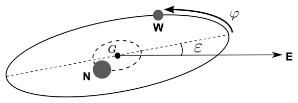
Binary star system.

We observe light pulses from N on E far away from N. The light path to E varies with time depending on the configuration of N and W. The delay in the time interval of arriving pulses on E has the maximum value \(\Delta t_{\max}\) for \(x_N\simeq-L\) and the minimum value \(\Delta t_{\min}\) for \(x_N\simeq L\) (see Fig. 1 (b) for the configuration).

Calculate \(\Delta t_{\max}-\Delta t_{\min}\) in a simple form disregarding higher order terms of small quantities as done in C.2. We note that the delays due to gravity from stellar objects other than W are assumed to cancel out in \(\Delta t_{\max}-\Delta t_{\min}\).

C.4 — 0.8pt

The below figure shows the observed time delays as a function of the orbital phase \(\varphi\) for the binary star system with \(L\approx6\times10^6\ \mathrm{km}\) and \(\cos\varepsilon\approx0.99989\). Estimate \(M_{\mathrm{WD}}\) in terms of the solar mass \(M_\odot\) and show the results for \(M_{\mathrm{WD}}/M_\odot\) up to the first significant digit. Here the approximate relation, \(GM_\odot/c^3\approx5\ \mu\mathrm{s}\), can be used.

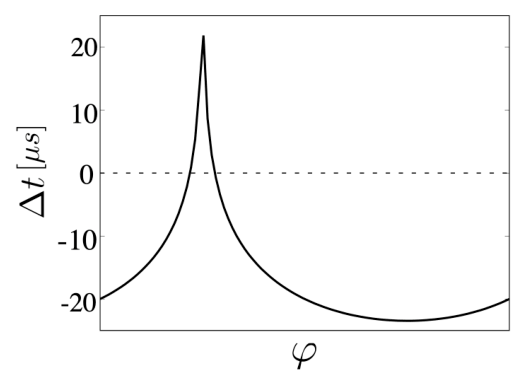
Observed time delays \(\Delta t\) as a function of the orbital phase \(\varphi\) (see the figure in C.3) to locate N and W on the orbits.

C.5 — 0.4pt

In the binary system of neutron stars, two stars release energy and angular momentum by emitting gravitational waves and eventually collide to merge. For simplicity, let us consider only a circular motion with the radius \(R\) and the angular velocity \(\omega\) and then \(\omega=\chi R^p\) holds with the constant \(\chi\) depending on neither \(\omega\) nor \(R\) if relativistic effects are ignored. Determine the value for \(p\).

C.6 — 0.2pt

The amplitude of the emitted gravitational wave from the binary system in C.5 is proportional to \(R^2\omega^2\). Figure below qualitatively shows four different temporal profiles of the observed gravitational waves before the two-star collision. Select the most appropriate profile from (a) to (d).

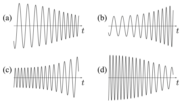
Observed data profiles of gravitational waves.

Official English text of the problem.

In this problem, we consider the phenomena caused by the interaction between water and objects, related to surface tension. Part A treats motion, while Parts B and C are regarding static situations.

If necessary, you can use the fact that if the function \(y(x)\) satisfies the differential equation \(y''(x)=ay(x)\) (\(a\) is a positive constant), then its general solution is \(y(x)=Ae^{\sqrt{a}x}+Be^{-\sqrt{a}x}\), where \(A\) and \(B\) are arbitrary constants.

Part A. Merger of water drops (2.0 points)

As shown in Fig.1, we consider two stationary, spherical water drops on the surface of a super-hydrophobic material, i.e., very strong repulsive force exists between material and water.

Initially neighboring two identical spherical water drops are placed on the surface; then these two drops are merged after touching each other and form a larger spherical water drop, which suddenly jumps up.

A.1 2.0pt

The radius \(a\) of both water drops before the merger is \(100\,\mu\mathrm{m}\). The density of water \(\rho\) is \(1.00\times10^3\,\mathrm{kg/m^3}\). The surface tension \(\gamma\) is \(7.27\times10^{-2}\,\mathrm{J/m^2}\).

A portion \(k\) of the difference of the surface energy before and after the merger, \(\Delta E\), is transformed into the kinetic energy of the jumped water drop. Then, determine the initial jump-up velocity, \(v\), of the merged water drop in two significant digits under the following assumptions:

• \(k=0.06\)
• Before and after merger, the total volume of water is conserved.

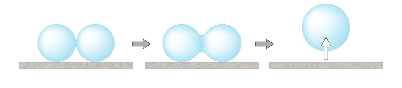
Fig. 1: Merger of two water drops and jump of the merged water drop.

Part B. A vertically placed board (4.5 points)

A flat board is immersed vertically in water. Figures 2(a) and 2(b) respectively show water surface forms for the hydrophilic (attractive) and hydrophobic board materials. We neglect the thickness of the board.

The board surface is on the \(yz\) plane, and the horizontal water surface far away from the board is on the \(xy\) plane with \(z=0\). The surface shape does not depend on the \(y\)-coordinate. Let \(\theta(x)\) be the angle between the water surface and the horizontal plane at a point \((x,z)\) on the water surface in the \(xz\) plane. Here \(\theta(x)\) is measured with respect to the positive \(x\) axis and the counterclockwise rotation is taken as positive. Let \(\theta(x)\) be \(\theta_0\) at the point of contact between the board and the water surface \((x=0)\). In the following, \(\theta_0\) is fixed by the properties of the board material.

Water density \(\rho\) is constant and water surface tension \(\gamma\) is uniform. The gravitational acceleration constant is given by \(g\). The atmospheric pressure, \(P_0\), is assumed to be always uniform. Let us determine the water surface form in the following steps. Note that the unit of surface tension is \(\mathrm{J/m^2}\) as well as \(\mathrm{N/m}\).

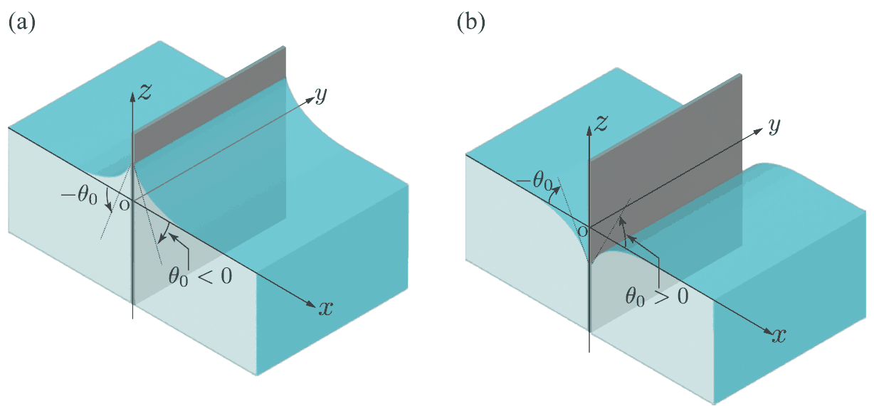
Fig. 2: Boards vertically immersed in the water. (a) hydrophilic board case; (b) hydrophobic board case.

B.1 0.6pt

We consider a hydrophilic board case, as shown in Fig.2(a). We note that the water pressure, \(P\), satisfies the conditions \(P<P_0\) for \(z>0\) and \(P=P_0\) for \(z=0\). Then, express \(P\) at \(z\) in terms of \(\rho\), \(g\), \(z\), and \(P_0\).

B.2 0.8pt

We consider a water block whose cutout is shown as shaded in Fig.3(a). Its \(xz\) plane cross-section is shown in a hatched area in Fig.3(b). Let \(z_1\) and \(z_2\) respectively be the left and right edge coordinates of the boundary (water surface) between the water block and the air.

Obtain a horizontal component (\(x\) component) of the net force per unit length along the \(y\)-axis, \(f_x\), which is exerted on the water block due to the pressure, in terms of \(\rho\), \(g\), \(z_1\), and \(z_2\). Note that \(P_0\) results in no net horizontal force on the water block.

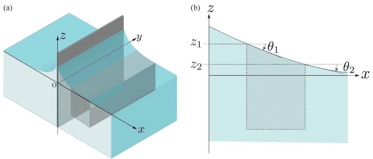
Fig. 3: Cutout form of water block on the water surface. (a) Bird's eye view and (b) cross-sectional view.

B.3 0.8pt

Surface tension acting on the water block is balanced with the force \(f_x\) discussed in B.2. We respectively define \(\theta_1\) and \(\theta_2\) as the angles between the water surface and the horizontal plane at the left and right edges. Express \(f_x\) in terms of \(\gamma\), \(\theta_1\), and \(\theta_2\).

B.4 0.8pt

The following equation holds at an arbitrary point \((x,z)\) on the water surface,

\[ \frac{1}{2}\left(\frac{z}{\ell}\right)^a+\cos\theta(x) =\text{constant}. \tag{1} \]

Determine the exponent \(a\) and express the constant \(\ell\) in terms of \(\gamma\) and \(\rho\). Note that this equation holds regardless of hydrophilic or hydrophobic board materials.

B.5 1.5pt

In Eq. (1) in B.4, we assume that variation of the water surface is slow, i.e., \(\lvert z'(x)\rvert\ll1\), so that we can expand \(\cos\theta(x)\) with respect to \(z'(x)\) up to the second order. Then, differentiating the resultant equation with respect to \(x\), we obtain the differential equation satisfied by \(z(x)\). Solve this differential equation and determine \(z(x)\) for \(x\geq0\) in terms of \(\tan\theta_0\) and \(\ell\). Note that the vertical directions of Figs. 2 and 3 are exaggerated for better view and they do not satisfy the condition, \(\lvert z'(x)\rvert\ll1\).

Part C. Interaction between two rods (3.5 points)

The identical rods A and B made of the same material floating in parallel on the water surface are placed at the same distance away from the \(y\)-axis (Fig.4).

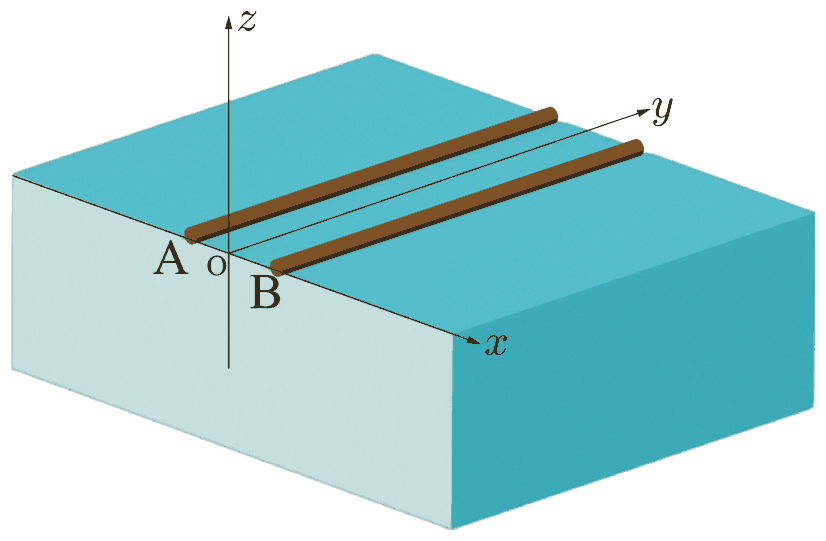
Fig. 4: Two rods A and B floating on the water surface.

C.1 1.0pt

At the contact points of the rod B and the water surface, we define the \(z\)-coordinates \(z_a\) and \(z_b\), and the angles \(\theta_a\) and \(\theta_b\), as shown in Fig.5. Determine the horizontal force component, \(F_x\), on the rod B per unit length along the \(y\)-axis in terms of \(\theta_a\), \(\theta_b\), \(z_a\), \(z_b\), \(\rho\), \(g\), and \(\gamma\).

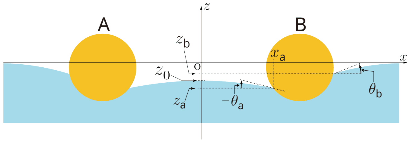
Fig. 5: Vertical cross-sectional view of two rods floating on the water surface.

C.2 1.5pt

We define the \(z\)-coordinate of the water surface, \(z_0\), at the midpoint of two rods in the \(xz\) plane. Express the force \(F_x\) obtained in C.1 without using \(\theta_a\), \(\theta_b\), \(z_a\), and \(z_b\).

C.3 1.0pt

Let \(x_a\) be the \(x\)-coordinate of the contact point between the water surface and the left side of the rod B. Using the differential equation obtained in B.5, express the water level coordinate \(z_0\) of the midpoint of these two rods A and B in terms of \(x_a\) and \(z_a\). You can use the constant \(\ell\) introduced in B.4.

Official English text of the problem.

Die Kolloidwissenschaft eignet sich zur Charakterisierung von Bodenpartikeln, da viele von ihnen als kolloidale Teilchen im Mikrometerbereich betrachtet werden können. Beispielsweise lässt sich die Brownsche Bewegung (zufällige Bewegung kolloidaler Teilchen) zur Messung von Teilchengrößen nutzen.

Teil A. Bewegungen kolloidaler Teilchen (1.6 Punkte)

Wir untersuchen die eindimensionale Brownsche Bewegung eines kolloidalen Teilchens mit der Masse \(M\). Die Bewegungsgleichung für seine Geschwindigkeit \(v(t)\) lautet:

\[ M\dot v=-\gamma v(t)+F(t)+F_{\mathrm{ext}}(t), \tag{1} \]

wobei \(\gamma\) der Reibungskoeffizient, \(F(t)\) eine durch zufällige Stöße mit Wassermolekülen verursachte Kraft und \(F_{\mathrm{ext}}(t)\) eine äußere Kraft ist. In Teil A nehmen wir \(F_{\mathrm{ext}}(t)=0\) an.

A.1 — 0.8 Punkte

Ein Wassermolekül stoße zum Zeitpunkt \(t=t_0\) mit dem Teilchen zusammen und übertrage dabei den Impuls \(I_0\); anschließend gelte \(F(t)=0\). Wenn vor dem Stoß \(v(t)=0\) gilt, ist \(v(t)=v_0e^{-(t-t_0)/\tau}\) für \(t>t_0\). Bestimmen Sie \(v_0\) und \(\tau\) mithilfe von \(I_0\) und den erforderlichen Parametern aus Gl.(1).

Im Folgenden dürfen Sie \(\tau\) in Ihren Antworten verwenden.

A.2 — 0.8 Punkte

Tatsächlich stoßen Wassermoleküle nacheinander mit dem Teilchen zusammen. Nehmen Sie an, dass der \(i\)-te Stoß zum Zeitpunkt \(t_i\) den Impuls \(I_i\) überträgt, und bestimmen Sie \(v(t)\) unter den Bedingungen \(t>0\) und \(v(0)=0\). Geben Sie außerdem die Ungleichung an, die den für ein gegebenes \(t\) zu berücksichtigenden Bereich von \(t_i\) festlegt. Auf dem Antwortbogen müssen Sie diesen Bereich im Ausdruck für \(v(t)\) nicht angeben.

Teil B. Effektive Bewegungsgleichung (1.8 Punkte)

Die bisherigen Ergebnisse legen nahe, dass die Teilchengeschwindigkeiten \(v(t)\) und \(v(t')\) als unkorrelierte Zufallsgrößen betrachtet werden können, wenn \(|t-t'|\gg\tau\) gilt. Auf dieser Grundlage führen wir ein theoretisches Modell zur näherungsweisen Beschreibung der eindimensionalen Brownschen Bewegung ein, in dem sich die Geschwindigkeit nach jedem Zeitintervall \(\delta\) \((\gg\tau)\) zufällig ändert, d. h.,

\[ v(t)=v_n\qquad(t_{n-1}<t\leq t_n), \tag{2} \]

mit \(t_n=n\delta\) \((n=0,1,2,\cdots)\) und einer Zufallsgröße \(v_n\). Sie erfüllt

\[ \langle v_n\rangle=0,\qquad \langle v_nv_m\rangle= \begin{cases} C &(n=m),\\ 0 &(n\neq m), \end{cases} \tag{3} \]

mit einem von \(\delta\) abhängigen Parameter \(C\). Hier bezeichnet \(\langle X\rangle\) den Erwartungswert von \(X\). Wenn man also unendlich oft Zufallszahlen \(X\) zieht, ist deren Mittelwert \(\langle X\rangle\).

Nun betrachten wir die Verschiebung des Teilchens \(\Delta x(t)=x(t)-x(0)\) für \(t=N\delta\) mit einer ganzen Zahl \(N\).

B.1 — 1.0 Punkte

Bestimmen Sie \(\langle\Delta x(t)\rangle\) und \(\langle\Delta x(t)^2\rangle\) mithilfe von \(C\), \(\delta\) und \(t\).

B.2 — 0.8 Punkte

Die Größe \(\langle\Delta x(t)^2\rangle\) heißt mittlere quadratische Verschiebung (MSD). Sie ist eine charakteristische Messgröße der Brownschen Bewegung, die dem Grenzfall \(\delta\to0\) entspricht. Daraus lässt sich zeigen, dass \(C\propto\delta^\alpha\) und \(\langle\Delta x(t)^2\rangle\propto t^\beta\) gelten. Bestimmen Sie die Werte von \(\alpha\) und \(\beta\).

Teil C. Elektrophorese (2.7 Punkte)

Hier behandeln wir die Elektrophorese, d. h. den Transport geladener Teilchen durch ein elektrisches Feld. Eine Suspension kolloidaler Teilchen mit der Masse \(M\) und der Ladung \(Q\) \((>0)\) wird in einen engen Kanal mit der Querschnittsfläche \(A\) eingebracht (Abb.1(a)). Wir vernachlässigen die Wechselwirkung zwischen den Teilchen, die Einflüsse der Wand, der Flüssigkeit und der darin enthaltenen Ionen sowie die Schwerkraft.

Abb.1: Anordnung für Teil C.

Durch Anlegen eines homogenen elektrischen Feldes \(E\) in \(x\)-Richtung werden die Teilchen transportiert, und ihre Konzentration \(n(x)\) (Teilchenzahl pro Volumeneinheit) wird inhomogen (Abb.1(b)). Wird \(E\) abgeschaltet, verschwindet diese Inhomogenität allmählich. Dies ist auf die Brownsche Bewegung der Teilchen zurückzuführen. Wenn \(n(x)\) nicht homogen ist, können sich die Anzahlen der nach rechts und nach links bewegten Teilchen unterscheiden (Abb.1(c)). Dadurch entsteht eine Teilchenstromdichte \(J_D(x)\), die mittlere Anzahl von Teilchen, die am Ort \(x\) entlang der \(x\)-Achse pro Querschnittsfläche und Zeit strömen. Für diese Stromdichte gilt bekanntermaßen

\[ J_D(x)=-D\frac{dn}{dx}(x), \tag{4} \]

wobei \(D\) als Diffusionskoeffizient bezeichnet wird.

Nehmen wir nun der Einfachheit halber an, dass die Hälfte der Teilchen die Geschwindigkeit \(+v\) und die andere Hälfte die Geschwindigkeit \(-v\) hat. Sei \(N_+(x_0)\) die Anzahl der Teilchen mit der Geschwindigkeit \(+v\), die \(x_0\) pro Querschnittsfläche und Zeit von links nach rechts passieren. Damit Teilchen mit der Geschwindigkeit \(+v\) den Ort \(x_0\) innerhalb des Zeitintervalls \(\delta\) passieren, müssen sie sich im schraffierten Bereich von Abb.1(c) befinden. Da \(\delta\) klein ist, gilt in diesem Bereich \(n(x)\simeq n(x_0)+(x-x_0)\frac{dn}{dx}(x_0)\).

C.1 — 0.5 Punkte

Drücken Sie \(N_+(x_0)\) mithilfe der erforderlichen Größen aus \(v\), \(\delta\), \(n(x_0)\) und \(\frac{dn}{dx}(x_0)\) aus.

Wir definieren \(N_-(x_0)\) als das Gegenstück zu \(N_+(x_0)\) für die Geschwindigkeit \(-v\). Damit gilt \(J_D(x_0)=\langle N_+(x_0)-N_-(x_0)\rangle\). Gemäß Gl.(3) gilt \(\langle v^2\rangle=C\).

C.2 — 0.7 Punkte

Bestimmen Sie \(J_D(x_0)\) mithilfe der erforderlichen Größen aus \(C\), \(\delta\), \(n(x_0)\) und \(\frac{dn}{dx}(x_0)\). Drücken Sie damit und mithilfe von Gl.(4) \(D\) durch \(C\) und \(\delta\) sowie \(\langle\Delta x(t)^2\rangle\) durch \(D\) und \(t\) aus.

Nun behandeln wir den Einfluss des osmotischen Drucks \(\Pi\). Er ist gegeben durch \(\Pi=\frac{n}{N_A}RT=nkT\), mit der Avogadro-Konstante \(N_A\), der Gaskonstante \(R\), der Temperatur \(T\) und der Boltzmann-Konstante \(k=\frac{R}{N_A}\). Betrachten wir die inhomogene Konzentration, die sich unter dem elektrischen Feld \(E\) ausgebildet hat (Abb.1(b)). Da \(n(x)\) von \(x\) abhängt, gilt dies auch für \(\Pi(x)\). Dann müssen die durch \(\Pi(x)\) und \(\Pi(x+\Delta x)\) verursachten Kräfte mit der Gesamtkraft im Gleichgewicht stehen, die das Feld \(E\) auf die Teilchen ausübt (Abb.2). Hier betrachten wir ein kleines \(\Delta x\), sodass \(n(x)\) über diesen Bereich als konstant angesehen werden kann, während \(n(x+\Delta x)-n(x)\simeq\Delta x\frac{dn}{dx}(x)\) gilt.

Abb.2: Kräftegleichgewicht.

C.3 — 0.5 Punkte

Drücken Sie \(\frac{dn}{dx}(x)\) mithilfe von \(n(x)\), \(T\), \(Q\), \(E\) und \(k\) aus.

Betrachten wir nun das Gleichgewicht der Teilchenströme. Neben der Stromdichte \(J_D(x)\) aufgrund der Brownschen Bewegung gibt es auch eine Stromdichte aufgrund des elektrischen Feldes, \(J_Q(x)\). Sie ist gegeben durch

\[ J_Q(x)=n(x)u, \tag{5} \]

wobei \(u\) die Endgeschwindigkeit der vom Feld angetriebenen Teilchen ist.

C.4 — 0.5 Punkte

Zur Bestimmung von \(u\) verwenden wir Gl.(1) mit \(F_{\mathrm{ext}}(t)=QE\). Da \(v(t)\) schwankt, betrachten wir \(\langle v(t)\rangle\). Berechnen Sie unter der Annahme \(\langle v(0)\rangle=0\) und mithilfe von \(\langle F(t)\rangle=0\) den Ausdruck \(\langle v(t)\rangle\), und bestimmen Sie \(u=\lim_{t\to\infty}\langle v(t)\rangle\).

C.5 — 0.5 Punkte

Das Gleichgewicht der Teilchenströme lautet \(J_D(x)+J_Q(x)=0\). Drücken Sie den Diffusionskoeffizienten \(D\) durch \(k\), \(\gamma\) und \(T\) aus.

Teil D. Mittlere quadratische Verschiebung (2.4 Punkte)

Angenommen, wir haben die Brownsche Bewegung eines isolierten, kugelförmigen kolloidalen Teilchens mit dem Radius \(a=5.0\,\mu\mathrm{m}\) in Wasser beobachtet. Abbildung 3 zeigt das Histogramm der Verschiebungen \(\Delta x\), die in \(x\)-Richtung jeweils über ein Intervall \(\Delta t=60\,\mathrm{s}\) gemessen wurden. Der Reibungskoeffizient ist gegeben durch \(\gamma=6\pi a\eta\), mit der Viskosität des Wassers \(\eta=8.9\times10^{-4}\,\mathrm{Pa\cdot s}\), und die Temperatur betrug \(T=25\,^\circ\mathrm{C}\).

Abb.3: Histogramm der Verschiebungen.

\(\Delta x\;(\mu\mathrm{m})\)	\(-10\)	\(-9\)	\(-8\)	\(-7\)	\(-6\)	\(-5\)	\(-4\)
\(N_{\mathrm{count}}\)	0	0	0	2	4	11	15

\(\Delta x\;(\mu\mathrm{m})\)	\(-3\)	\(-2\)	\(-1\)	\(0\)	\(1\)	\(2\)	\(3\)
\(N_{\mathrm{count}}\)	35	44	58	68	59	50	26

\(\Delta x\;(\mu\mathrm{m})\)	\(4\)	\(5\)	\(6\)	\(7\)	\(8\)	\(9\)	\(10\)
\(N_{\mathrm{count}}\)	15	5	4	3	0	1	0

D.1 — 1.0 Punkte

Schätzen Sie den Wert von \(N_A\) anhand der Daten in Abb.3 auf zwei signifikante Stellen, ohne die Tatsache zu nutzen, dass es sich um die Avogadro-Konstante handelt. Die Gaskonstante beträgt \(R=8.31\,\mathrm{J/K\cdot mol}\). Verwenden Sie nicht den in den allgemeinen Hinweisen angegebenen Wert der Boltzmann-Konstante \(k\). Für die Avogadro-Konstante erhalten Sie möglicherweise einen Wert, der von dem in den allgemeinen Hinweisen abweicht.

Nun erweitern wir das Modell aus Teil B, um die Bewegung eines Teilchens mit der Ladung \(Q\) in einem elektrischen Feld \(E\) zu beschreiben. Die in Gl.(2) betrachtete Teilchengeschwindigkeit \(v(t)\) ist durch \(v(t)=u+v_n\) \((t_{n-1}<t\leq t_n)\) zu ersetzen, wobei \(v_n\) Gl. (3) erfüllt und \(u\) die in Gl.(5) betrachtete Endgeschwindigkeit ist.

D.2 — 0.8 Punkte

Drücken Sie die MSD \(\langle\Delta x(t)^2\rangle\) durch \(u\), \(D\) und \(t\) aus. Bestimmen Sie näherungsweise Potenzgesetze für kleine \(t\) und große \(t\) sowie die charakteristische Zeit \(t_*\), bei der dieser Übergang auftritt. Skizzieren Sie den Verlauf der MSD in einem doppeltlogarithmischen Diagramm, und kennzeichnen Sie die ungefähre Lage von \(t_*\).

Als Nächstes betrachten wir schwimmende Mikroorganismen (Abb.4(a)), der Einfachheit halber in einer Dimension (Abb.4(b)). Es handelt sich um kugelförmige Teilchen mit dem Radius \(a\). Sie schwimmen entweder mit der Geschwindigkeit \(+u_0\) oder \(-u_0\), wobei das Vorzeichen nach jedem Zeitintervall \(\delta_0\) zufällig und ohne Korrelation gewählt wird. Die beobachtete Bewegung setzt sich aus den Verschiebungen durch das Schwimmen und denen durch die Brownsche Bewegung eines kugelförmigen Teilchens zusammen.

Abb.4: (a) Bewegung von Mikroorganismen. (b) Ihre eindimensionale Version.

D.3 — 0.6 Punkte

Abbildung 5 zeigt die MSD \(\langle\Delta x(t)^2\rangle\) dieser Mikroorganismen mit unterschiedlichen Potenzgesetzen für kleine, große und mittlere \(t\), die durch gestrichelte Linien dargestellt sind. Bestimmen Sie das Potenzgesetz für jeden Zeitbereich, und drücken Sie es mithilfe der erforderlichen Größen aus \(D\), \(u_0\), \(\delta_0\) und \(t\) aus.

Abb.5: Mittlere quadratische Verschiebung der Mikroorganismen.

Teil E. Wasserreinigung (1.5 Punkte)

Hier behandeln wir die Reinigung von Wasser, das kolloidartige Bodenpartikel enthält, durch Zugabe von Elektrolyten, die diese Teilchen koagulieren lassen. Die Teilchen wechselwirken durch die Van-der-Waals-Kraft und die elektrostatische Kraft, wobei Letztere die Einflüsse sowohl der Oberflächenladungen als auch der umgebenden Schicht entgegengesetzt geladener Ionen umfasst (solche Ionen und ihre Schicht werden als Gegenionen beziehungsweise elektrische Doppelschicht bezeichnet; siehe Abb.6(a)). Daraus ergibt sich für den Teilchenabstand \(d\) (Abb.6(b)) das Wechselwirkungspotential

\[ U(d)=-\frac{A}{d}+\frac{B\epsilon(kT)^2}{q^2}e^{-d/\lambda}, \tag{6} \]

wobei \(A\) und \(B\) positive Konstanten sind, \(\epsilon\) die Dielektrizitätskonstante des Wassers und \(\lambda\) die Dicke der elektrischen Doppelschicht ist. Unter der Annahme, dass die Ladungen der Ionen \(\pm q\) betragen, gilt

\[ \lambda=\sqrt{\frac{\epsilon kT}{2N_Aq^2c}}, \tag{7} \]

wobei \(c\) die molare Ionenkonzentration ist.

Abb.6: (a) Oberflächenladungen kolloidaler Teilchen und Gegenionen. (b) Definition des Abstands \(d\).

E.1 — 1.5 Punkte

Die Zugabe von Natriumchlorid (NaCl) zur Suspension bewirkt die Koagulation der kolloidalen Teilchen. Bestimmen Sie die niedrigste für die Koagulation erforderliche Konzentration \(c\) von NaCl. Es genügt, zwei Teilchen ohne thermische Fluktuationen zu betrachten, d. h. \(F(t)=0\) in Gl.(1), und anzunehmen, dass die Endgeschwindigkeit für die gegebene Potentialkraft augenblicklich erreicht wird.

Aufgabentext aus dem offiziellen englischen Text übersetzt.

Wir untersuchen die Stabilität großer Atomkerne und schätzen die Masse von Neutronensternen theoretisch und experimentell ab.

Teil A. Masse und Stabilität von Atomkernen (2.5 Punkte)

Die Ruheenergie eines aus \(Z\) Protonen und \(N\) Neutronen bestehenden Atomkerns \(m(Z,N)c^2\) ist um die Bindungsenergie \(B(Z,N)\) kleiner als die Summe der Ruheenergien der Protonen und Neutronen, die im Folgenden Nukleonen genannt werden; dabei ist \(c\) die Lichtgeschwindigkeit im Vakuum. Unter Vernachlässigung kleiner Korrekturen können wir die Bindungsenergie, die sich aus dem Volumenterm mit \(a_V\), dem Oberflächenterm mit \(a_S\), dem Coulomb-Energieterm mit \(a_C\) und dem Symmetrieenergieterm mit \(a_{\mathrm{sym}}\) zusammensetzt, wie folgt näherungsweise angeben.

\[ m(Z,N)c^2=Am_Nc^2-B(Z,N),\qquad B(Z,N)=a_VA-a_SA^{2/3}-a_C\frac{Z^2}{A^{1/3}} -a_{\mathrm{sym}}\frac{(N-Z)^2}{A}, \tag{1} \]

Dabei ist \(A=Z+N\) die Massenzahl und \(m_N\) die Nukleonenmasse. Verwenden Sie für die Rechnung \(a_V\approx15.8\ \mathrm{MeV}\), \(a_S\approx17.8\ \mathrm{MeV}\), \(a_C\approx0.711\ \mathrm{MeV}\) und \(a_{\mathrm{sym}}\approx23.7\ \mathrm{MeV}\) (\(\mathrm{MeV}=10^6\) Elektronenvolt).

A.1 — 0.9 Punkte

Bestimmen Sie unter der Bedingung \(Z=N\) den Wert von \(A\), für den die Bindungsenergie pro Nukleon, \(B/A\), maximal wird.

A.2 — 0.9 Punkte

Bei festem \(A\) wird die Ordnungszahl des stabilsten Atomkerns \(Z^*\) durch Maximierung von \(B(Z,A-Z)\) bestimmt. Berechnen Sie für \(A=197\) mithilfe von Gl. (1) den Wert von \(Z^*\).

A.3 — 0.7 Punkte

Ein Atomkern mit großem \(A\) zerfällt durch Kernspaltung in leichtere Kerne, um die gesamte Ruheenergie zu minimieren. Der Einfachheit halber betrachten wir eine von mehreren Möglichkeiten, einen Kern mit \((Z,N)\) in zwei gleiche Kerne zu spalten. Dies geschieht, wenn die folgende Energiebeziehung gilt:

\[ m(Z,N)c^2>2m(Z/2,N/2)c^2. \]

Wird diese Beziehung in der Form

\[ Z^2/A>C_{\mathrm{fission}}\frac{a_S}{a_C}, \]

geschrieben, bestimmen Sie \(C_{\mathrm{fission}}\) auf zwei signifikante Stellen.

Teil B. Der Neutronenstern als gigantischer Atomkern (1.5 Punkte)

Große Atomkerne mit einer hinreichend großen Massenzahl \(A>A_c\), wobei \(A_c\) ein Schwellenwert ist, bleiben aufgrund der ausreichend großen gravitativen Bindungsenergie gegenüber Kernspaltung stabil.

B.1 — 1.5 Punkte

Wir nehmen an, dass für hinreichend große \(A\) die Bedingungen \(N=A\) und \(Z=0\) erfüllt sind und Gl. (1) unter Hinzunahme der gravitativen Bindungsenergie weiterhin gilt. Die gravitative Bindungsenergie lautet

\[ B_{\mathrm{grav}}=\frac35\frac{GM^2}{R}, \]

wobei \(M=m_NA\) und \(R=R_0A^{1/3}\) mit \(R_0\simeq1.1\times10^{-15}\ \mathrm{m}=1.1\ \mathrm{fm}\) die Masse beziehungsweise den Radius des Atomkerns bezeichnen.

Bestimmen Sie für \(B_{\mathrm{grav}}=a_{\mathrm{grav}}A^{5/3}\) den Wert von \(a_{\mathrm{grav}}\) in der Einheit MeV auf eine signifikante Stelle. Schätzen Sie anschließend unter Vernachlässigung des Oberflächenterms \(A_c\) auf eine signifikante Stelle ab. Verwenden Sie für die Rechnung \(m_Nc^2\simeq939\ \mathrm{MeV}\) und \(G=\hbar c/M_P^2\), wobei \(M_Pc^2\simeq1.22\times10^{22}\ \mathrm{MeV}\) und \(\hbar c\simeq197\ \mathrm{MeV}\cdot\mathrm{fm}\).

Teil C. Ein Neutronenstern in einem Doppelsternsystem (6.0 Punkte)

Einige Neutronensterne sind Pulsare, die regelmäßig mit einer konstanten Periode elektromagnetische Wellen aussenden, die wir hier der Einfachheit halber als „Licht“ bezeichnen. Neutronensterne bilden häufig Doppelsternsysteme mit einem Weißen Zwerg. Betrachten wir die in Abb. 1 gezeigte Sternkonfiguration, bei der ein Lichtpuls von einem Neutronenstern N zur Erde E nahe an einem Weißen Zwerg W des Doppelsternsystems vorbeiläuft. Die Messung dieser durch die Gravitation des Sterns beeinflussten Pulse ermöglicht eine genaue Abschätzung der Masse von W, wie im Folgenden erläutert wird, und daraus eine Abschätzung der Masse von N.

Abb. 1: Konfigurationen mit der \(x\)-Achse entlang der Verbindungslinie zwischen N und E. (a) für \(x_N<0\) und (b) für \(x_N>0\).

C.1 — 1.0 Punkte

Wie in der folgenden Abbildung gezeigt, betrachten wir bei konstanter Fallbeschleunigung \(g\) zwei Höhenlagen I und II mit dem Höhenunterschied \(\Delta h(>0)\). Bei I, II und im frei fallenden System \(F\) werden identische Uhren aufgestellt, die als Uhr-I, Uhr-II beziehungsweise Uhr-\(F\) bezeichnet werden.

Aufbau des Gedankenexperiments.

Wir nehmen an, dass sich ein Beobachter bei Uhr-\(F\) befindet und dass \(F\) anfangs auf derselben Höhe wie Uhr-I ruht. Da die Uhren identisch sind, zeigen sie gleiche Zeitintervalle an, \(\Delta\tau_F=\Delta\tau_{\mathrm{I}}\). Anschließend lassen wir \(F\) frei fallen und betrachten das Bezugssystem von \(F\), das als Inertialsystem angesehen wird. In diesem Bezugssystem bewegt sich Uhr-II mit der Geschwindigkeit \(v\) an Uhr-\(F\) vorbei, sodass die Zeitdilatation von Uhr-II durch die Lorentz-Transformation bestimmt werden kann. Wenn auf Uhr-\(F\) die Zeit \(\Delta\tau_{\mathrm{I}}\) vergeht, vergeht auf Uhr-II die Zeit \(\Delta\tau_{\mathrm{II}}\).

Bestimmen Sie \(\Delta\tau_{\mathrm{II}}\) in Abhängigkeit von \(\Delta\tau_{\mathrm{I}}\) bis zur ersten Ordnung in \(\Delta\phi/c^2\), wobei \(\Delta\phi=g\Delta h\) eine Differenz des Gravitationspotentials, also der potentiellen Gravitationsenergie pro Masseneinheit, ist.

C.2 — 1.8 Punkte

Im Gravitationspotential \(\phi\) verändern Zeitverzögerungen die im Unendlichen beobachtete effektive Lichtgeschwindigkeit \(c_{\mathrm{eff}}\), obwohl die lokale Lichtgeschwindigkeit \(c\) beträgt. Für \(\phi(r=\infty)=0\) kann \(c_{\mathrm{eff}}\) bis zur ersten Ordnung in \(\phi/c^2\) als

\[ c_{\mathrm{eff}}\approx\left(1+\frac{2\phi}{c^2}\right)c \]

angegeben werden. Darin ist der Einfluss der Raumkrümmung berücksichtigt, der in C.1 nicht behandelt wurde. Der Lichtweg kann näherungsweise als gerade Linie betrachtet werden.

Wie in Abb. 1 (a) gezeigt, legen wir die \(x\)-Achse entlang des Lichtwegs vom Neutronenstern N zur Erde E und setzen \(x=0\) an den Punkt, an dem der Weiße Zwerg W dem Lichtweg am nächsten ist. Dabei sei \(x_N(<0)\) die \(x\)-Koordinate von N, \(x_E(>0)\) diejenige von E und \(d\) der Abstand zwischen W und dem Lichtweg.

Schätzen Sie die durch den Weißen Zwerg mit der Masse \(M_{\mathrm{WD}}\) verursachte Änderung der Ankunftszeit \(\Delta t\) des Lichts von N nach E ab und geben Sie das Ergebnis in einer einfachen Form an, indem Sie Terme höherer Ordnung in den folgenden kleinen Größen vernachlässigen: \(d/|x_N|\ll1\), \(d/x_E\ll1\) und \(GM_{\mathrm{WD}}/(c^2d)\ll1\). Verwenden Sie bei Bedarf die folgende Formel.

\[ \int\frac{dx}{\sqrt{x^2+d^2}} =\frac12\log\left( \frac{\sqrt{x^2+d^2}+x}{\sqrt{x^2+d^2}-x} \right)+C. \]

(\(\log\) ist der natürliche Logarithmus)

C.3 — 1.8 Punkte

Wie unten gezeigt, nehmen wir an, dass sich N und W in einem Doppelsternsystem auf Kreisbahnen mit Exzentrizität null um den Schwerpunkt \(G\) in der Bahnebene bewegen. Dabei sei \(\varepsilon\) der Bahnneigungswinkel, gemessen von der Bahnebene zur von \(G\) nach E gerichteten Linie, \(L\) der Abstand zwischen N und W und \(M_{\mathrm{WD}}\) die Masse des Weißen Zwergs. Im Folgenden nehmen wir \(\varepsilon\ll1\) an.

Doppelsternsystem.

Wir beobachten Lichtpulse von N auf der weit von N entfernten Erde E. Der Lichtweg zu E verändert sich mit der Zeit in Abhängigkeit von der Konfiguration von N und W. Die Verzögerung im Zeitintervall der auf E eintreffenden Pulse hat den Maximalwert \(\Delta t_{\max}\) für \(x_N\simeq-L\) und den Minimalwert \(\Delta t_{\min}\) für \(x_N\simeq L\) (die Konfiguration ist in Abb. 1 (b) dargestellt).

Berechnen Sie \(\Delta t_{\max}-\Delta t_{\min}\) in einer einfachen Form, indem Sie wie in C.2 Terme höherer Ordnung in kleinen Größen vernachlässigen. Dabei wird angenommen, dass sich die gravitativen Verzögerungen durch andere stellare Objekte als W in \(\Delta t_{\max}-\Delta t_{\min}\) aufheben.

C.4 — 0.8 Punkte

Die folgende Abbildung zeigt die beobachteten Zeitverzögerungen als Funktion der Bahnphase \(\varphi\) für das Doppelsternsystem mit \(L\approx6\times10^6\ \mathrm{km}\) und \(\cos\varepsilon\approx0.99989\). Schätzen Sie \(M_{\mathrm{WD}}\) in Einheiten der Sonnenmasse \(M_\odot\) ab und geben Sie das Ergebnis für \(M_{\mathrm{WD}}/M_\odot\) auf eine signifikante Stelle an. Hier kann die Näherungsbeziehung \(GM_\odot/c^3\approx5\ \mu\mathrm{s}\) verwendet werden.

Beobachtete Zeitverzögerungen \(\Delta t\) als Funktion der Bahnphase \(\varphi\) (siehe die Abbildung in C.3), welche die Positionen von N und W auf ihren Bahnen angibt.

C.5 — 0.4 Punkte

In einem Doppelsternsystem aus Neutronensternen geben die beiden Sterne durch die Emission von Gravitationswellen Energie und Drehimpuls ab und stoßen schließlich zusammen, wobei sie verschmelzen. Der Einfachheit halber betrachten wir nur eine Kreisbewegung mit dem Radius \(R\) und der Winkelgeschwindigkeit \(\omega\). Dann gilt bei Vernachlässigung relativistischer Effekte \(\omega=\chi R^p\) mit einer Konstanten \(\chi\), die weder von \(\omega\) noch von \(R\) abhängt. Bestimmen Sie den Wert von \(p\).

C.6 — 0.2 Punkte

Die Amplitude der vom Doppelsternsystem in C.5 ausgesandten Gravitationswelle ist proportional zu \(R^2\omega^2\). Die folgende Abbildung zeigt qualitativ vier verschiedene zeitliche Verläufe der beobachteten Gravitationswellen vor dem Zusammenstoß der beiden Sterne. Wählen Sie aus (a) bis (d) den am besten geeigneten Verlauf aus.

Verläufe der beobachteten Gravitationswellendaten.

Aufgabentext aus dem offiziellen englischen Text übersetzt.

In dieser Aufgabe betrachten wir Phänomene, die durch die Wechselwirkung zwischen Wasser und Körpern entstehen und mit der Oberflächenspannung zusammenhängen. Teil A behandelt Bewegungen, während sich die Teile B und C mit statischen Situationen befassen.

Falls erforderlich, können Sie die Tatsache verwenden, dass eine Funktion \(y(x)\), die die Differentialgleichung \(y''(x)=ay(x)\) erfüllt (\(a\) ist eine positive Konstante), die allgemeine Lösung \(y(x)=Ae^{\sqrt{a}x}+Be^{-\sqrt{a}x}\) hat, wobei \(A\) und \(B\) beliebige Konstanten sind.

Teil A. Verschmelzen von Wassertropfen (2.0 Punkte)

Wie in Abb. 1 dargestellt, betrachten wir zwei ruhende, kugelförmige Wassertropfen auf der Oberfläche eines superhydrophoben Materials, d. h., zwischen dem Material und dem Wasser wirkt eine sehr starke abstoßende Kraft.

Zu Beginn werden zwei identische kugelförmige Wassertropfen nebeneinander auf die Oberfläche gesetzt; anschließend verschmelzen diese beiden Tropfen, nachdem sie einander berührt haben, und bilden einen größeren kugelförmigen Wassertropfen, der plötzlich nach oben springt.

A.1 2.0 Punkte

Der Radius \(a\) beider Wassertropfen vor dem Verschmelzen beträgt \(100\,\mu\mathrm{m}\). Die Dichte des Wassers \(\rho\) beträgt \(1.00\times10^3\,\mathrm{kg/m^3}\). Die Oberflächenspannung \(\gamma\) beträgt \(7.27\times10^{-2}\,\mathrm{J/m^2}\).

Ein Anteil \(k\) der Differenz der Oberflächenenergie vor und nach dem Verschmelzen, \(\Delta E\), wird in die kinetische Energie des hochspringenden Wassertropfens umgewandelt. Bestimmen Sie unter den folgenden Annahmen die anfängliche Absprunggeschwindigkeit \(v\) des vereinigten Wassertropfens mit zwei signifikanten Stellen:

• \(k=0.06\)
• Beim Verschmelzen bleibt das gesamte Wasservolumen erhalten.

Abb. 1: Verschmelzen zweier Wassertropfen und Absprung des vereinigten Wassertropfens.

Teil B. Eine senkrecht aufgestellte Platte (4.5 Punkte)

Eine ebene Platte wird senkrecht in Wasser eingetaucht. Die Abbildungen 2(a) und 2(b) zeigen die Formen der Wasseroberfläche für hydrophiles (anziehendes) bzw. hydrophobes Plattenmaterial. Wir vernachlässigen die Dicke der Platte.

Die Plattenoberfläche liegt in der \(yz\)-Ebene, und die horizontale Wasseroberfläche weit entfernt von der Platte liegt in der \(xy\)-Ebene bei \(z=0\). Die Form der Oberfläche hängt nicht von der \(y\)-Koordinate ab. Sei \(\theta(x)\) der Winkel zwischen der Wasseroberfläche und der Horizontalebene an einem Punkt \((x,z)\) auf der Wasseroberfläche in der \(xz\)-Ebene. Dabei wird \(\theta(x)\) bezüglich der positiven \(x\)-Achse gemessen, und eine Drehung gegen den Uhrzeigersinn wird als positiv gewertet. Am Berührungspunkt zwischen der Platte und der Wasseroberfläche \((x=0)\) sei \(\theta(x)\) gleich \(\theta_0\). Im Folgenden ist \(\theta_0\) durch die Eigenschaften des Plattenmaterials festgelegt.

Die Wasserdichte \(\rho\) ist konstant, und die Oberflächenspannung des Wassers \(\gamma\) ist überall gleich. Die konstante Fallbeschleunigung ist durch \(g\) gegeben. Der Atmosphärendruck \(P_0\) wird als stets räumlich konstant angenommen. Wir bestimmen die Form der Wasseroberfläche in den folgenden Schritten. Beachten Sie, dass die Einheit der Oberflächenspannung sowohl \(\mathrm{J/m^2}\) als auch \(\mathrm{N/m}\) ist.

Abb. 2: Senkrecht in das Wasser eingetauchte Platten. (a) Fall einer hydrophilen Platte; (b) Fall einer hydrophoben Platte.

B.1 0.6 Punkte

Wir betrachten den Fall einer hydrophilen Platte, wie in Abb. 2(a) dargestellt. Wir stellen fest, dass der Wasserdruck \(P\) die Bedingungen \(P<P_0\) für \(z>0\) und \(P=P_0\) für \(z=0\) erfüllt. Drücken Sie nun \(P\) in der Höhe \(z\) durch \(\rho\), \(g\), \(z\) und \(P_0\) aus.

B.2 0.8 Punkte

Wir betrachten einen Wasserblock, dessen herausgeschnittene Form in Abb. 3(a) schattiert dargestellt ist. Sein Querschnitt in der \(xz\)-Ebene ist als schraffierter Bereich in Abb. 3(b) dargestellt. Seien \(z_1\) und \(z_2\) die Koordinaten des linken bzw. rechten Randes der Grenzfläche (Wasseroberfläche) zwischen dem Wasserblock und der Luft.

Bestimmen Sie die horizontale Komponente (\(x\)-Komponente) der resultierenden Kraft pro Längeneinheit entlang der \(y\)-Achse, \(f_x\), die aufgrund des Drucks auf den Wasserblock ausgeübt wird, in Abhängigkeit von \(\rho\), \(g\), \(z_1\) und \(z_2\). Beachten Sie, dass \(P_0\) keine resultierende horizontale Kraft auf den Wasserblock bewirkt.

Abb. 3: Form des aus der Wasseroberfläche herausgeschnittenen Wasserblocks. (a) Ansicht aus der Vogelperspektive und (b) Querschnittsansicht.

B.3 0.8 Punkte

Die auf den Wasserblock wirkende Oberflächenspannung steht mit der in B.2 betrachteten Kraft \(f_x\) im Gleichgewicht. Wir definieren \(\theta_1\) und \(\theta_2\) als die Winkel zwischen der Wasseroberfläche und der Horizontalebene am linken bzw. rechten Rand. Drücken Sie \(f_x\) durch \(\gamma\), \(\theta_1\) und \(\theta_2\) aus.

B.4 0.8 Punkte

An einem beliebigen Punkt \((x,z)\) auf der Wasseroberfläche gilt die folgende Gleichung:

\[ \frac{1}{2}\left(\frac{z}{\ell}\right)^a+\cos\theta(x) =\text{konstant}. \tag{1} \]

Bestimmen Sie den Exponenten \(a\) und drücken Sie die Konstante \(\ell\) durch \(\gamma\) und \(\rho\) aus. Beachten Sie, dass diese Gleichung unabhängig davon gilt, ob das Plattenmaterial hydrophil oder hydrophob ist.

B.5 1.5 Punkte

In Gl. (1) aus B.4 nehmen wir an, dass sich die Wasseroberfläche nur langsam ändert, d. h. \(\lvert z'(x)\rvert\ll1\), sodass wir \(\cos\theta(x)\) bezüglich \(z'(x)\) bis zur zweiten Ordnung entwickeln können. Durch anschließendes Differenzieren der erhaltenen Gleichung nach \(x\) erhalten wir die Differentialgleichung, die \(z(x)\) erfüllt. Lösen Sie diese Differentialgleichung und bestimmen Sie \(z(x)\) für \(x\geq0\) in Abhängigkeit von \(\tan\theta_0\) und \(\ell\). Beachten Sie, dass die vertikalen Abmessungen in den Abb. 2 und 3 zur besseren Veranschaulichung überhöht dargestellt sind und die Bedingung \(\lvert z'(x)\rvert\ll1\) dort nicht erfüllt ist.

Teil C. Wechselwirkung zwischen zwei Stäben (3.5 Punkte)

Die identischen Stäbe A und B bestehen aus demselben Material, schwimmen parallel auf der Wasseroberfläche und befinden sich im gleichen Abstand von der \(y\)-Achse (Abb. 4).

Abb. 4: Zwei auf der Wasseroberfläche schwimmende Stäbe A und B.

C.1 1.0 Punkte

An den Berührungspunkten des Stabes B mit der Wasseroberfläche definieren wir die \(z\)-Koordinaten \(z_a\) und \(z_b\) sowie die Winkel \(\theta_a\) und \(\theta_b\), wie in Abb. 5 dargestellt. Bestimmen Sie die horizontale Kraftkomponente \(F_x\) auf den Stab B pro Längeneinheit entlang der \(y\)-Achse in Abhängigkeit von \(\theta_a\), \(\theta_b\), \(z_a\), \(z_b\), \(\rho\), \(g\) und \(\gamma\).

Abb. 5: Vertikaler Querschnitt durch zwei auf der Wasseroberfläche schwimmende Stäbe.

C.2 1.5 Punkte

Wir definieren die \(z\)-Koordinate der Wasseroberfläche in der Mitte zwischen den beiden Stäben in der \(xz\)-Ebene als \(z_0\). Drücken Sie die in C.1 erhaltene Kraft \(F_x\) ohne Verwendung von \(\theta_a\), \(\theta_b\), \(z_a\) und \(z_b\) aus.

C.3 1.0 Punkte

Sei \(x_a\) die \(x\)-Koordinate des Berührungspunktes zwischen der Wasseroberfläche und der linken Seite des Stabes B. Drücken Sie mithilfe der in B.5 erhaltenen Differentialgleichung die Wasserstandskoordinate \(z_0\) in der Mitte zwischen diesen beiden Stäben A und B durch \(x_a\) und \(z_a\) aus. Sie können die in B.4 eingeführte Konstante \(\ell\) verwenden.

Aufgabentext aus dem offiziellen englischen Text übersetzt.

Kolloid bilimi, toprak parçacıklarını karakterize etmek için yararlıdır; çünkü bunların birçoğu mikrometre boyutunda kolloidal parçacıklar olarak ele alınabilir. Örneğin, parçacık boyutlarını ölçmek için Brown hareketinden (kolloidal parçacıkların rastgele hareketinden) yararlanılabilir.

Bölüm A. Kolloidal parçacıkların hareketleri (1.6 puan)

Kütlesi \(M\) olan bir kolloidal parçacığın bir boyutlu Brown hareketini inceliyoruz. Parçacığın \(v(t)\) hızı için hareket denklemi şöyledir:

\[ M\dot v=-\gamma v(t)+F(t)+F_{\mathrm{ext}}(t), \tag{1} \]

Burada \(\gamma\) sürtünme katsayısı, \(F(t)\) su molekülleriyle rastgele çarpışmalardan kaynaklanan kuvvet ve \(F_{\mathrm{ext}}(t)\) bir dış kuvvettir. Bölüm A'da \(F_{\mathrm{ext}}(t)=0\) olduğunu varsayıyoruz.

A.1 — 0.8 puan

Bir su molekülünün \(t=t_0\) anında parçacıkla çarpışarak ona \(I_0\) itmesini aktardığını ve sonrasında \(F(t)=0\) olduğunu düşünün. Çarpışmadan önce \(v(t)=0\) ise, \(t>t_0\) için \(v(t)=v_0e^{-(t-t_0)/\tau}\) olur. \(I_0\) ve Denklem (1)'deki gerekli parametreleri kullanarak \(v_0\) ve \(\tau\)'yu belirleyin.

Bundan sonraki cevaplarınızda \(\tau\)'yu kullanabilirsiniz.

A.2 — 0.8 puan

Gerçekte su molekülleri parçacıkla art arda çarpışır. \(i\). çarpışmanın \(t_i\) anında \(I_i\) itmesini aktardığını varsayın ve \(t>0\) ve \(v(0)=0\) koşulları altında \(v(t)\)'yi belirleyin. Ayrıca, verilen bir \(t\) için dikkate alınması gereken \(t_i\) aralığını belirten eşitsizliği yazın. Cevap kâğıdında, \(v(t)\) ifadesinde bu aralığı belirtmeniz gerekli değildir.

Bölüm B. Etkin hareket denklemi (1.8 puan)

Şimdiye kadarki sonuçlar, \(|t-t'|\gg\tau\) olduğunda parçacık hızları \(v(t)\) ve \(v(t')\)'nin birbiriyle korelasyonsuz rastgele nicelikler olarak ele alınabileceğini gösterir. Buna dayanarak, bir boyutlu Brown hareketini yaklaşık olarak betimlemek için hızın her \(\delta\) \((\gg\tau)\) zaman aralığında rastgele değiştiği bir kuramsal model tanımlıyoruz; yani,

\[ v(t)=v_n\qquad(t_{n-1}<t\leq t_n), \tag{2} \]

burada \(t_n=n\delta\) \((n=0,1,2,\cdots)\) ve \(v_n\) rastgele bir niceliktir. Bu nicelik,

\[ \langle v_n\rangle=0,\qquad \langle v_nv_m\rangle= \begin{cases} C &(n=m),\\ 0 &(n\neq m), \end{cases} \tag{3} \]

bağıntılarını sağlar; burada \(C\), \(\delta\)'ya bağlı bir parametredir. \(\langle X\rangle\), \(X\)'in beklenen değerini gösterir. Başka bir deyişle, sonsuz kez rastgele \(X\) sayıları seçerseniz, ortalama \(\langle X\rangle\) olacaktır.

Şimdi bir \(N\) tam sayısı için \(t=N\delta\) anındaki parçacık yer değiştirmesini, \(\Delta x(t)=x(t)-x(0)\), ele alıyoruz.

B.1 — 1.0 puan

\(C\), \(\delta\) ve \(t\)'yi kullanarak \(\langle\Delta x(t)\rangle\) ve \(\langle\Delta x(t)^2\rangle\)'yi belirleyin.

B.2 — 0.8 puan

\(\langle\Delta x(t)^2\rangle\) niceliğine ortalama kare yer değiştirme (MSD) denir. Bu nicelik, \(\delta\to0\) sınır durumuna karşılık gelen Brown hareketinin karakteristik bir gözlenebiliridir. Buradan, \(C\propto\delta^\alpha\) ve \(\langle\Delta x(t)^2\rangle\propto t^\beta\) olduğunu gösterebiliriz. \(\alpha\) ve \(\beta\)'nın değerlerini belirleyin.

Bölüm C. Elektroforez (2.7 puan)

Burada elektroforezi, yani yüklü parçacıkların bir elektrik alanla taşınmasını ele alıyoruz. Kütlesi \(M\) ve yükü \(Q\) \((>0)\) olan kolloidal parçacıkların süspansiyonu, kesit alanı \(A\) olan dar bir kanala konur (Şekil 1(a)). Parçacıklar arasındaki etkileşimi, duvarın, akışkanın ve akışkan içindeki iyonların etkilerini ve yer çekimini ihmal ediyoruz.

Şekil 1: Bölüm C için düzenek.

\(x\) yönünde düzgün bir \(E\) elektrik alanı uygulandığında parçacıklar taşınır ve \(n(x)\) derişimleri (birim hacimdeki parçacık sayısı) düzgün olmaktan çıkar (Şekil 1(b)). \(E\) kaldırıldığında bu düzensizlik yavaş yavaş kaybolur. Bunun nedeni parçacıkların Brown hareketidir. \(n(x)\) düzgün değilse, sağa ve sola giden parçacıkların sayıları farklı olabilir (Şekil 1(c)). Bu durum, \(x\) konumunda \(x\) ekseni boyunca birim kesit alanından birim zamanda geçen ortalama parçacık sayısı olan \(J_D(x)\) parçacık akısını oluşturur. Bu akının

\[ J_D(x)=-D\frac{dn}{dx}(x), \tag{4} \]

bağıntısını sağladığı bilinmektedir; burada \(D\)'ye difüzyon katsayısı denir.

Şimdi basitlik amacıyla parçacıkların yarısının \(+v\), diğer yarısının ise \(-v\) hızına sahip olduğunu varsayalım. \(N_+(x_0)\), \(x_0\)'dan soldan sağa birim kesit alanından birim zamanda geçen, hızı \(+v\) olan parçacıkların sayısı olsun. Hızı \(+v\) olan parçacıkların \(\delta\) zaman aralığında \(x_0\)'dan geçebilmesi için Şekil 1(c)'deki taralı bölgede bulunmaları gerekir. \(\delta\) küçük olduğundan bu bölgede \(n(x)\simeq n(x_0)+(x-x_0)\frac{dn}{dx}(x_0)\) olur.

C.1 — 0.5 puan

\(v\), \(\delta\), \(n(x_0)\) ve \(\frac{dn}{dx}(x_0)\) niceliklerinden gerekli olanları kullanarak \(N_+(x_0)\)'ı ifade edin.

\(N_-(x_0)\)'ı, \(N_+(x_0)\)'ın \(-v\) hızı için karşılığı olarak tanımlıyoruz. Böylece \(J_D(x_0)=\langle N_+(x_0)-N_-(x_0)\rangle\) olur. Denklem (3)'e göre \(\langle v^2\rangle=C\)'dir.

C.2 — 0.7 puan

\(C\), \(\delta\), \(n(x_0)\) ve \(\frac{dn}{dx}(x_0)\) niceliklerinden gerekli olanları kullanarak \(J_D(x_0)\)'ı belirleyin. Bu sonucu ve Denklem (4)'ü kullanarak \(D\)'yi \(C\) ve \(\delta\) cinsinden, \(\langle\Delta x(t)^2\rangle\)'yi ise \(D\) ve \(t\) cinsinden ifade edin.

Şimdi ozmotik basınç \(\Pi\)'nin etkisini ele alıyoruz. Ozmotik basınç, Avogadro sabiti \(N_A\), gaz sabiti \(R\), sıcaklık \(T\) ve Boltzmann sabiti \(k=\frac{R}{N_A}\) olmak üzere \(\Pi=\frac{n}{N_A}RT=nkT\) ile verilir. \(E\) elektrik alanı altında oluşan düzgün olmayan derişimi ele alalım (Şekil 1(b)). \(n(x)\), \(x\)'e bağlı olduğundan \(\Pi(x)\) de \(x\)'e bağlıdır. Bu durumda \(\Pi(x)\) ve \(\Pi(x+\Delta x)\)'ten kaynaklanan kuvvetler, \(E\) alanının parçacıklara uyguladığı toplam kuvvetle dengelenmelidir (Şekil 2). Burada küçük bir \(\Delta x\) ele alıyoruz; böylece \(n(x)\) bu aralıkta sabit kabul edilebilirken \(n(x+\Delta x)-n(x)\simeq\Delta x\frac{dn}{dx}(x)\) olur.

Şekil 2: Kuvvet dengesi.

C.3 — 0.5 puan

\(n(x)\), \(T\), \(Q\), \(E\) ve \(k\)'yi kullanarak \(\frac{dn}{dx}(x)\)'i ifade edin.

Şimdi akı dengesini ele alalım. Brown hareketinden kaynaklanan \(J_D(x)\) akısının yanı sıra elektrik alandan kaynaklanan \(J_Q(x)\) akısı da vardır. Bu akı,

\[ J_Q(x)=n(x)u, \tag{5} \]

ile verilir; burada \(u\), alanın etkisiyle hareket eden parçacıkların limit hızıdır.

C.4 — 0.5 puan

\(u\)'yu belirlemek için Denklem (1)'i \(F_{\mathrm{ext}}(t)=QE\) ile kullanıyoruz. \(v(t)\) dalgalandığı için \(\langle v(t)\rangle\)'yi ele alıyoruz. \(\langle v(0)\rangle=0\) varsayımı altında ve \(\langle F(t)\rangle=0\) bağıntısını kullanarak \(\langle v(t)\rangle\)'yi hesaplayın ve \(u=\lim_{t\to\infty}\langle v(t)\rangle\)'yi elde edin.

C.5 — 0.5 puan

Akı dengesi \(J_D(x)+J_Q(x)=0\) biçimindedir. Difüzyon katsayısı \(D\)'yi \(k\), \(\gamma\) ve \(T\) cinsinden ifade edin.

Bölüm D. Ortalama kare yer değiştirme (2.4 puan)

Suda, yarıçapı \(a=5.0\,\mu\mathrm{m}\) olan, diğer parçacıklardan yalıtılmış küresel bir kolloidal parçacığın Brown hareketini gözlemlediğimizi varsayalım. Şekil 3, her \(\Delta t=60\,\mathrm{s}\) aralığında \(x\) yönünde ölçülen \(\Delta x\) yer değiştirmelerinin histogramını göstermektedir. Sürtünme katsayısı, suyun viskozitesi \(\eta=8.9\times10^{-4}\,\mathrm{Pa\cdot s}\) olmak üzere \(\gamma=6\pi a\eta\) ile verilir ve sıcaklık \(T=25\,^\circ\mathrm{C}\) idi.

Şekil 3: Yer değiştirmelerin histogramı.

\(\Delta x\;(\mu\mathrm{m})\)	\(-10\)	\(-9\)	\(-8\)	\(-7\)	\(-6\)	\(-5\)	\(-4\)
\(N_{\mathrm{count}}\)	0	0	0	2	4	11	15

\(\Delta x\;(\mu\mathrm{m})\)	\(-3\)	\(-2\)	\(-1\)	\(0\)	\(1\)	\(2\)	\(3\)
\(N_{\mathrm{count}}\)	35	44	58	68	59	50	26

\(\Delta x\;(\mu\mathrm{m})\)	\(4\)	\(5\)	\(6\)	\(7\)	\(8\)	\(9\)	\(10\)
\(N_{\mathrm{count}}\)	15	5	4	3	0	1	0

D.1 — 1.0 puan

\(N_A\)'nın Avogadro sabiti olduğu bilgisini kullanmadan, Şekil 3'teki verilerden değerini iki anlamlı basamakla tahmin edin. Gaz sabiti \(R=8.31\,\mathrm{J/K\cdot mol}\)'dür. Genel Yönergeler'de verilen Boltzmann sabiti \(k\)'nin değerini kullanmayın. Avogadro sabiti için Genel Yönergeler'dekinden farklı bir değer elde edebilirsiniz.

Şimdi Bölüm B'deki modeli, \(E\) elektrik alanı altında \(Q\) yüklü bir parçacığın hareketini betimlemek üzere genişletiyoruz. Denklem (2)'de ele alınan parçacık hızı \(v(t)\), \(v(t)=u+v_n\) \((t_{n-1}<t\leq t_n)\) ile değiştirilmelidir; burada \(v_n\), Denklem (3)'ü sağlar ve \(u\), Denklem (5)'te ele alınan limit hızdır.

D.2 — 0.8 puan

MSD'yi, \(\langle\Delta x(t)^2\rangle\), \(u\), \(D\) ve \(t\) cinsinden ifade edin. Küçük \(t\) ve büyük \(t\) için yaklaşık kuvvet yasalarını ve bu değişimin gerçekleştiği karakteristik \(t_*\) zamanını elde edin. MSD'nin çift logaritmik bir grafiğini kabaca çizin ve \(t_*\)'ın yaklaşık konumunu belirtin.

Ardından, basitlik amacıyla bir boyutta (Şekil 4(b)), yüzen mikroorganizmaları (Şekil 4(a)) ele alıyoruz. Bunlar yarıçapı \(a\) olan küresel parçacıklardır. Her \(\delta_0\) zaman aralığında işaretin korelasyonsuz biçimde rastgele seçildiği \(+u_0\) veya \(-u_0\) hızıyla yüzerler. Gözlenen hareket, yüzmeden kaynaklanan yer değiştirmeler ile küresel bir parçacığın Brown hareketinden kaynaklanan yer değiştirmelerin birleşimidir.

Şekil 4: (a) Mikroorganizmaların hareketi. (b) Bunun bir boyutlu biçimi.

D.3 — 0.6 puan

Şekil 5, bu mikroorganizmaların MSD'sini, \(\langle\Delta x(t)^2\rangle\), göstermektedir; kesikli çizgilerle belirtildiği gibi küçük, büyük ve ara \(t\) değerlerinde farklı kuvvet yasaları görülür. Her zaman aralığı için kuvvet yasasını elde edin ve \(D\), \(u_0\), \(\delta_0\) ve \(t\) niceliklerinden gerekli olanları kullanarak ifade edin.

Şekil 5: Mikroorganizmaların ortalama kare yer değiştirmesi.

Bölüm E. Su arıtımı (1.5 puan)

Burada, kolloid benzeri toprak parçacıkları içeren suyun, bu parçacıkların pıhtılaşmasını sağlamak üzere elektrolit eklenerek arıtılmasını ele alıyoruz. Parçacıklar van der Waals kuvveti ve elektrostatik kuvvet aracılığıyla etkileşir; elektrostatik kuvvet hem yüzey yüklerinin hem de çevreleyen zıt yüklü iyon tabakasının etkilerini içerir (bu iyonlara karşı iyonlar, oluşturdukları tabakaya ise elektriksel çift tabaka denir; bkz. Şekil 6(a)). Sonuç olarak, parçacıklar arası uzaklık \(d\) (Şekil 6(b)) için etkileşim potansiyeli

\[ U(d)=-\frac{A}{d}+\frac{B\epsilon(kT)^2}{q^2}e^{-d/\lambda}, \tag{6} \]

ile verilir; burada \(A\) ve \(B\) pozitif sabitler, \(\epsilon\) suyun dielektrik sabiti ve \(\lambda\) elektriksel çift tabakanın kalınlığıdır. İyonların yüklerinin \(\pm q\) olduğunu varsayarsak,

\[ \lambda=\sqrt{\frac{\epsilon kT}{2N_Aq^2c}}, \tag{7} \]

olur; burada \(c\), iyonun molar derişimidir.

Şekil 6: (a) Kolloidal parçacıkların yüzey yükleri ve karşı iyonlar. (b) \(d\) uzaklığının tanımı.

E.1 — 1.5 puan

Süspansiyona sodyum klorür (NaCl) eklenmesi, kolloidal parçacıkların pıhtılaşmasına neden olur. Pıhtılaşma için gerekli en düşük NaCl derişimi \(c\)'yi belirleyin. Isıl dalgalanmalar olmaksızın iki parçacığı ele almak, yani Denklem (1)'de \(F(t)=0\) almak ve verilen potansiyel kuvveti için limit hıza anında ulaşıldığını varsaymak yeterlidir.

Soru metni resmi İngilizce metinden çevrilmiştir.

Büyük çekirdeklerin kararlılığını ele alıyor ve nötron yıldızlarının kütlesini kuramsal ve deneysel olarak tahmin ediyoruz.

Bölüm A. Çekirdeklerin kütlesi ve kararlılığı (2.5 puan)

\(Z\) proton ve \(N\) nötrondan oluşan bir çekirdeğin durgunluk enerjisi \(m(Z,N)c^2\), bundan böyle nükleon olarak adlandırılacak olan proton ve nötronların durgunluk enerjileri toplamından bağlanma enerjisi \(B(Z,N)\) kadar küçüktür; burada \(c\), ışığın boşluktaki hızıdır. Küçük düzeltmeleri ihmal ederek, \(a_V\) katsayılı hacim terimi, \(a_S\) katsayılı yüzey terimi, \(a_C\) katsayılı Coulomb enerjisi terimi ve \(a_{\mathrm{sym}}\) katsayılı simetri enerjisi teriminden oluşan bağlanma enerjisini aşağıdaki şekilde yaklaşık olarak ifade edebiliriz.

\[ m(Z,N)c^2=Am_Nc^2-B(Z,N),\qquad B(Z,N)=a_VA-a_SA^{2/3}-a_C\frac{Z^2}{A^{1/3}} -a_{\mathrm{sym}}\frac{(N-Z)^2}{A}, \tag{1} \]

Burada \(A=Z+N\) kütle sayısı, \(m_N\) ise nükleon kütlesidir. Hesaplamalarda \(a_V\approx15.8\ \mathrm{MeV}\), \(a_S\approx17.8\ \mathrm{MeV}\), \(a_C\approx0.711\ \mathrm{MeV}\) ve \(a_{\mathrm{sym}}\approx23.7\ \mathrm{MeV}\) değerlerini kullanın (\(\mathrm{MeV}=10^6\) elektron volt).

A.1 — 0.9 puan

\(Z=N\) koşulu altında, nükleon başına bağlanma enerjisi \(B/A\)'yı maksimum yapan \(A\) değerini belirleyin.

A.2 — 0.9 puan

\(A\) sabit tutulduğunda, en kararlı çekirdeğin atom numarası \(Z^*\), \(B(Z,A-Z)\)'nin maksimum yapılmasıyla belirlenir. \(A=197\) için Denklem (1)'i kullanarak \(Z^*\)'ı hesaplayın.

A.3 — 0.7 puan

\(A\) değeri büyük olan bir çekirdek, toplam durgunluk kütle enerjisini minimum yapmak için fisyon yoluyla daha hafif çekirdeklere ayrılır. Basitlik amacıyla, \((Z,N)\) ile belirtilen bir çekirdeğin iki eşit çekirdeğe ayrılmasının çeşitli yollarından birini ele alıyoruz; bu ayrılma, aşağıdaki enerji bağıntısı sağlandığında gerçekleşir:

\[ m(Z,N)c^2>2m(Z/2,N/2)c^2. \]

Bu bağıntı

\[ Z^2/A>C_{\mathrm{fission}}\frac{a_S}{a_C}, \]

şeklinde yazıldığında, \(C_{\mathrm{fission}}\) değerini iki anlamlı basamakla bulun.

Bölüm B. Devasa bir çekirdek olarak nötron yıldızı (1.5 puan)

\(A_c\) eşik değeri olmak üzere, kütle sayısı yeterince büyük olan \(A>A_c\) büyük çekirdekler, kütleçekimden kaynaklanan bağlanma enerjisinin yeterince büyük olması nedeniyle nükleer fisyona karşı kararlı kalır.

B.1 — 1.5 puan

Yeterince büyük \(A\) için \(N=A\) ve \(Z=0\) koşullarının gerçekleştiğini ve kütleçekimsel bağlanma enerjisi eklendiğinde Denklem (1)'in geçerliliğini koruduğunu varsayıyoruz. Kütleçekimden kaynaklanan bağlanma enerjisi

\[ B_{\mathrm{grav}}=\frac35\frac{GM^2}{R}, \]

şeklindedir; burada \(M=m_NA\) ve \(R=R_0A^{1/3}\) sırasıyla çekirdeğin kütlesi ve yarıçapıdır ve \(R_0\simeq1.1\times10^{-15}\ \mathrm{m}=1.1\ \mathrm{fm}\)'dir.

\(B_{\mathrm{grav}}=a_{\mathrm{grav}}A^{5/3}\) için \(a_{\mathrm{grav}}\) değerini MeV biriminde bir anlamlı basamakla bulun. Ardından yüzey terimini ihmal ederek \(A_c\)'yi bir anlamlı basamakla tahmin edin. Hesaplamalarda \(m_Nc^2\simeq939\ \mathrm{MeV}\) ve \(G=\hbar c/M_P^2\) bağıntısını kullanın; burada \(M_Pc^2\simeq1.22\times10^{22}\ \mathrm{MeV}\) ve \(\hbar c\simeq197\ \mathrm{MeV}\cdot\mathrm{fm}\)'dir.

Bölüm C. İkili sistemde nötron yıldızı (6.0 puan)

Bazı nötron yıldızları, burada basitlik amacıyla "ışık" olarak adlandıracağımız elektromanyetik dalgaları sabit bir periyotla düzenli olarak yayan pulsarlardır. Nötron yıldızları sıklıkla bir beyaz cüceyle ikili sistem oluşturur. Şekil 1'de gösterilen yıldız düzenini ele alalım; bu düzende nötron yıldızı N'den Dünya E'ye giden bir ışık atımı, ikili sistemin beyaz cücesi W'nin yakınından geçer. Yıldızın kütleçekiminden etkilenen bu atımların ölçülmesi, aşağıda açıklandığı gibi W'nin kütlesinin hassas biçimde tahmin edilmesini ve bunun sonucunda N'nin kütlesinin tahmin edilmesini sağlar.

Şekil 1: \(x\) ekseninin N ile E'yi birleştiren doğru boyunca uzandığı düzenler. (a) \(x_N<0\) ve (b) \(x_N>0\) için.

C.1 — 1.0 puan

Aşağıdaki şekilde gösterildiği gibi, sabit kütleçekimi ivmesi \(g\) altında, aralarında \(\Delta h(>0)\) yükseklik farkı bulunan I ve II düzeylerini belirliyoruz. I, II ve serbest düşen sistem \(F\)'ye, sırasıyla saat-I, saat-II ve saat-\(F\) olarak adlandırılan özdeş saatler yerleştirin.

Düşünce deneyinin düzeneği.

Bir gözlemcinin saat-\(F\)'nin yanında bulunduğunu ve başlangıçta \(F\)'nin saat-I ile aynı yükseklikte ve hızının sıfır olduğunu varsayıyoruz. Saatler özdeş olduğundan eşit zaman aralıkları kaydederler: \(\Delta\tau_F=\Delta\tau_{\mathrm{I}}\). Ardından \(F\)'yi serbest düşmeye bırakıyor ve eylemsiz kabul edilen \(F\) referans sisteminde çalışıyoruz. Bu sistemde saat-II, saat-\(F\)'nin yanından \(v\) hızıyla geçer; böylece saat-II'deki zaman genişlemesi Lorentz dönüşümüyle belirlenebilir. Saat-\(F\)'de \(\Delta\tau_{\mathrm{I}}\) süresi geçtiğinde saat-II'de \(\Delta\tau_{\mathrm{II}}\) süresi geçer.

\(\Delta\tau_{\mathrm{II}}\)'yi \(\Delta\tau_{\mathrm{I}}\) cinsinden, \(\Delta\phi/c^2\)'ye göre birinci mertebeye kadar belirleyin; burada \(\Delta\phi=g\Delta h\), kütleçekim potansiyeli, yani birim kütle başına kütleçekim potansiyel enerjisi farkıdır.

C.2 — 1.8 puan

\(\phi\) kütleçekim potansiyeli altında zaman gecikmeleri, ışığın yerel hızı \(c\) olmasına karşın, sonsuzda gözlenen etkin ışık hızı \(c_{\mathrm{eff}}\)'i değiştirir. \(\phi(r=\infty)=0\) olduğunda, \(c_{\mathrm{eff}}\), \(\phi/c^2\)'ye göre birinci mertebeye kadar

\[ c_{\mathrm{eff}}\approx\left(1+\frac{2\phi}{c^2}\right)c \]

şeklinde verilebilir; bu ifade, C.1'de yer almayan uzayın bükülmesi etkisini de içerir. Işığın izlediği yolun yaklaşık olarak bir doğru kabul edilebileceğini belirtelim.

Şekil 1 (a)'da gösterildiği gibi, \(x\) eksenini nötron yıldızı N'den Dünya E'ye giden ışığın yolu boyunca alıyor ve \(x=0\) noktasını, ışık yolu üzerinde beyaz cüce W'ye en yakın noktaya yerleştiriyoruz. N'nin \(x\) koordinatı \(x_N(<0)\), E'nin koordinatı \(x_E(>0)\) ve W ile ışık yolu arasındaki uzaklık \(d\) olsun.

\(M_{\mathrm{WD}}\) kütleli beyaz cücenin, N'den E'ye giden ışığın varış zamanında neden olduğu \(\Delta t\) değişimini tahmin edin ve aşağıdaki küçük niceliklerin yüksek mertebeli terimlerini ihmal ederek sonucu basit bir biçimde ifade edin: \(d/|x_N|\ll1\), \(d/x_E\ll1\) ve \(GM_{\mathrm{WD}}/(c^2d)\ll1\). Gerekirse aşağıdaki formülü kullanın.

\[ \int\frac{dx}{\sqrt{x^2+d^2}} =\frac12\log\left( \frac{\sqrt{x^2+d^2}+x}{\sqrt{x^2+d^2}-x} \right)+C. \]

(\(\log\) doğal logaritmadır)

C.3 — 1.8 puan

Aşağıda gösterildiği gibi, bir ikili yıldız sisteminde N ve W'nin, yörünge düzlemindeki kütle merkezi \(G\) çevresinde dışmerkezliği sıfır olan dairesel yörüngelerde hareket ettiği varsayılıyor. Yörünge düzleminden, \(G\)'den E'ye yönelen doğruya doğru ölçülen yörünge eğim açısı \(\varepsilon\), N ile W arasındaki uzaklık \(L\) ve beyaz cücenin kütlesi \(M_{\mathrm{WD}}\) olsun. Aşağıda \(\varepsilon\ll1\) olduğunu varsayıyoruz.

İkili yıldız sistemi.

N'den gelen ışık atımlarını, N'den çok uzaktaki E üzerinde gözlüyoruz. E'ye giden ışığın yolu, N ve W'nin konumlarına bağlı olarak zamanla değişir. E'ye ulaşan atımların zaman aralığındaki gecikme, \(x_N\simeq-L\) için maksimum \(\Delta t_{\max}\) değerini ve \(x_N\simeq L\) için minimum \(\Delta t_{\min}\) değerini alır (düzen için Şekil 1 (b)'ye bakın).

C.2'de yapıldığı gibi küçük niceliklerin yüksek mertebeli terimlerini ihmal ederek \(\Delta t_{\max}-\Delta t_{\min}\) farkını basit bir biçimde hesaplayın. W dışındaki yıldızsal cisimlerin kütleçekiminden kaynaklanan gecikmelerin \(\Delta t_{\max}-\Delta t_{\min}\) farkında birbirini götürdüğünün varsayıldığını belirtelim.

C.4 — 0.8 puan

Aşağıdaki şekil, \(L\approx6\times10^6\ \mathrm{km}\) ve \(\cos\varepsilon\approx0.99989\) olan ikili yıldız sistemi için gözlenen zaman gecikmelerini yörünge fazı \(\varphi\)'nin fonksiyonu olarak göstermektedir. \(M_{\mathrm{WD}}\)'yi Güneş kütlesi \(M_\odot\) cinsinden tahmin edin ve \(M_{\mathrm{WD}}/M_\odot\) için sonucu bir anlamlı basamakla gösterin. Burada \(GM_\odot/c^3\approx5\ \mu\mathrm{s}\) yaklaşık bağıntısı kullanılabilir.

N ve W'nin yörüngelerdeki konumlarını belirleyen yörünge fazı \(\varphi\)'nin fonksiyonu olarak gözlenen zaman gecikmeleri \(\Delta t\) (C.3'teki şekle bakın).

C.5 — 0.4 puan

İkili nötron yıldızı sisteminde iki yıldız, kütleçekim dalgaları yayarak enerji ve açısal momentum kaybeder ve sonunda çarpışarak birleşir. Basitlik amacıyla yalnızca \(R\) yarıçaplı ve \(\omega\) açısal hızlı dairesel hareketi ele alalım; görelilik etkileri ihmal edilirse, ne \(\omega\)'ya ne de \(R\)'ye bağlı olan \(\chi\) sabiti ile \(\omega=\chi R^p\) bağıntısı geçerlidir. \(p\)'nin değerini belirleyin.

C.6 — 0.2 puan

C.5'teki ikili sistemden yayılan kütleçekim dalgasının genliği \(R^2\omega^2\) ile orantılıdır. Aşağıdaki şekil, iki yıldızın çarpışmasından önce gözlenen kütleçekim dalgalarının zamana göre dört farklı profilini nitel olarak göstermektedir. (a) ile (d) arasından en uygun profili seçin.

Kütleçekim dalgalarının gözlenen veri profilleri.

Soru metni resmi İngilizce metinden çevrilmiştir.

Bu soruda, su ile cisimler arasındaki etkileşimin yol açtığı, yüzey gerilimiyle ilişkili olayları ele alıyoruz. Bölüm A hareketi ele alırken, Bölüm B ve C statik durumlarla ilgilidir.

Gerekirse, \(y(x)\) fonksiyonu \(y''(x)=ay(x)\) diferansiyel denklemini sağlıyorsa (\(a\) pozitif bir sabittir), genel çözümünün \(y(x)=Ae^{\sqrt{a}x}+Be^{-\sqrt{a}x}\) olduğu bilgisini kullanabilirsiniz; burada \(A\) ve \(B\) keyfî sabitlerdir.

Bölüm A. Su damlalarının birleşmesi (2.0 puan)

Şekil 1'de gösterildiği gibi, süperhidrofobik bir malzemenin yüzeyinde duran iki küresel su damlasını ele alıyoruz; başka bir deyişle, malzeme ile su arasında çok güçlü bir itme kuvveti vardır.

Başlangıçta birbirine komşu iki özdeş küresel su damlası yüzeye yerleştirilir; ardından bu iki damla birbirine temas ettikten sonra birleşerek daha büyük bir küresel su damlası oluşturur ve bu damla aniden yukarı sıçrar.

A.1 2.0 puan

Birleşmeden önce her iki su damlasının yarıçapı \(a\), \(100\,\mu\mathrm{m}\)'dir. Suyun yoğunluğu \(\rho\), \(1.00\times10^3\,\mathrm{kg/m^3}\)'tür. Yüzey gerilimi \(\gamma\), \(7.27\times10^{-2}\,\mathrm{J/m^2}\)'dir.

Birleşmeden önceki ve sonraki yüzey enerjileri arasındaki farkın, \(\Delta E\), \(k\) oranındaki bir kısmı sıçrayan su damlasının kinetik enerjisine dönüşür. Buna göre, aşağıdaki varsayımlar altında birleşen su damlasının ilk yukarı sıçrama hızını, \(v\), iki anlamlı basamakla belirleyiniz:

• \(k=0.06\)
• Birleşmeden önce ve sonra suyun toplam hacmi korunur.

Şekil 1: İki su damlasının birleşmesi ve birleşen su damlasının sıçraması.

Bölüm B. Düşey yerleştirilmiş bir levha (4.5 puan)

Düz bir levha suya düşey olarak daldırılmıştır. Şekil 2(a) ve 2(b), sırasıyla hidrofilik (çekici) ve hidrofobik levha malzemeleri için su yüzeyinin biçimlerini göstermektedir. Levhanın kalınlığını ihmal ediyoruz.

Levhanın yüzeyi \(yz\) düzlemindedir ve levhadan çok uzaktaki yatay su yüzeyi, \(z=0\) olan \(xy\) düzlemindedir. Yüzeyin biçimi \(y\) koordinatına bağlı değildir. \(\theta(x)\), \(xz\) düzlemindeki su yüzeyi üzerinde bulunan bir \((x,z)\) noktasında su yüzeyi ile yatay düzlem arasındaki açı olsun. Burada \(\theta(x)\), pozitif \(x\) eksenine göre ölçülür ve saat yönünün tersine dönme pozitif kabul edilir. Levha ile su yüzeyinin temas noktasında \((x=0)\), \(\theta(x)\) açısı \(\theta_0\) olsun. Aşağıda, \(\theta_0\) levha malzemesinin özellikleri tarafından belirlenen sabit bir değerdir.

Suyun yoğunluğu \(\rho\) sabittir ve suyun yüzey gerilimi \(\gamma\) her yerde aynıdır. Yerçekimi ivmesi sabiti \(g\) ile verilmiştir. Atmosfer basıncı \(P_0\)'ın her zaman her yerde aynı olduğu varsayılır. Su yüzeyinin biçimini aşağıdaki adımlarla belirleyelim. Yüzey geriliminin biriminin \(\mathrm{J/m^2}\) olduğu gibi \(\mathrm{N/m}\) de olduğuna dikkat ediniz.

Şekil 2: Suya düşey olarak daldırılmış levhalar. (a) hidrofilik levha durumu; (b) hidrofobik levha durumu.

B.1 0.6 puan

Şekil 2(a)'da gösterildiği gibi hidrofilik bir levha durumunu ele alıyoruz. Su basıncı \(P\)'nin, \(z>0\) için \(P<P_0\) ve \(z=0\) için \(P=P_0\) koşullarını sağladığına dikkat ediniz. Buna göre, \(z\) yüksekliğindeki \(P\)'yi \(\rho\), \(g\), \(z\) ve \(P_0\) cinsinden ifade ediniz.

B.2 0.8 puan

Şekil 3(a)'da gölgeli olarak gösterilen, kesilip ayrılmış bir su bloğunu ele alıyoruz. Bu bloğun \(xz\) düzlemindeki kesiti, Şekil 3(b)'de taralı alanla gösterilmiştir. \(z_1\) ve \(z_2\), sırasıyla su bloğu ile hava arasındaki sınırın (su yüzeyinin) sol ve sağ kenarlarının koordinatları olsun.

Basınç nedeniyle su bloğuna etki eden net kuvvetin, \(y\) ekseni boyunca birim uzunluk başına yatay bileşenini (\(x\) bileşenini), \(f_x\), \(\rho\), \(g\), \(z_1\) ve \(z_2\) cinsinden bulunuz. \(P_0\)'ın su bloğu üzerinde net bir yatay kuvvet oluşturmadığına dikkat ediniz.

Şekil 3: Su yüzeyinden kesilip ayrılan su bloğunun biçimi. (a) Kuş bakışı görünüm ve (b) kesit görünümü.

B.3 0.8 puan

Su bloğuna etki eden yüzey gerilimi, B.2'de ele alınan \(f_x\) kuvvetiyle dengelenir. Sol ve sağ kenarlarda su yüzeyi ile yatay düzlem arasındaki açıları sırasıyla \(\theta_1\) ve \(\theta_2\) olarak tanımlıyoruz. \(f_x\)'i \(\gamma\), \(\theta_1\) ve \(\theta_2\) cinsinden ifade ediniz.

B.4 0.8 puan

Su yüzeyi üzerindeki herhangi bir \((x,z)\) noktasında aşağıdaki denklem geçerlidir:

\[ \frac{1}{2}\left(\frac{z}{\ell}\right)^a+\cos\theta(x) =\text{sabit}. \tag{1} \]

\(a\) üssünü belirleyiniz ve \(\ell\) sabitini \(\gamma\) ve \(\rho\) cinsinden ifade ediniz. Bu denklemin levha malzemesinin hidrofilik ya da hidrofobik olmasından bağımsız olarak geçerli olduğuna dikkat ediniz.

B.5 1.5 puan

B.4'teki Denklem (1)'de, su yüzeyinin yavaş değiştiğini, yani \(\lvert z'(x)\rvert\ll1\) olduğunu varsayıyoruz; böylece \(\cos\theta(x)\)'i \(z'(x)\)'e göre ikinci mertebeye kadar açabiliriz. Ardından, elde edilen denklemin \(x\)'e göre türevini alarak \(z(x)\)'in sağladığı diferansiyel denklemi elde ederiz. Bu diferansiyel denklemi çözünüz ve \(x\geq0\) için \(z(x)\)'i \(\tan\theta_0\) ve \(\ell\) cinsinden belirleyiniz. Şekil 2 ve 3'te daha iyi bir görünüm için düşey boyutların abartıldığına ve bu şekillerin \(\lvert z'(x)\rvert\ll1\) koşulunu sağlamadığına dikkat ediniz.

Bölüm C. İki çubuk arasındaki etkileşim (3.5 puan)

Aynı malzemeden yapılmış, su yüzeyinde birbirine paralel olarak yüzen özdeş A ve B çubukları, \(y\) eksenine eşit uzaklıklarda yerleştirilmiştir (Şekil 4).

Şekil 4: Su yüzeyinde yüzen iki çubuk A ve B.

C.1 1.0 puan

B çubuğu ile su yüzeyinin temas noktalarında, Şekil 5'te gösterildiği gibi \(z\) koordinatlarını \(z_a\) ve \(z_b\), açıları ise \(\theta_a\) ve \(\theta_b\) olarak tanımlıyoruz. B çubuğuna etki eden kuvvetin \(y\) ekseni boyunca birim uzunluk başına yatay bileşenini, \(F_x\), \(\theta_a\), \(\theta_b\), \(z_a\), \(z_b\), \(\rho\), \(g\) ve \(\gamma\) cinsinden belirleyiniz.

Şekil 5: Su yüzeyinde yüzen iki çubuğun düşey kesit görünümü.

C.2 1.5 puan

\(xz\) düzleminde iki çubuğun orta noktasındaki su yüzeyinin \(z\) koordinatını \(z_0\) olarak tanımlıyoruz. C.1'de elde edilen \(F_x\) kuvvetini \(\theta_a\), \(\theta_b\), \(z_a\) ve \(z_b\) kullanmadan ifade ediniz.

C.3 1.0 puan

\(x_a\), su yüzeyi ile B çubuğunun sol tarafı arasındaki temas noktasının \(x\) koordinatı olsun. B.5'te elde edilen diferansiyel denklemi kullanarak, bu iki A ve B çubuğunun orta noktasındaki su seviyesi koordinatını, \(z_0\), \(x_a\) ve \(z_a\) cinsinden ifade ediniz. B.4'te tanımlanan \(\ell\) sabitini kullanabilirsiniz.

Soru metni resmi İngilizce metinden çevrilmiştir.

La ciencia de los coloides es útil para caracterizar las partículas del suelo, porque muchas de ellas pueden considerarse partículas coloidales de tamaño micrométrico. Por ejemplo, el movimiento browniano (movimiento aleatorio de las partículas coloidales) puede utilizarse para medir el tamaño de las partículas.

Parte A. Movimientos de las partículas coloidales (1.6 puntos)

Analizamos el movimiento browniano unidimensional de una partícula coloidal de masa \(M\). La ecuación de movimiento para su velocidad \(v(t)\) es:

\[ M\dot v=-\gamma v(t)+F(t)+F_{\mathrm{ext}}(t), \tag{1} \]

donde \(\gamma\) es el coeficiente de fricción, \(F(t)\) es una fuerza debida a las colisiones aleatorias con las moléculas de agua y \(F_{\mathrm{ext}}(t)\) es una fuerza externa. En la Parte A, suponemos que \(F_{\mathrm{ext}}(t)=0\).

A.1 — 0.8pt

Considere que una molécula de agua colisiona con la partícula en \(t=t_0\), transmitiéndole un impulso \(I_0\), y que \(F(t)=0\) después de la colisión. Si \(v(t)=0\) antes de la colisión, \(v(t)=v_0e^{-(t-t_0)/\tau}\) para \(t>t_0\). Determine \(v_0\) y \(\tau\), utilizando \(I_0\) y los parámetros necesarios de la Ec.(1).

En lo que sigue, puede utilizar \(\tau\) en sus respuestas.

A.2 — 0.8pt

En realidad, las moléculas de agua colisionan con la partícula una tras otra. Suponga que la colisión \(i\)-ésima transmite el impulso \(I_i\) en el instante \(t_i\) y determine \(v(t)\) bajo las condiciones \(t>0\) y \(v(0)=0\). Indique también la desigualdad que especifica el intervalo de \(t_i\) que debe considerarse para un \(t\) dado. En la hoja de respuestas, no es necesario especificar este intervalo en la expresión de \(v(t)\).

Parte B. Ecuación de movimiento efectiva (1.8 puntos)

Los resultados obtenidos hasta ahora implican que las velocidades de la partícula \(v(t)\) y \(v(t')\) pueden considerarse magnitudes aleatorias no correlacionadas si \(|t-t'|\gg\tau\). Sobre esta base, introducimos un modelo teórico para describir aproximadamente el movimiento browniano unidimensional, en el que la velocidad cambia aleatoriamente en cada intervalo de tiempo \(\delta\) \((\gg\tau)\), es decir,

\[ v(t)=v_n\qquad(t_{n-1}<t\leq t_n), \tag{2} \]

con \(t_n=n\delta\) \((n=0,1,2,\cdots)\) y una magnitud aleatoria \(v_n\). Esta satisface

\[ \langle v_n\rangle=0,\qquad \langle v_nv_m\rangle= \begin{cases} C &(n=m),\\ 0 &(n\neq m), \end{cases} \tag{3} \]

con un parámetro \(C\) que depende de \(\delta\). Aquí, \(\langle X\rangle\) indica el valor esperado de \(X\). Es decir, si se generan números aleatorios \(X\) infinitas veces, la media será \(\langle X\rangle\).

Ahora consideramos el desplazamiento de la partícula \(\Delta x(t)=x(t)-x(0)\) para \(t=N\delta\), con un entero \(N\).

B.1 — 1.0pt

Determine \(\langle\Delta x(t)\rangle\) y \(\langle\Delta x(t)^2\rangle\) utilizando \(C\), \(\delta\) y \(t\).

B.2 — 0.8pt

La magnitud \(\langle\Delta x(t)^2\rangle\) se denomina desplazamiento cuadrático medio (MSD). Es un observable característico del movimiento browniano, que corresponde al caso límite \(\delta\to0\). A partir de esto, podemos demostrar que \(C\propto\delta^\alpha\) y \(\langle\Delta x(t)^2\rangle\propto t^\beta\). Determine los valores de \(\alpha\) y \(\beta\).

Parte C. Electroforesis (2.7 puntos)

Aquí analizamos la electroforesis, es decir, el transporte de partículas cargadas por un campo eléctrico. Se coloca una suspensión de partículas coloidales de masa \(M\) y carga \(Q\) \((>0)\) en un canal estrecho de sección transversal \(A\) (Fig.1(a)). Despreciamos la interacción entre las partículas, los efectos de la pared, del fluido y de los iones que contiene, así como la gravedad.

Fig.1: Disposición para la Parte C.

Al aplicar un campo eléctrico uniforme \(E\) en la dirección \(x\), las partículas se transportan y su concentración \(n(x)\) (número de partículas por unidad de volumen) deja de ser uniforme (Fig.1(b)). Cuando se retira \(E\), esta falta de uniformidad desaparece gradualmente. Esto se debe al movimiento browniano de las partículas. Si \(n(x)\) no es uniforme, los números de partículas que se mueven hacia la derecha y hacia la izquierda pueden diferir (Fig.1(c)). Esto genera un flujo de partículas \(J_D(x)\), el número medio de partículas que fluyen en \(x\) a lo largo del eje \(x\) por unidad de área de la sección transversal y por unidad de tiempo. Se sabe que este flujo satisface

\[ J_D(x)=-D\frac{dn}{dx}(x), \tag{4} \]

donde \(D\) se denomina coeficiente de difusión.

Supongamos ahora, por simplicidad, que la mitad de las partículas tienen velocidad \(+v\) y la otra mitad tienen velocidad \(-v\). Sea \(N_+(x_0)\) el número de partículas con velocidad \(+v\) que cruzan \(x_0\) de izquierda a derecha por unidad de área de la sección transversal y por unidad de tiempo. Para que las partículas con velocidad \(+v\) crucen \(x_0\) en el intervalo de tiempo \(\delta\), deben encontrarse en la región sombreada de la Fig.1(c). Como \(\delta\) es pequeño, tenemos \(n(x)\simeq n(x_0)+(x-x_0)\frac{dn}{dx}(x_0)\) en esta región.

C.1 — 0.5pt

Exprese \(N_+(x_0)\) utilizando las magnitudes necesarias de entre \(v\), \(\delta\), \(n(x_0)\) y \(\frac{dn}{dx}(x_0)\).

Definimos \(N_-(x_0)\) como el análogo de \(N_+(x_0)\) para la velocidad \(-v\). Con ello, tenemos \(J_D(x_0)=\langle N_+(x_0)-N_-(x_0)\rangle\). Según la Ec.(3), tenemos \(\langle v^2\rangle=C\).

C.2 — 0.7pt

Determine \(J_D(x_0)\) utilizando las magnitudes necesarias de entre \(C\), \(\delta\), \(n(x_0)\) y \(\frac{dn}{dx}(x_0)\). Utilizando este resultado y la Ec.(4), exprese \(D\) en función de \(C\) y \(\delta\), y \(\langle\Delta x(t)^2\rangle\) en función de \(D\) y \(t\).

Ahora analizamos el efecto de la presión osmótica \(\Pi\). Viene dada por \(\Pi=\frac{n}{N_A}RT=nkT\), donde \(N_A\) es la constante de Avogadro, \(R\) la constante de los gases, \(T\) la temperatura y \(k=\frac{R}{N_A}\) la constante de Boltzmann. Consideremos la concentración no uniforme que se forma bajo el campo eléctrico \(E\) (Fig.1(b)). Como \(n(x)\) depende de \(x\), \(\Pi(x)\) también depende de \(x\). Entonces, las fuerzas debidas a \(\Pi(x)\) y \(\Pi(x+\Delta x)\) deben equilibrarse con la fuerza total del campo \(E\) que actúa sobre las partículas (Fig.2). Aquí consideramos un \(\Delta x\) pequeño, de modo que \(n(x)\) puede considerarse constante en este intervalo, mientras que \(n(x+\Delta x)-n(x)\simeq\Delta x\frac{dn}{dx}(x)\).

Fig.2: Equilibrio de fuerzas.

C.3 — 0.5pt

Exprese \(\frac{dn}{dx}(x)\) utilizando \(n(x)\), \(T\), \(Q\), \(E\) y \(k\).

Analicemos ahora el equilibrio de los flujos. Además del flujo \(J_D(x)\) debido al movimiento browniano, existe un flujo debido al campo eléctrico, \(J_Q(x)\). Viene dado por

\[ J_Q(x)=n(x)u, \tag{5} \]

donde \(u\) es la velocidad terminal de las partículas impulsadas por el campo.

C.4 — 0.5pt

Para determinar \(u\), utilizamos la Ec.(1) con \(F_{\mathrm{ext}}(t)=QE\). Como \(v(t)\) fluctúa, consideramos \(\langle v(t)\rangle\). Suponiendo que \(\langle v(0)\rangle=0\) y utilizando \(\langle F(t)\rangle=0\), calcule \(\langle v(t)\rangle\) y obtenga \(u=\lim_{t\to\infty}\langle v(t)\rangle\).

C.5 — 0.5pt

El equilibrio de los flujos se expresa como \(J_D(x)+J_Q(x)=0\). Exprese el coeficiente de difusión \(D\) en función de \(k\), \(\gamma\) y \(T\).

Parte D. Desplazamiento cuadrático medio (2.4 puntos)

Suponga que observamos el movimiento browniano de una partícula coloidal esférica aislada de radio \(a=5.0\,\mu\mathrm{m}\) en agua. La Figura 3 muestra el histograma de los desplazamientos \(\Delta x\) medidos en la dirección \(x\) en cada intervalo \(\Delta t=60\,\mathrm{s}\). El coeficiente de fricción viene dado por \(\gamma=6\pi a\eta\), con una viscosidad del agua \(\eta=8.9\times10^{-4}\,\mathrm{Pa\cdot s}\), y la temperatura era \(T=25\,^\circ\mathrm{C}\).

Fig.3: Histograma de los desplazamientos.

\(\Delta x\;(\mu\mathrm{m})\)	\(-10\)	\(-9\)	\(-8\)	\(-7\)	\(-6\)	\(-5\)	\(-4\)
\(N_{\mathrm{count}}\)	0	0	0	2	4	11	15

\(\Delta x\;(\mu\mathrm{m})\)	\(-3\)	\(-2\)	\(-1\)	\(0\)	\(1\)	\(2\)	\(3\)
\(N_{\mathrm{count}}\)	35	44	58	68	59	50	26

\(\Delta x\;(\mu\mathrm{m})\)	\(4\)	\(5\)	\(6\)	\(7\)	\(8\)	\(9\)	\(10\)
\(N_{\mathrm{count}}\)	15	5	4	3	0	1	0

D.1 — 1.0pt

Estime el valor de \(N_A\), sin utilizar el hecho de que es la constante de Avogadro, con dos cifras significativas a partir de los datos de la Fig.3. La constante de los gases es \(R=8.31\,\mathrm{J/K\cdot mol}\). No utilice el valor de la constante de Boltzmann \(k\) dado en las Instrucciones Generales. En cuanto a la constante de Avogadro, podría obtener un valor diferente del indicado en las Instrucciones Generales.

Ahora ampliamos el modelo de la Parte B para describir el movimiento de una partícula de carga \(Q\) bajo un campo eléctrico \(E\). La velocidad de la partícula \(v(t)\) considerada en la Ec.(2) debe sustituirse por \(v(t)=u+v_n\) \((t_{n-1}<t\leq t_n)\), donde \(v_n\) satisface la Ec. (3) y \(u\) es la velocidad terminal considerada en la Ec.(5).

D.2 — 0.8pt

Exprese el MSD \(\langle\Delta x(t)^2\rangle\) en función de \(u\), \(D\) y \(t\). Obtenga leyes de potencias aproximadas para \(t\) pequeño y \(t\) grande, así como el tiempo característico \(t_*\) en el que se produce este cambio. Esboce una gráfica del MSD en escala logarítmica en ambos ejes, indicando la posición aproximada de \(t_*\).

A continuación, consideramos microorganismos nadadores (Fig.4(a)), en una dimensión por simplicidad (Fig.4(b)). Son partículas esféricas de radio \(a\). Nadan a una velocidad \(+u_0\) o \(-u_0\), cuyo signo se elige aleatoriamente en cada intervalo de tiempo \(\delta_0\), sin correlación. El movimiento observado es una combinación de los desplazamientos debidos a la natación y de los debidos al movimiento browniano de una partícula esférica.

Fig.4: (a) Movimiento de los microorganismos. (b) Su versión unidimensional.

D.3 — 0.6pt

La Figura 5 muestra el MSD \(\langle\Delta x(t)^2\rangle\) de esos microorganismos, con distintas leyes de potencias para \(t\) pequeño, grande e intermedio, indicadas mediante líneas discontinuas. Obtenga la ley de potencias para cada intervalo de tiempo y exprésela utilizando las magnitudes necesarias de entre \(D\), \(u_0\), \(\delta_0\) y \(t\).

Fig.5: Desplazamiento cuadrático medio de los microorganismos.

Parte E. Purificación del agua (1.5 puntos)

Aquí analizamos la purificación del agua que contiene partículas de suelo de tipo coloidal, mediante la adición de electrolitos para hacerlas coagular. Las partículas interactúan mediante la fuerza de van der Waals y la fuerza electrostática; esta última incluye los efectos tanto de las cargas superficiales como de la capa circundante de iones de carga opuesta (estos iones y su capa se denominan contraiones y doble capa eléctrica, respectivamente; véase la Fig.6(a)). Como resultado, el potencial de interacción para una distancia entre partículas \(d\) (Fig.6(b)) viene dado por

\[ U(d)=-\frac{A}{d}+\frac{B\epsilon(kT)^2}{q^2}e^{-d/\lambda}, \tag{6} \]

donde \(A\) y \(B\) son constantes positivas, \(\epsilon\) es la constante dieléctrica del agua y \(\lambda\) es el espesor de la doble capa eléctrica. Suponiendo que las cargas de los iones son \(\pm q\), tenemos

\[ \lambda=\sqrt{\frac{\epsilon kT}{2N_Aq^2c}}, \tag{7} \]

donde \(c\) es la concentración molar de iones.

Fig.6: (a) Cargas superficiales de las partículas coloidales y contraiones. (b) Definición de la distancia \(d\).

E.1 — 1.5pt

La adición de cloruro de sodio (NaCl) a la suspensión provoca la coagulación de las partículas coloidales. Determine la concentración mínima \(c\) de NaCl necesaria para la coagulación. Basta con considerar dos partículas sin fluctuaciones térmicas, es decir, \(F(t)=0\) en la Ec.(1), y suponer que la velocidad terminal para la fuerza debida al potencial dado se alcanza instantáneamente.

Enunciado traducido del texto oficial en inglés.

Estudiamos la estabilidad de los núcleos grandes y estimamos la masa de las estrellas de neutrones de forma teórica y experimental.

Parte A. Masa y estabilidad de los núcleos (2.5 puntos)

La energía en reposo de un núcleo \(m(Z,N)c^2\) compuesto por \(Z\) protones y \(N\) neutrones es menor que la suma de las energías en reposo de los protones y neutrones, denominados en adelante nucleones, en una cantidad igual a la energía de enlace \(B(Z,N)\), donde \(c\) es la velocidad de la luz en el vacío. Despreciando pequeñas correcciones, podemos aproximar la energía de enlace, compuesta por el término de volumen con \(a_V\), el término de superficie con \(a_S\), el término de energía de Coulomb con \(a_C\) y el término de energía de simetría con \(a_{\mathrm{sym}}\), de la siguiente manera.

\[ m(Z,N)c^2=Am_Nc^2-B(Z,N),\qquad B(Z,N)=a_VA-a_SA^{2/3}-a_C\frac{Z^2}{A^{1/3}} -a_{\mathrm{sym}}\frac{(N-Z)^2}{A}, \tag{1} \]

Aquí, \(A=Z+N\) es el número másico y \(m_N\) es la masa del nucleón. En el cálculo, utilice \(a_V\approx15.8\ \mathrm{MeV}\), \(a_S\approx17.8\ \mathrm{MeV}\), \(a_C\approx0.711\ \mathrm{MeV}\) y \(a_{\mathrm{sym}}\approx23.7\ \mathrm{MeV}\) (\(\mathrm{MeV}=10^6\) electronvoltios).

A.1 — 0.9pt

Bajo la condición \(Z=N\), determine \(A\) para maximizar la energía de enlace por nucleón, \(B/A\).

A.2 — 0.9pt

Bajo la condición de que \(A\) sea fijo, el número atómico del núcleo más estable, \(Z^*\), se determina maximizando \(B(Z,A-Z)\). Para \(A=197\), calcule \(Z^*\) utilizando la ec. (1).

A.3 — 0.7pt

Un núcleo con un valor grande de \(A\) se divide en núcleos más ligeros mediante fisión para minimizar la energía total de masa en reposo. Por simplicidad, consideramos una de las múltiples formas de dividir un núcleo con \((Z,N)\) en dos núcleos iguales, lo cual ocurre cuando se cumple la siguiente relación energética:

\[ m(Z,N)c^2>2m(Z/2,N/2)c^2. \]

Si esta relación se escribe como

\[ Z^2/A>C_{\mathrm{fission}}\frac{a_S}{a_C}, \]

obtenga \(C_{\mathrm{fission}}\) con dos cifras significativas.

Parte B. La estrella de neutrones como un núcleo gigantesco (1.5 puntos)

Los núcleos grandes con un número másico suficientemente grande \(A>A_c\), donde \(A_c\) es un umbral, permanecen estables frente a la fisión nuclear gracias a una energía de enlace gravitatoria suficientemente grande.

B.1 — 1.5pt

Suponemos que, para un valor de \(A\) suficientemente grande, se cumplen \(N=A\) y \(Z=0\), y que la ec. (1) sigue siendo válida al añadir la energía de enlace gravitatoria. La energía de enlace debida a la gravedad es

\[ B_{\mathrm{grav}}=\frac35\frac{GM^2}{R}, \]

donde \(M=m_NA\) y \(R=R_0A^{1/3}\), con \(R_0\simeq1.1\times10^{-15}\ \mathrm{m}=1.1\ \mathrm{fm}\), son la masa y el radio del núcleo, respectivamente.

Para \(B_{\mathrm{grav}}=a_{\mathrm{grav}}A^{5/3}\), obtenga \(a_{\mathrm{grav}}\) en MeV con una cifra significativa. A continuación, despreciando el término de superficie, estime \(A_c\) con una cifra significativa. En el cálculo, utilice \(m_Nc^2\simeq939\ \mathrm{MeV}\) y \(G=\hbar c/M_P^2\), donde \(M_Pc^2\simeq1.22\times10^{22}\ \mathrm{MeV}\) y \(\hbar c\simeq197\ \mathrm{MeV}\cdot\mathrm{fm}\).

Parte C. Una estrella de neutrones en un sistema binario (6.0 puntos)

Algunas estrellas de neutrones son púlsares que emiten regularmente ondas electromagnéticas, que aquí llamamos «luz» por simplicidad, con un período constante. Las estrellas de neutrones suelen formar sistemas binarios con una enana blanca. Consideremos la configuración estelar mostrada en la Fig. 1, en la que un pulso de luz procedente de una estrella de neutrones N y dirigido hacia la Tierra E pasa cerca de una enana blanca W del sistema binario. La medición de estos pulsos, afectados por la gravedad de la estrella, permite estimar con precisión la masa de W, como se explica a continuación, lo que a su vez permite estimar la masa de N.

Fig. 1: Configuraciones con el eje \(x\) a lo largo de la línea que une N y E. (a) para \(x_N<0\) y (b) para \(x_N>0\).

C.1 — 1.0pt

Como se muestra en la figura siguiente, bajo una aceleración gravitatoria constante \(g\), situamos dos niveles I y II con una diferencia de altura \(\Delta h(>0)\). Coloque relojes idénticos en I, II y \(F\), el sistema en caída libre, denominados reloj-I, reloj-II y reloj-\(F\), respectivamente.

Disposición del experimento mental.

Suponemos que un observador se encuentra junto al reloj-\(F\) y que, inicialmente, \(F\) está situado a la misma altura que el reloj-I y su velocidad es cero. Como los relojes son idénticos, registran intervalos de tiempo iguales, \(\Delta\tau_F=\Delta\tau_{\mathrm{I}}\). A continuación, dejamos que \(F\) caiga libremente y trabajamos en el sistema de referencia de \(F\), que se considera inercial. En este sistema de referencia, el reloj-II pasa junto al reloj-\(F\) con velocidad \(v\), de modo que la dilatación temporal del reloj-II puede determinarse mediante la transformación de Lorentz. Cuando transcurre un tiempo \(\Delta\tau_{\mathrm{I}}\) en el reloj-\(F\), transcurre un tiempo \(\Delta\tau_{\mathrm{II}}\) en el reloj-II.

Determine \(\Delta\tau_{\mathrm{II}}\) en función de \(\Delta\tau_{\mathrm{I}}\) hasta primer orden en \(\Delta\phi/c^2\), donde \(\Delta\phi=g\Delta h\) es una diferencia de potencial gravitatorio, es decir, de energía potencial gravitatoria por unidad de masa.

C.2 — 1.8pt

Bajo el potencial gravitatorio \(\phi\), los retardos temporales modifican la velocidad efectiva de la luz, \(c_{\mathrm{eff}}\), observada desde el infinito, aunque la velocidad local de la luz es \(c\). Cuando \(\phi(r=\infty)=0\), \(c_{\mathrm{eff}}\) puede expresarse hasta primer orden en \(\phi/c^2\) como

\[ c_{\mathrm{eff}}\approx\left(1+\frac{2\phi}{c^2}\right)c \]

incluyendo el efecto de la distorsión del espacio, que no se tuvo en cuenta en C.1. Señalamos que la trayectoria de la luz puede aproximarse por una línea recta.

Como se muestra en la Fig. 1 (a), tomamos el eje \(x\) a lo largo de la trayectoria de la luz desde la estrella de neutrones N hasta la Tierra E y situamos \(x=0\) en el punto de la trayectoria de la luz más cercano a la enana blanca W. Sea \(x_N(<0)\) la coordenada \(x\) de N, \(x_E(>0)\) la de E y \(d\) la distancia entre W y la trayectoria de la luz.

Estime la variación del tiempo de llegada \(\Delta t\) de la luz de N a E causada por la enana blanca de masa \(M_{\mathrm{WD}}\) y exprese la respuesta de forma sencilla, despreciando los términos de orden superior de las siguientes cantidades pequeñas: \(d/|x_N|\ll1\), \(d/x_E\ll1\) y \(GM_{\mathrm{WD}}/(c^2d)\ll1\). Si es necesario, utilice la siguiente fórmula.

\[ \int\frac{dx}{\sqrt{x^2+d^2}} =\frac12\log\left( \frac{\sqrt{x^2+d^2}+x}{\sqrt{x^2+d^2}-x} \right)+C. \]

(\(\log\) es el logaritmo natural)

C.3 — 1.8pt

Como se muestra a continuación, en un sistema estelar binario se supone que N y W se mueven en órbitas circulares de excentricidad nula alrededor del centro de masas \(G\), en el plano orbital. Sea \(\varepsilon\) el ángulo de inclinación orbital medido desde el plano orbital hasta la línea dirigida hacia E desde \(G\), sea \(L\) la distancia entre N y W, y sea \(M_{\mathrm{WD}}\) la masa de la enana blanca. En lo que sigue, suponemos que \(\varepsilon\ll1\).

Sistema estelar binario.

Observamos en E, muy lejos de N, pulsos de luz procedentes de N. La trayectoria de la luz hasta E varía con el tiempo según la configuración de N y W. El retardo en el intervalo temporal de llegada de los pulsos a E tiene el valor máximo \(\Delta t_{\max}\) para \(x_N\simeq-L\) y el valor mínimo \(\Delta t_{\min}\) para \(x_N\simeq L\) (véase la configuración en la Fig. 1 (b)).

Calcule \(\Delta t_{\max}-\Delta t_{\min}\) de forma sencilla, despreciando los términos de orden superior de las cantidades pequeñas, como se hizo en C.2. Señalamos que se supone que los retardos debidos a la gravedad de objetos estelares distintos de W se cancelan en \(\Delta t_{\max}-\Delta t_{\min}\).

C.4 — 0.8pt

La figura siguiente muestra los retardos temporales observados en función de la fase orbital \(\varphi\) para el sistema estelar binario con \(L\approx6\times10^6\ \mathrm{km}\) y \(\cos\varepsilon\approx0.99989\). Estime \(M_{\mathrm{WD}}\) en términos de la masa solar \(M_\odot\) y dé el resultado de \(M_{\mathrm{WD}}/M_\odot\) con una cifra significativa. Aquí puede utilizarse la relación aproximada \(GM_\odot/c^3\approx5\ \mu\mathrm{s}\).

Retardos temporales observados \(\Delta t\) en función de la fase orbital \(\varphi\) (véase la figura de C.3) que permite situar N y W en sus órbitas.

C.5 — 0.4pt

En un sistema binario de estrellas de neutrones, las dos estrellas pierden energía y momento angular al emitir ondas gravitacionales y finalmente colisionan y se fusionan. Por simplicidad, consideremos únicamente un movimiento circular de radio \(R\) y velocidad angular \(\omega\); entonces se cumple \(\omega=\chi R^p\), con una constante \(\chi\) que no depende ni de \(\omega\) ni de \(R\), si se desprecian los efectos relativistas. Determine el valor de \(p\).

C.6 — 0.2pt

La amplitud de la onda gravitacional emitida por el sistema binario de C.5 es proporcional a \(R^2\omega^2\). La figura siguiente muestra cualitativamente cuatro perfiles temporales distintos de las ondas gravitacionales observadas antes de la colisión de las dos estrellas. Seleccione el perfil más apropiado entre (a) y (d).

Perfiles de los datos observados de ondas gravitacionales.

Enunciado traducido del texto oficial en inglés.

En este problema, consideramos los fenómenos causados por la interacción entre el agua y los objetos, relacionados con la tensión superficial. La Parte A trata del movimiento, mientras que las Partes B y C se refieren a situaciones estáticas.

Si es necesario, puede utilizar el hecho de que, si la función \(y(x)\) satisface la ecuación diferencial \(y''(x)=ay(x)\) (\(a\) es una constante positiva), entonces su solución general es \(y(x)=Ae^{\sqrt{a}x}+Be^{-\sqrt{a}x}\), donde \(A\) y \(B\) son constantes arbitrarias.

Parte A. Coalescencia de gotas de agua (2.0 puntos)

Como se muestra en la Fig.1, consideramos dos gotas de agua esféricas en reposo sobre la superficie de un material superhidrófobo, es decir, existe una fuerza de repulsión muy intensa entre el material y el agua.

Inicialmente, se colocan sobre la superficie dos gotas de agua esféricas idénticas, una junto a la otra; después, estas dos gotas se unen al entrar en contacto y forman una gota de agua esférica más grande, que de repente salta hacia arriba.

A.1 2.0pt

El radio \(a\) de ambas gotas de agua antes de la coalescencia es \(100\,\mu\mathrm{m}\). La densidad del agua \(\rho\) es \(1.00\times10^3\,\mathrm{kg/m^3}\). La tensión superficial \(\gamma\) es \(7.27\times10^{-2}\,\mathrm{J/m^2}\).

Una fracción \(k\) de la diferencia de energía superficial antes y después de la coalescencia, \(\Delta E\), se transforma en energía cinética de la gota de agua que salta. Determine entonces la velocidad inicial de ascenso, \(v\), de la gota de agua resultante, con dos cifras significativas, bajo las siguientes hipótesis:

• \(k=0.06\)
• Antes y después de la coalescencia, el volumen total de agua se conserva.

Fig. 1: Coalescencia de dos gotas de agua y salto de la gota de agua resultante.

Parte B. Una placa colocada verticalmente (4.5 puntos)

Una placa plana se sumerge verticalmente en agua. Las Figuras 2(a) y 2(b) muestran, respectivamente, las formas de la superficie del agua para placas de materiales hidrófilos (atractivos) e hidrófobos. Despreciamos el espesor de la placa.

La superficie de la placa se encuentra en el plano \(yz\), y la superficie horizontal del agua lejos de la placa se encuentra en el plano \(xy\), con \(z=0\). La forma de la superficie no depende de la coordenada \(y\). Sea \(\theta(x)\) el ángulo entre la superficie del agua y el plano horizontal en un punto \((x,z)\) de la superficie del agua en el plano \(xz\). Aquí, \(\theta(x)\) se mide respecto al semieje positivo \(x\), y se toma como positivo el sentido de giro antihorario. Sea \(\theta_0\) el valor de \(\theta(x)\) en el punto de contacto entre la placa y la superficie del agua \((x=0)\). En lo que sigue, \(\theta_0\) queda fijado por las propiedades del material de la placa.

La densidad del agua \(\rho\) es constante y la tensión superficial del agua \(\gamma\) es uniforme. La aceleración de la gravedad, constante, viene dada por \(g\). Se supone que la presión atmosférica, \(P_0\), es siempre uniforme. Determinemos la forma de la superficie del agua mediante los siguientes pasos. Tenga en cuenta que la unidad de la tensión superficial es tanto \(\mathrm{J/m^2}\) como \(\mathrm{N/m}\).

Fig. 2: Placas sumergidas verticalmente en el agua. (a) Caso de una placa hidrófila; (b) caso de una placa hidrófoba.

B.1 0.6pt

Consideramos el caso de una placa hidrófila, como se muestra en la Fig.2(a). Observamos que la presión del agua, \(P\), satisface las condiciones \(P<P_0\) para \(z>0\) y \(P=P_0\) para \(z=0\). Exprese entonces \(P\) a la altura \(z\) en función de \(\rho\), \(g\), \(z\) y \(P_0\).

B.2 0.8pt

Consideramos un bloque de agua cuya porción recortada se muestra sombreada en la Fig.3(a). Su sección transversal en el plano \(xz\) se muestra como una región rayada en la Fig.3(b). Sean \(z_1\) y \(z_2\), respectivamente, las coordenadas de los extremos izquierdo y derecho de la frontera (superficie del agua) entre el bloque de agua y el aire.

Obtenga la componente horizontal (componente \(x\)) de la fuerza neta por unidad de longitud a lo largo del eje \(y\), \(f_x\), que la presión ejerce sobre el bloque de agua, en función de \(\rho\), \(g\), \(z_1\) y \(z_2\). Tenga en cuenta que \(P_0\) no produce ninguna fuerza horizontal neta sobre el bloque de agua.

Fig. 3: Forma de la porción recortada del bloque de agua en la superficie del agua. (a) Vista aérea y (b) vista en sección transversal.

B.3 0.8pt

La tensión superficial que actúa sobre el bloque de agua se equilibra con la fuerza \(f_x\) considerada en B.2. Definimos \(\theta_1\) y \(\theta_2\), respectivamente, como los ángulos entre la superficie del agua y el plano horizontal en los extremos izquierdo y derecho. Exprese \(f_x\) en función de \(\gamma\), \(\theta_1\) y \(\theta_2\).

B.4 0.8pt

La siguiente ecuación se cumple en un punto arbitrario \((x,z)\) de la superficie del agua:

\[ \frac{1}{2}\left(\frac{z}{\ell}\right)^a+\cos\theta(x) =\text{constante}. \tag{1} \]

Determine el exponente \(a\) y exprese la constante \(\ell\) en función de \(\gamma\) y \(\rho\). Tenga en cuenta que esta ecuación se cumple independientemente de que el material de la placa sea hidrófilo o hidrófobo.

B.5 1.5pt

En la Ec. (1) de B.4, suponemos que la variación de la superficie del agua es lenta, es decir, \(\lvert z'(x)\rvert\ll1\), de modo que podemos desarrollar \(\cos\theta(x)\) respecto a \(z'(x)\) hasta segundo orden. A continuación, derivando la ecuación resultante respecto a \(x\), obtenemos la ecuación diferencial que satisface \(z(x)\). Resuelva esta ecuación diferencial y determine \(z(x)\) para \(x\geq0\) en función de \(\tan\theta_0\) y \(\ell\). Tenga en cuenta que las dimensiones verticales de las Figs. 2 y 3 están exageradas para facilitar la visualización y no satisfacen la condición \(\lvert z'(x)\rvert\ll1\).

Parte C. Interacción entre dos varillas (3.5 puntos)

Las varillas idénticas A y B, hechas del mismo material y que flotan paralelas sobre la superficie del agua, se colocan a la misma distancia del eje \(y\) (Fig.4).

Fig. 4: Dos varillas A y B que flotan sobre la superficie del agua.

C.1 1.0pt

En los puntos de contacto entre la varilla B y la superficie del agua, definimos las coordenadas \(z\), \(z_a\) y \(z_b\), y los ángulos \(\theta_a\) y \(\theta_b\), como se muestra en la Fig.5. Determine la componente horizontal de la fuerza, \(F_x\), sobre la varilla B por unidad de longitud a lo largo del eje \(y\), en función de \(\theta_a\), \(\theta_b\), \(z_a\), \(z_b\), \(\rho\), \(g\) y \(\gamma\).

Fig. 5: Vista en sección transversal vertical de dos varillas que flotan sobre la superficie del agua.

C.2 1.5pt

Definimos la coordenada \(z\) de la superficie del agua, \(z_0\), en el punto medio entre las dos varillas en el plano \(xz\). Exprese la fuerza \(F_x\) obtenida en C.1 sin utilizar \(\theta_a\), \(\theta_b\), \(z_a\) ni \(z_b\).

C.3 1.0pt

Sea \(x_a\) la coordenada \(x\) del punto de contacto entre la superficie del agua y el lado izquierdo de la varilla B. Utilizando la ecuación diferencial obtenida en B.5, exprese la coordenada del nivel del agua \(z_0\) en el punto medio entre estas dos varillas A y B en función de \(x_a\) y \(z_a\). Puede utilizar la constante \(\ell\) introducida en B.4.

Enunciado traducido del texto oficial en inglés.

胶体科学可用于表征土壤颗粒，因为其中许多颗粒可视为微米尺度的胶体颗粒。例如，可以利用布朗运动（胶体颗粒的无规则运动）测量颗粒的大小。

部分 A. 胶体颗粒的运动（1.6 分）

我们分析质量为 \(M\) 的胶体颗粒的一维布朗运动。其速度 \(v(t)\) 的运动方程为：

\[ M\dot v=-\gamma v(t)+F(t)+F_{\mathrm{ext}}(t), \tag{1} \]

其中，\(\gamma\) 为摩擦系数，\(F(t)\) 为水分子随机碰撞产生的力，\(F_{\mathrm{ext}}(t)\) 为外力。在部分 A 中，我们假设 \(F_{\mathrm{ext}}(t)=0\)。

A.1 — 0.8分

设一个水分子在 \(t=t_0\) 时与颗粒碰撞，给予颗粒冲量 \(I_0\)，此后 \(F(t)=0\)。若碰撞前 \(v(t)=0\)，则在 \(t>t_0\) 时，\(v(t)=v_0e^{-(t-t_0)/\tau}\)。用 \(I_0\) 及式(1)中必要的参数求出 \(v_0\) 和 \(\tau\)。

在后续各题中，你可以在答案中使用 \(\tau\)。

A.2 — 0.8分

实际上，水分子接连不断地与颗粒碰撞。设第 \(i\) 次碰撞在时刻 \(t_i\) 给予颗粒冲量 \(I_i\)，在 \(t>0\) 且 \(v(0)=0\) 的条件下求出 \(v(t)\)。同时，给出对于指定的 \(t\)，所需考虑的 \(t_i\) 的范围所满足的不等式。在答题纸上，无须在 \(v(t)\) 的表达式中注明这一范围。

部分 B. 有效运动方程（1.8 分）

以上结果表明，若 \(|t-t'|\gg\tau\)，则可将颗粒速度 \(v(t)\) 和 \(v(t')\) 视为不相关的随机量。在此基础上，我们引入一个理论模型，近似描述一维布朗运动。在该模型中，速度每隔时间 \(\delta\) \((\gg\tau)\) 随机改变一次，即

\[ v(t)=v_n\qquad(t_{n-1}<t\leq t_n), \tag{2} \]

其中 \(t_n=n\delta\) \((n=0,1,2,\cdots)\)，\(v_n\) 为随机量。它满足

\[ \langle v_n\rangle=0,\qquad \langle v_nv_m\rangle= \begin{cases} C &(n=m),\\ 0 &(n\neq m), \end{cases} \tag{3} \]

其中参数 \(C\) 依赖于 \(\delta\)。这里 \(\langle X\rangle\) 表示 \(X\) 的期望值。也就是说，若无限次抽取随机数 \(X\)，其平均值将为 \(\langle X\rangle\)。

现在考虑 \(t=N\delta\) 时颗粒的位移 \(\Delta x(t)=x(t)-x(0)\)，其中 \(N\) 为整数。

B.1 — 1.0分

用 \(C\)、\(\delta\) 和 \(t\) 求出 \(\langle\Delta x(t)\rangle\) 和 \(\langle\Delta x(t)^2\rangle\)。

B.2 — 0.8分

量 \(\langle\Delta x(t)^2\rangle\) 称为均方位移（MSD）。它是布朗运动的一个特征可观测量，而布朗运动对应于 \(\delta\to0\) 的极限情形。由此可以证明 \(C\propto\delta^\alpha\) 且 \(\langle\Delta x(t)^2\rangle\propto t^\beta\)。求出 \(\alpha\) 和 \(\beta\) 的值。

部分 C. 电泳（2.7 分）

这里讨论电泳，即带电颗粒在电场作用下的输运。将质量为 \(M\)、电荷量为 \(Q\) \((>0)\) 的胶体颗粒悬浮液置于横截面积为 \(A\) 的狭窄通道中（图1(a)）。忽略颗粒间的相互作用，以及壁面、流体、其中的离子和重力的影响。

图1：部分 C 的装置。

施加沿 \(x\) 方向的匀强电场 \(E\) 后，颗粒发生输运，其浓度 \(n(x)\)（单位体积内的颗粒数）变得不均匀（图1(b)）。撤去 \(E\) 后，这种不均匀性逐渐消失。这是颗粒布朗运动的结果。若 \(n(x)\) 不均匀，向右运动和向左运动的颗粒数可能不同（图1(c)）。这会产生颗粒通量 \(J_D(x)\)，即在 \(x\) 处沿 \(x\) 轴方向、单位时间内通过单位横截面积的平均颗粒数。已知该通量满足

\[ J_D(x)=-D\frac{dn}{dx}(x), \tag{4} \]

其中 \(D\) 称为扩散系数。

现在为简化讨论，假设一半颗粒的速度为 \(+v\)，另一半为 \(-v\)。令 \(N_+(x_0)\) 表示速度为 \(+v\) 的颗粒在单位时间内从左向右穿过 \(x_0\) 处单位横截面积的数量。速度为 \(+v\) 的颗粒若要在时间间隔 \(\delta\) 内穿过 \(x_0\)，就必须位于图1(c)的阴影区域内。由于 \(\delta\) 很小，在该区域内有 \(n(x)\simeq n(x_0)+(x-x_0)\frac{dn}{dx}(x_0)\)。

C.1 — 0.5分

从 \(v\)、\(\delta\)、\(n(x_0)\) 和 \(\frac{dn}{dx}(x_0)\) 中选取必要的量，表示 \(N_+(x_0)\)。

对于速度 \(-v\)，定义与 \(N_+(x_0)\) 对应的量 \(N_-(x_0)\)。于是有 \(J_D(x_0)=\langle N_+(x_0)-N_-(x_0)\rangle\)。根据式(3)，有 \(\langle v^2\rangle=C\)。

C.2 — 0.7分

从 \(C\)、\(\delta\)、\(n(x_0)\) 和 \(\frac{dn}{dx}(x_0)\) 中选取必要的量，求出 \(J_D(x_0)\)。利用该结果和式(4)，用 \(C\) 和 \(\delta\) 表示 \(D\)，并用 \(D\) 和 \(t\) 表示 \(\langle\Delta x(t)^2\rangle\)。

现在讨论渗透压 \(\Pi\) 的作用。渗透压由 \(\Pi=\frac{n}{N_A}RT=nkT\) 给出，其中 \(N_A\) 为阿伏伽德罗常数，\(R\) 为气体常数，\(T\) 为温度，\(k=\frac{R}{N_A}\) 为玻尔兹曼常数。考虑在电场 \(E\) 作用下形成的不均匀浓度分布（图1(b)）。由于 \(n(x)\) 随 \(x\) 变化，\(\Pi(x)\) 也随之变化。于是，由 \(\Pi(x)\) 和 \(\Pi(x+\Delta x)\) 产生的力必须与电场 \(E\) 作用于颗粒上的总力平衡（图2）。这里考虑很小的 \(\Delta x\)，使得在此范围内可将 \(n(x)\) 视为常量，同时 \(n(x+\Delta x)-n(x)\simeq\Delta x\frac{dn}{dx}(x)\)。

图2：力的平衡。

C.3 — 0.5分

用 \(n(x)\)、\(T\)、\(Q\)、\(E\) 和 \(k\) 表示 \(\frac{dn}{dx}(x)\)。

现在讨论通量的平衡。除了布朗运动产生的通量 \(J_D(x)\) 外，还有电场产生的通量 \(J_Q(x)\)。它由下式给出：

\[ J_Q(x)=n(x)u, \tag{5} \]

其中 \(u\) 是颗粒在电场驱动下的终端速度。

C.4 — 0.5分

为求出 \(u\)，使用式(1)，并令 \(F_{\mathrm{ext}}(t)=QE\)。由于 \(v(t)\) 存在涨落，我们考虑 \(\langle v(t)\rangle\)。假设 \(\langle v(0)\rangle=0\)，并利用 \(\langle F(t)\rangle=0\)，求出 \(\langle v(t)\rangle\)，进而得到 \(u=\lim_{t\to\infty}\langle v(t)\rangle\)。

C.5 — 0.5分

通量平衡条件为 \(J_D(x)+J_Q(x)=0\)。用 \(k\)、\(\gamma\) 和 \(T\) 表示扩散系数 \(D\)。

部分 D. 均方位移（2.4 分）

假设我们观测了水中一个孤立的球形胶体颗粒的布朗运动，其半径为 \(a=5.0\,\mu\mathrm{m}\)。图3给出了每隔 \(\Delta t=60\,\mathrm{s}\) 测量一次的 \(x\) 方向位移 \(\Delta x\) 的直方图。摩擦系数由 \(\gamma=6\pi a\eta\) 给出，其中水的黏度为 \(\eta=8.9\times10^{-4}\,\mathrm{Pa\cdot s}\)，温度为 \(T=25\,^\circ\mathrm{C}\)。

图3：位移直方图。

\(\Delta x\;(\mu\mathrm{m})\)	\(-10\)	\(-9\)	\(-8\)	\(-7\)	\(-6\)	\(-5\)	\(-4\)
\(N_{\mathrm{count}}\)	0	0	0	2	4	11	15

\(\Delta x\;(\mu\mathrm{m})\)	\(-3\)	\(-2\)	\(-1\)	\(0\)	\(1\)	\(2\)	\(3\)
\(N_{\mathrm{count}}\)	35	44	58	68	59	50	26

\(\Delta x\;(\mu\mathrm{m})\)	\(4\)	\(5\)	\(6\)	\(7\)	\(8\)	\(9\)	\(10\)
\(N_{\mathrm{count}}\)	15	5	4	3	0	1	0

D.1 — 1.0分

不利用 \(N_A\) 是阿伏伽德罗常数这一事实，根据图3的数据估算 \(N_A\) 的值，保留两位有效数字。气体常数为 \(R=8.31\,\mathrm{J/K\cdot mol}\)。不要使用《总则》中给出的玻尔兹曼常数 \(k\) 的数值。对于阿伏伽德罗常数，你得到的数值可能与《总则》中给出的不同。

现在将部分 B 的模型推广到电场 \(E\) 作用下电荷量为 \(Q\) 的颗粒运动。式(2)中的颗粒速度 \(v(t)\) 应替换为 \(v(t)=u+v_n\) \((t_{n-1}<t\leq t_n)\)，其中 \(v_n\) 满足式(3)，\(u\) 为式(5)中所考虑的终端速度。

D.2 — 0.8分

用 \(u\)、\(D\) 和 \(t\) 表示均方位移 \(\langle\Delta x(t)^2\rangle\)。求出 \(t\) 很小和很大时的近似幂律，以及发生这一变化的特征时间 \(t_*\)。在双对数坐标中画出均方位移的示意图，标出 \(t_*\) 的大致位置。

接下来考虑游动的微生物（图4(a)），为简化起见，仅讨论一维情形（图4(b)）。这些微生物是半径为 \(a\) 的球形颗粒。它们以 \(+u_0\) 或 \(-u_0\) 的速度游动，每隔时间 \(\delta_0\) 随机选择一次符号，各次选择之间互不相关。观测到的运动是游动引起的位移与球形颗粒布朗运动引起的位移的叠加。

图4：(a) 微生物的运动。(b) 其一维情形。

D.3 — 0.6分

图5给出了这些微生物的均方位移 \(\langle\Delta x(t)^2\rangle\)，如虚线所示，在 \(t\) 较小、较大和处于中间范围时呈现不同的幂律。求出各时间范围内的幂律，并从 \(D\)、\(u_0\)、\(\delta_0\) 和 \(t\) 中选取必要的量加以表示。

图5：微生物的均方位移。

部分 E. 水的净化（1.5 分）

这里讨论通过加入电解质使胶体状土壤颗粒凝聚，从而净化含有这些颗粒的水。颗粒通过范德华力和静电力相互作用，后者包含表面电荷及其周围带相反电荷的离子层的影响（这些离子及其形成的层分别称为反离子和双电层；见图6(a)）。因此，当颗粒间距为 \(d\) 时（图6(b)），相互作用势能为

\[ U(d)=-\frac{A}{d}+\frac{B\epsilon(kT)^2}{q^2}e^{-d/\lambda}, \tag{6} \]

其中 \(A\) 和 \(B\) 为正常量，\(\epsilon\) 为水的介电常数，\(\lambda\) 为双电层的厚度。假设离子的电荷量为 \(\pm q\)，则有

\[ \lambda=\sqrt{\frac{\epsilon kT}{2N_Aq^2c}}, \tag{7} \]

其中 \(c\) 为离子的摩尔浓度。

图6：(a) 胶体颗粒的表面电荷和反离子。(b) 间距 \(d\) 的定义。

E.1 — 1.5分

向悬浮液中加入氯化钠（NaCl）会使胶体颗粒凝聚。求凝聚所需的 NaCl 最低浓度 \(c\)。只需考虑两个颗粒，忽略热涨落，即令式(1)中的 \(F(t)=0\)，并假设颗粒在给定势能对应的力作用下瞬间达到终端速度。

题目译自官方英文原文。

我们将讨论大原子核的稳定性，并从理论和实验两方面估算中子星的质量。

部分 A. 原子核的质量与稳定性（2.5 分）

由 \(Z\) 个质子和 \(N\) 个中子组成的原子核，其静止能量 \(m(Z,N)c^2\) 小于这些质子和中子（以下统称为核子）的静止能量之和，两者之差为结合能 \(B(Z,N)\)，其中 \(c\) 为真空中的光速。忽略微小的修正，可以将结合能近似表示为以下形式，其中包括系数为 \(a_V\) 的体积项、系数为 \(a_S\) 的表面项、系数为 \(a_C\) 的库仑能项和系数为 \(a_{\mathrm{sym}}\) 的对称能项。

\[ m(Z,N)c^2=Am_Nc^2-B(Z,N),\qquad B(Z,N)=a_VA-a_SA^{2/3}-a_C\frac{Z^2}{A^{1/3}} -a_{\mathrm{sym}}\frac{(N-Z)^2}{A}, \tag{1} \]

其中 \(A=Z+N\) 为质量数，\(m_N\) 为核子质量。计算时取 \(a_V\approx15.8\ \mathrm{MeV}\)、\(a_S\approx17.8\ \mathrm{MeV}\)、\(a_C\approx0.711\ \mathrm{MeV}\) 和 \(a_{\mathrm{sym}}\approx23.7\ \mathrm{MeV}\)（\(\mathrm{MeV}=10^6\) 电子伏特）。

A.1 — 0.9 分

在 \(Z=N\) 的条件下，求使平均每个核子的结合能 \(B/A\) 最大的 \(A\)。

A.2 — 0.9 分

在 \(A\) 固定的条件下，使 \(B(Z,A-Z)\) 最大即可确定最稳定原子核的原子序数 \(Z^*\)。对于 \(A=197\)，利用式 (1) 计算 \(Z^*\)。

A.3 — 0.7 分

质量数 \(A\) 较大的原子核会通过裂变分裂为较轻的原子核，以使总静止质量能量最小。为简化起见，在原子核的多种分裂方式中，我们考虑将一个 \((Z,N)\) 原子核分裂为两个相同原子核的方式。当满足以下能量关系时，这一过程便可发生，

\[ m(Z,N)c^2>2m(Z/2,N/2)c^2. \]

将这一关系写为

\[ Z^2/A>C_{\mathrm{fission}}\frac{a_S}{a_C}, \]

求 \(C_{\mathrm{fission}}\)，保留两位有效数字。

部分 B. 作为巨型原子核的中子星（1.5 分）

对于质量数足够大的原子核，若其质量数 \(A>A_c\)，其中 \(A_c\) 为阈值，则引力所产生的结合能足够大，使这些原子核能够保持稳定而不发生核裂变。

B.1 — 1.5 分

我们假设，当 \(A\) 足够大时，\(N=A\) 且 \(Z=0\)，并且在加上引力结合能后，式 (1) 仍然成立。引力产生的结合能为

\[ B_{\mathrm{grav}}=\frac35\frac{GM^2}{R}, \]

其中 \(M=m_NA\) 和 \(R=R_0A^{1/3}\) 分别为原子核的质量和半径，\(R_0\simeq1.1\times10^{-15}\ \mathrm{m}=1.1\ \mathrm{fm}\)。

对于 \(B_{\mathrm{grav}}=a_{\mathrm{grav}}A^{5/3}\)，求以 MeV 为单位的 \(a_{\mathrm{grav}}\)，保留一位有效数字。然后忽略表面项，估算 \(A_c\)，保留一位有效数字。计算时取 \(m_Nc^2\simeq939\ \mathrm{MeV}\) 和 \(G=\hbar c/M_P^2\)，其中 \(M_Pc^2\simeq1.22\times10^{22}\ \mathrm{MeV}\)，\(\hbar c\simeq197\ \mathrm{MeV}\cdot\mathrm{fm}\)。

部分 C. 双星系统中的中子星（6.0 分）

有些中子星是脉冲星，会以固定周期规律地发射电磁波，为简便起见，这里将其称为“光”。中子星常与白矮星组成双星系统。考虑图 1 所示的星体位置关系：从中子星 N 发往地球 E 的光脉冲经过双星系统中白矮星 W 的附近。如下文所述，通过测量这些受星体引力影响的脉冲，可以准确估算 W 的质量，进而估算 N 的质量。

图 1：以连接 N 与 E 的直线为 \(x\) 轴的星体位置关系。(a) 对应 \(x_N<0\)，(b) 对应 \(x_N>0\)。

C.1 — 1.0 分

如下图所示，在恒定的重力加速度 \(g\) 下，设置高度差为 \(\Delta h(>0)\) 的两个高度位置 I 和 II。在 I、II 以及自由下落系统 \(F\) 中放置相同的钟，分别记为钟-I、钟-II 和钟-\(F\)。

思想实验的设置。

假设一位观察者与钟-\(F\) 一起运动，且初始时 \(F\) 与钟-I 位于同一高度，速度为零。由于这些钟完全相同，它们记录的时间间隔相等，即 \(\Delta\tau_F=\Delta\tau_{\mathrm{I}}\)。随后让 \(F\) 自由下落，并在 \(F\) 的参考系中进行分析，将该参考系视为惯性系。在此参考系中，钟-II 以速度 \(v\) 经过钟-\(F\)，因此可以通过洛伦兹变换确定钟-II 的时间膨胀。当钟-\(F\) 上经过时间 \(\Delta\tau_{\mathrm{I}}\) 时，钟-II 上经过的时间为 \(\Delta\tau_{\mathrm{II}}\)。

用 \(\Delta\tau_{\mathrm{I}}\) 表示 \(\Delta\tau_{\mathrm{II}}\)，保留到 \(\Delta\phi/c^2\) 的一阶，其中 \(\Delta\phi=g\Delta h\) 为引力势之差，引力势即单位质量的引力势能。

C.2 — 1.8 分

在引力势 \(\phi\) 下，虽然局部光速为 \(c\)，但时间延缓会改变在无穷远处观测到的有效光速 \(c_{\mathrm{eff}}\)。当 \(\phi(r=\infty)=0\) 时，保留到 \(\phi/c^2\) 的一阶，\(c_{\mathrm{eff}}\) 可表示为

\[ c_{\mathrm{eff}}\approx\left(1+\frac{2\phi}{c^2}\right)c \]

其中包含了 C.1 中未涉及的空间畸变效应。注意，光的传播路径可以近似为直线。

如图 1 (a) 所示，我们沿中子星 N 到地球 E 的光传播路径选取 \(x\) 轴，并将光路上距离白矮星 W 最近的点设为 \(x=0\)。设 N 的 \(x\) 坐标为 \(x_N(<0)\)，E 的 \(x\) 坐标为 \(x_E(>0)\)，W 与光路之间的距离为 \(d\)。

估算质量为 \(M_{\mathrm{WD}}\) 的白矮星导致的、从 N 到 E 的光到达时间的变化 \(\Delta t\)，并忽略以下小量的高阶项，将答案化为简洁形式：\(d/|x_N|\ll1\)、\(d/x_E\ll1\) 和 \(GM_{\mathrm{WD}}/(c^2d)\ll1\)。如有需要，可使用以下公式。

\[ \int\frac{dx}{\sqrt{x^2+d^2}} =\frac12\log\left( \frac{\sqrt{x^2+d^2}+x}{\sqrt{x^2+d^2}-x} \right)+C. \]

（\(\log\) 表示自然对数）

C.3 — 1.8 分

如下图所示，假设双星系统中的 N 和 W 在轨道平面内绕质心 \(G\) 沿偏心率为零的圆形轨道运动。设 \(\varepsilon\) 为从轨道平面量起、到由 \(G\) 指向 E 的方向的轨道倾角，\(L\) 为 N 与 W 之间的距离，\(M_{\mathrm{WD}}\) 为白矮星的质量。以下假设 \(\varepsilon\ll1\)。

双星系统。

我们在远离 N 的 E 上观测来自 N 的光脉冲。到达 E 的光路随 N 和 W 的位置关系而随时间变化。到达 E 的脉冲时间间隔的延迟，在 \(x_N\simeq-L\) 时达到最大值 \(\Delta t_{\max}\)，在 \(x_N\simeq L\) 时达到最小值 \(\Delta t_{\min}\)（相应的位置关系见图 1 (b)）。

与 C.2 中一样，忽略小量的高阶项，计算 \(\Delta t_{\max}-\Delta t_{\min}\) 并将结果化为简洁形式。注意，假设除 W 以外的其他天体引力所导致的延迟，在 \(\Delta t_{\max}-\Delta t_{\min}\) 中相互抵消。

C.4 — 0.8 分

下图给出了一个双星系统中观测到的时间延迟随轨道相位 \(\varphi\) 的变化，该系统中 \(L\approx6\times10^6\ \mathrm{km}\)，\(\cos\varepsilon\approx0.99989\)。以太阳质量 \(M_\odot\) 为单位估算 \(M_{\mathrm{WD}}\)，并给出 \(M_{\mathrm{WD}}/M_\odot\) 的结果，保留一位有效数字。这里可以使用近似关系 \(GM_\odot/c^3\approx5\ \mu\mathrm{s}\)。

观测到的时间延迟 \(\Delta t\) 随轨道相位 \(\varphi\) 的变化；轨道相位用于确定 N 和 W 在轨道上的位置（见 C.3 中的图）。

C.5 — 0.4 分

在中子星双星系统中，两颗星通过发射引力波释放能量和角动量，最终碰撞并合。为简化起见，我们只考虑半径为 \(R\)、角速度为 \(\omega\) 的圆周运动。忽略相对论效应时，有 \(\omega=\chi R^p\)，其中常数 \(\chi\) 既不依赖于 \(\omega\)，也不依赖于 \(R\)。求 \(p\) 的值。

C.6 — 0.2 分

C.5 中双星系统发射的引力波，其振幅正比于 \(R^2\omega^2\)。下图定性地给出了两颗星碰撞前观测到的引力波的四种不同时间波形。从 (a) 到 (d) 中选出最恰当的波形。

引力波的观测数据波形。

题目译自官方英文原文。

本题研究水与物体相互作用所引起的、与表面张力有关的现象。部分 A 讨论运动，而部分 B 和 C 讨论静态情形。

如有需要，可以使用以下结论：若函数 \(y(x)\) 满足微分方程 \(y''(x)=ay(x)\)（\(a\) 为正常数），则其通解为 \(y(x)=Ae^{\sqrt{a}x}+Be^{-\sqrt{a}x}\)，其中 \(A\) 和 \(B\) 为任意常数。

部分 A. 水滴的合并（2.0 分）

如图 1 所示，考虑超疏水材料表面上两个静止的球形水滴，即材料与水之间存在很强的排斥力。

最初，将两个相同的球形水滴相邻放置在该表面上；随后，这两个水滴相互接触后合并，形成一个较大的球形水滴，并突然向上跳起。

A.1 2.0 分

合并前两个水滴的半径 \(a\) 均为 \(100\,\mu\mathrm{m}\)。水的密度 \(\rho\) 为 \(1.00\times10^3\,\mathrm{kg/m^3}\)。表面张力 \(\gamma\) 为 \(7.27\times10^{-2}\,\mathrm{J/m^2}\)。

合并前后的表面能之差 \(\Delta E\) 中有比例为 \(k\) 的部分转化为跳起水滴的动能。在下列假设下，求合并后水滴向上跳起的初速度 \(v\)，结果保留两位有效数字：

• \(k=0.06\)
• 合并前后，水的总体积守恒。

图 1：两个水滴的合并及合并后水滴的跳起。

部分 B. 竖直放置的平板（4.5 分）

将一块平板竖直浸入水中。图 2(a) 和图 2(b) 分别展示了平板材料为亲水性（具有吸引作用）和疏水性时的水面形状。忽略平板的厚度。

平板表面位于 \(yz\) 平面内，远离平板处的水平水面位于 \(z=0\) 的 \(xy\) 平面内。水面形状与 \(y\) 坐标无关。设 \(\theta(x)\) 为 \(xz\) 平面内水面上某点 \((x,z)\) 处水面与水平面之间的夹角。这里，\(\theta(x)\) 从 \(x\) 轴正向量起，并以逆时针方向为正。设平板与水面的接触点 \((x=0)\) 处的 \(\theta(x)\) 为 \(\theta_0\)。下文中，\(\theta_0\) 由平板材料的性质确定。

水的密度 \(\rho\) 为常数，水的表面张力 \(\gamma\) 处处相同。重力加速度常量为 \(g\)。假设大气压强 \(P_0\) 始终均匀。下面分步求出水面的形状。注意，表面张力的单位既可以是 \(\mathrm{J/m^2}\)，也可以是 \(\mathrm{N/m}\)。

图 2：竖直浸入水中的平板。(a) 亲水性平板的情形；(b) 疏水性平板的情形。

B.1 0.6 分

考虑图 2(a) 所示的亲水性平板情形。注意，水中的压强 \(P\) 满足：当 \(z>0\) 时，\(P<P_0\)；当 \(z=0\) 时，\(P=P_0\)。用 \(\rho\)、\(g\)、\(z\) 和 \(P_0\) 表示高度 \(z\) 处的压强 \(P\)。

B.2 0.8 分

考虑从水中截取的一块水体，其形状如图 3(a) 中的阴影部分所示。它在 \(xz\) 平面内的截面如图 3(b) 中的斜线阴影区域所示。设 \(z_1\) 和 \(z_2\) 分别为该水体与空气之间的分界面（水面）左、右边缘的坐标。

求压强作用于该水体所产生的合力沿水平方向的分量（\(x\) 分量），按沿 \(y\) 轴的单位长度计，记为 \(f_x\)，用 \(\rho\)、\(g\)、\(z_1\) 和 \(z_2\) 表示。注意，\(P_0\) 对该水体产生的水平合力为零。

图 3：在水面处截取的水体形状。(a) 鸟瞰图及 (b) 截面图。

B.3 0.8 分

作用在该水体上的表面张力与 B.2 中讨论的力 \(f_x\) 平衡。分别将左、右边缘处水面与水平面之间的夹角定义为 \(\theta_1\) 和 \(\theta_2\)。用 \(\gamma\)、\(\theta_1\) 和 \(\theta_2\) 表示 \(f_x\)。

B.4 0.8 分

水面上任意一点 \((x,z)\) 均满足下式：

\[ \frac{1}{2}\left(\frac{z}{\ell}\right)^a+\cos\theta(x) =\text{常数}. \tag{1} \]

确定指数 \(a\)，并用 \(\gamma\) 和 \(\rho\) 表示常量 \(\ell\)。注意，无论平板材料是亲水性还是疏水性，该方程都成立。

B.5 1.5 分

对于 B.4 中的式 (1)，假设水面的变化缓慢，即 \(\lvert z'(x)\rvert\ll1\)，因而可以将 \(\cos\theta(x)\) 按 \(z'(x)\) 展开至二阶。然后，将所得方程对 \(x\) 求导，得到 \(z(x)\) 满足的微分方程。求解此微分方程，并用 \(\tan\theta_0\) 和 \(\ell\) 表示 \(x\geq0\) 时的 \(z(x)\)。注意，为了便于观察，图 2 和图 3 在竖直方向上作了夸张处理，并不满足条件 \(\lvert z'(x)\rvert\ll1\)。

部分 C. 两根杆之间的相互作用（3.5 分）

由同一种材料制成的两根相同的杆 A 和 B 平行漂浮在水面上，它们到 \(y\) 轴的距离相同（图 4）。

图 4：漂浮在水面上的两根杆 A 和 B。

C.1 1.0 分

在杆 B 与水面的接触点处，定义 \(z\) 坐标 \(z_a\) 和 \(z_b\)，以及角度 \(\theta_a\) 和 \(\theta_b\)，如图 5 所示。求杆 B 沿 \(y\) 轴单位长度所受力的水平分量 \(F_x\)，用 \(\theta_a\)、\(\theta_b\)、\(z_a\)、\(z_b\)、\(\rho\)、\(g\) 和 \(\gamma\) 表示。

图 5：漂浮在水面上的两根杆的竖直截面图。

C.2 1.5 分

定义 \(xz\) 平面内两杆中点处水面的 \(z\) 坐标为 \(z_0\)。在不使用 \(\theta_a\)、\(\theta_b\)、\(z_a\) 和 \(z_b\) 的情况下，表示 C.1 中求得的力 \(F_x\)。

C.3 1.0 分

设 \(x_a\) 为水面与杆 B 左侧接触点的 \(x\) 坐标。利用 B.5 中得到的微分方程，用 \(x_a\) 和 \(z_a\) 表示两根杆 A 和 B 的中点处的水面高度坐标 \(z_0\)。可以使用 B.4 中引入的常量 \(\ell\)。

题目译自官方英文原文。

Коллоидная наука позволяет определять характеристики почвенных частиц, поскольку многие из них можно рассматривать как коллоидные частицы микрометрового размера. Например, броуновское движение (хаотическое движение коллоидных частиц) можно использовать для измерения размеров частиц.

Часть A. Движение коллоидных частиц (1.6 балла)

Рассмотрим одномерное броуновское движение коллоидной частицы массой \(M\). Уравнение движения для её скорости \(v(t)\) имеет вид:

\[ M\dot v=-\gamma v(t)+F(t)+F_{\mathrm{ext}}(t), \tag{1} \]

где \(\gamma\) — коэффициент трения, \(F(t)\) — сила, обусловленная случайными столкновениями с молекулами воды, а \(F_{\mathrm{ext}}(t)\) — внешняя сила. В части A предполагается, что \(F_{\mathrm{ext}}(t)=0\).

A.1 — 0.8 балла

Пусть молекула воды сталкивается с частицей в момент \(t=t_0\), передавая ей импульс \(I_0\), а после этого \(F(t)=0\). Если до столкновения \(v(t)=0\), то при \(t>t_0\) имеем \(v(t)=v_0e^{-(t-t_0)/\tau}\). Определите \(v_0\) и \(\tau\), используя \(I_0\) и необходимые параметры из уравнения (1).

В дальнейшем в ответах можно использовать \(\tau\).

A.2 — 0.8 балла

В действительности молекулы воды сталкиваются с частицей одна за другой. Предположите, что при \(i\)-м столкновении в момент \(t_i\) частице передаётся импульс \(I_i\), и определите \(v(t)\) при условии, что \(t>0\) и \(v(0)=0\). Также запишите неравенство, задающее диапазон значений \(t_i\), которые необходимо учитывать при данном \(t\). В листе ответов не требуется указывать этот диапазон в выражении для \(v(t)\).

Часть B. Эффективное уравнение движения (1.8 балла)

Полученные результаты показывают, что скорости частицы \(v(t)\) и \(v(t')\) можно считать некоррелированными случайными величинами, если \(|t-t'|\gg\tau\). На этой основе введём теоретическую модель для приближённого описания одномерного броуновского движения, в которой скорость случайным образом меняется через каждый интервал времени \(\delta\) \((\gg\tau)\), то есть

\[ v(t)=v_n\qquad(t_{n-1}<t\leq t_n), \tag{2} \]

где \(t_n=n\delta\) \((n=0,1,2,\cdots)\), а \(v_n\) — случайная величина. Она удовлетворяет условиям

\[ \langle v_n\rangle=0,\qquad \langle v_nv_m\rangle= \begin{cases} C &(n=m),\\ 0 &(n\neq m), \end{cases} \tag{3} \]

где параметр \(C\) зависит от \(\delta\). Здесь \(\langle X\rangle\) обозначает математическое ожидание \(X\). Иными словами, если бесконечное число раз выбирать случайные значения \(X\), их среднее будет равно \(\langle X\rangle\).

Теперь рассмотрим перемещение частицы \(\Delta x(t)=x(t)-x(0)\) при \(t=N\delta\), где \(N\) — целое число.

B.1 — 1.0 балла

Определите \(\langle\Delta x(t)\rangle\) и \(\langle\Delta x(t)^2\rangle\), используя \(C\), \(\delta\) и \(t\).

B.2 — 0.8 балла

Величина \(\langle\Delta x(t)^2\rangle\) называется средним квадратом перемещения (MSD). Это характерная наблюдаемая величина броуновского движения, которому соответствует предельный случай \(\delta\to0\). Отсюда можно показать, что \(C\propto\delta^\alpha\) и \(\langle\Delta x(t)^2\rangle\propto t^\beta\). Определите значения \(\alpha\) и \(\beta\).

Часть C. Электрофорез (2.7 балла)

Здесь мы рассмотрим электрофорез, то есть перенос заряженных частиц электрическим полем. Суспензию коллоидных частиц массой \(M\) и зарядом \(Q\) \((>0)\) помещают в узкий канал с площадью поперечного сечения \(A\) (рис. 1(a)). Пренебрежём взаимодействием между частицами, влиянием стенок, жидкости, содержащихся в ней ионов и силы тяжести.

Рис. 1: Схема установки для части C.

При приложении однородного электрического поля \(E\), направленного вдоль оси \(x\), частицы перемещаются, и их концентрация \(n(x)\) (число частиц в единице объёма) становится неоднородной (рис. 1(b)). После выключения поля \(E\) эта неоднородность постепенно исчезает. Это происходит вследствие броуновского движения частиц. Если \(n(x)\) неоднородна, число частиц, движущихся вправо и влево, может различаться (рис. 1(c)). Это создаёт поток частиц \(J_D(x)\) — среднее число частиц, проходящих в точке \(x\) вдоль оси \(x\) через единицу площади поперечного сечения за единицу времени. Известно, что этот поток удовлетворяет соотношению

\[ J_D(x)=-D\frac{dn}{dx}(x), \tag{4} \]

где \(D\) называется коэффициентом диффузии.

Теперь для простоты предположим, что половина частиц имеет скорость \(+v\), а другая половина — скорость \(-v\). Обозначим через \(N_+(x_0)\) число частиц со скоростью \(+v\), пересекающих сечение \(x_0\) слева направо за единицу времени в расчёте на единицу площади поперечного сечения. Чтобы частицы со скоростью \(+v\) пересекли \(x_0\) за интервал времени \(\delta\), они должны находиться в заштрихованной области на рис. 1(c). Поскольку \(\delta\) мало, в этой области можно записать \(n(x)\simeq n(x_0)+(x-x_0)\frac{dn}{dx}(x_0)\).

C.1 — 0.5 балла

Выразите \(N_+(x_0)\) через необходимые величины из числа \(v\), \(\delta\), \(n(x_0)\) и \(\frac{dn}{dx}(x_0)\).

Определим \(N_-(x_0)\) аналогично \(N_+(x_0)\), но для скорости \(-v\). Тогда \(J_D(x_0)=\langle N_+(x_0)-N_-(x_0)\rangle\). Согласно уравнению (3), \(\langle v^2\rangle=C\).

C.2 — 0.7 балла

Определите \(J_D(x_0)\), используя необходимые величины из числа \(C\), \(\delta\), \(n(x_0)\) и \(\frac{dn}{dx}(x_0)\). Используя полученный результат и уравнение (4), выразите \(D\) через \(C\) и \(\delta\), а \(\langle\Delta x(t)^2\rangle\) — через \(D\) и \(t\).

Теперь рассмотрим влияние осмотического давления \(\Pi\). Оно определяется соотношением \(\Pi=\frac{n}{N_A}RT=nkT\), где \(N_A\) — постоянная Авогадро, \(R\) — универсальная газовая постоянная, \(T\) — температура, а \(k=\frac{R}{N_A}\) — постоянная Больцмана. Рассмотрим неоднородную концентрацию, возникающую под действием электрического поля \(E\) (рис. 1(b)). Поскольку \(n(x)\) зависит от \(x\), от \(x\) зависит и \(\Pi(x)\). Тогда силы, обусловленные \(\Pi(x)\) и \(\Pi(x+\Delta x)\), должны уравновешиваться суммарной силой, действующей на частицы со стороны поля \(E\) (рис. 2). Здесь рассматривается малое \(\Delta x\), так что \(n(x)\) можно считать постоянной на этом участке, при этом \(n(x+\Delta x)-n(x)\simeq\Delta x\frac{dn}{dx}(x)\).

Рис. 2: Баланс сил.

C.3 — 0.5 балла

Выразите \(\frac{dn}{dx}(x)\) через \(n(x)\), \(T\), \(Q\), \(E\) и \(k\).

Теперь рассмотрим баланс потоков. Помимо потока \(J_D(x)\), обусловленного броуновским движением, существует также поток, обусловленный электрическим полем, \(J_Q(x)\). Он задаётся выражением

\[ J_Q(x)=n(x)u, \tag{5} \]

где \(u\) — установившаяся скорость частиц, движущихся под действием поля.

C.4 — 0.5 балла

Для определения \(u\) используем уравнение (1) с \(F_{\mathrm{ext}}(t)=QE\). Поскольку \(v(t)\) флуктуирует, рассмотрим \(\langle v(t)\rangle\). Полагая \(\langle v(0)\rangle=0\) и используя \(\langle F(t)\rangle=0\), найдите \(\langle v(t)\rangle\) и получите \(u=\lim_{t\to\infty}\langle v(t)\rangle\).

C.5 — 0.5 балла

Баланс потоков имеет вид \(J_D(x)+J_Q(x)=0\). Выразите коэффициент диффузии \(D\) через \(k\), \(\gamma\) и \(T\).

Часть D. Средний квадрат перемещения (2.4 балла)

Предположим, что мы наблюдали броуновское движение отдельной сферической коллоидной частицы радиусом \(a=5.0\,\mu\mathrm{m}\) в воде. На рисунке 3 показана гистограмма перемещений \(\Delta x\), измеренных вдоль оси \(x\) через каждый интервал \(\Delta t=60\,\mathrm{s}\). Коэффициент трения определяется выражением \(\gamma=6\pi a\eta\), где вязкость воды \(\eta=8.9\times10^{-4}\,\mathrm{Pa\cdot s}\), а температура составляла \(T=25\,^\circ\mathrm{C}\).

Рис. 3: Гистограмма перемещений.

\(\Delta x\;(\mu\mathrm{m})\)	\(-10\)	\(-9\)	\(-8\)	\(-7\)	\(-6\)	\(-5\)	\(-4\)
\(N_{\mathrm{count}}\)	0	0	0	2	4	11	15

\(\Delta x\;(\mu\mathrm{m})\)	\(-3\)	\(-2\)	\(-1\)	\(0\)	\(1\)	\(2\)	\(3\)
\(N_{\mathrm{count}}\)	35	44	58	68	59	50	26

\(\Delta x\;(\mu\mathrm{m})\)	\(4\)	\(5\)	\(6\)	\(7\)	\(8\)	\(9\)	\(10\)
\(N_{\mathrm{count}}\)	15	5	4	3	0	1	0

D.1 — 1.0 балла

Оцените значение \(N_A\) по данным на рис. 3 с точностью до двух значащих цифр, не используя тот факт, что это постоянная Авогадро. Универсальная газовая постоянная равна \(R=8.31\,\mathrm{J/K\cdot mol}\). Не используйте значение постоянной Больцмана \(k\), приведённое в общих инструкциях. Для постоянной Авогадро у вас может получиться значение, отличающееся от указанного в общих инструкциях.

Теперь расширим модель из части B для описания движения частицы с зарядом \(Q\) в электрическом поле \(E\). Скорость частицы \(v(t)\), рассматриваемую в уравнении (2), следует заменить на \(v(t)=u+v_n\) \((t_{n-1}<t\leq t_n)\), где \(v_n\) удовлетворяет уравнению (3), а \(u\) — установившаяся скорость, рассматриваемая в уравнении (5).

D.2 — 0.8 балла

Выразите средний квадрат перемещения \(\langle\Delta x(t)^2\rangle\) через \(u\), \(D\) и \(t\). Получите приближённые степенные зависимости для малых \(t\) и больших \(t\), а также характерное время \(t_*\), при котором происходит переход между ними. Нарисуйте схематический график среднего квадрата перемещения в двойном логарифмическом масштабе, указав примерное положение \(t_*\).

Далее рассмотрим плавающие микроорганизмы (рис. 4(a)), для простоты — в одном измерении (рис. 4(b)). Это сферические частицы радиусом \(a\). Они плывут со скоростью либо \(+u_0\), либо \(-u_0\), причём знак выбирается случайным образом через каждый интервал времени \(\delta_0\) независимо от предыдущих выборов. Наблюдаемое движение представляет собой сочетание перемещений за счёт плавания и перемещений за счёт броуновского движения сферической частицы.

Рис. 4: (a) Движение микроорганизмов. (b) Его одномерный вариант.

D.3 — 0.6 балла

На рисунке 5 показан средний квадрат перемещения \(\langle\Delta x(t)^2\rangle\) этих микроорганизмов; для малых, больших и промежуточных \(t\) наблюдаются различные степенные зависимости, отмеченные штриховыми линиями. Получите степенную зависимость для каждого диапазона времени и выразите её через необходимые величины из числа \(D\), \(u_0\), \(\delta_0\) и \(t\).

Рис. 5: Средний квадрат перемещения микроорганизмов.

Часть E. Очистка воды (1.5 балла)

Здесь мы рассмотрим очистку воды, содержащей коллоидные почвенные частицы, путём добавления электролитов для их коагуляции. Частицы взаимодействуют посредством сил Ван-дер-Ваальса и электростатических сил; последние учитывают влияние как поверхностных зарядов, так и окружающего слоя противоположно заряженных ионов (такие ионы и их слой называются соответственно противоионами и двойным электрическим слоем; см. рис. 6(a)). В результате потенциальная энергия взаимодействия при расстоянии между частицами \(d\) (рис. 6(b)) задаётся выражением

\[ U(d)=-\frac{A}{d}+\frac{B\epsilon(kT)^2}{q^2}e^{-d/\lambda}, \tag{6} \]

где \(A\) и \(B\) — положительные постоянные, \(\epsilon\) — диэлектрическая проницаемость воды, а \(\lambda\) — толщина двойного электрического слоя. Если заряды ионов равны \(\pm q\), то

\[ \lambda=\sqrt{\frac{\epsilon kT}{2N_Aq^2c}}, \tag{7} \]

где \(c\) — молярная концентрация ионов.

Рис. 6: (a) Поверхностные заряды коллоидных частиц и противоионы. (b) Определение расстояния \(d\).

E.1 — 1.5 балла

Добавление хлорида натрия (NaCl) в суспензию вызывает коагуляцию коллоидных частиц. Определите наименьшую концентрацию \(c\) NaCl, необходимую для коагуляции. Достаточно рассмотреть две частицы без тепловых флуктуаций, то есть положить \(F(t)=0\) в уравнении (1), и предположить, что установившаяся скорость для данной потенциальной силы достигается мгновенно.

Условие переведено с официального английского текста.

Мы рассмотрим устойчивость больших ядер и оценим массу нейтронных звёзд теоретически и экспериментально.

Часть A. Масса и устойчивость ядер (2.5 балла)

Энергия покоя ядра \(m(Z,N)c^2\), состоящего из \(Z\) протонов и \(N\) нейтронов, меньше суммы энергий покоя протонов и нейтронов, далее называемых нуклонами, на величину энергии связи \(B(Z,N)\), где \(c\) — скорость света в вакууме. Пренебрегая малыми поправками, энергию связи, состоящую из объёмного члена с коэффициентом \(a_V\), поверхностного члена с коэффициентом \(a_S\), члена кулоновской энергии с коэффициентом \(a_C\) и члена энергии симметрии с коэффициентом \(a_{\mathrm{sym}}\), можно приближённо записать следующим образом.

\[ m(Z,N)c^2=Am_Nc^2-B(Z,N),\qquad B(Z,N)=a_VA-a_SA^{2/3}-a_C\frac{Z^2}{A^{1/3}} -a_{\mathrm{sym}}\frac{(N-Z)^2}{A}, \tag{1} \]

Здесь \(A=Z+N\) — массовое число, а \(m_N\) — масса нуклона. В расчётах используйте \(a_V\approx15.8\ \mathrm{MeV}\), \(a_S\approx17.8\ \mathrm{MeV}\), \(a_C\approx0.711\ \mathrm{MeV}\) и \(a_{\mathrm{sym}}\approx23.7\ \mathrm{MeV}\) (\(\mathrm{MeV}=10^6\) электронвольт).

A.1 — 0.9 балла

При условии \(Z=N\) определите \(A\), при котором энергия связи на нуклон, \(B/A\), максимальна.

A.2 — 0.9 балла

При фиксированном \(A\) атомный номер наиболее устойчивого ядра \(Z^*\) определяется максимизацией \(B(Z,A-Z)\). Для \(A=197\) вычислите \(Z^*\), используя уравнение (1).

A.3 — 0.7 балла

Ядро с большим \(A\) распадается на более лёгкие ядра в процессе деления, чтобы минимизировать полную энергию покоя. Для простоты рассмотрим один из возможных способов разделения ядра с \((Z,N)\) на два одинаковых ядра, которое происходит при выполнении следующего энергетического соотношения:

\[ m(Z,N)c^2>2m(Z/2,N/2)c^2. \]

Если записать это соотношение в виде

\[ Z^2/A>C_{\mathrm{fission}}\frac{a_S}{a_C}, \]

найдите \(C_{\mathrm{fission}}\) с точностью до двух значащих цифр.

Часть B. Нейтронная звезда как гигантское ядро (1.5 балла)

Большие ядра с достаточно большим массовым числом \(A>A_c\), где \(A_c\) — пороговое значение, остаются устойчивыми относительно деления благодаря достаточно большой гравитационной энергии связи.

B.1 — 1.5 балла

Предположим, что при достаточно больших \(A\) выполняются условия \(N=A\) и \(Z=0\), а уравнение (1) остаётся справедливым при добавлении гравитационной энергии связи. Гравитационная энергия связи равна

\[ B_{\mathrm{grav}}=\frac35\frac{GM^2}{R}, \]

где \(M=m_NA\) и \(R=R_0A^{1/3}\) при \(R_0\simeq1.1\times10^{-15}\ \mathrm{m}=1.1\ \mathrm{fm}\) — соответственно масса и радиус ядра.

Для \(B_{\mathrm{grav}}=a_{\mathrm{grav}}A^{5/3}\) найдите \(a_{\mathrm{grav}}\) в МэВ с точностью до одной значащей цифры. Затем, пренебрегая поверхностным членом, оцените \(A_c\) с точностью до одной значащей цифры. В расчётах используйте \(m_Nc^2\simeq939\ \mathrm{MeV}\) и \(G=\hbar c/M_P^2\), где \(M_Pc^2\simeq1.22\times10^{22}\ \mathrm{MeV}\) и \(\hbar c\simeq197\ \mathrm{MeV}\cdot\mathrm{fm}\).

Часть C. Нейтронная звезда в двойной системе (6.0 балла)

Некоторые нейтронные звёзды являются пульсарами, регулярно излучающими электромагнитные волны, которые мы здесь для простоты называем «светом», с постоянным периодом. Нейтронные звёзды часто образуют двойные системы с белыми карликами. Рассмотрим расположение звёзд, показанное на рис. 1, где световой импульс, идущий от нейтронной звезды N к Земле E, проходит вблизи белого карлика W, входящего в двойную систему. Измерение этих импульсов, на которые влияет гравитация звезды, позволяет точно оценить массу W, как объясняется ниже, и в результате оценить массу N.

Рис. 1: Расположение объектов с осью \(x\), направленной вдоль линии, соединяющей N и E. (a) при \(x_N<0\) и (b) при \(x_N>0\).

C.1 — 1.0 балла

Как показано на рисунке ниже, в поле с постоянным ускорением свободного падения \(g\) выберем два уровня I и II с разностью высот \(\Delta h(>0)\). Установим одинаковые часы на уровнях I, II и в свободно падающей системе \(F\), обозначив их соответственно как часы I, часы II и часы \(F\).

Схема мысленного эксперимента.

Предположим, что наблюдатель находится рядом с часами \(F\), причём первоначально \(F\) расположена на той же высоте, что и часы I, и её скорость равна нулю. Поскольку часы одинаковые, они отсчитывают равные промежутки времени: \(\Delta\tau_F=\Delta\tau_{\mathrm{I}}\). Затем позволим \(F\) свободно падать и будем работать в системе отсчёта \(F\), которую считаем инерциальной. В этой системе часы II проходят мимо часов \(F\) со скоростью \(v\), так что замедление хода часов II можно определить с помощью преобразования Лоренца. Когда по часам \(F\) проходит время \(\Delta\tau_{\mathrm{I}}\), по часам II проходит время \(\Delta\tau_{\mathrm{II}}\).

Выразите \(\Delta\tau_{\mathrm{II}}\) через \(\Delta\tau_{\mathrm{I}}\) с точностью до первого порядка по \(\Delta\phi/c^2\), где \(\Delta\phi=g\Delta h\) — разность гравитационных потенциалов, то есть гравитационных потенциальных энергий на единицу массы.

C.2 — 1.8 балла

В гравитационном поле с потенциалом \(\phi\) замедление времени изменяет эффективную скорость света \(c_{\mathrm{eff}}\), наблюдаемую на бесконечности, хотя локальная скорость света равна \(c\). При \(\phi(r=\infty)=0\) величину \(c_{\mathrm{eff}}\) с точностью до первого порядка по \(\phi/c^2\) можно записать как

\[ c_{\mathrm{eff}}\approx\left(1+\frac{2\phi}{c^2}\right)c \]

с учётом искривления пространства, которое не рассматривалось в C.1. Отметим, что траекторию света можно приближённо считать прямой линией.

Как показано на рис. 1 (a), направим ось \(x\) вдоль траектории света от нейтронной звезды N к Земле E и выберем \(x=0\) в точке, в которой расстояние от белого карлика W до траектории света минимально. Пусть \(x_N(<0)\) — координата \(x\) звезды N, \(x_E(>0)\) — координата Земли E, а \(d\) — расстояние между W и траекторией света.

Оцените изменение времени прихода \(\Delta t\) света от N к E, вызванное белым карликом с массой \(M_{\mathrm{WD}}\), и представьте ответ в простом виде, пренебрегая членами высших порядков по следующим малым величинам: \(d/|x_N|\ll1\), \(d/x_E\ll1\) и \(GM_{\mathrm{WD}}/(c^2d)\ll1\). При необходимости используйте следующую формулу.

\[ \int\frac{dx}{\sqrt{x^2+d^2}} =\frac12\log\left( \frac{\sqrt{x^2+d^2}+x}{\sqrt{x^2+d^2}-x} \right)+C. \]

(\(\log\) — натуральный логарифм)

C.3 — 1.8 балла

Предположим, что в двойной звёздной системе N и W, показанной ниже, звёзды движутся по круговым орбитам с нулевым эксцентриситетом вокруг центра масс \(G\) в плоскости орбит. Пусть \(\varepsilon\) — угол наклона, отсчитываемый от плоскости орбит до направления из \(G\) к E, \(L\) — расстояние между N и W, а \(M_{\mathrm{WD}}\) — масса белого карлика. Далее будем считать, что \(\varepsilon\ll1\).

Двойная звёздная система.

Мы наблюдаем световые импульсы от N на Земле E, находящейся далеко от N. Траектория света к E изменяется со временем в зависимости от расположения N и W. Задержка во временном интервале между импульсами, приходящими на E, имеет максимальное значение \(\Delta t_{\max}\) при \(x_N\simeq-L\) и минимальное значение \(\Delta t_{\min}\) при \(x_N\simeq L\) (расположение объектов см. на рис. 1 (b)).

Вычислите \(\Delta t_{\max}-\Delta t_{\min}\) в простом виде, пренебрегая членами высших порядков по малым величинам, как в C.2. Отметим, что задержки, обусловленные гравитацией звёздных объектов, отличных от W, считаются сокращающимися в разности \(\Delta t_{\max}-\Delta t_{\min}\).

C.4 — 0.8 балла

На рисунке ниже показаны наблюдаемые задержки времени в зависимости от орбитальной фазы \(\varphi\) для двойной звёздной системы с \(L\approx6\times10^6\ \mathrm{km}\) и \(\cos\varepsilon\approx0.99989\). Оцените \(M_{\mathrm{WD}}\) в единицах массы Солнца \(M_\odot\) и приведите результат для \(M_{\mathrm{WD}}/M_\odot\) с точностью до одной значащей цифры. Здесь можно использовать приближённое соотношение \(GM_\odot/c^3\approx5\ \mu\mathrm{s}\).

Наблюдаемые задержки времени \(\Delta t\) в зависимости от орбитальной фазы \(\varphi\) (см. рисунок в C.3), определяющей положение N и W на орбитах.

C.5 — 0.4 балла

В двойной системе нейтронных звёзд обе звезды теряют энергию и момент импульса, излучая гравитационные волны, и в конце концов сталкиваются и сливаются. Для простоты рассмотрим только движение по окружности радиуса \(R\) с угловой скоростью \(\omega\). Тогда, если пренебречь релятивистскими эффектами, выполняется соотношение \(\omega=\chi R^p\) с постоянной \(\chi\), не зависящей ни от \(\omega\), ни от \(R\). Определите значение \(p\).

C.6 — 0.2 балла

Амплитуда гравитационной волны, излучаемой двойной системой из C.5, пропорциональна \(R^2\omega^2\). На рисунке ниже качественно показаны четыре различные зависимости наблюдаемых гравитационных волн от времени перед столкновением двух звёзд. Выберите наиболее подходящую зависимость из вариантов (a)–(d).

Графики наблюдаемых сигналов гравитационных волн.

Условие переведено с официального английского текста.

В этой задаче рассматриваются явления, вызванные взаимодействием воды с телами и связанные с поверхностным натяжением. В части A рассматривается движение, а части B и C посвящены статическим ситуациям.

При необходимости можно воспользоваться тем, что если функция \(y(x)\) удовлетворяет дифференциальному уравнению \(y''(x)=ay(x)\) (\(a\) — положительная постоянная), то его общее решение имеет вид \(y(x)=Ae^{\sqrt{a}x}+Be^{-\sqrt{a}x}\), где \(A\) и \(B\) — произвольные постоянные.

Часть A. Слияние капель воды (2.0 балла)

Рассмотрим две неподвижные сферические капли воды на поверхности супергидрофобного материала, как показано на рис. 1; это означает, что между материалом и водой действует очень сильная сила отталкивания.

Вначале две одинаковые сферические капли воды расположены рядом на поверхности; затем, соприкоснувшись, они сливаются и образуют более крупную сферическую каплю воды, которая резко подскакивает вверх.

A.1 2.0 балла

Радиус \(a\) обеих капель воды до слияния равен \(100\,\mu\mathrm{m}\). Плотность воды \(\rho\) равна \(1.00\times10^3\,\mathrm{kg/m^3}\). Коэффициент поверхностного натяжения \(\gamma\) равен \(7.27\times10^{-2}\,\mathrm{J/m^2}\).

Доля \(k\) разности поверхностных энергий до и после слияния, \(\Delta E\), превращается в кинетическую энергию подскочившей капли воды. Определите начальную скорость подскока \(v\) образовавшейся капли воды с двумя значащими цифрами при следующих предположениях:

• \(k=0.06\)
• При слиянии общий объём воды сохраняется.

Рис. 1: Слияние двух капель воды и подскок образовавшейся капли.

Часть B. Вертикально расположенная пластина (4.5 балла)

Плоская пластина вертикально погружена в воду. На рис. 2(a) и 2(b) показана форма поверхности воды для гидрофильного (притягивающего воду) и гидрофобного материалов пластины соответственно. Толщиной пластины пренебрегаем.

Поверхность пластины лежит в плоскости \(yz\), а горизонтальная поверхность воды вдали от пластины — в плоскости \(xy\) при \(z=0\). Форма поверхности не зависит от координаты \(y\). Обозначим через \(\theta(x)\) угол между поверхностью воды и горизонтальной плоскостью в точке \((x,z)\) поверхности воды в плоскости \(xz\). Угол \(\theta(x)\) отсчитывается от положительного направления оси \(x\), причём положительным считается поворот против часовой стрелки. Пусть в точке контакта пластины с поверхностью воды \((x=0)\) угол \(\theta(x)\) равен \(\theta_0\). Далее считаем, что \(\theta_0\) определяется свойствами материала пластины и имеет фиксированное значение.

Плотность воды \(\rho\) постоянна, а коэффициент поверхностного натяжения воды \(\gamma\) одинаков во всех точках поверхности. Ускорение свободного падения обозначается через \(g\). Предполагается, что атмосферное давление \(P_0\) всегда одинаково во всех точках. Определим форму поверхности воды, выполнив следующие шаги. Обратите внимание, что единицей коэффициента поверхностного натяжения служит как \(\mathrm{J/m^2}\), так и \(\mathrm{N/m}\).

Рис. 2: Пластины, вертикально погружённые в воду. (a) Гидрофильная пластина; (b) гидрофобная пластина.

B.1 0.6 балла

Рассмотрим гидрофильную пластину, как показано на рис. 2(a). Заметим, что давление воды \(P\) удовлетворяет условиям \(P<P_0\) при \(z>0\) и \(P=P_0\) при \(z=0\). Выразите давление \(P\) на высоте \(z\) через \(\rho\), \(g\), \(z\) и \(P_0\).

B.2 0.8 балла

Рассмотрим выделенный объём воды, показанный затенением на рис. 3(a). Его сечение плоскостью \(xz\) показано заштрихованной областью на рис. 3(b). Пусть \(z_1\) и \(z_2\) — координаты левого и правого краёв границы (поверхности воды) между выделенным объёмом воды и воздухом соответственно.

Найдите горизонтальную составляющую (\(x\)-составляющую) равнодействующей сил давления, действующих на выделенный объём воды, в расчёте на единицу длины вдоль оси \(y\), \(f_x\), выразив её через \(\rho\), \(g\), \(z_1\) и \(z_2\). Учтите, что давление \(P_0\) не создаёт результирующей горизонтальной силы, действующей на выделенный объём воды.

Рис. 3: Форма объёма воды, выделенного у её поверхности. (a) Вид сверху под углом и (b) вид в поперечном сечении.

B.3 0.8 балла

Сила поверхностного натяжения, действующая на выделенный объём воды, уравновешивает силу \(f_x\), рассмотренную в B.2. Обозначим через \(\theta_1\) и \(\theta_2\) углы между поверхностью воды и горизонтальной плоскостью на левом и правом краях соответственно. Выразите \(f_x\) через \(\gamma\), \(\theta_1\) и \(\theta_2\).

B.4 0.8 балла

В произвольной точке \((x,z)\) поверхности воды выполняется следующее уравнение:

\[ \frac{1}{2}\left(\frac{z}{\ell}\right)^a+\cos\theta(x) =\text{постоянная}. \tag{1} \]

Определите показатель степени \(a\) и выразите постоянную \(\ell\) через \(\gamma\) и \(\rho\). Обратите внимание, что это уравнение справедливо как для гидрофильного, так и для гидрофобного материала пластины.

B.5 1.5 балла

В уравнении (1) из B.4 предположим, что высота поверхности воды меняется медленно, то есть \(\lvert z'(x)\rvert\ll1\), так что можно разложить \(\cos\theta(x)\) по \(z'(x)\) до второго порядка. Затем, дифференцируя полученное уравнение по \(x\), получим дифференциальное уравнение для \(z(x)\). Решите это дифференциальное уравнение и определите \(z(x)\) при \(x\geq0\), выразив результат через \(\tan\theta_0\) и \(\ell\). Обратите внимание, что для наглядности вертикальный масштаб на рис. 2 и 3 увеличен и изображённые профили не удовлетворяют условию \(\lvert z'(x)\rvert\ll1\).

Часть C. Взаимодействие двух стержней (3.5 балла)

Одинаковые стержни A и B, изготовленные из одного и того же материала и плавающие параллельно друг другу на поверхности воды, расположены на одинаковом расстоянии от оси \(y\) (рис. 4).

Рис. 4: Два стержня A и B, плавающие на поверхности воды.

C.1 1.0 балла

В точках контакта стержня B с поверхностью воды обозначим координаты \(z\) через \(z_a\) и \(z_b\), а углы — через \(\theta_a\) и \(\theta_b\), как показано на рис. 5. Определите горизонтальную составляющую силы \(F_x\), действующей на стержень B в расчёте на единицу длины вдоль оси \(y\), выразив её через \(\theta_a\), \(\theta_b\), \(z_a\), \(z_b\), \(\rho\), \(g\) и \(\gamma\).

Рис. 5: Вертикальное поперечное сечение двух стержней, плавающих на поверхности воды.

C.2 1.5 балла

Обозначим через \(z_0\) координату \(z\) поверхности воды посередине между двумя стержнями в плоскости \(xz\). Выразите силу \(F_x\), полученную в C.1, не используя \(\theta_a\), \(\theta_b\), \(z_a\) и \(z_b\).

C.3 1.0 балла

Пусть \(x_a\) — координата \(x\) точки контакта поверхности воды с левой стороной стержня B. Используя дифференциальное уравнение, полученное в B.5, выразите координату уровня воды \(z_0\) посередине между двумя стержнями A и B через \(x_a\) и \(z_a\). Можно использовать постоянную \(\ell\), введённую в B.4.

Условие переведено с официального английского текста.

يفيد علم الغرويات في توصيف جسيمات التربة، إذ يمكن اعتبار كثير منها جسيمات غروية ذات أحجام ميكرومترية. فعلى سبيل المثال، يمكن استخدام الحركة البراونية (الحركة العشوائية للجسيمات الغروية) لقياس أحجام الجسيمات.

الجزء A. حركات الجسيمات الغروية (1.6 نقطة)

نحلل الحركة البراونية أحادية البعد لجسيم غروي كتلته \(M\). تُكتب معادلة الحركة لسرعته \(v(t)\) على الصورة:

\[ M\dot v=-\gamma v(t)+F(t)+F_{\mathrm{ext}}(t), \tag{1} \]

حيث \(\gamma\) معامل الاحتكاك، و\(F(t)\) قوة ناتجة عن التصادمات العشوائية مع جزيئات الماء، و\(F_{\mathrm{ext}}(t)\) قوة خارجية. نفترض في الجزء A أن \(F_{\mathrm{ext}}(t)=0\).

A.1 — 0.8 نقطة

افترض أن جزيء ماء يصطدم بالجسيم عند \(t=t_0\)، فيمنحه دفعًا \(I_0\)، وأن \(F(t)=0\) بعد ذلك. إذا كانت \(v(t)=0\) قبل التصادم، فإن \(v(t)=v_0e^{-(t-t_0)/\tau}\) عندما \(t>t_0\). أوجد \(v_0\) و\(\tau\)، باستخدام \(I_0\) وما يلزم من معاملات المعادلة (1).

يمكنك فيما يلي استخدام \(\tau\) في إجاباتك.

A.2 — 0.8 نقطة

في الواقع، تتصادم جزيئات الماء مع الجسيم تباعًا. افترض أن التصادم رقم \(i\) يمنحه دفعًا \(I_i\) عند الزمن \(t_i\)، وأوجد \(v(t)\) بشرط أن \(t>0\) و\(v(0)=0\). اكتب أيضًا المتباينة التي تحدد مجال \(t_i\) الواجب أخذه في الحسبان عند قيمة معينة لـ\(t\). لا يلزم تحديد هذا المجال في تعبير \(v(t)\) في ورقة الإجابة.

الجزء B. معادلة الحركة الفعالة (1.8 نقطة)

تشير النتائج حتى الآن إلى أنه يمكن اعتبار سرعتي الجسيم \(v(t)\) و\(v(t')\) كميتين عشوائيتين غير مترابطتين إذا كان \(|t-t'|\gg\tau\). وبناءً على ذلك، نقدم نموذجًا نظريًا لوصف الحركة البراونية أحادية البعد وصفًا تقريبيًا، تتغير فيه السرعة عشوائيًا كل فترة زمنية \(\delta\) \((\gg\tau)\)، أي:

\[ v(t)=v_n\qquad(t_{n-1}<t\leq t_n), \tag{2} \]

حيث \(t_n=n\delta\) \((n=0,1,2,\cdots)\)، و\(v_n\) كمية عشوائية. وهي تحقق

\[ \langle v_n\rangle=0,\qquad \langle v_nv_m\rangle= \begin{cases} C &(n=m),\\ 0 &(n\neq m), \end{cases} \tag{3} \]

حيث المعامل \(C\) يعتمد على \(\delta\). هنا تشير \(\langle X\rangle\) إلى القيمة المتوقعة لـ\(X\). أي إنك إذا سحبت أعدادًا عشوائية \(X\) عددًا لا نهائيًا من المرات، فسيكون متوسطها \(\langle X\rangle\).

ندرس الآن إزاحة الجسيم \(\Delta x(t)=x(t)-x(0)\) عند \(t=N\delta\)، حيث \(N\) عدد صحيح.

B.1 — 1.0 نقطة

أوجد \(\langle\Delta x(t)\rangle\) و\(\langle\Delta x(t)^2\rangle\) باستخدام \(C\) و\(\delta\) و\(t\).

B.2 — 0.8 نقطة

تسمى الكمية \(\langle\Delta x(t)^2\rangle\) متوسط مربع الإزاحة (MSD). وهي كمية قابلة للرصد تميز الحركة البراونية، التي تقابل الحالة الحدية \(\delta\to0\). انطلاقًا من ذلك، يمكننا إثبات أن \(C\propto\delta^\alpha\) و\(\langle\Delta x(t)^2\rangle\propto t^\beta\). أوجد قيمتي \(\alpha\) و\(\beta\).

الجزء C. الرحلان الكهربائي (2.7 نقطة)

نناقش هنا الرحلان الكهربائي، أي نقل الجسيمات المشحونة بواسطة مجال كهربائي. يوضع معلق من جسيمات غروية كتلتها \(M\) وشحنتها \(Q\) \((>0)\) في قناة ضيقة مساحة مقطعها العرضي \(A\) (الشكل 1(a)). نهمل التفاعل بين الجسيمات، وتأثيرات الجدار والمائع والأيونات الموجودة فيه والجاذبية.

الشكل 1: ترتيب التجربة للجزء C.

بتطبيق مجال كهربائي منتظم \(E\) في اتجاه \(x\)، تنتقل الجسيمات ويصبح تركيزها \(n(x)\) (عدد الجسيمات في وحدة الحجم) غير منتظم (الشكل 1(b)). عند إزالة \(E\)، يزول عدم الانتظام هذا تدريجيًا. ويعود ذلك إلى الحركة البراونية للجسيمات. إذا لم يكن \(n(x)\) منتظمًا، فقد يختلف عدد الجسيمات المتجهة إلى اليمين عن عدد الجسيمات المتجهة إلى اليسار (الشكل 1(c)). وينشأ عن ذلك فيض جسيمات \(J_D(x)\)، وهو متوسط عدد الجسيمات المتدفقة عند \(x\) على امتداد محور \(x\) لكل وحدة مساحة مقطع عرضي ولكل وحدة زمن. ومن المعروف أن هذا الفيض يحقق

\[ J_D(x)=-D\frac{dn}{dx}(x), \tag{4} \]

حيث يسمى \(D\) معامل الانتشار.

لنفترض الآن، للتبسيط، أن نصف الجسيمات سرعتها \(+v\)، وأن النصف الآخر سرعتها \(-v\). لتكن \(N_+(x_0)\) عدد الجسيمات ذات السرعة \(+v\) التي تعبر \(x_0\) من اليسار إلى اليمين لكل وحدة مساحة مقطع عرضي ولكل وحدة زمن. ولكي تعبر الجسيمات ذات السرعة \(+v\) الموضع \(x_0\) خلال الفترة الزمنية \(\delta\)، يجب أن تكون في المنطقة المظللة من الشكل 1(c). وبما أن \(\delta\) صغيرة، فإن \(n(x)\simeq n(x_0)+(x-x_0)\frac{dn}{dx}(x_0)\) في هذه المنطقة.

C.1 — 0.5 نقطة

عبّر عن \(N_+(x_0)\) باستخدام ما يلزم من الكميات \(v\) و\(\delta\) و\(n(x_0)\) و\(\frac{dn}{dx}(x_0)\).

نعرّف \(N_-(x_0)\) بوصفها نظيرة \(N_+(x_0)\) للسرعة \(-v\). وبذلك يكون \(J_D(x_0)=\langle N_+(x_0)-N_-(x_0)\rangle\). وفقًا للمعادلة (3)، لدينا \(\langle v^2\rangle=C\).

C.2 — 0.7 نقطة

أوجد \(J_D(x_0)\) باستخدام ما يلزم من الكميات \(C\) و\(\delta\) و\(n(x_0)\) و\(\frac{dn}{dx}(x_0)\). باستخدام هذه النتيجة والمعادلة (4)، عبّر عن \(D\) بدلالة \(C\) و\(\delta\)، وعن \(\langle\Delta x(t)^2\rangle\) بدلالة \(D\) و\(t\).

نناقش الآن تأثير الضغط الأسموزي \(\Pi\). يُعطى هذا الضغط بالعلاقة \(\Pi=\frac{n}{N_A}RT=nkT\)، حيث \(N_A\) ثابت أفوغادرو، و\(R\) ثابت الغازات، و\(T\) درجة الحرارة، و\(k=\frac{R}{N_A}\) ثابت بولتزمان. لندرس التركيز غير المنتظم المتكون تحت تأثير المجال الكهربائي \(E\) (الشكل 1(b)). بما أن \(n(x)\) يعتمد على \(x\)، فإن \(\Pi(x)\) يعتمد عليه أيضًا. عندئذ يجب أن تتوازن القوتان الناشئتان عن \(\Pi(x)\) و\(\Pi(x+\Delta x)\) مع القوة الكلية التي يؤثر بها المجال \(E\) في الجسيمات (الشكل 2). نعتبر هنا أن \(\Delta x\) صغيرة، بحيث يمكن عدّ \(n(x)\) ثابتًا على هذا المجال، بينما \(n(x+\Delta x)-n(x)\simeq\Delta x\frac{dn}{dx}(x)\).

الشكل 2: توازن القوى.

C.3 — 0.5 نقطة

عبّر عن \(\frac{dn}{dx}(x)\) باستخدام \(n(x)\) و\(T\) و\(Q\) و\(E\) و\(k\).

لنناقش الآن توازن الفيض. إلى جانب الفيض \(J_D(x)\) الناتج عن الحركة البراونية، يوجد أيضًا فيض ناتج عن المجال الكهربائي، هو \(J_Q(x)\). ويُعطى بالعلاقة

\[ J_Q(x)=n(x)u, \tag{5} \]

حيث \(u\) السرعة الحدية للجسيمات المدفوعة بالمجال.

C.4 — 0.5 نقطة

لتحديد \(u\)، نستخدم المعادلة (1) مع \(F_{\mathrm{ext}}(t)=QE\). بما أن \(v(t)\) تتقلب، فإننا ندرس \(\langle v(t)\rangle\). بافتراض \(\langle v(0)\rangle=0\) وباستخدام \(\langle F(t)\rangle=0\)، احسب \(\langle v(t)\rangle\) وأوجد \(u=\lim_{t\to\infty}\langle v(t)\rangle\).

C.5 — 0.5 نقطة

يُكتب توازن الفيض على الصورة \(J_D(x)+J_Q(x)=0\). عبّر عن معامل الانتشار \(D\) بدلالة \(k\) و\(\gamma\) و\(T\).

الجزء D. متوسط مربع الإزاحة (2.4 نقطة)

افترض أننا رصدنا الحركة البراونية لجسيم غروي كروي معزول نصف قطره \(a=5.0\,\mu\mathrm{m}\) في الماء. يبين الشكل 3 المدرج التكراري للإزاحات \(\Delta x\) المقيسة في اتجاه \(x\) كل فترة زمنية \(\Delta t=60\,\mathrm{s}\). يُعطى معامل الاحتكاك بالعلاقة \(\gamma=6\pi a\eta\)، حيث لزوجة الماء \(\eta=8.9\times10^{-4}\,\mathrm{Pa\cdot s}\)، وكانت درجة الحرارة \(T=25\,^\circ\mathrm{C}\).

الشكل 3: المدرج التكراري للإزاحات.

\(\Delta x\;(\mu\mathrm{m})\)	\(-10\)	\(-9\)	\(-8\)	\(-7\)	\(-6\)	\(-5\)	\(-4\)
\(N_{\mathrm{count}}\)	0	0	0	2	4	11	15

\(\Delta x\;(\mu\mathrm{m})\)	\(-3\)	\(-2\)	\(-1\)	\(0\)	\(1\)	\(2\)	\(3\)
\(N_{\mathrm{count}}\)	35	44	58	68	59	50	26

\(\Delta x\;(\mu\mathrm{m})\)	\(4\)	\(5\)	\(6\)	\(7\)	\(8\)	\(9\)	\(10\)
\(N_{\mathrm{count}}\)	15	5	4	3	0	1	0

D.1 — 1.0 نقطة

قدّر قيمة \(N_A\) برقمين معنويين من بيانات الشكل 3، دون الاستعانة بكونه ثابت أفوغادرو. ثابت الغازات هو \(R=8.31\,\mathrm{J/K\cdot mol}\). لا تستخدم قيمة ثابت بولتزمان \(k\) الواردة في التعليمات العامة. أما ثابت أفوغادرو، فقد تحصل له على قيمة تختلف عن القيمة الواردة في التعليمات العامة.

نوسّع الآن النموذج الوارد في الجزء B لوصف حركة جسيم شحنته \(Q\) تحت تأثير مجال كهربائي \(E\). ينبغي استبدال سرعة الجسيم \(v(t)\) الواردة في المعادلة (2) بالتعبير \(v(t)=u+v_n\) \((t_{n-1}<t\leq t_n)\)، حيث تحقق \(v_n\) المعادلة (3)، و\(u\) هي السرعة الحدية الواردة في المعادلة (5).

D.2 — 0.8 نقطة

عبّر عن متوسط مربع الإزاحة \(\langle\Delta x(t)^2\rangle\) بدلالة \(u\) و\(D\) و\(t\). أوجد قوانين القوة التقريبية عند قيم \(t\) الصغيرة والكبيرة، وكذلك الزمن المميز \(t_*\) الذي يحدث عنده هذا التغير. ارسم مخططًا تقريبيًا لمتوسط مربع الإزاحة بمقياس لوغاريتمي على كلا المحورين، موضحًا الموضع التقريبي لـ\(t_*\).

ندرس بعد ذلك ميكروبات تسبح (الشكل 4(a))، في بعد واحد للتبسيط (الشكل 4(b)). وهي جسيمات كروية نصف قطرها \(a\). تسبح بسرعة إما \(+u_0\) أو \(-u_0\)، وتُختار الإشارة عشوائيًا كل فترة زمنية \(\delta_0\) دون ترابط. الحركة المرصودة هي مزيج من الإزاحات الناتجة عن السباحة وتلك الناتجة عن الحركة البراونية لجسيم كروي.

الشكل 4: (a) حركة الميكروبات. (b) صورتها أحادية البعد.

D.3 — 0.6 نقطة

يعرض الشكل 5 متوسط مربع الإزاحة \(\langle\Delta x(t)^2\rangle\) لتلك الميكروبات، ويُظهر قوانين قوة مختلفة عند قيم \(t\) الصغيرة والكبيرة والمتوسطة، كما تبين الخطوط المتقطعة. أوجد قانون القوة لكل مجال زمني، وعبّر عنه باستخدام ما يلزم من الكميات \(D\) و\(u_0\) و\(\delta_0\) و\(t\).

الشكل 5: متوسط مربع إزاحة الميكروبات.

الجزء E. تنقية الماء (1.5 نقطة)

نناقش هنا تنقية الماء المحتوي على جسيمات تربة شبيهة بالغرويات، بإضافة إلكتروليتات لتخثيرها. تتفاعل الجسيمات من خلال قوة فان دير فالس والقوة الكهروستاتيكية، وتشمل الأخيرة تأثيرات كل من الشحنات السطحية والطبقة المحيطة من الأيونات ذات الشحنة المعاكسة (تسمى هذه الأيونات وطبقتها بالأيونات المضادة والطبقة الكهربائية المزدوجة، على الترتيب؛ انظر الشكل 6(a)). ونتيجة لذلك، تُعطى طاقة وضع التفاعل عند المسافة \(d\) بين الجسيمات (الشكل 6(b)) بالعلاقة

\[ U(d)=-\frac{A}{d}+\frac{B\epsilon(kT)^2}{q^2}e^{-d/\lambda}, \tag{6} \]

حيث \(A\) و\(B\) ثابتان موجبان، و\(\epsilon\) ثابت العزل الكهربائي للماء، و\(\lambda\) سمك الطبقة الكهربائية المزدوجة. بافتراض أن شحنات الأيونات هي \(\pm q\)، لدينا

\[ \lambda=\sqrt{\frac{\epsilon kT}{2N_Aq^2c}}, \tag{7} \]

حيث \(c\) التركيز المولي للأيون.

الشكل 6: (a) الشحنات السطحية للجسيمات الغروية والأيونات المضادة. (b) تعريف المسافة \(d\).

E.1 — 1.5 نقطة

تؤدي إضافة كلوريد الصوديوم (NaCl) إلى المعلق إلى تخثر الجسيمات الغروية. أوجد أقل تركيز \(c\) من NaCl يلزم للتخثر. يكفي النظر في جسيمين دون تقلبات حرارية، أي \(F(t)=0\) في المعادلة (1)، وافتراض بلوغ السرعة الحدية الموافقة للقوة المشتقة من طاقة الوضع المعطاة بصورة آنية.

نص المسألة مترجم عن النص الإنجليزي الرسمي.

نناقش استقرار النوى الكبيرة ونقدّر كتلة النجوم النيوترونية نظريًا وتجريبيًا.

الجزء A. كتلة النوى واستقرارها (2.5 نقطة)

طاقة السكون لنواة \(m(Z,N)c^2\) تتكوّن من \(Z\) بروتونًا و\(N\) نيوترونًا أقل من مجموع طاقات سكون البروتونات والنيوترونات، التي سنسمّيها فيما يلي النوكليونات، بمقدار طاقة الربط \(B(Z,N)\)، حيث \(c\) سرعة الضوء في الفراغ. وبإهمال التصحيحات الصغيرة، يمكننا تقريب طاقة الربط، التي تتكوّن من حد الحجم ذي المعامل \(a_V\)، وحد السطح ذي المعامل \(a_S\)، وحد طاقة كولوم ذي المعامل \(a_C\)، وحد طاقة التناظر ذي المعامل \(a_{\mathrm{sym}}\)، على النحو الآتي.

\[ m(Z,N)c^2=Am_Nc^2-B(Z,N),\qquad B(Z,N)=a_VA-a_SA^{2/3}-a_C\frac{Z^2}{A^{1/3}} -a_{\mathrm{sym}}\frac{(N-Z)^2}{A}, \tag{1} \]

حيث \(A=Z+N\) هو العدد الكتلي و\(m_N\) كتلة النوكليون. استخدم في الحساب \(a_V\approx15.8\ \mathrm{MeV}\)، و\(a_S\approx17.8\ \mathrm{MeV}\)، و\(a_C\approx0.711\ \mathrm{MeV}\)، و\(a_{\mathrm{sym}}\approx23.7\ \mathrm{MeV}\) (\(\mathrm{MeV}=10^6\) إلكترون فولت).

A.1 — 0.9 نقطة

في ظل الشرط \(Z=N\)، حدّد \(A\) التي تجعل طاقة الربط لكل نوكليون، \(B/A\)، عظمى.

A.2 — 0.9 نقطة

عند ثبات \(A\)، يُحدَّد العدد الذري للنواة الأكثر استقرارًا \(Z^*\) بجعل \(B(Z,A-Z)\) عظمى. احسب \(Z^*\) عند \(A=197\) باستخدام المعادلة (1).

A.3 — 0.7 نقطة

تنقسم النواة ذات العدد الكتلي الكبير \(A\) إلى نوى أخف عن طريق الانشطار لتقليل طاقة كتلة السكون الكلية إلى أدنى قيمة. للتبسيط، ندرس إحدى الطرق المتعددة لانقسام نواة ذات \((Z,N)\) إلى نواتين متساويتين، وهو ما يحدث عندما تتحقق علاقة الطاقة الآتية،

\[ m(Z,N)c^2>2m(Z/2,N/2)c^2. \]

عندما تُكتب هذه العلاقة على الصورة

\[ Z^2/A>C_{\mathrm{fission}}\frac{a_S}{a_C}, \]

أوجد \(C_{\mathrm{fission}}\) بدقة رقمين معنويين.

الجزء B. النجم النيوتروني بوصفه نواة عملاقة (1.5 نقطة)

بالنسبة إلى النوى الكبيرة ذات العدد الكتلي الكبير بما يكفي \(A>A_c\)، حيث \(A_c\) قيمة عتبية، تبقى هذه النوى مستقرة إزاء الانشطار النووي بفضل طاقة الربط الناشئة عن الجاذبية، الكبيرة بما يكفي.

B.1 — 1.5 نقطة

نفترض أن \(N=A\) و\(Z=0\) يتحققان عندما تكون \(A\) كبيرة بما يكفي، وأن المعادلة (1) تظل صالحة مع إضافة طاقة الربط الثقالي. طاقة الربط الناشئة عن الجاذبية هي

\[ B_{\mathrm{grav}}=\frac35\frac{GM^2}{R}, \]

حيث \(M=m_NA\) و\(R=R_0A^{1/3}\)، مع \(R_0\simeq1.1\times10^{-15}\ \mathrm{m}=1.1\ \mathrm{fm}\)، هما كتلة النواة ونصف قطرها، على الترتيب.

من أجل \(B_{\mathrm{grav}}=a_{\mathrm{grav}}A^{5/3}\)، أوجد \(a_{\mathrm{grav}}\) بوحدة MeV بدقة رقم معنوي واحد. ثم، بإهمال حد السطح، قدّر \(A_c\) بدقة رقم معنوي واحد. استخدم في الحساب \(m_Nc^2\simeq939\ \mathrm{MeV}\) و\(G=\hbar c/M_P^2\)، حيث \(M_Pc^2\simeq1.22\times10^{22}\ \mathrm{MeV}\) و\(\hbar c\simeq197\ \mathrm{MeV}\cdot\mathrm{fm}\).

الجزء C. نجم نيوتروني في نظام ثنائي (6.0 نقاط)

بعض النجوم النيوترونية نجوم نابضة تبعث بانتظام موجات كهرومغناطيسية، سنسمّيها هنا «ضوءًا» للتبسيط، بدور ثابت. وغالبًا ما تكوّن النجوم النيوترونية أنظمة ثنائية مع أقزام بيضاء. لننظر في ترتيب النجوم المبيّن في الشكل 1، حيث تمر نبضة ضوئية من نجم نيوتروني N إلى الأرض E بالقرب من قزم أبيض W في النظام الثنائي. يتيح قياس هذه النبضات المتأثرة بجاذبية النجم تقديرًا دقيقًا لكتلة W، كما سيُشرح أدناه، مما يفضي إلى تقدير كتلة N.

الشكل 1: الترتيبان مع توجيه المحور \(x\) على امتداد الخط الواصل بين N وE. (a) من أجل \(x_N<0\) و(b) من أجل \(x_N>0\).

C.1 — 1.0 نقطة

كما هو مبيّن في الشكل أدناه، نضع، تحت تأثير تسارع جاذبية ثابت \(g\)، مستويين I وII فرق الارتفاع بينهما \(\Delta h(>0)\). نضع ساعات متطابقة عند I وII وفي \(F\)، وهو النظام الساقط سقوطًا حرًا، ونرمز إليها بالساعة-I والساعة-II والساعة-\(F\)، على الترتيب.

ترتيب التجربة الفكرية.

نفترض أن راصدًا يجلس بجانب الساعة-\(F\)، وأن \(F\) موضوع في البداية على ارتفاع الساعة-I نفسه وسرعته صفر. وبما أن الساعات متطابقة، فإنها تسجّل فترات زمنية متساوية، \(\Delta\tau_F=\Delta\tau_{\mathrm{I}}\). ثم نترك \(F\) يسقط سقوطًا حرًا، ونعمل في مرجع \(F\)، الذي نعدّه مرجعًا قصوريًا. في هذا المرجع، تمر الساعة-II بجانب الساعة-\(F\) بسرعة \(v\)، ومن ثم يمكن تحديد تمدد الزمن للساعة-II باستخدام تحويل لورنتز. عندما ينقضي زمن \(\Delta\tau_{\mathrm{I}}\) على الساعة-\(F\)، ينقضي زمن \(\Delta\tau_{\mathrm{II}}\) على الساعة-II.

حدّد \(\Delta\tau_{\mathrm{II}}\) بدلالة \(\Delta\tau_{\mathrm{I}}\) حتى الرتبة الأولى في \(\Delta\phi/c^2\)، حيث \(\Delta\phi=g\Delta h\) هو فرق الجهد الثقالي، أي طاقة الوضع الثقالية لكل وحدة كتلة.

C.2 — 1.8 نقطة

في وجود الجهد الثقالي \(\phi\)، تغيّر التأخيرات الزمنية سرعة الضوء الفعالة، \(c_{\mathrm{eff}}\)، المرصودة عند اللانهاية، على الرغم من أن سرعة الضوء محليًا هي \(c\). عندما يكون \(\phi(r=\infty)=0\)، يمكن إعطاء \(c_{\mathrm{eff}}\) حتى الرتبة الأولى في \(\phi/c^2\) على الصورة

\[ c_{\mathrm{eff}}\approx\left(1+\frac{2\phi}{c^2}\right)c \]

مع تضمين تأثير تشوّه الفضاء، الذي لم يُؤخذ في الحسبان في C.1. ونشير إلى أنه يمكن تقريب مسار الضوء بخط مستقيم.

كما هو مبيّن في الشكل 1 (a)، نختار المحور \(x\) على امتداد مسار الضوء من النجم النيوتروني N إلى الأرض E، ونضع \(x=0\) عند النقطة من مسار الضوء الأقرب إلى القزم الأبيض W. ليكن \(x_N(<0)\) الإحداثي \(x\) للنجم N، و\(x_E(>0)\) الإحداثي المناظر للأرض E، و\(d\) المسافة بين W ومسار الضوء.

قدّر التغيّر في زمن وصول الضوء \(\Delta t\) من N إلى E الناجم عن القزم الأبيض ذي الكتلة \(M_{\mathrm{WD}}\)، وأعطِ الإجابة في صورة بسيطة بإهمال الحدود ذات الرتب الأعلى في المقادير الصغيرة الآتية: \(d/|x_N|\ll1\)، و\(d/x_E\ll1\)، و\(GM_{\mathrm{WD}}/(c^2d)\ll1\). استخدم الصيغة الآتية إذا لزم الأمر.

\[ \int\frac{dx}{\sqrt{x^2+d^2}} =\frac12\log\left( \frac{\sqrt{x^2+d^2}+x}{\sqrt{x^2+d^2}-x} \right)+C. \]

(\(\log\) هو اللوغاريتم الطبيعي)

C.3 — 1.8 نقطة

كما هو مبيّن أدناه، نفترض أن N وW في نظام نجمي ثنائي يتحركان في مدارين دائريين ذوي اختلال مركزي صفري حول مركز الكتلة \(G\) في مستوى المدار. لتكن \(\varepsilon\) زاوية الميل المداري المقيسة من مستوى المدار إلى الخط المتجه من \(G\) نحو E، وليكن \(L\) المسافة بين N وW، و\(M_{\mathrm{WD}}\) كتلة القزم الأبيض. نفترض فيما يلي أن \(\varepsilon\ll1\).

نظام نجمي ثنائي.

نرصد النبضات الضوئية الصادرة عن N على الأرض E البعيدة عن N. ويتغيّر مسار الضوء إلى E مع الزمن تبعًا لترتيب N وW. يبلغ التأخر في الفاصل الزمني بين النبضات الواصلة إلى E قيمته العظمى \(\Delta t_{\max}\) عندما يكون \(x_N\simeq-L\)، وقيمته الصغرى \(\Delta t_{\min}\) عندما يكون \(x_N\simeq L\) (انظر الشكل 1 (b) للاطلاع على الترتيب).

احسب \(\Delta t_{\max}-\Delta t_{\min}\) في صورة بسيطة بإهمال الحدود ذات الرتب الأعلى في المقادير الصغيرة، كما في C.2. ونشير إلى أننا نفترض أن التأخيرات الناجمة عن جاذبية الأجرام النجمية الأخرى غير W تُلغى في الفرق \(\Delta t_{\max}-\Delta t_{\min}\).

C.4 — 0.8 نقطة

يبيّن الشكل أدناه التأخيرات الزمنية المرصودة بدلالة الطور المداري \(\varphi\) للنظام النجمي الثنائي الذي فيه \(L\approx6\times10^6\ \mathrm{km}\) و\(\cos\varepsilon\approx0.99989\). قدّر \(M_{\mathrm{WD}}\) بدلالة الكتلة الشمسية \(M_\odot\)، وأعطِ نتيجة \(M_{\mathrm{WD}}/M_\odot\) بدقة رقم معنوي واحد. يمكن هنا استخدام العلاقة التقريبية \(GM_\odot/c^3\approx5\ \mu\mathrm{s}\).

التأخيرات الزمنية المرصودة \(\Delta t\) بدلالة الطور المداري \(\varphi\) (انظر الشكل في C.3) الذي يحدّد موضعي N وW على المدارين.

C.5 — 0.4 نقطة

في النظام الثنائي للنجوم النيوترونية، يفقد النجمان الطاقة والزخم الزاوي بإصدار موجات ثقالية، وينتهي بهما الأمر إلى التصادم والاندماج. للتبسيط، لننظر فقط في حركة دائرية نصف قطرها \(R\) وسرعتها الزاوية \(\omega\)، وعندئذ تتحقق العلاقة \(\omega=\chi R^p\)، حيث الثابت \(\chi\) لا يعتمد على \(\omega\) ولا على \(R\)، إذا أُهملت التأثيرات النسبية. حدّد قيمة \(p\).

C.6 — 0.2 نقطة

تتناسب سعة الموجة الثقالية الصادرة عن النظام الثنائي في C.5 مع \(R^2\omega^2\). يبيّن الشكل أدناه، بصورة نوعية، أربعة أشكال زمنية مختلفة للموجات الثقالية المرصودة قبل تصادم النجمين. اختر الشكل الأنسب من (a) إلى (d).

أشكال البيانات المرصودة للموجات الثقالية.

نص المسألة مترجم عن النص الإنجليزي الرسمي.

في هذه المسألة، ندرس الظواهر الناجمة عن التفاعل بين الماء والأجسام، والمتعلقة بالتوتر السطحي. يتناول الجزء A الحركة، بينما يتناول الجزآن B وC حالات السكون.

يمكنك، عند الحاجة، استخدام الحقيقة الآتية: إذا كانت الدالة \(y(x)\) تحقق المعادلة التفاضلية \(y''(x)=ay(x)\) (حيث \(a\) ثابت موجب)، فإن حلها العام هو \(y(x)=Ae^{\sqrt{a}x}+Be^{-\sqrt{a}x}\)، حيث \(A\) و\(B\) ثابتان اختياريان.

الجزء A. اندماج قطرات الماء (2.0 نقطة)

كما هو موضح في الشكل 1، ندرس قطرتي ماء كرويتين ساكنتين على سطح مادة فائقة الكراهية للماء، أي إن هناك قوة تنافر شديدة جدًا بين المادة والماء.

في البداية، توضع قطرتا ماء كرويتان متماثلتان ومتجاورتان على السطح؛ ثم تندمجان بعد تلامسهما لتشكّلا قطرة ماء كروية أكبر، تقفز فجأة إلى أعلى.

A.1 2.0 نقطة

نصف قطر كلتا قطرتي الماء قبل الاندماج هو \(a\)، ويساوي \(100\,\mu\mathrm{m}\). كثافة الماء \(\rho\) هي \(1.00\times10^3\,\mathrm{kg/m^3}\). والتوتر السطحي \(\gamma\) هو \(7.27\times10^{-2}\,\mathrm{J/m^2}\).

يتحول جزء \(k\) من فرق الطاقة السطحية قبل الاندماج وبعده، \(\Delta E\)، إلى طاقة حركية لقطرة الماء التي تقفز. أوجد إذن السرعة الابتدائية للقفز إلى أعلى، \(v\)، لقطرة الماء الناتجة عن الاندماج، برقمين معنويين، وفق الافتراضين الآتيين:

• \(k=0.06\)
• يُحفظ الحجم الكلي للماء قبل الاندماج وبعده.

الشكل 1: اندماج قطرتي ماء وقفز قطرة الماء الناتجة عن الاندماج.

الجزء B. لوح موضوع رأسيًا (4.5 نقطة)

يُغمر لوح مستوٍ رأسيًا في الماء. يوضح الشكلان 2(a) و2(b) شكل سطح الماء لمادتي لوح محبة للماء (جاذبة له) وكارهة للماء، على الترتيب. نهمل سُمك اللوح.

يقع سطح اللوح في المستوى \(yz\)، ويقع سطح الماء الأفقي البعيد عن اللوح في المستوى \(xy\) حيث \(z=0\). لا يعتمد شكل السطح على الإحداثي \(y\). لتكن \(\theta(x)\) الزاوية بين سطح الماء والمستوى الأفقي عند نقطة \((x,z)\) على سطح الماء في المستوى \(xz\). تُقاس \(\theta(x)\) هنا بالنسبة إلى محور \(x\) الموجب، ويُعد الدوران عكس اتجاه عقارب الساعة موجبًا. لتكن قيمة \(\theta(x)\) هي \(\theta_0\) عند نقطة التلامس بين اللوح وسطح الماء \((x=0)\). فيما يأتي، تتحدد \(\theta_0\) بخصائص مادة اللوح.

كثافة الماء \(\rho\) ثابتة، والتوتر السطحي للماء \(\gamma\) منتظم. يُرمز إلى ثابت تسارع الجاذبية بـ \(g\). يُفترض أن الضغط الجوي، \(P_0\)، منتظم دائمًا. لنحدد شكل سطح الماء باتباع الخطوات الآتية. لاحظ أن وحدة التوتر السطحي هي \(\mathrm{J/m^2}\)، وكذلك \(\mathrm{N/m}\).

الشكل 2: لوحان مغموران رأسيًا في الماء. (a) حالة اللوح المحب للماء؛ (b) حالة اللوح الكاره للماء.

B.1 0.6 نقطة

ندرس حالة لوح محب للماء، كما هو موضح في الشكل 2(a). نلاحظ أن ضغط الماء، \(P\)، يحقق الشرطين \(P<P_0\) عندما \(z>0\)، و\(P=P_0\) عندما \(z=0\). عبّر إذن عن \(P\) عند \(z\) بدلالة \(\rho\) و\(g\) و\(z\) و\(P_0\).

B.2 0.8 نقطة

ندرس كتلة من الماء يُبيَّن الجزء المقتطع منها بالتظليل في الشكل 3(a). ويُبيَّن مقطعها في المستوى \(xz\) بالمنطقة المهشَّرة في الشكل 3(b). لتكن \(z_1\) و\(z_2\) إحداثيي الحافتين اليسرى واليمنى، على الترتيب، للحد الفاصل (سطح الماء) بين كتلة الماء والهواء.

أوجد المركبة الأفقية (المركبة \(x\)) لمحصلة القوة لكل وحدة طول على امتداد محور \(y\)، \(f_x\)، المؤثرة في كتلة الماء بسبب الضغط، بدلالة \(\rho\) و\(g\) و\(z_1\) و\(z_2\). لاحظ أن \(P_0\) لا ينتج عنه أي محصلة قوة أفقية على كتلة الماء.

الشكل 3: شكل كتلة ماء مقتطعة عند سطح الماء. (a) منظور علوي مائل و(b) منظر المقطع العرضي.

B.3 0.8 نقطة

يتوازن التوتر السطحي المؤثر في كتلة الماء مع القوة \(f_x\) التي نوقشت في B.2. نعرّف \(\theta_1\) و\(\theta_2\) بأنهما الزاويتان بين سطح الماء والمستوى الأفقي عند الحافتين اليسرى واليمنى، على الترتيب. عبّر عن \(f_x\) بدلالة \(\gamma\) و\(\theta_1\) و\(\theta_2\).

B.4 0.8 نقطة

تتحقق المعادلة الآتية عند نقطة اعتباطية \((x,z)\) على سطح الماء،

\[ \frac{1}{2}\left(\frac{z}{\ell}\right)^a+\cos\theta(x) =\text{ثابت}. \tag{1} \]

حدد الأس \(a\)، وعبّر عن الثابت \(\ell\) بدلالة \(\gamma\) و\(\rho\). لاحظ أن هذه المعادلة تصح سواء كانت مادة اللوح محبة للماء أم كارهة له.

B.5 1.5 نقطة

في المعادلة (1) في B.4، نفترض أن تغير سطح الماء بطيء، أي إن \(\lvert z'(x)\rvert\ll1\)، بحيث يمكننا توسيع \(\cos\theta(x)\) بدلالة \(z'(x)\) حتى الرتبة الثانية. ثم، باشتقاق المعادلة الناتجة بالنسبة إلى \(x\)، نحصل على المعادلة التفاضلية التي تحققها \(z(x)\). حل هذه المعادلة التفاضلية وحدد \(z(x)\) من أجل \(x\geq0\) بدلالة \(\tan\theta_0\) و\(\ell\). لاحظ أن الأبعاد الرأسية في الشكلين 2 و3 مبالغ فيها لتحسين الإيضاح، وأنهما لا يحققان الشرط \(\lvert z'(x)\rvert\ll1\).

الجزء C. التفاعل بين قضيبين (3.5 نقطة)

يوضع القضيبان المتماثلان A وB، المصنوعان من المادة نفسها والطافيان بالتوازي على سطح الماء، على المسافة نفسها من محور \(y\) (الشكل 4).

الشكل 4: قضيبان A وB يطفوان على سطح الماء.

C.1 1.0 نقطة

عند نقطتي تلامس القضيب B مع سطح الماء، نعرّف الإحداثيين \(z\)، وهما \(z_a\) و\(z_b\)، والزاويتين \(\theta_a\) و\(\theta_b\)، كما هو موضح في الشكل 5. حدد المركبة الأفقية للقوة، \(F_x\)، المؤثرة في القضيب B لكل وحدة طول على امتداد محور \(y\)، بدلالة \(\theta_a\) و\(\theta_b\) و\(z_a\) و\(z_b\) و\(\rho\) و\(g\) و\(\gamma\).

الشكل 5: منظر مقطع رأسي لقضيبين يطفوان على سطح الماء.

C.2 1.5 نقطة

نعرّف الإحداثي \(z\) لسطح الماء، \(z_0\)، عند نقطة المنتصف بين القضيبين في المستوى \(xz\). عبّر عن القوة \(F_x\) التي حصلت عليها في C.1 دون استخدام \(\theta_a\) و\(\theta_b\) و\(z_a\) و\(z_b\).

C.3 1.0 نقطة

ليكن \(x_a\) الإحداثي \(x\) لنقطة التلامس بين سطح الماء والجانب الأيسر من القضيب B. باستخدام المعادلة التفاضلية التي حصلت عليها في B.5، عبّر عن إحداثي منسوب الماء \(z_0\) عند نقطة المنتصف بين هذين القضيبين A وB بدلالة \(x_a\) و\(z_a\). يمكنك استخدام الثابت \(\ell\) الذي قُدِّم في B.4.

نص المسألة مترجم عن النص الإنجليزي الرسمي.