IPhO 2023 · Theory problem 1
Characterization of Soil Colloids
Colloidal science is useful to characterize soil particles because many of them can be regarded as colloidal particles of micrometer size. For example, Brownian motion (random motion of colloidal particles) can be used to measure particle sizes.
Part A. Motions of colloidal particles (1.6 points)
We analyze the one-dimensional Brownian motion of a colloidal particle with mass \(M\). The equation of motion for its velocity \(v(t)\) reads:
\[ M\dot v=-\gamma v(t)+F(t)+F_{\mathrm{ext}}(t), \tag{1} \]
where \(\gamma\) is the friction coefficient, \(F(t)\) is a force due to random collisions with water molecules, and \(F_{\mathrm{ext}}(t)\) is an external force. In Part A, we assume \(F_{\mathrm{ext}}(t)=0\).
A.1 — 0.8pt
Consider that a water molecule collides with the particle at \(t=t_0\), giving impulse \(I_0\), and \(F(t)=0\) afterward. If \(v(t)=0\) before the collision, \(v(t)=v_0e^{-(t-t_0)/\tau}\) for \(t>t_0\). Determine \(v_0\) and \(\tau\), using \(I_0\) and necessary parameters in Eq.(1).
In the following, you may use \(\tau\) in your answers.
A.2 — 0.8pt
Actually, water molecules collide with the particle one after another. Suppose the \(i\)th collision gives the impulse \(I_i\) at time \(t_i\) and determine \(v(t)\) on condition that \(t>0\) and \(v(0)=0\). Also give the inequality specifying the range of \(t_i\) that needs to be considered for a given \(t\). In the answer sheet, it is not necessary to specify this range in the expression for \(v(t)\).
Part B. Effective equation of motion (1.8 points)
Results so far imply that particle velocities \(v(t)\) and \(v(t')\) may be regarded as uncorrelated random quantities if \(|t-t'|\gg\tau\). On this basis, we introduce a theoretical model to approximately describe the one-dimensional Brownian motion, where the velocity changes randomly at each time interval \(\delta\) \((\gg\tau)\), i.e.,
\[ v(t)=v_n\qquad(t_{n-1}<t\leq t_n), \tag{2} \]
with \(t_n=n\delta\) \((n=0,1,2,\cdots)\) and a random quantity \(v_n\). It satisfies
\[ \langle v_n\rangle=0,\qquad \langle v_nv_m\rangle= \begin{cases} C &(n=m),\\ 0 &(n\neq m), \end{cases} \tag{3} \]
with a parameter \(C\) depending on \(\delta\). Here \(\langle X\rangle\) indicates the expectation value of \(X\). That is, if you draw random numbers \(X\) infinite times, the mean will be \(\langle X\rangle\).
Now we consider the particle displacement \(\Delta x(t)=x(t)-x(0)\) for \(t=N\delta\) with an integer \(N\).
B.1 — 1.0pt
Determine \(\langle\Delta x(t)\rangle\) and \(\langle\Delta x(t)^2\rangle\) using \(C\), \(\delta\), and \(t\).
B.2 — 0.8pt
The quantity \(\langle\Delta x(t)^2\rangle\) is called the mean square displacement (MSD). It is a characteristic observable of the Brownian motion, which corresponds to the limiting case \(\delta\to0\). From this, we can show \(C\propto\delta^\alpha\) and \(\langle\Delta x(t)^2\rangle\propto t^\beta\). Determine the values of \(\alpha\) and \(\beta\).
Part C. Electrophoresis (2.7 points)
Here we discuss electrophoresis, i.e., transport of charged particles by an electric field. Suspension of colloidal particles with mass \(M\) and charge \(Q\) \((>0)\) is put in a narrow channel with a cross-section \(A\) (Fig.1(a)). We ignore the interaction between particles, effects of the wall, the fluid, the ions therein, and gravity.
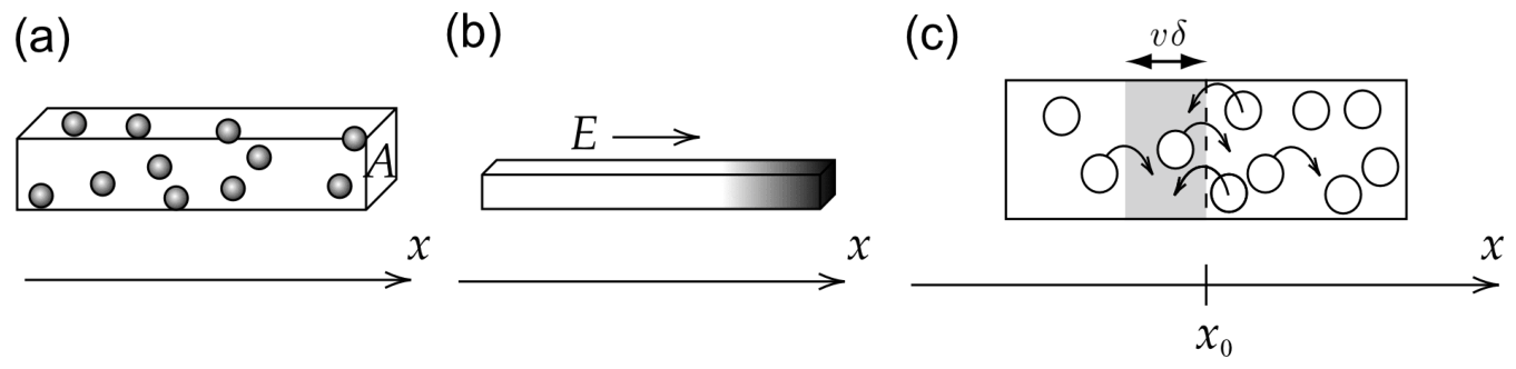
Fig.1: Setting for Part C.
By applying a uniform electric field \(E\) in the \(x\)-direction, particles are transported and their concentration \(n(x)\) (particle number per unit volume) becomes non-uniform (Fig.1(b)). When \(E\) is removed, this non-uniformity gradually disappears. This is due to Brownian motion of particles. If \(n(x)\) is not uniform, the numbers of right-going and left-going particles may differ (Fig.1(c)). This generates a particle flux \(J_D(x)\), the mean number of particles flowing at \(x\) along the \(x\)-axis per unit cross-sectional area and unit time. This flux is known to satisfy
\[ J_D(x)=-D\frac{dn}{dx}(x), \tag{4} \]
where \(D\) is called the diffusion coefficient.
Now let's assume, for simplicity, that half of the particles have velocity \(+v\) and the other half have velocity \(-v\). Let \(N_+(x_0)\) be the number of particles with velocity \(+v\) that cross \(x_0\) from left to right per unit cross-sectional area and unit time. For particles with velocity \(+v\) to cross \(x_0\) in the time interval \(\delta\), they should be in the shaded region of Fig.1(c). Since \(\delta\) is small, we have \(n(x)\simeq n(x_0)+(x-x_0)\frac{dn}{dx}(x_0)\) in this region.
C.1 — 0.5pt
Express \(N_+(x_0)\) using necessary quantities from \(v\), \(\delta\), \(n(x_0)\), and \(\frac{dn}{dx}(x_0)\).
We define \(N_-(x_0)\) as the counterpart of \(N_+(x_0)\) for the velocity \(-v\). With this, we have \(J_D(x_0)=\langle N_+(x_0)-N_-(x_0)\rangle\). According to Eq.(3), we have \(\langle v^2\rangle=C\).
C.2 — 0.7pt
Determine \(J_D(x_0)\) using necessary quantities from \(C\), \(\delta\), \(n(x_0)\), and \(\frac{dn}{dx}(x_0)\). Using this and Eq.(4), express \(D\) in terms of \(C\) and \(\delta\), and \(\langle\Delta x(t)^2\rangle\) in terms of \(D\) and \(t\).
Now we discuss the effect of osmotic pressure \(\Pi\). It is given by \(\Pi=\frac{n}{N_A}RT=nkT\) with the Avogadro constant \(N_A\), the gas constant \(R\), temperature \(T\), and the Boltzmann constant \(k=\frac{R}{N_A}\). Let us consider the non-uniform concentration formed under the electric field \(E\) (Fig.1(b)). Since \(n(x)\) depends on \(x\), so does \(\Pi(x)\). Then the forces due to \(\Pi(x)\) and \(\Pi(x+\Delta x)\) must be balanced with the total force from the field \(E\) acting on the particles (Fig.2). Here we consider small \(\Delta x\), so that \(n(x)\) can be regarded as constant over this range, while \(n(x+\Delta x)-n(x)\simeq\Delta x\frac{dn}{dx}(x)\).
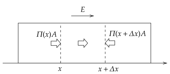
Fig.2: Force balance.
C.3 — 0.5pt
Express \(\frac{dn}{dx}(x)\) using \(n(x)\), \(T\), \(Q\), \(E\), and \(k\).
Let us discuss the balance of the flux now. Besides the flux \(J_D(x)\) due to the Brownian motion, there is also a flux due to the electric field, \(J_Q(x)\). It is given by
\[ J_Q(x)=n(x)u, \tag{5} \]
where \(u\) is the terminal velocity of particles driven by the field.
C.4 — 0.5pt
To determine \(u\), we use Eq.(1) with \(F_{\mathrm{ext}}(t)=QE\). Since \(v(t)\) is fluctuating, we consider \(\langle v(t)\rangle\). Assuming \(\langle v(0)\rangle=0\) and using \(\langle F(t)\rangle=0\), evaluate \(\langle v(t)\rangle\) and obtain \(u=\lim_{t\to\infty}\langle v(t)\rangle\).
C.5 — 0.5pt
The flux balance reads \(J_D(x)+J_Q(x)=0\). Express the diffusion coefficient \(D\) in terms of \(k\), \(\gamma\), and \(T\).
Part D. Mean square displacement (2.4 points)
Suppose we observed the Brownian motion of an isolated, spherical colloidal particle with radius \(a=5.0\,\mu\mathrm{m}\) in water. Figure 3 shows the histogram of displacements \(\Delta x\) measured in the \(x\)-direction at every interval \(\Delta t=60\,\mathrm{s}\). The friction coefficient is given by \(\gamma=6\pi a\eta\) with water viscosity \(\eta=8.9\times10^{-4}\,\mathrm{Pa\cdot s}\) and the temperature was \(T=25\,^\circ\mathrm{C}\).
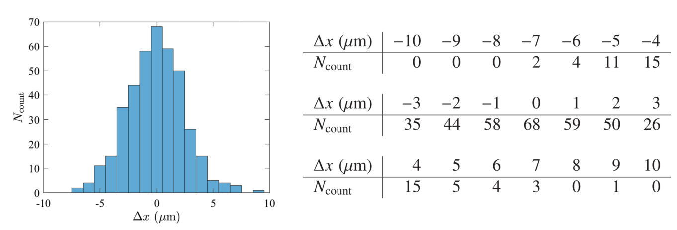
Fig.3: Histogram of displacements.
| \(\Delta x\;(\mu\mathrm{m})\) | \(-10\) | \(-9\) | \(-8\) | \(-7\) | \(-6\) | \(-5\) | \(-4\) |
|---|---|---|---|---|---|---|---|
| \(N_{\mathrm{count}}\) | 0 | 0 | 0 | 2 | 4 | 11 | 15 |
| \(\Delta x\;(\mu\mathrm{m})\) | \(-3\) | \(-2\) | \(-1\) | \(0\) | \(1\) | \(2\) | \(3\) |
|---|---|---|---|---|---|---|---|
| \(N_{\mathrm{count}}\) | 35 | 44 | 58 | 68 | 59 | 50 | 26 |
| \(\Delta x\;(\mu\mathrm{m})\) | \(4\) | \(5\) | \(6\) | \(7\) | \(8\) | \(9\) | \(10\) |
|---|---|---|---|---|---|---|---|
| \(N_{\mathrm{count}}\) | 15 | 5 | 4 | 3 | 0 | 1 | 0 |
D.1 — 1.0pt
Estimate the value of \(N_A\) without using the fact that it is the Avogadro constant, up to two significant digits from the data in Fig.3. The gas constant is \(R=8.31\,\mathrm{J/K\cdot mol}\). Do not use the value of the Boltzmann constant \(k\) given in General Instructions. As for the Avogadro constant, you might obtain a value different from that in General Instructions.
Now we extend the model in Part B to describe the motion of a particle with charge \(Q\) under an electric field \(E\). The particle velocity \(v(t)\) considered in Eq.(2) should be replaced by \(v(t)=u+v_n\) \((t_{n-1}<t\leq t_n)\) with \(v_n\) satisfying Eq. (3) and \(u\) being the terminal velocity considered in Eq.(5).
D.2 — 0.8pt
Express the MSD \(\langle\Delta x(t)^2\rangle\) in terms of \(u\), \(D\), and \(t\). Obtain approximate power laws for small \(t\) and large \(t\), as well as the characteristic time \(t_*\) where this change occurs. Draw a rough graph of MSD in a log-log plot, indicating the approximate location of \(t_*\).
Next, we consider swimming microbes (Fig.4(a)), in one dimension for simplicity (Fig.4(b)). These are spherical particles with radius \(a\). They swim at velocity either \(+u_0\) or \(-u_0\), the sign chosen randomly at every time interval \(\delta_0\) without correlation. The observed motion is a combination of displacements due to swimming and those due to the Brownian motion of a spherical particle.
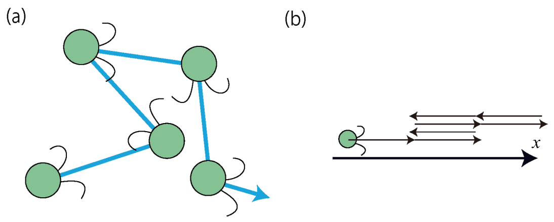
Fig.4: (a) Motion of microbes. (b) Its one-dimensional version.
D.3 — 0.6pt
Figure 5 displays the MSD \(\langle\Delta x(t)^2\rangle\) of those microbes, showing different power laws for small, large, and intermidiate \(t\), as indicated by dashed lines. Obtain the power law for each time range and express it using necessary quantities from \(D\), \(u_0\), \(\delta_0\), and \(t\).
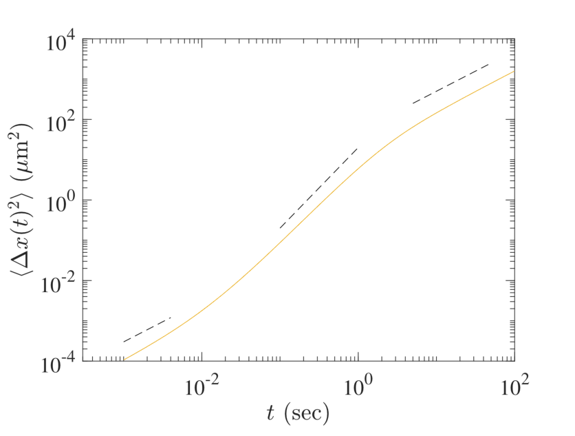
Fig.5: Mean square displacement of the microbes.
Part E. Water purification (1.5 points)
Here we discuss the purification of water including colloid-like soil particles, by adding electrolytes to coagulate them. Particles interact through van der Waals force and electrostatic force, the latter including effects of both surface charges and the surrounding layer of oppositely charged ions (such ions and their layer are called counter-ions and the electric double layer, respectively; see Fig.6(a)). As a result, the interaction potential for particle distance \(d\) (Fig.6(b)) is given by
\[ U(d)=-\frac{A}{d}+\frac{B\epsilon(kT)^2}{q^2}e^{-d/\lambda}, \tag{6} \]
where \(A\) and \(B\) are positive constants, \(\epsilon\) is the dielectric constant of water, and \(\lambda\) is the thickness of the electric double layer. Assuming that charges of ions are \(\pm q\), we have
\[ \lambda=\sqrt{\frac{\epsilon kT}{2N_Aq^2c}}, \tag{7} \]
where \(c\) is the molar concentration of ion.
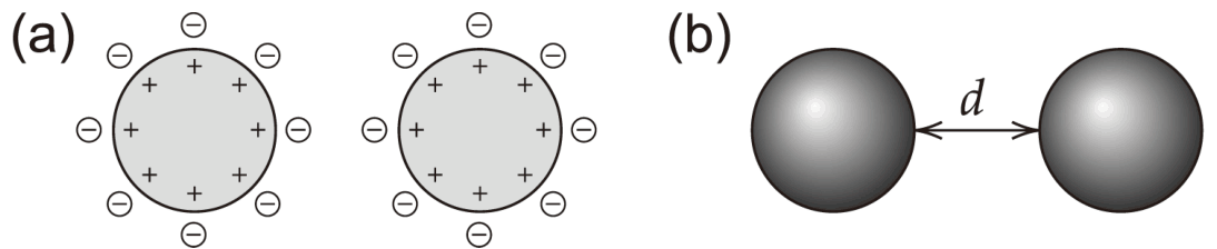
Fig.6: (a) Surface charges of colloidal particles and counter-ions. (b) Definition of the distance \(d\).
E.1 — 1.5pt
Addition of sodium chloride (NaCl) to the suspension causes colloidal particles to coagulate. Determine the lowest concentration \(c\) of NaCl necessary for coagulation. It is sufficient to consider two particles without thermal fluctuations, i.e., \(F(t)=0\) in Eq.(1), and assume that the terminal velocity for the given potential force is reached instantaneously.
Official English text of the problem.
Answers
-
A.1 \[ \boxed{v_0=\frac{I_0}{M},\qquad \tau=\frac{M}{\gamma}.} \]
-
A.2 \[ \boxed{v(t)=\frac1M\sum_{0<t_i<t}I_i e^{-(t-t_i)/\tau},\qquad 0<t_i<t.} \] Immediately after a collision at the observation time, include \(t_i=t\).
-
B.1 \[ \boxed{\langle\Delta x(t)\rangle=0,\qquad \langle\Delta x(t)^2\rangle=C\delta t.} \]
-
B.2 \[ \boxed{\alpha=-1,\qquad\beta=1.} \]
-
C.1 \[ \boxed{N_+(x_0)\simeq \frac v2n(x_0)-\frac{v^2\delta}{4}\frac{dn}{dx}(x_0).} \]
-
C.2 \[ \boxed{J_D(x_0)=-\frac{C\delta}{2}\frac{dn}{dx}(x_0),\qquad D=\frac{C\delta}{2},\qquad \langle\Delta x(t)^2\rangle=2Dt.} \]
-
C.3 \[ \boxed{\frac{dn}{dx}(x)=\frac{QE}{kT}n(x).} \]
-
C.4 \[ \boxed{\langle v(t)\rangle=\frac{QE}{\gamma} \left(1-e^{-t/\tau}\right),\qquad u=\frac{QE}{\gamma}.} \]
-
C.5 \[ \boxed{D=\frac{kT}{\gamma}.} \]
-
D.1 \[ \boxed{N_A\simeq5.6\times10^{23}\,\mathrm{mol}^{-1}.} \]
-
D.2 \[ \boxed{\langle\Delta x(t)^2\rangle=2Dt+u^2t^2,\qquad t_*=\frac{2D}{u^2}.} \] For \(t\ll t_*\), the MSD is approximately \(2Dt\), with log-log slope \(1\). For \(t\gg t_*\), it is approximately \(u^2t^2\), with slope \(2\).
-
D.3 Define \(t_s=2D/u_0^2\). For the three distinct regimes shown, \(t_s\ll\delta_0\), and \[ \boxed{ \langle\Delta x(t)^2\rangle\simeq \begin{cases} 2Dt,&t\ll t_s,\\ u_0^2t^2,&t_s\ll t\ll\delta_0,\\ (2D+u_0^2\delta_0)t\simeq u_0^2\delta_0t,&t\gg\delta_0. \end{cases}} \] The respective log-log slopes are \(1,2,1\).
-
E.1 The critical concentration is \[ \boxed{c_{\mathrm{crit}}= \frac{8B^2\epsilon^3(kT)^5} {\exp(4)\,N_AA^2q^6},} \] where \(q\) is the elementary charge magnitude for NaCl. Coagulation from large separation occurs for \(c>c_{\mathrm{crit}}\). Exactly at \(c=c_{\mathrm{crit}}\), the stated noiseless, overdamped dynamics are marginal: the particles approach a finite separation asymptotically.
Solution
A.1
Integrating the equation of motion over the very short collision gives the impulse–momentum relation. The frictional impulse vanishes as the collision duration tends to zero, so
\[ M\bigl[v(t_0^+)-v(t_0^-)\bigr]=I_0. \]
Since the particle was initially at rest,
\[ v_0=v(t_0^+)=\frac{I_0}{M}. \]
After the collision, both forces \(F\) and \(F_{\mathrm{ext}}\) vanish. Thus
\[ M\frac{dv}{dt}=-\gamma v, \]
whose solution is
\[ v(t)=\frac{I_0}{M} \exp\left[-\frac{\gamma}{M}(t-t_0)\right]. \]
Comparison with the given form yields
\[ \boxed{v_0=\frac{I_0}{M},\qquad \tau=\frac{M}{\gamma}.} \]
A.2
The equation of motion is linear. Each collision produces an instantaneous velocity increment \(I_i/M\), which subsequently decays with relaxation time \(\tau\). Superposition therefore gives
\[ \boxed{v(t)=\frac1M\sum_{0<t_i<t}I_i \exp\left[-\frac{t-t_i}{\tau}\right].} \]
Only collisions after the initial time and before the observation contribute:
\[ \boxed{0<t_i<t.} \]
At a collision instant, the velocity has a jump \(I_i/M\). If \(v(t)\) denotes the velocity immediately after that collision, the upper endpoint is included.
B.1
During interval \(n\), the displacement is \(v_n\delta\). Hence, at \(t=N\delta\),
\[ \Delta x(t)=\delta\sum_{n=1}^{N}v_n. \]
Its expectation is
\[ \langle\Delta x(t)\rangle =\delta\sum_{n=1}^{N}\langle v_n\rangle=0. \]
For the second moment,
\[ \begin{aligned} \langle\Delta x(t)^2\rangle &=\delta^2\sum_{n=1}^{N}\sum_{m=1}^{N} \langle v_nv_m\rangle\\ &=\delta^2NC\\ &=C\delta t. \end{aligned} \]
The cross terms vanish because different intervals have uncorrelated velocities. Thus
\[ \boxed{\langle\Delta x(t)\rangle=0,\qquad \langle\Delta x(t)^2\rangle=C\delta t.} \]
B.2
At a fixed positive observation time, Brownian motion must have a finite, nonzero MSD in the diffusion limit. Since
\[ \langle\Delta x(t)^2\rangle=C\delta t, \]
the product \(C\delta\) must tend to a finite, nonzero constant as \(\delta\to0\). Therefore
\[ C\propto\delta^{-1}. \]
The remaining time dependence is linear:
\[ \langle\Delta x(t)^2\rangle\propto t. \]
Consequently,
\[ \boxed{\alpha=-1,\qquad\beta=1.} \]
This is the continuum limit of the effective model, describing motion on time scales much longer than the microscopic relaxation time \(\tau\).
C.1
Particles moving rightward cross \(x_0\) during the next interval \(\delta\) if they initially lie between \(x_0-v\delta\) and \(x_0\). Half of the particles in this region move rightward. Dividing their number per unit area by \(\delta\),
\[ N_+(x_0)=\frac{1}{2\delta} \int_{x_0-v\delta}^{x_0}n(x)\,dx. \]
Using the prescribed linear approximation,
\[ n(x)\simeq n(x_0)+(x-x_0)n'(x_0), \]
we obtain
\[ \begin{aligned} N_+(x_0) &\simeq\frac{1}{2\delta} \left[v\delta\,n(x_0) -\frac{(v\delta)^2}{2}n'(x_0)\right]. \end{aligned} \]
Therefore,
\[ \boxed{N_+(x_0)\simeq \frac v2n(x_0)-\frac{v^2\delta}{4}n'(x_0).} \]
This approximation requires the concentration to vary slowly over a distance \(v\delta\).
C.2
Similarly, particles moving leftward originate in \(x_0<x<x_0+v\delta\), giving
\[ \begin{aligned} N_-(x_0) &=\frac{1}{2\delta}\int_{x_0}^{x_0+v\delta}n(x)\,dx\\ &\simeq\frac v2n(x_0)+\frac{v^2\delta}{4}n'(x_0). \end{aligned} \]
Subtracting and averaging,
\[ \begin{aligned} J_D(x_0) &=\langle N_+(x_0)-N_-(x_0)\rangle\\ &=-\frac{\delta}{2}\langle v^2\rangle n'(x_0)\\ &=-\frac{C\delta}{2}n'(x_0). \end{aligned} \]
Comparison with Fick’s law, \(J_D=-Dn'\), gives
\[ \boxed{D=\frac{C\delta}{2}.} \]
Substituting into B.1,
\[ \boxed{\langle\Delta x(t)^2\rangle=2Dt.} \]
C.3
Consider the slab of cross-sectional area \(A\) and thickness \(\Delta x\). Its electric force in the positive \(x\)-direction is
\[ F_E=n(x)A\Delta x\,QE. \]
The net osmotic-pressure force is
\[ F_\Pi=A\Pi(x)-A\Pi(x+\Delta x) \simeq-A\Delta x\,\frac{d\Pi}{dx}. \]
Force balance gives
\[ n(x)QE=\frac{d\Pi}{dx}. \]
At uniform temperature, \(\Pi=nkT\), so
\[ \frac{d\Pi}{dx}=kT\frac{dn}{dx}. \]
Hence
\[ \boxed{\frac{dn}{dx}(x)=\frac{QE}{kT}n(x).} \]
The positive gradient is consistent with positively charged particles accumulating in the direction of the electric field.
C.4
Taking the expectation of Eq.(1), using the constant applied force and \(\langle F(t)\rangle=0\), yields
\[ M\frac{d\langle v\rangle}{dt} =-\gamma\langle v\rangle+QE. \]
The solution satisfying \(\langle v(0)\rangle=0\) is
\[ \boxed{\langle v(t)\rangle= \frac{QE}{\gamma}\left(1-e^{-\gamma t/M}\right) =\frac{QE}{\gamma}\left(1-e^{-t/\tau}\right).} \]
Therefore the terminal velocity is
\[ \boxed{u=\lim_{t\to\infty}\langle v(t)\rangle=\frac{QE}{\gamma}.} \]
C.5
At equilibrium, the diffusive flux balances the electric drift flux:
\[ -D\frac{dn}{dx}+nu=0. \]
Substituting the results of C.3 and C.4,
\[ -D\frac{nQE}{kT}+n\frac{QE}{\gamma}=0. \]
Thus
\[ \boxed{D=\frac{kT}{\gamma}.} \]
This is the Einstein relation between diffusion and friction.
D.1
Using the tabulated displacements as the histogram bin representatives, the total number of measurements is
\[ N_{\mathrm{tot}}=\sum_jN_j=400. \]
The weighted sum of squared displacements is
\[ \sum_jN_j(\Delta x_j)^2=2536\,\mu\mathrm{m}^2. \]
Therefore the estimated MSD over \(\Delta t=60\,\mathrm{s}\) is
\[ \widehat{\langle\Delta x^2\rangle} =\frac{2536}{400}\,\mu\mathrm{m}^2 =6.34\times10^{-12}\,\mathrm{m}^2. \]
From C.2,
\[ D=\frac{\widehat{\langle\Delta x^2\rangle}}{2\Delta t} =\frac{6.34\times10^{-12}}{120} =5.2833\times10^{-14}\,\mathrm{m}^2\,\mathrm{s}^{-1}. \]
The friction coefficient is
\[ \begin{aligned} \gamma &=6\pi a\eta\\ &=6\pi(5.0\times10^{-6})(8.9\times10^{-4})\\ &=8.3881\times10^{-8}\,\mathrm{kg\,s^{-1}}. \end{aligned} \]
Using \(k=R/N_A\) in the Einstein relation gives
\[ D=\frac{RT}{N_A\gamma}, \]
so
\[ N_A=\frac{RT}{\gamma D} =\frac{2RT\Delta t} {\gamma\,\widehat{\langle\Delta x^2\rangle}}. \]
With \(T=298.15\,\mathrm{K}\),
\[ N_A =\frac{8.31(298.15)} {(8.3881\times10^{-8})(5.2833\times10^{-14})} =5.5907\times10^{23}\,\mathrm{mol}^{-1}. \]
To two significant digits,
\[ \boxed{N_A\simeq5.6\times10^{23}\,\mathrm{mol}^{-1}.} \]
Neither an accepted value of \(N_A\) nor a numerical value of \(k\) was used.
D.2
With the terminal drift included, the displacement is
\[ \Delta x(t)=ut+\delta\sum_{n=1}^{N}v_n. \]
The random part has zero mean and second moment \(2Dt\). Thus the cross term between drift and random displacement averages to zero:
\[ \begin{aligned} \langle\Delta x(t)^2\rangle &=u^2t^2 +2ut\,\delta\sum_n\langle v_n\rangle +\delta^2\sum_{n,m}\langle v_nv_m\rangle\\ &=u^2t^2+2Dt. \end{aligned} \]
Therefore,
\[ \boxed{\langle\Delta x(t)^2\rangle=2Dt+u^2t^2.} \]
The crossover occurs when the two contributions are equal:
\[ 2Dt_*=u^2t_*^2, \]
giving
\[ \boxed{t_*=\frac{2D}{u^2}.} \]
The limiting power laws are
\[ \boxed{ \begin{aligned} t\ll t_*:&\qquad \langle\Delta x(t)^2\rangle\simeq2Dt,\\ t\gg t_*:&\qquad \langle\Delta x(t)^2\rangle\simeq u^2t^2. \end{aligned}} \]
Here “small \(t\)” refers to the effective diffusive model, with the microscopic relaxation already neglected and the terminal drift established.
For a precise description of the requested log-log sketch, define
\[ s=\frac{t}{t_*},\qquad Y=\frac{\langle\Delta x(t)^2\rangle}{2Dt_*}. \]
Then
\[ Y=s+s^2. \]
The graph follows the straight asymptote \(Y=s\), of slope \(1\), at small \(s\), bends smoothly upward near \(s=1\), and approaches \(Y=s^2\), of slope \(2\), at large \(s\). The two asymptotes intersect at \((s,Y)=(1,1)\), while the actual curve passes through \((1,2)\). Thus mark \(t=t_*\) at the bend. At that point,
\[ \langle\Delta x(t_*)^2\rangle =\frac{8D^2}{u^2}. \]
D.3
Write the displacement as the sum of thermal and swimming contributions:
\[ \Delta x(t)=\Delta x_B(t)+\Delta x_S(t). \]
The thermal motion and the swimming direction choices are taken to be independent, and both contributions have zero mean. Hence
\[ \langle\Delta x(t)^2\rangle =2Dt+\langle\Delta x_S(t)^2\rangle. \]
For \(t\ll\delta_0\), the swimming direction is effectively unchanged during the observation interval. Therefore
\[ \Delta x_S(t)\simeq\pm u_0t, \qquad \langle\Delta x_S(t)^2\rangle\simeq u_0^2t^2. \]
Thus
\[ \langle\Delta x(t)^2\rangle\simeq2Dt+u_0^2t^2 \qquad(t\ll\delta_0). \]
The two terms become comparable at
\[ t_s=\frac{2D}{u_0^2}. \]
Consequently, thermal diffusion dominates for \(t\ll t_s\), and swimming produces a ballistic regime for \(t_s\ll t\ll\delta_0\).
For long times, consider \(N\) complete swimming intervals, with \(t=N\delta_0\). Let \(s_j=\pm1\) denote the independently chosen sign in interval \(j\). Then
\[ \Delta x_S(t)=u_0\delta_0\sum_{j=1}^{N}s_j. \]
Because \(\langle s_j\rangle=0\) and \(\langle s_js_\ell\rangle=0\) for \(j\neq\ell\),
\[ \begin{aligned} \langle\Delta x_S(t)^2\rangle &=u_0^2\delta_0^2N\\ &=u_0^2\delta_0t. \end{aligned} \]
An incomplete final interval does not alter this leading behavior at \(t\gg\delta_0\). Therefore the long-time MSD is
\[ \langle\Delta x(t)^2\rangle \simeq(2D+u_0^2\delta_0)t. \]
Equivalently, the long-time diffusion coefficient is
\[ D_{\mathrm{eff}}=D+\frac{u_0^2\delta_0}{2}. \]
For a well-developed intermediate regime, as in the figure, the time scales must satisfy
\[ \frac{2D}{u_0^2}\ll\delta_0. \]
This also implies \(u_0^2\delta_0\gg2D\). The three observed asymptotes are therefore
\[ \boxed{ \begin{array}{c|c|c} \text{Time range}&\langle\Delta x(t)^2\rangle&\text{Log-log slope}\\ \hline t\ll 2D/u_0^2&2Dt&1\\ 2D/u_0^2\ll t\ll\delta_0&u_0^2t^2&2\\ t\gg\delta_0&u_0^2\delta_0t&1 \end{array}} \]
with the full long-time coefficient \(2D+u_0^2\delta_0\) retained when thermal diffusion is appreciable.
E.1
Define the positive energy scale
\[ K=\frac{B\epsilon(kT)^2}{q^2}. \]
Then
\[ U(d)=-\frac{A}{d}+Ke^{-d/\lambda}, \]
and
\[ U'(d)=\frac{A}{d^2}-\frac{K}{\lambda}e^{-d/\lambda}. \]
The force tending to increase the separation is \(-U'(d)\). Under the instantaneous-terminal-velocity assumption, each particle’s velocity is proportional to its force. For two identical particles with friction coefficient \(\gamma\),
\[ \dot d=-\frac{2}{\gamma}U'(d). \]
Thus the particles approach each other wherever \(U'(d)>0\).
For particles approaching from large separation to reach contact without thermal fluctuations, there must be no intervening repulsive region or stable finite-separation equilibrium. The critical condition is therefore the disappearance of the region where \(U'(d)<0\).
Rewrite the derivative as
\[ U'(d)=\frac{A}{d^2} \left[ 1-\frac{K\lambda}{A} \left(\frac d\lambda\right)^2e^{-d/\lambda} \right]. \]
Set \(z=d/\lambda>0\). The function controlling the sign is
\[ f(z)=z^2e^{-z}. \]
Its derivative is
\[ f'(z)=ze^{-z}(2-z), \]
so its global maximum occurs at \(z=2\), with
\[ f_{\max}=4e^{-2}. \]
Accordingly, \(U'(d)\geq0\) for every separation precisely when
\[ \frac{K\lambda}{A}\,4e^{-2}\leq1. \]
The critical screening length is
\[ \boxed{\lambda_{\mathrm{crit}} =\frac{\exp(2)A}{4K} =\frac{\exp(2)Aq^2}{4B\epsilon(kT)^2}.} \]
At this threshold, the two stationary points of the potential merge at
\[ d_{\mathrm{crit}}=2\lambda_{\mathrm{crit}}, \]
where both \(U'(d_{\mathrm{crit}})\) and \(U''(d_{\mathrm{crit}})\) vanish.
Increasing the salt concentration decreases \(\lambda\). Substituting \(\lambda_{\mathrm{crit}}\) into Eq.(7),
\[ \begin{aligned} c_{\mathrm{crit}} &=\frac{\epsilon kT} {2N_Aq^2\lambda_{\mathrm{crit}}^2}\\ &=\frac{\epsilon kT}{2N_Aq^2} \left[ \frac{4B\epsilon(kT)^2}{\exp(2)Aq^2} \right]^2. \end{aligned} \]
Therefore,
\[ \boxed{c_{\mathrm{crit}}= \frac{8B^2\epsilon^3(kT)^5} {\exp(4)\,N_AA^2q^6}.} \]
For NaCl, the ions are monovalent, so \(q\) is the elementary charge magnitude. The concentration of each ionic species equals the NaCl molar concentration; the factor \(2\) in Eq.(7) already accounts for both species. With SI parameters, the result has units \(\mathrm{mol\,m^{-3}}\).
For \(c>c_{\mathrm{crit}}\), \(U'(d)>0\) at every positive separation, and the deterministic motion brings an initially separated pair into contact. For \(c<c_{\mathrm{crit}}\), a pair approaching from sufficiently large separation becomes trapped at the outer local minimum of \(U\).
There is a precise qualification at equality. At \(c=c_{\mathrm{crit}}\),
\[ U'(d)\propto(d-d_{\mathrm{crit}})^2 \]
near \(d_{\mathrm{crit}}\). The overdamped approach from above therefore takes infinite time to reach that separation. Thus \(c_{\mathrm{crit}}\) is the critical threshold, or infimum of concentrations producing coagulation from large separation; the idealized dynamics require \(c>c_{\mathrm{crit}}\) for actual passage to contact.
The solution was checked against the official solution.
IPhO 2023 · Theorieaufgabe 1
Charakterisierung von Bodenkolloiden
Die Kolloidwissenschaft eignet sich zur Charakterisierung von Bodenpartikeln, da viele von ihnen als kolloidale Teilchen im Mikrometerbereich betrachtet werden können. Beispielsweise lässt sich die Brownsche Bewegung (zufällige Bewegung kolloidaler Teilchen) zur Messung von Teilchengrößen nutzen.
Teil A. Bewegungen kolloidaler Teilchen (1.6 Punkte)
Wir untersuchen die eindimensionale Brownsche Bewegung eines kolloidalen Teilchens mit der Masse \(M\). Die Bewegungsgleichung für seine Geschwindigkeit \(v(t)\) lautet:
\[ M\dot v=-\gamma v(t)+F(t)+F_{\mathrm{ext}}(t), \tag{1} \]
wobei \(\gamma\) der Reibungskoeffizient, \(F(t)\) eine durch zufällige Stöße mit Wassermolekülen verursachte Kraft und \(F_{\mathrm{ext}}(t)\) eine äußere Kraft ist. In Teil A nehmen wir \(F_{\mathrm{ext}}(t)=0\) an.
A.1 — 0.8 Punkte
Ein Wassermolekül stoße zum Zeitpunkt \(t=t_0\) mit dem Teilchen zusammen und übertrage dabei den Impuls \(I_0\); anschließend gelte \(F(t)=0\). Wenn vor dem Stoß \(v(t)=0\) gilt, ist \(v(t)=v_0e^{-(t-t_0)/\tau}\) für \(t>t_0\). Bestimmen Sie \(v_0\) und \(\tau\) mithilfe von \(I_0\) und den erforderlichen Parametern aus Gl.(1).
Im Folgenden dürfen Sie \(\tau\) in Ihren Antworten verwenden.
A.2 — 0.8 Punkte
Tatsächlich stoßen Wassermoleküle nacheinander mit dem Teilchen zusammen. Nehmen Sie an, dass der \(i\)-te Stoß zum Zeitpunkt \(t_i\) den Impuls \(I_i\) überträgt, und bestimmen Sie \(v(t)\) unter den Bedingungen \(t>0\) und \(v(0)=0\). Geben Sie außerdem die Ungleichung an, die den für ein gegebenes \(t\) zu berücksichtigenden Bereich von \(t_i\) festlegt. Auf dem Antwortbogen müssen Sie diesen Bereich im Ausdruck für \(v(t)\) nicht angeben.
Teil B. Effektive Bewegungsgleichung (1.8 Punkte)
Die bisherigen Ergebnisse legen nahe, dass die Teilchengeschwindigkeiten \(v(t)\) und \(v(t')\) als unkorrelierte Zufallsgrößen betrachtet werden können, wenn \(|t-t'|\gg\tau\) gilt. Auf dieser Grundlage führen wir ein theoretisches Modell zur näherungsweisen Beschreibung der eindimensionalen Brownschen Bewegung ein, in dem sich die Geschwindigkeit nach jedem Zeitintervall \(\delta\) \((\gg\tau)\) zufällig ändert, d. h.,
\[ v(t)=v_n\qquad(t_{n-1}<t\leq t_n), \tag{2} \]
mit \(t_n=n\delta\) \((n=0,1,2,\cdots)\) und einer Zufallsgröße \(v_n\). Sie erfüllt
\[ \langle v_n\rangle=0,\qquad \langle v_nv_m\rangle= \begin{cases} C &(n=m),\\ 0 &(n\neq m), \end{cases} \tag{3} \]
mit einem von \(\delta\) abhängigen Parameter \(C\). Hier bezeichnet \(\langle X\rangle\) den Erwartungswert von \(X\). Wenn man also unendlich oft Zufallszahlen \(X\) zieht, ist deren Mittelwert \(\langle X\rangle\).
Nun betrachten wir die Verschiebung des Teilchens \(\Delta x(t)=x(t)-x(0)\) für \(t=N\delta\) mit einer ganzen Zahl \(N\).
B.1 — 1.0 Punkte
Bestimmen Sie \(\langle\Delta x(t)\rangle\) und \(\langle\Delta x(t)^2\rangle\) mithilfe von \(C\), \(\delta\) und \(t\).
B.2 — 0.8 Punkte
Die Größe \(\langle\Delta x(t)^2\rangle\) heißt mittlere quadratische Verschiebung (MSD). Sie ist eine charakteristische Messgröße der Brownschen Bewegung, die dem Grenzfall \(\delta\to0\) entspricht. Daraus lässt sich zeigen, dass \(C\propto\delta^\alpha\) und \(\langle\Delta x(t)^2\rangle\propto t^\beta\) gelten. Bestimmen Sie die Werte von \(\alpha\) und \(\beta\).
Teil C. Elektrophorese (2.7 Punkte)
Hier behandeln wir die Elektrophorese, d. h. den Transport geladener Teilchen durch ein elektrisches Feld. Eine Suspension kolloidaler Teilchen mit der Masse \(M\) und der Ladung \(Q\) \((>0)\) wird in einen engen Kanal mit der Querschnittsfläche \(A\) eingebracht (Abb.1(a)). Wir vernachlässigen die Wechselwirkung zwischen den Teilchen, die Einflüsse der Wand, der Flüssigkeit und der darin enthaltenen Ionen sowie die Schwerkraft.
Abb.1: Anordnung für Teil C.
Durch Anlegen eines homogenen elektrischen Feldes \(E\) in \(x\)-Richtung werden die Teilchen transportiert, und ihre Konzentration \(n(x)\) (Teilchenzahl pro Volumeneinheit) wird inhomogen (Abb.1(b)). Wird \(E\) abgeschaltet, verschwindet diese Inhomogenität allmählich. Dies ist auf die Brownsche Bewegung der Teilchen zurückzuführen. Wenn \(n(x)\) nicht homogen ist, können sich die Anzahlen der nach rechts und nach links bewegten Teilchen unterscheiden (Abb.1(c)). Dadurch entsteht eine Teilchenstromdichte \(J_D(x)\), die mittlere Anzahl von Teilchen, die am Ort \(x\) entlang der \(x\)-Achse pro Querschnittsfläche und Zeit strömen. Für diese Stromdichte gilt bekanntermaßen
\[ J_D(x)=-D\frac{dn}{dx}(x), \tag{4} \]
wobei \(D\) als Diffusionskoeffizient bezeichnet wird.
Nehmen wir nun der Einfachheit halber an, dass die Hälfte der Teilchen die Geschwindigkeit \(+v\) und die andere Hälfte die Geschwindigkeit \(-v\) hat. Sei \(N_+(x_0)\) die Anzahl der Teilchen mit der Geschwindigkeit \(+v\), die \(x_0\) pro Querschnittsfläche und Zeit von links nach rechts passieren. Damit Teilchen mit der Geschwindigkeit \(+v\) den Ort \(x_0\) innerhalb des Zeitintervalls \(\delta\) passieren, müssen sie sich im schraffierten Bereich von Abb.1(c) befinden. Da \(\delta\) klein ist, gilt in diesem Bereich \(n(x)\simeq n(x_0)+(x-x_0)\frac{dn}{dx}(x_0)\).
C.1 — 0.5 Punkte
Drücken Sie \(N_+(x_0)\) mithilfe der erforderlichen Größen aus \(v\), \(\delta\), \(n(x_0)\) und \(\frac{dn}{dx}(x_0)\) aus.
Wir definieren \(N_-(x_0)\) als das Gegenstück zu \(N_+(x_0)\) für die Geschwindigkeit \(-v\). Damit gilt \(J_D(x_0)=\langle N_+(x_0)-N_-(x_0)\rangle\). Gemäß Gl.(3) gilt \(\langle v^2\rangle=C\).
C.2 — 0.7 Punkte
Bestimmen Sie \(J_D(x_0)\) mithilfe der erforderlichen Größen aus \(C\), \(\delta\), \(n(x_0)\) und \(\frac{dn}{dx}(x_0)\). Drücken Sie damit und mithilfe von Gl.(4) \(D\) durch \(C\) und \(\delta\) sowie \(\langle\Delta x(t)^2\rangle\) durch \(D\) und \(t\) aus.
Nun behandeln wir den Einfluss des osmotischen Drucks \(\Pi\). Er ist gegeben durch \(\Pi=\frac{n}{N_A}RT=nkT\), mit der Avogadro-Konstante \(N_A\), der Gaskonstante \(R\), der Temperatur \(T\) und der Boltzmann-Konstante \(k=\frac{R}{N_A}\). Betrachten wir die inhomogene Konzentration, die sich unter dem elektrischen Feld \(E\) ausgebildet hat (Abb.1(b)). Da \(n(x)\) von \(x\) abhängt, gilt dies auch für \(\Pi(x)\). Dann müssen die durch \(\Pi(x)\) und \(\Pi(x+\Delta x)\) verursachten Kräfte mit der Gesamtkraft im Gleichgewicht stehen, die das Feld \(E\) auf die Teilchen ausübt (Abb.2). Hier betrachten wir ein kleines \(\Delta x\), sodass \(n(x)\) über diesen Bereich als konstant angesehen werden kann, während \(n(x+\Delta x)-n(x)\simeq\Delta x\frac{dn}{dx}(x)\) gilt.
Abb.2: Kräftegleichgewicht.
C.3 — 0.5 Punkte
Drücken Sie \(\frac{dn}{dx}(x)\) mithilfe von \(n(x)\), \(T\), \(Q\), \(E\) und \(k\) aus.
Betrachten wir nun das Gleichgewicht der Teilchenströme. Neben der Stromdichte \(J_D(x)\) aufgrund der Brownschen Bewegung gibt es auch eine Stromdichte aufgrund des elektrischen Feldes, \(J_Q(x)\). Sie ist gegeben durch
\[ J_Q(x)=n(x)u, \tag{5} \]
wobei \(u\) die Endgeschwindigkeit der vom Feld angetriebenen Teilchen ist.
C.4 — 0.5 Punkte
Zur Bestimmung von \(u\) verwenden wir Gl.(1) mit \(F_{\mathrm{ext}}(t)=QE\). Da \(v(t)\) schwankt, betrachten wir \(\langle v(t)\rangle\). Berechnen Sie unter der Annahme \(\langle v(0)\rangle=0\) und mithilfe von \(\langle F(t)\rangle=0\) den Ausdruck \(\langle v(t)\rangle\), und bestimmen Sie \(u=\lim_{t\to\infty}\langle v(t)\rangle\).
C.5 — 0.5 Punkte
Das Gleichgewicht der Teilchenströme lautet \(J_D(x)+J_Q(x)=0\). Drücken Sie den Diffusionskoeffizienten \(D\) durch \(k\), \(\gamma\) und \(T\) aus.
Teil D. Mittlere quadratische Verschiebung (2.4 Punkte)
Angenommen, wir haben die Brownsche Bewegung eines isolierten, kugelförmigen kolloidalen Teilchens mit dem Radius \(a=5.0\,\mu\mathrm{m}\) in Wasser beobachtet. Abbildung 3 zeigt das Histogramm der Verschiebungen \(\Delta x\), die in \(x\)-Richtung jeweils über ein Intervall \(\Delta t=60\,\mathrm{s}\) gemessen wurden. Der Reibungskoeffizient ist gegeben durch \(\gamma=6\pi a\eta\), mit der Viskosität des Wassers \(\eta=8.9\times10^{-4}\,\mathrm{Pa\cdot s}\), und die Temperatur betrug \(T=25\,^\circ\mathrm{C}\).
Abb.3: Histogramm der Verschiebungen.
| \(\Delta x\;(\mu\mathrm{m})\) | \(-10\) | \(-9\) | \(-8\) | \(-7\) | \(-6\) | \(-5\) | \(-4\) |
|---|---|---|---|---|---|---|---|
| \(N_{\mathrm{count}}\) | 0 | 0 | 0 | 2 | 4 | 11 | 15 |
| \(\Delta x\;(\mu\mathrm{m})\) | \(-3\) | \(-2\) | \(-1\) | \(0\) | \(1\) | \(2\) | \(3\) |
|---|---|---|---|---|---|---|---|
| \(N_{\mathrm{count}}\) | 35 | 44 | 58 | 68 | 59 | 50 | 26 |
| \(\Delta x\;(\mu\mathrm{m})\) | \(4\) | \(5\) | \(6\) | \(7\) | \(8\) | \(9\) | \(10\) |
|---|---|---|---|---|---|---|---|
| \(N_{\mathrm{count}}\) | 15 | 5 | 4 | 3 | 0 | 1 | 0 |
D.1 — 1.0 Punkte
Schätzen Sie den Wert von \(N_A\) anhand der Daten in Abb.3 auf zwei signifikante Stellen, ohne die Tatsache zu nutzen, dass es sich um die Avogadro-Konstante handelt. Die Gaskonstante beträgt \(R=8.31\,\mathrm{J/K\cdot mol}\). Verwenden Sie nicht den in den allgemeinen Hinweisen angegebenen Wert der Boltzmann-Konstante \(k\). Für die Avogadro-Konstante erhalten Sie möglicherweise einen Wert, der von dem in den allgemeinen Hinweisen abweicht.
Nun erweitern wir das Modell aus Teil B, um die Bewegung eines Teilchens mit der Ladung \(Q\) in einem elektrischen Feld \(E\) zu beschreiben. Die in Gl.(2) betrachtete Teilchengeschwindigkeit \(v(t)\) ist durch \(v(t)=u+v_n\) \((t_{n-1}<t\leq t_n)\) zu ersetzen, wobei \(v_n\) Gl. (3) erfüllt und \(u\) die in Gl.(5) betrachtete Endgeschwindigkeit ist.
D.2 — 0.8 Punkte
Drücken Sie die MSD \(\langle\Delta x(t)^2\rangle\) durch \(u\), \(D\) und \(t\) aus. Bestimmen Sie näherungsweise Potenzgesetze für kleine \(t\) und große \(t\) sowie die charakteristische Zeit \(t_*\), bei der dieser Übergang auftritt. Skizzieren Sie den Verlauf der MSD in einem doppeltlogarithmischen Diagramm, und kennzeichnen Sie die ungefähre Lage von \(t_*\).
Als Nächstes betrachten wir schwimmende Mikroorganismen (Abb.4(a)), der Einfachheit halber in einer Dimension (Abb.4(b)). Es handelt sich um kugelförmige Teilchen mit dem Radius \(a\). Sie schwimmen entweder mit der Geschwindigkeit \(+u_0\) oder \(-u_0\), wobei das Vorzeichen nach jedem Zeitintervall \(\delta_0\) zufällig und ohne Korrelation gewählt wird. Die beobachtete Bewegung setzt sich aus den Verschiebungen durch das Schwimmen und denen durch die Brownsche Bewegung eines kugelförmigen Teilchens zusammen.
Abb.4: (a) Bewegung von Mikroorganismen. (b) Ihre eindimensionale Version.
D.3 — 0.6 Punkte
Abbildung 5 zeigt die MSD \(\langle\Delta x(t)^2\rangle\) dieser Mikroorganismen mit unterschiedlichen Potenzgesetzen für kleine, große und mittlere \(t\), die durch gestrichelte Linien dargestellt sind. Bestimmen Sie das Potenzgesetz für jeden Zeitbereich, und drücken Sie es mithilfe der erforderlichen Größen aus \(D\), \(u_0\), \(\delta_0\) und \(t\) aus.
Abb.5: Mittlere quadratische Verschiebung der Mikroorganismen.
Teil E. Wasserreinigung (1.5 Punkte)
Hier behandeln wir die Reinigung von Wasser, das kolloidartige Bodenpartikel enthält, durch Zugabe von Elektrolyten, die diese Teilchen koagulieren lassen. Die Teilchen wechselwirken durch die Van-der-Waals-Kraft und die elektrostatische Kraft, wobei Letztere die Einflüsse sowohl der Oberflächenladungen als auch der umgebenden Schicht entgegengesetzt geladener Ionen umfasst (solche Ionen und ihre Schicht werden als Gegenionen beziehungsweise elektrische Doppelschicht bezeichnet; siehe Abb.6(a)). Daraus ergibt sich für den Teilchenabstand \(d\) (Abb.6(b)) das Wechselwirkungspotential
\[ U(d)=-\frac{A}{d}+\frac{B\epsilon(kT)^2}{q^2}e^{-d/\lambda}, \tag{6} \]
wobei \(A\) und \(B\) positive Konstanten sind, \(\epsilon\) die Dielektrizitätskonstante des Wassers und \(\lambda\) die Dicke der elektrischen Doppelschicht ist. Unter der Annahme, dass die Ladungen der Ionen \(\pm q\) betragen, gilt
\[ \lambda=\sqrt{\frac{\epsilon kT}{2N_Aq^2c}}, \tag{7} \]
wobei \(c\) die molare Ionenkonzentration ist.
Abb.6: (a) Oberflächenladungen kolloidaler Teilchen und Gegenionen. (b) Definition des Abstands \(d\).
E.1 — 1.5 Punkte
Die Zugabe von Natriumchlorid (NaCl) zur Suspension bewirkt die Koagulation der kolloidalen Teilchen. Bestimmen Sie die niedrigste für die Koagulation erforderliche Konzentration \(c\) von NaCl. Es genügt, zwei Teilchen ohne thermische Fluktuationen zu betrachten, d. h. \(F(t)=0\) in Gl.(1), und anzunehmen, dass die Endgeschwindigkeit für die gegebene Potentialkraft augenblicklich erreicht wird.
Aufgabentext aus dem offiziellen englischen Text übersetzt.
Antworten
-
A.1 \[ \boxed{v_0=\frac{I_0}{M},\qquad \tau=\frac{M}{\gamma}.} \]
-
A.2 \[ \boxed{v(t)=\frac1M\sum_{0<t_i<t}I_i e^{-(t-t_i)/\tau},\qquad 0<t_i<t.} \] Unmittelbar nach einem Stoß zum Beobachtungszeitpunkt ist \(t_i=t\) einzuschließen.
-
B.1 \[ \boxed{\langle\Delta x(t)\rangle=0,\qquad \langle\Delta x(t)^2\rangle=C\delta t.} \]
-
B.2 \[ \boxed{\alpha=-1,\qquad\beta=1.} \]
-
C.1 \[ \boxed{N_+(x_0)\simeq \frac v2n(x_0)-\frac{v^2\delta}{4}\frac{dn}{dx}(x_0).} \]
-
C.2 \[ \boxed{J_D(x_0)=-\frac{C\delta}{2}\frac{dn}{dx}(x_0),\qquad D=\frac{C\delta}{2},\qquad \langle\Delta x(t)^2\rangle=2Dt.} \]
-
C.3 \[ \boxed{\frac{dn}{dx}(x)=\frac{QE}{kT}n(x).} \]
-
C.4 \[ \boxed{\langle v(t)\rangle=\frac{QE}{\gamma} \left(1-e^{-t/\tau}\right),\qquad u=\frac{QE}{\gamma}.} \]
-
C.5 \[ \boxed{D=\frac{kT}{\gamma}.} \]
-
D.1 \[ \boxed{N_A\simeq5.6\times10^{23}\,\mathrm{mol}^{-1}.} \]
-
D.2 \[ \boxed{\langle\Delta x(t)^2\rangle=2Dt+u^2t^2,\qquad t_*=\frac{2D}{u^2}.} \] Für \(t\ll t_*\) beträgt die MSD näherungsweise \(2Dt\), mit der Steigung \(1\) im doppeltlogarithmischen Diagramm. Für \(t\gg t_*\) beträgt sie näherungsweise \(u^2t^2\), mit der Steigung \(2\).
-
D.3 Definieren wir \(t_s=2D/u_0^2\). Für die drei dargestellten, deutlich getrennten Bereiche gilt \(t_s\ll\delta_0\), und \[ \boxed{ \langle\Delta x(t)^2\rangle\simeq \begin{cases} 2Dt,&t\ll t_s,\\ u_0^2t^2,&t_s\ll t\ll\delta_0,\\ (2D+u_0^2\delta_0)t\simeq u_0^2\delta_0t,&t\gg\delta_0. \end{cases}} \] Die jeweiligen Steigungen im doppeltlogarithmischen Diagramm sind \(1,2,1\).
-
E.1 Die kritische Konzentration ist \[ \boxed{c_{\mathrm{crit}}= \frac{8B^2\epsilon^3(kT)^5} {\exp(4)\,N_AA^2q^6},} \] wobei \(q\) für NaCl der Betrag der Elementarladung ist. Koagulation ausgehend von großem Abstand tritt für \(c>c_{\mathrm{crit}}\) auf. Genau bei \(c=c_{\mathrm{crit}}\) liegt die angegebene rauschfreie, überdämpfte Dynamik im Grenzfall: Die Teilchen nähern sich asymptotisch einem endlichen Abstand.
Lösung
A.1
Die Integration der Bewegungsgleichung über den sehr kurzen Stoß ergibt den Zusammenhang zwischen Kraftstoß und Impulsänderung. Der Kraftstoß der Reibung verschwindet, wenn die Stoßdauer gegen null geht, sodass
\[ M\bigl[v(t_0^+)-v(t_0^-)\bigr]=I_0. \]
Da das Teilchen anfangs ruhte,
\[ v_0=v(t_0^+)=\frac{I_0}{M}. \]
Nach dem Stoß verschwinden die beiden Kräfte \(F\) und \(F_{\mathrm{ext}}\). Somit gilt
\[ M\frac{dv}{dt}=-\gamma v, \]
mit der Lösung
\[ v(t)=\frac{I_0}{M} \exp\left[-\frac{\gamma}{M}(t-t_0)\right]. \]
Der Vergleich mit der vorgegebenen Form ergibt
\[ \boxed{v_0=\frac{I_0}{M},\qquad \tau=\frac{M}{\gamma}.} \]
A.2
Die Bewegungsgleichung ist linear. Jeder Stoß erzeugt einen augenblicklichen Geschwindigkeitszuwachs \(I_i/M\), der anschließend mit der Relaxationszeit \(\tau\) abklingt. Durch Superposition ergibt sich daher
\[ \boxed{v(t)=\frac1M\sum_{0<t_i<t}I_i \exp\left[-\frac{t-t_i}{\tau}\right].} \]
Nur Stöße nach dem Anfangszeitpunkt und vor der Beobachtung tragen bei:
\[ \boxed{0<t_i<t.} \]
Zum Zeitpunkt eines Stoßes weist die Geschwindigkeit einen Sprung \(I_i/M\) auf. Bezeichnet \(v(t)\) die Geschwindigkeit unmittelbar nach diesem Stoß, wird der obere Endpunkt eingeschlossen.
B.1
Während des Intervalls \(n\) beträgt die Verschiebung \(v_n\delta\). Somit gilt bei \(t=N\delta\):
\[ \Delta x(t)=\delta\sum_{n=1}^{N}v_n. \]
Ihr Erwartungswert ist
\[ \langle\Delta x(t)\rangle =\delta\sum_{n=1}^{N}\langle v_n\rangle=0. \]
Für das zweite Moment gilt
\[ \begin{aligned} \langle\Delta x(t)^2\rangle &=\delta^2\sum_{n=1}^{N}\sum_{m=1}^{N} \langle v_nv_m\rangle\\ &=\delta^2NC\\ &=C\delta t. \end{aligned} \]
Die gemischten Terme verschwinden, da die Geschwindigkeiten in verschiedenen Intervallen unkorreliert sind. Somit
\[ \boxed{\langle\Delta x(t)\rangle=0,\qquad \langle\Delta x(t)^2\rangle=C\delta t.} \]
B.2
Bei einem festen positiven Beobachtungszeitpunkt muss die Brownsche Bewegung im Diffusionsgrenzfall eine endliche, von null verschiedene MSD aufweisen. Da
\[ \langle\Delta x(t)^2\rangle=C\delta t, \]
muss das Produkt \(C\delta\) für \(\delta\to0\) gegen eine endliche, von null verschiedene Konstante streben. Daher gilt
\[ C\propto\delta^{-1}. \]
Die verbleibende Zeitabhängigkeit ist linear:
\[ \langle\Delta x(t)^2\rangle\propto t. \]
Folglich
\[ \boxed{\alpha=-1,\qquad\beta=1.} \]
Dies ist der Kontinuumsgrenzfall des effektiven Modells, das die Bewegung auf Zeitskalen beschreibt, die viel länger als die mikroskopische Relaxationszeit \(\tau\) sind.
C.1
Nach rechts bewegte Teilchen passieren \(x_0\) während des nächsten Intervalls \(\delta\), wenn sie sich anfangs zwischen \(x_0-v\delta\) und \(x_0\) befinden. Die Hälfte der Teilchen in diesem Bereich bewegt sich nach rechts. Dividiert man ihre Anzahl pro Flächeneinheit durch \(\delta\), erhält man
\[ N_+(x_0)=\frac{1}{2\delta} \int_{x_0-v\delta}^{x_0}n(x)\,dx. \]
Mit der vorgegebenen linearen Näherung
\[ n(x)\simeq n(x_0)+(x-x_0)n'(x_0), \]
erhalten wir
\[ \begin{aligned} N_+(x_0) &\simeq\frac{1}{2\delta} \left[v\delta\,n(x_0) -\frac{(v\delta)^2}{2}n'(x_0)\right]. \end{aligned} \]
Daher
\[ \boxed{N_+(x_0)\simeq \frac v2n(x_0)-\frac{v^2\delta}{4}n'(x_0).} \]
Diese Näherung setzt voraus, dass sich die Konzentration über eine Strecke \(v\delta\) nur langsam ändert.
C.2
Entsprechend stammen nach links bewegte Teilchen aus dem Bereich \(x_0<x<x_0+v\delta\), sodass
\[ \begin{aligned} N_-(x_0) &=\frac{1}{2\delta}\int_{x_0}^{x_0+v\delta}n(x)\,dx\\ &\simeq\frac v2n(x_0)+\frac{v^2\delta}{4}n'(x_0). \end{aligned} \]
Subtraktion und Mittelung ergeben
\[ \begin{aligned} J_D(x_0) &=\langle N_+(x_0)-N_-(x_0)\rangle\\ &=-\frac{\delta}{2}\langle v^2\rangle n'(x_0)\\ &=-\frac{C\delta}{2}n'(x_0). \end{aligned} \]
Der Vergleich mit dem Fickschen Gesetz, \(J_D=-Dn'\), ergibt
\[ \boxed{D=\frac{C\delta}{2}.} \]
Einsetzen in B.1 liefert
\[ \boxed{\langle\Delta x(t)^2\rangle=2Dt.} \]
C.3
Betrachten wir die Schicht mit der Querschnittsfläche \(A\) und der Dicke \(\Delta x\). Die auf sie wirkende elektrische Kraft in positiver \(x\)-Richtung beträgt
\[ F_E=n(x)A\Delta x\,QE. \]
Die resultierende Kraft aufgrund des osmotischen Drucks ist
\[ F_\Pi=A\Pi(x)-A\Pi(x+\Delta x) \simeq-A\Delta x\,\frac{d\Pi}{dx}. \]
Das Kräftegleichgewicht ergibt
\[ n(x)QE=\frac{d\Pi}{dx}. \]
Bei homogener Temperatur gilt \(\Pi=nkT\), also
\[ \frac{d\Pi}{dx}=kT\frac{dn}{dx}. \]
Daher
\[ \boxed{\frac{dn}{dx}(x)=\frac{QE}{kT}n(x).} \]
Der positive Gradient stimmt damit überein, dass sich positiv geladene Teilchen in Richtung des elektrischen Feldes ansammeln.
C.4
Die Bildung des Erwartungswerts von Gl.(1) unter Verwendung der konstanten angelegten Kraft und von \(\langle F(t)\rangle=0\) ergibt
\[ M\frac{d\langle v\rangle}{dt} =-\gamma\langle v\rangle+QE. \]
Die Lösung, die \(\langle v(0)\rangle=0\) erfüllt, lautet
\[ \boxed{\langle v(t)\rangle= \frac{QE}{\gamma}\left(1-e^{-\gamma t/M}\right) =\frac{QE}{\gamma}\left(1-e^{-t/\tau}\right).} \]
Die Endgeschwindigkeit ist daher
\[ \boxed{u=\lim_{t\to\infty}\langle v(t)\rangle=\frac{QE}{\gamma}.} \]
C.5
Im Gleichgewicht gleicht die Diffusionsstromdichte die elektrische Driftstromdichte aus:
\[ -D\frac{dn}{dx}+nu=0. \]
Einsetzen der Ergebnisse aus C.3 und C.4 ergibt
\[ -D\frac{nQE}{kT}+n\frac{QE}{\gamma}=0. \]
Somit
\[ \boxed{D=\frac{kT}{\gamma}.} \]
Dies ist die Einstein-Beziehung zwischen Diffusion und Reibung.
D.1
Verwendet man die tabellierten Verschiebungen als repräsentative Werte der Histogrammklassen, beträgt die Gesamtzahl der Messungen
\[ N_{\mathrm{tot}}=\sum_jN_j=400. \]
Die gewichtete Summe der quadrierten Verschiebungen ist
\[ \sum_jN_j(\Delta x_j)^2=2536\,\mu\mathrm{m}^2. \]
Daher beträgt die geschätzte MSD über \(\Delta t=60\,\mathrm{s}\)
\[ \widehat{\langle\Delta x^2\rangle} =\frac{2536}{400}\,\mu\mathrm{m}^2 =6.34\times10^{-12}\,\mathrm{m}^2. \]
Aus C.2 folgt
\[ D=\frac{\widehat{\langle\Delta x^2\rangle}}{2\Delta t} =\frac{6.34\times10^{-12}}{120} =5.2833\times10^{-14}\,\mathrm{m}^2\,\mathrm{s}^{-1}. \]
Der Reibungskoeffizient beträgt
\[ \begin{aligned} \gamma &=6\pi a\eta\\ &=6\pi(5.0\times10^{-6})(8.9\times10^{-4})\\ &=8.3881\times10^{-8}\,\mathrm{kg\,s^{-1}}. \end{aligned} \]
Mit \(k=R/N_A\) ergibt sich aus der Einstein-Beziehung
\[ D=\frac{RT}{N_A\gamma}, \]
also
\[ N_A=\frac{RT}{\gamma D} =\frac{2RT\Delta t} {\gamma\,\widehat{\langle\Delta x^2\rangle}}. \]
Mit \(T=298.15\,\mathrm{K}\) gilt
\[ N_A =\frac{8.31(298.15)} {(8.3881\times10^{-8})(5.2833\times10^{-14})} =5.5907\times10^{23}\,\mathrm{mol}^{-1}. \]
Auf zwei signifikante Stellen gerundet,
\[ \boxed{N_A\simeq5.6\times10^{23}\,\mathrm{mol}^{-1}.} \]
Es wurde weder ein anerkannter Wert von \(N_A\) noch ein Zahlenwert von \(k\) verwendet.
D.2
Unter Berücksichtigung der Drift mit Endgeschwindigkeit lautet die Verschiebung
\[ \Delta x(t)=ut+\delta\sum_{n=1}^{N}v_n. \]
Der zufällige Anteil hat den Mittelwert null und das zweite Moment \(2Dt\). Daher verschwindet der gemischte Term aus Drift und zufälliger Verschiebung bei der Mittelung:
\[ \begin{aligned} \langle\Delta x(t)^2\rangle &=u^2t^2 +2ut\,\delta\sum_n\langle v_n\rangle +\delta^2\sum_{n,m}\langle v_nv_m\rangle\\ &=u^2t^2+2Dt. \end{aligned} \]
Daher
\[ \boxed{\langle\Delta x(t)^2\rangle=2Dt+u^2t^2.} \]
Der Übergang tritt auf, wenn die beiden Beiträge gleich groß sind:
\[ 2Dt_*=u^2t_*^2, \]
woraus folgt
\[ \boxed{t_*=\frac{2D}{u^2}.} \]
Die Potenzgesetze in den Grenzfällen lauten
\[ \boxed{ \begin{aligned} t\ll t_*:&\qquad \langle\Delta x(t)^2\rangle\simeq2Dt,\\ t\gg t_*:&\qquad \langle\Delta x(t)^2\rangle\simeq u^2t^2. \end{aligned}} \]
Hier bezieht sich „kleines \(t\)“ auf das effektive Diffusionsmodell, in dem die mikroskopische Relaxation bereits vernachlässigt wird und die Drift mit Endgeschwindigkeit bereits erreicht ist.
Für eine genaue Beschreibung der geforderten doppeltlogarithmischen Skizze definieren wir
\[ s=\frac{t}{t_*},\qquad Y=\frac{\langle\Delta x(t)^2\rangle}{2Dt_*}. \]
Dann gilt
\[ Y=s+s^2. \]
Der Graph folgt für kleine \(s\) der geraden Asymptote \(Y=s\) mit der Steigung \(1\), krümmt sich in der Nähe von \(s=1\) stetig nach oben und nähert sich für große \(s\) der Asymptote \(Y=s^2\) mit der Steigung \(2\). Die beiden Asymptoten schneiden sich bei \((s,Y)=(1,1)\), während die tatsächliche Kurve durch \((1,2)\) verläuft. Markieren Sie daher \(t=t_*\) im Übergangsbereich. An dieser Stelle gilt
\[ \langle\Delta x(t_*)^2\rangle =\frac{8D^2}{u^2}. \]
D.3
Schreiben wir die Verschiebung als Summe des thermischen Beitrags und des Schwimmbeitrags:
\[ \Delta x(t)=\Delta x_B(t)+\Delta x_S(t). \]
Die thermische Bewegung und die Wahl der Schwimmrichtung werden als unabhängig angenommen, und beide Beiträge haben den Mittelwert null. Daher
\[ \langle\Delta x(t)^2\rangle =2Dt+\langle\Delta x_S(t)^2\rangle. \]
Für \(t\ll\delta_0\) bleibt die Schwimmrichtung während des Beobachtungsintervalls praktisch unverändert. Daher
\[ \Delta x_S(t)\simeq\pm u_0t, \qquad \langle\Delta x_S(t)^2\rangle\simeq u_0^2t^2. \]
Somit
\[ \langle\Delta x(t)^2\rangle\simeq2Dt+u_0^2t^2 \qquad(t\ll\delta_0). \]
Die beiden Terme werden vergleichbar bei
\[ t_s=\frac{2D}{u_0^2}. \]
Folglich dominiert die thermische Diffusion für \(t\ll t_s\), und das Schwimmen erzeugt für \(t_s\ll t\ll\delta_0\) einen ballistischen Bereich.
Für lange Zeiten betrachten wir \(N\) vollständige Schwimmintervalle mit \(t=N\delta_0\). Sei \(s_j=\pm1\) das unabhängig gewählte Vorzeichen im Intervall \(j\). Dann gilt
\[ \Delta x_S(t)=u_0\delta_0\sum_{j=1}^{N}s_j. \]
Da \(\langle s_j\rangle=0\) und \(\langle s_js_\ell\rangle=0\) für \(j\neq\ell\) gelten,
\[ \begin{aligned} \langle\Delta x_S(t)^2\rangle &=u_0^2\delta_0^2N\\ &=u_0^2\delta_0t. \end{aligned} \]
Ein unvollständiges letztes Intervall ändert dieses führende Verhalten für \(t\gg\delta_0\) nicht. Daher lautet die MSD für lange Zeiten
\[ \langle\Delta x(t)^2\rangle \simeq(2D+u_0^2\delta_0)t. \]
Entsprechend ist der Diffusionskoeffizient für lange Zeiten
\[ D_{\mathrm{eff}}=D+\frac{u_0^2\delta_0}{2}. \]
Für einen deutlich ausgeprägten Zwischenbereich wie in der Abbildung muss für die Zeitskalen gelten:
\[ \frac{2D}{u_0^2}\ll\delta_0. \]
Daraus folgt auch \(u_0^2\delta_0\gg2D\). Die drei beobachteten Asymptoten lauten daher
\[ \boxed{ \begin{array}{c|c|c} \text{Zeitbereich}&\langle\Delta x(t)^2\rangle&\text{Doppeltlogarithmische Steigung}\\ \hline t\ll 2D/u_0^2&2Dt&1\\ 2D/u_0^2\ll t\ll\delta_0&u_0^2t^2&2\\ t\gg\delta_0&u_0^2\delta_0t&1 \end{array}} \]
wobei der vollständige Koeffizient für lange Zeiten \(2D+u_0^2\delta_0\) beibehalten wird, wenn die thermische Diffusion merklich beiträgt.
E.1
Definieren wir die positive Energieskala
\[ K=\frac{B\epsilon(kT)^2}{q^2}. \]
Dann gilt
\[ U(d)=-\frac{A}{d}+Ke^{-d/\lambda}, \]
und
\[ U'(d)=\frac{A}{d^2}-\frac{K}{\lambda}e^{-d/\lambda}. \]
Die Kraft, die den Abstand zu vergrößern sucht, ist \(-U'(d)\). Unter der Annahme, dass die Endgeschwindigkeit augenblicklich erreicht wird, ist die Geschwindigkeit jedes Teilchens proportional zur auf es wirkenden Kraft. Für zwei identische Teilchen mit dem Reibungskoeffizienten \(\gamma\) gilt
\[ \dot d=-\frac{2}{\gamma}U'(d). \]
Die Teilchen nähern sich also überall dort an, wo \(U'(d)>0\) gilt.
Damit Teilchen, die sich aus großem Abstand nähern, ohne thermische Fluktuationen in Kontakt kommen, darf dazwischen weder ein abstoßender Bereich noch ein stabiles Gleichgewicht bei endlichem Abstand liegen. Die kritische Bedingung ist daher das Verschwinden des Bereichs, in dem \(U'(d)<0\) gilt.
Schreiben wir die Ableitung um zu
\[ U'(d)=\frac{A}{d^2} \left[ 1-\frac{K\lambda}{A} \left(\frac d\lambda\right)^2e^{-d/\lambda} \right]. \]
Setzen wir \(z=d/\lambda>0\). Die für das Vorzeichen maßgebliche Funktion ist
\[ f(z)=z^2e^{-z}. \]
Ihre Ableitung lautet
\[ f'(z)=ze^{-z}(2-z), \]
sodass ihr globales Maximum bei \(z=2\) liegt, mit
\[ f_{\max}=4e^{-2}. \]
Dementsprechend gilt \(U'(d)\geq0\) für jeden Abstand genau dann, wenn
\[ \frac{K\lambda}{A}\,4e^{-2}\leq1. \]
Die kritische Abschirmlänge ist
\[ \boxed{\lambda_{\mathrm{crit}} =\frac{\exp(2)A}{4K} =\frac{\exp(2)Aq^2}{4B\epsilon(kT)^2}.} \]
An dieser Schwelle verschmelzen die beiden stationären Punkte des Potentials bei
\[ d_{\mathrm{crit}}=2\lambda_{\mathrm{crit}}, \]
wo sowohl \(U'(d_{\mathrm{crit}})\) als auch \(U''(d_{\mathrm{crit}})\) verschwinden.
Eine Erhöhung der Salzkonzentration verringert \(\lambda\). Einsetzen von \(\lambda_{\mathrm{crit}}\) in Gl.(7) ergibt
\[ \begin{aligned} c_{\mathrm{crit}} &=\frac{\epsilon kT} {2N_Aq^2\lambda_{\mathrm{crit}}^2}\\ &=\frac{\epsilon kT}{2N_Aq^2} \left[ \frac{4B\epsilon(kT)^2}{\exp(2)Aq^2} \right]^2. \end{aligned} \]
Daher
\[ \boxed{c_{\mathrm{crit}}= \frac{8B^2\epsilon^3(kT)^5} {\exp(4)\,N_AA^2q^6}.} \]
Bei NaCl sind die Ionen einwertig, sodass \(q\) der Betrag der Elementarladung ist. Die Konzentration jeder Ionensorte entspricht der molaren NaCl-Konzentration; der Faktor \(2\) in Gl.(7) berücksichtigt bereits beide Sorten. Bei Verwendung von SI-Parametern hat das Ergebnis die Einheit \(\mathrm{mol\,m^{-3}}\).
Für \(c>c_{\mathrm{crit}}\) gilt \(U'(d)>0\) bei jedem positiven Abstand, und die deterministische Bewegung bringt ein anfangs getrenntes Teilchenpaar in Kontakt. Für \(c<c_{\mathrm{crit}}\) bleibt ein Paar, das sich aus hinreichend großem Abstand nähert, im äußeren lokalen Minimum von \(U\) gefangen.
Für den Gleichheitsfall ist eine präzise Einschränkung erforderlich. Bei \(c=c_{\mathrm{crit}}\) gilt
\[ U'(d)\propto(d-d_{\mathrm{crit}})^2 \]
in der Nähe von \(d_{\mathrm{crit}}\). Die überdämpfte Annäherung von größeren Abständen aus benötigt daher unendlich lange, um diesen Abstand zu erreichen. Somit ist \(c_{\mathrm{crit}}\) die kritische Schwelle beziehungsweise das Infimum der Konzentrationen, die eine Koagulation aus großem Abstand bewirken; die idealisierte Dynamik erfordert \(c>c_{\mathrm{crit}}\), damit die Teilchen tatsächlich bis zum Kontakt gelangen.
Die Lösung wurde mit der offiziellen Lösung abgeglichen.
IPhO 2023 · Teori sorusu 1
Toprak Kolloidlerinin Karakterizasyonu
Kolloid bilimi, toprak parçacıklarını karakterize etmek için yararlıdır; çünkü bunların birçoğu mikrometre boyutunda kolloidal parçacıklar olarak ele alınabilir. Örneğin, parçacık boyutlarını ölçmek için Brown hareketinden (kolloidal parçacıkların rastgele hareketinden) yararlanılabilir.
Bölüm A. Kolloidal parçacıkların hareketleri (1.6 puan)
Kütlesi \(M\) olan bir kolloidal parçacığın bir boyutlu Brown hareketini inceliyoruz. Parçacığın \(v(t)\) hızı için hareket denklemi şöyledir:
\[ M\dot v=-\gamma v(t)+F(t)+F_{\mathrm{ext}}(t), \tag{1} \]
Burada \(\gamma\) sürtünme katsayısı, \(F(t)\) su molekülleriyle rastgele çarpışmalardan kaynaklanan kuvvet ve \(F_{\mathrm{ext}}(t)\) bir dış kuvvettir. Bölüm A'da \(F_{\mathrm{ext}}(t)=0\) olduğunu varsayıyoruz.
A.1 — 0.8 puan
Bir su molekülünün \(t=t_0\) anında parçacıkla çarpışarak ona \(I_0\) itmesini aktardığını ve sonrasında \(F(t)=0\) olduğunu düşünün. Çarpışmadan önce \(v(t)=0\) ise, \(t>t_0\) için \(v(t)=v_0e^{-(t-t_0)/\tau}\) olur. \(I_0\) ve Denklem (1)'deki gerekli parametreleri kullanarak \(v_0\) ve \(\tau\)'yu belirleyin.
Bundan sonraki cevaplarınızda \(\tau\)'yu kullanabilirsiniz.
A.2 — 0.8 puan
Gerçekte su molekülleri parçacıkla art arda çarpışır. \(i\). çarpışmanın \(t_i\) anında \(I_i\) itmesini aktardığını varsayın ve \(t>0\) ve \(v(0)=0\) koşulları altında \(v(t)\)'yi belirleyin. Ayrıca, verilen bir \(t\) için dikkate alınması gereken \(t_i\) aralığını belirten eşitsizliği yazın. Cevap kâğıdında, \(v(t)\) ifadesinde bu aralığı belirtmeniz gerekli değildir.
Bölüm B. Etkin hareket denklemi (1.8 puan)
Şimdiye kadarki sonuçlar, \(|t-t'|\gg\tau\) olduğunda parçacık hızları \(v(t)\) ve \(v(t')\)'nin birbiriyle korelasyonsuz rastgele nicelikler olarak ele alınabileceğini gösterir. Buna dayanarak, bir boyutlu Brown hareketini yaklaşık olarak betimlemek için hızın her \(\delta\) \((\gg\tau)\) zaman aralığında rastgele değiştiği bir kuramsal model tanımlıyoruz; yani,
\[ v(t)=v_n\qquad(t_{n-1}<t\leq t_n), \tag{2} \]
burada \(t_n=n\delta\) \((n=0,1,2,\cdots)\) ve \(v_n\) rastgele bir niceliktir. Bu nicelik,
\[ \langle v_n\rangle=0,\qquad \langle v_nv_m\rangle= \begin{cases} C &(n=m),\\ 0 &(n\neq m), \end{cases} \tag{3} \]
bağıntılarını sağlar; burada \(C\), \(\delta\)'ya bağlı bir parametredir. \(\langle X\rangle\), \(X\)'in beklenen değerini gösterir. Başka bir deyişle, sonsuz kez rastgele \(X\) sayıları seçerseniz, ortalama \(\langle X\rangle\) olacaktır.
Şimdi bir \(N\) tam sayısı için \(t=N\delta\) anındaki parçacık yer değiştirmesini, \(\Delta x(t)=x(t)-x(0)\), ele alıyoruz.
B.1 — 1.0 puan
\(C\), \(\delta\) ve \(t\)'yi kullanarak \(\langle\Delta x(t)\rangle\) ve \(\langle\Delta x(t)^2\rangle\)'yi belirleyin.
B.2 — 0.8 puan
\(\langle\Delta x(t)^2\rangle\) niceliğine ortalama kare yer değiştirme (MSD) denir. Bu nicelik, \(\delta\to0\) sınır durumuna karşılık gelen Brown hareketinin karakteristik bir gözlenebiliridir. Buradan, \(C\propto\delta^\alpha\) ve \(\langle\Delta x(t)^2\rangle\propto t^\beta\) olduğunu gösterebiliriz. \(\alpha\) ve \(\beta\)'nın değerlerini belirleyin.
Bölüm C. Elektroforez (2.7 puan)
Burada elektroforezi, yani yüklü parçacıkların bir elektrik alanla taşınmasını ele alıyoruz. Kütlesi \(M\) ve yükü \(Q\) \((>0)\) olan kolloidal parçacıkların süspansiyonu, kesit alanı \(A\) olan dar bir kanala konur (Şekil 1(a)). Parçacıklar arasındaki etkileşimi, duvarın, akışkanın ve akışkan içindeki iyonların etkilerini ve yer çekimini ihmal ediyoruz.
Şekil 1: Bölüm C için düzenek.
\(x\) yönünde düzgün bir \(E\) elektrik alanı uygulandığında parçacıklar taşınır ve \(n(x)\) derişimleri (birim hacimdeki parçacık sayısı) düzgün olmaktan çıkar (Şekil 1(b)). \(E\) kaldırıldığında bu düzensizlik yavaş yavaş kaybolur. Bunun nedeni parçacıkların Brown hareketidir. \(n(x)\) düzgün değilse, sağa ve sola giden parçacıkların sayıları farklı olabilir (Şekil 1(c)). Bu durum, \(x\) konumunda \(x\) ekseni boyunca birim kesit alanından birim zamanda geçen ortalama parçacık sayısı olan \(J_D(x)\) parçacık akısını oluşturur. Bu akının
\[ J_D(x)=-D\frac{dn}{dx}(x), \tag{4} \]
bağıntısını sağladığı bilinmektedir; burada \(D\)'ye difüzyon katsayısı denir.
Şimdi basitlik amacıyla parçacıkların yarısının \(+v\), diğer yarısının ise \(-v\) hızına sahip olduğunu varsayalım. \(N_+(x_0)\), \(x_0\)'dan soldan sağa birim kesit alanından birim zamanda geçen, hızı \(+v\) olan parçacıkların sayısı olsun. Hızı \(+v\) olan parçacıkların \(\delta\) zaman aralığında \(x_0\)'dan geçebilmesi için Şekil 1(c)'deki taralı bölgede bulunmaları gerekir. \(\delta\) küçük olduğundan bu bölgede \(n(x)\simeq n(x_0)+(x-x_0)\frac{dn}{dx}(x_0)\) olur.
C.1 — 0.5 puan
\(v\), \(\delta\), \(n(x_0)\) ve \(\frac{dn}{dx}(x_0)\) niceliklerinden gerekli olanları kullanarak \(N_+(x_0)\)'ı ifade edin.
\(N_-(x_0)\)'ı, \(N_+(x_0)\)'ın \(-v\) hızı için karşılığı olarak tanımlıyoruz. Böylece \(J_D(x_0)=\langle N_+(x_0)-N_-(x_0)\rangle\) olur. Denklem (3)'e göre \(\langle v^2\rangle=C\)'dir.
C.2 — 0.7 puan
\(C\), \(\delta\), \(n(x_0)\) ve \(\frac{dn}{dx}(x_0)\) niceliklerinden gerekli olanları kullanarak \(J_D(x_0)\)'ı belirleyin. Bu sonucu ve Denklem (4)'ü kullanarak \(D\)'yi \(C\) ve \(\delta\) cinsinden, \(\langle\Delta x(t)^2\rangle\)'yi ise \(D\) ve \(t\) cinsinden ifade edin.
Şimdi ozmotik basınç \(\Pi\)'nin etkisini ele alıyoruz. Ozmotik basınç, Avogadro sabiti \(N_A\), gaz sabiti \(R\), sıcaklık \(T\) ve Boltzmann sabiti \(k=\frac{R}{N_A}\) olmak üzere \(\Pi=\frac{n}{N_A}RT=nkT\) ile verilir. \(E\) elektrik alanı altında oluşan düzgün olmayan derişimi ele alalım (Şekil 1(b)). \(n(x)\), \(x\)'e bağlı olduğundan \(\Pi(x)\) de \(x\)'e bağlıdır. Bu durumda \(\Pi(x)\) ve \(\Pi(x+\Delta x)\)'ten kaynaklanan kuvvetler, \(E\) alanının parçacıklara uyguladığı toplam kuvvetle dengelenmelidir (Şekil 2). Burada küçük bir \(\Delta x\) ele alıyoruz; böylece \(n(x)\) bu aralıkta sabit kabul edilebilirken \(n(x+\Delta x)-n(x)\simeq\Delta x\frac{dn}{dx}(x)\) olur.
Şekil 2: Kuvvet dengesi.
C.3 — 0.5 puan
\(n(x)\), \(T\), \(Q\), \(E\) ve \(k\)'yi kullanarak \(\frac{dn}{dx}(x)\)'i ifade edin.
Şimdi akı dengesini ele alalım. Brown hareketinden kaynaklanan \(J_D(x)\) akısının yanı sıra elektrik alandan kaynaklanan \(J_Q(x)\) akısı da vardır. Bu akı,
\[ J_Q(x)=n(x)u, \tag{5} \]
ile verilir; burada \(u\), alanın etkisiyle hareket eden parçacıkların limit hızıdır.
C.4 — 0.5 puan
\(u\)'yu belirlemek için Denklem (1)'i \(F_{\mathrm{ext}}(t)=QE\) ile kullanıyoruz. \(v(t)\) dalgalandığı için \(\langle v(t)\rangle\)'yi ele alıyoruz. \(\langle v(0)\rangle=0\) varsayımı altında ve \(\langle F(t)\rangle=0\) bağıntısını kullanarak \(\langle v(t)\rangle\)'yi hesaplayın ve \(u=\lim_{t\to\infty}\langle v(t)\rangle\)'yi elde edin.
C.5 — 0.5 puan
Akı dengesi \(J_D(x)+J_Q(x)=0\) biçimindedir. Difüzyon katsayısı \(D\)'yi \(k\), \(\gamma\) ve \(T\) cinsinden ifade edin.
Bölüm D. Ortalama kare yer değiştirme (2.4 puan)
Suda, yarıçapı \(a=5.0\,\mu\mathrm{m}\) olan, diğer parçacıklardan yalıtılmış küresel bir kolloidal parçacığın Brown hareketini gözlemlediğimizi varsayalım. Şekil 3, her \(\Delta t=60\,\mathrm{s}\) aralığında \(x\) yönünde ölçülen \(\Delta x\) yer değiştirmelerinin histogramını göstermektedir. Sürtünme katsayısı, suyun viskozitesi \(\eta=8.9\times10^{-4}\,\mathrm{Pa\cdot s}\) olmak üzere \(\gamma=6\pi a\eta\) ile verilir ve sıcaklık \(T=25\,^\circ\mathrm{C}\) idi.
Şekil 3: Yer değiştirmelerin histogramı.
| \(\Delta x\;(\mu\mathrm{m})\) | \(-10\) | \(-9\) | \(-8\) | \(-7\) | \(-6\) | \(-5\) | \(-4\) |
|---|---|---|---|---|---|---|---|
| \(N_{\mathrm{count}}\) | 0 | 0 | 0 | 2 | 4 | 11 | 15 |
| \(\Delta x\;(\mu\mathrm{m})\) | \(-3\) | \(-2\) | \(-1\) | \(0\) | \(1\) | \(2\) | \(3\) |
|---|---|---|---|---|---|---|---|
| \(N_{\mathrm{count}}\) | 35 | 44 | 58 | 68 | 59 | 50 | 26 |
| \(\Delta x\;(\mu\mathrm{m})\) | \(4\) | \(5\) | \(6\) | \(7\) | \(8\) | \(9\) | \(10\) |
|---|---|---|---|---|---|---|---|
| \(N_{\mathrm{count}}\) | 15 | 5 | 4 | 3 | 0 | 1 | 0 |
D.1 — 1.0 puan
\(N_A\)'nın Avogadro sabiti olduğu bilgisini kullanmadan, Şekil 3'teki verilerden değerini iki anlamlı basamakla tahmin edin. Gaz sabiti \(R=8.31\,\mathrm{J/K\cdot mol}\)'dür. Genel Yönergeler'de verilen Boltzmann sabiti \(k\)'nin değerini kullanmayın. Avogadro sabiti için Genel Yönergeler'dekinden farklı bir değer elde edebilirsiniz.
Şimdi Bölüm B'deki modeli, \(E\) elektrik alanı altında \(Q\) yüklü bir parçacığın hareketini betimlemek üzere genişletiyoruz. Denklem (2)'de ele alınan parçacık hızı \(v(t)\), \(v(t)=u+v_n\) \((t_{n-1}<t\leq t_n)\) ile değiştirilmelidir; burada \(v_n\), Denklem (3)'ü sağlar ve \(u\), Denklem (5)'te ele alınan limit hızdır.
D.2 — 0.8 puan
MSD'yi, \(\langle\Delta x(t)^2\rangle\), \(u\), \(D\) ve \(t\) cinsinden ifade edin. Küçük \(t\) ve büyük \(t\) için yaklaşık kuvvet yasalarını ve bu değişimin gerçekleştiği karakteristik \(t_*\) zamanını elde edin. MSD'nin çift logaritmik bir grafiğini kabaca çizin ve \(t_*\)'ın yaklaşık konumunu belirtin.
Ardından, basitlik amacıyla bir boyutta (Şekil 4(b)), yüzen mikroorganizmaları (Şekil 4(a)) ele alıyoruz. Bunlar yarıçapı \(a\) olan küresel parçacıklardır. Her \(\delta_0\) zaman aralığında işaretin korelasyonsuz biçimde rastgele seçildiği \(+u_0\) veya \(-u_0\) hızıyla yüzerler. Gözlenen hareket, yüzmeden kaynaklanan yer değiştirmeler ile küresel bir parçacığın Brown hareketinden kaynaklanan yer değiştirmelerin birleşimidir.
Şekil 4: (a) Mikroorganizmaların hareketi. (b) Bunun bir boyutlu biçimi.
D.3 — 0.6 puan
Şekil 5, bu mikroorganizmaların MSD'sini, \(\langle\Delta x(t)^2\rangle\), göstermektedir; kesikli çizgilerle belirtildiği gibi küçük, büyük ve ara \(t\) değerlerinde farklı kuvvet yasaları görülür. Her zaman aralığı için kuvvet yasasını elde edin ve \(D\), \(u_0\), \(\delta_0\) ve \(t\) niceliklerinden gerekli olanları kullanarak ifade edin.
Şekil 5: Mikroorganizmaların ortalama kare yer değiştirmesi.
Bölüm E. Su arıtımı (1.5 puan)
Burada, kolloid benzeri toprak parçacıkları içeren suyun, bu parçacıkların pıhtılaşmasını sağlamak üzere elektrolit eklenerek arıtılmasını ele alıyoruz. Parçacıklar van der Waals kuvveti ve elektrostatik kuvvet aracılığıyla etkileşir; elektrostatik kuvvet hem yüzey yüklerinin hem de çevreleyen zıt yüklü iyon tabakasının etkilerini içerir (bu iyonlara karşı iyonlar, oluşturdukları tabakaya ise elektriksel çift tabaka denir; bkz. Şekil 6(a)). Sonuç olarak, parçacıklar arası uzaklık \(d\) (Şekil 6(b)) için etkileşim potansiyeli
\[ U(d)=-\frac{A}{d}+\frac{B\epsilon(kT)^2}{q^2}e^{-d/\lambda}, \tag{6} \]
ile verilir; burada \(A\) ve \(B\) pozitif sabitler, \(\epsilon\) suyun dielektrik sabiti ve \(\lambda\) elektriksel çift tabakanın kalınlığıdır. İyonların yüklerinin \(\pm q\) olduğunu varsayarsak,
\[ \lambda=\sqrt{\frac{\epsilon kT}{2N_Aq^2c}}, \tag{7} \]
olur; burada \(c\), iyonun molar derişimidir.
Şekil 6: (a) Kolloidal parçacıkların yüzey yükleri ve karşı iyonlar. (b) \(d\) uzaklığının tanımı.
E.1 — 1.5 puan
Süspansiyona sodyum klorür (NaCl) eklenmesi, kolloidal parçacıkların pıhtılaşmasına neden olur. Pıhtılaşma için gerekli en düşük NaCl derişimi \(c\)'yi belirleyin. Isıl dalgalanmalar olmaksızın iki parçacığı ele almak, yani Denklem (1)'de \(F(t)=0\) almak ve verilen potansiyel kuvveti için limit hıza anında ulaşıldığını varsaymak yeterlidir.
Soru metni resmi İngilizce metinden çevrilmiştir.
Cevaplar
-
A.1 \[ \boxed{v_0=\frac{I_0}{M},\qquad \tau=\frac{M}{\gamma}.} \]
-
A.2 \[ \boxed{v(t)=\frac1M\sum_{0<t_i<t}I_i e^{-(t-t_i)/\tau},\qquad 0<t_i<t.} \] Gözlem anında gerçekleşen bir çarpışmanın hemen sonrasında \(t_i=t\)'yi de dâhil edin.
-
B.1 \[ \boxed{\langle\Delta x(t)\rangle=0,\qquad \langle\Delta x(t)^2\rangle=C\delta t.} \]
-
B.2 \[ \boxed{\alpha=-1,\qquad\beta=1.} \]
-
C.1 \[ \boxed{N_+(x_0)\simeq \frac v2n(x_0)-\frac{v^2\delta}{4}\frac{dn}{dx}(x_0).} \]
-
C.2 \[ \boxed{J_D(x_0)=-\frac{C\delta}{2}\frac{dn}{dx}(x_0),\qquad D=\frac{C\delta}{2},\qquad \langle\Delta x(t)^2\rangle=2Dt.} \]
-
C.3 \[ \boxed{\frac{dn}{dx}(x)=\frac{QE}{kT}n(x).} \]
-
C.4 \[ \boxed{\langle v(t)\rangle=\frac{QE}{\gamma} \left(1-e^{-t/\tau}\right),\qquad u=\frac{QE}{\gamma}.} \]
-
C.5 \[ \boxed{D=\frac{kT}{\gamma}.} \]
-
D.1 \[ \boxed{N_A\simeq5.6\times10^{23}\,\mathrm{mol}^{-1}.} \]
-
D.2 \[ \boxed{\langle\Delta x(t)^2\rangle=2Dt+u^2t^2,\qquad t_*=\frac{2D}{u^2}.} \] \(t\ll t_*\) için MSD yaklaşık olarak \(2Dt\)'dir ve çift logaritmik grafikte eğimi \(1\)'dir. \(t\gg t_*\) için yaklaşık olarak \(u^2t^2\)'dir ve eğimi \(2\)'dir.
-
D.3 \(t_s=2D/u_0^2\) olarak tanımlayın. Gösterilen üç ayrı rejim için \(t_s\ll\delta_0\) olur ve \[ \boxed{ \langle\Delta x(t)^2\rangle\simeq \begin{cases} 2Dt,&t\ll t_s,\\ u_0^2t^2,&t_s\ll t\ll\delta_0,\\ (2D+u_0^2\delta_0)t\simeq u_0^2\delta_0t,&t\gg\delta_0. \end{cases}} \] Çift logaritmik grafikteki eğimler sırasıyla \(1,2,1\)'dir.
-
E.1 Kritik derişim \[ \boxed{c_{\mathrm{crit}}= \frac{8B^2\epsilon^3(kT)^5} {\exp(4)\,N_AA^2q^6},} \] olup, burada \(q\), NaCl için temel yükün büyüklüğüdür. Birbirinden uzakta bulunan parçacıkların pıhtılaşması \(c>c_{\mathrm{crit}}\) için gerçekleşir. Tam \(c=c_{\mathrm{crit}}\) durumunda, belirtilen gürültüsüz, aşırı sönümlü dinamik sınır durumdadır: parçacıklar sonlu bir ayrılma uzaklığına asimptotik olarak yaklaşır.
Çözüm
A.1
Hareket denkleminin çok kısa çarpışma süresi boyunca integrali alındığında itme–momentum bağıntısı elde edilir. Çarpışma süresi sıfıra giderken sürtünme kuvvetinin itmesi sıfıra gider; dolayısıyla
\[ M\bigl[v(t_0^+)-v(t_0^-)\bigr]=I_0. \]
Parçacık başlangıçta durgun olduğundan,
\[ v_0=v(t_0^+)=\frac{I_0}{M}. \]
Çarpışmadan sonra hem \(F\) hem de \(F_{\mathrm{ext}}\) kuvveti sıfır olur. Böylece
\[ M\frac{dv}{dt}=-\gamma v, \]
olur ve bunun çözümü
\[ v(t)=\frac{I_0}{M} \exp\left[-\frac{\gamma}{M}(t-t_0)\right]. \]
Verilen biçimle karşılaştırıldığında
\[ \boxed{v_0=\frac{I_0}{M},\qquad \tau=\frac{M}{\gamma}.} \]
A.2
Hareket denklemi doğrusaldır. Her çarpışma, daha sonra \(\tau\) gevşeme süresiyle azalan ani bir \(I_i/M\) hız artışı oluşturur. Dolayısıyla süperpozisyon ilkesiyle
\[ \boxed{v(t)=\frac1M\sum_{0<t_i<t}I_i \exp\left[-\frac{t-t_i}{\tau}\right].} \]
Yalnızca başlangıç anından sonra ve gözlemden önce gerçekleşen çarpışmalar katkıda bulunur:
\[ \boxed{0<t_i<t.} \]
Bir çarpışma anında hızda \(I_i/M\) büyüklüğünde bir sıçrama olur. \(v(t)\), bu çarpışmanın hemen sonrasındaki hızı gösteriyorsa üst uç nokta da dâhil edilir.
B.1
\(n\). aralık boyunca yer değiştirme \(v_n\delta\)'dır. Dolayısıyla \(t=N\delta\) anında,
\[ \Delta x(t)=\delta\sum_{n=1}^{N}v_n. \]
Bunun beklenen değeri
\[ \langle\Delta x(t)\rangle =\delta\sum_{n=1}^{N}\langle v_n\rangle=0. \]
İkinci moment için,
\[ \begin{aligned} \langle\Delta x(t)^2\rangle &=\delta^2\sum_{n=1}^{N}\sum_{m=1}^{N} \langle v_nv_m\rangle\\ &=\delta^2NC\\ &=C\delta t. \end{aligned} \]
Farklı aralıklardaki hızlar korelasyonsuz olduğu için çapraz terimler sıfır olur. Böylece
\[ \boxed{\langle\Delta x(t)\rangle=0,\qquad \langle\Delta x(t)^2\rangle=C\delta t.} \]
B.2
Sabit ve pozitif bir gözlem zamanında, Brown hareketinin difüzyon limitindeki MSD'si sonlu ve sıfırdan farklı olmalıdır.
\[ \langle\Delta x(t)^2\rangle=C\delta t, \]
olduğundan, \(\delta\to0\) iken \(C\delta\) çarpımı sonlu, sıfırdan farklı bir sabite yaklaşmalıdır. Bu nedenle
\[ C\propto\delta^{-1}. \]
Geriye kalan zaman bağımlılığı doğrusaldır:
\[ \langle\Delta x(t)^2\rangle\propto t. \]
Sonuç olarak,
\[ \boxed{\alpha=-1,\qquad\beta=1.} \]
Bu, mikroskobik gevşeme süresi \(\tau\)'dan çok daha uzun zaman ölçeklerindeki hareketi betimleyen etkin modelin sürekli ortam limitidir.
C.1
Sağa hareket eden parçacıklar, başlangıçta \(x_0-v\delta\) ile \(x_0\) arasında bulunuyorlarsa bir sonraki \(\delta\) aralığında \(x_0\)'dan geçerler. Bu bölgedeki parçacıkların yarısı sağa hareket eder. Birim alan başına sayıları \(\delta\)'ya bölündüğünde,
\[ N_+(x_0)=\frac{1}{2\delta} \int_{x_0-v\delta}^{x_0}n(x)\,dx. \]
Verilen doğrusal yaklaşıklığı,
\[ n(x)\simeq n(x_0)+(x-x_0)n'(x_0), \]
kullanarak
\[ \begin{aligned} N_+(x_0) &\simeq\frac{1}{2\delta} \left[v\delta\,n(x_0) -\frac{(v\delta)^2}{2}n'(x_0)\right]. \end{aligned} \]
elde edilir. Dolayısıyla,
\[ \boxed{N_+(x_0)\simeq \frac v2n(x_0)-\frac{v^2\delta}{4}n'(x_0).} \]
Bu yaklaşıklık, derişimin \(v\delta\) uzaklığı boyunca yavaş değişmesini gerektirir.
C.2
Benzer biçimde, sola hareket eden parçacıklar başlangıçta \(x_0<x<x_0+v\delta\) aralığında bulunur; buradan
\[ \begin{aligned} N_-(x_0) &=\frac{1}{2\delta}\int_{x_0}^{x_0+v\delta}n(x)\,dx\\ &\simeq\frac v2n(x_0)+\frac{v^2\delta}{4}n'(x_0). \end{aligned} \]
Fark alınarak ve ortalama hesaplanarak,
\[ \begin{aligned} J_D(x_0) &=\langle N_+(x_0)-N_-(x_0)\rangle\\ &=-\frac{\delta}{2}\langle v^2\rangle n'(x_0)\\ &=-\frac{C\delta}{2}n'(x_0). \end{aligned} \]
Fick yasası \(J_D=-Dn'\) ile karşılaştırıldığında
\[ \boxed{D=\frac{C\delta}{2}.} \]
B.1'de yerine koyarsak,
\[ \boxed{\langle\Delta x(t)^2\rangle=2Dt.} \]
C.3
Kesit alanı \(A\) ve kalınlığı \(\Delta x\) olan dilimi ele alalım. Bu dilime pozitif \(x\) yönünde etkiyen elektriksel kuvvet
\[ F_E=n(x)A\Delta x\,QE. \]
Ozmotik basınçtan kaynaklanan net kuvvet
\[ F_\Pi=A\Pi(x)-A\Pi(x+\Delta x) \simeq-A\Delta x\,\frac{d\Pi}{dx}. \]
Kuvvet dengesiyle
\[ n(x)QE=\frac{d\Pi}{dx}. \]
Sıcaklık her yerde aynı olduğunda \(\Pi=nkT\) olduğundan,
\[ \frac{d\Pi}{dx}=kT\frac{dn}{dx}. \]
Böylece
\[ \boxed{\frac{dn}{dx}(x)=\frac{QE}{kT}n(x).} \]
Gradyanın pozitif olması, pozitif yüklü parçacıkların elektrik alan yönünde birikmesiyle tutarlıdır.
C.4
Uygulanan sabit kuvvet ve \(\langle F(t)\rangle=0\) kullanılarak Denklem (1)'in beklenen değeri alındığında
\[ M\frac{d\langle v\rangle}{dt} =-\gamma\langle v\rangle+QE. \]
\(\langle v(0)\rangle=0\) koşulunu sağlayan çözüm
\[ \boxed{\langle v(t)\rangle= \frac{QE}{\gamma}\left(1-e^{-\gamma t/M}\right) =\frac{QE}{\gamma}\left(1-e^{-t/\tau}\right).} \]
Dolayısıyla limit hız
\[ \boxed{u=\lim_{t\to\infty}\langle v(t)\rangle=\frac{QE}{\gamma}.} \]
C.5
Dengede, difüzyon akısı elektriksel sürüklenme akısını dengeler:
\[ -D\frac{dn}{dx}+nu=0. \]
C.3 ve C.4'ün sonuçları yerine konulduğunda,
\[ -D\frac{nQE}{kT}+n\frac{QE}{\gamma}=0. \]
Böylece
\[ \boxed{D=\frac{kT}{\gamma}.} \]
Bu, difüzyon ile sürtünme arasındaki Einstein bağıntısıdır.
D.1
Tabloda verilen yer değiştirmeler histogram sınıflarını temsil eden değerler olarak kullanıldığında, toplam ölçüm sayısı
\[ N_{\mathrm{tot}}=\sum_jN_j=400. \]
Yer değiştirme karelerinin ağırlıklı toplamı
\[ \sum_jN_j(\Delta x_j)^2=2536\,\mu\mathrm{m}^2. \]
Dolayısıyla \(\Delta t=60\,\mathrm{s}\) süresi için tahmin edilen MSD
\[ \widehat{\langle\Delta x^2\rangle} =\frac{2536}{400}\,\mu\mathrm{m}^2 =6.34\times10^{-12}\,\mathrm{m}^2. \]
C.2'den,
\[ D=\frac{\widehat{\langle\Delta x^2\rangle}}{2\Delta t} =\frac{6.34\times10^{-12}}{120} =5.2833\times10^{-14}\,\mathrm{m}^2\,\mathrm{s}^{-1}. \]
Sürtünme katsayısı
\[ \begin{aligned} \gamma &=6\pi a\eta\\ &=6\pi(5.0\times10^{-6})(8.9\times10^{-4})\\ &=8.3881\times10^{-8}\,\mathrm{kg\,s^{-1}}. \end{aligned} \]
Einstein bağıntısında \(k=R/N_A\) kullanıldığında
\[ D=\frac{RT}{N_A\gamma}, \]
olur; dolayısıyla
\[ N_A=\frac{RT}{\gamma D} =\frac{2RT\Delta t} {\gamma\,\widehat{\langle\Delta x^2\rangle}}. \]
\(T=298.15\,\mathrm{K}\) ile,
\[ N_A =\frac{8.31(298.15)} {(8.3881\times10^{-8})(5.2833\times10^{-14})} =5.5907\times10^{23}\,\mathrm{mol}^{-1}. \]
İki anlamlı basamakla,
\[ \boxed{N_A\simeq5.6\times10^{23}\,\mathrm{mol}^{-1}.} \]
Ne \(N_A\)'nın kabul edilen değeri ne de \(k\)'nin sayısal bir değeri kullanılmıştır.
D.2
Limit hızdaki sürüklenme dâhil edildiğinde yer değiştirme
\[ \Delta x(t)=ut+\delta\sum_{n=1}^{N}v_n. \]
Rastgele kısmın ortalaması sıfır, ikinci momenti ise \(2Dt\)'dir. Dolayısıyla sürüklenme ile rastgele yer değiştirme arasındaki çapraz terimin ortalaması sıfır olur:
\[ \begin{aligned} \langle\Delta x(t)^2\rangle &=u^2t^2 +2ut\,\delta\sum_n\langle v_n\rangle +\delta^2\sum_{n,m}\langle v_nv_m\rangle\\ &=u^2t^2+2Dt. \end{aligned} \]
Dolayısıyla,
\[ \boxed{\langle\Delta x(t)^2\rangle=2Dt+u^2t^2.} \]
Geçiş, iki katkı eşit olduğunda gerçekleşir:
\[ 2Dt_*=u^2t_*^2, \]
buradan
\[ \boxed{t_*=\frac{2D}{u^2}.} \]
Sınır durumlarındaki kuvvet yasaları
\[ \boxed{ \begin{aligned} t\ll t_*:&\qquad \langle\Delta x(t)^2\rangle\simeq2Dt,\\ t\gg t_*:&\qquad \langle\Delta x(t)^2\rangle\simeq u^2t^2. \end{aligned}} \]
Burada “küçük \(t\)”, mikroskobik gevşemenin zaten ihmal edildiği ve limit hızdaki sürüklenmenin yerleştiği etkin difüzyon modeline ilişkindir.
İstenen çift logaritmik grafik taslağını kesin olarak betimlemek için
\[ s=\frac{t}{t_*},\qquad Y=\frac{\langle\Delta x(t)^2\rangle}{2Dt_*}. \]
tanımlarını yapalım. O hâlde
\[ Y=s+s^2. \]
Grafik, küçük \(s\) değerlerinde eğimi \(1\) olan \(Y=s\) doğrusal asimptotunu izler, \(s=1\) yakınında düzgün biçimde yukarı doğru kıvrılır ve büyük \(s\) değerlerinde eğimi \(2\) olan \(Y=s^2\) asimptotuna yaklaşır. İki asimptot \((s,Y)=(1,1)\) noktasında kesişirken gerçek eğri \((1,2)\) noktasından geçer. Bu nedenle kıvrılmanın olduğu yerde \(t=t_*\)'ı işaretleyin. Bu noktada,
\[ \langle\Delta x(t_*)^2\rangle =\frac{8D^2}{u^2}. \]
D.3
Yer değiştirmeyi ısıl hareket ve yüzme katkılarının toplamı olarak yazalım:
\[ \Delta x(t)=\Delta x_B(t)+\Delta x_S(t). \]
Isıl hareketin ve yüzme yönü seçimlerinin bağımsız olduğu kabul edilir ve her iki katkının da ortalaması sıfırdır. Dolayısıyla
\[ \langle\Delta x(t)^2\rangle =2Dt+\langle\Delta x_S(t)^2\rangle. \]
\(t\ll\delta_0\) için yüzme yönü gözlem aralığı boyunca pratik olarak değişmez. Bu nedenle
\[ \Delta x_S(t)\simeq\pm u_0t, \qquad \langle\Delta x_S(t)^2\rangle\simeq u_0^2t^2. \]
Böylece
\[ \langle\Delta x(t)^2\rangle\simeq2Dt+u_0^2t^2 \qquad(t\ll\delta_0). \]
İki terim
\[ t_s=\frac{2D}{u_0^2}. \]
anında karşılaştırılabilir büyüklüğe ulaşır. Sonuç olarak, \(t\ll t_s\) için ısıl difüzyon baskındır ve \(t_s\ll t\ll\delta_0\) için yüzme balistik bir rejim oluşturur.
Uzun zamanlar için, \(t=N\delta_0\) olmak üzere \(N\) tam yüzme aralığını ele alalım. \(s_j=\pm1\), \(j\). aralıkta bağımsız olarak seçilen işareti göstersin. O hâlde
\[ \Delta x_S(t)=u_0\delta_0\sum_{j=1}^{N}s_j. \]
\(\langle s_j\rangle=0\) ve \(j\neq\ell\) için \(\langle s_js_\ell\rangle=0\) olduğundan,
\[ \begin{aligned} \langle\Delta x_S(t)^2\rangle &=u_0^2\delta_0^2N\\ &=u_0^2\delta_0t. \end{aligned} \]
Tamamlanmamış bir son aralık, \(t\gg\delta_0\) için bu başat davranışı değiştirmez. Dolayısıyla uzun zamanlardaki MSD
\[ \langle\Delta x(t)^2\rangle \simeq(2D+u_0^2\delta_0)t. \]
Eşdeğer biçimde, uzun zamanlardaki difüzyon katsayısı
\[ D_{\mathrm{eff}}=D+\frac{u_0^2\delta_0}{2}. \]
Şekildeki gibi belirgin bir ara rejim için zaman ölçekleri
\[ \frac{2D}{u_0^2}\ll\delta_0. \]
koşulunu sağlamalıdır. Bu, aynı zamanda \(u_0^2\delta_0\gg2D\) anlamına gelir. Dolayısıyla gözlenen üç asimptot
\[ \boxed{ \begin{array}{c|c|c} \text{Zaman aralığı}&\langle\Delta x(t)^2\rangle&\text{Çift logaritmik eğim}\\ \hline t\ll 2D/u_0^2&2Dt&1\\ 2D/u_0^2\ll t\ll\delta_0&u_0^2t^2&2\\ t\gg\delta_0&u_0^2\delta_0t&1 \end{array}} \]
biçimindedir; ısıl difüzyonun kayda değer olduğu durumda uzun zaman katsayısının tam ifadesi \(2D+u_0^2\delta_0\) korunur.
E.1
Pozitif enerji ölçeğini
\[ K=\frac{B\epsilon(kT)^2}{q^2}. \]
olarak tanımlayalım. O hâlde
\[ U(d)=-\frac{A}{d}+Ke^{-d/\lambda}, \]
ve
\[ U'(d)=\frac{A}{d^2}-\frac{K}{\lambda}e^{-d/\lambda}. \]
Ayrılma uzaklığını artırma yönündeki kuvvet \(-U'(d)\)'dir. Limit hıza anında ulaşıldığı varsayımı altında her parçacığın hızı, üzerine etkiyen kuvvetle orantılıdır. Sürtünme katsayısı \(\gamma\) olan iki özdeş parçacık için,
\[ \dot d=-\frac{2}{\gamma}U'(d). \]
Dolayısıyla \(U'(d)>0\) olan her yerde parçacıklar birbirine yaklaşır.
Birbirinden uzakta başlayıp yaklaşan parçacıkların ısıl dalgalanmalar olmaksızın temas edebilmesi için arada itici bir bölge veya sonlu bir ayrılma uzaklığında kararlı denge bulunmamalıdır. Dolayısıyla kritik koşul, \(U'(d)<0\) olan bölgenin ortadan kalkmasıdır.
Türevi şu şekilde yeniden yazalım:
\[ U'(d)=\frac{A}{d^2} \left[ 1-\frac{K\lambda}{A} \left(\frac d\lambda\right)^2e^{-d/\lambda} \right]. \]
\(z=d/\lambda>0\) alalım. İşareti belirleyen fonksiyon
\[ f(z)=z^2e^{-z}. \]
Bunun türevi
\[ f'(z)=ze^{-z}(2-z), \]
olduğundan, global maksimumu \(z=2\)'de gerçekleşir ve
\[ f_{\max}=4e^{-2}. \]
Buna göre, her ayrılma uzaklığında \(U'(d)\geq0\) olması için gerek ve yeter koşul
\[ \frac{K\lambda}{A}\,4e^{-2}\leq1. \]
Kritik perdeleme uzunluğu
\[ \boxed{\lambda_{\mathrm{crit}} =\frac{\exp(2)A}{4K} =\frac{\exp(2)Aq^2}{4B\epsilon(kT)^2}.} \]
Bu eşikte, potansiyelin iki durağan noktası
\[ d_{\mathrm{crit}}=2\lambda_{\mathrm{crit}}, \]
konumunda birleşir; burada hem \(U'(d_{\mathrm{crit}})\) hem de \(U''(d_{\mathrm{crit}})\) sıfır olur.
Tuz derişiminin artırılması \(\lambda\)'yı azaltır. Denklem (7)'de \(\lambda_{\mathrm{crit}}\) yerine konulduğunda,
\[ \begin{aligned} c_{\mathrm{crit}} &=\frac{\epsilon kT} {2N_Aq^2\lambda_{\mathrm{crit}}^2}\\ &=\frac{\epsilon kT}{2N_Aq^2} \left[ \frac{4B\epsilon(kT)^2}{\exp(2)Aq^2} \right]^2. \end{aligned} \]
Dolayısıyla,
\[ \boxed{c_{\mathrm{crit}}= \frac{8B^2\epsilon^3(kT)^5} {\exp(4)\,N_AA^2q^6}.} \]
NaCl için iyonlar tek değerlidir; dolayısıyla \(q\), temel yükün büyüklüğüdür. Her bir iyon türünün derişimi, NaCl'nin molar derişimine eşittir; Denklem (7)'deki \(2\) çarpanı zaten her iki türü de hesaba katar. SI birimlerindeki parametrelerle sonucun birimi \(\mathrm{mol\,m^{-3}}\) olur.
\(c>c_{\mathrm{crit}}\) için her pozitif ayrılma uzaklığında \(U'(d)>0\) olur ve deterministik hareket, başlangıçta birbirinden ayrı olan bir parçacık çiftini temasa getirir. \(c<c_{\mathrm{crit}}\) için, yeterince büyük bir ayrılma uzaklığından yaklaşan bir çift, \(U\)'nun dıştaki yerel minimumunda hapsolur.
Eşitlik durumunda yapılması gereken kesin bir ayrım vardır. \(c=c_{\mathrm{crit}}\) iken, \(d_{\mathrm{crit}}\) yakınında
\[ U'(d)\propto(d-d_{\mathrm{crit}})^2 \]
olur. Bu nedenle daha büyük uzaklıklardan aşırı sönümlü yaklaşımda bu ayrılma uzaklığına ulaşmak sonsuz zaman alır. Dolayısıyla \(c_{\mathrm{crit}}\), kritik eşik ya da birbirinden uzakta bulunan parçacıkların pıhtılaşmasını sağlayan derişimlerin infimumudur; idealleştirilmiş dinamikte gerçekten temasa geçilebilmesi için \(c>c_{\mathrm{crit}}\) gerekir.
Çözüm, resmi çözümle karşılaştırılarak kontrol edildi.
IPhO 2023 · Problema teórico 1
Caracterización de los coloides del suelo
La ciencia de los coloides es útil para caracterizar las partículas del suelo, porque muchas de ellas pueden considerarse partículas coloidales de tamaño micrométrico. Por ejemplo, el movimiento browniano (movimiento aleatorio de las partículas coloidales) puede utilizarse para medir el tamaño de las partículas.
Parte A. Movimientos de las partículas coloidales (1.6 puntos)
Analizamos el movimiento browniano unidimensional de una partícula coloidal de masa \(M\). La ecuación de movimiento para su velocidad \(v(t)\) es:
\[ M\dot v=-\gamma v(t)+F(t)+F_{\mathrm{ext}}(t), \tag{1} \]
donde \(\gamma\) es el coeficiente de fricción, \(F(t)\) es una fuerza debida a las colisiones aleatorias con las moléculas de agua y \(F_{\mathrm{ext}}(t)\) es una fuerza externa. En la Parte A, suponemos que \(F_{\mathrm{ext}}(t)=0\).
A.1 — 0.8pt
Considere que una molécula de agua colisiona con la partícula en \(t=t_0\), transmitiéndole un impulso \(I_0\), y que \(F(t)=0\) después de la colisión. Si \(v(t)=0\) antes de la colisión, \(v(t)=v_0e^{-(t-t_0)/\tau}\) para \(t>t_0\). Determine \(v_0\) y \(\tau\), utilizando \(I_0\) y los parámetros necesarios de la Ec.(1).
En lo que sigue, puede utilizar \(\tau\) en sus respuestas.
A.2 — 0.8pt
En realidad, las moléculas de agua colisionan con la partícula una tras otra. Suponga que la colisión \(i\)-ésima transmite el impulso \(I_i\) en el instante \(t_i\) y determine \(v(t)\) bajo las condiciones \(t>0\) y \(v(0)=0\). Indique también la desigualdad que especifica el intervalo de \(t_i\) que debe considerarse para un \(t\) dado. En la hoja de respuestas, no es necesario especificar este intervalo en la expresión de \(v(t)\).
Parte B. Ecuación de movimiento efectiva (1.8 puntos)
Los resultados obtenidos hasta ahora implican que las velocidades de la partícula \(v(t)\) y \(v(t')\) pueden considerarse magnitudes aleatorias no correlacionadas si \(|t-t'|\gg\tau\). Sobre esta base, introducimos un modelo teórico para describir aproximadamente el movimiento browniano unidimensional, en el que la velocidad cambia aleatoriamente en cada intervalo de tiempo \(\delta\) \((\gg\tau)\), es decir,
\[ v(t)=v_n\qquad(t_{n-1}<t\leq t_n), \tag{2} \]
con \(t_n=n\delta\) \((n=0,1,2,\cdots)\) y una magnitud aleatoria \(v_n\). Esta satisface
\[ \langle v_n\rangle=0,\qquad \langle v_nv_m\rangle= \begin{cases} C &(n=m),\\ 0 &(n\neq m), \end{cases} \tag{3} \]
con un parámetro \(C\) que depende de \(\delta\). Aquí, \(\langle X\rangle\) indica el valor esperado de \(X\). Es decir, si se generan números aleatorios \(X\) infinitas veces, la media será \(\langle X\rangle\).
Ahora consideramos el desplazamiento de la partícula \(\Delta x(t)=x(t)-x(0)\) para \(t=N\delta\), con un entero \(N\).
B.1 — 1.0pt
Determine \(\langle\Delta x(t)\rangle\) y \(\langle\Delta x(t)^2\rangle\) utilizando \(C\), \(\delta\) y \(t\).
B.2 — 0.8pt
La magnitud \(\langle\Delta x(t)^2\rangle\) se denomina desplazamiento cuadrático medio (MSD). Es un observable característico del movimiento browniano, que corresponde al caso límite \(\delta\to0\). A partir de esto, podemos demostrar que \(C\propto\delta^\alpha\) y \(\langle\Delta x(t)^2\rangle\propto t^\beta\). Determine los valores de \(\alpha\) y \(\beta\).
Parte C. Electroforesis (2.7 puntos)
Aquí analizamos la electroforesis, es decir, el transporte de partículas cargadas por un campo eléctrico. Se coloca una suspensión de partículas coloidales de masa \(M\) y carga \(Q\) \((>0)\) en un canal estrecho de sección transversal \(A\) (Fig.1(a)). Despreciamos la interacción entre las partículas, los efectos de la pared, del fluido y de los iones que contiene, así como la gravedad.
Fig.1: Disposición para la Parte C.
Al aplicar un campo eléctrico uniforme \(E\) en la dirección \(x\), las partículas se transportan y su concentración \(n(x)\) (número de partículas por unidad de volumen) deja de ser uniforme (Fig.1(b)). Cuando se retira \(E\), esta falta de uniformidad desaparece gradualmente. Esto se debe al movimiento browniano de las partículas. Si \(n(x)\) no es uniforme, los números de partículas que se mueven hacia la derecha y hacia la izquierda pueden diferir (Fig.1(c)). Esto genera un flujo de partículas \(J_D(x)\), el número medio de partículas que fluyen en \(x\) a lo largo del eje \(x\) por unidad de área de la sección transversal y por unidad de tiempo. Se sabe que este flujo satisface
\[ J_D(x)=-D\frac{dn}{dx}(x), \tag{4} \]
donde \(D\) se denomina coeficiente de difusión.
Supongamos ahora, por simplicidad, que la mitad de las partículas tienen velocidad \(+v\) y la otra mitad tienen velocidad \(-v\). Sea \(N_+(x_0)\) el número de partículas con velocidad \(+v\) que cruzan \(x_0\) de izquierda a derecha por unidad de área de la sección transversal y por unidad de tiempo. Para que las partículas con velocidad \(+v\) crucen \(x_0\) en el intervalo de tiempo \(\delta\), deben encontrarse en la región sombreada de la Fig.1(c). Como \(\delta\) es pequeño, tenemos \(n(x)\simeq n(x_0)+(x-x_0)\frac{dn}{dx}(x_0)\) en esta región.
C.1 — 0.5pt
Exprese \(N_+(x_0)\) utilizando las magnitudes necesarias de entre \(v\), \(\delta\), \(n(x_0)\) y \(\frac{dn}{dx}(x_0)\).
Definimos \(N_-(x_0)\) como el análogo de \(N_+(x_0)\) para la velocidad \(-v\). Con ello, tenemos \(J_D(x_0)=\langle N_+(x_0)-N_-(x_0)\rangle\). Según la Ec.(3), tenemos \(\langle v^2\rangle=C\).
C.2 — 0.7pt
Determine \(J_D(x_0)\) utilizando las magnitudes necesarias de entre \(C\), \(\delta\), \(n(x_0)\) y \(\frac{dn}{dx}(x_0)\). Utilizando este resultado y la Ec.(4), exprese \(D\) en función de \(C\) y \(\delta\), y \(\langle\Delta x(t)^2\rangle\) en función de \(D\) y \(t\).
Ahora analizamos el efecto de la presión osmótica \(\Pi\). Viene dada por \(\Pi=\frac{n}{N_A}RT=nkT\), donde \(N_A\) es la constante de Avogadro, \(R\) la constante de los gases, \(T\) la temperatura y \(k=\frac{R}{N_A}\) la constante de Boltzmann. Consideremos la concentración no uniforme que se forma bajo el campo eléctrico \(E\) (Fig.1(b)). Como \(n(x)\) depende de \(x\), \(\Pi(x)\) también depende de \(x\). Entonces, las fuerzas debidas a \(\Pi(x)\) y \(\Pi(x+\Delta x)\) deben equilibrarse con la fuerza total del campo \(E\) que actúa sobre las partículas (Fig.2). Aquí consideramos un \(\Delta x\) pequeño, de modo que \(n(x)\) puede considerarse constante en este intervalo, mientras que \(n(x+\Delta x)-n(x)\simeq\Delta x\frac{dn}{dx}(x)\).
Fig.2: Equilibrio de fuerzas.
C.3 — 0.5pt
Exprese \(\frac{dn}{dx}(x)\) utilizando \(n(x)\), \(T\), \(Q\), \(E\) y \(k\).
Analicemos ahora el equilibrio de los flujos. Además del flujo \(J_D(x)\) debido al movimiento browniano, existe un flujo debido al campo eléctrico, \(J_Q(x)\). Viene dado por
\[ J_Q(x)=n(x)u, \tag{5} \]
donde \(u\) es la velocidad terminal de las partículas impulsadas por el campo.
C.4 — 0.5pt
Para determinar \(u\), utilizamos la Ec.(1) con \(F_{\mathrm{ext}}(t)=QE\). Como \(v(t)\) fluctúa, consideramos \(\langle v(t)\rangle\). Suponiendo que \(\langle v(0)\rangle=0\) y utilizando \(\langle F(t)\rangle=0\), calcule \(\langle v(t)\rangle\) y obtenga \(u=\lim_{t\to\infty}\langle v(t)\rangle\).
C.5 — 0.5pt
El equilibrio de los flujos se expresa como \(J_D(x)+J_Q(x)=0\). Exprese el coeficiente de difusión \(D\) en función de \(k\), \(\gamma\) y \(T\).
Parte D. Desplazamiento cuadrático medio (2.4 puntos)
Suponga que observamos el movimiento browniano de una partícula coloidal esférica aislada de radio \(a=5.0\,\mu\mathrm{m}\) en agua. La Figura 3 muestra el histograma de los desplazamientos \(\Delta x\) medidos en la dirección \(x\) en cada intervalo \(\Delta t=60\,\mathrm{s}\). El coeficiente de fricción viene dado por \(\gamma=6\pi a\eta\), con una viscosidad del agua \(\eta=8.9\times10^{-4}\,\mathrm{Pa\cdot s}\), y la temperatura era \(T=25\,^\circ\mathrm{C}\).
Fig.3: Histograma de los desplazamientos.
| \(\Delta x\;(\mu\mathrm{m})\) | \(-10\) | \(-9\) | \(-8\) | \(-7\) | \(-6\) | \(-5\) | \(-4\) |
|---|---|---|---|---|---|---|---|
| \(N_{\mathrm{count}}\) | 0 | 0 | 0 | 2 | 4 | 11 | 15 |
| \(\Delta x\;(\mu\mathrm{m})\) | \(-3\) | \(-2\) | \(-1\) | \(0\) | \(1\) | \(2\) | \(3\) |
|---|---|---|---|---|---|---|---|
| \(N_{\mathrm{count}}\) | 35 | 44 | 58 | 68 | 59 | 50 | 26 |
| \(\Delta x\;(\mu\mathrm{m})\) | \(4\) | \(5\) | \(6\) | \(7\) | \(8\) | \(9\) | \(10\) |
|---|---|---|---|---|---|---|---|
| \(N_{\mathrm{count}}\) | 15 | 5 | 4 | 3 | 0 | 1 | 0 |
D.1 — 1.0pt
Estime el valor de \(N_A\), sin utilizar el hecho de que es la constante de Avogadro, con dos cifras significativas a partir de los datos de la Fig.3. La constante de los gases es \(R=8.31\,\mathrm{J/K\cdot mol}\). No utilice el valor de la constante de Boltzmann \(k\) dado en las Instrucciones Generales. En cuanto a la constante de Avogadro, podría obtener un valor diferente del indicado en las Instrucciones Generales.
Ahora ampliamos el modelo de la Parte B para describir el movimiento de una partícula de carga \(Q\) bajo un campo eléctrico \(E\). La velocidad de la partícula \(v(t)\) considerada en la Ec.(2) debe sustituirse por \(v(t)=u+v_n\) \((t_{n-1}<t\leq t_n)\), donde \(v_n\) satisface la Ec. (3) y \(u\) es la velocidad terminal considerada en la Ec.(5).
D.2 — 0.8pt
Exprese el MSD \(\langle\Delta x(t)^2\rangle\) en función de \(u\), \(D\) y \(t\). Obtenga leyes de potencias aproximadas para \(t\) pequeño y \(t\) grande, así como el tiempo característico \(t_*\) en el que se produce este cambio. Esboce una gráfica del MSD en escala logarítmica en ambos ejes, indicando la posición aproximada de \(t_*\).
A continuación, consideramos microorganismos nadadores (Fig.4(a)), en una dimensión por simplicidad (Fig.4(b)). Son partículas esféricas de radio \(a\). Nadan a una velocidad \(+u_0\) o \(-u_0\), cuyo signo se elige aleatoriamente en cada intervalo de tiempo \(\delta_0\), sin correlación. El movimiento observado es una combinación de los desplazamientos debidos a la natación y de los debidos al movimiento browniano de una partícula esférica.
Fig.4: (a) Movimiento de los microorganismos. (b) Su versión unidimensional.
D.3 — 0.6pt
La Figura 5 muestra el MSD \(\langle\Delta x(t)^2\rangle\) de esos microorganismos, con distintas leyes de potencias para \(t\) pequeño, grande e intermedio, indicadas mediante líneas discontinuas. Obtenga la ley de potencias para cada intervalo de tiempo y exprésela utilizando las magnitudes necesarias de entre \(D\), \(u_0\), \(\delta_0\) y \(t\).
Fig.5: Desplazamiento cuadrático medio de los microorganismos.
Parte E. Purificación del agua (1.5 puntos)
Aquí analizamos la purificación del agua que contiene partículas de suelo de tipo coloidal, mediante la adición de electrolitos para hacerlas coagular. Las partículas interactúan mediante la fuerza de van der Waals y la fuerza electrostática; esta última incluye los efectos tanto de las cargas superficiales como de la capa circundante de iones de carga opuesta (estos iones y su capa se denominan contraiones y doble capa eléctrica, respectivamente; véase la Fig.6(a)). Como resultado, el potencial de interacción para una distancia entre partículas \(d\) (Fig.6(b)) viene dado por
\[ U(d)=-\frac{A}{d}+\frac{B\epsilon(kT)^2}{q^2}e^{-d/\lambda}, \tag{6} \]
donde \(A\) y \(B\) son constantes positivas, \(\epsilon\) es la constante dieléctrica del agua y \(\lambda\) es el espesor de la doble capa eléctrica. Suponiendo que las cargas de los iones son \(\pm q\), tenemos
\[ \lambda=\sqrt{\frac{\epsilon kT}{2N_Aq^2c}}, \tag{7} \]
donde \(c\) es la concentración molar de iones.
Fig.6: (a) Cargas superficiales de las partículas coloidales y contraiones. (b) Definición de la distancia \(d\).
E.1 — 1.5pt
La adición de cloruro de sodio (NaCl) a la suspensión provoca la coagulación de las partículas coloidales. Determine la concentración mínima \(c\) de NaCl necesaria para la coagulación. Basta con considerar dos partículas sin fluctuaciones térmicas, es decir, \(F(t)=0\) en la Ec.(1), y suponer que la velocidad terminal para la fuerza debida al potencial dado se alcanza instantáneamente.
Enunciado traducido del texto oficial en inglés.
Respuestas
-
A.1 \[ \boxed{v_0=\frac{I_0}{M},\qquad \tau=\frac{M}{\gamma}.} \]
-
A.2 \[ \boxed{v(t)=\frac1M\sum_{0<t_i<t}I_i e^{-(t-t_i)/\tau},\qquad 0<t_i<t.} \] Inmediatamente después de una colisión en el instante de observación, incluya \(t_i=t\).
-
B.1 \[ \boxed{\langle\Delta x(t)\rangle=0,\qquad \langle\Delta x(t)^2\rangle=C\delta t.} \]
-
B.2 \[ \boxed{\alpha=-1,\qquad\beta=1.} \]
-
C.1 \[ \boxed{N_+(x_0)\simeq \frac v2n(x_0)-\frac{v^2\delta}{4}\frac{dn}{dx}(x_0).} \]
-
C.2 \[ \boxed{J_D(x_0)=-\frac{C\delta}{2}\frac{dn}{dx}(x_0),\qquad D=\frac{C\delta}{2},\qquad \langle\Delta x(t)^2\rangle=2Dt.} \]
-
C.3 \[ \boxed{\frac{dn}{dx}(x)=\frac{QE}{kT}n(x).} \]
-
C.4 \[ \boxed{\langle v(t)\rangle=\frac{QE}{\gamma} \left(1-e^{-t/\tau}\right),\qquad u=\frac{QE}{\gamma}.} \]
-
C.5 \[ \boxed{D=\frac{kT}{\gamma}.} \]
-
D.1 \[ \boxed{N_A\simeq5.6\times10^{23}\,\mathrm{mol}^{-1}.} \]
-
D.2 \[ \boxed{\langle\Delta x(t)^2\rangle=2Dt+u^2t^2,\qquad t_*=\frac{2D}{u^2}.} \] Para \(t\ll t_*\), el MSD es aproximadamente \(2Dt\), con pendiente \(1\) en escala logarítmica en ambos ejes. Para \(t\gg t_*\), es aproximadamente \(u^2t^2\), con pendiente \(2\).
-
D.3 Definamos \(t_s=2D/u_0^2\). Para los tres regímenes distintos mostrados, \(t_s\ll\delta_0\), y \[ \boxed{ \langle\Delta x(t)^2\rangle\simeq \begin{cases} 2Dt,&t\ll t_s,\\ u_0^2t^2,&t_s\ll t\ll\delta_0,\\ (2D+u_0^2\delta_0)t\simeq u_0^2\delta_0t,&t\gg\delta_0. \end{cases}} \] Las pendientes respectivas en escala logarítmica en ambos ejes son \(1,2,1\).
-
E.1 La concentración crítica es \[ \boxed{c_{\mathrm{crit}}= \frac{8B^2\epsilon^3(kT)^5} {\exp(4)\,N_AA^2q^6},} \] donde \(q\) es la magnitud de la carga elemental para el NaCl. La coagulación desde una separación grande se produce para \(c>c_{\mathrm{crit}}\). Exactamente en \(c=c_{\mathrm{crit}}\), la dinámica sobreamortiguada y sin ruido planteada es marginal: las partículas se aproximan asintóticamente a una separación finita.
Solución
A.1
Al integrar la ecuación de movimiento durante la brevísima colisión, se obtiene la relación entre el impulso y la cantidad de movimiento. El impulso de la fuerza de fricción se anula cuando la duración de la colisión tiende a cero, por lo que
\[ M\bigl[v(t_0^+)-v(t_0^-)\bigr]=I_0. \]
Como la partícula estaba inicialmente en reposo,
\[ v_0=v(t_0^+)=\frac{I_0}{M}. \]
Después de la colisión, ambas fuerzas, \(F\) y \(F_{\mathrm{ext}}\), se anulan. Por tanto,
\[ M\frac{dv}{dt}=-\gamma v, \]
cuya solución es
\[ v(t)=\frac{I_0}{M} \exp\left[-\frac{\gamma}{M}(t-t_0)\right]. \]
La comparación con la forma dada proporciona
\[ \boxed{v_0=\frac{I_0}{M},\qquad \tau=\frac{M}{\gamma}.} \]
A.2
La ecuación de movimiento es lineal. Cada colisión produce un incremento instantáneo de velocidad \(I_i/M\), que posteriormente decae con un tiempo de relajación \(\tau\). Por superposición se obtiene, por tanto,
\[ \boxed{v(t)=\frac1M\sum_{0<t_i<t}I_i \exp\left[-\frac{t-t_i}{\tau}\right].} \]
Solo contribuyen las colisiones posteriores al instante inicial y anteriores a la observación:
\[ \boxed{0<t_i<t.} \]
En el instante de una colisión, la velocidad presenta un salto \(I_i/M\). Si \(v(t)\) denota la velocidad inmediatamente después de esa colisión, se incluye el extremo superior.
B.1
Durante el intervalo \(n\), el desplazamiento es \(v_n\delta\). Por tanto, en \(t=N\delta\),
\[ \Delta x(t)=\delta\sum_{n=1}^{N}v_n. \]
Su valor esperado es
\[ \langle\Delta x(t)\rangle =\delta\sum_{n=1}^{N}\langle v_n\rangle=0. \]
Para el segundo momento,
\[ \begin{aligned} \langle\Delta x(t)^2\rangle &=\delta^2\sum_{n=1}^{N}\sum_{m=1}^{N} \langle v_nv_m\rangle\\ &=\delta^2NC\\ &=C\delta t. \end{aligned} \]
Los términos cruzados se anulan porque las velocidades en intervalos distintos no están correlacionadas. Por tanto,
\[ \boxed{\langle\Delta x(t)\rangle=0,\qquad \langle\Delta x(t)^2\rangle=C\delta t.} \]
B.2
Para un tiempo de observación positivo fijo, el movimiento browniano debe tener un MSD finito y no nulo en el límite difusivo. Como
\[ \langle\Delta x(t)^2\rangle=C\delta t, \]
el producto \(C\delta\) debe tender a una constante finita y no nula cuando \(\delta\to0\). Por tanto,
\[ C\propto\delta^{-1}. \]
La dependencia temporal restante es lineal:
\[ \langle\Delta x(t)^2\rangle\propto t. \]
En consecuencia,
\[ \boxed{\alpha=-1,\qquad\beta=1.} \]
Este es el límite continuo del modelo efectivo, que describe el movimiento en escalas temporales mucho mayores que el tiempo de relajación microscópico \(\tau\).
C.1
Las partículas que se mueven hacia la derecha cruzan \(x_0\) durante el siguiente intervalo \(\delta\) si inicialmente se encuentran entre \(x_0-v\delta\) y \(x_0\). La mitad de las partículas de esta región se mueven hacia la derecha. Al dividir su número por unidad de área entre \(\delta\),
\[ N_+(x_0)=\frac{1}{2\delta} \int_{x_0-v\delta}^{x_0}n(x)\,dx. \]
Utilizando la aproximación lineal indicada,
\[ n(x)\simeq n(x_0)+(x-x_0)n'(x_0), \]
obtenemos
\[ \begin{aligned} N_+(x_0) &\simeq\frac{1}{2\delta} \left[v\delta\,n(x_0) -\frac{(v\delta)^2}{2}n'(x_0)\right]. \end{aligned} \]
Por tanto,
\[ \boxed{N_+(x_0)\simeq \frac v2n(x_0)-\frac{v^2\delta}{4}n'(x_0).} \]
Esta aproximación requiere que la concentración varíe lentamente a lo largo de una distancia \(v\delta\).
C.2
Análogamente, las partículas que se mueven hacia la izquierda proceden de \(x_0<x<x_0+v\delta\), lo que da
\[ \begin{aligned} N_-(x_0) &=\frac{1}{2\delta}\int_{x_0}^{x_0+v\delta}n(x)\,dx\\ &\simeq\frac v2n(x_0)+\frac{v^2\delta}{4}n'(x_0). \end{aligned} \]
Al restar y tomar el promedio,
\[ \begin{aligned} J_D(x_0) &=\langle N_+(x_0)-N_-(x_0)\rangle\\ &=-\frac{\delta}{2}\langle v^2\rangle n'(x_0)\\ &=-\frac{C\delta}{2}n'(x_0). \end{aligned} \]
La comparación con la ley de Fick, \(J_D=-Dn'\), da
\[ \boxed{D=\frac{C\delta}{2}.} \]
Sustituyendo en B.1,
\[ \boxed{\langle\Delta x(t)^2\rangle=2Dt.} \]
C.3
Consideremos la lámina de área transversal \(A\) y espesor \(\Delta x\). La fuerza eléctrica que actúa sobre ella en la dirección positiva de \(x\) es
\[ F_E=n(x)A\Delta x\,QE. \]
La fuerza neta debida a la presión osmótica es
\[ F_\Pi=A\Pi(x)-A\Pi(x+\Delta x) \simeq-A\Delta x\,\frac{d\Pi}{dx}. \]
El equilibrio de fuerzas da
\[ n(x)QE=\frac{d\Pi}{dx}. \]
A temperatura uniforme, \(\Pi=nkT\), por lo que
\[ \frac{d\Pi}{dx}=kT\frac{dn}{dx}. \]
De ahí,
\[ \boxed{\frac{dn}{dx}(x)=\frac{QE}{kT}n(x).} \]
El gradiente positivo es coherente con la acumulación de partículas cargadas positivamente en la dirección del campo eléctrico.
C.4
Al tomar el valor esperado de la Ec.(1), utilizando la fuerza aplicada constante y \(\langle F(t)\rangle=0\), se obtiene
\[ M\frac{d\langle v\rangle}{dt} =-\gamma\langle v\rangle+QE. \]
La solución que satisface \(\langle v(0)\rangle=0\) es
\[ \boxed{\langle v(t)\rangle= \frac{QE}{\gamma}\left(1-e^{-\gamma t/M}\right) =\frac{QE}{\gamma}\left(1-e^{-t/\tau}\right).} \]
Por tanto, la velocidad terminal es
\[ \boxed{u=\lim_{t\to\infty}\langle v(t)\rangle=\frac{QE}{\gamma}.} \]
C.5
En equilibrio, el flujo difusivo compensa el flujo de deriva eléctrica:
\[ -D\frac{dn}{dx}+nu=0. \]
Sustituyendo los resultados de C.3 y C.4,
\[ -D\frac{nQE}{kT}+n\frac{QE}{\gamma}=0. \]
Así,
\[ \boxed{D=\frac{kT}{\gamma}.} \]
Esta es la relación de Einstein entre la difusión y la fricción.
D.1
Utilizando los desplazamientos tabulados como valores representativos de los intervalos del histograma, el número total de mediciones es
\[ N_{\mathrm{tot}}=\sum_jN_j=400. \]
La suma ponderada de los cuadrados de los desplazamientos es
\[ \sum_jN_j(\Delta x_j)^2=2536\,\mu\mathrm{m}^2. \]
Por tanto, el MSD estimado para \(\Delta t=60\,\mathrm{s}\) es
\[ \widehat{\langle\Delta x^2\rangle} =\frac{2536}{400}\,\mu\mathrm{m}^2 =6.34\times10^{-12}\,\mathrm{m}^2. \]
A partir de C.2,
\[ D=\frac{\widehat{\langle\Delta x^2\rangle}}{2\Delta t} =\frac{6.34\times10^{-12}}{120} =5.2833\times10^{-14}\,\mathrm{m}^2\,\mathrm{s}^{-1}. \]
El coeficiente de fricción es
\[ \begin{aligned} \gamma &=6\pi a\eta\\ &=6\pi(5.0\times10^{-6})(8.9\times10^{-4})\\ &=8.3881\times10^{-8}\,\mathrm{kg\,s^{-1}}. \end{aligned} \]
Al utilizar \(k=R/N_A\) en la relación de Einstein se obtiene
\[ D=\frac{RT}{N_A\gamma}, \]
por lo que
\[ N_A=\frac{RT}{\gamma D} =\frac{2RT\Delta t} {\gamma\,\widehat{\langle\Delta x^2\rangle}}. \]
Con \(T=298.15\,\mathrm{K}\),
\[ N_A =\frac{8.31(298.15)} {(8.3881\times10^{-8})(5.2833\times10^{-14})} =5.5907\times10^{23}\,\mathrm{mol}^{-1}. \]
Con dos cifras significativas,
\[ \boxed{N_A\simeq5.6\times10^{23}\,\mathrm{mol}^{-1}.} \]
No se ha utilizado ni un valor aceptado de \(N_A\) ni un valor numérico de \(k\).
D.2
Al incluir la deriva a velocidad terminal, el desplazamiento es
\[ \Delta x(t)=ut+\delta\sum_{n=1}^{N}v_n. \]
La parte aleatoria tiene media nula y segundo momento \(2Dt\). Por tanto, el término cruzado entre la deriva y el desplazamiento aleatorio tiene promedio nulo:
\[ \begin{aligned} \langle\Delta x(t)^2\rangle &=u^2t^2 +2ut\,\delta\sum_n\langle v_n\rangle +\delta^2\sum_{n,m}\langle v_nv_m\rangle\\ &=u^2t^2+2Dt. \end{aligned} \]
Por tanto,
\[ \boxed{\langle\Delta x(t)^2\rangle=2Dt+u^2t^2.} \]
La transición se produce cuando las dos contribuciones son iguales:
\[ 2Dt_*=u^2t_*^2, \]
lo que da
\[ \boxed{t_*=\frac{2D}{u^2}.} \]
Las leyes de potencias en los límites son
\[ \boxed{ \begin{aligned} t\ll t_*:&\qquad \langle\Delta x(t)^2\rangle\simeq2Dt,\\ t\gg t_*:&\qquad \langle\Delta x(t)^2\rangle\simeq u^2t^2. \end{aligned}} \]
Aquí, «\(t\) pequeño» se refiere al modelo difusivo efectivo, en el que ya se ha despreciado la relajación microscópica y se ha establecido la deriva a velocidad terminal.
Para describir con precisión el esbozo solicitado en escala logarítmica en ambos ejes, definamos
\[ s=\frac{t}{t_*},\qquad Y=\frac{\langle\Delta x(t)^2\rangle}{2Dt_*}. \]
Entonces
\[ Y=s+s^2. \]
La gráfica sigue la asíntota recta \(Y=s\), de pendiente \(1\), para \(s\) pequeño, se curva suavemente hacia arriba cerca de \(s=1\) y se aproxima a \(Y=s^2\), de pendiente \(2\), para \(s\) grande. Las dos asíntotas se cortan en \((s,Y)=(1,1)\), mientras que la curva real pasa por \((1,2)\). Por tanto, se debe marcar \(t=t_*\) en la zona donde se curva la gráfica. En ese punto,
\[ \langle\Delta x(t_*)^2\rangle =\frac{8D^2}{u^2}. \]
D.3
Escribamos el desplazamiento como la suma de las contribuciones térmica y de natación:
\[ \Delta x(t)=\Delta x_B(t)+\Delta x_S(t). \]
Se supone que el movimiento térmico y las elecciones de la dirección de natación son independientes, y ambas contribuciones tienen media nula. Por tanto,
\[ \langle\Delta x(t)^2\rangle =2Dt+\langle\Delta x_S(t)^2\rangle. \]
Para \(t\ll\delta_0\), la dirección de natación permanece prácticamente invariable durante el intervalo de observación. Por tanto,
\[ \Delta x_S(t)\simeq\pm u_0t, \qquad \langle\Delta x_S(t)^2\rangle\simeq u_0^2t^2. \]
Así,
\[ \langle\Delta x(t)^2\rangle\simeq2Dt+u_0^2t^2 \qquad(t\ll\delta_0). \]
Los dos términos se hacen comparables en
\[ t_s=\frac{2D}{u_0^2}. \]
En consecuencia, la difusión térmica domina para \(t\ll t_s\), y la natación produce un régimen balístico para \(t_s\ll t\ll\delta_0\).
Para tiempos largos, consideremos \(N\) intervalos completos de natación, con \(t=N\delta_0\). Sea \(s_j=\pm1\) el signo elegido de forma independiente en el intervalo \(j\). Entonces
\[ \Delta x_S(t)=u_0\delta_0\sum_{j=1}^{N}s_j. \]
Como \(\langle s_j\rangle=0\) y \(\langle s_js_\ell\rangle=0\) para \(j\neq\ell\),
\[ \begin{aligned} \langle\Delta x_S(t)^2\rangle &=u_0^2\delta_0^2N\\ &=u_0^2\delta_0t. \end{aligned} \]
Un intervalo final incompleto no altera este comportamiento dominante para \(t\gg\delta_0\). Por tanto, el MSD a tiempos largos es
\[ \langle\Delta x(t)^2\rangle \simeq(2D+u_0^2\delta_0)t. \]
De forma equivalente, el coeficiente de difusión a tiempos largos es
\[ D_{\mathrm{eff}}=D+\frac{u_0^2\delta_0}{2}. \]
Para que exista un régimen intermedio bien desarrollado, como en la figura, las escalas temporales deben satisfacer
\[ \frac{2D}{u_0^2}\ll\delta_0. \]
Esto también implica \(u_0^2\delta_0\gg2D\). Por tanto, las tres asíntotas observadas son
\[ \boxed{ \begin{array}{c|c|c} \text{Intervalo de tiempo}&\langle\Delta x(t)^2\rangle&\text{Pendiente log-log}\\ \hline t\ll 2D/u_0^2&2Dt&1\\ 2D/u_0^2\ll t\ll\delta_0&u_0^2t^2&2\\ t\gg\delta_0&u_0^2\delta_0t&1 \end{array}} \]
conservando el coeficiente completo a tiempos largos \(2D+u_0^2\delta_0\) cuando la difusión térmica es apreciable.
E.1
Definamos la escala de energía positiva
\[ K=\frac{B\epsilon(kT)^2}{q^2}. \]
Entonces
\[ U(d)=-\frac{A}{d}+Ke^{-d/\lambda}, \]
y
\[ U'(d)=\frac{A}{d^2}-\frac{K}{\lambda}e^{-d/\lambda}. \]
La fuerza que tiende a aumentar la separación es \(-U'(d)\). Bajo la hipótesis de que la velocidad terminal se alcanza instantáneamente, la velocidad de cada partícula es proporcional a la fuerza que actúa sobre ella. Para dos partículas idénticas con coeficiente de fricción \(\gamma\),
\[ \dot d=-\frac{2}{\gamma}U'(d). \]
Por tanto, las partículas se acercan entre sí siempre que \(U'(d)>0\).
Para que las partículas que se aproximan desde una separación grande lleguen a entrar en contacto sin fluctuaciones térmicas, no debe existir ninguna región repulsiva intermedia ni un equilibrio estable a una separación finita. La condición crítica es, por tanto, la desaparición de la región en la que \(U'(d)<0\).
Reescribimos la derivada como
\[ U'(d)=\frac{A}{d^2} \left[ 1-\frac{K\lambda}{A} \left(\frac d\lambda\right)^2e^{-d/\lambda} \right]. \]
Sea \(z=d/\lambda>0\). La función que determina el signo es
\[ f(z)=z^2e^{-z}. \]
Su derivada es
\[ f'(z)=ze^{-z}(2-z), \]
por lo que su máximo global se alcanza en \(z=2\), con
\[ f_{\max}=4e^{-2}. \]
En consecuencia, \(U'(d)\geq0\) para cualquier separación si y solo si
\[ \frac{K\lambda}{A}\,4e^{-2}\leq1. \]
La longitud de apantallamiento crítica es
\[ \boxed{\lambda_{\mathrm{crit}} =\frac{\exp(2)A}{4K} =\frac{\exp(2)Aq^2}{4B\epsilon(kT)^2}.} \]
En este umbral, los dos puntos estacionarios del potencial se fusionan en
\[ d_{\mathrm{crit}}=2\lambda_{\mathrm{crit}}, \]
donde tanto \(U'(d_{\mathrm{crit}})\) como \(U''(d_{\mathrm{crit}})\) se anulan.
El aumento de la concentración de sal disminuye \(\lambda\). Al sustituir \(\lambda_{\mathrm{crit}}\) en la Ec.(7),
\[ \begin{aligned} c_{\mathrm{crit}} &=\frac{\epsilon kT} {2N_Aq^2\lambda_{\mathrm{crit}}^2}\\ &=\frac{\epsilon kT}{2N_Aq^2} \left[ \frac{4B\epsilon(kT)^2}{\exp(2)Aq^2} \right]^2. \end{aligned} \]
Por tanto,
\[ \boxed{c_{\mathrm{crit}}= \frac{8B^2\epsilon^3(kT)^5} {\exp(4)\,N_AA^2q^6}.} \]
Para el NaCl, los iones son monovalentes, por lo que \(q\) es la magnitud de la carga elemental. La concentración de cada especie iónica es igual a la concentración molar de NaCl; el factor \(2\) de la Ec.(7) ya tiene en cuenta ambas especies. Con parámetros en el SI, el resultado tiene unidades de \(\mathrm{mol\,m^{-3}}\).
Para \(c>c_{\mathrm{crit}}\), \(U'(d)>0\) para toda separación positiva, y el movimiento determinista lleva a un par inicialmente separado a entrar en contacto. Para \(c<c_{\mathrm{crit}}\), un par que se aproxima desde una separación suficientemente grande queda atrapado en el mínimo local exterior de \(U\).
Hay una salvedad precisa en el caso de igualdad. En \(c=c_{\mathrm{crit}}\),
\[ U'(d)\propto(d-d_{\mathrm{crit}})^2 \]
cerca de \(d_{\mathrm{crit}}\). Por tanto, la aproximación sobreamortiguada desde separaciones mayores tarda un tiempo infinito en alcanzar esa separación. Así, \(c_{\mathrm{crit}}\) es el umbral crítico, o ínfimo de las concentraciones que producen coagulación desde una separación grande; la dinámica idealizada requiere \(c>c_{\mathrm{crit}}\) para llegar efectivamente al contacto.
La solución se comprobó con la solución oficial.
IPhO 2023 · 理论题 1
土壤胶体的表征
胶体科学可用于表征土壤颗粒,因为其中许多颗粒可视为微米尺度的胶体颗粒。例如,可以利用布朗运动(胶体颗粒的无规则运动)测量颗粒的大小。
部分 A. 胶体颗粒的运动(1.6 分)
我们分析质量为 \(M\) 的胶体颗粒的一维布朗运动。其速度 \(v(t)\) 的运动方程为:
\[ M\dot v=-\gamma v(t)+F(t)+F_{\mathrm{ext}}(t), \tag{1} \]
其中,\(\gamma\) 为摩擦系数,\(F(t)\) 为水分子随机碰撞产生的力,\(F_{\mathrm{ext}}(t)\) 为外力。在部分 A 中,我们假设 \(F_{\mathrm{ext}}(t)=0\)。
A.1 — 0.8分
设一个水分子在 \(t=t_0\) 时与颗粒碰撞,给予颗粒冲量 \(I_0\),此后 \(F(t)=0\)。若碰撞前 \(v(t)=0\),则在 \(t>t_0\) 时,\(v(t)=v_0e^{-(t-t_0)/\tau}\)。用 \(I_0\) 及式(1)中必要的参数求出 \(v_0\) 和 \(\tau\)。
在后续各题中,你可以在答案中使用 \(\tau\)。
A.2 — 0.8分
实际上,水分子接连不断地与颗粒碰撞。设第 \(i\) 次碰撞在时刻 \(t_i\) 给予颗粒冲量 \(I_i\),在 \(t>0\) 且 \(v(0)=0\) 的条件下求出 \(v(t)\)。同时,给出对于指定的 \(t\),所需考虑的 \(t_i\) 的范围所满足的不等式。在答题纸上,无须在 \(v(t)\) 的表达式中注明这一范围。
部分 B. 有效运动方程(1.8 分)
以上结果表明,若 \(|t-t'|\gg\tau\),则可将颗粒速度 \(v(t)\) 和 \(v(t')\) 视为不相关的随机量。在此基础上,我们引入一个理论模型,近似描述一维布朗运动。在该模型中,速度每隔时间 \(\delta\) \((\gg\tau)\) 随机改变一次,即
\[ v(t)=v_n\qquad(t_{n-1}<t\leq t_n), \tag{2} \]
其中 \(t_n=n\delta\) \((n=0,1,2,\cdots)\),\(v_n\) 为随机量。它满足
\[ \langle v_n\rangle=0,\qquad \langle v_nv_m\rangle= \begin{cases} C &(n=m),\\ 0 &(n\neq m), \end{cases} \tag{3} \]
其中参数 \(C\) 依赖于 \(\delta\)。这里 \(\langle X\rangle\) 表示 \(X\) 的期望值。也就是说,若无限次抽取随机数 \(X\),其平均值将为 \(\langle X\rangle\)。
现在考虑 \(t=N\delta\) 时颗粒的位移 \(\Delta x(t)=x(t)-x(0)\),其中 \(N\) 为整数。
B.1 — 1.0分
用 \(C\)、\(\delta\) 和 \(t\) 求出 \(\langle\Delta x(t)\rangle\) 和 \(\langle\Delta x(t)^2\rangle\)。
B.2 — 0.8分
量 \(\langle\Delta x(t)^2\rangle\) 称为均方位移(MSD)。它是布朗运动的一个特征可观测量,而布朗运动对应于 \(\delta\to0\) 的极限情形。由此可以证明 \(C\propto\delta^\alpha\) 且 \(\langle\Delta x(t)^2\rangle\propto t^\beta\)。求出 \(\alpha\) 和 \(\beta\) 的值。
部分 C. 电泳(2.7 分)
这里讨论电泳,即带电颗粒在电场作用下的输运。将质量为 \(M\)、电荷量为 \(Q\) \((>0)\) 的胶体颗粒悬浮液置于横截面积为 \(A\) 的狭窄通道中(图1(a))。忽略颗粒间的相互作用,以及壁面、流体、其中的离子和重力的影响。
图1:部分 C 的装置。
施加沿 \(x\) 方向的匀强电场 \(E\) 后,颗粒发生输运,其浓度 \(n(x)\)(单位体积内的颗粒数)变得不均匀(图1(b))。撤去 \(E\) 后,这种不均匀性逐渐消失。这是颗粒布朗运动的结果。若 \(n(x)\) 不均匀,向右运动和向左运动的颗粒数可能不同(图1(c))。这会产生颗粒通量 \(J_D(x)\),即在 \(x\) 处沿 \(x\) 轴方向、单位时间内通过单位横截面积的平均颗粒数。已知该通量满足
\[ J_D(x)=-D\frac{dn}{dx}(x), \tag{4} \]
其中 \(D\) 称为扩散系数。
现在为简化讨论,假设一半颗粒的速度为 \(+v\),另一半为 \(-v\)。令 \(N_+(x_0)\) 表示速度为 \(+v\) 的颗粒在单位时间内从左向右穿过 \(x_0\) 处单位横截面积的数量。速度为 \(+v\) 的颗粒若要在时间间隔 \(\delta\) 内穿过 \(x_0\),就必须位于图1(c)的阴影区域内。由于 \(\delta\) 很小,在该区域内有 \(n(x)\simeq n(x_0)+(x-x_0)\frac{dn}{dx}(x_0)\)。
C.1 — 0.5分
从 \(v\)、\(\delta\)、\(n(x_0)\) 和 \(\frac{dn}{dx}(x_0)\) 中选取必要的量,表示 \(N_+(x_0)\)。
对于速度 \(-v\),定义与 \(N_+(x_0)\) 对应的量 \(N_-(x_0)\)。于是有 \(J_D(x_0)=\langle N_+(x_0)-N_-(x_0)\rangle\)。根据式(3),有 \(\langle v^2\rangle=C\)。
C.2 — 0.7分
从 \(C\)、\(\delta\)、\(n(x_0)\) 和 \(\frac{dn}{dx}(x_0)\) 中选取必要的量,求出 \(J_D(x_0)\)。利用该结果和式(4),用 \(C\) 和 \(\delta\) 表示 \(D\),并用 \(D\) 和 \(t\) 表示 \(\langle\Delta x(t)^2\rangle\)。
现在讨论渗透压 \(\Pi\) 的作用。渗透压由 \(\Pi=\frac{n}{N_A}RT=nkT\) 给出,其中 \(N_A\) 为阿伏伽德罗常数,\(R\) 为气体常数,\(T\) 为温度,\(k=\frac{R}{N_A}\) 为玻尔兹曼常数。考虑在电场 \(E\) 作用下形成的不均匀浓度分布(图1(b))。由于 \(n(x)\) 随 \(x\) 变化,\(\Pi(x)\) 也随之变化。于是,由 \(\Pi(x)\) 和 \(\Pi(x+\Delta x)\) 产生的力必须与电场 \(E\) 作用于颗粒上的总力平衡(图2)。这里考虑很小的 \(\Delta x\),使得在此范围内可将 \(n(x)\) 视为常量,同时 \(n(x+\Delta x)-n(x)\simeq\Delta x\frac{dn}{dx}(x)\)。
图2:力的平衡。
C.3 — 0.5分
用 \(n(x)\)、\(T\)、\(Q\)、\(E\) 和 \(k\) 表示 \(\frac{dn}{dx}(x)\)。
现在讨论通量的平衡。除了布朗运动产生的通量 \(J_D(x)\) 外,还有电场产生的通量 \(J_Q(x)\)。它由下式给出:
\[ J_Q(x)=n(x)u, \tag{5} \]
其中 \(u\) 是颗粒在电场驱动下的终端速度。
C.4 — 0.5分
为求出 \(u\),使用式(1),并令 \(F_{\mathrm{ext}}(t)=QE\)。由于 \(v(t)\) 存在涨落,我们考虑 \(\langle v(t)\rangle\)。假设 \(\langle v(0)\rangle=0\),并利用 \(\langle F(t)\rangle=0\),求出 \(\langle v(t)\rangle\),进而得到 \(u=\lim_{t\to\infty}\langle v(t)\rangle\)。
C.5 — 0.5分
通量平衡条件为 \(J_D(x)+J_Q(x)=0\)。用 \(k\)、\(\gamma\) 和 \(T\) 表示扩散系数 \(D\)。
部分 D. 均方位移(2.4 分)
假设我们观测了水中一个孤立的球形胶体颗粒的布朗运动,其半径为 \(a=5.0\,\mu\mathrm{m}\)。图3给出了每隔 \(\Delta t=60\,\mathrm{s}\) 测量一次的 \(x\) 方向位移 \(\Delta x\) 的直方图。摩擦系数由 \(\gamma=6\pi a\eta\) 给出,其中水的黏度为 \(\eta=8.9\times10^{-4}\,\mathrm{Pa\cdot s}\),温度为 \(T=25\,^\circ\mathrm{C}\)。
图3:位移直方图。
| \(\Delta x\;(\mu\mathrm{m})\) | \(-10\) | \(-9\) | \(-8\) | \(-7\) | \(-6\) | \(-5\) | \(-4\) |
|---|---|---|---|---|---|---|---|
| \(N_{\mathrm{count}}\) | 0 | 0 | 0 | 2 | 4 | 11 | 15 |
| \(\Delta x\;(\mu\mathrm{m})\) | \(-3\) | \(-2\) | \(-1\) | \(0\) | \(1\) | \(2\) | \(3\) |
|---|---|---|---|---|---|---|---|
| \(N_{\mathrm{count}}\) | 35 | 44 | 58 | 68 | 59 | 50 | 26 |
| \(\Delta x\;(\mu\mathrm{m})\) | \(4\) | \(5\) | \(6\) | \(7\) | \(8\) | \(9\) | \(10\) |
|---|---|---|---|---|---|---|---|
| \(N_{\mathrm{count}}\) | 15 | 5 | 4 | 3 | 0 | 1 | 0 |
D.1 — 1.0分
不利用 \(N_A\) 是阿伏伽德罗常数这一事实,根据图3的数据估算 \(N_A\) 的值,保留两位有效数字。气体常数为 \(R=8.31\,\mathrm{J/K\cdot mol}\)。不要使用《总则》中给出的玻尔兹曼常数 \(k\) 的数值。对于阿伏伽德罗常数,你得到的数值可能与《总则》中给出的不同。
现在将部分 B 的模型推广到电场 \(E\) 作用下电荷量为 \(Q\) 的颗粒运动。式(2)中的颗粒速度 \(v(t)\) 应替换为 \(v(t)=u+v_n\) \((t_{n-1}<t\leq t_n)\),其中 \(v_n\) 满足式(3),\(u\) 为式(5)中所考虑的终端速度。
D.2 — 0.8分
用 \(u\)、\(D\) 和 \(t\) 表示均方位移 \(\langle\Delta x(t)^2\rangle\)。求出 \(t\) 很小和很大时的近似幂律,以及发生这一变化的特征时间 \(t_*\)。在双对数坐标中画出均方位移的示意图,标出 \(t_*\) 的大致位置。
接下来考虑游动的微生物(图4(a)),为简化起见,仅讨论一维情形(图4(b))。这些微生物是半径为 \(a\) 的球形颗粒。它们以 \(+u_0\) 或 \(-u_0\) 的速度游动,每隔时间 \(\delta_0\) 随机选择一次符号,各次选择之间互不相关。观测到的运动是游动引起的位移与球形颗粒布朗运动引起的位移的叠加。
图4:(a) 微生物的运动。(b) 其一维情形。
D.3 — 0.6分
图5给出了这些微生物的均方位移 \(\langle\Delta x(t)^2\rangle\),如虚线所示,在 \(t\) 较小、较大和处于中间范围时呈现不同的幂律。求出各时间范围内的幂律,并从 \(D\)、\(u_0\)、\(\delta_0\) 和 \(t\) 中选取必要的量加以表示。
图5:微生物的均方位移。
部分 E. 水的净化(1.5 分)
这里讨论通过加入电解质使胶体状土壤颗粒凝聚,从而净化含有这些颗粒的水。颗粒通过范德华力和静电力相互作用,后者包含表面电荷及其周围带相反电荷的离子层的影响(这些离子及其形成的层分别称为反离子和双电层;见图6(a))。因此,当颗粒间距为 \(d\) 时(图6(b)),相互作用势能为
\[ U(d)=-\frac{A}{d}+\frac{B\epsilon(kT)^2}{q^2}e^{-d/\lambda}, \tag{6} \]
其中 \(A\) 和 \(B\) 为正常量,\(\epsilon\) 为水的介电常数,\(\lambda\) 为双电层的厚度。假设离子的电荷量为 \(\pm q\),则有
\[ \lambda=\sqrt{\frac{\epsilon kT}{2N_Aq^2c}}, \tag{7} \]
其中 \(c\) 为离子的摩尔浓度。
图6:(a) 胶体颗粒的表面电荷和反离子。(b) 间距 \(d\) 的定义。
E.1 — 1.5分
向悬浮液中加入氯化钠(NaCl)会使胶体颗粒凝聚。求凝聚所需的 NaCl 最低浓度 \(c\)。只需考虑两个颗粒,忽略热涨落,即令式(1)中的 \(F(t)=0\),并假设颗粒在给定势能对应的力作用下瞬间达到终端速度。
题目译自官方英文原文。
答案
-
A.1 \[ \boxed{v_0=\frac{I_0}{M},\qquad \tau=\frac{M}{\gamma}.} \]
-
A.2 \[ \boxed{v(t)=\frac1M\sum_{0<t_i<t}I_i e^{-(t-t_i)/\tau},\qquad 0<t_i<t.} \] 若观测的是观测时刻发生碰撞后的瞬时速度,则应包含 \(t_i=t\)。
-
B.1 \[ \boxed{\langle\Delta x(t)\rangle=0,\qquad \langle\Delta x(t)^2\rangle=C\delta t.} \]
-
B.2 \[ \boxed{\alpha=-1,\qquad\beta=1.} \]
-
C.1 \[ \boxed{N_+(x_0)\simeq \frac v2n(x_0)-\frac{v^2\delta}{4}\frac{dn}{dx}(x_0).} \]
-
C.2 \[ \boxed{J_D(x_0)=-\frac{C\delta}{2}\frac{dn}{dx}(x_0),\qquad D=\frac{C\delta}{2},\qquad \langle\Delta x(t)^2\rangle=2Dt.} \]
-
C.3 \[ \boxed{\frac{dn}{dx}(x)=\frac{QE}{kT}n(x).} \]
-
C.4 \[ \boxed{\langle v(t)\rangle=\frac{QE}{\gamma} \left(1-e^{-t/\tau}\right),\qquad u=\frac{QE}{\gamma}.} \]
-
C.5 \[ \boxed{D=\frac{kT}{\gamma}.} \]
-
D.1 \[ \boxed{N_A\simeq5.6\times10^{23}\,\mathrm{mol}^{-1}.} \]
-
D.2 \[ \boxed{\langle\Delta x(t)^2\rangle=2Dt+u^2t^2,\qquad t_*=\frac{2D}{u^2}.} \] 当 \(t\ll t_*\) 时,均方位移近似为 \(2Dt\),双对数图中的斜率为 \(1\)。当 \(t\gg t_*\) 时,均方位移近似为 \(u^2t^2\),斜率为 \(2\)。
-
D.3 定义 \(t_s=2D/u_0^2\)。对于图示的三个明显不同的区间,有 \(t_s\ll\delta_0\),且 \[ \boxed{ \langle\Delta x(t)^2\rangle\simeq \begin{cases} 2Dt,&t\ll t_s,\\ u_0^2t^2,&t_s\ll t\ll\delta_0,\\ (2D+u_0^2\delta_0)t\simeq u_0^2\delta_0t,&t\gg\delta_0. \end{cases}} \] 对应的双对数图斜率分别为 \(1,2,1\)。
-
E.1 临界浓度为 \[ \boxed{c_{\mathrm{crit}}= \frac{8B^2\epsilon^3(kT)^5} {\exp(4)\,N_AA^2q^6},} \] 其中,对于 NaCl,\(q\) 为元电荷的大小。当 \(c>c_{\mathrm{crit}}\) 时,初始间距很大的颗粒会发生凝聚。恰在 \(c=c_{\mathrm{crit}}\) 时,题设的无噪声、过阻尼动力学处于临界状态:颗粒间距渐近趋于一个有限值。
解答
A.1
在极短的碰撞时间内对运动方程积分,得到冲量—动量关系。当碰撞持续时间趋于零时,摩擦力的冲量趋于零,因此
\[ M\bigl[v(t_0^+)-v(t_0^-)\bigr]=I_0. \]
由于颗粒最初静止,
\[ v_0=v(t_0^+)=\frac{I_0}{M}. \]
碰撞后,力 \(F\) 和 \(F_{\mathrm{ext}}\) 均为零。因此
\[ M\frac{dv}{dt}=-\gamma v, \]
其解为
\[ v(t)=\frac{I_0}{M} \exp\left[-\frac{\gamma}{M}(t-t_0)\right]. \]
与给定形式比较可得
\[ \boxed{v_0=\frac{I_0}{M},\qquad \tau=\frac{M}{\gamma}.} \]
A.2
运动方程是线性的。每次碰撞都产生瞬时速度增量 \(I_i/M\),随后该增量以弛豫时间 \(\tau\) 衰减。因此,由叠加原理可得
\[ \boxed{v(t)=\frac1M\sum_{0<t_i<t}I_i \exp\left[-\frac{t-t_i}{\tau}\right].} \]
只有初始时刻之后、观测时刻之前的碰撞有贡献:
\[ \boxed{0<t_i<t.} \]
在碰撞瞬间,速度发生大小为 \(I_i/M\) 的跃变。若 \(v(t)\) 表示该次碰撞刚结束时的速度,则应包含上端点。
B.1
在第 \(n\) 个时间间隔内,位移为 \(v_n\delta\)。因此,在 \(t=N\delta\) 时,
\[ \Delta x(t)=\delta\sum_{n=1}^{N}v_n. \]
其期望值为
\[ \langle\Delta x(t)\rangle =\delta\sum_{n=1}^{N}\langle v_n\rangle=0. \]
对于二阶矩,
\[ \begin{aligned} \langle\Delta x(t)^2\rangle &=\delta^2\sum_{n=1}^{N}\sum_{m=1}^{N} \langle v_nv_m\rangle\\ &=\delta^2NC\\ &=C\delta t. \end{aligned} \]
由于不同时间间隔内的速度不相关,交叉项为零。因此
\[ \boxed{\langle\Delta x(t)\rangle=0,\qquad \langle\Delta x(t)^2\rangle=C\delta t.} \]
B.2
对于固定的正观测时间,布朗运动在扩散极限下必须具有有限且非零的均方位移。由于
\[ \langle\Delta x(t)^2\rangle=C\delta t, \]
当 \(\delta\to0\) 时,乘积 \(C\delta\) 必须趋于一个有限且非零的常数。因此
\[ C\propto\delta^{-1}. \]
剩余的时间依赖关系为线性关系:
\[ \langle\Delta x(t)^2\rangle\propto t. \]
所以,
\[ \boxed{\alpha=-1,\qquad\beta=1.} \]
这是有效模型的连续极限,描述的是远长于微观弛豫时间 \(\tau\) 的时间尺度上的运动。
C.1
向右运动的颗粒若最初位于 \(x_0-v\delta\) 与 \(x_0\) 之间,就会在接下来的时间间隔 \(\delta\) 内穿过 \(x_0\)。该区域内一半的颗粒向右运动。将单位面积对应的颗粒数除以 \(\delta\),得
\[ N_+(x_0)=\frac{1}{2\delta} \int_{x_0-v\delta}^{x_0}n(x)\,dx. \]
利用题设的线性近似,
\[ n(x)\simeq n(x_0)+(x-x_0)n'(x_0), \]
得到
\[ \begin{aligned} N_+(x_0) &\simeq\frac{1}{2\delta} \left[v\delta\,n(x_0) -\frac{(v\delta)^2}{2}n'(x_0)\right]. \end{aligned} \]
因此,
\[ \boxed{N_+(x_0)\simeq \frac v2n(x_0)-\frac{v^2\delta}{4}n'(x_0).} \]
这一近似要求浓度在距离 \(v\delta\) 内变化缓慢。
C.2
类似地,向左运动的颗粒来自 \(x_0<x<x_0+v\delta\) 区域,因此
\[ \begin{aligned} N_-(x_0) &=\frac{1}{2\delta}\int_{x_0}^{x_0+v\delta}n(x)\,dx\\ &\simeq\frac v2n(x_0)+\frac{v^2\delta}{4}n'(x_0). \end{aligned} \]
相减并取平均,得
\[ \begin{aligned} J_D(x_0) &=\langle N_+(x_0)-N_-(x_0)\rangle\\ &=-\frac{\delta}{2}\langle v^2\rangle n'(x_0)\\ &=-\frac{C\delta}{2}n'(x_0). \end{aligned} \]
与菲克定律 \(J_D=-Dn'\) 比较,得到
\[ \boxed{D=\frac{C\delta}{2}.} \]
代入 B.1 的结果,得
\[ \boxed{\langle\Delta x(t)^2\rangle=2Dt.} \]
C.3
考虑横截面积为 \(A\)、厚度为 \(\Delta x\) 的薄层。它受到沿 \(x\) 正方向的电场力为
\[ F_E=n(x)A\Delta x\,QE. \]
渗透压产生的合力为
\[ F_\Pi=A\Pi(x)-A\Pi(x+\Delta x) \simeq-A\Delta x\,\frac{d\Pi}{dx}. \]
由力的平衡可得
\[ n(x)QE=\frac{d\Pi}{dx}. \]
温度均匀时,\(\Pi=nkT\),因此
\[ \frac{d\Pi}{dx}=kT\frac{dn}{dx}. \]
于是
\[ \boxed{\frac{dn}{dx}(x)=\frac{QE}{kT}n(x).} \]
浓度梯度为正,与带正电颗粒沿电场方向聚集相符。
C.4
对式(1)取期望值,利用恒定的外加力和 \(\langle F(t)\rangle=0\),得到
\[ M\frac{d\langle v\rangle}{dt} =-\gamma\langle v\rangle+QE. \]
满足 \(\langle v(0)\rangle=0\) 的解为
\[ \boxed{\langle v(t)\rangle= \frac{QE}{\gamma}\left(1-e^{-\gamma t/M}\right) =\frac{QE}{\gamma}\left(1-e^{-t/\tau}\right).} \]
因此终端速度为
\[ \boxed{u=\lim_{t\to\infty}\langle v(t)\rangle=\frac{QE}{\gamma}.} \]
C.5
平衡时,扩散通量与电场引起的漂移通量相互抵消:
\[ -D\frac{dn}{dx}+nu=0. \]
代入 C.3 和 C.4 的结果,
\[ -D\frac{nQE}{kT}+n\frac{QE}{\gamma}=0. \]
因此
\[ \boxed{D=\frac{kT}{\gamma}.} \]
这就是联系扩散与摩擦的爱因斯坦关系。
D.1
以表中列出的位移作为直方图各组的代表值,测量总次数为
\[ N_{\mathrm{tot}}=\sum_jN_j=400. \]
位移平方的加权和为
\[ \sum_jN_j(\Delta x_j)^2=2536\,\mu\mathrm{m}^2. \]
因此,在 \(\Delta t=60\,\mathrm{s}\) 内的均方位移估计值为
\[ \widehat{\langle\Delta x^2\rangle} =\frac{2536}{400}\,\mu\mathrm{m}^2 =6.34\times10^{-12}\,\mathrm{m}^2. \]
根据 C.2,
\[ D=\frac{\widehat{\langle\Delta x^2\rangle}}{2\Delta t} =\frac{6.34\times10^{-12}}{120} =5.2833\times10^{-14}\,\mathrm{m}^2\,\mathrm{s}^{-1}. \]
摩擦系数为
\[ \begin{aligned} \gamma &=6\pi a\eta\\ &=6\pi(5.0\times10^{-6})(8.9\times10^{-4})\\ &=8.3881\times10^{-8}\,\mathrm{kg\,s^{-1}}. \end{aligned} \]
将 \(k=R/N_A\) 代入爱因斯坦关系,得到
\[ D=\frac{RT}{N_A\gamma}, \]
因此
\[ N_A=\frac{RT}{\gamma D} =\frac{2RT\Delta t} {\gamma\,\widehat{\langle\Delta x^2\rangle}}. \]
取 \(T=298.15\,\mathrm{K}\),
\[ N_A =\frac{8.31(298.15)} {(8.3881\times10^{-8})(5.2833\times10^{-14})} =5.5907\times10^{23}\,\mathrm{mol}^{-1}. \]
保留两位有效数字,
\[ \boxed{N_A\simeq5.6\times10^{23}\,\mathrm{mol}^{-1}.} \]
这里既未使用 \(N_A\) 的公认值,也未使用 \(k\) 的数值。
D.2
计入终端漂移后,位移为
\[ \Delta x(t)=ut+\delta\sum_{n=1}^{N}v_n. \]
随机部分的均值为零,二阶矩为 \(2Dt\)。因此,漂移与随机位移之间的交叉项平均为零:
\[ \begin{aligned} \langle\Delta x(t)^2\rangle &=u^2t^2 +2ut\,\delta\sum_n\langle v_n\rangle +\delta^2\sum_{n,m}\langle v_nv_m\rangle\\ &=u^2t^2+2Dt. \end{aligned} \]
因此,
\[ \boxed{\langle\Delta x(t)^2\rangle=2Dt+u^2t^2.} \]
当两项贡献相等时发生转变:
\[ 2Dt_*=u^2t_*^2, \]
由此得到
\[ \boxed{t_*=\frac{2D}{u^2}.} \]
极限情形下的幂律为
\[ \boxed{ \begin{aligned} t\ll t_*:&\qquad \langle\Delta x(t)^2\rangle\simeq2Dt,\\ t\gg t_*:&\qquad \langle\Delta x(t)^2\rangle\simeq u^2t^2. \end{aligned}} \]
这里“\(t\) 很小”是相对于有效扩散模型而言,此时已忽略微观弛豫过程,并已建立终端漂移。
为精确描述题目要求的双对数示意图,定义
\[ s=\frac{t}{t_*},\qquad Y=\frac{\langle\Delta x(t)^2\rangle}{2Dt_*}. \]
则
\[ Y=s+s^2. \]
在 \(s\) 较小时,图线沿着斜率为 \(1\) 的直线渐近线 \(Y=s\) 延伸,在 \(s=1\) 附近平滑地向上弯曲,在 \(s\) 较大时趋于斜率为 \(2\) 的渐近线 \(Y=s^2\)。两条渐近线交于 \((s,Y)=(1,1)\),而实际曲线经过 \((1,2)\)。因此,在弯曲处标出 \(t=t_*\)。在该点,
\[ \langle\Delta x(t_*)^2\rangle =\frac{8D^2}{u^2}. \]
D.3
将位移写为热运动与游动两部分贡献之和:
\[ \Delta x(t)=\Delta x_B(t)+\Delta x_S(t). \]
假设热运动与游动方向的选择相互独立,且两部分贡献的均值均为零。因此
\[ \langle\Delta x(t)^2\rangle =2Dt+\langle\Delta x_S(t)^2\rangle. \]
当 \(t\ll\delta_0\) 时,在观测时间间隔内,游动方向可视为不变。因此
\[ \Delta x_S(t)\simeq\pm u_0t, \qquad \langle\Delta x_S(t)^2\rangle\simeq u_0^2t^2. \]
于是
\[ \langle\Delta x(t)^2\rangle\simeq2Dt+u_0^2t^2 \qquad(t\ll\delta_0). \]
两项在以下时间尺度上相当:
\[ t_s=\frac{2D}{u_0^2}. \]
因此,在 \(t\ll t_s\) 时,热扩散占主导;在 \(t_s\ll t\ll\delta_0\) 时,游动产生弹道运动区间。
对于长时间情形,考虑 \(N\) 个完整的游动时间间隔,令 \(t=N\delta_0\)。用 \(s_j=\pm1\) 表示第 \(j\) 个时间间隔内独立选择的符号。则
\[ \Delta x_S(t)=u_0\delta_0\sum_{j=1}^{N}s_j. \]
由于 \(\langle s_j\rangle=0\),且当 \(j\neq\ell\) 时 \(\langle s_js_\ell\rangle=0\),
\[ \begin{aligned} \langle\Delta x_S(t)^2\rangle &=u_0^2\delta_0^2N\\ &=u_0^2\delta_0t. \end{aligned} \]
在 \(t\gg\delta_0\) 时,末尾一个不完整的时间间隔不会改变这一主导行为。因此,长时间下的均方位移为
\[ \langle\Delta x(t)^2\rangle \simeq(2D+u_0^2\delta_0)t. \]
等价地,长时间下的扩散系数为
\[ D_{\mathrm{eff}}=D+\frac{u_0^2\delta_0}{2}. \]
要出现图中那样充分展开的中间区间,各时间尺度必须满足
\[ \frac{2D}{u_0^2}\ll\delta_0. \]
这也意味着 \(u_0^2\delta_0\gg2D\)。因此,观测到的三个渐近关系为
\[ \boxed{ \begin{array}{c|c|c} \text{时间范围}&\langle\Delta x(t)^2\rangle&\text{双对数图斜率}\\ \hline t\ll 2D/u_0^2&2Dt&1\\ 2D/u_0^2\ll t\ll\delta_0&u_0^2t^2&2\\ t\gg\delta_0&u_0^2\delta_0t&1 \end{array}} \]
当热扩散不可忽略时,应保留完整的长时间系数 \(2D+u_0^2\delta_0\)。
E.1
定义正的能量尺度
\[ K=\frac{B\epsilon(kT)^2}{q^2}. \]
则
\[ U(d)=-\frac{A}{d}+Ke^{-d/\lambda}, \]
且
\[ U'(d)=\frac{A}{d^2}-\frac{K}{\lambda}e^{-d/\lambda}. \]
使间距增大的力为 \(-U'(d)\)。在瞬间达到终端速度的假设下,每个颗粒的速度与其所受的力成正比。对于摩擦系数均为 \(\gamma\) 的两个相同颗粒,
\[ \dot d=-\frac{2}{\gamma}U'(d). \]
因此,只要 \(U'(d)>0\),颗粒就会相互靠近。
要使初始间距很大的颗粒在没有热涨落的情况下相互靠近并最终接触,其间就不能存在排斥区域或有限间距处的稳定平衡。因此,临界条件是 \(U'(d)<0\) 的区域消失。
将导数改写为
\[ U'(d)=\frac{A}{d^2} \left[ 1-\frac{K\lambda}{A} \left(\frac d\lambda\right)^2e^{-d/\lambda} \right]. \]
令 \(z=d/\lambda>0\)。决定其符号的函数为
\[ f(z)=z^2e^{-z}. \]
其导数为
\[ f'(z)=ze^{-z}(2-z), \]
因此,它在 \(z=2\) 处取得全局最大值,且
\[ f_{\max}=4e^{-2}. \]
由此,对于所有间距都有 \(U'(d)\geq0\) 的充要条件为
\[ \frac{K\lambda}{A}\,4e^{-2}\leq1. \]
临界屏蔽长度为
\[ \boxed{\lambda_{\mathrm{crit}} =\frac{\exp(2)A}{4K} =\frac{\exp(2)Aq^2}{4B\epsilon(kT)^2}.} \]
在这一阈值处,势能的两个驻点合并于
\[ d_{\mathrm{crit}}=2\lambda_{\mathrm{crit}}, \]
此处 \(U'(d_{\mathrm{crit}})\) 和 \(U''(d_{\mathrm{crit}})\) 均为零。
增大盐浓度会减小 \(\lambda\)。将 \(\lambda_{\mathrm{crit}}\) 代入式(7),
\[ \begin{aligned} c_{\mathrm{crit}} &=\frac{\epsilon kT} {2N_Aq^2\lambda_{\mathrm{crit}}^2}\\ &=\frac{\epsilon kT}{2N_Aq^2} \left[ \frac{4B\epsilon(kT)^2}{\exp(2)Aq^2} \right]^2. \end{aligned} \]
因此,
\[ \boxed{c_{\mathrm{crit}}= \frac{8B^2\epsilon^3(kT)^5} {\exp(4)\,N_AA^2q^6}.} \]
对于 NaCl,离子均为一价,因此 \(q\) 为元电荷的大小。每种离子的浓度均等于 NaCl 的摩尔浓度;式(7)中的因子 \(2\) 已计入两种离子的贡献。若各参数采用国际单位制,结果的单位为 \(\mathrm{mol\,m^{-3}}\)。
当 \(c>c_{\mathrm{crit}}\) 时,对于任意正间距均有 \(U'(d)>0\),确定性运动会使一对最初分离的颗粒相互接触。当 \(c<c_{\mathrm{crit}}\) 时,从足够大的间距开始相互靠近的一对颗粒会被困在 \(U\) 的外侧局部极小值处。
对于等号成立的情形,需要作出一个精确的限定。当 \(c=c_{\mathrm{crit}}\) 时,在 \(d_{\mathrm{crit}}\) 附近有
\[ U'(d)\propto(d-d_{\mathrm{crit}})^2 \]
因此,颗粒从较大间距一侧以过阻尼方式靠近时,需要无限长的时间才能达到该间距。所以,\(c_{\mathrm{crit}}\) 是临界阈值,或者说是使初始间距很大的颗粒发生凝聚的浓度集合的下确界;在这一理想化动力学下,要真正越过该间距并达到接触,必须满足 \(c>c_{\mathrm{crit}}\)。
解答已与官方解答核对。
IPhO 2023 · Теоретическая задача 1
Определение характеристик почвенных коллоидов
Коллоидная наука позволяет определять характеристики почвенных частиц, поскольку многие из них можно рассматривать как коллоидные частицы микрометрового размера. Например, броуновское движение (хаотическое движение коллоидных частиц) можно использовать для измерения размеров частиц.
Часть A. Движение коллоидных частиц (1.6 балла)
Рассмотрим одномерное броуновское движение коллоидной частицы массой \(M\). Уравнение движения для её скорости \(v(t)\) имеет вид:
\[ M\dot v=-\gamma v(t)+F(t)+F_{\mathrm{ext}}(t), \tag{1} \]
где \(\gamma\) — коэффициент трения, \(F(t)\) — сила, обусловленная случайными столкновениями с молекулами воды, а \(F_{\mathrm{ext}}(t)\) — внешняя сила. В части A предполагается, что \(F_{\mathrm{ext}}(t)=0\).
A.1 — 0.8 балла
Пусть молекула воды сталкивается с частицей в момент \(t=t_0\), передавая ей импульс \(I_0\), а после этого \(F(t)=0\). Если до столкновения \(v(t)=0\), то при \(t>t_0\) имеем \(v(t)=v_0e^{-(t-t_0)/\tau}\). Определите \(v_0\) и \(\tau\), используя \(I_0\) и необходимые параметры из уравнения (1).
В дальнейшем в ответах можно использовать \(\tau\).
A.2 — 0.8 балла
В действительности молекулы воды сталкиваются с частицей одна за другой. Предположите, что при \(i\)-м столкновении в момент \(t_i\) частице передаётся импульс \(I_i\), и определите \(v(t)\) при условии, что \(t>0\) и \(v(0)=0\). Также запишите неравенство, задающее диапазон значений \(t_i\), которые необходимо учитывать при данном \(t\). В листе ответов не требуется указывать этот диапазон в выражении для \(v(t)\).
Часть B. Эффективное уравнение движения (1.8 балла)
Полученные результаты показывают, что скорости частицы \(v(t)\) и \(v(t')\) можно считать некоррелированными случайными величинами, если \(|t-t'|\gg\tau\). На этой основе введём теоретическую модель для приближённого описания одномерного броуновского движения, в которой скорость случайным образом меняется через каждый интервал времени \(\delta\) \((\gg\tau)\), то есть
\[ v(t)=v_n\qquad(t_{n-1}<t\leq t_n), \tag{2} \]
где \(t_n=n\delta\) \((n=0,1,2,\cdots)\), а \(v_n\) — случайная величина. Она удовлетворяет условиям
\[ \langle v_n\rangle=0,\qquad \langle v_nv_m\rangle= \begin{cases} C &(n=m),\\ 0 &(n\neq m), \end{cases} \tag{3} \]
где параметр \(C\) зависит от \(\delta\). Здесь \(\langle X\rangle\) обозначает математическое ожидание \(X\). Иными словами, если бесконечное число раз выбирать случайные значения \(X\), их среднее будет равно \(\langle X\rangle\).
Теперь рассмотрим перемещение частицы \(\Delta x(t)=x(t)-x(0)\) при \(t=N\delta\), где \(N\) — целое число.
B.1 — 1.0 балла
Определите \(\langle\Delta x(t)\rangle\) и \(\langle\Delta x(t)^2\rangle\), используя \(C\), \(\delta\) и \(t\).
B.2 — 0.8 балла
Величина \(\langle\Delta x(t)^2\rangle\) называется средним квадратом перемещения (MSD). Это характерная наблюдаемая величина броуновского движения, которому соответствует предельный случай \(\delta\to0\). Отсюда можно показать, что \(C\propto\delta^\alpha\) и \(\langle\Delta x(t)^2\rangle\propto t^\beta\). Определите значения \(\alpha\) и \(\beta\).
Часть C. Электрофорез (2.7 балла)
Здесь мы рассмотрим электрофорез, то есть перенос заряженных частиц электрическим полем. Суспензию коллоидных частиц массой \(M\) и зарядом \(Q\) \((>0)\) помещают в узкий канал с площадью поперечного сечения \(A\) (рис. 1(a)). Пренебрежём взаимодействием между частицами, влиянием стенок, жидкости, содержащихся в ней ионов и силы тяжести.
Рис. 1: Схема установки для части C.
При приложении однородного электрического поля \(E\), направленного вдоль оси \(x\), частицы перемещаются, и их концентрация \(n(x)\) (число частиц в единице объёма) становится неоднородной (рис. 1(b)). После выключения поля \(E\) эта неоднородность постепенно исчезает. Это происходит вследствие броуновского движения частиц. Если \(n(x)\) неоднородна, число частиц, движущихся вправо и влево, может различаться (рис. 1(c)). Это создаёт поток частиц \(J_D(x)\) — среднее число частиц, проходящих в точке \(x\) вдоль оси \(x\) через единицу площади поперечного сечения за единицу времени. Известно, что этот поток удовлетворяет соотношению
\[ J_D(x)=-D\frac{dn}{dx}(x), \tag{4} \]
где \(D\) называется коэффициентом диффузии.
Теперь для простоты предположим, что половина частиц имеет скорость \(+v\), а другая половина — скорость \(-v\). Обозначим через \(N_+(x_0)\) число частиц со скоростью \(+v\), пересекающих сечение \(x_0\) слева направо за единицу времени в расчёте на единицу площади поперечного сечения. Чтобы частицы со скоростью \(+v\) пересекли \(x_0\) за интервал времени \(\delta\), они должны находиться в заштрихованной области на рис. 1(c). Поскольку \(\delta\) мало, в этой области можно записать \(n(x)\simeq n(x_0)+(x-x_0)\frac{dn}{dx}(x_0)\).
C.1 — 0.5 балла
Выразите \(N_+(x_0)\) через необходимые величины из числа \(v\), \(\delta\), \(n(x_0)\) и \(\frac{dn}{dx}(x_0)\).
Определим \(N_-(x_0)\) аналогично \(N_+(x_0)\), но для скорости \(-v\). Тогда \(J_D(x_0)=\langle N_+(x_0)-N_-(x_0)\rangle\). Согласно уравнению (3), \(\langle v^2\rangle=C\).
C.2 — 0.7 балла
Определите \(J_D(x_0)\), используя необходимые величины из числа \(C\), \(\delta\), \(n(x_0)\) и \(\frac{dn}{dx}(x_0)\). Используя полученный результат и уравнение (4), выразите \(D\) через \(C\) и \(\delta\), а \(\langle\Delta x(t)^2\rangle\) — через \(D\) и \(t\).
Теперь рассмотрим влияние осмотического давления \(\Pi\). Оно определяется соотношением \(\Pi=\frac{n}{N_A}RT=nkT\), где \(N_A\) — постоянная Авогадро, \(R\) — универсальная газовая постоянная, \(T\) — температура, а \(k=\frac{R}{N_A}\) — постоянная Больцмана. Рассмотрим неоднородную концентрацию, возникающую под действием электрического поля \(E\) (рис. 1(b)). Поскольку \(n(x)\) зависит от \(x\), от \(x\) зависит и \(\Pi(x)\). Тогда силы, обусловленные \(\Pi(x)\) и \(\Pi(x+\Delta x)\), должны уравновешиваться суммарной силой, действующей на частицы со стороны поля \(E\) (рис. 2). Здесь рассматривается малое \(\Delta x\), так что \(n(x)\) можно считать постоянной на этом участке, при этом \(n(x+\Delta x)-n(x)\simeq\Delta x\frac{dn}{dx}(x)\).
Рис. 2: Баланс сил.
C.3 — 0.5 балла
Выразите \(\frac{dn}{dx}(x)\) через \(n(x)\), \(T\), \(Q\), \(E\) и \(k\).
Теперь рассмотрим баланс потоков. Помимо потока \(J_D(x)\), обусловленного броуновским движением, существует также поток, обусловленный электрическим полем, \(J_Q(x)\). Он задаётся выражением
\[ J_Q(x)=n(x)u, \tag{5} \]
где \(u\) — установившаяся скорость частиц, движущихся под действием поля.
C.4 — 0.5 балла
Для определения \(u\) используем уравнение (1) с \(F_{\mathrm{ext}}(t)=QE\). Поскольку \(v(t)\) флуктуирует, рассмотрим \(\langle v(t)\rangle\). Полагая \(\langle v(0)\rangle=0\) и используя \(\langle F(t)\rangle=0\), найдите \(\langle v(t)\rangle\) и получите \(u=\lim_{t\to\infty}\langle v(t)\rangle\).
C.5 — 0.5 балла
Баланс потоков имеет вид \(J_D(x)+J_Q(x)=0\). Выразите коэффициент диффузии \(D\) через \(k\), \(\gamma\) и \(T\).
Часть D. Средний квадрат перемещения (2.4 балла)
Предположим, что мы наблюдали броуновское движение отдельной сферической коллоидной частицы радиусом \(a=5.0\,\mu\mathrm{m}\) в воде. На рисунке 3 показана гистограмма перемещений \(\Delta x\), измеренных вдоль оси \(x\) через каждый интервал \(\Delta t=60\,\mathrm{s}\). Коэффициент трения определяется выражением \(\gamma=6\pi a\eta\), где вязкость воды \(\eta=8.9\times10^{-4}\,\mathrm{Pa\cdot s}\), а температура составляла \(T=25\,^\circ\mathrm{C}\).
Рис. 3: Гистограмма перемещений.
| \(\Delta x\;(\mu\mathrm{m})\) | \(-10\) | \(-9\) | \(-8\) | \(-7\) | \(-6\) | \(-5\) | \(-4\) |
|---|---|---|---|---|---|---|---|
| \(N_{\mathrm{count}}\) | 0 | 0 | 0 | 2 | 4 | 11 | 15 |
| \(\Delta x\;(\mu\mathrm{m})\) | \(-3\) | \(-2\) | \(-1\) | \(0\) | \(1\) | \(2\) | \(3\) |
|---|---|---|---|---|---|---|---|
| \(N_{\mathrm{count}}\) | 35 | 44 | 58 | 68 | 59 | 50 | 26 |
| \(\Delta x\;(\mu\mathrm{m})\) | \(4\) | \(5\) | \(6\) | \(7\) | \(8\) | \(9\) | \(10\) |
|---|---|---|---|---|---|---|---|
| \(N_{\mathrm{count}}\) | 15 | 5 | 4 | 3 | 0 | 1 | 0 |
D.1 — 1.0 балла
Оцените значение \(N_A\) по данным на рис. 3 с точностью до двух значащих цифр, не используя тот факт, что это постоянная Авогадро. Универсальная газовая постоянная равна \(R=8.31\,\mathrm{J/K\cdot mol}\). Не используйте значение постоянной Больцмана \(k\), приведённое в общих инструкциях. Для постоянной Авогадро у вас может получиться значение, отличающееся от указанного в общих инструкциях.
Теперь расширим модель из части B для описания движения частицы с зарядом \(Q\) в электрическом поле \(E\). Скорость частицы \(v(t)\), рассматриваемую в уравнении (2), следует заменить на \(v(t)=u+v_n\) \((t_{n-1}<t\leq t_n)\), где \(v_n\) удовлетворяет уравнению (3), а \(u\) — установившаяся скорость, рассматриваемая в уравнении (5).
D.2 — 0.8 балла
Выразите средний квадрат перемещения \(\langle\Delta x(t)^2\rangle\) через \(u\), \(D\) и \(t\). Получите приближённые степенные зависимости для малых \(t\) и больших \(t\), а также характерное время \(t_*\), при котором происходит переход между ними. Нарисуйте схематический график среднего квадрата перемещения в двойном логарифмическом масштабе, указав примерное положение \(t_*\).
Далее рассмотрим плавающие микроорганизмы (рис. 4(a)), для простоты — в одном измерении (рис. 4(b)). Это сферические частицы радиусом \(a\). Они плывут со скоростью либо \(+u_0\), либо \(-u_0\), причём знак выбирается случайным образом через каждый интервал времени \(\delta_0\) независимо от предыдущих выборов. Наблюдаемое движение представляет собой сочетание перемещений за счёт плавания и перемещений за счёт броуновского движения сферической частицы.
Рис. 4: (a) Движение микроорганизмов. (b) Его одномерный вариант.
D.3 — 0.6 балла
На рисунке 5 показан средний квадрат перемещения \(\langle\Delta x(t)^2\rangle\) этих микроорганизмов; для малых, больших и промежуточных \(t\) наблюдаются различные степенные зависимости, отмеченные штриховыми линиями. Получите степенную зависимость для каждого диапазона времени и выразите её через необходимые величины из числа \(D\), \(u_0\), \(\delta_0\) и \(t\).
Рис. 5: Средний квадрат перемещения микроорганизмов.
Часть E. Очистка воды (1.5 балла)
Здесь мы рассмотрим очистку воды, содержащей коллоидные почвенные частицы, путём добавления электролитов для их коагуляции. Частицы взаимодействуют посредством сил Ван-дер-Ваальса и электростатических сил; последние учитывают влияние как поверхностных зарядов, так и окружающего слоя противоположно заряженных ионов (такие ионы и их слой называются соответственно противоионами и двойным электрическим слоем; см. рис. 6(a)). В результате потенциальная энергия взаимодействия при расстоянии между частицами \(d\) (рис. 6(b)) задаётся выражением
\[ U(d)=-\frac{A}{d}+\frac{B\epsilon(kT)^2}{q^2}e^{-d/\lambda}, \tag{6} \]
где \(A\) и \(B\) — положительные постоянные, \(\epsilon\) — диэлектрическая проницаемость воды, а \(\lambda\) — толщина двойного электрического слоя. Если заряды ионов равны \(\pm q\), то
\[ \lambda=\sqrt{\frac{\epsilon kT}{2N_Aq^2c}}, \tag{7} \]
где \(c\) — молярная концентрация ионов.
Рис. 6: (a) Поверхностные заряды коллоидных частиц и противоионы. (b) Определение расстояния \(d\).
E.1 — 1.5 балла
Добавление хлорида натрия (NaCl) в суспензию вызывает коагуляцию коллоидных частиц. Определите наименьшую концентрацию \(c\) NaCl, необходимую для коагуляции. Достаточно рассмотреть две частицы без тепловых флуктуаций, то есть положить \(F(t)=0\) в уравнении (1), и предположить, что установившаяся скорость для данной потенциальной силы достигается мгновенно.
Условие переведено с официального английского текста.
Ответы
-
A.1 \[ \boxed{v_0=\frac{I_0}{M},\qquad \tau=\frac{M}{\gamma}.} \]
-
A.2 \[ \boxed{v(t)=\frac1M\sum_{0<t_i<t}I_i e^{-(t-t_i)/\tau},\qquad 0<t_i<t.} \] Непосредственно после столкновения, происходящего в момент наблюдения, следует включить \(t_i=t\).
-
B.1 \[ \boxed{\langle\Delta x(t)\rangle=0,\qquad \langle\Delta x(t)^2\rangle=C\delta t.} \]
-
B.2 \[ \boxed{\alpha=-1,\qquad\beta=1.} \]
-
C.1 \[ \boxed{N_+(x_0)\simeq \frac v2n(x_0)-\frac{v^2\delta}{4}\frac{dn}{dx}(x_0).} \]
-
C.2 \[ \boxed{J_D(x_0)=-\frac{C\delta}{2}\frac{dn}{dx}(x_0),\qquad D=\frac{C\delta}{2},\qquad \langle\Delta x(t)^2\rangle=2Dt.} \]
-
C.3 \[ \boxed{\frac{dn}{dx}(x)=\frac{QE}{kT}n(x).} \]
-
C.4 \[ \boxed{\langle v(t)\rangle=\frac{QE}{\gamma} \left(1-e^{-t/\tau}\right),\qquad u=\frac{QE}{\gamma}.} \]
-
C.5 \[ \boxed{D=\frac{kT}{\gamma}.} \]
-
D.1 \[ \boxed{N_A\simeq5.6\times10^{23}\,\mathrm{mol}^{-1}.} \]
-
D.2 \[ \boxed{\langle\Delta x(t)^2\rangle=2Dt+u^2t^2,\qquad t_*=\frac{2D}{u^2}.} \] При \(t\ll t_*\) средний квадрат перемещения приблизительно равен \(2Dt\), а наклон графика в двойном логарифмическом масштабе равен \(1\). При \(t\gg t_*\) он приблизительно равен \(u^2t^2\), а наклон равен \(2\).
-
D.3 Введём \(t_s=2D/u_0^2\). Для трёх показанных отчётливых режимов \(t_s\ll\delta_0\), и \[ \boxed{ \langle\Delta x(t)^2\rangle\simeq \begin{cases} 2Dt,&t\ll t_s,\\ u_0^2t^2,&t_s\ll t\ll\delta_0,\\ (2D+u_0^2\delta_0)t\simeq u_0^2\delta_0t,&t\gg\delta_0. \end{cases}} \] Соответствующие наклоны в двойном логарифмическом масштабе равны \(1,2,1\).
-
E.1 Критическая концентрация равна \[ \boxed{c_{\mathrm{crit}}= \frac{8B^2\epsilon^3(kT)^5} {\exp(4)\,N_AA^2q^6},} \] где для NaCl \(q\) — модуль элементарного заряда. Коагуляция частиц, первоначально находящихся на большом расстоянии друг от друга, происходит при \(c>c_{\mathrm{crit}}\). В точности при \(c=c_{\mathrm{crit}}\) заданная безынерционная динамика без шума соответствует предельному случаю: расстояние между частицами асимптотически стремится к конечному значению.
Решение
A.1
Интегрирование уравнения движения за очень короткое время столкновения даёт соотношение между импульсом силы и изменением импульса частицы. Импульс силы трения стремится к нулю при стремлении длительности столкновения к нулю, поэтому
\[ M\bigl[v(t_0^+)-v(t_0^-)\bigr]=I_0. \]
Поскольку первоначально частица покоилась,
\[ v_0=v(t_0^+)=\frac{I_0}{M}. \]
После столкновения обе силы \(F\) и \(F_{\mathrm{ext}}\) обращаются в нуль. Следовательно,
\[ M\frac{dv}{dt}=-\gamma v, \]
решение этого уравнения имеет вид
\[ v(t)=\frac{I_0}{M} \exp\left[-\frac{\gamma}{M}(t-t_0)\right]. \]
Сравнение с заданным видом зависимости даёт
\[ \boxed{v_0=\frac{I_0}{M},\qquad \tau=\frac{M}{\gamma}.} \]
A.2
Уравнение движения линейно. Каждое столкновение вызывает мгновенное приращение скорости \(I_i/M\), которое затем затухает со временем релаксации \(\tau\). Поэтому по принципу суперпозиции
\[ \boxed{v(t)=\frac1M\sum_{0<t_i<t}I_i \exp\left[-\frac{t-t_i}{\tau}\right].} \]
Вклад дают только столкновения, произошедшие после начального момента и до момента наблюдения:
\[ \boxed{0<t_i<t.} \]
В момент столкновения скорость скачком изменяется на \(I_i/M\). Если \(v(t)\) обозначает скорость непосредственно после этого столкновения, верхняя граница включается.
B.1
За интервал \(n\) перемещение равно \(v_n\delta\). Поэтому при \(t=N\delta\)
\[ \Delta x(t)=\delta\sum_{n=1}^{N}v_n. \]
Его математическое ожидание равно
\[ \langle\Delta x(t)\rangle =\delta\sum_{n=1}^{N}\langle v_n\rangle=0. \]
Для второго момента получаем
\[ \begin{aligned} \langle\Delta x(t)^2\rangle &=\delta^2\sum_{n=1}^{N}\sum_{m=1}^{N} \langle v_nv_m\rangle\\ &=\delta^2NC\\ &=C\delta t. \end{aligned} \]
Перекрёстные слагаемые обращаются в нуль, поскольку скорости на разных интервалах не коррелируют. Таким образом,
\[ \boxed{\langle\Delta x(t)\rangle=0,\qquad \langle\Delta x(t)^2\rangle=C\delta t.} \]
B.2
При фиксированном положительном времени наблюдения средний квадрат перемещения при броуновском движении в диффузионном пределе должен быть конечным и ненулевым. Поскольку
\[ \langle\Delta x(t)^2\rangle=C\delta t, \]
произведение \(C\delta\) должно стремиться к конечной ненулевой постоянной при \(\delta\to0\). Следовательно,
\[ C\propto\delta^{-1}. \]
Оставшаяся зависимость от времени линейна:
\[ \langle\Delta x(t)^2\rangle\propto t. \]
Таким образом,
\[ \boxed{\alpha=-1,\qquad\beta=1.} \]
Это непрерывный предел эффективной модели, описывающей движение на временах, значительно превышающих микроскопическое время релаксации \(\tau\).
C.1
Частицы, движущиеся вправо, пересекут \(x_0\) за следующий интервал \(\delta\), если вначале они находятся между \(x_0-v\delta\) и \(x_0\). Половина частиц в этой области движется вправо. Разделив их число в расчёте на единицу площади на \(\delta\), получаем
\[ N_+(x_0)=\frac{1}{2\delta} \int_{x_0-v\delta}^{x_0}n(x)\,dx. \]
Используя заданное линейное приближение,
\[ n(x)\simeq n(x_0)+(x-x_0)n'(x_0), \]
получаем
\[ \begin{aligned} N_+(x_0) &\simeq\frac{1}{2\delta} \left[v\delta\,n(x_0) -\frac{(v\delta)^2}{2}n'(x_0)\right]. \end{aligned} \]
Следовательно,
\[ \boxed{N_+(x_0)\simeq \frac v2n(x_0)-\frac{v^2\delta}{4}n'(x_0).} \]
Это приближение требует, чтобы концентрация медленно менялась на расстоянии \(v\delta\).
C.2
Аналогично, частицы, движущиеся влево, первоначально находятся в области \(x_0<x<x_0+v\delta\), что даёт
\[ \begin{aligned} N_-(x_0) &=\frac{1}{2\delta}\int_{x_0}^{x_0+v\delta}n(x)\,dx\\ &\simeq\frac v2n(x_0)+\frac{v^2\delta}{4}n'(x_0). \end{aligned} \]
Вычитая и усредняя, получаем
\[ \begin{aligned} J_D(x_0) &=\langle N_+(x_0)-N_-(x_0)\rangle\\ &=-\frac{\delta}{2}\langle v^2\rangle n'(x_0)\\ &=-\frac{C\delta}{2}n'(x_0). \end{aligned} \]
Сравнение с законом Фика, \(J_D=-Dn'\), даёт
\[ \boxed{D=\frac{C\delta}{2}.} \]
Подставляя в результат B.1, получаем
\[ \boxed{\langle\Delta x(t)^2\rangle=2Dt.} \]
C.3
Рассмотрим слой с площадью поперечного сечения \(A\) и толщиной \(\Delta x\). Действующая на него электрическая сила в положительном направлении оси \(x\) равна
\[ F_E=n(x)A\Delta x\,QE. \]
Результирующая сила осмотического давления равна
\[ F_\Pi=A\Pi(x)-A\Pi(x+\Delta x) \simeq-A\Delta x\,\frac{d\Pi}{dx}. \]
Баланс сил даёт
\[ n(x)QE=\frac{d\Pi}{dx}. \]
При однородной температуре \(\Pi=nkT\), поэтому
\[ \frac{d\Pi}{dx}=kT\frac{dn}{dx}. \]
Отсюда
\[ \boxed{\frac{dn}{dx}(x)=\frac{QE}{kT}n(x).} \]
Положительный градиент согласуется с накоплением положительно заряженных частиц в направлении электрического поля.
C.4
Усредняя уравнение (1) с учётом постоянства приложенной силы и условия \(\langle F(t)\rangle=0\), получаем
\[ M\frac{d\langle v\rangle}{dt} =-\gamma\langle v\rangle+QE. \]
Решение, удовлетворяющее условию \(\langle v(0)\rangle=0\), имеет вид
\[ \boxed{\langle v(t)\rangle= \frac{QE}{\gamma}\left(1-e^{-\gamma t/M}\right) =\frac{QE}{\gamma}\left(1-e^{-t/\tau}\right).} \]
Следовательно, установившаяся скорость равна
\[ \boxed{u=\lim_{t\to\infty}\langle v(t)\rangle=\frac{QE}{\gamma}.} \]
C.5
В равновесии диффузионный поток уравновешивает поток электрического дрейфа:
\[ -D\frac{dn}{dx}+nu=0. \]
Подставляя результаты C.3 и C.4, получаем
\[ -D\frac{nQE}{kT}+n\frac{QE}{\gamma}=0. \]
Таким образом,
\[ \boxed{D=\frac{kT}{\gamma}.} \]
Это соотношение Эйнштейна, связывающее диффузию и трение.
D.1
Используя приведённые в таблице перемещения как представительные значения интервалов гистограммы, находим полное число измерений:
\[ N_{\mathrm{tot}}=\sum_jN_j=400. \]
Взвешенная сумма квадратов перемещений равна
\[ \sum_jN_j(\Delta x_j)^2=2536\,\mu\mathrm{m}^2. \]
Следовательно, оценка среднего квадрата перемещения за \(\Delta t=60\,\mathrm{s}\) равна
\[ \widehat{\langle\Delta x^2\rangle} =\frac{2536}{400}\,\mu\mathrm{m}^2 =6.34\times10^{-12}\,\mathrm{m}^2. \]
Из C.2,
\[ D=\frac{\widehat{\langle\Delta x^2\rangle}}{2\Delta t} =\frac{6.34\times10^{-12}}{120} =5.2833\times10^{-14}\,\mathrm{m}^2\,\mathrm{s}^{-1}. \]
Коэффициент трения равен
\[ \begin{aligned} \gamma &=6\pi a\eta\\ &=6\pi(5.0\times10^{-6})(8.9\times10^{-4})\\ &=8.3881\times10^{-8}\,\mathrm{kg\,s^{-1}}. \end{aligned} \]
Подставляя \(k=R/N_A\) в соотношение Эйнштейна, получаем
\[ D=\frac{RT}{N_A\gamma}, \]
откуда
\[ N_A=\frac{RT}{\gamma D} =\frac{2RT\Delta t} {\gamma\,\widehat{\langle\Delta x^2\rangle}}. \]
При \(T=298.15\,\mathrm{K}\)
\[ N_A =\frac{8.31(298.15)} {(8.3881\times10^{-8})(5.2833\times10^{-14})} =5.5907\times10^{23}\,\mathrm{mol}^{-1}. \]
С точностью до двух значащих цифр
\[ \boxed{N_A\simeq5.6\times10^{23}\,\mathrm{mol}^{-1}.} \]
Ни общепринятое значение \(N_A\), ни численное значение \(k\) не использовались.
D.2
С учётом установившегося дрейфа перемещение равно
\[ \Delta x(t)=ut+\delta\sum_{n=1}^{N}v_n. \]
Случайная часть имеет нулевое среднее и второй момент \(2Dt\). Поэтому среднее перекрёстного слагаемого, содержащего дрейфовое и случайное перемещения, равно нулю:
\[ \begin{aligned} \langle\Delta x(t)^2\rangle &=u^2t^2 +2ut\,\delta\sum_n\langle v_n\rangle +\delta^2\sum_{n,m}\langle v_nv_m\rangle\\ &=u^2t^2+2Dt. \end{aligned} \]
Следовательно,
\[ \boxed{\langle\Delta x(t)^2\rangle=2Dt+u^2t^2.} \]
Переход происходит, когда два вклада равны:
\[ 2Dt_*=u^2t_*^2, \]
откуда
\[ \boxed{t_*=\frac{2D}{u^2}.} \]
Предельные степенные зависимости имеют вид
\[ \boxed{ \begin{aligned} t\ll t_*:&\qquad \langle\Delta x(t)^2\rangle\simeq2Dt,\\ t\gg t_*:&\qquad \langle\Delta x(t)^2\rangle\simeq u^2t^2. \end{aligned}} \]
Здесь «малые \(t\)» относятся к эффективной диффузионной модели, в которой микроскопической релаксацией уже пренебрегли, а дрейф достиг установившегося режима.
Для точного описания требуемого схематического графика в двойном логарифмическом масштабе введём
\[ s=\frac{t}{t_*},\qquad Y=\frac{\langle\Delta x(t)^2\rangle}{2Dt_*}. \]
Тогда
\[ Y=s+s^2. \]
При малых \(s\) график идёт вдоль прямолинейной асимптоты \(Y=s\) с наклоном \(1\), плавно загибается вверх вблизи \(s=1\) и при больших \(s\) приближается к \(Y=s^2\) с наклоном \(2\). Две асимптоты пересекаются в точке \((s,Y)=(1,1)\), тогда как сама кривая проходит через \((1,2)\). Поэтому на изгибе следует отметить \(t=t_*\). В этой точке
\[ \langle\Delta x(t_*)^2\rangle =\frac{8D^2}{u^2}. \]
D.3
Запишем перемещение как сумму вкладов теплового движения и плавания:
\[ \Delta x(t)=\Delta x_B(t)+\Delta x_S(t). \]
Тепловое движение и выбор направления плавания считаются независимыми, а оба вклада имеют нулевое среднее. Поэтому
\[ \langle\Delta x(t)^2\rangle =2Dt+\langle\Delta x_S(t)^2\rangle. \]
При \(t\ll\delta_0\) направление плавания практически не меняется за время наблюдения. Следовательно,
\[ \Delta x_S(t)\simeq\pm u_0t, \qquad \langle\Delta x_S(t)^2\rangle\simeq u_0^2t^2. \]
Таким образом,
\[ \langle\Delta x(t)^2\rangle\simeq2Dt+u_0^2t^2 \qquad(t\ll\delta_0). \]
Два слагаемых становятся сравнимыми при
\[ t_s=\frac{2D}{u_0^2}. \]
Следовательно, при \(t\ll t_s\) преобладает тепловая диффузия, а при \(t_s\ll t\ll\delta_0\) плавание приводит к баллистическому режиму.
Для больших времён рассмотрим \(N\) полных интервалов плавания, так что \(t=N\delta_0\). Пусть \(s_j=\pm1\) обозначает независимо выбранный знак на интервале \(j\). Тогда
\[ \Delta x_S(t)=u_0\delta_0\sum_{j=1}^{N}s_j. \]
Поскольку \(\langle s_j\rangle=0\) и \(\langle s_js_\ell\rangle=0\) при \(j\neq\ell\),
\[ \begin{aligned} \langle\Delta x_S(t)^2\rangle &=u_0^2\delta_0^2N\\ &=u_0^2\delta_0t. \end{aligned} \]
Неполный последний интервал не изменяет эту ведущую зависимость при \(t\gg\delta_0\). Поэтому средний квадрат перемещения на больших временах равен
\[ \langle\Delta x(t)^2\rangle \simeq(2D+u_0^2\delta_0)t. \]
Эквивалентно, коэффициент диффузии на больших временах равен
\[ D_{\mathrm{eff}}=D+\frac{u_0^2\delta_0}{2}. \]
Для хорошо выраженного промежуточного режима, как на рисунке, характерные времена должны удовлетворять условию
\[ \frac{2D}{u_0^2}\ll\delta_0. \]
Отсюда также следует \(u_0^2\delta_0\gg2D\). Поэтому три наблюдаемые асимптоты имеют вид
\[ \boxed{ \begin{array}{c|c|c} \text{Диапазон времени}&\langle\Delta x(t)^2\rangle&\text{Наклон в двойном логарифмическом масштабе}\\ \hline t\ll 2D/u_0^2&2Dt&1\\ 2D/u_0^2\ll t\ll\delta_0&u_0^2t^2&2\\ t\gg\delta_0&u_0^2\delta_0t&1 \end{array}} \]
причём, когда тепловая диффузия существенна, для больших времён следует сохранять полный коэффициент \(2D+u_0^2\delta_0\).
E.1
Введём положительный масштаб энергии
\[ K=\frac{B\epsilon(kT)^2}{q^2}. \]
Тогда
\[ U(d)=-\frac{A}{d}+Ke^{-d/\lambda}, \]
и
\[ U'(d)=\frac{A}{d^2}-\frac{K}{\lambda}e^{-d/\lambda}. \]
Сила, направленная в сторону увеличения расстояния, равна \(-U'(d)\). В предположении мгновенного достижения установившейся скорости скорость каждой частицы пропорциональна действующей на неё силе. Для двух одинаковых частиц с коэффициентом трения \(\gamma\)
\[ \dot d=-\frac{2}{\gamma}U'(d). \]
Таким образом, частицы сближаются везде, где \(U'(d)>0\).
Чтобы частицы, сближающиеся с большого расстояния, достигли контакта без тепловых флуктуаций, на их пути не должно быть области отталкивания или устойчивого равновесия при конечном расстоянии. Поэтому критическим условием является исчезновение области, в которой \(U'(d)<0\).
Перепишем производную в виде
\[ U'(d)=\frac{A}{d^2} \left[ 1-\frac{K\lambda}{A} \left(\frac d\lambda\right)^2e^{-d/\lambda} \right]. \]
Положим \(z=d/\lambda>0\). Функция, определяющая знак, имеет вид
\[ f(z)=z^2e^{-z}. \]
Её производная равна
\[ f'(z)=ze^{-z}(2-z), \]
поэтому её глобальный максимум достигается при \(z=2\) и равен
\[ f_{\max}=4e^{-2}. \]
Соответственно, \(U'(d)\geq0\) при любом расстоянии тогда и только тогда, когда
\[ \frac{K\lambda}{A}\,4e^{-2}\leq1. \]
Критическая длина экранирования равна
\[ \boxed{\lambda_{\mathrm{crit}} =\frac{\exp(2)A}{4K} =\frac{\exp(2)Aq^2}{4B\epsilon(kT)^2}.} \]
На этом пороге две стационарные точки потенциальной энергии сливаются при
\[ d_{\mathrm{crit}}=2\lambda_{\mathrm{crit}}, \]
где и \(U'(d_{\mathrm{crit}})\), и \(U''(d_{\mathrm{crit}})\) обращаются в нуль.
Увеличение концентрации соли уменьшает \(\lambda\). Подставляя \(\lambda_{\mathrm{crit}}\) в уравнение (7), получаем
\[ \begin{aligned} c_{\mathrm{crit}} &=\frac{\epsilon kT} {2N_Aq^2\lambda_{\mathrm{crit}}^2}\\ &=\frac{\epsilon kT}{2N_Aq^2} \left[ \frac{4B\epsilon(kT)^2}{\exp(2)Aq^2} \right]^2. \end{aligned} \]
Следовательно,
\[ \boxed{c_{\mathrm{crit}}= \frac{8B^2\epsilon^3(kT)^5} {\exp(4)\,N_AA^2q^6}.} \]
Для NaCl ионы одновалентны, поэтому \(q\) — модуль элементарного заряда. Концентрация ионов каждого вида равна молярной концентрации NaCl; множитель \(2\) в уравнении (7) уже учитывает оба вида ионов. При подстановке параметров в СИ результат имеет единицы \(\mathrm{mol\,m^{-3}}\).
При \(c>c_{\mathrm{crit}}\) имеем \(U'(d)>0\) при любом положительном расстоянии, и детерминированное движение приводит первоначально разделённую пару частиц к контакту. При \(c<c_{\mathrm{crit}}\) пара, сближающаяся с достаточно большого расстояния, оказывается захваченной во внешнем локальном минимуме \(U\).
Для случая равенства необходимо точное уточнение. При \(c=c_{\mathrm{crit}}\)
\[ U'(d)\propto(d-d_{\mathrm{crit}})^2 \]
вблизи \(d_{\mathrm{crit}}\). Поэтому при безынерционном сближении со стороны больших расстояний достижение этого расстояния занимает бесконечное время. Таким образом, \(c_{\mathrm{crit}}\) — критический порог, или точная нижняя грань концентраций, приводящих к коагуляции при сближении с большого расстояния; для фактического достижения контакта в рамках идеализированной динамики требуется \(c>c_{\mathrm{crit}}\).
Решение проверено по официальному решению.
IPhO 2023 · مسألة نظرية 1
توصيف غرويات التربة
يفيد علم الغرويات في توصيف جسيمات التربة، إذ يمكن اعتبار كثير منها جسيمات غروية ذات أحجام ميكرومترية. فعلى سبيل المثال، يمكن استخدام الحركة البراونية (الحركة العشوائية للجسيمات الغروية) لقياس أحجام الجسيمات.
الجزء A. حركات الجسيمات الغروية (1.6 نقطة)
نحلل الحركة البراونية أحادية البعد لجسيم غروي كتلته \(M\). تُكتب معادلة الحركة لسرعته \(v(t)\) على الصورة:
\[ M\dot v=-\gamma v(t)+F(t)+F_{\mathrm{ext}}(t), \tag{1} \]
حيث \(\gamma\) معامل الاحتكاك، و\(F(t)\) قوة ناتجة عن التصادمات العشوائية مع جزيئات الماء، و\(F_{\mathrm{ext}}(t)\) قوة خارجية. نفترض في الجزء A أن \(F_{\mathrm{ext}}(t)=0\).
A.1 — 0.8 نقطة
افترض أن جزيء ماء يصطدم بالجسيم عند \(t=t_0\)، فيمنحه دفعًا \(I_0\)، وأن \(F(t)=0\) بعد ذلك. إذا كانت \(v(t)=0\) قبل التصادم، فإن \(v(t)=v_0e^{-(t-t_0)/\tau}\) عندما \(t>t_0\). أوجد \(v_0\) و\(\tau\)، باستخدام \(I_0\) وما يلزم من معاملات المعادلة (1).
يمكنك فيما يلي استخدام \(\tau\) في إجاباتك.
A.2 — 0.8 نقطة
في الواقع، تتصادم جزيئات الماء مع الجسيم تباعًا. افترض أن التصادم رقم \(i\) يمنحه دفعًا \(I_i\) عند الزمن \(t_i\)، وأوجد \(v(t)\) بشرط أن \(t>0\) و\(v(0)=0\). اكتب أيضًا المتباينة التي تحدد مجال \(t_i\) الواجب أخذه في الحسبان عند قيمة معينة لـ\(t\). لا يلزم تحديد هذا المجال في تعبير \(v(t)\) في ورقة الإجابة.
الجزء B. معادلة الحركة الفعالة (1.8 نقطة)
تشير النتائج حتى الآن إلى أنه يمكن اعتبار سرعتي الجسيم \(v(t)\) و\(v(t')\) كميتين عشوائيتين غير مترابطتين إذا كان \(|t-t'|\gg\tau\). وبناءً على ذلك، نقدم نموذجًا نظريًا لوصف الحركة البراونية أحادية البعد وصفًا تقريبيًا، تتغير فيه السرعة عشوائيًا كل فترة زمنية \(\delta\) \((\gg\tau)\)، أي:
\[ v(t)=v_n\qquad(t_{n-1}<t\leq t_n), \tag{2} \]
حيث \(t_n=n\delta\) \((n=0,1,2,\cdots)\)، و\(v_n\) كمية عشوائية. وهي تحقق
\[ \langle v_n\rangle=0,\qquad \langle v_nv_m\rangle= \begin{cases} C &(n=m),\\ 0 &(n\neq m), \end{cases} \tag{3} \]
حيث المعامل \(C\) يعتمد على \(\delta\). هنا تشير \(\langle X\rangle\) إلى القيمة المتوقعة لـ\(X\). أي إنك إذا سحبت أعدادًا عشوائية \(X\) عددًا لا نهائيًا من المرات، فسيكون متوسطها \(\langle X\rangle\).
ندرس الآن إزاحة الجسيم \(\Delta x(t)=x(t)-x(0)\) عند \(t=N\delta\)، حيث \(N\) عدد صحيح.
B.1 — 1.0 نقطة
أوجد \(\langle\Delta x(t)\rangle\) و\(\langle\Delta x(t)^2\rangle\) باستخدام \(C\) و\(\delta\) و\(t\).
B.2 — 0.8 نقطة
تسمى الكمية \(\langle\Delta x(t)^2\rangle\) متوسط مربع الإزاحة (MSD). وهي كمية قابلة للرصد تميز الحركة البراونية، التي تقابل الحالة الحدية \(\delta\to0\). انطلاقًا من ذلك، يمكننا إثبات أن \(C\propto\delta^\alpha\) و\(\langle\Delta x(t)^2\rangle\propto t^\beta\). أوجد قيمتي \(\alpha\) و\(\beta\).
الجزء C. الرحلان الكهربائي (2.7 نقطة)
نناقش هنا الرحلان الكهربائي، أي نقل الجسيمات المشحونة بواسطة مجال كهربائي. يوضع معلق من جسيمات غروية كتلتها \(M\) وشحنتها \(Q\) \((>0)\) في قناة ضيقة مساحة مقطعها العرضي \(A\) (الشكل 1(a)). نهمل التفاعل بين الجسيمات، وتأثيرات الجدار والمائع والأيونات الموجودة فيه والجاذبية.
الشكل 1: ترتيب التجربة للجزء C.
بتطبيق مجال كهربائي منتظم \(E\) في اتجاه \(x\)، تنتقل الجسيمات ويصبح تركيزها \(n(x)\) (عدد الجسيمات في وحدة الحجم) غير منتظم (الشكل 1(b)). عند إزالة \(E\)، يزول عدم الانتظام هذا تدريجيًا. ويعود ذلك إلى الحركة البراونية للجسيمات. إذا لم يكن \(n(x)\) منتظمًا، فقد يختلف عدد الجسيمات المتجهة إلى اليمين عن عدد الجسيمات المتجهة إلى اليسار (الشكل 1(c)). وينشأ عن ذلك فيض جسيمات \(J_D(x)\)، وهو متوسط عدد الجسيمات المتدفقة عند \(x\) على امتداد محور \(x\) لكل وحدة مساحة مقطع عرضي ولكل وحدة زمن. ومن المعروف أن هذا الفيض يحقق
\[ J_D(x)=-D\frac{dn}{dx}(x), \tag{4} \]
حيث يسمى \(D\) معامل الانتشار.
لنفترض الآن، للتبسيط، أن نصف الجسيمات سرعتها \(+v\)، وأن النصف الآخر سرعتها \(-v\). لتكن \(N_+(x_0)\) عدد الجسيمات ذات السرعة \(+v\) التي تعبر \(x_0\) من اليسار إلى اليمين لكل وحدة مساحة مقطع عرضي ولكل وحدة زمن. ولكي تعبر الجسيمات ذات السرعة \(+v\) الموضع \(x_0\) خلال الفترة الزمنية \(\delta\)، يجب أن تكون في المنطقة المظللة من الشكل 1(c). وبما أن \(\delta\) صغيرة، فإن \(n(x)\simeq n(x_0)+(x-x_0)\frac{dn}{dx}(x_0)\) في هذه المنطقة.
C.1 — 0.5 نقطة
عبّر عن \(N_+(x_0)\) باستخدام ما يلزم من الكميات \(v\) و\(\delta\) و\(n(x_0)\) و\(\frac{dn}{dx}(x_0)\).
نعرّف \(N_-(x_0)\) بوصفها نظيرة \(N_+(x_0)\) للسرعة \(-v\). وبذلك يكون \(J_D(x_0)=\langle N_+(x_0)-N_-(x_0)\rangle\). وفقًا للمعادلة (3)، لدينا \(\langle v^2\rangle=C\).
C.2 — 0.7 نقطة
أوجد \(J_D(x_0)\) باستخدام ما يلزم من الكميات \(C\) و\(\delta\) و\(n(x_0)\) و\(\frac{dn}{dx}(x_0)\). باستخدام هذه النتيجة والمعادلة (4)، عبّر عن \(D\) بدلالة \(C\) و\(\delta\)، وعن \(\langle\Delta x(t)^2\rangle\) بدلالة \(D\) و\(t\).
نناقش الآن تأثير الضغط الأسموزي \(\Pi\). يُعطى هذا الضغط بالعلاقة \(\Pi=\frac{n}{N_A}RT=nkT\)، حيث \(N_A\) ثابت أفوغادرو، و\(R\) ثابت الغازات، و\(T\) درجة الحرارة، و\(k=\frac{R}{N_A}\) ثابت بولتزمان. لندرس التركيز غير المنتظم المتكون تحت تأثير المجال الكهربائي \(E\) (الشكل 1(b)). بما أن \(n(x)\) يعتمد على \(x\)، فإن \(\Pi(x)\) يعتمد عليه أيضًا. عندئذ يجب أن تتوازن القوتان الناشئتان عن \(\Pi(x)\) و\(\Pi(x+\Delta x)\) مع القوة الكلية التي يؤثر بها المجال \(E\) في الجسيمات (الشكل 2). نعتبر هنا أن \(\Delta x\) صغيرة، بحيث يمكن عدّ \(n(x)\) ثابتًا على هذا المجال، بينما \(n(x+\Delta x)-n(x)\simeq\Delta x\frac{dn}{dx}(x)\).
الشكل 2: توازن القوى.
C.3 — 0.5 نقطة
عبّر عن \(\frac{dn}{dx}(x)\) باستخدام \(n(x)\) و\(T\) و\(Q\) و\(E\) و\(k\).
لنناقش الآن توازن الفيض. إلى جانب الفيض \(J_D(x)\) الناتج عن الحركة البراونية، يوجد أيضًا فيض ناتج عن المجال الكهربائي، هو \(J_Q(x)\). ويُعطى بالعلاقة
\[ J_Q(x)=n(x)u, \tag{5} \]
حيث \(u\) السرعة الحدية للجسيمات المدفوعة بالمجال.
C.4 — 0.5 نقطة
لتحديد \(u\)، نستخدم المعادلة (1) مع \(F_{\mathrm{ext}}(t)=QE\). بما أن \(v(t)\) تتقلب، فإننا ندرس \(\langle v(t)\rangle\). بافتراض \(\langle v(0)\rangle=0\) وباستخدام \(\langle F(t)\rangle=0\)، احسب \(\langle v(t)\rangle\) وأوجد \(u=\lim_{t\to\infty}\langle v(t)\rangle\).
C.5 — 0.5 نقطة
يُكتب توازن الفيض على الصورة \(J_D(x)+J_Q(x)=0\). عبّر عن معامل الانتشار \(D\) بدلالة \(k\) و\(\gamma\) و\(T\).
الجزء D. متوسط مربع الإزاحة (2.4 نقطة)
افترض أننا رصدنا الحركة البراونية لجسيم غروي كروي معزول نصف قطره \(a=5.0\,\mu\mathrm{m}\) في الماء. يبين الشكل 3 المدرج التكراري للإزاحات \(\Delta x\) المقيسة في اتجاه \(x\) كل فترة زمنية \(\Delta t=60\,\mathrm{s}\). يُعطى معامل الاحتكاك بالعلاقة \(\gamma=6\pi a\eta\)، حيث لزوجة الماء \(\eta=8.9\times10^{-4}\,\mathrm{Pa\cdot s}\)، وكانت درجة الحرارة \(T=25\,^\circ\mathrm{C}\).
الشكل 3: المدرج التكراري للإزاحات.
| \(\Delta x\;(\mu\mathrm{m})\) | \(-10\) | \(-9\) | \(-8\) | \(-7\) | \(-6\) | \(-5\) | \(-4\) |
|---|---|---|---|---|---|---|---|
| \(N_{\mathrm{count}}\) | 0 | 0 | 0 | 2 | 4 | 11 | 15 |
| \(\Delta x\;(\mu\mathrm{m})\) | \(-3\) | \(-2\) | \(-1\) | \(0\) | \(1\) | \(2\) | \(3\) |
|---|---|---|---|---|---|---|---|
| \(N_{\mathrm{count}}\) | 35 | 44 | 58 | 68 | 59 | 50 | 26 |
| \(\Delta x\;(\mu\mathrm{m})\) | \(4\) | \(5\) | \(6\) | \(7\) | \(8\) | \(9\) | \(10\) |
|---|---|---|---|---|---|---|---|
| \(N_{\mathrm{count}}\) | 15 | 5 | 4 | 3 | 0 | 1 | 0 |
D.1 — 1.0 نقطة
قدّر قيمة \(N_A\) برقمين معنويين من بيانات الشكل 3، دون الاستعانة بكونه ثابت أفوغادرو. ثابت الغازات هو \(R=8.31\,\mathrm{J/K\cdot mol}\). لا تستخدم قيمة ثابت بولتزمان \(k\) الواردة في التعليمات العامة. أما ثابت أفوغادرو، فقد تحصل له على قيمة تختلف عن القيمة الواردة في التعليمات العامة.
نوسّع الآن النموذج الوارد في الجزء B لوصف حركة جسيم شحنته \(Q\) تحت تأثير مجال كهربائي \(E\). ينبغي استبدال سرعة الجسيم \(v(t)\) الواردة في المعادلة (2) بالتعبير \(v(t)=u+v_n\) \((t_{n-1}<t\leq t_n)\)، حيث تحقق \(v_n\) المعادلة (3)، و\(u\) هي السرعة الحدية الواردة في المعادلة (5).
D.2 — 0.8 نقطة
عبّر عن متوسط مربع الإزاحة \(\langle\Delta x(t)^2\rangle\) بدلالة \(u\) و\(D\) و\(t\). أوجد قوانين القوة التقريبية عند قيم \(t\) الصغيرة والكبيرة، وكذلك الزمن المميز \(t_*\) الذي يحدث عنده هذا التغير. ارسم مخططًا تقريبيًا لمتوسط مربع الإزاحة بمقياس لوغاريتمي على كلا المحورين، موضحًا الموضع التقريبي لـ\(t_*\).
ندرس بعد ذلك ميكروبات تسبح (الشكل 4(a))، في بعد واحد للتبسيط (الشكل 4(b)). وهي جسيمات كروية نصف قطرها \(a\). تسبح بسرعة إما \(+u_0\) أو \(-u_0\)، وتُختار الإشارة عشوائيًا كل فترة زمنية \(\delta_0\) دون ترابط. الحركة المرصودة هي مزيج من الإزاحات الناتجة عن السباحة وتلك الناتجة عن الحركة البراونية لجسيم كروي.
الشكل 4: (a) حركة الميكروبات. (b) صورتها أحادية البعد.
D.3 — 0.6 نقطة
يعرض الشكل 5 متوسط مربع الإزاحة \(\langle\Delta x(t)^2\rangle\) لتلك الميكروبات، ويُظهر قوانين قوة مختلفة عند قيم \(t\) الصغيرة والكبيرة والمتوسطة، كما تبين الخطوط المتقطعة. أوجد قانون القوة لكل مجال زمني، وعبّر عنه باستخدام ما يلزم من الكميات \(D\) و\(u_0\) و\(\delta_0\) و\(t\).
الشكل 5: متوسط مربع إزاحة الميكروبات.
الجزء E. تنقية الماء (1.5 نقطة)
نناقش هنا تنقية الماء المحتوي على جسيمات تربة شبيهة بالغرويات، بإضافة إلكتروليتات لتخثيرها. تتفاعل الجسيمات من خلال قوة فان دير فالس والقوة الكهروستاتيكية، وتشمل الأخيرة تأثيرات كل من الشحنات السطحية والطبقة المحيطة من الأيونات ذات الشحنة المعاكسة (تسمى هذه الأيونات وطبقتها بالأيونات المضادة والطبقة الكهربائية المزدوجة، على الترتيب؛ انظر الشكل 6(a)). ونتيجة لذلك، تُعطى طاقة وضع التفاعل عند المسافة \(d\) بين الجسيمات (الشكل 6(b)) بالعلاقة
\[ U(d)=-\frac{A}{d}+\frac{B\epsilon(kT)^2}{q^2}e^{-d/\lambda}, \tag{6} \]
حيث \(A\) و\(B\) ثابتان موجبان، و\(\epsilon\) ثابت العزل الكهربائي للماء، و\(\lambda\) سمك الطبقة الكهربائية المزدوجة. بافتراض أن شحنات الأيونات هي \(\pm q\)، لدينا
\[ \lambda=\sqrt{\frac{\epsilon kT}{2N_Aq^2c}}, \tag{7} \]
حيث \(c\) التركيز المولي للأيون.
الشكل 6: (a) الشحنات السطحية للجسيمات الغروية والأيونات المضادة. (b) تعريف المسافة \(d\).
E.1 — 1.5 نقطة
تؤدي إضافة كلوريد الصوديوم (NaCl) إلى المعلق إلى تخثر الجسيمات الغروية. أوجد أقل تركيز \(c\) من NaCl يلزم للتخثر. يكفي النظر في جسيمين دون تقلبات حرارية، أي \(F(t)=0\) في المعادلة (1)، وافتراض بلوغ السرعة الحدية الموافقة للقوة المشتقة من طاقة الوضع المعطاة بصورة آنية.
نص المسألة مترجم عن النص الإنجليزي الرسمي.
الإجابات
-
A.1 \[ \boxed{v_0=\frac{I_0}{M},\qquad \tau=\frac{M}{\gamma}.} \]
-
A.2 \[ \boxed{v(t)=\frac1M\sum_{0<t_i<t}I_i e^{-(t-t_i)/\tau},\qquad 0<t_i<t.} \] مباشرة بعد تصادم يقع عند زمن الرصد، أدرج \(t_i=t\).
-
B.1 \[ \boxed{\langle\Delta x(t)\rangle=0,\qquad \langle\Delta x(t)^2\rangle=C\delta t.} \]
-
B.2 \[ \boxed{\alpha=-1,\qquad\beta=1.} \]
-
C.1 \[ \boxed{N_+(x_0)\simeq \frac v2n(x_0)-\frac{v^2\delta}{4}\frac{dn}{dx}(x_0).} \]
-
C.2 \[ \boxed{J_D(x_0)=-\frac{C\delta}{2}\frac{dn}{dx}(x_0),\qquad D=\frac{C\delta}{2},\qquad \langle\Delta x(t)^2\rangle=2Dt.} \]
-
C.3 \[ \boxed{\frac{dn}{dx}(x)=\frac{QE}{kT}n(x).} \]
-
C.4 \[ \boxed{\langle v(t)\rangle=\frac{QE}{\gamma} \left(1-e^{-t/\tau}\right),\qquad u=\frac{QE}{\gamma}.} \]
-
C.5 \[ \boxed{D=\frac{kT}{\gamma}.} \]
-
D.1 \[ \boxed{N_A\simeq5.6\times10^{23}\,\mathrm{mol}^{-1}.} \]
-
D.2 \[ \boxed{\langle\Delta x(t)^2\rangle=2Dt+u^2t^2,\qquad t_*=\frac{2D}{u^2}.} \] عندما \(t\ll t_*\)، يساوي متوسط مربع الإزاحة تقريبًا \(2Dt\)، ويكون ميله على مخطط لوغاريتمي لكلا المحورين \(1\). وعندما \(t\gg t_*\)، يساوي تقريبًا \(u^2t^2\)، ويكون ميله \(2\).
-
D.3 نعرّف \(t_s=2D/u_0^2\). بالنسبة إلى الأنظمة الثلاثة المتميزة المبينة، يكون \(t_s\ll\delta_0\)، و \[ \boxed{ \langle\Delta x(t)^2\rangle\simeq \begin{cases} 2Dt,&t\ll t_s,\\ u_0^2t^2,&t_s\ll t\ll\delta_0,\\ (2D+u_0^2\delta_0)t\simeq u_0^2\delta_0t,&t\gg\delta_0. \end{cases}} \] الميول المقابلة على المخطط اللوغاريتمي لكلا المحورين هي \(1,2,1\).
-
E.1 التركيز الحرج هو \[ \boxed{c_{\mathrm{crit}}= \frac{8B^2\epsilon^3(kT)^5} {\exp(4)\,N_AA^2q^6},} \] حيث \(q\) مقدار الشحنة الأولية في حالة NaCl. يحدث التخثر انطلاقًا من تباعد كبير عندما \(c>c_{\mathrm{crit}}\). وعند \(c=c_{\mathrm{crit}}\) تمامًا، تكون الديناميكا المذكورة، الخالية من الضوضاء والمفرطة التخميد، في حالة حدية: يقترب الجسيمان تقاربيًا من مسافة فصل منتهية.
الحل
A.1
يعطي تكامل معادلة الحركة على مدى التصادم القصير جدًا علاقة الدفع بكمية الحركة. يتلاشى دفع الاحتكاك عندما تؤول مدة التصادم إلى الصفر، ومن ثم
\[ M\bigl[v(t_0^+)-v(t_0^-)\bigr]=I_0. \]
بما أن الجسيم كان ساكنًا في البداية،
\[ v_0=v(t_0^+)=\frac{I_0}{M}. \]
بعد التصادم، تنعدم القوتان \(F\) و\(F_{\mathrm{ext}}\). لذلك
\[ M\frac{dv}{dt}=-\gamma v, \]
وحل هذه المعادلة هو
\[ v(t)=\frac{I_0}{M} \exp\left[-\frac{\gamma}{M}(t-t_0)\right]. \]
بالمقارنة مع الصورة المعطاة نحصل على
\[ \boxed{v_0=\frac{I_0}{M},\qquad \tau=\frac{M}{\gamma}.} \]
A.2
معادلة الحركة خطية. يُحدث كل تصادم زيادة آنية في السرعة مقدارها \(I_i/M\)، ثم تتضاءل هذه الزيادة بزمن استرخاء \(\tau\). ومن ثم يعطي مبدأ التراكب
\[ \boxed{v(t)=\frac1M\sum_{0<t_i<t}I_i \exp\left[-\frac{t-t_i}{\tau}\right].} \]
لا تسهم إلا التصادمات التي تقع بعد الزمن الابتدائي وقبل الرصد:
\[ \boxed{0<t_i<t.} \]
عند لحظة التصادم، تقفز السرعة بمقدار \(I_i/M\). وإذا كانت \(v(t)\) تمثل السرعة مباشرة بعد ذلك التصادم، تُدرج النهاية العليا للمجال.
B.1
خلال الفترة \(n\)، تكون الإزاحة \(v_n\delta\). ومن ثم، عند \(t=N\delta\)،
\[ \Delta x(t)=\delta\sum_{n=1}^{N}v_n. \]
قيمتها المتوقعة هي
\[ \langle\Delta x(t)\rangle =\delta\sum_{n=1}^{N}\langle v_n\rangle=0. \]
أما العزم الثاني،
\[ \begin{aligned} \langle\Delta x(t)^2\rangle &=\delta^2\sum_{n=1}^{N}\sum_{m=1}^{N} \langle v_nv_m\rangle\\ &=\delta^2NC\\ &=C\delta t. \end{aligned} \]
تنعدم الحدود المختلطة لأن سرعات الفترات المختلفة غير مترابطة. لذلك
\[ \boxed{\langle\Delta x(t)\rangle=0,\qquad \langle\Delta x(t)^2\rangle=C\delta t.} \]
B.2
عند زمن رصد موجب وثابت، يجب أن يكون متوسط مربع الإزاحة للحركة البراونية منتهيًا وغير صفري في حد الانتشار. وبما أن
\[ \langle\Delta x(t)^2\rangle=C\delta t, \]
فيجب أن يؤول حاصل الضرب \(C\delta\) إلى ثابت منتهٍ وغير صفري عندما \(\delta\to0\). لذلك
\[ C\propto\delta^{-1}. \]
ويكون الاعتماد المتبقي على الزمن خطيًا:
\[ \langle\Delta x(t)^2\rangle\propto t. \]
وعليه،
\[ \boxed{\alpha=-1,\qquad\beta=1.} \]
هذا هو حد الاستمرارية للنموذج الفعال، الذي يصف الحركة على مقاييس زمنية أطول بكثير من زمن الاسترخاء المجهري \(\tau\).
C.1
تعبر الجسيمات المتحركة إلى اليمين الموضع \(x_0\) خلال الفترة التالية \(\delta\) إذا كانت تقع في البداية بين \(x_0-v\delta\) و\(x_0\). يتحرك نصف الجسيمات في هذه المنطقة إلى اليمين. وبقسمة عددها لكل وحدة مساحة على \(\delta\)،
\[ N_+(x_0)=\frac{1}{2\delta} \int_{x_0-v\delta}^{x_0}n(x)\,dx. \]
باستخدام التقريب الخطي المعطى،
\[ n(x)\simeq n(x_0)+(x-x_0)n'(x_0), \]
نحصل على
\[ \begin{aligned} N_+(x_0) &\simeq\frac{1}{2\delta} \left[v\delta\,n(x_0) -\frac{(v\delta)^2}{2}n'(x_0)\right]. \end{aligned} \]
لذلك،
\[ \boxed{N_+(x_0)\simeq \frac v2n(x_0)-\frac{v^2\delta}{4}n'(x_0).} \]
يتطلب هذا التقريب أن يتغير التركيز ببطء على مدى مسافة \(v\delta\).
C.2
وبالمثل، تنطلق الجسيمات المتحركة إلى اليسار من المجال \(x_0<x<x_0+v\delta\)، مما يعطي
\[ \begin{aligned} N_-(x_0) &=\frac{1}{2\delta}\int_{x_0}^{x_0+v\delta}n(x)\,dx\\ &\simeq\frac v2n(x_0)+\frac{v^2\delta}{4}n'(x_0). \end{aligned} \]
بالطرح وأخذ المتوسط،
\[ \begin{aligned} J_D(x_0) &=\langle N_+(x_0)-N_-(x_0)\rangle\\ &=-\frac{\delta}{2}\langle v^2\rangle n'(x_0)\\ &=-\frac{C\delta}{2}n'(x_0). \end{aligned} \]
بالمقارنة مع قانون فيك، \(J_D=-Dn'\)، نحصل على
\[ \boxed{D=\frac{C\delta}{2}.} \]
بالتعويض في B.1،
\[ \boxed{\langle\Delta x(t)^2\rangle=2Dt.} \]
C.3
لنعتبر الشريحة التي مساحة مقطعها العرضي \(A\) وسمكها \(\Delta x\). القوة الكهربائية المؤثرة فيها في اتجاه \(x\) الموجب هي
\[ F_E=n(x)A\Delta x\,QE. \]
محصلة قوة الضغط الأسموزي هي
\[ F_\Pi=A\Pi(x)-A\Pi(x+\Delta x) \simeq-A\Delta x\,\frac{d\Pi}{dx}. \]
يعطي توازن القوى
\[ n(x)QE=\frac{d\Pi}{dx}. \]
عند درجة حرارة منتظمة، \(\Pi=nkT\)، ومن ثم
\[ \frac{d\Pi}{dx}=kT\frac{dn}{dx}. \]
وعليه
\[ \boxed{\frac{dn}{dx}(x)=\frac{QE}{kT}n(x).} \]
يتفق التدرج الموجب مع تراكم الجسيمات الموجبة الشحنة في اتجاه المجال الكهربائي.
C.4
بأخذ القيمة المتوقعة للمعادلة (1)، واستخدام القوة المطبقة الثابتة و\(\langle F(t)\rangle=0\)، نحصل على
\[ M\frac{d\langle v\rangle}{dt} =-\gamma\langle v\rangle+QE. \]
الحل الذي يحقق \(\langle v(0)\rangle=0\) هو
\[ \boxed{\langle v(t)\rangle= \frac{QE}{\gamma}\left(1-e^{-\gamma t/M}\right) =\frac{QE}{\gamma}\left(1-e^{-t/\tau}\right).} \]
إذن السرعة الحدية هي
\[ \boxed{u=\lim_{t\to\infty}\langle v(t)\rangle=\frac{QE}{\gamma}.} \]
C.5
عند الاتزان، يوازن فيض الانتشار فيض الانجراف الكهربائي:
\[ -D\frac{dn}{dx}+nu=0. \]
بالتعويض بنتيجتي C.3 وC.4،
\[ -D\frac{nQE}{kT}+n\frac{QE}{\gamma}=0. \]
إذن
\[ \boxed{D=\frac{kT}{\gamma}.} \]
هذه هي علاقة أينشتاين بين الانتشار والاحتكاك.
D.1
باستخدام الإزاحات المدرجة في الجدول بوصفها قيمًا ممثلة لفئات المدرج التكراري، يكون العدد الكلي للقياسات
\[ N_{\mathrm{tot}}=\sum_jN_j=400. \]
المجموع المرجح لمربعات الإزاحات هو
\[ \sum_jN_j(\Delta x_j)^2=2536\,\mu\mathrm{m}^2. \]
إذن متوسط مربع الإزاحة المقدّر خلال \(\Delta t=60\,\mathrm{s}\) هو
\[ \widehat{\langle\Delta x^2\rangle} =\frac{2536}{400}\,\mu\mathrm{m}^2 =6.34\times10^{-12}\,\mathrm{m}^2. \]
من C.2،
\[ D=\frac{\widehat{\langle\Delta x^2\rangle}}{2\Delta t} =\frac{6.34\times10^{-12}}{120} =5.2833\times10^{-14}\,\mathrm{m}^2\,\mathrm{s}^{-1}. \]
معامل الاحتكاك هو
\[ \begin{aligned} \gamma &=6\pi a\eta\\ &=6\pi(5.0\times10^{-6})(8.9\times10^{-4})\\ &=8.3881\times10^{-8}\,\mathrm{kg\,s^{-1}}. \end{aligned} \]
باستخدام \(k=R/N_A\) في علاقة أينشتاين نحصل على
\[ D=\frac{RT}{N_A\gamma}, \]
ومن ثم
\[ N_A=\frac{RT}{\gamma D} =\frac{2RT\Delta t} {\gamma\,\widehat{\langle\Delta x^2\rangle}}. \]
عند \(T=298.15\,\mathrm{K}\)،
\[ N_A =\frac{8.31(298.15)} {(8.3881\times10^{-8})(5.2833\times10^{-14})} =5.5907\times10^{23}\,\mathrm{mol}^{-1}. \]
برقمين معنويين،
\[ \boxed{N_A\simeq5.6\times10^{23}\,\mathrm{mol}^{-1}.} \]
لم تُستخدم قيمة معتمدة لـ\(N_A\) ولا قيمة عددية لـ\(k\).
D.2
بإدراج الانجراف بالسرعة الحدية، تكون الإزاحة
\[ \Delta x(t)=ut+\delta\sum_{n=1}^{N}v_n. \]
للجزء العشوائي متوسط صفري وعزم ثانٍ \(2Dt\). لذلك يكون متوسط الحد المختلط بين الانجراف والإزاحة العشوائية صفرًا:
\[ \begin{aligned} \langle\Delta x(t)^2\rangle &=u^2t^2 +2ut\,\delta\sum_n\langle v_n\rangle +\delta^2\sum_{n,m}\langle v_nv_m\rangle\\ &=u^2t^2+2Dt. \end{aligned} \]
وعليه،
\[ \boxed{\langle\Delta x(t)^2\rangle=2Dt+u^2t^2.} \]
يحدث الانتقال عندما تتساوى المساهمتان:
\[ 2Dt_*=u^2t_*^2, \]
مما يعطي
\[ \boxed{t_*=\frac{2D}{u^2}.} \]
قوانين القوة الحدية هي
\[ \boxed{ \begin{aligned} t\ll t_*:&\qquad \langle\Delta x(t)^2\rangle\simeq2Dt,\\ t\gg t_*:&\qquad \langle\Delta x(t)^2\rangle\simeq u^2t^2. \end{aligned}} \]
تشير عبارة «\(t\) الصغيرة» هنا إلى نموذج الانتشار الفعال، الذي أُهمل فيه الاسترخاء المجهري بالفعل واستقر فيه الانجراف عند السرعة الحدية.
لوصف الرسم التقريبي المطلوب على مقياس لوغاريتمي لكلا المحورين وصفًا دقيقًا، نعرّف
\[ s=\frac{t}{t_*},\qquad Y=\frac{\langle\Delta x(t)^2\rangle}{2Dt_*}. \]
عندئذ
\[ Y=s+s^2. \]
يتبع الرسم الخط المقارب المستقيم \(Y=s\)، ذي الميل \(1\)، عند قيم \(s\) الصغيرة، وينحني بسلاسة إلى أعلى قرب \(s=1\)، ويقترب من \(Y=s^2\)، ذي الميل \(2\)، عند قيم \(s\) الكبيرة. يتقاطع الخطان المقاربان عند \((s,Y)=(1,1)\)، بينما يمر المنحنى الفعلي بالنقطة \((1,2)\). لذا ضع علامة \(t=t_*\) عند الانحناء. وعند هذه النقطة،
\[ \langle\Delta x(t_*)^2\rangle =\frac{8D^2}{u^2}. \]
D.3
نكتب الإزاحة بوصفها مجموع مساهمتي الحركة الحرارية والسباحة:
\[ \Delta x(t)=\Delta x_B(t)+\Delta x_S(t). \]
نفترض أن الحركة الحرارية واختيارات اتجاه السباحة مستقلة، وأن متوسط كل من المساهمتين صفري. ومن ثم
\[ \langle\Delta x(t)^2\rangle =2Dt+\langle\Delta x_S(t)^2\rangle. \]
عندما \(t\ll\delta_0\)، يظل اتجاه السباحة ثابتًا عمليًا خلال فترة الرصد. لذلك
\[ \Delta x_S(t)\simeq\pm u_0t, \qquad \langle\Delta x_S(t)^2\rangle\simeq u_0^2t^2. \]
إذن
\[ \langle\Delta x(t)^2\rangle\simeq2Dt+u_0^2t^2 \qquad(t\ll\delta_0). \]
يصبح الحدان متقاربين في المقدار عند
\[ t_s=\frac{2D}{u_0^2}. \]
وعليه، يسود الانتشار الحراري عندما \(t\ll t_s\)، وتنتج السباحة نظامًا باليستيًا عندما \(t_s\ll t\ll\delta_0\).
عند الأزمنة الطويلة، لنعتبر \(N\) فترات سباحة كاملة، حيث \(t=N\delta_0\). ولتكن \(s_j=\pm1\) الإشارة المختارة بصورة مستقلة في الفترة \(j\). عندئذ
\[ \Delta x_S(t)=u_0\delta_0\sum_{j=1}^{N}s_j. \]
بما أن \(\langle s_j\rangle=0\) و\(\langle s_js_\ell\rangle=0\) عندما \(j\neq\ell\)،
\[ \begin{aligned} \langle\Delta x_S(t)^2\rangle &=u_0^2\delta_0^2N\\ &=u_0^2\delta_0t. \end{aligned} \]
لا تغير فترة أخيرة غير مكتملة هذا السلوك السائد عندما \(t\gg\delta_0\). لذلك فإن متوسط مربع الإزاحة عند الأزمنة الطويلة هو
\[ \langle\Delta x(t)^2\rangle \simeq(2D+u_0^2\delta_0)t. \]
وبصورة مكافئة، فإن معامل الانتشار عند الأزمنة الطويلة هو
\[ D_{\mathrm{eff}}=D+\frac{u_0^2\delta_0}{2}. \]
لكي يكون النظام المتوسط واضحًا وممتدًا، كما في الشكل، يجب أن تحقق المقاييس الزمنية
\[ \frac{2D}{u_0^2}\ll\delta_0. \]
وهذا يعني أيضًا أن \(u_0^2\delta_0\gg2D\). لذا تكون الخطوط المقاربة الثلاثة المرصودة
\[ \boxed{ \begin{array}{c|c|c} \text{المجال الزمني}&\langle\Delta x(t)^2\rangle&\text{الميل على مقياس لوغاريتمي لكلا المحورين}\\ \hline t\ll 2D/u_0^2&2Dt&1\\ 2D/u_0^2\ll t\ll\delta_0&u_0^2t^2&2\\ t\gg\delta_0&u_0^2\delta_0t&1 \end{array}} \]
مع الاحتفاظ بالمعامل الكامل للأزمنة الطويلة \(2D+u_0^2\delta_0\) عندما يكون الانتشار الحراري ذا أثر ملحوظ.
E.1
نعرّف مقياس الطاقة الموجب
\[ K=\frac{B\epsilon(kT)^2}{q^2}. \]
عندئذ
\[ U(d)=-\frac{A}{d}+Ke^{-d/\lambda}, \]
و
\[ U'(d)=\frac{A}{d^2}-\frac{K}{\lambda}e^{-d/\lambda}. \]
القوة التي تميل إلى زيادة المسافة الفاصلة هي \(-U'(d)\). وفق افتراض بلوغ السرعة الحدية آنيًا، تتناسب سرعة كل جسيم مع القوة المؤثرة فيه. ولجسيمين متماثلين معامل احتكاك كل منهما \(\gamma\)،
\[ \dot d=-\frac{2}{\gamma}U'(d). \]
إذن يقترب الجسيمان أحدهما من الآخر حيثما \(U'(d)>0\).
لكي تصل الجسيمات المقتربة من تباعد كبير إلى التلامس دون تقلبات حرارية، يجب ألا تعترضها منطقة تنافر أو حالة اتزان مستقر عند مسافة فصل منتهية. لذلك يتمثل الشرط الحرج في اختفاء المنطقة التي فيها \(U'(d)<0\).
نعيد كتابة المشتقة على الصورة
\[ U'(d)=\frac{A}{d^2} \left[ 1-\frac{K\lambda}{A} \left(\frac d\lambda\right)^2e^{-d/\lambda} \right]. \]
نضع \(z=d/\lambda>0\). الدالة التي تتحكم في الإشارة هي
\[ f(z)=z^2e^{-z}. \]
مشتقتها هي
\[ f'(z)=ze^{-z}(2-z), \]
ومن ثم تبلغ قيمتها العظمى المطلقة عند \(z=2\)، حيث
\[ f_{\max}=4e^{-2}. \]
وعليه، يكون \(U'(d)\geq0\) عند كل مسافة فصل إذا وفقط إذا
\[ \frac{K\lambda}{A}\,4e^{-2}\leq1. \]
طول الحجب الحرج هو
\[ \boxed{\lambda_{\mathrm{crit}} =\frac{\exp(2)A}{4K} =\frac{\exp(2)Aq^2}{4B\epsilon(kT)^2}.} \]
عند هذه العتبة، تندمج النقطتان الساكنتان لطاقة الوضع عند
\[ d_{\mathrm{crit}}=2\lambda_{\mathrm{crit}}, \]
حيث تنعدم كل من \(U'(d_{\mathrm{crit}})\) و\(U''(d_{\mathrm{crit}})\).
تؤدي زيادة تركيز الملح إلى تقليل \(\lambda\). بالتعويض بـ\(\lambda_{\mathrm{crit}}\) في المعادلة (7)،
\[ \begin{aligned} c_{\mathrm{crit}} &=\frac{\epsilon kT} {2N_Aq^2\lambda_{\mathrm{crit}}^2}\\ &=\frac{\epsilon kT}{2N_Aq^2} \left[ \frac{4B\epsilon(kT)^2}{\exp(2)Aq^2} \right]^2. \end{aligned} \]
إذن،
\[ \boxed{c_{\mathrm{crit}}= \frac{8B^2\epsilon^3(kT)^5} {\exp(4)\,N_AA^2q^6}.} \]
في حالة NaCl، تكون الأيونات أحادية التكافؤ، ومن ثم فإن \(q\) هو مقدار الشحنة الأولية. يساوي تركيز كل نوع أيوني التركيز المولي لـNaCl؛ والعامل \(2\) في المعادلة (7) يأخذ النوعين في الحسبان بالفعل. عند استخدام معاملات بوحدات النظام الدولي، تكون وحدة النتيجة \(\mathrm{mol\,m^{-3}}\).
عندما \(c>c_{\mathrm{crit}}\)، يكون \(U'(d)>0\) عند كل مسافة فصل موجبة، وتؤدي الحركة الحتمية إلى تلامس زوج من الجسيمات كانا منفصلين في البداية. وعندما \(c<c_{\mathrm{crit}}\)، يُحتجز زوج يقترب من تباعد كبير بما يكفي عند الحد الأدنى المحلي الخارجي لـ\(U\).
يلزم قيد دقيق عند المساواة. فعندما \(c=c_{\mathrm{crit}}\)،
\[ U'(d)\propto(d-d_{\mathrm{crit}})^2 \]
بالقرب من \(d_{\mathrm{crit}}\). لذلك يستغرق الاقتراب المفرط التخميد من مسافة أكبر زمنًا لا نهائيًا للوصول إلى تلك المسافة. ومن ثم فإن \(c_{\mathrm{crit}}\) هو العتبة الحرجة، أو الحد السفلي الأعظم للتراكيز التي تُحدث التخثر انطلاقًا من تباعد كبير؛ وتتطلب الديناميكا المثالية \(c>c_{\mathrm{crit}}\) لكي يحدث العبور الفعلي إلى التلامس.
تمت مراجعة الحل بمقارنته بالحل الرسمي.