We discuss the stability of large nuclei and estimate the mass of neutron stars theoretically and experimentally.

Part A. Mass and stability of nuclei (2.5 points)

The rest-energy of a nucleus \(m(Z,N)c^2\) consisting of \(Z\) protons and \(N\) neutrons is smaller than the sum of rest-energies of protons and neutrons, hereafter called nucleons, by the binding energy \(B(Z,N)\), where \(c\) is the speed of light in vacuum. Ignoring minor corrections, we can approximate the binding energy consisting of the volume term with \(a_V\), the surface term with \(a_S\), the Coulomb energy term with \(a_C\), and the symmetry energy term with \(a_{\mathrm{sym}}\) in the following way.

\[ m(Z,N)c^2=Am_Nc^2-B(Z,N),\qquad B(Z,N)=a_VA-a_SA^{2/3}-a_C\frac{Z^2}{A^{1/3}} -a_{\mathrm{sym}}\frac{(N-Z)^2}{A}, \tag{1} \]

where \(A=Z+N\) is the mass number and \(m_N\) is the nucleon mass. In the calculation, use \(a_V\approx15.8\ \mathrm{MeV}\), \(a_S\approx17.8\ \mathrm{MeV}\), \(a_C\approx0.711\ \mathrm{MeV}\), and \(a_{\mathrm{sym}}\approx23.7\ \mathrm{MeV}\) (\(\mathrm{MeV}=10^6\) electron volts).

A.1 — 0.9pt

Under the condition of \(Z=N\), determine \(A\) for maximizing the binding energy per nucleon, \(B/A\).

A.2 — 0.9pt

Under the condition of fixed \(A\), the atomic number of the most stable nucleus \(Z^*\) is determined by maximizing \(B(Z,A-Z)\). For \(A=197\), calculate \(Z^*\) using Eq. (1).

A.3 — 0.7pt

A nucleus having large \(A\) breaks up into lighter nuclei through fission in order to minimize the total rest-mass energy. For simplicity, we consider one of multiple ways to break a nucleus with \((Z,N)\) into two equal nuclei, which occurs when the following energy relation holds,

\[ m(Z,N)c^2>2m(Z/2,N/2)c^2. \]

When this relation is written as

\[ Z^2/A>C_{\mathrm{fission}}\frac{a_S}{a_C}, \]

obtain \(C_{\mathrm{fission}}\) up to two significant digits.

Part B. Neutron star as a gigantic nucleus (1.5 points)

For large nuclei with a large enough mass number \(A>A_c\) with a threshold \(A_c\), these nuclei stay stable against nuclear fission because of the sufficiently large binding energy due to gravity.

B.1 — 1.5pt

We assume that \(N=A\) and \(Z=0\) is realized for sufficiently large \(A\) and Eq. (1) continues to hold with the addition of the gravitational binding energy. The binding energy due to gravity is

\[ B_{\mathrm{grav}}=\frac35\frac{GM^2}{R}, \]

where \(M=m_NA\) and \(R=R_0A^{1/3}\) with \(R_0\simeq1.1\times10^{-15}\ \mathrm{m}=1.1\ \mathrm{fm}\) are the mass and the radius of the nucleus, respectively.

For \(B_{\mathrm{grav}}=a_{\mathrm{grav}}A^{5/3}\), obtain \(a_{\mathrm{grav}}\) in the MeV unit up to the first significant digit. Then, ignoring the surface term, estimate \(A_c\) up to the first significant digit. In the calculation, use \(m_Nc^2\simeq939\ \mathrm{MeV}\) and \(G=\hbar c/M_P^2\) where \(M_Pc^2\simeq1.22\times10^{22}\ \mathrm{MeV}\) and \(\hbar c\simeq197\ \mathrm{MeV}\cdot\mathrm{fm}\).

Part C. Neutron star in a binary system (6.0 points)

Some neutron stars are pulsars regularly emitting electromagnetic waves, which we call "light" for simplicity here, at a constant period. Neutron stars often make binary systems with a White Dwarf. Let us consider the star configuration shown in Fig. 1, where a light pulse from a neutron star N to the Earth E passes near a White Dwarf W of the binary system. Measuring these pulses influenced by the star's gravity leads to an accurate estimation of the mass of W as explained below, resulting in the estimation of the mass of N.

Fig. 1: Configurations with the \(x\)-axis along the line connecting N and E. (a) for \(x_N<0\) and (b) for \(x_N>0\).

C.1 — 1.0pt

As shown in the figure below, under the constant gravitational acceleration \(g\) we place two levels I and II with the height difference \(\Delta h(>0)\). Set the identical clocks at I, II, and \(F\), the free-falling system, denoted by clock-I, clock-II, and clock-\(F\), respectively.

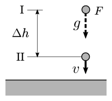
Set-up of the thought experiment.

We assume that an observer sits with clock-\(F\), and initially \(F\) is placed at the same height as that of clock-I and its velocity is zero. Since the clocks are identical, they register equal time intervals, \(\Delta\tau_F=\Delta\tau_{\mathrm{I}}\). Then, we let \(F\) fall freely, and work in the frame of \(F\), which is considered to be inertial. In this frame, clock-II passes by clock-\(F\) with velocity \(v\), so that the time dilation of clock-II can be determined by the Lorentz transformation. When time \(\Delta\tau_{\mathrm{I}}\) elapses on clock-\(F\), time \(\Delta\tau_{\mathrm{II}}\) elapses on clock-II.

Determine \(\Delta\tau_{\mathrm{II}}\) in terms of \(\Delta\tau_{\mathrm{I}}\) up to the first order in \(\Delta\phi/c^2\), where \(\Delta\phi=g\Delta h\) is a difference of the gravitational potential, i.e., the gravitational potential energy per unit mass.

C.2 — 1.8pt

Under the gravitational potential \(\phi\), time delays change the effective speed of light, \(c_{\mathrm{eff}}\), observed at the infinity, though the local speed of light is \(c\). When \(\phi(r=\infty)=0\), \(c_{\mathrm{eff}}\) can be given up to the first order in \(\phi/c^2\) as

\[ c_{\mathrm{eff}}\approx\left(1+\frac{2\phi}{c^2}\right)c \]

including the effect of space distortion, which was not featured in C.1. We note that the light path can be approximated as a straight line.

As shown in Fig. 1 (a), we take the \(x\)-axis along the light path from the neutron star N to the Earth E and place \(x=0\) at the point where the White Dwarf W is the closest to the light path. Let \(x_N(<0)\) be the \(x\)-coordinate of N, \(x_E(>0)\) be that of E, and \(d\) be the distance between W and the light path.

Estimate the changes of the arrival time \(\Delta t\) of the light from N to E caused by the White Dwarf with mass \(M_{\mathrm{WD}}\) and evaluate the answer in a simple form disregarding higher order terms of the following small quantities: \(d/|x_N|\ll1\), \(d/x_E\ll1\), and \(GM_{\mathrm{WD}}/(c^2d)\ll1\). If necessary, use the following formula.

\[ \int\frac{dx}{\sqrt{x^2+d^2}} =\frac12\log\left( \frac{\sqrt{x^2+d^2}+x}{\sqrt{x^2+d^2}-x} \right)+C. \]

(\(\log\) is the natural logarithm)

C.3 — 1.8pt

As shown below, in a binary star system N and W are assumed to be moving in circular orbits with zero eccentricity around the center of mass \(G\) on the orbit plane. Let \(\varepsilon\) be the orbital inclination angle measured from the orbit plane to the line directed toward E from \(G\), and let \(L\) be the length between N and W and \(M_{\mathrm{WD}}\) be the mass of the White Dwarf. In the following, we assume \(\varepsilon\ll1\).

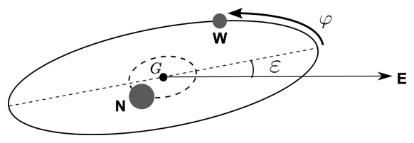
Binary star system.

We observe light pulses from N on E far away from N. The light path to E varies with time depending on the configuration of N and W. The delay in the time interval of arriving pulses on E has the maximum value \(\Delta t_{\max}\) for \(x_N\simeq-L\) and the minimum value \(\Delta t_{\min}\) for \(x_N\simeq L\) (see Fig. 1 (b) for the configuration).

Calculate \(\Delta t_{\max}-\Delta t_{\min}\) in a simple form disregarding higher order terms of small quantities as done in C.2. We note that the delays due to gravity from stellar objects other than W are assumed to cancel out in \(\Delta t_{\max}-\Delta t_{\min}\).

C.4 — 0.8pt

The below figure shows the observed time delays as a function of the orbital phase \(\varphi\) for the binary star system with \(L\approx6\times10^6\ \mathrm{km}\) and \(\cos\varepsilon\approx0.99989\). Estimate \(M_{\mathrm{WD}}\) in terms of the solar mass \(M_\odot\) and show the results for \(M_{\mathrm{WD}}/M_\odot\) up to the first significant digit. Here the approximate relation, \(GM_\odot/c^3\approx5\ \mu\mathrm{s}\), can be used.

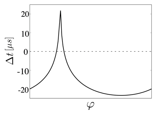
Observed time delays \(\Delta t\) as a function of the orbital phase \(\varphi\) (see the figure in C.3) to locate N and W on the orbits.

C.5 — 0.4pt

In the binary system of neutron stars, two stars release energy and angular momentum by emitting gravitational waves and eventually collide to merge. For simplicity, let us consider only a circular motion with the radius \(R\) and the angular velocity \(\omega\) and then \(\omega=\chi R^p\) holds with the constant \(\chi\) depending on neither \(\omega\) nor \(R\) if relativistic effects are ignored. Determine the value for \(p\).

C.6 — 0.2pt

The amplitude of the emitted gravitational wave from the binary system in C.5 is proportional to \(R^2\omega^2\). Figure below qualitatively shows four different temporal profiles of the observed gravitational waves before the two-star collision. Select the most appropriate profile from (a) to (d).

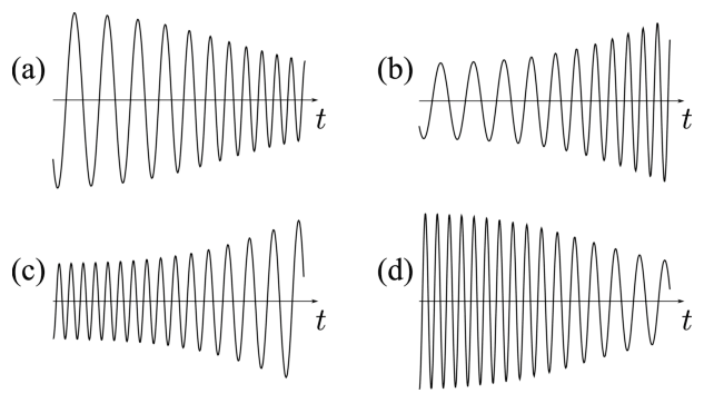
Observed data profiles of gravitational waves.

Official English text of the problem.

Wir untersuchen die Stabilität großer Atomkerne und schätzen die Masse von Neutronensternen theoretisch und experimentell ab.

Teil A. Masse und Stabilität von Atomkernen (2.5 Punkte)

Die Ruheenergie eines aus \(Z\) Protonen und \(N\) Neutronen bestehenden Atomkerns \(m(Z,N)c^2\) ist um die Bindungsenergie \(B(Z,N)\) kleiner als die Summe der Ruheenergien der Protonen und Neutronen, die im Folgenden Nukleonen genannt werden; dabei ist \(c\) die Lichtgeschwindigkeit im Vakuum. Unter Vernachlässigung kleiner Korrekturen können wir die Bindungsenergie, die sich aus dem Volumenterm mit \(a_V\), dem Oberflächenterm mit \(a_S\), dem Coulomb-Energieterm mit \(a_C\) und dem Symmetrieenergieterm mit \(a_{\mathrm{sym}}\) zusammensetzt, wie folgt näherungsweise angeben.

\[ m(Z,N)c^2=Am_Nc^2-B(Z,N),\qquad B(Z,N)=a_VA-a_SA^{2/3}-a_C\frac{Z^2}{A^{1/3}} -a_{\mathrm{sym}}\frac{(N-Z)^2}{A}, \tag{1} \]

Dabei ist \(A=Z+N\) die Massenzahl und \(m_N\) die Nukleonenmasse. Verwenden Sie für die Rechnung \(a_V\approx15.8\ \mathrm{MeV}\), \(a_S\approx17.8\ \mathrm{MeV}\), \(a_C\approx0.711\ \mathrm{MeV}\) und \(a_{\mathrm{sym}}\approx23.7\ \mathrm{MeV}\) (\(\mathrm{MeV}=10^6\) Elektronenvolt).

A.1 — 0.9 Punkte

Bestimmen Sie unter der Bedingung \(Z=N\) den Wert von \(A\), für den die Bindungsenergie pro Nukleon, \(B/A\), maximal wird.

A.2 — 0.9 Punkte

Bei festem \(A\) wird die Ordnungszahl des stabilsten Atomkerns \(Z^*\) durch Maximierung von \(B(Z,A-Z)\) bestimmt. Berechnen Sie für \(A=197\) mithilfe von Gl. (1) den Wert von \(Z^*\).

A.3 — 0.7 Punkte

Ein Atomkern mit großem \(A\) zerfällt durch Kernspaltung in leichtere Kerne, um die gesamte Ruheenergie zu minimieren. Der Einfachheit halber betrachten wir eine von mehreren Möglichkeiten, einen Kern mit \((Z,N)\) in zwei gleiche Kerne zu spalten. Dies geschieht, wenn die folgende Energiebeziehung gilt:

\[ m(Z,N)c^2>2m(Z/2,N/2)c^2. \]

Wird diese Beziehung in der Form

\[ Z^2/A>C_{\mathrm{fission}}\frac{a_S}{a_C}, \]

geschrieben, bestimmen Sie \(C_{\mathrm{fission}}\) auf zwei signifikante Stellen.

Teil B. Der Neutronenstern als gigantischer Atomkern (1.5 Punkte)

Große Atomkerne mit einer hinreichend großen Massenzahl \(A>A_c\), wobei \(A_c\) ein Schwellenwert ist, bleiben aufgrund der ausreichend großen gravitativen Bindungsenergie gegenüber Kernspaltung stabil.

B.1 — 1.5 Punkte

Wir nehmen an, dass für hinreichend große \(A\) die Bedingungen \(N=A\) und \(Z=0\) erfüllt sind und Gl. (1) unter Hinzunahme der gravitativen Bindungsenergie weiterhin gilt. Die gravitative Bindungsenergie lautet

\[ B_{\mathrm{grav}}=\frac35\frac{GM^2}{R}, \]

wobei \(M=m_NA\) und \(R=R_0A^{1/3}\) mit \(R_0\simeq1.1\times10^{-15}\ \mathrm{m}=1.1\ \mathrm{fm}\) die Masse beziehungsweise den Radius des Atomkerns bezeichnen.

Bestimmen Sie für \(B_{\mathrm{grav}}=a_{\mathrm{grav}}A^{5/3}\) den Wert von \(a_{\mathrm{grav}}\) in der Einheit MeV auf eine signifikante Stelle. Schätzen Sie anschließend unter Vernachlässigung des Oberflächenterms \(A_c\) auf eine signifikante Stelle ab. Verwenden Sie für die Rechnung \(m_Nc^2\simeq939\ \mathrm{MeV}\) und \(G=\hbar c/M_P^2\), wobei \(M_Pc^2\simeq1.22\times10^{22}\ \mathrm{MeV}\) und \(\hbar c\simeq197\ \mathrm{MeV}\cdot\mathrm{fm}\).

Teil C. Ein Neutronenstern in einem Doppelsternsystem (6.0 Punkte)

Einige Neutronensterne sind Pulsare, die regelmäßig mit einer konstanten Periode elektromagnetische Wellen aussenden, die wir hier der Einfachheit halber als „Licht“ bezeichnen. Neutronensterne bilden häufig Doppelsternsysteme mit einem Weißen Zwerg. Betrachten wir die in Abb. 1 gezeigte Sternkonfiguration, bei der ein Lichtpuls von einem Neutronenstern N zur Erde E nahe an einem Weißen Zwerg W des Doppelsternsystems vorbeiläuft. Die Messung dieser durch die Gravitation des Sterns beeinflussten Pulse ermöglicht eine genaue Abschätzung der Masse von W, wie im Folgenden erläutert wird, und daraus eine Abschätzung der Masse von N.

Abb. 1: Konfigurationen mit der \(x\)-Achse entlang der Verbindungslinie zwischen N und E. (a) für \(x_N<0\) und (b) für \(x_N>0\).

C.1 — 1.0 Punkte

Wie in der folgenden Abbildung gezeigt, betrachten wir bei konstanter Fallbeschleunigung \(g\) zwei Höhenlagen I und II mit dem Höhenunterschied \(\Delta h(>0)\). Bei I, II und im frei fallenden System \(F\) werden identische Uhren aufgestellt, die als Uhr-I, Uhr-II beziehungsweise Uhr-\(F\) bezeichnet werden.

Aufbau des Gedankenexperiments.

Wir nehmen an, dass sich ein Beobachter bei Uhr-\(F\) befindet und dass \(F\) anfangs auf derselben Höhe wie Uhr-I ruht. Da die Uhren identisch sind, zeigen sie gleiche Zeitintervalle an, \(\Delta\tau_F=\Delta\tau_{\mathrm{I}}\). Anschließend lassen wir \(F\) frei fallen und betrachten das Bezugssystem von \(F\), das als Inertialsystem angesehen wird. In diesem Bezugssystem bewegt sich Uhr-II mit der Geschwindigkeit \(v\) an Uhr-\(F\) vorbei, sodass die Zeitdilatation von Uhr-II durch die Lorentz-Transformation bestimmt werden kann. Wenn auf Uhr-\(F\) die Zeit \(\Delta\tau_{\mathrm{I}}\) vergeht, vergeht auf Uhr-II die Zeit \(\Delta\tau_{\mathrm{II}}\).

Bestimmen Sie \(\Delta\tau_{\mathrm{II}}\) in Abhängigkeit von \(\Delta\tau_{\mathrm{I}}\) bis zur ersten Ordnung in \(\Delta\phi/c^2\), wobei \(\Delta\phi=g\Delta h\) eine Differenz des Gravitationspotentials, also der potentiellen Gravitationsenergie pro Masseneinheit, ist.

C.2 — 1.8 Punkte

Im Gravitationspotential \(\phi\) verändern Zeitverzögerungen die im Unendlichen beobachtete effektive Lichtgeschwindigkeit \(c_{\mathrm{eff}}\), obwohl die lokale Lichtgeschwindigkeit \(c\) beträgt. Für \(\phi(r=\infty)=0\) kann \(c_{\mathrm{eff}}\) bis zur ersten Ordnung in \(\phi/c^2\) als

\[ c_{\mathrm{eff}}\approx\left(1+\frac{2\phi}{c^2}\right)c \]

angegeben werden. Darin ist der Einfluss der Raumkrümmung berücksichtigt, der in C.1 nicht behandelt wurde. Der Lichtweg kann näherungsweise als gerade Linie betrachtet werden.

Wie in Abb. 1 (a) gezeigt, legen wir die \(x\)-Achse entlang des Lichtwegs vom Neutronenstern N zur Erde E und setzen \(x=0\) an den Punkt, an dem der Weiße Zwerg W dem Lichtweg am nächsten ist. Dabei sei \(x_N(<0)\) die \(x\)-Koordinate von N, \(x_E(>0)\) diejenige von E und \(d\) der Abstand zwischen W und dem Lichtweg.

Schätzen Sie die durch den Weißen Zwerg mit der Masse \(M_{\mathrm{WD}}\) verursachte Änderung der Ankunftszeit \(\Delta t\) des Lichts von N nach E ab und geben Sie das Ergebnis in einer einfachen Form an, indem Sie Terme höherer Ordnung in den folgenden kleinen Größen vernachlässigen: \(d/|x_N|\ll1\), \(d/x_E\ll1\) und \(GM_{\mathrm{WD}}/(c^2d)\ll1\). Verwenden Sie bei Bedarf die folgende Formel.

\[ \int\frac{dx}{\sqrt{x^2+d^2}} =\frac12\log\left( \frac{\sqrt{x^2+d^2}+x}{\sqrt{x^2+d^2}-x} \right)+C. \]

(\(\log\) ist der natürliche Logarithmus)

C.3 — 1.8 Punkte

Wie unten gezeigt, nehmen wir an, dass sich N und W in einem Doppelsternsystem auf Kreisbahnen mit Exzentrizität null um den Schwerpunkt \(G\) in der Bahnebene bewegen. Dabei sei \(\varepsilon\) der Bahnneigungswinkel, gemessen von der Bahnebene zur von \(G\) nach E gerichteten Linie, \(L\) der Abstand zwischen N und W und \(M_{\mathrm{WD}}\) die Masse des Weißen Zwergs. Im Folgenden nehmen wir \(\varepsilon\ll1\) an.

Doppelsternsystem.

Wir beobachten Lichtpulse von N auf der weit von N entfernten Erde E. Der Lichtweg zu E verändert sich mit der Zeit in Abhängigkeit von der Konfiguration von N und W. Die Verzögerung im Zeitintervall der auf E eintreffenden Pulse hat den Maximalwert \(\Delta t_{\max}\) für \(x_N\simeq-L\) und den Minimalwert \(\Delta t_{\min}\) für \(x_N\simeq L\) (die Konfiguration ist in Abb. 1 (b) dargestellt).

Berechnen Sie \(\Delta t_{\max}-\Delta t_{\min}\) in einer einfachen Form, indem Sie wie in C.2 Terme höherer Ordnung in kleinen Größen vernachlässigen. Dabei wird angenommen, dass sich die gravitativen Verzögerungen durch andere stellare Objekte als W in \(\Delta t_{\max}-\Delta t_{\min}\) aufheben.

C.4 — 0.8 Punkte

Die folgende Abbildung zeigt die beobachteten Zeitverzögerungen als Funktion der Bahnphase \(\varphi\) für das Doppelsternsystem mit \(L\approx6\times10^6\ \mathrm{km}\) und \(\cos\varepsilon\approx0.99989\). Schätzen Sie \(M_{\mathrm{WD}}\) in Einheiten der Sonnenmasse \(M_\odot\) ab und geben Sie das Ergebnis für \(M_{\mathrm{WD}}/M_\odot\) auf eine signifikante Stelle an. Hier kann die Näherungsbeziehung \(GM_\odot/c^3\approx5\ \mu\mathrm{s}\) verwendet werden.

Beobachtete Zeitverzögerungen \(\Delta t\) als Funktion der Bahnphase \(\varphi\) (siehe die Abbildung in C.3), welche die Positionen von N und W auf ihren Bahnen angibt.

C.5 — 0.4 Punkte

In einem Doppelsternsystem aus Neutronensternen geben die beiden Sterne durch die Emission von Gravitationswellen Energie und Drehimpuls ab und stoßen schließlich zusammen, wobei sie verschmelzen. Der Einfachheit halber betrachten wir nur eine Kreisbewegung mit dem Radius \(R\) und der Winkelgeschwindigkeit \(\omega\). Dann gilt bei Vernachlässigung relativistischer Effekte \(\omega=\chi R^p\) mit einer Konstanten \(\chi\), die weder von \(\omega\) noch von \(R\) abhängt. Bestimmen Sie den Wert von \(p\).

C.6 — 0.2 Punkte

Die Amplitude der vom Doppelsternsystem in C.5 ausgesandten Gravitationswelle ist proportional zu \(R^2\omega^2\). Die folgende Abbildung zeigt qualitativ vier verschiedene zeitliche Verläufe der beobachteten Gravitationswellen vor dem Zusammenstoß der beiden Sterne. Wählen Sie aus (a) bis (d) den am besten geeigneten Verlauf aus.

Verläufe der beobachteten Gravitationswellendaten.

Aufgabentext aus dem offiziellen englischen Text übersetzt.

Büyük çekirdeklerin kararlılığını ele alıyor ve nötron yıldızlarının kütlesini kuramsal ve deneysel olarak tahmin ediyoruz.

Bölüm A. Çekirdeklerin kütlesi ve kararlılığı (2.5 puan)

\(Z\) proton ve \(N\) nötrondan oluşan bir çekirdeğin durgunluk enerjisi \(m(Z,N)c^2\), bundan böyle nükleon olarak adlandırılacak olan proton ve nötronların durgunluk enerjileri toplamından bağlanma enerjisi \(B(Z,N)\) kadar küçüktür; burada \(c\), ışığın boşluktaki hızıdır. Küçük düzeltmeleri ihmal ederek, \(a_V\) katsayılı hacim terimi, \(a_S\) katsayılı yüzey terimi, \(a_C\) katsayılı Coulomb enerjisi terimi ve \(a_{\mathrm{sym}}\) katsayılı simetri enerjisi teriminden oluşan bağlanma enerjisini aşağıdaki şekilde yaklaşık olarak ifade edebiliriz.

\[ m(Z,N)c^2=Am_Nc^2-B(Z,N),\qquad B(Z,N)=a_VA-a_SA^{2/3}-a_C\frac{Z^2}{A^{1/3}} -a_{\mathrm{sym}}\frac{(N-Z)^2}{A}, \tag{1} \]

Burada \(A=Z+N\) kütle sayısı, \(m_N\) ise nükleon kütlesidir. Hesaplamalarda \(a_V\approx15.8\ \mathrm{MeV}\), \(a_S\approx17.8\ \mathrm{MeV}\), \(a_C\approx0.711\ \mathrm{MeV}\) ve \(a_{\mathrm{sym}}\approx23.7\ \mathrm{MeV}\) değerlerini kullanın (\(\mathrm{MeV}=10^6\) elektron volt).

A.1 — 0.9 puan

\(Z=N\) koşulu altında, nükleon başına bağlanma enerjisi \(B/A\)'yı maksimum yapan \(A\) değerini belirleyin.

A.2 — 0.9 puan

\(A\) sabit tutulduğunda, en kararlı çekirdeğin atom numarası \(Z^*\), \(B(Z,A-Z)\)'nin maksimum yapılmasıyla belirlenir. \(A=197\) için Denklem (1)'i kullanarak \(Z^*\)'ı hesaplayın.

A.3 — 0.7 puan

\(A\) değeri büyük olan bir çekirdek, toplam durgunluk kütle enerjisini minimum yapmak için fisyon yoluyla daha hafif çekirdeklere ayrılır. Basitlik amacıyla, \((Z,N)\) ile belirtilen bir çekirdeğin iki eşit çekirdeğe ayrılmasının çeşitli yollarından birini ele alıyoruz; bu ayrılma, aşağıdaki enerji bağıntısı sağlandığında gerçekleşir:

\[ m(Z,N)c^2>2m(Z/2,N/2)c^2. \]

Bu bağıntı

\[ Z^2/A>C_{\mathrm{fission}}\frac{a_S}{a_C}, \]

şeklinde yazıldığında, \(C_{\mathrm{fission}}\) değerini iki anlamlı basamakla bulun.

Bölüm B. Devasa bir çekirdek olarak nötron yıldızı (1.5 puan)

\(A_c\) eşik değeri olmak üzere, kütle sayısı yeterince büyük olan \(A>A_c\) büyük çekirdekler, kütleçekimden kaynaklanan bağlanma enerjisinin yeterince büyük olması nedeniyle nükleer fisyona karşı kararlı kalır.

B.1 — 1.5 puan

Yeterince büyük \(A\) için \(N=A\) ve \(Z=0\) koşullarının gerçekleştiğini ve kütleçekimsel bağlanma enerjisi eklendiğinde Denklem (1)'in geçerliliğini koruduğunu varsayıyoruz. Kütleçekimden kaynaklanan bağlanma enerjisi

\[ B_{\mathrm{grav}}=\frac35\frac{GM^2}{R}, \]

şeklindedir; burada \(M=m_NA\) ve \(R=R_0A^{1/3}\) sırasıyla çekirdeğin kütlesi ve yarıçapıdır ve \(R_0\simeq1.1\times10^{-15}\ \mathrm{m}=1.1\ \mathrm{fm}\)'dir.

\(B_{\mathrm{grav}}=a_{\mathrm{grav}}A^{5/3}\) için \(a_{\mathrm{grav}}\) değerini MeV biriminde bir anlamlı basamakla bulun. Ardından yüzey terimini ihmal ederek \(A_c\)'yi bir anlamlı basamakla tahmin edin. Hesaplamalarda \(m_Nc^2\simeq939\ \mathrm{MeV}\) ve \(G=\hbar c/M_P^2\) bağıntısını kullanın; burada \(M_Pc^2\simeq1.22\times10^{22}\ \mathrm{MeV}\) ve \(\hbar c\simeq197\ \mathrm{MeV}\cdot\mathrm{fm}\)'dir.

Bölüm C. İkili sistemde nötron yıldızı (6.0 puan)

Bazı nötron yıldızları, burada basitlik amacıyla "ışık" olarak adlandıracağımız elektromanyetik dalgaları sabit bir periyotla düzenli olarak yayan pulsarlardır. Nötron yıldızları sıklıkla bir beyaz cüceyle ikili sistem oluşturur. Şekil 1'de gösterilen yıldız düzenini ele alalım; bu düzende nötron yıldızı N'den Dünya E'ye giden bir ışık atımı, ikili sistemin beyaz cücesi W'nin yakınından geçer. Yıldızın kütleçekiminden etkilenen bu atımların ölçülmesi, aşağıda açıklandığı gibi W'nin kütlesinin hassas biçimde tahmin edilmesini ve bunun sonucunda N'nin kütlesinin tahmin edilmesini sağlar.

Şekil 1: \(x\) ekseninin N ile E'yi birleştiren doğru boyunca uzandığı düzenler. (a) \(x_N<0\) ve (b) \(x_N>0\) için.

C.1 — 1.0 puan

Aşağıdaki şekilde gösterildiği gibi, sabit kütleçekimi ivmesi \(g\) altında, aralarında \(\Delta h(>0)\) yükseklik farkı bulunan I ve II düzeylerini belirliyoruz. I, II ve serbest düşen sistem \(F\)'ye, sırasıyla saat-I, saat-II ve saat-\(F\) olarak adlandırılan özdeş saatler yerleştirin.

Düşünce deneyinin düzeneği.

Bir gözlemcinin saat-\(F\)'nin yanında bulunduğunu ve başlangıçta \(F\)'nin saat-I ile aynı yükseklikte ve hızının sıfır olduğunu varsayıyoruz. Saatler özdeş olduğundan eşit zaman aralıkları kaydederler: \(\Delta\tau_F=\Delta\tau_{\mathrm{I}}\). Ardından \(F\)'yi serbest düşmeye bırakıyor ve eylemsiz kabul edilen \(F\) referans sisteminde çalışıyoruz. Bu sistemde saat-II, saat-\(F\)'nin yanından \(v\) hızıyla geçer; böylece saat-II'deki zaman genişlemesi Lorentz dönüşümüyle belirlenebilir. Saat-\(F\)'de \(\Delta\tau_{\mathrm{I}}\) süresi geçtiğinde saat-II'de \(\Delta\tau_{\mathrm{II}}\) süresi geçer.

\(\Delta\tau_{\mathrm{II}}\)'yi \(\Delta\tau_{\mathrm{I}}\) cinsinden, \(\Delta\phi/c^2\)'ye göre birinci mertebeye kadar belirleyin; burada \(\Delta\phi=g\Delta h\), kütleçekim potansiyeli, yani birim kütle başına kütleçekim potansiyel enerjisi farkıdır.

C.2 — 1.8 puan

\(\phi\) kütleçekim potansiyeli altında zaman gecikmeleri, ışığın yerel hızı \(c\) olmasına karşın, sonsuzda gözlenen etkin ışık hızı \(c_{\mathrm{eff}}\)'i değiştirir. \(\phi(r=\infty)=0\) olduğunda, \(c_{\mathrm{eff}}\), \(\phi/c^2\)'ye göre birinci mertebeye kadar

\[ c_{\mathrm{eff}}\approx\left(1+\frac{2\phi}{c^2}\right)c \]

şeklinde verilebilir; bu ifade, C.1'de yer almayan uzayın bükülmesi etkisini de içerir. Işığın izlediği yolun yaklaşık olarak bir doğru kabul edilebileceğini belirtelim.

Şekil 1 (a)'da gösterildiği gibi, \(x\) eksenini nötron yıldızı N'den Dünya E'ye giden ışığın yolu boyunca alıyor ve \(x=0\) noktasını, ışık yolu üzerinde beyaz cüce W'ye en yakın noktaya yerleştiriyoruz. N'nin \(x\) koordinatı \(x_N(<0)\), E'nin koordinatı \(x_E(>0)\) ve W ile ışık yolu arasındaki uzaklık \(d\) olsun.

\(M_{\mathrm{WD}}\) kütleli beyaz cücenin, N'den E'ye giden ışığın varış zamanında neden olduğu \(\Delta t\) değişimini tahmin edin ve aşağıdaki küçük niceliklerin yüksek mertebeli terimlerini ihmal ederek sonucu basit bir biçimde ifade edin: \(d/|x_N|\ll1\), \(d/x_E\ll1\) ve \(GM_{\mathrm{WD}}/(c^2d)\ll1\). Gerekirse aşağıdaki formülü kullanın.

\[ \int\frac{dx}{\sqrt{x^2+d^2}} =\frac12\log\left( \frac{\sqrt{x^2+d^2}+x}{\sqrt{x^2+d^2}-x} \right)+C. \]

(\(\log\) doğal logaritmadır)

C.3 — 1.8 puan

Aşağıda gösterildiği gibi, bir ikili yıldız sisteminde N ve W'nin, yörünge düzlemindeki kütle merkezi \(G\) çevresinde dışmerkezliği sıfır olan dairesel yörüngelerde hareket ettiği varsayılıyor. Yörünge düzleminden, \(G\)'den E'ye yönelen doğruya doğru ölçülen yörünge eğim açısı \(\varepsilon\), N ile W arasındaki uzaklık \(L\) ve beyaz cücenin kütlesi \(M_{\mathrm{WD}}\) olsun. Aşağıda \(\varepsilon\ll1\) olduğunu varsayıyoruz.

İkili yıldız sistemi.

N'den gelen ışık atımlarını, N'den çok uzaktaki E üzerinde gözlüyoruz. E'ye giden ışığın yolu, N ve W'nin konumlarına bağlı olarak zamanla değişir. E'ye ulaşan atımların zaman aralığındaki gecikme, \(x_N\simeq-L\) için maksimum \(\Delta t_{\max}\) değerini ve \(x_N\simeq L\) için minimum \(\Delta t_{\min}\) değerini alır (düzen için Şekil 1 (b)'ye bakın).

C.2'de yapıldığı gibi küçük niceliklerin yüksek mertebeli terimlerini ihmal ederek \(\Delta t_{\max}-\Delta t_{\min}\) farkını basit bir biçimde hesaplayın. W dışındaki yıldızsal cisimlerin kütleçekiminden kaynaklanan gecikmelerin \(\Delta t_{\max}-\Delta t_{\min}\) farkında birbirini götürdüğünün varsayıldığını belirtelim.

C.4 — 0.8 puan

Aşağıdaki şekil, \(L\approx6\times10^6\ \mathrm{km}\) ve \(\cos\varepsilon\approx0.99989\) olan ikili yıldız sistemi için gözlenen zaman gecikmelerini yörünge fazı \(\varphi\)'nin fonksiyonu olarak göstermektedir. \(M_{\mathrm{WD}}\)'yi Güneş kütlesi \(M_\odot\) cinsinden tahmin edin ve \(M_{\mathrm{WD}}/M_\odot\) için sonucu bir anlamlı basamakla gösterin. Burada \(GM_\odot/c^3\approx5\ \mu\mathrm{s}\) yaklaşık bağıntısı kullanılabilir.

N ve W'nin yörüngelerdeki konumlarını belirleyen yörünge fazı \(\varphi\)'nin fonksiyonu olarak gözlenen zaman gecikmeleri \(\Delta t\) (C.3'teki şekle bakın).

C.5 — 0.4 puan

İkili nötron yıldızı sisteminde iki yıldız, kütleçekim dalgaları yayarak enerji ve açısal momentum kaybeder ve sonunda çarpışarak birleşir. Basitlik amacıyla yalnızca \(R\) yarıçaplı ve \(\omega\) açısal hızlı dairesel hareketi ele alalım; görelilik etkileri ihmal edilirse, ne \(\omega\)'ya ne de \(R\)'ye bağlı olan \(\chi\) sabiti ile \(\omega=\chi R^p\) bağıntısı geçerlidir. \(p\)'nin değerini belirleyin.

C.6 — 0.2 puan

C.5'teki ikili sistemden yayılan kütleçekim dalgasının genliği \(R^2\omega^2\) ile orantılıdır. Aşağıdaki şekil, iki yıldızın çarpışmasından önce gözlenen kütleçekim dalgalarının zamana göre dört farklı profilini nitel olarak göstermektedir. (a) ile (d) arasından en uygun profili seçin.

Kütleçekim dalgalarının gözlenen veri profilleri.

Soru metni resmi İngilizce metinden çevrilmiştir.

Estudiamos la estabilidad de los núcleos grandes y estimamos la masa de las estrellas de neutrones de forma teórica y experimental.

Parte A. Masa y estabilidad de los núcleos (2.5 puntos)

La energía en reposo de un núcleo \(m(Z,N)c^2\) compuesto por \(Z\) protones y \(N\) neutrones es menor que la suma de las energías en reposo de los protones y neutrones, denominados en adelante nucleones, en una cantidad igual a la energía de enlace \(B(Z,N)\), donde \(c\) es la velocidad de la luz en el vacío. Despreciando pequeñas correcciones, podemos aproximar la energía de enlace, compuesta por el término de volumen con \(a_V\), el término de superficie con \(a_S\), el término de energía de Coulomb con \(a_C\) y el término de energía de simetría con \(a_{\mathrm{sym}}\), de la siguiente manera.

\[ m(Z,N)c^2=Am_Nc^2-B(Z,N),\qquad B(Z,N)=a_VA-a_SA^{2/3}-a_C\frac{Z^2}{A^{1/3}} -a_{\mathrm{sym}}\frac{(N-Z)^2}{A}, \tag{1} \]

Aquí, \(A=Z+N\) es el número másico y \(m_N\) es la masa del nucleón. En el cálculo, utilice \(a_V\approx15.8\ \mathrm{MeV}\), \(a_S\approx17.8\ \mathrm{MeV}\), \(a_C\approx0.711\ \mathrm{MeV}\) y \(a_{\mathrm{sym}}\approx23.7\ \mathrm{MeV}\) (\(\mathrm{MeV}=10^6\) electronvoltios).

A.1 — 0.9pt

Bajo la condición \(Z=N\), determine \(A\) para maximizar la energía de enlace por nucleón, \(B/A\).

A.2 — 0.9pt

Bajo la condición de que \(A\) sea fijo, el número atómico del núcleo más estable, \(Z^*\), se determina maximizando \(B(Z,A-Z)\). Para \(A=197\), calcule \(Z^*\) utilizando la ec. (1).

A.3 — 0.7pt

Un núcleo con un valor grande de \(A\) se divide en núcleos más ligeros mediante fisión para minimizar la energía total de masa en reposo. Por simplicidad, consideramos una de las múltiples formas de dividir un núcleo con \((Z,N)\) en dos núcleos iguales, lo cual ocurre cuando se cumple la siguiente relación energética:

\[ m(Z,N)c^2>2m(Z/2,N/2)c^2. \]

Si esta relación se escribe como

\[ Z^2/A>C_{\mathrm{fission}}\frac{a_S}{a_C}, \]

obtenga \(C_{\mathrm{fission}}\) con dos cifras significativas.

Parte B. La estrella de neutrones como un núcleo gigantesco (1.5 puntos)

Los núcleos grandes con un número másico suficientemente grande \(A>A_c\), donde \(A_c\) es un umbral, permanecen estables frente a la fisión nuclear gracias a una energía de enlace gravitatoria suficientemente grande.

B.1 — 1.5pt

Suponemos que, para un valor de \(A\) suficientemente grande, se cumplen \(N=A\) y \(Z=0\), y que la ec. (1) sigue siendo válida al añadir la energía de enlace gravitatoria. La energía de enlace debida a la gravedad es

\[ B_{\mathrm{grav}}=\frac35\frac{GM^2}{R}, \]

donde \(M=m_NA\) y \(R=R_0A^{1/3}\), con \(R_0\simeq1.1\times10^{-15}\ \mathrm{m}=1.1\ \mathrm{fm}\), son la masa y el radio del núcleo, respectivamente.

Para \(B_{\mathrm{grav}}=a_{\mathrm{grav}}A^{5/3}\), obtenga \(a_{\mathrm{grav}}\) en MeV con una cifra significativa. A continuación, despreciando el término de superficie, estime \(A_c\) con una cifra significativa. En el cálculo, utilice \(m_Nc^2\simeq939\ \mathrm{MeV}\) y \(G=\hbar c/M_P^2\), donde \(M_Pc^2\simeq1.22\times10^{22}\ \mathrm{MeV}\) y \(\hbar c\simeq197\ \mathrm{MeV}\cdot\mathrm{fm}\).

Parte C. Una estrella de neutrones en un sistema binario (6.0 puntos)

Algunas estrellas de neutrones son púlsares que emiten regularmente ondas electromagnéticas, que aquí llamamos «luz» por simplicidad, con un período constante. Las estrellas de neutrones suelen formar sistemas binarios con una enana blanca. Consideremos la configuración estelar mostrada en la Fig. 1, en la que un pulso de luz procedente de una estrella de neutrones N y dirigido hacia la Tierra E pasa cerca de una enana blanca W del sistema binario. La medición de estos pulsos, afectados por la gravedad de la estrella, permite estimar con precisión la masa de W, como se explica a continuación, lo que a su vez permite estimar la masa de N.

Fig. 1: Configuraciones con el eje \(x\) a lo largo de la línea que une N y E. (a) para \(x_N<0\) y (b) para \(x_N>0\).

C.1 — 1.0pt

Como se muestra en la figura siguiente, bajo una aceleración gravitatoria constante \(g\), situamos dos niveles I y II con una diferencia de altura \(\Delta h(>0)\). Coloque relojes idénticos en I, II y \(F\), el sistema en caída libre, denominados reloj-I, reloj-II y reloj-\(F\), respectivamente.

Disposición del experimento mental.

Suponemos que un observador se encuentra junto al reloj-\(F\) y que, inicialmente, \(F\) está situado a la misma altura que el reloj-I y su velocidad es cero. Como los relojes son idénticos, registran intervalos de tiempo iguales, \(\Delta\tau_F=\Delta\tau_{\mathrm{I}}\). A continuación, dejamos que \(F\) caiga libremente y trabajamos en el sistema de referencia de \(F\), que se considera inercial. En este sistema de referencia, el reloj-II pasa junto al reloj-\(F\) con velocidad \(v\), de modo que la dilatación temporal del reloj-II puede determinarse mediante la transformación de Lorentz. Cuando transcurre un tiempo \(\Delta\tau_{\mathrm{I}}\) en el reloj-\(F\), transcurre un tiempo \(\Delta\tau_{\mathrm{II}}\) en el reloj-II.

Determine \(\Delta\tau_{\mathrm{II}}\) en función de \(\Delta\tau_{\mathrm{I}}\) hasta primer orden en \(\Delta\phi/c^2\), donde \(\Delta\phi=g\Delta h\) es una diferencia de potencial gravitatorio, es decir, de energía potencial gravitatoria por unidad de masa.

C.2 — 1.8pt

Bajo el potencial gravitatorio \(\phi\), los retardos temporales modifican la velocidad efectiva de la luz, \(c_{\mathrm{eff}}\), observada desde el infinito, aunque la velocidad local de la luz es \(c\). Cuando \(\phi(r=\infty)=0\), \(c_{\mathrm{eff}}\) puede expresarse hasta primer orden en \(\phi/c^2\) como

\[ c_{\mathrm{eff}}\approx\left(1+\frac{2\phi}{c^2}\right)c \]

incluyendo el efecto de la distorsión del espacio, que no se tuvo en cuenta en C.1. Señalamos que la trayectoria de la luz puede aproximarse por una línea recta.

Como se muestra en la Fig. 1 (a), tomamos el eje \(x\) a lo largo de la trayectoria de la luz desde la estrella de neutrones N hasta la Tierra E y situamos \(x=0\) en el punto de la trayectoria de la luz más cercano a la enana blanca W. Sea \(x_N(<0)\) la coordenada \(x\) de N, \(x_E(>0)\) la de E y \(d\) la distancia entre W y la trayectoria de la luz.

Estime la variación del tiempo de llegada \(\Delta t\) de la luz de N a E causada por la enana blanca de masa \(M_{\mathrm{WD}}\) y exprese la respuesta de forma sencilla, despreciando los términos de orden superior de las siguientes cantidades pequeñas: \(d/|x_N|\ll1\), \(d/x_E\ll1\) y \(GM_{\mathrm{WD}}/(c^2d)\ll1\). Si es necesario, utilice la siguiente fórmula.

\[ \int\frac{dx}{\sqrt{x^2+d^2}} =\frac12\log\left( \frac{\sqrt{x^2+d^2}+x}{\sqrt{x^2+d^2}-x} \right)+C. \]

(\(\log\) es el logaritmo natural)

C.3 — 1.8pt

Como se muestra a continuación, en un sistema estelar binario se supone que N y W se mueven en órbitas circulares de excentricidad nula alrededor del centro de masas \(G\), en el plano orbital. Sea \(\varepsilon\) el ángulo de inclinación orbital medido desde el plano orbital hasta la línea dirigida hacia E desde \(G\), sea \(L\) la distancia entre N y W, y sea \(M_{\mathrm{WD}}\) la masa de la enana blanca. En lo que sigue, suponemos que \(\varepsilon\ll1\).

Sistema estelar binario.

Observamos en E, muy lejos de N, pulsos de luz procedentes de N. La trayectoria de la luz hasta E varía con el tiempo según la configuración de N y W. El retardo en el intervalo temporal de llegada de los pulsos a E tiene el valor máximo \(\Delta t_{\max}\) para \(x_N\simeq-L\) y el valor mínimo \(\Delta t_{\min}\) para \(x_N\simeq L\) (véase la configuración en la Fig. 1 (b)).

Calcule \(\Delta t_{\max}-\Delta t_{\min}\) de forma sencilla, despreciando los términos de orden superior de las cantidades pequeñas, como se hizo en C.2. Señalamos que se supone que los retardos debidos a la gravedad de objetos estelares distintos de W se cancelan en \(\Delta t_{\max}-\Delta t_{\min}\).

C.4 — 0.8pt

La figura siguiente muestra los retardos temporales observados en función de la fase orbital \(\varphi\) para el sistema estelar binario con \(L\approx6\times10^6\ \mathrm{km}\) y \(\cos\varepsilon\approx0.99989\). Estime \(M_{\mathrm{WD}}\) en términos de la masa solar \(M_\odot\) y dé el resultado de \(M_{\mathrm{WD}}/M_\odot\) con una cifra significativa. Aquí puede utilizarse la relación aproximada \(GM_\odot/c^3\approx5\ \mu\mathrm{s}\).

Retardos temporales observados \(\Delta t\) en función de la fase orbital \(\varphi\) (véase la figura de C.3) que permite situar N y W en sus órbitas.

C.5 — 0.4pt

En un sistema binario de estrellas de neutrones, las dos estrellas pierden energía y momento angular al emitir ondas gravitacionales y finalmente colisionan y se fusionan. Por simplicidad, consideremos únicamente un movimiento circular de radio \(R\) y velocidad angular \(\omega\); entonces se cumple \(\omega=\chi R^p\), con una constante \(\chi\) que no depende ni de \(\omega\) ni de \(R\), si se desprecian los efectos relativistas. Determine el valor de \(p\).

C.6 — 0.2pt

La amplitud de la onda gravitacional emitida por el sistema binario de C.5 es proporcional a \(R^2\omega^2\). La figura siguiente muestra cualitativamente cuatro perfiles temporales distintos de las ondas gravitacionales observadas antes de la colisión de las dos estrellas. Seleccione el perfil más apropiado entre (a) y (d).

Perfiles de los datos observados de ondas gravitacionales.

Enunciado traducido del texto oficial en inglés.

我们将讨论大原子核的稳定性，并从理论和实验两方面估算中子星的质量。

部分 A. 原子核的质量与稳定性（2.5 分）

由 \(Z\) 个质子和 \(N\) 个中子组成的原子核，其静止能量 \(m(Z,N)c^2\) 小于这些质子和中子（以下统称为核子）的静止能量之和，两者之差为结合能 \(B(Z,N)\)，其中 \(c\) 为真空中的光速。忽略微小的修正，可以将结合能近似表示为以下形式，其中包括系数为 \(a_V\) 的体积项、系数为 \(a_S\) 的表面项、系数为 \(a_C\) 的库仑能项和系数为 \(a_{\mathrm{sym}}\) 的对称能项。

\[ m(Z,N)c^2=Am_Nc^2-B(Z,N),\qquad B(Z,N)=a_VA-a_SA^{2/3}-a_C\frac{Z^2}{A^{1/3}} -a_{\mathrm{sym}}\frac{(N-Z)^2}{A}, \tag{1} \]

其中 \(A=Z+N\) 为质量数，\(m_N\) 为核子质量。计算时取 \(a_V\approx15.8\ \mathrm{MeV}\)、\(a_S\approx17.8\ \mathrm{MeV}\)、\(a_C\approx0.711\ \mathrm{MeV}\) 和 \(a_{\mathrm{sym}}\approx23.7\ \mathrm{MeV}\)（\(\mathrm{MeV}=10^6\) 电子伏特）。

A.1 — 0.9 分

在 \(Z=N\) 的条件下，求使平均每个核子的结合能 \(B/A\) 最大的 \(A\)。

A.2 — 0.9 分

在 \(A\) 固定的条件下，使 \(B(Z,A-Z)\) 最大即可确定最稳定原子核的原子序数 \(Z^*\)。对于 \(A=197\)，利用式 (1) 计算 \(Z^*\)。

A.3 — 0.7 分

质量数 \(A\) 较大的原子核会通过裂变分裂为较轻的原子核，以使总静止质量能量最小。为简化起见，在原子核的多种分裂方式中，我们考虑将一个 \((Z,N)\) 原子核分裂为两个相同原子核的方式。当满足以下能量关系时，这一过程便可发生，

\[ m(Z,N)c^2>2m(Z/2,N/2)c^2. \]

将这一关系写为

\[ Z^2/A>C_{\mathrm{fission}}\frac{a_S}{a_C}, \]

求 \(C_{\mathrm{fission}}\)，保留两位有效数字。

部分 B. 作为巨型原子核的中子星（1.5 分）

对于质量数足够大的原子核，若其质量数 \(A>A_c\)，其中 \(A_c\) 为阈值，则引力所产生的结合能足够大，使这些原子核能够保持稳定而不发生核裂变。

B.1 — 1.5 分

我们假设，当 \(A\) 足够大时，\(N=A\) 且 \(Z=0\)，并且在加上引力结合能后，式 (1) 仍然成立。引力产生的结合能为

\[ B_{\mathrm{grav}}=\frac35\frac{GM^2}{R}, \]

其中 \(M=m_NA\) 和 \(R=R_0A^{1/3}\) 分别为原子核的质量和半径，\(R_0\simeq1.1\times10^{-15}\ \mathrm{m}=1.1\ \mathrm{fm}\)。

对于 \(B_{\mathrm{grav}}=a_{\mathrm{grav}}A^{5/3}\)，求以 MeV 为单位的 \(a_{\mathrm{grav}}\)，保留一位有效数字。然后忽略表面项，估算 \(A_c\)，保留一位有效数字。计算时取 \(m_Nc^2\simeq939\ \mathrm{MeV}\) 和 \(G=\hbar c/M_P^2\)，其中 \(M_Pc^2\simeq1.22\times10^{22}\ \mathrm{MeV}\)，\(\hbar c\simeq197\ \mathrm{MeV}\cdot\mathrm{fm}\)。

部分 C. 双星系统中的中子星（6.0 分）

有些中子星是脉冲星，会以固定周期规律地发射电磁波，为简便起见，这里将其称为“光”。中子星常与白矮星组成双星系统。考虑图 1 所示的星体位置关系：从中子星 N 发往地球 E 的光脉冲经过双星系统中白矮星 W 的附近。如下文所述，通过测量这些受星体引力影响的脉冲，可以准确估算 W 的质量，进而估算 N 的质量。

图 1：以连接 N 与 E 的直线为 \(x\) 轴的星体位置关系。(a) 对应 \(x_N<0\)，(b) 对应 \(x_N>0\)。

C.1 — 1.0 分

如下图所示，在恒定的重力加速度 \(g\) 下，设置高度差为 \(\Delta h(>0)\) 的两个高度位置 I 和 II。在 I、II 以及自由下落系统 \(F\) 中放置相同的钟，分别记为钟-I、钟-II 和钟-\(F\)。

思想实验的设置。

假设一位观察者与钟-\(F\) 一起运动，且初始时 \(F\) 与钟-I 位于同一高度，速度为零。由于这些钟完全相同，它们记录的时间间隔相等，即 \(\Delta\tau_F=\Delta\tau_{\mathrm{I}}\)。随后让 \(F\) 自由下落，并在 \(F\) 的参考系中进行分析，将该参考系视为惯性系。在此参考系中，钟-II 以速度 \(v\) 经过钟-\(F\)，因此可以通过洛伦兹变换确定钟-II 的时间膨胀。当钟-\(F\) 上经过时间 \(\Delta\tau_{\mathrm{I}}\) 时，钟-II 上经过的时间为 \(\Delta\tau_{\mathrm{II}}\)。

用 \(\Delta\tau_{\mathrm{I}}\) 表示 \(\Delta\tau_{\mathrm{II}}\)，保留到 \(\Delta\phi/c^2\) 的一阶，其中 \(\Delta\phi=g\Delta h\) 为引力势之差，引力势即单位质量的引力势能。

C.2 — 1.8 分

在引力势 \(\phi\) 下，虽然局部光速为 \(c\)，但时间延缓会改变在无穷远处观测到的有效光速 \(c_{\mathrm{eff}}\)。当 \(\phi(r=\infty)=0\) 时，保留到 \(\phi/c^2\) 的一阶，\(c_{\mathrm{eff}}\) 可表示为

\[ c_{\mathrm{eff}}\approx\left(1+\frac{2\phi}{c^2}\right)c \]

其中包含了 C.1 中未涉及的空间畸变效应。注意，光的传播路径可以近似为直线。

如图 1 (a) 所示，我们沿中子星 N 到地球 E 的光传播路径选取 \(x\) 轴，并将光路上距离白矮星 W 最近的点设为 \(x=0\)。设 N 的 \(x\) 坐标为 \(x_N(<0)\)，E 的 \(x\) 坐标为 \(x_E(>0)\)，W 与光路之间的距离为 \(d\)。

估算质量为 \(M_{\mathrm{WD}}\) 的白矮星导致的、从 N 到 E 的光到达时间的变化 \(\Delta t\)，并忽略以下小量的高阶项，将答案化为简洁形式：\(d/|x_N|\ll1\)、\(d/x_E\ll1\) 和 \(GM_{\mathrm{WD}}/(c^2d)\ll1\)。如有需要，可使用以下公式。

\[ \int\frac{dx}{\sqrt{x^2+d^2}} =\frac12\log\left( \frac{\sqrt{x^2+d^2}+x}{\sqrt{x^2+d^2}-x} \right)+C. \]

（\(\log\) 表示自然对数）

C.3 — 1.8 分

如下图所示，假设双星系统中的 N 和 W 在轨道平面内绕质心 \(G\) 沿偏心率为零的圆形轨道运动。设 \(\varepsilon\) 为从轨道平面量起、到由 \(G\) 指向 E 的方向的轨道倾角，\(L\) 为 N 与 W 之间的距离，\(M_{\mathrm{WD}}\) 为白矮星的质量。以下假设 \(\varepsilon\ll1\)。

双星系统。

我们在远离 N 的 E 上观测来自 N 的光脉冲。到达 E 的光路随 N 和 W 的位置关系而随时间变化。到达 E 的脉冲时间间隔的延迟，在 \(x_N\simeq-L\) 时达到最大值 \(\Delta t_{\max}\)，在 \(x_N\simeq L\) 时达到最小值 \(\Delta t_{\min}\)（相应的位置关系见图 1 (b)）。

与 C.2 中一样，忽略小量的高阶项，计算 \(\Delta t_{\max}-\Delta t_{\min}\) 并将结果化为简洁形式。注意，假设除 W 以外的其他天体引力所导致的延迟，在 \(\Delta t_{\max}-\Delta t_{\min}\) 中相互抵消。

C.4 — 0.8 分

下图给出了一个双星系统中观测到的时间延迟随轨道相位 \(\varphi\) 的变化，该系统中 \(L\approx6\times10^6\ \mathrm{km}\)，\(\cos\varepsilon\approx0.99989\)。以太阳质量 \(M_\odot\) 为单位估算 \(M_{\mathrm{WD}}\)，并给出 \(M_{\mathrm{WD}}/M_\odot\) 的结果，保留一位有效数字。这里可以使用近似关系 \(GM_\odot/c^3\approx5\ \mu\mathrm{s}\)。

观测到的时间延迟 \(\Delta t\) 随轨道相位 \(\varphi\) 的变化；轨道相位用于确定 N 和 W 在轨道上的位置（见 C.3 中的图）。

C.5 — 0.4 分

在中子星双星系统中，两颗星通过发射引力波释放能量和角动量，最终碰撞并合。为简化起见，我们只考虑半径为 \(R\)、角速度为 \(\omega\) 的圆周运动。忽略相对论效应时，有 \(\omega=\chi R^p\)，其中常数 \(\chi\) 既不依赖于 \(\omega\)，也不依赖于 \(R\)。求 \(p\) 的值。

C.6 — 0.2 分

C.5 中双星系统发射的引力波，其振幅正比于 \(R^2\omega^2\)。下图定性地给出了两颗星碰撞前观测到的引力波的四种不同时间波形。从 (a) 到 (d) 中选出最恰当的波形。

引力波的观测数据波形。

题目译自官方英文原文。

Мы рассмотрим устойчивость больших ядер и оценим массу нейтронных звёзд теоретически и экспериментально.

Часть A. Масса и устойчивость ядер (2.5 балла)

Энергия покоя ядра \(m(Z,N)c^2\), состоящего из \(Z\) протонов и \(N\) нейтронов, меньше суммы энергий покоя протонов и нейтронов, далее называемых нуклонами, на величину энергии связи \(B(Z,N)\), где \(c\) — скорость света в вакууме. Пренебрегая малыми поправками, энергию связи, состоящую из объёмного члена с коэффициентом \(a_V\), поверхностного члена с коэффициентом \(a_S\), члена кулоновской энергии с коэффициентом \(a_C\) и члена энергии симметрии с коэффициентом \(a_{\mathrm{sym}}\), можно приближённо записать следующим образом.

\[ m(Z,N)c^2=Am_Nc^2-B(Z,N),\qquad B(Z,N)=a_VA-a_SA^{2/3}-a_C\frac{Z^2}{A^{1/3}} -a_{\mathrm{sym}}\frac{(N-Z)^2}{A}, \tag{1} \]

Здесь \(A=Z+N\) — массовое число, а \(m_N\) — масса нуклона. В расчётах используйте \(a_V\approx15.8\ \mathrm{MeV}\), \(a_S\approx17.8\ \mathrm{MeV}\), \(a_C\approx0.711\ \mathrm{MeV}\) и \(a_{\mathrm{sym}}\approx23.7\ \mathrm{MeV}\) (\(\mathrm{MeV}=10^6\) электронвольт).

A.1 — 0.9 балла

При условии \(Z=N\) определите \(A\), при котором энергия связи на нуклон, \(B/A\), максимальна.

A.2 — 0.9 балла

При фиксированном \(A\) атомный номер наиболее устойчивого ядра \(Z^*\) определяется максимизацией \(B(Z,A-Z)\). Для \(A=197\) вычислите \(Z^*\), используя уравнение (1).

A.3 — 0.7 балла

Ядро с большим \(A\) распадается на более лёгкие ядра в процессе деления, чтобы минимизировать полную энергию покоя. Для простоты рассмотрим один из возможных способов разделения ядра с \((Z,N)\) на два одинаковых ядра, которое происходит при выполнении следующего энергетического соотношения:

\[ m(Z,N)c^2>2m(Z/2,N/2)c^2. \]

Если записать это соотношение в виде

\[ Z^2/A>C_{\mathrm{fission}}\frac{a_S}{a_C}, \]

найдите \(C_{\mathrm{fission}}\) с точностью до двух значащих цифр.

Часть B. Нейтронная звезда как гигантское ядро (1.5 балла)

Большие ядра с достаточно большим массовым числом \(A>A_c\), где \(A_c\) — пороговое значение, остаются устойчивыми относительно деления благодаря достаточно большой гравитационной энергии связи.

B.1 — 1.5 балла

Предположим, что при достаточно больших \(A\) выполняются условия \(N=A\) и \(Z=0\), а уравнение (1) остаётся справедливым при добавлении гравитационной энергии связи. Гравитационная энергия связи равна

\[ B_{\mathrm{grav}}=\frac35\frac{GM^2}{R}, \]

где \(M=m_NA\) и \(R=R_0A^{1/3}\) при \(R_0\simeq1.1\times10^{-15}\ \mathrm{m}=1.1\ \mathrm{fm}\) — соответственно масса и радиус ядра.

Для \(B_{\mathrm{grav}}=a_{\mathrm{grav}}A^{5/3}\) найдите \(a_{\mathrm{grav}}\) в МэВ с точностью до одной значащей цифры. Затем, пренебрегая поверхностным членом, оцените \(A_c\) с точностью до одной значащей цифры. В расчётах используйте \(m_Nc^2\simeq939\ \mathrm{MeV}\) и \(G=\hbar c/M_P^2\), где \(M_Pc^2\simeq1.22\times10^{22}\ \mathrm{MeV}\) и \(\hbar c\simeq197\ \mathrm{MeV}\cdot\mathrm{fm}\).

Часть C. Нейтронная звезда в двойной системе (6.0 балла)

Некоторые нейтронные звёзды являются пульсарами, регулярно излучающими электромагнитные волны, которые мы здесь для простоты называем «светом», с постоянным периодом. Нейтронные звёзды часто образуют двойные системы с белыми карликами. Рассмотрим расположение звёзд, показанное на рис. 1, где световой импульс, идущий от нейтронной звезды N к Земле E, проходит вблизи белого карлика W, входящего в двойную систему. Измерение этих импульсов, на которые влияет гравитация звезды, позволяет точно оценить массу W, как объясняется ниже, и в результате оценить массу N.

Рис. 1: Расположение объектов с осью \(x\), направленной вдоль линии, соединяющей N и E. (a) при \(x_N<0\) и (b) при \(x_N>0\).

C.1 — 1.0 балла

Как показано на рисунке ниже, в поле с постоянным ускорением свободного падения \(g\) выберем два уровня I и II с разностью высот \(\Delta h(>0)\). Установим одинаковые часы на уровнях I, II и в свободно падающей системе \(F\), обозначив их соответственно как часы I, часы II и часы \(F\).

Схема мысленного эксперимента.

Предположим, что наблюдатель находится рядом с часами \(F\), причём первоначально \(F\) расположена на той же высоте, что и часы I, и её скорость равна нулю. Поскольку часы одинаковые, они отсчитывают равные промежутки времени: \(\Delta\tau_F=\Delta\tau_{\mathrm{I}}\). Затем позволим \(F\) свободно падать и будем работать в системе отсчёта \(F\), которую считаем инерциальной. В этой системе часы II проходят мимо часов \(F\) со скоростью \(v\), так что замедление хода часов II можно определить с помощью преобразования Лоренца. Когда по часам \(F\) проходит время \(\Delta\tau_{\mathrm{I}}\), по часам II проходит время \(\Delta\tau_{\mathrm{II}}\).

Выразите \(\Delta\tau_{\mathrm{II}}\) через \(\Delta\tau_{\mathrm{I}}\) с точностью до первого порядка по \(\Delta\phi/c^2\), где \(\Delta\phi=g\Delta h\) — разность гравитационных потенциалов, то есть гравитационных потенциальных энергий на единицу массы.

C.2 — 1.8 балла

В гравитационном поле с потенциалом \(\phi\) замедление времени изменяет эффективную скорость света \(c_{\mathrm{eff}}\), наблюдаемую на бесконечности, хотя локальная скорость света равна \(c\). При \(\phi(r=\infty)=0\) величину \(c_{\mathrm{eff}}\) с точностью до первого порядка по \(\phi/c^2\) можно записать как

\[ c_{\mathrm{eff}}\approx\left(1+\frac{2\phi}{c^2}\right)c \]

с учётом искривления пространства, которое не рассматривалось в C.1. Отметим, что траекторию света можно приближённо считать прямой линией.

Как показано на рис. 1 (a), направим ось \(x\) вдоль траектории света от нейтронной звезды N к Земле E и выберем \(x=0\) в точке, в которой расстояние от белого карлика W до траектории света минимально. Пусть \(x_N(<0)\) — координата \(x\) звезды N, \(x_E(>0)\) — координата Земли E, а \(d\) — расстояние между W и траекторией света.

Оцените изменение времени прихода \(\Delta t\) света от N к E, вызванное белым карликом с массой \(M_{\mathrm{WD}}\), и представьте ответ в простом виде, пренебрегая членами высших порядков по следующим малым величинам: \(d/|x_N|\ll1\), \(d/x_E\ll1\) и \(GM_{\mathrm{WD}}/(c^2d)\ll1\). При необходимости используйте следующую формулу.

\[ \int\frac{dx}{\sqrt{x^2+d^2}} =\frac12\log\left( \frac{\sqrt{x^2+d^2}+x}{\sqrt{x^2+d^2}-x} \right)+C. \]

(\(\log\) — натуральный логарифм)

C.3 — 1.8 балла

Предположим, что в двойной звёздной системе N и W, показанной ниже, звёзды движутся по круговым орбитам с нулевым эксцентриситетом вокруг центра масс \(G\) в плоскости орбит. Пусть \(\varepsilon\) — угол наклона, отсчитываемый от плоскости орбит до направления из \(G\) к E, \(L\) — расстояние между N и W, а \(M_{\mathrm{WD}}\) — масса белого карлика. Далее будем считать, что \(\varepsilon\ll1\).

Двойная звёздная система.

Мы наблюдаем световые импульсы от N на Земле E, находящейся далеко от N. Траектория света к E изменяется со временем в зависимости от расположения N и W. Задержка во временном интервале между импульсами, приходящими на E, имеет максимальное значение \(\Delta t_{\max}\) при \(x_N\simeq-L\) и минимальное значение \(\Delta t_{\min}\) при \(x_N\simeq L\) (расположение объектов см. на рис. 1 (b)).

Вычислите \(\Delta t_{\max}-\Delta t_{\min}\) в простом виде, пренебрегая членами высших порядков по малым величинам, как в C.2. Отметим, что задержки, обусловленные гравитацией звёздных объектов, отличных от W, считаются сокращающимися в разности \(\Delta t_{\max}-\Delta t_{\min}\).

C.4 — 0.8 балла

На рисунке ниже показаны наблюдаемые задержки времени в зависимости от орбитальной фазы \(\varphi\) для двойной звёздной системы с \(L\approx6\times10^6\ \mathrm{km}\) и \(\cos\varepsilon\approx0.99989\). Оцените \(M_{\mathrm{WD}}\) в единицах массы Солнца \(M_\odot\) и приведите результат для \(M_{\mathrm{WD}}/M_\odot\) с точностью до одной значащей цифры. Здесь можно использовать приближённое соотношение \(GM_\odot/c^3\approx5\ \mu\mathrm{s}\).

Наблюдаемые задержки времени \(\Delta t\) в зависимости от орбитальной фазы \(\varphi\) (см. рисунок в C.3), определяющей положение N и W на орбитах.

C.5 — 0.4 балла

В двойной системе нейтронных звёзд обе звезды теряют энергию и момент импульса, излучая гравитационные волны, и в конце концов сталкиваются и сливаются. Для простоты рассмотрим только движение по окружности радиуса \(R\) с угловой скоростью \(\omega\). Тогда, если пренебречь релятивистскими эффектами, выполняется соотношение \(\omega=\chi R^p\) с постоянной \(\chi\), не зависящей ни от \(\omega\), ни от \(R\). Определите значение \(p\).

C.6 — 0.2 балла

Амплитуда гравитационной волны, излучаемой двойной системой из C.5, пропорциональна \(R^2\omega^2\). На рисунке ниже качественно показаны четыре различные зависимости наблюдаемых гравитационных волн от времени перед столкновением двух звёзд. Выберите наиболее подходящую зависимость из вариантов (a)–(d).

Графики наблюдаемых сигналов гравитационных волн.

Условие переведено с официального английского текста.

نناقش استقرار النوى الكبيرة ونقدّر كتلة النجوم النيوترونية نظريًا وتجريبيًا.

الجزء A. كتلة النوى واستقرارها (2.5 نقطة)

طاقة السكون لنواة \(m(Z,N)c^2\) تتكوّن من \(Z\) بروتونًا و\(N\) نيوترونًا أقل من مجموع طاقات سكون البروتونات والنيوترونات، التي سنسمّيها فيما يلي النوكليونات، بمقدار طاقة الربط \(B(Z,N)\)، حيث \(c\) سرعة الضوء في الفراغ. وبإهمال التصحيحات الصغيرة، يمكننا تقريب طاقة الربط، التي تتكوّن من حد الحجم ذي المعامل \(a_V\)، وحد السطح ذي المعامل \(a_S\)، وحد طاقة كولوم ذي المعامل \(a_C\)، وحد طاقة التناظر ذي المعامل \(a_{\mathrm{sym}}\)، على النحو الآتي.

\[ m(Z,N)c^2=Am_Nc^2-B(Z,N),\qquad B(Z,N)=a_VA-a_SA^{2/3}-a_C\frac{Z^2}{A^{1/3}} -a_{\mathrm{sym}}\frac{(N-Z)^2}{A}, \tag{1} \]

حيث \(A=Z+N\) هو العدد الكتلي و\(m_N\) كتلة النوكليون. استخدم في الحساب \(a_V\approx15.8\ \mathrm{MeV}\)، و\(a_S\approx17.8\ \mathrm{MeV}\)، و\(a_C\approx0.711\ \mathrm{MeV}\)، و\(a_{\mathrm{sym}}\approx23.7\ \mathrm{MeV}\) (\(\mathrm{MeV}=10^6\) إلكترون فولت).

A.1 — 0.9 نقطة

في ظل الشرط \(Z=N\)، حدّد \(A\) التي تجعل طاقة الربط لكل نوكليون، \(B/A\)، عظمى.

A.2 — 0.9 نقطة

عند ثبات \(A\)، يُحدَّد العدد الذري للنواة الأكثر استقرارًا \(Z^*\) بجعل \(B(Z,A-Z)\) عظمى. احسب \(Z^*\) عند \(A=197\) باستخدام المعادلة (1).

A.3 — 0.7 نقطة

تنقسم النواة ذات العدد الكتلي الكبير \(A\) إلى نوى أخف عن طريق الانشطار لتقليل طاقة كتلة السكون الكلية إلى أدنى قيمة. للتبسيط، ندرس إحدى الطرق المتعددة لانقسام نواة ذات \((Z,N)\) إلى نواتين متساويتين، وهو ما يحدث عندما تتحقق علاقة الطاقة الآتية،

\[ m(Z,N)c^2>2m(Z/2,N/2)c^2. \]

عندما تُكتب هذه العلاقة على الصورة

\[ Z^2/A>C_{\mathrm{fission}}\frac{a_S}{a_C}, \]

أوجد \(C_{\mathrm{fission}}\) بدقة رقمين معنويين.

الجزء B. النجم النيوتروني بوصفه نواة عملاقة (1.5 نقطة)

بالنسبة إلى النوى الكبيرة ذات العدد الكتلي الكبير بما يكفي \(A>A_c\)، حيث \(A_c\) قيمة عتبية، تبقى هذه النوى مستقرة إزاء الانشطار النووي بفضل طاقة الربط الناشئة عن الجاذبية، الكبيرة بما يكفي.

B.1 — 1.5 نقطة

نفترض أن \(N=A\) و\(Z=0\) يتحققان عندما تكون \(A\) كبيرة بما يكفي، وأن المعادلة (1) تظل صالحة مع إضافة طاقة الربط الثقالي. طاقة الربط الناشئة عن الجاذبية هي

\[ B_{\mathrm{grav}}=\frac35\frac{GM^2}{R}, \]

حيث \(M=m_NA\) و\(R=R_0A^{1/3}\)، مع \(R_0\simeq1.1\times10^{-15}\ \mathrm{m}=1.1\ \mathrm{fm}\)، هما كتلة النواة ونصف قطرها، على الترتيب.

من أجل \(B_{\mathrm{grav}}=a_{\mathrm{grav}}A^{5/3}\)، أوجد \(a_{\mathrm{grav}}\) بوحدة MeV بدقة رقم معنوي واحد. ثم، بإهمال حد السطح، قدّر \(A_c\) بدقة رقم معنوي واحد. استخدم في الحساب \(m_Nc^2\simeq939\ \mathrm{MeV}\) و\(G=\hbar c/M_P^2\)، حيث \(M_Pc^2\simeq1.22\times10^{22}\ \mathrm{MeV}\) و\(\hbar c\simeq197\ \mathrm{MeV}\cdot\mathrm{fm}\).

الجزء C. نجم نيوتروني في نظام ثنائي (6.0 نقاط)

بعض النجوم النيوترونية نجوم نابضة تبعث بانتظام موجات كهرومغناطيسية، سنسمّيها هنا «ضوءًا» للتبسيط، بدور ثابت. وغالبًا ما تكوّن النجوم النيوترونية أنظمة ثنائية مع أقزام بيضاء. لننظر في ترتيب النجوم المبيّن في الشكل 1، حيث تمر نبضة ضوئية من نجم نيوتروني N إلى الأرض E بالقرب من قزم أبيض W في النظام الثنائي. يتيح قياس هذه النبضات المتأثرة بجاذبية النجم تقديرًا دقيقًا لكتلة W، كما سيُشرح أدناه، مما يفضي إلى تقدير كتلة N.

الشكل 1: الترتيبان مع توجيه المحور \(x\) على امتداد الخط الواصل بين N وE. (a) من أجل \(x_N<0\) و(b) من أجل \(x_N>0\).

C.1 — 1.0 نقطة

كما هو مبيّن في الشكل أدناه، نضع، تحت تأثير تسارع جاذبية ثابت \(g\)، مستويين I وII فرق الارتفاع بينهما \(\Delta h(>0)\). نضع ساعات متطابقة عند I وII وفي \(F\)، وهو النظام الساقط سقوطًا حرًا، ونرمز إليها بالساعة-I والساعة-II والساعة-\(F\)، على الترتيب.

ترتيب التجربة الفكرية.

نفترض أن راصدًا يجلس بجانب الساعة-\(F\)، وأن \(F\) موضوع في البداية على ارتفاع الساعة-I نفسه وسرعته صفر. وبما أن الساعات متطابقة، فإنها تسجّل فترات زمنية متساوية، \(\Delta\tau_F=\Delta\tau_{\mathrm{I}}\). ثم نترك \(F\) يسقط سقوطًا حرًا، ونعمل في مرجع \(F\)، الذي نعدّه مرجعًا قصوريًا. في هذا المرجع، تمر الساعة-II بجانب الساعة-\(F\) بسرعة \(v\)، ومن ثم يمكن تحديد تمدد الزمن للساعة-II باستخدام تحويل لورنتز. عندما ينقضي زمن \(\Delta\tau_{\mathrm{I}}\) على الساعة-\(F\)، ينقضي زمن \(\Delta\tau_{\mathrm{II}}\) على الساعة-II.

حدّد \(\Delta\tau_{\mathrm{II}}\) بدلالة \(\Delta\tau_{\mathrm{I}}\) حتى الرتبة الأولى في \(\Delta\phi/c^2\)، حيث \(\Delta\phi=g\Delta h\) هو فرق الجهد الثقالي، أي طاقة الوضع الثقالية لكل وحدة كتلة.

C.2 — 1.8 نقطة

في وجود الجهد الثقالي \(\phi\)، تغيّر التأخيرات الزمنية سرعة الضوء الفعالة، \(c_{\mathrm{eff}}\)، المرصودة عند اللانهاية، على الرغم من أن سرعة الضوء محليًا هي \(c\). عندما يكون \(\phi(r=\infty)=0\)، يمكن إعطاء \(c_{\mathrm{eff}}\) حتى الرتبة الأولى في \(\phi/c^2\) على الصورة

\[ c_{\mathrm{eff}}\approx\left(1+\frac{2\phi}{c^2}\right)c \]

مع تضمين تأثير تشوّه الفضاء، الذي لم يُؤخذ في الحسبان في C.1. ونشير إلى أنه يمكن تقريب مسار الضوء بخط مستقيم.

كما هو مبيّن في الشكل 1 (a)، نختار المحور \(x\) على امتداد مسار الضوء من النجم النيوتروني N إلى الأرض E، ونضع \(x=0\) عند النقطة من مسار الضوء الأقرب إلى القزم الأبيض W. ليكن \(x_N(<0)\) الإحداثي \(x\) للنجم N، و\(x_E(>0)\) الإحداثي المناظر للأرض E، و\(d\) المسافة بين W ومسار الضوء.

قدّر التغيّر في زمن وصول الضوء \(\Delta t\) من N إلى E الناجم عن القزم الأبيض ذي الكتلة \(M_{\mathrm{WD}}\)، وأعطِ الإجابة في صورة بسيطة بإهمال الحدود ذات الرتب الأعلى في المقادير الصغيرة الآتية: \(d/|x_N|\ll1\)، و\(d/x_E\ll1\)، و\(GM_{\mathrm{WD}}/(c^2d)\ll1\). استخدم الصيغة الآتية إذا لزم الأمر.

\[ \int\frac{dx}{\sqrt{x^2+d^2}} =\frac12\log\left( \frac{\sqrt{x^2+d^2}+x}{\sqrt{x^2+d^2}-x} \right)+C. \]

(\(\log\) هو اللوغاريتم الطبيعي)

C.3 — 1.8 نقطة

كما هو مبيّن أدناه، نفترض أن N وW في نظام نجمي ثنائي يتحركان في مدارين دائريين ذوي اختلال مركزي صفري حول مركز الكتلة \(G\) في مستوى المدار. لتكن \(\varepsilon\) زاوية الميل المداري المقيسة من مستوى المدار إلى الخط المتجه من \(G\) نحو E، وليكن \(L\) المسافة بين N وW، و\(M_{\mathrm{WD}}\) كتلة القزم الأبيض. نفترض فيما يلي أن \(\varepsilon\ll1\).

نظام نجمي ثنائي.

نرصد النبضات الضوئية الصادرة عن N على الأرض E البعيدة عن N. ويتغيّر مسار الضوء إلى E مع الزمن تبعًا لترتيب N وW. يبلغ التأخر في الفاصل الزمني بين النبضات الواصلة إلى E قيمته العظمى \(\Delta t_{\max}\) عندما يكون \(x_N\simeq-L\)، وقيمته الصغرى \(\Delta t_{\min}\) عندما يكون \(x_N\simeq L\) (انظر الشكل 1 (b) للاطلاع على الترتيب).

احسب \(\Delta t_{\max}-\Delta t_{\min}\) في صورة بسيطة بإهمال الحدود ذات الرتب الأعلى في المقادير الصغيرة، كما في C.2. ونشير إلى أننا نفترض أن التأخيرات الناجمة عن جاذبية الأجرام النجمية الأخرى غير W تُلغى في الفرق \(\Delta t_{\max}-\Delta t_{\min}\).

C.4 — 0.8 نقطة

يبيّن الشكل أدناه التأخيرات الزمنية المرصودة بدلالة الطور المداري \(\varphi\) للنظام النجمي الثنائي الذي فيه \(L\approx6\times10^6\ \mathrm{km}\) و\(\cos\varepsilon\approx0.99989\). قدّر \(M_{\mathrm{WD}}\) بدلالة الكتلة الشمسية \(M_\odot\)، وأعطِ نتيجة \(M_{\mathrm{WD}}/M_\odot\) بدقة رقم معنوي واحد. يمكن هنا استخدام العلاقة التقريبية \(GM_\odot/c^3\approx5\ \mu\mathrm{s}\).

التأخيرات الزمنية المرصودة \(\Delta t\) بدلالة الطور المداري \(\varphi\) (انظر الشكل في C.3) الذي يحدّد موضعي N وW على المدارين.

C.5 — 0.4 نقطة

في النظام الثنائي للنجوم النيوترونية، يفقد النجمان الطاقة والزخم الزاوي بإصدار موجات ثقالية، وينتهي بهما الأمر إلى التصادم والاندماج. للتبسيط، لننظر فقط في حركة دائرية نصف قطرها \(R\) وسرعتها الزاوية \(\omega\)، وعندئذ تتحقق العلاقة \(\omega=\chi R^p\)، حيث الثابت \(\chi\) لا يعتمد على \(\omega\) ولا على \(R\)، إذا أُهملت التأثيرات النسبية. حدّد قيمة \(p\).

C.6 — 0.2 نقطة

تتناسب سعة الموجة الثقالية الصادرة عن النظام الثنائي في C.5 مع \(R^2\omega^2\). يبيّن الشكل أدناه، بصورة نوعية، أربعة أشكال زمنية مختلفة للموجات الثقالية المرصودة قبل تصادم النجمين. اختر الشكل الأنسب من (a) إلى (d).

أشكال البيانات المرصودة للموجات الثقالية.

نص المسألة مترجم عن النص الإنجليزي الرسمي.