Strong permanent magnets are made from NdFeB alloy which obeys a very wide hysteresis loop so that the magnetization \(J\) can be assumed to be constant over a wide range of applications; in what follows, we assume that \(J\equiv 1.5\,\mathrm{T}/\mu_0\), where \(\mu_0=4\pi\times10^{-7}\,\mathrm{N/A^2}\), and the magnetization of all the permanent magnets is homogeneous. Magnetization is defined as the volume density of the magnetic dipole moment of the matter.

Hint 1. The following equality might be useful:

\[ \sum_{n=1}^{\infty}\frac{1}{n^4}=\frac{\pi^4}{90}. \]

Hint 2. The magnetic field created by a spherical magnet is identical to that of a point dipole. The magnetic fields created by magnets of other shapes become equivalent to a point dipole fields only at distances much larger than their diameter.

Hint 3. Electric and magnetic fields of electric and magnetic point dipoles as functions of coordinates and of the corresponding dipole moment are similar, i.e. one can be obtained from the other by multiplying it by a constant factor.

Hint 4. The induced field due to a boundary condition can always be replaced by some configuration of field sources outside the given boundaries.

Part A. Interaction of magnets (4.5 points)

When the distance to a magnet is much larger than its size, the magnetic field created by it can be approximated with the magnetic field of its dipole moment \(\vec m\),

\[ \vec B=\frac{\mu_0}{4\pi r^3}(2\vec m_{\parallel}-\vec m_{\perp}). \]

Here \(r=|\vec r|\), and we have decomposed the dipole moment into components parallel and perpendicular to the radius vector \(\vec r\) drawn from the dipole to the observation point, \(\vec m=\vec m_{\perp}+\vec m_{\parallel}\).

A.1 — 0.6pt

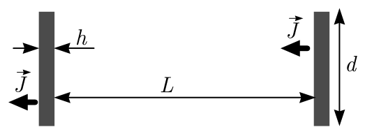
Find the magnitude of the interaction force between two coaxially placed cylindrical magnets of diameter \(d=20\,\mathrm{mm}\) and thickness \(h=2\,\mathrm{mm}\), magnetized parallel to their axis, if the distance between the centres of the magnets is \(L=20\,\mathrm{cm}\). You may assume that \(L\gg d,h\).

A.2 — 0.4pt

At distances much larger than \(\frac h2\), the field created by the magnet from task A.1 is the same as that created by a circular current \(I\). Find \(I\).

A.3 — 1.0pt

Find the interaction force between the magnets for the setup of task A.1 if instead \(L=5\,\mathrm{mm}\). You may assume that \(d\gg L\gg h\).

A.4 — 1.0pt

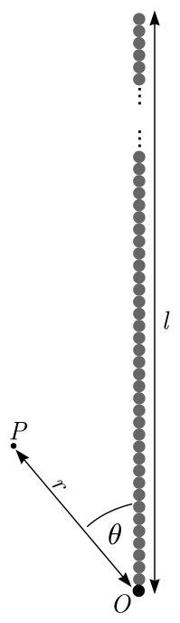
Identical spherical magnets of diameter \(\delta=5\,\mathrm{mm}\), bound together by magnetic attraction, form a chain. What is the maximal length \(l\) for such a chain which does not break under its own weight when hanging beneath the topmost magnet? The density of NdFeB magnets \(\rho=7500\,\mathrm{kg/m^3}\).

A.5 — 1.5pt

Consider the chain from part A.4. Obtain an expression for the magnitude of the magnetic \(B\)-field at such a point \(P\) which is at distance \(r\) from one of the chain's endpoint \(O\), and the angle between the chain and the line \(OP\) is \(\theta\) (cf. figure below), assuming that \(l\gg r\) and \(r\sin\theta\gg\delta\)

Part B. Interaction with ferromagnets (3.5 points)

Now we assume that in addition to the permanent magnets we have also plates made from a ferromagnetic material, similar to what is used in transformer cores. In the situations we're concerned with, it can be considered to have a constant but very large relative permeability \(\mu_r\sim10^5\).

Hint 5. Large permeability means that magnetic field lines near the outside surface of an object made of the material are nearly perpendicular to the surface. This is similar to the behavior of electric field lines near the outside surface of a conductor.

B.1 — 1.0pt

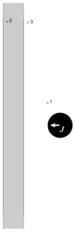
A spherical magnet from part A.4 is at a distance \(s=\delta\) from a thick infinite ferromagnetic plate (see the answer sheet). The magnetization of the sphere is oriented perpendicular to the plate. Sketch the field lines in the cross-section shown in the answer sheet. In that figure, three points (denoted as 1, 2, and 3) are marked; you need to show field lines passing through each of these points in their full length, i.e. as much as fits into the figure.

B.2 — 1.0pt

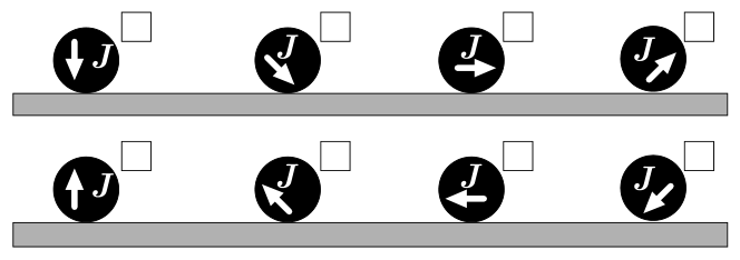
Now the spherical magnet is brought into direct contact with the plate. Which direction is taken by the magnetization vector of the spherical magnet at a stable equilibrium and what is the normal force between the plate and the magnet? Mark the correct direction(s) with a tick in the corresponding box in the answer sheet. Incorrect ticks will reduce your score.

B.3 — 1.5pt

Now a magnet from part A.1 is placed between two thick circular ferromagnetic plates of diameter \(D=2d\) so that the flat faces of the magnet are pressed against the plates and all three discs are coaxial. Find the magnetic force \(F\) acting on each plate. Hint: You may neglect the magnetic field both outside the ferromagnetic plates and outside the gap between them.

Part C. (Anti)ferromagnetic order (2 points)

The magnetic properties of materials are due to the magnetic dipole moments of electrons and atomic nuclei. If the dipole moments orient themselves parallel to each other, the field created by them is magnified — these are ferromagnetic materials. On the other hand, if for each dipole moment there is another antiparallel dipole moment nearby, the fields cancel out — these are anti-ferromagnetic materials.

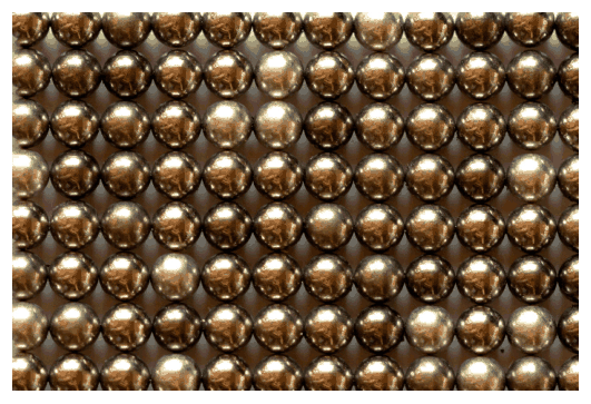
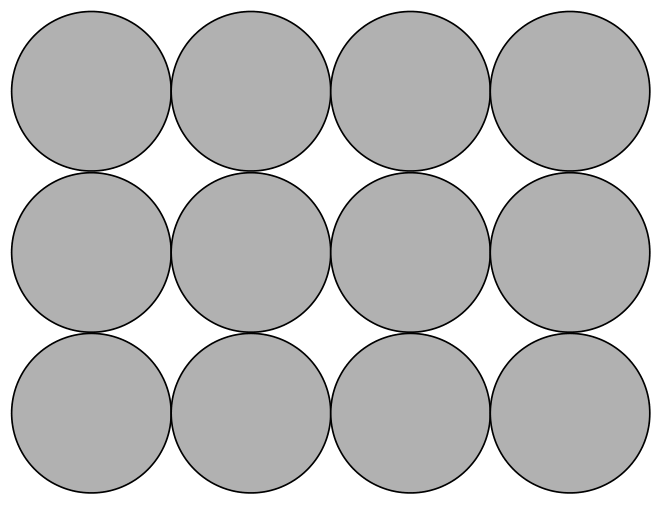
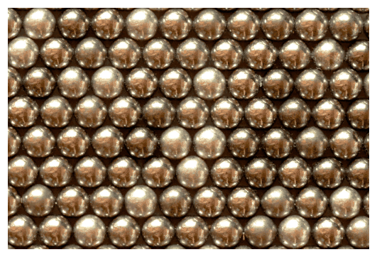
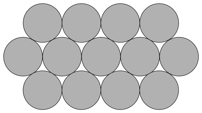
In what follows, we consider a very large number of spherical magnets of part A.4, arranged at the nodes of a two-dimensional lattice; see real photos of stable equilibrium configurations below. Assume that all the magnetization vectors lie in the plane of the figure. Consider in your calculations only nearest-neighbour interactions (on the figure of C.1, each magnet has four nearest neighbours, and on the figure of C.2 — six).

C.1 — 0.8pt

Show the magnetization directions of the magnets in the figure below. You are not required to prove that the configuration you suggested is the only possibility. You still need to justify that the configuration you suggested is indeed stable. Find the energy needed to pull one magnet out of this lattice from somewhere in the middle of the lattice, assuming the other magnets are kept stationary. Does this configuration correspond to the order of ferromagnetic or antiferromagnetic materials?

C.2 — 1.2pt

Answer the same questions as in task C.1 for the configuration shown in the figure below.

Physical Constants

Below is the list of physical constants you might use in your solution in addition to the quantities given in the problem text.

Physical constant	Notation	Numerical value
Speed of light in vacuum	\(c\)	\(299\,792\,458\,\mathrm{m/s}\)
Vacuum permeability (magnetic constant)	\(\mu_0\)	\(4\pi\cdot10^{-7}\,\mathrm{N/A^2}\); \([1\,\mathrm{N/A^2}=1\,\mathrm{Vs/Am}]\)
Vacuum permittivity (electric constant)	\(\varepsilon_0\)	\(8.8541878128(13)\cdot10^{-12}\,\mathrm{F/m}\); \([1\,\mathrm{F/m}=1\,\mathrm{As/Vm}]\)
Elementary charge	\(e\)	\(1.602176634\cdot10^{-19}\,\mathrm{C}\); \([1\,\mathrm{C}=1\,\mathrm{A\cdot s}]\)
Electron rest mass	\(m_{\mathrm e}\)	\(9.1093837015(28)\cdot10^{-31}\,\mathrm{kg}\)
Proton rest mass	\(m_{\mathrm p}\)	\(1.67262192369(51)\cdot10^{-27}\,\mathrm{kg}\)
Neutron rest mass	\(m_{\mathrm n}\)	\(1.67492749804(95)\cdot10^{-27}\,\mathrm{kg}\)
Atomic mass unit	\(m_{\mathrm{amu}}\)	\(1.66053906660(50)\cdot10^{-27}\,\mathrm{kg}\)
Gravitational constant	\(G\)	\(6.67430(15)\cdot10^{-11}\,\mathrm{m^3/(kg\cdot s^2)}\)
Avogadro constant	\(N_{\mathrm A}\)	\(6.02214076\cdot10^{23}\,\mathrm{mol^{-1}}\)
Molar gas constant	\(R\)	\(8.31446261815324\ldots\,\mathrm{J/(K\cdot mol)}\)
Boltzmann constant	\(k_{\mathrm B}\)	\(1.380649\cdot10^{-23}\,\mathrm{J/K}\)
Stefan–Boltzmann constant	\(\sigma\)	\(5.670374419\ldots\cdot10^{-8}\,\mathrm{W/(m^2\cdot K^4)}\)
Planck constant	\(h\)	\(6.62607015\cdot10^{-34}\,\mathrm{J\cdot s}\)
Reduced Planck constant	\(\hbar=h/(2\pi)\)	\(1.0545718176\ldots\cdot10^{-34}\,\mathrm{J\cdot s}\)

Official English text of the problem.

This is a question on the physics of the James Webb Space Telescope. Light from a star strikes the primary mirror, with an area of \(A_{\mathrm{mirror}}=25\,\mathrm{m^2}\), and reflects off of a secondary mirror. The focal length of the system is \(f=130\,\mathrm m\). The light is focused into the ISIM (Integrated Science Instrument Module), which contains the CCD (charged-coupled device) cameras.

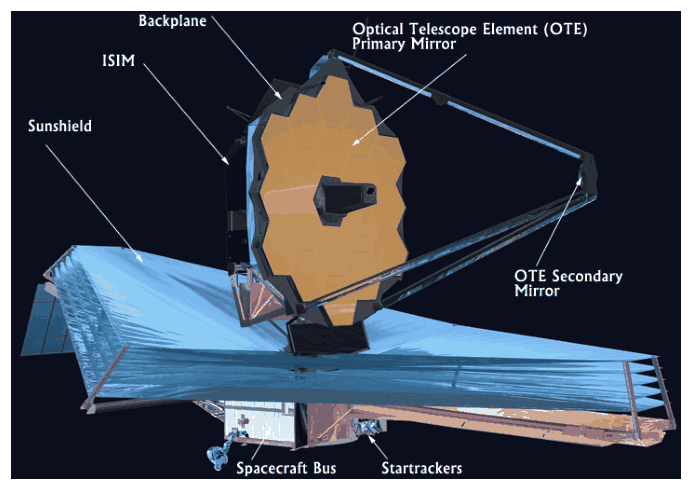
Image Credit: NASA

Part A. Imaging a Star (1.8 points)

The nearest Red Giant is 89 light-years distant, has a temperature of \(T_{\mathrm{star}}=3600\,\mathrm K\), and a diameter of \(d_o=1.7\times10^{11}\,\mathrm m\).

A.1 — 0.4pt

Calculate the diameter of a focused image of the star on the CCD camera imaging surface.

A.2 — 0.4pt

Estimate the diameter of a diffraction central maximum on the CCD camera imaging surface. Assume a wavelength of \(\lambda=800\,\mathrm{nm}\), which is the strongest intensity wavelength from the red giant star.

A.3 — 1.0pt

If the CCD is not cooled and can lose heat only by radiating from the top of the imaging surface, what would be the equilibrium temperature of the CCD at the location of the image of the red giant star? Assume the CCD surface is a blackbody. Provide a formula and a numerical estimate.

Part B. Counting Photons (1.8 points)

The absorption of a photon by the CCD camera leads to the emission of an electron within the apparatus. This occurs only if the photon has sufficient energy to excite an electron across an energy gap \(\Delta E_g\). Assume that every photon with sufficient energy succeeds. There is also leakage of electrons across the gap caused by the temperature of the CCD camera; this is the dark current \(i_d\) and is measured in the number of electrons per second. It is a function of temperature according to

\[ i_d=i_0e^{-|\Delta E_g|/(6k_BT)}. \tag{1} \]

where \(i_0\) is a constant.

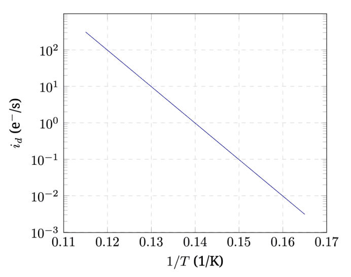
The graph shows how dark current varies with temperature. The units for dark current, \(\mathrm{e^-}/\mathrm s\) should be thought of as counting a number of electrons per second.

B.1 — 0.4pt

From the dark current graph, provide an order of magnitude estimate for the temperature of a distant source of thermal photons that would just be capable of exciting an electron on the pixel.

The electrons are collected in a capacitor, and after an exposure time \(\tau\), the electrons are counted. There are three main sources of uncertainty in the process: a fixed uncertainty in the counting process called read out noise; a Poisson distribution error associated with the dark current, and a Poisson distribution error associated with the detected incoming photons. Poisson distribution errors are equal to the square root of the number of counts associated with a process. The measured photon count is equal to the number of electrons in the capacitor, minus the number of electrons associated with the dark current.

B.2 — 0.4pt

Write an expression for the total count uncertainty \(\sigma_t\), if there is a readout noise \(\sigma_r\), a dark current \(i_d\), an incoming photon rate \(p\), and an exposure time \(\tau\).

For remaining questions in this part assume the exposure time is \(\tau=10^4\,\mathrm s\) and the read out noise is a fixed \(\sigma_r=14\).

B.3 — 0.5pt

Assume an operating temperature of \(T_p=7.5\,\mathrm K\). Calculate the minimum photon rate \(p\) so that the photon count is ten times the count uncertainty.

B.4 — 0.5pt

Assuming all photons are just capable of exciting an electron across the band gap, what is the intensity of the source of photons found in B.3 on the primary mirror? Express your answer in \(\mathrm{W/m^2}\)

Part C. Passive Cooling (4.4 points)

An infrared CCD camera must be kept at a low temperature. The first tool is a shield to protect from the sun's radiation.

The sun-shield consists of five separated reflective layers in thin sheets (black); radiant energy (gray) from the sun is incident on the first sheet on left, and some energy escapes between every pair of sheets.

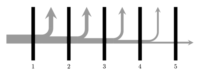
Schematic of energy flow: the vertical lines (black) are the sheets, the flow of energy (gray) is from the left to the right, however, between sheets, some energy flows up and out into space.

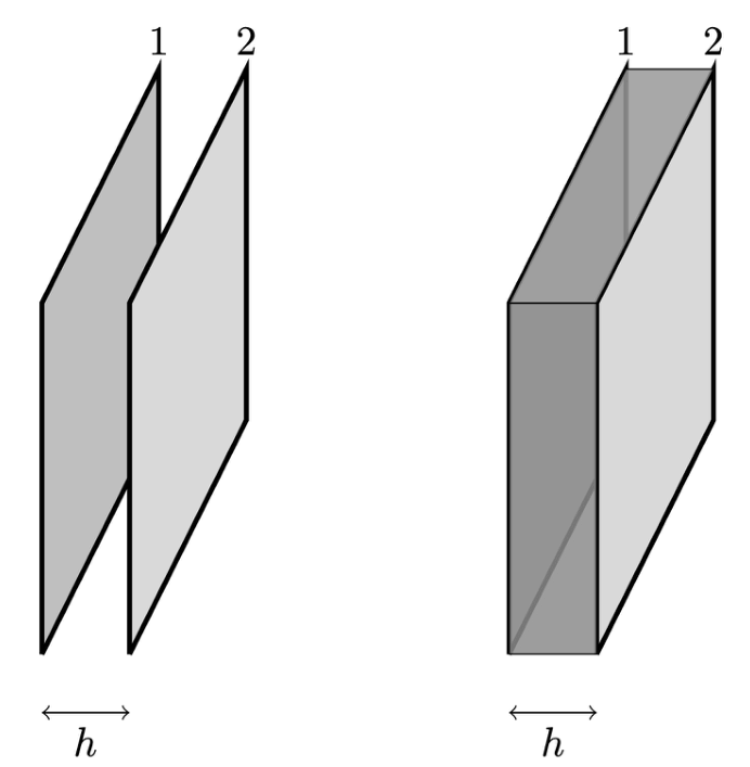
On the left is a simple model of two adjacent sheets 1 and 2 separated by a distance \(h\). The sheets are not connected, and the perimeter is open to space. Assume the sheets are parallel. Thermal radiation can be exchanged between the sheets, and thermal radiation can escape through the perimeter gap. On the right, the perimeter gap has been shaded to help visualize.

Assume the following simplifications:

• Sheets are square, each with area \(A_{\mathrm{sheet}}=200\,\mathrm{m^2}\).
• Sheets are parallel and separated by \(h=25\,\mathrm{cm}\) along the perimeter.
• Sheets have constant emissivity \(\epsilon\ll1\). Assume that all reflections off of sheet surfaces are diffuse.
• Sheets are thin with temperature on the front and back surfaces equal and uniform.
• The fraction of radiant flux emitted by a sheet that is absorbed by the adjacent sheet is \(\alpha\leq1\). This means that if sheet 1 in the figure above emits an amount of heat \(Q_1\) toward sheet 2 then sheet 2 will absorb an amount \(\alpha Q_1\) from sheet 1.
• The amount of radiant flux ejected out of the perimeter gap between two sheets is approximated as \(\beta Q_{12}\) where \(\alpha Q_{12}\) is the net flux between the two sheets. The fraction \(\beta<1\). This is equivalent to saying that the heat loss to space between two sheets is proportional to the net heat exchange between the sheets. This is a rough approximation for this problem.
• Background temperature of space is negligible.

C.1 — 2.4pt

Derive expressions for the equilibrium temperatures of the first sheet and fifth sheet in terms of the incident solar radiation intensity \(I_0\), the constants \(\alpha\) and \(\beta\), and any necessary physical constants. To simplify your expression, you may define additional constants in terms of \(\alpha\) and \(\beta\), etc.

C.2 — 1.6pt

Derive numerical estimates for \(\alpha\) and \(\beta\) from the information about the sheet geometry assuming an emissivity \(\epsilon=0.05\). You are encouraged to consider the rectangular box model of the sheets above, where the perimeter area effectively acts as a perfect absorber of radiant energy.

C.3 — 0.4pt

Numerically determine the temperatures of sheet 1 and sheet 5. The solar intensity is \(I_0=1360\,\mathrm{W/m^2}\).

Part D. Cryo-cooler (4 points)

The last stage of the cooling system directly cools the CCD camera. A closed cycle refrigeration system has a supply pipe line feeding helium gas at constant pressure \(P_1\) moving through a sponge like porous plug into a pipe with constant pressure \(P_2\). The pipe carries the gas to cool the CCD. The helium gas then passes through a pump before returning to the supply line.

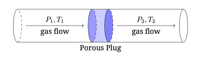
Helium gas supplied on the left at well defined pressure \(P_1\) and temperature \(T_1\) is forced through the plug to well defined pressure \(P_2\) and temperature \(T_2\), where it is carried away on the right.

As the gas moves through the porous plug, viscous friction with the narrow walls of the channels in the sponge becomes an important effect; however, no heat is transferred to or from the gas during the process. The bulk speed of the gas in region 2 is only marginally greater than the bulk speed in region 1.

Helium is not an ideal gas, but does remain in a gaseous state throughout this process.

D.1 — 1.0pt

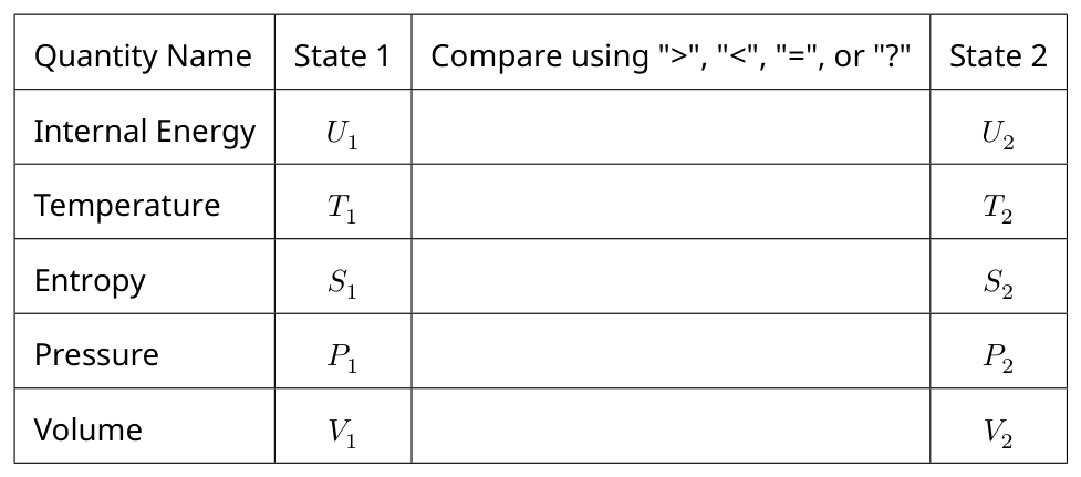
Consider a mole of gas that passes from left to right through the plug. Complete the table in your answer sheet by writing '>' or '<' to identify the quantity that must be greater, '=' to identify quantities that must be equal, or '?' if it is not possible to know which is greater or equal without more information.

D.2 — 0.6pt

Identify a conserved quantity constructed from \(U\) (internal energy), \(P\) (pressure), and \(V\) (volume) as a mole of gas moves through the plug; show work on how you derived this conserved quantity.

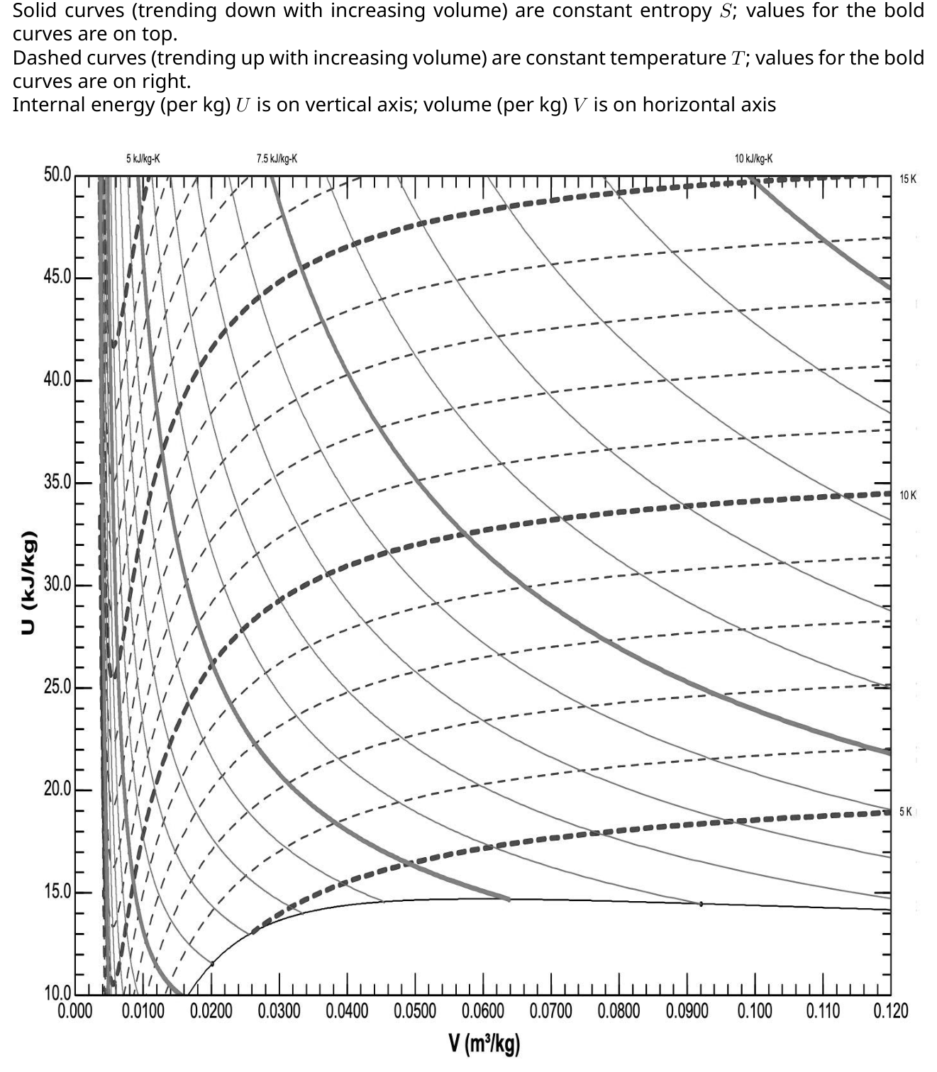
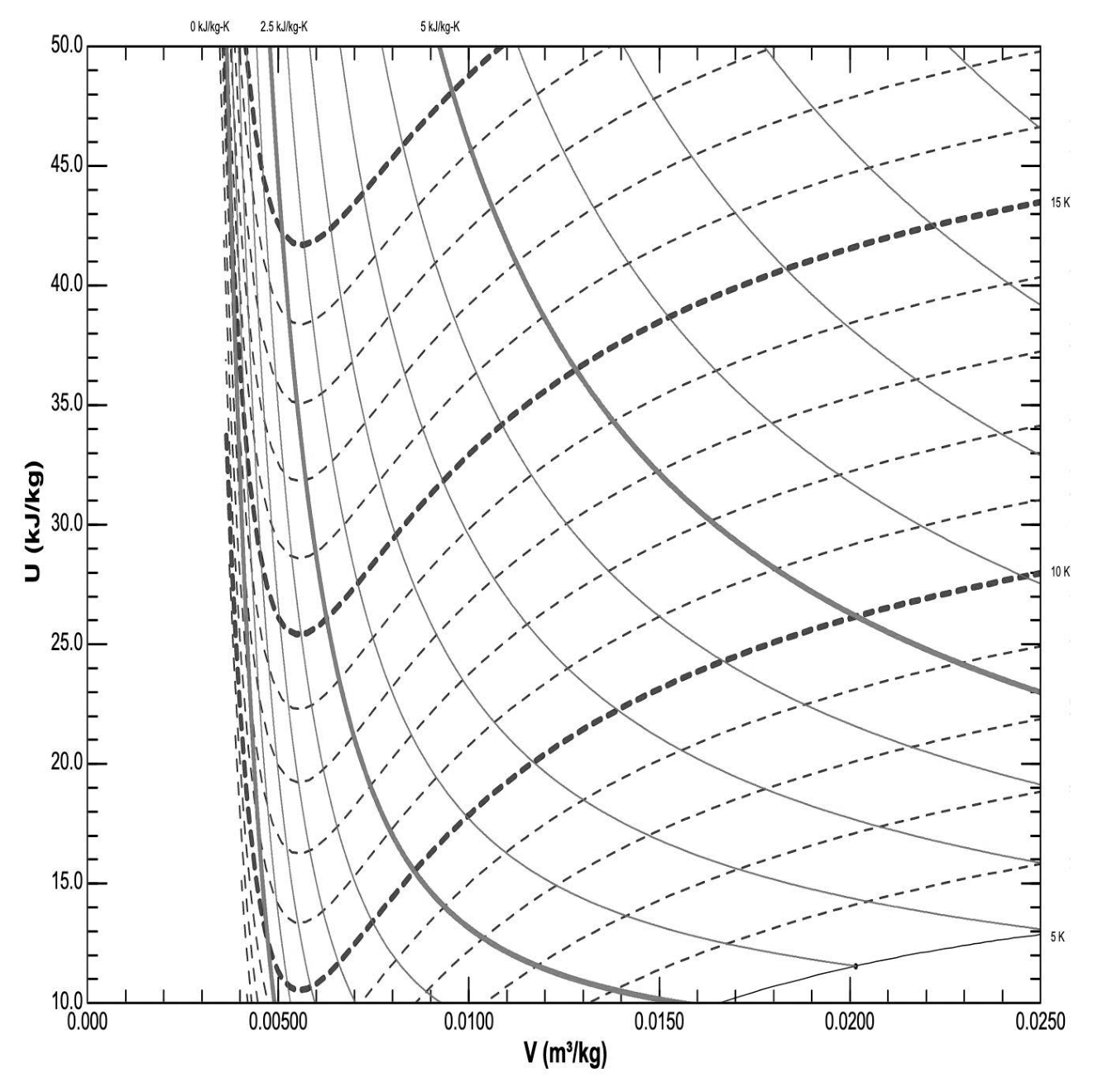
Your answer sheets have graphs of internal energy per mass against volume per mass for helium with isotherms and lines of constant entropy.

D.3 — 1.4pt

Assuming that \(V_2=0.100\,\mathrm{m^3/kg}\) and \(T_2=7.5\,\mathrm K\), use the graph to find a numerical value for the conserved quantity that you found in Part D.2. Show the construction on the graph!

D.4 — 0.8pt

Find the maximum possible temperature for \(T_1\). Show the construction on the graph!

D.5 — 0.2pt

Assuming your value for the maximum \(T_1\) found in D.4, find a numerical value for \(P_1\).

Physical Constants

Below is the list of physical constants you might use in your solution in addition to the quantities given in the problem text.

Physical constant	Notation	Numerical value
Speed of light in vacuum	\(c\)	\(299\,792\,458\,\mathrm{m/s}\)
Vacuum permeability (magnetic constant)	\(\mu_0\)	\(4\pi\cdot10^{-7}\,\mathrm{N/A^2};\quad[1\,\mathrm{N/A^2}=1\,\mathrm{V\,s/(A\,m)}]\)
Vacuum permittivity (electric constant)	\(\varepsilon_0\)	\(8.8541878128(13)\cdot10^{-12}\,\mathrm{F/m};\quad[1\,\mathrm{F/m}=1\,\mathrm{A\,s/(V\,m)}]\)
Elementary charge	\(e\)	\(1.602176634\cdot10^{-19}\,\mathrm C;\quad[1\,\mathrm C=1\,\mathrm{A\cdot s}]\)
Electron rest mass	\(m_e\)	\(9.1093837015(28)\cdot10^{-31}\,\mathrm{kg}\)
Proton rest mass	\(m_p\)	\(1.67262192369(51)\cdot10^{-27}\,\mathrm{kg}\)
Neutron rest mass	\(m_n\)	\(1.67492749804(95)\cdot10^{-27}\,\mathrm{kg}\)
Atomic mass unit	\(m_{\mathrm{amu}}\)	\(1.66053906660(50)\cdot10^{-27}\,\mathrm{kg}\)
Gravitational constant	\(G\)	\(6.67430(15)\cdot10^{-11}\,\mathrm{m^3/(kg\cdot s^2)}\)
Avogadro constant	\(N_A\)	\(6.02214076\cdot10^{23}\,\mathrm{mol^{-1}}\)
Molar gas constant	\(R\)	\(8.31446261815324\ldots\,\mathrm{J/(K\cdot mol)}\)
Boltzmann constant	\(k_B\)	\(1.380649\cdot10^{-23}\,\mathrm{J/K}\)
Stefan–Boltzmann constant	\(\sigma\)	\(5.670374419\ldots\cdot10^{-8}\,\mathrm{W/(m^2\cdot K^4)}\)
Planck constant	\(h\)	\(6.62607015\cdot10^{-34}\,\mathrm{J\cdot s}\)
Reduced Planck constant	\(\hbar=h/(2\pi)\)	\(1.0545718176\ldots\cdot10^{-34}\,\mathrm{J\cdot s}\)

Official English text of the problem.

Scaling laws describe the functional relationship between two physical quantities that scale with each other over a significant interval. This functional relationship can be a power law, but there are other possibilities, too. Oftentimes, exact expressions are beyond reach, but scaling laws can still be derived.

Part A. Spaghetto (2.0 points)

A.1 2.0pt

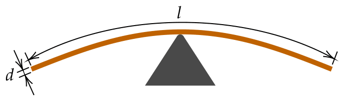
A spaghetto straw of diameter \(d\) is being balanced horizontally from its middle. If \(d = 1\,\mathrm{mm}\), the straw breaks under its own weight once its length reaches \(l = 50\,\mathrm{cm}\). What is the maximum length \(l'\) of the straw of diameter \(d' = 1\,\mathrm{cm}\) before it breaks under its own weight?

Part B. Sand castle (2.0 points)

B.1 2.0pt

The average grain volume of coarse-grained sand is 10 times as large as that of fine-grained sand. Wet fine-grained sand and wet coarse-grained sand have both optimal water content (i.e. assuming the maximal strength of the constructions from it) and are used to build two cylinders of exactly the same shape and size. The strength of each cylinder is tested by pressing it between two parallel plates. The cylinder made of coarse-grained sand gets destroyed once the force applied to press the plates reaches \(F_{\mathrm c} = 10\,\mathrm{N}\). How large is the force \(F_{\mathrm f}\) needed to destroy the cylinder made of fine-grained sand? You may ignore the effects of gravity.

Part C. Interstellar travel (2.0 points)

C.1 2.0pt

The spaceship of an interstellar expedition travels at a constant magnitude of the proper acceleration \(g = 10\,\mathrm{m/s^2}\), i.e., this is the acceleration of the spaceship in the inertial frame of reference where it is instantaneously at rest. The passengers must be able to return to Earth within their remaining expected lifetime of 50 years. The maximum distance from Earth reached by the spaceship is \(d\). If the acceleration is increased to \(g' = 15\,\mathrm{m/s^2}\), the spaceship can reach a farther distance \(d'\). What is the ratio \(d'/d\)?

Hint 1. You may wish to use the relativistic velocity addition formula, however, there are also other approaches.

Hint 2. You may need to deal with hyperbolic functions defined as follows: \[ \cosh x=\frac12(e^x+e^{-x}),\qquad \sinh x=\frac12(e^x-e^{-x}),\qquad \tanh x=\frac{e^x-e^{-x}}{e^x+e^{-x}}. \]

Hint 3. Depending on your approach, you may need one or more of these integrals: \[ \int\frac{\mathrm dx}{1-x^2}=\operatorname{atanh}x+C,\qquad \int\frac{\mathrm dx}{\sqrt{1+x^2}}=\operatorname{asinh}x+C,\qquad \int\sinh x\,\mathrm dx=\cosh x+C, \] where \(\operatorname{asinh}x\) and \(\operatorname{atanh}x\) are the inverse functions of the respective hyperbolic functions.

Part D. That sinking feeling (2.0 points)

D.1 2.0pt

A solid wooden ball of radius \(r_0\) is floating in the water. Ignoring frictional effects, the frequency of small oscillations would be \(\omega_0\), but because of viscous friction, after being displaced vertically, the frequency of decaying oscillations is actually \(0.99\,\omega_0\). What is the minimum radius \(r_{\min}\) of a wooden ball floating in water that undergos small oscillations when displaced? Hint: the viscous drag force acting on a given body is proportional to its speed relative to the bulk of the fluid, and to the viscosity \(\eta\) of the fluid it is moving in. The unit of the viscosity is \(\mathrm{kg/(m\cdot s)}\).

Official English text of the problem.

Starke Permanentmagnete werden aus einer NdFeB-Legierung hergestellt, die eine sehr breite Hystereseschleife aufweist, sodass die Magnetisierung \(J\) in einem weiten Anwendungsbereich als konstant angenommen werden kann; im Folgenden nehmen wir \(J\equiv 1.5\,\mathrm{T}/\mu_0\) an, wobei \(\mu_0=4\pi\times10^{-7}\,\mathrm{N/A^2}\), und die Magnetisierung aller Permanentmagnete ist homogen. Die Magnetisierung ist als Volumendichte des magnetischen Dipolmoments der Materie definiert.

Hinweis 1. Die folgende Gleichung könnte hilfreich sein:

\[ \sum_{n=1}^{\infty}\frac{1}{n^4}=\frac{\pi^4}{90}. \]

Hinweis 2. Das von einem kugelförmigen Magneten erzeugte Magnetfeld ist identisch mit dem eines Punktdipols. Die von Magneten anderer Formen erzeugten Magnetfelder entsprechen erst in Abständen, die viel größer als ihr Durchmesser sind, dem Feld eines Punktdipols.

Hinweis 3. Die elektrischen und magnetischen Felder elektrischer bzw. magnetischer Punktdipole sind als Funktionen der Koordinaten und des jeweiligen Dipolmoments ähnlich, d. h., das eine lässt sich durch Multiplikation mit einem konstanten Faktor aus dem anderen erhalten.

Hinweis 4. Das durch eine Randbedingung induzierte Feld kann stets durch eine geeignete Anordnung von Feldquellen außerhalb der vorgegebenen Grenzen ersetzt werden.

Teil A. Wechselwirkung zwischen Magneten (4.5 Punkte)

Wenn der Abstand zu einem Magneten viel größer als seine Größe ist, kann das von ihm erzeugte Magnetfeld durch das Magnetfeld seines Dipolmoments \(\vec m\) angenähert werden,

\[ \vec B=\frac{\mu_0}{4\pi r^3}(2\vec m_{\parallel}-\vec m_{\perp}). \]

Hierbei ist \(r=|\vec r|\), und wir haben das Dipolmoment in Komponenten parallel und senkrecht zum Ortsvektor \(\vec r\) zerlegt, der vom Dipol zum Beobachtungspunkt zeigt, \(\vec m=\vec m_{\perp}+\vec m_{\parallel}\).

A.1 — 0.6 Punkte

Bestimmen Sie den Betrag der Wechselwirkungskraft zwischen zwei koaxial angeordneten zylindrischen Magneten mit dem Durchmesser \(d=20\,\mathrm{mm}\) und der Dicke \(h=2\,\mathrm{mm}\), die parallel zu ihrer Achse magnetisiert sind, wenn der Abstand zwischen den Mittelpunkten der Magnete \(L=20\,\mathrm{cm}\) beträgt. Sie dürfen \(L\gg d,h\) annehmen.

A.2 — 0.4 Punkte

In Abständen, die viel größer als \(\frac h2\) sind, ist das vom Magneten aus Aufgabe A.1 erzeugte Feld dasselbe wie das eines Kreisstroms \(I\). Bestimmen Sie \(I\).

A.3 — 1.0 Punkte

Bestimmen Sie die Wechselwirkungskraft zwischen den Magneten für die Anordnung aus Aufgabe A.1, wenn stattdessen \(L=5\,\mathrm{mm}\) gilt. Sie dürfen \(d\gg L\gg h\) annehmen.

A.4 — 1.0 Punkte

Identische kugelförmige Magnete mit dem Durchmesser \(\delta=5\,\mathrm{mm}\), die durch magnetische Anziehung zusammengehalten werden, bilden eine Kette. Wie groß ist die maximale Länge \(l\) einer solchen Kette, die unter ihrem eigenen Gewicht nicht reißt, wenn sie am obersten Magneten hängt? Die Dichte der NdFeB-Magnete beträgt \(\rho=7500\,\mathrm{kg/m^3}\).

A.5 — 1.5 Punkte

Betrachten Sie die Kette aus Teil A.4. Leiten Sie einen Ausdruck für den Betrag des magnetischen \(B\)-Feldes an einem Punkt \(P\) her, der sich im Abstand \(r\) von einem der Endpunkte \(O\) der Kette befindet, wobei der Winkel zwischen der Kette und der Geraden \(OP\) gleich \(\theta\) ist (siehe Abbildung unten). Nehmen Sie dabei \(l\gg r\) und \(r\sin\theta\gg\delta\) an.

Teil B. Wechselwirkung mit Ferromagneten (3.5 Punkte)

Wir nehmen nun an, dass uns neben den Permanentmagneten auch Platten aus einem ferromagnetischen Material zur Verfügung stehen, ähnlich dem Material, das in Transformatorkernen verwendet wird. In den hier betrachteten Situationen kann seine relative Permeabilität als konstant, aber sehr groß angenommen werden, \(\mu_r\sim10^5\).

Hinweis 5. Eine große Permeabilität bedeutet, dass magnetische Feldlinien nahe der äußeren Oberfläche eines Körpers aus diesem Material nahezu senkrecht zur Oberfläche verlaufen. Dies ähnelt dem Verhalten elektrischer Feldlinien nahe der äußeren Oberfläche eines Leiters.

B.1 — 1.0 Punkte

Ein kugelförmiger Magnet aus Teil A.4 befindet sich im Abstand \(s=\delta\) von einer dicken, unendlich ausgedehnten ferromagnetischen Platte (siehe Antwortbogen). Die Magnetisierung der Kugel ist senkrecht zur Platte ausgerichtet. Skizzieren Sie die Feldlinien in dem auf dem Antwortbogen dargestellten Querschnitt. In dieser Abbildung sind drei Punkte (mit 1, 2 und 3 bezeichnet) markiert; Sie sollen die Feldlinien durch jeden dieser Punkte über ihre gesamte Länge darstellen, d. h. so weit, wie es in die Abbildung passt.

B.2 — 1.0 Punkte

Nun wird der kugelförmige Magnet in direkten Kontakt mit der Platte gebracht. Welche Richtung nimmt der Magnetisierungsvektor des kugelförmigen Magneten im stabilen Gleichgewicht ein, und wie groß ist die Normalkraft zwischen der Platte und dem Magneten? Markieren Sie die richtige(n) Richtung(en) mit einem Häkchen im entsprechenden Kästchen auf dem Antwortbogen. Falsch gesetzte Häkchen führen zu Punktabzug.

B.3 — 1.5 Punkte

Nun wird ein Magnet aus Teil A.1 zwischen zwei dicke kreisförmige ferromagnetische Platten mit dem Durchmesser \(D=2d\) gelegt, sodass die ebenen Stirnflächen des Magneten an die Platten gedrückt werden und alle drei Scheiben koaxial sind. Bestimmen Sie die auf jede Platte wirkende magnetische Kraft \(F\). Hinweis: Sie dürfen das Magnetfeld sowohl außerhalb der ferromagnetischen Platten als auch außerhalb des Spalts zwischen ihnen vernachlässigen.

Teil C. (Anti)ferromagnetische Ordnung (2 Punkte)

Die magnetischen Eigenschaften von Materialien beruhen auf den magnetischen Dipolmomenten der Elektronen und Atomkerne. Richten sich die Dipolmomente parallel zueinander aus, wird das von ihnen erzeugte Feld verstärkt — dies sind ferromagnetische Materialien. Gibt es hingegen zu jedem Dipolmoment ein weiteres, antiparalleles Dipolmoment in der Nähe, heben sich die Felder auf — dies sind antiferromagnetische Materialien.

Im Folgenden betrachten wir eine sehr große Anzahl kugelförmiger Magnete aus Teil A.4, die an den Gitterpunkten eines zweidimensionalen Gitters angeordnet sind; siehe die untenstehenden realen Fotos stabiler Gleichgewichtsanordnungen. Nehmen Sie an, dass alle Magnetisierungsvektoren in der Zeichenebene liegen. Berücksichtigen Sie in Ihren Berechnungen nur die Wechselwirkungen zwischen nächsten Nachbarn (in der Abbildung zu C.1 hat jeder Magnet vier nächste Nachbarn, in der Abbildung zu C.2 sechs).

C.1 — 0.8 Punkte

Zeichnen Sie die Magnetisierungsrichtungen der Magnete in die untenstehende Abbildung ein. Sie müssen nicht beweisen, dass die von Ihnen vorgeschlagene Anordnung die einzig mögliche ist. Sie müssen jedoch begründen, dass die von Ihnen vorgeschlagene Anordnung tatsächlich stabil ist. Bestimmen Sie die Energie, die benötigt wird, um einen Magneten aus dem Inneren dieses Gitters herauszuziehen, wobei die anderen Magnete festgehalten werden. Entspricht diese Anordnung der Ordnung ferromagnetischer oder antiferromagnetischer Materialien?

C.2 — 1.2 Punkte

Beantworten Sie für die in der untenstehenden Abbildung gezeigte Anordnung dieselben Fragen wie in Aufgabe C.1.

Physikalische Konstanten

Nachfolgend finden Sie eine Liste physikalischer Konstanten, die Sie zusätzlich zu den in der Aufgabenstellung angegebenen Größen für Ihre Lösung verwenden können.

Physikalische Konstante	Symbol	Zahlenwert
Lichtgeschwindigkeit im Vakuum	\(c\)	\(299\,792\,458\,\mathrm{m/s}\)
Vakuumpermeabilität (magnetische Feldkonstante)	\(\mu_0\)	\(4\pi\cdot10^{-7}\,\mathrm{N/A^2}\); \([1\,\mathrm{N/A^2}=1\,\mathrm{Vs/Am}]\)
Vakuumpermittivität (elektrische Feldkonstante)	\(\varepsilon_0\)	\(8.8541878128(13)\cdot10^{-12}\,\mathrm{F/m}\); \([1\,\mathrm{F/m}=1\,\mathrm{As/Vm}]\)
Elementarladung	\(e\)	\(1.602176634\cdot10^{-19}\,\mathrm{C}\); \([1\,\mathrm{C}=1\,\mathrm{A\cdot s}]\)
Ruhemasse des Elektrons	\(m_{\mathrm e}\)	\(9.1093837015(28)\cdot10^{-31}\,\mathrm{kg}\)
Ruhemasse des Protons	\(m_{\mathrm p}\)	\(1.67262192369(51)\cdot10^{-27}\,\mathrm{kg}\)
Ruhemasse des Neutrons	\(m_{\mathrm n}\)	\(1.67492749804(95)\cdot10^{-27}\,\mathrm{kg}\)
Atomare Masseneinheit	\(m_{\mathrm{amu}}\)	\(1.66053906660(50)\cdot10^{-27}\,\mathrm{kg}\)
Gravitationskonstante	\(G\)	\(6.67430(15)\cdot10^{-11}\,\mathrm{m^3/(kg\cdot s^2)}\)
Avogadro-Konstante	\(N_{\mathrm A}\)	\(6.02214076\cdot10^{23}\,\mathrm{mol^{-1}}\)
Molare Gaskonstante	\(R\)	\(8.31446261815324\ldots\,\mathrm{J/(K\cdot mol)}\)
Boltzmann-Konstante	\(k_{\mathrm B}\)	\(1.380649\cdot10^{-23}\,\mathrm{J/K}\)
Stefan–Boltzmann-Konstante	\(\sigma\)	\(5.670374419\ldots\cdot10^{-8}\,\mathrm{W/(m^2\cdot K^4)}\)
Planck-Konstante	\(h\)	\(6.62607015\cdot10^{-34}\,\mathrm{J\cdot s}\)
Reduzierte Planck-Konstante	\(\hbar=h/(2\pi)\)	\(1.0545718176\ldots\cdot10^{-34}\,\mathrm{J\cdot s}\)

Aufgabentext aus dem offiziellen englischen Text übersetzt.

In dieser Aufgabe geht es um die Physik des James-Webb-Weltraumteleskops. Das Licht eines Sterns trifft auf den Hauptspiegel mit einer Fläche von \(A_{\mathrm{mirror}}=25\,\mathrm{m^2}\) und wird an einem Sekundärspiegel reflektiert. Die Brennweite des Systems beträgt \(f=130\,\mathrm m\). Das Licht wird im ISIM (Integriertes Wissenschaftliches Instrumentenmodul) fokussiert, das die CCD-Kameras (ladungsgekoppelte Bauelemente) enthält.

Bildnachweis: NASA

Teil A. Abbildung eines Sterns (1.8 Punkte)

Der nächstgelegene Rote Riese ist 89 Lichtjahre entfernt, hat eine Temperatur von \(T_{\mathrm{star}}=3600\,\mathrm K\) und einen Durchmesser von \(d_o=1.7\times10^{11}\,\mathrm m\).

A.1 — 0.4 Punkte

Berechnen Sie den Durchmesser des scharf abgebildeten Sterns auf der Bildfläche der CCD-Kamera.

A.2 — 0.4 Punkte

Schätzen Sie den Durchmesser des zentralen Beugungsmaximums auf der Bildfläche der CCD-Kamera ab. Nehmen Sie eine Wellenlänge von \(\lambda=800\,\mathrm{nm}\) an; bei dieser Wellenlänge ist die Intensität des Roten Riesen am größten.

A.3 — 1.0 Punkte

Wenn der CCD nicht gekühlt wird und Wärme nur durch Abstrahlung von der Oberseite der Bildfläche abgeben kann, welche Gleichgewichtstemperatur würde sich dann am Ort des Bildes des Roten Riesen auf dem CCD einstellen? Nehmen Sie an, dass die CCD-Oberfläche ein schwarzer Körper ist. Geben Sie eine Formel und eine numerische Abschätzung an.

Teil B. Zählen von Photonen (1.8 Punkte)

Die Absorption eines Photons durch die CCD-Kamera führt zur Freisetzung eines Elektrons innerhalb der Apparatur. Dies geschieht nur, wenn das Photon genügend Energie besitzt, um ein Elektron über eine Energielücke \(\Delta E_g\) hinweg anzuregen. Nehmen Sie an, dass dies jedem Photon mit ausreichender Energie gelingt. Aufgrund der Temperatur der CCD-Kamera gelangen auch Elektronen als Leckstrom über die Energielücke; dies ist der Dunkelstrom \(i_d\), der als Anzahl von Elektronen pro Sekunde gemessen wird. Er hängt gemäß

\[ i_d=i_0e^{-|\Delta E_g|/(6k_BT)}. \tag{1} \]

von der Temperatur ab, wobei \(i_0\) eine Konstante ist.

Das Diagramm zeigt die Temperaturabhängigkeit des Dunkelstroms. Die Einheit des Dunkelstroms, \(\mathrm{e^-}/\mathrm s\), ist als Anzahl von Elektronen pro Sekunde zu verstehen.

B.1 — 0.4 Punkte

Schätzen Sie anhand des Dunkelstromdiagramms die Größenordnung der Temperatur einer entfernten Quelle thermischer Photonen ab, die gerade noch ein Elektron im Pixel anregen könnten.

Die Elektronen werden in einem Kondensator gesammelt und nach einer Belichtungszeit \(\tau\) gezählt. Bei diesem Vorgang gibt es drei wesentliche Unsicherheitsquellen: eine feste Unsicherheit beim Zählvorgang, die als Ausleserauschen bezeichnet wird; einen durch die Poisson-Verteilung beschriebenen Fehler des Dunkelstroms und einen durch die Poisson-Verteilung beschriebenen Fehler der nachgewiesenen einfallenden Photonen. Fehler gemäß der Poisson-Verteilung sind gleich der Quadratwurzel aus der Anzahl der zum jeweiligen Prozess gehörenden Zählereignisse. Die gemessene Photonenzahl ist gleich der Anzahl der Elektronen im Kondensator abzüglich der Anzahl der dem Dunkelstrom zuzuordnenden Elektronen.

B.2 — 0.4 Punkte

Geben Sie einen Ausdruck für die gesamte Zählunsicherheit \(\sigma_t\) an, wenn das Ausleserauschen \(\sigma_r\), der Dunkelstrom \(i_d\), die Rate einfallender Photonen \(p\) und die Belichtungszeit \(\tau\) betragen.

Nehmen Sie für die verbleibenden Fragen dieses Teils eine Belichtungszeit von \(\tau=10^4\,\mathrm s\) und ein festes Ausleserauschen von \(\sigma_r=14\) an.

B.3 — 0.5 Punkte

Nehmen Sie eine Betriebstemperatur von \(T_p=7.5\,\mathrm K\) an. Berechnen Sie die minimale Photonenrate \(p\), bei der die Photonenzahl das Zehnfache der Zählunsicherheit beträgt.

B.4 — 0.5 Punkte

Angenommen, alle Photonen können gerade noch ein Elektron über die Bandlücke hinweg anregen: Welche Intensität hat die in B.3 gefundene Photonenquelle am Hauptspiegel? Geben Sie Ihre Antwort in \(\mathrm{W/m^2}\) an.

Teil C. Passive Kühlung (4.4 Punkte)

Eine Infrarot-CCD-Kamera muss auf einer niedrigen Temperatur gehalten werden. Das erste Hilfsmittel ist ein Schild zum Schutz vor der Sonnenstrahlung.

Der Sonnenschild besteht aus fünf voneinander getrennten reflektierenden Schichten aus dünnen Folien (schwarz); Strahlungsenergie (grau) von der Sonne fällt auf die erste Folie links, und zwischen jedem Folienpaar entweicht ein Teil der Energie.

Schematische Darstellung des Energieflusses: Die vertikalen Linien (schwarz) sind die Folien, der Energiefluss (grau) verläuft von links nach rechts; zwischen den Folien fließt jedoch ein Teil der Energie nach oben und hinaus ins Weltall.

Links ist ein einfaches Modell zweier benachbarter Folien 1 und 2 dargestellt, die durch einen Abstand \(h\) voneinander getrennt sind. Die Folien sind nicht miteinander verbunden, und der Rand ist zum Weltall hin offen. Nehmen Sie an, dass die Folien parallel sind. Zwischen den Folien kann Wärmestrahlung ausgetauscht werden, und durch den umlaufenden Randspalt kann Wärmestrahlung entweichen. Rechts ist der Randspalt zur Veranschaulichung schattiert dargestellt.

Nehmen Sie die folgenden Vereinfachungen an:

• Die Folien sind quadratisch und haben jeweils eine Fläche von \(A_{\mathrm{sheet}}=200\,\mathrm{m^2}\).
• Die Folien sind parallel und haben entlang des Randes einen Abstand von \(h=25\,\mathrm{cm}\).
• Die Folien haben einen konstanten Emissionsgrad \(\epsilon\ll1\). Nehmen Sie an, dass alle Reflexionen an den Folienoberflächen diffus sind.
• Die Folien sind dünn, wobei die Temperatur auf Vorder- und Rückseite gleich und gleichmäßig ist.
• Der Anteil des von einer Folie emittierten Strahlungsflusses, der von der benachbarten Folie absorbiert wird, beträgt \(\alpha\leq1\). Das bedeutet: Wenn Folie 1 in der obigen Abbildung eine Wärmemenge \(Q_1\) in Richtung von Folie 2 emittiert, absorbiert Folie 2 davon eine Menge \(\alpha Q_1\).
• Der durch den Randspalt zwischen zwei Folien austretende Strahlungsfluss wird durch \(\beta Q_{12}\) angenähert, wobei \(\alpha Q_{12}\) der Nettofluss zwischen den beiden Folien ist. Für den Anteil gilt \(\beta<1\). Dies entspricht der Aussage, dass der Wärmeverlust ins Weltall zwischen zwei Folien proportional zum Nettowärmeaustausch zwischen den Folien ist. Dies ist eine grobe Näherung für diese Aufgabe.
• Die Hintergrundtemperatur des Weltalls ist vernachlässigbar.

C.1 — 2.4 Punkte

Leiten Sie Ausdrücke für die Gleichgewichtstemperaturen der ersten und der fünften Folie in Abhängigkeit von der Intensität der einfallenden Sonnenstrahlung \(I_0\), den Konstanten \(\alpha\) und \(\beta\) sowie gegebenenfalls benötigten physikalischen Konstanten her. Zur Vereinfachung Ihrer Ausdrücke dürfen Sie zusätzliche Konstanten in Abhängigkeit von \(\alpha\) und \(\beta\) usw. definieren.

C.2 — 1.6 Punkte

Leiten Sie aus den Angaben zur Foliengeometrie unter Annahme eines Emissionsgrades von \(\epsilon=0.05\) numerische Abschätzungen für \(\alpha\) und \(\beta\) her. Es empfiehlt sich, das oben dargestellte Quader-Modell der Folien zu betrachten, bei dem die umlaufende Seitenfläche effektiv als perfekter Absorber für Strahlungsenergie wirkt.

C.3 — 0.4 Punkte

Bestimmen Sie die Temperaturen von Folie 1 und Folie 5 numerisch. Die Intensität der Sonnenstrahlung beträgt \(I_0=1360\,\mathrm{W/m^2}\).

Teil D. Kryokühler (4 Punkte)

Die letzte Stufe des Kühlsystems kühlt die CCD-Kamera direkt. Ein Kältesystem mit geschlossenem Kreislauf besitzt eine Zuleitung, die Heliumgas bei konstantem Druck \(P_1\) zuführt. Das Gas strömt durch einen schwammartigen porösen Pfropfen in ein Rohr mit konstantem Druck \(P_2\). Das Rohr führt das Gas zur Kühlung des CCD weiter. Anschließend durchläuft das Heliumgas eine Pumpe, bevor es in die Zuleitung zurückkehrt.

Das links bei einem wohldefinierten Druck \(P_1\) und einer wohldefinierten Temperatur \(T_1\) zugeführte Heliumgas wird durch den Pfropfen auf einen wohldefinierten Druck \(P_2\) und eine wohldefinierte Temperatur \(T_2\) gebracht und rechts abgeführt.

Beim Durchströmen des porösen Pfropfens spielt die viskose Reibung an den Wänden der engen Kanäle im Schwamm eine wichtige Rolle; während dieses Vorgangs wird jedoch keine Wärme auf das Gas übertragen oder von ihm abgegeben. Die makroskopische Strömungsgeschwindigkeit des Gases in Bereich 2 ist nur geringfügig größer als diejenige in Bereich 1.

Helium ist kein ideales Gas, bleibt aber während des gesamten Vorgangs gasförmig.

D.1 — 1.0 Punkte

Betrachten Sie ein Mol Gas, das den Pfropfen von links nach rechts durchströmt. Vervollständigen Sie die Tabelle auf Ihrem Antwortbogen, indem Sie mit „>“ oder „<“ angeben, welche Größe größer sein muss, mit „=“ Größen kennzeichnen, die gleich sein müssen, oder „?“ eintragen, wenn sich ohne weitere Informationen nicht entscheiden lässt, welche Größe größer ist oder ob beide gleich sind.

D.2 — 0.6 Punkte

Bestimmen Sie eine aus \(U\) (innerer Energie), \(P\) (Druck) und \(V\) (Volumen) zusammengesetzte Größe, die beim Durchströmen eines Mols Gas durch den Pfropfen erhalten bleibt; zeigen Sie Ihre Herleitung dieser Erhaltungsgröße.

Auf Ihren Antwortbögen befinden sich Diagramme der inneren Energie pro Masse in Abhängigkeit vom Volumen pro Masse für Helium mit Isothermen und Linien konstanter Entropie.

D.3 — 1.4 Punkte

Nehmen Sie \(V_2=0.100\,\mathrm{m^3/kg}\) und \(T_2=7.5\,\mathrm K\) an und bestimmen Sie mithilfe des Diagramms einen Zahlenwert für die in Teil D.2 gefundene Erhaltungsgröße. Zeigen Sie die Konstruktion im Diagramm!

D.4 — 0.8 Punkte

Bestimmen Sie die maximal mögliche Temperatur für \(T_1\). Zeigen Sie die Konstruktion im Diagramm!

D.5 — 0.2 Punkte

Bestimmen Sie unter Annahme Ihres in D.4 gefundenen Wertes für das maximale \(T_1\) einen Zahlenwert für \(P_1\).

Physikalische Konstanten

Nachfolgend finden Sie eine Liste physikalischer Konstanten, die Sie zusätzlich zu den im Aufgabentext angegebenen Größen für Ihre Lösung verwenden können.

Physikalische Konstante	Symbol	Zahlenwert
Lichtgeschwindigkeit im Vakuum	\(c\)	\(299\,792\,458\,\mathrm{m/s}\)
Vakuumpermeabilität (magnetische Feldkonstante)	\(\mu_0\)	\(4\pi\cdot10^{-7}\,\mathrm{N/A^2};\quad[1\,\mathrm{N/A^2}=1\,\mathrm{V\,s/(A\,m)}]\)
Vakuumpermittivität (elektrische Feldkonstante)	\(\varepsilon_0\)	\(8.8541878128(13)\cdot10^{-12}\,\mathrm{F/m};\quad[1\,\mathrm{F/m}=1\,\mathrm{A\,s/(V\,m)}]\)
Elementarladung	\(e\)	\(1.602176634\cdot10^{-19}\,\mathrm C;\quad[1\,\mathrm C=1\,\mathrm{A\cdot s}]\)
Ruhemasse des Elektrons	\(m_e\)	\(9.1093837015(28)\cdot10^{-31}\,\mathrm{kg}\)
Ruhemasse des Protons	\(m_p\)	\(1.67262192369(51)\cdot10^{-27}\,\mathrm{kg}\)
Ruhemasse des Neutrons	\(m_n\)	\(1.67492749804(95)\cdot10^{-27}\,\mathrm{kg}\)
Atomare Masseneinheit	\(m_{\mathrm{amu}}\)	\(1.66053906660(50)\cdot10^{-27}\,\mathrm{kg}\)
Gravitationskonstante	\(G\)	\(6.67430(15)\cdot10^{-11}\,\mathrm{m^3/(kg\cdot s^2)}\)
Avogadro-Konstante	\(N_A\)	\(6.02214076\cdot10^{23}\,\mathrm{mol^{-1}}\)
Universelle Gaskonstante	\(R\)	\(8.31446261815324\ldots\,\mathrm{J/(K\cdot mol)}\)
Boltzmann-Konstante	\(k_B\)	\(1.380649\cdot10^{-23}\,\mathrm{J/K}\)
Stefan–Boltzmann-Konstante	\(\sigma\)	\(5.670374419\ldots\cdot10^{-8}\,\mathrm{W/(m^2\cdot K^4)}\)
Planck-Konstante	\(h\)	\(6.62607015\cdot10^{-34}\,\mathrm{J\cdot s}\)
Reduzierte Planck-Konstante	\(\hbar=h/(2\pi)\)	\(1.0545718176\ldots\cdot10^{-34}\,\mathrm{J\cdot s}\)

Aufgabentext aus dem offiziellen englischen Text übersetzt.

Skalierungsgesetze beschreiben den funktionalen Zusammenhang zwischen zwei physikalischen Größen, die über einen beträchtlichen Bereich miteinander skalieren. Dieser funktionale Zusammenhang kann ein Potenzgesetz sein, es gibt jedoch auch andere Möglichkeiten. Oft lassen sich keine exakten Ausdrücke bestimmen, aber dennoch Skalierungsgesetze herleiten.

Teil A. Spaghetto (2.0 Punkte)

A.1 2.0 Punkte

Ein Spaghetto mit dem Durchmesser \(d\) wird in seiner Mitte so unterstützt, dass er waagerecht im Gleichgewicht ist. Bei \(d = 1\,\mathrm{mm}\) bricht er unter seinem Eigengewicht, sobald seine Länge \(l = 50\,\mathrm{cm}\) erreicht. Wie groß ist die maximale Länge \(l'\) eines Spaghetto mit dem Durchmesser \(d' = 1\,\mathrm{cm}\), bevor er unter seinem Eigengewicht bricht?

Teil B. Sandburg (2.0 Punkte)

B.1 2.0 Punkte

Das mittlere Kornvolumen von grobkörnigem Sand ist 10-mal so groß wie das von feinkörnigem Sand. Feuchter feinkörniger Sand und feuchter grobkörniger Sand haben beide einen optimalen Wassergehalt (d. h., es wird die maximale Festigkeit der daraus errichteten Gebilde angenommen) und werden verwendet, um zwei Zylinder von genau gleicher Form und Größe zu bauen. Die Festigkeit jedes Zylinders wird geprüft, indem er zwischen zwei parallelen Platten zusammengedrückt wird. Der Zylinder aus grobkörnigem Sand wird zerstört, sobald die zum Zusammendrücken der Platten aufgebrachte Kraft \(F_{\mathrm c} = 10\,\mathrm{N}\) erreicht. Wie groß ist die Kraft \(F_{\mathrm f}\), die benötigt wird, um den Zylinder aus feinkörnigem Sand zu zerstören? Die Auswirkungen der Schwerkraft dürfen vernachlässigt werden.

Teil C. Interstellare Reise (2.0 Punkte)

C.1 2.0 Punkte

Das Raumschiff einer interstellaren Expedition bewegt sich mit einem konstanten Betrag der Eigenbeschleunigung \(g = 10\,\mathrm{m/s^2}\), d. h., dies ist die Beschleunigung des Raumschiffs in dem Inertialsystem, in dem es momentan ruht. Die Passagiere müssen innerhalb ihrer verbleibenden erwarteten Lebenszeit von 50 Jahren zur Erde zurückkehren können. Die maximale Entfernung von der Erde, die das Raumschiff erreicht, beträgt \(d\). Wird die Beschleunigung auf \(g' = 15\,\mathrm{m/s^2}\) erhöht, kann das Raumschiff eine größere Entfernung \(d'\) erreichen. Wie groß ist das Verhältnis \(d'/d\)?

Hinweis 1. Es kann hilfreich sein, das relativistische Geschwindigkeitsadditionstheorem zu verwenden; es gibt jedoch auch andere Ansätze.

Hinweis 2. Möglicherweise müssen Sie mit den folgenden Hyperbelfunktionen arbeiten: \[ \cosh x=\frac12(e^x+e^{-x}),\qquad \sinh x=\frac12(e^x-e^{-x}),\qquad \tanh x=\frac{e^x-e^{-x}}{e^x+e^{-x}}. \]

Hinweis 3. Je nach Ansatz benötigen Sie möglicherweise eines oder mehrere der folgenden Integrale: \[ \int\frac{\mathrm dx}{1-x^2}=\operatorname{atanh}x+C,\qquad \int\frac{\mathrm dx}{\sqrt{1+x^2}}=\operatorname{asinh}x+C,\qquad \int\sinh x\,\mathrm dx=\cosh x+C, \] wobei \(\operatorname{asinh}x\) und \(\operatorname{atanh}x\) die Umkehrfunktionen der jeweiligen Hyperbelfunktionen sind.

Teil D. Ein Gefühl des Versinkens (2.0 Punkte)

D.1 2.0 Punkte

Eine massive Holzkugel mit dem Radius \(r_0\) schwimmt im Wasser. Ohne Berücksichtigung von Reibungseffekten wäre die Frequenz kleiner Schwingungen \(\omega_0\), doch aufgrund der viskosen Reibung beträgt die Frequenz der abklingenden Schwingungen nach einer vertikalen Auslenkung tatsächlich \(0.99\,\omega_0\). Wie groß ist der minimale Radius \(r_{\min}\) einer im Wasser schwimmenden Holzkugel, die nach einer Auslenkung kleine Schwingungen ausführt? Hinweis: Die auf einen gegebenen Körper wirkende viskose Widerstandskraft ist proportional zu seiner Geschwindigkeit relativ zum umgebenden Fluid sowie zur Viskosität \(\eta\) des Fluids, in dem er sich bewegt. Die Einheit der Viskosität ist \(\mathrm{kg/(m\cdot s)}\).

Aufgabentext aus dem offiziellen englischen Text übersetzt.

Güçlü kalıcı mıknatıslar, çok geniş bir histerezis döngüsüne sahip olan NdFeB alaşımından yapılır; bu nedenle mıknatıslanma \(J\), geniş bir uygulama aralığında sabit kabul edilebilir. Aşağıda \(J\equiv 1.5\,\mathrm{T}/\mu_0\) olduğunu varsayacağız; burada \(\mu_0=4\pi\times10^{-7}\,\mathrm{N/A^2}\) olup tüm kalıcı mıknatısların mıknatıslanması homojendir. Mıknatıslanma, maddenin birim hacim başına manyetik dipol momenti olarak tanımlanır.

İpucu 1. Aşağıdaki eşitlik yararlı olabilir:

\[ \sum_{n=1}^{\infty}\frac{1}{n^4}=\frac{\pi^4}{90}. \]

İpucu 2. Küresel bir mıknatısın oluşturduğu manyetik alan, bir noktasal dipolün alanıyla aynıdır. Başka şekillerdeki mıknatısların oluşturduğu manyetik alanlar, ancak çaplarından çok daha büyük uzaklıklarda bir noktasal dipolün alanına eşdeğer hâle gelir.

İpucu 3. Elektriksel ve manyetik noktasal dipollerin elektrik ve manyetik alanları, koordinatların ve ilgili dipol momentinin fonksiyonları olarak birbirine benzer; yani biri, diğeri sabit bir çarpanla çarpılarak elde edilebilir.

İpucu 4. Bir sınır koşulu nedeniyle indüklenen alanın yerine her zaman, verilen sınırların dışında yer alan uygun bir alan kaynakları düzeninin oluşturduğu alan konulabilir.

Kısım A. Mıknatısların etkileşimi (4.5 puan)

Bir mıknatısa olan uzaklık, mıknatısın boyutundan çok daha büyük olduğunda, oluşturduğu manyetik alan yaklaşık olarak dipol momenti \(\vec m\)'nin manyetik alanıyla ifade edilebilir:

\[ \vec B=\frac{\mu_0}{4\pi r^3}(2\vec m_{\parallel}-\vec m_{\perp}). \]

Burada \(r=|\vec r|\) olup dipol momentini, dipolden gözlem noktasına çizilen \(\vec r\) konum vektörüne paralel ve dik bileşenlerine ayırdık: \(\vec m=\vec m_{\perp}+\vec m_{\parallel}\).

A.1 — 0.6 puan

Çapları \(d=20\,\mathrm{mm}\) ve kalınlıkları \(h=2\,\mathrm{mm}\) olan, eksenleri doğrultusunda mıknatıslanmış iki silindirik mıknatıs eş eksenli olarak yerleştirilmiştir. Mıknatısların merkezleri arasındaki uzaklık \(L=20\,\mathrm{cm}\) ise aralarındaki etkileşim kuvvetinin büyüklüğünü bulunuz. \(L\gg d,h\) olduğunu varsayabilirsiniz.

A.2 — 0.4 puan

\(\frac h2\)'den çok daha büyük uzaklıklarda, A.1 sorusundaki mıknatısın oluşturduğu alan, dairesel bir \(I\) akımının oluşturduğu alanla aynıdır. \(I\)'yı bulunuz.

A.3 — 1.0 puan

A.1 sorusundaki düzenekte uzaklık bunun yerine \(L=5\,\mathrm{mm}\) olduğunda mıknatıslar arasındaki etkileşim kuvvetini bulunuz. \(d\gg L\gg h\) olduğunu varsayabilirsiniz.

A.4 — 1.0 puan

Çapları \(\delta=5\,\mathrm{mm}\) olan özdeş küresel mıknatıslar, manyetik çekimle birbirine bağlanarak bir zincir oluşturur. En üstteki mıknatıstan aşağıya doğru asıldığında kendi ağırlığı altında kopmayan böyle bir zincirin en büyük \(l\) uzunluğu nedir? NdFeB mıknatısların yoğunluğu \(\rho=7500\,\mathrm{kg/m^3}\)'tür.

A.5 — 1.5 puan

A.4 kısmındaki zinciri ele alınız. Zincirin uç noktalarından biri olan \(O\)'ya uzaklığı \(r\) olan ve \(OP\) doğrusu ile zincir arasındaki açının \(\theta\) olduğu bir \(P\) noktasında (aşağıdaki şekle bakınız) manyetik \(B\) alanının büyüklüğü için bir ifade elde ediniz. \(l\gg r\) ve \(r\sin\theta\gg\delta\) olduğunu varsayınız.

Kısım B. Ferromıknatıslarla etkileşim (3.5 puan)

Şimdi kalıcı mıknatıslara ek olarak, transformatör çekirdeklerinde kullanılanlara benzer bir ferromanyetik malzemeden yapılmış levhalarımızın da olduğunu varsayıyoruz. Ele aldığımız durumlarda bu malzemenin sabit fakat çok büyük bir bağıl manyetik geçirgenliğe, \(\mu_r\sim10^5\), sahip olduğu kabul edilebilir.

İpucu 5. Büyük geçirgenlik, bu malzemeden yapılmış bir cismin dış yüzeyine yakın manyetik alan çizgilerinin yüzeye neredeyse dik olması anlamına gelir. Bu, bir iletkenin dış yüzeyine yakın elektrik alan çizgilerinin davranışına benzer.

B.1 — 1.0 puan

A.4 kısmındaki küresel mıknatıslardan biri, kalın ve sonsuz bir ferromanyetik levhadan \(s=\delta\) uzaklıktadır (cevap kâğıdına bakınız). Kürenin mıknatıslanması levhaya dik doğrultudadır. Cevap kâğıdında gösterilen kesitte alan çizgilerini kabaca çiziniz. Bu şekilde üç nokta (1, 2 ve 3 olarak belirtilmiş) işaretlenmiştir; bu noktaların her birinden geçen alan çizgilerini tüm uzunlukları boyunca, yani şekle sığdıkları kadarıyla göstermeniz gerekir.

B.2 — 1.0 puan

Şimdi küresel mıknatıs levhayla doğrudan temas ettiriliyor. Kararlı dengede küresel mıknatısın mıknatıslanma vektörü hangi yöne yönelir ve levha ile mıknatıs arasındaki normal kuvvet nedir? Cevap kâğıdındaki ilgili kutucuğa bir onay işareti koyarak doğru yönü veya yönleri belirtiniz. Yanlış işaretlemeler puanınızı düşürecektir.

B.3 — 1.5 puan

Şimdi A.1 kısmındaki mıknatıslardan biri, çapları \(D=2d\) olan iki kalın dairesel ferromanyetik levhanın arasına, mıknatısın düz yüzleri levhalara bastırılmış ve üç disk de eş eksenli olacak şekilde yerleştiriliyor. Her bir levhaya etki eden manyetik \(F\) kuvvetini bulunuz. İpucu: Hem ferromanyetik levhaların dışında hem de aralarındaki boşluğun dışında manyetik alanı ihmal edebilirsiniz.

Kısım C. (Anti)ferromanyetik düzen (2 puan)

Malzemelerin manyetik özellikleri, elektronların ve atom çekirdeklerinin manyetik dipol momentlerinden kaynaklanır. Dipol momentleri birbirlerine paralel yönelirse oluşturdukları alan güçlenir; bunlar ferromanyetik malzemelerdir. Öte yandan, her dipol momentinin yakınında ona antiparalel başka bir dipol momenti varsa alanlar birbirini yok eder; bunlar antiferromanyetik malzemelerdir.

Aşağıda, A.4 kısmındaki küresel mıknatıslardan çok sayıda alıp iki boyutlu bir örgünün düğüm noktalarına yerleştirdiğimiz bir düzeni ele alıyoruz; kararlı denge düzenlerinin gerçek fotoğrafları için aşağıya bakınız. Tüm mıknatıslanma vektörlerinin şeklin düzleminde olduğunu varsayınız. Hesaplamalarınızda yalnızca en yakın komşular arasındaki etkileşimleri dikkate alınız (C.1'in şeklinde her mıknatısın dört, C.2'nin şeklinde ise altı en yakın komşusu vardır).

C.1 — 0.8 puan

Aşağıdaki şekilde mıknatısların mıknatıslanma yönlerini gösteriniz. Önerdiğiniz düzenin tek olasılık olduğunu kanıtlamanız gerekmiyor. Ancak önerdiğiniz düzenin gerçekten kararlı olduğunu gerekçelendirmeniz gerekiyor. Diğer mıknatısların sabit tutulduğunu varsayarak, örgünün ortalarında bir yerde bulunan bir mıknatısı bu örgüden çekip çıkarmak için gereken enerjiyi bulunuz. Bu düzen, ferromanyetik malzemelerin düzenine mi yoksa antiferromanyetik malzemelerin düzenine mi karşılık gelir?

C.2 — 1.2 puan

Aşağıdaki şekilde gösterilen düzen için C.1 sorusundaki soruları cevaplayınız.

Fiziksel Sabitler

Aşağıda, soru metninde verilen niceliklere ek olarak çözümünüzde kullanabileceğiniz fiziksel sabitler listelenmiştir.

Fiziksel sabit	Gösterim	Sayısal değer
Işığın boşluktaki hızı	\(c\)	\(299\,792\,458\,\mathrm{m/s}\)
Boşluğun manyetik geçirgenliği (manyetik sabit)	\(\mu_0\)	\(4\pi\cdot10^{-7}\,\mathrm{N/A^2}\); \([1\,\mathrm{N/A^2}=1\,\mathrm{Vs/Am}]\)
Boşluğun elektriksel geçirgenliği (elektrik sabiti)	\(\varepsilon_0\)	\(8.8541878128(13)\cdot10^{-12}\,\mathrm{F/m}\); \([1\,\mathrm{F/m}=1\,\mathrm{As/Vm}]\)
Temel yük	\(e\)	\(1.602176634\cdot10^{-19}\,\mathrm{C}\); \([1\,\mathrm{C}=1\,\mathrm{A\cdot s}]\)
Elektronun durgun kütlesi	\(m_{\mathrm e}\)	\(9.1093837015(28)\cdot10^{-31}\,\mathrm{kg}\)
Protonun durgun kütlesi	\(m_{\mathrm p}\)	\(1.67262192369(51)\cdot10^{-27}\,\mathrm{kg}\)
Nötronun durgun kütlesi	\(m_{\mathrm n}\)	\(1.67492749804(95)\cdot10^{-27}\,\mathrm{kg}\)
Atomik kütle birimi	\(m_{\mathrm{amu}}\)	\(1.66053906660(50)\cdot10^{-27}\,\mathrm{kg}\)
Kütleçekim sabiti	\(G\)	\(6.67430(15)\cdot10^{-11}\,\mathrm{m^3/(kg\cdot s^2)}\)
Avogadro sabiti	\(N_{\mathrm A}\)	\(6.02214076\cdot10^{23}\,\mathrm{mol^{-1}}\)
Molar gaz sabiti	\(R\)	\(8.31446261815324\ldots\,\mathrm{J/(K\cdot mol)}\)
Boltzmann sabiti	\(k_{\mathrm B}\)	\(1.380649\cdot10^{-23}\,\mathrm{J/K}\)
Stefan–Boltzmann sabiti	\(\sigma\)	\(5.670374419\ldots\cdot10^{-8}\,\mathrm{W/(m^2\cdot K^4)}\)
Planck sabiti	\(h\)	\(6.62607015\cdot10^{-34}\,\mathrm{J\cdot s}\)
İndirgenmiş Planck sabiti	\(\hbar=h/(2\pi)\)	\(1.0545718176\ldots\cdot10^{-34}\,\mathrm{J\cdot s}\)

Soru metni resmi İngilizce metinden çevrilmiştir.

Bu soru, James Webb Uzay Teleskobu'nun fiziğiyle ilgilidir. Bir yıldızdan gelen ışık, alanı \(A_{\mathrm{mirror}}=25\,\mathrm{m^2}\) olan birincil aynaya çarpar ve ikincil bir aynadan yansır. Sistemin odak uzaklığı \(f=130\,\mathrm m\)'dir. Işık, CCD (yük bağlaşımlı aygıt) kameralarını içeren ISIM'e (Entegre Bilimsel Aygıt Modülü) odaklanır.

Görsel kaynağı: NASA

Bölüm A. Bir Yıldızın Görüntülenmesi (1.8 puan)

En yakın kırmızı dev 89 ışık yılı uzaklıktadır; sıcaklığı \(T_{\mathrm{star}}=3600\,\mathrm K\) ve çapı \(d_o=1.7\times10^{11}\,\mathrm m\)'dir.

A.1 — 0.4 puan

Yıldızın CCD kameranın görüntüleme yüzeyi üzerinde odaklanan görüntüsünün çapını hesaplayınız.

A.2 — 0.4 puan

CCD kameranın görüntüleme yüzeyi üzerindeki kırınım merkezî maksimumunun çapını tahmin ediniz. Kırmızı dev yıldızdan gelen ışığın şiddetinin en yüksek olduğu dalga boyunu \(\lambda=800\,\mathrm{nm}\) kabul ediniz.

A.3 — 1.0 puan

CCD soğutulmuyorsa ve yalnızca görüntüleme yüzeyinin üst tarafından ışınım yoluyla ısı kaybedebiliyorsa, kırmızı dev yıldızın görüntüsünün oluştuğu konumda CCD'nin denge sıcaklığı ne olur? CCD yüzeyini siyah cisim kabul ediniz. Bir formül ve sayısal bir tahmin veriniz.

Bölüm B. Fotonların Sayılması (1.8 puan)

CCD kamera tarafından bir fotonun soğurulması, aygıt içinde bir elektronun açığa çıkmasına yol açar. Bu, yalnızca fotonun bir elektronu \(\Delta E_g\) enerji aralığını aşacak şekilde uyarmaya yetecek enerjisi varsa gerçekleşir. Yeterli enerjiye sahip her fotonun bunu başardığını varsayınız. Ayrıca CCD kameranın sıcaklığından kaynaklanan, enerji aralığı üzerinden bir elektron sızıntısı da vardır; bu, karanlık akım \(i_d\)'dir ve saniyedeki elektron sayısı cinsinden ölçülür. Sıcaklığa bağımlılığı şu şekildedir:

\[ i_d=i_0e^{-|\Delta E_g|/(6k_BT)}. \tag{1} \]

Burada \(i_0\) bir sabittir.

Grafik, karanlık akımın sıcaklıkla nasıl değiştiğini göstermektedir. Karanlık akımın birimi olan \(\mathrm{e^-}/\mathrm s\), saniyedeki elektron sayısının sayılması olarak düşünülmelidir.

B.1 — 0.4 puan

Karanlık akım grafiğinden yararlanarak, pikseldeki bir elektronu ancak uyarabilecek ısıl fotonlar yayan uzak bir kaynağın sıcaklığı için bir büyüklük mertebesi tahmini veriniz.

Elektronlar bir kondansatörde toplanır ve \(\tau\) pozlama süresinden sonra sayılır. Bu süreçte üç temel belirsizlik kaynağı vardır: sayma işlemindeki, okuma gürültüsü adı verilen sabit bir belirsizlik; karanlık akımla ilişkili bir Poisson dağılımı hatası ve algılanan gelen fotonlarla ilişkili bir Poisson dağılımı hatası. Poisson dağılımı hataları, ilgili sürece ait sayımın kareköküne eşittir. Ölçülen foton sayısı, kondansatördeki elektron sayısından karanlık akıma karşılık gelen elektron sayısının çıkarılmasına eşittir.

B.2 — 0.4 puan

Okuma gürültüsü \(\sigma_r\), karanlık akım \(i_d\), gelen foton hızı \(p\) ve pozlama süresi \(\tau\) ise toplam sayım belirsizliği \(\sigma_t\) için bir ifade yazınız.

Bu bölümün kalan sorularında pozlama süresini \(\tau=10^4\,\mathrm s\) ve okuma gürültüsünü sabit bir \(\sigma_r=14\) değeri olarak kabul ediniz.

B.3 — 0.5 puan

Çalışma sıcaklığını \(T_p=7.5\,\mathrm K\) kabul ediniz. Foton sayısının sayım belirsizliğinin on katı olması için gereken minimum foton hızı \(p\)'yi hesaplayınız.

B.4 — 0.5 puan

Tüm fotonların bir elektronu bant aralığını aşacak şekilde uyarmaya ancak yetecek enerjiye sahip olduğunu varsayarsak, B.3'te bulunan foton kaynağının birincil ayna üzerindeki ışınım şiddeti nedir? Cevabınızı \(\mathrm{W/m^2}\) cinsinden ifade ediniz.

Bölüm C. Pasif Soğutma (4.4 puan)

Bir kızılötesi CCD kamera düşük sıcaklıkta tutulmalıdır. Bunun için kullanılan ilk araç, Güneş ışınımından koruyan bir kalkandır.

Güneş kalkanı, ince levhalar hâlindeki birbirinden ayrı beş yansıtıcı katmandan (siyah) oluşur; Güneş'ten gelen ışınım enerjisi (gri), soldaki ilk levhaya düşer ve her levha çifti arasından bir miktar enerji dışarı kaçar.

Enerji akışının şeması: düşey çizgiler (siyah) levhaları gösterir; enerji akışı (gri) soldan sağa doğrudur, ancak levhaların arasında bir miktar enerji yukarı doğru akarak uzaya kaçar.

Solda, aralarında \(h\) uzaklığı bulunan komşu 1 ve 2 levhalarının basit bir modeli gösterilmiştir. Levhalar birbirine bağlı değildir ve çevreleri uzaya açıktır. Levhaları paralel kabul ediniz. Levhalar arasında ısıl ışınım alışverişi olabilir ve ısıl ışınım çevre boşluğundan kaçabilir. Sağda, görselleştirmeyi kolaylaştırmak için çevre boşluğu gölgelendirilmiştir.

Aşağıdaki basitleştirmeleri kabul ediniz:

• Levhalar karedir ve her birinin alanı \(A_{\mathrm{sheet}}=200\,\mathrm{m^2}\)'dir.
• Levhalar paraleldir ve çevre boyunca aralarında \(h=25\,\mathrm{cm}\) uzaklık vardır.
• Levhaların yayma katsayısı sabittir ve \(\epsilon\ll1\)'dir. Levha yüzeylerinden tüm yansımaların dağınık olduğunu varsayınız.
• Levhalar incedir; ön ve arka yüzeylerindeki sıcaklıklar eşittir ve yüzey boyunca düzgündür.
• Bir levhanın yaydığı ışınım akısının komşu levha tarafından soğurulan oranı \(\alpha\leq1\)'dir. Bu, yukarıdaki şekilde levha 1'in levha 2'ye doğru \(Q_1\) miktarında ısı yayması durumunda, levha 2'nin levha 1'den \(\alpha Q_1\) miktarında ısı soğuracağı anlamına gelir.
• İki levha arasındaki çevre boşluğundan dışarı çıkan ışınım akısı, \(\beta Q_{12}\) olarak yaklaşık hesaplanır; burada \(\alpha Q_{12}\), iki levha arasındaki net akıdır. \(\beta<1\) oranı geçerlidir. Bu, iki levha arasından uzaya olan ısı kaybının, levhalar arasındaki net ısı alışverişiyle orantılı olduğunu söylemekle eşdeğerdir. Bu soru için kaba bir yaklaşımdır.
• Uzayın arka plan sıcaklığı ihmal edilebilir.

C.1 — 2.4 puan

Gelen Güneş ışınımının şiddeti \(I_0\), \(\alpha\) ve \(\beta\) sabitleri ve gerekli fiziksel sabitler cinsinden, birinci ve beşinci levhaların denge sıcaklıkları için ifadeler türetiniz. İfadenizi basitleştirmek için \(\alpha\), \(\beta\) vb. cinsinden ek sabitler tanımlayabilirsiniz.

C.2 — 1.6 puan

Yayma katsayısını \(\epsilon=0.05\) kabul ederek, levha geometrisi hakkındaki bilgilerden \(\alpha\) ve \(\beta\) için sayısal tahminler elde ediniz. Yukarıdaki levhaların, çevre alanının ışınım enerjisi için etkin olarak kusursuz bir soğurucu gibi davrandığı dikdörtgenler prizması modelini göz önünde bulundurmanız önerilir.

C.3 — 0.4 puan

Levha 1 ve levha 5'in sıcaklıklarını sayısal olarak belirleyiniz. Güneş ışınımının şiddeti \(I_0=1360\,\mathrm{W/m^2}\)'dir.

Bölüm D. Kriyojenik Soğutucu (4 puan)

Soğutma sisteminin son aşaması, CCD kamerayı doğrudan soğutur. Kapalı çevrimli bir soğutma sisteminde, sabit \(P_1\) basıncında helyum gazı besleyen bir boru hattı bulunur; gaz, sünger benzeri gözenekli bir tıkaçtan geçerek sabit \(P_2\) basıncındaki bir boruya girer. Boru, CCD'yi soğutmak üzere gazı taşır. Helyum gazı daha sonra besleme hattına dönmeden önce bir pompadan geçer.

Soldan, iyi tanımlanmış \(P_1\) basıncında ve \(T_1\) sıcaklığında beslenen helyum gazı, tıkaçtan geçirilerek iyi tanımlanmış \(P_2\) basıncına ve \(T_2\) sıcaklığına getirilir ve sağdan uzaklaştırılır.

Gaz gözenekli tıkaçtan geçerken, süngerdeki kanalların dar duvarlarıyla arasındaki viskoz sürtünme önemli bir etki hâline gelir; ancak süreç boyunca gaza veya gazdan dışarıya ısı aktarılmaz. Gazın 2 bölgesindeki makroskopik akış hızı, 1 bölgesindeki makroskopik akış hızından yalnızca biraz daha büyüktür.

Helyum ideal bir gaz değildir, ancak bu süreç boyunca gaz hâlinde kalır.

D.1 — 1.0 puan

Tıkaçtan soldan sağa geçen bir mol gazı ele alınız. Cevap kâğıdınızdaki tabloyu, daha büyük olması gereken niceliği belirtmek için '>' veya '<', eşit olması gereken nicelikleri belirtmek için '=' ya da daha fazla bilgi olmadan hangisinin daha büyük veya eşit olduğunu bilmek mümkün değilse '?' yazarak tamamlayınız.

D.2 — 0.6 puan

Bir mol gaz tıkaçtan geçerken \(U\) (iç enerji), \(P\) (basınç) ve \(V\) (hacim) kullanılarak oluşturulan korunan bir nicelik belirleyiniz; bu korunan niceliği nasıl türettiğinizi gösteriniz.

Cevap kâğıtlarınızda helyum için birim kütle başına iç enerjinin birim kütle başına hacme göre grafikleri, izotermler ve sabit entropi eğrileriyle birlikte verilmiştir.

D.3 — 1.4 puan

\(V_2=0.100\,\mathrm{m^3/kg}\) ve \(T_2=7.5\,\mathrm K\) olduğunu varsayarak, Bölüm D.2'de bulduğunuz korunan niceliğin sayısal değerini grafikten yararlanarak bulunuz. Çiziminizi grafik üzerinde gösteriniz!

D.4 — 0.8 puan

\(T_1\) için mümkün olan maksimum sıcaklığı bulunuz. Çiziminizi grafik üzerinde gösteriniz!

D.5 — 0.2 puan

D.4'te bulduğunuz maksimum \(T_1\) değerini kabul ederek \(P_1\) için sayısal bir değer bulunuz.

Fiziksel Sabitler

Aşağıda, soru metninde verilen niceliklere ek olarak çözümünüzde kullanabileceğiniz fiziksel sabitlerin listesi verilmiştir.

Fiziksel sabit	Gösterim	Sayısal değer
Işığın boşluktaki hızı	\(c\)	\(299\,792\,458\,\mathrm{m/s}\)
Boşluğun manyetik geçirgenliği (manyetik sabit)	\(\mu_0\)	\(4\pi\cdot10^{-7}\,\mathrm{N/A^2};\quad[1\,\mathrm{N/A^2}=1\,\mathrm{V\,s/(A\,m)}]\)
Boşluğun elektriksel geçirgenliği (elektrik sabiti)	\(\varepsilon_0\)	\(8.8541878128(13)\cdot10^{-12}\,\mathrm{F/m};\quad[1\,\mathrm{F/m}=1\,\mathrm{A\,s/(V\,m)}]\)
Temel yük	\(e\)	\(1.602176634\cdot10^{-19}\,\mathrm C;\quad[1\,\mathrm C=1\,\mathrm{A\cdot s}]\)
Elektronun durgun kütlesi	\(m_e\)	\(9.1093837015(28)\cdot10^{-31}\,\mathrm{kg}\)
Protonun durgun kütlesi	\(m_p\)	\(1.67262192369(51)\cdot10^{-27}\,\mathrm{kg}\)
Nötronun durgun kütlesi	\(m_n\)	\(1.67492749804(95)\cdot10^{-27}\,\mathrm{kg}\)
Atomik kütle birimi	\(m_{\mathrm{amu}}\)	\(1.66053906660(50)\cdot10^{-27}\,\mathrm{kg}\)
Kütleçekim sabiti	\(G\)	\(6.67430(15)\cdot10^{-11}\,\mathrm{m^3/(kg\cdot s^2)}\)
Avogadro sabiti	\(N_A\)	\(6.02214076\cdot10^{23}\,\mathrm{mol^{-1}}\)
Molar gaz sabiti	\(R\)	\(8.31446261815324\ldots\,\mathrm{J/(K\cdot mol)}\)
Boltzmann sabiti	\(k_B\)	\(1.380649\cdot10^{-23}\,\mathrm{J/K}\)
Stefan–Boltzmann sabiti	\(\sigma\)	\(5.670374419\ldots\cdot10^{-8}\,\mathrm{W/(m^2\cdot K^4)}\)
Planck sabiti	\(h\)	\(6.62607015\cdot10^{-34}\,\mathrm{J\cdot s}\)
İndirgenmiş Planck sabiti	\(\hbar=h/(2\pi)\)	\(1.0545718176\ldots\cdot10^{-34}\,\mathrm{J\cdot s}\)

Soru metni resmi İngilizce metinden çevrilmiştir.

Ölçekleme yasaları, geniş bir aralıkta birbiriyle ölçeklenen iki fiziksel nicelik arasındaki fonksiyonel ilişkiyi tanımlar. Bu fonksiyonel ilişki bir kuvvet yasası olabilir, ancak başka olasılıklar da vardır. Çoğu zaman kesin ifadeler elde edilemese de ölçekleme yasaları yine de türetilebilir.

Bölüm A. Spagetti çubuğu (2.0 puan)

A.1 2.0 puan

Çapı \(d\) olan bir spagetti çubuğu, ortasından desteklenerek yatay dengede tutulmaktadır. \(d = 1\,\mathrm{mm}\) olduğunda çubuk, uzunluğu \(l = 50\,\mathrm{cm}\) değerine ulaştığında kendi ağırlığı altında kırılır. Çapı \(d' = 1\,\mathrm{cm}\) olan çubuğun kendi ağırlığı altında kırılmadan ulaşabileceği en büyük uzunluk \(l'\) nedir?

Bölüm B. Kumdan kale (2.0 puan)

B.1 2.0 puan

İri taneli kumun ortalama tane hacmi, ince taneli kumunkinin 10 katıdır. Islak ince taneli kum ve ıslak iri taneli kumun her ikisi de en uygun su içeriğine sahiptir (yani bunlardan yapılan yapıların en yüksek dayanıma sahip olduğu varsayılmaktadır) ve bunlar, şekilleri ve boyutları tamamen aynı iki silindir yapmak için kullanılır. Her bir silindirin dayanımı, iki paralel plaka arasında sıkıştırılarak sınanır. İri taneli kumdan yapılan silindir, plakaları birbirine bastırmak için uygulanan kuvvet \(F_{\mathrm c} = 10\,\mathrm{N}\) değerine ulaştığında parçalanır. İnce taneli kumdan yapılan silindiri parçalamak için gereken \(F_{\mathrm f}\) kuvveti ne kadardır? Yer çekiminin etkilerini ihmal edebilirsiniz.

Bölüm C. Yıldızlararası yolculuk (2.0 puan)

C.1 2.0 puan

Yıldızlararası bir keşif seferinin uzay gemisi, büyüklüğü sabit ve \(g = 10\,\mathrm{m/s^2}\) olan bir öz ivmeyle yol almaktadır; yani bu, uzay gemisinin anlık olarak durgun olduğu eylemsiz referans sistemindeki ivmesidir. Yolcular, beklenen kalan ömürleri olan 50 yıl içinde Dünya'ya dönebilmelidir. Uzay gemisinin Dünya'dan ulaşabildiği en büyük uzaklık \(d\)'dir. İvme \(g' = 15\,\mathrm{m/s^2}\) değerine çıkarılırsa uzay gemisi daha büyük bir \(d'\) uzaklığına ulaşabilir. \(d'/d\) oranı nedir?

İpucu 1. Göreli hız toplama formülünü kullanmak isteyebilirsiniz; ancak başka yaklaşımlar da vardır.

İpucu 2. Aşağıdaki gibi tanımlanan hiperbolik fonksiyonlarla işlem yapmanız gerekebilir: \[ \cosh x=\frac12(e^x+e^{-x}),\qquad \sinh x=\frac12(e^x-e^{-x}),\qquad \tanh x=\frac{e^x-e^{-x}}{e^x+e^{-x}}. \]

İpucu 3. Yaklaşımınıza bağlı olarak aşağıdaki integrallerden birine veya birkaçına ihtiyaç duyabilirsiniz: \[ \int\frac{\mathrm dx}{1-x^2}=\operatorname{atanh}x+C,\qquad \int\frac{\mathrm dx}{\sqrt{1+x^2}}=\operatorname{asinh}x+C,\qquad \int\sinh x\,\mathrm dx=\cosh x+C, \] burada \(\operatorname{asinh}x\) ve \(\operatorname{atanh}x\), ilgili hiperbolik fonksiyonların ters fonksiyonlarıdır.

Bölüm D. Batma hissi (2.0 puan)

D.1 2.0 puan

Yarıçapı \(r_0\) olan içi dolu bir tahta küre suda yüzmektedir. Sürtünme etkileri ihmal edilseydi küçük salınımların frekansı \(\omega_0\) olurdu; ancak viskoz sürtünme nedeniyle, düşey doğrultuda yerinden uzaklaştırıldıktan sonra yaptığı sönümlü salınımların frekansı gerçekte \(0.99\,\omega_0\)'dır. Suda yüzen ve denge konumundan uzaklaştırıldığında küçük salınımlar yapan bir tahta kürenin en küçük yarıçapı \(r_{\min}\) nedir? İpucu: Belirli bir cisme etki eden viskoz sürükleme kuvveti, cismin akışkanın ana kütlesine göre süratiyle ve içinde hareket ettiği akışkanın \(\eta\) viskozitesiyle orantılıdır. Viskozitenin birimi \(\mathrm{kg/(m\cdot s)}\)'dir.

Soru metni resmi İngilizce metinden çevrilmiştir.

Los imanes permanentes potentes se fabrican con una aleación de NdFeB que presenta un ciclo de histéresis muy ancho, de modo que la magnetización \(J\) puede considerarse constante en una amplia variedad de aplicaciones; en lo que sigue, suponemos que \(J\equiv 1.5\,\mathrm{T}/\mu_0\), donde \(\mu_0=4\pi\times10^{-7}\,\mathrm{N/A^2}\), y que la magnetización de todos los imanes permanentes es homogénea. La magnetización se define como la densidad volumétrica del momento dipolar magnético de la materia.

Indicación 1. La siguiente igualdad puede resultar útil:

\[ \sum_{n=1}^{\infty}\frac{1}{n^4}=\frac{\pi^4}{90}. \]

Indicación 2. El campo magnético creado por un imán esférico es idéntico al de un dipolo puntual. Los campos magnéticos creados por imanes de otras formas solo se vuelven equivalentes a los de un dipolo puntual a distancias mucho mayores que su diámetro.

Indicación 3. Los campos eléctrico y magnético de dipolos puntuales eléctricos y magnéticos, como funciones de las coordenadas y del momento dipolar correspondiente, son semejantes; es decir, uno puede obtenerse a partir del otro multiplicándolo por un factor constante.

Indicación 4. El campo inducido debido a una condición de contorno siempre puede sustituirse por alguna configuración de fuentes de campo situadas fuera de los límites dados.

Parte A. Interacción entre imanes (4.5 puntos)

Cuando la distancia a un imán es mucho mayor que su tamaño, el campo magnético que crea puede aproximarse mediante el campo magnético de su momento dipolar \(\vec m\),

\[ \vec B=\frac{\mu_0}{4\pi r^3}(2\vec m_{\parallel}-\vec m_{\perp}). \]

Aquí \(r=|\vec r|\), y hemos descompuesto el momento dipolar en sus componentes paralela y perpendicular al vector de posición \(\vec r\) trazado desde el dipolo hasta el punto de observación, \(\vec m=\vec m_{\perp}+\vec m_{\parallel}\).

A.1 — 0.6pt

Halle el módulo de la fuerza de interacción entre dos imanes cilíndricos colocados coaxialmente, de diámetro \(d=20\,\mathrm{mm}\) y espesor \(h=2\,\mathrm{mm}\), magnetizados paralelamente a su eje, si la distancia entre los centros de los imanes es \(L=20\,\mathrm{cm}\). Puede suponer que \(L\gg d,h\).

A.2 — 0.4pt

A distancias mucho mayores que \(\frac h2\), el campo creado por el imán del apartado A.1 es el mismo que el creado por una corriente circular \(I\). Halle \(I\).

A.3 — 1.0pt

Halle la fuerza de interacción entre los imanes para la disposición del apartado A.1 si, en cambio, \(L=5\,\mathrm{mm}\). Puede suponer que \(d\gg L\gg h\).

A.4 — 1.0pt

Unos imanes esféricos idénticos de diámetro \(\delta=5\,\mathrm{mm}\), unidos por atracción magnética, forman una cadena. ¿Cuál es la longitud máxima \(l\) de una cadena de este tipo que no se rompe bajo su propio peso cuando cuelga del imán situado en el extremo superior? La densidad de los imanes de NdFeB es \(\rho=7500\,\mathrm{kg/m^3}\).

A.5 — 1.5pt

Considere la cadena del apartado A.4. Obtenga una expresión para el módulo del campo magnético \(B\) en un punto \(P\) situado a una distancia \(r\) de uno de los extremos \(O\) de la cadena, siendo \(\theta\) el ángulo entre la cadena y la recta \(OP\) (véase la figura siguiente), suponiendo que \(l\gg r\) y \(r\sin\theta\gg\delta\)

Parte B. Interacción con materiales ferromagnéticos (3.5 puntos)

Ahora suponemos que, además de los imanes permanentes, disponemos de placas de un material ferromagnético similar al que se utiliza en los núcleos de los transformadores. En las situaciones que nos interesan, puede considerarse que tiene una permeabilidad relativa constante pero muy grande, \(\mu_r\sim10^5\).

Indicación 5. Una permeabilidad grande implica que las líneas de campo magnético cerca de la superficie exterior de un objeto fabricado con ese material son casi perpendiculares a la superficie. Esto es similar al comportamiento de las líneas de campo eléctrico cerca de la superficie exterior de un conductor.

B.1 — 1.0pt

Un imán esférico del apartado A.4 se encuentra a una distancia \(s=\delta\) de una placa ferromagnética gruesa e infinita (véase la hoja de respuestas). La magnetización de la esfera está orientada perpendicularmente a la placa. Dibuje esquemáticamente las líneas de campo en la sección transversal mostrada en la hoja de respuestas. En esa figura se señalan tres puntos (indicados como 1, 2 y 3); debe mostrar las líneas de campo que pasan por cada uno de esos puntos en toda su longitud, es decir, hasta donde quepan en la figura.

B.2 — 1.0pt

Ahora se pone el imán esférico en contacto directo con la placa. ¿Qué dirección adopta el vector de magnetización del imán esférico en un equilibrio estable y cuál es la fuerza normal entre la placa y el imán? Marque la dirección o las direcciones correctas con una marca de verificación en la casilla correspondiente de la hoja de respuestas. Las marcas incorrectas reducirán su puntuación.

B.3 — 1.5pt

Ahora se coloca un imán del apartado A.1 entre dos placas ferromagnéticas circulares gruesas de diámetro \(D=2d\), de modo que las caras planas del imán quedan presionadas contra las placas y los tres discos son coaxiales. Halle la fuerza magnética \(F\) que actúa sobre cada placa. Indicación: Puede despreciar el campo magnético tanto fuera de las placas ferromagnéticas como fuera del espacio entre ellas.

Parte C. Orden (anti)ferromagnético (2 puntos)

Las propiedades magnéticas de los materiales se deben a los momentos dipolares magnéticos de los electrones y los núcleos atómicos. Si los momentos dipolares se orientan paralelamente entre sí, el campo que crean se intensifica: estos son los materiales ferromagnéticos. Por otro lado, si para cada momento dipolar hay otro momento dipolar antiparalelo cerca, los campos se cancelan: estos son los materiales antiferromagnéticos.

En lo que sigue, consideramos un número muy grande de imanes esféricos del apartado A.4, dispuestos en los nodos de una red bidimensional; véanse a continuación fotografías reales de configuraciones de equilibrio estable. Suponga que todos los vectores de magnetización se encuentran en el plano de la figura. Considere en sus cálculos únicamente las interacciones entre vecinos más próximos (en la figura de C.1, cada imán tiene cuatro vecinos más próximos, y en la figura de C.2, seis).

C.1 — 0.8pt

Indique las direcciones de magnetización de los imanes en la figura siguiente. No es necesario demostrar que la configuración que propone es la única posibilidad. Sin embargo, debe justificar que la configuración propuesta es realmente estable. Halle la energía necesaria para extraer un imán de algún lugar de la zona central de esta red, suponiendo que los demás imanes se mantienen inmóviles. ¿Corresponde esta configuración al orden de los materiales ferromagnéticos o al de los antiferromagnéticos?

C.2 — 1.2pt

Responda a las mismas preguntas que en el apartado C.1 para la configuración mostrada en la figura siguiente.

Constantes físicas

A continuación se presenta la lista de constantes físicas que puede utilizar en su solución, además de las magnitudes dadas en el enunciado del problema.

Constante física	Notación	Valor numérico
Velocidad de la luz en el vacío	\(c\)	\(299\,792\,458\,\mathrm{m/s}\)
Permeabilidad del vacío (constante magnética)	\(\mu_0\)	\(4\pi\cdot10^{-7}\,\mathrm{N/A^2}\); \([1\,\mathrm{N/A^2}=1\,\mathrm{Vs/Am}]\)
Permitividad del vacío (constante eléctrica)	\(\varepsilon_0\)	\(8.8541878128(13)\cdot10^{-12}\,\mathrm{F/m}\); \([1\,\mathrm{F/m}=1\,\mathrm{As/Vm}]\)
Carga elemental	\(e\)	\(1.602176634\cdot10^{-19}\,\mathrm{C}\); \([1\,\mathrm{C}=1\,\mathrm{A\cdot s}]\)
Masa en reposo del electrón	\(m_{\mathrm e}\)	\(9.1093837015(28)\cdot10^{-31}\,\mathrm{kg}\)
Masa en reposo del protón	\(m_{\mathrm p}\)	\(1.67262192369(51)\cdot10^{-27}\,\mathrm{kg}\)
Masa en reposo del neutrón	\(m_{\mathrm n}\)	\(1.67492749804(95)\cdot10^{-27}\,\mathrm{kg}\)
Unidad de masa atómica	\(m_{\mathrm{amu}}\)	\(1.66053906660(50)\cdot10^{-27}\,\mathrm{kg}\)
Constante de gravitación universal	\(G\)	\(6.67430(15)\cdot10^{-11}\,\mathrm{m^3/(kg\cdot s^2)}\)
Constante de Avogadro	\(N_{\mathrm A}\)	\(6.02214076\cdot10^{23}\,\mathrm{mol^{-1}}\)
Constante molar de los gases	\(R\)	\(8.31446261815324\ldots\,\mathrm{J/(K\cdot mol)}\)
Constante de Boltzmann	\(k_{\mathrm B}\)	\(1.380649\cdot10^{-23}\,\mathrm{J/K}\)
Constante de Stefan–Boltzmann	\(\sigma\)	\(5.670374419\ldots\cdot10^{-8}\,\mathrm{W/(m^2\cdot K^4)}\)
Constante de Planck	\(h\)	\(6.62607015\cdot10^{-34}\,\mathrm{J\cdot s}\)
Constante de Planck reducida	\(\hbar=h/(2\pi)\)	\(1.0545718176\ldots\cdot10^{-34}\,\mathrm{J\cdot s}\)

Enunciado traducido del texto oficial en inglés.

Esta es una pregunta sobre la física del telescopio espacial James Webb. La luz de una estrella incide sobre el espejo primario, de área \(A_{\mathrm{mirror}}=25\,\mathrm{m^2}\), y se refleja en un espejo secundario. La distancia focal del sistema es \(f=130\,\mathrm m\). La luz se enfoca en el ISIM (módulo integrado de instrumentos científicos), que contiene las cámaras CCD (dispositivos de carga acoplada).

Crédito de la imagen: NASA

Parte A. Formación de la imagen de una estrella (1.8 puntos)

La gigante roja más cercana se encuentra a 89 años luz, tiene una temperatura de \(T_{\mathrm{star}}=3600\,\mathrm K\) y un diámetro de \(d_o=1.7\times10^{11}\,\mathrm m\).

A.1 — 0.4pt

Calcule el diámetro de la imagen enfocada de la estrella sobre la superficie de formación de imágenes de la cámara CCD.

A.2 — 0.4pt

Estime el diámetro del máximo central de difracción sobre la superficie de formación de imágenes de la cámara CCD. Suponga una longitud de onda de \(\lambda=800\,\mathrm{nm}\), que es la longitud de onda de máxima intensidad de la estrella gigante roja.

A.3 — 1.0pt

Si el CCD no se refrigera y solo puede perder calor por radiación desde la cara superior de la superficie de formación de imágenes, ¿cuál sería su temperatura de equilibrio en la posición de la imagen de la estrella gigante roja? Suponga que la superficie del CCD es un cuerpo negro. Proporcione una fórmula y una estimación numérica.

Parte B. Recuento de fotones (1.8 puntos)

La absorción de un fotón por la cámara CCD provoca la emisión de un electrón dentro del aparato. Esto ocurre únicamente si el fotón tiene suficiente energía para excitar un electrón a través de una brecha de energía \(\Delta E_g\). Suponga que todo fotón con suficiente energía lo consigue. También hay una fuga de electrones a través de la brecha causada por la temperatura de la cámara CCD; esta es la corriente de oscuridad \(i_d\) y se mide en número de electrones por segundo. Depende de la temperatura según

\[ i_d=i_0e^{-|\Delta E_g|/(6k_BT)}. \tag{1} \]

donde \(i_0\) es una constante.

La gráfica muestra cómo varía la corriente de oscuridad con la temperatura. Las unidades de la corriente de oscuridad, \(\mathrm{e^-}/\mathrm s\), deben interpretarse como un recuento del número de electrones por segundo.

B.1 — 0.4pt

A partir de la gráfica de la corriente de oscuridad, proporcione una estimación del orden de magnitud de la temperatura de una fuente lejana de fotones térmicos que sea justo capaz de excitar un electrón en el píxel.

Los electrones se acumulan en un condensador y, tras un tiempo de exposición \(\tau\), se cuentan. Hay tres fuentes principales de incertidumbre en el proceso: una incertidumbre fija en el proceso de recuento, llamada ruido de lectura; un error de distribución de Poisson asociado a la corriente de oscuridad, y un error de distribución de Poisson asociado a los fotones incidentes detectados. Los errores de distribución de Poisson son iguales a la raíz cuadrada del número de cuentas asociado a un proceso. El recuento de fotones medido es igual al número de electrones en el condensador menos el número de electrones asociado a la corriente de oscuridad.

B.2 — 0.4pt

Escriba una expresión para la incertidumbre total del recuento \(\sigma_t\), si hay un ruido de lectura \(\sigma_r\), una corriente de oscuridad \(i_d\), una tasa de fotones incidentes \(p\) y un tiempo de exposición \(\tau\).

Para las preguntas restantes de esta parte, suponga que el tiempo de exposición es \(\tau=10^4\,\mathrm s\) y que el ruido de lectura tiene un valor fijo de \(\sigma_r=14\).

B.3 — 0.5pt

Suponga una temperatura de funcionamiento de \(T_p=7.5\,\mathrm K\). Calcule la tasa mínima de fotones \(p\) para que el recuento de fotones sea diez veces la incertidumbre del recuento.

B.4 — 0.5pt

Suponiendo que todos los fotones sean justo capaces de excitar un electrón a través de la banda prohibida, ¿cuál es la intensidad sobre el espejo primario de la fuente de fotones hallada en B.3? Exprese su respuesta en \(\mathrm{W/m^2}\)

Parte C. Enfriamiento pasivo (4.4 puntos)

Una cámara CCD infrarroja debe mantenerse a baja temperatura. El primer recurso es una pantalla que la proteja de la radiación solar.

La pantalla solar consta de cinco capas reflectantes separadas en forma de láminas delgadas (negras); la energía radiante (gris) procedente del Sol incide sobre la primera lámina de la izquierda, y parte de la energía escapa entre cada par de láminas.

Esquema del flujo de energía: las líneas verticales (negras) son las láminas; el flujo de energía (gris) va de izquierda a derecha, aunque, entre las láminas, parte de la energía fluye hacia arriba y sale al espacio.

A la izquierda se muestra un modelo sencillo de dos láminas adyacentes 1 y 2 separadas por una distancia \(h\). Las láminas no están conectadas y el perímetro está abierto al espacio. Suponga que las láminas son paralelas. Las láminas pueden intercambiar radiación térmica, y esta puede escapar por la abertura perimetral. A la derecha, se ha sombreado la abertura perimetral para facilitar su visualización.

Suponga las siguientes simplificaciones:

• Las láminas son cuadradas, cada una con un área \(A_{\mathrm{sheet}}=200\,\mathrm{m^2}\).
• Las láminas son paralelas y están separadas por \(h=25\,\mathrm{cm}\) a lo largo del perímetro.
• Las láminas tienen una emisividad constante \(\epsilon\ll1\). Suponga que todas las reflexiones en las superficies de las láminas son difusas.
• Las láminas son delgadas y la temperatura de sus superficies anterior y posterior es igual y uniforme.
• La fracción del flujo radiante emitido por una lámina que es absorbida por la lámina adyacente es \(\alpha\leq1\). Esto significa que, si la lámina 1 de la figura anterior emite una cantidad de calor \(Q_1\) hacia la lámina 2, la lámina 2 absorberá una cantidad \(\alpha Q_1\) procedente de la lámina 1.
• La cantidad de flujo radiante que sale por la abertura perimetral entre dos láminas se aproxima como \(\beta Q_{12}\), donde \(\alpha Q_{12}\) es el flujo neto entre ambas láminas. La fracción \(\beta<1\). Esto equivale a decir que la pérdida de calor hacia el espacio entre dos láminas es proporcional al intercambio neto de calor entre ellas. Se trata de una aproximación burda para este problema.
• La temperatura de fondo del espacio es despreciable.

C.1 — 2.4pt

Deduzca expresiones para las temperaturas de equilibrio de la primera y la quinta lámina en función de la intensidad de la radiación solar incidente \(I_0\), las constantes \(\alpha\) y \(\beta\), y las constantes físicas necesarias. Para simplificar su expresión, puede definir constantes adicionales en función de \(\alpha\) y \(\beta\), etc.

C.2 — 1.6pt

Obtenga estimaciones numéricas de \(\alpha\) y \(\beta\) a partir de la información sobre la geometría de las láminas, suponiendo una emisividad \(\epsilon=0.05\). Se recomienda considerar el modelo de caja rectangular de las láminas mostrado anteriormente, en el que el área perimetral actúa de hecho como un absorbente perfecto de energía radiante.

C.3 — 0.4pt

Determine numéricamente las temperaturas de las láminas 1 y 5. La intensidad solar es \(I_0=1360\,\mathrm{W/m^2}\).

Parte D. Refrigerador criogénico (4 puntos)

La última etapa del sistema de refrigeración enfría directamente la cámara CCD. Un sistema de refrigeración de ciclo cerrado dispone de una tubería de alimentación que suministra helio gaseoso a presión constante \(P_1\), el cual atraviesa un tapón poroso similar a una esponja y entra en una tubería a presión constante \(P_2\). La tubería transporta el gas para enfriar el CCD. A continuación, el helio gaseoso pasa por una bomba antes de regresar a la tubería de alimentación.

El helio gaseoso suministrado por la izquierda a una presión \(P_1\) y una temperatura \(T_1\) bien definidas se fuerza a atravesar el tapón hasta alcanzar una presión \(P_2\) y una temperatura \(T_2\) bien definidas, tras lo cual se evacua por la derecha.

Al atravesar el gas el tapón poroso, el rozamiento viscoso con las paredes estrechas de los canales de la esponja se convierte en un efecto importante; sin embargo, no se transfiere calor al gas ni desde él durante el proceso. La rapidez macroscópica del gas en la región 2 es solo ligeramente mayor que en la región 1.

El helio no es un gas ideal, pero permanece en estado gaseoso durante todo este proceso.

D.1 — 1.0pt

Considere un mol de gas que atraviesa el tapón de izquierda a derecha. Complete la tabla de su hoja de respuestas escribiendo '>' o '<' para identificar la magnitud que debe ser mayor, '=' para identificar magnitudes que deben ser iguales, o '?' si no es posible saber cuál es mayor o si son iguales sin más información.

D.2 — 0.6pt

Identifique una magnitud conservada construida a partir de \(U\) (energía interna), \(P\) (presión) y \(V\) (volumen) cuando un mol de gas atraviesa el tapón; muestre los pasos mediante los que ha deducido esta magnitud conservada.

Sus hojas de respuestas contienen gráficas de la energía interna por unidad de masa frente al volumen por unidad de masa para el helio, con isotermas y líneas de entropía constante.

D.3 — 1.4pt

Suponiendo que \(V_2=0.100\,\mathrm{m^3/kg}\) y \(T_2=7.5\,\mathrm K\), utilice la gráfica para hallar un valor numérico de la magnitud conservada que encontró en la Parte D.2. ¡Muestre la construcción en la gráfica!

D.4 — 0.8pt

Halle la temperatura máxima posible de \(T_1\). ¡Muestre la construcción en la gráfica!

D.5 — 0.2pt

Suponiendo el valor máximo de \(T_1\) hallado en D.4, encuentre un valor numérico de \(P_1\).

Constantes físicas

A continuación se presenta la lista de constantes físicas que puede utilizar en su solución, además de las magnitudes dadas en el enunciado del problema.

Constante física	Notación	Valor numérico
Velocidad de la luz en el vacío	\(c\)	\(299\,792\,458\,\mathrm{m/s}\)
Permeabilidad del vacío (constante magnética)	\(\mu_0\)	\(4\pi\cdot10^{-7}\,\mathrm{N/A^2};\quad[1\,\mathrm{N/A^2}=1\,\mathrm{V\,s/(A\,m)}]\)
Permitividad del vacío (constante eléctrica)	\(\varepsilon_0\)	\(8.8541878128(13)\cdot10^{-12}\,\mathrm{F/m};\quad[1\,\mathrm{F/m}=1\,\mathrm{A\,s/(V\,m)}]\)
Carga elemental	\(e\)	\(1.602176634\cdot10^{-19}\,\mathrm C;\quad[1\,\mathrm C=1\,\mathrm{A\cdot s}]\)
Masa en reposo del electrón	\(m_e\)	\(9.1093837015(28)\cdot10^{-31}\,\mathrm{kg}\)
Masa en reposo del protón	\(m_p\)	\(1.67262192369(51)\cdot10^{-27}\,\mathrm{kg}\)
Masa en reposo del neutrón	\(m_n\)	\(1.67492749804(95)\cdot10^{-27}\,\mathrm{kg}\)
Unidad de masa atómica	\(m_{\mathrm{amu}}\)	\(1.66053906660(50)\cdot10^{-27}\,\mathrm{kg}\)
Constante de gravitación	\(G\)	\(6.67430(15)\cdot10^{-11}\,\mathrm{m^3/(kg\cdot s^2)}\)
Constante de Avogadro	\(N_A\)	\(6.02214076\cdot10^{23}\,\mathrm{mol^{-1}}\)
Constante molar de los gases	\(R\)	\(8.31446261815324\ldots\,\mathrm{J/(K\cdot mol)}\)
Constante de Boltzmann	\(k_B\)	\(1.380649\cdot10^{-23}\,\mathrm{J/K}\)
Constante de Stefan–Boltzmann	\(\sigma\)	\(5.670374419\ldots\cdot10^{-8}\,\mathrm{W/(m^2\cdot K^4)}\)
Constante de Planck	\(h\)	\(6.62607015\cdot10^{-34}\,\mathrm{J\cdot s}\)
Constante de Planck reducida	\(\hbar=h/(2\pi)\)	\(1.0545718176\ldots\cdot10^{-34}\,\mathrm{J\cdot s}\)

Enunciado traducido del texto oficial en inglés.

Las leyes de escala describen la relación funcional entre dos magnitudes físicas que varían conjuntamente a lo largo de un intervalo considerable. Esta relación funcional puede ser una ley de potencias, pero también hay otras posibilidades. A menudo no es posible obtener expresiones exactas, pero aun así pueden deducirse leyes de escala.

Parte A. Espagueti (2.0 puntos)

A.1 2.0 puntos

Un espagueti de diámetro \(d\) se mantiene en equilibrio horizontal apoyado en su punto medio. Si \(d = 1\,\mathrm{mm}\), el espagueti se rompe por su propio peso cuando su longitud alcanza \(l = 50\,\mathrm{cm}\). ¿Cuál es la longitud máxima \(l'\) del espagueti de diámetro \(d' = 1\,\mathrm{cm}\) antes de romperse por su propio peso?

Parte B. Castillo de arena (2.0 puntos)

B.1 2.0 puntos

El volumen medio de los granos de una arena de grano grueso es 10 veces el de los granos de una arena de grano fino. Tanto la arena húmeda de grano fino como la de grano grueso tienen un contenido óptimo de agua (es decir, se supone que las construcciones hechas con ellas tienen la máxima resistencia) y se utilizan para construir dos cilindros de exactamente la misma forma y tamaño. La resistencia de cada cilindro se comprueba comprimiéndolo entre dos placas paralelas. El cilindro de arena de grano grueso se destruye cuando la fuerza aplicada para comprimir las placas alcanza \(F_{\mathrm c} = 10\,\mathrm{N}\). ¿Qué valor tiene la fuerza \(F_{\mathrm f}\) necesaria para destruir el cilindro de arena de grano fino? Puede despreciar los efectos de la gravedad.

Parte C. Viaje interestelar (2.0 puntos)

C.1 2.0 puntos

La nave espacial de una expedición interestelar viaja con una aceleración propia de módulo constante \(g = 10\,\mathrm{m/s^2}\), es decir, esta es la aceleración de la nave en el sistema de referencia inercial en el que se encuentra instantáneamente en reposo. Los pasajeros deben poder regresar a la Tierra dentro de los 50 años que les quedan de esperanza de vida. La distancia máxima a la Tierra que alcanza la nave es \(d\). Si la aceleración aumenta a \(g' = 15\,\mathrm{m/s^2}\), la nave puede alcanzar una distancia mayor \(d'\). ¿Cuál es la razón \(d'/d\)?

Pista 1. Puede resultar útil emplear la fórmula relativista de adición de velocidades, aunque también existen otros métodos.

Pista 2. Puede que necesite utilizar las funciones hiperbólicas definidas de la siguiente manera: \[ \cosh x=\frac12(e^x+e^{-x}),\qquad \sinh x=\frac12(e^x-e^{-x}),\qquad \tanh x=\frac{e^x-e^{-x}}{e^x+e^{-x}}. \]

Pista 3. Según el método que utilice, puede que necesite una o varias de estas integrales: \[ \int\frac{\mathrm dx}{1-x^2}=\operatorname{atanh}x+C,\qquad \int\frac{\mathrm dx}{\sqrt{1+x^2}}=\operatorname{asinh}x+C,\qquad \int\sinh x\,\mathrm dx=\cosh x+C, \] donde \(\operatorname{asinh}x\) y \(\operatorname{atanh}x\) son las funciones inversas de las respectivas funciones hiperbólicas.

Parte D. Esa sensación de hundirse (2.0 puntos)

D.1 2.0 puntos

Una esfera maciza de madera de radio \(r_0\) flota en el agua. Si se despreciaran los efectos del rozamiento, la frecuencia de las pequeñas oscilaciones sería \(\omega_0\), pero, debido al rozamiento viscoso, tras desplazarla verticalmente, la frecuencia de las oscilaciones amortiguadas es en realidad \(0.99\,\omega_0\). ¿Cuál es el radio mínimo \(r_{\min}\) de una esfera de madera que flota en el agua y experimenta pequeñas oscilaciones al desplazarla? Pista: la fuerza de resistencia viscosa que actúa sobre un cuerpo dado es proporcional a su velocidad respecto al conjunto del fluido y a la viscosidad \(\eta\) del fluido en el que se mueve. La unidad de viscosidad es \(\mathrm{kg/(m\cdot s)}\).

Enunciado traducido del texto oficial en inglés.

强永磁体由 NdFeB 合金制成，这种合金具有很宽的磁滞回线，因此在广泛的应用条件下，可以认为其磁化强度 \(J\) 保持不变；下文中，我们假设 \(J\equiv 1.5\,\mathrm{T}/\mu_0\)，其中 \(\mu_0=4\pi\times10^{-7}\,\mathrm{N/A^2}\)，并且所有永磁体都均匀磁化。磁化强度定义为物质的磁偶极矩的体积密度。

提示 1。 下列等式可能有用：

\[ \sum_{n=1}^{\infty}\frac{1}{n^4}=\frac{\pi^4}{90}. \]

提示 2。 球形磁体产生的磁场与点偶极子产生的磁场相同。其他形状的磁体产生的磁场，只有在距离远大于其直径时才等效于点偶极子的磁场。

提示 3。 电点偶极子产生的电场与磁点偶极子产生的磁场，作为坐标和相应偶极矩的函数，具有相似的形式，即其中一个场乘以一个常数因子即可得到另一个场。

提示 4。 由边界条件引起的感应场，总可以用给定边界之外的某种场源配置来替代。

部分 A. 磁体间的相互作用（4.5 分）

当到磁体的距离远大于磁体的尺寸时，它产生的磁场可以近似为其偶极矩 \(\vec m\) 产生的磁场，

\[ \vec B=\frac{\mu_0}{4\pi r^3}(2\vec m_{\parallel}-\vec m_{\perp}). \]

这里 \(r=|\vec r|\)，我们将偶极矩分解为平行和垂直于位矢 \(\vec r\) 的分量，即 \(\vec m=\vec m_{\perp}+\vec m_{\parallel}\)，其中位矢从偶极子指向观测点。

A.1 — 0.6 分

两个同轴放置的圆柱形磁体，直径为 \(d=20\,\mathrm{mm}\)，厚度为 \(h=2\,\mathrm{mm}\)，磁化方向平行于轴线。若两磁体中心之间的距离为 \(L=20\,\mathrm{cm}\)，求它们之间相互作用力的大小。可以假设 \(L\gg d,h\)。

A.2 — 0.4 分

在远大于 \(\frac h2\) 的距离处，A.1 中磁体产生的磁场与环形电流 \(I\) 产生的磁场相同。求 \(I\)。

A.3 — 1.0 分

对于 A.1 中的装置，若改为 \(L=5\,\mathrm{mm}\)，求磁体之间的相互作用力。可以假设 \(d\gg L\gg h\)。

A.4 — 1.0 分

直径为 \(\delta=5\,\mathrm{mm}\) 的相同球形磁体，由磁吸引力连接成一条链。当这条链悬挂在最上方的磁体下方时，不因自身重量而断开的最大长度 \(l\) 是多少？NdFeB 磁体的密度为 \(\rho=7500\,\mathrm{kg/m^3}\)。

A.5 — 1.5 分

考虑 A.4 部分中的磁体链。点 \(P\) 到链的一个端点 \(O\) 的距离为 \(r\)，链与直线 \(OP\) 的夹角为 \(\theta\)（见下图）。假设 \(l\gg r\) 且 \(r\sin\theta\gg\delta\)，求该点的磁感应强度 \(B\) 大小的表达式。

部分 B. 与铁磁体的相互作用（3.5 分）

现在假设，除了永磁体之外，我们还有一些由铁磁材料制成的板，其材料类似于变压器铁芯所用的材料。在我们所考虑的情形中，可以认为这种材料具有恒定且很大的相对磁导率 \(\mu_r\sim10^5\)。

提示 5。 磁导率很大意味着，在由这种材料制成的物体的外表面附近，磁感线几乎垂直于表面。这与导体外表面附近电场线的行为相似。

B.1 — 1.0 分

A.4 部分中的一个球形磁体与一块无限大厚铁磁板的距离为 \(s=\delta\)（见答题纸）。球体的磁化方向垂直于板。在答题纸所示的截面内画出磁感线的示意图。图中标出了三个点（分别标记为 1、2 和 3）；你需要画出通过这三个点的各条磁感线的完整路径，即尽可能画出图中容得下的全部部分。

B.2 — 1.0 分

现在使球形磁体与板直接接触。在稳定平衡时，球形磁体的磁化强度矢量沿什么方向？板与磁体之间的法向力是多少？在答题纸上相应的方框中打勾，标出正确的方向。勾选错误会扣分。

B.3 — 1.5 分

现在将 A.1 部分中的一个磁体放在两块直径为 \(D=2d\) 的圆形厚铁磁板之间，使磁体的两个平面端面紧贴两块板，且三个圆盘同轴。求作用在每块板上的磁力 \(F\)。提示： 可以忽略铁磁板外部以及两板间隙外部的磁场。

部分 C. （反）铁磁有序（2 分）

材料的磁性源于电子和原子核的磁偶极矩。如果这些偶极矩彼此平行排列，它们产生的磁场就会增强——这样的材料是铁磁材料。另一方面，如果每个偶极矩附近都有另一个与之反平行的偶极矩，磁场就会相互抵消——这样的材料是反铁磁材料。

下文中，我们考虑大量 A.4 部分中的球形磁体，将它们排列在二维晶格的格点上；稳定平衡构型的实物照片见下图。假设所有磁化强度矢量都位于图面内。计算时只考虑最近邻相互作用（在 C.1 的图中，每个磁体有四个最近邻；在 C.2 的图中则有六个）。

C.1 — 0.8 分

在下图中标出各磁体的磁化方向。无需证明你提出的构型是唯一可能的构型，但仍需说明它确实是稳定的。假设其他磁体保持不动，求从晶格中部某处将一个磁体拉出晶格所需的能量。这种构型对应于铁磁材料还是反铁磁材料的有序排列？

C.2 — 1.2 分

对于下图所示的构型，回答与 C.1 相同的问题。

物理常量

以下列出了解题时除题目给出的量之外还可能用到的物理常量。

物理常量	符号	数值
真空中的光速	\(c\)	\(299\,792\,458\,\mathrm{m/s}\)
真空磁导率（磁常量）	\(\mu_0\)	\(4\pi\cdot10^{-7}\,\mathrm{N/A^2}\); \([1\,\mathrm{N/A^2}=1\,\mathrm{Vs/Am}]\)
真空介电常数（电常量）	\(\varepsilon_0\)	\(8.8541878128(13)\cdot10^{-12}\,\mathrm{F/m}\); \([1\,\mathrm{F/m}=1\,\mathrm{As/Vm}]\)
元电荷	\(e\)	\(1.602176634\cdot10^{-19}\,\mathrm{C}\); \([1\,\mathrm{C}=1\,\mathrm{A\cdot s}]\)
电子静止质量	\(m_{\mathrm e}\)	\(9.1093837015(28)\cdot10^{-31}\,\mathrm{kg}\)
质子静止质量	\(m_{\mathrm p}\)	\(1.67262192369(51)\cdot10^{-27}\,\mathrm{kg}\)
中子静止质量	\(m_{\mathrm n}\)	\(1.67492749804(95)\cdot10^{-27}\,\mathrm{kg}\)
原子质量单位	\(m_{\mathrm{amu}}\)	\(1.66053906660(50)\cdot10^{-27}\,\mathrm{kg}\)
万有引力常量	\(G\)	\(6.67430(15)\cdot10^{-11}\,\mathrm{m^3/(kg\cdot s^2)}\)
阿伏伽德罗常量	\(N_{\mathrm A}\)	\(6.02214076\cdot10^{23}\,\mathrm{mol^{-1}}\)
摩尔气体常量	\(R\)	\(8.31446261815324\ldots\,\mathrm{J/(K\cdot mol)}\)
玻尔兹曼常量	\(k_{\mathrm B}\)	\(1.380649\cdot10^{-23}\,\mathrm{J/K}\)
斯特藩–玻尔兹曼常量	\(\sigma\)	\(5.670374419\ldots\cdot10^{-8}\,\mathrm{W/(m^2\cdot K^4)}\)
普朗克常量	\(h\)	\(6.62607015\cdot10^{-34}\,\mathrm{J\cdot s}\)
约化普朗克常量	\(\hbar=h/(2\pi)\)	\(1.0545718176\ldots\cdot10^{-34}\,\mathrm{J\cdot s}\)

题目译自官方英文原文。

本题讨论詹姆斯·韦布空间望远镜的物理原理。恒星发出的光照射到面积为 \(A_{\mathrm{mirror}}=25\,\mathrm{m^2}\) 的主镜上，再经次镜反射。该系统的焦距为 \(f=130\,\mathrm m\)。光被会聚到 ISIM（综合科学仪器舱）内，其中装有 CCD（电荷耦合器件）相机。

图片来源：NASA

部分 A. 恒星成像（1.8 分）

最近的红巨星距离我们 89 光年，温度为 \(T_{\mathrm{star}}=3600\,\mathrm K\)，直径为 \(d_o=1.7\times10^{11}\,\mathrm m\)。

A.1 — 0.4 分

计算该恒星在 CCD 相机成像面上所成清晰像的直径。

A.2 — 0.4 分

估算 CCD 相机成像面上衍射中央主极大的直径。假设波长为 \(\lambda=800\,\mathrm{nm}\)，这是该红巨星辐射强度最大的波长。

A.3 — 1.0 分

如果 CCD 不进行冷却，并且只能通过成像面的上表面辐射散热，那么 CCD 上红巨星像所在位置的平衡温度是多少？假设 CCD 表面为黑体。给出公式和数值估计。

部分 B. 光子计数（1.8 分）

CCD 相机吸收一个光子后，会在器件内部释放一个电子。只有当光子具有足够的能量，能够激发电子跨越能隙 \(\Delta E_g\) 时，这一过程才会发生。假设每个能量足够的光子都能成功激发电子。此外，CCD 相机的温度也会导致电子跨越能隙而产生漏电流；这就是暗电流 \(i_d\)，以每秒的电子数计量。它与温度的关系为

\[ i_d=i_0e^{-|\Delta E_g|/(6k_BT)}. \tag{1} \]

其中 \(i_0\) 为常数。

图中显示了暗电流随温度的变化。暗电流的单位 \(\mathrm{e^-}/\mathrm s\) 应理解为每秒计数的电子数。

B.1 — 0.4 分

根据暗电流图，估算一个遥远热辐射光源的温度数量级，使其发出的光子刚好能够在像素上激发电子。

电子收集在电容器中，经过曝光时间 \(\tau\) 后，对电子进行计数。该过程中有三种主要的不确定度来源：计数过程中称为读出噪声的固定不确定度、与暗电流有关的泊松分布误差，以及与探测到的入射光子有关的泊松分布误差。泊松分布误差等于相应过程计数值的平方根。测得的光子数等于电容器中的电子数减去暗电流产生的电子数。

B.2 — 0.4 分

若读出噪声为 \(\sigma_r\)、暗电流为 \(i_d\)、入射光子速率为 \(p\)、曝光时间为 \(\tau\)，写出总计数不确定度 \(\sigma_t\) 的表达式。

在本部分余下的问题中，假设曝光时间为 \(\tau=10^4\,\mathrm s\)，读出噪声固定为 \(\sigma_r=14\)。

B.3 — 0.5 分

假设工作温度为 \(T_p=7.5\,\mathrm K\)。计算使光子计数达到计数不确定度十倍的最小光子速率 \(p\)。

B.4 — 0.5 分

假设所有光子都刚好能够激发电子跨越带隙，那么 B.3 中求得的光源在主镜处的辐射强度是多少？用 \(\mathrm{W/m^2}\) 表示答案。

部分 C. 被动冷却（4.4 分）

红外 CCD 相机必须保持在低温下。首先采用的措施是用遮阳板屏蔽太阳辐射。

遮阳板由五层彼此分离的反射薄膜（黑色）组成；来自太阳的辐射能（灰色）入射到左侧第一层薄膜上，每对相邻薄膜之间都有部分能量逸出。

能量流动示意图：竖直线（黑色）表示薄膜，能量（灰色）从左向右流动，但在薄膜之间，有部分能量向上流动并逸入太空。

左图是相距 \(h\) 的两层相邻薄膜 1 和 2 的简单模型。薄膜彼此不连接，周边向太空敞开。假设薄膜相互平行。薄膜之间可以交换热辐射，热辐射也可以通过周边间隙逸出。右图将周边间隙涂成阴影，以便直观展示。

作如下简化假设：

• 薄膜为正方形，每层面积均为 \(A_{\mathrm{sheet}}=200\,\mathrm{m^2}\)。
• 薄膜相互平行，沿周边的间距为 \(h=25\,\mathrm{cm}\)。
• 薄膜具有恒定的发射率 \(\epsilon\ll1\)。假设薄膜表面上的所有反射均为漫反射。
• 薄膜很薄，正反两面的温度相等且均匀。
• 一层薄膜发出的辐射通量中，被相邻薄膜吸收的比例为 \(\alpha\leq1\)。这意味着，如果上图中的薄膜 1 朝薄膜 2 发出热量 \(Q_1\)，则薄膜 2 将从薄膜 1 吸收热量 \(\alpha Q_1\)。
• 从两层薄膜之间的周边间隙逸出的辐射通量近似为 \(\beta Q_{12}\)，其中 \(\alpha Q_{12}\) 为两层薄膜之间的净通量。比例 \(\beta<1\)。这等价于假设两层薄膜之间向太空散失的热量与薄膜之间的净热交换量成正比。这是本题采用的粗略近似。
• 太空的背景温度可忽略不计。

C.1 — 2.4 分

推导第一层和第五层薄膜平衡温度的表达式，用入射太阳辐射强度 \(I_0\)、常数 \(\alpha\) 和 \(\beta\) 以及任何必要的物理常数表示。为简化表达式，可以用 \(\alpha\) 和 \(\beta\) 等定义其他常数。

C.2 — 1.6 分

根据薄膜的几何信息，假设发射率 \(\epsilon=0.05\)，推导 \(\alpha\) 和 \(\beta\) 的数值估计。建议考虑上述薄膜构成的长方体模型，其中周边开口面积实际上起到完全吸收辐射能的作用。

C.3 — 0.4 分

求出薄膜 1 和薄膜 5 的温度数值。太阳辐射强度为 \(I_0=1360\,\mathrm{W/m^2}\)。

部分 D. 低温制冷机（4 分）

冷却系统的最后一级直接冷却 CCD 相机。一个闭式循环制冷系统通过供气管道，以恒定压强 \(P_1\) 输送氦气，使其流经海绵状多孔塞，进入压强恒为 \(P_2\) 的管道。该管道将气体输送至 CCD 以对其进行冷却。随后，氦气经过泵，返回供气管道。

左侧供应的氦气具有确定的压强 \(P_1\) 和温度 \(T_1\)，被迫通过多孔塞后，达到确定的压强 \(P_2\) 和温度 \(T_2\)，然后从右侧流走。

气体流经多孔塞时，与海绵中狭窄通道壁之间的黏滞摩擦产生显著影响；不过，在这一过程中，气体与外界没有热量交换。区域 2 中气体的宏观流速仅略大于区域 1 中的宏观流速。

氦气并非理想气体，但在整个过程中始终保持气态。

D.1 — 1.0 分

考虑从左向右通过多孔塞的一摩尔气体。在答题纸的表格中填写“>”或“<”，表示哪个量必定较大；填写“=”，表示两个量必定相等；若没有更多信息就无法判断大小或是否相等，则填写“?”。

D.2 — 0.6 分

找出由 \(U\)（内能）、\(P\)（压强）和 \(V\)（体积）构成的一个量，使其在一摩尔气体流经多孔塞时守恒；写出推导这一守恒量的过程。

答题纸上给出了氦气的单位质量内能随单位质量体积变化的图，其中标有等温线和等熵线。

D.3 — 1.4 分

假设 \(V_2=0.100\,\mathrm{m^3/kg}\) 且 \(T_2=7.5\,\mathrm K\)，利用图像求出部分 D.2 中所找到的守恒量的数值。在图中画出作图过程！

D.4 — 0.8 分

求 \(T_1\) 可能的最大值。在图中画出作图过程！

D.5 — 0.2 分

假设 \(T_1\) 取 D.4 中求得的最大值，求出 \(P_1\) 的数值。

物理常数

除题目正文中给出的量外，下面列出了在解答中可能用到的物理常数。

物理常数	符号	数值
真空中的光速	\(c\)	\(299\,792\,458\,\mathrm{m/s}\)
真空磁导率（磁常数）	\(\mu_0\)	\(4\pi\cdot10^{-7}\,\mathrm{N/A^2};\quad[1\,\mathrm{N/A^2}=1\,\mathrm{V\,s/(A\,m)}]\)
真空介电常数（电常数）	\(\varepsilon_0\)	\(8.8541878128(13)\cdot10^{-12}\,\mathrm{F/m};\quad[1\,\mathrm{F/m}=1\,\mathrm{A\,s/(V\,m)}]\)
元电荷	\(e\)	\(1.602176634\cdot10^{-19}\,\mathrm C;\quad[1\,\mathrm C=1\,\mathrm{A\cdot s}]\)
电子静止质量	\(m_e\)	\(9.1093837015(28)\cdot10^{-31}\,\mathrm{kg}\)
质子静止质量	\(m_p\)	\(1.67262192369(51)\cdot10^{-27}\,\mathrm{kg}\)
中子静止质量	\(m_n\)	\(1.67492749804(95)\cdot10^{-27}\,\mathrm{kg}\)
原子质量单位	\(m_{\mathrm{amu}}\)	\(1.66053906660(50)\cdot10^{-27}\,\mathrm{kg}\)
万有引力常数	\(G\)	\(6.67430(15)\cdot10^{-11}\,\mathrm{m^3/(kg\cdot s^2)}\)
阿伏伽德罗常数	\(N_A\)	\(6.02214076\cdot10^{23}\,\mathrm{mol^{-1}}\)
摩尔气体常数	\(R\)	\(8.31446261815324\ldots\,\mathrm{J/(K\cdot mol)}\)
玻尔兹曼常数	\(k_B\)	\(1.380649\cdot10^{-23}\,\mathrm{J/K}\)
斯特藩–玻尔兹曼常数	\(\sigma\)	\(5.670374419\ldots\cdot10^{-8}\,\mathrm{W/(m^2\cdot K^4)}\)
普朗克常数	\(h\)	\(6.62607015\cdot10^{-34}\,\mathrm{J\cdot s}\)
约化普朗克常数	\(\hbar=h/(2\pi)\)	\(1.0545718176\ldots\cdot10^{-34}\,\mathrm{J\cdot s}\)

题目译自官方英文原文。

标度律描述了两个物理量在相当大的取值区间内随彼此变化的函数关系。这种函数关系可以是幂律，但也有其他可能。很多时候，虽然无法得到精确的表达式，仍然可以推导出标度律。

部分 A. 一根意大利面条（2.0 分）

A.1 2.0 分

一根直径为 \(d\) 的意大利面条由其中点支撑，保持水平平衡。当 \(d = 1\,\mathrm{mm}\) 时，面条的长度一旦达到 \(l = 50\,\mathrm{cm}\)，就会在自身重力作用下折断。对于直径为 \(d' = 1\,\mathrm{cm}\) 的面条，在自身重力作用下折断之前的最大长度 \(l'\) 是多少？

部分 B. 沙堡（2.0 分）

B.1 2.0 分

粗沙的平均沙粒体积是细沙的 10 倍。湿细沙和湿粗沙均具有最佳含水量（即假定用它们堆成的结构具有最大的强度），用它们分别堆成两个形状和大小完全相同的圆柱体。将每个圆柱体放在两块平行板之间挤压，以测试其强度。当施加于平行板的压力达到 \(F_{\mathrm c} = 10\,\mathrm{N}\) 时，粗沙制成的圆柱体被压坏。压坏细沙制成的圆柱体所需的力 \(F_{\mathrm f}\) 是多少？可以忽略重力的影响。

部分 C. 星际旅行（2.0 分）

C.1 2.0 分

一艘进行星际探险的飞船以大小恒定的固有加速度 \(g = 10\,\mathrm{m/s^2}\) 飞行，即飞船在其瞬时静止的惯性参考系中的加速度为此值。乘客必须能够在其剩余的 50 年预期寿命内返回地球。飞船能够到达的距地球最远距离为 \(d\)。若将加速度增大至 \(g' = 15\,\mathrm{m/s^2}\)，飞船就可以到达更远的距离 \(d'\)。比值 \(d'/d\) 是多少？

提示 1. 可以考虑使用相对论速度叠加公式，不过也有其他方法。

提示 2. 可能需要用到如下定义的双曲函数： \[ \cosh x=\frac12(e^x+e^{-x}),\qquad \sinh x=\frac12(e^x-e^{-x}),\qquad \tanh x=\frac{e^x-e^{-x}}{e^x+e^{-x}}. \]

提示 3. 根据所用的方法，可能需要用到以下一个或多个积分： \[ \int\frac{\mathrm dx}{1-x^2}=\operatorname{atanh}x+C,\qquad \int\frac{\mathrm dx}{\sqrt{1+x^2}}=\operatorname{asinh}x+C,\qquad \int\sinh x\,\mathrm dx=\cosh x+C, \] 其中 \(\operatorname{asinh}x\) 和 \(\operatorname{atanh}x\) 分别是相应双曲函数的反函数。

部分 D. 下沉的感觉（2.0 分）

D.1 2.0 分

一个半径为 \(r_0\) 的实心木球漂浮在水中。若忽略摩擦效应，其小振动的频率应为 \(\omega_0\)，但由于黏性摩擦，将其沿竖直方向移离平衡位置后，衰减振动的实际频率为 \(0.99\,\omega_0\)。漂浮在水中的木球被移离平衡位置后能够发生小振动的最小半径 \(r_{\min}\) 是多少？提示：作用于给定物体的黏性阻力与它相对于流体主体的速率成正比，也与它所处流体的黏度 \(\eta\) 成正比。黏度的单位为 \(\mathrm{kg/(m\cdot s)}\)。

题目译自官方英文原文。

Сильные постоянные магниты изготавливают из сплава NdFeB, обладающего очень широкой петлёй гистерезиса, поэтому в широком диапазоне условий применения намагниченность \(J\) можно считать постоянной; далее мы полагаем, что \(J\equiv 1.5\,\mathrm{T}/\mu_0\), где \(\mu_0=4\pi\times10^{-7}\,\mathrm{N/A^2}\), а намагниченность всех постоянных магнитов однородна. Намагниченность определяется как объёмная плотность магнитного дипольного момента вещества.

Подсказка 1. Может оказаться полезным следующее равенство:

\[ \sum_{n=1}^{\infty}\frac{1}{n^4}=\frac{\pi^4}{90}. \]

Подсказка 2. Магнитное поле, создаваемое шарообразным магнитом, совпадает с полем точечного диполя. Магнитные поля, создаваемые магнитами другой формы, становятся эквивалентными полям точечных диполей лишь на расстояниях, значительно превышающих их диаметр.

Подсказка 3. Электрическое и магнитное поля точечных электрического и магнитного диполей имеют одинаковую зависимость от координат и соответствующего дипольного момента, то есть одно из них можно получить из другого умножением на постоянный коэффициент.

Подсказка 4. Индуцированное поле, обусловленное граничным условием, всегда можно заменить полем некоторой конфигурации источников, расположенных за заданными границами.

Часть A. Взаимодействие магнитов (4.5 балла)

Когда расстояние до магнита значительно превышает его размеры, создаваемое им магнитное поле можно приближённо заменить магнитным полем его дипольного момента \(\vec m\),

\[ \vec B=\frac{\mu_0}{4\pi r^3}(2\vec m_{\parallel}-\vec m_{\perp}). \]

Здесь \(r=|\vec r|\), а дипольный момент разложен на составляющие, параллельную и перпендикулярную радиус-вектору \(\vec r\), проведённому от диполя к точке наблюдения: \(\vec m=\vec m_{\perp}+\vec m_{\parallel}\).

A.1 — 0.6 балла

Найдите модуль силы взаимодействия между двумя соосно расположенными цилиндрическими магнитами диаметром \(d=20\,\mathrm{mm}\) и толщиной \(h=2\,\mathrm{mm}\), намагниченными параллельно своей оси, если расстояние между центрами магнитов равно \(L=20\,\mathrm{cm}\). Можно считать, что \(L\gg d,h\).

A.2 — 0.4 балла

На расстояниях, значительно превышающих \(\frac h2\), поле, создаваемое магнитом из задания A.1, совпадает с полем кругового тока \(I\). Найдите \(I\).

A.3 — 1.0 балла

Найдите силу взаимодействия между магнитами в установке из задания A.1, если теперь \(L=5\,\mathrm{mm}\). Можно считать, что \(d\gg L\gg h\).

A.4 — 1.0 балла

Одинаковые шарообразные магниты диаметром \(\delta=5\,\mathrm{mm}\), соединённые магнитным притяжением, образуют цепочку. Какова максимальная длина \(l\) такой цепочки, при которой она не разрывается под собственным весом, если подвесить её за самый верхний магнит? Плотность магнитов из NdFeB равна \(\rho=7500\,\mathrm{kg/m^3}\).

A.5 — 1.5 балла

Рассмотрите цепочку из части A.4. Получите выражение для модуля магнитной индукции \(B\) в точке \(P\), находящейся на расстоянии \(r\) от одного из концов цепочки \(O\), если угол между цепочкой и прямой \(OP\) равен \(\theta\) (см. рисунок ниже), считая, что \(l\gg r\) и \(r\sin\theta\gg\delta\)

Часть B. Взаимодействие с ферромагнетиками (3.5 балла)

Теперь предположим, что помимо постоянных магнитов у нас имеются пластины из ферромагнитного материала, подобного тому, который используется в сердечниках трансформаторов. В рассматриваемых условиях его относительную магнитную проницаемость можно считать постоянной и очень большой: \(\mu_r\sim10^5\).

Подсказка 5. Большая магнитная проницаемость означает, что линии магнитного поля вблизи внешней поверхности тела из этого материала почти перпендикулярны поверхности. Это похоже на поведение линий электрического поля вблизи внешней поверхности проводника.

B.1 — 1.0 балла

Шарообразный магнит из части A.4 находится на расстоянии \(s=\delta\) от толстой бесконечной ферромагнитной пластины (см. бланк ответов). Намагниченность шара направлена перпендикулярно пластине. Нарисуйте линии поля в сечении, показанном в бланке ответов. На этом рисунке отмечены три точки (обозначенные 1, 2 и 3); необходимо изобразить проходящие через каждую из них линии поля на всём их протяжении, то есть настолько, насколько позволяет рисунок.

B.2 — 1.0 балла

Теперь шарообразный магнит приводят в непосредственное соприкосновение с пластиной. Как направлен вектор намагниченности шарообразного магнита в положении устойчивого равновесия и какова нормальная сила между пластиной и магнитом? Отметьте правильное направление (направления) галочкой в соответствующей клетке бланка ответов. Неверно поставленные галочки приведут к снижению оценки.

B.3 — 1.5 балла

Теперь магнит из части A.1 помещают между двумя толстыми круглыми ферромагнитными пластинами диаметром \(D=2d\) так, что плоские грани магнита прижаты к пластинам, а все три диска соосны. Найдите магнитную силу \(F\), действующую на каждую пластину. Подсказка: Можно пренебречь магнитным полем как вне ферромагнитных пластин, так и вне зазора между ними.

Часть C. (Анти)ферромагнитный порядок (2 балла)

Магнитные свойства материалов обусловлены магнитными дипольными моментами электронов и атомных ядер. Если дипольные моменты ориентируются параллельно друг другу, создаваемое ими поле усиливается — такие материалы являются ферромагнитными. Если же вблизи каждого дипольного момента имеется другой, антипараллельный ему дипольный момент, поля компенсируются — такие материалы являются антиферромагнитными.

Далее мы рассматриваем очень большое число шарообразных магнитов из части A.4, расположенных в узлах двумерной решётки; ниже приведены реальные фотографии конфигураций устойчивого равновесия. Считайте, что все векторы намагниченности лежат в плоскости рисунка. В расчётах учитывайте только взаимодействия ближайших соседей (на рисунке к C.1 у каждого магнита четыре ближайших соседа, а на рисунке к C.2 — шесть).

C.1 — 0.8 балла

Покажите направления намагниченности магнитов на рисунке ниже. Доказывать, что предложенная вами конфигурация является единственно возможной, не требуется. Однако необходимо обосновать, что предложенная конфигурация действительно устойчива. Найдите энергию, необходимую для удаления одного магнита из этой решётки из некоторой точки в её середине, считая, что остальные магниты остаются неподвижными. Соответствует ли эта конфигурация порядку в ферромагнитных или антиферромагнитных материалах?

C.2 — 1.2 балла

Ответьте на те же вопросы, что и в задании C.1, для конфигурации, показанной на рисунке ниже.

Физические постоянные

Ниже приведён список физических постоянных, которые могут понадобиться при решении в дополнение к величинам, данным в условии задачи.

Физическая постоянная	Обозначение	Численное значение
Скорость света в вакууме	\(c\)	\(299\,792\,458\,\mathrm{m/s}\)
Магнитная проницаемость вакуума (магнитная постоянная)	\(\mu_0\)	\(4\pi\cdot10^{-7}\,\mathrm{N/A^2}\); \([1\,\mathrm{N/A^2}=1\,\mathrm{Vs/Am}]\)
Диэлектрическая проницаемость вакуума (электрическая постоянная)	\(\varepsilon_0\)	\(8.8541878128(13)\cdot10^{-12}\,\mathrm{F/m}\); \([1\,\mathrm{F/m}=1\,\mathrm{As/Vm}]\)
Элементарный заряд	\(e\)	\(1.602176634\cdot10^{-19}\,\mathrm{C}\); \([1\,\mathrm{C}=1\,\mathrm{A\cdot s}]\)
Масса покоя электрона	\(m_{\mathrm e}\)	\(9.1093837015(28)\cdot10^{-31}\,\mathrm{kg}\)
Масса покоя протона	\(m_{\mathrm p}\)	\(1.67262192369(51)\cdot10^{-27}\,\mathrm{kg}\)
Масса покоя нейтрона	\(m_{\mathrm n}\)	\(1.67492749804(95)\cdot10^{-27}\,\mathrm{kg}\)
Атомная единица массы	\(m_{\mathrm{amu}}\)	\(1.66053906660(50)\cdot10^{-27}\,\mathrm{kg}\)
Гравитационная постоянная	\(G\)	\(6.67430(15)\cdot10^{-11}\,\mathrm{m^3/(kg\cdot s^2)}\)
Постоянная Авогадро	\(N_{\mathrm A}\)	\(6.02214076\cdot10^{23}\,\mathrm{mol^{-1}}\)
Универсальная газовая постоянная	\(R\)	\(8.31446261815324\ldots\,\mathrm{J/(K\cdot mol)}\)
Постоянная Больцмана	\(k_{\mathrm B}\)	\(1.380649\cdot10^{-23}\,\mathrm{J/K}\)
Постоянная Стефана — Больцмана	\(\sigma\)	\(5.670374419\ldots\cdot10^{-8}\,\mathrm{W/(m^2\cdot K^4)}\)
Постоянная Планка	\(h\)	\(6.62607015\cdot10^{-34}\,\mathrm{J\cdot s}\)
Приведённая постоянная Планка	\(\hbar=h/(2\pi)\)	\(1.0545718176\ldots\cdot10^{-34}\,\mathrm{J\cdot s}\)

Условие переведено с официального английского текста.

Эта задача посвящена физике космического телескопа «Джеймс Уэбб». Свет звезды падает на главное зеркало площадью \(A_{\mathrm{mirror}}=25\,\mathrm{m^2}\), а затем отражается от вторичного зеркала. Фокусное расстояние системы составляет \(f=130\,\mathrm m\). Свет фокусируется в ISIM (интегрированном модуле научных приборов), в котором находятся ПЗС-камеры (камеры на приборах с зарядовой связью).

Источник изображения: NASA

Часть A. Изображение звезды (1.8 балла)

Ближайший красный гигант находится на расстоянии 89 световых лет, имеет температуру \(T_{\mathrm{star}}=3600\,\mathrm K\) и диаметр \(d_o=1.7\times10^{11}\,\mathrm m\).

A.1 — 0.4 балла

Вычислите диаметр сфокусированного изображения звезды на светочувствительной поверхности ПЗС-камеры.

A.2 — 0.4 балла

Оцените диаметр центрального дифракционного максимума на светочувствительной поверхности ПЗС-камеры. Примите длину волны равной \(\lambda=800\,\mathrm{nm}\): на этой длине волны интенсивность излучения красного гиганта максимальна.

A.3 — 1.0 балла

Если ПЗС не охлаждается и может отдавать тепло только за счёт излучения с верхней стороны светочувствительной поверхности, какой будет равновесная температура ПЗС в области изображения красного гиганта? Считайте поверхность ПЗС абсолютно чёрным телом. Приведите формулу и численную оценку.

Часть B. Подсчёт фотонов (1.8 балла)

Поглощение фотона ПЗС-камерой приводит к высвобождению электрона внутри устройства. Это происходит только в том случае, если энергии фотона достаточно для возбуждения электрона через запрещённую зону шириной \(\Delta E_g\). Считайте, что каждый фотон с достаточной энергией вызывает такой переход. Кроме того, электроны переходят через запрещённую зону вследствие теплового возбуждения в ПЗС-камере; это темновой ток \(i_d\), измеряемый числом электронов в секунду. Его зависимость от температуры имеет вид

\[ i_d=i_0e^{-|\Delta E_g|/(6k_BT)}. \tag{1} \]

где \(i_0\) — постоянная.

На графике показана зависимость темнового тока от температуры. Единицы темнового тока \(\mathrm{e^-}/\mathrm s\) следует понимать как число электронов в секунду.

B.1 — 0.4 балла

По графику темнового тока оцените порядок величины температуры удалённого источника тепловых фотонов, энергии которых едва достаточно для возбуждения электрона в пикселе.

Электроны накапливаются в конденсаторе, и по истечении времени экспозиции \(\tau\) производится их подсчёт. В этом процессе имеются три основных источника неопределённости: постоянная неопределённость подсчёта, называемая шумом считывания; пуассоновская погрешность, связанная с темновым током; и пуассоновская погрешность, связанная с регистрируемыми падающими фотонами. Пуассоновская погрешность равна квадратному корню из числа отсчётов, связанных с соответствующим процессом. Измеренное число фотонов равно числу электронов в конденсаторе за вычетом числа электронов, обусловленного темновым током.

B.2 — 0.4 балла

Запишите выражение для полной неопределённости числа отсчётов \(\sigma_t\), если шум считывания равен \(\sigma_r\), темновой ток — \(i_d\), число падающих фотонов в единицу времени — \(p\), а время экспозиции — \(\tau\).

В остальных вопросах этой части считайте время экспозиции равным \(\tau=10^4\,\mathrm s\), а шум считывания — постоянным и равным \(\sigma_r=14\).

B.3 — 0.5 балла

Примите рабочую температуру равной \(T_p=7.5\,\mathrm K\). Вычислите минимальное число фотонов в единицу времени \(p\), при котором число зарегистрированных фотонов в десять раз превышает неопределённость числа отсчётов.

B.4 — 0.5 балла

Считая, что энергии каждого фотона едва достаточно для возбуждения электрона через запрещённую зону, определите интенсивность излучения найденного в B.3 источника фотонов на главном зеркале. Выразите ответ в \(\mathrm{W/m^2}\)

Часть C. Пассивное охлаждение (4.4 балла)

Инфракрасную ПЗС-камеру необходимо поддерживать при низкой температуре. Первым средством для этого служит экран, защищающий от солнечного излучения.

Солнцезащитный экран состоит из пяти разнесённых отражающих слоёв в виде тонких листов (чёрные); лучистая энергия Солнца (серая) падает на первый лист слева, и часть энергии уходит через промежуток между каждой парой листов.

Схема потоков энергии: вертикальные линии (чёрные) — это листы, поток энергии (серый) направлен слева направо, однако между листами часть энергии уходит вверх, в космическое пространство.

Слева показана простая модель двух соседних листов 1 и 2, разделённых расстоянием \(h\). Листы не соединены между собой, а зазор по периметру открыт в космическое пространство. Считайте листы параллельными. Листы могут обмениваться тепловым излучением, а через зазор по периметру тепловое излучение может уходить наружу. Справа зазор по периметру заштрихован для наглядности.

Примите следующие упрощения:

• Листы квадратные, площадь каждого равна \(A_{\mathrm{sheet}}=200\,\mathrm{m^2}\).
• Листы параллельны, расстояние между ними по периметру равно \(h=25\,\mathrm{cm}\).
• Листы имеют постоянную степень черноты \(\epsilon\ll1\). Считайте все отражения от поверхностей листов диффузными.
• Листы тонкие; температура их передней и задней поверхностей одинакова и однородна.
• Доля потока излучения, испускаемого одним листом и поглощаемого соседним листом, равна \(\alpha\leq1\). Это означает, что если лист 1 на рисунке выше излучает количество теплоты \(Q_1\) в сторону листа 2, то лист 2 поглощает от листа 1 количество теплоты \(\alpha Q_1\).
• Поток излучения, уходящий через зазор по периметру между двумя листами, приближённо равен \(\beta Q_{12}\), где \(\alpha Q_{12}\) — результирующий поток между двумя листами. Доля \(\beta<1\). Иными словами, потери тепла в космическое пространство между двумя листами пропорциональны результирующему теплообмену между листами. Это грубое приближение, принятое в данной задаче.
• Фоновая температура космического пространства пренебрежимо мала.

C.1 — 2.4 балла

Выведите выражения для равновесных температур первого и пятого листов через интенсивность падающего солнечного излучения \(I_0\), постоянные \(\alpha\) и \(\beta\) и необходимые физические постоянные. Для упрощения выражения можно ввести дополнительные постоянные через \(\alpha\), \(\beta\) и т. д.

C.2 — 1.6 балла

Получите численные оценки \(\alpha\) и \(\beta\) из данных о геометрии листов, считая степень черноты равной \(\epsilon=0.05\). Рекомендуется рассмотреть приведённую выше модель листов в виде прямоугольного ящика, в которой поверхность зазора по периметру фактически играет роль идеального поглотителя лучистой энергии.

C.3 — 0.4 балла

Найдите численно температуры листов 1 и 5. Интенсивность солнечного излучения равна \(I_0=1360\,\mathrm{W/m^2}\).

Часть D. Криогенный охладитель (4 балла)

Последняя ступень системы охлаждения непосредственно охлаждает ПЗС-камеру. В холодильной системе с замкнутым циклом по подающей трубе поступает газообразный гелий под постоянным давлением \(P_1\), который проходит через губчатую пористую пробку в трубу с постоянным давлением \(P_2\). По этой трубе газ направляется к ПЗС для её охлаждения. Затем газообразный гелий проходит через насос и возвращается в подающую трубу.

Газообразный гелий, поступающий слева при определённых давлении \(P_1\) и температуре \(T_1\), продавливается через пробку в область с определёнными давлением \(P_2\) и температурой \(T_2\), откуда отводится вправо.

При движении газа через пористую пробку существенную роль играет вязкое трение о стенки узких каналов в губке; однако в ходе процесса газ не получает и не отдаёт тепла. Скорость направленного движения газа в области 2 лишь немного превышает скорость направленного движения газа в области 1.

Гелий не является идеальным газом, но на протяжении всего процесса остаётся в газообразном состоянии.

D.1 — 1.0 балла

Рассмотрите один моль газа, проходящий через пробку слева направо. Заполните таблицу в бланке ответов, поставив «>» или «<», чтобы указать, какая величина обязательно больше, «=», если величины обязательно равны, или «?», если без дополнительной информации нельзя определить, какая из величин больше или равны ли они.

D.2 — 0.6 балла

Найдите сохраняющуюся величину, составленную из \(U\) (внутренней энергии), \(P\) (давления) и \(V\) (объёма), при прохождении одного моля газа через пробку; покажите, как вы получили эту сохраняющуюся величину.

В бланках ответов приведены графики зависимости внутренней энергии единицы массы гелия от объёма единицы массы с изотермами и линиями постоянной энтропии.

D.3 — 1.4 балла

Считая, что \(V_2=0.100\,\mathrm{m^3/kg}\) и \(T_2=7.5\,\mathrm K\), найдите по графику численное значение сохраняющейся величины, полученной в части D.2. Покажите построение на графике!

D.4 — 0.8 балла

Найдите максимально возможную температуру \(T_1\). Покажите построение на графике!

D.5 — 0.2 балла

Используя найденное в D.4 максимальное значение \(T_1\), найдите численное значение \(P_1\).

Физические постоянные

Ниже приведён список физических постоянных, которые могут понадобиться при решении наряду с величинами, указанными в условии задачи.

Физическая постоянная	Обозначение	Численное значение
Скорость света в вакууме	\(c\)	\(299\,792\,458\,\mathrm{m/s}\)
Магнитная постоянная	\(\mu_0\)	\(4\pi\cdot10^{-7}\,\mathrm{N/A^2};\quad[1\,\mathrm{N/A^2}=1\,\mathrm{V\,s/(A\,m)}]\)
Электрическая постоянная	\(\varepsilon_0\)	\(8.8541878128(13)\cdot10^{-12}\,\mathrm{F/m};\quad[1\,\mathrm{F/m}=1\,\mathrm{A\,s/(V\,m)}]\)
Элементарный заряд	\(e\)	\(1.602176634\cdot10^{-19}\,\mathrm C;\quad[1\,\mathrm C=1\,\mathrm{A\cdot s}]\)
Масса покоя электрона	\(m_e\)	\(9.1093837015(28)\cdot10^{-31}\,\mathrm{kg}\)
Масса покоя протона	\(m_p\)	\(1.67262192369(51)\cdot10^{-27}\,\mathrm{kg}\)
Масса покоя нейтрона	\(m_n\)	\(1.67492749804(95)\cdot10^{-27}\,\mathrm{kg}\)
Атомная единица массы	\(m_{\mathrm{amu}}\)	\(1.66053906660(50)\cdot10^{-27}\,\mathrm{kg}\)
Гравитационная постоянная	\(G\)	\(6.67430(15)\cdot10^{-11}\,\mathrm{m^3/(kg\cdot s^2)}\)
Постоянная Авогадро	\(N_A\)	\(6.02214076\cdot10^{23}\,\mathrm{mol^{-1}}\)
Универсальная газовая постоянная	\(R\)	\(8.31446261815324\ldots\,\mathrm{J/(K\cdot mol)}\)
Постоянная Больцмана	\(k_B\)	\(1.380649\cdot10^{-23}\,\mathrm{J/K}\)
Постоянная Стефана — Больцмана	\(\sigma\)	\(5.670374419\ldots\cdot10^{-8}\,\mathrm{W/(m^2\cdot K^4)}\)
Постоянная Планка	\(h\)	\(6.62607015\cdot10^{-34}\,\mathrm{J\cdot s}\)
Приведённая постоянная Планка	\(\hbar=h/(2\pi)\)	\(1.0545718176\ldots\cdot10^{-34}\,\mathrm{J\cdot s}\)

Условие переведено с официального английского текста.

Законы масштабирования описывают функциональную зависимость между двумя физическими величинами, которые изменяются согласованно в широком диапазоне. Эта функциональная зависимость может быть степенной, но возможны и другие варианты. Часто получить точные выражения не удаётся, однако законы масштабирования всё же можно вывести.

Часть A. Спагеттина (2.0 балла)

A.1 2.0 балла

Спагеттину диаметром \(d\) удерживают в горизонтальном равновесии, поддерживая её посередине. При \(d = 1\,\mathrm{mm}\) спагеттина ломается под собственным весом, когда её длина достигает \(l = 50\,\mathrm{cm}\). Какова максимальная длина \(l'\) спагеттины диаметром \(d' = 1\,\mathrm{cm}\), при которой она ещё не ломается под собственным весом?

Часть B. Замок из песка (2.0 балла)

B.1 2.0 балла

Средний объём песчинки крупнозернистого песка в 10 раз больше, чем мелкозернистого. Влажный мелкозернистый и влажный крупнозернистый песок имеют оптимальное содержание воды (то есть такое, при котором прочность сооружений из них максимальна) и используются для изготовления двух цилиндров совершенно одинаковой формы и размеров. Прочность каждого цилиндра проверяют, сжимая его между двумя параллельными пластинами. Цилиндр из крупнозернистого песка разрушается, когда сила, сжимающая пластины, достигает \(F_{\mathrm c} = 10\,\mathrm{N}\). Какова сила \(F_{\mathrm f}\), необходимая для разрушения цилиндра из мелкозернистого песка? Влиянием силы тяжести можно пренебречь.

Часть C. Межзвёздное путешествие (2.0 балла)

C.1 2.0 балла

Космический корабль межзвёздной экспедиции движется с постоянным по модулю собственным ускорением \(g = 10\,\mathrm{m/s^2}\), то есть ускорением корабля в инерциальной системе отсчёта, в которой он в данный момент покоится. Пассажиры должны иметь возможность вернуться на Землю в течение оставшегося ожидаемого срока их жизни, составляющего 50 лет. Максимальное расстояние от Земли, которого достигает корабль, равно \(d\). Если увеличить ускорение до \(g' = 15\,\mathrm{m/s^2}\), корабль сможет достичь большего расстояния \(d'\). Чему равно отношение \(d'/d\)?

Подсказка 1. Можно воспользоваться релятивистской формулой сложения скоростей, однако существуют и другие подходы.

Подсказка 2. Вам могут понадобиться гиперболические функции, определяемые следующим образом: \[ \cosh x=\frac12(e^x+e^{-x}),\qquad \sinh x=\frac12(e^x-e^{-x}),\qquad \tanh x=\frac{e^x-e^{-x}}{e^x+e^{-x}}. \]

Подсказка 3. В зависимости от выбранного подхода вам могут понадобиться один или несколько из следующих интегралов: \[ \int\frac{\mathrm dx}{1-x^2}=\operatorname{atanh}x+C,\qquad \int\frac{\mathrm dx}{\sqrt{1+x^2}}=\operatorname{asinh}x+C,\qquad \int\sinh x\,\mathrm dx=\cosh x+C, \] где \(\operatorname{asinh}x\) и \(\operatorname{atanh}x\) — функции, обратные соответствующим гиперболическим функциям.

Часть D. Ощущение погружения (2.0 балла)

D.1 2.0 балла

Сплошной деревянный шар радиуса \(r_0\) плавает в воде. Если бы трением можно было пренебречь, частота малых колебаний была бы равна \(\omega_0\), но из-за вязкого трения частота затухающих колебаний после смещения шара по вертикали в действительности равна \(0.99\,\omega_0\). Каков минимальный радиус \(r_{\min}\) деревянного шара, плавающего в воде, который после смещения совершает малые колебания? Подсказка: сила вязкого сопротивления, действующая на данное тело, пропорциональна его скорости относительно основной массы жидкости и вязкости \(\eta\) жидкости, в которой оно движется. Единица измерения вязкости — \(\mathrm{kg/(m\cdot s)}\).

Условие переведено с официального английского текста.

تُصنع المغانط الدائمة القوية من سبيكة NdFeB التي تتميز بحلقة تخلف مغناطيسي عريضة جدًا، بحيث يمكن افتراض ثبات المغنطة \(J\) في نطاق واسع من التطبيقات؛ وفيما يلي، نفترض أن \(J\equiv 1.5\,\mathrm{T}/\mu_0\)، حيث \(\mu_0=4\pi\times10^{-7}\,\mathrm{N/A^2}\)، وأن مغنطة جميع المغانط الدائمة متجانسة. تُعرَّف المغنطة بأنها الكثافة الحجمية لعزم ثنائي القطب المغناطيسي للمادة.

تلميح 1. قد تكون المساواة الآتية مفيدة:

\[ \sum_{n=1}^{\infty}\frac{1}{n^4}=\frac{\pi^4}{90}. \]

تلميح 2. المجال المغناطيسي الذي يولّده مغناطيس كروي مطابق لمجال ثنائي قطب نقطي. أما المجالات المغناطيسية التي تولّدها مغانط ذات أشكال أخرى فلا تصبح مكافئة لمجالات ثنائيات أقطاب نقطية إلا عند مسافات أكبر بكثير من أقطارها.

تلميح 3. تتشابه المجالات الكهربائية والمغناطيسية لثنائيات الأقطاب الكهربائية والمغناطيسية النقطية، بوصفها دوال في الإحداثيات وفي عزم ثنائي القطب الموافق؛ أي إنه يمكن الحصول على أحدها من الآخر بضربه في عامل ثابت.

تلميح 4. يمكن دائمًا الاستعاضة عن المجال المستحث الناجم عن شرط حدّي بترتيب ما لمصادر المجال خارج الحدود المعطاة.

الجزء A. التآثر بين المغانط (4.5 نقاط)

عندما تكون المسافة إلى مغناطيس أكبر بكثير من حجمه، يمكن تقريب المجال المغناطيسي الذي يولّده بالمجال المغناطيسي لعزم ثنائي القطب الخاص به \(\vec m\)،

\[ \vec B=\frac{\mu_0}{4\pi r^3}(2\vec m_{\parallel}-\vec m_{\perp}). \]

هنا \(r=|\vec r|\)، وقد حلّلنا عزم ثنائي القطب إلى مركبتين موازية وعمودية على متجه الموضع \(\vec r\) المرسوم من ثنائي القطب إلى نقطة الرصد، \(\vec m=\vec m_{\perp}+\vec m_{\parallel}\).

A.1 — 0.6 نقطة

أوجد مقدار قوة التآثر بين مغناطيسين أسطوانيين موضوعين على محور مشترك، قطر كل منهما \(d=20\,\mathrm{mm}\) وسمكه \(h=2\,\mathrm{mm}\)، ومغنطتهما موازية لمحورهما، إذا كانت المسافة بين مركزي المغناطيسين \(L=20\,\mathrm{cm}\). يمكنك افتراض أن \(L\gg d,h\).

A.2 — 0.4 نقطة

عند مسافات أكبر بكثير من \(\frac h2\)، يكون المجال الذي يولّده المغناطيس في المهمة A.1 مماثلًا للمجال الذي يولّده تيار دائري \(I\). أوجد \(I\).

A.3 — 1.0 نقطة

أوجد قوة التآثر بين المغناطيسين في ترتيب المهمة A.1 إذا كانت المسافة بدلًا من ذلك \(L=5\,\mathrm{mm}\). يمكنك افتراض أن \(d\gg L\gg h\).

A.4 — 1.0 نقطة

تشكّل مغانط كروية متماثلة، قطر كل منها \(\delta=5\,\mathrm{mm}\)، سلسلةً تتماسك بفعل التجاذب المغناطيسي. ما الطول الأقصى \(l\) لمثل هذه السلسلة بحيث لا تنقطع تحت تأثير وزنها عند تعليقها من المغناطيس الأعلى؟ كثافة مغانط NdFeB هي \(\rho=7500\,\mathrm{kg/m^3}\).

A.5 — 1.5 نقطة

اعتبر السلسلة في الجزء A.4. استنتج تعبيرًا لمقدار المجال المغناطيسي \(B\) عند نقطة \(P\) تبعد مسافة \(r\) عن أحد طرفي السلسلة \(O\)، وتكون الزاوية بين السلسلة والمستقيم \(OP\) هي \(\theta\) (انظر الشكل أدناه)، بافتراض أن \(l\gg r\) و\(r\sin\theta\gg\delta\)

الجزء B. التآثر مع المواد الحديدية المغناطيسية (3.5 نقاط)

نفترض الآن أن لدينا، بالإضافة إلى المغانط الدائمة، صفائح مصنوعة من مادة حديدية مغناطيسية شبيهة بما يُستخدم في قلوب المحولات. وفي الحالات التي تعنينا، يمكن اعتبار نفاذيتها النسبية ثابتة وكبيرة جدًا، \(\mu_r\sim10^5\).

تلميح 5. تعني النفاذية الكبيرة أن خطوط المجال المغناطيسي قرب السطح الخارجي لجسم مصنوع من هذه المادة تكون شبه عمودية على السطح. وهذا يشبه سلوك خطوط المجال الكهربائي قرب السطح الخارجي لموصل.

B.1 — 1.0 نقطة

يوجد مغناطيس كروي من الجزء A.4 على مسافة \(s=\delta\) من صفيحة حديدية مغناطيسية سميكة لا نهائية الامتداد (انظر ورقة الإجابة). تتجه مغنطة الكرة عموديًا على الصفيحة. ارسم خطوط المجال في المقطع الموضح في ورقة الإجابة. عُلّمت في ذلك الشكل ثلاث نقاط (مشار إليها بالأرقام 1 و2 و3)؛ وعليك إظهار خطوط المجال المارة بكل من هذه النقاط على امتدادها الكامل، أي بالقدر الذي يتسع له الشكل.

B.2 — 1.0 نقطة

يُجلب المغناطيس الكروي الآن إلى تماس مباشر مع الصفيحة. ما الاتجاه الذي يتخذه متجه مغنطة المغناطيس الكروي في حالة اتزان مستقر، وما القوة العمودية بين الصفيحة والمغناطيس؟ ضع علامة صح للاتجاه الصحيح أو الاتجاهات الصحيحة في المربع الموافق في ورقة الإجابة. ستؤدي العلامات غير الصحيحة إلى خفض درجتك.

B.3 — 1.5 نقطة

يوضع الآن مغناطيس من الجزء A.1 بين صفيحتين دائريتين سميكتين من مادة حديدية مغناطيسية، قطر كل منهما \(D=2d\)، بحيث يضغط وجها المغناطيس المستويان على الصفيحتين، وتكون الأقراص الثلاثة جميعها متحدة المحور. أوجد القوة المغناطيسية \(F\) المؤثرة في كل صفيحة. تلميح: يمكنك إهمال المجال المغناطيسي سواء خارج الصفيحتين الحديديتين المغناطيسيتين أو خارج الفجوة بينهما.

الجزء C. الترتيب الحديدي المغناطيسي والمضاد له (نقطتان)

تعود الخواص المغناطيسية للمواد إلى عزوم ثنائيات الأقطاب المغناطيسية للإلكترونات والنوى الذرية. إذا اتجهت عزوم ثنائيات الأقطاب متوازيةً بعضها مع بعض، تعاظم المجال الذي تولّده؛ وهذه هي المواد الحديدية المغناطيسية. أما إذا وُجد قرب كل عزم ثنائي قطب عزم آخر موازٍ له ومعاكس في الاتجاه، فإن المجالات تتلاشى؛ وهذه هي المواد المضادة للحديدية المغناطيسية.

فيما يلي، نعتبر عددًا كبيرًا جدًا من المغانط الكروية الواردة في الجزء A.4، مرتبةً عند عقد شبكة ثنائية الأبعاد؛ انظر الصور الفوتوغرافية الحقيقية لترتيبات الاتزان المستقر أدناه. افترض أن جميع متجهات المغنطة تقع في مستوى الشكل. اقتصر في حساباتك على التآثرات مع أقرب الجيران (في شكل C.1، لكل مغناطيس أربعة جيران أقرب، وفي شكل C.2 ستة).

C.1 — 0.8 نقطة

بيّن اتجاهات مغنطة المغانط في الشكل أدناه. لا يُطلب منك إثبات أن الترتيب الذي اقترحته هو الإمكانية الوحيدة. ومع ذلك، عليك تبرير أن الترتيب المقترح مستقر بالفعل. أوجد الطاقة اللازمة لانتزاع مغناطيس واحد من هذه الشبكة من موضع ما في وسطها، بافتراض إبقاء المغانط الأخرى ثابتة. هل يوافق هذا الترتيب ترتيب المواد الحديدية المغناطيسية أم المواد المضادة للحديدية المغناطيسية؟

C.2 — 1.2 نقطة

أجب عن الأسئلة نفسها الواردة في المهمة C.1 للترتيب الموضح في الشكل أدناه.

الثوابت الفيزيائية

فيما يلي قائمة بالثوابت الفيزيائية التي قد تستخدمها في الحل، بالإضافة إلى الكميات المعطاة في نص المسألة.

الثابت الفيزيائي	الرمز	القيمة العددية
سرعة الضوء في الفراغ	\(c\)	\(299\,792\,458\,\mathrm{m/s}\)
نفاذية الفراغ (الثابت المغناطيسي)	\(\mu_0\)	\(4\pi\cdot10^{-7}\,\mathrm{N/A^2}\); \([1\,\mathrm{N/A^2}=1\,\mathrm{Vs/Am}]\)
سماحية الفراغ (الثابت الكهربائي)	\(\varepsilon_0\)	\(8.8541878128(13)\cdot10^{-12}\,\mathrm{F/m}\); \([1\,\mathrm{F/m}=1\,\mathrm{As/Vm}]\)
الشحنة الأولية	\(e\)	\(1.602176634\cdot10^{-19}\,\mathrm{C}\); \([1\,\mathrm{C}=1\,\mathrm{A\cdot s}]\)
كتلة سكون الإلكترون	\(m_{\mathrm e}\)	\(9.1093837015(28)\cdot10^{-31}\,\mathrm{kg}\)
كتلة سكون البروتون	\(m_{\mathrm p}\)	\(1.67262192369(51)\cdot10^{-27}\,\mathrm{kg}\)
كتلة سكون النيوترون	\(m_{\mathrm n}\)	\(1.67492749804(95)\cdot10^{-27}\,\mathrm{kg}\)
وحدة الكتلة الذرية	\(m_{\mathrm{amu}}\)	\(1.66053906660(50)\cdot10^{-27}\,\mathrm{kg}\)
ثابت الجذب العام	\(G\)	\(6.67430(15)\cdot10^{-11}\,\mathrm{m^3/(kg\cdot s^2)}\)
ثابت أفوغادرو	\(N_{\mathrm A}\)	\(6.02214076\cdot10^{23}\,\mathrm{mol^{-1}}\)
ثابت الغاز المولي	\(R\)	\(8.31446261815324\ldots\,\mathrm{J/(K\cdot mol)}\)
ثابت بولتزمان	\(k_{\mathrm B}\)	\(1.380649\cdot10^{-23}\,\mathrm{J/K}\)
ثابت ستيفان–بولتزمان	\(\sigma\)	\(5.670374419\ldots\cdot10^{-8}\,\mathrm{W/(m^2\cdot K^4)}\)
ثابت بلانك	\(h\)	\(6.62607015\cdot10^{-34}\,\mathrm{J\cdot s}\)
ثابت بلانك المختزل	\(\hbar=h/(2\pi)\)	\(1.0545718176\ldots\cdot10^{-34}\,\mathrm{J\cdot s}\)

نص المسألة مترجم عن النص الإنجليزي الرسمي.

تتناول هذه المسألة فيزياء تلسكوب جيمس ويب الفضائي. يسقط ضوء نجم على المرآة الأولية، التي تبلغ مساحتها \(A_{\mathrm{mirror}}=25\,\mathrm{m^2}\)، ثم ينعكس عن مرآة ثانوية. يبلغ البعد البؤري للنظام \(f=130\,\mathrm m\). يُركَّز الضوء داخل ISIM (وحدة الأجهزة العلمية المتكاملة)، التي تضم كاميرات CCD (أجهزة اقتران الشحنة).

مصدر الصورة: ناسا

الجزء A. تصوير نجم (1.8 نقطة)

يبعد أقرب عملاق أحمر مسافة 89 سنة ضوئية، وتبلغ درجة حرارته \(T_{\mathrm{star}}=3600\,\mathrm K\)، وقطره \(d_o=1.7\times10^{11}\,\mathrm m\).

A.1 — 0.4 نقطة

احسب قطر الصورة المركَّزة للنجم على سطح التصوير في كاميرا CCD.

A.2 — 0.4 نقطة

قدِّر قطر الهدب المركزي الأعظم للحيود على سطح التصوير في كاميرا CCD. افترض طولًا موجيًا مقداره \(\lambda=800\,\mathrm{nm}\)، وهو الطول الموجي الذي تكون عنده شدة الإشعاع الصادر عن النجم العملاق الأحمر أكبر ما يمكن.

A.3 — 1.0 نقطة

إذا لم يُبرَّد جهاز CCD، ولم يكن بوسعه فقدان الحرارة إلا بالإشعاع من الوجه العلوي لسطح التصوير، فما درجة حرارة اتزانه عند موضع صورة النجم العملاق الأحمر؟ افترض أن سطح CCD جسم أسود. قدِّم صيغة وتقديرًا عدديًا.

الجزء B. عدّ الفوتونات (1.8 نقطة)

يؤدي امتصاص كاميرا CCD لفوتون إلى انبعاث إلكترون داخل الجهاز. ولا يحدث ذلك إلا إذا امتلك الفوتون طاقة كافية لإثارة إلكترون عبر فجوة طاقة \(\Delta E_g\). افترض أن كل فوتون ذي طاقة كافية ينجح في ذلك. ويوجد أيضًا تسرّب للإلكترونات عبر الفجوة تسببه درجة حرارة كاميرا CCD؛ وهذا هو تيار الظلام \(i_d\)، ويُقاس بعدد الإلكترونات في الثانية. وهو دالة في درجة الحرارة وفقًا للعلاقة

\[ i_d=i_0e^{-|\Delta E_g|/(6k_BT)}. \tag{1} \]

حيث \(i_0\) ثابت.

يبين الرسم البياني كيفية تغيّر تيار الظلام مع درجة الحرارة. ينبغي فهم وحدة تيار الظلام \(\mathrm{e^-}/\mathrm s\) على أنها تعبّر عن عدّ الإلكترونات في الثانية.

B.1 — 0.4 نقطة

استنتج من الرسم البياني لتيار الظلام تقديرًا لرتبة مقدار درجة حرارة مصدر بعيد للفوتونات الحرارية يكون بالكاد قادرًا على إثارة إلكترون في البكسل.

تُجمَع الإلكترونات في مكثّف، ثم تُعَدّ بعد زمن تعريض \(\tau\). توجد ثلاثة مصادر رئيسية لعدم اليقين في هذه العملية: عدم يقين ثابت في عملية العدّ يُسمّى ضجيج القراءة؛ وخطأ توزيع بواسون المرتبط بتيار الظلام؛ وخطأ توزيع بواسون المرتبط بالفوتونات الواردة المكتشَفة. تساوي أخطاء توزيع بواسون الجذر التربيعي لعدد العدّات المرتبطة بالعملية. ويساوي عدد الفوتونات المقاس عدد الإلكترونات في المكثّف مطروحًا منه عدد الإلكترونات المرتبطة بتيار الظلام.

B.2 — 0.4 نقطة

اكتب تعبيرًا لعدم اليقين الكلي في العدّ \(\sigma_t\)، إذا كان ضجيج القراءة \(\sigma_r\)، وتيار الظلام \(i_d\)، ومعدل الفوتونات الواردة \(p\)، وزمن التعريض \(\tau\).

في الأسئلة المتبقية من هذا الجزء، افترض أن زمن التعريض هو \(\tau=10^4\,\mathrm s\)، وأن ضجيج القراءة ثابت ومقداره \(\sigma_r=14\).

B.3 — 0.5 نقطة

افترض درجة حرارة تشغيل \(T_p=7.5\,\mathrm K\). احسب أدنى معدل للفوتونات \(p\) بحيث يكون عدد الفوتونات عشرة أمثال عدم اليقين في العدّ.

B.4 — 0.5 نقطة

بافتراض أن جميع الفوتونات قادرة بالكاد على إثارة إلكترون عبر فجوة النطاق، فما شدة مصدر الفوتونات الذي وجدته في B.3 عند المرآة الأولية؟ عبّر عن إجابتك بوحدة \(\mathrm{W/m^2}\)

الجزء C. التبريد السلبي (4.4 نقطة)

يجب إبقاء كاميرا CCD للأشعة تحت الحمراء عند درجة حرارة منخفضة. والوسيلة الأولى هي درع يحمي من إشعاع الشمس.

يتكون الدرع الشمسي من خمس طبقات عاكسة منفصلة على هيئة صفائح رقيقة (بالأسود)؛ تسقط الطاقة الإشعاعية (بالرمادي) القادمة من الشمس على الصفيحة الأولى يسارًا، ويتسرب بعض الطاقة من بين كل زوج من الصفائح.

رسم تخطيطي لتدفق الطاقة: تمثل الخطوط الرأسية (بالأسود) الصفائح، وتتدفق الطاقة (بالرمادي) من اليسار إلى اليمين، إلا أن بعض الطاقة تتدفق إلى أعلى وإلى الفضاء من بين الصفائح.

على اليسار نموذج مبسّط لصفيحتين متجاورتين 1 و2 تفصل بينهما مسافة \(h\). الصفيحتان غير متصلتين، ومحيطهما مفتوح على الفضاء. افترض أن الصفيحتين متوازيتان. يمكن تبادل الإشعاع الحراري بين الصفيحتين، كما يمكن أن يتسرب الإشعاع الحراري عبر الفجوة المحيطية. وعلى اليمين، ظُلِّلت الفجوة المحيطية للمساعدة على تصورها.

افترض التبسيطات الآتية:

• الصفائح مربعة، ومساحة كل منها \(A_{\mathrm{sheet}}=200\,\mathrm{m^2}\).
• الصفائح متوازية، ويفصل بينها \(h=25\,\mathrm{cm}\) على امتداد المحيط.
• للصفائح انبعاثية ثابتة \(\epsilon\ll1\). افترض أن جميع الانعكاسات عن أسطح الصفائح منتشرة.
• الصفائح رقيقة، ودرجة الحرارة على السطحين الأمامي والخلفي متساوية ومتجانسة.
• نسبة الفيض الإشعاعي المنبعث من صفيحة التي تمتصها الصفيحة المجاورة هي \(\alpha\leq1\). وهذا يعني أنه إذا أصدرت الصفيحة 1 في الشكل أعلاه كمية حرارة \(Q_1\) باتجاه الصفيحة 2، فإن الصفيحة 2 ستمتص كمية \(\alpha Q_1\) من الصفيحة 1.
• يُقرَّب مقدار الفيض الإشعاعي المتسرب إلى الخارج من الفجوة المحيطية بين صفيحتين بالتعبير \(\beta Q_{12}\)، حيث \(\alpha Q_{12}\) هو صافي الفيض بين الصفيحتين. وتحقق النسبة \(\beta<1\). وهذا يكافئ القول إن فقدان الحرارة إلى الفضاء بين صفيحتين يتناسب مع صافي التبادل الحراري بينهما. وهذا تقريب خشن لأغراض هذه المسألة.
• درجة حرارة خلفية الفضاء مهملة.

C.1 — 2.4 نقطة

اشتق تعبيرين لدرجتي حرارة اتزان الصفيحتين الأولى والخامسة بدلالة شدة الإشعاع الشمسي الساقط \(I_0\)، والثابتين \(\alpha\) و\(\beta\)، وأي ثوابت فيزيائية لازمة. لتبسيط تعبيرك، يمكنك تعريف ثوابت إضافية بدلالة \(\alpha\) و\(\beta\)، وما إلى ذلك.

C.2 — 1.6 نقطة

اشتق تقديرين عدديين لـ \(\alpha\) و\(\beta\) من المعلومات المتعلقة بهندسة الصفائح، بافتراض انبعاثية \(\epsilon=0.05\). يُستحسن النظر في نموذج الصندوق المستطيل للصفائح أعلاه، حيث تعمل مساحة المحيط فعليًا بوصفها ماصًا مثاليًا للطاقة الإشعاعية.

C.3 — 0.4 نقطة

حدّد عدديًا درجتي حرارة الصفيحتين 1 و5. شدة الإشعاع الشمسي هي \(I_0=1360\,\mathrm{W/m^2}\).

الجزء D. المبرِّد العميق (4 نقاط)

تُبرِّد المرحلة الأخيرة من نظام التبريد كاميرا CCD مباشرة. يحتوي نظام تبريد ذي دورة مغلقة على أنبوب إمداد يغذي غاز الهيليوم عند ضغط ثابت \(P_1\)، ويمر الغاز عبر سدادة مسامية شبيهة بالإسفنج إلى أنبوب ذي ضغط ثابت \(P_2\). ينقل الأنبوب الغاز لتبريد CCD. ثم يمر غاز الهيليوم عبر مضخة قبل أن يعود إلى خط الإمداد.

يُدفَع غاز الهيليوم المُزوَّد من اليسار عند ضغط محدد جيدًا \(P_1\) ودرجة حرارة محددة جيدًا \(T_1\) عبر السدادة إلى ضغط محدد جيدًا \(P_2\) ودرجة حرارة محددة جيدًا \(T_2\)، ثم يُنقَل بعيدًا من جهة اليمين.

مع مرور الغاز عبر السدادة المسامية، يصبح الاحتكاك اللزج مع الجدران الضيقة للقنوات في الإسفنج مؤثرًا مهمًا؛ ومع ذلك، لا تنتقل حرارة إلى الغاز أو منه أثناء العملية. ولا تزيد سرعة الحركة العيانية للغاز في المنطقة 2 على مثيلتها في المنطقة 1 إلا زيادة طفيفة.

الهيليوم ليس غازًا مثاليًا، لكنه يظل في الحالة الغازية طوال هذه العملية.

D.1 — 1.0 نقطة

اعتبر مولًا من الغاز يمر عبر السدادة من اليسار إلى اليمين. أكمل الجدول في ورقة إجابتك بكتابة '>' أو '<' لتحديد الكمية التي يجب أن تكون أكبر، أو '=' لتحديد الكميتين اللتين يجب أن تتساويا، أو '?' إذا لم يكن من الممكن معرفة أيهما أكبر أو ما إذا كانتا متساويتين دون معلومات إضافية.

D.2 — 0.6 نقطة

حدّد كمية محفوظة تُركَّب من \(U\) (الطاقة الداخلية)، و\(P\) (الضغط)، و\(V\) (الحجم) أثناء مرور مول من الغاز عبر السدادة؛ وبيّن خطوات اشتقاقك لهذه الكمية المحفوظة.

تتضمن أوراق إجابتك رسومًا بيانية للطاقة الداخلية لكل وحدة كتلة بدلالة الحجم لكل وحدة كتلة للهيليوم، مع منحنيات تساوي درجة الحرارة وخطوط ثبات الإنتروبيا.

D.3 — 1.4 نقطة

بافتراض أن \(V_2=0.100\,\mathrm{m^3/kg}\) و\(T_2=7.5\,\mathrm K\)، استخدم الرسم البياني لإيجاد قيمة عددية للكمية المحفوظة التي وجدتها في الجزء D.2. بيّن الإنشاء على الرسم البياني!

D.4 — 0.8 نقطة

أوجد أقصى درجة حرارة ممكنة لـ \(T_1\). بيّن الإنشاء على الرسم البياني!

D.5 — 0.2 نقطة

بافتراض القيمة التي وجدتها لأقصى \(T_1\) في D.4، أوجد قيمة عددية لـ \(P_1\).

الثوابت الفيزيائية

فيما يلي قائمة بالثوابت الفيزيائية التي قد تستخدمها في الحل، إضافة إلى الكميات المعطاة في نص المسألة.

الثابت الفيزيائي	الرمز	القيمة العددية
سرعة الضوء في الفراغ	\(c\)	\(299\,792\,458\,\mathrm{m/s}\)
نفاذية الفراغ (الثابت المغناطيسي)	\(\mu_0\)	\(4\pi\cdot10^{-7}\,\mathrm{N/A^2};\quad[1\,\mathrm{N/A^2}=1\,\mathrm{V\,s/(A\,m)}]\)
سماحية الفراغ (الثابت الكهربائي)	\(\varepsilon_0\)	\(8.8541878128(13)\cdot10^{-12}\,\mathrm{F/m};\quad[1\,\mathrm{F/m}=1\,\mathrm{A\,s/(V\,m)}]\)
الشحنة الأولية	\(e\)	\(1.602176634\cdot10^{-19}\,\mathrm C;\quad[1\,\mathrm C=1\,\mathrm{A\cdot s}]\)
كتلة سكون الإلكترون	\(m_e\)	\(9.1093837015(28)\cdot10^{-31}\,\mathrm{kg}\)
كتلة سكون البروتون	\(m_p\)	\(1.67262192369(51)\cdot10^{-27}\,\mathrm{kg}\)
كتلة سكون النيوترون	\(m_n\)	\(1.67492749804(95)\cdot10^{-27}\,\mathrm{kg}\)
وحدة الكتلة الذرية	\(m_{\mathrm{amu}}\)	\(1.66053906660(50)\cdot10^{-27}\,\mathrm{kg}\)
ثابت الجاذبية	\(G\)	\(6.67430(15)\cdot10^{-11}\,\mathrm{m^3/(kg\cdot s^2)}\)
ثابت أفوغادرو	\(N_A\)	\(6.02214076\cdot10^{23}\,\mathrm{mol^{-1}}\)
ثابت الغاز المولي	\(R\)	\(8.31446261815324\ldots\,\mathrm{J/(K\cdot mol)}\)
ثابت بولتزمان	\(k_B\)	\(1.380649\cdot10^{-23}\,\mathrm{J/K}\)
ثابت ستيفان–بولتزمان	\(\sigma\)	\(5.670374419\ldots\cdot10^{-8}\,\mathrm{W/(m^2\cdot K^4)}\)
ثابت بلانك	\(h\)	\(6.62607015\cdot10^{-34}\,\mathrm{J\cdot s}\)
ثابت بلانك المختزل	\(\hbar=h/(2\pi)\)	\(1.0545718176\ldots\cdot10^{-34}\,\mathrm{J\cdot s}\)

نص المسألة مترجم عن النص الإنجليزي الرسمي.

تصف قوانين التحجيم العلاقة الدالية بين كميتين فيزيائيتين تتغيران إحداهما بتغير الأخرى على مدى واسع. وقد تكون هذه العلاقة الدالية قانون قوة، لكن ثمة احتمالات أخرى أيضًا. وكثيرًا ما يتعذر التوصل إلى تعبيرات دقيقة، ومع ذلك يظل من الممكن اشتقاق قوانين التحجيم.

الجزء A. عود السباغيتي (2.0 نقطة)

A.1 2.0 نقطة

يُوازَن عود سباغيتي قطره \(d\) أفقيًا بإسناده من منتصفه. إذا كان \(d = 1\,\mathrm{mm}\)، فإن العود ينكسر تحت تأثير وزنه عندما يبلغ طوله \(l = 50\,\mathrm{cm}\). ما أقصى طول \(l'\) لعود قطره \(d' = 1\,\mathrm{cm}\) قبل أن ينكسر تحت تأثير وزنه؟

الجزء B. قلعة رملية (2.0 نقطة)

B.1 2.0 نقطة

متوسط حجم الحبيبات في الرمل الخشن يساوي 10 أمثال متوسط حجمها في الرمل الناعم. يحتوي كل من الرمل الناعم الرطب والرمل الخشن الرطب على المقدار الأمثل من الماء (أي بافتراض بلوغ المنشآت المصنوعة منهما أقصى متانة)، ويُستخدمان لبناء أسطوانتين متطابقتين تمامًا في الشكل والحجم. تُختبر متانة كل أسطوانة بضغطها بين لوحين متوازيين. تنهار الأسطوانة المصنوعة من الرمل الخشن عندما تبلغ القوة المؤثرة لضغط اللوحين \(F_{\mathrm c} = 10\,\mathrm{N}\). ما مقدار القوة \(F_{\mathrm f}\) اللازمة لهدم الأسطوانة المصنوعة من الرمل الناعم؟ يمكنك إهمال تأثيرات الجاذبية.

الجزء C. السفر بين النجوم (2.0 نقطة)

C.1 2.0 نقطة

تسافر مركبة فضائية في بعثة بين النجوم بتسارع ذاتي ثابت المقدار \(g = 10\,\mathrm{m/s^2}\)، أي إن هذا هو تسارع المركبة في الإطار المرجعي العطالي الذي تكون فيه ساكنة لحظيًا. يجب أن يتمكن الركاب من العودة إلى الأرض خلال ما تبقى من أعمارهم المتوقعة، وهو 50 سنة. أقصى مسافة عن الأرض تبلغها المركبة هي \(d\). إذا زيد التسارع إلى \(g' = 15\,\mathrm{m/s^2}\)، أمكن للمركبة بلوغ مسافة أبعد \(d'\). ما النسبة \(d'/d\)؟

تلميح 1. قد ترغب في استخدام صيغة جمع السرعات النسبية، ولكن توجد طرائق أخرى أيضًا.

تلميح 2. قد تحتاج إلى التعامل مع الدوال الزائدية المعرّفة كما يأتي: \[ \cosh x=\frac12(e^x+e^{-x}),\qquad \sinh x=\frac12(e^x-e^{-x}),\qquad \tanh x=\frac{e^x-e^{-x}}{e^x+e^{-x}}. \]

تلميح 3. بحسب الطريقة التي تتبعها، قد تحتاج إلى واحد أو أكثر من التكاملات الآتية: \[ \int\frac{\mathrm dx}{1-x^2}=\operatorname{atanh}x+C,\qquad \int\frac{\mathrm dx}{\sqrt{1+x^2}}=\operatorname{asinh}x+C,\qquad \int\sinh x\,\mathrm dx=\cosh x+C, \] حيث إن \(\operatorname{asinh}x\) و\(\operatorname{atanh}x\) هما الدالتان العكسيتان للدالتين الزائديتين المعنيتين.

الجزء D. ذلك الشعور بالغوص (2.0 نقطة)

D.1 2.0 نقطة

تطفو كرة خشبية مصمتة نصف قطرها \(r_0\) في الماء. بإهمال تأثيرات الاحتكاك، يكون تردد الاهتزازات الصغيرة \(\omega_0\)، ولكن بسبب الاحتكاك اللزج، يكون تردد الاهتزازات المتخامدة بعد إزاحتها رأسيًا في الواقع \(0.99\,\omega_0\). ما أصغر نصف قطر \(r_{\min}\) لكرة خشبية تطفو في الماء وتؤدي اهتزازات صغيرة عند إزاحتها؟ تلميح: تتناسب قوة المقاومة اللزجة المؤثرة في جسم معين مع سرعته بالنسبة إلى كتلة المائع، ومع لزوجة \(\eta\) المائع الذي يتحرك فيه. وحدة اللزوجة هي \(\mathrm{kg/(m\cdot s)}\).

نص المسألة مترجم عن النص الإنجليزي الرسمي.