IPhO 2022 · Theory problem 2
James Webb Space Telescope
This is a question on the physics of the James Webb Space Telescope. Light from a star strikes the primary mirror, with an area of \(A_{\mathrm{mirror}}=25\,\mathrm{m^2}\), and reflects off of a secondary mirror. The focal length of the system is \(f=130\,\mathrm m\). The light is focused into the ISIM (Integrated Science Instrument Module), which contains the CCD (charged-coupled device) cameras.
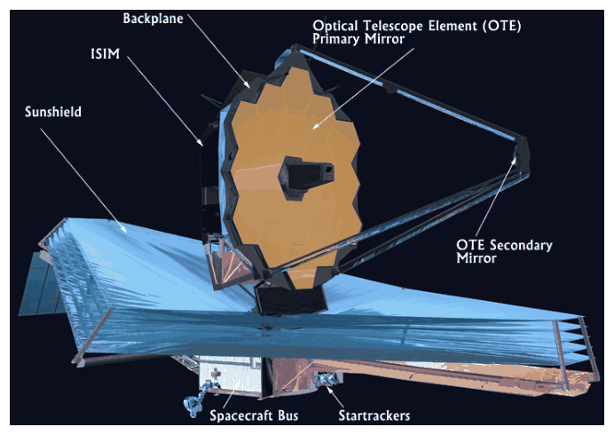
Image Credit: NASA
Part A. Imaging a Star (1.8 points)
The nearest Red Giant is 89 light-years distant, has a temperature of \(T_{\mathrm{star}}=3600\,\mathrm K\), and a diameter of \(d_o=1.7\times10^{11}\,\mathrm m\).
A.1 — 0.4pt
Calculate the diameter of a focused image of the star on the CCD camera imaging surface.
A.2 — 0.4pt
Estimate the diameter of a diffraction central maximum on the CCD camera imaging surface. Assume a wavelength of \(\lambda=800\,\mathrm{nm}\), which is the strongest intensity wavelength from the red giant star.
A.3 — 1.0pt
If the CCD is not cooled and can lose heat only by radiating from the top of the imaging surface, what would be the equilibrium temperature of the CCD at the location of the image of the red giant star? Assume the CCD surface is a blackbody. Provide a formula and a numerical estimate.
Part B. Counting Photons (1.8 points)
The absorption of a photon by the CCD camera leads to the emission of an electron within the apparatus. This occurs only if the photon has sufficient energy to excite an electron across an energy gap \(\Delta E_g\). Assume that every photon with sufficient energy succeeds. There is also leakage of electrons across the gap caused by the temperature of the CCD camera; this is the dark current \(i_d\) and is measured in the number of electrons per second. It is a function of temperature according to
\[ i_d=i_0e^{-|\Delta E_g|/(6k_BT)}. \tag{1} \]
where \(i_0\) is a constant.
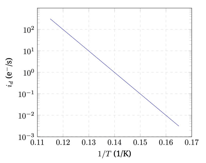
The graph shows how dark current varies with temperature. The units for dark current, \(\mathrm{e^-}/\mathrm s\) should be thought of as counting a number of electrons per second.
B.1 — 0.4pt
From the dark current graph, provide an order of magnitude estimate for the temperature of a distant source of thermal photons that would just be capable of exciting an electron on the pixel.
The electrons are collected in a capacitor, and after an exposure time \(\tau\), the electrons are counted. There are three main sources of uncertainty in the process: a fixed uncertainty in the counting process called read out noise; a Poisson distribution error associated with the dark current, and a Poisson distribution error associated with the detected incoming photons. Poisson distribution errors are equal to the square root of the number of counts associated with a process. The measured photon count is equal to the number of electrons in the capacitor, minus the number of electrons associated with the dark current.
B.2 — 0.4pt
Write an expression for the total count uncertainty \(\sigma_t\), if there is a readout noise \(\sigma_r\), a dark current \(i_d\), an incoming photon rate \(p\), and an exposure time \(\tau\).
For remaining questions in this part assume the exposure time is \(\tau=10^4\,\mathrm s\) and the read out noise is a fixed \(\sigma_r=14\).
B.3 — 0.5pt
Assume an operating temperature of \(T_p=7.5\,\mathrm K\). Calculate the minimum photon rate \(p\) so that the photon count is ten times the count uncertainty.
B.4 — 0.5pt
Assuming all photons are just capable of exciting an electron across the band gap, what is the intensity of the source of photons found in B.3 on the primary mirror? Express your answer in \(\mathrm{W/m^2}\)
Part C. Passive Cooling (4.4 points)
An infrared CCD camera must be kept at a low temperature. The first tool is a shield to protect from the sun's radiation.
The sun-shield consists of five separated reflective layers in thin sheets (black); radiant energy (gray) from the sun is incident on the first sheet on left, and some energy escapes between every pair of sheets.
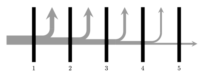
Schematic of energy flow: the vertical lines (black) are the sheets, the flow of energy (gray) is from the left to the right, however, between sheets, some energy flows up and out into space.
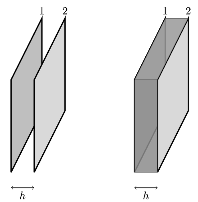
On the left is a simple model of two adjacent sheets 1 and 2 separated by a distance \(h\). The sheets are not connected, and the perimeter is open to space. Assume the sheets are parallel. Thermal radiation can be exchanged between the sheets, and thermal radiation can escape through the perimeter gap. On the right, the perimeter gap has been shaded to help visualize.
Assume the following simplifications:
- Sheets are square, each with area \(A_{\mathrm{sheet}}=200\,\mathrm{m^2}\).
- Sheets are parallel and separated by \(h=25\,\mathrm{cm}\) along the perimeter.
- Sheets have constant emissivity \(\epsilon\ll1\). Assume that all reflections off of sheet surfaces are diffuse.
- Sheets are thin with temperature on the front and back surfaces equal and uniform.
- The fraction of radiant flux emitted by a sheet that is absorbed by the adjacent sheet is \(\alpha\leq1\). This means that if sheet 1 in the figure above emits an amount of heat \(Q_1\) toward sheet 2 then sheet 2 will absorb an amount \(\alpha Q_1\) from sheet 1.
- The amount of radiant flux ejected out of the perimeter gap between two sheets is approximated as \(\beta Q_{12}\) where \(\alpha Q_{12}\) is the net flux between the two sheets. The fraction \(\beta<1\). This is equivalent to saying that the heat loss to space between two sheets is proportional to the net heat exchange between the sheets. This is a rough approximation for this problem.
- Background temperature of space is negligible.
C.1 — 2.4pt
Derive expressions for the equilibrium temperatures of the first sheet and fifth sheet in terms of the incident solar radiation intensity \(I_0\), the constants \(\alpha\) and \(\beta\), and any necessary physical constants. To simplify your expression, you may define additional constants in terms of \(\alpha\) and \(\beta\), etc.
C.2 — 1.6pt
Derive numerical estimates for \(\alpha\) and \(\beta\) from the information about the sheet geometry assuming an emissivity \(\epsilon=0.05\). You are encouraged to consider the rectangular box model of the sheets above, where the perimeter area effectively acts as a perfect absorber of radiant energy.
C.3 — 0.4pt
Numerically determine the temperatures of sheet 1 and sheet 5. The solar intensity is \(I_0=1360\,\mathrm{W/m^2}\).
Part D. Cryo-cooler (4 points)
The last stage of the cooling system directly cools the CCD camera. A closed cycle refrigeration system has a supply pipe line feeding helium gas at constant pressure \(P_1\) moving through a sponge like porous plug into a pipe with constant pressure \(P_2\). The pipe carries the gas to cool the CCD. The helium gas then passes through a pump before returning to the supply line.
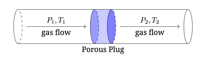
Helium gas supplied on the left at well defined pressure \(P_1\) and temperature \(T_1\) is forced through the plug to well defined pressure \(P_2\) and temperature \(T_2\), where it is carried away on the right.
As the gas moves through the porous plug, viscous friction with the narrow walls of the channels in the sponge becomes an important effect; however, no heat is transferred to or from the gas during the process. The bulk speed of the gas in region 2 is only marginally greater than the bulk speed in region 1.
Helium is not an ideal gas, but does remain in a gaseous state throughout this process.
D.1 — 1.0pt
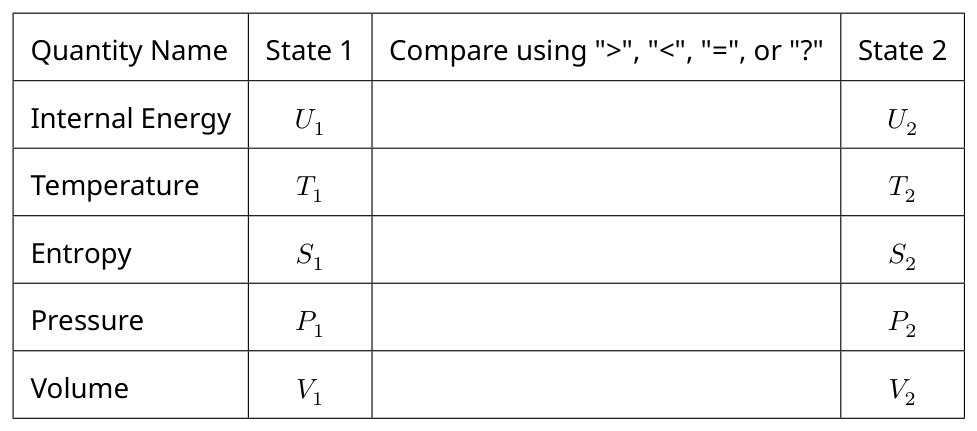
Consider a mole of gas that passes from left to right through the plug. Complete the table in your answer sheet by writing '>' or '<' to identify the quantity that must be greater, '=' to identify quantities that must be equal, or '?' if it is not possible to know which is greater or equal without more information.
D.2 — 0.6pt
Identify a conserved quantity constructed from \(U\) (internal energy), \(P\) (pressure), and \(V\) (volume) as a mole of gas moves through the plug; show work on how you derived this conserved quantity.
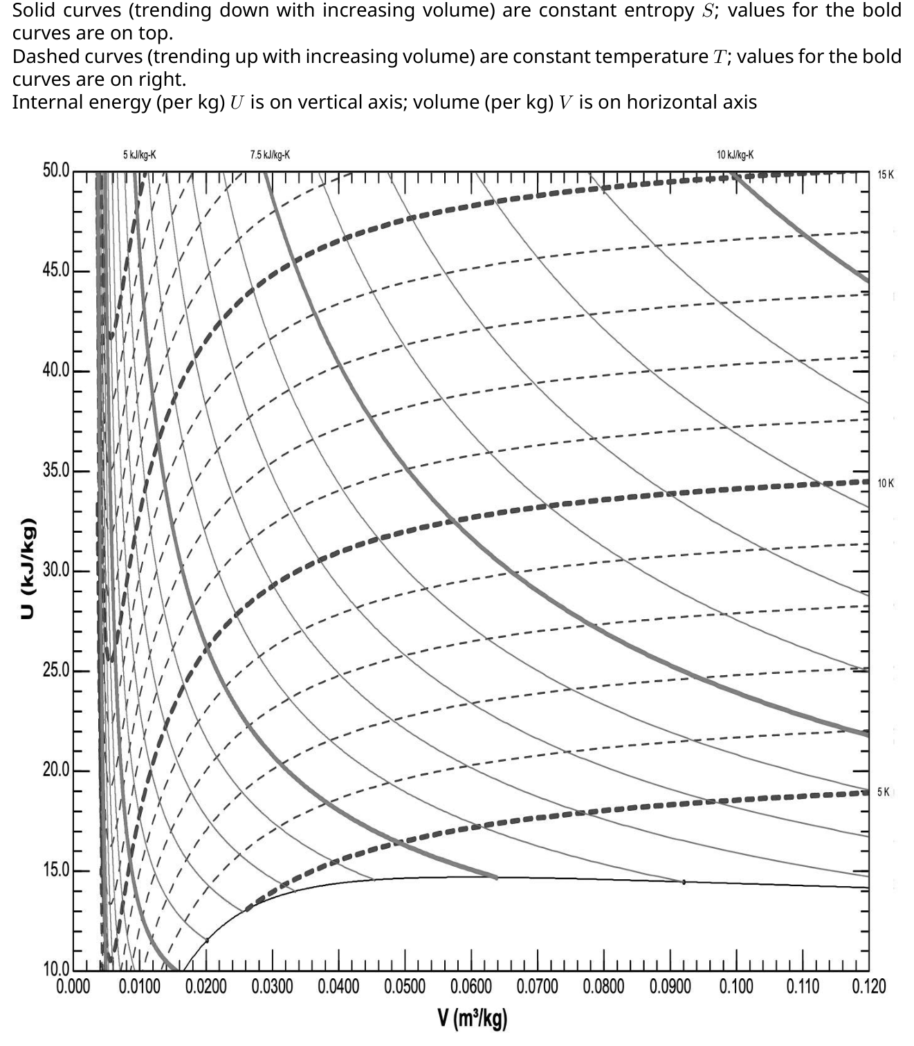
Your answer sheets have graphs of internal energy per mass against volume per mass for helium with isotherms and lines of constant entropy.
D.3 — 1.4pt
Assuming that \(V_2=0.100\,\mathrm{m^3/kg}\) and \(T_2=7.5\,\mathrm K\), use the graph to find a numerical value for the conserved quantity that you found in Part D.2. Show the construction on the graph!
D.4 — 0.8pt
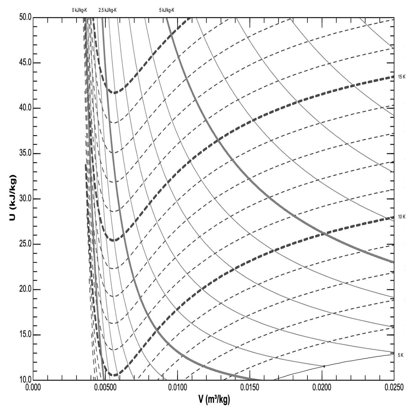
Find the maximum possible temperature for \(T_1\). Show the construction on the graph!
D.5 — 0.2pt
Assuming your value for the maximum \(T_1\) found in D.4, find a numerical value for \(P_1\).
Physical Constants
Below is the list of physical constants you might use in your solution in addition to the quantities given in the problem text.
| Physical constant | Notation | Numerical value |
|---|---|---|
| Speed of light in vacuum | \(c\) | \(299\,792\,458\,\mathrm{m/s}\) |
| Vacuum permeability (magnetic constant) | \(\mu_0\) | \(4\pi\cdot10^{-7}\,\mathrm{N/A^2};\quad[1\,\mathrm{N/A^2}=1\,\mathrm{V\,s/(A\,m)}]\) |
| Vacuum permittivity (electric constant) | \(\varepsilon_0\) | \(8.8541878128(13)\cdot10^{-12}\,\mathrm{F/m};\quad[1\,\mathrm{F/m}=1\,\mathrm{A\,s/(V\,m)}]\) |
| Elementary charge | \(e\) | \(1.602176634\cdot10^{-19}\,\mathrm C;\quad[1\,\mathrm C=1\,\mathrm{A\cdot s}]\) |
| Electron rest mass | \(m_e\) | \(9.1093837015(28)\cdot10^{-31}\,\mathrm{kg}\) |
| Proton rest mass | \(m_p\) | \(1.67262192369(51)\cdot10^{-27}\,\mathrm{kg}\) |
| Neutron rest mass | \(m_n\) | \(1.67492749804(95)\cdot10^{-27}\,\mathrm{kg}\) |
| Atomic mass unit | \(m_{\mathrm{amu}}\) | \(1.66053906660(50)\cdot10^{-27}\,\mathrm{kg}\) |
| Gravitational constant | \(G\) | \(6.67430(15)\cdot10^{-11}\,\mathrm{m^3/(kg\cdot s^2)}\) |
| Avogadro constant | \(N_A\) | \(6.02214076\cdot10^{23}\,\mathrm{mol^{-1}}\) |
| Molar gas constant | \(R\) | \(8.31446261815324\ldots\,\mathrm{J/(K\cdot mol)}\) |
| Boltzmann constant | \(k_B\) | \(1.380649\cdot10^{-23}\,\mathrm{J/K}\) |
| Stefan–Boltzmann constant | \(\sigma\) | \(5.670374419\ldots\cdot10^{-8}\,\mathrm{W/(m^2\cdot K^4)}\) |
| Planck constant | \(h\) | \(6.62607015\cdot10^{-34}\,\mathrm{J\cdot s}\) |
| Reduced Planck constant | \(\hbar=h/(2\pi)\) | \(1.0545718176\ldots\cdot10^{-34}\,\mathrm{J\cdot s}\) |
Official English text of the problem.
Answers
- A.1: \(d_{\mathrm{image}}\simeq2.6\times10^{-5}\,\mathrm m=26\,\mu\mathrm m\).
- A.2: \(d_{\mathrm{diff}}\simeq4.5\times10^{-5}\,\mathrm m=45\,\mu\mathrm m\), using an equivalent circular aperture.
- A.3: With distance \(L\) and a uniformly heated diffraction spot, \[ T_{\mathrm{image}}\simeq T_{\mathrm{star}} \left(\frac{A_{\mathrm{mirror}}d_o^2} {\pi L^2d_{\mathrm{diff}}^2}\right)^{1/4} \simeq4.1\times10^2\,\mathrm K. \]
- B.1: The characteristic-energy estimate is \(T_{\mathrm{source}}\sim10^3\,\mathrm K\), since \(|\Delta E_g|/k_B\simeq1.4\times10^3\,\mathrm K\). A wavelength-peak criterion instead gives approximately \(2.8\times10^2\,\mathrm K\).
- B.2: \(\displaystyle \sigma_t=\sqrt{\sigma_r^2+i_d\tau+p\tau}\).
- B.3: \(\displaystyle p_{\min}\simeq0.22\,\mathrm{s^{-1}}\).
- B.4: \(\displaystyle I\simeq1.7\times10^{-22}\,\mathrm{W/m^2}\).
- C.1: Define \[ r=1+\frac{\beta}{\alpha}, \qquad K=1+\frac{1+r+r^2+r^3}{\alpha}. \] Then \[ T_1=\left[\frac{I_0}{\sigma}\frac{K}{K+r^4}\right]^{1/4}, \qquad T_5=\left[\frac{I_0}{\sigma(K+r^4)}\right]^{1/4}. \]
- C.2: \(\alpha\simeq0.293,\quad\beta\simeq0.414\).
- C.3: \(T_1\simeq360\,\mathrm K,\quad T_5\simeq120\,\mathrm K\).
- D.1: In table order: \(?,\,?,\,<,\,>,\,<\).
- D.2: \(\displaystyle H=U+PV\), neglecting the small change in bulk kinetic energy.
- D.3: \(\displaystyle H/m\simeq4.0\times10^4\,\mathrm{J/kg}\), equivalent to approximately \(160\,\mathrm{J/mol}\) for helium.
- D.4: \(\displaystyle T_{1,\max}\simeq11\,\mathrm K\).
- D.5: \(\displaystyle P_1\simeq2\times10^6\,\mathrm{Pa}\).
Solution
A.1
Let the star’s distance be \(L\). Using \(1\) light-year \(\simeq9.46\times10^{15}\,\mathrm m\),
\[ L\simeq89(9.46\times10^{15}) =8.42\times10^{17}\,\mathrm m. \]
Since \(L\gg f\), the image lies essentially in the focal plane. Its angular diameter is \(d_o/L\), so
\[ d_{\mathrm{image}}=f\frac{d_o}{L} =\frac{130(1.7\times10^{11})}{8.42\times10^{17}} =2.62\times10^{-5}\,\mathrm m. \]
Thus
\[ \boxed{d_{\mathrm{image}}\simeq26\,\mu\mathrm m.} \]
A.2
Approximate the primary mirror by a circular aperture of the same area:
\[ D=2\sqrt{\frac{A_{\mathrm{mirror}}}{\pi}} =5.64\,\mathrm m. \]
For a circular aperture, the first diffraction minimum has angular radius \(1.22\lambda/D\). Consequently, the central maximum has diameter
\[ d_{\mathrm{diff}}=2.44\frac{\lambda f}{D}. \]
Numerically,
\[ d_{\mathrm{diff}} =2.44\frac{(800\times10^{-9})(130)}{5.64} =4.50\times10^{-5}\,\mathrm m. \]
Therefore,
\[ \boxed{d_{\mathrm{diff}}\simeq45\,\mu\mathrm m.} \]
The diffraction diameter exceeds the geometrical image diameter.
A.3
Treat the star as a blackbody and neglect optical losses. Its luminosity is
\[ P_{\mathrm{star}}=4\pi\left(\frac{d_o}{2}\right)^2 \sigma T_{\mathrm{star}}^4. \]
The power collected by the mirror is therefore
\[ P_{\mathrm{collected}} =A_{\mathrm{mirror}}\frac{P_{\mathrm{star}}}{4\pi L^2} =A_{\mathrm{mirror}}\sigma T_{\mathrm{star}}^4 \frac{d_o^2}{4L^2} \simeq2.43\times10^{-6}\,\mathrm W. \]
For the requested estimate, take the illuminated spot diameter to be the larger of the geometrical and diffraction diameters:
\[ d_{\mathrm{spot}}\simeq d_{\mathrm{diff}}, \qquad A_{\mathrm{spot}}\simeq\frac{\pi d_{\mathrm{diff}}^2}{4}. \]
Approximate the heating as uniform over this spot. Since only the top surface radiates, equilibrium requires
\[ P_{\mathrm{collected}} =\sigma A_{\mathrm{spot}}T_{\mathrm{image}}^4. \]
Thus
\[ \boxed{ T_{\mathrm{image}}\simeq T_{\mathrm{star}} \left( \frac{A_{\mathrm{mirror}}d_o^2} {\pi L^2d_{\mathrm{diff}}^2} \right)^{1/4} } \]
and
\[ \boxed{T_{\mathrm{image}}\simeq405\,\mathrm K \approx4.1\times10^2\,\mathrm K.} \]
This estimate neglects the detailed diffraction profile and the energy in its outer rings. In the geometrical-optics limit, substituting \(d_{\mathrm{spot}}=fd_o/L\) would instead give
\[ T_{\mathrm{image,geom}} =T_{\mathrm{star}} \left(\frac{A_{\mathrm{mirror}}}{\pi f^2}\right)^{1/4} \simeq530\,\mathrm K. \]
B.1
Taking logarithms of the dark-current law gives
\[ \ln i_d=\ln i_0-\frac{|\Delta E_g|}{6k_B}\frac1T. \]
From the graph, increasing \(1/T\) from \(0.12\,\mathrm{K^{-1}}\) to \(0.16\,\mathrm{K^{-1}}\) reduces the current from \(10^2\) to \(10^{-2}\,\mathrm{s^{-1}}\). Hence
\[ \frac{\Delta\ln i_d}{\Delta(1/T)} =\frac{\ln(10^{-4})}{0.04\,\mathrm{K^{-1}}} =-100\ln10\,\mathrm K. \]
It follows that
\[ \frac{|\Delta E_g|}{k_B} =600\ln10\,\mathrm K \simeq1.38\times10^3\,\mathrm K, \]
or
\[ \boxed{|\Delta E_g|\simeq1.91\times10^{-20}\,\mathrm J \simeq0.119\,\mathrm{eV}.} \]
Using the characteristic thermal-energy estimate \(E_\gamma\sim k_BT\),
\[ \boxed{T_{\mathrm{source}}\sim10^3\,\mathrm K.} \]
There is a convention-dependent numerical factor here. The threshold wavelength is
\[ \lambda_g=\frac{hc}{|\Delta E_g|} \simeq10.4\,\mu\mathrm m. \]
If “just capable” means that the wavelength peak of the thermal spectrum reaches this threshold, Wien scaling and the star’s given peak yield
\[ T_{\mathrm{source}} \simeq3600\,\mathrm K\, \frac{0.800\,\mu\mathrm m}{10.4\,\mu\mathrm m} \simeq2.8\times10^2\,\mathrm K. \]
Both calculations identify the relevant thermal scale; a thermal spectrum has no sharp upper photon-energy cutoff.
B.2
The mean photon count is \(p\tau\), and the mean dark count is \(i_d\tau\). Their Poisson variances equal their respective means.
Assuming independent noise sources, variances add:
\[ \boxed{\sigma_t^2=\sigma_r^2+i_d\tau+p\tau.} \]
Therefore,
\[ \boxed{\sigma_t=\sqrt{\sigma_r^2+i_d\tau+p\tau}.} \]
Subtracting the known mean dark count removes its mean contribution but leaves its statistical fluctuations.
B.3
The straight line on the graph corresponds approximately to
\[ i_d(T)=10^{\,14-100\,\mathrm K/T}\,\mathrm{s^{-1}}. \]
At \(T_p=7.5\,\mathrm K\),
\[ i_d=10^{14-100/7.5} =10^{2/3} \simeq4.64\,\mathrm{s^{-1}}. \]
Write \(N=p\tau\) for the expected photon count. The limiting condition is
\[ N=10\sqrt{\sigma_r^2+i_d\tau+N}. \]
Squaring and solving the resulting quadratic gives the positive root
\[ N=50+\sqrt{2500+100(\sigma_r^2+i_d\tau)}. \]
With \(\sigma_r=14\) and \(\tau=10^4\,\mathrm s\),
\[ N\simeq2.21\times10^3. \]
Thus
\[ \boxed{p_{\min}=\frac{N}{\tau} \simeq0.221\,\mathrm{s^{-1}} \approx0.22\,\mathrm{s^{-1}}.} \]
B.4
Each threshold photon has energy \(|\Delta E_g|\). With unit detection efficiency and lossless collection, the required power at the mirror is \(p|\Delta E_g|\). Hence
\[ I=\frac{p|\Delta E_g|}{A_{\mathrm{mirror}}}. \]
Substitution gives
\[ I=\frac{(0.221)(1.91\times10^{-20})}{25} \simeq1.69\times10^{-22}\,\mathrm{W/m^2}. \]
Therefore,
\[ \boxed{I\simeq1.7\times10^{-22}\,\mathrm{W/m^2}.} \]
C.1
Let \(A=A_{\mathrm{sheet}}\), and define the power emitted by one face of sheet \(i\) as
\[ q_i=\epsilon\sigma A T_i^4. \]
By Kirchhoff’s law, the constant emissivity also gives the absorptivity, so sheet 1 absorbs solar power
\[ P_\odot=\epsilon I_0A. \]
Following the stipulated left-to-right leakage model, define the net power received by sheet \(i+1\) from the preceding gap as
\[ F_i=\alpha(q_i-q_{i+1}). \]
The accompanying power escaping through that gap is
\[ L_i=\beta(q_i-q_{i+1}) =\frac{\beta}{\alpha}F_i. \]
Thus the total power entering a gap from its hotter side is
\[ F_i+L_i=rF_i, \qquad r=1+\frac{\beta}{\alpha}. \]
For each intermediate sheet, equilibrium requires
\[ F_{i-1}=rF_i, \qquad i=2,3,4. \]
The final sheet radiates \(q_5\) from its exposed face, so
\[ F_4=q_5. \]
Working back through the gaps,
\[ F_3=rq_5,\qquad F_2=r^2q_5,\qquad F_1=r^3q_5. \]
The temperature differences satisfy
\[ q_i-q_{i+1}=\frac{F_i}{\alpha}. \]
Adding all four differences gives
\[ q_1-q_5 =\frac{q_5}{\alpha}(1+r+r^2+r^3). \]
Define
\[ K=1+\frac{1+r+r^2+r^3}{\alpha}; \]
then \(q_1=Kq_5\).
Finally, the first sheet loses \(q_1\) through its Sun-facing surface and \(rF_1\) into the first gap:
\[ \epsilon I_0A=q_1+rF_1 =(K+r^4)q_5. \]
Using \(q_5=\epsilon\sigma AT_5^4\), we obtain
\[ \boxed{ T_5=\left[\frac{I_0}{\sigma(K+r^4)}\right]^{1/4} } \]
and, since \(T_1^4=KT_5^4\),
\[ \boxed{ T_1=\left[\frac{I_0}{\sigma}\frac{K}{K+r^4}\right]^{1/4}. } \]
The explicit factors of \(\epsilon A\) cancel; the emissivity still influences \(\alpha\) and \(\beta\).
C.2
The side length of a sheet is
\[ a=\sqrt{A}=\sqrt{200}=14.14\,\mathrm m. \]
The perimeter opening has area
\[ A_{\mathrm{gap}}=4ah =4(14.14)(0.25) =14.14\,\mathrm{m^2}. \]
Because the sheets are highly reflective and reflections are diffuse, approximate the radiation inside the box as well mixed after repeated reflections. Absorption probabilities are then proportional to absorbing area.
Each sheet has effective absorbing area \(\epsilon A\), while the opening acts as a black absorber with effective area \(A_{\mathrm{gap}}\). The total effective absorbing area is therefore
\[ 2\epsilon A+A_{\mathrm{gap}}. \]
The fraction ultimately absorbed by the other sheet is approximately
\[ \boxed{ \alpha\simeq \frac{\epsilon A}{2\epsilon A+A_{\mathrm{gap}}}. } \]
The fraction escaping is approximately
\[ \boxed{ \beta\simeq \frac{A_{\mathrm{gap}}}{2\epsilon A+A_{\mathrm{gap}}}. } \]
For \(\epsilon A=0.05(200)=10\,\mathrm{m^2}\),
\[ \boxed{\alpha\simeq\frac{10}{20+14.14}=0.293,} \]
\[ \boxed{\beta\simeq\frac{14.14}{20+14.14}=0.414.} \]
The remaining fraction, approximately \(\alpha\), returns to and is absorbed by the emitting sheet; accordingly, \(2\alpha+\beta=1\) in this estimate.
C.3
The preceding estimates give
\[ r=1+\frac{\beta}{\alpha}=2.414, \]
\[ r^4\simeq33.97,\qquad K\simeq80.60, \qquad K+r^4\simeq114.57. \]
Therefore,
\[ T_5= \left[ \frac{1360} {(5.670374419\times10^{-8})(114.57)} \right]^{1/4} \simeq120.3\,\mathrm K, \]
and
\[ T_1=K^{1/4}T_5\simeq360.4\,\mathrm K. \]
Thus
\[ \boxed{T_1\simeq360\,\mathrm K,\qquad T_5\simeq120\,\mathrm K.} \]
D.1
The required entries are:
| Quantity | Comparison |
|---|---|
| Internal energy | \(U_1\ ?\ U_2\) |
| Temperature | \(T_1\ ?\ T_2\) |
| Entropy | \(S_1<S_2\) |
| Pressure | \(P_1>P_2\) |
| Volume | \(V_1<V_2\) |
A pressure drop drives the flow through the resistive plug, so \(P_1>P_2\). Viscous dissipation makes the adiabatic process irreversible, giving \(S_2>S_1\).
Using the equal pipe cross sections shown, steady mass conservation gives
\[ \rho_1w_1=\rho_2w_2, \]
where \(w\) is bulk speed. Since \(w_2>w_1\), the density decreases and the volume occupied by one mole increases.
For a real gas, neither internal energy nor temperature has a universal direction of change during throttling. Their comparisons require further information about the states.
D.2
Follow one mole through the plug. The upstream gas does work \(P_1V_1\) on this mole, while it does work \(P_2V_2\) on the downstream gas.
There is no heat transfer. Neglecting the small change in bulk kinetic energy, the first law gives
\[ U_2-U_1=P_1V_1-P_2V_2. \]
Rearranging,
\[ \boxed{U_1+P_1V_1=U_2+P_2V_2.} \]
Thus the conserved quantity is the enthalpy,
\[ \boxed{H=U+PV.} \]
More precisely, steady adiabatic flow conserves \(h+w^2/2\) per unit mass. The stated approximation permits neglecting the kinetic-energy difference.
D.3
For clarity, write \(u\) and \(v\) for the specific internal energy and specific volume labelled \(U\) and \(V\) on the graphs.
The thermodynamic identity is
\[ du=T\,ds-P\,dv. \]
Along a constant-entropy curve,
\[ \left(\frac{\partial u}{\partial v}\right)_s=-P. \]
Therefore, the tangent to an isentrope at \((v,u)\) has equation
\[ u_{\mathrm{tan}}(x)=u-P(x-v) =(u+Pv)-Px. \]
Its intercept on the vertical axis is precisely the specific enthalpy:
\[ \boxed{h=u+Pv.} \]
The required construction on image 9 is:
- Locate \(v_2=0.100\,\mathrm{m^3/kg}\).
- Interpolate to the \(7.5\,\mathrm K\) isotherm.
- At this state, draw the tangent to the constant-entropy curve passing through it.
- Extend that tangent to \(v=0\); read its vertical intercept.
The state has approximately
\[ u_2\simeq26\,\mathrm{kJ/kg}. \]
The tangent slope is approximately
\[ -P_2\simeq-140\,\mathrm{kPa}. \]
Consequently,
\[ h_2=u_2+P_2v_2 \simeq26+(140)(0.100) =40\,\mathrm{kJ/kg}. \]
Thus
\[ \boxed{h_1=h_2\simeq4.0\times10^4\,\mathrm{J/kg}.} \]
For helium with molar mass approximately \(4.0\times10^{-3}\,\mathrm{kg/mol}\), this corresponds to
\[ H_{\mathrm{molar}}\simeq160\,\mathrm{J/mol}. \]
D.4
All admissible inlet states must have the same specific enthalpy \(h_0\simeq40\,\mathrm{kJ/kg}\).
The graphical construction on image 10 is:
- Mark the point \((0,h_0)\) on the vertical axis.
- Draw tangents from this point to several solid constant-entropy curves.
- Mark their points of tangency. Every such point has \(u+Pv=h_0\), so these points trace the constant-enthalpy curve.
- Find the highest-temperature dashed isotherm reached by this curve. At the maximum temperature, the constant-enthalpy curve touches that isotherm.
The limiting contact is close to the \(11\,\mathrm K\) isotherm, with graphical readings approximately
\[ v_1\sim1.0\times10^{-2}\,\mathrm{m^3/kg}, \qquad u_1\sim2.1\times10^4\,\mathrm{J/kg}. \]
The graph supports a maximum of roughly \(10.5\)–\(11\,\mathrm K\), so
\[ \boxed{T_{1,\max}\simeq11\,\mathrm K.} \]
D.5
The pressure is the magnitude of the isentropic tangent slope at the selected inlet state. Equivalently,
\[ P_1=\frac{h_0-u_1}{v_1}. \]
Using the approximate graphical coordinates,
\[ P_1\simeq \frac{(40-21)\times10^3}{1.0\times10^{-2}} =1.9\times10^6\,\mathrm{Pa}. \]
To the precision justified by the graph,
\[ \boxed{P_1\simeq2\times10^6\,\mathrm{Pa}.} \]
The solution was checked against the official solution.
IPhO 2022 · Theorieaufgabe 2
James-Webb-Weltraumteleskop
In dieser Aufgabe geht es um die Physik des James-Webb-Weltraumteleskops. Das Licht eines Sterns trifft auf den Hauptspiegel mit einer Fläche von \(A_{\mathrm{mirror}}=25\,\mathrm{m^2}\) und wird an einem Sekundärspiegel reflektiert. Die Brennweite des Systems beträgt \(f=130\,\mathrm m\). Das Licht wird im ISIM (Integriertes Wissenschaftliches Instrumentenmodul) fokussiert, das die CCD-Kameras (ladungsgekoppelte Bauelemente) enthält.
Bildnachweis: NASA
Teil A. Abbildung eines Sterns (1.8 Punkte)
Der nächstgelegene Rote Riese ist 89 Lichtjahre entfernt, hat eine Temperatur von \(T_{\mathrm{star}}=3600\,\mathrm K\) und einen Durchmesser von \(d_o=1.7\times10^{11}\,\mathrm m\).
A.1 — 0.4 Punkte
Berechnen Sie den Durchmesser des scharf abgebildeten Sterns auf der Bildfläche der CCD-Kamera.
A.2 — 0.4 Punkte
Schätzen Sie den Durchmesser des zentralen Beugungsmaximums auf der Bildfläche der CCD-Kamera ab. Nehmen Sie eine Wellenlänge von \(\lambda=800\,\mathrm{nm}\) an; bei dieser Wellenlänge ist die Intensität des Roten Riesen am größten.
A.3 — 1.0 Punkte
Wenn der CCD nicht gekühlt wird und Wärme nur durch Abstrahlung von der Oberseite der Bildfläche abgeben kann, welche Gleichgewichtstemperatur würde sich dann am Ort des Bildes des Roten Riesen auf dem CCD einstellen? Nehmen Sie an, dass die CCD-Oberfläche ein schwarzer Körper ist. Geben Sie eine Formel und eine numerische Abschätzung an.
Teil B. Zählen von Photonen (1.8 Punkte)
Die Absorption eines Photons durch die CCD-Kamera führt zur Freisetzung eines Elektrons innerhalb der Apparatur. Dies geschieht nur, wenn das Photon genügend Energie besitzt, um ein Elektron über eine Energielücke \(\Delta E_g\) hinweg anzuregen. Nehmen Sie an, dass dies jedem Photon mit ausreichender Energie gelingt. Aufgrund der Temperatur der CCD-Kamera gelangen auch Elektronen als Leckstrom über die Energielücke; dies ist der Dunkelstrom \(i_d\), der als Anzahl von Elektronen pro Sekunde gemessen wird. Er hängt gemäß
\[ i_d=i_0e^{-|\Delta E_g|/(6k_BT)}. \tag{1} \]
von der Temperatur ab, wobei \(i_0\) eine Konstante ist.
Das Diagramm zeigt die Temperaturabhängigkeit des Dunkelstroms. Die Einheit des Dunkelstroms, \(\mathrm{e^-}/\mathrm s\), ist als Anzahl von Elektronen pro Sekunde zu verstehen.
B.1 — 0.4 Punkte
Schätzen Sie anhand des Dunkelstromdiagramms die Größenordnung der Temperatur einer entfernten Quelle thermischer Photonen ab, die gerade noch ein Elektron im Pixel anregen könnten.
Die Elektronen werden in einem Kondensator gesammelt und nach einer Belichtungszeit \(\tau\) gezählt. Bei diesem Vorgang gibt es drei wesentliche Unsicherheitsquellen: eine feste Unsicherheit beim Zählvorgang, die als Ausleserauschen bezeichnet wird; einen durch die Poisson-Verteilung beschriebenen Fehler des Dunkelstroms und einen durch die Poisson-Verteilung beschriebenen Fehler der nachgewiesenen einfallenden Photonen. Fehler gemäß der Poisson-Verteilung sind gleich der Quadratwurzel aus der Anzahl der zum jeweiligen Prozess gehörenden Zählereignisse. Die gemessene Photonenzahl ist gleich der Anzahl der Elektronen im Kondensator abzüglich der Anzahl der dem Dunkelstrom zuzuordnenden Elektronen.
B.2 — 0.4 Punkte
Geben Sie einen Ausdruck für die gesamte Zählunsicherheit \(\sigma_t\) an, wenn das Ausleserauschen \(\sigma_r\), der Dunkelstrom \(i_d\), die Rate einfallender Photonen \(p\) und die Belichtungszeit \(\tau\) betragen.
Nehmen Sie für die verbleibenden Fragen dieses Teils eine Belichtungszeit von \(\tau=10^4\,\mathrm s\) und ein festes Ausleserauschen von \(\sigma_r=14\) an.
B.3 — 0.5 Punkte
Nehmen Sie eine Betriebstemperatur von \(T_p=7.5\,\mathrm K\) an. Berechnen Sie die minimale Photonenrate \(p\), bei der die Photonenzahl das Zehnfache der Zählunsicherheit beträgt.
B.4 — 0.5 Punkte
Angenommen, alle Photonen können gerade noch ein Elektron über die Bandlücke hinweg anregen: Welche Intensität hat die in B.3 gefundene Photonenquelle am Hauptspiegel? Geben Sie Ihre Antwort in \(\mathrm{W/m^2}\) an.
Teil C. Passive Kühlung (4.4 Punkte)
Eine Infrarot-CCD-Kamera muss auf einer niedrigen Temperatur gehalten werden. Das erste Hilfsmittel ist ein Schild zum Schutz vor der Sonnenstrahlung.
Der Sonnenschild besteht aus fünf voneinander getrennten reflektierenden Schichten aus dünnen Folien (schwarz); Strahlungsenergie (grau) von der Sonne fällt auf die erste Folie links, und zwischen jedem Folienpaar entweicht ein Teil der Energie.
Schematische Darstellung des Energieflusses: Die vertikalen Linien (schwarz) sind die Folien, der Energiefluss (grau) verläuft von links nach rechts; zwischen den Folien fließt jedoch ein Teil der Energie nach oben und hinaus ins Weltall.
Links ist ein einfaches Modell zweier benachbarter Folien 1 und 2 dargestellt, die durch einen Abstand \(h\) voneinander getrennt sind. Die Folien sind nicht miteinander verbunden, und der Rand ist zum Weltall hin offen. Nehmen Sie an, dass die Folien parallel sind. Zwischen den Folien kann Wärmestrahlung ausgetauscht werden, und durch den umlaufenden Randspalt kann Wärmestrahlung entweichen. Rechts ist der Randspalt zur Veranschaulichung schattiert dargestellt.
Nehmen Sie die folgenden Vereinfachungen an:
- Die Folien sind quadratisch und haben jeweils eine Fläche von \(A_{\mathrm{sheet}}=200\,\mathrm{m^2}\).
- Die Folien sind parallel und haben entlang des Randes einen Abstand von \(h=25\,\mathrm{cm}\).
- Die Folien haben einen konstanten Emissionsgrad \(\epsilon\ll1\). Nehmen Sie an, dass alle Reflexionen an den Folienoberflächen diffus sind.
- Die Folien sind dünn, wobei die Temperatur auf Vorder- und Rückseite gleich und gleichmäßig ist.
- Der Anteil des von einer Folie emittierten Strahlungsflusses, der von der benachbarten Folie absorbiert wird, beträgt \(\alpha\leq1\). Das bedeutet: Wenn Folie 1 in der obigen Abbildung eine Wärmemenge \(Q_1\) in Richtung von Folie 2 emittiert, absorbiert Folie 2 davon eine Menge \(\alpha Q_1\).
- Der durch den Randspalt zwischen zwei Folien austretende Strahlungsfluss wird durch \(\beta Q_{12}\) angenähert, wobei \(\alpha Q_{12}\) der Nettofluss zwischen den beiden Folien ist. Für den Anteil gilt \(\beta<1\). Dies entspricht der Aussage, dass der Wärmeverlust ins Weltall zwischen zwei Folien proportional zum Nettowärmeaustausch zwischen den Folien ist. Dies ist eine grobe Näherung für diese Aufgabe.
- Die Hintergrundtemperatur des Weltalls ist vernachlässigbar.
C.1 — 2.4 Punkte
Leiten Sie Ausdrücke für die Gleichgewichtstemperaturen der ersten und der fünften Folie in Abhängigkeit von der Intensität der einfallenden Sonnenstrahlung \(I_0\), den Konstanten \(\alpha\) und \(\beta\) sowie gegebenenfalls benötigten physikalischen Konstanten her. Zur Vereinfachung Ihrer Ausdrücke dürfen Sie zusätzliche Konstanten in Abhängigkeit von \(\alpha\) und \(\beta\) usw. definieren.
C.2 — 1.6 Punkte
Leiten Sie aus den Angaben zur Foliengeometrie unter Annahme eines Emissionsgrades von \(\epsilon=0.05\) numerische Abschätzungen für \(\alpha\) und \(\beta\) her. Es empfiehlt sich, das oben dargestellte Quader-Modell der Folien zu betrachten, bei dem die umlaufende Seitenfläche effektiv als perfekter Absorber für Strahlungsenergie wirkt.
C.3 — 0.4 Punkte
Bestimmen Sie die Temperaturen von Folie 1 und Folie 5 numerisch. Die Intensität der Sonnenstrahlung beträgt \(I_0=1360\,\mathrm{W/m^2}\).
Teil D. Kryokühler (4 Punkte)
Die letzte Stufe des Kühlsystems kühlt die CCD-Kamera direkt. Ein Kältesystem mit geschlossenem Kreislauf besitzt eine Zuleitung, die Heliumgas bei konstantem Druck \(P_1\) zuführt. Das Gas strömt durch einen schwammartigen porösen Pfropfen in ein Rohr mit konstantem Druck \(P_2\). Das Rohr führt das Gas zur Kühlung des CCD weiter. Anschließend durchläuft das Heliumgas eine Pumpe, bevor es in die Zuleitung zurückkehrt.
Das links bei einem wohldefinierten Druck \(P_1\) und einer wohldefinierten Temperatur \(T_1\) zugeführte Heliumgas wird durch den Pfropfen auf einen wohldefinierten Druck \(P_2\) und eine wohldefinierte Temperatur \(T_2\) gebracht und rechts abgeführt.
Beim Durchströmen des porösen Pfropfens spielt die viskose Reibung an den Wänden der engen Kanäle im Schwamm eine wichtige Rolle; während dieses Vorgangs wird jedoch keine Wärme auf das Gas übertragen oder von ihm abgegeben. Die makroskopische Strömungsgeschwindigkeit des Gases in Bereich 2 ist nur geringfügig größer als diejenige in Bereich 1.
Helium ist kein ideales Gas, bleibt aber während des gesamten Vorgangs gasförmig.
D.1 — 1.0 Punkte
Betrachten Sie ein Mol Gas, das den Pfropfen von links nach rechts durchströmt. Vervollständigen Sie die Tabelle auf Ihrem Antwortbogen, indem Sie mit „>“ oder „<“ angeben, welche Größe größer sein muss, mit „=“ Größen kennzeichnen, die gleich sein müssen, oder „?“ eintragen, wenn sich ohne weitere Informationen nicht entscheiden lässt, welche Größe größer ist oder ob beide gleich sind.
D.2 — 0.6 Punkte
Bestimmen Sie eine aus \(U\) (innerer Energie), \(P\) (Druck) und \(V\) (Volumen) zusammengesetzte Größe, die beim Durchströmen eines Mols Gas durch den Pfropfen erhalten bleibt; zeigen Sie Ihre Herleitung dieser Erhaltungsgröße.
Auf Ihren Antwortbögen befinden sich Diagramme der inneren Energie pro Masse in Abhängigkeit vom Volumen pro Masse für Helium mit Isothermen und Linien konstanter Entropie.
D.3 — 1.4 Punkte
Nehmen Sie \(V_2=0.100\,\mathrm{m^3/kg}\) und \(T_2=7.5\,\mathrm K\) an und bestimmen Sie mithilfe des Diagramms einen Zahlenwert für die in Teil D.2 gefundene Erhaltungsgröße. Zeigen Sie die Konstruktion im Diagramm!
D.4 — 0.8 Punkte
Bestimmen Sie die maximal mögliche Temperatur für \(T_1\). Zeigen Sie die Konstruktion im Diagramm!
D.5 — 0.2 Punkte
Bestimmen Sie unter Annahme Ihres in D.4 gefundenen Wertes für das maximale \(T_1\) einen Zahlenwert für \(P_1\).
Physikalische Konstanten
Nachfolgend finden Sie eine Liste physikalischer Konstanten, die Sie zusätzlich zu den im Aufgabentext angegebenen Größen für Ihre Lösung verwenden können.
| Physikalische Konstante | Symbol | Zahlenwert |
|---|---|---|
| Lichtgeschwindigkeit im Vakuum | \(c\) | \(299\,792\,458\,\mathrm{m/s}\) |
| Vakuumpermeabilität (magnetische Feldkonstante) | \(\mu_0\) | \(4\pi\cdot10^{-7}\,\mathrm{N/A^2};\quad[1\,\mathrm{N/A^2}=1\,\mathrm{V\,s/(A\,m)}]\) |
| Vakuumpermittivität (elektrische Feldkonstante) | \(\varepsilon_0\) | \(8.8541878128(13)\cdot10^{-12}\,\mathrm{F/m};\quad[1\,\mathrm{F/m}=1\,\mathrm{A\,s/(V\,m)}]\) |
| Elementarladung | \(e\) | \(1.602176634\cdot10^{-19}\,\mathrm C;\quad[1\,\mathrm C=1\,\mathrm{A\cdot s}]\) |
| Ruhemasse des Elektrons | \(m_e\) | \(9.1093837015(28)\cdot10^{-31}\,\mathrm{kg}\) |
| Ruhemasse des Protons | \(m_p\) | \(1.67262192369(51)\cdot10^{-27}\,\mathrm{kg}\) |
| Ruhemasse des Neutrons | \(m_n\) | \(1.67492749804(95)\cdot10^{-27}\,\mathrm{kg}\) |
| Atomare Masseneinheit | \(m_{\mathrm{amu}}\) | \(1.66053906660(50)\cdot10^{-27}\,\mathrm{kg}\) |
| Gravitationskonstante | \(G\) | \(6.67430(15)\cdot10^{-11}\,\mathrm{m^3/(kg\cdot s^2)}\) |
| Avogadro-Konstante | \(N_A\) | \(6.02214076\cdot10^{23}\,\mathrm{mol^{-1}}\) |
| Universelle Gaskonstante | \(R\) | \(8.31446261815324\ldots\,\mathrm{J/(K\cdot mol)}\) |
| Boltzmann-Konstante | \(k_B\) | \(1.380649\cdot10^{-23}\,\mathrm{J/K}\) |
| Stefan–Boltzmann-Konstante | \(\sigma\) | \(5.670374419\ldots\cdot10^{-8}\,\mathrm{W/(m^2\cdot K^4)}\) |
| Planck-Konstante | \(h\) | \(6.62607015\cdot10^{-34}\,\mathrm{J\cdot s}\) |
| Reduzierte Planck-Konstante | \(\hbar=h/(2\pi)\) | \(1.0545718176\ldots\cdot10^{-34}\,\mathrm{J\cdot s}\) |
Aufgabentext aus dem offiziellen englischen Text übersetzt.
Antworten
- A.1: \(d_{\mathrm{image}}\simeq2.6\times10^{-5}\,\mathrm m=26\,\mu\mathrm m\).
- A.2: \(d_{\mathrm{diff}}\simeq4.5\times10^{-5}\,\mathrm m=45\,\mu\mathrm m\), unter Verwendung einer äquivalenten kreisförmigen Apertur.
- A.3: Mit dem Abstand \(L\) und einem gleichmäßig erwärmten Beugungsfleck gilt \[ T_{\mathrm{image}}\simeq T_{\mathrm{star}} \left(\frac{A_{\mathrm{mirror}}d_o^2} {\pi L^2d_{\mathrm{diff}}^2}\right)^{1/4} \simeq4.1\times10^2\,\mathrm K. \]
- B.1: Die Abschätzung anhand der charakteristischen Energie ergibt \(T_{\mathrm{source}}\sim10^3\,\mathrm K\), da \(|\Delta E_g|/k_B\simeq1.4\times10^3\,\mathrm K\). Ein Kriterium anhand des Maximums der Wellenlängenverteilung ergibt stattdessen ungefähr \(2.8\times10^2\,\mathrm K\).
- B.2: \(\displaystyle \sigma_t=\sqrt{\sigma_r^2+i_d\tau+p\tau}\).
- B.3: \(\displaystyle p_{\min}\simeq0.22\,\mathrm{s^{-1}}\).
- B.4: \(\displaystyle I\simeq1.7\times10^{-22}\,\mathrm{W/m^2}\).
- C.1: Wir definieren \[ r=1+\frac{\beta}{\alpha}, \qquad K=1+\frac{1+r+r^2+r^3}{\alpha}. \] Dann gilt \[ T_1=\left[\frac{I_0}{\sigma}\frac{K}{K+r^4}\right]^{1/4}, \qquad T_5=\left[\frac{I_0}{\sigma(K+r^4)}\right]^{1/4}. \]
- C.2: \(\alpha\simeq0.293,\quad\beta\simeq0.414\).
- C.3: \(T_1\simeq360\,\mathrm K,\quad T_5\simeq120\,\mathrm K\).
- D.1: In der Reihenfolge der Tabelle: \(?,\,?,\,<,\,>,\,<\).
- D.2: \(\displaystyle H=U+PV\), unter Vernachlässigung der kleinen Änderung der makroskopischen kinetischen Energie.
- D.3: \(\displaystyle H/m\simeq4.0\times10^4\,\mathrm{J/kg}\), entsprechend ungefähr \(160\,\mathrm{J/mol}\) für Helium.
- D.4: \(\displaystyle T_{1,\max}\simeq11\,\mathrm K\).
- D.5: \(\displaystyle P_1\simeq2\times10^6\,\mathrm{Pa}\).
Lösung
A.1
Der Abstand des Sterns sei \(L\). Mit \(1\) Lichtjahr \(\simeq9.46\times10^{15}\,\mathrm m\) ergibt sich
\[ L\simeq89(9.46\times10^{15}) =8.42\times10^{17}\,\mathrm m. \]
Da \(L\gg f\), liegt das Bild praktisch in der Brennebene. Sein Winkeldurchmesser beträgt \(d_o/L\), sodass
\[ d_{\mathrm{image}}=f\frac{d_o}{L} =\frac{130(1.7\times10^{11})}{8.42\times10^{17}} =2.62\times10^{-5}\,\mathrm m. \]
Damit folgt
\[ \boxed{d_{\mathrm{image}}\simeq26\,\mu\mathrm m.} \]
A.2
Wir nähern den Hauptspiegel durch eine kreisförmige Apertur gleicher Fläche an:
\[ D=2\sqrt{\frac{A_{\mathrm{mirror}}}{\pi}} =5.64\,\mathrm m. \]
Bei einer kreisförmigen Apertur hat das erste Beugungsminimum einen Winkelradius von \(1.22\lambda/D\). Folglich hat das zentrale Maximum den Durchmesser
\[ d_{\mathrm{diff}}=2.44\frac{\lambda f}{D}. \]
Numerisch ergibt sich
\[ d_{\mathrm{diff}} =2.44\frac{(800\times10^{-9})(130)}{5.64} =4.50\times10^{-5}\,\mathrm m. \]
Also gilt
\[ \boxed{d_{\mathrm{diff}}\simeq45\,\mu\mathrm m.} \]
Der Beugungsdurchmesser ist größer als der geometrische Bilddurchmesser.
A.3
Wir behandeln den Stern als schwarzen Körper und vernachlässigen optische Verluste. Seine Leuchtkraft beträgt
\[ P_{\mathrm{star}}=4\pi\left(\frac{d_o}{2}\right)^2 \sigma T_{\mathrm{star}}^4. \]
Die vom Spiegel gesammelte Leistung ist daher
\[ P_{\mathrm{collected}} =A_{\mathrm{mirror}}\frac{P_{\mathrm{star}}}{4\pi L^2} =A_{\mathrm{mirror}}\sigma T_{\mathrm{star}}^4 \frac{d_o^2}{4L^2} \simeq2.43\times10^{-6}\,\mathrm W. \]
Für die verlangte Abschätzung setzen wir den Durchmesser des beleuchteten Flecks gleich dem größeren der beiden Durchmesser, dem geometrischen Bilddurchmesser und dem Beugungsdurchmesser:
\[ d_{\mathrm{spot}}\simeq d_{\mathrm{diff}}, \qquad A_{\mathrm{spot}}\simeq\frac{\pi d_{\mathrm{diff}}^2}{4}. \]
Wir nehmen näherungsweise eine gleichmäßige Erwärmung über diesen Fleck an. Da nur die Oberseite abstrahlt, erfordert das Gleichgewicht
\[ P_{\mathrm{collected}} =\sigma A_{\mathrm{spot}}T_{\mathrm{image}}^4. \]
Damit folgt
\[ \boxed{ T_{\mathrm{image}}\simeq T_{\mathrm{star}} \left( \frac{A_{\mathrm{mirror}}d_o^2} {\pi L^2d_{\mathrm{diff}}^2} \right)^{1/4} } \]
und
\[ \boxed{T_{\mathrm{image}}\simeq405\,\mathrm K \approx4.1\times10^2\,\mathrm K.} \]
Diese Abschätzung vernachlässigt das genaue Beugungsprofil und die Energie in dessen äußeren Ringen. Im Grenzfall der geometrischen Optik würde das Einsetzen von \(d_{\mathrm{spot}}=fd_o/L\) stattdessen Folgendes ergeben:
\[ T_{\mathrm{image,geom}} =T_{\mathrm{star}} \left(\frac{A_{\mathrm{mirror}}}{\pi f^2}\right)^{1/4} \simeq530\,\mathrm K. \]
B.1
Durch Logarithmieren des Dunkelstromgesetzes ergibt sich
\[ \ln i_d=\ln i_0-\frac{|\Delta E_g|}{6k_B}\frac1T. \]
Aus dem Diagramm lässt sich ablesen, dass eine Erhöhung von \(1/T\) von \(0.12\,\mathrm{K^{-1}}\) auf \(0.16\,\mathrm{K^{-1}}\) den Strom von \(10^2\) auf \(10^{-2}\,\mathrm{s^{-1}}\) verringert. Somit gilt
\[ \frac{\Delta\ln i_d}{\Delta(1/T)} =\frac{\ln(10^{-4})}{0.04\,\mathrm{K^{-1}}} =-100\ln10\,\mathrm K. \]
Daraus folgt
\[ \frac{|\Delta E_g|}{k_B} =600\ln10\,\mathrm K \simeq1.38\times10^3\,\mathrm K, \]
oder
\[ \boxed{|\Delta E_g|\simeq1.91\times10^{-20}\,\mathrm J \simeq0.119\,\mathrm{eV}.} \]
Mit der Abschätzung für die charakteristische thermische Energie \(E_\gamma\sim k_BT\) ergibt sich
\[ \boxed{T_{\mathrm{source}}\sim10^3\,\mathrm K.} \]
Hier tritt ein von der Konvention abhängiger Zahlenfaktor auf. Die Schwellenwellenlänge beträgt
\[ \lambda_g=\frac{hc}{|\Delta E_g|} \simeq10.4\,\mu\mathrm m. \]
Wenn „gerade noch“ bedeutet, dass das Maximum der Wellenlängenverteilung des thermischen Spektrums diese Schwelle erreicht, ergeben das Wiensche Verschiebungsgesetz und das angegebene Maximum des Sterns
\[ T_{\mathrm{source}} \simeq3600\,\mathrm K\, \frac{0.800\,\mu\mathrm m}{10.4\,\mu\mathrm m} \simeq2.8\times10^2\,\mathrm K. \]
Beide Rechnungen bestimmen die relevante thermische Skala; ein thermisches Spektrum besitzt keine scharfe obere Grenze der Photonenenergie.
B.2
Die mittlere Photonenzahl beträgt \(p\tau\), und die mittlere Dunkelzählung beträgt \(i_d\tau\). Ihre Poisson-Varianzen sind gleich den jeweiligen Mittelwerten.
Unter der Annahme unabhängiger Rauschquellen addieren sich die Varianzen:
\[ \boxed{\sigma_t^2=\sigma_r^2+i_d\tau+p\tau.} \]
Daher gilt
\[ \boxed{\sigma_t=\sqrt{\sigma_r^2+i_d\tau+p\tau}.} \]
Das Subtrahieren der bekannten mittleren Dunkelzählung entfernt deren mittleren Beitrag, lässt aber ihre statistischen Schwankungen bestehen.
B.3
Die Gerade im Diagramm entspricht näherungsweise
\[ i_d(T)=10^{\,14-100\,\mathrm K/T}\,\mathrm{s^{-1}}. \]
Bei \(T_p=7.5\,\mathrm K\) gilt
\[ i_d=10^{14-100/7.5} =10^{2/3} \simeq4.64\,\mathrm{s^{-1}}. \]
Wir schreiben \(N=p\tau\) für die erwartete Photonenzahl. Die Grenzbedingung lautet
\[ N=10\sqrt{\sigma_r^2+i_d\tau+N}. \]
Quadrieren und Lösen der entstehenden quadratischen Gleichung liefert die positive Lösung
\[ N=50+\sqrt{2500+100(\sigma_r^2+i_d\tau)}. \]
Mit \(\sigma_r=14\) und \(\tau=10^4\,\mathrm s\) ergibt sich
\[ N\simeq2.21\times10^3. \]
Damit folgt
\[ \boxed{p_{\min}=\frac{N}{\tau} \simeq0.221\,\mathrm{s^{-1}} \approx0.22\,\mathrm{s^{-1}}.} \]
B.4
Jedes Photon an der Schwelle hat die Energie \(|\Delta E_g|\). Bei einem Nachweiswirkungsgrad von eins und verlustfreier Sammlung beträgt die erforderliche Leistung am Spiegel \(p|\Delta E_g|\). Somit gilt
\[ I=\frac{p|\Delta E_g|}{A_{\mathrm{mirror}}}. \]
Einsetzen liefert
\[ I=\frac{(0.221)(1.91\times10^{-20})}{25} \simeq1.69\times10^{-22}\,\mathrm{W/m^2}. \]
Also gilt
\[ \boxed{I\simeq1.7\times10^{-22}\,\mathrm{W/m^2}.} \]
C.1
Es sei \(A=A_{\mathrm{sheet}}\), und wir definieren die von einer Seite der Folie \(i\) emittierte Leistung als
\[ q_i=\epsilon\sigma A T_i^4. \]
Nach dem Kirchhoffschen Strahlungsgesetz ist der konstante Emissionsgrad zugleich der Absorptionsgrad, sodass Folie 1 folgende Sonnenstrahlungsleistung absorbiert:
\[ P_\odot=\epsilon I_0A. \]
Gemäß dem vorgegebenen Modell für das Entweichen von Strahlung beim Energietransport von links nach rechts definieren wir die von Folie \(i+1\) aus dem vorangehenden Spalt empfangene Nettoleistung als
\[ F_i=\alpha(q_i-q_{i+1}). \]
Die damit einhergehende, durch diesen Spalt entweichende Leistung beträgt
\[ L_i=\beta(q_i-q_{i+1}) =\frac{\beta}{\alpha}F_i. \]
Somit beträgt die gesamte Leistung, die von der heißeren Seite in einen Spalt eintritt,
\[ F_i+L_i=rF_i, \qquad r=1+\frac{\beta}{\alpha}. \]
Für jede der dazwischenliegenden Folien erfordert das Gleichgewicht
\[ F_{i-1}=rF_i, \qquad i=2,3,4. \]
Die letzte Folie strahlt von ihrer freiliegenden Seite \(q_5\) ab, sodass
\[ F_4=q_5. \]
Gehen wir die Spalte rückwärts durch, erhalten wir
\[ F_3=rq_5,\qquad F_2=r^2q_5,\qquad F_1=r^3q_5. \]
Für die Temperaturunterschiede gilt
\[ q_i-q_{i+1}=\frac{F_i}{\alpha}. \]
Die Summe aller vier Differenzen ergibt
\[ q_1-q_5 =\frac{q_5}{\alpha}(1+r+r^2+r^3). \]
Wir definieren
\[ K=1+\frac{1+r+r^2+r^3}{\alpha}; \]
dann gilt \(q_1=Kq_5\).
Schließlich gibt die erste Folie über ihre der Sonne zugewandte Oberfläche \(q_1\) und in den ersten Spalt \(rF_1\) ab:
\[ \epsilon I_0A=q_1+rF_1 =(K+r^4)q_5. \]
Mit \(q_5=\epsilon\sigma AT_5^4\) erhalten wir
\[ \boxed{ T_5=\left[\frac{I_0}{\sigma(K+r^4)}\right]^{1/4} } \]
und wegen \(T_1^4=KT_5^4\)
\[ \boxed{ T_1=\left[\frac{I_0}{\sigma}\frac{K}{K+r^4}\right]^{1/4}. } \]
Die expliziten Faktoren \(\epsilon A\) kürzen sich heraus; der Emissionsgrad beeinflusst jedoch weiterhin \(\alpha\) und \(\beta\).
C.2
Die Seitenlänge einer Folie beträgt
\[ a=\sqrt{A}=\sqrt{200}=14.14\,\mathrm m. \]
Die umlaufende Randöffnung hat die Fläche
\[ A_{\mathrm{gap}}=4ah =4(14.14)(0.25) =14.14\,\mathrm{m^2}. \]
Da die Folien stark reflektieren und die Reflexionen diffus sind, nehmen wir näherungsweise an, dass die Strahlung im Inneren des Quaders nach wiederholten Reflexionen gut durchmischt ist. Die Absorptionswahrscheinlichkeiten sind dann proportional zur absorbierenden Fläche.
Jede Folie besitzt eine effektive absorbierende Fläche von \(\epsilon A\), während die Öffnung als schwarzer Absorber mit der effektiven Fläche \(A_{\mathrm{gap}}\) wirkt. Die gesamte effektive absorbierende Fläche beträgt daher
\[ 2\epsilon A+A_{\mathrm{gap}}. \]
Der schließlich von der anderen Folie absorbierte Anteil beträgt näherungsweise
\[ \boxed{ \alpha\simeq \frac{\epsilon A}{2\epsilon A+A_{\mathrm{gap}}}. } \]
Der entweichende Anteil beträgt näherungsweise
\[ \boxed{ \beta\simeq \frac{A_{\mathrm{gap}}}{2\epsilon A+A_{\mathrm{gap}}}. } \]
Für \(\epsilon A=0.05(200)=10\,\mathrm{m^2}\) gilt
\[ \boxed{\alpha\simeq\frac{10}{20+14.14}=0.293,} \]
\[ \boxed{\beta\simeq\frac{14.14}{20+14.14}=0.414.} \]
Der verbleibende Anteil, ungefähr \(\alpha\), kehrt zur emittierenden Folie zurück und wird von ihr absorbiert; dementsprechend gilt in dieser Abschätzung \(2\alpha+\beta=1\).
C.3
Die vorangehenden Abschätzungen ergeben
\[ r=1+\frac{\beta}{\alpha}=2.414, \]
\[ r^4\simeq33.97,\qquad K\simeq80.60, \qquad K+r^4\simeq114.57. \]
Daher gilt
\[ T_5= \left[ \frac{1360} {(5.670374419\times10^{-8})(114.57)} \right]^{1/4} \simeq120.3\,\mathrm K, \]
und
\[ T_1=K^{1/4}T_5\simeq360.4\,\mathrm K. \]
Damit folgt
\[ \boxed{T_1\simeq360\,\mathrm K,\qquad T_5\simeq120\,\mathrm K.} \]
D.1
Die erforderlichen Einträge lauten:
| Größe | Vergleich |
|---|---|
| Innere Energie | \(U_1\ ?\ U_2\) |
| Temperatur | \(T_1\ ?\ T_2\) |
| Entropie | \(S_1<S_2\) |
| Druck | \(P_1>P_2\) |
| Volumen | \(V_1<V_2\) |
Ein Druckabfall treibt die Strömung durch den Strömungswiderstand des Pfropfens an, sodass \(P_1>P_2\). Viskose Dissipation macht den adiabatischen Prozess irreversibel, woraus \(S_2>S_1\) folgt.
Für die dargestellten gleichen Rohrquerschnitte liefert die Massenerhaltung bei stationärer Strömung
\[ \rho_1w_1=\rho_2w_2, \]
wobei \(w\) die makroskopische Strömungsgeschwindigkeit ist. Da \(w_2>w_1\), nimmt die Dichte ab und das von einem Mol eingenommene Volumen zu.
Bei einem realen Gas gibt es während der Drosselung weder für die innere Energie noch für die Temperatur eine allgemeingültige Änderungsrichtung. Für ihren Vergleich sind weitere Informationen über die Zustände erforderlich.
D.2
Wir verfolgen ein Mol durch den Pfropfen. Das stromaufwärts befindliche Gas verrichtet an diesem Mol die Arbeit \(P_1V_1\), während dieses Mol am stromabwärts befindlichen Gas die Arbeit \(P_2V_2\) verrichtet.
Es findet kein Wärmeaustausch statt. Unter Vernachlässigung der kleinen Änderung der makroskopischen kinetischen Energie liefert der erste Hauptsatz
\[ U_2-U_1=P_1V_1-P_2V_2. \]
Umstellen ergibt
\[ \boxed{U_1+P_1V_1=U_2+P_2V_2.} \]
Die Erhaltungsgröße ist somit die Enthalpie,
\[ \boxed{H=U+PV.} \]
Genauer bleibt bei stationärer adiabatischer Strömung \(h+w^2/2\) pro Masseneinheit erhalten. Die angegebene Näherung erlaubt es, den Unterschied der kinetischen Energie zu vernachlässigen.
D.3
Der Übersichtlichkeit halber bezeichnen wir die spezifische innere Energie und das spezifische Volumen, die in den Diagrammen mit \(U\) und \(V\) beschriftet sind, mit \(u\) und \(v\).
Die thermodynamische Identität lautet
\[ du=T\,ds-P\,dv. \]
Entlang einer Kurve konstanter Entropie gilt
\[ \left(\frac{\partial u}{\partial v}\right)_s=-P. \]
Daher hat die Tangente an eine Isentrope im Punkt \((v,u)\) die Gleichung
\[ u_{\mathrm{tan}}(x)=u-P(x-v) =(u+Pv)-Px. \]
Ihr Achsenabschnitt auf der vertikalen Achse ist genau die spezifische Enthalpie:
\[ \boxed{h=u+Pv.} \]
Die erforderliche Konstruktion in Abbildung 9 lautet:
- Suchen Sie \(v_2=0.100\,\mathrm{m^3/kg}\).
- Interpolieren Sie zur Isotherme bei \(7.5\,\mathrm K\).
- Zeichnen Sie in diesem Zustand die Tangente an die durch ihn verlaufende Kurve konstanter Entropie.
- Verlängern Sie diese Tangente bis \(v=0\) und lesen Sie ihren Achsenabschnitt auf der vertikalen Achse ab.
Für diesen Zustand gilt näherungsweise
\[ u_2\simeq26\,\mathrm{kJ/kg}. \]
Die Tangentensteigung beträgt näherungsweise
\[ -P_2\simeq-140\,\mathrm{kPa}. \]
Folglich gilt
\[ h_2=u_2+P_2v_2 \simeq26+(140)(0.100) =40\,\mathrm{kJ/kg}. \]
Damit folgt
\[ \boxed{h_1=h_2\simeq4.0\times10^4\,\mathrm{J/kg}.} \]
Für Helium mit einer molaren Masse von ungefähr \(4.0\times10^{-3}\,\mathrm{kg/mol}\) entspricht dies
\[ H_{\mathrm{molar}}\simeq160\,\mathrm{J/mol}. \]
D.4
Alle zulässigen Eintrittszustände müssen dieselbe spezifische Enthalpie \(h_0\simeq40\,\mathrm{kJ/kg}\) besitzen.
Die grafische Konstruktion in Abbildung 10 lautet:
- Markieren Sie den Punkt \((0,h_0)\) auf der vertikalen Achse.
- Zeichnen Sie von diesem Punkt aus Tangenten an mehrere durchgezogene Kurven konstanter Entropie.
- Markieren Sie deren Berührpunkte. Für jeden solchen Punkt gilt \(u+Pv=h_0\), sodass diese Punkte die Kurve konstanter Enthalpie nachzeichnen.
- Bestimmen Sie die gestrichelte Isotherme mit der höchsten Temperatur, die diese Kurve erreicht. Bei der maximalen Temperatur berührt die Kurve konstanter Enthalpie diese Isotherme.
Die Berührung im Grenzfall liegt nahe der Isotherme bei \(11\,\mathrm K\); die grafisch abgelesenen Werte betragen näherungsweise
\[ v_1\sim1.0\times10^{-2}\,\mathrm{m^3/kg}, \qquad u_1\sim2.1\times10^4\,\mathrm{J/kg}. \]
Das Diagramm lässt auf ein Maximum von ungefähr \(10.5\)–\(11\,\mathrm K\) schließen, sodass
\[ \boxed{T_{1,\max}\simeq11\,\mathrm K.} \]
D.5
Der Druck ist der Betrag der Steigung der Tangente an die Isentrope im gewählten Eintrittszustand. Gleichwertig gilt
\[ P_1=\frac{h_0-u_1}{v_1}. \]
Mit den näherungsweise aus dem Diagramm abgelesenen Koordinaten ergibt sich
\[ P_1\simeq \frac{(40-21)\times10^3}{1.0\times10^{-2}} =1.9\times10^6\,\mathrm{Pa}. \]
Mit der durch das Diagramm gerechtfertigten Genauigkeit gilt
\[ \boxed{P_1\simeq2\times10^6\,\mathrm{Pa}.} \]
Die Lösung wurde mit der offiziellen Lösung abgeglichen.
IPhO 2022 · Teori sorusu 2
James Webb Uzay Teleskobu
Bu soru, James Webb Uzay Teleskobu'nun fiziğiyle ilgilidir. Bir yıldızdan gelen ışık, alanı \(A_{\mathrm{mirror}}=25\,\mathrm{m^2}\) olan birincil aynaya çarpar ve ikincil bir aynadan yansır. Sistemin odak uzaklığı \(f=130\,\mathrm m\)'dir. Işık, CCD (yük bağlaşımlı aygıt) kameralarını içeren ISIM'e (Entegre Bilimsel Aygıt Modülü) odaklanır.
Görsel kaynağı: NASA
Bölüm A. Bir Yıldızın Görüntülenmesi (1.8 puan)
En yakın kırmızı dev 89 ışık yılı uzaklıktadır; sıcaklığı \(T_{\mathrm{star}}=3600\,\mathrm K\) ve çapı \(d_o=1.7\times10^{11}\,\mathrm m\)'dir.
A.1 — 0.4 puan
Yıldızın CCD kameranın görüntüleme yüzeyi üzerinde odaklanan görüntüsünün çapını hesaplayınız.
A.2 — 0.4 puan
CCD kameranın görüntüleme yüzeyi üzerindeki kırınım merkezî maksimumunun çapını tahmin ediniz. Kırmızı dev yıldızdan gelen ışığın şiddetinin en yüksek olduğu dalga boyunu \(\lambda=800\,\mathrm{nm}\) kabul ediniz.
A.3 — 1.0 puan
CCD soğutulmuyorsa ve yalnızca görüntüleme yüzeyinin üst tarafından ışınım yoluyla ısı kaybedebiliyorsa, kırmızı dev yıldızın görüntüsünün oluştuğu konumda CCD'nin denge sıcaklığı ne olur? CCD yüzeyini siyah cisim kabul ediniz. Bir formül ve sayısal bir tahmin veriniz.
Bölüm B. Fotonların Sayılması (1.8 puan)
CCD kamera tarafından bir fotonun soğurulması, aygıt içinde bir elektronun açığa çıkmasına yol açar. Bu, yalnızca fotonun bir elektronu \(\Delta E_g\) enerji aralığını aşacak şekilde uyarmaya yetecek enerjisi varsa gerçekleşir. Yeterli enerjiye sahip her fotonun bunu başardığını varsayınız. Ayrıca CCD kameranın sıcaklığından kaynaklanan, enerji aralığı üzerinden bir elektron sızıntısı da vardır; bu, karanlık akım \(i_d\)'dir ve saniyedeki elektron sayısı cinsinden ölçülür. Sıcaklığa bağımlılığı şu şekildedir:
\[ i_d=i_0e^{-|\Delta E_g|/(6k_BT)}. \tag{1} \]
Burada \(i_0\) bir sabittir.
Grafik, karanlık akımın sıcaklıkla nasıl değiştiğini göstermektedir. Karanlık akımın birimi olan \(\mathrm{e^-}/\mathrm s\), saniyedeki elektron sayısının sayılması olarak düşünülmelidir.
B.1 — 0.4 puan
Karanlık akım grafiğinden yararlanarak, pikseldeki bir elektronu ancak uyarabilecek ısıl fotonlar yayan uzak bir kaynağın sıcaklığı için bir büyüklük mertebesi tahmini veriniz.
Elektronlar bir kondansatörde toplanır ve \(\tau\) pozlama süresinden sonra sayılır. Bu süreçte üç temel belirsizlik kaynağı vardır: sayma işlemindeki, okuma gürültüsü adı verilen sabit bir belirsizlik; karanlık akımla ilişkili bir Poisson dağılımı hatası ve algılanan gelen fotonlarla ilişkili bir Poisson dağılımı hatası. Poisson dağılımı hataları, ilgili sürece ait sayımın kareköküne eşittir. Ölçülen foton sayısı, kondansatördeki elektron sayısından karanlık akıma karşılık gelen elektron sayısının çıkarılmasına eşittir.
B.2 — 0.4 puan
Okuma gürültüsü \(\sigma_r\), karanlık akım \(i_d\), gelen foton hızı \(p\) ve pozlama süresi \(\tau\) ise toplam sayım belirsizliği \(\sigma_t\) için bir ifade yazınız.
Bu bölümün kalan sorularında pozlama süresini \(\tau=10^4\,\mathrm s\) ve okuma gürültüsünü sabit bir \(\sigma_r=14\) değeri olarak kabul ediniz.
B.3 — 0.5 puan
Çalışma sıcaklığını \(T_p=7.5\,\mathrm K\) kabul ediniz. Foton sayısının sayım belirsizliğinin on katı olması için gereken minimum foton hızı \(p\)'yi hesaplayınız.
B.4 — 0.5 puan
Tüm fotonların bir elektronu bant aralığını aşacak şekilde uyarmaya ancak yetecek enerjiye sahip olduğunu varsayarsak, B.3'te bulunan foton kaynağının birincil ayna üzerindeki ışınım şiddeti nedir? Cevabınızı \(\mathrm{W/m^2}\) cinsinden ifade ediniz.
Bölüm C. Pasif Soğutma (4.4 puan)
Bir kızılötesi CCD kamera düşük sıcaklıkta tutulmalıdır. Bunun için kullanılan ilk araç, Güneş ışınımından koruyan bir kalkandır.
Güneş kalkanı, ince levhalar hâlindeki birbirinden ayrı beş yansıtıcı katmandan (siyah) oluşur; Güneş'ten gelen ışınım enerjisi (gri), soldaki ilk levhaya düşer ve her levha çifti arasından bir miktar enerji dışarı kaçar.
Enerji akışının şeması: düşey çizgiler (siyah) levhaları gösterir; enerji akışı (gri) soldan sağa doğrudur, ancak levhaların arasında bir miktar enerji yukarı doğru akarak uzaya kaçar.
Solda, aralarında \(h\) uzaklığı bulunan komşu 1 ve 2 levhalarının basit bir modeli gösterilmiştir. Levhalar birbirine bağlı değildir ve çevreleri uzaya açıktır. Levhaları paralel kabul ediniz. Levhalar arasında ısıl ışınım alışverişi olabilir ve ısıl ışınım çevre boşluğundan kaçabilir. Sağda, görselleştirmeyi kolaylaştırmak için çevre boşluğu gölgelendirilmiştir.
Aşağıdaki basitleştirmeleri kabul ediniz:
- Levhalar karedir ve her birinin alanı \(A_{\mathrm{sheet}}=200\,\mathrm{m^2}\)'dir.
- Levhalar paraleldir ve çevre boyunca aralarında \(h=25\,\mathrm{cm}\) uzaklık vardır.
- Levhaların yayma katsayısı sabittir ve \(\epsilon\ll1\)'dir. Levha yüzeylerinden tüm yansımaların dağınık olduğunu varsayınız.
- Levhalar incedir; ön ve arka yüzeylerindeki sıcaklıklar eşittir ve yüzey boyunca düzgündür.
- Bir levhanın yaydığı ışınım akısının komşu levha tarafından soğurulan oranı \(\alpha\leq1\)'dir. Bu, yukarıdaki şekilde levha 1'in levha 2'ye doğru \(Q_1\) miktarında ısı yayması durumunda, levha 2'nin levha 1'den \(\alpha Q_1\) miktarında ısı soğuracağı anlamına gelir.
- İki levha arasındaki çevre boşluğundan dışarı çıkan ışınım akısı, \(\beta Q_{12}\) olarak yaklaşık hesaplanır; burada \(\alpha Q_{12}\), iki levha arasındaki net akıdır. \(\beta<1\) oranı geçerlidir. Bu, iki levha arasından uzaya olan ısı kaybının, levhalar arasındaki net ısı alışverişiyle orantılı olduğunu söylemekle eşdeğerdir. Bu soru için kaba bir yaklaşımdır.
- Uzayın arka plan sıcaklığı ihmal edilebilir.
C.1 — 2.4 puan
Gelen Güneş ışınımının şiddeti \(I_0\), \(\alpha\) ve \(\beta\) sabitleri ve gerekli fiziksel sabitler cinsinden, birinci ve beşinci levhaların denge sıcaklıkları için ifadeler türetiniz. İfadenizi basitleştirmek için \(\alpha\), \(\beta\) vb. cinsinden ek sabitler tanımlayabilirsiniz.
C.2 — 1.6 puan
Yayma katsayısını \(\epsilon=0.05\) kabul ederek, levha geometrisi hakkındaki bilgilerden \(\alpha\) ve \(\beta\) için sayısal tahminler elde ediniz. Yukarıdaki levhaların, çevre alanının ışınım enerjisi için etkin olarak kusursuz bir soğurucu gibi davrandığı dikdörtgenler prizması modelini göz önünde bulundurmanız önerilir.
C.3 — 0.4 puan
Levha 1 ve levha 5'in sıcaklıklarını sayısal olarak belirleyiniz. Güneş ışınımının şiddeti \(I_0=1360\,\mathrm{W/m^2}\)'dir.
Bölüm D. Kriyojenik Soğutucu (4 puan)
Soğutma sisteminin son aşaması, CCD kamerayı doğrudan soğutur. Kapalı çevrimli bir soğutma sisteminde, sabit \(P_1\) basıncında helyum gazı besleyen bir boru hattı bulunur; gaz, sünger benzeri gözenekli bir tıkaçtan geçerek sabit \(P_2\) basıncındaki bir boruya girer. Boru, CCD'yi soğutmak üzere gazı taşır. Helyum gazı daha sonra besleme hattına dönmeden önce bir pompadan geçer.
Soldan, iyi tanımlanmış \(P_1\) basıncında ve \(T_1\) sıcaklığında beslenen helyum gazı, tıkaçtan geçirilerek iyi tanımlanmış \(P_2\) basıncına ve \(T_2\) sıcaklığına getirilir ve sağdan uzaklaştırılır.
Gaz gözenekli tıkaçtan geçerken, süngerdeki kanalların dar duvarlarıyla arasındaki viskoz sürtünme önemli bir etki hâline gelir; ancak süreç boyunca gaza veya gazdan dışarıya ısı aktarılmaz. Gazın 2 bölgesindeki makroskopik akış hızı, 1 bölgesindeki makroskopik akış hızından yalnızca biraz daha büyüktür.
Helyum ideal bir gaz değildir, ancak bu süreç boyunca gaz hâlinde kalır.
D.1 — 1.0 puan
Tıkaçtan soldan sağa geçen bir mol gazı ele alınız. Cevap kâğıdınızdaki tabloyu, daha büyük olması gereken niceliği belirtmek için '>' veya '<', eşit olması gereken nicelikleri belirtmek için '=' ya da daha fazla bilgi olmadan hangisinin daha büyük veya eşit olduğunu bilmek mümkün değilse '?' yazarak tamamlayınız.
D.2 — 0.6 puan
Bir mol gaz tıkaçtan geçerken \(U\) (iç enerji), \(P\) (basınç) ve \(V\) (hacim) kullanılarak oluşturulan korunan bir nicelik belirleyiniz; bu korunan niceliği nasıl türettiğinizi gösteriniz.
Cevap kâğıtlarınızda helyum için birim kütle başına iç enerjinin birim kütle başına hacme göre grafikleri, izotermler ve sabit entropi eğrileriyle birlikte verilmiştir.
D.3 — 1.4 puan
\(V_2=0.100\,\mathrm{m^3/kg}\) ve \(T_2=7.5\,\mathrm K\) olduğunu varsayarak, Bölüm D.2'de bulduğunuz korunan niceliğin sayısal değerini grafikten yararlanarak bulunuz. Çiziminizi grafik üzerinde gösteriniz!
D.4 — 0.8 puan
\(T_1\) için mümkün olan maksimum sıcaklığı bulunuz. Çiziminizi grafik üzerinde gösteriniz!
D.5 — 0.2 puan
D.4'te bulduğunuz maksimum \(T_1\) değerini kabul ederek \(P_1\) için sayısal bir değer bulunuz.
Fiziksel Sabitler
Aşağıda, soru metninde verilen niceliklere ek olarak çözümünüzde kullanabileceğiniz fiziksel sabitlerin listesi verilmiştir.
| Fiziksel sabit | Gösterim | Sayısal değer |
|---|---|---|
| Işığın boşluktaki hızı | \(c\) | \(299\,792\,458\,\mathrm{m/s}\) |
| Boşluğun manyetik geçirgenliği (manyetik sabit) | \(\mu_0\) | \(4\pi\cdot10^{-7}\,\mathrm{N/A^2};\quad[1\,\mathrm{N/A^2}=1\,\mathrm{V\,s/(A\,m)}]\) |
| Boşluğun elektriksel geçirgenliği (elektrik sabiti) | \(\varepsilon_0\) | \(8.8541878128(13)\cdot10^{-12}\,\mathrm{F/m};\quad[1\,\mathrm{F/m}=1\,\mathrm{A\,s/(V\,m)}]\) |
| Temel yük | \(e\) | \(1.602176634\cdot10^{-19}\,\mathrm C;\quad[1\,\mathrm C=1\,\mathrm{A\cdot s}]\) |
| Elektronun durgun kütlesi | \(m_e\) | \(9.1093837015(28)\cdot10^{-31}\,\mathrm{kg}\) |
| Protonun durgun kütlesi | \(m_p\) | \(1.67262192369(51)\cdot10^{-27}\,\mathrm{kg}\) |
| Nötronun durgun kütlesi | \(m_n\) | \(1.67492749804(95)\cdot10^{-27}\,\mathrm{kg}\) |
| Atomik kütle birimi | \(m_{\mathrm{amu}}\) | \(1.66053906660(50)\cdot10^{-27}\,\mathrm{kg}\) |
| Kütleçekim sabiti | \(G\) | \(6.67430(15)\cdot10^{-11}\,\mathrm{m^3/(kg\cdot s^2)}\) |
| Avogadro sabiti | \(N_A\) | \(6.02214076\cdot10^{23}\,\mathrm{mol^{-1}}\) |
| Molar gaz sabiti | \(R\) | \(8.31446261815324\ldots\,\mathrm{J/(K\cdot mol)}\) |
| Boltzmann sabiti | \(k_B\) | \(1.380649\cdot10^{-23}\,\mathrm{J/K}\) |
| Stefan–Boltzmann sabiti | \(\sigma\) | \(5.670374419\ldots\cdot10^{-8}\,\mathrm{W/(m^2\cdot K^4)}\) |
| Planck sabiti | \(h\) | \(6.62607015\cdot10^{-34}\,\mathrm{J\cdot s}\) |
| İndirgenmiş Planck sabiti | \(\hbar=h/(2\pi)\) | \(1.0545718176\ldots\cdot10^{-34}\,\mathrm{J\cdot s}\) |
Soru metni resmi İngilizce metinden çevrilmiştir.
Cevaplar
- A.1: \(d_{\mathrm{image}}\simeq2.6\times10^{-5}\,\mathrm m=26\,\mu\mathrm m\).
- A.2: Eşdeğer bir dairesel açıklık kullanıldığında \(d_{\mathrm{diff}}\simeq4.5\times10^{-5}\,\mathrm m=45\,\mu\mathrm m\).
- A.3: \(L\) uzaklığı ve düzgün biçimde ısıtılan bir kırınım lekesi için, \[ T_{\mathrm{image}}\simeq T_{\mathrm{star}} \left(\frac{A_{\mathrm{mirror}}d_o^2} {\pi L^2d_{\mathrm{diff}}^2}\right)^{1/4} \simeq4.1\times10^2\,\mathrm K. \]
- B.1: Karakteristik enerjiye dayalı tahmin \(T_{\mathrm{source}}\sim10^3\,\mathrm K\)'dir; çünkü \(|\Delta E_g|/k_B\simeq1.4\times10^3\,\mathrm K\)'dir. Bunun yerine dalga boyu tepesine dayalı bir ölçüt yaklaşık \(2.8\times10^2\,\mathrm K\) verir.
- B.2: \(\displaystyle \sigma_t=\sqrt{\sigma_r^2+i_d\tau+p\tau}\).
- B.3: \(\displaystyle p_{\min}\simeq0.22\,\mathrm{s^{-1}}\).
- B.4: \(\displaystyle I\simeq1.7\times10^{-22}\,\mathrm{W/m^2}\).
- C.1: Şu tanımları yapalım: \[ r=1+\frac{\beta}{\alpha}, \qquad K=1+\frac{1+r+r^2+r^3}{\alpha}. \] Bu durumda \[ T_1=\left[\frac{I_0}{\sigma}\frac{K}{K+r^4}\right]^{1/4}, \qquad T_5=\left[\frac{I_0}{\sigma(K+r^4)}\right]^{1/4}. \]
- C.2: \(\alpha\simeq0.293,\quad\beta\simeq0.414\).
- C.3: \(T_1\simeq360\,\mathrm K,\quad T_5\simeq120\,\mathrm K\).
- D.1: Tablodaki sırayla: \(?,\,?,\,<,\,>,\,<\).
- D.2: Makroskopik kinetik enerjideki küçük değişim ihmal edildiğinde \(\displaystyle H=U+PV\).
- D.3: \(\displaystyle H/m\simeq4.0\times10^4\,\mathrm{J/kg}\); helyum için yaklaşık \(160\,\mathrm{J/mol}\)'e eşdeğerdir.
- D.4: \(\displaystyle T_{1,\max}\simeq11\,\mathrm K\).
- D.5: \(\displaystyle P_1\simeq2\times10^6\,\mathrm{Pa}\).
Çözüm
A.1
Yıldızın uzaklığı \(L\) olsun. \(1\) ışık yılı \(\simeq9.46\times10^{15}\,\mathrm m\) kullanılarak,
\[ L\simeq89(9.46\times10^{15}) =8.42\times10^{17}\,\mathrm m. \]
\(L\gg f\) olduğundan görüntü hemen hemen odak düzleminde oluşur. Açısal çapı \(d_o/L\) olduğundan
\[ d_{\mathrm{image}}=f\frac{d_o}{L} =\frac{130(1.7\times10^{11})}{8.42\times10^{17}} =2.62\times10^{-5}\,\mathrm m. \]
Böylece
\[ \boxed{d_{\mathrm{image}}\simeq26\,\mu\mathrm m.} \]
A.2
Birincil aynayı, aynı alana sahip dairesel bir açıklıkla yaklaşık olarak temsil edelim:
\[ D=2\sqrt{\frac{A_{\mathrm{mirror}}}{\pi}} =5.64\,\mathrm m. \]
Dairesel bir açıklık için ilk kırınım minimumunun açısal yarıçapı \(1.22\lambda/D\)'dir. Dolayısıyla merkezî maksimumun çapı
\[ d_{\mathrm{diff}}=2.44\frac{\lambda f}{D}. \]
Sayısal olarak,
\[ d_{\mathrm{diff}} =2.44\frac{(800\times10^{-9})(130)}{5.64} =4.50\times10^{-5}\,\mathrm m. \]
Dolayısıyla,
\[ \boxed{d_{\mathrm{diff}}\simeq45\,\mu\mathrm m.} \]
Kırınım çapı, geometrik görüntü çapından büyüktür.
A.3
Yıldızı siyah cisim olarak ele alalım ve optik kayıpları ihmal edelim. Işınım gücü
\[ P_{\mathrm{star}}=4\pi\left(\frac{d_o}{2}\right)^2 \sigma T_{\mathrm{star}}^4. \]
Dolayısıyla aynanın topladığı güç
\[ P_{\mathrm{collected}} =A_{\mathrm{mirror}}\frac{P_{\mathrm{star}}}{4\pi L^2} =A_{\mathrm{mirror}}\sigma T_{\mathrm{star}}^4 \frac{d_o^2}{4L^2} \simeq2.43\times10^{-6}\,\mathrm W. \]
İstenen tahmin için aydınlatılan lekenin çapını, geometrik çap ile kırınım çapının büyüğü olarak alalım:
\[ d_{\mathrm{spot}}\simeq d_{\mathrm{diff}}, \qquad A_{\mathrm{spot}}\simeq\frac{\pi d_{\mathrm{diff}}^2}{4}. \]
Isınmanın bu leke üzerinde düzgün olduğunu varsayalım. Yalnızca üst yüzey ışınım yaptığından denge koşulu
\[ P_{\mathrm{collected}} =\sigma A_{\mathrm{spot}}T_{\mathrm{image}}^4. \]
Böylece
\[ \boxed{ T_{\mathrm{image}}\simeq T_{\mathrm{star}} \left( \frac{A_{\mathrm{mirror}}d_o^2} {\pi L^2d_{\mathrm{diff}}^2} \right)^{1/4} } \]
ve
\[ \boxed{T_{\mathrm{image}}\simeq405\,\mathrm K \approx4.1\times10^2\,\mathrm K.} \]
Bu tahmin, ayrıntılı kırınım profilini ve dış halkalardaki enerjiyi ihmal eder. Geometrik optik limitinde, bunun yerine \(d_{\mathrm{spot}}=fd_o/L\) yazılması şu sonucu verirdi:
\[ T_{\mathrm{image,geom}} =T_{\mathrm{star}} \left(\frac{A_{\mathrm{mirror}}}{\pi f^2}\right)^{1/4} \simeq530\,\mathrm K. \]
B.1
Karanlık akım yasasının logaritması alındığında
\[ \ln i_d=\ln i_0-\frac{|\Delta E_g|}{6k_B}\frac1T. \]
Grafiğe göre \(1/T\)'nin \(0.12\,\mathrm{K^{-1}}\)'den \(0.16\,\mathrm{K^{-1}}\)'e artması, akımı \(10^2\)'den \(10^{-2}\,\mathrm{s^{-1}}\)'e düşürür. Dolayısıyla
\[ \frac{\Delta\ln i_d}{\Delta(1/T)} =\frac{\ln(10^{-4})}{0.04\,\mathrm{K^{-1}}} =-100\ln10\,\mathrm K. \]
Buradan
\[ \frac{|\Delta E_g|}{k_B} =600\ln10\,\mathrm K \simeq1.38\times10^3\,\mathrm K, \]
veya
\[ \boxed{|\Delta E_g|\simeq1.91\times10^{-20}\,\mathrm J \simeq0.119\,\mathrm{eV}.} \]
Karakteristik ısıl enerji tahmini \(E_\gamma\sim k_BT\) kullanılarak,
\[ \boxed{T_{\mathrm{source}}\sim10^3\,\mathrm K.} \]
Burada kullanılan tanıma bağlı bir sayısal çarpan vardır. Eşik dalga boyu
\[ \lambda_g=\frac{hc}{|\Delta E_g|} \simeq10.4\,\mu\mathrm m. \]
“Ancak uyarabilecek” ifadesi, ısıl spektrumun dalga boyuna göre tepesinin bu eşiğe ulaşması anlamına geliyorsa, Wien ölçeklemesi ve yıldızın verilen tepe dalga boyu şu sonucu verir:
\[ T_{\mathrm{source}} \simeq3600\,\mathrm K\, \frac{0.800\,\mu\mathrm m}{10.4\,\mu\mathrm m} \simeq2.8\times10^2\,\mathrm K. \]
Her iki hesaplama da ilgili ısıl ölçeği belirler; bir ısıl spektrumda foton enerjisi için keskin bir üst sınır yoktur.
B.2
Ortalama foton sayısı \(p\tau\), ortalama karanlık sayım ise \(i_d\tau\)'dur. Bunların Poisson varyansları kendi ortalamalarına eşittir.
Gürültü kaynaklarının bağımsız olduğu varsayılırsa varyanslar toplanır:
\[ \boxed{\sigma_t^2=\sigma_r^2+i_d\tau+p\tau.} \]
Dolayısıyla,
\[ \boxed{\sigma_t=\sqrt{\sigma_r^2+i_d\tau+p\tau}.} \]
Bilinen ortalama karanlık sayımın çıkarılması, bunun ortalama katkısını ortadan kaldırır, ancak istatistiksel dalgalanmaları kalır.
B.3
Grafikteki doğru yaklaşık olarak şu bağıntıya karşılık gelir:
\[ i_d(T)=10^{\,14-100\,\mathrm K/T}\,\mathrm{s^{-1}}. \]
\(T_p=7.5\,\mathrm K\) için,
\[ i_d=10^{14-100/7.5} =10^{2/3} \simeq4.64\,\mathrm{s^{-1}}. \]
Beklenen foton sayısını \(N=p\tau\) olarak yazalım. Sınır koşulu
\[ N=10\sqrt{\sigma_r^2+i_d\tau+N}. \]
Karesi alınıp elde edilen ikinci dereceden denklem çözüldüğünde pozitif kök
\[ N=50+\sqrt{2500+100(\sigma_r^2+i_d\tau)}. \]
\(\sigma_r=14\) ve \(\tau=10^4\,\mathrm s\) için,
\[ N\simeq2.21\times10^3. \]
Böylece
\[ \boxed{p_{\min}=\frac{N}{\tau} \simeq0.221\,\mathrm{s^{-1}} \approx0.22\,\mathrm{s^{-1}}.} \]
B.4
Her eşik fotonunun enerjisi \(|\Delta E_g|\)'dir. Algılama verimi bir ve ışığın toplanması kayıpsız olduğunda, aynada gereken güç \(p|\Delta E_g|\)'dir. Dolayısıyla
\[ I=\frac{p|\Delta E_g|}{A_{\mathrm{mirror}}}. \]
Değerler yerine konulduğunda
\[ I=\frac{(0.221)(1.91\times10^{-20})}{25} \simeq1.69\times10^{-22}\,\mathrm{W/m^2}. \]
Dolayısıyla,
\[ \boxed{I\simeq1.7\times10^{-22}\,\mathrm{W/m^2}.} \]
C.1
\(A=A_{\mathrm{sheet}}\) olsun ve \(i\) levhasının bir yüzünden yayılan gücü şöyle tanımlayalım:
\[ q_i=\epsilon\sigma A T_i^4. \]
Kirchhoff yasasına göre sabit yayma katsayısı aynı zamanda soğurma katsayısını da verir; dolayısıyla levha 1'in soğurduğu Güneş ışınımı gücü
\[ P_\odot=\epsilon I_0A. \]
Verilen soldan sağa kaçış modeline uyarak, \(i+1\) levhasının önceki boşluktan aldığı net gücü şöyle tanımlayalım:
\[ F_i=\alpha(q_i-q_{i+1}). \]
Buna eşlik eden ve o boşluktan kaçan güç
\[ L_i=\beta(q_i-q_{i+1}) =\frac{\beta}{\alpha}F_i. \]
Böylece bir boşluğa daha sıcak tarafından giren toplam güç
\[ F_i+L_i=rF_i, \qquad r=1+\frac{\beta}{\alpha}. \]
Her ara levha için denge koşulu
\[ F_{i-1}=rF_i, \qquad i=2,3,4. \]
Son levha, uzaya açık yüzünden \(q_5\) gücünde ışınım yayar; dolayısıyla
\[ F_4=q_5. \]
Boşluklar boyunca geriye doğru ilerleyerek,
\[ F_3=rq_5,\qquad F_2=r^2q_5,\qquad F_1=r^3q_5. \]
Sıcaklık farkları şu bağıntıyı sağlar:
\[ q_i-q_{i+1}=\frac{F_i}{\alpha}. \]
Dört farkın tamamı toplandığında
\[ q_1-q_5 =\frac{q_5}{\alpha}(1+r+r^2+r^3). \]
Şu tanımı yapalım:
\[ K=1+\frac{1+r+r^2+r^3}{\alpha}; \]
bu durumda \(q_1=Kq_5\).
Son olarak, birinci levha Güneş'e bakan yüzeyinden \(q_1\), ilk boşluğa ise \(rF_1\) gücünü kaybeder:
\[ \epsilon I_0A=q_1+rF_1 =(K+r^4)q_5. \]
\(q_5=\epsilon\sigma AT_5^4\) kullanılarak
\[ \boxed{ T_5=\left[\frac{I_0}{\sigma(K+r^4)}\right]^{1/4} } \]
ve \(T_1^4=KT_5^4\) olduğundan,
\[ \boxed{ T_1=\left[\frac{I_0}{\sigma}\frac{K}{K+r^4}\right]^{1/4}. } \]
Açıkça görünen \(\epsilon A\) çarpanları sadeleşir; yayma katsayısı yine de \(\alpha\) ve \(\beta\)'yı etkiler.
C.2
Bir levhanın kenar uzunluğu
\[ a=\sqrt{A}=\sqrt{200}=14.14\,\mathrm m. \]
Çevre açıklığının alanı
\[ A_{\mathrm{gap}}=4ah =4(14.14)(0.25) =14.14\,\mathrm{m^2}. \]
Levhaların yansıtıcılığı yüksek ve yansımalar dağınık olduğundan, tekrarlanan yansımaların ardından kutu içindeki ışınımın iyice karıştığını varsayalım. Bu durumda soğurulma olasılıkları, soğurucu alanla orantılıdır.
Her levhanın etkin soğurucu alanı \(\epsilon A\) iken açıklık, etkin alanı \(A_{\mathrm{gap}}\) olan bir siyah soğurucu gibi davranır. Dolayısıyla toplam etkin soğurucu alan
\[ 2\epsilon A+A_{\mathrm{gap}}. \]
Sonunda diğer levha tarafından soğurulan oran yaklaşık olarak
\[ \boxed{ \alpha\simeq \frac{\epsilon A}{2\epsilon A+A_{\mathrm{gap}}}. } \]
Kaçan oran yaklaşık olarak
\[ \boxed{ \beta\simeq \frac{A_{\mathrm{gap}}}{2\epsilon A+A_{\mathrm{gap}}}. } \]
\(\epsilon A=0.05(200)=10\,\mathrm{m^2}\) için,
\[ \boxed{\alpha\simeq\frac{10}{20+14.14}=0.293,} \]
\[ \boxed{\beta\simeq\frac{14.14}{20+14.14}=0.414.} \]
Geriye kalan yaklaşık \(\alpha\) oranındaki kısım, ışınımı yayan levhaya geri dönerek onun tarafından soğurulur; dolayısıyla bu tahminde \(2\alpha+\beta=1\)'dir.
C.3
Önceki tahminler şu değerleri verir:
\[ r=1+\frac{\beta}{\alpha}=2.414, \]
\[ r^4\simeq33.97,\qquad K\simeq80.60, \qquad K+r^4\simeq114.57. \]
Dolayısıyla,
\[ T_5= \left[ \frac{1360} {(5.670374419\times10^{-8})(114.57)} \right]^{1/4} \simeq120.3\,\mathrm K, \]
ve
\[ T_1=K^{1/4}T_5\simeq360.4\,\mathrm K. \]
Böylece
\[ \boxed{T_1\simeq360\,\mathrm K,\qquad T_5\simeq120\,\mathrm K.} \]
D.1
İstenen girdiler şunlardır:
| Nicelik | Karşılaştırma |
|---|---|
| İç enerji | \(U_1\ ?\ U_2\) |
| Sıcaklık | \(T_1\ ?\ T_2\) |
| Entropi | \(S_1<S_2\) |
| Basınç | \(P_1>P_2\) |
| Hacim | \(V_1<V_2\) |
Akışa direnç gösteren tıkaçtan geçen akışı bir basınç düşüşü sağlar; dolayısıyla \(P_1>P_2\)'dir. Viskoz enerji kaybı, adyabatik süreci tersinmez kılar ve \(S_2>S_1\) sonucunu verir.
Şekilde gösterilen eşit boru kesitleri kullanıldığında, kararlı akışta kütlenin korunumu
\[ \rho_1w_1=\rho_2w_2, \]
bağıntısını verir; burada \(w\), makroskopik akış hızıdır. \(w_2>w_1\) olduğundan yoğunluk azalır ve bir molün kapladığı hacim artar.
Gerçek bir gaz için kısılma sırasında ne iç enerjinin ne de sıcaklığın evrensel bir değişim yönü vardır. Bunları karşılaştırmak için durumlar hakkında daha fazla bilgi gerekir.
D.2
Bir mol gazı tıkaç boyunca izleyelim. Akışın üst tarafındaki gaz bu mol üzerinde \(P_1V_1\) işi yaparken, bu mol de akışın alt tarafındaki gaz üzerinde \(P_2V_2\) işi yapar.
Isı aktarımı yoktur. Makroskopik kinetik enerjideki küçük değişim ihmal edildiğinde, birinci yasa şu bağıntıyı verir:
\[ U_2-U_1=P_1V_1-P_2V_2. \]
Yeniden düzenlenirse,
\[ \boxed{U_1+P_1V_1=U_2+P_2V_2.} \]
Dolayısıyla korunan nicelik entalpidir:
\[ \boxed{H=U+PV.} \]
Daha kesin olarak, kararlı adyabatik akışta birim kütle başına \(h+w^2/2\) korunur. Belirtilen yaklaşım, kinetik enerji farkının ihmal edilmesine izin verir.
D.3
Açıklık için, grafiklerde \(U\) ve \(V\) olarak etiketlenmiş olan özgül iç enerji ve özgül hacmi \(u\) ve \(v\) ile gösterelim.
Termodinamik özdeşlik
\[ du=T\,ds-P\,dv. \]
Sabit entropi eğrisi boyunca,
\[ \left(\frac{\partial u}{\partial v}\right)_s=-P. \]
Dolayısıyla bir izentropun \((v,u)\) noktasındaki teğetinin denklemi
\[ u_{\mathrm{tan}}(x)=u-P(x-v) =(u+Pv)-Px. \]
Bu teğetin düşey ekseni kestiği değer, tam olarak özgül entalpidir:
\[ \boxed{h=u+Pv.} \]
Görsel 9 üzerinde yapılması gereken çizim şöyledir:
- \(v_2=0.100\,\mathrm{m^3/kg}\) değerini bulunuz.
- Ara değerleme yaparak \(7.5\,\mathrm K\) izotermini bulunuz.
- Bu durumda, o noktadan geçen sabit entropi eğrisine teğet çiziniz.
- Bu teğeti \(v=0\)'a kadar uzatınız; düşey ekseni kestiği değeri okuyunuz.
Bu durumda yaklaşık olarak
\[ u_2\simeq26\,\mathrm{kJ/kg}. \]
Teğetin eğimi yaklaşık olarak
\[ -P_2\simeq-140\,\mathrm{kPa}. \]
Bunun sonucunda,
\[ h_2=u_2+P_2v_2 \simeq26+(140)(0.100) =40\,\mathrm{kJ/kg}. \]
Böylece
\[ \boxed{h_1=h_2\simeq4.0\times10^4\,\mathrm{J/kg}.} \]
Molar kütlesi yaklaşık \(4.0\times10^{-3}\,\mathrm{kg/mol}\) olan helyum için bu değer şuna karşılık gelir:
\[ H_{\mathrm{molar}}\simeq160\,\mathrm{J/mol}. \]
D.4
İzin verilen tüm giriş durumları aynı \(h_0\simeq40\,\mathrm{kJ/kg}\) özgül entalpisine sahip olmalıdır.
Görsel 10 üzerindeki grafiksel çizim şöyledir:
- Düşey eksen üzerinde \((0,h_0)\) noktasını işaretleyiniz.
- Bu noktadan, kesintisiz çizilmiş birkaç sabit entropi eğrisine teğetler çiziniz.
- Teğet noktalarını işaretleyiniz. Bu noktaların her biri \(u+Pv=h_0\) koşulunu sağlar; dolayısıyla bu noktalar sabit entalpi eğrisini oluşturur.
- Bu eğrinin ulaştığı en yüksek sıcaklıklı kesikli izotermi bulunuz. Maksimum sıcaklıkta sabit entalpi eğrisi bu izoterme teğet olur.
Sınırdaki temas noktası \(11\,\mathrm K\) izotermine yakındır ve grafikten okunan değerler yaklaşık olarak
\[ v_1\sim1.0\times10^{-2}\,\mathrm{m^3/kg}, \qquad u_1\sim2.1\times10^4\,\mathrm{J/kg}. \]
Grafik, yaklaşık \(10.5\)–\(11\,\mathrm K\) aralığında bir maksimumu destekler; dolayısıyla
\[ \boxed{T_{1,\max}\simeq11\,\mathrm K.} \]
D.5
Basınç, seçilen giriş durumunda izentropik teğetin eğiminin büyüklüğüdür. Eşdeğer olarak,
\[ P_1=\frac{h_0-u_1}{v_1}. \]
Grafikten elde edilen yaklaşık koordinatlar kullanılarak,
\[ P_1\simeq \frac{(40-21)\times10^3}{1.0\times10^{-2}} =1.9\times10^6\,\mathrm{Pa}. \]
Grafiğin izin verdiği hassasiyetle,
\[ \boxed{P_1\simeq2\times10^6\,\mathrm{Pa}.} \]
Çözüm, resmi çözümle karşılaştırılarak kontrol edildi.
IPhO 2022 · Problema teórico 2
Telescopio espacial James Webb
Esta es una pregunta sobre la física del telescopio espacial James Webb. La luz de una estrella incide sobre el espejo primario, de área \(A_{\mathrm{mirror}}=25\,\mathrm{m^2}\), y se refleja en un espejo secundario. La distancia focal del sistema es \(f=130\,\mathrm m\). La luz se enfoca en el ISIM (módulo integrado de instrumentos científicos), que contiene las cámaras CCD (dispositivos de carga acoplada).
Crédito de la imagen: NASA
Parte A. Formación de la imagen de una estrella (1.8 puntos)
La gigante roja más cercana se encuentra a 89 años luz, tiene una temperatura de \(T_{\mathrm{star}}=3600\,\mathrm K\) y un diámetro de \(d_o=1.7\times10^{11}\,\mathrm m\).
A.1 — 0.4pt
Calcule el diámetro de la imagen enfocada de la estrella sobre la superficie de formación de imágenes de la cámara CCD.
A.2 — 0.4pt
Estime el diámetro del máximo central de difracción sobre la superficie de formación de imágenes de la cámara CCD. Suponga una longitud de onda de \(\lambda=800\,\mathrm{nm}\), que es la longitud de onda de máxima intensidad de la estrella gigante roja.
A.3 — 1.0pt
Si el CCD no se refrigera y solo puede perder calor por radiación desde la cara superior de la superficie de formación de imágenes, ¿cuál sería su temperatura de equilibrio en la posición de la imagen de la estrella gigante roja? Suponga que la superficie del CCD es un cuerpo negro. Proporcione una fórmula y una estimación numérica.
Parte B. Recuento de fotones (1.8 puntos)
La absorción de un fotón por la cámara CCD provoca la emisión de un electrón dentro del aparato. Esto ocurre únicamente si el fotón tiene suficiente energía para excitar un electrón a través de una brecha de energía \(\Delta E_g\). Suponga que todo fotón con suficiente energía lo consigue. También hay una fuga de electrones a través de la brecha causada por la temperatura de la cámara CCD; esta es la corriente de oscuridad \(i_d\) y se mide en número de electrones por segundo. Depende de la temperatura según
\[ i_d=i_0e^{-|\Delta E_g|/(6k_BT)}. \tag{1} \]
donde \(i_0\) es una constante.
La gráfica muestra cómo varía la corriente de oscuridad con la temperatura. Las unidades de la corriente de oscuridad, \(\mathrm{e^-}/\mathrm s\), deben interpretarse como un recuento del número de electrones por segundo.
B.1 — 0.4pt
A partir de la gráfica de la corriente de oscuridad, proporcione una estimación del orden de magnitud de la temperatura de una fuente lejana de fotones térmicos que sea justo capaz de excitar un electrón en el píxel.
Los electrones se acumulan en un condensador y, tras un tiempo de exposición \(\tau\), se cuentan. Hay tres fuentes principales de incertidumbre en el proceso: una incertidumbre fija en el proceso de recuento, llamada ruido de lectura; un error de distribución de Poisson asociado a la corriente de oscuridad, y un error de distribución de Poisson asociado a los fotones incidentes detectados. Los errores de distribución de Poisson son iguales a la raíz cuadrada del número de cuentas asociado a un proceso. El recuento de fotones medido es igual al número de electrones en el condensador menos el número de electrones asociado a la corriente de oscuridad.
B.2 — 0.4pt
Escriba una expresión para la incertidumbre total del recuento \(\sigma_t\), si hay un ruido de lectura \(\sigma_r\), una corriente de oscuridad \(i_d\), una tasa de fotones incidentes \(p\) y un tiempo de exposición \(\tau\).
Para las preguntas restantes de esta parte, suponga que el tiempo de exposición es \(\tau=10^4\,\mathrm s\) y que el ruido de lectura tiene un valor fijo de \(\sigma_r=14\).
B.3 — 0.5pt
Suponga una temperatura de funcionamiento de \(T_p=7.5\,\mathrm K\). Calcule la tasa mínima de fotones \(p\) para que el recuento de fotones sea diez veces la incertidumbre del recuento.
B.4 — 0.5pt
Suponiendo que todos los fotones sean justo capaces de excitar un electrón a través de la banda prohibida, ¿cuál es la intensidad sobre el espejo primario de la fuente de fotones hallada en B.3? Exprese su respuesta en \(\mathrm{W/m^2}\)
Parte C. Enfriamiento pasivo (4.4 puntos)
Una cámara CCD infrarroja debe mantenerse a baja temperatura. El primer recurso es una pantalla que la proteja de la radiación solar.
La pantalla solar consta de cinco capas reflectantes separadas en forma de láminas delgadas (negras); la energía radiante (gris) procedente del Sol incide sobre la primera lámina de la izquierda, y parte de la energía escapa entre cada par de láminas.
Esquema del flujo de energía: las líneas verticales (negras) son las láminas; el flujo de energía (gris) va de izquierda a derecha, aunque, entre las láminas, parte de la energía fluye hacia arriba y sale al espacio.
A la izquierda se muestra un modelo sencillo de dos láminas adyacentes 1 y 2 separadas por una distancia \(h\). Las láminas no están conectadas y el perímetro está abierto al espacio. Suponga que las láminas son paralelas. Las láminas pueden intercambiar radiación térmica, y esta puede escapar por la abertura perimetral. A la derecha, se ha sombreado la abertura perimetral para facilitar su visualización.
Suponga las siguientes simplificaciones:
- Las láminas son cuadradas, cada una con un área \(A_{\mathrm{sheet}}=200\,\mathrm{m^2}\).
- Las láminas son paralelas y están separadas por \(h=25\,\mathrm{cm}\) a lo largo del perímetro.
- Las láminas tienen una emisividad constante \(\epsilon\ll1\). Suponga que todas las reflexiones en las superficies de las láminas son difusas.
- Las láminas son delgadas y la temperatura de sus superficies anterior y posterior es igual y uniforme.
- La fracción del flujo radiante emitido por una lámina que es absorbida por la lámina adyacente es \(\alpha\leq1\). Esto significa que, si la lámina 1 de la figura anterior emite una cantidad de calor \(Q_1\) hacia la lámina 2, la lámina 2 absorberá una cantidad \(\alpha Q_1\) procedente de la lámina 1.
- La cantidad de flujo radiante que sale por la abertura perimetral entre dos láminas se aproxima como \(\beta Q_{12}\), donde \(\alpha Q_{12}\) es el flujo neto entre ambas láminas. La fracción \(\beta<1\). Esto equivale a decir que la pérdida de calor hacia el espacio entre dos láminas es proporcional al intercambio neto de calor entre ellas. Se trata de una aproximación burda para este problema.
- La temperatura de fondo del espacio es despreciable.
C.1 — 2.4pt
Deduzca expresiones para las temperaturas de equilibrio de la primera y la quinta lámina en función de la intensidad de la radiación solar incidente \(I_0\), las constantes \(\alpha\) y \(\beta\), y las constantes físicas necesarias. Para simplificar su expresión, puede definir constantes adicionales en función de \(\alpha\) y \(\beta\), etc.
C.2 — 1.6pt
Obtenga estimaciones numéricas de \(\alpha\) y \(\beta\) a partir de la información sobre la geometría de las láminas, suponiendo una emisividad \(\epsilon=0.05\). Se recomienda considerar el modelo de caja rectangular de las láminas mostrado anteriormente, en el que el área perimetral actúa de hecho como un absorbente perfecto de energía radiante.
C.3 — 0.4pt
Determine numéricamente las temperaturas de las láminas 1 y 5. La intensidad solar es \(I_0=1360\,\mathrm{W/m^2}\).
Parte D. Refrigerador criogénico (4 puntos)
La última etapa del sistema de refrigeración enfría directamente la cámara CCD. Un sistema de refrigeración de ciclo cerrado dispone de una tubería de alimentación que suministra helio gaseoso a presión constante \(P_1\), el cual atraviesa un tapón poroso similar a una esponja y entra en una tubería a presión constante \(P_2\). La tubería transporta el gas para enfriar el CCD. A continuación, el helio gaseoso pasa por una bomba antes de regresar a la tubería de alimentación.
El helio gaseoso suministrado por la izquierda a una presión \(P_1\) y una temperatura \(T_1\) bien definidas se fuerza a atravesar el tapón hasta alcanzar una presión \(P_2\) y una temperatura \(T_2\) bien definidas, tras lo cual se evacua por la derecha.
Al atravesar el gas el tapón poroso, el rozamiento viscoso con las paredes estrechas de los canales de la esponja se convierte en un efecto importante; sin embargo, no se transfiere calor al gas ni desde él durante el proceso. La rapidez macroscópica del gas en la región 2 es solo ligeramente mayor que en la región 1.
El helio no es un gas ideal, pero permanece en estado gaseoso durante todo este proceso.
D.1 — 1.0pt
Considere un mol de gas que atraviesa el tapón de izquierda a derecha. Complete la tabla de su hoja de respuestas escribiendo '>' o '<' para identificar la magnitud que debe ser mayor, '=' para identificar magnitudes que deben ser iguales, o '?' si no es posible saber cuál es mayor o si son iguales sin más información.
D.2 — 0.6pt
Identifique una magnitud conservada construida a partir de \(U\) (energía interna), \(P\) (presión) y \(V\) (volumen) cuando un mol de gas atraviesa el tapón; muestre los pasos mediante los que ha deducido esta magnitud conservada.
Sus hojas de respuestas contienen gráficas de la energía interna por unidad de masa frente al volumen por unidad de masa para el helio, con isotermas y líneas de entropía constante.
D.3 — 1.4pt
Suponiendo que \(V_2=0.100\,\mathrm{m^3/kg}\) y \(T_2=7.5\,\mathrm K\), utilice la gráfica para hallar un valor numérico de la magnitud conservada que encontró en la Parte D.2. ¡Muestre la construcción en la gráfica!
D.4 — 0.8pt
Halle la temperatura máxima posible de \(T_1\). ¡Muestre la construcción en la gráfica!
D.5 — 0.2pt
Suponiendo el valor máximo de \(T_1\) hallado en D.4, encuentre un valor numérico de \(P_1\).
Constantes físicas
A continuación se presenta la lista de constantes físicas que puede utilizar en su solución, además de las magnitudes dadas en el enunciado del problema.
| Constante física | Notación | Valor numérico |
|---|---|---|
| Velocidad de la luz en el vacío | \(c\) | \(299\,792\,458\,\mathrm{m/s}\) |
| Permeabilidad del vacío (constante magnética) | \(\mu_0\) | \(4\pi\cdot10^{-7}\,\mathrm{N/A^2};\quad[1\,\mathrm{N/A^2}=1\,\mathrm{V\,s/(A\,m)}]\) |
| Permitividad del vacío (constante eléctrica) | \(\varepsilon_0\) | \(8.8541878128(13)\cdot10^{-12}\,\mathrm{F/m};\quad[1\,\mathrm{F/m}=1\,\mathrm{A\,s/(V\,m)}]\) |
| Carga elemental | \(e\) | \(1.602176634\cdot10^{-19}\,\mathrm C;\quad[1\,\mathrm C=1\,\mathrm{A\cdot s}]\) |
| Masa en reposo del electrón | \(m_e\) | \(9.1093837015(28)\cdot10^{-31}\,\mathrm{kg}\) |
| Masa en reposo del protón | \(m_p\) | \(1.67262192369(51)\cdot10^{-27}\,\mathrm{kg}\) |
| Masa en reposo del neutrón | \(m_n\) | \(1.67492749804(95)\cdot10^{-27}\,\mathrm{kg}\) |
| Unidad de masa atómica | \(m_{\mathrm{amu}}\) | \(1.66053906660(50)\cdot10^{-27}\,\mathrm{kg}\) |
| Constante de gravitación | \(G\) | \(6.67430(15)\cdot10^{-11}\,\mathrm{m^3/(kg\cdot s^2)}\) |
| Constante de Avogadro | \(N_A\) | \(6.02214076\cdot10^{23}\,\mathrm{mol^{-1}}\) |
| Constante molar de los gases | \(R\) | \(8.31446261815324\ldots\,\mathrm{J/(K\cdot mol)}\) |
| Constante de Boltzmann | \(k_B\) | \(1.380649\cdot10^{-23}\,\mathrm{J/K}\) |
| Constante de Stefan–Boltzmann | \(\sigma\) | \(5.670374419\ldots\cdot10^{-8}\,\mathrm{W/(m^2\cdot K^4)}\) |
| Constante de Planck | \(h\) | \(6.62607015\cdot10^{-34}\,\mathrm{J\cdot s}\) |
| Constante de Planck reducida | \(\hbar=h/(2\pi)\) | \(1.0545718176\ldots\cdot10^{-34}\,\mathrm{J\cdot s}\) |
Enunciado traducido del texto oficial en inglés.
Respuestas
- A.1: \(d_{\mathrm{image}}\simeq2.6\times10^{-5}\,\mathrm m=26\,\mu\mathrm m\).
- A.2: \(d_{\mathrm{diff}}\simeq4.5\times10^{-5}\,\mathrm m=45\,\mu\mathrm m\), utilizando una abertura circular equivalente.
- A.3: Con una distancia \(L\) y una mancha de difracción calentada uniformemente, \[ T_{\mathrm{image}}\simeq T_{\mathrm{star}} \left(\frac{A_{\mathrm{mirror}}d_o^2} {\pi L^2d_{\mathrm{diff}}^2}\right)^{1/4} \simeq4.1\times10^2\,\mathrm K. \]
- B.1: La estimación basada en la energía característica es \(T_{\mathrm{source}}\sim10^3\,\mathrm K\), puesto que \(|\Delta E_g|/k_B\simeq1.4\times10^3\,\mathrm K\). Un criterio basado en la longitud de onda del máximo da, en cambio, aproximadamente \(2.8\times10^2\,\mathrm K\).
- B.2: \(\displaystyle \sigma_t=\sqrt{\sigma_r^2+i_d\tau+p\tau}\).
- B.3: \(\displaystyle p_{\min}\simeq0.22\,\mathrm{s^{-1}}\).
- B.4: \(\displaystyle I\simeq1.7\times10^{-22}\,\mathrm{W/m^2}\).
- C.1: Definamos \[ r=1+\frac{\beta}{\alpha}, \qquad K=1+\frac{1+r+r^2+r^3}{\alpha}. \] Entonces \[ T_1=\left[\frac{I_0}{\sigma}\frac{K}{K+r^4}\right]^{1/4}, \qquad T_5=\left[\frac{I_0}{\sigma(K+r^4)}\right]^{1/4}. \]
- C.2: \(\alpha\simeq0.293,\quad\beta\simeq0.414\).
- C.3: \(T_1\simeq360\,\mathrm K,\quad T_5\simeq120\,\mathrm K\).
- D.1: En el orden de la tabla: \(?,\,?,\,<,\,>,\,<\).
- D.2: \(\displaystyle H=U+PV\), despreciando el pequeño cambio de energía cinética macroscópica.
- D.3: \(\displaystyle H/m\simeq4.0\times10^4\,\mathrm{J/kg}\), equivalente a aproximadamente \(160\,\mathrm{J/mol}\) para el helio.
- D.4: \(\displaystyle T_{1,\max}\simeq11\,\mathrm K\).
- D.5: \(\displaystyle P_1\simeq2\times10^6\,\mathrm{Pa}\).
Solución
A.1
Sea \(L\) la distancia a la estrella. Utilizando \(1\) año luz \(\simeq9.46\times10^{15}\,\mathrm m\),
\[ L\simeq89(9.46\times10^{15}) =8.42\times10^{17}\,\mathrm m. \]
Como \(L\gg f\), la imagen se encuentra prácticamente en el plano focal. Su diámetro angular es \(d_o/L\), por lo que
\[ d_{\mathrm{image}}=f\frac{d_o}{L} =\frac{130(1.7\times10^{11})}{8.42\times10^{17}} =2.62\times10^{-5}\,\mathrm m. \]
Así,
\[ \boxed{d_{\mathrm{image}}\simeq26\,\mu\mathrm m.} \]
A.2
Aproximamos el espejo primario mediante una abertura circular de la misma área:
\[ D=2\sqrt{\frac{A_{\mathrm{mirror}}}{\pi}} =5.64\,\mathrm m. \]
Para una abertura circular, el primer mínimo de difracción tiene un radio angular de \(1.22\lambda/D\). En consecuencia, el máximo central tiene un diámetro
\[ d_{\mathrm{diff}}=2.44\frac{\lambda f}{D}. \]
Numéricamente,
\[ d_{\mathrm{diff}} =2.44\frac{(800\times10^{-9})(130)}{5.64} =4.50\times10^{-5}\,\mathrm m. \]
Por tanto,
\[ \boxed{d_{\mathrm{diff}}\simeq45\,\mu\mathrm m.} \]
El diámetro de difracción supera el diámetro de la imagen geométrica.
A.3
Tratamos la estrella como un cuerpo negro y despreciamos las pérdidas ópticas. Su luminosidad es
\[ P_{\mathrm{star}}=4\pi\left(\frac{d_o}{2}\right)^2 \sigma T_{\mathrm{star}}^4. \]
La potencia recogida por el espejo es, por tanto,
\[ P_{\mathrm{collected}} =A_{\mathrm{mirror}}\frac{P_{\mathrm{star}}}{4\pi L^2} =A_{\mathrm{mirror}}\sigma T_{\mathrm{star}}^4 \frac{d_o^2}{4L^2} \simeq2.43\times10^{-6}\,\mathrm W. \]
Para la estimación solicitada, tomamos como diámetro de la mancha iluminada el mayor de los diámetros geométrico y de difracción:
\[ d_{\mathrm{spot}}\simeq d_{\mathrm{diff}}, \qquad A_{\mathrm{spot}}\simeq\frac{\pi d_{\mathrm{diff}}^2}{4}. \]
Aproximamos el calentamiento como uniforme en toda esta mancha. Como solo radia la superficie superior, el equilibrio exige
\[ P_{\mathrm{collected}} =\sigma A_{\mathrm{spot}}T_{\mathrm{image}}^4. \]
Así,
\[ \boxed{ T_{\mathrm{image}}\simeq T_{\mathrm{star}} \left( \frac{A_{\mathrm{mirror}}d_o^2} {\pi L^2d_{\mathrm{diff}}^2} \right)^{1/4} } \]
y
\[ \boxed{T_{\mathrm{image}}\simeq405\,\mathrm K \approx4.1\times10^2\,\mathrm K.} \]
Esta estimación desprecia el perfil detallado de difracción y la energía de sus anillos exteriores. En el límite de la óptica geométrica, sustituir \(d_{\mathrm{spot}}=fd_o/L\) daría, en cambio,
\[ T_{\mathrm{image,geom}} =T_{\mathrm{star}} \left(\frac{A_{\mathrm{mirror}}}{\pi f^2}\right)^{1/4} \simeq530\,\mathrm K. \]
B.1
Tomando logaritmos en la ley de la corriente de oscuridad se obtiene
\[ \ln i_d=\ln i_0-\frac{|\Delta E_g|}{6k_B}\frac1T. \]
Según la gráfica, aumentar \(1/T\) de \(0.12\,\mathrm{K^{-1}}\) a \(0.16\,\mathrm{K^{-1}}\) reduce la corriente de \(10^2\) a \(10^{-2}\,\mathrm{s^{-1}}\). Por consiguiente,
\[ \frac{\Delta\ln i_d}{\Delta(1/T)} =\frac{\ln(10^{-4})}{0.04\,\mathrm{K^{-1}}} =-100\ln10\,\mathrm K. \]
Se deduce que
\[ \frac{|\Delta E_g|}{k_B} =600\ln10\,\mathrm K \simeq1.38\times10^3\,\mathrm K, \]
o bien
\[ \boxed{|\Delta E_g|\simeq1.91\times10^{-20}\,\mathrm J \simeq0.119\,\mathrm{eV}.} \]
Utilizando la estimación de la energía térmica característica \(E_\gamma\sim k_BT\),
\[ \boxed{T_{\mathrm{source}}\sim10^3\,\mathrm K.} \]
Aquí aparece un factor numérico que depende de la convención. La longitud de onda umbral es
\[ \lambda_g=\frac{hc}{|\Delta E_g|} \simeq10.4\,\mu\mathrm m. \]
Si «justo capaz» significa que el máximo del espectro térmico en función de la longitud de onda alcanza este umbral, la relación de escala de Wien y el máximo dado para la estrella proporcionan
\[ T_{\mathrm{source}} \simeq3600\,\mathrm K\, \frac{0.800\,\mu\mathrm m}{10.4\,\mu\mathrm m} \simeq2.8\times10^2\,\mathrm K. \]
Ambos cálculos identifican la escala térmica pertinente; un espectro térmico no tiene un límite superior abrupto para la energía de los fotones.
B.2
El recuento medio de fotones es \(p\tau\), y el recuento medio de oscuridad es \(i_d\tau\). Sus varianzas de Poisson son iguales a sus respectivas medias.
Suponiendo fuentes de ruido independientes, las varianzas se suman:
\[ \boxed{\sigma_t^2=\sigma_r^2+i_d\tau+p\tau.} \]
Por tanto,
\[ \boxed{\sigma_t=\sqrt{\sigma_r^2+i_d\tau+p\tau}.} \]
Restar el recuento medio de oscuridad conocido elimina su contribución media, pero conserva sus fluctuaciones estadísticas.
B.3
La recta de la gráfica corresponde aproximadamente a
\[ i_d(T)=10^{\,14-100\,\mathrm K/T}\,\mathrm{s^{-1}}. \]
A \(T_p=7.5\,\mathrm K\),
\[ i_d=10^{14-100/7.5} =10^{2/3} \simeq4.64\,\mathrm{s^{-1}}. \]
Escribimos \(N=p\tau\) para el recuento esperado de fotones. La condición límite es
\[ N=10\sqrt{\sigma_r^2+i_d\tau+N}. \]
Elevando al cuadrado y resolviendo la ecuación cuadrática resultante se obtiene la raíz positiva
\[ N=50+\sqrt{2500+100(\sigma_r^2+i_d\tau)}. \]
Con \(\sigma_r=14\) y \(\tau=10^4\,\mathrm s\),
\[ N\simeq2.21\times10^3. \]
Así,
\[ \boxed{p_{\min}=\frac{N}{\tau} \simeq0.221\,\mathrm{s^{-1}} \approx0.22\,\mathrm{s^{-1}}.} \]
B.4
Cada fotón en el umbral tiene una energía \(|\Delta E_g|\). Con una eficiencia de detección unitaria y una captación sin pérdidas, la potencia necesaria en el espejo es \(p|\Delta E_g|\). Por consiguiente,
\[ I=\frac{p|\Delta E_g|}{A_{\mathrm{mirror}}}. \]
Al sustituir se obtiene
\[ I=\frac{(0.221)(1.91\times10^{-20})}{25} \simeq1.69\times10^{-22}\,\mathrm{W/m^2}. \]
Por tanto,
\[ \boxed{I\simeq1.7\times10^{-22}\,\mathrm{W/m^2}.} \]
C.1
Sea \(A=A_{\mathrm{sheet}}\), y definamos la potencia emitida por una cara de la lámina \(i\) como
\[ q_i=\epsilon\sigma A T_i^4. \]
Por la ley de Kirchhoff, la emisividad constante también determina la absortividad, de modo que la lámina 1 absorbe una potencia solar
\[ P_\odot=\epsilon I_0A. \]
Siguiendo el modelo estipulado de escape de izquierda a derecha, definamos la potencia neta recibida por la lámina \(i+1\) desde el espacio anterior como
\[ F_i=\alpha(q_i-q_{i+1}). \]
La potencia que escapa simultáneamente a través de ese espacio es
\[ L_i=\beta(q_i-q_{i+1}) =\frac{\beta}{\alpha}F_i. \]
Así, la potencia total que entra en un espacio entre láminas desde su lado más caliente es
\[ F_i+L_i=rF_i, \qquad r=1+\frac{\beta}{\alpha}. \]
Para cada lámina intermedia, el equilibrio exige
\[ F_{i-1}=rF_i, \qquad i=2,3,4. \]
La última lámina radia \(q_5\) desde su cara expuesta, por lo que
\[ F_4=q_5. \]
Retrocediendo a través de los espacios entre láminas,
\[ F_3=rq_5,\qquad F_2=r^2q_5,\qquad F_1=r^3q_5. \]
Las diferencias de temperatura satisfacen
\[ q_i-q_{i+1}=\frac{F_i}{\alpha}. \]
Al sumar las cuatro diferencias se obtiene
\[ q_1-q_5 =\frac{q_5}{\alpha}(1+r+r^2+r^3). \]
Definamos
\[ K=1+\frac{1+r+r^2+r^3}{\alpha}; \]
entonces \(q_1=Kq_5\).
Finalmente, la primera lámina pierde \(q_1\) por su superficie orientada hacia el Sol y \(rF_1\) hacia el primer espacio entre láminas:
\[ \epsilon I_0A=q_1+rF_1 =(K+r^4)q_5. \]
Utilizando \(q_5=\epsilon\sigma AT_5^4\), obtenemos
\[ \boxed{ T_5=\left[\frac{I_0}{\sigma(K+r^4)}\right]^{1/4} } \]
y, como \(T_1^4=KT_5^4\),
\[ \boxed{ T_1=\left[\frac{I_0}{\sigma}\frac{K}{K+r^4}\right]^{1/4}. } \]
Los factores explícitos de \(\epsilon A\) se cancelan; la emisividad sigue influyendo en \(\alpha\) y \(\beta\).
C.2
La longitud del lado de una lámina es
\[ a=\sqrt{A}=\sqrt{200}=14.14\,\mathrm m. \]
La abertura perimetral tiene un área
\[ A_{\mathrm{gap}}=4ah =4(14.14)(0.25) =14.14\,\mathrm{m^2}. \]
Como las láminas son muy reflectantes y las reflexiones son difusas, aproximamos la radiación dentro de la caja como bien mezclada tras sucesivas reflexiones. Las probabilidades de absorción son entonces proporcionales al área absorbente.
Cada lámina tiene un área absorbente efectiva \(\epsilon A\), mientras que la abertura actúa como un absorbente negro de área efectiva \(A_{\mathrm{gap}}\). El área absorbente efectiva total es, por tanto,
\[ 2\epsilon A+A_{\mathrm{gap}}. \]
La fracción finalmente absorbida por la otra lámina es aproximadamente
\[ \boxed{ \alpha\simeq \frac{\epsilon A}{2\epsilon A+A_{\mathrm{gap}}}. } \]
La fracción que escapa es aproximadamente
\[ \boxed{ \beta\simeq \frac{A_{\mathrm{gap}}}{2\epsilon A+A_{\mathrm{gap}}}. } \]
Para \(\epsilon A=0.05(200)=10\,\mathrm{m^2}\),
\[ \boxed{\alpha\simeq\frac{10}{20+14.14}=0.293,} \]
\[ \boxed{\beta\simeq\frac{14.14}{20+14.14}=0.414.} \]
La fracción restante, aproximadamente \(\alpha\), regresa a la lámina emisora y es absorbida por ella; en consecuencia, \(2\alpha+\beta=1\) en esta estimación.
C.3
Las estimaciones anteriores dan
\[ r=1+\frac{\beta}{\alpha}=2.414, \]
\[ r^4\simeq33.97,\qquad K\simeq80.60, \qquad K+r^4\simeq114.57. \]
Por tanto,
\[ T_5= \left[ \frac{1360} {(5.670374419\times10^{-8})(114.57)} \right]^{1/4} \simeq120.3\,\mathrm K, \]
y
\[ T_1=K^{1/4}T_5\simeq360.4\,\mathrm K. \]
Así,
\[ \boxed{T_1\simeq360\,\mathrm K,\qquad T_5\simeq120\,\mathrm K.} \]
D.1
Las entradas requeridas son:
| Magnitud | Comparación |
|---|---|
| Energía interna | \(U_1\ ?\ U_2\) |
| Temperatura | \(T_1\ ?\ T_2\) |
| Entropía | \(S_1<S_2\) |
| Presión | \(P_1>P_2\) |
| Volumen | \(V_1<V_2\) |
Una caída de presión impulsa el flujo a través del tapón que ofrece resistencia, por lo que \(P_1>P_2\). La disipación viscosa hace irreversible el proceso adiabático, lo que da \(S_2>S_1\).
Utilizando las secciones transversales iguales de las tuberías que se muestran, la conservación de la masa en régimen estacionario da
\[ \rho_1w_1=\rho_2w_2, \]
donde \(w\) es la rapidez macroscópica. Como \(w_2>w_1\), la densidad disminuye y el volumen ocupado por un mol aumenta.
Para un gas real, ni la energía interna ni la temperatura tienen un sentido universal de variación durante el estrangulamiento. Para compararlas se necesita más información sobre los estados.
D.2
Sigamos un mol a través del tapón. El gas situado aguas arriba realiza un trabajo \(P_1V_1\) sobre este mol, mientras que este realiza un trabajo \(P_2V_2\) sobre el gas situado aguas abajo.
No hay transferencia de calor. Despreciando el pequeño cambio de energía cinética macroscópica, el primer principio da
\[ U_2-U_1=P_1V_1-P_2V_2. \]
Reordenando,
\[ \boxed{U_1+P_1V_1=U_2+P_2V_2.} \]
Así, la magnitud conservada es la entalpía,
\[ \boxed{H=U+PV.} \]
Más precisamente, un flujo adiabático estacionario conserva \(h+w^2/2\) por unidad de masa. La aproximación indicada permite despreciar la diferencia de energía cinética.
D.3
Para mayor claridad, escribimos \(u\) y \(v\) para la energía interna específica y el volumen específico, designados como \(U\) y \(V\) en las gráficas.
La identidad termodinámica es
\[ du=T\,ds-P\,dv. \]
A lo largo de una curva de entropía constante,
\[ \left(\frac{\partial u}{\partial v}\right)_s=-P. \]
Por tanto, la tangente a una isentrópica en \((v,u)\) tiene la ecuación
\[ u_{\mathrm{tan}}(x)=u-P(x-v) =(u+Pv)-Px. \]
Su ordenada en el origen es precisamente la entalpía específica:
\[ \boxed{h=u+Pv.} \]
La construcción requerida en la imagen 9 es:
- Localizar \(v_2=0.100\,\mathrm{m^3/kg}\).
- Interpolar hasta la isoterma de \(7.5\,\mathrm K\).
- En este estado, trazar la tangente a la curva de entropía constante que pasa por él.
- Prolongar esa tangente hasta \(v=0\); leer su ordenada en el origen.
El estado tiene aproximadamente
\[ u_2\simeq26\,\mathrm{kJ/kg}. \]
La pendiente de la tangente es aproximadamente
\[ -P_2\simeq-140\,\mathrm{kPa}. \]
En consecuencia,
\[ h_2=u_2+P_2v_2 \simeq26+(140)(0.100) =40\,\mathrm{kJ/kg}. \]
Así,
\[ \boxed{h_1=h_2\simeq4.0\times10^4\,\mathrm{J/kg}.} \]
Para el helio, cuya masa molar es aproximadamente \(4.0\times10^{-3}\,\mathrm{kg/mol}\), esto corresponde a
\[ H_{\mathrm{molar}}\simeq160\,\mathrm{J/mol}. \]
D.4
Todos los estados de entrada admisibles deben tener la misma entalpía específica \(h_0\simeq40\,\mathrm{kJ/kg}\).
La construcción gráfica en la imagen 10 es:
- Marcar el punto \((0,h_0)\) en el eje vertical.
- Trazar tangentes desde este punto a varias curvas de entropía constante dibujadas con línea continua.
- Marcar sus puntos de tangencia. Cada uno de estos puntos satisface \(u+Pv=h_0\), de modo que estos puntos trazan la curva de entalpía constante.
- Encontrar la isoterma de mayor temperatura, dibujada con línea discontinua, que alcanza esta curva. A la temperatura máxima, la curva de entalpía constante es tangente a esa isoterma.
El contacto límite está cerca de la isoterma de \(11\,\mathrm K\), con lecturas gráficas aproximadas
\[ v_1\sim1.0\times10^{-2}\,\mathrm{m^3/kg}, \qquad u_1\sim2.1\times10^4\,\mathrm{J/kg}. \]
La gráfica permite estimar un máximo de aproximadamente \(10.5\)–\(11\,\mathrm K\), por lo que
\[ \boxed{T_{1,\max}\simeq11\,\mathrm K.} \]
D.5
La presión es el valor absoluto de la pendiente de la tangente isentrópica en el estado de entrada seleccionado. De forma equivalente,
\[ P_1=\frac{h_0-u_1}{v_1}. \]
Utilizando las coordenadas gráficas aproximadas,
\[ P_1\simeq \frac{(40-21)\times10^3}{1.0\times10^{-2}} =1.9\times10^6\,\mathrm{Pa}. \]
Con la precisión que permite la gráfica,
\[ \boxed{P_1\simeq2\times10^6\,\mathrm{Pa}.} \]
La solución se comprobó con la solución oficial.
IPhO 2022 · 理论题 2
詹姆斯·韦布空间望远镜
本题讨论詹姆斯·韦布空间望远镜的物理原理。恒星发出的光照射到面积为 \(A_{\mathrm{mirror}}=25\,\mathrm{m^2}\) 的主镜上,再经次镜反射。该系统的焦距为 \(f=130\,\mathrm m\)。光被会聚到 ISIM(综合科学仪器舱)内,其中装有 CCD(电荷耦合器件)相机。
图片来源:NASA
部分 A. 恒星成像(1.8 分)
最近的红巨星距离我们 89 光年,温度为 \(T_{\mathrm{star}}=3600\,\mathrm K\),直径为 \(d_o=1.7\times10^{11}\,\mathrm m\)。
A.1 — 0.4 分
计算该恒星在 CCD 相机成像面上所成清晰像的直径。
A.2 — 0.4 分
估算 CCD 相机成像面上衍射中央主极大的直径。假设波长为 \(\lambda=800\,\mathrm{nm}\),这是该红巨星辐射强度最大的波长。
A.3 — 1.0 分
如果 CCD 不进行冷却,并且只能通过成像面的上表面辐射散热,那么 CCD 上红巨星像所在位置的平衡温度是多少?假设 CCD 表面为黑体。给出公式和数值估计。
部分 B. 光子计数(1.8 分)
CCD 相机吸收一个光子后,会在器件内部释放一个电子。只有当光子具有足够的能量,能够激发电子跨越能隙 \(\Delta E_g\) 时,这一过程才会发生。假设每个能量足够的光子都能成功激发电子。此外,CCD 相机的温度也会导致电子跨越能隙而产生漏电流;这就是暗电流 \(i_d\),以每秒的电子数计量。它与温度的关系为
\[ i_d=i_0e^{-|\Delta E_g|/(6k_BT)}. \tag{1} \]
其中 \(i_0\) 为常数。
图中显示了暗电流随温度的变化。暗电流的单位 \(\mathrm{e^-}/\mathrm s\) 应理解为每秒计数的电子数。
B.1 — 0.4 分
根据暗电流图,估算一个遥远热辐射光源的温度数量级,使其发出的光子刚好能够在像素上激发电子。
电子收集在电容器中,经过曝光时间 \(\tau\) 后,对电子进行计数。该过程中有三种主要的不确定度来源:计数过程中称为读出噪声的固定不确定度、与暗电流有关的泊松分布误差,以及与探测到的入射光子有关的泊松分布误差。泊松分布误差等于相应过程计数值的平方根。测得的光子数等于电容器中的电子数减去暗电流产生的电子数。
B.2 — 0.4 分
若读出噪声为 \(\sigma_r\)、暗电流为 \(i_d\)、入射光子速率为 \(p\)、曝光时间为 \(\tau\),写出总计数不确定度 \(\sigma_t\) 的表达式。
在本部分余下的问题中,假设曝光时间为 \(\tau=10^4\,\mathrm s\),读出噪声固定为 \(\sigma_r=14\)。
B.3 — 0.5 分
假设工作温度为 \(T_p=7.5\,\mathrm K\)。计算使光子计数达到计数不确定度十倍的最小光子速率 \(p\)。
B.4 — 0.5 分
假设所有光子都刚好能够激发电子跨越带隙,那么 B.3 中求得的光源在主镜处的辐射强度是多少?用 \(\mathrm{W/m^2}\) 表示答案。
部分 C. 被动冷却(4.4 分)
红外 CCD 相机必须保持在低温下。首先采用的措施是用遮阳板屏蔽太阳辐射。
遮阳板由五层彼此分离的反射薄膜(黑色)组成;来自太阳的辐射能(灰色)入射到左侧第一层薄膜上,每对相邻薄膜之间都有部分能量逸出。
能量流动示意图:竖直线(黑色)表示薄膜,能量(灰色)从左向右流动,但在薄膜之间,有部分能量向上流动并逸入太空。
左图是相距 \(h\) 的两层相邻薄膜 1 和 2 的简单模型。薄膜彼此不连接,周边向太空敞开。假设薄膜相互平行。薄膜之间可以交换热辐射,热辐射也可以通过周边间隙逸出。右图将周边间隙涂成阴影,以便直观展示。
作如下简化假设:
- 薄膜为正方形,每层面积均为 \(A_{\mathrm{sheet}}=200\,\mathrm{m^2}\)。
- 薄膜相互平行,沿周边的间距为 \(h=25\,\mathrm{cm}\)。
- 薄膜具有恒定的发射率 \(\epsilon\ll1\)。假设薄膜表面上的所有反射均为漫反射。
- 薄膜很薄,正反两面的温度相等且均匀。
- 一层薄膜发出的辐射通量中,被相邻薄膜吸收的比例为 \(\alpha\leq1\)。这意味着,如果上图中的薄膜 1 朝薄膜 2 发出热量 \(Q_1\),则薄膜 2 将从薄膜 1 吸收热量 \(\alpha Q_1\)。
- 从两层薄膜之间的周边间隙逸出的辐射通量近似为 \(\beta Q_{12}\),其中 \(\alpha Q_{12}\) 为两层薄膜之间的净通量。比例 \(\beta<1\)。这等价于假设两层薄膜之间向太空散失的热量与薄膜之间的净热交换量成正比。这是本题采用的粗略近似。
- 太空的背景温度可忽略不计。
C.1 — 2.4 分
推导第一层和第五层薄膜平衡温度的表达式,用入射太阳辐射强度 \(I_0\)、常数 \(\alpha\) 和 \(\beta\) 以及任何必要的物理常数表示。为简化表达式,可以用 \(\alpha\) 和 \(\beta\) 等定义其他常数。
C.2 — 1.6 分
根据薄膜的几何信息,假设发射率 \(\epsilon=0.05\),推导 \(\alpha\) 和 \(\beta\) 的数值估计。建议考虑上述薄膜构成的长方体模型,其中周边开口面积实际上起到完全吸收辐射能的作用。
C.3 — 0.4 分
求出薄膜 1 和薄膜 5 的温度数值。太阳辐射强度为 \(I_0=1360\,\mathrm{W/m^2}\)。
部分 D. 低温制冷机(4 分)
冷却系统的最后一级直接冷却 CCD 相机。一个闭式循环制冷系统通过供气管道,以恒定压强 \(P_1\) 输送氦气,使其流经海绵状多孔塞,进入压强恒为 \(P_2\) 的管道。该管道将气体输送至 CCD 以对其进行冷却。随后,氦气经过泵,返回供气管道。
左侧供应的氦气具有确定的压强 \(P_1\) 和温度 \(T_1\),被迫通过多孔塞后,达到确定的压强 \(P_2\) 和温度 \(T_2\),然后从右侧流走。
气体流经多孔塞时,与海绵中狭窄通道壁之间的黏滞摩擦产生显著影响;不过,在这一过程中,气体与外界没有热量交换。区域 2 中气体的宏观流速仅略大于区域 1 中的宏观流速。
氦气并非理想气体,但在整个过程中始终保持气态。
D.1 — 1.0 分
考虑从左向右通过多孔塞的一摩尔气体。在答题纸的表格中填写“>”或“<”,表示哪个量必定较大;填写“=”,表示两个量必定相等;若没有更多信息就无法判断大小或是否相等,则填写“?”。
D.2 — 0.6 分
找出由 \(U\)(内能)、\(P\)(压强)和 \(V\)(体积)构成的一个量,使其在一摩尔气体流经多孔塞时守恒;写出推导这一守恒量的过程。
答题纸上给出了氦气的单位质量内能随单位质量体积变化的图,其中标有等温线和等熵线。
D.3 — 1.4 分
假设 \(V_2=0.100\,\mathrm{m^3/kg}\) 且 \(T_2=7.5\,\mathrm K\),利用图像求出部分 D.2 中所找到的守恒量的数值。在图中画出作图过程!
D.4 — 0.8 分
求 \(T_1\) 可能的最大值。在图中画出作图过程!
D.5 — 0.2 分
假设 \(T_1\) 取 D.4 中求得的最大值,求出 \(P_1\) 的数值。
物理常数
除题目正文中给出的量外,下面列出了在解答中可能用到的物理常数。
| 物理常数 | 符号 | 数值 |
|---|---|---|
| 真空中的光速 | \(c\) | \(299\,792\,458\,\mathrm{m/s}\) |
| 真空磁导率(磁常数) | \(\mu_0\) | \(4\pi\cdot10^{-7}\,\mathrm{N/A^2};\quad[1\,\mathrm{N/A^2}=1\,\mathrm{V\,s/(A\,m)}]\) |
| 真空介电常数(电常数) | \(\varepsilon_0\) | \(8.8541878128(13)\cdot10^{-12}\,\mathrm{F/m};\quad[1\,\mathrm{F/m}=1\,\mathrm{A\,s/(V\,m)}]\) |
| 元电荷 | \(e\) | \(1.602176634\cdot10^{-19}\,\mathrm C;\quad[1\,\mathrm C=1\,\mathrm{A\cdot s}]\) |
| 电子静止质量 | \(m_e\) | \(9.1093837015(28)\cdot10^{-31}\,\mathrm{kg}\) |
| 质子静止质量 | \(m_p\) | \(1.67262192369(51)\cdot10^{-27}\,\mathrm{kg}\) |
| 中子静止质量 | \(m_n\) | \(1.67492749804(95)\cdot10^{-27}\,\mathrm{kg}\) |
| 原子质量单位 | \(m_{\mathrm{amu}}\) | \(1.66053906660(50)\cdot10^{-27}\,\mathrm{kg}\) |
| 万有引力常数 | \(G\) | \(6.67430(15)\cdot10^{-11}\,\mathrm{m^3/(kg\cdot s^2)}\) |
| 阿伏伽德罗常数 | \(N_A\) | \(6.02214076\cdot10^{23}\,\mathrm{mol^{-1}}\) |
| 摩尔气体常数 | \(R\) | \(8.31446261815324\ldots\,\mathrm{J/(K\cdot mol)}\) |
| 玻尔兹曼常数 | \(k_B\) | \(1.380649\cdot10^{-23}\,\mathrm{J/K}\) |
| 斯特藩–玻尔兹曼常数 | \(\sigma\) | \(5.670374419\ldots\cdot10^{-8}\,\mathrm{W/(m^2\cdot K^4)}\) |
| 普朗克常数 | \(h\) | \(6.62607015\cdot10^{-34}\,\mathrm{J\cdot s}\) |
| 约化普朗克常数 | \(\hbar=h/(2\pi)\) | \(1.0545718176\ldots\cdot10^{-34}\,\mathrm{J\cdot s}\) |
题目译自官方英文原文。
答案
- A.1: \(d_{\mathrm{image}}\simeq2.6\times10^{-5}\,\mathrm m=26\,\mu\mathrm m\)。
- A.2: \(d_{\mathrm{diff}}\simeq4.5\times10^{-5}\,\mathrm m=45\,\mu\mathrm m\),采用等效圆孔径。
- A.3: 设距离为 \(L\),并假设衍射光斑受热均匀,则 \[ T_{\mathrm{image}}\simeq T_{\mathrm{star}} \left(\frac{A_{\mathrm{mirror}}d_o^2} {\pi L^2d_{\mathrm{diff}}^2}\right)^{1/4} \simeq4.1\times10^2\,\mathrm K. \]
- B.1: 按特征能量估算,\(T_{\mathrm{source}}\sim10^3\,\mathrm K\),因为 \(|\Delta E_g|/k_B\simeq1.4\times10^3\,\mathrm K\)。若改用波长峰值判据,则得到约 \(2.8\times10^2\,\mathrm K\)。
- B.2: \(\displaystyle \sigma_t=\sqrt{\sigma_r^2+i_d\tau+p\tau}\)。
- B.3: \(\displaystyle p_{\min}\simeq0.22\,\mathrm{s^{-1}}\)。
- B.4: \(\displaystyle I\simeq1.7\times10^{-22}\,\mathrm{W/m^2}\)。
- C.1: 定义 \[ r=1+\frac{\beta}{\alpha}, \qquad K=1+\frac{1+r+r^2+r^3}{\alpha}. \] 则 \[ T_1=\left[\frac{I_0}{\sigma}\frac{K}{K+r^4}\right]^{1/4}, \qquad T_5=\left[\frac{I_0}{\sigma(K+r^4)}\right]^{1/4}. \]
- C.2: \(\alpha\simeq0.293,\quad\beta\simeq0.414\)。
- C.3: \(T_1\simeq360\,\mathrm K,\quad T_5\simeq120\,\mathrm K\)。
- D.1: 按表格顺序:\(?,\,?,\,<,\,>,\,<\)。
- D.2: \(\displaystyle H=U+PV\),忽略宏观动能的微小变化。
- D.3: \(\displaystyle H/m\simeq4.0\times10^4\,\mathrm{J/kg}\),对于氦气,相当于约 \(160\,\mathrm{J/mol}\)。
- D.4: \(\displaystyle T_{1,\max}\simeq11\,\mathrm K\)。
- D.5: \(\displaystyle P_1\simeq2\times10^6\,\mathrm{Pa}\)。
解答
A.1
设恒星的距离为 \(L\)。利用 \(1\) 光年 \(\simeq9.46\times10^{15}\,\mathrm m\),
\[ L\simeq89(9.46\times10^{15}) =8.42\times10^{17}\,\mathrm m. \]
由于 \(L\gg f\),像基本上位于焦平面内。恒星的角直径为 \(d_o/L\),因此
\[ d_{\mathrm{image}}=f\frac{d_o}{L} =\frac{130(1.7\times10^{11})}{8.42\times10^{17}} =2.62\times10^{-5}\,\mathrm m. \]
于是
\[ \boxed{d_{\mathrm{image}}\simeq26\,\mu\mathrm m.} \]
A.2
将主镜近似为面积相同的圆孔径:
\[ D=2\sqrt{\frac{A_{\mathrm{mirror}}}{\pi}} =5.64\,\mathrm m. \]
对于圆孔径,第一衍射极小的角半径为 \(1.22\lambda/D\)。因此,中央主极大的直径为
\[ d_{\mathrm{diff}}=2.44\frac{\lambda f}{D}. \]
代入数值得
\[ d_{\mathrm{diff}} =2.44\frac{(800\times10^{-9})(130)}{5.64} =4.50\times10^{-5}\,\mathrm m. \]
因此,
\[ \boxed{d_{\mathrm{diff}}\simeq45\,\mu\mathrm m.} \]
衍射直径大于几何成像直径。
A.3
将恒星视为黑体,并忽略光学损耗。其光度为
\[ P_{\mathrm{star}}=4\pi\left(\frac{d_o}{2}\right)^2 \sigma T_{\mathrm{star}}^4. \]
因此,主镜收集的功率为
\[ P_{\mathrm{collected}} =A_{\mathrm{mirror}}\frac{P_{\mathrm{star}}}{4\pi L^2} =A_{\mathrm{mirror}}\sigma T_{\mathrm{star}}^4 \frac{d_o^2}{4L^2} \simeq2.43\times10^{-6}\,\mathrm W. \]
为完成所要求的估算,取几何成像直径和衍射直径中较大者作为受照光斑的直径:
\[ d_{\mathrm{spot}}\simeq d_{\mathrm{diff}}, \qquad A_{\mathrm{spot}}\simeq\frac{\pi d_{\mathrm{diff}}^2}{4}. \]
近似认为整个光斑受热均匀。由于只有上表面辐射散热,平衡条件为
\[ P_{\mathrm{collected}} =\sigma A_{\mathrm{spot}}T_{\mathrm{image}}^4. \]
于是
\[ \boxed{ T_{\mathrm{image}}\simeq T_{\mathrm{star}} \left( \frac{A_{\mathrm{mirror}}d_o^2} {\pi L^2d_{\mathrm{diff}}^2} \right)^{1/4} } \]
并且
\[ \boxed{T_{\mathrm{image}}\simeq405\,\mathrm K \approx4.1\times10^2\,\mathrm K.} \]
这一估算忽略了衍射强度分布的具体形状及其外侧各环中的能量。在几何光学极限下,代入 \(d_{\mathrm{spot}}=fd_o/L\) 则会得到
\[ T_{\mathrm{image,geom}} =T_{\mathrm{star}} \left(\frac{A_{\mathrm{mirror}}}{\pi f^2}\right)^{1/4} \simeq530\,\mathrm K. \]
B.1
对暗电流定律取对数,得
\[ \ln i_d=\ln i_0-\frac{|\Delta E_g|}{6k_B}\frac1T. \]
由图可知,当 \(1/T\) 从 \(0.12\,\mathrm{K^{-1}}\) 增加到 \(0.16\,\mathrm{K^{-1}}\) 时,暗电流从 \(10^2\) 减小到 \(10^{-2}\,\mathrm{s^{-1}}\)。因此
\[ \frac{\Delta\ln i_d}{\Delta(1/T)} =\frac{\ln(10^{-4})}{0.04\,\mathrm{K^{-1}}} =-100\ln10\,\mathrm K. \]
由此可得
\[ \frac{|\Delta E_g|}{k_B} =600\ln10\,\mathrm K \simeq1.38\times10^3\,\mathrm K, \]
即
\[ \boxed{|\Delta E_g|\simeq1.91\times10^{-20}\,\mathrm J \simeq0.119\,\mathrm{eV}.} \]
利用特征热能估算 \(E_\gamma\sim k_BT\),
\[ \boxed{T_{\mathrm{source}}\sim10^3\,\mathrm K.} \]
这里存在一个取决于所用约定的数值因子。阈值波长为
\[ \lambda_g=\frac{hc}{|\Delta E_g|} \simeq10.4\,\mu\mathrm m. \]
如果“刚好能够”是指热辐射光谱的波长峰值达到这一阈值,则由维恩位移定律及题目给出的恒星辐射峰值可得
\[ T_{\mathrm{source}} \simeq3600\,\mathrm K\, \frac{0.800\,\mu\mathrm m}{10.4\,\mu\mathrm m} \simeq2.8\times10^2\,\mathrm K. \]
两种计算都给出了相关的热学尺度;热辐射光谱并不存在严格的光子能量上限。
B.2
平均光子计数为 \(p\tau\),平均暗计数为 \(i_d\tau\)。它们的泊松方差分别等于各自的均值。
假设各噪声源相互独立,则方差相加:
\[ \boxed{\sigma_t^2=\sigma_r^2+i_d\tau+p\tau.} \]
因此,
\[ \boxed{\sigma_t=\sqrt{\sigma_r^2+i_d\tau+p\tau}.} \]
减去已知的平均暗计数可以消除其平均贡献,但其统计涨落仍然存在。
B.3
图中的直线近似对应于
\[ i_d(T)=10^{\,14-100\,\mathrm K/T}\,\mathrm{s^{-1}}. \]
在 \(T_p=7.5\,\mathrm K\) 时,
\[ i_d=10^{14-100/7.5} =10^{2/3} \simeq4.64\,\mathrm{s^{-1}}. \]
用 \(N=p\tau\) 表示期望光子计数。临界条件为
\[ N=10\sqrt{\sigma_r^2+i_d\tau+N}. \]
两边平方并求解所得二次方程,得到正根
\[ N=50+\sqrt{2500+100(\sigma_r^2+i_d\tau)}. \]
取 \(\sigma_r=14\) 和 \(\tau=10^4\,\mathrm s\),得
\[ N\simeq2.21\times10^3. \]
于是
\[ \boxed{p_{\min}=\frac{N}{\tau} \simeq0.221\,\mathrm{s^{-1}} \approx0.22\,\mathrm{s^{-1}}.} \]
B.4
每个处于阈值的光子具有能量 \(|\Delta E_g|\)。当探测效率为一且收集过程无损耗时,主镜处所需的功率为 \(p|\Delta E_g|\)。因此
\[ I=\frac{p|\Delta E_g|}{A_{\mathrm{mirror}}}. \]
代入得
\[ I=\frac{(0.221)(1.91\times10^{-20})}{25} \simeq1.69\times10^{-22}\,\mathrm{W/m^2}. \]
因此,
\[ \boxed{I\simeq1.7\times10^{-22}\,\mathrm{W/m^2}.} \]
C.1
令 \(A=A_{\mathrm{sheet}}\),并将薄膜 \(i\) 单面发出的功率定义为
\[ q_i=\epsilon\sigma A T_i^4. \]
根据基尔霍夫定律,恒定的发射率也等于吸收率,因此薄膜 1 吸收的太阳辐射功率为
\[ P_\odot=\epsilon I_0A. \]
按照题目规定的从左向右的能量逸出模型,将薄膜 \(i+1\) 从其前方间隙接收的净功率定义为
\[ F_i=\alpha(q_i-q_{i+1}). \]
同时通过该间隙逸出的功率为
\[ L_i=\beta(q_i-q_{i+1}) =\frac{\beta}{\alpha}F_i. \]
因此,从较热一侧进入间隙的总功率为
\[ F_i+L_i=rF_i, \qquad r=1+\frac{\beta}{\alpha}. \]
对每层中间薄膜,平衡条件为
\[ F_{i-1}=rF_i, \qquad i=2,3,4. \]
最后一层薄膜从其暴露于太空的一面辐射功率 \(q_5\),因此
\[ F_4=q_5. \]
沿各间隙向前反推,得
\[ F_3=rq_5,\qquad F_2=r^2q_5,\qquad F_1=r^3q_5. \]
各层之间的温差满足
\[ q_i-q_{i+1}=\frac{F_i}{\alpha}. \]
将全部四个差值相加,得
\[ q_1-q_5 =\frac{q_5}{\alpha}(1+r+r^2+r^3). \]
定义
\[ K=1+\frac{1+r+r^2+r^3}{\alpha}; \]
则 \(q_1=Kq_5\)。
最后,第一层薄膜通过朝向太阳的表面散失功率 \(q_1\),并向第一个间隙输出功率 \(rF_1\):
\[ \epsilon I_0A=q_1+rF_1 =(K+r^4)q_5. \]
利用 \(q_5=\epsilon\sigma AT_5^4\),可得
\[ \boxed{ T_5=\left[\frac{I_0}{\sigma(K+r^4)}\right]^{1/4} } \]
又因为 \(T_1^4=KT_5^4\),所以
\[ \boxed{ T_1=\left[\frac{I_0}{\sigma}\frac{K}{K+r^4}\right]^{1/4}. } \]
显式出现的因子 \(\epsilon A\) 相互抵消;发射率仍会影响 \(\alpha\) 和 \(\beta\)。
C.2
薄膜的边长为
\[ a=\sqrt{A}=\sqrt{200}=14.14\,\mathrm m. \]
周边开口的面积为
\[ A_{\mathrm{gap}}=4ah =4(14.14)(0.25) =14.14\,\mathrm{m^2}. \]
由于薄膜的反射率很高,且反射为漫反射,可近似认为箱内辐射经过多次反射后已充分混合。于是,吸收概率与吸收面积成正比。
每层薄膜的有效吸收面积为 \(\epsilon A\),而开口相当于一个有效面积为 \(A_{\mathrm{gap}}\) 的黑体吸收面。因此,总有效吸收面积为
\[ 2\epsilon A+A_{\mathrm{gap}}. \]
最终被另一层薄膜吸收的比例近似为
\[ \boxed{ \alpha\simeq \frac{\epsilon A}{2\epsilon A+A_{\mathrm{gap}}}. } \]
逸出的比例近似为
\[ \boxed{ \beta\simeq \frac{A_{\mathrm{gap}}}{2\epsilon A+A_{\mathrm{gap}}}. } \]
对于 \(\epsilon A=0.05(200)=10\,\mathrm{m^2}\),
\[ \boxed{\alpha\simeq\frac{10}{20+14.14}=0.293,} \]
\[ \boxed{\beta\simeq\frac{14.14}{20+14.14}=0.414.} \]
剩余部分的比例约为 \(\alpha\),它返回发射薄膜并被其吸收;因此,在这一估算中,\(2\alpha+\beta=1\)。
C.3
由前面的估算可得
\[ r=1+\frac{\beta}{\alpha}=2.414, \]
\[ r^4\simeq33.97,\qquad K\simeq80.60, \qquad K+r^4\simeq114.57. \]
因此,
\[ T_5= \left[ \frac{1360} {(5.670374419\times10^{-8})(114.57)} \right]^{1/4} \simeq120.3\,\mathrm K, \]
并且
\[ T_1=K^{1/4}T_5\simeq360.4\,\mathrm K. \]
于是
\[ \boxed{T_1\simeq360\,\mathrm K,\qquad T_5\simeq120\,\mathrm K.} \]
D.1
所需填写的内容如下:
| 物理量 | 比较关系 |
|---|---|
| 内能 | \(U_1\ ?\ U_2\) |
| 温度 | \(T_1\ ?\ T_2\) |
| 熵 | \(S_1<S_2\) |
| 压强 | \(P_1>P_2\) |
| 体积 | \(V_1<V_2\) |
压强降驱动气体流经具有阻力的多孔塞,因此 \(P_1>P_2\)。黏滞耗散使这一绝热过程不可逆,从而有 \(S_2>S_1\)。
利用图示中管道两侧横截面积相等这一条件,稳态质量守恒给出
\[ \rho_1w_1=\rho_2w_2, \]
其中 \(w\) 为宏观流速。由于 \(w_2>w_1\),密度减小,一摩尔气体所占的体积增大。
对于实际气体,在节流过程中,内能和温度都没有普遍适用的变化方向。要比较它们的大小,需要更多有关状态的信息。
D.2
跟踪一摩尔气体通过多孔塞的过程。上游气体对这一摩尔气体做功 \(P_1V_1\),而它对下游气体做功 \(P_2V_2\)。
过程中没有热量传递。忽略宏观动能的微小变化,热力学第一定律给出
\[ U_2-U_1=P_1V_1-P_2V_2. \]
整理得
\[ \boxed{U_1+P_1V_1=U_2+P_2V_2.} \]
因此,守恒量为焓,
\[ \boxed{H=U+PV.} \]
更准确地说,稳态绝热流动中,单位质量的 \(h+w^2/2\) 守恒。题目给出的近似条件允许忽略动能之差。
D.3
为清楚起见,用 \(u\) 和 \(v\) 分别表示图中标为 \(U\) 和 \(V\) 的比内能与比体积。
热力学恒等式为
\[ du=T\,ds-P\,dv. \]
沿等熵线,
\[ \left(\frac{\partial u}{\partial v}\right)_s=-P. \]
因此,等熵线在 \((v,u)\) 处的切线方程为
\[ u_{\mathrm{tan}}(x)=u-P(x-v) =(u+Pv)-Px. \]
其在纵轴上的截距恰好是比焓:
\[ \boxed{h=u+Pv.} \]
在图 9 上所需的作图步骤为:
- 找到 \(v_2=0.100\,\mathrm{m^3/kg}\) 的位置。
- 通过插值确定 \(7.5\,\mathrm K\) 等温线上的对应点。
- 在该状态点处,作通过该点的等熵线的切线。
- 将该切线延伸到 \(v=0\),读出其纵轴截距。
该状态的比内能约为
\[ u_2\simeq26\,\mathrm{kJ/kg}. \]
切线斜率约为
\[ -P_2\simeq-140\,\mathrm{kPa}. \]
因此,
\[ h_2=u_2+P_2v_2 \simeq26+(140)(0.100) =40\,\mathrm{kJ/kg}. \]
于是
\[ \boxed{h_1=h_2\simeq4.0\times10^4\,\mathrm{J/kg}.} \]
对于摩尔质量约为 \(4.0\times10^{-3}\,\mathrm{kg/mol}\) 的氦气,这对应于
\[ H_{\mathrm{molar}}\simeq160\,\mathrm{J/mol}. \]
D.4
所有允许的入口状态都必须具有相同的比焓 \(h_0\simeq40\,\mathrm{kJ/kg}\)。
图 10 上的作图步骤为:
- 在纵轴上标出点 \((0,h_0)\)。
- 从该点向若干条实线表示的等熵线作切线。
- 标出各切点。每个这样的点都满足 \(u+Pv=h_0\),因此这些点描出一条等焓线。
- 找出该曲线所能达到的、温度最高的虚线等温线。在最高温度处,等焓线与该等温线相切。
极限相切位置接近 \(11\,\mathrm K\) 等温线,图上读数约为
\[ v_1\sim1.0\times10^{-2}\,\mathrm{m^3/kg}, \qquad u_1\sim2.1\times10^4\,\mathrm{J/kg}. \]
由图可判断最高温度约为 \(10.5\)–\(11\,\mathrm K\),因此
\[ \boxed{T_{1,\max}\simeq11\,\mathrm K.} \]
D.5
压强等于所选入口状态处等熵线切线斜率的绝对值。等价地,
\[ P_1=\frac{h_0-u_1}{v_1}. \]
利用从图上读出的近似坐标,得
\[ P_1\simeq \frac{(40-21)\times10^3}{1.0\times10^{-2}} =1.9\times10^6\,\mathrm{Pa}. \]
按图像所能支持的精度,
\[ \boxed{P_1\simeq2\times10^6\,\mathrm{Pa}.} \]
解答已与官方解答核对。
IPhO 2022 · Теоретическая задача 2
Космический телескоп «Джеймс Уэбб»
Эта задача посвящена физике космического телескопа «Джеймс Уэбб». Свет звезды падает на главное зеркало площадью \(A_{\mathrm{mirror}}=25\,\mathrm{m^2}\), а затем отражается от вторичного зеркала. Фокусное расстояние системы составляет \(f=130\,\mathrm m\). Свет фокусируется в ISIM (интегрированном модуле научных приборов), в котором находятся ПЗС-камеры (камеры на приборах с зарядовой связью).
Источник изображения: NASA
Часть A. Изображение звезды (1.8 балла)
Ближайший красный гигант находится на расстоянии 89 световых лет, имеет температуру \(T_{\mathrm{star}}=3600\,\mathrm K\) и диаметр \(d_o=1.7\times10^{11}\,\mathrm m\).
A.1 — 0.4 балла
Вычислите диаметр сфокусированного изображения звезды на светочувствительной поверхности ПЗС-камеры.
A.2 — 0.4 балла
Оцените диаметр центрального дифракционного максимума на светочувствительной поверхности ПЗС-камеры. Примите длину волны равной \(\lambda=800\,\mathrm{nm}\): на этой длине волны интенсивность излучения красного гиганта максимальна.
A.3 — 1.0 балла
Если ПЗС не охлаждается и может отдавать тепло только за счёт излучения с верхней стороны светочувствительной поверхности, какой будет равновесная температура ПЗС в области изображения красного гиганта? Считайте поверхность ПЗС абсолютно чёрным телом. Приведите формулу и численную оценку.
Часть B. Подсчёт фотонов (1.8 балла)
Поглощение фотона ПЗС-камерой приводит к высвобождению электрона внутри устройства. Это происходит только в том случае, если энергии фотона достаточно для возбуждения электрона через запрещённую зону шириной \(\Delta E_g\). Считайте, что каждый фотон с достаточной энергией вызывает такой переход. Кроме того, электроны переходят через запрещённую зону вследствие теплового возбуждения в ПЗС-камере; это темновой ток \(i_d\), измеряемый числом электронов в секунду. Его зависимость от температуры имеет вид
\[ i_d=i_0e^{-|\Delta E_g|/(6k_BT)}. \tag{1} \]
где \(i_0\) — постоянная.
На графике показана зависимость темнового тока от температуры. Единицы темнового тока \(\mathrm{e^-}/\mathrm s\) следует понимать как число электронов в секунду.
B.1 — 0.4 балла
По графику темнового тока оцените порядок величины температуры удалённого источника тепловых фотонов, энергии которых едва достаточно для возбуждения электрона в пикселе.
Электроны накапливаются в конденсаторе, и по истечении времени экспозиции \(\tau\) производится их подсчёт. В этом процессе имеются три основных источника неопределённости: постоянная неопределённость подсчёта, называемая шумом считывания; пуассоновская погрешность, связанная с темновым током; и пуассоновская погрешность, связанная с регистрируемыми падающими фотонами. Пуассоновская погрешность равна квадратному корню из числа отсчётов, связанных с соответствующим процессом. Измеренное число фотонов равно числу электронов в конденсаторе за вычетом числа электронов, обусловленного темновым током.
B.2 — 0.4 балла
Запишите выражение для полной неопределённости числа отсчётов \(\sigma_t\), если шум считывания равен \(\sigma_r\), темновой ток — \(i_d\), число падающих фотонов в единицу времени — \(p\), а время экспозиции — \(\tau\).
В остальных вопросах этой части считайте время экспозиции равным \(\tau=10^4\,\mathrm s\), а шум считывания — постоянным и равным \(\sigma_r=14\).
B.3 — 0.5 балла
Примите рабочую температуру равной \(T_p=7.5\,\mathrm K\). Вычислите минимальное число фотонов в единицу времени \(p\), при котором число зарегистрированных фотонов в десять раз превышает неопределённость числа отсчётов.
B.4 — 0.5 балла
Считая, что энергии каждого фотона едва достаточно для возбуждения электрона через запрещённую зону, определите интенсивность излучения найденного в B.3 источника фотонов на главном зеркале. Выразите ответ в \(\mathrm{W/m^2}\)
Часть C. Пассивное охлаждение (4.4 балла)
Инфракрасную ПЗС-камеру необходимо поддерживать при низкой температуре. Первым средством для этого служит экран, защищающий от солнечного излучения.
Солнцезащитный экран состоит из пяти разнесённых отражающих слоёв в виде тонких листов (чёрные); лучистая энергия Солнца (серая) падает на первый лист слева, и часть энергии уходит через промежуток между каждой парой листов.
Схема потоков энергии: вертикальные линии (чёрные) — это листы, поток энергии (серый) направлен слева направо, однако между листами часть энергии уходит вверх, в космическое пространство.
Слева показана простая модель двух соседних листов 1 и 2, разделённых расстоянием \(h\). Листы не соединены между собой, а зазор по периметру открыт в космическое пространство. Считайте листы параллельными. Листы могут обмениваться тепловым излучением, а через зазор по периметру тепловое излучение может уходить наружу. Справа зазор по периметру заштрихован для наглядности.
Примите следующие упрощения:
- Листы квадратные, площадь каждого равна \(A_{\mathrm{sheet}}=200\,\mathrm{m^2}\).
- Листы параллельны, расстояние между ними по периметру равно \(h=25\,\mathrm{cm}\).
- Листы имеют постоянную степень черноты \(\epsilon\ll1\). Считайте все отражения от поверхностей листов диффузными.
- Листы тонкие; температура их передней и задней поверхностей одинакова и однородна.
- Доля потока излучения, испускаемого одним листом и поглощаемого соседним листом, равна \(\alpha\leq1\). Это означает, что если лист 1 на рисунке выше излучает количество теплоты \(Q_1\) в сторону листа 2, то лист 2 поглощает от листа 1 количество теплоты \(\alpha Q_1\).
- Поток излучения, уходящий через зазор по периметру между двумя листами, приближённо равен \(\beta Q_{12}\), где \(\alpha Q_{12}\) — результирующий поток между двумя листами. Доля \(\beta<1\). Иными словами, потери тепла в космическое пространство между двумя листами пропорциональны результирующему теплообмену между листами. Это грубое приближение, принятое в данной задаче.
- Фоновая температура космического пространства пренебрежимо мала.
C.1 — 2.4 балла
Выведите выражения для равновесных температур первого и пятого листов через интенсивность падающего солнечного излучения \(I_0\), постоянные \(\alpha\) и \(\beta\) и необходимые физические постоянные. Для упрощения выражения можно ввести дополнительные постоянные через \(\alpha\), \(\beta\) и т. д.
C.2 — 1.6 балла
Получите численные оценки \(\alpha\) и \(\beta\) из данных о геометрии листов, считая степень черноты равной \(\epsilon=0.05\). Рекомендуется рассмотреть приведённую выше модель листов в виде прямоугольного ящика, в которой поверхность зазора по периметру фактически играет роль идеального поглотителя лучистой энергии.
C.3 — 0.4 балла
Найдите численно температуры листов 1 и 5. Интенсивность солнечного излучения равна \(I_0=1360\,\mathrm{W/m^2}\).
Часть D. Криогенный охладитель (4 балла)
Последняя ступень системы охлаждения непосредственно охлаждает ПЗС-камеру. В холодильной системе с замкнутым циклом по подающей трубе поступает газообразный гелий под постоянным давлением \(P_1\), который проходит через губчатую пористую пробку в трубу с постоянным давлением \(P_2\). По этой трубе газ направляется к ПЗС для её охлаждения. Затем газообразный гелий проходит через насос и возвращается в подающую трубу.
Газообразный гелий, поступающий слева при определённых давлении \(P_1\) и температуре \(T_1\), продавливается через пробку в область с определёнными давлением \(P_2\) и температурой \(T_2\), откуда отводится вправо.
При движении газа через пористую пробку существенную роль играет вязкое трение о стенки узких каналов в губке; однако в ходе процесса газ не получает и не отдаёт тепла. Скорость направленного движения газа в области 2 лишь немного превышает скорость направленного движения газа в области 1.
Гелий не является идеальным газом, но на протяжении всего процесса остаётся в газообразном состоянии.
D.1 — 1.0 балла
Рассмотрите один моль газа, проходящий через пробку слева направо. Заполните таблицу в бланке ответов, поставив «>» или «<», чтобы указать, какая величина обязательно больше, «=», если величины обязательно равны, или «?», если без дополнительной информации нельзя определить, какая из величин больше или равны ли они.
D.2 — 0.6 балла
Найдите сохраняющуюся величину, составленную из \(U\) (внутренней энергии), \(P\) (давления) и \(V\) (объёма), при прохождении одного моля газа через пробку; покажите, как вы получили эту сохраняющуюся величину.
В бланках ответов приведены графики зависимости внутренней энергии единицы массы гелия от объёма единицы массы с изотермами и линиями постоянной энтропии.
D.3 — 1.4 балла
Считая, что \(V_2=0.100\,\mathrm{m^3/kg}\) и \(T_2=7.5\,\mathrm K\), найдите по графику численное значение сохраняющейся величины, полученной в части D.2. Покажите построение на графике!
D.4 — 0.8 балла
Найдите максимально возможную температуру \(T_1\). Покажите построение на графике!
D.5 — 0.2 балла
Используя найденное в D.4 максимальное значение \(T_1\), найдите численное значение \(P_1\).
Физические постоянные
Ниже приведён список физических постоянных, которые могут понадобиться при решении наряду с величинами, указанными в условии задачи.
| Физическая постоянная | Обозначение | Численное значение |
|---|---|---|
| Скорость света в вакууме | \(c\) | \(299\,792\,458\,\mathrm{m/s}\) |
| Магнитная постоянная | \(\mu_0\) | \(4\pi\cdot10^{-7}\,\mathrm{N/A^2};\quad[1\,\mathrm{N/A^2}=1\,\mathrm{V\,s/(A\,m)}]\) |
| Электрическая постоянная | \(\varepsilon_0\) | \(8.8541878128(13)\cdot10^{-12}\,\mathrm{F/m};\quad[1\,\mathrm{F/m}=1\,\mathrm{A\,s/(V\,m)}]\) |
| Элементарный заряд | \(e\) | \(1.602176634\cdot10^{-19}\,\mathrm C;\quad[1\,\mathrm C=1\,\mathrm{A\cdot s}]\) |
| Масса покоя электрона | \(m_e\) | \(9.1093837015(28)\cdot10^{-31}\,\mathrm{kg}\) |
| Масса покоя протона | \(m_p\) | \(1.67262192369(51)\cdot10^{-27}\,\mathrm{kg}\) |
| Масса покоя нейтрона | \(m_n\) | \(1.67492749804(95)\cdot10^{-27}\,\mathrm{kg}\) |
| Атомная единица массы | \(m_{\mathrm{amu}}\) | \(1.66053906660(50)\cdot10^{-27}\,\mathrm{kg}\) |
| Гравитационная постоянная | \(G\) | \(6.67430(15)\cdot10^{-11}\,\mathrm{m^3/(kg\cdot s^2)}\) |
| Постоянная Авогадро | \(N_A\) | \(6.02214076\cdot10^{23}\,\mathrm{mol^{-1}}\) |
| Универсальная газовая постоянная | \(R\) | \(8.31446261815324\ldots\,\mathrm{J/(K\cdot mol)}\) |
| Постоянная Больцмана | \(k_B\) | \(1.380649\cdot10^{-23}\,\mathrm{J/K}\) |
| Постоянная Стефана — Больцмана | \(\sigma\) | \(5.670374419\ldots\cdot10^{-8}\,\mathrm{W/(m^2\cdot K^4)}\) |
| Постоянная Планка | \(h\) | \(6.62607015\cdot10^{-34}\,\mathrm{J\cdot s}\) |
| Приведённая постоянная Планка | \(\hbar=h/(2\pi)\) | \(1.0545718176\ldots\cdot10^{-34}\,\mathrm{J\cdot s}\) |
Условие переведено с официального английского текста.
Ответы
- A.1: \(d_{\mathrm{image}}\simeq2.6\times10^{-5}\,\mathrm m=26\,\mu\mathrm m\).
- A.2: \(d_{\mathrm{diff}}\simeq4.5\times10^{-5}\,\mathrm m=45\,\mu\mathrm m\), при использовании эквивалентной круглой апертуры.
- A.3: При расстоянии \(L\) и равномерно нагретом дифракционном пятне \[ T_{\mathrm{image}}\simeq T_{\mathrm{star}} \left(\frac{A_{\mathrm{mirror}}d_o^2} {\pi L^2d_{\mathrm{diff}}^2}\right)^{1/4} \simeq4.1\times10^2\,\mathrm K. \]
- B.1: Оценка по характерной энергии даёт \(T_{\mathrm{source}}\sim10^3\,\mathrm K\), поскольку \(|\Delta E_g|/k_B\simeq1.4\times10^3\,\mathrm K\). Критерий, основанный на длине волны максимума спектра, даёт вместо этого приблизительно \(2.8\times10^2\,\mathrm K\).
- B.2: \(\displaystyle \sigma_t=\sqrt{\sigma_r^2+i_d\tau+p\tau}\).
- B.3: \(\displaystyle p_{\min}\simeq0.22\,\mathrm{s^{-1}}\).
- B.4: \(\displaystyle I\simeq1.7\times10^{-22}\,\mathrm{W/m^2}\).
- C.1: Введём \[ r=1+\frac{\beta}{\alpha}, \qquad K=1+\frac{1+r+r^2+r^3}{\alpha}. \] Тогда \[ T_1=\left[\frac{I_0}{\sigma}\frac{K}{K+r^4}\right]^{1/4}, \qquad T_5=\left[\frac{I_0}{\sigma(K+r^4)}\right]^{1/4}. \]
- C.2: \(\alpha\simeq0.293,\quad\beta\simeq0.414\).
- C.3: \(T_1\simeq360\,\mathrm K,\quad T_5\simeq120\,\mathrm K\).
- D.1: В порядке строк таблицы: \(?,\,?,\,<,\,>,\,<\).
- D.2: \(\displaystyle H=U+PV\), если пренебречь малым изменением кинетической энергии направленного движения.
- D.3: \(\displaystyle H/m\simeq4.0\times10^4\,\mathrm{J/kg}\), что для гелия эквивалентно приблизительно \(160\,\mathrm{J/mol}\).
- D.4: \(\displaystyle T_{1,\max}\simeq11\,\mathrm K\).
- D.5: \(\displaystyle P_1\simeq2\times10^6\,\mathrm{Pa}\).
Решение
A.1
Обозначим расстояние до звезды через \(L\). Используя соотношение \(1\) световой год \(\simeq9.46\times10^{15}\,\mathrm m\), получаем
\[ L\simeq89(9.46\times10^{15}) =8.42\times10^{17}\,\mathrm m. \]
Поскольку \(L\gg f\), изображение находится практически в фокальной плоскости. Угловой диаметр звезды равен \(d_o/L\), поэтому
\[ d_{\mathrm{image}}=f\frac{d_o}{L} =\frac{130(1.7\times10^{11})}{8.42\times10^{17}} =2.62\times10^{-5}\,\mathrm m. \]
Таким образом,
\[ \boxed{d_{\mathrm{image}}\simeq26\,\mu\mathrm m.} \]
A.2
Заменим главное зеркало круглой апертурой той же площади:
\[ D=2\sqrt{\frac{A_{\mathrm{mirror}}}{\pi}} =5.64\,\mathrm m. \]
Для круглой апертуры угловой радиус первого дифракционного минимума равен \(1.22\lambda/D\). Следовательно, диаметр центрального максимума равен
\[ d_{\mathrm{diff}}=2.44\frac{\lambda f}{D}. \]
Численно
\[ d_{\mathrm{diff}} =2.44\frac{(800\times10^{-9})(130)}{5.64} =4.50\times10^{-5}\,\mathrm m. \]
Следовательно,
\[ \boxed{d_{\mathrm{diff}}\simeq45\,\mu\mathrm m.} \]
Дифракционный диаметр превышает диаметр геометрического изображения.
A.3
Будем считать звезду абсолютно чёрным телом и пренебрежём оптическими потерями. Её светимость равна
\[ P_{\mathrm{star}}=4\pi\left(\frac{d_o}{2}\right)^2 \sigma T_{\mathrm{star}}^4. \]
Поэтому мощность, собираемая зеркалом, составляет
\[ P_{\mathrm{collected}} =A_{\mathrm{mirror}}\frac{P_{\mathrm{star}}}{4\pi L^2} =A_{\mathrm{mirror}}\sigma T_{\mathrm{star}}^4 \frac{d_o^2}{4L^2} \simeq2.43\times10^{-6}\,\mathrm W. \]
Для требуемой оценки примем диаметр освещённого пятна равным большему из геометрического и дифракционного диаметров:
\[ d_{\mathrm{spot}}\simeq d_{\mathrm{diff}}, \qquad A_{\mathrm{spot}}\simeq\frac{\pi d_{\mathrm{diff}}^2}{4}. \]
Приближённо будем считать нагрев равномерным по всему пятну. Поскольку излучает только верхняя поверхность, условие равновесия имеет вид
\[ P_{\mathrm{collected}} =\sigma A_{\mathrm{spot}}T_{\mathrm{image}}^4. \]
Таким образом,
\[ \boxed{ T_{\mathrm{image}}\simeq T_{\mathrm{star}} \left( \frac{A_{\mathrm{mirror}}d_o^2} {\pi L^2d_{\mathrm{diff}}^2} \right)^{1/4} } \]
и
\[ \boxed{T_{\mathrm{image}}\simeq405\,\mathrm K \approx4.1\times10^2\,\mathrm K.} \]
Эта оценка не учитывает подробное распределение интенсивности в дифракционной картине и энергию в её внешних кольцах. В пределе геометрической оптики подстановка \(d_{\mathrm{spot}}=fd_o/L\) дала бы вместо этого
\[ T_{\mathrm{image,geom}} =T_{\mathrm{star}} \left(\frac{A_{\mathrm{mirror}}}{\pi f^2}\right)^{1/4} \simeq530\,\mathrm K. \]
B.1
Логарифмируя закон зависимости темнового тока, получаем
\[ \ln i_d=\ln i_0-\frac{|\Delta E_g|}{6k_B}\frac1T. \]
Из графика видно, что при увеличении \(1/T\) от \(0.12\,\mathrm{K^{-1}}\) до \(0.16\,\mathrm{K^{-1}}\) ток уменьшается от \(10^2\) до \(10^{-2}\,\mathrm{s^{-1}}\). Поэтому
\[ \frac{\Delta\ln i_d}{\Delta(1/T)} =\frac{\ln(10^{-4})}{0.04\,\mathrm{K^{-1}}} =-100\ln10\,\mathrm K. \]
Отсюда следует, что
\[ \frac{|\Delta E_g|}{k_B} =600\ln10\,\mathrm K \simeq1.38\times10^3\,\mathrm K, \]
или
\[ \boxed{|\Delta E_g|\simeq1.91\times10^{-20}\,\mathrm J \simeq0.119\,\mathrm{eV}.} \]
Используя оценку характерной тепловой энергии \(E_\gamma\sim k_BT\), получаем
\[ \boxed{T_{\mathrm{source}}\sim10^3\,\mathrm K.} \]
Численный множитель здесь зависит от выбора критерия. Пороговая длина волны равна
\[ \lambda_g=\frac{hc}{|\Delta E_g|} \simeq10.4\,\mu\mathrm m. \]
Если под словами «едва достаточно» понимать достижение этого порога длиной волны максимума теплового спектра, то закон смещения Вина и заданное положение максимума спектра звезды дают
\[ T_{\mathrm{source}} \simeq3600\,\mathrm K\, \frac{0.800\,\mu\mathrm m}{10.4\,\mu\mathrm m} \simeq2.8\times10^2\,\mathrm K. \]
Оба расчёта определяют соответствующий температурный масштаб; у теплового спектра нет резкой верхней границы энергии фотонов.
B.2
Среднее число зарегистрированных фотонов равно \(p\tau\), а среднее число темновых отсчётов — \(i_d\tau\). Их пуассоновские дисперсии равны соответствующим средним значениям.
При независимых источниках шума дисперсии складываются:
\[ \boxed{\sigma_t^2=\sigma_r^2+i_d\tau+p\tau.} \]
Следовательно,
\[ \boxed{\sigma_t=\sqrt{\sigma_r^2+i_d\tau+p\tau}.} \]
Вычитание известного среднего числа темновых отсчётов устраняет его средний вклад, но сохраняет статистические флуктуации.
B.3
Прямая на графике приближённо соответствует зависимости
\[ i_d(T)=10^{\,14-100\,\mathrm K/T}\,\mathrm{s^{-1}}. \]
При \(T_p=7.5\,\mathrm K\)
\[ i_d=10^{14-100/7.5} =10^{2/3} \simeq4.64\,\mathrm{s^{-1}}. \]
Обозначим ожидаемое число фотонов через \(N=p\tau\). Предельное условие имеет вид
\[ N=10\sqrt{\sigma_r^2+i_d\tau+N}. \]
Возведя в квадрат и решив полученное квадратное уравнение, находим положительный корень
\[ N=50+\sqrt{2500+100(\sigma_r^2+i_d\tau)}. \]
При \(\sigma_r=14\) и \(\tau=10^4\,\mathrm s\)
\[ N\simeq2.21\times10^3. \]
Таким образом,
\[ \boxed{p_{\min}=\frac{N}{\tau} \simeq0.221\,\mathrm{s^{-1}} \approx0.22\,\mathrm{s^{-1}}.} \]
B.4
Каждый пороговый фотон имеет энергию \(|\Delta E_g|\). При единичной эффективности регистрации и сборе света без потерь требуемая мощность на зеркале равна \(p|\Delta E_g|\). Поэтому
\[ I=\frac{p|\Delta E_g|}{A_{\mathrm{mirror}}}. \]
Подстановка даёт
\[ I=\frac{(0.221)(1.91\times10^{-20})}{25} \simeq1.69\times10^{-22}\,\mathrm{W/m^2}. \]
Следовательно,
\[ \boxed{I\simeq1.7\times10^{-22}\,\mathrm{W/m^2}.} \]
C.1
Пусть \(A=A_{\mathrm{sheet}}\); обозначим мощность, излучаемую одной стороной листа \(i\), через
\[ q_i=\epsilon\sigma A T_i^4. \]
По закону Кирхгофа постоянная степень черноты равна также поглощательной способности, поэтому лист 1 поглощает солнечную мощность
\[ P_\odot=\epsilon I_0A. \]
Следуя заданной модели утечки энергии при её переносе слева направо, определим результирующую мощность, получаемую листом \(i+1\) из предшествующего зазора, как
\[ F_i=\alpha(q_i-q_{i+1}). \]
Сопутствующая мощность, уходящая через этот зазор наружу, равна
\[ L_i=\beta(q_i-q_{i+1}) =\frac{\beta}{\alpha}F_i. \]
Таким образом, полная мощность, поступающая в зазор с его более горячей стороны, равна
\[ F_i+L_i=rF_i, \qquad r=1+\frac{\beta}{\alpha}. \]
Для каждого промежуточного листа условие равновесия имеет вид
\[ F_{i-1}=rF_i, \qquad i=2,3,4. \]
Последний лист излучает со своей внешней стороны мощность \(q_5\), поэтому
\[ F_4=q_5. \]
Последовательно переходя к предыдущим зазорам, получаем
\[ F_3=rq_5,\qquad F_2=r^2q_5,\qquad F_1=r^3q_5. \]
Разностям температур соответствует соотношение
\[ q_i-q_{i+1}=\frac{F_i}{\alpha}. \]
Сложив все четыре разности, получаем
\[ q_1-q_5 =\frac{q_5}{\alpha}(1+r+r^2+r^3). \]
Введём
\[ K=1+\frac{1+r+r^2+r^3}{\alpha}; \]
тогда \(q_1=Kq_5\).
Наконец, первый лист теряет мощность \(q_1\) через поверхность, обращённую к Солнцу, и \(rF_1\) в первый зазор:
\[ \epsilon I_0A=q_1+rF_1 =(K+r^4)q_5. \]
Используя \(q_5=\epsilon\sigma AT_5^4\), получаем
\[ \boxed{ T_5=\left[\frac{I_0}{\sigma(K+r^4)}\right]^{1/4} } \]
и, поскольку \(T_1^4=KT_5^4\),
\[ \boxed{ T_1=\left[\frac{I_0}{\sigma}\frac{K}{K+r^4}\right]^{1/4}. } \]
Явные множители \(\epsilon A\) сокращаются; степень черноты по-прежнему влияет на \(\alpha\) и \(\beta\).
C.2
Длина стороны листа равна
\[ a=\sqrt{A}=\sqrt{200}=14.14\,\mathrm m. \]
Площадь отверстия по периметру составляет
\[ A_{\mathrm{gap}}=4ah =4(14.14)(0.25) =14.14\,\mathrm{m^2}. \]
Поскольку листы обладают высокой отражательной способностью, а отражения диффузны, будем приближённо считать, что после многократных отражений излучение внутри ящика хорошо перемешано. Тогда вероятности поглощения пропорциональны поглощающей площади.
Эффективная поглощающая площадь каждого листа равна \(\epsilon A\), а отверстие действует как абсолютно чёрный поглотитель с эффективной площадью \(A_{\mathrm{gap}}\). Поэтому полная эффективная поглощающая площадь равна
\[ 2\epsilon A+A_{\mathrm{gap}}. \]
Доля излучения, в конечном счёте поглощаемая другим листом, приближённо равна
\[ \boxed{ \alpha\simeq \frac{\epsilon A}{2\epsilon A+A_{\mathrm{gap}}}. } \]
Доля излучения, уходящая наружу, приближённо равна
\[ \boxed{ \beta\simeq \frac{A_{\mathrm{gap}}}{2\epsilon A+A_{\mathrm{gap}}}. } \]
При \(\epsilon A=0.05(200)=10\,\mathrm{m^2}\)
\[ \boxed{\alpha\simeq\frac{10}{20+14.14}=0.293,} \]
\[ \boxed{\beta\simeq\frac{14.14}{20+14.14}=0.414.} \]
Оставшаяся доля, приблизительно равная \(\alpha\), возвращается к излучающему листу и поглощается им; соответственно, в этой оценке \(2\alpha+\beta=1\).
C.3
Полученные выше оценки дают
\[ r=1+\frac{\beta}{\alpha}=2.414, \]
\[ r^4\simeq33.97,\qquad K\simeq80.60, \qquad K+r^4\simeq114.57. \]
Следовательно,
\[ T_5= \left[ \frac{1360} {(5.670374419\times10^{-8})(114.57)} \right]^{1/4} \simeq120.3\,\mathrm K, \]
и
\[ T_1=K^{1/4}T_5\simeq360.4\,\mathrm K. \]
Таким образом,
\[ \boxed{T_1\simeq360\,\mathrm K,\qquad T_5\simeq120\,\mathrm K.} \]
D.1
В таблицу следует внести:
| Величина | Сравнение |
|---|---|
| Внутренняя энергия | \(U_1\ ?\ U_2\) |
| Температура | \(T_1\ ?\ T_2\) |
| Энтропия | \(S_1<S_2\) |
| Давление | \(P_1>P_2\) |
| Объём | \(V_1<V_2\) |
Перепад давления вызывает течение через оказывающую сопротивление пробку, поэтому \(P_1>P_2\). Вязкая диссипация делает адиабатический процесс необратимым, откуда \(S_2>S_1\).
При показанных одинаковых поперечных сечениях труб закон сохранения массы для установившегося течения даёт
\[ \rho_1w_1=\rho_2w_2, \]
где \(w\) — скорость направленного движения. Поскольку \(w_2>w_1\), плотность уменьшается, а объём, занимаемый одним молем, увеличивается.
Для реального газа при дросселировании нет универсального направления изменения ни внутренней энергии, ни температуры. Для их сравнения необходима дополнительная информация о состояниях.
D.2
Проследим за одним молем, проходящим через пробку. Газ перед пробкой совершает над этим молем работу \(P_1V_1\), а сам этот моль совершает над газом за пробкой работу \(P_2V_2\).
Теплообмен отсутствует. Пренебрегая малым изменением кинетической энергии направленного движения, из первого начала термодинамики получаем
\[ U_2-U_1=P_1V_1-P_2V_2. \]
Перегруппировав слагаемые, находим
\[ \boxed{U_1+P_1V_1=U_2+P_2V_2.} \]
Таким образом, сохраняющейся величиной является энтальпия:
\[ \boxed{H=U+PV.} \]
Точнее, при установившемся адиабатическом течении сохраняется величина \(h+w^2/2\) на единицу массы. Указанное приближение позволяет пренебречь разностью кинетических энергий.
D.3
Для ясности обозначим через \(u\) и \(v\) удельную внутреннюю энергию и удельный объём, обозначенные на графиках через \(U\) и \(V\).
Термодинамическое тождество имеет вид
\[ du=T\,ds-P\,dv. \]
Вдоль линии постоянной энтропии
\[ \left(\frac{\partial u}{\partial v}\right)_s=-P. \]
Следовательно, касательная к изоэнтропе в точке \((v,u)\) задаётся уравнением
\[ u_{\mathrm{tan}}(x)=u-P(x-v) =(u+Pv)-Px. \]
Её отрезок на вертикальной оси в точности равен удельной энтальпии:
\[ \boxed{h=u+Pv.} \]
Требуемое построение на изображении 9:
- Найдите \(v_2=0.100\,\mathrm{m^3/kg}\).
- С помощью интерполяции найдите точку на изотерме \(7.5\,\mathrm K\).
- В этой точке состояния проведите касательную к проходящей через неё линии постоянной энтропии.
- Продлите касательную до \(v=0\); считайте её отрезок на вертикальной оси.
Для этого состояния приближённо
\[ u_2\simeq26\,\mathrm{kJ/kg}. \]
Наклон касательной приближённо равен
\[ -P_2\simeq-140\,\mathrm{kPa}. \]
Следовательно,
\[ h_2=u_2+P_2v_2 \simeq26+(140)(0.100) =40\,\mathrm{kJ/kg}. \]
Таким образом,
\[ \boxed{h_1=h_2\simeq4.0\times10^4\,\mathrm{J/kg}.} \]
Для гелия с молярной массой приблизительно \(4.0\times10^{-3}\,\mathrm{kg/mol}\) это соответствует
\[ H_{\mathrm{molar}}\simeq160\,\mathrm{J/mol}. \]
D.4
Все допустимые состояния на входе должны иметь одну и ту же удельную энтальпию \(h_0\simeq40\,\mathrm{kJ/kg}\).
Графическое построение на изображении 10:
- Отметьте точку \((0,h_0)\) на вертикальной оси.
- Проведите из этой точки касательные к нескольким сплошным линиям постоянной энтропии.
- Отметьте точки касания. В каждой такой точке \(u+Pv=h_0\), поэтому эти точки образуют линию постоянной энтальпии.
- Найдите пунктирную изотерму с наибольшей температурой, которой достигает эта линия. При максимальной температуре линия постоянной энтальпии касается этой изотермы.
Предельное касание находится вблизи изотермы \(11\,\mathrm K\); приблизительные значения, считываемые с графика, равны
\[ v_1\sim1.0\times10^{-2}\,\mathrm{m^3/kg}, \qquad u_1\sim2.1\times10^4\,\mathrm{J/kg}. \]
График позволяет оценить максимум примерно как \(10.5\)–\(11\,\mathrm K\), поэтому
\[ \boxed{T_{1,\max}\simeq11\,\mathrm K.} \]
D.5
Давление равно модулю наклона касательной к изоэнтропе в выбранной точке состояния на входе. Эквивалентно,
\[ P_1=\frac{h_0-u_1}{v_1}. \]
Используя приблизительные координаты, считанные с графика, получаем
\[ P_1\simeq \frac{(40-21)\times10^3}{1.0\times10^{-2}} =1.9\times10^6\,\mathrm{Pa}. \]
С точностью, которую позволяет график,
\[ \boxed{P_1\simeq2\times10^6\,\mathrm{Pa}.} \]
Решение проверено по официальному решению.
IPhO 2022 · مسألة نظرية 2
تلسكوب جيمس ويب الفضائي
تتناول هذه المسألة فيزياء تلسكوب جيمس ويب الفضائي. يسقط ضوء نجم على المرآة الأولية، التي تبلغ مساحتها \(A_{\mathrm{mirror}}=25\,\mathrm{m^2}\)، ثم ينعكس عن مرآة ثانوية. يبلغ البعد البؤري للنظام \(f=130\,\mathrm m\). يُركَّز الضوء داخل ISIM (وحدة الأجهزة العلمية المتكاملة)، التي تضم كاميرات CCD (أجهزة اقتران الشحنة).
مصدر الصورة: ناسا
الجزء A. تصوير نجم (1.8 نقطة)
يبعد أقرب عملاق أحمر مسافة 89 سنة ضوئية، وتبلغ درجة حرارته \(T_{\mathrm{star}}=3600\,\mathrm K\)، وقطره \(d_o=1.7\times10^{11}\,\mathrm m\).
A.1 — 0.4 نقطة
احسب قطر الصورة المركَّزة للنجم على سطح التصوير في كاميرا CCD.
A.2 — 0.4 نقطة
قدِّر قطر الهدب المركزي الأعظم للحيود على سطح التصوير في كاميرا CCD. افترض طولًا موجيًا مقداره \(\lambda=800\,\mathrm{nm}\)، وهو الطول الموجي الذي تكون عنده شدة الإشعاع الصادر عن النجم العملاق الأحمر أكبر ما يمكن.
A.3 — 1.0 نقطة
إذا لم يُبرَّد جهاز CCD، ولم يكن بوسعه فقدان الحرارة إلا بالإشعاع من الوجه العلوي لسطح التصوير، فما درجة حرارة اتزانه عند موضع صورة النجم العملاق الأحمر؟ افترض أن سطح CCD جسم أسود. قدِّم صيغة وتقديرًا عدديًا.
الجزء B. عدّ الفوتونات (1.8 نقطة)
يؤدي امتصاص كاميرا CCD لفوتون إلى انبعاث إلكترون داخل الجهاز. ولا يحدث ذلك إلا إذا امتلك الفوتون طاقة كافية لإثارة إلكترون عبر فجوة طاقة \(\Delta E_g\). افترض أن كل فوتون ذي طاقة كافية ينجح في ذلك. ويوجد أيضًا تسرّب للإلكترونات عبر الفجوة تسببه درجة حرارة كاميرا CCD؛ وهذا هو تيار الظلام \(i_d\)، ويُقاس بعدد الإلكترونات في الثانية. وهو دالة في درجة الحرارة وفقًا للعلاقة
\[ i_d=i_0e^{-|\Delta E_g|/(6k_BT)}. \tag{1} \]
حيث \(i_0\) ثابت.
يبين الرسم البياني كيفية تغيّر تيار الظلام مع درجة الحرارة. ينبغي فهم وحدة تيار الظلام \(\mathrm{e^-}/\mathrm s\) على أنها تعبّر عن عدّ الإلكترونات في الثانية.
B.1 — 0.4 نقطة
استنتج من الرسم البياني لتيار الظلام تقديرًا لرتبة مقدار درجة حرارة مصدر بعيد للفوتونات الحرارية يكون بالكاد قادرًا على إثارة إلكترون في البكسل.
تُجمَع الإلكترونات في مكثّف، ثم تُعَدّ بعد زمن تعريض \(\tau\). توجد ثلاثة مصادر رئيسية لعدم اليقين في هذه العملية: عدم يقين ثابت في عملية العدّ يُسمّى ضجيج القراءة؛ وخطأ توزيع بواسون المرتبط بتيار الظلام؛ وخطأ توزيع بواسون المرتبط بالفوتونات الواردة المكتشَفة. تساوي أخطاء توزيع بواسون الجذر التربيعي لعدد العدّات المرتبطة بالعملية. ويساوي عدد الفوتونات المقاس عدد الإلكترونات في المكثّف مطروحًا منه عدد الإلكترونات المرتبطة بتيار الظلام.
B.2 — 0.4 نقطة
اكتب تعبيرًا لعدم اليقين الكلي في العدّ \(\sigma_t\)، إذا كان ضجيج القراءة \(\sigma_r\)، وتيار الظلام \(i_d\)، ومعدل الفوتونات الواردة \(p\)، وزمن التعريض \(\tau\).
في الأسئلة المتبقية من هذا الجزء، افترض أن زمن التعريض هو \(\tau=10^4\,\mathrm s\)، وأن ضجيج القراءة ثابت ومقداره \(\sigma_r=14\).
B.3 — 0.5 نقطة
افترض درجة حرارة تشغيل \(T_p=7.5\,\mathrm K\). احسب أدنى معدل للفوتونات \(p\) بحيث يكون عدد الفوتونات عشرة أمثال عدم اليقين في العدّ.
B.4 — 0.5 نقطة
بافتراض أن جميع الفوتونات قادرة بالكاد على إثارة إلكترون عبر فجوة النطاق، فما شدة مصدر الفوتونات الذي وجدته في B.3 عند المرآة الأولية؟ عبّر عن إجابتك بوحدة \(\mathrm{W/m^2}\)
الجزء C. التبريد السلبي (4.4 نقطة)
يجب إبقاء كاميرا CCD للأشعة تحت الحمراء عند درجة حرارة منخفضة. والوسيلة الأولى هي درع يحمي من إشعاع الشمس.
يتكون الدرع الشمسي من خمس طبقات عاكسة منفصلة على هيئة صفائح رقيقة (بالأسود)؛ تسقط الطاقة الإشعاعية (بالرمادي) القادمة من الشمس على الصفيحة الأولى يسارًا، ويتسرب بعض الطاقة من بين كل زوج من الصفائح.
رسم تخطيطي لتدفق الطاقة: تمثل الخطوط الرأسية (بالأسود) الصفائح، وتتدفق الطاقة (بالرمادي) من اليسار إلى اليمين، إلا أن بعض الطاقة تتدفق إلى أعلى وإلى الفضاء من بين الصفائح.
على اليسار نموذج مبسّط لصفيحتين متجاورتين 1 و2 تفصل بينهما مسافة \(h\). الصفيحتان غير متصلتين، ومحيطهما مفتوح على الفضاء. افترض أن الصفيحتين متوازيتان. يمكن تبادل الإشعاع الحراري بين الصفيحتين، كما يمكن أن يتسرب الإشعاع الحراري عبر الفجوة المحيطية. وعلى اليمين، ظُلِّلت الفجوة المحيطية للمساعدة على تصورها.
افترض التبسيطات الآتية:
- الصفائح مربعة، ومساحة كل منها \(A_{\mathrm{sheet}}=200\,\mathrm{m^2}\).
- الصفائح متوازية، ويفصل بينها \(h=25\,\mathrm{cm}\) على امتداد المحيط.
- للصفائح انبعاثية ثابتة \(\epsilon\ll1\). افترض أن جميع الانعكاسات عن أسطح الصفائح منتشرة.
- الصفائح رقيقة، ودرجة الحرارة على السطحين الأمامي والخلفي متساوية ومتجانسة.
- نسبة الفيض الإشعاعي المنبعث من صفيحة التي تمتصها الصفيحة المجاورة هي \(\alpha\leq1\). وهذا يعني أنه إذا أصدرت الصفيحة 1 في الشكل أعلاه كمية حرارة \(Q_1\) باتجاه الصفيحة 2، فإن الصفيحة 2 ستمتص كمية \(\alpha Q_1\) من الصفيحة 1.
- يُقرَّب مقدار الفيض الإشعاعي المتسرب إلى الخارج من الفجوة المحيطية بين صفيحتين بالتعبير \(\beta Q_{12}\)، حيث \(\alpha Q_{12}\) هو صافي الفيض بين الصفيحتين. وتحقق النسبة \(\beta<1\). وهذا يكافئ القول إن فقدان الحرارة إلى الفضاء بين صفيحتين يتناسب مع صافي التبادل الحراري بينهما. وهذا تقريب خشن لأغراض هذه المسألة.
- درجة حرارة خلفية الفضاء مهملة.
C.1 — 2.4 نقطة
اشتق تعبيرين لدرجتي حرارة اتزان الصفيحتين الأولى والخامسة بدلالة شدة الإشعاع الشمسي الساقط \(I_0\)، والثابتين \(\alpha\) و\(\beta\)، وأي ثوابت فيزيائية لازمة. لتبسيط تعبيرك، يمكنك تعريف ثوابت إضافية بدلالة \(\alpha\) و\(\beta\)، وما إلى ذلك.
C.2 — 1.6 نقطة
اشتق تقديرين عدديين لـ \(\alpha\) و\(\beta\) من المعلومات المتعلقة بهندسة الصفائح، بافتراض انبعاثية \(\epsilon=0.05\). يُستحسن النظر في نموذج الصندوق المستطيل للصفائح أعلاه، حيث تعمل مساحة المحيط فعليًا بوصفها ماصًا مثاليًا للطاقة الإشعاعية.
C.3 — 0.4 نقطة
حدّد عدديًا درجتي حرارة الصفيحتين 1 و5. شدة الإشعاع الشمسي هي \(I_0=1360\,\mathrm{W/m^2}\).
الجزء D. المبرِّد العميق (4 نقاط)
تُبرِّد المرحلة الأخيرة من نظام التبريد كاميرا CCD مباشرة. يحتوي نظام تبريد ذي دورة مغلقة على أنبوب إمداد يغذي غاز الهيليوم عند ضغط ثابت \(P_1\)، ويمر الغاز عبر سدادة مسامية شبيهة بالإسفنج إلى أنبوب ذي ضغط ثابت \(P_2\). ينقل الأنبوب الغاز لتبريد CCD. ثم يمر غاز الهيليوم عبر مضخة قبل أن يعود إلى خط الإمداد.
يُدفَع غاز الهيليوم المُزوَّد من اليسار عند ضغط محدد جيدًا \(P_1\) ودرجة حرارة محددة جيدًا \(T_1\) عبر السدادة إلى ضغط محدد جيدًا \(P_2\) ودرجة حرارة محددة جيدًا \(T_2\)، ثم يُنقَل بعيدًا من جهة اليمين.
مع مرور الغاز عبر السدادة المسامية، يصبح الاحتكاك اللزج مع الجدران الضيقة للقنوات في الإسفنج مؤثرًا مهمًا؛ ومع ذلك، لا تنتقل حرارة إلى الغاز أو منه أثناء العملية. ولا تزيد سرعة الحركة العيانية للغاز في المنطقة 2 على مثيلتها في المنطقة 1 إلا زيادة طفيفة.
الهيليوم ليس غازًا مثاليًا، لكنه يظل في الحالة الغازية طوال هذه العملية.
D.1 — 1.0 نقطة
اعتبر مولًا من الغاز يمر عبر السدادة من اليسار إلى اليمين. أكمل الجدول في ورقة إجابتك بكتابة '>' أو '<' لتحديد الكمية التي يجب أن تكون أكبر، أو '=' لتحديد الكميتين اللتين يجب أن تتساويا، أو '?' إذا لم يكن من الممكن معرفة أيهما أكبر أو ما إذا كانتا متساويتين دون معلومات إضافية.
D.2 — 0.6 نقطة
حدّد كمية محفوظة تُركَّب من \(U\) (الطاقة الداخلية)، و\(P\) (الضغط)، و\(V\) (الحجم) أثناء مرور مول من الغاز عبر السدادة؛ وبيّن خطوات اشتقاقك لهذه الكمية المحفوظة.
تتضمن أوراق إجابتك رسومًا بيانية للطاقة الداخلية لكل وحدة كتلة بدلالة الحجم لكل وحدة كتلة للهيليوم، مع منحنيات تساوي درجة الحرارة وخطوط ثبات الإنتروبيا.
D.3 — 1.4 نقطة
بافتراض أن \(V_2=0.100\,\mathrm{m^3/kg}\) و\(T_2=7.5\,\mathrm K\)، استخدم الرسم البياني لإيجاد قيمة عددية للكمية المحفوظة التي وجدتها في الجزء D.2. بيّن الإنشاء على الرسم البياني!
D.4 — 0.8 نقطة
أوجد أقصى درجة حرارة ممكنة لـ \(T_1\). بيّن الإنشاء على الرسم البياني!
D.5 — 0.2 نقطة
بافتراض القيمة التي وجدتها لأقصى \(T_1\) في D.4، أوجد قيمة عددية لـ \(P_1\).
الثوابت الفيزيائية
فيما يلي قائمة بالثوابت الفيزيائية التي قد تستخدمها في الحل، إضافة إلى الكميات المعطاة في نص المسألة.
| الثابت الفيزيائي | الرمز | القيمة العددية |
|---|---|---|
| سرعة الضوء في الفراغ | \(c\) | \(299\,792\,458\,\mathrm{m/s}\) |
| نفاذية الفراغ (الثابت المغناطيسي) | \(\mu_0\) | \(4\pi\cdot10^{-7}\,\mathrm{N/A^2};\quad[1\,\mathrm{N/A^2}=1\,\mathrm{V\,s/(A\,m)}]\) |
| سماحية الفراغ (الثابت الكهربائي) | \(\varepsilon_0\) | \(8.8541878128(13)\cdot10^{-12}\,\mathrm{F/m};\quad[1\,\mathrm{F/m}=1\,\mathrm{A\,s/(V\,m)}]\) |
| الشحنة الأولية | \(e\) | \(1.602176634\cdot10^{-19}\,\mathrm C;\quad[1\,\mathrm C=1\,\mathrm{A\cdot s}]\) |
| كتلة سكون الإلكترون | \(m_e\) | \(9.1093837015(28)\cdot10^{-31}\,\mathrm{kg}\) |
| كتلة سكون البروتون | \(m_p\) | \(1.67262192369(51)\cdot10^{-27}\,\mathrm{kg}\) |
| كتلة سكون النيوترون | \(m_n\) | \(1.67492749804(95)\cdot10^{-27}\,\mathrm{kg}\) |
| وحدة الكتلة الذرية | \(m_{\mathrm{amu}}\) | \(1.66053906660(50)\cdot10^{-27}\,\mathrm{kg}\) |
| ثابت الجاذبية | \(G\) | \(6.67430(15)\cdot10^{-11}\,\mathrm{m^3/(kg\cdot s^2)}\) |
| ثابت أفوغادرو | \(N_A\) | \(6.02214076\cdot10^{23}\,\mathrm{mol^{-1}}\) |
| ثابت الغاز المولي | \(R\) | \(8.31446261815324\ldots\,\mathrm{J/(K\cdot mol)}\) |
| ثابت بولتزمان | \(k_B\) | \(1.380649\cdot10^{-23}\,\mathrm{J/K}\) |
| ثابت ستيفان–بولتزمان | \(\sigma\) | \(5.670374419\ldots\cdot10^{-8}\,\mathrm{W/(m^2\cdot K^4)}\) |
| ثابت بلانك | \(h\) | \(6.62607015\cdot10^{-34}\,\mathrm{J\cdot s}\) |
| ثابت بلانك المختزل | \(\hbar=h/(2\pi)\) | \(1.0545718176\ldots\cdot10^{-34}\,\mathrm{J\cdot s}\) |
نص المسألة مترجم عن النص الإنجليزي الرسمي.
الإجابات
- A.1: \(d_{\mathrm{image}}\simeq2.6\times10^{-5}\,\mathrm m=26\,\mu\mathrm m\).
- A.2: \(d_{\mathrm{diff}}\simeq4.5\times10^{-5}\,\mathrm m=45\,\mu\mathrm m\)، باستخدام فتحة دائرية مكافئة.
- A.3: عند مسافة \(L\)، ومع بقعة حيود مسخَّنة بانتظام، \[ T_{\mathrm{image}}\simeq T_{\mathrm{star}} \left(\frac{A_{\mathrm{mirror}}d_o^2} {\pi L^2d_{\mathrm{diff}}^2}\right)^{1/4} \simeq4.1\times10^2\,\mathrm K. \]
- B.1: تقدير الطاقة المميزة هو \(T_{\mathrm{source}}\sim10^3\,\mathrm K\)، لأن \(|\Delta E_g|/k_B\simeq1.4\times10^3\,\mathrm K\). أما معيار ذروة الطول الموجي فيعطي نحو \(2.8\times10^2\,\mathrm K\).
- B.2: \(\displaystyle \sigma_t=\sqrt{\sigma_r^2+i_d\tau+p\tau}\).
- B.3: \(\displaystyle p_{\min}\simeq0.22\,\mathrm{s^{-1}}\).
- B.4: \(\displaystyle I\simeq1.7\times10^{-22}\,\mathrm{W/m^2}\).
- C.1: نعرّف \[ r=1+\frac{\beta}{\alpha}, \qquad K=1+\frac{1+r+r^2+r^3}{\alpha}. \] عندئذٍ \[ T_1=\left[\frac{I_0}{\sigma}\frac{K}{K+r^4}\right]^{1/4}, \qquad T_5=\left[\frac{I_0}{\sigma(K+r^4)}\right]^{1/4}. \]
- C.2: \(\alpha\simeq0.293,\quad\beta\simeq0.414\).
- C.3: \(T_1\simeq360\,\mathrm K,\quad T_5\simeq120\,\mathrm K\).
- D.1: بترتيب الجدول: \(?,\,?,\,<,\,>,\,<\).
- D.2: \(\displaystyle H=U+PV\)، بإهمال التغير الصغير في طاقة الحركة العيانية.
- D.3: \(\displaystyle H/m\simeq4.0\times10^4\,\mathrm{J/kg}\)، وهو ما يكافئ نحو \(160\,\mathrm{J/mol}\) للهيليوم.
- D.4: \(\displaystyle T_{1,\max}\simeq11\,\mathrm K\).
- D.5: \(\displaystyle P_1\simeq2\times10^6\,\mathrm{Pa}\).
الحل
A.1
لتكن مسافة النجم \(L\). باستخدام أن \(1\) سنة ضوئية \(\simeq9.46\times10^{15}\,\mathrm m\)،
\[ L\simeq89(9.46\times10^{15}) =8.42\times10^{17}\,\mathrm m. \]
بما أن \(L\gg f\)، فإن الصورة تقع عمليًا في المستوى البؤري. وقطرها الزاوي هو \(d_o/L\)، ومن ثم
\[ d_{\mathrm{image}}=f\frac{d_o}{L} =\frac{130(1.7\times10^{11})}{8.42\times10^{17}} =2.62\times10^{-5}\,\mathrm m. \]
إذن
\[ \boxed{d_{\mathrm{image}}\simeq26\,\mu\mathrm m.} \]
A.2
نقرّب المرآة الأولية بفتحة دائرية ذات المساحة نفسها:
\[ D=2\sqrt{\frac{A_{\mathrm{mirror}}}{\pi}} =5.64\,\mathrm m. \]
لفتحة دائرية، يكون نصف القطر الزاوي لأول حد أدنى للحيود \(1.22\lambda/D\). وبناءً عليه، يكون قطر الهدب المركزي الأعظم
\[ d_{\mathrm{diff}}=2.44\frac{\lambda f}{D}. \]
عدديًا،
\[ d_{\mathrm{diff}} =2.44\frac{(800\times10^{-9})(130)}{5.64} =4.50\times10^{-5}\,\mathrm m. \]
وعليه،
\[ \boxed{d_{\mathrm{diff}}\simeq45\,\mu\mathrm m.} \]
قطر الحيود أكبر من قطر الصورة الهندسية.
A.3
نعامل النجم بوصفه جسمًا أسود ونهمل الفواقد البصرية. تكون قدرته الإشعاعية
\[ P_{\mathrm{star}}=4\pi\left(\frac{d_o}{2}\right)^2 \sigma T_{\mathrm{star}}^4. \]
ومن ثم تكون القدرة التي تجمعها المرآة
\[ P_{\mathrm{collected}} =A_{\mathrm{mirror}}\frac{P_{\mathrm{star}}}{4\pi L^2} =A_{\mathrm{mirror}}\sigma T_{\mathrm{star}}^4 \frac{d_o^2}{4L^2} \simeq2.43\times10^{-6}\,\mathrm W. \]
للتقدير المطلوب، نأخذ قطر البقعة المضاءة مساويًا للأكبر بين القطر الهندسي وقطر الحيود:
\[ d_{\mathrm{spot}}\simeq d_{\mathrm{diff}}, \qquad A_{\mathrm{spot}}\simeq\frac{\pi d_{\mathrm{diff}}^2}{4}. \]
نقرّب التسخين بأنه منتظم على هذه البقعة. ولأن السطح العلوي وحده يشع، فإن الاتزان يتطلب
\[ P_{\mathrm{collected}} =\sigma A_{\mathrm{spot}}T_{\mathrm{image}}^4. \]
إذن
\[ \boxed{ T_{\mathrm{image}}\simeq T_{\mathrm{star}} \left( \frac{A_{\mathrm{mirror}}d_o^2} {\pi L^2d_{\mathrm{diff}}^2} \right)^{1/4} } \]
و
\[ \boxed{T_{\mathrm{image}}\simeq405\,\mathrm K \approx4.1\times10^2\,\mathrm K.} \]
يهمل هذا التقدير الشكل التفصيلي لتوزيع شدة الحيود والطاقة الموجودة في حلقاته الخارجية. وفي حد البصريات الهندسية، يعطي التعويض بـ \(d_{\mathrm{spot}}=fd_o/L\) بدلًا من ذلك
\[ T_{\mathrm{image,geom}} =T_{\mathrm{star}} \left(\frac{A_{\mathrm{mirror}}}{\pi f^2}\right)^{1/4} \simeq530\,\mathrm K. \]
B.1
بأخذ لوغاريتم قانون تيار الظلام نحصل على
\[ \ln i_d=\ln i_0-\frac{|\Delta E_g|}{6k_B}\frac1T. \]
من الرسم البياني، تؤدي زيادة \(1/T\) من \(0.12\,\mathrm{K^{-1}}\) إلى \(0.16\,\mathrm{K^{-1}}\) إلى انخفاض التيار من \(10^2\) إلى \(10^{-2}\,\mathrm{s^{-1}}\). ومن ثم
\[ \frac{\Delta\ln i_d}{\Delta(1/T)} =\frac{\ln(10^{-4})}{0.04\,\mathrm{K^{-1}}} =-100\ln10\,\mathrm K. \]
يترتب على ذلك أن
\[ \frac{|\Delta E_g|}{k_B} =600\ln10\,\mathrm K \simeq1.38\times10^3\,\mathrm K, \]
أو
\[ \boxed{|\Delta E_g|\simeq1.91\times10^{-20}\,\mathrm J \simeq0.119\,\mathrm{eV}.} \]
باستخدام تقدير الطاقة الحرارية المميزة \(E_\gamma\sim k_BT\)،
\[ \boxed{T_{\mathrm{source}}\sim10^3\,\mathrm K.} \]
يوجد هنا عامل عددي يعتمد على الاصطلاح المتّبع. ويكون الطول الموجي للعتبة
\[ \lambda_g=\frac{hc}{|\Delta E_g|} \simeq10.4\,\mu\mathrm m. \]
إذا كان المقصود بعبارة «قادر بالكاد» أن ذروة الطيف الحراري بدلالة الطول الموجي تصل إلى هذه العتبة، فإن علاقة التناسب في قانون فين وذروة النجم المعطاة تعطيان
\[ T_{\mathrm{source}} \simeq3600\,\mathrm K\, \frac{0.800\,\mu\mathrm m}{10.4\,\mu\mathrm m} \simeq2.8\times10^2\,\mathrm K. \]
يحدد كلا الحسابين المقياس الحراري ذي الصلة؛ فالطيف الحراري ليس له حد علوي حاد لطاقة الفوتونات.
B.2
متوسط عدد الفوتونات هو \(p\tau\)، ومتوسط عدد إلكترونات الظلام هو \(i_d\tau\). وتساوي تبايناتهما البواسونية متوسطيهما على الترتيب.
بافتراض استقلال مصادر الضجيج، تُجمع التباينات:
\[ \boxed{\sigma_t^2=\sigma_r^2+i_d\tau+p\tau.} \]
وعليه،
\[ \boxed{\sigma_t=\sqrt{\sigma_r^2+i_d\tau+p\tau}.} \]
يؤدي طرح متوسط عدّ الظلام المعلوم إلى إزالة مساهمته المتوسطة، لكنه يُبقي تقلباته الإحصائية.
B.3
يقابل الخط المستقيم على الرسم البياني تقريبًا العلاقة
\[ i_d(T)=10^{\,14-100\,\mathrm K/T}\,\mathrm{s^{-1}}. \]
عند \(T_p=7.5\,\mathrm K\)،
\[ i_d=10^{14-100/7.5} =10^{2/3} \simeq4.64\,\mathrm{s^{-1}}. \]
نكتب \(N=p\tau\) لعدد الفوتونات المتوقع. ويكون الشرط الحدّي
\[ N=10\sqrt{\sigma_r^2+i_d\tau+N}. \]
بالتربيع وحل المعادلة التربيعية الناتجة نحصل على الجذر الموجب
\[ N=50+\sqrt{2500+100(\sigma_r^2+i_d\tau)}. \]
مع \(\sigma_r=14\) و\(\tau=10^4\,\mathrm s\)،
\[ N\simeq2.21\times10^3. \]
إذن
\[ \boxed{p_{\min}=\frac{N}{\tau} \simeq0.221\,\mathrm{s^{-1}} \approx0.22\,\mathrm{s^{-1}}.} \]
B.4
لكل فوتون عند العتبة طاقة \(|\Delta E_g|\). ومع كفاءة كشف تساوي الواحد وجمع بلا فواقد، تكون القدرة المطلوبة عند المرآة \(p|\Delta E_g|\). ومن ثم
\[ I=\frac{p|\Delta E_g|}{A_{\mathrm{mirror}}}. \]
بالتعويض نحصل على
\[ I=\frac{(0.221)(1.91\times10^{-20})}{25} \simeq1.69\times10^{-22}\,\mathrm{W/m^2}. \]
وعليه،
\[ \boxed{I\simeq1.7\times10^{-22}\,\mathrm{W/m^2}.} \]
C.1
لتكن \(A=A_{\mathrm{sheet}}\)، ولنعرّف القدرة المنبعثة من أحد وجهي الصفيحة \(i\) بأنها
\[ q_i=\epsilon\sigma A T_i^4. \]
وفقًا لقانون كيرشوف، تعطي الانبعاثية الثابتة أيضًا الامتصاصية، ولذلك تمتص الصفيحة 1 قدرة شمسية
\[ P_\odot=\epsilon I_0A. \]
باتّباع نموذج التسرّب المفروض من اليسار إلى اليمين، نعرّف صافي القدرة التي تتلقاها الصفيحة \(i+1\) من الفجوة السابقة بأنه
\[ F_i=\alpha(q_i-q_{i+1}). \]
وتكون القدرة المصاحبة المتسربة عبر تلك الفجوة
\[ L_i=\beta(q_i-q_{i+1}) =\frac{\beta}{\alpha}F_i. \]
ومن ثم تكون القدرة الكلية الداخلة إلى الفجوة من جانبها الأسخن
\[ F_i+L_i=rF_i, \qquad r=1+\frac{\beta}{\alpha}. \]
لكل صفيحة وسطية، يتطلب الاتزان
\[ F_{i-1}=rF_i, \qquad i=2,3,4. \]
تشع الصفيحة الأخيرة \(q_5\) من وجهها المكشوف، لذا
\[ F_4=q_5. \]
بالرجوع عبر الفجوات بالتتابع،
\[ F_3=rq_5,\qquad F_2=r^2q_5,\qquad F_1=r^3q_5. \]
تحقق فروق درجات الحرارة العلاقة
\[ q_i-q_{i+1}=\frac{F_i}{\alpha}. \]
بجمع الفروق الأربعة كلها نحصل على
\[ q_1-q_5 =\frac{q_5}{\alpha}(1+r+r^2+r^3). \]
نعرّف
\[ K=1+\frac{1+r+r^2+r^3}{\alpha}; \]
وعندئذٍ \(q_1=Kq_5\).
أخيرًا، تفقد الصفيحة الأولى \(q_1\) عبر سطحها المواجه للشمس، و\(rF_1\) إلى الفجوة الأولى:
\[ \epsilon I_0A=q_1+rF_1 =(K+r^4)q_5. \]
باستخدام \(q_5=\epsilon\sigma AT_5^4\)، نحصل على
\[ \boxed{ T_5=\left[\frac{I_0}{\sigma(K+r^4)}\right]^{1/4} } \]
وبما أن \(T_1^4=KT_5^4\)، فإن
\[ \boxed{ T_1=\left[\frac{I_0}{\sigma}\frac{K}{K+r^4}\right]^{1/4}. } \]
تُختزل عوامل \(\epsilon A\) الظاهرة صراحة؛ لكن الانبعاثية تظل مؤثرة في \(\alpha\) و\(\beta\).
C.2
طول ضلع الصفيحة هو
\[ a=\sqrt{A}=\sqrt{200}=14.14\,\mathrm m. \]
ومساحة الفتحة المحيطية هي
\[ A_{\mathrm{gap}}=4ah =4(14.14)(0.25) =14.14\,\mathrm{m^2}. \]
لأن الصفائح شديدة الانعكاسية والانعكاسات منتشرة، نقرّب الإشعاع داخل الصندوق بأنه ممتزج جيدًا بعد انعكاسات متكررة. وعندئذٍ تتناسب احتمالات الامتصاص مع المساحة الماصّة.
لكل صفيحة مساحة امتصاص فعالة \(\epsilon A\)، بينما تعمل الفتحة بوصفها ماصًا أسود ذا مساحة فعالة \(A_{\mathrm{gap}}\). ومن ثم تكون مساحة الامتصاص الفعالة الكلية
\[ 2\epsilon A+A_{\mathrm{gap}}. \]
وتكون النسبة التي تمتصها الصفيحة الأخرى في النهاية تقريبًا
\[ \boxed{ \alpha\simeq \frac{\epsilon A}{2\epsilon A+A_{\mathrm{gap}}}. } \]
أما النسبة المتسربة فهي تقريبًا
\[ \boxed{ \beta\simeq \frac{A_{\mathrm{gap}}}{2\epsilon A+A_{\mathrm{gap}}}. } \]
عند \(\epsilon A=0.05(200)=10\,\mathrm{m^2}\)،
\[ \boxed{\alpha\simeq\frac{10}{20+14.14}=0.293,} \]
\[ \boxed{\beta\simeq\frac{14.14}{20+14.14}=0.414.} \]
تعود النسبة المتبقية، التي تساوي تقريبًا \(\alpha\)، إلى الصفيحة الباعثة وتمتصها؛ وبناءً عليه، فإن \(2\alpha+\beta=1\) في هذا التقدير.
C.3
تعطي التقديرات السابقة
\[ r=1+\frac{\beta}{\alpha}=2.414, \]
\[ r^4\simeq33.97,\qquad K\simeq80.60, \qquad K+r^4\simeq114.57. \]
وعليه،
\[ T_5= \left[ \frac{1360} {(5.670374419\times10^{-8})(114.57)} \right]^{1/4} \simeq120.3\,\mathrm K, \]
و
\[ T_1=K^{1/4}T_5\simeq360.4\,\mathrm K. \]
إذن
\[ \boxed{T_1\simeq360\,\mathrm K,\qquad T_5\simeq120\,\mathrm K.} \]
D.1
القيم المطلوب إدخالها هي:
| الكمية | المقارنة |
|---|---|
| الطاقة الداخلية | \(U_1\ ?\ U_2\) |
| درجة الحرارة | \(T_1\ ?\ T_2\) |
| الإنتروبيا | \(S_1<S_2\) |
| الضغط | \(P_1>P_2\) |
| الحجم | \(V_1<V_2\) |
يدفع هبوط الضغط الجريان عبر السدادة المقاومة، لذا \(P_1>P_2\). ويجعل التبدد اللزج العملية الكظومة غير عكوسة، مما يعطي \(S_2>S_1\).
باستخدام تساوي مساحتي المقطع العرضي للأنبوبين الموضّح، يعطي حفظ الكتلة في الجريان المستقر
\[ \rho_1w_1=\rho_2w_2, \]
حيث \(w\) سرعة الحركة العيانية. وبما أن \(w_2>w_1\)، فإن الكثافة تنخفض ويزداد الحجم الذي يشغله مول واحد.
بالنسبة إلى غاز حقيقي، لا يوجد اتجاه تغيّر عام للطاقة الداخلية أو لدرجة الحرارة أثناء الخنق. وتتطلب المقارنة بين قيمتي كل منهما معلومات إضافية عن الحالتين.
D.2
نتتبع مولًا واحدًا عبر السدادة. يبذل الغاز في جهة المنبع شغلًا \(P_1V_1\) على هذا المول، بينما يبذل المول شغلًا \(P_2V_2\) على الغاز في جهة المصب.
لا يوجد انتقال للحرارة. وبإهمال التغير الصغير في طاقة الحركة العيانية، يعطي القانون الأول
\[ U_2-U_1=P_1V_1-P_2V_2. \]
بإعادة الترتيب،
\[ \boxed{U_1+P_1V_1=U_2+P_2V_2.} \]
إذن الكمية المحفوظة هي الإنثالبي،
\[ \boxed{H=U+PV.} \]
وبصورة أدق، يحفظ الجريان الكظوم المستقر \(h+w^2/2\) لكل وحدة كتلة. ويسمح التقريب المذكور بإهمال فرق طاقة الحركة.
D.3
للتوضيح، نرمز بـ \(u\) و\(v\) إلى الطاقة الداخلية النوعية والحجم النوعي، اللذين يرمز إليهما بـ \(U\) و\(V\) على الرسوم البيانية.
متطابقة الديناميكا الحرارية هي
\[ du=T\,ds-P\,dv. \]
على امتداد منحنى ثابت الإنتروبيا،
\[ \left(\frac{\partial u}{\partial v}\right)_s=-P. \]
وعليه، فإن معادلة المماس لمنحنى ثابت الإنتروبيا عند \((v,u)\) هي
\[ u_{\mathrm{tan}}(x)=u-P(x-v) =(u+Pv)-Px. \]
وقيمة تقاطعه مع المحور الرأسي هي تحديدًا الإنثالبي النوعي:
\[ \boxed{h=u+Pv.} \]
الإنشاء المطلوب على الصورة 9 هو:
- حدّد موضع \(v_2=0.100\,\mathrm{m^3/kg}\).
- استوفِ لتحديد موضع منحنى تساوي درجة الحرارة \(7.5\,\mathrm K\).
- عند هذه الحالة، ارسم مماسًا لمنحنى ثبات الإنتروبيا المار بها.
- مدّ ذلك المماس إلى \(v=0\)؛ واقرأ قيمة تقاطعه مع المحور الرأسي.
لهذه الحالة تقريبًا
\[ u_2\simeq26\,\mathrm{kJ/kg}. \]
ويكون ميل المماس تقريبًا
\[ -P_2\simeq-140\,\mathrm{kPa}. \]
وبالتالي،
\[ h_2=u_2+P_2v_2 \simeq26+(140)(0.100) =40\,\mathrm{kJ/kg}. \]
إذن
\[ \boxed{h_1=h_2\simeq4.0\times10^4\,\mathrm{J/kg}.} \]
للهيليوم ذي الكتلة المولية التي تبلغ تقريبًا \(4.0\times10^{-3}\,\mathrm{kg/mol}\)، يقابل ذلك
\[ H_{\mathrm{molar}}\simeq160\,\mathrm{J/mol}. \]
D.4
يجب أن يكون لجميع حالات الدخول المسموح بها الإنثالبي النوعي نفسه \(h_0\simeq40\,\mathrm{kJ/kg}\).
الإنشاء البياني على الصورة 10 هو:
- علّم النقطة \((0,h_0)\) على المحور الرأسي.
- ارسم من هذه النقطة مماسات لعدة منحنيات متصلة لثبات الإنتروبيا.
- علّم نقاط تماسها. تحقق كل نقطة منها \(u+Pv=h_0\)، ولذلك ترسم هذه النقاط منحنى ثبات الإنثالبي.
- أوجد منحنى تساوي درجة الحرارة المتقطع ذا أعلى درجة حرارة يصل إليها هذا المنحنى. عند درجة الحرارة القصوى، يمس منحنى ثبات الإنثالبي منحنى تساوي درجة الحرارة ذاك.
يقع التماس الحدّي قريبًا من منحنى تساوي درجة الحرارة \(11\,\mathrm K\)، مع قراءات بيانية تقريبية
\[ v_1\sim1.0\times10^{-2}\,\mathrm{m^3/kg}, \qquad u_1\sim2.1\times10^4\,\mathrm{J/kg}. \]
يدعم الرسم البياني قيمة قصوى تقارب \(10.5\)–\(11\,\mathrm K\)، لذا
\[ \boxed{T_{1,\max}\simeq11\,\mathrm K.} \]
D.5
الضغط هو القيمة المطلقة لميل المماس لمنحنى ثبات الإنتروبيا عند حالة الدخول المختارة. وبصورة مكافئة،
\[ P_1=\frac{h_0-u_1}{v_1}. \]
باستخدام الإحداثيات البيانية التقريبية،
\[ P_1\simeq \frac{(40-21)\times10^3}{1.0\times10^{-2}} =1.9\times10^6\,\mathrm{Pa}. \]
ضمن الدقة التي يبررها الرسم البياني،
\[ \boxed{P_1\simeq2\times10^6\,\mathrm{Pa}.} \]
تمت مراجعة الحل بمقارنته بالحل الرسمي.