IPhO 2022 · Theory problem 1
Permanent magnets
Strong permanent magnets are made from NdFeB alloy which obeys a very wide hysteresis loop so that the magnetization \(J\) can be assumed to be constant over a wide range of applications; in what follows, we assume that \(J\equiv 1.5\,\mathrm{T}/\mu_0\), where \(\mu_0=4\pi\times10^{-7}\,\mathrm{N/A^2}\), and the magnetization of all the permanent magnets is homogeneous. Magnetization is defined as the volume density of the magnetic dipole moment of the matter.
Hint 1. The following equality might be useful:
\[ \sum_{n=1}^{\infty}\frac{1}{n^4}=\frac{\pi^4}{90}. \]
Hint 2. The magnetic field created by a spherical magnet is identical to that of a point dipole. The magnetic fields created by magnets of other shapes become equivalent to a point dipole fields only at distances much larger than their diameter.
Hint 3. Electric and magnetic fields of electric and magnetic point dipoles as functions of coordinates and of the corresponding dipole moment are similar, i.e. one can be obtained from the other by multiplying it by a constant factor.
Hint 4. The induced field due to a boundary condition can always be replaced by some configuration of field sources outside the given boundaries.
Part A. Interaction of magnets (4.5 points)
When the distance to a magnet is much larger than its size, the magnetic field created by it can be approximated with the magnetic field of its dipole moment \(\vec m\),
\[ \vec B=\frac{\mu_0}{4\pi r^3}(2\vec m_{\parallel}-\vec m_{\perp}). \]
Here \(r=|\vec r|\), and we have decomposed the dipole moment into components parallel and perpendicular to the radius vector \(\vec r\) drawn from the dipole to the observation point, \(\vec m=\vec m_{\perp}+\vec m_{\parallel}\).
A.1 — 0.6pt
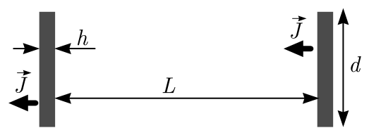
Find the magnitude of the interaction force between two coaxially placed cylindrical magnets of diameter \(d=20\,\mathrm{mm}\) and thickness \(h=2\,\mathrm{mm}\), magnetized parallel to their axis, if the distance between the centres of the magnets is \(L=20\,\mathrm{cm}\). You may assume that \(L\gg d,h\).
A.2 — 0.4pt
At distances much larger than \(\frac h2\), the field created by the magnet from task A.1 is the same as that created by a circular current \(I\). Find \(I\).
A.3 — 1.0pt
Find the interaction force between the magnets for the setup of task A.1 if instead \(L=5\,\mathrm{mm}\). You may assume that \(d\gg L\gg h\).
A.4 — 1.0pt
Identical spherical magnets of diameter \(\delta=5\,\mathrm{mm}\), bound together by magnetic attraction, form a chain. What is the maximal length \(l\) for such a chain which does not break under its own weight when hanging beneath the topmost magnet? The density of NdFeB magnets \(\rho=7500\,\mathrm{kg/m^3}\).
A.5 — 1.5pt
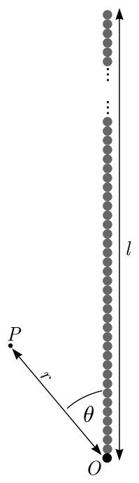
Consider the chain from part A.4. Obtain an expression for the magnitude of the magnetic \(B\)-field at such a point \(P\) which is at distance \(r\) from one of the chain's endpoint \(O\), and the angle between the chain and the line \(OP\) is \(\theta\) (cf. figure below), assuming that \(l\gg r\) and \(r\sin\theta\gg\delta\)
Part B. Interaction with ferromagnets (3.5 points)
Now we assume that in addition to the permanent magnets we have also plates made from a ferromagnetic material, similar to what is used in transformer cores. In the situations we're concerned with, it can be considered to have a constant but very large relative permeability \(\mu_r\sim10^5\).
Hint 5. Large permeability means that magnetic field lines near the outside surface of an object made of the material are nearly perpendicular to the surface. This is similar to the behavior of electric field lines near the outside surface of a conductor.
B.1 — 1.0pt
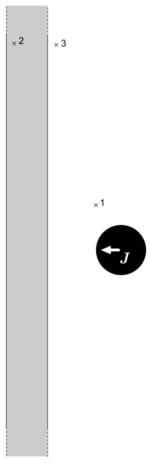
A spherical magnet from part A.4 is at a distance \(s=\delta\) from a thick infinite ferromagnetic plate (see the answer sheet). The magnetization of the sphere is oriented perpendicular to the plate. Sketch the field lines in the cross-section shown in the answer sheet. In that figure, three points (denoted as 1, 2, and 3) are marked; you need to show field lines passing through each of these points in their full length, i.e. as much as fits into the figure.
B.2 — 1.0pt
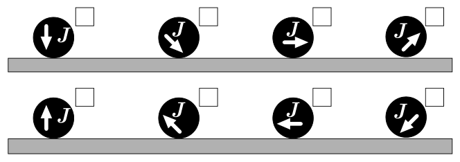
Now the spherical magnet is brought into direct contact with the plate. Which direction is taken by the magnetization vector of the spherical magnet at a stable equilibrium and what is the normal force between the plate and the magnet? Mark the correct direction(s) with a tick in the corresponding box in the answer sheet. Incorrect ticks will reduce your score.
B.3 — 1.5pt
Now a magnet from part A.1 is placed between two thick circular ferromagnetic plates of diameter \(D=2d\) so that the flat faces of the magnet are pressed against the plates and all three discs are coaxial. Find the magnetic force \(F\) acting on each plate. Hint: You may neglect the magnetic field both outside the ferromagnetic plates and outside the gap between them.
Part C. (Anti)ferromagnetic order (2 points)
The magnetic properties of materials are due to the magnetic dipole moments of electrons and atomic nuclei. If the dipole moments orient themselves parallel to each other, the field created by them is magnified — these are ferromagnetic materials. On the other hand, if for each dipole moment there is another antiparallel dipole moment nearby, the fields cancel out — these are anti-ferromagnetic materials.
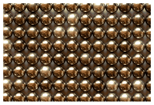
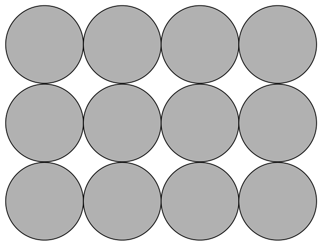
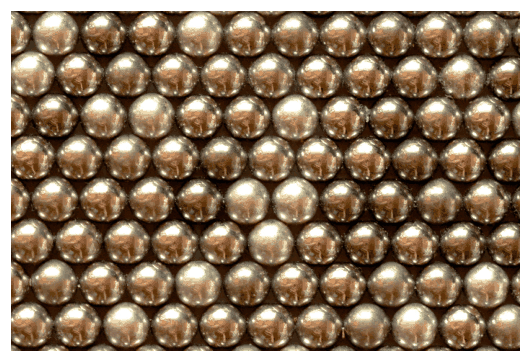
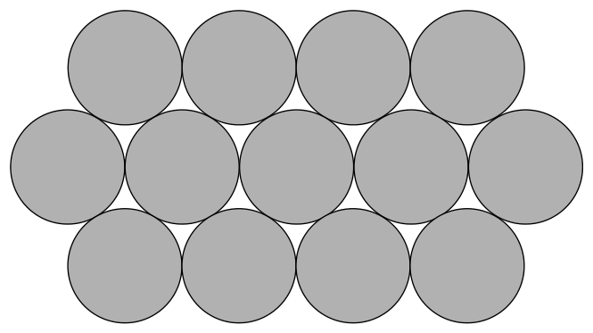
In what follows, we consider a very large number of spherical magnets of part A.4, arranged at the nodes of a two-dimensional lattice; see real photos of stable equilibrium configurations below. Assume that all the magnetization vectors lie in the plane of the figure. Consider in your calculations only nearest-neighbour interactions (on the figure of C.1, each magnet has four nearest neighbours, and on the figure of C.2 — six).
C.1 — 0.8pt
Show the magnetization directions of the magnets in the figure below. You are not required to prove that the configuration you suggested is the only possibility. You still need to justify that the configuration you suggested is indeed stable. Find the energy needed to pull one magnet out of this lattice from somewhere in the middle of the lattice, assuming the other magnets are kept stationary. Does this configuration correspond to the order of ferromagnetic or antiferromagnetic materials?
C.2 — 1.2pt
Answer the same questions as in task C.1 for the configuration shown in the figure below.
Physical Constants
Below is the list of physical constants you might use in your solution in addition to the quantities given in the problem text.
| Physical constant | Notation | Numerical value |
|---|---|---|
| Speed of light in vacuum | \(c\) | \(299\,792\,458\,\mathrm{m/s}\) |
| Vacuum permeability (magnetic constant) | \(\mu_0\) | \(4\pi\cdot10^{-7}\,\mathrm{N/A^2}\); \([1\,\mathrm{N/A^2}=1\,\mathrm{Vs/Am}]\) |
| Vacuum permittivity (electric constant) | \(\varepsilon_0\) | \(8.8541878128(13)\cdot10^{-12}\,\mathrm{F/m}\); \([1\,\mathrm{F/m}=1\,\mathrm{As/Vm}]\) |
| Elementary charge | \(e\) | \(1.602176634\cdot10^{-19}\,\mathrm{C}\); \([1\,\mathrm{C}=1\,\mathrm{A\cdot s}]\) |
| Electron rest mass | \(m_{\mathrm e}\) | \(9.1093837015(28)\cdot10^{-31}\,\mathrm{kg}\) |
| Proton rest mass | \(m_{\mathrm p}\) | \(1.67262192369(51)\cdot10^{-27}\,\mathrm{kg}\) |
| Neutron rest mass | \(m_{\mathrm n}\) | \(1.67492749804(95)\cdot10^{-27}\,\mathrm{kg}\) |
| Atomic mass unit | \(m_{\mathrm{amu}}\) | \(1.66053906660(50)\cdot10^{-27}\,\mathrm{kg}\) |
| Gravitational constant | \(G\) | \(6.67430(15)\cdot10^{-11}\,\mathrm{m^3/(kg\cdot s^2)}\) |
| Avogadro constant | \(N_{\mathrm A}\) | \(6.02214076\cdot10^{23}\,\mathrm{mol^{-1}}\) |
| Molar gas constant | \(R\) | \(8.31446261815324\ldots\,\mathrm{J/(K\cdot mol)}\) |
| Boltzmann constant | \(k_{\mathrm B}\) | \(1.380649\cdot10^{-23}\,\mathrm{J/K}\) |
| Stefan–Boltzmann constant | \(\sigma\) | \(5.670374419\ldots\cdot10^{-8}\,\mathrm{W/(m^2\cdot K^4)}\) |
| Planck constant | \(h\) | \(6.62607015\cdot10^{-34}\,\mathrm{J\cdot s}\) |
| Reduced Planck constant | \(\hbar=h/(2\pi)\) | \(1.0545718176\ldots\cdot10^{-34}\,\mathrm{J\cdot s}\) |
Official English text of the problem.
Answers
All force values below are magnitudes.
-
A.1:
\[ \boxed{F=\frac{3\pi\mu_0J^2d^4h^2}{32L^4} \simeq2.1\times10^{-4}\,\mathrm N} \] The force is attractive for the directions shown. -
A.2: A circular current of diameter \(d\), with \[ \boxed{I=Jh\simeq2.4\times10^3\,\mathrm A}. \]
-
A.3:
\[ \boxed{F\simeq\frac{\mu_0J^2h^2d}{2L}\simeq14\,\mathrm N} \] The force is attractive. -
A.4: In the long-chain approximation, \[ \boxed{l_{\max}\simeq\frac{\pi^4\mu_0J^2}{360\rho g} \simeq6.6\,\mathrm m}. \]
-
A.5:
\[ \boxed{B\simeq\frac{\mu_0J\delta^2}{24r^2}} \] This magnitude is independent of \(\theta\) within the stated approximations. -
B.1: The exterior field is that of the real dipole together with an equally strong mirror dipole pointing in the same direction. Field lines meet the plate normally. The line through 1 forms a short return loop in air; the lines through 2 and 3 belong to larger loops carrying flux through the plate. Their detailed directions are described in the Solution.
-
B.2: Tick the first drawing in each row: magnetization perpendicular to the plate, either toward it or away from it. \[ \boxed{F=\frac{\pi\mu_0J^2\delta^2}{24}\simeq5.9\,\mathrm N} \] The magnetic force is attractive.
-
B.3: Each plate is pulled toward the magnet and the other plate, with \[ \boxed{F=\frac{3\pi\mu_0J^2d^2}{32} \simeq2.1\times10^2\,\mathrm N}. \]
-
C.1: All moments in a horizontal row point in the same direction; successive rows point oppositely. This is antiferromagnetic order. \[ \boxed{W=\frac{\pi\mu_0J^2\delta^3}{24} \simeq2.9\times10^{-2}\,\mathrm J}. \]
-
C.2: All moments point in the same horizontal direction. This is ferromagnetic order, passing the single-magnet rotational stability test described below. \[ \boxed{W=\frac{\pi\mu_0J^2\delta^3}{48} \simeq1.5\times10^{-2}\,\mathrm J}. \] This shows stability against rotating a single magnet only; in the nearest-neighbour model, some collective rotations of many magnets lower the energy.
Solution
The magnetization and the two relevant dipole moments are
\[ J=\frac{1.5}{\mu_0} =1.19366\times10^6\,\mathrm{A/m}, \]
\[ m_{\mathrm c}=J\frac{\pi d^2h}{4} =0.750\,\mathrm{A\,m^2}, \qquad m_{\mathrm s}=J\frac{\pi\delta^3}{6} =0.078125\,\mathrm{A\,m^2}. \]
For two permanent dipoles, the interaction energy is
\[ U_{12}= \frac{\mu_0}{4\pi r^3} \left[ \vec m_1\cdot\vec m_2 -3(\vec m_1\cdot\hat r)(\vec m_2\cdot\hat r) \right]. \]
Equivalently, \(U_{12}=-\vec m_2\cdot\vec B_1\). Forces follow by differentiating this energy with respect to position, holding the permanent moments fixed.
A.1
Since \(L\gg d,h\), both cylinders can be replaced by point dipoles. Their moments are parallel to each other and to their common axis, so
\[ U(L)=-\frac{\mu_0m_{\mathrm c}^2}{2\pi L^3}. \]
The force tends to decrease \(L\), and its magnitude is
\[ F=\frac{dU}{dL} =\frac{3\mu_0m_{\mathrm c}^2}{2\pi L^4}. \]
Substituting \(m_{\mathrm c}=J\pi d^2h/4\),
\[ \boxed{F=\frac{3\pi\mu_0J^2d^4h^2}{32L^4}}. \]
With \(L=0.20\,\mathrm m\),
\[ F=2.109375\times10^{-4}\,\mathrm N \simeq\boxed{2.1\times10^{-4}\,\mathrm N}. \]
A.2
A uniformly magnetized body can be represented by bound currents. Its bound surface-current density is
\[ \vec K_{\mathrm b}=\vec J\times\hat n. \]
For an axially magnetized cylinder, this current flows around the curved side, with magnitude \(K_{\mathrm b}=J\). Integrating over the cylinder thickness gives an equivalent circular current
\[ \boxed{I=Jh}. \]
At distances large compared with the thickness, the thin cylindrical current sheet can be replaced by a single loop of diameter \(d\).
The same result follows by equating the magnetic moments:
\[ I\frac{\pi d^2}{4} =J\frac{\pi d^2h}{4}. \]
Numerically,
\[ I=(1.19366\times10^6)(2.0\times10^{-3}) =2.3873\times10^3\,\mathrm A \simeq\boxed{2.4\,\mathrm{kA}}. \]
Its circulation is chosen by the right-hand rule to produce the specified magnetization direction.
A.3
The condition \(L\gg h\) permits the current-loop representation from A.2. Because \(L\ll d\), corresponding nearby portions of the two loops can be treated as parallel straight wires separated by \(L\).
The attractive force per unit length between parallel currents is
\[ \frac{dF}{d\ell}=\frac{\mu_0I^2}{2\pi L}. \]
To leading order, this force acts along the common axis. Multiplying by the circumference \(\pi d\) gives
\[ F\simeq\frac{\mu_0I^2}{2\pi L}\,\pi d =\frac{\mu_0I^2d}{2L}. \]
Thus
\[ \boxed{F\simeq\frac{\mu_0J^2h^2d}{2L}}. \]
For \(L=5.0\times10^{-3}\,\mathrm m\),
\[ F\simeq14.3239\,\mathrm N \simeq\boxed{14\,\mathrm N}. \]
This is the leading result under the stated hierarchy \(d\gg L\gg h\).
A.4
The spheres align with their moments along the chain, all pointing in the same direction. Each sphere has mass
\[ M=\rho\frac{\pi\delta^3}{6}. \]
Two spheres whose centres are \(n\delta\) apart attract with force
\[ F_n=\frac{3\mu_0m_{\mathrm s}^2}{2\pi(n\delta)^4} =\frac{F_1}{n^4}, \]
where
\[ F_1=\frac{3\mu_0m_{\mathrm s}^2}{2\pi\delta^4} =\frac{\pi\mu_0J^2\delta^2}{24}. \]
For a chain containing \(N\) spheres, the held top sphere must support the other \(N-1\) spheres. The largest upward magnetic force it can exert on them, while all spheres remain touching, is
\[ F_{\mathrm{top}} =F_1\sum_{n=1}^{N-1}\frac1{n^4}. \]
Consequently,
\[ (N-1)Mg \leq F_1\sum_{n=1}^{N-1}\frac1{n^4}. \]
The uppermost junction is limiting: a cut farther down supports less weight, while its magnetic attraction includes at least one pair at every separation present across the uppermost junction.
For a long chain,
\[ F_{\mathrm{top}} \simeq F_1\frac{\pi^4}{90}. \]
Also, to leading order in \(1/N\), the suspended weight is
\[ Mg\frac l\delta =\frac{\rho\pi\delta^2g}{6}\,l. \]
Equating this to the limiting magnetic force,
\[ \frac{\rho\pi\delta^2g}{6}\,l_{\max} = \frac{\pi\mu_0J^2\delta^2}{24}\frac{\pi^4}{90}. \]
Therefore,
\[ \boxed{l_{\max}\simeq \frac{\pi^4\mu_0J^2}{360\rho g}}. \]
The sphere diameter cancels: the magnetic holding force and the chain’s mass per unit length both scale as \(\delta^2\).
Taking \(g=9.81\,\mathrm{m/s^2}\),
\[ F_1=5.8594\,\mathrm N,\qquad F_{\mathrm{top}}\simeq6.3417\,\mathrm N, \]
\[ l_{\max}\simeq6.5848\,\mathrm m \simeq\boxed{6.6\,\mathrm m}. \]
Counting the supported top sphere and rounding to a whole number of spheres changes the length only by an amount of order \(\delta\).
A.5
Because \(r\sin\theta\gg\delta\), the discrete chain can be replaced by a continuous line of dipoles. Its dipole moment per unit length is
\[ \lambda_m=\frac{m_{\mathrm s}}{\delta} =\frac{\pi J\delta^2}{6}. \]
Place \(O\) at the origin and let the chain extend along \(+z\), from \(0\) to \(l\). Choose all moments along \(+z\). In the exterior region, define a magnetic scalar potential by
\[ \vec B=-\mu_0\nabla\Phi. \]
The potential of the line is
\[ \Phi(\vec r) =\frac{\lambda_m}{4\pi} \int_0^l \frac{z-z'}{|\vec r-z'\hat z|^3}\,dz'. \]
Since
\[ \frac{\partial}{\partial z'} \frac1{|\vec r-z'\hat z|} = \frac{z-z'}{|\vec r-z'\hat z|^3}, \]
integration gives
\[ \Phi(\vec r) =\frac{\lambda_m}{4\pi} \left( \frac1{|\vec r-l\hat z|} -\frac1r \right). \]
Thus the exterior field is equivalent to that of two opposite effective magnetic poles at the endpoints:
\[ \vec B= \frac{\mu_0\lambda_m}{4\pi} \left[ \frac{\vec r-l\hat z}{|\vec r-l\hat z|^3} -\frac{\vec r}{r^3} \right]. \]
For \(l\gg r\), the distant endpoint contributes negligibly, leaving
\[ \vec B\simeq -\frac{\mu_0\lambda_m}{4\pi r^2}\hat r. \]
Hence
\[ \boxed{B\simeq\frac{\mu_0J\delta^2}{24r^2}}. \]
The field is radial about the nearby endpoint, so its magnitude is independent of \(\theta\). Reversing all moments reverses the field direction.
B.1
Let the plate occupy \(x<0\), with its surface at \(x=0\), and let the sphere’s centre be at \(x=a>0\). In the answer-sheet drawing,
\[ \vec m=-m_{\mathrm s}\hat x. \]
For a highly permeable plate, the exterior tangential field must nearly vanish. This boundary condition is produced by placing a mirror dipole at \(x=-a\), with the same normal orientation:
\[ \vec m_{\mathrm{image}}\simeq-m_{\mathrm s}\hat x. \]
More precisely, its magnitude is multiplied by
\[ \frac{\mu_r-1}{\mu_r+1}\simeq1. \]
At the surface, the tangential components of the two dipole fields cancel. If \(y\) denotes height above the sphere’s centre, the remaining normal component is
\[ B_x(0,y) = \frac{\mu_0m_{\mathrm s}}{2\pi} \frac{y^2-2a^2}{(a^2+y^2)^{5/2}}. \]
Thus flux enters the plate near the sphere’s axis, where \(|y|<\sqrt2\,a\), and emerges farther away, where \(|y|>\sqrt2\,a\).
The requested sketch is described as follows:
- The sphere’s left side is its north side, and its right side is its south side. Exterior arrows run from the left side toward the right side along curved return paths. Inside the sphere, arrows run approximately right to left.
- Through point 1: draw a short upper return loop entirely in the air outside the plate. It leaves the sphere’s upper-left surface, rises through point 1, bends over toward the right, and enters the sphere’s upper-right surface.
- Through point 2: draw a larger loop carrying flux upward through the plate. At point 2 it points mainly upward and somewhat toward the surface. It bends rightward and emerges from the surface above point 3, perpendicular to the surface, before curving back to the sphere’s south side. Traced backward, its segment inside the plate descends and connects to flux entering the plate nearer the magnet.
- Through point 3: draw a line emerging approximately horizontally to the right from the plate. It then curves downward and rightward toward the sphere’s south side. Continue it backward through the plate as a curved path returning to a lower entry point, supplied by flux from the sphere’s north side.
- The lower-half pattern is the reflection of the upper-half pattern about the horizontal line through the sphere’s centre. Every line continues through the material and magnet to form a closed magnetic-field line.
For the ideal half-space limit, the field inside the plate is approximately twice the field that the real dipole alone would create there. This fixes the curved continuations through point 2 as well as their directions.
B.2
Let \(\hat n\) point normally out of the plate, and decompose the sphere’s moment as
\[ \vec m=m_n\hat n+\vec m_t. \]
Its image has moment
\[ \vec m'=m_n\hat n-\vec m_t. \]
If the sphere’s centre is distance \(a\) from the plate, the image is \(2a\) away. Its field at the real dipole is
\[ \vec B_{\mathrm{image}} = \frac{\mu_0}{4\pi(2a)^3} \left(2m_n\hat n+\vec m_t\right). \]
Because the plate magnetization is induced, the interaction energy is
\[ U=-\frac12\vec m\cdot\vec B_{\mathrm{image}}. \]
Writing \(\theta\) for the angle between \(\vec m\) and the plate normal,
\[ U(a,\theta) = -\frac{\mu_0m_{\mathrm s}^2} {8\pi(2a)^3} (1+\cos^2\theta). \]
This is minimized at
\[ \theta=0\quad\text{or}\quad\theta=\pi. \]
Therefore, both directions perpendicular to the plate are stable: toward the plate and away from it. These are the first drawings in the upper and lower rows.
At either stable orientation, the attractive force has magnitude
\[ F=\frac{\partial U}{\partial a} =\frac{3\mu_0m_{\mathrm s}^2}{2\pi(2a)^4}. \]
At contact, \(a=\delta/2\), so
\[ F=\frac{3\mu_0m_{\mathrm s}^2}{2\pi\delta^4} =\boxed{\frac{\pi\mu_0J^2\delta^2}{24}}. \]
Numerically,
\[ F=5.8594\,\mathrm N \simeq\boxed{5.9\,\mathrm N}. \]
B.3
Let
\[ A=\frac{\pi d^2}{4} \]
be the magnet’s face area, and
\[ A_p=\frac{\pi D^2}{4}=4A \]
the area of each plate.
The permeability of the plates is very large, so their internal \(H\)-field is negligible. Each plate is therefore approximately an equipotential surface for the magnetic scalar potential. Neglecting fringing, the axial \(H\)-field has the same value in the magnet and in the surrounding annular air gap.
Let \(B_m\) be the signed axial field in the magnet and \(B_a\) that in the annular gap. Since the magnetization is fixed,
\[ B_m=\mu_0(H+J),\qquad B_a=\mu_0H. \]
Hence
\[ B_m-B_a=\mu_0J. \]
All flux passing through the magnet must return through the annular gap, because exterior flux is neglected. Therefore,
\[ AB_m+(A_p-A)B_a=0. \]
Solving,
\[ B_m=\mu_0J\left(1-\frac A{A_p}\right), \qquad B_a=-\mu_0J\frac A{A_p}. \]
For \(A_p=4A\),
\[ B_m=\frac34\mu_0J=1.125\,\mathrm T, \qquad B_a=-\frac14\mu_0J=-0.375\,\mathrm T. \]
A magnetic field normal to a highly permeable surface produces an attractive pressure
\[ p=\frac{B^2}{2\mu_0}. \]
At the magnet–plate contact this can be evaluated by imagining an infinitesimal vacuum slit: normal \(B\) is continuous across it. Both the central region and the annular return-flux region pull the plate inward, irrespective of their opposite field directions.
Thus
\[ F= \frac{AB_m^2+(A_p-A)B_a^2}{2\mu_0}. \]
Substitution gives
\[ F= \frac{\mu_0J^2A}{2} \left(1-\frac A{A_p}\right). \]
With \(A_p=4A\),
\[ \boxed{F=\frac{3\pi\mu_0J^2d^2}{32}}. \]
Numerically,
\[ F=210.9375\,\mathrm N \simeq\boxed{2.1\times10^2\,\mathrm N} \]
on each plate.
C.1
Define the nearest-neighbour dipolar energy scale
\[ \varepsilon_d= \frac{\mu_0m_{\mathrm s}^2}{4\pi\delta^3} =\frac{\pi\mu_0J^2\delta^3}{144} =4.8828125\times10^{-3}\,\mathrm J. \]
Choose moments along horizontal rows, reversing their direction in successive rows. On the answer sheet, the top row can point right, the middle row left, and the bottom row right:
\[ \begin{matrix} \rightarrow&\rightarrow&\rightarrow&\rightarrow\\ \leftarrow&\leftarrow&\leftarrow&\leftarrow\\ \rightarrow&\rightarrow&\rightarrow&\rightarrow \end{matrix} \]
Consider a central magnet pointing right.
Its two horizontal neighbours also point right and lie on its dipole axis. Each contributes interaction energy
\[ U_{\mathrm{horizontal}}=-2\varepsilon_d. \]
Its two vertical neighbours point left and lie perpendicular to its moment. Each contributes
\[ U_{\mathrm{vertical}}=-\varepsilon_d. \]
The central magnet’s total interaction energy with its neighbours is therefore
\[ U_{\mathrm{central}} =2(-2\varepsilon_d)+2(-\varepsilon_d) =-6\varepsilon_d. \]
All four neighbours produce fields parallel to the central moment, with total magnitude
\[ B_{\mathrm{nn}}=\frac{6\varepsilon_d}{m_{\mathrm s}}. \]
Rotating that magnet through an angle \(\alpha\), while keeping its neighbours fixed, increases the energy by
\[ \Delta U=6\varepsilon_d(1-\cos\alpha)>0. \]
Thus it experiences a restoring torque.
For fixed square-lattice sites, the pattern also minimizes the full nearest-neighbour orientational energy. To see this, write a unit moment as \((u_i,v_i)\). Then
\[ \frac{U}{\varepsilon_d} = \sum_{\langle ij\rangle_x}(-2u_iu_j+v_iv_j) + \sum_{\langle ij\rangle_y}(u_iu_j-2v_iv_j) \geq -3\sum_i(u_i^2+v_i^2) =-3N. \]
The inequality follows from \(2|ab|\leq a^2+b^2\), and the proposed stripe pattern attains the bound in the bulk.
Removing the central magnet to infinity eliminates its four bonds, so the required work is
\[ W=0-U_{\mathrm{central}}=6\varepsilon_d. \]
There is no factor of \(1/2\): each bond involving the removed magnet is counted once. Therefore,
\[ \boxed{W=\frac{\pi\mu_0J^2\delta^3}{24} \simeq2.9\times10^{-2}\,\mathrm J}. \]
Successive rows have opposite magnetization, giving antiferromagnetic order.
C.2
Choose all moments horizontal and pointing right, including every sphere in the answer-sheet diagram.
A central sphere has two horizontal neighbours and four diagonal neighbours whose displacement vectors make angles of \(60^\circ\) or \(120^\circ\) with the moments.
Each horizontal pair contributes
\[ U_{\mathrm{horizontal}}=-2\varepsilon_d. \]
For parallel moments at angle \(\beta\) to their separation,
\[ U_{\mathrm{pair}} =\varepsilon_d(1-3\cos^2\beta). \]
Thus each diagonal neighbour contributes
\[ U_{\mathrm{diagonal}} =\varepsilon_d\left(1-\frac34\right) =\frac14\varepsilon_d. \]
Summing the six bonds,
\[ U_{\mathrm{central}} =2(-2\varepsilon_d)+4\left(\frac14\varepsilon_d\right) =-3\varepsilon_d. \]
The transverse components of the neighbours’ fields cancel. The remaining field points along the central moment and has magnitude
\[ B_{\mathrm{nn}}=\frac{3\varepsilon_d}{m_{\mathrm s}}. \]
Consequently, rotating one magnet through \(\alpha\) with all its neighbours fixed costs
\[ \Delta U=3\varepsilon_d(1-\cos\alpha)>0. \]
This establishes a restoring torque against an individual rotation. It does not establish stability against collective rotations: in the nearest-neighbour model, rotating all moments together through the same angle leaves the energy unchanged, because the six bond directions are \(60^\circ\) apart, and some non-uniform collective rotations lower the energy.
The work required to remove the central magnet is
\[ W=0-U_{\mathrm{central}}=3\varepsilon_d, \]
so
\[ \boxed{W=\frac{\pi\mu_0J^2\delta^3}{48} \simeq1.5\times10^{-2}\,\mathrm J}. \]
All moments point in the same direction, so this configuration has ferromagnetic order.
The solution was checked against the official solution.
IPhO 2022 · Theorieaufgabe 1
Permanentmagnete
Starke Permanentmagnete werden aus einer NdFeB-Legierung hergestellt, die eine sehr breite Hystereseschleife aufweist, sodass die Magnetisierung \(J\) in einem weiten Anwendungsbereich als konstant angenommen werden kann; im Folgenden nehmen wir \(J\equiv 1.5\,\mathrm{T}/\mu_0\) an, wobei \(\mu_0=4\pi\times10^{-7}\,\mathrm{N/A^2}\), und die Magnetisierung aller Permanentmagnete ist homogen. Die Magnetisierung ist als Volumendichte des magnetischen Dipolmoments der Materie definiert.
Hinweis 1. Die folgende Gleichung könnte hilfreich sein:
\[ \sum_{n=1}^{\infty}\frac{1}{n^4}=\frac{\pi^4}{90}. \]
Hinweis 2. Das von einem kugelförmigen Magneten erzeugte Magnetfeld ist identisch mit dem eines Punktdipols. Die von Magneten anderer Formen erzeugten Magnetfelder entsprechen erst in Abständen, die viel größer als ihr Durchmesser sind, dem Feld eines Punktdipols.
Hinweis 3. Die elektrischen und magnetischen Felder elektrischer bzw. magnetischer Punktdipole sind als Funktionen der Koordinaten und des jeweiligen Dipolmoments ähnlich, d. h., das eine lässt sich durch Multiplikation mit einem konstanten Faktor aus dem anderen erhalten.
Hinweis 4. Das durch eine Randbedingung induzierte Feld kann stets durch eine geeignete Anordnung von Feldquellen außerhalb der vorgegebenen Grenzen ersetzt werden.
Teil A. Wechselwirkung zwischen Magneten (4.5 Punkte)
Wenn der Abstand zu einem Magneten viel größer als seine Größe ist, kann das von ihm erzeugte Magnetfeld durch das Magnetfeld seines Dipolmoments \(\vec m\) angenähert werden,
\[ \vec B=\frac{\mu_0}{4\pi r^3}(2\vec m_{\parallel}-\vec m_{\perp}). \]
Hierbei ist \(r=|\vec r|\), und wir haben das Dipolmoment in Komponenten parallel und senkrecht zum Ortsvektor \(\vec r\) zerlegt, der vom Dipol zum Beobachtungspunkt zeigt, \(\vec m=\vec m_{\perp}+\vec m_{\parallel}\).
A.1 — 0.6 Punkte
Bestimmen Sie den Betrag der Wechselwirkungskraft zwischen zwei koaxial angeordneten zylindrischen Magneten mit dem Durchmesser \(d=20\,\mathrm{mm}\) und der Dicke \(h=2\,\mathrm{mm}\), die parallel zu ihrer Achse magnetisiert sind, wenn der Abstand zwischen den Mittelpunkten der Magnete \(L=20\,\mathrm{cm}\) beträgt. Sie dürfen \(L\gg d,h\) annehmen.
A.2 — 0.4 Punkte
In Abständen, die viel größer als \(\frac h2\) sind, ist das vom Magneten aus Aufgabe A.1 erzeugte Feld dasselbe wie das eines Kreisstroms \(I\). Bestimmen Sie \(I\).
A.3 — 1.0 Punkte
Bestimmen Sie die Wechselwirkungskraft zwischen den Magneten für die Anordnung aus Aufgabe A.1, wenn stattdessen \(L=5\,\mathrm{mm}\) gilt. Sie dürfen \(d\gg L\gg h\) annehmen.
A.4 — 1.0 Punkte
Identische kugelförmige Magnete mit dem Durchmesser \(\delta=5\,\mathrm{mm}\), die durch magnetische Anziehung zusammengehalten werden, bilden eine Kette. Wie groß ist die maximale Länge \(l\) einer solchen Kette, die unter ihrem eigenen Gewicht nicht reißt, wenn sie am obersten Magneten hängt? Die Dichte der NdFeB-Magnete beträgt \(\rho=7500\,\mathrm{kg/m^3}\).
A.5 — 1.5 Punkte
Betrachten Sie die Kette aus Teil A.4. Leiten Sie einen Ausdruck für den Betrag des magnetischen \(B\)-Feldes an einem Punkt \(P\) her, der sich im Abstand \(r\) von einem der Endpunkte \(O\) der Kette befindet, wobei der Winkel zwischen der Kette und der Geraden \(OP\) gleich \(\theta\) ist (siehe Abbildung unten). Nehmen Sie dabei \(l\gg r\) und \(r\sin\theta\gg\delta\) an.
Teil B. Wechselwirkung mit Ferromagneten (3.5 Punkte)
Wir nehmen nun an, dass uns neben den Permanentmagneten auch Platten aus einem ferromagnetischen Material zur Verfügung stehen, ähnlich dem Material, das in Transformatorkernen verwendet wird. In den hier betrachteten Situationen kann seine relative Permeabilität als konstant, aber sehr groß angenommen werden, \(\mu_r\sim10^5\).
Hinweis 5. Eine große Permeabilität bedeutet, dass magnetische Feldlinien nahe der äußeren Oberfläche eines Körpers aus diesem Material nahezu senkrecht zur Oberfläche verlaufen. Dies ähnelt dem Verhalten elektrischer Feldlinien nahe der äußeren Oberfläche eines Leiters.
B.1 — 1.0 Punkte
Ein kugelförmiger Magnet aus Teil A.4 befindet sich im Abstand \(s=\delta\) von einer dicken, unendlich ausgedehnten ferromagnetischen Platte (siehe Antwortbogen). Die Magnetisierung der Kugel ist senkrecht zur Platte ausgerichtet. Skizzieren Sie die Feldlinien in dem auf dem Antwortbogen dargestellten Querschnitt. In dieser Abbildung sind drei Punkte (mit 1, 2 und 3 bezeichnet) markiert; Sie sollen die Feldlinien durch jeden dieser Punkte über ihre gesamte Länge darstellen, d. h. so weit, wie es in die Abbildung passt.
B.2 — 1.0 Punkte
Nun wird der kugelförmige Magnet in direkten Kontakt mit der Platte gebracht. Welche Richtung nimmt der Magnetisierungsvektor des kugelförmigen Magneten im stabilen Gleichgewicht ein, und wie groß ist die Normalkraft zwischen der Platte und dem Magneten? Markieren Sie die richtige(n) Richtung(en) mit einem Häkchen im entsprechenden Kästchen auf dem Antwortbogen. Falsch gesetzte Häkchen führen zu Punktabzug.
B.3 — 1.5 Punkte
Nun wird ein Magnet aus Teil A.1 zwischen zwei dicke kreisförmige ferromagnetische Platten mit dem Durchmesser \(D=2d\) gelegt, sodass die ebenen Stirnflächen des Magneten an die Platten gedrückt werden und alle drei Scheiben koaxial sind. Bestimmen Sie die auf jede Platte wirkende magnetische Kraft \(F\). Hinweis: Sie dürfen das Magnetfeld sowohl außerhalb der ferromagnetischen Platten als auch außerhalb des Spalts zwischen ihnen vernachlässigen.
Teil C. (Anti)ferromagnetische Ordnung (2 Punkte)
Die magnetischen Eigenschaften von Materialien beruhen auf den magnetischen Dipolmomenten der Elektronen und Atomkerne. Richten sich die Dipolmomente parallel zueinander aus, wird das von ihnen erzeugte Feld verstärkt — dies sind ferromagnetische Materialien. Gibt es hingegen zu jedem Dipolmoment ein weiteres, antiparalleles Dipolmoment in der Nähe, heben sich die Felder auf — dies sind antiferromagnetische Materialien.
Im Folgenden betrachten wir eine sehr große Anzahl kugelförmiger Magnete aus Teil A.4, die an den Gitterpunkten eines zweidimensionalen Gitters angeordnet sind; siehe die untenstehenden realen Fotos stabiler Gleichgewichtsanordnungen. Nehmen Sie an, dass alle Magnetisierungsvektoren in der Zeichenebene liegen. Berücksichtigen Sie in Ihren Berechnungen nur die Wechselwirkungen zwischen nächsten Nachbarn (in der Abbildung zu C.1 hat jeder Magnet vier nächste Nachbarn, in der Abbildung zu C.2 sechs).
C.1 — 0.8 Punkte
Zeichnen Sie die Magnetisierungsrichtungen der Magnete in die untenstehende Abbildung ein. Sie müssen nicht beweisen, dass die von Ihnen vorgeschlagene Anordnung die einzig mögliche ist. Sie müssen jedoch begründen, dass die von Ihnen vorgeschlagene Anordnung tatsächlich stabil ist. Bestimmen Sie die Energie, die benötigt wird, um einen Magneten aus dem Inneren dieses Gitters herauszuziehen, wobei die anderen Magnete festgehalten werden. Entspricht diese Anordnung der Ordnung ferromagnetischer oder antiferromagnetischer Materialien?
C.2 — 1.2 Punkte
Beantworten Sie für die in der untenstehenden Abbildung gezeigte Anordnung dieselben Fragen wie in Aufgabe C.1.
Physikalische Konstanten
Nachfolgend finden Sie eine Liste physikalischer Konstanten, die Sie zusätzlich zu den in der Aufgabenstellung angegebenen Größen für Ihre Lösung verwenden können.
| Physikalische Konstante | Symbol | Zahlenwert |
|---|---|---|
| Lichtgeschwindigkeit im Vakuum | \(c\) | \(299\,792\,458\,\mathrm{m/s}\) |
| Vakuumpermeabilität (magnetische Feldkonstante) | \(\mu_0\) | \(4\pi\cdot10^{-7}\,\mathrm{N/A^2}\); \([1\,\mathrm{N/A^2}=1\,\mathrm{Vs/Am}]\) |
| Vakuumpermittivität (elektrische Feldkonstante) | \(\varepsilon_0\) | \(8.8541878128(13)\cdot10^{-12}\,\mathrm{F/m}\); \([1\,\mathrm{F/m}=1\,\mathrm{As/Vm}]\) |
| Elementarladung | \(e\) | \(1.602176634\cdot10^{-19}\,\mathrm{C}\); \([1\,\mathrm{C}=1\,\mathrm{A\cdot s}]\) |
| Ruhemasse des Elektrons | \(m_{\mathrm e}\) | \(9.1093837015(28)\cdot10^{-31}\,\mathrm{kg}\) |
| Ruhemasse des Protons | \(m_{\mathrm p}\) | \(1.67262192369(51)\cdot10^{-27}\,\mathrm{kg}\) |
| Ruhemasse des Neutrons | \(m_{\mathrm n}\) | \(1.67492749804(95)\cdot10^{-27}\,\mathrm{kg}\) |
| Atomare Masseneinheit | \(m_{\mathrm{amu}}\) | \(1.66053906660(50)\cdot10^{-27}\,\mathrm{kg}\) |
| Gravitationskonstante | \(G\) | \(6.67430(15)\cdot10^{-11}\,\mathrm{m^3/(kg\cdot s^2)}\) |
| Avogadro-Konstante | \(N_{\mathrm A}\) | \(6.02214076\cdot10^{23}\,\mathrm{mol^{-1}}\) |
| Molare Gaskonstante | \(R\) | \(8.31446261815324\ldots\,\mathrm{J/(K\cdot mol)}\) |
| Boltzmann-Konstante | \(k_{\mathrm B}\) | \(1.380649\cdot10^{-23}\,\mathrm{J/K}\) |
| Stefan–Boltzmann-Konstante | \(\sigma\) | \(5.670374419\ldots\cdot10^{-8}\,\mathrm{W/(m^2\cdot K^4)}\) |
| Planck-Konstante | \(h\) | \(6.62607015\cdot10^{-34}\,\mathrm{J\cdot s}\) |
| Reduzierte Planck-Konstante | \(\hbar=h/(2\pi)\) | \(1.0545718176\ldots\cdot10^{-34}\,\mathrm{J\cdot s}\) |
Aufgabentext aus dem offiziellen englischen Text übersetzt.
Antworten
Alle nachfolgenden Kraftangaben sind Beträge.
-
A.1:
\[ \boxed{F=\frac{3\pi\mu_0J^2d^4h^2}{32L^4} \simeq2.1\times10^{-4}\,\mathrm N} \] Für die gezeigten Richtungen ist die Kraft anziehend. -
A.2: Ein Kreisstrom mit dem Durchmesser \(d\) und \[ \boxed{I=Jh\simeq2.4\times10^3\,\mathrm A}. \]
-
A.3:
\[ \boxed{F\simeq\frac{\mu_0J^2h^2d}{2L}\simeq14\,\mathrm N} \] Die Kraft ist anziehend. -
A.4: In der Näherung einer langen Kette gilt \[ \boxed{l_{\max}\simeq\frac{\pi^4\mu_0J^2}{360\rho g} \simeq6.6\,\mathrm m}. \]
-
A.5:
\[ \boxed{B\simeq\frac{\mu_0J\delta^2}{24r^2}} \] Dieser Betrag ist im Rahmen der angegebenen Näherungen unabhängig von \(\theta\). -
B.1: Das äußere Feld entspricht dem Feld des realen Dipols zusammen mit einem gleich starken, gleichgerichteten Spiegeldipol. Die Feldlinien treffen senkrecht auf die Platte. Die Linie durch 1 bildet eine kurze Rücklaufschleife in der Luft; die Linien durch 2 und 3 gehören zu größeren Schleifen, die Fluss durch die Platte führen. Ihre genauen Richtungen werden in der Lösung beschrieben.
-
B.2: Markieren Sie die erste Zeichnung in jeder Zeile: Magnetisierung senkrecht zur Platte, entweder auf sie zu oder von ihr weg. \[ \boxed{F=\frac{\pi\mu_0J^2\delta^2}{24}\simeq5.9\,\mathrm N} \] Die magnetische Kraft ist anziehend.
-
B.3: Jede Platte wird zum Magneten und zur anderen Platte hingezogen, mit \[ \boxed{F=\frac{3\pi\mu_0J^2d^2}{32} \simeq2.1\times10^2\,\mathrm N}. \]
-
C.1: Alle Momente einer horizontalen Reihe zeigen in dieselbe Richtung; aufeinanderfolgende Reihen zeigen in entgegengesetzte Richtungen. Dies ist eine antiferromagnetische Ordnung. \[ \boxed{W=\frac{\pi\mu_0J^2\delta^3}{24} \simeq2.9\times10^{-2}\,\mathrm J}. \]
-
C.2: Alle Momente zeigen in dieselbe horizontale Richtung. Dies ist eine ferromagnetische Ordnung, die die unten beschriebene Stabilitätsprüfung gegenüber der Drehung eines einzelnen Magneten besteht. \[ \boxed{W=\frac{\pi\mu_0J^2\delta^3}{48} \simeq1.5\times10^{-2}\,\mathrm J}. \] Dies zeigt nur die Stabilität gegenüber der Drehung eines einzelnen Magneten; im Modell mit Wechselwirkung nur zwischen nächsten Nachbarn senken manche kollektiven Drehungen vieler Magnete die Energie.
Lösung
Die Magnetisierung und die beiden relevanten Dipolmomente sind
\[ J=\frac{1.5}{\mu_0} =1.19366\times10^6\,\mathrm{A/m}, \]
\[ m_{\mathrm c}=J\frac{\pi d^2h}{4} =0.750\,\mathrm{A\,m^2}, \qquad m_{\mathrm s}=J\frac{\pi\delta^3}{6} =0.078125\,\mathrm{A\,m^2}. \]
Für zwei permanente Dipole lautet die Wechselwirkungsenergie
\[ U_{12}= \frac{\mu_0}{4\pi r^3} \left[ \vec m_1\cdot\vec m_2 -3(\vec m_1\cdot\hat r)(\vec m_2\cdot\hat r) \right]. \]
Äquivalent gilt \(U_{12}=-\vec m_2\cdot\vec B_1\). Die Kräfte erhält man durch Ableiten dieser Energie nach dem Ort, wobei die permanenten Momente festgehalten werden.
A.1
Da \(L\gg d,h\) gilt, können beide Zylinder durch Punktdipole ersetzt werden. Ihre Momente sind parallel zueinander und zu ihrer gemeinsamen Achse, sodass
\[ U(L)=-\frac{\mu_0m_{\mathrm c}^2}{2\pi L^3}. \]
Die Kraft wirkt so, dass \(L\) abnimmt, und ihr Betrag ist
\[ F=\frac{dU}{dL} =\frac{3\mu_0m_{\mathrm c}^2}{2\pi L^4}. \]
Einsetzen von \(m_{\mathrm c}=J\pi d^2h/4\) ergibt
\[ \boxed{F=\frac{3\pi\mu_0J^2d^4h^2}{32L^4}}. \]
Mit \(L=0.20\,\mathrm m\) folgt
\[ F=2.109375\times10^{-4}\,\mathrm N \simeq\boxed{2.1\times10^{-4}\,\mathrm N}. \]
A.2
Ein homogen magnetisierter Körper kann durch gebundene Ströme dargestellt werden. Seine gebundene Flächenstromdichte ist
\[ \vec K_{\mathrm b}=\vec J\times\hat n. \]
Bei einem axial magnetisierten Zylinder fließt dieser Strom um die Mantelfläche, mit dem Betrag \(K_{\mathrm b}=J\). Die Integration über die Zylinderdicke ergibt einen äquivalenten Kreisstrom
\[ \boxed{I=Jh}. \]
In Abständen, die groß gegenüber der Dicke sind, kann die dünne zylindrische Stromschicht durch eine einzelne Stromschleife mit dem Durchmesser \(d\) ersetzt werden.
Dasselbe Ergebnis erhält man durch Gleichsetzen der magnetischen Momente:
\[ I\frac{\pi d^2}{4} =J\frac{\pi d^2h}{4}. \]
Numerisch ergibt sich
\[ I=(1.19366\times10^6)(2.0\times10^{-3}) =2.3873\times10^3\,\mathrm A \simeq\boxed{2.4\,\mathrm{kA}}. \]
Sein Umlaufsinn wird nach der Rechte-Hand-Regel so gewählt, dass er die vorgegebene Magnetisierungsrichtung erzeugt.
A.3
Die Bedingung \(L\gg h\) erlaubt die Darstellung durch Stromschleifen aus A.2. Da \(L\ll d\) gilt, können einander entsprechende, nahe beieinanderliegende Abschnitte der beiden Schleifen als parallele gerade Drähte im Abstand \(L\) behandelt werden.
Die anziehende Kraft pro Längeneinheit zwischen parallelen Strömen ist
\[ \frac{dF}{d\ell}=\frac{\mu_0I^2}{2\pi L}. \]
In führender Ordnung wirkt diese Kraft entlang der gemeinsamen Achse. Multiplikation mit dem Umfang \(\pi d\) ergibt
\[ F\simeq\frac{\mu_0I^2}{2\pi L}\,\pi d =\frac{\mu_0I^2d}{2L}. \]
Somit gilt
\[ \boxed{F\simeq\frac{\mu_0J^2h^2d}{2L}}. \]
Für \(L=5.0\times10^{-3}\,\mathrm m\) folgt
\[ F\simeq14.3239\,\mathrm N \simeq\boxed{14\,\mathrm N}. \]
Dies ist das Ergebnis in führender Ordnung unter der angegebenen Größenhierarchie \(d\gg L\gg h\).
A.4
Die Kugeln richten sich mit ihren Momenten entlang der Kette aus, wobei alle in dieselbe Richtung zeigen. Jede Kugel hat die Masse
\[ M=\rho\frac{\pi\delta^3}{6}. \]
Zwei Kugeln, deren Mittelpunkte den Abstand \(n\delta\) haben, ziehen einander mit der Kraft
\[ F_n=\frac{3\mu_0m_{\mathrm s}^2}{2\pi(n\delta)^4} =\frac{F_1}{n^4}, \]
an, wobei
\[ F_1=\frac{3\mu_0m_{\mathrm s}^2}{2\pi\delta^4} =\frac{\pi\mu_0J^2\delta^2}{24}. \]
Bei einer Kette aus \(N\) Kugeln muss die festgehaltene oberste Kugel die übrigen \(N-1\) Kugeln tragen. Die größte nach oben gerichtete magnetische Kraft, die sie auf diese ausüben kann, während alle Kugeln einander weiterhin berühren, ist
\[ F_{\mathrm{top}} =F_1\sum_{n=1}^{N-1}\frac1{n^4}. \]
Folglich gilt
\[ (N-1)Mg \leq F_1\sum_{n=1}^{N-1}\frac1{n^4}. \]
Die oberste Verbindungsstelle ist maßgebend: Ein Querschnitt weiter unten trägt weniger Gewicht, während die magnetische Anziehung über diesen Querschnitt mindestens ein Paar für jeden Abstand umfasst, der auch über die oberste Verbindungsstelle hinweg vorkommt.
Für eine lange Kette gilt
\[ F_{\mathrm{top}} \simeq F_1\frac{\pi^4}{90}. \]
Außerdem beträgt die Gewichtskraft des hängenden Teils in führender Ordnung in \(1/N\)
\[ Mg\frac l\delta =\frac{\rho\pi\delta^2g}{6}\,l. \]
Gleichsetzen mit der maximalen magnetischen Haltekraft ergibt
\[ \frac{\rho\pi\delta^2g}{6}\,l_{\max} = \frac{\pi\mu_0J^2\delta^2}{24}\frac{\pi^4}{90}. \]
Daher gilt
\[ \boxed{l_{\max}\simeq \frac{\pi^4\mu_0J^2}{360\rho g}}. \]
Der Kugeldurchmesser kürzt sich heraus: Sowohl die magnetische Haltekraft als auch die Masse der Kette pro Längeneinheit skalieren mit \(\delta^2\).
Mit \(g=9.81\,\mathrm{m/s^2}\) erhält man
\[ F_1=5.8594\,\mathrm N,\qquad F_{\mathrm{top}}\simeq6.3417\,\mathrm N, \]
\[ l_{\max}\simeq6.5848\,\mathrm m \simeq\boxed{6.6\,\mathrm m}. \]
Das Mitzählen der festgehaltenen obersten Kugel und das Runden auf eine ganze Anzahl von Kugeln ändern die Länge nur um einen Betrag der Größenordnung \(\delta\).
A.5
Da \(r\sin\theta\gg\delta\) gilt, kann die diskrete Kette durch eine kontinuierliche Dipollinie ersetzt werden. Ihr Dipolmoment pro Längeneinheit beträgt
\[ \lambda_m=\frac{m_{\mathrm s}}{\delta} =\frac{\pi J\delta^2}{6}. \]
Wir legen \(O\) in den Ursprung und lassen die Kette entlang \(+z\) von \(0\) bis \(l\) verlaufen. Alle Momente seien entlang \(+z\) ausgerichtet. Im Außenraum definieren wir ein magnetisches Skalarpotential durch
\[ \vec B=-\mu_0\nabla\Phi. \]
Das Potential der Linie ist
\[ \Phi(\vec r) =\frac{\lambda_m}{4\pi} \int_0^l \frac{z-z'}{|\vec r-z'\hat z|^3}\,dz'. \]
Wegen
\[ \frac{\partial}{\partial z'} \frac1{|\vec r-z'\hat z|} = \frac{z-z'}{|\vec r-z'\hat z|^3}, \]
ergibt die Integration
\[ \Phi(\vec r) =\frac{\lambda_m}{4\pi} \left( \frac1{|\vec r-l\hat z|} -\frac1r \right). \]
Das äußere Feld entspricht somit dem zweier entgegengesetzter effektiver magnetischer Pole an den Endpunkten:
\[ \vec B= \frac{\mu_0\lambda_m}{4\pi} \left[ \frac{\vec r-l\hat z}{|\vec r-l\hat z|^3} -\frac{\vec r}{r^3} \right]. \]
Für \(l\gg r\) ist der Beitrag des entfernten Endpunkts vernachlässigbar, sodass
\[ \vec B\simeq -\frac{\mu_0\lambda_m}{4\pi r^2}\hat r. \]
Daraus folgt
\[ \boxed{B\simeq\frac{\mu_0J\delta^2}{24r^2}}. \]
Das Feld verläuft radial zum nahen Endpunkt, sein Betrag ist also unabhängig von \(\theta\). Eine Umkehr aller Momente kehrt die Feldrichtung um.
B.1
Die Platte nehme den Bereich \(x<0\) ein, ihre Oberfläche liege bei \(x=0\), und der Kugelmittelpunkt befinde sich bei \(x=a>0\). In der Zeichnung auf dem Antwortbogen gilt
\[ \vec m=-m_{\mathrm s}\hat x. \]
Bei einer hochpermeablen Platte muss die tangentiale Feldkomponente unmittelbar außerhalb nahezu verschwinden. Diese Randbedingung wird durch einen Spiegeldipol bei \(x=-a\) mit derselben Ausrichtung in Normalenrichtung erfüllt:
\[ \vec m_{\mathrm{image}}\simeq-m_{\mathrm s}\hat x. \]
Genauer wird sein Betrag mit folgendem Faktor multipliziert:
\[ \frac{\mu_r-1}{\mu_r+1}\simeq1. \]
An der Oberfläche heben sich die tangentialen Komponenten der beiden Dipolfelder auf. Bezeichnet \(y\) die Höhe über dem Kugelmittelpunkt, so ist die verbleibende Normalkomponente
\[ B_x(0,y) = \frac{\mu_0m_{\mathrm s}}{2\pi} \frac{y^2-2a^2}{(a^2+y^2)^{5/2}}. \]
Der Fluss tritt daher nahe der Kugelachse, wo \(|y|<\sqrt2\,a\) gilt, in die Platte ein und weiter entfernt, wo \(|y|>\sqrt2\,a\) gilt, wieder aus.
Die verlangte Skizze lässt sich wie folgt beschreiben:
- Die linke Seite der Kugel ist ihre Nordpolseite, die rechte Seite ihre Südpolseite. Außerhalb verlaufen die Pfeile von der linken Seite entlang gekrümmter Rückwege zur rechten Seite. Im Inneren der Kugel verlaufen die Pfeile ungefähr von rechts nach links.
- Durch Punkt 1: Zeichnen Sie eine kurze obere Rücklaufschleife, die vollständig in der Luft außerhalb der Platte liegt. Sie verlässt die Kugeloberfläche oben links, steigt durch Punkt 1 an, biegt nach rechts um und tritt oben rechts wieder in die Kugeloberfläche ein.
- Durch Punkt 2: Zeichnen Sie eine größere Schleife, die Fluss durch die Platte nach oben führt. An Punkt 2 zeigt sie hauptsächlich nach oben und etwas zur Oberfläche hin. Sie biegt nach rechts ab und tritt oberhalb von Punkt 3 senkrecht zur Oberfläche aus, bevor sie sich zur Südpolseite der Kugel zurückkrümmt. Verfolgt man sie rückwärts, so führt ihr Abschnitt innerhalb der Platte nach unten und schließt an Fluss an, der näher am Magneten in die Platte eintritt.
- Durch Punkt 3: Zeichnen Sie eine Linie, die ungefähr horizontal nach rechts aus der Platte austritt. Anschließend krümmt sie sich nach unten und rechts zur Südpolseite der Kugel. Setzen Sie sie rückwärts durch die Platte als gekrümmten Weg zu einer tiefer gelegenen Eintrittsstelle fort, die vom Fluss der Nordpolseite der Kugel gespeist wird.
- Das Muster in der unteren Hälfte ist die Spiegelung des Musters in der oberen Hälfte an der Horizontalen durch den Kugelmittelpunkt. Jede Linie setzt sich durch das Material und den Magneten fort und bildet eine geschlossene Magnetfeldlinie.
Im idealen Halbraumgrenzfall ist das Feld innerhalb der Platte ungefähr doppelt so groß wie das Feld, das der reale Dipol allein dort erzeugen würde. Dadurch sind die gekrümmten Fortsetzungen durch Punkt 2 sowie ihre Richtungen festgelegt.
B.2
Der Vektor \(\hat n\) zeige senkrecht aus der Platte heraus, und wir zerlegen das Moment der Kugel gemäß
\[ \vec m=m_n\hat n+\vec m_t. \]
Ihr Spiegelbild hat das Moment
\[ \vec m'=m_n\hat n-\vec m_t. \]
Liegt der Kugelmittelpunkt im Abstand \(a\) von der Platte, so ist das Spiegelbild \(2a\) entfernt. Sein Feld am Ort des realen Dipols ist
\[ \vec B_{\mathrm{image}} = \frac{\mu_0}{4\pi(2a)^3} \left(2m_n\hat n+\vec m_t\right). \]
Da die Magnetisierung der Platte induziert ist, beträgt die Wechselwirkungsenergie
\[ U=-\frac12\vec m\cdot\vec B_{\mathrm{image}}. \]
Bezeichnen wir den Winkel zwischen \(\vec m\) und der Plattennormalen mit \(\theta\), so gilt
\[ U(a,\theta) = -\frac{\mu_0m_{\mathrm s}^2} {8\pi(2a)^3} (1+\cos^2\theta). \]
Diese Energie ist minimal bei
\[ \theta=0\quad\text{oder}\quad\theta=\pi. \]
Daher sind beide Richtungen senkrecht zur Platte stabil: auf die Platte zu und von ihr weg. Dies sind die ersten Zeichnungen in der oberen und unteren Zeile.
Bei jeder der beiden stabilen Ausrichtungen beträgt der Betrag der anziehenden Kraft
\[ F=\frac{\partial U}{\partial a} =\frac{3\mu_0m_{\mathrm s}^2}{2\pi(2a)^4}. \]
Bei Berührung gilt \(a=\delta/2\), also
\[ F=\frac{3\mu_0m_{\mathrm s}^2}{2\pi\delta^4} =\boxed{\frac{\pi\mu_0J^2\delta^2}{24}}. \]
Numerisch ergibt sich
\[ F=5.8594\,\mathrm N \simeq\boxed{5.9\,\mathrm N}. \]
B.3
Es sei
\[ A=\frac{\pi d^2}{4} \]
die Stirnfläche des Magneten und
\[ A_p=\frac{\pi D^2}{4}=4A \]
die Fläche jeder Platte.
Die Permeabilität der Platten ist sehr groß, daher ist das \(H\)-Feld in ihrem Inneren vernachlässigbar. Jede Platte ist somit näherungsweise eine Äquipotentialfläche des magnetischen Skalarpotentials. Vernachlässigt man Randeffekte, so hat das axiale \(H\)-Feld im Magneten und im umgebenden ringförmigen Luftspalt denselben Wert.
Es bezeichne \(B_m\) das vorzeichenbehaftete axiale Feld im Magneten und \(B_a\) dasjenige im Ringspalt. Da die Magnetisierung fest ist, gilt
\[ B_m=\mu_0(H+J),\qquad B_a=\mu_0H. \]
Daraus folgt
\[ B_m-B_a=\mu_0J. \]
Der gesamte Fluss durch den Magneten muss durch den Ringspalt zurückkehren, da der äußere Fluss vernachlässigt wird. Daher gilt
\[ AB_m+(A_p-A)B_a=0. \]
Die Lösung ergibt
\[ B_m=\mu_0J\left(1-\frac A{A_p}\right), \qquad B_a=-\mu_0J\frac A{A_p}. \]
Für \(A_p=4A\) gilt
\[ B_m=\frac34\mu_0J=1.125\,\mathrm T, \qquad B_a=-\frac14\mu_0J=-0.375\,\mathrm T. \]
Ein Magnetfeld senkrecht zu einer hochpermeablen Oberfläche erzeugt einen anziehenden Druck
\[ p=\frac{B^2}{2\mu_0}. \]
An der Kontaktfläche zwischen Magnet und Platte lässt sich dieser berechnen, indem man sich einen infinitesimalen Vakuumspalt vorstellt: Die Normalkomponente von \(B\) ist über diesen hinweg stetig. Sowohl der zentrale Bereich als auch der ringförmige Bereich des Rückflusses ziehen die Platte nach innen, unabhängig von ihren entgegengesetzten Feldrichtungen.
Somit gilt
\[ F= \frac{AB_m^2+(A_p-A)B_a^2}{2\mu_0}. \]
Einsetzen ergibt
\[ F= \frac{\mu_0J^2A}{2} \left(1-\frac A{A_p}\right). \]
Mit \(A_p=4A\) folgt
\[ \boxed{F=\frac{3\pi\mu_0J^2d^2}{32}}. \]
Numerisch ergibt sich
\[ F=210.9375\,\mathrm N \simeq\boxed{2.1\times10^2\,\mathrm N} \]
für jede Platte.
C.1
Wir definieren die Energieskala der Dipolwechselwirkung zwischen nächsten Nachbarn als
\[ \varepsilon_d= \frac{\mu_0m_{\mathrm s}^2}{4\pi\delta^3} =\frac{\pi\mu_0J^2\delta^3}{144} =4.8828125\times10^{-3}\,\mathrm J. \]
Wir wählen die Momente entlang horizontaler Reihen und kehren ihre Richtung in aufeinanderfolgenden Reihen um. Auf dem Antwortbogen können die Momente der oberen Reihe nach rechts, die der mittleren Reihe nach links und die der unteren Reihe nach rechts zeigen:
\[ \begin{matrix} \rightarrow&\rightarrow&\rightarrow&\rightarrow\\ \leftarrow&\leftarrow&\leftarrow&\leftarrow\\ \rightarrow&\rightarrow&\rightarrow&\rightarrow \end{matrix} \]
Betrachten wir einen zentralen Magneten, dessen Moment nach rechts zeigt.
Seine beiden horizontalen Nachbarn zeigen ebenfalls nach rechts und liegen auf seiner Dipolachse. Die Wechselwirkungsenergie mit jedem von ihnen beträgt
\[ U_{\mathrm{horizontal}}=-2\varepsilon_d. \]
Seine beiden vertikalen Nachbarn zeigen nach links und liegen senkrecht zu seinem Moment. Der Beitrag jedes dieser Nachbarn beträgt
\[ U_{\mathrm{vertical}}=-\varepsilon_d. \]
Die gesamte Wechselwirkungsenergie des zentralen Magneten mit seinen Nachbarn beträgt daher
\[ U_{\mathrm{central}} =2(-2\varepsilon_d)+2(-\varepsilon_d) =-6\varepsilon_d. \]
Alle vier Nachbarn erzeugen Felder parallel zum zentralen Moment, mit dem Gesamtbetrag
\[ B_{\mathrm{nn}}=\frac{6\varepsilon_d}{m_{\mathrm s}}. \]
Eine Drehung dieses Magneten um den Winkel \(\alpha\) bei festgehaltenen Nachbarn erhöht die Energie um
\[ \Delta U=6\varepsilon_d(1-\cos\alpha)>0. \]
Er erfährt somit ein rücktreibendes Drehmoment.
Bei festen Plätzen auf dem Quadratgitter minimiert das Muster auch die gesamte orientierungsabhängige Energie der Wechselwirkung zwischen nächsten Nachbarn. Um dies zu zeigen, schreiben wir ein Einheitsmoment als \((u_i,v_i)\). Dann gilt
\[ \frac{U}{\varepsilon_d} = \sum_{\langle ij\rangle_x}(-2u_iu_j+v_iv_j) + \sum_{\langle ij\rangle_y}(u_iu_j-2v_iv_j) \geq -3\sum_i(u_i^2+v_i^2) =-3N. \]
Die Ungleichung folgt aus \(2|ab|\leq a^2+b^2\), und das vorgeschlagene Streifenmuster erreicht diese Schranke im Gitterinneren.
Wird der zentrale Magnet ins Unendliche entfernt, entfallen seine vier Bindungen; die erforderliche Arbeit beträgt also
\[ W=0-U_{\mathrm{central}}=6\varepsilon_d. \]
Es tritt kein Faktor \(1/2\) auf: Jede Bindung, an der der entfernte Magnet beteiligt ist, wird einmal gezählt. Daher gilt
\[ \boxed{W=\frac{\pi\mu_0J^2\delta^3}{24} \simeq2.9\times10^{-2}\,\mathrm J}. \]
Aufeinanderfolgende Reihen haben entgegengesetzte Magnetisierungen, sodass eine antiferromagnetische Ordnung vorliegt.
C.2
Wir wählen alle Momente horizontal nach rechts gerichtet, einschließlich jeder Kugel in der Abbildung auf dem Antwortbogen.
Eine zentrale Kugel hat zwei horizontale Nachbarn und vier diagonale Nachbarn, deren Verbindungsvektoren mit den Momenten Winkel von \(60^\circ\) oder \(120^\circ\) bilden.
Der Beitrag jedes horizontalen Paares beträgt
\[ U_{\mathrm{horizontal}}=-2\varepsilon_d. \]
Für parallele Momente, die mit ihrem Verbindungsvektor den Winkel \(\beta\) bilden, gilt
\[ U_{\mathrm{pair}} =\varepsilon_d(1-3\cos^2\beta). \]
Somit beträgt der Beitrag jedes diagonalen Nachbarn
\[ U_{\mathrm{diagonal}} =\varepsilon_d\left(1-\frac34\right) =\frac14\varepsilon_d. \]
Die Summe über die sechs Bindungen ergibt
\[ U_{\mathrm{central}} =2(-2\varepsilon_d)+4\left(\frac14\varepsilon_d\right) =-3\varepsilon_d. \]
Die transversalen Komponenten der Felder der Nachbarn heben sich auf. Das verbleibende Feld zeigt entlang des zentralen Moments und hat den Betrag
\[ B_{\mathrm{nn}}=\frac{3\varepsilon_d}{m_{\mathrm s}}. \]
Folglich erfordert die Drehung eines Magneten um \(\alpha\) bei festgehaltenen Nachbarn die Energie
\[ \Delta U=3\varepsilon_d(1-\cos\alpha)>0. \]
Damit ist ein rücktreibendes Drehmoment gegenüber einer einzelnen Drehung nachgewiesen. Stabilität gegenüber kollektiven Drehungen ist damit nicht nachgewiesen: Im Modell mit Wechselwirkung nur zwischen nächsten Nachbarn bleibt die Energie unverändert, wenn alle Momente gemeinsam um denselben Winkel gedreht werden, weil die sechs Bindungsrichtungen jeweils \(60^\circ\) auseinanderliegen, und manche nicht einheitlichen kollektiven Drehungen senken die Energie.
Die zum Entfernen des zentralen Magneten erforderliche Arbeit beträgt
\[ W=0-U_{\mathrm{central}}=3\varepsilon_d, \]
also
\[ \boxed{W=\frac{\pi\mu_0J^2\delta^3}{48} \simeq1.5\times10^{-2}\,\mathrm J}. \]
Alle Momente zeigen in dieselbe Richtung, daher weist diese Anordnung eine ferromagnetische Ordnung auf.
Die Lösung wurde mit der offiziellen Lösung abgeglichen.
IPhO 2022 · Teori sorusu 1
Kalıcı mıknatıslar
Güçlü kalıcı mıknatıslar, çok geniş bir histerezis döngüsüne sahip olan NdFeB alaşımından yapılır; bu nedenle mıknatıslanma \(J\), geniş bir uygulama aralığında sabit kabul edilebilir. Aşağıda \(J\equiv 1.5\,\mathrm{T}/\mu_0\) olduğunu varsayacağız; burada \(\mu_0=4\pi\times10^{-7}\,\mathrm{N/A^2}\) olup tüm kalıcı mıknatısların mıknatıslanması homojendir. Mıknatıslanma, maddenin birim hacim başına manyetik dipol momenti olarak tanımlanır.
İpucu 1. Aşağıdaki eşitlik yararlı olabilir:
\[ \sum_{n=1}^{\infty}\frac{1}{n^4}=\frac{\pi^4}{90}. \]
İpucu 2. Küresel bir mıknatısın oluşturduğu manyetik alan, bir noktasal dipolün alanıyla aynıdır. Başka şekillerdeki mıknatısların oluşturduğu manyetik alanlar, ancak çaplarından çok daha büyük uzaklıklarda bir noktasal dipolün alanına eşdeğer hâle gelir.
İpucu 3. Elektriksel ve manyetik noktasal dipollerin elektrik ve manyetik alanları, koordinatların ve ilgili dipol momentinin fonksiyonları olarak birbirine benzer; yani biri, diğeri sabit bir çarpanla çarpılarak elde edilebilir.
İpucu 4. Bir sınır koşulu nedeniyle indüklenen alanın yerine her zaman, verilen sınırların dışında yer alan uygun bir alan kaynakları düzeninin oluşturduğu alan konulabilir.
Kısım A. Mıknatısların etkileşimi (4.5 puan)
Bir mıknatısa olan uzaklık, mıknatısın boyutundan çok daha büyük olduğunda, oluşturduğu manyetik alan yaklaşık olarak dipol momenti \(\vec m\)'nin manyetik alanıyla ifade edilebilir:
\[ \vec B=\frac{\mu_0}{4\pi r^3}(2\vec m_{\parallel}-\vec m_{\perp}). \]
Burada \(r=|\vec r|\) olup dipol momentini, dipolden gözlem noktasına çizilen \(\vec r\) konum vektörüne paralel ve dik bileşenlerine ayırdık: \(\vec m=\vec m_{\perp}+\vec m_{\parallel}\).
A.1 — 0.6 puan
Çapları \(d=20\,\mathrm{mm}\) ve kalınlıkları \(h=2\,\mathrm{mm}\) olan, eksenleri doğrultusunda mıknatıslanmış iki silindirik mıknatıs eş eksenli olarak yerleştirilmiştir. Mıknatısların merkezleri arasındaki uzaklık \(L=20\,\mathrm{cm}\) ise aralarındaki etkileşim kuvvetinin büyüklüğünü bulunuz. \(L\gg d,h\) olduğunu varsayabilirsiniz.
A.2 — 0.4 puan
\(\frac h2\)'den çok daha büyük uzaklıklarda, A.1 sorusundaki mıknatısın oluşturduğu alan, dairesel bir \(I\) akımının oluşturduğu alanla aynıdır. \(I\)'yı bulunuz.
A.3 — 1.0 puan
A.1 sorusundaki düzenekte uzaklık bunun yerine \(L=5\,\mathrm{mm}\) olduğunda mıknatıslar arasındaki etkileşim kuvvetini bulunuz. \(d\gg L\gg h\) olduğunu varsayabilirsiniz.
A.4 — 1.0 puan
Çapları \(\delta=5\,\mathrm{mm}\) olan özdeş küresel mıknatıslar, manyetik çekimle birbirine bağlanarak bir zincir oluşturur. En üstteki mıknatıstan aşağıya doğru asıldığında kendi ağırlığı altında kopmayan böyle bir zincirin en büyük \(l\) uzunluğu nedir? NdFeB mıknatısların yoğunluğu \(\rho=7500\,\mathrm{kg/m^3}\)'tür.
A.5 — 1.5 puan
A.4 kısmındaki zinciri ele alınız. Zincirin uç noktalarından biri olan \(O\)'ya uzaklığı \(r\) olan ve \(OP\) doğrusu ile zincir arasındaki açının \(\theta\) olduğu bir \(P\) noktasında (aşağıdaki şekle bakınız) manyetik \(B\) alanının büyüklüğü için bir ifade elde ediniz. \(l\gg r\) ve \(r\sin\theta\gg\delta\) olduğunu varsayınız.
Kısım B. Ferromıknatıslarla etkileşim (3.5 puan)
Şimdi kalıcı mıknatıslara ek olarak, transformatör çekirdeklerinde kullanılanlara benzer bir ferromanyetik malzemeden yapılmış levhalarımızın da olduğunu varsayıyoruz. Ele aldığımız durumlarda bu malzemenin sabit fakat çok büyük bir bağıl manyetik geçirgenliğe, \(\mu_r\sim10^5\), sahip olduğu kabul edilebilir.
İpucu 5. Büyük geçirgenlik, bu malzemeden yapılmış bir cismin dış yüzeyine yakın manyetik alan çizgilerinin yüzeye neredeyse dik olması anlamına gelir. Bu, bir iletkenin dış yüzeyine yakın elektrik alan çizgilerinin davranışına benzer.
B.1 — 1.0 puan
A.4 kısmındaki küresel mıknatıslardan biri, kalın ve sonsuz bir ferromanyetik levhadan \(s=\delta\) uzaklıktadır (cevap kâğıdına bakınız). Kürenin mıknatıslanması levhaya dik doğrultudadır. Cevap kâğıdında gösterilen kesitte alan çizgilerini kabaca çiziniz. Bu şekilde üç nokta (1, 2 ve 3 olarak belirtilmiş) işaretlenmiştir; bu noktaların her birinden geçen alan çizgilerini tüm uzunlukları boyunca, yani şekle sığdıkları kadarıyla göstermeniz gerekir.
B.2 — 1.0 puan
Şimdi küresel mıknatıs levhayla doğrudan temas ettiriliyor. Kararlı dengede küresel mıknatısın mıknatıslanma vektörü hangi yöne yönelir ve levha ile mıknatıs arasındaki normal kuvvet nedir? Cevap kâğıdındaki ilgili kutucuğa bir onay işareti koyarak doğru yönü veya yönleri belirtiniz. Yanlış işaretlemeler puanınızı düşürecektir.
B.3 — 1.5 puan
Şimdi A.1 kısmındaki mıknatıslardan biri, çapları \(D=2d\) olan iki kalın dairesel ferromanyetik levhanın arasına, mıknatısın düz yüzleri levhalara bastırılmış ve üç disk de eş eksenli olacak şekilde yerleştiriliyor. Her bir levhaya etki eden manyetik \(F\) kuvvetini bulunuz. İpucu: Hem ferromanyetik levhaların dışında hem de aralarındaki boşluğun dışında manyetik alanı ihmal edebilirsiniz.
Kısım C. (Anti)ferromanyetik düzen (2 puan)
Malzemelerin manyetik özellikleri, elektronların ve atom çekirdeklerinin manyetik dipol momentlerinden kaynaklanır. Dipol momentleri birbirlerine paralel yönelirse oluşturdukları alan güçlenir; bunlar ferromanyetik malzemelerdir. Öte yandan, her dipol momentinin yakınında ona antiparalel başka bir dipol momenti varsa alanlar birbirini yok eder; bunlar antiferromanyetik malzemelerdir.
Aşağıda, A.4 kısmındaki küresel mıknatıslardan çok sayıda alıp iki boyutlu bir örgünün düğüm noktalarına yerleştirdiğimiz bir düzeni ele alıyoruz; kararlı denge düzenlerinin gerçek fotoğrafları için aşağıya bakınız. Tüm mıknatıslanma vektörlerinin şeklin düzleminde olduğunu varsayınız. Hesaplamalarınızda yalnızca en yakın komşular arasındaki etkileşimleri dikkate alınız (C.1'in şeklinde her mıknatısın dört, C.2'nin şeklinde ise altı en yakın komşusu vardır).
C.1 — 0.8 puan
Aşağıdaki şekilde mıknatısların mıknatıslanma yönlerini gösteriniz. Önerdiğiniz düzenin tek olasılık olduğunu kanıtlamanız gerekmiyor. Ancak önerdiğiniz düzenin gerçekten kararlı olduğunu gerekçelendirmeniz gerekiyor. Diğer mıknatısların sabit tutulduğunu varsayarak, örgünün ortalarında bir yerde bulunan bir mıknatısı bu örgüden çekip çıkarmak için gereken enerjiyi bulunuz. Bu düzen, ferromanyetik malzemelerin düzenine mi yoksa antiferromanyetik malzemelerin düzenine mi karşılık gelir?
C.2 — 1.2 puan
Aşağıdaki şekilde gösterilen düzen için C.1 sorusundaki soruları cevaplayınız.
Fiziksel Sabitler
Aşağıda, soru metninde verilen niceliklere ek olarak çözümünüzde kullanabileceğiniz fiziksel sabitler listelenmiştir.
| Fiziksel sabit | Gösterim | Sayısal değer |
|---|---|---|
| Işığın boşluktaki hızı | \(c\) | \(299\,792\,458\,\mathrm{m/s}\) |
| Boşluğun manyetik geçirgenliği (manyetik sabit) | \(\mu_0\) | \(4\pi\cdot10^{-7}\,\mathrm{N/A^2}\); \([1\,\mathrm{N/A^2}=1\,\mathrm{Vs/Am}]\) |
| Boşluğun elektriksel geçirgenliği (elektrik sabiti) | \(\varepsilon_0\) | \(8.8541878128(13)\cdot10^{-12}\,\mathrm{F/m}\); \([1\,\mathrm{F/m}=1\,\mathrm{As/Vm}]\) |
| Temel yük | \(e\) | \(1.602176634\cdot10^{-19}\,\mathrm{C}\); \([1\,\mathrm{C}=1\,\mathrm{A\cdot s}]\) |
| Elektronun durgun kütlesi | \(m_{\mathrm e}\) | \(9.1093837015(28)\cdot10^{-31}\,\mathrm{kg}\) |
| Protonun durgun kütlesi | \(m_{\mathrm p}\) | \(1.67262192369(51)\cdot10^{-27}\,\mathrm{kg}\) |
| Nötronun durgun kütlesi | \(m_{\mathrm n}\) | \(1.67492749804(95)\cdot10^{-27}\,\mathrm{kg}\) |
| Atomik kütle birimi | \(m_{\mathrm{amu}}\) | \(1.66053906660(50)\cdot10^{-27}\,\mathrm{kg}\) |
| Kütleçekim sabiti | \(G\) | \(6.67430(15)\cdot10^{-11}\,\mathrm{m^3/(kg\cdot s^2)}\) |
| Avogadro sabiti | \(N_{\mathrm A}\) | \(6.02214076\cdot10^{23}\,\mathrm{mol^{-1}}\) |
| Molar gaz sabiti | \(R\) | \(8.31446261815324\ldots\,\mathrm{J/(K\cdot mol)}\) |
| Boltzmann sabiti | \(k_{\mathrm B}\) | \(1.380649\cdot10^{-23}\,\mathrm{J/K}\) |
| Stefan–Boltzmann sabiti | \(\sigma\) | \(5.670374419\ldots\cdot10^{-8}\,\mathrm{W/(m^2\cdot K^4)}\) |
| Planck sabiti | \(h\) | \(6.62607015\cdot10^{-34}\,\mathrm{J\cdot s}\) |
| İndirgenmiş Planck sabiti | \(\hbar=h/(2\pi)\) | \(1.0545718176\ldots\cdot10^{-34}\,\mathrm{J\cdot s}\) |
Soru metni resmi İngilizce metinden çevrilmiştir.
Cevaplar
Aşağıdaki tüm kuvvet değerleri büyüklük olarak verilmiştir.
-
A.1:
\[ \boxed{F=\frac{3\pi\mu_0J^2d^4h^2}{32L^4} \simeq2.1\times10^{-4}\,\mathrm N} \] Gösterilen yönler için kuvvet çekicidir. -
A.2: Çapı \(d\) olan dairesel bir akım: \[ \boxed{I=Jh\simeq2.4\times10^3\,\mathrm A}. \]
-
A.3:
\[ \boxed{F\simeq\frac{\mu_0J^2h^2d}{2L}\simeq14\,\mathrm N} \] Kuvvet çekicidir. -
A.4: Uzun zincir yaklaşımında, \[ \boxed{l_{\max}\simeq\frac{\pi^4\mu_0J^2}{360\rho g} \simeq6.6\,\mathrm m}. \]
-
A.5:
\[ \boxed{B\simeq\frac{\mu_0J\delta^2}{24r^2}} \] Belirtilen yaklaşımlar çerçevesinde bu büyüklük \(\theta\)'dan bağımsızdır. -
B.1: Dış bölgedeki alan, gerçek dipol ile aynı yöne yönelmiş, eşit büyüklükte bir görüntü dipolünün birlikte oluşturduğu alandır. Alan çizgileri levhayla dik olarak kesişir. 1'den geçen çizgi havada kısa bir dönüş halkası oluşturur; 2 ve 3'ten geçen çizgiler, levhanın içinden akı taşıyan daha büyük halkalara aittir. Bunların ayrıntılı yönleri Çözüm bölümünde açıklanmıştır.
-
B.2: Her sıradaki ilk çizimi işaretleyiniz: mıknatıslanma levhaya diktir ve levhaya doğru ya da levhadan dışarı doğru yönelmiştir. \[ \boxed{F=\frac{\pi\mu_0J^2\delta^2}{24}\simeq5.9\,\mathrm N} \] Manyetik kuvvet çekicidir.
-
B.3: Her levha, mıknatısa ve diğer levhaya doğru şu büyüklükte bir kuvvetle çekilir: \[ \boxed{F=\frac{3\pi\mu_0J^2d^2}{32} \simeq2.1\times10^2\,\mathrm N}. \]
-
C.1: Yatay bir sıradaki tüm momentler aynı yöne yönelir; ardışık sıralar zıt yönlere yönelir. Bu, antiferromanyetik düzendir. \[ \boxed{W=\frac{\pi\mu_0J^2\delta^3}{24} \simeq2.9\times10^{-2}\,\mathrm J}. \]
-
C.2: Tüm momentler aynı yatay yöne yönelir. Bu, aşağıda açıklanan tek mıknatısın dönmesine karşı kararlılık sınamasını geçen ferromanyetik düzendir. \[ \boxed{W=\frac{\pi\mu_0J^2\delta^3}{48} \simeq1.5\times10^{-2}\,\mathrm J}. \] Bu yalnızca tek bir mıknatısın dönmesine karşı kararlılığı gösterir; yalnızca en yakın komşu etkileşimlerini içeren modelde, çok sayıda mıknatısın bazı kolektif dönmeleri enerjiyi düşürür.
Çözüm
Mıknatıslanma ve ilgili iki dipol momenti şöyledir:
\[ J=\frac{1.5}{\mu_0} =1.19366\times10^6\,\mathrm{A/m}, \]
\[ m_{\mathrm c}=J\frac{\pi d^2h}{4} =0.750\,\mathrm{A\,m^2}, \qquad m_{\mathrm s}=J\frac{\pi\delta^3}{6} =0.078125\,\mathrm{A\,m^2}. \]
İki kalıcı dipolün etkileşim enerjisi
\[ U_{12}= \frac{\mu_0}{4\pi r^3} \left[ \vec m_1\cdot\vec m_2 -3(\vec m_1\cdot\hat r)(\vec m_2\cdot\hat r) \right]. \]
Eşdeğer olarak, \(U_{12}=-\vec m_2\cdot\vec B_1\) yazılabilir. Kuvvetler, kalıcı momentler sabit tutularak bu enerjinin konuma göre türevi alınarak bulunur.
A.1
\(L\gg d,h\) olduğundan, her iki silindirin yerine noktasal dipoller konulabilir. Momentleri birbirine ve ortak eksenlerine paraleldir; dolayısıyla
\[ U(L)=-\frac{\mu_0m_{\mathrm c}^2}{2\pi L^3}. \]
Kuvvet, \(L\)'yi azaltma eğilimindedir ve büyüklüğü
\[ F=\frac{dU}{dL} =\frac{3\mu_0m_{\mathrm c}^2}{2\pi L^4}. \]
\(m_{\mathrm c}=J\pi d^2h/4\) yerine konulduğunda,
\[ \boxed{F=\frac{3\pi\mu_0J^2d^4h^2}{32L^4}}. \]
\(L=0.20\,\mathrm m\) için,
\[ F=2.109375\times10^{-4}\,\mathrm N \simeq\boxed{2.1\times10^{-4}\,\mathrm N}. \]
A.2
Düzgün mıknatıslanmış bir cisim, bağlı akımlarla temsil edilebilir. Bağlı yüzey akımı yoğunluğu
\[ \vec K_{\mathrm b}=\vec J\times\hat n. \]
Ekseni boyunca mıknatıslanmış bir silindirde bu akım, eğri yan yüzeyin çevresinde akar ve büyüklüğü \(K_{\mathrm b}=J\)'dir. Silindirin kalınlığı boyunca integral alınması, eşdeğer bir dairesel akım verir:
\[ \boxed{I=Jh}. \]
Kalınlığa kıyasla büyük uzaklıklarda, ince silindirik akım tabakasının yerine çapı \(d\) olan tek bir halka konulabilir.
Aynı sonuç, manyetik momentler eşitlenerek de elde edilir:
\[ I\frac{\pi d^2}{4} =J\frac{\pi d^2h}{4}. \]
Sayısal olarak,
\[ I=(1.19366\times10^6)(2.0\times10^{-3}) =2.3873\times10^3\,\mathrm A \simeq\boxed{2.4\,\mathrm{kA}}. \]
Akımın dolanım yönü, belirtilen mıknatıslanma yönünü oluşturacak şekilde sağ el kuralıyla seçilir.
A.3
\(L\gg h\) koşulu, A.2'deki akım halkası temsilinin kullanılmasına olanak verir. \(L\ll d\) olduğundan, iki halkanın birbirine yakın karşılıklı parçaları, aralarındaki uzaklık \(L\) olan paralel düz teller olarak ele alınabilir.
Paralel akımlar arasındaki birim uzunluk başına çekim kuvveti
\[ \frac{dF}{d\ell}=\frac{\mu_0I^2}{2\pi L}. \]
En düşük mertebeli yaklaşımda bu kuvvet ortak eksen boyunca etki eder. Çevre uzunluğu \(\pi d\) ile çarpıldığında
\[ F\simeq\frac{\mu_0I^2}{2\pi L}\,\pi d =\frac{\mu_0I^2d}{2L}. \]
Böylece
\[ \boxed{F\simeq\frac{\mu_0J^2h^2d}{2L}}. \]
\(L=5.0\times10^{-3}\,\mathrm m\) için,
\[ F\simeq14.3239\,\mathrm N \simeq\boxed{14\,\mathrm N}. \]
Bu, belirtilen \(d\gg L\gg h\) büyüklük sıralaması altında en düşük mertebeli sonuçtur.
A.4
Küreler, momentleri zincir boyunca ve hepsi aynı yöne bakacak şekilde hizalanır. Her kürenin kütlesi
\[ M=\rho\frac{\pi\delta^3}{6}. \]
Merkezleri arasındaki uzaklık \(n\delta\) olan iki küre, birbirini şu kuvvetle çeker:
\[ F_n=\frac{3\mu_0m_{\mathrm s}^2}{2\pi(n\delta)^4} =\frac{F_1}{n^4}, \]
burada
\[ F_1=\frac{3\mu_0m_{\mathrm s}^2}{2\pi\delta^4} =\frac{\pi\mu_0J^2\delta^2}{24}. \]
\(N\) küreden oluşan bir zincirde, tutulan en üstteki küre diğer \(N-1\) küreyi taşımalıdır. Tüm küreler birbirine temas hâlindeyken bunlara uygulayabileceği en büyük yukarı yönlü manyetik kuvvet
\[ F_{\mathrm{top}} =F_1\sum_{n=1}^{N-1}\frac1{n^4}. \]
Dolayısıyla,
\[ (N-1)Mg \leq F_1\sum_{n=1}^{N-1}\frac1{n^4}. \]
Sınırlayıcı olan, en üstteki bağlantıdır: daha aşağıdaki bir kesit daha az ağırlık taşırken, bu kesitin iki tarafı arasındaki manyetik çekim, en üstteki bağlantının iki tarafı arasında bulunan her uzaklık için en az bir çift içerir.
Uzun bir zincir için,
\[ F_{\mathrm{top}} \simeq F_1\frac{\pi^4}{90}. \]
Ayrıca, \(1/N\) cinsinden en düşük mertebede, asılı ağırlık
\[ Mg\frac l\delta =\frac{\rho\pi\delta^2g}{6}\,l. \]
Bu ağırlık, sınır manyetik kuvvetine eşitlendiğinde,
\[ \frac{\rho\pi\delta^2g}{6}\,l_{\max} = \frac{\pi\mu_0J^2\delta^2}{24}\frac{\pi^4}{90}. \]
Böylece,
\[ \boxed{l_{\max}\simeq \frac{\pi^4\mu_0J^2}{360\rho g}}. \]
Küre çapı sadeleşir: hem manyetik tutma kuvveti hem de zincirin birim uzunluk başına kütlesi \(\delta^2\) ile orantılıdır.
\(g=9.81\,\mathrm{m/s^2}\) alınırsa,
\[ F_1=5.8594\,\mathrm N,\qquad F_{\mathrm{top}}\simeq6.3417\,\mathrm N, \]
\[ l_{\max}\simeq6.5848\,\mathrm m \simeq\boxed{6.6\,\mathrm m}. \]
Tutulan en üstteki kürenin de sayılması ve küre sayısının tam sayıya yuvarlanması, uzunluğu yalnızca \(\delta\) mertebesinde değiştirir.
A.5
\(r\sin\theta\gg\delta\) olduğundan, kesikli zincirin yerine sürekli bir dipol çizgisi konulabilir. Birim uzunluk başına dipol momenti
\[ \lambda_m=\frac{m_{\mathrm s}}{\delta} =\frac{\pi J\delta^2}{6}. \]
\(O\)'yu başlangıç noktasına yerleştirelim ve zincir \(+z\) doğrultusunda, \(0\)'dan \(l\)'ye uzansın. Tüm momentleri \(+z\) yönünde seçelim. Dış bölgede manyetik skaler potansiyeli şöyle tanımlayalım:
\[ \vec B=-\mu_0\nabla\Phi. \]
Çizginin potansiyeli
\[ \Phi(\vec r) =\frac{\lambda_m}{4\pi} \int_0^l \frac{z-z'}{|\vec r-z'\hat z|^3}\,dz'. \]
Şu eşitlik geçerli olduğundan,
\[ \frac{\partial}{\partial z'} \frac1{|\vec r-z'\hat z|} = \frac{z-z'}{|\vec r-z'\hat z|^3}, \]
integral alınmasıyla
\[ \Phi(\vec r) =\frac{\lambda_m}{4\pi} \left( \frac1{|\vec r-l\hat z|} -\frac1r \right). \]
Dolayısıyla dış bölgedeki alan, uç noktalarda bulunan zıt işaretli iki etkin manyetik kutbun alanına eşdeğerdir:
\[ \vec B= \frac{\mu_0\lambda_m}{4\pi} \left[ \frac{\vec r-l\hat z}{|\vec r-l\hat z|^3} -\frac{\vec r}{r^3} \right]. \]
\(l\gg r\) için uzak uç noktanın katkısı ihmal edilebilir ve geriye
\[ \vec B\simeq -\frac{\mu_0\lambda_m}{4\pi r^2}\hat r. \]
Böylece
\[ \boxed{B\simeq\frac{\mu_0J\delta^2}{24r^2}}. \]
Alan, yakındaki uç noktaya göre radyaldir; bu nedenle büyüklüğü \(\theta\)'dan bağımsızdır. Tüm momentlerin yönü ters çevrilirse alanın yönü de tersine döner.
B.1
Levha, yüzeyi \(x=0\)'da olacak şekilde \(x<0\) bölgesini kaplasın ve kürenin merkezi \(x=a>0\)'da bulunsun. Cevap kâğıdındaki çizimde,
\[ \vec m=-m_{\mathrm s}\hat x. \]
Geçirgenliği yüksek bir levhanın dışındaki teğetsel alan, neredeyse sıfır olmalıdır. Bu sınır koşulu, \(x=-a\)'ya aynı normal yönde bir görüntü dipolü yerleştirilerek sağlanır:
\[ \vec m_{\mathrm{image}}\simeq-m_{\mathrm s}\hat x. \]
Daha kesin olarak, büyüklüğü şu çarpanla çarpılır:
\[ \frac{\mu_r-1}{\mu_r+1}\simeq1. \]
Yüzeyde iki dipol alanının teğetsel bileşenleri birbirini yok eder. \(y\), kürenin merkezinden yukarıya doğru yüksekliği gösteriyorsa geriye kalan normal bileşen
\[ B_x(0,y) = \frac{\mu_0m_{\mathrm s}}{2\pi} \frac{y^2-2a^2}{(a^2+y^2)^{5/2}}. \]
Dolayısıyla akı, kürenin ekseninin yakınında, \(|y|<\sqrt2\,a\) olan bölgede levhaya girer ve daha uzakta, \(|y|>\sqrt2\,a\) olan bölgede levhadan çıkar.
İstenen çizim şöyle tarif edilebilir:
- Kürenin sol tarafı kuzey kutbu tarafıdır, sağ tarafı ise güney kutbu tarafıdır. Dışarıdaki oklar, eğri dönüş yolları boyunca sol taraftan sağ tarafa yönelir. Kürenin içinde oklar yaklaşık olarak sağdan sola yönelir.
- 1 noktasından geçen çizgi: levhanın dışında, bütünüyle havada kalan kısa bir üst dönüş halkası çiziniz. Çizgi, kürenin sol üst yüzeyinden çıkar, 1 noktasından geçerek yükselir, sağa doğru kıvrılır ve kürenin sağ üst yüzeyine girer.
- 2 noktasından geçen çizgi: levhanın içinden yukarıya doğru akı taşıyan daha büyük bir halka çiziniz. Çizgi, 2 noktasında ağırlıklı olarak yukarıya ve bir miktar yüzeye doğru yönelir. Sağa doğru bükülür ve kürenin güney kutbu tarafına geri kıvrılmadan önce, 3 noktasının üstünde yüzeye dik olarak levhadan çıkar. Ters yönde izlendiğinde, levhanın içindeki parçası aşağıya iner ve mıknatısa daha yakın bir yerden levhaya giren akıya bağlanır.
- 3 noktasından geçen çizgi: levhadan yaklaşık yatay olarak sağa doğru çıkan bir çizgi çiziniz. Bu çizgi daha sonra aşağıya ve sağa doğru kıvrılarak kürenin güney kutbu tarafına yönelir. Çizgiyi levhanın içinde geriye doğru, kürenin kuzey kutbu tarafından gelen akıyla beslenen daha alçak bir giriş noktasına dönen eğri bir yol olarak sürdürünüz.
- Alt yarıdaki desen, üst yarıdaki desenin kürenin merkezinden geçen yatay doğruya göre yansımasıdır. Her çizgi, kapalı bir manyetik alan çizgisi oluşturacak şekilde malzemenin ve mıknatısın içinden devam eder.
İdeal yarı uzay sınırında, levhanın içindeki alan, gerçek dipolün tek başına orada oluşturacağı alanın yaklaşık iki katıdır. Bu, 2 noktasından geçen eğri devam parçalarını ve bunların yönlerini belirler.
B.2
\(\hat n\), levhadan dışarıya doğru normal yönde olsun ve kürenin momentini şöyle bileşenlerine ayıralım:
\[ \vec m=m_n\hat n+\vec m_t. \]
Görüntüsünün momenti
\[ \vec m'=m_n\hat n-\vec m_t. \]
Kürenin merkezi levhadan \(a\) uzaklıktaysa görüntüsü kendisinden \(2a\) uzaklıktadır. Görüntünün gerçek dipolün bulunduğu yerdeki alanı
\[ \vec B_{\mathrm{image}} = \frac{\mu_0}{4\pi(2a)^3} \left(2m_n\hat n+\vec m_t\right). \]
Levhanın mıknatıslanması indüklendiğinden etkileşim enerjisi
\[ U=-\frac12\vec m\cdot\vec B_{\mathrm{image}}. \]
\(\vec m\) ile levha normali arasındaki açıyı \(\theta\) ile gösterirsek,
\[ U(a,\theta) = -\frac{\mu_0m_{\mathrm s}^2} {8\pi(2a)^3} (1+\cos^2\theta). \]
Bu ifade şu açılarda en küçük değerini alır:
\[ \theta=0\quad\text{veya}\quad\theta=\pi. \]
Dolayısıyla levhaya dik her iki yön de kararlıdır: levhaya doğru ve levhadan dışarı doğru. Bunlar, üst ve alt sıralardaki ilk çizimlerdir.
Her iki kararlı yönelimde de çekim kuvvetinin büyüklüğü
\[ F=\frac{\partial U}{\partial a} =\frac{3\mu_0m_{\mathrm s}^2}{2\pi(2a)^4}. \]
Temas durumunda \(a=\delta/2\) olduğundan,
\[ F=\frac{3\mu_0m_{\mathrm s}^2}{2\pi\delta^4} =\boxed{\frac{\pi\mu_0J^2\delta^2}{24}}. \]
Sayısal olarak,
\[ F=5.8594\,\mathrm N \simeq\boxed{5.9\,\mathrm N}. \]
B.3
Mıknatısın yüzey alanı
\[ A=\frac{\pi d^2}{4} \]
ve her bir levhanın alanı
\[ A_p=\frac{\pi D^2}{4}=4A \]
olsun.
Levhaların geçirgenliği çok büyük olduğundan içlerindeki \(H\) alanı ihmal edilebilir. Bu nedenle her levha, manyetik skaler potansiyel için yaklaşık olarak bir eşpotansiyel yüzeydir. Kenar etkileri ihmal edildiğinde, eksenel \(H\) alanı mıknatısın içinde ve onu çevreleyen halka biçimli hava aralığında aynı değere sahiptir.
Mıknatısın içindeki işaretli eksenel alan \(B_m\), halka biçimli aralıktaki ise \(B_a\) olsun. Mıknatıslanma sabit olduğundan,
\[ B_m=\mu_0(H+J),\qquad B_a=\mu_0H. \]
Böylece
\[ B_m-B_a=\mu_0J. \]
Dışarıdaki akı ihmal edildiğinden, mıknatıstan geçen tüm akı halka biçimli aralıktan geri dönmelidir. Dolayısıyla,
\[ AB_m+(A_p-A)B_a=0. \]
Çözüldüğünde,
\[ B_m=\mu_0J\left(1-\frac A{A_p}\right), \qquad B_a=-\mu_0J\frac A{A_p}. \]
\(A_p=4A\) için,
\[ B_m=\frac34\mu_0J=1.125\,\mathrm T, \qquad B_a=-\frac14\mu_0J=-0.375\,\mathrm T. \]
Geçirgenliği yüksek bir yüzeye dik manyetik alan, çekici bir basınç oluşturur:
\[ p=\frac{B^2}{2\mu_0}. \]
Mıknatıs ile levhanın temasında bu basınç, sonsuz küçük bir vakum aralığı düşünülerek hesaplanabilir: \(B\)'nin normal bileşeni bu aralık boyunca süreklidir. Hem merkezdeki bölge hem de dönüş akısının geçtiği halka biçimli bölge, alan yönleri zıt olmasına rağmen levhayı içeriye doğru çeker.
Böylece
\[ F= \frac{AB_m^2+(A_p-A)B_a^2}{2\mu_0}. \]
Yerine koyarak
\[ F= \frac{\mu_0J^2A}{2} \left(1-\frac A{A_p}\right). \]
\(A_p=4A\) için,
\[ \boxed{F=\frac{3\pi\mu_0J^2d^2}{32}}. \]
Sayısal olarak, her bir levha üzerindeki kuvvet
\[ F=210.9375\,\mathrm N \simeq\boxed{2.1\times10^2\,\mathrm N} \]
olur.
C.1
En yakın komşular arasındaki dipol etkileşiminin enerji ölçeğini şöyle tanımlayalım:
\[ \varepsilon_d= \frac{\mu_0m_{\mathrm s}^2}{4\pi\delta^3} =\frac{\pi\mu_0J^2\delta^3}{144} =4.8828125\times10^{-3}\,\mathrm J. \]
Momentleri yatay sıralar boyunca seçelim ve ardışık sıralarda yönlerini ters çevirelim. Cevap kâğıdında üst sıra sağa, orta sıra sola, alt sıra ise sağa yönelebilir:
\[ \begin{matrix} \rightarrow&\rightarrow&\rightarrow&\rightarrow\\ \leftarrow&\leftarrow&\leftarrow&\leftarrow\\ \rightarrow&\rightarrow&\rightarrow&\rightarrow \end{matrix} \]
Ortada bulunan ve sağa yönelmiş bir mıknatısı ele alalım.
Yatay doğrultudaki iki komşusu da sağa yönelmiştir ve dipol ekseni üzerinde bulunur. Her biri şu etkileşim enerjisi katkısını verir:
\[ U_{\mathrm{horizontal}}=-2\varepsilon_d. \]
Düşey doğrultudaki iki komşusu sola yönelmiştir ve momentine dik doğrultuda bulunur. Her birinin katkısı
\[ U_{\mathrm{vertical}}=-\varepsilon_d. \]
Dolayısıyla ortadaki mıknatısın komşularıyla toplam etkileşim enerjisi
\[ U_{\mathrm{central}} =2(-2\varepsilon_d)+2(-\varepsilon_d) =-6\varepsilon_d. \]
Dört komşunun tamamı, ortadaki momente paralel alanlar oluşturur ve toplam alanın büyüklüğü
\[ B_{\mathrm{nn}}=\frac{6\varepsilon_d}{m_{\mathrm s}}. \]
Komşuları sabit tutulurken bu mıknatısın \(\alpha\) açısı kadar döndürülmesi, enerjiyi şu kadar artırır:
\[ \Delta U=6\varepsilon_d(1-\cos\alpha)>0. \]
Dolayısıyla mıknatısa geri çağırıcı bir tork etki eder.
Kare örgüdeki konumlar sabit tutulduğunda bu desen, en yakın komşular arasındaki toplam yönelim enerjisini de en aza indirir. Bunu görmek için birim momenti \((u_i,v_i)\) olarak yazalım. O hâlde
\[ \frac{U}{\varepsilon_d} = \sum_{\langle ij\rangle_x}(-2u_iu_j+v_iv_j) + \sum_{\langle ij\rangle_y}(u_iu_j-2v_iv_j) \geq -3\sum_i(u_i^2+v_i^2) =-3N. \]
Bu eşitsizlik \(2|ab|\leq a^2+b^2\) bağıntısından elde edilir ve önerilen şerit deseni örgünün iç bölgesinde bu sınıra ulaşır.
Ortadaki mıknatısın sonsuza götürülmesi, dört bağını ortadan kaldırır; dolayısıyla gereken iş
\[ W=0-U_{\mathrm{central}}=6\varepsilon_d. \]
\(1/2\) çarpanı yoktur: çıkarılan mıknatısı içeren her bağ bir kez sayılır. Böylece,
\[ \boxed{W=\frac{\pi\mu_0J^2\delta^3}{24} \simeq2.9\times10^{-2}\,\mathrm J}. \]
Ardışık sıraların mıknatıslanmaları zıt olduğundan antiferromanyetik düzen oluşur.
C.2
Cevap kâğıdındaki şemada bulunan tüm küreler dâhil olmak üzere, tüm momentleri yatay ve sağa yönelmiş olarak seçelim.
Ortadaki bir kürenin yatay doğrultuda iki komşusu ve yer değiştirme vektörleri momentlerle \(60^\circ\) veya \(120^\circ\) açı yapan dört çapraz komşusu vardır.
Yatay doğrultudaki her çiftin katkısı
\[ U_{\mathrm{horizontal}}=-2\varepsilon_d. \]
Aralarındaki yer değiştirme doğrultusuyla \(\beta\) açısı yapan paralel momentler için,
\[ U_{\mathrm{pair}} =\varepsilon_d(1-3\cos^2\beta). \]
Dolayısıyla her çapraz komşunun katkısı
\[ U_{\mathrm{diagonal}} =\varepsilon_d\left(1-\frac34\right) =\frac14\varepsilon_d. \]
Altı bağın katkıları toplandığında,
\[ U_{\mathrm{central}} =2(-2\varepsilon_d)+4\left(\frac14\varepsilon_d\right) =-3\varepsilon_d. \]
Komşuların alanlarının enine bileşenleri birbirini yok eder. Geriye kalan alan, ortadaki momentin yönündedir ve büyüklüğü
\[ B_{\mathrm{nn}}=\frac{3\varepsilon_d}{m_{\mathrm s}}. \]
Sonuç olarak, tüm komşuları sabit tutulurken bir mıknatısın \(\alpha\) kadar döndürülmesi şu kadar enerji gerektirir:
\[ \Delta U=3\varepsilon_d(1-\cos\alpha)>0. \]
Bu, tek bir mıknatısın dönmesine karşı geri çağırıcı bir tork olduğunu gösterir. Ancak bu, kolektif dönmelere karşı kararlılığı kanıtlamaz: Yalnızca en yakın komşu etkileşimlerini içeren modelde, altı bağ doğrultusundan ardışık ikisi arasında \(60^\circ\) açı bulunduğundan tüm momentlerin birlikte aynı açıyla dönmesi enerjiyi değiştirmez; bazı düzgün olmayan kolektif dönmeler ise enerjiyi düşürür.
Ortadaki mıknatısı çıkarmak için gereken iş
\[ W=0-U_{\mathrm{central}}=3\varepsilon_d, \]
dolayısıyla
\[ \boxed{W=\frac{\pi\mu_0J^2\delta^3}{48} \simeq1.5\times10^{-2}\,\mathrm J}. \]
Tüm momentler aynı yöne yöneldiğinden bu yapı ferromanyetik düzene sahiptir.
Çözüm, resmi çözümle karşılaştırılarak kontrol edildi.
IPhO 2022 · Problema teórico 1
Imanes permanentes
Los imanes permanentes potentes se fabrican con una aleación de NdFeB que presenta un ciclo de histéresis muy ancho, de modo que la magnetización \(J\) puede considerarse constante en una amplia variedad de aplicaciones; en lo que sigue, suponemos que \(J\equiv 1.5\,\mathrm{T}/\mu_0\), donde \(\mu_0=4\pi\times10^{-7}\,\mathrm{N/A^2}\), y que la magnetización de todos los imanes permanentes es homogénea. La magnetización se define como la densidad volumétrica del momento dipolar magnético de la materia.
Indicación 1. La siguiente igualdad puede resultar útil:
\[ \sum_{n=1}^{\infty}\frac{1}{n^4}=\frac{\pi^4}{90}. \]
Indicación 2. El campo magnético creado por un imán esférico es idéntico al de un dipolo puntual. Los campos magnéticos creados por imanes de otras formas solo se vuelven equivalentes a los de un dipolo puntual a distancias mucho mayores que su diámetro.
Indicación 3. Los campos eléctrico y magnético de dipolos puntuales eléctricos y magnéticos, como funciones de las coordenadas y del momento dipolar correspondiente, son semejantes; es decir, uno puede obtenerse a partir del otro multiplicándolo por un factor constante.
Indicación 4. El campo inducido debido a una condición de contorno siempre puede sustituirse por alguna configuración de fuentes de campo situadas fuera de los límites dados.
Parte A. Interacción entre imanes (4.5 puntos)
Cuando la distancia a un imán es mucho mayor que su tamaño, el campo magnético que crea puede aproximarse mediante el campo magnético de su momento dipolar \(\vec m\),
\[ \vec B=\frac{\mu_0}{4\pi r^3}(2\vec m_{\parallel}-\vec m_{\perp}). \]
Aquí \(r=|\vec r|\), y hemos descompuesto el momento dipolar en sus componentes paralela y perpendicular al vector de posición \(\vec r\) trazado desde el dipolo hasta el punto de observación, \(\vec m=\vec m_{\perp}+\vec m_{\parallel}\).
A.1 — 0.6pt
Halle el módulo de la fuerza de interacción entre dos imanes cilíndricos colocados coaxialmente, de diámetro \(d=20\,\mathrm{mm}\) y espesor \(h=2\,\mathrm{mm}\), magnetizados paralelamente a su eje, si la distancia entre los centros de los imanes es \(L=20\,\mathrm{cm}\). Puede suponer que \(L\gg d,h\).
A.2 — 0.4pt
A distancias mucho mayores que \(\frac h2\), el campo creado por el imán del apartado A.1 es el mismo que el creado por una corriente circular \(I\). Halle \(I\).
A.3 — 1.0pt
Halle la fuerza de interacción entre los imanes para la disposición del apartado A.1 si, en cambio, \(L=5\,\mathrm{mm}\). Puede suponer que \(d\gg L\gg h\).
A.4 — 1.0pt
Unos imanes esféricos idénticos de diámetro \(\delta=5\,\mathrm{mm}\), unidos por atracción magnética, forman una cadena. ¿Cuál es la longitud máxima \(l\) de una cadena de este tipo que no se rompe bajo su propio peso cuando cuelga del imán situado en el extremo superior? La densidad de los imanes de NdFeB es \(\rho=7500\,\mathrm{kg/m^3}\).
A.5 — 1.5pt
Considere la cadena del apartado A.4. Obtenga una expresión para el módulo del campo magnético \(B\) en un punto \(P\) situado a una distancia \(r\) de uno de los extremos \(O\) de la cadena, siendo \(\theta\) el ángulo entre la cadena y la recta \(OP\) (véase la figura siguiente), suponiendo que \(l\gg r\) y \(r\sin\theta\gg\delta\)
Parte B. Interacción con materiales ferromagnéticos (3.5 puntos)
Ahora suponemos que, además de los imanes permanentes, disponemos de placas de un material ferromagnético similar al que se utiliza en los núcleos de los transformadores. En las situaciones que nos interesan, puede considerarse que tiene una permeabilidad relativa constante pero muy grande, \(\mu_r\sim10^5\).
Indicación 5. Una permeabilidad grande implica que las líneas de campo magnético cerca de la superficie exterior de un objeto fabricado con ese material son casi perpendiculares a la superficie. Esto es similar al comportamiento de las líneas de campo eléctrico cerca de la superficie exterior de un conductor.
B.1 — 1.0pt
Un imán esférico del apartado A.4 se encuentra a una distancia \(s=\delta\) de una placa ferromagnética gruesa e infinita (véase la hoja de respuestas). La magnetización de la esfera está orientada perpendicularmente a la placa. Dibuje esquemáticamente las líneas de campo en la sección transversal mostrada en la hoja de respuestas. En esa figura se señalan tres puntos (indicados como 1, 2 y 3); debe mostrar las líneas de campo que pasan por cada uno de esos puntos en toda su longitud, es decir, hasta donde quepan en la figura.
B.2 — 1.0pt
Ahora se pone el imán esférico en contacto directo con la placa. ¿Qué dirección adopta el vector de magnetización del imán esférico en un equilibrio estable y cuál es la fuerza normal entre la placa y el imán? Marque la dirección o las direcciones correctas con una marca de verificación en la casilla correspondiente de la hoja de respuestas. Las marcas incorrectas reducirán su puntuación.
B.3 — 1.5pt
Ahora se coloca un imán del apartado A.1 entre dos placas ferromagnéticas circulares gruesas de diámetro \(D=2d\), de modo que las caras planas del imán quedan presionadas contra las placas y los tres discos son coaxiales. Halle la fuerza magnética \(F\) que actúa sobre cada placa. Indicación: Puede despreciar el campo magnético tanto fuera de las placas ferromagnéticas como fuera del espacio entre ellas.
Parte C. Orden (anti)ferromagnético (2 puntos)
Las propiedades magnéticas de los materiales se deben a los momentos dipolares magnéticos de los electrones y los núcleos atómicos. Si los momentos dipolares se orientan paralelamente entre sí, el campo que crean se intensifica: estos son los materiales ferromagnéticos. Por otro lado, si para cada momento dipolar hay otro momento dipolar antiparalelo cerca, los campos se cancelan: estos son los materiales antiferromagnéticos.
En lo que sigue, consideramos un número muy grande de imanes esféricos del apartado A.4, dispuestos en los nodos de una red bidimensional; véanse a continuación fotografías reales de configuraciones de equilibrio estable. Suponga que todos los vectores de magnetización se encuentran en el plano de la figura. Considere en sus cálculos únicamente las interacciones entre vecinos más próximos (en la figura de C.1, cada imán tiene cuatro vecinos más próximos, y en la figura de C.2, seis).
C.1 — 0.8pt
Indique las direcciones de magnetización de los imanes en la figura siguiente. No es necesario demostrar que la configuración que propone es la única posibilidad. Sin embargo, debe justificar que la configuración propuesta es realmente estable. Halle la energía necesaria para extraer un imán de algún lugar de la zona central de esta red, suponiendo que los demás imanes se mantienen inmóviles. ¿Corresponde esta configuración al orden de los materiales ferromagnéticos o al de los antiferromagnéticos?
C.2 — 1.2pt
Responda a las mismas preguntas que en el apartado C.1 para la configuración mostrada en la figura siguiente.
Constantes físicas
A continuación se presenta la lista de constantes físicas que puede utilizar en su solución, además de las magnitudes dadas en el enunciado del problema.
| Constante física | Notación | Valor numérico |
|---|---|---|
| Velocidad de la luz en el vacío | \(c\) | \(299\,792\,458\,\mathrm{m/s}\) |
| Permeabilidad del vacío (constante magnética) | \(\mu_0\) | \(4\pi\cdot10^{-7}\,\mathrm{N/A^2}\); \([1\,\mathrm{N/A^2}=1\,\mathrm{Vs/Am}]\) |
| Permitividad del vacío (constante eléctrica) | \(\varepsilon_0\) | \(8.8541878128(13)\cdot10^{-12}\,\mathrm{F/m}\); \([1\,\mathrm{F/m}=1\,\mathrm{As/Vm}]\) |
| Carga elemental | \(e\) | \(1.602176634\cdot10^{-19}\,\mathrm{C}\); \([1\,\mathrm{C}=1\,\mathrm{A\cdot s}]\) |
| Masa en reposo del electrón | \(m_{\mathrm e}\) | \(9.1093837015(28)\cdot10^{-31}\,\mathrm{kg}\) |
| Masa en reposo del protón | \(m_{\mathrm p}\) | \(1.67262192369(51)\cdot10^{-27}\,\mathrm{kg}\) |
| Masa en reposo del neutrón | \(m_{\mathrm n}\) | \(1.67492749804(95)\cdot10^{-27}\,\mathrm{kg}\) |
| Unidad de masa atómica | \(m_{\mathrm{amu}}\) | \(1.66053906660(50)\cdot10^{-27}\,\mathrm{kg}\) |
| Constante de gravitación universal | \(G\) | \(6.67430(15)\cdot10^{-11}\,\mathrm{m^3/(kg\cdot s^2)}\) |
| Constante de Avogadro | \(N_{\mathrm A}\) | \(6.02214076\cdot10^{23}\,\mathrm{mol^{-1}}\) |
| Constante molar de los gases | \(R\) | \(8.31446261815324\ldots\,\mathrm{J/(K\cdot mol)}\) |
| Constante de Boltzmann | \(k_{\mathrm B}\) | \(1.380649\cdot10^{-23}\,\mathrm{J/K}\) |
| Constante de Stefan–Boltzmann | \(\sigma\) | \(5.670374419\ldots\cdot10^{-8}\,\mathrm{W/(m^2\cdot K^4)}\) |
| Constante de Planck | \(h\) | \(6.62607015\cdot10^{-34}\,\mathrm{J\cdot s}\) |
| Constante de Planck reducida | \(\hbar=h/(2\pi)\) | \(1.0545718176\ldots\cdot10^{-34}\,\mathrm{J\cdot s}\) |
Enunciado traducido del texto oficial en inglés.
Respuestas
Todos los valores de fuerza que se indican a continuación son módulos.
-
A.1:
\[ \boxed{F=\frac{3\pi\mu_0J^2d^4h^2}{32L^4} \simeq2.1\times10^{-4}\,\mathrm N} \] La fuerza es atractiva para las direcciones mostradas. -
A.2: Una corriente circular de diámetro \(d\), con \[ \boxed{I=Jh\simeq2.4\times10^3\,\mathrm A}. \]
-
A.3:
\[ \boxed{F\simeq\frac{\mu_0J^2h^2d}{2L}\simeq14\,\mathrm N} \] La fuerza es atractiva. -
A.4: En la aproximación de cadena larga, \[ \boxed{l_{\max}\simeq\frac{\pi^4\mu_0J^2}{360\rho g} \simeq6.6\,\mathrm m}. \]
-
A.5:
\[ \boxed{B\simeq\frac{\mu_0J\delta^2}{24r^2}} \] Este módulo es independiente de \(\theta\) dentro de las aproximaciones indicadas. -
B.1: El campo exterior es el del dipolo real junto con un dipolo imagen de igual intensidad que apunta en la misma dirección. Las líneas de campo inciden perpendicularmente en la placa. La línea que pasa por 1 forma un lazo corto de retorno en el aire; las líneas que pasan por 2 y 3 pertenecen a lazos mayores que transportan flujo a través de la placa. Sus direcciones se describen en detalle en la Solución.
-
B.2: Marque el primer dibujo de cada fila: magnetización perpendicular a la placa, ya sea hacia ella o en sentido opuesto. \[ \boxed{F=\frac{\pi\mu_0J^2\delta^2}{24}\simeq5.9\,\mathrm N} \] La fuerza magnética es atractiva.
-
B.3: Cada placa es atraída hacia el imán y la otra placa, con \[ \boxed{F=\frac{3\pi\mu_0J^2d^2}{32} \simeq2.1\times10^2\,\mathrm N}. \]
-
C.1: Todos los momentos de una fila horizontal apuntan en la misma dirección; las filas sucesivas apuntan en sentidos opuestos. Esto es orden antiferromagnético. \[ \boxed{W=\frac{\pi\mu_0J^2\delta^3}{24} \simeq2.9\times10^{-2}\,\mathrm J}. \]
-
C.2: Todos los momentos apuntan en la misma dirección horizontal. Esto es orden ferromagnético, que satisface la prueba de estabilidad frente a la rotación de un solo imán descrita más adelante. \[ \boxed{W=\frac{\pi\mu_0J^2\delta^3}{48} \simeq1.5\times10^{-2}\,\mathrm J}. \] Esto solo muestra la estabilidad frente a la rotación de un único imán; en el modelo de vecinos más próximos, algunas rotaciones colectivas de muchos imanes reducen la energía.
Solución
La magnetización y los dos momentos dipolares pertinentes son
\[ J=\frac{1.5}{\mu_0} =1.19366\times10^6\,\mathrm{A/m}, \]
\[ m_{\mathrm c}=J\frac{\pi d^2h}{4} =0.750\,\mathrm{A\,m^2}, \qquad m_{\mathrm s}=J\frac{\pi\delta^3}{6} =0.078125\,\mathrm{A\,m^2}. \]
Para dos dipolos permanentes, la energía de interacción es
\[ U_{12}= \frac{\mu_0}{4\pi r^3} \left[ \vec m_1\cdot\vec m_2 -3(\vec m_1\cdot\hat r)(\vec m_2\cdot\hat r) \right]. \]
De forma equivalente, \(U_{12}=-\vec m_2\cdot\vec B_1\). Las fuerzas se obtienen derivando esta energía respecto a la posición, manteniendo fijos los momentos permanentes.
A.1
Como \(L\gg d,h\), ambos cilindros pueden sustituirse por dipolos puntuales. Sus momentos son paralelos entre sí y a su eje común, por lo que
\[ U(L)=-\frac{\mu_0m_{\mathrm c}^2}{2\pi L^3}. \]
La fuerza tiende a disminuir \(L\), y su módulo es
\[ F=\frac{dU}{dL} =\frac{3\mu_0m_{\mathrm c}^2}{2\pi L^4}. \]
Sustituyendo \(m_{\mathrm c}=J\pi d^2h/4\),
\[ \boxed{F=\frac{3\pi\mu_0J^2d^4h^2}{32L^4}}. \]
Con \(L=0.20\,\mathrm m\),
\[ F=2.109375\times10^{-4}\,\mathrm N \simeq\boxed{2.1\times10^{-4}\,\mathrm N}. \]
A.2
Un cuerpo uniformemente magnetizado puede representarse mediante corrientes ligadas. Su densidad superficial de corriente ligada es
\[ \vec K_{\mathrm b}=\vec J\times\hat n. \]
Para un cilindro magnetizado axialmente, esta corriente circula por la superficie lateral curva, con módulo \(K_{\mathrm b}=J\). Al integrar sobre el espesor del cilindro se obtiene una corriente circular equivalente
\[ \boxed{I=Jh}. \]
A distancias grandes en comparación con el espesor, la delgada lámina cilíndrica de corriente puede sustituirse por una sola espira de diámetro \(d\).
El mismo resultado se obtiene igualando los momentos magnéticos:
\[ I\frac{\pi d^2}{4} =J\frac{\pi d^2h}{4}. \]
Numéricamente,
\[ I=(1.19366\times10^6)(2.0\times10^{-3}) =2.3873\times10^3\,\mathrm A \simeq\boxed{2.4\,\mathrm{kA}}. \]
Su sentido de circulación se elige mediante la regla de la mano derecha para producir la dirección de magnetización especificada.
A.3
La condición \(L\gg h\) permite utilizar la representación mediante espiras de corriente de A.2. Como \(L\ll d\), los tramos correspondientes próximos de las dos espiras pueden tratarse como hilos rectilíneos paralelos separados una distancia \(L\).
La fuerza atractiva por unidad de longitud entre corrientes paralelas es
\[ \frac{dF}{d\ell}=\frac{\mu_0I^2}{2\pi L}. \]
En el orden dominante, esta fuerza actúa a lo largo del eje común. Al multiplicar por la longitud de la circunferencia \(\pi d\), se obtiene
\[ F\simeq\frac{\mu_0I^2}{2\pi L}\,\pi d =\frac{\mu_0I^2d}{2L}. \]
Por tanto,
\[ \boxed{F\simeq\frac{\mu_0J^2h^2d}{2L}}. \]
Para \(L=5.0\times10^{-3}\,\mathrm m\),
\[ F\simeq14.3239\,\mathrm N \simeq\boxed{14\,\mathrm N}. \]
Este es el resultado de orden dominante bajo la jerarquía indicada \(d\gg L\gg h\).
A.4
Las esferas se alinean con sus momentos a lo largo de la cadena, todos apuntando en el mismo sentido. Cada esfera tiene una masa
\[ M=\rho\frac{\pi\delta^3}{6}. \]
Dos esferas cuyos centros están separados una distancia \(n\delta\) se atraen con una fuerza
\[ F_n=\frac{3\mu_0m_{\mathrm s}^2}{2\pi(n\delta)^4} =\frac{F_1}{n^4}, \]
donde
\[ F_1=\frac{3\mu_0m_{\mathrm s}^2}{2\pi\delta^4} =\frac{\pi\mu_0J^2\delta^2}{24}. \]
Para una cadena que contiene \(N\) esferas, la esfera superior, que se mantiene sujeta, debe sostener las otras \(N-1\) esferas. La mayor fuerza magnética hacia arriba que puede ejercer sobre ellas, mientras todas las esferas permanecen en contacto, es
\[ F_{\mathrm{top}} =F_1\sum_{n=1}^{N-1}\frac1{n^4}. \]
Por consiguiente,
\[ (N-1)Mg \leq F_1\sum_{n=1}^{N-1}\frac1{n^4}. \]
La unión superior es la que impone el límite: un corte más abajo sostiene menos peso, mientras que su atracción magnética incluye al menos un par a cada una de las separaciones presentes a través de la unión superior.
Para una cadena larga,
\[ F_{\mathrm{top}} \simeq F_1\frac{\pi^4}{90}. \]
Además, en el orden dominante en \(1/N\), el peso suspendido es
\[ Mg\frac l\delta =\frac{\rho\pi\delta^2g}{6}\,l. \]
Igualándolo a la fuerza magnética límite,
\[ \frac{\rho\pi\delta^2g}{6}\,l_{\max} = \frac{\pi\mu_0J^2\delta^2}{24}\frac{\pi^4}{90}. \]
Por lo tanto,
\[ \boxed{l_{\max}\simeq \frac{\pi^4\mu_0J^2}{360\rho g}}. \]
El diámetro de las esferas se cancela: tanto la fuerza magnética de sujeción como la masa por unidad de longitud de la cadena son proporcionales a \(\delta^2\).
Tomando \(g=9.81\,\mathrm{m/s^2}\),
\[ F_1=5.8594\,\mathrm N,\qquad F_{\mathrm{top}}\simeq6.3417\,\mathrm N, \]
\[ l_{\max}\simeq6.5848\,\mathrm m \simeq\boxed{6.6\,\mathrm m}. \]
Contar la esfera superior sujeta y redondear a un número entero de esferas solo cambia la longitud en una cantidad del orden de \(\delta\).
A.5
Como \(r\sin\theta\gg\delta\), la cadena discreta puede sustituirse por una línea continua de dipolos. Su momento dipolar por unidad de longitud es
\[ \lambda_m=\frac{m_{\mathrm s}}{\delta} =\frac{\pi J\delta^2}{6}. \]
Situemos \(O\) en el origen y hagamos que la cadena se extienda a lo largo de \(+z\), desde \(0\) hasta \(l\). Elijamos todos los momentos en la dirección \(+z\). En la región exterior, definimos un potencial escalar magnético mediante
\[ \vec B=-\mu_0\nabla\Phi. \]
El potencial de la línea es
\[ \Phi(\vec r) =\frac{\lambda_m}{4\pi} \int_0^l \frac{z-z'}{|\vec r-z'\hat z|^3}\,dz'. \]
Como
\[ \frac{\partial}{\partial z'} \frac1{|\vec r-z'\hat z|} = \frac{z-z'}{|\vec r-z'\hat z|^3}, \]
la integración da
\[ \Phi(\vec r) =\frac{\lambda_m}{4\pi} \left( \frac1{|\vec r-l\hat z|} -\frac1r \right). \]
Así, el campo exterior es equivalente al de dos polos magnéticos efectivos opuestos situados en los extremos:
\[ \vec B= \frac{\mu_0\lambda_m}{4\pi} \left[ \frac{\vec r-l\hat z}{|\vec r-l\hat z|^3} -\frac{\vec r}{r^3} \right]. \]
Para \(l\gg r\), la contribución del extremo lejano es despreciable, de modo que queda
\[ \vec B\simeq -\frac{\mu_0\lambda_m}{4\pi r^2}\hat r. \]
Por tanto,
\[ \boxed{B\simeq\frac{\mu_0J\delta^2}{24r^2}}. \]
El campo es radial respecto al extremo cercano, por lo que su módulo es independiente de \(\theta\). Invertir todos los momentos invierte el sentido del campo.
B.1
Sea la placa la región \(x<0\), con su superficie en \(x=0\), y sea \(x=a>0\) la posición del centro de la esfera. En el dibujo de la hoja de respuestas,
\[ \vec m=-m_{\mathrm s}\hat x. \]
Para una placa de gran permeabilidad, la componente tangencial del campo exterior debe ser casi nula. Esta condición de contorno se reproduce colocando un dipolo imagen en \(x=-a\), con la misma orientación normal:
\[ \vec m_{\mathrm{image}}\simeq-m_{\mathrm s}\hat x. \]
Más precisamente, su módulo se multiplica por
\[ \frac{\mu_r-1}{\mu_r+1}\simeq1. \]
En la superficie, las componentes tangenciales de los campos de los dos dipolos se cancelan. Si \(y\) denota la altura sobre el centro de la esfera, la componente normal restante es
\[ B_x(0,y) = \frac{\mu_0m_{\mathrm s}}{2\pi} \frac{y^2-2a^2}{(a^2+y^2)^{5/2}}. \]
Así, el flujo entra en la placa cerca del eje de la esfera, donde \(|y|<\sqrt2\,a\), y sale más lejos, donde \(|y|>\sqrt2\,a\).
El esquema solicitado se describe de la siguiente manera:
- El lado izquierdo de la esfera es su lado norte, y el derecho es su lado sur. Las flechas exteriores van desde el lado izquierdo hacia el derecho a lo largo de trayectorias curvas de retorno. Dentro de la esfera, las flechas van aproximadamente de derecha a izquierda.
- Por el punto 1: dibuje un lazo corto de retorno por la parte superior, enteramente en el aire fuera de la placa. Sale de la superficie superior izquierda de la esfera, asciende pasando por el punto 1, se curva hacia la derecha y entra en la superficie superior derecha de la esfera.
- Por el punto 2: dibuje un lazo mayor que transporte flujo hacia arriba a través de la placa. En el punto 2 apunta principalmente hacia arriba y ligeramente hacia la superficie. Se curva hacia la derecha y sale de la superficie por encima del punto 3, perpendicularmente a ella, antes de curvarse de vuelta hacia el lado sur de la esfera. Si se sigue en sentido inverso, su tramo dentro de la placa desciende y conecta con el flujo que entra en la placa más cerca del imán.
- Por el punto 3: dibuje una línea que salga de la placa aproximadamente en horizontal hacia la derecha. Después se curva hacia abajo y hacia la derecha, en dirección al lado sur de la esfera. Prolónguese en sentido inverso por el interior de la placa como una trayectoria curva que regresa a un punto de entrada más bajo, alimentado por el flujo procedente del lado norte de la esfera.
- El patrón de la mitad inferior es el reflejo del de la mitad superior respecto a la recta horizontal que pasa por el centro de la esfera. Cada línea continúa a través del material y del imán para formar una línea cerrada de campo magnético.
En el límite ideal de un semiespacio, el campo dentro de la placa es aproximadamente el doble del campo que el dipolo real por sí solo crearía allí. Esto determina las prolongaciones curvas que pasan por el punto 2, así como sus sentidos.
B.2
Sea \(\hat n\) la normal a la placa dirigida hacia fuera, y descompongamos el momento de la esfera como
\[ \vec m=m_n\hat n+\vec m_t. \]
Su imagen tiene un momento
\[ \vec m'=m_n\hat n-\vec m_t. \]
Si el centro de la esfera se encuentra a una distancia \(a\) de la placa, la imagen está a una distancia \(2a\). Su campo en el dipolo real es
\[ \vec B_{\mathrm{image}} = \frac{\mu_0}{4\pi(2a)^3} \left(2m_n\hat n+\vec m_t\right). \]
Como la magnetización de la placa es inducida, la energía de interacción es
\[ U=-\frac12\vec m\cdot\vec B_{\mathrm{image}}. \]
Denotando por \(\theta\) el ángulo entre \(\vec m\) y la normal a la placa,
\[ U(a,\theta) = -\frac{\mu_0m_{\mathrm s}^2} {8\pi(2a)^3} (1+\cos^2\theta). \]
Esta energía se minimiza en
\[ \theta=0\quad\text{o}\quad\theta=\pi. \]
Por tanto, las dos orientaciones perpendiculares a la placa son estables: hacia la placa y en sentido opuesto. Corresponden a los primeros dibujos de las filas superior e inferior.
En cualquiera de las dos orientaciones estables, la fuerza atractiva tiene un módulo
\[ F=\frac{\partial U}{\partial a} =\frac{3\mu_0m_{\mathrm s}^2}{2\pi(2a)^4}. \]
En contacto, \(a=\delta/2\), por lo que
\[ F=\frac{3\mu_0m_{\mathrm s}^2}{2\pi\delta^4} =\boxed{\frac{\pi\mu_0J^2\delta^2}{24}}. \]
Numéricamente,
\[ F=5.8594\,\mathrm N \simeq\boxed{5.9\,\mathrm N}. \]
B.3
Sea
\[ A=\frac{\pi d^2}{4} \]
el área de una cara del imán, y
\[ A_p=\frac{\pi D^2}{4}=4A \]
el área de cada placa.
La permeabilidad de las placas es muy grande, por lo que su campo \(H\) interno es despreciable. Cada placa es, por tanto, aproximadamente una superficie equipotencial del potencial escalar magnético. Despreciando los efectos de borde, el campo axial \(H\) tiene el mismo valor en el imán y en el espacio anular de aire que lo rodea.
Sea \(B_m\) el campo axial con signo en el imán y \(B_a\) el del espacio anular. Como la magnetización es fija,
\[ B_m=\mu_0(H+J),\qquad B_a=\mu_0H. \]
Por tanto,
\[ B_m-B_a=\mu_0J. \]
Todo el flujo que atraviesa el imán debe regresar por el espacio anular, porque se desprecia el flujo exterior. Por consiguiente,
\[ AB_m+(A_p-A)B_a=0. \]
Resolviendo,
\[ B_m=\mu_0J\left(1-\frac A{A_p}\right), \qquad B_a=-\mu_0J\frac A{A_p}. \]
Para \(A_p=4A\),
\[ B_m=\frac34\mu_0J=1.125\,\mathrm T, \qquad B_a=-\frac14\mu_0J=-0.375\,\mathrm T. \]
Un campo magnético normal a una superficie de gran permeabilidad produce una presión atractiva
\[ p=\frac{B^2}{2\mu_0}. \]
En el contacto entre el imán y la placa, esta puede evaluarse imaginando una rendija de vacío infinitesimal: la componente normal de \(B\) es continua a través de ella. Tanto la región central como la región anular de flujo de retorno atraen la placa hacia dentro, independientemente de que sus campos tengan sentidos opuestos.
Así,
\[ F= \frac{AB_m^2+(A_p-A)B_a^2}{2\mu_0}. \]
La sustitución da
\[ F= \frac{\mu_0J^2A}{2} \left(1-\frac A{A_p}\right). \]
Con \(A_p=4A\),
\[ \boxed{F=\frac{3\pi\mu_0J^2d^2}{32}}. \]
Numéricamente,
\[ F=210.9375\,\mathrm N \simeq\boxed{2.1\times10^2\,\mathrm N} \]
sobre cada placa.
C.1
Definimos la escala de energía dipolar entre vecinos más próximos
\[ \varepsilon_d= \frac{\mu_0m_{\mathrm s}^2}{4\pi\delta^3} =\frac{\pi\mu_0J^2\delta^3}{144} =4.8828125\times10^{-3}\,\mathrm J. \]
Elijamos momentos orientados a lo largo de las filas horizontales, invirtiendo su sentido en filas sucesivas. En la hoja de respuestas, la fila superior puede apuntar hacia la derecha, la fila central hacia la izquierda y la fila inferior hacia la derecha:
\[ \begin{matrix} \rightarrow&\rightarrow&\rightarrow&\rightarrow\\ \leftarrow&\leftarrow&\leftarrow&\leftarrow\\ \rightarrow&\rightarrow&\rightarrow&\rightarrow \end{matrix} \]
Consideremos un imán central que apunta hacia la derecha.
Sus dos vecinos horizontales también apuntan hacia la derecha y se encuentran sobre su eje dipolar. Cada uno aporta una energía de interacción
\[ U_{\mathrm{horizontal}}=-2\varepsilon_d. \]
Sus dos vecinos verticales apuntan hacia la izquierda y se encuentran en la dirección perpendicular a su momento. Cada uno aporta
\[ U_{\mathrm{vertical}}=-\varepsilon_d. \]
La energía total de interacción del imán central con sus vecinos es, por tanto,
\[ U_{\mathrm{central}} =2(-2\varepsilon_d)+2(-\varepsilon_d) =-6\varepsilon_d. \]
Los cuatro vecinos producen campos paralelos al momento central, con un módulo total
\[ B_{\mathrm{nn}}=\frac{6\varepsilon_d}{m_{\mathrm s}}. \]
Girar ese imán un ángulo \(\alpha\), manteniendo fijos sus vecinos, aumenta la energía en
\[ \Delta U=6\varepsilon_d(1-\cos\alpha)>0. \]
Por tanto, experimenta un par de restitución.
Para posiciones fijas en la red cuadrada, el patrón también minimiza la energía orientacional total entre vecinos más próximos. Para verlo, escribamos un momento unitario como \((u_i,v_i)\). Entonces
\[ \frac{U}{\varepsilon_d} = \sum_{\langle ij\rangle_x}(-2u_iu_j+v_iv_j) + \sum_{\langle ij\rangle_y}(u_iu_j-2v_iv_j) \geq -3\sum_i(u_i^2+v_i^2) =-3N. \]
La desigualdad se deduce de \(2|ab|\leq a^2+b^2\), y el patrón de franjas propuesto alcanza la cota en el interior de la red.
Extraer el imán central hasta el infinito elimina sus cuatro enlaces, por lo que el trabajo necesario es
\[ W=0-U_{\mathrm{central}}=6\varepsilon_d. \]
No hay un factor de \(1/2\): cada enlace que incluye al imán extraído se cuenta una sola vez. Por tanto,
\[ \boxed{W=\frac{\pi\mu_0J^2\delta^3}{24} \simeq2.9\times10^{-2}\,\mathrm J}. \]
Las filas sucesivas tienen magnetizaciones opuestas, lo que da lugar a un orden antiferromagnético.
C.2
Elijamos todos los momentos horizontales y apuntando hacia la derecha, incluidos los de todas las esferas del diagrama de la hoja de respuestas.
Una esfera central tiene dos vecinos horizontales y cuatro vecinos diagonales cuyos vectores de desplazamiento forman ángulos de \(60^\circ\) o \(120^\circ\) con los momentos.
Cada par horizontal aporta
\[ U_{\mathrm{horizontal}}=-2\varepsilon_d. \]
Para momentos paralelos que forman un ángulo \(\beta\) con la dirección que los separa,
\[ U_{\mathrm{pair}} =\varepsilon_d(1-3\cos^2\beta). \]
Así, cada vecino diagonal aporta
\[ U_{\mathrm{diagonal}} =\varepsilon_d\left(1-\frac34\right) =\frac14\varepsilon_d. \]
Sumando los seis enlaces,
\[ U_{\mathrm{central}} =2(-2\varepsilon_d)+4\left(\frac14\varepsilon_d\right) =-3\varepsilon_d. \]
Las componentes transversales de los campos de los vecinos se cancelan. El campo restante apunta en la dirección del momento central y tiene un módulo
\[ B_{\mathrm{nn}}=\frac{3\varepsilon_d}{m_{\mathrm s}}. \]
Por consiguiente, girar un imán un ángulo \(\alpha\) manteniendo fijos todos sus vecinos requiere una energía
\[ \Delta U=3\varepsilon_d(1-\cos\alpha)>0. \]
Esto demuestra la existencia de un par de restitución frente a una rotación individual. Sin embargo, no demuestra la estabilidad frente a rotaciones colectivas: en el modelo de vecinos más próximos, girar todos los momentos a la vez el mismo ángulo deja la energía invariable, porque las seis direcciones de enlace están separadas \(60^\circ\) entre sí, y algunas rotaciones colectivas no uniformes reducen la energía.
El trabajo necesario para extraer el imán central es
\[ W=0-U_{\mathrm{central}}=3\varepsilon_d, \]
por lo que
\[ \boxed{W=\frac{\pi\mu_0J^2\delta^3}{48} \simeq1.5\times10^{-2}\,\mathrm J}. \]
Todos los momentos apuntan en la misma dirección, por lo que esta configuración presenta orden ferromagnético.
La solución se comprobó con la solución oficial.
IPhO 2022 · 理论题 1
永磁体
强永磁体由 NdFeB 合金制成,这种合金具有很宽的磁滞回线,因此在广泛的应用条件下,可以认为其磁化强度 \(J\) 保持不变;下文中,我们假设 \(J\equiv 1.5\,\mathrm{T}/\mu_0\),其中 \(\mu_0=4\pi\times10^{-7}\,\mathrm{N/A^2}\),并且所有永磁体都均匀磁化。磁化强度定义为物质的磁偶极矩的体积密度。
提示 1。 下列等式可能有用:
\[ \sum_{n=1}^{\infty}\frac{1}{n^4}=\frac{\pi^4}{90}. \]
提示 2。 球形磁体产生的磁场与点偶极子产生的磁场相同。其他形状的磁体产生的磁场,只有在距离远大于其直径时才等效于点偶极子的磁场。
提示 3。 电点偶极子产生的电场与磁点偶极子产生的磁场,作为坐标和相应偶极矩的函数,具有相似的形式,即其中一个场乘以一个常数因子即可得到另一个场。
提示 4。 由边界条件引起的感应场,总可以用给定边界之外的某种场源配置来替代。
部分 A. 磁体间的相互作用(4.5 分)
当到磁体的距离远大于磁体的尺寸时,它产生的磁场可以近似为其偶极矩 \(\vec m\) 产生的磁场,
\[ \vec B=\frac{\mu_0}{4\pi r^3}(2\vec m_{\parallel}-\vec m_{\perp}). \]
这里 \(r=|\vec r|\),我们将偶极矩分解为平行和垂直于位矢 \(\vec r\) 的分量,即 \(\vec m=\vec m_{\perp}+\vec m_{\parallel}\),其中位矢从偶极子指向观测点。
A.1 — 0.6 分
两个同轴放置的圆柱形磁体,直径为 \(d=20\,\mathrm{mm}\),厚度为 \(h=2\,\mathrm{mm}\),磁化方向平行于轴线。若两磁体中心之间的距离为 \(L=20\,\mathrm{cm}\),求它们之间相互作用力的大小。可以假设 \(L\gg d,h\)。
A.2 — 0.4 分
在远大于 \(\frac h2\) 的距离处,A.1 中磁体产生的磁场与环形电流 \(I\) 产生的磁场相同。求 \(I\)。
A.3 — 1.0 分
对于 A.1 中的装置,若改为 \(L=5\,\mathrm{mm}\),求磁体之间的相互作用力。可以假设 \(d\gg L\gg h\)。
A.4 — 1.0 分
直径为 \(\delta=5\,\mathrm{mm}\) 的相同球形磁体,由磁吸引力连接成一条链。当这条链悬挂在最上方的磁体下方时,不因自身重量而断开的最大长度 \(l\) 是多少?NdFeB 磁体的密度为 \(\rho=7500\,\mathrm{kg/m^3}\)。
A.5 — 1.5 分
考虑 A.4 部分中的磁体链。点 \(P\) 到链的一个端点 \(O\) 的距离为 \(r\),链与直线 \(OP\) 的夹角为 \(\theta\)(见下图)。假设 \(l\gg r\) 且 \(r\sin\theta\gg\delta\),求该点的磁感应强度 \(B\) 大小的表达式。
部分 B. 与铁磁体的相互作用(3.5 分)
现在假设,除了永磁体之外,我们还有一些由铁磁材料制成的板,其材料类似于变压器铁芯所用的材料。在我们所考虑的情形中,可以认为这种材料具有恒定且很大的相对磁导率 \(\mu_r\sim10^5\)。
提示 5。 磁导率很大意味着,在由这种材料制成的物体的外表面附近,磁感线几乎垂直于表面。这与导体外表面附近电场线的行为相似。
B.1 — 1.0 分
A.4 部分中的一个球形磁体与一块无限大厚铁磁板的距离为 \(s=\delta\)(见答题纸)。球体的磁化方向垂直于板。在答题纸所示的截面内画出磁感线的示意图。图中标出了三个点(分别标记为 1、2 和 3);你需要画出通过这三个点的各条磁感线的完整路径,即尽可能画出图中容得下的全部部分。
B.2 — 1.0 分
现在使球形磁体与板直接接触。在稳定平衡时,球形磁体的磁化强度矢量沿什么方向?板与磁体之间的法向力是多少?在答题纸上相应的方框中打勾,标出正确的方向。勾选错误会扣分。
B.3 — 1.5 分
现在将 A.1 部分中的一个磁体放在两块直径为 \(D=2d\) 的圆形厚铁磁板之间,使磁体的两个平面端面紧贴两块板,且三个圆盘同轴。求作用在每块板上的磁力 \(F\)。提示: 可以忽略铁磁板外部以及两板间隙外部的磁场。
部分 C. (反)铁磁有序(2 分)
材料的磁性源于电子和原子核的磁偶极矩。如果这些偶极矩彼此平行排列,它们产生的磁场就会增强——这样的材料是铁磁材料。另一方面,如果每个偶极矩附近都有另一个与之反平行的偶极矩,磁场就会相互抵消——这样的材料是反铁磁材料。
下文中,我们考虑大量 A.4 部分中的球形磁体,将它们排列在二维晶格的格点上;稳定平衡构型的实物照片见下图。假设所有磁化强度矢量都位于图面内。计算时只考虑最近邻相互作用(在 C.1 的图中,每个磁体有四个最近邻;在 C.2 的图中则有六个)。
C.1 — 0.8 分
在下图中标出各磁体的磁化方向。无需证明你提出的构型是唯一可能的构型,但仍需说明它确实是稳定的。假设其他磁体保持不动,求从晶格中部某处将一个磁体拉出晶格所需的能量。这种构型对应于铁磁材料还是反铁磁材料的有序排列?
C.2 — 1.2 分
对于下图所示的构型,回答与 C.1 相同的问题。
物理常量
以下列出了解题时除题目给出的量之外还可能用到的物理常量。
| 物理常量 | 符号 | 数值 |
|---|---|---|
| 真空中的光速 | \(c\) | \(299\,792\,458\,\mathrm{m/s}\) |
| 真空磁导率(磁常量) | \(\mu_0\) | \(4\pi\cdot10^{-7}\,\mathrm{N/A^2}\); \([1\,\mathrm{N/A^2}=1\,\mathrm{Vs/Am}]\) |
| 真空介电常数(电常量) | \(\varepsilon_0\) | \(8.8541878128(13)\cdot10^{-12}\,\mathrm{F/m}\); \([1\,\mathrm{F/m}=1\,\mathrm{As/Vm}]\) |
| 元电荷 | \(e\) | \(1.602176634\cdot10^{-19}\,\mathrm{C}\); \([1\,\mathrm{C}=1\,\mathrm{A\cdot s}]\) |
| 电子静止质量 | \(m_{\mathrm e}\) | \(9.1093837015(28)\cdot10^{-31}\,\mathrm{kg}\) |
| 质子静止质量 | \(m_{\mathrm p}\) | \(1.67262192369(51)\cdot10^{-27}\,\mathrm{kg}\) |
| 中子静止质量 | \(m_{\mathrm n}\) | \(1.67492749804(95)\cdot10^{-27}\,\mathrm{kg}\) |
| 原子质量单位 | \(m_{\mathrm{amu}}\) | \(1.66053906660(50)\cdot10^{-27}\,\mathrm{kg}\) |
| 万有引力常量 | \(G\) | \(6.67430(15)\cdot10^{-11}\,\mathrm{m^3/(kg\cdot s^2)}\) |
| 阿伏伽德罗常量 | \(N_{\mathrm A}\) | \(6.02214076\cdot10^{23}\,\mathrm{mol^{-1}}\) |
| 摩尔气体常量 | \(R\) | \(8.31446261815324\ldots\,\mathrm{J/(K\cdot mol)}\) |
| 玻尔兹曼常量 | \(k_{\mathrm B}\) | \(1.380649\cdot10^{-23}\,\mathrm{J/K}\) |
| 斯特藩–玻尔兹曼常量 | \(\sigma\) | \(5.670374419\ldots\cdot10^{-8}\,\mathrm{W/(m^2\cdot K^4)}\) |
| 普朗克常量 | \(h\) | \(6.62607015\cdot10^{-34}\,\mathrm{J\cdot s}\) |
| 约化普朗克常量 | \(\hbar=h/(2\pi)\) | \(1.0545718176\ldots\cdot10^{-34}\,\mathrm{J\cdot s}\) |
题目译自官方英文原文。
答案
以下所有力的数值均为大小。
-
A.1:
\[ \boxed{F=\frac{3\pi\mu_0J^2d^4h^2}{32L^4} \simeq2.1\times10^{-4}\,\mathrm N} \] 对于图示方向,作用力为吸引力。 -
A.2: 直径为 \(d\) 的环形电流,其电流为 \[ \boxed{I=Jh\simeq2.4\times10^3\,\mathrm A}. \]
-
A.3:
\[ \boxed{F\simeq\frac{\mu_0J^2h^2d}{2L}\simeq14\,\mathrm N} \] 作用力为吸引力。 -
A.4: 在长链近似下, \[ \boxed{l_{\max}\simeq\frac{\pi^4\mu_0J^2}{360\rho g} \simeq6.6\,\mathrm m}. \]
-
A.5:
\[ \boxed{B\simeq\frac{\mu_0J\delta^2}{24r^2}} \] 在所述近似下,该大小与 \(\theta\) 无关。 -
B.1: 外部磁场等于真实偶极子与一个强度相等、指向相同的镜像偶极子共同产生的磁场。磁感线垂直于板面。通过 1 的磁感线在空气中形成一条短的回返弧线;通过 2 和 3 的磁感线属于更大的闭合回路,其磁通穿过板。它们的具体方向在解答中说明。
-
B.2: 勾选每行的第一幅图:磁化方向垂直于板,既可朝向板,也可背离板。 \[ \boxed{F=\frac{\pi\mu_0J^2\delta^2}{24}\simeq5.9\,\mathrm N} \] 磁力为吸引力。
-
B.3: 每块板都受到朝向磁体和另一块板的拉力,其大小为 \[ \boxed{F=\frac{3\pi\mu_0J^2d^2}{32} \simeq2.1\times10^2\,\mathrm N}. \]
-
C.1: 每一水平行内的所有磁矩都指向同一方向;相邻两行的磁矩方向相反。这是反铁磁有序。 \[ \boxed{W=\frac{\pi\mu_0J^2\delta^3}{24} \simeq2.9\times10^{-2}\,\mathrm J}. \]
-
C.2: 所有磁矩都沿同一水平方向。这是铁磁有序,满足下文所述的单个磁体转动稳定性检验。 \[ \boxed{W=\frac{\pi\mu_0J^2\delta^3}{48} \simeq1.5\times10^{-2}\,\mathrm J}. \] 这只说明了对单个磁体转动的稳定性;在只考虑最近邻相互作用的模型中,许多磁体的某些集体转动会降低能量。
解答
磁化强度和两个相关的偶极矩为
\[ J=\frac{1.5}{\mu_0} =1.19366\times10^6\,\mathrm{A/m}, \]
\[ m_{\mathrm c}=J\frac{\pi d^2h}{4} =0.750\,\mathrm{A\,m^2}, \qquad m_{\mathrm s}=J\frac{\pi\delta^3}{6} =0.078125\,\mathrm{A\,m^2}. \]
两个永久偶极子之间的相互作用能为
\[ U_{12}= \frac{\mu_0}{4\pi r^3} \left[ \vec m_1\cdot\vec m_2 -3(\vec m_1\cdot\hat r)(\vec m_2\cdot\hat r) \right]. \]
等价地,\(U_{12}=-\vec m_2\cdot\vec B_1\)。保持永久磁矩不变,对该能量关于位置求导,即可得到力。
A.1
由于 \(L\gg d,h\),两个圆柱体都可以用点偶极子替代。它们的磁矩彼此平行,并平行于共同轴线,因此
\[ U(L)=-\frac{\mu_0m_{\mathrm c}^2}{2\pi L^3}. \]
该力趋向于减小 \(L\),其大小为
\[ F=\frac{dU}{dL} =\frac{3\mu_0m_{\mathrm c}^2}{2\pi L^4}. \]
代入 \(m_{\mathrm c}=J\pi d^2h/4\),
\[ \boxed{F=\frac{3\pi\mu_0J^2d^4h^2}{32L^4}}. \]
取 \(L=0.20\,\mathrm m\),
\[ F=2.109375\times10^{-4}\,\mathrm N \simeq\boxed{2.1\times10^{-4}\,\mathrm N}. \]
A.2
均匀磁化的物体可以用束缚电流来表示。其束缚面电流密度为
\[ \vec K_{\mathrm b}=\vec J\times\hat n. \]
对于沿轴向磁化的圆柱体,该电流沿曲面侧壁环向流动,大小为 \(K_{\mathrm b}=J\)。沿圆柱体的厚度积分,得到等效环形电流
\[ \boxed{I=Jh}. \]
在距离远大于厚度时,可以用一个直径为 \(d\) 的单匝线圈替代这个薄的圆柱面电流层。
令两者的磁矩相等,也能得到同样的结果:
\[ I\frac{\pi d^2}{4} =J\frac{\pi d^2h}{4}. \]
数值上,
\[ I=(1.19366\times10^6)(2.0\times10^{-3}) =2.3873\times10^3\,\mathrm A \simeq\boxed{2.4\,\mathrm{kA}}. \]
其环流方向按照右手定则选取,使之产生指定的磁化方向。
A.3
条件 \(L\gg h\) 允许使用 A.2 中的电流环表示。由于 \(L\ll d\),两个电流环上彼此靠近的对应部分可以视为间距为 \(L\) 的平行直导线。
平行电流之间单位长度的吸引力为
\[ \frac{dF}{d\ell}=\frac{\mu_0I^2}{2\pi L}. \]
在最低阶近似下,该力沿共同轴线方向。乘以周长 \(\pi d\),得到
\[ F\simeq\frac{\mu_0I^2}{2\pi L}\,\pi d =\frac{\mu_0I^2d}{2L}. \]
因此
\[ \boxed{F\simeq\frac{\mu_0J^2h^2d}{2L}}. \]
对于 \(L=5.0\times10^{-3}\,\mathrm m\),
\[ F\simeq14.3239\,\mathrm N \simeq\boxed{14\,\mathrm N}. \]
这是在给定尺度关系 \(d\gg L\gg h\) 下的最低阶结果。
A.4
各球体的磁矩沿链排列,且全部指向同一方向。每个球体的质量为
\[ M=\rho\frac{\pi\delta^3}{6}. \]
中心间距为 \(n\delta\) 的两个球体之间的吸引力为
\[ F_n=\frac{3\mu_0m_{\mathrm s}^2}{2\pi(n\delta)^4} =\frac{F_1}{n^4}, \]
其中
\[ F_1=\frac{3\mu_0m_{\mathrm s}^2}{2\pi\delta^4} =\frac{\pi\mu_0J^2\delta^2}{24}. \]
对于含有 \(N\) 个球体的链,被固定的顶部球体必须支撑其余 \(N-1\) 个球体。在所有球体仍保持接触时,它能够对其余球体施加的最大向上磁力为
\[ F_{\mathrm{top}} =F_1\sum_{n=1}^{N-1}\frac1{n^4}. \]
因此,
\[ (N-1)Mg \leq F_1\sum_{n=1}^{N-1}\frac1{n^4}. \]
最上方的接合处决定承重极限:在更下方的任意截断处,其下悬挂的重量更小,而跨越该截断处的磁吸引作用,对于最上方接合处两侧出现的每一种球心间距,都至少包含一对具有该间距的球体。
对于长链,
\[ F_{\mathrm{top}} \simeq F_1\frac{\pi^4}{90}. \]
此外,在 \(1/N\) 的最低阶近似下,悬挂部分的重量为
\[ Mg\frac l\delta =\frac{\rho\pi\delta^2g}{6}\,l. \]
令其等于极限磁力,
\[ \frac{\rho\pi\delta^2g}{6}\,l_{\max} = \frac{\pi\mu_0J^2\delta^2}{24}\frac{\pi^4}{90}. \]
因此,
\[ \boxed{l_{\max}\simeq \frac{\pi^4\mu_0J^2}{360\rho g}}. \]
球体直径消去了:磁力的承重能力和链的单位长度质量都正比于 \(\delta^2\)。
取 \(g=9.81\,\mathrm{m/s^2}\),
\[ F_1=5.8594\,\mathrm N,\qquad F_{\mathrm{top}}\simeq6.3417\,\mathrm N, \]
\[ l_{\max}\simeq6.5848\,\mathrm m \simeq\boxed{6.6\,\mathrm m}. \]
计入被支撑的顶部球体,并将球体数取整,只会使长度改变一个 \(\delta\) 量级的量。
A.5
由于 \(r\sin\theta\gg\delta\),可以用连续的偶极子线替代离散的链。其单位长度的偶极矩为
\[ \lambda_m=\frac{m_{\mathrm s}}{\delta} =\frac{\pi J\delta^2}{6}. \]
将 \(O\) 置于原点,让链沿 \(+z\) 方向从 \(0\) 延伸至 \(l\)。取所有磁矩均沿 \(+z\) 方向。在外部区域,定义磁标势,使得
\[ \vec B=-\mu_0\nabla\Phi. \]
该偶极子线的势为
\[ \Phi(\vec r) =\frac{\lambda_m}{4\pi} \int_0^l \frac{z-z'}{|\vec r-z'\hat z|^3}\,dz'. \]
由于
\[ \frac{\partial}{\partial z'} \frac1{|\vec r-z'\hat z|} = \frac{z-z'}{|\vec r-z'\hat z|^3}, \]
积分得到
\[ \Phi(\vec r) =\frac{\lambda_m}{4\pi} \left( \frac1{|\vec r-l\hat z|} -\frac1r \right). \]
因此,外部磁场等效于位于两端的两个异号等效磁极所产生的磁场:
\[ \vec B= \frac{\mu_0\lambda_m}{4\pi} \left[ \frac{\vec r-l\hat z}{|\vec r-l\hat z|^3} -\frac{\vec r}{r^3} \right]. \]
当 \(l\gg r\) 时,远端的贡献可以忽略,剩下
\[ \vec B\simeq -\frac{\mu_0\lambda_m}{4\pi r^2}\hat r. \]
于是
\[ \boxed{B\simeq\frac{\mu_0J\delta^2}{24r^2}}. \]
磁场相对于近端沿径向分布,因此其大小与 \(\theta\) 无关。将所有磁矩反向,磁场方向也随之反向。
B.1
设板占据 \(x<0\) 的区域,表面位于 \(x=0\),球心位于 \(x=a>0\)。在答题纸的图中,
\[ \vec m=-m_{\mathrm s}\hat x. \]
对于高磁导率板,外部磁场的切向分量必须近乎为零。在 \(x=-a\) 处放置一个具有相同法向取向的镜像偶极子,即可满足这一边界条件:
\[ \vec m_{\mathrm{image}}\simeq-m_{\mathrm s}\hat x. \]
更准确地说,其大小还应乘以
\[ \frac{\mu_r-1}{\mu_r+1}\simeq1. \]
在表面处,两个偶极子磁场的切向分量相互抵消。若用 \(y\) 表示相对于球心的高度,则剩余的法向分量为
\[ B_x(0,y) = \frac{\mu_0m_{\mathrm s}}{2\pi} \frac{y^2-2a^2}{(a^2+y^2)^{5/2}}. \]
因此,在球体轴线附近,即 \(|y|<\sqrt2\,a\) 的区域,磁通进入板;在更远处,即 \(|y|>\sqrt2\,a\) 的区域,磁通从板中穿出。
所要求的示意图可描述如下:
- 球体的左侧是北极一侧,右侧是南极一侧。外部箭头沿弯曲的回返路径从左侧指向右侧。在球体内部,箭头大致从右指向左。
- 通过点 1:画一条短的上方回返弧线,完全位于板外的空气中。它从球体左上方表面出发,上升并经过点 1,向右弯曲,然后进入球体右上方表面。
- 通过点 2:画一条较大的闭合回路,其磁通在板内向上传递。在点 2 处,磁感线主要朝上,并略微朝向板面。它向右弯曲,在点 3 上方垂直于表面穿出,然后弯回球体的南极一侧。沿反方向追踪时,其位于板内的部分向下延伸,与更靠近磁体处进入板的磁通相连。
- 通过点 3:画一条从板中近乎水平向右穿出的磁感线。它随后向右下方弯曲,通向球体的南极一侧。沿反方向将它延伸到板内,画成一条弯曲路径,返回较低处的入射点,该处的磁通来自球体的北极一侧。
- 下半部分的图样是上半部分关于通过球心的水平线的镜像。每条磁感线都继续穿过材料和磁体,形成闭合的磁感线。
在理想半空间极限下,板内磁场约为真实偶极子单独在该处产生的磁场的两倍。这确定了通过点 2 的磁感线的弯曲延伸路径及其方向。
B.2
令 \(\hat n\) 沿板的外法线方向,并将球体的磁矩分解为
\[ \vec m=m_n\hat n+\vec m_t. \]
其镜像的磁矩为
\[ \vec m'=m_n\hat n-\vec m_t. \]
若球心距板为 \(a\),则镜像与它的距离为 \(2a\)。镜像在真实偶极子处产生的磁场为
\[ \vec B_{\mathrm{image}} = \frac{\mu_0}{4\pi(2a)^3} \left(2m_n\hat n+\vec m_t\right). \]
由于板的磁化是感应产生的,相互作用能为
\[ U=-\frac12\vec m\cdot\vec B_{\mathrm{image}}. \]
用 \(\theta\) 表示 \(\vec m\) 与板法线的夹角,则
\[ U(a,\theta) = -\frac{\mu_0m_{\mathrm s}^2} {8\pi(2a)^3} (1+\cos^2\theta). \]
它在下列情形取最小值:
\[ \theta=0\quad\text{或}\quad\theta=\pi. \]
因此,垂直于板的两个方向都是稳定的:朝向板和背离板。它们分别对应上、下两行中的第一幅图。
在任一稳定取向下,吸引力的大小为
\[ F=\frac{\partial U}{\partial a} =\frac{3\mu_0m_{\mathrm s}^2}{2\pi(2a)^4}. \]
接触时,\(a=\delta/2\),因此
\[ F=\frac{3\mu_0m_{\mathrm s}^2}{2\pi\delta^4} =\boxed{\frac{\pi\mu_0J^2\delta^2}{24}}. \]
数值上,
\[ F=5.8594\,\mathrm N \simeq\boxed{5.9\,\mathrm N}. \]
B.3
令
\[ A=\frac{\pi d^2}{4} \]
为磁体的端面面积,而
\[ A_p=\frac{\pi D^2}{4}=4A \]
为每块板的面积。
板的磁导率很大,因此其内部的磁场强度 \(H\) 可以忽略。所以,每块板近似为磁标势的等势面。忽略边缘效应时,磁体内和周围环形空气隙内的轴向磁场强度 \(H\) 相同。
令 \(B_m\) 为磁体内带符号的轴向磁感应强度,\(B_a\) 为环形间隙内带符号的轴向磁感应强度。由于磁化强度固定,
\[ B_m=\mu_0(H+J),\qquad B_a=\mu_0H. \]
于是
\[ B_m-B_a=\mu_0J. \]
由于忽略了外部磁通,所有穿过磁体的磁通都必须经环形间隙返回。因此,
\[ AB_m+(A_p-A)B_a=0. \]
解得,
\[ B_m=\mu_0J\left(1-\frac A{A_p}\right), \qquad B_a=-\mu_0J\frac A{A_p}. \]
对于 \(A_p=4A\),
\[ B_m=\frac34\mu_0J=1.125\,\mathrm T, \qquad B_a=-\frac14\mu_0J=-0.375\,\mathrm T. \]
垂直于高磁导率表面的磁场会产生吸引性的磁压力
\[ p=\frac{B^2}{2\mu_0}. \]
在磁体与板的接触处,可以设想存在一条无限薄的真空狭缝来计算该压力:法向 \(B\) 跨过狭缝时连续。中央区域和环形回流磁通区域都将板向内拉,尽管两处磁场方向相反。
因此
\[ F= \frac{AB_m^2+(A_p-A)B_a^2}{2\mu_0}. \]
代入得
\[ F= \frac{\mu_0J^2A}{2} \left(1-\frac A{A_p}\right). \]
取 \(A_p=4A\),
\[ \boxed{F=\frac{3\pi\mu_0J^2d^2}{32}}. \]
数值上,
\[ F=210.9375\,\mathrm N \simeq\boxed{2.1\times10^2\,\mathrm N} \]
为每块板所受的力。
C.1
定义最近邻偶极相互作用的能量尺度
\[ \varepsilon_d= \frac{\mu_0m_{\mathrm s}^2}{4\pi\delta^3} =\frac{\pi\mu_0J^2\delta^3}{144} =4.8828125\times10^{-3}\,\mathrm J. \]
取磁矩沿水平行排列,相邻两行方向相反。在答题纸上,可以使顶行指向右,中间行指向左,底行指向右:
\[ \begin{matrix} \rightarrow&\rightarrow&\rightarrow&\rightarrow\\ \leftarrow&\leftarrow&\leftarrow&\leftarrow\\ \rightarrow&\rightarrow&\rightarrow&\rightarrow \end{matrix} \]
考虑一个磁矩指向右的中央磁体。
它的两个水平方向的邻居也指向右,且位于其偶极轴线上。每个邻居贡献的相互作用能为
\[ U_{\mathrm{horizontal}}=-2\varepsilon_d. \]
它的两个竖直方向的邻居指向左,且位于与其磁矩垂直的方向上。每个邻居贡献
\[ U_{\mathrm{vertical}}=-\varepsilon_d. \]
因此,中央磁体与其邻居的总相互作用能为
\[ U_{\mathrm{central}} =2(-2\varepsilon_d)+2(-\varepsilon_d) =-6\varepsilon_d. \]
四个邻居产生的磁场都与中央磁矩平行,总大小为
\[ B_{\mathrm{nn}}=\frac{6\varepsilon_d}{m_{\mathrm s}}. \]
保持邻居不动,将该磁体转过角度 \(\alpha\),能量增加
\[ \Delta U=6\varepsilon_d(1-\cos\alpha)>0. \]
因此,它受到回复力矩。
对于固定的正方晶格格点,该排列也使全部最近邻取向相互作用能最小。为说明这一点,将单位磁矩写为 \((u_i,v_i)\)。则
\[ \frac{U}{\varepsilon_d} = \sum_{\langle ij\rangle_x}(-2u_iu_j+v_iv_j) + \sum_{\langle ij\rangle_y}(u_iu_j-2v_iv_j) \geq -3\sum_i(u_i^2+v_i^2) =-3N. \]
该不等式由 \(2|ab|\leq a^2+b^2\) 得出,而所提出的条纹排列在晶格内部达到这一下界。
将中央磁体移至无穷远,会消除它的四条相互作用键,因此所需的功为
\[ W=0-U_{\mathrm{central}}=6\varepsilon_d. \]
这里没有 \(1/2\) 因子:每条涉及被移走磁体的相互作用键都只计数一次。因此,
\[ \boxed{W=\frac{\pi\mu_0J^2\delta^3}{24} \simeq2.9\times10^{-2}\,\mathrm J}. \]
相邻两行的磁化方向相反,形成反铁磁有序。
C.2
取所有磁矩均沿水平方向指向右,包括答题纸图中的每个球体。
中央球体有两个水平方向的邻居和四个斜向邻居,后者的位移矢量与磁矩成 \(60^\circ\) 或 \(120^\circ\) 角。
每一对水平方向的磁体贡献
\[ U_{\mathrm{horizontal}}=-2\varepsilon_d. \]
对于与两者连线成 \(\beta\) 角的平行磁矩,
\[ U_{\mathrm{pair}} =\varepsilon_d(1-3\cos^2\beta). \]
因此,每个斜向邻居贡献
\[ U_{\mathrm{diagonal}} =\varepsilon_d\left(1-\frac34\right) =\frac14\varepsilon_d. \]
将六条相互作用键求和,
\[ U_{\mathrm{central}} =2(-2\varepsilon_d)+4\left(\frac14\varepsilon_d\right) =-3\varepsilon_d. \]
各邻居磁场的横向分量相互抵消。剩余磁场沿中央磁矩方向,大小为
\[ B_{\mathrm{nn}}=\frac{3\varepsilon_d}{m_{\mathrm s}}. \]
因此,保持所有邻居不动,将一个磁体转过 \(\alpha\),所需的能量为
\[ \Delta U=3\varepsilon_d(1-\cos\alpha)>0. \]
这说明针对单个磁体的转动存在回复力矩。但这并不能证明对集体转动的稳定性:在只考虑最近邻相互作用的模型中,由于六条键的方向依次相隔 \(60^\circ\),所有磁矩一起转过同一角度时能量不变;而某些非均匀的集体转动会降低能量。
移走中央磁体所需的功为
\[ W=0-U_{\mathrm{central}}=3\varepsilon_d, \]
所以
\[ \boxed{W=\frac{\pi\mu_0J^2\delta^3}{48} \simeq1.5\times10^{-2}\,\mathrm J}. \]
所有磁矩都指向同一方向,因此该构型具有铁磁有序。
解答已与官方解答核对。
IPhO 2022 · Теоретическая задача 1
Постоянные магниты
Сильные постоянные магниты изготавливают из сплава NdFeB, обладающего очень широкой петлёй гистерезиса, поэтому в широком диапазоне условий применения намагниченность \(J\) можно считать постоянной; далее мы полагаем, что \(J\equiv 1.5\,\mathrm{T}/\mu_0\), где \(\mu_0=4\pi\times10^{-7}\,\mathrm{N/A^2}\), а намагниченность всех постоянных магнитов однородна. Намагниченность определяется как объёмная плотность магнитного дипольного момента вещества.
Подсказка 1. Может оказаться полезным следующее равенство:
\[ \sum_{n=1}^{\infty}\frac{1}{n^4}=\frac{\pi^4}{90}. \]
Подсказка 2. Магнитное поле, создаваемое шарообразным магнитом, совпадает с полем точечного диполя. Магнитные поля, создаваемые магнитами другой формы, становятся эквивалентными полям точечных диполей лишь на расстояниях, значительно превышающих их диаметр.
Подсказка 3. Электрическое и магнитное поля точечных электрического и магнитного диполей имеют одинаковую зависимость от координат и соответствующего дипольного момента, то есть одно из них можно получить из другого умножением на постоянный коэффициент.
Подсказка 4. Индуцированное поле, обусловленное граничным условием, всегда можно заменить полем некоторой конфигурации источников, расположенных за заданными границами.
Часть A. Взаимодействие магнитов (4.5 балла)
Когда расстояние до магнита значительно превышает его размеры, создаваемое им магнитное поле можно приближённо заменить магнитным полем его дипольного момента \(\vec m\),
\[ \vec B=\frac{\mu_0}{4\pi r^3}(2\vec m_{\parallel}-\vec m_{\perp}). \]
Здесь \(r=|\vec r|\), а дипольный момент разложен на составляющие, параллельную и перпендикулярную радиус-вектору \(\vec r\), проведённому от диполя к точке наблюдения: \(\vec m=\vec m_{\perp}+\vec m_{\parallel}\).
A.1 — 0.6 балла
Найдите модуль силы взаимодействия между двумя соосно расположенными цилиндрическими магнитами диаметром \(d=20\,\mathrm{mm}\) и толщиной \(h=2\,\mathrm{mm}\), намагниченными параллельно своей оси, если расстояние между центрами магнитов равно \(L=20\,\mathrm{cm}\). Можно считать, что \(L\gg d,h\).
A.2 — 0.4 балла
На расстояниях, значительно превышающих \(\frac h2\), поле, создаваемое магнитом из задания A.1, совпадает с полем кругового тока \(I\). Найдите \(I\).
A.3 — 1.0 балла
Найдите силу взаимодействия между магнитами в установке из задания A.1, если теперь \(L=5\,\mathrm{mm}\). Можно считать, что \(d\gg L\gg h\).
A.4 — 1.0 балла
Одинаковые шарообразные магниты диаметром \(\delta=5\,\mathrm{mm}\), соединённые магнитным притяжением, образуют цепочку. Какова максимальная длина \(l\) такой цепочки, при которой она не разрывается под собственным весом, если подвесить её за самый верхний магнит? Плотность магнитов из NdFeB равна \(\rho=7500\,\mathrm{kg/m^3}\).
A.5 — 1.5 балла
Рассмотрите цепочку из части A.4. Получите выражение для модуля магнитной индукции \(B\) в точке \(P\), находящейся на расстоянии \(r\) от одного из концов цепочки \(O\), если угол между цепочкой и прямой \(OP\) равен \(\theta\) (см. рисунок ниже), считая, что \(l\gg r\) и \(r\sin\theta\gg\delta\)
Часть B. Взаимодействие с ферромагнетиками (3.5 балла)
Теперь предположим, что помимо постоянных магнитов у нас имеются пластины из ферромагнитного материала, подобного тому, который используется в сердечниках трансформаторов. В рассматриваемых условиях его относительную магнитную проницаемость можно считать постоянной и очень большой: \(\mu_r\sim10^5\).
Подсказка 5. Большая магнитная проницаемость означает, что линии магнитного поля вблизи внешней поверхности тела из этого материала почти перпендикулярны поверхности. Это похоже на поведение линий электрического поля вблизи внешней поверхности проводника.
B.1 — 1.0 балла
Шарообразный магнит из части A.4 находится на расстоянии \(s=\delta\) от толстой бесконечной ферромагнитной пластины (см. бланк ответов). Намагниченность шара направлена перпендикулярно пластине. Нарисуйте линии поля в сечении, показанном в бланке ответов. На этом рисунке отмечены три точки (обозначенные 1, 2 и 3); необходимо изобразить проходящие через каждую из них линии поля на всём их протяжении, то есть настолько, насколько позволяет рисунок.
B.2 — 1.0 балла
Теперь шарообразный магнит приводят в непосредственное соприкосновение с пластиной. Как направлен вектор намагниченности шарообразного магнита в положении устойчивого равновесия и какова нормальная сила между пластиной и магнитом? Отметьте правильное направление (направления) галочкой в соответствующей клетке бланка ответов. Неверно поставленные галочки приведут к снижению оценки.
B.3 — 1.5 балла
Теперь магнит из части A.1 помещают между двумя толстыми круглыми ферромагнитными пластинами диаметром \(D=2d\) так, что плоские грани магнита прижаты к пластинам, а все три диска соосны. Найдите магнитную силу \(F\), действующую на каждую пластину. Подсказка: Можно пренебречь магнитным полем как вне ферромагнитных пластин, так и вне зазора между ними.
Часть C. (Анти)ферромагнитный порядок (2 балла)
Магнитные свойства материалов обусловлены магнитными дипольными моментами электронов и атомных ядер. Если дипольные моменты ориентируются параллельно друг другу, создаваемое ими поле усиливается — такие материалы являются ферромагнитными. Если же вблизи каждого дипольного момента имеется другой, антипараллельный ему дипольный момент, поля компенсируются — такие материалы являются антиферромагнитными.
Далее мы рассматриваем очень большое число шарообразных магнитов из части A.4, расположенных в узлах двумерной решётки; ниже приведены реальные фотографии конфигураций устойчивого равновесия. Считайте, что все векторы намагниченности лежат в плоскости рисунка. В расчётах учитывайте только взаимодействия ближайших соседей (на рисунке к C.1 у каждого магнита четыре ближайших соседа, а на рисунке к C.2 — шесть).
C.1 — 0.8 балла
Покажите направления намагниченности магнитов на рисунке ниже. Доказывать, что предложенная вами конфигурация является единственно возможной, не требуется. Однако необходимо обосновать, что предложенная конфигурация действительно устойчива. Найдите энергию, необходимую для удаления одного магнита из этой решётки из некоторой точки в её середине, считая, что остальные магниты остаются неподвижными. Соответствует ли эта конфигурация порядку в ферромагнитных или антиферромагнитных материалах?
C.2 — 1.2 балла
Ответьте на те же вопросы, что и в задании C.1, для конфигурации, показанной на рисунке ниже.
Физические постоянные
Ниже приведён список физических постоянных, которые могут понадобиться при решении в дополнение к величинам, данным в условии задачи.
| Физическая постоянная | Обозначение | Численное значение |
|---|---|---|
| Скорость света в вакууме | \(c\) | \(299\,792\,458\,\mathrm{m/s}\) |
| Магнитная проницаемость вакуума (магнитная постоянная) | \(\mu_0\) | \(4\pi\cdot10^{-7}\,\mathrm{N/A^2}\); \([1\,\mathrm{N/A^2}=1\,\mathrm{Vs/Am}]\) |
| Диэлектрическая проницаемость вакуума (электрическая постоянная) | \(\varepsilon_0\) | \(8.8541878128(13)\cdot10^{-12}\,\mathrm{F/m}\); \([1\,\mathrm{F/m}=1\,\mathrm{As/Vm}]\) |
| Элементарный заряд | \(e\) | \(1.602176634\cdot10^{-19}\,\mathrm{C}\); \([1\,\mathrm{C}=1\,\mathrm{A\cdot s}]\) |
| Масса покоя электрона | \(m_{\mathrm e}\) | \(9.1093837015(28)\cdot10^{-31}\,\mathrm{kg}\) |
| Масса покоя протона | \(m_{\mathrm p}\) | \(1.67262192369(51)\cdot10^{-27}\,\mathrm{kg}\) |
| Масса покоя нейтрона | \(m_{\mathrm n}\) | \(1.67492749804(95)\cdot10^{-27}\,\mathrm{kg}\) |
| Атомная единица массы | \(m_{\mathrm{amu}}\) | \(1.66053906660(50)\cdot10^{-27}\,\mathrm{kg}\) |
| Гравитационная постоянная | \(G\) | \(6.67430(15)\cdot10^{-11}\,\mathrm{m^3/(kg\cdot s^2)}\) |
| Постоянная Авогадро | \(N_{\mathrm A}\) | \(6.02214076\cdot10^{23}\,\mathrm{mol^{-1}}\) |
| Универсальная газовая постоянная | \(R\) | \(8.31446261815324\ldots\,\mathrm{J/(K\cdot mol)}\) |
| Постоянная Больцмана | \(k_{\mathrm B}\) | \(1.380649\cdot10^{-23}\,\mathrm{J/K}\) |
| Постоянная Стефана — Больцмана | \(\sigma\) | \(5.670374419\ldots\cdot10^{-8}\,\mathrm{W/(m^2\cdot K^4)}\) |
| Постоянная Планка | \(h\) | \(6.62607015\cdot10^{-34}\,\mathrm{J\cdot s}\) |
| Приведённая постоянная Планка | \(\hbar=h/(2\pi)\) | \(1.0545718176\ldots\cdot10^{-34}\,\mathrm{J\cdot s}\) |
Условие переведено с официального английского текста.
Ответы
Все приведённые ниже значения сил являются их модулями.
-
A.1:
\[ \boxed{F=\frac{3\pi\mu_0J^2d^4h^2}{32L^4} \simeq2.1\times10^{-4}\,\mathrm N} \] При показанных направлениях сила является силой притяжения. -
A.2: Круговой ток диаметром \(d\), равный \[ \boxed{I=Jh\simeq2.4\times10^3\,\mathrm A}. \]
-
A.3:
\[ \boxed{F\simeq\frac{\mu_0J^2h^2d}{2L}\simeq14\,\mathrm N} \] Сила является силой притяжения. -
A.4: В приближении длинной цепочки \[ \boxed{l_{\max}\simeq\frac{\pi^4\mu_0J^2}{360\rho g} \simeq6.6\,\mathrm m}. \]
-
A.5:
\[ \boxed{B\simeq\frac{\mu_0J\delta^2}{24r^2}} \] В рамках указанных приближений этот модуль не зависит от \(\theta\). -
B.1: Внешнее поле совпадает с полем реального диполя вместе с зеркальным диполем той же величины, направленным в ту же сторону. Линии поля подходят к пластине перпендикулярно. Линия, проходящая через 1, образует короткую возвратную петлю в воздухе; линии, проходящие через 2 и 3, принадлежат более крупным петлям, поток которых проходит через пластину. Их направления подробно описаны в решении.
-
B.2: Отметьте галочкой первый рисунок в каждом ряду: намагниченность перпендикулярна пластине и направлена либо к ней, либо от неё. \[ \boxed{F=\frac{\pi\mu_0J^2\delta^2}{24}\simeq5.9\,\mathrm N} \] Магнитная сила является силой притяжения.
-
B.3: Каждая пластина притягивается к магниту и другой пластине с силой \[ \boxed{F=\frac{3\pi\mu_0J^2d^2}{32} \simeq2.1\times10^2\,\mathrm N}. \]
-
C.1: Все моменты в одном горизонтальном ряду направлены одинаково; в соседних рядах направления противоположны. Это антиферромагнитный порядок. \[ \boxed{W=\frac{\pi\mu_0J^2\delta^3}{24} \simeq2.9\times10^{-2}\,\mathrm J}. \]
-
C.2: Все моменты направлены в одну и ту же сторону по горизонтали. Это ферромагнитный порядок, удовлетворяющий описанному ниже критерию устойчивости относительно поворота одного магнита. \[ \boxed{W=\frac{\pi\mu_0J^2\delta^3}{48} \simeq1.5\times10^{-2}\,\mathrm J}. \] Это показывает устойчивость лишь относительно поворота одного магнита; в модели взаимодействия ближайших соседей некоторые коллективные повороты многих магнитов понижают энергию.
Решение
Намагниченность и два используемых далее дипольных момента равны
\[ J=\frac{1.5}{\mu_0} =1.19366\times10^6\,\mathrm{A/m}, \]
\[ m_{\mathrm c}=J\frac{\pi d^2h}{4} =0.750\,\mathrm{A\,m^2}, \qquad m_{\mathrm s}=J\frac{\pi\delta^3}{6} =0.078125\,\mathrm{A\,m^2}. \]
Энергия взаимодействия двух постоянных диполей равна
\[ U_{12}= \frac{\mu_0}{4\pi r^3} \left[ \vec m_1\cdot\vec m_2 -3(\vec m_1\cdot\hat r)(\vec m_2\cdot\hat r) \right]. \]
Эквивалентная запись: \(U_{12}=-\vec m_2\cdot\vec B_1\). Силы определяются дифференцированием этой энергии по координатам при неизменных постоянных моментах.
A.1
Поскольку \(L\gg d,h\), оба цилиндра можно заменить точечными диполями. Их моменты параллельны друг другу и общей оси, поэтому
\[ U(L)=-\frac{\mu_0m_{\mathrm c}^2}{2\pi L^3}. \]
Сила стремится уменьшить \(L\), а её модуль равен
\[ F=\frac{dU}{dL} =\frac{3\mu_0m_{\mathrm c}^2}{2\pi L^4}. \]
Подставляя \(m_{\mathrm c}=J\pi d^2h/4\), получаем
\[ \boxed{F=\frac{3\pi\mu_0J^2d^4h^2}{32L^4}}. \]
При \(L=0.20\,\mathrm m\)
\[ F=2.109375\times10^{-4}\,\mathrm N \simeq\boxed{2.1\times10^{-4}\,\mathrm N}. \]
A.2
Однородно намагниченное тело можно представить с помощью связанных токов. Плотность его связанного поверхностного тока равна
\[ \vec K_{\mathrm b}=\vec J\times\hat n. \]
У цилиндра, намагниченного вдоль оси, этот ток течёт по окружности боковой поверхности, а его плотность имеет модуль \(K_{\mathrm b}=J\). Интегрирование по толщине цилиндра даёт эквивалентный круговой ток
\[ \boxed{I=Jh}. \]
На расстояниях, больших по сравнению с толщиной, тонкий цилиндрический слой тока можно заменить одним витком диаметром \(d\).
Тот же результат получается приравниванием магнитных моментов:
\[ I\frac{\pi d^2}{4} =J\frac{\pi d^2h}{4}. \]
Численно
\[ I=(1.19366\times10^6)(2.0\times10^{-3}) =2.3873\times10^3\,\mathrm A \simeq\boxed{2.4\,\mathrm{kA}}. \]
Направление обхода тока выбирается по правилу правой руки так, чтобы получить заданное направление намагниченности.
A.3
Условие \(L\gg h\) позволяет использовать представление круговым током из A.2. Поскольку \(L\ll d\), соответствующие близкие участки двух витков можно рассматривать как параллельные прямые проводники, разделённые расстоянием \(L\).
Сила притяжения параллельных токов на единицу длины равна
\[ \frac{dF}{d\ell}=\frac{\mu_0I^2}{2\pi L}. \]
В главном порядке эта сила действует вдоль общей оси. Умножая на длину окружности \(\pi d\), получаем
\[ F\simeq\frac{\mu_0I^2}{2\pi L}\,\pi d =\frac{\mu_0I^2d}{2L}. \]
Таким образом,
\[ \boxed{F\simeq\frac{\mu_0J^2h^2d}{2L}}. \]
При \(L=5.0\times10^{-3}\,\mathrm m\)
\[ F\simeq14.3239\,\mathrm N \simeq\boxed{14\,\mathrm N}. \]
Это результат в главном порядке при заданном соотношении масштабов \(d\gg L\gg h\).
A.4
Моменты шаров ориентируются вдоль цепочки и направлены в одну сторону. Масса каждого шара равна
\[ M=\rho\frac{\pi\delta^3}{6}. \]
Два шара, расстояние между центрами которых равно \(n\delta\), притягиваются с силой
\[ F_n=\frac{3\mu_0m_{\mathrm s}^2}{2\pi(n\delta)^4} =\frac{F_1}{n^4}, \]
где
\[ F_1=\frac{3\mu_0m_{\mathrm s}^2}{2\pi\delta^4} =\frac{\pi\mu_0J^2\delta^2}{24}. \]
В цепочке из \(N\) шаров закреплённый верхний шар должен удерживать остальные \(N-1\) шаров. Максимальная направленная вверх магнитная сила, с которой он может действовать на них, пока все шары соприкасаются, равна
\[ F_{\mathrm{top}} =F_1\sum_{n=1}^{N-1}\frac1{n^4}. \]
Следовательно,
\[ (N-1)Mg \leq F_1\sum_{n=1}^{N-1}\frac1{n^4}. \]
Предельным является самое верхнее соединение: любое сечение ниже него удерживает меньший вес, тогда как магнитное притяжение через это сечение включает хотя бы одну пару с каждым из расстояний, встречающихся между парами по разные стороны верхнего соединения.
Для длинной цепочки
\[ F_{\mathrm{top}} \simeq F_1\frac{\pi^4}{90}. \]
Кроме того, в главном порядке по \(1/N\) вес подвешенной части равен
\[ Mg\frac l\delta =\frac{\rho\pi\delta^2g}{6}\,l. \]
Приравнивая его предельной магнитной силе, получаем
\[ \frac{\rho\pi\delta^2g}{6}\,l_{\max} = \frac{\pi\mu_0J^2\delta^2}{24}\frac{\pi^4}{90}. \]
Следовательно,
\[ \boxed{l_{\max}\simeq \frac{\pi^4\mu_0J^2}{360\rho g}}. \]
Диаметр шара сокращается: и удерживающая магнитная сила, и масса цепочки на единицу длины пропорциональны \(\delta^2\).
Принимая \(g=9.81\,\mathrm{m/s^2}\), получаем
\[ F_1=5.8594\,\mathrm N,\qquad F_{\mathrm{top}}\simeq6.3417\,\mathrm N, \]
\[ l_{\max}\simeq6.5848\,\mathrm m \simeq\boxed{6.6\,\mathrm m}. \]
Учёт закреплённого верхнего шара и округление до целого числа шаров изменяют длину лишь на величину порядка \(\delta\).
A.5
Поскольку \(r\sin\theta\gg\delta\), дискретную цепочку можно заменить непрерывной линией диполей. Её дипольный момент на единицу длины равен
\[ \lambda_m=\frac{m_{\mathrm s}}{\delta} =\frac{\pi J\delta^2}{6}. \]
Поместим \(O\) в начало координат и направим цепочку вдоль \(+z\), от \(0\) до \(l\). Выберем все моменты направленными вдоль \(+z\). Во внешней области определим магнитный скалярный потенциал соотношением
\[ \vec B=-\mu_0\nabla\Phi. \]
Потенциал линии равен
\[ \Phi(\vec r) =\frac{\lambda_m}{4\pi} \int_0^l \frac{z-z'}{|\vec r-z'\hat z|^3}\,dz'. \]
Поскольку
\[ \frac{\partial}{\partial z'} \frac1{|\vec r-z'\hat z|} = \frac{z-z'}{|\vec r-z'\hat z|^3}, \]
интегрирование даёт
\[ \Phi(\vec r) =\frac{\lambda_m}{4\pi} \left( \frac1{|\vec r-l\hat z|} -\frac1r \right). \]
Таким образом, внешнее поле эквивалентно полю двух противоположных эффективных магнитных полюсов на концах цепочки:
\[ \vec B= \frac{\mu_0\lambda_m}{4\pi} \left[ \frac{\vec r-l\hat z}{|\vec r-l\hat z|^3} -\frac{\vec r}{r^3} \right]. \]
При \(l\gg r\) вклад далёкого конца пренебрежимо мал, и остаётся
\[ \vec B\simeq -\frac{\mu_0\lambda_m}{4\pi r^2}\hat r. \]
Отсюда
\[ \boxed{B\simeq\frac{\mu_0J\delta^2}{24r^2}}. \]
Поле радиально относительно ближайшего конца, поэтому его модуль не зависит от \(\theta\). Изменение направления всех моментов на противоположное меняет направление поля на противоположное.
B.1
Пусть пластина занимает область \(x<0\), её поверхность находится при \(x=0\), а центр шара — при \(x=a>0\). На рисунке в бланке ответов
\[ \vec m=-m_{\mathrm s}\hat x. \]
Для пластины с большой магнитной проницаемостью касательная составляющая внешнего поля должна быть почти нулевой. Это граничное условие обеспечивается зеркальным диполем, помещённым в точку \(x=-a\), с тем же направлением по нормали:
\[ \vec m_{\mathrm{image}}\simeq-m_{\mathrm s}\hat x. \]
Точнее, его величина умножается на
\[ \frac{\mu_r-1}{\mu_r+1}\simeq1. \]
На поверхности касательные составляющие полей двух диполей компенсируются. Если \(y\) обозначает высоту над центром шара, оставшаяся нормальная составляющая равна
\[ B_x(0,y) = \frac{\mu_0m_{\mathrm s}}{2\pi} \frac{y^2-2a^2}{(a^2+y^2)^{5/2}}. \]
Следовательно, поток входит в пластину вблизи оси шара, где \(|y|<\sqrt2\,a\), и выходит из неё дальше от оси, где \(|y|>\sqrt2\,a\).
Требуемый рисунок можно описать следующим образом:
- Левая сторона шара — северная, а правая — южная. Снаружи стрелки направлены от левой стороны к правой вдоль изогнутых возвратных линий. Внутри шара стрелки направлены приблизительно справа налево.
- Через точку 1: проведите короткую верхнюю возвратную петлю, целиком лежащую в воздухе вне пластины. Она выходит из верхней левой части поверхности шара, поднимается через точку 1, изгибается вправо и входит в верхнюю правую часть поверхности шара.
- Через точку 2: проведите более крупную петлю, несущую поток вверх через пластину. В точке 2 она направлена преимущественно вверх и немного к поверхности. Она изгибается вправо и выходит из поверхности выше точки 3 перпендикулярно поверхности, после чего изгибается обратно к южной стороне шара. Если прослеживать её в обратном направлении, участок внутри пластины опускается и соединяется с потоком, входящим в пластину ближе к магниту.
- Через точку 3: проведите линию, выходящую из пластины приблизительно горизонтально вправо. Затем она изгибается вниз и вправо к южной стороне шара. Продолжите её в обратном направлении через пластину в виде кривой, возвращающейся к расположенной ниже точке входа, в которую поступает поток от северной стороны шара.
- Картина в нижней половине является отражением картины в верхней половине относительно горизонтальной прямой, проходящей через центр шара. Каждая линия продолжается через материал и магнит, образуя замкнутую линию магнитного поля.
В идеальном пределе полупространства поле внутри пластины приблизительно вдвое больше поля, которое создал бы там один реальный диполь. Это определяет изогнутые продолжения через точку 2 и их направления.
B.2
Пусть \(\hat n\) направлен по нормали наружу из пластины; разложим момент шара в виде
\[ \vec m=m_n\hat n+\vec m_t. \]
Его изображение имеет момент
\[ \vec m'=m_n\hat n-\vec m_t. \]
Если центр шара находится на расстоянии \(a\) от пластины, изображение удалено от него на \(2a\). Поле изображения в месте расположения реального диполя равно
\[ \vec B_{\mathrm{image}} = \frac{\mu_0}{4\pi(2a)^3} \left(2m_n\hat n+\vec m_t\right). \]
Поскольку намагниченность пластины индуцирована, энергия взаимодействия равна
\[ U=-\frac12\vec m\cdot\vec B_{\mathrm{image}}. \]
Обозначая через \(\theta\) угол между \(\vec m\) и нормалью к пластине, получаем
\[ U(a,\theta) = -\frac{\mu_0m_{\mathrm s}^2} {8\pi(2a)^3} (1+\cos^2\theta). \]
Эта энергия минимальна при
\[ \theta=0\quad\text{или}\quad\theta=\pi. \]
Следовательно, оба направления, перпендикулярные пластине, устойчивы: к пластине и от неё. Им соответствуют первые рисунки в верхнем и нижнем рядах.
При любой из устойчивых ориентаций модуль силы притяжения равен
\[ F=\frac{\partial U}{\partial a} =\frac{3\mu_0m_{\mathrm s}^2}{2\pi(2a)^4}. \]
При соприкосновении \(a=\delta/2\), поэтому
\[ F=\frac{3\mu_0m_{\mathrm s}^2}{2\pi\delta^4} =\boxed{\frac{\pi\mu_0J^2\delta^2}{24}}. \]
Численно
\[ F=5.8594\,\mathrm N \simeq\boxed{5.9\,\mathrm N}. \]
B.3
Обозначим через
\[ A=\frac{\pi d^2}{4} \]
площадь грани магнита, а через
\[ A_p=\frac{\pi D^2}{4}=4A \]
площадь каждой пластины.
Магнитная проницаемость пластин очень велика, поэтому напряжённостью поля \(H\) внутри них можно пренебречь. Следовательно, каждая пластина представляет собой приближённо эквипотенциальную поверхность магнитного скалярного потенциала. Пренебрегая краевыми эффектами, получаем, что осевая составляющая напряжённости поля \(H\) одинакова в магните и в окружающем его кольцевом воздушном зазоре.
Пусть \(B_m\) — осевая составляющая магнитной индукции в магните с учётом знака, а \(B_a\) — соответствующая составляющая в кольцевом зазоре. Поскольку намагниченность фиксирована,
\[ B_m=\mu_0(H+J),\qquad B_a=\mu_0H. \]
Отсюда
\[ B_m-B_a=\mu_0J. \]
Весь поток, проходящий через магнит, должен возвращаться через кольцевой зазор, поскольку внешним потоком пренебрегаем. Поэтому
\[ AB_m+(A_p-A)B_a=0. \]
Решая эти уравнения, получаем
\[ B_m=\mu_0J\left(1-\frac A{A_p}\right), \qquad B_a=-\mu_0J\frac A{A_p}. \]
При \(A_p=4A\)
\[ B_m=\frac34\mu_0J=1.125\,\mathrm T, \qquad B_a=-\frac14\mu_0J=-0.375\,\mathrm T. \]
Магнитное поле, нормальное к поверхности с большой магнитной проницаемостью, создаёт притягивающее давление
\[ p=\frac{B^2}{2\mu_0}. \]
В месте контакта магнита и пластины его можно вычислить, мысленно введя бесконечно тонкую вакуумную щель: нормальная составляющая \(B\) непрерывна при переходе через неё. И центральная область, и кольцевая область обратного потока притягивают пластину внутрь независимо от противоположных направлений поля в этих областях.
Таким образом,
\[ F= \frac{AB_m^2+(A_p-A)B_a^2}{2\mu_0}. \]
Подстановка даёт
\[ F= \frac{\mu_0J^2A}{2} \left(1-\frac A{A_p}\right). \]
При \(A_p=4A\)
\[ \boxed{F=\frac{3\pi\mu_0J^2d^2}{32}}. \]
Численно
\[ F=210.9375\,\mathrm N \simeq\boxed{2.1\times10^2\,\mathrm N} \]
для каждой пластины.
C.1
Введём характерную энергию дипольного взаимодействия ближайших соседей
\[ \varepsilon_d= \frac{\mu_0m_{\mathrm s}^2}{4\pi\delta^3} =\frac{\pi\mu_0J^2\delta^3}{144} =4.8828125\times10^{-3}\,\mathrm J. \]
Выберем моменты направленными вдоль горизонтальных рядов, меняя их направление на противоположное в соседних рядах. В бланке ответов моменты верхнего ряда можно направить вправо, среднего — влево, а нижнего — вправо:
\[ \begin{matrix} \rightarrow&\rightarrow&\rightarrow&\rightarrow\\ \leftarrow&\leftarrow&\leftarrow&\leftarrow\\ \rightarrow&\rightarrow&\rightarrow&\rightarrow \end{matrix} \]
Рассмотрим центральный магнит, момент которого направлен вправо.
Моменты его двух горизонтальных соседей также направлены вправо, а сами соседи лежат на оси его диполя. Каждый из них даёт вклад в энергию взаимодействия
\[ U_{\mathrm{horizontal}}=-2\varepsilon_d. \]
Моменты двух его вертикальных соседей направлены влево, а сами соседи расположены в направлении, перпендикулярном его моменту. Каждый даёт вклад
\[ U_{\mathrm{vertical}}=-\varepsilon_d. \]
Следовательно, полная энергия взаимодействия центрального магнита с его соседями равна
\[ U_{\mathrm{central}} =2(-2\varepsilon_d)+2(-\varepsilon_d) =-6\varepsilon_d. \]
Все четыре соседа создают поля, направленные параллельно моменту центрального магнита, с суммарным модулем
\[ B_{\mathrm{nn}}=\frac{6\varepsilon_d}{m_{\mathrm s}}. \]
Поворот этого магнита на угол \(\alpha\) при неподвижных соседях увеличивает энергию на
\[ \Delta U=6\varepsilon_d(1-\cos\alpha)>0. \]
Следовательно, на него действует возвращающий момент сил.
При фиксированных узлах квадратной решётки эта конфигурация также минимизирует полную ориентационную энергию взаимодействия ближайших соседей. Чтобы это показать, запишем единичный момент в виде \((u_i,v_i)\). Тогда
\[ \frac{U}{\varepsilon_d} = \sum_{\langle ij\rangle_x}(-2u_iu_j+v_iv_j) + \sum_{\langle ij\rangle_y}(u_iu_j-2v_iv_j) \geq -3\sum_i(u_i^2+v_i^2) =-3N. \]
Неравенство следует из \(2|ab|\leq a^2+b^2\), а предложенная полосовая конфигурация достигает этой границы вдали от краёв решётки.
Удаление центрального магнита на бесконечность устраняет его четыре связи, поэтому требуемая работа равна
\[ W=0-U_{\mathrm{central}}=6\varepsilon_d. \]
Множитель \(1/2\) отсутствует: каждая связь с участием удаляемого магнита учитывается один раз. Следовательно,
\[ \boxed{W=\frac{\pi\mu_0J^2\delta^3}{24} \simeq2.9\times10^{-2}\,\mathrm J}. \]
Соседние ряды имеют противоположную намагниченность, что даёт антиферромагнитный порядок.
C.2
Выберем все моменты направленными горизонтально вправо, включая каждый шар на рисунке в бланке ответов.
У центрального шара есть два горизонтальных соседа и четыре диагональных соседа, векторы смещения к которым образуют с моментами углы \(60^\circ\) или \(120^\circ\).
Каждая горизонтальная пара даёт вклад
\[ U_{\mathrm{horizontal}}=-2\varepsilon_d. \]
Для параллельных моментов, образующих угол \(\beta\) с направлением соединяющего их вектора,
\[ U_{\mathrm{pair}} =\varepsilon_d(1-3\cos^2\beta). \]
Поэтому каждый диагональный сосед даёт вклад
\[ U_{\mathrm{diagonal}} =\varepsilon_d\left(1-\frac34\right) =\frac14\varepsilon_d. \]
Суммируя по шести связям, получаем
\[ U_{\mathrm{central}} =2(-2\varepsilon_d)+4\left(\frac14\varepsilon_d\right) =-3\varepsilon_d. \]
Поперечные составляющие полей соседей компенсируются. Оставшееся поле направлено вдоль момента центрального магнита и имеет модуль
\[ B_{\mathrm{nn}}=\frac{3\varepsilon_d}{m_{\mathrm s}}. \]
Следовательно, поворот одного магнита на угол \(\alpha\) при неподвижных соседях требует энергии
\[ \Delta U=3\varepsilon_d(1-\cos\alpha)>0. \]
Это устанавливает наличие возвращающего момента сил при повороте отдельного магнита. Однако устойчивость относительно коллективных поворотов этим не доказана: в модели взаимодействия ближайших соседей одновременный поворот всех моментов на один и тот же угол не меняет энергию, поскольку шесть направлений связей отстоят друг от друга на \(60^\circ\), а некоторые неоднородные коллективные повороты понижают энергию.
Работа, необходимая для удаления центрального магнита, равна
\[ W=0-U_{\mathrm{central}}=3\varepsilon_d, \]
поэтому
\[ \boxed{W=\frac{\pi\mu_0J^2\delta^3}{48} \simeq1.5\times10^{-2}\,\mathrm J}. \]
Все моменты направлены в одну сторону, поэтому эта конфигурация обладает ферромагнитным порядком.
Решение проверено по официальному решению.
IPhO 2022 · مسألة نظرية 1
المغانط الدائمة
تُصنع المغانط الدائمة القوية من سبيكة NdFeB التي تتميز بحلقة تخلف مغناطيسي عريضة جدًا، بحيث يمكن افتراض ثبات المغنطة \(J\) في نطاق واسع من التطبيقات؛ وفيما يلي، نفترض أن \(J\equiv 1.5\,\mathrm{T}/\mu_0\)، حيث \(\mu_0=4\pi\times10^{-7}\,\mathrm{N/A^2}\)، وأن مغنطة جميع المغانط الدائمة متجانسة. تُعرَّف المغنطة بأنها الكثافة الحجمية لعزم ثنائي القطب المغناطيسي للمادة.
تلميح 1. قد تكون المساواة الآتية مفيدة:
\[ \sum_{n=1}^{\infty}\frac{1}{n^4}=\frac{\pi^4}{90}. \]
تلميح 2. المجال المغناطيسي الذي يولّده مغناطيس كروي مطابق لمجال ثنائي قطب نقطي. أما المجالات المغناطيسية التي تولّدها مغانط ذات أشكال أخرى فلا تصبح مكافئة لمجالات ثنائيات أقطاب نقطية إلا عند مسافات أكبر بكثير من أقطارها.
تلميح 3. تتشابه المجالات الكهربائية والمغناطيسية لثنائيات الأقطاب الكهربائية والمغناطيسية النقطية، بوصفها دوال في الإحداثيات وفي عزم ثنائي القطب الموافق؛ أي إنه يمكن الحصول على أحدها من الآخر بضربه في عامل ثابت.
تلميح 4. يمكن دائمًا الاستعاضة عن المجال المستحث الناجم عن شرط حدّي بترتيب ما لمصادر المجال خارج الحدود المعطاة.
الجزء A. التآثر بين المغانط (4.5 نقاط)
عندما تكون المسافة إلى مغناطيس أكبر بكثير من حجمه، يمكن تقريب المجال المغناطيسي الذي يولّده بالمجال المغناطيسي لعزم ثنائي القطب الخاص به \(\vec m\)،
\[ \vec B=\frac{\mu_0}{4\pi r^3}(2\vec m_{\parallel}-\vec m_{\perp}). \]
هنا \(r=|\vec r|\)، وقد حلّلنا عزم ثنائي القطب إلى مركبتين موازية وعمودية على متجه الموضع \(\vec r\) المرسوم من ثنائي القطب إلى نقطة الرصد، \(\vec m=\vec m_{\perp}+\vec m_{\parallel}\).
A.1 — 0.6 نقطة
أوجد مقدار قوة التآثر بين مغناطيسين أسطوانيين موضوعين على محور مشترك، قطر كل منهما \(d=20\,\mathrm{mm}\) وسمكه \(h=2\,\mathrm{mm}\)، ومغنطتهما موازية لمحورهما، إذا كانت المسافة بين مركزي المغناطيسين \(L=20\,\mathrm{cm}\). يمكنك افتراض أن \(L\gg d,h\).
A.2 — 0.4 نقطة
عند مسافات أكبر بكثير من \(\frac h2\)، يكون المجال الذي يولّده المغناطيس في المهمة A.1 مماثلًا للمجال الذي يولّده تيار دائري \(I\). أوجد \(I\).
A.3 — 1.0 نقطة
أوجد قوة التآثر بين المغناطيسين في ترتيب المهمة A.1 إذا كانت المسافة بدلًا من ذلك \(L=5\,\mathrm{mm}\). يمكنك افتراض أن \(d\gg L\gg h\).
A.4 — 1.0 نقطة
تشكّل مغانط كروية متماثلة، قطر كل منها \(\delta=5\,\mathrm{mm}\)، سلسلةً تتماسك بفعل التجاذب المغناطيسي. ما الطول الأقصى \(l\) لمثل هذه السلسلة بحيث لا تنقطع تحت تأثير وزنها عند تعليقها من المغناطيس الأعلى؟ كثافة مغانط NdFeB هي \(\rho=7500\,\mathrm{kg/m^3}\).
A.5 — 1.5 نقطة
اعتبر السلسلة في الجزء A.4. استنتج تعبيرًا لمقدار المجال المغناطيسي \(B\) عند نقطة \(P\) تبعد مسافة \(r\) عن أحد طرفي السلسلة \(O\)، وتكون الزاوية بين السلسلة والمستقيم \(OP\) هي \(\theta\) (انظر الشكل أدناه)، بافتراض أن \(l\gg r\) و\(r\sin\theta\gg\delta\)
الجزء B. التآثر مع المواد الحديدية المغناطيسية (3.5 نقاط)
نفترض الآن أن لدينا، بالإضافة إلى المغانط الدائمة، صفائح مصنوعة من مادة حديدية مغناطيسية شبيهة بما يُستخدم في قلوب المحولات. وفي الحالات التي تعنينا، يمكن اعتبار نفاذيتها النسبية ثابتة وكبيرة جدًا، \(\mu_r\sim10^5\).
تلميح 5. تعني النفاذية الكبيرة أن خطوط المجال المغناطيسي قرب السطح الخارجي لجسم مصنوع من هذه المادة تكون شبه عمودية على السطح. وهذا يشبه سلوك خطوط المجال الكهربائي قرب السطح الخارجي لموصل.
B.1 — 1.0 نقطة
يوجد مغناطيس كروي من الجزء A.4 على مسافة \(s=\delta\) من صفيحة حديدية مغناطيسية سميكة لا نهائية الامتداد (انظر ورقة الإجابة). تتجه مغنطة الكرة عموديًا على الصفيحة. ارسم خطوط المجال في المقطع الموضح في ورقة الإجابة. عُلّمت في ذلك الشكل ثلاث نقاط (مشار إليها بالأرقام 1 و2 و3)؛ وعليك إظهار خطوط المجال المارة بكل من هذه النقاط على امتدادها الكامل، أي بالقدر الذي يتسع له الشكل.
B.2 — 1.0 نقطة
يُجلب المغناطيس الكروي الآن إلى تماس مباشر مع الصفيحة. ما الاتجاه الذي يتخذه متجه مغنطة المغناطيس الكروي في حالة اتزان مستقر، وما القوة العمودية بين الصفيحة والمغناطيس؟ ضع علامة صح للاتجاه الصحيح أو الاتجاهات الصحيحة في المربع الموافق في ورقة الإجابة. ستؤدي العلامات غير الصحيحة إلى خفض درجتك.
B.3 — 1.5 نقطة
يوضع الآن مغناطيس من الجزء A.1 بين صفيحتين دائريتين سميكتين من مادة حديدية مغناطيسية، قطر كل منهما \(D=2d\)، بحيث يضغط وجها المغناطيس المستويان على الصفيحتين، وتكون الأقراص الثلاثة جميعها متحدة المحور. أوجد القوة المغناطيسية \(F\) المؤثرة في كل صفيحة. تلميح: يمكنك إهمال المجال المغناطيسي سواء خارج الصفيحتين الحديديتين المغناطيسيتين أو خارج الفجوة بينهما.
الجزء C. الترتيب الحديدي المغناطيسي والمضاد له (نقطتان)
تعود الخواص المغناطيسية للمواد إلى عزوم ثنائيات الأقطاب المغناطيسية للإلكترونات والنوى الذرية. إذا اتجهت عزوم ثنائيات الأقطاب متوازيةً بعضها مع بعض، تعاظم المجال الذي تولّده؛ وهذه هي المواد الحديدية المغناطيسية. أما إذا وُجد قرب كل عزم ثنائي قطب عزم آخر موازٍ له ومعاكس في الاتجاه، فإن المجالات تتلاشى؛ وهذه هي المواد المضادة للحديدية المغناطيسية.
فيما يلي، نعتبر عددًا كبيرًا جدًا من المغانط الكروية الواردة في الجزء A.4، مرتبةً عند عقد شبكة ثنائية الأبعاد؛ انظر الصور الفوتوغرافية الحقيقية لترتيبات الاتزان المستقر أدناه. افترض أن جميع متجهات المغنطة تقع في مستوى الشكل. اقتصر في حساباتك على التآثرات مع أقرب الجيران (في شكل C.1، لكل مغناطيس أربعة جيران أقرب، وفي شكل C.2 ستة).
C.1 — 0.8 نقطة
بيّن اتجاهات مغنطة المغانط في الشكل أدناه. لا يُطلب منك إثبات أن الترتيب الذي اقترحته هو الإمكانية الوحيدة. ومع ذلك، عليك تبرير أن الترتيب المقترح مستقر بالفعل. أوجد الطاقة اللازمة لانتزاع مغناطيس واحد من هذه الشبكة من موضع ما في وسطها، بافتراض إبقاء المغانط الأخرى ثابتة. هل يوافق هذا الترتيب ترتيب المواد الحديدية المغناطيسية أم المواد المضادة للحديدية المغناطيسية؟
C.2 — 1.2 نقطة
أجب عن الأسئلة نفسها الواردة في المهمة C.1 للترتيب الموضح في الشكل أدناه.
الثوابت الفيزيائية
فيما يلي قائمة بالثوابت الفيزيائية التي قد تستخدمها في الحل، بالإضافة إلى الكميات المعطاة في نص المسألة.
| الثابت الفيزيائي | الرمز | القيمة العددية |
|---|---|---|
| سرعة الضوء في الفراغ | \(c\) | \(299\,792\,458\,\mathrm{m/s}\) |
| نفاذية الفراغ (الثابت المغناطيسي) | \(\mu_0\) | \(4\pi\cdot10^{-7}\,\mathrm{N/A^2}\); \([1\,\mathrm{N/A^2}=1\,\mathrm{Vs/Am}]\) |
| سماحية الفراغ (الثابت الكهربائي) | \(\varepsilon_0\) | \(8.8541878128(13)\cdot10^{-12}\,\mathrm{F/m}\); \([1\,\mathrm{F/m}=1\,\mathrm{As/Vm}]\) |
| الشحنة الأولية | \(e\) | \(1.602176634\cdot10^{-19}\,\mathrm{C}\); \([1\,\mathrm{C}=1\,\mathrm{A\cdot s}]\) |
| كتلة سكون الإلكترون | \(m_{\mathrm e}\) | \(9.1093837015(28)\cdot10^{-31}\,\mathrm{kg}\) |
| كتلة سكون البروتون | \(m_{\mathrm p}\) | \(1.67262192369(51)\cdot10^{-27}\,\mathrm{kg}\) |
| كتلة سكون النيوترون | \(m_{\mathrm n}\) | \(1.67492749804(95)\cdot10^{-27}\,\mathrm{kg}\) |
| وحدة الكتلة الذرية | \(m_{\mathrm{amu}}\) | \(1.66053906660(50)\cdot10^{-27}\,\mathrm{kg}\) |
| ثابت الجذب العام | \(G\) | \(6.67430(15)\cdot10^{-11}\,\mathrm{m^3/(kg\cdot s^2)}\) |
| ثابت أفوغادرو | \(N_{\mathrm A}\) | \(6.02214076\cdot10^{23}\,\mathrm{mol^{-1}}\) |
| ثابت الغاز المولي | \(R\) | \(8.31446261815324\ldots\,\mathrm{J/(K\cdot mol)}\) |
| ثابت بولتزمان | \(k_{\mathrm B}\) | \(1.380649\cdot10^{-23}\,\mathrm{J/K}\) |
| ثابت ستيفان–بولتزمان | \(\sigma\) | \(5.670374419\ldots\cdot10^{-8}\,\mathrm{W/(m^2\cdot K^4)}\) |
| ثابت بلانك | \(h\) | \(6.62607015\cdot10^{-34}\,\mathrm{J\cdot s}\) |
| ثابت بلانك المختزل | \(\hbar=h/(2\pi)\) | \(1.0545718176\ldots\cdot10^{-34}\,\mathrm{J\cdot s}\) |
نص المسألة مترجم عن النص الإنجليزي الرسمي.
الإجابات
جميع قيم القوى أدناه هي مقاديرها.
-
A.1:
\[ \boxed{F=\frac{3\pi\mu_0J^2d^4h^2}{32L^4} \simeq2.1\times10^{-4}\,\mathrm N} \] القوة تجاذبية للاتجاهات الموضحة. -
A.2: تيار دائري قطره \(d\)، حيث \[ \boxed{I=Jh\simeq2.4\times10^3\,\mathrm A}. \]
-
A.3:
\[ \boxed{F\simeq\frac{\mu_0J^2h^2d}{2L}\simeq14\,\mathrm N} \] القوة تجاذبية. -
A.4: في تقريب السلسلة الطويلة، \[ \boxed{l_{\max}\simeq\frac{\pi^4\mu_0J^2}{360\rho g} \simeq6.6\,\mathrm m}. \]
-
A.5:
\[ \boxed{B\simeq\frac{\mu_0J\delta^2}{24r^2}} \] هذا المقدار مستقل عن \(\theta\) ضمن التقريبات المذكورة. -
B.1: المجال الخارجي هو مجال ثنائي القطب الحقيقي مع ثنائي قطب صوري مماثل له في الشدة ومتجه في الاتجاه نفسه. تلتقي خطوط المجال بالصفيحة عموديًا. يشكّل الخط المار بالنقطة 1 حلقة عودة قصيرة في الهواء؛ أما الخطان الماران بالنقطتين 2 و3 فينتميان إلى حلقتين أكبر تحملان الفيض عبر الصفيحة. وتُوصَف اتجاهاتهما بالتفصيل في الحل.
-
B.2: ضع علامة صح عند الرسم الأول في كل صف: تكون المغنطة عمودية على الصفيحة، إما نحوها أو بعيدًا عنها. \[ \boxed{F=\frac{\pi\mu_0J^2\delta^2}{24}\simeq5.9\,\mathrm N} \] القوة المغناطيسية تجاذبية.
-
B.3: تنجذب كل صفيحة نحو المغناطيس والصفيحة الأخرى، بقوة \[ \boxed{F=\frac{3\pi\mu_0J^2d^2}{32} \simeq2.1\times10^2\,\mathrm N}. \]
-
C.1: تتجه جميع العزوم في الصف الأفقي الواحد في الاتجاه نفسه؛ وتتجه عزوم الصفوف المتتالية في اتجاهات متعاكسة. وهذا ترتيب مضاد للحديدية المغناطيسية. \[ \boxed{W=\frac{\pi\mu_0J^2\delta^3}{24} \simeq2.9\times10^{-2}\,\mathrm J}. \]
-
C.2: تتجه جميع العزوم في الاتجاه الأفقي نفسه. وهذا ترتيب حديدي مغناطيسي، يجتاز اختبار الاستقرار الدوراني لمغناطيس منفرد الموصوف أدناه. \[ \boxed{W=\frac{\pi\mu_0J^2\delta^3}{48} \simeq1.5\times10^{-2}\,\mathrm J}. \] وهذا يثبت الاستقرار تجاه دوران مغناطيس منفرد فقط؛ ففي نموذج تآثرات أقرب الجيران، توجد دورانات جماعية لمغانط كثيرة تُخفّض الطاقة.
الحل
المغنطة وعزما ثنائي القطب المعنيان هما
\[ J=\frac{1.5}{\mu_0} =1.19366\times10^6\,\mathrm{A/m}, \]
\[ m_{\mathrm c}=J\frac{\pi d^2h}{4} =0.750\,\mathrm{A\,m^2}, \qquad m_{\mathrm s}=J\frac{\pi\delta^3}{6} =0.078125\,\mathrm{A\,m^2}. \]
لثنائيي قطب دائمين، تكون طاقة التآثر
\[ U_{12}= \frac{\mu_0}{4\pi r^3} \left[ \vec m_1\cdot\vec m_2 -3(\vec m_1\cdot\hat r)(\vec m_2\cdot\hat r) \right]. \]
وبصورة مكافئة، \(U_{12}=-\vec m_2\cdot\vec B_1\). تُستنتج القوى باشتقاق هذه الطاقة بالنسبة إلى الموضع، مع إبقاء العزوم الدائمة ثابتة.
A.1
بما أن \(L\gg d,h\)، يمكن استبدال الأسطوانتين بثنائيي قطب نقطيين. عزماهما متوازيان بعضهما مع بعض ومع محورهما المشترك، ومن ثم
\[ U(L)=-\frac{\mu_0m_{\mathrm c}^2}{2\pi L^3}. \]
تميل القوة إلى إنقاص \(L\)، ومقدارها هو
\[ F=\frac{dU}{dL} =\frac{3\mu_0m_{\mathrm c}^2}{2\pi L^4}. \]
بالتعويض عن \(m_{\mathrm c}=J\pi d^2h/4\)،
\[ \boxed{F=\frac{3\pi\mu_0J^2d^4h^2}{32L^4}}. \]
عند \(L=0.20\,\mathrm m\)،
\[ F=2.109375\times10^{-4}\,\mathrm N \simeq\boxed{2.1\times10^{-4}\,\mathrm N}. \]
A.2
يمكن تمثيل جسم ذي مغنطة منتظمة بتيارات مقيدة. وكثافة التيار السطحي المقيد فيه هي
\[ \vec K_{\mathrm b}=\vec J\times\hat n. \]
في أسطوانة ممغنطة محوريًا، يسري هذا التيار حول السطح الجانبي المنحني، بمقدار \(K_{\mathrm b}=J\). ويعطي التكامل على سمك الأسطوانة تيارًا دائريًا مكافئًا
\[ \boxed{I=Jh}. \]
عند مسافات كبيرة مقارنة بالسمك، يمكن استبدال طبقة التيار الأسطوانية الرقيقة بحلقة واحدة قطرها \(d\).
وتُستنتج النتيجة نفسها بمساواة العزمين المغناطيسيين:
\[ I\frac{\pi d^2}{4} =J\frac{\pi d^2h}{4}. \]
عدديًا،
\[ I=(1.19366\times10^6)(2.0\times10^{-3}) =2.3873\times10^3\,\mathrm A \simeq\boxed{2.4\,\mathrm{kA}}. \]
يُختار اتجاه دورانه وفق قاعدة اليد اليمنى بحيث ينتج اتجاه المغنطة المحدد.
A.3
يسمح الشرط \(L\gg h\) باستخدام تمثيل الحلقة التيارية من A.2. ولأن \(L\ll d\)، يمكن معاملة الأجزاء المتناظرة المتقاربة من الحلقتين كأسلاك مستقيمة متوازية تفصل بينها مسافة \(L\).
قوة التجاذب لكل وحدة طول بين تيارين متوازيين هي
\[ \frac{dF}{d\ell}=\frac{\mu_0I^2}{2\pi L}. \]
في الرتبة الأولى للتقريب، تؤثر هذه القوة على امتداد المحور المشترك. ويعطي الضرب في المحيط \(\pi d\)
\[ F\simeq\frac{\mu_0I^2}{2\pi L}\,\pi d =\frac{\mu_0I^2d}{2L}. \]
إذن
\[ \boxed{F\simeq\frac{\mu_0J^2h^2d}{2L}}. \]
عند \(L=5.0\times10^{-3}\,\mathrm m\)،
\[ F\simeq14.3239\,\mathrm N \simeq\boxed{14\,\mathrm N}. \]
هذه هي النتيجة في الرتبة الأولى للتقريب ضمن التفاوت المفترض بين المقاييس \(d\gg L\gg h\).
A.4
تصطف الكرات بحيث تكون عزومها على امتداد السلسلة، ومتجهة جميعها في الاتجاه نفسه. كتلة كل كرة هي
\[ M=\rho\frac{\pi\delta^3}{6}. \]
تتجاذب كرتان تفصل بين مركزيهما مسافة \(n\delta\) بقوة
\[ F_n=\frac{3\mu_0m_{\mathrm s}^2}{2\pi(n\delta)^4} =\frac{F_1}{n^4}, \]
حيث
\[ F_1=\frac{3\mu_0m_{\mathrm s}^2}{2\pi\delta^4} =\frac{\pi\mu_0J^2\delta^2}{24}. \]
في سلسلة تحتوي على \(N\) كرة، يجب أن تحمل الكرة العليا المثبتة الكرات الأخرى وعددها \(N-1\). وأكبر قوة مغناطيسية إلى أعلى يمكن أن تؤثر بها فيها، مع بقاء جميع الكرات متلامسة، هي
\[ F_{\mathrm{top}} =F_1\sum_{n=1}^{N-1}\frac1{n^4}. \]
وبالتالي،
\[ (N-1)Mg \leq F_1\sum_{n=1}^{N-1}\frac1{n^4}. \]
موضع الاتصال الأعلى هو الذي يحدد الحد الأقصى: فالمقطع الواقع أسفله يحمل وزنًا أقل، بينما يتضمن التجاذب المغناطيسي عبره زوجًا واحدًا على الأقل عند كل مسافة فصل موجودة عبر موضع الاتصال الأعلى.
لسلسلة طويلة،
\[ F_{\mathrm{top}} \simeq F_1\frac{\pi^4}{90}. \]
كذلك، في الرتبة الأولى بالنسبة إلى \(1/N\)، يكون الوزن المعلّق
\[ Mg\frac l\delta =\frac{\rho\pi\delta^2g}{6}\,l. \]
بمساواة هذا بالقوة المغناطيسية الحدية،
\[ \frac{\rho\pi\delta^2g}{6}\,l_{\max} = \frac{\pi\mu_0J^2\delta^2}{24}\frac{\pi^4}{90}. \]
وعليه،
\[ \boxed{l_{\max}\simeq \frac{\pi^4\mu_0J^2}{360\rho g}}. \]
يُختزل قطر الكرة: فقوة التماسك المغناطيسية وكتلة السلسلة لكل وحدة طول تتناسبان كلتاهما مع \(\delta^2\).
بأخذ \(g=9.81\,\mathrm{m/s^2}\)،
\[ F_1=5.8594\,\mathrm N,\qquad F_{\mathrm{top}}\simeq6.3417\,\mathrm N, \]
\[ l_{\max}\simeq6.5848\,\mathrm m \simeq\boxed{6.6\,\mathrm m}. \]
إن احتساب الكرة العليا المثبتة والتقريب إلى عدد صحيح من الكرات لا يغيّران الطول إلا بمقدار من رتبة \(\delta\).
A.5
لأن \(r\sin\theta\gg\delta\)، يمكن استبدال السلسلة المتقطعة بخط متصل من ثنائيات الأقطاب. وعزم ثنائي القطب لكل وحدة طول فيه هو
\[ \lambda_m=\frac{m_{\mathrm s}}{\delta} =\frac{\pi J\delta^2}{6}. \]
ضع \(O\) عند نقطة الأصل، ولتمتد السلسلة على طول \(+z\)، من \(0\) إلى \(l\). اختر جميع العزوم في اتجاه \(+z\). في المنطقة الخارجية، عرّف جهدًا مغناطيسيًا قياسيًا بالعلاقة
\[ \vec B=-\mu_0\nabla\Phi. \]
جهد الخط هو
\[ \Phi(\vec r) =\frac{\lambda_m}{4\pi} \int_0^l \frac{z-z'}{|\vec r-z'\hat z|^3}\,dz'. \]
بما أن
\[ \frac{\partial}{\partial z'} \frac1{|\vec r-z'\hat z|} = \frac{z-z'}{|\vec r-z'\hat z|^3}, \]
فإن التكامل يعطي
\[ \Phi(\vec r) =\frac{\lambda_m}{4\pi} \left( \frac1{|\vec r-l\hat z|} -\frac1r \right). \]
إذن يكافئ المجال الخارجي مجال قطبين مغناطيسيين فعّالين متعاكسين عند الطرفين:
\[ \vec B= \frac{\mu_0\lambda_m}{4\pi} \left[ \frac{\vec r-l\hat z}{|\vec r-l\hat z|^3} -\frac{\vec r}{r^3} \right]. \]
عندما \(l\gg r\)، تكون مساهمة الطرف البعيد مهملة، ويتبقى
\[ \vec B\simeq -\frac{\mu_0\lambda_m}{4\pi r^2}\hat r. \]
ومن ثم
\[ \boxed{B\simeq\frac{\mu_0J\delta^2}{24r^2}}. \]
المجال شعاعي حول الطرف القريب، لذا فإن مقداره مستقل عن \(\theta\). ويؤدي عكس جميع العزوم إلى عكس اتجاه المجال.
B.1
لتشغل الصفيحة المنطقة \(x<0\)، وليكن سطحها عند \(x=0\)، وليكن مركز الكرة عند \(x=a>0\). في الرسم الوارد في ورقة الإجابة،
\[ \vec m=-m_{\mathrm s}\hat x. \]
لصفيحة عالية النفاذية، يجب أن تنعدم تقريبًا المركبة المماسية للمجال الخارجي. يتحقق هذا الشرط الحدّي بوضع ثنائي قطب صوري عند \(x=-a\)، له الاتجاه العمودي نفسه:
\[ \vec m_{\mathrm{image}}\simeq-m_{\mathrm s}\hat x. \]
وبصورة أدق، يُضرب مقداره في
\[ \frac{\mu_r-1}{\mu_r+1}\simeq1. \]
عند السطح، تتلاشى المركبتان المماسيتان لمجالي ثنائيي القطب. إذا رمز \(y\) إلى الارتفاع فوق مركز الكرة، فإن المركبة العمودية المتبقية هي
\[ B_x(0,y) = \frac{\mu_0m_{\mathrm s}}{2\pi} \frac{y^2-2a^2}{(a^2+y^2)^{5/2}}. \]
وهكذا يدخل الفيض الصفيحة قرب محور الكرة، حيث \(|y|<\sqrt2\,a\)، ويخرج منها على مسافة أبعد، حيث \(|y|>\sqrt2\,a\).
يمكن وصف الرسم المطلوب كما يلي:
- الجانب الأيسر للكرة هو جانبها الشمالي، وجانبها الأيمن هو جانبها الجنوبي. تتجه الأسهم الخارجية من الجانب الأيسر نحو الجانب الأيمن على مسارات عودة منحنية. وداخل الكرة، تتجه الأسهم تقريبًا من اليمين إلى اليسار.
- عبر النقطة 1: ارسم حلقة عودة علوية قصيرة تقع بكاملها في الهواء خارج الصفيحة. تخرج من سطح الكرة العلوي الأيسر، وتصعد عبر النقطة 1، وتنحني نحو اليمين، ثم تدخل سطح الكرة العلوي الأيمن.
- عبر النقطة 2: ارسم حلقة أكبر تحمل الفيض إلى أعلى عبر الصفيحة. عند النقطة 2 تتجه أساسًا إلى أعلى، وإلى حد ما نحو السطح. تنحني يمينًا وتخرج من السطح فوق النقطة 3، عموديًا على السطح، قبل أن تنحني عائدةً إلى الجانب الجنوبي للكرة. وعند تتبعها عكسيًا، يهبط جزؤها الموجود داخل الصفيحة ويتصل بالفيض الداخل إلى الصفيحة في موضع أقرب إلى المغناطيس.
- عبر النقطة 3: ارسم خطًا يخرج من الصفيحة أفقيًا تقريبًا نحو اليمين. ثم ينحني إلى أسفل وإلى اليمين نحو الجانب الجنوبي للكرة. واصل رسمه عكسيًا عبر الصفيحة على هيئة مسار منحنٍ يعود إلى نقطة دخول أدنى، يغذيها الفيض القادم من الجانب الشمالي للكرة.
- نمط النصف السفلي هو انعكاس نمط النصف العلوي حول الخط الأفقي المار بمركز الكرة. يستمر كل خط عبر المادة والمغناطيس ليشكّل خط مجال مغناطيسي مغلقًا.
في حد نصف الفضاء المثالي، يكون المجال داخل الصفيحة تقريبًا ضعف المجال الذي كان سيولّده ثنائي القطب الحقيقي وحده هناك. وهذا يحدد الامتدادات المنحنية عبر النقطة 2، وكذلك اتجاهاتها.
B.2
ليتجه \(\hat n\) عموديًا إلى خارج الصفيحة، ولنحلّل عزم الكرة على النحو الآتي
\[ \vec m=m_n\hat n+\vec m_t. \]
لصورته العزم
\[ \vec m'=m_n\hat n-\vec m_t. \]
إذا كان مركز الكرة على مسافة \(a\) من الصفيحة، فإن الصورة تبعد عنه مسافة \(2a\). ومجالها عند ثنائي القطب الحقيقي هو
\[ \vec B_{\mathrm{image}} = \frac{\mu_0}{4\pi(2a)^3} \left(2m_n\hat n+\vec m_t\right). \]
لأن مغنطة الصفيحة مستحثة، فإن طاقة التآثر هي
\[ U=-\frac12\vec m\cdot\vec B_{\mathrm{image}}. \]
بالرمز \(\theta\) إلى الزاوية بين \(\vec m\) والعمود على الصفيحة،
\[ U(a,\theta) = -\frac{\mu_0m_{\mathrm s}^2} {8\pi(2a)^3} (1+\cos^2\theta). \]
تبلغ هذه الطاقة قيمتها الدنيا عند
\[ \theta=0\quad\text{أو}\quad\theta=\pi. \]
إذن كلا الاتجاهين العموديين على الصفيحة مستقر: نحو الصفيحة وبعيدًا عنها. وهما الرسمان الأولان في الصفين العلوي والسفلي.
عند أي من الاتجاهين المستقرين، يكون مقدار قوة التجاذب
\[ F=\frac{\partial U}{\partial a} =\frac{3\mu_0m_{\mathrm s}^2}{2\pi(2a)^4}. \]
عند التماس، \(a=\delta/2\)، ومن ثم
\[ F=\frac{3\mu_0m_{\mathrm s}^2}{2\pi\delta^4} =\boxed{\frac{\pi\mu_0J^2\delta^2}{24}}. \]
عدديًا،
\[ F=5.8594\,\mathrm N \simeq\boxed{5.9\,\mathrm N}. \]
B.3
لتكن
\[ A=\frac{\pi d^2}{4} \]
مساحة وجه المغناطيس، ولتكن
\[ A_p=\frac{\pi D^2}{4}=4A \]
مساحة كل صفيحة.
نفاذية الصفيحتين كبيرة جدًا، لذا فإن المجال \(H\) داخلهما مهمل. وبالتالي تكون كل صفيحة تقريبًا سطحًا متساوي الجهد المغناطيسي القياسي. وبإهمال تأثيرات الحواف، تكون للمجال المحوري \(H\) القيمة نفسها في المغناطيس وفي الفجوة الهوائية الحلقية المحيطة به.
ليكن \(B_m\) المجال المحوري بإشارته في المغناطيس، و\(B_a\) نظيره في الفجوة الحلقية. بما أن المغنطة ثابتة،
\[ B_m=\mu_0(H+J),\qquad B_a=\mu_0H. \]
ومن ثم
\[ B_m-B_a=\mu_0J. \]
يجب أن يعود كل الفيض المار عبر المغناطيس عبر الفجوة الحلقية، لأن الفيض الخارجي مهمل. لذلك،
\[ AB_m+(A_p-A)B_a=0. \]
بالحل،
\[ B_m=\mu_0J\left(1-\frac A{A_p}\right), \qquad B_a=-\mu_0J\frac A{A_p}. \]
عند \(A_p=4A\)،
\[ B_m=\frac34\mu_0J=1.125\,\mathrm T, \qquad B_a=-\frac14\mu_0J=-0.375\,\mathrm T. \]
يولّد المجال المغناطيسي العمودي على سطح عالي النفاذية ضغطًا تجاذبيًا
\[ p=\frac{B^2}{2\mu_0}. \]
عند تماس المغناطيس والصفيحة، يمكن حساب هذا الضغط بتخيّل شق فراغي متناهي الصغر: فالمركبة العمودية لـ\(B\) متصلة عبره. تسحب كل من المنطقة المركزية ومنطقة فيض العودة الحلقية الصفيحة إلى الداخل، بغض النظر عن تعاكس اتجاهي المجال فيهما.
إذن
\[ F= \frac{AB_m^2+(A_p-A)B_a^2}{2\mu_0}. \]
يعطي التعويض
\[ F= \frac{\mu_0J^2A}{2} \left(1-\frac A{A_p}\right). \]
مع \(A_p=4A\)،
\[ \boxed{F=\frac{3\pi\mu_0J^2d^2}{32}}. \]
عدديًا،
\[ F=210.9375\,\mathrm N \simeq\boxed{2.1\times10^2\,\mathrm N} \]
على كل صفيحة.
C.1
نعرّف مقياس طاقة التآثر ثنائي القطب بين أقرب الجيران
\[ \varepsilon_d= \frac{\mu_0m_{\mathrm s}^2}{4\pi\delta^3} =\frac{\pi\mu_0J^2\delta^3}{144} =4.8828125\times10^{-3}\,\mathrm J. \]
اختر العزوم على امتداد الصفوف الأفقية، مع عكس اتجاهها في الصفوف المتتالية. في ورقة الإجابة، يمكن أن تتجه عزوم الصف العلوي يمينًا، والصف الأوسط يسارًا، والصف السفلي يمينًا:
\[ \begin{matrix} \rightarrow&\rightarrow&\rightarrow&\rightarrow\\ \leftarrow&\leftarrow&\leftarrow&\leftarrow\\ \rightarrow&\rightarrow&\rightarrow&\rightarrow \end{matrix} \]
اعتبر مغناطيسًا مركزيًا يتجه عزمه يمينًا.
يتجه عزما جاريه الأفقيين يمينًا أيضًا، ويقعان على محور ثنائي القطب الخاص به. ويساهم كل منهما بطاقة تآثر
\[ U_{\mathrm{horizontal}}=-2\varepsilon_d. \]
يتجه عزما جاريه الرأسيين يسارًا، ويقعان في اتجاه عمودي على عزمه. ويساهم كل منهما بمقدار
\[ U_{\mathrm{vertical}}=-\varepsilon_d. \]
وعليه، فإن طاقة التآثر الكلية للمغناطيس المركزي مع جيرانه هي
\[ U_{\mathrm{central}} =2(-2\varepsilon_d)+2(-\varepsilon_d) =-6\varepsilon_d. \]
يولّد الجيران الأربعة جميعهم مجالات موازية للعزم المركزي، بمقدار كلي
\[ B_{\mathrm{nn}}=\frac{6\varepsilon_d}{m_{\mathrm s}}. \]
تؤدي إدارة ذلك المغناطيس بزاوية \(\alpha\)، مع إبقاء جيرانه ثابتين، إلى زيادة الطاقة بمقدار
\[ \Delta U=6\varepsilon_d(1-\cos\alpha)>0. \]
ومن ثم يتعرض لعزم إرجاع.
عند ثبات مواقع الشبكة المربعة، يجعل هذا النمط أيضًا طاقة الاتجاهات الكلية لتآثرات أقرب الجيران في قيمتها الدنيا. لإثبات ذلك، اكتب عزمًا وحديًا على الصورة \((u_i,v_i)\). عندئذ
\[ \frac{U}{\varepsilon_d} = \sum_{\langle ij\rangle_x}(-2u_iu_j+v_iv_j) + \sum_{\langle ij\rangle_y}(u_iu_j-2v_iv_j) \geq -3\sum_i(u_i^2+v_i^2) =-3N. \]
تنتج المتباينة من \(2|ab|\leq a^2+b^2\)، ويبلغ النمط الشريطي المقترح هذا الحد في داخل الشبكة بعيدًا عن حوافها.
تؤدي إزالة المغناطيس المركزي إلى اللانهاية إلى إلغاء روابطه الأربع، لذا فإن الشغل المطلوب هو
\[ W=0-U_{\mathrm{central}}=6\varepsilon_d. \]
لا يوجد عامل \(1/2\): إذ تُحتسب كل رابطة يشترك فيها المغناطيس المزال مرة واحدة. وعليه،
\[ \boxed{W=\frac{\pi\mu_0J^2\delta^3}{24} \simeq2.9\times10^{-2}\,\mathrm J}. \]
للصفوف المتتالية مغنطة متعاكسة، مما يعطي ترتيبًا مضادًا للحديدية المغناطيسية.
C.2
اختر جميع العزوم أفقية ومتجهة يمينًا، بما في ذلك كل كرة في الرسم الوارد في ورقة الإجابة.
للكرة المركزية جاران أفقيان وأربعة جيران في اتجاهات مائلة تصنع متجهات إزاحتهم زاويتين \(60^\circ\) أو \(120^\circ\) مع العزوم.
يساهم كل زوج أفقي بمقدار
\[ U_{\mathrm{horizontal}}=-2\varepsilon_d. \]
للعزوم المتوازية التي تصنع زاوية \(\beta\) مع اتجاه الفصل بينها،
\[ U_{\mathrm{pair}} =\varepsilon_d(1-3\cos^2\beta). \]
ومن ثم يساهم كل جار في اتجاه مائل بمقدار
\[ U_{\mathrm{diagonal}} =\varepsilon_d\left(1-\frac34\right) =\frac14\varepsilon_d. \]
بجمع الروابط الست،
\[ U_{\mathrm{central}} =2(-2\varepsilon_d)+4\left(\frac14\varepsilon_d\right) =-3\varepsilon_d. \]
تتلاشى المركبات العرضية لمجالات الجيران. ويتجه المجال المتبقي على امتداد العزم المركزي، ومقداره
\[ B_{\mathrm{nn}}=\frac{3\varepsilon_d}{m_{\mathrm s}}. \]
وبالتالي، تتطلب إدارة مغناطيس واحد بزاوية \(\alpha\)، مع ثبات جميع جيرانه، طاقة
\[ \Delta U=3\varepsilon_d(1-\cos\alpha)>0. \]
يثبت هذا وجود عزم إرجاع يقاوم الدوران الفردي. لكنه لا يثبت الاستقرار تجاه الدورانات الجماعية: ففي نموذج تآثرات أقرب الجيران، لا تتغير الطاقة عند تدوير جميع العزوم معًا بالزاوية نفسها، لأن الزاوية بين كل اتجاهين متتاليين من اتجاهات الروابط الست هي \(60^\circ\)، كما أن بعض الدورانات الجماعية غير المنتظمة تُخفّض الطاقة.
الشغل المطلوب لإزالة المغناطيس المركزي هو
\[ W=0-U_{\mathrm{central}}=3\varepsilon_d, \]
ومن ثم
\[ \boxed{W=\frac{\pi\mu_0J^2\delta^3}{48} \simeq1.5\times10^{-2}\,\mathrm J}. \]
تتجه جميع العزوم في الاتجاه نفسه، لذا فإن هذا الترتيب هو ترتيب حديدي مغناطيسي.
تمت مراجعة الحل بمقارنته بالحل الرسمي.