This problem consists of two independent problems related to the interior of planets. The effects of the surface curvature of the planets can be neglected. You might need to use the formula

\[ (1+x)^\varepsilon\approx 1+\varepsilon x,\quad \text{when }|x|\ll 1. \tag{1} \]

Part A. Mid-ocean ridge (5.0 points)

Consider a large vessel of water that is situated in a uniform gravitational field with free-fall acceleration \(g\). Two vertical rectangular plates parallel to each other are fitted into the vessel so that the vertical edges of the plates are in a tight gap-less contact with the vertical walls of the vessel. Length \(h\) of each plate is immersed in water (Fig. 1). The width of the plates along the \(y\)-axis is \(w\), water density is \(\rho_0\).

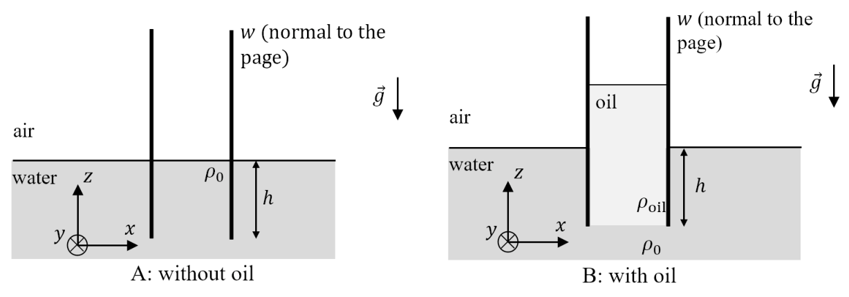
Figure 1. Parallel plates in water.

Oil of density \(\rho_{\mathrm{oil}}\) (\(\rho_{\mathrm{oil}}<\rho_0\)) is poured into the space between the plates until the lower level of the oil has reached the lower edges of the plates. Assume that plates and vessel edges are high enough for oil not to overflow them. Surface tension and mixing of fluids can be neglected.

A.1 — 0.8pt

What is the \(x\)-component of the net force \(F_x\) acting on the right plate (magnitude and direction)?

Fig. 2 shows a cross-section of a mid-ocean ridge. It consists of overlaying layers of mantle, crust and ocean water. The mantle is composed of rocks that we assume can flow in geological timescales and therefore, in this problem will be treated as a fluid. The thickness of the crust is much smaller than the characteristic length scale in the \(x\)-direction, hence, the crust behaves as a freely bendable plate. To high accuracy, such a ridge can be modeled as a two-dimensional system, without any variation of variables along the \(y\)-axis, which is perpendicular to the plane of Fig. 2. Assume that the ridge length \(L\) along the \(y\)-axis is much larger than any other length introduced in this problem.

At the centre of the ridge the thickness of the crust is assumed to be zero. As the horizontal distance \(x\) from the centre increases, the crust gets thicker and approaches a constant thickness \(D\) as \(x\to\infty\). Correspondingly, the ocean floor subsides by a vertical height \(h\) below the top of the ridge O, which we define as the origin of our coordinate system (see Fig. 2). Water density \(\rho_0\) and temperature \(T_0\) can be assumed to be constant in space and time. The same can be assumed for mantle density \(\rho_1\) and its temperature \(T_1\). The temperature of the crust \(T\) is also constant in time but can depend on position.

It is known that, to high accuracy, the crustal material expands linearly with temperature \(T\). Since water and mantle temperatures are assumed to be constant, it is convenient to use a rescaled version of the thermal expansion coefficient. Then \(l(T)=l_1[1-k_l(T_1-T)/(T_1-T_0)]\), where \(l\) is the length of a piece of crustal material, \(l_1\) is its length at temperature \(T_1\), and \(k_l\) is the rescaled thermal expansion coefficient, which can be assumed to be constant.

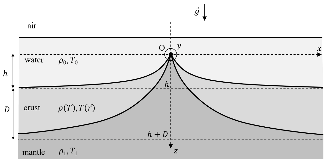
Figure 2. Mid-ocean ridge. Note that the \(z\)-axis is pointing downwards.

A.2 — 0.6pt

Assuming that the crust is isotropic, find how its density \(\rho\) depends on its temperature \(T\). Assuming that \(|k_l|\ll 1\), write your answer in the approximate form

\[ \rho(T)\approx \rho_1\left[1+k\frac{T_1-T}{T_1-T_0}\right], \tag{2} \]

where terms of order \(k_l^2\) and higher are neglected. Then, identify constant \(k\).

It is known that \(k>0\). Also, thermal conductivity of the crust \(\kappa\) can be assumed to be constant. As a consequence, very far away from the ridge axis the temperature of the crust depends linearly with depth.

A.3 — 1.1pt

By assuming that mantle and water each behave like an incompressible fluid at hydrostatic equilibrium, express the far-distance crust thickness \(D\) in terms of \(h\), \(\rho_0\), \(\rho_1\), and \(k\). Any motion of the material can be neglected.

A.4 — 1.6pt

Find, to the leading order in \(k\), the net horizontal force \(F\) acting on the right half (\(x>0\)) of the crust in terms of \(\rho_0\), \(\rho_1\), \(h\), \(L\), \(k\) and \(g\).

Suppose that crust is thermally isolated from the rest of the Earth. As a result of heat conduction, the temperatures of the upper and lower surfaces of the crust are going to get closer to each other until the crust reaches thermal equilibrium. Specific heat of the crust is \(c\) and can be assumed to be constant.

A.5 — 0.9pt

By using dimensional analysis or order-of-magnitude analysis, estimate the characteristic time \(\tau\) in which the difference between the upper and lower surface temperatures of the crust far away from the ridge axis is going to approach zero. You can assume that \(\tau\) does not depend on the two initial surface temperatures of the crust.

Part B. Seismic waves in a stratified medium (5.0 points)

Suppose that a short earthquake happens at the surface of some planet. The seismic waves can be assumed to originate from a line source situated at \(z=x=0\), where \(x\) is the horizontal coordinate and \(z\) is the depth below the surface (Fig. 3). The seismic wave source can be assumed to be much longer than any other length considered in this question.

As a result of the earthquake, a uniform flux of the so-called longitudinal P waves is emitted along all the directions in the \(x\)-\(z\) plane that have positive component along the \(z\)-axis. Since the wave theory in a solid is generally complicated, in this problem we neglect all the other waves emitted by the earthquake. The crust of the planet is stratified so that the P-wave speed \(v\) depends on depth \(z\) according to \(v=v_0(1+z/z_0)\), where \(v_0\) is the speed at the surface and \(z_0\) is a known positive constant.

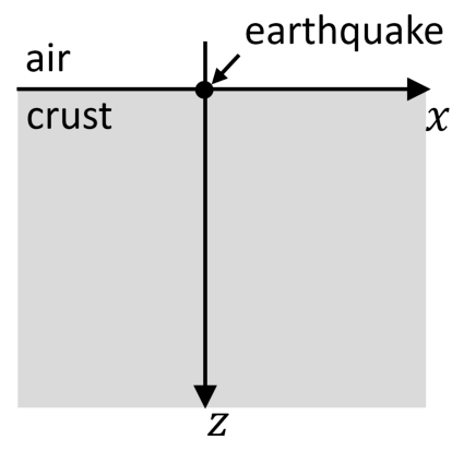
Figure 3. Coordinate system used in part B.

B.1 — 1.5pt

Consider a single ray emitted by the earthquake that makes an initial angle \(0<\theta_0<\pi/2\) with the \(z\)-axis and travels in the \(x\)-\(z\) plane. What is the horizontal coordinate \(x_1(\theta_0)\ne 0\) at which this ray can be detected at the surface of the planet? It is known that the ray path is an arc of a circle. Write your answer in the form \(x_1(\theta_0)=A\cot(b\theta_0)\), where \(A\) and \(b\) are constants to be found.

If you were unable to find \(A\) and \(b\), in the following questions you can use the result \(x_1(\theta_0)=A\cot(b\theta_0)\) as given. Suppose that total energy per unit length of the source released as P waves into the crust during the earthquake is \(E\). Assume that waves are completely absorbed when they reach the surface of the planet from below.

B.2 — 1.5pt

Find how the energy density per unit area \(\varepsilon(x)\) absorbed by the surface depends on the distance along the surface \(x\). Sketch the plot of \(\varepsilon(x)\).

From now on, assume that the waves are instead fully reflected when reaching the surface. Imagine a device positioned at \(z=x=0\) that has the same geometry as the previously considered earthquake source. The device is capable of emitting P waves in a freely chosen angular distribution. We make the device emit a signal with a narrow range of emission angles. In particular, the initial angle the signal makes with the vertical belongs to the interval \([\theta_0-\tfrac12\delta\theta_0,\theta_0+\tfrac12\delta\theta_0]\), where \(0<\theta_0<\pi/2\), \(\delta\theta_0\ll 1\) and \(\delta\theta_0\ll\theta_0\).

B.3 — 2.0pt

At what distance \(x_{\max}\) along the surface from the source is the furthest point that the signal does not reach? Write your answer in terms of \(\theta_0\), \(\delta\theta_0\) and other constants given above.

Official English text of the problem.

Consider a uniformly charged metallic ring of radius \(R\) and total charge \(q\). The ring is a hollow toroid of thickness \(2a\ll R\). This thickness can be neglected in parts A, B, C, and E. The \(xy\) plane coincides with the plane of the ring, while the \(z\)-axis is perpendicular to it, as shown in Figure 1. In parts A and B you might need to use the formula (Taylor expansion)

\[ (1+x)^\varepsilon\approx 1+\varepsilon x+\frac12\varepsilon(\varepsilon-1)x^2, \quad\text{when }|x|\ll1. \]

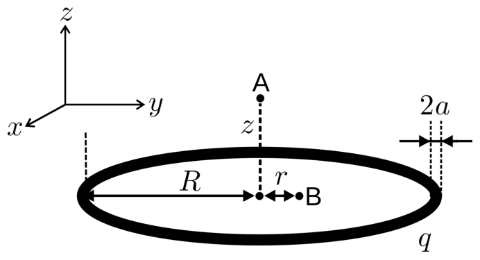
Figure 1. A charged ring of radius \(R\).

Part A. Electrostatic potential on the axis of the ring (1 point)

A.1	Calculate the electrostatic potential \(\Phi(z)\) along the axis of the ring at a \(z\) distance from its center (point A in Figure 1).	0.3pt
A.2	Calculate the electrostatic potential \(\Phi(z)\) to the lowest non-zero power of \(z\), assuming \(z\ll R\).	0.4pt
A.3	An electron (mass \(m\) and charge \(-e\)) is placed at point A (Figure 1, \(z\ll R\)). What is the force acting on the electron? Looking at the expression of the force, determine the sign of \(q\) so that the resulting motion would correspond to oscillations. The moving electron does not influence the charge distribution on the ring.	0.2pt
A.4	What is the angular frequency \(\omega\) of such harmonic oscillations?	0.1pt

Part B. Electrostatic potential in the plane of the ring (1.7 points)

In this part of the problem you will have to analyze the potential \(\Phi(r)\) in the plane of the ring (\(z=0\)) for \(r\ll R\) (point B in Figure 1). To the lowest non-zero power of \(r\) the electrostatic potential is given by \(\Phi(r)\approx q(\alpha+\beta r^2)\).

B.1	Find the expression for \(\beta\). You might need to use the Taylor expansion formula given above.	1.5pt
B.2	An electron is placed at point B (Figure 1, \(r\ll R\)). What is the force acting on the electron? Looking at the expression of the force, determine the sign of \(q\) so that the resulting motion would correspond to harmonic oscillations. The moving electron does not influence the charge distribution on the ring.	0.2pt

Part C. The focal length of the idealized electrostatic lens: instantaneous charging (2.3 points)

One wants to build a device to focus electrons—an electrostatic lens. Let us consider the following construction. The ring is situated perpendicularly to the \(z\)-axis, as shown in Figure 2. We have a source that produces on-demand packets of non-relativistic electrons. Kinetic energy of these electrons is \(E=mv^2/2\) (\(v\) is velocity) and they leave the source at precisely controlled moments. The system is programmed so that the ring is charge-neutral most of the time, but its charge becomes \(q\) when electrons are closer than a distance \(d/2\) (\(d\ll R\)) from the plane of the ring (shaded region in Figure 2, called “active region”). In part C assume that charging and de-charging processes are instantaneous and the electric field ”fills the space” instantaneously as well. One can neglect magnetic fields and assume that the velocity of electrons in the \(z\)-direction is constant. Moving electrons do not perturb the charge distribution on the ring.

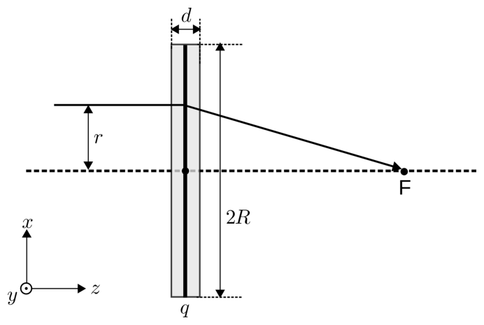
Figure 2. A model of an electrostatic lens.

C.1

Determine the focal length \(f\) of this lens. Assume that \(f\gg d\). Express your answer in terms of the constant \(\beta\) from question B.1 and other known quantities. Assume that before reaching the ”active region” the electron packet is parallel to the \(z\)-axis and \(r\ll R\). The sign of \(q\) is such so that the lens is focusing.

1.3pt

In reality the electron source is placed on the \(z\)-axis at a distance \(b>f\) from the center of the ring. Consider that electrons are no longer parallel to the \(z\)-axis before reaching the ”active region”, but are emitted from a point source at a range of different angles \(\gamma\ll1\) rad to the \(z\)-axis. Electrons are focused in a point situated at a distance \(c\) from the center of the ring.

C.2	Find \(c\). Express your answer in terms of the constant \(\beta\) from question B.1 and other known quantities.	0.8pt
C.3	Is the equation of a thin optical lens \(\displaystyle \frac1b+\frac1c=\frac1f\) fulfilled for the electrostatic lens? Show it by explicitly calculating \(1/b+1/c\).	0.2pt

Part D. The ring as a capacitor (3 points)

The model considered above was idealized and we assumed that the ring charged instantaneously. In reality charging is non-instantaneous, as the ring is a capacitor with a finite capacitance \(C\). In this part we will analyze the properties of this capacitor. You might need the following integrals:

\[ \int\frac{\mathrm dx}{\sin x} =-\ln\left|\frac{\cos x+1}{\sin x}\right|+\mathrm{const} \]

and

\[ \int\frac{\mathrm dx}{\sqrt{1+x^2}} =\ln\left|x+\sqrt{1+x^2}\right|+\mathrm{const}. \]

D.1

Calculate the capacitance \(C\) of the ring. Consider that the ring has a finite width \(2a\), but remember that \(a\ll R\).

2.0pt

When electrons reach the “active region”, the ring is connected to a source of voltage \(V_0\) (Figure 3). When electrons pass the “active region”, the ring is connected to the ground. The resistance of contacts is \(R_0\) and the resistance of the ring itself can be neglected.

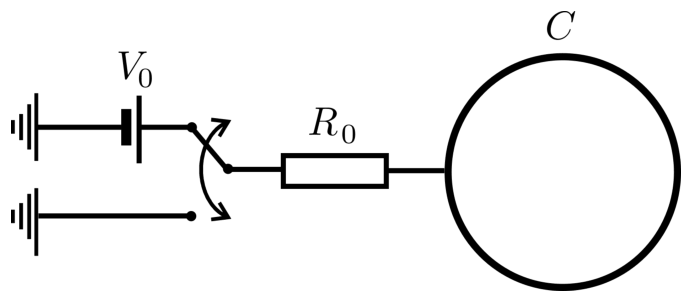
Figure 3. Charging of the electrostatic lens.

D.2

Determine the dependence of the charge on the ring as a function of time, \(q(t)\), and make a schematic plot of this dependence. \(t=0\) corresponds to a time moment when electrons are in the plane of the ring. What is the charge on the ring \(q_0\) when the absolute value \(q(t)\) is maximal? The capacitance of the ring is \(C\) (i.e., you do not have to use the actual expression found in D.1). Remark: the drawn polarity in Figure 3 is for indicative purposes only. The sign should be chosen so that the lens is focusing.

1.0pt

Part E. Focal length of a more realistic lens: non-instantaneous charging (2 points)

In this part of the problem, we will consider the action of this more realistic lens. Here we will again neglect the width of the ring \(2a\) and will assume that electrons travel parallel to the \(z\)-axis before reaching the ”active region”. However, the charging of the ring is no longer instantaneous.

E.1	Find the focal length \(f\) of the lens. Assume that \(f/v\gg R_0C\), but \(d/v\) and \(R_0C\) are of the same order of magnitude. Express your answer in terms of the constant \(\beta\) from part B and other known quantities.	1.7pt
E.2	You will see, that the result for \(f\) is similar to that obtained in part C, whereby the value \(q\) is substituted with \(q_{\mathrm{eff}}\). Find the expression for \(q_{\mathrm{eff}}\) in terms of quantities given in formulation of the problem.	0.3pt

Official English text of the problem.

Wave–particle duality, which states that each particle can be described as a wave and vice versa, is one of the central concepts of quantum mechanics. In this problem, we will rely on this notion and just a few other basic assumptions to explore a selection of quantum phenomena covering the two distinct types of particles of the microworld—fermions and bosons.

Part A. Quantum particle in a box (1.4 points)

Consider a particle of mass \(m\) moving in a one-dimensional potential well, where its potential energy \(V(x)\) is given by

\[ V(x)= \begin{cases} 0, & 0\leq x\leq L;\\ \infty, & x<0\text{ or }x>L. \end{cases} \tag{1} \]

While classical particle can move in such a potential having any kinetic energy, for quantum particle only some specific positive discrete energy levels are allowed. In any such allowed state, the particle can be described as a standing de Broglie wave with nodes at the walls.

A.1 — 0.4pt

Determine the minimal possible energy \(E_{\min}\) of the quantum particle in the well. Express your answer in terms of \(m\), \(L\), and the Planck’s constant \(h\).

The particle’s state with minimal possible energy is called the ground state, and all the rest allowed states are called excited states. Let us sort all the possible energy values in the increasing order and denote them as \(E_n\), starting from \(E_1\) for the ground state.

A.2 — 0.6pt

Find the general expression for the energy \(E_n\) (here \(n=1,\ 2,\ 3,\ldots\)).

A.3 — 0.4pt

Particle can undergo instantaneous transition from one state to another only by emitting or absorbing a photon of the corresponding energy difference. Find the wavelength \(\lambda_{21}\) of the photon emitted during the transition of the particle from the first excited state (\(E_2\)) to the ground state (\(E_1\)).

Part B. Optical properties of molecules (2.1 points)

In this part, we will study several optical properties of the cyanine Cy5 molecule—a widely used dye molecule, schematically shown in Fig. 1a. Its optical properties are determined mainly by the carbon backbone, composed of the alternating single and double bonds between carbon atoms, shown in Fig. 1b, while the influence of the rings at the molecule’s ends as well as radicals R is much smaller. Three of the four valence electrons of each C atom (and of N atoms) in the backbone form the chemical bonds, while the remaining valence electrons are “shared” and can move along the whole backbone. The net potential energy of each such electron is shown with oscillating thin line in Fig. 1c, with minima corresponding to the positions of the C and N atoms.

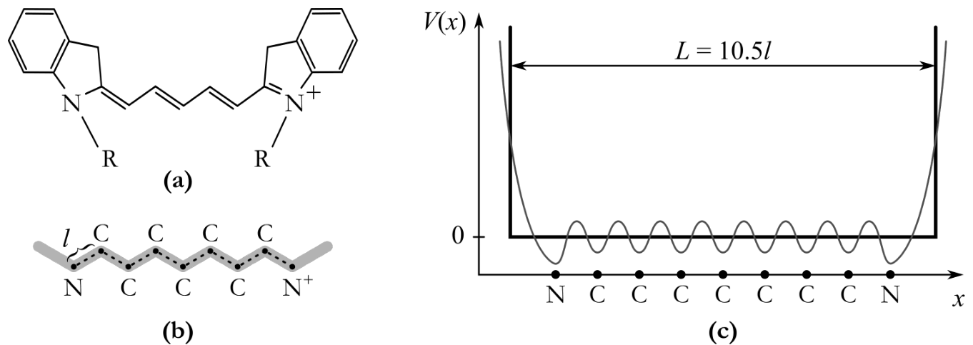
Figure 1. (a) Chemical structure of the cyanine Cy5 molecule (for simplicity, hydrogen atoms are not shown, and R denote some radicals). (b) The backbone of the Cy5 molecule, with mean inter-atomic distance \(l\). (c) Potential energy of the electron along the backbone (thin line) and its approximation by the step function given by Eq. 1 (thick line).

For simplicity, we will approximate this potential energy profile by a simple function given in Eq. 1 with the width \(L=10.5l\) (see thick line in Fig. 1c), here \(l=140\ \mathrm{pm}\) is the mean inter-atomic distance (see also Fig. 1b). As a result, we obtain the “electronic gas” composed of 10 electrons (7 from C atoms, 2 from the N atom, and 1 from the \(\mathrm{N}^{+}\) ion), moving in a one-dimensional potential well discussed in part A. In our evaluation, we can neglect the mutual interaction of these electrons; however, we should account for the fact that electrons are fermions and thus obey the Pauli exclusion principle. We also neglect the influence of other electrons as well as motion of the nuclei.

B.1 — 0.8pt

Evaluate the largest wavelength \(\lambda\) of the photon that can be absorbed by the Cy5 molecule assuming that the electron system is initially in its ground state. Express your answer in terms of \(l\), physical constants and some numerical prefactor, and calculate the numerical value.

B.2 — 0.4pt

Another dye molecule Cy3 has similar structure, but its backbone is shorter by 2 carbon atoms. Is its absorption spectrum shifted to the bluer or to the redder spectral region compared to the Cy5 molecule? Evaluate numerically the magnitude \(\Delta\lambda\) of this spectral shift. You can assume that removing two carbon atoms doesn’t change the molecule shape and only makes the backbone length shorter by two interatomic distances.

Being in the excited state, molecule can undergo a spontaneous transition to the ground state while emitting photon. The mean rate \(K\) of such events (i.e. the relative decrease of the molecules being in the excited state, \(\mathrm dN/N\), over time \(\mathrm dt\), \(K=\frac{1}{N}\frac{\mathrm dN}{\mathrm dt}\)) is determined by the wavelength \(\lambda\) of the emitted photon, the transition electrical dipole moment \(d\) (which is of the order of \(d\simeq el\), here \(e\) is elementary charge) as well as vacuum permittivity \(\varepsilon_0\) and Planck’s constant \(h\).

B.3 — 0.7pt

Using dimension analysis, determine the expression for the rate of spontaneous emission in terms of \(\varepsilon_0\), \(h\), \(\lambda\), and \(d\). The numerical prefactor for your expression is \(=\frac{16}{3}\pi^3\).

B.4 — 0.2pt

For Cy5 molecule, \(d\approx2.4\,el\). Evaluate the mean fluorescence lifetime of the lowest excited state of Cy5 molecule, \(\tau_{\mathrm{Cy5}}\), which is reciprocal to the rate of its emissive transition to the ground state.

Part C. Bose-Einstein condensation (1.5 points)

This part is not directly related to Parts A and B. Here, we will study the collective behaviour of bosonic particles. Bosons do not respect the Pauli exclusion principle, and—at low temperatures or high densities—experience a dramatic phenomenon known as the Bose–Einstein condensation (BEC). This is a phase transition to an intriguing collective quantum state: a large number of identical particles ‘condense’ into a single quantum state and start behaving as a single wave. The transition is typically reached by cooling a fixed number of particles below the critical temperature. In principle, it can also be induced by keeping the temperature fixed and driving the particle density past its critical value.

We begin by exploring the relation between the temperature and the particle density at the transition. As it turns out, estimates of their critical values can be deduced from a simple observation: Bose-Einstein condensation takes place when the de Broglie wavelength corresponding to the mean square speed of the particles is equal to the characteristic distance between the particles in a gas.

C.1 — 0.4pt

Given a non-interacting gas of \({}^{87}\mathrm{Rb}\) atoms in thermal equilibrium, write the expressions for their typical linear momentum \(p\) and the typical de Broglie wavelength \(\lambda_{\mathrm{dB}}\) as a function of atom’s mass \(m\), temperature \(T\) and physical constants.

C.2 — 0.5pt

Calculate the typical distance between the particles in a gas, \(\ell\), as a function of particle density \(n\). Hence deduce the critical temperature \(T_c\) as a function of atom’s mass, their density and physical constants.

To realize BEC in the lab, the experimentalists have to cool gases to temperatures as low as \(T_c=100\ \mathrm{nK}\).

C.3 — 0.6pt

What is the particle density of the Rb gas \(n_c\) if the transition takes place at such a temperature? For the sake of comparison, calculate also the ‘ordinary’ particle density \(n_0\) of an ideal gas at the standard temperature and pressure (STP), i.e. \(T_0=300\ \mathrm K\) and \(p_0=10^5\ \mathrm{Pa}\). How many times is the ‘ordinary’ gas denser? You may assume that the mass of the atoms is equal to 87 atomic mass units (\(m_{\mathrm{amu}}\)).

Part D. Three-beam optical lattices (5 points)

The first Bose-Einstein condensates were produced back in 1995, and since then the experimental work has branched out in diverse directions. In this part, you will investigate one particularly fruitful idea to load the condensate into spatially periodic potentials created by interfering a number of coherent laser beams. Due to the periodic nature of the resulting interference patterns, they are referred to as optical lattices. The potential energy \(V(\vec r)\) of an atom moving in an optical lattice is proportional to the local intensity of the light, and in your calculations you may assume that

\[ V(\vec r)=-\alpha\left\langle\left|\vec E(\vec r,t)\right|^2\right\rangle. \tag{2} \]

Here, \(\alpha\) is a positive constant, and the angle brackets indicate time-averaging which eliminates the rapidly oscillating terms. The electric field produced by the \(i\)-th laser is described by

\[ \vec E_i=E_{0,i}\,\vec\varepsilon_i\cos(\vec k_i\cdot\vec r-\omega t), \tag{3} \]

with the amplitude \(E_{0,i}\), the wave vector \(\vec k_i\), and the unit-length polarization vector \(\vec\varepsilon_i\).

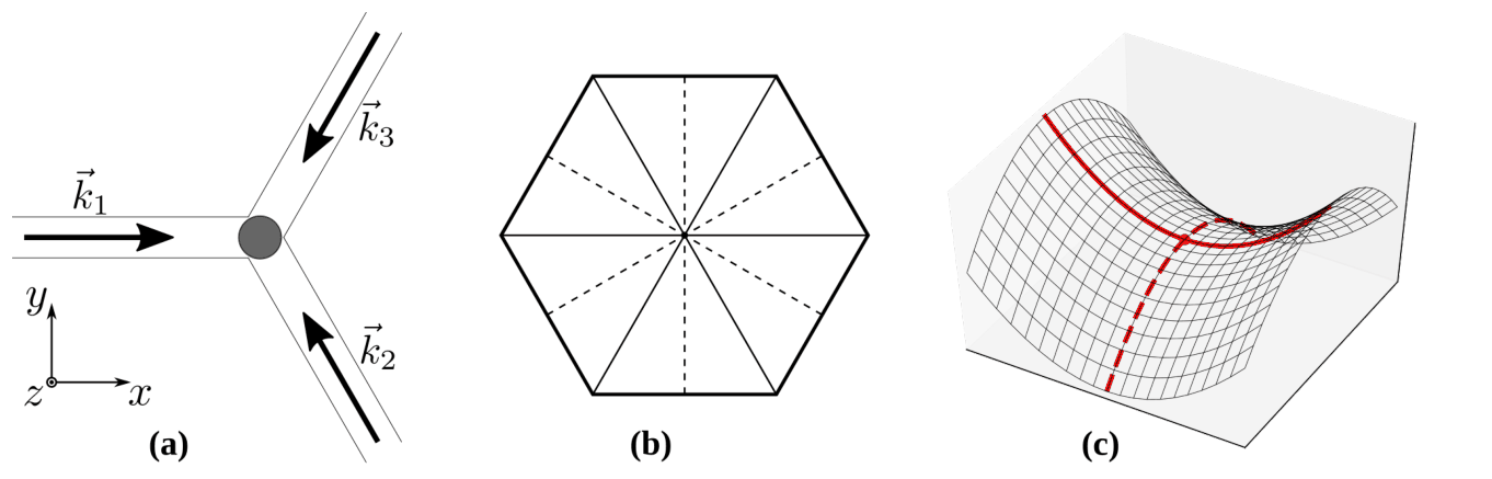
Figure 2. (a) Three-beam optical lattice: three plane waves with wave vectors \(\vec k_{1,2,3}\) intersect and interfere in the area indicated by the grey circle. (b) Symmetries of a regular hexagon: solid and dashed lines show two sets of symmetry axes. (c) Saddle point: a point on a surface where the slopes in orthogonal directions are all zero, but which is not a local extremum of the plotted function. Travelling along the trajectory marked by the full line one encounters an apparent minimum. Additional analysis of the perpendicular direction (dashed line) is needed to distinguish a true minimum from a saddle point (shown).

Your task is to study triangular optical lattices that are produced by interfering three coherent laser beams of equal intensity. A typical setup is shown in Fig. 2a. Here, all three beams are polarized in the \(z\) direction, propagate in the \(xy\) plane and intersect at equal angles of \(120^\circ\). Choose the direction of the \(x\) axis parallel to the wave vector \(\vec k_1\).

D.1 — 1.4pt

Using Eqs. 2 and 3 obtain the expression for the potential energy \(V(\vec r)\) as a function of \(\vec r=(x,y)\) in the plane of the beams.

Hint: the result can be neatly expressed as a constant term plus a sum of three cosine functions of arguments \(\vec b_i\cdot\vec r\). Please write your result in this form and identify the vectors \(\vec b_i\).

D.2 — 0.5pt

The resulting potential energy has a sixfold rotational symmetry axis, i.e., the potential distribution is invariant with respect to a rotation by a multiple of \(60^\circ\) around the origin. Provide a simple argument to prove that this is indeed the case.

The above observation of symmetry simplifies the analysis of the two-dimensional potential distribution \(V(\vec r)\). As shown in Fig. 2b, a regular hexagon has symmetry lines that, respectively, connect opposite vertices (solid lines) and midpoints of opposite edges (dashed lines). Therefore, in our situation one does not need to produce and study two-dimensional potential plots as many insights can be deduced by focusing on the coordinate axes \(x\) and \(y\) that run along the symmetry lines.

D.3 — 1.2pt

Derive the behavior of the potential \(V(\vec r)\) along the coordinate axes, i.e., determine the functions \(V_X(x)\equiv V(x,0)\) and \(V_Y(y)\equiv V(0,y)\). Identify the locations of the extrema of \(V_X(x)\) and \(V_Y(y)\) as functions of a single argument. As these functions are periodic, please include in your lists only one representative from each family of periodically repeated minima and maxima.

We are interested in determining the locations of so-called lattice sites, i.e., the minima of the full two-dimensional potential \(V(\vec r)\). The obtained minima of single-argument functions \(V_X\) and \(V_Y\) identify their suspected positions but still have to be checked to eliminate the saddle points. As shown in Fig. 2c, when studied along a single line, saddle points may disguise as minima but they are not.

D.4 — 0.8pt

Review your results in the previous question to determine actual minima of the optical lattice: Identify all equivalent minima nearest to (but not coinciding with) the origin. What is the distance \(a\) between the nearest minima, in other words—the lattice constant of our optical lattice? Express the answer in terms of the laser wavelength \(\lambda_{\mathrm{las}}\).

Charge neutrality of ultracold atoms suggests that their interactions become relevant only when two or more atoms occupy the same site of an optical lattice. However, experimentalists are also able to explore setups that sustain long-range atomic interactions. A possible approach relies on creation of the so-called Rydberg atoms that are physically large and feature other exaggerated properties. Rydberg atoms are excited atoms with one electron promoted to a state with a very high principal quantum number \(n\). The size of a Rydberg atom can be estimated by calculating the radius of the classical circular orbit of that electron with the orbital angular momentum \(n\hbar\), here \(\hbar\) is the reduced Planck constant.

D.5 — 1.1pt

Calculate the value of \(n\) that corresponds to the radius of the Rb Rydberg atom comparable to the wavelength of laser light \(\lambda_{\mathrm{las}}=380\ \mathrm{nm}\). Give your answer in terms of \(\lambda_{\mathrm{las}}\) and physical constants and find its numerical value.

Official English text of the problem.

Diese Aufgabe besteht aus zwei voneinander unabhängigen Teilaufgaben zum Inneren von Planeten. Die Auswirkungen der Oberflächenkrümmung der Planeten können vernachlässigt werden. Möglicherweise benötigen Sie die Formel

\[ (1+x)^\varepsilon\approx 1+\varepsilon x,\quad \text{wenn }|x|\ll 1. \tag{1} \]

Teil A. Mittelozeanischer Rücken (5.0 Punkte)

Betrachten Sie ein großes Wassergefäß in einem homogenen Gravitationsfeld mit der Fallbeschleunigung \(g\). Zwei zueinander parallele, senkrechte rechteckige Platten sind so in das Gefäß eingesetzt, dass ihre senkrechten Kanten dicht und lückenlos an den senkrechten Gefäßwänden anliegen. Jede Platte taucht über eine Länge \(h\) in das Wasser ein (Abb. 1). Die Breite der Platten entlang der \(y\)-Achse beträgt \(w\), die Dichte des Wassers ist \(\rho_0\).

Abbildung 1. Parallele Platten im Wasser.

Öl der Dichte \(\rho_{\mathrm{oil}}\) (\(\rho_{\mathrm{oil}}<\rho_0\)) wird in den Raum zwischen den Platten gegossen, bis die untere Grenzfläche des Öls die Unterkanten der Platten erreicht hat. Nehmen Sie an, dass die Platten und die Gefäßränder hoch genug sind, sodass kein Öl darüberläuft. Oberflächenspannung und Durchmischung der Flüssigkeiten können vernachlässigt werden.

A.1 — 0.8 Punkte

Wie groß ist die \(x\)-Komponente der resultierenden Kraft \(F_x\), die auf die rechte Platte wirkt (Betrag und Richtung)?

Abb. 2 zeigt einen Querschnitt durch einen mittelozeanischen Rücken. Er besteht aus übereinanderliegenden Schichten aus Mantel, Kruste und Ozeanwasser. Der Mantel besteht aus Gesteinen, von denen wir annehmen, dass sie auf geologischen Zeitskalen fließen können; daher wird er in dieser Aufgabe als Fluid behandelt. Die Dicke der Kruste ist wesentlich kleiner als die charakteristische Längenskala in \(x\)-Richtung, sodass sich die Kruste wie eine frei biegsame Platte verhält. Ein solcher Rücken lässt sich mit hoher Genauigkeit als zweidimensionales System modellieren, dessen Größen sich entlang der \(y\)-Achse, die senkrecht zur Zeichenebene von Abb. 2 steht, nicht ändern. Nehmen Sie an, dass die Länge \(L\) des Rückens entlang der \(y\)-Achse wesentlich größer ist als jede andere in dieser Aufgabe eingeführte Länge.

Im Zentrum des Rückens wird die Dicke der Kruste als null angenommen. Mit zunehmendem horizontalem Abstand \(x\) vom Zentrum wird die Kruste dicker und nähert sich für \(x\to\infty\) einer konstanten Dicke \(D\). Entsprechend senkt sich der Meeresboden um eine vertikale Höhe \(h\) unter den Scheitel O des Rückens ab, den wir als Ursprung unseres Koordinatensystems festlegen (siehe Abb. 2). Die Dichte \(\rho_0\) und die Temperatur \(T_0\) des Wassers können als räumlich und zeitlich konstant angenommen werden. Dasselbe gilt für die Dichte \(\rho_1\) und die Temperatur \(T_1\) des Mantels. Die Temperatur \(T\) der Kruste ist ebenfalls zeitlich konstant, kann jedoch vom Ort abhängen.

Es ist bekannt, dass sich das Krustenmaterial mit hoher Genauigkeit linear mit der Temperatur \(T\) ausdehnt. Da die Temperaturen von Wasser und Mantel als konstant angenommen werden, ist es zweckmäßig, eine umskalierte Form des Wärmeausdehnungskoeffizienten zu verwenden. Dann gilt \(l(T)=l_1[1-k_l(T_1-T)/(T_1-T_0)]\), wobei \(l\) die Länge eines Stücks Krustenmaterial, \(l_1\) dessen Länge bei der Temperatur \(T_1\) und \(k_l\) der umskalierte Wärmeausdehnungskoeffizient ist, der als konstant angenommen werden kann.

Abbildung 2. Mittelozeanischer Rücken. Beachten Sie, dass die \(z\)-Achse nach unten zeigt.

A.2 — 0.6 Punkte

Bestimmen Sie unter der Annahme einer isotropen Kruste, wie ihre Dichte \(\rho\) von ihrer Temperatur \(T\) abhängt. Schreiben Sie Ihre Antwort unter der Annahme \(|k_l|\ll 1\) in der Näherungsform

\[ \rho(T)\approx \rho_1\left[1+k\frac{T_1-T}{T_1-T_0}\right], \tag{2} \]

wobei Terme der Ordnung \(k_l^2\) und höher vernachlässigt werden. Bestimmen Sie anschließend die Konstante \(k\).

Es ist bekannt, dass \(k>0\) gilt. Außerdem kann die Wärmeleitfähigkeit \(\kappa\) der Kruste als konstant angenommen werden. Daher hängt die Temperatur der Kruste in sehr großer Entfernung von der Rückenachse linear von der Tiefe ab.

A.3 — 1.1 Punkte

Drücken Sie unter der Annahme, dass sich Mantel und Wasser jeweils wie ein inkompressibles Fluid im hydrostatischen Gleichgewicht verhalten, die Krustendicke \(D\) in großer Entfernung durch \(h\), \(\rho_0\), \(\rho_1\) und \(k\) aus. Jegliche Bewegung des Materials kann vernachlässigt werden.

A.4 — 1.6 Punkte

Bestimmen Sie in führender Ordnung in \(k\) die resultierende horizontale Kraft \(F\), die auf die rechte Hälfte (\(x>0\)) der Kruste wirkt, in Abhängigkeit von \(\rho_0\), \(\rho_1\), \(h\), \(L\), \(k\) und \(g\).

Nehmen Sie an, die Kruste sei vom Rest der Erde thermisch isoliert. Durch Wärmeleitung nähern sich die Temperaturen der Ober- und Unterseite der Kruste einander an, bis die Kruste das thermische Gleichgewicht erreicht. Die spezifische Wärmekapazität der Kruste beträgt \(c\) und kann als konstant angenommen werden.

A.5 — 0.9 Punkte

Schätzen Sie mithilfe einer Dimensionsanalyse oder einer Größenordnungsabschätzung die charakteristische Zeit \(\tau\) ab, innerhalb derer sich die Temperaturdifferenz zwischen Ober- und Unterseite der Kruste in großer Entfernung von der Rückenachse null annähert. Sie können annehmen, dass \(\tau\) nicht von den beiden anfänglichen Oberflächentemperaturen der Kruste abhängt.

Teil B. Seismische Wellen in einem geschichteten Medium (5.0 Punkte)

Nehmen Sie an, an der Oberfläche eines Planeten ereigne sich ein kurzes Erdbeben. Es kann angenommen werden, dass die seismischen Wellen von einer Linienquelle bei \(z=x=0\) ausgehen, wobei \(x\) die horizontale Koordinate und \(z\) die Tiefe unterhalb der Oberfläche ist (Abb. 3). Die Quelle der seismischen Wellen kann als wesentlich länger als jede andere in dieser Teilaufgabe betrachtete Länge angenommen werden.

Infolge des Erdbebens wird ein gleichmäßiger Fluss sogenannter longitudinaler P-Wellen in alle Richtungen in der \(x\)-\(z\)-Ebene ausgesandt, die eine positive Komponente entlang der \(z\)-Achse aufweisen. Da die Wellentheorie in einem Festkörper im Allgemeinen kompliziert ist, vernachlässigen wir in dieser Aufgabe alle anderen vom Erdbeben ausgesandten Wellen. Die Kruste des Planeten ist so geschichtet, dass die Geschwindigkeit \(v\) der P-Wellen gemäß \(v=v_0(1+z/z_0)\) von der Tiefe \(z\) abhängt, wobei \(v_0\) die Geschwindigkeit an der Oberfläche und \(z_0\) eine bekannte positive Konstante ist.

Abbildung 3. Das in Teil B verwendete Koordinatensystem.

B.1 — 1.5 Punkte

Betrachten Sie einen einzelnen, vom Erdbeben ausgesandten Strahl, der anfangs einen Winkel \(0<\theta_0<\pi/2\) mit der \(z\)-Achse bildet und sich in der \(x\)-\(z\)-Ebene ausbreitet. Bei welcher horizontalen Koordinate \(x_1(\theta_0)\ne 0\) kann dieser Strahl an der Oberfläche des Planeten nachgewiesen werden? Es ist bekannt, dass die Strahlbahn ein Kreisbogen ist. Schreiben Sie Ihre Antwort in der Form \(x_1(\theta_0)=A\cot(b\theta_0)\), wobei \(A\) und \(b\) zu bestimmende Konstanten sind.

Falls Sie \(A\) und \(b\) nicht bestimmen konnten, können Sie in den folgenden Teilaufgaben das Ergebnis \(x_1(\theta_0)=A\cot(b\theta_0)\) als gegeben verwenden. Nehmen Sie an, dass die gesamte Energie pro Längeneinheit der Quelle, die während des Erdbebens als P-Wellen in die Kruste abgegeben wird, \(E\) beträgt. Nehmen Sie an, dass die Wellen vollständig absorbiert werden, wenn sie die Oberfläche des Planeten von unten erreichen.

B.2 — 1.5 Punkte

Bestimmen Sie, wie die von der Oberfläche absorbierte Energie pro Flächeneinheit \(\varepsilon(x)\) vom Abstand \(x\) entlang der Oberfläche abhängt. Skizzieren Sie den Graphen von \(\varepsilon(x)\).

Nehmen Sie von nun an an, dass die Wellen beim Erreichen der Oberfläche stattdessen vollständig reflektiert werden. Stellen Sie sich eine bei \(z=x=0\) angeordnete Vorrichtung vor, die dieselbe Geometrie wie die zuvor betrachtete Erdbebenquelle besitzt. Die Vorrichtung kann P-Wellen mit einer frei wählbaren Winkelverteilung aussenden. Wir lassen die Vorrichtung ein Signal in einem engen Bereich von Emissionswinkeln aussenden. Insbesondere liegt der anfängliche Winkel des Signals zur Vertikalen im Intervall \([\theta_0-\tfrac12\delta\theta_0,\theta_0+\tfrac12\delta\theta_0]\), wobei \(0<\theta_0<\pi/2\), \(\delta\theta_0\ll 1\) und \(\delta\theta_0\ll\theta_0\) gelten.

B.3 — 2.0 Punkte

In welchem Abstand \(x_{\max}\) von der Quelle entlang der Oberfläche liegt der am weitesten entfernte Punkt, den das Signal nicht erreicht? Drücken Sie Ihre Antwort durch \(\theta_0\), \(\delta\theta_0\) und die anderen oben angegebenen Konstanten aus.

Aufgabentext aus dem offiziellen englischen Text übersetzt.

Betrachten Sie einen gleichmäßig geladenen metallischen Ring mit dem Radius \(R\) und der Gesamtladung \(q\). Der Ring ist ein hohler Torus mit der Dicke \(2a\ll R\). Diese Dicke kann in den Teilen A, B, C und E vernachlässigt werden. Die \(xy\)-Ebene fällt mit der Ringebene zusammen, während die \(z\)-Achse senkrecht dazu steht, wie in Abbildung 1 gezeigt. In den Teilen A und B benötigen Sie möglicherweise die Formel (Taylorentwicklung)

\[ (1+x)^\varepsilon\approx 1+\varepsilon x+\frac12\varepsilon(\varepsilon-1)x^2, \quad\text{wenn }|x|\ll1. \]

Abbildung 1. Ein geladener Ring mit dem Radius \(R\).

Teil A. Elektrostatisches Potential auf der Ringachse (1 Punkt)

A.1	Berechnen Sie das elektrostatische Potential \(\Phi(z)\) entlang der Ringachse im Abstand \(z\) vom Mittelpunkt des Rings (Punkt A in Abbildung 1).	0.3 Pkt.
A.2	Berechnen Sie das elektrostatische Potential \(\Phi(z)\) bis zur niedrigsten nichtverschwindenden Potenz von \(z\) unter der Annahme \(z\ll R\).	0.4 Pkt.
A.3	Ein Elektron (Masse \(m\) und Ladung \(-e\)) wird in Punkt A platziert (Abbildung 1, \(z\ll R\)). Welche Kraft wirkt auf das Elektron? Bestimmen Sie anhand des Ausdrucks für die Kraft das Vorzeichen von \(q\), bei dem die resultierende Bewegung eine Schwingung ist. Das bewegte Elektron beeinflusst die Ladungsverteilung auf dem Ring nicht.	0.2 Pkt.
A.4	Welche Kreisfrequenz \(\omega\) haben solche harmonischen Schwingungen?	0.1 Pkt.

Teil B. Elektrostatisches Potential in der Ringebene (1.7 Punkte)

In diesem Teil der Aufgabe sollen Sie das Potential \(\Phi(r)\) in der Ringebene (\(z=0\)) für \(r\ll R\) untersuchen (Punkt B in Abbildung 1). Bis zur niedrigsten nichtverschwindenden Potenz von \(r\) ist das elektrostatische Potential durch \(\Phi(r)\approx q(\alpha+\beta r^2)\) gegeben.

B.1	Bestimmen Sie den Ausdruck für \(\beta\). Möglicherweise benötigen Sie die oben angegebene Taylorentwicklung.	1.5 Pkt.
B.2	Ein Elektron wird in Punkt B platziert (Abbildung 1, \(r\ll R\)). Welche Kraft wirkt auf das Elektron? Bestimmen Sie anhand des Ausdrucks für die Kraft das Vorzeichen von \(q\), bei dem die resultierende Bewegung eine harmonische Schwingung ist. Das bewegte Elektron beeinflusst die Ladungsverteilung auf dem Ring nicht.	0.2 Pkt.

Teil C. Die Brennweite der idealisierten elektrostatischen Linse: augenblickliches Aufladen (2.3 Punkte)

Man möchte eine Vorrichtung zur Fokussierung von Elektronen bauen — eine elektrostatische Linse. Betrachten wir dazu den folgenden Aufbau. Der Ring steht senkrecht zur \(z\)-Achse, wie in Abbildung 2 gezeigt. Es steht eine Quelle zur Verfügung, die auf Abruf Pakete nichtrelativistischer Elektronen erzeugt. Die kinetische Energie dieser Elektronen beträgt \(E=mv^2/2\) (\(v\) ist die Geschwindigkeit), und sie verlassen die Quelle zu genau gesteuerten Zeitpunkten. Das System ist so programmiert, dass der Ring die meiste Zeit elektrisch neutral ist, seine Ladung jedoch \(q\) beträgt, wenn die Elektronen weniger als den Abstand \(d/2\) (\(d\ll R\)) von der Ringebene entfernt sind (schattierter Bereich in Abbildung 2, als „aktiver Bereich“ bezeichnet). Nehmen Sie in Teil C an, dass das Aufladen und Entladen augenblicklich erfolgen und das elektrische Feld ebenfalls augenblicklich „den Raum erfüllt“. Magnetfelder können vernachlässigt werden, und die Geschwindigkeit der Elektronen in \(z\)-Richtung kann als konstant angenommen werden. Die bewegten Elektronen stören die Ladungsverteilung auf dem Ring nicht.

Abbildung 2. Ein Modell einer elektrostatischen Linse.

C.1

Bestimmen Sie die Brennweite \(f\) dieser Linse. Nehmen Sie an, dass \(f\gg d\). Drücken Sie Ihre Antwort durch die Konstante \(\beta\) aus Frage B.1 und andere bekannte Größen aus. Nehmen Sie an, dass sich das Elektronenpaket vor dem Erreichen des „aktiven Bereichs“ parallel zur \(z\)-Achse bewegt und \(r\ll R\) gilt. Das Vorzeichen von \(q\) ist so gewählt, dass die Linse fokussiert.

1.3 Pkt.

In Wirklichkeit befindet sich die Elektronenquelle auf der \(z\)-Achse im Abstand \(b>f\) vom Mittelpunkt des Rings. Gehen Sie davon aus, dass sich die Elektronen vor dem Erreichen des „aktiven Bereichs“ nicht mehr parallel zur \(z\)-Achse bewegen, sondern von einer Punktquelle unter verschiedenen Winkeln \(\gamma\ll1\) rad zur \(z\)-Achse emittiert werden. Die Elektronen werden in einem Punkt im Abstand \(c\) vom Mittelpunkt des Rings fokussiert.

C.2	Bestimmen Sie \(c\). Drücken Sie Ihre Antwort durch die Konstante \(\beta\) aus Frage B.1 und andere bekannte Größen aus.	0.8 Pkt.
C.3	Gilt die Gleichung einer dünnen optischen Linse \(\displaystyle \frac1b+\frac1c=\frac1f\) für die elektrostatische Linse? Zeigen Sie dies, indem Sie \(1/b+1/c\) explizit berechnen.	0.2 Pkt.

Teil D. Der Ring als Kondensator (3 Punkte)

Das oben betrachtete Modell war idealisiert, und wir haben angenommen, dass der Ring augenblicklich aufgeladen wird. In Wirklichkeit erfolgt das Aufladen nicht augenblicklich, da der Ring ein Kondensator mit einer endlichen Kapazität \(C\) ist. In diesem Teil untersuchen wir die Eigenschaften dieses Kondensators. Möglicherweise benötigen Sie die folgenden Integrale:

\[ \int\frac{\mathrm dx}{\sin x} =-\ln\left|\frac{\cos x+1}{\sin x}\right|+\mathrm{const} \]

und

\[ \int\frac{\mathrm dx}{\sqrt{1+x^2}} =\ln\left|x+\sqrt{1+x^2}\right|+\mathrm{const}. \]

D.1

Berechnen Sie die Kapazität \(C\) des Rings. Berücksichtigen Sie, dass der Ring eine endliche Dicke \(2a\) hat, beachten Sie aber, dass \(a\ll R\) gilt.

2.0 Pkt.

Wenn die Elektronen den „aktiven Bereich“ erreichen, wird der Ring an eine Spannungsquelle mit der Spannung \(V_0\) angeschlossen (Abbildung 3). Wenn die Elektronen den „aktiven Bereich“ durchquert haben, wird der Ring geerdet. Der Widerstand der Kontakte beträgt \(R_0\), und der Widerstand des Rings selbst kann vernachlässigt werden.

Abbildung 3. Aufladen der elektrostatischen Linse.

D.2

Bestimmen Sie die Ladung auf dem Ring als Funktion der Zeit, \(q(t)\), und skizzieren Sie diesen Verlauf. \(t=0\) entspricht dem Zeitpunkt, zu dem sich die Elektronen in der Ringebene befinden. Wie groß ist die Ladung auf dem Ring \(q_0\), wenn der Betrag von \(q(t)\) maximal ist? Die Kapazität des Rings beträgt \(C\) (Sie müssen also nicht den in D.1 gefundenen tatsächlichen Ausdruck verwenden). Anmerkung: Die in Abbildung 3 eingezeichnete Polarität dient lediglich der Veranschaulichung. Das Vorzeichen ist so zu wählen, dass die Linse fokussiert.

1.0 Pkt.

Teil E. Brennweite einer realistischeren Linse: nicht augenblickliches Aufladen (2 Punkte)

In diesem Teil der Aufgabe betrachten wir die Wirkung dieser realistischeren Linse. Dabei vernachlässigen wir erneut die Dicke des Rings \(2a\) und nehmen an, dass sich die Elektronen vor dem Erreichen des „aktiven Bereichs“ parallel zur \(z\)-Achse bewegen. Das Aufladen des Rings erfolgt jedoch nicht mehr augenblicklich.

E.1	Bestimmen Sie die Brennweite \(f\) der Linse. Nehmen Sie an, dass \(f/v\gg R_0C\), während \(d/v\) und \(R_0C\) von derselben Größenordnung sind. Drücken Sie Ihre Antwort durch die Konstante \(\beta\) aus Teil B und andere bekannte Größen aus.	1.7 Pkt.
E.2	Sie werden feststellen, dass das Ergebnis für \(f\) dem in Teil C erhaltenen ähnelt, wobei der Wert \(q\) durch \(q_{\mathrm{eff}}\) ersetzt wird. Bestimmen Sie den Ausdruck für \(q_{\mathrm{eff}}\) in Abhängigkeit von den in der Aufgabenstellung gegebenen Größen.	0.3 Pkt.

Aufgabentext aus dem offiziellen englischen Text übersetzt.

Der Welle-Teilchen-Dualismus, dem zufolge jedes Teilchen als Welle beschrieben werden kann und umgekehrt, ist eines der zentralen Konzepte der Quantenmechanik. In dieser Aufgabe werden wir auf Grundlage dieses Konzepts und nur weniger weiterer grundlegender Annahmen eine Auswahl von Quantenphänomenen untersuchen, die die beiden unterschiedlichen Teilchenarten der Mikrowelt betreffen: Fermionen und Bosonen.

Teil A. Quantenteilchen im Kasten (1.4 Punkte)

Betrachten Sie ein Teilchen der Masse \(m\), das sich in einem eindimensionalen Potentialtopf bewegt, in dem seine potentielle Energie \(V(x)\) gegeben ist durch

\[ V(x)= \begin{cases} 0, & 0\leq x\leq L;\\ \infty, & x<0\text{ oder }x>L. \end{cases} \tag{1} \]

Während sich ein klassisches Teilchen in einem solchen Potential mit beliebiger kinetischer Energie bewegen kann, sind für ein Quantenteilchen nur bestimmte positive, diskrete Energieniveaus erlaubt. In jedem dieser erlaubten Zustände lässt sich das Teilchen als stehende de-Broglie-Welle mit Knoten an den Wänden beschreiben.

A.1 — 0.4 Punkte

Bestimmen Sie die kleinstmögliche Energie \(E_{\min}\) des Quantenteilchens im Potentialtopf. Drücken Sie Ihre Antwort durch \(m\), \(L\) und die Planck-Konstante \(h\) aus.

Der Zustand des Teilchens mit der kleinstmöglichen Energie heißt Grundzustand, alle übrigen erlaubten Zustände heißen angeregte Zustände. Wir ordnen alle möglichen Energiewerte aufsteigend und bezeichnen sie mit \(E_n\), beginnend mit \(E_1\) für den Grundzustand.

A.2 — 0.6 Punkte

Bestimmen Sie den allgemeinen Ausdruck für die Energie \(E_n\) (hier ist \(n=1,\ 2,\ 3,\ldots\)).

A.3 — 0.4 Punkte

Das Teilchen kann nur unter Emission oder Absorption eines Photons mit der entsprechenden Energiedifferenz einen instantanen Übergang von einem Zustand in einen anderen vollziehen. Bestimmen Sie die Wellenlänge \(\lambda_{21}\) des Photons, das beim Übergang des Teilchens vom ersten angeregten Zustand (\(E_2\)) in den Grundzustand (\(E_1\)) emittiert wird.

Teil B. Optische Eigenschaften von Molekülen (2.1 Punkte)

In diesem Teil untersuchen wir verschiedene optische Eigenschaften des Cyaninmoleküls Cy5, eines häufig verwendeten Farbstoffmoleküls, das in Abb. 1a schematisch dargestellt ist. Seine optischen Eigenschaften werden hauptsächlich durch das Kohlenstoffgerüst bestimmt, das aus abwechselnden Einfach- und Doppelbindungen zwischen Kohlenstoffatomen besteht und in Abb. 1b gezeigt ist; der Einfluss der Ringe an den Molekülenden sowie der Reste R ist wesentlich geringer. Drei der vier Valenzelektronen jedes C-Atoms (und der N-Atome) im Gerüst bilden die chemischen Bindungen, während die verbleibenden Valenzelektronen „gemeinsam genutzt“ werden und sich entlang des gesamten Gerüsts bewegen können. Die gesamte potentielle Energie jedes dieser Elektronen ist in Abb. 1c durch eine oszillierende dünne Linie dargestellt, deren Minima den Positionen der C- und N-Atome entsprechen.

Abbildung 1. (a) Chemische Struktur des Cyaninmoleküls Cy5 (der Einfachheit halber sind Wasserstoffatome nicht dargestellt, und R bezeichnet bestimmte Reste). (b) Das Gerüst des Cy5-Moleküls mit dem mittleren Atomabstand \(l\). (c) Potentielle Energie des Elektrons entlang des Gerüsts (dünne Linie) und ihre Näherung durch die in Gl. 1 angegebene Stufenfunktion (dicke Linie).

Der Einfachheit halber nähern wir dieses Profil der potentiellen Energie durch die einfache Funktion aus Gl. 1 mit der Breite \(L=10.5l\) an (siehe dicke Linie in Abb. 1c); dabei ist \(l=140\ \mathrm{pm}\) der mittlere Atomabstand (siehe auch Abb. 1b). Dadurch erhalten wir ein „Elektronengas“ aus 10 Elektronen (7 von C-Atomen, 2 vom N-Atom und 1 vom \(\mathrm{N}^{+}\)-Ion), die sich in dem in Teil A behandelten eindimensionalen Potentialtopf bewegen. Bei unserer Abschätzung können wir die gegenseitige Wechselwirkung dieser Elektronen vernachlässigen; wir müssen jedoch berücksichtigen, dass Elektronen Fermionen sind und daher dem Pauli-Prinzip gehorchen. Wir vernachlässigen außerdem den Einfluss anderer Elektronen sowie die Bewegung der Atomkerne.

B.1 — 0.8 Punkte

Schätzen Sie die größte Wellenlänge \(\lambda\) eines Photons ab, das vom Cy5-Molekül absorbiert werden kann, wenn sich das Elektronensystem anfangs im Grundzustand befindet. Drücken Sie Ihre Antwort durch \(l\), physikalische Konstanten und einen numerischen Vorfaktor aus und berechnen Sie den Zahlenwert.

B.2 — 0.4 Punkte

Ein weiteres Farbstoffmolekül, Cy3, hat eine ähnliche Struktur, sein Gerüst ist jedoch um 2 Kohlenstoffatome kürzer. Ist sein Absorptionsspektrum gegenüber dem des Cy5-Moleküls zum blauen oder zum roten Spektralbereich hin verschoben? Berechnen Sie näherungsweise den Betrag \(\Delta\lambda\) dieser spektralen Verschiebung. Sie dürfen annehmen, dass das Entfernen zweier Kohlenstoffatome die Form des Moleküls nicht verändert und lediglich die Länge des Gerüsts um zwei Atomabstände verkürzt.

Im angeregten Zustand kann das Molekül unter Emission eines Photons spontan in den Grundzustand übergehen. Die mittlere Rate \(K\) solcher Ereignisse (d. h. die relative Abnahme der Zahl der Moleküle im angeregten Zustand, \(\mathrm dN/N\), während der Zeit \(\mathrm dt\), \(K=\frac{1}{N}\frac{\mathrm dN}{\mathrm dt}\)) wird durch die Wellenlänge \(\lambda\) des emittierten Photons, das elektrische Übergangsdipolmoment \(d\) (das von der Größenordnung \(d\simeq el\) ist, wobei \(e\) die Elementarladung ist) sowie die Vakuumpermittivität \(\varepsilon_0\) und die Planck-Konstante \(h\) bestimmt.

B.3 — 0.7 Punkte

Bestimmen Sie mithilfe einer Dimensionsanalyse den Ausdruck für die Rate der spontanen Emission in Abhängigkeit von \(\varepsilon_0\), \(h\), \(\lambda\) und \(d\). Der numerische Vorfaktor für Ihren Ausdruck ist \(=\frac{16}{3}\pi^3\).

B.4 — 0.2 Punkte

Für das Cy5-Molekül gilt \(d\approx2.4\,el\). Schätzen Sie die mittlere Fluoreszenzlebensdauer des niedrigsten angeregten Zustands des Cy5-Moleküls, \(\tau_{\mathrm{Cy5}}\), ab; sie ist der Kehrwert der Rate seines strahlenden Übergangs in den Grundzustand.

Teil C. Bose-Einstein-Kondensation (1.5 Punkte)

Dieser Teil steht nicht in direktem Zusammenhang mit den Teilen A und B. Hier untersuchen wir das kollektive Verhalten bosonischer Teilchen. Bosonen unterliegen nicht dem Pauli-Prinzip und zeigen bei niedrigen Temperaturen oder hohen Dichten ein ausgeprägtes Phänomen, das als Bose-Einstein-Kondensation (BEC) bekannt ist. Dabei handelt es sich um einen Phasenübergang in einen faszinierenden kollektiven Quantenzustand: Eine große Anzahl identischer Teilchen „kondensiert“ in einen einzigen Quantenzustand und beginnt, sich wie eine einzige Welle zu verhalten. Der Übergang wird üblicherweise erreicht, indem eine feste Anzahl von Teilchen unter die kritische Temperatur abgekühlt wird. Grundsätzlich lässt er sich auch herbeiführen, indem man die Temperatur konstant hält und die Teilchendichte über ihren kritischen Wert erhöht.

Wir beginnen mit der Untersuchung des Zusammenhangs zwischen Temperatur und Teilchendichte beim Übergang. Wie sich zeigt, lassen sich ihre kritischen Werte anhand einer einfachen Beobachtung abschätzen: Bose-Einstein-Kondensation tritt ein, wenn die de-Broglie-Wellenlänge, die dem mittleren Geschwindigkeitsquadrat der Teilchen entspricht, gleich dem charakteristischen Abstand zwischen den Teilchen im Gas ist.

C.1 — 0.4 Punkte

Gegeben sei ein wechselwirkungsfreies Gas aus \({}^{87}\mathrm{Rb}\)-Atomen im thermischen Gleichgewicht. Geben Sie die Ausdrücke für ihren typischen Impuls \(p\) und ihre typische de-Broglie-Wellenlänge \(\lambda_{\mathrm{dB}}\) als Funktion der Atommasse \(m\), der Temperatur \(T\) und physikalischer Konstanten an.

C.2 — 0.5 Punkte

Berechnen Sie den typischen Abstand zwischen den Teilchen im Gas, \(\ell\), als Funktion der Teilchendichte \(n\). Leiten Sie daraus die kritische Temperatur \(T_c\) als Funktion der Atommasse, der Teilchendichte und physikalischer Konstanten ab.

Um BEC im Labor zu realisieren, müssen die Experimentatoren Gase auf Temperaturen von nur \(T_c=100\ \mathrm{nK}\) abkühlen.

C.3 — 0.6 Punkte

Wie groß ist die Teilchendichte des Rb-Gases \(n_c\), wenn der Übergang bei einer solchen Temperatur stattfindet? Berechnen Sie zum Vergleich auch die „gewöhnliche“ Teilchendichte \(n_0\) eines idealen Gases bei Standardtemperatur und Standarddruck (STP), d. h. \(T_0=300\ \mathrm K\) und \(p_0=10^5\ \mathrm{Pa}\). Um welchen Faktor ist das „gewöhnliche“ Gas dichter? Sie dürfen annehmen, dass die Masse der Atome 87 atomaren Masseneinheiten (\(m_{\mathrm{amu}}\)) entspricht.

Teil D. Optische Gitter aus drei Strahlen (5 Punkte)

Die ersten Bose-Einstein-Kondensate wurden bereits 1995 erzeugt, und seitdem hat sich die experimentelle Forschung in vielfältige Richtungen entwickelt. In diesem Teil untersuchen Sie eine besonders fruchtbare Idee: das Kondensat in räumlich periodische Potentiale zu laden, die durch Interferenz mehrerer kohärenter Laserstrahlen erzeugt werden. Aufgrund der Periodizität der entstehenden Interferenzmuster bezeichnet man sie als optische Gitter. Die potentielle Energie \(V(\vec r)\) eines Atoms, das sich in einem optischen Gitter bewegt, ist proportional zur lokalen Lichtintensität. Für Ihre Rechnungen dürfen Sie annehmen, dass

\[ V(\vec r)=-\alpha\left\langle\left|\vec E(\vec r,t)\right|^2\right\rangle. \tag{2} \]

Dabei ist \(\alpha\) eine positive Konstante, und die spitzen Klammern bezeichnen die zeitliche Mittelung, durch die die schnell oszillierenden Terme verschwinden. Das vom \(i\)-ten Laser erzeugte elektrische Feld wird beschrieben durch

\[ \vec E_i=E_{0,i}\,\vec\varepsilon_i\cos(\vec k_i\cdot\vec r-\omega t), \tag{3} \]

mit der Amplitude \(E_{0,i}\), dem Wellenvektor \(\vec k_i\) und dem Polarisationsvektor \(\vec\varepsilon_i\) der Länge eins.

Abbildung 2. (a) Optisches Gitter aus drei Strahlen: Drei ebene Wellen mit den Wellenvektoren \(\vec k_{1,2,3}\) kreuzen sich und interferieren in dem durch den grauen Kreis gekennzeichneten Bereich. (b) Symmetrien eines regelmäßigen Sechsecks: Durchgezogene und gestrichelte Linien zeigen zwei Gruppen von Symmetrieachsen. (c) Sattelpunkt: ein Punkt auf einer Fläche, an dem die Steigungen in zueinander orthogonalen Richtungen alle null sind, der jedoch kein lokales Extremum der dargestellten Funktion ist. Entlang der durch die durchgezogene Linie markierten Bahn stößt man auf ein scheinbares Minimum. Um ein echtes Minimum von einem Sattelpunkt (hier dargestellt) zu unterscheiden, muss zusätzlich die senkrechte Richtung (gestrichelte Linie) untersucht werden.

Ihre Aufgabe besteht darin, dreieckige optische Gitter zu untersuchen, die durch Interferenz dreier kohärenter Laserstrahlen gleicher Intensität entstehen. Ein typischer Aufbau ist in Abb. 2a dargestellt. Hier sind alle drei Strahlen in \(z\)-Richtung polarisiert, breiten sich in der \(xy\)-Ebene aus und kreuzen sich unter gleichen Winkeln von \(120^\circ\). Wählen Sie die Richtung der \(x\)-Achse parallel zum Wellenvektor \(\vec k_1\).

D.1 — 1.4 Punkte

Leiten Sie mithilfe der Gln. 2 und 3 den Ausdruck für die potentielle Energie \(V(\vec r)\) als Funktion von \(\vec r=(x,y)\) in der Ebene der Strahlen her.

Hinweis: Das Ergebnis lässt sich übersichtlich als konstanter Term plus einer Summe aus drei Kosinusfunktionen mit den Argumenten \(\vec b_i\cdot\vec r\) ausdrücken. Schreiben Sie Ihr Ergebnis in dieser Form und geben Sie die Vektoren \(\vec b_i\) an.

D.2 — 0.5 Punkte

Die resultierende potentielle Energie besitzt eine sechszählige Drehachse, d. h., die Potentialverteilung ist unter einer Drehung um ein Vielfaches von \(60^\circ\) um den Ursprung invariant. Beweisen Sie mit einem einfachen Argument, dass dies tatsächlich der Fall ist.

Die obige Symmetriebetrachtung vereinfacht die Analyse der zweidimensionalen Potentialverteilung \(V(\vec r)\). Wie in Abb. 2b gezeigt, besitzt ein regelmäßiges Sechseck Symmetrielinien, die jeweils gegenüberliegende Eckpunkte (durchgezogene Linien) oder die Mittelpunkte gegenüberliegender Seiten (gestrichelte Linien) verbinden. Daher muss man in unserem Fall keine zweidimensionalen Potentialdarstellungen erstellen und untersuchen, da sich viele Erkenntnisse gewinnen lassen, indem man sich auf die Koordinatenachsen \(x\) und \(y\) konzentriert, die entlang der Symmetrielinien verlaufen.

D.3 — 1.2 Punkte

Leiten Sie den Verlauf des Potentials \(V(\vec r)\) entlang der Koordinatenachsen her, d. h., bestimmen Sie die Funktionen \(V_X(x)\equiv V(x,0)\) und \(V_Y(y)\equiv V(0,y)\). Bestimmen Sie die Lagen der Extrema von \(V_X(x)\) und \(V_Y(y)\), jeweils als Funktionen einer einzigen Variablen. Da diese Funktionen periodisch sind, geben Sie in Ihren Aufstellungen bitte nur einen Vertreter jeder Familie periodisch wiederkehrender Minima und Maxima an.

Wir möchten die Lagen der sogenannten Gitterplätze bestimmen, also der Minima des vollständigen zweidimensionalen Potentials \(V(\vec r)\). Die ermittelten Minima der Funktionen einer Variablen \(V_X\) und \(V_Y\) liefern mögliche Positionen, müssen jedoch noch überprüft werden, um Sattelpunkte auszuschließen. Wie in Abb. 2c gezeigt, können Sattelpunkte bei einer Untersuchung entlang einer einzigen Linie wie Minima erscheinen, obwohl sie keine sind.

D.4 — 0.8 Punkte

Überprüfen Sie Ihre Ergebnisse aus der vorherigen Teilaufgabe, um die tatsächlichen Minima des optischen Gitters zu bestimmen: Geben Sie alle äquivalenten Minima an, die dem Ursprung am nächsten liegen (aber nicht mit ihm zusammenfallen). Wie groß ist der Abstand \(a\) zwischen den nächstgelegenen Minima, also die Gitterkonstante unseres optischen Gitters? Drücken Sie die Antwort durch die Laserwellenlänge \(\lambda_{\mathrm{las}}\) aus.

Die Ladungsneutralität ultrakalter Atome legt nahe, dass ihre Wechselwirkungen erst dann relevant werden, wenn zwei oder mehr Atome denselben Platz eines optischen Gitters besetzen. Experimentatoren können jedoch auch Anordnungen untersuchen, in denen langreichweitige Wechselwirkungen zwischen Atomen auftreten. Ein möglicher Ansatz beruht auf der Erzeugung sogenannter Rydberg-Atome, die eine große räumliche Ausdehnung aufweisen und auch andere stark ausgeprägte Eigenschaften besitzen. Rydberg-Atome sind angeregte Atome, bei denen ein Elektron in einen Zustand mit einer sehr hohen Hauptquantenzahl \(n\) angehoben wurde. Die Größe eines Rydberg-Atoms lässt sich abschätzen, indem man den Radius der klassischen Kreisbahn dieses Elektrons mit dem Bahndrehimpuls \(n\hbar\) berechnet; dabei ist \(\hbar\) die reduzierte Planck-Konstante.

D.5 — 1.1 Punkte

Berechnen Sie den Wert von \(n\), bei dem der Radius des Rb-Rydberg-Atoms mit der Wellenlänge des Laserlichts \(\lambda_{\mathrm{las}}=380\ \mathrm{nm}\) vergleichbar ist. Geben Sie Ihre Antwort in Abhängigkeit von \(\lambda_{\mathrm{las}}\) und physikalischen Konstanten an und bestimmen Sie ihren Zahlenwert.

Aufgabentext aus dem offiziellen englischen Text übersetzt.

Bu soru, gezegenlerin iç yapısıyla ilgili birbirinden bağımsız iki sorudan oluşmaktadır. Gezegenlerin yüzey eğriliğinin etkileri ihmal edilebilir. Şu formülü kullanmanız gerekebilir:

\[ (1+x)^\varepsilon\approx 1+\varepsilon x,\quad \text{eğer }|x|\ll 1. \tag{1} \]

Bölüm A. Okyanus ortası sırtı (5.0 puan)

Serbest düşme ivmesi \(g\) olan düzgün bir kütleçekim alanında bulunan, su dolu büyük bir kap düşünün. Birbirine paralel iki düşey dikdörtgen levha, düşey kenarları kabın düşey duvarlarıyla arada boşluk kalmadan sıkıca temas edecek şekilde kabın içine yerleştirilmiştir. Her levhanın \(h\) uzunluğundaki kısmı suya batırılmıştır (Şekil 1). Levhaların \(y\) ekseni boyunca genişliği \(w\), suyun yoğunluğu \(\rho_0\)'dır.

Şekil 1. Su içindeki paralel levhalar.

Levhaların arasındaki boşluğa, yağın alt seviyesi levhaların alt kenarlarına ulaşıncaya kadar yoğunluğu \(\rho_{\mathrm{oil}}\) (\(\rho_{\mathrm{oil}}<\rho_0\)) olan yağ dökülür. Levhaların ve kabın kenarlarının, yağın üzerlerinden taşmasını önleyecek kadar yüksek olduğunu varsayın. Yüzey gerilimi ve sıvıların karışması ihmal edilebilir.

A.1 — 0.8 puan

Sağ levhaya etki eden net kuvvetin \(x\) bileşeni \(F_x\) nedir (büyüklüğü ve yönü)?

Şekil 2, bir okyanus ortası sırtının enine kesitini göstermektedir. Bu yapı, üst üste bulunan manto, yer kabuğu ve okyanus suyu katmanlarından oluşur. Manto, jeolojik zaman ölçeklerinde akabildiğini varsaydığımız kayaçlardan oluşur ve bu nedenle bu soruda bir akışkan olarak ele alınacaktır. Yer kabuğunun kalınlığı, \(x\) doğrultusundaki karakteristik uzunluk ölçeğinden çok daha küçüktür; dolayısıyla yer kabuğu serbestçe bükülebilen bir levha gibi davranır. Böyle bir sırt, Şekil 2'nin düzlemine dik olan \(y\) ekseni boyunca değişkenlerin hiçbir değişim göstermediği iki boyutlu bir sistem olarak yüksek doğrulukla modellenebilir. Sırtın \(y\) ekseni boyunca uzunluğu \(L\)'nin, bu soruda tanımlanan diğer tüm uzunluklardan çok daha büyük olduğunu varsayın.

Sırtın merkezinde yer kabuğunun kalınlığının sıfır olduğu varsayılmaktadır. Merkezden yatay uzaklık \(x\) arttıkça yer kabuğu kalınlaşır ve \(x\to\infty\) iken sabit bir \(D\) kalınlığına yaklaşır. Buna karşılık okyanus tabanı, koordinat sistemimizin başlangıç noktası olarak tanımladığımız sırtın tepesi O'nun düşey olarak \(h\) kadar altına çöker (bkz. Şekil 2). Suyun yoğunluğu \(\rho_0\) ve sıcaklığı \(T_0\)'ın uzayda ve zamanda sabit olduğu varsayılabilir. Aynı varsayım mantonun yoğunluğu \(\rho_1\) ve sıcaklığı \(T_1\) için de yapılabilir. Yer kabuğunun sıcaklığı \(T\) de zamanda sabittir, ancak konuma bağlı olabilir.

Yer kabuğu malzemesinin, yüksek doğrulukla, sıcaklık \(T\) ile doğrusal olarak genleştiği bilinmektedir. Su ve manto sıcaklıklarının sabit olduğu varsayıldığından, ısıl genleşme katsayısının yeniden ölçeklendirilmiş bir biçimini kullanmak uygundur. Bu durumda \(l(T)=l_1[1-k_l(T_1-T)/(T_1-T_0)]\) olur; burada \(l\), bir yer kabuğu malzemesi parçasının uzunluğu, \(l_1\), bu parçanın \(T_1\) sıcaklığındaki uzunluğu ve \(k_l\), sabit olduğu varsayılabilen yeniden ölçeklendirilmiş ısıl genleşme katsayısıdır.

Şekil 2. Okyanus ortası sırtı. \(z\) ekseninin aşağıya doğru yöneldiğine dikkat edin.

A.2 — 0.6 puan

Yer kabuğunun izotropik olduğunu varsayarak yoğunluğu \(\rho\)'nun sıcaklığı \(T\)'ye nasıl bağlı olduğunu bulun. \(|k_l|\ll 1\) olduğunu varsayarak cevabınızı şu yaklaşık biçimde yazın:

\[ \rho(T)\approx \rho_1\left[1+k\frac{T_1-T}{T_1-T_0}\right], \tag{2} \]

Burada \(k_l^2\) ve daha yüksek mertebeden terimler ihmal edilmektedir. Ardından \(k\) sabitini belirleyin.

\(k>0\) olduğu bilinmektedir. Ayrıca yer kabuğunun ısıl iletkenliği \(\kappa\)'nın sabit olduğu varsayılabilir. Bunun sonucunda, sırt ekseninden çok uzakta yer kabuğunun sıcaklığı derinlikle doğrusal olarak değişir.

A.3 — 1.1 puan

Manto ve suyun her birinin hidrostatik dengede sıkıştırılamaz bir akışkan gibi davrandığını varsayarak, sırtın çok uzağındaki yer kabuğu kalınlığı \(D\)'yi \(h\), \(\rho_0\), \(\rho_1\) ve \(k\) cinsinden ifade edin. Malzemenin her türlü hareketi ihmal edilebilir.

A.4 — 1.6 puan

Yer kabuğunun sağ yarısına (\(x>0\)) etki eden net yatay kuvvet \(F\)'yi, \(k\)'ya göre başat mertebede, \(\rho_0\), \(\rho_1\), \(h\), \(L\), \(k\) ve \(g\) cinsinden bulun.

Yer kabuğunun, Dünya'nın geri kalanından ısıl olarak yalıtıldığını varsayın. Isı iletimi sonucunda yer kabuğunun üst ve alt yüzeylerinin sıcaklıkları, yer kabuğu ısıl dengeye ulaşıncaya kadar birbirine yaklaşacaktır. Yer kabuğunun özgül ısısı \(c\)'dir ve sabit olduğu varsayılabilir.

A.5 — 0.9 puan

Boyut analizi veya büyüklük mertebesi analizi kullanarak, sırt ekseninden uzaktaki yer kabuğunun üst ve alt yüzey sıcaklıkları arasındaki farkın sıfıra yaklaşacağı karakteristik süre \(\tau\)'yu tahmin edin. \(\tau\)'nun yer kabuğunun iki başlangıç yüzey sıcaklığına bağlı olmadığını varsayabilirsiniz.

Bölüm B. Katmanlı bir ortamda sismik dalgalar (5.0 puan)

Bir gezegenin yüzeyinde kısa süreli bir deprem meydana geldiğini varsayın. Sismik dalgaların \(z=x=0\) konumunda bulunan çizgisel bir kaynaktan çıktığı varsayılabilir; burada \(x\) yatay koordinat, \(z\) ise yüzeyin altındaki derinliktir (Şekil 3). Sismik dalga kaynağının, bu soruda ele alınan diğer tüm uzunluklardan çok daha uzun olduğu varsayılabilir.

Deprem sonucunda, boyuna P dalgaları olarak adlandırılan dalgalar, \(x\)-\(z\) düzleminde \(z\) ekseni boyunca pozitif bileşeni olan tüm yönlerde eşit akıyla yayılır. Katılardaki dalga kuramı genel olarak karmaşık olduğundan, bu soruda depremin yaydığı diğer tüm dalgaları ihmal ediyoruz. Gezegenin kabuğu, P dalgası hızı \(v\)'nin derinlik \(z\)'ye \(v=v_0(1+z/z_0)\) bağıntısına göre bağlı olacağı şekilde katmanlıdır; burada \(v_0\) yüzeydeki hız, \(z_0\) ise bilinen pozitif bir sabittir.

Şekil 3. Bölüm B'de kullanılan koordinat sistemi.

B.1 — 1.5 puan

Depremden çıkan, başlangıçta \(z\) ekseniyle \(0<\theta_0<\pi/2\) açısı yapan ve \(x\)-\(z\) düzleminde ilerleyen tek bir ışın düşünün. Bu ışının gezegenin yüzeyinde algılanabileceği yatay koordinat \(x_1(\theta_0)\ne 0\) nedir? Işının izlediği yolun bir çember yayı olduğu bilinmektedir. Cevabınızı, \(A\) ve \(b\) bulunması gereken sabitler olmak üzere, \(x_1(\theta_0)=A\cot(b\theta_0)\) biçiminde yazın.

\(A\) ve \(b\)'yi bulamadıysanız, sonraki sorularda \(x_1(\theta_0)=A\cot(b\theta_0)\) sonucunu verilmiş olarak kullanabilirsiniz. Deprem sırasında kabuğa P dalgaları olarak salınan toplam enerjinin, kaynağın birim uzunluğu başına \(E\) olduğunu varsayın. Dalgaların gezegenin yüzeyine alttan ulaştıklarında tamamen soğurulduğunu varsayın.

B.2 — 1.5 puan

Yüzey tarafından soğurulan birim alan başına enerji yoğunluğu \(\varepsilon(x)\)'in, yüzey boyunca uzaklık \(x\)'e nasıl bağlı olduğunu bulun. \(\varepsilon(x)\)'in grafiğini kabaca çizin.

Bundan sonra, dalgaların yüzeye ulaştıklarında bunun yerine tamamen yansıdığını varsayın. \(z=x=0\) konumuna yerleştirilmiş, daha önce ele alınan deprem kaynağıyla aynı geometriye sahip bir aygıt düşünün. Aygıt, serbestçe seçilen bir açısal dağılımla P dalgaları yayabilmektedir. Aygıtın dar bir yayılma açısı aralığında bir sinyal yaymasını sağlıyoruz. Özellikle, sinyalin başlangıçta düşeyle yaptığı açı \([\theta_0-\tfrac12\delta\theta_0,\theta_0+\tfrac12\delta\theta_0]\) aralığındadır; burada \(0<\theta_0<\pi/2\), \(\delta\theta_0\ll 1\) ve \(\delta\theta_0\ll\theta_0\)'dır.

B.3 — 2.0 puan

Sinyalin ulaşmadığı en uzak nokta, kaynaktan yüzey boyunca hangi \(x_{\max}\) uzaklığındadır? Cevabınızı \(\theta_0\), \(\delta\theta_0\) ve yukarıda verilen diğer sabitler cinsinden yazın.

Soru metni resmi İngilizce metinden çevrilmiştir.

Yarıçapı \(R\) ve toplam yükü \(q\) olan, düzgün yüklü metal bir halka ele alınız. Halka, kalınlığı \(2a\ll R\) olan içi boş bir toroiddir. A, B, C ve E bölümlerinde bu kalınlık ihmal edilebilir. Şekil 1'de gösterildiği gibi, \(xy\) düzlemi halkanın düzlemiyle çakışırken \(z\) ekseni bu düzleme diktir. A ve B bölümlerinde şu formülü (Taylor açılımını) kullanmanız gerekebilir:

\[ (1+x)^\varepsilon\approx 1+\varepsilon x+\frac12\varepsilon(\varepsilon-1)x^2, \quad\text{eğer }|x|\ll1. \]

Şekil 1. Yarıçapı \(R\) olan yüklü bir halka.

Bölüm A. Halkanın ekseni üzerindeki elektrostatik potansiyel (1 puan)

A.1	Halkanın ekseni üzerinde, merkezinden \(z\) uzaklıkta bulunan noktadaki (Şekil 1'deki A noktası) elektrostatik potansiyeli \(\Phi(z)\) hesaplayınız.	0.3 puan
A.2	\(z\ll R\) olduğunu varsayarak, elektrostatik potansiyeli \(\Phi(z)\), \(z\)'nin sıfırdan farklı en düşük kuvvetine kadar hesaplayınız.	0.4 puan
A.3	A noktasına (Şekil 1, \(z\ll R\)) bir elektron (kütlesi \(m\) ve yükü \(-e\)) yerleştiriliyor. Elektrona etki eden kuvvet nedir? Kuvvet ifadesine bakarak, ortaya çıkan hareketin salınım olması için \(q\)'nun işaretini belirleyiniz. Hareket eden elektron, halkadaki yük dağılımını etkilememektedir.	0.2 puan
A.4	Bu harmonik salınımların açısal frekansı \(\omega\) nedir?	0.1 puan

Bölüm B. Halkanın düzlemindeki elektrostatik potansiyel (1.7 puan)

Sorunun bu bölümünde, halkanın düzlemindeki (\(z=0\)) potansiyeli \(\Phi(r)\), \(r\ll R\) için (Şekil 1'deki B noktası) incelemeniz gerekmektedir. \(r\)'nin sıfırdan farklı en düşük kuvvetine kadar elektrostatik potansiyel, \(\Phi(r)\approx q(\alpha+\beta r^2)\) ile verilmektedir.

B.1	\(\beta\) için bir ifade bulunuz. Yukarıda verilen Taylor açılımı formülünü kullanmanız gerekebilir.	1.5 puan
B.2	B noktasına (Şekil 1, \(r\ll R\)) bir elektron yerleştiriliyor. Elektrona etki eden kuvvet nedir? Kuvvet ifadesine bakarak, ortaya çıkan hareketin harmonik salınım olması için \(q\)'nun işaretini belirleyiniz. Hareket eden elektron, halkadaki yük dağılımını etkilememektedir.	0.2 puan

Bölüm C. İdealleştirilmiş elektrostatik merceğin odak uzaklığı: anlık yüklenme (2.3 puan)

Elektronları odaklayacak bir düzenek, yani bir elektrostatik mercek yapılmak isteniyor. Şu düzeni ele alalım. Halka, Şekil 2'de gösterildiği gibi \(z\) eksenine dik olarak yerleştirilmiştir. İstenildiğinde relativistik olmayan elektron paketleri üreten bir kaynağımız vardır. Bu elektronların kinetik enerjisi \(E=mv^2/2\)'dir (\(v\) hızdır) ve kaynaktan, hassas biçimde kontrol edilen anlarda çıkarlar. Sistem, halka çoğu zaman elektriksel olarak nötr olacak, ancak elektronlar halkanın düzlemine \(d/2\) uzaklıktan daha yakın olduğunda (\(d\ll R\)) yükü \(q\) olacak şekilde programlanmıştır (Şekil 2'deki taralı bölgeye “etkin bölge” denir). C bölümünde, yüklenme ve boşalma süreçlerinin anlık olduğunu ve elektrik alanın da anında “uzayı doldurduğunu” varsayınız. Manyetik alanlar ihmal edilebilir ve elektronların \(z\) doğrultusundaki hızının sabit olduğu varsayılabilir. Hareket eden elektronlar, halkadaki yük dağılımını bozmamaktadır.

Şekil 2. Bir elektrostatik mercek modeli.

C.1

Bu merceğin odak uzaklığını \(f\) belirleyiniz. \(f\gg d\) olduğunu varsayınız. Cevabınızı B.1 sorusundaki \(\beta\) sabiti ve bilinen diğer nicelikler cinsinden ifade ediniz. “Etkin bölgeye” ulaşmadan önce elektron paketinin \(z\) eksenine paralel olduğunu ve \(r\ll R\) olduğunu varsayınız. \(q\)'nun işareti, mercek yakınsak olacak şekildedir.

1.3 puan

Gerçekte elektron kaynağı, \(z\) ekseni üzerinde halkanın merkezinden \(b>f\) uzaklığa yerleştirilir. Elektronların “etkin bölgeye” ulaşmadan önce artık \(z\) eksenine paralel olmadığını, bunun yerine noktasal bir kaynaktan \(z\) ekseniyle farklı \(\gamma\ll1\) rad açıları yapacak şekilde yayıldığını düşününüz. Elektronlar, halkanın merkezinden \(c\) uzaklıkta bulunan bir noktada odaklanır.

C.2	\(c\)'yi bulunuz. Cevabınızı B.1 sorusundaki \(\beta\) sabiti ve bilinen diğer nicelikler cinsinden ifade ediniz.	0.8 puan
C.3	İnce optik mercek denklemi \(\displaystyle \frac1b+\frac1c=\frac1f\), elektrostatik mercek için sağlanır mı? \(1/b+1/c\)'yi açıkça hesaplayarak gösteriniz.	0.2 puan

Bölüm D. Bir kondansatör olarak halka (3 puan)

Yukarıda ele alınan model idealleştirilmişti ve halkanın anında yüklendiğini varsaymıştık. Gerçekte yüklenme anlık değildir; çünkü halka, sonlu bir \(C\) sığasına sahip bir kondansatördür. Bu bölümde bu kondansatörün özelliklerini inceleyeceğiz. Aşağıdaki integrallere ihtiyaç duyabilirsiniz:

\[ \int\frac{\mathrm dx}{\sin x} =-\ln\left|\frac{\cos x+1}{\sin x}\right|+\mathrm{const} \]

ve

\[ \int\frac{\mathrm dx}{\sqrt{1+x^2}} =\ln\left|x+\sqrt{1+x^2}\right|+\mathrm{const}. \]

D.1

Halkanın sığasını \(C\) hesaplayınız. Halkanın sonlu bir \(2a\) kalınlığı olduğunu dikkate alınız, ancak \(a\ll R\) olduğunu unutmayınız.

2.0 puan

Elektronlar “etkin bölgeye” ulaştığında halka, gerilimi \(V_0\) olan bir kaynağa bağlanır (Şekil 3). Elektronlar “etkin bölgeyi” geçtiklerinde halka toprağa bağlanır. Kontakların direnci \(R_0\)'dır ve halkanın kendi direnci ihmal edilebilir.

Şekil 3. Elektrostatik merceğin yüklenmesi.

D.2

Halkadaki yükün zamana bağlılığını, \(q(t)\), belirleyiniz ve bu bağımlılığın şematik grafiğini çiziniz. \(t=0\), elektronların halkanın düzleminde olduğu ana karşılık gelmektedir. \(q(t)\)'nin mutlak değeri en büyük olduğunda halkadaki yük \(q_0\) nedir? Halkanın sığası \(C\)'dir (yani D.1'de bulunan ifadeyi kullanmanız gerekmemektedir). Not: Şekil 3'te çizilen kutupluluk yalnızca gösterim amaçlıdır. İşaret, mercek yakınsak olacak şekilde seçilmelidir.

1.0 puan

Bölüm E. Daha gerçekçi bir merceğin odak uzaklığı: anlık olmayan yüklenme (2 puan)

Sorunun bu bölümünde, daha gerçekçi olan bu merceğin etkisini ele alacağız. Burada yine halkanın kalınlığını \(2a\) ihmal edeceğiz ve elektronların “etkin bölgeye” ulaşmadan önce \(z\) eksenine paralel hareket ettiğini varsayacağız. Ancak halkanın yüklenmesi artık anlık değildir.

E.1	Merceğin odak uzaklığını \(f\) bulunuz. \(f/v\gg R_0C\) olduğunu, ancak \(d/v\) ile \(R_0C\)'nin aynı büyüklük mertebesinde olduğunu varsayınız. Cevabınızı B bölümündeki \(\beta\) sabiti ve bilinen diğer nicelikler cinsinden ifade ediniz.	1.7 puan
E.2	\(f\) için elde edilen sonucun, \(q\) yerine \(q_{\mathrm{eff}}\) konulmasıyla C bölümünde elde edilen sonuca benzediğini göreceksiniz. \(q_{\mathrm{eff}}\) için soruda verilen nicelikler cinsinden bir ifade bulunuz.	0.3 puan

Soru metni resmi İngilizce metinden çevrilmiştir.

Her parçacığın bir dalga olarak ve her dalganın bir parçacık olarak betimlenebileceğini ifade eden dalga–parçacık ikiliği, kuantum mekaniğinin temel kavramlarından biridir. Bu soruda, mikro dünyanın iki farklı parçacık türünü —fermiyonları ve bozonları— kapsayan çeşitli kuantum olaylarını incelemek için bu kavrama ve yalnızca birkaç başka temel varsayıma dayanacağız.

Bölüm A. Kutudaki kuantum parçacığı (1.4 puan)

Potansiyel enerjisi \(V(x)\) aşağıdaki gibi verilen bir boyutlu potansiyel kuyusunda hareket eden, kütlesi \(m\) olan bir parçacık düşünün:

\[ V(x)= \begin{cases} 0, & 0\leq x\leq L;\\ \infty, & x<0\text{ veya }x>L. \end{cases} \tag{1} \]

Klasik bir parçacık böyle bir potansiyelde herhangi bir kinetik enerjiyle hareket edebilirken, kuantum parçacığı için yalnızca belirli pozitif, kesikli enerji düzeylerine izin verilir. İzin verilen bu durumların her birinde parçacık, duvarlarda düğümleri bulunan bir duran de Broglie dalgası olarak betimlenebilir.

A.1 — 0.4 puan

Kuyudaki kuantum parçacığının mümkün olan en düşük enerjisini \(E_{\min}\) belirleyin. Cevabınızı \(m\), \(L\) ve Planck sabiti \(h\) cinsinden ifade edin.

Parçacığın mümkün olan en düşük enerjiye sahip durumuna temel durum, izin verilen diğer tüm durumlarına ise uyarılmış durumlar denir. Mümkün olan tüm enerji değerlerini artan sırada sıralayalım ve temel durum için \(E_1\)'den başlayarak bunları \(E_n\) ile gösterelim.

A.2 — 0.6 puan

\(E_n\) enerjisinin genel ifadesini bulun (burada \(n=1,\ 2,\ 3,\ldots\)).

A.3 — 0.4 puan

Parçacık bir durumdan diğerine ancak ilgili enerji farkına eşit enerjili bir foton yayarak veya soğurarak anlık geçiş yapabilir. Parçacığın birinci uyarılmış durumdan (\(E_2\)) temel duruma (\(E_1\)) geçişi sırasında yayılan fotonun dalga boyunu \(\lambda_{21}\) bulun.

Bölüm B. Moleküllerin optik özellikleri (2.1 puan)

Bu bölümde, yaygın olarak kullanılan ve Şekil 1a'da şematik olarak gösterilen bir boya molekülü olan siyanin Cy5 molekülünün çeşitli optik özelliklerini inceleyeceğiz. Molekülün optik özelliklerini esas olarak, karbon atomları arasındaki tekli ve çiftli bağların dönüşümlü olarak sıralanmasıyla oluşan ve Şekil 1b'de gösterilen karbon omurgası belirler; molekülün uçlarındaki halkaların ve R radikallerinin etkisi ise çok daha küçüktür. Omurgadaki her C atomunun (ve N atomlarının) dört değerlik elektronundan üçü kimyasal bağları oluştururken, geriye kalan değerlik elektronları “ortaklaşa kullanılır” ve tüm omurga boyunca hareket edebilir. Bu elektronların her birinin net potansiyel enerjisi Şekil 1c'de salınımlı ince çizgiyle gösterilmiştir; minimumlar C ve N atomlarının konumlarına karşılık gelir.

Şekil 1. (a) Siyanin Cy5 molekülünün kimyasal yapısı (basitlik amacıyla hidrojen atomları gösterilmemiştir ve R bazı radikalleri belirtir). (b) Ortalama atomlar arası uzaklığı \(l\) olan Cy5 molekülünün omurgası. (c) Elektronun omurga boyunca potansiyel enerjisi (ince çizgi) ve Denklem 1'de verilen basamak fonksiyonuyla yapılan yaklaştırması (kalın çizgi).

Basitlik amacıyla bu potansiyel enerji profilini, Denklem 1'de verilen ve genişliği \(L=10.5l\) olan basit fonksiyonla yaklaşık olarak temsil edeceğiz (Şekil 1c'deki kalın çizgiye bakınız); burada \(l=140\ \mathrm{pm}\) ortalama atomlar arası uzaklıktır (ayrıca Şekil 1b'ye bakınız). Sonuç olarak, bölüm A'da ele alınan bir boyutlu potansiyel kuyusunda hareket eden 10 elektrondan (C atomlarından 7, N atomundan 2 ve \(\mathrm{N}^{+}\) iyonundan 1 elektron) oluşan bir “elektron gazı” elde ederiz. Hesaplamamızda bu elektronların birbirleriyle etkileşimini ihmal edebiliriz; ancak elektronların fermiyon olduğunu ve dolayısıyla Pauli dışarlama ilkesine uyduğunu hesaba katmalıyız. Diğer elektronların etkisini ve çekirdeklerin hareketini de ihmal ediyoruz.

B.1 — 0.8 puan

Elektron sisteminin başlangıçta temel durumda olduğunu varsayarak, Cy5 molekülünün soğurabileceği fotonun en büyük dalga boyunu \(\lambda\) hesaplayın. Cevabınızı \(l\), fiziksel sabitler ve bir sayısal çarpan cinsinden ifade edin ve sayısal değerini hesaplayın.

B.2 — 0.4 puan

Bir başka boya molekülü olan Cy3 benzer bir yapıya sahiptir, ancak omurgası 2 karbon atomu daha kısadır. Cy5 molekülüne kıyasla soğurma spektrumu, spektrumun daha mavi bölgesine mi yoksa daha kırmızı bölgesine mi kaymıştır? Bu spektral kaymanın büyüklüğünü \(\Delta\lambda\) sayısal olarak hesaplayın. İki karbon atomunun çıkarılmasının molekülün şeklini değiştirmediğini ve yalnızca omurganın uzunluğunu iki atomlar arası uzaklık kadar kısalttığını varsayabilirsiniz.

Uyarılmış durumdaki bir molekül, foton yayarak temel duruma kendiliğinden geçiş yapabilir. Bu olayların ortalama hızı \(K\) (yani uyarılmış durumdaki moleküllerin sayısının \(\mathrm dt\) süresindeki bağıl azalması, \(\mathrm dN/N\), \(K=\frac{1}{N}\frac{\mathrm dN}{\mathrm dt}\)), yayılan fotonun dalga boyu \(\lambda\), geçiş elektrik dipol momenti \(d\) (\(d\simeq el\) mertebesindedir; burada \(e\) temel yüktür), boşluğun elektriksel geçirgenliği \(\varepsilon_0\) ve Planck sabiti \(h\) tarafından belirlenir.

B.3 — 0.7 puan

Boyut analizini kullanarak kendiliğinden yayım hızının \(\varepsilon_0\), \(h\), \(\lambda\) ve \(d\) cinsinden ifadesini belirleyin. İfadenizin sayısal çarpanı \(=\frac{16}{3}\pi^3\)'tür.

B.4 — 0.2 puan

Cy5 molekülü için \(d\approx2.4\,el\)'dir. Cy5 molekülünün en düşük uyarılmış durumunun ortalama floresans ömrünü, \(\tau_{\mathrm{Cy5}}\), hesaplayın; bu süre, temel duruma ışınımlı geçiş hızının tersidir.

Bölüm C. Bose-Einstein yoğunlaşması (1.5 puan)

Bu bölüm, Bölüm A ve B ile doğrudan ilişkili değildir. Burada bozonik parçacıkların kolektif davranışını inceleyeceğiz. Bozonlar Pauli dışarlama ilkesine uymaz ve düşük sıcaklıklarda ya da yüksek yoğunluklarda Bose–Einstein yoğunlaşması (BEC) olarak bilinen çarpıcı bir olay yaşar. Bu, ilgi çekici bir kolektif kuantum durumuna faz geçişidir: çok sayıda özdeş parçacık tek bir kuantum durumunda ‘yoğunlaşır’ ve tek bir dalga gibi davranmaya başlar. Bu geçişe genellikle sabit sayıda parçacığın kritik sıcaklığın altına soğutulmasıyla ulaşılır. İlke olarak sıcaklık sabit tutularak ve parçacık yoğunluğu kritik değerinin üzerine çıkarılarak da geçiş sağlanabilir.

Geçişteki sıcaklık ile parçacık yoğunluğu arasındaki ilişkiyi inceleyerek başlayacağız. Görüleceği üzere, bunların kritik değerleri basit bir gözlemden hareketle kestirilebilir: Bose-Einstein yoğunlaşması, parçacıkların hız kareleri ortalamasına karşılık gelen de Broglie dalga boyu, gazdaki parçacıklar arasındaki karakteristik uzaklığa eşit olduğunda gerçekleşir.

C.1 — 0.4 puan

Isıl dengede bulunan, etkileşmeyen \({}^{87}\mathrm{Rb}\) atomlarından oluşan bir gaz için, atomların tipik doğrusal momentumunun \(p\) ve tipik de Broglie dalga boyunun \(\lambda_{\mathrm{dB}}\) ifadelerini atomun kütlesi \(m\), sıcaklık \(T\) ve fiziksel sabitlerin fonksiyonu olarak yazın.

C.2 — 0.5 puan

Gazdaki parçacıklar arasındaki tipik uzaklığı, \(\ell\), parçacık yoğunluğu \(n\)'nin fonksiyonu olarak hesaplayın. Buradan kritik sıcaklığı \(T_c\), atomların kütlesi, yoğunluğu ve fiziksel sabitlerin fonksiyonu olarak elde edin.

Laboratuvarda BEC elde etmek için deneycilerin gazları \(T_c=100\ \mathrm{nK}\) kadar düşük sıcaklıklara soğutmaları gerekir.

C.3 — 0.6 puan

Geçiş böyle bir sıcaklıkta gerçekleşiyorsa Rb gazının parçacık yoğunluğu \(n_c\) nedir? Karşılaştırma amacıyla, standart sıcaklık ve basınçta (STP), yani \(T_0=300\ \mathrm K\) ve \(p_0=10^5\ \mathrm{Pa}\) koşullarında bir ideal gazın ‘olağan’ parçacık yoğunluğunu \(n_0\) da hesaplayın. ‘Olağan’ gaz kaç kat daha yoğundur? Atomların kütlesinin 87 atomik kütle birimine (\(m_{\mathrm{amu}}\)) eşit olduğunu varsayabilirsiniz.

Bölüm D. Üç demetli optik örgüler (5 puan)

İlk Bose-Einstein yoğuşukları 1995 yılında üretildi ve o zamandan bu yana deneysel çalışmalar farklı yönlere yayıldı. Bu bölümde, yoğuşuğun birkaç eşevreli lazer demetinin girişimiyle oluşturulan, uzayda periyodik potansiyellere yüklenmesi şeklindeki özellikle verimli bir fikri inceleyeceksiniz. Ortaya çıkan girişim desenlerinin periyodik yapısı nedeniyle bunlara optik örgüler denir. Optik örgüde hareket eden bir atomun potansiyel enerjisi \(V(\vec r)\), ışığın yerel şiddetiyle orantılıdır ve hesaplamalarınızda aşağıdaki ifadeyi varsayabilirsiniz:

\[ V(\vec r)=-\alpha\left\langle\left|\vec E(\vec r,t)\right|^2\right\rangle. \tag{2} \]

Burada \(\alpha\) pozitif bir sabittir ve açılı parantezler, hızla salınan terimleri ortadan kaldıran zaman ortalamasını belirtir. \(i\). lazerin oluşturduğu elektrik alan şu şekilde betimlenir:

\[ \vec E_i=E_{0,i}\,\vec\varepsilon_i\cos(\vec k_i\cdot\vec r-\omega t), \tag{3} \]

burada \(E_{0,i}\) genlik, \(\vec k_i\) dalga vektörü ve \(\vec\varepsilon_i\) birim uzunluklu kutuplanma vektörüdür.

Şekil 2. (a) Üç demetli optik örgü: dalga vektörleri \(\vec k_{1,2,3}\) olan üç düzlem dalga, gri daireyle belirtilen bölgede kesişir ve girişim yapar. (b) Düzgün altıgenin simetrileri: düz ve kesikli çizgiler iki simetri ekseni kümesini gösterir. (c) Eyer noktası: bir yüzey üzerinde, birbirine dik yönlerdeki eğimlerin tümünün sıfır olduğu, ancak çizilen fonksiyonun yerel ekstremumu olmayan bir nokta. Düz çizgiyle işaretlenmiş yol boyunca ilerlerken görünürde bir minimumla karşılaşılır. Gerçek bir minimumu bir eyer noktasından (gösterilen) ayırt etmek için dik yönde (kesikli çizgi) ek bir inceleme gerekir.

Göreviniz, eşit şiddette üç eşevreli lazer demetinin girişimiyle oluşturulan üçgensel optik örgüleri incelemektir. Tipik bir düzenek Şekil 2a'da gösterilmiştir. Burada üç demetin tümü \(z\) yönünde kutuplanmıştır, \(xy\) düzleminde yayılır ve eşit \(120^\circ\) açılarla kesişir. \(x\) ekseninin yönünü \(\vec k_1\) dalga vektörüne paralel seçin.

D.1 — 1.4 puan

Denklem 2 ve 3'ü kullanarak demetlerin düzlemindeki potansiyel enerjinin \(V(\vec r)\), \(\vec r=(x,y)\)'nin fonksiyonu olarak ifadesini elde edin.

İpucu: Sonuç, sabit bir terim ile argümanları \(\vec b_i\cdot\vec r\) olan üç kosinüs fonksiyonunun toplamı olarak sade bir biçimde ifade edilebilir. Lütfen sonucunuzu bu biçimde yazın ve \(\vec b_i\) vektörlerini belirleyin.

D.2 — 0.5 puan

Ortaya çıkan potansiyel enerjinin altı katlı dönme simetrisi ekseni vardır; yani potansiyel dağılımı, orijin etrafında \(60^\circ\)'nin bir katı kadar döndürüldüğünde değişmez. Bunun gerçekten böyle olduğunu kanıtlayan basit bir gerekçe sunun.

Yukarıdaki simetri gözlemi, iki boyutlu potansiyel dağılımının \(V(\vec r)\) incelenmesini kolaylaştırır. Şekil 2b'de gösterildiği gibi düzgün bir altıgenin, sırasıyla karşılıklı köşeleri (düz çizgiler) ve karşılıklı kenarların orta noktalarını (kesikli çizgiler) birleştiren simetri doğruları vardır. Bu nedenle, bizim durumumuzda iki boyutlu potansiyel grafikleri çizip incelemek gerekmez; çünkü simetri doğruları boyunca uzanan \(x\) ve \(y\) koordinat eksenlerine odaklanarak birçok sonuca ulaşılabilir.

D.3 — 1.2 puan

Potansiyelin \(V(\vec r)\) koordinat eksenleri boyunca davranışını türetin; yani \(V_X(x)\equiv V(x,0)\) ve \(V_Y(y)\equiv V(0,y)\) fonksiyonlarını belirleyin. Tek değişkenli fonksiyonlar olarak \(V_X(x)\) ve \(V_Y(y)\)'nin ekstremumlarının konumlarını belirleyin. Bu fonksiyonlar periyodik olduğundan, lütfen listelerinize periyodik olarak tekrarlanan minimum ve maksimum ailelerinin her birinden yalnızca bir temsilci ekleyin.

Örgü noktaları olarak adlandırılan noktaların, yani tam iki boyutlu potansiyelin \(V(\vec r)\) minimumlarının konumlarını belirlemek istiyoruz. Tek değişkenli \(V_X\) ve \(V_Y\) fonksiyonları için elde edilen minimumlar, bunların olası konumlarını gösterir; ancak eyer noktalarını elemek için yine de kontrol edilmeleri gerekir. Şekil 2c'de gösterildiği gibi eyer noktaları, tek bir doğru boyunca incelendiğinde minimum gibi görünebilir, ancak minimum değildir.

D.4 — 0.8 puan

Optik örgünün gerçek minimumlarını belirlemek için önceki sorudaki sonuçlarınızı gözden geçirin: Orijine en yakın olan (ancak orijinle çakışmayan) tüm eşdeğer minimumları belirleyin. En yakın minimumlar arasındaki uzaklık \(a\), başka bir deyişle optik örgümüzün örgü sabiti nedir? Cevabınızı lazerin dalga boyu \(\lambda_{\mathrm{las}}\) cinsinden ifade edin.

Aşırı soğuk atomların elektriksel olarak nötr olması, etkileşimlerinin yalnızca iki veya daha fazla atomun optik örgünün aynı noktasını işgal etmesi durumunda önem kazandığını düşündürür. Bununla birlikte deneyciler, uzun menzilli atomik etkileşimlere olanak veren düzenekleri de inceleyebilir. Olası bir yaklaşım, fiziksel olarak büyük olan ve diğer bazı özellikleri de olağandışı ölçüde büyük olan Rydberg atomları denilen atomların oluşturulmasına dayanır. Rydberg atomları, bir elektronu çok yüksek bir baş kuantum sayısına \(n\) sahip bir duruma çıkarılmış uyarılmış atomlardır. Bir Rydberg atomunun boyutu, yörüngesel açısal momentumu \(n\hbar\) olan bu elektronun klasik dairesel yörüngesinin yarıçapı hesaplanarak kestirilebilir; burada \(\hbar\) indirgenmiş Planck sabitidir.

D.5 — 1.1 puan

Rb Rydberg atomunun yarıçapının lazer ışığının dalga boyuyla \(\lambda_{\mathrm{las}}=380\ \mathrm{nm}\) karşılaştırılabilir olmasına karşılık gelen \(n\) değerini hesaplayın. Cevabınızı \(\lambda_{\mathrm{las}}\) ve fiziksel sabitler cinsinden verin ve sayısal değerini bulun.

Soru metni resmi İngilizce metinden çevrilmiştir.

Este problema consta de dos problemas independientes relacionados con el interior de los planetas. Se pueden despreciar los efectos de la curvatura de la superficie de los planetas. Puede que necesite utilizar la fórmula

\[ (1+x)^\varepsilon\approx 1+\varepsilon x,\quad \text{cuando }|x|\ll 1. \tag{1} \]

Parte A. Dorsal oceánica (5.0 puntos)

Considere un recipiente grande con agua situado en un campo gravitatorio uniforme con aceleración de caída libre \(g\). En el recipiente se colocan dos placas rectangulares verticales paralelas entre sí, de modo que sus bordes verticales estén en contacto estrecho, sin huecos, con las paredes verticales del recipiente. Una longitud \(h\) de cada placa está sumergida en el agua (Fig. 1). La anchura de las placas a lo largo del eje \(y\) es \(w\), y la densidad del agua es \(\rho_0\).

Figura 1. Placas paralelas en agua.

Se vierte aceite de densidad \(\rho_{\mathrm{oil}}\) (\(\rho_{\mathrm{oil}}<\rho_0\)) en el espacio entre las placas hasta que el nivel inferior del aceite alcanza los bordes inferiores de las placas. Suponga que las placas y los bordes del recipiente son lo suficientemente altos como para que el aceite no rebose. Se pueden despreciar la tensión superficial y la mezcla de los fluidos.

A.1 — 0.8pt

¿Cuál es la componente \(x\) de la fuerza neta \(F_x\) que actúa sobre la placa derecha (módulo y sentido)?

La Fig. 2 muestra una sección transversal de una dorsal oceánica. Consta de capas superpuestas de manto, corteza y agua oceánica. El manto está compuesto de rocas que suponemos que pueden fluir en escalas de tiempo geológicas y, por tanto, en este problema se tratará como un fluido. El espesor de la corteza es mucho menor que la escala de longitud característica en la dirección \(x\), por lo que la corteza se comporta como una placa que puede flexionarse libremente. Con gran precisión, una dorsal de este tipo puede modelarse como un sistema bidimensional, sin variación de las variables a lo largo del eje \(y\), que es perpendicular al plano de la Fig. 2. Suponga que la longitud \(L\) de la dorsal a lo largo del eje \(y\) es mucho mayor que cualquier otra longitud introducida en este problema.

Se supone que, en el centro de la dorsal, el espesor de la corteza es cero. A medida que aumenta la distancia horizontal \(x\) desde el centro, la corteza se hace más gruesa y se aproxima a un espesor constante \(D\) cuando \(x\to\infty\). En correspondencia, el fondo oceánico desciende una altura vertical \(h\) por debajo de la cima de la dorsal O, que definimos como el origen de nuestro sistema de coordenadas (véase la Fig. 2). Se puede suponer que la densidad \(\rho_0\) y la temperatura \(T_0\) del agua son constantes en el espacio y en el tiempo. Lo mismo puede suponerse para la densidad \(\rho_1\) del manto y su temperatura \(T_1\). La temperatura \(T\) de la corteza también es constante en el tiempo, pero puede depender de la posición.

Se sabe que, con gran precisión, el material de la corteza se dilata linealmente con la temperatura \(T\). Dado que se supone que las temperaturas del agua y del manto son constantes, conviene utilizar una versión reescalada del coeficiente de dilatación térmica. Entonces, \(l(T)=l_1[1-k_l(T_1-T)/(T_1-T_0)]\), donde \(l\) es la longitud de un trozo de material de la corteza, \(l_1\) es su longitud a la temperatura \(T_1\) y \(k_l\) es el coeficiente de dilatación térmica reescalado, que puede suponerse constante.

Figura 2. Dorsal oceánica. Observe que el eje \(z\) apunta hacia abajo.

A.2 — 0.6pt

Suponiendo que la corteza es isótropa, determine cómo depende su densidad \(\rho\) de su temperatura \(T\). Suponiendo que \(|k_l|\ll 1\), escriba su respuesta en la forma aproximada

\[ \rho(T)\approx \rho_1\left[1+k\frac{T_1-T}{T_1-T_0}\right], \tag{2} \]

donde se desprecian los términos de orden \(k_l^2\) y superiores. A continuación, identifique la constante \(k\).

Se sabe que \(k>0\). Además, se puede suponer que la conductividad térmica \(\kappa\) de la corteza es constante. En consecuencia, muy lejos del eje de la dorsal, la temperatura de la corteza depende linealmente de la profundidad.

A.3 — 1.1pt

Suponiendo que tanto el manto como el agua se comportan como fluidos incompresibles en equilibrio hidrostático, exprese el espesor \(D\) de la corteza a gran distancia en función de \(h\), \(\rho_0\), \(\rho_1\) y \(k\). Puede despreciarse cualquier movimiento del material.

A.4 — 1.6pt

Determine, al orden dominante en \(k\), la fuerza horizontal neta \(F\) que actúa sobre la mitad derecha (\(x>0\)) de la corteza en función de \(\rho_0\), \(\rho_1\), \(h\), \(L\), \(k\) y \(g\).

Suponga que la corteza está térmicamente aislada del resto de la Tierra. Como resultado de la conducción de calor, las temperaturas de las superficies superior e inferior de la corteza se irán acercando hasta que la corteza alcance el equilibrio térmico. El calor específico de la corteza es \(c\) y puede suponerse constante.

A.5 — 0.9pt

Mediante análisis dimensional o un análisis de orden de magnitud, estime el tiempo característico \(\tau\) en el que la diferencia entre las temperaturas de las superficies superior e inferior de la corteza, lejos del eje de la dorsal, se aproximará a cero. Puede suponer que \(\tau\) no depende de las dos temperaturas superficiales iniciales de la corteza.

Parte B. Ondas sísmicas en un medio estratificado (5.0 puntos)

Suponga que se produce un terremoto breve en la superficie de un planeta. Se puede suponer que las ondas sísmicas se originan en una fuente lineal situada en \(z=x=0\), donde \(x\) es la coordenada horizontal y \(z\) es la profundidad bajo la superficie (Fig. 3). Se puede suponer que la fuente de ondas sísmicas es mucho más larga que cualquier otra longitud considerada en esta cuestión.

Como resultado del terremoto, se emite un flujo uniforme de las denominadas ondas P longitudinales en todas las direcciones del plano \(x\)-\(z\) que tienen una componente positiva a lo largo del eje \(z\). Dado que la teoría de ondas en un sólido es, en general, complicada, en este problema despreciamos todas las demás ondas emitidas por el terremoto. La corteza del planeta está estratificada de modo que la velocidad \(v\) de las ondas P depende de la profundidad \(z\) según \(v=v_0(1+z/z_0)\), donde \(v_0\) es la velocidad en la superficie y \(z_0\) es una constante positiva conocida.

Figura 3. Sistema de coordenadas utilizado en la parte B.

B.1 — 1.5pt

Considere un único rayo emitido por el terremoto que forma un ángulo inicial \(0<\theta_0<\pi/2\) con el eje \(z\) y se propaga en el plano \(x\)-\(z\). ¿Cuál es la coordenada horizontal \(x_1(\theta_0)\ne 0\) en la que puede detectarse este rayo en la superficie del planeta? Se sabe que la trayectoria del rayo es un arco de circunferencia. Escriba su respuesta en la forma \(x_1(\theta_0)=A\cot(b\theta_0)\), donde \(A\) y \(b\) son constantes que deben determinarse.

Si no ha podido determinar \(A\) y \(b\), en las siguientes cuestiones puede utilizar el resultado \(x_1(\theta_0)=A\cot(b\theta_0)\) como dato. Suponga que la energía total por unidad de longitud de la fuente liberada en forma de ondas P hacia la corteza durante el terremoto es \(E\). Suponga que las ondas se absorben por completo cuando alcanzan la superficie del planeta desde abajo.

B.2 — 1.5pt

Determine cómo depende la densidad de energía por unidad de área \(\varepsilon(x)\) absorbida por la superficie de la distancia \(x\) a lo largo de la superficie. Esboce la gráfica de \(\varepsilon(x)\).

A partir de ahora, suponga que, en cambio, las ondas se reflejan por completo al alcanzar la superficie. Imagine un dispositivo situado en \(z=x=0\) que tiene la misma geometría que la fuente sísmica considerada anteriormente. El dispositivo es capaz de emitir ondas P con una distribución angular elegida libremente. Hacemos que el dispositivo emita una señal con un intervalo estrecho de ángulos de emisión. En particular, el ángulo inicial que forma la señal con la vertical pertenece al intervalo \([\theta_0-\tfrac12\delta\theta_0,\theta_0+\tfrac12\delta\theta_0]\), donde \(0<\theta_0<\pi/2\), \(\delta\theta_0\ll 1\) y \(\delta\theta_0\ll\theta_0\).

B.3 — 2.0pt

¿A qué distancia \(x_{\max}\) de la fuente, medida a lo largo de la superficie, se encuentra el punto más lejano al que no llega la señal? Escriba su respuesta en función de \(\theta_0\), \(\delta\theta_0\) y las demás constantes dadas anteriormente.

Enunciado traducido del texto oficial en inglés.

Considérese un anillo metálico cargado uniformemente, de radio \(R\) y carga total \(q\). El anillo es un toroide hueco de espesor \(2a\ll R\). Este espesor puede despreciarse en las partes A, B, C y E. El plano \(xy\) coincide con el plano del anillo, mientras que el eje \(z\) es perpendicular a él, como se muestra en la Figura 1. En las partes A y B puede ser necesario utilizar la fórmula (desarrollo de Taylor)

\[ (1+x)^\varepsilon\approx 1+\varepsilon x+\frac12\varepsilon(\varepsilon-1)x^2, \quad\text{cuando }|x|\ll1. \]

Figura 1. Un anillo cargado de radio \(R\).

Parte A. Potencial electrostático en el eje del anillo (1 punto)

A.1	Calcule el potencial electrostático \(\Phi(z)\) a lo largo del eje del anillo a una distancia \(z\) de su centro (punto A de la Figura 1).	0.3pt
A.2	Calcule el potencial electrostático \(\Phi(z)\) hasta la menor potencia no nula de \(z\), suponiendo que \(z\ll R\).	0.4pt
A.3	Se coloca un electrón (de masa \(m\) y carga \(-e\)) en el punto A (Figura 1, \(z\ll R\)). ¿Qué fuerza actúa sobre el electrón? A partir de la expresión de la fuerza, determine el signo de \(q\) para que el movimiento resultante corresponda a oscilaciones. El electrón en movimiento no influye en la distribución de carga del anillo.	0.2pt
A.4	¿Cuál es la frecuencia angular \(\omega\) de estas oscilaciones armónicas?	0.1pt

Parte B. Potencial electrostático en el plano del anillo (1.7 puntos)

En esta parte del problema deberá analizar el potencial \(\Phi(r)\) en el plano del anillo (\(z=0\)) para \(r\ll R\) (punto B de la Figura 1). Hasta la menor potencia no nula de \(r\), el potencial electrostático viene dado por \(\Phi(r)\approx q(\alpha+\beta r^2)\).

B.1	Obtenga la expresión de \(\beta\). Puede ser necesario utilizar la fórmula del desarrollo de Taylor indicada anteriormente.	1.5pt
B.2	Se coloca un electrón en el punto B (Figura 1, \(r\ll R\)). ¿Qué fuerza actúa sobre el electrón? A partir de la expresión de la fuerza, determine el signo de \(q\) para que el movimiento resultante corresponda a oscilaciones armónicas. El electrón en movimiento no influye en la distribución de carga del anillo.	0.2pt

Parte C. Distancia focal de la lente electrostática idealizada: carga instantánea (2.3 puntos)

Se desea construir un dispositivo para enfocar electrones: una lente electrostática. Consideremos la siguiente configuración. El anillo está situado perpendicularmente al eje \(z\), como se muestra en la Figura 2. Disponemos de una fuente que produce paquetes de electrones no relativistas cuando se solicita. La energía cinética de estos electrones es \(E=mv^2/2\) (\(v\) es la velocidad) y salen de la fuente en instantes controlados con precisión. El sistema está programado de modo que el anillo sea eléctricamente neutro la mayor parte del tiempo, pero su carga pase a ser \(q\) cuando los electrones se encuentren a una distancia inferior a \(d/2\) (\(d\ll R\)) del plano del anillo (región sombreada de la Figura 2, denominada «región activa»). En la parte C suponga que los procesos de carga y descarga son instantáneos y que el campo eléctrico también «llena el espacio» instantáneamente. Se pueden despreciar los campos magnéticos y suponer que la velocidad de los electrones en la dirección \(z\) es constante. Los electrones en movimiento no perturban la distribución de carga del anillo.

Figura 2. Un modelo de lente electrostática.

C.1

Determine la distancia focal \(f\) de esta lente. Suponga que \(f\gg d\). Exprese su respuesta en función de la constante \(\beta\) de la pregunta B.1 y de otras magnitudes conocidas. Suponga que, antes de alcanzar la «región activa», el paquete de electrones es paralelo al eje \(z\) y que \(r\ll R\). El signo de \(q\) es tal que la lente es convergente.

1.3pt

En realidad, la fuente de electrones se coloca sobre el eje \(z\), a una distancia \(b>f\) del centro del anillo. Considere que los electrones ya no se desplazan paralelamente al eje \(z\) antes de alcanzar la «región activa», sino que se emiten desde una fuente puntual con distintos ángulos \(\gamma\ll1\) rad respecto al eje \(z\). Los electrones se enfocan en un punto situado a una distancia \(c\) del centro del anillo.

C.2	Halle \(c\). Exprese su respuesta en función de la constante \(\beta\) de la pregunta B.1 y de otras magnitudes conocidas.	0.8pt
C.3	¿Se cumple la ecuación de una lente óptica delgada \(\displaystyle \frac1b+\frac1c=\frac1f\) para la lente electrostática? Demuéstrelo calculando explícitamente \(1/b+1/c\).	0.2pt

Parte D. El anillo como condensador (3 puntos)

El modelo considerado anteriormente era idealizado y supusimos que el anillo se cargaba instantáneamente. En realidad, la carga no es instantánea, pues el anillo es un condensador con una capacidad finita \(C\). En esta parte analizaremos las propiedades de este condensador. Puede necesitar las siguientes integrales:

\[ \int\frac{\mathrm dx}{\sin x} =-\ln\left|\frac{\cos x+1}{\sin x}\right|+\mathrm{const} \]

y

\[ \int\frac{\mathrm dx}{\sqrt{1+x^2}} =\ln\left|x+\sqrt{1+x^2}\right|+\mathrm{const}. \]

D.1

Calcule la capacidad \(C\) del anillo. Considere que el anillo tiene un espesor finito \(2a\), pero recuerde que \(a\ll R\).

2.0pt

Cuando los electrones alcanzan la «región activa», el anillo se conecta a una fuente de tensión \(V_0\) (Figura 3). Cuando los electrones abandonan la «región activa», el anillo se conecta a tierra. La resistencia de los contactos es \(R_0\) y la resistencia del propio anillo puede despreciarse.

Figura 3. Carga de la lente electrostática.

D.2

Determine la carga del anillo en función del tiempo, \(q(t)\), y represente esquemáticamente esta dependencia. \(t=0\) corresponde al instante en que los electrones se encuentran en el plano del anillo. ¿Cuál es la carga del anillo \(q_0\) cuando el valor absoluto de \(q(t)\) es máximo? La capacidad del anillo es \(C\) (es decir, no es necesario utilizar la expresión concreta obtenida en D.1). Observación: la polaridad dibujada en la Figura 3 es meramente orientativa. El signo debe elegirse de modo que la lente sea convergente.

1.0pt

Parte E. Distancia focal de una lente más realista: carga no instantánea (2 puntos)

En esta parte del problema consideraremos la acción de esta lente más realista. Aquí volveremos a despreciar el espesor del anillo \(2a\) y supondremos que los electrones se desplazan paralelamente al eje \(z\) antes de alcanzar la «región activa». Sin embargo, la carga del anillo ya no es instantánea.

E.1	Halle la distancia focal \(f\) de la lente. Suponga que \(f/v\gg R_0C\), pero que \(d/v\) y \(R_0C\) son del mismo orden de magnitud. Exprese su respuesta en función de la constante \(\beta\) de la parte B y de otras magnitudes conocidas.	1.7pt
E.2	Verá que el resultado para \(f\) es similar al obtenido en la parte C, sustituyendo el valor \(q\) por \(q_{\mathrm{eff}}\). Obtenga la expresión de \(q_{\mathrm{eff}}\) en función de las magnitudes dadas en el enunciado del problema.	0.3pt

Enunciado traducido del texto oficial en inglés.

La dualidad onda-partícula, que establece que cada partícula puede describirse como una onda y viceversa, es uno de los conceptos centrales de la mecánica cuántica. En este problema, nos basaremos en esta noción y en unas pocas hipótesis básicas más para explorar una selección de fenómenos cuánticos que abarcan los dos tipos distintos de partículas del micromundo: fermiones y bosones.

Parte A. Partícula cuántica en una caja (1.4 puntos)

Consideremos una partícula de masa \(m\) que se mueve en un pozo de potencial unidimensional, donde su energía potencial \(V(x)\) viene dada por

\[ V(x)= \begin{cases} 0, & 0\leq x\leq L;\\ \infty, & x<0\text{ o }x>L. \end{cases} \tag{1} \]

Mientras que una partícula clásica puede moverse en un potencial de este tipo con cualquier energía cinética, para una partícula cuántica solo se permiten ciertos niveles de energía discretos y positivos. En cualquiera de estos estados permitidos, la partícula puede describirse como una onda estacionaria de de Broglie con nodos en las paredes.

A.1 — 0.4pt

Determine la energía mínima posible \(E_{\min}\) de la partícula cuántica en el pozo. Exprese su respuesta en función de \(m\), \(L\) y la constante de Planck \(h\).

El estado de la partícula con la energía mínima posible se denomina estado fundamental, y todos los demás estados permitidos se denominan estados excitados. Ordenemos todos los valores posibles de la energía en orden creciente y denotémoslos por \(E_n\), comenzando por \(E_1\) para el estado fundamental.

A.2 — 0.6pt

Obtenga la expresión general de la energía \(E_n\) (aquí \(n=1,\ 2,\ 3,\ldots\)).

A.3 — 0.4pt

La partícula solo puede experimentar una transición instantánea de un estado a otro mediante la emisión o absorción de un fotón cuya energía sea igual a la diferencia de energía correspondiente. Obtenga la longitud de onda \(\lambda_{21}\) del fotón emitido durante la transición de la partícula desde el primer estado excitado (\(E_2\)) al estado fundamental (\(E_1\)).

Parte B. Propiedades ópticas de las moléculas (2.1 puntos)

En esta parte, estudiaremos varias propiedades ópticas de la molécula de cianina Cy5, una molécula de colorante ampliamente utilizada, representada esquemáticamente en la Fig. 1a. Sus propiedades ópticas están determinadas principalmente por la cadena principal de carbono, compuesta por enlaces simples y dobles alternos entre átomos de carbono, que se muestra en la Fig. 1b, mientras que la influencia de los anillos situados en los extremos de la molécula, así como de los radicales R, es mucho menor. Tres de los cuatro electrones de valencia de cada átomo de C (y de los átomos de N) de la cadena principal forman los enlaces químicos, mientras que los electrones de valencia restantes son «compartidos» y pueden moverse a lo largo de toda la cadena principal. La energía potencial neta de cada uno de estos electrones se representa mediante la línea fina oscilante de la Fig. 1c, cuyos mínimos corresponden a las posiciones de los átomos de C y N.

Figura 1. (a) Estructura química de la molécula de cianina Cy5 (por simplicidad, no se muestran los átomos de hidrógeno, y R representa ciertos radicales). (b) La cadena principal de la molécula Cy5, con distancia interatómica media \(l\). (c) Energía potencial del electrón a lo largo de la cadena principal (línea fina) y su aproximación mediante la función escalón dada por la Ec. 1 (línea gruesa).

Por simplicidad, aproximaremos este perfil de energía potencial mediante la función sencilla dada en la Ec. 1, con anchura \(L=10.5l\) (véase la línea gruesa en la Fig. 1c); aquí \(l=140\ \mathrm{pm}\) es la distancia interatómica media (véase también la Fig. 1b). Como resultado, obtenemos un «gas electrónico» compuesto por 10 electrones (7 de los átomos de C, 2 del átomo de N y 1 del ion \(\mathrm{N}^{+}\)), que se mueven en el pozo de potencial unidimensional estudiado en la parte A. En nuestra estimación, podemos despreciar la interacción mutua entre estos electrones; sin embargo, debemos tener en cuenta que los electrones son fermiones y, por tanto, obedecen al principio de exclusión de Pauli. También despreciamos la influencia de otros electrones, así como el movimiento de los núcleos.

B.1 — 0.8pt

Estime la mayor longitud de onda \(\lambda\) del fotón que puede absorber la molécula Cy5, suponiendo que el sistema electrónico se encuentra inicialmente en su estado fundamental. Exprese su respuesta en función de \(l\), las constantes físicas y un factor numérico, y calcule su valor numérico.

B.2 — 0.4pt

Otra molécula de colorante, Cy3, tiene una estructura similar, pero su cadena principal tiene 2 átomos de carbono menos. ¿Está su espectro de absorción desplazado hacia la región azul o hacia la región roja del espectro en comparación con el de la molécula Cy5? Estime numéricamente la magnitud \(\Delta\lambda\) de este desplazamiento espectral. Puede suponer que eliminar dos átomos de carbono no cambia la forma de la molécula y solo reduce la longitud de la cadena principal en dos distancias interatómicas.

Cuando se encuentra en el estado excitado, la molécula puede experimentar una transición espontánea al estado fundamental emitiendo un fotón. La tasa media \(K\) de estos sucesos (es decir, la disminución relativa del número de moléculas que se encuentran en el estado excitado, \(\mathrm dN/N\), durante el tiempo \(\mathrm dt\), \(K=\frac{1}{N}\frac{\mathrm dN}{\mathrm dt}\)) está determinada por la longitud de onda \(\lambda\) del fotón emitido, el momento dipolar eléctrico de transición \(d\) (que es del orden de \(d\simeq el\), donde \(e\) es la carga elemental), así como por la permitividad del vacío \(\varepsilon_0\) y la constante de Planck \(h\).

B.3 — 0.7pt

Mediante análisis dimensional, determine la expresión de la tasa de emisión espontánea en función de \(\varepsilon_0\), \(h\), \(\lambda\) y \(d\). El factor numérico de su expresión es \(=\frac{16}{3}\pi^3\).

B.4 — 0.2pt

Para la molécula Cy5, \(d\approx2.4\,el\). Estime la vida media de fluorescencia del estado excitado de menor energía de la molécula Cy5, \(\tau_{\mathrm{Cy5}}\), que es el inverso de la tasa de su transición radiativa al estado fundamental.

Parte C. Condensación de Bose-Einstein (1.5 puntos)

Esta parte no está directamente relacionada con las partes A y B. Aquí estudiaremos el comportamiento colectivo de las partículas bosónicas. Los bosones no obedecen al principio de exclusión de Pauli y, a bajas temperaturas o altas densidades, experimentan un fenómeno notable conocido como condensación de Bose–Einstein (BEC). Se trata de una transición de fase a un fascinante estado cuántico colectivo: un gran número de partículas idénticas se «condensan» en un único estado cuántico y comienzan a comportarse como una sola onda. La transición suele alcanzarse enfriando un número fijo de partículas por debajo de la temperatura crítica. En principio, también puede inducirse manteniendo fija la temperatura y aumentando la densidad de partículas por encima de su valor crítico.

Comenzamos explorando la relación entre la temperatura y la densidad de partículas en la transición. Resulta que pueden deducirse estimaciones de sus valores críticos a partir de una observación sencilla: la condensación de Bose-Einstein se produce cuando la longitud de onda de de Broglie correspondiente a la velocidad cuadrática media de las partículas es igual a la distancia característica entre las partículas de un gas.

C.1 — 0.4pt

Dado un gas de átomos de \({}^{87}\mathrm{Rb}\) sin interacciones en equilibrio térmico, escriba las expresiones de su momento lineal típico \(p\) y de su longitud de onda de de Broglie típica \(\lambda_{\mathrm{dB}}\) en función de la masa del átomo \(m\), la temperatura \(T\) y las constantes físicas.

C.2 — 0.5pt

Calcule la distancia típica entre las partículas de un gas, \(\ell\), en función de la densidad de partículas \(n\). A partir de ello, deduzca la temperatura crítica \(T_c\) en función de la masa de los átomos, su densidad y las constantes físicas.

Para obtener la BEC en el laboratorio, los físicos experimentales deben enfriar los gases hasta temperaturas tan bajas como \(T_c=100\ \mathrm{nK}\).

C.3 — 0.6pt

¿Cuál es la densidad de partículas del gas de Rb \(n_c\) si la transición tiene lugar a esa temperatura? A efectos de comparación, calcule también la densidad de partículas «ordinaria» \(n_0\) de un gas ideal en condiciones estándar de temperatura y presión (STP), es decir, \(T_0=300\ \mathrm K\) y \(p_0=10^5\ \mathrm{Pa}\). ¿Cuántas veces más denso es el gas «ordinario»? Puede suponer que la masa de los átomos es igual a 87 unidades de masa atómica (\(m_{\mathrm{amu}}\)).

Parte D. Redes ópticas de tres haces (5 puntos)

Los primeros condensados de Bose-Einstein se produjeron en 1995 y, desde entonces, el trabajo experimental se ha diversificado en múltiples direcciones. En esta parte, investigará una idea especialmente fructífera: introducir el condensado en potenciales espacialmente periódicos creados mediante la interferencia de varios haces láser coherentes. Debido al carácter periódico de los patrones de interferencia resultantes, estos se denominan redes ópticas. La energía potencial \(V(\vec r)\) de un átomo que se mueve en una red óptica es proporcional a la intensidad local de la luz, y en sus cálculos puede suponer que

\[ V(\vec r)=-\alpha\left\langle\left|\vec E(\vec r,t)\right|^2\right\rangle. \tag{2} \]

Aquí, \(\alpha\) es una constante positiva, y los corchetes angulares indican un promedio temporal que elimina los términos que oscilan rápidamente. El campo eléctrico producido por el láser \(i\)-ésimo se describe mediante

\[ \vec E_i=E_{0,i}\,\vec\varepsilon_i\cos(\vec k_i\cdot\vec r-\omega t), \tag{3} \]

con la amplitud \(E_{0,i}\), el vector de onda \(\vec k_i\) y el vector unitario de polarización \(\vec\varepsilon_i\).

Figura 2. (a) Red óptica de tres haces: tres ondas planas con vectores de onda \(\vec k_{1,2,3}\) se cruzan e interfieren en la región indicada por el círculo gris. (b) Simetrías de un hexágono regular: las líneas continuas y discontinuas muestran dos conjuntos de ejes de simetría. (c) Punto de silla: un punto de una superficie donde las pendientes en direcciones ortogonales son todas nulas, pero que no es un extremo local de la función representada. Al recorrer la trayectoria marcada por la línea continua se encuentra un mínimo aparente. Es necesario analizar también la dirección perpendicular (línea discontinua) para distinguir un mínimo verdadero de un punto de silla (representado).

Su tarea consiste en estudiar las redes ópticas triangulares producidas por la interferencia de tres haces láser coherentes de igual intensidad. En la Fig. 2a se muestra un montaje típico. En él, los tres haces están polarizados en la dirección \(z\), se propagan en el plano \(xy\) y se cruzan formando ángulos iguales de \(120^\circ\). Elija la dirección del eje \(x\) paralela al vector de onda \(\vec k_1\).

D.1 — 1.4pt

Utilizando las Ecs. 2 y 3, obtenga la expresión de la energía potencial \(V(\vec r)\) en función de \(\vec r=(x,y)\) en el plano de los haces.

Pista: el resultado puede expresarse de forma sencilla como un término constante más una suma de tres funciones coseno con argumentos \(\vec b_i\cdot\vec r\). Escriba su resultado en esta forma e identifique los vectores \(\vec b_i\).

D.2 — 0.5pt

La energía potencial resultante tiene un eje de simetría de rotación de orden seis, es decir, la distribución del potencial es invariante frente a una rotación de un múltiplo de \(60^\circ\) alrededor del origen. Proporcione un argumento sencillo que demuestre que esto es así.

La observación anterior sobre la simetría simplifica el análisis de la distribución bidimensional del potencial \(V(\vec r)\). Como se muestra en la Fig. 2b, un hexágono regular tiene ejes de simetría que unen, respectivamente, vértices opuestos (líneas continuas) y puntos medios de lados opuestos (líneas discontinuas). Por tanto, en nuestra situación no es necesario elaborar y estudiar gráficas bidimensionales del potencial, ya que pueden deducirse muchas de sus características centrándose en los ejes de coordenadas \(x\) e \(y\), que discurren a lo largo de los ejes de simetría.

D.3 — 1.2pt

Deduzca el comportamiento del potencial \(V(\vec r)\) a lo largo de los ejes de coordenadas, es decir, determine las funciones \(V_X(x)\equiv V(x,0)\) y \(V_Y(y)\equiv V(0,y)\). Identifique las posiciones de los extremos de \(V_X(x)\) y \(V_Y(y)\) como funciones de una sola variable. Puesto que estas funciones son periódicas, incluya en sus listas un solo representante de cada familia de mínimos y máximos que se repiten periódicamente.

Nos interesa determinar las posiciones de los llamados sitios de la red, es decir, los mínimos del potencial bidimensional completo \(V(\vec r)\). Los mínimos obtenidos para las funciones de una sola variable \(V_X\) y \(V_Y\) identifican sus posibles posiciones, pero aún deben comprobarse para descartar los puntos de silla. Como se muestra en la Fig. 2c, al estudiarlos a lo largo de una sola recta, los puntos de silla pueden parecer mínimos, aunque no lo sean.

D.4 — 0.8pt

Revise sus resultados de la pregunta anterior para determinar los mínimos verdaderos de la red óptica: identifique todos los mínimos equivalentes más cercanos al origen (pero que no coincidan con él). ¿Cuál es la distancia \(a\) entre los mínimos más próximos, es decir, la constante de red de nuestra red óptica? Exprese la respuesta en función de la longitud de onda del láser \(\lambda_{\mathrm{las}}\).

La neutralidad eléctrica de los átomos ultrafríos sugiere que sus interacciones solo resultan relevantes cuando dos o más átomos ocupan el mismo sitio de una red óptica. Sin embargo, los físicos experimentales también pueden explorar montajes que permiten interacciones atómicas de largo alcance. Un enfoque posible se basa en la creación de los llamados átomos de Rydberg, que tienen un gran tamaño físico y presentan otras propiedades acentuadas. Los átomos de Rydberg son átomos excitados con un electrón promovido a un estado con un número cuántico principal \(n\) muy elevado. El tamaño de un átomo de Rydberg puede estimarse calculando el radio de la órbita circular clásica de ese electrón con momento angular orbital \(n\hbar\), donde \(\hbar\) es la constante de Planck reducida.

D.5 — 1.1pt

Calcule el valor de \(n\) que corresponde a un radio del átomo de Rydberg de Rb comparable a la longitud de onda de la luz láser \(\lambda_{\mathrm{las}}=380\ \mathrm{nm}\). Dé su respuesta en función de \(\lambda_{\mathrm{las}}\) y las constantes físicas, y calcule su valor numérico.

Enunciado traducido del texto oficial en inglés.

本题由两个与行星内部有关的独立问题组成。可以忽略行星表面曲率的影响。你可能需要使用公式

\[ (1+x)^\varepsilon\approx 1+\varepsilon x,\quad \text{当 }|x|\ll 1. \tag{1} \]

部分 A. 洋中脊（5.0 分）

考虑一个盛水的大容器，置于自由落体加速度为 \(g\) 的均匀重力场中。将两块相互平行的竖直矩形板安装在容器内，使板的竖直边缘与容器的竖直壁紧密接触，不留缝隙。每块板浸入水中的长度为 \(h\)（图 1）。板沿 \(y\) 轴方向的宽度为 \(w\)，水的密度为 \(\rho_0\)。

图 1. 水中的平行板。

向两板之间倒入密度为 \(\rho_{\mathrm{oil}}\)（\(\rho_{\mathrm{oil}}<\rho_0\)）的油，直到油的下表面到达两板的下边缘。假设板和容器的边缘足够高，油不会从上方溢出。可以忽略表面张力和流体的混合。

A.1 — 0.8 分

作用在右侧板上的合力的 \(x\) 分量 \(F_x\) 是多少（大小和方向）？

图 2 展示了洋中脊的横截面。它由地幔、地壳和海水各层叠置而成。地幔由岩石组成，我们假设这些岩石在地质时间尺度上可以流动，因此在本题中将其视为流体。地壳的厚度远小于 \(x\) 方向上的特征长度尺度，因此地壳的行为如同一块可自由弯曲的板。可以将这样的洋中脊以很高的精度建模为二维系统，各物理量沿垂直于图 2 平面的 \(y\) 轴方向均不发生变化。假设洋中脊沿 \(y\) 轴方向的长度 \(L\) 远大于本题中引入的任何其他长度。

假设在洋中脊中心，地壳厚度为零。随着距中心的水平距离 \(x\) 增大，地壳逐渐变厚，并在 \(x\to\infty\) 时趋于恒定厚度 \(D\)。相应地，海底下沉到洋中脊顶部 O 以下，竖直高度差为 \(h\)；我们将 O 定义为坐标系的原点（见图 2）。可以认为水的密度 \(\rho_0\) 和温度 \(T_0\) 在空间和时间上均为常量。地幔的密度 \(\rho_1\) 及其温度 \(T_1\) 也可作相同假设。地壳的温度 \(T\) 同样不随时间变化，但可以随位置变化。

已知地壳物质随温度 \(T\) 发生的膨胀在很高精度下呈线性关系。由于假设水和地幔的温度恒定，使用重新标度后的热膨胀系数更为方便。于是有 \(l(T)=l_1[1-k_l(T_1-T)/(T_1-T_0)]\)，其中 \(l\) 是一块地壳物质的长度，\(l_1\) 是它在温度 \(T_1\) 时的长度，\(k_l\) 是重新标度后的热膨胀系数，可以认为它是常量。

图 2. 洋中脊。注意，\(z\) 轴指向下方。

A.2 — 0.6 分

假设地壳是各向同性的，求其密度 \(\rho\) 如何依赖于温度 \(T\)。假设 \(|k_l|\ll 1\)，将答案写成近似形式

\[ \rho(T)\approx \rho_1\left[1+k\frac{T_1-T}{T_1-T_0}\right], \tag{2} \]

其中忽略了 \(k_l^2\) 阶及更高阶的项。然后确定常量 \(k\)。

已知 \(k>0\)。此外，可以认为地壳的热导率 \(\kappa\) 为常量。因此，在远离洋中脊轴线的地方，地壳温度随深度呈线性变化。

A.3 — 1.1 分

假设地幔和水均表现为处于流体静力平衡的不可压缩流体，用 \(h\)、\(\rho_0\)、\(\rho_1\) 和 \(k\) 表示远处的地壳厚度 \(D\)。可以忽略物质的任何运动。

A.4 — 1.6 分

求作用在地壳右半部分（\(x>0\)）上的水平合力 \(F\)，保留关于 \(k\) 的主导阶，并用 \(\rho_0\)、\(\rho_1\)、\(h\)、\(L\)、\(k\) 和 \(g\) 表示。

假设地壳与地球其余部分绝热。由于热传导，地壳上、下表面的温度将逐渐接近，直到地壳达到热平衡。地壳的比热容为 \(c\)，可以认为它是常量。

A.5 — 0.9 分

利用量纲分析或数量级分析，估算远离洋中脊轴线处地壳上、下表面温度差趋于零的特征时间 \(\tau\)。可以假设 \(\tau\) 不依赖于地壳两个表面的初始温度。

部分 B. 分层介质中的地震波（5.0 分）

假设某颗行星表面发生了一次短暂的地震。可以认为地震波来自位于 \(z=x=0\) 的线源，其中 \(x\) 是水平坐标，\(z\) 是地表以下的深度（图 3）。可以认为地震波源的长度远大于本题考虑的任何其他长度。

地震发生后，所谓的纵波 P 波沿 \(x\)-\(z\) 平面内所有沿 \(z\) 轴具有正分量的方向均匀发射。由于固体中的波动理论通常较为复杂，本题忽略地震发出的所有其他波。行星的地壳具有分层结构，使得 P 波波速 \(v\) 随深度 \(z\) 按照 \(v=v_0(1+z/z_0)\) 变化，其中 \(v_0\) 是地表处的波速，\(z_0\) 是已知的正常量。

图 3. 部分 B 中使用的坐标系。

B.1 — 1.5 分

考虑地震发出的一条射线，它与 \(z\) 轴的初始夹角为 \(0<\theta_0<\pi/2\)，并在 \(x\)-\(z\) 平面内传播。在行星表面的哪个水平坐标 \(x_1(\theta_0)\ne 0\) 处可以探测到这条射线？已知射线路径是一段圆弧。将答案写成 \(x_1(\theta_0)=A\cot(b\theta_0)\) 的形式，其中 \(A\) 和 \(b\) 是待求的常量。

如果未能求出 \(A\) 和 \(b\)，在后续问题中可以将结果 \(x_1(\theta_0)=A\cot(b\theta_0)\) 作为已知条件使用。假设地震期间，以 P 波形式释放到地壳中的能量按波源单位长度计为 \(E\)。假设波从下方到达行星表面时被完全吸收。

B.2 — 1.5 分

求地表吸收的单位面积能量密度 \(\varepsilon(x)\) 如何随沿地表的距离 \(x\) 变化。画出 \(\varepsilon(x)\) 的示意图。

从现在起，改为假设波到达地表时被完全反射。设想在 \(z=x=0\) 处放置一个装置，它具有与前面所考虑的地震波源相同的几何形状。该装置能够按照任意选定的角分布发射 P 波。让装置发射一个发射角范围很窄的信号。具体而言，信号与竖直方向的初始夹角属于区间 \([\theta_0-\tfrac12\delta\theta_0,\theta_0+\tfrac12\delta\theta_0]\)，其中 \(0<\theta_0<\pi/2\)、\(\delta\theta_0\ll 1\) 且 \(\delta\theta_0\ll\theta_0\)。

B.3 — 2.0 分

信号无法到达的最远点沿地表距波源的距离 \(x_{\max}\) 是多少？用 \(\theta_0\)、\(\delta\theta_0\) 及上文给出的其他常量表示答案。

题目译自官方英文原文。

考虑一个半径为 \(R\)、总电荷量为 \(q\) 的均匀带电金属圆环。该圆环是厚度为 \(2a\ll R\) 的空心环面体。在 A、B、C 和 E 部分中，可以忽略这一厚度。\(xy\) 平面与圆环所在平面重合，\(z\) 轴则垂直于该平面，如图 1 所示。在 A 和 B 部分中，你可能需要使用以下公式（泰勒展开）：

\[ (1+x)^\varepsilon\approx 1+\varepsilon x+\frac12\varepsilon(\varepsilon-1)x^2, \quad\text{当 }|x|\ll1. \]

图 1. 半径为 \(R\) 的带电圆环。

部分 A. 圆环轴线上的静电势（1 分）

A.1	计算圆环轴线上距圆心 \(z\) 处（图 1 中的 A 点）的静电势 \(\Phi(z)\)。	0.3 分
A.2	假设 \(z\ll R\)，计算静电势 \(\Phi(z)\)，保留到 \(z\) 的最低非零次幂项。	0.4 分
A.3	将一个电子（质量为 \(m\)，电荷量为 \(-e\)）放在 A 点（图 1，\(z\ll R\)）。电子受到的力是什么？根据力的表达式，确定 \(q\) 应取何种符号，才能使电子做振动。运动的电子不影响圆环上的电荷分布。	0.2 分
A.4	这种简谐振动的角频率 \(\omega\) 是多少？	0.1 分

部分 B. 圆环平面内的静电势（1.7 分）

在本部分中，你需要分析圆环所在平面（\(z=0\)）内、\(r\ll R\) 处（图 1 中的 B 点）的电势 \(\Phi(r)\)。保留到 \(r\) 的最低非零次幂项时，静电势可写为 \(\Phi(r)\approx q(\alpha+\beta r^2)\)。

B.1	求 \(\beta\) 的表达式。你可能需要使用上面给出的泰勒展开公式。	1.5 分
B.2	将一个电子放在 B 点（图 1，\(r\ll R\)）。电子受到的力是什么？根据力的表达式，确定 \(q\) 应取何种符号，才能使电子做简谐振动。运动的电子不影响圆环上的电荷分布。	0.2 分

部分 C. 理想化静电透镜的焦距：瞬时充电（2.3 分）

我们希望制造一种聚焦电子的装置——静电透镜。考虑以下结构。圆环垂直于 \(z\) 轴放置，如图 2 所示。我们有一个能够按需产生非相对论性电子束团的电子源。这些电子的动能为 \(E=mv^2/2\)（\(v\) 为速度），它们在精确控制的时刻离开电子源。系统经过设定，使圆环在大多数时间内保持电中性，但当电子距圆环平面的距离小于 \(d/2\)（\(d\ll R\)）时，圆环的电荷量变为 \(q\)（图 2 中的阴影区域，称为“作用区”）。在 C 部分中，假设充电和放电过程都是瞬时完成的，电场也瞬时“充满空间”。可以忽略磁场，并假设电子沿 \(z\) 方向的速度保持不变。运动的电子不会扰动圆环上的电荷分布。

图 2. 静电透镜模型。

C.1

确定该透镜的焦距 \(f\)。假设 \(f\gg d\)。用 B.1 问中的常量 \(\beta\) 及其他已知量表示你的答案。假设电子束团到达“作用区”之前平行于 \(z\) 轴运动，且 \(r\ll R\)。\(q\) 的符号应使透镜具有聚焦作用。

1.3 分

实际中，电子源放置在 \(z\) 轴上，距圆环中心的距离为 \(b>f\)。考虑电子在到达“作用区”之前不再平行于 \(z\) 轴运动，而是从一个点源以相对于 \(z\) 轴的不同角度 \(\gamma\ll1\) 弧度发射。电子聚焦于距圆环中心 \(c\) 处的一点。

C.2	求 \(c\)。用 B.1 问中的常量 \(\beta\) 及其他已知量表示你的答案。	0.8 分
C.3	静电透镜是否满足光学薄透镜公式 \(\displaystyle \frac1b+\frac1c=\frac1f\)？通过显式计算 \(1/b+1/c\) 加以说明。	0.2 分

部分 D. 作为电容器的圆环（3 分）

上面考虑的是理想化模型，我们假设圆环瞬时完成充电。实际中，充电并非瞬时完成，因为圆环是一个具有有限电容 \(C\) 的电容器。在本部分中，我们将分析这个电容器的性质。你可能需要以下积分：

\[ \int\frac{\mathrm dx}{\sin x} =-\ln\left|\frac{\cos x+1}{\sin x}\right|+\mathrm{const} \]

以及

\[ \int\frac{\mathrm dx}{\sqrt{1+x^2}} =\ln\left|x+\sqrt{1+x^2}\right|+\mathrm{const}. \]

D.1

计算圆环的电容 \(C\)。考虑圆环具有有限宽度 \(2a\)，但请记住 \(a\ll R\)。

2.0 分

当电子到达“作用区”时，将圆环接到电压为 \(V_0\) 的电源上（图 3）。当电子穿过“作用区”后，将圆环接地。接触电阻为 \(R_0\)，圆环自身的电阻可以忽略。

图 3. 静电透镜的充电。

D.2

确定圆环上的电荷量随时间变化的函数 \(q(t)\)，并画出其示意图。\(t=0\) 对应于电子位于圆环平面内的时刻。当 \(q(t)\) 的绝对值最大时，圆环上的电荷量 \(q_0\) 是多少？圆环的电容为 \(C\)（即不必使用 D.1 中求出的具体表达式）。注：图 3 中画出的极性仅作示意。应选择使透镜具有聚焦作用的符号。

1.0 分

部分 E. 更真实的透镜的焦距：非瞬时充电（2 分）

在本部分中，我们将考虑这种更真实的透镜的作用。这里再次忽略圆环的宽度 \(2a\)，并假设电子在到达“作用区”之前平行于 \(z\) 轴运动。然而，圆环的充电不再是瞬时完成的。

E.1	求该透镜的焦距 \(f\)。假设 \(f/v\gg R_0C\)，但 \(d/v\) 与 \(R_0C\) 为同一数量级。用 B 部分中的常量 \(\beta\) 及其他已知量表示你的答案。	1.7 分
E.2	你会发现，\(f\) 的结果与 C 部分所得的结果类似，只是将 \(q\) 替换为 \(q_{\mathrm{eff}}\)。用题目中给出的量求出 \(q_{\mathrm{eff}}\) 的表达式。	0.3 分

题目译自官方英文原文。

波粒二象性指出，每个粒子都可以用波来描述，反之亦然；这是量子力学的核心概念之一。在本题中，我们将依靠这一概念以及另外几个基本假设，探索一些量子现象，涉及微观世界中两种不同类型的粒子——费米子和玻色子。

部分 A. 箱中的量子粒子（1.4 分）

考虑一个质量为 \(m\) 的粒子在一维势阱中运动，其势能 \(V(x)\) 为

\[ V(x)= \begin{cases} 0, & 0\leq x\leq L;\\ \infty, & x<0\text{ 或 }x>L. \end{cases} \tag{1} \]

经典粒子在这样的势场中运动时可以具有任意动能，而量子粒子只允许具有某些特定的正的离散能级。在任一这样的允许态中，粒子都可以描述为在阱壁处有波节的德布罗意驻波。

A.1 — 0.4 分

确定阱中量子粒子可能具有的最低能量 \(E_{\min}\)。用 \(m\)、\(L\) 和普朗克常量 \(h\) 表示答案。

粒子具有最低可能能量的状态称为基态，其余所有允许态称为激发态。将所有可能的能量值按递增顺序排列，并记作 \(E_n\)，其中从基态的 \(E_1\) 开始编号。

A.2 — 0.6 分

求能量 \(E_n\) 的一般表达式（这里 \(n=1,\ 2,\ 3,\ldots\)）。

A.3 — 0.4 分

粒子只有通过发射或吸收能量等于相应能量差的光子，才能从一个状态瞬时跃迁到另一个状态。求粒子从第一激发态（\(E_2\)）跃迁到基态（\(E_1\)）时所发射光子的波长 \(\lambda_{21}\)。

部分 B. 分子的光学性质（2.1 分）

在本部分中，我们将研究花菁 Cy5 分子的若干光学性质。这是一种广泛使用的染料分子，其结构示意图见图 1a。它的光学性质主要由碳骨架决定，骨架由碳原子之间交替排列的单键和双键组成，如图 1b 所示；分子两端的环以及基团 R 的影响则小得多。骨架中每个 C 原子（以及 N 原子）的四个价电子中，有三个形成化学键，其余价电子则被“共享”，可以沿整个骨架运动。每个这样的电子的总势能用图 1c 中起伏的细线表示，其中极小值对应 C 原子和 N 原子的位置。

图 1. (a) 花菁 Cy5 分子的化学结构（为简明起见，未画出氢原子，R 表示某些基团）。(b) Cy5 分子的骨架，平均原子间距为 \(l\)。(c) 电子沿骨架的势能（细线），以及用式 1 给出的阶跃函数对其作的近似（粗线）。

为简化起见，我们用式 1 给出的简单函数近似这一势能分布，取宽度 \(L=10.5l\)（见图 1c 中的粗线），这里 \(l=140\ \mathrm{pm}\) 是平均原子间距（另见图 1b）。这样，我们得到由 10 个电子（7 个来自 C 原子，2 个来自 N 原子，1 个来自 \(\mathrm{N}^{+}\) 离子）组成的“电子气”，它们在部分 A 所讨论的一维势阱中运动。在估算中，可以忽略这些电子之间的相互作用；但应考虑到电子是费米子，因此遵守泡利不相容原理。我们还忽略其他电子的影响以及原子核的运动。

B.1 — 0.8 分

假设电子系统最初处于基态，估算 Cy5 分子能够吸收的光子的最大波长 \(\lambda\)。用 \(l\)、物理常量和一个数值系数表示答案，并计算其数值。

B.2 — 0.4 分

另一种染料分子 Cy3 具有类似结构，但其骨架少了 2 个碳原子。与 Cy5 分子相比，它的吸收光谱向蓝端还是红端移动？估算这一光谱位移的大小 \(\Delta\lambda\) 的数值。可以假设，去掉两个碳原子不会改变分子的形状，只会使骨架长度缩短两个原子间距。

处于激发态的分子可以通过发射光子自发跃迁到基态。这类事件的平均速率 \(K\)（即在时间 \(\mathrm dt\) 内，处于激发态的分子数的相对减少量 \(\mathrm dN/N\)，\(K=\frac{1}{N}\frac{\mathrm dN}{\mathrm dt}\)）由所发射光子的波长 \(\lambda\)、跃迁电偶极矩 \(d\)（其数量级为 \(d\simeq el\)，这里 \(e\) 为元电荷），以及真空介电常数 \(\varepsilon_0\) 和普朗克常量 \(h\) 决定。

B.3 — 0.7 分

利用量纲分析，确定以 \(\varepsilon_0\)、\(h\)、\(\lambda\) 和 \(d\) 表示的自发辐射速率表达式。该表达式中的数值系数为 \(=\frac{16}{3}\pi^3\)。

B.4 — 0.2 分

对于 Cy5 分子，\(d\approx2.4\,el\)。估算 Cy5 分子最低激发态的平均荧光寿命 \(\tau_{\mathrm{Cy5}}\)，它等于该态向基态辐射跃迁的速率的倒数。

部分 C. 玻色–爱因斯坦凝聚（1.5 分）

本部分与部分 A 和 B 没有直接联系。这里，我们将研究玻色子的集体行为。玻色子不遵守泡利不相容原理，在低温或高密度下会发生一种显著的现象，称为玻色–爱因斯坦凝聚（BEC）。这是向一种奇特的集体量子态转变的相变：大量全同粒子“凝聚”到同一个量子态中，开始表现为一个整体的波。通常，通过将数目固定的粒子冷却至临界温度以下来实现这一转变。原则上，也可以保持温度不变，使粒子数密度超过其临界值，从而诱发这一转变。

我们首先探索转变发生时温度与粒子数密度之间的关系。事实表明，对它们临界值的估算可以从一个简单的观察推导出来：当与粒子均方速率相对应的德布罗意波长等于气体中粒子之间的特征间距时，就会发生玻色–爱因斯坦凝聚。

C.1 — 0.4 分

给定一团处于热平衡、原子间无相互作用的 \({}^{87}\mathrm{Rb}\) 原子气体，写出其典型动量 \(p\) 和典型德布罗意波长 \(\lambda_{\mathrm{dB}}\) 关于原子质量 \(m\)、温度 \(T\) 和物理常量的表达式。

C.2 — 0.5 分

计算气体中粒子之间的典型距离 \(\ell\) 与粒子数密度 \(n\) 的关系。由此推导临界温度 \(T_c\) 关于原子质量、原子数密度和物理常量的表达式。

为了在实验室中实现 BEC，实验人员必须将气体冷却到低至 \(T_c=100\ \mathrm{nK}\) 的温度。

C.3 — 0.6 分

如果转变在这样的温度下发生，Rb 气体的粒子数密度 \(n_c\) 是多少？作为比较，还请计算标准温度和压强（STP），即 \(T_0=300\ \mathrm K\) 和 \(p_0=10^5\ \mathrm{Pa}\) 下理想气体的“普通”粒子数密度 \(n_0\)。“普通”气体的数密度是前者的多少倍？可以假设原子的质量等于 87 个原子质量单位（\(m_{\mathrm{amu}}\)）。

部分 D. 三光束光晶格（5 分）

早在 1995 年，人们就制备出了首批玻色–爱因斯坦凝聚体，此后实验研究沿着多个方向发展。在本部分中，你将研究一个成果尤其丰富的思路：把凝聚体装载到由多束相干激光干涉形成的空间周期性势场中。由于所形成的干涉图样具有周期性，这种势场被称为光晶格。原子在光晶格中运动时的势能 \(V(\vec r)\) 与局部光强成正比，在计算中可以假设

\[ V(\vec r)=-\alpha\left\langle\left|\vec E(\vec r,t)\right|^2\right\rangle. \tag{2} \]

这里，\(\alpha\) 是一个正常量，尖括号表示对时间取平均，从而消去快速振荡的项。第 \(i\) 束激光产生的电场描述为

\[ \vec E_i=E_{0,i}\,\vec\varepsilon_i\cos(\vec k_i\cdot\vec r-\omega t), \tag{3} \]

其中振幅为 \(E_{0,i}\)，波矢为 \(\vec k_i\)，单位长度的偏振矢量为 \(\vec\varepsilon_i\)。

图 2. (a) 三光束光晶格：波矢为 \(\vec k_{1,2,3}\) 的三个平面波在灰色圆圈所示区域内相交并发生干涉。(b) 正六边形的对称性：实线和虚线表示两组对称轴。(c) 鞍点：曲面上沿各正交方向的斜率均为零，但并非所绘函数局部极值的点。沿实线标出的路径移动时，会遇到一个表观极小值。要区分真正的极小值与图中所示的鞍点，还需要分析垂直方向（虚线）。

你的任务是研究由三束强度相等的相干激光干涉形成的三角光晶格。典型装置如图 2a 所示。这里，三束光均沿 \(z\) 方向偏振，在 \(xy\) 平面内传播，并以相等的 \(120^\circ\) 夹角相交。选择 \(x\) 轴方向平行于波矢 \(\vec k_1\)。

D.1 — 1.4 分

利用式 2 和式 3，求光束所在平面内势能 \(V(\vec r)\) 关于 \(\vec r=(x,y)\) 的表达式。

提示：结果可以简洁地表示为一个常数项加上三个余弦函数之和，余弦函数的自变量为 \(\vec b_i\cdot\vec r\)。请将结果写成这种形式，并给出矢量 \(\vec b_i\)。

D.2 — 0.5 分

所得势能具有六重旋转对称轴，即势能分布绕原点旋转 \(60^\circ\) 的整数倍角度后保持不变。请给出一个简单论证，证明它确实具有这一性质。

上述对称性简化了对二维势能分布 \(V(\vec r)\) 的分析。如图 2b 所示，正六边形的对称轴分别连接相对的顶点（实线）和相对边的中点（虚线）。因此，在本题中，无需绘制和研究二维势能图，只需着重考察沿对称轴的坐标轴 \(x\) 和 \(y\)，就能得到许多结论。

D.3 — 1.2 分

推导势能 \(V(\vec r)\) 沿坐标轴的变化规律，即确定函数 \(V_X(x)\equiv V(x,0)\) 和 \(V_Y(y)\equiv V(0,y)\)。找出作为一元函数的 \(V_X(x)\) 和 \(V_Y(y)\) 的极值位置。由于这些函数具有周期性，对于每一组周期性重复的极小值和极大值，请在列表中只列出一个代表。

我们希望确定所谓的格点的位置，即完整二维势能 \(V(\vec r)\) 的极小值位置。所得一元函数 \(V_X\) 和 \(V_Y\) 的极小值给出了格点的候选位置，但仍需检查以排除鞍点。如图 2c 所示，只沿一条直线研究时，鞍点可能看起来像极小值，但实际上并不是。

D.4 — 0.8 分

重新检查上一问的结果，以确定光晶格真正的极小值：找出距离原点最近（但不与原点重合）的所有等价极小值。最近的极小值之间的距离 \(a\)，也就是该光晶格的晶格常数，是多少？用激光波长 \(\lambda_{\mathrm{las}}\) 表示答案。

超冷原子的电中性意味着，只有两个或更多原子占据光晶格的同一格点时，它们之间的相互作用才变得重要。不过，实验人员也能研究支持原子间长程相互作用的装置。一种可行方法是制备所谓的里德伯原子，这类原子的尺寸很大，其他性质也表现得格外显著。里德伯原子是一个电子被激发到主量子数 \(n\) 很高的状态的激发态原子。可以通过计算该电子轨道角动量为 \(n\hbar\) 时的经典圆轨道半径，估算里德伯原子的大小，这里 \(\hbar\) 为约化普朗克常量。

D.5 — 1.1 分

计算当 Rb 里德伯原子的半径与激光波长 \(\lambda_{\mathrm{las}}=380\ \mathrm{nm}\) 相当时所对应的 \(n\) 值。用 \(\lambda_{\mathrm{las}}\) 和物理常量表示答案，并求出其数值。

题目译自官方英文原文。

Эта задача состоит из двух независимых задач, связанных с внутренним строением планет. Влиянием кривизны поверхности планет можно пренебречь. Вам может понадобиться формула

\[ (1+x)^\varepsilon\approx 1+\varepsilon x,\quad \text{при }|x|\ll 1. \tag{1} \]

Часть A. Срединно-океанический хребет (5.0 балла)

Рассмотрим большой сосуд с водой, находящийся в однородном гравитационном поле с ускорением свободного падения \(g\). В сосуд установлены две параллельные друг другу вертикальные прямоугольные пластины так, что их вертикальные края плотно, без зазоров прилегают к вертикальным стенкам сосуда. Каждая пластина погружена в воду на длину \(h\) (рис. 1). Ширина пластин вдоль оси \(y\) равна \(w\), плотность воды равна \(\rho_0\).

Рисунок 1. Параллельные пластины в воде.

В пространство между пластинами наливают масло плотностью \(\rho_{\mathrm{oil}}\) (\(\rho_{\mathrm{oil}}<\rho_0\)) до тех пор, пока нижний уровень масла не достигнет нижних краёв пластин. Считайте, что пластины и стенки сосуда достаточно высоки, чтобы масло не переливалось через них. Поверхностным натяжением и смешиванием жидкостей можно пренебречь.

A.1 — 0.8 балла

Чему равна \(x\)-компонента равнодействующей силы \(F_x\), действующей на правую пластину (укажите величину и направление)?

На рис. 2 показано поперечное сечение срединно-океанического хребта. Он состоит из расположенных друг над другом слоёв мантии, коры и океанской воды. Мантия состоит из горных пород, которые, как мы предполагаем, могут течь на геологических масштабах времени и поэтому в данной задаче будут рассматриваться как жидкость. Толщина коры гораздо меньше характерного масштаба длины в направлении \(x\), поэтому кора ведёт себя как свободно изгибающаяся пластина. С высокой точностью такой хребет можно моделировать двумерной системой, в которой никакие величины не изменяются вдоль оси \(y\), перпендикулярной плоскости рис. 2. Считайте, что длина хребта \(L\) вдоль оси \(y\) гораздо больше любой другой длины, введённой в этой задаче.

В центре хребта толщина коры считается равной нулю. По мере увеличения горизонтального расстояния \(x\) от центра кора утолщается, и при \(x\to\infty\) её толщина стремится к постоянному значению \(D\). Соответственно, океанское дно опускается по вертикали на величину \(h\) ниже вершины хребта O, которую мы принимаем за начало системы координат (см. рис. 2). Плотность воды \(\rho_0\) и её температуру \(T_0\) можно считать постоянными в пространстве и времени. То же можно предположить для плотности мантии \(\rho_1\) и её температуры \(T_1\). Температура коры \(T\) также постоянна во времени, но может зависеть от положения.

Известно, что с высокой точностью материал коры расширяется линейно с температурой \(T\). Поскольку температуры воды и мантии считаются постоянными, удобно использовать перенормированный коэффициент теплового расширения. Тогда \(l(T)=l_1[1-k_l(T_1-T)/(T_1-T_0)]\), где \(l\) — длина образца материала коры, \(l_1\) — его длина при температуре \(T_1\), а \(k_l\) — перенормированный коэффициент теплового расширения, который можно считать постоянным.

Рисунок 2. Срединно-океанический хребет. Обратите внимание, что ось \(z\) направлена вниз.

A.2 — 0.6 балла

Считая кору изотропной, найдите зависимость её плотности \(\rho\) от температуры \(T\). В предположении \(|k_l|\ll 1\) запишите ответ в приближённом виде

\[ \rho(T)\approx \rho_1\left[1+k\frac{T_1-T}{T_1-T_0}\right], \tag{2} \]

где члены порядка \(k_l^2\) и выше отброшены. Затем определите постоянную \(k\).

Известно, что \(k>0\). Кроме того, коэффициент теплопроводности коры \(\kappa\) можно считать постоянным. Следовательно, на очень большом расстоянии от оси хребта температура коры линейно зависит от глубины.

A.3 — 1.1 балла

Считая мантию и воду несжимаемыми жидкостями, находящимися в гидростатическом равновесии, выразите толщину коры \(D\) вдали от хребта через \(h\), \(\rho_0\), \(\rho_1\) и \(k\). Любым движением вещества можно пренебречь.

A.4 — 1.6 балла

Найдите в главном порядке по \(k\) результирующую горизонтальную силу \(F\), действующую на правую половину (\(x>0\)) коры, выразив её через \(\rho_0\), \(\rho_1\), \(h\), \(L\), \(k\) и \(g\).

Предположим, что кора теплоизолирована от остальной Земли. В результате теплопроводности температуры верхней и нижней поверхностей коры будут сближаться до тех пор, пока кора не достигнет теплового равновесия. Удельная теплоёмкость коры равна \(c\), и её можно считать постоянной.

A.5 — 0.9 балла

Используя анализ размерностей или оценку по порядку величины, оцените характерное время \(\tau\), за которое разность температур верхней и нижней поверхностей коры вдали от оси хребта приблизится к нулю. Можно считать, что \(\tau\) не зависит от двух начальных температур поверхностей коры.

Часть B. Сейсмические волны в слоистой среде (5.0 балла)

Предположим, что на поверхности некоторой планеты происходит кратковременное землетрясение. Можно считать, что сейсмические волны исходят от линейного источника, расположенного при \(z=x=0\), где \(x\) — горизонтальная координата, а \(z\) — глубина под поверхностью (рис. 3). Длину источника сейсмических волн можно считать гораздо большей любой другой длины, рассматриваемой в этой задаче.

В результате землетрясения равномерный поток так называемых продольных P-волн излучается по всем направлениям в плоскости \(x\)-\(z\), имеющим положительную компоненту вдоль оси \(z\). Поскольку теория волн в твёрдом теле в общем случае сложна, в этой задаче мы пренебрегаем всеми остальными волнами, излучаемыми при землетрясении. Кора планеты имеет слоистое строение, так что скорость P-волн \(v\) зависит от глубины \(z\) согласно закону \(v=v_0(1+z/z_0)\), где \(v_0\) — скорость на поверхности, а \(z_0\) — известная положительная постоянная.

Рисунок 3. Система координат, используемая в части B.

B.1 — 1.5 балла

Рассмотрим отдельный луч, испущенный при землетрясении, который первоначально составляет угол \(0<\theta_0<\pi/2\) с осью \(z\) и распространяется в плоскости \(x\)-\(z\). Какова горизонтальная координата \(x_1(\theta_0)\ne 0\), при которой этот луч можно обнаружить на поверхности планеты? Известно, что траектория луча представляет собой дугу окружности. Запишите ответ в виде \(x_1(\theta_0)=A\cot(b\theta_0)\), где \(A\) и \(b\) — постоянные, которые требуется найти.

Если вам не удалось найти \(A\) и \(b\), в следующих вопросах можно использовать результат \(x_1(\theta_0)=A\cot(b\theta_0)\) как заданный. Предположим, что полная энергия на единицу длины источника, выделившаяся в виде P-волн в кору во время землетрясения, равна \(E\). Считайте, что волны полностью поглощаются, когда достигают поверхности планеты снизу.

B.2 — 1.5 балла

Найдите, как плотность энергии на единицу площади \(\varepsilon(x)\), поглощённой поверхностью, зависит от расстояния вдоль поверхности \(x\). Схематически изобразите график \(\varepsilon(x)\).

Далее считайте, что при достижении поверхности волны, напротив, полностью отражаются. Представьте себе устройство, расположенное при \(z=x=0\) и имеющее ту же геометрию, что и рассмотренный ранее источник землетрясения. Устройство способно излучать P-волны с произвольно выбранным угловым распределением. Заставим устройство испустить сигнал в узком диапазоне углов излучения. А именно, начальный угол сигнала с вертикалью принадлежит интервалу \([\theta_0-\tfrac12\delta\theta_0,\theta_0+\tfrac12\delta\theta_0]\), где \(0<\theta_0<\pi/2\), \(\delta\theta_0\ll 1\) и \(\delta\theta_0\ll\theta_0\).

B.3 — 2.0 балла

На каком расстоянии \(x_{\max}\) вдоль поверхности от источника находится самая дальняя точка, которой сигнал не достигает? Запишите ответ через \(\theta_0\), \(\delta\theta_0\) и другие приведённые выше постоянные.

Условие переведено с официального английского текста.

Рассмотрим равномерно заряженное металлическое кольцо радиуса \(R\) с полным зарядом \(q\). Кольцо представляет собой полый тор толщиной \(2a\ll R\). Этой толщиной можно пренебречь в частях A, B, C и E. Плоскость \(xy\) совпадает с плоскостью кольца, а ось \(z\) перпендикулярна ей, как показано на рисунке 1. В частях A и B вам может понадобиться формула (разложение Тейлора)

\[ (1+x)^\varepsilon\approx 1+\varepsilon x+\frac12\varepsilon(\varepsilon-1)x^2, \quad\text{при }|x|\ll1. \]

Рисунок 1. Заряженное кольцо радиуса \(R\).

Часть A. Электростатический потенциал на оси кольца (1 балл)

A.1	Вычислите электростатический потенциал \(\Phi(z)\) на оси кольца на расстоянии \(z\) от его центра (точка A на рисунке 1).	0.3 балла
A.2	Вычислите электростатический потенциал \(\Phi(z)\) с точностью до наименьшей ненулевой степени \(z\), полагая \(z\ll R\).	0.4 балла
A.3	Электрон (с массой \(m\) и зарядом \(-e\)) помещают в точку A (рисунок 1, \(z\ll R\)). Какая сила действует на электрон? По выражению для силы определите знак \(q\), при котором движение будет колебательным. Движущийся электрон не влияет на распределение заряда по кольцу.	0.2 балла
A.4	Какова циклическая частота \(\omega\) таких гармонических колебаний?	0.1 балла

Часть B. Электростатический потенциал в плоскости кольца (1.7 балла)

В этой части задачи вам предстоит исследовать потенциал \(\Phi(r)\) в плоскости кольца (\(z=0\)) при \(r\ll R\) (точка B на рисунке 1). С точностью до наименьшей ненулевой степени \(r\) электростатический потенциал задаётся выражением \(\Phi(r)\approx q(\alpha+\beta r^2)\).

B.1	Найдите выражение для \(\beta\). Вам может понадобиться приведённая выше формула разложения Тейлора.	1.5 балла
B.2	Электрон помещают в точку B (рисунок 1, \(r\ll R\)). Какая сила действует на электрон? По выражению для силы определите знак \(q\), при котором движение будет представлять собой гармонические колебания. Движущийся электрон не влияет на распределение заряда по кольцу.	0.2 балла

Часть C. Фокусное расстояние идеализированной электростатической линзы: мгновенная зарядка (2.3 балла)

Требуется создать устройство для фокусировки электронов — электростатическую линзу. Рассмотрим следующую конструкцию. Кольцо расположено перпендикулярно оси \(z\), как показано на рисунке 2. Имеется источник, который по команде испускает сгустки нерелятивистских электронов. Кинетическая энергия этих электронов равна \(E=mv^2/2\) (\(v\) — скорость), и они покидают источник в точно заданные моменты времени. Система запрограммирована так, что большую часть времени кольцо электрически нейтрально, но его заряд становится равным \(q\), когда электроны находятся на расстоянии менее \(d/2\) (\(d\ll R\)) от плоскости кольца (заштрихованная область на рисунке 2, называемая «активной областью»). В части C считайте, что процессы зарядки и разрядки происходят мгновенно и электрическое поле также мгновенно «заполняет пространство». Магнитными полями можно пренебречь, а скорость электронов вдоль оси \(z\) считать постоянной. Движущиеся электроны не возмущают распределение заряда по кольцу.

Рисунок 2. Модель электростатической линзы.

C.1

Определите фокусное расстояние \(f\) этой линзы. Считайте, что \(f\gg d\). Выразите ответ через постоянную \(\beta\) из вопроса B.1 и другие известные величины. Считайте, что до входа в «активную область» сгусток электронов движется параллельно оси \(z\) и \(r\ll R\). Знак \(q\) выбран так, чтобы линза была собирающей.

1.3 балла

В действительности источник электронов расположен на оси \(z\) на расстоянии \(b>f\) от центра кольца. Теперь считайте, что до входа в «активную область» электроны движутся не параллельно оси \(z\), а испускаются из точечного источника под различными углами \(\gamma\ll1\) рад к оси \(z\). Электроны фокусируются в точке, расположенной на расстоянии \(c\) от центра кольца.

C.2	Найдите \(c\). Выразите ответ через постоянную \(\beta\) из вопроса B.1 и другие известные величины.	0.8 балла
C.3	Выполняется ли для электростатической линзы формула тонкой оптической линзы \(\displaystyle \frac1b+\frac1c=\frac1f\)? Покажите это, явно вычислив \(1/b+1/c\).	0.2 балла

Часть D. Кольцо как конденсатор (3 балла)

Рассмотренная выше модель была идеализированной: мы предполагали, что кольцо заряжается мгновенно. В действительности зарядка не является мгновенной, поскольку кольцо представляет собой конденсатор с конечной ёмкостью \(C\). В этой части мы исследуем свойства этого конденсатора. Вам могут понадобиться следующие интегралы:

\[ \int\frac{\mathrm dx}{\sin x} =-\ln\left|\frac{\cos x+1}{\sin x}\right|+\mathrm{const} \]

и

\[ \int\frac{\mathrm dx}{\sqrt{1+x^2}} =\ln\left|x+\sqrt{1+x^2}\right|+\mathrm{const}. \]

D.1

Вычислите ёмкость \(C\) кольца. Учтите, что кольцо имеет конечную толщину \(2a\), но помните, что \(a\ll R\).

2.0 балла

Когда электроны входят в «активную область», кольцо подключают к источнику напряжения \(V_0\) (рисунок 3). Когда электроны выходят из «активной области», кольцо заземляют. Сопротивление контактов равно \(R_0\), а сопротивлением самого кольца можно пренебречь.

Рисунок 3. Зарядка электростатической линзы.

D.2

Определите зависимость заряда кольца от времени, \(q(t)\), и схематически изобразите график этой зависимости. Момент \(t=0\) соответствует моменту, когда электроны находятся в плоскости кольца. Чему равен заряд кольца \(q_0\), когда модуль \(q(t)\) максимален? Ёмкость кольца равна \(C\) (то есть использовать конкретное выражение, найденное в D.1, не требуется). Примечание: полярность на рисунке 3 показана лишь условно. Знак следует выбрать так, чтобы линза была собирающей.

1.0 балла

Часть E. Фокусное расстояние более реалистичной линзы: немгновенная зарядка (2 балла)

В этой части задачи мы рассмотрим действие более реалистичной линзы. Здесь мы вновь пренебрежём толщиной кольца \(2a\) и будем считать, что до входа в «активную область» электроны движутся параллельно оси \(z\). Однако зарядка кольца теперь не является мгновенной.

E.1	Найдите фокусное расстояние \(f\) линзы. Считайте, что \(f/v\gg R_0C\), а \(d/v\) и \(R_0C\) имеют один порядок величины. Выразите ответ через постоянную \(\beta\) из части B и другие известные величины.	1.7 балла
E.2	Вы увидите, что результат для \(f\) аналогичен полученному в части C, причём величина \(q\) заменяется на \(q_{\mathrm{eff}}\). Найдите выражение для \(q_{\mathrm{eff}}\) через величины, заданные в условии задачи.	0.3 балла

Условие переведено с официального английского текста.

Корпускулярно-волновой дуализм, согласно которому каждую частицу можно описать как волну и наоборот, — одно из центральных понятий квантовой механики. В этой задаче, опираясь на это представление и лишь несколько других основных предположений, мы исследуем ряд квантовых явлений, связанных с двумя различными типами частиц микромира — фермионами и бозонами.

Часть A. Квантовая частица в ящике (1.4 балла)

Рассмотрим частицу массой \(m\), движущуюся в одномерной потенциальной яме, где её потенциальная энергия \(V(x)\) задаётся выражением

\[ V(x)= \begin{cases} 0, & 0\leq x\leq L;\\ \infty, & x<0\text{ или }x>L. \end{cases} \tag{1} \]

Классическая частица может двигаться в таком потенциале с любой кинетической энергией, тогда как для квантовой частицы разрешены лишь определённые положительные дискретные уровни энергии. В любом таком разрешённом состоянии частицу можно описать стоячей волной де Бройля с узлами на стенках.

A.1 — 0.4 балла

Определите минимально возможную энергию \(E_{\min}\) квантовой частицы в яме. Выразите ответ через \(m\), \(L\) и постоянную Планка \(h\).

Состояние частицы с минимально возможной энергией называется основным, а все остальные разрешённые состояния — возбуждёнными. Расположим все возможные значения энергии в порядке возрастания и обозначим их через \(E_n\), начиная с \(E_1\) для основного состояния.

A.2 — 0.6 балла

Найдите общее выражение для энергии \(E_n\) (здесь \(n=1,\ 2,\ 3,\ldots\)).

A.3 — 0.4 балла

Частица может мгновенно переходить из одного состояния в другое только за счёт испускания или поглощения фотона с энергией, равной соответствующей разности энергий. Найдите длину волны \(\lambda_{21}\) фотона, испускаемого при переходе частицы из первого возбуждённого состояния (\(E_2\)) в основное состояние (\(E_1\)).

Часть B. Оптические свойства молекул (2.1 балла)

В этой части мы изучим некоторые оптические свойства молекулы цианина Cy5 — широко используемого красителя, схематически изображённого на рис. 1a. Её оптические свойства определяются главным образом углеродной цепочкой с чередующимися одинарными и двойными связями между атомами углерода, показанной на рис. 1b, тогда как влияние колец на концах молекулы, а также радикалов R значительно меньше. Три из четырёх валентных электронов каждого атома C (а также атомов N) в цепочке образуют химические связи, а остальные валентные электроны «обобществлены» и могут перемещаться вдоль всей цепочки. Полная потенциальная энергия каждого такого электрона показана тонкой колеблющейся линией на рис. 1c; её минимумы соответствуют положениям атомов C и N.

Рисунок 1. (a) Химическая структура молекулы цианина Cy5 (для простоты атомы водорода не показаны, а R обозначает некоторые радикалы). (b) Цепочка молекулы Cy5 со средним межатомным расстоянием \(l\). (c) Потенциальная энергия электрона вдоль цепочки (тонкая линия) и её приближение ступенчатой функцией, заданной формулой 1 (толстая линия).

Для простоты приблизим этот профиль потенциальной энергии простой функцией, заданной формулой 1, с шириной \(L=10.5l\) (см. толстую линию на рис. 1c); здесь \(l=140\ \mathrm{pm}\) — среднее межатомное расстояние (см. также рис. 1b). В результате получим «электронный газ», состоящий из 10 электронов (7 от атомов C, 2 от атома N и 1 от иона \(\mathrm{N}^{+}\)), движущихся в одномерной потенциальной яме, рассмотренной в части A. В нашей оценке можно пренебречь взаимным взаимодействием этих электронов; однако необходимо учесть, что электроны являются фермионами и поэтому подчиняются принципу запрета Паули. Влиянием остальных электронов и движением ядер также пренебрегаем.

B.1 — 0.8 балла

Оцените наибольшую длину волны \(\lambda\) фотона, который может быть поглощён молекулой Cy5, предполагая, что электронная система первоначально находится в основном состоянии. Выразите ответ через \(l\), физические постоянные и некоторый числовой коэффициент и вычислите численное значение.

B.2 — 0.4 балла

Молекула другого красителя, Cy3, имеет сходную структуру, но её цепочка короче на 2 атома углерода. Смещён ли её спектр поглощения в синюю или в красную область спектра по сравнению с молекулой Cy5? Оцените численно величину \(\Delta\lambda\) этого спектрального сдвига. Можно считать, что удаление двух атомов углерода не изменяет форму молекулы, а лишь уменьшает длину цепочки на два межатомных расстояния.

Находясь в возбуждённом состоянии, молекула может спонтанно перейти в основное состояние с испусканием фотона. Средняя частота \(K\) таких событий (то есть относительное уменьшение числа молекул в возбуждённом состоянии, \(\mathrm dN/N\), за время \(\mathrm dt\), \(K=\frac{1}{N}\frac{\mathrm dN}{\mathrm dt}\)) определяется длиной волны \(\lambda\) испускаемого фотона, электрическим дипольным моментом перехода \(d\) (порядка \(d\simeq el\), где \(e\) — элементарный заряд), а также электрической постоянной \(\varepsilon_0\) и постоянной Планка \(h\).

B.3 — 0.7 балла

Используя анализ размерностей, определите выражение для скорости спонтанного излучения через \(\varepsilon_0\), \(h\), \(\lambda\) и \(d\). Числовой коэффициент в этом выражении \(=\frac{16}{3}\pi^3\).

B.4 — 0.2 балла

Для молекулы Cy5 \(d\approx2.4\,el\). Оцените среднее время жизни флуоресценции низшего возбуждённого состояния молекулы Cy5, \(\tau_{\mathrm{Cy5}}\), равное величине, обратной скорости её излучательного перехода в основное состояние.

Часть C. Конденсация Бозе–Эйнштейна (1.5 балла)

Эта часть непосредственно не связана с частями A и B. Здесь мы изучим коллективное поведение бозонных частиц. Бозоны не подчиняются принципу запрета Паули, и при низких температурах или высоких концентрациях с ними происходит необычное явление, известное как конденсация Бозе–Эйнштейна (BEC). Это фазовый переход в своеобразное коллективное квантовое состояние: большое число одинаковых частиц «конденсируется» в одно квантовое состояние и начинает вести себя как единая волна. Обычно переход достигается охлаждением фиксированного числа частиц ниже критической температуры. В принципе, его также можно вызвать, поддерживая постоянную температуру и повышая концентрацию частиц выше критического значения.

Начнём с исследования связи между температурой и концентрацией частиц при переходе. Оказывается, оценки их критических значений можно получить из простого наблюдения: конденсация Бозе–Эйнштейна происходит, когда длина волны де Бройля, соответствующая среднеквадратичной скорости частиц, равна характерному расстоянию между частицами в газе.

C.1 — 0.4 балла

Для газа невзаимодействующих атомов \({}^{87}\mathrm{Rb}\), находящегося в тепловом равновесии, запишите выражения для характерного импульса \(p\) и характерной длины волны де Бройля \(\lambda_{\mathrm{dB}}\) через массу атома \(m\), температуру \(T\) и физические постоянные.

C.2 — 0.5 балла

Вычислите характерное расстояние между частицами газа \(\ell\) как функцию концентрации частиц \(n\). Отсюда получите выражение для критической температуры \(T_c\) через массу атомов, их концентрацию и физические постоянные.

Чтобы получить BEC в лаборатории, экспериментаторам приходится охлаждать газы до температур порядка \(T_c=100\ \mathrm{nK}\).

C.3 — 0.6 балла

Какова концентрация частиц газа Rb \(n_c\), если переход происходит при такой температуре? Для сравнения вычислите также «обычную» концентрацию частиц \(n_0\) идеального газа при стандартных температуре и давлении (STP), то есть при \(T_0=300\ \mathrm K\) и \(p_0=10^5\ \mathrm{Pa}\). Во сколько раз «обычный» газ плотнее? Можно считать, что масса атомов равна 87 атомным единицам массы (\(m_{\mathrm{amu}}\)).

Часть D. Трёхлучевые оптические решётки (5 баллов)

Первые конденсаты Бозе–Эйнштейна были получены ещё в 1995 году, и с тех пор экспериментальные исследования развиваются во множестве направлений. В этой части вы исследуете одну особенно плодотворную идею: помещать конденсат в пространственно-периодические потенциалы, создаваемые интерференцией нескольких когерентных лазерных пучков. Из-за периодического характера возникающих интерференционных картин их называют оптическими решётками. Потенциальная энергия \(V(\vec r)\) атома, движущегося в оптической решётке, пропорциональна локальной интенсивности света; в расчётах можно считать, что

\[ V(\vec r)=-\alpha\left\langle\left|\vec E(\vec r,t)\right|^2\right\rangle. \tag{2} \]

Здесь \(\alpha\) — положительная постоянная, а угловые скобки обозначают усреднение по времени, устраняющее быстро осциллирующие слагаемые. Электрическое поле, создаваемое \(i\)-м лазером, описывается выражением

\[ \vec E_i=E_{0,i}\,\vec\varepsilon_i\cos(\vec k_i\cdot\vec r-\omega t), \tag{3} \]

где \(E_{0,i}\) — амплитуда, \(\vec k_i\) — волновой вектор, а \(\vec\varepsilon_i\) — единичный вектор поляризации.

Рисунок 2. (a) Трёхлучевая оптическая решётка: три плоские волны с волновыми векторами \(\vec k_{1,2,3}\) пересекаются и интерферируют в области, обозначенной серым кругом. (b) Симметрии правильного шестиугольника: сплошные и штриховые линии показывают два набора осей симметрии. (c) Седловая точка: точка поверхности, в которой наклоны во взаимно перпендикулярных направлениях равны нулю, но которая не является локальным экстремумом изображённой функции. При движении вдоль траектории, обозначенной сплошной линией, наблюдается кажущийся минимум. Чтобы отличить истинный минимум от седловой точки (показанной на рисунке), необходим дополнительный анализ в перпендикулярном направлении (штриховая линия).

Ваша задача — изучить треугольные оптические решётки, создаваемые интерференцией трёх когерентных лазерных пучков одинаковой интенсивности. Типичная схема показана на рис. 2a. Здесь все три пучка поляризованы в направлении \(z\), распространяются в плоскости \(xy\) и пересекаются под одинаковыми углами \(120^\circ\). Выберите направление оси \(x\) параллельно волновому вектору \(\vec k_1\).

D.1 — 1.4 балла

Используя формулы 2 и 3, получите выражение для потенциальной энергии \(V(\vec r)\) как функции \(\vec r=(x,y)\) в плоскости пучков.

Указание: результат удобно представить в виде постоянного слагаемого и суммы трёх косинусов с аргументами \(\vec b_i\cdot\vec r\). Запишите результат в таком виде и определите векторы \(\vec b_i\).

D.2 — 0.5 балла

Полученная потенциальная энергия обладает осью вращательной симметрии шестого порядка, то есть распределение потенциала не меняется при повороте вокруг начала координат на угол, кратный \(60^\circ\). Приведите простое рассуждение, доказывающее, что это действительно так.

Указанное свойство симметрии упрощает анализ двумерного распределения потенциала \(V(\vec r)\). Как показано на рис. 2b, у правильного шестиугольника есть оси симметрии, соединяющие соответственно противоположные вершины (сплошные линии) и середины противоположных сторон (штриховые линии). Поэтому в нашем случае нет необходимости строить и исследовать двумерные графики потенциала: многие выводы можно сделать, сосредоточившись на координатных осях \(x\) и \(y\), проходящих вдоль осей симметрии.

D.3 — 1.2 балла

Найдите зависимость потенциала \(V(\vec r)\) вдоль координатных осей, то есть определите функции \(V_X(x)\equiv V(x,0)\) и \(V_Y(y)\equiv V(0,y)\). Найдите положения экстремумов \(V_X(x)\) и \(V_Y(y)\) как функций одного аргумента. Поскольку эти функции периодичны, включите в свои списки лишь по одному представителю каждого семейства периодически повторяющихся минимумов и максимумов.

Нас интересуют положения так называемых узлов решётки, то есть минимумов полного двумерного потенциала \(V(\vec r)\). Найденные минимумы функций одного аргумента \(V_X\) и \(V_Y\) указывают их предполагаемые положения, но их ещё нужно проверить, чтобы исключить седловые точки. Как показано на рис. 2c, при исследовании вдоль одной прямой седловые точки могут выглядеть как минимумы, хотя таковыми не являются.

D.4 — 0.8 балла

Проанализируйте результаты предыдущего пункта, чтобы найти истинные минимумы оптической решётки: определите все эквивалентные минимумы, ближайшие к началу координат (но не совпадающие с ним). Каково расстояние \(a\) между ближайшими минимумами, иначе говоря — постоянная нашей оптической решётки? Выразите ответ через длину волны лазера \(\lambda_{\mathrm{las}}\).

Электрическая нейтральность ультрахолодных атомов позволяет предположить, что их взаимодействия становятся существенными, лишь когда два или более атомов занимают один и тот же узел оптической решётки. Однако экспериментаторы могут исследовать и системы с дальнодействующим взаимодействием атомов. Один из возможных подходов основан на создании так называемых ридберговских атомов, которые имеют большие размеры и отличаются необычно большими значениями ряда других характеристик. Ридберговские атомы — это возбуждённые атомы, в которых один электрон переведён в состояние с очень большим главным квантовым числом \(n\). Размер ридберговского атома можно оценить, вычислив радиус классической круговой орбиты этого электрона с орбитальным моментом импульса \(n\hbar\), где \(\hbar\) — приведённая постоянная Планка.

D.5 — 1.1 балла

Вычислите значение \(n\), при котором радиус ридберговского атома Rb сравним с длиной волны лазерного света \(\lambda_{\mathrm{las}}=380\ \mathrm{nm}\). Выразите ответ через \(\lambda_{\mathrm{las}}\) и физические постоянные и найдите его численное значение.

Условие переведено с официального английского текста.

تتكون هذه المسألة من مسألتين مستقلتين تتعلقان بباطن الكواكب. يمكن إهمال تأثيرات تقوس أسطح الكواكب. قد تحتاج إلى استخدام الصيغة

\[ (1+x)^\varepsilon\approx 1+\varepsilon x,\quad \text{عندما }|x|\ll 1. \tag{1} \]

الجزء A. حيد وسط المحيط (5.0 نقاط)

اعتبر وعاءً كبيرًا من الماء موضوعًا في مجال جاذبية منتظم تسارع السقوط الحر فيه \(g\). ثُبّت لوحان مستطيلان رأسيان متوازيان داخل الوعاء بحيث تكون حوافهما الرأسية متلامسة بإحكام، ومن دون فجوات، مع جدران الوعاء الرأسية. يُغمر طول \(h\) من كل لوح في الماء (الشكل 1). عرض اللوحين على امتداد المحور \(y\) هو \(w\)، وكثافة الماء هي \(\rho_0\).

الشكل 1. لوحان متوازيان في الماء.

يُصب زيت كثافته \(\rho_{\mathrm{oil}}\) (\(\rho_{\mathrm{oil}}<\rho_0\)) في الحيز بين اللوحين حتى يصل المستوى السفلي للزيت إلى الحافتين السفليتين للوحين. افترض أن اللوحين وحواف الوعاء مرتفعة بما يكفي لمنع فيضان الزيت من فوقها. يمكن إهمال التوتر السطحي واختلاط المائعين.

A.1 — 0.8 نقطة

ما المركبة على المحور \(x\) للقوة المحصلة \(F_x\) المؤثرة في اللوح الأيمن (مقدارًا واتجاهًا)؟

يوضح الشكل 2 مقطعًا عرضيًا لحيد وسط المحيط. يتكون الحيد من طبقات تعلو بعضها بعضًا من الوشاح والقشرة ومياه المحيط. يتكون الوشاح من صخور نفترض أنها قادرة على الجريان على المقاييس الزمنية الجيولوجية، ولذلك سنعامله في هذه المسألة بوصفه مائعًا. سمك القشرة أصغر بكثير من مقياس الطول المميز في اتجاه \(x\)، لذا تتصرف القشرة كصفيحة قابلة للانثناء بحرية. يمكن، بدقة عالية، نمذجة حيد كهذا بنظام ثنائي الأبعاد، لا تتغير فيه المتغيرات على امتداد المحور \(y\)، العمودي على مستوى الشكل 2. افترض أن طول الحيد \(L\) على امتداد المحور \(y\) أكبر بكثير من أي طول آخر يرد في هذه المسألة.

يُفترض أن سمك القشرة يساوي صفرًا عند مركز الحيد. ومع ازدياد المسافة الأفقية \(x\) عن المركز، يزداد سمك القشرة ويقترب من سمك ثابت \(D\) عندما \(x\to\infty\). وبالمقابل، يهبط قاع المحيط بمقدار رأسي \(h\) أسفل قمة الحيد O، التي نعرّفها بأنها مبدأ نظام إحداثياتنا (انظر الشكل 2). يمكن افتراض أن كثافة الماء \(\rho_0\) ودرجة حرارته \(T_0\) ثابتتان في المكان والزمان. ويمكن افتراض الأمر نفسه لكثافة الوشاح \(\rho_1\) ودرجة حرارته \(T_1\). ودرجة حرارة القشرة \(T\) ثابتة أيضًا مع الزمن، لكنها قد تعتمد على الموضع.

من المعلوم أن مادة القشرة تتمدد خطيًا مع درجة الحرارة \(T\) بدقة عالية. وبما أننا نفترض ثبات درجتي حرارة الماء والوشاح، فمن الملائم استخدام معامل تمدد حراري معاد التحجيم. وعندئذ يكون \(l(T)=l_1[1-k_l(T_1-T)/(T_1-T_0)]\)، حيث \(l\) طول قطعة من مادة القشرة، و\(l_1\) طولها عند درجة الحرارة \(T_1\)، و\(k_l\) معامل التمدد الحراري المعاد تحجيمه، الذي يمكن افتراض ثباته.

الشكل 2. حيد وسط المحيط. لاحظ أن المحور \(z\) يتجه إلى الأسفل.

A.2 — 0.6 نقطة

بافتراض أن القشرة متساوية الخواص، أوجد اعتماد كثافتها \(\rho\) على درجة حرارتها \(T\). وبافتراض أن \(|k_l|\ll 1\)، اكتب إجابتك بالصيغة التقريبية

\[ \rho(T)\approx \rho_1\left[1+k\frac{T_1-T}{T_1-T_0}\right], \tag{2} \]

حيث تُهمل الحدود من الرتبة \(k_l^2\) وما فوقها. ثم حدد الثابت \(k\).

من المعلوم أن \(k>0\). كذلك يمكن افتراض ثبات الموصلية الحرارية للقشرة \(\kappa\). ونتيجة لذلك، تعتمد درجة حرارة القشرة خطيًا على العمق في المناطق البعيدة جدًا عن محور الحيد.

A.3 — 1.1 نقطة

بافتراض أن كلًا من الوشاح والماء يتصرف كمائع غير قابل للانضغاط في حالة اتزان هيدروستاتيكي، عبّر عن سمك القشرة البعيد \(D\) بدلالة \(h\) و\(\rho_0\) و\(\rho_1\) و\(k\). يمكن إهمال أي حركة للمادة.

A.4 — 1.6 نقطة

أوجد، إلى الرتبة السائدة في \(k\)، القوة الأفقية المحصلة \(F\) المؤثرة في النصف الأيمن (\(x>0\)) من القشرة بدلالة \(\rho_0\) و\(\rho_1\) و\(h\) و\(L\) و\(k\) و\(g\).

افترض أن القشرة معزولة حراريًا عن بقية الأرض. نتيجة للتوصيل الحراري، ستتقارب درجتا حرارة السطحين العلوي والسفلي للقشرة حتى تبلغ القشرة الاتزان الحراري. الحرارة النوعية للقشرة هي \(c\)، ويمكن افتراض ثباتها.

A.5 — 0.9 نقطة

باستخدام تحليل الأبعاد أو تحليل رتبة المقدار، قدّر الزمن المميز \(\tau\) الذي يقترب خلاله الفرق بين درجتي حرارة السطحين العلوي والسفلي للقشرة، بعيدًا عن محور الحيد، من الصفر. يمكنك افتراض أن \(\tau\) لا يعتمد على درجتي الحرارة الابتدائيتين لسطحي القشرة.

الجزء B. الموجات الزلزالية في وسط طبقي (5.0 نقاط)

افترض وقوع زلزال قصير المدة عند سطح كوكب ما. يمكن افتراض أن الموجات الزلزالية تنبعث من مصدر خطي يقع عند \(z=x=0\)، حيث \(x\) هو الإحداثي الأفقي و\(z\) هو العمق تحت السطح (الشكل 3). ويمكن افتراض أن طول مصدر الموجات الزلزالية أكبر بكثير من أي طول آخر يؤخذ في الاعتبار في هذا السؤال.

نتيجة للزلزال، ينبعث تدفق منتظم مما يُسمى الموجات الطولية P في جميع الاتجاهات الواقعة في المستوى \(x\)-\(z\) والتي لها مركبة موجبة على المحور \(z\). ولأن نظرية الموجات في الأجسام الصلبة معقدة عمومًا، فإننا نهمل في هذه المسألة جميع الموجات الأخرى المنبعثة من الزلزال. قشرة الكوكب طبقية بحيث تعتمد سرعة موجات P، وهي \(v\)، على العمق \(z\) وفقًا للعلاقة \(v=v_0(1+z/z_0)\)، حيث \(v_0\) هي السرعة عند السطح و\(z_0\) ثابت موجب معلوم.

الشكل 3. نظام الإحداثيات المستخدم في الجزء B.

B.1 — 1.5 نقطة

اعتبر شعاعًا واحدًا منبعثًا من الزلزال يصنع زاوية ابتدائية \(0<\theta_0<\pi/2\) مع المحور \(z\) وينتقل في المستوى \(x\)-\(z\). ما الإحداثي الأفقي \(x_1(\theta_0)\ne 0\) الذي يمكن عنده رصد هذا الشعاع على سطح الكوكب؟ من المعلوم أن مسار الشعاع قوس دائرة. اكتب إجابتك على الصورة \(x_1(\theta_0)=A\cot(b\theta_0)\)، حيث \(A\) و\(b\) ثابتان مطلوب إيجادهما.

إذا لم تتمكن من إيجاد \(A\) و\(b\)، فيمكنك في الأسئلة التالية استخدام النتيجة \(x_1(\theta_0)=A\cot(b\theta_0)\) بوصفها معطاة. افترض أن الطاقة الكلية لكل وحدة طول من المصدر، المنطلقة على هيئة موجات P داخل القشرة أثناء الزلزال، هي \(E\). وافترض أن الموجات تُمتص تمامًا عندما تصل إلى سطح الكوكب من الأسفل.

B.2 — 1.5 نقطة

أوجد اعتماد كثافة الطاقة لكل وحدة مساحة \(\varepsilon(x)\) التي يمتصها السطح على المسافة على امتداد السطح \(x\). ارسم منحنى تقريبيًا للدالة \(\varepsilon(x)\).

من الآن فصاعدًا، افترض أن الموجات تنعكس انعكاسًا تامًا عند وصولها إلى السطح بدلًا من امتصاصها. تخيل جهازًا موضوعًا عند \(z=x=0\) له الشكل الهندسي نفسه لمصدر الزلزال الذي تناولناه سابقًا. يستطيع الجهاز إصدار موجات P بتوزيع زاوي يُختار بحرية. نجعل الجهاز يصدر إشارة ضمن نطاق ضيق من زوايا الانبعاث. وعلى وجه التحديد، تقع الزاوية الابتدائية التي تصنعها الإشارة مع الاتجاه الرأسي ضمن الفترة \([\theta_0-\tfrac12\delta\theta_0,\theta_0+\tfrac12\delta\theta_0]\)، حيث \(0<\theta_0<\pi/2\)، و\(\delta\theta_0\ll 1\)، و\(\delta\theta_0\ll\theta_0\).

B.3 — 2.0 نقطة

على أي مسافة \(x_{\max}\) من المصدر، مقيسة على امتداد السطح، تقع أبعد نقطة لا تصل إليها الإشارة؟ اكتب إجابتك بدلالة \(\theta_0\) و\(\delta\theta_0\) والثوابت الأخرى المعطاة أعلاه.

نص المسألة مترجم عن النص الإنجليزي الرسمي.

لنعتبر حلقة معدنية مشحونة بانتظام، نصف قطرها \(R\) وشحنتها الكلية \(q\). الحلقة طارة مجوفة بسماكة \(2a\ll R\). يمكن إهمال هذه السماكة في الأجزاء A وB وC وE. ينطبق المستوى \(xy\) على مستوى الحلقة، بينما يكون المحور \(z\) عموديًا عليه، كما يوضح الشكل 1. قد تحتاج في الجزأين A وB إلى استخدام الصيغة الآتية (متسلسلة تايلور)

\[ (1+x)^\varepsilon\approx 1+\varepsilon x+\frac12\varepsilon(\varepsilon-1)x^2, \quad\text{عندما }|x|\ll1. \]

الشكل 1. حلقة مشحونة نصف قطرها \(R\).

الجزء A. الجهد الكهروستاتيكي على محور الحلقة (1 نقطة)

A.1	احسب الجهد الكهروستاتيكي \(\Phi(z)\) على طول محور الحلقة على مسافة \(z\) من مركزها (النقطة A في الشكل 1).	0.3 نقطة
A.2	احسب الجهد الكهروستاتيكي \(\Phi(z)\) حتى أدنى قوة غير صفرية لـ \(z\)، بافتراض أن \(z\ll R\).	0.4 نقطة
A.3	يوضع إلكترون (كتلته \(m\) وشحنته \(-e\)) عند النقطة A (الشكل 1، \(z\ll R\)). ما القوة المؤثرة في الإلكترون؟ بالاستناد إلى تعبير القوة، حدد إشارة \(q\) التي تجعل الحركة الناتجة اهتزازية. لا يؤثر الإلكترون المتحرك في توزيع الشحنة على الحلقة.	0.2 نقطة
A.4	ما التردد الزاوي \(\omega\) لهذه الاهتزازات التوافقية؟	0.1 نقطة

الجزء B. الجهد الكهروستاتيكي في مستوى الحلقة (1.7 نقطة)

في هذا الجزء من المسألة، عليك تحليل الجهد \(\Phi(r)\) في مستوى الحلقة (\(z=0\)) عندما \(r\ll R\) (النقطة B في الشكل 1). حتى أدنى قوة غير صفرية لـ \(r\)، يُعطى الجهد الكهروستاتيكي بالعلاقة \(\Phi(r)\approx q(\alpha+\beta r^2)\).

B.1	أوجد تعبير \(\beta\). قد تحتاج إلى استخدام صيغة متسلسلة تايلور المعطاة أعلاه.	1.5 نقطة
B.2	يوضع إلكترون عند النقطة B (الشكل 1، \(r\ll R\)). ما القوة المؤثرة في الإلكترون؟ بالاستناد إلى تعبير القوة، حدد إشارة \(q\) التي تجعل الحركة الناتجة اهتزازية توافقية. لا يؤثر الإلكترون المتحرك في توزيع الشحنة على الحلقة.	0.2 نقطة

الجزء C. البعد البؤري للعدسة الكهروستاتيكية المثالية: الشحن اللحظي (2.3 نقطة)

نريد بناء جهاز لتجميع الإلكترونات، أي عدسة كهروستاتيكية. لننظر في التركيب الآتي. توضع الحلقة عموديًا على المحور \(z\)، كما يوضح الشكل 2. لدينا مصدر ينتج عند الطلب حزمًا من الإلكترونات غير النسبية. الطاقة الحركية لهذه الإلكترونات هي \(E=mv^2/2\) (حيث \(v\) هي السرعة)، وتغادر المصدر في لحظات مضبوطة بدقة. يُبرمج النظام بحيث تكون الحلقة متعادلة الشحنة معظم الوقت، لكن شحنتها تصبح \(q\) عندما تكون الإلكترونات على مسافة أقل من \(d/2\) (\(d\ll R\)) من مستوى الحلقة (المنطقة المظللة في الشكل 2، وتسمى «المنطقة الفعالة»). افترض في الجزء C أن عمليتي الشحن والتفريغ لحظيتان، وأن المجال الكهربائي «يملأ الفضاء» لحظيًا أيضًا. يمكن إهمال المجالات المغناطيسية وافتراض أن سرعة الإلكترونات في اتجاه \(z\) ثابتة. لا تخل الإلكترونات المتحركة بتوزيع الشحنة على الحلقة.

الشكل 2. نموذج لعدسة كهروستاتيكية.

C.1

حدد البعد البؤري \(f\) لهذه العدسة. افترض أن \(f\gg d\). عبّر عن إجابتك بدلالة الثابت \(\beta\) من السؤال B.1 والكميات المعلومة الأخرى. افترض أن حزمة الإلكترونات، قبل بلوغ «المنطقة الفعالة»، تكون موازية للمحور \(z\)، وأن \(r\ll R\). تكون إشارة \(q\) بحيث تكون العدسة مجمِّعة.

1.3 نقطة

في الواقع، يوضع مصدر الإلكترونات على المحور \(z\) على مسافة \(b>f\) من مركز الحلقة. اعتبر أن الإلكترونات لم تعد موازية للمحور \(z\) قبل بلوغ «المنطقة الفعالة»، بل تنبعث من مصدر نقطي ضمن نطاق من الزوايا المختلفة \(\gamma\ll1\) راديان مع المحور \(z\). تتجمع الإلكترونات في نقطة تقع على مسافة \(c\) من مركز الحلقة.

C.2	أوجد \(c\). عبّر عن إجابتك بدلالة الثابت \(\beta\) من السؤال B.1 والكميات المعلومة الأخرى.	0.8 نقطة
C.3	هل تتحقق معادلة العدسة البصرية الرقيقة \(\displaystyle \frac1b+\frac1c=\frac1f\) للعدسة الكهروستاتيكية؟ بيّن ذلك بحساب \(1/b+1/c\) صراحةً.	0.2 نقطة

الجزء D. الحلقة بوصفها مكثفًا (3 نقاط)

كان النموذج الذي تناولناه أعلاه مثاليًا، وافترضنا أن الحلقة تُشحن لحظيًا. في الواقع، لا يحدث الشحن لحظيًا، لأن الحلقة مكثف ذو سعة محدودة \(C\). سنحلل في هذا الجزء خصائص هذا المكثف. قد تحتاج إلى التكاملين الآتيين:

\[ \int\frac{\mathrm dx}{\sin x} =-\ln\left|\frac{\cos x+1}{\sin x}\right|+\mathrm{const} \]

و

\[ \int\frac{\mathrm dx}{\sqrt{1+x^2}} =\ln\left|x+\sqrt{1+x^2}\right|+\mathrm{const}. \]

D.1

احسب السعة \(C\) للحلقة. اعتبر أن للحلقة عرضًا محدودًا \(2a\)، لكن تذكر أن \(a\ll R\).

2.0 نقطة

عندما تصل الإلكترونات إلى «المنطقة الفعالة»، تُوصل الحلقة بمصدر جهد \(V_0\) (الشكل 3). وعندما تجتاز الإلكترونات «المنطقة الفعالة»، تُوصل الحلقة بالأرضي. مقاومة التلامسات هي \(R_0\)، ويمكن إهمال مقاومة الحلقة نفسها.

الشكل 3. شحن العدسة الكهروستاتيكية.

D.2

حدد شحنة الحلقة بدلالة الزمن، \(q(t)\)، وارسم رسمًا تخطيطيًا لهذا الاعتماد. يقابل \(t=0\) اللحظة التي تكون فيها الإلكترونات في مستوى الحلقة. ما شحنة الحلقة \(q_0\) عندما تبلغ القيمة المطلقة لـ \(q(t)\) أقصاها؟ سعة الحلقة هي \(C\) (أي إنك لست مضطرًا إلى استخدام التعبير الفعلي الذي وجدته في D.1). ملاحظة: القطبية المرسومة في الشكل 3 توضيحية فقط. يجب اختيار الإشارة بحيث تكون العدسة مجمِّعة.

1.0 نقطة

الجزء E. البعد البؤري لعدسة أكثر واقعية: الشحن غير اللحظي (2 نقطة)

في هذا الجزء من المسألة، سندرس عمل هذه العدسة الأكثر واقعية. سنهمل هنا مجددًا عرض الحلقة \(2a\)، وسنفترض أن الإلكترونات تتحرك موازية للمحور \(z\) قبل بلوغ «المنطقة الفعالة». لكن شحن الحلقة لم يعد لحظيًا.

E.1	أوجد البعد البؤري \(f\) للعدسة. افترض أن \(f/v\gg R_0C\)، لكن \(d/v\) و\(R_0C\) من رتبة المقدار نفسها. عبّر عن إجابتك بدلالة الثابت \(\beta\) من الجزء B والكميات المعلومة الأخرى.	1.7 نقطة
E.2	ستجد أن نتيجة \(f\) مشابهة للنتيجة التي حصلت عليها في الجزء C، مع استبدال القيمة \(q\) بـ \(q_{\mathrm{eff}}\). أوجد تعبير \(q_{\mathrm{eff}}\) بدلالة الكميات المعطاة في نص المسألة.	0.3 نقطة

نص المسألة مترجم عن النص الإنجليزي الرسمي.

تُعد ازدواجية الموجة والجسيم، التي تنص على أن كل جسيم يمكن وصفه بموجة والعكس صحيح، أحد المفاهيم الأساسية لميكانيكا الكم. في هذه المسألة، سنعتمد على هذا المفهوم وعلى بضعة افتراضات أساسية أخرى فقط لاستكشاف مجموعة من الظواهر الكمومية التي تشمل النوعين المختلفين من جسيمات العالم المجهري: الفرميونات والبوزونات.

الجزء A. جسيم كمومي في صندوق (1.4 نقطة)

اعتبر جسيمًا كتلته \(m\) يتحرك في بئر جهد أحادي البعد، حيث تُعطى طاقة وضعه \(V(x)\) بالعلاقة

\[ V(x)= \begin{cases} 0, & 0\leq x\leq L;\\ \infty, & x<0\text{ أو }x>L. \end{cases} \tag{1} \]

بينما يستطيع الجسيم الكلاسيكي التحرك في مثل هذا الجهد بأي طاقة حركية، لا يُسمح للجسيم الكمومي إلا ببعض مستويات الطاقة الموجبة المنفصلة المحددة. وفي أي حالة مسموحة من هذه الحالات، يمكن وصف الجسيم بموجة دي برولي واقفة لها عقد عند الجدران.

A.1 — 0.4 نقطة

حدّد أقل طاقة ممكنة \(E_{\min}\) للجسيم الكمومي في البئر. عبّر عن إجابتك بدلالة \(m\) و\(L\) وثابت بلانك \(h\).

تُسمّى حالة الجسيم ذات أقل طاقة ممكنة الحالة الأرضية، وتُسمّى سائر الحالات المسموحة حالات مثارة. لنرتّب جميع قيم الطاقة الممكنة ترتيبًا تصاعديًا ونرمز إليها بـ \(E_n\)، بدءًا من \(E_1\) للحالة الأرضية.

A.2 — 0.6 نقطة

أوجد التعبير العام للطاقة \(E_n\) (حيث \(n=1,\ 2,\ 3,\ldots\)).

A.3 — 0.4 نقطة

لا يمكن للجسيم أن ينتقل انتقالًا لحظيًا من حالة إلى أخرى إلا بإصدار فوتون أو امتصاصه، بحيث تساوي طاقته فرق الطاقة الموافق. أوجد الطول الموجي \(\lambda_{21}\) للفوتون المنبعث أثناء انتقال الجسيم من الحالة المثارة الأولى (\(E_2\)) إلى الحالة الأرضية (\(E_1\)).

الجزء B. الخصائص البصرية للجزيئات (2.1 نقطة)

في هذا الجزء، سندرس عددًا من الخصائص البصرية لجزيء السيانين Cy5، وهو جزيء صبغة واسع الاستخدام، مُبيَّن تخطيطيًا في الشكل 1a. تتحدد خصائصه البصرية أساسًا بالهيكل الكربوني المكوّن من روابط أحادية ومزدوجة متناوبة بين ذرات الكربون، والمبيّن في الشكل 1b، في حين أن تأثير الحلقات عند طرفي الجزيء وكذلك الجذور R أصغر بكثير. تشكّل ثلاثة من إلكترونات التكافؤ الأربعة لكل ذرة C (ولذرات N) في الهيكل الروابط الكيميائية، بينما تكون إلكترونات التكافؤ المتبقية «مشتركة» ويمكنها التحرك على امتداد الهيكل كله. يُبيّن الخط الرفيع المتذبذب في الشكل 1c طاقة الوضع المحصلة لكل إلكترون من هذه الإلكترونات، وتوافق قيمها الصغرى مواضع ذرات C وN.

الشكل 1. (a) البنية الكيميائية لجزيء السيانين Cy5 (للتبسيط، لم تُرسم ذرات الهيدروجين، ويرمز R إلى بعض الجذور). (b) هيكل جزيء Cy5، حيث \(l\) هو متوسط المسافة بين الذرات. (c) طاقة وضع الإلكترون على امتداد الهيكل (الخط الرفيع) وتقريبها بالدالة الدرجية المعطاة في المعادلة 1 (الخط السميك).

للتبسيط، سنقرّب منحنى طاقة الوضع هذا بدالة بسيطة معطاة في المعادلة 1 بعرض \(L=10.5l\) (انظر الخط السميك في الشكل 1c)، حيث \(l=140\ \mathrm{pm}\) هو متوسط المسافة بين الذرات (انظر أيضًا الشكل 1b). ونتيجة لذلك، نحصل على «غاز إلكتروني» يتكوّن من 10 إلكترونات (7 من ذرات C، و2 من ذرة N، و1 من أيون \(\mathrm{N}^{+}\)) تتحرك في بئر جهد أحادي البعد كما نوقش في الجزء A. يمكننا في تقديرنا إهمال التآثر المتبادل بين هذه الإلكترونات؛ غير أنه ينبغي مراعاة أن الإلكترونات فرميونات، ومن ثم تخضع لمبدأ استبعاد باولي. ونهمل أيضًا تأثير الإلكترونات الأخرى وحركة النوى.

B.1 — 0.8 نقطة

قدّر أكبر طول موجي \(\lambda\) لفوتون يمكن أن يمتصه جزيء Cy5، بافتراض أن المنظومة الإلكترونية في حالتها الأرضية ابتداءً. عبّر عن إجابتك بدلالة \(l\) والثوابت الفيزيائية ومعامل عددي، واحسب القيمة العددية.

B.2 — 0.4 نقطة

لجزيء صبغة آخر، Cy3، بنية مشابهة، لكن هيكله أقصر بمقدار ذرتي كربون. هل ينزاح طيف امتصاصه نحو المنطقة الأكثر زرقة أم الأكثر حمرة من الطيف مقارنة بجزيء Cy5؟ قدّر عدديًا مقدار \(\Delta\lambda\) لهذه الإزاحة الطيفية. يمكنك افتراض أن إزالة ذرتي كربون لا تغيّر شكل الجزيء، بل تقصّر طول الهيكل فقط بمقدار مسافتين بين ذريتين.

عندما يكون الجزيء في الحالة المثارة، يمكنه أن ينتقل تلقائيًا إلى الحالة الأرضية مع إصدار فوتون. يتحدد المعدل المتوسط \(K\) لهذه الأحداث (أي النقص النسبي في عدد الجزيئات الموجودة في الحالة المثارة، \(\mathrm dN/N\)، خلال الزمن \(\mathrm dt\)، حيث \(K=\frac{1}{N}\frac{\mathrm dN}{\mathrm dt}\)) بالطول الموجي \(\lambda\) للفوتون المنبعث، وعزم ثنائي القطب الكهربائي للانتقال \(d\) (وهو من رتبة \(d\simeq el\)، حيث \(e\) هي الشحنة الأولية)، وكذلك بسماحية الفراغ \(\varepsilon_0\) وثابت بلانك \(h\).

B.3 — 0.7 نقطة

باستخدام تحليل الأبعاد، حدّد التعبير عن معدل الانبعاث التلقائي بدلالة \(\varepsilon_0\) و\(h\) و\(\lambda\) و\(d\). المعامل العددي في تعبيرك هو \(=\frac{16}{3}\pi^3\).

B.4 — 0.2 نقطة

لجزيء Cy5، لدينا \(d\approx2.4\,el\). قدّر متوسط عمر الفلورة لأدنى حالة مثارة لجزيء Cy5، \(\tau_{\mathrm{Cy5}}\)، وهو مقلوب معدل انتقاله الإشعاعي إلى الحالة الأرضية.

الجزء C. تكاثف بوز–أينشتاين (1.5 نقطة)

لا يرتبط هذا الجزء مباشرة بالجزأين A وB. سندرس هنا السلوك الجماعي للجسيمات البوزونية. لا تخضع البوزونات لمبدأ استبعاد باولي، وتشهد عند درجات الحرارة المنخفضة أو الكثافات العالية ظاهرة لافتة تُعرف باسم تكاثف بوز–أينشتاين (BEC). وهذه الظاهرة انتقال طوري إلى حالة كمومية جماعية مثيرة للاهتمام: إذ «يتكاثف» عدد كبير من الجسيمات المتطابقة في حالة كمومية واحدة، ويبدأ بالتصرف كموجة واحدة. يُبلَغ هذا الانتقال عادة بتبريد عدد ثابت من الجسيمات إلى ما دون درجة الحرارة الحرجة. ومن حيث المبدأ، يمكن أيضًا إحداثه بإبقاء درجة الحرارة ثابتة وزيادة كثافة الجسيمات إلى ما يتجاوز قيمتها الحرجة.

نبدأ باستكشاف العلاقة بين درجة الحرارة وكثافة الجسيمات عند الانتقال. ويتبيّن أنه يمكن استنتاج تقديرات لقيمتيهما الحرجتين من ملاحظة بسيطة: يحدث تكاثف بوز–أينشتاين عندما يكون طول موجة دي برولي الموافق لمتوسط مربع سرعة الجسيمات مساويًا للمسافة المميزة بين الجسيمات في الغاز.

C.1 — 0.4 نقطة

لغاز غير متآثر من ذرات \({}^{87}\mathrm{Rb}\) في حالة اتزان حراري، اكتب التعبيرين عن كمية حركتها الخطية النموذجية \(p\) وطول موجة دي برولي النموذجي \(\lambda_{\mathrm{dB}}\) بدلالة كتلة الذرة \(m\) ودرجة الحرارة \(T\) والثوابت الفيزيائية.

C.2 — 0.5 نقطة

احسب المسافة النموذجية بين الجسيمات في الغاز، \(\ell\)، بدلالة كثافة الجسيمات \(n\). ومن ثم استنتج درجة الحرارة الحرجة \(T_c\) بدلالة كتلة الذرات وكثافتها والثوابت الفيزيائية.

لتحقيق تكاثف بوز–أينشتاين في المختبر، يتعيّن على التجريبيين تبريد الغازات إلى درجات حرارة منخفضة تصل إلى \(T_c=100\ \mathrm{nK}\).

C.3 — 0.6 نقطة

ما كثافة جسيمات غاز Rb، \(n_c\)، إذا حدث الانتقال عند درجة الحرارة هذه؟ وللمقارنة، احسب أيضًا كثافة الجسيمات «العادية» \(n_0\) لغاز مثالي عند درجة الحرارة والضغط القياسيين (STP)، أي \(T_0=300\ \mathrm K\) و\(p_0=10^5\ \mathrm{Pa}\). بكم مرة يكون الغاز «العادي» أعلى كثافة؟ يمكنك افتراض أن كتلة الذرات تساوي 87 وحدة كتلة ذرية (\(m_{\mathrm{amu}}\)).

الجزء D. شبكات بصرية بثلاث حزم (5 نقاط)

أُنتجت أولى مكثفات بوز–أينشتاين في عام 1995، ومنذ ذلك الحين تفرّع العمل التجريبي في اتجاهات متنوعة. في هذا الجزء، ستبحث فكرة مثمرة على نحو خاص تتمثل في إدخال المكثف في جهود دورية مكانيًا تنشأ من تداخل عدد من حزم الليزر المترابطة. وبسبب الطبيعة الدورية لأنماط التداخل الناتجة، يُشار إليها باسم الشبكات البصرية. تتناسب طاقة الوضع \(V(\vec r)\) لذرة تتحرك في شبكة بصرية مع شدة الضوء المحلية، ويمكنك في حساباتك افتراض أن

\[ V(\vec r)=-\alpha\left\langle\left|\vec E(\vec r,t)\right|^2\right\rangle. \tag{2} \]

هنا، \(\alpha\) ثابت موجب، وتشير الأقواس الزاوية إلى أخذ المتوسط الزمني الذي يزيل الحدود سريعة التذبذب. يُوصف المجال الكهربائي الناتج عن الليزر ذي الرقم \(i\) بالعلاقة

\[ \vec E_i=E_{0,i}\,\vec\varepsilon_i\cos(\vec k_i\cdot\vec r-\omega t), \tag{3} \]

حيث \(E_{0,i}\) هي السعة، و\(\vec k_i\) متجه الموجة، و\(\vec\varepsilon_i\) متجه الاستقطاب الوحدي.

الشكل 2. (a) شبكة بصرية بثلاث حزم: تتقاطع ثلاث موجات مستوية ذات متجهات موجية \(\vec k_{1,2,3}\) وتتداخل في المنطقة المشار إليها بالدائرة الرمادية. (b) تناظرات سداسي منتظم: تُبيّن الخطوط المتصلة والمتقطعة مجموعتين من محاور التناظر. (c) نقطة سرجية: نقطة على سطح تكون عندها الميول في الاتجاهات المتعامدة جميعها صفرًا، لكنها ليست قيمة قصوى أو صغرى محلية للدالة المرسومة. عند السير على المسار المحدد بالخط المتصل، نصادف قيمة صغرى ظاهرية. ويلزم تحليل إضافي في الاتجاه العمودي (الخط المتقطع) للتمييز بين قيمة صغرى حقيقية ونقطة سرجية (كما في الرسم).

مهمتك هي دراسة الشبكات البصرية المثلثية التي تنتج من تداخل ثلاث حزم ليزر مترابطة ومتساوية الشدة. يُبيّن الشكل 2a ترتيبًا نموذجيًا. هنا، تكون الحزم الثلاث جميعها مستقطبة في اتجاه \(z\)، وتنتشر في المستوى \(xy\)، وتتقاطع بزوايا متساوية قدرها \(120^\circ\). اختر اتجاه المحور \(x\) موازيًا لمتجه الموجة \(\vec k_1\).

D.1 — 1.4 نقطة

باستخدام المعادلتين 2 و3، استخرج التعبير عن طاقة الوضع \(V(\vec r)\) بدلالة \(\vec r=(x,y)\) في مستوى الحزم.

تلميح: يمكن التعبير عن النتيجة بصورة موجزة على هيئة حد ثابت مضاف إليه مجموع ثلاث دوال جيب تمام ذات وسائط \(\vec b_i\cdot\vec r\). اكتب نتيجتك بهذه الصورة وحدّد المتجهات \(\vec b_i\).

D.2 — 0.5 نقطة

لطاقة الوضع الناتجة محور تناظر دوراني سداسي، أي إن توزيع الجهد لا يتغير عند الدوران حول نقطة الأصل بزاوية تساوي مضاعفًا لـ \(60^\circ\). قدّم حجة بسيطة تثبت أن هذا هو الحال فعلًا.

تُبسّط ملاحظة التناظر أعلاه تحليل توزيع الجهد ثنائي البعد \(V(\vec r)\). وكما هو مبيّن في الشكل 2b، للسداسي المنتظم خطوط تناظر تصل، على الترتيب، بين الرؤوس المتقابلة (الخطوط المتصلة) وبين منتصفات الأضلاع المتقابلة (الخطوط المتقطعة). لذلك، لا نحتاج في حالتنا إلى إنشاء رسوم ثنائية الأبعاد للجهد ودراستها، إذ يمكن استنتاج الكثير بالتركيز على محوري الإحداثيات \(x\) و\(y\) الممتدين على طول خطي تناظر.

D.3 — 1.2 نقطة

اشتق سلوك الجهد \(V(\vec r)\) على امتداد محوري الإحداثيات، أي حدّد الدالتين \(V_X(x)\equiv V(x,0)\) و\(V_Y(y)\equiv V(0,y)\). حدّد مواضع القيم القصوى والصغرى لـ \(V_X(x)\) و\(V_Y(y)\) بوصفهما دالتين في متغير واحد. ولأن هاتين الدالتين دوريتان، أدرج في قوائمك ممثلًا واحدًا فقط لكل عائلة من القيم الصغرى والعظمى المتكررة دوريًا.

نحن مهتمون بتحديد مواضع ما يُسمّى مواقع الشبكة، أي القيم الصغرى للجهد الكامل ثنائي البعد \(V(\vec r)\). تحدّد القيم الصغرى التي حصلنا عليها للدالتين ذواتي المتغير الواحد \(V_X\) و\(V_Y\) مواضعها المحتملة، لكن لا بد من فحصها لاستبعاد النقاط السرجية. وكما هو مبيّن في الشكل 2c، قد تبدو النقاط السرجية كأنها قيم صغرى عند دراستها على طول خط واحد، لكنها ليست كذلك.

D.4 — 0.8 نقطة

راجع نتائجك في السؤال السابق لتحديد القيم الصغرى الفعلية للشبكة البصرية: حدّد جميع القيم الصغرى المتكافئة الأقرب إلى نقطة الأصل (ولكن غير المنطبقة عليها). ما المسافة \(a\) بين أقرب قيمتين صغريين، أي ما ثابت شبكتنا البصرية؟ عبّر عن الإجابة بدلالة الطول الموجي لليزر \(\lambda_{\mathrm{las}}\).

يشير التعادل الكهربائي للذرات فائقة البرودة إلى أن تآثراتها لا تصبح ذات أهمية إلا عندما تشغل ذرتان أو أكثر الموقع نفسه في شبكة بصرية. غير أن التجريبيين قادرون أيضًا على استكشاف ترتيبات تدعم تآثرات ذرية بعيدة المدى. تعتمد إحدى الطرق الممكنة على إنشاء ما يُسمّى ذرات ريدبرغ، وهي ذرات كبيرة الحجم فعليًا وتتسم بخصائص أخرى معززة بشدة. ذرات ريدبرغ ذرات مثارة انتقل فيها إلكترون واحد إلى حالة ذات عدد كم رئيسي \(n\) كبير جدًا. يمكن تقدير حجم ذرة ريدبرغ بحساب نصف قطر المدار الدائري الكلاسيكي لذلك الإلكترون عندما تكون كمية حركته الزاوية المدارية \(n\hbar\)، حيث \(\hbar\) هو ثابت بلانك المختزل.

D.5 — 1.1 نقطة

احسب قيمة \(n\) التي تقابل نصف قطر لذرة ريدبرغ من Rb مماثلًا للطول الموجي لضوء الليزر \(\lambda_{\mathrm{las}}=380\ \mathrm{nm}\). أعط إجابتك بدلالة \(\lambda_{\mathrm{las}}\) والثوابت الفيزيائية، وأوجد قيمتها العددية.

نص المسألة مترجم عن النص الإنجليزي الرسمي.