IPhO 2021 · Theory problem 2
Electrostatic lens
Consider a uniformly charged metallic ring of radius \(R\) and total charge \(q\). The ring is a hollow toroid of thickness \(2a\ll R\). This thickness can be neglected in parts A, B, C, and E. The \(xy\) plane coincides with the plane of the ring, while the \(z\)-axis is perpendicular to it, as shown in Figure 1. In parts A and B you might need to use the formula (Taylor expansion)
\[ (1+x)^\varepsilon\approx 1+\varepsilon x+\frac12\varepsilon(\varepsilon-1)x^2, \quad\text{when }|x|\ll1. \]
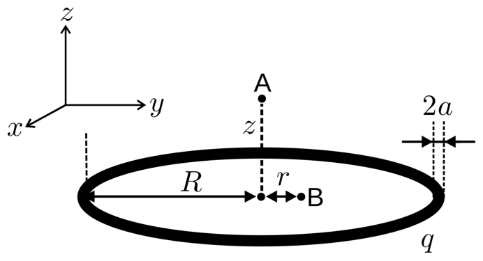
Figure 1. A charged ring of radius \(R\).
Part A. Electrostatic potential on the axis of the ring (1 point)
| A.1 | Calculate the electrostatic potential \(\Phi(z)\) along the axis of the ring at a \(z\) distance from its center (point A in Figure 1). | 0.3pt |
| A.2 | Calculate the electrostatic potential \(\Phi(z)\) to the lowest non-zero power of \(z\), assuming \(z\ll R\). | 0.4pt |
| A.3 | An electron (mass \(m\) and charge \(-e\)) is placed at point A (Figure 1, \(z\ll R\)). What is the force acting on the electron? Looking at the expression of the force, determine the sign of \(q\) so that the resulting motion would correspond to oscillations. The moving electron does not influence the charge distribution on the ring. | 0.2pt |
| A.4 | What is the angular frequency \(\omega\) of such harmonic oscillations? | 0.1pt |
Part B. Electrostatic potential in the plane of the ring (1.7 points)
In this part of the problem you will have to analyze the potential \(\Phi(r)\) in the plane of the ring (\(z=0\)) for \(r\ll R\) (point B in Figure 1). To the lowest non-zero power of \(r\) the electrostatic potential is given by \(\Phi(r)\approx q(\alpha+\beta r^2)\).
| B.1 | Find the expression for \(\beta\). You might need to use the Taylor expansion formula given above. | 1.5pt |
| B.2 | An electron is placed at point B (Figure 1, \(r\ll R\)). What is the force acting on the electron? Looking at the expression of the force, determine the sign of \(q\) so that the resulting motion would correspond to harmonic oscillations. The moving electron does not influence the charge distribution on the ring. | 0.2pt |
Part C. The focal length of the idealized electrostatic lens: instantaneous charging (2.3 points)
One wants to build a device to focus electrons—an electrostatic lens. Let us consider the following construction. The ring is situated perpendicularly to the \(z\)-axis, as shown in Figure 2. We have a source that produces on-demand packets of non-relativistic electrons. Kinetic energy of these electrons is \(E=mv^2/2\) (\(v\) is velocity) and they leave the source at precisely controlled moments. The system is programmed so that the ring is charge-neutral most of the time, but its charge becomes \(q\) when electrons are closer than a distance \(d/2\) (\(d\ll R\)) from the plane of the ring (shaded region in Figure 2, called “active region”). In part C assume that charging and de-charging processes are instantaneous and the electric field ”fills the space” instantaneously as well. One can neglect magnetic fields and assume that the velocity of electrons in the \(z\)-direction is constant. Moving electrons do not perturb the charge distribution on the ring.
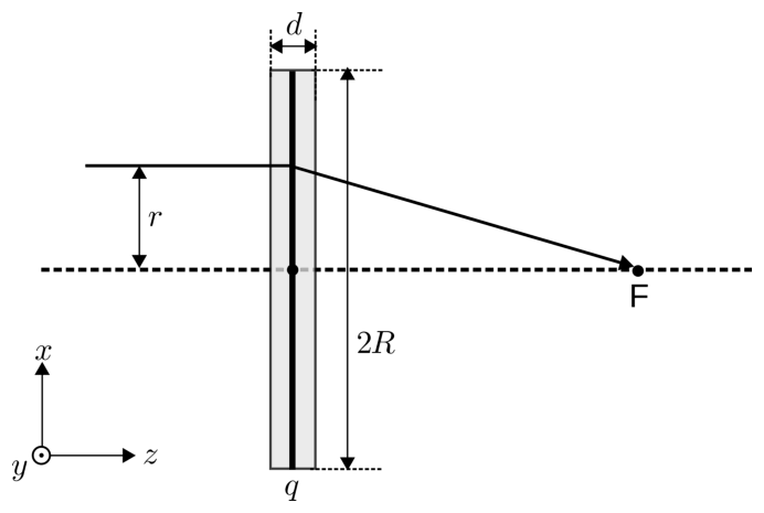
Figure 2. A model of an electrostatic lens.
| C.1 | Determine the focal length \(f\) of this lens. Assume that \(f\gg d\). Express your answer in terms of the constant \(\beta\) from question B.1 and other known quantities. Assume that before reaching the ”active region” the electron packet is parallel to the \(z\)-axis and \(r\ll R\). The sign of \(q\) is such so that the lens is focusing. | 1.3pt |
In reality the electron source is placed on the \(z\)-axis at a distance \(b>f\) from the center of the ring. Consider that electrons are no longer parallel to the \(z\)-axis before reaching the ”active region”, but are emitted from a point source at a range of different angles \(\gamma\ll1\) rad to the \(z\)-axis. Electrons are focused in a point situated at a distance \(c\) from the center of the ring.
| C.2 | Find \(c\). Express your answer in terms of the constant \(\beta\) from question B.1 and other known quantities. | 0.8pt |
| C.3 | Is the equation of a thin optical lens \(\displaystyle \frac1b+\frac1c=\frac1f\) fulfilled for the electrostatic lens? Show it by explicitly calculating \(1/b+1/c\). | 0.2pt |
Part D. The ring as a capacitor (3 points)
The model considered above was idealized and we assumed that the ring charged instantaneously. In reality charging is non-instantaneous, as the ring is a capacitor with a finite capacitance \(C\). In this part we will analyze the properties of this capacitor. You might need the following integrals:
\[ \int\frac{\mathrm dx}{\sin x} =-\ln\left|\frac{\cos x+1}{\sin x}\right|+\mathrm{const} \]
and
\[ \int\frac{\mathrm dx}{\sqrt{1+x^2}} =\ln\left|x+\sqrt{1+x^2}\right|+\mathrm{const}. \]
| D.1 | Calculate the capacitance \(C\) of the ring. Consider that the ring has a finite width \(2a\), but remember that \(a\ll R\). | 2.0pt |
When electrons reach the “active region”, the ring is connected to a source of voltage \(V_0\) (Figure 3). When electrons pass the “active region”, the ring is connected to the ground. The resistance of contacts is \(R_0\) and the resistance of the ring itself can be neglected.
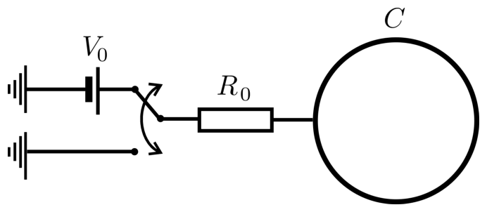
Figure 3. Charging of the electrostatic lens.
| D.2 | Determine the dependence of the charge on the ring as a function of time, \(q(t)\), and make a schematic plot of this dependence. \(t=0\) corresponds to a time moment when electrons are in the plane of the ring. What is the charge on the ring \(q_0\) when the absolute value \(q(t)\) is maximal? The capacitance of the ring is \(C\) (i.e., you do not have to use the actual expression found in D.1). Remark: the drawn polarity in Figure 3 is for indicative purposes only. The sign should be chosen so that the lens is focusing. | 1.0pt |
Part E. Focal length of a more realistic lens: non-instantaneous charging (2 points)
In this part of the problem, we will consider the action of this more realistic lens. Here we will again neglect the width of the ring \(2a\) and will assume that electrons travel parallel to the \(z\)-axis before reaching the ”active region”. However, the charging of the ring is no longer instantaneous.
| E.1 | Find the focal length \(f\) of the lens. Assume that \(f/v\gg R_0C\), but \(d/v\) and \(R_0C\) are of the same order of magnitude. Express your answer in terms of the constant \(\beta\) from part B and other known quantities. | 1.7pt |
| E.2 | You will see, that the result for \(f\) is similar to that obtained in part C, whereby the value \(q\) is substituted with \(q_{\mathrm{eff}}\). Find the expression for \(q_{\mathrm{eff}}\) in terms of quantities given in formulation of the problem. | 0.3pt |
Official English text of the problem.
Answers
Use \[ k=\frac{1}{4\pi\varepsilon_0},\qquad T=\frac dv,\qquad \tau=R_0C,\qquad Q=CV_0. \] Here \(e>0\), the potential vanishes at infinity, and \(V_0\) is the signed applied voltage: focusing requires \(V_0<0\), hence \(Q<0\). All approximate results have the accuracy stipulated in the problem.
- A.1: \(\displaystyle \Phi(z)=\frac{kq}{\sqrt{R^2+z^2}}\).
- A.2: \(\displaystyle \Phi(z)\approx\frac{kq}{R}\left(1-\frac{z^2}{2R^2}\right)\).
- A.3: \(\displaystyle \mathbf F\approx-\frac{keq}{R^3}z\,\hat{\mathbf z}\). Axial oscillations require \(q>0\).
- A.4: \(\displaystyle \omega=\sqrt{\frac{keq}{mR^3}}\), for \(q>0\).
- B.1: \(\displaystyle \beta=\frac{k}{4R^3}=\frac{1}{16\pi\varepsilon_0R^3}\).
- B.2: \(\displaystyle \mathbf F_\perp=2e\beta q\,\mathbf r_\perp=\frac{keq}{2R^3}\mathbf r_\perp\). Oscillations in the plane require \(q<0\).
- C.1: \(\displaystyle f=-\frac{E}{e\beta qd}=\frac{E}{e\beta|q|d}\).
- C.2: \(\displaystyle c=\frac{bE}{e\beta|q|bd-E}=\frac{bf}{b-f}\).
- C.3: Yes: \(\displaystyle \frac1b+\frac1c=\frac{e\beta|q|d}{E}=\frac1f\).
- D.1: \(\displaystyle C\approx\frac{4\pi^2\varepsilon_0R}{\ln(8R/a)}\).
- D.2: \[ q(t)= \begin{cases} 0, & t<-T/2,\\[2pt] Q\left[1-\exp\!\left(-\dfrac{t+T/2}{\tau}\right)\right], & -T/2\le t\le T/2,\\[5pt] q_0\exp\!\left(-\dfrac{t-T/2}{\tau}\right), & t>T/2, \end{cases} \qquad q_0=Q\left(1-e^{-T/\tau}\right)<0. \] The graph falls from zero to its minimum \(q_0\) at \(t=T/2\), then approaches zero exponentially from below.
- E.1: \(\displaystyle f=-\frac{E}{e\beta CV_0d}=\frac{E}{e\beta C|V_0|d}\).
- E.2: \(\displaystyle q_{\mathrm{eff}}=CV_0=\frac{q_0}{1-e^{-d/(vR_0C)}}\).
Solution
For an electron, the potential energy is \(U=-e\Phi\). Therefore \[ \mathbf F=-\boldsymbol\nabla U=e\boldsymbol\nabla\Phi. \] This fixes the force signs throughout the solution.
A.1
Every charge element on the ring is at the same distance \(\sqrt{R^2+z^2}\) from the observation point on its axis. Superposition gives \[ \Phi(z)=k\int\frac{\mathrm dq}{\sqrt{R^2+z^2}} =\boxed{\frac{kq}{\sqrt{R^2+z^2}}}. \]
A.2
For \(|z|\ll R\), \[ \Phi(z)=\frac{kq}{R} \left(1+\frac{z^2}{R^2}\right)^{-1/2}. \] Using the supplied expansion with \(\varepsilon=-1/2\), \[ \boxed{\Phi(z)\approx\frac{kq}{R}-\frac{kq}{2R^3}z^2}. \] The first nonconstant term is quadratic because the potential is unchanged by \(z\mapsto-z\).
A.3
Differentiating the axial potential, \[ F_z=e\frac{\mathrm d\Phi}{\mathrm dz} =-\frac{keqz}{(R^2+z^2)^{3/2}} \approx-\frac{keq}{R^3}z. \] Thus \[ \boxed{\mathbf F\approx-\frac{keq}{R^3}z\,\hat{\mathbf z}}. \]
A restoring force must point towards \(z=0\). Consequently, \[ \boxed{q>0} \] is required for axial oscillations.
A.4
Newton’s equation becomes \[ m\ddot z=-\frac{keq}{R^3}z. \] Comparison with \(\ddot z+\omega^2z=0\) gives \[ \boxed{\omega=\sqrt{\frac{keq}{mR^3}} =\sqrt{\frac{eq}{4\pi\varepsilon_0mR^3}}}. \]
B.1
Place the observation point at \((r,0,0)\). A ring element at polar angle \(\theta\) has charge \[ \mathrm dq=\frac{q}{2\pi}\,\mathrm d\theta \] and distance \[ s=\sqrt{R^2+r^2-2Rr\cos\theta} \] from that point. Hence, with \(\rho=r/R\), \[ \Phi(r)=\frac{kq}{2\pi R} \int_0^{2\pi} \frac{\mathrm d\theta}{\sqrt{1+\rho^2-2\rho\cos\theta}}. \]
Expanding through second order in \(\rho\), \[ \begin{aligned} (1+\rho^2-2\rho\cos\theta)^{-1/2} &\approx 1-\frac12(\rho^2-2\rho\cos\theta) +\frac38(4\rho^2\cos^2\theta)\\ &= 1+\rho\cos\theta +\rho^2\left(-\frac12+\frac32\cos^2\theta\right). \end{aligned} \] The angular averages are \[ \langle\cos\theta\rangle=0,\qquad \langle\cos^2\theta\rangle=\frac12. \] Therefore \[ \Phi(r)\approx\frac{kq}{R} \left(1+\frac{r^2}{4R^2}\right). \] Comparing with \(q(\alpha+\beta r^2)\), \[ \alpha=\frac{k}{R},\qquad \boxed{\beta=\frac{k}{4R^3} =\frac{1}{16\pi\varepsilon_0R^3}}. \]
B.2
Let \(\mathbf r_\perp=x\hat{\mathbf x}+y\hat{\mathbf y}\). Since \(r^2=x^2+y^2\), \[ \boxed{\mathbf F_\perp =e\boldsymbol\nabla_\perp\Phi =2e\beta q\,\mathbf r_\perp =\frac{keq}{2R^3}\mathbf r_\perp}. \] The force is restoring in the ring’s plane precisely when \[ \boxed{q<0}. \] For this sign, each transverse coordinate satisfies a harmonic-oscillator equation. Thus axial and transverse stability require opposite signs of ring charge.
C.1
The electron spends \[ T=\frac dv \] in the active region. Since \(d\ll R\), the transverse force there can be evaluated using B.2. Also, \(f\gg d\) allows us to neglect the change of transverse position during the interaction.
For an incident electron at transverse distance \(r\), its transverse impulse is \[ m\Delta v_r =F_rT =2e\beta qr\,\frac dv. \] The incident transverse velocity is zero, so \[ v_{r,\mathrm{out}}=\frac{2e\beta qrd}{mv}<0 \] for the focusing choice \(q<0\).
After leaving the active region, the electron moves along a straight line. To thin-lens accuracy, the distance to the axis is \[ f=-\frac{vr}{v_{r,\mathrm{out}}}. \] Consequently, \[ \boxed{f=-\frac{mv^2}{2e\beta qd} =-\frac{E}{e\beta qd} =\frac{E}{e\beta|q|d}}. \] The cancellation of \(r\) shows that all sufficiently near-axis parallel rays have the same focal length.
C.2
An electron emitted at angle \(\gamma\ll1\) from a source at distance \(b\) reaches the lens at \[ r\approx b\gamma. \] Its incoming transverse velocity satisfies \[ \frac{v_{r,\mathrm{in}}}{v}\approx\gamma\approx\frac rb. \]
The lens produces the same transverse velocity change as in C.1. Thus \[ \frac{v_{r,\mathrm{out}}}{v} =\frac rb+\frac{2e\beta qrd}{mv^2} =r\left(\frac1b+\frac{e\beta qd}{E}\right). \] For the outgoing trajectory to cross the axis a distance \(c\) beyond the ring, \[ \frac{v_{r,\mathrm{out}}}{v}=-\frac rc. \] It follows that \[ \frac1c=-\frac1b-\frac{e\beta qd}{E} =\frac{e\beta|q|d}{E}-\frac1b. \] Therefore \[ \boxed{c=\frac{bE}{e\beta|q|bd-E} =\frac{bf}{b-f}}. \] The specified condition \(b>f\) ensures \(c>0\).
C.3
Using the result just obtained, \[ \frac1b+\frac1c =\frac1b+\left(\frac{e\beta|q|d}{E}-\frac1b\right) =\frac{e\beta|q|d}{E}. \] By C.1 this equals \(1/f\), so \[ \boxed{\frac1b+\frac1c=\frac1f}. \] The thin optical lens equation is therefore fulfilled within the stated approximations.
D.1
The isolated ring’s capacitance is \[ C=\frac{q}{\Phi_s}, \] where \(\Phi_s\) is its surface potential relative to infinity.
For a thin torus, introduce the charge per unit length \[ \lambda=\frac{q}{2\pi R}. \] Choose an intermediate length \(\ell\) satisfying \[ a\ll\ell\ll R. \] We calculate the surface potential by combining a nearby, approximately straight portion of the ring with its distant curved portion.
Locally the conductor resembles a cylinder of radius \(a\). Its exterior potential can be represented, to the required accuracy, by charge on its axis. The contribution from the segment \(-\ell<s<\ell\) is therefore \[ \begin{aligned} \Phi_{\mathrm{near}} &\approx k\lambda\int_{-\ell}^{\ell} \frac{\mathrm ds}{\sqrt{s^2+a^2}}\\ &=2k\lambda \ln\left(\frac{\ell+\sqrt{\ell^2+a^2}}{a}\right)\\ &\approx2k\lambda\ln\frac{2\ell}{a}. \end{aligned} \]
For the distant portion, the thickness can be neglected. Let \[ \delta=\frac{\ell}{R}\ll1. \] The distance between two points on the ring separated by angle \(\theta\) is \(2R\sin(\theta/2)\). Hence \[ \begin{aligned} \Phi_{\mathrm{far}} &\approx k\lambda \int_\delta^{2\pi-\delta} \frac{R\,\mathrm d\theta}{2R\sin(\theta/2)}\\ &=k\lambda\int_{\delta/2}^{\pi-\delta/2} \frac{\mathrm du}{\sin u}\\ &=2k\lambda\ln\cot\frac{\delta}{4}\\ &\approx2k\lambda\ln\frac{4R}{\ell}. \end{aligned} \]
Adding the contributions eliminates the arbitrary intermediate length: \[ \begin{aligned} \Phi_s &\approx2k\lambda \left(\ln\frac{2\ell}{a}+\ln\frac{4R}{\ell}\right)\\ &=2k\lambda\ln\frac{8R}{a}\\ &=\frac{q}{4\pi^2\varepsilon_0R}\ln\frac{8R}{a}. \end{aligned} \] Thus \[ \boxed{C\approx\frac{4\pi^2\varepsilon_0R}{\ln(8R/a)}}. \] The finite radius \(a\) supplies the short-distance cutoff that makes the surface potential finite.
D.2
The electrons enter and leave the active region at \[ t_-=-\frac{T}{2},\qquad t_+=\frac{T}{2},\qquad T=\frac dv. \] The ring is initially neutral. Define \[ \tau=R_0C,\qquad Q=CV_0<0. \]
While connected to the source, the circuit equation is \[ R_0\frac{\mathrm dq}{\mathrm dt}+\frac qC=V_0, \] or \[ \tau\dot q+q=Q. \] With \(q(t_-)=0\), \[ q(t)=Q\left[1-e^{-(t+T/2)/\tau}\right], \qquad -T/2\le t\le T/2. \]
When the ring is grounded, \[ \tau\dot q+q=0. \] Charge is continuous at switching, so \[ q(t)=q_0e^{-(t-T/2)/\tau}, \qquad t>T/2, \] where \[ \boxed{q_0=Q(1-e^{-T/\tau}) =CV_0\left[1-\exp\left(-\frac{d}{vR_0C}\right)\right]}. \]
Combining the intervals, \[ \boxed{ q(t)= \begin{cases} 0, & t<-T/2,\\[2pt] Q\left[1-e^{-(t+T/2)/\tau}\right], & -T/2\le t\le T/2,\\[2pt] Q(1-e^{-T/\tau})e^{-(t-T/2)/\tau}, & t>T/2. \end{cases}} \]
For the requested sketch, draw \(q(t)\) below the time axis after charging begins. It is initially zero, falls continuously and with decreasing steepness during charging, reaches its most negative value at \(t=T/2\), and then rises exponentially towards zero. Its slope changes discontinuously at both switching times, while \(q(t)\) remains continuous.
Useful points are:
| Time | Charge |
|---|---|
| \(-T/2\) | \(0\) |
| \(0\) | \(Q(1-e^{-T/(2\tau)})\) |
| \(T/2\) | \(q_0=Q(1-e^{-T/\tau})\) |
| \(T/2+\tau\) | \(q_0\exp(-1)\) |
| \(t\to+\infty\) | \(0\), approached from below |
Thus \(|q(t)|\) is maximal when the electrons leave the active region.
E.1
Here \(\tau\) and \(T=d/v\) are comparable. Therefore the charging and appreciable discharge occur while the electrons remain within a longitudinal distance of order \(d\) from the ring. Since \(d\ll R\), the transverse force from B.2 remains applicable: \[ F_r(t)\approx2e\beta q(t)r. \]
Also, \(f/v\gg\tau\) means that focusing occurs long after the charge has substantially decayed. During the force pulse, the transverse displacement is small compared with \(r\), so \(r\) can be held constant when calculating the impulse: \[ m\Delta v_r =2e\beta r\int_{-T/2}^{\infty}q(t)\,\mathrm dt. \]
The charging contribution is \[ \begin{aligned} I_{\mathrm{ch}} &=Q\int_{-T/2}^{T/2} \left[1-e^{-(t+T/2)/\tau}\right]\mathrm dt\\ &=Q\left[T-\tau(1-e^{-T/\tau})\right]. \end{aligned} \] The discharge contribution is \[ \begin{aligned} I_{\mathrm{dis}} &=q_0\int_{T/2}^{\infty}e^{-(t-T/2)/\tau}\,\mathrm dt\\ &=q_0\tau =Q\tau(1-e^{-T/\tau}). \end{aligned} \] Their sum is \[ \boxed{\int_{-T/2}^{\infty}q(t)\,\mathrm dt=QT =CV_0\frac dv}. \]
Consequently, \[ \Delta v_r =\frac{2e\beta rQd}{mv}. \] Using the same thin-lens geometry as in C.1, \[ \boxed{ f=-\frac{vr}{\Delta v_r} =-\frac{mv^2}{2e\beta CV_0d} =-\frac{E}{e\beta CV_0d} =\frac{E}{e\beta C|V_0|d}}. \]
The resistance changes the shape and duration of the charge pulse, but its contributions to the total impulse cancel between charging and discharging. The finite extent of the interaction produces corrections beyond the assumed thin-lens accuracy.
E.2
Comparing \[ f=-\frac{E}{e\beta qd} \quad\text{and}\quad f=-\frac{E}{e\beta CV_0d}, \] we obtain \[ \boxed{q_{\mathrm{eff}}=CV_0}. \] Equivalently, using D.2, \[ \boxed{q_{\mathrm{eff}} =\frac{q_0}{1-\exp[-d/(vR_0C)]}}. \]
This effective charge equals the charge the ring would reach if held at the applied voltage indefinitely. Its magnitude exceeds the actual peak charge because the discharge tail also contributes to focusing.
The solution was checked against the official solution.
IPhO 2021 · Theorieaufgabe 2
Elektrostatische Linse
Betrachten Sie einen gleichmäßig geladenen metallischen Ring mit dem Radius \(R\) und der Gesamtladung \(q\). Der Ring ist ein hohler Torus mit der Dicke \(2a\ll R\). Diese Dicke kann in den Teilen A, B, C und E vernachlässigt werden. Die \(xy\)-Ebene fällt mit der Ringebene zusammen, während die \(z\)-Achse senkrecht dazu steht, wie in Abbildung 1 gezeigt. In den Teilen A und B benötigen Sie möglicherweise die Formel (Taylorentwicklung)
\[ (1+x)^\varepsilon\approx 1+\varepsilon x+\frac12\varepsilon(\varepsilon-1)x^2, \quad\text{wenn }|x|\ll1. \]
Abbildung 1. Ein geladener Ring mit dem Radius \(R\).
Teil A. Elektrostatisches Potential auf der Ringachse (1 Punkt)
| A.1 | Berechnen Sie das elektrostatische Potential \(\Phi(z)\) entlang der Ringachse im Abstand \(z\) vom Mittelpunkt des Rings (Punkt A in Abbildung 1). | 0.3 Pkt. |
| A.2 | Berechnen Sie das elektrostatische Potential \(\Phi(z)\) bis zur niedrigsten nichtverschwindenden Potenz von \(z\) unter der Annahme \(z\ll R\). | 0.4 Pkt. |
| A.3 | Ein Elektron (Masse \(m\) und Ladung \(-e\)) wird in Punkt A platziert (Abbildung 1, \(z\ll R\)). Welche Kraft wirkt auf das Elektron? Bestimmen Sie anhand des Ausdrucks für die Kraft das Vorzeichen von \(q\), bei dem die resultierende Bewegung eine Schwingung ist. Das bewegte Elektron beeinflusst die Ladungsverteilung auf dem Ring nicht. | 0.2 Pkt. |
| A.4 | Welche Kreisfrequenz \(\omega\) haben solche harmonischen Schwingungen? | 0.1 Pkt. |
Teil B. Elektrostatisches Potential in der Ringebene (1.7 Punkte)
In diesem Teil der Aufgabe sollen Sie das Potential \(\Phi(r)\) in der Ringebene (\(z=0\)) für \(r\ll R\) untersuchen (Punkt B in Abbildung 1). Bis zur niedrigsten nichtverschwindenden Potenz von \(r\) ist das elektrostatische Potential durch \(\Phi(r)\approx q(\alpha+\beta r^2)\) gegeben.
| B.1 | Bestimmen Sie den Ausdruck für \(\beta\). Möglicherweise benötigen Sie die oben angegebene Taylorentwicklung. | 1.5 Pkt. |
| B.2 | Ein Elektron wird in Punkt B platziert (Abbildung 1, \(r\ll R\)). Welche Kraft wirkt auf das Elektron? Bestimmen Sie anhand des Ausdrucks für die Kraft das Vorzeichen von \(q\), bei dem die resultierende Bewegung eine harmonische Schwingung ist. Das bewegte Elektron beeinflusst die Ladungsverteilung auf dem Ring nicht. | 0.2 Pkt. |
Teil C. Die Brennweite der idealisierten elektrostatischen Linse: augenblickliches Aufladen (2.3 Punkte)
Man möchte eine Vorrichtung zur Fokussierung von Elektronen bauen — eine elektrostatische Linse. Betrachten wir dazu den folgenden Aufbau. Der Ring steht senkrecht zur \(z\)-Achse, wie in Abbildung 2 gezeigt. Es steht eine Quelle zur Verfügung, die auf Abruf Pakete nichtrelativistischer Elektronen erzeugt. Die kinetische Energie dieser Elektronen beträgt \(E=mv^2/2\) (\(v\) ist die Geschwindigkeit), und sie verlassen die Quelle zu genau gesteuerten Zeitpunkten. Das System ist so programmiert, dass der Ring die meiste Zeit elektrisch neutral ist, seine Ladung jedoch \(q\) beträgt, wenn die Elektronen weniger als den Abstand \(d/2\) (\(d\ll R\)) von der Ringebene entfernt sind (schattierter Bereich in Abbildung 2, als „aktiver Bereich“ bezeichnet). Nehmen Sie in Teil C an, dass das Aufladen und Entladen augenblicklich erfolgen und das elektrische Feld ebenfalls augenblicklich „den Raum erfüllt“. Magnetfelder können vernachlässigt werden, und die Geschwindigkeit der Elektronen in \(z\)-Richtung kann als konstant angenommen werden. Die bewegten Elektronen stören die Ladungsverteilung auf dem Ring nicht.
Abbildung 2. Ein Modell einer elektrostatischen Linse.
| C.1 | Bestimmen Sie die Brennweite \(f\) dieser Linse. Nehmen Sie an, dass \(f\gg d\). Drücken Sie Ihre Antwort durch die Konstante \(\beta\) aus Frage B.1 und andere bekannte Größen aus. Nehmen Sie an, dass sich das Elektronenpaket vor dem Erreichen des „aktiven Bereichs“ parallel zur \(z\)-Achse bewegt und \(r\ll R\) gilt. Das Vorzeichen von \(q\) ist so gewählt, dass die Linse fokussiert. | 1.3 Pkt. |
In Wirklichkeit befindet sich die Elektronenquelle auf der \(z\)-Achse im Abstand \(b>f\) vom Mittelpunkt des Rings. Gehen Sie davon aus, dass sich die Elektronen vor dem Erreichen des „aktiven Bereichs“ nicht mehr parallel zur \(z\)-Achse bewegen, sondern von einer Punktquelle unter verschiedenen Winkeln \(\gamma\ll1\) rad zur \(z\)-Achse emittiert werden. Die Elektronen werden in einem Punkt im Abstand \(c\) vom Mittelpunkt des Rings fokussiert.
| C.2 | Bestimmen Sie \(c\). Drücken Sie Ihre Antwort durch die Konstante \(\beta\) aus Frage B.1 und andere bekannte Größen aus. | 0.8 Pkt. |
| C.3 | Gilt die Gleichung einer dünnen optischen Linse \(\displaystyle \frac1b+\frac1c=\frac1f\) für die elektrostatische Linse? Zeigen Sie dies, indem Sie \(1/b+1/c\) explizit berechnen. | 0.2 Pkt. |
Teil D. Der Ring als Kondensator (3 Punkte)
Das oben betrachtete Modell war idealisiert, und wir haben angenommen, dass der Ring augenblicklich aufgeladen wird. In Wirklichkeit erfolgt das Aufladen nicht augenblicklich, da der Ring ein Kondensator mit einer endlichen Kapazität \(C\) ist. In diesem Teil untersuchen wir die Eigenschaften dieses Kondensators. Möglicherweise benötigen Sie die folgenden Integrale:
\[ \int\frac{\mathrm dx}{\sin x} =-\ln\left|\frac{\cos x+1}{\sin x}\right|+\mathrm{const} \]
und
\[ \int\frac{\mathrm dx}{\sqrt{1+x^2}} =\ln\left|x+\sqrt{1+x^2}\right|+\mathrm{const}. \]
| D.1 | Berechnen Sie die Kapazität \(C\) des Rings. Berücksichtigen Sie, dass der Ring eine endliche Dicke \(2a\) hat, beachten Sie aber, dass \(a\ll R\) gilt. | 2.0 Pkt. |
Wenn die Elektronen den „aktiven Bereich“ erreichen, wird der Ring an eine Spannungsquelle mit der Spannung \(V_0\) angeschlossen (Abbildung 3). Wenn die Elektronen den „aktiven Bereich“ durchquert haben, wird der Ring geerdet. Der Widerstand der Kontakte beträgt \(R_0\), und der Widerstand des Rings selbst kann vernachlässigt werden.
Abbildung 3. Aufladen der elektrostatischen Linse.
| D.2 | Bestimmen Sie die Ladung auf dem Ring als Funktion der Zeit, \(q(t)\), und skizzieren Sie diesen Verlauf. \(t=0\) entspricht dem Zeitpunkt, zu dem sich die Elektronen in der Ringebene befinden. Wie groß ist die Ladung auf dem Ring \(q_0\), wenn der Betrag von \(q(t)\) maximal ist? Die Kapazität des Rings beträgt \(C\) (Sie müssen also nicht den in D.1 gefundenen tatsächlichen Ausdruck verwenden). Anmerkung: Die in Abbildung 3 eingezeichnete Polarität dient lediglich der Veranschaulichung. Das Vorzeichen ist so zu wählen, dass die Linse fokussiert. | 1.0 Pkt. |
Teil E. Brennweite einer realistischeren Linse: nicht augenblickliches Aufladen (2 Punkte)
In diesem Teil der Aufgabe betrachten wir die Wirkung dieser realistischeren Linse. Dabei vernachlässigen wir erneut die Dicke des Rings \(2a\) und nehmen an, dass sich die Elektronen vor dem Erreichen des „aktiven Bereichs“ parallel zur \(z\)-Achse bewegen. Das Aufladen des Rings erfolgt jedoch nicht mehr augenblicklich.
| E.1 | Bestimmen Sie die Brennweite \(f\) der Linse. Nehmen Sie an, dass \(f/v\gg R_0C\), während \(d/v\) und \(R_0C\) von derselben Größenordnung sind. Drücken Sie Ihre Antwort durch die Konstante \(\beta\) aus Teil B und andere bekannte Größen aus. | 1.7 Pkt. |
| E.2 | Sie werden feststellen, dass das Ergebnis für \(f\) dem in Teil C erhaltenen ähnelt, wobei der Wert \(q\) durch \(q_{\mathrm{eff}}\) ersetzt wird. Bestimmen Sie den Ausdruck für \(q_{\mathrm{eff}}\) in Abhängigkeit von den in der Aufgabenstellung gegebenen Größen. | 0.3 Pkt. |
Aufgabentext aus dem offiziellen englischen Text übersetzt.
Antworten
Wir verwenden \[ k=\frac{1}{4\pi\varepsilon_0},\qquad T=\frac dv,\qquad \tau=R_0C,\qquad Q=CV_0. \] Dabei gilt \(e>0\), das Potential verschwindet im Unendlichen, und \(V_0\) ist die angelegte Spannung mit Vorzeichen: Für eine Fokussierung muss \(V_0<0\) gelten, also \(Q<0\). Alle Näherungsergebnisse haben die in der Aufgabe geforderte Genauigkeit.
- A.1: \(\displaystyle \Phi(z)=\frac{kq}{\sqrt{R^2+z^2}}\).
- A.2: \(\displaystyle \Phi(z)\approx\frac{kq}{R}\left(1-\frac{z^2}{2R^2}\right)\).
- A.3: \(\displaystyle \mathbf F\approx-\frac{keq}{R^3}z\,\hat{\mathbf z}\). Axiale Schwingungen erfordern \(q>0\).
- A.4: \(\displaystyle \omega=\sqrt{\frac{keq}{mR^3}}\), für \(q>0\).
- B.1: \(\displaystyle \beta=\frac{k}{4R^3}=\frac{1}{16\pi\varepsilon_0R^3}\).
- B.2: \(\displaystyle \mathbf F_\perp=2e\beta q\,\mathbf r_\perp=\frac{keq}{2R^3}\mathbf r_\perp\). Schwingungen in der Ebene erfordern \(q<0\).
- C.1: \(\displaystyle f=-\frac{E}{e\beta qd}=\frac{E}{e\beta|q|d}\).
- C.2: \(\displaystyle c=\frac{bE}{e\beta|q|bd-E}=\frac{bf}{b-f}\).
- C.3: Ja: \(\displaystyle \frac1b+\frac1c=\frac{e\beta|q|d}{E}=\frac1f\).
- D.1: \(\displaystyle C\approx\frac{4\pi^2\varepsilon_0R}{\ln(8R/a)}\).
- D.2: \[ q(t)= \begin{cases} 0, & t<-T/2,\\[2pt] Q\left[1-\exp\!\left(-\dfrac{t+T/2}{\tau}\right)\right], & -T/2\le t\le T/2,\\[5pt] q_0\exp\!\left(-\dfrac{t-T/2}{\tau}\right), & t>T/2, \end{cases} \qquad q_0=Q\left(1-e^{-T/\tau}\right)<0. \] Der Graph fällt von null auf sein Minimum \(q_0\) bei \(t=T/2\) und nähert sich anschließend von unten exponentiell null an.
- E.1: \(\displaystyle f=-\frac{E}{e\beta CV_0d}=\frac{E}{e\beta C|V_0|d}\).
- E.2: \(\displaystyle q_{\mathrm{eff}}=CV_0=\frac{q_0}{1-e^{-d/(vR_0C)}}\).
Lösung
Für ein Elektron ist die potentielle Energie \(U=-e\Phi\). Daher gilt \[ \mathbf F=-\boldsymbol\nabla U=e\boldsymbol\nabla\Phi. \] Damit sind die Vorzeichen der Kräfte in der gesamten Lösung festgelegt.
A.1
Jedes Ladungselement auf dem Ring hat vom Beobachtungspunkt auf der Ringachse denselben Abstand \(\sqrt{R^2+z^2}\). Nach dem Superpositionsprinzip gilt \[ \Phi(z)=k\int\frac{\mathrm dq}{\sqrt{R^2+z^2}} =\boxed{\frac{kq}{\sqrt{R^2+z^2}}}. \]
A.2
Für \(|z|\ll R\) gilt \[ \Phi(z)=\frac{kq}{R} \left(1+\frac{z^2}{R^2}\right)^{-1/2}. \] Mit der angegebenen Entwicklung für \(\varepsilon=-1/2\) ergibt sich \[ \boxed{\Phi(z)\approx\frac{kq}{R}-\frac{kq}{2R^3}z^2}. \] Der erste nichtkonstante Term ist quadratisch, weil das Potential unter \(z\mapsto-z\) unverändert bleibt.
A.3
Durch Ableiten des Potentials auf der Achse erhält man \[ F_z=e\frac{\mathrm d\Phi}{\mathrm dz} =-\frac{keqz}{(R^2+z^2)^{3/2}} \approx-\frac{keq}{R^3}z. \] Somit gilt \[ \boxed{\mathbf F\approx-\frac{keq}{R^3}z\,\hat{\mathbf z}}. \]
Eine rücktreibende Kraft muss in Richtung \(z=0\) zeigen. Daher ist \[ \boxed{q>0} \] für axiale Schwingungen erforderlich.
A.4
Die Newtonsche Bewegungsgleichung lautet \[ m\ddot z=-\frac{keq}{R^3}z. \] Der Vergleich mit \(\ddot z+\omega^2z=0\) liefert \[ \boxed{\omega=\sqrt{\frac{keq}{mR^3}} =\sqrt{\frac{eq}{4\pi\varepsilon_0mR^3}}}. \]
B.1
Wir legen den Beobachtungspunkt nach \((r,0,0)\). Ein Ringelement beim Polarwinkel \(\theta\) hat die Ladung \[ \mathrm dq=\frac{q}{2\pi}\,\mathrm d\theta \] und den Abstand \[ s=\sqrt{R^2+r^2-2Rr\cos\theta} \] von diesem Punkt. Mit \(\rho=r/R\) folgt somit \[ \Phi(r)=\frac{kq}{2\pi R} \int_0^{2\pi} \frac{\mathrm d\theta}{\sqrt{1+\rho^2-2\rho\cos\theta}}. \]
Die Entwicklung bis zur zweiten Ordnung in \(\rho\) ergibt \[ \begin{aligned} (1+\rho^2-2\rho\cos\theta)^{-1/2} &\approx 1-\frac12(\rho^2-2\rho\cos\theta) +\frac38(4\rho^2\cos^2\theta)\\ &= 1+\rho\cos\theta +\rho^2\left(-\frac12+\frac32\cos^2\theta\right). \end{aligned} \] Die Winkelmittelwerte lauten \[ \langle\cos\theta\rangle=0,\qquad \langle\cos^2\theta\rangle=\frac12. \] Daher gilt \[ \Phi(r)\approx\frac{kq}{R} \left(1+\frac{r^2}{4R^2}\right). \] Der Vergleich mit \(q(\alpha+\beta r^2)\) liefert \[ \alpha=\frac{k}{R},\qquad \boxed{\beta=\frac{k}{4R^3} =\frac{1}{16\pi\varepsilon_0R^3}}. \]
B.2
Sei \(\mathbf r_\perp=x\hat{\mathbf x}+y\hat{\mathbf y}\). Wegen \(r^2=x^2+y^2\) gilt \[ \boxed{\mathbf F_\perp =e\boldsymbol\nabla_\perp\Phi =2e\beta q\,\mathbf r_\perp =\frac{keq}{2R^3}\mathbf r_\perp}. \] Die Kraft in der Ringebene ist genau dann rücktreibend, wenn \[ \boxed{q<0}. \] Für dieses Vorzeichen erfüllt jede transversale Koordinate die Gleichung eines harmonischen Oszillators. Axiale und transversale Stabilität erfordern somit entgegengesetzte Vorzeichen der Ringladung.
C.1
Das Elektron verbringt die Zeit \[ T=\frac dv \] im aktiven Bereich. Da \(d\ll R\) gilt, kann die transversale Kraft dort mithilfe von B.2 berechnet werden. Außerdem erlaubt uns \(f\gg d\), die Änderung der transversalen Position während der Wechselwirkung zu vernachlässigen.
Für ein einfallendes Elektron im transversalen Abstand \(r\) beträgt der transversale Kraftstoß \[ m\Delta v_r =F_rT =2e\beta qr\,\frac dv. \] Die transversale Anfangsgeschwindigkeit ist null, daher gilt \[ v_{r,\mathrm{out}}=\frac{2e\beta qrd}{mv}<0 \] für die fokussierende Wahl \(q<0\).
Nach dem Verlassen des aktiven Bereichs bewegt sich das Elektron geradlinig. In der Näherung einer dünnen Linse beträgt die Entfernung bis zum Achsenschnittpunkt \[ f=-\frac{vr}{v_{r,\mathrm{out}}}. \] Folglich gilt \[ \boxed{f=-\frac{mv^2}{2e\beta qd} =-\frac{E}{e\beta qd} =\frac{E}{e\beta|q|d}}. \] Dass sich \(r\) herauskürzt, zeigt, dass alle hinreichend achsennahen parallelen Strahlen dieselbe Brennweite haben.
C.2
Ein Elektron, das unter dem Winkel \(\gamma\ll1\) aus einer Quelle im Abstand \(b\) emittiert wird, erreicht die Linse bei \[ r\approx b\gamma. \] Für seine transversale Eintrittsgeschwindigkeit gilt \[ \frac{v_{r,\mathrm{in}}}{v}\approx\gamma\approx\frac rb. \]
Die Linse bewirkt dieselbe Änderung der transversalen Geschwindigkeit wie in C.1. Somit gilt \[ \frac{v_{r,\mathrm{out}}}{v} =\frac rb+\frac{2e\beta qrd}{mv^2} =r\left(\frac1b+\frac{e\beta qd}{E}\right). \] Damit die austretende Bahn die Achse im Abstand \(c\) hinter dem Ring schneidet, muss gelten \[ \frac{v_{r,\mathrm{out}}}{v}=-\frac rc. \] Daraus folgt \[ \frac1c=-\frac1b-\frac{e\beta qd}{E} =\frac{e\beta|q|d}{E}-\frac1b. \] Also erhält man \[ \boxed{c=\frac{bE}{e\beta|q|bd-E} =\frac{bf}{b-f}}. \] Die vorgegebene Bedingung \(b>f\) stellt sicher, dass \(c>0\) gilt.
C.3
Mit dem gerade erhaltenen Ergebnis folgt \[ \frac1b+\frac1c =\frac1b+\left(\frac{e\beta|q|d}{E}-\frac1b\right) =\frac{e\beta|q|d}{E}. \] Nach C.1 ist dies gleich \(1/f\), sodass \[ \boxed{\frac1b+\frac1c=\frac1f}. \] Die Gleichung der dünnen optischen Linse ist daher im Rahmen der angegebenen Näherungen erfüllt.
D.1
Die Kapazität des isolierten Rings beträgt \[ C=\frac{q}{\Phi_s}, \] wobei \(\Phi_s\) sein Oberflächenpotential relativ zum Unendlichen ist.
Für einen dünnen Torus führen wir die Ladung pro Längeneinheit ein: \[ \lambda=\frac{q}{2\pi R}. \] Wir wählen eine Zwischenlänge \(\ell\), für die gilt \[ a\ll\ell\ll R. \] Wir berechnen das Oberflächenpotential, indem wir die Beiträge eines nahen, näherungsweise geraden Ringabschnitts und des entfernten, gekrümmten Ringabschnitts zusammenfassen.
Lokal ähnelt der Leiter einem Zylinder mit dem Radius \(a\). Sein äußeres Potential kann mit der erforderlichen Genauigkeit durch eine Ladung auf seiner Achse dargestellt werden. Der Beitrag des Abschnitts \(-\ell<s<\ell\) ist daher \[ \begin{aligned} \Phi_{\mathrm{near}} &\approx k\lambda\int_{-\ell}^{\ell} \frac{\mathrm ds}{\sqrt{s^2+a^2}}\\ &=2k\lambda \ln\left(\frac{\ell+\sqrt{\ell^2+a^2}}{a}\right)\\ &\approx2k\lambda\ln\frac{2\ell}{a}. \end{aligned} \]
Für den entfernten Abschnitt kann die Dicke vernachlässigt werden. Sei \[ \delta=\frac{\ell}{R}\ll1. \] Der Abstand zwischen zwei Punkten auf dem Ring, die um den Winkel \(\theta\) voneinander getrennt sind, beträgt \(2R\sin(\theta/2)\). Daher gilt \[ \begin{aligned} \Phi_{\mathrm{far}} &\approx k\lambda \int_\delta^{2\pi-\delta} \frac{R\,\mathrm d\theta}{2R\sin(\theta/2)}\\ &=k\lambda\int_{\delta/2}^{\pi-\delta/2} \frac{\mathrm du}{\sin u}\\ &=2k\lambda\ln\cot\frac{\delta}{4}\\ &\approx2k\lambda\ln\frac{4R}{\ell}. \end{aligned} \]
Beim Addieren der Beiträge fällt die willkürlich gewählte Zwischenlänge heraus: \[ \begin{aligned} \Phi_s &\approx2k\lambda \left(\ln\frac{2\ell}{a}+\ln\frac{4R}{\ell}\right)\\ &=2k\lambda\ln\frac{8R}{a}\\ &=\frac{q}{4\pi^2\varepsilon_0R}\ln\frac{8R}{a}. \end{aligned} \] Somit gilt \[ \boxed{C\approx\frac{4\pi^2\varepsilon_0R}{\ln(8R/a)}}. \] Der endliche Radius \(a\) liefert die untere Abstandsschranke, durch die das Oberflächenpotential endlich bleibt.
D.2
Die Elektronen betreten und verlassen den aktiven Bereich zu den Zeitpunkten \[ t_-=-\frac{T}{2},\qquad t_+=\frac{T}{2},\qquad T=\frac dv. \] Der Ring ist anfangs neutral. Wir definieren \[ \tau=R_0C,\qquad Q=CV_0<0. \]
Solange der Ring mit der Quelle verbunden ist, lautet die Schaltungsgleichung \[ R_0\frac{\mathrm dq}{\mathrm dt}+\frac qC=V_0, \] oder \[ \tau\dot q+q=Q. \] Mit \(q(t_-)=0\) ergibt sich \[ q(t)=Q\left[1-e^{-(t+T/2)/\tau}\right], \qquad -T/2\le t\le T/2. \]
Wenn der Ring geerdet ist, gilt \[ \tau\dot q+q=0. \] Die Ladung ist beim Umschalten stetig, daher gilt \[ q(t)=q_0e^{-(t-T/2)/\tau}, \qquad t>T/2, \] wobei \[ \boxed{q_0=Q(1-e^{-T/\tau}) =CV_0\left[1-\exp\left(-\frac{d}{vR_0C}\right)\right]}. \]
Fasst man die Zeitintervalle zusammen, erhält man \[ \boxed{ q(t)= \begin{cases} 0, & t<-T/2,\\[2pt] Q\left[1-e^{-(t+T/2)/\tau}\right], & -T/2\le t\le T/2,\\[2pt] Q(1-e^{-T/\tau})e^{-(t-T/2)/\tau}, & t>T/2. \end{cases}} \]
Für die geforderte Skizze zeichnen Sie \(q(t)\) nach Beginn des Aufladens unterhalb der Zeitachse. Die Ladung ist zunächst null, fällt während des Aufladens stetig mit abnehmender Steilheit, erreicht bei \(t=T/2\) ihren negativsten Wert und steigt anschließend exponentiell gegen null an. Die Steigung ändert sich an beiden Umschaltzeitpunkten sprunghaft, während \(q(t)\) stetig bleibt.
Hilfreiche Punkte sind:
| Zeit | Ladung |
|---|---|
| \(-T/2\) | \(0\) |
| \(0\) | \(Q(1-e^{-T/(2\tau)})\) |
| \(T/2\) | \(q_0=Q(1-e^{-T/\tau})\) |
| \(T/2+\tau\) | \(q_0\exp(-1)\) |
| \(t\to+\infty\) | \(0\), Annäherung von unten |
Somit ist \(|q(t)|\) maximal, wenn die Elektronen den aktiven Bereich verlassen.
E.1
Hier sind \(\tau\) und \(T=d/v\) vergleichbar. Daher erfolgen das Aufladen und der wesentliche Teil des Entladens, während sich die Elektronen noch innerhalb eines longitudinalen Abstands der Größenordnung \(d\) vom Ring befinden. Da \(d\ll R\) gilt, bleibt die transversale Kraft aus B.2 anwendbar: \[ F_r(t)\approx2e\beta q(t)r. \]
Außerdem bedeutet \(f/v\gg\tau\), dass die Fokussierung erst lange nach dem weitgehenden Abklingen der Ladung erfolgt. Während des Kraftpulses ist die transversale Verschiebung klein gegenüber \(r\), sodass \(r\) bei der Berechnung des Kraftstoßes konstant gehalten werden kann: \[ m\Delta v_r =2e\beta r\int_{-T/2}^{\infty}q(t)\,\mathrm dt. \]
Der Beitrag des Aufladens ist \[ \begin{aligned} I_{\mathrm{ch}} &=Q\int_{-T/2}^{T/2} \left[1-e^{-(t+T/2)/\tau}\right]\mathrm dt\\ &=Q\left[T-\tau(1-e^{-T/\tau})\right]. \end{aligned} \] Der Beitrag des Entladens ist \[ \begin{aligned} I_{\mathrm{dis}} &=q_0\int_{T/2}^{\infty}e^{-(t-T/2)/\tau}\,\mathrm dt\\ &=q_0\tau =Q\tau(1-e^{-T/\tau}). \end{aligned} \] Ihre Summe beträgt \[ \boxed{\int_{-T/2}^{\infty}q(t)\,\mathrm dt=QT =CV_0\frac dv}. \]
Folglich gilt \[ \Delta v_r =\frac{2e\beta rQd}{mv}. \] Mit derselben Geometrie der dünnen Linse wie in C.1 ergibt sich \[ \boxed{ f=-\frac{vr}{\Delta v_r} =-\frac{mv^2}{2e\beta CV_0d} =-\frac{E}{e\beta CV_0d} =\frac{E}{e\beta C|V_0|d}}. \]
Der Widerstand verändert die Form und Dauer des Ladungspulses, doch seine Beiträge zum gesamten Kraftstoß heben sich zwischen Aufladen und Entladen auf. Die endliche räumliche Ausdehnung der Wechselwirkung führt zu Korrekturen jenseits der angenommenen Genauigkeit der Näherung einer dünnen Linse.
E.2
Durch Vergleich von \[ f=-\frac{E}{e\beta qd} \quad\text{und}\quad f=-\frac{E}{e\beta CV_0d}, \] erhalten wir \[ \boxed{q_{\mathrm{eff}}=CV_0}. \] Gleichwertig folgt mit D.2 \[ \boxed{q_{\mathrm{eff}} =\frac{q_0}{1-\exp[-d/(vR_0C)]}}. \]
Diese effektive Ladung entspricht der Ladung, die der Ring erreichen würde, wenn er unbegrenzt lange an der angelegten Spannung gehalten würde. Ihr Betrag übersteigt den tatsächlichen Spitzenwert der Ladung, weil auch der ausklingende Entladeverlauf zur Fokussierung beiträgt.
Die Lösung wurde mit der offiziellen Lösung abgeglichen.
IPhO 2021 · Teori sorusu 2
Elektrostatik mercek
Yarıçapı \(R\) ve toplam yükü \(q\) olan, düzgün yüklü metal bir halka ele alınız. Halka, kalınlığı \(2a\ll R\) olan içi boş bir toroiddir. A, B, C ve E bölümlerinde bu kalınlık ihmal edilebilir. Şekil 1'de gösterildiği gibi, \(xy\) düzlemi halkanın düzlemiyle çakışırken \(z\) ekseni bu düzleme diktir. A ve B bölümlerinde şu formülü (Taylor açılımını) kullanmanız gerekebilir:
\[ (1+x)^\varepsilon\approx 1+\varepsilon x+\frac12\varepsilon(\varepsilon-1)x^2, \quad\text{eğer }|x|\ll1. \]
Şekil 1. Yarıçapı \(R\) olan yüklü bir halka.
Bölüm A. Halkanın ekseni üzerindeki elektrostatik potansiyel (1 puan)
| A.1 | Halkanın ekseni üzerinde, merkezinden \(z\) uzaklıkta bulunan noktadaki (Şekil 1'deki A noktası) elektrostatik potansiyeli \(\Phi(z)\) hesaplayınız. | 0.3 puan |
| A.2 | \(z\ll R\) olduğunu varsayarak, elektrostatik potansiyeli \(\Phi(z)\), \(z\)'nin sıfırdan farklı en düşük kuvvetine kadar hesaplayınız. | 0.4 puan |
| A.3 | A noktasına (Şekil 1, \(z\ll R\)) bir elektron (kütlesi \(m\) ve yükü \(-e\)) yerleştiriliyor. Elektrona etki eden kuvvet nedir? Kuvvet ifadesine bakarak, ortaya çıkan hareketin salınım olması için \(q\)'nun işaretini belirleyiniz. Hareket eden elektron, halkadaki yük dağılımını etkilememektedir. | 0.2 puan |
| A.4 | Bu harmonik salınımların açısal frekansı \(\omega\) nedir? | 0.1 puan |
Bölüm B. Halkanın düzlemindeki elektrostatik potansiyel (1.7 puan)
Sorunun bu bölümünde, halkanın düzlemindeki (\(z=0\)) potansiyeli \(\Phi(r)\), \(r\ll R\) için (Şekil 1'deki B noktası) incelemeniz gerekmektedir. \(r\)'nin sıfırdan farklı en düşük kuvvetine kadar elektrostatik potansiyel, \(\Phi(r)\approx q(\alpha+\beta r^2)\) ile verilmektedir.
| B.1 | \(\beta\) için bir ifade bulunuz. Yukarıda verilen Taylor açılımı formülünü kullanmanız gerekebilir. | 1.5 puan |
| B.2 | B noktasına (Şekil 1, \(r\ll R\)) bir elektron yerleştiriliyor. Elektrona etki eden kuvvet nedir? Kuvvet ifadesine bakarak, ortaya çıkan hareketin harmonik salınım olması için \(q\)'nun işaretini belirleyiniz. Hareket eden elektron, halkadaki yük dağılımını etkilememektedir. | 0.2 puan |
Bölüm C. İdealleştirilmiş elektrostatik merceğin odak uzaklığı: anlık yüklenme (2.3 puan)
Elektronları odaklayacak bir düzenek, yani bir elektrostatik mercek yapılmak isteniyor. Şu düzeni ele alalım. Halka, Şekil 2'de gösterildiği gibi \(z\) eksenine dik olarak yerleştirilmiştir. İstenildiğinde relativistik olmayan elektron paketleri üreten bir kaynağımız vardır. Bu elektronların kinetik enerjisi \(E=mv^2/2\)'dir (\(v\) hızdır) ve kaynaktan, hassas biçimde kontrol edilen anlarda çıkarlar. Sistem, halka çoğu zaman elektriksel olarak nötr olacak, ancak elektronlar halkanın düzlemine \(d/2\) uzaklıktan daha yakın olduğunda (\(d\ll R\)) yükü \(q\) olacak şekilde programlanmıştır (Şekil 2'deki taralı bölgeye “etkin bölge” denir). C bölümünde, yüklenme ve boşalma süreçlerinin anlık olduğunu ve elektrik alanın da anında “uzayı doldurduğunu” varsayınız. Manyetik alanlar ihmal edilebilir ve elektronların \(z\) doğrultusundaki hızının sabit olduğu varsayılabilir. Hareket eden elektronlar, halkadaki yük dağılımını bozmamaktadır.
Şekil 2. Bir elektrostatik mercek modeli.
| C.1 | Bu merceğin odak uzaklığını \(f\) belirleyiniz. \(f\gg d\) olduğunu varsayınız. Cevabınızı B.1 sorusundaki \(\beta\) sabiti ve bilinen diğer nicelikler cinsinden ifade ediniz. “Etkin bölgeye” ulaşmadan önce elektron paketinin \(z\) eksenine paralel olduğunu ve \(r\ll R\) olduğunu varsayınız. \(q\)'nun işareti, mercek yakınsak olacak şekildedir. | 1.3 puan |
Gerçekte elektron kaynağı, \(z\) ekseni üzerinde halkanın merkezinden \(b>f\) uzaklığa yerleştirilir. Elektronların “etkin bölgeye” ulaşmadan önce artık \(z\) eksenine paralel olmadığını, bunun yerine noktasal bir kaynaktan \(z\) ekseniyle farklı \(\gamma\ll1\) rad açıları yapacak şekilde yayıldığını düşününüz. Elektronlar, halkanın merkezinden \(c\) uzaklıkta bulunan bir noktada odaklanır.
| C.2 | \(c\)'yi bulunuz. Cevabınızı B.1 sorusundaki \(\beta\) sabiti ve bilinen diğer nicelikler cinsinden ifade ediniz. | 0.8 puan |
| C.3 | İnce optik mercek denklemi \(\displaystyle \frac1b+\frac1c=\frac1f\), elektrostatik mercek için sağlanır mı? \(1/b+1/c\)'yi açıkça hesaplayarak gösteriniz. | 0.2 puan |
Bölüm D. Bir kondansatör olarak halka (3 puan)
Yukarıda ele alınan model idealleştirilmişti ve halkanın anında yüklendiğini varsaymıştık. Gerçekte yüklenme anlık değildir; çünkü halka, sonlu bir \(C\) sığasına sahip bir kondansatördür. Bu bölümde bu kondansatörün özelliklerini inceleyeceğiz. Aşağıdaki integrallere ihtiyaç duyabilirsiniz:
\[ \int\frac{\mathrm dx}{\sin x} =-\ln\left|\frac{\cos x+1}{\sin x}\right|+\mathrm{const} \]
ve
\[ \int\frac{\mathrm dx}{\sqrt{1+x^2}} =\ln\left|x+\sqrt{1+x^2}\right|+\mathrm{const}. \]
| D.1 | Halkanın sığasını \(C\) hesaplayınız. Halkanın sonlu bir \(2a\) kalınlığı olduğunu dikkate alınız, ancak \(a\ll R\) olduğunu unutmayınız. | 2.0 puan |
Elektronlar “etkin bölgeye” ulaştığında halka, gerilimi \(V_0\) olan bir kaynağa bağlanır (Şekil 3). Elektronlar “etkin bölgeyi” geçtiklerinde halka toprağa bağlanır. Kontakların direnci \(R_0\)'dır ve halkanın kendi direnci ihmal edilebilir.
Şekil 3. Elektrostatik merceğin yüklenmesi.
| D.2 | Halkadaki yükün zamana bağlılığını, \(q(t)\), belirleyiniz ve bu bağımlılığın şematik grafiğini çiziniz. \(t=0\), elektronların halkanın düzleminde olduğu ana karşılık gelmektedir. \(q(t)\)'nin mutlak değeri en büyük olduğunda halkadaki yük \(q_0\) nedir? Halkanın sığası \(C\)'dir (yani D.1'de bulunan ifadeyi kullanmanız gerekmemektedir). Not: Şekil 3'te çizilen kutupluluk yalnızca gösterim amaçlıdır. İşaret, mercek yakınsak olacak şekilde seçilmelidir. | 1.0 puan |
Bölüm E. Daha gerçekçi bir merceğin odak uzaklığı: anlık olmayan yüklenme (2 puan)
Sorunun bu bölümünde, daha gerçekçi olan bu merceğin etkisini ele alacağız. Burada yine halkanın kalınlığını \(2a\) ihmal edeceğiz ve elektronların “etkin bölgeye” ulaşmadan önce \(z\) eksenine paralel hareket ettiğini varsayacağız. Ancak halkanın yüklenmesi artık anlık değildir.
| E.1 | Merceğin odak uzaklığını \(f\) bulunuz. \(f/v\gg R_0C\) olduğunu, ancak \(d/v\) ile \(R_0C\)'nin aynı büyüklük mertebesinde olduğunu varsayınız. Cevabınızı B bölümündeki \(\beta\) sabiti ve bilinen diğer nicelikler cinsinden ifade ediniz. | 1.7 puan |
| E.2 | \(f\) için elde edilen sonucun, \(q\) yerine \(q_{\mathrm{eff}}\) konulmasıyla C bölümünde elde edilen sonuca benzediğini göreceksiniz. \(q_{\mathrm{eff}}\) için soruda verilen nicelikler cinsinden bir ifade bulunuz. | 0.3 puan |
Soru metni resmi İngilizce metinden çevrilmiştir.
Cevaplar
Şu tanımları kullanınız: \[ k=\frac{1}{4\pi\varepsilon_0},\qquad T=\frac dv,\qquad \tau=R_0C,\qquad Q=CV_0. \] Burada \(e>0\)'dır, potansiyel sonsuzda sıfırdır ve \(V_0\), uygulanan gerilimin işaretli değeridir: odaklama için \(V_0<0\), dolayısıyla \(Q<0\) olmalıdır. Tüm yaklaşık sonuçlar, soruda belirtilen doğruluk düzeyindedir.
- A.1: \(\displaystyle \Phi(z)=\frac{kq}{\sqrt{R^2+z^2}}\).
- A.2: \(\displaystyle \Phi(z)\approx\frac{kq}{R}\left(1-\frac{z^2}{2R^2}\right)\).
- A.3: \(\displaystyle \mathbf F\approx-\frac{keq}{R^3}z\,\hat{\mathbf z}\). Eksen doğrultusundaki salınımlar için \(q>0\) olmalıdır.
- A.4: \(\displaystyle \omega=\sqrt{\frac{keq}{mR^3}}\), \(q>0\) için.
- B.1: \(\displaystyle \beta=\frac{k}{4R^3}=\frac{1}{16\pi\varepsilon_0R^3}\).
- B.2: \(\displaystyle \mathbf F_\perp=2e\beta q\,\mathbf r_\perp=\frac{keq}{2R^3}\mathbf r_\perp\). Düzlem içindeki salınımlar için \(q<0\) olmalıdır.
- C.1: \(\displaystyle f=-\frac{E}{e\beta qd}=\frac{E}{e\beta|q|d}\).
- C.2: \(\displaystyle c=\frac{bE}{e\beta|q|bd-E}=\frac{bf}{b-f}\).
- C.3: Evet: \(\displaystyle \frac1b+\frac1c=\frac{e\beta|q|d}{E}=\frac1f\).
- D.1: \(\displaystyle C\approx\frac{4\pi^2\varepsilon_0R}{\ln(8R/a)}\).
- D.2: \[ q(t)= \begin{cases} 0, & t<-T/2,\\[2pt] Q\left[1-\exp\!\left(-\dfrac{t+T/2}{\tau}\right)\right], & -T/2\le t\le T/2,\\[5pt] q_0\exp\!\left(-\dfrac{t-T/2}{\tau}\right), & t>T/2, \end{cases} \qquad q_0=Q\left(1-e^{-T/\tau}\right)<0. \] Grafik sıfırdan başlayıp \(t=T/2\)'de en küçük değeri olan \(q_0\)'a düşer, ardından sıfıra aşağıdan üstel olarak yaklaşır.
- E.1: \(\displaystyle f=-\frac{E}{e\beta CV_0d}=\frac{E}{e\beta C|V_0|d}\).
- E.2: \(\displaystyle q_{\mathrm{eff}}=CV_0=\frac{q_0}{1-e^{-d/(vR_0C)}}\).
Çözüm
Bir elektronun potansiyel enerjisi \(U=-e\Phi\)'dir. Dolayısıyla \[ \mathbf F=-\boldsymbol\nabla U=e\boldsymbol\nabla\Phi. \] Bu bağıntı, çözüm boyunca kuvvetin işaretlerini belirler.
A.1
Halkadaki her yük elemanı, eksen üzerindeki gözlem noktasından aynı \(\sqrt{R^2+z^2}\) uzaklığındadır. Süperpozisyon ilkesinden \[ \Phi(z)=k\int\frac{\mathrm dq}{\sqrt{R^2+z^2}} =\boxed{\frac{kq}{\sqrt{R^2+z^2}}}. \]
A.2
\(|z|\ll R\) için, \[ \Phi(z)=\frac{kq}{R} \left(1+\frac{z^2}{R^2}\right)^{-1/2}. \] Verilen açılımı \(\varepsilon=-1/2\) ile kullanarak, \[ \boxed{\Phi(z)\approx\frac{kq}{R}-\frac{kq}{2R^3}z^2}. \] Potansiyel \(z\mapsto-z\) dönüşümünde değişmediği için sabit olmayan ilk terim ikinci derecedendir.
A.3
Eksen üzerindeki potansiyelin türevini alarak, \[ F_z=e\frac{\mathrm d\Phi}{\mathrm dz} =-\frac{keqz}{(R^2+z^2)^{3/2}} \approx-\frac{keq}{R^3}z. \] Böylece \[ \boxed{\mathbf F\approx-\frac{keq}{R^3}z\,\hat{\mathbf z}}. \]
Geri çağırıcı kuvvet \(z=0\)'a doğru yönelmelidir. Bu nedenle, eksen doğrultusundaki salınımlar için \[ \boxed{q>0} \] olmalıdır.
A.4
Newton'un hareket denklemi şu hâli alır: \[ m\ddot z=-\frac{keq}{R^3}z. \] \(\ddot z+\omega^2z=0\) ile karşılaştırıldığında, \[ \boxed{\omega=\sqrt{\frac{keq}{mR^3}} =\sqrt{\frac{eq}{4\pi\varepsilon_0mR^3}}}. \]
B.1
Gözlem noktasını \((r,0,0)\)'a yerleştirelim. Kutupsal açısı \(\theta\) olan bir halka elemanının yükü \[ \mathrm dq=\frac{q}{2\pi}\,\mathrm d\theta \] ve bu noktaya uzaklığı \[ s=\sqrt{R^2+r^2-2Rr\cos\theta} \] olur. Dolayısıyla, \(\rho=r/R\) tanımıyla, \[ \Phi(r)=\frac{kq}{2\pi R} \int_0^{2\pi} \frac{\mathrm d\theta}{\sqrt{1+\rho^2-2\rho\cos\theta}}. \]
\(\rho\)'ya göre ikinci mertebeye kadar açılım yaparak, \[ \begin{aligned} (1+\rho^2-2\rho\cos\theta)^{-1/2} &\approx 1-\frac12(\rho^2-2\rho\cos\theta) +\frac38(4\rho^2\cos^2\theta)\\ &= 1+\rho\cos\theta +\rho^2\left(-\frac12+\frac32\cos^2\theta\right). \end{aligned} \] Açısal ortalamalar şöyledir: \[ \langle\cos\theta\rangle=0,\qquad \langle\cos^2\theta\rangle=\frac12. \] Dolayısıyla \[ \Phi(r)\approx\frac{kq}{R} \left(1+\frac{r^2}{4R^2}\right). \] \(q(\alpha+\beta r^2)\) ile karşılaştırıldığında, \[ \alpha=\frac{k}{R},\qquad \boxed{\beta=\frac{k}{4R^3} =\frac{1}{16\pi\varepsilon_0R^3}}. \]
B.2
\(\mathbf r_\perp=x\hat{\mathbf x}+y\hat{\mathbf y}\) olsun. \(r^2=x^2+y^2\) olduğundan, \[ \boxed{\mathbf F_\perp =e\boldsymbol\nabla_\perp\Phi =2e\beta q\,\mathbf r_\perp =\frac{keq}{2R^3}\mathbf r_\perp}. \] Kuvvetin halkanın düzleminde geri çağırıcı olması için gerek ve yeter koşul \[ \boxed{q<0}. \] Bu işaret için her enine koordinat bir harmonik osilatör denklemini sağlar. Dolayısıyla eksen doğrultusunda ve enine doğrultuda kararlılık, halka yükünün zıt işaretli olmasını gerektirir.
C.1
Elektronun etkin bölgede geçirdiği süre \[ T=\frac dv \] olur. \(d\ll R\) olduğundan, buradaki enine kuvvet B.2 kullanılarak hesaplanabilir. Ayrıca \(f\gg d\) koşulu, etkileşim sırasında enine konumun değişimini ihmal etmemize olanak verir.
Enine uzaklığı \(r\) olan bir gelen elektron için enine itme \[ m\Delta v_r =F_rT =2e\beta qr\,\frac dv. \] Gelen elektronun enine hızı sıfırdır, dolayısıyla odaklama sağlayan \(q<0\) seçimi için \[ v_{r,\mathrm{out}}=\frac{2e\beta qrd}{mv}<0 \] olur.
Elektron etkin bölgeden çıktıktan sonra bir doğru boyunca hareket eder. İnce mercek yaklaşımının doğruluğu içinde, eksene ulaşıncaya kadar eksen doğrultusunda aldığı yol \[ f=-\frac{vr}{v_{r,\mathrm{out}}}. \] Bunun sonucunda, \[ \boxed{f=-\frac{mv^2}{2e\beta qd} =-\frac{E}{e\beta qd} =\frac{E}{e\beta|q|d}}. \] \(r\)'nin sadeleşmesi, eksene yeterince yakın tüm paralel ışınların aynı odak uzaklığına sahip olduğunu gösterir.
C.2
\(b\) uzaklığındaki bir kaynaktan \(\gamma\ll1\) açısıyla yayılan elektron, merceğe şu enine uzaklıkta ulaşır: \[ r\approx b\gamma. \] Girişteki enine hızı şu bağıntıyı sağlar: \[ \frac{v_{r,\mathrm{in}}}{v}\approx\gamma\approx\frac rb. \]
Mercek, C.1'dekiyle aynı enine hız değişimini oluşturur. Böylece \[ \frac{v_{r,\mathrm{out}}}{v} =\frac rb+\frac{2e\beta qrd}{mv^2} =r\left(\frac1b+\frac{e\beta qd}{E}\right). \] Çıkış yörüngesinin ekseni halkanın ilerisinde \(c\) uzaklıkta kesmesi için, \[ \frac{v_{r,\mathrm{out}}}{v}=-\frac rc. \] Buradan \[ \frac1c=-\frac1b-\frac{e\beta qd}{E} =\frac{e\beta|q|d}{E}-\frac1b. \] Dolayısıyla \[ \boxed{c=\frac{bE}{e\beta|q|bd-E} =\frac{bf}{b-f}}. \] Verilen \(b>f\) koşulu, \(c>0\) olmasını sağlar.
C.3
Az önce elde edilen sonucu kullanarak, \[ \frac1b+\frac1c =\frac1b+\left(\frac{e\beta|q|d}{E}-\frac1b\right) =\frac{e\beta|q|d}{E}. \] C.1'e göre bu, \(1/f\)'ye eşittir; dolayısıyla \[ \boxed{\frac1b+\frac1c=\frac1f}. \] Böylece ince optik mercek denklemi, belirtilen yaklaşımlar çerçevesinde sağlanır.
D.1
Yalıtılmış halkanın sığası \[ C=\frac{q}{\Phi_s}, \] burada \(\Phi_s\), sonsuza göre yüzey potansiyelidir.
İnce bir torus için birim uzunluk başına yükü tanımlayalım: \[ \lambda=\frac{q}{2\pi R}. \] Şu koşulu sağlayan bir ara uzunluk \(\ell\) seçelim: \[ a\ll\ell\ll R. \] Yüzey potansiyelini, halkanın yakındaki yaklaşık düz kısmıyla uzaktaki eğri kısmının katkılarını birleştirerek hesaplarız.
İletken, yerel olarak yarıçapı \(a\) olan bir silindire benzer. Dışındaki potansiyel, istenen doğruluk düzeyinde, ekseni üzerine yerleştirilmiş bir yükle temsil edilebilir. Dolayısıyla \(-\ell<s<\ell\) parçasının katkısı \[ \begin{aligned} \Phi_{\mathrm{near}} &\approx k\lambda\int_{-\ell}^{\ell} \frac{\mathrm ds}{\sqrt{s^2+a^2}}\\ &=2k\lambda \ln\left(\frac{\ell+\sqrt{\ell^2+a^2}}{a}\right)\\ &\approx2k\lambda\ln\frac{2\ell}{a}. \end{aligned} \]
Uzaktaki kısım için kalınlık ihmal edilebilir. Şöyle tanımlayalım: \[ \delta=\frac{\ell}{R}\ll1. \] Halka üzerinde aralarında \(\theta\) açısı bulunan iki nokta arasındaki uzaklık \(2R\sin(\theta/2)\)'dir. Dolayısıyla \[ \begin{aligned} \Phi_{\mathrm{far}} &\approx k\lambda \int_\delta^{2\pi-\delta} \frac{R\,\mathrm d\theta}{2R\sin(\theta/2)}\\ &=k\lambda\int_{\delta/2}^{\pi-\delta/2} \frac{\mathrm du}{\sin u}\\ &=2k\lambda\ln\cot\frac{\delta}{4}\\ &\approx2k\lambda\ln\frac{4R}{\ell}. \end{aligned} \]
Katkılar toplandığında keyfî ara uzunluk ortadan kalkar: \[ \begin{aligned} \Phi_s &\approx2k\lambda \left(\ln\frac{2\ell}{a}+\ln\frac{4R}{\ell}\right)\\ &=2k\lambda\ln\frac{8R}{a}\\ &=\frac{q}{4\pi^2\varepsilon_0R}\ln\frac{8R}{a}. \end{aligned} \] Böylece \[ \boxed{C\approx\frac{4\pi^2\varepsilon_0R}{\ln(8R/a)}}. \] Sonlu \(a\) yarıçapı, yüzey potansiyelini sonlu kılan kısa uzaklık alt sınırını sağlar.
D.2
Elektronlar etkin bölgeye şu anlarda girer ve bölgeden çıkar: \[ t_-=-\frac{T}{2},\qquad t_+=\frac{T}{2},\qquad T=\frac dv. \] Halka başlangıçta nötrdür. Şu tanımları yapalım: \[ \tau=R_0C,\qquad Q=CV_0<0. \]
Kaynağa bağlıyken devre denklemi \[ R_0\frac{\mathrm dq}{\mathrm dt}+\frac qC=V_0, \] ya da \[ \tau\dot q+q=Q. \] \(q(t_-)=0\) koşuluyla, \[ q(t)=Q\left[1-e^{-(t+T/2)/\tau}\right], \qquad -T/2\le t\le T/2. \]
Halka topraklandığında, \[ \tau\dot q+q=0. \] Anahtarlama anında yük süreklidir; dolayısıyla \[ q(t)=q_0e^{-(t-T/2)/\tau}, \qquad t>T/2, \] burada \[ \boxed{q_0=Q(1-e^{-T/\tau}) =CV_0\left[1-\exp\left(-\frac{d}{vR_0C}\right)\right]}. \]
Zaman aralıklarını birleştirerek, \[ \boxed{ q(t)= \begin{cases} 0, & t<-T/2,\\[2pt] Q\left[1-e^{-(t+T/2)/\tau}\right], & -T/2\le t\le T/2,\\[2pt] Q(1-e^{-T/\tau})e^{-(t-T/2)/\tau}, & t>T/2. \end{cases}} \]
İstenen şematik grafik için, yüklenme başladıktan sonra \(q(t)\)'yi zaman ekseninin altında çiziniz. Başlangıçta sıfırdır; yüklenme sırasında sürekli olarak ve giderek azalan bir diklikle düşer, \(t=T/2\)'de en negatif değerine ulaşır ve ardından sıfıra doğru üstel olarak yükselir. Her iki anahtarlama anında da eğimi süreksiz biçimde değişirken \(q(t)\) sürekli kalır.
Yararlı noktalar şunlardır:
| Zaman | Yük |
|---|---|
| \(-T/2\) | \(0\) |
| \(0\) | \(Q(1-e^{-T/(2\tau)})\) |
| \(T/2\) | \(q_0=Q(1-e^{-T/\tau})\) |
| \(T/2+\tau\) | \(q_0\exp(-1)\) |
| \(t\to+\infty\) | \(0\), aşağıdan yaklaşılır |
Dolayısıyla \(|q(t)|\), elektronlar etkin bölgeden çıkarken en büyüktür.
E.1
Burada \(\tau\) ile \(T=d/v\) karşılaştırılabilir büyüklüktedir. Bu nedenle yüklenme ve boşalmanın kayda değer kısmı, elektronlar halkadan boyuna doğrultuda \(d\) mertebesinde bir uzaklık içinde kalırken gerçekleşir. \(d\ll R\) olduğundan, B.2'deki enine kuvvet ifadesi geçerliliğini korur: \[ F_r(t)\approx2e\beta q(t)r. \]
Ayrıca \(f/v\gg\tau\) koşulu, odaklamanın yük büyük ölçüde azaldıktan çok sonra gerçekleştiği anlamına gelir. Kuvvet darbesi sırasında enine yer değiştirme \(r\)'ye göre küçüktür; bu nedenle itme hesaplanırken \(r\) sabit tutulabilir: \[ m\Delta v_r =2e\beta r\int_{-T/2}^{\infty}q(t)\,\mathrm dt. \]
Yüklenmenin katkısı \[ \begin{aligned} I_{\mathrm{ch}} &=Q\int_{-T/2}^{T/2} \left[1-e^{-(t+T/2)/\tau}\right]\mathrm dt\\ &=Q\left[T-\tau(1-e^{-T/\tau})\right]. \end{aligned} \] Boşalmanın katkısı \[ \begin{aligned} I_{\mathrm{dis}} &=q_0\int_{T/2}^{\infty}e^{-(t-T/2)/\tau}\,\mathrm dt\\ &=q_0\tau =Q\tau(1-e^{-T/\tau}). \end{aligned} \] Toplamları \[ \boxed{\int_{-T/2}^{\infty}q(t)\,\mathrm dt=QT =CV_0\frac dv}. \]
Bunun sonucunda, \[ \Delta v_r =\frac{2e\beta rQd}{mv}. \] C.1'dekiyle aynı ince mercek geometrisini kullanarak, \[ \boxed{ f=-\frac{vr}{\Delta v_r} =-\frac{mv^2}{2e\beta CV_0d} =-\frac{E}{e\beta CV_0d} =\frac{E}{e\beta C|V_0|d}}. \]
Direnç, yük darbesinin biçimini ve süresini değiştirir; ancak toplam itmeye yaptığı katkılar yüklenme ve boşalma arasında birbirini götürür. Etkileşimin sonlu bir bölgeye yayılması, varsayılan ince mercek doğruluğunun ötesinde düzeltmeler doğurur.
E.2
Şu ifadeleri karşılaştırarak, \[ f=-\frac{E}{e\beta qd} \quad\text{ve}\quad f=-\frac{E}{e\beta CV_0d}, \] şunu elde ederiz: \[ \boxed{q_{\mathrm{eff}}=CV_0}. \] Eşdeğer olarak, D.2'yi kullanarak, \[ \boxed{q_{\mathrm{eff}} =\frac{q_0}{1-\exp[-d/(vR_0C)]}}. \]
Bu etkin yük, halkanın uygulanan gerilimde süresiz olarak tutulması durumunda ulaşacağı yüke eşittir. Boşalma kuyruğu da odaklamaya katkıda bulunduğu için büyüklüğü, gerçekte ulaşılan en büyük yük büyüklüğünü aşar.
Çözüm, resmi çözümle karşılaştırılarak kontrol edildi.
IPhO 2021 · Problema teórico 2
Lente electrostática
Considérese un anillo metálico cargado uniformemente, de radio \(R\) y carga total \(q\). El anillo es un toroide hueco de espesor \(2a\ll R\). Este espesor puede despreciarse en las partes A, B, C y E. El plano \(xy\) coincide con el plano del anillo, mientras que el eje \(z\) es perpendicular a él, como se muestra en la Figura 1. En las partes A y B puede ser necesario utilizar la fórmula (desarrollo de Taylor)
\[ (1+x)^\varepsilon\approx 1+\varepsilon x+\frac12\varepsilon(\varepsilon-1)x^2, \quad\text{cuando }|x|\ll1. \]
Figura 1. Un anillo cargado de radio \(R\).
Parte A. Potencial electrostático en el eje del anillo (1 punto)
| A.1 | Calcule el potencial electrostático \(\Phi(z)\) a lo largo del eje del anillo a una distancia \(z\) de su centro (punto A de la Figura 1). | 0.3pt |
| A.2 | Calcule el potencial electrostático \(\Phi(z)\) hasta la menor potencia no nula de \(z\), suponiendo que \(z\ll R\). | 0.4pt |
| A.3 | Se coloca un electrón (de masa \(m\) y carga \(-e\)) en el punto A (Figura 1, \(z\ll R\)). ¿Qué fuerza actúa sobre el electrón? A partir de la expresión de la fuerza, determine el signo de \(q\) para que el movimiento resultante corresponda a oscilaciones. El electrón en movimiento no influye en la distribución de carga del anillo. | 0.2pt |
| A.4 | ¿Cuál es la frecuencia angular \(\omega\) de estas oscilaciones armónicas? | 0.1pt |
Parte B. Potencial electrostático en el plano del anillo (1.7 puntos)
En esta parte del problema deberá analizar el potencial \(\Phi(r)\) en el plano del anillo (\(z=0\)) para \(r\ll R\) (punto B de la Figura 1). Hasta la menor potencia no nula de \(r\), el potencial electrostático viene dado por \(\Phi(r)\approx q(\alpha+\beta r^2)\).
| B.1 | Obtenga la expresión de \(\beta\). Puede ser necesario utilizar la fórmula del desarrollo de Taylor indicada anteriormente. | 1.5pt |
| B.2 | Se coloca un electrón en el punto B (Figura 1, \(r\ll R\)). ¿Qué fuerza actúa sobre el electrón? A partir de la expresión de la fuerza, determine el signo de \(q\) para que el movimiento resultante corresponda a oscilaciones armónicas. El electrón en movimiento no influye en la distribución de carga del anillo. | 0.2pt |
Parte C. Distancia focal de la lente electrostática idealizada: carga instantánea (2.3 puntos)
Se desea construir un dispositivo para enfocar electrones: una lente electrostática. Consideremos la siguiente configuración. El anillo está situado perpendicularmente al eje \(z\), como se muestra en la Figura 2. Disponemos de una fuente que produce paquetes de electrones no relativistas cuando se solicita. La energía cinética de estos electrones es \(E=mv^2/2\) (\(v\) es la velocidad) y salen de la fuente en instantes controlados con precisión. El sistema está programado de modo que el anillo sea eléctricamente neutro la mayor parte del tiempo, pero su carga pase a ser \(q\) cuando los electrones se encuentren a una distancia inferior a \(d/2\) (\(d\ll R\)) del plano del anillo (región sombreada de la Figura 2, denominada «región activa»). En la parte C suponga que los procesos de carga y descarga son instantáneos y que el campo eléctrico también «llena el espacio» instantáneamente. Se pueden despreciar los campos magnéticos y suponer que la velocidad de los electrones en la dirección \(z\) es constante. Los electrones en movimiento no perturban la distribución de carga del anillo.
Figura 2. Un modelo de lente electrostática.
| C.1 | Determine la distancia focal \(f\) de esta lente. Suponga que \(f\gg d\). Exprese su respuesta en función de la constante \(\beta\) de la pregunta B.1 y de otras magnitudes conocidas. Suponga que, antes de alcanzar la «región activa», el paquete de electrones es paralelo al eje \(z\) y que \(r\ll R\). El signo de \(q\) es tal que la lente es convergente. | 1.3pt |
En realidad, la fuente de electrones se coloca sobre el eje \(z\), a una distancia \(b>f\) del centro del anillo. Considere que los electrones ya no se desplazan paralelamente al eje \(z\) antes de alcanzar la «región activa», sino que se emiten desde una fuente puntual con distintos ángulos \(\gamma\ll1\) rad respecto al eje \(z\). Los electrones se enfocan en un punto situado a una distancia \(c\) del centro del anillo.
| C.2 | Halle \(c\). Exprese su respuesta en función de la constante \(\beta\) de la pregunta B.1 y de otras magnitudes conocidas. | 0.8pt |
| C.3 | ¿Se cumple la ecuación de una lente óptica delgada \(\displaystyle \frac1b+\frac1c=\frac1f\) para la lente electrostática? Demuéstrelo calculando explícitamente \(1/b+1/c\). | 0.2pt |
Parte D. El anillo como condensador (3 puntos)
El modelo considerado anteriormente era idealizado y supusimos que el anillo se cargaba instantáneamente. En realidad, la carga no es instantánea, pues el anillo es un condensador con una capacidad finita \(C\). En esta parte analizaremos las propiedades de este condensador. Puede necesitar las siguientes integrales:
\[ \int\frac{\mathrm dx}{\sin x} =-\ln\left|\frac{\cos x+1}{\sin x}\right|+\mathrm{const} \]
y
\[ \int\frac{\mathrm dx}{\sqrt{1+x^2}} =\ln\left|x+\sqrt{1+x^2}\right|+\mathrm{const}. \]
| D.1 | Calcule la capacidad \(C\) del anillo. Considere que el anillo tiene un espesor finito \(2a\), pero recuerde que \(a\ll R\). | 2.0pt |
Cuando los electrones alcanzan la «región activa», el anillo se conecta a una fuente de tensión \(V_0\) (Figura 3). Cuando los electrones abandonan la «región activa», el anillo se conecta a tierra. La resistencia de los contactos es \(R_0\) y la resistencia del propio anillo puede despreciarse.
Figura 3. Carga de la lente electrostática.
| D.2 | Determine la carga del anillo en función del tiempo, \(q(t)\), y represente esquemáticamente esta dependencia. \(t=0\) corresponde al instante en que los electrones se encuentran en el plano del anillo. ¿Cuál es la carga del anillo \(q_0\) cuando el valor absoluto de \(q(t)\) es máximo? La capacidad del anillo es \(C\) (es decir, no es necesario utilizar la expresión concreta obtenida en D.1). Observación: la polaridad dibujada en la Figura 3 es meramente orientativa. El signo debe elegirse de modo que la lente sea convergente. | 1.0pt |
Parte E. Distancia focal de una lente más realista: carga no instantánea (2 puntos)
En esta parte del problema consideraremos la acción de esta lente más realista. Aquí volveremos a despreciar el espesor del anillo \(2a\) y supondremos que los electrones se desplazan paralelamente al eje \(z\) antes de alcanzar la «región activa». Sin embargo, la carga del anillo ya no es instantánea.
| E.1 | Halle la distancia focal \(f\) de la lente. Suponga que \(f/v\gg R_0C\), pero que \(d/v\) y \(R_0C\) son del mismo orden de magnitud. Exprese su respuesta en función de la constante \(\beta\) de la parte B y de otras magnitudes conocidas. | 1.7pt |
| E.2 | Verá que el resultado para \(f\) es similar al obtenido en la parte C, sustituyendo el valor \(q\) por \(q_{\mathrm{eff}}\). Obtenga la expresión de \(q_{\mathrm{eff}}\) en función de las magnitudes dadas en el enunciado del problema. | 0.3pt |
Enunciado traducido del texto oficial en inglés.
Respuestas
Utilícese \[ k=\frac{1}{4\pi\varepsilon_0},\qquad T=\frac dv,\qquad \tau=R_0C,\qquad Q=CV_0. \] Aquí \(e>0\), el potencial se anula en el infinito y \(V_0\) es la tensión aplicada con su signo: para que la lente sea convergente se requiere \(V_0<0\), por lo que \(Q<0\). Todos los resultados aproximados tienen la precisión estipulada en el problema.
- A.1: \(\displaystyle \Phi(z)=\frac{kq}{\sqrt{R^2+z^2}}\).
- A.2: \(\displaystyle \Phi(z)\approx\frac{kq}{R}\left(1-\frac{z^2}{2R^2}\right)\).
- A.3: \(\displaystyle \mathbf F\approx-\frac{keq}{R^3}z\,\hat{\mathbf z}\). Las oscilaciones axiales requieren \(q>0\).
- A.4: \(\displaystyle \omega=\sqrt{\frac{keq}{mR^3}}\), para \(q>0\).
- B.1: \(\displaystyle \beta=\frac{k}{4R^3}=\frac{1}{16\pi\varepsilon_0R^3}\).
- B.2: \(\displaystyle \mathbf F_\perp=2e\beta q\,\mathbf r_\perp=\frac{keq}{2R^3}\mathbf r_\perp\). Las oscilaciones en el plano requieren \(q<0\).
- C.1: \(\displaystyle f=-\frac{E}{e\beta qd}=\frac{E}{e\beta|q|d}\).
- C.2: \(\displaystyle c=\frac{bE}{e\beta|q|bd-E}=\frac{bf}{b-f}\).
- C.3: Sí: \(\displaystyle \frac1b+\frac1c=\frac{e\beta|q|d}{E}=\frac1f\).
- D.1: \(\displaystyle C\approx\frac{4\pi^2\varepsilon_0R}{\ln(8R/a)}\).
- D.2: \[ q(t)= \begin{cases} 0, & t<-T/2,\\[2pt] Q\left[1-\exp\!\left(-\dfrac{t+T/2}{\tau}\right)\right], & -T/2\le t\le T/2,\\[5pt] q_0\exp\!\left(-\dfrac{t-T/2}{\tau}\right), & t>T/2, \end{cases} \qquad q_0=Q\left(1-e^{-T/\tau}\right)<0. \] La gráfica desciende desde cero hasta su mínimo \(q_0\) en \(t=T/2\) y después se aproxima exponencialmente a cero desde valores negativos.
- E.1: \(\displaystyle f=-\frac{E}{e\beta CV_0d}=\frac{E}{e\beta C|V_0|d}\).
- E.2: \(\displaystyle q_{\mathrm{eff}}=CV_0=\frac{q_0}{1-e^{-d/(vR_0C)}}\).
Solución
Para un electrón, la energía potencial es \(U=-e\Phi\). Por tanto, \[ \mathbf F=-\boldsymbol\nabla U=e\boldsymbol\nabla\Phi. \] Esto fija los signos de las fuerzas en toda la solución.
A.1
Todos los elementos de carga del anillo se encuentran a la misma distancia \(\sqrt{R^2+z^2}\) del punto de observación situado sobre su eje. Por superposición se obtiene \[ \Phi(z)=k\int\frac{\mathrm dq}{\sqrt{R^2+z^2}} =\boxed{\frac{kq}{\sqrt{R^2+z^2}}}. \]
A.2
Para \(|z|\ll R\), \[ \Phi(z)=\frac{kq}{R} \left(1+\frac{z^2}{R^2}\right)^{-1/2}. \] Utilizando el desarrollo proporcionado con \(\varepsilon=-1/2\), \[ \boxed{\Phi(z)\approx\frac{kq}{R}-\frac{kq}{2R^3}z^2}. \] El primer término no constante es cuadrático porque el potencial no cambia bajo la transformación \(z\mapsto-z\).
A.3
Derivando el potencial axial, \[ F_z=e\frac{\mathrm d\Phi}{\mathrm dz} =-\frac{keqz}{(R^2+z^2)^{3/2}} \approx-\frac{keq}{R^3}z. \] Así, \[ \boxed{\mathbf F\approx-\frac{keq}{R^3}z\,\hat{\mathbf z}}. \]
Una fuerza restauradora debe apuntar hacia \(z=0\). En consecuencia, \[ \boxed{q>0} \] es la condición necesaria para que haya oscilaciones axiales.
A.4
La ecuación de Newton se convierte en \[ m\ddot z=-\frac{keq}{R^3}z. \] Al compararla con \(\ddot z+\omega^2z=0\), se obtiene \[ \boxed{\omega=\sqrt{\frac{keq}{mR^3}} =\sqrt{\frac{eq}{4\pi\varepsilon_0mR^3}}}. \]
B.1
Situemos el punto de observación en \((r,0,0)\). Un elemento del anillo situado en el ángulo polar \(\theta\) tiene una carga \[ \mathrm dq=\frac{q}{2\pi}\,\mathrm d\theta \] y se encuentra a una distancia \[ s=\sqrt{R^2+r^2-2Rr\cos\theta} \] de ese punto. Por tanto, con \(\rho=r/R\), \[ \Phi(r)=\frac{kq}{2\pi R} \int_0^{2\pi} \frac{\mathrm d\theta}{\sqrt{1+\rho^2-2\rho\cos\theta}}. \]
Desarrollando hasta segundo orden en \(\rho\), \[ \begin{aligned} (1+\rho^2-2\rho\cos\theta)^{-1/2} &\approx 1-\frac12(\rho^2-2\rho\cos\theta) +\frac38(4\rho^2\cos^2\theta)\\ &= 1+\rho\cos\theta +\rho^2\left(-\frac12+\frac32\cos^2\theta\right). \end{aligned} \] Los promedios angulares son \[ \langle\cos\theta\rangle=0,\qquad \langle\cos^2\theta\rangle=\frac12. \] Por tanto, \[ \Phi(r)\approx\frac{kq}{R} \left(1+\frac{r^2}{4R^2}\right). \] Comparando con \(q(\alpha+\beta r^2)\), \[ \alpha=\frac{k}{R},\qquad \boxed{\beta=\frac{k}{4R^3} =\frac{1}{16\pi\varepsilon_0R^3}}. \]
B.2
Sea \(\mathbf r_\perp=x\hat{\mathbf x}+y\hat{\mathbf y}\). Puesto que \(r^2=x^2+y^2\), \[ \boxed{\mathbf F_\perp =e\boldsymbol\nabla_\perp\Phi =2e\beta q\,\mathbf r_\perp =\frac{keq}{2R^3}\mathbf r_\perp}. \] La fuerza es restauradora en el plano del anillo precisamente cuando \[ \boxed{q<0}. \] Para este signo, cada coordenada transversal satisface una ecuación de oscilador armónico. Así pues, la estabilidad axial y la transversal requieren signos opuestos de la carga del anillo.
C.1
El electrón permanece un tiempo \[ T=\frac dv \] en la región activa. Como \(d\ll R\), la fuerza transversal en ella puede evaluarse utilizando B.2. Además, \(f\gg d\) permite despreciar el cambio de posición transversal durante la interacción.
Para un electrón incidente a una distancia transversal \(r\), el impulso transversal es \[ m\Delta v_r =F_rT =2e\beta qr\,\frac dv. \] La velocidad transversal incidente es nula, por lo que \[ v_{r,\mathrm{out}}=\frac{2e\beta qrd}{mv}<0 \] para la elección convergente \(q<0\).
Tras abandonar la región activa, el electrón se mueve en línea recta. Con la precisión de la aproximación de lente delgada, la distancia hasta el eje es \[ f=-\frac{vr}{v_{r,\mathrm{out}}}. \] En consecuencia, \[ \boxed{f=-\frac{mv^2}{2e\beta qd} =-\frac{E}{e\beta qd} =\frac{E}{e\beta|q|d}}. \] La cancelación de \(r\) muestra que todos los rayos paralelos suficientemente próximos al eje tienen la misma distancia focal.
C.2
Un electrón emitido con un ángulo \(\gamma\ll1\) desde una fuente situada a una distancia \(b\) alcanza la lente en \[ r\approx b\gamma. \] Su velocidad transversal de entrada satisface \[ \frac{v_{r,\mathrm{in}}}{v}\approx\gamma\approx\frac rb. \]
La lente produce el mismo cambio de velocidad transversal que en C.1. Así, \[ \frac{v_{r,\mathrm{out}}}{v} =\frac rb+\frac{2e\beta qrd}{mv^2} =r\left(\frac1b+\frac{e\beta qd}{E}\right). \] Para que la trayectoria de salida cruce el eje a una distancia \(c\) más allá del anillo, \[ \frac{v_{r,\mathrm{out}}}{v}=-\frac rc. \] Se deduce que \[ \frac1c=-\frac1b-\frac{e\beta qd}{E} =\frac{e\beta|q|d}{E}-\frac1b. \] Por tanto, \[ \boxed{c=\frac{bE}{e\beta|q|bd-E} =\frac{bf}{b-f}}. \] La condición especificada \(b>f\) garantiza que \(c>0\).
C.3
Utilizando el resultado que acabamos de obtener, \[ \frac1b+\frac1c =\frac1b+\left(\frac{e\beta|q|d}{E}-\frac1b\right) =\frac{e\beta|q|d}{E}. \] Por C.1, esto es igual a \(1/f\), de modo que \[ \boxed{\frac1b+\frac1c=\frac1f}. \] Por tanto, la ecuación de la lente óptica delgada se cumple dentro de las aproximaciones indicadas.
D.1
La capacidad del anillo aislado es \[ C=\frac{q}{\Phi_s}, \] donde \(\Phi_s\) es su potencial superficial respecto al infinito.
Para un toro delgado, introduzcamos la carga por unidad de longitud \[ \lambda=\frac{q}{2\pi R}. \] Elijamos una longitud intermedia \(\ell\) que satisfaga \[ a\ll\ell\ll R. \] Calculamos el potencial superficial combinando una porción cercana y aproximadamente recta del anillo con su porción lejana y curva.
Localmente, el conductor se asemeja a un cilindro de radio \(a\). Su potencial exterior puede representarse, con la precisión requerida, mediante una carga situada en su eje. Por tanto, la contribución del segmento \(-\ell<s<\ell\) es \[ \begin{aligned} \Phi_{\mathrm{near}} &\approx k\lambda\int_{-\ell}^{\ell} \frac{\mathrm ds}{\sqrt{s^2+a^2}}\\ &=2k\lambda \ln\left(\frac{\ell+\sqrt{\ell^2+a^2}}{a}\right)\\ &\approx2k\lambda\ln\frac{2\ell}{a}. \end{aligned} \]
Para la porción lejana, puede despreciarse el espesor. Sea \[ \delta=\frac{\ell}{R}\ll1. \] La distancia entre dos puntos del anillo separados por un ángulo \(\theta\) es \(2R\sin(\theta/2)\). Por tanto, \[ \begin{aligned} \Phi_{\mathrm{far}} &\approx k\lambda \int_\delta^{2\pi-\delta} \frac{R\,\mathrm d\theta}{2R\sin(\theta/2)}\\ &=k\lambda\int_{\delta/2}^{\pi-\delta/2} \frac{\mathrm du}{\sin u}\\ &=2k\lambda\ln\cot\frac{\delta}{4}\\ &\approx2k\lambda\ln\frac{4R}{\ell}. \end{aligned} \]
Al sumar las contribuciones, se elimina la longitud intermedia arbitraria: \[ \begin{aligned} \Phi_s &\approx2k\lambda \left(\ln\frac{2\ell}{a}+\ln\frac{4R}{\ell}\right)\\ &=2k\lambda\ln\frac{8R}{a}\\ &=\frac{q}{4\pi^2\varepsilon_0R}\ln\frac{8R}{a}. \end{aligned} \] Así, \[ \boxed{C\approx\frac{4\pi^2\varepsilon_0R}{\ln(8R/a)}}. \] El radio finito \(a\) proporciona el límite inferior de distancia que hace que el potencial superficial sea finito.
D.2
Los electrones entran en la región activa y salen de ella en \[ t_-=-\frac{T}{2},\qquad t_+=\frac{T}{2},\qquad T=\frac dv. \] El anillo es inicialmente neutro. Definamos \[ \tau=R_0C,\qquad Q=CV_0<0. \]
Mientras está conectado a la fuente, la ecuación del circuito es \[ R_0\frac{\mathrm dq}{\mathrm dt}+\frac qC=V_0, \] o bien \[ \tau\dot q+q=Q. \] Con \(q(t_-)=0\), \[ q(t)=Q\left[1-e^{-(t+T/2)/\tau}\right], \qquad -T/2\le t\le T/2. \]
Cuando el anillo se conecta a tierra, \[ \tau\dot q+q=0. \] La carga es continua en el instante de conmutación, de modo que \[ q(t)=q_0e^{-(t-T/2)/\tau}, \qquad t>T/2, \] donde \[ \boxed{q_0=Q(1-e^{-T/\tau}) =CV_0\left[1-\exp\left(-\frac{d}{vR_0C}\right)\right]}. \]
Combinando los intervalos, \[ \boxed{ q(t)= \begin{cases} 0, & t<-T/2,\\[2pt] Q\left[1-e^{-(t+T/2)/\tau}\right], & -T/2\le t\le T/2,\\[2pt] Q(1-e^{-T/\tau})e^{-(t-T/2)/\tau}, & t>T/2. \end{cases}} \]
Para el esbozo solicitado, dibuje \(q(t)\) por debajo del eje del tiempo después de que comience la carga. Inicialmente es cero, desciende de forma continua y con una pendiente cada vez menos pronunciada durante la carga, alcanza su valor más negativo en \(t=T/2\) y después asciende exponencialmente hacia cero. Su pendiente cambia de forma discontinua en ambos instantes de conmutación, mientras que \(q(t)\) permanece continua.
Algunos puntos útiles son:
| Tiempo | Carga |
|---|---|
| \(-T/2\) | \(0\) |
| \(0\) | \(Q(1-e^{-T/(2\tau)})\) |
| \(T/2\) | \(q_0=Q(1-e^{-T/\tau})\) |
| \(T/2+\tau\) | \(q_0\exp(-1)\) |
| \(t\to+\infty\) | \(0\), al que se aproxima desde valores negativos |
Así, \(|q(t)|\) es máximo cuando los electrones abandonan la región activa.
E.1
Aquí \(\tau\) y \(T=d/v\) son comparables. Por tanto, la carga y la parte apreciable de la descarga tienen lugar mientras los electrones permanecen a una distancia longitudinal del anillo del orden de \(d\). Como \(d\ll R\), la fuerza transversal de B.2 sigue siendo aplicable: \[ F_r(t)\approx2e\beta q(t)r. \]
Además, \(f/v\gg\tau\) significa que el enfoque se produce mucho después de que la carga haya disminuido sustancialmente. Durante el pulso de fuerza, el desplazamiento transversal es pequeño en comparación con \(r\), por lo que \(r\) puede mantenerse constante al calcular el impulso: \[ m\Delta v_r =2e\beta r\int_{-T/2}^{\infty}q(t)\,\mathrm dt. \]
La contribución de la carga es \[ \begin{aligned} I_{\mathrm{ch}} &=Q\int_{-T/2}^{T/2} \left[1-e^{-(t+T/2)/\tau}\right]\mathrm dt\\ &=Q\left[T-\tau(1-e^{-T/\tau})\right]. \end{aligned} \] La contribución de la descarga es \[ \begin{aligned} I_{\mathrm{dis}} &=q_0\int_{T/2}^{\infty}e^{-(t-T/2)/\tau}\,\mathrm dt\\ &=q_0\tau =Q\tau(1-e^{-T/\tau}). \end{aligned} \] Su suma es \[ \boxed{\int_{-T/2}^{\infty}q(t)\,\mathrm dt=QT =CV_0\frac dv}. \]
En consecuencia, \[ \Delta v_r =\frac{2e\beta rQd}{mv}. \] Utilizando la misma geometría de lente delgada que en C.1, \[ \boxed{ f=-\frac{vr}{\Delta v_r} =-\frac{mv^2}{2e\beta CV_0d} =-\frac{E}{e\beta CV_0d} =\frac{E}{e\beta C|V_0|d}}. \]
La resistencia cambia la forma y la duración del pulso de carga, pero sus contribuciones al impulso total se cancelan entre la carga y la descarga. La extensión finita de la interacción produce correcciones que exceden la precisión supuesta en la aproximación de lente delgada.
E.2
Comparando \[ f=-\frac{E}{e\beta qd} \quad\text{y}\quad f=-\frac{E}{e\beta CV_0d}, \] obtenemos \[ \boxed{q_{\mathrm{eff}}=CV_0}. \] De forma equivalente, utilizando D.2, \[ \boxed{q_{\mathrm{eff}} =\frac{q_0}{1-\exp[-d/(vR_0C)]}}. \]
Esta carga efectiva es igual a la carga que alcanzaría el anillo si se mantuviera indefinidamente a la tensión aplicada. Su magnitud supera la carga máxima real porque la cola de descarga también contribuye al enfoque.
La solución se comprobó con la solución oficial.
IPhO 2021 · 理论题 2
静电透镜
考虑一个半径为 \(R\)、总电荷量为 \(q\) 的均匀带电金属圆环。该圆环是厚度为 \(2a\ll R\) 的空心环面体。在 A、B、C 和 E 部分中,可以忽略这一厚度。\(xy\) 平面与圆环所在平面重合,\(z\) 轴则垂直于该平面,如图 1 所示。在 A 和 B 部分中,你可能需要使用以下公式(泰勒展开):
\[ (1+x)^\varepsilon\approx 1+\varepsilon x+\frac12\varepsilon(\varepsilon-1)x^2, \quad\text{当 }|x|\ll1. \]
图 1. 半径为 \(R\) 的带电圆环。
部分 A. 圆环轴线上的静电势(1 分)
| A.1 | 计算圆环轴线上距圆心 \(z\) 处(图 1 中的 A 点)的静电势 \(\Phi(z)\)。 | 0.3 分 |
| A.2 | 假设 \(z\ll R\),计算静电势 \(\Phi(z)\),保留到 \(z\) 的最低非零次幂项。 | 0.4 分 |
| A.3 | 将一个电子(质量为 \(m\),电荷量为 \(-e\))放在 A 点(图 1,\(z\ll R\))。电子受到的力是什么?根据力的表达式,确定 \(q\) 应取何种符号,才能使电子做振动。运动的电子不影响圆环上的电荷分布。 | 0.2 分 |
| A.4 | 这种简谐振动的角频率 \(\omega\) 是多少? | 0.1 分 |
部分 B. 圆环平面内的静电势(1.7 分)
在本部分中,你需要分析圆环所在平面(\(z=0\))内、\(r\ll R\) 处(图 1 中的 B 点)的电势 \(\Phi(r)\)。保留到 \(r\) 的最低非零次幂项时,静电势可写为 \(\Phi(r)\approx q(\alpha+\beta r^2)\)。
| B.1 | 求 \(\beta\) 的表达式。你可能需要使用上面给出的泰勒展开公式。 | 1.5 分 |
| B.2 | 将一个电子放在 B 点(图 1,\(r\ll R\))。电子受到的力是什么?根据力的表达式,确定 \(q\) 应取何种符号,才能使电子做简谐振动。运动的电子不影响圆环上的电荷分布。 | 0.2 分 |
部分 C. 理想化静电透镜的焦距:瞬时充电(2.3 分)
我们希望制造一种聚焦电子的装置——静电透镜。考虑以下结构。圆环垂直于 \(z\) 轴放置,如图 2 所示。我们有一个能够按需产生非相对论性电子束团的电子源。这些电子的动能为 \(E=mv^2/2\)(\(v\) 为速度),它们在精确控制的时刻离开电子源。系统经过设定,使圆环在大多数时间内保持电中性,但当电子距圆环平面的距离小于 \(d/2\)(\(d\ll R\))时,圆环的电荷量变为 \(q\)(图 2 中的阴影区域,称为“作用区”)。在 C 部分中,假设充电和放电过程都是瞬时完成的,电场也瞬时“充满空间”。可以忽略磁场,并假设电子沿 \(z\) 方向的速度保持不变。运动的电子不会扰动圆环上的电荷分布。
图 2. 静电透镜模型。
| C.1 | 确定该透镜的焦距 \(f\)。假设 \(f\gg d\)。用 B.1 问中的常量 \(\beta\) 及其他已知量表示你的答案。假设电子束团到达“作用区”之前平行于 \(z\) 轴运动,且 \(r\ll R\)。\(q\) 的符号应使透镜具有聚焦作用。 | 1.3 分 |
实际中,电子源放置在 \(z\) 轴上,距圆环中心的距离为 \(b>f\)。考虑电子在到达“作用区”之前不再平行于 \(z\) 轴运动,而是从一个点源以相对于 \(z\) 轴的不同角度 \(\gamma\ll1\) 弧度发射。电子聚焦于距圆环中心 \(c\) 处的一点。
| C.2 | 求 \(c\)。用 B.1 问中的常量 \(\beta\) 及其他已知量表示你的答案。 | 0.8 分 |
| C.3 | 静电透镜是否满足光学薄透镜公式 \(\displaystyle \frac1b+\frac1c=\frac1f\)?通过显式计算 \(1/b+1/c\) 加以说明。 | 0.2 分 |
部分 D. 作为电容器的圆环(3 分)
上面考虑的是理想化模型,我们假设圆环瞬时完成充电。实际中,充电并非瞬时完成,因为圆环是一个具有有限电容 \(C\) 的电容器。在本部分中,我们将分析这个电容器的性质。你可能需要以下积分:
\[ \int\frac{\mathrm dx}{\sin x} =-\ln\left|\frac{\cos x+1}{\sin x}\right|+\mathrm{const} \]
以及
\[ \int\frac{\mathrm dx}{\sqrt{1+x^2}} =\ln\left|x+\sqrt{1+x^2}\right|+\mathrm{const}. \]
| D.1 | 计算圆环的电容 \(C\)。考虑圆环具有有限宽度 \(2a\),但请记住 \(a\ll R\)。 | 2.0 分 |
当电子到达“作用区”时,将圆环接到电压为 \(V_0\) 的电源上(图 3)。当电子穿过“作用区”后,将圆环接地。接触电阻为 \(R_0\),圆环自身的电阻可以忽略。
图 3. 静电透镜的充电。
| D.2 | 确定圆环上的电荷量随时间变化的函数 \(q(t)\),并画出其示意图。\(t=0\) 对应于电子位于圆环平面内的时刻。当 \(q(t)\) 的绝对值最大时,圆环上的电荷量 \(q_0\) 是多少?圆环的电容为 \(C\)(即不必使用 D.1 中求出的具体表达式)。注:图 3 中画出的极性仅作示意。应选择使透镜具有聚焦作用的符号。 | 1.0 分 |
部分 E. 更真实的透镜的焦距:非瞬时充电(2 分)
在本部分中,我们将考虑这种更真实的透镜的作用。这里再次忽略圆环的宽度 \(2a\),并假设电子在到达“作用区”之前平行于 \(z\) 轴运动。然而,圆环的充电不再是瞬时完成的。
| E.1 | 求该透镜的焦距 \(f\)。假设 \(f/v\gg R_0C\),但 \(d/v\) 与 \(R_0C\) 为同一数量级。用 B 部分中的常量 \(\beta\) 及其他已知量表示你的答案。 | 1.7 分 |
| E.2 | 你会发现,\(f\) 的结果与 C 部分所得的结果类似,只是将 \(q\) 替换为 \(q_{\mathrm{eff}}\)。用题目中给出的量求出 \(q_{\mathrm{eff}}\) 的表达式。 | 0.3 分 |
题目译自官方英文原文。
答案
采用以下记号: \[ k=\frac{1}{4\pi\varepsilon_0},\qquad T=\frac dv,\qquad \tau=R_0C,\qquad Q=CV_0. \] 这里 \(e>0\),无穷远处的电势为零,\(V_0\) 是带符号的外加电压:聚焦要求 \(V_0<0\),因此 \(Q<0\)。所有近似结果均满足题目规定的精度。
- A.1: \(\displaystyle \Phi(z)=\frac{kq}{\sqrt{R^2+z^2}}\)。
- A.2: \(\displaystyle \Phi(z)\approx\frac{kq}{R}\left(1-\frac{z^2}{2R^2}\right)\)。
- A.3: \(\displaystyle \mathbf F\approx-\frac{keq}{R^3}z\,\hat{\mathbf z}\)。轴向振动要求 \(q>0\)。
- A.4: \(\displaystyle \omega=\sqrt{\frac{keq}{mR^3}}\),其中 \(q>0\)。
- B.1: \(\displaystyle \beta=\frac{k}{4R^3}=\frac{1}{16\pi\varepsilon_0R^3}\)。
- B.2: \(\displaystyle \mathbf F_\perp=2e\beta q\,\mathbf r_\perp=\frac{keq}{2R^3}\mathbf r_\perp\)。平面内的振动要求 \(q<0\)。
- C.1: \(\displaystyle f=-\frac{E}{e\beta qd}=\frac{E}{e\beta|q|d}\)。
- C.2: \(\displaystyle c=\frac{bE}{e\beta|q|bd-E}=\frac{bf}{b-f}\)。
- C.3: 是:\(\displaystyle \frac1b+\frac1c=\frac{e\beta|q|d}{E}=\frac1f\)。
- D.1: \(\displaystyle C\approx\frac{4\pi^2\varepsilon_0R}{\ln(8R/a)}\)。
- D.2: \[ q(t)= \begin{cases} 0, & t<-T/2,\\[2pt] Q\left[1-\exp\!\left(-\dfrac{t+T/2}{\tau}\right)\right], & -T/2\le t\le T/2,\\[5pt] q_0\exp\!\left(-\dfrac{t-T/2}{\tau}\right), & t>T/2, \end{cases} \qquad q_0=Q\left(1-e^{-T/\tau}\right)<0. \] 曲线从零下降,在 \(t=T/2\) 时达到最小值 \(q_0\),随后从负值一侧按指数规律趋近于零。
- E.1: \(\displaystyle f=-\frac{E}{e\beta CV_0d}=\frac{E}{e\beta C|V_0|d}\)。
- E.2: \(\displaystyle q_{\mathrm{eff}}=CV_0=\frac{q_0}{1-e^{-d/(vR_0C)}}\)。
解答
对于电子,势能为 \(U=-e\Phi\)。因此 \[ \mathbf F=-\boldsymbol\nabla U=e\boldsymbol\nabla\Phi. \] 整个解答中力的符号均由此确定。
A.1
圆环上的每个电荷元到轴线上观察点的距离都相同,均为 \(\sqrt{R^2+z^2}\)。由叠加原理可得 \[ \Phi(z)=k\int\frac{\mathrm dq}{\sqrt{R^2+z^2}} =\boxed{\frac{kq}{\sqrt{R^2+z^2}}}. \]
A.2
当 \(|z|\ll R\) 时, \[ \Phi(z)=\frac{kq}{R} \left(1+\frac{z^2}{R^2}\right)^{-1/2}. \] 在给出的展开式中取 \(\varepsilon=-1/2\),得到 \[ \boxed{\Phi(z)\approx\frac{kq}{R}-\frac{kq}{2R^3}z^2}. \] 第一个非常数项为二次项,因为电势在 \(z\mapsto-z\) 变换下保持不变。
A.3
对轴向电势求导, \[ F_z=e\frac{\mathrm d\Phi}{\mathrm dz} =-\frac{keqz}{(R^2+z^2)^{3/2}} \approx-\frac{keq}{R^3}z. \] 因此 \[ \boxed{\mathbf F\approx-\frac{keq}{R^3}z\,\hat{\mathbf z}}. \]
回复力必须指向 \(z=0\)。因此,轴向振动要求 \[ \boxed{q>0} \] 成立。
A.4
牛顿运动方程为 \[ m\ddot z=-\frac{keq}{R^3}z. \] 与 \(\ddot z+\omega^2z=0\) 比较可得 \[ \boxed{\omega=\sqrt{\frac{keq}{mR^3}} =\sqrt{\frac{eq}{4\pi\varepsilon_0mR^3}}}. \]
B.1
将观察点置于 \((r,0,0)\)。极角为 \(\theta\) 处的圆环微元所带电荷为 \[ \mathrm dq=\frac{q}{2\pi}\,\mathrm d\theta \] 且到该点的距离为 \[ s=\sqrt{R^2+r^2-2Rr\cos\theta}\text{。} \] 因此,令 \(\rho=r/R\),有 \[ \Phi(r)=\frac{kq}{2\pi R} \int_0^{2\pi} \frac{\mathrm d\theta}{\sqrt{1+\rho^2-2\rho\cos\theta}}. \]
展开至 \(\rho\) 的二阶, \[ \begin{aligned} (1+\rho^2-2\rho\cos\theta)^{-1/2} &\approx 1-\frac12(\rho^2-2\rho\cos\theta) +\frac38(4\rho^2\cos^2\theta)\\ &= 1+\rho\cos\theta +\rho^2\left(-\frac12+\frac32\cos^2\theta\right). \end{aligned} \] 角向平均值为 \[ \langle\cos\theta\rangle=0,\qquad \langle\cos^2\theta\rangle=\frac12. \] 因此 \[ \Phi(r)\approx\frac{kq}{R} \left(1+\frac{r^2}{4R^2}\right). \] 与 \(q(\alpha+\beta r^2)\) 比较,得到 \[ \alpha=\frac{k}{R},\qquad \boxed{\beta=\frac{k}{4R^3} =\frac{1}{16\pi\varepsilon_0R^3}}. \]
B.2
令 \(\mathbf r_\perp=x\hat{\mathbf x}+y\hat{\mathbf y}\)。由于 \(r^2=x^2+y^2\), \[ \boxed{\mathbf F_\perp =e\boldsymbol\nabla_\perp\Phi =2e\beta q\,\mathbf r_\perp =\frac{keq}{2R^3}\mathbf r_\perp}. \] 当且仅当 \[ \boxed{q<0}. \] 时,该力在圆环平面内为回复力。 取这一符号时,每个横向坐标都满足简谐振子方程。因此,轴向稳定性与横向稳定性要求圆环电荷具有相反的符号。
C.1
电子在作用区内停留的时间为 \[ T=\frac dv\text{。} \] 由于 \(d\ll R\),可用 B.2 的结果计算该区域内的横向力。此外,\(f\gg d\) 使我们可以忽略相互作用过程中横向位置的变化。
对于横向距离为 \(r\) 的入射电子,其横向冲量为 \[ m\Delta v_r =F_rT =2e\beta qr\,\frac dv. \] 入射横向速度为零,因此,取产生聚焦作用的 \(q<0\) 时, \[ v_{r,\mathrm{out}}=\frac{2e\beta qrd}{mv}<0 \] 成立。
离开作用区后,电子沿直线运动。在薄透镜近似的精度下,到轴线交点的距离为 \[ f=-\frac{vr}{v_{r,\mathrm{out}}}. \] 因此, \[ \boxed{f=-\frac{mv^2}{2e\beta qd} =-\frac{E}{e\beta qd} =\frac{E}{e\beta|q|d}}. \] \(r\) 被约去,说明所有充分靠近轴线的平行入射轨迹具有相同的焦距。
C.2
从距离为 \(b\) 的电子源以角度 \(\gamma\ll1\) 发射的电子,到达透镜时位于 \[ r\approx b\gamma. \] 其入射横向速度满足 \[ \frac{v_{r,\mathrm{in}}}{v}\approx\gamma\approx\frac rb. \]
透镜产生的横向速度变化与 C.1 中相同。因此 \[ \frac{v_{r,\mathrm{out}}}{v} =\frac rb+\frac{2e\beta qrd}{mv^2} =r\left(\frac1b+\frac{e\beta qd}{E}\right). \] 要使出射轨迹在圆环之后距离为 \(c\) 处与轴线相交,必须有 \[ \frac{v_{r,\mathrm{out}}}{v}=-\frac rc. \] 由此可得 \[ \frac1c=-\frac1b-\frac{e\beta qd}{E} =\frac{e\beta|q|d}{E}-\frac1b. \] 因此 \[ \boxed{c=\frac{bE}{e\beta|q|bd-E} =\frac{bf}{b-f}}. \] 题设条件 \(b>f\) 保证了 \(c>0\)。
C.3
利用刚得到的结果, \[ \frac1b+\frac1c =\frac1b+\left(\frac{e\beta|q|d}{E}-\frac1b\right) =\frac{e\beta|q|d}{E}. \] 根据 C.1,这等于 \(1/f\),所以 \[ \boxed{\frac1b+\frac1c=\frac1f}. \] 因此,在上述近似范围内,光学薄透镜公式成立。
D.1
孤立圆环的电容为 \[ C=\frac{q}{\Phi_s}, \] 其中 \(\Phi_s\) 是圆环表面相对于无穷远处的电势。
对于细环面体,引入单位长度的电荷量 \[ \lambda=\frac{q}{2\pi R}. \] 选择一个满足 \[ a\ll\ell\ll R. \] 的中间长度 \(\ell\)。 我们将圆环附近近似为直线的一段与远处的弯曲部分的贡献相加,以计算表面电势。
导体局部近似为半径为 \(a\) 的圆柱。在所需精度下,其外部电势可由分布在其轴线上的电荷表示。因此,\(-\ell<s<\ell\) 这一段的贡献为 \[ \begin{aligned} \Phi_{\mathrm{near}} &\approx k\lambda\int_{-\ell}^{\ell} \frac{\mathrm ds}{\sqrt{s^2+a^2}}\\ &=2k\lambda \ln\left(\frac{\ell+\sqrt{\ell^2+a^2}}{a}\right)\\ &\approx2k\lambda\ln\frac{2\ell}{a}. \end{aligned} \]
对于远处的部分,可以忽略厚度。令 \[ \delta=\frac{\ell}{R}\ll1. \] 圆环上角间隔为 \(\theta\) 的两点之间的距离为 \(2R\sin(\theta/2)\)。因此 \[ \begin{aligned} \Phi_{\mathrm{far}} &\approx k\lambda \int_\delta^{2\pi-\delta} \frac{R\,\mathrm d\theta}{2R\sin(\theta/2)}\\ &=k\lambda\int_{\delta/2}^{\pi-\delta/2} \frac{\mathrm du}{\sin u}\\ &=2k\lambda\ln\cot\frac{\delta}{4}\\ &\approx2k\lambda\ln\frac{4R}{\ell}. \end{aligned} \]
将两部分贡献相加,任意选取的中间长度被消去: \[ \begin{aligned} \Phi_s &\approx2k\lambda \left(\ln\frac{2\ell}{a}+\ln\frac{4R}{\ell}\right)\\ &=2k\lambda\ln\frac{8R}{a}\\ &=\frac{q}{4\pi^2\varepsilon_0R}\ln\frac{8R}{a}. \end{aligned} \] 因此 \[ \boxed{C\approx\frac{4\pi^2\varepsilon_0R}{\ln(8R/a)}}. \] 有限半径 \(a\) 提供了短距离截断,使表面电势保持有限。
D.2
电子进入和离开作用区的时刻分别为 \[ t_-=-\frac{T}{2},\qquad t_+=\frac{T}{2},\qquad T=\frac dv. \] 圆环最初呈电中性。定义 \[ \tau=R_0C,\qquad Q=CV_0<0. \]
接通电源期间,电路方程为 \[ R_0\frac{\mathrm dq}{\mathrm dt}+\frac qC=V_0, \] 即 \[ \tau\dot q+q=Q. \] 由 \(q(t_-)=0\),得 \[ q(t)=Q\left[1-e^{-(t+T/2)/\tau}\right], \qquad -T/2\le t\le T/2. \]
圆环接地后, \[ \tau\dot q+q=0. \] 切换时电荷量连续,因此 \[ q(t)=q_0e^{-(t-T/2)/\tau}, \qquad t>T/2, \] 其中 \[ \boxed{q_0=Q(1-e^{-T/\tau}) =CV_0\left[1-\exp\left(-\frac{d}{vR_0C}\right)\right]}. \]
合并各时间区间,得到 \[ \boxed{ q(t)= \begin{cases} 0, & t<-T/2,\\[2pt] Q\left[1-e^{-(t+T/2)/\tau}\right], & -T/2\le t\le T/2,\\[2pt] Q(1-e^{-T/\tau})e^{-(t-T/2)/\tau}, & t>T/2. \end{cases}} \]
绘制所要求的示意图时,充电开始后的 \(q(t)\) 应画在时间轴下方。它最初为零,充电期间连续下降且逐渐变缓,在 \(t=T/2\) 时达到最负值,随后按指数规律上升并趋近于零。两个切换时刻处的斜率均发生突变,而 \(q(t)\) 保持连续。
可用于作图的点如下:
| 时间 | 电荷量 |
|---|---|
| \(-T/2\) | \(0\) |
| \(0\) | \(Q(1-e^{-T/(2\tau)})\) |
| \(T/2\) | \(q_0=Q(1-e^{-T/\tau})\) |
| \(T/2+\tau\) | \(q_0\exp(-1)\) |
| \(t\to+\infty\) | \(0\),从负值一侧趋近 |
因此,电子离开作用区时,\(|q(t)|\) 达到最大值。
E.1
这里 \(\tau\) 与 \(T=d/v\) 相当。因此,充电及显著的放电过程发生时,电子与圆环的纵向距离仍在 \(d\) 的量级内。由于 \(d\ll R\),B.2 中的横向力表达式仍然适用: \[ F_r(t)\approx2e\beta q(t)r. \]
此外,\(f/v\gg\tau\) 意味着聚焦发生在电荷已大幅衰减之后很久。在力脉冲持续期间,横向位移相对于 \(r\) 很小,因此计算冲量时可将 \(r\) 视为常量: \[ m\Delta v_r =2e\beta r\int_{-T/2}^{\infty}q(t)\,\mathrm dt. \]
充电过程的贡献为 \[ \begin{aligned} I_{\mathrm{ch}} &=Q\int_{-T/2}^{T/2} \left[1-e^{-(t+T/2)/\tau}\right]\mathrm dt\\ &=Q\left[T-\tau(1-e^{-T/\tau})\right]. \end{aligned} \] 放电过程的贡献为 \[ \begin{aligned} I_{\mathrm{dis}} &=q_0\int_{T/2}^{\infty}e^{-(t-T/2)/\tau}\,\mathrm dt\\ &=q_0\tau =Q\tau(1-e^{-T/\tau}). \end{aligned} \] 两者之和为 \[ \boxed{\int_{-T/2}^{\infty}q(t)\,\mathrm dt=QT =CV_0\frac dv}. \]
因此, \[ \Delta v_r =\frac{2e\beta rQd}{mv}. \] 采用与 C.1 相同的薄透镜几何关系, \[ \boxed{ f=-\frac{vr}{\Delta v_r} =-\frac{mv^2}{2e\beta CV_0d} =-\frac{E}{e\beta CV_0d} =\frac{E}{e\beta C|V_0|d}}. \]
电阻改变了电荷脉冲的形状和持续时间,但充电与放电过程中由电阻引起的总冲量贡献相互抵消。相互作用区域的有限范围会产生超出所采用的薄透镜近似精度的修正。
E.2
比较 \[ f=-\frac{E}{e\beta qd} \quad\text{与}\quad f=-\frac{E}{e\beta CV_0d}, \] 可得 \[ \boxed{q_{\mathrm{eff}}=CV_0}. \] 等价地,利用 D.2, \[ \boxed{q_{\mathrm{eff}} =\frac{q_0}{1-\exp[-d/(vR_0C)]}}. \]
这一有效电荷量等于圆环在无限长时间内保持外加电压时所能达到的电荷量。其绝对值超过实际的峰值电荷量,因为放电过程的尾部也对聚焦有贡献。
解答已与官方解答核对。
IPhO 2021 · Теоретическая задача 2
Электростатическая линза
Рассмотрим равномерно заряженное металлическое кольцо радиуса \(R\) с полным зарядом \(q\). Кольцо представляет собой полый тор толщиной \(2a\ll R\). Этой толщиной можно пренебречь в частях A, B, C и E. Плоскость \(xy\) совпадает с плоскостью кольца, а ось \(z\) перпендикулярна ей, как показано на рисунке 1. В частях A и B вам может понадобиться формула (разложение Тейлора)
\[ (1+x)^\varepsilon\approx 1+\varepsilon x+\frac12\varepsilon(\varepsilon-1)x^2, \quad\text{при }|x|\ll1. \]
Рисунок 1. Заряженное кольцо радиуса \(R\).
Часть A. Электростатический потенциал на оси кольца (1 балл)
| A.1 | Вычислите электростатический потенциал \(\Phi(z)\) на оси кольца на расстоянии \(z\) от его центра (точка A на рисунке 1). | 0.3 балла |
| A.2 | Вычислите электростатический потенциал \(\Phi(z)\) с точностью до наименьшей ненулевой степени \(z\), полагая \(z\ll R\). | 0.4 балла |
| A.3 | Электрон (с массой \(m\) и зарядом \(-e\)) помещают в точку A (рисунок 1, \(z\ll R\)). Какая сила действует на электрон? По выражению для силы определите знак \(q\), при котором движение будет колебательным. Движущийся электрон не влияет на распределение заряда по кольцу. | 0.2 балла |
| A.4 | Какова циклическая частота \(\omega\) таких гармонических колебаний? | 0.1 балла |
Часть B. Электростатический потенциал в плоскости кольца (1.7 балла)
В этой части задачи вам предстоит исследовать потенциал \(\Phi(r)\) в плоскости кольца (\(z=0\)) при \(r\ll R\) (точка B на рисунке 1). С точностью до наименьшей ненулевой степени \(r\) электростатический потенциал задаётся выражением \(\Phi(r)\approx q(\alpha+\beta r^2)\).
| B.1 | Найдите выражение для \(\beta\). Вам может понадобиться приведённая выше формула разложения Тейлора. | 1.5 балла |
| B.2 | Электрон помещают в точку B (рисунок 1, \(r\ll R\)). Какая сила действует на электрон? По выражению для силы определите знак \(q\), при котором движение будет представлять собой гармонические колебания. Движущийся электрон не влияет на распределение заряда по кольцу. | 0.2 балла |
Часть C. Фокусное расстояние идеализированной электростатической линзы: мгновенная зарядка (2.3 балла)
Требуется создать устройство для фокусировки электронов — электростатическую линзу. Рассмотрим следующую конструкцию. Кольцо расположено перпендикулярно оси \(z\), как показано на рисунке 2. Имеется источник, который по команде испускает сгустки нерелятивистских электронов. Кинетическая энергия этих электронов равна \(E=mv^2/2\) (\(v\) — скорость), и они покидают источник в точно заданные моменты времени. Система запрограммирована так, что большую часть времени кольцо электрически нейтрально, но его заряд становится равным \(q\), когда электроны находятся на расстоянии менее \(d/2\) (\(d\ll R\)) от плоскости кольца (заштрихованная область на рисунке 2, называемая «активной областью»). В части C считайте, что процессы зарядки и разрядки происходят мгновенно и электрическое поле также мгновенно «заполняет пространство». Магнитными полями можно пренебречь, а скорость электронов вдоль оси \(z\) считать постоянной. Движущиеся электроны не возмущают распределение заряда по кольцу.
Рисунок 2. Модель электростатической линзы.
| C.1 | Определите фокусное расстояние \(f\) этой линзы. Считайте, что \(f\gg d\). Выразите ответ через постоянную \(\beta\) из вопроса B.1 и другие известные величины. Считайте, что до входа в «активную область» сгусток электронов движется параллельно оси \(z\) и \(r\ll R\). Знак \(q\) выбран так, чтобы линза была собирающей. | 1.3 балла |
В действительности источник электронов расположен на оси \(z\) на расстоянии \(b>f\) от центра кольца. Теперь считайте, что до входа в «активную область» электроны движутся не параллельно оси \(z\), а испускаются из точечного источника под различными углами \(\gamma\ll1\) рад к оси \(z\). Электроны фокусируются в точке, расположенной на расстоянии \(c\) от центра кольца.
| C.2 | Найдите \(c\). Выразите ответ через постоянную \(\beta\) из вопроса B.1 и другие известные величины. | 0.8 балла |
| C.3 | Выполняется ли для электростатической линзы формула тонкой оптической линзы \(\displaystyle \frac1b+\frac1c=\frac1f\)? Покажите это, явно вычислив \(1/b+1/c\). | 0.2 балла |
Часть D. Кольцо как конденсатор (3 балла)
Рассмотренная выше модель была идеализированной: мы предполагали, что кольцо заряжается мгновенно. В действительности зарядка не является мгновенной, поскольку кольцо представляет собой конденсатор с конечной ёмкостью \(C\). В этой части мы исследуем свойства этого конденсатора. Вам могут понадобиться следующие интегралы:
\[ \int\frac{\mathrm dx}{\sin x} =-\ln\left|\frac{\cos x+1}{\sin x}\right|+\mathrm{const} \]
и
\[ \int\frac{\mathrm dx}{\sqrt{1+x^2}} =\ln\left|x+\sqrt{1+x^2}\right|+\mathrm{const}. \]
| D.1 | Вычислите ёмкость \(C\) кольца. Учтите, что кольцо имеет конечную толщину \(2a\), но помните, что \(a\ll R\). | 2.0 балла |
Когда электроны входят в «активную область», кольцо подключают к источнику напряжения \(V_0\) (рисунок 3). Когда электроны выходят из «активной области», кольцо заземляют. Сопротивление контактов равно \(R_0\), а сопротивлением самого кольца можно пренебречь.
Рисунок 3. Зарядка электростатической линзы.
| D.2 | Определите зависимость заряда кольца от времени, \(q(t)\), и схематически изобразите график этой зависимости. Момент \(t=0\) соответствует моменту, когда электроны находятся в плоскости кольца. Чему равен заряд кольца \(q_0\), когда модуль \(q(t)\) максимален? Ёмкость кольца равна \(C\) (то есть использовать конкретное выражение, найденное в D.1, не требуется). Примечание: полярность на рисунке 3 показана лишь условно. Знак следует выбрать так, чтобы линза была собирающей. | 1.0 балла |
Часть E. Фокусное расстояние более реалистичной линзы: немгновенная зарядка (2 балла)
В этой части задачи мы рассмотрим действие более реалистичной линзы. Здесь мы вновь пренебрежём толщиной кольца \(2a\) и будем считать, что до входа в «активную область» электроны движутся параллельно оси \(z\). Однако зарядка кольца теперь не является мгновенной.
| E.1 | Найдите фокусное расстояние \(f\) линзы. Считайте, что \(f/v\gg R_0C\), а \(d/v\) и \(R_0C\) имеют один порядок величины. Выразите ответ через постоянную \(\beta\) из части B и другие известные величины. | 1.7 балла |
| E.2 | Вы увидите, что результат для \(f\) аналогичен полученному в части C, причём величина \(q\) заменяется на \(q_{\mathrm{eff}}\). Найдите выражение для \(q_{\mathrm{eff}}\) через величины, заданные в условии задачи. | 0.3 балла |
Условие переведено с официального английского текста.
Ответы
Используем обозначения \[ k=\frac{1}{4\pi\varepsilon_0},\qquad T=\frac dv,\qquad \tau=R_0C,\qquad Q=CV_0. \] Здесь \(e>0\), потенциал обращается в нуль на бесконечности, а \(V_0\) — приложенное напряжение с учётом знака: для фокусировки требуется \(V_0<0\), следовательно, \(Q<0\). Все приближённые результаты имеют точность, оговорённую в условии задачи.
- A.1: \(\displaystyle \Phi(z)=\frac{kq}{\sqrt{R^2+z^2}}\).
- A.2: \(\displaystyle \Phi(z)\approx\frac{kq}{R}\left(1-\frac{z^2}{2R^2}\right)\).
- A.3: \(\displaystyle \mathbf F\approx-\frac{keq}{R^3}z\,\hat{\mathbf z}\). Для колебаний вдоль оси требуется \(q>0\).
- A.4: \(\displaystyle \omega=\sqrt{\frac{keq}{mR^3}}\), при \(q>0\).
- B.1: \(\displaystyle \beta=\frac{k}{4R^3}=\frac{1}{16\pi\varepsilon_0R^3}\).
- B.2: \(\displaystyle \mathbf F_\perp=2e\beta q\,\mathbf r_\perp=\frac{keq}{2R^3}\mathbf r_\perp\). Для колебаний в плоскости кольца требуется \(q<0\).
- C.1: \(\displaystyle f=-\frac{E}{e\beta qd}=\frac{E}{e\beta|q|d}\).
- C.2: \(\displaystyle c=\frac{bE}{e\beta|q|bd-E}=\frac{bf}{b-f}\).
- C.3: Да: \(\displaystyle \frac1b+\frac1c=\frac{e\beta|q|d}{E}=\frac1f\).
- D.1: \(\displaystyle C\approx\frac{4\pi^2\varepsilon_0R}{\ln(8R/a)}\).
- D.2: \[ q(t)= \begin{cases} 0, & t<-T/2,\\[2pt] Q\left[1-\exp\!\left(-\dfrac{t+T/2}{\tau}\right)\right], & -T/2\le t\le T/2,\\[5pt] q_0\exp\!\left(-\dfrac{t-T/2}{\tau}\right), & t>T/2, \end{cases} \qquad q_0=Q\left(1-e^{-T/\tau}\right)<0. \] График убывает от нуля до минимума \(q_0\) при \(t=T/2\), затем экспоненциально приближается к нулю снизу.
- E.1: \(\displaystyle f=-\frac{E}{e\beta CV_0d}=\frac{E}{e\beta C|V_0|d}\).
- E.2: \(\displaystyle q_{\mathrm{eff}}=CV_0=\frac{q_0}{1-e^{-d/(vR_0C)}}\).
Решение
Потенциальная энергия электрона равна \(U=-e\Phi\). Поэтому \[ \mathbf F=-\boldsymbol\nabla U=e\boldsymbol\nabla\Phi. \] Это определяет знаки сил во всём решении.
A.1
Каждый элемент заряда кольца находится на одном и том же расстоянии \(\sqrt{R^2+z^2}\) от точки наблюдения на его оси. По принципу суперпозиции \[ \Phi(z)=k\int\frac{\mathrm dq}{\sqrt{R^2+z^2}} =\boxed{\frac{kq}{\sqrt{R^2+z^2}}}. \]
A.2
При \(|z|\ll R\) \[ \Phi(z)=\frac{kq}{R} \left(1+\frac{z^2}{R^2}\right)^{-1/2}. \] Используя приведённое разложение с \(\varepsilon=-1/2\), получаем \[ \boxed{\Phi(z)\approx\frac{kq}{R}-\frac{kq}{2R^3}z^2}. \] Первый непостоянный член является квадратичным, поскольку потенциал не меняется при \(z\mapsto-z\).
A.3
Дифференцируя потенциал на оси, получаем \[ F_z=e\frac{\mathrm d\Phi}{\mathrm dz} =-\frac{keqz}{(R^2+z^2)^{3/2}} \approx-\frac{keq}{R^3}z. \] Таким образом, \[ \boxed{\mathbf F\approx-\frac{keq}{R^3}z\,\hat{\mathbf z}}. \]
Возвращающая сила должна быть направлена к \(z=0\). Следовательно, условие \[ \boxed{q>0} \] необходимо для колебаний вдоль оси.
A.4
Уравнение Ньютона принимает вид \[ m\ddot z=-\frac{keq}{R^3}z. \] Сравнивая с \(\ddot z+\omega^2z=0\), получаем \[ \boxed{\omega=\sqrt{\frac{keq}{mR^3}} =\sqrt{\frac{eq}{4\pi\varepsilon_0mR^3}}}. \]
B.1
Поместим точку наблюдения в \((r,0,0)\). Элемент кольца с полярным углом \(\theta\) имеет заряд \[ \mathrm dq=\frac{q}{2\pi}\,\mathrm d\theta \] и находится на расстоянии \[ s=\sqrt{R^2+r^2-2Rr\cos\theta} \] от этой точки. Поэтому, обозначив \(\rho=r/R\), получаем \[ \Phi(r)=\frac{kq}{2\pi R} \int_0^{2\pi} \frac{\mathrm d\theta}{\sqrt{1+\rho^2-2\rho\cos\theta}}. \]
Разлагая до второго порядка по \(\rho\), получаем \[ \begin{aligned} (1+\rho^2-2\rho\cos\theta)^{-1/2} &\approx 1-\frac12(\rho^2-2\rho\cos\theta) +\frac38(4\rho^2\cos^2\theta)\\ &= 1+\rho\cos\theta +\rho^2\left(-\frac12+\frac32\cos^2\theta\right). \end{aligned} \] Средние значения по углу равны \[ \langle\cos\theta\rangle=0,\qquad \langle\cos^2\theta\rangle=\frac12. \] Следовательно, \[ \Phi(r)\approx\frac{kq}{R} \left(1+\frac{r^2}{4R^2}\right). \] Сравнивая с \(q(\alpha+\beta r^2)\), получаем \[ \alpha=\frac{k}{R},\qquad \boxed{\beta=\frac{k}{4R^3} =\frac{1}{16\pi\varepsilon_0R^3}}. \]
B.2
Пусть \(\mathbf r_\perp=x\hat{\mathbf x}+y\hat{\mathbf y}\). Поскольку \(r^2=x^2+y^2\), \[ \boxed{\mathbf F_\perp =e\boldsymbol\nabla_\perp\Phi =2e\beta q\,\mathbf r_\perp =\frac{keq}{2R^3}\mathbf r_\perp}. \] Сила в плоскости кольца является возвращающей тогда и только тогда, когда \[ \boxed{q<0}. \] При таком знаке каждая поперечная координата удовлетворяет уравнению гармонического осциллятора. Таким образом, устойчивость в продольном и поперечном направлениях требует противоположных знаков заряда кольца.
C.1
Электрон проводит время \[ T=\frac dv \] в активной области. Поскольку \(d\ll R\), поперечную силу в этой области можно вычислить по результату B.2. Кроме того, условие \(f\gg d\) позволяет пренебречь изменением поперечной координаты за время взаимодействия.
Для входящего электрона, находящегося на поперечном расстоянии \(r\) от оси, поперечный импульс силы равен \[ m\Delta v_r =F_rT =2e\beta qr\,\frac dv. \] Начальная поперечная скорость равна нулю, поэтому \[ v_{r,\mathrm{out}}=\frac{2e\beta qrd}{mv}<0 \] при выборе \(q<0\), обеспечивающем фокусировку.
После выхода из активной области электрон движется по прямой. В приближении тонкой линзы расстояние до точки пересечения с осью равно \[ f=-\frac{vr}{v_{r,\mathrm{out}}}. \] Следовательно, \[ \boxed{f=-\frac{mv^2}{2e\beta qd} =-\frac{E}{e\beta qd} =\frac{E}{e\beta|q|d}}. \] Сокращение \(r\) показывает, что все параллельные лучи, проходящие достаточно близко к оси, имеют одно и то же фокусное расстояние.
C.2
Электрон, испущенный под углом \(\gamma\ll1\) из источника на расстоянии \(b\), достигает линзы на расстоянии от оси \[ r\approx b\gamma. \] Его входящая поперечная скорость удовлетворяет соотношению \[ \frac{v_{r,\mathrm{in}}}{v}\approx\gamma\approx\frac rb. \]
Линза вызывает такое же изменение поперечной скорости, как в C.1. Поэтому \[ \frac{v_{r,\mathrm{out}}}{v} =\frac rb+\frac{2e\beta qrd}{mv^2} =r\left(\frac1b+\frac{e\beta qd}{E}\right). \] Чтобы выходящая траектория пересекла ось на расстоянии \(c\) за кольцом, необходимо \[ \frac{v_{r,\mathrm{out}}}{v}=-\frac rc. \] Отсюда следует \[ \frac1c=-\frac1b-\frac{e\beta qd}{E} =\frac{e\beta|q|d}{E}-\frac1b. \] Следовательно, \[ \boxed{c=\frac{bE}{e\beta|q|bd-E} =\frac{bf}{b-f}}. \] Заданное условие \(b>f\) обеспечивает \(c>0\).
C.3
Используя только что полученный результат, находим \[ \frac1b+\frac1c =\frac1b+\left(\frac{e\beta|q|d}{E}-\frac1b\right) =\frac{e\beta|q|d}{E}. \] Согласно C.1, это равно \(1/f\), поэтому \[ \boxed{\frac1b+\frac1c=\frac1f}. \] Таким образом, формула тонкой оптической линзы выполняется в рамках указанных приближений.
D.1
Ёмкость изолированного кольца равна \[ C=\frac{q}{\Phi_s}, \] где \(\Phi_s\) — потенциал его поверхности относительно бесконечности.
Для тонкого тора введём линейную плотность заряда \[ \lambda=\frac{q}{2\pi R}. \] Выберем промежуточную длину \(\ell\), удовлетворяющую условию \[ a\ll\ell\ll R. \] Вычислим потенциал поверхности, складывая вклады близкого, приближённо прямолинейного участка кольца и его удалённой криволинейной части.
Локально проводник имеет форму цилиндра радиуса \(a\). Его потенциал снаружи с требуемой точностью можно представить потенциалом заряда, расположенного на его оси. Поэтому вклад от участка \(-\ell<s<\ell\) равен \[ \begin{aligned} \Phi_{\mathrm{near}} &\approx k\lambda\int_{-\ell}^{\ell} \frac{\mathrm ds}{\sqrt{s^2+a^2}}\\ &=2k\lambda \ln\left(\frac{\ell+\sqrt{\ell^2+a^2}}{a}\right)\\ &\approx2k\lambda\ln\frac{2\ell}{a}. \end{aligned} \]
Для удалённой части толщиной можно пренебречь. Пусть \[ \delta=\frac{\ell}{R}\ll1. \] Расстояние между двумя точками кольца, разделёнными углом \(\theta\), равно \(2R\sin(\theta/2)\). Поэтому \[ \begin{aligned} \Phi_{\mathrm{far}} &\approx k\lambda \int_\delta^{2\pi-\delta} \frac{R\,\mathrm d\theta}{2R\sin(\theta/2)}\\ &=k\lambda\int_{\delta/2}^{\pi-\delta/2} \frac{\mathrm du}{\sin u}\\ &=2k\lambda\ln\cot\frac{\delta}{4}\\ &\approx2k\lambda\ln\frac{4R}{\ell}. \end{aligned} \]
При сложении вкладов произвольная промежуточная длина исключается: \[ \begin{aligned} \Phi_s &\approx2k\lambda \left(\ln\frac{2\ell}{a}+\ln\frac{4R}{\ell}\right)\\ &=2k\lambda\ln\frac{8R}{a}\\ &=\frac{q}{4\pi^2\varepsilon_0R}\ln\frac{8R}{a}. \end{aligned} \] Таким образом, \[ \boxed{C\approx\frac{4\pi^2\varepsilon_0R}{\ln(8R/a)}}. \] Конечный радиус \(a\) задаёт отсечку на малых расстояниях, благодаря которой потенциал поверхности остаётся конечным.
D.2
Электроны входят в активную область и покидают её в моменты \[ t_-=-\frac{T}{2},\qquad t_+=\frac{T}{2},\qquad T=\frac dv. \] Изначально кольцо нейтрально. Введём обозначения \[ \tau=R_0C,\qquad Q=CV_0<0. \]
Пока кольцо подключено к источнику, уравнение цепи имеет вид \[ R_0\frac{\mathrm dq}{\mathrm dt}+\frac qC=V_0, \] или \[ \tau\dot q+q=Q. \] При \(q(t_-)=0\) \[ q(t)=Q\left[1-e^{-(t+T/2)/\tau}\right], \qquad -T/2\le t\le T/2. \]
Когда кольцо заземлено, \[ \tau\dot q+q=0. \] При переключении заряд непрерывен, поэтому \[ q(t)=q_0e^{-(t-T/2)/\tau}, \qquad t>T/2, \] где \[ \boxed{q_0=Q(1-e^{-T/\tau}) =CV_0\left[1-\exp\left(-\frac{d}{vR_0C}\right)\right]}. \]
Объединяя интервалы, получаем \[ \boxed{ q(t)= \begin{cases} 0, & t<-T/2,\\[2pt] Q\left[1-e^{-(t+T/2)/\tau}\right], & -T/2\le t\le T/2,\\[2pt] Q(1-e^{-T/\tau})e^{-(t-T/2)/\tau}, & t>T/2. \end{cases}} \]
На требуемом схематическом графике изобразите \(q(t)\) ниже оси времени после начала зарядки. Изначально заряд равен нулю, затем во время зарядки непрерывно убывает со всё меньшей крутизной, достигает своего наименьшего отрицательного значения при \(t=T/2\), а затем экспоненциально возрастает к нулю. Наклон графика изменяется скачком в оба момента переключения, тогда как \(q(t)\) остаётся непрерывной.
Характерные точки:
| Время | Заряд |
|---|---|
| \(-T/2\) | \(0\) |
| \(0\) | \(Q(1-e^{-T/(2\tau)})\) |
| \(T/2\) | \(q_0=Q(1-e^{-T/\tau})\) |
| \(T/2+\tau\) | \(q_0\exp(-1)\) |
| \(t\to+\infty\) | \(0\), приближение снизу |
Таким образом, \(|q(t)|\) максимален в момент выхода электронов из активной области.
E.1
Здесь \(\tau\) и \(T=d/v\) сравнимы. Поэтому зарядка и существенная часть разрядки происходят, пока продольное расстояние электронов от кольца остаётся порядка \(d\). Поскольку \(d\ll R\), выражение для поперечной силы из B.2 остаётся применимым: \[ F_r(t)\approx2e\beta q(t)r. \]
Кроме того, условие \(f/v\gg\tau\) означает, что фокусировка происходит значительно позже того, как заряд существенно уменьшится. За время действия импульса силы поперечное смещение мало по сравнению с \(r\), поэтому при вычислении импульса силы величину \(r\) можно считать постоянной: \[ m\Delta v_r =2e\beta r\int_{-T/2}^{\infty}q(t)\,\mathrm dt. \]
Вклад зарядки равен \[ \begin{aligned} I_{\mathrm{ch}} &=Q\int_{-T/2}^{T/2} \left[1-e^{-(t+T/2)/\tau}\right]\mathrm dt\\ &=Q\left[T-\tau(1-e^{-T/\tau})\right]. \end{aligned} \] Вклад разрядки равен \[ \begin{aligned} I_{\mathrm{dis}} &=q_0\int_{T/2}^{\infty}e^{-(t-T/2)/\tau}\,\mathrm dt\\ &=q_0\tau =Q\tau(1-e^{-T/\tau}). \end{aligned} \] Их сумма равна \[ \boxed{\int_{-T/2}^{\infty}q(t)\,\mathrm dt=QT =CV_0\frac dv}. \]
Следовательно, \[ \Delta v_r =\frac{2e\beta rQd}{mv}. \] Используя те же геометрические соотношения для тонкой линзы, что и в C.1, получаем \[ \boxed{ f=-\frac{vr}{\Delta v_r} =-\frac{mv^2}{2e\beta CV_0d} =-\frac{E}{e\beta CV_0d} =\frac{E}{e\beta C|V_0|d}}. \]
Сопротивление изменяет форму и длительность импульса заряда, но зависящие от него вклады в полный импульс силы при зарядке и разрядке взаимно компенсируются. Конечная протяжённость области взаимодействия приводит к поправкам, выходящим за пределы принятой точности приближения тонкой линзы.
E.2
Сравнивая \[ f=-\frac{E}{e\beta qd} \quad\text{и}\quad f=-\frac{E}{e\beta CV_0d}, \] получаем \[ \boxed{q_{\mathrm{eff}}=CV_0}. \] Эквивалентно, используя D.2, \[ \boxed{q_{\mathrm{eff}} =\frac{q_0}{1-\exp[-d/(vR_0C)]}}. \]
Этот эффективный заряд равен заряду, который установился бы на кольце, если бы оно оставалось под приложенным напряжением неограниченно долго. Его модуль превышает фактический максимальный модуль заряда, поскольку хвост разрядки также вносит вклад в фокусировку.
Решение проверено по официальному решению.
IPhO 2021 · مسألة نظرية 2
عدسة كهروستاتيكية
لنعتبر حلقة معدنية مشحونة بانتظام، نصف قطرها \(R\) وشحنتها الكلية \(q\). الحلقة طارة مجوفة بسماكة \(2a\ll R\). يمكن إهمال هذه السماكة في الأجزاء A وB وC وE. ينطبق المستوى \(xy\) على مستوى الحلقة، بينما يكون المحور \(z\) عموديًا عليه، كما يوضح الشكل 1. قد تحتاج في الجزأين A وB إلى استخدام الصيغة الآتية (متسلسلة تايلور)
\[ (1+x)^\varepsilon\approx 1+\varepsilon x+\frac12\varepsilon(\varepsilon-1)x^2, \quad\text{عندما }|x|\ll1. \]
الشكل 1. حلقة مشحونة نصف قطرها \(R\).
الجزء A. الجهد الكهروستاتيكي على محور الحلقة (1 نقطة)
| A.1 | احسب الجهد الكهروستاتيكي \(\Phi(z)\) على طول محور الحلقة على مسافة \(z\) من مركزها (النقطة A في الشكل 1). | 0.3 نقطة |
| A.2 | احسب الجهد الكهروستاتيكي \(\Phi(z)\) حتى أدنى قوة غير صفرية لـ \(z\)، بافتراض أن \(z\ll R\). | 0.4 نقطة |
| A.3 | يوضع إلكترون (كتلته \(m\) وشحنته \(-e\)) عند النقطة A (الشكل 1، \(z\ll R\)). ما القوة المؤثرة في الإلكترون؟ بالاستناد إلى تعبير القوة، حدد إشارة \(q\) التي تجعل الحركة الناتجة اهتزازية. لا يؤثر الإلكترون المتحرك في توزيع الشحنة على الحلقة. | 0.2 نقطة |
| A.4 | ما التردد الزاوي \(\omega\) لهذه الاهتزازات التوافقية؟ | 0.1 نقطة |
الجزء B. الجهد الكهروستاتيكي في مستوى الحلقة (1.7 نقطة)
في هذا الجزء من المسألة، عليك تحليل الجهد \(\Phi(r)\) في مستوى الحلقة (\(z=0\)) عندما \(r\ll R\) (النقطة B في الشكل 1). حتى أدنى قوة غير صفرية لـ \(r\)، يُعطى الجهد الكهروستاتيكي بالعلاقة \(\Phi(r)\approx q(\alpha+\beta r^2)\).
| B.1 | أوجد تعبير \(\beta\). قد تحتاج إلى استخدام صيغة متسلسلة تايلور المعطاة أعلاه. | 1.5 نقطة |
| B.2 | يوضع إلكترون عند النقطة B (الشكل 1، \(r\ll R\)). ما القوة المؤثرة في الإلكترون؟ بالاستناد إلى تعبير القوة، حدد إشارة \(q\) التي تجعل الحركة الناتجة اهتزازية توافقية. لا يؤثر الإلكترون المتحرك في توزيع الشحنة على الحلقة. | 0.2 نقطة |
الجزء C. البعد البؤري للعدسة الكهروستاتيكية المثالية: الشحن اللحظي (2.3 نقطة)
نريد بناء جهاز لتجميع الإلكترونات، أي عدسة كهروستاتيكية. لننظر في التركيب الآتي. توضع الحلقة عموديًا على المحور \(z\)، كما يوضح الشكل 2. لدينا مصدر ينتج عند الطلب حزمًا من الإلكترونات غير النسبية. الطاقة الحركية لهذه الإلكترونات هي \(E=mv^2/2\) (حيث \(v\) هي السرعة)، وتغادر المصدر في لحظات مضبوطة بدقة. يُبرمج النظام بحيث تكون الحلقة متعادلة الشحنة معظم الوقت، لكن شحنتها تصبح \(q\) عندما تكون الإلكترونات على مسافة أقل من \(d/2\) (\(d\ll R\)) من مستوى الحلقة (المنطقة المظللة في الشكل 2، وتسمى «المنطقة الفعالة»). افترض في الجزء C أن عمليتي الشحن والتفريغ لحظيتان، وأن المجال الكهربائي «يملأ الفضاء» لحظيًا أيضًا. يمكن إهمال المجالات المغناطيسية وافتراض أن سرعة الإلكترونات في اتجاه \(z\) ثابتة. لا تخل الإلكترونات المتحركة بتوزيع الشحنة على الحلقة.
الشكل 2. نموذج لعدسة كهروستاتيكية.
| C.1 | حدد البعد البؤري \(f\) لهذه العدسة. افترض أن \(f\gg d\). عبّر عن إجابتك بدلالة الثابت \(\beta\) من السؤال B.1 والكميات المعلومة الأخرى. افترض أن حزمة الإلكترونات، قبل بلوغ «المنطقة الفعالة»، تكون موازية للمحور \(z\)، وأن \(r\ll R\). تكون إشارة \(q\) بحيث تكون العدسة مجمِّعة. | 1.3 نقطة |
في الواقع، يوضع مصدر الإلكترونات على المحور \(z\) على مسافة \(b>f\) من مركز الحلقة. اعتبر أن الإلكترونات لم تعد موازية للمحور \(z\) قبل بلوغ «المنطقة الفعالة»، بل تنبعث من مصدر نقطي ضمن نطاق من الزوايا المختلفة \(\gamma\ll1\) راديان مع المحور \(z\). تتجمع الإلكترونات في نقطة تقع على مسافة \(c\) من مركز الحلقة.
| C.2 | أوجد \(c\). عبّر عن إجابتك بدلالة الثابت \(\beta\) من السؤال B.1 والكميات المعلومة الأخرى. | 0.8 نقطة |
| C.3 | هل تتحقق معادلة العدسة البصرية الرقيقة \(\displaystyle \frac1b+\frac1c=\frac1f\) للعدسة الكهروستاتيكية؟ بيّن ذلك بحساب \(1/b+1/c\) صراحةً. | 0.2 نقطة |
الجزء D. الحلقة بوصفها مكثفًا (3 نقاط)
كان النموذج الذي تناولناه أعلاه مثاليًا، وافترضنا أن الحلقة تُشحن لحظيًا. في الواقع، لا يحدث الشحن لحظيًا، لأن الحلقة مكثف ذو سعة محدودة \(C\). سنحلل في هذا الجزء خصائص هذا المكثف. قد تحتاج إلى التكاملين الآتيين:
\[ \int\frac{\mathrm dx}{\sin x} =-\ln\left|\frac{\cos x+1}{\sin x}\right|+\mathrm{const} \]
و
\[ \int\frac{\mathrm dx}{\sqrt{1+x^2}} =\ln\left|x+\sqrt{1+x^2}\right|+\mathrm{const}. \]
| D.1 | احسب السعة \(C\) للحلقة. اعتبر أن للحلقة عرضًا محدودًا \(2a\)، لكن تذكر أن \(a\ll R\). | 2.0 نقطة |
عندما تصل الإلكترونات إلى «المنطقة الفعالة»، تُوصل الحلقة بمصدر جهد \(V_0\) (الشكل 3). وعندما تجتاز الإلكترونات «المنطقة الفعالة»، تُوصل الحلقة بالأرضي. مقاومة التلامسات هي \(R_0\)، ويمكن إهمال مقاومة الحلقة نفسها.
الشكل 3. شحن العدسة الكهروستاتيكية.
| D.2 | حدد شحنة الحلقة بدلالة الزمن، \(q(t)\)، وارسم رسمًا تخطيطيًا لهذا الاعتماد. يقابل \(t=0\) اللحظة التي تكون فيها الإلكترونات في مستوى الحلقة. ما شحنة الحلقة \(q_0\) عندما تبلغ القيمة المطلقة لـ \(q(t)\) أقصاها؟ سعة الحلقة هي \(C\) (أي إنك لست مضطرًا إلى استخدام التعبير الفعلي الذي وجدته في D.1). ملاحظة: القطبية المرسومة في الشكل 3 توضيحية فقط. يجب اختيار الإشارة بحيث تكون العدسة مجمِّعة. | 1.0 نقطة |
الجزء E. البعد البؤري لعدسة أكثر واقعية: الشحن غير اللحظي (2 نقطة)
في هذا الجزء من المسألة، سندرس عمل هذه العدسة الأكثر واقعية. سنهمل هنا مجددًا عرض الحلقة \(2a\)، وسنفترض أن الإلكترونات تتحرك موازية للمحور \(z\) قبل بلوغ «المنطقة الفعالة». لكن شحن الحلقة لم يعد لحظيًا.
| E.1 | أوجد البعد البؤري \(f\) للعدسة. افترض أن \(f/v\gg R_0C\)، لكن \(d/v\) و\(R_0C\) من رتبة المقدار نفسها. عبّر عن إجابتك بدلالة الثابت \(\beta\) من الجزء B والكميات المعلومة الأخرى. | 1.7 نقطة |
| E.2 | ستجد أن نتيجة \(f\) مشابهة للنتيجة التي حصلت عليها في الجزء C، مع استبدال القيمة \(q\) بـ \(q_{\mathrm{eff}}\). أوجد تعبير \(q_{\mathrm{eff}}\) بدلالة الكميات المعطاة في نص المسألة. | 0.3 نقطة |
نص المسألة مترجم عن النص الإنجليزي الرسمي.
الإجابات
نستخدم \[ k=\frac{1}{4\pi\varepsilon_0},\qquad T=\frac dv,\qquad \tau=R_0C,\qquad Q=CV_0. \] هنا \(e>0\)، وينعدم الجهد عند اللانهاية، و\(V_0\) هو الجهد المطبق بإشارته: يتطلب التجميع \(V_0<0\)، ومن ثم \(Q<0\). جميع النتائج التقريبية لها الدقة المحددة في المسألة.
- A.1: \(\displaystyle \Phi(z)=\frac{kq}{\sqrt{R^2+z^2}}\).
- A.2: \(\displaystyle \Phi(z)\approx\frac{kq}{R}\left(1-\frac{z^2}{2R^2}\right)\).
- A.3: \(\displaystyle \mathbf F\approx-\frac{keq}{R^3}z\,\hat{\mathbf z}\). تتطلب الاهتزازات المحورية \(q>0\).
- A.4: \(\displaystyle \omega=\sqrt{\frac{keq}{mR^3}}\)، عندما \(q>0\).
- B.1: \(\displaystyle \beta=\frac{k}{4R^3}=\frac{1}{16\pi\varepsilon_0R^3}\).
- B.2: \(\displaystyle \mathbf F_\perp=2e\beta q\,\mathbf r_\perp=\frac{keq}{2R^3}\mathbf r_\perp\). تتطلب الاهتزازات في المستوى \(q<0\).
- C.1: \(\displaystyle f=-\frac{E}{e\beta qd}=\frac{E}{e\beta|q|d}\).
- C.2: \(\displaystyle c=\frac{bE}{e\beta|q|bd-E}=\frac{bf}{b-f}\).
- C.3: نعم: \(\displaystyle \frac1b+\frac1c=\frac{e\beta|q|d}{E}=\frac1f\).
- D.1: \(\displaystyle C\approx\frac{4\pi^2\varepsilon_0R}{\ln(8R/a)}\).
- D.2: \[ q(t)= \begin{cases} 0, & t<-T/2,\\[2pt] Q\left[1-\exp\!\left(-\dfrac{t+T/2}{\tau}\right)\right], & -T/2\le t\le T/2,\\[5pt] q_0\exp\!\left(-\dfrac{t-T/2}{\tau}\right), & t>T/2, \end{cases} \qquad q_0=Q\left(1-e^{-T/\tau}\right)<0. \] ينخفض المنحنى من الصفر إلى قيمته الدنيا \(q_0\) عند \(t=T/2\)، ثم يقترب من الصفر أسيًا من جهة القيم السالبة.
- E.1: \(\displaystyle f=-\frac{E}{e\beta CV_0d}=\frac{E}{e\beta C|V_0|d}\).
- E.2: \(\displaystyle q_{\mathrm{eff}}=CV_0=\frac{q_0}{1-e^{-d/(vR_0C)}}\).
الحل
طاقة الوضع للإلكترون هي \(U=-e\Phi\). لذلك \[ \mathbf F=-\boldsymbol\nabla U=e\boldsymbol\nabla\Phi. \] وهذا يحدد إشارات القوة في جميع مراحل الحل.
A.1
يقع كل عنصر شحنة على الحلقة على المسافة نفسها \(\sqrt{R^2+z^2}\) من نقطة الرصد على محورها. ويعطي مبدأ التراكب \[ \Phi(z)=k\int\frac{\mathrm dq}{\sqrt{R^2+z^2}} =\boxed{\frac{kq}{\sqrt{R^2+z^2}}}. \]
A.2
عندما \(|z|\ll R\)، \[ \Phi(z)=\frac{kq}{R} \left(1+\frac{z^2}{R^2}\right)^{-1/2}. \] باستخدام المتسلسلة المعطاة مع \(\varepsilon=-1/2\)، \[ \boxed{\Phi(z)\approx\frac{kq}{R}-\frac{kq}{2R^3}z^2}. \] أول حد غير ثابت تربيعي، لأن الجهد لا يتغير تحت التحويل \(z\mapsto-z\).
A.3
باشتقاق الجهد المحوري، \[ F_z=e\frac{\mathrm d\Phi}{\mathrm dz} =-\frac{keqz}{(R^2+z^2)^{3/2}} \approx-\frac{keq}{R^3}z. \] إذن \[ \boxed{\mathbf F\approx-\frac{keq}{R^3}z\,\hat{\mathbf z}}. \]
يجب أن تتجه قوة الإرجاع نحو \(z=0\). وبالتالي، فإن \[ \boxed{q>0} \] شرط لازم للاهتزازات المحورية.
A.4
تصبح معادلة نيوتن \[ m\ddot z=-\frac{keq}{R^3}z. \] وبالمقارنة مع \(\ddot z+\omega^2z=0\) نحصل على \[ \boxed{\omega=\sqrt{\frac{keq}{mR^3}} =\sqrt{\frac{eq}{4\pi\varepsilon_0mR^3}}}. \]
B.1
لنضع نقطة الرصد عند \((r,0,0)\). يحمل عنصر من الحلقة عند الزاوية القطبية \(\theta\) شحنة \[ \mathrm dq=\frac{q}{2\pi}\,\mathrm d\theta \] ويبعد مسافة \[ s=\sqrt{R^2+r^2-2Rr\cos\theta} \] عن تلك النقطة. ومن ثم، بوضع \(\rho=r/R\)، \[ \Phi(r)=\frac{kq}{2\pi R} \int_0^{2\pi} \frac{\mathrm d\theta}{\sqrt{1+\rho^2-2\rho\cos\theta}}. \]
بالتوسيع حتى الرتبة الثانية في \(\rho\)، \[ \begin{aligned} (1+\rho^2-2\rho\cos\theta)^{-1/2} &\approx 1-\frac12(\rho^2-2\rho\cos\theta) +\frac38(4\rho^2\cos^2\theta)\\ &= 1+\rho\cos\theta +\rho^2\left(-\frac12+\frac32\cos^2\theta\right). \end{aligned} \] المتوسطان الزاويان هما \[ \langle\cos\theta\rangle=0,\qquad \langle\cos^2\theta\rangle=\frac12. \] لذلك \[ \Phi(r)\approx\frac{kq}{R} \left(1+\frac{r^2}{4R^2}\right). \] وبالمقارنة مع \(q(\alpha+\beta r^2)\)، \[ \alpha=\frac{k}{R},\qquad \boxed{\beta=\frac{k}{4R^3} =\frac{1}{16\pi\varepsilon_0R^3}}. \]
B.2
ليكن \(\mathbf r_\perp=x\hat{\mathbf x}+y\hat{\mathbf y}\). بما أن \(r^2=x^2+y^2\)، \[ \boxed{\mathbf F_\perp =e\boldsymbol\nabla_\perp\Phi =2e\beta q\,\mathbf r_\perp =\frac{keq}{2R^3}\mathbf r_\perp}. \] تكون القوة قوة إرجاع في مستوى الحلقة إذا وفقط إذا \[ \boxed{q<0}. \] عند هذه الإشارة، يحقق كل إحداثي عرضي معادلة مهتز توافقي. وهكذا، يتطلب الاستقرار المحوري والاستقرار العرضي إشارتين متعاكستين لشحنة الحلقة.
C.1
يمضي الإلكترون زمنًا \[ T=\frac dv \] في المنطقة الفعالة. وبما أن \(d\ll R\)، يمكن حساب القوة العرضية فيها باستخدام B.2. كذلك، تتيح لنا العلاقة \(f\gg d\) إهمال تغير الموضع العرضي أثناء التفاعل.
لإلكترون ساقط على بعد عرضي \(r\)، يكون الدفع العرضي الذي يتلقاه \[ m\Delta v_r =F_rT =2e\beta qr\,\frac dv. \] السرعة العرضية عند السقوط تساوي صفرًا، لذا \[ v_{r,\mathrm{out}}=\frac{2e\beta qrd}{mv}<0 \] عند اختيار \(q<0\) اللازم للتجميع.
بعد مغادرة المنطقة الفعالة، يتحرك الإلكترون في خط مستقيم. ضمن دقة تقريب العدسة الرقيقة، تكون المسافة حتى المحور \[ f=-\frac{vr}{v_{r,\mathrm{out}}}. \] وبالتالي، \[ \boxed{f=-\frac{mv^2}{2e\beta qd} =-\frac{E}{e\beta qd} =\frac{E}{e\beta|q|d}}. \] يبيّن اختزال \(r\) أن لجميع الأشعة المتوازية القريبة بما يكفي من المحور البعد البؤري نفسه.
C.2
يصل إلكترون منبعث بزاوية \(\gamma\ll1\) من مصدر على مسافة \(b\) إلى العدسة عند \[ r\approx b\gamma. \] وتحقق سرعته العرضية الداخلة \[ \frac{v_{r,\mathrm{in}}}{v}\approx\gamma\approx\frac rb. \]
تُحدث العدسة التغير نفسه في السرعة العرضية كما في C.1. إذن \[ \frac{v_{r,\mathrm{out}}}{v} =\frac rb+\frac{2e\beta qrd}{mv^2} =r\left(\frac1b+\frac{e\beta qd}{E}\right). \] لكي يقطع المسار الخارج المحور على مسافة \(c\) بعد الحلقة، \[ \frac{v_{r,\mathrm{out}}}{v}=-\frac rc. \] ينتج من ذلك أن \[ \frac1c=-\frac1b-\frac{e\beta qd}{E} =\frac{e\beta|q|d}{E}-\frac1b. \] لذلك \[ \boxed{c=\frac{bE}{e\beta|q|bd-E} =\frac{bf}{b-f}}. \] يضمن الشرط المحدد \(b>f\) أن \(c>0\).
C.3
باستخدام النتيجة التي حصلنا عليها للتو، \[ \frac1b+\frac1c =\frac1b+\left(\frac{e\beta|q|d}{E}-\frac1b\right) =\frac{e\beta|q|d}{E}. \] وفقًا لـ C.1، يساوي هذا \(1/f\)، ومن ثم \[ \boxed{\frac1b+\frac1c=\frac1f}. \] إذن تتحقق معادلة العدسة البصرية الرقيقة ضمن التقريبات المذكورة.
D.1
سعة الحلقة المعزولة هي \[ C=\frac{q}{\Phi_s}, \] حيث \(\Phi_s\) هو جهد سطحها بالنسبة إلى اللانهاية.
لطارة رقيقة، نعرّف الشحنة لكل وحدة طول \[ \lambda=\frac{q}{2\pi R}. \] نختار طولًا وسيطًا \(\ell\) يحقق \[ a\ll\ell\ll R. \] نحسب جهد السطح بجمع مساهمة جزء قريب من الحلقة، مستقيم تقريبًا، ومساهمة جزئها المنحني البعيد.
يشبه الموصل محليًا أسطوانة نصف قطرها \(a\). ويمكن تمثيل جهده الخارجي، ضمن الدقة المطلوبة، بشحنة على محوره. لذا تكون مساهمة القطعة \(-\ell<s<\ell\) \[ \begin{aligned} \Phi_{\mathrm{near}} &\approx k\lambda\int_{-\ell}^{\ell} \frac{\mathrm ds}{\sqrt{s^2+a^2}}\\ &=2k\lambda \ln\left(\frac{\ell+\sqrt{\ell^2+a^2}}{a}\right)\\ &\approx2k\lambda\ln\frac{2\ell}{a}. \end{aligned} \]
بالنسبة إلى الجزء البعيد، يمكن إهمال السماكة. ليكن \[ \delta=\frac{\ell}{R}\ll1. \] المسافة بين نقطتين على الحلقة تفصل بينهما زاوية \(\theta\) هي \(2R\sin(\theta/2)\). ومن ثم \[ \begin{aligned} \Phi_{\mathrm{far}} &\approx k\lambda \int_\delta^{2\pi-\delta} \frac{R\,\mathrm d\theta}{2R\sin(\theta/2)}\\ &=k\lambda\int_{\delta/2}^{\pi-\delta/2} \frac{\mathrm du}{\sin u}\\ &=2k\lambda\ln\cot\frac{\delta}{4}\\ &\approx2k\lambda\ln\frac{4R}{\ell}. \end{aligned} \]
بجمع المساهمتين يُحذف الطول الوسيط الاعتباطي: \[ \begin{aligned} \Phi_s &\approx2k\lambda \left(\ln\frac{2\ell}{a}+\ln\frac{4R}{\ell}\right)\\ &=2k\lambda\ln\frac{8R}{a}\\ &=\frac{q}{4\pi^2\varepsilon_0R}\ln\frac{8R}{a}. \end{aligned} \] إذن \[ \boxed{C\approx\frac{4\pi^2\varepsilon_0R}{\ln(8R/a)}}. \] يوفر نصف القطر المحدود \(a\) حد القطع عند المسافات الصغيرة الذي يجعل جهد السطح محدودًا.
D.2
تدخل الإلكترونات المنطقة الفعالة وتغادرها عند \[ t_-=-\frac{T}{2},\qquad t_+=\frac{T}{2},\qquad T=\frac dv. \] تكون الحلقة متعادلة في البداية. نعرّف \[ \tau=R_0C,\qquad Q=CV_0<0. \]
أثناء توصيل الحلقة بالمصدر، تكون معادلة الدارة \[ R_0\frac{\mathrm dq}{\mathrm dt}+\frac qC=V_0, \] أو \[ \tau\dot q+q=Q. \] مع \(q(t_-)=0\)، \[ q(t)=Q\left[1-e^{-(t+T/2)/\tau}\right], \qquad -T/2\le t\le T/2. \]
عندما تُؤرَّض الحلقة، \[ \tau\dot q+q=0. \] تكون الشحنة متصلة عند التبديل، لذا \[ q(t)=q_0e^{-(t-T/2)/\tau}, \qquad t>T/2, \] حيث \[ \boxed{q_0=Q(1-e^{-T/\tau}) =CV_0\left[1-\exp\left(-\frac{d}{vR_0C}\right)\right]}. \]
بجمع الفترات، \[ \boxed{ q(t)= \begin{cases} 0, & t<-T/2,\\[2pt] Q\left[1-e^{-(t+T/2)/\tau}\right], & -T/2\le t\le T/2,\\[2pt] Q(1-e^{-T/\tau})e^{-(t-T/2)/\tau}, & t>T/2. \end{cases}} \]
لرسم المخطط المطلوب، ارسم \(q(t)\) أسفل محور الزمن بعد بدء الشحن. تكون الشحنة صفرًا في البداية، ثم تنخفض باستمرار وبانحدار تتناقص شدته أثناء الشحن، وتبلغ أكثر قيمها سلبية عند \(t=T/2\)، ثم ترتفع أسيًا نحو الصفر. يتغير ميل المنحنى بصورة غير متصلة عند لحظتي التبديل، بينما تبقى \(q(t)\) متصلة.
من النقاط المفيدة:
| الزمن | الشحنة |
|---|---|
| \(-T/2\) | \(0\) |
| \(0\) | \(Q(1-e^{-T/(2\tau)})\) |
| \(T/2\) | \(q_0=Q(1-e^{-T/\tau})\) |
| \(T/2+\tau\) | \(q_0\exp(-1)\) |
| \(t\to+\infty\) | \(0\)، مع الاقتراب من جهة القيم السالبة |
إذن تبلغ \(|q(t)|\) أقصاها عندما تغادر الإلكترونات المنطقة الفعالة.
E.1
هنا \(\tau\) و\(T=d/v\) متقاربان في المقدار. لذلك يحدث الشحن والجزء المعتد به من التفريغ بينما تبقى الإلكترونات ضمن مسافة طولية من الحلقة من رتبة \(d\). وبما أن \(d\ll R\)، تظل القوة العرضية من B.2 صالحة: \[ F_r(t)\approx2e\beta q(t)r. \]
كذلك، تعني العلاقة \(f/v\gg\tau\) أن التجميع يحدث بعد زمن طويل من تضاؤل الشحنة إلى حد كبير. خلال نبضة القوة، تكون الإزاحة العرضية صغيرة مقارنةً بـ \(r\)، لذا يمكن تثبيت \(r\) عند حساب الدفع: \[ m\Delta v_r =2e\beta r\int_{-T/2}^{\infty}q(t)\,\mathrm dt. \]
مساهمة الشحن هي \[ \begin{aligned} I_{\mathrm{ch}} &=Q\int_{-T/2}^{T/2} \left[1-e^{-(t+T/2)/\tau}\right]\mathrm dt\\ &=Q\left[T-\tau(1-e^{-T/\tau})\right]. \end{aligned} \] ومساهمة التفريغ هي \[ \begin{aligned} I_{\mathrm{dis}} &=q_0\int_{T/2}^{\infty}e^{-(t-T/2)/\tau}\,\mathrm dt\\ &=q_0\tau =Q\tau(1-e^{-T/\tau}). \end{aligned} \] ومجموعهما هو \[ \boxed{\int_{-T/2}^{\infty}q(t)\,\mathrm dt=QT =CV_0\frac dv}. \]
وبالتالي، \[ \Delta v_r =\frac{2e\beta rQd}{mv}. \] باستخدام هندسة العدسة الرقيقة نفسها كما في C.1، \[ \boxed{ f=-\frac{vr}{\Delta v_r} =-\frac{mv^2}{2e\beta CV_0d} =-\frac{E}{e\beta CV_0d} =\frac{E}{e\beta C|V_0|d}}. \]
تغير المقاومة شكل نبضة الشحنة ومدتها، لكن مساهماتها في الدفع الكلي تتلاشى بين الشحن والتفريغ. ويؤدي الامتداد المحدود للتفاعل إلى تصحيحات تتجاوز الدقة المفترضة لتقريب العدسة الرقيقة.
E.2
بمقارنة \[ f=-\frac{E}{e\beta qd} \quad\text{و}\quad f=-\frac{E}{e\beta CV_0d}, \] نحصل على \[ \boxed{q_{\mathrm{eff}}=CV_0}. \] وبصورة مكافئة، باستخدام D.2، \[ \boxed{q_{\mathrm{eff}} =\frac{q_0}{1-\exp[-d/(vR_0C)]}}. \]
تساوي هذه الشحنة الفعالة الشحنة التي ستبلغها الحلقة إذا أُبقيت عند الجهد المطبق إلى أجل غير مسمى. ويتجاوز مقدارها القيمة العظمى الفعلية للشحنة، لأن ذيل التفريغ يسهم أيضًا في التجميع.
تمت مراجعة الحل بمقارنته بالحل الرسمي.