IPhO 2021 · Theory problem 1
Planetary Physics
This problem consists of two independent problems related to the interior of planets. The effects of the surface curvature of the planets can be neglected. You might need to use the formula
\[ (1+x)^\varepsilon\approx 1+\varepsilon x,\quad \text{when }|x|\ll 1. \tag{1} \]
Part A. Mid-ocean ridge (5.0 points)
Consider a large vessel of water that is situated in a uniform gravitational field with free-fall acceleration \(g\). Two vertical rectangular plates parallel to each other are fitted into the vessel so that the vertical edges of the plates are in a tight gap-less contact with the vertical walls of the vessel. Length \(h\) of each plate is immersed in water (Fig. 1). The width of the plates along the \(y\)-axis is \(w\), water density is \(\rho_0\).
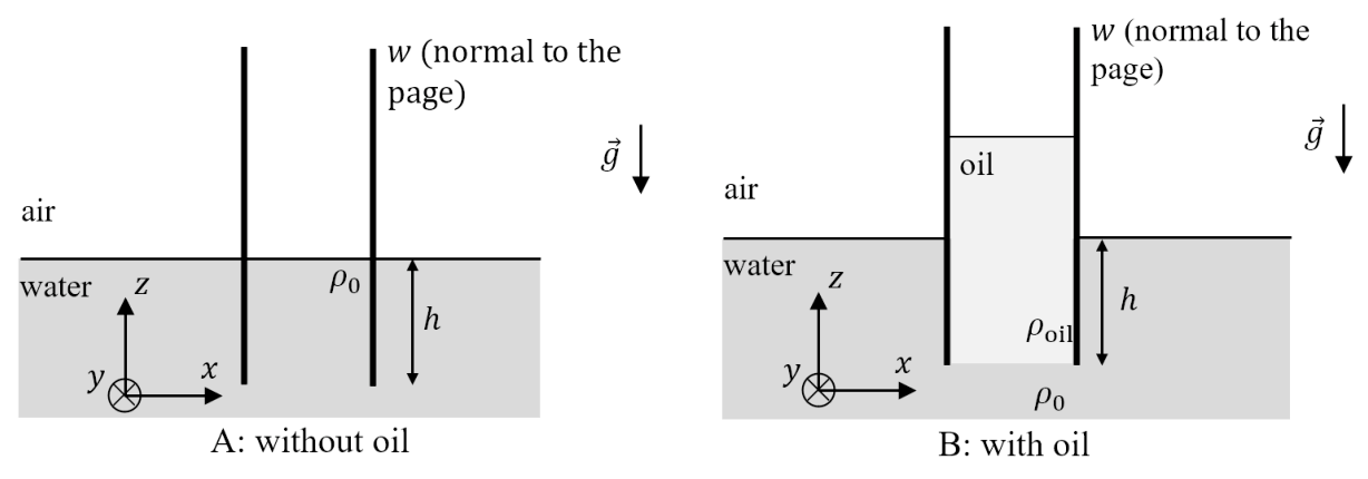
Figure 1. Parallel plates in water.
Oil of density \(\rho_{\mathrm{oil}}\) (\(\rho_{\mathrm{oil}}<\rho_0\)) is poured into the space between the plates until the lower level of the oil has reached the lower edges of the plates. Assume that plates and vessel edges are high enough for oil not to overflow them. Surface tension and mixing of fluids can be neglected.
A.1 — 0.8pt
What is the \(x\)-component of the net force \(F_x\) acting on the right plate (magnitude and direction)?
Fig. 2 shows a cross-section of a mid-ocean ridge. It consists of overlaying layers of mantle, crust and ocean water. The mantle is composed of rocks that we assume can flow in geological timescales and therefore, in this problem will be treated as a fluid. The thickness of the crust is much smaller than the characteristic length scale in the \(x\)-direction, hence, the crust behaves as a freely bendable plate. To high accuracy, such a ridge can be modeled as a two-dimensional system, without any variation of variables along the \(y\)-axis, which is perpendicular to the plane of Fig. 2. Assume that the ridge length \(L\) along the \(y\)-axis is much larger than any other length introduced in this problem.
At the centre of the ridge the thickness of the crust is assumed to be zero. As the horizontal distance \(x\) from the centre increases, the crust gets thicker and approaches a constant thickness \(D\) as \(x\to\infty\). Correspondingly, the ocean floor subsides by a vertical height \(h\) below the top of the ridge O, which we define as the origin of our coordinate system (see Fig. 2). Water density \(\rho_0\) and temperature \(T_0\) can be assumed to be constant in space and time. The same can be assumed for mantle density \(\rho_1\) and its temperature \(T_1\). The temperature of the crust \(T\) is also constant in time but can depend on position.
It is known that, to high accuracy, the crustal material expands linearly with temperature \(T\). Since water and mantle temperatures are assumed to be constant, it is convenient to use a rescaled version of the thermal expansion coefficient. Then \(l(T)=l_1[1-k_l(T_1-T)/(T_1-T_0)]\), where \(l\) is the length of a piece of crustal material, \(l_1\) is its length at temperature \(T_1\), and \(k_l\) is the rescaled thermal expansion coefficient, which can be assumed to be constant.
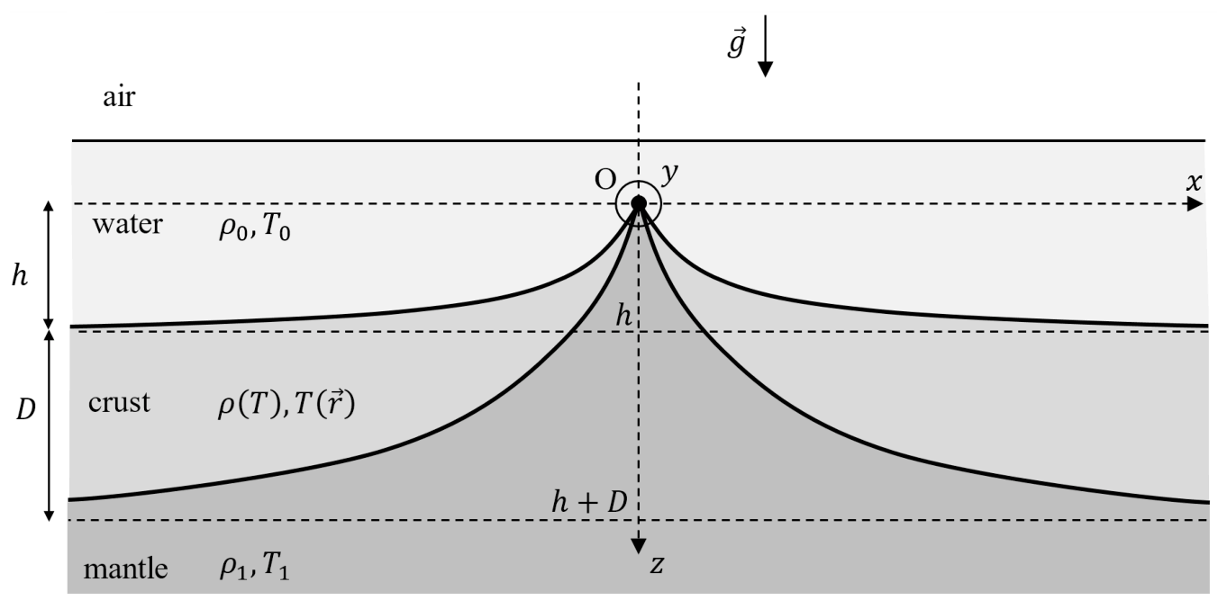
Figure 2. Mid-ocean ridge. Note that the \(z\)-axis is pointing downwards.
A.2 — 0.6pt
Assuming that the crust is isotropic, find how its density \(\rho\) depends on its temperature \(T\). Assuming that \(|k_l|\ll 1\), write your answer in the approximate form
\[ \rho(T)\approx \rho_1\left[1+k\frac{T_1-T}{T_1-T_0}\right], \tag{2} \]
where terms of order \(k_l^2\) and higher are neglected. Then, identify constant \(k\).
It is known that \(k>0\). Also, thermal conductivity of the crust \(\kappa\) can be assumed to be constant. As a consequence, very far away from the ridge axis the temperature of the crust depends linearly with depth.
A.3 — 1.1pt
By assuming that mantle and water each behave like an incompressible fluid at hydrostatic equilibrium, express the far-distance crust thickness \(D\) in terms of \(h\), \(\rho_0\), \(\rho_1\), and \(k\). Any motion of the material can be neglected.
A.4 — 1.6pt
Find, to the leading order in \(k\), the net horizontal force \(F\) acting on the right half (\(x>0\)) of the crust in terms of \(\rho_0\), \(\rho_1\), \(h\), \(L\), \(k\) and \(g\).
Suppose that crust is thermally isolated from the rest of the Earth. As a result of heat conduction, the temperatures of the upper and lower surfaces of the crust are going to get closer to each other until the crust reaches thermal equilibrium. Specific heat of the crust is \(c\) and can be assumed to be constant.
A.5 — 0.9pt
By using dimensional analysis or order-of-magnitude analysis, estimate the characteristic time \(\tau\) in which the difference between the upper and lower surface temperatures of the crust far away from the ridge axis is going to approach zero. You can assume that \(\tau\) does not depend on the two initial surface temperatures of the crust.
Part B. Seismic waves in a stratified medium (5.0 points)
Suppose that a short earthquake happens at the surface of some planet. The seismic waves can be assumed to originate from a line source situated at \(z=x=0\), where \(x\) is the horizontal coordinate and \(z\) is the depth below the surface (Fig. 3). The seismic wave source can be assumed to be much longer than any other length considered in this question.
As a result of the earthquake, a uniform flux of the so-called longitudinal P waves is emitted along all the directions in the \(x\)-\(z\) plane that have positive component along the \(z\)-axis. Since the wave theory in a solid is generally complicated, in this problem we neglect all the other waves emitted by the earthquake. The crust of the planet is stratified so that the P-wave speed \(v\) depends on depth \(z\) according to \(v=v_0(1+z/z_0)\), where \(v_0\) is the speed at the surface and \(z_0\) is a known positive constant.
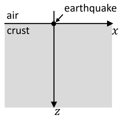
Figure 3. Coordinate system used in part B.
B.1 — 1.5pt
Consider a single ray emitted by the earthquake that makes an initial angle \(0<\theta_0<\pi/2\) with the \(z\)-axis and travels in the \(x\)-\(z\) plane. What is the horizontal coordinate \(x_1(\theta_0)\ne 0\) at which this ray can be detected at the surface of the planet? It is known that the ray path is an arc of a circle. Write your answer in the form \(x_1(\theta_0)=A\cot(b\theta_0)\), where \(A\) and \(b\) are constants to be found.
If you were unable to find \(A\) and \(b\), in the following questions you can use the result \(x_1(\theta_0)=A\cot(b\theta_0)\) as given. Suppose that total energy per unit length of the source released as P waves into the crust during the earthquake is \(E\). Assume that waves are completely absorbed when they reach the surface of the planet from below.
B.2 — 1.5pt
Find how the energy density per unit area \(\varepsilon(x)\) absorbed by the surface depends on the distance along the surface \(x\). Sketch the plot of \(\varepsilon(x)\).
From now on, assume that the waves are instead fully reflected when reaching the surface. Imagine a device positioned at \(z=x=0\) that has the same geometry as the previously considered earthquake source. The device is capable of emitting P waves in a freely chosen angular distribution. We make the device emit a signal with a narrow range of emission angles. In particular, the initial angle the signal makes with the vertical belongs to the interval \([\theta_0-\tfrac12\delta\theta_0,\theta_0+\tfrac12\delta\theta_0]\), where \(0<\theta_0<\pi/2\), \(\delta\theta_0\ll 1\) and \(\delta\theta_0\ll\theta_0\).
B.3 — 2.0pt
At what distance \(x_{\max}\) along the surface from the source is the furthest point that the signal does not reach? Write your answer in terms of \(\theta_0\), \(\delta\theta_0\) and other constants given above.
Official English text of the problem.
Answers
-
A.1 \[ \boxed{F_x=\frac{\rho_0gwh^2}{2} \left(\frac{\rho_0}{\rho_{\mathrm{oil}}}-1\right)} \] The force points in the \(+x\) direction, away from the oil.
-
A.2 \[ \boxed{\rho(T)=\rho_1 \left[1-k_l\frac{T_1-T}{T_1-T_0}\right]^{-3} \approx\rho_1\left[1+3k_l\frac{T_1-T}{T_1-T_0}\right], \qquad k=3k_l.} \]
-
A.3 \[ \boxed{D=\frac{2(\rho_1-\rho_0)h}{\rho_1k}} \] within the first-order density approximation.
-
A.4 The total horizontal force exerted by the fluids is, to leading order, \[ \boxed{F_x\simeq \frac{2gLh^2(\rho_1-\rho_0)^2}{\rho_1k^2},} \] directed away from the ridge, along \(+x\).
-
A.5 \[ \boxed{\tau\sim\frac{\rho_1cD^2}{\kappa} =\frac{4c(\rho_1-\rho_0)^2h^2}{\kappa\rho_1k^2}.} \] This is an order-of-magnitude estimate.
-
B.1 \[ \boxed{x_1(\theta_0)=2z_0\cot\theta_0,\qquad A=2z_0,\qquad b=1.} \]
-
B.2 \[ \boxed{\varepsilon(x)= \frac{2Ez_0}{\pi(x^2+4z_0^2)}.} \] The graph is even, peaks at \(\varepsilon(0)=E/(2\pi z_0)\), reaches half its maximum at \(x=\pm2z_0\), and approaches zero as \(x^{-2}\).
-
B.3 In the narrow-band limit, \[ \boxed{x_{\max}\simeq \frac{2z_0\cos^2\theta_0}{\delta\theta_0}.} \] This is the outer boundary of the last unreached interval along the beam’s propagation direction. An exact expression accounting for the integer number of reflections is derived below.
Solution
A.1
Let \(H\) be the height of the oil column above the lower edges of the plates. At those edges, the oil and water pressures must agree. With atmospheric pressure subtracted,
\[ \rho_{\mathrm{oil}}gH=\rho_0gh, \qquad H=\frac{\rho_0}{\rho_{\mathrm{oil}}}h. \]
A fluid column of height \(a\) and density \(\rho\) exerts a horizontal force
\[ w\int_0^a \rho g(a-u)\,du=\frac12\rho gwa^2 \]
on a vertical plate, where \(u\) measures height above the column’s bottom.
The oil pushes the right plate towards \(+x\); the water pushes it towards \(-x\). Atmospheric pressure cancels between the two sides. Including the oil above the exterior water level gives
\[ F_x=\frac{gw}{2} \left(\rho_{\mathrm{oil}}H^2-\rho_0h^2\right). \]
Substituting \(H\),
\[ \boxed{F_x= \frac{\rho_0gwh^2}{2} \left(\frac{\rho_0}{\rho_{\mathrm{oil}}}-1\right)>0.} \]
Thus the plate is pushed outwards.
A.2
Define the dimensionless temperature difference
\[ q=\frac{T_1-T}{T_1-T_0}. \]
Isotropic expansion changes all three linear dimensions by the same factor. Consequently,
\[ \frac{V(T)}{V(T_1)}=(1-k_lq)^3. \]
Mass is conserved, and the reference density at \(T_1\) is \(\rho_1\), so
\[ \rho(T)=\rho_1(1-k_lq)^{-3}. \]
Using the given expansion and neglecting terms of order \(k_l^2\),
\[ \rho(T)\approx\rho_1(1+3k_lq). \]
Comparison with equation (2) gives
\[ \boxed{k=3k_l.} \]
A.3
Use the downward-pointing \(z\)-axis of Fig. 2. Far from the ridge, the crust extends from \(z=h\) to \(z=h+D\). Its temperature is
\[ T(z)=T_0+(T_1-T_0)\frac{z-h}{D}, \]
and therefore its density is
\[ \rho(z)\approx \rho_1\left[1+k\left(1-\frac{z-h}{D}\right)\right]. \]
Its mean density is
\[ \overline{\rho} =\frac1D\int_h^{h+D}\rho(z)\,dz =\rho_1\left(1+\frac{k}{2}\right). \]
Let \(p_O\) be the common fluid pressure at the ridge crest, where the crust has zero thickness. Hydrostatic equilibrium gives the pressures immediately above and below the distant crust:
\[ p_{\mathrm{top}}=p_O+\rho_0gh, \]
\[ p_{\mathrm{bottom}}=p_O+\rho_1g(h+D). \]
Vertical force balance on a distant horizontal column of crust requires
\[ p_{\mathrm{bottom}}-p_{\mathrm{top}} =\overline{\rho}\,gD. \]
Thus
\[ \rho_1(h+D)-\rho_0h =\rho_1D\left(1+\frac{k}{2}\right). \]
After cancelling the common term \(\rho_1D\),
\[ (\rho_1-\rho_0)h=\frac12\rho_1kD, \]
so
\[ \boxed{D=\frac{2(\rho_1-\rho_0)h}{\rho_1k}.} \]
A.4
We calculate the pressure forces on the actual water–crust and mantle–crust interfaces.
Write the upper and lower crust surfaces as \(z=z_t(x)\) and \(z=z_b(x)\). Their endpoint values are
\[ z_t(0)=z_b(0)=0, \qquad z_t(\infty)=h, \qquad z_b(\infty)=h+D. \]
The fluid pressure fields are
\[ p_w(z)=p_O+\rho_0gz, \qquad p_m(z)=p_O+\rho_1gz. \]
For an interface element of horizontal length \(dx\) and width \(L\), the horizontal component of pressure force contains the surface slope. The upper fluid pushes towards negative \(x\), while the lower fluid pushes towards positive \(x\):
\[ dF_x =L\left[ p_m(z_b)\frac{dz_b}{dx} -p_w(z_t)\frac{dz_t}{dx} \right]dx. \]
The factors from the inclined surface area and the unit normal cancel, so this expression does not require an additional small-slope approximation. Integrating,
\[ \begin{aligned} F_x &=L\int_0^{h+D}(p_O+\rho_1gz)\,dz -L\int_0^h(p_O+\rho_0gz)\,dz\\ &=p_OLD+\frac{gL}{2} \left[\rho_1(h+D)^2-\rho_0h^2\right]. \end{aligned} \]
Equivalently,
\[ F_x= \frac12\rho_1gLD^2 +(p_O+\rho_1gh)LD +\frac12(\rho_1-\rho_0)gLh^2. \]
From A.3, \(D\propto k^{-1}\) at fixed \(h\). With the background pressure fixed, these three contributions are respectively of orders \(k^{-2}\), \(k^{-1}\), and \(k^0\). Hence the leading term is
\[ F_x\simeq\frac12\rho_1gLD^2. \]
Substituting the expression for \(D\),
\[ \boxed{ F_x\simeq \frac{2gLh^2(\rho_1-\rho_0)^2}{\rho_1k^2}. } \]
It points along \(+x\), away from the ridge. This is the total force exerted by the fluids; no lithostatic force on an artificial cut through the distant crust has been subtracted.
A.5
To leading order in \(k\), the crust has volumetric heat capacity \(\rho_1c\), giving thermal diffusivity
\[ \chi=\frac{\kappa}{\rho_1c}. \]
Far from the ridge, the relevant distance over which heat must diffuse is \(D\). The heat equation,
\[ \frac{\partial T}{\partial t} =\chi\frac{\partial^2T}{\partial z^2}, \]
therefore gives the scale estimate
\[ \frac{\Delta T}{\tau}\sim \chi\frac{\Delta T}{D^2}. \]
The temperature difference cancels, as required:
\[ \boxed{\tau\sim\frac{D^2}{\chi} =\frac{\rho_1cD^2}{\kappa}.} \]
Using A.3,
\[ \boxed{ \tau\sim \frac{4c(\rho_1-\rho_0)^2h^2} {\kappa\rho_1k^2}. } \]
Dimensional analysis does not determine a numerical prefactor. The surface temperature difference approaches zero asymptotically rather than vanishing at a finite time.
B.1
In a medium whose wave speed depends only on depth, Snell’s law preserves the horizontal slowness:
\[ \frac{\sin\theta(z)}{v(z)} =\frac{\sin\theta_0}{v_0}, \]
where \(\theta(z)\) is the local angle with the vertical. Since
\[ v(z)=v_0\frac{z+z_0}{z_0}, \]
we obtain
\[ \sin\theta(z) =\frac{z+z_0}{z_0}\sin\theta_0. \]
Define
\[ R=\frac{z_0}{\sin\theta_0}. \]
On the descending part of the ray,
\[ \frac{dx}{dz}=\tan\theta =\frac{z+z_0}{\sqrt{R^2-(z+z_0)^2}}. \]
Integration with \(x=0\) at \(z=0\) gives
\[ x=\sqrt{R^2-z_0^2} -\sqrt{R^2-(z+z_0)^2}. \]
Thus the trajectory belongs to the circle
\[ (x-x_c)^2+(z+z_0)^2=R^2, \]
whose centre has coordinates
\[ x_c=\sqrt{R^2-z_0^2}=z_0\cot\theta_0, \qquad z_c=-z_0. \]
The ray turns at the deepest point of this circle and returns symmetrically to the surface. Its two intersections with \(z=0\) are \(x=0\) and \(x=2x_c\). Therefore
\[ \boxed{x_1(\theta_0)=2z_0\cot\theta_0,} \]
and
\[ \boxed{A=2z_0,\qquad b=1.} \]
The surface speed \(v_0\) affects travel times but cancels from the ray geometry.
B.2
The downward half-plane spans an angular range \(\pi\). Uniform emission therefore assigns energy per unit source length
\[ dE=\frac{E}{\pi}\,d\theta \]
to an angular interval \(d\theta\).
For rays returning at \(x>0\),
\[ x=2z_0\cot\theta, \qquad \left|\frac{dx}{d\theta}\right| =2z_0\csc^2\theta. \]
Energy conservation between the emitted angular interval and its receiving surface strip gives
\[ \varepsilon(x)\,dx =\frac{E}{\pi}|d\theta|. \]
Hence
\[ \varepsilon(x) =\frac{E}{2\pi z_0}\sin^2\theta. \]
Using
\[ \cot\theta=\frac{x}{2z_0}, \qquad \sin^2\theta=\frac{1}{1+x^2/(4z_0^2)}, \]
we find
\[ \boxed{\varepsilon(x) =\frac{2Ez_0}{\pi(x^2+4z_0^2)}.} \]
Left-going emission gives the same expression for \(x<0\). Its normalization is
\[ \int_{-\infty}^{\infty}\varepsilon(x)\,dx =\frac{E}{\pi} \left[\arctan\frac{x}{2z_0}\right]_{-\infty}^{\infty} =E. \]
For the requested sketch: the curve is smooth and symmetric about \(x=0\), with a single maximum \(E/(2\pi z_0)\). At \(x=\pm2z_0\) its height is \(E/(4\pi z_0)\), so its full width at half maximum is \(4z_0\). It remains positive at every finite \(x\), and its tails satisfy
\[ \varepsilon(x)\sim\frac{2Ez_0}{\pi x^2} \qquad (|x|\gg z_0). \]
Since \(E\) is energy per unit source length, \(\varepsilon\) has units of energy per unit area.
B.3
At a specular surface reflection, the vertical component of the ray velocity reverses while its horizontal component is preserved. Each ray therefore repeats the same arc, translated horizontally. Its surface encounters occur at
\[ x_n(\theta)=n\ell(\theta), \qquad \ell(\theta)=2z_0\cot\theta, \qquad n=1,2,\ldots. \]
Let
\[ \theta_\pm=\theta_0\pm\frac{\delta\theta_0}{2}. \]
For a band lying entirely within \(0<\theta<\pi/2\), the shortest and longest distances between successive surface encounters are
\[ \ell_{\min}=2z_0\cot\theta_+, \qquad \ell_{\max}=2z_0\cot\theta_-. \]
Because the beam fills the angular interval, the surface interval reached at the \(n\)-th encounter is
\[ I_n=[n\ell_{\min},\,n\ell_{\max}]. \]
A gap exists between \(I_n\) and \(I_{n+1}\) precisely when
\[ n\ell_{\max}<(n+1)\ell_{\min}, \]
or
\[ n(\ell_{\max}-\ell_{\min})<\ell_{\min}. \]
Put \(\Delta\ell=\ell_{\max}-\ell_{\min}\). Once \(n\Delta\ell\ge\ell_{\min}\), adjacent intervals overlap, and they continue to overlap for every larger \(n\). Consequently, the exact outer boundary of the last gap is
\[ \boxed{ x_{\max} =\ell_{\min} \left\lceil\frac{\ell_{\min}}{\Delta\ell}\right\rceil. } \]
The ceiling accounts for the integer number of surface encounters. The boundary itself is reached; unreached points approach it from below.
For the requested narrow-band approximation,
\[ \ell_0=2z_0\cot\theta_0, \]
and
\[ \Delta\ell \simeq \left|\frac{d\ell}{d\theta}\right|_{\theta_0} \delta\theta_0 = 2z_0\csc^2\theta_0\,\delta\theta_0. \]
At fixed \(\theta_0\), a sufficiently narrow band requires many reflections before the intervals overlap. To leading order, the integer rounding can then be neglected:
\[ x_{\max}\simeq\frac{\ell_0^2}{\Delta\ell}. \]
Therefore
\[ \boxed{ x_{\max}\simeq \frac{(2z_0\cot\theta_0)^2} {2z_0\csc^2\theta_0\,\delta\theta_0} = \frac{2z_0\cos^2\theta_0}{\delta\theta_0}. } \]
The solution was checked against the official solution.
IPhO 2021 · Theorieaufgabe 1
Planetenphysik
Diese Aufgabe besteht aus zwei voneinander unabhängigen Teilaufgaben zum Inneren von Planeten. Die Auswirkungen der Oberflächenkrümmung der Planeten können vernachlässigt werden. Möglicherweise benötigen Sie die Formel
\[ (1+x)^\varepsilon\approx 1+\varepsilon x,\quad \text{wenn }|x|\ll 1. \tag{1} \]
Teil A. Mittelozeanischer Rücken (5.0 Punkte)
Betrachten Sie ein großes Wassergefäß in einem homogenen Gravitationsfeld mit der Fallbeschleunigung \(g\). Zwei zueinander parallele, senkrechte rechteckige Platten sind so in das Gefäß eingesetzt, dass ihre senkrechten Kanten dicht und lückenlos an den senkrechten Gefäßwänden anliegen. Jede Platte taucht über eine Länge \(h\) in das Wasser ein (Abb. 1). Die Breite der Platten entlang der \(y\)-Achse beträgt \(w\), die Dichte des Wassers ist \(\rho_0\).
Abbildung 1. Parallele Platten im Wasser.
Öl der Dichte \(\rho_{\mathrm{oil}}\) (\(\rho_{\mathrm{oil}}<\rho_0\)) wird in den Raum zwischen den Platten gegossen, bis die untere Grenzfläche des Öls die Unterkanten der Platten erreicht hat. Nehmen Sie an, dass die Platten und die Gefäßränder hoch genug sind, sodass kein Öl darüberläuft. Oberflächenspannung und Durchmischung der Flüssigkeiten können vernachlässigt werden.
A.1 — 0.8 Punkte
Wie groß ist die \(x\)-Komponente der resultierenden Kraft \(F_x\), die auf die rechte Platte wirkt (Betrag und Richtung)?
Abb. 2 zeigt einen Querschnitt durch einen mittelozeanischen Rücken. Er besteht aus übereinanderliegenden Schichten aus Mantel, Kruste und Ozeanwasser. Der Mantel besteht aus Gesteinen, von denen wir annehmen, dass sie auf geologischen Zeitskalen fließen können; daher wird er in dieser Aufgabe als Fluid behandelt. Die Dicke der Kruste ist wesentlich kleiner als die charakteristische Längenskala in \(x\)-Richtung, sodass sich die Kruste wie eine frei biegsame Platte verhält. Ein solcher Rücken lässt sich mit hoher Genauigkeit als zweidimensionales System modellieren, dessen Größen sich entlang der \(y\)-Achse, die senkrecht zur Zeichenebene von Abb. 2 steht, nicht ändern. Nehmen Sie an, dass die Länge \(L\) des Rückens entlang der \(y\)-Achse wesentlich größer ist als jede andere in dieser Aufgabe eingeführte Länge.
Im Zentrum des Rückens wird die Dicke der Kruste als null angenommen. Mit zunehmendem horizontalem Abstand \(x\) vom Zentrum wird die Kruste dicker und nähert sich für \(x\to\infty\) einer konstanten Dicke \(D\). Entsprechend senkt sich der Meeresboden um eine vertikale Höhe \(h\) unter den Scheitel O des Rückens ab, den wir als Ursprung unseres Koordinatensystems festlegen (siehe Abb. 2). Die Dichte \(\rho_0\) und die Temperatur \(T_0\) des Wassers können als räumlich und zeitlich konstant angenommen werden. Dasselbe gilt für die Dichte \(\rho_1\) und die Temperatur \(T_1\) des Mantels. Die Temperatur \(T\) der Kruste ist ebenfalls zeitlich konstant, kann jedoch vom Ort abhängen.
Es ist bekannt, dass sich das Krustenmaterial mit hoher Genauigkeit linear mit der Temperatur \(T\) ausdehnt. Da die Temperaturen von Wasser und Mantel als konstant angenommen werden, ist es zweckmäßig, eine umskalierte Form des Wärmeausdehnungskoeffizienten zu verwenden. Dann gilt \(l(T)=l_1[1-k_l(T_1-T)/(T_1-T_0)]\), wobei \(l\) die Länge eines Stücks Krustenmaterial, \(l_1\) dessen Länge bei der Temperatur \(T_1\) und \(k_l\) der umskalierte Wärmeausdehnungskoeffizient ist, der als konstant angenommen werden kann.
Abbildung 2. Mittelozeanischer Rücken. Beachten Sie, dass die \(z\)-Achse nach unten zeigt.
A.2 — 0.6 Punkte
Bestimmen Sie unter der Annahme einer isotropen Kruste, wie ihre Dichte \(\rho\) von ihrer Temperatur \(T\) abhängt. Schreiben Sie Ihre Antwort unter der Annahme \(|k_l|\ll 1\) in der Näherungsform
\[ \rho(T)\approx \rho_1\left[1+k\frac{T_1-T}{T_1-T_0}\right], \tag{2} \]
wobei Terme der Ordnung \(k_l^2\) und höher vernachlässigt werden. Bestimmen Sie anschließend die Konstante \(k\).
Es ist bekannt, dass \(k>0\) gilt. Außerdem kann die Wärmeleitfähigkeit \(\kappa\) der Kruste als konstant angenommen werden. Daher hängt die Temperatur der Kruste in sehr großer Entfernung von der Rückenachse linear von der Tiefe ab.
A.3 — 1.1 Punkte
Drücken Sie unter der Annahme, dass sich Mantel und Wasser jeweils wie ein inkompressibles Fluid im hydrostatischen Gleichgewicht verhalten, die Krustendicke \(D\) in großer Entfernung durch \(h\), \(\rho_0\), \(\rho_1\) und \(k\) aus. Jegliche Bewegung des Materials kann vernachlässigt werden.
A.4 — 1.6 Punkte
Bestimmen Sie in führender Ordnung in \(k\) die resultierende horizontale Kraft \(F\), die auf die rechte Hälfte (\(x>0\)) der Kruste wirkt, in Abhängigkeit von \(\rho_0\), \(\rho_1\), \(h\), \(L\), \(k\) und \(g\).
Nehmen Sie an, die Kruste sei vom Rest der Erde thermisch isoliert. Durch Wärmeleitung nähern sich die Temperaturen der Ober- und Unterseite der Kruste einander an, bis die Kruste das thermische Gleichgewicht erreicht. Die spezifische Wärmekapazität der Kruste beträgt \(c\) und kann als konstant angenommen werden.
A.5 — 0.9 Punkte
Schätzen Sie mithilfe einer Dimensionsanalyse oder einer Größenordnungsabschätzung die charakteristische Zeit \(\tau\) ab, innerhalb derer sich die Temperaturdifferenz zwischen Ober- und Unterseite der Kruste in großer Entfernung von der Rückenachse null annähert. Sie können annehmen, dass \(\tau\) nicht von den beiden anfänglichen Oberflächentemperaturen der Kruste abhängt.
Teil B. Seismische Wellen in einem geschichteten Medium (5.0 Punkte)
Nehmen Sie an, an der Oberfläche eines Planeten ereigne sich ein kurzes Erdbeben. Es kann angenommen werden, dass die seismischen Wellen von einer Linienquelle bei \(z=x=0\) ausgehen, wobei \(x\) die horizontale Koordinate und \(z\) die Tiefe unterhalb der Oberfläche ist (Abb. 3). Die Quelle der seismischen Wellen kann als wesentlich länger als jede andere in dieser Teilaufgabe betrachtete Länge angenommen werden.
Infolge des Erdbebens wird ein gleichmäßiger Fluss sogenannter longitudinaler P-Wellen in alle Richtungen in der \(x\)-\(z\)-Ebene ausgesandt, die eine positive Komponente entlang der \(z\)-Achse aufweisen. Da die Wellentheorie in einem Festkörper im Allgemeinen kompliziert ist, vernachlässigen wir in dieser Aufgabe alle anderen vom Erdbeben ausgesandten Wellen. Die Kruste des Planeten ist so geschichtet, dass die Geschwindigkeit \(v\) der P-Wellen gemäß \(v=v_0(1+z/z_0)\) von der Tiefe \(z\) abhängt, wobei \(v_0\) die Geschwindigkeit an der Oberfläche und \(z_0\) eine bekannte positive Konstante ist.
Abbildung 3. Das in Teil B verwendete Koordinatensystem.
B.1 — 1.5 Punkte
Betrachten Sie einen einzelnen, vom Erdbeben ausgesandten Strahl, der anfangs einen Winkel \(0<\theta_0<\pi/2\) mit der \(z\)-Achse bildet und sich in der \(x\)-\(z\)-Ebene ausbreitet. Bei welcher horizontalen Koordinate \(x_1(\theta_0)\ne 0\) kann dieser Strahl an der Oberfläche des Planeten nachgewiesen werden? Es ist bekannt, dass die Strahlbahn ein Kreisbogen ist. Schreiben Sie Ihre Antwort in der Form \(x_1(\theta_0)=A\cot(b\theta_0)\), wobei \(A\) und \(b\) zu bestimmende Konstanten sind.
Falls Sie \(A\) und \(b\) nicht bestimmen konnten, können Sie in den folgenden Teilaufgaben das Ergebnis \(x_1(\theta_0)=A\cot(b\theta_0)\) als gegeben verwenden. Nehmen Sie an, dass die gesamte Energie pro Längeneinheit der Quelle, die während des Erdbebens als P-Wellen in die Kruste abgegeben wird, \(E\) beträgt. Nehmen Sie an, dass die Wellen vollständig absorbiert werden, wenn sie die Oberfläche des Planeten von unten erreichen.
B.2 — 1.5 Punkte
Bestimmen Sie, wie die von der Oberfläche absorbierte Energie pro Flächeneinheit \(\varepsilon(x)\) vom Abstand \(x\) entlang der Oberfläche abhängt. Skizzieren Sie den Graphen von \(\varepsilon(x)\).
Nehmen Sie von nun an an, dass die Wellen beim Erreichen der Oberfläche stattdessen vollständig reflektiert werden. Stellen Sie sich eine bei \(z=x=0\) angeordnete Vorrichtung vor, die dieselbe Geometrie wie die zuvor betrachtete Erdbebenquelle besitzt. Die Vorrichtung kann P-Wellen mit einer frei wählbaren Winkelverteilung aussenden. Wir lassen die Vorrichtung ein Signal in einem engen Bereich von Emissionswinkeln aussenden. Insbesondere liegt der anfängliche Winkel des Signals zur Vertikalen im Intervall \([\theta_0-\tfrac12\delta\theta_0,\theta_0+\tfrac12\delta\theta_0]\), wobei \(0<\theta_0<\pi/2\), \(\delta\theta_0\ll 1\) und \(\delta\theta_0\ll\theta_0\) gelten.
B.3 — 2.0 Punkte
In welchem Abstand \(x_{\max}\) von der Quelle entlang der Oberfläche liegt der am weitesten entfernte Punkt, den das Signal nicht erreicht? Drücken Sie Ihre Antwort durch \(\theta_0\), \(\delta\theta_0\) und die anderen oben angegebenen Konstanten aus.
Aufgabentext aus dem offiziellen englischen Text übersetzt.
Antworten
-
A.1 \[ \boxed{F_x=\frac{\rho_0gwh^2}{2} \left(\frac{\rho_0}{\rho_{\mathrm{oil}}}-1\right)} \] Die Kraft zeigt in \(+x\)-Richtung, vom Öl weg.
-
A.2 \[ \boxed{\rho(T)=\rho_1 \left[1-k_l\frac{T_1-T}{T_1-T_0}\right]^{-3} \approx\rho_1\left[1+3k_l\frac{T_1-T}{T_1-T_0}\right], \qquad k=3k_l.} \]
-
A.3 \[ \boxed{D=\frac{2(\rho_1-\rho_0)h}{\rho_1k}} \] im Rahmen der Dichtenäherung erster Ordnung.
-
A.4 Die gesamte von den Fluiden ausgeübte horizontale Kraft beträgt in führender Ordnung \[ \boxed{F_x\simeq \frac{2gLh^2(\rho_1-\rho_0)^2}{\rho_1k^2},} \] und ist vom Rücken weg entlang \(+x\) gerichtet.
-
A.5 \[ \boxed{\tau\sim\frac{\rho_1cD^2}{\kappa} =\frac{4c(\rho_1-\rho_0)^2h^2}{\kappa\rho_1k^2}.} \] Dies ist eine Größenordnungsabschätzung.
-
B.1 \[ \boxed{x_1(\theta_0)=2z_0\cot\theta_0,\qquad A=2z_0,\qquad b=1.} \]
-
B.2 \[ \boxed{\varepsilon(x)= \frac{2Ez_0}{\pi(x^2+4z_0^2)}.} \] Der Graph ist achsensymmetrisch zur vertikalen Achse, hat sein Maximum bei \(\varepsilon(0)=E/(2\pi z_0)\), erreicht bei \(x=\pm2z_0\) die Hälfte seines Maximalwerts und nähert sich wie \(x^{-2}\) null an.
-
B.3 Im Grenzfall eines schmalen Winkelbands gilt \[ \boxed{x_{\max}\simeq \frac{2z_0\cos^2\theta_0}{\delta\theta_0}.} \] Dies ist die äußere Grenze des letzten nicht erreichten Intervalls in Ausbreitungsrichtung des Strahlenbündels. Ein exakter Ausdruck, der die ganzzahlige Anzahl der Reflexionen berücksichtigt, wird unten hergeleitet.
Lösung
A.1
Sei \(H\) die Höhe der Ölsäule über den Unterkanten der Platten. An diesen Kanten müssen die Drücke von Öl und Wasser übereinstimmen. Nach Abzug des Atmosphärendrucks gilt
\[ \rho_{\mathrm{oil}}gH=\rho_0gh, \qquad H=\frac{\rho_0}{\rho_{\mathrm{oil}}}h. \]
Eine Flüssigkeitssäule der Höhe \(a\) und der Dichte \(\rho\) übt auf eine senkrechte Platte die horizontale Kraft
\[ w\int_0^a \rho g(a-u)\,du=\frac12\rho gwa^2 \]
aus, wobei \(u\) die Höhe über dem unteren Ende der Säule angibt.
Das Öl drückt die rechte Platte in Richtung \(+x\); das Wasser drückt sie in Richtung \(-x\). Die Beiträge des Atmosphärendrucks auf beiden Seiten heben sich auf. Unter Einbeziehung des Öls oberhalb des äußeren Wasserspiegels ergibt sich
\[ F_x=\frac{gw}{2} \left(\rho_{\mathrm{oil}}H^2-\rho_0h^2\right). \]
Einsetzen von \(H\) ergibt
\[ \boxed{F_x= \frac{\rho_0gwh^2}{2} \left(\frac{\rho_0}{\rho_{\mathrm{oil}}}-1\right)>0.} \]
Die Platte wird also nach außen gedrückt.
A.2
Wir definieren die dimensionslose Temperaturdifferenz
\[ q=\frac{T_1-T}{T_1-T_0}. \]
Bei isotroper Ausdehnung ändern sich alle drei linearen Abmessungen um denselben Faktor. Folglich gilt
\[ \frac{V(T)}{V(T_1)}=(1-k_lq)^3. \]
Die Masse bleibt erhalten, und die Referenzdichte bei \(T_1\) ist \(\rho_1\), also gilt
\[ \rho(T)=\rho_1(1-k_lq)^{-3}. \]
Mit der angegebenen Näherungsentwicklung und unter Vernachlässigung von Termen der Ordnung \(k_l^2\) folgt
\[ \rho(T)\approx\rho_1(1+3k_lq). \]
Der Vergleich mit Gleichung (2) ergibt
\[ \boxed{k=3k_l.} \]
A.3
Wir verwenden die nach unten gerichtete \(z\)-Achse aus Abb. 2. Weit vom Rücken entfernt erstreckt sich die Kruste von \(z=h\) bis \(z=h+D\). Ihre Temperatur ist
\[ T(z)=T_0+(T_1-T_0)\frac{z-h}{D}, \]
und damit ist ihre Dichte
\[ \rho(z)\approx \rho_1\left[1+k\left(1-\frac{z-h}{D}\right)\right]. \]
Ihre mittlere Dichte ist
\[ \overline{\rho} =\frac1D\int_h^{h+D}\rho(z)\,dz =\rho_1\left(1+\frac{k}{2}\right). \]
Sei \(p_O\) der gemeinsame Fluiddruck am Scheitel des Rückens, wo die Kruste die Dicke null hat. Aus dem hydrostatischen Gleichgewicht ergeben sich die Drücke unmittelbar oberhalb und unterhalb der weit entfernten Kruste:
\[ p_{\mathrm{top}}=p_O+\rho_0gh, \]
\[ p_{\mathrm{bottom}}=p_O+\rho_1g(h+D). \]
Das vertikale Kräftegleichgewicht an einer Säule der weit entfernten, horizontal liegenden Kruste erfordert
\[ p_{\mathrm{bottom}}-p_{\mathrm{top}} =\overline{\rho}\,gD. \]
Somit gilt
\[ \rho_1(h+D)-\rho_0h =\rho_1D\left(1+\frac{k}{2}\right). \]
Nach Kürzen des gemeinsamen Terms \(\rho_1D\) erhält man
\[ (\rho_1-\rho_0)h=\frac12\rho_1kD, \]
also
\[ \boxed{D=\frac{2(\rho_1-\rho_0)h}{\rho_1k}.} \]
A.4
Wir berechnen die Druckkräfte an den tatsächlichen Grenzflächen zwischen Wasser und Kruste sowie zwischen Mantel und Kruste.
Wir beschreiben die Ober- und Unterseite der Kruste durch \(z=z_t(x)\) und \(z=z_b(x)\). Ihre Werte an den Endpunkten sind
\[ z_t(0)=z_b(0)=0, \qquad z_t(\infty)=h, \qquad z_b(\infty)=h+D. \]
Die Druckfelder der Fluide lauten
\[ p_w(z)=p_O+\rho_0gz, \qquad p_m(z)=p_O+\rho_1gz. \]
Für ein Grenzflächenelement mit horizontaler Länge \(dx\) und Breite \(L\) enthält die horizontale Komponente der Druckkraft die Steigung der Oberfläche. Das obere Fluid drückt in negative \(x\)-Richtung, das untere dagegen in positive \(x\)-Richtung:
\[ dF_x =L\left[ p_m(z_b)\frac{dz_b}{dx} -p_w(z_t)\frac{dz_t}{dx} \right]dx. \]
Die Faktoren, die sich aus der geneigten Fläche und dem Einheitsnormalenvektor ergeben, heben sich auf, sodass dieser Ausdruck keine zusätzliche Näherung für kleine Steigungen erfordert. Durch Integration folgt
\[ \begin{aligned} F_x &=L\int_0^{h+D}(p_O+\rho_1gz)\,dz -L\int_0^h(p_O+\rho_0gz)\,dz\\ &=p_OLD+\frac{gL}{2} \left[\rho_1(h+D)^2-\rho_0h^2\right]. \end{aligned} \]
Gleichwertig dazu ist
\[ F_x= \frac12\rho_1gLD^2 +(p_O+\rho_1gh)LD +\frac12(\rho_1-\rho_0)gLh^2. \]
Aus A.3 folgt bei festem \(h\), dass \(D\propto k^{-1}\) gilt. Bei festem Hintergrunddruck sind diese drei Beiträge von den Ordnungen \(k^{-2}\), \(k^{-1}\) beziehungsweise \(k^0\). Der führende Term ist daher
\[ F_x\simeq\frac12\rho_1gLD^2. \]
Einsetzen des Ausdrucks für \(D\) ergibt
\[ \boxed{ F_x\simeq \frac{2gLh^2(\rho_1-\rho_0)^2}{\rho_1k^2}. } \]
Die Kraft zeigt entlang \(+x\), vom Rücken weg. Dies ist die gesamte von den Fluiden ausgeübte Kraft; es wurde keine lithostatische Kraft an einer künstlichen Schnittfläche durch die weit entfernte Kruste abgezogen.
A.5
In führender Ordnung in \(k\) besitzt die Kruste die volumetrische Wärmekapazität \(\rho_1c\). Daraus ergibt sich die Temperaturleitfähigkeit
\[ \chi=\frac{\kappa}{\rho_1c}. \]
Weit vom Rücken entfernt beträgt die maßgebliche Strecke, über die Wärme diffundieren muss, \(D\). Die Wärmeleitungsgleichung
\[ \frac{\partial T}{\partial t} =\chi\frac{\partial^2T}{\partial z^2}, \]
liefert daher die Größenordnungsabschätzung
\[ \frac{\Delta T}{\tau}\sim \chi\frac{\Delta T}{D^2}. \]
Die Temperaturdifferenz kürzt sich wie gefordert heraus:
\[ \boxed{\tau\sim\frac{D^2}{\chi} =\frac{\rho_1cD^2}{\kappa}.} \]
Mit A.3 folgt
\[ \boxed{ \tau\sim \frac{4c(\rho_1-\rho_0)^2h^2} {\kappa\rho_1k^2}. } \]
Eine Dimensionsanalyse bestimmt keinen numerischen Vorfaktor. Die Temperaturdifferenz zwischen den Oberflächen nähert sich asymptotisch null an, statt nach einer endlichen Zeit zu verschwinden.
B.1
In einem Medium, dessen Wellengeschwindigkeit nur von der Tiefe abhängt, bleibt nach dem Snelliusschen Brechungsgesetz die horizontale Langsamkeit erhalten:
\[ \frac{\sin\theta(z)}{v(z)} =\frac{\sin\theta_0}{v_0}, \]
wobei \(\theta(z)\) der lokale Winkel zur Vertikalen ist. Da
\[ v(z)=v_0\frac{z+z_0}{z_0}, \]
erhalten wir
\[ \sin\theta(z) =\frac{z+z_0}{z_0}\sin\theta_0. \]
Wir definieren
\[ R=\frac{z_0}{\sin\theta_0}. \]
Auf dem absteigenden Abschnitt des Strahls gilt
\[ \frac{dx}{dz}=\tan\theta =\frac{z+z_0}{\sqrt{R^2-(z+z_0)^2}}. \]
Integration mit \(x=0\) bei \(z=0\) ergibt
\[ x=\sqrt{R^2-z_0^2} -\sqrt{R^2-(z+z_0)^2}. \]
Die Bahn liegt somit auf dem Kreis
\[ (x-x_c)^2+(z+z_0)^2=R^2, \]
dessen Mittelpunkt folgende Koordinaten hat:
\[ x_c=\sqrt{R^2-z_0^2}=z_0\cot\theta_0, \qquad z_c=-z_0. \]
Der Strahl kehrt am tiefsten Punkt dieses Kreises um und kehrt symmetrisch zur Oberfläche zurück. Seine beiden Schnittpunkte mit \(z=0\) liegen bei \(x=0\) und \(x=2x_c\). Daher gilt
\[ \boxed{x_1(\theta_0)=2z_0\cot\theta_0,} \]
und
\[ \boxed{A=2z_0,\qquad b=1.} \]
Die Geschwindigkeit \(v_0\) an der Oberfläche beeinflusst die Laufzeiten, kürzt sich jedoch bei der Bestimmung der Strahlgeometrie heraus.
B.2
Die nach unten gerichtete Halbebene umfasst einen Winkelbereich von \(\pi\). Bei gleichmäßiger Emission entfällt daher die Energie pro Längeneinheit der Quelle
\[ dE=\frac{E}{\pi}\,d\theta \]
auf ein Winkelintervall \(d\theta\).
Für Strahlen, die bei \(x>0\) zurückkehren, gilt
\[ x=2z_0\cot\theta, \qquad \left|\frac{dx}{d\theta}\right| =2z_0\csc^2\theta. \]
Die Energieerhaltung zwischen dem ausgesandten Winkelintervall und dem zugehörigen empfangenden Oberflächenstreifen ergibt
\[ \varepsilon(x)\,dx =\frac{E}{\pi}|d\theta|. \]
Somit gilt
\[ \varepsilon(x) =\frac{E}{2\pi z_0}\sin^2\theta. \]
Mit
\[ \cot\theta=\frac{x}{2z_0}, \qquad \sin^2\theta=\frac{1}{1+x^2/(4z_0^2)}, \]
erhalten wir
\[ \boxed{\varepsilon(x) =\frac{2Ez_0}{\pi(x^2+4z_0^2)}.} \]
Für die nach links gerichtete Emission ergibt sich derselbe Ausdruck für \(x<0\). Die Normierung lautet
\[ \int_{-\infty}^{\infty}\varepsilon(x)\,dx =\frac{E}{\pi} \left[\arctan\frac{x}{2z_0}\right]_{-\infty}^{\infty} =E. \]
Zur geforderten Skizze: Die Kurve ist glatt und symmetrisch bezüglich \(x=0\) und besitzt ein einziges Maximum \(E/(2\pi z_0)\). Bei \(x=\pm2z_0\) beträgt ihre Höhe \(E/(4\pi z_0)\), sodass ihre volle Halbwertsbreite \(4z_0\) beträgt. Sie bleibt für jedes endliche \(x\) positiv, und ihre Ausläufer erfüllen
\[ \varepsilon(x)\sim\frac{2Ez_0}{\pi x^2} \qquad (|x|\gg z_0). \]
Da \(E\) die Energie pro Längeneinheit der Quelle ist, hat \(\varepsilon\) die Einheit Energie pro Flächeneinheit.
B.3
Bei einer spiegelnden Reflexion an der Oberfläche kehrt sich die vertikale Komponente der Strahlgeschwindigkeit um, während ihre horizontale Komponente erhalten bleibt. Jeder Strahl durchläuft daher wiederholt denselben, jeweils horizontal verschobenen Kreisbogen. Er trifft an den Stellen
\[ x_n(\theta)=n\ell(\theta), \qquad \ell(\theta)=2z_0\cot\theta, \qquad n=1,2,\ldots. \]
auf die Oberfläche.
Sei
\[ \theta_\pm=\theta_0\pm\frac{\delta\theta_0}{2}. \]
Für ein Winkelband, das vollständig innerhalb von \(0<\theta<\pi/2\) liegt, sind der kürzeste und der längste Abstand zwischen aufeinanderfolgenden Auftreffpunkten an der Oberfläche
\[ \ell_{\min}=2z_0\cot\theta_+, \qquad \ell_{\max}=2z_0\cot\theta_-. \]
Da das Strahlenbündel das Winkelintervall ausfüllt, ist das beim \(n\)-ten Auftreffen erreichte Oberflächenintervall
\[ I_n=[n\ell_{\min},\,n\ell_{\max}]. \]
Zwischen \(I_n\) und \(I_{n+1}\) besteht genau dann eine Lücke, wenn
\[ n\ell_{\max}<(n+1)\ell_{\min}, \]
oder
\[ n(\ell_{\max}-\ell_{\min})<\ell_{\min}. \]
Setzen wir \(\Delta\ell=\ell_{\max}-\ell_{\min}\). Sobald \(n\Delta\ell\ge\ell_{\min}\) gilt, überlappen sich benachbarte Intervalle, und dies gilt auch für jedes größere \(n\). Folglich ist die exakte äußere Grenze der letzten Lücke
\[ \boxed{ x_{\max} =\ell_{\min} \left\lceil\frac{\ell_{\min}}{\Delta\ell}\right\rceil. } \]
Die Aufrundungsfunktion berücksichtigt die ganzzahlige Anzahl der Auftreffvorgänge an der Oberfläche. Die Grenze selbst wird erreicht; nicht erreichte Punkte nähern sich ihr von unten an.
Für die geforderte Näherung eines schmalen Winkelbands gilt
\[ \ell_0=2z_0\cot\theta_0, \]
und
\[ \Delta\ell \simeq \left|\frac{d\ell}{d\theta}\right|_{\theta_0} \delta\theta_0 = 2z_0\csc^2\theta_0\,\delta\theta_0. \]
Bei festem \(\theta_0\) sind für ein hinreichend schmales Winkelband viele Reflexionen erforderlich, bevor sich die Intervalle überlappen. In führender Ordnung kann die ganzzahlige Rundung dann vernachlässigt werden:
\[ x_{\max}\simeq\frac{\ell_0^2}{\Delta\ell}. \]
Daher gilt
\[ \boxed{ x_{\max}\simeq \frac{(2z_0\cot\theta_0)^2} {2z_0\csc^2\theta_0\,\delta\theta_0} = \frac{2z_0\cos^2\theta_0}{\delta\theta_0}. } \]
Die Lösung wurde mit der offiziellen Lösung abgeglichen.
IPhO 2021 · Teori sorusu 1
Gezegen Fiziği
Bu soru, gezegenlerin iç yapısıyla ilgili birbirinden bağımsız iki sorudan oluşmaktadır. Gezegenlerin yüzey eğriliğinin etkileri ihmal edilebilir. Şu formülü kullanmanız gerekebilir:
\[ (1+x)^\varepsilon\approx 1+\varepsilon x,\quad \text{eğer }|x|\ll 1. \tag{1} \]
Bölüm A. Okyanus ortası sırtı (5.0 puan)
Serbest düşme ivmesi \(g\) olan düzgün bir kütleçekim alanında bulunan, su dolu büyük bir kap düşünün. Birbirine paralel iki düşey dikdörtgen levha, düşey kenarları kabın düşey duvarlarıyla arada boşluk kalmadan sıkıca temas edecek şekilde kabın içine yerleştirilmiştir. Her levhanın \(h\) uzunluğundaki kısmı suya batırılmıştır (Şekil 1). Levhaların \(y\) ekseni boyunca genişliği \(w\), suyun yoğunluğu \(\rho_0\)'dır.
Şekil 1. Su içindeki paralel levhalar.
Levhaların arasındaki boşluğa, yağın alt seviyesi levhaların alt kenarlarına ulaşıncaya kadar yoğunluğu \(\rho_{\mathrm{oil}}\) (\(\rho_{\mathrm{oil}}<\rho_0\)) olan yağ dökülür. Levhaların ve kabın kenarlarının, yağın üzerlerinden taşmasını önleyecek kadar yüksek olduğunu varsayın. Yüzey gerilimi ve sıvıların karışması ihmal edilebilir.
A.1 — 0.8 puan
Sağ levhaya etki eden net kuvvetin \(x\) bileşeni \(F_x\) nedir (büyüklüğü ve yönü)?
Şekil 2, bir okyanus ortası sırtının enine kesitini göstermektedir. Bu yapı, üst üste bulunan manto, yer kabuğu ve okyanus suyu katmanlarından oluşur. Manto, jeolojik zaman ölçeklerinde akabildiğini varsaydığımız kayaçlardan oluşur ve bu nedenle bu soruda bir akışkan olarak ele alınacaktır. Yer kabuğunun kalınlığı, \(x\) doğrultusundaki karakteristik uzunluk ölçeğinden çok daha küçüktür; dolayısıyla yer kabuğu serbestçe bükülebilen bir levha gibi davranır. Böyle bir sırt, Şekil 2'nin düzlemine dik olan \(y\) ekseni boyunca değişkenlerin hiçbir değişim göstermediği iki boyutlu bir sistem olarak yüksek doğrulukla modellenebilir. Sırtın \(y\) ekseni boyunca uzunluğu \(L\)'nin, bu soruda tanımlanan diğer tüm uzunluklardan çok daha büyük olduğunu varsayın.
Sırtın merkezinde yer kabuğunun kalınlığının sıfır olduğu varsayılmaktadır. Merkezden yatay uzaklık \(x\) arttıkça yer kabuğu kalınlaşır ve \(x\to\infty\) iken sabit bir \(D\) kalınlığına yaklaşır. Buna karşılık okyanus tabanı, koordinat sistemimizin başlangıç noktası olarak tanımladığımız sırtın tepesi O'nun düşey olarak \(h\) kadar altına çöker (bkz. Şekil 2). Suyun yoğunluğu \(\rho_0\) ve sıcaklığı \(T_0\)'ın uzayda ve zamanda sabit olduğu varsayılabilir. Aynı varsayım mantonun yoğunluğu \(\rho_1\) ve sıcaklığı \(T_1\) için de yapılabilir. Yer kabuğunun sıcaklığı \(T\) de zamanda sabittir, ancak konuma bağlı olabilir.
Yer kabuğu malzemesinin, yüksek doğrulukla, sıcaklık \(T\) ile doğrusal olarak genleştiği bilinmektedir. Su ve manto sıcaklıklarının sabit olduğu varsayıldığından, ısıl genleşme katsayısının yeniden ölçeklendirilmiş bir biçimini kullanmak uygundur. Bu durumda \(l(T)=l_1[1-k_l(T_1-T)/(T_1-T_0)]\) olur; burada \(l\), bir yer kabuğu malzemesi parçasının uzunluğu, \(l_1\), bu parçanın \(T_1\) sıcaklığındaki uzunluğu ve \(k_l\), sabit olduğu varsayılabilen yeniden ölçeklendirilmiş ısıl genleşme katsayısıdır.
Şekil 2. Okyanus ortası sırtı. \(z\) ekseninin aşağıya doğru yöneldiğine dikkat edin.
A.2 — 0.6 puan
Yer kabuğunun izotropik olduğunu varsayarak yoğunluğu \(\rho\)'nun sıcaklığı \(T\)'ye nasıl bağlı olduğunu bulun. \(|k_l|\ll 1\) olduğunu varsayarak cevabınızı şu yaklaşık biçimde yazın:
\[ \rho(T)\approx \rho_1\left[1+k\frac{T_1-T}{T_1-T_0}\right], \tag{2} \]
Burada \(k_l^2\) ve daha yüksek mertebeden terimler ihmal edilmektedir. Ardından \(k\) sabitini belirleyin.
\(k>0\) olduğu bilinmektedir. Ayrıca yer kabuğunun ısıl iletkenliği \(\kappa\)'nın sabit olduğu varsayılabilir. Bunun sonucunda, sırt ekseninden çok uzakta yer kabuğunun sıcaklığı derinlikle doğrusal olarak değişir.
A.3 — 1.1 puan
Manto ve suyun her birinin hidrostatik dengede sıkıştırılamaz bir akışkan gibi davrandığını varsayarak, sırtın çok uzağındaki yer kabuğu kalınlığı \(D\)'yi \(h\), \(\rho_0\), \(\rho_1\) ve \(k\) cinsinden ifade edin. Malzemenin her türlü hareketi ihmal edilebilir.
A.4 — 1.6 puan
Yer kabuğunun sağ yarısına (\(x>0\)) etki eden net yatay kuvvet \(F\)'yi, \(k\)'ya göre başat mertebede, \(\rho_0\), \(\rho_1\), \(h\), \(L\), \(k\) ve \(g\) cinsinden bulun.
Yer kabuğunun, Dünya'nın geri kalanından ısıl olarak yalıtıldığını varsayın. Isı iletimi sonucunda yer kabuğunun üst ve alt yüzeylerinin sıcaklıkları, yer kabuğu ısıl dengeye ulaşıncaya kadar birbirine yaklaşacaktır. Yer kabuğunun özgül ısısı \(c\)'dir ve sabit olduğu varsayılabilir.
A.5 — 0.9 puan
Boyut analizi veya büyüklük mertebesi analizi kullanarak, sırt ekseninden uzaktaki yer kabuğunun üst ve alt yüzey sıcaklıkları arasındaki farkın sıfıra yaklaşacağı karakteristik süre \(\tau\)'yu tahmin edin. \(\tau\)'nun yer kabuğunun iki başlangıç yüzey sıcaklığına bağlı olmadığını varsayabilirsiniz.
Bölüm B. Katmanlı bir ortamda sismik dalgalar (5.0 puan)
Bir gezegenin yüzeyinde kısa süreli bir deprem meydana geldiğini varsayın. Sismik dalgaların \(z=x=0\) konumunda bulunan çizgisel bir kaynaktan çıktığı varsayılabilir; burada \(x\) yatay koordinat, \(z\) ise yüzeyin altındaki derinliktir (Şekil 3). Sismik dalga kaynağının, bu soruda ele alınan diğer tüm uzunluklardan çok daha uzun olduğu varsayılabilir.
Deprem sonucunda, boyuna P dalgaları olarak adlandırılan dalgalar, \(x\)-\(z\) düzleminde \(z\) ekseni boyunca pozitif bileşeni olan tüm yönlerde eşit akıyla yayılır. Katılardaki dalga kuramı genel olarak karmaşık olduğundan, bu soruda depremin yaydığı diğer tüm dalgaları ihmal ediyoruz. Gezegenin kabuğu, P dalgası hızı \(v\)'nin derinlik \(z\)'ye \(v=v_0(1+z/z_0)\) bağıntısına göre bağlı olacağı şekilde katmanlıdır; burada \(v_0\) yüzeydeki hız, \(z_0\) ise bilinen pozitif bir sabittir.
Şekil 3. Bölüm B'de kullanılan koordinat sistemi.
B.1 — 1.5 puan
Depremden çıkan, başlangıçta \(z\) ekseniyle \(0<\theta_0<\pi/2\) açısı yapan ve \(x\)-\(z\) düzleminde ilerleyen tek bir ışın düşünün. Bu ışının gezegenin yüzeyinde algılanabileceği yatay koordinat \(x_1(\theta_0)\ne 0\) nedir? Işının izlediği yolun bir çember yayı olduğu bilinmektedir. Cevabınızı, \(A\) ve \(b\) bulunması gereken sabitler olmak üzere, \(x_1(\theta_0)=A\cot(b\theta_0)\) biçiminde yazın.
\(A\) ve \(b\)'yi bulamadıysanız, sonraki sorularda \(x_1(\theta_0)=A\cot(b\theta_0)\) sonucunu verilmiş olarak kullanabilirsiniz. Deprem sırasında kabuğa P dalgaları olarak salınan toplam enerjinin, kaynağın birim uzunluğu başına \(E\) olduğunu varsayın. Dalgaların gezegenin yüzeyine alttan ulaştıklarında tamamen soğurulduğunu varsayın.
B.2 — 1.5 puan
Yüzey tarafından soğurulan birim alan başına enerji yoğunluğu \(\varepsilon(x)\)'in, yüzey boyunca uzaklık \(x\)'e nasıl bağlı olduğunu bulun. \(\varepsilon(x)\)'in grafiğini kabaca çizin.
Bundan sonra, dalgaların yüzeye ulaştıklarında bunun yerine tamamen yansıdığını varsayın. \(z=x=0\) konumuna yerleştirilmiş, daha önce ele alınan deprem kaynağıyla aynı geometriye sahip bir aygıt düşünün. Aygıt, serbestçe seçilen bir açısal dağılımla P dalgaları yayabilmektedir. Aygıtın dar bir yayılma açısı aralığında bir sinyal yaymasını sağlıyoruz. Özellikle, sinyalin başlangıçta düşeyle yaptığı açı \([\theta_0-\tfrac12\delta\theta_0,\theta_0+\tfrac12\delta\theta_0]\) aralığındadır; burada \(0<\theta_0<\pi/2\), \(\delta\theta_0\ll 1\) ve \(\delta\theta_0\ll\theta_0\)'dır.
B.3 — 2.0 puan
Sinyalin ulaşmadığı en uzak nokta, kaynaktan yüzey boyunca hangi \(x_{\max}\) uzaklığındadır? Cevabınızı \(\theta_0\), \(\delta\theta_0\) ve yukarıda verilen diğer sabitler cinsinden yazın.
Soru metni resmi İngilizce metinden çevrilmiştir.
Cevaplar
-
A.1 \[ \boxed{F_x=\frac{\rho_0gwh^2}{2} \left(\frac{\rho_0}{\rho_{\mathrm{oil}}}-1\right)} \] Kuvvet, yağdan uzağa doğru, \(+x\) yönündedir.
-
A.2 \[ \boxed{\rho(T)=\rho_1 \left[1-k_l\frac{T_1-T}{T_1-T_0}\right]^{-3} \approx\rho_1\left[1+3k_l\frac{T_1-T}{T_1-T_0}\right], \qquad k=3k_l.} \]
-
A.3 \[ \boxed{D=\frac{2(\rho_1-\rho_0)h}{\rho_1k}} \] birinci mertebeden yoğunluk yaklaşımı kapsamında.
-
A.4 Akışkanların uyguladığı toplam yatay kuvvet, başat mertebede, \[ \boxed{F_x\simeq \frac{2gLh^2(\rho_1-\rho_0)^2}{\rho_1k^2},} \] olup sırttan uzağa doğru, \(+x\) yönündedir.
-
A.5 \[ \boxed{\tau\sim\frac{\rho_1cD^2}{\kappa} =\frac{4c(\rho_1-\rho_0)^2h^2}{\kappa\rho_1k^2}.} \] Bu, bir büyüklük mertebesi tahminidir.
-
B.1 \[ \boxed{x_1(\theta_0)=2z_0\cot\theta_0,\qquad A=2z_0,\qquad b=1.} \]
-
B.2 \[ \boxed{\varepsilon(x)= \frac{2Ez_0}{\pi(x^2+4z_0^2)}.} \] Grafik çift fonksiyon grafiğidir; tepe değeri \(\varepsilon(0)=E/(2\pi z_0)\)'dır, \(x=\pm2z_0\)'da maksimum değerinin yarısına ulaşır ve \(x^{-2}\) ile orantılı olarak sıfıra yaklaşır.
-
B.3 Dar bant limitinde, \[ \boxed{x_{\max}\simeq \frac{2z_0\cos^2\theta_0}{\delta\theta_0}.} \] Bu, demetin yayılma yönü boyunca ulaşılmayan son aralığın dış sınırıdır. Yansıma sayısının tam sayı olmasını hesaba katan kesin bir ifade aşağıda türetilmiştir.
Çözüm
A.1
Yağ sütununun levhaların alt kenarlarından itibaren yüksekliği \(H\) olsun. Bu kenarlarda yağ ve su basınçları eşit olmalıdır. Atmosfer basıncı çıkarıldığında,
\[ \rho_{\mathrm{oil}}gH=\rho_0gh, \qquad H=\frac{\rho_0}{\rho_{\mathrm{oil}}}h. \]
Yüksekliği \(a\) ve yoğunluğu \(\rho\) olan bir akışkan sütunu, düşey bir levhaya
\[ w\int_0^a \rho g(a-u)\,du=\frac12\rho gwa^2 \]
yatay kuvvetini uygular; burada \(u\), sütunun tabanından itibaren yüksekliği ölçer.
Yağ, sağ levhayı \(+x\) yönüne; su ise \(-x\) yönüne iter. Atmosfer basıncının iki taraftaki etkileri birbirini götürür. Dışarıdaki su seviyesinin üzerindeki yağ da hesaba katıldığında
\[ F_x=\frac{gw}{2} \left(\rho_{\mathrm{oil}}H^2-\rho_0h^2\right). \]
\(H\) yerine ifadesini koyarsak,
\[ \boxed{F_x= \frac{\rho_0gwh^2}{2} \left(\frac{\rho_0}{\rho_{\mathrm{oil}}}-1\right)>0.} \]
Dolayısıyla levha dışarıya doğru itilir.
A.2
Boyutsuz sıcaklık farkını şöyle tanımlayalım:
\[ q=\frac{T_1-T}{T_1-T_0}. \]
İzotropik genleşme, üç doğrusal boyutun tümünü aynı çarpanla değiştirir. Dolayısıyla,
\[ \frac{V(T)}{V(T_1)}=(1-k_lq)^3. \]
Kütle korunur ve \(T_1\)'deki referans yoğunluk \(\rho_1\)'dir; bu nedenle
\[ \rho(T)=\rho_1(1-k_lq)^{-3}. \]
Verilen açılımı kullanıp \(k_l^2\) mertebesindeki terimleri ihmal edersek,
\[ \rho(T)\approx\rho_1(1+3k_lq). \]
Denklem (2) ile karşılaştırma sonucunda
\[ \boxed{k=3k_l.} \]
A.3
Şekil 2'deki aşağıya yönelmiş \(z\) eksenini kullanalım. Sırttan uzakta yer kabuğu \(z=h\)'den \(z=h+D\)'ye kadar uzanır. Sıcaklığı
\[ T(z)=T_0+(T_1-T_0)\frac{z-h}{D}, \]
ve dolayısıyla yoğunluğu
\[ \rho(z)\approx \rho_1\left[1+k\left(1-\frac{z-h}{D}\right)\right]. \]
Ortalama yoğunluğu ise
\[ \overline{\rho} =\frac1D\int_h^{h+D}\rho(z)\,dz =\rho_1\left(1+\frac{k}{2}\right). \]
Yer kabuğunun kalınlığının sıfır olduğu sırt tepesindeki ortak akışkan basıncı \(p_O\) olsun. Hidrostatik denge, uzaktaki yer kabuğunun hemen üstündeki ve altındaki basınçları verir:
\[ p_{\mathrm{top}}=p_O+\rho_0gh, \]
\[ p_{\mathrm{bottom}}=p_O+\rho_1g(h+D). \]
Uzaktaki yatay yer kabuğundan alınan bir sütun üzerinde düşey kuvvet dengesi şu koşulu gerektirir:
\[ p_{\mathrm{bottom}}-p_{\mathrm{top}} =\overline{\rho}\,gD. \]
Böylece
\[ \rho_1(h+D)-\rho_0h =\rho_1D\left(1+\frac{k}{2}\right). \]
Ortak \(\rho_1D\) terimi sadeleştirildikten sonra,
\[ (\rho_1-\rho_0)h=\frac12\rho_1kD, \]
dolayısıyla
\[ \boxed{D=\frac{2(\rho_1-\rho_0)h}{\rho_1k}.} \]
A.4
Gerçek su–yer kabuğu ve manto–yer kabuğu ara yüzeylerindeki basınç kuvvetlerini hesaplayalım.
Yer kabuğunun üst ve alt yüzeylerini \(z=z_t(x)\) ve \(z=z_b(x)\) olarak yazalım. Uç noktalardaki değerleri şöyledir:
\[ z_t(0)=z_b(0)=0, \qquad z_t(\infty)=h, \qquad z_b(\infty)=h+D. \]
Akışkanların basınç alanları
\[ p_w(z)=p_O+\rho_0gz, \qquad p_m(z)=p_O+\rho_1gz. \]
Yatay uzunluğu \(dx\) ve genişliği \(L\) olan bir ara yüzey elemanı için basınç kuvvetinin yatay bileşeni, yüzeyin eğimini içerir. Üstteki akışkan negatif \(x\) yönüne, alttaki akışkan ise pozitif \(x\) yönüne iter:
\[ dF_x =L\left[ p_m(z_b)\frac{dz_b}{dx} -p_w(z_t)\frac{dz_t}{dx} \right]dx. \]
Eğimli yüzey alanından ve birim normalden gelen çarpanlar birbirini götürür; dolayısıyla bu ifade ek bir küçük eğim yaklaşımı gerektirmez. İntegral alındığında,
\[ \begin{aligned} F_x &=L\int_0^{h+D}(p_O+\rho_1gz)\,dz -L\int_0^h(p_O+\rho_0gz)\,dz\\ &=p_OLD+\frac{gL}{2} \left[\rho_1(h+D)^2-\rho_0h^2\right]. \end{aligned} \]
Eşdeğer olarak,
\[ F_x= \frac12\rho_1gLD^2 +(p_O+\rho_1gh)LD +\frac12(\rho_1-\rho_0)gLh^2. \]
A.3'e göre, sabit \(h\) için \(D\propto k^{-1}\)'dir. Arka plan basıncı sabit tutulduğunda bu üç katkı sırasıyla \(k^{-2}\), \(k^{-1}\) ve \(k^0\) mertebesindedir. Dolayısıyla başat terim
\[ F_x\simeq\frac12\rho_1gLD^2. \]
\(D\) yerine ifadesini koyarsak,
\[ \boxed{ F_x\simeq \frac{2gLh^2(\rho_1-\rho_0)^2}{\rho_1k^2}. } \]
Kuvvet sırttan uzağa, \(+x\) yönüne doğrudur. Bu, akışkanların uyguladığı toplam kuvvettir; uzaktaki yer kabuğundan geçen yapay bir kesit üzerindeki herhangi bir litostatik kuvvet çıkarılmamıştır.
A.5
\(k\)'ya göre başat mertebede yer kabuğunun hacimsel ısı kapasitesi \(\rho_1c\)'dir; bu da ısıl yayınım katsayısını verir:
\[ \chi=\frac{\kappa}{\rho_1c}. \]
Sırttan uzakta, ısının yayılması gereken ilgili uzaklık \(D\)'dir. Bu nedenle ısı denklemi,
\[ \frac{\partial T}{\partial t} =\chi\frac{\partial^2T}{\partial z^2}, \]
şu ölçek tahminini verir:
\[ \frac{\Delta T}{\tau}\sim \chi\frac{\Delta T}{D^2}. \]
Gerektiği gibi sıcaklık farkı sadeleşir:
\[ \boxed{\tau\sim\frac{D^2}{\chi} =\frac{\rho_1cD^2}{\kappa}.} \]
A.3 kullanıldığında,
\[ \boxed{ \tau\sim \frac{4c(\rho_1-\rho_0)^2h^2} {\kappa\rho_1k^2}. } \]
Boyut analizi sayısal bir ön çarpan belirlemez. Yüzey sıcaklıkları arasındaki fark, sonlu bir zamanda sıfır olmak yerine asimptotik olarak sıfıra yaklaşır.
B.1
Dalga hızının yalnızca derinliğe bağlı olduğu bir ortamda Snell yasası, yatay yavaşlık bileşenini korur:
\[ \frac{\sin\theta(z)}{v(z)} =\frac{\sin\theta_0}{v_0}, \]
burada \(\theta(z)\), düşeyle yapılan yerel açıdır.
\[ v(z)=v_0\frac{z+z_0}{z_0}, \]
olduğundan,
\[ \sin\theta(z) =\frac{z+z_0}{z_0}\sin\theta_0. \]
Şunu tanımlayalım:
\[ R=\frac{z_0}{\sin\theta_0}. \]
Işının aşağıya ilerleyen kısmında,
\[ \frac{dx}{dz}=\tan\theta =\frac{z+z_0}{\sqrt{R^2-(z+z_0)^2}}. \]
\(z=0\)'da \(x=0\) koşuluyla integral alındığında
\[ x=\sqrt{R^2-z_0^2} -\sqrt{R^2-(z+z_0)^2}. \]
Dolayısıyla yörünge,
\[ (x-x_c)^2+(z+z_0)^2=R^2, \]
çemberi üzerinde yer alır; bu çemberin merkezinin koordinatları
\[ x_c=\sqrt{R^2-z_0^2}=z_0\cot\theta_0, \qquad z_c=-z_0. \]
Işın bu çemberin en derin noktasında yön değiştirir ve simetrik olarak yüzeye döner. \(z=0\) ile iki kesişimi \(x=0\) ve \(x=2x_c\)'dir. Bu nedenle
\[ \boxed{x_1(\theta_0)=2z_0\cot\theta_0,} \]
ve
\[ \boxed{A=2z_0,\qquad b=1.} \]
Yüzeydeki hız \(v_0\), ilerleme sürelerini etkiler; ancak ışın geometrisini belirleyen ifadelerde sadeleşir.
B.2
Aşağıya doğru olan yarı düzlem, \(\pi\) büyüklüğünde bir açı aralığını kapsar. Dolayısıyla düzgün yayılım, kaynağın birim uzunluğu başına
\[ dE=\frac{E}{\pi}\,d\theta \]
enerjisini \(d\theta\) açısal aralığına atar.
\(x>0\)'da geri dönen ışınlar için,
\[ x=2z_0\cot\theta, \qquad \left|\frac{dx}{d\theta}\right| =2z_0\csc^2\theta. \]
Yayılımın gerçekleştiği açı aralığı ile bu enerjiyi alan yüzey şeridi arasındaki enerji korunumu şu bağıntıyı verir:
\[ \varepsilon(x)\,dx =\frac{E}{\pi}|d\theta|. \]
Böylece
\[ \varepsilon(x) =\frac{E}{2\pi z_0}\sin^2\theta. \]
Şu bağıntıları kullanarak
\[ \cot\theta=\frac{x}{2z_0}, \qquad \sin^2\theta=\frac{1}{1+x^2/(4z_0^2)}, \]
şunu buluruz:
\[ \boxed{\varepsilon(x) =\frac{2Ez_0}{\pi(x^2+4z_0^2)}.} \]
Sola doğru yayılım, \(x<0\) için aynı ifadeyi verir. Normalizasyonu şöyledir:
\[ \int_{-\infty}^{\infty}\varepsilon(x)\,dx =\frac{E}{\pi} \left[\arctan\frac{x}{2z_0}\right]_{-\infty}^{\infty} =E. \]
İstenen kaba çizim için: eğri düzgündür ve \(x=0\)'a göre simetriktir; tek maksimum değeri \(E/(2\pi z_0)\)'dır. \(x=\pm2z_0\)'da yüksekliği \(E/(4\pi z_0)\) olduğundan, yarı maksimumdaki tam genişliği \(4z_0\)'dır. Her sonlu \(x\) için pozitif kalır ve kuyrukları şu bağıntıyı sağlar:
\[ \varepsilon(x)\sim\frac{2Ez_0}{\pi x^2} \qquad (|x|\gg z_0). \]
\(E\), kaynağın birim uzunluğu başına enerji olduğundan, \(\varepsilon\)'un birimi birim alan başına enerjidir.
B.3
Yüzeydeki düzgün yansımada, ışın hızının düşey bileşeni yön değiştirirken yatay bileşeni korunur. Dolayısıyla her ışın, yatay olarak ötelenmiş aynı yayı tekrarlar. Yüzeyle karşılaşmaları şu konumlarda gerçekleşir:
\[ x_n(\theta)=n\ell(\theta), \qquad \ell(\theta)=2z_0\cot\theta, \qquad n=1,2,\ldots. \]
Şöyle tanımlayalım:
\[ \theta_\pm=\theta_0\pm\frac{\delta\theta_0}{2}. \]
Tamamı \(0<\theta<\pi/2\) içinde kalan bir bant için, yüzeyle ardışık karşılaşmalar arasındaki en kısa ve en uzun uzaklıklar
\[ \ell_{\min}=2z_0\cot\theta_+, \qquad \ell_{\max}=2z_0\cot\theta_-. \]
Demet açı aralığını doldurduğundan, \(n\). karşılaşmada ulaşılan yüzey aralığı
\[ I_n=[n\ell_{\min},\,n\ell_{\max}]. \]
\(I_n\) ile \(I_{n+1}\) arasında bir boşluk bulunması için gerekli ve yeterli koşul
\[ n\ell_{\max}<(n+1)\ell_{\min}, \]
veya
\[ n(\ell_{\max}-\ell_{\min})<\ell_{\min}. \]
\(\Delta\ell=\ell_{\max}-\ell_{\min}\) olarak tanımlayalım. \(n\Delta\ell\ge\ell_{\min}\) olduğunda komşu aralıklar örtüşür ve daha büyük her \(n\) için örtüşmeye devam eder. Sonuç olarak son boşluğun kesin dış sınırı
\[ \boxed{ x_{\max} =\ell_{\min} \left\lceil\frac{\ell_{\min}}{\Delta\ell}\right\rceil. } \]
Tavan fonksiyonu, yüzeyle karşılaşma sayısının tam sayı olmasını hesaba katar. Sınırın kendisine ulaşılır; ulaşılmayan noktalar bu sınıra daha küçük uzaklıklardan yaklaşır.
İstenen dar bant yaklaşımı için,
\[ \ell_0=2z_0\cot\theta_0, \]
ve
\[ \Delta\ell \simeq \left|\frac{d\ell}{d\theta}\right|_{\theta_0} \delta\theta_0 = 2z_0\csc^2\theta_0\,\delta\theta_0. \]
Sabit \(\theta_0\) için yeterince dar bir bantta, aralıklar örtüşmeden önce çok sayıda yansıma gerekir. Bu durumda başat mertebede tam sayıya yuvarlama ihmal edilebilir:
\[ x_{\max}\simeq\frac{\ell_0^2}{\Delta\ell}. \]
Dolayısıyla
\[ \boxed{ x_{\max}\simeq \frac{(2z_0\cot\theta_0)^2} {2z_0\csc^2\theta_0\,\delta\theta_0} = \frac{2z_0\cos^2\theta_0}{\delta\theta_0}. } \]
Çözüm, resmi çözümle karşılaştırılarak kontrol edildi.
IPhO 2021 · Problema teórico 1
Física planetaria
Este problema consta de dos problemas independientes relacionados con el interior de los planetas. Se pueden despreciar los efectos de la curvatura de la superficie de los planetas. Puede que necesite utilizar la fórmula
\[ (1+x)^\varepsilon\approx 1+\varepsilon x,\quad \text{cuando }|x|\ll 1. \tag{1} \]
Parte A. Dorsal oceánica (5.0 puntos)
Considere un recipiente grande con agua situado en un campo gravitatorio uniforme con aceleración de caída libre \(g\). En el recipiente se colocan dos placas rectangulares verticales paralelas entre sí, de modo que sus bordes verticales estén en contacto estrecho, sin huecos, con las paredes verticales del recipiente. Una longitud \(h\) de cada placa está sumergida en el agua (Fig. 1). La anchura de las placas a lo largo del eje \(y\) es \(w\), y la densidad del agua es \(\rho_0\).
Figura 1. Placas paralelas en agua.
Se vierte aceite de densidad \(\rho_{\mathrm{oil}}\) (\(\rho_{\mathrm{oil}}<\rho_0\)) en el espacio entre las placas hasta que el nivel inferior del aceite alcanza los bordes inferiores de las placas. Suponga que las placas y los bordes del recipiente son lo suficientemente altos como para que el aceite no rebose. Se pueden despreciar la tensión superficial y la mezcla de los fluidos.
A.1 — 0.8pt
¿Cuál es la componente \(x\) de la fuerza neta \(F_x\) que actúa sobre la placa derecha (módulo y sentido)?
La Fig. 2 muestra una sección transversal de una dorsal oceánica. Consta de capas superpuestas de manto, corteza y agua oceánica. El manto está compuesto de rocas que suponemos que pueden fluir en escalas de tiempo geológicas y, por tanto, en este problema se tratará como un fluido. El espesor de la corteza es mucho menor que la escala de longitud característica en la dirección \(x\), por lo que la corteza se comporta como una placa que puede flexionarse libremente. Con gran precisión, una dorsal de este tipo puede modelarse como un sistema bidimensional, sin variación de las variables a lo largo del eje \(y\), que es perpendicular al plano de la Fig. 2. Suponga que la longitud \(L\) de la dorsal a lo largo del eje \(y\) es mucho mayor que cualquier otra longitud introducida en este problema.
Se supone que, en el centro de la dorsal, el espesor de la corteza es cero. A medida que aumenta la distancia horizontal \(x\) desde el centro, la corteza se hace más gruesa y se aproxima a un espesor constante \(D\) cuando \(x\to\infty\). En correspondencia, el fondo oceánico desciende una altura vertical \(h\) por debajo de la cima de la dorsal O, que definimos como el origen de nuestro sistema de coordenadas (véase la Fig. 2). Se puede suponer que la densidad \(\rho_0\) y la temperatura \(T_0\) del agua son constantes en el espacio y en el tiempo. Lo mismo puede suponerse para la densidad \(\rho_1\) del manto y su temperatura \(T_1\). La temperatura \(T\) de la corteza también es constante en el tiempo, pero puede depender de la posición.
Se sabe que, con gran precisión, el material de la corteza se dilata linealmente con la temperatura \(T\). Dado que se supone que las temperaturas del agua y del manto son constantes, conviene utilizar una versión reescalada del coeficiente de dilatación térmica. Entonces, \(l(T)=l_1[1-k_l(T_1-T)/(T_1-T_0)]\), donde \(l\) es la longitud de un trozo de material de la corteza, \(l_1\) es su longitud a la temperatura \(T_1\) y \(k_l\) es el coeficiente de dilatación térmica reescalado, que puede suponerse constante.
Figura 2. Dorsal oceánica. Observe que el eje \(z\) apunta hacia abajo.
A.2 — 0.6pt
Suponiendo que la corteza es isótropa, determine cómo depende su densidad \(\rho\) de su temperatura \(T\). Suponiendo que \(|k_l|\ll 1\), escriba su respuesta en la forma aproximada
\[ \rho(T)\approx \rho_1\left[1+k\frac{T_1-T}{T_1-T_0}\right], \tag{2} \]
donde se desprecian los términos de orden \(k_l^2\) y superiores. A continuación, identifique la constante \(k\).
Se sabe que \(k>0\). Además, se puede suponer que la conductividad térmica \(\kappa\) de la corteza es constante. En consecuencia, muy lejos del eje de la dorsal, la temperatura de la corteza depende linealmente de la profundidad.
A.3 — 1.1pt
Suponiendo que tanto el manto como el agua se comportan como fluidos incompresibles en equilibrio hidrostático, exprese el espesor \(D\) de la corteza a gran distancia en función de \(h\), \(\rho_0\), \(\rho_1\) y \(k\). Puede despreciarse cualquier movimiento del material.
A.4 — 1.6pt
Determine, al orden dominante en \(k\), la fuerza horizontal neta \(F\) que actúa sobre la mitad derecha (\(x>0\)) de la corteza en función de \(\rho_0\), \(\rho_1\), \(h\), \(L\), \(k\) y \(g\).
Suponga que la corteza está térmicamente aislada del resto de la Tierra. Como resultado de la conducción de calor, las temperaturas de las superficies superior e inferior de la corteza se irán acercando hasta que la corteza alcance el equilibrio térmico. El calor específico de la corteza es \(c\) y puede suponerse constante.
A.5 — 0.9pt
Mediante análisis dimensional o un análisis de orden de magnitud, estime el tiempo característico \(\tau\) en el que la diferencia entre las temperaturas de las superficies superior e inferior de la corteza, lejos del eje de la dorsal, se aproximará a cero. Puede suponer que \(\tau\) no depende de las dos temperaturas superficiales iniciales de la corteza.
Parte B. Ondas sísmicas en un medio estratificado (5.0 puntos)
Suponga que se produce un terremoto breve en la superficie de un planeta. Se puede suponer que las ondas sísmicas se originan en una fuente lineal situada en \(z=x=0\), donde \(x\) es la coordenada horizontal y \(z\) es la profundidad bajo la superficie (Fig. 3). Se puede suponer que la fuente de ondas sísmicas es mucho más larga que cualquier otra longitud considerada en esta cuestión.
Como resultado del terremoto, se emite un flujo uniforme de las denominadas ondas P longitudinales en todas las direcciones del plano \(x\)-\(z\) que tienen una componente positiva a lo largo del eje \(z\). Dado que la teoría de ondas en un sólido es, en general, complicada, en este problema despreciamos todas las demás ondas emitidas por el terremoto. La corteza del planeta está estratificada de modo que la velocidad \(v\) de las ondas P depende de la profundidad \(z\) según \(v=v_0(1+z/z_0)\), donde \(v_0\) es la velocidad en la superficie y \(z_0\) es una constante positiva conocida.
Figura 3. Sistema de coordenadas utilizado en la parte B.
B.1 — 1.5pt
Considere un único rayo emitido por el terremoto que forma un ángulo inicial \(0<\theta_0<\pi/2\) con el eje \(z\) y se propaga en el plano \(x\)-\(z\). ¿Cuál es la coordenada horizontal \(x_1(\theta_0)\ne 0\) en la que puede detectarse este rayo en la superficie del planeta? Se sabe que la trayectoria del rayo es un arco de circunferencia. Escriba su respuesta en la forma \(x_1(\theta_0)=A\cot(b\theta_0)\), donde \(A\) y \(b\) son constantes que deben determinarse.
Si no ha podido determinar \(A\) y \(b\), en las siguientes cuestiones puede utilizar el resultado \(x_1(\theta_0)=A\cot(b\theta_0)\) como dato. Suponga que la energía total por unidad de longitud de la fuente liberada en forma de ondas P hacia la corteza durante el terremoto es \(E\). Suponga que las ondas se absorben por completo cuando alcanzan la superficie del planeta desde abajo.
B.2 — 1.5pt
Determine cómo depende la densidad de energía por unidad de área \(\varepsilon(x)\) absorbida por la superficie de la distancia \(x\) a lo largo de la superficie. Esboce la gráfica de \(\varepsilon(x)\).
A partir de ahora, suponga que, en cambio, las ondas se reflejan por completo al alcanzar la superficie. Imagine un dispositivo situado en \(z=x=0\) que tiene la misma geometría que la fuente sísmica considerada anteriormente. El dispositivo es capaz de emitir ondas P con una distribución angular elegida libremente. Hacemos que el dispositivo emita una señal con un intervalo estrecho de ángulos de emisión. En particular, el ángulo inicial que forma la señal con la vertical pertenece al intervalo \([\theta_0-\tfrac12\delta\theta_0,\theta_0+\tfrac12\delta\theta_0]\), donde \(0<\theta_0<\pi/2\), \(\delta\theta_0\ll 1\) y \(\delta\theta_0\ll\theta_0\).
B.3 — 2.0pt
¿A qué distancia \(x_{\max}\) de la fuente, medida a lo largo de la superficie, se encuentra el punto más lejano al que no llega la señal? Escriba su respuesta en función de \(\theta_0\), \(\delta\theta_0\) y las demás constantes dadas anteriormente.
Enunciado traducido del texto oficial en inglés.
Respuestas
-
A.1 \[ \boxed{F_x=\frac{\rho_0gwh^2}{2} \left(\frac{\rho_0}{\rho_{\mathrm{oil}}}-1\right)} \] La fuerza apunta en el sentido \(+x\), alejándose del aceite.
-
A.2 \[ \boxed{\rho(T)=\rho_1 \left[1-k_l\frac{T_1-T}{T_1-T_0}\right]^{-3} \approx\rho_1\left[1+3k_l\frac{T_1-T}{T_1-T_0}\right], \qquad k=3k_l.} \]
-
A.3 \[ \boxed{D=\frac{2(\rho_1-\rho_0)h}{\rho_1k}} \] dentro de la aproximación de primer orden para la densidad.
-
A.4 La fuerza horizontal total ejercida por los fluidos es, al orden dominante, \[ \boxed{F_x\simeq \frac{2gLh^2(\rho_1-\rho_0)^2}{\rho_1k^2},} \] dirigida en sentido opuesto a la dorsal, a lo largo de \(+x\).
-
A.5 \[ \boxed{\tau\sim\frac{\rho_1cD^2}{\kappa} =\frac{4c(\rho_1-\rho_0)^2h^2}{\kappa\rho_1k^2}.} \] Esta es una estimación de orden de magnitud.
-
B.1 \[ \boxed{x_1(\theta_0)=2z_0\cot\theta_0,\qquad A=2z_0,\qquad b=1.} \]
-
B.2 \[ \boxed{\varepsilon(x)= \frac{2Ez_0}{\pi(x^2+4z_0^2)}.} \] La gráfica es par, alcanza su máximo en \(\varepsilon(0)=E/(2\pi z_0)\), llega a la mitad de su máximo en \(x=\pm2z_0\) y tiende a cero como \(x^{-2}\).
-
B.3 En el límite de una banda estrecha, \[ \boxed{x_{\max}\simeq \frac{2z_0\cos^2\theta_0}{\delta\theta_0}.} \] Este es el límite exterior del último intervalo no alcanzado en la dirección de propagación del haz. Más adelante se deduce una expresión exacta que tiene en cuenta el número entero de reflexiones.
Solución
A.1
Sea \(H\) la altura de la columna de aceite sobre los bordes inferiores de las placas. En esos bordes, las presiones del aceite y del agua deben coincidir. Restando la presión atmosférica,
\[ \rho_{\mathrm{oil}}gH=\rho_0gh, \qquad H=\frac{\rho_0}{\rho_{\mathrm{oil}}}h. \]
Una columna de fluido de altura \(a\) y densidad \(\rho\) ejerce una fuerza horizontal
\[ w\int_0^a \rho g(a-u)\,du=\frac12\rho gwa^2 \]
sobre una placa vertical, donde \(u\) mide la altura sobre la base de la columna.
El aceite empuja la placa derecha hacia \(+x\); el agua la empuja hacia \(-x\). La presión atmosférica se cancela entre ambos lados. Al incluir el aceite situado por encima del nivel exterior del agua, se obtiene
\[ F_x=\frac{gw}{2} \left(\rho_{\mathrm{oil}}H^2-\rho_0h^2\right). \]
Sustituyendo \(H\),
\[ \boxed{F_x= \frac{\rho_0gwh^2}{2} \left(\frac{\rho_0}{\rho_{\mathrm{oil}}}-1\right)>0.} \]
Por tanto, la placa es empujada hacia fuera.
A.2
Definimos la diferencia de temperatura adimensional
\[ q=\frac{T_1-T}{T_1-T_0}. \]
La dilatación isótropa modifica las tres dimensiones lineales por el mismo factor. En consecuencia,
\[ \frac{V(T)}{V(T_1)}=(1-k_lq)^3. \]
La masa se conserva y la densidad de referencia a \(T_1\) es \(\rho_1\), de modo que
\[ \rho(T)=\rho_1(1-k_lq)^{-3}. \]
Utilizando el desarrollo dado y despreciando los términos de orden \(k_l^2\),
\[ \rho(T)\approx\rho_1(1+3k_lq). \]
La comparación con la ecuación (2) da
\[ \boxed{k=3k_l.} \]
A.3
Utilizamos el eje \(z\) de la Fig. 2, que apunta hacia abajo. Lejos de la dorsal, la corteza se extiende desde \(z=h\) hasta \(z=h+D\). Su temperatura es
\[ T(z)=T_0+(T_1-T_0)\frac{z-h}{D}, \]
y, por tanto, su densidad es
\[ \rho(z)\approx \rho_1\left[1+k\left(1-\frac{z-h}{D}\right)\right]. \]
Su densidad media es
\[ \overline{\rho} =\frac1D\int_h^{h+D}\rho(z)\,dz =\rho_1\left(1+\frac{k}{2}\right). \]
Sea \(p_O\) la presión común de los fluidos en la cima de la dorsal, donde la corteza tiene espesor nulo. El equilibrio hidrostático da las presiones inmediatamente por encima y por debajo de la corteza lejana:
\[ p_{\mathrm{top}}=p_O+\rho_0gh, \]
\[ p_{\mathrm{bottom}}=p_O+\rho_1g(h+D). \]
El equilibrio de fuerzas verticales sobre una columna de corteza horizontal alejada exige
\[ p_{\mathrm{bottom}}-p_{\mathrm{top}} =\overline{\rho}\,gD. \]
Así,
\[ \rho_1(h+D)-\rho_0h =\rho_1D\left(1+\frac{k}{2}\right). \]
Tras cancelar el término común \(\rho_1D\),
\[ (\rho_1-\rho_0)h=\frac12\rho_1kD, \]
de modo que
\[ \boxed{D=\frac{2(\rho_1-\rho_0)h}{\rho_1k}.} \]
A.4
Calculamos las fuerzas de presión sobre las interfaces reales agua–corteza y manto–corteza.
Escribimos las superficies superior e inferior de la corteza como \(z=z_t(x)\) y \(z=z_b(x)\). Sus valores en los extremos son
\[ z_t(0)=z_b(0)=0, \qquad z_t(\infty)=h, \qquad z_b(\infty)=h+D. \]
Los campos de presión de los fluidos son
\[ p_w(z)=p_O+\rho_0gz, \qquad p_m(z)=p_O+\rho_1gz. \]
Para un elemento de interfaz de longitud horizontal \(dx\) y anchura \(L\), la componente horizontal de la fuerza de presión contiene la pendiente de la superficie. El fluido superior empuja hacia los valores negativos de \(x\), mientras que el fluido inferior empuja hacia los valores positivos de \(x\):
\[ dF_x =L\left[ p_m(z_b)\frac{dz_b}{dx} -p_w(z_t)\frac{dz_t}{dx} \right]dx. \]
Los factores procedentes del área de la superficie inclinada y del vector normal unitario se cancelan, por lo que esta expresión no requiere una aproximación adicional de pendiente pequeña. Integrando,
\[ \begin{aligned} F_x &=L\int_0^{h+D}(p_O+\rho_1gz)\,dz -L\int_0^h(p_O+\rho_0gz)\,dz\\ &=p_OLD+\frac{gL}{2} \left[\rho_1(h+D)^2-\rho_0h^2\right]. \end{aligned} \]
Equivalentemente,
\[ F_x= \frac12\rho_1gLD^2 +(p_O+\rho_1gh)LD +\frac12(\rho_1-\rho_0)gLh^2. \]
Según A.3, \(D\propto k^{-1}\) para \(h\) fijo. Con la presión de fondo fija, estas tres contribuciones son, respectivamente, de órdenes \(k^{-2}\), \(k^{-1}\) y \(k^0\). Por tanto, el término dominante es
\[ F_x\simeq\frac12\rho_1gLD^2. \]
Sustituyendo la expresión de \(D\),
\[ \boxed{ F_x\simeq \frac{2gLh^2(\rho_1-\rho_0)^2}{\rho_1k^2}. } \]
Apunta a lo largo de \(+x\), alejándose de la dorsal. Esta es la fuerza total ejercida por los fluidos; no se ha restado ninguna fuerza litostática sobre un corte artificial a través de la corteza lejana.
A.5
Al orden dominante en \(k\), la corteza tiene una capacidad calorífica volumétrica \(\rho_1c\), lo que da la difusividad térmica
\[ \chi=\frac{\kappa}{\rho_1c}. \]
Lejos de la dorsal, la distancia relevante a lo largo de la cual debe difundirse el calor es \(D\). La ecuación del calor,
\[ \frac{\partial T}{\partial t} =\chi\frac{\partial^2T}{\partial z^2}, \]
da, por tanto, la estimación de escala
\[ \frac{\Delta T}{\tau}\sim \chi\frac{\Delta T}{D^2}. \]
La diferencia de temperatura se cancela, como se requiere:
\[ \boxed{\tau\sim\frac{D^2}{\chi} =\frac{\rho_1cD^2}{\kappa}.} \]
Utilizando A.3,
\[ \boxed{ \tau\sim \frac{4c(\rho_1-\rho_0)^2h^2} {\kappa\rho_1k^2}. } \]
El análisis dimensional no determina un prefactor numérico. La diferencia de temperatura entre las superficies se aproxima a cero asintóticamente, en lugar de anularse en un tiempo finito.
B.1
En un medio cuya velocidad de onda depende únicamente de la profundidad, la ley de Snell conserva la lentitud horizontal:
\[ \frac{\sin\theta(z)}{v(z)} =\frac{\sin\theta_0}{v_0}, \]
donde \(\theta(z)\) es el ángulo local con la vertical. Puesto que
\[ v(z)=v_0\frac{z+z_0}{z_0}, \]
obtenemos
\[ \sin\theta(z) =\frac{z+z_0}{z_0}\sin\theta_0. \]
Definimos
\[ R=\frac{z_0}{\sin\theta_0}. \]
En la parte descendente del rayo,
\[ \frac{dx}{dz}=\tan\theta =\frac{z+z_0}{\sqrt{R^2-(z+z_0)^2}}. \]
La integración con \(x=0\) en \(z=0\) da
\[ x=\sqrt{R^2-z_0^2} -\sqrt{R^2-(z+z_0)^2}. \]
Así, la trayectoria pertenece a la circunferencia
\[ (x-x_c)^2+(z+z_0)^2=R^2, \]
cuyo centro tiene las coordenadas
\[ x_c=\sqrt{R^2-z_0^2}=z_0\cot\theta_0, \qquad z_c=-z_0. \]
El rayo cambia de sentido vertical en el punto más profundo de esta circunferencia y regresa simétricamente a la superficie. Sus dos intersecciones con \(z=0\) son \(x=0\) y \(x=2x_c\). Por tanto,
\[ \boxed{x_1(\theta_0)=2z_0\cot\theta_0,} \]
y
\[ \boxed{A=2z_0,\qquad b=1.} \]
La velocidad en la superficie \(v_0\) afecta a los tiempos de recorrido, pero se cancela en la geometría del rayo.
B.2
El semiplano inferior abarca un intervalo angular \(\pi\). Por tanto, la emisión uniforme asigna una energía por unidad de longitud de la fuente
\[ dE=\frac{E}{\pi}\,d\theta \]
a un intervalo angular \(d\theta\).
Para los rayos que regresan en \(x>0\),
\[ x=2z_0\cot\theta, \qquad \left|\frac{dx}{d\theta}\right| =2z_0\csc^2\theta. \]
La conservación de la energía entre el intervalo angular emitido y la franja de superficie que lo recibe da
\[ \varepsilon(x)\,dx =\frac{E}{\pi}|d\theta|. \]
Por tanto,
\[ \varepsilon(x) =\frac{E}{2\pi z_0}\sin^2\theta. \]
Utilizando
\[ \cot\theta=\frac{x}{2z_0}, \qquad \sin^2\theta=\frac{1}{1+x^2/(4z_0^2)}, \]
obtenemos
\[ \boxed{\varepsilon(x) =\frac{2Ez_0}{\pi(x^2+4z_0^2)}.} \]
La emisión hacia la izquierda da la misma expresión para \(x<0\). Su normalización es
\[ \int_{-\infty}^{\infty}\varepsilon(x)\,dx =\frac{E}{\pi} \left[\arctan\frac{x}{2z_0}\right]_{-\infty}^{\infty} =E. \]
Para el esbozo solicitado: la curva es suave y simétrica respecto a \(x=0\), con un único máximo \(E/(2\pi z_0)\). En \(x=\pm2z_0\), su altura es \(E/(4\pi z_0)\), por lo que su anchura total a media altura es \(4z_0\). Se mantiene positiva para todo \(x\) finito, y sus colas satisfacen
\[ \varepsilon(x)\sim\frac{2Ez_0}{\pi x^2} \qquad (|x|\gg z_0). \]
Como \(E\) es la energía por unidad de longitud de la fuente, \(\varepsilon\) tiene unidades de energía por unidad de área.
B.3
En una reflexión especular en la superficie, la componente vertical de la velocidad del rayo invierte su sentido, mientras que su componente horizontal se conserva. Por tanto, cada rayo repite el mismo arco, trasladado horizontalmente. Sus encuentros con la superficie se producen en
\[ x_n(\theta)=n\ell(\theta), \qquad \ell(\theta)=2z_0\cot\theta, \qquad n=1,2,\ldots. \]
Sea
\[ \theta_\pm=\theta_0\pm\frac{\delta\theta_0}{2}. \]
Para una banda situada completamente dentro de \(0<\theta<\pi/2\), las distancias mínima y máxima entre encuentros sucesivos con la superficie son
\[ \ell_{\min}=2z_0\cot\theta_+, \qquad \ell_{\max}=2z_0\cot\theta_-. \]
Como el haz ocupa todo el intervalo angular, el intervalo de la superficie alcanzado en el encuentro número \(n\) es
\[ I_n=[n\ell_{\min},\,n\ell_{\max}]. \]
Existe un hueco entre \(I_n\) e \(I_{n+1}\) precisamente cuando
\[ n\ell_{\max}<(n+1)\ell_{\min}, \]
o bien
\[ n(\ell_{\max}-\ell_{\min})<\ell_{\min}. \]
Definimos \(\Delta\ell=\ell_{\max}-\ell_{\min}\). Una vez que \(n\Delta\ell\ge\ell_{\min}\), los intervalos adyacentes se solapan y siguen solapándose para todo \(n\) mayor. En consecuencia, el límite exterior exacto del último hueco es
\[ \boxed{ x_{\max} =\ell_{\min} \left\lceil\frac{\ell_{\min}}{\Delta\ell}\right\rceil. } \]
La función techo tiene en cuenta el número entero de encuentros con la superficie. El propio límite sí se alcanza; los puntos no alcanzados se aproximan a él por debajo.
Para la aproximación de banda estrecha solicitada,
\[ \ell_0=2z_0\cot\theta_0, \]
y
\[ \Delta\ell \simeq \left|\frac{d\ell}{d\theta}\right|_{\theta_0} \delta\theta_0 = 2z_0\csc^2\theta_0\,\delta\theta_0. \]
Para \(\theta_0\) fijo, una banda suficientemente estrecha requiere muchas reflexiones antes de que los intervalos se solapen. Al orden dominante, puede entonces despreciarse el redondeo a un entero:
\[ x_{\max}\simeq\frac{\ell_0^2}{\Delta\ell}. \]
Por tanto,
\[ \boxed{ x_{\max}\simeq \frac{(2z_0\cot\theta_0)^2} {2z_0\csc^2\theta_0\,\delta\theta_0} = \frac{2z_0\cos^2\theta_0}{\delta\theta_0}. } \]
La solución se comprobó con la solución oficial.
IPhO 2021 · 理论题 1
行星物理
本题由两个与行星内部有关的独立问题组成。可以忽略行星表面曲率的影响。你可能需要使用公式
\[ (1+x)^\varepsilon\approx 1+\varepsilon x,\quad \text{当 }|x|\ll 1. \tag{1} \]
部分 A. 洋中脊(5.0 分)
考虑一个盛水的大容器,置于自由落体加速度为 \(g\) 的均匀重力场中。将两块相互平行的竖直矩形板安装在容器内,使板的竖直边缘与容器的竖直壁紧密接触,不留缝隙。每块板浸入水中的长度为 \(h\)(图 1)。板沿 \(y\) 轴方向的宽度为 \(w\),水的密度为 \(\rho_0\)。
图 1. 水中的平行板。
向两板之间倒入密度为 \(\rho_{\mathrm{oil}}\)(\(\rho_{\mathrm{oil}}<\rho_0\))的油,直到油的下表面到达两板的下边缘。假设板和容器的边缘足够高,油不会从上方溢出。可以忽略表面张力和流体的混合。
A.1 — 0.8 分
作用在右侧板上的合力的 \(x\) 分量 \(F_x\) 是多少(大小和方向)?
图 2 展示了洋中脊的横截面。它由地幔、地壳和海水各层叠置而成。地幔由岩石组成,我们假设这些岩石在地质时间尺度上可以流动,因此在本题中将其视为流体。地壳的厚度远小于 \(x\) 方向上的特征长度尺度,因此地壳的行为如同一块可自由弯曲的板。可以将这样的洋中脊以很高的精度建模为二维系统,各物理量沿垂直于图 2 平面的 \(y\) 轴方向均不发生变化。假设洋中脊沿 \(y\) 轴方向的长度 \(L\) 远大于本题中引入的任何其他长度。
假设在洋中脊中心,地壳厚度为零。随着距中心的水平距离 \(x\) 增大,地壳逐渐变厚,并在 \(x\to\infty\) 时趋于恒定厚度 \(D\)。相应地,海底下沉到洋中脊顶部 O 以下,竖直高度差为 \(h\);我们将 O 定义为坐标系的原点(见图 2)。可以认为水的密度 \(\rho_0\) 和温度 \(T_0\) 在空间和时间上均为常量。地幔的密度 \(\rho_1\) 及其温度 \(T_1\) 也可作相同假设。地壳的温度 \(T\) 同样不随时间变化,但可以随位置变化。
已知地壳物质随温度 \(T\) 发生的膨胀在很高精度下呈线性关系。由于假设水和地幔的温度恒定,使用重新标度后的热膨胀系数更为方便。于是有 \(l(T)=l_1[1-k_l(T_1-T)/(T_1-T_0)]\),其中 \(l\) 是一块地壳物质的长度,\(l_1\) 是它在温度 \(T_1\) 时的长度,\(k_l\) 是重新标度后的热膨胀系数,可以认为它是常量。
图 2. 洋中脊。注意,\(z\) 轴指向下方。
A.2 — 0.6 分
假设地壳是各向同性的,求其密度 \(\rho\) 如何依赖于温度 \(T\)。假设 \(|k_l|\ll 1\),将答案写成近似形式
\[ \rho(T)\approx \rho_1\left[1+k\frac{T_1-T}{T_1-T_0}\right], \tag{2} \]
其中忽略了 \(k_l^2\) 阶及更高阶的项。然后确定常量 \(k\)。
已知 \(k>0\)。此外,可以认为地壳的热导率 \(\kappa\) 为常量。因此,在远离洋中脊轴线的地方,地壳温度随深度呈线性变化。
A.3 — 1.1 分
假设地幔和水均表现为处于流体静力平衡的不可压缩流体,用 \(h\)、\(\rho_0\)、\(\rho_1\) 和 \(k\) 表示远处的地壳厚度 \(D\)。可以忽略物质的任何运动。
A.4 — 1.6 分
求作用在地壳右半部分(\(x>0\))上的水平合力 \(F\),保留关于 \(k\) 的主导阶,并用 \(\rho_0\)、\(\rho_1\)、\(h\)、\(L\)、\(k\) 和 \(g\) 表示。
假设地壳与地球其余部分绝热。由于热传导,地壳上、下表面的温度将逐渐接近,直到地壳达到热平衡。地壳的比热容为 \(c\),可以认为它是常量。
A.5 — 0.9 分
利用量纲分析或数量级分析,估算远离洋中脊轴线处地壳上、下表面温度差趋于零的特征时间 \(\tau\)。可以假设 \(\tau\) 不依赖于地壳两个表面的初始温度。
部分 B. 分层介质中的地震波(5.0 分)
假设某颗行星表面发生了一次短暂的地震。可以认为地震波来自位于 \(z=x=0\) 的线源,其中 \(x\) 是水平坐标,\(z\) 是地表以下的深度(图 3)。可以认为地震波源的长度远大于本题考虑的任何其他长度。
地震发生后,所谓的纵波 P 波沿 \(x\)-\(z\) 平面内所有沿 \(z\) 轴具有正分量的方向均匀发射。由于固体中的波动理论通常较为复杂,本题忽略地震发出的所有其他波。行星的地壳具有分层结构,使得 P 波波速 \(v\) 随深度 \(z\) 按照 \(v=v_0(1+z/z_0)\) 变化,其中 \(v_0\) 是地表处的波速,\(z_0\) 是已知的正常量。
图 3. 部分 B 中使用的坐标系。
B.1 — 1.5 分
考虑地震发出的一条射线,它与 \(z\) 轴的初始夹角为 \(0<\theta_0<\pi/2\),并在 \(x\)-\(z\) 平面内传播。在行星表面的哪个水平坐标 \(x_1(\theta_0)\ne 0\) 处可以探测到这条射线?已知射线路径是一段圆弧。将答案写成 \(x_1(\theta_0)=A\cot(b\theta_0)\) 的形式,其中 \(A\) 和 \(b\) 是待求的常量。
如果未能求出 \(A\) 和 \(b\),在后续问题中可以将结果 \(x_1(\theta_0)=A\cot(b\theta_0)\) 作为已知条件使用。假设地震期间,以 P 波形式释放到地壳中的能量按波源单位长度计为 \(E\)。假设波从下方到达行星表面时被完全吸收。
B.2 — 1.5 分
求地表吸收的单位面积能量密度 \(\varepsilon(x)\) 如何随沿地表的距离 \(x\) 变化。画出 \(\varepsilon(x)\) 的示意图。
从现在起,改为假设波到达地表时被完全反射。设想在 \(z=x=0\) 处放置一个装置,它具有与前面所考虑的地震波源相同的几何形状。该装置能够按照任意选定的角分布发射 P 波。让装置发射一个发射角范围很窄的信号。具体而言,信号与竖直方向的初始夹角属于区间 \([\theta_0-\tfrac12\delta\theta_0,\theta_0+\tfrac12\delta\theta_0]\),其中 \(0<\theta_0<\pi/2\)、\(\delta\theta_0\ll 1\) 且 \(\delta\theta_0\ll\theta_0\)。
B.3 — 2.0 分
信号无法到达的最远点沿地表距波源的距离 \(x_{\max}\) 是多少?用 \(\theta_0\)、\(\delta\theta_0\) 及上文给出的其他常量表示答案。
题目译自官方英文原文。
答案
-
A.1 \[ \boxed{F_x=\frac{\rho_0gwh^2}{2} \left(\frac{\rho_0}{\rho_{\mathrm{oil}}}-1\right)} \] 力沿 \(+x\) 方向,背离油。
-
A.2 \[ \boxed{\rho(T)=\rho_1 \left[1-k_l\frac{T_1-T}{T_1-T_0}\right]^{-3} \approx\rho_1\left[1+3k_l\frac{T_1-T}{T_1-T_0}\right], \qquad k=3k_l.} \]
-
A.3 \[ \boxed{D=\frac{2(\rho_1-\rho_0)h}{\rho_1k}} \] 该结果在密度的一阶近似下成立。
-
A.4 流体施加的总水平力在主导阶为 \[ \boxed{F_x\simeq \frac{2gLh^2(\rho_1-\rho_0)^2}{\rho_1k^2},} \] 方向沿 \(+x\),背离洋中脊。
-
A.5 \[ \boxed{\tau\sim\frac{\rho_1cD^2}{\kappa} =\frac{4c(\rho_1-\rho_0)^2h^2}{\kappa\rho_1k^2}.} \] 这是一个数量级估算。
-
B.1 \[ \boxed{x_1(\theta_0)=2z_0\cot\theta_0,\qquad A=2z_0,\qquad b=1.} \]
-
B.2 \[ \boxed{\varepsilon(x)= \frac{2Ez_0}{\pi(x^2+4z_0^2)}.} \] 图像关于纵轴对称,在 \(\varepsilon(0)=E/(2\pi z_0)\) 处取得峰值,在 \(x=\pm2z_0\) 处降至最大值的一半,并按 \(x^{-2}\) 趋于零。
-
B.3 在窄角带极限下, \[ \boxed{x_{\max}\simeq \frac{2z_0\cos^2\theta_0}{\delta\theta_0}.} \] 这是沿波束传播方向最后一个未被信号到达的区间的外边界。下文将推导计及反射次数为整数的精确表达式。
解答
A.1
设 \(H\) 为油柱在板下边缘以上的高度。在这些边缘处,油和水的压强必须相等。减去大气压后,
\[ \rho_{\mathrm{oil}}gH=\rho_0gh, \qquad H=\frac{\rho_0}{\rho_{\mathrm{oil}}}h. \]
高度为 \(a\)、密度为 \(\rho\) 的流体柱对竖直板施加的水平力为
\[ w\int_0^a \rho g(a-u)\,du=\frac12\rho gwa^2 \]
其中 \(u\) 表示距流体柱底部的高度。
油将右侧板推向 \(+x\) 方向;水将其推向 \(-x\) 方向。两侧的大气压作用相互抵消。计入外侧水面以上的油,可得
\[ F_x=\frac{gw}{2} \left(\rho_{\mathrm{oil}}H^2-\rho_0h^2\right). \]
代入 \(H\),
\[ \boxed{F_x= \frac{\rho_0gwh^2}{2} \left(\frac{\rho_0}{\rho_{\mathrm{oil}}}-1\right)>0.} \]
因此,板被向外推。
A.2
定义无量纲温差
\[ q=\frac{T_1-T}{T_1-T_0}. \]
各向同性膨胀使三个方向的线度均按相同的比例变化。因此,
\[ \frac{V(T)}{V(T_1)}=(1-k_lq)^3. \]
质量守恒,且 \(T_1\) 时的参考密度为 \(\rho_1\),故
\[ \rho(T)=\rho_1(1-k_lq)^{-3}. \]
利用题给的展开式并忽略 \(k_l^2\) 阶的项,
\[ \rho(T)\approx\rho_1(1+3k_lq). \]
与式 (2) 比较可得
\[ \boxed{k=3k_l.} \]
A.3
采用图 2 中指向下方的 \(z\) 轴。远离洋中脊处,地壳从 \(z=h\) 延伸至 \(z=h+D\)。其温度为
\[ T(z)=T_0+(T_1-T_0)\frac{z-h}{D}, \]
因此,其密度为
\[ \rho(z)\approx \rho_1\left[1+k\left(1-\frac{z-h}{D}\right)\right]. \]
其平均密度为
\[ \overline{\rho} =\frac1D\int_h^{h+D}\rho(z)\,dz =\rho_1\left(1+\frac{k}{2}\right). \]
设 \(p_O\) 为洋中脊顶部两种流体共同的压强,该处地壳厚度为零。由流体静力平衡可得,远处地壳紧邻上、下表面的压强分别为:
\[ p_{\mathrm{top}}=p_O+\rho_0gh, \]
\[ p_{\mathrm{bottom}}=p_O+\rho_1g(h+D). \]
远处水平地壳中的一个柱状单元在竖直方向上的受力平衡要求
\[ p_{\mathrm{bottom}}-p_{\mathrm{top}} =\overline{\rho}\,gD. \]
因此
\[ \rho_1(h+D)-\rho_0h =\rho_1D\left(1+\frac{k}{2}\right). \]
消去两边共有的项 \(\rho_1D\) 后,
\[ (\rho_1-\rho_0)h=\frac12\rho_1kD, \]
所以
\[ \boxed{D=\frac{2(\rho_1-\rho_0)h}{\rho_1k}.} \]
A.4
我们计算实际的水—地壳界面和地幔—地壳界面上的压力。
将地壳的上、下表面分别写为 \(z=z_t(x)\) 和 \(z=z_b(x)\)。它们的端点值为
\[ z_t(0)=z_b(0)=0, \qquad z_t(\infty)=h, \qquad z_b(\infty)=h+D. \]
流体的压强场为
\[ p_w(z)=p_O+\rho_0gz, \qquad p_m(z)=p_O+\rho_1gz. \]
对于水平长度为 \(dx\)、宽度为 \(L\) 的界面微元,压力的水平分量包含表面斜率。上方流体向 \(x\) 负方向推,下方流体则向 \(x\) 正方向推:
\[ dF_x =L\left[ p_m(z_b)\frac{dz_b}{dx} -p_w(z_t)\frac{dz_t}{dx} \right]dx. \]
倾斜表面积与单位法向量所引入的因子相互抵消,因此该表达式不需要额外采用小斜率近似。积分得
\[ \begin{aligned} F_x &=L\int_0^{h+D}(p_O+\rho_1gz)\,dz -L\int_0^h(p_O+\rho_0gz)\,dz\\ &=p_OLD+\frac{gL}{2} \left[\rho_1(h+D)^2-\rho_0h^2\right]. \end{aligned} \]
等价地,
\[ F_x= \frac12\rho_1gLD^2 +(p_O+\rho_1gh)LD +\frac12(\rho_1-\rho_0)gLh^2. \]
由 A.3 可知,在 \(h\) 固定时,\(D\propto k^{-1}\)。在背景压强固定的情况下,这三项贡献分别为 \(k^{-2}\)、\(k^{-1}\) 和 \(k^0\) 阶。因此,主导项为
\[ F_x\simeq\frac12\rho_1gLD^2. \]
代入 \(D\) 的表达式,
\[ \boxed{ F_x\simeq \frac{2gLh^2(\rho_1-\rho_0)^2}{\rho_1k^2}. } \]
其方向沿 \(+x\),背离洋中脊。这是流体施加的总力;并未减去远处地壳内人为截面上的岩静压力。
A.5
保留关于 \(k\) 的主导阶,地壳的体积热容为 \(\rho_1c\),相应的热扩散率为
\[ \chi=\frac{\kappa}{\rho_1c}. \]
远离洋中脊处,热量必须扩散经过的相关距离为 \(D\)。因此,热传导方程
\[ \frac{\partial T}{\partial t} =\chi\frac{\partial^2T}{\partial z^2}, \]
给出尺度估算
\[ \frac{\Delta T}{\tau}\sim \chi\frac{\Delta T}{D^2}. \]
温差如题目要求那样被消去:
\[ \boxed{\tau\sim\frac{D^2}{\chi} =\frac{\rho_1cD^2}{\kappa}.} \]
利用 A.3,
\[ \boxed{ \tau\sim \frac{4c(\rho_1-\rho_0)^2h^2} {\kappa\rho_1k^2}. } \]
量纲分析无法确定数值系数。表面温差是渐近趋于零的,而非在有限时间内消失。
B.1
在波速仅依赖于深度的介质中,斯涅尔定律使水平慢度保持不变:
\[ \frac{\sin\theta(z)}{v(z)} =\frac{\sin\theta_0}{v_0}, \]
其中 \(\theta(z)\) 是射线在该处与竖直方向的夹角。由于
\[ v(z)=v_0\frac{z+z_0}{z_0}, \]
可得
\[ \sin\theta(z) =\frac{z+z_0}{z_0}\sin\theta_0. \]
定义
\[ R=\frac{z_0}{\sin\theta_0}. \]
在射线向下传播的部分,
\[ \frac{dx}{dz}=\tan\theta =\frac{z+z_0}{\sqrt{R^2-(z+z_0)^2}}. \]
积分并使用 \(z=0\) 时 \(x=0\) 的条件,得
\[ x=\sqrt{R^2-z_0^2} -\sqrt{R^2-(z+z_0)^2}. \]
因此,轨迹位于圆
\[ (x-x_c)^2+(z+z_0)^2=R^2, \]
上,其圆心坐标为
\[ x_c=\sqrt{R^2-z_0^2}=z_0\cot\theta_0, \qquad z_c=-z_0. \]
射线在这个圆的最深处转向,并对称地返回地表。它与 \(z=0\) 的两个交点为 \(x=0\) 和 \(x=2x_c\)。因此
\[ \boxed{x_1(\theta_0)=2z_0\cot\theta_0,} \]
且
\[ \boxed{A=2z_0,\qquad b=1.} \]
地表波速 \(v_0\) 影响传播时间,但在射线的几何关系中被消去。
B.2
向下的半平面对应的角度范围为 \(\pi\)。因此,均匀发射将按波源单位长度计的能量
\[ dE=\frac{E}{\pi}\,d\theta \]
分配给角度区间 \(d\theta\)。
对于返回到 \(x>0\) 处的射线,
\[ x=2z_0\cot\theta, \qquad \left|\frac{dx}{d\theta}\right| =2z_0\csc^2\theta. \]
发射角区间与接收它的地表条带之间的能量守恒给出
\[ \varepsilon(x)\,dx =\frac{E}{\pi}|d\theta|. \]
因此
\[ \varepsilon(x) =\frac{E}{2\pi z_0}\sin^2\theta. \]
利用
\[ \cot\theta=\frac{x}{2z_0}, \qquad \sin^2\theta=\frac{1}{1+x^2/(4z_0^2)}, \]
可得
\[ \boxed{\varepsilon(x) =\frac{2Ez_0}{\pi(x^2+4z_0^2)}.} \]
向左发射的波对 \(x<0\) 给出相同的表达式。其归一化关系为
\[ \int_{-\infty}^{\infty}\varepsilon(x)\,dx =\frac{E}{\pi} \left[\arctan\frac{x}{2z_0}\right]_{-\infty}^{\infty} =E. \]
题目所要求的示意图具有如下特征:曲线光滑且关于 \(x=0\) 对称,只有一个最大值 \(E/(2\pi z_0)\)。在 \(x=\pm2z_0\) 处,其高度为 \(E/(4\pi z_0)\),因此半高全宽为 \(4z_0\)。它在任意有限的 \(x\) 处均为正,其尾部满足
\[ \varepsilon(x)\sim\frac{2Ez_0}{\pi x^2} \qquad (|x|\gg z_0). \]
由于 \(E\) 是按波源单位长度计的能量,\(\varepsilon\) 的单位是单位面积的能量。
B.3
在地表发生镜面反射时,射线速度的竖直分量反向,而水平分量保持不变。因此,每条射线都会重复相同的圆弧,只是沿水平方向平移。它与地表相遇的位置为
\[ x_n(\theta)=n\ell(\theta), \qquad \ell(\theta)=2z_0\cot\theta, \qquad n=1,2,\ldots. \]
令
\[ \theta_\pm=\theta_0\pm\frac{\delta\theta_0}{2}. \]
对于完全位于 \(0<\theta<\pi/2\) 内的角带,相邻两次与地表相遇之间的最短和最长距离为
\[ \ell_{\min}=2z_0\cot\theta_+, \qquad \ell_{\max}=2z_0\cot\theta_-. \]
由于波束充满整个角度区间,第 \(n\) 次与地表相遇时所到达的地表区间为
\[ I_n=[n\ell_{\min},\,n\ell_{\max}]. \]
\(I_n\) 和 \(I_{n+1}\) 之间存在空隙,当且仅当
\[ n\ell_{\max}<(n+1)\ell_{\min}, \]
即
\[ n(\ell_{\max}-\ell_{\min})<\ell_{\min}. \]
令 \(\Delta\ell=\ell_{\max}-\ell_{\min}\)。一旦 \(n\Delta\ell\ge\ell_{\min}\),相邻区间便会重叠,并且对于每个更大的 \(n\) 都会继续重叠。因此,最后一个空隙的精确外边界为
\[ \boxed{ x_{\max} =\ell_{\min} \left\lceil\frac{\ell_{\min}}{\Delta\ell}\right\rceil. } \]
向上取整体现了与地表相遇的次数必须为整数。边界本身可以被信号到达;未被信号到达的点从较小坐标一侧趋近该边界。
对于题目要求的窄角带近似,
\[ \ell_0=2z_0\cot\theta_0, \]
且
\[ \Delta\ell \simeq \left|\frac{d\ell}{d\theta}\right|_{\theta_0} \delta\theta_0 = 2z_0\csc^2\theta_0\,\delta\theta_0. \]
在 \(\theta_0\) 固定时,足够窄的角带需要经过多次反射,区间才会发生重叠。因此,在主导阶可以忽略整数取整的影响:
\[ x_{\max}\simeq\frac{\ell_0^2}{\Delta\ell}. \]
因此
\[ \boxed{ x_{\max}\simeq \frac{(2z_0\cot\theta_0)^2} {2z_0\csc^2\theta_0\,\delta\theta_0} = \frac{2z_0\cos^2\theta_0}{\delta\theta_0}. } \]
解答已与官方解答核对。
IPhO 2021 · Теоретическая задача 1
Физика планет
Эта задача состоит из двух независимых задач, связанных с внутренним строением планет. Влиянием кривизны поверхности планет можно пренебречь. Вам может понадобиться формула
\[ (1+x)^\varepsilon\approx 1+\varepsilon x,\quad \text{при }|x|\ll 1. \tag{1} \]
Часть A. Срединно-океанический хребет (5.0 балла)
Рассмотрим большой сосуд с водой, находящийся в однородном гравитационном поле с ускорением свободного падения \(g\). В сосуд установлены две параллельные друг другу вертикальные прямоугольные пластины так, что их вертикальные края плотно, без зазоров прилегают к вертикальным стенкам сосуда. Каждая пластина погружена в воду на длину \(h\) (рис. 1). Ширина пластин вдоль оси \(y\) равна \(w\), плотность воды равна \(\rho_0\).
Рисунок 1. Параллельные пластины в воде.
В пространство между пластинами наливают масло плотностью \(\rho_{\mathrm{oil}}\) (\(\rho_{\mathrm{oil}}<\rho_0\)) до тех пор, пока нижний уровень масла не достигнет нижних краёв пластин. Считайте, что пластины и стенки сосуда достаточно высоки, чтобы масло не переливалось через них. Поверхностным натяжением и смешиванием жидкостей можно пренебречь.
A.1 — 0.8 балла
Чему равна \(x\)-компонента равнодействующей силы \(F_x\), действующей на правую пластину (укажите величину и направление)?
На рис. 2 показано поперечное сечение срединно-океанического хребта. Он состоит из расположенных друг над другом слоёв мантии, коры и океанской воды. Мантия состоит из горных пород, которые, как мы предполагаем, могут течь на геологических масштабах времени и поэтому в данной задаче будут рассматриваться как жидкость. Толщина коры гораздо меньше характерного масштаба длины в направлении \(x\), поэтому кора ведёт себя как свободно изгибающаяся пластина. С высокой точностью такой хребет можно моделировать двумерной системой, в которой никакие величины не изменяются вдоль оси \(y\), перпендикулярной плоскости рис. 2. Считайте, что длина хребта \(L\) вдоль оси \(y\) гораздо больше любой другой длины, введённой в этой задаче.
В центре хребта толщина коры считается равной нулю. По мере увеличения горизонтального расстояния \(x\) от центра кора утолщается, и при \(x\to\infty\) её толщина стремится к постоянному значению \(D\). Соответственно, океанское дно опускается по вертикали на величину \(h\) ниже вершины хребта O, которую мы принимаем за начало системы координат (см. рис. 2). Плотность воды \(\rho_0\) и её температуру \(T_0\) можно считать постоянными в пространстве и времени. То же можно предположить для плотности мантии \(\rho_1\) и её температуры \(T_1\). Температура коры \(T\) также постоянна во времени, но может зависеть от положения.
Известно, что с высокой точностью материал коры расширяется линейно с температурой \(T\). Поскольку температуры воды и мантии считаются постоянными, удобно использовать перенормированный коэффициент теплового расширения. Тогда \(l(T)=l_1[1-k_l(T_1-T)/(T_1-T_0)]\), где \(l\) — длина образца материала коры, \(l_1\) — его длина при температуре \(T_1\), а \(k_l\) — перенормированный коэффициент теплового расширения, который можно считать постоянным.
Рисунок 2. Срединно-океанический хребет. Обратите внимание, что ось \(z\) направлена вниз.
A.2 — 0.6 балла
Считая кору изотропной, найдите зависимость её плотности \(\rho\) от температуры \(T\). В предположении \(|k_l|\ll 1\) запишите ответ в приближённом виде
\[ \rho(T)\approx \rho_1\left[1+k\frac{T_1-T}{T_1-T_0}\right], \tag{2} \]
где члены порядка \(k_l^2\) и выше отброшены. Затем определите постоянную \(k\).
Известно, что \(k>0\). Кроме того, коэффициент теплопроводности коры \(\kappa\) можно считать постоянным. Следовательно, на очень большом расстоянии от оси хребта температура коры линейно зависит от глубины.
A.3 — 1.1 балла
Считая мантию и воду несжимаемыми жидкостями, находящимися в гидростатическом равновесии, выразите толщину коры \(D\) вдали от хребта через \(h\), \(\rho_0\), \(\rho_1\) и \(k\). Любым движением вещества можно пренебречь.
A.4 — 1.6 балла
Найдите в главном порядке по \(k\) результирующую горизонтальную силу \(F\), действующую на правую половину (\(x>0\)) коры, выразив её через \(\rho_0\), \(\rho_1\), \(h\), \(L\), \(k\) и \(g\).
Предположим, что кора теплоизолирована от остальной Земли. В результате теплопроводности температуры верхней и нижней поверхностей коры будут сближаться до тех пор, пока кора не достигнет теплового равновесия. Удельная теплоёмкость коры равна \(c\), и её можно считать постоянной.
A.5 — 0.9 балла
Используя анализ размерностей или оценку по порядку величины, оцените характерное время \(\tau\), за которое разность температур верхней и нижней поверхностей коры вдали от оси хребта приблизится к нулю. Можно считать, что \(\tau\) не зависит от двух начальных температур поверхностей коры.
Часть B. Сейсмические волны в слоистой среде (5.0 балла)
Предположим, что на поверхности некоторой планеты происходит кратковременное землетрясение. Можно считать, что сейсмические волны исходят от линейного источника, расположенного при \(z=x=0\), где \(x\) — горизонтальная координата, а \(z\) — глубина под поверхностью (рис. 3). Длину источника сейсмических волн можно считать гораздо большей любой другой длины, рассматриваемой в этой задаче.
В результате землетрясения равномерный поток так называемых продольных P-волн излучается по всем направлениям в плоскости \(x\)-\(z\), имеющим положительную компоненту вдоль оси \(z\). Поскольку теория волн в твёрдом теле в общем случае сложна, в этой задаче мы пренебрегаем всеми остальными волнами, излучаемыми при землетрясении. Кора планеты имеет слоистое строение, так что скорость P-волн \(v\) зависит от глубины \(z\) согласно закону \(v=v_0(1+z/z_0)\), где \(v_0\) — скорость на поверхности, а \(z_0\) — известная положительная постоянная.
Рисунок 3. Система координат, используемая в части B.
B.1 — 1.5 балла
Рассмотрим отдельный луч, испущенный при землетрясении, который первоначально составляет угол \(0<\theta_0<\pi/2\) с осью \(z\) и распространяется в плоскости \(x\)-\(z\). Какова горизонтальная координата \(x_1(\theta_0)\ne 0\), при которой этот луч можно обнаружить на поверхности планеты? Известно, что траектория луча представляет собой дугу окружности. Запишите ответ в виде \(x_1(\theta_0)=A\cot(b\theta_0)\), где \(A\) и \(b\) — постоянные, которые требуется найти.
Если вам не удалось найти \(A\) и \(b\), в следующих вопросах можно использовать результат \(x_1(\theta_0)=A\cot(b\theta_0)\) как заданный. Предположим, что полная энергия на единицу длины источника, выделившаяся в виде P-волн в кору во время землетрясения, равна \(E\). Считайте, что волны полностью поглощаются, когда достигают поверхности планеты снизу.
B.2 — 1.5 балла
Найдите, как плотность энергии на единицу площади \(\varepsilon(x)\), поглощённой поверхностью, зависит от расстояния вдоль поверхности \(x\). Схематически изобразите график \(\varepsilon(x)\).
Далее считайте, что при достижении поверхности волны, напротив, полностью отражаются. Представьте себе устройство, расположенное при \(z=x=0\) и имеющее ту же геометрию, что и рассмотренный ранее источник землетрясения. Устройство способно излучать P-волны с произвольно выбранным угловым распределением. Заставим устройство испустить сигнал в узком диапазоне углов излучения. А именно, начальный угол сигнала с вертикалью принадлежит интервалу \([\theta_0-\tfrac12\delta\theta_0,\theta_0+\tfrac12\delta\theta_0]\), где \(0<\theta_0<\pi/2\), \(\delta\theta_0\ll 1\) и \(\delta\theta_0\ll\theta_0\).
B.3 — 2.0 балла
На каком расстоянии \(x_{\max}\) вдоль поверхности от источника находится самая дальняя точка, которой сигнал не достигает? Запишите ответ через \(\theta_0\), \(\delta\theta_0\) и другие приведённые выше постоянные.
Условие переведено с официального английского текста.
Ответы
-
A.1 \[ \boxed{F_x=\frac{\rho_0gwh^2}{2} \left(\frac{\rho_0}{\rho_{\mathrm{oil}}}-1\right)} \] Сила направлена в сторону \(+x\), от масла.
-
A.2 \[ \boxed{\rho(T)=\rho_1 \left[1-k_l\frac{T_1-T}{T_1-T_0}\right]^{-3} \approx\rho_1\left[1+3k_l\frac{T_1-T}{T_1-T_0}\right], \qquad k=3k_l.} \]
-
A.3 \[ \boxed{D=\frac{2(\rho_1-\rho_0)h}{\rho_1k}} \] в рамках приближения первого порядка для плотности.
-
A.4 Полная горизонтальная сила, действующая со стороны жидкостей, в главном порядке равна \[ \boxed{F_x\simeq \frac{2gLh^2(\rho_1-\rho_0)^2}{\rho_1k^2},} \] и направлена от хребта вдоль \(+x\).
-
A.5 \[ \boxed{\tau\sim\frac{\rho_1cD^2}{\kappa} =\frac{4c(\rho_1-\rho_0)^2h^2}{\kappa\rho_1k^2}.} \] Это оценка по порядку величины.
-
B.1 \[ \boxed{x_1(\theta_0)=2z_0\cot\theta_0,\qquad A=2z_0,\qquad b=1.} \]
-
B.2 \[ \boxed{\varepsilon(x)= \frac{2Ez_0}{\pi(x^2+4z_0^2)}.} \] График соответствует чётной функции с максимумом \(\varepsilon(0)=E/(2\pi z_0)\), достигает половины максимума при \(x=\pm2z_0\) и стремится к нулю как \(x^{-2}\).
-
B.3 В пределе узкого углового диапазона \[ \boxed{x_{\max}\simeq \frac{2z_0\cos^2\theta_0}{\delta\theta_0}.} \] Это внешняя граница последнего недостигаемого интервала вдоль направления распространения пучка. Ниже выведено точное выражение, учитывающее целое число отражений.
Решение
A.1
Пусть \(H\) — высота столба масла над нижними краями пластин. На уровне этих краёв давления масла и воды должны совпадать. После вычитания атмосферного давления получаем
\[ \rho_{\mathrm{oil}}gH=\rho_0gh, \qquad H=\frac{\rho_0}{\rho_{\mathrm{oil}}}h. \]
Столб жидкости высотой \(a\) и плотностью \(\rho\) действует на вертикальную пластину с горизонтальной силой
\[ w\int_0^a \rho g(a-u)\,du=\frac12\rho gwa^2 \]
где \(u\) — высота над нижним основанием столба.
Масло толкает правую пластину в направлении \(+x\), а вода — в направлении \(-x\). Действие атмосферного давления с двух сторон взаимно компенсируется. Учитывая масло выше внешнего уровня воды, получаем
\[ F_x=\frac{gw}{2} \left(\rho_{\mathrm{oil}}H^2-\rho_0h^2\right). \]
Подставляя \(H\), находим
\[ \boxed{F_x= \frac{\rho_0gwh^2}{2} \left(\frac{\rho_0}{\rho_{\mathrm{oil}}}-1\right)>0.} \]
Таким образом, пластина выталкивается наружу.
A.2
Введём безразмерную разность температур
\[ q=\frac{T_1-T}{T_1-T_0}. \]
При изотропном расширении все три линейных размера изменяются в одинаковое число раз. Следовательно,
\[ \frac{V(T)}{V(T_1)}=(1-k_lq)^3. \]
Масса сохраняется, а исходная плотность при \(T_1\) равна \(\rho_1\), поэтому
\[ \rho(T)=\rho_1(1-k_lq)^{-3}. \]
Используя приведённое разложение и пренебрегая членами порядка \(k_l^2\), получаем
\[ \rho(T)\approx\rho_1(1+3k_lq). \]
Сравнение с уравнением (2) даёт
\[ \boxed{k=3k_l.} \]
A.3
Воспользуемся направленной вниз осью \(z\) на рис. 2. Вдали от хребта кора простирается от \(z=h\) до \(z=h+D\). Её температура равна
\[ T(z)=T_0+(T_1-T_0)\frac{z-h}{D}, \]
и, следовательно, её плотность равна
\[ \rho(z)\approx \rho_1\left[1+k\left(1-\frac{z-h}{D}\right)\right]. \]
Её средняя плотность составляет
\[ \overline{\rho} =\frac1D\int_h^{h+D}\rho(z)\,dz =\rho_1\left(1+\frac{k}{2}\right). \]
Пусть \(p_O\) — общее давление жидкостей на вершине хребта, где толщина коры равна нулю. Из условия гидростатического равновесия получаем давления непосредственно над и под корой вдали от хребта:
\[ p_{\mathrm{top}}=p_O+\rho_0gh, \]
\[ p_{\mathrm{bottom}}=p_O+\rho_1g(h+D). \]
Для равновесия вертикальных сил, действующих на столб коры в её удалённом горизонтальном участке, необходимо
\[ p_{\mathrm{bottom}}-p_{\mathrm{top}} =\overline{\rho}\,gD. \]
Таким образом,
\[ \rho_1(h+D)-\rho_0h =\rho_1D\left(1+\frac{k}{2}\right). \]
После сокращения общего слагаемого \(\rho_1D\) получаем
\[ (\rho_1-\rho_0)h=\frac12\rho_1kD, \]
откуда
\[ \boxed{D=\frac{2(\rho_1-\rho_0)h}{\rho_1k}.} \]
A.4
Вычислим силы давления на действительных границах раздела вода–кора и мантия–кора.
Запишем верхнюю и нижнюю поверхности коры в виде \(z=z_t(x)\) и \(z=z_b(x)\). Их значения на концах равны
\[ z_t(0)=z_b(0)=0, \qquad z_t(\infty)=h, \qquad z_b(\infty)=h+D. \]
Поля давления жидкостей имеют вид
\[ p_w(z)=p_O+\rho_0gz, \qquad p_m(z)=p_O+\rho_1gz. \]
Для элемента границы раздела с горизонтальной длиной \(dx\) и шириной \(L\) горизонтальная компонента силы давления содержит наклон поверхности. Верхняя жидкость толкает в направлении отрицательных \(x\), а нижняя — в направлении положительных \(x\):
\[ dF_x =L\left[ p_m(z_b)\frac{dz_b}{dx} -p_w(z_t)\frac{dz_t}{dx} \right]dx. \]
Множители, связанные с площадью наклонной поверхности и единичной нормалью, сокращаются, поэтому это выражение не требует дополнительного приближения малого наклона. Интегрируя, получаем
\[ \begin{aligned} F_x &=L\int_0^{h+D}(p_O+\rho_1gz)\,dz -L\int_0^h(p_O+\rho_0gz)\,dz\\ &=p_OLD+\frac{gL}{2} \left[\rho_1(h+D)^2-\rho_0h^2\right]. \end{aligned} \]
Это можно также записать в виде
\[ F_x= \frac12\rho_1gLD^2 +(p_O+\rho_1gh)LD +\frac12(\rho_1-\rho_0)gLh^2. \]
Согласно A.3, при фиксированном \(h\) имеем \(D\propto k^{-1}\). При фиксированном фоновом давлении эти три вклада имеют соответственно порядки \(k^{-2}\), \(k^{-1}\) и \(k^0\). Следовательно, главный член равен
\[ F_x\simeq\frac12\rho_1gLD^2. \]
Подставляя выражение для \(D\), получаем
\[ \boxed{ F_x\simeq \frac{2gLh^2(\rho_1-\rho_0)^2}{\rho_1k^2}. } \]
Сила направлена вдоль \(+x\), от хребта. Это полная сила, действующая со стороны жидкостей; литостатическая сила на искусственном разрезе через удалённый участок коры не вычиталась.
A.5
В главном порядке по \(k\) объёмная теплоёмкость коры равна \(\rho_1c\), что даёт коэффициент температуропроводности
\[ \chi=\frac{\kappa}{\rho_1c}. \]
Вдали от хребта характерное расстояние, на которое должна распространиться теплота, равно \(D\). Поэтому уравнение теплопроводности
\[ \frac{\partial T}{\partial t} =\chi\frac{\partial^2T}{\partial z^2}, \]
даёт оценку характерных масштабов
\[ \frac{\Delta T}{\tau}\sim \chi\frac{\Delta T}{D^2}. \]
Разность температур сокращается, как и требуется:
\[ \boxed{\tau\sim\frac{D^2}{\chi} =\frac{\rho_1cD^2}{\kappa}.} \]
Используя A.3, получаем
\[ \boxed{ \tau\sim \frac{4c(\rho_1-\rho_0)^2h^2} {\kappa\rho_1k^2}. } \]
Анализ размерностей не определяет численный множитель. Разность температур поверхностей асимптотически стремится к нулю, а не обращается в нуль за конечное время.
B.1
В среде, где скорость волн зависит только от глубины, согласно закону Снеллиуса сохраняется горизонтальная компонента вектора медленности:
\[ \frac{\sin\theta(z)}{v(z)} =\frac{\sin\theta_0}{v_0}, \]
где \(\theta(z)\) — локальный угол с вертикалью. Поскольку
\[ v(z)=v_0\frac{z+z_0}{z_0}, \]
получаем
\[ \sin\theta(z) =\frac{z+z_0}{z_0}\sin\theta_0. \]
Введём обозначение
\[ R=\frac{z_0}{\sin\theta_0}. \]
На нисходящем участке луча
\[ \frac{dx}{dz}=\tan\theta =\frac{z+z_0}{\sqrt{R^2-(z+z_0)^2}}. \]
Интегрирование с условием \(x=0\) при \(z=0\) даёт
\[ x=\sqrt{R^2-z_0^2} -\sqrt{R^2-(z+z_0)^2}. \]
Таким образом, траектория лежит на окружности
\[ (x-x_c)^2+(z+z_0)^2=R^2, \]
центр которой имеет координаты
\[ x_c=\sqrt{R^2-z_0^2}=z_0\cot\theta_0, \qquad z_c=-z_0. \]
Луч поворачивает в самой глубокой точке этой окружности и симметрично возвращается к поверхности. Две точки его пересечения с \(z=0\) соответствуют \(x=0\) и \(x=2x_c\). Поэтому
\[ \boxed{x_1(\theta_0)=2z_0\cot\theta_0,} \]
и
\[ \boxed{A=2z_0,\qquad b=1.} \]
Скорость на поверхности \(v_0\) влияет на время распространения, но сокращается в выражениях, определяющих геометрию луча.
B.2
Нижняя полуплоскость охватывает угловой диапазон \(\pi\). Поэтому при равномерном излучении энергия на единицу длины источника, равная
\[ dE=\frac{E}{\pi}\,d\theta \]
приходится на угловой интервал \(d\theta\).
Для лучей, возвращающихся при \(x>0\),
\[ x=2z_0\cot\theta, \qquad \left|\frac{dx}{d\theta}\right| =2z_0\csc^2\theta. \]
Закон сохранения энергии для излучаемого углового интервала и принимающей его полоски поверхности даёт
\[ \varepsilon(x)\,dx =\frac{E}{\pi}|d\theta|. \]
Следовательно,
\[ \varepsilon(x) =\frac{E}{2\pi z_0}\sin^2\theta. \]
Используя
\[ \cot\theta=\frac{x}{2z_0}, \qquad \sin^2\theta=\frac{1}{1+x^2/(4z_0^2)}, \]
находим
\[ \boxed{\varepsilon(x) =\frac{2Ez_0}{\pi(x^2+4z_0^2)}.} \]
Излучение, направленное влево, даёт то же выражение при \(x<0\). Его нормировка имеет вид
\[ \int_{-\infty}^{\infty}\varepsilon(x)\,dx =\frac{E}{\pi} \left[\arctan\frac{x}{2z_0}\right]_{-\infty}^{\infty} =E. \]
Для построения требуемого эскиза: кривая гладкая и симметричная относительно \(x=0\), с единственным максимумом \(E/(2\pi z_0)\). При \(x=\pm2z_0\) её высота равна \(E/(4\pi z_0)\), поэтому её полная ширина на половине высоты составляет \(4z_0\). Она остаётся положительной при любом конечном \(x\), а её хвосты удовлетворяют соотношению
\[ \varepsilon(x)\sim\frac{2Ez_0}{\pi x^2} \qquad (|x|\gg z_0). \]
Поскольку \(E\) — энергия на единицу длины источника, \(\varepsilon\) имеет размерность энергии на единицу площади.
B.3
При зеркальном отражении от поверхности вертикальная компонента скорости луча меняет знак, а горизонтальная сохраняется. Поэтому каждый луч повторяет ту же дугу, сдвинутую по горизонтали. Он достигает поверхности в точках
\[ x_n(\theta)=n\ell(\theta), \qquad \ell(\theta)=2z_0\cot\theta, \qquad n=1,2,\ldots. \]
Пусть
\[ \theta_\pm=\theta_0\pm\frac{\delta\theta_0}{2}. \]
Для углового диапазона, целиком лежащего внутри \(0<\theta<\pi/2\), наименьшее и наибольшее расстояния между последовательными выходами на поверхность равны
\[ \ell_{\min}=2z_0\cot\theta_+, \qquad \ell_{\max}=2z_0\cot\theta_-. \]
Поскольку пучок заполняет весь угловой интервал, при \(n\)-м выходе на поверхность он достигает интервала
\[ I_n=[n\ell_{\min},\,n\ell_{\max}]. \]
Промежуток между \(I_n\) и \(I_{n+1}\) существует тогда и только тогда, когда
\[ n\ell_{\max}<(n+1)\ell_{\min}, \]
или
\[ n(\ell_{\max}-\ell_{\min})<\ell_{\min}. \]
Положим \(\Delta\ell=\ell_{\max}-\ell_{\min}\). Как только \(n\Delta\ell\ge\ell_{\min}\), соседние интервалы перекрываются и продолжают перекрываться при всех бо́льших \(n\). Следовательно, точная внешняя граница последнего промежутка равна
\[ \boxed{ x_{\max} =\ell_{\min} \left\lceil\frac{\ell_{\min}}{\Delta\ell}\right\rceil. } \]
Округление вверх учитывает целое число выходов на поверхность. Сама граница достигается; недостигаемые точки приближаются к ней со стороны меньших координат.
В требуемом приближении узкого углового диапазона
\[ \ell_0=2z_0\cot\theta_0, \]
и
\[ \Delta\ell \simeq \left|\frac{d\ell}{d\theta}\right|_{\theta_0} \delta\theta_0 = 2z_0\csc^2\theta_0\,\delta\theta_0. \]
При фиксированном \(\theta_0\) для достаточно узкого углового диапазона требуется много отражений, прежде чем интервалы начнут перекрываться. Тогда в главном порядке округлением до целого можно пренебречь:
\[ x_{\max}\simeq\frac{\ell_0^2}{\Delta\ell}. \]
Поэтому
\[ \boxed{ x_{\max}\simeq \frac{(2z_0\cot\theta_0)^2} {2z_0\csc^2\theta_0\,\delta\theta_0} = \frac{2z_0\cos^2\theta_0}{\delta\theta_0}. } \]
Решение проверено по официальному решению.
IPhO 2021 · مسألة نظرية 1
فيزياء الكواكب
تتكون هذه المسألة من مسألتين مستقلتين تتعلقان بباطن الكواكب. يمكن إهمال تأثيرات تقوس أسطح الكواكب. قد تحتاج إلى استخدام الصيغة
\[ (1+x)^\varepsilon\approx 1+\varepsilon x,\quad \text{عندما }|x|\ll 1. \tag{1} \]
الجزء A. حيد وسط المحيط (5.0 نقاط)
اعتبر وعاءً كبيرًا من الماء موضوعًا في مجال جاذبية منتظم تسارع السقوط الحر فيه \(g\). ثُبّت لوحان مستطيلان رأسيان متوازيان داخل الوعاء بحيث تكون حوافهما الرأسية متلامسة بإحكام، ومن دون فجوات، مع جدران الوعاء الرأسية. يُغمر طول \(h\) من كل لوح في الماء (الشكل 1). عرض اللوحين على امتداد المحور \(y\) هو \(w\)، وكثافة الماء هي \(\rho_0\).
الشكل 1. لوحان متوازيان في الماء.
يُصب زيت كثافته \(\rho_{\mathrm{oil}}\) (\(\rho_{\mathrm{oil}}<\rho_0\)) في الحيز بين اللوحين حتى يصل المستوى السفلي للزيت إلى الحافتين السفليتين للوحين. افترض أن اللوحين وحواف الوعاء مرتفعة بما يكفي لمنع فيضان الزيت من فوقها. يمكن إهمال التوتر السطحي واختلاط المائعين.
A.1 — 0.8 نقطة
ما المركبة على المحور \(x\) للقوة المحصلة \(F_x\) المؤثرة في اللوح الأيمن (مقدارًا واتجاهًا)؟
يوضح الشكل 2 مقطعًا عرضيًا لحيد وسط المحيط. يتكون الحيد من طبقات تعلو بعضها بعضًا من الوشاح والقشرة ومياه المحيط. يتكون الوشاح من صخور نفترض أنها قادرة على الجريان على المقاييس الزمنية الجيولوجية، ولذلك سنعامله في هذه المسألة بوصفه مائعًا. سمك القشرة أصغر بكثير من مقياس الطول المميز في اتجاه \(x\)، لذا تتصرف القشرة كصفيحة قابلة للانثناء بحرية. يمكن، بدقة عالية، نمذجة حيد كهذا بنظام ثنائي الأبعاد، لا تتغير فيه المتغيرات على امتداد المحور \(y\)، العمودي على مستوى الشكل 2. افترض أن طول الحيد \(L\) على امتداد المحور \(y\) أكبر بكثير من أي طول آخر يرد في هذه المسألة.
يُفترض أن سمك القشرة يساوي صفرًا عند مركز الحيد. ومع ازدياد المسافة الأفقية \(x\) عن المركز، يزداد سمك القشرة ويقترب من سمك ثابت \(D\) عندما \(x\to\infty\). وبالمقابل، يهبط قاع المحيط بمقدار رأسي \(h\) أسفل قمة الحيد O، التي نعرّفها بأنها مبدأ نظام إحداثياتنا (انظر الشكل 2). يمكن افتراض أن كثافة الماء \(\rho_0\) ودرجة حرارته \(T_0\) ثابتتان في المكان والزمان. ويمكن افتراض الأمر نفسه لكثافة الوشاح \(\rho_1\) ودرجة حرارته \(T_1\). ودرجة حرارة القشرة \(T\) ثابتة أيضًا مع الزمن، لكنها قد تعتمد على الموضع.
من المعلوم أن مادة القشرة تتمدد خطيًا مع درجة الحرارة \(T\) بدقة عالية. وبما أننا نفترض ثبات درجتي حرارة الماء والوشاح، فمن الملائم استخدام معامل تمدد حراري معاد التحجيم. وعندئذ يكون \(l(T)=l_1[1-k_l(T_1-T)/(T_1-T_0)]\)، حيث \(l\) طول قطعة من مادة القشرة، و\(l_1\) طولها عند درجة الحرارة \(T_1\)، و\(k_l\) معامل التمدد الحراري المعاد تحجيمه، الذي يمكن افتراض ثباته.
الشكل 2. حيد وسط المحيط. لاحظ أن المحور \(z\) يتجه إلى الأسفل.
A.2 — 0.6 نقطة
بافتراض أن القشرة متساوية الخواص، أوجد اعتماد كثافتها \(\rho\) على درجة حرارتها \(T\). وبافتراض أن \(|k_l|\ll 1\)، اكتب إجابتك بالصيغة التقريبية
\[ \rho(T)\approx \rho_1\left[1+k\frac{T_1-T}{T_1-T_0}\right], \tag{2} \]
حيث تُهمل الحدود من الرتبة \(k_l^2\) وما فوقها. ثم حدد الثابت \(k\).
من المعلوم أن \(k>0\). كذلك يمكن افتراض ثبات الموصلية الحرارية للقشرة \(\kappa\). ونتيجة لذلك، تعتمد درجة حرارة القشرة خطيًا على العمق في المناطق البعيدة جدًا عن محور الحيد.
A.3 — 1.1 نقطة
بافتراض أن كلًا من الوشاح والماء يتصرف كمائع غير قابل للانضغاط في حالة اتزان هيدروستاتيكي، عبّر عن سمك القشرة البعيد \(D\) بدلالة \(h\) و\(\rho_0\) و\(\rho_1\) و\(k\). يمكن إهمال أي حركة للمادة.
A.4 — 1.6 نقطة
أوجد، إلى الرتبة السائدة في \(k\)، القوة الأفقية المحصلة \(F\) المؤثرة في النصف الأيمن (\(x>0\)) من القشرة بدلالة \(\rho_0\) و\(\rho_1\) و\(h\) و\(L\) و\(k\) و\(g\).
افترض أن القشرة معزولة حراريًا عن بقية الأرض. نتيجة للتوصيل الحراري، ستتقارب درجتا حرارة السطحين العلوي والسفلي للقشرة حتى تبلغ القشرة الاتزان الحراري. الحرارة النوعية للقشرة هي \(c\)، ويمكن افتراض ثباتها.
A.5 — 0.9 نقطة
باستخدام تحليل الأبعاد أو تحليل رتبة المقدار، قدّر الزمن المميز \(\tau\) الذي يقترب خلاله الفرق بين درجتي حرارة السطحين العلوي والسفلي للقشرة، بعيدًا عن محور الحيد، من الصفر. يمكنك افتراض أن \(\tau\) لا يعتمد على درجتي الحرارة الابتدائيتين لسطحي القشرة.
الجزء B. الموجات الزلزالية في وسط طبقي (5.0 نقاط)
افترض وقوع زلزال قصير المدة عند سطح كوكب ما. يمكن افتراض أن الموجات الزلزالية تنبعث من مصدر خطي يقع عند \(z=x=0\)، حيث \(x\) هو الإحداثي الأفقي و\(z\) هو العمق تحت السطح (الشكل 3). ويمكن افتراض أن طول مصدر الموجات الزلزالية أكبر بكثير من أي طول آخر يؤخذ في الاعتبار في هذا السؤال.
نتيجة للزلزال، ينبعث تدفق منتظم مما يُسمى الموجات الطولية P في جميع الاتجاهات الواقعة في المستوى \(x\)-\(z\) والتي لها مركبة موجبة على المحور \(z\). ولأن نظرية الموجات في الأجسام الصلبة معقدة عمومًا، فإننا نهمل في هذه المسألة جميع الموجات الأخرى المنبعثة من الزلزال. قشرة الكوكب طبقية بحيث تعتمد سرعة موجات P، وهي \(v\)، على العمق \(z\) وفقًا للعلاقة \(v=v_0(1+z/z_0)\)، حيث \(v_0\) هي السرعة عند السطح و\(z_0\) ثابت موجب معلوم.
الشكل 3. نظام الإحداثيات المستخدم في الجزء B.
B.1 — 1.5 نقطة
اعتبر شعاعًا واحدًا منبعثًا من الزلزال يصنع زاوية ابتدائية \(0<\theta_0<\pi/2\) مع المحور \(z\) وينتقل في المستوى \(x\)-\(z\). ما الإحداثي الأفقي \(x_1(\theta_0)\ne 0\) الذي يمكن عنده رصد هذا الشعاع على سطح الكوكب؟ من المعلوم أن مسار الشعاع قوس دائرة. اكتب إجابتك على الصورة \(x_1(\theta_0)=A\cot(b\theta_0)\)، حيث \(A\) و\(b\) ثابتان مطلوب إيجادهما.
إذا لم تتمكن من إيجاد \(A\) و\(b\)، فيمكنك في الأسئلة التالية استخدام النتيجة \(x_1(\theta_0)=A\cot(b\theta_0)\) بوصفها معطاة. افترض أن الطاقة الكلية لكل وحدة طول من المصدر، المنطلقة على هيئة موجات P داخل القشرة أثناء الزلزال، هي \(E\). وافترض أن الموجات تُمتص تمامًا عندما تصل إلى سطح الكوكب من الأسفل.
B.2 — 1.5 نقطة
أوجد اعتماد كثافة الطاقة لكل وحدة مساحة \(\varepsilon(x)\) التي يمتصها السطح على المسافة على امتداد السطح \(x\). ارسم منحنى تقريبيًا للدالة \(\varepsilon(x)\).
من الآن فصاعدًا، افترض أن الموجات تنعكس انعكاسًا تامًا عند وصولها إلى السطح بدلًا من امتصاصها. تخيل جهازًا موضوعًا عند \(z=x=0\) له الشكل الهندسي نفسه لمصدر الزلزال الذي تناولناه سابقًا. يستطيع الجهاز إصدار موجات P بتوزيع زاوي يُختار بحرية. نجعل الجهاز يصدر إشارة ضمن نطاق ضيق من زوايا الانبعاث. وعلى وجه التحديد، تقع الزاوية الابتدائية التي تصنعها الإشارة مع الاتجاه الرأسي ضمن الفترة \([\theta_0-\tfrac12\delta\theta_0,\theta_0+\tfrac12\delta\theta_0]\)، حيث \(0<\theta_0<\pi/2\)، و\(\delta\theta_0\ll 1\)، و\(\delta\theta_0\ll\theta_0\).
B.3 — 2.0 نقطة
على أي مسافة \(x_{\max}\) من المصدر، مقيسة على امتداد السطح، تقع أبعد نقطة لا تصل إليها الإشارة؟ اكتب إجابتك بدلالة \(\theta_0\) و\(\delta\theta_0\) والثوابت الأخرى المعطاة أعلاه.
نص المسألة مترجم عن النص الإنجليزي الرسمي.
الإجابات
-
A.1 \[ \boxed{F_x=\frac{\rho_0gwh^2}{2} \left(\frac{\rho_0}{\rho_{\mathrm{oil}}}-1\right)} \] تتجه القوة في اتجاه \(+x\)، مبتعدةً عن الزيت.
-
A.2 \[ \boxed{\rho(T)=\rho_1 \left[1-k_l\frac{T_1-T}{T_1-T_0}\right]^{-3} \approx\rho_1\left[1+3k_l\frac{T_1-T}{T_1-T_0}\right], \qquad k=3k_l.} \]
-
A.3 \[ \boxed{D=\frac{2(\rho_1-\rho_0)h}{\rho_1k}} \] ضمن تقريب الكثافة من الرتبة الأولى.
-
A.4 القوة الأفقية الكلية التي تؤثر بها الموائع، إلى الرتبة السائدة، هي \[ \boxed{F_x\simeq \frac{2gLh^2(\rho_1-\rho_0)^2}{\rho_1k^2},} \] وتتجه مبتعدةً عن الحيد، على امتداد \(+x\).
-
A.5 \[ \boxed{\tau\sim\frac{\rho_1cD^2}{\kappa} =\frac{4c(\rho_1-\rho_0)^2h^2}{\kappa\rho_1k^2}.} \] هذا تقدير لرتبة المقدار.
-
B.1 \[ \boxed{x_1(\theta_0)=2z_0\cot\theta_0,\qquad A=2z_0,\qquad b=1.} \]
-
B.2 \[ \boxed{\varepsilon(x)= \frac{2Ez_0}{\pi(x^2+4z_0^2)}.} \] المنحنى زوجي، وتبلغ قيمته العظمى \(\varepsilon(0)=E/(2\pi z_0)\)، ويبلغ نصف قيمته العظمى عند \(x=\pm2z_0\)، ويقترب من الصفر وفقًا لـ \(x^{-2}\).
-
B.3 في حد النطاق الضيق، \[ \boxed{x_{\max}\simeq \frac{2z_0\cos^2\theta_0}{\delta\theta_0}.} \] هذا هو الحد الخارجي لآخر فترة لا تصل إليها الإشارة على امتداد اتجاه انتشار الحزمة. ويُشتق أدناه تعبير دقيق يأخذ في الحسبان العدد الصحيح للانعكاسات.
الحل
A.1
لتكن \(H\) ارتفاع عمود الزيت فوق الحافتين السفليتين للوحين. يجب أن يتساوى ضغطا الزيت والماء عند هاتين الحافتين. وبعد طرح الضغط الجوي،
\[ \rho_{\mathrm{oil}}gH=\rho_0gh, \qquad H=\frac{\rho_0}{\rho_{\mathrm{oil}}}h. \]
يؤثر عمود مائع ارتفاعه \(a\) وكثافته \(\rho\) بقوة أفقية
\[ w\int_0^a \rho g(a-u)\,du=\frac12\rho gwa^2 \]
في لوح رأسي، حيث يقيس \(u\) الارتفاع فوق قاع العمود.
يدفع الزيت اللوح الأيمن نحو \(+x\)، ويدفعه الماء نحو \(-x\). يُلغى تأثير الضغط الجوي بين الجانبين. وباحتساب الزيت الموجود فوق مستوى الماء الخارجي نحصل على
\[ F_x=\frac{gw}{2} \left(\rho_{\mathrm{oil}}H^2-\rho_0h^2\right). \]
بالتعويض عن \(H\)،
\[ \boxed{F_x= \frac{\rho_0gwh^2}{2} \left(\frac{\rho_0}{\rho_{\mathrm{oil}}}-1\right)>0.} \]
إذن يُدفع اللوح نحو الخارج.
A.2
نعرّف فرق درجة الحرارة اللابعدي
\[ q=\frac{T_1-T}{T_1-T_0}. \]
يغيّر التمدد المتساوي الخواص الأبعاد الخطية الثلاثة جميعها بالعامل نفسه. وبالتالي،
\[ \frac{V(T)}{V(T_1)}=(1-k_lq)^3. \]
تُحفظ الكتلة، والكثافة المرجعية عند \(T_1\) هي \(\rho_1\)، لذا
\[ \rho(T)=\rho_1(1-k_lq)^{-3}. \]
باستخدام التوسع المعطى وإهمال الحدود من الرتبة \(k_l^2\)،
\[ \rho(T)\approx\rho_1(1+3k_lq). \]
تعطي المقارنة مع المعادلة (2)
\[ \boxed{k=3k_l.} \]
A.3
نستخدم المحور \(z\) المتجه إلى الأسفل في الشكل 2. بعيدًا عن الحيد، تمتد القشرة من \(z=h\) إلى \(z=h+D\). ودرجة حرارتها هي
\[ T(z)=T_0+(T_1-T_0)\frac{z-h}{D}, \]
ولذلك تكون كثافتها
\[ \rho(z)\approx \rho_1\left[1+k\left(1-\frac{z-h}{D}\right)\right]. \]
ومتوسط كثافتها هو
\[ \overline{\rho} =\frac1D\int_h^{h+D}\rho(z)\,dz =\rho_1\left(1+\frac{k}{2}\right). \]
ليكن \(p_O\) ضغط المائع المشترك عند قمة الحيد، حيث يكون سمك القشرة صفرًا. يعطي الاتزان الهيدروستاتيكي الضغطين مباشرة فوق القشرة البعيدة وتحتها:
\[ p_{\mathrm{top}}=p_O+\rho_0gh, \]
\[ p_{\mathrm{bottom}}=p_O+\rho_1g(h+D). \]
يتطلب اتزان القوى الرأسية على عمود من القشرة في المنطقة البعيدة التي تكون فيها القشرة أفقيةً أن يكون
\[ p_{\mathrm{bottom}}-p_{\mathrm{top}} =\overline{\rho}\,gD. \]
ومن ثم
\[ \rho_1(h+D)-\rho_0h =\rho_1D\left(1+\frac{k}{2}\right). \]
بعد حذف الحد المشترك \(\rho_1D\)،
\[ (\rho_1-\rho_0)h=\frac12\rho_1kD, \]
وعليه
\[ \boxed{D=\frac{2(\rho_1-\rho_0)h}{\rho_1k}.} \]
A.4
نحسب قوى الضغط على السطحين الفاصلين الفعليين بين الماء والقشرة وبين الوشاح والقشرة.
نكتب سطحي القشرة العلوي والسفلي على الصورة \(z=z_t(x)\) و\(z=z_b(x)\). وقيمهما عند الطرفين هي
\[ z_t(0)=z_b(0)=0, \qquad z_t(\infty)=h, \qquad z_b(\infty)=h+D. \]
حقلا ضغط المائعين هما
\[ p_w(z)=p_O+\rho_0gz, \qquad p_m(z)=p_O+\rho_1gz. \]
لعنصر من السطح الفاصل طوله الأفقي \(dx\) وعرضه \(L\)، تتضمن المركبة الأفقية لقوة الضغط ميل السطح. يدفع المائع العلوي في اتجاه \(x\) السالب، بينما يدفع المائع السفلي في اتجاه \(x\) الموجب:
\[ dF_x =L\left[ p_m(z_b)\frac{dz_b}{dx} -p_w(z_t)\frac{dz_t}{dx} \right]dx. \]
تُختزل العوامل الناشئة عن مساحة السطح المائل ومتجه الوحدة العمودي عليه، لذا لا يتطلب هذا التعبير تقريبًا إضافيًا لصغر الميل. وبالتكامل،
\[ \begin{aligned} F_x &=L\int_0^{h+D}(p_O+\rho_1gz)\,dz -L\int_0^h(p_O+\rho_0gz)\,dz\\ &=p_OLD+\frac{gL}{2} \left[\rho_1(h+D)^2-\rho_0h^2\right]. \end{aligned} \]
وبصورة مكافئة،
\[ F_x= \frac12\rho_1gLD^2 +(p_O+\rho_1gh)LD +\frac12(\rho_1-\rho_0)gLh^2. \]
من A.3، نجد أن \(D\propto k^{-1}\) عند ثبات \(h\). ومع ثبات الضغط الخلفي، تكون هذه المساهمات الثلاث من الرتب \(k^{-2}\) و\(k^{-1}\) و\(k^0\) على الترتيب. ومن ثم يكون الحد السائد
\[ F_x\simeq\frac12\rho_1gLD^2. \]
بالتعويض عن \(D\) بتعبيره،
\[ \boxed{ F_x\simeq \frac{2gLh^2(\rho_1-\rho_0)^2}{\rho_1k^2}. } \]
تتجه هذه القوة على امتداد \(+x\)، مبتعدةً عن الحيد. وهي القوة الكلية التي تؤثر بها الموائع؛ ولم تُطرح منها أي قوة ضغط صخري على مقطع افتراضي عبر القشرة البعيدة.
A.5
إلى الرتبة السائدة في \(k\)، تكون السعة الحرارية الحجمية للقشرة \(\rho_1c\)، مما يعطي الانتشارية الحرارية
\[ \chi=\frac{\kappa}{\rho_1c}. \]
بعيدًا عن الحيد، تكون المسافة ذات الصلة التي يجب أن تنتشر الحرارة عبرها هي \(D\). لذلك تعطي معادلة الحرارة،
\[ \frac{\partial T}{\partial t} =\chi\frac{\partial^2T}{\partial z^2}, \]
التقدير التالي للمقياس المميز
\[ \frac{\Delta T}{\tau}\sim \chi\frac{\Delta T}{D^2}. \]
يُختزل فرق درجة الحرارة، كما هو مطلوب:
\[ \boxed{\tau\sim\frac{D^2}{\chi} =\frac{\rho_1cD^2}{\kappa}.} \]
باستخدام A.3،
\[ \boxed{ \tau\sim \frac{4c(\rho_1-\rho_0)^2h^2} {\kappa\rho_1k^2}. } \]
لا يحدد تحليل الأبعاد معاملًا عدديًا. ويقترب الفرق بين درجتي حرارة السطحين من الصفر تقاربيًا، بدلًا من أن ينعدم عند زمن منتهٍ.
B.1
في وسط تعتمد فيه سرعة الموجة على العمق فقط، يحافظ قانون سنيل على ثبات البطء الأفقي:
\[ \frac{\sin\theta(z)}{v(z)} =\frac{\sin\theta_0}{v_0}, \]
حيث \(\theta(z)\) هي الزاوية المحلية مع الاتجاه الرأسي. وبما أن
\[ v(z)=v_0\frac{z+z_0}{z_0}, \]
نحصل على
\[ \sin\theta(z) =\frac{z+z_0}{z_0}\sin\theta_0. \]
نعرّف
\[ R=\frac{z_0}{\sin\theta_0}. \]
على الجزء الهابط من الشعاع،
\[ \frac{dx}{dz}=\tan\theta =\frac{z+z_0}{\sqrt{R^2-(z+z_0)^2}}. \]
يعطي التكامل، مع الشرط \(x=0\) عند \(z=0\)،
\[ x=\sqrt{R^2-z_0^2} -\sqrt{R^2-(z+z_0)^2}. \]
إذن يقع المسار على الدائرة
\[ (x-x_c)^2+(z+z_0)^2=R^2, \]
التي إحداثيا مركزها هما
\[ x_c=\sqrt{R^2-z_0^2}=z_0\cot\theta_0, \qquad z_c=-z_0. \]
ينعطف الشعاع عند أعمق نقطة من هذه الدائرة ويعود إلى السطح بصورة متناظرة. ونقطتا تقاطعه مع \(z=0\) هما \(x=0\) و\(x=2x_c\). لذلك
\[ \boxed{x_1(\theta_0)=2z_0\cot\theta_0,} \]
و
\[ \boxed{A=2z_0,\qquad b=1.} \]
تؤثر السرعة السطحية \(v_0\) في أزمنة الانتقال، لكنها تُختزل من العلاقات الهندسية لمسار الشعاع.
B.2
يمتد نصف المستوى السفلي على مجال زاوي مقداره \(\pi\). لذلك يخصص الانبعاث المنتظم طاقة لكل وحدة طول من المصدر مقدارها
\[ dE=\frac{E}{\pi}\,d\theta \]
لفترة زاوية \(d\theta\).
للأشعة العائدة عند \(x>0\)،
\[ x=2z_0\cot\theta, \qquad \left|\frac{dx}{d\theta}\right| =2z_0\csc^2\theta. \]
يعطي حفظ الطاقة بين الفترة الزاوية المنبعثة والشريط السطحي المستقبل لها
\[ \varepsilon(x)\,dx =\frac{E}{\pi}|d\theta|. \]
ومن ثم
\[ \varepsilon(x) =\frac{E}{2\pi z_0}\sin^2\theta. \]
باستخدام
\[ \cot\theta=\frac{x}{2z_0}, \qquad \sin^2\theta=\frac{1}{1+x^2/(4z_0^2)}, \]
نجد
\[ \boxed{\varepsilon(x) =\frac{2Ez_0}{\pi(x^2+4z_0^2)}.} \]
يعطي الانبعاث المتجه إلى اليسار التعبير نفسه عند \(x<0\). وشرط التطبيع هو
\[ \int_{-\infty}^{\infty}\varepsilon(x)\,dx =\frac{E}{\pi} \left[\arctan\frac{x}{2z_0}\right]_{-\infty}^{\infty} =E. \]
للرسم التقريبي المطلوب: المنحنى أملس ومتناظر حول \(x=0\)، وله قيمة عظمى واحدة هي \(E/(2\pi z_0)\). عند \(x=\pm2z_0\) يكون ارتفاعه \(E/(4\pi z_0)\)، لذا فإن عرضه الكامل عند نصف القيمة العظمى هو \(4z_0\). ويبقى موجبًا عند كل قيمة منتهية لـ \(x\)، ويحقق طرفاه
\[ \varepsilon(x)\sim\frac{2Ez_0}{\pi x^2} \qquad (|x|\gg z_0). \]
بما أن \(E\) طاقة لكل وحدة طول من المصدر، فإن وحدات \(\varepsilon\) هي طاقة لكل وحدة مساحة.
B.3
عند انعكاس مرآوي على السطح، تنعكس المركبة الرأسية لسرعة الشعاع، بينما تبقى مركبته الأفقية محفوظة. لذلك يكرر كل شعاع القوس نفسه مزاحًا أفقيًا. وتقع نقاط لقائه بالسطح عند
\[ x_n(\theta)=n\ell(\theta), \qquad \ell(\theta)=2z_0\cot\theta, \qquad n=1,2,\ldots. \]
لتكن
\[ \theta_\pm=\theta_0\pm\frac{\delta\theta_0}{2}. \]
لنطاق يقع بكامله ضمن \(0<\theta<\pi/2\)، تكون أقصر وأطول مسافتين بين لقاءين متتاليين بالسطح هما
\[ \ell_{\min}=2z_0\cot\theta_+, \qquad \ell_{\max}=2z_0\cot\theta_-. \]
لأن الحزمة تملأ الفترة الزاوية، فإن الفترة السطحية التي تصل إليها عند اللقاء رقم \(n\) هي
\[ I_n=[n\ell_{\min},\,n\ell_{\max}]. \]
توجد فجوة بين \(I_n\) و\(I_{n+1}\) إذا وفقط إذا
\[ n\ell_{\max}<(n+1)\ell_{\min}, \]
أو
\[ n(\ell_{\max}-\ell_{\min})<\ell_{\min}. \]
نضع \(\Delta\ell=\ell_{\max}-\ell_{\min}\). ما إن يتحقق \(n\Delta\ell\ge\ell_{\min}\)، حتى تتداخل الفترات المتجاورة، وتستمر في التداخل لكل قيمة أكبر لـ \(n\). وبناءً عليه، فإن الحد الخارجي الدقيق لآخر فجوة هو
\[ \boxed{ x_{\max} =\ell_{\min} \left\lceil\frac{\ell_{\min}}{\Delta\ell}\right\rceil. } \]
تأخذ دالة السقف في الحسبان أن عدد مرات اللقاء بالسطح عدد صحيح. وتصل الإشارة إلى الحد نفسه؛ أما النقاط التي لا تصل إليها فتقترب منه من جهة القيم الأصغر.
لتقريب النطاق الضيق المطلوب،
\[ \ell_0=2z_0\cot\theta_0, \]
و
\[ \Delta\ell \simeq \left|\frac{d\ell}{d\theta}\right|_{\theta_0} \delta\theta_0 = 2z_0\csc^2\theta_0\,\delta\theta_0. \]
عند ثبات \(\theta_0\)، يتطلب النطاق الضيق بما يكفي انعكاسات كثيرة قبل أن تتداخل الفترات. وعندئذ يمكن، إلى الرتبة السائدة، إهمال التقريب إلى عدد صحيح:
\[ x_{\max}\simeq\frac{\ell_0^2}{\Delta\ell}. \]
لذلك
\[ \boxed{ x_{\max}\simeq \frac{(2z_0\cot\theta_0)^2} {2z_0\csc^2\theta_0\,\delta\theta_0} = \frac{2z_0\cos^2\theta_0}{\delta\theta_0}. } \]
تمت مراجعة الحل بمقارنته بالحل الرسمي.