IPhO 2021 · Theory problem 3
Particles and Waves
Wave–particle duality, which states that each particle can be described as a wave and vice versa, is one of the central concepts of quantum mechanics. In this problem, we will rely on this notion and just a few other basic assumptions to explore a selection of quantum phenomena covering the two distinct types of particles of the microworld—fermions and bosons.
Part A. Quantum particle in a box (1.4 points)
Consider a particle of mass \(m\) moving in a one-dimensional potential well, where its potential energy \(V(x)\) is given by
\[ V(x)= \begin{cases} 0, & 0\leq x\leq L;\\ \infty, & x<0\text{ or }x>L. \end{cases} \tag{1} \]
While classical particle can move in such a potential having any kinetic energy, for quantum particle only some specific positive discrete energy levels are allowed. In any such allowed state, the particle can be described as a standing de Broglie wave with nodes at the walls.
A.1 — 0.4pt
Determine the minimal possible energy \(E_{\min}\) of the quantum particle in the well. Express your answer in terms of \(m\), \(L\), and the Planck’s constant \(h\).
The particle’s state with minimal possible energy is called the ground state, and all the rest allowed states are called excited states. Let us sort all the possible energy values in the increasing order and denote them as \(E_n\), starting from \(E_1\) for the ground state.
A.2 — 0.6pt
Find the general expression for the energy \(E_n\) (here \(n=1,\ 2,\ 3,\ldots\)).
A.3 — 0.4pt
Particle can undergo instantaneous transition from one state to another only by emitting or absorbing a photon of the corresponding energy difference. Find the wavelength \(\lambda_{21}\) of the photon emitted during the transition of the particle from the first excited state (\(E_2\)) to the ground state (\(E_1\)).
Part B. Optical properties of molecules (2.1 points)
In this part, we will study several optical properties of the cyanine Cy5 molecule—a widely used dye molecule, schematically shown in Fig. 1a. Its optical properties are determined mainly by the carbon backbone, composed of the alternating single and double bonds between carbon atoms, shown in Fig. 1b, while the influence of the rings at the molecule’s ends as well as radicals R is much smaller. Three of the four valence electrons of each C atom (and of N atoms) in the backbone form the chemical bonds, while the remaining valence electrons are “shared” and can move along the whole backbone. The net potential energy of each such electron is shown with oscillating thin line in Fig. 1c, with minima corresponding to the positions of the C and N atoms.
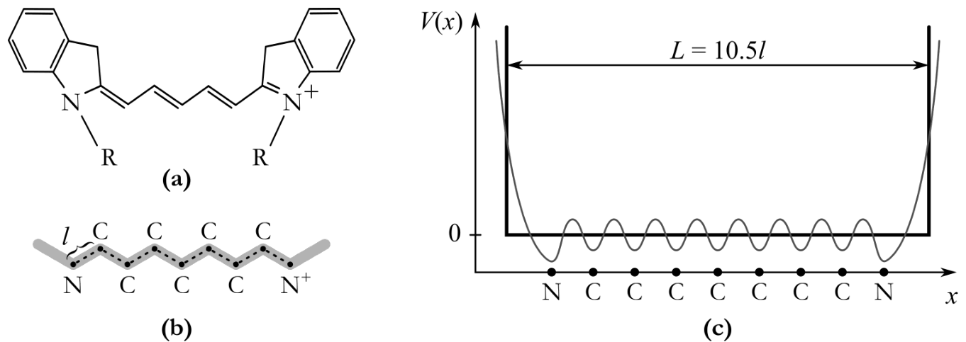
Figure 1. (a) Chemical structure of the cyanine Cy5 molecule (for simplicity, hydrogen atoms are not shown, and R denote some radicals). (b) The backbone of the Cy5 molecule, with mean inter-atomic distance \(l\). (c) Potential energy of the electron along the backbone (thin line) and its approximation by the step function given by Eq. 1 (thick line).
For simplicity, we will approximate this potential energy profile by a simple function given in Eq. 1 with the width \(L=10.5l\) (see thick line in Fig. 1c), here \(l=140\ \mathrm{pm}\) is the mean inter-atomic distance (see also Fig. 1b). As a result, we obtain the “electronic gas” composed of 10 electrons (7 from C atoms, 2 from the N atom, and 1 from the \(\mathrm{N}^{+}\) ion), moving in a one-dimensional potential well discussed in part A. In our evaluation, we can neglect the mutual interaction of these electrons; however, we should account for the fact that electrons are fermions and thus obey the Pauli exclusion principle. We also neglect the influence of other electrons as well as motion of the nuclei.
B.1 — 0.8pt
Evaluate the largest wavelength \(\lambda\) of the photon that can be absorbed by the Cy5 molecule assuming that the electron system is initially in its ground state. Express your answer in terms of \(l\), physical constants and some numerical prefactor, and calculate the numerical value.
B.2 — 0.4pt
Another dye molecule Cy3 has similar structure, but its backbone is shorter by 2 carbon atoms. Is its absorption spectrum shifted to the bluer or to the redder spectral region compared to the Cy5 molecule? Evaluate numerically the magnitude \(\Delta\lambda\) of this spectral shift. You can assume that removing two carbon atoms doesn’t change the molecule shape and only makes the backbone length shorter by two interatomic distances.
Being in the excited state, molecule can undergo a spontaneous transition to the ground state while emitting photon. The mean rate \(K\) of such events (i.e. the relative decrease of the molecules being in the excited state, \(\mathrm dN/N\), over time \(\mathrm dt\), \(K=\frac{1}{N}\frac{\mathrm dN}{\mathrm dt}\)) is determined by the wavelength \(\lambda\) of the emitted photon, the transition electrical dipole moment \(d\) (which is of the order of \(d\simeq el\), here \(e\) is elementary charge) as well as vacuum permittivity \(\varepsilon_0\) and Planck’s constant \(h\).
B.3 — 0.7pt
Using dimension analysis, determine the expression for the rate of spontaneous emission in terms of \(\varepsilon_0\), \(h\), \(\lambda\), and \(d\). The numerical prefactor for your expression is \(=\frac{16}{3}\pi^3\).
B.4 — 0.2pt
For Cy5 molecule, \(d\approx2.4\,el\). Evaluate the mean fluorescence lifetime of the lowest excited state of Cy5 molecule, \(\tau_{\mathrm{Cy5}}\), which is reciprocal to the rate of its emissive transition to the ground state.
Part C. Bose-Einstein condensation (1.5 points)
This part is not directly related to Parts A and B. Here, we will study the collective behaviour of bosonic particles. Bosons do not respect the Pauli exclusion principle, and—at low temperatures or high densities—experience a dramatic phenomenon known as the Bose–Einstein condensation (BEC). This is a phase transition to an intriguing collective quantum state: a large number of identical particles ‘condense’ into a single quantum state and start behaving as a single wave. The transition is typically reached by cooling a fixed number of particles below the critical temperature. In principle, it can also be induced by keeping the temperature fixed and driving the particle density past its critical value.
We begin by exploring the relation between the temperature and the particle density at the transition. As it turns out, estimates of their critical values can be deduced from a simple observation: Bose-Einstein condensation takes place when the de Broglie wavelength corresponding to the mean square speed of the particles is equal to the characteristic distance between the particles in a gas.
C.1 — 0.4pt
Given a non-interacting gas of \({}^{87}\mathrm{Rb}\) atoms in thermal equilibrium, write the expressions for their typical linear momentum \(p\) and the typical de Broglie wavelength \(\lambda_{\mathrm{dB}}\) as a function of atom’s mass \(m\), temperature \(T\) and physical constants.
C.2 — 0.5pt
Calculate the typical distance between the particles in a gas, \(\ell\), as a function of particle density \(n\). Hence deduce the critical temperature \(T_c\) as a function of atom’s mass, their density and physical constants.
To realize BEC in the lab, the experimentalists have to cool gases to temperatures as low as \(T_c=100\ \mathrm{nK}\).
C.3 — 0.6pt
What is the particle density of the Rb gas \(n_c\) if the transition takes place at such a temperature? For the sake of comparison, calculate also the ‘ordinary’ particle density \(n_0\) of an ideal gas at the standard temperature and pressure (STP), i.e. \(T_0=300\ \mathrm K\) and \(p_0=10^5\ \mathrm{Pa}\). How many times is the ‘ordinary’ gas denser? You may assume that the mass of the atoms is equal to 87 atomic mass units (\(m_{\mathrm{amu}}\)).
Part D. Three-beam optical lattices (5 points)
The first Bose-Einstein condensates were produced back in 1995, and since then the experimental work has branched out in diverse directions. In this part, you will investigate one particularly fruitful idea to load the condensate into spatially periodic potentials created by interfering a number of coherent laser beams. Due to the periodic nature of the resulting interference patterns, they are referred to as optical lattices. The potential energy \(V(\vec r)\) of an atom moving in an optical lattice is proportional to the local intensity of the light, and in your calculations you may assume that
\[ V(\vec r)=-\alpha\left\langle\left|\vec E(\vec r,t)\right|^2\right\rangle. \tag{2} \]
Here, \(\alpha\) is a positive constant, and the angle brackets indicate time-averaging which eliminates the rapidly oscillating terms. The electric field produced by the \(i\)-th laser is described by
\[ \vec E_i=E_{0,i}\,\vec\varepsilon_i\cos(\vec k_i\cdot\vec r-\omega t), \tag{3} \]
with the amplitude \(E_{0,i}\), the wave vector \(\vec k_i\), and the unit-length polarization vector \(\vec\varepsilon_i\).
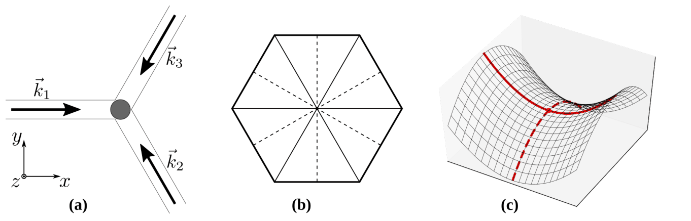
Figure 2. (a) Three-beam optical lattice: three plane waves with wave vectors \(\vec k_{1,2,3}\) intersect and interfere in the area indicated by the grey circle. (b) Symmetries of a regular hexagon: solid and dashed lines show two sets of symmetry axes. (c) Saddle point: a point on a surface where the slopes in orthogonal directions are all zero, but which is not a local extremum of the plotted function. Travelling along the trajectory marked by the full line one encounters an apparent minimum. Additional analysis of the perpendicular direction (dashed line) is needed to distinguish a true minimum from a saddle point (shown).
Your task is to study triangular optical lattices that are produced by interfering three coherent laser beams of equal intensity. A typical setup is shown in Fig. 2a. Here, all three beams are polarized in the \(z\) direction, propagate in the \(xy\) plane and intersect at equal angles of \(120^\circ\). Choose the direction of the \(x\) axis parallel to the wave vector \(\vec k_1\).
D.1 — 1.4pt
Using Eqs. 2 and 3 obtain the expression for the potential energy \(V(\vec r)\) as a function of \(\vec r=(x,y)\) in the plane of the beams.
Hint: the result can be neatly expressed as a constant term plus a sum of three cosine functions of arguments \(\vec b_i\cdot\vec r\). Please write your result in this form and identify the vectors \(\vec b_i\).
D.2 — 0.5pt
The resulting potential energy has a sixfold rotational symmetry axis, i.e., the potential distribution is invariant with respect to a rotation by a multiple of \(60^\circ\) around the origin. Provide a simple argument to prove that this is indeed the case.
The above observation of symmetry simplifies the analysis of the two-dimensional potential distribution \(V(\vec r)\). As shown in Fig. 2b, a regular hexagon has symmetry lines that, respectively, connect opposite vertices (solid lines) and midpoints of opposite edges (dashed lines). Therefore, in our situation one does not need to produce and study two-dimensional potential plots as many insights can be deduced by focusing on the coordinate axes \(x\) and \(y\) that run along the symmetry lines.
D.3 — 1.2pt
Derive the behavior of the potential \(V(\vec r)\) along the coordinate axes, i.e., determine the functions \(V_X(x)\equiv V(x,0)\) and \(V_Y(y)\equiv V(0,y)\). Identify the locations of the extrema of \(V_X(x)\) and \(V_Y(y)\) as functions of a single argument. As these functions are periodic, please include in your lists only one representative from each family of periodically repeated minima and maxima.
We are interested in determining the locations of so-called lattice sites, i.e., the minima of the full two-dimensional potential \(V(\vec r)\). The obtained minima of single-argument functions \(V_X\) and \(V_Y\) identify their suspected positions but still have to be checked to eliminate the saddle points. As shown in Fig. 2c, when studied along a single line, saddle points may disguise as minima but they are not.
D.4 — 0.8pt
Review your results in the previous question to determine actual minima of the optical lattice: Identify all equivalent minima nearest to (but not coinciding with) the origin. What is the distance \(a\) between the nearest minima, in other words—the lattice constant of our optical lattice? Express the answer in terms of the laser wavelength \(\lambda_{\mathrm{las}}\).
Charge neutrality of ultracold atoms suggests that their interactions become relevant only when two or more atoms occupy the same site of an optical lattice. However, experimentalists are also able to explore setups that sustain long-range atomic interactions. A possible approach relies on creation of the so-called Rydberg atoms that are physically large and feature other exaggerated properties. Rydberg atoms are excited atoms with one electron promoted to a state with a very high principal quantum number \(n\). The size of a Rydberg atom can be estimated by calculating the radius of the classical circular orbit of that electron with the orbital angular momentum \(n\hbar\), here \(\hbar\) is the reduced Planck constant.
D.5 — 1.1pt
Calculate the value of \(n\) that corresponds to the radius of the Rb Rydberg atom comparable to the wavelength of laser light \(\lambda_{\mathrm{las}}=380\ \mathrm{nm}\). Give your answer in terms of \(\lambda_{\mathrm{las}}\) and physical constants and find its numerical value.
Official English text of the problem.
Answers
Here \(m_e\) denotes the electron mass. For Part D, define the common field amplitude \(E_0\), \(U=\alpha E_0^2>0\), and \[ k=\frac{2\pi}{\lambda_{\mathrm{las}}},\qquad P_X=\frac{4\pi}{3k},\qquad P_Y=\frac{4\pi}{\sqrt3\,k}. \]
- A.1: \(\displaystyle E_{\min}=\frac{h^2}{8mL^2}\).
- A.2: \(\displaystyle E_n=\frac{n^2h^2}{8mL^2}\), \(n=1,2,3,\ldots\).
- A.3: \(\displaystyle \lambda_{21}=\frac{8mcL^2}{3h}\).
- B.1: \(\displaystyle \lambda_{\mathrm{Cy5}}=\frac{882}{11}\frac{m_ec\,l^2}{h}\simeq648\ \mathrm{nm}\).
- B.2: A blue shift: \(\lambda_{\mathrm{Cy3}}\simeq519\ \mathrm{nm}\), and \(\displaystyle \Delta\lambda=\frac{1580}{99}\frac{m_ec\,l^2}{h}\simeq129\ \mathrm{nm}\).
- B.3: \(\displaystyle K=\frac{16\pi^3d^2}{3\varepsilon_0h\lambda^3}\).
- B.4: \(\displaystyle \tau_{\mathrm{Cy5}}=\frac{3\varepsilon_0h\lambda_{\mathrm{Cy5}}^3}{16\pi^3(2.4\,el)^2}\simeq3.3\ \mathrm{ns}\).
- C.1: \(\displaystyle p=\sqrt{3mk_{\mathrm B}T}\), \(\displaystyle \lambda_{\mathrm{dB}}=\frac{h}{\sqrt{3mk_{\mathrm B}T}}\).
- C.2: \(\displaystyle \ell=n^{-1/3}\), \(\displaystyle T_c=\frac{h^2n^{2/3}}{3mk_{\mathrm B}}\), within the stated transition estimate.
- C.3: \(\displaystyle n_c\simeq1.59\times10^{18}\ \mathrm{m^{-3}}\), \(\displaystyle n_0\simeq2.41\times10^{25}\ \mathrm{m^{-3}}\); the ordinary gas is \(\displaystyle 1.52\times10^7\) times denser.
- D.1: \(\displaystyle V(\vec r)=-U\left[\frac32+\sum_{i=1}^3\cos(\vec b_i\cdot\vec r)\right]\), with \(\displaystyle \vec b_1=k\left(\frac32,-\frac{\sqrt3}{2}\right)\), \(\displaystyle \vec b_2=k(0,\sqrt3)\), and \(\displaystyle \vec b_3=k\left(-\frac32,-\frac{\sqrt3}{2}\right)\).
- D.2: The six vectors \(\{\pm\vec b_1,\pm\vec b_2,\pm\vec b_3\}\) form a regular hexagon. A \(60^\circ\) rotation permutes them, and cosine is even, so \(V\) is unchanged.
- D.3: \(\displaystyle V_X(x)=-U\left[\frac52+2\cos\left(\frac{3kx}{2}\right)\right]\), and \(\displaystyle V_Y(y)=-\frac U2\left[1+2\cos\left(\frac{\sqrt3\,ky}{2}\right)\right]^2\). Modulo \(P_X\), the \(x\)-section has a minimum at \(0\) and a maximum at \(P_X/2\). Modulo \(P_Y\), the \(y\)-section has minima at \(0,P_Y/2\) and maxima at \(P_Y/3,2P_Y/3\).
- D.4: \(\displaystyle a=\frac{2}{3}\lambda_{\mathrm{las}}\). The six nearest minima are \((\pm a,0)\) and \(\left(\pm a/2,\pm\sqrt3\,a/2\right)\), with independent signs in the latter pair.
- D.5: \(\displaystyle n=\sqrt{\frac{m_e e^2\lambda_{\mathrm{las}}}{4\pi\varepsilon_0\hbar^2}}\simeq84.7\), corresponding to \(n\approx85\).
Solution
The numerical evaluations use \[ \begin{aligned} h&=6.62607015\times10^{-34}\ \mathrm{J\,s}, &c&=2.99792458\times10^8\ \mathrm{m\,s^{-1}},\\ m_e&\simeq9.10938\times10^{-31}\ \mathrm{kg}, &e&=1.602176634\times10^{-19}\ \mathrm C,\\ \varepsilon_0&\simeq8.85419\times10^{-12}\ \mathrm{F\,m^{-1}}, &k_{\mathrm B}&=1.380649\times10^{-23}\ \mathrm{J\,K^{-1}},\\ m_{\mathrm{amu}}&\simeq1.66054\times10^{-27}\ \mathrm{kg}. \end{aligned} \]
A.1
The wave must have a node at each wall. The longest nonzero standing wave fitting into the well has one half-wavelength across its width: \[ L=\frac{\lambda_{\mathrm{dB},1}}2. \] The de Broglie relation therefore gives \[ p_1=\frac{h}{\lambda_{\mathrm{dB},1}}=\frac{h}{2L}. \] Using nonrelativistic kinetic energy, with zero potential energy inside the well, \[ \boxed{E_{\min}=\frac{p_1^2}{2m}=\frac{h^2}{8mL^2}}. \] A zero-wave-number state cannot satisfy both boundary conditions unless the wave is identically zero, so it is not an allowed particle state.
A.2
In the \(n\)-th standing-wave mode, \(n\) half-wavelengths fit between the walls: \[ L=n\frac{\lambda_{\mathrm{dB},n}}2,\qquad n=1,2,3,\ldots. \] Consequently, \[ \lambda_{\mathrm{dB},n}=\frac{2L}{n}, \qquad p_n=\frac{nh}{2L}, \] and \[ \boxed{E_n=\frac{n^2h^2}{8mL^2}}. \]
A.3
Energy conservation equates the emitted photon energy to the decrease in the particle’s energy: \[ \frac{hc}{\lambda_{21}} =E_2-E_1 =\frac{(4-1)h^2}{8mL^2}. \] Hence \[ \boxed{\lambda_{21}=\frac{8mcL^2}{3h}}. \]
B.1
Each spatial energy level can hold two electrons with opposite spins. Thus the ground state of the ten-electron system fills levels \(n=1,\ldots,5\), two electrons per level.
The smallest possible excitation promotes an electron from \(n=5\) to the first unoccupied level, \(n=6\). Its energy is \[ \Delta E_{\mathrm{Cy5}} =E_6-E_5 =\frac{(6^2-5^2)h^2}{8m_eL^2} =\frac{11h^2}{8m_eL^2}. \] The smallest absorbed photon energy corresponds to the largest wavelength: \[ \lambda_{\mathrm{Cy5}} =\frac{hc}{\Delta E_{\mathrm{Cy5}}} =\frac{8m_ecL^2}{11h}. \] With \(L=10.5l\), \[ \boxed{ \lambda_{\mathrm{Cy5}} =\frac{8(10.5)^2}{11}\frac{m_ec\,l^2}{h} =\frac{882}{11}\frac{m_ec\,l^2}{h} }. \] Substituting \(l=140\times10^{-12}\ \mathrm m\), \[ \boxed{\lambda_{\mathrm{Cy5}}\simeq6.48\times10^{-7}\ \mathrm m =648\ \mathrm{nm}}. \]
B.2
Removing two carbon atoms removes two shared electrons and shortens the well by \(2l\). Therefore Cy3 has eight electrons and \[ L_{\mathrm{Cy3}}=8.5l. \] Its ground state fills levels \(n=1,\ldots,4\). The lowest excitation is \(4\to5\), so \[ \Delta E_{\mathrm{Cy3}} =\frac{(5^2-4^2)h^2}{8m_e(8.5l)^2} =\frac{9h^2}{8m_e(8.5l)^2}. \] Thus \[ \lambda_{\mathrm{Cy3}} =\frac{8(8.5)^2}{9}\frac{m_ec\,l^2}{h} =\frac{578}{9}\frac{m_ec\,l^2}{h} \simeq519\ \mathrm{nm}. \] This is shorter than the Cy5 wavelength, so the shift is toward the blue. Its magnitude is \[ \begin{aligned} \Delta\lambda &=\lambda_{\mathrm{Cy5}}-\lambda_{\mathrm{Cy3}}\\ &=\left(\frac{882}{11}-\frac{578}{9}\right) \frac{m_ec\,l^2}{h}\\ &=\frac{1580}{99}\frac{m_ec\,l^2}{h}. \end{aligned} \] Therefore \[ \boxed{\Delta\lambda\simeq1.29\times10^{-7}\ \mathrm m=129\ \mathrm{nm}}. \]
B.3
The dipole moment has dimensions of charge times length: \[ [d]=\mathrm{C\,m}. \] Because \[ [\varepsilon_0]=\frac{\mathrm C^2}{\mathrm{J\,m}}, \] we have \[ \left[\frac{d^2}{\varepsilon_0}\right]=\mathrm{J\,m^3}. \] Dividing by \(h\), whose dimensions are \(\mathrm{J\,s}\), and by \(\lambda^3\) produces the required inverse-time dimension: \[ \left[\frac{d^2}{\varepsilon_0h\lambda^3}\right]=\mathrm{s^{-1}}. \] Using the supplied dimensionless prefactor, \[ \boxed{K=\frac{16\pi^3d^2}{3\varepsilon_0h\lambda^3}}. \]
Here \(K\) is the positive decay rate. For the number \(N(t)\) of molecules remaining excited, the decay equation is \(\mathrm dN/\mathrm dt=-KN\); the statement’s “relative decrease” is interpreted as the positive loss.
B.4
Under the given model, the lowest excited state emits a photon of wavelength \(\lambda_{\mathrm{Cy5}}\) when it returns to the ground state. Its dipole moment is \[ d=2.4\,el \simeq5.38\times10^{-29}\ \mathrm{C\,m}. \] The spontaneous-emission rate is \[ K=\frac{16\pi^3(2.4\,el)^2} {3\varepsilon_0h\lambda_{\mathrm{Cy5}}^3} \simeq3.01\times10^8\ \mathrm{s^{-1}}. \] For exponential decay, the mean lifetime is \(1/K\): \[ \boxed{ \tau_{\mathrm{Cy5}} =\frac{3\varepsilon_0h\lambda_{\mathrm{Cy5}}^3} {16\pi^3(2.4\,el)^2} \simeq3.3\ \mathrm{ns} }. \]
C.1
For the temperature estimate specified in the problem, equipartition gives the mean translational kinetic energy in three dimensions: \[ \frac12m\langle v^2\rangle=\frac32k_{\mathrm B}T. \] The typical momentum associated with the root-mean-square speed is therefore \[ \boxed{p=m\sqrt{\langle v^2\rangle}=\sqrt{3mk_{\mathrm B}T}}. \] Its de Broglie wavelength is \[ \boxed{\lambda_{\mathrm{dB}}=\frac hp =\frac{h}{\sqrt{3mk_{\mathrm B}T}}}. \]
C.2
At number density \(n\), the mean volume per particle is \(1/n\). The characteristic linear spacing is consequently \[ \boxed{\ell=n^{-1/3}}. \] Applying the problem’s transition criterion, \[ \lambda_{\mathrm{dB}}(T_c)=\ell, \] gives \[ \frac{h}{\sqrt{3mk_{\mathrm B}T_c}}=n^{-1/3}. \] Squaring and rearranging, \[ \boxed{T_c=\frac{h^2n^{2/3}}{3mk_{\mathrm B}}}. \] This is the critical-temperature estimate obtained from the stated wavelength–spacing criterion.
C.3
For rubidium, \[ m=87m_{\mathrm{amu}}\simeq1.44467\times10^{-25}\ \mathrm{kg}, \qquad T_c=100\ \mathrm{nK}=1.00\times10^{-7}\ \mathrm K. \] Inverting the result of C.2, \[ n_c=\left(\frac{3mk_{\mathrm B}T_c}{h^2}\right)^{3/2}. \] Numerically, \[ \boxed{n_c\simeq1.59\times10^{18}\ \mathrm{m^{-3}}}. \] The corresponding spacing is approximately \(8.57\times10^{-7}\ \mathrm m\).
For the ordinary ideal gas, the ideal-gas law gives \[ p_0=n_0k_{\mathrm B}T_0. \] Using the temperature and pressure specified in the question, \[ n_0=\frac{10^5}{k_{\mathrm B}(300)} \simeq2.41\times10^{25}\ \mathrm{m^{-3}}. \] Thus \[ \boxed{\frac{n_0}{n_c}\simeq1.52\times10^7}. \] The ordinary gas is about fifteen million times denser.
D.1
Let all three field amplitudes be \(E_0\). Choosing the wave vectors consistently with Fig. 2a, \[ \vec k_1=k(1,0),\qquad \vec k_2=k\left(-\frac12,\frac{\sqrt3}{2}\right),\qquad \vec k_3=k\left(-\frac12,-\frac{\sqrt3}{2}\right), \] where \(k=2\pi/\lambda_{\mathrm{las}}\).
All polarizations are along \(z\), so the fields add as scalars in that direction: \[ \vec E(\vec r,t) =E_0\hat z\sum_{i=1}^{3}\cos(\vec k_i\cdot\vec r-\omega t). \] The required time averages are \[ \left\langle\cos^2(\phi-\omega t)\right\rangle=\frac12, \] and \[ \left\langle \cos(\phi_i-\omega t)\cos(\phi_j-\omega t) \right\rangle =\frac12\cos(\phi_i-\phi_j). \] Therefore \[ \left\langle|\vec E|^2\right\rangle =E_0^2\left[ \frac32+\sum_{i<j}\cos\big((\vec k_i-\vec k_j)\cdot\vec r\big) \right]. \] Define \[ \begin{aligned} \vec b_1&=\vec k_1-\vec k_2 =k\left(\frac32,-\frac{\sqrt3}{2}\right),\\ \vec b_2&=\vec k_2-\vec k_3=k(0,\sqrt3),\\ \vec b_3&=\vec k_3-\vec k_1 =k\left(-\frac32,-\frac{\sqrt3}{2}\right). \end{aligned} \] Since cosine is even, the sign chosen for each difference is immaterial. With \(U=\alpha E_0^2\), \[ \boxed{ V(\vec r)=-U\left[\frac32+ \cos(\vec b_1\cdot\vec r)+ \cos(\vec b_2\cdot\vec r)+ \cos(\vec b_3\cdot\vec r)\right] }. \] Combining the first and third cosines gives the useful coordinate form \[ \boxed{ V(x,y)=-U\left[ \frac32+ 2\cos\left(\frac{3kx}{2}\right) \cos\left(\frac{\sqrt3\,ky}{2}\right) +\cos(\sqrt3\,ky) \right] }. \]
D.2
The three \(\vec b_i\) have equal magnitude \(\sqrt3\,k\) and are separated by \(120^\circ\). Including their negatives gives six vectors at successive angular intervals of \(60^\circ\).
Rotating the position vector by \(60^\circ\) is equivalent, in each dot product, to rotating the corresponding \(\vec b_i\) by \(-60^\circ\). This sends every \(\vec b_i\) to another member of the set \(\{\pm\vec b_j\}\). Since \[ \cos(-\vec b_j\cdot\vec r)=\cos(\vec b_j\cdot\vec r), \] the sum is unchanged. Thus the potential has the stated sixfold rotational symmetry.
D.3
Setting \(y=0\), \[ \boxed{ V_X(x)=-U\left[\frac52+2\cos\left(\frac{3kx}{2}\right)\right] }. \] Its fundamental period is \[ P_X=\frac{4\pi}{3k}=\frac{2\lambda_{\mathrm{las}}}{3}. \] The derivative is \[ V_X'(x)=3Uk\sin\left(\frac{3kx}{2}\right). \] Within \(0\leq x<P_X\), the minimum is at \(x=0\), and the maximum is at \(x=P_X/2\).
For the \(y\)-axis, introduce \[ q=\frac{\sqrt3\,ky}{2}. \] Then \[ V_Y(y)=-U\left(\frac32+2\cos q+\cos2q\right). \] Using \(\cos2q=2\cos^2q-1\), \[ \boxed{V_Y(y)=-\frac U2(1+2\cos q)^2}. \] Its fundamental period is \[ P_Y=\frac{4\pi}{\sqrt3\,k} =\frac{2\lambda_{\mathrm{las}}}{\sqrt3}. \] Differentiation gives \[ V_Y'(y)=\sqrt3\,Uk(1+2\cos q)\sin q. \] Hence the stationary points satisfy either \(\sin q=0\) or \(\cos q=-1/2\).
One representative of every family of extrema is:
| Section | Coordinate in one period | Character along that axis | Potential |
|---|---|---|---|
| \(V_X\) | \(x=0\) | Minimum | \(-9U/2\) |
| \(V_X\) | \(x=P_X/2\) | Maximum | \(-U/2\) |
| \(V_Y\) | \(y=0\) | Minimum | \(-9U/2\) |
| \(V_Y\) | \(y=P_Y/3\) | Maximum | \(0\) |
| \(V_Y\) | \(y=P_Y/2\) | Minimum | \(-U/2\) |
| \(V_Y\) | \(y=2P_Y/3\) | Maximum | \(0\) |
Thus \(V_X\) is a sinusoid about \(-5U/2\). Over one period, \(V_Y\) rises from a deep minimum to zero, falls to a shallower minimum, rises to zero again, and returns to the deep minimum at the next period boundary.
D.4
First check the apparently shallow minimum at \[ (x,y)=\left(0,\frac{P_Y}{2}\right). \] Here the second derivatives of the full potential are \[ V_{xx}=-\frac92Uk^2,\qquad V_{yy}=\frac32Uk^2,\qquad V_{xy}=0. \] The curvatures have opposite signs, so this point is a saddle, not a lattice site.
At the origin, \[ V_{xx}=V_{yy}=\frac92Uk^2,\qquad V_{xy}=0, \] so the origin is a true minimum.
To locate all true minima, write \[ t=\frac{3kx}{2},\qquad q=\frac{\sqrt3\,ky}{2}. \] The stationarity conditions are \[ \sin t\cos q=0,\qquad \sin q(\cos t+2\cos q)=0. \] If \(\cos q\neq0\), stationarity in \(x\) requires \(\sin t=0\). Positive curvature in \(x\) then requires \[ \cos t\cos q>0. \] Since \(\cos t\) and \(\cos q\) have the same sign, \(\cos t+2\cos q\) cannot vanish. Thus \(\sin q=0\). The minima therefore have \[ t=\pi r,\qquad q=\pi s, \] where integers \(r,s\) have the same parity. The remaining stationary possibility, \(\cos q=0\), also requires \(\cos t=0\); its Hessian has negative determinant, so it gives only saddles.
Writing \(r=2j+s\), the lattice sites are \[ \vec r_{j,s} =a\left(j+\frac{s}{2},\frac{\sqrt3\,s}{2}\right), \qquad j,s\in\mathbb Z, \] with \[ a=\frac{4\pi}{3k}. \] At these points all three interference cosines equal \(1\), and \[ V_{\min}=-\frac92U. \]
The squared distance from the origin is \[ |\vec r_{j,s}|^2=a^2(j^2+js+s^2). \] For nonzero integer pairs, the smallest value of the positive integer \(j^2+js+s^2\) is \(1\). It occurs at six sites: \[ \boxed{ (a,0),\ (-a,0),\ \left(\frac a2,\frac{\sqrt3a}{2}\right),\ \left(-\frac a2,\frac{\sqrt3a}{2}\right),\ \left(\frac a2,-\frac{\sqrt3a}{2}\right),\ \left(-\frac a2,-\frac{\sqrt3a}{2}\right) }. \] They form a regular hexagon around the origin. Therefore \[ \boxed{a=\frac{4\pi}{3k}=\frac23\lambda_{\mathrm{las}}}. \]
D.5
For a highly excited outer electron, the nucleus and inner electrons act approximately as a core of net charge \(+e\). We use the stated classical circular-orbit model, neglecting core-penetration effects and the motion of the much heavier core.
Coulomb attraction supplies the centripetal force: \[ \frac{m_ev^2}{r} =\frac{e^2}{4\pi\varepsilon_0r^2}. \] The prescribed angular momentum is \[ m_evr=n\hbar. \] Eliminating \(v\), \[ \frac{n^2\hbar^2}{m_er^3} =\frac{e^2}{4\pi\varepsilon_0r^2}, \] so \[ r=\frac{4\pi\varepsilon_0\hbar^2}{m_ee^2}n^2 =a_0n^2, \] where \[ a_0\simeq5.292\times10^{-11}\ \mathrm m. \] Taking the estimated radius to equal \(\lambda_{\mathrm{las}}\), \[ \boxed{ n=\sqrt{\frac{\lambda_{\mathrm{las}}}{a_0}} =\sqrt{\frac{m_ee^2\lambda_{\mathrm{las}}} {4\pi\varepsilon_0\hbar^2}} }. \] For \(\lambda_{\mathrm{las}}=380\ \mathrm{nm}\), \[ n=\sqrt{\frac{380\times10^{-9}}{5.292\times10^{-11}}} \simeq84.7. \] Thus the corresponding integer principal quantum number is \[ \boxed{n\approx85}. \]
The solution was checked against the official solution.
IPhO 2021 · Theorieaufgabe 3
Teilchen und Wellen
Der Welle-Teilchen-Dualismus, dem zufolge jedes Teilchen als Welle beschrieben werden kann und umgekehrt, ist eines der zentralen Konzepte der Quantenmechanik. In dieser Aufgabe werden wir auf Grundlage dieses Konzepts und nur weniger weiterer grundlegender Annahmen eine Auswahl von Quantenphänomenen untersuchen, die die beiden unterschiedlichen Teilchenarten der Mikrowelt betreffen: Fermionen und Bosonen.
Teil A. Quantenteilchen im Kasten (1.4 Punkte)
Betrachten Sie ein Teilchen der Masse \(m\), das sich in einem eindimensionalen Potentialtopf bewegt, in dem seine potentielle Energie \(V(x)\) gegeben ist durch
\[ V(x)= \begin{cases} 0, & 0\leq x\leq L;\\ \infty, & x<0\text{ oder }x>L. \end{cases} \tag{1} \]
Während sich ein klassisches Teilchen in einem solchen Potential mit beliebiger kinetischer Energie bewegen kann, sind für ein Quantenteilchen nur bestimmte positive, diskrete Energieniveaus erlaubt. In jedem dieser erlaubten Zustände lässt sich das Teilchen als stehende de-Broglie-Welle mit Knoten an den Wänden beschreiben.
A.1 — 0.4 Punkte
Bestimmen Sie die kleinstmögliche Energie \(E_{\min}\) des Quantenteilchens im Potentialtopf. Drücken Sie Ihre Antwort durch \(m\), \(L\) und die Planck-Konstante \(h\) aus.
Der Zustand des Teilchens mit der kleinstmöglichen Energie heißt Grundzustand, alle übrigen erlaubten Zustände heißen angeregte Zustände. Wir ordnen alle möglichen Energiewerte aufsteigend und bezeichnen sie mit \(E_n\), beginnend mit \(E_1\) für den Grundzustand.
A.2 — 0.6 Punkte
Bestimmen Sie den allgemeinen Ausdruck für die Energie \(E_n\) (hier ist \(n=1,\ 2,\ 3,\ldots\)).
A.3 — 0.4 Punkte
Das Teilchen kann nur unter Emission oder Absorption eines Photons mit der entsprechenden Energiedifferenz einen instantanen Übergang von einem Zustand in einen anderen vollziehen. Bestimmen Sie die Wellenlänge \(\lambda_{21}\) des Photons, das beim Übergang des Teilchens vom ersten angeregten Zustand (\(E_2\)) in den Grundzustand (\(E_1\)) emittiert wird.
Teil B. Optische Eigenschaften von Molekülen (2.1 Punkte)
In diesem Teil untersuchen wir verschiedene optische Eigenschaften des Cyaninmoleküls Cy5, eines häufig verwendeten Farbstoffmoleküls, das in Abb. 1a schematisch dargestellt ist. Seine optischen Eigenschaften werden hauptsächlich durch das Kohlenstoffgerüst bestimmt, das aus abwechselnden Einfach- und Doppelbindungen zwischen Kohlenstoffatomen besteht und in Abb. 1b gezeigt ist; der Einfluss der Ringe an den Molekülenden sowie der Reste R ist wesentlich geringer. Drei der vier Valenzelektronen jedes C-Atoms (und der N-Atome) im Gerüst bilden die chemischen Bindungen, während die verbleibenden Valenzelektronen „gemeinsam genutzt“ werden und sich entlang des gesamten Gerüsts bewegen können. Die gesamte potentielle Energie jedes dieser Elektronen ist in Abb. 1c durch eine oszillierende dünne Linie dargestellt, deren Minima den Positionen der C- und N-Atome entsprechen.
Abbildung 1. (a) Chemische Struktur des Cyaninmoleküls Cy5 (der Einfachheit halber sind Wasserstoffatome nicht dargestellt, und R bezeichnet bestimmte Reste). (b) Das Gerüst des Cy5-Moleküls mit dem mittleren Atomabstand \(l\). (c) Potentielle Energie des Elektrons entlang des Gerüsts (dünne Linie) und ihre Näherung durch die in Gl. 1 angegebene Stufenfunktion (dicke Linie).
Der Einfachheit halber nähern wir dieses Profil der potentiellen Energie durch die einfache Funktion aus Gl. 1 mit der Breite \(L=10.5l\) an (siehe dicke Linie in Abb. 1c); dabei ist \(l=140\ \mathrm{pm}\) der mittlere Atomabstand (siehe auch Abb. 1b). Dadurch erhalten wir ein „Elektronengas“ aus 10 Elektronen (7 von C-Atomen, 2 vom N-Atom und 1 vom \(\mathrm{N}^{+}\)-Ion), die sich in dem in Teil A behandelten eindimensionalen Potentialtopf bewegen. Bei unserer Abschätzung können wir die gegenseitige Wechselwirkung dieser Elektronen vernachlässigen; wir müssen jedoch berücksichtigen, dass Elektronen Fermionen sind und daher dem Pauli-Prinzip gehorchen. Wir vernachlässigen außerdem den Einfluss anderer Elektronen sowie die Bewegung der Atomkerne.
B.1 — 0.8 Punkte
Schätzen Sie die größte Wellenlänge \(\lambda\) eines Photons ab, das vom Cy5-Molekül absorbiert werden kann, wenn sich das Elektronensystem anfangs im Grundzustand befindet. Drücken Sie Ihre Antwort durch \(l\), physikalische Konstanten und einen numerischen Vorfaktor aus und berechnen Sie den Zahlenwert.
B.2 — 0.4 Punkte
Ein weiteres Farbstoffmolekül, Cy3, hat eine ähnliche Struktur, sein Gerüst ist jedoch um 2 Kohlenstoffatome kürzer. Ist sein Absorptionsspektrum gegenüber dem des Cy5-Moleküls zum blauen oder zum roten Spektralbereich hin verschoben? Berechnen Sie näherungsweise den Betrag \(\Delta\lambda\) dieser spektralen Verschiebung. Sie dürfen annehmen, dass das Entfernen zweier Kohlenstoffatome die Form des Moleküls nicht verändert und lediglich die Länge des Gerüsts um zwei Atomabstände verkürzt.
Im angeregten Zustand kann das Molekül unter Emission eines Photons spontan in den Grundzustand übergehen. Die mittlere Rate \(K\) solcher Ereignisse (d. h. die relative Abnahme der Zahl der Moleküle im angeregten Zustand, \(\mathrm dN/N\), während der Zeit \(\mathrm dt\), \(K=\frac{1}{N}\frac{\mathrm dN}{\mathrm dt}\)) wird durch die Wellenlänge \(\lambda\) des emittierten Photons, das elektrische Übergangsdipolmoment \(d\) (das von der Größenordnung \(d\simeq el\) ist, wobei \(e\) die Elementarladung ist) sowie die Vakuumpermittivität \(\varepsilon_0\) und die Planck-Konstante \(h\) bestimmt.
B.3 — 0.7 Punkte
Bestimmen Sie mithilfe einer Dimensionsanalyse den Ausdruck für die Rate der spontanen Emission in Abhängigkeit von \(\varepsilon_0\), \(h\), \(\lambda\) und \(d\). Der numerische Vorfaktor für Ihren Ausdruck ist \(=\frac{16}{3}\pi^3\).
B.4 — 0.2 Punkte
Für das Cy5-Molekül gilt \(d\approx2.4\,el\). Schätzen Sie die mittlere Fluoreszenzlebensdauer des niedrigsten angeregten Zustands des Cy5-Moleküls, \(\tau_{\mathrm{Cy5}}\), ab; sie ist der Kehrwert der Rate seines strahlenden Übergangs in den Grundzustand.
Teil C. Bose-Einstein-Kondensation (1.5 Punkte)
Dieser Teil steht nicht in direktem Zusammenhang mit den Teilen A und B. Hier untersuchen wir das kollektive Verhalten bosonischer Teilchen. Bosonen unterliegen nicht dem Pauli-Prinzip und zeigen bei niedrigen Temperaturen oder hohen Dichten ein ausgeprägtes Phänomen, das als Bose-Einstein-Kondensation (BEC) bekannt ist. Dabei handelt es sich um einen Phasenübergang in einen faszinierenden kollektiven Quantenzustand: Eine große Anzahl identischer Teilchen „kondensiert“ in einen einzigen Quantenzustand und beginnt, sich wie eine einzige Welle zu verhalten. Der Übergang wird üblicherweise erreicht, indem eine feste Anzahl von Teilchen unter die kritische Temperatur abgekühlt wird. Grundsätzlich lässt er sich auch herbeiführen, indem man die Temperatur konstant hält und die Teilchendichte über ihren kritischen Wert erhöht.
Wir beginnen mit der Untersuchung des Zusammenhangs zwischen Temperatur und Teilchendichte beim Übergang. Wie sich zeigt, lassen sich ihre kritischen Werte anhand einer einfachen Beobachtung abschätzen: Bose-Einstein-Kondensation tritt ein, wenn die de-Broglie-Wellenlänge, die dem mittleren Geschwindigkeitsquadrat der Teilchen entspricht, gleich dem charakteristischen Abstand zwischen den Teilchen im Gas ist.
C.1 — 0.4 Punkte
Gegeben sei ein wechselwirkungsfreies Gas aus \({}^{87}\mathrm{Rb}\)-Atomen im thermischen Gleichgewicht. Geben Sie die Ausdrücke für ihren typischen Impuls \(p\) und ihre typische de-Broglie-Wellenlänge \(\lambda_{\mathrm{dB}}\) als Funktion der Atommasse \(m\), der Temperatur \(T\) und physikalischer Konstanten an.
C.2 — 0.5 Punkte
Berechnen Sie den typischen Abstand zwischen den Teilchen im Gas, \(\ell\), als Funktion der Teilchendichte \(n\). Leiten Sie daraus die kritische Temperatur \(T_c\) als Funktion der Atommasse, der Teilchendichte und physikalischer Konstanten ab.
Um BEC im Labor zu realisieren, müssen die Experimentatoren Gase auf Temperaturen von nur \(T_c=100\ \mathrm{nK}\) abkühlen.
C.3 — 0.6 Punkte
Wie groß ist die Teilchendichte des Rb-Gases \(n_c\), wenn der Übergang bei einer solchen Temperatur stattfindet? Berechnen Sie zum Vergleich auch die „gewöhnliche“ Teilchendichte \(n_0\) eines idealen Gases bei Standardtemperatur und Standarddruck (STP), d. h. \(T_0=300\ \mathrm K\) und \(p_0=10^5\ \mathrm{Pa}\). Um welchen Faktor ist das „gewöhnliche“ Gas dichter? Sie dürfen annehmen, dass die Masse der Atome 87 atomaren Masseneinheiten (\(m_{\mathrm{amu}}\)) entspricht.
Teil D. Optische Gitter aus drei Strahlen (5 Punkte)
Die ersten Bose-Einstein-Kondensate wurden bereits 1995 erzeugt, und seitdem hat sich die experimentelle Forschung in vielfältige Richtungen entwickelt. In diesem Teil untersuchen Sie eine besonders fruchtbare Idee: das Kondensat in räumlich periodische Potentiale zu laden, die durch Interferenz mehrerer kohärenter Laserstrahlen erzeugt werden. Aufgrund der Periodizität der entstehenden Interferenzmuster bezeichnet man sie als optische Gitter. Die potentielle Energie \(V(\vec r)\) eines Atoms, das sich in einem optischen Gitter bewegt, ist proportional zur lokalen Lichtintensität. Für Ihre Rechnungen dürfen Sie annehmen, dass
\[ V(\vec r)=-\alpha\left\langle\left|\vec E(\vec r,t)\right|^2\right\rangle. \tag{2} \]
Dabei ist \(\alpha\) eine positive Konstante, und die spitzen Klammern bezeichnen die zeitliche Mittelung, durch die die schnell oszillierenden Terme verschwinden. Das vom \(i\)-ten Laser erzeugte elektrische Feld wird beschrieben durch
\[ \vec E_i=E_{0,i}\,\vec\varepsilon_i\cos(\vec k_i\cdot\vec r-\omega t), \tag{3} \]
mit der Amplitude \(E_{0,i}\), dem Wellenvektor \(\vec k_i\) und dem Polarisationsvektor \(\vec\varepsilon_i\) der Länge eins.
Abbildung 2. (a) Optisches Gitter aus drei Strahlen: Drei ebene Wellen mit den Wellenvektoren \(\vec k_{1,2,3}\) kreuzen sich und interferieren in dem durch den grauen Kreis gekennzeichneten Bereich. (b) Symmetrien eines regelmäßigen Sechsecks: Durchgezogene und gestrichelte Linien zeigen zwei Gruppen von Symmetrieachsen. (c) Sattelpunkt: ein Punkt auf einer Fläche, an dem die Steigungen in zueinander orthogonalen Richtungen alle null sind, der jedoch kein lokales Extremum der dargestellten Funktion ist. Entlang der durch die durchgezogene Linie markierten Bahn stößt man auf ein scheinbares Minimum. Um ein echtes Minimum von einem Sattelpunkt (hier dargestellt) zu unterscheiden, muss zusätzlich die senkrechte Richtung (gestrichelte Linie) untersucht werden.
Ihre Aufgabe besteht darin, dreieckige optische Gitter zu untersuchen, die durch Interferenz dreier kohärenter Laserstrahlen gleicher Intensität entstehen. Ein typischer Aufbau ist in Abb. 2a dargestellt. Hier sind alle drei Strahlen in \(z\)-Richtung polarisiert, breiten sich in der \(xy\)-Ebene aus und kreuzen sich unter gleichen Winkeln von \(120^\circ\). Wählen Sie die Richtung der \(x\)-Achse parallel zum Wellenvektor \(\vec k_1\).
D.1 — 1.4 Punkte
Leiten Sie mithilfe der Gln. 2 und 3 den Ausdruck für die potentielle Energie \(V(\vec r)\) als Funktion von \(\vec r=(x,y)\) in der Ebene der Strahlen her.
Hinweis: Das Ergebnis lässt sich übersichtlich als konstanter Term plus einer Summe aus drei Kosinusfunktionen mit den Argumenten \(\vec b_i\cdot\vec r\) ausdrücken. Schreiben Sie Ihr Ergebnis in dieser Form und geben Sie die Vektoren \(\vec b_i\) an.
D.2 — 0.5 Punkte
Die resultierende potentielle Energie besitzt eine sechszählige Drehachse, d. h., die Potentialverteilung ist unter einer Drehung um ein Vielfaches von \(60^\circ\) um den Ursprung invariant. Beweisen Sie mit einem einfachen Argument, dass dies tatsächlich der Fall ist.
Die obige Symmetriebetrachtung vereinfacht die Analyse der zweidimensionalen Potentialverteilung \(V(\vec r)\). Wie in Abb. 2b gezeigt, besitzt ein regelmäßiges Sechseck Symmetrielinien, die jeweils gegenüberliegende Eckpunkte (durchgezogene Linien) oder die Mittelpunkte gegenüberliegender Seiten (gestrichelte Linien) verbinden. Daher muss man in unserem Fall keine zweidimensionalen Potentialdarstellungen erstellen und untersuchen, da sich viele Erkenntnisse gewinnen lassen, indem man sich auf die Koordinatenachsen \(x\) und \(y\) konzentriert, die entlang der Symmetrielinien verlaufen.
D.3 — 1.2 Punkte
Leiten Sie den Verlauf des Potentials \(V(\vec r)\) entlang der Koordinatenachsen her, d. h., bestimmen Sie die Funktionen \(V_X(x)\equiv V(x,0)\) und \(V_Y(y)\equiv V(0,y)\). Bestimmen Sie die Lagen der Extrema von \(V_X(x)\) und \(V_Y(y)\), jeweils als Funktionen einer einzigen Variablen. Da diese Funktionen periodisch sind, geben Sie in Ihren Aufstellungen bitte nur einen Vertreter jeder Familie periodisch wiederkehrender Minima und Maxima an.
Wir möchten die Lagen der sogenannten Gitterplätze bestimmen, also der Minima des vollständigen zweidimensionalen Potentials \(V(\vec r)\). Die ermittelten Minima der Funktionen einer Variablen \(V_X\) und \(V_Y\) liefern mögliche Positionen, müssen jedoch noch überprüft werden, um Sattelpunkte auszuschließen. Wie in Abb. 2c gezeigt, können Sattelpunkte bei einer Untersuchung entlang einer einzigen Linie wie Minima erscheinen, obwohl sie keine sind.
D.4 — 0.8 Punkte
Überprüfen Sie Ihre Ergebnisse aus der vorherigen Teilaufgabe, um die tatsächlichen Minima des optischen Gitters zu bestimmen: Geben Sie alle äquivalenten Minima an, die dem Ursprung am nächsten liegen (aber nicht mit ihm zusammenfallen). Wie groß ist der Abstand \(a\) zwischen den nächstgelegenen Minima, also die Gitterkonstante unseres optischen Gitters? Drücken Sie die Antwort durch die Laserwellenlänge \(\lambda_{\mathrm{las}}\) aus.
Die Ladungsneutralität ultrakalter Atome legt nahe, dass ihre Wechselwirkungen erst dann relevant werden, wenn zwei oder mehr Atome denselben Platz eines optischen Gitters besetzen. Experimentatoren können jedoch auch Anordnungen untersuchen, in denen langreichweitige Wechselwirkungen zwischen Atomen auftreten. Ein möglicher Ansatz beruht auf der Erzeugung sogenannter Rydberg-Atome, die eine große räumliche Ausdehnung aufweisen und auch andere stark ausgeprägte Eigenschaften besitzen. Rydberg-Atome sind angeregte Atome, bei denen ein Elektron in einen Zustand mit einer sehr hohen Hauptquantenzahl \(n\) angehoben wurde. Die Größe eines Rydberg-Atoms lässt sich abschätzen, indem man den Radius der klassischen Kreisbahn dieses Elektrons mit dem Bahndrehimpuls \(n\hbar\) berechnet; dabei ist \(\hbar\) die reduzierte Planck-Konstante.
D.5 — 1.1 Punkte
Berechnen Sie den Wert von \(n\), bei dem der Radius des Rb-Rydberg-Atoms mit der Wellenlänge des Laserlichts \(\lambda_{\mathrm{las}}=380\ \mathrm{nm}\) vergleichbar ist. Geben Sie Ihre Antwort in Abhängigkeit von \(\lambda_{\mathrm{las}}\) und physikalischen Konstanten an und bestimmen Sie ihren Zahlenwert.
Aufgabentext aus dem offiziellen englischen Text übersetzt.
Antworten
Hier bezeichnet \(m_e\) die Elektronenmasse. Für Teil D definieren wir die gemeinsame Feldamplitude \(E_0\), \(U=\alpha E_0^2>0\) und \[ k=\frac{2\pi}{\lambda_{\mathrm{las}}},\qquad P_X=\frac{4\pi}{3k},\qquad P_Y=\frac{4\pi}{\sqrt3\,k}. \]
- A.1: \(\displaystyle E_{\min}=\frac{h^2}{8mL^2}\).
- A.2: \(\displaystyle E_n=\frac{n^2h^2}{8mL^2}\), \(n=1,2,3,\ldots\).
- A.3: \(\displaystyle \lambda_{21}=\frac{8mcL^2}{3h}\).
- B.1: \(\displaystyle \lambda_{\mathrm{Cy5}}=\frac{882}{11}\frac{m_ec\,l^2}{h}\simeq648\ \mathrm{nm}\).
- B.2: Eine Blauverschiebung: \(\lambda_{\mathrm{Cy3}}\simeq519\ \mathrm{nm}\), und \(\displaystyle \Delta\lambda=\frac{1580}{99}\frac{m_ec\,l^2}{h}\simeq129\ \mathrm{nm}\).
- B.3: \(\displaystyle K=\frac{16\pi^3d^2}{3\varepsilon_0h\lambda^3}\).
- B.4: \(\displaystyle \tau_{\mathrm{Cy5}}=\frac{3\varepsilon_0h\lambda_{\mathrm{Cy5}}^3}{16\pi^3(2.4\,el)^2}\simeq3.3\ \mathrm{ns}\).
- C.1: \(\displaystyle p=\sqrt{3mk_{\mathrm B}T}\), \(\displaystyle \lambda_{\mathrm{dB}}=\frac{h}{\sqrt{3mk_{\mathrm B}T}}\).
- C.2: \(\displaystyle \ell=n^{-1/3}\), \(\displaystyle T_c=\frac{h^2n^{2/3}}{3mk_{\mathrm B}}\), im Rahmen der angegebenen Abschätzung für den Übergang.
- C.3: \(\displaystyle n_c\simeq1.59\times10^{18}\ \mathrm{m^{-3}}\), \(\displaystyle n_0\simeq2.41\times10^{25}\ \mathrm{m^{-3}}\); das gewöhnliche Gas ist \(\displaystyle 1.52\times10^7\)-mal so dicht.
- D.1: \(\displaystyle V(\vec r)=-U\left[\frac32+\sum_{i=1}^3\cos(\vec b_i\cdot\vec r)\right]\), mit \(\displaystyle \vec b_1=k\left(\frac32,-\frac{\sqrt3}{2}\right)\), \(\displaystyle \vec b_2=k(0,\sqrt3)\) und \(\displaystyle \vec b_3=k\left(-\frac32,-\frac{\sqrt3}{2}\right)\).
- D.2: Die sechs Vektoren \(\{\pm\vec b_1,\pm\vec b_2,\pm\vec b_3\}\) bilden ein regelmäßiges Sechseck. Eine Drehung um \(60^\circ\) vertauscht sie untereinander, und der Kosinus ist eine gerade Funktion, sodass \(V\) unverändert bleibt.
- D.3: \(\displaystyle V_X(x)=-U\left[\frac52+2\cos\left(\frac{3kx}{2}\right)\right]\) und \(\displaystyle V_Y(y)=-\frac U2\left[1+2\cos\left(\frac{\sqrt3\,ky}{2}\right)\right]^2\). Modulo \(P_X\) hat der Schnitt entlang der \(x\)-Achse ein Minimum bei \(0\) und ein Maximum bei \(P_X/2\). Modulo \(P_Y\) hat der Schnitt entlang der \(y\)-Achse Minima bei \(0,P_Y/2\) und Maxima bei \(P_Y/3,2P_Y/3\).
- D.4: \(\displaystyle a=\frac{2}{3}\lambda_{\mathrm{las}}\). Die sechs nächstgelegenen Minima sind \((\pm a,0)\) und \(\left(\pm a/2,\pm\sqrt3\,a/2\right)\), wobei die Vorzeichen im letzteren Koordinatenpaar unabhängig voneinander sind.
- D.5: \(\displaystyle n=\sqrt{\frac{m_e e^2\lambda_{\mathrm{las}}}{4\pi\varepsilon_0\hbar^2}}\simeq84.7\), entsprechend \(n\approx85\).
Lösung
Für die numerischen Berechnungen werden folgende Werte verwendet: \[ \begin{aligned} h&=6.62607015\times10^{-34}\ \mathrm{J\,s}, &c&=2.99792458\times10^8\ \mathrm{m\,s^{-1}},\\ m_e&\simeq9.10938\times10^{-31}\ \mathrm{kg}, &e&=1.602176634\times10^{-19}\ \mathrm C,\\ \varepsilon_0&\simeq8.85419\times10^{-12}\ \mathrm{F\,m^{-1}}, &k_{\mathrm B}&=1.380649\times10^{-23}\ \mathrm{J\,K^{-1}},\\ m_{\mathrm{amu}}&\simeq1.66054\times10^{-27}\ \mathrm{kg}. \end{aligned} \]
A.1
Die Welle muss an jeder Wand einen Knoten haben. Die längste nichtverschwindende stehende Welle, die in den Potentialtopf passt, hat über dessen Breite eine halbe Wellenlänge: \[ L=\frac{\lambda_{\mathrm{dB},1}}2. \] Aus der de-Broglie-Beziehung folgt daher \[ p_1=\frac{h}{\lambda_{\mathrm{dB},1}}=\frac{h}{2L}. \] Mit der nichtrelativistischen kinetischen Energie und einer potentiellen Energie von null im Inneren des Potentialtopfs ergibt sich \[ \boxed{E_{\min}=\frac{p_1^2}{2m}=\frac{h^2}{8mL^2}}. \] Ein Zustand mit der Wellenzahl null kann beide Randbedingungen nur erfüllen, wenn die Welle identisch null ist; er ist daher kein erlaubter Teilchenzustand.
A.2
In der \(n\)-ten stehenden Wellenmode passen \(n\) halbe Wellenlängen zwischen die Wände: \[ L=n\frac{\lambda_{\mathrm{dB},n}}2,\qquad n=1,2,3,\ldots. \] Folglich gilt \[ \lambda_{\mathrm{dB},n}=\frac{2L}{n}, \qquad p_n=\frac{nh}{2L}, \] und \[ \boxed{E_n=\frac{n^2h^2}{8mL^2}}. \]
A.3
Nach dem Energieerhaltungssatz ist die Energie des emittierten Photons gleich der Abnahme der Teilchenenergie: \[ \frac{hc}{\lambda_{21}} =E_2-E_1 =\frac{(4-1)h^2}{8mL^2}. \] Daraus folgt \[ \boxed{\lambda_{21}=\frac{8mcL^2}{3h}}. \]
B.1
Jedes räumliche Energieniveau kann zwei Elektronen mit entgegengesetztem Spin aufnehmen. Im Grundzustand des Systems aus zehn Elektronen sind daher die Niveaus \(n=1,\ldots,5\) mit jeweils zwei Elektronen besetzt.
Bei der kleinstmöglichen Anregung wird ein Elektron von \(n=5\) auf das erste unbesetzte Niveau \(n=6\) angehoben. Die dafür erforderliche Energie ist \[ \Delta E_{\mathrm{Cy5}} =E_6-E_5 =\frac{(6^2-5^2)h^2}{8m_eL^2} =\frac{11h^2}{8m_eL^2}. \] Die kleinste Energie eines absorbierten Photons entspricht der größten Wellenlänge: \[ \lambda_{\mathrm{Cy5}} =\frac{hc}{\Delta E_{\mathrm{Cy5}}} =\frac{8m_ecL^2}{11h}. \] Mit \(L=10.5l\) gilt \[ \boxed{ \lambda_{\mathrm{Cy5}} =\frac{8(10.5)^2}{11}\frac{m_ec\,l^2}{h} =\frac{882}{11}\frac{m_ec\,l^2}{h} }. \] Einsetzen von \(l=140\times10^{-12}\ \mathrm m\) ergibt \[ \boxed{\lambda_{\mathrm{Cy5}}\simeq6.48\times10^{-7}\ \mathrm m =648\ \mathrm{nm}}. \]
B.2
Durch das Entfernen zweier Kohlenstoffatome werden zwei gemeinsam genutzte Elektronen entfernt und der Potentialtopf um \(2l\) verkürzt. Cy3 hat daher acht Elektronen, und es gilt \[ L_{\mathrm{Cy3}}=8.5l. \] Im Grundzustand sind die Niveaus \(n=1,\ldots,4\) besetzt. Die niedrigste Anregung ist \(4\to5\), also \[ \Delta E_{\mathrm{Cy3}} =\frac{(5^2-4^2)h^2}{8m_e(8.5l)^2} =\frac{9h^2}{8m_e(8.5l)^2}. \] Somit gilt \[ \lambda_{\mathrm{Cy3}} =\frac{8(8.5)^2}{9}\frac{m_ec\,l^2}{h} =\frac{578}{9}\frac{m_ec\,l^2}{h} \simeq519\ \mathrm{nm}. \] Diese Wellenlänge ist kürzer als die von Cy5, die Verschiebung erfolgt also zum Blauen hin. Ihr Betrag ist \[ \begin{aligned} \Delta\lambda &=\lambda_{\mathrm{Cy5}}-\lambda_{\mathrm{Cy3}}\\ &=\left(\frac{882}{11}-\frac{578}{9}\right) \frac{m_ec\,l^2}{h}\\ &=\frac{1580}{99}\frac{m_ec\,l^2}{h}. \end{aligned} \] Daher ergibt sich \[ \boxed{\Delta\lambda\simeq1.29\times10^{-7}\ \mathrm m=129\ \mathrm{nm}}. \]
B.3
Das Dipolmoment hat die Dimension Ladung mal Länge: \[ [d]=\mathrm{C\,m}. \] Da \[ [\varepsilon_0]=\frac{\mathrm C^2}{\mathrm{J\,m}}, \] gilt \[ \left[\frac{d^2}{\varepsilon_0}\right]=\mathrm{J\,m^3}. \] Division durch \(h\), dessen Dimension \(\mathrm{J\,s}\) ist, und durch \(\lambda^3\) liefert die erforderliche Dimension einer inversen Zeit: \[ \left[\frac{d^2}{\varepsilon_0h\lambda^3}\right]=\mathrm{s^{-1}}. \] Mit dem angegebenen dimensionslosen Vorfaktor ergibt sich \[ \boxed{K=\frac{16\pi^3d^2}{3\varepsilon_0h\lambda^3}}. \]
Hier ist \(K\) die positive Zerfallsrate. Für die Anzahl \(N(t)\) der noch angeregten Moleküle lautet die Zerfallsgleichung \(\mathrm dN/\mathrm dt=-KN\); die „relative Abnahme“ in der Aufgabenstellung wird als positiver Verlust interpretiert.
B.4
Im gegebenen Modell emittiert der niedrigste angeregte Zustand bei der Rückkehr in den Grundzustand ein Photon der Wellenlänge \(\lambda_{\mathrm{Cy5}}\). Sein Dipolmoment beträgt \[ d=2.4\,el \simeq5.38\times10^{-29}\ \mathrm{C\,m}. \] Die Rate der spontanen Emission ist \[ K=\frac{16\pi^3(2.4\,el)^2} {3\varepsilon_0h\lambda_{\mathrm{Cy5}}^3} \simeq3.01\times10^8\ \mathrm{s^{-1}}. \] Bei exponentiellem Zerfall beträgt die mittlere Lebensdauer \(1/K\): \[ \boxed{ \tau_{\mathrm{Cy5}} =\frac{3\varepsilon_0h\lambda_{\mathrm{Cy5}}^3} {16\pi^3(2.4\,el)^2} \simeq3.3\ \mathrm{ns} }. \]
C.1
Für die in der Aufgabe vorgegebene Temperaturabschätzung liefert der Gleichverteilungssatz die mittlere kinetische Translationsenergie in drei Dimensionen: \[ \frac12m\langle v^2\rangle=\frac32k_{\mathrm B}T. \] Der typische Impuls, der zur Wurzel aus dem mittleren Geschwindigkeitsquadrat gehört, ist daher \[ \boxed{p=m\sqrt{\langle v^2\rangle}=\sqrt{3mk_{\mathrm B}T}}. \] Die zugehörige de-Broglie-Wellenlänge ist \[ \boxed{\lambda_{\mathrm{dB}}=\frac hp =\frac{h}{\sqrt{3mk_{\mathrm B}T}}}. \]
C.2
Bei der Teilchendichte \(n\) beträgt das mittlere Volumen pro Teilchen \(1/n\). Der charakteristische lineare Abstand ist folglich \[ \boxed{\ell=n^{-1/3}}. \] Die Anwendung des in der Aufgabe angegebenen Übergangskriteriums \[ \lambda_{\mathrm{dB}}(T_c)=\ell, \] ergibt \[ \frac{h}{\sqrt{3mk_{\mathrm B}T_c}}=n^{-1/3}. \] Quadrieren und Umstellen liefert \[ \boxed{T_c=\frac{h^2n^{2/3}}{3mk_{\mathrm B}}}. \] Dies ist die Abschätzung der kritischen Temperatur, die sich aus dem angegebenen Kriterium der Gleichheit von Wellenlänge und Teilchenabstand ergibt.
C.3
Für Rubidium gilt \[ m=87m_{\mathrm{amu}}\simeq1.44467\times10^{-25}\ \mathrm{kg}, \qquad T_c=100\ \mathrm{nK}=1.00\times10^{-7}\ \mathrm K. \] Umstellen des Ergebnisses aus C.2 liefert \[ n_c=\left(\frac{3mk_{\mathrm B}T_c}{h^2}\right)^{3/2}. \] Numerisch ergibt sich \[ \boxed{n_c\simeq1.59\times10^{18}\ \mathrm{m^{-3}}}. \] Der entsprechende Abstand beträgt ungefähr \(8.57\times10^{-7}\ \mathrm m\).
Für das gewöhnliche ideale Gas liefert die ideale Gasgleichung \[ p_0=n_0k_{\mathrm B}T_0. \] Mit der in der Aufgabe angegebenen Temperatur und dem angegebenen Druck ergibt sich \[ n_0=\frac{10^5}{k_{\mathrm B}(300)} \simeq2.41\times10^{25}\ \mathrm{m^{-3}}. \] Somit gilt \[ \boxed{\frac{n_0}{n_c}\simeq1.52\times10^7}. \] Das gewöhnliche Gas ist etwa fünfzehn Millionen Mal so dicht.
D.1
Alle drei Feldamplituden seien \(E_0\). Wir wählen die Wellenvektoren entsprechend Abb. 2a: \[ \vec k_1=k(1,0),\qquad \vec k_2=k\left(-\frac12,\frac{\sqrt3}{2}\right),\qquad \vec k_3=k\left(-\frac12,-\frac{\sqrt3}{2}\right), \] wobei \(k=2\pi/\lambda_{\mathrm{las}}\).
Alle Polarisationen liegen entlang der \(z\)-Richtung, sodass sich die Felder in dieser Richtung skalar addieren: \[ \vec E(\vec r,t) =E_0\hat z\sum_{i=1}^{3}\cos(\vec k_i\cdot\vec r-\omega t). \] Die benötigten zeitlichen Mittelwerte sind \[ \left\langle\cos^2(\phi-\omega t)\right\rangle=\frac12, \] und \[ \left\langle \cos(\phi_i-\omega t)\cos(\phi_j-\omega t) \right\rangle =\frac12\cos(\phi_i-\phi_j). \] Daher gilt \[ \left\langle|\vec E|^2\right\rangle =E_0^2\left[ \frac32+\sum_{i<j}\cos\big((\vec k_i-\vec k_j)\cdot\vec r\big) \right]. \] Wir definieren \[ \begin{aligned} \vec b_1&=\vec k_1-\vec k_2 =k\left(\frac32,-\frac{\sqrt3}{2}\right),\\ \vec b_2&=\vec k_2-\vec k_3=k(0,\sqrt3),\\ \vec b_3&=\vec k_3-\vec k_1 =k\left(-\frac32,-\frac{\sqrt3}{2}\right). \end{aligned} \] Da der Kosinus eine gerade Funktion ist, spielt das für jede Differenz gewählte Vorzeichen keine Rolle. Mit \(U=\alpha E_0^2\) folgt \[ \boxed{ V(\vec r)=-U\left[\frac32+ \cos(\vec b_1\cdot\vec r)+ \cos(\vec b_2\cdot\vec r)+ \cos(\vec b_3\cdot\vec r)\right] }. \] Durch Zusammenfassen des ersten und dritten Kosinusterms erhält man die nützliche Koordinatendarstellung \[ \boxed{ V(x,y)=-U\left[ \frac32+ 2\cos\left(\frac{3kx}{2}\right) \cos\left(\frac{\sqrt3\,ky}{2}\right) +\cos(\sqrt3\,ky) \right] }. \]
D.2
Die drei \(\vec b_i\) haben denselben Betrag \(\sqrt3\,k\) und schließen jeweils Winkel von \(120^\circ\) ein. Zusammen mit ihren negativen Vektoren erhält man sechs Vektoren mit aufeinanderfolgenden Winkelabständen von \(60^\circ\).
Eine Drehung des Ortsvektors um \(60^\circ\) entspricht in jedem Skalarprodukt einer Drehung des jeweiligen \(\vec b_i\) um \(-60^\circ\). Dabei wird jeder \(\vec b_i\) auf ein anderes Element der Menge \(\{\pm\vec b_j\}\) abgebildet. Da \[ \cos(-\vec b_j\cdot\vec r)=\cos(\vec b_j\cdot\vec r), \] bleibt die Summe unverändert. Das Potential besitzt somit die angegebene sechszählige Drehsymmetrie.
D.3
Setzt man \(y=0\), so erhält man \[ \boxed{ V_X(x)=-U\left[\frac52+2\cos\left(\frac{3kx}{2}\right)\right] }. \] Die Grundperiode ist \[ P_X=\frac{4\pi}{3k}=\frac{2\lambda_{\mathrm{las}}}{3}. \] Die Ableitung lautet \[ V_X'(x)=3Uk\sin\left(\frac{3kx}{2}\right). \] Im Bereich \(0\leq x<P_X\) liegt das Minimum bei \(x=0\) und das Maximum bei \(x=P_X/2\).
Für die \(y\)-Achse führen wir \[ q=\frac{\sqrt3\,ky}{2}. \] ein. Dann gilt \[ V_Y(y)=-U\left(\frac32+2\cos q+\cos2q\right). \] Mit \(\cos2q=2\cos^2q-1\) folgt \[ \boxed{V_Y(y)=-\frac U2(1+2\cos q)^2}. \] Die Grundperiode ist \[ P_Y=\frac{4\pi}{\sqrt3\,k} =\frac{2\lambda_{\mathrm{las}}}{\sqrt3}. \] Differenzieren ergibt \[ V_Y'(y)=\sqrt3\,Uk(1+2\cos q)\sin q. \] Die stationären Punkte erfüllen daher entweder \(\sin q=0\) oder \(\cos q=-1/2\).
Jeweils ein Vertreter jeder Familie von Extrema ist:
| Schnitt | Koordinate innerhalb einer Periode | Art entlang dieser Achse | Potential |
|---|---|---|---|
| \(V_X\) | \(x=0\) | Minimum | \(-9U/2\) |
| \(V_X\) | \(x=P_X/2\) | Maximum | \(-U/2\) |
| \(V_Y\) | \(y=0\) | Minimum | \(-9U/2\) |
| \(V_Y\) | \(y=P_Y/3\) | Maximum | \(0\) |
| \(V_Y\) | \(y=P_Y/2\) | Minimum | \(-U/2\) |
| \(V_Y\) | \(y=2P_Y/3\) | Maximum | \(0\) |
Somit ist \(V_X\) eine Sinuskurve um \(-5U/2\). Innerhalb einer Periode steigt \(V_Y\) von einem tiefen Minimum auf null, fällt auf ein flacheres Minimum, steigt erneut auf null und kehrt an der nächsten Periodengrenze zum tiefen Minimum zurück.
D.4
Zunächst überprüfen wir das scheinbare flache Minimum bei \[ (x,y)=\left(0,\frac{P_Y}{2}\right). \] Hier lauten die zweiten Ableitungen des vollständigen Potentials \[ V_{xx}=-\frac92Uk^2,\qquad V_{yy}=\frac32Uk^2,\qquad V_{xy}=0. \] Die Krümmungen haben entgegengesetzte Vorzeichen; dieser Punkt ist also ein Sattelpunkt und kein Gitterplatz.
Im Ursprung gilt \[ V_{xx}=V_{yy}=\frac92Uk^2,\qquad V_{xy}=0, \] sodass der Ursprung ein echtes Minimum ist.
Um alle echten Minima zu finden, schreiben wir \[ t=\frac{3kx}{2},\qquad q=\frac{\sqrt3\,ky}{2}. \] Die Bedingungen für stationäre Punkte lauten \[ \sin t\cos q=0,\qquad \sin q(\cos t+2\cos q)=0. \] Falls \(\cos q\neq0\), erfordert die Stationarität in \(x\)-Richtung \(\sin t=0\). Eine positive Krümmung in \(x\)-Richtung verlangt dann \[ \cos t\cos q>0. \] Da \(\cos t\) und \(\cos q\) dasselbe Vorzeichen haben, kann \(\cos t+2\cos q\) nicht verschwinden. Somit gilt \(\sin q=0\). An den Minima gilt daher \[ t=\pi r,\qquad q=\pi s, \] wobei die ganzen Zahlen \(r,s\) dieselbe Parität haben. Die verbleibende Möglichkeit für stationäre Punkte, \(\cos q=0\), erfordert außerdem \(\cos t=0\); die zugehörige Hesse-Matrix hat eine negative Determinante, sodass sich dabei ausschließlich Sattelpunkte ergeben.
Mit \(r=2j+s\) lauten die Gitterplätze \[ \vec r_{j,s} =a\left(j+\frac{s}{2},\frac{\sqrt3\,s}{2}\right), \qquad j,s\in\mathbb Z, \] mit \[ a=\frac{4\pi}{3k}. \] An diesen Punkten sind alle drei Interferenzkosinusterme gleich \(1\), und es gilt \[ V_{\min}=-\frac92U. \]
Das Quadrat des Abstands vom Ursprung beträgt \[ |\vec r_{j,s}|^2=a^2(j^2+js+s^2). \] Für ganzzahlige Paare, die nicht beide null sind, ist der kleinste Wert der positiven ganzen Zahl \(j^2+js+s^2\) gleich \(1\). Er tritt an sechs Gitterplätzen auf: \[ \boxed{ (a,0),\ (-a,0),\ \left(\frac a2,\frac{\sqrt3a}{2}\right),\ \left(-\frac a2,\frac{\sqrt3a}{2}\right),\ \left(\frac a2,-\frac{\sqrt3a}{2}\right),\ \left(-\frac a2,-\frac{\sqrt3a}{2}\right) }. \] Sie bilden ein regelmäßiges Sechseck um den Ursprung. Daher gilt \[ \boxed{a=\frac{4\pi}{3k}=\frac23\lambda_{\mathrm{las}}}. \]
D.5
Für ein hoch angeregtes äußeres Elektron wirken der Atomkern und die inneren Elektronen näherungsweise wie ein Atomrumpf mit der Nettoladung \(+e\). Wir verwenden das vorgegebene klassische Kreisbahnmodell und vernachlässigen Effekte des Eindringens in den Atomrumpf sowie die Bewegung des wesentlich schwereren Atomrumpfs.
Die Coulomb-Anziehung liefert die Zentripetalkraft: \[ \frac{m_ev^2}{r} =\frac{e^2}{4\pi\varepsilon_0r^2}. \] Der vorgegebene Drehimpuls beträgt \[ m_evr=n\hbar. \] Eliminieren von \(v\) ergibt \[ \frac{n^2\hbar^2}{m_er^3} =\frac{e^2}{4\pi\varepsilon_0r^2}, \] also \[ r=\frac{4\pi\varepsilon_0\hbar^2}{m_ee^2}n^2 =a_0n^2, \] wobei \[ a_0\simeq5.292\times10^{-11}\ \mathrm m. \] Setzen wir den abgeschätzten Radius gleich \(\lambda_{\mathrm{las}}\), so erhalten wir \[ \boxed{ n=\sqrt{\frac{\lambda_{\mathrm{las}}}{a_0}} =\sqrt{\frac{m_ee^2\lambda_{\mathrm{las}}} {4\pi\varepsilon_0\hbar^2}} }. \] Für \(\lambda_{\mathrm{las}}=380\ \mathrm{nm}\) gilt \[ n=\sqrt{\frac{380\times10^{-9}}{5.292\times10^{-11}}} \simeq84.7. \] Die entsprechende ganzzahlige Hauptquantenzahl ist somit \[ \boxed{n\approx85}. \]
Die Lösung wurde mit der offiziellen Lösung abgeglichen.
IPhO 2021 · Teori sorusu 3
Parçacıklar ve Dalgalar
Her parçacığın bir dalga olarak ve her dalganın bir parçacık olarak betimlenebileceğini ifade eden dalga–parçacık ikiliği, kuantum mekaniğinin temel kavramlarından biridir. Bu soruda, mikro dünyanın iki farklı parçacık türünü —fermiyonları ve bozonları— kapsayan çeşitli kuantum olaylarını incelemek için bu kavrama ve yalnızca birkaç başka temel varsayıma dayanacağız.
Bölüm A. Kutudaki kuantum parçacığı (1.4 puan)
Potansiyel enerjisi \(V(x)\) aşağıdaki gibi verilen bir boyutlu potansiyel kuyusunda hareket eden, kütlesi \(m\) olan bir parçacık düşünün:
\[ V(x)= \begin{cases} 0, & 0\leq x\leq L;\\ \infty, & x<0\text{ veya }x>L. \end{cases} \tag{1} \]
Klasik bir parçacık böyle bir potansiyelde herhangi bir kinetik enerjiyle hareket edebilirken, kuantum parçacığı için yalnızca belirli pozitif, kesikli enerji düzeylerine izin verilir. İzin verilen bu durumların her birinde parçacık, duvarlarda düğümleri bulunan bir duran de Broglie dalgası olarak betimlenebilir.
A.1 — 0.4 puan
Kuyudaki kuantum parçacığının mümkün olan en düşük enerjisini \(E_{\min}\) belirleyin. Cevabınızı \(m\), \(L\) ve Planck sabiti \(h\) cinsinden ifade edin.
Parçacığın mümkün olan en düşük enerjiye sahip durumuna temel durum, izin verilen diğer tüm durumlarına ise uyarılmış durumlar denir. Mümkün olan tüm enerji değerlerini artan sırada sıralayalım ve temel durum için \(E_1\)'den başlayarak bunları \(E_n\) ile gösterelim.
A.2 — 0.6 puan
\(E_n\) enerjisinin genel ifadesini bulun (burada \(n=1,\ 2,\ 3,\ldots\)).
A.3 — 0.4 puan
Parçacık bir durumdan diğerine ancak ilgili enerji farkına eşit enerjili bir foton yayarak veya soğurarak anlık geçiş yapabilir. Parçacığın birinci uyarılmış durumdan (\(E_2\)) temel duruma (\(E_1\)) geçişi sırasında yayılan fotonun dalga boyunu \(\lambda_{21}\) bulun.
Bölüm B. Moleküllerin optik özellikleri (2.1 puan)
Bu bölümde, yaygın olarak kullanılan ve Şekil 1a'da şematik olarak gösterilen bir boya molekülü olan siyanin Cy5 molekülünün çeşitli optik özelliklerini inceleyeceğiz. Molekülün optik özelliklerini esas olarak, karbon atomları arasındaki tekli ve çiftli bağların dönüşümlü olarak sıralanmasıyla oluşan ve Şekil 1b'de gösterilen karbon omurgası belirler; molekülün uçlarındaki halkaların ve R radikallerinin etkisi ise çok daha küçüktür. Omurgadaki her C atomunun (ve N atomlarının) dört değerlik elektronundan üçü kimyasal bağları oluştururken, geriye kalan değerlik elektronları “ortaklaşa kullanılır” ve tüm omurga boyunca hareket edebilir. Bu elektronların her birinin net potansiyel enerjisi Şekil 1c'de salınımlı ince çizgiyle gösterilmiştir; minimumlar C ve N atomlarının konumlarına karşılık gelir.
Şekil 1. (a) Siyanin Cy5 molekülünün kimyasal yapısı (basitlik amacıyla hidrojen atomları gösterilmemiştir ve R bazı radikalleri belirtir). (b) Ortalama atomlar arası uzaklığı \(l\) olan Cy5 molekülünün omurgası. (c) Elektronun omurga boyunca potansiyel enerjisi (ince çizgi) ve Denklem 1'de verilen basamak fonksiyonuyla yapılan yaklaştırması (kalın çizgi).
Basitlik amacıyla bu potansiyel enerji profilini, Denklem 1'de verilen ve genişliği \(L=10.5l\) olan basit fonksiyonla yaklaşık olarak temsil edeceğiz (Şekil 1c'deki kalın çizgiye bakınız); burada \(l=140\ \mathrm{pm}\) ortalama atomlar arası uzaklıktır (ayrıca Şekil 1b'ye bakınız). Sonuç olarak, bölüm A'da ele alınan bir boyutlu potansiyel kuyusunda hareket eden 10 elektrondan (C atomlarından 7, N atomundan 2 ve \(\mathrm{N}^{+}\) iyonundan 1 elektron) oluşan bir “elektron gazı” elde ederiz. Hesaplamamızda bu elektronların birbirleriyle etkileşimini ihmal edebiliriz; ancak elektronların fermiyon olduğunu ve dolayısıyla Pauli dışarlama ilkesine uyduğunu hesaba katmalıyız. Diğer elektronların etkisini ve çekirdeklerin hareketini de ihmal ediyoruz.
B.1 — 0.8 puan
Elektron sisteminin başlangıçta temel durumda olduğunu varsayarak, Cy5 molekülünün soğurabileceği fotonun en büyük dalga boyunu \(\lambda\) hesaplayın. Cevabınızı \(l\), fiziksel sabitler ve bir sayısal çarpan cinsinden ifade edin ve sayısal değerini hesaplayın.
B.2 — 0.4 puan
Bir başka boya molekülü olan Cy3 benzer bir yapıya sahiptir, ancak omurgası 2 karbon atomu daha kısadır. Cy5 molekülüne kıyasla soğurma spektrumu, spektrumun daha mavi bölgesine mi yoksa daha kırmızı bölgesine mi kaymıştır? Bu spektral kaymanın büyüklüğünü \(\Delta\lambda\) sayısal olarak hesaplayın. İki karbon atomunun çıkarılmasının molekülün şeklini değiştirmediğini ve yalnızca omurganın uzunluğunu iki atomlar arası uzaklık kadar kısalttığını varsayabilirsiniz.
Uyarılmış durumdaki bir molekül, foton yayarak temel duruma kendiliğinden geçiş yapabilir. Bu olayların ortalama hızı \(K\) (yani uyarılmış durumdaki moleküllerin sayısının \(\mathrm dt\) süresindeki bağıl azalması, \(\mathrm dN/N\), \(K=\frac{1}{N}\frac{\mathrm dN}{\mathrm dt}\)), yayılan fotonun dalga boyu \(\lambda\), geçiş elektrik dipol momenti \(d\) (\(d\simeq el\) mertebesindedir; burada \(e\) temel yüktür), boşluğun elektriksel geçirgenliği \(\varepsilon_0\) ve Planck sabiti \(h\) tarafından belirlenir.
B.3 — 0.7 puan
Boyut analizini kullanarak kendiliğinden yayım hızının \(\varepsilon_0\), \(h\), \(\lambda\) ve \(d\) cinsinden ifadesini belirleyin. İfadenizin sayısal çarpanı \(=\frac{16}{3}\pi^3\)'tür.
B.4 — 0.2 puan
Cy5 molekülü için \(d\approx2.4\,el\)'dir. Cy5 molekülünün en düşük uyarılmış durumunun ortalama floresans ömrünü, \(\tau_{\mathrm{Cy5}}\), hesaplayın; bu süre, temel duruma ışınımlı geçiş hızının tersidir.
Bölüm C. Bose-Einstein yoğunlaşması (1.5 puan)
Bu bölüm, Bölüm A ve B ile doğrudan ilişkili değildir. Burada bozonik parçacıkların kolektif davranışını inceleyeceğiz. Bozonlar Pauli dışarlama ilkesine uymaz ve düşük sıcaklıklarda ya da yüksek yoğunluklarda Bose–Einstein yoğunlaşması (BEC) olarak bilinen çarpıcı bir olay yaşar. Bu, ilgi çekici bir kolektif kuantum durumuna faz geçişidir: çok sayıda özdeş parçacık tek bir kuantum durumunda ‘yoğunlaşır’ ve tek bir dalga gibi davranmaya başlar. Bu geçişe genellikle sabit sayıda parçacığın kritik sıcaklığın altına soğutulmasıyla ulaşılır. İlke olarak sıcaklık sabit tutularak ve parçacık yoğunluğu kritik değerinin üzerine çıkarılarak da geçiş sağlanabilir.
Geçişteki sıcaklık ile parçacık yoğunluğu arasındaki ilişkiyi inceleyerek başlayacağız. Görüleceği üzere, bunların kritik değerleri basit bir gözlemden hareketle kestirilebilir: Bose-Einstein yoğunlaşması, parçacıkların hız kareleri ortalamasına karşılık gelen de Broglie dalga boyu, gazdaki parçacıklar arasındaki karakteristik uzaklığa eşit olduğunda gerçekleşir.
C.1 — 0.4 puan
Isıl dengede bulunan, etkileşmeyen \({}^{87}\mathrm{Rb}\) atomlarından oluşan bir gaz için, atomların tipik doğrusal momentumunun \(p\) ve tipik de Broglie dalga boyunun \(\lambda_{\mathrm{dB}}\) ifadelerini atomun kütlesi \(m\), sıcaklık \(T\) ve fiziksel sabitlerin fonksiyonu olarak yazın.
C.2 — 0.5 puan
Gazdaki parçacıklar arasındaki tipik uzaklığı, \(\ell\), parçacık yoğunluğu \(n\)'nin fonksiyonu olarak hesaplayın. Buradan kritik sıcaklığı \(T_c\), atomların kütlesi, yoğunluğu ve fiziksel sabitlerin fonksiyonu olarak elde edin.
Laboratuvarda BEC elde etmek için deneycilerin gazları \(T_c=100\ \mathrm{nK}\) kadar düşük sıcaklıklara soğutmaları gerekir.
C.3 — 0.6 puan
Geçiş böyle bir sıcaklıkta gerçekleşiyorsa Rb gazının parçacık yoğunluğu \(n_c\) nedir? Karşılaştırma amacıyla, standart sıcaklık ve basınçta (STP), yani \(T_0=300\ \mathrm K\) ve \(p_0=10^5\ \mathrm{Pa}\) koşullarında bir ideal gazın ‘olağan’ parçacık yoğunluğunu \(n_0\) da hesaplayın. ‘Olağan’ gaz kaç kat daha yoğundur? Atomların kütlesinin 87 atomik kütle birimine (\(m_{\mathrm{amu}}\)) eşit olduğunu varsayabilirsiniz.
Bölüm D. Üç demetli optik örgüler (5 puan)
İlk Bose-Einstein yoğuşukları 1995 yılında üretildi ve o zamandan bu yana deneysel çalışmalar farklı yönlere yayıldı. Bu bölümde, yoğuşuğun birkaç eşevreli lazer demetinin girişimiyle oluşturulan, uzayda periyodik potansiyellere yüklenmesi şeklindeki özellikle verimli bir fikri inceleyeceksiniz. Ortaya çıkan girişim desenlerinin periyodik yapısı nedeniyle bunlara optik örgüler denir. Optik örgüde hareket eden bir atomun potansiyel enerjisi \(V(\vec r)\), ışığın yerel şiddetiyle orantılıdır ve hesaplamalarınızda aşağıdaki ifadeyi varsayabilirsiniz:
\[ V(\vec r)=-\alpha\left\langle\left|\vec E(\vec r,t)\right|^2\right\rangle. \tag{2} \]
Burada \(\alpha\) pozitif bir sabittir ve açılı parantezler, hızla salınan terimleri ortadan kaldıran zaman ortalamasını belirtir. \(i\). lazerin oluşturduğu elektrik alan şu şekilde betimlenir:
\[ \vec E_i=E_{0,i}\,\vec\varepsilon_i\cos(\vec k_i\cdot\vec r-\omega t), \tag{3} \]
burada \(E_{0,i}\) genlik, \(\vec k_i\) dalga vektörü ve \(\vec\varepsilon_i\) birim uzunluklu kutuplanma vektörüdür.
Şekil 2. (a) Üç demetli optik örgü: dalga vektörleri \(\vec k_{1,2,3}\) olan üç düzlem dalga, gri daireyle belirtilen bölgede kesişir ve girişim yapar. (b) Düzgün altıgenin simetrileri: düz ve kesikli çizgiler iki simetri ekseni kümesini gösterir. (c) Eyer noktası: bir yüzey üzerinde, birbirine dik yönlerdeki eğimlerin tümünün sıfır olduğu, ancak çizilen fonksiyonun yerel ekstremumu olmayan bir nokta. Düz çizgiyle işaretlenmiş yol boyunca ilerlerken görünürde bir minimumla karşılaşılır. Gerçek bir minimumu bir eyer noktasından (gösterilen) ayırt etmek için dik yönde (kesikli çizgi) ek bir inceleme gerekir.
Göreviniz, eşit şiddette üç eşevreli lazer demetinin girişimiyle oluşturulan üçgensel optik örgüleri incelemektir. Tipik bir düzenek Şekil 2a'da gösterilmiştir. Burada üç demetin tümü \(z\) yönünde kutuplanmıştır, \(xy\) düzleminde yayılır ve eşit \(120^\circ\) açılarla kesişir. \(x\) ekseninin yönünü \(\vec k_1\) dalga vektörüne paralel seçin.
D.1 — 1.4 puan
Denklem 2 ve 3'ü kullanarak demetlerin düzlemindeki potansiyel enerjinin \(V(\vec r)\), \(\vec r=(x,y)\)'nin fonksiyonu olarak ifadesini elde edin.
İpucu: Sonuç, sabit bir terim ile argümanları \(\vec b_i\cdot\vec r\) olan üç kosinüs fonksiyonunun toplamı olarak sade bir biçimde ifade edilebilir. Lütfen sonucunuzu bu biçimde yazın ve \(\vec b_i\) vektörlerini belirleyin.
D.2 — 0.5 puan
Ortaya çıkan potansiyel enerjinin altı katlı dönme simetrisi ekseni vardır; yani potansiyel dağılımı, orijin etrafında \(60^\circ\)'nin bir katı kadar döndürüldüğünde değişmez. Bunun gerçekten böyle olduğunu kanıtlayan basit bir gerekçe sunun.
Yukarıdaki simetri gözlemi, iki boyutlu potansiyel dağılımının \(V(\vec r)\) incelenmesini kolaylaştırır. Şekil 2b'de gösterildiği gibi düzgün bir altıgenin, sırasıyla karşılıklı köşeleri (düz çizgiler) ve karşılıklı kenarların orta noktalarını (kesikli çizgiler) birleştiren simetri doğruları vardır. Bu nedenle, bizim durumumuzda iki boyutlu potansiyel grafikleri çizip incelemek gerekmez; çünkü simetri doğruları boyunca uzanan \(x\) ve \(y\) koordinat eksenlerine odaklanarak birçok sonuca ulaşılabilir.
D.3 — 1.2 puan
Potansiyelin \(V(\vec r)\) koordinat eksenleri boyunca davranışını türetin; yani \(V_X(x)\equiv V(x,0)\) ve \(V_Y(y)\equiv V(0,y)\) fonksiyonlarını belirleyin. Tek değişkenli fonksiyonlar olarak \(V_X(x)\) ve \(V_Y(y)\)'nin ekstremumlarının konumlarını belirleyin. Bu fonksiyonlar periyodik olduğundan, lütfen listelerinize periyodik olarak tekrarlanan minimum ve maksimum ailelerinin her birinden yalnızca bir temsilci ekleyin.
Örgü noktaları olarak adlandırılan noktaların, yani tam iki boyutlu potansiyelin \(V(\vec r)\) minimumlarının konumlarını belirlemek istiyoruz. Tek değişkenli \(V_X\) ve \(V_Y\) fonksiyonları için elde edilen minimumlar, bunların olası konumlarını gösterir; ancak eyer noktalarını elemek için yine de kontrol edilmeleri gerekir. Şekil 2c'de gösterildiği gibi eyer noktaları, tek bir doğru boyunca incelendiğinde minimum gibi görünebilir, ancak minimum değildir.
D.4 — 0.8 puan
Optik örgünün gerçek minimumlarını belirlemek için önceki sorudaki sonuçlarınızı gözden geçirin: Orijine en yakın olan (ancak orijinle çakışmayan) tüm eşdeğer minimumları belirleyin. En yakın minimumlar arasındaki uzaklık \(a\), başka bir deyişle optik örgümüzün örgü sabiti nedir? Cevabınızı lazerin dalga boyu \(\lambda_{\mathrm{las}}\) cinsinden ifade edin.
Aşırı soğuk atomların elektriksel olarak nötr olması, etkileşimlerinin yalnızca iki veya daha fazla atomun optik örgünün aynı noktasını işgal etmesi durumunda önem kazandığını düşündürür. Bununla birlikte deneyciler, uzun menzilli atomik etkileşimlere olanak veren düzenekleri de inceleyebilir. Olası bir yaklaşım, fiziksel olarak büyük olan ve diğer bazı özellikleri de olağandışı ölçüde büyük olan Rydberg atomları denilen atomların oluşturulmasına dayanır. Rydberg atomları, bir elektronu çok yüksek bir baş kuantum sayısına \(n\) sahip bir duruma çıkarılmış uyarılmış atomlardır. Bir Rydberg atomunun boyutu, yörüngesel açısal momentumu \(n\hbar\) olan bu elektronun klasik dairesel yörüngesinin yarıçapı hesaplanarak kestirilebilir; burada \(\hbar\) indirgenmiş Planck sabitidir.
D.5 — 1.1 puan
Rb Rydberg atomunun yarıçapının lazer ışığının dalga boyuyla \(\lambda_{\mathrm{las}}=380\ \mathrm{nm}\) karşılaştırılabilir olmasına karşılık gelen \(n\) değerini hesaplayın. Cevabınızı \(\lambda_{\mathrm{las}}\) ve fiziksel sabitler cinsinden verin ve sayısal değerini bulun.
Soru metni resmi İngilizce metinden çevrilmiştir.
Cevaplar
Burada \(m_e\) elektron kütlesini belirtir. Bölüm D için ortak alan genliğini \(E_0\), \(U=\alpha E_0^2>0\) ve aşağıdaki büyüklükleri tanımlayalım: \[ k=\frac{2\pi}{\lambda_{\mathrm{las}}},\qquad P_X=\frac{4\pi}{3k},\qquad P_Y=\frac{4\pi}{\sqrt3\,k}. \]
- A.1: \(\displaystyle E_{\min}=\frac{h^2}{8mL^2}\).
- A.2: \(\displaystyle E_n=\frac{n^2h^2}{8mL^2}\), \(n=1,2,3,\ldots\).
- A.3: \(\displaystyle \lambda_{21}=\frac{8mcL^2}{3h}\).
- B.1: \(\displaystyle \lambda_{\mathrm{Cy5}}=\frac{882}{11}\frac{m_ec\,l^2}{h}\simeq648\ \mathrm{nm}\).
- B.2: Maviye kayma: \(\lambda_{\mathrm{Cy3}}\simeq519\ \mathrm{nm}\) ve \(\displaystyle \Delta\lambda=\frac{1580}{99}\frac{m_ec\,l^2}{h}\simeq129\ \mathrm{nm}\).
- B.3: \(\displaystyle K=\frac{16\pi^3d^2}{3\varepsilon_0h\lambda^3}\).
- B.4: \(\displaystyle \tau_{\mathrm{Cy5}}=\frac{3\varepsilon_0h\lambda_{\mathrm{Cy5}}^3}{16\pi^3(2.4\,el)^2}\simeq3.3\ \mathrm{ns}\).
- C.1: \(\displaystyle p=\sqrt{3mk_{\mathrm B}T}\), \(\displaystyle \lambda_{\mathrm{dB}}=\frac{h}{\sqrt{3mk_{\mathrm B}T}}\).
- C.2: Belirtilen geçiş kestirimi kapsamında \(\displaystyle \ell=n^{-1/3}\), \(\displaystyle T_c=\frac{h^2n^{2/3}}{3mk_{\mathrm B}}\).
- C.3: \(\displaystyle n_c\simeq1.59\times10^{18}\ \mathrm{m^{-3}}\), \(\displaystyle n_0\simeq2.41\times10^{25}\ \mathrm{m^{-3}}\); olağan gaz \(\displaystyle 1.52\times10^7\) kat daha yoğundur.
- D.1: \(\displaystyle V(\vec r)=-U\left[\frac32+\sum_{i=1}^3\cos(\vec b_i\cdot\vec r)\right]\); burada \(\displaystyle \vec b_1=k\left(\frac32,-\frac{\sqrt3}{2}\right)\), \(\displaystyle \vec b_2=k(0,\sqrt3)\) ve \(\displaystyle \vec b_3=k\left(-\frac32,-\frac{\sqrt3}{2}\right)\).
- D.2: Altı vektör \(\{\pm\vec b_1,\pm\vec b_2,\pm\vec b_3\}\) düzgün bir altıgen oluşturur. \(60^\circ\)'lik bir dönme bunların yerlerini değiştirir ve kosinüs çift fonksiyondur; dolayısıyla \(V\) değişmez.
- D.3: \(\displaystyle V_X(x)=-U\left[\frac52+2\cos\left(\frac{3kx}{2}\right)\right]\) ve \(\displaystyle V_Y(y)=-\frac U2\left[1+2\cos\left(\frac{\sqrt3\,ky}{2}\right)\right]^2\). \(P_X\) modülüne göre \(x\) kesitinin \(0\)'da bir minimumu ve \(P_X/2\)'de bir maksimumu vardır. \(P_Y\) modülüne göre \(y\) kesitinin \(0,P_Y/2\)'de minimumları ve \(P_Y/3,2P_Y/3\)'te maksimumları vardır.
- D.4: \(\displaystyle a=\frac{2}{3}\lambda_{\mathrm{las}}\). En yakın altı minimum \((\pm a,0)\) ve \(\left(\pm a/2,\pm\sqrt3\,a/2\right)\) noktalarıdır; son koordinat çiftindeki işaretler birbirinden bağımsızdır.
- D.5: \(\displaystyle n=\sqrt{\frac{m_e e^2\lambda_{\mathrm{las}}}{4\pi\varepsilon_0\hbar^2}}\simeq84.7\); bu, \(n\approx85\)'e karşılık gelir.
Çözüm
Sayısal hesaplamalarda şu değerler kullanılmıştır: \[ \begin{aligned} h&=6.62607015\times10^{-34}\ \mathrm{J\,s}, &c&=2.99792458\times10^8\ \mathrm{m\,s^{-1}},\\ m_e&\simeq9.10938\times10^{-31}\ \mathrm{kg}, &e&=1.602176634\times10^{-19}\ \mathrm C,\\ \varepsilon_0&\simeq8.85419\times10^{-12}\ \mathrm{F\,m^{-1}}, &k_{\mathrm B}&=1.380649\times10^{-23}\ \mathrm{J\,K^{-1}},\\ m_{\mathrm{amu}}&\simeq1.66054\times10^{-27}\ \mathrm{kg}. \end{aligned} \]
A.1
Dalganın her duvarda bir düğümü olmalıdır. Kuyuya sığan, özdeş olarak sıfır olmayan en uzun dalga boylu duran dalganın yarım dalga boyu, kuyunun genişliğine eşittir: \[ L=\frac{\lambda_{\mathrm{dB},1}}2. \] Dolayısıyla de Broglie bağıntısı şu sonucu verir: \[ p_1=\frac{h}{\lambda_{\mathrm{dB},1}}=\frac{h}{2L}. \] Kuyu içinde potansiyel enerji sıfır olduğundan, göreli olmayan kinetik enerji ifadesi kullanılarak \[ \boxed{E_{\min}=\frac{p_1^2}{2m}=\frac{h^2}{8mL^2}} \] elde edilir. Dalga sayısı sıfır olan bir durum, dalga özdeş olarak sıfır olmadıkça her iki sınır koşulunu da sağlayamaz; dolayısıyla izin verilen bir parçacık durumu değildir.
A.2
\(n\). duran dalga modunda duvarların arasına \(n\) yarım dalga boyu sığar: \[ L=n\frac{\lambda_{\mathrm{dB},n}}2,\qquad n=1,2,3,\ldots. \] Bunun sonucunda \[ \lambda_{\mathrm{dB},n}=\frac{2L}{n}, \qquad p_n=\frac{nh}{2L}, \] ve \[ \boxed{E_n=\frac{n^2h^2}{8mL^2}} \] elde edilir.
A.3
Enerjinin korunumu gereği yayılan fotonun enerjisi, parçacığın enerjisindeki azalmaya eşittir: \[ \frac{hc}{\lambda_{21}} =E_2-E_1 =\frac{(4-1)h^2}{8mL^2}. \] Buradan \[ \boxed{\lambda_{21}=\frac{8mcL^2}{3h}} \] bulunur.
B.1
Her uzaysal enerji düzeyinde zıt spinli iki elektron bulunabilir. Dolayısıyla on elektronlu sistemin temel durumunda \(n=1,\ldots,5\) düzeyleri, her düzeyde iki elektron olacak şekilde doludur.
Mümkün olan en küçük uyarılma, bir elektronu \(n=5\) düzeyinden ilk boş düzey olan \(n=6\)'ya çıkarır. Bu uyarılmanın enerjisi \[ \Delta E_{\mathrm{Cy5}} =E_6-E_5 =\frac{(6^2-5^2)h^2}{8m_eL^2} =\frac{11h^2}{8m_eL^2} \] şeklindedir. Soğurulan en küçük foton enerjisi en büyük dalga boyuna karşılık gelir: \[ \lambda_{\mathrm{Cy5}} =\frac{hc}{\Delta E_{\mathrm{Cy5}}} =\frac{8m_ecL^2}{11h}. \] \(L=10.5l\) kullanıldığında \[ \boxed{ \lambda_{\mathrm{Cy5}} =\frac{8(10.5)^2}{11}\frac{m_ec\,l^2}{h} =\frac{882}{11}\frac{m_ec\,l^2}{h} } \] elde edilir. \(l=140\times10^{-12}\ \mathrm m\) yerine konulduğunda \[ \boxed{\lambda_{\mathrm{Cy5}}\simeq6.48\times10^{-7}\ \mathrm m =648\ \mathrm{nm}} \] bulunur.
B.2
İki karbon atomunun çıkarılması, ortaklaşa kullanılan iki elektronu ortadan kaldırır ve kuyuyu \(2l\) kadar kısaltır. Dolayısıyla Cy3'ün sekiz elektronu vardır ve \[ L_{\mathrm{Cy3}}=8.5l. \] Temel durumda \(n=1,\ldots,4\) düzeyleri doludur. En düşük uyarılma \(4\to5\) geçişidir; dolayısıyla \[ \Delta E_{\mathrm{Cy3}} =\frac{(5^2-4^2)h^2}{8m_e(8.5l)^2} =\frac{9h^2}{8m_e(8.5l)^2}. \] Böylece \[ \lambda_{\mathrm{Cy3}} =\frac{8(8.5)^2}{9}\frac{m_ec\,l^2}{h} =\frac{578}{9}\frac{m_ec\,l^2}{h} \simeq519\ \mathrm{nm}. \] Bu, Cy5'in dalga boyundan daha kısadır; dolayısıyla kayma maviye doğrudur. Kaymanın büyüklüğü \[ \begin{aligned} \Delta\lambda &=\lambda_{\mathrm{Cy5}}-\lambda_{\mathrm{Cy3}}\\ &=\left(\frac{882}{11}-\frac{578}{9}\right) \frac{m_ec\,l^2}{h}\\ &=\frac{1580}{99}\frac{m_ec\,l^2}{h}. \end{aligned} \] şeklindedir. Dolayısıyla \[ \boxed{\Delta\lambda\simeq1.29\times10^{-7}\ \mathrm m=129\ \mathrm{nm}}. \]
B.3
Dipol momentinin boyutu yük ile uzunluğun çarpımıdır: \[ [d]=\mathrm{C\,m}. \] \[ [\varepsilon_0]=\frac{\mathrm C^2}{\mathrm{J\,m}}, \] olduğundan \[ \left[\frac{d^2}{\varepsilon_0}\right]=\mathrm{J\,m^3} \] elde edilir. Boyutu \(\mathrm{J\,s}\) olan \(h\)'ye ve \(\lambda^3\)'e bölmek, gereken ters zaman boyutunu verir: \[ \left[\frac{d^2}{\varepsilon_0h\lambda^3}\right]=\mathrm{s^{-1}}. \] Verilen boyutsuz çarpan kullanılarak \[ \boxed{K=\frac{16\pi^3d^2}{3\varepsilon_0h\lambda^3}} \] bulunur.
Burada \(K\) pozitif bozunma hızıdır. Uyarılmış durumda kalan moleküllerin sayısı \(N(t)\) için bozunma denklemi \(\mathrm dN/\mathrm dt=-KN\)'dir; soru metnindeki “bağıl azalma” pozitif kayıp olarak yorumlanır.
B.4
Verilen modele göre, en düşük uyarılmış durum temel duruma dönerken dalga boyu \(\lambda_{\mathrm{Cy5}}\) olan bir foton yayar. Dipol momenti \[ d=2.4\,el \simeq5.38\times10^{-29}\ \mathrm{C\,m} \] şeklindedir. Kendiliğinden yayım hızı \[ K=\frac{16\pi^3(2.4\,el)^2} {3\varepsilon_0h\lambda_{\mathrm{Cy5}}^3} \simeq3.01\times10^8\ \mathrm{s^{-1}} \] olur. Üstel bozunmada ortalama ömür \(1/K\)'dir: \[ \boxed{ \tau_{\mathrm{Cy5}} =\frac{3\varepsilon_0h\lambda_{\mathrm{Cy5}}^3} {16\pi^3(2.4\,el)^2} \simeq3.3\ \mathrm{ns} }. \]
C.1
Soruda belirtilen sıcaklık kestirimi için, eşbölüşüm ilkesi üç boyuttaki ortalama öteleme kinetik enerjisini verir: \[ \frac12m\langle v^2\rangle=\frac32k_{\mathrm B}T. \] Dolayısıyla hızın karesinin ortalamasının kareköküne karşılık gelen tipik momentum \[ \boxed{p=m\sqrt{\langle v^2\rangle}=\sqrt{3mk_{\mathrm B}T}} \] olur. Bunun de Broglie dalga boyu \[ \boxed{\lambda_{\mathrm{dB}}=\frac hp =\frac{h}{\sqrt{3mk_{\mathrm B}T}}} \] şeklindedir.
C.2
Sayı yoğunluğu \(n\) olduğunda parçacık başına ortalama hacim \(1/n\)'dir. Dolayısıyla karakteristik doğrusal uzaklık \[ \boxed{\ell=n^{-1/3}} \] olur. Sorudaki geçiş ölçütü olan \[ \lambda_{\mathrm{dB}}(T_c)=\ell, \] uygulandığında \[ \frac{h}{\sqrt{3mk_{\mathrm B}T_c}}=n^{-1/3} \] elde edilir. Karesi alınıp yeniden düzenlendiğinde \[ \boxed{T_c=\frac{h^2n^{2/3}}{3mk_{\mathrm B}}} \] bulunur. Bu, belirtilen dalga boyu–uzaklık ölçütünden elde edilen kritik sıcaklık kestirimidir.
C.3
Rubidyum için \[ m=87m_{\mathrm{amu}}\simeq1.44467\times10^{-25}\ \mathrm{kg}, \qquad T_c=100\ \mathrm{nK}=1.00\times10^{-7}\ \mathrm K. \] C.2'nin sonucu yoğunluk için çözüldüğünde \[ n_c=\left(\frac{3mk_{\mathrm B}T_c}{h^2}\right)^{3/2} \] bulunur. Sayısal olarak \[ \boxed{n_c\simeq1.59\times10^{18}\ \mathrm{m^{-3}}}. \] Buna karşılık gelen uzaklık yaklaşık \(8.57\times10^{-7}\ \mathrm m\)'dir.
Olağan ideal gaz için ideal gaz yasası \[ p_0=n_0k_{\mathrm B}T_0 \] sonucunu verir. Soruda belirtilen sıcaklık ve basınç kullanılarak \[ n_0=\frac{10^5}{k_{\mathrm B}(300)} \simeq2.41\times10^{25}\ \mathrm{m^{-3}} \] bulunur. Böylece \[ \boxed{\frac{n_0}{n_c}\simeq1.52\times10^7}. \] Olağan gaz yaklaşık on beş milyon kat daha yoğundur.
D.1
Üç alanın genliği de \(E_0\) olsun. Dalga vektörlerini Şekil 2a ile uyumlu seçersek \[ \vec k_1=k(1,0),\qquad \vec k_2=k\left(-\frac12,\frac{\sqrt3}{2}\right),\qquad \vec k_3=k\left(-\frac12,-\frac{\sqrt3}{2}\right), \] burada \(k=2\pi/\lambda_{\mathrm{las}}\)'tır.
Tüm kutuplanmalar \(z\) doğrultusunda olduğundan alanlar bu doğrultuda skaler olarak toplanır: \[ \vec E(\vec r,t) =E_0\hat z\sum_{i=1}^{3}\cos(\vec k_i\cdot\vec r-\omega t). \] Gerekli zaman ortalamaları \[ \left\langle\cos^2(\phi-\omega t)\right\rangle=\frac12, \] ve \[ \left\langle \cos(\phi_i-\omega t)\cos(\phi_j-\omega t) \right\rangle =\frac12\cos(\phi_i-\phi_j) \] şeklindedir. Dolayısıyla \[ \left\langle|\vec E|^2\right\rangle =E_0^2\left[ \frac32+\sum_{i<j}\cos\big((\vec k_i-\vec k_j)\cdot\vec r\big) \right]. \] Şu tanımları yapalım: \[ \begin{aligned} \vec b_1&=\vec k_1-\vec k_2 =k\left(\frac32,-\frac{\sqrt3}{2}\right),\\ \vec b_2&=\vec k_2-\vec k_3=k(0,\sqrt3),\\ \vec b_3&=\vec k_3-\vec k_1 =k\left(-\frac32,-\frac{\sqrt3}{2}\right). \end{aligned} \] Kosinüs çift fonksiyon olduğundan her fark için seçilen işaret önemsizdir. \(U=\alpha E_0^2\) ile \[ \boxed{ V(\vec r)=-U\left[\frac32+ \cos(\vec b_1\cdot\vec r)+ \cos(\vec b_2\cdot\vec r)+ \cos(\vec b_3\cdot\vec r)\right] } \] elde edilir. Birinci ve üçüncü kosinüsün birleştirilmesi, koordinatlar cinsinden şu kullanışlı biçimi verir: \[ \boxed{ V(x,y)=-U\left[ \frac32+ 2\cos\left(\frac{3kx}{2}\right) \cos\left(\frac{\sqrt3\,ky}{2}\right) +\cos(\sqrt3\,ky) \right] }. \]
D.2
Üç \(\vec b_i\) vektörünün büyüklüğü \(\sqrt3\,k\)'ya eşittir ve aralarındaki açılar \(120^\circ\)'dir. Negatifleri de dahil edildiğinde, ardışık açısal aralıkları \(60^\circ\) olan altı vektör elde edilir.
Konum vektörünü \(60^\circ\) döndürmek, her skaler çarpımda ilgili \(\vec b_i\)'yi \(-60^\circ\) döndürmeye eşdeğerdir. Bu işlem her \(\vec b_i\)'yi \(\{\pm\vec b_j\}\) kümesinin başka bir elemanına götürür. \[ \cos(-\vec b_j\cdot\vec r)=\cos(\vec b_j\cdot\vec r), \] olduğundan toplam değişmez. Dolayısıyla potansiyel, belirtilen altı katlı dönme simetrisine sahiptir.
D.3
\(y=0\) alınırsa \[ \boxed{ V_X(x)=-U\left[\frac52+2\cos\left(\frac{3kx}{2}\right)\right] }. \] Temel periyodu \[ P_X=\frac{4\pi}{3k}=\frac{2\lambda_{\mathrm{las}}}{3} \] şeklindedir. Türevi \[ V_X'(x)=3Uk\sin\left(\frac{3kx}{2}\right) \] olur. \(0\leq x<P_X\) aralığında minimum \(x=0\)'da, maksimum ise \(x=P_X/2\)'dedir.
\(y\) ekseni için \[ q=\frac{\sqrt3\,ky}{2} \] tanımını yapalım. O hâlde \[ V_Y(y)=-U\left(\frac32+2\cos q+\cos2q\right). \] \(\cos2q=2\cos^2q-1\) kullanıldığında \[ \boxed{V_Y(y)=-\frac U2(1+2\cos q)^2} \] elde edilir. Temel periyodu \[ P_Y=\frac{4\pi}{\sqrt3\,k} =\frac{2\lambda_{\mathrm{las}}}{\sqrt3} \] şeklindedir. Türev alındığında \[ V_Y'(y)=\sqrt3\,Uk(1+2\cos q)\sin q \] bulunur. Dolayısıyla durağan noktalar ya \(\sin q=0\) ya da \(\cos q=-1/2\) koşulunu sağlar.
Her ekstremum ailesinin bir temsilcisi şöyledir:
| Kesit | Bir periyot içindeki koordinat | O eksen boyunca niteliği | Potansiyel |
|---|---|---|---|
| \(V_X\) | \(x=0\) | Minimum | \(-9U/2\) |
| \(V_X\) | \(x=P_X/2\) | Maksimum | \(-U/2\) |
| \(V_Y\) | \(y=0\) | Minimum | \(-9U/2\) |
| \(V_Y\) | \(y=P_Y/3\) | Maksimum | \(0\) |
| \(V_Y\) | \(y=P_Y/2\) | Minimum | \(-U/2\) |
| \(V_Y\) | \(y=2P_Y/3\) | Maksimum | \(0\) |
Böylece \(V_X\), \(-5U/2\) etrafında bir sinüzoiddir. Bir periyot boyunca \(V_Y\), derin bir minimumdan sıfıra yükselir, daha sığ bir minimuma düşer, yeniden sıfıra yükselir ve bir sonraki periyot sınırında derin minimuma geri döner.
D.4
Önce \[ (x,y)=\left(0,\frac{P_Y}{2}\right) \] noktasındaki görünürde sığ minimumu kontrol edelim. Burada tam potansiyelin ikinci türevleri \[ V_{xx}=-\frac92Uk^2,\qquad V_{yy}=\frac32Uk^2,\qquad V_{xy}=0 \] şeklindedir. Eğrilikler zıt işaretli olduğundan bu nokta bir örgü noktası değil, bir eyer noktasıdır.
Orijinde \[ V_{xx}=V_{yy}=\frac92Uk^2,\qquad V_{xy}=0, \] olduğundan orijin gerçek bir minimumdur.
Tüm gerçek minimumların yerlerini bulmak için \[ t=\frac{3kx}{2},\qquad q=\frac{\sqrt3\,ky}{2} \] yazalım. Durağanlık koşulları \[ \sin t\cos q=0,\qquad \sin q(\cos t+2\cos q)=0 \] şeklindedir. \(\cos q\neq0\) ise \(x\) yönündeki durağanlık \(\sin t=0\) gerektirir. Bu durumda \(x\) yönünde pozitif eğrilik olması için \[ \cos t\cos q>0. \] olmalıdır. \(\cos t\) ve \(\cos q\) aynı işaretli olduğundan \(\cos t+2\cos q\) sıfır olamaz. Dolayısıyla \(\sin q=0\)'dır. Bu nedenle minimumlarda \[ t=\pi r,\qquad q=\pi s, \] olur; burada \(r,s\) tamsayıları aynı tek-çift özelliğine sahiptir. Geriye kalan durağanlık olasılığı olan \(\cos q=0\), ayrıca \(\cos t=0\) gerektirir; bu durumda Hess matrisinin determinantı negatiftir, dolayısıyla yalnızca eyer noktaları elde edilir.
\(r=2j+s\) yazılırsa örgü noktaları \[ \vec r_{j,s} =a\left(j+\frac{s}{2},\frac{\sqrt3\,s}{2}\right), \qquad j,s\in\mathbb Z, \] şeklindedir; burada \[ a=\frac{4\pi}{3k}. \] Bu noktalarda üç girişim kosinüsünün tümü \(1\)'e eşittir ve \[ V_{\min}=-\frac92U. \]
Orijinden uzaklığın karesi \[ |\vec r_{j,s}|^2=a^2(j^2+js+s^2) \] şeklindedir. Sıfırdan farklı tamsayı çiftleri için pozitif tamsayı \(j^2+js+s^2\)'nin en küçük değeri \(1\)'dir. Bu değer altı noktada elde edilir: \[ \boxed{ (a,0),\ (-a,0),\ \left(\frac a2,\frac{\sqrt3a}{2}\right),\ \left(-\frac a2,\frac{\sqrt3a}{2}\right),\ \left(\frac a2,-\frac{\sqrt3a}{2}\right),\ \left(-\frac a2,-\frac{\sqrt3a}{2}\right) }. \] Bu noktalar orijin etrafında düzgün bir altıgen oluşturur. Dolayısıyla \[ \boxed{a=\frac{4\pi}{3k}=\frac23\lambda_{\mathrm{las}}}. \]
D.5
Yüksek derecede uyarılmış bir dış elektron için çekirdek ve iç elektronlar, net yükü \(+e\) olan bir merkez gibi davranır. Belirtilen klasik dairesel yörünge modelini kullanıyor, elektronun bu merkez bölgesine nüfuz etmesinden kaynaklanan etkileri ve çok daha ağır olan merkezin hareketini ihmal ediyoruz.
Coulomb çekimi merkezcil kuvveti sağlar: \[ \frac{m_ev^2}{r} =\frac{e^2}{4\pi\varepsilon_0r^2}. \] Verilen açısal momentum \[ m_evr=n\hbar \] şeklindedir. \(v\) yok edildiğinde \[ \frac{n^2\hbar^2}{m_er^3} =\frac{e^2}{4\pi\varepsilon_0r^2}, \] böylece \[ r=\frac{4\pi\varepsilon_0\hbar^2}{m_ee^2}n^2 =a_0n^2, \] elde edilir; burada \[ a_0\simeq5.292\times10^{-11}\ \mathrm m. \] Kestirilen yarıçapı \(\lambda_{\mathrm{las}}\)'a eşit alırsak \[ \boxed{ n=\sqrt{\frac{\lambda_{\mathrm{las}}}{a_0}} =\sqrt{\frac{m_ee^2\lambda_{\mathrm{las}}} {4\pi\varepsilon_0\hbar^2}} }. \] \(\lambda_{\mathrm{las}}=380\ \mathrm{nm}\) için \[ n=\sqrt{\frac{380\times10^{-9}}{5.292\times10^{-11}}} \simeq84.7. \] Dolayısıyla karşılık gelen tamsayı baş kuantum sayısı \[ \boxed{n\approx85} \] olur.
Çözüm, resmi çözümle karşılaştırılarak kontrol edildi.
IPhO 2021 · Problema teórico 3
Partículas y ondas
La dualidad onda-partícula, que establece que cada partícula puede describirse como una onda y viceversa, es uno de los conceptos centrales de la mecánica cuántica. En este problema, nos basaremos en esta noción y en unas pocas hipótesis básicas más para explorar una selección de fenómenos cuánticos que abarcan los dos tipos distintos de partículas del micromundo: fermiones y bosones.
Parte A. Partícula cuántica en una caja (1.4 puntos)
Consideremos una partícula de masa \(m\) que se mueve en un pozo de potencial unidimensional, donde su energía potencial \(V(x)\) viene dada por
\[ V(x)= \begin{cases} 0, & 0\leq x\leq L;\\ \infty, & x<0\text{ o }x>L. \end{cases} \tag{1} \]
Mientras que una partícula clásica puede moverse en un potencial de este tipo con cualquier energía cinética, para una partícula cuántica solo se permiten ciertos niveles de energía discretos y positivos. En cualquiera de estos estados permitidos, la partícula puede describirse como una onda estacionaria de de Broglie con nodos en las paredes.
A.1 — 0.4pt
Determine la energía mínima posible \(E_{\min}\) de la partícula cuántica en el pozo. Exprese su respuesta en función de \(m\), \(L\) y la constante de Planck \(h\).
El estado de la partícula con la energía mínima posible se denomina estado fundamental, y todos los demás estados permitidos se denominan estados excitados. Ordenemos todos los valores posibles de la energía en orden creciente y denotémoslos por \(E_n\), comenzando por \(E_1\) para el estado fundamental.
A.2 — 0.6pt
Obtenga la expresión general de la energía \(E_n\) (aquí \(n=1,\ 2,\ 3,\ldots\)).
A.3 — 0.4pt
La partícula solo puede experimentar una transición instantánea de un estado a otro mediante la emisión o absorción de un fotón cuya energía sea igual a la diferencia de energía correspondiente. Obtenga la longitud de onda \(\lambda_{21}\) del fotón emitido durante la transición de la partícula desde el primer estado excitado (\(E_2\)) al estado fundamental (\(E_1\)).
Parte B. Propiedades ópticas de las moléculas (2.1 puntos)
En esta parte, estudiaremos varias propiedades ópticas de la molécula de cianina Cy5, una molécula de colorante ampliamente utilizada, representada esquemáticamente en la Fig. 1a. Sus propiedades ópticas están determinadas principalmente por la cadena principal de carbono, compuesta por enlaces simples y dobles alternos entre átomos de carbono, que se muestra en la Fig. 1b, mientras que la influencia de los anillos situados en los extremos de la molécula, así como de los radicales R, es mucho menor. Tres de los cuatro electrones de valencia de cada átomo de C (y de los átomos de N) de la cadena principal forman los enlaces químicos, mientras que los electrones de valencia restantes son «compartidos» y pueden moverse a lo largo de toda la cadena principal. La energía potencial neta de cada uno de estos electrones se representa mediante la línea fina oscilante de la Fig. 1c, cuyos mínimos corresponden a las posiciones de los átomos de C y N.
Figura 1. (a) Estructura química de la molécula de cianina Cy5 (por simplicidad, no se muestran los átomos de hidrógeno, y R representa ciertos radicales). (b) La cadena principal de la molécula Cy5, con distancia interatómica media \(l\). (c) Energía potencial del electrón a lo largo de la cadena principal (línea fina) y su aproximación mediante la función escalón dada por la Ec. 1 (línea gruesa).
Por simplicidad, aproximaremos este perfil de energía potencial mediante la función sencilla dada en la Ec. 1, con anchura \(L=10.5l\) (véase la línea gruesa en la Fig. 1c); aquí \(l=140\ \mathrm{pm}\) es la distancia interatómica media (véase también la Fig. 1b). Como resultado, obtenemos un «gas electrónico» compuesto por 10 electrones (7 de los átomos de C, 2 del átomo de N y 1 del ion \(\mathrm{N}^{+}\)), que se mueven en el pozo de potencial unidimensional estudiado en la parte A. En nuestra estimación, podemos despreciar la interacción mutua entre estos electrones; sin embargo, debemos tener en cuenta que los electrones son fermiones y, por tanto, obedecen al principio de exclusión de Pauli. También despreciamos la influencia de otros electrones, así como el movimiento de los núcleos.
B.1 — 0.8pt
Estime la mayor longitud de onda \(\lambda\) del fotón que puede absorber la molécula Cy5, suponiendo que el sistema electrónico se encuentra inicialmente en su estado fundamental. Exprese su respuesta en función de \(l\), las constantes físicas y un factor numérico, y calcule su valor numérico.
B.2 — 0.4pt
Otra molécula de colorante, Cy3, tiene una estructura similar, pero su cadena principal tiene 2 átomos de carbono menos. ¿Está su espectro de absorción desplazado hacia la región azul o hacia la región roja del espectro en comparación con el de la molécula Cy5? Estime numéricamente la magnitud \(\Delta\lambda\) de este desplazamiento espectral. Puede suponer que eliminar dos átomos de carbono no cambia la forma de la molécula y solo reduce la longitud de la cadena principal en dos distancias interatómicas.
Cuando se encuentra en el estado excitado, la molécula puede experimentar una transición espontánea al estado fundamental emitiendo un fotón. La tasa media \(K\) de estos sucesos (es decir, la disminución relativa del número de moléculas que se encuentran en el estado excitado, \(\mathrm dN/N\), durante el tiempo \(\mathrm dt\), \(K=\frac{1}{N}\frac{\mathrm dN}{\mathrm dt}\)) está determinada por la longitud de onda \(\lambda\) del fotón emitido, el momento dipolar eléctrico de transición \(d\) (que es del orden de \(d\simeq el\), donde \(e\) es la carga elemental), así como por la permitividad del vacío \(\varepsilon_0\) y la constante de Planck \(h\).
B.3 — 0.7pt
Mediante análisis dimensional, determine la expresión de la tasa de emisión espontánea en función de \(\varepsilon_0\), \(h\), \(\lambda\) y \(d\). El factor numérico de su expresión es \(=\frac{16}{3}\pi^3\).
B.4 — 0.2pt
Para la molécula Cy5, \(d\approx2.4\,el\). Estime la vida media de fluorescencia del estado excitado de menor energía de la molécula Cy5, \(\tau_{\mathrm{Cy5}}\), que es el inverso de la tasa de su transición radiativa al estado fundamental.
Parte C. Condensación de Bose-Einstein (1.5 puntos)
Esta parte no está directamente relacionada con las partes A y B. Aquí estudiaremos el comportamiento colectivo de las partículas bosónicas. Los bosones no obedecen al principio de exclusión de Pauli y, a bajas temperaturas o altas densidades, experimentan un fenómeno notable conocido como condensación de Bose–Einstein (BEC). Se trata de una transición de fase a un fascinante estado cuántico colectivo: un gran número de partículas idénticas se «condensan» en un único estado cuántico y comienzan a comportarse como una sola onda. La transición suele alcanzarse enfriando un número fijo de partículas por debajo de la temperatura crítica. En principio, también puede inducirse manteniendo fija la temperatura y aumentando la densidad de partículas por encima de su valor crítico.
Comenzamos explorando la relación entre la temperatura y la densidad de partículas en la transición. Resulta que pueden deducirse estimaciones de sus valores críticos a partir de una observación sencilla: la condensación de Bose-Einstein se produce cuando la longitud de onda de de Broglie correspondiente a la velocidad cuadrática media de las partículas es igual a la distancia característica entre las partículas de un gas.
C.1 — 0.4pt
Dado un gas de átomos de \({}^{87}\mathrm{Rb}\) sin interacciones en equilibrio térmico, escriba las expresiones de su momento lineal típico \(p\) y de su longitud de onda de de Broglie típica \(\lambda_{\mathrm{dB}}\) en función de la masa del átomo \(m\), la temperatura \(T\) y las constantes físicas.
C.2 — 0.5pt
Calcule la distancia típica entre las partículas de un gas, \(\ell\), en función de la densidad de partículas \(n\). A partir de ello, deduzca la temperatura crítica \(T_c\) en función de la masa de los átomos, su densidad y las constantes físicas.
Para obtener la BEC en el laboratorio, los físicos experimentales deben enfriar los gases hasta temperaturas tan bajas como \(T_c=100\ \mathrm{nK}\).
C.3 — 0.6pt
¿Cuál es la densidad de partículas del gas de Rb \(n_c\) si la transición tiene lugar a esa temperatura? A efectos de comparación, calcule también la densidad de partículas «ordinaria» \(n_0\) de un gas ideal en condiciones estándar de temperatura y presión (STP), es decir, \(T_0=300\ \mathrm K\) y \(p_0=10^5\ \mathrm{Pa}\). ¿Cuántas veces más denso es el gas «ordinario»? Puede suponer que la masa de los átomos es igual a 87 unidades de masa atómica (\(m_{\mathrm{amu}}\)).
Parte D. Redes ópticas de tres haces (5 puntos)
Los primeros condensados de Bose-Einstein se produjeron en 1995 y, desde entonces, el trabajo experimental se ha diversificado en múltiples direcciones. En esta parte, investigará una idea especialmente fructífera: introducir el condensado en potenciales espacialmente periódicos creados mediante la interferencia de varios haces láser coherentes. Debido al carácter periódico de los patrones de interferencia resultantes, estos se denominan redes ópticas. La energía potencial \(V(\vec r)\) de un átomo que se mueve en una red óptica es proporcional a la intensidad local de la luz, y en sus cálculos puede suponer que
\[ V(\vec r)=-\alpha\left\langle\left|\vec E(\vec r,t)\right|^2\right\rangle. \tag{2} \]
Aquí, \(\alpha\) es una constante positiva, y los corchetes angulares indican un promedio temporal que elimina los términos que oscilan rápidamente. El campo eléctrico producido por el láser \(i\)-ésimo se describe mediante
\[ \vec E_i=E_{0,i}\,\vec\varepsilon_i\cos(\vec k_i\cdot\vec r-\omega t), \tag{3} \]
con la amplitud \(E_{0,i}\), el vector de onda \(\vec k_i\) y el vector unitario de polarización \(\vec\varepsilon_i\).
Figura 2. (a) Red óptica de tres haces: tres ondas planas con vectores de onda \(\vec k_{1,2,3}\) se cruzan e interfieren en la región indicada por el círculo gris. (b) Simetrías de un hexágono regular: las líneas continuas y discontinuas muestran dos conjuntos de ejes de simetría. (c) Punto de silla: un punto de una superficie donde las pendientes en direcciones ortogonales son todas nulas, pero que no es un extremo local de la función representada. Al recorrer la trayectoria marcada por la línea continua se encuentra un mínimo aparente. Es necesario analizar también la dirección perpendicular (línea discontinua) para distinguir un mínimo verdadero de un punto de silla (representado).
Su tarea consiste en estudiar las redes ópticas triangulares producidas por la interferencia de tres haces láser coherentes de igual intensidad. En la Fig. 2a se muestra un montaje típico. En él, los tres haces están polarizados en la dirección \(z\), se propagan en el plano \(xy\) y se cruzan formando ángulos iguales de \(120^\circ\). Elija la dirección del eje \(x\) paralela al vector de onda \(\vec k_1\).
D.1 — 1.4pt
Utilizando las Ecs. 2 y 3, obtenga la expresión de la energía potencial \(V(\vec r)\) en función de \(\vec r=(x,y)\) en el plano de los haces.
Pista: el resultado puede expresarse de forma sencilla como un término constante más una suma de tres funciones coseno con argumentos \(\vec b_i\cdot\vec r\). Escriba su resultado en esta forma e identifique los vectores \(\vec b_i\).
D.2 — 0.5pt
La energía potencial resultante tiene un eje de simetría de rotación de orden seis, es decir, la distribución del potencial es invariante frente a una rotación de un múltiplo de \(60^\circ\) alrededor del origen. Proporcione un argumento sencillo que demuestre que esto es así.
La observación anterior sobre la simetría simplifica el análisis de la distribución bidimensional del potencial \(V(\vec r)\). Como se muestra en la Fig. 2b, un hexágono regular tiene ejes de simetría que unen, respectivamente, vértices opuestos (líneas continuas) y puntos medios de lados opuestos (líneas discontinuas). Por tanto, en nuestra situación no es necesario elaborar y estudiar gráficas bidimensionales del potencial, ya que pueden deducirse muchas de sus características centrándose en los ejes de coordenadas \(x\) e \(y\), que discurren a lo largo de los ejes de simetría.
D.3 — 1.2pt
Deduzca el comportamiento del potencial \(V(\vec r)\) a lo largo de los ejes de coordenadas, es decir, determine las funciones \(V_X(x)\equiv V(x,0)\) y \(V_Y(y)\equiv V(0,y)\). Identifique las posiciones de los extremos de \(V_X(x)\) y \(V_Y(y)\) como funciones de una sola variable. Puesto que estas funciones son periódicas, incluya en sus listas un solo representante de cada familia de mínimos y máximos que se repiten periódicamente.
Nos interesa determinar las posiciones de los llamados sitios de la red, es decir, los mínimos del potencial bidimensional completo \(V(\vec r)\). Los mínimos obtenidos para las funciones de una sola variable \(V_X\) y \(V_Y\) identifican sus posibles posiciones, pero aún deben comprobarse para descartar los puntos de silla. Como se muestra en la Fig. 2c, al estudiarlos a lo largo de una sola recta, los puntos de silla pueden parecer mínimos, aunque no lo sean.
D.4 — 0.8pt
Revise sus resultados de la pregunta anterior para determinar los mínimos verdaderos de la red óptica: identifique todos los mínimos equivalentes más cercanos al origen (pero que no coincidan con él). ¿Cuál es la distancia \(a\) entre los mínimos más próximos, es decir, la constante de red de nuestra red óptica? Exprese la respuesta en función de la longitud de onda del láser \(\lambda_{\mathrm{las}}\).
La neutralidad eléctrica de los átomos ultrafríos sugiere que sus interacciones solo resultan relevantes cuando dos o más átomos ocupan el mismo sitio de una red óptica. Sin embargo, los físicos experimentales también pueden explorar montajes que permiten interacciones atómicas de largo alcance. Un enfoque posible se basa en la creación de los llamados átomos de Rydberg, que tienen un gran tamaño físico y presentan otras propiedades acentuadas. Los átomos de Rydberg son átomos excitados con un electrón promovido a un estado con un número cuántico principal \(n\) muy elevado. El tamaño de un átomo de Rydberg puede estimarse calculando el radio de la órbita circular clásica de ese electrón con momento angular orbital \(n\hbar\), donde \(\hbar\) es la constante de Planck reducida.
D.5 — 1.1pt
Calcule el valor de \(n\) que corresponde a un radio del átomo de Rydberg de Rb comparable a la longitud de onda de la luz láser \(\lambda_{\mathrm{las}}=380\ \mathrm{nm}\). Dé su respuesta en función de \(\lambda_{\mathrm{las}}\) y las constantes físicas, y calcule su valor numérico.
Enunciado traducido del texto oficial en inglés.
Respuestas
Aquí \(m_e\) denota la masa del electrón. Para la parte D, se definen la amplitud común del campo \(E_0\), \(U=\alpha E_0^2>0\) y \[ k=\frac{2\pi}{\lambda_{\mathrm{las}}},\qquad P_X=\frac{4\pi}{3k},\qquad P_Y=\frac{4\pi}{\sqrt3\,k}. \]
- A.1: \(\displaystyle E_{\min}=\frac{h^2}{8mL^2}\).
- A.2: \(\displaystyle E_n=\frac{n^2h^2}{8mL^2}\), \(n=1,2,3,\ldots\).
- A.3: \(\displaystyle \lambda_{21}=\frac{8mcL^2}{3h}\).
- B.1: \(\displaystyle \lambda_{\mathrm{Cy5}}=\frac{882}{11}\frac{m_ec\,l^2}{h}\simeq648\ \mathrm{nm}\).
- B.2: Un desplazamiento hacia el azul: \(\lambda_{\mathrm{Cy3}}\simeq519\ \mathrm{nm}\), y \(\displaystyle \Delta\lambda=\frac{1580}{99}\frac{m_ec\,l^2}{h}\simeq129\ \mathrm{nm}\).
- B.3: \(\displaystyle K=\frac{16\pi^3d^2}{3\varepsilon_0h\lambda^3}\).
- B.4: \(\displaystyle \tau_{\mathrm{Cy5}}=\frac{3\varepsilon_0h\lambda_{\mathrm{Cy5}}^3}{16\pi^3(2.4\,el)^2}\simeq3.3\ \mathrm{ns}\).
- C.1: \(\displaystyle p=\sqrt{3mk_{\mathrm B}T}\), \(\displaystyle \lambda_{\mathrm{dB}}=\frac{h}{\sqrt{3mk_{\mathrm B}T}}\).
- C.2: \(\displaystyle \ell=n^{-1/3}\), \(\displaystyle T_c=\frac{h^2n^{2/3}}{3mk_{\mathrm B}}\), dentro de la estimación de la transición indicada.
- C.3: \(\displaystyle n_c\simeq1.59\times10^{18}\ \mathrm{m^{-3}}\), \(\displaystyle n_0\simeq2.41\times10^{25}\ \mathrm{m^{-3}}\); el gas ordinario es \(\displaystyle 1.52\times10^7\) veces más denso.
- D.1: \(\displaystyle V(\vec r)=-U\left[\frac32+\sum_{i=1}^3\cos(\vec b_i\cdot\vec r)\right]\), con \(\displaystyle \vec b_1=k\left(\frac32,-\frac{\sqrt3}{2}\right)\), \(\displaystyle \vec b_2=k(0,\sqrt3)\) y \(\displaystyle \vec b_3=k\left(-\frac32,-\frac{\sqrt3}{2}\right)\).
- D.2: Los seis vectores \(\{\pm\vec b_1,\pm\vec b_2,\pm\vec b_3\}\) forman un hexágono regular. Una rotación de \(60^\circ\) los permuta, y el coseno es una función par, de modo que \(V\) permanece invariable.
- D.3: \(\displaystyle V_X(x)=-U\left[\frac52+2\cos\left(\frac{3kx}{2}\right)\right]\), y \(\displaystyle V_Y(y)=-\frac U2\left[1+2\cos\left(\frac{\sqrt3\,ky}{2}\right)\right]^2\). Módulo \(P_X\), el corte a lo largo de \(x\) tiene un mínimo en \(0\) y un máximo en \(P_X/2\). Módulo \(P_Y\), el corte a lo largo de \(y\) tiene mínimos en \(0,P_Y/2\) y máximos en \(P_Y/3,2P_Y/3\).
- D.4: \(\displaystyle a=\frac{2}{3}\lambda_{\mathrm{las}}\). Los seis mínimos más próximos son \((\pm a,0)\) y \(\left(\pm a/2,\pm\sqrt3\,a/2\right)\), con signos independientes en el último par de coordenadas.
- D.5: \(\displaystyle n=\sqrt{\frac{m_e e^2\lambda_{\mathrm{las}}}{4\pi\varepsilon_0\hbar^2}}\simeq84.7\), que corresponde a \(n\approx85\).
Solución
En los cálculos numéricos se utilizan \[ \begin{aligned} h&=6.62607015\times10^{-34}\ \mathrm{J\,s}, &c&=2.99792458\times10^8\ \mathrm{m\,s^{-1}},\\ m_e&\simeq9.10938\times10^{-31}\ \mathrm{kg}, &e&=1.602176634\times10^{-19}\ \mathrm C,\\ \varepsilon_0&\simeq8.85419\times10^{-12}\ \mathrm{F\,m^{-1}}, &k_{\mathrm B}&=1.380649\times10^{-23}\ \mathrm{J\,K^{-1}},\\ m_{\mathrm{amu}}&\simeq1.66054\times10^{-27}\ \mathrm{kg}. \end{aligned} \]
A.1
La onda debe tener un nodo en cada pared. La onda estacionaria no nula de mayor longitud de onda que cabe en el pozo tiene media longitud de onda a lo ancho de este: \[ L=\frac{\lambda_{\mathrm{dB},1}}2. \] Por tanto, la relación de de Broglie da \[ p_1=\frac{h}{\lambda_{\mathrm{dB},1}}=\frac{h}{2L}. \] Utilizando la energía cinética no relativista, con energía potencial nula dentro del pozo, \[ \boxed{E_{\min}=\frac{p_1^2}{2m}=\frac{h^2}{8mL^2}}. \] Un estado con número de onda nulo no puede satisfacer ambas condiciones de contorno a menos que la onda sea idénticamente nula, por lo que no es un estado permitido de la partícula.
A.2
En el modo de onda estacionaria \(n\)-ésimo, caben \(n\) semilongitudes de onda entre las paredes: \[ L=n\frac{\lambda_{\mathrm{dB},n}}2,\qquad n=1,2,3,\ldots. \] En consecuencia, \[ \lambda_{\mathrm{dB},n}=\frac{2L}{n}, \qquad p_n=\frac{nh}{2L}, \] y \[ \boxed{E_n=\frac{n^2h^2}{8mL^2}}. \]
A.3
La conservación de la energía iguala la energía del fotón emitido a la disminución de la energía de la partícula: \[ \frac{hc}{\lambda_{21}} =E_2-E_1 =\frac{(4-1)h^2}{8mL^2}. \] Por tanto, \[ \boxed{\lambda_{21}=\frac{8mcL^2}{3h}}. \]
B.1
Cada nivel de energía espacial puede alojar dos electrones con espines opuestos. Así, el estado fundamental del sistema de diez electrones llena los niveles \(n=1,\ldots,5\), con dos electrones por nivel.
La excitación mínima posible promueve un electrón desde \(n=5\) al primer nivel desocupado, \(n=6\). Su energía es \[ \Delta E_{\mathrm{Cy5}} =E_6-E_5 =\frac{(6^2-5^2)h^2}{8m_eL^2} =\frac{11h^2}{8m_eL^2}. \] La menor energía del fotón absorbido corresponde a la mayor longitud de onda: \[ \lambda_{\mathrm{Cy5}} =\frac{hc}{\Delta E_{\mathrm{Cy5}}} =\frac{8m_ecL^2}{11h}. \] Con \(L=10.5l\), \[ \boxed{ \lambda_{\mathrm{Cy5}} =\frac{8(10.5)^2}{11}\frac{m_ec\,l^2}{h} =\frac{882}{11}\frac{m_ec\,l^2}{h} }. \] Sustituyendo \(l=140\times10^{-12}\ \mathrm m\), \[ \boxed{\lambda_{\mathrm{Cy5}}\simeq6.48\times10^{-7}\ \mathrm m =648\ \mathrm{nm}}. \]
B.2
Al eliminar dos átomos de carbono se eliminan dos electrones compartidos y se acorta el pozo en \(2l\). Por tanto, Cy3 tiene ocho electrones y \[ L_{\mathrm{Cy3}}=8.5l. \] Su estado fundamental llena los niveles \(n=1,\ldots,4\). La excitación de menor energía es \(4\to5\), por lo que \[ \Delta E_{\mathrm{Cy3}} =\frac{(5^2-4^2)h^2}{8m_e(8.5l)^2} =\frac{9h^2}{8m_e(8.5l)^2}. \] Así, \[ \lambda_{\mathrm{Cy3}} =\frac{8(8.5)^2}{9}\frac{m_ec\,l^2}{h} =\frac{578}{9}\frac{m_ec\,l^2}{h} \simeq519\ \mathrm{nm}. \] Esta longitud de onda es menor que la de Cy5, por lo que el desplazamiento es hacia el azul. Su magnitud es \[ \begin{aligned} \Delta\lambda &=\lambda_{\mathrm{Cy5}}-\lambda_{\mathrm{Cy3}}\\ &=\left(\frac{882}{11}-\frac{578}{9}\right) \frac{m_ec\,l^2}{h}\\ &=\frac{1580}{99}\frac{m_ec\,l^2}{h}. \end{aligned} \] Por tanto, \[ \boxed{\Delta\lambda\simeq1.29\times10^{-7}\ \mathrm m=129\ \mathrm{nm}}. \]
B.3
El momento dipolar tiene dimensiones de carga por longitud: \[ [d]=\mathrm{C\,m}. \] Puesto que \[ [\varepsilon_0]=\frac{\mathrm C^2}{\mathrm{J\,m}}, \] tenemos \[ \left[\frac{d^2}{\varepsilon_0}\right]=\mathrm{J\,m^3}. \] Al dividir por \(h\), cuyas dimensiones son \(\mathrm{J\,s}\), y por \(\lambda^3\), se obtiene la dimensión requerida de inverso del tiempo: \[ \left[\frac{d^2}{\varepsilon_0h\lambda^3}\right]=\mathrm{s^{-1}}. \] Utilizando el factor adimensional proporcionado, \[ \boxed{K=\frac{16\pi^3d^2}{3\varepsilon_0h\lambda^3}}. \]
Aquí \(K\) es la tasa positiva de desexcitación. Para el número \(N(t)\) de moléculas que permanecen excitadas, la ecuación de decaimiento es \(\mathrm dN/\mathrm dt=-KN\); la «disminución relativa» del enunciado se interpreta como la pérdida positiva.
B.4
En el modelo dado, el estado excitado de menor energía emite un fotón de longitud de onda \(\lambda_{\mathrm{Cy5}}\) al volver al estado fundamental. Su momento dipolar es \[ d=2.4\,el \simeq5.38\times10^{-29}\ \mathrm{C\,m}. \] La tasa de emisión espontánea es \[ K=\frac{16\pi^3(2.4\,el)^2} {3\varepsilon_0h\lambda_{\mathrm{Cy5}}^3} \simeq3.01\times10^8\ \mathrm{s^{-1}}. \] Para un decaimiento exponencial, la vida media es \(1/K\): \[ \boxed{ \tau_{\mathrm{Cy5}} =\frac{3\varepsilon_0h\lambda_{\mathrm{Cy5}}^3} {16\pi^3(2.4\,el)^2} \simeq3.3\ \mathrm{ns} }. \]
C.1
Para la estimación de temperatura especificada en el problema, la equipartición da la energía cinética media de traslación en tres dimensiones: \[ \frac12m\langle v^2\rangle=\frac32k_{\mathrm B}T. \] Por tanto, el momento típico asociado a la velocidad cuadrática media es \[ \boxed{p=m\sqrt{\langle v^2\rangle}=\sqrt{3mk_{\mathrm B}T}}. \] Su longitud de onda de de Broglie es \[ \boxed{\lambda_{\mathrm{dB}}=\frac hp =\frac{h}{\sqrt{3mk_{\mathrm B}T}}}. \]
C.2
Para una densidad numérica \(n\), el volumen medio por partícula es \(1/n\). Por consiguiente, la separación lineal característica es \[ \boxed{\ell=n^{-1/3}}. \] Al aplicar el criterio de transición del problema, \[ \lambda_{\mathrm{dB}}(T_c)=\ell, \] se obtiene \[ \frac{h}{\sqrt{3mk_{\mathrm B}T_c}}=n^{-1/3}. \] Elevando al cuadrado y reordenando, \[ \boxed{T_c=\frac{h^2n^{2/3}}{3mk_{\mathrm B}}}. \] Esta es la estimación de la temperatura crítica obtenida a partir del criterio indicado de igualdad entre la longitud de onda y la separación.
C.3
Para el rubidio, \[ m=87m_{\mathrm{amu}}\simeq1.44467\times10^{-25}\ \mathrm{kg}, \qquad T_c=100\ \mathrm{nK}=1.00\times10^{-7}\ \mathrm K. \] Despejando la densidad en el resultado de C.2, \[ n_c=\left(\frac{3mk_{\mathrm B}T_c}{h^2}\right)^{3/2}. \] Numéricamente, \[ \boxed{n_c\simeq1.59\times10^{18}\ \mathrm{m^{-3}}}. \] La separación correspondiente es aproximadamente \(8.57\times10^{-7}\ \mathrm m\).
Para el gas ideal ordinario, la ley de los gases ideales da \[ p_0=n_0k_{\mathrm B}T_0. \] Utilizando la temperatura y la presión especificadas en la pregunta, \[ n_0=\frac{10^5}{k_{\mathrm B}(300)} \simeq2.41\times10^{25}\ \mathrm{m^{-3}}. \] Así, \[ \boxed{\frac{n_0}{n_c}\simeq1.52\times10^7}. \] El gas ordinario es aproximadamente quince millones de veces más denso.
D.1
Sea \(E_0\) la amplitud común de los tres campos. Eligiendo los vectores de onda de acuerdo con la Fig. 2a, \[ \vec k_1=k(1,0),\qquad \vec k_2=k\left(-\frac12,\frac{\sqrt3}{2}\right),\qquad \vec k_3=k\left(-\frac12,-\frac{\sqrt3}{2}\right), \] donde \(k=2\pi/\lambda_{\mathrm{las}}\).
Todas las polarizaciones están orientadas según \(z\), de modo que los campos se suman como escalares en esa dirección: \[ \vec E(\vec r,t) =E_0\hat z\sum_{i=1}^{3}\cos(\vec k_i\cdot\vec r-\omega t). \] Los promedios temporales necesarios son \[ \left\langle\cos^2(\phi-\omega t)\right\rangle=\frac12, \] y \[ \left\langle \cos(\phi_i-\omega t)\cos(\phi_j-\omega t) \right\rangle =\frac12\cos(\phi_i-\phi_j). \] Por tanto, \[ \left\langle|\vec E|^2\right\rangle =E_0^2\left[ \frac32+\sum_{i<j}\cos\big((\vec k_i-\vec k_j)\cdot\vec r\big) \right]. \] Definimos \[ \begin{aligned} \vec b_1&=\vec k_1-\vec k_2 =k\left(\frac32,-\frac{\sqrt3}{2}\right),\\ \vec b_2&=\vec k_2-\vec k_3=k(0,\sqrt3),\\ \vec b_3&=\vec k_3-\vec k_1 =k\left(-\frac32,-\frac{\sqrt3}{2}\right). \end{aligned} \] Puesto que el coseno es una función par, el signo elegido para cada diferencia es irrelevante. Con \(U=\alpha E_0^2\), \[ \boxed{ V(\vec r)=-U\left[\frac32+ \cos(\vec b_1\cdot\vec r)+ \cos(\vec b_2\cdot\vec r)+ \cos(\vec b_3\cdot\vec r)\right] }. \] Al combinar el primer y el tercer coseno se obtiene la siguiente forma útil en coordenadas: \[ \boxed{ V(x,y)=-U\left[ \frac32+ 2\cos\left(\frac{3kx}{2}\right) \cos\left(\frac{\sqrt3\,ky}{2}\right) +\cos(\sqrt3\,ky) \right] }. \]
D.2
Los tres \(\vec b_i\) tienen el mismo módulo \(\sqrt3\,k\) y están separados por \(120^\circ\). Al incluir sus opuestos se obtienen seis vectores con intervalos angulares sucesivos de \(60^\circ\).
Rotar el vector de posición \(60^\circ\) equivale, en cada producto escalar, a rotar el correspondiente \(\vec b_i\) un ángulo de \(-60^\circ\). Esto transforma cada \(\vec b_i\) en otro elemento del conjunto \(\{\pm\vec b_j\}\). Puesto que \[ \cos(-\vec b_j\cdot\vec r)=\cos(\vec b_j\cdot\vec r), \] la suma no cambia. Así, el potencial tiene la simetría de rotación de orden seis indicada.
D.3
Haciendo \(y=0\), \[ \boxed{ V_X(x)=-U\left[\frac52+2\cos\left(\frac{3kx}{2}\right)\right] }. \] Su período fundamental es \[ P_X=\frac{4\pi}{3k}=\frac{2\lambda_{\mathrm{las}}}{3}. \] La derivada es \[ V_X'(x)=3Uk\sin\left(\frac{3kx}{2}\right). \] En el intervalo \(0\leq x<P_X\), el mínimo está en \(x=0\) y el máximo en \(x=P_X/2\).
Para el eje \(y\), introducimos \[ q=\frac{\sqrt3\,ky}{2}. \] Entonces \[ V_Y(y)=-U\left(\frac32+2\cos q+\cos2q\right). \] Utilizando \(\cos2q=2\cos^2q-1\), \[ \boxed{V_Y(y)=-\frac U2(1+2\cos q)^2}. \] Su período fundamental es \[ P_Y=\frac{4\pi}{\sqrt3\,k} =\frac{2\lambda_{\mathrm{las}}}{\sqrt3}. \] Al derivar se obtiene \[ V_Y'(y)=\sqrt3\,Uk(1+2\cos q)\sin q. \] Por tanto, los puntos estacionarios satisfacen \(\sin q=0\) o bien \(\cos q=-1/2\).
Un representante de cada familia de extremos es:
| Corte | Coordenada en un período | Tipo a lo largo de ese eje | Potencial |
|---|---|---|---|
| \(V_X\) | \(x=0\) | Mínimo | \(-9U/2\) |
| \(V_X\) | \(x=P_X/2\) | Máximo | \(-U/2\) |
| \(V_Y\) | \(y=0\) | Mínimo | \(-9U/2\) |
| \(V_Y\) | \(y=P_Y/3\) | Máximo | \(0\) |
| \(V_Y\) | \(y=P_Y/2\) | Mínimo | \(-U/2\) |
| \(V_Y\) | \(y=2P_Y/3\) | Máximo | \(0\) |
Así, \(V_X\) es una sinusoide en torno a \(-5U/2\). A lo largo de un período, \(V_Y\) asciende desde un mínimo profundo hasta cero, desciende hasta un mínimo menos profundo, vuelve a ascender hasta cero y regresa al mínimo profundo en el límite con el período siguiente.
D.4
Primero comprobamos el mínimo aparentemente poco profundo situado en \[ (x,y)=\left(0,\frac{P_Y}{2}\right). \] Aquí, las derivadas segundas del potencial completo son \[ V_{xx}=-\frac92Uk^2,\qquad V_{yy}=\frac32Uk^2,\qquad V_{xy}=0. \] Las curvaturas tienen signos opuestos, de modo que este punto es un punto de silla, no un sitio de la red.
En el origen, \[ V_{xx}=V_{yy}=\frac92Uk^2,\qquad V_{xy}=0, \] por lo que el origen es un mínimo verdadero.
Para localizar todos los mínimos verdaderos, escribimos \[ t=\frac{3kx}{2},\qquad q=\frac{\sqrt3\,ky}{2}. \] Las condiciones de estacionariedad son \[ \sin t\cos q=0,\qquad \sin q(\cos t+2\cos q)=0. \] Si \(\cos q\neq0\), la estacionariedad en \(x\) exige \(\sin t=0\). Una curvatura positiva en \(x\) exige entonces \[ \cos t\cos q>0. \] Puesto que \(\cos t\) y \(\cos q\) tienen el mismo signo, \(\cos t+2\cos q\) no puede anularse. Por tanto, \(\sin q=0\). En consecuencia, los mínimos cumplen \[ t=\pi r,\qquad q=\pi s, \] donde los enteros \(r,s\) tienen la misma paridad. La posibilidad estacionaria restante, \(\cos q=0\), también exige \(\cos t=0\); su matriz hessiana tiene determinante negativo, por lo que solo da puntos de silla.
Escribiendo \(r=2j+s\), los sitios de la red son \[ \vec r_{j,s} =a\left(j+\frac{s}{2},\frac{\sqrt3\,s}{2}\right), \qquad j,s\in\mathbb Z, \] con \[ a=\frac{4\pi}{3k}. \] En estos puntos, los tres cosenos de interferencia valen \(1\), y \[ V_{\min}=-\frac92U. \]
La distancia al origen al cuadrado es \[ |\vec r_{j,s}|^2=a^2(j^2+js+s^2). \] Para pares de enteros distintos del par nulo, el menor valor del entero positivo \(j^2+js+s^2\) es \(1\). Se alcanza en seis sitios: \[ \boxed{ (a,0),\ (-a,0),\ \left(\frac a2,\frac{\sqrt3a}{2}\right),\ \left(-\frac a2,\frac{\sqrt3a}{2}\right),\ \left(\frac a2,-\frac{\sqrt3a}{2}\right),\ \left(-\frac a2,-\frac{\sqrt3a}{2}\right) }. \] Forman un hexágono regular alrededor del origen. Por tanto, \[ \boxed{a=\frac{4\pi}{3k}=\frac23\lambda_{\mathrm{las}}}. \]
D.5
Para un electrón externo muy excitado, el núcleo y los electrones internos actúan aproximadamente como un centro de carga neta \(+e\). Utilizamos el modelo clásico de órbita circular indicado, despreciando los efectos de penetración en ese centro y el movimiento de este, mucho más pesado.
La atracción de Coulomb proporciona la fuerza centrípeta: \[ \frac{m_ev^2}{r} =\frac{e^2}{4\pi\varepsilon_0r^2}. \] El momento angular prescrito es \[ m_evr=n\hbar. \] Eliminando \(v\), \[ \frac{n^2\hbar^2}{m_er^3} =\frac{e^2}{4\pi\varepsilon_0r^2}, \] de modo que \[ r=\frac{4\pi\varepsilon_0\hbar^2}{m_ee^2}n^2 =a_0n^2, \] donde \[ a_0\simeq5.292\times10^{-11}\ \mathrm m. \] Tomando el radio estimado igual a \(\lambda_{\mathrm{las}}\), \[ \boxed{ n=\sqrt{\frac{\lambda_{\mathrm{las}}}{a_0}} =\sqrt{\frac{m_ee^2\lambda_{\mathrm{las}}} {4\pi\varepsilon_0\hbar^2}} }. \] Para \(\lambda_{\mathrm{las}}=380\ \mathrm{nm}\), \[ n=\sqrt{\frac{380\times10^{-9}}{5.292\times10^{-11}}} \simeq84.7. \] Así, el número cuántico principal entero correspondiente es \[ \boxed{n\approx85}. \]
La solución se comprobó con la solución oficial.
IPhO 2021 · 理论题 3
粒子与波
波粒二象性指出,每个粒子都可以用波来描述,反之亦然;这是量子力学的核心概念之一。在本题中,我们将依靠这一概念以及另外几个基本假设,探索一些量子现象,涉及微观世界中两种不同类型的粒子——费米子和玻色子。
部分 A. 箱中的量子粒子(1.4 分)
考虑一个质量为 \(m\) 的粒子在一维势阱中运动,其势能 \(V(x)\) 为
\[ V(x)= \begin{cases} 0, & 0\leq x\leq L;\\ \infty, & x<0\text{ 或 }x>L. \end{cases} \tag{1} \]
经典粒子在这样的势场中运动时可以具有任意动能,而量子粒子只允许具有某些特定的正的离散能级。在任一这样的允许态中,粒子都可以描述为在阱壁处有波节的德布罗意驻波。
A.1 — 0.4 分
确定阱中量子粒子可能具有的最低能量 \(E_{\min}\)。用 \(m\)、\(L\) 和普朗克常量 \(h\) 表示答案。
粒子具有最低可能能量的状态称为基态,其余所有允许态称为激发态。将所有可能的能量值按递增顺序排列,并记作 \(E_n\),其中从基态的 \(E_1\) 开始编号。
A.2 — 0.6 分
求能量 \(E_n\) 的一般表达式(这里 \(n=1,\ 2,\ 3,\ldots\))。
A.3 — 0.4 分
粒子只有通过发射或吸收能量等于相应能量差的光子,才能从一个状态瞬时跃迁到另一个状态。求粒子从第一激发态(\(E_2\))跃迁到基态(\(E_1\))时所发射光子的波长 \(\lambda_{21}\)。
部分 B. 分子的光学性质(2.1 分)
在本部分中,我们将研究花菁 Cy5 分子的若干光学性质。这是一种广泛使用的染料分子,其结构示意图见图 1a。它的光学性质主要由碳骨架决定,骨架由碳原子之间交替排列的单键和双键组成,如图 1b 所示;分子两端的环以及基团 R 的影响则小得多。骨架中每个 C 原子(以及 N 原子)的四个价电子中,有三个形成化学键,其余价电子则被“共享”,可以沿整个骨架运动。每个这样的电子的总势能用图 1c 中起伏的细线表示,其中极小值对应 C 原子和 N 原子的位置。
图 1. (a) 花菁 Cy5 分子的化学结构(为简明起见,未画出氢原子,R 表示某些基团)。(b) Cy5 分子的骨架,平均原子间距为 \(l\)。(c) 电子沿骨架的势能(细线),以及用式 1 给出的阶跃函数对其作的近似(粗线)。
为简化起见,我们用式 1 给出的简单函数近似这一势能分布,取宽度 \(L=10.5l\)(见图 1c 中的粗线),这里 \(l=140\ \mathrm{pm}\) 是平均原子间距(另见图 1b)。这样,我们得到由 10 个电子(7 个来自 C 原子,2 个来自 N 原子,1 个来自 \(\mathrm{N}^{+}\) 离子)组成的“电子气”,它们在部分 A 所讨论的一维势阱中运动。在估算中,可以忽略这些电子之间的相互作用;但应考虑到电子是费米子,因此遵守泡利不相容原理。我们还忽略其他电子的影响以及原子核的运动。
B.1 — 0.8 分
假设电子系统最初处于基态,估算 Cy5 分子能够吸收的光子的最大波长 \(\lambda\)。用 \(l\)、物理常量和一个数值系数表示答案,并计算其数值。
B.2 — 0.4 分
另一种染料分子 Cy3 具有类似结构,但其骨架少了 2 个碳原子。与 Cy5 分子相比,它的吸收光谱向蓝端还是红端移动?估算这一光谱位移的大小 \(\Delta\lambda\) 的数值。可以假设,去掉两个碳原子不会改变分子的形状,只会使骨架长度缩短两个原子间距。
处于激发态的分子可以通过发射光子自发跃迁到基态。这类事件的平均速率 \(K\)(即在时间 \(\mathrm dt\) 内,处于激发态的分子数的相对减少量 \(\mathrm dN/N\),\(K=\frac{1}{N}\frac{\mathrm dN}{\mathrm dt}\))由所发射光子的波长 \(\lambda\)、跃迁电偶极矩 \(d\)(其数量级为 \(d\simeq el\),这里 \(e\) 为元电荷),以及真空介电常数 \(\varepsilon_0\) 和普朗克常量 \(h\) 决定。
B.3 — 0.7 分
利用量纲分析,确定以 \(\varepsilon_0\)、\(h\)、\(\lambda\) 和 \(d\) 表示的自发辐射速率表达式。该表达式中的数值系数为 \(=\frac{16}{3}\pi^3\)。
B.4 — 0.2 分
对于 Cy5 分子,\(d\approx2.4\,el\)。估算 Cy5 分子最低激发态的平均荧光寿命 \(\tau_{\mathrm{Cy5}}\),它等于该态向基态辐射跃迁的速率的倒数。
部分 C. 玻色–爱因斯坦凝聚(1.5 分)
本部分与部分 A 和 B 没有直接联系。这里,我们将研究玻色子的集体行为。玻色子不遵守泡利不相容原理,在低温或高密度下会发生一种显著的现象,称为玻色–爱因斯坦凝聚(BEC)。这是向一种奇特的集体量子态转变的相变:大量全同粒子“凝聚”到同一个量子态中,开始表现为一个整体的波。通常,通过将数目固定的粒子冷却至临界温度以下来实现这一转变。原则上,也可以保持温度不变,使粒子数密度超过其临界值,从而诱发这一转变。
我们首先探索转变发生时温度与粒子数密度之间的关系。事实表明,对它们临界值的估算可以从一个简单的观察推导出来:当与粒子均方速率相对应的德布罗意波长等于气体中粒子之间的特征间距时,就会发生玻色–爱因斯坦凝聚。
C.1 — 0.4 分
给定一团处于热平衡、原子间无相互作用的 \({}^{87}\mathrm{Rb}\) 原子气体,写出其典型动量 \(p\) 和典型德布罗意波长 \(\lambda_{\mathrm{dB}}\) 关于原子质量 \(m\)、温度 \(T\) 和物理常量的表达式。
C.2 — 0.5 分
计算气体中粒子之间的典型距离 \(\ell\) 与粒子数密度 \(n\) 的关系。由此推导临界温度 \(T_c\) 关于原子质量、原子数密度和物理常量的表达式。
为了在实验室中实现 BEC,实验人员必须将气体冷却到低至 \(T_c=100\ \mathrm{nK}\) 的温度。
C.3 — 0.6 分
如果转变在这样的温度下发生,Rb 气体的粒子数密度 \(n_c\) 是多少?作为比较,还请计算标准温度和压强(STP),即 \(T_0=300\ \mathrm K\) 和 \(p_0=10^5\ \mathrm{Pa}\) 下理想气体的“普通”粒子数密度 \(n_0\)。“普通”气体的数密度是前者的多少倍?可以假设原子的质量等于 87 个原子质量单位(\(m_{\mathrm{amu}}\))。
部分 D. 三光束光晶格(5 分)
早在 1995 年,人们就制备出了首批玻色–爱因斯坦凝聚体,此后实验研究沿着多个方向发展。在本部分中,你将研究一个成果尤其丰富的思路:把凝聚体装载到由多束相干激光干涉形成的空间周期性势场中。由于所形成的干涉图样具有周期性,这种势场被称为光晶格。原子在光晶格中运动时的势能 \(V(\vec r)\) 与局部光强成正比,在计算中可以假设
\[ V(\vec r)=-\alpha\left\langle\left|\vec E(\vec r,t)\right|^2\right\rangle. \tag{2} \]
这里,\(\alpha\) 是一个正常量,尖括号表示对时间取平均,从而消去快速振荡的项。第 \(i\) 束激光产生的电场描述为
\[ \vec E_i=E_{0,i}\,\vec\varepsilon_i\cos(\vec k_i\cdot\vec r-\omega t), \tag{3} \]
其中振幅为 \(E_{0,i}\),波矢为 \(\vec k_i\),单位长度的偏振矢量为 \(\vec\varepsilon_i\)。
图 2. (a) 三光束光晶格:波矢为 \(\vec k_{1,2,3}\) 的三个平面波在灰色圆圈所示区域内相交并发生干涉。(b) 正六边形的对称性:实线和虚线表示两组对称轴。(c) 鞍点:曲面上沿各正交方向的斜率均为零,但并非所绘函数局部极值的点。沿实线标出的路径移动时,会遇到一个表观极小值。要区分真正的极小值与图中所示的鞍点,还需要分析垂直方向(虚线)。
你的任务是研究由三束强度相等的相干激光干涉形成的三角光晶格。典型装置如图 2a 所示。这里,三束光均沿 \(z\) 方向偏振,在 \(xy\) 平面内传播,并以相等的 \(120^\circ\) 夹角相交。选择 \(x\) 轴方向平行于波矢 \(\vec k_1\)。
D.1 — 1.4 分
利用式 2 和式 3,求光束所在平面内势能 \(V(\vec r)\) 关于 \(\vec r=(x,y)\) 的表达式。
提示:结果可以简洁地表示为一个常数项加上三个余弦函数之和,余弦函数的自变量为 \(\vec b_i\cdot\vec r\)。请将结果写成这种形式,并给出矢量 \(\vec b_i\)。
D.2 — 0.5 分
所得势能具有六重旋转对称轴,即势能分布绕原点旋转 \(60^\circ\) 的整数倍角度后保持不变。请给出一个简单论证,证明它确实具有这一性质。
上述对称性简化了对二维势能分布 \(V(\vec r)\) 的分析。如图 2b 所示,正六边形的对称轴分别连接相对的顶点(实线)和相对边的中点(虚线)。因此,在本题中,无需绘制和研究二维势能图,只需着重考察沿对称轴的坐标轴 \(x\) 和 \(y\),就能得到许多结论。
D.3 — 1.2 分
推导势能 \(V(\vec r)\) 沿坐标轴的变化规律,即确定函数 \(V_X(x)\equiv V(x,0)\) 和 \(V_Y(y)\equiv V(0,y)\)。找出作为一元函数的 \(V_X(x)\) 和 \(V_Y(y)\) 的极值位置。由于这些函数具有周期性,对于每一组周期性重复的极小值和极大值,请在列表中只列出一个代表。
我们希望确定所谓的格点的位置,即完整二维势能 \(V(\vec r)\) 的极小值位置。所得一元函数 \(V_X\) 和 \(V_Y\) 的极小值给出了格点的候选位置,但仍需检查以排除鞍点。如图 2c 所示,只沿一条直线研究时,鞍点可能看起来像极小值,但实际上并不是。
D.4 — 0.8 分
重新检查上一问的结果,以确定光晶格真正的极小值:找出距离原点最近(但不与原点重合)的所有等价极小值。最近的极小值之间的距离 \(a\),也就是该光晶格的晶格常数,是多少?用激光波长 \(\lambda_{\mathrm{las}}\) 表示答案。
超冷原子的电中性意味着,只有两个或更多原子占据光晶格的同一格点时,它们之间的相互作用才变得重要。不过,实验人员也能研究支持原子间长程相互作用的装置。一种可行方法是制备所谓的里德伯原子,这类原子的尺寸很大,其他性质也表现得格外显著。里德伯原子是一个电子被激发到主量子数 \(n\) 很高的状态的激发态原子。可以通过计算该电子轨道角动量为 \(n\hbar\) 时的经典圆轨道半径,估算里德伯原子的大小,这里 \(\hbar\) 为约化普朗克常量。
D.5 — 1.1 分
计算当 Rb 里德伯原子的半径与激光波长 \(\lambda_{\mathrm{las}}=380\ \mathrm{nm}\) 相当时所对应的 \(n\) 值。用 \(\lambda_{\mathrm{las}}\) 和物理常量表示答案,并求出其数值。
题目译自官方英文原文。
答案
这里 \(m_e\) 表示电子质量。对于部分 D,定义共同的电场振幅为 \(E_0\),\(U=\alpha E_0^2>0\),并定义 \[ k=\frac{2\pi}{\lambda_{\mathrm{las}}},\qquad P_X=\frac{4\pi}{3k},\qquad P_Y=\frac{4\pi}{\sqrt3\,k}. \]
- A.1: \(\displaystyle E_{\min}=\frac{h^2}{8mL^2}\)。
- A.2: \(\displaystyle E_n=\frac{n^2h^2}{8mL^2}\),\(n=1,2,3,\ldots\)。
- A.3: \(\displaystyle \lambda_{21}=\frac{8mcL^2}{3h}\)。
- B.1: \(\displaystyle \lambda_{\mathrm{Cy5}}=\frac{882}{11}\frac{m_ec\,l^2}{h}\simeq648\ \mathrm{nm}\)。
- B.2: 发生蓝移:\(\lambda_{\mathrm{Cy3}}\simeq519\ \mathrm{nm}\),且 \(\displaystyle \Delta\lambda=\frac{1580}{99}\frac{m_ec\,l^2}{h}\simeq129\ \mathrm{nm}\)。
- B.3: \(\displaystyle K=\frac{16\pi^3d^2}{3\varepsilon_0h\lambda^3}\)。
- B.4: \(\displaystyle \tau_{\mathrm{Cy5}}=\frac{3\varepsilon_0h\lambda_{\mathrm{Cy5}}^3}{16\pi^3(2.4\,el)^2}\simeq3.3\ \mathrm{ns}\)。
- C.1: \(\displaystyle p=\sqrt{3mk_{\mathrm B}T}\),\(\displaystyle \lambda_{\mathrm{dB}}=\frac{h}{\sqrt{3mk_{\mathrm B}T}}\)。
- C.2: \(\displaystyle \ell=n^{-1/3}\),\(\displaystyle T_c=\frac{h^2n^{2/3}}{3mk_{\mathrm B}}\),采用题目给出的转变估算条件。
- C.3: \(\displaystyle n_c\simeq1.59\times10^{18}\ \mathrm{m^{-3}}\),\(\displaystyle n_0\simeq2.41\times10^{25}\ \mathrm{m^{-3}}\);普通气体的数密度是前者的 \(\displaystyle 1.52\times10^7\) 倍。
- D.1: \(\displaystyle V(\vec r)=-U\left[\frac32+\sum_{i=1}^3\cos(\vec b_i\cdot\vec r)\right]\),其中 \(\displaystyle \vec b_1=k\left(\frac32,-\frac{\sqrt3}{2}\right)\),\(\displaystyle \vec b_2=k(0,\sqrt3)\),\(\displaystyle \vec b_3=k\left(-\frac32,-\frac{\sqrt3}{2}\right)\)。
- D.2: 六个矢量 \(\{\pm\vec b_1,\pm\vec b_2,\pm\vec b_3\}\) 构成一个正六边形。旋转 \(60^\circ\) 会使它们相互置换,而余弦是偶函数,因此 \(V\) 保持不变。
- D.3: \(\displaystyle V_X(x)=-U\left[\frac52+2\cos\left(\frac{3kx}{2}\right)\right]\),且 \(\displaystyle V_Y(y)=-\frac U2\left[1+2\cos\left(\frac{\sqrt3\,ky}{2}\right)\right]^2\)。以 \(P_X\) 为周期,沿 \(x\) 轴的截面在 \(0\) 处有极小值,在 \(P_X/2\) 处有极大值。以 \(P_Y\) 为周期,沿 \(y\) 轴的截面在 \(0,P_Y/2\) 处有极小值,在 \(P_Y/3,2P_Y/3\) 处有极大值。
- D.4: \(\displaystyle a=\frac{2}{3}\lambda_{\mathrm{las}}\)。最近的六个极小值位于 \((\pm a,0)\) 和 \(\left(\pm a/2,\pm\sqrt3\,a/2\right)\),后一坐标对中的正负号独立选取。
- D.5: \(\displaystyle n=\sqrt{\frac{m_e e^2\lambda_{\mathrm{las}}}{4\pi\varepsilon_0\hbar^2}}\simeq84.7\),对应于 \(n\approx85\)。
解答
数值计算采用 \[ \begin{aligned} h&=6.62607015\times10^{-34}\ \mathrm{J\,s}, &c&=2.99792458\times10^8\ \mathrm{m\,s^{-1}},\\ m_e&\simeq9.10938\times10^{-31}\ \mathrm{kg}, &e&=1.602176634\times10^{-19}\ \mathrm C,\\ \varepsilon_0&\simeq8.85419\times10^{-12}\ \mathrm{F\,m^{-1}}, &k_{\mathrm B}&=1.380649\times10^{-23}\ \mathrm{J\,K^{-1}},\\ m_{\mathrm{amu}}&\simeq1.66054\times10^{-27}\ \mathrm{kg}. \end{aligned} \]
A.1
波在每一侧阱壁处都必须有波节。能够容纳在阱内的非零驻波,其最长波长对应阱宽等于半个波长: \[ L=\frac{\lambda_{\mathrm{dB},1}}2. \] 因此,德布罗意关系给出 \[ p_1=\frac{h}{\lambda_{\mathrm{dB},1}}=\frac{h}{2L}. \] 采用非相对论动能,并注意阱内势能为零,得到 \[ \boxed{E_{\min}=\frac{p_1^2}{2m}=\frac{h^2}{8mL^2}}. \] 波数为零的状态无法同时满足两个边界条件,除非波恒为零,因此它不是允许的粒子态。
A.2
在第 \(n\) 个驻波模式中,两阱壁之间容纳 \(n\) 个半波长: \[ L=n\frac{\lambda_{\mathrm{dB},n}}2,\qquad n=1,2,3,\ldots. \] 因此, \[ \lambda_{\mathrm{dB},n}=\frac{2L}{n}, \qquad p_n=\frac{nh}{2L}, \] 且 \[ \boxed{E_n=\frac{n^2h^2}{8mL^2}}. \]
A.3
由能量守恒,所发射光子的能量等于粒子能量的减少量: \[ \frac{hc}{\lambda_{21}} =E_2-E_1 =\frac{(4-1)h^2}{8mL^2}. \] 所以 \[ \boxed{\lambda_{21}=\frac{8mcL^2}{3h}}. \]
B.1
每个空间能级可以容纳两个自旋相反的电子。因此,十电子系统的基态填满 \(n=1,\ldots,5\) 的能级,每个能级有两个电子。
能量最小的可能激发是将一个电子从 \(n=5\) 提升到第一个未占据能级 \(n=6\)。其能量为 \[ \Delta E_{\mathrm{Cy5}} =E_6-E_5 =\frac{(6^2-5^2)h^2}{8m_eL^2} =\frac{11h^2}{8m_eL^2}. \] 所吸收光子的最小能量对应最大波长: \[ \lambda_{\mathrm{Cy5}} =\frac{hc}{\Delta E_{\mathrm{Cy5}}} =\frac{8m_ecL^2}{11h}. \] 代入 \(L=10.5l\), \[ \boxed{ \lambda_{\mathrm{Cy5}} =\frac{8(10.5)^2}{11}\frac{m_ec\,l^2}{h} =\frac{882}{11}\frac{m_ec\,l^2}{h} }. \] 代入 \(l=140\times10^{-12}\ \mathrm m\), \[ \boxed{\lambda_{\mathrm{Cy5}}\simeq6.48\times10^{-7}\ \mathrm m =648\ \mathrm{nm}}. \]
B.2
去掉两个碳原子会减少两个共享电子,并使势阱缩短 \(2l\)。因此,Cy3 有八个电子,且 \[ L_{\mathrm{Cy3}}=8.5l. \] 其基态填满 \(n=1,\ldots,4\) 的能级。最低能量的激发为 \(4\to5\),因此 \[ \Delta E_{\mathrm{Cy3}} =\frac{(5^2-4^2)h^2}{8m_e(8.5l)^2} =\frac{9h^2}{8m_e(8.5l)^2}. \] 于是 \[ \lambda_{\mathrm{Cy3}} =\frac{8(8.5)^2}{9}\frac{m_ec\,l^2}{h} =\frac{578}{9}\frac{m_ec\,l^2}{h} \simeq519\ \mathrm{nm}. \] 这一波长比 Cy5 的波长短,因此发生蓝移。位移大小为 \[ \begin{aligned} \Delta\lambda &=\lambda_{\mathrm{Cy5}}-\lambda_{\mathrm{Cy3}}\\ &=\left(\frac{882}{11}-\frac{578}{9}\right) \frac{m_ec\,l^2}{h}\\ &=\frac{1580}{99}\frac{m_ec\,l^2}{h}. \end{aligned} \] 因此 \[ \boxed{\Delta\lambda\simeq1.29\times10^{-7}\ \mathrm m=129\ \mathrm{nm}}. \]
B.3
电偶极矩的量纲为电荷乘以长度: \[ [d]=\mathrm{C\,m}. \] 由于 \[ [\varepsilon_0]=\frac{\mathrm C^2}{\mathrm{J\,m}}, \] 可得 \[ \left[\frac{d^2}{\varepsilon_0}\right]=\mathrm{J\,m^3}. \] 除以量纲为 \(\mathrm{J\,s}\) 的 \(h\),再除以 \(\lambda^3\),便得到所需的时间倒数的量纲: \[ \left[\frac{d^2}{\varepsilon_0h\lambda^3}\right]=\mathrm{s^{-1}}. \] 利用题目给出的无量纲系数, \[ \boxed{K=\frac{16\pi^3d^2}{3\varepsilon_0h\lambda^3}}. \]
这里 \(K\) 是正的衰减速率。对于仍处于激发态的分子数 \(N(t)\),衰减方程为 \(\mathrm dN/\mathrm dt=-KN\);题目中的“相对减少量”理解为正的损失量。
B.4
在给定模型下,最低激发态返回基态时会发射波长为 \(\lambda_{\mathrm{Cy5}}\) 的光子。其电偶极矩为 \[ d=2.4\,el \simeq5.38\times10^{-29}\ \mathrm{C\,m}. \] 自发辐射速率为 \[ K=\frac{16\pi^3(2.4\,el)^2} {3\varepsilon_0h\lambda_{\mathrm{Cy5}}^3} \simeq3.01\times10^8\ \mathrm{s^{-1}}. \] 对于指数衰减,平均寿命为 \(1/K\): \[ \boxed{ \tau_{\mathrm{Cy5}} =\frac{3\varepsilon_0h\lambda_{\mathrm{Cy5}}^3} {16\pi^3(2.4\,el)^2} \simeq3.3\ \mathrm{ns} }. \]
C.1
对于题目所规定的温度估算,能量均分定理给出三维空间中的平均平动动能: \[ \frac12m\langle v^2\rangle=\frac32k_{\mathrm B}T. \] 因此,与方均根速率对应的典型动量为 \[ \boxed{p=m\sqrt{\langle v^2\rangle}=\sqrt{3mk_{\mathrm B}T}}. \] 其德布罗意波长为 \[ \boxed{\lambda_{\mathrm{dB}}=\frac hp =\frac{h}{\sqrt{3mk_{\mathrm B}T}}}. \]
C.2
在数密度为 \(n\) 时,每个粒子平均占据的体积为 \(1/n\)。因此,特征线性间距为 \[ \boxed{\ell=n^{-1/3}}. \] 应用题目给出的转变判据, \[ \lambda_{\mathrm{dB}}(T_c)=\ell, \] 得到 \[ \frac{h}{\sqrt{3mk_{\mathrm B}T_c}}=n^{-1/3}. \] 平方并整理, \[ \boxed{T_c=\frac{h^2n^{2/3}}{3mk_{\mathrm B}}}. \] 这就是由给定的波长与间距判据得到的临界温度估算值。
C.3
对于铷, \[ m=87m_{\mathrm{amu}}\simeq1.44467\times10^{-25}\ \mathrm{kg}, \qquad T_c=100\ \mathrm{nK}=1.00\times10^{-7}\ \mathrm K. \] 由 C.2 的结果反解得 \[ n_c=\left(\frac{3mk_{\mathrm B}T_c}{h^2}\right)^{3/2}. \] 数值上, \[ \boxed{n_c\simeq1.59\times10^{18}\ \mathrm{m^{-3}}}. \] 对应的间距约为 \(8.57\times10^{-7}\ \mathrm m\)。
对于普通理想气体,理想气体状态方程给出 \[ p_0=n_0k_{\mathrm B}T_0. \] 采用题目指定的温度和压强, \[ n_0=\frac{10^5}{k_{\mathrm B}(300)} \simeq2.41\times10^{25}\ \mathrm{m^{-3}}. \] 于是 \[ \boxed{\frac{n_0}{n_c}\simeq1.52\times10^7}. \] 普通气体的数密度约为前者的一千五百万倍。
D.1
设三束光的电场振幅均为 \(E_0\)。按照图 2a 选取波矢, \[ \vec k_1=k(1,0),\qquad \vec k_2=k\left(-\frac12,\frac{\sqrt3}{2}\right),\qquad \vec k_3=k\left(-\frac12,-\frac{\sqrt3}{2}\right), \] 其中 \(k=2\pi/\lambda_{\mathrm{las}}\)。
所有偏振方向均沿 \(z\) 轴,因此各电场沿该方向按标量相加: \[ \vec E(\vec r,t) =E_0\hat z\sum_{i=1}^{3}\cos(\vec k_i\cdot\vec r-\omega t). \] 所需的时间平均为 \[ \left\langle\cos^2(\phi-\omega t)\right\rangle=\frac12, \] 以及 \[ \left\langle \cos(\phi_i-\omega t)\cos(\phi_j-\omega t) \right\rangle =\frac12\cos(\phi_i-\phi_j). \] 因此 \[ \left\langle|\vec E|^2\right\rangle =E_0^2\left[ \frac32+\sum_{i<j}\cos\big((\vec k_i-\vec k_j)\cdot\vec r\big) \right]. \] 定义 \[ \begin{aligned} \vec b_1&=\vec k_1-\vec k_2 =k\left(\frac32,-\frac{\sqrt3}{2}\right),\\ \vec b_2&=\vec k_2-\vec k_3=k(0,\sqrt3),\\ \vec b_3&=\vec k_3-\vec k_1 =k\left(-\frac32,-\frac{\sqrt3}{2}\right). \end{aligned} \] 由于余弦是偶函数,每个差矢量的正负号选择不影响结果。令 \(U=\alpha E_0^2\),则 \[ \boxed{ V(\vec r)=-U\left[\frac32+ \cos(\vec b_1\cdot\vec r)+ \cos(\vec b_2\cdot\vec r)+ \cos(\vec b_3\cdot\vec r)\right] }. \] 合并第一项和第三项余弦,可得便于使用的坐标形式 \[ \boxed{ V(x,y)=-U\left[ \frac32+ 2\cos\left(\frac{3kx}{2}\right) \cos\left(\frac{\sqrt3\,ky}{2}\right) +\cos(\sqrt3\,ky) \right] }. \]
D.2
三个 \(\vec b_i\) 的大小均为 \(\sqrt3\,k\),彼此夹角为 \(120^\circ\)。加入它们的反向矢量后,得到六个依次相隔 \(60^\circ\) 的矢量。
将位置矢量旋转 \(60^\circ\),在每个点积中等价于将相应的 \(\vec b_i\) 旋转 \(-60^\circ\)。这会将每个 \(\vec b_i\) 映射到集合 \(\{\pm\vec b_j\}\) 中的另一个成员。由于 \[ \cos(-\vec b_j\cdot\vec r)=\cos(\vec b_j\cdot\vec r), \] 总和保持不变。因此,该势能具有题述的六重旋转对称性。
D.3
令 \(y=0\), \[ \boxed{ V_X(x)=-U\left[\frac52+2\cos\left(\frac{3kx}{2}\right)\right] }. \] 其基本周期为 \[ P_X=\frac{4\pi}{3k}=\frac{2\lambda_{\mathrm{las}}}{3}. \] 导数为 \[ V_X'(x)=3Uk\sin\left(\frac{3kx}{2}\right). \] 在 \(0\leq x<P_X\) 内,极小值位于 \(x=0\),极大值位于 \(x=P_X/2\)。
对于 \(y\) 轴,引入 \[ q=\frac{\sqrt3\,ky}{2}. \] 于是 \[ V_Y(y)=-U\left(\frac32+2\cos q+\cos2q\right). \] 利用 \(\cos2q=2\cos^2q-1\), \[ \boxed{V_Y(y)=-\frac U2(1+2\cos q)^2}. \] 其基本周期为 \[ P_Y=\frac{4\pi}{\sqrt3\,k} =\frac{2\lambda_{\mathrm{las}}}{\sqrt3}. \] 求导得 \[ V_Y'(y)=\sqrt3\,Uk(1+2\cos q)\sin q. \] 因此,驻点满足 \(\sin q=0\) 或 \(\cos q=-1/2\)。
每一组极值的一个代表如下:
| 截面 | 一个周期内的坐标 | 沿该轴的性质 | 势能 |
|---|---|---|---|
| \(V_X\) | \(x=0\) | 极小值 | \(-9U/2\) |
| \(V_X\) | \(x=P_X/2\) | 极大值 | \(-U/2\) |
| \(V_Y\) | \(y=0\) | 极小值 | \(-9U/2\) |
| \(V_Y\) | \(y=P_Y/3\) | 极大值 | \(0\) |
| \(V_Y\) | \(y=P_Y/2\) | 极小值 | \(-U/2\) |
| \(V_Y\) | \(y=2P_Y/3\) | 极大值 | \(0\) |
因此,\(V_X\) 是以 \(-5U/2\) 为中线的正弦型函数。在一个周期内,\(V_Y\) 从一个较深的极小值上升至零,下降至一个较浅的极小值,再次上升至零,并在下一个周期的边界处回到较深的极小值。
D.4
首先检查位于下述位置的表观浅极小值: \[ (x,y)=\left(0,\frac{P_Y}{2}\right). \] 此处完整势能的二阶导数为 \[ V_{xx}=-\frac92Uk^2,\qquad V_{yy}=\frac32Uk^2,\qquad V_{xy}=0. \] 两个方向的曲率符号相反,因此该点是鞍点,并非格点。
在原点处, \[ V_{xx}=V_{yy}=\frac92Uk^2,\qquad V_{xy}=0, \] 因此原点是真正的极小值点。
为找出所有真正的极小值,令 \[ t=\frac{3kx}{2},\qquad q=\frac{\sqrt3\,ky}{2}. \] 驻点条件为 \[ \sin t\cos q=0,\qquad \sin q(\cos t+2\cos q)=0. \] 如果 \(\cos q\neq0\),沿 \(x\) 方向的驻点条件要求 \(\sin t=0\)。沿 \(x\) 方向的曲率为正又要求 \[ \cos t\cos q>0. \] 由于 \(\cos t\) 与 \(\cos q\) 同号,\(\cos t+2\cos q\) 不可能为零。因此 \(\sin q=0\)。所以极小值满足 \[ t=\pi r,\qquad q=\pi s, \] 其中整数 \(r,s\) 具有相同的奇偶性。剩余的驻点情形 \(\cos q=0\) 还要求 \(\cos t=0\);其黑塞矩阵的行列式为负,因此只给出鞍点。
写成 \(r=2j+s\),格点为 \[ \vec r_{j,s} =a\left(j+\frac{s}{2},\frac{\sqrt3\,s}{2}\right), \qquad j,s\in\mathbb Z, \] 其中 \[ a=\frac{4\pi}{3k}. \] 在这些点处,三个干涉余弦项均等于 \(1\),且 \[ V_{\min}=-\frac92U. \]
到原点的距离平方为 \[ |\vec r_{j,s}|^2=a^2(j^2+js+s^2). \] 对于非零整数对,正整数 \(j^2+js+s^2\) 的最小值为 \(1\)。它在六个格点处取得: \[ \boxed{ (a,0),\ (-a,0),\ \left(\frac a2,\frac{\sqrt3a}{2}\right),\ \left(-\frac a2,\frac{\sqrt3a}{2}\right),\ \left(\frac a2,-\frac{\sqrt3a}{2}\right),\ \left(-\frac a2,-\frac{\sqrt3a}{2}\right) }. \] 它们在原点周围构成一个正六边形。因此 \[ \boxed{a=\frac{4\pi}{3k}=\frac23\lambda_{\mathrm{las}}}. \]
D.5
对于高度激发的外层电子,原子核和内层电子近似构成净电荷为 \(+e\) 的原子实。我们采用题目给出的经典圆轨道模型,忽略穿透原子实的效应,以及质量大得多的原子实的运动。
库仑引力提供向心力: \[ \frac{m_ev^2}{r} =\frac{e^2}{4\pi\varepsilon_0r^2}. \] 给定的角动量为 \[ m_evr=n\hbar. \] 消去 \(v\), \[ \frac{n^2\hbar^2}{m_er^3} =\frac{e^2}{4\pi\varepsilon_0r^2}, \] 所以 \[ r=\frac{4\pi\varepsilon_0\hbar^2}{m_ee^2}n^2 =a_0n^2, \] 其中 \[ a_0\simeq5.292\times10^{-11}\ \mathrm m. \] 令估算的半径等于 \(\lambda_{\mathrm{las}}\), \[ \boxed{ n=\sqrt{\frac{\lambda_{\mathrm{las}}}{a_0}} =\sqrt{\frac{m_ee^2\lambda_{\mathrm{las}}} {4\pi\varepsilon_0\hbar^2}} }. \] 对于 \(\lambda_{\mathrm{las}}=380\ \mathrm{nm}\), \[ n=\sqrt{\frac{380\times10^{-9}}{5.292\times10^{-11}}} \simeq84.7. \] 因此,对应的整数主量子数为 \[ \boxed{n\approx85}. \]
解答已与官方解答核对。
IPhO 2021 · Теоретическая задача 3
Частицы и волны
Корпускулярно-волновой дуализм, согласно которому каждую частицу можно описать как волну и наоборот, — одно из центральных понятий квантовой механики. В этой задаче, опираясь на это представление и лишь несколько других основных предположений, мы исследуем ряд квантовых явлений, связанных с двумя различными типами частиц микромира — фермионами и бозонами.
Часть A. Квантовая частица в ящике (1.4 балла)
Рассмотрим частицу массой \(m\), движущуюся в одномерной потенциальной яме, где её потенциальная энергия \(V(x)\) задаётся выражением
\[ V(x)= \begin{cases} 0, & 0\leq x\leq L;\\ \infty, & x<0\text{ или }x>L. \end{cases} \tag{1} \]
Классическая частица может двигаться в таком потенциале с любой кинетической энергией, тогда как для квантовой частицы разрешены лишь определённые положительные дискретные уровни энергии. В любом таком разрешённом состоянии частицу можно описать стоячей волной де Бройля с узлами на стенках.
A.1 — 0.4 балла
Определите минимально возможную энергию \(E_{\min}\) квантовой частицы в яме. Выразите ответ через \(m\), \(L\) и постоянную Планка \(h\).
Состояние частицы с минимально возможной энергией называется основным, а все остальные разрешённые состояния — возбуждёнными. Расположим все возможные значения энергии в порядке возрастания и обозначим их через \(E_n\), начиная с \(E_1\) для основного состояния.
A.2 — 0.6 балла
Найдите общее выражение для энергии \(E_n\) (здесь \(n=1,\ 2,\ 3,\ldots\)).
A.3 — 0.4 балла
Частица может мгновенно переходить из одного состояния в другое только за счёт испускания или поглощения фотона с энергией, равной соответствующей разности энергий. Найдите длину волны \(\lambda_{21}\) фотона, испускаемого при переходе частицы из первого возбуждённого состояния (\(E_2\)) в основное состояние (\(E_1\)).
Часть B. Оптические свойства молекул (2.1 балла)
В этой части мы изучим некоторые оптические свойства молекулы цианина Cy5 — широко используемого красителя, схематически изображённого на рис. 1a. Её оптические свойства определяются главным образом углеродной цепочкой с чередующимися одинарными и двойными связями между атомами углерода, показанной на рис. 1b, тогда как влияние колец на концах молекулы, а также радикалов R значительно меньше. Три из четырёх валентных электронов каждого атома C (а также атомов N) в цепочке образуют химические связи, а остальные валентные электроны «обобществлены» и могут перемещаться вдоль всей цепочки. Полная потенциальная энергия каждого такого электрона показана тонкой колеблющейся линией на рис. 1c; её минимумы соответствуют положениям атомов C и N.
Рисунок 1. (a) Химическая структура молекулы цианина Cy5 (для простоты атомы водорода не показаны, а R обозначает некоторые радикалы). (b) Цепочка молекулы Cy5 со средним межатомным расстоянием \(l\). (c) Потенциальная энергия электрона вдоль цепочки (тонкая линия) и её приближение ступенчатой функцией, заданной формулой 1 (толстая линия).
Для простоты приблизим этот профиль потенциальной энергии простой функцией, заданной формулой 1, с шириной \(L=10.5l\) (см. толстую линию на рис. 1c); здесь \(l=140\ \mathrm{pm}\) — среднее межатомное расстояние (см. также рис. 1b). В результате получим «электронный газ», состоящий из 10 электронов (7 от атомов C, 2 от атома N и 1 от иона \(\mathrm{N}^{+}\)), движущихся в одномерной потенциальной яме, рассмотренной в части A. В нашей оценке можно пренебречь взаимным взаимодействием этих электронов; однако необходимо учесть, что электроны являются фермионами и поэтому подчиняются принципу запрета Паули. Влиянием остальных электронов и движением ядер также пренебрегаем.
B.1 — 0.8 балла
Оцените наибольшую длину волны \(\lambda\) фотона, который может быть поглощён молекулой Cy5, предполагая, что электронная система первоначально находится в основном состоянии. Выразите ответ через \(l\), физические постоянные и некоторый числовой коэффициент и вычислите численное значение.
B.2 — 0.4 балла
Молекула другого красителя, Cy3, имеет сходную структуру, но её цепочка короче на 2 атома углерода. Смещён ли её спектр поглощения в синюю или в красную область спектра по сравнению с молекулой Cy5? Оцените численно величину \(\Delta\lambda\) этого спектрального сдвига. Можно считать, что удаление двух атомов углерода не изменяет форму молекулы, а лишь уменьшает длину цепочки на два межатомных расстояния.
Находясь в возбуждённом состоянии, молекула может спонтанно перейти в основное состояние с испусканием фотона. Средняя частота \(K\) таких событий (то есть относительное уменьшение числа молекул в возбуждённом состоянии, \(\mathrm dN/N\), за время \(\mathrm dt\), \(K=\frac{1}{N}\frac{\mathrm dN}{\mathrm dt}\)) определяется длиной волны \(\lambda\) испускаемого фотона, электрическим дипольным моментом перехода \(d\) (порядка \(d\simeq el\), где \(e\) — элементарный заряд), а также электрической постоянной \(\varepsilon_0\) и постоянной Планка \(h\).
B.3 — 0.7 балла
Используя анализ размерностей, определите выражение для скорости спонтанного излучения через \(\varepsilon_0\), \(h\), \(\lambda\) и \(d\). Числовой коэффициент в этом выражении \(=\frac{16}{3}\pi^3\).
B.4 — 0.2 балла
Для молекулы Cy5 \(d\approx2.4\,el\). Оцените среднее время жизни флуоресценции низшего возбуждённого состояния молекулы Cy5, \(\tau_{\mathrm{Cy5}}\), равное величине, обратной скорости её излучательного перехода в основное состояние.
Часть C. Конденсация Бозе–Эйнштейна (1.5 балла)
Эта часть непосредственно не связана с частями A и B. Здесь мы изучим коллективное поведение бозонных частиц. Бозоны не подчиняются принципу запрета Паули, и при низких температурах или высоких концентрациях с ними происходит необычное явление, известное как конденсация Бозе–Эйнштейна (BEC). Это фазовый переход в своеобразное коллективное квантовое состояние: большое число одинаковых частиц «конденсируется» в одно квантовое состояние и начинает вести себя как единая волна. Обычно переход достигается охлаждением фиксированного числа частиц ниже критической температуры. В принципе, его также можно вызвать, поддерживая постоянную температуру и повышая концентрацию частиц выше критического значения.
Начнём с исследования связи между температурой и концентрацией частиц при переходе. Оказывается, оценки их критических значений можно получить из простого наблюдения: конденсация Бозе–Эйнштейна происходит, когда длина волны де Бройля, соответствующая среднеквадратичной скорости частиц, равна характерному расстоянию между частицами в газе.
C.1 — 0.4 балла
Для газа невзаимодействующих атомов \({}^{87}\mathrm{Rb}\), находящегося в тепловом равновесии, запишите выражения для характерного импульса \(p\) и характерной длины волны де Бройля \(\lambda_{\mathrm{dB}}\) через массу атома \(m\), температуру \(T\) и физические постоянные.
C.2 — 0.5 балла
Вычислите характерное расстояние между частицами газа \(\ell\) как функцию концентрации частиц \(n\). Отсюда получите выражение для критической температуры \(T_c\) через массу атомов, их концентрацию и физические постоянные.
Чтобы получить BEC в лаборатории, экспериментаторам приходится охлаждать газы до температур порядка \(T_c=100\ \mathrm{nK}\).
C.3 — 0.6 балла
Какова концентрация частиц газа Rb \(n_c\), если переход происходит при такой температуре? Для сравнения вычислите также «обычную» концентрацию частиц \(n_0\) идеального газа при стандартных температуре и давлении (STP), то есть при \(T_0=300\ \mathrm K\) и \(p_0=10^5\ \mathrm{Pa}\). Во сколько раз «обычный» газ плотнее? Можно считать, что масса атомов равна 87 атомным единицам массы (\(m_{\mathrm{amu}}\)).
Часть D. Трёхлучевые оптические решётки (5 баллов)
Первые конденсаты Бозе–Эйнштейна были получены ещё в 1995 году, и с тех пор экспериментальные исследования развиваются во множестве направлений. В этой части вы исследуете одну особенно плодотворную идею: помещать конденсат в пространственно-периодические потенциалы, создаваемые интерференцией нескольких когерентных лазерных пучков. Из-за периодического характера возникающих интерференционных картин их называют оптическими решётками. Потенциальная энергия \(V(\vec r)\) атома, движущегося в оптической решётке, пропорциональна локальной интенсивности света; в расчётах можно считать, что
\[ V(\vec r)=-\alpha\left\langle\left|\vec E(\vec r,t)\right|^2\right\rangle. \tag{2} \]
Здесь \(\alpha\) — положительная постоянная, а угловые скобки обозначают усреднение по времени, устраняющее быстро осциллирующие слагаемые. Электрическое поле, создаваемое \(i\)-м лазером, описывается выражением
\[ \vec E_i=E_{0,i}\,\vec\varepsilon_i\cos(\vec k_i\cdot\vec r-\omega t), \tag{3} \]
где \(E_{0,i}\) — амплитуда, \(\vec k_i\) — волновой вектор, а \(\vec\varepsilon_i\) — единичный вектор поляризации.
Рисунок 2. (a) Трёхлучевая оптическая решётка: три плоские волны с волновыми векторами \(\vec k_{1,2,3}\) пересекаются и интерферируют в области, обозначенной серым кругом. (b) Симметрии правильного шестиугольника: сплошные и штриховые линии показывают два набора осей симметрии. (c) Седловая точка: точка поверхности, в которой наклоны во взаимно перпендикулярных направлениях равны нулю, но которая не является локальным экстремумом изображённой функции. При движении вдоль траектории, обозначенной сплошной линией, наблюдается кажущийся минимум. Чтобы отличить истинный минимум от седловой точки (показанной на рисунке), необходим дополнительный анализ в перпендикулярном направлении (штриховая линия).
Ваша задача — изучить треугольные оптические решётки, создаваемые интерференцией трёх когерентных лазерных пучков одинаковой интенсивности. Типичная схема показана на рис. 2a. Здесь все три пучка поляризованы в направлении \(z\), распространяются в плоскости \(xy\) и пересекаются под одинаковыми углами \(120^\circ\). Выберите направление оси \(x\) параллельно волновому вектору \(\vec k_1\).
D.1 — 1.4 балла
Используя формулы 2 и 3, получите выражение для потенциальной энергии \(V(\vec r)\) как функции \(\vec r=(x,y)\) в плоскости пучков.
Указание: результат удобно представить в виде постоянного слагаемого и суммы трёх косинусов с аргументами \(\vec b_i\cdot\vec r\). Запишите результат в таком виде и определите векторы \(\vec b_i\).
D.2 — 0.5 балла
Полученная потенциальная энергия обладает осью вращательной симметрии шестого порядка, то есть распределение потенциала не меняется при повороте вокруг начала координат на угол, кратный \(60^\circ\). Приведите простое рассуждение, доказывающее, что это действительно так.
Указанное свойство симметрии упрощает анализ двумерного распределения потенциала \(V(\vec r)\). Как показано на рис. 2b, у правильного шестиугольника есть оси симметрии, соединяющие соответственно противоположные вершины (сплошные линии) и середины противоположных сторон (штриховые линии). Поэтому в нашем случае нет необходимости строить и исследовать двумерные графики потенциала: многие выводы можно сделать, сосредоточившись на координатных осях \(x\) и \(y\), проходящих вдоль осей симметрии.
D.3 — 1.2 балла
Найдите зависимость потенциала \(V(\vec r)\) вдоль координатных осей, то есть определите функции \(V_X(x)\equiv V(x,0)\) и \(V_Y(y)\equiv V(0,y)\). Найдите положения экстремумов \(V_X(x)\) и \(V_Y(y)\) как функций одного аргумента. Поскольку эти функции периодичны, включите в свои списки лишь по одному представителю каждого семейства периодически повторяющихся минимумов и максимумов.
Нас интересуют положения так называемых узлов решётки, то есть минимумов полного двумерного потенциала \(V(\vec r)\). Найденные минимумы функций одного аргумента \(V_X\) и \(V_Y\) указывают их предполагаемые положения, но их ещё нужно проверить, чтобы исключить седловые точки. Как показано на рис. 2c, при исследовании вдоль одной прямой седловые точки могут выглядеть как минимумы, хотя таковыми не являются.
D.4 — 0.8 балла
Проанализируйте результаты предыдущего пункта, чтобы найти истинные минимумы оптической решётки: определите все эквивалентные минимумы, ближайшие к началу координат (но не совпадающие с ним). Каково расстояние \(a\) между ближайшими минимумами, иначе говоря — постоянная нашей оптической решётки? Выразите ответ через длину волны лазера \(\lambda_{\mathrm{las}}\).
Электрическая нейтральность ультрахолодных атомов позволяет предположить, что их взаимодействия становятся существенными, лишь когда два или более атомов занимают один и тот же узел оптической решётки. Однако экспериментаторы могут исследовать и системы с дальнодействующим взаимодействием атомов. Один из возможных подходов основан на создании так называемых ридберговских атомов, которые имеют большие размеры и отличаются необычно большими значениями ряда других характеристик. Ридберговские атомы — это возбуждённые атомы, в которых один электрон переведён в состояние с очень большим главным квантовым числом \(n\). Размер ридберговского атома можно оценить, вычислив радиус классической круговой орбиты этого электрона с орбитальным моментом импульса \(n\hbar\), где \(\hbar\) — приведённая постоянная Планка.
D.5 — 1.1 балла
Вычислите значение \(n\), при котором радиус ридберговского атома Rb сравним с длиной волны лазерного света \(\lambda_{\mathrm{las}}=380\ \mathrm{nm}\). Выразите ответ через \(\lambda_{\mathrm{las}}\) и физические постоянные и найдите его численное значение.
Условие переведено с официального английского текста.
Ответы
Здесь \(m_e\) обозначает массу электрона. Для части D введём общую амплитуду поля \(E_0\), \(U=\alpha E_0^2>0\) и \[ k=\frac{2\pi}{\lambda_{\mathrm{las}}},\qquad P_X=\frac{4\pi}{3k},\qquad P_Y=\frac{4\pi}{\sqrt3\,k}. \]
- A.1: \(\displaystyle E_{\min}=\frac{h^2}{8mL^2}\).
- A.2: \(\displaystyle E_n=\frac{n^2h^2}{8mL^2}\), \(n=1,2,3,\ldots\).
- A.3: \(\displaystyle \lambda_{21}=\frac{8mcL^2}{3h}\).
- B.1: \(\displaystyle \lambda_{\mathrm{Cy5}}=\frac{882}{11}\frac{m_ec\,l^2}{h}\simeq648\ \mathrm{nm}\).
- B.2: Синий сдвиг: \(\lambda_{\mathrm{Cy3}}\simeq519\ \mathrm{nm}\), и \(\displaystyle \Delta\lambda=\frac{1580}{99}\frac{m_ec\,l^2}{h}\simeq129\ \mathrm{nm}\).
- B.3: \(\displaystyle K=\frac{16\pi^3d^2}{3\varepsilon_0h\lambda^3}\).
- B.4: \(\displaystyle \tau_{\mathrm{Cy5}}=\frac{3\varepsilon_0h\lambda_{\mathrm{Cy5}}^3}{16\pi^3(2.4\,el)^2}\simeq3.3\ \mathrm{ns}\).
- C.1: \(\displaystyle p=\sqrt{3mk_{\mathrm B}T}\), \(\displaystyle \lambda_{\mathrm{dB}}=\frac{h}{\sqrt{3mk_{\mathrm B}T}}\).
- C.2: \(\displaystyle \ell=n^{-1/3}\), \(\displaystyle T_c=\frac{h^2n^{2/3}}{3mk_{\mathrm B}}\) в рамках заданной оценки условия перехода.
- C.3: \(\displaystyle n_c\simeq1.59\times10^{18}\ \mathrm{m^{-3}}\), \(\displaystyle n_0\simeq2.41\times10^{25}\ \mathrm{m^{-3}}\); обычный газ плотнее в \(\displaystyle 1.52\times10^7\) раза.
- D.1: \(\displaystyle V(\vec r)=-U\left[\frac32+\sum_{i=1}^3\cos(\vec b_i\cdot\vec r)\right]\), где \(\displaystyle \vec b_1=k\left(\frac32,-\frac{\sqrt3}{2}\right)\), \(\displaystyle \vec b_2=k(0,\sqrt3)\) и \(\displaystyle \vec b_3=k\left(-\frac32,-\frac{\sqrt3}{2}\right)\).
- D.2: Шесть векторов \(\{\pm\vec b_1,\pm\vec b_2,\pm\vec b_3\}\) образуют правильный шестиугольник. Поворот на \(60^\circ\) переставляет их, а косинус — чётная функция, поэтому \(V\) не меняется.
- D.3: \(\displaystyle V_X(x)=-U\left[\frac52+2\cos\left(\frac{3kx}{2}\right)\right]\), и \(\displaystyle V_Y(y)=-\frac U2\left[1+2\cos\left(\frac{\sqrt3\,ky}{2}\right)\right]^2\). По модулю \(P_X\) сечение вдоль \(x\) имеет минимум в \(0\) и максимум в \(P_X/2\). По модулю \(P_Y\) сечение вдоль \(y\) имеет минимумы в \(0,P_Y/2\) и максимумы в \(P_Y/3,2P_Y/3\).
- D.4: \(\displaystyle a=\frac{2}{3}\lambda_{\mathrm{las}}\). Шесть ближайших минимумов находятся в точках \((\pm a,0)\) и \(\left(\pm a/2,\pm\sqrt3\,a/2\right)\), причём в последней паре координат знаки независимы.
- D.5: \(\displaystyle n=\sqrt{\frac{m_e e^2\lambda_{\mathrm{las}}}{4\pi\varepsilon_0\hbar^2}}\simeq84.7\), что соответствует \(n\approx85\).
Решение
В численных расчётах используются \[ \begin{aligned} h&=6.62607015\times10^{-34}\ \mathrm{J\,s}, &c&=2.99792458\times10^8\ \mathrm{m\,s^{-1}},\\ m_e&\simeq9.10938\times10^{-31}\ \mathrm{kg}, &e&=1.602176634\times10^{-19}\ \mathrm C,\\ \varepsilon_0&\simeq8.85419\times10^{-12}\ \mathrm{F\,m^{-1}}, &k_{\mathrm B}&=1.380649\times10^{-23}\ \mathrm{J\,K^{-1}},\\ m_{\mathrm{amu}}&\simeq1.66054\times10^{-27}\ \mathrm{kg}. \end{aligned} \]
A.1
На каждой стенке должен находиться узел волны. У ненулевой стоячей волны с наибольшей длиной, помещающейся в яме, на ширине ямы укладывается одна полуволна: \[ L=\frac{\lambda_{\mathrm{dB},1}}2. \] Поэтому соотношение де Бройля даёт \[ p_1=\frac{h}{\lambda_{\mathrm{dB},1}}=\frac{h}{2L}. \] Используя нерелятивистское выражение для кинетической энергии и учитывая, что потенциальная энергия внутри ямы равна нулю, получаем \[ \boxed{E_{\min}=\frac{p_1^2}{2m}=\frac{h^2}{8mL^2}}. \] Состояние с нулевым волновым числом не может удовлетворять обоим граничным условиям, если только волна не равна нулю тождественно, поэтому оно не является разрешённым состоянием частицы.
A.2
В \(n\)-й моде стоячей волны между стенками укладывается \(n\) полуволн: \[ L=n\frac{\lambda_{\mathrm{dB},n}}2,\qquad n=1,2,3,\ldots. \] Следовательно, \[ \lambda_{\mathrm{dB},n}=\frac{2L}{n}, \qquad p_n=\frac{nh}{2L}, \] и \[ \boxed{E_n=\frac{n^2h^2}{8mL^2}}. \]
A.3
По закону сохранения энергии энергия испускаемого фотона равна уменьшению энергии частицы: \[ \frac{hc}{\lambda_{21}} =E_2-E_1 =\frac{(4-1)h^2}{8mL^2}. \] Отсюда \[ \boxed{\lambda_{21}=\frac{8mcL^2}{3h}}. \]
B.1
На каждом пространственном энергетическом уровне могут находиться два электрона с противоположными спинами. Поэтому в основном состоянии десятиэлектронной системы заполнены уровни \(n=1,\ldots,5\), по два электрона на каждом.
При возбуждении с наименьшей возможной энергией электрон переходит с уровня \(n=5\) на первый незанятый уровень \(n=6\). Энергия этого возбуждения равна \[ \Delta E_{\mathrm{Cy5}} =E_6-E_5 =\frac{(6^2-5^2)h^2}{8m_eL^2} =\frac{11h^2}{8m_eL^2}. \] Наименьшей энергии поглощаемого фотона соответствует наибольшая длина волны: \[ \lambda_{\mathrm{Cy5}} =\frac{hc}{\Delta E_{\mathrm{Cy5}}} =\frac{8m_ecL^2}{11h}. \] При \(L=10.5l\) \[ \boxed{ \lambda_{\mathrm{Cy5}} =\frac{8(10.5)^2}{11}\frac{m_ec\,l^2}{h} =\frac{882}{11}\frac{m_ec\,l^2}{h} }. \] Подставляя \(l=140\times10^{-12}\ \mathrm m\), получаем \[ \boxed{\lambda_{\mathrm{Cy5}}\simeq6.48\times10^{-7}\ \mathrm m =648\ \mathrm{nm}}. \]
B.2
При удалении двух атомов углерода число обобществлённых электронов уменьшается на два, а ширина ямы — на \(2l\). Поэтому у Cy3 восемь электронов и \[ L_{\mathrm{Cy3}}=8.5l. \] В её основном состоянии заполнены уровни \(n=1,\ldots,4\). Возбуждение с наименьшей энергией соответствует переходу \(4\to5\), поэтому \[ \Delta E_{\mathrm{Cy3}} =\frac{(5^2-4^2)h^2}{8m_e(8.5l)^2} =\frac{9h^2}{8m_e(8.5l)^2}. \] Таким образом, \[ \lambda_{\mathrm{Cy3}} =\frac{8(8.5)^2}{9}\frac{m_ec\,l^2}{h} =\frac{578}{9}\frac{m_ec\,l^2}{h} \simeq519\ \mathrm{nm}. \] Эта длина волны меньше, чем для Cy5, поэтому сдвиг направлен в синюю область. Его величина равна \[ \begin{aligned} \Delta\lambda &=\lambda_{\mathrm{Cy5}}-\lambda_{\mathrm{Cy3}}\\ &=\left(\frac{882}{11}-\frac{578}{9}\right) \frac{m_ec\,l^2}{h}\\ &=\frac{1580}{99}\frac{m_ec\,l^2}{h}. \end{aligned} \] Следовательно, \[ \boxed{\Delta\lambda\simeq1.29\times10^{-7}\ \mathrm m=129\ \mathrm{nm}}. \]
B.3
Размерность дипольного момента равна произведению размерностей заряда и длины: \[ [d]=\mathrm{C\,m}. \] Поскольку \[ [\varepsilon_0]=\frac{\mathrm C^2}{\mathrm{J\,m}}, \] имеем \[ \left[\frac{d^2}{\varepsilon_0}\right]=\mathrm{J\,m^3}. \] Деление на \(h\), имеющую размерность \(\mathrm{J\,s}\), и на \(\lambda^3\) даёт требуемую размерность обратного времени: \[ \left[\frac{d^2}{\varepsilon_0h\lambda^3}\right]=\mathrm{s^{-1}}. \] Используя заданный безразмерный коэффициент, получаем \[ \boxed{K=\frac{16\pi^3d^2}{3\varepsilon_0h\lambda^3}}. \]
Здесь \(K\) — положительная постоянная распада. Для числа \(N(t)\) молекул, остающихся возбуждёнными, уравнение распада имеет вид \(\mathrm dN/\mathrm dt=-KN\); «относительное уменьшение» в условии понимается как положительная величина убыли.
B.4
В рамках заданной модели при возвращении из низшего возбуждённого состояния в основное испускается фотон с длиной волны \(\lambda_{\mathrm{Cy5}}\). Дипольный момент перехода равен \[ d=2.4\,el \simeq5.38\times10^{-29}\ \mathrm{C\,m}. \] Скорость спонтанного излучения равна \[ K=\frac{16\pi^3(2.4\,el)^2} {3\varepsilon_0h\lambda_{\mathrm{Cy5}}^3} \simeq3.01\times10^8\ \mathrm{s^{-1}}. \] При экспоненциальном распаде среднее время жизни равно \(1/K\): \[ \boxed{ \tau_{\mathrm{Cy5}} =\frac{3\varepsilon_0h\lambda_{\mathrm{Cy5}}^3} {16\pi^3(2.4\,el)^2} \simeq3.3\ \mathrm{ns} }. \]
C.1
Для оценки температуры, предусмотренной условием, теорема о равнораспределении энергии даёт среднюю кинетическую энергию поступательного движения в трёх измерениях: \[ \frac12m\langle v^2\rangle=\frac32k_{\mathrm B}T. \] Поэтому характерный импульс, соответствующий среднеквадратичной скорости, равен \[ \boxed{p=m\sqrt{\langle v^2\rangle}=\sqrt{3mk_{\mathrm B}T}}. \] Соответствующая длина волны де Бройля равна \[ \boxed{\lambda_{\mathrm{dB}}=\frac hp =\frac{h}{\sqrt{3mk_{\mathrm B}T}}}. \]
C.2
При концентрации \(n\) средний объём, приходящийся на одну частицу, равен \(1/n\). Следовательно, характерное расстояние между частицами равно \[ \boxed{\ell=n^{-1/3}}. \] Применяя заданный в условии критерий перехода \[ \lambda_{\mathrm{dB}}(T_c)=\ell, \] получаем \[ \frac{h}{\sqrt{3mk_{\mathrm B}T_c}}=n^{-1/3}. \] Возводя в квадрат и преобразуя, находим \[ \boxed{T_c=\frac{h^2n^{2/3}}{3mk_{\mathrm B}}}. \] Это оценка критической температуры, полученная из заданного критерия равенства длины волны и расстояния между частицами.
C.3
Для рубидия \[ m=87m_{\mathrm{amu}}\simeq1.44467\times10^{-25}\ \mathrm{kg}, \qquad T_c=100\ \mathrm{nK}=1.00\times10^{-7}\ \mathrm K. \] Выражая концентрацию из результата C.2, получаем \[ n_c=\left(\frac{3mk_{\mathrm B}T_c}{h^2}\right)^{3/2}. \] Численно \[ \boxed{n_c\simeq1.59\times10^{18}\ \mathrm{m^{-3}}}. \] Соответствующее расстояние между частицами составляет приблизительно \(8.57\times10^{-7}\ \mathrm m\).
Для обычного идеального газа уравнение состояния даёт \[ p_0=n_0k_{\mathrm B}T_0. \] Используя температуру и давление, заданные в вопросе, получаем \[ n_0=\frac{10^5}{k_{\mathrm B}(300)} \simeq2.41\times10^{25}\ \mathrm{m^{-3}}. \] Таким образом, \[ \boxed{\frac{n_0}{n_c}\simeq1.52\times10^7}. \] Обычный газ плотнее примерно в пятнадцать миллионов раз.
D.1
Пусть амплитуды всех трёх полей равны \(E_0\). Выберем волновые векторы в соответствии с рис. 2a: \[ \vec k_1=k(1,0),\qquad \vec k_2=k\left(-\frac12,\frac{\sqrt3}{2}\right),\qquad \vec k_3=k\left(-\frac12,-\frac{\sqrt3}{2}\right), \] где \(k=2\pi/\lambda_{\mathrm{las}}\).
Все поляризации направлены вдоль \(z\), поэтому поля складываются как скаляры в этом направлении: \[ \vec E(\vec r,t) =E_0\hat z\sum_{i=1}^{3}\cos(\vec k_i\cdot\vec r-\omega t). \] Необходимые средние по времени равны \[ \left\langle\cos^2(\phi-\omega t)\right\rangle=\frac12, \] и \[ \left\langle \cos(\phi_i-\omega t)\cos(\phi_j-\omega t) \right\rangle =\frac12\cos(\phi_i-\phi_j). \] Поэтому \[ \left\langle|\vec E|^2\right\rangle =E_0^2\left[ \frac32+\sum_{i<j}\cos\big((\vec k_i-\vec k_j)\cdot\vec r\big) \right]. \] Введём \[ \begin{aligned} \vec b_1&=\vec k_1-\vec k_2 =k\left(\frac32,-\frac{\sqrt3}{2}\right),\\ \vec b_2&=\vec k_2-\vec k_3=k(0,\sqrt3),\\ \vec b_3&=\vec k_3-\vec k_1 =k\left(-\frac32,-\frac{\sqrt3}{2}\right). \end{aligned} \] Поскольку косинус — чётная функция, выбор знака каждой разности несущественен. При \(U=\alpha E_0^2\) \[ \boxed{ V(\vec r)=-U\left[\frac32+ \cos(\vec b_1\cdot\vec r)+ \cos(\vec b_2\cdot\vec r)+ \cos(\vec b_3\cdot\vec r)\right] }. \] Объединяя первый и третий косинусы, получаем удобное выражение в координатах: \[ \boxed{ V(x,y)=-U\left[ \frac32+ 2\cos\left(\frac{3kx}{2}\right) \cos\left(\frac{\sqrt3\,ky}{2}\right) +\cos(\sqrt3\,ky) \right] }. \]
D.2
Три вектора \(\vec b_i\) имеют одинаковый модуль \(\sqrt3\,k\), а углы между ними равны \(120^\circ\). Добавляя противоположные им векторы, получаем шесть векторов с последовательными угловыми интервалами \(60^\circ\).
Поворот радиус-вектора на \(60^\circ\) эквивалентен в каждом скалярном произведении повороту соответствующего вектора \(\vec b_i\) на \(-60^\circ\). При этом каждый \(\vec b_i\) переходит в другой элемент множества \(\{\pm\vec b_j\}\). Поскольку \[ \cos(-\vec b_j\cdot\vec r)=\cos(\vec b_j\cdot\vec r), \] сумма остаётся неизменной. Следовательно, потенциал обладает указанной вращательной симметрией шестого порядка.
D.3
Полагая \(y=0\), получаем \[ \boxed{ V_X(x)=-U\left[\frac52+2\cos\left(\frac{3kx}{2}\right)\right] }. \] Её наименьший положительный период равен \[ P_X=\frac{4\pi}{3k}=\frac{2\lambda_{\mathrm{las}}}{3}. \] Производная равна \[ V_X'(x)=3Uk\sin\left(\frac{3kx}{2}\right). \] В интервале \(0\leq x<P_X\) минимум находится при \(x=0\), а максимум — при \(x=P_X/2\).
Для оси \(y\) введём \[ q=\frac{\sqrt3\,ky}{2}. \] Тогда \[ V_Y(y)=-U\left(\frac32+2\cos q+\cos2q\right). \] Используя \(\cos2q=2\cos^2q-1\), получаем \[ \boxed{V_Y(y)=-\frac U2(1+2\cos q)^2}. \] Её наименьший положительный период равен \[ P_Y=\frac{4\pi}{\sqrt3\,k} =\frac{2\lambda_{\mathrm{las}}}{\sqrt3}. \] Дифференцирование даёт \[ V_Y'(y)=\sqrt3\,Uk(1+2\cos q)\sin q. \] Следовательно, стационарные точки удовлетворяют либо \(\sin q=0\), либо \(\cos q=-1/2\).
По одному представителю каждого семейства экстремумов приведено ниже:
| Сечение | Координата в пределах одного периода | Характер экстремума вдоль этой оси | Потенциал |
|---|---|---|---|
| \(V_X\) | \(x=0\) | Минимум | \(-9U/2\) |
| \(V_X\) | \(x=P_X/2\) | Максимум | \(-U/2\) |
| \(V_Y\) | \(y=0\) | Минимум | \(-9U/2\) |
| \(V_Y\) | \(y=P_Y/3\) | Максимум | \(0\) |
| \(V_Y\) | \(y=P_Y/2\) | Минимум | \(-U/2\) |
| \(V_Y\) | \(y=2P_Y/3\) | Максимум | \(0\) |
Таким образом, \(V_X\) — синусоида относительно уровня \(-5U/2\). В пределах одного периода \(V_Y\) возрастает от глубокого минимума до нуля, убывает до менее глубокого минимума, снова возрастает до нуля и возвращается к глубокому минимуму на границе следующего периода.
D.4
Сначала проверим кажущийся неглубокий минимум в точке \[ (x,y)=\left(0,\frac{P_Y}{2}\right). \] Здесь вторые производные полного потенциала равны \[ V_{xx}=-\frac92Uk^2,\qquad V_{yy}=\frac32Uk^2,\qquad V_{xy}=0. \] Кривизны имеют противоположные знаки, поэтому эта точка — седловая, а не узел решётки.
В начале координат \[ V_{xx}=V_{yy}=\frac92Uk^2,\qquad V_{xy}=0, \] поэтому начало координат является истинным минимумом.
Чтобы найти все истинные минимумы, запишем \[ t=\frac{3kx}{2},\qquad q=\frac{\sqrt3\,ky}{2}. \] Условия стационарности имеют вид \[ \sin t\cos q=0,\qquad \sin q(\cos t+2\cos q)=0. \] Если \(\cos q\neq0\), то стационарность по \(x\) требует \(\sin t=0\). Для положительной кривизны по \(x\) тогда необходимо \[ \cos t\cos q>0. \] Поскольку \(\cos t\) и \(\cos q\) имеют одинаковый знак, выражение \(\cos t+2\cos q\) не может обращаться в нуль. Значит, \(\sin q=0\). Поэтому в минимумах \[ t=\pi r,\qquad q=\pi s, \] где целые числа \(r,s\) имеют одинаковую чётность. Оставшаяся возможность стационарности, \(\cos q=0\), также требует \(\cos t=0\); определитель матрицы Гессе в этом случае отрицателен, поэтому получаются только седловые точки.
Записывая \(r=2j+s\), получаем положения узлов решётки: \[ \vec r_{j,s} =a\left(j+\frac{s}{2},\frac{\sqrt3\,s}{2}\right), \qquad j,s\in\mathbb Z, \] где \[ a=\frac{4\pi}{3k}. \] В этих точках все три косинуса в интерференционном выражении равны \(1\), и \[ V_{\min}=-\frac92U. \]
Квадрат расстояния от начала координат равен \[ |\vec r_{j,s}|^2=a^2(j^2+js+s^2). \] Для ненулевых пар целых чисел наименьшее значение положительного целого числа \(j^2+js+s^2\) равно \(1\). Оно достигается в шести узлах: \[ \boxed{ (a,0),\ (-a,0),\ \left(\frac a2,\frac{\sqrt3a}{2}\right),\ \left(-\frac a2,\frac{\sqrt3a}{2}\right),\ \left(\frac a2,-\frac{\sqrt3a}{2}\right),\ \left(-\frac a2,-\frac{\sqrt3a}{2}\right) }. \] Они образуют правильный шестиугольник вокруг начала координат. Поэтому \[ \boxed{a=\frac{4\pi}{3k}=\frac23\lambda_{\mathrm{las}}}. \]
D.5
Для сильно возбуждённого внешнего электрона ядро и внутренние электроны действуют приближённо как атомный остов с суммарным зарядом \(+e\). Используем заданную классическую модель круговой орбиты, пренебрегая эффектами проникновения в остов и движением значительно более тяжёлого остова.
Кулоновское притяжение создаёт центростремительную силу: \[ \frac{m_ev^2}{r} =\frac{e^2}{4\pi\varepsilon_0r^2}. \] Заданный момент импульса равен \[ m_evr=n\hbar. \] Исключая \(v\), получаем \[ \frac{n^2\hbar^2}{m_er^3} =\frac{e^2}{4\pi\varepsilon_0r^2}, \] откуда \[ r=\frac{4\pi\varepsilon_0\hbar^2}{m_ee^2}n^2 =a_0n^2, \] где \[ a_0\simeq5.292\times10^{-11}\ \mathrm m. \] Полагая оцениваемый радиус равным \(\lambda_{\mathrm{las}}\), получаем \[ \boxed{ n=\sqrt{\frac{\lambda_{\mathrm{las}}}{a_0}} =\sqrt{\frac{m_ee^2\lambda_{\mathrm{las}}} {4\pi\varepsilon_0\hbar^2}} }. \] При \(\lambda_{\mathrm{las}}=380\ \mathrm{nm}\) \[ n=\sqrt{\frac{380\times10^{-9}}{5.292\times10^{-11}}} \simeq84.7. \] Таким образом, соответствующее целое главное квантовое число равно \[ \boxed{n\approx85}. \]
Решение проверено по официальному решению.
IPhO 2021 · مسألة نظرية 3
الجسيمات والموجات
تُعد ازدواجية الموجة والجسيم، التي تنص على أن كل جسيم يمكن وصفه بموجة والعكس صحيح، أحد المفاهيم الأساسية لميكانيكا الكم. في هذه المسألة، سنعتمد على هذا المفهوم وعلى بضعة افتراضات أساسية أخرى فقط لاستكشاف مجموعة من الظواهر الكمومية التي تشمل النوعين المختلفين من جسيمات العالم المجهري: الفرميونات والبوزونات.
الجزء A. جسيم كمومي في صندوق (1.4 نقطة)
اعتبر جسيمًا كتلته \(m\) يتحرك في بئر جهد أحادي البعد، حيث تُعطى طاقة وضعه \(V(x)\) بالعلاقة
\[ V(x)= \begin{cases} 0, & 0\leq x\leq L;\\ \infty, & x<0\text{ أو }x>L. \end{cases} \tag{1} \]
بينما يستطيع الجسيم الكلاسيكي التحرك في مثل هذا الجهد بأي طاقة حركية، لا يُسمح للجسيم الكمومي إلا ببعض مستويات الطاقة الموجبة المنفصلة المحددة. وفي أي حالة مسموحة من هذه الحالات، يمكن وصف الجسيم بموجة دي برولي واقفة لها عقد عند الجدران.
A.1 — 0.4 نقطة
حدّد أقل طاقة ممكنة \(E_{\min}\) للجسيم الكمومي في البئر. عبّر عن إجابتك بدلالة \(m\) و\(L\) وثابت بلانك \(h\).
تُسمّى حالة الجسيم ذات أقل طاقة ممكنة الحالة الأرضية، وتُسمّى سائر الحالات المسموحة حالات مثارة. لنرتّب جميع قيم الطاقة الممكنة ترتيبًا تصاعديًا ونرمز إليها بـ \(E_n\)، بدءًا من \(E_1\) للحالة الأرضية.
A.2 — 0.6 نقطة
أوجد التعبير العام للطاقة \(E_n\) (حيث \(n=1,\ 2,\ 3,\ldots\)).
A.3 — 0.4 نقطة
لا يمكن للجسيم أن ينتقل انتقالًا لحظيًا من حالة إلى أخرى إلا بإصدار فوتون أو امتصاصه، بحيث تساوي طاقته فرق الطاقة الموافق. أوجد الطول الموجي \(\lambda_{21}\) للفوتون المنبعث أثناء انتقال الجسيم من الحالة المثارة الأولى (\(E_2\)) إلى الحالة الأرضية (\(E_1\)).
الجزء B. الخصائص البصرية للجزيئات (2.1 نقطة)
في هذا الجزء، سندرس عددًا من الخصائص البصرية لجزيء السيانين Cy5، وهو جزيء صبغة واسع الاستخدام، مُبيَّن تخطيطيًا في الشكل 1a. تتحدد خصائصه البصرية أساسًا بالهيكل الكربوني المكوّن من روابط أحادية ومزدوجة متناوبة بين ذرات الكربون، والمبيّن في الشكل 1b، في حين أن تأثير الحلقات عند طرفي الجزيء وكذلك الجذور R أصغر بكثير. تشكّل ثلاثة من إلكترونات التكافؤ الأربعة لكل ذرة C (ولذرات N) في الهيكل الروابط الكيميائية، بينما تكون إلكترونات التكافؤ المتبقية «مشتركة» ويمكنها التحرك على امتداد الهيكل كله. يُبيّن الخط الرفيع المتذبذب في الشكل 1c طاقة الوضع المحصلة لكل إلكترون من هذه الإلكترونات، وتوافق قيمها الصغرى مواضع ذرات C وN.
الشكل 1. (a) البنية الكيميائية لجزيء السيانين Cy5 (للتبسيط، لم تُرسم ذرات الهيدروجين، ويرمز R إلى بعض الجذور). (b) هيكل جزيء Cy5، حيث \(l\) هو متوسط المسافة بين الذرات. (c) طاقة وضع الإلكترون على امتداد الهيكل (الخط الرفيع) وتقريبها بالدالة الدرجية المعطاة في المعادلة 1 (الخط السميك).
للتبسيط، سنقرّب منحنى طاقة الوضع هذا بدالة بسيطة معطاة في المعادلة 1 بعرض \(L=10.5l\) (انظر الخط السميك في الشكل 1c)، حيث \(l=140\ \mathrm{pm}\) هو متوسط المسافة بين الذرات (انظر أيضًا الشكل 1b). ونتيجة لذلك، نحصل على «غاز إلكتروني» يتكوّن من 10 إلكترونات (7 من ذرات C، و2 من ذرة N، و1 من أيون \(\mathrm{N}^{+}\)) تتحرك في بئر جهد أحادي البعد كما نوقش في الجزء A. يمكننا في تقديرنا إهمال التآثر المتبادل بين هذه الإلكترونات؛ غير أنه ينبغي مراعاة أن الإلكترونات فرميونات، ومن ثم تخضع لمبدأ استبعاد باولي. ونهمل أيضًا تأثير الإلكترونات الأخرى وحركة النوى.
B.1 — 0.8 نقطة
قدّر أكبر طول موجي \(\lambda\) لفوتون يمكن أن يمتصه جزيء Cy5، بافتراض أن المنظومة الإلكترونية في حالتها الأرضية ابتداءً. عبّر عن إجابتك بدلالة \(l\) والثوابت الفيزيائية ومعامل عددي، واحسب القيمة العددية.
B.2 — 0.4 نقطة
لجزيء صبغة آخر، Cy3، بنية مشابهة، لكن هيكله أقصر بمقدار ذرتي كربون. هل ينزاح طيف امتصاصه نحو المنطقة الأكثر زرقة أم الأكثر حمرة من الطيف مقارنة بجزيء Cy5؟ قدّر عدديًا مقدار \(\Delta\lambda\) لهذه الإزاحة الطيفية. يمكنك افتراض أن إزالة ذرتي كربون لا تغيّر شكل الجزيء، بل تقصّر طول الهيكل فقط بمقدار مسافتين بين ذريتين.
عندما يكون الجزيء في الحالة المثارة، يمكنه أن ينتقل تلقائيًا إلى الحالة الأرضية مع إصدار فوتون. يتحدد المعدل المتوسط \(K\) لهذه الأحداث (أي النقص النسبي في عدد الجزيئات الموجودة في الحالة المثارة، \(\mathrm dN/N\)، خلال الزمن \(\mathrm dt\)، حيث \(K=\frac{1}{N}\frac{\mathrm dN}{\mathrm dt}\)) بالطول الموجي \(\lambda\) للفوتون المنبعث، وعزم ثنائي القطب الكهربائي للانتقال \(d\) (وهو من رتبة \(d\simeq el\)، حيث \(e\) هي الشحنة الأولية)، وكذلك بسماحية الفراغ \(\varepsilon_0\) وثابت بلانك \(h\).
B.3 — 0.7 نقطة
باستخدام تحليل الأبعاد، حدّد التعبير عن معدل الانبعاث التلقائي بدلالة \(\varepsilon_0\) و\(h\) و\(\lambda\) و\(d\). المعامل العددي في تعبيرك هو \(=\frac{16}{3}\pi^3\).
B.4 — 0.2 نقطة
لجزيء Cy5، لدينا \(d\approx2.4\,el\). قدّر متوسط عمر الفلورة لأدنى حالة مثارة لجزيء Cy5، \(\tau_{\mathrm{Cy5}}\)، وهو مقلوب معدل انتقاله الإشعاعي إلى الحالة الأرضية.
الجزء C. تكاثف بوز–أينشتاين (1.5 نقطة)
لا يرتبط هذا الجزء مباشرة بالجزأين A وB. سندرس هنا السلوك الجماعي للجسيمات البوزونية. لا تخضع البوزونات لمبدأ استبعاد باولي، وتشهد عند درجات الحرارة المنخفضة أو الكثافات العالية ظاهرة لافتة تُعرف باسم تكاثف بوز–أينشتاين (BEC). وهذه الظاهرة انتقال طوري إلى حالة كمومية جماعية مثيرة للاهتمام: إذ «يتكاثف» عدد كبير من الجسيمات المتطابقة في حالة كمومية واحدة، ويبدأ بالتصرف كموجة واحدة. يُبلَغ هذا الانتقال عادة بتبريد عدد ثابت من الجسيمات إلى ما دون درجة الحرارة الحرجة. ومن حيث المبدأ، يمكن أيضًا إحداثه بإبقاء درجة الحرارة ثابتة وزيادة كثافة الجسيمات إلى ما يتجاوز قيمتها الحرجة.
نبدأ باستكشاف العلاقة بين درجة الحرارة وكثافة الجسيمات عند الانتقال. ويتبيّن أنه يمكن استنتاج تقديرات لقيمتيهما الحرجتين من ملاحظة بسيطة: يحدث تكاثف بوز–أينشتاين عندما يكون طول موجة دي برولي الموافق لمتوسط مربع سرعة الجسيمات مساويًا للمسافة المميزة بين الجسيمات في الغاز.
C.1 — 0.4 نقطة
لغاز غير متآثر من ذرات \({}^{87}\mathrm{Rb}\) في حالة اتزان حراري، اكتب التعبيرين عن كمية حركتها الخطية النموذجية \(p\) وطول موجة دي برولي النموذجي \(\lambda_{\mathrm{dB}}\) بدلالة كتلة الذرة \(m\) ودرجة الحرارة \(T\) والثوابت الفيزيائية.
C.2 — 0.5 نقطة
احسب المسافة النموذجية بين الجسيمات في الغاز، \(\ell\)، بدلالة كثافة الجسيمات \(n\). ومن ثم استنتج درجة الحرارة الحرجة \(T_c\) بدلالة كتلة الذرات وكثافتها والثوابت الفيزيائية.
لتحقيق تكاثف بوز–أينشتاين في المختبر، يتعيّن على التجريبيين تبريد الغازات إلى درجات حرارة منخفضة تصل إلى \(T_c=100\ \mathrm{nK}\).
C.3 — 0.6 نقطة
ما كثافة جسيمات غاز Rb، \(n_c\)، إذا حدث الانتقال عند درجة الحرارة هذه؟ وللمقارنة، احسب أيضًا كثافة الجسيمات «العادية» \(n_0\) لغاز مثالي عند درجة الحرارة والضغط القياسيين (STP)، أي \(T_0=300\ \mathrm K\) و\(p_0=10^5\ \mathrm{Pa}\). بكم مرة يكون الغاز «العادي» أعلى كثافة؟ يمكنك افتراض أن كتلة الذرات تساوي 87 وحدة كتلة ذرية (\(m_{\mathrm{amu}}\)).
الجزء D. شبكات بصرية بثلاث حزم (5 نقاط)
أُنتجت أولى مكثفات بوز–أينشتاين في عام 1995، ومنذ ذلك الحين تفرّع العمل التجريبي في اتجاهات متنوعة. في هذا الجزء، ستبحث فكرة مثمرة على نحو خاص تتمثل في إدخال المكثف في جهود دورية مكانيًا تنشأ من تداخل عدد من حزم الليزر المترابطة. وبسبب الطبيعة الدورية لأنماط التداخل الناتجة، يُشار إليها باسم الشبكات البصرية. تتناسب طاقة الوضع \(V(\vec r)\) لذرة تتحرك في شبكة بصرية مع شدة الضوء المحلية، ويمكنك في حساباتك افتراض أن
\[ V(\vec r)=-\alpha\left\langle\left|\vec E(\vec r,t)\right|^2\right\rangle. \tag{2} \]
هنا، \(\alpha\) ثابت موجب، وتشير الأقواس الزاوية إلى أخذ المتوسط الزمني الذي يزيل الحدود سريعة التذبذب. يُوصف المجال الكهربائي الناتج عن الليزر ذي الرقم \(i\) بالعلاقة
\[ \vec E_i=E_{0,i}\,\vec\varepsilon_i\cos(\vec k_i\cdot\vec r-\omega t), \tag{3} \]
حيث \(E_{0,i}\) هي السعة، و\(\vec k_i\) متجه الموجة، و\(\vec\varepsilon_i\) متجه الاستقطاب الوحدي.
الشكل 2. (a) شبكة بصرية بثلاث حزم: تتقاطع ثلاث موجات مستوية ذات متجهات موجية \(\vec k_{1,2,3}\) وتتداخل في المنطقة المشار إليها بالدائرة الرمادية. (b) تناظرات سداسي منتظم: تُبيّن الخطوط المتصلة والمتقطعة مجموعتين من محاور التناظر. (c) نقطة سرجية: نقطة على سطح تكون عندها الميول في الاتجاهات المتعامدة جميعها صفرًا، لكنها ليست قيمة قصوى أو صغرى محلية للدالة المرسومة. عند السير على المسار المحدد بالخط المتصل، نصادف قيمة صغرى ظاهرية. ويلزم تحليل إضافي في الاتجاه العمودي (الخط المتقطع) للتمييز بين قيمة صغرى حقيقية ونقطة سرجية (كما في الرسم).
مهمتك هي دراسة الشبكات البصرية المثلثية التي تنتج من تداخل ثلاث حزم ليزر مترابطة ومتساوية الشدة. يُبيّن الشكل 2a ترتيبًا نموذجيًا. هنا، تكون الحزم الثلاث جميعها مستقطبة في اتجاه \(z\)، وتنتشر في المستوى \(xy\)، وتتقاطع بزوايا متساوية قدرها \(120^\circ\). اختر اتجاه المحور \(x\) موازيًا لمتجه الموجة \(\vec k_1\).
D.1 — 1.4 نقطة
باستخدام المعادلتين 2 و3، استخرج التعبير عن طاقة الوضع \(V(\vec r)\) بدلالة \(\vec r=(x,y)\) في مستوى الحزم.
تلميح: يمكن التعبير عن النتيجة بصورة موجزة على هيئة حد ثابت مضاف إليه مجموع ثلاث دوال جيب تمام ذات وسائط \(\vec b_i\cdot\vec r\). اكتب نتيجتك بهذه الصورة وحدّد المتجهات \(\vec b_i\).
D.2 — 0.5 نقطة
لطاقة الوضع الناتجة محور تناظر دوراني سداسي، أي إن توزيع الجهد لا يتغير عند الدوران حول نقطة الأصل بزاوية تساوي مضاعفًا لـ \(60^\circ\). قدّم حجة بسيطة تثبت أن هذا هو الحال فعلًا.
تُبسّط ملاحظة التناظر أعلاه تحليل توزيع الجهد ثنائي البعد \(V(\vec r)\). وكما هو مبيّن في الشكل 2b، للسداسي المنتظم خطوط تناظر تصل، على الترتيب، بين الرؤوس المتقابلة (الخطوط المتصلة) وبين منتصفات الأضلاع المتقابلة (الخطوط المتقطعة). لذلك، لا نحتاج في حالتنا إلى إنشاء رسوم ثنائية الأبعاد للجهد ودراستها، إذ يمكن استنتاج الكثير بالتركيز على محوري الإحداثيات \(x\) و\(y\) الممتدين على طول خطي تناظر.
D.3 — 1.2 نقطة
اشتق سلوك الجهد \(V(\vec r)\) على امتداد محوري الإحداثيات، أي حدّد الدالتين \(V_X(x)\equiv V(x,0)\) و\(V_Y(y)\equiv V(0,y)\). حدّد مواضع القيم القصوى والصغرى لـ \(V_X(x)\) و\(V_Y(y)\) بوصفهما دالتين في متغير واحد. ولأن هاتين الدالتين دوريتان، أدرج في قوائمك ممثلًا واحدًا فقط لكل عائلة من القيم الصغرى والعظمى المتكررة دوريًا.
نحن مهتمون بتحديد مواضع ما يُسمّى مواقع الشبكة، أي القيم الصغرى للجهد الكامل ثنائي البعد \(V(\vec r)\). تحدّد القيم الصغرى التي حصلنا عليها للدالتين ذواتي المتغير الواحد \(V_X\) و\(V_Y\) مواضعها المحتملة، لكن لا بد من فحصها لاستبعاد النقاط السرجية. وكما هو مبيّن في الشكل 2c، قد تبدو النقاط السرجية كأنها قيم صغرى عند دراستها على طول خط واحد، لكنها ليست كذلك.
D.4 — 0.8 نقطة
راجع نتائجك في السؤال السابق لتحديد القيم الصغرى الفعلية للشبكة البصرية: حدّد جميع القيم الصغرى المتكافئة الأقرب إلى نقطة الأصل (ولكن غير المنطبقة عليها). ما المسافة \(a\) بين أقرب قيمتين صغريين، أي ما ثابت شبكتنا البصرية؟ عبّر عن الإجابة بدلالة الطول الموجي لليزر \(\lambda_{\mathrm{las}}\).
يشير التعادل الكهربائي للذرات فائقة البرودة إلى أن تآثراتها لا تصبح ذات أهمية إلا عندما تشغل ذرتان أو أكثر الموقع نفسه في شبكة بصرية. غير أن التجريبيين قادرون أيضًا على استكشاف ترتيبات تدعم تآثرات ذرية بعيدة المدى. تعتمد إحدى الطرق الممكنة على إنشاء ما يُسمّى ذرات ريدبرغ، وهي ذرات كبيرة الحجم فعليًا وتتسم بخصائص أخرى معززة بشدة. ذرات ريدبرغ ذرات مثارة انتقل فيها إلكترون واحد إلى حالة ذات عدد كم رئيسي \(n\) كبير جدًا. يمكن تقدير حجم ذرة ريدبرغ بحساب نصف قطر المدار الدائري الكلاسيكي لذلك الإلكترون عندما تكون كمية حركته الزاوية المدارية \(n\hbar\)، حيث \(\hbar\) هو ثابت بلانك المختزل.
D.5 — 1.1 نقطة
احسب قيمة \(n\) التي تقابل نصف قطر لذرة ريدبرغ من Rb مماثلًا للطول الموجي لضوء الليزر \(\lambda_{\mathrm{las}}=380\ \mathrm{nm}\). أعط إجابتك بدلالة \(\lambda_{\mathrm{las}}\) والثوابت الفيزيائية، وأوجد قيمتها العددية.
نص المسألة مترجم عن النص الإنجليزي الرسمي.
الإجابات
يرمز \(m_e\) هنا إلى كتلة الإلكترون. وللجزء D، نعرّف سعة المجال المشتركة \(E_0\)، و\(U=\alpha E_0^2>0\)، و \[ k=\frac{2\pi}{\lambda_{\mathrm{las}}},\qquad P_X=\frac{4\pi}{3k},\qquad P_Y=\frac{4\pi}{\sqrt3\,k}. \]
- A.1: \(\displaystyle E_{\min}=\frac{h^2}{8mL^2}\).
- A.2: \(\displaystyle E_n=\frac{n^2h^2}{8mL^2}\)، \(n=1,2,3,\ldots\).
- A.3: \(\displaystyle \lambda_{21}=\frac{8mcL^2}{3h}\).
- B.1: \(\displaystyle \lambda_{\mathrm{Cy5}}=\frac{882}{11}\frac{m_ec\,l^2}{h}\simeq648\ \mathrm{nm}\).
- B.2: انزياح نحو الأزرق: \(\lambda_{\mathrm{Cy3}}\simeq519\ \mathrm{nm}\)، و\(\displaystyle \Delta\lambda=\frac{1580}{99}\frac{m_ec\,l^2}{h}\simeq129\ \mathrm{nm}\).
- B.3: \(\displaystyle K=\frac{16\pi^3d^2}{3\varepsilon_0h\lambda^3}\).
- B.4: \(\displaystyle \tau_{\mathrm{Cy5}}=\frac{3\varepsilon_0h\lambda_{\mathrm{Cy5}}^3}{16\pi^3(2.4\,el)^2}\simeq3.3\ \mathrm{ns}\).
- C.1: \(\displaystyle p=\sqrt{3mk_{\mathrm B}T}\)، \(\displaystyle \lambda_{\mathrm{dB}}=\frac{h}{\sqrt{3mk_{\mathrm B}T}}\).
- C.2: \(\displaystyle \ell=n^{-1/3}\)، \(\displaystyle T_c=\frac{h^2n^{2/3}}{3mk_{\mathrm B}}\)، ضمن التقدير المذكور للانتقال.
- C.3: \(\displaystyle n_c\simeq1.59\times10^{18}\ \mathrm{m^{-3}}\)، \(\displaystyle n_0\simeq2.41\times10^{25}\ \mathrm{m^{-3}}\)؛ الغاز العادي أعلى كثافة بمقدار \(\displaystyle 1.52\times10^7\) مرة.
- D.1: \(\displaystyle V(\vec r)=-U\left[\frac32+\sum_{i=1}^3\cos(\vec b_i\cdot\vec r)\right]\)، حيث \(\displaystyle \vec b_1=k\left(\frac32,-\frac{\sqrt3}{2}\right)\)، و\(\displaystyle \vec b_2=k(0,\sqrt3)\)، و\(\displaystyle \vec b_3=k\left(-\frac32,-\frac{\sqrt3}{2}\right)\).
- D.2: تشكّل المتجهات الستة \(\{\pm\vec b_1,\pm\vec b_2,\pm\vec b_3\}\) سداسيًا منتظمًا. يبدّل دوران بزاوية \(60^\circ\) هذه المتجهات فيما بينها، وجيب التمام دالة زوجية، لذا لا يتغير \(V\).
- D.3: \(\displaystyle V_X(x)=-U\left[\frac52+2\cos\left(\frac{3kx}{2}\right)\right]\)، و\(\displaystyle V_Y(y)=-\frac U2\left[1+2\cos\left(\frac{\sqrt3\,ky}{2}\right)\right]^2\). بترديد \(P_X\)، للمقطع على محور \(x\) قيمة صغرى عند \(0\) وقيمة عظمى عند \(P_X/2\). وبترديد \(P_Y\)، للمقطع على محور \(y\) قيمتان صغريان عند \(0,P_Y/2\) وقيمتان عظميان عند \(P_Y/3,2P_Y/3\).
- D.4: \(\displaystyle a=\frac{2}{3}\lambda_{\mathrm{las}}\). أقرب ست قيم صغرى تقع عند \((\pm a,0)\) و\(\left(\pm a/2,\pm\sqrt3\,a/2\right)\)، مع استقلال الإشارتين في الزوج الأخير.
- D.5: \(\displaystyle n=\sqrt{\frac{m_e e^2\lambda_{\mathrm{las}}}{4\pi\varepsilon_0\hbar^2}}\simeq84.7\)، وهو ما يقابل \(n\approx85\).
الحل
تستخدم الحسابات العددية القيم \[ \begin{aligned} h&=6.62607015\times10^{-34}\ \mathrm{J\,s}, &c&=2.99792458\times10^8\ \mathrm{m\,s^{-1}},\\ m_e&\simeq9.10938\times10^{-31}\ \mathrm{kg}, &e&=1.602176634\times10^{-19}\ \mathrm C,\\ \varepsilon_0&\simeq8.85419\times10^{-12}\ \mathrm{F\,m^{-1}}, &k_{\mathrm B}&=1.380649\times10^{-23}\ \mathrm{J\,K^{-1}},\\ m_{\mathrm{amu}}&\simeq1.66054\times10^{-27}\ \mathrm{kg}. \end{aligned} \]
A.1
يجب أن تكون للموجة عقدة عند كل جدار. أطول موجة واقفة غير منعدمة تلائم البئر يمتد نصف طولها الموجي على عرض البئر: \[ L=\frac{\lambda_{\mathrm{dB},1}}2. \] ومن ثم تعطي علاقة دي برولي \[ p_1=\frac{h}{\lambda_{\mathrm{dB},1}}=\frac{h}{2L}. \] وباستخدام الطاقة الحركية غير النسبية، مع انعدام طاقة الوضع داخل البئر، \[ \boxed{E_{\min}=\frac{p_1^2}{2m}=\frac{h^2}{8mL^2}}. \] لا يمكن لحالة ذات عدد موجي صفري أن تحقق الشرطين الحدّيين معًا إلا إذا كانت الموجة منعدمة في كل موضع، ولذلك فهي ليست حالة مسموحة للجسيم.
A.2
في النمط \(n\) للموجة الواقفة، يتسع الحيز بين الجدارين لـ \(n\) من أنصاف الأطوال الموجية: \[ L=n\frac{\lambda_{\mathrm{dB},n}}2,\qquad n=1,2,3,\ldots. \] وبالتالي، \[ \lambda_{\mathrm{dB},n}=\frac{2L}{n}, \qquad p_n=\frac{nh}{2L}, \] و \[ \boxed{E_n=\frac{n^2h^2}{8mL^2}}. \]
A.3
بموجب حفظ الطاقة، تساوي طاقة الفوتون المنبعث النقص في طاقة الجسيم: \[ \frac{hc}{\lambda_{21}} =E_2-E_1 =\frac{(4-1)h^2}{8mL^2}. \] ومن ثم \[ \boxed{\lambda_{21}=\frac{8mcL^2}{3h}}. \]
B.1
يمكن لكل مستوى طاقة مكاني أن يستوعب إلكترونين ذوي لفين مغزليين متعاكسين. لذا تملأ الحالة الأرضية للمنظومة ذات الإلكترونات العشرة المستويات \(n=1,\ldots,5\)، بإلكترونين في كل مستوى.
تتمثل أصغر إثارة ممكنة في رفع إلكترون من \(n=5\) إلى أول مستوى غير مشغول، \(n=6\). وتكون طاقتها \[ \Delta E_{\mathrm{Cy5}} =E_6-E_5 =\frac{(6^2-5^2)h^2}{8m_eL^2} =\frac{11h^2}{8m_eL^2}. \] تقابل أصغر طاقة فوتون ممتص أكبر طول موجي: \[ \lambda_{\mathrm{Cy5}} =\frac{hc}{\Delta E_{\mathrm{Cy5}}} =\frac{8m_ecL^2}{11h}. \] ومع \(L=10.5l\)، \[ \boxed{ \lambda_{\mathrm{Cy5}} =\frac{8(10.5)^2}{11}\frac{m_ec\,l^2}{h} =\frac{882}{11}\frac{m_ec\,l^2}{h} }. \] بالتعويض بـ \(l=140\times10^{-12}\ \mathrm m\)، \[ \boxed{\lambda_{\mathrm{Cy5}}\simeq6.48\times10^{-7}\ \mathrm m =648\ \mathrm{nm}}. \]
B.2
تؤدي إزالة ذرتي كربون إلى إزالة إلكترونين مشتركين وتقصير البئر بمقدار \(2l\). ولذلك يحتوي Cy3 على ثمانية إلكترونات، ويكون \[ L_{\mathrm{Cy3}}=8.5l. \] تملأ حالته الأرضية المستويات \(n=1,\ldots,4\). وأدنى إثارة هي \(4\to5\)، لذا \[ \Delta E_{\mathrm{Cy3}} =\frac{(5^2-4^2)h^2}{8m_e(8.5l)^2} =\frac{9h^2}{8m_e(8.5l)^2}. \] إذن \[ \lambda_{\mathrm{Cy3}} =\frac{8(8.5)^2}{9}\frac{m_ec\,l^2}{h} =\frac{578}{9}\frac{m_ec\,l^2}{h} \simeq519\ \mathrm{nm}. \] هذا الطول الموجي أقصر من الطول الموجي لـ Cy5، لذا يكون الانزياح نحو الأزرق. ومقداره \[ \begin{aligned} \Delta\lambda &=\lambda_{\mathrm{Cy5}}-\lambda_{\mathrm{Cy3}}\\ &=\left(\frac{882}{11}-\frac{578}{9}\right) \frac{m_ec\,l^2}{h}\\ &=\frac{1580}{99}\frac{m_ec\,l^2}{h}. \end{aligned} \] وعليه \[ \boxed{\Delta\lambda\simeq1.29\times10^{-7}\ \mathrm m=129\ \mathrm{nm}}. \]
B.3
أبعاد عزم ثنائي القطب هي أبعاد الشحنة مضروبة في الطول: \[ [d]=\mathrm{C\,m}. \] وبما أن \[ [\varepsilon_0]=\frac{\mathrm C^2}{\mathrm{J\,m}}, \] فإن \[ \left[\frac{d^2}{\varepsilon_0}\right]=\mathrm{J\,m^3}. \] تؤدي القسمة على \(h\)، الذي أبعاده \(\mathrm{J\,s}\)، وعلى \(\lambda^3\) إلى الحصول على بُعد مقلوب الزمن المطلوب: \[ \left[\frac{d^2}{\varepsilon_0h\lambda^3}\right]=\mathrm{s^{-1}}. \] وباستخدام المعامل العديم الأبعاد المعطى، \[ \boxed{K=\frac{16\pi^3d^2}{3\varepsilon_0h\lambda^3}}. \]
هنا \(K\) هو معدل الاضمحلال الموجب. وبالنسبة إلى عدد الجزيئات التي تبقى مثارة \(N(t)\)، فإن معادلة الاضمحلال هي \(\mathrm dN/\mathrm dt=-KN\)؛ ويُفسَّر «النقص النسبي» الوارد في نص المسألة بوصفه مقدار الفقد الموجب.
B.4
وفق النموذج المعطى، تُصدر أدنى حالة مثارة فوتونًا بطول موجي \(\lambda_{\mathrm{Cy5}}\) عند عودتها إلى الحالة الأرضية. ويكون عزم ثنائي القطب لها \[ d=2.4\,el \simeq5.38\times10^{-29}\ \mathrm{C\,m}. \] ومعدل الانبعاث التلقائي هو \[ K=\frac{16\pi^3(2.4\,el)^2} {3\varepsilon_0h\lambda_{\mathrm{Cy5}}^3} \simeq3.01\times10^8\ \mathrm{s^{-1}}. \] في الاضمحلال الأُسّي، يكون متوسط العمر \(1/K\): \[ \boxed{ \tau_{\mathrm{Cy5}} =\frac{3\varepsilon_0h\lambda_{\mathrm{Cy5}}^3} {16\pi^3(2.4\,el)^2} \simeq3.3\ \mathrm{ns} }. \]
C.1
لإجراء تقدير درجة الحرارة المحدد في المسألة، يعطي مبدأ تساوي توزيع الطاقة متوسط الطاقة الحركية الانتقالية في ثلاثة أبعاد: \[ \frac12m\langle v^2\rangle=\frac32k_{\mathrm B}T. \] ومن ثم تكون كمية الحركة النموذجية المرتبطة بسرعة الجذر التربيعي لمتوسط المربع \[ \boxed{p=m\sqrt{\langle v^2\rangle}=\sqrt{3mk_{\mathrm B}T}}. \] ويكون طول موجة دي برولي الموافق لها \[ \boxed{\lambda_{\mathrm{dB}}=\frac hp =\frac{h}{\sqrt{3mk_{\mathrm B}T}}}. \]
C.2
عند كثافة عددية \(n\)، يكون متوسط الحجم المتاح لكل جسيم \(1/n\). وبالتالي تكون المسافة الخطية المميزة \[ \boxed{\ell=n^{-1/3}}. \] بتطبيق معيار الانتقال الوارد في المسألة، \[ \lambda_{\mathrm{dB}}(T_c)=\ell, \] نحصل على \[ \frac{h}{\sqrt{3mk_{\mathrm B}T_c}}=n^{-1/3}. \] وبالتربيع وإعادة الترتيب، \[ \boxed{T_c=\frac{h^2n^{2/3}}{3mk_{\mathrm B}}}. \] هذا هو تقدير درجة الحرارة الحرجة المستنتج من معيار الطول الموجي والمسافة الفاصلة المذكور.
C.3
بالنسبة إلى الروبيديوم، \[ m=87m_{\mathrm{amu}}\simeq1.44467\times10^{-25}\ \mathrm{kg}, \qquad T_c=100\ \mathrm{nK}=1.00\times10^{-7}\ \mathrm K. \] بحل نتيجة C.2 لإيجاد الكثافة، \[ n_c=\left(\frac{3mk_{\mathrm B}T_c}{h^2}\right)^{3/2}. \] وعدديًا، \[ \boxed{n_c\simeq1.59\times10^{18}\ \mathrm{m^{-3}}}. \] تبلغ المسافة الفاصلة الموافقة نحو \(8.57\times10^{-7}\ \mathrm m\).
أما للغاز المثالي العادي، فيعطي قانون الغاز المثالي \[ p_0=n_0k_{\mathrm B}T_0. \] وباستخدام درجة الحرارة والضغط المحددين في السؤال، \[ n_0=\frac{10^5}{k_{\mathrm B}(300)} \simeq2.41\times10^{25}\ \mathrm{m^{-3}}. \] إذن \[ \boxed{\frac{n_0}{n_c}\simeq1.52\times10^7}. \] الغاز العادي أعلى كثافة بنحو خمسة عشر مليون مرة.
D.1
لتكن سعات المجالات الثلاثة جميعها \(E_0\). نختار متجهات الموجة بما يتفق مع الشكل 2a، \[ \vec k_1=k(1,0),\qquad \vec k_2=k\left(-\frac12,\frac{\sqrt3}{2}\right),\qquad \vec k_3=k\left(-\frac12,-\frac{\sqrt3}{2}\right), \] حيث \(k=2\pi/\lambda_{\mathrm{las}}\).
جميع الاستقطابات في اتجاه \(z\)، لذا تُجمع المجالات ككميات قياسية في ذلك الاتجاه: \[ \vec E(\vec r,t) =E_0\hat z\sum_{i=1}^{3}\cos(\vec k_i\cdot\vec r-\omega t). \] المتوسطات الزمنية المطلوبة هي \[ \left\langle\cos^2(\phi-\omega t)\right\rangle=\frac12, \] و \[ \left\langle \cos(\phi_i-\omega t)\cos(\phi_j-\omega t) \right\rangle =\frac12\cos(\phi_i-\phi_j). \] وعليه \[ \left\langle|\vec E|^2\right\rangle =E_0^2\left[ \frac32+\sum_{i<j}\cos\big((\vec k_i-\vec k_j)\cdot\vec r\big) \right]. \] نعرّف \[ \begin{aligned} \vec b_1&=\vec k_1-\vec k_2 =k\left(\frac32,-\frac{\sqrt3}{2}\right),\\ \vec b_2&=\vec k_2-\vec k_3=k(0,\sqrt3),\\ \vec b_3&=\vec k_3-\vec k_1 =k\left(-\frac32,-\frac{\sqrt3}{2}\right). \end{aligned} \] بما أن جيب التمام دالة زوجية، فلا تؤثر الإشارة المختارة لكل فرق. ومع \(U=\alpha E_0^2\)، \[ \boxed{ V(\vec r)=-U\left[\frac32+ \cos(\vec b_1\cdot\vec r)+ \cos(\vec b_2\cdot\vec r)+ \cos(\vec b_3\cdot\vec r)\right] }. \] يعطي جمع حدي جيب التمام الأول والثالث الصيغة الإحداثية المفيدة \[ \boxed{ V(x,y)=-U\left[ \frac32+ 2\cos\left(\frac{3kx}{2}\right) \cos\left(\frac{\sqrt3\,ky}{2}\right) +\cos(\sqrt3\,ky) \right] }. \]
D.2
للمتجهات الثلاثة \(\vec b_i\) المقدار نفسه \(\sqrt3\,k\)، وتفصل بينها زوايا مقدارها \(120^\circ\). وبإضافة متجهاتها المعاكسة، نحصل على ستة متجهات بفواصل زاوية متتالية مقدارها \(60^\circ\).
يكافئ تدوير متجه الموضع بزاوية \(60^\circ\)، في كل حاصل ضرب قياسي، تدوير متجه \(\vec b_i\) الموافق بزاوية \(-60^\circ\). وهذا يحوّل كل \(\vec b_i\) إلى عنصر آخر من المجموعة \(\{\pm\vec b_j\}\). وبما أن \[ \cos(-\vec b_j\cdot\vec r)=\cos(\vec b_j\cdot\vec r), \] فإن المجموع لا يتغير. ومن ثم يمتلك الجهد التناظر الدوراني السداسي المذكور.
D.3
بوضع \(y=0\)، \[ \boxed{ V_X(x)=-U\left[\frac52+2\cos\left(\frac{3kx}{2}\right)\right] }. \] دورها الأساسي هو \[ P_X=\frac{4\pi}{3k}=\frac{2\lambda_{\mathrm{las}}}{3}. \] والمشتقة هي \[ V_X'(x)=3Uk\sin\left(\frac{3kx}{2}\right). \] ضمن \(0\leq x<P_X\)، تقع القيمة الصغرى عند \(x=0\)، والقيمة العظمى عند \(x=P_X/2\).
بالنسبة إلى المحور \(y\)، نعرّف \[ q=\frac{\sqrt3\,ky}{2}. \] وعندئذ \[ V_Y(y)=-U\left(\frac32+2\cos q+\cos2q\right). \] وباستخدام \(\cos2q=2\cos^2q-1\)، \[ \boxed{V_Y(y)=-\frac U2(1+2\cos q)^2}. \] دورها الأساسي هو \[ P_Y=\frac{4\pi}{\sqrt3\,k} =\frac{2\lambda_{\mathrm{las}}}{\sqrt3}. \] ويعطي الاشتقاق \[ V_Y'(y)=\sqrt3\,Uk(1+2\cos q)\sin q. \] ومن ثم تحقق النقاط الساكنة إما \(\sin q=0\) أو \(\cos q=-1/2\).
فيما يلي ممثل واحد لكل عائلة من القيم القصوى والصغرى:
| المقطع | الإحداثي خلال دور واحد | الطبيعة على امتداد ذلك المحور | الجهد |
|---|---|---|---|
| \(V_X\) | \(x=0\) | قيمة صغرى | \(-9U/2\) |
| \(V_X\) | \(x=P_X/2\) | قيمة عظمى | \(-U/2\) |
| \(V_Y\) | \(y=0\) | قيمة صغرى | \(-9U/2\) |
| \(V_Y\) | \(y=P_Y/3\) | قيمة عظمى | \(0\) |
| \(V_Y\) | \(y=P_Y/2\) | قيمة صغرى | \(-U/2\) |
| \(V_Y\) | \(y=2P_Y/3\) | قيمة عظمى | \(0\) |
إذن تتغير \(V_X\) تغيرًا جيبيًا حول \(-5U/2\). وخلال دور واحد، ترتفع \(V_Y\) من قيمة صغرى عميقة إلى الصفر، ثم تنخفض إلى قيمة صغرى أقل عمقًا، ثم ترتفع إلى الصفر مجددًا، وتعود إلى القيمة الصغرى العميقة عند حد الدور التالي.
D.4
نبدأ بفحص القيمة الصغرى الضحلة ظاهريًا عند \[ (x,y)=\left(0,\frac{P_Y}{2}\right). \] هنا تكون المشتقات الثانية للجهد الكامل \[ V_{xx}=-\frac92Uk^2,\qquad V_{yy}=\frac32Uk^2,\qquad V_{xy}=0. \] للانحناءين إشارتان متعاكستان، لذا فهذه النقطة سرجية وليست موقعًا من مواقع الشبكة.
عند نقطة الأصل، \[ V_{xx}=V_{yy}=\frac92Uk^2,\qquad V_{xy}=0, \] لذا فإن نقطة الأصل موضع قيمة صغرى حقيقية.
لتحديد مواضع جميع القيم الصغرى الحقيقية، نكتب \[ t=\frac{3kx}{2},\qquad q=\frac{\sqrt3\,ky}{2}. \] شرطا السكون هما \[ \sin t\cos q=0,\qquad \sin q(\cos t+2\cos q)=0. \] إذا كان \(\cos q\neq0\)، فإن السكون في اتجاه \(x\) يتطلب \(\sin t=0\). وعندئذ يتطلب الانحناء الموجب في اتجاه \(x\) أن يكون \[ \cos t\cos q>0. \] وبما أن \(\cos t\) و\(\cos q\) لهما الإشارة نفسها، فلا يمكن أن ينعدم \(\cos t+2\cos q\). لذا \(\sin q=0\). ومن ثم تحقق القيم الصغرى \[ t=\pi r,\qquad q=\pi s, \] حيث العددان الصحيحان \(r,s\) كلاهما زوجي أو كلاهما فردي. أما الاحتمال المتبقي للسكون، \(\cos q=0\)، فيتطلب أيضًا \(\cos t=0\)؛ ومحدد مصفوفة هِس فيه سالب، لذا فهو لا يعطي إلا نقاطًا سرجية.
بكتابة \(r=2j+s\)، تكون مواقع الشبكة \[ \vec r_{j,s} =a\left(j+\frac{s}{2},\frac{\sqrt3\,s}{2}\right), \qquad j,s\in\mathbb Z, \] حيث \[ a=\frac{4\pi}{3k}. \] عند هذه النقاط، تساوي حدود جيب التمام الثلاثة الناتجة عن التداخل \(1\) جميعها، و \[ V_{\min}=-\frac92U. \]
مربع المسافة من نقطة الأصل هو \[ |\vec r_{j,s}|^2=a^2(j^2+js+s^2). \] بالنسبة إلى أزواج الأعداد الصحيحة غير الصفرية، فإن أصغر قيمة للعدد الصحيح الموجب \(j^2+js+s^2\) هي \(1\). وتتحقق عند ستة مواقع: \[ \boxed{ (a,0),\ (-a,0),\ \left(\frac a2,\frac{\sqrt3a}{2}\right),\ \left(-\frac a2,\frac{\sqrt3a}{2}\right),\ \left(\frac a2,-\frac{\sqrt3a}{2}\right),\ \left(-\frac a2,-\frac{\sqrt3a}{2}\right) }. \] تشكّل هذه المواقع سداسيًا منتظمًا حول نقطة الأصل. وعليه \[ \boxed{a=\frac{4\pi}{3k}=\frac23\lambda_{\mathrm{las}}}. \]
D.5
بالنسبة إلى إلكترون خارجي شديد الإثارة، تؤثر النواة والإلكترونات الداخلية تقريبًا بوصفها قلبًا ذا شحنة محصلة \(+e\). نستخدم نموذج المدار الدائري الكلاسيكي المذكور، مع إهمال تأثيرات اختراق القلب وحركة القلب الأثقل بكثير.
يوفر تجاذب كولوم القوة الجاذبة المركزية: \[ \frac{m_ev^2}{r} =\frac{e^2}{4\pi\varepsilon_0r^2}. \] وكمية الحركة الزاوية المحددة هي \[ m_evr=n\hbar. \] بحذف \(v\)، \[ \frac{n^2\hbar^2}{m_er^3} =\frac{e^2}{4\pi\varepsilon_0r^2}, \] ومن ثم \[ r=\frac{4\pi\varepsilon_0\hbar^2}{m_ee^2}n^2 =a_0n^2, \] حيث \[ a_0\simeq5.292\times10^{-11}\ \mathrm m. \] بأخذ نصف القطر المقدَّر مساويًا لـ \(\lambda_{\mathrm{las}}\)، \[ \boxed{ n=\sqrt{\frac{\lambda_{\mathrm{las}}}{a_0}} =\sqrt{\frac{m_ee^2\lambda_{\mathrm{las}}} {4\pi\varepsilon_0\hbar^2}} }. \] عندما \(\lambda_{\mathrm{las}}=380\ \mathrm{nm}\)، \[ n=\sqrt{\frac{380\times10^{-9}}{5.292\times10^{-11}}} \simeq84.7. \] إذن العدد الصحيح الموافق لعدد الكم الرئيسي هو \[ \boxed{n\approx85}. \]
تمت مراجعة الحل بمقارنته بالحل الرسمي.