IPhO 2025 · Theory problem 2
Cox's Timepiece
In 1765, British clockmaker James Cox invented a clock whose only source of energy is the fluctuations in atmospheric pressure. Cox's clock used two vessels containing mercury. Changes in atmospheric pressure caused mercury to move between the vessels, and the two vessels to move relative to each other. This movement acted as an energy source for the actual clock.
We propose an analysis of this device. Throughout, we assume that
- the Earth's gravitational field \(\vec g=-g\vec u_z\) is uniform with \(g=9.8\,\mathrm{m\cdot s^{-2}}\) and \(\vec u_z\) a unit vector;
- all liquids are incompressible and their density is denoted \(\rho\);
- no surface tension effects will be considered;
- the variations of atmospheric pressure with altitude are neglected;
- the surrounding temperature \(T_a\) is uniform and all transformations are isothermal.
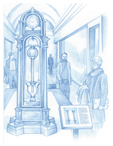
Fig. 1. Artistic view of Cox's clock \({}^{1}\)
Part A - Pulling on a submerged tube
We first consider a bath of water that occupies the semi-infinite space \(z\leq0\). The air above it is at a pressure \(P_a=P_0\). A cylindrical vertical tube of length \(H=1\,\mathrm m\), cross-sectional area \(S=10\,\mathrm{cm^2}\) and mass \(m=0.5\,\mathrm{kg}\) is dipped into the bath. The bottom end of the tube is open, and the top end of the tube is closed. We denote \(h\) the altitude of the top of the tube and \(z_\ell\) that of the water inside the tube. The thickness of the tube walls is neglected.
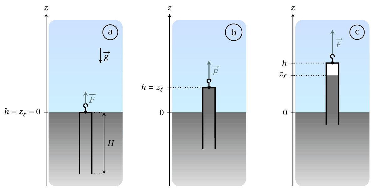
Fig. 2. Sketch of the tube in different configurations
We start from the situation where the tube in Fig. 2 contains no gas and its top is at the bath level: in other words, \(h=0\) and \(z_\ell=0\) (case a). The tube is then slowly lifted until its bottom end reaches the bath level. The pulling force exerted on the tube is denoted \(\vec F=F\vec u_z\).
A.1 — 0.2pt
For the configuration shown in Fig. 2 (case b), express the pressure \(P_w\) in the water at the top of the tube. Also express the force \(\vec F\) necessary to maintain the tube at this position. Expressions must be written in terms of \(P_0,\rho,m,S,h,g\) and \(\vec u_z\).
Three experiments are performed. In each, the tube is lifted from the initial state shown in Fig. 2(a) under the conditions specified in Table 1.
| Experiment | Liquid | \(T_a\) (°C) | \(\rho\) (\(\mathrm{kg\cdot m^{-3}}\)) | \(P_{\mathrm{sat}}\) (Pa) |
|---|---|---|---|---|
| 1 | Water | 20 | \(1.00\times10^3\) | \(2.34\times10^3\) |
| 2 | Water | 80 | \(0.97\times10^3\) | \(47.4\times10^3\) |
| 3 | Water | 99 | \(0.96\times10^3\) | \(99.8\times10^3\) |
Table 1. Experimental conditions and numerical values of physical quantities for each experiment
(\(P_{\mathrm{sat}}\) designates the saturated vapour pressure of the pure fluid)
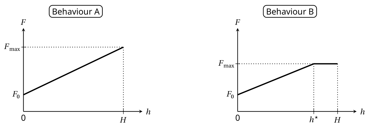
In each case, we study the evolution of the force \(F\) that must be applied in order to maintain the tube in equilibrium at an altitude \(h\), the external pressure being fixed at \(P_a=P_0=1.000\times10^5\,\mathrm{Pa}\). Two different behaviours are possible
A.2 — 0.8pt
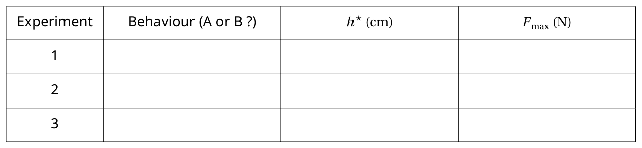
For each experiment, complete the table in the answer sheet to indicate the expected behaviour and the numerical values for \(F_{\max}\) and for \(h^\star\) (when pertinent), where \(F_{\max}\) and \(h^\star\) are defined in the figures illustrating the two behaviours.
When we replace the water with liquid mercury (whose properties are given below), behaviour B is observed.
| Liquid | \(T_a\) (°C) | \(\rho\) (\(\mathrm{kg\cdot m^{-3}}\)) | \(P_{\mathrm{sat}}\) (Pa) |
|---|---|---|---|
| Mercury | 20 | \(13.5\times10^3\) | \(0.163\) |
A.3 — 0.3pt
Express the relative error, denoted \(\varepsilon\), committed when we evaluate the maximal force \(F_{\max}\) neglecting \(P_{\mathrm{sat}}\) compared to \(P_0\). Give the numerical value of \(\varepsilon\).
Part B - Two-part barometric tube
From now on, we work with mercury (density \(\rho=13.5\times10^3\,\mathrm{kg\cdot m^{-3}}\)) at the ambient temperature \(T_a=20^\circ\mathrm C\) and we take \(P_{\mathrm{sat}}=0\).
Let us consider a tube with a reservoir on top, modeled as two superposed cylinders of different dimensions, as shown in Fig. 3.
- the bottom part (still called the tube) has cross-sectional area \(S_t\) and height \(H_t=80\,\mathrm{cm}\);
- the top part (called the bulb) has cross-sectional area \(S_b>S_t\) and height \(H_b=20\,\mathrm{cm}\).
This two-part tube is dipped into a semi-infinite liquid bath.
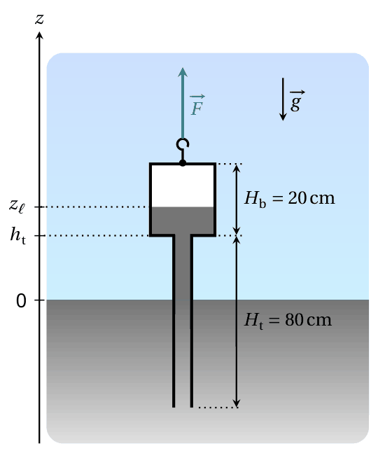
Fig. 3. Sketch of the two-part barometric tube
As in Part A, the system is prepared such that the tube contains no air. We identify the vertical position of the tube by the altitude \(h_t\) of the junction between the tube and the bulb. The height of the column of mercury is again denoted \(z_\ell\). The force \(\vec F\) that must be exerted to maintain the tube in equilibrium in the configuration shown in Fig. 3 can now be written as
\[ \vec F=(m_{\mathrm{tb}}+m_{\mathrm{add}})g\vec u_z \tag{1} \]
where \(m_{\mathrm{tb}}\) is the total mass of the two-part tube (when empty of mercury).
B.1 — 0.3pt
On the answer sheet, color the area corresponding to the volume of liquid mercury that is responsible for the term \(m_{\mathrm{add}}\) appearing in equation (1).
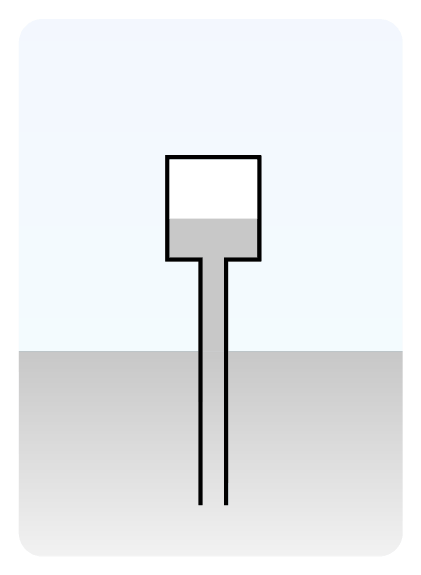
The mass \(m_{\mathrm{add}}\) depends both on the height \(h_t\) and the atmospheric pressure \(P_a\). For the next question, assume that the atmospheric pressure is fixed at \(P_a=P_0=1.000\times10^5\,\mathrm{Pa}\). Starting from the situation where the system is completely submerged, the tube is slowly lifted until its base is flush with the liquid bath.
B.2 — 1.4pt
Sketch the evolution of the mass \(m_{\mathrm{add}}\) as a function of \(h_t\) for \(h_t\in[-H_b,H_t]\). On the graph, provide the expression for the slopes of the different segments, as well as the \(h_t\) analytical value of any angular points, in terms of \(P_0,\rho,g,S_b,S_t,H_b\) and \(H_t\).
As the system is lifted while \(P_a=P_0=10^5\,\mathrm{Pa}\), we stop when the free surface of the liquid is in the middle of the bulb. The value of \(h_t\) is fixed and then we observe variations in the mass \(m_{\mathrm{add}}\) due to variations in the atmospheric pressure described by
\[ P_a(t)=P_0+P_1(t) \tag{2} \]
where \(P_0\) designates the average value and \(P_1\) is a perturbative term. We model \(P_1\) by a periodic triangular function of amplitude \(A=5\times10^2\,\mathrm{Pa}\) and period \(\tau_1\) of 1 week.
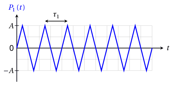
Fig. 4. Simplified model of the perturbative term \(P_1(t)\)
B.3 — 0.3pt
Given that \(S_t=5\,\mathrm{cm^2}\) and \(S_b=200\,\mathrm{cm^2}\), express the amplitude \(\Delta m_{\mathrm{add}}\) of the variations of the mass \(m_{\mathrm{add}}\) over time, then give its numerical value. Assume that the liquid surface always stays in the bulb.
Part C - Cox's timepiece
The real mechanism developed by Cox is complex (Fig. 5). We study a simplified version, depicted in Fig. 6, and described below
- a cylindrical bottom cistern containing a mercury bath;
- a two-part barometric tube identical to that studied in part B, which is still completely emptied of any air, is dipped into the bath;
- the cistern and the two-part tube are each suspended by a cable. Both cables (assumed to be inextensible and of negligible mass) pass through a system of ideal pullies and finish attached to either side of the same mass \(M\), which can slide on a horizontal surface;
- the total volume of liquid mercury contained in the system is \(V_\ell=5\,\mathrm L\).
The height, cross-section and masses of each part are given in Table 2. The position of mass \(M\) is referenced by the coordinate \(x\) of its center of mass. We consider solid friction between the horizontal support and the mass \(M\), without distinction between static and dynamic coefficients; the magnitude of this force when sliding occurs is denoted \(F_s\).
Two stops limit the displacement of the mass \(M\) such that \(-X\leq x\leq X\) (with \(X>0\)). Assume that the value of \(X\) guarantees that
- the bottom of the two-part tube never touches the bottom of the cistern nor comes out of the liquid bath;
- the altitude \(z_\ell\) of the mercury column is always in the upper bulb.
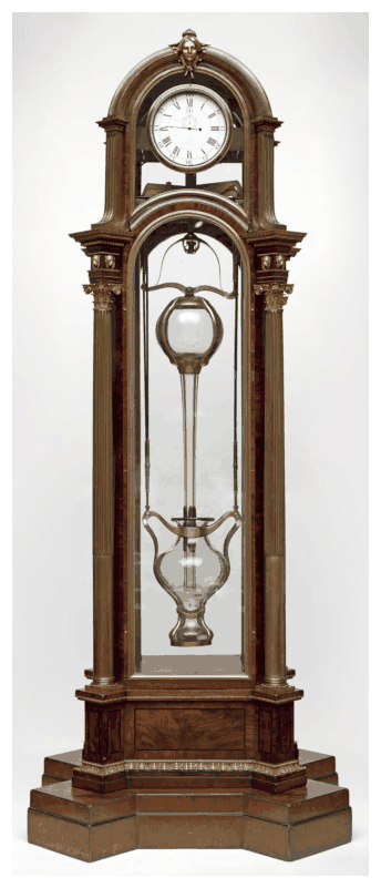
Fig. 5. Real Cox's timepiece \({}^{2}\) (without mercury)
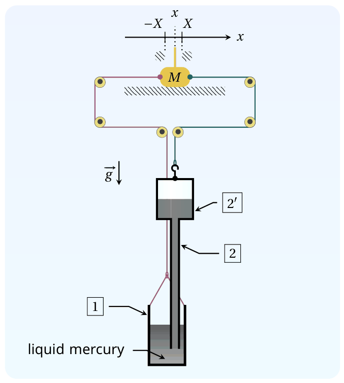
Fig. 6. Sketch of the system modeling the timepiece
| Reference | Name | Height | Cross section area | Empty mass |
|---|---|---|---|---|
| \(\boxed{1}\) | cistern | \(H_c=30\,\mathrm{cm}\) | \(S_c=210\,\mathrm{cm^2}\) | \(m_c\) |
| \(\boxed{2}\) | tubular part of the barometric tube | \(H_t=80\,\mathrm{cm}\) | \(S_t=5\,\mathrm{cm^2}\) | total mass of the barometric tube: \(m_{\mathrm{tb}}\) |
| \(\boxed{2'}\) | bulb of the barometric tube | \(H_b=20\,\mathrm{cm}\) | \(S_b=200\,\mathrm{cm^2}\) |
Table 2. Dimensions and notations for the model system
The system evolves in contact with the atmosphere, whose pressure fluctuates as in Fig. 4 (still with amplitude \(A=5\times10^2\,\mathrm{Pa}\) and period \(\tau_1=1\) week). At the start \(t=0\), the mass \(M\) is at rest at \(x=0\) and the tensions exerted by the two cables on either side of the mass \(M\) are in balance while \(P_1(0)=0\). We define
\[ \xi= \frac{S_b+S_c-S_t}{S_bS_c}\frac{F_s}{A} \simeq \frac{S_b+S_c}{S_bS_c}\frac{F_s}{A} \tag{3} \]
where the last expression uses that \(S_t\ll S_b,S_c\) (which we will assume is valid until the end of the problem).
C.1 — 1pt
Determine the threshold \(\xi^\star\) such that \(M\) remains indefinitely at rest when \(\xi>\xi^\star\).
For the next question only, suppose that the mass \(M\) is temporarily blocked at \(x=X\).
C.2 — 1pt
Give an expression for the total tension force \(\vec T=T\vec u_x\) acting on the mass \(M\) due to the tension in two cables at this position, when \(P_1=0\), in terms of \(\rho,g,X\) and pertinent cross-sections.
When \(\xi<\xi^\star\), starting again from \(x=0\) and \(P_1=0\), two different behaviours can be observed for \(t\geq0\). To distinguish them, we need to introduce another parameter
\[ \lambda= \frac{2(S_b-S_t)}{S_b}\frac{\rho gX}{A} \simeq \frac{2\rho gX}{A} \tag{4} \]
C.3 — 2pt
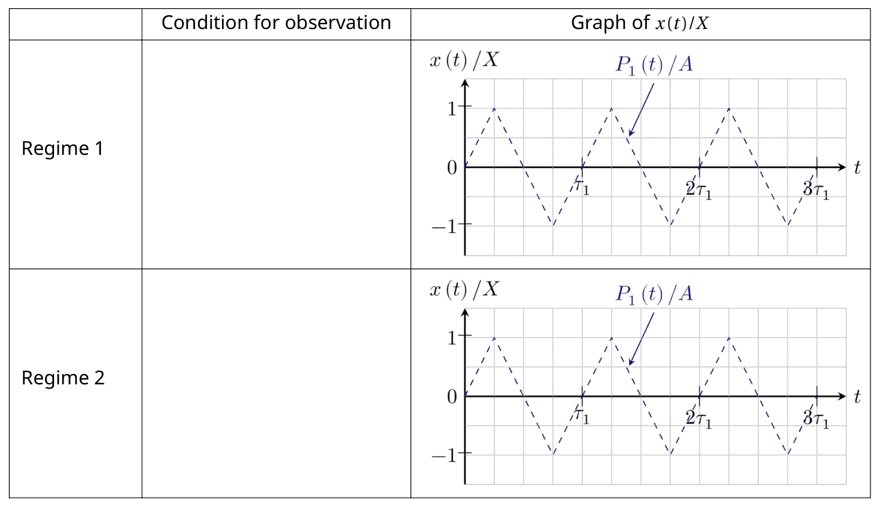
Complete the table in the answer sheet to indicate the condition under which each regime is obtained. Conditions must be expressed as inequalities on \(\xi\) and/or \(\lambda\). In addition, sketch the variations of \(x(t)/X\) for \(t\in[0,3\tau_1]\) that are consistent with the variations of \(P_1(t)/A\) already present. Specification of remarkable points coordinates is not required.
In the real Cox's timepiece, energy provided by the mechanism is stored using a system of ratchets and used to raise a counterweight, like in a traditional clock. In the simplified model studied here, the energy recovered by the clock corresponds to the energy dissipated by the friction force exerted by the horizontal surface on the mass \(M\). From now on, we assume that the system is dimensioned such that to work in the regime that allows the clock to recuperate energy. We also assume that the permanent regime is established. We denote \(W\) the energy dissipated by the solid friction force during a period \(\tau_1\), which can be expressed only in terms of \(F_s\) and \(X\).
All else equal, \(F_s\) and \(X\) can be adjusted to maximize the energy \(W\); we denote \(F_s^\star\) and \(X^\star\) their respective values in the optimal situation.
C.4 — 1pt
Considering \(S_b\simeq S_c\) and \(S_t\ll S_b\), determine the expressions for \(F_s^\star\) and \(X^\star\) as functions of \(\rho,g,S_c\) and \(A\). Express the corresponding maximum energy \(W^\star\), then calculate its numerical value with \(A=5\times10^2\,\mathrm{Pa}\).
We denote \(W_{\mathrm{pr}}^\star\) the work of atmospheric pressure forces received by the system in the optimal situation during a period \(\tau_1\).
C.5 — 1.7pt
Express \(W_{\mathrm{pr}}^\star\), then calculate the ratio \(W^\star/W_{\mathrm{pr}}^\star\). It could be useful to represent the evolution of the system in a \((P,V)\) diagram, where \(V\) is the system's volume.
Credits:
[1]: Bruno Vacaro;
[2]: Victoria and Albert Museum, London.
Official English text of the problem.
Answers
Define \[ L=\frac{P_0}{\rho g},\qquad D=S_b+S_c-S_t,\qquad q=\lambda+\frac{\xi}{2}. \]
-
A.1 \[ \boxed{P_w=P_0-\rho gh},\qquad \boxed{\vec F=(mg+\rho gSh)\vec u_z}. \]
-
A.2
| Experiment | Behaviour | \(h^\star\) (cm), when pertinent | \(F_{\max}\) (N) |
|---|---|---|---|
| 1 | A | — | \(14.7\) |
| 2 | A | — | \(14.4\) |
| 3 | B | \(2.13\) | \(5.10\) |
-
A.3 \[ \boxed{\varepsilon= \frac{SP_{\mathrm{sat}}}{mg+S(P_0-P_{\mathrm{sat}})} =1.55\times10^{-6}}. \] Neglecting mercury vapour pressure overestimates the force.
-
B.1 Shade all mercury inside the tube and bulb above the external bath level. In the depicted configuration, \[ \boxed{m_{\mathrm{add}}=\rho\bigl[S_th_t+S_b(z_\ell-h_t)\bigr]}. \]
-
B.2 \[ \boxed{ m_{\mathrm{add}}(h_t)= \begin{cases} \rho S_b(h_t+H_b),&-H_b\le h_t\le0,\\ \rho(S_bH_b+S_th_t),&0\le h_t\le L-H_b,\\ \rho\bigl[S_bL-(S_b-S_t)h_t\bigr],&L-H_b\le h_t\le L,\\ \rho S_tL,&L\le h_t\le H_t. \end{cases}} \] The successive slopes are \[ \boxed{\rho S_b,\quad \rho S_t,\quad-\rho(S_b-S_t),\quad0}. \] The angular points occur at \[ \boxed{h_t=0,\quad L-H_b\simeq0.556\,\mathrm m,\quad L\simeq0.756\,\mathrm m}. \]
-
B.3 \[ \boxed{\Delta m_{\mathrm{add}}=\frac{S_bA}{g}=1.02\,\mathrm{kg}}. \]
-
C.1 \[ \boxed{\xi^\star=2}. \]
-
C.2 \[ \boxed{ \vec T= \frac{4\rho gS_c(S_b-S_t)}{S_b+S_c-S_t}X\,\vec u_x \simeq \frac{4\rho gS_bS_c}{S_b+S_c}X\,\vec u_x}. \]
-
C.3, for \(\xi<2\):
| Regime | Condition | Description of \(x(t)/X\) |
|---|---|---|
| 1: remains at one stop | \(q>1\), equivalently \(\xi+2\lambda>2\) | Initially \(0\), then rises rapidly to \(+1\) and remains there. |
| 2: repeated strokes | \(q<1\), equivalently \(\xi+2\lambda<2\) | Initially \(0\), then switches between plateaus at \(+1\) and \(-1\). |
The first positive stroke begins when \(P_1/A=\xi/2\). Subsequent negative strokes begin at \(P_1/A=-q\) on falling pressure, and positive strokes at \(P_1/A=q\) on rising pressure. The boundary \(q=1\) is marginal; ideal static friction permits the mass to remain at the stop.
-
C.4 The ideal limiting optimum is \[ \boxed{F_s^\star=\frac{S_cA}{2}\simeq5.25\,\mathrm N}, \qquad \boxed{X^\star=\frac{A}{4\rho g}\simeq0.945\,\mathrm{mm}}, \] \[ \boxed{W^\star=\frac{S_cA^2}{2\rho g} \simeq1.98\times10^{-2}\,\mathrm J}. \]
-
C.5 \[ \boxed{W_{\mathrm{pr}}^\star=\frac{S_cA^2}{\rho g} \simeq3.97\times10^{-2}\,\mathrm J}, \qquad \boxed{\frac{W^\star}{W_{\mathrm{pr}}^\star}=\frac12}. \]
Solution
A.1
Hydrostatic equilibrium gives \[ \frac{dP}{dz}=-\rho g. \] The water is connected to the bath, where \(P=P_0\) at \(z=0\). Consequently, while the water remains in contact with the closed top, \[ P_w=P_0-\rho gh. \]
The pressure on the outside of the top produces a downward force \(P_0S\), while the water underneath produces an upward force \(P_wS\). The vertical walls contribute no vertical pressure force, and their thickness is neglected. Equilibrium therefore requires \[ F+P_wS-P_0S-mg=0. \] Thus \[ \boxed{\vec F=(mg+\rho gSh)\vec u_z}. \]
A.2
A vapour cavity appears when the pressure at the top reaches the saturated vapour pressure: \[ P_0-\rho gh^\star=P_{\mathrm{sat}}. \] Hence \[ \boxed{h^\star=\frac{P_0-P_{\mathrm{sat}}}{\rho g}}. \]
Before this happens, \(F=mg+\rho gSh\). After a vapour cavity has formed, its pressure remains \(P_{\mathrm{sat}}\) at the prescribed temperature, so \[ F=mg+S(P_0-P_{\mathrm{sat}}). \] These expressions combine into \[ F(h)=mg+S\min\{\rho gh,\ P_0-P_{\mathrm{sat}}\}, \qquad 0\le h\le H. \]
Therefore:
- if \(h^\star\ge H\), behaviour A occurs and \(F_{\max}=mg+\rho gSH\);
- if \(h^\star<H\), behaviour B occurs and \(F_{\max}=mg+S(P_0-P_{\mathrm{sat}})\).
Using \(S=10^{-3}\,\mathrm{m^2}\), \(H=1\,\mathrm m\), and \(mg=4.90\,\mathrm N\):
| Experiment | Calculated saturation height | Comparison with \(H\) | Result |
|---|---|---|---|
| 1 | \(\dfrac{100000-2340}{1000(9.8)}=9.97\,\mathrm m\) | Above \(H\) | A; \(F_{\max}=14.7\,\mathrm N\) |
| 2 | \(\dfrac{100000-47400}{970(9.8)}=5.53\,\mathrm m\) | Above \(H\) | A; \(F_{\max}=14.406\,\mathrm N\simeq14.4\,\mathrm N\) |
| 3 | \(\dfrac{100000-99800}{960(9.8)}=0.02126\,\mathrm m\) | Below \(H\) | B; \(h^\star=2.13\,\mathrm{cm}\), \(F_{\max}=5.10\,\mathrm N\) |
Both graphs begin at \(F_0=mg=4.90\,\mathrm N\).
A.3
For mercury, the actual maximum force and its approximation are \[ F_{\max}=mg+S(P_0-P_{\mathrm{sat}}), \qquad F_{\max}^{(0)}=mg+SP_0. \] The approximation overestimates the force by \(SP_{\mathrm{sat}}\). Relative to the actual force, \[ \varepsilon =\frac{F_{\max}^{(0)}-F_{\max}}{F_{\max}} =\frac{SP_{\mathrm{sat}}}{mg+S(P_0-P_{\mathrm{sat}})}. \] Numerically, \[ \boxed{ \varepsilon= \frac{10^{-3}(0.163)} {0.5(9.8)+10^{-3}(100000-0.163)} =1.55\times10^{-6}}. \] This is approximately \(0.000155\%\).
B.1
The additional load is the weight of the mercury raised above the external bath surface. Mercury below that level is supported hydrostatically by the bath.
Thus, on the answer-sheet diagram, shade:
- the mercury in the narrow tube from the external bath level up to the tube–bulb junction;
- all the mercury in the bulb, from its bottom up to its internal free surface.
Do not shade the mercury below the external bath level. For the configuration shown, \[ \boxed{m_{\mathrm{add}} =\rho\bigl[S_th_t+S_b(z_\ell-h_t)\bigr]}. \]
Since the pressure above the internal surface is zero, \[ z_\ell=\frac{P_a}{\rho g}. \] An equivalent useful expression is therefore \[ \boxed{ m_{\mathrm{add}} =\frac{S_bP_a}{g}-\rho(S_b-S_t)h_t } \] when the free surface lies in the bulb and the junction is above the external bath.
B.2
Introduce the barometric height \[ L=\frac{P_0}{\rho g} =\frac{10^5}{(13.5\times10^3)(9.8)} =0.75586\,\mathrm m. \] For the given dimensions, \[ 0<L-H_b<L<H_t. \]
Until the top reaches \(L\), the tube remains completely filled. Subsequently the internal free surface stays at \(z_\ell=L\), while the tube continues to rise.
There are four geometrically distinct intervals.
-
\(-H_b\le h_t\le0\).
Only a height \(h_t+H_b\) of the bulb is above the bath: \[ m_{\mathrm{add}}=\rho S_b(h_t+H_b). \] The graph starts at \((-H_b,0)\), with slope \(\rho S_b\). -
\(0\le h_t\le L-H_b\).
The entire bulb and a length \(h_t\) of narrow tube are above the bath, all filled with mercury: \[ m_{\mathrm{add}}=\rho(S_bH_b+S_th_t). \] The graph continues upward with the smaller slope \(\rho S_t\). -
\(L-H_b\le h_t\le L\).
A vacuum forms above the mercury, whose surface remains at \(L\) inside the bulb: \[ m_{\mathrm{add}} =\rho\bigl[S_th_t+S_b(L-h_t)\bigr]. \] The slope is \(-\rho(S_b-S_t)\), so the graph decreases. -
\(L\le h_t\le H_t\).
The bulb is empty and the internal free surface lies in the narrow tube: \[ m_{\mathrm{add}}=\rho S_tL=\frac{S_tP_0}{g}. \] The graph is horizontal.
The graph is continuous, with the following vertices and endpoint:
| \(h_t\) | \(m_{\mathrm{add}}\) |
|---|---|
| \(-H_b\) | \(0\) |
| \(0\) | \(\rho S_bH_b\) |
| \(L-H_b\) | \(\rho[S_bH_b+S_t(L-H_b)]\), the maximum |
| \(L\) | \(\rho S_tL\) |
| \(H_t\) | \(\rho S_tL\) |
Its three angular points have horizontal coordinates \[ \boxed{0,\quad \frac{P_0}{\rho g}-H_b,\quad\frac{P_0}{\rho g}}, \] numerically \(0\), \(55.6\,\mathrm{cm}\), and \(75.6\,\mathrm{cm}\).
B.3
At the prescribed fixed position, the free surface remains inside the bulb. Thus \[ m_{\mathrm{add}}(t) =\frac{S_b[P_0+P_1(t)]}{g} -\rho(S_b-S_t)h_t. \] Only the first term varies, so the amplitude is \[ \boxed{\Delta m_{\mathrm{add}}=\frac{S_bA}{g}}. \] With \(S_b=200\,\mathrm{cm^2}=0.0200\,\mathrm{m^2}\), \[ \boxed{\Delta m_{\mathrm{add}} =\frac{0.0200(500)}{9.8} =1.02\,\mathrm{kg}}. \]
This is the amplitude about the mean; the peak-to-peak variation is \(2.04\,\mathrm{kg}\). The corresponding surface-height amplitude is \[ \frac{A}{\rho g}=3.78\,\mathrm{mm}, \] well below the \(10\,\mathrm{cm}\) distance from the middle of the bulb to either end.
C.1
We first obtain the cable-force difference for arbitrary \(x\) and \(P_1\).
Let \(z_s\) denote the external mercury surface and \(z_c\) the cistern bottom. From the cable arrangement, displacement of the mass to the right by \(x\):
- raises the cistern by \(x\);
- lowers the barometric tube by \(x\).
Therefore \[ z_c=z_{c0}+x,\qquad h_t=h_{t0}-x. \]
Hydrostatic equilibrium gives \[ z_\ell-z_s=\frac{P_a}{\rho g}. \] The mercury above the external surface has mass \[ m_{\mathrm{add}} =\rho\bigl[S_t(h_t-z_s)+S_b(z_\ell-h_t)\bigr] =\frac{S_bP_a}{g}-\rho(S_b-S_t)(h_t-z_s). \]
Because the tube walls have negligible volume, mercury conservation can be written as \[ V_\ell=S_c(z_s-z_c)+\frac{m_{\mathrm{add}}}{\rho}. \] Writing \(\delta m=m_{\mathrm{add}}-m_{\mathrm{add},0}\), this implies \[ \delta z_s=x-\frac{\delta m}{\rho S_c}. \] Subtracting the initial expression for \(m_{\mathrm{add}}\) from its current value gives \[ \delta m=\frac{S_bP_1}{g} +\rho(S_b-S_t)(x+\delta z_s). \] Consequently, \[ \boxed{ \delta m= \frac{S_bS_c}{(S_b+S_c-S_t)g}P_1 +\frac{2\rho S_c(S_b-S_t)}{S_b+S_c-S_t}x }. \]
In a stationary configuration, the tube-side cable tension is \[ T_{\mathrm{tb}}=(m_{\mathrm{tb}}+m_{\mathrm{add}})g, \] whereas the cistern-side tension is \[ T_c=(m_c+\rho V_\ell-m_{\mathrm{add}})g. \] Their initial difference is zero. Hence the signed force on \(M\), positive to the right, is \[ T=T_{\mathrm{tb}}-T_c=2g\,\delta m. \]
Define \[ K=\frac{S_bS_c}{S_b+S_c-S_t}, \qquad \alpha=\frac{2\rho g(S_b-S_t)}{S_b}. \] The resulting force law is \[ \boxed{T=2K(P_1+\alpha x)}. \] The given parameters satisfy \[ F_s=KA\xi,\qquad \alpha X=A\lambda. \]
At \(x=0\), the maximum force magnitude over the atmospheric cycle is \(2KA\). Static friction can balance it throughout the cycle if \[ F_s\ge2KA \quad\Longleftrightarrow\quad \xi\ge2. \] Thus the requested threshold is \[ \boxed{\xi^\star=2}. \]
C.2
Setting \(P_1=0\) and \(x=X\) in the force law, \[ \boxed{ \vec T= \frac{4\rho gS_c(S_b-S_t)}{S_b+S_c-S_t}X\,\vec u_x }. \] Using \(S_t\ll S_b,S_c\), \[ \boxed{ \vec T\simeq \frac{4\rho gS_bS_c}{S_b+S_c}X\,\vec u_x }. \]
The positive sign is significant: a displacement to the right produces a further force to the right. The equilibrium is mechanically unstable once friction can no longer hold the mass.
C.3
For the sketches, use the slow atmospheric driving limit: transfer between stops is rapid compared with the one-week pressure period. The stops arrest the moving system.
Write \[ p=\frac{P_1}{A},\qquad y=\frac{x}{X}. \] Then \[ \frac{T}{KA}=2(p+\lambda y), \qquad \frac{F_s}{KA}=\xi. \]
Initially \(y=0\) and \(p\) increases from zero. Motion to the right starts as \(p\) exceeds \[ p=\frac{\xi}{2}. \] Since \(\partial T/\partial x=2K\alpha>0\), movement to the right increases the driving force. The mass rapidly reaches \(y=+1\).
At the right stop, release to the left requires \[ T<-F_s. \] Thus \[ 2(p+\lambda)<-\xi \quad\Longleftrightarrow\quad p<-\left(\lambda+\frac{\xi}{2}\right). \] Define \[ q=\lambda+\frac{\xi}{2}. \]
If \(q>1\), the pressure never becomes sufficiently low to release the mass. If \(q<1\), release occurs during every decreasing-pressure half-cycle. The analogous release condition at the left stop is \(p>q\).
Therefore the two regimes are:
| Regime | Condition | Precise sketch description |
|---|---|---|
| 1: permanent residence at the right stop | \(\xi<2\), \(\xi+2\lambda>2\) | Draw \(x/X=0\) initially, followed by a rapid rise to \(+1\) on the first rising pressure branch at \(p=\xi/2\). Continue horizontally at \(+1\) through \(3\tau_1\). |
| 2: repeated motion between stops | \(\xi<2\), \(\xi+2\lambda<2\) | Start with the same initial rise. Then draw horizontal plateaus at \(+1\) and \(-1\), joined by rapid downward transitions whenever falling pressure reaches \(p=-q\), and upward transitions whenever rising pressure reaches \(p=q\). |
For an explicit placement of the transitions, let \(s=t/\tau_1\). The first positive transition is at \[ s=\frac{\xi}{8}. \] In the cycling regime, the negative transitions within the requested interval are at \[ s=\frac12+\frac q4,\quad \frac32+\frac q4,\quad \frac52+\frac q4, \] and subsequent positive transitions are at \[ s=1+\frac q4,\quad 2+\frac q4. \] These specify the requested three-period sketch completely.
At \(q=1\), the release threshold is only touched at a pressure extremum. Exact ideal static friction can keep the mass at the stop; sustained cycling is guaranteed by the strict inequality \(q<1\).
C.4
In the permanent cycling regime, the mass travels from one stop to the other and back during each period. Its total sliding distance is \(4X\), so \[ \boxed{W=4F_sX}. \]
With \(S_b\simeq S_c\) and \(S_t\ll S_b\), \[ \xi\simeq\frac{2F_s}{S_cA}, \qquad \lambda\simeq\frac{2\rho gX}{A}. \] The cycling condition becomes \[ \xi+2\lambda<2 \quad\Longleftrightarrow\quad F_s<S_c(A-2\rho gX). \]
For a fixed \(X\), the greatest attainable energy is approached as \(F_s\) approaches this upper bound. Its limiting envelope is \[ W(X)=4S_cX(A-2\rho gX). \] Differentiating, \[ \frac{dW}{dX}=4S_c(A-4\rho gX). \] The optimum is therefore \[ \boxed{X^\star=\frac{A}{4\rho g}}, \qquad \boxed{F_s^\star=\frac{S_cA}{2}}. \] Equivalently, \[ \xi_{\mathrm{opt}}=1,\qquad \lambda_{\mathrm{opt}}=\frac12. \] Thus \[ \boxed{W^\star=4F_s^\star X^\star =\frac{S_cA^2}{2\rho g}}. \]
With \(S_c=0.0210\,\mathrm{m^2}\), \[ F_s^\star=\frac{0.0210(500)}2=5.25\,\mathrm N, \] \[ X^\star=\frac{500}{4(13.5\times10^3)(9.8)} =9.45\times10^{-4}\,\mathrm m, \] and \[ \boxed{ W^\star= \frac{0.0210(500)^2}{2(13.5\times10^3)(9.8)} =1.98\times10^{-2}\,\mathrm J }. \]
Strictly, these values lie on the marginal switching boundary. They give the ideal limiting maximum, approached from the cycling side; reliable operation requires a small margin inside that boundary.
C.5
The volume relevant to atmospheric work includes the vacuum enclosed above the mercury. The liquid volume and the material volume of the vessels are constant, so \[ V=V_{\mathrm{constant}}+V_{\mathrm{vac}}, \qquad V_{\mathrm{vac}}=S_b(h_t+H_b-z_\ell). \]
Use the same approximation as in C.4: \[ S_b=S_c=S,\qquad S_t=0. \] The conservation and hydrostatic relations derived in C.1 then give \[ \delta z_s=-\frac{P_1}{2\rho g}, \qquad \delta z_\ell=\frac{P_1}{2\rho g}. \] Since \(\delta h_t=-x\), \[ \boxed{ V=V_{\mathrm{ref}}-Sx-\frac{S}{2\rho g}P_1 }. \]
The atmospheric work received by the system is \[ W_{\mathrm{pr}}=-\oint P_a\,dV. \] Substitution yields \[ W_{\mathrm{pr}} =S\oint P_a\,dx +\frac{S}{2\rho g}\oint P_a\,dP_1. \] The second integral vanishes over a closed cycle. Also \(P_0\oint dx=0\). Therefore \[ \boxed{W_{\mathrm{pr}}=S\oint P_1\,dx}. \]
At the limiting optimum, \(q=1\). The positive stroke occurs at \(P_1=+A\), with \(\Delta x=2X^\star\), while the negative stroke occurs at \(P_1=-A\), with \(\Delta x=-2X^\star\). Consequently, \[ W_{\mathrm{pr}}^\star =S\bigl[A(2X^\star)+(-A)(-2X^\star)\bigr] =4SAX^\star. \] Thus \[ \boxed{ W_{\mathrm{pr}}^\star=\frac{S_cA^2}{\rho g} =3.97\times10^{-2}\,\mathrm J }. \]
In a diagram with \(V\) horizontal and \(P_a\) vertical, the cycle is a parallelogram:
- at each fixed stop, \(dV/dP_a=-S_c/(2\rho g)\), giving two parallel sloping branches;
- their horizontal separation is \(2S_cX^\star\);
- constant-pressure strokes connect them at \(P_0+A\) and \(P_0-A\);
- the cycle is traversed counterclockwise, giving positive work received equal to its area, \[ (2A)(2S_cX^\star)=4S_cAX^\star. \]
Finally, \[ \boxed{ \frac{W^\star}{W_{\mathrm{pr}}^\star} = \frac{S_cA^2/(2\rho g)}{S_cA^2/(\rho g)} =\frac12 }. \] The other half becomes kinetic energy during the rapid strokes and is dissipated when the moving system is arrested at the stops.
The solution was checked against the official solution.
IPhO 2025 · Theorieaufgabe 2
Cox' Uhr
Im Jahr 1765 erfand der britische Uhrmacher James Cox eine Uhr, deren einzige Energiequelle die Schwankungen des Luftdrucks sind. Cox' Uhr verwendete zwei Gefäße mit Quecksilber. Änderungen des Luftdrucks bewirkten, dass Quecksilber zwischen den Gefäßen strömte und sich die beiden Gefäße relativ zueinander bewegten. Diese Bewegung diente als Energiequelle für das eigentliche Uhrwerk.
Wir untersuchen diese Vorrichtung. Dabei nehmen wir durchgehend an, dass
- das Schwerefeld der Erde \(\vec g=-g\vec u_z\) homogen ist, mit \(g=9.8\,\mathrm{m\cdot s^{-2}}\) und dem Einheitsvektor \(\vec u_z\);
- alle Flüssigkeiten inkompressibel sind und ihre Dichte mit \(\rho\) bezeichnet wird;
- keine Effekte der Oberflächenspannung berücksichtigt werden;
- die Höhenabhängigkeit des Luftdrucks vernachlässigt wird;
- die Umgebungstemperatur \(T_a\) räumlich konstant ist und alle Zustandsänderungen isotherm verlaufen.
Abb. 1. Künstlerische Darstellung von Cox' Uhr \({}^{1}\)
Teil A - Ziehen an einem eingetauchten Rohr
Wir betrachten zunächst ein Wasserbad, das den Halbraum \(z\leq0\) einnimmt. Die Luft darüber steht unter dem Druck \(P_a=P_0\). Ein senkrechtes zylindrisches Rohr der Länge \(H=1\,\mathrm m\), der Querschnittsfläche \(S=10\,\mathrm{cm^2}\) und der Masse \(m=0.5\,\mathrm{kg}\) wird in das Bad eingetaucht. Das untere Ende des Rohrs ist offen, das obere Ende geschlossen. Mit \(h\) bezeichnen wir die Höhe des oberen Rohrendes und mit \(z_\ell\) die Höhe des Wassers im Rohr. Die Wanddicke des Rohrs wird vernachlässigt.
Abb. 2. Skizze des Rohrs in verschiedenen Anordnungen
Wir gehen von der Situation aus, in der das Rohr in Abb. 2 kein Gas enthält und sein oberes Ende auf Höhe der Badoberfläche liegt: Mit anderen Worten gilt \(h=0\) und \(z_\ell=0\) (Fall a). Anschließend wird das Rohr langsam angehoben, bis sein unteres Ende die Badoberfläche erreicht. Die auf das Rohr ausgeübte Zugkraft wird mit \(\vec F=F\vec u_z\) bezeichnet.
A.1 — 0.2 Punkte
Geben Sie für die in Abb. 2 gezeigte Anordnung (Fall b) den Druck \(P_w\) im Wasser am oberen Rohrende an. Geben Sie außerdem die Kraft \(\vec F\) an, die erforderlich ist, um das Rohr in dieser Position zu halten. Die Ausdrücke sind in Abhängigkeit von \(P_0,\rho,m,S,h,g\) und \(\vec u_z\) anzugeben.
Es werden drei Versuche durchgeführt. In jedem Versuch wird das Rohr ausgehend vom Anfangszustand in Abb. 2(a) unter den in Tabelle 1 angegebenen Bedingungen angehoben.
| Versuch | Flüssigkeit | \(T_a\) (°C) | \(\rho\) (\(\mathrm{kg\cdot m^{-3}}\)) | \(P_{\mathrm{sat}}\) (Pa) |
|---|---|---|---|---|
| 1 | Wasser | 20 | \(1.00\times10^3\) | \(2.34\times10^3\) |
| 2 | Wasser | 80 | \(0.97\times10^3\) | \(47.4\times10^3\) |
| 3 | Wasser | 99 | \(0.96\times10^3\) | \(99.8\times10^3\) |
Tabelle 1. Versuchsbedingungen und Zahlenwerte der physikalischen Größen für die einzelnen Versuche
(\(P_{\mathrm{sat}}\) bezeichnet den Sättigungsdampfdruck des reinen Fluids)
In jedem Fall untersuchen wir den Verlauf der Kraft \(F\), die aufgebracht werden muss, um das Rohr in einer Höhe \(h\) im Gleichgewicht zu halten, wobei der Außendruck auf \(P_a=P_0=1.000\times10^5\,\mathrm{Pa}\) festgelegt ist. Zwei unterschiedliche Verhaltensweisen sind möglich
A.2 — 0.8 Punkte
Vervollständigen Sie für jeden Versuch die Tabelle auf dem Antwortblatt, indem Sie das erwartete Verhalten und die Zahlenwerte für \(F_{\max}\) und für \(h^\star\) (sofern zutreffend) angeben. Dabei sind \(F_{\max}\) und \(h^\star\) in den Abbildungen definiert, welche die beiden Verhaltensweisen veranschaulichen.
Wenn wir das Wasser durch flüssiges Quecksilber ersetzen (dessen Eigenschaften unten angegeben sind), wird Verhalten B beobachtet.
| Flüssigkeit | \(T_a\) (°C) | \(\rho\) (\(\mathrm{kg\cdot m^{-3}}\)) | \(P_{\mathrm{sat}}\) (Pa) |
|---|---|---|---|
| Quecksilber | 20 | \(13.5\times10^3\) | \(0.163\) |
A.3 — 0.3 Punkte
Geben Sie den relativen Fehler \(\varepsilon\) an, der entsteht, wenn wir bei der Berechnung der maximalen Kraft \(F_{\max}\) den Druck \(P_{\mathrm{sat}}\) gegenüber \(P_0\) vernachlässigen. Geben Sie den Zahlenwert von \(\varepsilon\) an.
Teil B - Zweiteiliges Barometerrohr
Von nun an arbeiten wir mit Quecksilber (Dichte \(\rho=13.5\times10^3\,\mathrm{kg\cdot m^{-3}}\)) bei der Umgebungstemperatur \(T_a=20^\circ\mathrm C\) und setzen \(P_{\mathrm{sat}}=0\).
Wir betrachten ein Rohr mit einem Vorratsgefäß am oberen Ende, das als zwei übereinander angeordnete Zylinder unterschiedlicher Abmessungen modelliert wird, wie in Abb. 3 gezeigt.
- Der untere Teil (weiterhin als Rohr bezeichnet) hat die Querschnittsfläche \(S_t\) und die Höhe \(H_t=80\,\mathrm{cm}\);
- der obere Teil (als Erweiterung bezeichnet) hat die Querschnittsfläche \(S_b>S_t\) und die Höhe \(H_b=20\,\mathrm{cm}\).
Dieses zweiteilige Rohr wird in ein Flüssigkeitsbad eingetaucht, das einen Halbraum einnimmt.
Abb. 3. Skizze des zweiteiligen Barometerrohrs
Wie in Teil A wird das System so vorbereitet, dass das Rohr keine Luft enthält. Wir kennzeichnen die vertikale Position des Rohrs durch die Höhe \(h_t\) des Übergangs zwischen dem Rohr und der Erweiterung. Die Höhe der Quecksilbersäule wird wiederum mit \(z_\ell\) bezeichnet. Die Kraft \(\vec F\), die aufgebracht werden muss, um das Rohr in der in Abb. 3 gezeigten Anordnung im Gleichgewicht zu halten, lässt sich nun schreiben als
\[ \vec F=(m_{\mathrm{tb}}+m_{\mathrm{add}})g\vec u_z \tag{1} \]
wobei \(m_{\mathrm{tb}}\) die Gesamtmasse des zweiteiligen Rohrs (ohne Quecksilber) ist.
B.1 — 0.3 Punkte
Markieren Sie auf dem Antwortblatt die Fläche farbig, die dem Volumen des flüssigen Quecksilbers entspricht, das für den Term \(m_{\mathrm{add}}\) in Gleichung (1) verantwortlich ist.
Die Masse \(m_{\mathrm{add}}\) hängt sowohl von der Höhe \(h_t\) als auch vom Luftdruck \(P_a\) ab. Nehmen Sie für die nächste Frage an, dass der Luftdruck auf \(P_a=P_0=1.000\times10^5\,\mathrm{Pa}\) festgelegt ist. Ausgehend von einem vollständig eingetauchten System wird das Rohr langsam angehoben, bis sein unteres Ende bündig mit der Oberfläche des Flüssigkeitsbads liegt.
B.2 — 1.4 Punkte
Skizzieren Sie den Verlauf der Masse \(m_{\mathrm{add}}\) als Funktion von \(h_t\) für \(h_t\in[-H_b,H_t]\). Geben Sie im Diagramm die Ausdrücke für die Steigungen der einzelnen Abschnitte sowie die analytischen Werte von \(h_t\) an allen Knickpunkten in Abhängigkeit von \(P_0,\rho,g,S_b,S_t,H_b\) und \(H_t\) an.
Beim Anheben des Systems unter \(P_a=P_0=10^5\,\mathrm{Pa}\) halten wir an, sobald sich die freie Flüssigkeitsoberfläche in der Mitte der Erweiterung befindet. Der Wert von \(h_t\) wird festgehalten. Anschließend beobachten wir Änderungen der Masse \(m_{\mathrm{add}}\) infolge von Luftdruckschwankungen, die beschrieben werden durch
\[ P_a(t)=P_0+P_1(t) \tag{2} \]
wobei \(P_0\) den Mittelwert bezeichnet und \(P_1\) einen Störterm darstellt. Wir modellieren \(P_1\) durch eine periodische Dreiecksfunktion mit der Amplitude \(A=5\times10^2\,\mathrm{Pa}\) und der Periode \(\tau_1\) von 1 Woche.
Abb. 4. Vereinfachtes Modell des Störterms \(P_1(t)\)
B.3 — 0.3 Punkte
Geben Sie für \(S_t=5\,\mathrm{cm^2}\) und \(S_b=200\,\mathrm{cm^2}\) einen Ausdruck für die Amplitude \(\Delta m_{\mathrm{add}}\) der zeitlichen Schwankungen der Masse \(m_{\mathrm{add}}\) an und berechnen Sie anschließend ihren Zahlenwert. Nehmen Sie an, dass die Flüssigkeitsoberfläche stets in der Erweiterung bleibt.
Teil C - Cox' Uhr
Der von Cox entwickelte tatsächliche Mechanismus ist komplex (Abb. 5). Wir untersuchen eine vereinfachte Version, die in Abb. 6 dargestellt und nachfolgend beschrieben ist
- ein zylindrischer unterer Behälter mit einem Quecksilberbad;
- ein zweiteiliges Barometerrohr, das mit dem in Teil B untersuchten identisch und weiterhin vollständig luftleer ist, wird in das Bad eingetaucht;
- der Behälter und das zweiteilige Rohr hängen jeweils an einem Seil. Beide Seile (als undehnbar und von vernachlässigbarer Masse angenommen) laufen über ein System idealer Rollen und sind mit ihren Enden an gegenüberliegenden Seiten derselben Masse \(M\) befestigt, die auf einer horizontalen Fläche gleiten kann;
- das gesamte im System enthaltene Volumen an flüssigem Quecksilber beträgt \(V_\ell=5\,\mathrm L\).
Die Höhen, Querschnittsflächen und Massen der einzelnen Teile sind in Tabelle 2 angegeben. Die Position der Masse \(M\) wird durch die Koordinate \(x\) ihres Schwerpunkts beschrieben. Wir berücksichtigen Festkörperreibung zwischen der horizontalen Unterlage und der Masse \(M\), ohne zwischen Haft- und Gleitreibungskoeffizienten zu unterscheiden; der Betrag dieser Kraft beim Gleiten wird mit \(F_s\) bezeichnet.
Zwei Anschläge begrenzen die Verschiebung der Masse \(M\), sodass \(-X\leq x\leq X\) (mit \(X>0\)) gilt. Nehmen Sie an, dass der Wert von \(X\) gewährleistet, dass
- das untere Ende des zweiteiligen Rohrs weder den Boden des Behälters berührt noch aus dem Flüssigkeitsbad austritt;
- die Höhe \(z_\ell\) der Quecksilbersäule stets innerhalb der oberen Erweiterung liegt.
Abb. 5. Tatsächliche Uhr von Cox \({}^{2}\) (ohne Quecksilber)
Abb. 6. Skizze des Systems zur Modellierung der Uhr
| Kennzeichnung | Bezeichnung | Höhe | Querschnittsfläche | Leermasse |
|---|---|---|---|---|
| \(\boxed{1}\) | Behälter | \(H_c=30\,\mathrm{cm}\) | \(S_c=210\,\mathrm{cm^2}\) | \(m_c\) |
| \(\boxed{2}\) | röhrenförmiger Teil des Barometerrohrs | \(H_t=80\,\mathrm{cm}\) | \(S_t=5\,\mathrm{cm^2}\) | Gesamtmasse des Barometerrohrs: \(m_{\mathrm{tb}}\) |
| \(\boxed{2'}\) | Erweiterung des Barometerrohrs | \(H_b=20\,\mathrm{cm}\) | \(S_b=200\,\mathrm{cm^2}\) |
Tabelle 2. Abmessungen und Bezeichnungen des Modellsystems
Das System entwickelt sich im Kontakt mit der Atmosphäre, deren Druck wie in Abb. 4 schwankt (weiterhin mit der Amplitude \(A=5\times10^2\,\mathrm{Pa}\) und der Periode \(\tau_1=1\) Woche). Zu Beginn, bei \(t=0\), ruht die Masse \(M\) bei \(x=0\), und die von den beiden Seilen auf gegenüberliegenden Seiten der Masse \(M\) ausgeübten Zugkräfte gleichen sich aus, während \(P_1(0)=0\) gilt. Wir definieren
\[ \xi= \frac{S_b+S_c-S_t}{S_bS_c}\frac{F_s}{A} \simeq \frac{S_b+S_c}{S_bS_c}\frac{F_s}{A} \tag{3} \]
wobei im letzten Ausdruck \(S_t\ll S_b,S_c\) verwendet wird (was wir bis zum Ende der Aufgabe als gültig annehmen).
C.1 — 1 Punkt
Bestimmen Sie den Schwellenwert \(\xi^\star\), sodass \(M\) für \(\xi>\xi^\star\) unbegrenzt in Ruhe bleibt.
Nehmen Sie nur für die nächste Frage an, dass die Masse \(M\) vorübergehend bei \(x=X\) blockiert ist.
C.2 — 1 Punkt
Geben Sie für \(P_1=0\) einen Ausdruck für die resultierende Seilkraft \(\vec T=T\vec u_x\) an, die in dieser Position aufgrund der Zugkräfte in den beiden Seilen auf die Masse \(M\) wirkt, in Abhängigkeit von \(\rho,g,X\) und den relevanten Querschnittsflächen.
Für \(\xi<\xi^\star\) können, erneut ausgehend von \(x=0\) und \(P_1=0\), für \(t\geq0\) zwei unterschiedliche Verhaltensweisen beobachtet werden. Um sie zu unterscheiden, müssen wir einen weiteren Parameter einführen
\[ \lambda= \frac{2(S_b-S_t)}{S_b}\frac{\rho gX}{A} \simeq \frac{2\rho gX}{A} \tag{4} \]
C.3 — 2 Punkte
Vervollständigen Sie die Tabelle auf dem Antwortblatt, indem Sie die Bedingung angeben, unter der das jeweilige Regime auftritt. Die Bedingungen sind als Ungleichungen für \(\xi\) und/oder \(\lambda\) auszudrücken. Skizzieren Sie außerdem die Verläufe von \(x(t)/X\) für \(t\in[0,3\tau_1]\), die mit dem bereits eingezeichneten Verlauf von \(P_1(t)/A\) übereinstimmen. Die Koordinaten besonderer Punkte müssen nicht angegeben werden.
In der tatsächlichen Uhr von Cox wird die vom Mechanismus bereitgestellte Energie mithilfe eines Systems von Sperrklinken gespeichert und wie bei einer herkömmlichen Uhr zum Anheben eines Gegengewichts genutzt. Im hier untersuchten vereinfachten Modell entspricht die von der Uhr gewonnene Energie der Energie, die durch die von der horizontalen Fläche auf die Masse \(M\) ausgeübte Reibungskraft dissipiert wird. Von nun an nehmen wir an, dass das System so dimensioniert ist, dass es in dem Regime arbeitet, in dem die Uhr Energie gewinnen kann. Außerdem nehmen wir an, dass der eingeschwungene Zustand erreicht ist. Wir bezeichnen mit \(W\) die während einer Periode \(\tau_1\) durch die Festkörperreibung dissipierte Energie, die allein durch \(F_s\) und \(X\) ausgedrückt werden kann.
Bei ansonsten gleichen Bedingungen können \(F_s\) und \(X\) so eingestellt werden, dass die Energie \(W\) maximal wird; ihre jeweiligen Werte im optimalen Fall bezeichnen wir mit \(F_s^\star\) und \(X^\star\).
C.4 — 1 Punkt
Bestimmen Sie unter den Annahmen \(S_b\simeq S_c\) und \(S_t\ll S_b\) die Ausdrücke für \(F_s^\star\) und \(X^\star\) als Funktionen von \(\rho,g,S_c\) und \(A\). Geben Sie die entsprechende maximale Energie \(W^\star\) an und berechnen Sie anschließend ihren Zahlenwert für \(A=5\times10^2\,\mathrm{Pa}\).
Mit \(W_{\mathrm{pr}}^\star\) bezeichnen wir die Arbeit der Luftdruckkräfte, die dem System im optimalen Fall während einer Periode \(\tau_1\) zugeführt wird.
C.5 — 1.7 Punkte
Geben Sie \(W_{\mathrm{pr}}^\star\) an und berechnen Sie anschließend das Verhältnis \(W^\star/W_{\mathrm{pr}}^\star\). Es kann hilfreich sein, den Verlauf des Systems in einem \((P,V)\)-Diagramm darzustellen, wobei \(V\) das Volumen des Systems ist.
Bildnachweise:
[1]: Bruno Vacaro;
[2]: Victoria and Albert Museum, London.
Aufgabentext aus dem offiziellen englischen Text übersetzt.
Antworten
Wir definieren \[ L=\frac{P_0}{\rho g},\qquad D=S_b+S_c-S_t,\qquad q=\lambda+\frac{\xi}{2}. \]
-
A.1 \[ \boxed{P_w=P_0-\rho gh},\qquad \boxed{\vec F=(mg+\rho gSh)\vec u_z}. \]
-
A.2
| Versuch | Verhalten | \(h^\star\) (cm), sofern zutreffend | \(F_{\max}\) (N) |
|---|---|---|---|
| 1 | A | — | \(14.7\) |
| 2 | A | — | \(14.4\) |
| 3 | B | \(2.13\) | \(5.10\) |
-
A.3 \[ \boxed{\varepsilon= \frac{SP_{\mathrm{sat}}}{mg+S(P_0-P_{\mathrm{sat}})} =1.55\times10^{-6}}. \] Wenn der Quecksilberdampfdruck vernachlässigt wird, wird die Kraft überschätzt.
-
B.1 Schraffieren Sie das gesamte Quecksilber innerhalb des Rohrs und der Erweiterung oberhalb der äußeren Badoberfläche. In der dargestellten Anordnung gilt \[ \boxed{m_{\mathrm{add}}=\rho\bigl[S_th_t+S_b(z_\ell-h_t)\bigr]}. \]
-
B.2 \[ \boxed{ m_{\mathrm{add}}(h_t)= \begin{cases} \rho S_b(h_t+H_b),&-H_b\le h_t\le0,\\ \rho(S_bH_b+S_th_t),&0\le h_t\le L-H_b,\\ \rho\bigl[S_bL-(S_b-S_t)h_t\bigr],&L-H_b\le h_t\le L,\\ \rho S_tL,&L\le h_t\le H_t. \end{cases}} \] Die aufeinanderfolgenden Steigungen sind \[ \boxed{\rho S_b,\quad \rho S_t,\quad-\rho(S_b-S_t),\quad0}. \] Die Knickpunkte liegen bei \[ \boxed{h_t=0,\quad L-H_b\simeq0.556\,\mathrm m,\quad L\simeq0.756\,\mathrm m}. \]
-
B.3 \[ \boxed{\Delta m_{\mathrm{add}}=\frac{S_bA}{g}=1.02\,\mathrm{kg}}. \]
-
C.1 \[ \boxed{\xi^\star=2}. \]
-
C.2 \[ \boxed{ \vec T= \frac{4\rho gS_c(S_b-S_t)}{S_b+S_c-S_t}X\,\vec u_x \simeq \frac{4\rho gS_bS_c}{S_b+S_c}X\,\vec u_x}. \]
-
C.3, für \(\xi<2\):
| Regime | Bedingung | Beschreibung von \(x(t)/X\) |
|---|---|---|
| 1: Verbleib an einem Anschlag | \(q>1\), äquivalent zu \(\xi+2\lambda>2\) | Zunächst \(0\), dann rascher Anstieg auf \(+1\) und anschließender Verbleib dort. |
| 2: wiederholte Hübe | \(q<1\), äquivalent zu \(\xi+2\lambda<2\) | Zunächst \(0\), dann Wechsel zwischen Plateaus bei \(+1\) und \(-1\). |
Der erste positive Hub beginnt bei \(P_1/A=\xi/2\). Nachfolgende negative Hübe beginnen bei \(P_1/A=-q\) bei fallendem Druck und positive Hübe bei \(P_1/A=q\) bei steigendem Druck. Die Grenze \(q=1\) ist ein Grenzfall; ideale Haftreibung erlaubt es der Masse, am Anschlag zu verbleiben.
-
C.4 Das ideale Grenzoptimum ist \[ \boxed{F_s^\star=\frac{S_cA}{2}\simeq5.25\,\mathrm N}, \qquad \boxed{X^\star=\frac{A}{4\rho g}\simeq0.945\,\mathrm{mm}}, \] \[ \boxed{W^\star=\frac{S_cA^2}{2\rho g} \simeq1.98\times10^{-2}\,\mathrm J}. \]
-
C.5 \[ \boxed{W_{\mathrm{pr}}^\star=\frac{S_cA^2}{\rho g} \simeq3.97\times10^{-2}\,\mathrm J}, \qquad \boxed{\frac{W^\star}{W_{\mathrm{pr}}^\star}=\frac12}. \]
Lösung
A.1
Aus dem hydrostatischen Gleichgewicht folgt \[ \frac{dP}{dz}=-\rho g. \] Das Wasser steht mit dem Bad in Verbindung, in dem bei \(z=0\) der Druck \(P=P_0\) herrscht. Solange das Wasser mit dem geschlossenen oberen Ende in Kontakt bleibt, gilt folglich \[ P_w=P_0-\rho gh. \]
Der Druck auf der Außenseite des oberen Rohrendes erzeugt eine nach unten gerichtete Kraft \(P_0S\), während das Wasser darunter eine nach oben gerichtete Kraft \(P_wS\) erzeugt. Die senkrechten Wände tragen keine vertikale Druckkraft bei, und ihre Dicke wird vernachlässigt. Für das Gleichgewicht muss daher gelten \[ F+P_wS-P_0S-mg=0. \] Somit ist \[ \boxed{\vec F=(mg+\rho gSh)\vec u_z}. \]
A.2
Ein Dampfhohlraum entsteht, sobald der Druck am oberen Ende den Sättigungsdampfdruck erreicht: \[ P_0-\rho gh^\star=P_{\mathrm{sat}}. \] Daraus folgt \[ \boxed{h^\star=\frac{P_0-P_{\mathrm{sat}}}{\rho g}}. \]
Zuvor gilt \(F=mg+\rho gSh\). Nachdem sich ein Dampfhohlraum gebildet hat, bleibt sein Druck bei der vorgegebenen Temperatur gleich \(P_{\mathrm{sat}}\), sodass \[ F=mg+S(P_0-P_{\mathrm{sat}}). \] Diese Ausdrücke lassen sich zusammenfassen zu \[ F(h)=mg+S\min\{\rho gh,\ P_0-P_{\mathrm{sat}}\}, \qquad 0\le h\le H. \]
Damit gilt:
- Falls \(h^\star\ge H\), tritt Verhalten A auf, und es gilt \(F_{\max}=mg+\rho gSH\);
- falls \(h^\star<H\), tritt Verhalten B auf, und es gilt \(F_{\max}=mg+S(P_0-P_{\mathrm{sat}})\).
Mit \(S=10^{-3}\,\mathrm{m^2}\), \(H=1\,\mathrm m\) und \(mg=4.90\,\mathrm N\) ergibt sich:
| Versuch | Berechnete Sättigungshöhe | Vergleich mit \(H\) | Ergebnis |
|---|---|---|---|
| 1 | \(\dfrac{100000-2340}{1000(9.8)}=9.97\,\mathrm m\) | Oberhalb von \(H\) | A; \(F_{\max}=14.7\,\mathrm N\) |
| 2 | \(\dfrac{100000-47400}{970(9.8)}=5.53\,\mathrm m\) | Oberhalb von \(H\) | A; \(F_{\max}=14.406\,\mathrm N\simeq14.4\,\mathrm N\) |
| 3 | \(\dfrac{100000-99800}{960(9.8)}=0.02126\,\mathrm m\) | Unterhalb von \(H\) | B; \(h^\star=2.13\,\mathrm{cm}\), \(F_{\max}=5.10\,\mathrm N\) |
Beide Graphen beginnen bei \(F_0=mg=4.90\,\mathrm N\).
A.3
Für Quecksilber lauten die tatsächliche maximale Kraft und ihr Näherungswert \[ F_{\max}=mg+S(P_0-P_{\mathrm{sat}}), \qquad F_{\max}^{(0)}=mg+SP_0. \] Die Näherung überschätzt die Kraft um \(SP_{\mathrm{sat}}\). Bezogen auf die tatsächliche Kraft gilt \[ \varepsilon =\frac{F_{\max}^{(0)}-F_{\max}}{F_{\max}} =\frac{SP_{\mathrm{sat}}}{mg+S(P_0-P_{\mathrm{sat}})}. \] Numerisch ergibt sich \[ \boxed{ \varepsilon= \frac{10^{-3}(0.163)} {0.5(9.8)+10^{-3}(100000-0.163)} =1.55\times10^{-6}}. \] Dies entspricht ungefähr \(0.000155\%\).
B.1
Die zusätzliche Last ist das Gewicht des Quecksilbers, das über die äußere Badoberfläche angehoben wurde. Quecksilber unterhalb dieses Niveaus wird hydrostatisch vom Bad getragen.
Daher sind in der Abbildung auf dem Antwortblatt zu schraffieren:
- das Quecksilber im engen Rohr von der äußeren Badoberfläche bis zum Übergang zwischen Rohr und Erweiterung;
- das gesamte Quecksilber in der Erweiterung, von ihrem Boden bis zu ihrer inneren freien Oberfläche.
Das Quecksilber unterhalb der äußeren Badoberfläche darf nicht schraffiert werden. Für die dargestellte Anordnung gilt \[ \boxed{m_{\mathrm{add}} =\rho\bigl[S_th_t+S_b(z_\ell-h_t)\bigr]}. \]
Da der Druck oberhalb der inneren Oberfläche null ist, gilt \[ z_\ell=\frac{P_a}{\rho g}. \] Ein äquivalenter nützlicher Ausdruck lautet daher \[ \boxed{ m_{\mathrm{add}} =\frac{S_bP_a}{g}-\rho(S_b-S_t)h_t } \] wenn die freie Oberfläche in der Erweiterung und der Übergang oberhalb der äußeren Badoberfläche liegt.
B.2
Wir führen die barometrische Höhe ein: \[ L=\frac{P_0}{\rho g} =\frac{10^5}{(13.5\times10^3)(9.8)} =0.75586\,\mathrm m. \] Für die gegebenen Abmessungen gilt \[ 0<L-H_b<L<H_t. \]
Bis das obere Ende die Höhe \(L\) erreicht, bleibt das Rohr vollständig gefüllt. Danach bleibt die innere freie Oberfläche bei \(z_\ell=L\), während das Rohr weiter angehoben wird.
Es gibt vier geometrisch unterschiedliche Intervalle.
-
\(-H_b\le h_t\le0\).
Nur ein Abschnitt der Erweiterung mit der Höhe \(h_t+H_b\) liegt oberhalb des Bads: \[ m_{\mathrm{add}}=\rho S_b(h_t+H_b). \] Der Graph beginnt bei \((-H_b,0)\) mit der Steigung \(\rho S_b\). -
\(0\le h_t\le L-H_b\).
Die gesamte Erweiterung und ein Abschnitt des engen Rohrs der Länge \(h_t\) liegen oberhalb des Bads und sind vollständig mit Quecksilber gefüllt: \[ m_{\mathrm{add}}=\rho(S_bH_b+S_th_t). \] Der Graph steigt mit der kleineren Steigung \(\rho S_t\) weiter an. -
\(L-H_b\le h_t\le L\).
Über dem Quecksilber bildet sich ein Vakuum, während seine Oberfläche innerhalb der Erweiterung auf der Höhe \(L\) bleibt: \[ m_{\mathrm{add}} =\rho\bigl[S_th_t+S_b(L-h_t)\bigr]. \] Die Steigung beträgt \(-\rho(S_b-S_t)\), der Graph fällt also ab. -
\(L\le h_t\le H_t\).
Die Erweiterung ist leer, und die innere freie Oberfläche liegt im engen Rohr: \[ m_{\mathrm{add}}=\rho S_tL=\frac{S_tP_0}{g}. \] Der Graph verläuft horizontal.
Der Graph ist stetig und hat die folgenden Eckpunkte und den folgenden Endpunkt:
| \(h_t\) | \(m_{\mathrm{add}}\) |
|---|---|
| \(-H_b\) | \(0\) |
| \(0\) | \(\rho S_bH_b\) |
| \(L-H_b\) | \(\rho[S_bH_b+S_t(L-H_b)]\), das Maximum |
| \(L\) | \(\rho S_tL\) |
| \(H_t\) | \(\rho S_tL\) |
Die horizontalen Koordinaten seiner drei Knickpunkte lauten \[ \boxed{0,\quad \frac{P_0}{\rho g}-H_b,\quad\frac{P_0}{\rho g}}, \] numerisch \(0\), \(55.6\,\mathrm{cm}\) und \(75.6\,\mathrm{cm}\).
B.3
In der vorgegebenen festen Position bleibt die freie Oberfläche innerhalb der Erweiterung. Somit gilt \[ m_{\mathrm{add}}(t) =\frac{S_b[P_0+P_1(t)]}{g} -\rho(S_b-S_t)h_t. \] Nur der erste Term ändert sich, sodass die Amplitude beträgt \[ \boxed{\Delta m_{\mathrm{add}}=\frac{S_bA}{g}}. \] Mit \(S_b=200\,\mathrm{cm^2}=0.0200\,\mathrm{m^2}\) folgt \[ \boxed{\Delta m_{\mathrm{add}} =\frac{0.0200(500)}{9.8} =1.02\,\mathrm{kg}}. \]
Dies ist die Amplitude um den Mittelwert; die Differenz zwischen Höchst- und Tiefstwert beträgt \(2.04\,\mathrm{kg}\). Die entsprechende Amplitude der Oberflächenhöhe ist \[ \frac{A}{\rho g}=3.78\,\mathrm{mm}, \] also deutlich kleiner als der Abstand von \(10\,\mathrm{cm}\) zwischen der Mitte der Erweiterung und ihrem jeweiligen Ende.
C.1
Wir bestimmen zunächst die Differenz der Seilkräfte für beliebige \(x\) und \(P_1\).
Mit \(z_s\) bezeichnen wir die äußere Quecksilberoberfläche und mit \(z_c\) den Behälterboden. Aufgrund der Seilanordnung bewirkt eine Verschiebung der Masse um \(x\) nach rechts:
- ein Anheben des Behälters um \(x\);
- ein Absenken des Barometerrohrs um \(x\).
Daher gilt \[ z_c=z_{c0}+x,\qquad h_t=h_{t0}-x. \]
Aus dem hydrostatischen Gleichgewicht folgt \[ z_\ell-z_s=\frac{P_a}{\rho g}. \] Das Quecksilber oberhalb der äußeren Oberfläche hat die Masse \[ m_{\mathrm{add}} =\rho\bigl[S_t(h_t-z_s)+S_b(z_\ell-h_t)\bigr] =\frac{S_bP_a}{g}-\rho(S_b-S_t)(h_t-z_s). \]
Da das Volumen der Rohrwände vernachlässigbar ist, lässt sich die Erhaltung der Quecksilbermenge schreiben als \[ V_\ell=S_c(z_s-z_c)+\frac{m_{\mathrm{add}}}{\rho}. \] Mit \(\delta m=m_{\mathrm{add}}-m_{\mathrm{add},0}\) folgt daraus \[ \delta z_s=x-\frac{\delta m}{\rho S_c}. \] Subtrahiert man den anfänglichen Ausdruck für \(m_{\mathrm{add}}\) von seinem aktuellen Wert, erhält man \[ \delta m=\frac{S_bP_1}{g} +\rho(S_b-S_t)(x+\delta z_s). \] Folglich gilt \[ \boxed{ \delta m= \frac{S_bS_c}{(S_b+S_c-S_t)g}P_1 +\frac{2\rho S_c(S_b-S_t)}{S_b+S_c-S_t}x }. \]
In einer ruhenden Anordnung beträgt die Seilkraft auf der Rohrseite \[ T_{\mathrm{tb}}=(m_{\mathrm{tb}}+m_{\mathrm{add}})g, \] während die Seilkraft auf der Behälterseite beträgt \[ T_c=(m_c+\rho V_\ell-m_{\mathrm{add}})g. \] Ihre anfängliche Differenz ist null. Die vorzeichenbehaftete Kraft auf \(M\), positiv nach rechts, ist daher \[ T=T_{\mathrm{tb}}-T_c=2g\,\delta m. \]
Wir definieren \[ K=\frac{S_bS_c}{S_b+S_c-S_t}, \qquad \alpha=\frac{2\rho g(S_b-S_t)}{S_b}. \] Das resultierende Kraftgesetz lautet \[ \boxed{T=2K(P_1+\alpha x)}. \] Für die gegebenen Parameter gilt \[ F_s=KA\xi,\qquad \alpha X=A\lambda. \]
Bei \(x=0\) beträgt der maximale Kraftbetrag während des Luftdruckzyklus \(2KA\). Die Haftreibung kann ihn während des gesamten Zyklus ausgleichen, wenn \[ F_s\ge2KA \quad\Longleftrightarrow\quad \xi\ge2. \] Somit lautet der gesuchte Schwellenwert \[ \boxed{\xi^\star=2}. \]
C.2
Setzen wir \(P_1=0\) und \(x=X\) in das Kraftgesetz ein, erhalten wir \[ \boxed{ \vec T= \frac{4\rho gS_c(S_b-S_t)}{S_b+S_c-S_t}X\,\vec u_x }. \] Mit \(S_t\ll S_b,S_c\) folgt \[ \boxed{ \vec T\simeq \frac{4\rho gS_bS_c}{S_b+S_c}X\,\vec u_x }. \]
Das positive Vorzeichen ist wesentlich: Eine Verschiebung nach rechts erzeugt eine zusätzliche Kraft nach rechts. Das Gleichgewicht ist mechanisch instabil, sobald die Reibung die Masse nicht mehr halten kann.
C.3
Für die Skizzen verwenden wir den Grenzfall langsamer Anregung durch den Luftdruck: Der Übergang zwischen den Anschlägen erfolgt schnell im Vergleich zur einwöchigen Druckperiode. Die Anschläge bringen das bewegte System zum Stillstand.
Wir schreiben \[ p=\frac{P_1}{A},\qquad y=\frac{x}{X}. \] Dann gilt \[ \frac{T}{KA}=2(p+\lambda y), \qquad \frac{F_s}{KA}=\xi. \]
Anfangs ist \(y=0\), und \(p\) steigt von null an. Die Bewegung nach rechts beginnt, sobald \(p\) den folgenden Wert überschreitet: \[ p=\frac{\xi}{2}. \] Da \(\partial T/\partial x=2K\alpha>0\) gilt, erhöht eine Bewegung nach rechts die antreibende Kraft. Die Masse erreicht rasch \(y=+1\).
Am rechten Anschlag erfordert das Loslösen nach links \[ T<-F_s. \] Somit gilt \[ 2(p+\lambda)<-\xi \quad\Longleftrightarrow\quad p<-\left(\lambda+\frac{\xi}{2}\right). \] Wir definieren \[ q=\lambda+\frac{\xi}{2}. \]
Für \(q>1\) wird der Druck niemals niedrig genug, um die Masse vom Anschlag zu lösen. Für \(q<1\) löst sie sich in jedem Halbzyklus mit abnehmendem Druck. Die entsprechende Bedingung für das Loslösen am linken Anschlag lautet \(p>q\).
Die beiden Regime sind daher:
| Regime | Bedingung | Genaue Beschreibung der Skizze |
|---|---|---|
| 1: dauerhafter Verbleib am rechten Anschlag | \(\xi<2\), \(\xi+2\lambda>2\) | Zeichnen Sie zunächst \(x/X=0\), gefolgt von einem raschen Anstieg auf \(+1\) auf dem ersten ansteigenden Druckast bei \(p=\xi/2\). Führen Sie den Graphen bei \(+1\) horizontal bis \(3\tau_1\) fort. |
| 2: wiederholte Bewegung zwischen den Anschlägen | \(\xi<2\), \(\xi+2\lambda<2\) | Beginnen Sie mit demselben anfänglichen Anstieg. Zeichnen Sie anschließend horizontale Plateaus bei \(+1\) und \(-1\), verbunden durch rasche Übergänge nach unten, sobald der fallende Druck \(p=-q\) erreicht, und durch Übergänge nach oben, sobald der steigende Druck \(p=q\) erreicht. |
Um die Übergänge explizit zu positionieren, setzen wir \(s=t/\tau_1\). Der erste positive Übergang liegt bei \[ s=\frac{\xi}{8}. \] Im zyklischen Regime liegen die negativen Übergänge innerhalb des gefragten Intervalls bei \[ s=\frac12+\frac q4,\quad \frac32+\frac q4,\quad \frac52+\frac q4, \] und die nachfolgenden positiven Übergänge liegen bei \[ s=1+\frac q4,\quad 2+\frac q4. \] Damit ist die geforderte Skizze über drei Perioden vollständig festgelegt.
Bei \(q=1\) wird die Loslöseschwelle lediglich an einem Druckextremum berührt. Exakte ideale Haftreibung kann die Masse am Anschlag halten; ein anhaltender zyklischer Betrieb wird durch die strikte Ungleichung \(q<1\) gewährleistet.
C.4
Im eingeschwungenen zyklischen Regime bewegt sich die Masse während jeder Periode von einem Anschlag zum anderen und zurück. Ihre gesamte Gleitstrecke beträgt \(4X\), sodass \[ \boxed{W=4F_sX}. \]
Mit \(S_b\simeq S_c\) und \(S_t\ll S_b\) gilt \[ \xi\simeq\frac{2F_s}{S_cA}, \qquad \lambda\simeq\frac{2\rho gX}{A}. \] Die Bedingung für den zyklischen Betrieb wird zu \[ \xi+2\lambda<2 \quad\Longleftrightarrow\quad F_s<S_c(A-2\rho gX). \]
Bei festem \(X\) nähert sich die Energie ihrem größtmöglichen Wert, wenn sich \(F_s\) dieser oberen Schranke nähert. Ihre Grenzkurve lautet \[ W(X)=4S_cX(A-2\rho gX). \] Durch Differenzieren erhalten wir \[ \frac{dW}{dX}=4S_c(A-4\rho gX). \] Das Optimum liegt daher bei \[ \boxed{X^\star=\frac{A}{4\rho g}}, \qquad \boxed{F_s^\star=\frac{S_cA}{2}}. \] Äquivalent gilt \[ \xi_{\mathrm{opt}}=1,\qquad \lambda_{\mathrm{opt}}=\frac12. \] Somit ist \[ \boxed{W^\star=4F_s^\star X^\star =\frac{S_cA^2}{2\rho g}}. \]
Mit \(S_c=0.0210\,\mathrm{m^2}\) ergibt sich \[ F_s^\star=\frac{0.0210(500)}2=5.25\,\mathrm N, \] \[ X^\star=\frac{500}{4(13.5\times10^3)(9.8)} =9.45\times10^{-4}\,\mathrm m, \] und \[ \boxed{ W^\star= \frac{0.0210(500)^2}{2(13.5\times10^3)(9.8)} =1.98\times10^{-2}\,\mathrm J }. \]
Streng genommen liegen diese Werte auf der Grenzlinie des Umschaltens. Sie ergeben das ideale Grenzmaximum, dem man sich von der Seite des zyklischen Betriebs nähert; für einen zuverlässigen Betrieb ist ein kleiner Abstand innerhalb dieser Grenze erforderlich.
C.5
Das für die Arbeit des Luftdrucks relevante Volumen umfasst das oberhalb des Quecksilbers eingeschlossene Vakuum. Das Flüssigkeitsvolumen und das Materialvolumen der Gefäße sind konstant, sodass \[ V=V_{\mathrm{constant}}+V_{\mathrm{vac}}, \qquad V_{\mathrm{vac}}=S_b(h_t+H_b-z_\ell). \]
Wir verwenden dieselbe Näherung wie in C.4: \[ S_b=S_c=S,\qquad S_t=0. \] Aus der in C.1 hergeleiteten Erhaltungsbeziehung und den hydrostatischen Beziehungen folgt dann \[ \delta z_s=-\frac{P_1}{2\rho g}, \qquad \delta z_\ell=\frac{P_1}{2\rho g}. \] Da \(\delta h_t=-x\) gilt, erhalten wir \[ \boxed{ V=V_{\mathrm{ref}}-Sx-\frac{S}{2\rho g}P_1 }. \]
Die dem System zugeführte Arbeit des Luftdrucks ist \[ W_{\mathrm{pr}}=-\oint P_a\,dV. \] Einsetzen ergibt \[ W_{\mathrm{pr}} =S\oint P_a\,dx +\frac{S}{2\rho g}\oint P_a\,dP_1. \] Das zweite Integral verschwindet über einen geschlossenen Zyklus. Außerdem gilt \(P_0\oint dx=0\). Daher ist \[ \boxed{W_{\mathrm{pr}}=S\oint P_1\,dx}. \]
Im Grenzoptimum gilt \(q=1\). Der positive Hub erfolgt bei \(P_1=+A\) mit \(\Delta x=2X^\star\), während der negative Hub bei \(P_1=-A\) mit \(\Delta x=-2X^\star\) erfolgt. Folglich gilt \[ W_{\mathrm{pr}}^\star =S\bigl[A(2X^\star)+(-A)(-2X^\star)\bigr] =4SAX^\star. \] Somit ist \[ \boxed{ W_{\mathrm{pr}}^\star=\frac{S_cA^2}{\rho g} =3.97\times10^{-2}\,\mathrm J }. \]
In einem Diagramm mit \(V\) auf der horizontalen und \(P_a\) auf der vertikalen Achse ist der Zyklus ein Parallelogramm:
- An jedem festen Anschlag gilt \(dV/dP_a=-S_c/(2\rho g)\), wodurch zwei parallele geneigte Äste entstehen;
- ihr horizontaler Abstand beträgt \(2S_cX^\star\);
- Hübe bei konstantem Druck verbinden sie bei \(P_0+A\) und \(P_0-A\);
- der Zyklus wird gegen den Uhrzeigersinn durchlaufen, wodurch eine positive zugeführte Arbeit entsteht, die seinem Flächeninhalt entspricht, \[ (2A)(2S_cX^\star)=4S_cAX^\star. \]
Schließlich gilt \[ \boxed{ \frac{W^\star}{W_{\mathrm{pr}}^\star} = \frac{S_cA^2/(2\rho g)}{S_cA^2/(\rho g)} =\frac12 }. \] Die andere Hälfte wird während der raschen Hübe in kinetische Energie umgewandelt und dissipiert, wenn das bewegte System an den Anschlägen zum Stillstand gebracht wird.
Die Lösung wurde mit der offiziellen Lösung abgeglichen.
IPhO 2025 · Teori sorusu 2
Cox'un Saati
1765 yılında İngiliz saat ustası James Cox, tek enerji kaynağı atmosfer basıncındaki dalgalanmalar olan bir saat icat etti. Cox'un saatinde cıva içeren iki kap kullanılıyordu. Atmosfer basıncındaki değişimler, cıvanın kaplar arasında hareket etmesine ve iki kabın birbirine göre yer değiştirmesine neden oluyordu. Bu hareket, saatin kendisi için bir enerji kaynağı görevi görüyordu.
Bu düzeneğin bir analizini yapmayı öneriyoruz. Problem boyunca şu varsayımları kullanacağız:
- Dünya'nın yer çekimi alanı \(\vec g=-g\vec u_z\) düzgündür; burada \(g=9.8\,\mathrm{m\cdot s^{-2}}\) ve \(\vec u_z\) birim vektördür;
- tüm sıvılar sıkıştırılamazdır ve yoğunlukları \(\rho\) ile gösterilir;
- yüzey gerilimi etkileri dikkate alınmayacaktır;
- atmosfer basıncının yükseklikle değişimi ihmal edilir;
- çevre sıcaklığı \(T_a\) düzgündür ve tüm dönüşümler izotermaldir.
Şekil 1. Cox'un saatinin sanatsal bir tasviri \({}^{1}\)
Bölüm A - Sıvıya batırılmış bir boruyu çekmek
Önce \(z\leq0\) yarı sonsuz uzayını kaplayan bir su banyosunu ele alalım. Üzerindeki havanın basıncı \(P_a=P_0\)'dır. Uzunluğu \(H=1\,\mathrm m\), kesit alanı \(S=10\,\mathrm{cm^2}\) ve kütlesi \(m=0.5\,\mathrm{kg}\) olan düşey, silindirik bir boru banyoya daldırılır. Borunun alt ucu açık, üst ucu kapalıdır. Borunun üst ucunun yüksekliğini \(h\), borunun içindeki suyun yüksekliğini ise \(z_\ell\) ile gösteriyoruz. Boru duvarlarının kalınlığı ihmal edilir.
Şekil 2. Borunun farklı durumlarının şematik gösterimi
Şekil 2'deki borunun hiç gaz içermediği ve üst ucunun banyo seviyesinde olduğu durumdan başlıyoruz: başka bir deyişle, \(h=0\) ve \(z_\ell=0\) (a durumu). Ardından boru, alt ucu banyo seviyesine ulaşıncaya kadar yavaşça kaldırılır. Boruya uygulanan çekme kuvveti \(\vec F=F\vec u_z\) ile gösterilir.
A.1 — 0.2 puan
Şekil 2'de gösterilen durum (b durumu) için, borunun üst ucundaki suyun basıncı \(P_w\)'yi ifade ediniz. Ayrıca boruyu bu konumda tutmak için gerekli \(\vec F\) kuvvetini ifade ediniz. İfadeler \(P_0,\rho,m,S,h,g\) ve \(\vec u_z\) cinsinden yazılmalıdır.
Üç deney yapılır. Her birinde boru, Tablo 1'de belirtilen koşullar altında, Şekil 2(a)'da gösterilen başlangıç durumundan itibaren kaldırılır.
| Deney | Sıvı | \(T_a\) (°C) | \(\rho\) (\(\mathrm{kg\cdot m^{-3}}\)) | \(P_{\mathrm{sat}}\) (Pa) |
|---|---|---|---|---|
| 1 | Su | 20 | \(1.00\times10^3\) | \(2.34\times10^3\) |
| 2 | Su | 80 | \(0.97\times10^3\) | \(47.4\times10^3\) |
| 3 | Su | 99 | \(0.96\times10^3\) | \(99.8\times10^3\) |
Tablo 1. Her deney için deney koşulları ve fiziksel niceliklerin sayısal değerleri
(\(P_{\mathrm{sat}}\), saf akışkanın doymuş buhar basıncını gösterir)
Her durumda, dış basınç \(P_a=P_0=1.000\times10^5\,\mathrm{Pa}\) değerinde sabit tutulurken, boruyu \(h\) yüksekliğinde dengede tutmak için uygulanması gereken \(F\) kuvvetinin değişimini inceliyoruz. İki farklı davranış mümkündür
A.2 — 0.8 puan
Her deney için cevap kâğıdındaki tabloyu doldurarak beklenen davranışı ve \(F_{\max}\) ile (uygun olduğunda) \(h^\star\)'ın sayısal değerlerini belirtiniz; burada \(F_{\max}\) ve \(h^\star\), iki davranışı gösteren şekillerde tanımlanmıştır.
Suyun yerine (özellikleri aşağıda verilen) sıvı cıva koyduğumuzda B davranışı gözlenir.
| Sıvı | \(T_a\) (°C) | \(\rho\) (\(\mathrm{kg\cdot m^{-3}}\)) | \(P_{\mathrm{sat}}\) (Pa) |
|---|---|---|---|
| Cıva | 20 | \(13.5\times10^3\) | \(0.163\) |
A.3 — 0.3 puan
\(P_{\mathrm{sat}}\)'ı \(P_0\)'a kıyasla ihmal ederek en büyük kuvvet \(F_{\max}\)'ı hesaplarken yapılan ve \(\varepsilon\) ile gösterilen bağıl hatayı ifade ediniz. \(\varepsilon\)'un sayısal değerini veriniz.
Bölüm B - İki parçalı barometre borusu
Bundan sonra, \(T_a=20^\circ\mathrm C\) ortam sıcaklığındaki cıva (yoğunluğu \(\rho=13.5\times10^3\,\mathrm{kg\cdot m^{-3}}\)) ile çalışıyoruz ve \(P_{\mathrm{sat}}=0\) alıyoruz.
Üst kısmında bir hazne bulunan ve Şekil 3'te gösterildiği gibi, farklı boyutlarda üst üste yerleştirilmiş iki silindir olarak modellenen bir boruyu ele alalım.
- alt kısmın (yine boru olarak adlandırılır) kesit alanı \(S_t\), yüksekliği \(H_t=80\,\mathrm{cm}\)'dir;
- üst kısmın (hazne olarak adlandırılır) kesit alanı \(S_b>S_t\), yüksekliği \(H_b=20\,\mathrm{cm}\)'dir.
Bu iki parçalı boru, yarı sonsuz bir sıvı banyosuna daldırılır.
Şekil 3. İki parçalı barometre borusunun şematik gösterimi
Bölüm A'da olduğu gibi, sistem borunun içinde hiç hava bulunmayacak şekilde hazırlanır. Borunun düşey konumunu, boru ile haznenin birleşim yerinin \(h_t\) yüksekliğiyle belirtiyoruz. Cıva sütununun yüksekliği yine \(z_\ell\) ile gösterilir. Boruyu Şekil 3'te gösterilen durumda dengede tutmak için uygulanması gereken \(\vec F\) kuvveti artık şöyle yazılabilir:
\[ \vec F=(m_{\mathrm{tb}}+m_{\mathrm{add}})g\vec u_z \tag{1} \]
Burada \(m_{\mathrm{tb}}\), iki parçalı borunun (içinde cıva yokken) toplam kütlesidir.
B.1 — 0.3 puan
Cevap kâğıdında, (1) denkleminde yer alan \(m_{\mathrm{add}}\) terimine karşılık gelen sıvı cıva hacminin bulunduğu bölgeyi boyayınız.
\(m_{\mathrm{add}}\) kütlesi hem \(h_t\) yüksekliğine hem de \(P_a\) atmosfer basıncına bağlıdır. Sonraki soru için atmosfer basıncının \(P_a=P_0=1.000\times10^5\,\mathrm{Pa}\) değerinde sabit olduğunu varsayınız. Sistemin tamamen sıvıya batırılmış olduğu durumdan başlanarak boru, tabanı sıvı banyosuyla aynı seviyeye gelinceye kadar yavaşça kaldırılır.
B.2 — 1.4 puan
\(h_t\in[-H_b,H_t]\) için \(m_{\mathrm{add}}\) kütlesinin \(h_t\)'ye bağlı değişiminin grafiğini çiziniz. Grafikte, farklı doğru parçalarının eğimlerinin ifadelerini ve tüm köşe noktalarının \(h_t\) koordinatlarının analitik değerlerini \(P_0,\rho,g,S_b,S_t,H_b\) ve \(H_t\) cinsinden veriniz.
Sistem \(P_a=P_0=10^5\,\mathrm{Pa}\) iken kaldırılırken, sıvının serbest yüzeyi haznenin ortasına geldiğinde duruyoruz. \(h_t\) değeri sabit tutulur ve ardından atmosfer basıncının
\[ P_a(t)=P_0+P_1(t) \tag{2} \]
ile tanımlanan değişimlerinden kaynaklanan \(m_{\mathrm{add}}\) kütlesindeki değişimler gözlenir. Burada \(P_0\) ortalama değeri, \(P_1\) ise bir pertürbasyon terimini gösterir. \(P_1\)'i, genliği \(A=5\times10^2\,\mathrm{Pa}\) ve periyodu \(\tau_1\) 1 hafta olan periyodik bir üçgen fonksiyonla modelliyoruz.
Şekil 4. \(P_1(t)\) pertürbasyon teriminin basitleştirilmiş modeli
B.3 — 0.3 puan
\(S_t=5\,\mathrm{cm^2}\) ve \(S_b=200\,\mathrm{cm^2}\) verildiğine göre, \(m_{\mathrm{add}}\) kütlesinin zaman içindeki değişimlerinin genliği \(\Delta m_{\mathrm{add}}\)'i ifade ediniz, ardından sayısal değerini veriniz. Sıvı yüzeyinin daima haznenin içinde kaldığını varsayınız.
Bölüm C - Cox'un saati
Cox'un geliştirdiği gerçek mekanizma karmaşıktır (Şekil 5). Şekil 6'da gösterilen ve aşağıda açıklanan basitleştirilmiş bir modeli inceliyoruz:
- cıva banyosu içeren silindirik bir alt kap;
- Bölüm B'de incelenenle özdeş ve içindeki hava yine tamamen boşaltılmış olan iki parçalı bir barometre borusu banyoya daldırılmıştır;
- kap ve iki parçalı boru, ayrı ayrı birer kabloyla asılmıştır. Her iki kablo da (uzamaz ve kütleleri ihmal edilebilir kabul edilir) ideal makaralardan oluşan bir sistemden geçer ve uçları yatay bir yüzey üzerinde kayabilen aynı \(M\) kütlesinin iki yanına bağlanır;
- sistemde bulunan toplam sıvı cıva hacmi \(V_\ell=5\,\mathrm L\)'dir.
Her parçanın yüksekliği, kesit alanı ve kütlesi Tablo 2'de verilmiştir. \(M\) kütlesinin konumu, kütle merkezinin \(x\) koordinatıyla belirtilir. Yatay destek ile \(M\) kütlesi arasındaki kuru sürtünmeyi, statik ve kinetik sürtünme katsayıları arasında ayrım yapmadan ele alıyoruz; kayma sırasında bu kuvvetin büyüklüğü \(F_s\) ile gösterilir.
İki durdurucu, \(M\) kütlesinin yer değiştirmesini \(-X\leq x\leq X\) olacak şekilde sınırlar (\(X>0\)). \(X\) değerinin şu koşulları sağladığını varsayınız:
- iki parçalı borunun alt ucu hiçbir zaman kabın tabanına değmez ve sıvı banyosunun dışına çıkmaz;
- cıva sütununun \(z_\ell\) yüksekliği daima üst haznenin içindedir.
Şekil 5. Gerçek Cox saati \({}^{2}\) (cıva olmadan)
Şekil 6. Saati modelleyen sistemin şematik gösterimi
| Referans | Adı | Yükseklik | Kesit alanı | Boş kütle |
|---|---|---|---|---|
| \(\boxed{1}\) | kap | \(H_c=30\,\mathrm{cm}\) | \(S_c=210\,\mathrm{cm^2}\) | \(m_c\) |
| \(\boxed{2}\) | barometre borusunun boru kısmı | \(H_t=80\,\mathrm{cm}\) | \(S_t=5\,\mathrm{cm^2}\) | barometre borusunun toplam kütlesi: \(m_{\mathrm{tb}}\) |
| \(\boxed{2'}\) | barometre borusunun haznesi | \(H_b=20\,\mathrm{cm}\) | \(S_b=200\,\mathrm{cm^2}\) |
Tablo 2. Model sistemin boyutları ve kullanılan gösterimler
Sistem, basıncı Şekil 4'teki gibi dalgalanan atmosferle temas hâlinde değişim geçirir (genlik yine \(A=5\times10^2\,\mathrm{Pa}\), periyot ise \(\tau_1=1\) haftadır). Başlangıçta, \(t=0\) anında, \(M\) kütlesi \(x=0\) konumunda durmaktadır ve \(P_1(0)=0\) iken iki kablonun \(M\) kütlesinin iki yanına uyguladığı gerilme kuvvetleri dengededir. Şu tanımı yapıyoruz:
\[ \xi= \frac{S_b+S_c-S_t}{S_bS_c}\frac{F_s}{A} \simeq \frac{S_b+S_c}{S_bS_c}\frac{F_s}{A} \tag{3} \]
Burada son ifadede \(S_t\ll S_b,S_c\) olduğu kullanılmıştır (bu varsayımın problemin sonuna kadar geçerli olduğunu kabul edeceğiz).
C.1 — 1 puan
\(\xi>\xi^\star\) olduğunda \(M\)'nin süresiz olarak hareketsiz kalmasını sağlayan \(\xi^\star\) eşik değerini belirleyiniz.
Yalnızca sonraki soru için, \(M\) kütlesinin geçici olarak \(x=X\) konumunda sabitlendiğini varsayınız.
C.2 — 1 puan
Bu konumda, \(P_1=0\) iken iki kablonun gerilmesinden dolayı \(M\) kütlesine etki eden toplam gerilme kuvveti \(\vec T=T\vec u_x\) için \(\rho,g,X\) ve ilgili kesit alanları cinsinden bir ifade veriniz.
\(\xi<\xi^\star\) olduğunda, yine \(x=0\) ve \(P_1=0\) durumundan başlanırsa \(t\geq0\) için iki farklı davranış gözlenebilir. Bunları ayırt etmek için başka bir parametre tanımlamamız gerekir:
\[ \lambda= \frac{2(S_b-S_t)}{S_b}\frac{\rho gX}{A} \simeq \frac{2\rho gX}{A} \tag{4} \]
C.3 — 2 puan
Cevap kâğıdındaki tabloyu doldurarak her rejimin hangi koşul altında ortaya çıktığını belirtiniz. Koşullar, \(\xi\) ve/veya \(\lambda\) için eşitsizlikler olarak ifade edilmelidir. Ayrıca \(t\in[0,3\tau_1]\) için \(x(t)/X\)'in değişimini, önceden verilmiş olan \(P_1(t)/A\) değişimleriyle uyumlu olacak şekilde çiziniz. Önemli noktaların koordinatlarının belirtilmesi gerekli değildir.
Gerçek Cox saatinde, mekanizmanın sağladığı enerji bir mandal sistemi kullanılarak depolanır ve geleneksel bir saatte olduğu gibi bir karşı ağırlığı kaldırmak için kullanılır. Burada incelenen basitleştirilmiş modelde, saatin elde ettiği enerji, yatay yüzeyin \(M\) kütlesine uyguladığı sürtünme kuvvetiyle harcanan enerjiye karşılık gelir. Bundan sonra, sistemin saatin enerji elde etmesini sağlayan rejimde çalışacak şekilde boyutlandırıldığını varsayıyoruz. Ayrıca kalıcı rejimin oluştuğunu da varsayıyoruz. Bir \(\tau_1\) periyodu boyunca kuru sürtünme kuvvetiyle harcanan enerjiyi \(W\) ile gösteriyoruz; bu enerji yalnızca \(F_s\) ve \(X\) cinsinden ifade edilebilir.
Diğer her şey aynı kalmak üzere, \(W\) enerjisini en büyük yapmak için \(F_s\) ve \(X\) ayarlanabilir; optimum durumdaki değerlerini sırasıyla \(F_s^\star\) ve \(X^\star\) ile gösteriyoruz.
C.4 — 1 puan
\(S_b\simeq S_c\) ve \(S_t\ll S_b\) olduğunu dikkate alarak, \(F_s^\star\) ve \(X^\star\) ifadelerini \(\rho,g,S_c\) ve \(A\)'nın fonksiyonları olarak belirleyiniz. Buna karşılık gelen en büyük enerji \(W^\star\)'ı ifade ediniz, ardından \(A=5\times10^2\,\mathrm{Pa}\) için sayısal değerini hesaplayınız.
Optimum durumda, bir \(\tau_1\) periyodu boyunca atmosfer basıncı kuvvetlerinin sistem üzerinde yaptığı işi \(W_{\mathrm{pr}}^\star\) ile gösteriyoruz.
C.5 — 1.7 puan
\(W_{\mathrm{pr}}^\star\)'ı ifade ediniz, ardından \(W^\star/W_{\mathrm{pr}}^\star\) oranını hesaplayınız. Sistemin değişimini, \(V\)'nin sistemin hacmi olduğu bir \((P,V)\) diyagramında göstermek yararlı olabilir.
Görsel kaynakları:
[1]: Bruno Vacaro;
[2]: Victoria and Albert Museum, Londra.
Soru metni resmi İngilizce metinden çevrilmiştir.
Cevaplar
Şu tanımları yapalım: \[ L=\frac{P_0}{\rho g},\qquad D=S_b+S_c-S_t,\qquad q=\lambda+\frac{\xi}{2}. \]
-
A.1 \[ \boxed{P_w=P_0-\rho gh},\qquad \boxed{\vec F=(mg+\rho gSh)\vec u_z}. \]
-
A.2
| Deney | Davranış | \(h^\star\) (cm), uygun olduğunda | \(F_{\max}\) (N) |
|---|---|---|---|
| 1 | A | — | \(14.7\) |
| 2 | A | — | \(14.4\) |
| 3 | B | \(2.13\) | \(5.10\) |
-
A.3 \[ \boxed{\varepsilon= \frac{SP_{\mathrm{sat}}}{mg+S(P_0-P_{\mathrm{sat}})} =1.55\times10^{-6}}. \] Cıvanın buhar basıncının ihmal edilmesi, kuvvetin olduğundan büyük hesaplanmasına yol açar.
-
B.1 Boru ve haznenin içinde, dış banyo seviyesinin üzerinde bulunan cıvanın tamamını tarayınız. Gösterilen durumda, \[ \boxed{m_{\mathrm{add}}=\rho\bigl[S_th_t+S_b(z_\ell-h_t)\bigr]}. \]
-
B.2 \[ \boxed{ m_{\mathrm{add}}(h_t)= \begin{cases} \rho S_b(h_t+H_b),&-H_b\le h_t\le0,\\ \rho(S_bH_b+S_th_t),&0\le h_t\le L-H_b,\\ \rho\bigl[S_bL-(S_b-S_t)h_t\bigr],&L-H_b\le h_t\le L,\\ \rho S_tL,&L\le h_t\le H_t. \end{cases}} \] Ardışık eğimler şöyledir: \[ \boxed{\rho S_b,\quad \rho S_t,\quad-\rho(S_b-S_t),\quad0}. \] Köşe noktaları şu konumlardadır: \[ \boxed{h_t=0,\quad L-H_b\simeq0.556\,\mathrm m,\quad L\simeq0.756\,\mathrm m}. \]
-
B.3 \[ \boxed{\Delta m_{\mathrm{add}}=\frac{S_bA}{g}=1.02\,\mathrm{kg}}. \]
-
C.1 \[ \boxed{\xi^\star=2}. \]
-
C.2 \[ \boxed{ \vec T= \frac{4\rho gS_c(S_b-S_t)}{S_b+S_c-S_t}X\,\vec u_x \simeq \frac{4\rho gS_bS_c}{S_b+S_c}X\,\vec u_x}. \]
-
C.3, \(\xi<2\) için:
| Rejim | Koşul | \(x(t)/X\)'in betimlemesi |
|---|---|---|
| 1: bir durdurucuda kalır | \(q>1\), eşdeğer olarak \(\xi+2\lambda>2\) | Başlangıçta \(0\)'dır, ardından hızla \(+1\)'e yükselir ve orada kalır. |
| 2: tekrarlanan hareketler | \(q<1\), eşdeğer olarak \(\xi+2\lambda<2\) | Başlangıçta \(0\)'dır, ardından \(+1\) ve \(-1\) düzeylerindeki platolar arasında geçiş yapar. |
İlk pozitif yöndeki hareket \(P_1/A=\xi/2\) olduğunda başlar. Sonraki negatif yöndeki hareketler, basınç azalırken \(P_1/A=-q\) olduğunda; pozitif yöndeki hareketler ise basınç artarken \(P_1/A=q\) olduğunda başlar. \(q=1\) sınırı kritik durumdur; ideal statik sürtünme kütlenin durdurucuda kalmasına izin verir.
-
C.4 İdeal sınırdaki optimum değerler şöyledir: \[ \boxed{F_s^\star=\frac{S_cA}{2}\simeq5.25\,\mathrm N}, \qquad \boxed{X^\star=\frac{A}{4\rho g}\simeq0.945\,\mathrm{mm}}, \] \[ \boxed{W^\star=\frac{S_cA^2}{2\rho g} \simeq1.98\times10^{-2}\,\mathrm J}. \]
-
C.5 \[ \boxed{W_{\mathrm{pr}}^\star=\frac{S_cA^2}{\rho g} \simeq3.97\times10^{-2}\,\mathrm J}, \qquad \boxed{\frac{W^\star}{W_{\mathrm{pr}}^\star}=\frac12}. \]
Çözüm
A.1
Hidrostatik denge şu bağıntıyı verir: \[ \frac{dP}{dz}=-\rho g. \] Su, \(z=0\) seviyesinde \(P=P_0\) olan banyoyla bağlantılıdır. Dolayısıyla, su kapalı üst uçla temas hâlinde kaldığı sürece, \[ P_w=P_0-\rho gh. \]
Üst ucun dış tarafındaki basınç aşağı yönlü \(P_0S\) kuvvetini oluştururken, altındaki su yukarı yönlü \(P_wS\) kuvvetini oluşturur. Düşey duvarların düşey basınç kuvvetine katkısı yoktur ve kalınlıkları ihmal edilir. Bu nedenle denge koşulu şöyledir: \[ F+P_wS-P_0S-mg=0. \] Böylece \[ \boxed{\vec F=(mg+\rho gSh)\vec u_z}. \]
A.2
Üst uçtaki basınç doymuş buhar basıncına ulaştığında bir buhar boşluğu oluşur: \[ P_0-\rho gh^\star=P_{\mathrm{sat}}. \] Buradan \[ \boxed{h^\star=\frac{P_0-P_{\mathrm{sat}}}{\rho g}}. \]
Bu gerçekleşmeden önce \(F=mg+\rho gSh\)'dir. Buhar boşluğu oluştuktan sonra, basıncı belirtilen sıcaklıkta \(P_{\mathrm{sat}}\) değerinde kalır; dolayısıyla \[ F=mg+S(P_0-P_{\mathrm{sat}}). \] Bu ifadeler birleştirilirse \[ F(h)=mg+S\min\{\rho gh,\ P_0-P_{\mathrm{sat}}\}, \qquad 0\le h\le H. \]
Dolayısıyla:
- \(h^\star\ge H\) ise A davranışı ortaya çıkar ve \(F_{\max}=mg+\rho gSH\) olur;
- \(h^\star<H\) ise B davranışı ortaya çıkar ve \(F_{\max}=mg+S(P_0-P_{\mathrm{sat}})\) olur.
\(S=10^{-3}\,\mathrm{m^2}\), \(H=1\,\mathrm m\) ve \(mg=4.90\,\mathrm N\) kullanılarak:
| Deney | Hesaplanan doyma yüksekliği | \(H\) ile karşılaştırma | Sonuç |
|---|---|---|---|
| 1 | \(\dfrac{100000-2340}{1000(9.8)}=9.97\,\mathrm m\) | \(H\)'nin üzerinde | A; \(F_{\max}=14.7\,\mathrm N\) |
| 2 | \(\dfrac{100000-47400}{970(9.8)}=5.53\,\mathrm m\) | \(H\)'nin üzerinde | A; \(F_{\max}=14.406\,\mathrm N\simeq14.4\,\mathrm N\) |
| 3 | \(\dfrac{100000-99800}{960(9.8)}=0.02126\,\mathrm m\) | \(H\)'nin altında | B; \(h^\star=2.13\,\mathrm{cm}\), \(F_{\max}=5.10\,\mathrm N\) |
Her iki grafik de \(F_0=mg=4.90\,\mathrm N\) değerinden başlar.
A.3
Cıva için gerçek en büyük kuvvet ve bunun yaklaşık değeri şöyledir: \[ F_{\max}=mg+S(P_0-P_{\mathrm{sat}}), \qquad F_{\max}^{(0)}=mg+SP_0. \] Yaklaşım, kuvveti \(SP_{\mathrm{sat}}\) kadar fazla verir. Gerçek kuvvete göre bağıl hata, \[ \varepsilon =\frac{F_{\max}^{(0)}-F_{\max}}{F_{\max}} =\frac{SP_{\mathrm{sat}}}{mg+S(P_0-P_{\mathrm{sat}})}. \] Sayısal olarak, \[ \boxed{ \varepsilon= \frac{10^{-3}(0.163)} {0.5(9.8)+10^{-3}(100000-0.163)} =1.55\times10^{-6}}. \] Bu, yaklaşık \(0.000155\%\)'tir.
B.1
Ek yük, dış banyo yüzeyinin üzerine kaldırılmış cıvanın ağırlığıdır. Bu seviyenin altındaki cıva, banyo tarafından hidrostatik olarak desteklenir.
Bu nedenle cevap kâğıdındaki şekilde şunları tarayınız:
- dış banyo seviyesinden boru–hazne birleşim yerine kadar dar boruda bulunan cıva;
- haznenin tabanından iç serbest yüzeyine kadar haznede bulunan cıvanın tamamı.
Dış banyo seviyesinin altındaki cıvayı taramayınız. Gösterilen durum için, \[ \boxed{m_{\mathrm{add}} =\rho\bigl[S_th_t+S_b(z_\ell-h_t)\bigr]}. \]
İç yüzeyin üzerindeki basınç sıfır olduğundan, \[ z_\ell=\frac{P_a}{\rho g}. \] Dolayısıyla, serbest yüzey haznenin içindeyken ve birleşim yeri dış banyonun üzerindeyken kullanılabilecek eşdeğer bir ifade şöyledir: \[ \boxed{ m_{\mathrm{add}} =\frac{S_bP_a}{g}-\rho(S_b-S_t)h_t } \]
B.2
Barometrik yüksekliği tanımlayalım: \[ L=\frac{P_0}{\rho g} =\frac{10^5}{(13.5\times10^3)(9.8)} =0.75586\,\mathrm m. \] Verilen boyutlar için, \[ 0<L-H_b<L<H_t. \]
Üst uç \(L\)'ye ulaşıncaya kadar boru tamamen dolu kalır. Bundan sonra boru yükselmeye devam ederken iç serbest yüzey \(z_\ell=L\) seviyesinde kalır.
Geometrik olarak birbirinden farklı dört aralık vardır.
-
\(-H_b\le h_t\le0\).
Haznenin yalnızca \(h_t+H_b\) yüksekliğindeki kısmı banyonun üzerindedir: \[ m_{\mathrm{add}}=\rho S_b(h_t+H_b). \] Grafik, \((-H_b,0)\) noktasından \(\rho S_b\) eğimiyle başlar. -
\(0\le h_t\le L-H_b\).
Haznenin tamamı ve dar borunun \(h_t\) uzunluğundaki kısmı banyonun üzerindedir ve hepsi cıvayla doludur: \[ m_{\mathrm{add}}=\rho(S_bH_b+S_th_t). \] Grafik, daha küçük olan \(\rho S_t\) eğimiyle yükselmeye devam eder. -
\(L-H_b\le h_t\le L\).
Yüzeyi haznenin içinde \(L\) seviyesinde kalan cıvanın üzerinde vakum oluşur: \[ m_{\mathrm{add}} =\rho\bigl[S_th_t+S_b(L-h_t)\bigr]. \] Eğim \(-\rho(S_b-S_t)\) olduğundan grafik azalır. -
\(L\le h_t\le H_t\).
Hazne boştur ve iç serbest yüzey dar borunun içindedir: \[ m_{\mathrm{add}}=\rho S_tL=\frac{S_tP_0}{g}. \] Grafik yataydır.
Grafik süreklidir; köşe ve uç noktaları şöyledir:
| \(h_t\) | \(m_{\mathrm{add}}\) |
|---|---|
| \(-H_b\) | \(0\) |
| \(0\) | \(\rho S_bH_b\) |
| \(L-H_b\) | \(\rho[S_bH_b+S_t(L-H_b)]\), en büyük değer |
| \(L\) | \(\rho S_tL\) |
| \(H_t\) | \(\rho S_tL\) |
Üç köşe noktasının yatay koordinatları \[ \boxed{0,\quad \frac{P_0}{\rho g}-H_b,\quad\frac{P_0}{\rho g}}, \] sayısal olarak ise \(0\), \(55.6\,\mathrm{cm}\) ve \(75.6\,\mathrm{cm}\)'dir.
B.3
Belirtilen sabit konumda serbest yüzey haznenin içinde kalır. Böylece \[ m_{\mathrm{add}}(t) =\frac{S_b[P_0+P_1(t)]}{g} -\rho(S_b-S_t)h_t. \] Yalnızca ilk terim değiştiğinden genlik şöyledir: \[ \boxed{\Delta m_{\mathrm{add}}=\frac{S_bA}{g}}. \] \(S_b=200\,\mathrm{cm^2}=0.0200\,\mathrm{m^2}\) ile, \[ \boxed{\Delta m_{\mathrm{add}} =\frac{0.0200(500)}{9.8} =1.02\,\mathrm{kg}}. \]
Bu, ortalama etrafındaki genliktir; tepeden tepeye değişim \(2.04\,\mathrm{kg}\)'dır. Buna karşılık gelen yüzey yüksekliği genliği \[ \frac{A}{\rho g}=3.78\,\mathrm{mm}, \] olup haznenin ortasından her iki ucuna olan \(10\,\mathrm{cm}\) uzaklığın oldukça altındadır.
C.1
Önce herhangi bir \(x\) ve \(P_1\) için kablo kuvvetleri arasındaki farkı elde edelim.
Dış cıva yüzeyini \(z_s\), kabın tabanını ise \(z_c\) ile gösterelim. Kablo düzenine göre, kütlenin sağa doğru \(x\) kadar yer değiştirmesi:
- kabı \(x\) kadar yükseltir;
- barometre borusunu \(x\) kadar alçaltır.
Dolayısıyla \[ z_c=z_{c0}+x,\qquad h_t=h_{t0}-x. \]
Hidrostatik denge şu bağıntıyı verir: \[ z_\ell-z_s=\frac{P_a}{\rho g}. \] Dış yüzeyin üzerindeki cıvanın kütlesi şöyledir: \[ m_{\mathrm{add}} =\rho\bigl[S_t(h_t-z_s)+S_b(z_\ell-h_t)\bigr] =\frac{S_bP_a}{g}-\rho(S_b-S_t)(h_t-z_s). \]
Boru duvarlarının hacmi ihmal edilebilir olduğundan, cıvanın korunumu şöyle yazılabilir: \[ V_\ell=S_c(z_s-z_c)+\frac{m_{\mathrm{add}}}{\rho}. \] \(\delta m=m_{\mathrm{add}}-m_{\mathrm{add},0}\) yazıldığında buradan \[ \delta z_s=x-\frac{\delta m}{\rho S_c}. \] \(m_{\mathrm{add}}\)'in başlangıç ifadesi mevcut değerinden çıkarıldığında \[ \delta m=\frac{S_bP_1}{g} +\rho(S_b-S_t)(x+\delta z_s). \] Sonuç olarak, \[ \boxed{ \delta m= \frac{S_bS_c}{(S_b+S_c-S_t)g}P_1 +\frac{2\rho S_c(S_b-S_t)}{S_b+S_c-S_t}x }. \]
Durgun bir durumda, boru tarafındaki kablonun gerilmesi \[ T_{\mathrm{tb}}=(m_{\mathrm{tb}}+m_{\mathrm{add}})g, \] iken kap tarafındaki gerilme \[ T_c=(m_c+\rho V_\ell-m_{\mathrm{add}})g. \] Başlangıçtaki farkları sıfırdır. Dolayısıyla \(M\)'ye etki eden, sağ yön pozitif kabul edilerek işaretlendirilmiş kuvvet şöyledir: \[ T=T_{\mathrm{tb}}-T_c=2g\,\delta m. \]
Şu tanımları yapalım: \[ K=\frac{S_bS_c}{S_b+S_c-S_t}, \qquad \alpha=\frac{2\rho g(S_b-S_t)}{S_b}. \] Elde edilen kuvvet bağıntısı şöyledir: \[ \boxed{T=2K(P_1+\alpha x)}. \] Verilen parametreler şu bağıntıları sağlar: \[ F_s=KA\xi,\qquad \alpha X=A\lambda. \]
\(x=0\)'da atmosfer basıncı çevrimi boyunca kuvvetin en büyük büyüklüğü \(2KA\)'dır. Statik sürtünme, aşağıdaki koşul sağlanırsa çevrim boyunca bu kuvveti dengeleyebilir: \[ F_s\ge2KA \quad\Longleftrightarrow\quad \xi\ge2. \] Dolayısıyla istenen eşik değeri \[ \boxed{\xi^\star=2}. \]
C.2
Kuvvet bağıntısında \(P_1=0\) ve \(x=X\) konularak, \[ \boxed{ \vec T= \frac{4\rho gS_c(S_b-S_t)}{S_b+S_c-S_t}X\,\vec u_x }. \] \(S_t\ll S_b,S_c\) kullanılarak, \[ \boxed{ \vec T\simeq \frac{4\rho gS_bS_c}{S_b+S_c}X\,\vec u_x }. \]
Pozitif işaret önemlidir: sağa doğru bir yer değiştirme, yine sağa doğru ek bir kuvvet oluşturur. Sürtünme artık kütleyi tutamadığında denge mekanik olarak kararsızdır.
C.3
Grafikleri çizerken atmosferik zorlamanın yavaş olduğu sınırı kullanınız: durdurucular arasındaki geçiş, bir haftalık basınç periyoduna kıyasla hızlıdır. Durdurucular, hareket eden sistemi durdurur.
Şöyle yazalım: \[ p=\frac{P_1}{A},\qquad y=\frac{x}{X}. \] Böylece \[ \frac{T}{KA}=2(p+\lambda y), \qquad \frac{F_s}{KA}=\xi. \]
Başlangıçta \(y=0\)'dır ve \(p\) sıfırdan itibaren artar. Sağa doğru hareket, \(p\) aşağıdaki değeri aştığında başlar: \[ p=\frac{\xi}{2}. \] \(\partial T/\partial x=2K\alpha>0\) olduğundan, sağa doğru hareket itici kuvveti artırır. Kütle hızla \(y=+1\)'e ulaşır.
Sağ durdurucudan sola doğru ayrılma koşulu şudur: \[ T<-F_s. \] Böylece \[ 2(p+\lambda)<-\xi \quad\Longleftrightarrow\quad p<-\left(\lambda+\frac{\xi}{2}\right). \] Şu tanımı yapalım: \[ q=\lambda+\frac{\xi}{2}. \]
\(q>1\) ise basınç hiçbir zaman kütlenin durdurucudan ayrılmasını sağlayacak kadar düşmez. \(q<1\) ise basıncın azaldığı her yarım çevrimde durdurucudan ayrılma gerçekleşir. Sol durdurucudaki benzer ayrılma koşulu \(p>q\)'dur.
Dolayısıyla iki rejim şöyledir:
| Rejim | Koşul | Grafiğin ayrıntılı betimlemesi |
|---|---|---|
| 1: sağ durdurucuda sürekli kalma | \(\xi<2\), \(\xi+2\lambda>2\) | Başlangıçta \(x/X=0\) çiziniz; ardından basıncın ilk yükselen kolunda \(p=\xi/2\) olduğunda \(+1\)'e hızlı bir yükseliş çiziniz. \(3\tau_1\)'e kadar \(+1\) düzeyinde yatay olarak devam ediniz. |
| 2: durdurucular arasında tekrarlanan hareket | \(\xi<2\), \(\xi+2\lambda<2\) | Aynı başlangıç yükselişiyle başlayınız. Ardından \(+1\) ve \(-1\) düzeylerinde yatay platolar çiziniz; bunları, azalan basınç \(p=-q\)'ya her ulaştığında hızlı aşağı geçişlerle, artan basınç \(p=q\)'ya her ulaştığında ise hızlı yukarı geçişlerle birleştiriniz. |
Geçişlerin yerlerini açıkça belirlemek için \(s=t/\tau_1\) olsun. İlk pozitif yöndeki geçiş şu anda gerçekleşir: \[ s=\frac{\xi}{8}. \] Çevrimsel rejimde, istenen aralık içindeki negatif yöndeki geçişler şu anlardadır: \[ s=\frac12+\frac q4,\quad \frac32+\frac q4,\quad \frac52+\frac q4, \] ve sonraki pozitif yöndeki geçişler şu anlardadır: \[ s=1+\frac q4,\quad 2+\frac q4. \] Bunlar, istenen üç periyotluk grafiği tamamen belirler.
\(q=1\) olduğunda ayrılma eşiğine yalnızca basıncın bir uç değerinde ulaşılır. Tam ideal statik sürtünme kütleyi durdurucuda tutabilir; sürekli çevrimsel hareket \(q<1\) kesin eşitsizliğiyle garanti edilir.
C.4
Kalıcı çevrimsel rejimde kütle, her periyotta bir durdurucudan diğerine gidip geri döner. Toplam kayma mesafesi \(4X\) olduğundan, \[ \boxed{W=4F_sX}. \]
\(S_b\simeq S_c\) ve \(S_t\ll S_b\) ile, \[ \xi\simeq\frac{2F_s}{S_cA}, \qquad \lambda\simeq\frac{2\rho gX}{A}. \] Çevrimsel hareket koşulu şu hâle gelir: \[ \xi+2\lambda<2 \quad\Longleftrightarrow\quad F_s<S_c(A-2\rho gX). \]
Sabit bir \(X\) için, \(F_s\) bu üst sınıra yaklaştıkça ulaşılabilecek en büyük enerjiye yaklaşılır. Bu enerjinin sınır zarfı şöyledir: \[ W(X)=4S_cX(A-2\rho gX). \] Türev alınırsa, \[ \frac{dW}{dX}=4S_c(A-4\rho gX). \] Dolayısıyla optimum değerler \[ \boxed{X^\star=\frac{A}{4\rho g}}, \qquad \boxed{F_s^\star=\frac{S_cA}{2}}. \] Eşdeğer olarak, \[ \xi_{\mathrm{opt}}=1,\qquad \lambda_{\mathrm{opt}}=\frac12. \] Böylece \[ \boxed{W^\star=4F_s^\star X^\star =\frac{S_cA^2}{2\rho g}}. \]
\(S_c=0.0210\,\mathrm{m^2}\) ile, \[ F_s^\star=\frac{0.0210(500)}2=5.25\,\mathrm N, \] \[ X^\star=\frac{500}{4(13.5\times10^3)(9.8)} =9.45\times10^{-4}\,\mathrm m, \] ve \[ \boxed{ W^\star= \frac{0.0210(500)^2}{2(13.5\times10^3)(9.8)} =1.98\times10^{-2}\,\mathrm J }. \]
Kesin olarak bakıldığında, bu değerler kritik geçiş sınırı üzerinde yer alır. Çevrimsel hareketin gerçekleştiği taraftan yaklaşılan ideal sınır maksimumunu verirler; güvenilir çalışma için bu sınırın içinde küçük bir pay bırakılması gerekir.
C.5
Atmosferin yaptığı iş açısından ilgili hacim, cıvanın üzerinde kapalı kalan vakum hacmini de içerir. Sıvı hacmi ve kapları oluşturan malzemenin hacmi sabittir; dolayısıyla \[ V=V_{\mathrm{constant}}+V_{\mathrm{vac}}, \qquad V_{\mathrm{vac}}=S_b(h_t+H_b-z_\ell). \]
C.4'tekiyle aynı yaklaşımı kullanalım: \[ S_b=S_c=S,\qquad S_t=0. \] Bu durumda C.1'de türetilen korunum ve hidrostatik bağıntılar şunları verir: \[ \delta z_s=-\frac{P_1}{2\rho g}, \qquad \delta z_\ell=\frac{P_1}{2\rho g}. \] \(\delta h_t=-x\) olduğundan, \[ \boxed{ V=V_{\mathrm{ref}}-Sx-\frac{S}{2\rho g}P_1 }. \]
Atmosferin sistem üzerinde yaptığı iş şöyledir: \[ W_{\mathrm{pr}}=-\oint P_a\,dV. \] Yerine koyma işlemiyle \[ W_{\mathrm{pr}} =S\oint P_a\,dx +\frac{S}{2\rho g}\oint P_a\,dP_1. \] Kapalı bir çevrim boyunca ikinci integral sıfır olur. Ayrıca \(P_0\oint dx=0\)'dır. Dolayısıyla \[ \boxed{W_{\mathrm{pr}}=S\oint P_1\,dx}. \]
Sınırdaki optimum durumda \(q=1\)'dir. Pozitif yöndeki hareket \(P_1=+A\) basıncında, \(\Delta x=2X^\star\) yer değiştirmesiyle gerçekleşirken, negatif yöndeki hareket \(P_1=-A\) basıncında, \(\Delta x=-2X^\star\) yer değiştirmesiyle gerçekleşir. Sonuç olarak, \[ W_{\mathrm{pr}}^\star =S\bigl[A(2X^\star)+(-A)(-2X^\star)\bigr] =4SAX^\star. \] Böylece \[ \boxed{ W_{\mathrm{pr}}^\star=\frac{S_cA^2}{\rho g} =3.97\times10^{-2}\,\mathrm J }. \]
\(V\)'nin yatay, \(P_a\)'nın düşey eksende olduğu bir diyagramda çevrim bir paralelkenardır:
- her sabit durdurucuda \(dV/dP_a=-S_c/(2\rho g)\) olup birbirine paralel iki eğik kol verir;
- bu kolların yatay uzaklığı \(2S_cX^\star\)'dır;
- sabit basınçta gerçekleşen hareketler, bu kolları \(P_0+A\) ve \(P_0-A\) basınçlarında birbirine bağlar;
- çevrim saat yönünün tersine izlenir ve sistem üzerinde yapılan pozitif iş, çevrimin alanına eşittir: \[ (2A)(2S_cX^\star)=4S_cAX^\star. \]
Son olarak, \[ \boxed{ \frac{W^\star}{W_{\mathrm{pr}}^\star} = \frac{S_cA^2/(2\rho g)}{S_cA^2/(\rho g)} =\frac12 }. \] Diğer yarısı, hızlı hareketler sırasında kinetik enerjiye dönüşür ve hareket eden sistem durdurucularda durdurulduğunda harcanır.
Çözüm, resmi çözümle karşılaştırılarak kontrol edildi.
IPhO 2025 · Problema teórico 2
El reloj de Cox
En 1765, el relojero británico James Cox inventó un reloj cuya única fuente de energía son las fluctuaciones de la presión atmosférica. El reloj de Cox utilizaba dos recipientes que contenían mercurio. Los cambios de presión atmosférica hacían que el mercurio se desplazara entre los recipientes y que estos se movieran uno respecto al otro. Este movimiento servía como fuente de energía para el reloj propiamente dicho.
Proponemos un análisis de este dispositivo. En todo el problema, suponemos que
- el campo gravitatorio terrestre \(\vec g=-g\vec u_z\) es uniforme, con \(g=9.8\,\mathrm{m\cdot s^{-2}}\) y \(\vec u_z\) un vector unitario;
- todos los líquidos son incompresibles y su densidad se denota por \(\rho\);
- no se considerarán los efectos de la tensión superficial;
- se desprecian las variaciones de la presión atmosférica con la altitud;
- la temperatura del entorno \(T_a\) es uniforme y todas las transformaciones son isotérmicas.
Fig. 1. Representación artística del reloj de Cox \({}^{1}\)
Parte A - Tracción sobre un tubo sumergido
Consideramos primero un baño de agua que ocupa el semiespacio \(z\leq0\). El aire situado encima está a una presión \(P_a=P_0\). Se introduce en el baño un tubo cilíndrico vertical de longitud \(H=1\,\mathrm m\), área de sección transversal \(S=10\,\mathrm{cm^2}\) y masa \(m=0.5\,\mathrm{kg}\). El extremo inferior del tubo está abierto y el superior está cerrado. Denotamos por \(h\) la altitud de la parte superior del tubo y por \(z_\ell\) la del agua dentro del tubo. Se desprecia el espesor de las paredes del tubo.
Fig. 2. Esquema del tubo en distintas configuraciones
Partimos de la situación en la que el tubo de la Fig. 2 no contiene gas y su parte superior se encuentra al nivel del baño: es decir, \(h=0\) y \(z_\ell=0\) (caso a). A continuación, se eleva lentamente el tubo hasta que su extremo inferior alcanza el nivel del baño. La fuerza de tracción ejercida sobre el tubo se denota por \(\vec F=F\vec u_z\).
A.1 — 0.2pt
Para la configuración mostrada en la Fig. 2 (caso b), exprese la presión \(P_w\) en el agua en la parte superior del tubo. Exprese también la fuerza \(\vec F\) necesaria para mantener el tubo en esta posición. Las expresiones deben escribirse en función de \(P_0,\rho,m,S,h,g\) y \(\vec u_z\).
Se realizan tres experimentos. En cada uno, se eleva el tubo desde el estado inicial mostrado en la Fig. 2(a), en las condiciones especificadas en la Tabla 1.
| Experimento | Líquido | \(T_a\) (°C) | \(\rho\) (\(\mathrm{kg\cdot m^{-3}}\)) | \(P_{\mathrm{sat}}\) (Pa) |
|---|---|---|---|---|
| 1 | Agua | 20 | \(1.00\times10^3\) | \(2.34\times10^3\) |
| 2 | Agua | 80 | \(0.97\times10^3\) | \(47.4\times10^3\) |
| 3 | Agua | 99 | \(0.96\times10^3\) | \(99.8\times10^3\) |
Tabla 1. Condiciones experimentales y valores numéricos de las magnitudes físicas para cada experimento
(\(P_{\mathrm{sat}}\) designa la presión de vapor saturado del fluido puro)
En cada caso, estudiamos la evolución de la fuerza \(F\) que debe aplicarse para mantener el tubo en equilibrio a una altitud \(h\), con la presión exterior fijada en \(P_a=P_0=1.000\times10^5\,\mathrm{Pa}\). Son posibles dos comportamientos diferentes
A.2 — 0.8pt
Para cada experimento, complete la tabla de la hoja de respuestas indicando el comportamiento esperado y los valores numéricos de \(F_{\max}\) y de \(h^\star\) (cuando corresponda), donde \(F_{\max}\) y \(h^\star\) se definen en las figuras que ilustran los dos comportamientos.
Cuando sustituimos el agua por mercurio líquido (cuyas propiedades se indican a continuación), se observa el comportamiento B.
| Líquido | \(T_a\) (°C) | \(\rho\) (\(\mathrm{kg\cdot m^{-3}}\)) | \(P_{\mathrm{sat}}\) (Pa) |
|---|---|---|---|
| Mercurio | 20 | \(13.5\times10^3\) | \(0.163\) |
A.3 — 0.3pt
Exprese el error relativo, denotado por \(\varepsilon\), que se comete al evaluar la fuerza máxima \(F_{\max}\) despreciando \(P_{\mathrm{sat}}\) frente a \(P_0\). Dé el valor numérico de \(\varepsilon\).
Parte B - Tubo barométrico de dos partes
A partir de ahora, trabajamos con mercurio (densidad \(\rho=13.5\times10^3\,\mathrm{kg\cdot m^{-3}}\)) a la temperatura ambiente \(T_a=20^\circ\mathrm C\) y tomamos \(P_{\mathrm{sat}}=0\).
Consideremos un tubo con un depósito en su parte superior, modelado como dos cilindros superpuestos de dimensiones diferentes, como se muestra en la Fig. 3.
- la parte inferior (que seguimos llamando tubo) tiene un área de sección transversal \(S_t\) y una altura \(H_t=80\,\mathrm{cm}\);
- la parte superior (llamada bulbo) tiene un área de sección transversal \(S_b>S_t\) y una altura \(H_b=20\,\mathrm{cm}\).
Este tubo de dos partes se introduce en un baño líquido semiinfinito.
Fig. 3. Esquema del tubo barométrico de dos partes
Como en la Parte A, el sistema se prepara de modo que el tubo no contenga aire. Identificamos la posición vertical del tubo mediante la altitud \(h_t\) de la unión entre el tubo y el bulbo. La altura de la columna de mercurio se denota de nuevo por \(z_\ell\). La fuerza \(\vec F\) que debe ejercerse para mantener el tubo en equilibrio en la configuración mostrada en la Fig. 3 puede escribirse ahora como
\[ \vec F=(m_{\mathrm{tb}}+m_{\mathrm{add}})g\vec u_z \tag{1} \]
donde \(m_{\mathrm{tb}}\) es la masa total del tubo de dos partes (cuando no contiene mercurio).
B.1 — 0.3pt
En la hoja de respuestas, coloree la zona correspondiente al volumen de mercurio líquido responsable del término \(m_{\mathrm{add}}\) que aparece en la ecuación (1).
La masa \(m_{\mathrm{add}}\) depende tanto de la altura \(h_t\) como de la presión atmosférica \(P_a\). Para la siguiente pregunta, suponga que la presión atmosférica está fijada en \(P_a=P_0=1.000\times10^5\,\mathrm{Pa}\). Partiendo de la situación en la que el sistema está completamente sumergido, se eleva lentamente el tubo hasta que su base queda al nivel de la superficie del baño líquido.
B.2 — 1.4pt
Esboce la evolución de la masa \(m_{\mathrm{add}}\) en función de \(h_t\) para \(h_t\in[-H_b,H_t]\). En la gráfica, indique la expresión de las pendientes de los distintos segmentos, así como el valor analítico de \(h_t\) de todos los puntos angulosos, en función de \(P_0,\rho,g,S_b,S_t,H_b\) y \(H_t\).
Mientras se eleva el sistema con \(P_a=P_0=10^5\,\mathrm{Pa}\), nos detenemos cuando la superficie libre del líquido se encuentra en el centro del bulbo. Se fija el valor de \(h_t\) y, a continuación, observamos variaciones de la masa \(m_{\mathrm{add}}\) debidas a variaciones de la presión atmosférica descritas por
\[ P_a(t)=P_0+P_1(t) \tag{2} \]
donde \(P_0\) designa el valor medio y \(P_1\) es un término perturbativo. Modelamos \(P_1\) mediante una función triangular periódica de amplitud \(A=5\times10^2\,\mathrm{Pa}\) y período \(\tau_1\) de 1 semana.
Fig. 4. Modelo simplificado del término perturbativo \(P_1(t)\)
B.3 — 0.3pt
Dado que \(S_t=5\,\mathrm{cm^2}\) y \(S_b=200\,\mathrm{cm^2}\), exprese la amplitud \(\Delta m_{\mathrm{add}}\) de las variaciones de la masa \(m_{\mathrm{add}}\) a lo largo del tiempo y dé su valor numérico. Suponga que la superficie del líquido permanece siempre en el bulbo.
Parte C - El reloj de Cox
El mecanismo real desarrollado por Cox es complejo (Fig. 5). Estudiamos una versión simplificada, representada en la Fig. 6 y descrita a continuación
- una cubeta inferior cilíndrica que contiene un baño de mercurio;
- un tubo barométrico de dos partes idéntico al estudiado en la parte B, del que se ha extraído por completo todo el aire, se introduce en el baño;
- la cubeta y el tubo de dos partes están suspendidos, cada uno, de un cable. Ambos cables (supuestos inextensibles y de masa despreciable) pasan por un sistema de poleas ideales y sus extremos se unen a lados opuestos de una misma masa \(M\), que puede deslizarse sobre una superficie horizontal;
- el volumen total de mercurio líquido contenido en el sistema es \(V_\ell=5\,\mathrm L\).
La altura, la sección transversal y las masas de cada parte se indican en la Tabla 2. La posición de la masa \(M\) se determina mediante la coordenada \(x\) de su centro de masas. Consideramos rozamiento seco entre el soporte horizontal y la masa \(M\), sin distinguir entre los coeficientes estático y dinámico; el módulo de esta fuerza cuando se produce deslizamiento se denota por \(F_s\).
Dos topes limitan el desplazamiento de la masa \(M\) de modo que \(-X\leq x\leq X\) (con \(X>0\)). Suponga que el valor de \(X\) garantiza que
- el extremo inferior del tubo de dos partes nunca toca el fondo de la cubeta ni sale del baño líquido;
- la altitud \(z_\ell\) de la columna de mercurio se encuentra siempre en el bulbo superior.
Fig. 5. Reloj real de Cox \({}^{2}\) (sin mercurio)
Fig. 6. Esquema del sistema que modela el reloj
| Referencia | Nombre | Altura | Área de sección transversal | Masa en vacío |
|---|---|---|---|---|
| \(\boxed{1}\) | cubeta | \(H_c=30\,\mathrm{cm}\) | \(S_c=210\,\mathrm{cm^2}\) | \(m_c\) |
| \(\boxed{2}\) | parte tubular del tubo barométrico | \(H_t=80\,\mathrm{cm}\) | \(S_t=5\,\mathrm{cm^2}\) | masa total del tubo barométrico: \(m_{\mathrm{tb}}\) |
| \(\boxed{2'}\) | bulbo del tubo barométrico | \(H_b=20\,\mathrm{cm}\) | \(S_b=200\,\mathrm{cm^2}\) |
Tabla 2. Dimensiones y notación del sistema modelo
El sistema evoluciona en contacto con la atmósfera, cuya presión fluctúa como en la Fig. 4 (también con amplitud \(A=5\times10^2\,\mathrm{Pa}\) y período \(\tau_1=1\) semana). Al inicio, \(t=0\), la masa \(M\) está en reposo en \(x=0\) y las tensiones ejercidas por los dos cables a ambos lados de la masa \(M\) se equilibran, mientras que \(P_1(0)=0\). Definimos
\[ \xi= \frac{S_b+S_c-S_t}{S_bS_c}\frac{F_s}{A} \simeq \frac{S_b+S_c}{S_bS_c}\frac{F_s}{A} \tag{3} \]
donde la última expresión utiliza que \(S_t\ll S_b,S_c\) (lo cual supondremos válido hasta el final del problema).
C.1 — 1pt
Determine el umbral \(\xi^\star\) tal que \(M\) permanece indefinidamente en reposo cuando \(\xi>\xi^\star\).
Solo para la siguiente pregunta, suponga que la masa \(M\) está bloqueada temporalmente en \(x=X\).
C.2 — 1pt
Dé una expresión de la fuerza de tensión total \(\vec T=T\vec u_x\) que actúa sobre la masa \(M\) debida a la tensión de los dos cables en esta posición, cuando \(P_1=0\), en función de \(\rho,g,X\) y de las secciones transversales pertinentes.
Cuando \(\xi<\xi^\star\), partiendo de nuevo de \(x=0\) y \(P_1=0\), pueden observarse dos comportamientos diferentes para \(t\geq0\). Para distinguirlos, debemos introducir otro parámetro
\[ \lambda= \frac{2(S_b-S_t)}{S_b}\frac{\rho gX}{A} \simeq \frac{2\rho gX}{A} \tag{4} \]
C.3 — 2pt
Complete la tabla de la hoja de respuestas indicando la condición en la que se obtiene cada régimen. Las condiciones deben expresarse como desigualdades para \(\xi\) y/o \(\lambda\). Además, esboce las variaciones de \(x(t)/X\) para \(t\in[0,3\tau_1]\) que sean coherentes con las variaciones de \(P_1(t)/A\) ya representadas. No es necesario especificar las coordenadas de los puntos notables.
En el reloj real de Cox, la energía proporcionada por el mecanismo se almacena mediante un sistema de trinquetes y se utiliza para elevar un contrapeso, como en un reloj tradicional. En el modelo simplificado que estudiamos aquí, la energía recuperada por el reloj corresponde a la energía disipada por la fuerza de rozamiento que ejerce la superficie horizontal sobre la masa \(M\). A partir de ahora, suponemos que el sistema está dimensionado para funcionar en el régimen que permite al reloj recuperar energía. Suponemos también que se ha establecido el régimen permanente. Denotamos por \(W\) la energía disipada por la fuerza de rozamiento seco durante un período \(\tau_1\), que puede expresarse únicamente en función de \(F_s\) y \(X\).
Manteniendo todo lo demás constante, \(F_s\) y \(X\) pueden ajustarse para maximizar la energía \(W\); denotamos por \(F_s^\star\) y \(X^\star\) sus respectivos valores en la situación óptima.
C.4 — 1pt
Considerando \(S_b\simeq S_c\) y \(S_t\ll S_b\), determine las expresiones de \(F_s^\star\) y \(X^\star\) en función de \(\rho,g,S_c\) y \(A\). Exprese la energía máxima correspondiente \(W^\star\) y calcule su valor numérico con \(A=5\times10^2\,\mathrm{Pa}\).
Denotamos por \(W_{\mathrm{pr}}^\star\) el trabajo de las fuerzas de presión atmosférica recibido por el sistema en la situación óptima durante un período \(\tau_1\).
C.5 — 1.7pt
Exprese \(W_{\mathrm{pr}}^\star\) y calcule el cociente \(W^\star/W_{\mathrm{pr}}^\star\). Puede resultar útil representar la evolución del sistema en un diagrama \((P,V)\), donde \(V\) es el volumen del sistema.
Créditos:
[1]: Bruno Vacaro;
[2]: Victoria and Albert Museum, Londres.
Enunciado traducido del texto oficial en inglés.
Respuestas
Definimos \[ L=\frac{P_0}{\rho g},\qquad D=S_b+S_c-S_t,\qquad q=\lambda+\frac{\xi}{2}. \]
-
A.1 \[ \boxed{P_w=P_0-\rho gh},\qquad \boxed{\vec F=(mg+\rho gSh)\vec u_z}. \]
-
A.2
| Experimento | Comportamiento | \(h^\star\) (cm), cuando corresponda | \(F_{\max}\) (N) |
|---|---|---|---|
| 1 | A | — | \(14.7\) |
| 2 | A | — | \(14.4\) |
| 3 | B | \(2.13\) | \(5.10\) |
-
A.3 \[ \boxed{\varepsilon= \frac{SP_{\mathrm{sat}}}{mg+S(P_0-P_{\mathrm{sat}})} =1.55\times10^{-6}}. \] Despreciar la presión de vapor del mercurio sobreestima la fuerza.
-
B.1 Sombree todo el mercurio dentro del tubo y del bulbo por encima del nivel del baño exterior. En la configuración representada, \[ \boxed{m_{\mathrm{add}}=\rho\bigl[S_th_t+S_b(z_\ell-h_t)\bigr]}. \]
-
B.2 \[ \boxed{ m_{\mathrm{add}}(h_t)= \begin{cases} \rho S_b(h_t+H_b),&-H_b\le h_t\le0,\\ \rho(S_bH_b+S_th_t),&0\le h_t\le L-H_b,\\ \rho\bigl[S_bL-(S_b-S_t)h_t\bigr],&L-H_b\le h_t\le L,\\ \rho S_tL,&L\le h_t\le H_t. \end{cases}} \] Las pendientes sucesivas son \[ \boxed{\rho S_b,\quad \rho S_t,\quad-\rho(S_b-S_t),\quad0}. \] Los puntos angulosos se encuentran en \[ \boxed{h_t=0,\quad L-H_b\simeq0.556\,\mathrm m,\quad L\simeq0.756\,\mathrm m}. \]
-
B.3 \[ \boxed{\Delta m_{\mathrm{add}}=\frac{S_bA}{g}=1.02\,\mathrm{kg}}. \]
-
C.1 \[ \boxed{\xi^\star=2}. \]
-
C.2 \[ \boxed{ \vec T= \frac{4\rho gS_c(S_b-S_t)}{S_b+S_c-S_t}X\,\vec u_x \simeq \frac{4\rho gS_bS_c}{S_b+S_c}X\,\vec u_x}. \]
-
C.3, para \(\xi<2\):
| Régimen | Condición | Descripción de \(x(t)/X\) |
|---|---|---|
| 1: permanece en un tope | \(q>1\), equivalentemente \(\xi+2\lambda>2\) | Inicialmente \(0\), luego aumenta rápidamente hasta \(+1\) y permanece allí. |
| 2: recorridos repetidos | \(q<1\), equivalentemente \(\xi+2\lambda<2\) | Inicialmente \(0\), luego alterna entre tramos constantes en \(+1\) y \(-1\). |
El primer recorrido positivo comienza cuando \(P_1/A=\xi/2\). Los recorridos negativos posteriores comienzan en \(P_1/A=-q\) cuando la presión disminuye, y los positivos en \(P_1/A=q\) cuando la presión aumenta. La frontera \(q=1\) es marginal; el rozamiento estático ideal permite que la masa permanezca en el tope.
-
C.4 El óptimo límite ideal es \[ \boxed{F_s^\star=\frac{S_cA}{2}\simeq5.25\,\mathrm N}, \qquad \boxed{X^\star=\frac{A}{4\rho g}\simeq0.945\,\mathrm{mm}}, \] \[ \boxed{W^\star=\frac{S_cA^2}{2\rho g} \simeq1.98\times10^{-2}\,\mathrm J}. \]
-
C.5 \[ \boxed{W_{\mathrm{pr}}^\star=\frac{S_cA^2}{\rho g} \simeq3.97\times10^{-2}\,\mathrm J}, \qquad \boxed{\frac{W^\star}{W_{\mathrm{pr}}^\star}=\frac12}. \]
Solución
A.1
El equilibrio hidrostático da \[ \frac{dP}{dz}=-\rho g. \] El agua está conectada con el baño, donde \(P=P_0\) en \(z=0\). Por consiguiente, mientras el agua permanece en contacto con el extremo superior cerrado, \[ P_w=P_0-\rho gh. \]
La presión sobre el exterior de la tapa superior produce una fuerza hacia abajo \(P_0S\), mientras que el agua situada debajo produce una fuerza hacia arriba \(P_wS\). Las paredes verticales no aportan ninguna fuerza vertical de presión y se desprecia su espesor. Por tanto, el equilibrio exige \[ F+P_wS-P_0S-mg=0. \] Así, \[ \boxed{\vec F=(mg+\rho gSh)\vec u_z}. \]
A.2
Aparece una cavidad de vapor cuando la presión en la parte superior alcanza la presión de vapor saturado: \[ P_0-\rho gh^\star=P_{\mathrm{sat}}. \] Por tanto, \[ \boxed{h^\star=\frac{P_0-P_{\mathrm{sat}}}{\rho g}}. \]
Antes de que esto ocurra, \(F=mg+\rho gSh\). Una vez formada la cavidad de vapor, su presión permanece en \(P_{\mathrm{sat}}\) a la temperatura prescrita, de modo que \[ F=mg+S(P_0-P_{\mathrm{sat}}). \] Estas expresiones se combinan en \[ F(h)=mg+S\min\{\rho gh,\ P_0-P_{\mathrm{sat}}\}, \qquad 0\le h\le H. \]
Por tanto:
- si \(h^\star\ge H\), se produce el comportamiento A y \(F_{\max}=mg+\rho gSH\);
- si \(h^\star<H\), se produce el comportamiento B y \(F_{\max}=mg+S(P_0-P_{\mathrm{sat}})\).
Utilizando \(S=10^{-3}\,\mathrm{m^2}\), \(H=1\,\mathrm m\) y \(mg=4.90\,\mathrm N\):
| Experimento | Altura de saturación calculada | Comparación con \(H\) | Resultado |
|---|---|---|---|
| 1 | \(\dfrac{100000-2340}{1000(9.8)}=9.97\,\mathrm m\) | Superior a \(H\) | A; \(F_{\max}=14.7\,\mathrm N\) |
| 2 | \(\dfrac{100000-47400}{970(9.8)}=5.53\,\mathrm m\) | Superior a \(H\) | A; \(F_{\max}=14.406\,\mathrm N\simeq14.4\,\mathrm N\) |
| 3 | \(\dfrac{100000-99800}{960(9.8)}=0.02126\,\mathrm m\) | Inferior a \(H\) | B; \(h^\star=2.13\,\mathrm{cm}\), \(F_{\max}=5.10\,\mathrm N\) |
Ambas gráficas comienzan en \(F_0=mg=4.90\,\mathrm N\).
A.3
Para el mercurio, la fuerza máxima real y su aproximación son \[ F_{\max}=mg+S(P_0-P_{\mathrm{sat}}), \qquad F_{\max}^{(0)}=mg+SP_0. \] La aproximación sobreestima la fuerza en \(SP_{\mathrm{sat}}\). Con respecto a la fuerza real, \[ \varepsilon =\frac{F_{\max}^{(0)}-F_{\max}}{F_{\max}} =\frac{SP_{\mathrm{sat}}}{mg+S(P_0-P_{\mathrm{sat}})}. \] Numéricamente, \[ \boxed{ \varepsilon= \frac{10^{-3}(0.163)} {0.5(9.8)+10^{-3}(100000-0.163)} =1.55\times10^{-6}}. \] Esto equivale aproximadamente a \(0.000155\%\).
B.1
La carga adicional es el peso del mercurio elevado por encima de la superficie del baño exterior. El mercurio situado por debajo de ese nivel está sostenido hidrostáticamente por el baño.
Por tanto, en el diagrama de la hoja de respuestas, sombree:
- el mercurio del tubo estrecho desde el nivel del baño exterior hasta la unión entre el tubo y el bulbo;
- todo el mercurio del bulbo, desde su fondo hasta su superficie libre interna.
No sombree el mercurio situado por debajo del nivel del baño exterior. Para la configuración mostrada, \[ \boxed{m_{\mathrm{add}} =\rho\bigl[S_th_t+S_b(z_\ell-h_t)\bigr]}. \]
Como la presión por encima de la superficie interna es cero, \[ z_\ell=\frac{P_a}{\rho g}. \] Por tanto, una expresión equivalente útil es \[ \boxed{ m_{\mathrm{add}} =\frac{S_bP_a}{g}-\rho(S_b-S_t)h_t } \] cuando la superficie libre se encuentra en el bulbo y la unión está por encima del baño exterior.
B.2
Introducimos la altura barométrica \[ L=\frac{P_0}{\rho g} =\frac{10^5}{(13.5\times10^3)(9.8)} =0.75586\,\mathrm m. \] Para las dimensiones dadas, \[ 0<L-H_b<L<H_t. \]
Hasta que la parte superior alcanza \(L\), el tubo permanece completamente lleno. Después, la superficie libre interna permanece en \(z_\ell=L\), mientras el tubo sigue ascendiendo.
Hay cuatro intervalos geométricamente distintos.
-
\(-H_b\le h_t\le0\).
Solo una altura \(h_t+H_b\) del bulbo se encuentra por encima del baño: \[ m_{\mathrm{add}}=\rho S_b(h_t+H_b). \] La gráfica comienza en \((-H_b,0)\), con pendiente \(\rho S_b\). -
\(0\le h_t\le L-H_b\).
Todo el bulbo y una longitud \(h_t\) del tubo estrecho se encuentran por encima del baño, completamente llenos de mercurio: \[ m_{\mathrm{add}}=\rho(S_bH_b+S_th_t). \] La gráfica sigue creciendo con una pendiente menor, \(\rho S_t\). -
\(L-H_b\le h_t\le L\).
Se forma un vacío por encima del mercurio, cuya superficie permanece en \(L\) dentro del bulbo: \[ m_{\mathrm{add}} =\rho\bigl[S_th_t+S_b(L-h_t)\bigr]. \] La pendiente es \(-\rho(S_b-S_t)\), por lo que la gráfica decrece. -
\(L\le h_t\le H_t\).
El bulbo está vacío y la superficie libre interna se encuentra en el tubo estrecho: \[ m_{\mathrm{add}}=\rho S_tL=\frac{S_tP_0}{g}. \] La gráfica es horizontal.
La gráfica es continua, con los siguientes vértices y punto final:
| \(h_t\) | \(m_{\mathrm{add}}\) |
|---|---|
| \(-H_b\) | \(0\) |
| \(0\) | \(\rho S_bH_b\) |
| \(L-H_b\) | \(\rho[S_bH_b+S_t(L-H_b)]\), el máximo |
| \(L\) | \(\rho S_tL\) |
| \(H_t\) | \(\rho S_tL\) |
Sus tres puntos angulosos tienen coordenadas horizontales \[ \boxed{0,\quad \frac{P_0}{\rho g}-H_b,\quad\frac{P_0}{\rho g}}, \] numéricamente \(0\), \(55.6\,\mathrm{cm}\) y \(75.6\,\mathrm{cm}\).
B.3
En la posición fija prescrita, la superficie libre permanece dentro del bulbo. Así, \[ m_{\mathrm{add}}(t) =\frac{S_b[P_0+P_1(t)]}{g} -\rho(S_b-S_t)h_t. \] Solo varía el primer término, de modo que la amplitud es \[ \boxed{\Delta m_{\mathrm{add}}=\frac{S_bA}{g}}. \] Con \(S_b=200\,\mathrm{cm^2}=0.0200\,\mathrm{m^2}\), \[ \boxed{\Delta m_{\mathrm{add}} =\frac{0.0200(500)}{9.8} =1.02\,\mathrm{kg}}. \]
Esta es la amplitud respecto al valor medio; la variación de pico a pico es \(2.04\,\mathrm{kg}\). La amplitud correspondiente de la altura de la superficie es \[ \frac{A}{\rho g}=3.78\,\mathrm{mm}, \] muy inferior a la distancia de \(10\,\mathrm{cm}\) desde el centro del bulbo hasta cualquiera de sus extremos.
C.1
Primero obtenemos la diferencia entre las fuerzas de los cables para valores arbitrarios de \(x\) y \(P_1\).
Sean \(z_s\) la superficie exterior del mercurio y \(z_c\) el fondo de la cubeta. Debido a la disposición de los cables, un desplazamiento de la masa hacia la derecha de valor \(x\):
- eleva la cubeta en \(x\);
- hace descender el tubo barométrico en \(x\).
Por tanto, \[ z_c=z_{c0}+x,\qquad h_t=h_{t0}-x. \]
El equilibrio hidrostático da \[ z_\ell-z_s=\frac{P_a}{\rho g}. \] El mercurio situado por encima de la superficie exterior tiene una masa \[ m_{\mathrm{add}} =\rho\bigl[S_t(h_t-z_s)+S_b(z_\ell-h_t)\bigr] =\frac{S_bP_a}{g}-\rho(S_b-S_t)(h_t-z_s). \]
Como las paredes del tubo tienen un volumen despreciable, la conservación del mercurio puede escribirse como \[ V_\ell=S_c(z_s-z_c)+\frac{m_{\mathrm{add}}}{\rho}. \] Escribiendo \(\delta m=m_{\mathrm{add}}-m_{\mathrm{add},0}\), esto implica \[ \delta z_s=x-\frac{\delta m}{\rho S_c}. \] Al restar la expresión inicial de \(m_{\mathrm{add}}\) de su valor actual, se obtiene \[ \delta m=\frac{S_bP_1}{g} +\rho(S_b-S_t)(x+\delta z_s). \] Por consiguiente, \[ \boxed{ \delta m= \frac{S_bS_c}{(S_b+S_c-S_t)g}P_1 +\frac{2\rho S_c(S_b-S_t)}{S_b+S_c-S_t}x }. \]
En una configuración estacionaria, la tensión del cable del lado del tubo es \[ T_{\mathrm{tb}}=(m_{\mathrm{tb}}+m_{\mathrm{add}})g, \] mientras que la tensión del lado de la cubeta es \[ T_c=(m_c+\rho V_\ell-m_{\mathrm{add}})g. \] Su diferencia inicial es cero. Por tanto, la fuerza con signo sobre \(M\), positiva hacia la derecha, es \[ T=T_{\mathrm{tb}}-T_c=2g\,\delta m. \]
Definimos \[ K=\frac{S_bS_c}{S_b+S_c-S_t}, \qquad \alpha=\frac{2\rho g(S_b-S_t)}{S_b}. \] La ley de fuerza resultante es \[ \boxed{T=2K(P_1+\alpha x)}. \] Los parámetros dados satisfacen \[ F_s=KA\xi,\qquad \alpha X=A\lambda. \]
En \(x=0\), el módulo máximo de la fuerza durante el ciclo atmosférico es \(2KA\). El rozamiento estático puede equilibrarla durante todo el ciclo si \[ F_s\ge2KA \quad\Longleftrightarrow\quad \xi\ge2. \] Así, el umbral solicitado es \[ \boxed{\xi^\star=2}. \]
C.2
Sustituyendo \(P_1=0\) y \(x=X\) en la ley de fuerza, \[ \boxed{ \vec T= \frac{4\rho gS_c(S_b-S_t)}{S_b+S_c-S_t}X\,\vec u_x }. \] Utilizando \(S_t\ll S_b,S_c\), \[ \boxed{ \vec T\simeq \frac{4\rho gS_bS_c}{S_b+S_c}X\,\vec u_x }. \]
El signo positivo es significativo: un desplazamiento hacia la derecha produce una fuerza adicional hacia la derecha. El equilibrio es mecánicamente inestable una vez que el rozamiento ya no puede mantener inmóvil la masa.
C.3
Para los esbozos, utilice el límite de variación atmosférica lenta: el traslado entre topes es rápido en comparación con el período de presión de una semana. Los topes detienen el sistema en movimiento.
Escribimos \[ p=\frac{P_1}{A},\qquad y=\frac{x}{X}. \] Entonces \[ \frac{T}{KA}=2(p+\lambda y), \qquad \frac{F_s}{KA}=\xi. \]
Inicialmente \(y=0\) y \(p\) aumenta desde cero. El movimiento hacia la derecha comienza cuando \(p\) supera \[ p=\frac{\xi}{2}. \] Como \(\partial T/\partial x=2K\alpha>0\), el movimiento hacia la derecha aumenta la fuerza motriz. La masa alcanza rápidamente \(y=+1\).
En el tope derecho, para separarse de él hacia la izquierda se requiere \[ T<-F_s. \] Así, \[ 2(p+\lambda)<-\xi \quad\Longleftrightarrow\quad p<-\left(\lambda+\frac{\xi}{2}\right). \] Definimos \[ q=\lambda+\frac{\xi}{2}. \]
Si \(q>1\), la presión nunca llega a ser lo bastante baja como para que la masa se separe del tope. Si \(q<1\), la separación se produce durante cada semiciclo de presión decreciente. La condición análoga de separación en el tope izquierdo es \(p>q\).
Por tanto, los dos regímenes son:
| Régimen | Condición | Descripción precisa del esbozo |
|---|---|---|
| 1: permanencia indefinida en el tope derecho | \(\xi<2\), \(\xi+2\lambda>2\) | Dibuje \(x/X=0\) inicialmente, seguido de un ascenso rápido hasta \(+1\) en la primera rama de presión creciente, en \(p=\xi/2\). Continúe horizontalmente en \(+1\) hasta \(3\tau_1\). |
| 2: movimiento repetido entre topes | \(\xi<2\), \(\xi+2\lambda<2\) | Comience con el mismo ascenso inicial. Después, dibuje tramos horizontales en \(+1\) y \(-1\), unidos por transiciones rápidas descendentes cada vez que la presión decreciente alcance \(p=-q\), y por transiciones ascendentes cada vez que la presión creciente alcance \(p=q\). |
Para situar explícitamente las transiciones, sea \(s=t/\tau_1\). La primera transición positiva ocurre en \[ s=\frac{\xi}{8}. \] En el régimen cíclico, las transiciones negativas dentro del intervalo solicitado ocurren en \[ s=\frac12+\frac q4,\quad \frac32+\frac q4,\quad \frac52+\frac q4, \] y las transiciones positivas posteriores ocurren en \[ s=1+\frac q4,\quad 2+\frac q4. \] Estas especifican por completo el esbozo solicitado de tres períodos.
En \(q=1\), el umbral de separación solo se alcanza en un extremo de la presión. El rozamiento estático ideal exacto puede mantener la masa en el tope; la desigualdad estricta \(q<1\) garantiza un funcionamiento cíclico sostenido.
C.4
En el régimen cíclico permanente, la masa se desplaza de un tope al otro y regresa durante cada período. Su distancia total de deslizamiento es \(4X\), de modo que \[ \boxed{W=4F_sX}. \]
Con \(S_b\simeq S_c\) y \(S_t\ll S_b\), \[ \xi\simeq\frac{2F_s}{S_cA}, \qquad \lambda\simeq\frac{2\rho gX}{A}. \] La condición de funcionamiento cíclico se convierte en \[ \xi+2\lambda<2 \quad\Longleftrightarrow\quad F_s<S_c(A-2\rho gX). \]
Para un \(X\) fijo, la mayor energía alcanzable se aproxima cuando \(F_s\) se acerca a esta cota superior. Su envolvente límite es \[ W(X)=4S_cX(A-2\rho gX). \] Derivando, \[ \frac{dW}{dX}=4S_c(A-4\rho gX). \] Por tanto, el óptimo es \[ \boxed{X^\star=\frac{A}{4\rho g}}, \qquad \boxed{F_s^\star=\frac{S_cA}{2}}. \] Equivalentemente, \[ \xi_{\mathrm{opt}}=1,\qquad \lambda_{\mathrm{opt}}=\frac12. \] Así, \[ \boxed{W^\star=4F_s^\star X^\star =\frac{S_cA^2}{2\rho g}}. \]
Con \(S_c=0.0210\,\mathrm{m^2}\), \[ F_s^\star=\frac{0.0210(500)}2=5.25\,\mathrm N, \] \[ X^\star=\frac{500}{4(13.5\times10^3)(9.8)} =9.45\times10^{-4}\,\mathrm m, \] y \[ \boxed{ W^\star= \frac{0.0210(500)^2}{2(13.5\times10^3)(9.8)} =1.98\times10^{-2}\,\mathrm J }. \]
Estrictamente, estos valores se encuentran en la frontera marginal de conmutación. Dan el máximo límite ideal, al que se tiende desde el lado de funcionamiento cíclico; un funcionamiento fiable requiere un pequeño margen hacia el interior de esa frontera.
C.5
El volumen relevante para el trabajo atmosférico incluye el vacío encerrado por encima del mercurio. El volumen del líquido y el volumen del material de los recipientes son constantes, de modo que \[ V=V_{\mathrm{constant}}+V_{\mathrm{vac}}, \qquad V_{\mathrm{vac}}=S_b(h_t+H_b-z_\ell). \]
Utilizamos la misma aproximación que en C.4: \[ S_b=S_c=S,\qquad S_t=0. \] Las relaciones de conservación y de equilibrio hidrostático deducidas en C.1 dan entonces \[ \delta z_s=-\frac{P_1}{2\rho g}, \qquad \delta z_\ell=\frac{P_1}{2\rho g}. \] Como \(\delta h_t=-x\), \[ \boxed{ V=V_{\mathrm{ref}}-Sx-\frac{S}{2\rho g}P_1 }. \]
El trabajo atmosférico recibido por el sistema es \[ W_{\mathrm{pr}}=-\oint P_a\,dV. \] La sustitución da \[ W_{\mathrm{pr}} =S\oint P_a\,dx +\frac{S}{2\rho g}\oint P_a\,dP_1. \] La segunda integral se anula en un ciclo cerrado. Además, \(P_0\oint dx=0\). Por tanto, \[ \boxed{W_{\mathrm{pr}}=S\oint P_1\,dx}. \]
En el óptimo límite, \(q=1\). El recorrido positivo se produce en \(P_1=+A\), con \(\Delta x=2X^\star\), mientras que el recorrido negativo se produce en \(P_1=-A\), con \(\Delta x=-2X^\star\). Por consiguiente, \[ W_{\mathrm{pr}}^\star =S\bigl[A(2X^\star)+(-A)(-2X^\star)\bigr] =4SAX^\star. \] Así, \[ \boxed{ W_{\mathrm{pr}}^\star=\frac{S_cA^2}{\rho g} =3.97\times10^{-2}\,\mathrm J }. \]
En un diagrama con \(V\) en el eje horizontal y \(P_a\) en el vertical, el ciclo es un paralelogramo:
- en cada tope fijo, \(dV/dP_a=-S_c/(2\rho g)\), lo que da dos ramas inclinadas paralelas;
- su separación horizontal es \(2S_cX^\star\);
- los recorridos a presión constante las conectan en \(P_0+A\) y \(P_0-A\);
- el ciclo se recorre en sentido antihorario, lo que da un trabajo recibido positivo igual a su área, \[ (2A)(2S_cX^\star)=4S_cAX^\star. \]
Finalmente, \[ \boxed{ \frac{W^\star}{W_{\mathrm{pr}}^\star} = \frac{S_cA^2/(2\rho g)}{S_cA^2/(\rho g)} =\frac12 }. \] La otra mitad se convierte en energía cinética durante los recorridos rápidos y se disipa cuando el sistema en movimiento se detiene en los topes.
La solución se comprobó con la solución oficial.
IPhO 2025 · 理论题 2
考克斯的时钟
1765 年,英国钟表匠詹姆斯·考克斯发明了一种仅以大气压波动为能源的时钟。考克斯的时钟使用两个装有汞的容器。大气压的变化使汞在两个容器之间流动,并使两个容器发生相对运动。这种运动为时钟本身提供能量。
我们将对这一装置进行分析。在整个问题中,假设
- 地球重力场 \(\vec g=-g\vec u_z\) 是均匀的,其中 \(g=9.8\,\mathrm{m\cdot s^{-2}}\),\(\vec u_z\) 为单位矢量;
- 所有液体均不可压缩,其密度记为 \(\rho\);
- 不考虑表面张力效应;
- 忽略大气压随高度的变化;
- 周围环境温度 \(T_a\) 均匀,所有过程均为等温过程。
图 1. 考克斯时钟的艺术示意图 \({}^{1}\)
部分 A - 拉起浸没的管子
首先考虑占据半无限空间 \(z\leq0\) 的水浴。其上方空气的压强为 \(P_a=P_0\)。将一根长度为 \(H=1\,\mathrm m\)、横截面积为 \(S=10\,\mathrm{cm^2}\)、质量为 \(m=0.5\,\mathrm{kg}\) 的竖直圆柱形管浸入水浴。管子下端开口,上端封闭。管子顶端的高度记为 \(h\),管内水面的高度记为 \(z_\ell\)。忽略管壁厚度。
图 2. 管子在不同状态下的示意图
初始时,图 2 中的管子内没有气体,且管子顶端与水浴液面齐平:换言之,\(h=0\) 且 \(z_\ell=0\)(情形 a)。随后缓慢提起管子,直到其下端到达水浴液面。施加在管子上的拉力记为 \(\vec F=F\vec u_z\)。
A.1 — 0.2 分
对于图 2(情形 b)所示的状态,写出管子顶端处水的压强 \(P_w\) 的表达式。再写出使管子保持在该位置所需的力 \(\vec F\) 的表达式。表达式须用 \(P_0,\rho,m,S,h,g\) 和 \(\vec u_z\) 表示。
进行三次实验。每次实验均在表 1 指定的条件下,从图 2(a) 所示的初始状态开始提起管子。
| 实验 | 液体 | \(T_a\) (°C) | \(\rho\) (\(\mathrm{kg\cdot m^{-3}}\)) | \(P_{\mathrm{sat}}\) (Pa) |
|---|---|---|---|---|
| 1 | 水 | 20 | \(1.00\times10^3\) | \(2.34\times10^3\) |
| 2 | 水 | 80 | \(0.97\times10^3\) | \(47.4\times10^3\) |
| 3 | 水 | 99 | \(0.96\times10^3\) | \(99.8\times10^3\) |
表 1. 各次实验的实验条件及物理量数值
(\(P_{\mathrm{sat}}\) 表示纯流体的饱和蒸气压)
在每种情况下,研究为使管子在高度 \(h\) 处保持平衡而必须施加的力 \(F\) 的变化,外界压强固定为 \(P_a=P_0=1.000\times10^5\,\mathrm{Pa}\)。可能出现两种不同的变化情况
A.2 — 0.8 分
对于每次实验,填写答题纸上的表格,指出预期出现的变化情况,并给出 \(F_{\max}\) 和 \(h^\star\)(适用时)的数值,其中 \(F_{\max}\) 和 \(h^\star\) 的定义见展示这两种变化情况的图。
当用液态汞(其性质如下表所示)替代水时,观察到变化情况 B。
| 液体 | \(T_a\) (°C) | \(\rho\) (\(\mathrm{kg\cdot m^{-3}}\)) | \(P_{\mathrm{sat}}\) (Pa) |
|---|---|---|---|
| 汞 | 20 | \(13.5\times10^3\) | \(0.163\) |
A.3 — 0.3 分
在计算最大力 \(F_{\max}\) 时,若相对于 \(P_0\) 忽略 \(P_{\mathrm{sat}}\),写出由此产生的相对误差 \(\varepsilon\) 的表达式。给出 \(\varepsilon\) 的数值。
部分 B - 两段式气压管
从现在起,使用环境温度 \(T_a=20^\circ\mathrm C\) 下的汞(密度 \(\rho=13.5\times10^3\,\mathrm{kg\cdot m^{-3}}\)),并取 \(P_{\mathrm{sat}}=0\)。
考虑一根顶部带有储液室的管子,将其建模为上下叠置的两个尺寸不同的圆柱体,如图 3 所示。
- 下部(仍称为管子)的横截面积为 \(S_t\),高度为 \(H_t=80\,\mathrm{cm}\);
- 上部(称为膨大部)的横截面积为 \(S_b>S_t\),高度为 \(H_b=20\,\mathrm{cm}\)。
将这根两段式管浸入半无限的液浴中。
图 3. 两段式气压管示意图
与部分 A 一样,制备系统,使管内不含空气。用管子与膨大部连接处的高度 \(h_t\) 表示管子的竖直位置。汞柱的高度仍记为 \(z_\ell\)。为使管子在图 3 所示状态下保持平衡而必须施加的力 \(\vec F\),现在可以写成
\[ \vec F=(m_{\mathrm{tb}}+m_{\mathrm{add}})g\vec u_z \tag{1} \]
其中 \(m_{\mathrm{tb}}\) 是两段式管(未装汞时)的总质量。
B.1 — 0.3 分
在答题纸上,将与方程 (1) 中 \(m_{\mathrm{add}}\) 项对应的液态汞所占区域涂色。
质量 \(m_{\mathrm{add}}\) 同时取决于高度 \(h_t\) 和大气压 \(P_a\)。在下一问中,假设大气压固定为 \(P_a=P_0=1.000\times10^5\,\mathrm{Pa}\)。从系统完全浸没的状态开始,缓慢提起管子,直到其底端与液浴液面齐平。
B.2 — 1.4 分
在 \(h_t\in[-H_b,H_t]\) 范围内,画出质量 \(m_{\mathrm{add}}\) 随 \(h_t\) 变化的示意图。在图上给出各线段斜率的表达式,以及所有折点的 \(h_t\) 解析值,用 \(P_0,\rho,g,S_b,S_t,H_b\) 和 \(H_t\) 表示。
在 \(P_a=P_0=10^5\,\mathrm{Pa}\) 时提起系统,当液体自由表面位于膨大部中部时停止。固定 \(h_t\) 的值,然后观察大气压变化引起的质量 \(m_{\mathrm{add}}\) 的变化,其中大气压的变化描述为
\[ P_a(t)=P_0+P_1(t) \tag{2} \]
其中 \(P_0\) 表示平均值,\(P_1\) 为扰动项。将 \(P_1\) 建模为振幅为 \(A=5\times10^2\,\mathrm{Pa}\)、周期 \(\tau_1\) 为 1 周的周期性三角波函数。
图 4. 扰动项 \(P_1(t)\) 的简化模型
B.3 — 0.3 分
已知 \(S_t=5\,\mathrm{cm^2}\) 且 \(S_b=200\,\mathrm{cm^2}\),写出质量 \(m_{\mathrm{add}}\) 随时间变化的振幅 \(\Delta m_{\mathrm{add}}\) 的表达式,并给出其数值。假设液面始终位于膨大部内。
部分 C - 考克斯的时钟
考克斯设计的实际机构很复杂(图 5)。我们研究图 6 所示的简化版本,其构成如下
- 下方一个圆柱形储液槽,内装汞浴;
- 一根与部分 B 中所研究的相同的两段式气压管,管内仍完全排尽空气,浸入汞浴中;
- 储液槽和两段式管各由一根绳索悬挂。两根绳索(假设不可伸长且质量可忽略)均穿过一个理想滑轮系统,末端分别连接在同一质量为 \(M\) 的物块两侧,物块可在水平面上滑动;
- 系统内液态汞的总体积为 \(V_\ell=5\,\mathrm L\)。
各部分的高度、横截面积和质量见表 2。质量为 \(M\) 的物块的位置由其质心坐标 \(x\) 表示。考虑水平支承面与物块 \(M\) 之间的干摩擦,不区分静摩擦系数和动摩擦系数;滑动时该摩擦力的大小记为 \(F_s\)。
两个限位挡块限制物块 \(M\) 的位移,使其满足 \(-X\leq x\leq X\)(其中 \(X>0\))。假设 \(X\) 的取值保证
- 两段式管的底端既不会接触储液槽底部,也不会露出液浴;
- 汞柱液面的高度 \(z_\ell\) 始终位于上方的膨大部内。
图 5. 实际的考克斯时钟 \({}^{2}\)(未装汞)
图 6. 时钟模型系统示意图
| 标号 | 名称 | 高度 | 横截面积 | 空载质量 |
|---|---|---|---|---|
| \(\boxed{1}\) | 储液槽 | \(H_c=30\,\mathrm{cm}\) | \(S_c=210\,\mathrm{cm^2}\) | \(m_c\) |
| \(\boxed{2}\) | 气压管的细管部分 | \(H_t=80\,\mathrm{cm}\) | \(S_t=5\,\mathrm{cm^2}\) | 气压管的总质量:\(m_{\mathrm{tb}}\) |
| \(\boxed{2'}\) | 气压管的膨大部 | \(H_b=20\,\mathrm{cm}\) | \(S_b=200\,\mathrm{cm^2}\) |
表 2. 模型系统的尺寸与符号
系统在与大气接触的条件下演化,大气压如图 4 所示波动(振幅仍为 \(A=5\times10^2\,\mathrm{Pa}\),周期 \(\tau_1=1\) 周)。初始时刻 \(t=0\),物块 \(M\) 静止于 \(x=0\),两根绳索在物块 \(M\) 两侧施加的张力平衡,此时 \(P_1(0)=0\)。定义
\[ \xi= \frac{S_b+S_c-S_t}{S_bS_c}\frac{F_s}{A} \simeq \frac{S_b+S_c}{S_bS_c}\frac{F_s}{A} \tag{3} \]
其中最后一个表达式利用了 \(S_t\ll S_b,S_c\)(在本题余下部分均假设此条件成立)。
C.1 — 1 分
求阈值 \(\xi^\star\),使得当 \(\xi>\xi^\star\) 时,\(M\) 始终保持静止。
仅在下一问中,假设物块 \(M\) 暂时被固定在 \(x=X\) 处。
C.2 — 1 分
当 \(P_1=0\) 时,写出物块 \(M\) 在该位置受到的两根绳索张力的合力 \(\vec T=T\vec u_x\) 的表达式,用 \(\rho,g,X\) 和相关横截面积表示。
当 \(\xi<\xi^\star\) 时,再次从 \(x=0\) 且 \(P_1=0\) 出发,对于 \(t\geq0\) 可以观察到两种不同的运动状态。为区分这两种状态,需要引入另一个参数
\[ \lambda= \frac{2(S_b-S_t)}{S_b}\frac{\rho gX}{A} \simeq \frac{2\rho gX}{A} \tag{4} \]
C.3 — 2 分
填写答题纸上的表格,指出出现每种运动状态的条件。条件须表示为关于 \(\xi\) 和/或 \(\lambda\) 的不等式。此外,根据已给出的 \(P_1(t)/A\) 的变化,在 \(t\in[0,3\tau_1]\) 范围内画出相应的 \(x(t)/X\) 变化示意图。不要求标明特殊点的坐标。
在实际的考克斯时钟中,机构提供的能量通过棘轮系统储存起来,并像传统时钟那样用于提升重锤。在这里研究的简化模型中,时钟回收的能量对应于水平面施加在物块 \(M\) 上的摩擦力所耗散的能量。从现在起,假设系统的尺寸参数使其工作在能够让时钟回收能量的运动状态下。同时假设系统已进入稳定运行状态。用 \(W\) 表示干摩擦力在一个周期 \(\tau_1\) 内耗散的能量,它可以仅用 \(F_s\) 和 \(X\) 表示。
在其他条件相同的情况下,可以调节 \(F_s\) 和 \(X\),使能量 \(W\) 最大;将最优情况下二者的值分别记为 \(F_s^\star\) 和 \(X^\star\)。
C.4 — 1 分
考虑 \(S_b\simeq S_c\) 且 \(S_t\ll S_b\),求 \(F_s^\star\) 和 \(X^\star\) 关于 \(\rho,g,S_c\) 和 \(A\) 的表达式。写出相应的最大能量 \(W^\star\),然后取 \(A=5\times10^2\,\mathrm{Pa}\) 计算其数值。
用 \(W_{\mathrm{pr}}^\star\) 表示在最优情况下,大气压力在一个周期 \(\tau_1\) 内对系统所做的功。
C.5 — 1.7 分
写出 \(W_{\mathrm{pr}}^\star\) 的表达式,然后计算比值 \(W^\star/W_{\mathrm{pr}}^\star\)。在 \((P,V)\) 图上表示系统的演化过程可能有所帮助,其中 \(V\) 为系统体积。
图片来源:
[1]: Bruno Vacaro;
[2]: 伦敦维多利亚与艾伯特博物馆。
题目译自官方英文原文。
答案
定义 \[ L=\frac{P_0}{\rho g},\qquad D=S_b+S_c-S_t,\qquad q=\lambda+\frac{\xi}{2}. \]
-
A.1 \[ \boxed{P_w=P_0-\rho gh},\qquad \boxed{\vec F=(mg+\rho gSh)\vec u_z}. \]
-
A.2
| 实验 | 变化情况 | \(h^\star\) (cm),适用时 | \(F_{\max}\) (N) |
|---|---|---|---|
| 1 | A | — | \(14.7\) |
| 2 | A | — | \(14.4\) |
| 3 | B | \(2.13\) | \(5.10\) |
-
A.3 \[ \boxed{\varepsilon= \frac{SP_{\mathrm{sat}}}{mg+S(P_0-P_{\mathrm{sat}})} =1.55\times10^{-6}}. \] 忽略汞蒸气压会高估该力。
-
B.1 将管子和膨大部内部、高于外部液浴液面的所有汞涂色。在图示状态下, \[ \boxed{m_{\mathrm{add}}=\rho\bigl[S_th_t+S_b(z_\ell-h_t)\bigr]}. \]
-
B.2 \[ \boxed{ m_{\mathrm{add}}(h_t)= \begin{cases} \rho S_b(h_t+H_b),&-H_b\le h_t\le0,\\ \rho(S_bH_b+S_th_t),&0\le h_t\le L-H_b,\\ \rho\bigl[S_bL-(S_b-S_t)h_t\bigr],&L-H_b\le h_t\le L,\\ \rho S_tL,&L\le h_t\le H_t. \end{cases}} \] 各段斜率依次为 \[ \boxed{\rho S_b,\quad \rho S_t,\quad-\rho(S_b-S_t),\quad0}. \] 折点位于 \[ \boxed{h_t=0,\quad L-H_b\simeq0.556\,\mathrm m,\quad L\simeq0.756\,\mathrm m}. \]
-
B.3 \[ \boxed{\Delta m_{\mathrm{add}}=\frac{S_bA}{g}=1.02\,\mathrm{kg}}. \]
-
C.1 \[ \boxed{\xi^\star=2}. \]
-
C.2 \[ \boxed{ \vec T= \frac{4\rho gS_c(S_b-S_t)}{S_b+S_c-S_t}X\,\vec u_x \simeq \frac{4\rho gS_bS_c}{S_b+S_c}X\,\vec u_x}. \]
-
C.3,对于 \(\xi<2\):
| 运动状态 | 条件 | \(x(t)/X\) 的变化描述 |
|---|---|---|
| 1:停留在一个挡块处 | \(q>1\),等价于 \(\xi+2\lambda>2\) | 初始为 \(0\),随后迅速升至 \(+1\),并保持不变。 |
| 2:反复往复运动 | \(q<1\),等价于 \(\xi+2\lambda<2\) | 初始为 \(0\),随后在 \(+1\) 和 \(-1\) 两个平台之间切换。 |
第一次正向行程在 \(P_1/A=\xi/2\) 时开始。此后的负向行程在压强下降至 \(P_1/A=-q\) 时开始,正向行程在压强上升至 \(P_1/A=q\) 时开始。边界 \(q=1\) 是临界情形;理想静摩擦允许物块停留在挡块处。
-
C.4 理想极限下的最优值为 \[ \boxed{F_s^\star=\frac{S_cA}{2}\simeq5.25\,\mathrm N}, \qquad \boxed{X^\star=\frac{A}{4\rho g}\simeq0.945\,\mathrm{mm}}, \] \[ \boxed{W^\star=\frac{S_cA^2}{2\rho g} \simeq1.98\times10^{-2}\,\mathrm J}. \]
-
C.5 \[ \boxed{W_{\mathrm{pr}}^\star=\frac{S_cA^2}{\rho g} \simeq3.97\times10^{-2}\,\mathrm J}, \qquad \boxed{\frac{W^\star}{W_{\mathrm{pr}}^\star}=\frac12}. \]
解答
A.1
由流体静力平衡可得 \[ \frac{dP}{dz}=-\rho g. \] 管内的水与水浴相连,水浴中 \(z=0\) 处有 \(P=P_0\)。因此,只要水仍与封闭顶端接触,就有 \[ P_w=P_0-\rho gh. \]
顶端外侧的压强产生向下的力 \(P_0S\),而下方的水产生向上的力 \(P_wS\)。竖直管壁不产生竖直方向的压力,且忽略其厚度。因此,平衡条件要求 \[ F+P_wS-P_0S-mg=0. \] 于是 \[ \boxed{\vec F=(mg+\rho gSh)\vec u_z}. \]
A.2
当顶端处的压强达到饱和蒸气压时,会出现蒸气空腔: \[ P_0-\rho gh^\star=P_{\mathrm{sat}}. \] 因此 \[ \boxed{h^\star=\frac{P_0-P_{\mathrm{sat}}}{\rho g}}. \]
在此之前,\(F=mg+\rho gSh\)。蒸气空腔形成后,在给定温度下,其压强保持为 \(P_{\mathrm{sat}}\),所以 \[ F=mg+S(P_0-P_{\mathrm{sat}}). \] 将这些表达式合并得 \[ F(h)=mg+S\min\{\rho gh,\ P_0-P_{\mathrm{sat}}\}, \qquad 0\le h\le H. \]
因此:
- 若 \(h^\star\ge H\),则出现变化情况 A,且 \(F_{\max}=mg+\rho gSH\);
- 若 \(h^\star<H\),则出现变化情况 B,且 \(F_{\max}=mg+S(P_0-P_{\mathrm{sat}})\)。
代入 \(S=10^{-3}\,\mathrm{m^2}\)、\(H=1\,\mathrm m\) 和 \(mg=4.90\,\mathrm N\):
| 实验 | 计算得到的饱和高度 | 与 \(H\) 的比较 | 结果 |
|---|---|---|---|
| 1 | \(\dfrac{100000-2340}{1000(9.8)}=9.97\,\mathrm m\) | 高于 \(H\) | A;\(F_{\max}=14.7\,\mathrm N\) |
| 2 | \(\dfrac{100000-47400}{970(9.8)}=5.53\,\mathrm m\) | 高于 \(H\) | A;\(F_{\max}=14.406\,\mathrm N\simeq14.4\,\mathrm N\) |
| 3 | \(\dfrac{100000-99800}{960(9.8)}=0.02126\,\mathrm m\) | 低于 \(H\) | B;\(h^\star=2.13\,\mathrm{cm}\),\(F_{\max}=5.10\,\mathrm N\) |
两幅图均从 \(F_0=mg=4.90\,\mathrm N\) 开始。
A.3
对于汞,实际最大力及其近似值为 \[ F_{\max}=mg+S(P_0-P_{\mathrm{sat}}), \qquad F_{\max}^{(0)}=mg+SP_0. \] 近似值比实际值大 \(SP_{\mathrm{sat}}\)。相对于实际力的误差为 \[ \varepsilon =\frac{F_{\max}^{(0)}-F_{\max}}{F_{\max}} =\frac{SP_{\mathrm{sat}}}{mg+S(P_0-P_{\mathrm{sat}})}. \] 数值上, \[ \boxed{ \varepsilon= \frac{10^{-3}(0.163)} {0.5(9.8)+10^{-3}(100000-0.163)} =1.55\times10^{-6}}. \] 这约为 \(0.000155\%\)。
B.1
附加载荷是被提升到外部液浴液面以上的汞的重量。低于该液面的汞由液浴通过静水压力支承。
因此,在答题纸的图中,应涂色的区域为:
- 细管内从外部液浴液面到管子与膨大部连接处之间的汞;
- 膨大部内从其底部到内部自由表面之间的全部汞。
不要给外部液浴液面以下的汞涂色。对于图示状态, \[ \boxed{m_{\mathrm{add}} =\rho\bigl[S_th_t+S_b(z_\ell-h_t)\bigr]}. \]
由于内部液面上方的压强为零, \[ z_\ell=\frac{P_a}{\rho g}. \] 因此,一个等价且有用的表达式为 \[ \boxed{ m_{\mathrm{add}} =\frac{S_bP_a}{g}-\rho(S_b-S_t)h_t } \] 该式适用于自由表面位于膨大部内、且连接处高于外部液浴液面的情形。
B.2
引入气压高度 \[ L=\frac{P_0}{\rho g} =\frac{10^5}{(13.5\times10^3)(9.8)} =0.75586\,\mathrm m. \] 对于给定的尺寸, \[ 0<L-H_b<L<H_t. \]
在顶端到达 \(L\) 之前,管内始终完全充满液体。此后,内部自由表面保持在 \(z_\ell=L\),而管子继续上升。
从几何关系上可分为四个不同区间。
-
\(-H_b\le h_t\le0\)。
只有膨大部中高度为 \(h_t+H_b\) 的部分位于液浴液面以上: \[ m_{\mathrm{add}}=\rho S_b(h_t+H_b). \] 图线从 \((-H_b,0)\) 开始,斜率为 \(\rho S_b\)。 -
\(0\le h_t\le L-H_b\)。
整个膨大部以及长度为 \(h_t\) 的细管位于液浴液面以上,且都充满汞: \[ m_{\mathrm{add}}=\rho(S_bH_b+S_th_t). \] 图线继续上升,但斜率减小为 \(\rho S_t\)。 -
\(L-H_b\le h_t\le L\)。
汞上方形成真空,汞的液面保持在膨大部内的高度 \(L\) 处: \[ m_{\mathrm{add}} =\rho\bigl[S_th_t+S_b(L-h_t)\bigr]. \] 斜率为 \(-\rho(S_b-S_t)\),所以图线下降。 -
\(L\le h_t\le H_t\)。
膨大部内已无汞,内部自由表面位于细管内: \[ m_{\mathrm{add}}=\rho S_tL=\frac{S_tP_0}{g}. \] 图线为水平线。
图线连续,其顶点和端点如下:
| \(h_t\) | \(m_{\mathrm{add}}\) |
|---|---|
| \(-H_b\) | \(0\) |
| \(0\) | \(\rho S_bH_b\) |
| \(L-H_b\) | \(\rho[S_bH_b+S_t(L-H_b)]\),最大值 |
| \(L\) | \(\rho S_tL\) |
| \(H_t\) | \(\rho S_tL\) |
三个折点的横坐标为 \[ \boxed{0,\quad \frac{P_0}{\rho g}-H_b,\quad\frac{P_0}{\rho g}}, \] 数值分别为 \(0\)、\(55.6\,\mathrm{cm}\) 和 \(75.6\,\mathrm{cm}\)。
B.3
在指定的固定位置,自由表面始终位于膨大部内。因此 \[ m_{\mathrm{add}}(t) =\frac{S_b[P_0+P_1(t)]}{g} -\rho(S_b-S_t)h_t. \] 只有第一项发生变化,所以振幅为 \[ \boxed{\Delta m_{\mathrm{add}}=\frac{S_bA}{g}}. \] 代入 \(S_b=200\,\mathrm{cm^2}=0.0200\,\mathrm{m^2}\), \[ \boxed{\Delta m_{\mathrm{add}} =\frac{0.0200(500)}{9.8} =1.02\,\mathrm{kg}}. \]
这是相对于平均值的振幅;峰峰值为 \(2.04\,\mathrm{kg}\)。相应的液面高度振幅为 \[ \frac{A}{\rho g}=3.78\,\mathrm{mm}, \] 远小于膨大部中点到任一端的距离 \(10\,\mathrm{cm}\)。
C.1
首先求任意 \(x\) 和 \(P_1\) 下的绳索张力差。
用 \(z_s\) 表示外部汞液面的高度,\(z_c\) 表示储液槽底部的高度。由绳索的布置可知,物块向右位移 \(x\) 时:
- 储液槽上升 \(x\);
- 气压管下降 \(x\)。
因此 \[ z_c=z_{c0}+x,\qquad h_t=h_{t0}-x. \]
由流体静力平衡可得 \[ z_\ell-z_s=\frac{P_a}{\rho g}. \] 外部液面以上的汞的质量为 \[ m_{\mathrm{add}} =\rho\bigl[S_t(h_t-z_s)+S_b(z_\ell-h_t)\bigr] =\frac{S_bP_a}{g}-\rho(S_b-S_t)(h_t-z_s). \]
由于管壁体积可忽略,汞的体积守恒可写为 \[ V_\ell=S_c(z_s-z_c)+\frac{m_{\mathrm{add}}}{\rho}. \] 记 \(\delta m=m_{\mathrm{add}}-m_{\mathrm{add},0}\),由此可得 \[ \delta z_s=x-\frac{\delta m}{\rho S_c}. \] 用当前的 \(m_{\mathrm{add}}\) 表达式减去初始表达式,得到 \[ \delta m=\frac{S_bP_1}{g} +\rho(S_b-S_t)(x+\delta z_s). \] 因此, \[ \boxed{ \delta m= \frac{S_bS_c}{(S_b+S_c-S_t)g}P_1 +\frac{2\rho S_c(S_b-S_t)}{S_b+S_c-S_t}x }. \]
在静止状态下,管子一侧的绳索张力为 \[ T_{\mathrm{tb}}=(m_{\mathrm{tb}}+m_{\mathrm{add}})g, \] 而储液槽一侧的张力为 \[ T_c=(m_c+\rho V_\ell-m_{\mathrm{add}})g. \] 二者的初始差值为零。因此,以向右为正,作用在 \(M\) 上的带符号的力为 \[ T=T_{\mathrm{tb}}-T_c=2g\,\delta m. \]
定义 \[ K=\frac{S_bS_c}{S_b+S_c-S_t}, \qquad \alpha=\frac{2\rho g(S_b-S_t)}{S_b}. \] 所得的力的关系式为 \[ \boxed{T=2K(P_1+\alpha x)}. \] 给定的参数满足 \[ F_s=KA\xi,\qquad \alpha X=A\lambda. \]
在 \(x=0\) 处,整个大气压变化周期中力的最大大小为 \(2KA\)。静摩擦力可在整个周期内平衡该力,条件是 \[ F_s\ge2KA \quad\Longleftrightarrow\quad \xi\ge2. \] 因此,所求阈值为 \[ \boxed{\xi^\star=2}. \]
C.2
在力的关系式中令 \(P_1=0\) 且 \(x=X\),得到 \[ \boxed{ \vec T= \frac{4\rho gS_c(S_b-S_t)}{S_b+S_c-S_t}X\,\vec u_x }. \] 利用 \(S_t\ll S_b,S_c\), \[ \boxed{ \vec T\simeq \frac{4\rho gS_bS_c}{S_b+S_c}X\,\vec u_x }. \]
正号具有重要意义:向右的位移会产生进一步向右的力。一旦摩擦力无法再使物块保持静止,该平衡在力学上就是不稳定的。
C.3
画示意图时,采用大气压缓慢驱动的极限:与一周的压强变化周期相比,挡块之间的运动非常迅速。挡块使运动中的系统停止。
记 \[ p=\frac{P_1}{A},\qquad y=\frac{x}{X}. \] 则 \[ \frac{T}{KA}=2(p+\lambda y), \qquad \frac{F_s}{KA}=\xi. \]
初始时 \(y=0\),且 \(p\) 从零开始增大。物块开始向右运动时,\(p\) 超过的阈值为 \[ p=\frac{\xi}{2}. \] 由于 \(\partial T/\partial x=2K\alpha>0\),向右运动会使驱动力增大。物块迅速到达 \(y=+1\)。
在右侧挡块处,物块向左脱离挡块需要满足 \[ T<-F_s. \] 因此 \[ 2(p+\lambda)<-\xi \quad\Longleftrightarrow\quad p<-\left(\lambda+\frac{\xi}{2}\right). \] 定义 \[ q=\lambda+\frac{\xi}{2}. \]
若 \(q>1\),压强永远不会降到足以使物块脱离挡块的程度。若 \(q<1\),则在每个压强下降的半周期内,物块都会脱离挡块。类似地,在左侧挡块处的脱离条件为 \(p>q\)。
因此,两种运动状态为:
| 运动状态 | 条件 | 示意图的精确描述 |
|---|---|---|
| 1:始终停留在右侧挡块处 | \(\xi<2\),\(\xi+2\lambda>2\) | 初始画为 \(x/X=0\),随后在第一次压强上升段的 \(p=\xi/2\) 处迅速升至 \(+1\)。此后在 \(+1\) 处保持水平,直到 \(3\tau_1\)。 |
| 2:在挡块之间反复运动 | \(\xi<2\),\(\xi+2\lambda<2\) | 开始时画出相同的初始上升过程。随后画出位于 \(+1\) 和 \(-1\) 的水平平台;每当下降的压强达到 \(p=-q\) 时,以迅速向下的跃迁连接,每当上升的压强达到 \(p=q\) 时,以迅速向上的跃迁连接。 |
为明确标出跃迁位置,令 \(s=t/\tau_1\)。第一次正向跃迁发生在 \[ s=\frac{\xi}{8}. \] 在循环运动状态下,所要求的时间区间内,负向跃迁发生在 \[ s=\frac12+\frac q4,\quad \frac32+\frac q4,\quad \frac52+\frac q4, \] 此后的正向跃迁发生在 \[ s=1+\frac q4,\quad 2+\frac q4. \] 这些信息完整确定了所要求的三个周期的示意图。
在 \(q=1\) 时,只有在压强极值处才恰好达到脱离阈值。严格理想的静摩擦可以使物块保持在挡块处;严格不等式 \(q<1\) 保证持续的循环运动。
C.4
在稳定的循环运动状态下,物块每个周期从一个挡块运动到另一个挡块,再返回。总滑动路程为 \(4X\),所以 \[ \boxed{W=4F_sX}. \]
在 \(S_b\simeq S_c\) 且 \(S_t\ll S_b\) 时, \[ \xi\simeq\frac{2F_s}{S_cA}, \qquad \lambda\simeq\frac{2\rho gX}{A}. \] 循环运动条件变为 \[ \xi+2\lambda<2 \quad\Longleftrightarrow\quad F_s<S_c(A-2\rho gX). \]
对于固定的 \(X\),当 \(F_s\) 趋近这一上界时,能量趋近可达到的最大值。其极限包络为 \[ W(X)=4S_cX(A-2\rho gX). \] 求导得 \[ \frac{dW}{dX}=4S_c(A-4\rho gX). \] 因此,最优值为 \[ \boxed{X^\star=\frac{A}{4\rho g}}, \qquad \boxed{F_s^\star=\frac{S_cA}{2}}. \] 等价地, \[ \xi_{\mathrm{opt}}=1,\qquad \lambda_{\mathrm{opt}}=\frac12. \] 于是 \[ \boxed{W^\star=4F_s^\star X^\star =\frac{S_cA^2}{2\rho g}}. \]
代入 \(S_c=0.0210\,\mathrm{m^2}\), \[ F_s^\star=\frac{0.0210(500)}2=5.25\,\mathrm N, \] \[ X^\star=\frac{500}{4(13.5\times10^3)(9.8)} =9.45\times10^{-4}\,\mathrm m, \] 以及 \[ \boxed{ W^\star= \frac{0.0210(500)^2}{2(13.5\times10^3)(9.8)} =1.98\times10^{-2}\,\mathrm J }. \]
严格来说,这些数值位于切换的临界边界上。它们给出的是从循环运动一侧趋近时的理想极限最大值;为确保可靠运行,需要在该边界内留出少量裕度。
C.5
与大气压力做功有关的体积包括汞上方封闭的真空空间。液体体积和容器材料的体积均为常量,所以 \[ V=V_{\mathrm{constant}}+V_{\mathrm{vac}}, \qquad V_{\mathrm{vac}}=S_b(h_t+H_b-z_\ell). \]
采用与 C.4 相同的近似: \[ S_b=S_c=S,\qquad S_t=0. \] 于是,C.1 中推导的守恒关系与流体静力学关系给出 \[ \delta z_s=-\frac{P_1}{2\rho g}, \qquad \delta z_\ell=\frac{P_1}{2\rho g}. \] 由于 \(\delta h_t=-x\), \[ \boxed{ V=V_{\mathrm{ref}}-Sx-\frac{S}{2\rho g}P_1 }. \]
大气压力对系统所做的功为 \[ W_{\mathrm{pr}}=-\oint P_a\,dV. \] 代入得 \[ W_{\mathrm{pr}} =S\oint P_a\,dx +\frac{S}{2\rho g}\oint P_a\,dP_1. \] 第二个积分在一个闭合循环上为零。此外,\(P_0\oint dx=0\)。因此 \[ \boxed{W_{\mathrm{pr}}=S\oint P_1\,dx}. \]
在极限最优情况下,\(q=1\)。正向行程发生在 \(P_1=+A\) 时,位移为 \(\Delta x=2X^\star\);负向行程发生在 \(P_1=-A\) 时,位移为 \(\Delta x=-2X^\star\)。因此, \[ W_{\mathrm{pr}}^\star =S\bigl[A(2X^\star)+(-A)(-2X^\star)\bigr] =4SAX^\star. \] 于是 \[ \boxed{ W_{\mathrm{pr}}^\star=\frac{S_cA^2}{\rho g} =3.97\times10^{-2}\,\mathrm J }. \]
在以 \(V\) 为横轴、\(P_a\) 为纵轴的图中,循环是一个平行四边形:
- 在每个固定挡块处,\(dV/dP_a=-S_c/(2\rho g)\),得到两条相互平行的倾斜分支;
- 两条分支的水平间距为 \(2S_cX^\star\);
- 在 \(P_0+A\) 和 \(P_0-A\) 处,等压行程将它们连接起来;
- 循环沿逆时针方向进行,系统获得的功为正,等于该平行四边形的面积, \[ (2A)(2S_cX^\star)=4S_cAX^\star. \]
最后, \[ \boxed{ \frac{W^\star}{W_{\mathrm{pr}}^\star} = \frac{S_cA^2/(2\rho g)}{S_cA^2/(\rho g)} =\frac12 }. \] 另一半能量在快速行程中转化为动能,并在运动系统被挡块制停时耗散。
解答已与官方解答核对。
IPhO 2025 · Теоретическая задача 2
Часы Кокса
В 1765 году британский часовщик Джеймс Кокс изобрёл часы, единственным источником энергии для которых служат колебания атмосферного давления. В часах Кокса использовались два сосуда с ртутью. Изменения атмосферного давления заставляли ртуть перетекать между сосудами, а сами сосуды — перемещаться друг относительно друга. Это движение служило источником энергии для часового механизма.
Предлагаем проанализировать это устройство. На протяжении всей задачи будем считать, что
- поле тяжести Земли \(\vec g=-g\vec u_z\) однородно, причём \(g=9.8\,\mathrm{m\cdot s^{-2}}\), а \(\vec u_z\) — единичный вектор;
- все жидкости несжимаемы, а их плотность обозначается \(\rho\);
- эффекты поверхностного натяжения не учитываются;
- изменением атмосферного давления с высотой можно пренебречь;
- температура окружающей среды \(T_a\) всюду одинакова, а все процессы изотермические.
Рис. 1. Художественное изображение часов Кокса \({}^{1}\)
Часть A - Вытягивание погружённой трубки
Сначала рассмотрим резервуар с водой, занимающей полубесконечное пространство \(z\leq0\). Давление воздуха над водой равно \(P_a=P_0\). В воду погружена вертикальная цилиндрическая трубка длиной \(H=1\,\mathrm m\), площадью поперечного сечения \(S=10\,\mathrm{cm^2}\) и массой \(m=0.5\,\mathrm{kg}\). Нижний конец трубки открыт, а верхний закрыт. Обозначим через \(h\) высоту верхнего конца трубки, а через \(z_\ell\) — уровень воды внутри трубки. Толщиной стенок трубки пренебрегаем.
Рис. 2. Схематическое изображение трубки в различных состояниях
Начнём с ситуации, когда трубка на рис. 2 не содержит газа, а её верхний конец находится на уровне поверхности воды в резервуаре: иными словами, \(h=0\) и \(z_\ell=0\) (случай a). Затем трубку медленно поднимают до тех пор, пока её нижний конец не достигнет уровня поверхности воды в резервуаре. Силу, с которой тянут трубку, обозначим \(\vec F=F\vec u_z\).
A.1 — 0.2 балла
Для конфигурации, показанной на рис. 2 (случай b), выразите давление \(P_w\) в воде у верхнего конца трубки. Также выразите силу \(\vec F\), необходимую для удержания трубки в этом положении. Выражения должны быть записаны через \(P_0,\rho,m,S,h,g\) и \(\vec u_z\).
Проводят три опыта. В каждом из них трубку поднимают из начального состояния, показанного на рис. 2(a), при условиях, указанных в таблице 1.
| Опыт | Жидкость | \(T_a\) (°C) | \(\rho\) (\(\mathrm{kg\cdot m^{-3}}\)) | \(P_{\mathrm{sat}}\) (Pa) |
|---|---|---|---|---|
| 1 | Вода | 20 | \(1.00\times10^3\) | \(2.34\times10^3\) |
| 2 | Вода | 80 | \(0.97\times10^3\) | \(47.4\times10^3\) |
| 3 | Вода | 99 | \(0.96\times10^3\) | \(99.8\times10^3\) |
Таблица 1. Условия проведения опытов и численные значения физических величин для каждого опыта
(\(P_{\mathrm{sat}}\) обозначает давление насыщенного пара чистой жидкости)
В каждом случае исследуется изменение силы \(F\), которую необходимо приложить для удержания трубки в равновесии на высоте \(h\), при постоянном внешнем давлении \(P_a=P_0=1.000\times10^5\,\mathrm{Pa}\). Возможны два различных типа поведения
A.2 — 0.8 балла
Для каждого опыта заполните таблицу в бланке ответов, указав ожидаемый тип поведения и численные значения \(F_{\max}\) и \(h^\star\) (когда это применимо), где \(F_{\max}\) и \(h^\star\) определены на рисунках, иллюстрирующих два типа поведения.
Если заменить воду жидкой ртутью (свойства которой приведены ниже), наблюдается поведение B.
| Жидкость | \(T_a\) (°C) | \(\rho\) (\(\mathrm{kg\cdot m^{-3}}\)) | \(P_{\mathrm{sat}}\) (Pa) |
|---|---|---|---|
| Ртуть | 20 | \(13.5\times10^3\) | \(0.163\) |
A.3 — 0.3 балла
Выразите относительную погрешность, обозначаемую \(\varepsilon\), возникающую при вычислении максимальной силы \(F_{\max}\), если пренебречь \(P_{\mathrm{sat}}\) по сравнению с \(P_0\). Приведите численное значение \(\varepsilon\).
Часть B - Барометрическая трубка из двух частей
Далее будем работать с ртутью (плотность \(\rho=13.5\times10^3\,\mathrm{kg\cdot m^{-3}}\)) при температуре окружающей среды \(T_a=20^\circ\mathrm C\) и считать \(P_{\mathrm{sat}}=0\).
Рассмотрим трубку с расширением в верхней части, которую моделируем двумя цилиндрами разных размеров, расположенными один над другим, как показано на рис. 3.
- нижняя часть (по-прежнему называемая трубкой) имеет площадь поперечного сечения \(S_t\) и высоту \(H_t=80\,\mathrm{cm}\);
- верхняя часть (называемая колбой) имеет площадь поперечного сечения \(S_b>S_t\) и высоту \(H_b=20\,\mathrm{cm}\).
Эта двухчастная трубка погружена в полубесконечный резервуар с жидкостью.
Рис. 3. Схема барометрической трубки из двух частей
Как и в части A, систему подготавливают так, чтобы в трубке не было воздуха. Вертикальное положение трубки зададим высотой \(h_t\) границы между трубкой и колбой. Высоту столба ртути вновь обозначим \(z_\ell\). Силу \(\vec F\), которую необходимо приложить для удержания трубки в равновесии в конфигурации, показанной на рис. 3, теперь можно записать в виде
\[ \vec F=(m_{\mathrm{tb}}+m_{\mathrm{add}})g\vec u_z \tag{1} \]
где \(m_{\mathrm{tb}}\) — полная масса двухчастной трубки (без ртути).
B.1 — 0.3 балла
В бланке ответов закрасьте область, соответствующую объёму жидкой ртути, который обусловливает слагаемое \(m_{\mathrm{add}}\) в уравнении (1).
Масса \(m_{\mathrm{add}}\) зависит как от высоты \(h_t\), так и от атмосферного давления \(P_a\). В следующем вопросе считайте, что атмосферное давление постоянно и равно \(P_a=P_0=1.000\times10^5\,\mathrm{Pa}\). Начиная с полностью погружённого состояния системы, трубку медленно поднимают до тех пор, пока её основание не окажется вровень с поверхностью жидкости в резервуаре.
B.2 — 1.4 балла
Изобразите качественный график зависимости массы \(m_{\mathrm{add}}\) от \(h_t\) при \(h_t\in[-H_b,H_t]\). Укажите на графике выражения для угловых коэффициентов различных участков, а также аналитические значения \(h_t\) всех точек излома через \(P_0,\rho,g,S_b,S_t,H_b\) и \(H_t\).
При подъёме системы при \(P_a=P_0=10^5\,\mathrm{Pa}\) остановимся, когда свободная поверхность жидкости окажется посередине колбы. Значение \(h_t\) фиксируется, после чего наблюдают изменения массы \(m_{\mathrm{add}}\), вызванные изменениями атмосферного давления, описываемыми выражением
\[ P_a(t)=P_0+P_1(t) \tag{2} \]
где \(P_0\) обозначает среднее значение, а \(P_1\) — малое возмущение. Моделируем \(P_1\) периодической треугольной функцией с амплитудой \(A=5\times10^2\,\mathrm{Pa}\) и периодом \(\tau_1\), равным 1 неделе.
Рис. 4. Упрощённая модель возмущения \(P_1(t)\)
B.3 — 0.3 балла
При \(S_t=5\,\mathrm{cm^2}\) и \(S_b=200\,\mathrm{cm^2}\) выразите амплитуду \(\Delta m_{\mathrm{add}}\) изменений массы \(m_{\mathrm{add}}\) со временем, затем приведите её численное значение. Считайте, что поверхность жидкости всегда остаётся внутри колбы.
Часть C - Часы Кокса
Реальный механизм, разработанный Коксом, сложен (рис. 5). Мы исследуем упрощённую версию, изображённую на рис. 6 и описанную ниже
- нижний цилиндрический резервуар содержит ртуть;
- в ртуть погружена двухчастная барометрическая трубка, идентичная рассмотренной в части B, из которой по-прежнему полностью удалён воздух;
- резервуар и двухчастная трубка подвешены каждый на своём тросе. Оба троса (которые считаются нерастяжимыми и имеют пренебрежимо малую массу) проходят через систему идеальных блоков и прикреплены к противоположным сторонам одного и того же груза массой \(M\), способного скользить по горизонтальной поверхности;
- общий объём жидкой ртути в системе равен \(V_\ell=5\,\mathrm L\).
Высота, площадь поперечного сечения и масса каждой части приведены в таблице 2. Положение груза \(M\) задаётся координатой \(x\) его центра масс. Учитывается сухое трение между горизонтальной опорой и грузом \(M\), причём коэффициенты трения покоя и скольжения считаются одинаковыми; модуль этой силы при скольжении обозначим \(F_s\).
Два упора ограничивают перемещение груза \(M\) так, что \(-X\leq x\leq X\) (где \(X>0\)). Считайте, что значение \(X\) гарантирует выполнение следующих условий:
- нижний конец двухчастной трубки никогда не касается дна резервуара и не выходит из жидкости;
- уровень \(z_\ell\) столба ртути всегда находится внутри верхней колбы.
Рис. 5. Настоящие часы Кокса \({}^{2}\) (без ртути)
Рис. 6. Схема системы, моделирующей часы
| Обозначение | Название | Высота | Площадь поперечного сечения | Масса без ртути |
|---|---|---|---|---|
| \(\boxed{1}\) | резервуар | \(H_c=30\,\mathrm{cm}\) | \(S_c=210\,\mathrm{cm^2}\) | \(m_c\) |
| \(\boxed{2}\) | трубчатая часть барометрической трубки | \(H_t=80\,\mathrm{cm}\) | \(S_t=5\,\mathrm{cm^2}\) | полная масса барометрической трубки: \(m_{\mathrm{tb}}\) |
| \(\boxed{2'}\) | колба барометрической трубки | \(H_b=20\,\mathrm{cm}\) | \(S_b=200\,\mathrm{cm^2}\) |
Таблица 2. Размеры и обозначения для модельной системы
Система взаимодействует с атмосферой, давление которой колеблется, как на рис. 4 (по-прежнему с амплитудой \(A=5\times10^2\,\mathrm{Pa}\) и периодом \(\tau_1=1\) неделя). В начальный момент \(t=0\) груз \(M\) покоится при \(x=0\), а силы натяжения двух тросов, действующие на груз \(M\) с противоположных сторон, уравновешивают друг друга при \(P_1(0)=0\). Введём
\[ \xi= \frac{S_b+S_c-S_t}{S_bS_c}\frac{F_s}{A} \simeq \frac{S_b+S_c}{S_bS_c}\frac{F_s}{A} \tag{3} \]
где в последнем выражении использовано условие \(S_t\ll S_b,S_c\) (которое будем считать выполненным до конца задачи).
C.1 — 1 балл
Определите пороговое значение \(\xi^\star\), такое, что при \(\xi>\xi^\star\) груз \(M\) остаётся в покое неограниченно долго.
Только в следующем вопросе предположим, что груз \(M\) временно зафиксирован при \(x=X\).
C.2 — 1 балл
Запишите выражение для суммарной силы натяжения \(\vec T=T\vec u_x\), действующей на груз \(M\) со стороны двух тросов в этом положении при \(P_1=0\), через \(\rho,g,X\) и соответствующие площади поперечных сечений.
При \(\xi<\xi^\star\), если вновь начать с \(x=0\) и \(P_1=0\), при \(t\geq0\) могут наблюдаться два различных типа поведения. Чтобы различить их, необходимо ввести ещё один параметр
\[ \lambda= \frac{2(S_b-S_t)}{S_b}\frac{\rho gX}{A} \simeq \frac{2\rho gX}{A} \tag{4} \]
C.3 — 2 балла
Заполните таблицу в бланке ответов, указав условие реализации каждого режима. Условия должны быть выражены в виде неравенств для \(\xi\) и/или \(\lambda\). Кроме того, изобразите качественные графики зависимости \(x(t)/X\) для \(t\in[0,3\tau_1]\), согласующиеся с уже изображёнными изменениями \(P_1(t)/A\). Указывать координаты характерных точек не требуется.
В настоящих часах Кокса энергия, вырабатываемая механизмом, запасается с помощью системы храповых механизмов и используется для подъёма противовеса, как в обычных часах. В рассматриваемой упрощённой модели энергия, получаемая часами, соответствует энергии, рассеиваемой силой трения, действующей на груз \(M\) со стороны горизонтальной поверхности. Далее будем считать, что параметры системы выбраны так, чтобы она работала в режиме, позволяющем часам получать энергию. Также будем считать, что установившийся режим уже достигнут. Обозначим через \(W\) энергию, рассеиваемую силой сухого трения за период \(\tau_1\); её можно выразить только через \(F_s\) и \(X\).
При прочих равных \(F_s\) и \(X\) можно изменять так, чтобы максимизировать энергию \(W\); обозначим их значения в оптимальном случае через \(F_s^\star\) и \(X^\star\) соответственно.
C.4 — 1 балл
Считая \(S_b\simeq S_c\) и \(S_t\ll S_b\), определите выражения для \(F_s^\star\) и \(X^\star\) как функций \(\rho,g,S_c\) и \(A\). Выразите соответствующую максимальную энергию \(W^\star\), затем вычислите её численное значение при \(A=5\times10^2\,\mathrm{Pa}\).
Обозначим через \(W_{\mathrm{pr}}^\star\) работу сил атмосферного давления, полученную системой в оптимальном случае за период \(\tau_1\).
C.5 — 1.7 балла
Выразите \(W_{\mathrm{pr}}^\star\), затем вычислите отношение \(W^\star/W_{\mathrm{pr}}^\star\). Может оказаться полезным изобразить эволюцию системы на диаграмме \((P,V)\), где \(V\) — объём системы.
Источники изображений:
[1]: Бруно Вакаро;
[2]: Музей Виктории и Альберта, Лондон.
Условие переведено с официального английского текста.
Ответы
Введём \[ L=\frac{P_0}{\rho g},\qquad D=S_b+S_c-S_t,\qquad q=\lambda+\frac{\xi}{2}. \]
-
A.1 \[ \boxed{P_w=P_0-\rho gh},\qquad \boxed{\vec F=(mg+\rho gSh)\vec u_z}. \]
-
A.2
| Опыт | Тип поведения | \(h^\star\) (cm), когда применимо | \(F_{\max}\) (N) |
|---|---|---|---|
| 1 | A | — | \(14.7\) |
| 2 | A | — | \(14.4\) |
| 3 | B | \(2.13\) | \(5.10\) |
-
A.3 \[ \boxed{\varepsilon= \frac{SP_{\mathrm{sat}}}{mg+S(P_0-P_{\mathrm{sat}})} =1.55\times10^{-6}}. \] Пренебрежение давлением паров ртути приводит к завышению силы.
-
B.1 Заштрихуйте всю ртуть внутри трубки и колбы выше внешнего уровня жидкости в резервуаре. В изображённой конфигурации \[ \boxed{m_{\mathrm{add}}=\rho\bigl[S_th_t+S_b(z_\ell-h_t)\bigr]}. \]
-
B.2 \[ \boxed{ m_{\mathrm{add}}(h_t)= \begin{cases} \rho S_b(h_t+H_b),&-H_b\le h_t\le0,\\ \rho(S_bH_b+S_th_t),&0\le h_t\le L-H_b,\\ \rho\bigl[S_bL-(S_b-S_t)h_t\bigr],&L-H_b\le h_t\le L,\\ \rho S_tL,&L\le h_t\le H_t. \end{cases}} \] Последовательные угловые коэффициенты равны \[ \boxed{\rho S_b,\quad \rho S_t,\quad-\rho(S_b-S_t),\quad0}. \] Точки излома находятся при \[ \boxed{h_t=0,\quad L-H_b\simeq0.556\,\mathrm m,\quad L\simeq0.756\,\mathrm m}. \]
-
B.3 \[ \boxed{\Delta m_{\mathrm{add}}=\frac{S_bA}{g}=1.02\,\mathrm{kg}}. \]
-
C.1 \[ \boxed{\xi^\star=2}. \]
-
C.2 \[ \boxed{ \vec T= \frac{4\rho gS_c(S_b-S_t)}{S_b+S_c-S_t}X\,\vec u_x \simeq \frac{4\rho gS_bS_c}{S_b+S_c}X\,\vec u_x}. \]
-
C.3, при \(\xi<2\):
| Режим | Условие | Описание \(x(t)/X\) |
|---|---|---|
| 1: остаётся у одного упора | \(q>1\), что эквивалентно \(\xi+2\lambda>2\) | Сначала равно \(0\), затем быстро возрастает до \(+1\) и остаётся на этом уровне. |
| 2: повторяющиеся ходы | \(q<1\), что эквивалентно \(\xi+2\lambda<2\) | Сначала равно \(0\), затем переключается между плато на уровнях \(+1\) и \(-1\). |
Первый ход в положительном направлении начинается при \(P_1/A=\xi/2\). Последующие ходы в отрицательном направлении начинаются при \(P_1/A=-q\) на спадающем участке давления, а в положительном — при \(P_1/A=q\) на возрастающем участке. Граница \(q=1\) является предельным случаем; идеальное трение покоя допускает, что груз останется у упора.
-
C.4 Идеальный предельный оптимум имеет вид \[ \boxed{F_s^\star=\frac{S_cA}{2}\simeq5.25\,\mathrm N}, \qquad \boxed{X^\star=\frac{A}{4\rho g}\simeq0.945\,\mathrm{mm}}, \] \[ \boxed{W^\star=\frac{S_cA^2}{2\rho g} \simeq1.98\times10^{-2}\,\mathrm J}. \]
-
C.5 \[ \boxed{W_{\mathrm{pr}}^\star=\frac{S_cA^2}{\rho g} \simeq3.97\times10^{-2}\,\mathrm J}, \qquad \boxed{\frac{W^\star}{W_{\mathrm{pr}}^\star}=\frac12}. \]
Решение
A.1
Из условия гидростатического равновесия следует \[ \frac{dP}{dz}=-\rho g. \] Вода сообщается с резервуаром, где \(P=P_0\) при \(z=0\). Поэтому, пока вода остаётся в контакте с закрытым верхним концом, \[ P_w=P_0-\rho gh. \]
Давление снаружи на верхнюю крышку создаёт направленную вниз силу \(P_0S\), а вода под ней создаёт направленную вверх силу \(P_wS\). Силы давления на вертикальные стенки не имеют вертикальной составляющей, а толщиной стенок пренебрегаем. Поэтому условие равновесия имеет вид \[ F+P_wS-P_0S-mg=0. \] Следовательно, \[ \boxed{\vec F=(mg+\rho gSh)\vec u_z}. \]
A.2
Паровая полость возникает, когда давление у верхнего конца достигает давления насыщенного пара: \[ P_0-\rho gh^\star=P_{\mathrm{sat}}. \] Отсюда \[ \boxed{h^\star=\frac{P_0-P_{\mathrm{sat}}}{\rho g}}. \]
До этого момента \(F=mg+\rho gSh\). После образования паровой полости давление в ней при заданной температуре остаётся равным \(P_{\mathrm{sat}}\), поэтому \[ F=mg+S(P_0-P_{\mathrm{sat}}). \] Эти выражения можно объединить: \[ F(h)=mg+S\min\{\rho gh,\ P_0-P_{\mathrm{sat}}\}, \qquad 0\le h\le H. \]
Таким образом:
- если \(h^\star\ge H\), наблюдается поведение A и \(F_{\max}=mg+\rho gSH\);
- если \(h^\star<H\), наблюдается поведение B и \(F_{\max}=mg+S(P_0-P_{\mathrm{sat}})\).
Используя \(S=10^{-3}\,\mathrm{m^2}\), \(H=1\,\mathrm m\) и \(mg=4.90\,\mathrm N\), получаем:
| Опыт | Расчётная высота достижения насыщения | Сравнение с \(H\) | Результат |
|---|---|---|---|
| 1 | \(\dfrac{100000-2340}{1000(9.8)}=9.97\,\mathrm m\) | Выше \(H\) | A; \(F_{\max}=14.7\,\mathrm N\) |
| 2 | \(\dfrac{100000-47400}{970(9.8)}=5.53\,\mathrm m\) | Выше \(H\) | A; \(F_{\max}=14.406\,\mathrm N\simeq14.4\,\mathrm N\) |
| 3 | \(\dfrac{100000-99800}{960(9.8)}=0.02126\,\mathrm m\) | Ниже \(H\) | B; \(h^\star=2.13\,\mathrm{cm}\), \(F_{\max}=5.10\,\mathrm N\) |
Оба графика начинаются при \(F_0=mg=4.90\,\mathrm N\).
A.3
Для ртути истинное значение максимальной силы и его приближение равны \[ F_{\max}=mg+S(P_0-P_{\mathrm{sat}}), \qquad F_{\max}^{(0)}=mg+SP_0. \] Приближение завышает силу на \(SP_{\mathrm{sat}}\). Относительно истинной силы \[ \varepsilon =\frac{F_{\max}^{(0)}-F_{\max}}{F_{\max}} =\frac{SP_{\mathrm{sat}}}{mg+S(P_0-P_{\mathrm{sat}})}. \] Численно \[ \boxed{ \varepsilon= \frac{10^{-3}(0.163)} {0.5(9.8)+10^{-3}(100000-0.163)} =1.55\times10^{-6}}. \] Это составляет приблизительно \(0.000155\%\).
B.1
Дополнительная нагрузка равна весу ртути, поднятой над внешней поверхностью жидкости в резервуаре. Ртуть ниже этого уровня гидростатически поддерживается жидкостью в резервуаре.
Поэтому на рисунке в бланке ответов следует заштриховать:
- ртуть в узкой трубке от внешнего уровня жидкости в резервуаре до границы между трубкой и колбой;
- всю ртуть в колбе, от её дна до внутренней свободной поверхности.
Не следует заштриховывать ртуть ниже внешнего уровня жидкости в резервуаре. Для показанной конфигурации \[ \boxed{m_{\mathrm{add}} =\rho\bigl[S_th_t+S_b(z_\ell-h_t)\bigr]}. \]
Поскольку давление над внутренней поверхностью равно нулю, \[ z_\ell=\frac{P_a}{\rho g}. \] Поэтому эквивалентное полезное выражение имеет вид \[ \boxed{ m_{\mathrm{add}} =\frac{S_bP_a}{g}-\rho(S_b-S_t)h_t } \] когда свободная поверхность находится в колбе, а граница между трубкой и колбой — выше внешней поверхности жидкости в резервуаре.
B.2
Введём барометрическую высоту \[ L=\frac{P_0}{\rho g} =\frac{10^5}{(13.5\times10^3)(9.8)} =0.75586\,\mathrm m. \] Для заданных размеров \[ 0<L-H_b<L<H_t. \]
Пока верхний конец не достигнет высоты \(L\), трубка остаётся полностью заполненной. После этого внутренняя свободная поверхность остаётся на уровне \(z_\ell=L\), а трубка продолжает подниматься.
Имеются четыре геометрически различных интервала.
-
\(-H_b\le h_t\le0\).
Над поверхностью жидкости в резервуаре находится лишь часть колбы высотой \(h_t+H_b\): \[ m_{\mathrm{add}}=\rho S_b(h_t+H_b). \] График начинается в точке \((-H_b,0)\) и имеет угловой коэффициент \(\rho S_b\). -
\(0\le h_t\le L-H_b\).
Над поверхностью жидкости в резервуаре находятся вся колба и участок узкой трубки длиной \(h_t\), полностью заполненные ртутью: \[ m_{\mathrm{add}}=\rho(S_bH_b+S_th_t). \] График продолжает возрастать с меньшим угловым коэффициентом \(\rho S_t\). -
\(L-H_b\le h_t\le L\).
Над ртутью образуется вакуум, а её поверхность остаётся на уровне \(L\) внутри колбы: \[ m_{\mathrm{add}} =\rho\bigl[S_th_t+S_b(L-h_t)\bigr]. \] Угловой коэффициент равен \(-\rho(S_b-S_t)\), поэтому график убывает. -
\(L\le h_t\le H_t\).
Колба пуста, а внутренняя свободная поверхность находится в узкой трубке: \[ m_{\mathrm{add}}=\rho S_tL=\frac{S_tP_0}{g}. \] График горизонтален.
График непрерывен; его вершины и конечная точка приведены ниже:
| \(h_t\) | \(m_{\mathrm{add}}\) |
|---|---|
| \(-H_b\) | \(0\) |
| \(0\) | \(\rho S_bH_b\) |
| \(L-H_b\) | \(\rho[S_bH_b+S_t(L-H_b)]\), максимум |
| \(L\) | \(\rho S_tL\) |
| \(H_t\) | \(\rho S_tL\) |
Абсциссы трёх точек излома равны \[ \boxed{0,\quad \frac{P_0}{\rho g}-H_b,\quad\frac{P_0}{\rho g}}, \] то есть численно \(0\), \(55.6\,\mathrm{cm}\) и \(75.6\,\mathrm{cm}\).
B.3
При заданном фиксированном положении свободная поверхность остаётся внутри колбы. Поэтому \[ m_{\mathrm{add}}(t) =\frac{S_b[P_0+P_1(t)]}{g} -\rho(S_b-S_t)h_t. \] Изменяется только первое слагаемое, поэтому амплитуда равна \[ \boxed{\Delta m_{\mathrm{add}}=\frac{S_bA}{g}}. \] При \(S_b=200\,\mathrm{cm^2}=0.0200\,\mathrm{m^2}\) \[ \boxed{\Delta m_{\mathrm{add}} =\frac{0.0200(500)}{9.8} =1.02\,\mathrm{kg}}. \]
Это амплитуда относительно среднего значения; размах колебаний равен \(2.04\,\mathrm{kg}\). Соответствующая амплитуда изменения высоты поверхности равна \[ \frac{A}{\rho g}=3.78\,\mathrm{mm}, \] что значительно меньше расстояния \(10\,\mathrm{cm}\) от середины колбы до любого из её концов.
C.1
Сначала найдём разность сил натяжения тросов для произвольных \(x\) и \(P_1\).
Обозначим через \(z_s\) уровень внешней поверхности ртути, а через \(z_c\) — высоту дна резервуара. Согласно схеме тросов, смещение груза вправо на \(x\):
- поднимает резервуар на \(x\);
- опускает барометрическую трубку на \(x\).
Поэтому \[ z_c=z_{c0}+x,\qquad h_t=h_{t0}-x. \]
Из условия гидростатического равновесия следует \[ z_\ell-z_s=\frac{P_a}{\rho g}. \] Масса ртути над внешней поверхностью равна \[ m_{\mathrm{add}} =\rho\bigl[S_t(h_t-z_s)+S_b(z_\ell-h_t)\bigr] =\frac{S_bP_a}{g}-\rho(S_b-S_t)(h_t-z_s). \]
Поскольку объём стенок трубки пренебрежимо мал, закон сохранения объёма ртути можно записать как \[ V_\ell=S_c(z_s-z_c)+\frac{m_{\mathrm{add}}}{\rho}. \] Обозначив \(\delta m=m_{\mathrm{add}}-m_{\mathrm{add},0}\), получаем отсюда \[ \delta z_s=x-\frac{\delta m}{\rho S_c}. \] Вычитая начальное выражение для \(m_{\mathrm{add}}\) из текущего, получаем \[ \delta m=\frac{S_bP_1}{g} +\rho(S_b-S_t)(x+\delta z_s). \] Следовательно, \[ \boxed{ \delta m= \frac{S_bS_c}{(S_b+S_c-S_t)g}P_1 +\frac{2\rho S_c(S_b-S_t)}{S_b+S_c-S_t}x }. \]
В неподвижной конфигурации сила натяжения троса со стороны трубки равна \[ T_{\mathrm{tb}}=(m_{\mathrm{tb}}+m_{\mathrm{add}})g, \] а сила натяжения со стороны резервуара равна \[ T_c=(m_c+\rho V_\ell-m_{\mathrm{add}})g. \] В начальный момент их разность равна нулю. Поэтому проекция силы, действующей на \(M\), положительная при направлении вправо, равна \[ T=T_{\mathrm{tb}}-T_c=2g\,\delta m. \]
Введём \[ K=\frac{S_bS_c}{S_b+S_c-S_t}, \qquad \alpha=\frac{2\rho g(S_b-S_t)}{S_b}. \] В результате получаем закон для силы \[ \boxed{T=2K(P_1+\alpha x)}. \] Заданные параметры удовлетворяют соотношениям \[ F_s=KA\xi,\qquad \alpha X=A\lambda. \]
При \(x=0\) максимальный модуль силы за цикл изменения атмосферного давления равен \(2KA\). Трение покоя может уравновешивать её в течение всего цикла, если \[ F_s\ge2KA \quad\Longleftrightarrow\quad \xi\ge2. \] Таким образом, искомое пороговое значение равно \[ \boxed{\xi^\star=2}. \]
C.2
Подставляя \(P_1=0\) и \(x=X\) в закон для силы, получаем \[ \boxed{ \vec T= \frac{4\rho gS_c(S_b-S_t)}{S_b+S_c-S_t}X\,\vec u_x }. \] Используя \(S_t\ll S_b,S_c\), получаем \[ \boxed{ \vec T\simeq \frac{4\rho gS_bS_c}{S_b+S_c}X\,\vec u_x }. \]
Положительный знак имеет существенное значение: смещение вправо создаёт дополнительную силу, направленную вправо. Равновесие механически неустойчиво, как только трение перестаёт удерживать груз.
C.3
При построении графиков используем предел медленного изменения атмосферного давления: переход между упорами происходит быстро по сравнению с недельным периодом изменения давления. Упоры останавливают движущуюся систему.
Запишем \[ p=\frac{P_1}{A},\qquad y=\frac{x}{X}. \] Тогда \[ \frac{T}{KA}=2(p+\lambda y), \qquad \frac{F_s}{KA}=\xi. \]
Вначале \(y=0\), а \(p\) возрастает от нуля. Движение вправо начинается, когда \(p\) превышает \[ p=\frac{\xi}{2}. \] Поскольку \(\partial T/\partial x=2K\alpha>0\), движение вправо увеличивает движущую силу. Груз быстро достигает \(y=+1\).
Для отхода от правого упора влево необходимо \[ T<-F_s. \] Следовательно, \[ 2(p+\lambda)<-\xi \quad\Longleftrightarrow\quad p<-\left(\lambda+\frac{\xi}{2}\right). \] Введём \[ q=\lambda+\frac{\xi}{2}. \]
Если \(q>1\), давление никогда не становится достаточно низким, чтобы груз отошёл от упора. Если \(q<1\), отход происходит в каждом полупериоде убывания давления. Аналогичное условие отхода от левого упора имеет вид \(p>q\).
Таким образом, два режима имеют следующий вид:
| Режим | Условие | Точное описание качественного графика |
|---|---|---|
| 1: постоянное пребывание у правого упора | \(\xi<2\), \(\xi+2\lambda>2\) | Вначале изобразите \(x/X=0\), затем быстрый подъём до \(+1\) на первом возрастающем участке давления при \(p=\xi/2\). Продолжите горизонтальную линию на уровне \(+1\) вплоть до \(3\tau_1\). |
| 2: повторяющееся движение между упорами | \(\xi<2\), \(\xi+2\lambda<2\) | Начните с такого же начального подъёма. Затем изобразите горизонтальные плато на уровнях \(+1\) и \(-1\), соединённые быстрыми переходами вниз всякий раз, когда убывающее давление достигает \(p=-q\), и переходами вверх всякий раз, когда возрастающее давление достигает \(p=q\). |
Чтобы явно указать моменты переходов, положим \(s=t/\tau_1\). Первый переход в положительном направлении происходит при \[ s=\frac{\xi}{8}. \] В циклическом режиме переходы в отрицательном направлении на заданном интервале происходят при \[ s=\frac12+\frac q4,\quad \frac32+\frac q4,\quad \frac52+\frac q4, \] а последующие переходы в положительном направлении — при \[ s=1+\frac q4,\quad 2+\frac q4. \] Эти значения полностью определяют требуемый качественный график за три периода.
При \(q=1\) порог отхода лишь достигается в экстремуме давления. В точной идеализированной модели трение покоя может удерживать груз у упора; устойчивое циклическое движение гарантируется строгим неравенством \(q<1\).
C.4
В установившемся циклическом режиме за каждый период груз проходит от одного упора до другого и обратно. Полный путь скольжения равен \(4X\), поэтому \[ \boxed{W=4F_sX}. \]
При \(S_b\simeq S_c\) и \(S_t\ll S_b\) \[ \xi\simeq\frac{2F_s}{S_cA}, \qquad \lambda\simeq\frac{2\rho gX}{A}. \] Условие циклического движения принимает вид \[ \xi+2\lambda<2 \quad\Longleftrightarrow\quad F_s<S_c(A-2\rho gX). \]
При фиксированном \(X\) энергия приближается к наибольшему достижимому значению, когда \(F_s\) приближается к этой верхней границе. Её предельная огибающая имеет вид \[ W(X)=4S_cX(A-2\rho gX). \] Дифференцируя, получаем \[ \frac{dW}{dX}=4S_c(A-4\rho gX). \] Следовательно, оптимальные значения равны \[ \boxed{X^\star=\frac{A}{4\rho g}}, \qquad \boxed{F_s^\star=\frac{S_cA}{2}}. \] Эквивалентно, \[ \xi_{\mathrm{opt}}=1,\qquad \lambda_{\mathrm{opt}}=\frac12. \] Таким образом, \[ \boxed{W^\star=4F_s^\star X^\star =\frac{S_cA^2}{2\rho g}}. \]
При \(S_c=0.0210\,\mathrm{m^2}\) \[ F_s^\star=\frac{0.0210(500)}2=5.25\,\mathrm N, \] \[ X^\star=\frac{500}{4(13.5\times10^3)(9.8)} =9.45\times10^{-4}\,\mathrm m, \] и \[ \boxed{ W^\star= \frac{0.0210(500)^2}{2(13.5\times10^3)(9.8)} =1.98\times10^{-2}\,\mathrm J }. \]
Строго говоря, эти значения лежат на предельной границе переключения. Они дают идеальный предельный максимум, к которому можно приблизиться со стороны циклического режима; для надёжной работы необходим небольшой запас внутри этой границы.
C.5
Объём, существенный для работы атмосферного давления, включает вакуумную полость над ртутью. Объём жидкости и объём материала сосудов постоянны, поэтому \[ V=V_{\mathrm{constant}}+V_{\mathrm{vac}}, \qquad V_{\mathrm{vac}}=S_b(h_t+H_b-z_\ell). \]
Используем то же приближение, что и в C.4: \[ S_b=S_c=S,\qquad S_t=0. \] Тогда из соотношений сохранения объёма и гидростатики, полученных в C.1, следует \[ \delta z_s=-\frac{P_1}{2\rho g}, \qquad \delta z_\ell=\frac{P_1}{2\rho g}. \] Поскольку \(\delta h_t=-x\), \[ \boxed{ V=V_{\mathrm{ref}}-Sx-\frac{S}{2\rho g}P_1 }. \]
Работа атмосферного давления, полученная системой, равна \[ W_{\mathrm{pr}}=-\oint P_a\,dV. \] Подстановка даёт \[ W_{\mathrm{pr}} =S\oint P_a\,dx +\frac{S}{2\rho g}\oint P_a\,dP_1. \] Второй интеграл по замкнутому циклу равен нулю. Кроме того, \(P_0\oint dx=0\). Поэтому \[ \boxed{W_{\mathrm{pr}}=S\oint P_1\,dx}. \]
В предельном оптимальном случае \(q=1\). Ход в положительном направлении происходит при \(P_1=+A\), причём \(\Delta x=2X^\star\), а ход в отрицательном направлении — при \(P_1=-A\), причём \(\Delta x=-2X^\star\). Следовательно, \[ W_{\mathrm{pr}}^\star =S\bigl[A(2X^\star)+(-A)(-2X^\star)\bigr] =4SAX^\star. \] Таким образом, \[ \boxed{ W_{\mathrm{pr}}^\star=\frac{S_cA^2}{\rho g} =3.97\times10^{-2}\,\mathrm J }. \]
На диаграмме с \(V\) по горизонтальной оси и \(P_a\) по вертикальной цикл представляет собой параллелограмм:
- у каждого неподвижного упора \(dV/dP_a=-S_c/(2\rho g)\), что даёт две параллельные наклонные ветви;
- расстояние между ними по горизонтали равно \(2S_cX^\star\);
- ходы при постоянном давлении соединяют их на уровнях \(P_0+A\) и \(P_0-A\);
- цикл проходится против часовой стрелки, поэтому полученная системой работа положительна и равна его площади, \[ (2A)(2S_cX^\star)=4S_cAX^\star. \]
Наконец, \[ \boxed{ \frac{W^\star}{W_{\mathrm{pr}}^\star} = \frac{S_cA^2/(2\rho g)}{S_cA^2/(\rho g)} =\frac12 }. \] Оставшаяся половина превращается в кинетическую энергию во время быстрых ходов и рассеивается при остановке движущейся системы у упоров.
Решение проверено по официальному решению.
IPhO 2025 · مسألة نظرية 2
ساعة كوكس
في عام 1765، اخترع صانع الساعات البريطاني جيمس كوكس ساعةً مصدر طاقتها الوحيد هو تقلبات الضغط الجوي. استخدمت ساعة كوكس وعاءين يحتويان على الزئبق. وكانت تغيرات الضغط الجوي تتسبب في انتقال الزئبق بين الوعاءين، وفي حركة الوعاءين أحدهما بالنسبة إلى الآخر. وقد مثّلت هذه الحركة مصدرًا للطاقة اللازمة لتشغيل الساعة نفسها.
نقترح تحليل هذا الجهاز. ونفترض في جميع ما يلي أن
- مجال الجاذبية الأرضية \(\vec g=-g\vec u_z\) منتظم، حيث \(g=9.8\,\mathrm{m\cdot s^{-2}}\) و\(\vec u_z\) متجه وحدة؛
- جميع السوائل غير قابلة للانضغاط، ويُرمز إلى كثافتها بـ\(\rho\)؛
- لن تؤخذ تأثيرات التوتر السطحي في الحسبان؛
- تُهمل تغيرات الضغط الجوي مع الارتفاع؛
- درجة حرارة الوسط المحيط \(T_a\) منتظمة، وجميع التحولات متساوية الحرارة.
الشكل 1. تصور فني لساعة كوكس \({}^{1}\)
الجزء A - سحب أنبوب مغمور
ننظر أولًا في حوض ماء يشغل الحيز نصف اللانهائي \(z\leq0\). ويكون الهواء فوقه عند ضغط \(P_a=P_0\). يُغمر في الحوض أنبوب أسطواني رأسي طوله \(H=1\,\mathrm m\)، ومساحة مقطعه \(S=10\,\mathrm{cm^2}\)، وكتلته \(m=0.5\,\mathrm{kg}\). الطرف السفلي للأنبوب مفتوح، وطرفه العلوي مغلق. نرمز بـ\(h\) إلى منسوب قمة الأنبوب، وبـ\(z_\ell\) إلى منسوب الماء داخل الأنبوب. ويُهمل سمك جدران الأنبوب.
الشكل 2. رسم تخطيطي للأنبوب في أوضاع مختلفة
نبدأ من الحالة التي لا يحتوي فيها الأنبوب في الشكل 2 على أي غاز، وتكون قمته عند مستوى سطح الحوض: أي إن \(h=0\) و\(z_\ell=0\) (الحالة a). ثم يُرفع الأنبوب ببطء حتى يصل طرفه السفلي إلى مستوى سطح الحوض. ويُرمز إلى قوة السحب المؤثرة في الأنبوب بـ\(\vec F=F\vec u_z\).
A.1 — 0.2 نقطة
للوضع المبين في الشكل 2 (الحالة b)، عبّر عن الضغط \(P_w\) في الماء عند قمة الأنبوب. وعبّر أيضًا عن القوة \(\vec F\) اللازمة لإبقاء الأنبوب في هذا الموضع. يجب كتابة التعابير بدلالة \(P_0,\rho,m,S,h,g\) و\(\vec u_z\).
تُجرى ثلاث تجارب. وفي كل منها، يُرفع الأنبوب من الحالة الابتدائية المبينة في الشكل 2(a)، وفق الشروط المحددة في الجدول 1.
| التجربة | السائل | \(T_a\) (°C) | \(\rho\) (\(\mathrm{kg\cdot m^{-3}}\)) | \(P_{\mathrm{sat}}\) (Pa) |
|---|---|---|---|---|
| 1 | الماء | 20 | \(1.00\times10^3\) | \(2.34\times10^3\) |
| 2 | الماء | 80 | \(0.97\times10^3\) | \(47.4\times10^3\) |
| 3 | الماء | 99 | \(0.96\times10^3\) | \(99.8\times10^3\) |
الجدول 1. الشروط التجريبية والقيم العددية للكميات الفيزيائية في كل تجربة
(يشير \(P_{\mathrm{sat}}\) إلى ضغط البخار المشبع للمائع النقي)
في كل حالة، ندرس تغير القوة \(F\) التي يجب تطبيقها لإبقاء الأنبوب في حالة اتزان عند منسوب \(h\)، مع تثبيت الضغط الخارجي عند \(P_a=P_0=1.000\times10^5\,\mathrm{Pa}\). ويمكن أن يظهر سلوكان مختلفان
A.2 — 0.8 نقطة
لكل تجربة، أكمل الجدول في ورقة الإجابة لتبيين السلوك المتوقع والقيم العددية لكل من \(F_{\max}\) و\(h^\star\) (عندما يكون ذلك ذا صلة)، حيث يُعرَّف \(F_{\max}\) و\(h^\star\) في الشكلين اللذين يوضحان السلوكين.
عندما نستبدل الماء بالزئبق السائل (الذي ترد خواصه أدناه)، يُلاحظ السلوك B.
| السائل | \(T_a\) (°C) | \(\rho\) (\(\mathrm{kg\cdot m^{-3}}\)) | \(P_{\mathrm{sat}}\) (Pa) |
|---|---|---|---|
| الزئبق | 20 | \(13.5\times10^3\) | \(0.163\) |
A.3 — 0.3 نقطة
عبّر عن الخطأ النسبي، الذي يُرمز إليه بـ\(\varepsilon\)، المرتكب عند حساب القوة العظمى \(F_{\max}\) بإهمال \(P_{\mathrm{sat}}\) مقارنةً بـ\(P_0\). أعطِ القيمة العددية لـ\(\varepsilon\).
الجزء B - أنبوب بارومتري ذو جزأين
من الآن فصاعدًا، نستخدم الزئبق (كثافته \(\rho=13.5\times10^3\,\mathrm{kg\cdot m^{-3}}\)) عند درجة حرارة الوسط المحيط \(T_a=20^\circ\mathrm C\)، ونأخذ \(P_{\mathrm{sat}}=0\).
لننظر في أنبوب يعلوه خزان، نمثله بأسطوانتين موضوعتين إحداهما فوق الأخرى ولهما أبعاد مختلفة، كما هو مبين في الشكل 3.
- الجزء السفلي (الذي سنظل نسميه الأنبوب) مساحة مقطعه \(S_t\) وارتفاعه \(H_t=80\,\mathrm{cm}\)؛
- الجزء العلوي (المسمى الانتفاخ) مساحة مقطعه \(S_b>S_t\) وارتفاعه \(H_b=20\,\mathrm{cm}\).
يُغمر هذا الأنبوب ذو الجزأين في حوض سائل نصف لانهائي.
الشكل 3. رسم تخطيطي للأنبوب البارومتري ذي الجزأين
كما في الجزء A، يُحضَّر النظام بحيث لا يحتوي الأنبوب على أي هواء. ونحدد الموضع الرأسي للأنبوب بمنسوب \(h_t\) لنقطة اتصال الأنبوب بالانتفاخ. ونرمز مجددًا إلى ارتفاع عمود الزئبق بـ\(z_\ell\). ويمكن الآن كتابة القوة \(\vec F\) التي يجب بذلها لإبقاء الأنبوب في حالة اتزان في الوضع المبين في الشكل 3 على الصورة
\[ \vec F=(m_{\mathrm{tb}}+m_{\mathrm{add}})g\vec u_z \tag{1} \]
حيث \(m_{\mathrm{tb}}\) هي الكتلة الكلية للأنبوب ذي الجزأين (عندما يكون خاليًا من الزئبق).
B.1 — 0.3 نقطة
لوّن في ورقة الإجابة المنطقة التي تقابل حجم الزئبق السائل المسؤول عن الحد \(m_{\mathrm{add}}\) الوارد في المعادلة (1).
تعتمد الكتلة \(m_{\mathrm{add}}\) على كل من الارتفاع \(h_t\) والضغط الجوي \(P_a\). في السؤال التالي، افترض أن الضغط الجوي ثابت عند \(P_a=P_0=1.000\times10^5\,\mathrm{Pa}\). انطلاقًا من الحالة التي يكون فيها النظام مغمورًا بالكامل، يُرفع الأنبوب ببطء حتى تصبح قاعدته بمحاذاة سطح حوض السائل.
B.2 — 1.4 نقطة
ارسم رسمًا تخطيطيًا لتغير الكتلة \(m_{\mathrm{add}}\) بدلالة \(h_t\)، من أجل \(h_t\in[-H_b,H_t]\). بيّن على الرسم تعابير ميول القطع المختلفة، وكذلك القيمة التحليلية لـ\(h_t\) عند كل نقطة زاوية، بدلالة \(P_0,\rho,g,S_b,S_t,H_b\) و\(H_t\).
أثناء رفع النظام مع بقاء \(P_a=P_0=10^5\,\mathrm{Pa}\)، نتوقف عندما يكون السطح الحر للسائل في منتصف الانتفاخ. نثبت قيمة \(h_t\)، ثم نلاحظ تغيرات الكتلة \(m_{\mathrm{add}}\) الناتجة عن تغيرات الضغط الجوي الموصوفة بالعلاقة
\[ P_a(t)=P_0+P_1(t) \tag{2} \]
حيث يشير \(P_0\) إلى القيمة المتوسطة، و\(P_1\) حد اضطرابي. نمثل \(P_1\) بدالة مثلثية دورية سعتها \(A=5\times10^2\,\mathrm{Pa}\) ودورها \(\tau_1\) أسبوع واحد.
الشكل 4. نموذج مبسط للحد الاضطرابي \(P_1(t)\)
B.3 — 0.3 نقطة
علمًا بأن \(S_t=5\,\mathrm{cm^2}\) و\(S_b=200\,\mathrm{cm^2}\)، عبّر عن سعة \(\Delta m_{\mathrm{add}}\) تغيرات الكتلة \(m_{\mathrm{add}}\) مع الزمن، ثم أعطِ قيمتها العددية. افترض أن سطح السائل يبقى دائمًا داخل الانتفاخ.
الجزء C - ساعة كوكس
الآلية الفعلية التي طوّرها كوكس معقدة (الشكل 5). ندرس نسخة مبسطة، مبينة في الشكل 6 وموصوفة أدناه
- حوض سفلي أسطواني يحتوي على حمام من الزئبق؛
- أنبوب بارومتري ذو جزأين مماثل لذلك المدروس في الجزء B، ما يزال مفرغًا تمامًا من أي هواء، ومغمور في الحمام؛
- يُعلَّق كل من الحوض والأنبوب ذي الجزأين بكبل. يمر الكبلان (المفترض أنهما غير قابلين للاستطالة وكتلتهما مهملة) عبر منظومة بكرات مثالية، وينتهيان مثبتين على جانبي الكتلة نفسها \(M\)، التي يمكنها الانزلاق على سطح أفقي؛
- الحجم الكلي للزئبق السائل الموجود في النظام هو \(V_\ell=5\,\mathrm L\).
ترد ارتفاعات الأجزاء ومساحات مقاطعها وكتلها في الجدول 2. يُحدد موضع الكتلة \(M\) بالإحداثي \(x\) لمركز كتلتها. نأخذ في الحسبان الاحتكاك الجاف بين المسند الأفقي والكتلة \(M\)، دون تمييز بين معاملي الاحتكاك السكوني والحركي؛ ويُرمز إلى مقدار هذه القوة عند حدوث الانزلاق بـ\(F_s\).
يحدّ مصدّان من إزاحة الكتلة \(M\) بحيث \(-X\leq x\leq X\) (مع \(X>0\)). افترض أن قيمة \(X\) تضمن أن
- قاع الأنبوب ذي الجزأين لا يلامس قاع الحوض أبدًا، ولا يخرج من حمام السائل؛
- منسوب \(z_\ell\) عمود الزئبق يقع دائمًا داخل الانتفاخ العلوي.
الشكل 5. ساعة كوكس الفعلية \({}^{2}\) (من دون زئبق)
الشكل 6. رسم تخطيطي للنظام الذي يمثل الساعة
| الرمز المرجعي | الاسم | الارتفاع | مساحة المقطع | الكتلة عند الفراغ |
|---|---|---|---|---|
| \(\boxed{1}\) | الحوض | \(H_c=30\,\mathrm{cm}\) | \(S_c=210\,\mathrm{cm^2}\) | \(m_c\) |
| \(\boxed{2}\) | الجزء الأنبوبي من الأنبوب البارومتري | \(H_t=80\,\mathrm{cm}\) | \(S_t=5\,\mathrm{cm^2}\) | الكتلة الكلية للأنبوب البارومتري: \(m_{\mathrm{tb}}\) |
| \(\boxed{2'}\) | انتفاخ الأنبوب البارومتري | \(H_b=20\,\mathrm{cm}\) | \(S_b=200\,\mathrm{cm^2}\) |
الجدول 2. أبعاد النظام النموذجي ورموزه
يتطور النظام وهو على تماس مع الغلاف الجوي، الذي يتقلب ضغطه كما في الشكل 4 (مع بقاء السعة \(A=5\times10^2\,\mathrm{Pa}\) والدور \(\tau_1=1\) أسبوع). في البداية \(t=0\)، تكون الكتلة \(M\) ساكنة عند \(x=0\)، وتكون قوتا الشد اللتان يبذلهما الكبلان على جانبي الكتلة \(M\) متوازنتين، مع \(P_1(0)=0\). نعرّف
\[ \xi= \frac{S_b+S_c-S_t}{S_bS_c}\frac{F_s}{A} \simeq \frac{S_b+S_c}{S_bS_c}\frac{F_s}{A} \tag{3} \]
حيث يستخدم التعبير الأخير العلاقة \(S_t\ll S_b,S_c\) (التي سنفترض صحتها حتى نهاية المسألة).
C.1 — 1 نقطة
حدد العتبة \(\xi^\star\) التي تبقى الكتلة \(M\) عند تجاوزها ساكنة إلى أجل غير مسمى، أي عندما \(\xi>\xi^\star\).
للسؤال التالي فقط، افترض أن الكتلة \(M\) مثبتة مؤقتًا عند \(x=X\).
C.2 — 1 نقطة
أعطِ تعبيرًا لقوة الشد الكلية \(\vec T=T\vec u_x\) المؤثرة في الكتلة \(M\) بفعل شد الكبلين عند هذا الموضع، عندما \(P_1=0\)، بدلالة \(\rho,g,X\) ومساحات المقاطع ذات الصلة.
عندما \(\xi<\xi^\star\)، وبالبدء مجددًا من \(x=0\) و\(P_1=0\)، يمكن ملاحظة سلوكين مختلفين من أجل \(t\geq0\). وللتمييز بينهما، نحتاج إلى إدخال معامل آخر
\[ \lambda= \frac{2(S_b-S_t)}{S_b}\frac{\rho gX}{A} \simeq \frac{2\rho gX}{A} \tag{4} \]
C.3 — 2 نقطة
أكمل الجدول في ورقة الإجابة لتبيين الشرط الذي يتحقق في ظله كل نمط. يجب التعبير عن الشروط بمتباينات تتعلق بـ\(\xi\) و/أو \(\lambda\). وارسم أيضًا رسمًا تخطيطيًا لتغيرات \(x(t)/X\) من أجل \(t\in[0,3\tau_1]\)، بحيث تتوافق مع تغيرات \(P_1(t)/A\) المبينة مسبقًا. لا يلزم تحديد إحداثيات النقاط المميزة.
في ساعة كوكس الفعلية، تُخزَّن الطاقة التي توفرها الآلية باستخدام منظومة مسننات ذات سقّاطات، وتُستخدم لرفع ثقل موازن، كما في الساعة التقليدية. وفي النموذج المبسط المدروس هنا، تقابل الطاقة التي تستخلصها الساعة الطاقة المبددة بفعل قوة الاحتكاك التي يبذلها السطح الأفقي على الكتلة \(M\). من الآن فصاعدًا، نفترض أن أبعاد النظام مختارة بحيث يعمل في النمط الذي يتيح للساعة استخلاص الطاقة. ونفترض أيضًا أن النظام قد بلغ الحالة الدائمة. نرمز بـ\(W\) إلى الطاقة المبددة بفعل قوة الاحتكاك الجاف خلال دور \(\tau_1\)، والتي يمكن التعبير عنها بدلالة \(F_s\) و\(X\) فقط.
مع ثبات سائر العوامل، يمكن ضبط \(F_s\) و\(X\) لتعظيم الطاقة \(W\)؛ ونرمز بـ\(F_s^\star\) و\(X^\star\) إلى قيمتيهما، على الترتيب، في الحالة المثلى.
C.4 — 1 نقطة
باعتبار \(S_b\simeq S_c\) و\(S_t\ll S_b\)، حدد تعبيري \(F_s^\star\) و\(X^\star\) بدلالة \(\rho,g,S_c\) و\(A\). عبّر عن الطاقة العظمى الموافقة \(W^\star\)، ثم احسب قيمتها العددية مع \(A=5\times10^2\,\mathrm{Pa}\).
نرمز بـ\(W_{\mathrm{pr}}^\star\) إلى شغل قوى الضغط الجوي الذي يتلقاه النظام في الحالة المثلى خلال دور \(\tau_1\).
C.5 — 1.7 نقطة
عبّر عن \(W_{\mathrm{pr}}^\star\)، ثم احسب النسبة \(W^\star/W_{\mathrm{pr}}^\star\). قد يكون من المفيد تمثيل تطور النظام في مخطط \((P,V)\)، حيث \(V\) حجم النظام.
نَسب الصور:
[1]: Bruno Vacaro;
[2]: متحف فيكتوريا وألبرت، لندن.
نص المسألة مترجم عن النص الإنجليزي الرسمي.
الإجابات
نعرّف \[ L=\frac{P_0}{\rho g},\qquad D=S_b+S_c-S_t,\qquad q=\lambda+\frac{\xi}{2}. \]
-
A.1 \[ \boxed{P_w=P_0-\rho gh},\qquad \boxed{\vec F=(mg+\rho gSh)\vec u_z}. \]
-
A.2
| التجربة | السلوك | \(h^\star\) (cm)، عندما يكون ذا صلة | \(F_{\max}\) (N) |
|---|---|---|---|
| 1 | A | — | \(14.7\) |
| 2 | A | — | \(14.4\) |
| 3 | B | \(2.13\) | \(5.10\) |
-
A.3 \[ \boxed{\varepsilon= \frac{SP_{\mathrm{sat}}}{mg+S(P_0-P_{\mathrm{sat}})} =1.55\times10^{-6}}. \] يؤدي إهمال ضغط بخار الزئبق إلى تقدير القوة بأكبر من قيمتها الفعلية.
-
B.1 ظلّل كل الزئبق داخل الأنبوب والانتفاخ فوق مستوى سطح الحمام الخارجي. في الوضع المبين، \[ \boxed{m_{\mathrm{add}}=\rho\bigl[S_th_t+S_b(z_\ell-h_t)\bigr]}. \]
-
B.2 \[ \boxed{ m_{\mathrm{add}}(h_t)= \begin{cases} \rho S_b(h_t+H_b),&-H_b\le h_t\le0,\\ \rho(S_bH_b+S_th_t),&0\le h_t\le L-H_b,\\ \rho\bigl[S_bL-(S_b-S_t)h_t\bigr],&L-H_b\le h_t\le L,\\ \rho S_tL,&L\le h_t\le H_t. \end{cases}} \] الميول المتعاقبة هي \[ \boxed{\rho S_b,\quad \rho S_t,\quad-\rho(S_b-S_t),\quad0}. \] تقع نقاط الزوايا عند \[ \boxed{h_t=0,\quad L-H_b\simeq0.556\,\mathrm m,\quad L\simeq0.756\,\mathrm m}. \]
-
B.3 \[ \boxed{\Delta m_{\mathrm{add}}=\frac{S_bA}{g}=1.02\,\mathrm{kg}}. \]
-
C.1 \[ \boxed{\xi^\star=2}. \]
-
C.2 \[ \boxed{ \vec T= \frac{4\rho gS_c(S_b-S_t)}{S_b+S_c-S_t}X\,\vec u_x \simeq \frac{4\rho gS_bS_c}{S_b+S_c}X\,\vec u_x}. \]
-
C.3، من أجل \(\xi<2\):
| النمط | الشرط | وصف \(x(t)/X\) |
|---|---|---|
| 1: البقاء عند أحد المصدّين | \(q>1\)، أو بصورة مكافئة \(\xi+2\lambda>2\) | تساوي في البداية \(0\)، ثم ترتفع سريعًا إلى \(+1\) وتبقى هناك. |
| 2: أشواط متكررة | \(q<1\)، أو بصورة مكافئة \(\xi+2\lambda<2\) | تساوي في البداية \(0\)، ثم تتناوب بين مستويين ثابتين عند \(+1\) و\(-1\). |
يبدأ أول شوط موجب عندما \(P_1/A=\xi/2\). وتبدأ الأشواط السالبة اللاحقة عند \(P_1/A=-q\) أثناء انخفاض الضغط، وتبدأ الأشواط الموجبة عند \(P_1/A=q\) أثناء ارتفاع الضغط. الحد الفاصل \(q=1\) حالة حدّية؛ إذ يسمح الاحتكاك السكوني المثالي ببقاء الكتلة عند المصدّ.
-
C.4 الحالة المثلى الحدّية المثالية هي \[ \boxed{F_s^\star=\frac{S_cA}{2}\simeq5.25\,\mathrm N}, \qquad \boxed{X^\star=\frac{A}{4\rho g}\simeq0.945\,\mathrm{mm}}, \] \[ \boxed{W^\star=\frac{S_cA^2}{2\rho g} \simeq1.98\times10^{-2}\,\mathrm J}. \]
-
C.5 \[ \boxed{W_{\mathrm{pr}}^\star=\frac{S_cA^2}{\rho g} \simeq3.97\times10^{-2}\,\mathrm J}, \qquad \boxed{\frac{W^\star}{W_{\mathrm{pr}}^\star}=\frac12}. \]
الحل
A.1
يعطي الاتزان الهيدروستاتيكي \[ \frac{dP}{dz}=-\rho g. \] الماء متصل بالحوض، حيث \(P=P_0\) عند \(z=0\). ومن ثم، ما دام الماء ملامسًا للقمة المغلقة، \[ P_w=P_0-\rho gh. \]
يولّد الضغط على السطح الخارجي للقمة قوة نحو الأسفل \(P_0S\)، بينما يولّد الماء أسفلها قوة نحو الأعلى \(P_wS\). ولا تسهم الجدران الرأسية بأي قوة ضغط رأسية، كما أن سمكها مهمل. لذلك يتطلب الاتزان \[ F+P_wS-P_0S-mg=0. \] إذن \[ \boxed{\vec F=(mg+\rho gSh)\vec u_z}. \]
A.2
يظهر تجويف بخاري عندما يبلغ الضغط عند القمة ضغط البخار المشبع: \[ P_0-\rho gh^\star=P_{\mathrm{sat}}. \] ومن ثم \[ \boxed{h^\star=\frac{P_0-P_{\mathrm{sat}}}{\rho g}}. \]
قبل حدوث ذلك، \(F=mg+\rho gSh\). وبعد تشكّل التجويف البخاري، يبقى ضغطه مساويًا لـ\(P_{\mathrm{sat}}\) عند درجة الحرارة المحددة، ولذلك \[ F=mg+S(P_0-P_{\mathrm{sat}}). \] تُجمع هذه التعابير في العلاقة \[ F(h)=mg+S\min\{\rho gh,\ P_0-P_{\mathrm{sat}}\}, \qquad 0\le h\le H. \]
وعليه:
- إذا كان \(h^\star\ge H\)، يظهر السلوك A، وتكون \(F_{\max}=mg+\rho gSH\)؛
- إذا كان \(h^\star<H\)، يظهر السلوك B، وتكون \(F_{\max}=mg+S(P_0-P_{\mathrm{sat}})\).
باستخدام \(S=10^{-3}\,\mathrm{m^2}\)، و\(H=1\,\mathrm m\)، و\(mg=4.90\,\mathrm N\):
| التجربة | ارتفاع التشبع المحسوب | المقارنة مع \(H\) | النتيجة |
|---|---|---|---|
| 1 | \(\dfrac{100000-2340}{1000(9.8)}=9.97\,\mathrm m\) | أكبر من \(H\) | A؛ \(F_{\max}=14.7\,\mathrm N\) |
| 2 | \(\dfrac{100000-47400}{970(9.8)}=5.53\,\mathrm m\) | أكبر من \(H\) | A؛ \(F_{\max}=14.406\,\mathrm N\simeq14.4\,\mathrm N\) |
| 3 | \(\dfrac{100000-99800}{960(9.8)}=0.02126\,\mathrm m\) | أصغر من \(H\) | B؛ \(h^\star=2.13\,\mathrm{cm}\)، \(F_{\max}=5.10\,\mathrm N\) |
يبدأ كلا المنحنيين عند \(F_0=mg=4.90\,\mathrm N\).
A.3
بالنسبة إلى الزئبق، تكون القوة العظمى الفعلية وتقريبها \[ F_{\max}=mg+S(P_0-P_{\mathrm{sat}}), \qquad F_{\max}^{(0)}=mg+SP_0. \] يزيد التقريب عن القوة الفعلية بمقدار \(SP_{\mathrm{sat}}\). وبالنسبة إلى القوة الفعلية، \[ \varepsilon =\frac{F_{\max}^{(0)}-F_{\max}}{F_{\max}} =\frac{SP_{\mathrm{sat}}}{mg+S(P_0-P_{\mathrm{sat}})}. \] عدديًا، \[ \boxed{ \varepsilon= \frac{10^{-3}(0.163)} {0.5(9.8)+10^{-3}(100000-0.163)} =1.55\times10^{-6}}. \] وهذا يساوي تقريبًا \(0.000155\%\).
B.1
الحمل الإضافي هو وزن الزئبق المرفوع فوق سطح الحمام الخارجي. أما الزئبق الواقع أسفل ذلك المستوى فيسنده الحمام هيدروستاتيكيًا.
لذلك، ظلّل في الرسم الموجود في ورقة الإجابة:
- الزئبق الموجود في الأنبوب الضيق من مستوى سطح الحمام الخارجي حتى نقطة اتصال الأنبوب بالانتفاخ؛
- كل الزئبق الموجود في الانتفاخ، من قاعه حتى سطحه الحر الداخلي.
لا تظلّل الزئبق الواقع أسفل مستوى سطح الحمام الخارجي. في الوضع المبين، \[ \boxed{m_{\mathrm{add}} =\rho\bigl[S_th_t+S_b(z_\ell-h_t)\bigr]}. \]
بما أن الضغط فوق السطح الداخلي يساوي صفرًا، \[ z_\ell=\frac{P_a}{\rho g}. \] ومن ثم، فإن تعبيرًا مكافئًا مفيدًا هو \[ \boxed{ m_{\mathrm{add}} =\frac{S_bP_a}{g}-\rho(S_b-S_t)h_t } \] عندما يقع السطح الحر داخل الانتفاخ وتكون نقطة الاتصال فوق الحمام الخارجي.
B.2
نُدخل الارتفاع البارومتري \[ L=\frac{P_0}{\rho g} =\frac{10^5}{(13.5\times10^3)(9.8)} =0.75586\,\mathrm m. \] للأبعاد المعطاة، \[ 0<L-H_b<L<H_t. \]
يبقى الأنبوب ممتلئًا تمامًا حتى تبلغ قمته المنسوب \(L\). وبعد ذلك، يبقى السطح الحر الداخلي عند \(z_\ell=L\)، بينما يواصل الأنبوب الارتفاع.
هناك أربعة مجالات متميزة هندسيًا.
-
\(-H_b\le h_t\le0\).
لا يعلو سطح الحمام سوى جزء من الانتفاخ ارتفاعه \(h_t+H_b\): \[ m_{\mathrm{add}}=\rho S_b(h_t+H_b). \] يبدأ المنحنى عند \((-H_b,0)\)، بميل \(\rho S_b\). -
\(0\le h_t\le L-H_b\).
يقع الانتفاخ بأكمله وجزء من الأنبوب الضيق طوله \(h_t\) فوق سطح الحمام، وتكون جميعها ممتلئة بالزئبق: \[ m_{\mathrm{add}}=\rho(S_bH_b+S_th_t). \] يواصل المنحنى الصعود بميل أصغر \(\rho S_t\). -
\(L-H_b\le h_t\le L\).
يتشكل فراغ فوق الزئبق، الذي يبقى سطحه عند المنسوب \(L\) داخل الانتفاخ: \[ m_{\mathrm{add}} =\rho\bigl[S_th_t+S_b(L-h_t)\bigr]. \] الميل هو \(-\rho(S_b-S_t)\)، لذا يتناقص المنحنى. -
\(L\le h_t\le H_t\).
يكون الانتفاخ فارغًا، ويقع السطح الحر الداخلي داخل الأنبوب الضيق: \[ m_{\mathrm{add}}=\rho S_tL=\frac{S_tP_0}{g}. \] يكون المنحنى أفقيًا.
المنحنى متصل، وله الرؤوس ونقطة النهاية الآتية:
| \(h_t\) | \(m_{\mathrm{add}}\) |
|---|---|
| \(-H_b\) | \(0\) |
| \(0\) | \(\rho S_bH_b\) |
| \(L-H_b\) | \(\rho[S_bH_b+S_t(L-H_b)]\)، القيمة العظمى |
| \(L\) | \(\rho S_tL\) |
| \(H_t\) | \(\rho S_tL\) |
الإحداثيات الأفقية لنقاط الزوايا الثلاث هي \[ \boxed{0,\quad \frac{P_0}{\rho g}-H_b,\quad\frac{P_0}{\rho g}}, \] وتساوي عدديًا \(0\)، و\(55.6\,\mathrm{cm}\)، و\(75.6\,\mathrm{cm}\).
B.3
عند الموضع الثابت المحدد، يبقى السطح الحر داخل الانتفاخ. إذن \[ m_{\mathrm{add}}(t) =\frac{S_b[P_0+P_1(t)]}{g} -\rho(S_b-S_t)h_t. \] الحد الأول وحده هو الذي يتغير، لذا تكون السعة \[ \boxed{\Delta m_{\mathrm{add}}=\frac{S_bA}{g}}. \] مع \(S_b=200\,\mathrm{cm^2}=0.0200\,\mathrm{m^2}\)، \[ \boxed{\Delta m_{\mathrm{add}} =\frac{0.0200(500)}{9.8} =1.02\,\mathrm{kg}}. \]
هذه هي السعة حول القيمة المتوسطة؛ أما التغير من القيمة الدنيا إلى القيمة العليا فهو \(2.04\,\mathrm{kg}\). وسعة تغير ارتفاع السطح الموافقة هي \[ \frac{A}{\rho g}=3.78\,\mathrm{mm}, \] وهي أصغر بكثير من المسافة \(10\,\mathrm{cm}\) الفاصلة بين منتصف الانتفاخ وأي من طرفيه.
C.1
نستخرج أولًا فرق قوتي شد الكبلين لقيمتين اعتباطيتين لـ\(x\) و\(P_1\).
ليكن \(z_s\) منسوب سطح الزئبق الخارجي، و\(z_c\) منسوب قاع الحوض. وفق ترتيب الكبلين، فإن إزاحة الكتلة إلى اليمين بمقدار \(x\):
- ترفع الحوض بمقدار \(x\)؛
- تخفض الأنبوب البارومتري بمقدار \(x\).
وعليه \[ z_c=z_{c0}+x,\qquad h_t=h_{t0}-x. \]
يعطي الاتزان الهيدروستاتيكي \[ z_\ell-z_s=\frac{P_a}{\rho g}. \] كتلة الزئبق الواقع فوق السطح الخارجي هي \[ m_{\mathrm{add}} =\rho\bigl[S_t(h_t-z_s)+S_b(z_\ell-h_t)\bigr] =\frac{S_bP_a}{g}-\rho(S_b-S_t)(h_t-z_s). \]
بما أن حجم جدران الأنبوب مهمل، يمكن كتابة انحفاظ الزئبق على الصورة \[ V_\ell=S_c(z_s-z_c)+\frac{m_{\mathrm{add}}}{\rho}. \] بوضع \(\delta m=m_{\mathrm{add}}-m_{\mathrm{add},0}\)، ينتج من ذلك \[ \delta z_s=x-\frac{\delta m}{\rho S_c}. \] بطرح التعبير الابتدائي لـ\(m_{\mathrm{add}}\) من قيمته الحالية نحصل على \[ \delta m=\frac{S_bP_1}{g} +\rho(S_b-S_t)(x+\delta z_s). \] وبالتالي، \[ \boxed{ \delta m= \frac{S_bS_c}{(S_b+S_c-S_t)g}P_1 +\frac{2\rho S_c(S_b-S_t)}{S_b+S_c-S_t}x }. \]
في وضع ساكن، تكون قوة شد الكبل من جهة الأنبوب \[ T_{\mathrm{tb}}=(m_{\mathrm{tb}}+m_{\mathrm{add}})g, \] بينما تكون قوة الشد من جهة الحوض \[ T_c=(m_c+\rho V_\ell-m_{\mathrm{add}})g. \] الفرق الابتدائي بينهما يساوي صفرًا. ومن ثم فإن القوة الجبرية المؤثرة في \(M\)، والموجبة نحو اليمين، هي \[ T=T_{\mathrm{tb}}-T_c=2g\,\delta m. \]
نعرّف \[ K=\frac{S_bS_c}{S_b+S_c-S_t}, \qquad \alpha=\frac{2\rho g(S_b-S_t)}{S_b}. \] قانون القوة الناتج هو \[ \boxed{T=2K(P_1+\alpha x)}. \] وتحقق المعاملات المعطاة \[ F_s=KA\xi,\qquad \alpha X=A\lambda. \]
عند \(x=0\)، يكون أكبر مقدار للقوة خلال دورة الضغط الجوي هو \(2KA\). ويمكن للاحتكاك السكوني موازنتها طوال الدورة إذا كان \[ F_s\ge2KA \quad\Longleftrightarrow\quad \xi\ge2. \] إذن العتبة المطلوبة هي \[ \boxed{\xi^\star=2}. \]
C.2
بوضع \(P_1=0\) و\(x=X\) في قانون القوة، \[ \boxed{ \vec T= \frac{4\rho gS_c(S_b-S_t)}{S_b+S_c-S_t}X\,\vec u_x }. \] وباستخدام \(S_t\ll S_b,S_c\)، \[ \boxed{ \vec T\simeq \frac{4\rho gS_bS_c}{S_b+S_c}X\,\vec u_x }. \]
للإشارة الموجبة دلالة مهمة: فالإزاحة نحو اليمين تولّد قوة إضافية نحو اليمين. ويصبح الاتزان غير مستقر ميكانيكيًا بمجرد أن يعجز الاحتكاك عن إبقاء الكتلة ساكنة.
C.3
لرسم المنحنيات التخطيطية، استخدم حدّ التغير البطيء للضغط الجوي المحرّك: إذ يكون الانتقال بين المصدّين سريعًا مقارنةً بدور الضغط البالغ أسبوعًا واحدًا. ويوقف المصدّان النظام المتحرك.
نكتب \[ p=\frac{P_1}{A},\qquad y=\frac{x}{X}. \] عندئذ \[ \frac{T}{KA}=2(p+\lambda y), \qquad \frac{F_s}{KA}=\xi. \]
في البداية \(y=0\)، ويزداد \(p\) انطلاقًا من الصفر. تبدأ الحركة نحو اليمين عندما يتجاوز \(p\) القيمة \[ p=\frac{\xi}{2}. \] بما أن \(\partial T/\partial x=2K\alpha>0\)، تزيد الحركة نحو اليمين القوة المحرّكة. وتصل الكتلة سريعًا إلى \(y=+1\).
عند المصدّ الأيمن، يتطلب الانطلاق نحو اليسار \[ T<-F_s. \] إذن \[ 2(p+\lambda)<-\xi \quad\Longleftrightarrow\quad p<-\left(\lambda+\frac{\xi}{2}\right). \] نعرّف \[ q=\lambda+\frac{\xi}{2}. \]
إذا كان \(q>1\)، لا ينخفض الضغط أبدًا بما يكفي لتحرير الكتلة. وإذا كان \(q<1\)، يحدث الانطلاق خلال كل نصف دورة يتناقص فيه الضغط. والشرط المناظر للانطلاق عند المصدّ الأيسر هو \(p>q\).
وعليه، فإن النمطين هما:
| النمط | الشرط | الوصف الدقيق للرسم التخطيطي |
|---|---|---|
| 1: البقاء الدائم عند المصدّ الأيمن | \(\xi<2\)، \(\xi+2\lambda>2\) | ارسم \(x/X=0\) في البداية، ثم ارتفاعًا سريعًا إلى \(+1\) على أول فرع يتزايد فيه الضغط عند \(p=\xi/2\). تابع أفقيًا عند \(+1\) حتى \(3\tau_1\). |
| 2: حركة متكررة بين المصدّين | \(\xi<2\)، \(\xi+2\lambda<2\) | ابدأ بالارتفاع الابتدائي نفسه. ثم ارسم مقاطع أفقية ثابتة عند \(+1\) و\(-1\)، تصل بينها انتقالات سريعة هابطة كلما بلغ الضغط المتناقص \(p=-q\)، وانتقالات صاعدة كلما بلغ الضغط المتزايد \(p=q\). |
لتحديد مواضع الانتقالات صراحةً، نضع \(s=t/\tau_1\). يقع أول انتقال موجب عند \[ s=\frac{\xi}{8}. \] في النمط الدوري، تقع الانتقالات السالبة ضمن المجال المطلوب عند \[ s=\frac12+\frac q4,\quad \frac32+\frac q4,\quad \frac52+\frac q4, \] وتقع الانتقالات الموجبة اللاحقة عند \[ s=1+\frac q4,\quad 2+\frac q4. \] تحدد هذه القيم بالكامل الرسم التخطيطي المطلوب لثلاثة أدوار.
عند \(q=1\)، لا تُبلغ عتبة الانطلاق إلا عند قيمة قصوى أو دنيا للضغط، من دون تجاوزها. ويمكن للاحتكاك السكوني المثالي تمامًا أن يُبقي الكتلة عند المصدّ؛ وتضمن المتباينة الصارمة \(q<1\) استمرار الحركة الدورية.
C.4
في النمط الدوري الدائم، تنتقل الكتلة من أحد المصدّين إلى الآخر ثم تعود خلال كل دور. وتكون مسافة انزلاقها الكلية \(4X\)، لذا \[ \boxed{W=4F_sX}. \]
مع \(S_b\simeq S_c\) و\(S_t\ll S_b\)، \[ \xi\simeq\frac{2F_s}{S_cA}, \qquad \lambda\simeq\frac{2\rho gX}{A}. \] يصبح شرط الحركة الدورية \[ \xi+2\lambda<2 \quad\Longleftrightarrow\quad F_s<S_c(A-2\rho gX). \]
عند تثبيت \(X\)، نقترب من أكبر طاقة ممكنة عندما يقترب \(F_s\) من هذا الحد الأعلى. ويكون غلافها الحدّي \[ W(X)=4S_cX(A-2\rho gX). \] بالتفاضل، \[ \frac{dW}{dX}=4S_c(A-4\rho gX). \] وعليه، تكون الحالة المثلى \[ \boxed{X^\star=\frac{A}{4\rho g}}, \qquad \boxed{F_s^\star=\frac{S_cA}{2}}. \] وبصورة مكافئة، \[ \xi_{\mathrm{opt}}=1,\qquad \lambda_{\mathrm{opt}}=\frac12. \] إذن \[ \boxed{W^\star=4F_s^\star X^\star =\frac{S_cA^2}{2\rho g}}. \]
مع \(S_c=0.0210\,\mathrm{m^2}\)، \[ F_s^\star=\frac{0.0210(500)}2=5.25\,\mathrm N, \] \[ X^\star=\frac{500}{4(13.5\times10^3)(9.8)} =9.45\times10^{-4}\,\mathrm m, \] و \[ \boxed{ W^\star= \frac{0.0210(500)^2}{2(13.5\times10^3)(9.8)} =1.98\times10^{-2}\,\mathrm J }. \]
على وجه الدقة، تقع هذه القيم على الحد الفاصل الحدّي للانتقال. وهي تعطي القيمة العظمى الحدّية المثالية التي نقترب منها من جهة النمط الدوري؛ ويتطلب التشغيل الموثوق هامشًا صغيرًا داخل ذلك الحد.
C.5
يشمل الحجم المعني بشغل الضغط الجوي الفراغ المحصور فوق الزئبق. وحجم السائل وحجم مادة الوعاءين ثابتان، لذا \[ V=V_{\mathrm{constant}}+V_{\mathrm{vac}}, \qquad V_{\mathrm{vac}}=S_b(h_t+H_b-z_\ell). \]
نستخدم التقريب نفسه المستخدم في C.4: \[ S_b=S_c=S,\qquad S_t=0. \] تعطي عندئذ علاقتا الانحفاظ والاتزان الهيدروستاتيكي المشتقتان في C.1 \[ \delta z_s=-\frac{P_1}{2\rho g}, \qquad \delta z_\ell=\frac{P_1}{2\rho g}. \] بما أن \(\delta h_t=-x\)، \[ \boxed{ V=V_{\mathrm{ref}}-Sx-\frac{S}{2\rho g}P_1 }. \]
شغل الضغط الجوي الذي يتلقاه النظام هو \[ W_{\mathrm{pr}}=-\oint P_a\,dV. \] بالتعويض نحصل على \[ W_{\mathrm{pr}} =S\oint P_a\,dx +\frac{S}{2\rho g}\oint P_a\,dP_1. \] ينعدم التكامل الثاني على دورة مغلقة. وكذلك \(P_0\oint dx=0\). ولذلك \[ \boxed{W_{\mathrm{pr}}=S\oint P_1\,dx}. \]
في الحالة المثلى الحدّية، \(q=1\). يحدث الشوط الموجب عند \(P_1=+A\)، مع \(\Delta x=2X^\star\)، بينما يحدث الشوط السالب عند \(P_1=-A\)، مع \(\Delta x=-2X^\star\). وبالتالي، \[ W_{\mathrm{pr}}^\star =S\bigl[A(2X^\star)+(-A)(-2X^\star)\bigr] =4SAX^\star. \] إذن \[ \boxed{ W_{\mathrm{pr}}^\star=\frac{S_cA^2}{\rho g} =3.97\times10^{-2}\,\mathrm J }. \]
في مخطط يكون فيه \(V\) على المحور الأفقي و\(P_a\) على المحور الرأسي، تكون الدورة متوازي أضلاع:
- عند كل مصدّ ثابت، \(dV/dP_a=-S_c/(2\rho g)\)، مما يعطي فرعين مائلين متوازيين؛
- المسافة الأفقية بينهما هي \(2S_cX^\star\)؛
- تصلهما أشواط عند ضغط ثابت، عند \(P_0+A\) و\(P_0-A\)؛
- تُجتاز الدورة عكس اتجاه عقارب الساعة، فيكون الشغل المتلقى موجبًا ويساوي مساحتها، \[ (2A)(2S_cX^\star)=4S_cAX^\star. \]
أخيرًا، \[ \boxed{ \frac{W^\star}{W_{\mathrm{pr}}^\star} = \frac{S_cA^2/(2\rho g)}{S_cA^2/(\rho g)} =\frac12 }. \] يتحول النصف الآخر إلى طاقة حركية أثناء الأشواط السريعة، ويتبدد عندما يُوقَف النظام المتحرك عند المصدّين.
تمت مراجعة الحل بمقارنته بالحل الرسمي.