IPhO 2025 · Theory problem 1
Hydrogen and galaxies
This problem aims to study the peculiar physics of galaxies, such as their dynamics and structure. In particular, we explain how to measure the mass distribution of our galaxy from the inside. For this we will focus on hydrogen, its main constituent.
Throughout this problem we will only use \(\hbar\), defined as \(\hbar=h/2\pi\).
Part A - Introduction
Bohr model
We assume that the hydrogen atom consists of a non-relativistic electron, with mass \(m_e\), orbiting a fixed proton. Throughout this part, we assume its motion is on a circular orbit.
A.1 — 0.2pt
Determine the electron's velocity \(v\) in a circular orbit of radius \(r\).
In the Bohr model, we assume the magnitude of the electron's angular momentum \(L\) is quantized, \(L=n\hbar\) where \(n>0\) is an integer. We define \(\alpha=\dfrac{e^2}{4\pi\varepsilon_0\hbar c}\approx7.27\times10^{-3}\).
A.2 — 0.5pt
Show that the radius of each orbit is given by \(r_n=n^2r_1\), where \(r_1\) is called the Bohr radius. Express \(r_1\) in terms of \(\alpha\), \(m_e\), \(c\) and \(\hbar\) and calculate its numerical value with 3 digits. Express \(v_1\), the velocity on the orbit of radius \(r_1\), in terms of \(\alpha\) and \(c\).
A.3 — 0.5pt
Determine the electron's mechanical energy \(E_n\) on an orbit of radius \(r_n\) in terms of \(e\), \(\varepsilon_0\), \(r_1\) and \(n\). Determine \(E_1\) in the ground state in terms of \(\alpha\), \(m_e\) and \(c\). Compute its numerical value in eV.
Hydrogen fine and hyperfine structures
The rare spontaneous inversion of the electron's spin causes a photon to be emitted on average once per 10 million years per hydrogen atom. This emission serves as a hydrogen tracer in the universe and is thus fundamental in astrophysics. We will study the transition responsible for this emission in two steps.
First, consider the interaction between the electron spin and the relative motion of the electron and the proton. Working in the electron's frame of reference, the proton orbits the electron at a distance \(r_1\). This produces a magnetic field \(\vec B_1\).
A.4 — 0.5pt
Determine the magnitude \(B_1\) of \(\vec B_1\) at the position of the electron in terms of \(\mu_0\), \(e\), \(\alpha\), \(c\) and \(r_1\).
Second, the electron spin creates a magnetic moment \(\vec{\mathcal M}_s\). Its magnitude is roughly \(\mathcal M_s=\dfrac{e}{m_e}\hbar\). The fine (F) structure is related to the energy difference \(\Delta E_{\mathrm F}\) between an electron with a magnetic moment \(\vec{\mathcal M}_s\) parallel to \(\vec B_1\) and that of an electron with \(\vec{\mathcal M}_s\) anti-parallel to \(\vec B_1\). Similarly, the hyperfine (HF) structure is related to the energy difference \(\Delta E_{\mathrm{HF}}\), due to the interaction between parallel and anti-parallel magnetic moments of the electron and the proton. It is known to be approximately \(\Delta E_{\mathrm{HF}}\simeq3.72\dfrac{m_e}{m_p}\Delta E_{\mathrm F}\) where \(m_p\) is the proton mass.
A.5 — 0.5pt
Express \(\Delta E_{\mathrm F}\) as a function of \(\alpha\) and \(E_1\).
Express the wavelength \(\lambda_{\mathrm{HF}}\) of a photon emitted during a transition between the two states of the hyperfine structure and give its numerical value with two digits.
Part B - Rotation curves of galaxies
Data
- Kiloparsec: \(1\,\mathrm{kpc}=3.09\times10^{19}\,\mathrm m\)
- Solar mass : \(1\,M_\odot=1.99\times10^{30}\,\mathrm{kg}\)
We consider a spherical galaxy centered around a fixed point \(O\). At any point \(P\), let \(\rho=\rho(P)\) be the volumetric mass density and \(\varphi=\varphi(P)\) the associated gravitational potential (i.e. potential energy per unit mass). Both \(\rho\) and \(\varphi\) depend only on \(r=\|\overrightarrow{OP}\|\). The motion of a mass \(m\) located at \(P\), due to the field \(\varphi\), is restricted to a plane containing \(O\).
B.1 — 0.2pt
In the case of a circular orbit, determine the velocity \(v_c\) of an object on a circular orbit passing through \(P\) in terms of \(r\) and \(\dfrac{d\varphi}{dr}\).
Fig. 1(A) is a picture of the spiral galaxy NGC 6946 in the visible band (from the 0.8m Schulman Telescope at the Mount Lemmon Sky Center in Arizona). The little ellipses in Fig. 1(B) show experimental measurements of \(v_c\) for this galaxy. The central region (\(r<1\,\mathrm{kpc}\)) is named the bulge. In this region, the mass distribution is roughly homogeneous. The red curve is a prediction for \(v_c\) if the system were homogeneous in the bulge and keplerian (\(\varphi(r)=-\beta/r\) with \(\beta>0\)) outside it, i.e. considering that the total mass of the galaxy is concentrated in the bulge.
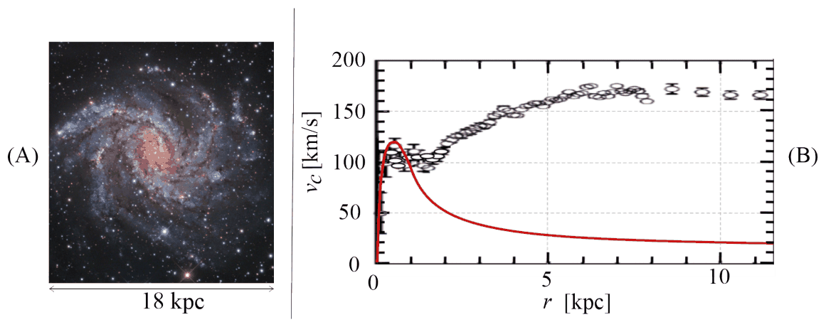
Fig. 1: NGC 6946 galaxy: Picture (A) and rotation curve (B).
B.2 — 0.5pt
Deduce the mass \(M_b\) of the bulge of NGC 6946 from the red rotation curve in Fig. 1(B), in solar mass units.
Comparing the keplerian model and the experimental data makes astronomers confident that part of the mass is invisible in the picture. They thus suppose that the galaxy's actual mass density is given by
\[ \rho_m(r)=\frac{C_m}{r_m^2+r^2} \tag{1} \]
where \(C_m>0\) and \(r_m>0\) are constants.
B.3 — 1.8pt
Show that the velocity profile \(v_{c,m}(r)\), corresponding to the mass density in Eq. 1, can be written \[ v_{c,m}(r)=\sqrt{k_1-\frac{k_2\cdot\arctan\!\left(\frac r{r_m}\right)}r}. \] Express \(k_1\) and \(k_2\) in terms of \(C_m\), \(r_m\) and \(G\).
(Hints: \(\displaystyle\int_0^r\frac{x^2}{a^2+x^2}\,dx=r-a\arctan(r/a)\), and: \(\arctan(x)\simeq x-x^3/3\) for \(x\ll1\).)
Simplify \(v_{c,m}(r)\) when \(r\ll r_m\) and when \(r\gg r_m\).
Show that if \(r\gg r_m\), the mass \(M_m(r)\) embedded in a sphere of radius \(r\) with the mass density given by Eq. 1 simplifies and depends only on \(C_m\) and \(r\).
Estimate the mass of the galaxy NGC 6946 actually present in the picture in Fig. 1(A).
Part C - Mass distribution in our galaxy
For a spiral galaxy, the model for Eq. 1 is modified and one usually considers the gravitational potential is given by \[ \varphi_G(r,z)=\varphi_0\ln\!\left(\frac r{r_0}\right) \exp\!\left[-\left(\frac z{z_0}\right)^2\right], \] where \(z\) is the distance to the galactic plane (defined by \(z=0\)), and \(r<r_0\) is now the axial radius and \(\varphi_0>0\) a constant to be determined. \(r_0\) and \(z_0\) are constant values.
C.1 — 0.5pt
Find the equation of motion on \(z\) for the vertical motion of a point mass \(m\) in such a potential, assuming \(r\) is constant. Show that, if \(r<r_0\) the galactic plane is a stable equilibrium state by giving the angular frequency \(\omega_0\) of small oscillations around it.
From here on, we set \(z=0\).
C.2 — 0.6pt
Identify the regime, either \(r\gg r_m\) or \(r\ll r_m\), in which the model of Eq. 1 recovers a potential of the form \(\varphi_G(r,0)\) with a suitable definition of \(\varphi_0\).
Under this condition \(v_c(r)\) no longer depends on \(r\). Express it in terms of \(\varphi_0\).
Therefore, outside the bulge the velocity modulus \(v_c\) does not depend on the distance to the galactic center. We will use this fact, as astronomers do, to measure the galaxy's mass distribution from the inside.
All galactic objects considered here for astronomical observations, such as stars or nebulae, are primarily composed of hydrogen. Outside the bulge, we assume that they rotate on circular orbits around the galactic center \(C\). \(S\) is the sun's position and \(E\) that of a given galactic object emitting in the hydrogen spectrum. In the galactic plane, we consider a line of sight \(SE\) corresponding to the orientation of an observation, on the unit vector \(\hat u_v\) (see Fig. 2).
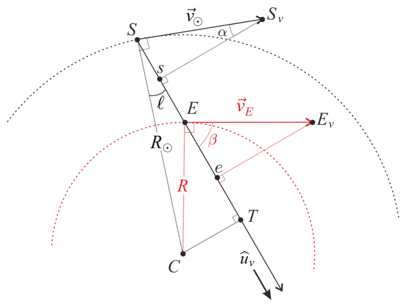
Fig. 2: Geometry of the measurement
Let \(\ell\) be the galactic longitude, measuring the angle between \(SC\) and the \(SE\). The sun's velocity on its circular orbit of radius \(R_\odot=8.00\,\mathrm{kpc}\) is denoted \(\vec v_\odot\). A galactic object in \(E\) orbits on another circle of radius \(R\) at velocity \(\vec v_E\). Using a Doppler effect on the previously studied 21cm line, one can obtain the relative radial velocity \(v_{rE/S}\) of the emitter \(E\) with respect to the sun \(S\): it is the projection of \(\vec v_E-\vec v_\odot\) on the line of sight.
C.3 — 0.7pt
Determine \(v_{rE/S}\) in terms of \(\ell\), \(R\), \(R_\odot\) and \(v_\odot\). Then, express \(R\) in terms of \(R_\odot\), \(v_\odot\), \(\ell\) and \(v_{rE/S}\).
Using a radio telescope, we make observations in the plane of our galaxy toward a longitude \(\ell=30^\circ\). The frequency band used contains the 21cm line, whose frequency is \(f_0=1.42\,\mathrm{GHz}\). The results are reported in Fig. 3.
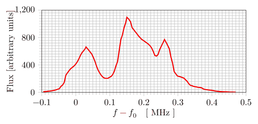
Fig. 3: Electromagnetic signal as a function of the frequency shift, measured in the radio frequency band at \(\ell=30^\circ\) using EU-HOU RadioAstronomy
C.4 — 0.6pt
In our galaxy, \(v_\odot=220\,\mathrm{km\cdot s^{-1}}\). Determine the values of the relative radial velocity (with 3 significant digits) and the distance from the galactic center (with 2 significant digits) of the 3 sources observed in Fig. 3. Distances should be expressed as multiples of \(R_\odot\).
C.5 — 0.6pt
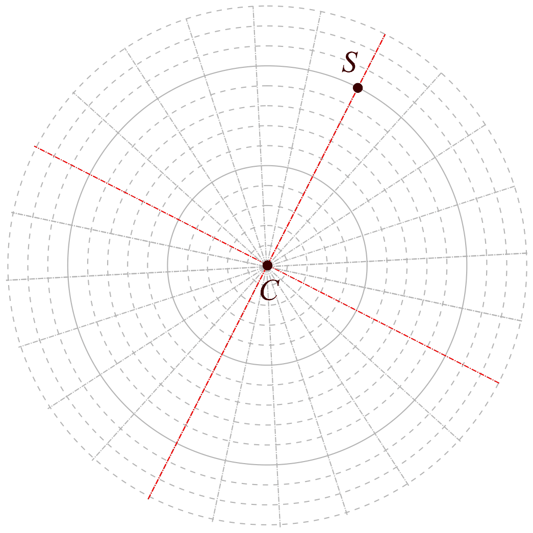
On the top view of our galaxy (in the answer box), indicate the positions of the sources observed in Fig. 3.
What could be deduced from repeated measurements changing \(\ell\)?
Part D - Tully-Fisher relation and MOND theory
The flat external velocity curve of NGC 6946 in Fig. 1 is a common property of spiral galaxies, as can be seen in Fig. 4 (left). Plotting the external constant velocity value \(v_{c,\infty}\) as a function of the measured total mass \(M_{\mathrm{tot}}\) of each galaxy gives an interesting correlation called the Tully-Fischer relation, see Fig. 4 (right).
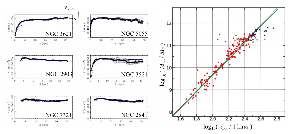
Fig. 4. Left: Rotation curves for typical spiral galaxies - Right: \(\log_{10}(M_{\mathrm{tot}})\) as a function of \(\log_{10}(v_{c,\infty})\) on linear scales. Colored dots correspond to different galaxies and different surveys. The green line is the Tully-Fischer relation which is in very good agreement with the best fit line of the data (in black).
D.1 — 0.4pt
Assuming that the radius \(R\) of a galaxy doesn't depend on its mass, show that the model of Eq. 1 (part B) gives a relation of the form \(M_{\mathrm{tot}}=\eta v_{c,\infty}^{\gamma}\) where \(\gamma\) and \(\eta\) should be specified.
Compare this expression to the Tully-Fischer relation by computing \(\gamma_{TF}\).
In the extremely low acceleration regime, of the order of \(a_0=10^{-10}\,\mathrm{m\cdot s^{-2}}\), the MOdified Newtonian Dynamics (MOND) theory suggests that one can modify Newton's second law using \[ \vec F=m\mu\!\left(\frac a{a_0}\right)\vec a \] where \(a=\|\vec a\|\) is the modulus of the acceleration and the \(\mu\) function is defined by \(\mu(x)=\dfrac{x}{1+x}\).
D.2 — 0.2pt
Using data for NGC 6946 in Fig. 1, estimate, within Newton's theory, the modulus of the acceleration \(a_m\) of a mass in the outer regions of NGC 6946.
D.3 — 0.8pt
Let \(m\) be a mass on a circular orbit of radius \(r\) with velocity \(v_{c,\infty}\) in the gravity field of a fixed mass \(M\).
Within the MOND theory, with \(a\ll a_0\), determine the Tully-Fischer exponent.
Using data for NGC 6946 and/or Tully-Fischer law, calculate \(a_0\) to show that MOND operates in the correct regime.
D.4 — 0.9pt
Considering relevant cases, determine \(v_c(r)\) for all values of \(r\) in the MOND theory in the case of a gravitational field due to a homogeneously distributed mass \(M\) with radius \(R_b\).
General Data Sheet
| Constant | Notation | Value | Unit |
|---|---|---|---|
| Speed of light in vacuum | \(c\) | \(2.997\,924\,58\times10^8\) | \(\mathrm{m\cdot s^{-1}}\) |
| Planck constant | \(h\) | \(6.626\,070\,15\times10^{-34}\) | \(\mathrm{kg\cdot m^2\cdot s^{-1}}\) |
| Reduced Planck constant | \(\hbar=\dfrac h{2\pi}\) | \(1.054\,571\,818\times10^{-34}\) | \(\mathrm{kg\cdot m^2\cdot s^{-1}}\) |
| Boltzmann constant | \(k_{\mathrm B}\) | \(1.380\,649\times10^{-23}\) | \(\mathrm{kg\cdot m^2\cdot s^{-2}\cdot K^{-1}}\) |
| Avogadro constant | \(N_{\mathrm A}\) | \(6.022\,140\,76\times10^{23}\) | \(\mathrm{mol^{-1}}\) |
| Molar gas constant | \(R\) | \(8.314\,462\,618\,153\,24\) | \(\mathrm{kg\cdot m^2\cdot s^{-2}\cdot mol^{-1}\cdot K^{-1}}\) |
| Elementary charge | \(e\) | \(1.602\,176\,634\times10^{-19}\) | \(\mathrm{A\cdot s}\) |
| Universal constant of gravitation | \(G\) | \(6.674\,30(15)\times10^{-11}\) | \(\mathrm{m^3\cdot kg^{-1}\cdot s^{-2}}\) |
| Standard acceleration due to gravity | \(g\) | \(9.806\,65\) | \(\mathrm{m\cdot s^{-2}}\) |
| Stefan Boltzmann constant | \(\sigma\) | \(5.670\,374\,419\times10^{-8}\) | \(\mathrm{kg\cdot s^{-3}\cdot K^{-4}}\) |
| Vacuum permeability (magnetic constant) | \(\mu_0\) | \(1.256\,637\,061\,27(20)\times10^{-6}\) | \(\mathrm{kg\cdot m\cdot A^{-2}\cdot s^{-2}}\) |
| Vacuum permittivity (electrical constant) | \(\epsilon_0\) | \(8.854\,187\,818\,8(14)\times10^{-12}\) | \(\mathrm{A^2\cdot s^4\cdot kg^{-1}\cdot m^{-3}}\) |
| Rydberg constant | \(R_\infty\) | \(1.097\,373\,156\,815\,7(12)\times10^7\) | \(\mathrm{m^{-1}}\) |
| Mass of the electron | \(m_e\) | \(9.109\,383\,713\,9(28)\times10^{-31}\) | \(\mathrm{kg}\) |
| Mass of the proton | \(m_p\) | \(1.672\,621\,925\,95(52)\times10^{-27}\) | \(\mathrm{kg}\) |
| Mass of the neutron | \(m_n\) | \(1.674\,927\,500\,56(85)\times10^{-27}\) | \(\mathrm{kg}\) |
| Atomic mass constant | \(m_u\) | \(1.660\,539\,068\,92(52)\times10^{-27}\) | \(\mathrm{kg}\) |
| Electronvolt | \(\mathrm{eV}\) | \(1.602\,176\,634\times10^{-19}\) | \(\mathrm{kg\cdot m^2\cdot s^{-2}}\) |
Official English text of the problem.
Answers
-
A.1 \[ \boxed{v=\sqrt{\frac{e^2}{4\pi\varepsilon_0m_er}}}. \]
-
A.2 \[ \boxed{r_n=n^2r_1,\qquad r_1=\frac{\hbar}{m_e\alpha c}=5.29\times10^{-11}\,\mathrm m,\qquad v_1=\alpha c}. \]
-
A.3 \[ \boxed{E_n=-\frac{e^2}{8\pi\varepsilon_0r_1n^2},\qquad E_1=-\frac12m_e\alpha^2c^2=-13.6\,\mathrm{eV}}. \]
-
A.4 \[ \boxed{B_1=\frac{\mu_0e\alpha c}{4\pi r_1^2}}. \]
-
A.5 \[ \boxed{\Delta E_{\mathrm F}=-4\alpha^2E_1}, \qquad \boxed{\lambda_{\mathrm{HF}} =\frac{\pi m_p\hbar}{3.72\,m_e^2\alpha^4c} \simeq0.21\,\mathrm m}. \]
-
B.1 \[ \boxed{v_c=\sqrt{r\frac{d\varphi}{dr}}}. \]
-
B.2 \[ \boxed{M_b\sim1\times10^9\,M_\odot}. \]
-
B.3 \[ \boxed{k_1=4\pi GC_m,\qquad k_2=4\pi GC_mr_m}, \] \[ \boxed{v_{c,m}(r\ll r_m)\simeq \sqrt{\frac{4\pi GC_m}{3}}\frac r{r_m}}, \qquad \boxed{v_{c,m}(r\gg r_m)\simeq\sqrt{4\pi GC_m}}, \] \[ \boxed{M_m(r\gg r_m)\simeq4\pi C_mr,\qquad M_{\text{in the figure}}\simeq6.1\times10^{10}\,M_\odot}. \]
-
C.1 \[ \boxed{\ddot z= \frac{2\varphi_0}{z_0^2}\ln\!\left(\frac r{r_0}\right) z\,e^{-z^2/z_0^2}}, \qquad \boxed{\omega_0= \sqrt{\frac{2\varphi_0}{z_0^2}\ln\!\left(\frac{r_0}r\right)}}. \]
-
C.2 \[ \boxed{r\gg r_m,\qquad \varphi_0=4\pi GC_m,\qquad v_c(r)=\sqrt{\varphi_0}}. \]
-
C.3 \[ \boxed{v_{rE/S}=v_\odot\left(\frac{R_\odot}{R}-1\right)\sin\ell}, \qquad \boxed{R=\frac{R_\odot v_\odot\sin\ell} {v_\odot\sin\ell+v_{rE/S}}}. \]
-
C.4 Numbering the peaks by increasing frequency shift: \[ \boxed{(v_{r,1},v_{r,2},v_{r,3}) =(6.33,\ 31.7,\ 54.9)\,\mathrm{km\,s^{-1}}}, \] \[ \boxed{(R_1,R_2,R_3)=(0.95,\ 0.78,\ 0.67)\,R_\odot}. \]
-
C.5 On the \(\ell=30^\circ\) sightline, mark both intersections with each of the three circles of radii \(0.95R_\odot\), \(0.78R_\odot\), and \(0.67R_\odot\). The near and far distances from the Sun are \[ \boxed{\frac{(d_{1,-},d_{2,-},d_{3,-})}{R_\odot} \simeq(0.0635,\ 0.272,\ 0.424)}, \] \[ \boxed{\frac{(d_{1,+},d_{2,+},d_{3,+})}{R_\odot} \simeq(1.67,\ 1.46,\ 1.31)}. \] Repeated longitude scans reveal the hydrogen distribution and spiral structure, subject to this near–far ambiguity.
-
D.1 \[ \boxed{\eta=\frac RG,\qquad \gamma=2,\qquad \gamma_{TF}\approx3.7\ \text{(graphically close to }4\text{)}}. \]
-
D.2 \[ \boxed{a_m\simeq9.4\times10^{-11}\,\mathrm{m\,s^{-2}}}. \]
-
D.3 \[ \boxed{v_{c,\infty}^4=GMa_0,\qquad \gamma_{\mathrm{MOND}}=4,\qquad a_0\sim2\times10^{-10}\,\mathrm{m\,s^{-2}}}. \] This is the relevant acceleration scale; the plotted NGC 6946 data alone do not establish the stronger inequality \(a\ll a_0\).
-
D.4 \[ \boxed{ v_c(r)= \begin{cases} \displaystyle \left[ \frac{GMr^2}{2R_b^3} \left(1+\sqrt{1+\frac{4a_0R_b^3}{GMr}}\right) \right]^{1/2},&0<r\le R_b,\\[1.2em] \displaystyle \left[ \frac{GM}{2r} \left(1+\sqrt{1+\frac{4a_0r^2}{GM}}\right) \right]^{1/2},&r\ge R_b . \end{cases}} \] The continuous limit is \(v_c(0)=0\).
Solution
For the atomic numerical values, I evaluate \(\alpha\) from its defining expression and the supplied constants: \[ \alpha=\frac{e^2}{4\pi\varepsilon_0\hbar c} =7.29735\times10^{-3}. \] This differs slightly from the approximation printed in the statement.
A.1
The attractive Coulomb force supplies the centripetal force: \[ \frac{m_ev^2}{r}=\frac{e^2}{4\pi\varepsilon_0r^2}. \] Therefore, \[ \boxed{v=\sqrt{\frac{e^2}{4\pi\varepsilon_0m_er}}}. \]
A.2
Bohr quantization gives \[ m_ev_nr_n=n\hbar. \] Squaring this and using the force balance from A.1, \[ n^2\hbar^2 =m_e^2v_n^2r_n^2 =\frac{m_ee^2r_n}{4\pi\varepsilon_0}. \] Consequently, \[ r_n=\frac{4\pi\varepsilon_0n^2\hbar^2}{m_ee^2} =n^2\frac{\hbar}{m_e\alpha c}. \] Thus \[ \boxed{r_1=\frac{\hbar}{m_e\alpha c} =5.29\times10^{-11}\,\mathrm m}. \]
For the ground orbit, \[ v_1=\frac{\hbar}{m_er_1}=\boxed{\alpha c}. \] More generally, \(v_n=\alpha c/n\). Since \(\alpha\ll1\), the non-relativistic approximation is consistent.
A.3
Taking the electrostatic potential energy to vanish at infinity, \[ U(r)=-\frac{e^2}{4\pi\varepsilon_0r}. \] The force balance gives \[ K=\frac12m_ev^2=\frac{e^2}{8\pi\varepsilon_0r}. \] Hence the total mechanical energy is \[ E=K+U=-\frac{e^2}{8\pi\varepsilon_0r}. \] At \(r_n=n^2r_1\), \[ \boxed{E_n=-\frac{e^2}{8\pi\varepsilon_0r_1n^2}}. \] In particular, \[ E_1=-\frac{\alpha\hbar c}{2r_1} =\boxed{-\frac12m_e\alpha^2c^2}. \] Numerically, \[ E_1=-2.17987\times10^{-18}\,\mathrm J =\boxed{-13.6\,\mathrm{eV}}. \]
A.4
In the prescribed electron-frame picture, the proton circulates with speed \(v_1=\alpha c\). Its orbital period and equivalent current are \[ T=\frac{2\pi r_1}{v_1}, \qquad I=\frac eT=\frac{ev_1}{2\pi r_1}. \] The magnetic field at the centre of a circular current loop is \[ B_1=\frac{\mu_0I}{2r_1}. \] Therefore, \[ \boxed{B_1=\frac{\mu_0e\alpha c}{4\pi r_1^2}}. \]
A.5
A magnetic dipole in a field has energy \[ U=-\vec{\mathcal M}_s\cdot\vec B_1. \] The parallel and anti-parallel states consequently have energies \(-\mathcal M_sB_1\) and \(+\mathcal M_sB_1\). Their positive energy separation is \[ \Delta E_{\mathrm F}=2\mathcal M_sB_1. \] Using the magnetic moment specified in the problem, \[ \Delta E_{\mathrm F} =2\frac{e\hbar}{m_e}\frac{\mu_0e\alpha c}{4\pi r_1^2}. \] With \(\mu_0\varepsilon_0c^2=1\) and \(e^2/(4\pi\varepsilon_0)=\alpha\hbar c\), \[ \Delta E_{\mathrm F} =\frac{2\alpha^2\hbar^2}{m_er_1^2} =2m_e\alpha^4c^2. \] Since \(E_1=-m_e\alpha^2c^2/2\), \[ \boxed{\Delta E_{\mathrm F}=-4\alpha^2E_1}. \]
The hyperfine photon satisfies \[ \frac{2\pi\hbar c}{\lambda_{\mathrm{HF}}} =\Delta E_{\mathrm{HF}} \simeq3.72\frac{m_e}{m_p}\Delta E_{\mathrm F}. \] Thus \[ \boxed{\lambda_{\mathrm{HF}} =\frac{\pi m_p\hbar}{3.72\,m_e^2\alpha^4c}}. \] The numerical intermediate values are \[ \Delta E_{\mathrm F}\simeq2.898\times10^{-3}\,\mathrm{eV}, \qquad \lambda_{\mathrm{HF}}\simeq0.21116\,\mathrm m. \] To two significant digits, \[ \boxed{\lambda_{\mathrm{HF}}=0.21\,\mathrm m=21\,\mathrm{cm}}. \]
B.1
The gravitational acceleration is \[ \vec g=-\frac{d\varphi}{dr}\hat r. \] Equating this to the inward acceleration of a circular orbit, \[ -\frac{v_c^2}{r}\hat r=-\frac{d\varphi}{dr}\hat r. \] Therefore, \[ \boxed{v_c=\sqrt{r\frac{d\varphi}{dr}}}. \]
B.2
Outside a spherical bulge, the shell theorem gives \[ \varphi(r)=-\frac{GM_b}{r}+\text{constant}. \] It follows that \[ v_c^2=\frac{GM_b}{r}, \qquad M_b=\frac{rv_c^2}{G}. \]
A convenient approximate reading of the red curve is \[ r\simeq10\,\mathrm{kpc}, \qquad v_c\simeq20\,\mathrm{km\,s^{-1}}. \] Hence \[ M_b\simeq \frac{(10\times3.09\times10^{19})(2.0\times10^4)^2} {6.67430\times10^{-11}} =1.85\times10^{39}\,\mathrm{kg}. \] In solar units this is approximately \(9.3\times10^8M_\odot\). Given the graphical precision, \[ \boxed{M_b\sim10^9M_\odot}. \]
B.3
The mass enclosed within radius \(r\) is \[ M_m(r)=4\pi\int_0^r\rho_m(x)x^2\,dx =4\pi C_m\int_0^r\frac{x^2}{r_m^2+x^2}\,dx. \] Applying the supplied integral, \[ \boxed{M_m(r)=4\pi C_m \left[r-r_m\arctan\!\left(\frac r{r_m}\right)\right]}. \]
By spherical symmetry, \[ v_{c,m}^2(r)=\frac{GM_m(r)}r =4\pi GC_m \left[1-\frac{r_m}{r}\arctan\!\left(\frac r{r_m}\right)\right]. \] Comparison with the requested form gives \[ \boxed{k_1=4\pi GC_m,\qquad k_2=4\pi GC_mr_m}. \]
For \(r\ll r_m\), set \(x=r/r_m\). Then \[ 1-\frac{\arctan x}{x} \simeq1-\frac{x-x^3/3}{x} =\frac{x^2}{3}. \] Therefore, \[ \boxed{v_{c,m}(r)\simeq \sqrt{\frac{4\pi GC_m}{3}}\frac r{r_m}}. \] The central rotation curve rises linearly, as expected for approximately uniform density.
For \(r\gg r_m\), \(\arctan(r/r_m)\to\pi/2\), while \(r_m/r\to0\). Thus \[ \boxed{v_{c,m}(r)\simeq\sqrt{4\pi GC_m} \equiv v_{c,\infty}}, \] and \[ \boxed{M_m(r)\simeq4\pi C_mr =\frac{v_{c,\infty}^2r}{G}}. \]
The pictured diameter is approximately \(18\,\mathrm{kpc}\), so take the enclosing radius as \(9\,\mathrm{kpc}\). The observed outer speed is approximately \(170\,\mathrm{km\,s^{-1}}\). Hence \[ M_{\text{in the figure}} \simeq \frac{(1.70\times10^5)^2(9\times3.09\times10^{19})} {6.67430\times10^{-11}} \simeq1.20\times10^{41}\,\mathrm{kg}. \] Therefore, \[ \boxed{M_{\text{in the figure}}\simeq6.1\times10^{10}M_\odot}. \]
C.1
For fixed \(r\), the vertical equation of motion is \[ m\ddot z=-m\frac{\partial\varphi_G}{\partial z}. \] Differentiating the prescribed potential gives \[ \boxed{\ddot z= \frac{2\varphi_0}{z_0^2}\ln\!\left(\frac r{r_0}\right) z\,e^{-z^2/z_0^2}}. \]
At \(z=0\), the force vanishes. For small oscillations, \(|z|\ll z_0\), so \[ e^{-z^2/z_0^2}\simeq1. \] The linearized equation becomes \[ \ddot z+ \frac{2\varphi_0}{z_0^2}\ln\!\left(\frac{r_0}r\right)z=0. \] For \(r<r_0\), its coefficient is positive. Thus the plane is a stable equilibrium, with \[ \boxed{\omega_0= \sqrt{\frac{2\varphi_0}{z_0^2} \ln\!\left(\frac{r_0}r\right)}}. \]
C.2
For \(r\gg r_m\), B.3 gives \[ M_m(r)\simeq4\pi C_mr. \] The radial potential gradient is therefore \[ \frac{d\varphi}{dr}=\frac{GM_m(r)}{r^2} \simeq\frac{4\pi GC_m}{r}. \] Integrating and choosing the additive constant appropriately, \[ \varphi(r)\simeq4\pi GC_m\ln\!\left(\frac r{r_0}\right). \] Thus the required regime and coefficient are \[ \boxed{r\gg r_m,\qquad \varphi_0=4\pi GC_m}. \]
In the plane, \[ v_c^2=r\frac{\partial\varphi_G(r,0)}{\partial r} =r\frac{\varphi_0}{r}=\varphi_0, \] so \[ \boxed{v_c(r)=\sqrt{\varphi_0}}. \]
C.3
Let \(T\) be the foot of the perpendicular from \(C\) to the line of sight. The geometry gives \[ CT=R_\odot\sin\ell. \] The Sun's tangential velocity projects onto the sightline as \[ \vec v_\odot\cdot\hat u_v=v_\odot\sin\ell. \]
For the emitter, its tangential velocity is perpendicular to \(CE\). Its projection onto the sightline is \[ \vec v_E\cdot\hat u_v=v_E\frac{CT}{R} =v_E\frac{R_\odot}{R}\sin\ell. \] The flat rotation curve implies \(v_E=v_\odot\). Consequently, \[ v_{rE/S} =(\vec v_E-\vec v_\odot)\cdot\hat u_v =\boxed{v_\odot\left(\frac{R_\odot}{R}-1\right)\sin\ell}. \] Solving for \(R\), \[ \boxed{R=\frac{R_\odot v_\odot\sin\ell} {v_\odot\sin\ell+v_{rE/S}}}. \]
C.4
Following the intended convention, which is consistent with the answer sheet, use \[ v_r=+c\frac{f-f_0}{f_0}, \] with positive values denoting recession. The printed \(f-f_0\) axis therefore has the opposite sign from the usual frequency shift for positive recession.
The three peaks occur approximately at \[ \Delta f_1=0.030\,\mathrm{MHz},\qquad \Delta f_2=0.150\,\mathrm{MHz},\qquad \Delta f_3=0.260\,\mathrm{MHz}. \] Since \[ v_\odot\sin\ell =220\sin30^\circ =110\,\mathrm{km\,s^{-1}}, \] the radius formula becomes \[ \frac R{R_\odot}=\frac{110}{110+v_r}, \] where \(v_r\) is expressed in \(\mathrm{km\,s^{-1}}\).
| Source, in increasing peak frequency | \(\Delta f\) (\(\mathrm{MHz}\)) | \(v_r\) (\(\mathrm{km\,s^{-1}}\)), 3 significant digits | \(R/R_\odot\), 2 significant digits |
|---|---|---|---|
| 1 | \(0.030\) | \(+6.33\) | \(0.95\) |
| 2 | \(0.150\) | \(+31.7\) | \(0.78\) |
| 3 | \(0.260\) | \(+54.9\) | \(0.67\) |
C.5
On the answer-sheet diagram, draw the observation ray from \(S\), making \(30^\circ\) with \(SC\) on the side indicated by Fig. 2. Draw, or identify, the circles centred at \(C\) with radii \[ 0.95R_\odot,\qquad0.78R_\odot,\qquad0.67R_\odot. \] Each circle intersects the observation ray twice.
To specify the positions quantitatively, let \(d=SE\). The cosine rule gives \[ R^2=R_\odot^2+d^2-2R_\odot d\cos\ell. \] Thus \[ \boxed{d_\pm= R_\odot\cos\ell \pm\sqrt{R^2-R_\odot^2\sin^2\ell}}. \] At \(\ell=30^\circ\), the sightline's closest approach to the centre is \[ CT=0.50R_\odot, \qquad ST=R_\odot\cos30^\circ=0.866R_\odot. \] All three inferred radii exceed \(CT\) and are smaller than \(R_\odot\), so both intersections lie forward of the Sun.
Using the unrounded radii from C.4:
| Source | Near position \(d_-/R_\odot\) | Far position \(d_+/R_\odot\) |
|---|---|---|
| 1 | \(0.0635\) | \(1.67\) |
| 2 | \(0.272\) | \(1.46\) |
| 3 | \(0.424\) | \(1.31\) |
Moving away from \(S\) along the ray, the candidate points occur in the order \[ 1_{\rm near},\quad2_{\rm near},\quad3_{\rm near}, \quad T,\quad 3_{\rm far},\quad2_{\rm far},\quad1_{\rm far}. \]
The spectrum determines the galactocentric radius of each source but cannot distinguish its near and far positions. Repeating the observations at different longitudes maps hydrogen-rich structures and reveals the galaxy's spiral arms; additional information is needed to resolve individual near–far ambiguities.
D.1
In the outer regime of B.3, \[ M_{\mathrm{tot}}\simeq4\pi C_mR, \qquad v_{c,\infty}^2=4\pi GC_m. \] Eliminating \(C_m\), \[ M_{\mathrm{tot}}\simeq\frac RGv_{c,\infty}^2. \] For a mass-independent radius, \[ \boxed{\eta=\frac RG,\qquad\gamma=2}. \]
For an empirical power law, taking logarithms gives \[ \log_{10}\!\left(\frac{M_{\mathrm{tot}}}{M_\odot}\right) =\gamma_{TF} \log_{10}\!\left(\frac{v_{c,\infty}}{1\,\mathrm{km\,s^{-1}}}\right) +\text{constant}. \] Thus \(\gamma_{TF}\) is the slope in Fig. 4.
Approximate readings of the green line are \[ (x,y)\simeq(1.6,8.2),\qquad(2.8,12.6). \] They give \[ \boxed{\gamma_{TF}\simeq \frac{12.6-8.2}{2.8-1.6}\simeq3.7}. \] The observed scaling is close to a fourth-power law and substantially steeper than the second-power prediction of the fixed-radius Newtonian model.
D.2
The magnitude of the acceleration in a circular orbit is \[ a_m=\frac{v_c^2}{r}. \] Using an outer observed point, \[ v_c\simeq170\,\mathrm{km\,s^{-1}}, \qquad r\simeq10\,\mathrm{kpc}, \] gives \[ a_m\simeq \frac{(1.70\times10^5)^2} {10\times3.09\times10^{19}} =\boxed{9.4\times10^{-11}\,\mathrm{m\,s^{-2}}}. \]
D.3
In the deep-MOND limit \(a\ll a_0\), \[ \mu\!\left(\frac a{a_0}\right) =\frac{a/a_0}{1+a/a_0} \simeq\frac a{a_0}. \] The modified equation of motion in the Newtonian gravitational field of \(M\) becomes \[ \frac{GMm}{r^2}\simeq m\frac{a^2}{a_0}. \] For a circular orbit, \(a=v_{c,\infty}^2/r\), so \[ \frac{GM}{r^2} =\frac{v_{c,\infty}^4}{a_0r^2}. \] The radius cancels: \[ \boxed{v_{c,\infty}^4=GMa_0}. \] Consequently, \[ M=\frac1{Ga_0}v_{c,\infty}^4, \qquad \boxed{\gamma_{\mathrm{MOND}}=4}. \] This also explains why the asymptotic circular speed is independent of radius.
For a graphical estimate of \(a_0\), Fig. 4 gives approximately \[ v_{c,\infty}\simeq100\,\mathrm{km\,s^{-1}}, \qquad M\simeq4\times10^9M_\odot. \] Therefore, \[ a_0\simeq \frac{(1.0\times10^5)^4} {(6.67430\times10^{-11})(4\times10^9)(1.99\times10^{30})} \simeq1.9\times10^{-10}\,\mathrm{m\,s^{-2}}. \] At the precision of the plot, \[ \boxed{a_0\sim2\times10^{-10}\,\mathrm{m\,s^{-2}}}. \]
This is of the stated order \(10^{-10}\,\mathrm{m\,s^{-2}}\). Comparing with D.2 gives \(a_m/a_0\sim0.5\): the displayed outer-galaxy data probe the MOND acceleration scale, but do not establish \(a_m\ll a_0\).
For an asymptotically flat speed of \(170\,\mathrm{km\,s^{-1}}\), the strict deep-MOND condition is \[ r\gg\frac{v_{c,\infty}^2}{a_0}\sim5\,\mathrm{kpc}. \] It becomes increasingly accurate farther out. Near the transition, the full interpolation function must be used, as in D.4.
D.4
The homogeneous sphere has density \[ \rho=\frac{3M}{4\pi R_b^3}. \] Its enclosed mass is \[ M(<r)= \begin{cases} M(r/R_b)^3,&r\le R_b,\\ M,&r\ge R_b. \end{cases} \] The gravitational force remains Newtonian in the modified-second-law formulation specified in the problem. Define its magnitude per unit test mass as \[ g_N(r)=\frac{GM(<r)}{r^2} = \begin{cases} \dfrac{GMr}{R_b^3},&r\le R_b,\\[0.5em] \dfrac{GM}{r^2},&r\ge R_b. \end{cases} \]
Using the full interpolation function, \[ g_N=\mu\!\left(\frac a{a_0}\right)a =\frac{a^2}{a+a_0}. \] Hence \[ a^2-g_Na-g_Na_0=0. \] The physical, non-negative root is \[ a=\frac{g_N+\sqrt{g_N^2+4a_0g_N}}2. \] Since \(v_c^2=ra\), \[ v_c(r)= \left[\frac r2 \left(g_N+\sqrt{g_N^2+4a_0g_N}\right)\right]^{1/2}. \]
Substitution gives the expression valid throughout both regions: \[ \boxed{ v_c(r)= \begin{cases} \displaystyle \left[ \frac{GMr^2}{2R_b^3} \left(1+\sqrt{1+\frac{4a_0R_b^3}{GMr}}\right) \right]^{1/2}, &0<r\le R_b,\\[1.2em] \displaystyle \left[ \frac{GM}{2r} \left(1+\sqrt{1+\frac{4a_0r^2}{GM}}\right) \right]^{1/2}, &r\ge R_b. \end{cases}} \] The two expressions agree at \(r=R_b\), and the limit at the centre is \(v_c(0)=0\).
The limiting cases clarify the shape of the rotation curve:
| Region | Acceleration regime | Circular speed |
|---|---|---|
| Inside, \(r<R_b\) | \(g_N\gg a_0\) | \(\displaystyle v_c\simeq\sqrt{\frac{GM}{R_b^3}}\,r\) |
| Inside, \(r<R_b\) | \(g_N\ll a_0\) | \(\displaystyle v_c\simeq\left(\frac{GMa_0}{R_b^3}\right)^{1/4}r^{3/4}\) |
| Outside, \(r>R_b\) | \(g_N\gg a_0\) | \(\displaystyle v_c\simeq\sqrt{\frac{GM}{r}}\) |
| Outside, \(r>R_b\) | \(g_N\ll a_0\) | \(\displaystyle v_c\simeq(GMa_0)^{1/4}\) |
Thus the curve starts at zero, behaves as \(r^{3/4}\) sufficiently close to the centre, and approaches a constant far outside. Newtonian intermediate regions occur only if the sphere's surface acceleration \(GM/R_b^2\) is sufficiently larger than \(a_0\).
The solution was checked against the official solution. Where this solution differs from the official solution, the official solution contains an error or a misprint.
IPhO 2025 · Theorieaufgabe 1
Wasserstoff und Galaxien
Diese Aufgabe untersucht die besonderen physikalischen Eigenschaften von Galaxien, etwa ihre Dynamik und Struktur. Insbesondere erläutern wir, wie sich die Massenverteilung unserer Galaxie von innen heraus messen lässt. Dazu konzentrieren wir uns auf Wasserstoff, ihren Hauptbestandteil.
In dieser gesamten Aufgabe verwenden wir ausschließlich \(\hbar\), definiert durch \(\hbar=h/2\pi\).
Teil A - Einführung
Bohrsches Atommodell
Wir nehmen an, dass das Wasserstoffatom aus einem nichtrelativistischen Elektron der Masse \(m_e\) besteht, das ein ortsfestes Proton umkreist. In diesem gesamten Teil nehmen wir an, dass es sich auf einer Kreisbahn bewegt.
A.1 — 0.2 Punkte
Bestimmen Sie die Geschwindigkeit \(v\) des Elektrons auf einer Kreisbahn mit Radius \(r\).
Im Bohrschen Atommodell nehmen wir an, dass der Betrag des Drehimpulses \(L\) des Elektrons quantisiert ist: \(L=n\hbar\), wobei \(n>0\) eine ganze Zahl ist. Wir definieren \(\alpha=\dfrac{e^2}{4\pi\varepsilon_0\hbar c}\approx7.27\times10^{-3}\).
A.2 — 0.5 Punkte
Zeigen Sie, dass der Radius jeder Bahn durch \(r_n=n^2r_1\) gegeben ist, wobei \(r_1\) als Bohrscher Radius bezeichnet wird. Drücken Sie \(r_1\) durch \(\alpha\), \(m_e\), \(c\) und \(\hbar\) aus und berechnen Sie seinen Zahlenwert mit 3 signifikanten Stellen. Drücken Sie \(v_1\), die Geschwindigkeit auf der Bahn mit Radius \(r_1\), durch \(\alpha\) und \(c\) aus.
A.3 — 0.5 Punkte
Bestimmen Sie die mechanische Energie \(E_n\) des Elektrons auf einer Bahn mit Radius \(r_n\) in Abhängigkeit von \(e\), \(\varepsilon_0\), \(r_1\) und \(n\). Bestimmen Sie \(E_1\) im Grundzustand in Abhängigkeit von \(\alpha\), \(m_e\) und \(c\). Berechnen Sie ihren Zahlenwert in eV.
Fein- und Hyperfeinstruktur des Wasserstoffs
Die seltene spontane Umkehr des Elektronenspins führt dazu, dass pro Wasserstoffatom im Mittel einmal in 10 Millionen Jahren ein Photon emittiert wird. Diese Emission dient als Nachweis für Wasserstoff im Universum und ist daher von grundlegender Bedeutung für die Astrophysik. Wir untersuchen den für diese Emission verantwortlichen Übergang in zwei Schritten.
Betrachten Sie zunächst die Wechselwirkung zwischen dem Elektronenspin und der Relativbewegung von Elektron und Proton. Im Bezugssystem des Elektrons umkreist das Proton das Elektron im Abstand \(r_1\). Dadurch entsteht ein Magnetfeld \(\vec B_1\).
A.4 — 0.5 Punkte
Bestimmen Sie den Betrag \(B_1\) von \(\vec B_1\) am Ort des Elektrons in Abhängigkeit von \(\mu_0\), \(e\), \(\alpha\), \(c\) und \(r_1\).
Zweitens erzeugt der Elektronenspin ein magnetisches Moment \(\vec{\mathcal M}_s\). Sein Betrag ist näherungsweise \(\mathcal M_s=\dfrac{e}{m_e}\hbar\). Die Feinstruktur (F) hängt mit der Energiedifferenz \(\Delta E_{\mathrm F}\) zwischen einem Elektron, dessen magnetisches Moment \(\vec{\mathcal M}_s\) parallel zu \(\vec B_1\) ausgerichtet ist, und einem Elektron, dessen \(\vec{\mathcal M}_s\) antiparallel zu \(\vec B_1\) ausgerichtet ist, zusammen. Analog hängt die Hyperfeinstruktur (HF) mit der Energiedifferenz \(\Delta E_{\mathrm{HF}}\) zusammen, die sich aus der Wechselwirkung bei paralleler bzw. antiparalleler Ausrichtung der magnetischen Momente von Elektron und Proton ergibt. Es ist bekannt, dass näherungsweise \(\Delta E_{\mathrm{HF}}\simeq3.72\dfrac{m_e}{m_p}\Delta E_{\mathrm F}\) gilt, wobei \(m_p\) die Protonenmasse ist.
A.5 — 0.5 Punkte
Drücken Sie \(\Delta E_{\mathrm F}\) als Funktion von \(\alpha\) und \(E_1\) aus.
Geben Sie einen Ausdruck für die Wellenlänge \(\lambda_{\mathrm{HF}}\) eines Photons an, das bei einem Übergang zwischen den beiden Zuständen der Hyperfeinstruktur emittiert wird, und geben Sie ihren Zahlenwert mit zwei signifikanten Stellen an.
Teil B - Rotationskurven von Galaxien
Daten
- Kiloparsec: \(1\,\mathrm{kpc}=3.09\times10^{19}\,\mathrm m\)
- Sonnenmasse: \(1\,M_\odot=1.99\times10^{30}\,\mathrm{kg}\)
Wir betrachten eine kugelförmige Galaxie mit einem ortsfesten Punkt \(O\) als Zentrum. An einem beliebigen Punkt \(P\) sei \(\rho=\rho(P)\) die Massendichte und \(\varphi=\varphi(P)\) das zugehörige Gravitationspotential (d. h. die potentielle Energie pro Masseneinheit). Sowohl \(\rho\) als auch \(\varphi\) hängen nur von \(r=\|\overrightarrow{OP}\|\) ab. Die Bewegung einer am Punkt \(P\) befindlichen Masse \(m\) unter dem Einfluss des Feldes \(\varphi\) ist auf eine Ebene beschränkt, die \(O\) enthält.
B.1 — 0.2 Punkte
Bestimmen Sie für eine Kreisbahn die Geschwindigkeit \(v_c\) eines Objekts auf einer durch \(P\) verlaufenden Kreisbahn in Abhängigkeit von \(r\) und \(\dfrac{d\varphi}{dr}\).
Abb. 1(A) zeigt eine Aufnahme der Spiralgalaxie NGC 6946 im sichtbaren Spektralbereich (aufgenommen mit dem 0,8-m-Schulman-Teleskop am Mount Lemmon Sky Center in Arizona). Die kleinen Ellipsen in Abb. 1(B) zeigen experimentelle Messwerte von \(v_c\) für diese Galaxie. Der zentrale Bereich (\(r<1\,\mathrm{kpc}\)) wird als Bulge bezeichnet. In diesem Bereich ist die Massenverteilung näherungsweise homogen. Die rote Kurve ist eine Vorhersage für \(v_c\) unter der Annahme, dass das System im Bulge homogen und außerhalb keplersch (\(\varphi(r)=-\beta/r\) mit \(\beta>0\)) ist, d. h., dass die gesamte Masse der Galaxie im Bulge konzentriert ist.
Abb. 1: Galaxie NGC 6946: Aufnahme (A) und Rotationskurve (B).
B.2 — 0.5 Punkte
Leiten Sie aus der roten Rotationskurve in Abb. 1(B) die Masse \(M_b\) des Bulges von NGC 6946 in Einheiten der Sonnenmasse ab.
Der Vergleich des keplerschen Modells mit den experimentellen Daten überzeugt Astronomen davon, dass ein Teil der Masse auf dem Bild unsichtbar ist. Sie nehmen daher an, dass die tatsächliche Massendichte der Galaxie durch
\[ \rho_m(r)=\frac{C_m}{r_m^2+r^2} \tag{1} \]
gegeben ist, wobei \(C_m>0\) und \(r_m>0\) Konstanten sind.
B.3 — 1.8 Punkte
Zeigen Sie, dass das zur Massendichte aus Gl. 1 gehörende Geschwindigkeitsprofil \(v_{c,m}(r)\) in der Form \[ v_{c,m}(r)=\sqrt{k_1-\frac{k_2\cdot\arctan\!\left(\frac r{r_m}\right)}r}. \] geschrieben werden kann. Drücken Sie \(k_1\) und \(k_2\) durch \(C_m\), \(r_m\) und \(G\) aus.
(Hinweise: \(\displaystyle\int_0^r\frac{x^2}{a^2+x^2}\,dx=r-a\arctan(r/a)\), und: \(\arctan(x)\simeq x-x^3/3\) für \(x\ll1\).)
Vereinfachen Sie \(v_{c,m}(r)\) für \(r\ll r_m\) und für \(r\gg r_m\).
Zeigen Sie, dass sich für \(r\gg r_m\) die Masse \(M_m(r)\), die bei der Massendichte aus Gl. 1 in einer Kugel mit Radius \(r\) enthalten ist, vereinfacht und nur von \(C_m\) und \(r\) abhängt.
Schätzen Sie die tatsächlich im Bildausschnitt von Abb. 1(A) enthaltene Masse der Galaxie NGC 6946 ab.
Teil C - Massenverteilung in unserer Galaxie
Für eine Spiralgalaxie wird das Modell aus Gl. 1 abgeändert, und man nimmt üblicherweise an, dass das Gravitationspotential durch \[ \varphi_G(r,z)=\varphi_0\ln\!\left(\frac r{r_0}\right) \exp\!\left[-\left(\frac z{z_0}\right)^2\right], \] gegeben ist, wobei \(z\) der Abstand von der galaktischen Ebene (definiert durch \(z=0\)) ist, \(r<r_0\) nun den Abstand von der Achse bezeichnet und \(\varphi_0>0\) eine zu bestimmende Konstante ist. \(r_0\) und \(z_0\) sind konstante Größen.
C.1 — 0.5 Punkte
Bestimmen Sie die Bewegungsgleichung für \(z\) für die vertikale Bewegung einer Punktmasse \(m\) in einem solchen Potential unter der Annahme, dass \(r\) konstant ist. Zeigen Sie, dass die galaktische Ebene für \(r<r_0\) eine stabile Gleichgewichtslage ist, indem Sie die Kreisfrequenz \(\omega_0\) kleiner Schwingungen um diese Ebene angeben.
Von nun an setzen wir \(z=0\).
C.2 — 0.6 Punkte
Bestimmen Sie, in welchem Bereich, \(r\gg r_m\) oder \(r\ll r_m\), das Modell aus Gl. 1 bei geeigneter Definition von \(\varphi_0\) ein Potential der Form \(\varphi_G(r,0)\) ergibt.
Unter dieser Bedingung hängt \(v_c(r)\) nicht mehr von \(r\) ab. Drücken Sie es durch \(\varphi_0\) aus.
Außerhalb des Bulges hängt der Geschwindigkeitsbetrag \(v_c\) somit nicht vom Abstand zum galaktischen Zentrum ab. Wie Astronomen werden wir diese Tatsache nutzen, um die Massenverteilung der Galaxie von innen heraus zu messen.
Alle hier für astronomische Beobachtungen betrachteten galaktischen Objekte, etwa Sterne oder Nebel, bestehen hauptsächlich aus Wasserstoff. Außerhalb des Bulges nehmen wir an, dass sie sich auf Kreisbahnen um das galaktische Zentrum \(C\) bewegen. \(S\) ist der Ort der Sonne und \(E\) derjenige eines bestimmten galaktischen Objekts, das im Wasserstoffspektrum emittiert. In der galaktischen Ebene betrachten wir eine Sichtlinie \(SE\), die der Beobachtungsrichtung entspricht und entlang des Einheitsvektors \(\hat u_v\) verläuft (siehe Abb. 2).
Abb. 2: Geometrie der Messung
Sei \(\ell\) die galaktische Länge, die den Winkel zwischen \(SC\) und \(SE\) angibt. Die Geschwindigkeit der Sonne auf ihrer Kreisbahn mit Radius \(R_\odot=8.00\,\mathrm{kpc}\) wird mit \(\vec v_\odot\) bezeichnet. Ein galaktisches Objekt in \(E\) bewegt sich auf einer anderen Kreisbahn mit Radius \(R\) und Geschwindigkeit \(\vec v_E\). Mithilfe des Dopplereffekts an der zuvor untersuchten 21-cm-Linie lässt sich die relative Radialgeschwindigkeit \(v_{rE/S}\) des Emitters \(E\) bezüglich der Sonne \(S\) bestimmen: Sie ist die Projektion von \(\vec v_E-\vec v_\odot\) auf die Sichtlinie.
C.3 — 0.7 Punkte
Bestimmen Sie \(v_{rE/S}\) in Abhängigkeit von \(\ell\), \(R\), \(R_\odot\) und \(v_\odot\). Drücken Sie anschließend \(R\) durch \(R_\odot\), \(v_\odot\), \(\ell\) und \(v_{rE/S}\) aus.
Mit einem Radioteleskop führen wir Beobachtungen in der Ebene unserer Galaxie in Richtung der galaktischen Länge \(\ell=30^\circ\) durch. Das verwendete Frequenzband enthält die 21-cm-Linie mit der Frequenz \(f_0=1.42\,\mathrm{GHz}\). Die Ergebnisse sind in Abb. 3 dargestellt.
Abb. 3: Elektromagnetisches Signal als Funktion der Frequenzverschiebung, gemessen im Radiofrequenzbereich bei \(\ell=30^\circ\) mithilfe von EU-HOU RadioAstronomy
C.4 — 0.6 Punkte
In unserer Galaxie gilt \(v_\odot=220\,\mathrm{km\cdot s^{-1}}\). Bestimmen Sie für die 3 in Abb. 3 beobachteten Quellen die relative Radialgeschwindigkeit (mit 3 signifikanten Stellen) und den Abstand vom galaktischen Zentrum (mit 2 signifikanten Stellen). Die Abstände sind als Vielfache von \(R_\odot\) anzugeben.
C.5 — 0.6 Punkte
Markieren Sie in der Draufsicht unserer Galaxie (im Antwortfeld) die Positionen der in Abb. 3 beobachteten Quellen.
Was ließe sich aus wiederholten Messungen bei unterschiedlichen Werten von \(\ell\) ableiten?
Teil D - Tully-Fisher-Beziehung und MOND-Theorie
Die flache äußere Geschwindigkeitskurve von NGC 6946 in Abb. 1 ist eine gemeinsame Eigenschaft von Spiralgalaxien, wie in Abb. 4 (links) zu sehen ist. Trägt man den äußeren konstanten Geschwindigkeitswert \(v_{c,\infty}\) als Funktion der gemessenen Gesamtmasse \(M_{\mathrm{tot}}\) jeder Galaxie auf, ergibt sich eine interessante Korrelation, die als Tully-Fischer-Beziehung bezeichnet wird, siehe Abb. 4 (rechts).
Abb. 4. Links: Rotationskurven typischer Spiralgalaxien - Rechts: \(\log_{10}(M_{\mathrm{tot}})\) als Funktion von \(\log_{10}(v_{c,\infty})\) auf linearen Skalen. Die farbigen Punkte entsprechen verschiedenen Galaxien und verschiedenen Durchmusterungen. Die grüne Linie stellt die Tully-Fischer-Beziehung dar, die sehr gut mit der Ausgleichsgeraden der Daten (schwarz) übereinstimmt.
D.1 — 0.4 Punkte
Zeigen Sie unter der Annahme, dass der Radius \(R\) einer Galaxie nicht von ihrer Masse abhängt, dass das Modell aus Gl. 1 (Teil B) eine Beziehung der Form \(M_{\mathrm{tot}}=\eta v_{c,\infty}^{\gamma}\) ergibt, wobei \(\gamma\) und \(\eta\) anzugeben sind.
Vergleichen Sie diesen Ausdruck mit der Tully-Fischer-Beziehung, indem Sie \(\gamma_{TF}\) berechnen.
Im Bereich extrem kleiner Beschleunigungen in der Größenordnung von \(a_0=10^{-10}\,\mathrm{m\cdot s^{-2}}\) schlägt die Theorie der modifizierten Newtonschen Dynamik (MOND) vor, das zweite Newtonsche Gesetz durch \[ \vec F=m\mu\!\left(\frac a{a_0}\right)\vec a \] zu modifizieren, wobei \(a=\|\vec a\|\) der Betrag der Beschleunigung ist und die Funktion \(\mu\) durch \(\mu(x)=\dfrac{x}{1+x}\) definiert ist.
D.2 — 0.2 Punkte
Schätzen Sie anhand der Daten für NGC 6946 in Abb. 1 im Rahmen der Newtonschen Theorie den Betrag der Beschleunigung \(a_m\) einer Masse in den äußeren Bereichen von NGC 6946 ab.
D.3 — 0.8 Punkte
Eine Masse \(m\) bewege sich mit der Geschwindigkeit \(v_{c,\infty}\) auf einer Kreisbahn mit Radius \(r\) im Gravitationsfeld einer ortsfesten Masse \(M\).
Bestimmen Sie im Rahmen der MOND-Theorie für \(a\ll a_0\) den Tully-Fischer-Exponenten.
Berechnen Sie anhand der Daten für NGC 6946 und/oder des Tully-Fischer-Gesetzes \(a_0\), um zu zeigen, dass MOND im richtigen Bereich wirksam ist.
D.4 — 0.9 Punkte
Bestimmen Sie unter Berücksichtigung der relevanten Fälle \(v_c(r)\) für alle Werte von \(r\) in der MOND-Theorie für das Gravitationsfeld einer homogen verteilten Masse \(M\) mit Radius \(R_b\).
Allgemeines Datenblatt
| Konstante | Symbol | Wert | Einheit |
|---|---|---|---|
| Lichtgeschwindigkeit im Vakuum | \(c\) | \(2.997\,924\,58\times10^8\) | \(\mathrm{m\cdot s^{-1}}\) |
| Planck-Konstante | \(h\) | \(6.626\,070\,15\times10^{-34}\) | \(\mathrm{kg\cdot m^2\cdot s^{-1}}\) |
| Reduzierte Planck-Konstante | \(\hbar=\dfrac h{2\pi}\) | \(1.054\,571\,818\times10^{-34}\) | \(\mathrm{kg\cdot m^2\cdot s^{-1}}\) |
| Boltzmann-Konstante | \(k_{\mathrm B}\) | \(1.380\,649\times10^{-23}\) | \(\mathrm{kg\cdot m^2\cdot s^{-2}\cdot K^{-1}}\) |
| Avogadro-Konstante | \(N_{\mathrm A}\) | \(6.022\,140\,76\times10^{23}\) | \(\mathrm{mol^{-1}}\) |
| Molare Gaskonstante | \(R\) | \(8.314\,462\,618\,153\,24\) | \(\mathrm{kg\cdot m^2\cdot s^{-2}\cdot mol^{-1}\cdot K^{-1}}\) |
| Elementarladung | \(e\) | \(1.602\,176\,634\times10^{-19}\) | \(\mathrm{A\cdot s}\) |
| Universelle Gravitationskonstante | \(G\) | \(6.674\,30(15)\times10^{-11}\) | \(\mathrm{m^3\cdot kg^{-1}\cdot s^{-2}}\) |
| Normfallbeschleunigung | \(g\) | \(9.806\,65\) | \(\mathrm{m\cdot s^{-2}}\) |
| Stefan-Boltzmann-Konstante | \(\sigma\) | \(5.670\,374\,419\times10^{-8}\) | \(\mathrm{kg\cdot s^{-3}\cdot K^{-4}}\) |
| Vakuumpermeabilität (magnetische Feldkonstante) | \(\mu_0\) | \(1.256\,637\,061\,27(20)\times10^{-6}\) | \(\mathrm{kg\cdot m\cdot A^{-2}\cdot s^{-2}}\) |
| Vakuumpermittivität (elektrische Feldkonstante) | \(\epsilon_0\) | \(8.854\,187\,818\,8(14)\times10^{-12}\) | \(\mathrm{A^2\cdot s^4\cdot kg^{-1}\cdot m^{-3}}\) |
| Rydberg-Konstante | \(R_\infty\) | \(1.097\,373\,156\,815\,7(12)\times10^7\) | \(\mathrm{m^{-1}}\) |
| Elektronenmasse | \(m_e\) | \(9.109\,383\,713\,9(28)\times10^{-31}\) | \(\mathrm{kg}\) |
| Protonenmasse | \(m_p\) | \(1.672\,621\,925\,95(52)\times10^{-27}\) | \(\mathrm{kg}\) |
| Neutronenmasse | \(m_n\) | \(1.674\,927\,500\,56(85)\times10^{-27}\) | \(\mathrm{kg}\) |
| Atomare Massenkonstante | \(m_u\) | \(1.660\,539\,068\,92(52)\times10^{-27}\) | \(\mathrm{kg}\) |
| Elektronenvolt | \(\mathrm{eV}\) | \(1.602\,176\,634\times10^{-19}\) | \(\mathrm{kg\cdot m^2\cdot s^{-2}}\) |
Aufgabentext aus dem offiziellen englischen Text übersetzt.
Antworten
-
A.1 \[ \boxed{v=\sqrt{\frac{e^2}{4\pi\varepsilon_0m_er}}}. \]
-
A.2 \[ \boxed{r_n=n^2r_1,\qquad r_1=\frac{\hbar}{m_e\alpha c}=5.29\times10^{-11}\,\mathrm m,\qquad v_1=\alpha c}. \]
-
A.3 \[ \boxed{E_n=-\frac{e^2}{8\pi\varepsilon_0r_1n^2},\qquad E_1=-\frac12m_e\alpha^2c^2=-13.6\,\mathrm{eV}}. \]
-
A.4 \[ \boxed{B_1=\frac{\mu_0e\alpha c}{4\pi r_1^2}}. \]
-
A.5 \[ \boxed{\Delta E_{\mathrm F}=-4\alpha^2E_1}, \qquad \boxed{\lambda_{\mathrm{HF}} =\frac{\pi m_p\hbar}{3.72\,m_e^2\alpha^4c} \simeq0.21\,\mathrm m}. \]
-
B.1 \[ \boxed{v_c=\sqrt{r\frac{d\varphi}{dr}}}. \]
-
B.2 \[ \boxed{M_b\sim1\times10^9\,M_\odot}. \]
-
B.3 \[ \boxed{k_1=4\pi GC_m,\qquad k_2=4\pi GC_mr_m}, \] \[ \boxed{v_{c,m}(r\ll r_m)\simeq \sqrt{\frac{4\pi GC_m}{3}}\frac r{r_m}}, \qquad \boxed{v_{c,m}(r\gg r_m)\simeq\sqrt{4\pi GC_m}}, \] \[ \boxed{M_m(r\gg r_m)\simeq4\pi C_mr,\qquad M_{\text{in der Abbildung}}\simeq6.1\times10^{10}\,M_\odot}. \]
-
C.1 \[ \boxed{\ddot z= \frac{2\varphi_0}{z_0^2}\ln\!\left(\frac r{r_0}\right) z\,e^{-z^2/z_0^2}}, \qquad \boxed{\omega_0= \sqrt{\frac{2\varphi_0}{z_0^2}\ln\!\left(\frac{r_0}r\right)}}. \]
-
C.2 \[ \boxed{r\gg r_m,\qquad \varphi_0=4\pi GC_m,\qquad v_c(r)=\sqrt{\varphi_0}}. \]
-
C.3 \[ \boxed{v_{rE/S}=v_\odot\left(\frac{R_\odot}{R}-1\right)\sin\ell}, \qquad \boxed{R=\frac{R_\odot v_\odot\sin\ell} {v_\odot\sin\ell+v_{rE/S}}}. \]
-
C.4 Nummeriert man die Maxima nach zunehmender Frequenzverschiebung: \[ \boxed{(v_{r,1},v_{r,2},v_{r,3}) =(6.33,\ 31.7,\ 54.9)\,\mathrm{km\,s^{-1}}}, \] \[ \boxed{(R_1,R_2,R_3)=(0.95,\ 0.78,\ 0.67)\,R_\odot}. \]
-
C.5 Markieren Sie auf der Sichtlinie \(\ell=30^\circ\) beide Schnittpunkte mit jedem der drei Kreise mit den Radien \(0.95R_\odot\), \(0.78R_\odot\) und \(0.67R_\odot\). Die nahen und fernen Abstände von der Sonne sind \[ \boxed{\frac{(d_{1,-},d_{2,-},d_{3,-})}{R_\odot} \simeq(0.0635,\ 0.272,\ 0.424)}, \] \[ \boxed{\frac{(d_{1,+},d_{2,+},d_{3,+})}{R_\odot} \simeq(1.67,\ 1.46,\ 1.31)}. \] Wiederholte Messreihen bei verschiedenen galaktischen Längen lassen die Wasserstoffverteilung und die Spiralstruktur erkennen, wobei diese Nah-Fern-Mehrdeutigkeit bestehen bleibt.
-
D.1 \[ \boxed{\eta=\frac RG,\qquad \gamma=2,\qquad \gamma_{TF}\approx3.7\ \text{(grafisch nahe bei }4\text{)}}. \]
-
D.2 \[ \boxed{a_m\simeq9.4\times10^{-11}\,\mathrm{m\,s^{-2}}}. \]
-
D.3 \[ \boxed{v_{c,\infty}^4=GMa_0,\qquad \gamma_{\mathrm{MOND}}=4,\qquad a_0\sim2\times10^{-10}\,\mathrm{m\,s^{-2}}}. \] Dies ist die relevante Beschleunigungsskala; die dargestellten Daten für NGC 6946 allein belegen die stärkere Ungleichung \(a\ll a_0\) nicht.
-
D.4 \[ \boxed{ v_c(r)= \begin{cases} \displaystyle \left[ \frac{GMr^2}{2R_b^3} \left(1+\sqrt{1+\frac{4a_0R_b^3}{GMr}}\right) \right]^{1/2},&0<r\le R_b,\\[1.2em] \displaystyle \left[ \frac{GM}{2r} \left(1+\sqrt{1+\frac{4a_0r^2}{GM}}\right) \right]^{1/2},&r\ge R_b . \end{cases}} \] Die stetige Fortsetzung ergibt \(v_c(0)=0\).
Lösung
Für die atomaren Zahlenwerte berechne ich \(\alpha\) aus seiner Definitionsgleichung und den angegebenen Konstanten: \[ \alpha=\frac{e^2}{4\pi\varepsilon_0\hbar c} =7.29735\times10^{-3}. \] Dieser Wert weicht geringfügig von der in der Aufgabenstellung angegebenen Näherung ab.
A.1
Die anziehende Coulomb-Kraft liefert die Zentripetalkraft: \[ \frac{m_ev^2}{r}=\frac{e^2}{4\pi\varepsilon_0r^2}. \] Daher gilt \[ \boxed{v=\sqrt{\frac{e^2}{4\pi\varepsilon_0m_er}}}. \]
A.2
Die Bohrsche Quantisierungsbedingung ergibt \[ m_ev_nr_n=n\hbar. \] Quadrieren dieser Gleichung und Einsetzen der Kräftebeziehung aus A.1 liefert \[ n^2\hbar^2 =m_e^2v_n^2r_n^2 =\frac{m_ee^2r_n}{4\pi\varepsilon_0}. \] Folglich gilt \[ r_n=\frac{4\pi\varepsilon_0n^2\hbar^2}{m_ee^2} =n^2\frac{\hbar}{m_e\alpha c}. \] Somit ist \[ \boxed{r_1=\frac{\hbar}{m_e\alpha c} =5.29\times10^{-11}\,\mathrm m}. \]
Für die Bahn im Grundzustand gilt \[ v_1=\frac{\hbar}{m_er_1}=\boxed{\alpha c}. \] Allgemeiner gilt \(v_n=\alpha c/n\). Da \(\alpha\ll1\), ist die nichtrelativistische Näherung konsistent.
A.3
Wählt man die elektrostatische potentielle Energie im Unendlichen gleich null, so gilt \[ U(r)=-\frac{e^2}{4\pi\varepsilon_0r}. \] Die Kräftebeziehung liefert \[ K=\frac12m_ev^2=\frac{e^2}{8\pi\varepsilon_0r}. \] Damit ist die gesamte mechanische Energie \[ E=K+U=-\frac{e^2}{8\pi\varepsilon_0r}. \] Bei \(r_n=n^2r_1\) gilt \[ \boxed{E_n=-\frac{e^2}{8\pi\varepsilon_0r_1n^2}}. \] Insbesondere ist \[ E_1=-\frac{\alpha\hbar c}{2r_1} =\boxed{-\frac12m_e\alpha^2c^2}. \] Numerisch ergibt sich \[ E_1=-2.17987\times10^{-18}\,\mathrm J =\boxed{-13.6\,\mathrm{eV}}. \]
A.4
In der vorgegebenen Betrachtung im Bezugssystem des Elektrons umläuft das Proton dieses mit der Geschwindigkeit \(v_1=\alpha c\). Seine Umlaufzeit und der äquivalente Strom sind \[ T=\frac{2\pi r_1}{v_1}, \qquad I=\frac eT=\frac{ev_1}{2\pi r_1}. \] Das Magnetfeld im Mittelpunkt einer kreisförmigen Stromschleife ist \[ B_1=\frac{\mu_0I}{2r_1}. \] Daher gilt \[ \boxed{B_1=\frac{\mu_0e\alpha c}{4\pi r_1^2}}. \]
A.5
Ein magnetischer Dipol in einem Feld hat die Energie \[ U=-\vec{\mathcal M}_s\cdot\vec B_1. \] Die parallelen und antiparallelen Zustände haben somit die Energien \(-\mathcal M_sB_1\) bzw. \(+\mathcal M_sB_1\). Ihr positiver Energieabstand ist \[ \Delta E_{\mathrm F}=2\mathcal M_sB_1. \] Mit dem in der Aufgabe angegebenen magnetischen Moment ergibt sich \[ \Delta E_{\mathrm F} =2\frac{e\hbar}{m_e}\frac{\mu_0e\alpha c}{4\pi r_1^2}. \] Mit \(\mu_0\varepsilon_0c^2=1\) und \(e^2/(4\pi\varepsilon_0)=\alpha\hbar c\) folgt \[ \Delta E_{\mathrm F} =\frac{2\alpha^2\hbar^2}{m_er_1^2} =2m_e\alpha^4c^2. \] Da \(E_1=-m_e\alpha^2c^2/2\), gilt \[ \boxed{\Delta E_{\mathrm F}=-4\alpha^2E_1}. \]
Für das Hyperfeinstrukturphoton gilt \[ \frac{2\pi\hbar c}{\lambda_{\mathrm{HF}}} =\Delta E_{\mathrm{HF}} \simeq3.72\frac{m_e}{m_p}\Delta E_{\mathrm F}. \] Somit ist \[ \boxed{\lambda_{\mathrm{HF}} =\frac{\pi m_p\hbar}{3.72\,m_e^2\alpha^4c}}. \] Die numerischen Zwischenwerte lauten \[ \Delta E_{\mathrm F}\simeq2.898\times10^{-3}\,\mathrm{eV}, \qquad \lambda_{\mathrm{HF}}\simeq0.21116\,\mathrm m. \] Auf zwei signifikante Stellen gerundet: \[ \boxed{\lambda_{\mathrm{HF}}=0.21\,\mathrm m=21\,\mathrm{cm}}. \]
B.1
Die Gravitationsbeschleunigung ist \[ \vec g=-\frac{d\varphi}{dr}\hat r. \] Gleichsetzen mit der nach innen gerichteten Beschleunigung auf einer Kreisbahn ergibt \[ -\frac{v_c^2}{r}\hat r=-\frac{d\varphi}{dr}\hat r. \] Daher gilt \[ \boxed{v_c=\sqrt{r\frac{d\varphi}{dr}}}. \]
B.2
Außerhalb eines kugelförmigen Bulges liefert das Newtonsche Schalentheorem \[ \varphi(r)=-\frac{GM_b}{r}+\text{Konstante}. \] Daraus folgt \[ v_c^2=\frac{GM_b}{r}, \qquad M_b=\frac{rv_c^2}{G}. \]
Ein geeigneter näherungsweise von der roten Kurve abgelesener Punkt ist \[ r\simeq10\,\mathrm{kpc}, \qquad v_c\simeq20\,\mathrm{km\,s^{-1}}. \] Damit ergibt sich \[ M_b\simeq \frac{(10\times3.09\times10^{19})(2.0\times10^4)^2} {6.67430\times10^{-11}} =1.85\times10^{39}\,\mathrm{kg}. \] In Einheiten der Sonnenmasse sind dies ungefähr \(9.3\times10^8M_\odot\). Angesichts der grafischen Genauigkeit gilt \[ \boxed{M_b\sim10^9M_\odot}. \]
B.3
Die innerhalb des Radius \(r\) eingeschlossene Masse ist \[ M_m(r)=4\pi\int_0^r\rho_m(x)x^2\,dx =4\pi C_m\int_0^r\frac{x^2}{r_m^2+x^2}\,dx. \] Mit dem angegebenen Integral folgt \[ \boxed{M_m(r)=4\pi C_m \left[r-r_m\arctan\!\left(\frac r{r_m}\right)\right]}. \]
Aufgrund der Kugelsymmetrie gilt \[ v_{c,m}^2(r)=\frac{GM_m(r)}r =4\pi GC_m \left[1-\frac{r_m}{r}\arctan\!\left(\frac r{r_m}\right)\right]. \] Der Vergleich mit der gesuchten Form ergibt \[ \boxed{k_1=4\pi GC_m,\qquad k_2=4\pi GC_mr_m}. \]
Für \(r\ll r_m\) setzen wir \(x=r/r_m\). Dann ist \[ 1-\frac{\arctan x}{x} \simeq1-\frac{x-x^3/3}{x} =\frac{x^2}{3}. \] Daher gilt \[ \boxed{v_{c,m}(r)\simeq \sqrt{\frac{4\pi GC_m}{3}}\frac r{r_m}}. \] Die zentrale Rotationskurve steigt linear an, wie bei einer näherungsweise homogenen Dichte zu erwarten ist.
Für \(r\gg r_m\) gilt \(\arctan(r/r_m)\to\pi/2\), während \(r_m/r\to0\). Somit ist \[ \boxed{v_{c,m}(r)\simeq\sqrt{4\pi GC_m} \equiv v_{c,\infty}}, \] und \[ \boxed{M_m(r)\simeq4\pi C_mr =\frac{v_{c,\infty}^2r}{G}}. \]
Der abgebildete Durchmesser beträgt ungefähr \(18\,\mathrm{kpc}\), sodass wir als einschließenden Radius \(9\,\mathrm{kpc}\) ansetzen. Die beobachtete äußere Geschwindigkeit beträgt ungefähr \(170\,\mathrm{km\,s^{-1}}\). Damit ergibt sich \[ M_{\text{in der Abbildung}} \simeq \frac{(1.70\times10^5)^2(9\times3.09\times10^{19})} {6.67430\times10^{-11}} \simeq1.20\times10^{41}\,\mathrm{kg}. \] Daher gilt \[ \boxed{M_{\text{in der Abbildung}}\simeq6.1\times10^{10}M_\odot}. \]
C.1
Für festes \(r\) lautet die vertikale Bewegungsgleichung \[ m\ddot z=-m\frac{\partial\varphi_G}{\partial z}. \] Ableiten des vorgegebenen Potentials ergibt \[ \boxed{\ddot z= \frac{2\varphi_0}{z_0^2}\ln\!\left(\frac r{r_0}\right) z\,e^{-z^2/z_0^2}}. \]
Bei \(z=0\) verschwindet die Kraft. Für kleine Schwingungen gilt \(|z|\ll z_0\), sodass \[ e^{-z^2/z_0^2}\simeq1. \] Die linearisierte Gleichung lautet \[ \ddot z+ \frac{2\varphi_0}{z_0^2}\ln\!\left(\frac{r_0}r\right)z=0. \] Für \(r<r_0\) ist ihr Koeffizient positiv. Damit ist die Ebene eine stabile Gleichgewichtslage mit \[ \boxed{\omega_0= \sqrt{\frac{2\varphi_0}{z_0^2} \ln\!\left(\frac{r_0}r\right)}}. \]
C.2
Für \(r\gg r_m\) ergibt B.3 \[ M_m(r)\simeq4\pi C_mr. \] Der radiale Potentialgradient ist daher \[ \frac{d\varphi}{dr}=\frac{GM_m(r)}{r^2} \simeq\frac{4\pi GC_m}{r}. \] Integration und geeignete Wahl der additiven Konstante liefern \[ \varphi(r)\simeq4\pi GC_m\ln\!\left(\frac r{r_0}\right). \] Damit lauten der gesuchte Bereich und der Koeffizient \[ \boxed{r\gg r_m,\qquad \varphi_0=4\pi GC_m}. \]
In der Ebene gilt \[ v_c^2=r\frac{\partial\varphi_G(r,0)}{\partial r} =r\frac{\varphi_0}{r}=\varphi_0, \] also \[ \boxed{v_c(r)=\sqrt{\varphi_0}}. \]
C.3
Sei \(T\) der Lotfußpunkt von \(C\) auf der Sichtlinie. Aus der Geometrie folgt \[ CT=R_\odot\sin\ell. \] Die Projektion der Tangentialgeschwindigkeit der Sonne auf die Sichtlinie ist \[ \vec v_\odot\cdot\hat u_v=v_\odot\sin\ell. \]
Die Tangentialgeschwindigkeit des Emitters steht senkrecht auf \(CE\). Ihre Projektion auf die Sichtlinie ist \[ \vec v_E\cdot\hat u_v=v_E\frac{CT}{R} =v_E\frac{R_\odot}{R}\sin\ell. \] Aus der flachen Rotationskurve folgt \(v_E=v_\odot\). Somit gilt \[ v_{rE/S} =(\vec v_E-\vec v_\odot)\cdot\hat u_v =\boxed{v_\odot\left(\frac{R_\odot}{R}-1\right)\sin\ell}. \] Auflösen nach \(R\) ergibt \[ \boxed{R=\frac{R_\odot v_\odot\sin\ell} {v_\odot\sin\ell+v_{rE/S}}}. \]
C.4
Entsprechend der beabsichtigten Konvention, die mit dem Antwortblatt übereinstimmt, verwenden wir \[ v_r=+c\frac{f-f_0}{f_0}, \] wobei positive Werte eine Entfernung vom Beobachter bezeichnen. Die abgedruckte \(f-f_0\)-Achse hat daher das entgegengesetzte Vorzeichen zur üblichen Frequenzverschiebung bei positiver Fluchtgeschwindigkeit.
Die drei Maxima liegen ungefähr bei \[ \Delta f_1=0.030\,\mathrm{MHz},\qquad \Delta f_2=0.150\,\mathrm{MHz},\qquad \Delta f_3=0.260\,\mathrm{MHz}. \] Da \[ v_\odot\sin\ell =220\sin30^\circ =110\,\mathrm{km\,s^{-1}}, \] wird die Radiusformel zu \[ \frac R{R_\odot}=\frac{110}{110+v_r}, \] wobei \(v_r\) in \(\mathrm{km\,s^{-1}}\) angegeben wird.
| Quelle, nach zunehmender Frequenz des Maximums | \(\Delta f\) (\(\mathrm{MHz}\)) | \(v_r\) (\(\mathrm{km\,s^{-1}}\)), 3 signifikante Stellen | \(R/R_\odot\), 2 signifikante Stellen |
|---|---|---|---|
| 1 | \(0.030\) | \(+6.33\) | \(0.95\) |
| 2 | \(0.150\) | \(+31.7\) | \(0.78\) |
| 3 | \(0.260\) | \(+54.9\) | \(0.67\) |
C.5
Zeichnen Sie im Diagramm des Antwortblatts den Beobachtungsstrahl von \(S\) aus so ein, dass er auf der in Abb. 2 angegebenen Seite einen Winkel von \(30^\circ\) mit \(SC\) bildet. Zeichnen oder identifizieren Sie die Kreise um \(C\) mit den Radien \[ 0.95R_\odot,\qquad0.78R_\odot,\qquad0.67R_\odot. \] Jeder Kreis schneidet den Beobachtungsstrahl zweimal.
Zur quantitativen Angabe der Positionen sei \(d=SE\). Der Kosinussatz ergibt \[ R^2=R_\odot^2+d^2-2R_\odot d\cos\ell. \] Somit gilt \[ \boxed{d_\pm= R_\odot\cos\ell \pm\sqrt{R^2-R_\odot^2\sin^2\ell}}. \] Bei \(\ell=30^\circ\) beträgt der kleinste Abstand der Sichtlinie vom Zentrum \[ CT=0.50R_\odot, \qquad ST=R_\odot\cos30^\circ=0.866R_\odot. \] Alle drei ermittelten Radien sind größer als \(CT\) und kleiner als \(R_\odot\), sodass beide Schnittpunkte von der Sonne aus in Beobachtungsrichtung liegen.
Mit den ungerundeten Radien aus C.4:
| Quelle | Nahe Position \(d_-/R_\odot\) | Ferne Position \(d_+/R_\odot\) |
|---|---|---|
| 1 | \(0.0635\) | \(1.67\) |
| 2 | \(0.272\) | \(1.46\) |
| 3 | \(0.424\) | \(1.31\) |
Bewegt man sich von \(S\) aus entlang des Strahls, so treten die möglichen Positionen in folgender Reihenfolge auf: \[ 1_{\rm near},\quad2_{\rm near},\quad3_{\rm near}, \quad T,\quad 3_{\rm far},\quad2_{\rm far},\quad1_{\rm far}. \]
Das Spektrum bestimmt den galaktozentrischen Radius jeder Quelle, erlaubt aber keine Unterscheidung zwischen ihrer nahen und ihrer fernen Position. Wiederholt man die Beobachtungen bei verschiedenen galaktischen Längen, lassen sich wasserstoffreiche Strukturen kartieren und die Spiralarme der Galaxie erkennen; um einzelne Nah-Fern-Mehrdeutigkeiten aufzulösen, sind zusätzliche Informationen erforderlich.
D.1
Im äußeren Bereich aus B.3 gilt \[ M_{\mathrm{tot}}\simeq4\pi C_mR, \qquad v_{c,\infty}^2=4\pi GC_m. \] Eliminieren von \(C_m\) ergibt \[ M_{\mathrm{tot}}\simeq\frac RGv_{c,\infty}^2. \] Für einen massenunabhängigen Radius gilt \[ \boxed{\eta=\frac RG,\qquad\gamma=2}. \]
Für ein empirisches Potenzgesetz ergibt Logarithmieren \[ \log_{10}\!\left(\frac{M_{\mathrm{tot}}}{M_\odot}\right) =\gamma_{TF} \log_{10}\!\left(\frac{v_{c,\infty}}{1\,\mathrm{km\,s^{-1}}}\right) +\text{Konstante}. \] Somit ist \(\gamma_{TF}\) die Steigung in Abb. 4.
Von der grünen Geraden lassen sich näherungsweise die Werte \[ (x,y)\simeq(1.6,8.2),\qquad(2.8,12.6). \] ablesen. Daraus folgt \[ \boxed{\gamma_{TF}\simeq \frac{12.6-8.2}{2.8-1.6}\simeq3.7}. \] Die beobachtete Skalierung liegt nahe an einem Gesetz mit der vierten Potenz und ist deutlich steiler als die quadratische Vorhersage des Newtonschen Modells mit festem Radius.
D.2
Der Betrag der Beschleunigung auf einer Kreisbahn ist \[ a_m=\frac{v_c^2}{r}. \] Mit einem äußeren beobachteten Punkt, \[ v_c\simeq170\,\mathrm{km\,s^{-1}}, \qquad r\simeq10\,\mathrm{kpc}, \] ergibt sich \[ a_m\simeq \frac{(1.70\times10^5)^2} {10\times3.09\times10^{19}} =\boxed{9.4\times10^{-11}\,\mathrm{m\,s^{-2}}}. \]
D.3
Im tiefen MOND-Grenzfall \(a\ll a_0\) gilt \[ \mu\!\left(\frac a{a_0}\right) =\frac{a/a_0}{1+a/a_0} \simeq\frac a{a_0}. \] Die modifizierte Bewegungsgleichung im Newtonschen Gravitationsfeld von \(M\) wird zu \[ \frac{GMm}{r^2}\simeq m\frac{a^2}{a_0}. \] Für eine Kreisbahn gilt \(a=v_{c,\infty}^2/r\), also \[ \frac{GM}{r^2} =\frac{v_{c,\infty}^4}{a_0r^2}. \] Der Radius kürzt sich heraus: \[ \boxed{v_{c,\infty}^4=GMa_0}. \] Folglich gilt \[ M=\frac1{Ga_0}v_{c,\infty}^4, \qquad \boxed{\gamma_{\mathrm{MOND}}=4}. \] Dies erklärt auch, weshalb die asymptotische Kreisbahngeschwindigkeit vom Radius unabhängig ist.
Für eine grafische Abschätzung von \(a_0\) liefert Abb. 4 näherungsweise \[ v_{c,\infty}\simeq100\,\mathrm{km\,s^{-1}}, \qquad M\simeq4\times10^9M_\odot. \] Daher gilt \[ a_0\simeq \frac{(1.0\times10^5)^4} {(6.67430\times10^{-11})(4\times10^9)(1.99\times10^{30})} \simeq1.9\times10^{-10}\,\mathrm{m\,s^{-2}}. \] Mit der Genauigkeit des Diagramms ergibt sich \[ \boxed{a_0\sim2\times10^{-10}\,\mathrm{m\,s^{-2}}}. \]
Dies entspricht der angegebenen Größenordnung \(10^{-10}\,\mathrm{m\,s^{-2}}\). Der Vergleich mit D.2 ergibt \(a_m/a_0\sim0.5\): Die dargestellten Daten aus den äußeren Bereichen der Galaxie erfassen die MOND-Beschleunigungsskala, belegen aber nicht \(a_m\ll a_0\).
Für eine asymptotisch konstante Geschwindigkeit von \(170\,\mathrm{km\,s^{-1}}\) lautet die strenge Bedingung für den tiefen MOND-Bereich \[ r\gg\frac{v_{c,\infty}^2}{a_0}\sim5\,\mathrm{kpc}. \] Weiter außen wird diese Näherung zunehmend genauer. In der Nähe des Übergangs muss die vollständige Interpolationsfunktion verwendet werden, wie in D.4.
D.4
Die homogene Kugel hat die Dichte \[ \rho=\frac{3M}{4\pi R_b^3}. \] Ihre eingeschlossene Masse ist \[ M(<r)= \begin{cases} M(r/R_b)^3,&r\le R_b,\\ M,&r\ge R_b. \end{cases} \] In der in der Aufgabe vorgegebenen Formulierung mit modifiziertem zweitem Newtonschem Gesetz bleibt die Gravitationskraft newtonsch. Wir definieren ihren Betrag pro Einheit der Testmasse als \[ g_N(r)=\frac{GM(<r)}{r^2} = \begin{cases} \dfrac{GMr}{R_b^3},&r\le R_b,\\[0.5em] \dfrac{GM}{r^2},&r\ge R_b. \end{cases} \]
Mit der vollständigen Interpolationsfunktion gilt \[ g_N=\mu\!\left(\frac a{a_0}\right)a =\frac{a^2}{a+a_0}. \] Daraus folgt \[ a^2-g_Na-g_Na_0=0. \] Die physikalische, nichtnegative Lösung ist \[ a=\frac{g_N+\sqrt{g_N^2+4a_0g_N}}2. \] Da \(v_c^2=ra\), gilt \[ v_c(r)= \left[\frac r2 \left(g_N+\sqrt{g_N^2+4a_0g_N}\right)\right]^{1/2}. \]
Einsetzen liefert den in beiden Bereichen durchgehend gültigen Ausdruck: \[ \boxed{ v_c(r)= \begin{cases} \displaystyle \left[ \frac{GMr^2}{2R_b^3} \left(1+\sqrt{1+\frac{4a_0R_b^3}{GMr}}\right) \right]^{1/2}, &0<r\le R_b,\\[1.2em] \displaystyle \left[ \frac{GM}{2r} \left(1+\sqrt{1+\frac{4a_0r^2}{GM}}\right) \right]^{1/2}, &r\ge R_b. \end{cases}} \] Die beiden Ausdrücke stimmen bei \(r=R_b\) überein, und der Grenzwert im Zentrum ist \(v_c(0)=0\).
Die Grenzfälle verdeutlichen den Verlauf der Rotationskurve:
| Bereich | Beschleunigungsbereich | Kreisbahngeschwindigkeit |
|---|---|---|
| Innen, \(r<R_b\) | \(g_N\gg a_0\) | \(\displaystyle v_c\simeq\sqrt{\frac{GM}{R_b^3}}\,r\) |
| Innen, \(r<R_b\) | \(g_N\ll a_0\) | \(\displaystyle v_c\simeq\left(\frac{GMa_0}{R_b^3}\right)^{1/4}r^{3/4}\) |
| Außen, \(r>R_b\) | \(g_N\gg a_0\) | \(\displaystyle v_c\simeq\sqrt{\frac{GM}{r}}\) |
| Außen, \(r>R_b\) | \(g_N\ll a_0\) | \(\displaystyle v_c\simeq(GMa_0)^{1/4}\) |
Die Kurve beginnt somit bei null, verhält sich hinreichend nahe am Zentrum wie \(r^{3/4}\) und nähert sich weit außerhalb einer Konstante. Newtonsche Zwischenbereiche treten nur auf, wenn die Oberflächenbeschleunigung der Kugel \(GM/R_b^2\) hinreichend größer als \(a_0\) ist.
Die Lösung wurde mit der offiziellen Lösung abgeglichen. Wo diese Lösung von der offiziellen Lösung abweicht, enthält die offizielle Lösung einen Fehler oder Druckfehler.
IPhO 2025 · Teori sorusu 1
Hidrojen ve galaksiler
Bu soru, galaksilerin dinamikleri ve yapıları gibi kendilerine özgü fiziksel özelliklerini incelemeyi amaçlamaktadır. Özellikle, galaksimizin kütle dağılımının içeriden nasıl ölçüleceğini açıklıyoruz. Bunun için galaksimizin başlıca bileşeni olan hidrojene odaklanacağız.
Bu soru boyunca yalnızca \(\hbar=h/2\pi\) olarak tanımlanan \(\hbar\) kullanacağız.
Bölüm A - Giriş
Bohr modeli
Hidrojen atomunun, sabit bir protonun çevresinde dolanan, kütlesi \(m_e\) olan göreli olmayan bir elektrondan oluştuğunu varsayıyoruz. Bu bölüm boyunca elektronun dairesel bir yörüngede hareket ettiğini varsayıyoruz.
A.1 — 0.2 puan
Elektronun, yarıçapı \(r\) olan dairesel bir yörüngedeki \(v\) hızını belirleyiniz.
Bohr modelinde, elektronun açısal momentumunun büyüklüğü \(L\)'nin kuantumlandığını, yani \(n>0\) bir tam sayı olmak üzere \(L=n\hbar\) olduğunu varsayıyoruz. \(\alpha=\dfrac{e^2}{4\pi\varepsilon_0\hbar c}\approx7.27\times10^{-3}\) tanımını yapıyoruz.
A.2 — 0.5 puan
Her bir yörüngenin yarıçapının, \(r_1\) Bohr yarıçapı olarak adlandırılmak üzere, \(r_n=n^2r_1\) ile verildiğini gösteriniz. \(r_1\)'i \(\alpha\), \(m_e\), \(c\) ve \(\hbar\) cinsinden ifade ediniz ve sayısal değerini 3 basamakla hesaplayınız. Yarıçapı \(r_1\) olan yörüngedeki hız \(v_1\)'i, \(\alpha\) ve \(c\) cinsinden ifade ediniz.
A.3 — 0.5 puan
Elektronun, yarıçapı \(r_n\) olan bir yörüngedeki mekanik enerjisi \(E_n\)'yi \(e\), \(\varepsilon_0\), \(r_1\) ve \(n\) cinsinden belirleyiniz. Temel durumdaki \(E_1\)'i \(\alpha\), \(m_e\) ve \(c\) cinsinden belirleyiniz. Sayısal değerini eV cinsinden hesaplayınız.
Hidrojenin ince ve aşırı ince yapıları
Elektron spininin nadiren gerçekleşen kendiliğinden ters dönmesi, hidrojen atomu başına ortalama 10 milyon yılda bir foton yayılmasına neden olur. Bu ışıma, evrendeki hidrojenin izini sürmeye yarar ve dolayısıyla astrofizikte temel bir öneme sahiptir. Bu ışımanın kaynağı olan geçişi iki adımda inceleyeceğiz.
İlk olarak, elektron spini ile elektron ve protonun bağıl hareketi arasındaki etkileşimi ele alalım. Elektronun referans çerçevesinde proton, elektrondan \(r_1\) uzaklıkta onun çevresinde dolanır. Bu, bir \(\vec B_1\) manyetik alanı oluşturur.
A.4 — 0.5 puan
Elektronun bulunduğu konumda \(\vec B_1\)'in büyüklüğü \(B_1\)'i \(\mu_0\), \(e\), \(\alpha\), \(c\) ve \(r_1\) cinsinden belirleyiniz.
İkinci olarak, elektron spini bir \(\vec{\mathcal M}_s\) manyetik momenti oluşturur. Bunun büyüklüğü yaklaşık olarak \(\mathcal M_s=\dfrac{e}{m_e}\hbar\)'tır. İnce (F) yapı, manyetik momenti \(\vec{\mathcal M}_s\), \(\vec B_1\)'e paralel olan bir elektron ile \(\vec{\mathcal M}_s\)'si \(\vec B_1\)'e antiparalel olan bir elektron arasındaki \(\Delta E_{\mathrm F}\) enerji farkıyla ilişkilidir. Benzer şekilde, aşırı ince (HF) yapı, elektron ve protonun paralel ve antiparalel manyetik momentleri arasındaki etkileşimden kaynaklanan \(\Delta E_{\mathrm{HF}}\) enerji farkıyla ilişkilidir. Bu farkın, \(m_p\) protonun kütlesi olmak üzere, yaklaşık olarak \(\Delta E_{\mathrm{HF}}\simeq3.72\dfrac{m_e}{m_p}\Delta E_{\mathrm F}\) olduğu bilinmektedir.
A.5 — 0.5 puan
\(\Delta E_{\mathrm F}\)'yi \(\alpha\) ve \(E_1\)'in bir fonksiyonu olarak ifade ediniz.
Aşırı ince yapının iki durumu arasındaki geçiş sırasında yayılan bir fotonun dalga boyu \(\lambda_{\mathrm{HF}}\)'yi ifade ediniz ve sayısal değerini iki basamakla veriniz.
Bölüm B - Galaksilerin dönme eğrileri
Veriler
- Kiloparsek: \(1\,\mathrm{kpc}=3.09\times10^{19}\,\mathrm m\)
- Güneş kütlesi: \(1\,M_\odot=1.99\times10^{30}\,\mathrm{kg}\)
Merkezi sabit bir \(O\) noktası olan küresel bir galaksiyi ele alıyoruz. Herhangi bir \(P\) noktasında hacimsel kütle yoğunluğu \(\rho=\rho(P)\), buna karşılık gelen kütleçekim potansiyeli (yani birim kütle başına potansiyel enerji) ise \(\varphi=\varphi(P)\) olsun. Hem \(\rho\) hem de \(\varphi\) yalnızca \(r=\|\overrightarrow{OP}\|\)'ye bağlıdır. \(P\)'de bulunan \(m\) kütlesinin \(\varphi\) alanından kaynaklanan hareketi, \(O\)'yu içeren bir düzlemle sınırlıdır.
B.1 — 0.2 puan
Dairesel bir yörünge durumunda, \(P\)'den geçen dairesel bir yörüngedeki cismin \(v_c\) hızını \(r\) ve \(\dfrac{d\varphi}{dr}\) cinsinden belirleyiniz.
Şekil 1(A), sarmal galaksi NGC 6946'nın görünür banttaki bir görüntüsüdür (Arizona'daki Mount Lemmon Sky Center'da bulunan 0.8 m'lik Schulman Teleskobu ile alınmıştır). Şekil 1(B)'deki küçük elipsler, bu galaksi için \(v_c\)'nin deneysel ölçümlerini göstermektedir. Merkezdeki bölge (\(r<1\,\mathrm{kpc}\)) şişkinlik olarak adlandırılır. Bu bölgede kütle dağılımı yaklaşık olarak homojendir. Kırmızı eğri, sistemin şişkinlikte homojen, şişkinliğin dışında ise Kepler tipi (\(\beta>0\) olmak üzere \(\varphi(r)=-\beta/r\)) olduğu, yani galaksinin toplam kütlesinin şişkinlikte toplandığı kabul edilirse \(v_c\) için elde edilen bir öngörüdür.
Şekil 1: NGC 6946 galaksisi: Görüntü (A) ve dönme eğrisi (B).
B.2 — 0.5 puan
Şekil 1(B)'deki kırmızı dönme eğrisinden NGC 6946'nın şişkinliğinin \(M_b\) kütlesini Güneş kütlesi biriminde çıkarınız.
Kepler tipi model ile deneysel verilerin karşılaştırılması, gökbilimcileri kütlenin bir kısmının görüntüde görünmez olduğuna ikna etmektedir. Bu nedenle galaksinin gerçek kütle yoğunluğunun
\[ \rho_m(r)=\frac{C_m}{r_m^2+r^2} \tag{1} \]
ile verildiğini varsayarlar; burada \(C_m>0\) ve \(r_m>0\) sabitlerdir.
B.3 — 1.8 puan
Denklem 1'deki kütle yoğunluğuna karşılık gelen \(v_{c,m}(r)\) hız profilinin \[ v_{c,m}(r)=\sqrt{k_1-\frac{k_2\cdot\arctan\!\left(\frac r{r_m}\right)}r} \] biçiminde yazılabileceğini gösteriniz. \(k_1\) ve \(k_2\)'yi \(C_m\), \(r_m\) ve \(G\) cinsinden ifade ediniz.
(İpuçları: \(\displaystyle\int_0^r\frac{x^2}{a^2+x^2}\,dx=r-a\arctan(r/a)\) ve \(x\ll1\) için \(\arctan(x)\simeq x-x^3/3\).)
\(r\ll r_m\) ve \(r\gg r_m\) durumlarında \(v_{c,m}(r)\)'yi sadeleştiriniz.
\(r\gg r_m\) ise, kütle yoğunluğu Denklem 1 ile verilen, yarıçapı \(r\) olan bir kürenin içerdiği \(M_m(r)\) kütlesinin ifadesinin sadeleştiğini ve yalnızca \(C_m\) ile \(r\)'ye bağlı olduğunu gösteriniz.
NGC 6946 galaksisinin Şekil 1(A)'daki görüntünün kapsadığı bölgede gerçekte bulunan kütlesini tahmin ediniz.
Bölüm C - Galaksimizdeki kütle dağılımı
Sarmal bir galaksi için Denklem 1'deki model değiştirilir ve genellikle kütleçekim potansiyelinin \[ \varphi_G(r,z)=\varphi_0\ln\!\left(\frac r{r_0}\right) \exp\!\left[-\left(\frac z{z_0}\right)^2\right], \] ile verildiği kabul edilir; burada \(z\), (\(z=0\) ile tanımlanan) galaksi düzlemine olan uzaklıktır, \(r<r_0\) artık eksene olan uzaklığı belirten yarıçaptır ve \(\varphi_0>0\) belirlenecek bir sabittir. \(r_0\) ve \(z_0\) sabit değerlerdir.
C.1 — 0.5 puan
\(r\)'nin sabit olduğunu varsayarak, böyle bir potansiyelde \(m\) noktasal kütlesinin düşey hareketi için \(z\)'ye ilişkin hareket denklemini bulunuz. \(r<r_0\) ise, galaksi düzlemi çevresindeki küçük salınımların \(\omega_0\) açısal frekansını vererek bu düzlemin kararlı bir denge durumu olduğunu gösteriniz.
Bundan sonra \(z=0\) alıyoruz.
C.2 — 0.6 puan
\(\varphi_0\)'ın uygun bir tanımıyla, Denklem 1'deki modelin \(\varphi_G(r,0)\) biçiminde bir potansiyel verdiği rejimin \(r\gg r_m\) mi yoksa \(r\ll r_m\) mi olduğunu belirleyiniz.
Bu koşul altında \(v_c(r)\) artık \(r\)'ye bağlı değildir. Bunu \(\varphi_0\) cinsinden ifade ediniz.
Dolayısıyla, şişkinliğin dışında hızın büyüklüğü \(v_c\), galaksi merkezine olan uzaklığa bağlı değildir. Gökbilimcilerin yaptığı gibi, bu olguyu galaksinin kütle dağılımını içeriden ölçmek için kullanacağız.
Burada astronomik gözlemler için ele alınan yıldızlar veya bulutsular gibi tüm galaktik cisimler, başlıca hidrojenden oluşur. Şişkinliğin dışında bunların galaksi merkezi \(C\) çevresinde dairesel yörüngelerde döndüklerini varsayıyoruz. \(S\), Güneş'in; \(E\) ise hidrojen tayfında ışıma yapan belirli bir galaktik cismin konumudur. Galaksi düzleminde, bir gözlemin yönüne karşılık gelen ve \(\hat u_v\) birim vektörü doğrultusundaki \(SE\) görüş hattını ele alıyoruz (bkz. Şekil 2).
Şekil 2: Ölçümün geometrisi
\(\ell\), \(SC\) ile \(SE\) arasındaki açıyı ölçen galaktik boylam olsun. Güneş'in, yarıçapı \(R_\odot=8.00\,\mathrm{kpc}\) olan dairesel yörüngesindeki hızı \(\vec v_\odot\) ile gösterilir. \(E\)'deki bir galaktik cisim, yarıçapı \(R\) olan başka bir çember üzerinde \(\vec v_E\) hızıyla dolanır. Daha önce incelenen 21 cm çizgisindeki Doppler etkisi kullanılarak, ışımayı yapan \(E\)'nin Güneş \(S\)'ye göre bağıl radyal hızı \(v_{rE/S}\) elde edilebilir: bu, \(\vec v_E-\vec v_\odot\)'nin görüş hattı üzerindeki izdüşümüdür.
C.3 — 0.7 puan
\(v_{rE/S}\)'yi \(\ell\), \(R\), \(R_\odot\) ve \(v_\odot\) cinsinden belirleyiniz. Ardından \(R\)'yi \(R_\odot\), \(v_\odot\), \(\ell\) ve \(v_{rE/S}\) cinsinden ifade ediniz.
Bir radyo teleskop kullanarak galaksimizin düzleminde \(\ell=30^\circ\) boylamına doğru gözlemler yapıyoruz. Kullanılan frekans bandı, frekansı \(f_0=1.42\,\mathrm{GHz}\) olan 21 cm çizgisini içermektedir. Sonuçlar Şekil 3'te verilmiştir.
Şekil 3: EU-HOU RadioAstronomy kullanılarak \(\ell=30^\circ\)'de radyo frekansı bandında ölçülen, frekans kaymasının fonksiyonu olarak elektromanyetik sinyal
C.4 — 0.6 puan
Galaksimizde \(v_\odot=220\,\mathrm{km\cdot s^{-1}}\)'dir. Şekil 3'te gözlenen 3 kaynağın bağıl radyal hızlarını (3 anlamlı basamakla) ve galaksi merkezine uzaklıklarını (2 anlamlı basamakla) belirleyiniz. Uzaklıklar \(R_\odot\)'in katları olarak ifade edilmelidir.
C.5 — 0.6 puan
Galaksimizin üstten görünümü üzerinde (cevap kutusunda), Şekil 3'te gözlenen kaynakların konumlarını belirtiniz.
\(\ell\) değiştirilerek tekrarlanan ölçümlerden ne çıkarılabilir?
Bölüm D - Tully-Fisher bağıntısı ve MOND kuramı
NGC 6946'nın Şekil 1'deki dış bölgelerde yatay seyreden hız eğrisi, Şekil 4'te (solda) görülebileceği gibi, sarmal galaksilerin ortak bir özelliğidir. Her galaksinin dış bölgelerindeki sabit hız değeri \(v_{c,\infty}\)'nin, ölçülen toplam kütlesi \(M_{\mathrm{tot}}\)'un bir fonksiyonu olarak grafiğe geçirilmesi, Tully-Fischer bağıntısı adı verilen ilginç bir korelasyon verir; bkz. Şekil 4 (sağ).
Şekil 4. Sol: Tipik sarmal galaksilerin dönme eğrileri - Sağ: Doğrusal ölçeklerde \(\log_{10}(v_{c,\infty})\)'nin fonksiyonu olarak \(\log_{10}(M_{\mathrm{tot}})\). Renkli noktalar farklı galaksilere ve farklı gökyüzü taramalarına karşılık gelir. Yeşil doğru, verilere en iyi uyan doğruyla (siyah) çok iyi bir uyum gösteren Tully-Fischer bağıntısıdır.
D.1 — 0.4 puan
Bir galaksinin \(R\) yarıçapının kütlesine bağlı olmadığını varsayarak, Denklem 1'deki modelin (bölüm B) \(M_{\mathrm{tot}}=\eta v_{c,\infty}^{\gamma}\) biçiminde bir bağıntı verdiğini gösteriniz; \(\gamma\) ve \(\eta\) belirlenmelidir.
\(\gamma_{TF}\)'yi hesaplayarak bu ifadeyi Tully-Fischer bağıntısıyla karşılaştırınız.
\(a_0=10^{-10}\,\mathrm{m\cdot s^{-2}}\) mertebesindeki son derece düşük ivme rejiminde, Değiştirilmiş Newton Dinamiği (MOND) kuramı, Newton'un ikinci yasasının \[ \vec F=m\mu\!\left(\frac a{a_0}\right)\vec a \] kullanılarak değiştirilebileceğini öne sürer; burada \(a=\|\vec a\|\) ivmenin büyüklüğüdür ve \(\mu\) fonksiyonu \(\mu(x)=\dfrac{x}{1+x}\) ile tanımlanır.
D.2 — 0.2 puan
Şekil 1'deki NGC 6946 verilerini kullanarak, Newton kuramı çerçevesinde, NGC 6946'nın dış bölgelerindeki bir kütlenin ivmesinin \(a_m\) büyüklüğünü tahmin ediniz.
D.3 — 0.8 puan
\(m\), sabit bir \(M\) kütlesinin kütleçekim alanında, yarıçapı \(r\) olan dairesel bir yörüngede \(v_{c,\infty}\) hızıyla hareket eden bir kütle olsun.
MOND kuramı çerçevesinde, \(a\ll a_0\) iken Tully-Fischer üssünü belirleyiniz.
NGC 6946 verilerini ve/veya Tully-Fischer yasasını kullanarak, MOND'un doğru rejimde işlediğini göstermek için \(a_0\)'ı hesaplayınız.
D.4 — 0.9 puan
İlgili durumları ele alarak, yarıçapı \(R_b\) olan ve homojen olarak dağılmış \(M\) kütlesinin oluşturduğu kütleçekim alanı için MOND kuramında tüm \(r\) değerlerinde \(v_c(r)\)'yi belirleyiniz.
Genel Veri Tablosu
| Sabit | Gösterim | Değer | Birim |
|---|---|---|---|
| Işığın boşluktaki hızı | \(c\) | \(2.997\,924\,58\times10^8\) | \(\mathrm{m\cdot s^{-1}}\) |
| Planck sabiti | \(h\) | \(6.626\,070\,15\times10^{-34}\) | \(\mathrm{kg\cdot m^2\cdot s^{-1}}\) |
| İndirgenmiş Planck sabiti | \(\hbar=\dfrac h{2\pi}\) | \(1.054\,571\,818\times10^{-34}\) | \(\mathrm{kg\cdot m^2\cdot s^{-1}}\) |
| Boltzmann sabiti | \(k_{\mathrm B}\) | \(1.380\,649\times10^{-23}\) | \(\mathrm{kg\cdot m^2\cdot s^{-2}\cdot K^{-1}}\) |
| Avogadro sabiti | \(N_{\mathrm A}\) | \(6.022\,140\,76\times10^{23}\) | \(\mathrm{mol^{-1}}\) |
| Molar gaz sabiti | \(R\) | \(8.314\,462\,618\,153\,24\) | \(\mathrm{kg\cdot m^2\cdot s^{-2}\cdot mol^{-1}\cdot K^{-1}}\) |
| Temel yük | \(e\) | \(1.602\,176\,634\times10^{-19}\) | \(\mathrm{A\cdot s}\) |
| Evrensel kütleçekim sabiti | \(G\) | \(6.674\,30(15)\times10^{-11}\) | \(\mathrm{m^3\cdot kg^{-1}\cdot s^{-2}}\) |
| Standart yerçekimi ivmesi | \(g\) | \(9.806\,65\) | \(\mathrm{m\cdot s^{-2}}\) |
| Stefan Boltzmann sabiti | \(\sigma\) | \(5.670\,374\,419\times10^{-8}\) | \(\mathrm{kg\cdot s^{-3}\cdot K^{-4}}\) |
| Boşluğun manyetik geçirgenliği (manyetik sabit) | \(\mu_0\) | \(1.256\,637\,061\,27(20)\times10^{-6}\) | \(\mathrm{kg\cdot m\cdot A^{-2}\cdot s^{-2}}\) |
| Boşluğun elektriksel geçirgenliği (elektriksel sabit) | \(\epsilon_0\) | \(8.854\,187\,818\,8(14)\times10^{-12}\) | \(\mathrm{A^2\cdot s^4\cdot kg^{-1}\cdot m^{-3}}\) |
| Rydberg sabiti | \(R_\infty\) | \(1.097\,373\,156\,815\,7(12)\times10^7\) | \(\mathrm{m^{-1}}\) |
| Elektronun kütlesi | \(m_e\) | \(9.109\,383\,713\,9(28)\times10^{-31}\) | \(\mathrm{kg}\) |
| Protonun kütlesi | \(m_p\) | \(1.672\,621\,925\,95(52)\times10^{-27}\) | \(\mathrm{kg}\) |
| Nötronun kütlesi | \(m_n\) | \(1.674\,927\,500\,56(85)\times10^{-27}\) | \(\mathrm{kg}\) |
| Atomik kütle sabiti | \(m_u\) | \(1.660\,539\,068\,92(52)\times10^{-27}\) | \(\mathrm{kg}\) |
| Elektronvolt | \(\mathrm{eV}\) | \(1.602\,176\,634\times10^{-19}\) | \(\mathrm{kg\cdot m^2\cdot s^{-2}}\) |
Soru metni resmi İngilizce metinden çevrilmiştir.
Cevaplar
-
A.1 \[ \boxed{v=\sqrt{\frac{e^2}{4\pi\varepsilon_0m_er}}}. \]
-
A.2 \[ \boxed{r_n=n^2r_1,\qquad r_1=\frac{\hbar}{m_e\alpha c}=5.29\times10^{-11}\,\mathrm m,\qquad v_1=\alpha c}. \]
-
A.3 \[ \boxed{E_n=-\frac{e^2}{8\pi\varepsilon_0r_1n^2},\qquad E_1=-\frac12m_e\alpha^2c^2=-13.6\,\mathrm{eV}}. \]
-
A.4 \[ \boxed{B_1=\frac{\mu_0e\alpha c}{4\pi r_1^2}}. \]
-
A.5 \[ \boxed{\Delta E_{\mathrm F}=-4\alpha^2E_1}, \qquad \boxed{\lambda_{\mathrm{HF}} =\frac{\pi m_p\hbar}{3.72\,m_e^2\alpha^4c} \simeq0.21\,\mathrm m}. \]
-
B.1 \[ \boxed{v_c=\sqrt{r\frac{d\varphi}{dr}}}. \]
-
B.2 \[ \boxed{M_b\sim1\times10^9\,M_\odot}. \]
-
B.3 \[ \boxed{k_1=4\pi GC_m,\qquad k_2=4\pi GC_mr_m}, \] \[ \boxed{v_{c,m}(r\ll r_m)\simeq \sqrt{\frac{4\pi GC_m}{3}}\frac r{r_m}}, \qquad \boxed{v_{c,m}(r\gg r_m)\simeq\sqrt{4\pi GC_m}}, \] \[ \boxed{M_m(r\gg r_m)\simeq4\pi C_mr,\qquad M_{\text{şekildeki}}\simeq6.1\times10^{10}\,M_\odot}. \]
-
C.1 \[ \boxed{\ddot z= \frac{2\varphi_0}{z_0^2}\ln\!\left(\frac r{r_0}\right) z\,e^{-z^2/z_0^2}}, \qquad \boxed{\omega_0= \sqrt{\frac{2\varphi_0}{z_0^2}\ln\!\left(\frac{r_0}r\right)}}. \]
-
C.2 \[ \boxed{r\gg r_m,\qquad \varphi_0=4\pi GC_m,\qquad v_c(r)=\sqrt{\varphi_0}}. \]
-
C.3 \[ \boxed{v_{rE/S}=v_\odot\left(\frac{R_\odot}{R}-1\right)\sin\ell}, \qquad \boxed{R=\frac{R_\odot v_\odot\sin\ell} {v_\odot\sin\ell+v_{rE/S}}}. \]
-
C.4 Tepeler artan frekans kaymasına göre numaralandırıldığında: \[ \boxed{(v_{r,1},v_{r,2},v_{r,3}) =(6.33,\ 31.7,\ 54.9)\,\mathrm{km\,s^{-1}}}, \] \[ \boxed{(R_1,R_2,R_3)=(0.95,\ 0.78,\ 0.67)\,R_\odot}. \]
-
C.5 \(\ell=30^\circ\) görüş hattı üzerinde, yarıçapları \(0.95R_\odot\), \(0.78R_\odot\) ve \(0.67R_\odot\) olan üç çemberin her biriyle oluşan iki kesişimi de işaretleyiniz. Güneş'e olan yakın ve uzak mesafeler \[ \boxed{\frac{(d_{1,-},d_{2,-},d_{3,-})}{R_\odot} \simeq(0.0635,\ 0.272,\ 0.424)}, \] \[ \boxed{\frac{(d_{1,+},d_{2,+},d_{3,+})}{R_\odot} \simeq(1.67,\ 1.46,\ 1.31)}. \] biçimindedir. Tekrarlanan boylam taramaları, bu yakın–uzak belirsizliğine tabi olarak, hidrojen dağılımını ve sarmal yapıyı ortaya çıkarır.
-
D.1 \[ \boxed{\eta=\frac RG,\qquad \gamma=2,\qquad \gamma_{TF}\approx3.7\ \text{(grafiksel olarak }4\text{'e yakın)}}. \]
-
D.2 \[ \boxed{a_m\simeq9.4\times10^{-11}\,\mathrm{m\,s^{-2}}}. \]
-
D.3 \[ \boxed{v_{c,\infty}^4=GMa_0,\qquad \gamma_{\mathrm{MOND}}=4,\qquad a_0\sim2\times10^{-10}\,\mathrm{m\,s^{-2}}}. \] İlgili ivme ölçeği budur; grafikteki NGC 6946 verileri tek başına daha güçlü olan \(a\ll a_0\) eşitsizliğini doğrulamaz.
-
D.4 \[ \boxed{ v_c(r)= \begin{cases} \displaystyle \left[ \frac{GMr^2}{2R_b^3} \left(1+\sqrt{1+\frac{4a_0R_b^3}{GMr}}\right) \right]^{1/2},&0<r\le R_b,\\[1.2em] \displaystyle \left[ \frac{GM}{2r} \left(1+\sqrt{1+\frac{4a_0r^2}{GM}}\right) \right]^{1/2},&r\ge R_b . \end{cases}} \] Sürekli limit \(v_c(0)=0\)'dır.
Çözüm
Atomla ilgili sayısal değerler için \(\alpha\)'yı tanım bağıntısından ve verilen sabitlerden hesaplıyorum: \[ \alpha=\frac{e^2}{4\pi\varepsilon_0\hbar c} =7.29735\times10^{-3}. \] Bu, soru metninde basılı olan yaklaşık değerden biraz farklıdır.
A.1
Çekici Coulomb kuvveti, merkezcil kuvveti sağlar: \[ \frac{m_ev^2}{r}=\frac{e^2}{4\pi\varepsilon_0r^2}. \] Dolayısıyla, \[ \boxed{v=\sqrt{\frac{e^2}{4\pi\varepsilon_0m_er}}}. \]
A.2
Bohr kuantumlama koşulu \[ m_ev_nr_n=n\hbar \] bağıntısını verir. Bunun karesini alıp A.1'deki kuvvet eşitliğini kullanırsak, \[ n^2\hbar^2 =m_e^2v_n^2r_n^2 =\frac{m_ee^2r_n}{4\pi\varepsilon_0}. \] Böylece, \[ r_n=\frac{4\pi\varepsilon_0n^2\hbar^2}{m_ee^2} =n^2\frac{\hbar}{m_e\alpha c}. \] O hâlde \[ \boxed{r_1=\frac{\hbar}{m_e\alpha c} =5.29\times10^{-11}\,\mathrm m}. \]
Temel durum yörüngesi için, \[ v_1=\frac{\hbar}{m_er_1}=\boxed{\alpha c}. \] Daha genel olarak, \(v_n=\alpha c/n\)'dir. \(\alpha\ll1\) olduğundan, göreli olmayan yaklaşım tutarlıdır.
A.3
Elektrostatik potansiyel enerjiyi sonsuzda sıfır alırsak, \[ U(r)=-\frac{e^2}{4\pi\varepsilon_0r}. \] Kuvvet eşitliği \[ K=\frac12m_ev^2=\frac{e^2}{8\pi\varepsilon_0r} \] sonucunu verir. Böylece toplam mekanik enerji \[ E=K+U=-\frac{e^2}{8\pi\varepsilon_0r} \] olur. \(r_n=n^2r_1\)'de, \[ \boxed{E_n=-\frac{e^2}{8\pi\varepsilon_0r_1n^2}}. \] Özel olarak, \[ E_1=-\frac{\alpha\hbar c}{2r_1} =\boxed{-\frac12m_e\alpha^2c^2}. \] Sayısal olarak, \[ E_1=-2.17987\times10^{-18}\,\mathrm J =\boxed{-13.6\,\mathrm{eV}}. \]
A.4
Verilen elektron referans çerçevesi tasvirinde proton, \(v_1=\alpha c\) süratiyle dolanır. Yörünge periyodu ve eşdeğer akımı \[ T=\frac{2\pi r_1}{v_1}, \qquad I=\frac eT=\frac{ev_1}{2\pi r_1} \] şeklindedir. Dairesel bir akım halkasının merkezindeki manyetik alan \[ B_1=\frac{\mu_0I}{2r_1} \] ile verilir. Dolayısıyla, \[ \boxed{B_1=\frac{\mu_0e\alpha c}{4\pi r_1^2}}. \]
A.5
Bir alan içindeki manyetik dipolün enerjisi \[ U=-\vec{\mathcal M}_s\cdot\vec B_1 \] ile verilir. Dolayısıyla paralel ve antiparalel durumların enerjileri \(-\mathcal M_sB_1\) ve \(+\mathcal M_sB_1\)'dir. Aralarındaki pozitif enerji farkı \[ \Delta E_{\mathrm F}=2\mathcal M_sB_1 \] olur. Soruda belirtilen manyetik momenti kullanırsak, \[ \Delta E_{\mathrm F} =2\frac{e\hbar}{m_e}\frac{\mu_0e\alpha c}{4\pi r_1^2}. \] \(\mu_0\varepsilon_0c^2=1\) ve \(e^2/(4\pi\varepsilon_0)=\alpha\hbar c\) ile, \[ \Delta E_{\mathrm F} =\frac{2\alpha^2\hbar^2}{m_er_1^2} =2m_e\alpha^4c^2. \] \(E_1=-m_e\alpha^2c^2/2\) olduğundan, \[ \boxed{\Delta E_{\mathrm F}=-4\alpha^2E_1}. \]
Aşırı ince geçişte yayılan foton \[ \frac{2\pi\hbar c}{\lambda_{\mathrm{HF}}} =\Delta E_{\mathrm{HF}} \simeq3.72\frac{m_e}{m_p}\Delta E_{\mathrm F} \] bağıntısını sağlar. Böylece \[ \boxed{\lambda_{\mathrm{HF}} =\frac{\pi m_p\hbar}{3.72\,m_e^2\alpha^4c}}. \] Ara sayısal değerler \[ \Delta E_{\mathrm F}\simeq2.898\times10^{-3}\,\mathrm{eV}, \qquad \lambda_{\mathrm{HF}}\simeq0.21116\,\mathrm m \] şeklindedir. İki anlamlı basamakla, \[ \boxed{\lambda_{\mathrm{HF}}=0.21\,\mathrm m=21\,\mathrm{cm}}. \]
B.1
Kütleçekim ivmesi \[ \vec g=-\frac{d\varphi}{dr}\hat r \] ile verilir. Bunu dairesel bir yörüngenin içe doğru ivmesine eşitlersek, \[ -\frac{v_c^2}{r}\hat r=-\frac{d\varphi}{dr}\hat r. \] Dolayısıyla, \[ \boxed{v_c=\sqrt{r\frac{d\varphi}{dr}}}. \]
B.2
Küresel bir şişkinliğin dışında, kabuk teoremi \[ \varphi(r)=-\frac{GM_b}{r}+\text{sabit} \] sonucunu verir. Buradan \[ v_c^2=\frac{GM_b}{r}, \qquad M_b=\frac{rv_c^2}{G} \] elde edilir.
Kırmızı eğriden okunabilecek uygun yaklaşık değerler \[ r\simeq10\,\mathrm{kpc}, \qquad v_c\simeq20\,\mathrm{km\,s^{-1}} \] şeklindedir. Böylece \[ M_b\simeq \frac{(10\times3.09\times10^{19})(2.0\times10^4)^2} {6.67430\times10^{-11}} =1.85\times10^{39}\,\mathrm{kg}. \] Güneş kütlesi biriminde bu, yaklaşık \(9.3\times10^8M_\odot\)'tir. Grafiğin hassasiyeti göz önüne alındığında, \[ \boxed{M_b\sim10^9M_\odot}. \]
B.3
\(r\) yarıçapı içinde kalan kütle \[ M_m(r)=4\pi\int_0^r\rho_m(x)x^2\,dx =4\pi C_m\int_0^r\frac{x^2}{r_m^2+x^2}\,dx \] ile verilir. Verilen integrali uygularsak, \[ \boxed{M_m(r)=4\pi C_m \left[r-r_m\arctan\!\left(\frac r{r_m}\right)\right]}. \]
Küresel simetriden, \[ v_{c,m}^2(r)=\frac{GM_m(r)}r =4\pi GC_m \left[1-\frac{r_m}{r}\arctan\!\left(\frac r{r_m}\right)\right]. \] İstenen biçimle karşılaştırma \[ \boxed{k_1=4\pi GC_m,\qquad k_2=4\pi GC_mr_m} \] sonucunu verir.
\(r\ll r_m\) için \(x=r/r_m\) alalım. O zaman \[ 1-\frac{\arctan x}{x} \simeq1-\frac{x-x^3/3}{x} =\frac{x^2}{3}. \] Dolayısıyla, \[ \boxed{v_{c,m}(r)\simeq \sqrt{\frac{4\pi GC_m}{3}}\frac r{r_m}}. \] Merkezdeki dönme eğrisi, yaklaşık olarak düzgün bir yoğunluk için beklendiği gibi doğrusal olarak yükselir.
\(r\gg r_m\) için \(\arctan(r/r_m)\to\pi/2\) iken \(r_m/r\to0\) olur. Böylece \[ \boxed{v_{c,m}(r)\simeq\sqrt{4\pi GC_m} \equiv v_{c,\infty}}, \] ve \[ \boxed{M_m(r)\simeq4\pi C_mr =\frac{v_{c,\infty}^2r}{G}}. \]
Görüntüdeki çap yaklaşık \(18\,\mathrm{kpc}\) olduğundan, bölgeyi çevreleyen yarıçapı \(9\,\mathrm{kpc}\) alalım. Gözlenen dış bölge sürati yaklaşık \(170\,\mathrm{km\,s^{-1}}\)'dir. Böylece \[ M_{\text{şekildeki}} \simeq \frac{(1.70\times10^5)^2(9\times3.09\times10^{19})} {6.67430\times10^{-11}} \simeq1.20\times10^{41}\,\mathrm{kg}. \] Dolayısıyla, \[ \boxed{M_{\text{şekildeki}}\simeq6.1\times10^{10}M_\odot}. \]
C.1
Sabit \(r\) için düşey hareket denklemi \[ m\ddot z=-m\frac{\partial\varphi_G}{\partial z} \] şeklindedir. Verilen potansiyelin türevi alınırsa \[ \boxed{\ddot z= \frac{2\varphi_0}{z_0^2}\ln\!\left(\frac r{r_0}\right) z\,e^{-z^2/z_0^2}} \] elde edilir.
\(z=0\)'da kuvvet sıfır olur. Küçük salınımlar için \(|z|\ll z_0\) olduğundan \[ e^{-z^2/z_0^2}\simeq1. \] Doğrusallaştırılmış denklem \[ \ddot z+ \frac{2\varphi_0}{z_0^2}\ln\!\left(\frac{r_0}r\right)z=0 \] hâline gelir. \(r<r_0\) için katsayı pozitiftir. Dolayısıyla düzlem kararlı bir dengedir ve açısal frekans \[ \boxed{\omega_0= \sqrt{\frac{2\varphi_0}{z_0^2} \ln\!\left(\frac{r_0}r\right)}} \] olur.
C.2
\(r\gg r_m\) için B.3, \[ M_m(r)\simeq4\pi C_mr \] sonucunu verir. Dolayısıyla potansiyelin radyal gradyanı \[ \frac{d\varphi}{dr}=\frac{GM_m(r)}{r^2} \simeq\frac{4\pi GC_m}{r} \] olur. İntegral alıp toplamsal sabiti uygun seçersek, \[ \varphi(r)\simeq4\pi GC_m\ln\!\left(\frac r{r_0}\right). \] Böylece istenen rejim ve katsayı \[ \boxed{r\gg r_m,\qquad \varphi_0=4\pi GC_m} \] olarak bulunur.
Düzlemde, \[ v_c^2=r\frac{\partial\varphi_G(r,0)}{\partial r} =r\frac{\varphi_0}{r}=\varphi_0, \] olduğundan \[ \boxed{v_c(r)=\sqrt{\varphi_0}}. \]
C.3
\(T\), \(C\)'den görüş hattına indirilen dikmenin ayağı olsun. Geometriden \[ CT=R_\odot\sin\ell \] elde edilir. Güneş'in teğetsel hızının görüş hattı üzerindeki izdüşümü \[ \vec v_\odot\cdot\hat u_v=v_\odot\sin\ell \] şeklindedir.
Işıma yapan cismin teğetsel hızı \(CE\)'ye diktir. Görüş hattı üzerindeki izdüşümü \[ \vec v_E\cdot\hat u_v=v_E\frac{CT}{R} =v_E\frac{R_\odot}{R}\sin\ell \] olur. Yatay dönme eğrisi \(v_E=v_\odot\) olduğunu gösterir. Böylece, \[ v_{rE/S} =(\vec v_E-\vec v_\odot)\cdot\hat u_v =\boxed{v_\odot\left(\frac{R_\odot}{R}-1\right)\sin\ell}. \] \(R\) için çözersek, \[ \boxed{R=\frac{R_\odot v_\odot\sin\ell} {v_\odot\sin\ell+v_{rE/S}}}. \]
C.4
Cevap kâğıdıyla tutarlı olan, amaçlanan işaret kuralına uyarak, \[ v_r=+c\frac{f-f_0}{f_0}, \] bağıntısını kullanalım; pozitif değerler uzaklaşmayı belirtir. Dolayısıyla basılı \(f-f_0\) ekseni, pozitif uzaklaşma için alışılmış frekans kaymasının ters işaretine sahiptir.
Üç tepe yaklaşık olarak \[ \Delta f_1=0.030\,\mathrm{MHz},\qquad \Delta f_2=0.150\,\mathrm{MHz},\qquad \Delta f_3=0.260\,\mathrm{MHz} \] değerlerinde oluşur. \[ v_\odot\sin\ell =220\sin30^\circ =110\,\mathrm{km\,s^{-1}}, \] olduğundan, yarıçap bağıntısı \[ \frac R{R_\odot}=\frac{110}{110+v_r}, \] hâline gelir; burada \(v_r\), \(\mathrm{km\,s^{-1}}\) cinsinden ifade edilir.
| Artan tepe frekansına göre kaynak | \(\Delta f\) (\(\mathrm{MHz}\)) | \(v_r\) (\(\mathrm{km\,s^{-1}}\)), 3 anlamlı basamak | \(R/R_\odot\), 2 anlamlı basamak |
|---|---|---|---|
| 1 | \(0.030\) | \(+6.33\) | \(0.95\) |
| 2 | \(0.150\) | \(+31.7\) | \(0.78\) |
| 3 | \(0.260\) | \(+54.9\) | \(0.67\) |
C.5
Cevap kâğıdındaki şema üzerinde, \(S\)'den başlayan ve Şekil 2'de belirtilen tarafta \(SC\) ile \(30^\circ\) yapan gözlem ışınını çiziniz. Merkezi \(C\) olan ve yarıçapları \[ 0.95R_\odot,\qquad0.78R_\odot,\qquad0.67R_\odot. \] olan çemberleri çiziniz veya belirleyiniz. Her çember gözlem ışınıyla iki kez kesişir.
Konumları nicel olarak belirtmek için \(d=SE\) olsun. Kosinüs teoremi \[ R^2=R_\odot^2+d^2-2R_\odot d\cos\ell \] bağıntısını verir. Böylece \[ \boxed{d_\pm= R_\odot\cos\ell \pm\sqrt{R^2-R_\odot^2\sin^2\ell}}. \] \(\ell=30^\circ\)'de görüş hattının merkeze en yakın olduğu nokta için \[ CT=0.50R_\odot, \qquad ST=R_\odot\cos30^\circ=0.866R_\odot \] elde edilir. Çıkarılan üç yarıçapın tümü \(CT\)'den büyük ve \(R_\odot\)'ten küçüktür; dolayısıyla her iki kesişim de Güneş'ten bakıldığında ileri yöndedir.
C.4'teki yuvarlanmamış yarıçaplar kullanıldığında:
| Kaynak | Yakın konum \(d_-/R_\odot\) | Uzak konum \(d_+/R_\odot\) |
|---|---|---|
| 1 | \(0.0635\) | \(1.67\) |
| 2 | \(0.272\) | \(1.46\) |
| 3 | \(0.424\) | \(1.31\) |
Işın boyunca \(S\)'den uzaklaşırken olası noktalar şu sırayla karşımıza çıkar: \[ 1_{\rm near},\quad2_{\rm near},\quad3_{\rm near}, \quad T,\quad 3_{\rm far},\quad2_{\rm far},\quad1_{\rm far}. \]
Tayf, her kaynağın galaksi merkezine olan uzaklığını belirler, ancak yakın ve uzak konumlarını ayırt edemez. Gözlemlerin farklı boylamlarda tekrarlanması, hidrojen bakımından zengin yapıların haritasını çıkarır ve galaksinin sarmal kollarını ortaya koyar; tek tek kaynakların yakın–uzak belirsizliklerini gidermek için ek bilgi gerekir.
D.1
B.3'teki dış bölge rejiminde, \[ M_{\mathrm{tot}}\simeq4\pi C_mR, \qquad v_{c,\infty}^2=4\pi GC_m. \] \(C_m\)'yi yok edersek, \[ M_{\mathrm{tot}}\simeq\frac RGv_{c,\infty}^2. \] Kütleden bağımsız bir yarıçap için, \[ \boxed{\eta=\frac RG,\qquad\gamma=2}. \]
Ampirik bir kuvvet yasasının logaritması alınırsa \[ \log_{10}\!\left(\frac{M_{\mathrm{tot}}}{M_\odot}\right) =\gamma_{TF} \log_{10}\!\left(\frac{v_{c,\infty}}{1\,\mathrm{km\,s^{-1}}}\right) +\text{sabit} \] elde edilir. Dolayısıyla \(\gamma_{TF}\), Şekil 4'teki eğimdir.
Yeşil doğrudan yaklaşık olarak okunan değerler \[ (x,y)\simeq(1.6,8.2),\qquad(2.8,12.6) \] şeklindedir. Bunlar \[ \boxed{\gamma_{TF}\simeq \frac{12.6-8.2}{2.8-1.6}\simeq3.7} \] sonucunu verir. Gözlenen ölçeklenme, dördüncü kuvvet yasasına yakındır ve sabit yarıçaplı Newton modelinin ikinci kuvvet öngörüsünden belirgin biçimde daha diktir.
D.2
Dairesel bir yörüngedeki ivmenin büyüklüğü \[ a_m=\frac{v_c^2}{r} \] ile verilir. Dış bölgede gözlenen bir nokta için \[ v_c\simeq170\,\mathrm{km\,s^{-1}}, \qquad r\simeq10\,\mathrm{kpc}, \] değerlerinin kullanılması \[ a_m\simeq \frac{(1.70\times10^5)^2} {10\times3.09\times10^{19}} =\boxed{9.4\times10^{-11}\,\mathrm{m\,s^{-2}}} \] sonucunu verir.
D.3
Derin MOND limitinde, \(a\ll a_0\) iken, \[ \mu\!\left(\frac a{a_0}\right) =\frac{a/a_0}{1+a/a_0} \simeq\frac a{a_0}. \] \(M\)'nin Newton tipi kütleçekim alanındaki değiştirilmiş hareket denklemi \[ \frac{GMm}{r^2}\simeq m\frac{a^2}{a_0} \] hâline gelir. Dairesel bir yörünge için \(a=v_{c,\infty}^2/r\) olduğundan \[ \frac{GM}{r^2} =\frac{v_{c,\infty}^4}{a_0r^2}. \] Yarıçap sadeleşir: \[ \boxed{v_{c,\infty}^4=GMa_0}. \] Böylece, \[ M=\frac1{Ga_0}v_{c,\infty}^4, \qquad \boxed{\gamma_{\mathrm{MOND}}=4}. \] Bu aynı zamanda asimptotik dairesel yörünge süratinin neden yarıçaptan bağımsız olduğunu da açıklar.
\(a_0\)'ın grafiksel bir tahmini için Şekil 4 yaklaşık olarak \[ v_{c,\infty}\simeq100\,\mathrm{km\,s^{-1}}, \qquad M\simeq4\times10^9M_\odot \] değerlerini verir. Dolayısıyla, \[ a_0\simeq \frac{(1.0\times10^5)^4} {(6.67430\times10^{-11})(4\times10^9)(1.99\times10^{30})} \simeq1.9\times10^{-10}\,\mathrm{m\,s^{-2}}. \] Grafiğin hassasiyeti düzeyinde, \[ \boxed{a_0\sim2\times10^{-10}\,\mathrm{m\,s^{-2}}}. \]
Bu, belirtilen \(10^{-10}\,\mathrm{m\,s^{-2}}\) mertebesindedir. D.2 ile karşılaştırma \(a_m/a_0\sim0.5\) verir: gösterilen dış galaksi verileri MOND ivme ölçeğini yoklar, ancak \(a_m\ll a_0\) olduğunu doğrulamaz.
Asimptotik olarak sabit \(170\,\mathrm{km\,s^{-1}}\) sürat için, derin MOND rejiminin kesin koşulu \[ r\gg\frac{v_{c,\infty}^2}{a_0}\sim5\,\mathrm{kpc} \] şeklindedir. Daha dışarı gidildikçe yaklaşımın doğruluğu artar. Geçişin yakınında, D.4'te olduğu gibi tam ara değerleme fonksiyonu kullanılmalıdır.
D.4
Homojen kürenin yoğunluğu \[ \rho=\frac{3M}{4\pi R_b^3} \] ile verilir. İçerdiği kütle \[ M(<r)= \begin{cases} M(r/R_b)^3,&r\le R_b,\\ M,&r\ge R_b. \end{cases} \] şeklindedir. Soruda belirtilen değiştirilmiş ikinci yasa formülasyonunda kütleçekim kuvveti Newton tipi olarak kalır. Birim deneme kütlesi başına büyüklüğünü \[ g_N(r)=\frac{GM(<r)}{r^2} = \begin{cases} \dfrac{GMr}{R_b^3},&r\le R_b,\\[0.5em] \dfrac{GM}{r^2},&r\ge R_b. \end{cases} \] olarak tanımlayalım.
Tam ara değerleme fonksiyonunu kullanırsak, \[ g_N=\mu\!\left(\frac a{a_0}\right)a =\frac{a^2}{a+a_0}. \] Böylece \[ a^2-g_Na-g_Na_0=0. \] Fiziksel, negatif olmayan kök \[ a=\frac{g_N+\sqrt{g_N^2+4a_0g_N}}2 \] olur. \(v_c^2=ra\) olduğundan, \[ v_c(r)= \left[\frac r2 \left(g_N+\sqrt{g_N^2+4a_0g_N}\right)\right]^{1/2}. \]
Yerine koyma işlemi, her iki bölgenin tamamında geçerli olan ifadeyi verir: \[ \boxed{ v_c(r)= \begin{cases} \displaystyle \left[ \frac{GMr^2}{2R_b^3} \left(1+\sqrt{1+\frac{4a_0R_b^3}{GMr}}\right) \right]^{1/2}, &0<r\le R_b,\\[1.2em] \displaystyle \left[ \frac{GM}{2r} \left(1+\sqrt{1+\frac{4a_0r^2}{GM}}\right) \right]^{1/2}, &r\ge R_b. \end{cases}} \] İki ifade \(r=R_b\)'de aynı değeri verir ve merkezdeki limit \(v_c(0)=0\)'dır.
Limit durumları dönme eğrisinin biçimini açıklığa kavuşturur:
| Bölge | İvme rejimi | Dairesel yörünge sürati |
|---|---|---|
| İçeride, \(r<R_b\) | \(g_N\gg a_0\) | \(\displaystyle v_c\simeq\sqrt{\frac{GM}{R_b^3}}\,r\) |
| İçeride, \(r<R_b\) | \(g_N\ll a_0\) | \(\displaystyle v_c\simeq\left(\frac{GMa_0}{R_b^3}\right)^{1/4}r^{3/4}\) |
| Dışarıda, \(r>R_b\) | \(g_N\gg a_0\) | \(\displaystyle v_c\simeq\sqrt{\frac{GM}{r}}\) |
| Dışarıda, \(r>R_b\) | \(g_N\ll a_0\) | \(\displaystyle v_c\simeq(GMa_0)^{1/4}\) |
Dolayısıyla eğri sıfırdan başlar, merkeze yeterince yakınken \(r^{3/4}\) gibi davranır ve çok uzak dış bölgelerde sabit bir değere yaklaşır. Newton tipi ara bölgeler, yalnızca kürenin yüzeyindeki \(GM/R_b^2\) ivmesi \(a_0\)'dan yeterince büyükse oluşur.
Çözüm, resmi çözümle karşılaştırılarak kontrol edildi. Bu çözümün resmi çözümden ayrıldığı yerlerde resmi çözümde bir hata ya da baskı hatası vardır.
IPhO 2025 · Problema teórico 1
Hidrógeno y galaxias
Este problema tiene como objetivo estudiar la peculiar física de las galaxias, como su dinámica y estructura. En particular, explicamos cómo medir la distribución de masa de nuestra galaxia desde su interior. Para ello nos centraremos en el hidrógeno, su principal constituyente.
A lo largo de este problema utilizaremos únicamente \(\hbar\), definida como \(\hbar=h/2\pi\).
Parte A - Introducción
Modelo de Bohr
Suponemos que el átomo de hidrógeno consta de un electrón no relativista, de masa \(m_e\), que orbita alrededor de un protón fijo. A lo largo de esta parte, suponemos que su movimiento describe una órbita circular.
A.1 — 0.2pt
Determine la velocidad \(v\) del electrón en una órbita circular de radio \(r\).
En el modelo de Bohr, suponemos que el módulo del momento angular \(L\) del electrón está cuantizado, \(L=n\hbar\), donde \(n>0\) es un entero. Definimos \(\alpha=\dfrac{e^2}{4\pi\varepsilon_0\hbar c}\approx7.27\times10^{-3}\).
A.2 — 0.5pt
Demuestre que el radio de cada órbita viene dado por \(r_n=n^2r_1\), donde \(r_1\) se denomina radio de Bohr. Exprese \(r_1\) en función de \(\alpha\), \(m_e\), \(c\) y \(\hbar\) y calcule su valor numérico con 3 cifras. Exprese \(v_1\), la velocidad en la órbita de radio \(r_1\), en función de \(\alpha\) y \(c\).
A.3 — 0.5pt
Determine la energía mecánica \(E_n\) del electrón en una órbita de radio \(r_n\) en función de \(e\), \(\varepsilon_0\), \(r_1\) y \(n\). Determine \(E_1\) en el estado fundamental en función de \(\alpha\), \(m_e\) y \(c\). Calcule su valor numérico en eV.
Estructuras fina e hiperfina del hidrógeno
La infrecuente inversión espontánea del espín del electrón provoca la emisión de un fotón, en promedio, una vez cada 10 millones de años por átomo de hidrógeno. Esta emisión sirve como trazador del hidrógeno en el universo y, por tanto, es fundamental en astrofísica. Estudiaremos en dos pasos la transición responsable de esta emisión.
En primer lugar, considere la interacción entre el espín del electrón y el movimiento relativo del electrón y el protón. En el sistema de referencia del electrón, el protón orbita alrededor del electrón a una distancia \(r_1\). Esto produce un campo magnético \(\vec B_1\).
A.4 — 0.5pt
Determine el módulo \(B_1\) de \(\vec B_1\) en la posición del electrón en función de \(\mu_0\), \(e\), \(\alpha\), \(c\) y \(r_1\).
En segundo lugar, el espín del electrón crea un momento magnético \(\vec{\mathcal M}_s\). Su módulo es aproximadamente \(\mathcal M_s=\dfrac{e}{m_e}\hbar\). La estructura fina (F) está relacionada con la diferencia de energía \(\Delta E_{\mathrm F}\) entre un electrón con un momento magnético \(\vec{\mathcal M}_s\) paralelo a \(\vec B_1\) y un electrón con \(\vec{\mathcal M}_s\) antiparalelo a \(\vec B_1\). De manera similar, la estructura hiperfina (HF) está relacionada con la diferencia de energía \(\Delta E_{\mathrm{HF}}\), debida a la interacción entre los momentos magnéticos paralelos y antiparalelos del electrón y del protón. Se sabe que es aproximadamente \(\Delta E_{\mathrm{HF}}\simeq3.72\dfrac{m_e}{m_p}\Delta E_{\mathrm F}\), donde \(m_p\) es la masa del protón.
A.5 — 0.5pt
Exprese \(\Delta E_{\mathrm F}\) en función de \(\alpha\) y \(E_1\).
Exprese la longitud de onda \(\lambda_{\mathrm{HF}}\) de un fotón emitido durante una transición entre los dos estados de la estructura hiperfina y dé su valor numérico con dos cifras.
Parte B - Curvas de rotación de galaxias
Datos
- Kilopársec: \(1\,\mathrm{kpc}=3.09\times10^{19}\,\mathrm m\)
- Masa solar: \(1\,M_\odot=1.99\times10^{30}\,\mathrm{kg}\)
Consideramos una galaxia esférica centrada en un punto fijo \(O\). En cualquier punto \(P\), sean \(\rho=\rho(P)\) la densidad volumétrica de masa y \(\varphi=\varphi(P)\) el potencial gravitatorio asociado (es decir, la energía potencial por unidad de masa). Tanto \(\rho\) como \(\varphi\) dependen únicamente de \(r=\|\overrightarrow{OP}\|\). El movimiento de una masa \(m\) situada en \(P\), debido al campo \(\varphi\), está restringido a un plano que contiene a \(O\).
B.1 — 0.2pt
En el caso de una órbita circular, determine la velocidad \(v_c\) de un objeto en una órbita circular que pasa por \(P\) en función de \(r\) y \(\dfrac{d\varphi}{dr}\).
La Fig. 1(A) es una imagen de la galaxia espiral NGC 6946 en la banda visible (obtenida con el telescopio Schulman de 0.8 m del Mount Lemmon Sky Center, en Arizona). Las pequeñas elipses de la Fig. 1(B) muestran medidas experimentales de \(v_c\) para esta galaxia. La región central (\(r<1\,\mathrm{kpc}\)) se denomina bulbo. En esta región, la distribución de masa es aproximadamente homogénea. La curva roja es una predicción de \(v_c\) si el sistema fuera homogéneo en el bulbo y kepleriano (\(\varphi(r)=-\beta/r\), con \(\beta>0\)) fuera de él, es decir, considerando que la masa total de la galaxia está concentrada en el bulbo.
Fig. 1: Galaxia NGC 6946: imagen (A) y curva de rotación (B).
B.2 — 0.5pt
Deduzca la masa \(M_b\) del bulbo de NGC 6946 a partir de la curva de rotación roja de la Fig. 1(B), en unidades de masa solar.
La comparación del modelo kepleriano con los datos experimentales lleva a los astrónomos a concluir que parte de la masa es invisible en la imagen. Por ello, suponen que la densidad de masa real de la galaxia viene dada por
\[ \rho_m(r)=\frac{C_m}{r_m^2+r^2} \tag{1} \]
donde \(C_m>0\) y \(r_m>0\) son constantes.
B.3 — 1.8pt
Demuestre que el perfil de velocidades \(v_{c,m}(r)\), correspondiente a la densidad de masa de la Ec. 1, puede escribirse como \[ v_{c,m}(r)=\sqrt{k_1-\frac{k_2\cdot\arctan\!\left(\frac r{r_m}\right)}r}. \] Exprese \(k_1\) y \(k_2\) en función de \(C_m\), \(r_m\) y \(G\).
(Pistas: \(\displaystyle\int_0^r\frac{x^2}{a^2+x^2}\,dx=r-a\arctan(r/a)\), y: \(\arctan(x)\simeq x-x^3/3\) para \(x\ll1\).)
Simplifique \(v_{c,m}(r)\) cuando \(r\ll r_m\) y cuando \(r\gg r_m\).
Demuestre que, si \(r\gg r_m\), la masa \(M_m(r)\) contenida en una esfera de radio \(r\) con la densidad de masa dada por la Ec. 1 se simplifica y depende únicamente de \(C_m\) y \(r\).
Estime la masa de la galaxia NGC 6946 que está realmente presente en la imagen de la Fig. 1(A).
Parte C - Distribución de masa en nuestra galaxia
Para una galaxia espiral, el modelo de la Ec. 1 se modifica y habitualmente se considera que el potencial gravitatorio viene dado por \[ \varphi_G(r,z)=\varphi_0\ln\!\left(\frac r{r_0}\right) \exp\!\left[-\left(\frac z{z_0}\right)^2\right], \] donde \(z\) es la distancia al plano galáctico (definido por \(z=0\)), y \(r<r_0\) es ahora el radio respecto al eje y \(\varphi_0>0\) una constante que debe determinarse. \(r_0\) y \(z_0\) son valores constantes.
C.1 — 0.5pt
Halle la ecuación de movimiento para \(z\) correspondiente al movimiento vertical de una masa puntual \(m\) en este potencial, suponiendo que \(r\) es constante. Demuestre que, si \(r<r_0\), el plano galáctico es un estado de equilibrio estable, dando la frecuencia angular \(\omega_0\) de las pequeñas oscilaciones a su alrededor.
A partir de aquí, fijamos \(z=0\).
C.2 — 0.6pt
Identifique el régimen, ya sea \(r\gg r_m\) o \(r\ll r_m\), en el que el modelo de la Ec. 1 recupera un potencial de la forma \(\varphi_G(r,0)\) con una definición adecuada de \(\varphi_0\).
En esta condición, \(v_c(r)\) deja de depender de \(r\). Exprésela en función de \(\varphi_0\).
Por tanto, fuera del bulbo, el módulo de la velocidad \(v_c\) no depende de la distancia al centro galáctico. Utilizaremos este hecho, como hacen los astrónomos, para medir la distribución de masa de la galaxia desde su interior.
Todos los objetos galácticos considerados aquí para las observaciones astronómicas, como estrellas o nebulosas, están compuestos principalmente de hidrógeno. Fuera del bulbo, suponemos que giran en órbitas circulares alrededor del centro galáctico \(C\). \(S\) es la posición del Sol y \(E\) la de un objeto galáctico dado que emite en el espectro del hidrógeno. En el plano galáctico, consideramos una línea de visión \(SE\) correspondiente a la orientación de una observación, en la dirección del vector unitario \(\hat u_v\) (véase la Fig. 2).
Fig. 2: Geometría de la medida
Sea \(\ell\) la longitud galáctica, que mide el ángulo entre \(SC\) y \(SE\). La velocidad del Sol en su órbita circular de radio \(R_\odot=8.00\,\mathrm{kpc}\) se denota por \(\vec v_\odot\). Un objeto galáctico en \(E\) orbita en otra circunferencia de radio \(R\) con velocidad \(\vec v_E\). Mediante el efecto Doppler en la línea de 21 cm estudiada anteriormente, se puede obtener la velocidad radial relativa \(v_{rE/S}\) del emisor \(E\) respecto al Sol \(S\): es la proyección de \(\vec v_E-\vec v_\odot\) sobre la línea de visión.
C.3 — 0.7pt
Determine \(v_{rE/S}\) en función de \(\ell\), \(R\), \(R_\odot\) y \(v_\odot\). A continuación, exprese \(R\) en función de \(R_\odot\), \(v_\odot\), \(\ell\) y \(v_{rE/S}\).
Con un radiotelescopio, realizamos observaciones en el plano de nuestra galaxia hacia una longitud \(\ell=30^\circ\). La banda de frecuencias utilizada contiene la línea de 21 cm, cuya frecuencia es \(f_0=1.42\,\mathrm{GHz}\). Los resultados se presentan en la Fig. 3.
Fig. 3: Señal electromagnética en función del desplazamiento de frecuencia, medida en la banda de radiofrecuencias a \(\ell=30^\circ\) utilizando EU-HOU RadioAstronomy
C.4 — 0.6pt
En nuestra galaxia, \(v_\odot=220\,\mathrm{km\cdot s^{-1}}\). Determine los valores de la velocidad radial relativa (con 3 cifras significativas) y de la distancia al centro galáctico (con 2 cifras significativas) de las 3 fuentes observadas en la Fig. 3. Las distancias deben expresarse como múltiplos de \(R_\odot\).
C.5 — 0.6pt
En la vista superior de nuestra galaxia (en el recuadro de respuesta), indique las posiciones de las fuentes observadas en la Fig. 3.
¿Qué podría deducirse al repetir las medidas variando \(\ell\)?
Parte D - Relación de Tully-Fisher y teoría MOND
La curva plana de velocidad en las regiones externas de NGC 6946 en la Fig. 1 es una propiedad común de las galaxias espirales, como puede verse en la Fig. 4 (izquierda). Al representar el valor constante de la velocidad externa \(v_{c,\infty}\) en función de la masa total medida \(M_{\mathrm{tot}}\) de cada galaxia, se obtiene una interesante correlación denominada relación de Tully-Fischer; véase la Fig. 4 (derecha).
Fig. 4. Izquierda: curvas de rotación de galaxias espirales típicas. Derecha: \(\log_{10}(M_{\mathrm{tot}})\) en función de \(\log_{10}(v_{c,\infty})\) en escalas lineales. Los puntos de colores corresponden a distintas galaxias y a distintos sondeos. La línea verde es la relación de Tully-Fischer, que concuerda muy bien con la recta de mejor ajuste a los datos (en negro).
D.1 — 0.4pt
Suponiendo que el radio \(R\) de una galaxia no depende de su masa, demuestre que el modelo de la Ec. 1 (parte B) da una relación de la forma \(M_{\mathrm{tot}}=\eta v_{c,\infty}^{\gamma}\), donde deben especificarse \(\gamma\) y \(\eta\).
Compare esta expresión con la relación de Tully-Fischer calculando \(\gamma_{TF}\).
En el régimen de aceleraciones extremadamente bajas, del orden de \(a_0=10^{-10}\,\mathrm{m\cdot s^{-2}}\), la teoría de la dinámica newtoniana modificada (MOND) propone modificar la segunda ley de Newton mediante \[ \vec F=m\mu\!\left(\frac a{a_0}\right)\vec a \] donde \(a=\|\vec a\|\) es el módulo de la aceleración y la función \(\mu\) se define como \(\mu(x)=\dfrac{x}{1+x}\).
D.2 — 0.2pt
Utilizando los datos de NGC 6946 de la Fig. 1, estime, en el marco de la teoría de Newton, el módulo de la aceleración \(a_m\) de una masa en las regiones externas de NGC 6946.
D.3 — 0.8pt
Sea \(m\) una masa en una órbita circular de radio \(r\) con velocidad \(v_{c,\infty}\) en el campo gravitatorio de una masa fija \(M\).
En el marco de la teoría MOND, con \(a\ll a_0\), determine el exponente de Tully-Fischer.
Utilizando los datos de NGC 6946 y/o la ley de Tully-Fischer, calcule \(a_0\) para demostrar que MOND opera en el régimen correcto.
D.4 — 0.9pt
Considerando los casos pertinentes, determine \(v_c(r)\) para todos los valores de \(r\) en la teoría MOND en el caso de un campo gravitatorio debido a una masa \(M\) distribuida homogéneamente con radio \(R_b\).
Hoja de datos generales
| Constante | Notación | Valor | Unidad |
|---|---|---|---|
| Velocidad de la luz en el vacío | \(c\) | \(2.997\,924\,58\times10^8\) | \(\mathrm{m\cdot s^{-1}}\) |
| Constante de Planck | \(h\) | \(6.626\,070\,15\times10^{-34}\) | \(\mathrm{kg\cdot m^2\cdot s^{-1}}\) |
| Constante de Planck reducida | \(\hbar=\dfrac h{2\pi}\) | \(1.054\,571\,818\times10^{-34}\) | \(\mathrm{kg\cdot m^2\cdot s^{-1}}\) |
| Constante de Boltzmann | \(k_{\mathrm B}\) | \(1.380\,649\times10^{-23}\) | \(\mathrm{kg\cdot m^2\cdot s^{-2}\cdot K^{-1}}\) |
| Constante de Avogadro | \(N_{\mathrm A}\) | \(6.022\,140\,76\times10^{23}\) | \(\mathrm{mol^{-1}}\) |
| Constante molar de los gases | \(R\) | \(8.314\,462\,618\,153\,24\) | \(\mathrm{kg\cdot m^2\cdot s^{-2}\cdot mol^{-1}\cdot K^{-1}}\) |
| Carga elemental | \(e\) | \(1.602\,176\,634\times10^{-19}\) | \(\mathrm{A\cdot s}\) |
| Constante de gravitación universal | \(G\) | \(6.674\,30(15)\times10^{-11}\) | \(\mathrm{m^3\cdot kg^{-1}\cdot s^{-2}}\) |
| Aceleración normal de la gravedad | \(g\) | \(9.806\,65\) | \(\mathrm{m\cdot s^{-2}}\) |
| Constante de Stefan-Boltzmann | \(\sigma\) | \(5.670\,374\,419\times10^{-8}\) | \(\mathrm{kg\cdot s^{-3}\cdot K^{-4}}\) |
| Permeabilidad del vacío (constante magnética) | \(\mu_0\) | \(1.256\,637\,061\,27(20)\times10^{-6}\) | \(\mathrm{kg\cdot m\cdot A^{-2}\cdot s^{-2}}\) |
| Permitividad del vacío (constante eléctrica) | \(\epsilon_0\) | \(8.854\,187\,818\,8(14)\times10^{-12}\) | \(\mathrm{A^2\cdot s^4\cdot kg^{-1}\cdot m^{-3}}\) |
| Constante de Rydberg | \(R_\infty\) | \(1.097\,373\,156\,815\,7(12)\times10^7\) | \(\mathrm{m^{-1}}\) |
| Masa del electrón | \(m_e\) | \(9.109\,383\,713\,9(28)\times10^{-31}\) | \(\mathrm{kg}\) |
| Masa del protón | \(m_p\) | \(1.672\,621\,925\,95(52)\times10^{-27}\) | \(\mathrm{kg}\) |
| Masa del neutrón | \(m_n\) | \(1.674\,927\,500\,56(85)\times10^{-27}\) | \(\mathrm{kg}\) |
| Constante de masa atómica | \(m_u\) | \(1.660\,539\,068\,92(52)\times10^{-27}\) | \(\mathrm{kg}\) |
| Electronvoltio | \(\mathrm{eV}\) | \(1.602\,176\,634\times10^{-19}\) | \(\mathrm{kg\cdot m^2\cdot s^{-2}}\) |
Enunciado traducido del texto oficial en inglés.
Respuestas
-
A.1 \[ \boxed{v=\sqrt{\frac{e^2}{4\pi\varepsilon_0m_er}}}. \]
-
A.2 \[ \boxed{r_n=n^2r_1,\qquad r_1=\frac{\hbar}{m_e\alpha c}=5.29\times10^{-11}\,\mathrm m,\qquad v_1=\alpha c}. \]
-
A.3 \[ \boxed{E_n=-\frac{e^2}{8\pi\varepsilon_0r_1n^2},\qquad E_1=-\frac12m_e\alpha^2c^2=-13.6\,\mathrm{eV}}. \]
-
A.4 \[ \boxed{B_1=\frac{\mu_0e\alpha c}{4\pi r_1^2}}. \]
-
A.5 \[ \boxed{\Delta E_{\mathrm F}=-4\alpha^2E_1}, \qquad \boxed{\lambda_{\mathrm{HF}} =\frac{\pi m_p\hbar}{3.72\,m_e^2\alpha^4c} \simeq0.21\,\mathrm m}. \]
-
B.1 \[ \boxed{v_c=\sqrt{r\frac{d\varphi}{dr}}}. \]
-
B.2 \[ \boxed{M_b\sim1\times10^9\,M_\odot}. \]
-
B.3 \[ \boxed{k_1=4\pi GC_m,\qquad k_2=4\pi GC_mr_m}, \] \[ \boxed{v_{c,m}(r\ll r_m)\simeq \sqrt{\frac{4\pi GC_m}{3}}\frac r{r_m}}, \qquad \boxed{v_{c,m}(r\gg r_m)\simeq\sqrt{4\pi GC_m}}, \] \[ \boxed{M_m(r\gg r_m)\simeq4\pi C_mr,\qquad M_{\text{en la figura}}\simeq6.1\times10^{10}\,M_\odot}. \]
-
C.1 \[ \boxed{\ddot z= \frac{2\varphi_0}{z_0^2}\ln\!\left(\frac r{r_0}\right) z\,e^{-z^2/z_0^2}}, \qquad \boxed{\omega_0= \sqrt{\frac{2\varphi_0}{z_0^2}\ln\!\left(\frac{r_0}r\right)}}. \]
-
C.2 \[ \boxed{r\gg r_m,\qquad \varphi_0=4\pi GC_m,\qquad v_c(r)=\sqrt{\varphi_0}}. \]
-
C.3 \[ \boxed{v_{rE/S}=v_\odot\left(\frac{R_\odot}{R}-1\right)\sin\ell}, \qquad \boxed{R=\frac{R_\odot v_\odot\sin\ell} {v_\odot\sin\ell+v_{rE/S}}}. \]
-
C.4 Numerando los picos por orden creciente de desplazamiento de frecuencia: \[ \boxed{(v_{r,1},v_{r,2},v_{r,3}) =(6.33,\ 31.7,\ 54.9)\,\mathrm{km\,s^{-1}}}, \] \[ \boxed{(R_1,R_2,R_3)=(0.95,\ 0.78,\ 0.67)\,R_\odot}. \]
-
C.5 En la línea de visión \(\ell=30^\circ\), marque las dos intersecciones con cada una de las tres circunferencias de radios \(0.95R_\odot\), \(0.78R_\odot\) y \(0.67R_\odot\). Las distancias cercana y lejana al Sol son \[ \boxed{\frac{(d_{1,-},d_{2,-},d_{3,-})}{R_\odot} \simeq(0.0635,\ 0.272,\ 0.424)}, \] \[ \boxed{\frac{(d_{1,+},d_{2,+},d_{3,+})}{R_\odot} \simeq(1.67,\ 1.46,\ 1.31)}. \] Los barridos repetidos en longitud revelan la distribución del hidrógeno y la estructura espiral, sujetos a esta ambigüedad entre la posición cercana y la lejana.
-
D.1 \[ \boxed{\eta=\frac RG,\qquad \gamma=2,\qquad \gamma_{TF}\approx3.7\ \text{(gráficamente próximo a }4\text{)}}. \]
-
D.2 \[ \boxed{a_m\simeq9.4\times10^{-11}\,\mathrm{m\,s^{-2}}}. \]
-
D.3 \[ \boxed{v_{c,\infty}^4=GMa_0,\qquad \gamma_{\mathrm{MOND}}=4,\qquad a_0\sim2\times10^{-10}\,\mathrm{m\,s^{-2}}}. \] Esta es la escala de aceleración pertinente; los datos representados de NGC 6946, por sí solos, no establecen la desigualdad más fuerte \(a\ll a_0\).
-
D.4 \[ \boxed{ v_c(r)= \begin{cases} \displaystyle \left[ \frac{GMr^2}{2R_b^3} \left(1+\sqrt{1+\frac{4a_0R_b^3}{GMr}}\right) \right]^{1/2},&0<r\le R_b,\\[1.2em] \displaystyle \left[ \frac{GM}{2r} \left(1+\sqrt{1+\frac{4a_0r^2}{GM}}\right) \right]^{1/2},&r\ge R_b . \end{cases}} \] El límite continuo es \(v_c(0)=0\).
Solución
Para los valores numéricos atómicos, evalúo \(\alpha\) a partir de su expresión de definición y de las constantes proporcionadas: \[ \alpha=\frac{e^2}{4\pi\varepsilon_0\hbar c} =7.29735\times10^{-3}. \] Este valor difiere ligeramente de la aproximación impresa en el enunciado.
A.1
La fuerza de atracción de Coulomb proporciona la fuerza centrípeta: \[ \frac{m_ev^2}{r}=\frac{e^2}{4\pi\varepsilon_0r^2}. \] Por tanto, \[ \boxed{v=\sqrt{\frac{e^2}{4\pi\varepsilon_0m_er}}}. \]
A.2
La cuantización de Bohr da \[ m_ev_nr_n=n\hbar. \] Elevando esta expresión al cuadrado y utilizando la igualdad de fuerzas de A.1, \[ n^2\hbar^2 =m_e^2v_n^2r_n^2 =\frac{m_ee^2r_n}{4\pi\varepsilon_0}. \] En consecuencia, \[ r_n=\frac{4\pi\varepsilon_0n^2\hbar^2}{m_ee^2} =n^2\frac{\hbar}{m_e\alpha c}. \] Así, \[ \boxed{r_1=\frac{\hbar}{m_e\alpha c} =5.29\times10^{-11}\,\mathrm m}. \]
Para la órbita fundamental, \[ v_1=\frac{\hbar}{m_er_1}=\boxed{\alpha c}. \] En general, \(v_n=\alpha c/n\). Dado que \(\alpha\ll1\), la aproximación no relativista es coherente.
A.3
Tomando la energía potencial electrostática nula en el infinito, \[ U(r)=-\frac{e^2}{4\pi\varepsilon_0r}. \] La igualdad de fuerzas da \[ K=\frac12m_ev^2=\frac{e^2}{8\pi\varepsilon_0r}. \] Por consiguiente, la energía mecánica total es \[ E=K+U=-\frac{e^2}{8\pi\varepsilon_0r}. \] En \(r_n=n^2r_1\), \[ \boxed{E_n=-\frac{e^2}{8\pi\varepsilon_0r_1n^2}}. \] En particular, \[ E_1=-\frac{\alpha\hbar c}{2r_1} =\boxed{-\frac12m_e\alpha^2c^2}. \] Numéricamente, \[ E_1=-2.17987\times10^{-18}\,\mathrm J =\boxed{-13.6\,\mathrm{eV}}. \]
A.4
En la descripción propuesta en el sistema de referencia del electrón, el protón circula con una rapidez \(v_1=\alpha c\). Su período orbital y la corriente equivalente son \[ T=\frac{2\pi r_1}{v_1}, \qquad I=\frac eT=\frac{ev_1}{2\pi r_1}. \] El campo magnético en el centro de una espira circular de corriente es \[ B_1=\frac{\mu_0I}{2r_1}. \] Por tanto, \[ \boxed{B_1=\frac{\mu_0e\alpha c}{4\pi r_1^2}}. \]
A.5
Un dipolo magnético en un campo tiene una energía \[ U=-\vec{\mathcal M}_s\cdot\vec B_1. \] En consecuencia, los estados paralelo y antiparalelo tienen energías \(-\mathcal M_sB_1\) y \(+\mathcal M_sB_1\). Su separación energética positiva es \[ \Delta E_{\mathrm F}=2\mathcal M_sB_1. \] Utilizando el momento magnético especificado en el problema, \[ \Delta E_{\mathrm F} =2\frac{e\hbar}{m_e}\frac{\mu_0e\alpha c}{4\pi r_1^2}. \] Con \(\mu_0\varepsilon_0c^2=1\) y \(e^2/(4\pi\varepsilon_0)=\alpha\hbar c\), \[ \Delta E_{\mathrm F} =\frac{2\alpha^2\hbar^2}{m_er_1^2} =2m_e\alpha^4c^2. \] Dado que \(E_1=-m_e\alpha^2c^2/2\), \[ \boxed{\Delta E_{\mathrm F}=-4\alpha^2E_1}. \]
El fotón hiperfino satisface \[ \frac{2\pi\hbar c}{\lambda_{\mathrm{HF}}} =\Delta E_{\mathrm{HF}} \simeq3.72\frac{m_e}{m_p}\Delta E_{\mathrm F}. \] Así, \[ \boxed{\lambda_{\mathrm{HF}} =\frac{\pi m_p\hbar}{3.72\,m_e^2\alpha^4c}}. \] Los valores numéricos intermedios son \[ \Delta E_{\mathrm F}\simeq2.898\times10^{-3}\,\mathrm{eV}, \qquad \lambda_{\mathrm{HF}}\simeq0.21116\,\mathrm m. \] Con dos cifras significativas, \[ \boxed{\lambda_{\mathrm{HF}}=0.21\,\mathrm m=21\,\mathrm{cm}}. \]
B.1
La aceleración gravitatoria es \[ \vec g=-\frac{d\varphi}{dr}\hat r. \] Igualándola a la aceleración dirigida hacia el centro de una órbita circular, \[ -\frac{v_c^2}{r}\hat r=-\frac{d\varphi}{dr}\hat r. \] Por tanto, \[ \boxed{v_c=\sqrt{r\frac{d\varphi}{dr}}}. \]
B.2
Fuera de un bulbo esférico, el teorema de las capas esféricas da \[ \varphi(r)=-\frac{GM_b}{r}+\text{constante}. \] Se deduce que \[ v_c^2=\frac{GM_b}{r}, \qquad M_b=\frac{rv_c^2}{G}. \]
Una lectura aproximada conveniente de la curva roja es \[ r\simeq10\,\mathrm{kpc}, \qquad v_c\simeq20\,\mathrm{km\,s^{-1}}. \] Por consiguiente, \[ M_b\simeq \frac{(10\times3.09\times10^{19})(2.0\times10^4)^2} {6.67430\times10^{-11}} =1.85\times10^{39}\,\mathrm{kg}. \] En unidades solares, esto es aproximadamente \(9.3\times10^8M_\odot\). Dada la precisión gráfica, \[ \boxed{M_b\sim10^9M_\odot}. \]
B.3
La masa encerrada dentro del radio \(r\) es \[ M_m(r)=4\pi\int_0^r\rho_m(x)x^2\,dx =4\pi C_m\int_0^r\frac{x^2}{r_m^2+x^2}\,dx. \] Aplicando la integral proporcionada, \[ \boxed{M_m(r)=4\pi C_m \left[r-r_m\arctan\!\left(\frac r{r_m}\right)\right]}. \]
Por simetría esférica, \[ v_{c,m}^2(r)=\frac{GM_m(r)}r =4\pi GC_m \left[1-\frac{r_m}{r}\arctan\!\left(\frac r{r_m}\right)\right]. \] La comparación con la forma solicitada da \[ \boxed{k_1=4\pi GC_m,\qquad k_2=4\pi GC_mr_m}. \]
Para \(r\ll r_m\), tomamos \(x=r/r_m\). Entonces \[ 1-\frac{\arctan x}{x} \simeq1-\frac{x-x^3/3}{x} =\frac{x^2}{3}. \] Por tanto, \[ \boxed{v_{c,m}(r)\simeq \sqrt{\frac{4\pi GC_m}{3}}\frac r{r_m}}. \] La curva de rotación central crece linealmente, como cabe esperar para una densidad aproximadamente uniforme.
Para \(r\gg r_m\), \(\arctan(r/r_m)\to\pi/2\), mientras que \(r_m/r\to0\). Así, \[ \boxed{v_{c,m}(r)\simeq\sqrt{4\pi GC_m} \equiv v_{c,\infty}}, \] y \[ \boxed{M_m(r)\simeq4\pi C_mr =\frac{v_{c,\infty}^2r}{G}}. \]
El diámetro representado en la imagen es aproximadamente \(18\,\mathrm{kpc}\), por lo que tomamos \(9\,\mathrm{kpc}\) como radio de la región que la engloba. La rapidez externa observada es aproximadamente \(170\,\mathrm{km\,s^{-1}}\). Por consiguiente, \[ M_{\text{en la figura}} \simeq \frac{(1.70\times10^5)^2(9\times3.09\times10^{19})} {6.67430\times10^{-11}} \simeq1.20\times10^{41}\,\mathrm{kg}. \] Por tanto, \[ \boxed{M_{\text{en la figura}}\simeq6.1\times10^{10}M_\odot}. \]
C.1
Para \(r\) fijo, la ecuación del movimiento vertical es \[ m\ddot z=-m\frac{\partial\varphi_G}{\partial z}. \] Al derivar el potencial propuesto se obtiene \[ \boxed{\ddot z= \frac{2\varphi_0}{z_0^2}\ln\!\left(\frac r{r_0}\right) z\,e^{-z^2/z_0^2}}. \]
En \(z=0\), la fuerza se anula. Para pequeñas oscilaciones, \(|z|\ll z_0\), por lo que \[ e^{-z^2/z_0^2}\simeq1. \] La ecuación linealizada se convierte en \[ \ddot z+ \frac{2\varphi_0}{z_0^2}\ln\!\left(\frac{r_0}r\right)z=0. \] Para \(r<r_0\), su coeficiente es positivo. Por tanto, el plano es un equilibrio estable, con \[ \boxed{\omega_0= \sqrt{\frac{2\varphi_0}{z_0^2} \ln\!\left(\frac{r_0}r\right)}}. \]
C.2
Para \(r\gg r_m\), B.3 da \[ M_m(r)\simeq4\pi C_mr. \] Por tanto, el gradiente radial del potencial es \[ \frac{d\varphi}{dr}=\frac{GM_m(r)}{r^2} \simeq\frac{4\pi GC_m}{r}. \] Integrando y eligiendo adecuadamente la constante aditiva, \[ \varphi(r)\simeq4\pi GC_m\ln\!\left(\frac r{r_0}\right). \] Así, el régimen y el coeficiente requeridos son \[ \boxed{r\gg r_m,\qquad \varphi_0=4\pi GC_m}. \]
En el plano, \[ v_c^2=r\frac{\partial\varphi_G(r,0)}{\partial r} =r\frac{\varphi_0}{r}=\varphi_0, \] por lo que \[ \boxed{v_c(r)=\sqrt{\varphi_0}}. \]
C.3
Sea \(T\) el pie de la perpendicular trazada desde \(C\) a la línea de visión. La geometría da \[ CT=R_\odot\sin\ell. \] La velocidad tangencial del Sol se proyecta sobre la línea de visión como \[ \vec v_\odot\cdot\hat u_v=v_\odot\sin\ell. \]
Para el emisor, su velocidad tangencial es perpendicular a \(CE\). Su proyección sobre la línea de visión es \[ \vec v_E\cdot\hat u_v=v_E\frac{CT}{R} =v_E\frac{R_\odot}{R}\sin\ell. \] La curva de rotación plana implica \(v_E=v_\odot\). En consecuencia, \[ v_{rE/S} =(\vec v_E-\vec v_\odot)\cdot\hat u_v =\boxed{v_\odot\left(\frac{R_\odot}{R}-1\right)\sin\ell}. \] Despejando \(R\), \[ \boxed{R=\frac{R_\odot v_\odot\sin\ell} {v_\odot\sin\ell+v_{rE/S}}}. \]
C.4
Siguiendo la convención prevista, que es coherente con la hoja de respuestas, utilizamos \[ v_r=+c\frac{f-f_0}{f_0}, \] donde los valores positivos indican alejamiento. Por tanto, el eje \(f-f_0\) impreso tiene el signo opuesto al del desplazamiento de frecuencia habitual para un alejamiento positivo.
Los tres picos se encuentran aproximadamente en \[ \Delta f_1=0.030\,\mathrm{MHz},\qquad \Delta f_2=0.150\,\mathrm{MHz},\qquad \Delta f_3=0.260\,\mathrm{MHz}. \] Dado que \[ v_\odot\sin\ell =220\sin30^\circ =110\,\mathrm{km\,s^{-1}}, \] la fórmula del radio se convierte en \[ \frac R{R_\odot}=\frac{110}{110+v_r}, \] donde \(v_r\) se expresa en \(\mathrm{km\,s^{-1}}\).
| Fuente, en orden creciente de frecuencia del pico | \(\Delta f\) (\(\mathrm{MHz}\)) | \(v_r\) (\(\mathrm{km\,s^{-1}}\)), 3 cifras significativas | \(R/R_\odot\), 2 cifras significativas |
|---|---|---|---|
| 1 | \(0.030\) | \(+6.33\) | \(0.95\) |
| 2 | \(0.150\) | \(+31.7\) | \(0.78\) |
| 3 | \(0.260\) | \(+54.9\) | \(0.67\) |
C.5
En el diagrama de la hoja de respuestas, trace el rayo de observación desde \(S\), formando \(30^\circ\) con \(SC\) en el lado indicado en la Fig. 2. Trace, o identifique, las circunferencias centradas en \(C\) con radios \[ 0.95R_\odot,\qquad0.78R_\odot,\qquad0.67R_\odot. \] Cada circunferencia corta al rayo de observación dos veces.
Para especificar las posiciones cuantitativamente, sea \(d=SE\). El teorema del coseno da \[ R^2=R_\odot^2+d^2-2R_\odot d\cos\ell. \] Así, \[ \boxed{d_\pm= R_\odot\cos\ell \pm\sqrt{R^2-R_\odot^2\sin^2\ell}}. \] Para \(\ell=30^\circ\), la distancia mínima de la línea de visión al centro es \[ CT=0.50R_\odot, \qquad ST=R_\odot\cos30^\circ=0.866R_\odot. \] Los tres radios inferidos superan \(CT\) y son menores que \(R_\odot\), por lo que ambas intersecciones se encuentran por delante del Sol.
Utilizando los radios sin redondear de C.4:
| Fuente | Posición cercana \(d_-/R_\odot\) | Posición lejana \(d_+/R_\odot\) |
|---|---|---|
| 1 | \(0.0635\) | \(1.67\) |
| 2 | \(0.272\) | \(1.46\) |
| 3 | \(0.424\) | \(1.31\) |
Al alejarnos de \(S\) a lo largo del rayo, los puntos candidatos aparecen en el orden \[ 1_{\rm near},\quad2_{\rm near},\quad3_{\rm near}, \quad T,\quad 3_{\rm far},\quad2_{\rm far},\quad1_{\rm far}. \]
El espectro determina el radio galactocéntrico de cada fuente, pero no permite distinguir entre sus posiciones cercana y lejana. Repetir las observaciones a distintas longitudes permite cartografiar las estructuras ricas en hidrógeno y revela los brazos espirales de la galaxia; se necesita información adicional para resolver las ambigüedades individuales entre las posiciones cercana y lejana.
D.1
En el régimen externo de B.3, \[ M_{\mathrm{tot}}\simeq4\pi C_mR, \qquad v_{c,\infty}^2=4\pi GC_m. \] Eliminando \(C_m\), \[ M_{\mathrm{tot}}\simeq\frac RGv_{c,\infty}^2. \] Para un radio independiente de la masa, \[ \boxed{\eta=\frac RG,\qquad\gamma=2}. \]
Para una ley de potencias empírica, al tomar logaritmos se obtiene \[ \log_{10}\!\left(\frac{M_{\mathrm{tot}}}{M_\odot}\right) =\gamma_{TF} \log_{10}\!\left(\frac{v_{c,\infty}}{1\,\mathrm{km\,s^{-1}}}\right) +\text{constante}. \] Por tanto, \(\gamma_{TF}\) es la pendiente en la Fig. 4.
Unas lecturas aproximadas de la línea verde son \[ (x,y)\simeq(1.6,8.2),\qquad(2.8,12.6). \] De ellas se obtiene \[ \boxed{\gamma_{TF}\simeq \frac{12.6-8.2}{2.8-1.6}\simeq3.7}. \] La relación de escala observada se aproxima a una ley de cuarta potencia y tiene una pendiente considerablemente mayor que la predicción de segunda potencia del modelo newtoniano de radio fijo.
D.2
El módulo de la aceleración en una órbita circular es \[ a_m=\frac{v_c^2}{r}. \] Utilizando un punto observado en la región externa, \[ v_c\simeq170\,\mathrm{km\,s^{-1}}, \qquad r\simeq10\,\mathrm{kpc}, \] se obtiene \[ a_m\simeq \frac{(1.70\times10^5)^2} {10\times3.09\times10^{19}} =\boxed{9.4\times10^{-11}\,\mathrm{m\,s^{-2}}}. \]
D.3
En el límite MOND profundo \(a\ll a_0\), \[ \mu\!\left(\frac a{a_0}\right) =\frac{a/a_0}{1+a/a_0} \simeq\frac a{a_0}. \] La ecuación de movimiento modificada en el campo gravitatorio newtoniano de \(M\) se convierte en \[ \frac{GMm}{r^2}\simeq m\frac{a^2}{a_0}. \] Para una órbita circular, \(a=v_{c,\infty}^2/r\), por lo que \[ \frac{GM}{r^2} =\frac{v_{c,\infty}^4}{a_0r^2}. \] El radio se cancela: \[ \boxed{v_{c,\infty}^4=GMa_0}. \] En consecuencia, \[ M=\frac1{Ga_0}v_{c,\infty}^4, \qquad \boxed{\gamma_{\mathrm{MOND}}=4}. \] Esto también explica por qué la rapidez circular asintótica es independiente del radio.
Para una estimación gráfica de \(a_0\), la Fig. 4 da aproximadamente \[ v_{c,\infty}\simeq100\,\mathrm{km\,s^{-1}}, \qquad M\simeq4\times10^9M_\odot. \] Por tanto, \[ a_0\simeq \frac{(1.0\times10^5)^4} {(6.67430\times10^{-11})(4\times10^9)(1.99\times10^{30})} \simeq1.9\times10^{-10}\,\mathrm{m\,s^{-2}}. \] Con la precisión de la gráfica, \[ \boxed{a_0\sim2\times10^{-10}\,\mathrm{m\,s^{-2}}}. \]
Este valor es del orden indicado, \(10^{-10}\,\mathrm{m\,s^{-2}}\). Al compararlo con D.2 se obtiene \(a_m/a_0\sim0.5\): los datos mostrados de las regiones externas de la galaxia exploran la escala de aceleración de MOND, pero no establecen \(a_m\ll a_0\).
Para una rapidez asintóticamente constante de \(170\,\mathrm{km\,s^{-1}}\), la condición estricta del régimen MOND profundo es \[ r\gg\frac{v_{c,\infty}^2}{a_0}\sim5\,\mathrm{kpc}. \] Se cumple con precisión cada vez mayor a distancias más grandes. Cerca de la transición, debe utilizarse la función de interpolación completa, como en D.4.
D.4
La esfera homogénea tiene densidad \[ \rho=\frac{3M}{4\pi R_b^3}. \] Su masa encerrada es \[ M(<r)= \begin{cases} M(r/R_b)^3,&r\le R_b,\\ M,&r\ge R_b. \end{cases} \] La fuerza gravitatoria sigue siendo newtoniana en la formulación de la segunda ley modificada especificada en el problema. Definimos su módulo por unidad de masa de prueba como \[ g_N(r)=\frac{GM(<r)}{r^2} = \begin{cases} \dfrac{GMr}{R_b^3},&r\le R_b,\\[0.5em] \dfrac{GM}{r^2},&r\ge R_b. \end{cases} \]
Utilizando la función de interpolación completa, \[ g_N=\mu\!\left(\frac a{a_0}\right)a =\frac{a^2}{a+a_0}. \] Por consiguiente, \[ a^2-g_Na-g_Na_0=0. \] La raíz física, no negativa, es \[ a=\frac{g_N+\sqrt{g_N^2+4a_0g_N}}2. \] Dado que \(v_c^2=ra\), \[ v_c(r)= \left[\frac r2 \left(g_N+\sqrt{g_N^2+4a_0g_N}\right)\right]^{1/2}. \]
La sustitución da la expresión válida en ambas regiones: \[ \boxed{ v_c(r)= \begin{cases} \displaystyle \left[ \frac{GMr^2}{2R_b^3} \left(1+\sqrt{1+\frac{4a_0R_b^3}{GMr}}\right) \right]^{1/2}, &0<r\le R_b,\\[1.2em] \displaystyle \left[ \frac{GM}{2r} \left(1+\sqrt{1+\frac{4a_0r^2}{GM}}\right) \right]^{1/2}, &r\ge R_b. \end{cases}} \] Las dos expresiones coinciden en \(r=R_b\), y el límite en el centro es \(v_c(0)=0\).
Los casos límite aclaran la forma de la curva de rotación:
| Región | Régimen de aceleración | Rapidez circular |
|---|---|---|
| Interior, \(r<R_b\) | \(g_N\gg a_0\) | \(\displaystyle v_c\simeq\sqrt{\frac{GM}{R_b^3}}\,r\) |
| Interior, \(r<R_b\) | \(g_N\ll a_0\) | \(\displaystyle v_c\simeq\left(\frac{GMa_0}{R_b^3}\right)^{1/4}r^{3/4}\) |
| Exterior, \(r>R_b\) | \(g_N\gg a_0\) | \(\displaystyle v_c\simeq\sqrt{\frac{GM}{r}}\) |
| Exterior, \(r>R_b\) | \(g_N\ll a_0\) | \(\displaystyle v_c\simeq(GMa_0)^{1/4}\) |
Así, la curva parte de cero, se comporta como \(r^{3/4}\) suficientemente cerca del centro y tiende a una constante a grandes distancias en el exterior. Solo existen regiones intermedias newtonianas si la aceleración en la superficie de la esfera, \(GM/R_b^2\), es suficientemente mayor que \(a_0\).
La solución se comprobó con la solución oficial. Donde esta solución difiere de la solución oficial, la solución oficial contiene un error o una errata.
IPhO 2025 · 理论题 1
氢与星系
本题旨在研究星系独特的物理性质,例如其动力学和结构。具体而言,我们将说明如何从银河系内部测量其质量分布。为此,我们将着重研究银河系的主要组成成分——氢。
本题始终只使用 \(\hbar\),其定义为 \(\hbar=h/2\pi\)。
部分 A - 引言
玻尔模型
我们假设氢原子由一个质量为 \(m_e\) 的非相对论性电子绕一个固定的质子运动而构成。在本部分中,我们始终假设电子沿圆形轨道运动。
A.1 — 0.2 分
求电子在半径为 \(r\) 的圆形轨道上的速率 \(v\)。
在玻尔模型中,我们假设电子角动量 \(L\) 的大小是量子化的,即 \(L=n\hbar\),其中 \(n>0\) 为整数。定义 \(\alpha=\dfrac{e^2}{4\pi\varepsilon_0\hbar c}\approx7.27\times10^{-3}\)。
A.2 — 0.5 分
证明各轨道的半径为 \(r_n=n^2r_1\),其中 \(r_1\) 称为玻尔半径。用 \(\alpha\)、\(m_e\)、\(c\) 和 \(\hbar\) 表示 \(r_1\),并计算其数值,保留 3 位有效数字。用 \(\alpha\) 和 \(c\) 表示半径为 \(r_1\) 的轨道上的速率 \(v_1\)。
A.3 — 0.5 分
用 \(e\)、\(\varepsilon_0\)、\(r_1\) 和 \(n\) 表示电子在半径为 \(r_n\) 的轨道上的机械能 \(E_n\)。用 \(\alpha\)、\(m_e\) 和 \(c\) 表示基态能量 \(E_1\)。计算其数值,以 eV 为单位。
氢的精细结构和超精细结构
电子自旋罕见的自发翻转会导致光子发射,平均每个氢原子每 1000 万年发生一次。这种辐射可用于示踪宇宙中的氢,因此在天体物理学中具有根本性的重要意义。我们将分两步研究产生这种辐射的跃迁。
首先,考虑电子自旋与电子和质子相对运动之间的相互作用。在电子参考系中,质子在距电子 \(r_1\) 处绕电子运动。这会产生磁场 \(\vec B_1\)。
A.4 — 0.5 分
用 \(\mu_0\)、\(e\)、\(\alpha\)、\(c\) 和 \(r_1\) 表示电子所在位置处 \(\vec B_1\) 的大小 \(B_1\)。
其次,电子自旋产生磁矩 \(\vec{\mathcal M}_s\)。其大小约为 \(\mathcal M_s=\dfrac{e}{m_e}\hbar\)。精细(F)结构与电子磁矩 \(\vec{\mathcal M}_s\) 平行于 \(\vec B_1\) 和反平行于 \(\vec B_1\) 时的能量差 \(\Delta E_{\mathrm F}\) 有关。类似地,超精细(HF)结构与能量差 \(\Delta E_{\mathrm{HF}}\) 有关,这一能量差源于电子和质子的磁矩在平行与反平行两种取向下的相互作用。已知其近似为 \(\Delta E_{\mathrm{HF}}\simeq3.72\dfrac{m_e}{m_p}\Delta E_{\mathrm F}\),其中 \(m_p\) 为质子质量。
A.5 — 0.5 分
将 \(\Delta E_{\mathrm F}\) 表示为 \(\alpha\) 和 \(E_1\) 的函数。
写出超精细结构的两个状态之间发生跃迁时所发射光子的波长 \(\lambda_{\mathrm{HF}}\),并给出其数值,保留两位有效数字。
部分 B - 星系的旋转曲线
数据
- 千秒差距:\(1\,\mathrm{kpc}=3.09\times10^{19}\,\mathrm m\)
- 太阳质量:\(1\,M_\odot=1.99\times10^{30}\,\mathrm{kg}\)
考虑一个以固定点 \(O\) 为中心的球对称星系。在任意点 \(P\) 处,设 \(\rho=\rho(P)\) 为体积质量密度,\(\varphi=\varphi(P)\) 为相应的引力势(即单位质量的势能)。\(\rho\) 和 \(\varphi\) 都仅依赖于 \(r=\|\overrightarrow{OP}\|\)。位于 \(P\) 处、质量为 \(m\) 的物体在势场 \(\varphi\) 中的运动局限于一个包含 \(O\) 的平面内。
B.1 — 0.2 分
对于圆形轨道,用 \(r\) 和 \(\dfrac{d\varphi}{dr}\) 表示沿经过 \(P\) 点的圆形轨道运动的物体的速率 \(v_c\)。
图 1(A) 是旋涡星系 NGC 6946 的可见光图像(由亚利桑那州莱蒙山天空中心的 0.8m 舒尔曼望远镜拍摄)。图 1(B) 中的小椭圆表示该星系 \(v_c\) 的实验测量结果。中心区域(\(r<1\,\mathrm{kpc}\))称为核球。在这一区域内,质量分布近似均匀。红色曲线表示假设系统在核球内均匀分布、在核球外遵循开普勒模型(\(\varphi(r)=-\beta/r\),其中 \(\beta>0\))时对 \(v_c\) 的预测,即认为星系的全部质量都集中在核球中。
图 1:NGC 6946 星系:图像 (A) 和旋转曲线 (B)。
B.2 — 0.5 分
根据图 1(B) 中的红色旋转曲线,推算 NGC 6946 核球的质量 \(M_b\),以太阳质量为单位。
对比开普勒模型和实验数据,使天文学家确信有一部分质量在图像中不可见。因此,他们假设星系的实际质量密度为
\[ \rho_m(r)=\frac{C_m}{r_m^2+r^2} \tag{1} \]
其中 \(C_m>0\) 和 \(r_m>0\) 为常量。
B.3 — 1.8 分
证明,与式 1 中的质量密度对应的速率分布 \(v_{c,m}(r)\) 可写为 \[ v_{c,m}(r)=\sqrt{k_1-\frac{k_2\cdot\arctan\!\left(\frac r{r_m}\right)}r}. \] 用 \(C_m\)、\(r_m\) 和 \(G\) 表示 \(k_1\) 和 \(k_2\)。
(提示:\(\displaystyle\int_0^r\frac{x^2}{a^2+x^2}\,dx=r-a\arctan(r/a)\),以及:当 \(x\ll1\) 时,\(\arctan(x)\simeq x-x^3/3\)。)
分别在 \(r\ll r_m\) 和 \(r\gg r_m\) 时化简 \(v_{c,m}(r)\)。
证明,当 \(r\gg r_m\) 时,质量密度由式 1 给出的半径为 \(r\) 的球内所包含的质量 \(M_m(r)\) 可化简为仅依赖于 \(C_m\) 和 \(r\) 的表达式。
估算图 1(A) 所示范围内 NGC 6946 星系实际包含的质量。
部分 C - 银河系中的质量分布
对于旋涡星系,需要修正式 1 所对应的模型,通常认为引力势为 \[ \varphi_G(r,z)=\varphi_0\ln\!\left(\frac r{r_0}\right) \exp\!\left[-\left(\frac z{z_0}\right)^2\right], \] 其中 \(z\) 为到银道面(定义为 \(z=0\))的距离,\(r<r_0\) 现在表示到对称轴的径向距离,\(\varphi_0>0\) 为待确定的常量。\(r_0\) 和 \(z_0\) 为常量。
C.1 — 0.5 分
假设 \(r\) 保持不变,求质量为 \(m\) 的质点在此势场中沿竖直方向运动时关于 \(z\) 的运动方程。给出质点在银道面附近小振动的角频率 \(\omega_0\),从而证明当 \(r<r_0\) 时,银道面对应稳定平衡状态。
从此处起,令 \(z=0\)。
C.2 — 0.6 分
判断在 \(r\gg r_m\) 和 \(r\ll r_m\) 这两种情形中的哪一种下,通过适当定义 \(\varphi_0\),式 1 的模型可得到形式为 \(\varphi_G(r,0)\) 的势。
在此条件下,\(v_c(r)\) 不再依赖于 \(r\)。用 \(\varphi_0\) 表示它。
因此,在核球以外,速率 \(v_c\) 与到银心的距离无关。我们将像天文学家那样,利用这一事实从银河系内部测量其质量分布。
这里用于天文观测的所有银河系天体,例如恒星或星云,都主要由氢构成。在核球以外,我们假设它们沿圆形轨道绕银心 \(C\) 运动。\(S\) 为太阳的位置,\(E\) 为某个发射氢光谱辐射的银河系天体的位置。在银道面内,考虑一条与观测方向对应的视线 \(SE\),其方向沿单位矢量 \(\hat u_v\)(见图 2)。
图 2:测量的几何关系
设 \(\ell\) 为银经,即 \(SC\) 与 \(SE\) 之间的夹角。太阳在半径为 \(R_\odot=8.00\,\mathrm{kpc}\) 的圆形轨道上的速度记为 \(\vec v_\odot\)。位于 \(E\) 的银河系天体以速度 \(\vec v_E\) 沿另一个半径为 \(R\) 的圆形轨道运动。利用前面研究的 21cm 谱线的多普勒效应,可以获得辐射源 \(E\) 相对于太阳 \(S\) 的相对径向速度 \(v_{rE/S}\):它是 \(\vec v_E-\vec v_\odot\) 在视线方向上的投影。
C.3 — 0.7 分
用 \(\ell\)、\(R\)、\(R_\odot\) 和 \(v_\odot\) 表示 \(v_{rE/S}\)。然后,用 \(R_\odot\)、\(v_\odot\)、\(\ell\) 和 \(v_{rE/S}\) 表示 \(R\)。
使用射电望远镜,在银道面内朝银经 \(\ell=30^\circ\) 的方向进行观测。所用频段包含 21cm 谱线,其频率为 \(f_0=1.42\,\mathrm{GHz}\)。结果如图 3 所示。
图 3:使用 EU-HOU RadioAstronomy 在 \(\ell=30^\circ\) 方向的射电频段测得的电磁信号随频移的变化
C.4 — 0.6 分
在银河系中,\(v_\odot=220\,\mathrm{km\cdot s^{-1}}\)。求图 3 中观测到的 3 个辐射源的相对径向速度(保留 3 位有效数字)和到银心的距离(保留 2 位有效数字)。距离应表示为 \(R_\odot\) 的倍数。
C.5 — 0.6 分
在银河系俯视图(答题框内)上标出图 3 中观测到的辐射源的位置。
改变 \(\ell\) 并重复测量,可以推断出什么?
部分 D - 塔利–费舍尔关系与 MOND 理论
图 1 中 NGC 6946 的外部速度曲线呈平坦形态,这是旋涡星系的共同性质,如图 4(左)所示。将各星系外部的恒定速率值 \(v_{c,\infty}\) 作为测得的总质量 \(M_{\mathrm{tot}}\) 的函数作图,可得到一个有趣的相关关系,称为塔利–费舍尔关系,见图 4(右)。
图 4。左:典型旋涡星系的旋转曲线;右:在线性坐标轴上绘制的 \(\log_{10}(M_{\mathrm{tot}})\) 随 \(\log_{10}(v_{c,\infty})\) 的变化。彩色点对应不同的星系和不同的巡天观测。绿色直线表示塔利–费舍尔关系,与数据的最佳拟合直线(黑色)非常吻合。
D.1 — 0.4 分
假设星系半径 \(R\) 与其质量无关,证明式 1 的模型(部分 B)给出形如 \(M_{\mathrm{tot}}=\eta v_{c,\infty}^{\gamma}\) 的关系,并确定 \(\gamma\) 和 \(\eta\)。
通过计算 \(\gamma_{TF}\),将此表达式与塔利–费舍尔关系进行比较。
在加速度极低、量级为 \(a_0=10^{-10}\,\mathrm{m\cdot s^{-2}}\) 的情形下,修正牛顿动力学(MOND)理论提出,可以将牛顿第二定律修正为 \[ \vec F=m\mu\!\left(\frac a{a_0}\right)\vec a \] 其中 \(a=\|\vec a\|\) 为加速度的大小,函数 \(\mu\) 定义为 \(\mu(x)=\dfrac{x}{1+x}\)。
D.2 — 0.2 分
利用图 1 中 NGC 6946 的数据,在牛顿理论框架内估算 NGC 6946 外部区域中一个物体的加速度大小 \(a_m\)。
D.3 — 0.8 分
设质量为 \(m\) 的物体在一个固定质量 \(M\) 的引力场中,以速率 \(v_{c,\infty}\) 沿半径为 \(r\) 的圆形轨道运动。
在 MOND 理论中,当 \(a\ll a_0\) 时,求塔利–费舍尔关系的指数。
利用 NGC 6946 的数据和/或塔利–费舍尔定律,计算 \(a_0\),以说明 MOND 适用于恰当的加速度范围。
D.4 — 0.9 分
考虑相关的不同情形,在 MOND 理论中,求由半径为 \(R_b\)、总质量为 \(M\) 的均匀质量分布产生的引力场中,对所有 \(r\) 值均适用的 \(v_c(r)\)。
通用数据表
| 常量 | 符号 | 数值 | 单位 |
|---|---|---|---|
| 真空光速 | \(c\) | \(2.997\,924\,58\times10^8\) | \(\mathrm{m\cdot s^{-1}}\) |
| 普朗克常量 | \(h\) | \(6.626\,070\,15\times10^{-34}\) | \(\mathrm{kg\cdot m^2\cdot s^{-1}}\) |
| 约化普朗克常量 | \(\hbar=\dfrac h{2\pi}\) | \(1.054\,571\,818\times10^{-34}\) | \(\mathrm{kg\cdot m^2\cdot s^{-1}}\) |
| 玻尔兹曼常量 | \(k_{\mathrm B}\) | \(1.380\,649\times10^{-23}\) | \(\mathrm{kg\cdot m^2\cdot s^{-2}\cdot K^{-1}}\) |
| 阿伏伽德罗常量 | \(N_{\mathrm A}\) | \(6.022\,140\,76\times10^{23}\) | \(\mathrm{mol^{-1}}\) |
| 摩尔气体常量 | \(R\) | \(8.314\,462\,618\,153\,24\) | \(\mathrm{kg\cdot m^2\cdot s^{-2}\cdot mol^{-1}\cdot K^{-1}}\) |
| 元电荷 | \(e\) | \(1.602\,176\,634\times10^{-19}\) | \(\mathrm{A\cdot s}\) |
| 万有引力常量 | \(G\) | \(6.674\,30(15)\times10^{-11}\) | \(\mathrm{m^3\cdot kg^{-1}\cdot s^{-2}}\) |
| 标准重力加速度 | \(g\) | \(9.806\,65\) | \(\mathrm{m\cdot s^{-2}}\) |
| 斯特藩–玻尔兹曼常量 | \(\sigma\) | \(5.670\,374\,419\times10^{-8}\) | \(\mathrm{kg\cdot s^{-3}\cdot K^{-4}}\) |
| 真空磁导率(磁学常量) | \(\mu_0\) | \(1.256\,637\,061\,27(20)\times10^{-6}\) | \(\mathrm{kg\cdot m\cdot A^{-2}\cdot s^{-2}}\) |
| 真空介电常数(电学常量) | \(\epsilon_0\) | \(8.854\,187\,818\,8(14)\times10^{-12}\) | \(\mathrm{A^2\cdot s^4\cdot kg^{-1}\cdot m^{-3}}\) |
| 里德伯常量 | \(R_\infty\) | \(1.097\,373\,156\,815\,7(12)\times10^7\) | \(\mathrm{m^{-1}}\) |
| 电子质量 | \(m_e\) | \(9.109\,383\,713\,9(28)\times10^{-31}\) | \(\mathrm{kg}\) |
| 质子质量 | \(m_p\) | \(1.672\,621\,925\,95(52)\times10^{-27}\) | \(\mathrm{kg}\) |
| 中子质量 | \(m_n\) | \(1.674\,927\,500\,56(85)\times10^{-27}\) | \(\mathrm{kg}\) |
| 原子质量常量 | \(m_u\) | \(1.660\,539\,068\,92(52)\times10^{-27}\) | \(\mathrm{kg}\) |
| 电子伏特 | \(\mathrm{eV}\) | \(1.602\,176\,634\times10^{-19}\) | \(\mathrm{kg\cdot m^2\cdot s^{-2}}\) |
题目译自官方英文原文。
答案
-
A.1 \[ \boxed{v=\sqrt{\frac{e^2}{4\pi\varepsilon_0m_er}}}. \]
-
A.2 \[ \boxed{r_n=n^2r_1,\qquad r_1=\frac{\hbar}{m_e\alpha c}=5.29\times10^{-11}\,\mathrm m,\qquad v_1=\alpha c}. \]
-
A.3 \[ \boxed{E_n=-\frac{e^2}{8\pi\varepsilon_0r_1n^2},\qquad E_1=-\frac12m_e\alpha^2c^2=-13.6\,\mathrm{eV}}. \]
-
A.4 \[ \boxed{B_1=\frac{\mu_0e\alpha c}{4\pi r_1^2}}. \]
-
A.5 \[ \boxed{\Delta E_{\mathrm F}=-4\alpha^2E_1}, \qquad \boxed{\lambda_{\mathrm{HF}} =\frac{\pi m_p\hbar}{3.72\,m_e^2\alpha^4c} \simeq0.21\,\mathrm m}. \]
-
B.1 \[ \boxed{v_c=\sqrt{r\frac{d\varphi}{dr}}}. \]
-
B.2 \[ \boxed{M_b\sim1\times10^9\,M_\odot}. \]
-
B.3 \[ \boxed{k_1=4\pi GC_m,\qquad k_2=4\pi GC_mr_m}, \] \[ \boxed{v_{c,m}(r\ll r_m)\simeq \sqrt{\frac{4\pi GC_m}{3}}\frac r{r_m}}, \qquad \boxed{v_{c,m}(r\gg r_m)\simeq\sqrt{4\pi GC_m}}, \] \[ \boxed{M_m(r\gg r_m)\simeq4\pi C_mr,\qquad M_{\text{图示范围内}}\simeq6.1\times10^{10}\,M_\odot}. \]
-
C.1 \[ \boxed{\ddot z= \frac{2\varphi_0}{z_0^2}\ln\!\left(\frac r{r_0}\right) z\,e^{-z^2/z_0^2}}, \qquad \boxed{\omega_0= \sqrt{\frac{2\varphi_0}{z_0^2}\ln\!\left(\frac{r_0}r\right)}}. \]
-
C.2 \[ \boxed{r\gg r_m,\qquad \varphi_0=4\pi GC_m,\qquad v_c(r)=\sqrt{\varphi_0}}. \]
-
C.3 \[ \boxed{v_{rE/S}=v_\odot\left(\frac{R_\odot}{R}-1\right)\sin\ell}, \qquad \boxed{R=\frac{R_\odot v_\odot\sin\ell} {v_\odot\sin\ell+v_{rE/S}}}. \]
-
C.4 按频移递增的顺序给各峰编号: \[ \boxed{(v_{r,1},v_{r,2},v_{r,3}) =(6.33,\ 31.7,\ 54.9)\,\mathrm{km\,s^{-1}}}, \] \[ \boxed{(R_1,R_2,R_3)=(0.95,\ 0.78,\ 0.67)\,R_\odot}. \]
-
C.5 在 \(\ell=30^\circ\) 的视线上,标出它与半径分别为 \(0.95R_\odot\)、\(0.78R_\odot\) 和 \(0.67R_\odot\) 的三个圆各自的两个交点。距太阳的近、远两组距离为 \[ \boxed{\frac{(d_{1,-},d_{2,-},d_{3,-})}{R_\odot} \simeq(0.0635,\ 0.272,\ 0.424)}, \] \[ \boxed{\frac{(d_{1,+},d_{2,+},d_{3,+})}{R_\odot} \simeq(1.67,\ 1.46,\ 1.31)}. \] 反复进行银经扫描可揭示氢的分布和旋臂结构,但受到这种近远距离二义性的限制。
-
D.1 \[ \boxed{\eta=\frac RG,\qquad \gamma=2,\qquad \gamma_{TF}\approx3.7\ \text{(从图上看接近 }4\text{)}}. \]
-
D.2 \[ \boxed{a_m\simeq9.4\times10^{-11}\,\mathrm{m\,s^{-2}}}. \]
-
D.3 \[ \boxed{v_{c,\infty}^4=GMa_0,\qquad \gamma_{\mathrm{MOND}}=4,\qquad a_0\sim2\times10^{-10}\,\mathrm{m\,s^{-2}}}. \] 这是相关的加速度尺度;仅凭图中 NGC 6946 的数据,不能确立更强的不等式 \(a\ll a_0\)。
-
D.4 \[ \boxed{ v_c(r)= \begin{cases} \displaystyle \left[ \frac{GMr^2}{2R_b^3} \left(1+\sqrt{1+\frac{4a_0R_b^3}{GMr}}\right) \right]^{1/2},&0<r\le R_b,\\[1.2em] \displaystyle \left[ \frac{GM}{2r} \left(1+\sqrt{1+\frac{4a_0r^2}{GM}}\right) \right]^{1/2},&r\ge R_b . \end{cases}} \] 连续延拓到原点的极限为 \(v_c(0)=0\)。
解答
计算原子相关的数值时,我根据 \(\alpha\) 的定义式和所给常量求得: \[ \alpha=\frac{e^2}{4\pi\varepsilon_0\hbar c} =7.29735\times10^{-3}. \] 这与题目中印出的近似值略有不同。
A.1
库仑吸引力提供向心力: \[ \frac{m_ev^2}{r}=\frac{e^2}{4\pi\varepsilon_0r^2}. \] 因此, \[ \boxed{v=\sqrt{\frac{e^2}{4\pi\varepsilon_0m_er}}}. \]
A.2
玻尔量子化条件给出 \[ m_ev_nr_n=n\hbar. \] 将此式平方,并利用 A.1 中的受力关系,得到 \[ n^2\hbar^2 =m_e^2v_n^2r_n^2 =\frac{m_ee^2r_n}{4\pi\varepsilon_0}. \] 于是, \[ r_n=\frac{4\pi\varepsilon_0n^2\hbar^2}{m_ee^2} =n^2\frac{\hbar}{m_e\alpha c}. \] 因此 \[ \boxed{r_1=\frac{\hbar}{m_e\alpha c} =5.29\times10^{-11}\,\mathrm m}. \]
对于基态轨道, \[ v_1=\frac{\hbar}{m_er_1}=\boxed{\alpha c}. \] 更一般地,\(v_n=\alpha c/n\)。由于 \(\alpha\ll1\),非相对论近似是自洽的。
A.3
取无穷远处的静电势能为零, \[ U(r)=-\frac{e^2}{4\pi\varepsilon_0r}. \] 由受力关系可得 \[ K=\frac12m_ev^2=\frac{e^2}{8\pi\varepsilon_0r}. \] 因此总机械能为 \[ E=K+U=-\frac{e^2}{8\pi\varepsilon_0r}. \] 在 \(r_n=n^2r_1\) 处, \[ \boxed{E_n=-\frac{e^2}{8\pi\varepsilon_0r_1n^2}}. \] 特别地, \[ E_1=-\frac{\alpha\hbar c}{2r_1} =\boxed{-\frac12m_e\alpha^2c^2}. \] 数值为 \[ E_1=-2.17987\times10^{-18}\,\mathrm J =\boxed{-13.6\,\mathrm{eV}}. \]
A.4
在题设的电子参考系图景中,质子以速率 \(v_1=\alpha c\) 做圆周运动。其轨道周期和等效电流为 \[ T=\frac{2\pi r_1}{v_1}, \qquad I=\frac eT=\frac{ev_1}{2\pi r_1}. \] 圆形电流环中心处的磁场为 \[ B_1=\frac{\mu_0I}{2r_1}. \] 因此, \[ \boxed{B_1=\frac{\mu_0e\alpha c}{4\pi r_1^2}}. \]
A.5
磁偶极子在磁场中的能量为 \[ U=-\vec{\mathcal M}_s\cdot\vec B_1. \] 因此,平行态和反平行态的能量分别为 \(-\mathcal M_sB_1\) 和 \(+\mathcal M_sB_1\)。两者之间的正能量差为 \[ \Delta E_{\mathrm F}=2\mathcal M_sB_1. \] 使用题目给定的磁矩, \[ \Delta E_{\mathrm F} =2\frac{e\hbar}{m_e}\frac{\mu_0e\alpha c}{4\pi r_1^2}. \] 利用 \(\mu_0\varepsilon_0c^2=1\) 和 \(e^2/(4\pi\varepsilon_0)=\alpha\hbar c\), \[ \Delta E_{\mathrm F} =\frac{2\alpha^2\hbar^2}{m_er_1^2} =2m_e\alpha^4c^2. \] 由于 \(E_1=-m_e\alpha^2c^2/2\), \[ \boxed{\Delta E_{\mathrm F}=-4\alpha^2E_1}. \]
超精细跃迁光子满足 \[ \frac{2\pi\hbar c}{\lambda_{\mathrm{HF}}} =\Delta E_{\mathrm{HF}} \simeq3.72\frac{m_e}{m_p}\Delta E_{\mathrm F}. \] 因此 \[ \boxed{\lambda_{\mathrm{HF}} =\frac{\pi m_p\hbar}{3.72\,m_e^2\alpha^4c}}. \] 中间计算结果为 \[ \Delta E_{\mathrm F}\simeq2.898\times10^{-3}\,\mathrm{eV}, \qquad \lambda_{\mathrm{HF}}\simeq0.21116\,\mathrm m. \] 保留两位有效数字, \[ \boxed{\lambda_{\mathrm{HF}}=0.21\,\mathrm m=21\,\mathrm{cm}}. \]
B.1
引力加速度为 \[ \vec g=-\frac{d\varphi}{dr}\hat r. \] 令它等于圆周运动指向内侧的加速度, \[ -\frac{v_c^2}{r}\hat r=-\frac{d\varphi}{dr}\hat r. \] 因此, \[ \boxed{v_c=\sqrt{r\frac{d\varphi}{dr}}}. \]
B.2
在球对称核球之外,由球壳定理可得 \[ \varphi(r)=-\frac{GM_b}{r}+\text{常量}. \] 由此得到 \[ v_c^2=\frac{GM_b}{r}, \qquad M_b=\frac{rv_c^2}{G}. \]
从红色曲线上方便读取的一组近似值为 \[ r\simeq10\,\mathrm{kpc}, \qquad v_c\simeq20\,\mathrm{km\,s^{-1}}. \] 于是 \[ M_b\simeq \frac{(10\times3.09\times10^{19})(2.0\times10^4)^2} {6.67430\times10^{-11}} =1.85\times10^{39}\,\mathrm{kg}. \] 以太阳质量为单位,这约为 \(9.3\times10^8M_\odot\)。考虑到读图精度, \[ \boxed{M_b\sim10^9M_\odot}. \]
B.3
半径 \(r\) 内包含的质量为 \[ M_m(r)=4\pi\int_0^r\rho_m(x)x^2\,dx =4\pi C_m\int_0^r\frac{x^2}{r_m^2+x^2}\,dx. \] 利用给定的积分公式, \[ \boxed{M_m(r)=4\pi C_m \left[r-r_m\arctan\!\left(\frac r{r_m}\right)\right]}. \]
由球对称性, \[ v_{c,m}^2(r)=\frac{GM_m(r)}r =4\pi GC_m \left[1-\frac{r_m}{r}\arctan\!\left(\frac r{r_m}\right)\right]. \] 与题目要求的形式比较,得到 \[ \boxed{k_1=4\pi GC_m,\qquad k_2=4\pi GC_mr_m}. \]
对于 \(r\ll r_m\),令 \(x=r/r_m\)。则 \[ 1-\frac{\arctan x}{x} \simeq1-\frac{x-x^3/3}{x} =\frac{x^2}{3}. \] 因此, \[ \boxed{v_{c,m}(r)\simeq \sqrt{\frac{4\pi GC_m}{3}}\frac r{r_m}}. \] 中心区域的旋转曲线呈线性上升,这与近似均匀密度的预期一致。
对于 \(r\gg r_m\),\(\arctan(r/r_m)\to\pi/2\),而 \(r_m/r\to0\)。因此 \[ \boxed{v_{c,m}(r)\simeq\sqrt{4\pi GC_m} \equiv v_{c,\infty}}, \] 并且 \[ \boxed{M_m(r)\simeq4\pi C_mr =\frac{v_{c,\infty}^2r}{G}}. \]
图示范围的直径约为 \(18\,\mathrm{kpc}\),因此取包围该范围的半径为 \(9\,\mathrm{kpc}\)。观测到的外部速率约为 \(170\,\mathrm{km\,s^{-1}}\)。于是 \[ M_{\text{图示范围内}} \simeq \frac{(1.70\times10^5)^2(9\times3.09\times10^{19})} {6.67430\times10^{-11}} \simeq1.20\times10^{41}\,\mathrm{kg}. \] 因此, \[ \boxed{M_{\text{图示范围内}}\simeq6.1\times10^{10}M_\odot}. \]
C.1
对于固定的 \(r\),竖直方向的运动方程为 \[ m\ddot z=-m\frac{\partial\varphi_G}{\partial z}. \] 对题设引力势求导,得到 \[ \boxed{\ddot z= \frac{2\varphi_0}{z_0^2}\ln\!\left(\frac r{r_0}\right) z\,e^{-z^2/z_0^2}}. \]
在 \(z=0\) 处,力为零。对于小振动,\(|z|\ll z_0\),所以 \[ e^{-z^2/z_0^2}\simeq1. \] 线性化后的方程为 \[ \ddot z+ \frac{2\varphi_0}{z_0^2}\ln\!\left(\frac{r_0}r\right)z=0. \] 对于 \(r<r_0\),该系数为正。因此银道面对应稳定平衡,其小振动角频率为 \[ \boxed{\omega_0= \sqrt{\frac{2\varphi_0}{z_0^2} \ln\!\left(\frac{r_0}r\right)}}. \]
C.2
当 \(r\gg r_m\) 时,B.3 给出 \[ M_m(r)\simeq4\pi C_mr. \] 因此,势的径向梯度为 \[ \frac{d\varphi}{dr}=\frac{GM_m(r)}{r^2} \simeq\frac{4\pi GC_m}{r}. \] 积分并适当选取加法常量,得到 \[ \varphi(r)\simeq4\pi GC_m\ln\!\left(\frac r{r_0}\right). \] 所以所需的适用情形和系数为 \[ \boxed{r\gg r_m,\qquad \varphi_0=4\pi GC_m}. \]
在银道面内, \[ v_c^2=r\frac{\partial\varphi_G(r,0)}{\partial r} =r\frac{\varphi_0}{r}=\varphi_0, \] 所以 \[ \boxed{v_c(r)=\sqrt{\varphi_0}}. \]
C.3
设 \(T\) 为从 \(C\) 向视线作垂线的垂足。由几何关系可得 \[ CT=R_\odot\sin\ell. \] 太阳的切向速度在视线上的投影为 \[ \vec v_\odot\cdot\hat u_v=v_\odot\sin\ell. \]
对于辐射源,其切向速度垂直于 \(CE\)。它在视线上的投影为 \[ \vec v_E\cdot\hat u_v=v_E\frac{CT}{R} =v_E\frac{R_\odot}{R}\sin\ell. \] 平坦的旋转曲线意味着 \(v_E=v_\odot\)。因此, \[ v_{rE/S} =(\vec v_E-\vec v_\odot)\cdot\hat u_v =\boxed{v_\odot\left(\frac{R_\odot}{R}-1\right)\sin\ell}. \] 解出 \(R\), \[ \boxed{R=\frac{R_\odot v_\odot\sin\ell} {v_\odot\sin\ell+v_{rE/S}}}. \]
C.4
按照题目预期且与答案表一致的约定,使用 \[ v_r=+c\frac{f-f_0}{f_0}, \] 其中正值表示远离。因此,图中印出的 \(f-f_0\) 轴的符号与通常约定下正的退行速度所对应频移的符号相反。
三个峰大致位于 \[ \Delta f_1=0.030\,\mathrm{MHz},\qquad \Delta f_2=0.150\,\mathrm{MHz},\qquad \Delta f_3=0.260\,\mathrm{MHz}. \] 由于 \[ v_\odot\sin\ell =220\sin30^\circ =110\,\mathrm{km\,s^{-1}}, \] 半径公式变为 \[ \frac R{R_\odot}=\frac{110}{110+v_r}, \] 其中 \(v_r\) 以 \(\mathrm{km\,s^{-1}}\) 为单位。
| 辐射源,按峰频率递增排列 | \(\Delta f\)(\(\mathrm{MHz}\)) | \(v_r\)(\(\mathrm{km\,s^{-1}}\)),3 位有效数字 | \(R/R_\odot\),2 位有效数字 |
|---|---|---|---|
| 1 | \(0.030\) | \(+6.33\) | \(0.95\) |
| 2 | \(0.150\) | \(+31.7\) | \(0.78\) |
| 3 | \(0.260\) | \(+54.9\) | \(0.67\) |
C.5
在答题纸的示意图上,从 \(S\) 出发,在图 2 所示的一侧画出与 \(SC\) 成 \(30^\circ\) 角的观测射线。画出或找出以 \(C\) 为圆心、半径分别为 \[ 0.95R_\odot,\qquad0.78R_\odot,\qquad0.67R_\odot. \] 的圆。每个圆都与观测射线相交两次。
为定量确定位置,令 \(d=SE\)。由余弦定理可得 \[ R^2=R_\odot^2+d^2-2R_\odot d\cos\ell. \] 因此 \[ \boxed{d_\pm= R_\odot\cos\ell \pm\sqrt{R^2-R_\odot^2\sin^2\ell}}. \] 在 \(\ell=30^\circ\) 时,视线距银心最近处满足 \[ CT=0.50R_\odot, \qquad ST=R_\odot\cos30^\circ=0.866R_\odot. \] 推算出的三个半径均大于 \(CT\) 且小于 \(R_\odot\),所以每个圆的两个交点都位于从太阳出发的观测方向上。
使用 C.4 中未经舍入的半径:
| 辐射源 | 近端位置 \(d_-/R_\odot\) | 远端位置 \(d_+/R_\odot\) |
|---|---|---|
| 1 | \(0.0635\) | \(1.67\) |
| 2 | \(0.272\) | \(1.46\) |
| 3 | \(0.424\) | \(1.31\) |
沿射线从 \(S\) 向外移动,各候选点依次为 \[ 1_{\rm near},\quad2_{\rm near},\quad3_{\rm near}, \quad T,\quad 3_{\rm far},\quad2_{\rm far},\quad1_{\rm far}. \]
光谱可以确定每个辐射源到银心的距离,但无法区分其近端和远端位置。在不同银经重复观测,可以绘制富氢结构的分布并揭示银河系的旋臂;要消除各个辐射源的近远距离二义性,还需要额外信息。
D.1
在 B.3 的外部区域极限下, \[ M_{\mathrm{tot}}\simeq4\pi C_mR, \qquad v_{c,\infty}^2=4\pi GC_m. \] 消去 \(C_m\), \[ M_{\mathrm{tot}}\simeq\frac RGv_{c,\infty}^2. \] 当半径与质量无关时, \[ \boxed{\eta=\frac RG,\qquad\gamma=2}. \]
对于经验幂律关系,取对数可得 \[ \log_{10}\!\left(\frac{M_{\mathrm{tot}}}{M_\odot}\right) =\gamma_{TF} \log_{10}\!\left(\frac{v_{c,\infty}}{1\,\mathrm{km\,s^{-1}}}\right) +\text{常量}. \] 因此,\(\gamma_{TF}\) 就是图 4 中的斜率。
从绿色直线上读取的近似坐标为 \[ (x,y)\simeq(1.6,8.2),\qquad(2.8,12.6). \] 由此得到 \[ \boxed{\gamma_{TF}\simeq \frac{12.6-8.2}{2.8-1.6}\simeq3.7}. \] 观测到的标度关系接近四次幂定律,明显比固定半径牛顿模型预测的二次幂关系更陡。
D.2
圆周运动的加速度大小为 \[ a_m=\frac{v_c^2}{r}. \] 选取一个外部观测点, \[ v_c\simeq170\,\mathrm{km\,s^{-1}}, \qquad r\simeq10\,\mathrm{kpc}, \] 可得 \[ a_m\simeq \frac{(1.70\times10^5)^2} {10\times3.09\times10^{19}} =\boxed{9.4\times10^{-11}\,\mathrm{m\,s^{-2}}}. \]
D.3
在深 MOND 极限 \(a\ll a_0\) 下, \[ \mu\!\left(\frac a{a_0}\right) =\frac{a/a_0}{1+a/a_0} \simeq\frac a{a_0}. \] 在质量 \(M\) 产生的牛顿引力场中,修正后的运动方程变为 \[ \frac{GMm}{r^2}\simeq m\frac{a^2}{a_0}. \] 对于圆形轨道,\(a=v_{c,\infty}^2/r\),所以 \[ \frac{GM}{r^2} =\frac{v_{c,\infty}^4}{a_0r^2}. \] 半径消去后得到: \[ \boxed{v_{c,\infty}^4=GMa_0}. \] 因此, \[ M=\frac1{Ga_0}v_{c,\infty}^4, \qquad \boxed{\gamma_{\mathrm{MOND}}=4}. \] 这也解释了为什么渐近圆周速率与半径无关。
为通过读图估算 \(a_0\),从图 4 可近似读出 \[ v_{c,\infty}\simeq100\,\mathrm{km\,s^{-1}}, \qquad M\simeq4\times10^9M_\odot. \] 因此, \[ a_0\simeq \frac{(1.0\times10^5)^4} {(6.67430\times10^{-11})(4\times10^9)(1.99\times10^{30})} \simeq1.9\times10^{-10}\,\mathrm{m\,s^{-2}}. \] 按图的精度, \[ \boxed{a_0\sim2\times10^{-10}\,\mathrm{m\,s^{-2}}}. \]
这与题述的 \(10^{-10}\,\mathrm{m\,s^{-2}}\) 量级一致。与 D.2 比较可得 \(a_m/a_0\sim0.5\):图示的星系外部数据探测到了 MOND 的加速度尺度,但并不能确立 \(a_m\ll a_0\)。
对于 \(170\,\mathrm{km\,s^{-1}}\) 的渐近平坦速率,严格的深 MOND 条件为 \[ r\gg\frac{v_{c,\infty}^2}{a_0}\sim5\,\mathrm{kpc}. \] 越往外,这一近似就越准确。在过渡区域附近,必须使用完整的插值函数,如 D.4 所示。
D.4
均匀球体的密度为 \[ \rho=\frac{3M}{4\pi R_b^3}. \] 其内部包含的质量为 \[ M(<r)= \begin{cases} M(r/R_b)^3,&r\le R_b,\\ M,&r\ge R_b. \end{cases} \] 在题目指定的修正第二定律表述中,引力仍然服从牛顿引力定律。将单位试验质量所受引力的大小定义为 \[ g_N(r)=\frac{GM(<r)}{r^2} = \begin{cases} \dfrac{GMr}{R_b^3},&r\le R_b,\\[0.5em] \dfrac{GM}{r^2},&r\ge R_b. \end{cases} \]
使用完整的插值函数, \[ g_N=\mu\!\left(\frac a{a_0}\right)a =\frac{a^2}{a+a_0}. \] 于是 \[ a^2-g_Na-g_Na_0=0. \] 符合物理要求的非负根为 \[ a=\frac{g_N+\sqrt{g_N^2+4a_0g_N}}2. \] 由于 \(v_c^2=ra\), \[ v_c(r)= \left[\frac r2 \left(g_N+\sqrt{g_N^2+4a_0g_N}\right)\right]^{1/2}. \]
代入后,得到在内外两个区域均适用的表达式: \[ \boxed{ v_c(r)= \begin{cases} \displaystyle \left[ \frac{GMr^2}{2R_b^3} \left(1+\sqrt{1+\frac{4a_0R_b^3}{GMr}}\right) \right]^{1/2}, &0<r\le R_b,\\[1.2em] \displaystyle \left[ \frac{GM}{2r} \left(1+\sqrt{1+\frac{4a_0r^2}{GM}}\right) \right]^{1/2}, &r\ge R_b. \end{cases}} \] 这两个表达式在 \(r=R_b\) 处相等,且中心处的极限为 \(v_c(0)=0\)。
各极限情形说明了旋转曲线的形状:
| 区域 | 加速度范围 | 圆周速率 |
|---|---|---|
| 内部,\(r<R_b\) | \(g_N\gg a_0\) | \(\displaystyle v_c\simeq\sqrt{\frac{GM}{R_b^3}}\,r\) |
| 内部,\(r<R_b\) | \(g_N\ll a_0\) | \(\displaystyle v_c\simeq\left(\frac{GMa_0}{R_b^3}\right)^{1/4}r^{3/4}\) |
| 外部,\(r>R_b\) | \(g_N\gg a_0\) | \(\displaystyle v_c\simeq\sqrt{\frac{GM}{r}}\) |
| 外部,\(r>R_b\) | \(g_N\ll a_0\) | \(\displaystyle v_c\simeq(GMa_0)^{1/4}\) |
因此,曲线从零开始,在足够接近中心处按 \(r^{3/4}\) 变化,并在远处趋于常量。只有当球体表面的加速度 \(GM/R_b^2\) 比 \(a_0\) 大得足够多时,才会出现服从牛顿动力学的中间区域。
解答已与官方解答核对。本解答与官方解答不同之处,均为官方解答中的错误或印刷错误。
IPhO 2025 · Теоретическая задача 1
Водород и галактики
Цель этой задачи — изучить особенности физики галактик, в частности их динамику и структуру. Мы выясним, как можно измерить распределение массы нашей Галактики, находясь внутри неё. Для этого мы сосредоточимся на водороде — её основном компоненте.
Во всей задаче мы будем использовать только \(\hbar\), определяемую как \(\hbar=h/2\pi\).
Часть A - Введение
Модель Бора
Будем считать, что атом водорода состоит из нерелятивистского электрона массой \(m_e\), обращающегося вокруг неподвижного протона. Во всей этой части будем предполагать, что электрон движется по круговой орбите.
A.1 — 0.2 балла
Определите скорость электрона \(v\) на круговой орбите радиуса \(r\).
В модели Бора предполагается, что модуль момента импульса электрона \(L\) квантован: \(L=n\hbar\), где \(n>0\) — целое число. Введём \(\alpha=\dfrac{e^2}{4\pi\varepsilon_0\hbar c}\approx7.27\times10^{-3}\).
A.2 — 0.5 балла
Покажите, что радиус каждой орбиты задаётся выражением \(r_n=n^2r_1\), где \(r_1\) называется боровским радиусом. Выразите \(r_1\) через \(\alpha\), \(m_e\), \(c\) и \(\hbar\) и вычислите его численное значение с 3 значащими цифрами. Выразите \(v_1\), скорость на орбите радиуса \(r_1\), через \(\alpha\) и \(c\).
A.3 — 0.5 балла
Определите механическую энергию электрона \(E_n\) на орбите радиуса \(r_n\) через \(e\), \(\varepsilon_0\), \(r_1\) и \(n\). Определите \(E_1\) в основном состоянии через \(\alpha\), \(m_e\) и \(c\). Вычислите её численное значение в эВ.
Тонкая и сверхтонкая структура водорода
Редкое спонтанное изменение направления спина электрона приводит к испусканию фотона, которое происходит в среднем один раз в 10 миллионов лет на атом водорода. Это излучение служит индикатором водорода во Вселенной и потому имеет фундаментальное значение в астрофизике. Мы изучим переход, ответственный за это излучение, в два этапа.
Сначала рассмотрим взаимодействие спина электрона с относительным движением электрона и протона. В системе отсчёта электрона протон обращается вокруг него на расстоянии \(r_1\). При этом возникает магнитное поле \(\vec B_1\).
A.4 — 0.5 балла
Определите модуль \(B_1\) поля \(\vec B_1\) в точке нахождения электрона через \(\mu_0\), \(e\), \(\alpha\), \(c\) и \(r_1\).
Далее, спин электрона создаёт магнитный момент \(\vec{\mathcal M}_s\). Его модуль приближённо равен \(\mathcal M_s=\dfrac{e}{m_e}\hbar\). Тонкая (F) структура связана с разностью энергий \(\Delta E_{\mathrm F}\) электрона с магнитным моментом \(\vec{\mathcal M}_s\), параллельным \(\vec B_1\), и электрона с \(\vec{\mathcal M}_s\), антипараллельным \(\vec B_1\). Аналогично, сверхтонкая (HF) структура связана с разностью энергий \(\Delta E_{\mathrm{HF}}\), обусловленной взаимодействием параллельных и антипараллельных магнитных моментов электрона и протона. Известно, что приближённо \(\Delta E_{\mathrm{HF}}\simeq3.72\dfrac{m_e}{m_p}\Delta E_{\mathrm F}\), где \(m_p\) — масса протона.
A.5 — 0.5 балла
Выразите \(\Delta E_{\mathrm F}\) как функцию \(\alpha\) и \(E_1\).
Выразите длину волны \(\lambda_{\mathrm{HF}}\) фотона, испускаемого при переходе между двумя состояниями сверхтонкой структуры, и приведите её численное значение с двумя значащими цифрами.
Часть B - Кривые вращения галактик
Данные
- Килопарсек: \(1\,\mathrm{kpc}=3.09\times10^{19}\,\mathrm m\)
- Масса Солнца: \(1\,M_\odot=1.99\times10^{30}\,\mathrm{kg}\)
Рассмотрим сферическую галактику с центром в неподвижной точке \(O\). В произвольной точке \(P\) обозначим через \(\rho=\rho(P)\) объёмную плотность массы, а через \(\varphi=\varphi(P)\) — соответствующий гравитационный потенциал (то есть потенциальную энергию на единицу массы). И \(\rho\), и \(\varphi\) зависят только от \(r=\|\overrightarrow{OP}\|\). Движение тела массой \(m\), находящегося в \(P\), под действием поля \(\varphi\) происходит в плоскости, содержащей \(O\).
B.1 — 0.2 балла
Для круговой орбиты определите скорость \(v_c\) объекта на круговой орбите, проходящей через \(P\), через \(r\) и \(\dfrac{d\varphi}{dr}\).
На рис. 1(A) показано изображение спиральной галактики NGC 6946 в видимом диапазоне (полученное с помощью 0.8-метрового телескопа Шульмана в обсерватории Маунт-Леммон в Аризоне). Маленькие эллипсы на рис. 1(B) показывают экспериментальные измерения \(v_c\) для этой галактики. Центральная область (\(r<1\,\mathrm{kpc}\)) называется балджем. В этой области распределение массы приблизительно однородно. Красная кривая показывает предсказание для \(v_c\), если система однородна в балдже, а за его пределами является кеплеровской (\(\varphi(r)=-\beta/r\) при \(\beta>0\)), то есть если считать, что вся масса галактики сосредоточена в балдже.
Рис. 1: Галактика NGC 6946: изображение (A) и кривая вращения (B).
B.2 — 0.5 балла
Определите массу \(M_b\) балджа NGC 6946 по красной кривой вращения на рис. 1(B) в единицах массы Солнца.
Сравнение кеплеровской модели с экспериментальными данными убеждает астрономов в том, что часть массы не видна на изображении. Поэтому они предполагают, что фактическая плотность массы галактики задаётся выражением
\[ \rho_m(r)=\frac{C_m}{r_m^2+r^2} \tag{1} \]
где \(C_m>0\) и \(r_m>0\) — постоянные.
B.3 — 1.8 балла
Покажите, что профиль скорости \(v_{c,m}(r)\), соответствующий плотности массы из уравнения 1, можно записать в виде \[ v_{c,m}(r)=\sqrt{k_1-\frac{k_2\cdot\arctan\!\left(\frac r{r_m}\right)}r}. \] Выразите \(k_1\) и \(k_2\) через \(C_m\), \(r_m\) и \(G\).
(Подсказки: \(\displaystyle\int_0^r\frac{x^2}{a^2+x^2}\,dx=r-a\arctan(r/a)\), а также: \(\arctan(x)\simeq x-x^3/3\) при \(x\ll1\).)
Упростите \(v_{c,m}(r)\) при \(r\ll r_m\) и при \(r\gg r_m\).
Покажите, что при \(r\gg r_m\) выражение для массы \(M_m(r)\), заключённой в сфере радиуса \(r\) с плотностью массы, задаваемой уравнением 1, упрощается и зависит только от \(C_m\) и \(r\).
Оцените массу галактики NGC 6946, фактически заключённую в области, показанной на рис. 1(A).
Часть C - Распределение массы в нашей Галактике
Для спиральной галактики модель, описываемую уравнением 1, модифицируют и обычно считают, что гравитационный потенциал задаётся выражением \[ \varphi_G(r,z)=\varphi_0\ln\!\left(\frac r{r_0}\right) \exp\!\left[-\left(\frac z{z_0}\right)^2\right], \] где \(z\) — расстояние до галактической плоскости (определяемой условием \(z=0\)), \(r<r_0\) теперь обозначает расстояние до оси, а \(\varphi_0>0\) — постоянная, которую нужно определить. Величины \(r_0\) и \(z_0\) постоянны.
C.1 — 0.5 балла
Найдите уравнение движения по координате \(z\) для вертикального движения материальной точки массой \(m\) в таком потенциале, предполагая, что \(r\) постоянно. Покажите, что при \(r<r_0\) галактическая плоскость является положением устойчивого равновесия, и найдите угловую частоту \(\omega_0\) малых колебаний около неё.
Далее полагаем \(z=0\).
C.2 — 0.6 балла
Определите режим, \(r\gg r_m\) или \(r\ll r_m\), в котором модель уравнения 1 даёт потенциал вида \(\varphi_G(r,0)\) при подходящем определении \(\varphi_0\).
При этом условии \(v_c(r)\) больше не зависит от \(r\). Выразите её через \(\varphi_0\).
Таким образом, вне балджа модуль скорости \(v_c\) не зависит от расстояния до галактического центра. Мы воспользуемся этим фактом, как это делают астрономы, чтобы измерить распределение массы Галактики изнутри.
Все галактические объекты, рассматриваемые здесь в астрономических наблюдениях, такие как звёзды или туманности, состоят преимущественно из водорода. Предположим, что вне балджа они обращаются по круговым орбитам вокруг галактического центра \(C\). Точка \(S\) обозначает положение Солнца, а \(E\) — положение некоторого галактического объекта, излучающего в спектре водорода. В галактической плоскости рассмотрим луч зрения \(SE\), соответствующий направлению наблюдения, вдоль единичного вектора \(\hat u_v\) (см. рис. 2).
Рис. 2: Геометрия измерения
Пусть \(\ell\) — галактическая долгота, равная углу между \(SC\) и \(SE\). Скорость Солнца на его круговой орбите радиуса \(R_\odot=8.00\,\mathrm{kpc}\) обозначим \(\vec v_\odot\). Галактический объект в \(E\) обращается по другой окружности радиуса \(R\) со скоростью \(\vec v_E\). Используя эффект Доплера для рассмотренной ранее линии 21 см, можно получить относительную лучевую скорость \(v_{rE/S}\) излучателя \(E\) относительно Солнца \(S\): это проекция \(\vec v_E-\vec v_\odot\) на луч зрения.
C.3 — 0.7 балла
Определите \(v_{rE/S}\) через \(\ell\), \(R\), \(R_\odot\) и \(v_\odot\). Затем выразите \(R\) через \(R_\odot\), \(v_\odot\), \(\ell\) и \(v_{rE/S}\).
С помощью радиотелескопа проведём наблюдения в плоскости нашей Галактики в направлении с долготой \(\ell=30^\circ\). Используемый частотный диапазон содержит линию 21 см, частота которой равна \(f_0=1.42\,\mathrm{GHz}\). Результаты представлены на рис. 3.
Рис. 3: Электромагнитный сигнал в зависимости от сдвига частоты, измеренный в радиочастотном диапазоне при \(\ell=30^\circ\) с помощью EU-HOU RadioAstronomy
C.4 — 0.6 балла
В нашей Галактике \(v_\odot=220\,\mathrm{km\cdot s^{-1}}\). Определите значения относительной лучевой скорости (с 3 значащими цифрами) и расстояния от галактического центра (с 2 значащими цифрами) для 3 источников, наблюдаемых на рис. 3. Расстояния следует выразить в единицах \(R_\odot\).
C.5 — 0.6 балла
На виде нашей Галактики сверху (в поле для ответа) укажите положения источников, наблюдаемых на рис. 3.
Что можно было бы установить, повторяя измерения при различных \(\ell\)?
Часть D - Соотношение Талли — Фишера и теория MOND
Плоский внешний участок кривой вращения NGC 6946 на рис. 1 — общее свойство спиральных галактик, как видно на рис. 4 (слева). Если построить зависимость постоянной скорости во внешней области \(v_{c,\infty}\) от измеренной полной массы \(M_{\mathrm{tot}}\) каждой галактики, обнаруживается интересная корреляция, называемая соотношением Талли — Фишера, см. рис. 4 (справа).
Рис. 4. Слева: кривые вращения типичных спиральных галактик. Справа: \(\log_{10}(M_{\mathrm{tot}})\) в зависимости от \(\log_{10}(v_{c,\infty})\) в линейных масштабах. Цветные точки соответствуют различным галактикам и различным обзорам. Зелёная линия — соотношение Талли — Фишера, очень хорошо согласующееся с линией наилучшей аппроксимации данных (чёрной).
D.1 — 0.4 балла
Предполагая, что радиус \(R\) галактики не зависит от её массы, покажите, что модель уравнения 1 (часть B) даёт соотношение вида \(M_{\mathrm{tot}}=\eta v_{c,\infty}^{\gamma}\), и определите \(\gamma\) и \(\eta\).
Сравните это выражение с соотношением Талли — Фишера, вычислив \(\gamma_{TF}\).
В режиме чрезвычайно малых ускорений, порядка \(a_0=10^{-10}\,\mathrm{m\cdot s^{-2}}\), теория модифицированной ньютоновской динамики (MOND) предлагает изменить второй закон Ньютона следующим образом: \[ \vec F=m\mu\!\left(\frac a{a_0}\right)\vec a \] где \(a=\|\vec a\|\) — модуль ускорения, а функция \(\mu\) определяется как \(\mu(x)=\dfrac{x}{1+x}\).
D.2 — 0.2 балла
Используя данные для NGC 6946 на рис. 1, оцените в рамках теории Ньютона модуль ускорения \(a_m\) тела во внешних областях NGC 6946.
D.3 — 0.8 балла
Пусть тело массой \(m\) движется по круговой орбите радиуса \(r\) со скоростью \(v_{c,\infty}\) в гравитационном поле неподвижной массы \(M\).
В рамках теории MOND при \(a\ll a_0\) определите показатель степени в соотношении Талли — Фишера.
Используя данные для NGC 6946 и/или закон Талли — Фишера, вычислите \(a_0\), чтобы показать, что MOND применяется в соответствующем режиме.
D.4 — 0.9 балла
Рассмотрев соответствующие случаи, определите \(v_c(r)\) для всех значений \(r\) в теории MOND для гравитационного поля, создаваемого однородно распределённой массой \(M\) радиуса \(R_b\).
Общие справочные данные
| Постоянная | Обозначение | Значение | Единица измерения |
|---|---|---|---|
| Скорость света в вакууме | \(c\) | \(2.997\,924\,58\times10^8\) | \(\mathrm{m\cdot s^{-1}}\) |
| Постоянная Планка | \(h\) | \(6.626\,070\,15\times10^{-34}\) | \(\mathrm{kg\cdot m^2\cdot s^{-1}}\) |
| Приведённая постоянная Планка | \(\hbar=\dfrac h{2\pi}\) | \(1.054\,571\,818\times10^{-34}\) | \(\mathrm{kg\cdot m^2\cdot s^{-1}}\) |
| Постоянная Больцмана | \(k_{\mathrm B}\) | \(1.380\,649\times10^{-23}\) | \(\mathrm{kg\cdot m^2\cdot s^{-2}\cdot K^{-1}}\) |
| Постоянная Авогадро | \(N_{\mathrm A}\) | \(6.022\,140\,76\times10^{23}\) | \(\mathrm{mol^{-1}}\) |
| Универсальная газовая постоянная | \(R\) | \(8.314\,462\,618\,153\,24\) | \(\mathrm{kg\cdot m^2\cdot s^{-2}\cdot mol^{-1}\cdot K^{-1}}\) |
| Элементарный заряд | \(e\) | \(1.602\,176\,634\times10^{-19}\) | \(\mathrm{A\cdot s}\) |
| Гравитационная постоянная | \(G\) | \(6.674\,30(15)\times10^{-11}\) | \(\mathrm{m^3\cdot kg^{-1}\cdot s^{-2}}\) |
| Стандартное ускорение свободного падения | \(g\) | \(9.806\,65\) | \(\mathrm{m\cdot s^{-2}}\) |
| Постоянная Стефана — Больцмана | \(\sigma\) | \(5.670\,374\,419\times10^{-8}\) | \(\mathrm{kg\cdot s^{-3}\cdot K^{-4}}\) |
| Магнитная проницаемость вакуума (магнитная постоянная) | \(\mu_0\) | \(1.256\,637\,061\,27(20)\times10^{-6}\) | \(\mathrm{kg\cdot m\cdot A^{-2}\cdot s^{-2}}\) |
| Диэлектрическая проницаемость вакуума (электрическая постоянная) | \(\epsilon_0\) | \(8.854\,187\,818\,8(14)\times10^{-12}\) | \(\mathrm{A^2\cdot s^4\cdot kg^{-1}\cdot m^{-3}}\) |
| Постоянная Ридберга | \(R_\infty\) | \(1.097\,373\,156\,815\,7(12)\times10^7\) | \(\mathrm{m^{-1}}\) |
| Масса электрона | \(m_e\) | \(9.109\,383\,713\,9(28)\times10^{-31}\) | \(\mathrm{kg}\) |
| Масса протона | \(m_p\) | \(1.672\,621\,925\,95(52)\times10^{-27}\) | \(\mathrm{kg}\) |
| Масса нейтрона | \(m_n\) | \(1.674\,927\,500\,56(85)\times10^{-27}\) | \(\mathrm{kg}\) |
| Атомная единица массы | \(m_u\) | \(1.660\,539\,068\,92(52)\times10^{-27}\) | \(\mathrm{kg}\) |
| Электронвольт | \(\mathrm{eV}\) | \(1.602\,176\,634\times10^{-19}\) | \(\mathrm{kg\cdot m^2\cdot s^{-2}}\) |
Условие переведено с официального английского текста.
Ответы
-
A.1 \[ \boxed{v=\sqrt{\frac{e^2}{4\pi\varepsilon_0m_er}}}. \]
-
A.2 \[ \boxed{r_n=n^2r_1,\qquad r_1=\frac{\hbar}{m_e\alpha c}=5.29\times10^{-11}\,\mathrm m,\qquad v_1=\alpha c}. \]
-
A.3 \[ \boxed{E_n=-\frac{e^2}{8\pi\varepsilon_0r_1n^2},\qquad E_1=-\frac12m_e\alpha^2c^2=-13.6\,\mathrm{eV}}. \]
-
A.4 \[ \boxed{B_1=\frac{\mu_0e\alpha c}{4\pi r_1^2}}. \]
-
A.5 \[ \boxed{\Delta E_{\mathrm F}=-4\alpha^2E_1}, \qquad \boxed{\lambda_{\mathrm{HF}} =\frac{\pi m_p\hbar}{3.72\,m_e^2\alpha^4c} \simeq0.21\,\mathrm m}. \]
-
B.1 \[ \boxed{v_c=\sqrt{r\frac{d\varphi}{dr}}}. \]
-
B.2 \[ \boxed{M_b\sim1\times10^9\,M_\odot}. \]
-
B.3 \[ \boxed{k_1=4\pi GC_m,\qquad k_2=4\pi GC_mr_m}, \] \[ \boxed{v_{c,m}(r\ll r_m)\simeq \sqrt{\frac{4\pi GC_m}{3}}\frac r{r_m}}, \qquad \boxed{v_{c,m}(r\gg r_m)\simeq\sqrt{4\pi GC_m}}, \] \[ \boxed{M_m(r\gg r_m)\simeq4\pi C_mr,\qquad M_{\text{на рисунке}}\simeq6.1\times10^{10}\,M_\odot}. \]
-
C.1 \[ \boxed{\ddot z= \frac{2\varphi_0}{z_0^2}\ln\!\left(\frac r{r_0}\right) z\,e^{-z^2/z_0^2}}, \qquad \boxed{\omega_0= \sqrt{\frac{2\varphi_0}{z_0^2}\ln\!\left(\frac{r_0}r\right)}}. \]
-
C.2 \[ \boxed{r\gg r_m,\qquad \varphi_0=4\pi GC_m,\qquad v_c(r)=\sqrt{\varphi_0}}. \]
-
C.3 \[ \boxed{v_{rE/S}=v_\odot\left(\frac{R_\odot}{R}-1\right)\sin\ell}, \qquad \boxed{R=\frac{R_\odot v_\odot\sin\ell} {v_\odot\sin\ell+v_{rE/S}}}. \]
-
C.4 Нумеруя пики в порядке возрастания сдвига частоты: \[ \boxed{(v_{r,1},v_{r,2},v_{r,3}) =(6.33,\ 31.7,\ 54.9)\,\mathrm{km\,s^{-1}}}, \] \[ \boxed{(R_1,R_2,R_3)=(0.95,\ 0.78,\ 0.67)\,R_\odot}. \]
-
C.5 На луче зрения \(\ell=30^\circ\) отметьте обе точки пересечения с каждой из трёх окружностей радиусов \(0.95R_\odot\), \(0.78R_\odot\) и \(0.67R_\odot\). Ближние и дальние расстояния от Солнца равны \[ \boxed{\frac{(d_{1,-},d_{2,-},d_{3,-})}{R_\odot} \simeq(0.0635,\ 0.272,\ 0.424)}, \] \[ \boxed{\frac{(d_{1,+},d_{2,+},d_{3,+})}{R_\odot} \simeq(1.67,\ 1.46,\ 1.31)}. \] Повторные сканирования по долготе позволяют выявить распределение водорода и спиральную структуру с учётом этой неоднозначности между ближним и дальним положениями.
-
D.1 \[ \boxed{\eta=\frac RG,\qquad \gamma=2,\qquad \gamma_{TF}\approx3.7\ \text{(по графику близко к }4\text{)}}. \]
-
D.2 \[ \boxed{a_m\simeq9.4\times10^{-11}\,\mathrm{m\,s^{-2}}}. \]
-
D.3 \[ \boxed{v_{c,\infty}^4=GMa_0,\qquad \gamma_{\mathrm{MOND}}=4,\qquad a_0\sim2\times10^{-10}\,\mathrm{m\,s^{-2}}}. \] Это соответствующий масштаб ускорения; сами по себе приведённые на графике данные для NGC 6946 не устанавливают более сильное неравенство \(a\ll a_0\).
-
D.4 \[ \boxed{ v_c(r)= \begin{cases} \displaystyle \left[ \frac{GMr^2}{2R_b^3} \left(1+\sqrt{1+\frac{4a_0R_b^3}{GMr}}\right) \right]^{1/2},&0<r\le R_b,\\[1.2em] \displaystyle \left[ \frac{GM}{2r} \left(1+\sqrt{1+\frac{4a_0r^2}{GM}}\right) \right]^{1/2},&r\ge R_b . \end{cases}} \] Непрерывное продолжение в нуль даёт \(v_c(0)=0\).
Решение
Для численных расчётов атомных величин я вычисляю \(\alpha\) по её определению и приведённым постоянным: \[ \alpha=\frac{e^2}{4\pi\varepsilon_0\hbar c} =7.29735\times10^{-3}. \] Это немного отличается от приближённого значения, напечатанного в условии.
A.1
Кулоновская сила притяжения служит центростремительной силой: \[ \frac{m_ev^2}{r}=\frac{e^2}{4\pi\varepsilon_0r^2}. \] Следовательно, \[ \boxed{v=\sqrt{\frac{e^2}{4\pi\varepsilon_0m_er}}}. \]
A.2
Условие квантования Бора даёт \[ m_ev_nr_n=n\hbar. \] Возводя это равенство в квадрат и используя уравнение сил из A.1, получаем \[ n^2\hbar^2 =m_e^2v_n^2r_n^2 =\frac{m_ee^2r_n}{4\pi\varepsilon_0}. \] Следовательно, \[ r_n=\frac{4\pi\varepsilon_0n^2\hbar^2}{m_ee^2} =n^2\frac{\hbar}{m_e\alpha c}. \] Таким образом, \[ \boxed{r_1=\frac{\hbar}{m_e\alpha c} =5.29\times10^{-11}\,\mathrm m}. \]
Для орбиты основного состояния \[ v_1=\frac{\hbar}{m_er_1}=\boxed{\alpha c}. \] В общем случае \(v_n=\alpha c/n\). Поскольку \(\alpha\ll1\), нерелятивистское приближение согласуется с полученным результатом.
A.3
Полагая электростатическую потенциальную энергию равной нулю на бесконечности, получаем \[ U(r)=-\frac{e^2}{4\pi\varepsilon_0r}. \] Уравнение сил даёт \[ K=\frac12m_ev^2=\frac{e^2}{8\pi\varepsilon_0r}. \] Следовательно, полная механическая энергия равна \[ E=K+U=-\frac{e^2}{8\pi\varepsilon_0r}. \] При \(r_n=n^2r_1\) \[ \boxed{E_n=-\frac{e^2}{8\pi\varepsilon_0r_1n^2}}. \] В частности, \[ E_1=-\frac{\alpha\hbar c}{2r_1} =\boxed{-\frac12m_e\alpha^2c^2}. \] Численно \[ E_1=-2.17987\times10^{-18}\,\mathrm J =\boxed{-13.6\,\mathrm{eV}}. \]
A.4
В заданной картине движения в системе отсчёта электрона протон обращается со скоростью \(v_1=\alpha c\). Его период обращения и эквивалентный ток равны \[ T=\frac{2\pi r_1}{v_1}, \qquad I=\frac eT=\frac{ev_1}{2\pi r_1}. \] Магнитное поле в центре кругового витка с током равно \[ B_1=\frac{\mu_0I}{2r_1}. \] Следовательно, \[ \boxed{B_1=\frac{\mu_0e\alpha c}{4\pi r_1^2}}. \]
A.5
Магнитный диполь в поле имеет энергию \[ U=-\vec{\mathcal M}_s\cdot\vec B_1. \] Следовательно, состояния с параллельной и антипараллельной ориентациями имеют энергии \(-\mathcal M_sB_1\) и \(+\mathcal M_sB_1\). Положительная разность их энергий равна \[ \Delta E_{\mathrm F}=2\mathcal M_sB_1. \] Используя магнитный момент, заданный в условии, получаем \[ \Delta E_{\mathrm F} =2\frac{e\hbar}{m_e}\frac{\mu_0e\alpha c}{4\pi r_1^2}. \] С учётом \(\mu_0\varepsilon_0c^2=1\) и \(e^2/(4\pi\varepsilon_0)=\alpha\hbar c\) \[ \Delta E_{\mathrm F} =\frac{2\alpha^2\hbar^2}{m_er_1^2} =2m_e\alpha^4c^2. \] Поскольку \(E_1=-m_e\alpha^2c^2/2\), \[ \boxed{\Delta E_{\mathrm F}=-4\alpha^2E_1}. \]
Для фотона сверхтонкого перехода выполняется \[ \frac{2\pi\hbar c}{\lambda_{\mathrm{HF}}} =\Delta E_{\mathrm{HF}} \simeq3.72\frac{m_e}{m_p}\Delta E_{\mathrm F}. \] Таким образом, \[ \boxed{\lambda_{\mathrm{HF}} =\frac{\pi m_p\hbar}{3.72\,m_e^2\alpha^4c}}. \] Промежуточные численные значения равны \[ \Delta E_{\mathrm F}\simeq2.898\times10^{-3}\,\mathrm{eV}, \qquad \lambda_{\mathrm{HF}}\simeq0.21116\,\mathrm m. \] С двумя значащими цифрами \[ \boxed{\lambda_{\mathrm{HF}}=0.21\,\mathrm m=21\,\mathrm{cm}}. \]
B.1
Гравитационное ускорение равно \[ \vec g=-\frac{d\varphi}{dr}\hat r. \] Приравнивая его ускорению на круговой орбите, направленному к центру, получаем \[ -\frac{v_c^2}{r}\hat r=-\frac{d\varphi}{dr}\hat r. \] Следовательно, \[ \boxed{v_c=\sqrt{r\frac{d\varphi}{dr}}}. \]
B.2
Вне сферического балджа теорема о сферическом слое даёт \[ \varphi(r)=-\frac{GM_b}{r}+\text{постоянная}. \] Отсюда следует \[ v_c^2=\frac{GM_b}{r}, \qquad M_b=\frac{rv_c^2}{G}. \]
Удобные приближённые значения, считываемые с красной кривой: \[ r\simeq10\,\mathrm{kpc}, \qquad v_c\simeq20\,\mathrm{km\,s^{-1}}. \] Следовательно, \[ M_b\simeq \frac{(10\times3.09\times10^{19})(2.0\times10^4)^2} {6.67430\times10^{-11}} =1.85\times10^{39}\,\mathrm{kg}. \] В единицах массы Солнца это приблизительно \(9.3\times10^8M_\odot\). С учётом точности графика \[ \boxed{M_b\sim10^9M_\odot}. \]
B.3
Масса, заключённая внутри радиуса \(r\), равна \[ M_m(r)=4\pi\int_0^r\rho_m(x)x^2\,dx =4\pi C_m\int_0^r\frac{x^2}{r_m^2+x^2}\,dx. \] Используя приведённый интеграл, получаем \[ \boxed{M_m(r)=4\pi C_m \left[r-r_m\arctan\!\left(\frac r{r_m}\right)\right]}. \]
В силу сферической симметрии \[ v_{c,m}^2(r)=\frac{GM_m(r)}r =4\pi GC_m \left[1-\frac{r_m}{r}\arctan\!\left(\frac r{r_m}\right)\right]. \] Сравнение с требуемым видом даёт \[ \boxed{k_1=4\pi GC_m,\qquad k_2=4\pi GC_mr_m}. \]
При \(r\ll r_m\) положим \(x=r/r_m\). Тогда \[ 1-\frac{\arctan x}{x} \simeq1-\frac{x-x^3/3}{x} =\frac{x^2}{3}. \] Следовательно, \[ \boxed{v_{c,m}(r)\simeq \sqrt{\frac{4\pi GC_m}{3}}\frac r{r_m}}. \] В центральной области кривая вращения возрастает линейно, как и ожидается при приблизительно однородной плотности.
При \(r\gg r_m\) имеем \(\arctan(r/r_m)\to\pi/2\), а \(r_m/r\to0\). Таким образом, \[ \boxed{v_{c,m}(r)\simeq\sqrt{4\pi GC_m} \equiv v_{c,\infty}}, \] и \[ \boxed{M_m(r)\simeq4\pi C_mr =\frac{v_{c,\infty}^2r}{G}}. \]
Диаметр на изображении составляет приблизительно \(18\,\mathrm{kpc}\), поэтому примем радиус охватывающей сферы равным \(9\,\mathrm{kpc}\). Наблюдаемая скорость во внешней области составляет приблизительно \(170\,\mathrm{km\,s^{-1}}\). Следовательно, \[ M_{\text{на рисунке}} \simeq \frac{(1.70\times10^5)^2(9\times3.09\times10^{19})} {6.67430\times10^{-11}} \simeq1.20\times10^{41}\,\mathrm{kg}. \] Следовательно, \[ \boxed{M_{\text{на рисунке}}\simeq6.1\times10^{10}M_\odot}. \]
C.1
При фиксированном \(r\) уравнение вертикального движения имеет вид \[ m\ddot z=-m\frac{\partial\varphi_G}{\partial z}. \] Дифференцируя заданный потенциал, получаем \[ \boxed{\ddot z= \frac{2\varphi_0}{z_0^2}\ln\!\left(\frac r{r_0}\right) z\,e^{-z^2/z_0^2}}. \]
При \(z=0\) сила обращается в нуль. Для малых колебаний \(|z|\ll z_0\), поэтому \[ e^{-z^2/z_0^2}\simeq1. \] Линеаризованное уравнение принимает вид \[ \ddot z+ \frac{2\varphi_0}{z_0^2}\ln\!\left(\frac{r_0}r\right)z=0. \] При \(r<r_0\) его коэффициент положителен. Следовательно, плоскость является положением устойчивого равновесия, причём \[ \boxed{\omega_0= \sqrt{\frac{2\varphi_0}{z_0^2} \ln\!\left(\frac{r_0}r\right)}}. \]
C.2
При \(r\gg r_m\) из B.3 следует \[ M_m(r)\simeq4\pi C_mr. \] Поэтому радиальная производная потенциала равна \[ \frac{d\varphi}{dr}=\frac{GM_m(r)}{r^2} \simeq\frac{4\pi GC_m}{r}. \] Интегрируя и соответствующим образом выбирая аддитивную постоянную, получаем \[ \varphi(r)\simeq4\pi GC_m\ln\!\left(\frac r{r_0}\right). \] Таким образом, требуемые режим и коэффициент имеют вид \[ \boxed{r\gg r_m,\qquad \varphi_0=4\pi GC_m}. \]
В плоскости \[ v_c^2=r\frac{\partial\varphi_G(r,0)}{\partial r} =r\frac{\varphi_0}{r}=\varphi_0, \] поэтому \[ \boxed{v_c(r)=\sqrt{\varphi_0}}. \]
C.3
Пусть \(T\) — основание перпендикуляра, опущенного из \(C\) на луч зрения. Из геометрии следует \[ CT=R_\odot\sin\ell. \] Проекция касательной скорости Солнца на луч зрения равна \[ \vec v_\odot\cdot\hat u_v=v_\odot\sin\ell. \]
Касательная скорость излучателя перпендикулярна \(CE\). Её проекция на луч зрения равна \[ \vec v_E\cdot\hat u_v=v_E\frac{CT}{R} =v_E\frac{R_\odot}{R}\sin\ell. \] Из плоской кривой вращения следует \(v_E=v_\odot\). Следовательно, \[ v_{rE/S} =(\vec v_E-\vec v_\odot)\cdot\hat u_v =\boxed{v_\odot\left(\frac{R_\odot}{R}-1\right)\sin\ell}. \] Решая относительно \(R\), получаем \[ \boxed{R=\frac{R_\odot v_\odot\sin\ell} {v_\odot\sin\ell+v_{rE/S}}}. \]
C.4
Следуя подразумеваемому соглашению, согласующемуся с листом ответов, используем \[ v_r=+c\frac{f-f_0}{f_0}, \] где положительные значения означают удаление. Таким образом, знак на напечатанной оси \(f-f_0\) противоположен обычному знаку сдвига частоты при удалении.
Три пика находятся приблизительно при \[ \Delta f_1=0.030\,\mathrm{MHz},\qquad \Delta f_2=0.150\,\mathrm{MHz},\qquad \Delta f_3=0.260\,\mathrm{MHz}. \] Поскольку \[ v_\odot\sin\ell =220\sin30^\circ =110\,\mathrm{km\,s^{-1}}, \] формула для радиуса принимает вид \[ \frac R{R_\odot}=\frac{110}{110+v_r}, \] где \(v_r\) выражена в \(\mathrm{km\,s^{-1}}\).
| Источник, в порядке возрастания частоты пика | \(\Delta f\) (\(\mathrm{MHz}\)) | \(v_r\) (\(\mathrm{km\,s^{-1}}\)), 3 значащие цифры | \(R/R_\odot\), 2 значащие цифры |
|---|---|---|---|
| 1 | \(0.030\) | \(+6.33\) | \(0.95\) |
| 2 | \(0.150\) | \(+31.7\) | \(0.78\) |
| 3 | \(0.260\) | \(+54.9\) | \(0.67\) |
C.5
На схеме в листе ответов проведите луч наблюдения из \(S\) под углом \(30^\circ\) к \(SC\) с той стороны, которая указана на рис. 2. Проведите или найдите окружности с центром в \(C\) и радиусами \[ 0.95R_\odot,\qquad0.78R_\odot,\qquad0.67R_\odot. \] Каждая окружность пересекает луч наблюдения дважды.
Чтобы задать положения количественно, положим \(d=SE\). По теореме косинусов \[ R^2=R_\odot^2+d^2-2R_\odot d\cos\ell. \] Таким образом, \[ \boxed{d_\pm= R_\odot\cos\ell \pm\sqrt{R^2-R_\odot^2\sin^2\ell}}. \] При \(\ell=30^\circ\) наименьшее расстояние от луча зрения до центра равно \[ CT=0.50R_\odot, \qquad ST=R_\odot\cos30^\circ=0.866R_\odot. \] Все три найденных радиуса больше \(CT\) и меньше \(R_\odot\), поэтому обе точки пересечения лежат впереди Солнца по направлению наблюдения.
Используя неокруглённые радиусы из C.4:
| Источник | Ближнее положение \(d_-/R_\odot\) | Дальнее положение \(d_+/R_\odot\) |
|---|---|---|
| 1 | \(0.0635\) | \(1.67\) |
| 2 | \(0.272\) | \(1.46\) |
| 3 | \(0.424\) | \(1.31\) |
При удалении от \(S\) вдоль луча возможные точки расположены в следующем порядке: \[ 1_{\rm near},\quad2_{\rm near},\quad3_{\rm near}, \quad T,\quad 3_{\rm far},\quad2_{\rm far},\quad1_{\rm far}. \]
Спектр определяет галактоцентрический радиус каждого источника, но не позволяет различить его ближнее и дальнее положения. Повторение наблюдений на разных долготах позволяет составить карту структур, богатых водородом, и выявить спиральные рукава Галактики; для устранения неоднозначности между ближним и дальним положениями отдельных источников необходима дополнительная информация.
D.1
Во внешней области из B.3 \[ M_{\mathrm{tot}}\simeq4\pi C_mR, \qquad v_{c,\infty}^2=4\pi GC_m. \] Исключая \(C_m\), получаем \[ M_{\mathrm{tot}}\simeq\frac RGv_{c,\infty}^2. \] Для радиуса, не зависящего от массы, \[ \boxed{\eta=\frac RG,\qquad\gamma=2}. \]
Логарифмирование эмпирического степенного закона даёт \[ \log_{10}\!\left(\frac{M_{\mathrm{tot}}}{M_\odot}\right) =\gamma_{TF} \log_{10}\!\left(\frac{v_{c,\infty}}{1\,\mathrm{km\,s^{-1}}}\right) +\text{постоянная}. \] Таким образом, \(\gamma_{TF}\) — угловой коэффициент прямой на рис. 4.
Приближённые значения, считываемые с зелёной линии: \[ (x,y)\simeq(1.6,8.2),\qquad(2.8,12.6). \] Они дают \[ \boxed{\gamma_{TF}\simeq \frac{12.6-8.2}{2.8-1.6}\simeq3.7}. \] Наблюдаемая зависимость близка к закону четвёртой степени и существенно круче квадратичной зависимости, предсказываемой ньютоновской моделью с фиксированным радиусом.
D.2
Модуль ускорения на круговой орбите равен \[ a_m=\frac{v_c^2}{r}. \] Используя наблюдаемую точку во внешней области, \[ v_c\simeq170\,\mathrm{km\,s^{-1}}, \qquad r\simeq10\,\mathrm{kpc}, \] получаем \[ a_m\simeq \frac{(1.70\times10^5)^2} {10\times3.09\times10^{19}} =\boxed{9.4\times10^{-11}\,\mathrm{m\,s^{-2}}}. \]
D.3
В глубоком режиме MOND \(a\ll a_0\) \[ \mu\!\left(\frac a{a_0}\right) =\frac{a/a_0}{1+a/a_0} \simeq\frac a{a_0}. \] Модифицированное уравнение движения в ньютоновском гравитационном поле массы \(M\) принимает вид \[ \frac{GMm}{r^2}\simeq m\frac{a^2}{a_0}. \] Для круговой орбиты \(a=v_{c,\infty}^2/r\), поэтому \[ \frac{GM}{r^2} =\frac{v_{c,\infty}^4}{a_0r^2}. \] Радиус сокращается: \[ \boxed{v_{c,\infty}^4=GMa_0}. \] Следовательно, \[ M=\frac1{Ga_0}v_{c,\infty}^4, \qquad \boxed{\gamma_{\mathrm{MOND}}=4}. \] Это также объясняет, почему асимптотическая скорость на круговой орбите не зависит от радиуса.
Для графической оценки \(a_0\) по рис. 4 получаем приблизительно \[ v_{c,\infty}\simeq100\,\mathrm{km\,s^{-1}}, \qquad M\simeq4\times10^9M_\odot. \] Следовательно, \[ a_0\simeq \frac{(1.0\times10^5)^4} {(6.67430\times10^{-11})(4\times10^9)(1.99\times10^{30})} \simeq1.9\times10^{-10}\,\mathrm{m\,s^{-2}}. \] С точностью графика \[ \boxed{a_0\sim2\times10^{-10}\,\mathrm{m\,s^{-2}}}. \]
Это соответствует указанному порядку величины \(10^{-10}\,\mathrm{m\,s^{-2}}\). Сравнение с D.2 даёт \(a_m/a_0\sim0.5\): приведённые данные для внешней области галактики относятся к масштабу ускорений MOND, но не устанавливают \(a_m\ll a_0\).
Для асимптотически постоянной скорости \(170\,\mathrm{km\,s^{-1}}\) строгое условие глубокого режима MOND имеет вид \[ r\gg\frac{v_{c,\infty}^2}{a_0}\sim5\,\mathrm{kpc}. \] Оно выполняется всё точнее при удалении от центра. Вблизи перехода необходимо использовать полную интерполяционную функцию, как в D.4.
D.4
Однородный шар имеет плотность \[ \rho=\frac{3M}{4\pi R_b^3}. \] Масса, заключённая внутри радиуса \(r\), равна \[ M(<r)= \begin{cases} M(r/R_b)^3,&r\le R_b,\\ M,&r\ge R_b. \end{cases} \] В заданной в условии формулировке с модифицированным вторым законом гравитационная сила остаётся ньютоновской. Обозначим её модуль на единицу пробной массы как \[ g_N(r)=\frac{GM(<r)}{r^2} = \begin{cases} \dfrac{GMr}{R_b^3},&r\le R_b,\\[0.5em] \dfrac{GM}{r^2},&r\ge R_b. \end{cases} \]
Используя полную интерполяционную функцию, получаем \[ g_N=\mu\!\left(\frac a{a_0}\right)a =\frac{a^2}{a+a_0}. \] Следовательно, \[ a^2-g_Na-g_Na_0=0. \] Физический, неотрицательный корень равен \[ a=\frac{g_N+\sqrt{g_N^2+4a_0g_N}}2. \] Поскольку \(v_c^2=ra\), \[ v_c(r)= \left[\frac r2 \left(g_N+\sqrt{g_N^2+4a_0g_N}\right)\right]^{1/2}. \]
Подстановка даёт выражение, справедливое во всех точках обеих областей: \[ \boxed{ v_c(r)= \begin{cases} \displaystyle \left[ \frac{GMr^2}{2R_b^3} \left(1+\sqrt{1+\frac{4a_0R_b^3}{GMr}}\right) \right]^{1/2}, &0<r\le R_b,\\[1.2em] \displaystyle \left[ \frac{GM}{2r} \left(1+\sqrt{1+\frac{4a_0r^2}{GM}}\right) \right]^{1/2}, &r\ge R_b. \end{cases}} \] Оба выражения совпадают при \(r=R_b\), а предел в центре равен \(v_c(0)=0\).
Предельные случаи поясняют форму кривой вращения:
| Область | Режим ускорений | Скорость на круговой орбите |
|---|---|---|
| Внутри, \(r<R_b\) | \(g_N\gg a_0\) | \(\displaystyle v_c\simeq\sqrt{\frac{GM}{R_b^3}}\,r\) |
| Внутри, \(r<R_b\) | \(g_N\ll a_0\) | \(\displaystyle v_c\simeq\left(\frac{GMa_0}{R_b^3}\right)^{1/4}r^{3/4}\) |
| Снаружи, \(r>R_b\) | \(g_N\gg a_0\) | \(\displaystyle v_c\simeq\sqrt{\frac{GM}{r}}\) |
| Снаружи, \(r>R_b\) | \(g_N\ll a_0\) | \(\displaystyle v_c\simeq(GMa_0)^{1/4}\) |
Таким образом, кривая начинается с нуля, ведёт себя как \(r^{3/4}\) достаточно близко к центру и стремится к постоянной далеко за пределами шара. Промежуточные ньютоновские области возникают лишь в том случае, если ускорение на поверхности шара \(GM/R_b^2\) достаточно велико по сравнению с \(a_0\).
Решение проверено по официальному решению. Там, где это решение расходится с официальным, в официальном решении есть ошибка или опечатка.
IPhO 2025 · مسألة نظرية 1
الهيدروجين والمجرات
تهدف هذه المسألة إلى دراسة الخصائص الفيزيائية المميزة للمجرات، مثل ديناميكيتها وبنيتها. وعلى وجه الخصوص، نوضح كيفية قياس توزيع الكتلة في مجرتنا من داخلها. ولهذا سنركز على الهيدروجين، وهو مكوّنها الرئيسي.
سنستخدم في هذه المسألة كلها \(\hbar\) فقط، وهو معرّف بالعلاقة \(\hbar=h/2\pi\).
الجزء A - مقدمة
نموذج بور
نفترض أن ذرة الهيدروجين تتكون من إلكترون غير نسبي، كتلته \(m_e\)، يدور حول بروتون ثابت. ونفترض طوال هذا الجزء أن حركته تجري في مدار دائري.
A.1 — 0.2 نقطة
حدّد سرعة الإلكترون \(v\) في مدار دائري نصف قطره \(r\).
في نموذج بور، نفترض أن مقدار الزخم الزاوي للإلكترون \(L\) مكمّم، بحيث \(L=n\hbar\)، حيث \(n>0\) عدد صحيح. ونعرّف \(\alpha=\dfrac{e^2}{4\pi\varepsilon_0\hbar c}\approx7.27\times10^{-3}\).
A.2 — 0.5 نقطة
بيّن أن نصف قطر كل مدار يُعطى بالعلاقة \(r_n=n^2r_1\)، حيث يُسمّى \(r_1\) نصف قطر بور. عبّر عن \(r_1\) بدلالة \(\alpha\) و\(m_e\) و\(c\) و\(\hbar\)، واحسب قيمته العددية بثلاثة أرقام معنوية. عبّر عن \(v_1\)، وهي السرعة في المدار ذي نصف القطر \(r_1\)، بدلالة \(\alpha\) و\(c\).
A.3 — 0.5 نقطة
حدّد الطاقة الميكانيكية للإلكترون \(E_n\) في مدار نصف قطره \(r_n\) بدلالة \(e\) و\(\varepsilon_0\) و\(r_1\) و\(n\). حدّد \(E_1\) في الحالة القاعية بدلالة \(\alpha\) و\(m_e\) و\(c\). احسب قيمتها العددية بوحدة eV.
البنيتان الدقيقة وفائقة الدقة للهيدروجين
يؤدي الانقلاب التلقائي النادر للفّ المغزلي للإلكترون إلى انبعاث فوتون، بمعدل مرة واحدة كل 10 ملايين سنة لكل ذرة هيدروجين. ويُستخدم هذا الانبعاث لتتبّع الهيدروجين في الكون، ولذلك فهو أساسي في الفيزياء الفلكية. سندرس الانتقال المسؤول عن هذا الانبعاث على خطوتين.
أولًا، لننظر في التآثر بين اللفّ المغزلي للإلكترون والحركة النسبية للإلكترون والبروتون. في الإطار المرجعي للإلكترون، يدور البروتون حول الإلكترون على مسافة \(r_1\). وينشأ عن ذلك مجال مغناطيسي \(\vec B_1\).
A.4 — 0.5 نقطة
حدّد مقدار المجال \(\vec B_1\)، أي \(B_1\)، عند موضع الإلكترون، بدلالة \(\mu_0\) و\(e\) و\(\alpha\) و\(c\) و\(r_1\).
ثانيًا، يولّد اللفّ المغزلي للإلكترون عزمًا مغناطيسيًا \(\vec{\mathcal M}_s\). ويبلغ مقداره تقريبًا \(\mathcal M_s=\dfrac{e}{m_e}\hbar\). ترتبط البنية الدقيقة (F) بفرق الطاقة \(\Delta E_{\mathrm F}\) بين إلكترون عزمه المغناطيسي \(\vec{\mathcal M}_s\) موازٍ للمجال \(\vec B_1\)، وإلكترون عزمه \(\vec{\mathcal M}_s\) معاكس لاتجاه \(\vec B_1\). وبالمثل، ترتبط البنية فائقة الدقة (HF) بفرق الطاقة \(\Delta E_{\mathrm{HF}}\)، الناتج عن التآثر بين العزمين المغناطيسيين للإلكترون والبروتون في حالتي توازيهما وتعاكس اتجاهيهما. ومن المعلوم أنه يُعطى تقريبًا بالعلاقة \(\Delta E_{\mathrm{HF}}\simeq3.72\dfrac{m_e}{m_p}\Delta E_{\mathrm F}\)، حيث \(m_p\) كتلة البروتون.
A.5 — 0.5 نقطة
عبّر عن \(\Delta E_{\mathrm F}\) بدلالة \(\alpha\) و\(E_1\).
أوجد تعبيرًا للطول الموجي \(\lambda_{\mathrm{HF}}\) لفوتون ينبعث أثناء انتقال بين حالتي البنية فائقة الدقة، وأعطِ قيمته العددية برقمين معنويين.
الجزء B - منحنيات دوران المجرات
المعطيات
- الكيلوفرسخ الفلكي: \(1\,\mathrm{kpc}=3.09\times10^{19}\,\mathrm m\)
- الكتلة الشمسية: \(1\,M_\odot=1.99\times10^{30}\,\mathrm{kg}\)
نعتبر مجرة كروية مركزها نقطة ثابتة \(O\). عند أي نقطة \(P\)، لتكن \(\rho=\rho(P)\) كثافة الكتلة الحجمية، و\(\varphi=\varphi(P)\) جهد الجاذبية المرتبط بها (أي طاقة الوضع لكل وحدة كتلة). يعتمد كلٌّ من \(\rho\) و\(\varphi\) على \(r=\|\overrightarrow{OP}\|\) فقط. وتقتصر حركة كتلة \(m\) تقع عند \(P\)، بفعل المجال \(\varphi\)، على مستوى يحتوي على \(O\).
B.1 — 0.2 نقطة
في حالة المدار الدائري، حدّد سرعة جسم \(v_c\) في مدار دائري يمرّ بالنقطة \(P\)، بدلالة \(r\) و\(\dfrac{d\varphi}{dr}\).
الشكل 1(A) صورة للمجرة الحلزونية NGC 6946 في النطاق المرئي (التُقطت بتلسكوب شولمان ذي القطر 0.8m في مركز ماونت ليمون لرصد السماء في أريزونا). وتمثّل الأشكال البيضاوية الصغيرة في الشكل 1(B) القياسات التجريبية للسرعة \(v_c\) في هذه المجرة. تُسمّى المنطقة المركزية (\(r<1\,\mathrm{kpc}\)) الانتفاخ المركزي. وفي هذه المنطقة، يكون توزيع الكتلة متجانسًا تقريبًا. يمثّل المنحنى الأحمر تنبؤًا بالسرعة \(v_c\) إذا كان النظام متجانسًا في الانتفاخ المركزي وكبلريًا (\(\varphi(r)=-\beta/r\) مع \(\beta>0\)) خارجه، أي بافتراض أن الكتلة الكلية للمجرة متركزة في الانتفاخ المركزي.
الشكل 1: المجرة NGC 6946: الصورة (A) ومنحنى الدوران (B).
B.2 — 0.5 نقطة
استنتج كتلة الانتفاخ المركزي \(M_b\) للمجرة NGC 6946 من منحنى الدوران الأحمر في الشكل 1(B)، بوحدات الكتلة الشمسية.
إن مقارنة النموذج الكبلري بالبيانات التجريبية تجعل الفلكيين واثقين من أن جزءًا من الكتلة غير مرئي في الصورة. لذا يفترضون أن كثافة الكتلة الفعلية للمجرة تُعطى بالعلاقة
\[ \rho_m(r)=\frac{C_m}{r_m^2+r^2} \tag{1} \]
حيث \(C_m>0\) و\(r_m>0\) ثابتان.
B.3 — 1.8 نقطة
بيّن أن توزيع السرعة \(v_{c,m}(r)\)، الموافق لكثافة الكتلة في المعادلة 1، يمكن كتابته على الصورة \[ v_{c,m}(r)=\sqrt{k_1-\frac{k_2\cdot\arctan\!\left(\frac r{r_m}\right)}r}. \] عبّر عن \(k_1\) و\(k_2\) بدلالة \(C_m\) و\(r_m\) و\(G\).
(تلميحان: \(\displaystyle\int_0^r\frac{x^2}{a^2+x^2}\,dx=r-a\arctan(r/a)\)، وكذلك: \(\arctan(x)\simeq x-x^3/3\) عندما \(x\ll1\).)
بسّط \(v_{c,m}(r)\) عندما \(r\ll r_m\) وعندما \(r\gg r_m\).
بيّن أنه إذا كان \(r\gg r_m\)، فإن الكتلة \(M_m(r)\) المحتواة داخل كرة نصف قطرها \(r\)، ذات كثافة الكتلة المعطاة بالمعادلة 1، تأخذ صورة مبسطة لا تعتمد إلا على \(C_m\) و\(r\).
قدّر كتلة المجرة NGC 6946 الموجودة فعليًا ضمن الصورة في الشكل 1(A).
الجزء C - توزيع الكتلة في مجرتنا
في حالة المجرة الحلزونية، يُعدَّل نموذج المعادلة 1، ويُفترض عادةً أن جهد الجاذبية يُعطى بالعلاقة \[ \varphi_G(r,z)=\varphi_0\ln\!\left(\frac r{r_0}\right) \exp\!\left[-\left(\frac z{z_0}\right)^2\right], \] حيث \(z\) هو البعد عن المستوى المجري (المعرّف بالعلاقة \(z=0\))، وأصبح \(r<r_0\) الآن نصف القطر المحوري، و\(\varphi_0>0\) ثابت مطلوب تحديده. أما \(r_0\) و\(z_0\) فقيمتان ثابتتان.
C.1 — 0.5 نقطة
أوجد معادلة الحركة بالنسبة إلى \(z\) للحركة الرأسية لكتلة نقطية \(m\) في هذا الجهد، بافتراض ثبات \(r\). بيّن أنه إذا كان \(r<r_0\)، فإن المستوى المجري يمثّل حالة اتزان مستقر، وذلك بإعطاء التردد الزاوي \(\omega_0\) للاهتزازات الصغيرة حوله.
من الآن فصاعدًا، نضع \(z=0\).
C.2 — 0.6 نقطة
حدّد النظام، إما \(r\gg r_m\) أو \(r\ll r_m\)، الذي يستعيد فيه نموذج المعادلة 1 جهدًا من الشكل \(\varphi_G(r,0)\)، مع تعريف مناسب للثابت \(\varphi_0\).
في ظل هذا الشرط، لا تعود \(v_c(r)\) معتمدة على \(r\). عبّر عنها بدلالة \(\varphi_0\).
إذن، خارج الانتفاخ المركزي، لا يعتمد مقدار السرعة \(v_c\) على البعد عن مركز المجرة. وسنستخدم هذه الحقيقة، كما يفعل الفلكيون، لقياس توزيع الكتلة في المجرة من داخلها.
تتكون جميع الأجرام المجرية التي نعتبرها هنا لأغراض الرصد الفلكي، مثل النجوم أو السدم، أساسًا من الهيدروجين. ونفترض أنها تدور خارج الانتفاخ المركزي في مدارات دائرية حول مركز المجرة \(C\). تمثّل \(S\) موضع الشمس، وتمثّل \(E\) موضع جرم مجري معيّن يصدر إشعاعًا في طيف الهيدروجين. في المستوى المجري، نعتبر خط نظر \(SE\) يوافق اتجاه الرصد، على متجه الوحدة \(\hat u_v\) (انظر الشكل 2).
الشكل 2: هندسة القياس
ليكن \(\ell\) خط الطول المجري، الذي يقيس الزاوية بين \(SC\) و\(SE\). نرمز لسرعة الشمس في مدارها الدائري ذي نصف القطر \(R_\odot=8.00\,\mathrm{kpc}\) بالرمز \(\vec v_\odot\). ويدور جرم مجري عند \(E\) على دائرة أخرى نصف قطرها \(R\) بسرعة \(\vec v_E\). باستخدام تأثير دوبلر على خط 21cm الذي درسناه سابقًا، يمكن الحصول على السرعة الشعاعية النسبية \(v_{rE/S}\) للمصدر \(E\) بالنسبة إلى الشمس \(S\): وهي إسقاط \(\vec v_E-\vec v_\odot\) على خط النظر.
C.3 — 0.7 نقطة
حدّد \(v_{rE/S}\) بدلالة \(\ell\) و\(R\) و\(R_\odot\) و\(v_\odot\). ثم عبّر عن \(R\) بدلالة \(R_\odot\) و\(v_\odot\) و\(\ell\) و\(v_{rE/S}\).
باستخدام تلسكوب راديوي، نجري أرصادًا في مستوى مجرتنا باتجاه خط الطول \(\ell=30^\circ\). يحتوي نطاق التردد المستخدم على خط 21cm، الذي يبلغ تردده \(f_0=1.42\,\mathrm{GHz}\). وتُعرض النتائج في الشكل 3.
الشكل 3: الإشارة الكهرومغناطيسية بدلالة انزياح التردد، مقيسة في نطاق الترددات الراديوية عند \(\ell=30^\circ\) باستخدام EU-HOU RadioAstronomy
C.4 — 0.6 نقطة
في مجرتنا، \(v_\odot=220\,\mathrm{km\cdot s^{-1}}\). حدّد قيم السرعة الشعاعية النسبية (بثلاثة أرقام معنوية) والبعد عن مركز المجرة (برقمين معنويين) للمصادر الثلاثة المرصودة في الشكل 3. ينبغي التعبير عن المسافات بمضاعفات \(R_\odot\).
C.5 — 0.6 نقطة
على المنظر العلوي لمجرتنا (في مربع الإجابة)، حدّد مواضع المصادر المرصودة في الشكل 3.
ما الذي يمكن استنتاجه من تكرار القياسات مع تغيير \(\ell\)؟
الجزء D - علاقة تولي–فيشر ونظرية MOND
يُعدّ استواء منحنى السرعة في المناطق الخارجية للمجرة NGC 6946 في الشكل 1 خاصية شائعة للمجرات الحلزونية، كما يُرى في الشكل 4 (يسارًا). إن رسم قيمة السرعة الخارجية الثابتة \(v_{c,\infty}\) بدلالة الكتلة الكلية المقيسة \(M_{\mathrm{tot}}\) لكل مجرة يكشف عن ارتباط مثير للاهتمام يُسمّى علاقة تولي–فيشر، انظر الشكل 4 (يمينًا).
الشكل 4. يسارًا: منحنيات دوران لمجرات حلزونية نموذجية - يمينًا: \(\log_{10}(M_{\mathrm{tot}})\) بدلالة \(\log_{10}(v_{c,\infty})\) على مقياسين خطيين. تقابل النقاط الملونة مجرات مختلفة ومسوحًا مختلفة. ويمثّل الخط الأخضر علاقة تولي–فيشر، وهي تتفق اتفاقًا جيدًا جدًا مع خط أفضل ملاءمة للبيانات (بالأسود).
D.1 — 0.4 نقطة
بافتراض أن نصف قطر المجرة \(R\) لا يعتمد على كتلتها، بيّن أن نموذج المعادلة 1 (الجزء B) يعطي علاقة من الشكل \(M_{\mathrm{tot}}=\eta v_{c,\infty}^{\gamma}\)، حيث ينبغي تحديد \(\gamma\) و\(\eta\).
قارن هذا التعبير بعلاقة تولي–فيشر بحساب \(\gamma_{TF}\).
في نظام التسارع المنخفض للغاية، من رتبة \(a_0=10^{-10}\,\mathrm{m\cdot s^{-2}}\)، تقترح نظرية الديناميكا النيوتونية المعدّلة (MOND) إمكانية تعديل قانون نيوتن الثاني باستخدام \[ \vec F=m\mu\!\left(\frac a{a_0}\right)\vec a \] حيث \(a=\|\vec a\|\) هو مقدار التسارع، والدالة \(\mu\) معرّفة بالعلاقة \(\mu(x)=\dfrac{x}{1+x}\).
D.2 — 0.2 نقطة
باستخدام بيانات المجرة NGC 6946 في الشكل 1، قدّر، ضمن نظرية نيوتن، مقدار التسارع \(a_m\) لكتلة في المناطق الخارجية للمجرة NGC 6946.
D.3 — 0.8 نقطة
لتكن \(m\) كتلة تتحرك في مدار دائري نصف قطره \(r\) بسرعة \(v_{c,\infty}\) في مجال جاذبية كتلة ثابتة \(M\).
ضمن نظرية MOND، مع \(a\ll a_0\)، حدّد أسّ علاقة تولي–فيشر.
باستخدام بيانات المجرة NGC 6946 و/أو قانون تولي–فيشر، احسب \(a_0\) لتبيّن أن MOND تعمل في النظام الصحيح.
D.4 — 0.9 نقطة
بالنظر في الحالات ذات الصلة، حدّد \(v_c(r)\) لجميع قيم \(r\) في نظرية MOND، في حالة مجال جاذبية ناشئ عن كتلة \(M\) موزعة توزيعًا متجانسًا ضمن نصف قطر \(R_b\).
ورقة المعطيات العامة
| الثابت | الرمز | القيمة | الوحدة |
|---|---|---|---|
| سرعة الضوء في الفراغ | \(c\) | \(2.997\,924\,58\times10^8\) | \(\mathrm{m\cdot s^{-1}}\) |
| ثابت بلانك | \(h\) | \(6.626\,070\,15\times10^{-34}\) | \(\mathrm{kg\cdot m^2\cdot s^{-1}}\) |
| ثابت بلانك المختزل | \(\hbar=\dfrac h{2\pi}\) | \(1.054\,571\,818\times10^{-34}\) | \(\mathrm{kg\cdot m^2\cdot s^{-1}}\) |
| ثابت بولتزمان | \(k_{\mathrm B}\) | \(1.380\,649\times10^{-23}\) | \(\mathrm{kg\cdot m^2\cdot s^{-2}\cdot K^{-1}}\) |
| ثابت أفوغادرو | \(N_{\mathrm A}\) | \(6.022\,140\,76\times10^{23}\) | \(\mathrm{mol^{-1}}\) |
| ثابت الغاز المولي | \(R\) | \(8.314\,462\,618\,153\,24\) | \(\mathrm{kg\cdot m^2\cdot s^{-2}\cdot mol^{-1}\cdot K^{-1}}\) |
| الشحنة الأولية | \(e\) | \(1.602\,176\,634\times10^{-19}\) | \(\mathrm{A\cdot s}\) |
| ثابت الجذب العام | \(G\) | \(6.674\,30(15)\times10^{-11}\) | \(\mathrm{m^3\cdot kg^{-1}\cdot s^{-2}}\) |
| التسارع القياسي للجاذبية | \(g\) | \(9.806\,65\) | \(\mathrm{m\cdot s^{-2}}\) |
| ثابت ستيفان–بولتزمان | \(\sigma\) | \(5.670\,374\,419\times10^{-8}\) | \(\mathrm{kg\cdot s^{-3}\cdot K^{-4}}\) |
| نفاذية الفراغ (الثابت المغناطيسي) | \(\mu_0\) | \(1.256\,637\,061\,27(20)\times10^{-6}\) | \(\mathrm{kg\cdot m\cdot A^{-2}\cdot s^{-2}}\) |
| سماحية الفراغ (الثابت الكهربائي) | \(\epsilon_0\) | \(8.854\,187\,818\,8(14)\times10^{-12}\) | \(\mathrm{A^2\cdot s^4\cdot kg^{-1}\cdot m^{-3}}\) |
| ثابت ريدبرغ | \(R_\infty\) | \(1.097\,373\,156\,815\,7(12)\times10^7\) | \(\mathrm{m^{-1}}\) |
| كتلة الإلكترون | \(m_e\) | \(9.109\,383\,713\,9(28)\times10^{-31}\) | \(\mathrm{kg}\) |
| كتلة البروتون | \(m_p\) | \(1.672\,621\,925\,95(52)\times10^{-27}\) | \(\mathrm{kg}\) |
| كتلة النيوترون | \(m_n\) | \(1.674\,927\,500\,56(85)\times10^{-27}\) | \(\mathrm{kg}\) |
| ثابت الكتلة الذرية | \(m_u\) | \(1.660\,539\,068\,92(52)\times10^{-27}\) | \(\mathrm{kg}\) |
| الإلكترون فولت | \(\mathrm{eV}\) | \(1.602\,176\,634\times10^{-19}\) | \(\mathrm{kg\cdot m^2\cdot s^{-2}}\) |
نص المسألة مترجم عن النص الإنجليزي الرسمي.
الإجابات
-
A.1 \[ \boxed{v=\sqrt{\frac{e^2}{4\pi\varepsilon_0m_er}}}. \]
-
A.2 \[ \boxed{r_n=n^2r_1,\qquad r_1=\frac{\hbar}{m_e\alpha c}=5.29\times10^{-11}\,\mathrm m,\qquad v_1=\alpha c}. \]
-
A.3 \[ \boxed{E_n=-\frac{e^2}{8\pi\varepsilon_0r_1n^2},\qquad E_1=-\frac12m_e\alpha^2c^2=-13.6\,\mathrm{eV}}. \]
-
A.4 \[ \boxed{B_1=\frac{\mu_0e\alpha c}{4\pi r_1^2}}. \]
-
A.5 \[ \boxed{\Delta E_{\mathrm F}=-4\alpha^2E_1}, \qquad \boxed{\lambda_{\mathrm{HF}} =\frac{\pi m_p\hbar}{3.72\,m_e^2\alpha^4c} \simeq0.21\,\mathrm m}. \]
-
B.1 \[ \boxed{v_c=\sqrt{r\frac{d\varphi}{dr}}}. \]
-
B.2 \[ \boxed{M_b\sim1\times10^9\,M_\odot}. \]
-
B.3 \[ \boxed{k_1=4\pi GC_m,\qquad k_2=4\pi GC_mr_m}, \] \[ \boxed{v_{c,m}(r\ll r_m)\simeq \sqrt{\frac{4\pi GC_m}{3}}\frac r{r_m}}, \qquad \boxed{v_{c,m}(r\gg r_m)\simeq\sqrt{4\pi GC_m}}, \] \[ \boxed{M_m(r\gg r_m)\simeq4\pi C_mr,\qquad M_{\text{في الشكل}}\simeq6.1\times10^{10}\,M_\odot}. \]
-
C.1 \[ \boxed{\ddot z= \frac{2\varphi_0}{z_0^2}\ln\!\left(\frac r{r_0}\right) z\,e^{-z^2/z_0^2}}, \qquad \boxed{\omega_0= \sqrt{\frac{2\varphi_0}{z_0^2}\ln\!\left(\frac{r_0}r\right)}}. \]
-
C.2 \[ \boxed{r\gg r_m,\qquad \varphi_0=4\pi GC_m,\qquad v_c(r)=\sqrt{\varphi_0}}. \]
-
C.3 \[ \boxed{v_{rE/S}=v_\odot\left(\frac{R_\odot}{R}-1\right)\sin\ell}, \qquad \boxed{R=\frac{R_\odot v_\odot\sin\ell} {v_\odot\sin\ell+v_{rE/S}}}. \]
-
C.4 بترقيم القمم وفق تزايد انزياح التردد: \[ \boxed{(v_{r,1},v_{r,2},v_{r,3}) =(6.33,\ 31.7,\ 54.9)\,\mathrm{km\,s^{-1}}}, \] \[ \boxed{(R_1,R_2,R_3)=(0.95,\ 0.78,\ 0.67)\,R_\odot}. \]
-
C.5 على خط النظر \(\ell=30^\circ\)، ضع علامتين عند نقطتي تقاطعه مع كلٍّ من الدوائر الثلاث ذات أنصاف الأقطار \(0.95R_\odot\) و\(0.78R_\odot\) و\(0.67R_\odot\). المسافات القريبة والبعيدة عن الشمس هي \[ \boxed{\frac{(d_{1,-},d_{2,-},d_{3,-})}{R_\odot} \simeq(0.0635,\ 0.272,\ 0.424)}, \] \[ \boxed{\frac{(d_{1,+},d_{2,+},d_{3,+})}{R_\odot} \simeq(1.67,\ 1.46,\ 1.31)}. \] تكشف المسوح المتكررة لخطوط الطول عن توزيع الهيدروجين والبنية الحلزونية، مع بقاء هذا الالتباس بين الموضعين القريب والبعيد.
-
D.1 \[ \boxed{\eta=\frac RG,\qquad \gamma=2,\qquad \gamma_{TF}\approx3.7\ \text{(قريب بيانيًا من }4\text{)}}. \]
-
D.2 \[ \boxed{a_m\simeq9.4\times10^{-11}\,\mathrm{m\,s^{-2}}}. \]
-
D.3 \[ \boxed{v_{c,\infty}^4=GMa_0,\qquad \gamma_{\mathrm{MOND}}=4,\qquad a_0\sim2\times10^{-10}\,\mathrm{m\,s^{-2}}}. \] هذا هو مقياس التسارع ذي الصلة؛ ولا تثبت بيانات NGC 6946 المرسومة وحدها المتباينة الأقوى \(a\ll a_0\).
-
D.4 \[ \boxed{ v_c(r)= \begin{cases} \displaystyle \left[ \frac{GMr^2}{2R_b^3} \left(1+\sqrt{1+\frac{4a_0R_b^3}{GMr}}\right) \right]^{1/2},&0<r\le R_b,\\[1.2em] \displaystyle \left[ \frac{GM}{2r} \left(1+\sqrt{1+\frac{4a_0r^2}{GM}}\right) \right]^{1/2},&r\ge R_b . \end{cases}} \] النهاية المستمرة هي \(v_c(0)=0\).
الحل
لحساب القيم العددية الذرية، أحسب \(\alpha\) من تعريفه والثوابت المعطاة: \[ \alpha=\frac{e^2}{4\pi\varepsilon_0\hbar c} =7.29735\times10^{-3}. \] وهذا يختلف قليلًا عن التقريب المطبوع في نص المسألة.
A.1
توفّر قوة كولوم التجاذبية القوة المركزية: \[ \frac{m_ev^2}{r}=\frac{e^2}{4\pi\varepsilon_0r^2}. \] ومن ثم، \[ \boxed{v=\sqrt{\frac{e^2}{4\pi\varepsilon_0m_er}}}. \]
A.2
يعطي شرط بور للتكميم \[ m_ev_nr_n=n\hbar. \] بتربيع هذه العلاقة واستخدام معادلة القوى من A.1، \[ n^2\hbar^2 =m_e^2v_n^2r_n^2 =\frac{m_ee^2r_n}{4\pi\varepsilon_0}. \] وبالتالي، \[ r_n=\frac{4\pi\varepsilon_0n^2\hbar^2}{m_ee^2} =n^2\frac{\hbar}{m_e\alpha c}. \] إذن \[ \boxed{r_1=\frac{\hbar}{m_e\alpha c} =5.29\times10^{-11}\,\mathrm m}. \]
بالنسبة إلى مدار الحالة القاعية، \[ v_1=\frac{\hbar}{m_er_1}=\boxed{\alpha c}. \] وبصورة أعم، \(v_n=\alpha c/n\). وبما أن \(\alpha\ll1\)، فإن التقريب غير النسبي متسق.
A.3
باعتبار طاقة الوضع الكهروستاتيكية منعدمة عند اللانهاية، \[ U(r)=-\frac{e^2}{4\pi\varepsilon_0r}. \] تعطي معادلة القوى \[ K=\frac12m_ev^2=\frac{e^2}{8\pi\varepsilon_0r}. \] ومن ثم تكون الطاقة الميكانيكية الكلية \[ E=K+U=-\frac{e^2}{8\pi\varepsilon_0r}. \] عند \(r_n=n^2r_1\)، \[ \boxed{E_n=-\frac{e^2}{8\pi\varepsilon_0r_1n^2}}. \] وعلى وجه الخصوص، \[ E_1=-\frac{\alpha\hbar c}{2r_1} =\boxed{-\frac12m_e\alpha^2c^2}. \] عدديًا، \[ E_1=-2.17987\times10^{-18}\,\mathrm J =\boxed{-13.6\,\mathrm{eV}}. \]
A.4
في التصور المحدد ضمن الإطار المرجعي للإلكترون، يدور البروتون بسرعة \(v_1=\alpha c\). وزمن دورته المدارية والتيار المكافئ له هما \[ T=\frac{2\pi r_1}{v_1}, \qquad I=\frac eT=\frac{ev_1}{2\pi r_1}. \] المجال المغناطيسي عند مركز حلقة تيار دائرية هو \[ B_1=\frac{\mu_0I}{2r_1}. \] ومن ثم، \[ \boxed{B_1=\frac{\mu_0e\alpha c}{4\pi r_1^2}}. \]
A.5
طاقة ثنائي قطب مغناطيسي في مجال هي \[ U=-\vec{\mathcal M}_s\cdot\vec B_1. \] وعليه، فإن طاقتي حالتي التوازي وتعاكس الاتجاه هما \(-\mathcal M_sB_1\) و\(+\mathcal M_sB_1\). والفرق الموجب بين طاقتيهما هو \[ \Delta E_{\mathrm F}=2\mathcal M_sB_1. \] باستخدام العزم المغناطيسي المحدد في المسألة، \[ \Delta E_{\mathrm F} =2\frac{e\hbar}{m_e}\frac{\mu_0e\alpha c}{4\pi r_1^2}. \] ومع \(\mu_0\varepsilon_0c^2=1\) و\(e^2/(4\pi\varepsilon_0)=\alpha\hbar c\)، \[ \Delta E_{\mathrm F} =\frac{2\alpha^2\hbar^2}{m_er_1^2} =2m_e\alpha^4c^2. \] بما أن \(E_1=-m_e\alpha^2c^2/2\)، \[ \boxed{\Delta E_{\mathrm F}=-4\alpha^2E_1}. \]
يحقق فوتون الانتقال فائق الدقة العلاقة \[ \frac{2\pi\hbar c}{\lambda_{\mathrm{HF}}} =\Delta E_{\mathrm{HF}} \simeq3.72\frac{m_e}{m_p}\Delta E_{\mathrm F}. \] إذن \[ \boxed{\lambda_{\mathrm{HF}} =\frac{\pi m_p\hbar}{3.72\,m_e^2\alpha^4c}}. \] القيم العددية الوسيطة هي \[ \Delta E_{\mathrm F}\simeq2.898\times10^{-3}\,\mathrm{eV}, \qquad \lambda_{\mathrm{HF}}\simeq0.21116\,\mathrm m. \] وبرقمين معنويين، \[ \boxed{\lambda_{\mathrm{HF}}=0.21\,\mathrm m=21\,\mathrm{cm}}. \]
B.1
تسارع الجاذبية هو \[ \vec g=-\frac{d\varphi}{dr}\hat r. \] بمساواته بالتسارع المتجه إلى الداخل في مدار دائري، \[ -\frac{v_c^2}{r}\hat r=-\frac{d\varphi}{dr}\hat r. \] ومن ثم، \[ \boxed{v_c=\sqrt{r\frac{d\varphi}{dr}}}. \]
B.2
خارج انتفاخ مركزي كروي، تعطي مبرهنة القشرة \[ \varphi(r)=-\frac{GM_b}{r}+\text{ثابت}. \] وينتج عن ذلك \[ v_c^2=\frac{GM_b}{r}, \qquad M_b=\frac{rv_c^2}{G}. \]
قراءة تقريبية مناسبة للمنحنى الأحمر هي \[ r\simeq10\,\mathrm{kpc}, \qquad v_c\simeq20\,\mathrm{km\,s^{-1}}. \] ومن ثم \[ M_b\simeq \frac{(10\times3.09\times10^{19})(2.0\times10^4)^2} {6.67430\times10^{-11}} =1.85\times10^{39}\,\mathrm{kg}. \] بوحدات الكتلة الشمسية، تساوي هذه القيمة تقريبًا \(9.3\times10^8M_\odot\). وبالنظر إلى دقة القراءة البيانية، \[ \boxed{M_b\sim10^9M_\odot}. \]
B.3
الكتلة المحتواة ضمن نصف القطر \(r\) هي \[ M_m(r)=4\pi\int_0^r\rho_m(x)x^2\,dx =4\pi C_m\int_0^r\frac{x^2}{r_m^2+x^2}\,dx. \] بتطبيق التكامل المعطى، \[ \boxed{M_m(r)=4\pi C_m \left[r-r_m\arctan\!\left(\frac r{r_m}\right)\right]}. \]
بفضل التناظر الكروي، \[ v_{c,m}^2(r)=\frac{GM_m(r)}r =4\pi GC_m \left[1-\frac{r_m}{r}\arctan\!\left(\frac r{r_m}\right)\right]. \] بالمقارنة مع الصورة المطلوبة نحصل على \[ \boxed{k_1=4\pi GC_m,\qquad k_2=4\pi GC_mr_m}. \]
عندما \(r\ll r_m\)، نضع \(x=r/r_m\). عندئذٍ \[ 1-\frac{\arctan x}{x} \simeq1-\frac{x-x^3/3}{x} =\frac{x^2}{3}. \] ومن ثم، \[ \boxed{v_{c,m}(r)\simeq \sqrt{\frac{4\pi GC_m}{3}}\frac r{r_m}}. \] يرتفع منحنى الدوران في المنطقة المركزية خطيًا، كما هو متوقع لكثافة متجانسة تقريبًا.
عندما \(r\gg r_m\)، فإن \(\arctan(r/r_m)\to\pi/2\)، بينما \(r_m/r\to0\). إذن \[ \boxed{v_{c,m}(r)\simeq\sqrt{4\pi GC_m} \equiv v_{c,\infty}}, \] و \[ \boxed{M_m(r)\simeq4\pi C_mr =\frac{v_{c,\infty}^2r}{G}}. \]
القطر الظاهر في الصورة يساوي تقريبًا \(18\,\mathrm{kpc}\)، لذا نأخذ نصف القطر المحيط به مساويًا \(9\,\mathrm{kpc}\). وتبلغ السرعة الخارجية المرصودة تقريبًا \(170\,\mathrm{km\,s^{-1}}\). ومن ثم \[ M_{\text{في الشكل}} \simeq \frac{(1.70\times10^5)^2(9\times3.09\times10^{19})} {6.67430\times10^{-11}} \simeq1.20\times10^{41}\,\mathrm{kg}. \] ومن ثم، \[ \boxed{M_{\text{في الشكل}}\simeq6.1\times10^{10}M_\odot}. \]
C.1
عند ثبات \(r\)، تكون معادلة الحركة الرأسية \[ m\ddot z=-m\frac{\partial\varphi_G}{\partial z}. \] باشتقاق الجهد المحدد نحصل على \[ \boxed{\ddot z= \frac{2\varphi_0}{z_0^2}\ln\!\left(\frac r{r_0}\right) z\,e^{-z^2/z_0^2}}. \]
عند \(z=0\)، تنعدم القوة. وللاهتزازات الصغيرة، \(|z|\ll z_0\)، لذا \[ e^{-z^2/z_0^2}\simeq1. \] تصبح المعادلة بعد التقريب الخطي \[ \ddot z+ \frac{2\varphi_0}{z_0^2}\ln\!\left(\frac{r_0}r\right)z=0. \] عندما \(r<r_0\)، يكون معاملها موجبًا. لذا يمثّل المستوى موضع اتزان مستقر، حيث \[ \boxed{\omega_0= \sqrt{\frac{2\varphi_0}{z_0^2} \ln\!\left(\frac{r_0}r\right)}}. \]
C.2
عندما \(r\gg r_m\)، نحصل من B.3 على \[ M_m(r)\simeq4\pi C_mr. \] وعليه، يكون تدرّج الجهد الشعاعي \[ \frac{d\varphi}{dr}=\frac{GM_m(r)}{r^2} \simeq\frac{4\pi GC_m}{r}. \] بالتكامل واختيار الثابت المضاف اختيارًا مناسبًا، \[ \varphi(r)\simeq4\pi GC_m\ln\!\left(\frac r{r_0}\right). \] إذن النظام والمعامل المطلوبان هما \[ \boxed{r\gg r_m,\qquad \varphi_0=4\pi GC_m}. \]
في المستوى، \[ v_c^2=r\frac{\partial\varphi_G(r,0)}{\partial r} =r\frac{\varphi_0}{r}=\varphi_0, \] لذا \[ \boxed{v_c(r)=\sqrt{\varphi_0}}. \]
C.3
لتكن \(T\) قدم العمود النازل من \(C\) على خط النظر. تعطينا الهندسة \[ CT=R_\odot\sin\ell. \] يكون إسقاط السرعة المماسية للشمس على خط النظر \[ \vec v_\odot\cdot\hat u_v=v_\odot\sin\ell. \]
بالنسبة إلى المصدر، تكون سرعته المماسية عمودية على \(CE\). وإسقاطها على خط النظر هو \[ \vec v_E\cdot\hat u_v=v_E\frac{CT}{R} =v_E\frac{R_\odot}{R}\sin\ell. \] يقتضي استواء منحنى الدوران أن \(v_E=v_\odot\). وبالتالي، \[ v_{rE/S} =(\vec v_E-\vec v_\odot)\cdot\hat u_v =\boxed{v_\odot\left(\frac{R_\odot}{R}-1\right)\sin\ell}. \] بحل المعادلة لإيجاد \(R\)، \[ \boxed{R=\frac{R_\odot v_\odot\sin\ell} {v_\odot\sin\ell+v_{rE/S}}}. \]
C.4
باتباع الاصطلاح المقصود، المتسق مع ورقة الإجابة، نستخدم \[ v_r=+c\frac{f-f_0}{f_0}, \] حيث تدل القيم الموجبة على الابتعاد. وعليه، فإن محور \(f-f_0\) المطبوع يحمل إشارة معاكسة لإشارة انزياح التردد المعتادة عند الابتعاد الموجب.
تقع القمم الثلاث تقريبًا عند \[ \Delta f_1=0.030\,\mathrm{MHz},\qquad \Delta f_2=0.150\,\mathrm{MHz},\qquad \Delta f_3=0.260\,\mathrm{MHz}. \] بما أن \[ v_\odot\sin\ell =220\sin30^\circ =110\,\mathrm{km\,s^{-1}}, \] تصبح صيغة نصف القطر \[ \frac R{R_\odot}=\frac{110}{110+v_r}, \] حيث يُعبَّر عن \(v_r\) بوحدة \(\mathrm{km\,s^{-1}}\).
| المصدر، بترتيب تزايد تردد القمة | \(\Delta f\) (\(\mathrm{MHz}\)) | \(v_r\) (\(\mathrm{km\,s^{-1}}\))، ثلاثة أرقام معنوية | \(R/R_\odot\)، رقمان معنويان |
|---|---|---|---|
| 1 | \(0.030\) | \(+6.33\) | \(0.95\) |
| 2 | \(0.150\) | \(+31.7\) | \(0.78\) |
| 3 | \(0.260\) | \(+54.9\) | \(0.67\) |
C.5
على الرسم في ورقة الإجابة، ارسم شعاع الرصد من \(S\)، بحيث يصنع زاوية \(30^\circ\) مع \(SC\) على الجانب المبيّن في الشكل 2. ارسم، أو حدّد، الدوائر التي مركزها \(C\) وأنصاف أقطارها \[ 0.95R_\odot,\qquad0.78R_\odot,\qquad0.67R_\odot. \] تتقاطع كل دائرة مع شعاع الرصد مرتين.
لتحديد المواضع كميًا، ليكن \(d=SE\). يعطي قانون جيب التمام \[ R^2=R_\odot^2+d^2-2R_\odot d\cos\ell. \] إذن \[ \boxed{d_\pm= R_\odot\cos\ell \pm\sqrt{R^2-R_\odot^2\sin^2\ell}}. \] عند \(\ell=30^\circ\)، تكون أقرب نقطة من خط النظر إلى المركز محددة بالعلاقتين \[ CT=0.50R_\odot, \qquad ST=R_\odot\cos30^\circ=0.866R_\odot. \] جميع أنصاف الأقطار الثلاثة المستنتجة أكبر من \(CT\) وأصغر من \(R_\odot\)، لذا تقع نقطتا التقاطع كلتاهما أمام الشمس في اتجاه الرصد.
باستخدام أنصاف الأقطار غير المقربة من C.4:
| المصدر | الموضع القريب \(d_-/R_\odot\) | الموضع البعيد \(d_+/R_\odot\) |
|---|---|---|
| 1 | \(0.0635\) | \(1.67\) |
| 2 | \(0.272\) | \(1.46\) |
| 3 | \(0.424\) | \(1.31\) |
عند الابتعاد عن \(S\) على طول الشعاع، تَرِد النقاط المحتملة بالترتيب \[ 1_{\rm near},\quad2_{\rm near},\quad3_{\rm near}, \quad T,\quad 3_{\rm far},\quad2_{\rm far},\quad1_{\rm far}. \]
يحدّد الطيف البعد عن مركز المجرة لكل مصدر، لكنه لا يستطيع التمييز بين موضعيه القريب والبعيد. ويتيح تكرار الرصد عند خطوط طول مختلفة رسم خريطة للبنى الغنية بالهيدروجين وكشف الأذرع الحلزونية للمجرة؛ وتلزم معلومات إضافية لإزالة الالتباس بين الموضعين القريب والبعيد لكل مصدر على حدة.
D.1
في النظام الخارجي من B.3، \[ M_{\mathrm{tot}}\simeq4\pi C_mR, \qquad v_{c,\infty}^2=4\pi GC_m. \] بحذف \(C_m\)، \[ M_{\mathrm{tot}}\simeq\frac RGv_{c,\infty}^2. \] عندما يكون نصف القطر مستقلًا عن الكتلة، \[ \boxed{\eta=\frac RG,\qquad\gamma=2}. \]
لقانون قوة تجريبي، يعطي أخذ اللوغاريتمات \[ \log_{10}\!\left(\frac{M_{\mathrm{tot}}}{M_\odot}\right) =\gamma_{TF} \log_{10}\!\left(\frac{v_{c,\infty}}{1\,\mathrm{km\,s^{-1}}}\right) +\text{ثابت}. \] إذن \(\gamma_{TF}\) هو الميل في الشكل 4.
القراءتان التقريبيتان للخط الأخضر هما \[ (x,y)\simeq(1.6,8.2),\qquad(2.8,12.6). \] وهما تعطيان \[ \boxed{\gamma_{TF}\simeq \frac{12.6-8.2}{2.8-1.6}\simeq3.7}. \] تقترب علاقة التناسب المرصودة من قانون القوة الرابعة، وهي أشد انحدارًا بدرجة كبيرة من تنبؤ القوة الثانية الذي يعطيه النموذج النيوتوني ذو نصف القطر الثابت.
D.2
مقدار التسارع في مدار دائري هو \[ a_m=\frac{v_c^2}{r}. \] باستخدام نقطة مرصودة في المنطقة الخارجية، \[ v_c\simeq170\,\mathrm{km\,s^{-1}}, \qquad r\simeq10\,\mathrm{kpc}, \] نحصل على \[ a_m\simeq \frac{(1.70\times10^5)^2} {10\times3.09\times10^{19}} =\boxed{9.4\times10^{-11}\,\mathrm{m\,s^{-2}}}. \]
D.3
في حدّ MOND العميق \(a\ll a_0\)، \[ \mu\!\left(\frac a{a_0}\right) =\frac{a/a_0}{1+a/a_0} \simeq\frac a{a_0}. \] تصبح معادلة الحركة المعدّلة في مجال الجاذبية النيوتوني للكتلة \(M\) \[ \frac{GMm}{r^2}\simeq m\frac{a^2}{a_0}. \] في مدار دائري، \(a=v_{c,\infty}^2/r\)، لذا \[ \frac{GM}{r^2} =\frac{v_{c,\infty}^4}{a_0r^2}. \] يُختزل نصف القطر: \[ \boxed{v_{c,\infty}^4=GMa_0}. \] وبالتالي، \[ M=\frac1{Ga_0}v_{c,\infty}^4, \qquad \boxed{\gamma_{\mathrm{MOND}}=4}. \] ويفسّر ذلك أيضًا سبب استقلال السرعة المدارية الدائرية التقاربية عن نصف القطر.
للحصول على تقدير بياني للثابت \(a_0\)، يعطي الشكل 4 تقريبًا \[ v_{c,\infty}\simeq100\,\mathrm{km\,s^{-1}}, \qquad M\simeq4\times10^9M_\odot. \] ومن ثم، \[ a_0\simeq \frac{(1.0\times10^5)^4} {(6.67430\times10^{-11})(4\times10^9)(1.99\times10^{30})} \simeq1.9\times10^{-10}\,\mathrm{m\,s^{-2}}. \] ضمن دقة الرسم، \[ \boxed{a_0\sim2\times10^{-10}\,\mathrm{m\,s^{-2}}}. \]
وهذه القيمة من الرتبة المذكورة \(10^{-10}\,\mathrm{m\,s^{-2}}\). وتعطي المقارنة مع D.2 النسبة \(a_m/a_0\sim0.5\): فالبيانات المعروضة للمناطق الخارجية للمجرة تستكشف مقياس تسارع MOND، لكنها لا تثبت أن \(a_m\ll a_0\).
لسرعة تقاربية ثابتة مقدارها \(170\,\mathrm{km\,s^{-1}}\)، يكون الشرط الصارم لحدّ MOND العميق \[ r\gg\frac{v_{c,\infty}^2}{a_0}\sim5\,\mathrm{kpc}. \] ويزداد هذا التقريب دقة كلما ابتعدنا إلى الخارج. أما قرب الانتقال، فيجب استخدام دالة الاستيفاء الكاملة، كما في D.4.
D.4
كثافة الكرة المتجانسة هي \[ \rho=\frac{3M}{4\pi R_b^3}. \] والكتلة المحتواة داخلها هي \[ M(<r)= \begin{cases} M(r/R_b)^3,&r\le R_b,\\ M,&r\ge R_b. \end{cases} \] تبقى قوة الجاذبية نيوتونية في صياغة القانون الثاني المعدّل المحددة في المسألة. ونعرّف مقدارها لكل وحدة من كتلة الاختبار بالعلاقة \[ g_N(r)=\frac{GM(<r)}{r^2} = \begin{cases} \dfrac{GMr}{R_b^3},&r\le R_b,\\[0.5em] \dfrac{GM}{r^2},&r\ge R_b. \end{cases} \]
باستخدام دالة الاستيفاء الكاملة، \[ g_N=\mu\!\left(\frac a{a_0}\right)a =\frac{a^2}{a+a_0}. \] ومن ثم \[ a^2-g_Na-g_Na_0=0. \] الجذر الفيزيائي غير السالب هو \[ a=\frac{g_N+\sqrt{g_N^2+4a_0g_N}}2. \] بما أن \(v_c^2=ra\)، \[ v_c(r)= \left[\frac r2 \left(g_N+\sqrt{g_N^2+4a_0g_N}\right)\right]^{1/2}. \]
يعطي التعويض التعبير الصالح في كامل المنطقتين: \[ \boxed{ v_c(r)= \begin{cases} \displaystyle \left[ \frac{GMr^2}{2R_b^3} \left(1+\sqrt{1+\frac{4a_0R_b^3}{GMr}}\right) \right]^{1/2}, &0<r\le R_b,\\[1.2em] \displaystyle \left[ \frac{GM}{2r} \left(1+\sqrt{1+\frac{4a_0r^2}{GM}}\right) \right]^{1/2}, &r\ge R_b. \end{cases}} \] يتطابق التعبيران عند \(r=R_b\)، وتكون النهاية عند المركز \(v_c(0)=0\).
توضّح الحالات الحدّية شكل منحنى الدوران:
| المنطقة | نظام التسارع | السرعة المدارية الدائرية |
|---|---|---|
| في الداخل، \(r<R_b\) | \(g_N\gg a_0\) | \(\displaystyle v_c\simeq\sqrt{\frac{GM}{R_b^3}}\,r\) |
| في الداخل، \(r<R_b\) | \(g_N\ll a_0\) | \(\displaystyle v_c\simeq\left(\frac{GMa_0}{R_b^3}\right)^{1/4}r^{3/4}\) |
| في الخارج، \(r>R_b\) | \(g_N\gg a_0\) | \(\displaystyle v_c\simeq\sqrt{\frac{GM}{r}}\) |
| في الخارج، \(r>R_b\) | \(g_N\ll a_0\) | \(\displaystyle v_c\simeq(GMa_0)^{1/4}\) |
إذن يبدأ المنحنى من الصفر، ويتناسب مع \(r^{3/4}\) بالقرب الكافي من المركز، ويقترب من قيمة ثابتة بعيدًا في الخارج. ولا تظهر مناطق نيوتونية وسيطة إلا إذا كان التسارع عند سطح الكرة \(GM/R_b^2\) أكبر من \(a_0\) بدرجة كافية.
تمت مراجعة الحل بمقارنته بالحل الرسمي. حيثما يختلف هذا الحل عن الحل الرسمي، يحتوي الحل الرسمي على خطأ أو خطأ مطبعي.