In 2015, the gravitational-wave observatory LIGO detected, for the first time, the passing of gravitational waves (GW) through Earth. This event, named GW150914, was triggered by waves produced by two black holes that were orbiting on quasi-circular orbits. This problem will make you estimate some physical parameters of the system, from the properties of the detected signal.

Part A: Newtonian (conservative) orbits (3.0 points)

A.1 1.0pt

Consider a system of two stars with masses \(M_1,M_2\), at locations \(\vec r_1,\vec r_2\), respectively, with respect to the center-of-mass of the system, that is,

\[ M_1\vec r_1+M_2\vec r_2=0\,. \tag{1} \]

The stars are isolated from the rest of the Universe and moving at non-relativistic velocities. Using Newton's laws, the acceleration vector of mass \(M_1\) can be expressed as

\[ \frac{d^2\vec r_1}{dt^2} =-\alpha\frac{\vec r_1}{r_1^n}\,, \tag{2} \]

where \(r_1=|\vec r_1|,r_2=|\vec r_2|\). Find \(n\in\mathbb N\) and \(\alpha=\alpha(G,M_1,M_2)\), where \(G\) is Newton's constant \([G\simeq6.67\times10^{-11}\,\mathrm{N\,m^2\,kg^{-2}}]\).

A.2 1.0pt

The total energy of the 2-mass system, in circular orbits, can be expressed as:

\[ E=A(\mu,\Omega,L)-G\frac{M\mu}{L}\,, \tag{3} \]

where

\[ \mu\equiv\frac{M_1M_2}{M_1+M_2}\,, \qquad M\equiv M_1+M_2\,, \tag{4} \]

are the reduced mass and total mass of the system, \(\Omega\) is the angular velocity of each mass and \(L\) is the total separation \(L=r_1+r_2\). Obtain the explicit form of the term \(A(\mu,\Omega,L)\).

A.3 1.0pt

Equation 3 can be simplified to \(E=\beta G\frac{M\mu}{L}\). Determine the number \(\beta\).

Part B: Introducing relativistic dissipation (7.0 points)

The correct theory of gravity, General Relativity, was formulated by Einstein in 1915, and predicts that gravity travels with the speed of light. The messengers carrying information about the interaction are called GWs. GWs are emitted whenever masses are accelerated, making the system of masses lose energy.

Consider a system of two point-like particles, isolated from the rest of the Universe. Einstein proved that for small enough velocities the emitted GWs: 1) have a frequency which is twice as large as the orbital frequency; 2) can be characterized by a luminosity, i.e. emitted power \(\mathcal P\), which is dominated by Einstein's quadrupole formula,

\[ \mathcal P=\frac{G}{5c^5} \sum_{i=1}^{3}\sum_{j=1}^{3} \left(\frac{d^3Q_{ij}}{dt^3}\right) \left(\frac{d^3Q_{ij}}{dt^3}\right)\,. \tag{5} \]

Here, \(c\) is the velocity of light \(c\simeq3\times10^8\,\mathrm{m/s}\). For a system of 2 pointlike particles orbiting on the \(x-y\) plane, \(Q_{ij}\) is the following table (\(i,j\) label the row/column number)

\[ \begin{aligned} Q_{11}&=\sum_{A=1}^{2}\frac{M_A}{3}(2x_A^2-y_A^2)\,,\\ Q_{22}&=\sum_{A=1}^{2}\frac{M_A}{3}(2y_A^2-x_A^2)\,,\\ Q_{33}&=-\sum_{A=1}^{2}\frac{M_A}{3}(x_A^2+y_A^2)\,, \end{aligned} \tag{6} \]

\[ Q_{12}=Q_{21}=\sum_{A=1}^{2}M_Ax_Ay_A\,, \tag{7} \]

and \(Q_{ij}=0\) for all other possibilities. Here, \((x_A,y_A)\) is the position of mass A in the center-of-mass frame.

B.1 1.0pt

For the circular orbits described in A.2 the components of \(Q_{ij}\) can be expressed as a function of time \(t\) as:

\[ Q_{ii}=\frac{\mu L^2}{2}(a_i+b_i\cos kt)\,, \qquad Q_{ij}\overset{i\ne j}{=}\frac{\mu L^2}{2}c_{ij}\sin kt\,. \tag{8} \]

Determine \(k\) in terms of \(\Omega\) and the numerical values of the constants \(a_i,b_i,c_{ij}\).

B.2 1.0pt

Compute the power \(\mathcal P\) emitted in gravitational waves for that system, and obtain:

\[ \mathcal P=\xi\frac{G}{c^5}\mu^2L^4\Omega^6\,. \tag{9} \]

What is the number \(\xi\)? [If you could not obtain \(\xi\), use \(\xi=6.4\) in the following.]

B.3 1.0pt

In the absence of GW emission the two masses will orbit on a fixed circular orbit indefinitely. However, the emission of GWs causes the system to lose energy and to slowly evolve towards smaller circular orbits. Obtain that the rate of change \(\frac{d\Omega}{dt}\) of the orbital angular velocity takes the form

\[ \left(\frac{d\Omega}{dt}\right)^3 =(3\xi)^3\frac{\Omega^{11}}{c^{15}}(GM_c)^5\,, \tag{10} \]

where \(M_c\) is called the chirp mass. Obtain \(M_c\) as a function of \(M\) and \(\mu\). This mass determines the increase in frequency during the orbital decay. [The name "chirp" is inspired by the high pitch sound (increasing frequency) produced by small birds.]

B.4 2.0pt

Using the information provided above, relate the orbital angular velocity \(\Omega\) with the GW frequency \(f_{\mathrm{GW}}\). Knowing that, for any smooth function \(F(t)\) and \(a\ne1\),

\[ \frac{dF(t)}{dt}=\chi F(t)^a \quad\Rightarrow\quad F(t)^{1-a}=\chi(1-a)(t-t_0)\,, \tag{11} \]

where \(\chi\) is a constant and \(t_0\) is an integration constant, show that (10) implies that the GW frequency is

\[ f_{\mathrm{GW}}^{-8/3} =8\pi^{8/3}\xi \left(\frac{GM_c}{c^3}\right)^{(2/3)+p} (t_0-t)^{2-p} \tag{12} \]

and determine the constant \(p\).

On September 14, 2015 GW150914 was registered by the LIGO detectors, consisting of two L-shaped arms, each 4 km long. These arms changed by a relative length according to Fig. 1. The arms of the detector respond linearly to a passing gravitational wave, and the response pattern mimics the wave. This wave was created by two black holes on quasi-circular orbits; the loss of energy through gravitational radiation caused the orbit to shrink and the black holes to eventually collide. The collision point corresponds, roughly, to the peak of the signal after point D, in Fig. 1.

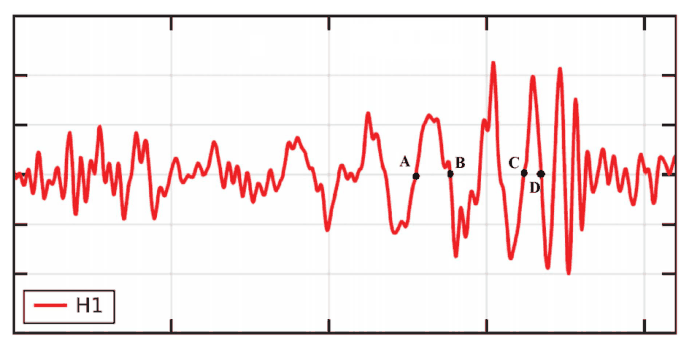
Figure 1. Strain, i.e. relative variation of the size of each arm, at the LIGO detector H1. The horizontal axis is time, and the points A, B, C, D correspond to \(t=0.000,0.009,0.034,0.040\) seconds, respectively.

B.5 1.0pt

From the figure, estimate \(f_{\mathrm{GW}}(t)\) at

\[ t_{\overline{\mathrm{AB}}}=\frac{t_{\mathrm B}+t_{\mathrm A}}{2} \qquad\text{and}\qquad t_{\overline{\mathrm{CD}}}=\frac{t_{\mathrm D}+t_{\mathrm C}}{2}\,. \tag{13} \]

Assuming that (12) is valid all the way until the collision (which strictly speaking is not true) and that the two objects have equal mass, estimate the chirp mass, \(M_c\), and total mass of the system, in terms of solar masses \(M_\odot\simeq2\times10^{30}\,\mathrm{kg}\).

B.6 1.0pt

Estimate the minimal orbital separation between the two objects at \(t_{\overline{\mathrm{CD}}}\). Hence estimate a maximum size for each object, \(R_{\max}\). Obtain \(R_\odot/R_{\max}\) to compare this size with the radius of our Sun, \(R_\odot\simeq7\times10^5\,\mathrm{km}\). Estimate also their orbital linear velocity at the same instant, \(v_{\mathrm{col}}\), comparing it with the speed of light, \(v_{\mathrm{col}}/c\).

Conclude that these are extremely fast moving, extremely compact objects indeed!

Official English text of the problem.

When two protons collide with a very high energy at the Large Hadron Collider (LHC), several particles may be produced as a result of that collision, such as electrons, muons, neutrinos, quarks, and their respective anti-particles. Most of these particles can be detected by the particle detector surrounding the collision point. For example, quarks undergo a process called hadronisation in which they become a shower of subatomic particles, called "jet". In addition, the high magnetic field present in the detectors allows even very energetic charged particles to curve enough for their momentum to be determined. The ATLAS detector uses a superconducting solenoid system that produces a constant and uniform 2.00 Tesla magnetic field in the inner part of the detector, surrounding the collision point. Charged particles with momenta below a certain value will be curved so strongly that they will loop repeatedly in the field and most likely not be measured. Due to its nature, the neutrino is not detected at all, as it escapes through the detector without interacting.

Data: Electron rest mass, \(m=9.11\times10^{-31}\ \mathrm{kg}\); Elementary charge, \(e=1.60\times10^{-19}\ \mathrm{C}\);

Speed of light, \(c=3.00\times10^8\ \mathrm{m\,s^{-1}}\); Vacuum permittivity, \(\epsilon_0=8.85\times10^{-12}\ \mathrm{F\,m^{-1}}\)

Part A. ATLAS Detector physics (4.0 points)

A.1 — 0.5pt

Derive an expression for the cyclotron radius, \(r\), of the circular trajectory of an electron acted upon by a magnetic force perpendicular to its velocity, and express that radius as a function of its kinetic energy, \(K\); charge modulus, \(e\); mass, \(m\); and magnetic field, \(B\). Assume that the electron is a non-relativistic classical particle.

Electrons produced inside the ATLAS detector must be treated relativistically. However, the formula for the cyclotron radius also holds for relativistic motion when the relativistic momentum is considered.

A.2 — 0.5pt

Calculate the minimum value of the momentum of an electron that allows it to escape the inner part of the detector in the radial direction. The inner part of the detector has a cylindrical shape with a radius of 1.1 meters, and the electron is produced in the collision point exactly in the center of the cylinder. Express your answer in MeV/\(c\).

When accelerated perpendicularly to the velocity, relativistic particles of charge \(e\) and rest mass \(m\) emitt electromagnetic radiation, called synchrotron radiation. The emitted power is given by

\[ P=\frac{e^2a^2\gamma^4}{6\pi\epsilon_0c^3} \]

where \(a\) is the acceleration and \(\gamma=[1-(v/c)^2]^{-1/2}\).

A.3 — 1.0pt

A particle is called ultrarelativistic when its speed is very close to the speed of light. For an ultrarelativistic particle the emitted power can be expressed as:

\[ P=\xi\frac{e^4}{\epsilon_0m^kc^n}E^2B^2, \]

where \(\xi\) is a real number, \(n\), \(k\) are integers, \(E\) is the energy of the charged particle and \(B\) is the magnetic field. Find \(\xi\), \(n\) and \(k\).

A.4 — 1.0pt

In the ultrarelativistic limit, the energy of the electron as a function of time is:

\[ E(t)=\frac{E_0}{1+\alpha E_0t}, \]

where \(E_0\) is the initial energy of the electron. Find \(\alpha\) as a function of \(e\), \(c\), \(B\), \(\epsilon_0\) and \(m\).

A.5 — 0.5pt

Consider an electron produced at the collision point along the radial direction with an energy of 100 GeV. Estimate the amount of energy that is lost due to synchrotron radiation until the electron escapes the inner part of the detector? Express your answer in MeV.

A.6 — 0.5pt

Find an expression for the cyclotron frequency of the electron as a function of time in the ultrarelativistic limit.

Part B. Finding the neutrino (6.0 points)

The collision between the two protons shown in Figure 1 leads to the production of a top quark (\(t\)) and an anti-top quark (\(\bar t\)), the heaviest elementary particles ever detected. The top quark decays into a \(W^+\) boson and a bottom quark (\(b\)), while the anti-top quark decays into a \(W^-\) boson and an anti-bottom quark (\(\bar b\)). In the case depicted in Figure 1, the \(W^+\) boson decays into a anti-muon (\(\mu^+\)) and a neutrino (\(\nu\)), and the \(W^-\) boson decays into a quark and an anti-quark. The task of this problem is to reconstruct the full momentum of the neutrino using the momenta of some detected particles. For simplicity, all particles and jets in this problem will be considered massless, except for the top quark and \(W^\pm\) bosons.

The momenta of the top quark decay products can be determined from the experiment (see Table), except for the neutrino momentum component along the (\(z\)-axis). The total linear momentum of the final state particles caught by the detector is only zero on the transverse plane (\(xy\) plane), and not along the collision line (\(z\)-axis). As such, one can find the transverse momentum of the neutrino from the missing momentum in the transverse plane.

On June 4, 2015, the ATLAS experiment at the LHC recorded a proton-proton collision at 00:21:24 GMT+1 like the one represented in Figure 1.

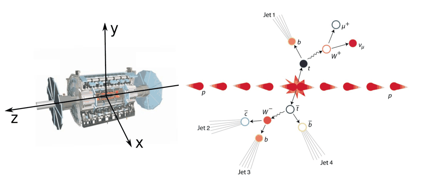
Figure 1. Schematic representation of the ATLAS detector coordinate system (left) and proton-proton collision (right).

The linear momenta of the three final-state particles coming from the top quark decay, including the neutrino, is presented below for each component.

Particle	\(p_x\) (GeV/\(c\))	\(p_y\) (GeV/\(c\))	\(p_z\) (GeV/\(c\))
anti-muon (\(\mu^+\))	\(-24.7\)	\(-24.9\)	\(-12.4\)
jet 1 (\(j_1\))	\(-14.2\)	\(+50.1\)	\(+94.1\)
neutrino (\(\nu\))	\(-104.1\)	\(+5.3\)	---

B.1 — 1.5pt

Find an equation which relates the square of the \(W^+\) boson mass, \(m_{\mathrm W}^2\), with the neutrino and anti-muon momentum components presented in the table above. Express your answer in terms of the neutrino and anti-muon transverse momentum,

\[ \vec p_{\mathrm T}^{(\nu)} =p_x^{(\nu)}\hat\imath+p_y^{(\nu)}\hat\jmath \quad\text{and}\quad \vec p_{\mathrm T}^{(\mu)} =p_x^{(\mu)}\hat\imath+p_y^{(\mu)}\hat\jmath, \]

and their \(z\)-axis momentum components, \(p_z^{(\mu)}\) and \(p_z^{(\nu)}\).

B.2 — 1.5pt

Assuming a \(W^+\) boson mass of \(m_{\mathrm W}=80.4\ \mathrm{GeV}/c^2\) calculate the two possible solutions for the neutrino momentum along the \(z\)-axis, \(p_z^{(\nu)}\). Express your answer in GeV/c.

B.3 — 1.0pt

Calculate the top quark mass for each one of the two previous solutions. Express your answer in GeV/\(c^2\).

[If you did not obtain the two solutions in B.2, use \(p_z^{(\nu)}=70\ \mathrm{GeV}/c\) and \(p_z^{(\nu)}=-180\ \mathrm{GeV}/c\).]

The normalised number of collision events for the measurement of the top quark mass (as determined from the experiment), has two components: the so-called "signal" (corresponding to the decay of top quarks) and "background" (corresponding to events from other processes that do not include top quarks). Experimental data include both processes, see Fig. 2.

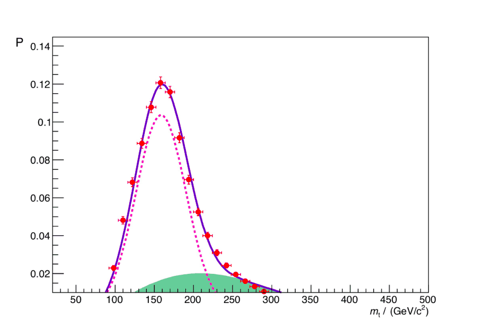
Figure 2. Top quark mass distribution as determined from the experiment, i.e. the normalised number of events plotted against the top quark mass. The dots correspond to the data. The dashed line corresponds to the "signal" and the shade to the "background".

B.4 — 1.0pt

According to the top quark mass distribution, which one of the two previous solutions is more likely to be the right one? Estimate the probability for the most likely solution.

B.5 — 1.0pt

Calculate the distance traveled by the top quark before decaying, using the most likely solution. Assume the top quark has a mean lifetime at rest of \(5\times10^{-25}\ \mathrm{s}\).

Official English text of the problem.

Data: Normal atmospheric pressure, \(P_0 = 1.013 \times 10^5\ \mathrm{Pa} = 760\ \mathrm{mmHg}\)

Part A. The physics of blood flow (4.5 points)

In this part you will analyse two simplified models of blood flow in vessels.

Blood vessels are approximately cylindrical in shape, and it is known that for a steady, non turbulent flow of an incompressible fluid in a rigid cylinder, the difference in pressure of the fluid at the two ends of the cylinder is given by

\[ \Delta P=\frac{8\ell\eta}{\pi r^4}Q, \tag{1} \]

where \(\ell\) and \(r\) are the length and radius of the cylinder, \(\eta\) is the fluid viscosity and \(Q\) is the volumetric flow rate, i.e. the fluid volume that passes the cylinder cross section per unit time. This expression is often able to provide the correct order of magnitude for the pressure difference in a vessel, even without taking into account the pulsatile flow, the vessel's compressibility and irregular shape, and the fact that blood is not a simple fluid but a mixture of cells and plasma. Moreover, this expression has the same form as Ohm's law, with the volumetric flow rate being interpreted as a current, the difference in pressure as a voltage, and the factor \(R=\frac{8\ell\eta}{\pi r^4}\) as a resistance.

Consider for example the symmetrical network of arterioles (small arteries) depicted in Figure 1 that delivers blood to the capillary bed of a tissue. In this network, at each bifurcation a vessel is divided in two identical vessels. However, the vessels of higher levels are thinner and shorter: consider that the radii and lengths of vessels in two consecutive levels, \(i\) and \(i+1\), are related by \(r_{i+1}=r_i/2^{1/3}\) and by \(\ell_{i+1}=\ell_i/2^{1/3}\).

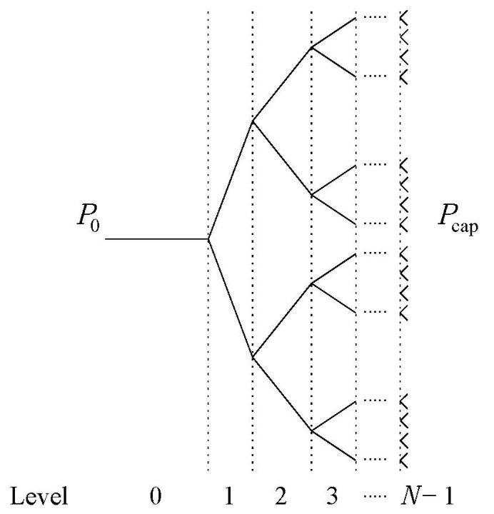
Figure 1. Network of arterioles.

A.1 (1.3pt)

Obtain an expression for the volumetric flow rate, \(Q_i\), in a vessel at any level \(i\), as a function of the total number of levels \(N\), of the viscosity \(\eta\), of the radius \(r_0\) and length \(\ell_0\) of the first vessel, and of the difference \(\Delta P=P_0-P_{\mathrm{cap}}\) between the pressure at the arteriole at level 0, \(P_0\), and the pressure at the capillary bed, \(P_{\mathrm{cap}}\).

A.2 (0.5pt)

Calculate the numerical value of the volumetric flow rate \(Q_0\) of the arteriole at level 0, if its radius is \(6.0\times10^{-5}\ \mathrm{m}\) and its length is \(2.0\times10^{-3}\ \mathrm{m}\). Consider that the pressure at the arteriole inlet is 55 mmHg and the vessel network has \(N=6\) levels linking this arteriole to the capillary bed at the pressure 30 mmHg. Consider that the blood viscosity is \(\eta=3.5\times10^{-3}\ \mathrm{kg\,m^{-1}\,s^{-1}}\). Express your result in ml/h.

A blood vessel as an LCR circuit

The approximation of rigid cylindrical vessels falls short for several reasons. It is particularly important to include the time dependent flow and to take into account the change in vessel diameter that occurs when the pressure varies during a blood pumping cycle done by the heart. Moreover, it is observed that in the larger vessels the blood pressure varies significantly during a cycle, while in the smaller vessels the amplitude of the oscillations in pressure is much smaller, and the flow is almost time independent.

When the pressure increases in a single elastic vessel, there will be an increase in its diameter, thus permitting to store more fluid in the vessel, and to deliver it when the pressure drops. For this reason, the elastic behaviour of the vessel can be simulated by adding a capacitor to our initial description. Moreover, when taking into account the time dependent blood flow rate, one has to consider the inertia of the fluid, proportional to its density \(\rho=1.05\times10^3\ \mathrm{kg\,m^{-3}}\). This inertia can be described by an inductance in our model. In Figure 2 we represent the equivalent circuit for a single vessel in this model. The equivalent capacitance and inductance are given by

\[ C=\frac{3\ell\pi r^3}{2Eh} \quad\text{and}\quad L=\frac{9\ell\rho}{4\pi r^2}, \tag{2} \]

respectively, where \(h\) is the width of the vessel wall and \(E\) is the artery Young's modulus, a coefficient that describes the alteration in size of the vessel tissue when a force is applied. The Young's modulus has units of pressure and is on the order of \(E=0.06\ \mathrm{MPa}\) for arterioles.

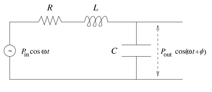
Figure 2. Equivalent electric circuit for a single vessel.

A.3 (2.0pt)

Obtain, in the stationary regime, the pressure amplitude at the vessel outlet, \(P_{\mathrm{out}}\), as a function of the pressure amplitude at the inlet, \(P_{\mathrm{in}}\), the equivalent resistance, \(R\), inductance, \(L\) and capacitance, \(C\), for a flow with angular frequency \(\omega\). Establish the condition between \(\eta\), \(\rho\), \(E\), \(h\), \(r\) and \(\ell\) so that, for low frequencies, the pressure oscillation amplitude at the outlet is smaller than that of \(P_{\mathrm{in}}\).

A.4 (0.7pt)

For the vessel network in A.2 estimate the maximum arteriole wall thickness \(h\) so that the condition established in A.3 is satisfied (consider that \(h\) is level independent).

Part B. Tumour growth (5.5 points)

Tumour growth is a very complex process where biological mechanisms such as cell proliferation and natural selection are intertwined with physics. In this problem we will consider a simplified model of tumour growth that addresses the increase in pressure commonly observed in solid tumors.

Consider a group of normal cells forming a tissue surrounded by an inextensible basement membrane, which forces the tissue to maintain always the same form: a sphere of radius \(R\) (Figure 3).

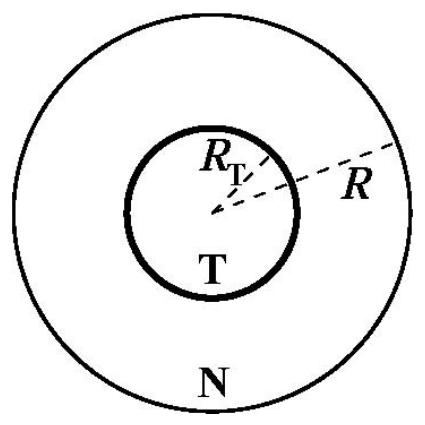
Figure 3. Simplified tumour.

Initially the tissue does not have residual stresses, i.e. the pressure at every point is equal to the atmospheric pressure.

At time \(t=0\), a tumour starts growing at the centre of this sphere and, as it grows, the pressure inside the tissue increases. Consider that both tissues (normal, N, and tumour, T) are compressible such that their densities, \(\rho_{\mathrm N}\) and \(\rho_{\mathrm T}\), increase linearly with pressure:

\[ \rho_{\mathrm N}=\rho_0\left(1+\frac{p}{K_{\mathrm N}}\right), \qquad \rho_{\mathrm T}=\rho_0\left(1+\frac{p}{K_{\mathrm T}}\right), \tag{3} \]

where \(\rho_0\) is the rest tissue density, \(p\) is the pressure difference to the atmospheric pressure and \(K_{\mathrm N}\), \(K_{\mathrm T}\) are the compressibility moduli (bulk moduli) of the normal and tumour tissues, respectively. In general, tumours are stiffer and so they have a higher bulk modulus.

B.1 (1.0pt)

The mass of normal cells is not altered while the tumour is growing. Obtain the ratio between the tumour volume and the total tissue volume, \(v=V_{\mathrm T}/V\), as a function of the ratio between the tumour mass (\(M_{\mathrm T}\)) and the normal tissue mass (\(M_{\mathrm N}\)), \(\mu=M_{\mathrm T}/M_{\mathrm N}\) and the ratio of the bulk moduli, \(\kappa=K_{\mathrm N}/K_{\mathrm T}\).

Hyperthermia is sometimes used together with chemotherapy and radiotherapy in the treatment of cancer. In hyperthermia the cancer cells are selectively heated from the normal human body temperature, \(37\,^\circ\mathrm C\), to temperatures above \(43\,^\circ\mathrm C\), inducing their death. Researchers are currently developing carbon nanotubes covered with special proteins capable of binding to tumour cells. When the tissue is irradiated with near-infrared radiation, the nanotubes absorb it in a much greater extent than the surrounding tissues and therefore can be selectively heated as well as the tumour cells to which they are attached.

Consider that the tumour, the normal cells and the surrounding tissue have a constant thermal conductivity \(k\), i.e. in the geometry of this problem, the energy that crosses a spherical surface of radius \(r\) per unit time and per unit area is equal to \(k\) times the derivative of the temperature with respect to \(r\). The nanotubes are uniformly distributed in the tumour volume and are able to deliver a power \(\mathcal P\) of thermal energy per unit volume. Assume that the temperature is equal to the normal human body temperature very far away from the tumour.

B.2 (1.7pt)

Obtain, for the stationary state, the temperature at the centre of the tumour as a function of \(\mathcal P\), \(k\), the human body temperature and the tumour radius, \(R_{\mathrm T}\).

B.3 (0.5pt)

Obtain the minimum power per unit volume, \(\mathcal P_{\min}\), needed to heat up all tumour cells in a tumour with 5.0 cm radius to a temperature larger than \(43.0\,^\circ\mathrm C\). Take the thermal conductivity of the tissue to be equal to \(k=0.60\ \mathrm{W\,K^{-1}\,m^{-1}}\).

Consider that the tumour is irrigated by a vessel network with a branched structure like in question A.1. As the tumour grows, when its pressure \(p\) becomes larger than the pressure \(P_{\mathrm{cap}}\) at the thinnest vessels, the radii of these vessels will decrease by a small amount \(\delta r\). If this pressure reaches a critical value \(p_c\) (which would correspond to a radius decrease of \(\delta r_c\)), the thinnest vessels would collapse, compromising seriously the irrigation to the tumour. The pressure and the radius change can be related by the following phenomenological relation:

\[ \frac{p}{P_{\mathrm{cap}}}-1 = \left(\frac{p_c}{P_{\mathrm{cap}}}-1\right) \left(2-\frac{\delta r}{\delta r_c}\right) \frac{\delta r}{\delta r_c}. \tag{4} \]

Consider that just the smallest vessels (of level \(N-1\)) have their radius altered when the tumour increases its pressure.

B.4 (2.3pt)

In the linear regime (i.e. consider that \(p-P_{\mathrm{cap}}\) is very small), express the relative drop in the flow rate, \(\frac{\delta Q_{N-1}}{Q_{N-1}}\), in these thinnest vessels, as a function of the tumour volume ratio \(v=V_{\mathrm T}/V\) and \(K_{\mathrm N}\), \(N\), \(p_c\), \(\delta r_c\), \(r_{N-1}\), \(P_{\mathrm{cap}}\).

Official English text of the problem.

Im Jahr 2015 registrierte das Gravitationswellenobservatorium LIGO erstmals den Durchgang von Gravitationswellen (GW) durch die Erde. Dieses Ereignis mit der Bezeichnung GW150914 wurde durch Wellen ausgelöst, die von zwei schwarzen Löchern auf nahezu kreisförmigen Umlaufbahnen erzeugt wurden. In dieser Aufgabe werden Sie aus den Eigenschaften des gemessenen Signals einige physikalische Parameter des Systems abschätzen.

Teil A: Newtonsche (konservative) Umlaufbahnen (3.0 Punkte)

A.1 1.0 Punkte

Betrachten Sie ein System aus zwei Sternen mit den Massen \(M_1,M_2\), die sich bezüglich des Schwerpunkts des Systems an den Orten \(\vec r_1,\vec r_2\) befinden, das heißt,

\[ M_1\vec r_1+M_2\vec r_2=0\,. \tag{1} \]

Die Sterne sind vom Rest des Universums isoliert und bewegen sich mit nichtrelativistischen Geschwindigkeiten. Mithilfe der Newtonschen Gesetze lässt sich der Beschleunigungsvektor der Masse \(M_1\) ausdrücken als

\[ \frac{d^2\vec r_1}{dt^2} =-\alpha\frac{\vec r_1}{r_1^n}\,, \tag{2} \]

wobei \(r_1=|\vec r_1|,r_2=|\vec r_2|\). Bestimmen Sie \(n\in\mathbb N\) und \(\alpha=\alpha(G,M_1,M_2)\), wobei \(G\) die Newtonsche Gravitationskonstante ist \([G\simeq6.67\times10^{-11}\,\mathrm{N\,m^2\,kg^{-2}}]\).

A.2 1.0 Punkte

Die Gesamtenergie des Systems aus zwei Massen auf Kreisbahnen lässt sich ausdrücken als:

\[ E=A(\mu,\Omega,L)-G\frac{M\mu}{L}\,, \tag{3} \]

wobei

\[ \mu\equiv\frac{M_1M_2}{M_1+M_2}\,, \qquad M\equiv M_1+M_2\,, \tag{4} \]

die reduzierte Masse und die Gesamtmasse des Systems sind, \(\Omega\) die Winkelgeschwindigkeit jeder Masse ist und \(L\) den gesamten Abstand \(L=r_1+r_2\) bezeichnet. Bestimmen Sie die explizite Form des Terms \(A(\mu,\Omega,L)\).

A.3 1.0 Punkte

Gleichung 3 lässt sich zu \(E=\beta G\frac{M\mu}{L}\) vereinfachen. Bestimmen Sie die Zahl \(\beta\).

Teil B: Einführung relativistischer Dissipation (7.0 Punkte)

Die korrekte Gravitationstheorie, die allgemeine Relativitätstheorie, wurde 1915 von Einstein formuliert und sagt voraus, dass sich die Gravitation mit Lichtgeschwindigkeit ausbreitet. Die Träger der Information über die Wechselwirkung werden GW genannt. GW werden immer dann ausgesendet, wenn Massen beschleunigt werden, wodurch das System aus diesen Massen Energie verliert.

Betrachten Sie ein System aus zwei punktförmigen Teilchen, das vom Rest des Universums isoliert ist. Einstein bewies, dass die ausgesendeten GW bei hinreichend kleinen Geschwindigkeiten: 1) eine Frequenz haben, die doppelt so groß wie die Umlauffrequenz ist; 2) durch eine Leuchtkraft, also eine abgestrahlte Leistung \(\mathcal P\), charakterisiert werden können, deren dominierender Beitrag durch Einsteins Quadrupolformel gegeben ist,

\[ \mathcal P=\frac{G}{5c^5} \sum_{i=1}^{3}\sum_{j=1}^{3} \left(\frac{d^3Q_{ij}}{dt^3}\right) \left(\frac{d^3Q_{ij}}{dt^3}\right)\,. \tag{5} \]

Hier ist \(c\) die Lichtgeschwindigkeit \(c\simeq3\times10^8\,\mathrm{m/s}\). Für ein System aus zwei punktförmigen Teilchen, die in der \(x-y\)-Ebene umlaufen, ist \(Q_{ij}\) durch die folgende Tabelle gegeben (\(i,j\) bezeichnen die Zeilen- bzw. Spaltennummer)

\[ \begin{aligned} Q_{11}&=\sum_{A=1}^{2}\frac{M_A}{3}(2x_A^2-y_A^2)\,,\\ Q_{22}&=\sum_{A=1}^{2}\frac{M_A}{3}(2y_A^2-x_A^2)\,,\\ Q_{33}&=-\sum_{A=1}^{2}\frac{M_A}{3}(x_A^2+y_A^2)\,, \end{aligned} \tag{6} \]

\[ Q_{12}=Q_{21}=\sum_{A=1}^{2}M_Ax_Ay_A\,, \tag{7} \]

und \(Q_{ij}=0\) für alle anderen Kombinationen. Hier ist \((x_A,y_A)\) die Position der Masse A im Schwerpunktsystem.

B.1 1.0 Punkte

Für die in A.2 beschriebenen Kreisbahnen lassen sich die Komponenten von \(Q_{ij}\) als Funktion der Zeit \(t\) ausdrücken als:

\[ Q_{ii}=\frac{\mu L^2}{2}(a_i+b_i\cos kt)\,, \qquad Q_{ij}\overset{i\ne j}{=}\frac{\mu L^2}{2}c_{ij}\sin kt\,. \tag{8} \]

Bestimmen Sie \(k\) in Abhängigkeit von \(\Omega\) sowie die Zahlenwerte der Konstanten \(a_i,b_i,c_{ij}\).

B.2 1.0 Punkte

Berechnen Sie die von diesem System in Form von Gravitationswellen abgestrahlte Leistung \(\mathcal P\), und leiten Sie her:

\[ \mathcal P=\xi\frac{G}{c^5}\mu^2L^4\Omega^6\,. \tag{9} \]

Welchen Wert hat die Zahl \(\xi\)? [Falls Sie \(\xi\) nicht bestimmen konnten, verwenden Sie im Folgenden \(\xi=6.4\).]

B.3 1.0 Punkte

Ohne die Emission von GW würden die beiden Massen unbegrenzt auf einer unveränderlichen Kreisbahn umlaufen. Durch die Emission von GW verliert das System jedoch Energie und geht langsam zu kleineren Kreisbahnen über. Zeigen Sie, dass die Änderungsrate \(\frac{d\Omega}{dt}\) der Bahnwinkelgeschwindigkeit die Form

\[ \left(\frac{d\Omega}{dt}\right)^3 =(3\xi)^3\frac{\Omega^{11}}{c^{15}}(GM_c)^5\,, \tag{10} \]

annimmt, wobei \(M_c\) als Chirp-Masse bezeichnet wird. Bestimmen Sie \(M_c\) als Funktion von \(M\) und \(\mu\). Diese Masse bestimmt die Zunahme der Frequenz während des Schrumpfens der Umlaufbahn. [Die Bezeichnung „Chirp“ ist vom hohen Zwitschern (mit zunehmender Frequenz) kleiner Vögel inspiriert.]

B.4 2.0 Punkte

Stellen Sie mithilfe der oben gegebenen Informationen den Zusammenhang zwischen der Bahnwinkelgeschwindigkeit \(\Omega\) und der GW-Frequenz \(f_{\mathrm{GW}}\) her. Für jede glatte Funktion \(F(t)\) und \(a\ne1\) gilt

\[ \frac{dF(t)}{dt}=\chi F(t)^a \quad\Rightarrow\quad F(t)^{1-a}=\chi(1-a)(t-t_0)\,, \tag{11} \]

wobei \(\chi\) eine Konstante und \(t_0\) eine Integrationskonstante ist. Zeigen Sie damit, dass aus (10) für die GW-Frequenz

\[ f_{\mathrm{GW}}^{-8/3} =8\pi^{8/3}\xi \left(\frac{GM_c}{c^3}\right)^{(2/3)+p} (t_0-t)^{2-p} \tag{12} \]

folgt, und bestimmen Sie die Konstante \(p\).

Am 14. September 2015 wurde GW150914 von den LIGO-Detektoren registriert, die aus zwei L-förmig angeordneten Armen von jeweils 4 km Länge bestehen. Die relative Längenänderung dieser Arme ist in Abb. 1 dargestellt. Die Arme des Detektors reagieren linear auf eine durchlaufende Gravitationswelle, und der Verlauf ihrer Reaktion bildet die Welle nach. Diese Welle wurde von zwei schwarzen Löchern auf nahezu kreisförmigen Umlaufbahnen erzeugt; der Energieverlust durch Gravitationsstrahlung führte dazu, dass die Umlaufbahn schrumpfte und die schwarzen Löcher schließlich kollidierten. Der Zeitpunkt der Kollision entspricht ungefähr dem Maximum des Signals nach Punkt D in Abb. 1.

Abbildung 1. Dehnung, also die relative Längenänderung jedes Arms, am LIGO-Detektor H1. Die horizontale Achse zeigt die Zeit, und die Punkte A, B, C, D entsprechen den Zeiten \(t=0.000,0.009,0.034,0.040\) Sekunden.

B.5 1.0 Punkte

Schätzen Sie anhand der Abbildung \(f_{\mathrm{GW}}(t)\) zu den Zeitpunkten

\[ t_{\overline{\mathrm{AB}}}=\frac{t_{\mathrm B}+t_{\mathrm A}}{2} \qquad\text{und}\qquad t_{\overline{\mathrm{CD}}}=\frac{t_{\mathrm D}+t_{\mathrm C}}{2}\,. \tag{13} \]

Nehmen Sie an, dass (12) bis zur Kollision gültig bleibt (was streng genommen nicht zutrifft) und dass die beiden Objekte die gleiche Masse haben. Schätzen Sie die Chirp-Masse \(M_c\) und die Gesamtmasse des Systems in Einheiten der Sonnenmasse \(M_\odot\simeq2\times10^{30}\,\mathrm{kg}\).

B.6 1.0 Punkte

Schätzen Sie den minimalen Bahnabstand zwischen den beiden Objekten zum Zeitpunkt \(t_{\overline{\mathrm{CD}}}\). Schätzen Sie daraus eine maximale Größe für jedes Objekt, \(R_{\max}\). Bestimmen Sie \(R_\odot/R_{\max}\), um diese Größe mit dem Radius unserer Sonne, \(R_\odot\simeq7\times10^5\,\mathrm{km}\), zu vergleichen. Schätzen Sie auch ihre lineare Bahngeschwindigkeit zu diesem Zeitpunkt, \(v_{\mathrm{col}}\), und vergleichen Sie diese mit der Lichtgeschwindigkeit, \(v_{\mathrm{col}}/c\).

Schließen Sie daraus, dass es sich tatsächlich um extrem schnell bewegte, extrem kompakte Objekte handelt!

Aufgabentext aus dem offiziellen englischen Text übersetzt.

Wenn am Large Hadron Collider (LHC) zwei Protonen mit sehr hoher Energie kollidieren, können bei dieser Kollision verschiedene Teilchen entstehen, etwa Elektronen, Myonen, Neutrinos, Quarks und ihre jeweiligen Antiteilchen. Die meisten dieser Teilchen können mit dem Teilchendetektor nachgewiesen werden, der den Kollisionspunkt umgibt. Beispielsweise durchlaufen Quarks einen Prozess namens Hadronisierung, bei dem sie sich in einen Schauer subatomarer Teilchen verwandeln, der als „Jet“ bezeichnet wird. Außerdem bewirkt das starke Magnetfeld in den Detektoren, dass die Bahnen selbst sehr energiereicher geladener Teilchen ausreichend gekrümmt werden, um ihren Impuls bestimmen zu können. Der ATLAS-Detektor verwendet ein supraleitendes Solenoidsystem, das im inneren Teil des Detektors um den Kollisionspunkt ein zeitlich konstantes und homogenes Magnetfeld von 2.00 Tesla erzeugt. Die Bahnen geladener Teilchen mit Impulsen unterhalb eines bestimmten Wertes werden so stark gekrümmt, dass die Teilchen das Feld wiederholt auf geschlossenen Bahnen durchlaufen und höchstwahrscheinlich nicht gemessen werden. Das Neutrino wird aufgrund seiner Eigenschaften überhaupt nicht nachgewiesen, da es den Detektor ohne Wechselwirkung durchquert und entkommt.

Gegebene Daten: Ruhemasse des Elektrons, \(m=9.11\times10^{-31}\ \mathrm{kg}\); Elementarladung, \(e=1.60\times10^{-19}\ \mathrm{C}\);

Lichtgeschwindigkeit, \(c=3.00\times10^8\ \mathrm{m\,s^{-1}}\); elektrische Feldkonstante, \(\epsilon_0=8.85\times10^{-12}\ \mathrm{F\,m^{-1}}\)

Teil A. Physik des ATLAS-Detektors (4.0 Punkte)

A.1 — 0.5 Punkte

Leiten Sie einen Ausdruck für den Zyklotronradius \(r\) der Kreisbahn eines Elektrons her, auf das eine magnetische Kraft senkrecht zu seiner Geschwindigkeit wirkt, und drücken Sie diesen Radius als Funktion seiner kinetischen Energie \(K\), seines Ladungsbetrags \(e\), seiner Masse \(m\) und des Magnetfelds \(B\) aus. Nehmen Sie an, dass das Elektron ein nichtrelativistisches klassisches Teilchen ist.

Elektronen, die im ATLAS-Detektor entstehen, müssen relativistisch behandelt werden. Die Formel für den Zyklotronradius gilt jedoch auch für relativistische Bewegungen, wenn der relativistische Impuls verwendet wird.

A.2 — 0.5 Punkte

Berechnen Sie den Mindestwert des Impulses eines Elektrons, bei dem es den inneren Teil des Detektors in radialer Richtung verlassen kann. Der innere Teil des Detektors hat die Form eines Zylinders mit einem Radius von 1.1 Metern, und das Elektron entsteht am Kollisionspunkt genau im Zentrum des Zylinders. Geben Sie Ihre Antwort in MeV/\(c\) an.

Werden relativistische Teilchen mit der Ladung \(e\) und der Ruhemasse \(m\) senkrecht zu ihrer Geschwindigkeit beschleunigt, so emittieren sie elektromagnetische Strahlung, die als Synchrotronstrahlung bezeichnet wird. Die abgestrahlte Leistung ist gegeben durch

\[ P=\frac{e^2a^2\gamma^4}{6\pi\epsilon_0c^3} \]

wobei \(a\) die Beschleunigung ist und \(\gamma=[1-(v/c)^2]^{-1/2}\) gilt.

A.3 — 1.0 Punkte

Ein Teilchen wird als ultrarelativistisch bezeichnet, wenn seine Geschwindigkeit sehr nahe an der Lichtgeschwindigkeit liegt. Für ein ultrarelativistisches Teilchen lässt sich die abgestrahlte Leistung folgendermaßen ausdrücken:

\[ P=\xi\frac{e^4}{\epsilon_0m^kc^n}E^2B^2, \]

wobei \(\xi\) eine reelle Zahl ist, \(n\) und \(k\) ganze Zahlen sind, \(E\) die Energie des geladenen Teilchens und \(B\) das Magnetfeld ist. Bestimmen Sie \(\xi\), \(n\) und \(k\).

A.4 — 1.0 Punkte

Im ultrarelativistischen Grenzfall ist die Energie des Elektrons als Funktion der Zeit gegeben durch:

\[ E(t)=\frac{E_0}{1+\alpha E_0t}, \]

wobei \(E_0\) die Anfangsenergie des Elektrons ist. Bestimmen Sie \(\alpha\) als Funktion von \(e\), \(c\), \(B\), \(\epsilon_0\) und \(m\).

A.5 — 0.5 Punkte

Betrachten Sie ein Elektron, das am Kollisionspunkt mit einer Energie von 100 GeV in radialer Richtung erzeugt wird. Schätzen Sie die Energie ab, die durch Synchrotronstrahlung verloren geht, bis das Elektron den inneren Teil des Detektors verlässt. Geben Sie Ihre Antwort in MeV an.

A.6 — 0.5 Punkte

Bestimmen Sie im ultrarelativistischen Grenzfall einen Ausdruck für die Zyklotronfrequenz des Elektrons als Funktion der Zeit.

Teil B. Das Neutrino finden (6.0 Punkte)

Die in Abbildung 1 dargestellte Kollision zweier Protonen führt zur Erzeugung eines Top-Quarks (\(t\)) und eines Anti-Top-Quarks (\(\bar t\)), der schwersten jemals nachgewiesenen Elementarteilchen. Das Top-Quark zerfällt in ein \(W^+\)-Boson und ein Bottom-Quark (\(b\)), während das Anti-Top-Quark in ein \(W^-\)-Boson und ein Anti-Bottom-Quark (\(\bar b\)) zerfällt. Im in Abbildung 1 dargestellten Fall zerfällt das \(W^+\)-Boson in ein Antimyon (\(\mu^+\)) und ein Neutrino (\(\nu\)), und das \(W^-\)-Boson zerfällt in ein Quark und ein Antiquark. Ziel dieser Aufgabe ist es, den vollständigen Impuls des Neutrinos mithilfe der Impulse einiger nachgewiesener Teilchen zu rekonstruieren. Der Einfachheit halber werden alle Teilchen und Jets in dieser Aufgabe als masselos betrachtet, mit Ausnahme des Top-Quarks und der \(W^\pm\)-Bosonen.

Die Impulse der Zerfallsprodukte des Top-Quarks können experimentell bestimmt werden (siehe Tabelle), mit Ausnahme der Impulskomponente des Neutrinos entlang der \(z\)-Achse. Der Gesamtimpuls der vom Detektor erfassten Teilchen im Endzustand ist nur in der Transversalebene (\(xy\)-Ebene) null, nicht aber entlang der Kollisionsachse (\(z\)-Achse). Daher lässt sich der Transversalimpuls des Neutrinos aus dem fehlenden Impuls in der Transversalebene bestimmen.

Am 4. Juni 2015 zeichnete das ATLAS-Experiment am LHC um 00:21:24 GMT+1 eine Proton-Proton-Kollision auf, wie sie in Abbildung 1 dargestellt ist.

Abbildung 1. Schematische Darstellung des Koordinatensystems des ATLAS-Detektors (links) und der Proton-Proton-Kollision (rechts).

Die Impulse der drei Teilchen im Endzustand, die aus dem Zerfall des Top-Quarks hervorgehen, einschließlich des Neutrinos, sind nachfolgend für jede Komponente angegeben.

Teilchen	\(p_x\) (GeV/\(c\))	\(p_y\) (GeV/\(c\))	\(p_z\) (GeV/\(c\))
Antimyon (\(\mu^+\))	\(-24.7\)	\(-24.9\)	\(-12.4\)
Jet 1 (\(j_1\))	\(-14.2\)	\(+50.1\)	\(+94.1\)
Neutrino (\(\nu\))	\(-104.1\)	\(+5.3\)	---

B.1 — 1.5 Punkte

Bestimmen Sie eine Gleichung, die das Quadrat der Masse des \(W^+\)-Bosons, \(m_{\mathrm W}^2\), mit den in der obigen Tabelle angegebenen Impulskomponenten des Neutrinos und des Antimyons verknüpft. Drücken Sie Ihre Antwort durch die Transversalimpulse des Neutrinos und des Antimyons,

\[ \vec p_{\mathrm T}^{(\nu)} =p_x^{(\nu)}\hat\imath+p_y^{(\nu)}\hat\jmath \quad\text{und}\quad \vec p_{\mathrm T}^{(\mu)} =p_x^{(\mu)}\hat\imath+p_y^{(\mu)}\hat\jmath, \]

und ihre Impulskomponenten entlang der \(z\)-Achse, \(p_z^{(\mu)}\) und \(p_z^{(\nu)}\), aus.

B.2 — 1.5 Punkte

Berechnen Sie unter der Annahme einer Masse des \(W^+\)-Bosons von \(m_{\mathrm W}=80.4\ \mathrm{GeV}/c^2\) die beiden möglichen Lösungen für den Impuls des Neutrinos entlang der \(z\)-Achse, \(p_z^{(\nu)}\). Geben Sie Ihre Antwort in GeV/c an.

B.3 — 1.0 Punkte

Berechnen Sie die Masse des Top-Quarks für jede der beiden vorherigen Lösungen. Geben Sie Ihre Antwort in GeV/\(c^2\) an.

[Falls Sie in B.2 die beiden Lösungen nicht erhalten haben, verwenden Sie \(p_z^{(\nu)}=70\ \mathrm{GeV}/c\) und \(p_z^{(\nu)}=-180\ \mathrm{GeV}/c\).]

Die normierte Anzahl der Kollisionsereignisse zur Messung der Masse des Top-Quarks (wie sie experimentell bestimmt wird) hat zwei Komponenten: das sogenannte „Signal“ (das dem Zerfall von Top-Quarks entspricht) und den „Untergrund“ (der Ereignissen aus anderen Prozessen entspricht, an denen keine Top-Quarks beteiligt sind). Die experimentellen Daten enthalten beide Prozesse, siehe Abb. 2.

Abbildung 2. Experimentell bestimmte Massenverteilung des Top-Quarks, d. h. die normierte Anzahl der Ereignisse, aufgetragen gegen die Masse des Top-Quarks. Die Punkte entsprechen den Daten. Die gestrichelte Linie entspricht dem „Signal“ und die schattierte Fläche dem „Untergrund“.

B.4 — 1.0 Punkte

Welche der beiden vorherigen Lösungen ist gemäß der Massenverteilung des Top-Quarks mit größerer Wahrscheinlichkeit die richtige? Schätzen Sie die Wahrscheinlichkeit für die wahrscheinlichere Lösung ab.

B.5 — 1.0 Punkte

Berechnen Sie anhand der wahrscheinlicheren Lösung die Strecke, die das Top-Quark vor seinem Zerfall zurücklegt. Nehmen Sie für das Top-Quark eine mittlere Lebensdauer in Ruhe von \(5\times10^{-25}\ \mathrm{s}\) an.

Aufgabentext aus dem offiziellen englischen Text übersetzt.

Gegeben: Normaler Atmosphärendruck, \(P_0 = 1.013 \times 10^5\ \mathrm{Pa} = 760\ \mathrm{mmHg}\)

Teil A. Die Physik der Blutströmung (4.5 Punkte)

In diesem Teil untersuchen Sie zwei vereinfachte Modelle der Blutströmung in Gefäßen.

Blutgefäße sind näherungsweise zylinderförmig. Für eine stationäre, nicht turbulente Strömung einer inkompressiblen Flüssigkeit in einem starren Zylinder ist bekannt, dass die Druckdifferenz der Flüssigkeit zwischen den beiden Enden des Zylinders gegeben ist durch

\[ \Delta P=\frac{8\ell\eta}{\pi r^4}Q, \tag{1} \]

wobei \(\ell\) und \(r\) die Länge und der Radius des Zylinders sind, \(\eta\) die Viskosität der Flüssigkeit und \(Q\) der Volumenstrom, also das Flüssigkeitsvolumen, das pro Zeiteinheit durch den Zylinderquerschnitt strömt. Dieser Ausdruck liefert häufig die richtige Größenordnung der Druckdifferenz in einem Gefäß, selbst wenn die pulsierende Strömung, die Kompressibilität und die unregelmäßige Form des Gefäßes sowie die Tatsache unberücksichtigt bleiben, dass Blut keine einfache Flüssigkeit, sondern ein Gemisch aus Zellen und Plasma ist. Außerdem hat dieser Ausdruck dieselbe Form wie das ohmsche Gesetz, wobei der Volumenstrom als Stromstärke, die Druckdifferenz als Spannung und der Faktor \(R=\frac{8\ell\eta}{\pi r^4}\) als Widerstand interpretiert werden.

Betrachten Sie beispielsweise das in Abbildung 1 dargestellte symmetrische Netzwerk aus Arteriolen (kleinen Arterien), das das Kapillarbett eines Gewebes mit Blut versorgt. In diesem Netzwerk teilt sich an jeder Verzweigung ein Gefäß in zwei identische Gefäße. Die Gefäße höherer Ebenen sind jedoch dünner und kürzer: Nehmen Sie an, dass die Radien und Längen der Gefäße zweier aufeinanderfolgender Ebenen, \(i\) und \(i+1\), durch \(r_{i+1}=r_i/2^{1/3}\) und \(\ell_{i+1}=\ell_i/2^{1/3}\) miteinander verknüpft sind.

Abbildung 1. Netzwerk aus Arteriolen.

A.1 (1.3 Punkte)

Leiten Sie einen Ausdruck für den Volumenstrom \(Q_i\) in einem Gefäß einer beliebigen Ebene \(i\) her, als Funktion der Gesamtzahl der Ebenen \(N\), der Viskosität \(\eta\), des Radius \(r_0\) und der Länge \(\ell_0\) des ersten Gefäßes sowie der Differenz \(\Delta P=P_0-P_{\mathrm{cap}}\) zwischen dem Druck \(P_0\) in der Arteriole auf Ebene 0 und dem Druck \(P_{\mathrm{cap}}\) im Kapillarbett.

A.2 (0.5 Punkte)

Berechnen Sie den Zahlenwert des Volumenstroms \(Q_0\) der Arteriole auf Ebene 0, wenn ihr Radius \(6.0\times10^{-5}\ \mathrm{m}\) und ihre Länge \(2.0\times10^{-3}\ \mathrm{m}\) betragen. Nehmen Sie an, dass der Druck am Einlass der Arteriole 55 mmHg beträgt und das Gefäßnetzwerk \(N=6\) Ebenen besitzt, die diese Arteriole mit dem Kapillarbett bei einem Druck von 30 mmHg verbinden. Nehmen Sie für die Viskosität des Blutes \(\eta=3.5\times10^{-3}\ \mathrm{kg\,m^{-1}\,s^{-1}}\) an. Geben Sie Ihr Ergebnis in ml/h an.

Ein Blutgefäß als LCR-Schaltung

Die Näherung starrer zylindrischer Gefäße ist aus mehreren Gründen unzureichend. Besonders wichtig ist es, die zeitabhängige Strömung einzubeziehen und die Änderung des Gefäßdurchmessers zu berücksichtigen, die auftritt, wenn sich der Druck während eines Pumpzyklus des Herzens ändert. Außerdem beobachtet man, dass der Blutdruck in größeren Gefäßen während eines Zyklus erheblich schwankt, während in kleineren Gefäßen die Amplitude der Druckschwingungen wesentlich geringer und die Strömung nahezu zeitunabhängig ist.

Wenn der Druck in einem einzelnen elastischen Gefäß zunimmt, vergrößert sich dessen Durchmesser. Dadurch kann das Gefäß mehr Flüssigkeit speichern und diese bei sinkendem Druck wieder abgeben. Aus diesem Grund lässt sich das elastische Verhalten des Gefäßes simulieren, indem wir unsere ursprüngliche Beschreibung um einen Kondensator ergänzen. Berücksichtigt man zudem den zeitabhängigen Blutvolumenstrom, muss man die Trägheit der Flüssigkeit einbeziehen, die proportional zu ihrer Dichte \(\rho=1.05\times10^3\ \mathrm{kg\,m^{-3}}\) ist. Diese Trägheit lässt sich in unserem Modell durch eine Induktivität beschreiben. In Abbildung 2 ist das Ersatzschaltbild für ein einzelnes Gefäß in diesem Modell dargestellt. Die Ersatzkapazität und die Ersatzinduktivität sind gegeben durch

\[ C=\frac{3\ell\pi r^3}{2Eh} \quad\text{und}\quad L=\frac{9\ell\rho}{4\pi r^2}, \tag{2} \]

wobei \(h\) die Dicke der Gefäßwand und \(E\) der Elastizitätsmodul der Arterie ist, ein Koeffizient, der die Größenänderung des Gefäßgewebes unter Einwirkung einer Kraft beschreibt. Der Elastizitätsmodul hat die Einheit eines Drucks und liegt bei Arteriolen in der Größenordnung von \(E=0.06\ \mathrm{MPa}\).

Abbildung 2. Elektrisches Ersatzschaltbild für ein einzelnes Gefäß.

A.3 (2.0 Punkte)

Bestimmen Sie im eingeschwungenen Zustand die Druckamplitude am Gefäßauslass, \(P_{\mathrm{out}}\), als Funktion der Druckamplitude am Einlass, \(P_{\mathrm{in}}\), des Ersatzwiderstands \(R\), der Ersatzinduktivität \(L\) und der Ersatzkapazität \(C\) für eine Strömung mit der Kreisfrequenz \(\omega\). Stellen Sie die Bedingung zwischen \(\eta\), \(\rho\), \(E\), \(h\), \(r\) und \(\ell\) auf, unter der bei niedrigen Frequenzen die Amplitude der Druckschwingung am Auslass kleiner als \(P_{\mathrm{in}}\) ist.

A.4 (0.7 Punkte)

Schätzen Sie für das Gefäßnetzwerk aus A.2 die maximale Wanddicke \(h\) der Arteriolen ab, für die die in A.3 aufgestellte Bedingung erfüllt ist (nehmen Sie an, dass \(h\) von der Ebene unabhängig ist).

Teil B. Tumorwachstum (5.5 Punkte)

Tumorwachstum ist ein sehr komplexer Prozess, bei dem biologische Mechanismen wie Zellvermehrung und natürliche Selektion mit physikalischen Vorgängen verflochten sind. In dieser Aufgabe betrachten wir ein vereinfachtes Modell des Tumorwachstums, das den häufig in soliden Tumoren beobachteten Druckanstieg beschreibt.

Betrachten Sie eine Gruppe normaler Zellen, die ein Gewebe bilden, das von einer undehnbaren Basalmembran umgeben ist. Diese zwingt das Gewebe, stets dieselbe Form beizubehalten: eine Kugel mit dem Radius \(R\) (Abbildung 3).

Abbildung 3. Vereinfachter Tumor.

Anfangs weist das Gewebe keine Eigenspannungen auf, d. h., der Druck ist an jedem Punkt gleich dem Atmosphärendruck.

Zum Zeitpunkt \(t=0\) beginnt im Zentrum dieser Kugel ein Tumor zu wachsen, und mit seinem Wachstum steigt der Druck im Gewebe. Nehmen Sie an, dass beide Gewebe (normales Gewebe, N, und Tumorgewebe, T) kompressibel sind, sodass ihre Dichten \(\rho_{\mathrm N}\) und \(\rho_{\mathrm T}\) linear mit dem Druck zunehmen:

\[ \rho_{\mathrm N}=\rho_0\left(1+\frac{p}{K_{\mathrm N}}\right), \qquad \rho_{\mathrm T}=\rho_0\left(1+\frac{p}{K_{\mathrm T}}\right), \tag{3} \]

wobei \(\rho_0\) die Gewebedichte im Ruhezustand, \(p\) die Druckdifferenz gegenüber dem Atmosphärendruck und \(K_{\mathrm N}\), \(K_{\mathrm T}\) die Kompressionsmoduln des normalen Gewebes bzw. des Tumorgewebes sind. Im Allgemeinen sind Tumoren steifer und besitzen daher einen höheren Kompressionsmodul.

B.1 (1.0 Punkte)

Die Masse der normalen Zellen ändert sich während des Tumorwachstums nicht. Bestimmen Sie das Verhältnis zwischen Tumorvolumen und gesamtem Gewebevolumen, \(v=V_{\mathrm T}/V\), als Funktion des Verhältnisses zwischen der Tumormasse (\(M_{\mathrm T}\)) und der Masse des normalen Gewebes (\(M_{\mathrm N}\)), \(\mu=M_{\mathrm T}/M_{\mathrm N}\), sowie des Verhältnisses der Kompressionsmoduln, \(\kappa=K_{\mathrm N}/K_{\mathrm T}\).

Hyperthermie wird bei der Krebsbehandlung gelegentlich gemeinsam mit Chemotherapie und Strahlentherapie eingesetzt. Bei der Hyperthermie werden die Krebszellen gezielt von der normalen menschlichen Körpertemperatur von \(37\,^\circ\mathrm C\) auf Temperaturen über \(43\,^\circ\mathrm C\) erwärmt, wodurch ihr Absterben ausgelöst wird. Forschende entwickeln derzeit Kohlenstoffnanoröhren, die mit speziellen Proteinen beschichtet sind, die an Tumorzellen binden können. Wird das Gewebe mit nahinfraroter Strahlung bestrahlt, absorbieren die Nanoröhren diese wesentlich stärker als das umgebende Gewebe und können daher zusammen mit den Tumorzellen, an die sie gebunden sind, gezielt erwärmt werden.

Nehmen Sie an, dass der Tumor, die normalen Zellen und das umgebende Gewebe eine konstante Wärmeleitfähigkeit \(k\) besitzen, d. h., in der Geometrie dieser Aufgabe ist die Energie, die eine Kugeloberfläche mit dem Radius \(r\) pro Zeiteinheit und Flächeneinheit durchquert, gleich \(k\) mal der Ableitung der Temperatur nach \(r\). Die Nanoröhren sind gleichmäßig im Tumorvolumen verteilt und können pro Volumeneinheit eine Wärmeleistung \(\mathcal P\) abgeben. Nehmen Sie an, dass die Temperatur in sehr großer Entfernung vom Tumor gleich der normalen menschlichen Körpertemperatur ist.

B.2 (1.7 Punkte)

Bestimmen Sie für den stationären Zustand die Temperatur im Zentrum des Tumors als Funktion von \(\mathcal P\), \(k\), der menschlichen Körpertemperatur und dem Tumorradius \(R_{\mathrm T}\).

B.3 (0.5 Punkte)

Bestimmen Sie die minimale Leistung pro Volumeneinheit, \(\mathcal P_{\min}\), die benötigt wird, um alle Tumorzellen in einem Tumor mit einem Radius von 5.0 cm auf eine Temperatur über \(43.0\,^\circ\mathrm C\) zu erwärmen. Nehmen Sie für die Wärmeleitfähigkeit des Gewebes \(k=0.60\ \mathrm{W\,K^{-1}\,m^{-1}}\) an.

Nehmen Sie an, dass der Tumor von einem Gefäßnetzwerk mit einer Verzweigungsstruktur wie in Aufgabe A.1 durchblutet wird. Wenn der Tumor wächst und sein Druck \(p\) den Druck \(P_{\mathrm{cap}}\) in den dünnsten Gefäßen übersteigt, verringern sich die Radien dieser Gefäße um einen kleinen Betrag \(\delta r\). Erreicht dieser Druck einen kritischen Wert \(p_c\) (der einer Radiusverringerung von \(\delta r_c\) entspräche), würden die dünnsten Gefäße kollabieren, wodurch die Durchblutung des Tumors stark beeinträchtigt würde. Druck und Radiusänderung lassen sich durch die folgende phänomenologische Beziehung miteinander verknüpfen:

\[ \frac{p}{P_{\mathrm{cap}}}-1 = \left(\frac{p_c}{P_{\mathrm{cap}}}-1\right) \left(2-\frac{\delta r}{\delta r_c}\right) \frac{\delta r}{\delta r_c}. \tag{4} \]

Nehmen Sie an, dass sich bei steigendem Tumordruck nur die Radien der kleinsten Gefäße (auf Ebene \(N-1\)) ändern.

B.4 (2.3 Punkte)

Drücken Sie im linearen Bereich (nehmen Sie also an, dass \(p-P_{\mathrm{cap}}\) sehr klein ist) die relative Abnahme des Volumenstroms \(\frac{\delta Q_{N-1}}{Q_{N-1}}\) in diesen dünnsten Gefäßen als Funktion des Tumorvolumenanteils \(v=V_{\mathrm T}/V\) sowie von \(K_{\mathrm N}\), \(N\), \(p_c\), \(\delta r_c\), \(r_{N-1}\), \(P_{\mathrm{cap}}\) aus.

Aufgabentext aus dem offiziellen englischen Text übersetzt.

2015 yılında kütleçekim dalgası gözlemevi LIGO, kütleçekim dalgalarının (GW) Dünya'dan geçişini ilk kez tespit etti. GW150914 adı verilen bu olay, yaklaşık dairesel yörüngelerde dolanan iki kara deliğin ürettiği dalgalardan kaynaklandı. Bu soruda, tespit edilen sinyalin özelliklerinden yararlanarak sistemin bazı fiziksel parametrelerini tahmin edeceksiniz.

Bölüm A: Newton mekaniğinde (korunumlu) yörüngeler (3.0 puan)

A.1 1.0 puan

Kütleleri \(M_1,M_2\) olan ve sistemin kütle merkezine göre sırasıyla \(\vec r_1,\vec r_2\) konumlarında bulunan iki yıldızdan oluşan bir sistem düşünün; yani,

\[ M_1\vec r_1+M_2\vec r_2=0\,. \tag{1} \]

Yıldızlar Evren'in geri kalanından yalıtılmıştır ve göreli olmayan hızlarla hareket etmektedir. Newton yasaları kullanılarak \(M_1\) kütlesinin ivme vektörü

\[ \frac{d^2\vec r_1}{dt^2} =-\alpha\frac{\vec r_1}{r_1^n}\,, \tag{2} \]

şeklinde ifade edilebilir; burada \(r_1=|\vec r_1|,r_2=|\vec r_2|\). \(n\in\mathbb N\) ve \(\alpha=\alpha(G,M_1,M_2)\) ifadelerini bulun; burada \(G\), Newton'un kütleçekim sabitidir \([G\simeq6.67\times10^{-11}\,\mathrm{N\,m^2\,kg^{-2}}]\).

A.2 1.0 puan

Dairesel yörüngelerdeki iki kütleli sistemin toplam enerjisi şöyle ifade edilebilir:

\[ E=A(\mu,\Omega,L)-G\frac{M\mu}{L}\,, \tag{3} \]

burada

\[ \mu\equiv\frac{M_1M_2}{M_1+M_2}\,, \qquad M\equiv M_1+M_2\,, \tag{4} \]

sırasıyla sistemin indirgenmiş kütlesi ve toplam kütlesidir; \(\Omega\), her bir kütlenin açısal hızı, \(L\) ise aralarındaki toplam uzaklıktır: \(L=r_1+r_2\). \(A(\mu,\Omega,L)\) teriminin açık ifadesini elde edin.

A.3 1.0 puan

Denklem 3, \(E=\beta G\frac{M\mu}{L}\) biçiminde sadeleştirilebilir. \(\beta\) sayısını belirleyin.

Bölüm B: Göreli enerji kaybının hesaba katılması (7.0 puan)

Doğru kütleçekim kuramı olan Genel Görelilik, Einstein tarafından 1915 yılında ortaya konmuş olup kütleçekiminin ışık hızıyla yayıldığını öngörür. Etkileşim hakkında bilgi taşıyan habercilere kütleçekim dalgaları (GW) denir. Kütleler ivmelendiğinde GW yayılır ve bu da kütlelerden oluşan sistemin enerji kaybetmesine neden olur.

Evren'in geri kalanından yalıtılmış, iki noktasal parçacıktan oluşan bir sistem düşünün. Einstein, yeterince küçük hızlarda yayılan GW'lerin: 1) yörünge frekansının iki katı frekansa sahip olduğunu; 2) baskın katkısı Einstein'ın dört kutup formülüyle verilen bir ışınım gücü, yani yayılan güç \(\mathcal P\), ile karakterize edilebildiğini kanıtlamıştır:

\[ \mathcal P=\frac{G}{5c^5} \sum_{i=1}^{3}\sum_{j=1}^{3} \left(\frac{d^3Q_{ij}}{dt^3}\right) \left(\frac{d^3Q_{ij}}{dt^3}\right)\,. \tag{5} \]

Burada \(c\), ışık hızıdır: \(c\simeq3\times10^8\,\mathrm{m/s}\). \(x-y\) düzleminde dolanan iki noktasal parçacıktan oluşan bir sistem için \(Q_{ij}\), aşağıdaki tablodur (\(i,j\), satır/sütun numarasını belirtir):

\[ \begin{aligned} Q_{11}&=\sum_{A=1}^{2}\frac{M_A}{3}(2x_A^2-y_A^2)\,,\\ Q_{22}&=\sum_{A=1}^{2}\frac{M_A}{3}(2y_A^2-x_A^2)\,,\\ Q_{33}&=-\sum_{A=1}^{2}\frac{M_A}{3}(x_A^2+y_A^2)\,, \end{aligned} \tag{6} \]

\[ Q_{12}=Q_{21}=\sum_{A=1}^{2}M_Ax_Ay_A\,, \tag{7} \]

ve diğer tüm durumlar için \(Q_{ij}=0\) olur. Burada \((x_A,y_A)\), A kütlesinin kütle merkezi referans sistemindeki konumudur.

B.1 1.0 puan

A.2'de açıklanan dairesel yörüngeler için \(Q_{ij}\) bileşenleri, \(t\) zamanının fonksiyonu olarak şöyle ifade edilebilir:

\[ Q_{ii}=\frac{\mu L^2}{2}(a_i+b_i\cos kt)\,, \qquad Q_{ij}\overset{i\ne j}{=}\frac{\mu L^2}{2}c_{ij}\sin kt\,. \tag{8} \]

\(k\)'yı \(\Omega\) cinsinden ve \(a_i,b_i,c_{ij}\) sabitlerinin sayısal değerlerini belirleyin.

B.2 1.0 puan

Bu sistemin kütleçekim dalgaları biçiminde yaydığı \(\mathcal P\) gücünü hesaplayın ve şu ifadeyi elde edin:

\[ \mathcal P=\xi\frac{G}{c^5}\mu^2L^4\Omega^6\,. \tag{9} \]

\(\xi\) sayısı nedir? [\(\xi\)'yi elde edemediyseniz bundan sonra \(\xi=6.4\) kullanın.]

B.3 1.0 puan

GW yayımı olmadığında iki kütle sabit bir dairesel yörüngede süresiz olarak dolanır. Ancak GW yayımı, sistemin enerji kaybetmesine ve yavaşça daha küçük dairesel yörüngelere doğru evrilmesine neden olur. Yörünge açısal hızının değişim hızı \(\frac{d\Omega}{dt}\)'nin

\[ \left(\frac{d\Omega}{dt}\right)^3 =(3\xi)^3\frac{\Omega^{11}}{c^{15}}(GM_c)^5\,, \tag{10} \]

biçimini aldığını elde edin; burada \(M_c\), cıvıltı kütlesi olarak adlandırılır. \(M_c\)'yi \(M\) ve \(\mu\)'nün fonksiyonu olarak elde edin. Bu kütle, yörüngenin daralması sırasında frekanstaki artışı belirler. ["Cıvıltı" adı, küçük kuşların çıkardığı tiz sesten (artan frekans) esinlenilmiştir.]

B.4 2.0 puan

Yukarıda verilen bilgileri kullanarak yörünge açısal hızı \(\Omega\) ile GW frekansı \(f_{\mathrm{GW}}\) arasındaki ilişkiyi kurun. Herhangi bir düzgün \(F(t)\) fonksiyonu ve \(a\ne1\) için,

\[ \frac{dF(t)}{dt}=\chi F(t)^a \quad\Rightarrow\quad F(t)^{1-a}=\chi(1-a)(t-t_0)\,, \tag{11} \]

olduğunu kullanarak (burada \(\chi\) bir sabit, \(t_0\) ise bir integrasyon sabitidir), (10)'dan GW frekansı için

\[ f_{\mathrm{GW}}^{-8/3} =8\pi^{8/3}\xi \left(\frac{GM_c}{c^3}\right)^{(2/3)+p} (t_0-t)^{2-p} \tag{12} \]

ifadesinin çıktığını gösterin ve \(p\) sabitini belirleyin.

14 Eylül 2015'te GW150914, her biri 4 km uzunluğunda, L biçiminde yerleştirilmiş iki koldan oluşan LIGO dedektörleri tarafından kaydedildi. Bu kolların bağıl uzunlukları Şekil 1'deki gibi değişti. Dedektörün kolları, içlerinden geçen kütleçekim dalgasına doğrusal olarak tepki verir ve bu tepkinin biçimi dalganın biçimini yansıtır. Bu dalga, yaklaşık dairesel yörüngelerde dolanan iki kara delik tarafından oluşturulmuştur; kütleçekim ışıması yoluyla enerji kaybı, yörüngenin daralmasına ve sonunda kara deliklerin çarpışmasına neden olmuştur. Çarpışma anı, yaklaşık olarak Şekil 1'de D noktasından sonraki sinyal tepesine karşılık gelir.

Şekil 1. LIGO H1 dedektöründeki gerinim, yani her bir kolun boyutundaki bağıl değişim. Yatay eksen zamandır ve A, B, C, D noktaları sırasıyla \(t=0.000,0.009,0.034,0.040\) saniyeye karşılık gelir.

B.5 1.0 puan

Şekilden yararlanarak aşağıdaki anlardaki \(f_{\mathrm{GW}}(t)\)'yi tahmin edin:

\[ t_{\overline{\mathrm{AB}}}=\frac{t_{\mathrm B}+t_{\mathrm A}}{2} \qquad\text{ve}\qquad t_{\overline{\mathrm{CD}}}=\frac{t_{\mathrm D}+t_{\mathrm C}}{2}\,. \tag{13} \]

(12)'nin çarpışmaya kadar geçerli olduğunu (bu, tam olarak doğru değildir) ve iki cismin eşit kütleli olduğunu varsayarak cıvıltı kütlesini, \(M_c\), ve sistemin toplam kütlesini Güneş kütlesi \(M_\odot\simeq2\times10^{30}\,\mathrm{kg}\) cinsinden tahmin edin.

B.6 1.0 puan

\(t_{\overline{\mathrm{CD}}}\) anında iki cisim arasındaki en küçük yörünge uzaklığını tahmin edin. Buradan her bir cismin en büyük boyutunu, \(R_{\max}\), tahmin edin. Bu boyutu Güneş'imizin yarıçapı \(R_\odot\simeq7\times10^5\,\mathrm{km}\) ile karşılaştırmak için \(R_\odot/R_{\max}\) oranını elde edin. Aynı andaki yörüngesel çizgisel hızlarını, \(v_{\mathrm{col}}\), da tahmin ederek ışık hızıyla karşılaştırın: \(v_{\mathrm{col}}/c\).

Bunların gerçekten de son derece hızlı hareket eden, son derece kompakt cisimler olduğu sonucuna varın!

Soru metni resmi İngilizce metinden çevrilmiştir.

Büyük Hadron Çarpıştırıcısı'nda (LHC) iki proton çok yüksek bir enerjiyle çarpıştığında, bu çarpışma sonucunda elektronlar, müonlar, nötrinolar, kuarklar ve bunların karşı parçacıkları gibi çeşitli parçacıklar üretilebilir. Bu parçacıkların çoğu, çarpışma noktasını çevreleyen parçacık dedektörü tarafından algılanabilir. Örneğin kuarklar, hadronlaşma adı verilen bir süreç geçirerek “jet” olarak adlandırılan bir atomaltı parçacık sağanağına dönüşür. Ayrıca dedektörlerde bulunan yüksek manyetik alan, çok yüksek enerjili yüklü parçacıkların bile momentumlarının belirlenmesine yetecek kadar sapmasını sağlar. ATLAS dedektörü, dedektörün çarpışma noktasını çevreleyen iç kısmında sabit ve düzgün bir 2.00 Tesla manyetik alan üreten süperiletken bir solenoid sistemi kullanır. Momentumları belirli bir değerin altında olan yüklü parçacıkların yörüngeleri o kadar güçlü biçimde bükülür ki bu parçacıklar alan içinde tekrar tekrar dolanır ve büyük olasılıkla ölçülemez. Nötrino ise doğası gereği dedektörle etkileşmeden içinden geçip kaçtığı için hiç algılanmaz.

Veriler: Elektronun durgun kütlesi, \(m=9.11\times10^{-31}\ \mathrm{kg}\); Temel yük, \(e=1.60\times10^{-19}\ \mathrm{C}\);

Işık hızı, \(c=3.00\times10^8\ \mathrm{m\,s^{-1}}\); Boşluğun elektriksel geçirgenliği, \(\epsilon_0=8.85\times10^{-12}\ \mathrm{F\,m^{-1}}\)

Bölüm A. ATLAS dedektörünün fiziği (4.0 puan)

A.1 — 0.5 puan

Hızına dik bir manyetik kuvvetin etkisindeki bir elektronun dairesel yörüngesinin siklotron yarıçapı \(r\) için bir ifade türetin ve bu yarıçapı kinetik enerjisi \(K\), yükünün büyüklüğü \(e\), kütlesi \(m\) ve manyetik alan \(B\) cinsinden ifade edin. Elektronun göreli olmayan klasik bir parçacık olduğunu varsayın.

ATLAS dedektörü içinde üretilen elektronlar göreli olarak ele alınmalıdır. Bununla birlikte, göreli momentum kullanıldığında siklotron yarıçapı formülü göreli hareket için de geçerlidir.

A.2 — 0.5 puan

Bir elektronun dedektörün iç kısmından radyal yönde çıkmasını sağlayan en küçük momentum değerini hesaplayın. Dedektörün iç kısmı, yarıçapı 1.1 metre olan silindir biçimindedir ve elektron, silindirin tam merkezindeki çarpışma noktasında üretilir. Cevabınızı MeV/\(c\) cinsinden ifade edin.

Yükü \(e\) ve durgun kütlesi \(m\) olan göreli parçacıklar, hızlarına dik yönde ivmelendirildiklerinde sinkrotron ışınımı adı verilen elektromanyetik ışınım yayar. Yayılan güç şu şekilde verilir:

\[ P=\frac{e^2a^2\gamma^4}{6\pi\epsilon_0c^3} \]

Burada \(a\) ivmedir ve \(\gamma=[1-(v/c)^2]^{-1/2}\).

A.3 — 1.0 puan

Hızı ışık hızına çok yakın olan bir parçacığa aşırı göreli parçacık denir. Aşırı göreli bir parçacığın yaydığı güç şu şekilde ifade edilebilir:

\[ P=\xi\frac{e^4}{\epsilon_0m^kc^n}E^2B^2, \]

Burada \(\xi\) bir gerçek sayı, \(n\), \(k\) tam sayılar, \(E\) yüklü parçacığın enerjisi ve \(B\) manyetik alandır. \(\xi\), \(n\) ve \(k\) değerlerini bulun.

A.4 — 1.0 puan

Aşırı göreli limitte elektronun enerjisinin zamana bağlılığı şöyledir:

\[ E(t)=\frac{E_0}{1+\alpha E_0t}, \]

Burada \(E_0\), elektronun başlangıç enerjisidir. \(\alpha\)'yı \(e\), \(c\), \(B\), \(\epsilon_0\) ve \(m\) cinsinden bulun.

A.5 — 0.5 puan

Çarpışma noktasında radyal yönde 100 GeV enerjiyle üretilen bir elektronu ele alın. Elektron dedektörün iç kısmından çıkana kadar sinkrotron ışınımı nedeniyle kaybettiği enerji miktarını tahmin edin. Cevabınızı MeV cinsinden ifade edin.

A.6 — 0.5 puan

Aşırı göreli limitte elektronun siklotron frekansının zamana bağlı ifadesini bulun.

Bölüm B. Nötrinoyu bulmak (6.0 puan)

Şekil 1'de gösterilen iki protonun çarpışması, şimdiye kadar algılanmış en ağır temel parçacıklar olan bir üst kuarkın (\(t\)) ve bir karşı üst kuarkın (\(\bar t\)) üretilmesine yol açar. Üst kuark bir \(W^+\) bozonuna ve bir alt kuarka (\(b\)) bozunurken, karşı üst kuark bir \(W^-\) bozonuna ve bir karşı alt kuarka (\(\bar b\)) bozunur. Şekil 1'de gösterilen durumda \(W^+\) bozonu bir karşı müona (\(\mu^+\)) ve bir nötrinoya (\(\nu\)), \(W^-\) bozonu ise bir kuarka ve bir karşı kuarka bozunur. Bu sorudaki görev, algılanan bazı parçacıkların momentumlarını kullanarak nötrinonun momentumunu tüm bileşenleriyle yeniden belirlemektir. Basitlik açısından, bu sorudaki tüm parçacıklar ve jetler, üst kuark ve \(W^\pm\) bozonları dışında kütlesiz kabul edilecektir.

Üst kuarkın bozunma ürünlerinin momentumları, nötrinonun (\(z\) ekseni) doğrultusundaki momentum bileşeni dışında deneyden belirlenebilir (tabloya bakınız). Dedektörün yakaladığı son durum parçacıklarının toplam doğrusal momentumu yalnızca enine düzlemde (\(xy\) düzlemi) sıfırdır; çarpışma doğrultusunda (\(z\) ekseni) sıfır değildir. Dolayısıyla nötrinonun enine momentumu, enine düzlemdeki eksik momentumdan bulunabilir.

4 Haziran 2015 tarihinde LHC'deki ATLAS deneyi, GMT+1 saat dilimine göre 00:21:24'te Şekil 1'de gösterilene benzer bir proton-proton çarpışması kaydetti.

Şekil 1. ATLAS dedektörünün koordinat sisteminin (solda) ve proton-proton çarpışmasının (sağda) şematik gösterimi.

Üst kuarkın bozunmasından gelen, nötrino dâhil üç son durum parçacığının doğrusal momentumları aşağıda her bir bileşen için verilmiştir.

Parçacık	\(p_x\) (GeV/\(c\))	\(p_y\) (GeV/\(c\))	\(p_z\) (GeV/\(c\))
karşı müon (\(\mu^+\))	\(-24.7\)	\(-24.9\)	\(-12.4\)
jet 1 (\(j_1\))	\(-14.2\)	\(+50.1\)	\(+94.1\)
nötrino (\(\nu\))	\(-104.1\)	\(+5.3\)	---

B.1 — 1.5 puan

\(W^+\) bozonunun kütlesinin karesini, \(m_{\mathrm W}^2\), yukarıdaki tabloda verilen nötrino ve karşı müon momentum bileşenleriyle ilişkilendiren bir denklem bulun. Cevabınızı nötrino ve karşı müonun enine momentumları

\[ \vec p_{\mathrm T}^{(\nu)} =p_x^{(\nu)}\hat\imath+p_y^{(\nu)}\hat\jmath \quad\text{ve}\quad \vec p_{\mathrm T}^{(\mu)} =p_x^{(\mu)}\hat\imath+p_y^{(\mu)}\hat\jmath, \]

ve \(z\) ekseni doğrultusundaki momentum bileşenleri \(p_z^{(\mu)}\) ve \(p_z^{(\nu)}\) cinsinden ifade edin.

B.2 — 1.5 puan

\(W^+\) bozonunun kütlesini \(m_{\mathrm W}=80.4\ \mathrm{GeV}/c^2\) kabul ederek nötrinonun \(z\) ekseni doğrultusundaki momentumu \(p_z^{(\nu)}\) için iki olası çözümü hesaplayın. Cevabınızı GeV/c cinsinden ifade edin.

B.3 — 1.0 puan

Önceki iki çözümün her biri için üst kuarkın kütlesini hesaplayın. Cevabınızı GeV/\(c^2\) cinsinden ifade edin.

[B.2'de iki çözümü elde edemediyseniz \(p_z^{(\nu)}=70\ \mathrm{GeV}/c\) ve \(p_z^{(\nu)}=-180\ \mathrm{GeV}/c\) değerlerini kullanın.]

Üst kuarkın kütlesinin ölçümüne ilişkin normalize edilmiş çarpışma olayı sayısı (deneyden belirlendiği şekliyle) iki bileşenden oluşur: “sinyal” (üst kuarkların bozunmasına karşılık gelir) ve “arka plan” (üst kuark içermeyen diğer süreçlerden kaynaklanan olaylara karşılık gelir). Deneysel veriler her iki süreci de içerir; Şekil 2'ye bakınız.

Şekil 2. Deneyden belirlenen üst kuark kütle dağılımı, yani üst kuark kütlesine karşı çizilen normalize edilmiş olay sayısı. Noktalar verilere karşılık gelir. Kesikli çizgi “sinyale”, gölgeli bölge ise “arka plana” karşılık gelir.

B.4 — 1.0 puan

Üst kuark kütle dağılımına göre önceki iki çözümden hangisinin doğru olma olasılığı daha yüksektir? Daha olası çözümün olasılığını tahmin edin.

B.5 — 1.0 puan

Daha olası çözümü kullanarak üst kuarkın bozunmadan önce aldığı yolu hesaplayın. Üst kuarkın durgun hâldeki ortalama ömrünün \(5\times10^{-25}\ \mathrm{s}\) olduğunu varsayın.

Soru metni resmi İngilizce metinden çevrilmiştir.

Veriler: Normal atmosfer basıncı, \(P_0 = 1.013 \times 10^5\ \mathrm{Pa} = 760\ \mathrm{mmHg}\)

Bölüm A. Kan akışının fiziği (4.5 puan)

Bu bölümde, damarlardaki kan akışına ilişkin iki basitleştirilmiş modeli inceleyeceksiniz.

Kan damarları yaklaşık olarak silindir biçimindedir. Sıkıştırılamaz bir akışkanın rijit bir silindir içindeki kararlı ve türbülanssız akışı için, silindirin iki ucundaki akışkan basınçları arasındaki farkın aşağıdaki bağıntıyla verildiği bilinmektedir:

\[ \Delta P=\frac{8\ell\eta}{\pi r^4}Q, \tag{1} \]

Burada \(\ell\) ve \(r\) silindirin uzunluğu ve yarıçapı, \(\eta\) akışkanın viskozitesi ve \(Q\) hacimsel debidir; yani birim zamanda silindirin en kesitinden geçen akışkan hacmidir. Bu ifade, akışın atımlı olması, damarın sıkıştırılabilirliği ve düzensiz biçimi ile kanın basit bir akışkan değil, hücreler ve plazmadan oluşan bir karışım olması hesaba katılmadan bile, bir damardaki basınç farkının büyüklük mertebesini çoğu zaman doğru verebilir. Ayrıca bu ifade, hacimsel debi akım, basınç farkı gerilim ve \(R=\frac{8\ell\eta}{\pi r^4}\) çarpanı direnç olarak yorumlandığında, Ohm yasasıyla aynı biçimdedir.

Örneğin, bir dokunun kılcal damar yatağına kan taşıyan ve Şekil 1'de gösterilen simetrik arteriyol (küçük atardamar) ağını ele alın. Bu ağda, her çatallanma noktasında bir damar iki özdeş damara ayrılır. Ancak daha yüksek düzeylerdeki damarlar daha ince ve daha kısadır: ardışık iki düzeydeki, \(i\) ve \(i+1\), damarların yarıçap ve uzunluklarının \(r_{i+1}=r_i/2^{1/3}\) ve \(\ell_{i+1}=\ell_i/2^{1/3}\) bağıntılarıyla ilişkili olduğunu kabul edin.

Şekil 1. Arteriyol ağı.

A.1 (1.3 puan)

Herhangi bir \(i\) düzeyindeki bir damarın hacimsel debisi \(Q_i\) için; toplam düzey sayısı \(N\), viskozite \(\eta\), ilk damarın yarıçapı \(r_0\) ve uzunluğu \(\ell_0\) ile 0. düzeydeki arteriyolün basıncı \(P_0\) ve kılcal damar yatağının basıncı \(P_{\mathrm{cap}}\) arasındaki \(\Delta P=P_0-P_{\mathrm{cap}}\) farkının fonksiyonu olan bir ifade elde edin.

A.2 (0.5 puan)

Yarıçapı \(6.0\times10^{-5}\ \mathrm{m}\) ve uzunluğu \(2.0\times10^{-3}\ \mathrm{m}\) olan 0. düzeydeki arteriyolün hacimsel debisi \(Q_0\)'ın sayısal değerini hesaplayın. Arteriyol girişindeki basıncın 55 mmHg olduğunu ve bu arteriyolü 30 mmHg basınçtaki kılcal damar yatağına bağlayan damar ağının \(N=6\) düzeyden oluştuğunu kabul edin. Kanın viskozitesini \(\eta=3.5\times10^{-3}\ \mathrm{kg\,m^{-1}\,s^{-1}}\) alın. Sonucunuzu ml/h cinsinden ifade edin.

Bir LCR devresi olarak kan damarı

Rijit silindirik damar yaklaşımı çeşitli nedenlerle yetersiz kalır. Zamana bağlı akışı modele katmak ve kalbin gerçekleştirdiği bir kan pompalama çevrimi sırasında basınç değiştikçe damar çapında meydana gelen değişimi hesaba katmak özellikle önemlidir. Ayrıca, büyük damarlarda kan basıncının bir çevrim boyunca önemli ölçüde değiştiği, küçük damarlarda ise basınç salınımlarının genliğinin çok daha küçük olduğu ve akışın neredeyse zamandan bağımsız olduğu gözlenir.

Tek bir elastik damarda basınç arttığında damarın çapı da artar; böylece damarda daha fazla akışkan depolanabilir ve basınç düştüğünde bu akışkan dışarı verilebilir. Bu nedenle, başlangıçtaki betimlememize bir kondansatör ekleyerek damarın elastik davranışını modelleyebiliriz. Ayrıca, zamana bağlı kan debisini hesaba katarken akışkanın, yoğunluğu \(\rho=1.05\times10^3\ \mathrm{kg\,m^{-3}}\) ile orantılı olan eylemsizliğini de dikkate almak gerekir. Bu eylemsizlik, modelimizde bir endüktans ile betimlenebilir. Şekil 2'de bu modeldeki tek bir damarın eşdeğer devresi gösterilmiştir. Eşdeğer kapasitans ve endüktans sırasıyla

\[ C=\frac{3\ell\pi r^3}{2Eh} \quad\text{ve}\quad L=\frac{9\ell\rho}{4\pi r^2}, \tag{2} \]

ile verilir. Burada \(h\) damar duvarının kalınlığı, \(E\) ise atardamarın Young modülüdür; bu katsayı, bir kuvvet uygulandığında damar dokusunun boyutlarında meydana gelen değişimi betimler. Young modülü basınç birimine sahiptir ve arteriyoller için \(E=0.06\ \mathrm{MPa}\) mertebesindedir.

Şekil 2. Tek bir damarın eşdeğer elektrik devresi.

A.3 (2.0 puan)

Kararlı rejimde, açısal frekansı \(\omega\) olan bir akış için damar çıkışındaki basınç genliği \(P_{\mathrm{out}}\)'u; girişteki basınç genliği \(P_{\mathrm{in}}\), eşdeğer direnç \(R\), endüktans \(L\) ve kapasitans \(C\)'nin fonksiyonu olarak elde edin. Düşük frekanslarda çıkıştaki basınç salınımı genliğinin \(P_{\mathrm{in}}\)'den küçük olması için \(\eta\), \(\rho\), \(E\), \(h\), \(r\) ve \(\ell\) arasındaki koşulu belirleyin.

A.4 (0.7 puan)

A.2'deki damar ağı için, A.3'te belirlenen koşulun sağlanmasını mümkün kılan en büyük arteriyol duvar kalınlığı \(h\)'yi tahmin edin (\(h\)'nin düzeyden bağımsız olduğunu kabul edin).

Bölüm B. Tümör büyümesi (5.5 puan)

Tümör büyümesi, hücre çoğalması ve doğal seçilim gibi biyolojik mekanizmaların fizikle iç içe geçtiği çok karmaşık bir süreçtir. Bu soruda, katı tümörlerde yaygın olarak gözlenen basınç artışını ele alan basitleştirilmiş bir tümör büyümesi modelini inceleyeceğiz.

Uzamayan bir bazal membranla çevrili bir doku oluşturan normal hücreler grubunu ele alın. Bu membran, dokunun her zaman aynı biçimi, yani \(R\) yarıçaplı bir küre biçimini korumasını zorunlu kılar (Şekil 3).

Şekil 3. Basitleştirilmiş tümör.

Başlangıçta dokuda artık gerilme yoktur; yani her noktadaki basınç atmosfer basıncına eşittir.

\(t=0\) anında bu kürenin merkezinde bir tümör büyümeye başlar ve büyüdükçe doku içindeki basınç artar. Her iki dokunun da (normal, N, ve tümör, T) sıkıştırılabilir olduğunu ve yoğunluklarının, \(\rho_{\mathrm N}\) ve \(\rho_{\mathrm T}\), basınçla doğrusal olarak arttığını kabul edin:

\[ \rho_{\mathrm N}=\rho_0\left(1+\frac{p}{K_{\mathrm N}}\right), \qquad \rho_{\mathrm T}=\rho_0\left(1+\frac{p}{K_{\mathrm T}}\right), \tag{3} \]

Burada \(\rho_0\) dokunun gerilmesiz durumdaki yoğunluğu, \(p\) atmosfer basıncına göre basınç farkı ve \(K_{\mathrm N}\), \(K_{\mathrm T}\) sırasıyla normal ve tümör dokularının sıkıştırılabilirlik modülleridir (hacim modülleri). Genel olarak tümörler daha serttir ve bu nedenle hacim modülleri daha büyüktür.

B.1 (1.0 puan)

Tümör büyürken normal hücrelerin kütlesi değişmez. Tümör hacminin toplam doku hacmine oranı \(v=V_{\mathrm T}/V\)'yi; tümör kütlesinin (\(M_{\mathrm T}\)) normal doku kütlesine (\(M_{\mathrm N}\)) oranı \(\mu=M_{\mathrm T}/M_{\mathrm N}\) ve hacim modüllerinin oranı \(\kappa=K_{\mathrm N}/K_{\mathrm T}\)'nın fonksiyonu olarak elde edin.

Kanser tedavisinde hipertermi bazen kemoterapi ve radyoterapiyle birlikte kullanılır. Hipertermide kanser hücreleri, normal insan vücut sıcaklığı olan \(37\,^\circ\mathrm C\)'den \(43\,^\circ\mathrm C\)'nin üzerindeki sıcaklıklara seçici olarak ısıtılarak ölmeleri sağlanır. Araştırmacılar günümüzde tümör hücrelerine bağlanabilen özel proteinlerle kaplanmış karbon nanotüpler geliştirmektedir. Doku yakın kızılötesi ışınımla ışınlandığında nanotüpler bu ışınımı çevredeki dokulara göre çok daha fazla soğurur; bu nedenle, bağlandıkları tümör hücreleriyle birlikte seçici olarak ısıtılabilirler.

Tümörün, normal hücrelerin ve çevredeki dokunun sabit bir \(k\) ısıl iletkenliğine sahip olduğunu kabul edin; yani bu sorunun geometrisinde, \(r\) yarıçaplı küresel bir yüzeyden birim zamanda ve birim alan başına geçen enerji, sıcaklığın \(r\)'ye göre türevinin \(k\) katına eşittir. Nanotüpler tümör hacmi içinde düzgün dağılmıştır ve birim hacim başına \(\mathcal P\) gücünde ısıl enerji sağlayabilmektedir. Tümörden çok uzakta sıcaklığın normal insan vücut sıcaklığına eşit olduğunu varsayın.

B.2 (1.7 puan)

Kararlı durumda tümörün merkezindeki sıcaklığı; \(\mathcal P\), \(k\), insan vücut sıcaklığı ve tümör yarıçapı \(R_{\mathrm T}\)'nin fonksiyonu olarak elde edin.

B.3 (0.5 puan)

Yarıçapı 5.0 cm olan bir tümördeki tüm tümör hücrelerini \(43.0\,^\circ\mathrm C\)'den daha yüksek bir sıcaklığa ısıtmak için gereken birim hacim başına en küçük güç \(\mathcal P_{\min}\)'i elde edin. Dokunun ısıl iletkenliğini \(k=0.60\ \mathrm{W\,K^{-1}\,m^{-1}}\) alın.

Tümörün, A.1 sorusundakine benzer dallanmış bir yapıya sahip damar ağıyla kanlandığını kabul edin. Tümör büyürken basıncı \(p\), en ince damarlardaki \(P_{\mathrm{cap}}\) basıncından büyük olduğunda, bu damarların yarıçapları küçük bir \(\delta r\) miktarı kadar azalır. Bu basınç kritik bir \(p_c\) değerine ulaşırsa (bu da \(\delta r_c\) kadar bir yarıçap azalmasına karşılık gelir), en ince damarlar çöker ve tümörün kanlanması ciddi biçimde bozulur. Basınç ile yarıçap değişimi arasında aşağıdaki fenomenolojik bağıntı kurulabilir:

\[ \frac{p}{P_{\mathrm{cap}}}-1 = \left(\frac{p_c}{P_{\mathrm{cap}}}-1\right) \left(2-\frac{\delta r}{\delta r_c}\right) \frac{\delta r}{\delta r_c}. \tag{4} \]

Tümörün basıncı arttığında yalnızca en küçük damarların (\(N-1\) düzeyindekilerin) yarıçaplarının değiştiğini kabul edin.

B.4 (2.3 puan)

Doğrusal rejimde (yani \(p-P_{\mathrm{cap}}\)'ın çok küçük olduğunu kabul ederek), bu en ince damarlardaki debinin bağıl azalmasını, \(\frac{\delta Q_{N-1}}{Q_{N-1}}\), tümör hacim oranı \(v=V_{\mathrm T}/V\) ile \(K_{\mathrm N}\), \(N\), \(p_c\), \(\delta r_c\), \(r_{N-1}\), \(P_{\mathrm{cap}}\)'ın fonksiyonu olarak ifade edin.

Soru metni resmi İngilizce metinden çevrilmiştir.

En 2015, el observatorio de ondas gravitacionales LIGO detectó, por primera vez, el paso de ondas gravitacionales (GW) a través de la Tierra. Este evento, denominado GW150914, se debió a las ondas producidas por dos agujeros negros que describían órbitas cuasicirculares. En este problema estimará algunos parámetros físicos del sistema a partir de las propiedades de la señal detectada.

Parte A: Órbitas newtonianas (conservativas) (3.0 puntos)

A.1 1.0pt

Considere un sistema de dos estrellas de masas \(M_1,M_2\), situadas en las posiciones \(\vec r_1,\vec r_2\), respectivamente, con respecto al centro de masas del sistema, es decir,

\[ M_1\vec r_1+M_2\vec r_2=0\,. \tag{1} \]

Las estrellas están aisladas del resto del Universo y se mueven a velocidades no relativistas. Utilizando las leyes de Newton, el vector aceleración de la masa \(M_1\) puede expresarse como

\[ \frac{d^2\vec r_1}{dt^2} =-\alpha\frac{\vec r_1}{r_1^n}\,, \tag{2} \]

donde \(r_1=|\vec r_1|,r_2=|\vec r_2|\). Halle \(n\in\mathbb N\) y \(\alpha=\alpha(G,M_1,M_2)\), donde \(G\) es la constante de gravitación de Newton \([G\simeq6.67\times10^{-11}\,\mathrm{N\,m^2\,kg^{-2}}]\).

A.2 1.0pt

La energía total del sistema de 2 masas, en órbitas circulares, puede expresarse como:

\[ E=A(\mu,\Omega,L)-G\frac{M\mu}{L}\,, \tag{3} \]

donde

\[ \mu\equiv\frac{M_1M_2}{M_1+M_2}\,, \qquad M\equiv M_1+M_2\,, \tag{4} \]

son la masa reducida y la masa total del sistema, \(\Omega\) es la velocidad angular de cada masa y \(L\) es la separación total \(L=r_1+r_2\). Obtenga la forma explícita del término \(A(\mu,\Omega,L)\).

A.3 1.0pt

La ecuación 3 puede simplificarse a \(E=\beta G\frac{M\mu}{L}\). Determine el número \(\beta\).

Parte B: Introducción de la disipación relativista (7.0 puntos)

La teoría correcta de la gravedad, la relatividad general, fue formulada por Einstein en 1915 y predice que la gravedad se propaga a la velocidad de la luz. Los mensajeros que transportan información sobre la interacción se denominan GW. Las GW se emiten siempre que las masas se aceleran, lo que hace que el sistema de masas pierda energía.

Considere un sistema de dos partículas puntuales, aislado del resto del Universo. Einstein demostró que, para velocidades suficientemente pequeñas, las GW emitidas: 1) tienen una frecuencia igual al doble de la frecuencia orbital; 2) pueden caracterizarse mediante una luminosidad, es decir, una potencia emitida \(\mathcal P\), cuyo término dominante viene dado por la fórmula cuadrupolar de Einstein,

\[ \mathcal P=\frac{G}{5c^5} \sum_{i=1}^{3}\sum_{j=1}^{3} \left(\frac{d^3Q_{ij}}{dt^3}\right) \left(\frac{d^3Q_{ij}}{dt^3}\right)\,. \tag{5} \]

Aquí, \(c\) es la velocidad de la luz \(c\simeq3\times10^8\,\mathrm{m/s}\). Para un sistema de 2 partículas puntuales que orbitan en el plano \(x-y\), \(Q_{ij}\) es la siguiente matriz (\(i,j\) indican el número de fila/columna)

\[ \begin{aligned} Q_{11}&=\sum_{A=1}^{2}\frac{M_A}{3}(2x_A^2-y_A^2)\,,\\ Q_{22}&=\sum_{A=1}^{2}\frac{M_A}{3}(2y_A^2-x_A^2)\,,\\ Q_{33}&=-\sum_{A=1}^{2}\frac{M_A}{3}(x_A^2+y_A^2)\,, \end{aligned} \tag{6} \]

\[ Q_{12}=Q_{21}=\sum_{A=1}^{2}M_Ax_Ay_A\,, \tag{7} \]

y \(Q_{ij}=0\) para todas las demás posibilidades. Aquí, \((x_A,y_A)\) es la posición de la masa A en el sistema de referencia del centro de masas.

B.1 1.0pt

Para las órbitas circulares descritas en A.2, las componentes de \(Q_{ij}\) pueden expresarse en función del tiempo \(t\) como:

\[ Q_{ii}=\frac{\mu L^2}{2}(a_i+b_i\cos kt)\,, \qquad Q_{ij}\overset{i\ne j}{=}\frac{\mu L^2}{2}c_{ij}\sin kt\,. \tag{8} \]

Determine \(k\) en función de \(\Omega\) y los valores numéricos de las constantes \(a_i,b_i,c_{ij}\).

B.2 1.0pt

Calcule la potencia \(\mathcal P\) emitida en ondas gravitacionales por ese sistema y obtenga:

\[ \mathcal P=\xi\frac{G}{c^5}\mu^2L^4\Omega^6\,. \tag{9} \]

¿Cuál es el número \(\xi\)? [Si no ha podido obtener \(\xi\), utilice \(\xi=6.4\) en lo que sigue.]

B.3 1.0pt

En ausencia de emisión de GW, las dos masas describirán una órbita circular fija indefinidamente. Sin embargo, la emisión de GW hace que el sistema pierda energía y evolucione lentamente hacia órbitas circulares más pequeñas. Demuestre que la tasa de variación \(\frac{d\Omega}{dt}\) de la velocidad angular orbital tiene la forma

\[ \left(\frac{d\Omega}{dt}\right)^3 =(3\xi)^3\frac{\Omega^{11}}{c^{15}}(GM_c)^5\,, \tag{10} \]

donde \(M_c\) se denomina masa de chirrido. Obtenga \(M_c\) en función de \(M\) y \(\mu\). Esta masa determina el aumento de la frecuencia durante el decaimiento orbital. [El nombre «chirrido» se inspira en el sonido agudo (de frecuencia creciente) producido por los pájaros pequeños.]

B.4 2.0pt

Utilizando la información anterior, relacione la velocidad angular orbital \(\Omega\) con la frecuencia de las GW \(f_{\mathrm{GW}}\). Sabiendo que, para cualquier función suave \(F(t)\) y \(a\ne1\),

\[ \frac{dF(t)}{dt}=\chi F(t)^a \quad\Rightarrow\quad F(t)^{1-a}=\chi(1-a)(t-t_0)\,, \tag{11} \]

donde \(\chi\) es una constante y \(t_0\) es una constante de integración, demuestre que (10) implica que la frecuencia de las GW es

\[ f_{\mathrm{GW}}^{-8/3} =8\pi^{8/3}\xi \left(\frac{GM_c}{c^3}\right)^{(2/3)+p} (t_0-t)^{2-p} \tag{12} \]

y determine la constante \(p\).

El 14 de septiembre de 2015, GW150914 fue registrado por los detectores LIGO, que constan de dos brazos dispuestos en forma de L, cada uno de 4 km de longitud. La longitud relativa de estos brazos varió según la Fig. 1. Los brazos del detector responden linealmente al paso de una onda gravitacional, y el patrón de respuesta reproduce la onda. Esta onda fue generada por dos agujeros negros en órbitas cuasicirculares; la pérdida de energía por radiación gravitacional hizo que la órbita se contrajera y que los agujeros negros acabaran colisionando. El instante de la colisión corresponde, aproximadamente, al máximo de la señal posterior al punto D de la Fig. 1.

Figura 1. Deformación, es decir, variación relativa del tamaño de cada brazo, en el detector LIGO H1. El eje horizontal representa el tiempo, y los puntos A, B, C, D corresponden a \(t=0.000,0.009,0.034,0.040\) segundos, respectivamente.

B.5 1.0pt

A partir de la figura, estime \(f_{\mathrm{GW}}(t)\) en

\[ t_{\overline{\mathrm{AB}}}=\frac{t_{\mathrm B}+t_{\mathrm A}}{2} \qquad\text{y}\qquad t_{\overline{\mathrm{CD}}}=\frac{t_{\mathrm D}+t_{\mathrm C}}{2}\,. \tag{13} \]

Suponiendo que (12) es válida hasta la colisión (lo cual, estrictamente hablando, no es cierto) y que los dos objetos tienen la misma masa, estime la masa de chirrido, \(M_c\), y la masa total del sistema, en unidades de masas solares \(M_\odot\simeq2\times10^{30}\,\mathrm{kg}\).

B.6 1.0pt

Estime la separación orbital mínima entre los dos objetos en \(t_{\overline{\mathrm{CD}}}\). A partir de ella, estime un tamaño máximo para cada objeto, \(R_{\max}\). Obtenga \(R_\odot/R_{\max}\) para comparar este tamaño con el radio de nuestro Sol, \(R_\odot\simeq7\times10^5\,\mathrm{km}\). Estime también su velocidad lineal orbital en ese mismo instante, \(v_{\mathrm{col}}\), comparándola con la velocidad de la luz, \(v_{\mathrm{col}}/c\).

¡Concluya que se trata, en efecto, de objetos extremadamente compactos que se mueven a velocidades extremadamente altas!

Enunciado traducido del texto oficial en inglés.

Cuando dos protones colisionan con una energía muy elevada en el Gran Colisionador de Hadrones (LHC), pueden producirse varias partículas como resultado de esa colisión, tales como electrones, muones, neutrinos, quarks y sus respectivas antipartículas. La mayoría de estas partículas pueden detectarse mediante el detector de partículas que rodea el punto de colisión. Por ejemplo, los quarks experimentan un proceso llamado hadronización, en el que se convierten en una cascada de partículas subatómicas denominada «jet». Además, el intenso campo magnético presente en los detectores permite que incluso las trayectorias de partículas cargadas muy energéticas se curven lo suficiente para determinar su cantidad de movimiento. El detector ATLAS utiliza un sistema de solenoides superconductores que produce un campo magnético constante y uniforme de 2.00 teslas en la parte interior del detector, alrededor del punto de colisión. Las trayectorias de las partículas cargadas con cantidades de movimiento inferiores a cierto valor se curvarán tanto que estas darán vueltas repetidamente en el campo y, muy probablemente, no serán medidas. Debido a su naturaleza, el neutrino no se detecta en absoluto, pues escapa atravesando el detector sin interaccionar.

Datos: masa en reposo del electrón, \(m=9.11\times10^{-31}\ \mathrm{kg}\); carga elemental, \(e=1.60\times10^{-19}\ \mathrm{C}\);

Velocidad de la luz, \(c=3.00\times10^8\ \mathrm{m\,s^{-1}}\); permitividad del vacío, \(\epsilon_0=8.85\times10^{-12}\ \mathrm{F\,m^{-1}}\)

Parte A. Física del detector ATLAS (4.0 puntos)

A.1 — 0.5pt

Deduzca una expresión para el radio ciclotrón, \(r\), de la trayectoria circular de un electrón sometido a una fuerza magnética perpendicular a su velocidad, y exprese dicho radio en función de su energía cinética, \(K\); el módulo de su carga, \(e\); su masa, \(m\); y el campo magnético, \(B\). Suponga que el electrón es una partícula clásica no relativista.

Los electrones producidos en el interior del detector ATLAS deben tratarse relativísticamente. Sin embargo, la fórmula del radio ciclotrón también es válida para el movimiento relativista cuando se considera la cantidad de movimiento relativista.

A.2 — 0.5pt

Calcule el valor mínimo de la cantidad de movimiento de un electrón que le permita escapar de la parte interior del detector en la dirección radial. La parte interior del detector tiene forma cilíndrica, con un radio de 1.1 metros, y el electrón se produce en el punto de colisión, exactamente en el centro del cilindro. Exprese su respuesta en MeV/\(c\).

Cuando se aceleran perpendicularmente a su velocidad, las partículas relativistas de carga \(e\) y masa en reposo \(m\) emiten radiación electromagnética, llamada radiación sincrotrón. La potencia emitida viene dada por

\[ P=\frac{e^2a^2\gamma^4}{6\pi\epsilon_0c^3} \]

donde \(a\) es la aceleración y \(\gamma=[1-(v/c)^2]^{-1/2}\).

A.3 — 1.0pt

Una partícula se denomina ultrarrelativista cuando su rapidez es muy próxima a la velocidad de la luz. Para una partícula ultrarrelativista, la potencia emitida puede expresarse como:

\[ P=\xi\frac{e^4}{\epsilon_0m^kc^n}E^2B^2, \]

donde \(\xi\) es un número real, \(n\), \(k\) son enteros, \(E\) es la energía de la partícula cargada y \(B\) es el campo magnético. Halle \(\xi\), \(n\) y \(k\).

A.4 — 1.0pt

En el límite ultrarrelativista, la energía del electrón en función del tiempo es:

\[ E(t)=\frac{E_0}{1+\alpha E_0t}, \]

donde \(E_0\) es la energía inicial del electrón. Halle \(\alpha\) en función de \(e\), \(c\), \(B\), \(\epsilon_0\) y \(m\).

A.5 — 0.5pt

Considere un electrón producido en el punto de colisión en la dirección radial con una energía de 100 GeV. Estime la cantidad de energía que pierde por radiación sincrotrón hasta que escapa de la parte interior del detector. Exprese su respuesta en MeV.

A.6 — 0.5pt

Halle una expresión para la frecuencia ciclotrón del electrón en función del tiempo en el límite ultrarrelativista.

Parte B. En busca del neutrino (6.0 puntos)

La colisión entre los dos protones mostrada en la Figura 1 da lugar a la producción de un quark top (\(t\)) y un antiquark top (\(\bar t\)), las partículas elementales más pesadas jamás detectadas. El quark top se desintegra en un bosón \(W^+\) y un quark bottom (\(b\)), mientras que el antiquark top se desintegra en un bosón \(W^-\) y un antiquark bottom (\(\bar b\)). En el caso representado en la Figura 1, el bosón \(W^+\) se desintegra en un antimuón (\(\mu^+\)) y un neutrino (\(\nu\)), y el bosón \(W^-\) se desintegra en un quark y un antiquark. El objetivo de este problema es reconstruir la cantidad de movimiento completa del neutrino utilizando las cantidades de movimiento de algunas partículas detectadas. Para simplificar, todas las partículas y los jets de este problema se considerarán sin masa, excepto el quark top y los bosones \(W^\pm\).

Las cantidades de movimiento de los productos de desintegración del quark top pueden determinarse a partir del experimento (véase la tabla), excepto la componente de la cantidad de movimiento del neutrino a lo largo del eje \(z\). La cantidad de movimiento total de las partículas del estado final captadas por el detector solo es cero en el plano transversal (plano \(xy\)), y no a lo largo de la línea de colisión (eje \(z\)). Por tanto, se puede hallar la cantidad de movimiento transversal del neutrino a partir de la cantidad de movimiento faltante en el plano transversal.

El 4 de junio de 2015, el experimento ATLAS del LHC registró, a las 00:21:24 GMT+1, una colisión protón-protón como la representada en la Figura 1.

Figura 1. Representación esquemática del sistema de coordenadas del detector ATLAS (izquierda) y de la colisión protón-protón (derecha).

A continuación se presentan las componentes de las cantidades de movimiento de las tres partículas del estado final procedentes de la desintegración del quark top, incluido el neutrino.

Partícula	\(p_x\) (GeV/\(c\))	\(p_y\) (GeV/\(c\))	\(p_z\) (GeV/\(c\))
antimuón (\(\mu^+\))	\(-24.7\)	\(-24.9\)	\(-12.4\)
jet 1 (\(j_1\))	\(-14.2\)	\(+50.1\)	\(+94.1\)
neutrino (\(\nu\))	\(-104.1\)	\(+5.3\)	---

B.1 — 1.5pt

Halle una ecuación que relacione el cuadrado de la masa del bosón \(W^+\), \(m_{\mathrm W}^2\), con las componentes de las cantidades de movimiento del neutrino y del antimuón presentadas en la tabla anterior. Exprese su respuesta en términos de las cantidades de movimiento transversales del neutrino y del antimuón,

\[ \vec p_{\mathrm T}^{(\nu)} =p_x^{(\nu)}\hat\imath+p_y^{(\nu)}\hat\jmath \quad\text{y}\quad \vec p_{\mathrm T}^{(\mu)} =p_x^{(\mu)}\hat\imath+p_y^{(\mu)}\hat\jmath, \]

y de sus componentes de la cantidad de movimiento en el eje \(z\), \(p_z^{(\mu)}\) y \(p_z^{(\nu)}\).

B.2 — 1.5pt

Suponiendo una masa del bosón \(W^+\) de \(m_{\mathrm W}=80.4\ \mathrm{GeV}/c^2\), calcule las dos soluciones posibles para la cantidad de movimiento del neutrino a lo largo del eje \(z\), \(p_z^{(\nu)}\). Exprese su respuesta en GeV/c.

B.3 — 1.0pt

Calcule la masa del quark top para cada una de las dos soluciones anteriores. Exprese su respuesta en GeV/\(c^2\).

[Si no ha obtenido las dos soluciones en B.2, utilice \(p_z^{(\nu)}=70\ \mathrm{GeV}/c\) y \(p_z^{(\nu)}=-180\ \mathrm{GeV}/c\).]

El número normalizado de sucesos de colisión para la medida de la masa del quark top (determinado a partir del experimento) tiene dos componentes: la denominada «señal» (correspondiente a la desintegración de quarks top) y el «fondo» (correspondiente a sucesos de otros procesos que no incluyen quarks top). Los datos experimentales incluyen ambos procesos; véase la Fig. 2.

Figura 2. Distribución de la masa del quark top determinada a partir del experimento, es decir, el número normalizado de sucesos representado en función de la masa del quark top. Los puntos corresponden a los datos. La línea discontinua corresponde a la «señal» y la zona sombreada al «fondo».

B.4 — 1.0pt

Según la distribución de la masa del quark top, ¿cuál de las dos soluciones anteriores es más probable que sea la correcta? Estime la probabilidad de la solución más probable.

B.5 — 1.0pt

Calcule la distancia recorrida por el quark top antes de desintegrarse, utilizando la solución más probable. Suponga que el quark top tiene una vida media en reposo de \(5\times10^{-25}\ \mathrm{s}\).

Enunciado traducido del texto oficial en inglés.

Datos: Presión atmosférica normal, \(P_0 = 1.013 \times 10^5\ \mathrm{Pa} = 760\ \mathrm{mmHg}\)

Parte A. La física del flujo sanguíneo (4.5 puntos)

En esta parte analizará dos modelos simplificados del flujo sanguíneo en los vasos.

Los vasos sanguíneos tienen una forma aproximadamente cilíndrica, y se sabe que, para un flujo estacionario y no turbulento de un fluido incompresible en un cilindro rígido, la diferencia de presión del fluido entre los dos extremos del cilindro viene dada por

\[ \Delta P=\frac{8\ell\eta}{\pi r^4}Q, \tag{1} \]

donde \(\ell\) y \(r\) son la longitud y el radio del cilindro, \(\eta\) es la viscosidad del fluido y \(Q\) es el caudal volumétrico, es decir, el volumen de fluido que atraviesa la sección transversal del cilindro por unidad de tiempo. Esta expresión suele proporcionar el orden de magnitud correcto de la diferencia de presión en un vaso, incluso sin tener en cuenta el flujo pulsátil, la compresibilidad y la forma irregular del vaso, ni el hecho de que la sangre no es un fluido simple, sino una mezcla de células y plasma. Además, esta expresión tiene la misma forma que la ley de Ohm, si se interpreta el caudal volumétrico como una corriente, la diferencia de presión como una tensión y el factor \(R=\frac{8\ell\eta}{\pi r^4}\) como una resistencia.

Considere, por ejemplo, la red simétrica de arteriolas (arterias pequeñas) representada en la Figura 1, que lleva sangre al lecho capilar de un tejido. En esta red, en cada bifurcación un vaso se divide en dos vasos idénticos. Sin embargo, los vasos de los niveles superiores son más estrechos y más cortos: considere que los radios y las longitudes de los vasos de dos niveles consecutivos, \(i\) e \(i+1\), están relacionados mediante \(r_{i+1}=r_i/2^{1/3}\) y \(\ell_{i+1}=\ell_i/2^{1/3}\).

Figura 1. Red de arteriolas.

A.1 (1.3 puntos)

Obtenga una expresión para el caudal volumétrico, \(Q_i\), en un vaso de cualquier nivel \(i\), en función del número total de niveles \(N\), de la viscosidad \(\eta\), del radio \(r_0\) y la longitud \(\ell_0\) del primer vaso, y de la diferencia \(\Delta P=P_0-P_{\mathrm{cap}}\) entre la presión en la arteriola del nivel 0, \(P_0\), y la presión en el lecho capilar, \(P_{\mathrm{cap}}\).

A.2 (0.5 puntos)

Calcule el valor numérico del caudal volumétrico \(Q_0\) de la arteriola del nivel 0, si su radio es \(6.0\times10^{-5}\ \mathrm{m}\) y su longitud es \(2.0\times10^{-3}\ \mathrm{m}\). Considere que la presión a la entrada de la arteriola es de 55 mmHg y que la red de vasos tiene \(N=6\) niveles que conectan esta arteriola con el lecho capilar, cuya presión es de 30 mmHg. Considere que la viscosidad de la sangre es \(\eta=3.5\times10^{-3}\ \mathrm{kg\,m^{-1}\,s^{-1}}\). Exprese el resultado en ml/h.

Un vaso sanguíneo como circuito LCR

La aproximación de vasos cilíndricos rígidos resulta insuficiente por varias razones. Es especialmente importante incluir la dependencia temporal del flujo y tener en cuenta el cambio de diámetro del vaso que se produce cuando la presión varía durante un ciclo de bombeo de sangre realizado por el corazón. Además, se observa que en los vasos de mayor tamaño la presión sanguínea varía significativamente durante un ciclo, mientras que en los vasos más pequeños la amplitud de las oscilaciones de presión es mucho menor y el flujo es casi independiente del tiempo.

Cuando aumenta la presión en un vaso elástico, su diámetro aumenta, lo que permite almacenar más fluido en el vaso y liberarlo cuando la presión disminuye. Por este motivo, el comportamiento elástico del vaso puede simularse añadiendo un condensador a nuestra descripción inicial. Además, al tener en cuenta la dependencia temporal del caudal sanguíneo, hay que considerar la inercia del fluido, proporcional a su densidad \(\rho=1.05\times10^3\ \mathrm{kg\,m^{-3}}\). Esta inercia puede describirse mediante una inductancia en nuestro modelo. En la Figura 2 representamos el circuito equivalente para un solo vaso en este modelo. La capacidad y la inductancia equivalentes vienen dadas por

\[ C=\frac{3\ell\pi r^3}{2Eh} \quad\text{y}\quad L=\frac{9\ell\rho}{4\pi r^2}, \tag{2} \]

respectivamente, donde \(h\) es el espesor de la pared del vaso y \(E\) es el módulo de Young de la arteria, un coeficiente que describe el cambio de tamaño del tejido del vaso cuando se aplica una fuerza. El módulo de Young tiene unidades de presión y es del orden de \(E=0.06\ \mathrm{MPa}\) para las arteriolas.

Figura 2. Circuito eléctrico equivalente para un solo vaso.

A.3 (2.0 puntos)

Obtenga, en régimen estacionario, la amplitud de presión a la salida del vaso, \(P_{\mathrm{out}}\), en función de la amplitud de presión a la entrada, \(P_{\mathrm{in}}\), de la resistencia equivalente, \(R\), de la inductancia, \(L\), y de la capacidad, \(C\), para un flujo de frecuencia angular \(\omega\). Establezca la condición entre \(\eta\), \(\rho\), \(E\), \(h\), \(r\) y \(\ell\) para que, a bajas frecuencias, la amplitud de las oscilaciones de presión a la salida sea menor que \(P_{\mathrm{in}}\).

A.4 (0.7 puntos)

Para la red de vasos de A.2, estime el espesor máximo \(h\) de la pared de las arteriolas para que se cumpla la condición establecida en A.3 (considere que \(h\) es independiente del nivel).

Parte B. Crecimiento tumoral (5.5 puntos)

El crecimiento tumoral es un proceso muy complejo en el que mecanismos biológicos como la proliferación celular y la selección natural se entrelazan con la física. En este problema consideraremos un modelo simplificado del crecimiento tumoral que aborda el aumento de presión observado habitualmente en los tumores sólidos.

Considere un grupo de células normales que forman un tejido rodeado por una membrana basal inextensible, que obliga al tejido a mantener siempre la misma forma: una esfera de radio \(R\) (Figura 3).

Figura 3. Tumor simplificado.

Inicialmente, el tejido no presenta tensiones residuales, es decir, la presión en todos sus puntos es igual a la presión atmosférica.

En el instante \(t=0\), un tumor comienza a crecer en el centro de esta esfera y, a medida que crece, la presión en el interior del tejido aumenta. Considere que ambos tejidos (normal, N, y tumoral, T) son compresibles, de modo que sus densidades, \(\rho_{\mathrm N}\) y \(\rho_{\mathrm T}\), aumentan linealmente con la presión:

\[ \rho_{\mathrm N}=\rho_0\left(1+\frac{p}{K_{\mathrm N}}\right), \qquad \rho_{\mathrm T}=\rho_0\left(1+\frac{p}{K_{\mathrm T}}\right), \tag{3} \]

donde \(\rho_0\) es la densidad del tejido en reposo, \(p\) es la diferencia de presión respecto a la presión atmosférica y \(K_{\mathrm N}\), \(K_{\mathrm T}\) son los módulos de compresibilidad (módulos volumétricos) de los tejidos normal y tumoral, respectivamente. En general, los tumores son más rígidos y, por tanto, tienen un módulo volumétrico mayor.

B.1 (1.0 puntos)

La masa de las células normales no cambia mientras el tumor crece. Obtenga la razón entre el volumen del tumor y el volumen total del tejido, \(v=V_{\mathrm T}/V\), en función de la razón entre la masa del tumor (\(M_{\mathrm T}\)) y la masa del tejido normal (\(M_{\mathrm N}\)), \(\mu=M_{\mathrm T}/M_{\mathrm N}\), y de la razón entre los módulos volumétricos, \(\kappa=K_{\mathrm N}/K_{\mathrm T}\).

La hipertermia se utiliza a veces junto con la quimioterapia y la radioterapia en el tratamiento del cáncer. En la hipertermia, las células cancerosas se calientan selectivamente desde la temperatura normal del cuerpo humano, \(37\,^\circ\mathrm C\), hasta temperaturas superiores a \(43\,^\circ\mathrm C\), lo que provoca su muerte. Actualmente, los investigadores están desarrollando nanotubos de carbono recubiertos de proteínas especiales capaces de unirse a las células tumorales. Cuando el tejido se irradia con radiación infrarroja cercana, los nanotubos la absorben en una proporción mucho mayor que los tejidos circundantes y, por tanto, pueden calentarse selectivamente, al igual que las células tumorales a las que están unidos.

Considere que el tumor, las células normales y el tejido circundante tienen una conductividad térmica constante \(k\), es decir, en la geometría de este problema, la energía que atraviesa una superficie esférica de radio \(r\) por unidad de tiempo y por unidad de área es igual a \(k\) multiplicado por la derivada de la temperatura respecto a \(r\). Los nanotubos están distribuidos uniformemente en el volumen del tumor y pueden aportar una potencia \(\mathcal P\) de energía térmica por unidad de volumen. Suponga que la temperatura es igual a la temperatura normal del cuerpo humano a una distancia muy grande del tumor.

B.2 (1.7 puntos)

Obtenga, en el estado estacionario, la temperatura en el centro del tumor en función de \(\mathcal P\), \(k\), la temperatura del cuerpo humano y el radio del tumor, \(R_{\mathrm T}\).

B.3 (0.5 puntos)

Obtenga la potencia mínima por unidad de volumen, \(\mathcal P_{\min}\), necesaria para calentar todas las células tumorales de un tumor de 5.0 cm de radio hasta una temperatura superior a \(43.0\,^\circ\mathrm C\). Tome la conductividad térmica del tejido igual a \(k=0.60\ \mathrm{W\,K^{-1}\,m^{-1}}\).

Considere que el tumor está irrigado por una red de vasos con una estructura ramificada como la de la pregunta A.1. A medida que el tumor crece, cuando su presión \(p\) supera la presión \(P_{\mathrm{cap}}\) en los vasos más estrechos, los radios de estos vasos disminuyen una pequeña cantidad \(\delta r\). Si esta presión alcanza un valor crítico \(p_c\) (que correspondería a una disminución del radio de \(\delta r_c\)), los vasos más estrechos colapsarían, comprometiendo gravemente la irrigación del tumor. La presión y el cambio de radio pueden relacionarse mediante la siguiente relación fenomenológica:

\[ \frac{p}{P_{\mathrm{cap}}}-1 = \left(\frac{p_c}{P_{\mathrm{cap}}}-1\right) \left(2-\frac{\delta r}{\delta r_c}\right) \frac{\delta r}{\delta r_c}. \tag{4} \]

Considere que solo los vasos más pequeños (del nivel \(N-1\)) modifican su radio cuando aumenta la presión del tumor.

B.4 (2.3 puntos)

En el régimen lineal (es decir, considere que \(p-P_{\mathrm{cap}}\) es muy pequeño), exprese la disminución relativa del caudal, \(\frac{\delta Q_{N-1}}{Q_{N-1}}\), en estos vasos más estrechos, en función de la razón de volúmenes del tumor \(v=V_{\mathrm T}/V\) y de \(K_{\mathrm N}\), \(N\), \(p_c\), \(\delta r_c\), \(r_{N-1}\), \(P_{\mathrm{cap}}\).

Enunciado traducido del texto oficial en inglés.

2015 年，引力波天文台 LIGO 首次探测到引力波（GW）穿过地球。这一事件被命名为 GW150914，其信号来自两个沿准圆轨道相互绕转的黑洞所产生的引力波。本题将要求你根据探测到的信号的特征，估算该系统的一些物理参数。

部分 A: 牛顿力学中的（保守）轨道（3.0 分）

A.1 1.0分

考虑一个由两颗恒星组成的系统，它们的质量分别为 \(M_1,M_2\)，相对于系统质心的位置分别为 \(\vec r_1,\vec r_2\)，即

\[ M_1\vec r_1+M_2\vec r_2=0\,. \tag{1} \]

这两颗恒星与宇宙中的其他物体隔离，并以非相对论性速度运动。利用牛顿定律，质量为 \(M_1\) 的恒星的加速度矢量可表示为

\[ \frac{d^2\vec r_1}{dt^2} =-\alpha\frac{\vec r_1}{r_1^n}\,, \tag{2} \]

其中 \(r_1=|\vec r_1|,r_2=|\vec r_2|\)。求 \(n\in\mathbb N\) 和 \(\alpha=\alpha(G,M_1,M_2)\)，其中 \(G\) 为牛顿引力常量 \([G\simeq6.67\times10^{-11}\,\mathrm{N\,m^2\,kg^{-2}}]\)。

A.2 1.0分

这两个质量体沿圆轨道运动时，系统的总能量可表示为：

\[ E=A(\mu,\Omega,L)-G\frac{M\mu}{L}\,, \tag{3} \]

其中

\[ \mu\equiv\frac{M_1M_2}{M_1+M_2}\,, \qquad M\equiv M_1+M_2\,, \tag{4} \]

分别为系统的约化质量和总质量，\(\Omega\) 为每个质量体的角速度，\(L\) 为两者之间的总距离 \(L=r_1+r_2\)。求 \(A(\mu,\Omega,L)\) 项的显式表达式。

A.3 1.0分

式 3 可简化为 \(E=\beta G\frac{M\mu}{L}\)。确定数值 \(\beta\)。

部分 B: 引入相对论性耗散（7.0 分）

正确的引力理论——广义相对论——由爱因斯坦于 1915 年提出，它预言引力以光速传播。传递有关相互作用信息的信使称为引力波。只要质量体发生加速运动，就会发射引力波，使质量体组成的系统损失能量。

考虑一个由两个点状粒子组成、与宇宙中的其他物体隔离的系统。爱因斯坦证明，在速度足够小时，发射的引力波：1）频率为轨道频率的两倍；2）可用光度，即辐射功率 \(\mathcal P\) 来表征，其主要贡献由爱因斯坦四极矩公式给出，

\[ \mathcal P=\frac{G}{5c^5} \sum_{i=1}^{3}\sum_{j=1}^{3} \left(\frac{d^3Q_{ij}}{dt^3}\right) \left(\frac{d^3Q_{ij}}{dt^3}\right)\,. \tag{5} \]

这里，\(c\) 为光速，\(c\simeq3\times10^8\,\mathrm{m/s}\)。对于两个在 \(x-y\) 平面内绕转的点状粒子组成的系统，\(Q_{ij}\) 由下列矩阵元素给出（\(i,j\) 分别表示行号和列号）

\[ \begin{aligned} Q_{11}&=\sum_{A=1}^{2}\frac{M_A}{3}(2x_A^2-y_A^2)\,,\\ Q_{22}&=\sum_{A=1}^{2}\frac{M_A}{3}(2y_A^2-x_A^2)\,,\\ Q_{33}&=-\sum_{A=1}^{2}\frac{M_A}{3}(x_A^2+y_A^2)\,, \end{aligned} \tag{6} \]

\[ Q_{12}=Q_{21}=\sum_{A=1}^{2}M_Ax_Ay_A\,, \tag{7} \]

其余所有情况下均有 \(Q_{ij}=0\)。这里，\((x_A,y_A)\) 为质量体 A 在质心参考系中的位置。

B.1 1.0分

对于 A.2 中描述的圆轨道，\(Q_{ij}\) 的各分量可表示为时间 \(t\) 的函数：

\[ Q_{ii}=\frac{\mu L^2}{2}(a_i+b_i\cos kt)\,, \qquad Q_{ij}\overset{i\ne j}{=}\frac{\mu L^2}{2}c_{ij}\sin kt\,. \tag{8} \]

用 \(\Omega\) 表示 \(k\)，并确定常数 \(a_i,b_i,c_{ij}\) 的数值。

B.2 1.0分

计算该系统以引力波形式辐射的功率 \(\mathcal P\)，并得到：

\[ \mathcal P=\xi\frac{G}{c^5}\mu^2L^4\Omega^6\,. \tag{9} \]

数值 \(\xi\) 是多少？[如果你未能求出 \(\xi\)，请在后续计算中使用 \(\xi=6.4\)。]

B.3 1.0分

如果不发射引力波，两个质量体将无限期地沿固定圆轨道绕转。然而，引力波的发射使系统损失能量，并缓慢演化至更小的圆轨道。推导出轨道角速度的变化率 \(\frac{d\Omega}{dt}\) 具有以下形式

\[ \left(\frac{d\Omega}{dt}\right)^3 =(3\xi)^3\frac{\Omega^{11}}{c^{15}}(GM_c)^5\,, \tag{10} \]

其中 \(M_c\) 称为啁啾质量。求 \(M_c\) 关于 \(M\) 和 \(\mu\) 的表达式。这一质量决定了轨道衰减过程中频率的增长。[“啁啾”这一名称源于小鸟发出的音调逐渐升高（频率逐渐增大）的鸣叫声。]

B.4 2.0分

利用上述信息，建立轨道角速度 \(\Omega\) 与引力波频率 \(f_{\mathrm{GW}}\) 之间的关系。已知，对于任意光滑函数 \(F(t)\) 和 \(a\ne1\)，

\[ \frac{dF(t)}{dt}=\chi F(t)^a \quad\Rightarrow\quad F(t)^{1-a}=\chi(1-a)(t-t_0)\,, \tag{11} \]

其中 \(\chi\) 为常数，\(t_0\) 为积分常数，证明由式 (10) 可得引力波频率为

\[ f_{\mathrm{GW}}^{-8/3} =8\pi^{8/3}\xi \left(\frac{GM_c}{c^3}\right)^{(2/3)+p} (t_0-t)^{2-p} \tag{12} \]

并确定常数 \(p\)。

2015 年 9 月 14 日，LIGO 探测器记录到了 GW150914。探测器由两条呈 L 形布置的臂组成，每条臂长 4 km。这些臂的相对长度变化如图 1 所示。探测器的臂对通过的引力波作出线性响应，响应的变化形态与引力波一致。这一引力波由两个沿准圆轨道绕转的黑洞产生；引力辐射造成的能量损失使轨道收缩，黑洞最终相撞。碰撞时刻大致对应于图 1 中 D 点之后的信号峰值。

图 1. LIGO 的 H1 探测器处的应变，即每条臂长度的相对变化。横轴为时间，A、B、C、D 点分别对应于 \(t=0.000,0.009,0.034,0.040\) 秒。

B.5 1.0分

根据图像，估算以下时刻的 \(f_{\mathrm{GW}}(t)\)：

\[ t_{\overline{\mathrm{AB}}}=\frac{t_{\mathrm B}+t_{\mathrm A}}{2} \qquad\text{和}\qquad t_{\overline{\mathrm{CD}}}=\frac{t_{\mathrm D}+t_{\mathrm C}}{2}\,. \tag{13} \]

假设式 (12) 一直适用到碰撞发生（严格来说并非如此），且两个天体质量相等，估算啁啾质量 \(M_c\) 和系统的总质量，以太阳质量 \(M_\odot\simeq2\times10^{30}\,\mathrm{kg}\) 为单位。

B.6 1.0分

估算在 \(t_{\overline{\mathrm{CD}}}\) 时刻两个天体之间的最小轨道间距。由此估算每个天体的最大尺度 \(R_{\max}\)。求 \(R_\odot/R_{\max}\)，以将这一尺度与太阳半径 \(R_\odot\simeq7\times10^5\,\mathrm{km}\) 进行比较。还需估算它们在同一时刻的轨道线速度 \(v_{\mathrm{col}}\)，并通过 \(v_{\mathrm{col}}/c\) 将其与光速比较。

由此得出结论：这些天体确实运动极快且极为致密！

题目译自官方英文原文。

当两个质子在大型强子对撞机（LHC）中以极高的能量碰撞时，碰撞可能产生多种粒子，例如电子、μ子、中微子、夸克及其各自的反粒子。这些粒子中的大多数都能被环绕碰撞点的粒子探测器探测到。例如，夸克会经历一个称为强子化的过程，在这一过程中，它们转变成一簇亚原子粒子，称为“喷注”。此外，探测器中的强磁场能使即使能量很高的带电粒子也发生足够大的偏转，从而测定其动量。ATLAS 探测器采用超导螺线管系统，在探测器内部环绕碰撞点的区域产生恒定、均匀的 2.00 特斯拉磁场。动量低于某一数值的带电粒子会发生很强的偏转，以至于在磁场中反复绕圈，因此很可能无法被测量。由于中微子自身的性质，它会穿过探测器而不发生相互作用，因此完全无法被探测到。

已知数据：电子静止质量，\(m=9.11\times10^{-31}\ \mathrm{kg}\)；元电荷，\(e=1.60\times10^{-19}\ \mathrm{C}\)；

光速，\(c=3.00\times10^8\ \mathrm{m\,s^{-1}}\)；真空介电常数，\(\epsilon_0=8.85\times10^{-12}\ \mathrm{F\,m^{-1}}\)

部分 A. ATLAS 探测器的物理原理（4.0 分）

A.1 — 0.5分

电子受到垂直于其速度方向的磁力作用而做圆周运动。推导其圆形轨迹的回旋半径 \(r\) 的表达式，并将该半径表示为其动能 \(K\)、电荷量的绝对值 \(e\)、质量 \(m\) 和磁场 \(B\) 的函数。假设电子是非相对论性的经典粒子。

ATLAS 探测器内部产生的电子必须用相对论处理。不过，只要采用相对论动量，回旋半径公式同样适用于相对论运动。

A.2 — 0.5分

计算使电子能够沿径向逃出探测器内部区域所需的最小动量。探测器内部区域呈圆柱形，半径为 1.1 米，电子在恰好位于圆柱中心的碰撞点产生。用 MeV/\(c\) 表示答案。

当电荷量为 \(e\)、静止质量为 \(m\) 的相对论性粒子沿垂直于速度的方向加速时，会发出称为同步辐射的电磁辐射。辐射功率为

\[ P=\frac{e^2a^2\gamma^4}{6\pi\epsilon_0c^3} \]

其中 \(a\) 为加速度，\(\gamma=[1-(v/c)^2]^{-1/2}\)。

A.3 — 1.0分

当粒子的速率非常接近光速时，称其为超相对论性粒子。对于超相对论性粒子，辐射功率可表示为：

\[ P=\xi\frac{e^4}{\epsilon_0m^kc^n}E^2B^2, \]

其中 \(\xi\) 为实数，\(n\)、\(k\) 为整数，\(E\) 为带电粒子的能量，\(B\) 为磁场。求 \(\xi\)、\(n\) 和 \(k\)。

A.4 — 1.0分

在超相对论极限下，电子能量随时间的变化为：

\[ E(t)=\frac{E_0}{1+\alpha E_0t}, \]

其中 \(E_0\) 为电子的初始能量。求 \(\alpha\) 关于 \(e\)、\(c\)、\(B\)、\(\epsilon_0\) 和 \(m\) 的表达式。

A.5 — 0.5分

考虑一个在碰撞点沿径向产生、能量为 100 GeV 的电子。估算该电子逃出探测器内部区域之前因同步辐射而损失的能量。用 MeV 表示答案。

A.6 — 0.5分

求超相对论极限下电子的回旋频率随时间变化的表达式。

部分 B. 寻找中微子（6.0 分）

图 1 所示的两个质子的碰撞产生了一个顶夸克（\(t\)）和一个反顶夸克（\(\bar t\)），它们是迄今探测到的最重的基本粒子。顶夸克衰变为一个 \(W^+\) 玻色子和一个底夸克（\(b\)），而反顶夸克衰变为一个 \(W^-\) 玻色子和一个反底夸克（\(\bar b\)）。在图 1 所示的情形中，\(W^+\) 玻色子衰变为一个反μ子（\(\mu^+\)）和一个中微子（\(\nu\)），而 \(W^-\) 玻色子衰变为一个夸克和一个反夸克。本题的任务是利用部分已探测粒子的动量，重建中微子的完整动量。为简单起见，本题中除顶夸克和 \(W^\pm\) 玻色子外，所有粒子和喷注均视为无质量。

除中微子沿（\(z\) 轴）的动量分量外，顶夸克衰变产物的动量均可由实验确定（见表）。探测器捕获的末态粒子的总线动量仅在横向平面（\(xy\) 平面）内为零，而沿碰撞轴线（\(z\) 轴）方向并不为零。因此，可以由横向平面内的缺失动量求出中微子的横向动量。

2015 年 6 月 4 日，LHC 的 ATLAS 实验在 GMT+1 时间 00:21:24 记录到一次如图 1 所示的质子—质子碰撞。

图 1. ATLAS 探测器坐标系（左）和质子—质子碰撞（右）的示意图。

顶夸克衰变产生的三个末态粒子（包括中微子）的线动量各分量列于下表。

粒子	\(p_x\) (GeV/\(c\))	\(p_y\) (GeV/\(c\))	\(p_z\) (GeV/\(c\))
反μ子（\(\mu^+\)）	\(-24.7\)	\(-24.9\)	\(-12.4\)
喷注 1（\(j_1\)）	\(-14.2\)	\(+50.1\)	\(+94.1\)
中微子（\(\nu\)）	\(-104.1\)	\(+5.3\)	---

B.1 — 1.5分

求一个方程，将 \(W^+\) 玻色子质量的平方 \(m_{\mathrm W}^2\) 与上表中中微子和反μ子的动量分量联系起来。用中微子和反μ子的横向动量

\[ \vec p_{\mathrm T}^{(\nu)} =p_x^{(\nu)}\hat\imath+p_y^{(\nu)}\hat\jmath \quad\text{和}\quad \vec p_{\mathrm T}^{(\mu)} =p_x^{(\mu)}\hat\imath+p_y^{(\mu)}\hat\jmath, \]

以及它们沿 \(z\) 轴的动量分量 \(p_z^{(\mu)}\) 和 \(p_z^{(\nu)}\) 表示答案。

B.2 — 1.5分

假设 \(W^+\) 玻色子的质量为 \(m_{\mathrm W}=80.4\ \mathrm{GeV}/c^2\)，计算中微子沿 \(z\) 轴的动量 \(p_z^{(\nu)}\) 的两个可能解。用 GeV/c 表示答案。

B.3 — 1.0分

分别计算上述两个解对应的顶夸克质量。用 GeV/\(c^2\) 表示答案。

[如果你未能在 B.2 中求出这两个解，请使用 \(p_z^{(\nu)}=70\ \mathrm{GeV}/c\) 和 \(p_z^{(\nu)}=-180\ \mathrm{GeV}/c\)。]

用于测量顶夸克质量的碰撞事件的归一化数目（由实验确定）包含两个部分：所谓的“信号”（对应于顶夸克的衰变）和“本底”（对应于其他不包含顶夸克的过程所产生的事件）。实验数据包含这两种过程，见图 2。

图 2. 由实验确定的顶夸克质量分布，即归一化事件数随顶夸克质量的变化。圆点对应于数据。虚线对应于“信号”，阴影对应于“本底”。

B.4 — 1.0分

根据顶夸克质量分布，上述两个解中哪一个更可能是正确的？估算最可能的解所对应的概率。

B.5 — 1.0分

利用最可能的解，计算顶夸克在衰变之前运动的距离。假设顶夸克在静止时的平均寿命为 \(5\times10^{-25}\ \mathrm{s}\)。

题目译自官方英文原文。

已知数据：标准大气压，\(P_0 = 1.013 \times 10^5\ \mathrm{Pa} = 760\ \mathrm{mmHg}\)

部分 A. 血液流动的物理学（4.5 分）

在本部分中，你将分析两个描述血管内血液流动的简化模型。

血管的形状近似为圆柱形。已知不可压缩流体在刚性圆柱管内作稳定的非湍流流动时，圆柱管两端的流体压强差为

\[ \Delta P=\frac{8\ell\eta}{\pi r^4}Q, \tag{1} \]

其中，\(\ell\) 和 \(r\) 分别为圆柱管的长度和半径，\(\eta\) 为流体的黏度，\(Q\) 为体积流量，即单位时间内通过圆柱管横截面的流体体积。即使不考虑脉动流、血管的可压缩性和不规则形状，以及血液并非简单流体而是细胞与血浆的混合物这一事实，该表达式通常也能给出血管内压强差的正确数量级。此外，该表达式与欧姆定律具有相同的形式：体积流量可类比为电流，压强差可类比为电压，而因子 \(R=\frac{8\ell\eta}{\pi r^4}\) 则可类比为电阻。

例如，考虑图 1 所示的对称微动脉（小动脉）网络，它向组织的毛细血管床输送血液。在该网络中，每个分叉处的一条血管都分成两条相同的血管。不过，级数较高的血管更细、更短：设相邻两级 \(i\) 和 \(i+1\) 的血管半径和长度满足 \(r_{i+1}=r_i/2^{1/3}\) 和 \(\ell_{i+1}=\ell_i/2^{1/3}\)。

图 1. 微动脉网络。

A.1（1.3 分）

求任意第 \(i\) 级的一条血管中的体积流量 \(Q_i\) 的表达式，用总级数 \(N\)、黏度 \(\eta\)、第一条血管的半径 \(r_0\) 和长度 \(\ell_0\)，以及第 0 级微动脉处的压强 \(P_0\) 与毛细血管床处的压强 \(P_{\mathrm{cap}}\) 之差 \(\Delta P=P_0-P_{\mathrm{cap}}\) 表示。

A.2（0.5 分）

若第 0 级微动脉的半径为 \(6.0\times10^{-5}\ \mathrm{m}\)，长度为 \(2.0\times10^{-3}\ \mathrm{m}\)，计算其体积流量 \(Q_0\) 的数值。设微动脉入口处的压强为 55 mmHg，血管网络共有 \(N=6\) 级，将这条微动脉与压强为 30 mmHg 的毛细血管床相连。设血液的黏度为 \(\eta=3.5\times10^{-3}\ \mathrm{kg\,m^{-1}\,s^{-1}}\)。用 ml/h 表示结果。

将血管视为 LCR 电路

将血管近似为刚性圆柱管存在若干不足。尤其重要的是，需要纳入随时间变化的流动，并考虑心脏一次泵血周期中压强变化所引起的血管直径变化。此外，观察表明，较大血管中的血压在一个周期内变化显著，而在较小血管中，压强振荡的振幅要小得多，流动几乎不随时间变化。

当一条弹性血管内的压强升高时，其直径会增大，从而使血管能够储存更多流体，并在压强降低时将其输送出去。因此，可以在最初的描述中加入一个电容器来模拟血管的弹性行为。此外，在考虑随时间变化的血液流量时，还必须考虑流体的惯性，它与流体密度 \(\rho=1.05\times10^3\ \mathrm{kg\,m^{-3}}\) 成正比。在本模型中，这种惯性可用电感来描述。图 2 给出了本模型中单条血管的等效电路。等效电容和电感分别为

\[ C=\frac{3\ell\pi r^3}{2Eh} \quad\text{和}\quad L=\frac{9\ell\rho}{4\pi r^2}, \tag{2} \]

其中，\(h\) 为血管壁厚度，\(E\) 为动脉的杨氏模量，即描述血管组织在受力时尺寸变化的系数。杨氏模量的单位与压强相同，微动脉的杨氏模量约为 \(E=0.06\ \mathrm{MPa}\)。

图 2. 单条血管的等效电路。

A.3（2.0 分）

对于角频率为 \(\omega\) 的流动，求稳态下血管出口处的压强振幅 \(P_{\mathrm{out}}\)，用入口处的压强振幅 \(P_{\mathrm{in}}\)、等效电阻 \(R\)、电感 \(L\) 和电容 \(C\) 表示。求出 \(\eta\)、\(\rho\)、\(E\)、\(h\)、\(r\) 和 \(\ell\) 之间应满足的条件，使得在低频下，出口处的压强振荡振幅小于 \(P_{\mathrm{in}}\)。

A.4（0.7 分）

对于 A.2 中的血管网络，估算使 A.3 中所得条件成立的最大微动脉壁厚 \(h\)（设 \(h\) 与级数无关）。

部分 B. 肿瘤生长（5.5 分）

肿瘤生长是一个极其复杂的过程，其中细胞增殖和自然选择等生物学机制与物理过程相互交织。本题将考虑一个简化的肿瘤生长模型，以研究实体肿瘤中普遍观察到的压强升高现象。

考虑一组正常细胞所形成的组织，其外部包围着一层不可伸展的基底膜，迫使组织始终保持相同的形状：半径为 \(R\) 的球体（图 3）。

图 3. 简化的肿瘤。

初始时，组织内不存在残余应力，即各处的压强均等于大气压。

在 \(t=0\) 时刻，一个肿瘤开始在该球体的中心生长；随着肿瘤生长，组织内部的压强升高。设两种组织（正常组织 N 和肿瘤组织 T）均可压缩，其密度 \(\rho_{\mathrm N}\) 和 \(\rho_{\mathrm T}\) 随压强线性增大：

\[ \rho_{\mathrm N}=\rho_0\left(1+\frac{p}{K_{\mathrm N}}\right), \qquad \rho_{\mathrm T}=\rho_0\left(1+\frac{p}{K_{\mathrm T}}\right), \tag{3} \]

其中，\(\rho_0\) 为组织的初始密度，\(p\) 为相对于大气压的压强差，\(K_{\mathrm N}\)、\(K_{\mathrm T}\) 分别为正常组织和肿瘤组织的压缩模量（体积弹性模量）。一般而言，肿瘤更硬，因此具有更大的体积弹性模量。

B.1（1.0 分）

肿瘤生长过程中，正常细胞的质量保持不变。求肿瘤体积与组织总体积之比 \(v=V_{\mathrm T}/V\)，用肿瘤质量（\(M_{\mathrm T}\)）与正常组织质量（\(M_{\mathrm N}\)）之比 \(\mu=M_{\mathrm T}/M_{\mathrm N}\) 以及体积弹性模量之比 \(\kappa=K_{\mathrm N}/K_{\mathrm T}\) 表示。

在癌症治疗中，有时会将热疗与化疗、放疗结合使用。热疗选择性地将癌细胞从正常人体体温 \(37\,^\circ\mathrm C\) 加热至 \(43\,^\circ\mathrm C\) 以上，从而使其死亡。研究人员目前正在开发表面覆盖特殊蛋白质的碳纳米管，这些蛋白质能够与肿瘤细胞结合。当用近红外辐射照射组织时，纳米管对辐射的吸收远强于周围组织，因此可以选择性地加热纳米管及其附着的肿瘤细胞。

设肿瘤、正常细胞及周围组织具有恒定的热导率 \(k\)，即在本题的几何构型中，单位时间内通过半径为 \(r\) 的球面单位面积的能量，等于 \(k\) 乘以温度对 \(r\) 的导数。纳米管均匀分布于肿瘤体积内，能够在单位体积内提供功率为 \(\mathcal P\) 的热能。假设在距肿瘤非常远的地方，温度等于正常人体体温。

B.2（1.7 分）

求稳态下肿瘤中心的温度，用 \(\mathcal P\)、\(k\)、人体体温和肿瘤半径 \(R_{\mathrm T}\) 表示。

B.3（0.5 分）

求将半径为 5.0 cm 的肿瘤中所有肿瘤细胞加热至 \(43.0\,^\circ\mathrm C\) 以上所需的最小单位体积功率 \(\mathcal P_{\min}\)。取组织的热导率为 \(k=0.60\ \mathrm{W\,K^{-1}\,m^{-1}}\)。

设肿瘤由一个具有 A.1 中所述分支结构的血管网络供血。随着肿瘤生长，当其压强 \(p\) 超过最细血管内的压强 \(P_{\mathrm{cap}}\) 时，这些血管的半径将减小一个微小量 \(\delta r\)。若该压强达到临界值 \(p_c\)（对应于半径减小量 \(\delta r_c\)），最细的血管就会塌陷，严重影响肿瘤的血液灌注。压强与半径变化可由以下唯象关系联系起来：

\[ \frac{p}{P_{\mathrm{cap}}}-1 = \left(\frac{p_c}{P_{\mathrm{cap}}}-1\right) \left(2-\frac{\delta r}{\delta r_c}\right) \frac{\delta r}{\delta r_c}. \tag{4} \]

设肿瘤压强升高时，只有最细的血管（第 \(N-1\) 级）的半径发生变化。

B.4（2.3 分）

在线性范围内（即认为 \(p-P_{\mathrm{cap}}\) 非常小），将这些最细血管中流量的相对下降量 \(\frac{\delta Q_{N-1}}{Q_{N-1}}\) 表示为肿瘤体积比 \(v=V_{\mathrm T}/V\) 以及 \(K_{\mathrm N}\)、\(N\)、\(p_c\)、\(\delta r_c\)、\(r_{N-1}\)、\(P_{\mathrm{cap}}\) 的函数。

题目译自官方英文原文。

В 2015 году гравитационно-волновая обсерватория LIGO впервые зарегистрировала прохождение гравитационных волн (ГВ) через Землю. Это событие, получившее название GW150914, было вызвано волнами, созданными двумя чёрными дырами, которые двигались по квазикруговым орбитам. В этой задаче вам предстоит оценить некоторые физические параметры системы по свойствам зарегистрированного сигнала.

Часть A: Ньютоновские (консервативные) орбиты (3.0 балла)

A.1 1.0 балла

Рассмотрим систему двух звёзд с массами \(M_1,M_2\), положения которых относительно центра масс системы задаются радиус-векторами \(\vec r_1,\vec r_2\) соответственно, то есть

\[ M_1\vec r_1+M_2\vec r_2=0\,. \tag{1} \]

Звёзды изолированы от остальной Вселенной и движутся с нерелятивистскими скоростями. Используя законы Ньютона, вектор ускорения тела массой \(M_1\) можно выразить как

\[ \frac{d^2\vec r_1}{dt^2} =-\alpha\frac{\vec r_1}{r_1^n}\,, \tag{2} \]

где \(r_1=|\vec r_1|,r_2=|\vec r_2|\). Найдите \(n\in\mathbb N\) и \(\alpha=\alpha(G,M_1,M_2)\), где \(G\) — гравитационная постоянная \([G\simeq6.67\times10^{-11}\,\mathrm{N\,m^2\,kg^{-2}}]\).

A.2 1.0 балла

Полную энергию системы двух тел, движущихся по круговым орбитам, можно выразить как:

\[ E=A(\mu,\Omega,L)-G\frac{M\mu}{L}\,, \tag{3} \]

где

\[ \mu\equiv\frac{M_1M_2}{M_1+M_2}\,, \qquad M\equiv M_1+M_2\,, \tag{4} \]

— приведённая масса и полная масса системы, \(\Omega\) — угловая скорость каждого тела, а \(L\) — расстояние между телами \(L=r_1+r_2\). Получите явный вид слагаемого \(A(\mu,\Omega,L)\).

A.3 1.0 балла

Уравнение 3 можно упростить до \(E=\beta G\frac{M\mu}{L}\). Определите число \(\beta\).

Часть B: Учёт релятивистской диссипации (7.0 балла)

Верная теория гравитации, общая теория относительности, была сформулирована Эйнштейном в 1915 году и предсказывает, что гравитационное взаимодействие распространяется со скоростью света. Носители информации об этом взаимодействии называются ГВ. ГВ излучаются всякий раз, когда тела движутся с ускорением, в результате чего система тел теряет энергию.

Рассмотрим систему двух точечных частиц, изолированную от остальной Вселенной. Эйнштейн доказал, что при достаточно малых скоростях излучаемые ГВ: 1) имеют частоту, вдвое превышающую орбитальную частоту; 2) могут быть охарактеризованы светимостью, то есть мощностью излучения \(\mathcal P\), основной вклад в которую задаётся квадрупольной формулой Эйнштейна,

\[ \mathcal P=\frac{G}{5c^5} \sum_{i=1}^{3}\sum_{j=1}^{3} \left(\frac{d^3Q_{ij}}{dt^3}\right) \left(\frac{d^3Q_{ij}}{dt^3}\right)\,. \tag{5} \]

Здесь \(c\) — скорость света \(c\simeq3\times10^8\,\mathrm{m/s}\). Для системы двух точечных частиц, движущихся по орбитам в плоскости \(x-y\), \(Q_{ij}\) задаётся следующей таблицей (\(i,j\) обозначают номер строки и столбца)

\[ \begin{aligned} Q_{11}&=\sum_{A=1}^{2}\frac{M_A}{3}(2x_A^2-y_A^2)\,,\\ Q_{22}&=\sum_{A=1}^{2}\frac{M_A}{3}(2y_A^2-x_A^2)\,,\\ Q_{33}&=-\sum_{A=1}^{2}\frac{M_A}{3}(x_A^2+y_A^2)\,, \end{aligned} \tag{6} \]

\[ Q_{12}=Q_{21}=\sum_{A=1}^{2}M_Ax_Ay_A\,, \tag{7} \]

а \(Q_{ij}=0\) для всех остальных сочетаний индексов. Здесь \((x_A,y_A)\) — положение тела A в системе отсчёта центра масс.

B.1 1.0 балла

Для круговых орбит, описанных в A.2, компоненты \(Q_{ij}\) можно выразить как функции времени \(t\):

\[ Q_{ii}=\frac{\mu L^2}{2}(a_i+b_i\cos kt)\,, \qquad Q_{ij}\overset{i\ne j}{=}\frac{\mu L^2}{2}c_{ij}\sin kt\,. \tag{8} \]

Выразите \(k\) через \(\Omega\) и определите численные значения постоянных \(a_i,b_i,c_{ij}\).

B.2 1.0 балла

Вычислите мощность \(\mathcal P\), излучаемую этой системой в виде гравитационных волн, и получите:

\[ \mathcal P=\xi\frac{G}{c^5}\mu^2L^4\Omega^6\,. \tag{9} \]

Чему равно число \(\xi\)? [Если вам не удалось получить \(\xi\), далее используйте \(\xi=6.4\).]

B.3 1.0 балла

В отсутствие излучения ГВ два тела будут неограниченно долго двигаться по неизменным круговым орбитам. Однако излучение ГВ приводит к потере энергии системой и медленному переходу на круговые орбиты меньшего радиуса. Покажите, что скорость изменения \(\frac{d\Omega}{dt}\) орбитальной угловой скорости имеет вид

\[ \left(\frac{d\Omega}{dt}\right)^3 =(3\xi)^3\frac{\Omega^{11}}{c^{15}}(GM_c)^5\,, \tag{10} \]

где \(M_c\) называется чирп-массой. Выразите \(M_c\) через \(M\) и \(\mu\). Эта масса определяет рост частоты при уменьшении орбиты. [Название «чирп» происходит от английского слова, обозначающего щебетание — высокий звук с возрастающей частотой, издаваемый маленькими птицами.]

B.4 2.0 балла

Используя приведённые выше сведения, установите связь орбитальной угловой скорости \(\Omega\) с частотой ГВ \(f_{\mathrm{GW}}\). Зная, что для любой гладкой функции \(F(t)\) и \(a\ne1\)

\[ \frac{dF(t)}{dt}=\chi F(t)^a \quad\Rightarrow\quad F(t)^{1-a}=\chi(1-a)(t-t_0)\,, \tag{11} \]

где \(\chi\) — постоянная, а \(t_0\) — постоянная интегрирования, покажите, что из (10) следует выражение для частоты ГВ

\[ f_{\mathrm{GW}}^{-8/3} =8\pi^{8/3}\xi \left(\frac{GM_c}{c^3}\right)^{(2/3)+p} (t_0-t)^{2-p} \tag{12} \]

и определите постоянную \(p\).

14 сентября 2015 года событие GW150914 было зарегистрировано детекторами LIGO, состоящими из двух плеч, расположенных в форме буквы L, длиной 4 км каждое. Относительное изменение длины этих плеч показано на рис. 1. Плечи детектора линейно откликаются на проходящую гравитационную волну, и форма отклика повторяет форму волны. Эта волна была создана двумя чёрными дырами, двигавшимися по квазикруговым орбитам; потеря энергии за счёт гравитационного излучения привела к уменьшению орбиты и в конечном счёте к столкновению чёрных дыр. Момент столкновения приблизительно соответствует максимуму сигнала после точки D на рис. 1.

Рисунок 1. Деформация, то есть относительное изменение длины каждого плеча, в детекторе LIGO H1. По горизонтальной оси отложено время, а точки A, B, C, D соответствуют \(t=0.000,0.009,0.034,0.040\) секунды соответственно.

B.5 1.0 балла

По рисунку оцените \(f_{\mathrm{GW}}(t)\) в моменты времени

\[ t_{\overline{\mathrm{AB}}}=\frac{t_{\mathrm B}+t_{\mathrm A}}{2} \qquad\text{и}\qquad t_{\overline{\mathrm{CD}}}=\frac{t_{\mathrm D}+t_{\mathrm C}}{2}\,. \tag{13} \]

Предполагая, что (12) справедливо вплоть до столкновения (что, строго говоря, неверно) и что оба объекта имеют одинаковую массу, оцените чирп-массу \(M_c\) и полную массу системы в единицах массы Солнца \(M_\odot\simeq2\times10^{30}\,\mathrm{kg}\).

B.6 1.0 балла

Оцените минимальное расстояние между двумя объектами на орбитах в момент \(t_{\overline{\mathrm{CD}}}\). Затем оцените максимальный размер каждого объекта \(R_{\max}\). Найдите \(R_\odot/R_{\max}\), чтобы сравнить этот размер с радиусом нашего Солнца \(R_\odot\simeq7\times10^5\,\mathrm{km}\). Оцените также их линейную орбитальную скорость в тот же момент \(v_{\mathrm{col}}\), сравнив её со скоростью света с помощью отношения \(v_{\mathrm{col}}/c\).

Сделайте вывод о том, что это действительно чрезвычайно компактные объекты, движущиеся с чрезвычайно высокой скоростью!

Условие переведено с официального английского текста.

При столкновении двух протонов с очень высокой энергией на Большом адронном коллайдере (LHC) могут образовываться различные частицы, например электроны, мюоны, нейтрино, кварки и соответствующие им античастицы. Большинство этих частиц можно зарегистрировать с помощью детектора частиц, окружающего точку столкновения. Например, кварки претерпевают процесс, называемый адронизацией, в ходе которого они превращаются в ливень субатомных частиц, называемый «струёй». Кроме того, сильное магнитное поле в детекторах позволяет достаточно сильно искривлять траектории даже очень энергичных заряженных частиц, чтобы можно было определить их импульс. В детекторе ATLAS используется система сверхпроводящих соленоидов, создающая постоянное однородное магнитное поле величиной 2.00 тесла во внутренней части детектора, окружающей точку столкновения. Траектории заряженных частиц с импульсами ниже некоторого значения искривляются настолько сильно, что частицы совершают многократные обороты в магнитном поле и, скорее всего, не будут зарегистрированы. В силу своих свойств нейтрино вообще не регистрируется, поскольку проходит сквозь детектор, не взаимодействуя с ним.

Данные: масса покоя электрона, \(m=9.11\times10^{-31}\ \mathrm{kg}\); элементарный заряд, \(e=1.60\times10^{-19}\ \mathrm{C}\);

скорость света, \(c=3.00\times10^8\ \mathrm{m\,s^{-1}}\); электрическая постоянная, \(\epsilon_0=8.85\times10^{-12}\ \mathrm{F\,m^{-1}}\)

Часть A. Физика детектора ATLAS (4.0 балла)

A.1 — 0.5 балла

Выведите выражение для циклотронного радиуса \(r\) круговой траектории электрона, на который действует магнитная сила, перпендикулярная его скорости, и выразите этот радиус через его кинетическую энергию \(K\), модуль заряда \(e\), массу \(m\) и магнитное поле \(B\). Считайте электрон нерелятивистской классической частицей.

Электроны, рождающиеся внутри детектора ATLAS, необходимо рассматривать релятивистски. Однако формула для циклотронного радиуса справедлива и для релятивистского движения, если использовать релятивистский импульс.

A.2 — 0.5 балла

Вычислите минимальное значение импульса электрона, при котором он может покинуть внутреннюю часть детектора в радиальном направлении. Внутренняя часть детектора имеет форму цилиндра радиусом 1.1 метра, а электрон рождается в точке столкновения точно в центре цилиндра. Выразите ответ в МэВ/\(c\).

При ускорении, перпендикулярном скорости, релятивистские частицы с зарядом \(e\) и массой покоя \(m\) испускают электромагнитное излучение, называемое синхротронным. Мощность излучения задаётся выражением

\[ P=\frac{e^2a^2\gamma^4}{6\pi\epsilon_0c^3} \]

где \(a\) — ускорение, а \(\gamma=[1-(v/c)^2]^{-1/2}\).

A.3 — 1.0 балла

Частица называется ультрарелятивистской, если её скорость очень близка к скорости света. Для ультрарелятивистской частицы мощность излучения можно выразить следующим образом:

\[ P=\xi\frac{e^4}{\epsilon_0m^kc^n}E^2B^2, \]

где \(\xi\) — действительное число, \(n\), \(k\) — целые числа, \(E\) — энергия заряженной частицы, а \(B\) — магнитное поле. Найдите \(\xi\), \(n\) и \(k\).

A.4 — 1.0 балла

В ультрарелятивистском пределе энергия электрона зависит от времени следующим образом:

\[ E(t)=\frac{E_0}{1+\alpha E_0t}, \]

где \(E_0\) — начальная энергия электрона. Найдите \(\alpha\) как функцию \(e\), \(c\), \(B\), \(\epsilon_0\) и \(m\).

A.5 — 0.5 балла

Рассмотрите электрон, родившийся в точке столкновения и движущийся в радиальном направлении с энергией 100 ГэВ. Оцените энергию, потерянную вследствие синхротронного излучения к моменту выхода электрона из внутренней части детектора. Выразите ответ в МэВ.

A.6 — 0.5 балла

Найдите выражение для циклотронной частоты электрона как функции времени в ультрарелятивистском пределе.

Часть B. Поиск нейтрино (6.0 балла)

Столкновение двух протонов, показанное на рисунке 1, приводит к рождению топ-кварка (\(t\)) и анти-топ-кварка (\(\bar t\)) — самых тяжёлых из когда-либо зарегистрированных элементарных частиц. Топ-кварк распадается на бозон \(W^+\) и боттом-кварк (\(b\)), а анти-топ-кварк — на бозон \(W^-\) и анти-боттом-кварк (\(\bar b\)). В случае, изображённом на рисунке 1, бозон \(W^+\) распадается на антимюон (\(\mu^+\)) и нейтрино (\(\nu\)), а бозон \(W^-\) — на кварк и антикварк. Цель этой задачи — восстановить полный импульс нейтрино по импульсам некоторых зарегистрированных частиц. Для простоты все частицы и струи в этой задаче считаются безмассовыми, за исключением топ-кварка и бозонов \(W^\pm\).

Импульсы продуктов распада топ-кварка можно определить экспериментально (см. таблицу), за исключением компоненты импульса нейтрино вдоль оси \(z\). Полный импульс частиц конечного состояния, зарегистрированных детектором, равен нулю только в поперечной плоскости (плоскости \(xy\)), но не вдоль линии столкновения (оси \(z\)). Таким образом, поперечный импульс нейтрино можно найти по недостающему импульсу в поперечной плоскости.

4 июня 2015 года в эксперименте ATLAS на LHC в 00:21:24 GMT+1 было зарегистрировано протон-протонное столкновение, подобное изображённому на рисунке 1.

Рисунок 1. Схематическое изображение системы координат детектора ATLAS (слева) и протон-протонного столкновения (справа).

Ниже приведены компоненты импульсов трёх частиц конечного состояния, образовавшихся при распаде топ-кварка, включая нейтрино.

Частица	\(p_x\) (ГэВ/\(c\))	\(p_y\) (ГэВ/\(c\))	\(p_z\) (ГэВ/\(c\))
антимюон (\(\mu^+\))	\(-24.7\)	\(-24.9\)	\(-12.4\)
струя 1 (\(j_1\))	\(-14.2\)	\(+50.1\)	\(+94.1\)
нейтрино (\(\nu\))	\(-104.1\)	\(+5.3\)	---

B.1 — 1.5 балла

Найдите уравнение, связывающее квадрат массы бозона \(W^+\), \(m_{\mathrm W}^2\), с компонентами импульсов нейтрино и антимюона, приведёнными в таблице выше. Выразите ответ через поперечные импульсы нейтрино и антимюона,

\[ \vec p_{\mathrm T}^{(\nu)} =p_x^{(\nu)}\hat\imath+p_y^{(\nu)}\hat\jmath \quad\text{и}\quad \vec p_{\mathrm T}^{(\mu)} =p_x^{(\mu)}\hat\imath+p_y^{(\mu)}\hat\jmath, \]

и компоненты их импульсов вдоль оси \(z\), \(p_z^{(\mu)}\) и \(p_z^{(\nu)}\).

B.2 — 1.5 балла

Считая массу бозона \(W^+\) равной \(m_{\mathrm W}=80.4\ \mathrm{GeV}/c^2\), вычислите два возможных значения импульса нейтрино вдоль оси \(z\), \(p_z^{(\nu)}\). Выразите ответ в ГэВ/c.

B.3 — 1.0 балла

Вычислите массу топ-кварка для каждого из двух полученных выше решений. Выразите ответ в ГэВ/\(c^2\).

[Если вы не получили два решения в B.2, используйте \(p_z^{(\nu)}=70\ \mathrm{GeV}/c\) и \(p_z^{(\nu)}=-180\ \mathrm{GeV}/c\).]

Нормированное число событий столкновения, используемых для измерения массы топ-кварка (определённое экспериментально), имеет две составляющие: так называемый «сигнал» (соответствующий распадам топ-кварков) и «фон» (соответствующий событиям других процессов, в которых топ-кварки не участвуют). Экспериментальные данные включают оба процесса, см. рис. 2.

Рисунок 2. Экспериментально определённое распределение массы топ-кварка, то есть нормированное число событий в зависимости от массы топ-кварка. Точки соответствуют данным. Штриховая линия соответствует «сигналу», а затенённая область — «фону».

B.4 — 1.0 балла

Судя по распределению массы топ-кварка, какое из двух полученных выше решений с большей вероятностью является правильным? Оцените вероятность для наиболее вероятного решения.

B.5 — 1.0 балла

Вычислите расстояние, пройденное топ-кварком до распада, используя наиболее вероятное решение. Считайте, что среднее время жизни топ-кварка в покое равно \(5\times10^{-25}\ \mathrm{s}\).

Условие переведено с официального английского текста.

Дано: нормальное атмосферное давление, \(P_0 = 1.013 \times 10^5\ \mathrm{Pa} = 760\ \mathrm{mmHg}\)

Часть A. Физика кровотока (4.5 балла)

В этой части вы проанализируете две упрощённые модели течения крови в сосудах.

Кровеносные сосуды имеют приблизительно цилиндрическую форму. Известно, что при стационарном нетурбулентном течении несжимаемой жидкости в жёстком цилиндре разность давлений жидкости на двух концах цилиндра определяется выражением

\[ \Delta P=\frac{8\ell\eta}{\pi r^4}Q, \tag{1} \]

где \(\ell\) и \(r\) — длина и радиус цилиндра, \(\eta\) — вязкость жидкости, а \(Q\) — объёмный расход, то есть объём жидкости, проходящий через поперечное сечение цилиндра за единицу времени. Это выражение часто позволяет правильно оценить порядок величины разности давлений в сосуде даже без учёта пульсирующего характера течения, сжимаемости сосуда и неправильности его формы, а также того факта, что кровь представляет собой не простую жидкость, а смесь клеток и плазмы. Кроме того, это выражение имеет тот же вид, что и закон Ома: объёмный расход можно интерпретировать как ток, разность давлений — как напряжение, а множитель \(R=\frac{8\ell\eta}{\pi r^4}\) — как сопротивление.

Рассмотрим, например, симметричную сеть артериол (мелких артерий), изображённую на рисунке 1, которая доставляет кровь к капиллярному руслу ткани. В этой сети при каждом разветвлении сосуд разделяется на два одинаковых сосуда. Однако сосуды более высоких уровней тоньше и короче: считайте, что радиусы и длины сосудов двух последовательных уровней, \(i\) и \(i+1\), связаны соотношениями \(r_{i+1}=r_i/2^{1/3}\) и \(\ell_{i+1}=\ell_i/2^{1/3}\).

Рисунок 1. Сеть артериол.

A.1 (1.3 балла)

Получите выражение для объёмного расхода \(Q_i\) в сосуде произвольного уровня \(i\) как функции общего числа уровней \(N\), вязкости \(\eta\), радиуса \(r_0\) и длины \(\ell_0\) первого сосуда, а также разности \(\Delta P=P_0-P_{\mathrm{cap}}\) между давлением в артериоле уровня 0, \(P_0\), и давлением в капиллярном русле, \(P_{\mathrm{cap}}\).

A.2 (0.5 балла)

Вычислите численное значение объёмного расхода \(Q_0\) в артериоле уровня 0, если её радиус равен \(6.0\times10^{-5}\ \mathrm{m}\), а длина — \(2.0\times10^{-3}\ \mathrm{m}\). Считайте, что давление на входе в артериолу равно 55 мм рт. ст., а сеть сосудов имеет \(N=6\) уровней, соединяющих эту артериолу с капиллярным руслом, давление в котором равно 30 мм рт. ст. Считайте, что вязкость крови равна \(\eta=3.5\times10^{-3}\ \mathrm{kg\,m^{-1}\,s^{-1}}\). Выразите результат в мл/ч.

Кровеносный сосуд как LCR-цепь

Приближение жёстких цилиндрических сосудов оказывается недостаточным по нескольким причинам. Особенно важно учесть зависимость кровотока от времени и изменение диаметра сосуда при изменении давления в течение цикла перекачивания крови сердцем. Кроме того, наблюдается, что в крупных сосудах давление крови существенно меняется в течение цикла, тогда как в мелких сосудах амплитуда колебаний давления гораздо меньше и течение почти не зависит от времени.

При повышении давления в отдельном эластичном сосуде его диаметр увеличивается, что позволяет накапливать в сосуде дополнительную жидкость и отдавать её при падении давления. Поэтому упругие свойства сосуда можно моделировать, добавив конденсатор к нашему исходному описанию. Кроме того, при учёте зависимости объёмного расхода крови от времени необходимо учитывать инерцию жидкости, пропорциональную её плотности \(\rho=1.05\times10^3\ \mathrm{kg\,m^{-3}}\). В нашей модели эту инерцию можно описать с помощью индуктивности. На рисунке 2 представлена эквивалентная цепь для отдельного сосуда в этой модели. Эквивалентные ёмкость и индуктивность задаются выражениями

\[ C=\frac{3\ell\pi r^3}{2Eh} \quad\text{и}\quad L=\frac{9\ell\rho}{4\pi r^2}, \tag{2} \]

соответственно, где \(h\) — толщина стенки сосуда, а \(E\) — модуль Юнга артерии, коэффициент, описывающий изменение размеров ткани сосуда при приложении силы. Модуль Юнга имеет размерность давления и для артериол составляет величину порядка \(E=0.06\ \mathrm{MPa}\).

Рисунок 2. Эквивалентная электрическая цепь для отдельного сосуда.

A.3 (2.0 балла)

Получите для установившегося режима амплитуду давления на выходе из сосуда \(P_{\mathrm{out}}\) как функцию амплитуды давления на входе \(P_{\mathrm{in}}\), эквивалентного сопротивления \(R\), индуктивности \(L\) и ёмкости \(C\) для течения с угловой частотой \(\omega\). Установите условие на \(\eta\), \(\rho\), \(E\), \(h\), \(r\) и \(\ell\), при котором на низких частотах амплитуда колебаний давления на выходе меньше \(P_{\mathrm{in}}\).

A.4 (0.7 балла)

Для сети сосудов из A.2 оцените максимальную толщину стенки артериолы \(h\), при которой выполняется условие, установленное в A.3 (считайте, что \(h\) не зависит от уровня).

Часть B. Рост опухоли (5.5 балла)

Рост опухоли — очень сложный процесс, в котором биологические механизмы, такие как размножение клеток и естественный отбор, переплетаются с физическими явлениями. В этой задаче мы рассмотрим упрощённую модель роста опухоли, описывающую повышение давления, обычно наблюдаемое в солидных опухолях.

Рассмотрим группу нормальных клеток, образующих ткань, окружённую нерастяжимой базальной мембраной, которая заставляет ткань всегда сохранять одну и ту же форму: шар радиуса \(R\) (рисунок 3).

Рисунок 3. Упрощённая модель опухоли.

Первоначально в ткани отсутствуют остаточные напряжения, то есть давление в каждой точке равно атмосферному.

В момент времени \(t=0\) в центре этого шара начинает расти опухоль, и по мере её роста давление внутри ткани повышается. Считайте, что обе ткани (нормальная, N, и опухолевая, T) сжимаемы, причём их плотности, \(\rho_{\mathrm N}\) и \(\rho_{\mathrm T}\), линейно возрастают с давлением:

\[ \rho_{\mathrm N}=\rho_0\left(1+\frac{p}{K_{\mathrm N}}\right), \qquad \rho_{\mathrm T}=\rho_0\left(1+\frac{p}{K_{\mathrm T}}\right), \tag{3} \]

где \(\rho_0\) — плотность ткани в ненапряжённом состоянии, \(p\) — разность между давлением в ткани и атмосферным давлением, а \(K_{\mathrm N}\), \(K_{\mathrm T}\) — модули объёмного сжатия нормальной и опухолевой тканей соответственно. Как правило, опухоли более жёсткие и поэтому имеют больший модуль объёмного сжатия.

B.1 (1.0 балла)

Масса нормальных клеток не изменяется при росте опухоли. Получите отношение объёма опухоли к общему объёму ткани, \(v=V_{\mathrm T}/V\), как функцию отношения массы опухоли (\(M_{\mathrm T}\)) к массе нормальной ткани (\(M_{\mathrm N}\)), \(\mu=M_{\mathrm T}/M_{\mathrm N}\), и отношения модулей объёмного сжатия, \(\kappa=K_{\mathrm N}/K_{\mathrm T}\).

При лечении рака наряду с химиотерапией и лучевой терапией иногда применяется гипертермия. При гипертермии раковые клетки избирательно нагревают от нормальной температуры человеческого тела, \(37\,^\circ\mathrm C\), до температуры выше \(43\,^\circ\mathrm C\), вызывая их гибель. В настоящее время исследователи разрабатывают углеродные нанотрубки, покрытые специальными белками, способными связываться с опухолевыми клетками. При облучении ткани излучением ближнего инфракрасного диапазона нанотрубки поглощают его гораздо сильнее, чем окружающие ткани, и поэтому могут избирательно нагреваться вместе с опухолевыми клетками, к которым они прикреплены.

Считайте, что опухоль, нормальные клетки и окружающая ткань имеют постоянный коэффициент теплопроводности \(k\), то есть в геометрии данной задачи энергия, проходящая через сферическую поверхность радиуса \(r\) за единицу времени на единицу площади, равна произведению \(k\) на производную температуры по \(r\). Нанотрубки равномерно распределены по объёму опухоли и могут выделять тепловую мощность \(\mathcal P\) на единицу объёма. Предположите, что очень далеко от опухоли температура равна нормальной температуре человеческого тела.

B.2 (1.7 балла)

Получите для стационарного состояния температуру в центре опухоли как функцию \(\mathcal P\), \(k\), температуры человеческого тела и радиуса опухоли \(R_{\mathrm T}\).

B.3 (0.5 балла)

Получите минимальную мощность на единицу объёма \(\mathcal P_{\min}\), необходимую для нагревания всех опухолевых клеток в опухоли радиуса 5.0 см до температуры выше \(43.0\,^\circ\mathrm C\). Примите коэффициент теплопроводности ткани равным \(k=0.60\ \mathrm{W\,K^{-1}\,m^{-1}}\).

Считайте, что опухоль снабжается кровью через сеть сосудов с разветвлённой структурой, как в вопросе A.1. По мере роста опухоли, когда давление в ней \(p\) становится больше давления \(P_{\mathrm{cap}}\) в самых тонких сосудах, радиусы этих сосудов уменьшаются на малую величину \(\delta r\). Если это давление достигнет критического значения \(p_c\) (которому соответствовало бы уменьшение радиуса на \(\delta r_c\)), самые тонкие сосуды спадутся, что серьёзно нарушит кровоснабжение опухоли. Давление и изменение радиуса можно связать следующим феноменологическим соотношением:

\[ \frac{p}{P_{\mathrm{cap}}}-1 = \left(\frac{p_c}{P_{\mathrm{cap}}}-1\right) \left(2-\frac{\delta r}{\delta r_c}\right) \frac{\delta r}{\delta r_c}. \tag{4} \]

Считайте, что при повышении давления в опухоли радиус изменяется только у самых мелких сосудов (уровня \(N-1\)).

B.4 (2.3 балла)

В линейном режиме (то есть считая \(p-P_{\mathrm{cap}}\) очень малой величиной) выразите относительное уменьшение расхода \(\frac{\delta Q_{N-1}}{Q_{N-1}}\) в этих самых тонких сосудах как функцию объёмной доли опухоли \(v=V_{\mathrm T}/V\) и величин \(K_{\mathrm N}\), \(N\), \(p_c\), \(\delta r_c\), \(r_{N-1}\), \(P_{\mathrm{cap}}\).

Условие переведено с официального английского текста.

في عام 2015، رصد مرصد الموجات الثقالية LIGO، للمرة الأولى، مرور موجات ثقالية (GW) عبر الأرض. وقد نتج هذا الحدث، الذي سُمّي GW150914، عن موجات ولّدها ثقبان أسودان كانا يدوران في مدارين شبه دائريين. ستقدّر في هذه المسألة بعض المعلمات الفيزيائية للنظام انطلاقًا من خصائص الإشارة المرصودة.

الجزء A: المدارات النيوتونية (المحافظة) (3.0 نقاط)

A.1 1.0 نقطة

اعتبر نظامًا من نجمين كتلتيهما \(M_1,M_2\)، يقعان عند الموضعين \(\vec r_1,\vec r_2\)، على الترتيب، بالنسبة إلى مركز كتلة النظام، أي إن

\[ M_1\vec r_1+M_2\vec r_2=0\,. \tag{1} \]

النجمان معزولان عن بقية الكون ويتحركان بسرعات غير نسبية. باستخدام قوانين نيوتن، يمكن التعبير عن متجه تسارع الكتلة \(M_1\) على النحو الآتي:

\[ \frac{d^2\vec r_1}{dt^2} =-\alpha\frac{\vec r_1}{r_1^n}\,, \tag{2} \]

حيث \(r_1=|\vec r_1|,r_2=|\vec r_2|\). أوجد \(n\in\mathbb N\) و\(\alpha=\alpha(G,M_1,M_2)\)، حيث \(G\) هو ثابت نيوتن \([G\simeq6.67\times10^{-11}\,\mathrm{N\,m^2\,kg^{-2}}]\).

A.2 1.0 نقطة

يمكن التعبير عن الطاقة الكلية لنظام الكتلتين، في مدارين دائريين، كما يأتي:

\[ E=A(\mu,\Omega,L)-G\frac{M\mu}{L}\,, \tag{3} \]

حيث

\[ \mu\equiv\frac{M_1M_2}{M_1+M_2}\,, \qquad M\equiv M_1+M_2\,, \tag{4} \]

هما الكتلة المختزلة والكتلة الكلية للنظام، و\(\Omega\) هي السرعة الزاوية لكل كتلة، و\(L\) هي المسافة الكلية الفاصلة بينهما \(L=r_1+r_2\). أوجد الصيغة الصريحة للحد \(A(\mu,\Omega,L)\).

A.3 1.0 نقطة

يمكن تبسيط المعادلة 3 إلى \(E=\beta G\frac{M\mu}{L}\). حدّد العدد \(\beta\).

الجزء B: إدخال التبدّد النسبي (7.0 نقاط)

صاغ أينشتاين النظرية الصحيحة للجاذبية، النسبية العامة، في عام 1915، وهي تتنبأ بأن الجاذبية تنتشر بسرعة الضوء. وتُسمّى الوسائط التي تحمل المعلومات عن التفاعل بالموجات الثقالية. تنبعث الموجات الثقالية كلما تسارعت الكتل، مما يؤدي إلى فقدان نظام الكتل للطاقة.

اعتبر نظامًا من جسيمين نقطيين معزولًا عن بقية الكون. أثبت أينشتاين أنه عند السرعات الصغيرة بما يكفي، تكون الموجات الثقالية المنبعثة: 1) ذات تردد يساوي ضعف التردد المداري؛ 2) قابلة للوصف بلمعان، أي بقدرة منبعثة \(\mathcal P\)، تهيمن عليها صيغة أينشتاين لرباعي القطب،

\[ \mathcal P=\frac{G}{5c^5} \sum_{i=1}^{3}\sum_{j=1}^{3} \left(\frac{d^3Q_{ij}}{dt^3}\right) \left(\frac{d^3Q_{ij}}{dt^3}\right)\,. \tag{5} \]

هنا، \(c\) هي سرعة الضوء \(c\simeq3\times10^8\,\mathrm{m/s}\). بالنسبة إلى نظام من جسيمين نقطيين يدوران في المستوى \(x-y\)، يُعطى \(Q_{ij}\) بالجدول الآتي (يشير \(i,j\) إلى رقم الصف/العمود):

\[ \begin{aligned} Q_{11}&=\sum_{A=1}^{2}\frac{M_A}{3}(2x_A^2-y_A^2)\,,\\ Q_{22}&=\sum_{A=1}^{2}\frac{M_A}{3}(2y_A^2-x_A^2)\,,\\ Q_{33}&=-\sum_{A=1}^{2}\frac{M_A}{3}(x_A^2+y_A^2)\,, \end{aligned} \tag{6} \]

\[ Q_{12}=Q_{21}=\sum_{A=1}^{2}M_Ax_Ay_A\,, \tag{7} \]

و\(Q_{ij}=0\) في جميع الحالات الأخرى. هنا، \((x_A,y_A)\) هو موضع الكتلة A في إطار مركز الكتلة.

B.1 1.0 نقطة

بالنسبة إلى المدارين الدائريين الموصوفين في A.2، يمكن التعبير عن مركبات \(Q_{ij}\) بدلالة الزمن \(t\) كما يأتي:

\[ Q_{ii}=\frac{\mu L^2}{2}(a_i+b_i\cos kt)\,, \qquad Q_{ij}\overset{i\ne j}{=}\frac{\mu L^2}{2}c_{ij}\sin kt\,. \tag{8} \]

حدّد \(k\) بدلالة \(\Omega\)، والقيم العددية للثوابت \(a_i,b_i,c_{ij}\).

B.2 1.0 نقطة

احسب القدرة \(\mathcal P\) المنبعثة على هيئة موجات ثقالية من هذا النظام، وتوصّل إلى:

\[ \mathcal P=\xi\frac{G}{c^5}\mu^2L^4\Omega^6\,. \tag{9} \]

ما قيمة العدد \(\xi\)؟ [إذا لم تتمكن من إيجاد \(\xi\)، فاستخدم \(\xi=6.4\) فيما يأتي.]

B.3 1.0 نقطة

في غياب انبعاث الموجات الثقالية، ستستمر الكتلتان في الدوران في مدارين دائريين ثابتين إلى أجل غير مسمّى. لكن انبعاث الموجات الثقالية يجعل النظام يفقد الطاقة ويتطور ببطء نحو مدارين دائريين أصغر. بيّن أن معدل تغيّر السرعة الزاوية المدارية \(\frac{d\Omega}{dt}\) يأخذ الصورة

\[ \left(\frac{d\Omega}{dt}\right)^3 =(3\xi)^3\frac{\Omega^{11}}{c^{15}}(GM_c)^5\,, \tag{10} \]

حيث تُسمّى \(M_c\) كتلة الزقزقة. أوجد \(M_c\) بدلالة \(M\) و\(\mu\). تحدّد هذه الكتلة زيادة التردد أثناء اضمحلال المدار. [استُوحي اسم «الزقزقة» من الصوت الحاد (المتزايد التردد) الذي تصدره الطيور الصغيرة.]

B.4 2.0 نقطة

باستخدام المعلومات المعطاة أعلاه، اربط السرعة الزاوية المدارية \(\Omega\) بتردد الموجات الثقالية \(f_{\mathrm{GW}}\). مع العلم أنه لأي دالة ملساء \(F(t)\) و\(a\ne1\)،

\[ \frac{dF(t)}{dt}=\chi F(t)^a \quad\Rightarrow\quad F(t)^{1-a}=\chi(1-a)(t-t_0)\,, \tag{11} \]

حيث \(\chi\) ثابت و\(t_0\) ثابت تكامل، بيّن أن (10) تستلزم أن تردد الموجات الثقالية هو

\[ f_{\mathrm{GW}}^{-8/3} =8\pi^{8/3}\xi \left(\frac{GM_c}{c^3}\right)^{(2/3)+p} (t_0-t)^{2-p} \tag{12} \]

وحدّد الثابت \(p\).

في 14 سبتمبر 2015، سجّلت كواشف LIGO الحدث GW150914، ويتكوّن كل كاشف من ذراعين على شكل حرف L، طول كل منهما 4 km. تغيّر الطول النسبي لهاتين الذراعين وفقًا للشكل 1. تستجيب أذرع الكاشف خطيًا لموجة ثقالية عابرة، ويحاكي نمط الاستجابة الموجة. وقد ولّد هذه الموجة ثقبان أسودان في مدارين شبه دائريين؛ إذ أدّى فقدان الطاقة عبر الإشعاع الثقالي إلى تقلّص المدار وإلى تصادم الثقبين الأسودين في النهاية. تقابل نقطة التصادم، على نحو تقريبي، ذروة الإشارة بعد النقطة D في الشكل 1.

الشكل 1. الانفعال، أي التغيّر النسبي في طول كل ذراع، عند كاشف LIGO المسمّى H1. يمثّل المحور الأفقي الزمن، وتقابل النقاط A وB وC وD الأزمنة \(t=0.000,0.009,0.034,0.040\) ثانية، على الترتيب.

B.5 1.0 نقطة

قدّر من الشكل \(f_{\mathrm{GW}}(t)\) عند

\[ t_{\overline{\mathrm{AB}}}=\frac{t_{\mathrm B}+t_{\mathrm A}}{2} \qquad\text{و}\qquad t_{\overline{\mathrm{CD}}}=\frac{t_{\mathrm D}+t_{\mathrm C}}{2}\,. \tag{13} \]

بافتراض أن (12) تظل صالحة حتى التصادم (وهو أمر غير صحيح بالمعنى الدقيق)، وأن الجسمين متساويا الكتلة، قدّر كتلة الزقزقة \(M_c\) والكتلة الكلية للنظام بوحدات الكتلة الشمسية \(M_\odot\simeq2\times10^{30}\,\mathrm{kg}\).

B.6 1.0 نقطة

قدّر المسافة المدارية الدنيا الفاصلة بين الجسمين عند \(t_{\overline{\mathrm{CD}}}\). ومن ثمّ قدّر الحجم الأقصى لكل جسم، \(R_{\max}\). أوجد \(R_\odot/R_{\max}\) لمقارنة هذا الحجم بنصف قطر شمسنا، \(R_\odot\simeq7\times10^5\,\mathrm{km}\). قدّر أيضًا سرعتهما الخطية المدارية عند اللحظة نفسها، \(v_{\mathrm{col}}\)، مع مقارنتها بسرعة الضوء، \(v_{\mathrm{col}}/c\).

استنتج أن هذين الجسمين شديدا السرعة وشديدا التراص بالفعل!

نص المسألة مترجم عن النص الإنجليزي الرسمي.

عندما يتصادم بروتونان بطاقة عالية جدًا في مصادم الهادرونات الكبير (LHC)، قد ينتج عن هذا التصادم عدد من الجسيمات، مثل الإلكترونات والميونات والنيوترينوات والكواركات والجسيمات المضادة المناظرة لها. ويمكن رصد معظم هذه الجسيمات بواسطة كاشف الجسيمات المحيط بنقطة التصادم. فعلى سبيل المثال، تخضع الكواركات لعملية تسمى التهدرن، تتحول فيها إلى وابل من الجسيمات دون الذرية يسمى «نفاثة». إضافة إلى ذلك، يسمح المجال المغناطيسي الشديد الموجود في الكواشف بانحناء مسارات الجسيمات المشحونة، حتى ذات الطاقات العالية جدًا، بمقدار يكفي لتحديد زخمها. ويستخدم كاشف ATLAS منظومة ملفات لولبية فائقة التوصيل تولّد مجالًا مغناطيسيًا ثابتًا ومنتظمًا مقداره 2.00 تسلا في الجزء الداخلي من الكاشف، المحيط بنقطة التصادم. أما الجسيمات المشحونة التي يقل زخمها عن قيمة معينة، فتنحني مساراتها بشدة بحيث تدور مرارًا داخل المجال، وعلى الأرجح لا تُقاس. وبحكم طبيعة النيوترينو، لا يُرصد إطلاقًا، إذ ينفذ عبر الكاشف دون أن يتفاعل.

المعطيات: كتلة سكون الإلكترون، \(m=9.11\times10^{-31}\ \mathrm{kg}\)؛ الشحنة الأولية، \(e=1.60\times10^{-19}\ \mathrm{C}\)؛

سرعة الضوء، \(c=3.00\times10^8\ \mathrm{m\,s^{-1}}\)؛ سماحية الفراغ، \(\epsilon_0=8.85\times10^{-12}\ \mathrm{F\,m^{-1}}\)

الجزء A. فيزياء كاشف ATLAS (4.0 نقاط)

A.1 — 0.5 نقطة

اشتق تعبيرًا لنصف قطر السيكلوترون، \(r\)، للمسار الدائري لإلكترون تؤثر فيه قوة مغناطيسية عمودية على سرعته، وعبّر عن نصف القطر هذا بدلالة طاقته الحركية، \(K\)؛ ومقدار شحنته، \(e\)؛ وكتلته، \(m\)؛ والمجال المغناطيسي، \(B\). افترض أن الإلكترون جسيم كلاسيكي غير نسبي.

يجب التعامل مع الإلكترونات الناتجة داخل كاشف ATLAS وفقًا للنظرية النسبية. ومع ذلك، فإن صيغة نصف قطر السيكلوترون تصح أيضًا للحركة النسبية عند استخدام الزخم النسبي.

A.2 — 0.5 نقطة

احسب القيمة الدنيا لزخم إلكترون التي تتيح له الخروج من الجزء الداخلي للكاشف في الاتجاه الشعاعي. يتخذ الجزء الداخلي للكاشف شكل أسطوانة نصف قطرها 1.1 متر، وينتج الإلكترون عند نقطة التصادم الواقعة تمامًا في مركز الأسطوانة. عبّر عن إجابتك بوحدة MeV/\(c\).

عندما تتسارع جسيمات نسبية ذات شحنة \(e\) وكتلة سكون \(m\) في اتجاه عمودي على سرعتها، فإنها تبعث إشعاعًا كهرومغناطيسيًا يسمى إشعاع السنكروترون. وتُعطى القدرة المنبعثة بالعلاقة

\[ P=\frac{e^2a^2\gamma^4}{6\pi\epsilon_0c^3} \]

حيث \(a\) هو التسارع و\(\gamma=[1-(v/c)^2]^{-1/2}\).

A.3 — 1.0 نقطة

يسمى الجسيم فائق النسبية عندما تكون سرعته قريبة جدًا من سرعة الضوء. ويمكن التعبير عن القدرة المنبعثة من جسيم فائق النسبية كما يلي:

\[ P=\xi\frac{e^4}{\epsilon_0m^kc^n}E^2B^2, \]

حيث \(\xi\) عدد حقيقي، و\(n\)، \(k\) عددان صحيحان، و\(E\) طاقة الجسيم المشحون، و\(B\) المجال المغناطيسي. أوجد \(\xi\) و\(n\) و\(k\).

A.4 — 1.0 نقطة

في الحد فائق النسبية، تكون طاقة الإلكترون بدلالة الزمن:

\[ E(t)=\frac{E_0}{1+\alpha E_0t}, \]

حيث \(E_0\) هي الطاقة الابتدائية للإلكترون. أوجد \(\alpha\) بدلالة \(e\) و\(c\) و\(B\) و\(\epsilon_0\) و\(m\).

A.5 — 0.5 نقطة

اعتبر إلكترونًا ينتج عند نقطة التصادم ويتحرك في الاتجاه الشعاعي بطاقة مقدارها 100 GeV. قدّر مقدار الطاقة التي يفقدها بسبب إشعاع السنكروترون حتى يخرج من الجزء الداخلي للكاشف. عبّر عن إجابتك بوحدة MeV.

A.6 — 0.5 نقطة

أوجد تعبيرًا لتردد السيكلوترون للإلكترون بدلالة الزمن في الحد فائق النسبية.

الجزء B. العثور على النيوترينو (6.0 نقاط)

يؤدي التصادم بين البروتونين الموضح في الشكل 1 إلى إنتاج كوارك قمي (\(t\)) وكوارك قمي مضاد (\(\bar t\))، وهما أثقل الجسيمات الأولية التي رُصدت على الإطلاق. يضمحل الكوارك القمي إلى بوزون \(W^+\) وكوارك قعري (\(b\))، بينما يضمحل الكوارك القمي المضاد إلى بوزون \(W^-\) وكوارك قعري مضاد (\(\bar b\)). وفي الحالة المبينة في الشكل 1، يضمحل البوزون \(W^+\) إلى ميون مضاد (\(\mu^+\)) ونيوترينو (\(\nu\))، ويضمحل البوزون \(W^-\) إلى كوارك وكوارك مضاد. والمطلوب في هذه المسألة هو إعادة بناء الزخم الكامل للنيوترينو باستخدام زخوم بعض الجسيمات المرصودة. للتبسيط، ستُعد جميع الجسيمات والنفاثات في هذه المسألة عديمة الكتلة، باستثناء الكوارك القمي وبوزونات \(W^\pm\).

يمكن تحديد زخوم نواتج اضمحلال الكوارك القمي من التجربة (انظر الجدول)، باستثناء مركبة زخم النيوترينو على امتداد المحور (\(z\)). ولا ينعدم الزخم الخطي الكلي لجسيمات الحالة النهائية التي يرصدها الكاشف إلا في المستوى المستعرض (المستوى \(xy\))، ولا ينعدم على امتداد خط التصادم (المحور \(z\)). لذلك، يمكن إيجاد الزخم المستعرض للنيوترينو من الزخم المفقود في المستوى المستعرض.

في 4 يونيو 2015، سجلت تجربة ATLAS في LHC تصادمًا بين بروتونين عند الساعة 00:21:24 بتوقيت GMT+1 مماثلًا للتصادم الممثل في الشكل 1.

الشكل 1. تمثيل تخطيطي لنظام إحداثيات كاشف ATLAS (يسارًا) ولتصادم بروتونين (يمينًا).

تُعرض أدناه مركبات الزخوم الخطية لجسيمات الحالة النهائية الثلاثة الناتجة عن اضمحلال الكوارك القمي، بما فيها النيوترينو.

الجسيم	\(p_x\) (GeV/\(c\))	\(p_y\) (GeV/\(c\))	\(p_z\) (GeV/\(c\))
ميون مضاد (\(\mu^+\))	\(-24.7\)	\(-24.9\)	\(-12.4\)
النفاثة 1 (\(j_1\))	\(-14.2\)	\(+50.1\)	\(+94.1\)
نيوترينو (\(\nu\))	\(-104.1\)	\(+5.3\)	---

B.1 — 1.5 نقطة

أوجد معادلة تربط مربع كتلة البوزون \(W^+\)، أي \(m_{\mathrm W}^2\)، بمركبات زخمي النيوترينو والميون المضاد الواردة في الجدول أعلاه. عبّر عن إجابتك بدلالة الزخمين المستعرضين للنيوترينو والميون المضاد،

\[ \vec p_{\mathrm T}^{(\nu)} =p_x^{(\nu)}\hat\imath+p_y^{(\nu)}\hat\jmath \quad\text{و}\quad \vec p_{\mathrm T}^{(\mu)} =p_x^{(\mu)}\hat\imath+p_y^{(\mu)}\hat\jmath, \]

ومركبتي زخميهما على المحور \(z\)، أي \(p_z^{(\mu)}\) و\(p_z^{(\nu)}\).

B.2 — 1.5 نقطة

بافتراض أن كتلة البوزون \(W^+\) هي \(m_{\mathrm W}=80.4\ \mathrm{GeV}/c^2\)، احسب الحلين الممكنين لزخم النيوترينو على امتداد المحور \(z\)، أي \(p_z^{(\nu)}\). عبّر عن إجابتك بوحدة GeV/c.

B.3 — 1.0 نقطة

احسب كتلة الكوارك القمي لكل من الحلين السابقين. عبّر عن إجابتك بوحدة GeV/\(c^2\).

[إذا لم تحصل على الحلين في B.2، فاستخدم \(p_z^{(\nu)}=70\ \mathrm{GeV}/c\) و\(p_z^{(\nu)}=-180\ \mathrm{GeV}/c\).]

يتألف العدد المُطبَّع لأحداث التصادم المستخدمة في قياس كتلة الكوارك القمي (كما تحدده التجربة) من مكونين: ما يسمى «الإشارة» (المقابلة لاضمحلال الكواركات القمية) و«الخلفية» (المقابلة لأحداث ناتجة عن عمليات أخرى لا تتضمن كواركات قمية). وتشمل البيانات التجريبية كلا النوعين من العمليات، انظر الشكل 2.

الشكل 2. توزيع كتلة الكوارك القمي كما تحدده التجربة، أي العدد المُطبَّع للأحداث مرسومًا بدلالة كتلة الكوارك القمي. تمثل النقاط البيانات. ويمثل الخط المتقطع «الإشارة»، وتمثل المنطقة المظللة «الخلفية».

B.4 — 1.0 نقطة

وفقًا لتوزيع كتلة الكوارك القمي، أي الحلين السابقين أرجح أن يكون صحيحًا؟ قدّر احتمال الحل الأرجح.

B.5 — 1.0 نقطة

احسب المسافة التي يقطعها الكوارك القمي قبل اضمحلاله، باستخدام الحل الأرجح. افترض أن متوسط عمر الكوارك القمي في حالة السكون هو \(5\times10^{-25}\ \mathrm{s}\).

نص المسألة مترجم عن النص الإنجليزي الرسمي.

المعطيات: الضغط الجوي المعتاد، \(P_0 = 1.013 \times 10^5\ \mathrm{Pa} = 760\ \mathrm{mmHg}\)

الجزء A. فيزياء جريان الدم (4.5 نقاط)

ستحلّل في هذا الجزء نموذجين مبسّطين لجريان الدم في الأوعية.

الأوعية الدموية أسطوانية الشكل تقريبًا، ومن المعلوم أنه في حالة الجريان المستقر غير المضطرب لمائع غير قابل للانضغاط داخل أسطوانة صلبة، يُعطى فرق ضغط المائع بين طرفي الأسطوانة بالعلاقة

\[ \Delta P=\frac{8\ell\eta}{\pi r^4}Q, \tag{1} \]

حيث \(\ell\) و\(r\) هما طول الأسطوانة ونصف قطرها، و\(\eta\) لزوجة المائع، و\(Q\) معدل التدفق الحجمي، أي حجم المائع الذي يعبر المقطع العرضي للأسطوانة في وحدة الزمن. غالبًا ما يتيح هذا التعبير الحصول على رتبة المقدار الصحيحة لفرق الضغط في وعاء، حتى من دون مراعاة الجريان النابض، وقابلية الوعاء للانضغاط وشكله غير المنتظم، وحقيقة أن الدم ليس مائعًا بسيطًا، بل مزيج من الخلايا والبلازما. علاوة على ذلك، يتخذ هذا التعبير الشكل نفسه لقانون أوم، إذ يُفسَّر معدل التدفق الحجمي على أنه تيار، وفرق الضغط على أنه فرق جهد، والعامل \(R=\frac{8\ell\eta}{\pi r^4}\) على أنه مقاومة.

لننظر، على سبيل المثال، إلى الشبكة المتناظرة من الشُّرَيْنات (الشرايين الصغيرة) المبيّنة في الشكل 1، التي توصل الدم إلى شبكة الشعيرات الدموية في نسيج. في هذه الشبكة، ينقسم الوعاء عند كل تفرّع إلى وعاءين متماثلين. غير أن الأوعية في المستويات الأعلى أضيق وأقصر: اعتبر أن أنصاف أقطار الأوعية وأطوالها في مستويين متتاليين، \(i\) و\(i+1\)، ترتبط بالعلاقتين \(r_{i+1}=r_i/2^{1/3}\) و\(\ell_{i+1}=\ell_i/2^{1/3}\).

الشكل 1. شبكة من الشُّرَيْنات.

A.1 (1.3 نقطة)

أوجد تعبيرًا لمعدل التدفق الحجمي، \(Q_i\)، في وعاء عند أي مستوى \(i\)، بدلالة العدد الكلي للمستويات \(N\)، واللزوجة \(\eta\)، ونصف قطر الوعاء الأول \(r_0\) وطوله \(\ell_0\)، والفرق \(\Delta P=P_0-P_{\mathrm{cap}}\) بين الضغط في الشُّرَيْن عند المستوى 0، \(P_0\)، والضغط في شبكة الشعيرات الدموية، \(P_{\mathrm{cap}}\).

A.2 (0.5 نقطة)

احسب القيمة العددية لمعدل التدفق الحجمي \(Q_0\) للشُّرَيْن عند المستوى 0، إذا كان نصف قطره \(6.0\times10^{-5}\ \mathrm{m}\) وطوله \(2.0\times10^{-3}\ \mathrm{m}\). اعتبر أن الضغط عند مدخل الشُّرَيْن هو 55 mmHg، وأن شبكة الأوعية تتكوّن من \(N=6\) مستويات تصل هذا الشُّرَيْن بشبكة الشعيرات الدموية التي يبلغ ضغطها 30 mmHg. اعتبر أن لزوجة الدم هي \(\eta=3.5\times10^{-3}\ \mathrm{kg\,m^{-1}\,s^{-1}}\). عبّر عن نتيجتك بوحدة ml/h.

وعاء دموي بوصفه دارة LCR

إن تقريب الأوعية بأسطوانات صلبة قاصر لعدة أسباب. ومن المهم على نحو خاص إدراج الجريان المتغيّر مع الزمن، ومراعاة تغيّر قطر الوعاء الذي يحدث عندما يتغيّر الضغط خلال دورة ضخّ الدم التي يقوم بها القلب. علاوة على ذلك، يُلاحظ أن ضغط الدم في الأوعية الأكبر يتغيّر بدرجة كبيرة خلال الدورة، بينما تكون سعة تذبذبات الضغط في الأوعية الأصغر أقل بكثير، ويكون الجريان مستقلًا عن الزمن تقريبًا.

عندما يزداد الضغط في وعاء مرن منفرد، يزداد قطره، مما يتيح تخزين المزيد من المائع في الوعاء وإطلاقه عند انخفاض الضغط. ولهذا السبب، يمكن محاكاة السلوك المرن للوعاء بإضافة مكثّف إلى وصفنا الأولي. كذلك، عند مراعاة معدل تدفق الدم المتغيّر مع الزمن، ينبغي أخذ قصور المائع الذاتي في الحسبان، وهو يتناسب مع كثافته \(\rho=1.05\times10^3\ \mathrm{kg\,m^{-3}}\). ويمكن وصف هذا القصور الذاتي بمحاثة في نموذجنا. نمثّل في الشكل 2 الدارة المكافئة لوعاء منفرد في هذا النموذج. وتُعطى السعة والمحاثة المكافئتان بالعلاقتين

\[ C=\frac{3\ell\pi r^3}{2Eh} \quad\text{و}\quad L=\frac{9\ell\rho}{4\pi r^2}, \tag{2} \]

على الترتيب، حيث \(h\) سُمك جدار الوعاء، و\(E\) معامل يونغ للشريان، وهو معامل يصف تغيّر أبعاد نسيج الوعاء عند تطبيق قوة عليه. لمعامل يونغ وحدات الضغط، وهو من رتبة \(E=0.06\ \mathrm{MPa}\) في الشُّرَيْنات.

الشكل 2. الدارة الكهربائية المكافئة لوعاء منفرد.

A.3 (2.0 نقطة)

أوجد، في النظام المستقر، سعة الضغط عند مخرج الوعاء، \(P_{\mathrm{out}}\)، بدلالة سعة الضغط عند المدخل، \(P_{\mathrm{in}}\)، والمقاومة المكافئة، \(R\)، والمحاثة، \(L\)، والسعة، \(C\)، لجريان ذي تردد زاوي \(\omega\). حدّد الشرط الذي يربط بين \(\eta\) و\(\rho\) و\(E\) و\(h\) و\(r\) و\(\ell\) لكي تكون سعة تذبذب الضغط عند المخرج، عند الترددات المنخفضة، أصغر من \(P_{\mathrm{in}}\).

A.4 (0.7 نقطة)

قدّر، لشبكة الأوعية الواردة في A.2، أقصى سُمك \(h\) لجدار الشُّرَيْن بحيث يتحقق الشرط المحدّد في A.3 (اعتبر أن \(h\) مستقل عن المستوى).

الجزء B. نموّ الورم (5.5 نقاط)

نموّ الورم عملية شديدة التعقيد تتداخل فيها الآليات البيولوجية، مثل تكاثر الخلايا والانتقاء الطبيعي، مع الفيزياء. سننظر في هذه المسألة إلى نموذج مبسّط لنموّ الورم يتناول ازدياد الضغط الذي يُلاحظ عادةً في الأورام الصلبة.

لنعتبر مجموعة من الخلايا الطبيعية تكوّن نسيجًا محاطًا بغشاء قاعدي غير قابل للتمدد، يُلزم النسيج بالحفاظ دائمًا على الشكل نفسه: كرة نصف قطرها \(R\) (الشكل 3).

الشكل 3. ورم مبسّط.

في البداية لا توجد إجهادات متبقية في النسيج، أي إن الضغط عند كل نقطة يساوي الضغط الجوي.

عند الزمن \(t=0\)، يبدأ ورم بالنمو في مركز هذه الكرة، ومع نموّه يزداد الضغط داخل النسيج. اعتبر أن كلا النسيجين (الطبيعي، N، والورمي، T) قابل للانضغاط بحيث تزداد كثافتاهما، \(\rho_{\mathrm N}\) و\(\rho_{\mathrm T}\)، خطيًا مع الضغط:

\[ \rho_{\mathrm N}=\rho_0\left(1+\frac{p}{K_{\mathrm N}}\right), \qquad \rho_{\mathrm T}=\rho_0\left(1+\frac{p}{K_{\mathrm T}}\right), \tag{3} \]

حيث \(\rho_0\) كثافة النسيج في حالته غير المجهدة، و\(p\) فرق الضغط عن الضغط الجوي، و\(K_{\mathrm N}\) و\(K_{\mathrm T}\) معاملا الانضغاط الحجمي للنسيجين الطبيعي والورمي، على الترتيب. وبوجه عام، تكون الأورام أكثر صلابة، ولذلك يكون معامل انضغاطها الحجمي أكبر.

B.1 (1.0 نقطة)

لا تتغيّر كتلة الخلايا الطبيعية أثناء نموّ الورم. أوجد النسبة بين حجم الورم والحجم الكلي للنسيج، \(v=V_{\mathrm T}/V\)، بدلالة النسبة بين كتلة الورم (\(M_{\mathrm T}\)) وكتلة النسيج الطبيعي (\(M_{\mathrm N}\))، \(\mu=M_{\mathrm T}/M_{\mathrm N}\)، ونسبة معاملي الانضغاط الحجمي، \(\kappa=K_{\mathrm N}/K_{\mathrm T}\).

يُستخدم العلاج بفرط الحرارة أحيانًا مع العلاج الكيميائي والعلاج الإشعاعي لعلاج السرطان. في العلاج بفرط الحرارة، تُسخَّن الخلايا السرطانية انتقائيًا من درجة حرارة جسم الإنسان الطبيعية، \(37\,^\circ\mathrm C\)، إلى درجات حرارة أعلى من \(43\,^\circ\mathrm C\)، مما يتسبب في موتها. ويطوّر الباحثون حاليًا أنابيب نانوية كربونية مغطّاة ببروتينات خاصة قادرة على الارتباط بالخلايا الورمية. عند تعريض النسيج للأشعة تحت الحمراء القريبة، تمتصها الأنابيب النانوية بدرجة أكبر بكثير من الأنسجة المحيطة، ولذلك يمكن تسخينها انتقائيًا، وكذلك الخلايا الورمية التي ترتبط بها.

اعتبر أن للورم والخلايا الطبيعية والنسيج المحيط موصلية حرارية ثابتة \(k\)، أي إن الطاقة التي تعبر سطحًا كرويًا نصف قطره \(r\) في وحدة الزمن ووحدة المساحة، في هندسة هذه المسألة، تساوي \(k\) مضروبة في مشتقة درجة الحرارة بالنسبة إلى \(r\). تتوزّع الأنابيب النانوية بانتظام في حجم الورم، ويمكنها توفير قدرة حرارية \(\mathcal P\) لكل وحدة حجم. افترض أن درجة الحرارة تساوي درجة حرارة جسم الإنسان الطبيعية بعيدًا جدًا عن الورم.

B.2 (1.7 نقطة)

أوجد، في الحالة المستقرة، درجة الحرارة عند مركز الورم بدلالة \(\mathcal P\) و\(k\) ودرجة حرارة جسم الإنسان ونصف قطر الورم، \(R_{\mathrm T}\).

B.3 (0.5 نقطة)

أوجد الحد الأدنى للقدرة لكل وحدة حجم، \(\mathcal P_{\min}\)، اللازمة لتسخين جميع الخلايا الورمية في ورم نصف قطره 5.0 cm إلى درجة حرارة أعلى من \(43.0\,^\circ\mathrm C\). خذ الموصلية الحرارية للنسيج مساويةً لـ \(k=0.60\ \mathrm{W\,K^{-1}\,m^{-1}}\).

اعتبر أن الورم يتغذّى بالدم عبر شبكة أوعية ذات بنية متفرّعة كما في السؤال A.1. مع نموّ الورم، عندما يصبح ضغطه \(p\) أكبر من الضغط \(P_{\mathrm{cap}}\) في أضيق الأوعية، تنقص أنصاف أقطار هذه الأوعية بمقدار صغير \(\delta r\). وإذا بلغ هذا الضغط قيمة حرجة \(p_c\) (تقابل نقصانًا في نصف القطر مقداره \(\delta r_c\))، فإن أضيق الأوعية تنهار، مما يعرّض تروية الورم لخطر شديد. ويمكن الربط بين الضغط وتغيّر نصف القطر بالعلاقة الظاهراتية الآتية:

\[ \frac{p}{P_{\mathrm{cap}}}-1 = \left(\frac{p_c}{P_{\mathrm{cap}}}-1\right) \left(2-\frac{\delta r}{\delta r_c}\right) \frac{\delta r}{\delta r_c}. \tag{4} \]

اعتبر أن أنصاف أقطار الأوعية الأصغر فقط (عند المستوى \(N-1\)) تتغيّر عندما يزداد ضغط الورم.

B.4 (2.3 نقطة)

في النظام الخطي (أي باعتبار \(p-P_{\mathrm{cap}}\) صغيرًا جدًا)، عبّر عن الانخفاض النسبي في معدل التدفق، \(\frac{\delta Q_{N-1}}{Q_{N-1}}\)، في هذه الأوعية الأضيق، بدلالة نسبة حجم الورم \(v=V_{\mathrm T}/V\) و\(K_{\mathrm N}\) و\(N\) و\(p_c\) و\(\delta r_c\) و\(r_{N-1}\) و\(P_{\mathrm{cap}}\).

نص المسألة مترجم عن النص الإنجليزي الرسمي.