Data: Normal atmospheric pressure, \(P_0 = 1.013 \times 10^5\ \mathrm{Pa} = 760\ \mathrm{mmHg}\)

Part A. The physics of blood flow (4.5 points)

In this part you will analyse two simplified models of blood flow in vessels.

Blood vessels are approximately cylindrical in shape, and it is known that for a steady, non turbulent flow of an incompressible fluid in a rigid cylinder, the difference in pressure of the fluid at the two ends of the cylinder is given by

\[ \Delta P=\frac{8\ell\eta}{\pi r^4}Q, \tag{1} \]

where \(\ell\) and \(r\) are the length and radius of the cylinder, \(\eta\) is the fluid viscosity and \(Q\) is the volumetric flow rate, i.e. the fluid volume that passes the cylinder cross section per unit time. This expression is often able to provide the correct order of magnitude for the pressure difference in a vessel, even without taking into account the pulsatile flow, the vessel's compressibility and irregular shape, and the fact that blood is not a simple fluid but a mixture of cells and plasma. Moreover, this expression has the same form as Ohm's law, with the volumetric flow rate being interpreted as a current, the difference in pressure as a voltage, and the factor \(R=\frac{8\ell\eta}{\pi r^4}\) as a resistance.

Consider for example the symmetrical network of arterioles (small arteries) depicted in Figure 1 that delivers blood to the capillary bed of a tissue. In this network, at each bifurcation a vessel is divided in two identical vessels. However, the vessels of higher levels are thinner and shorter: consider that the radii and lengths of vessels in two consecutive levels, \(i\) and \(i+1\), are related by \(r_{i+1}=r_i/2^{1/3}\) and by \(\ell_{i+1}=\ell_i/2^{1/3}\).

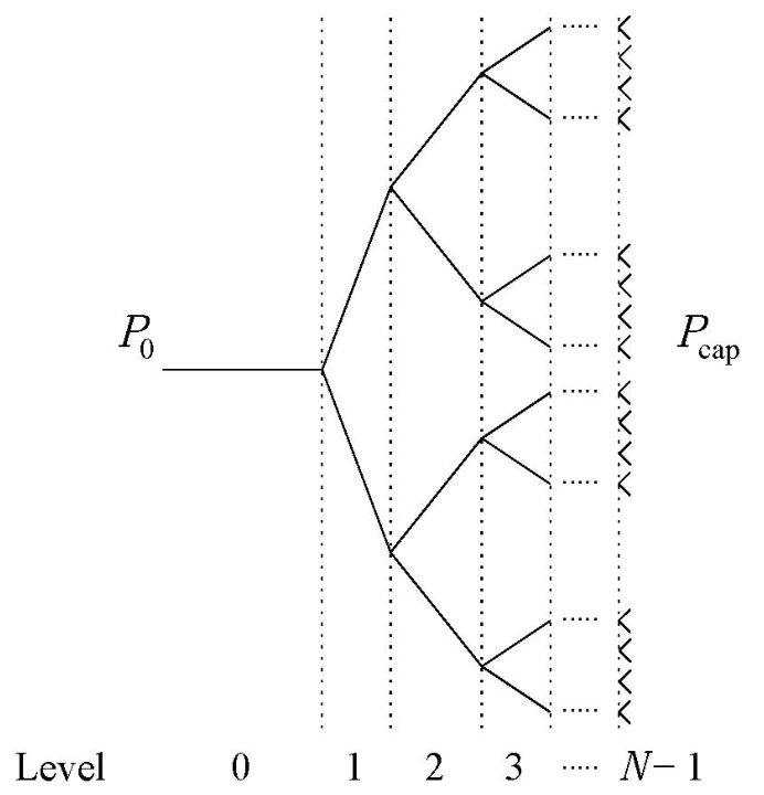
Figure 1. Network of arterioles.

A.1 (1.3pt)

Obtain an expression for the volumetric flow rate, \(Q_i\), in a vessel at any level \(i\), as a function of the total number of levels \(N\), of the viscosity \(\eta\), of the radius \(r_0\) and length \(\ell_0\) of the first vessel, and of the difference \(\Delta P=P_0-P_{\mathrm{cap}}\) between the pressure at the arteriole at level 0, \(P_0\), and the pressure at the capillary bed, \(P_{\mathrm{cap}}\).

A.2 (0.5pt)

Calculate the numerical value of the volumetric flow rate \(Q_0\) of the arteriole at level 0, if its radius is \(6.0\times10^{-5}\ \mathrm{m}\) and its length is \(2.0\times10^{-3}\ \mathrm{m}\). Consider that the pressure at the arteriole inlet is 55 mmHg and the vessel network has \(N=6\) levels linking this arteriole to the capillary bed at the pressure 30 mmHg. Consider that the blood viscosity is \(\eta=3.5\times10^{-3}\ \mathrm{kg\,m^{-1}\,s^{-1}}\). Express your result in ml/h.

A blood vessel as an LCR circuit

The approximation of rigid cylindrical vessels falls short for several reasons. It is particularly important to include the time dependent flow and to take into account the change in vessel diameter that occurs when the pressure varies during a blood pumping cycle done by the heart. Moreover, it is observed that in the larger vessels the blood pressure varies significantly during a cycle, while in the smaller vessels the amplitude of the oscillations in pressure is much smaller, and the flow is almost time independent.

When the pressure increases in a single elastic vessel, there will be an increase in its diameter, thus permitting to store more fluid in the vessel, and to deliver it when the pressure drops. For this reason, the elastic behaviour of the vessel can be simulated by adding a capacitor to our initial description. Moreover, when taking into account the time dependent blood flow rate, one has to consider the inertia of the fluid, proportional to its density \(\rho=1.05\times10^3\ \mathrm{kg\,m^{-3}}\). This inertia can be described by an inductance in our model. In Figure 2 we represent the equivalent circuit for a single vessel in this model. The equivalent capacitance and inductance are given by

\[ C=\frac{3\ell\pi r^3}{2Eh} \quad\text{and}\quad L=\frac{9\ell\rho}{4\pi r^2}, \tag{2} \]

respectively, where \(h\) is the width of the vessel wall and \(E\) is the artery Young's modulus, a coefficient that describes the alteration in size of the vessel tissue when a force is applied. The Young's modulus has units of pressure and is on the order of \(E=0.06\ \mathrm{MPa}\) for arterioles.

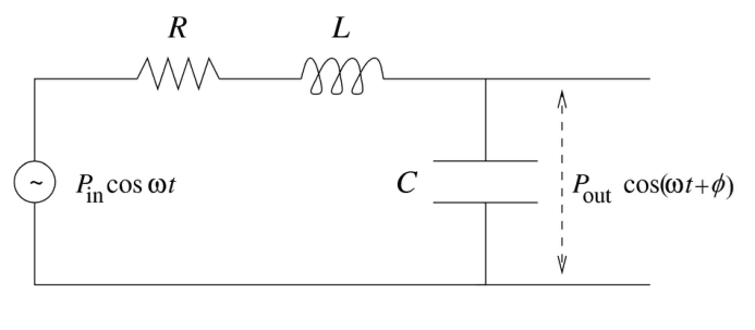
Figure 2. Equivalent electric circuit for a single vessel.

A.3 (2.0pt)

Obtain, in the stationary regime, the pressure amplitude at the vessel outlet, \(P_{\mathrm{out}}\), as a function of the pressure amplitude at the inlet, \(P_{\mathrm{in}}\), the equivalent resistance, \(R\), inductance, \(L\) and capacitance, \(C\), for a flow with angular frequency \(\omega\). Establish the condition between \(\eta\), \(\rho\), \(E\), \(h\), \(r\) and \(\ell\) so that, for low frequencies, the pressure oscillation amplitude at the outlet is smaller than that of \(P_{\mathrm{in}}\).

A.4 (0.7pt)

For the vessel network in A.2 estimate the maximum arteriole wall thickness \(h\) so that the condition established in A.3 is satisfied (consider that \(h\) is level independent).

Part B. Tumour growth (5.5 points)

Tumour growth is a very complex process where biological mechanisms such as cell proliferation and natural selection are intertwined with physics. In this problem we will consider a simplified model of tumour growth that addresses the increase in pressure commonly observed in solid tumors.

Consider a group of normal cells forming a tissue surrounded by an inextensible basement membrane, which forces the tissue to maintain always the same form: a sphere of radius \(R\) (Figure 3).

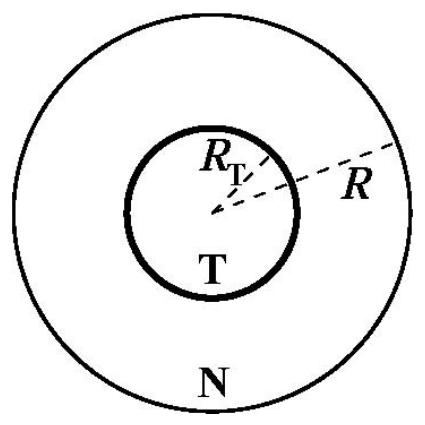
Figure 3. Simplified tumour.

Initially the tissue does not have residual stresses, i.e. the pressure at every point is equal to the atmospheric pressure.

At time \(t=0\), a tumour starts growing at the centre of this sphere and, as it grows, the pressure inside the tissue increases. Consider that both tissues (normal, N, and tumour, T) are compressible such that their densities, \(\rho_{\mathrm N}\) and \(\rho_{\mathrm T}\), increase linearly with pressure:

\[ \rho_{\mathrm N}=\rho_0\left(1+\frac{p}{K_{\mathrm N}}\right), \qquad \rho_{\mathrm T}=\rho_0\left(1+\frac{p}{K_{\mathrm T}}\right), \tag{3} \]

where \(\rho_0\) is the rest tissue density, \(p\) is the pressure difference to the atmospheric pressure and \(K_{\mathrm N}\), \(K_{\mathrm T}\) are the compressibility moduli (bulk moduli) of the normal and tumour tissues, respectively. In general, tumours are stiffer and so they have a higher bulk modulus.

B.1 (1.0pt)

The mass of normal cells is not altered while the tumour is growing. Obtain the ratio between the tumour volume and the total tissue volume, \(v=V_{\mathrm T}/V\), as a function of the ratio between the tumour mass (\(M_{\mathrm T}\)) and the normal tissue mass (\(M_{\mathrm N}\)), \(\mu=M_{\mathrm T}/M_{\mathrm N}\) and the ratio of the bulk moduli, \(\kappa=K_{\mathrm N}/K_{\mathrm T}\).

Hyperthermia is sometimes used together with chemotherapy and radiotherapy in the treatment of cancer. In hyperthermia the cancer cells are selectively heated from the normal human body temperature, \(37\,^\circ\mathrm C\), to temperatures above \(43\,^\circ\mathrm C\), inducing their death. Researchers are currently developing carbon nanotubes covered with special proteins capable of binding to tumour cells. When the tissue is irradiated with near-infrared radiation, the nanotubes absorb it in a much greater extent than the surrounding tissues and therefore can be selectively heated as well as the tumour cells to which they are attached.

Consider that the tumour, the normal cells and the surrounding tissue have a constant thermal conductivity \(k\), i.e. in the geometry of this problem, the energy that crosses a spherical surface of radius \(r\) per unit time and per unit area is equal to \(k\) times the derivative of the temperature with respect to \(r\). The nanotubes are uniformly distributed in the tumour volume and are able to deliver a power \(\mathcal P\) of thermal energy per unit volume. Assume that the temperature is equal to the normal human body temperature very far away from the tumour.

B.2 (1.7pt)

Obtain, for the stationary state, the temperature at the centre of the tumour as a function of \(\mathcal P\), \(k\), the human body temperature and the tumour radius, \(R_{\mathrm T}\).

B.3 (0.5pt)

Obtain the minimum power per unit volume, \(\mathcal P_{\min}\), needed to heat up all tumour cells in a tumour with 5.0 cm radius to a temperature larger than \(43.0\,^\circ\mathrm C\). Take the thermal conductivity of the tissue to be equal to \(k=0.60\ \mathrm{W\,K^{-1}\,m^{-1}}\).

Consider that the tumour is irrigated by a vessel network with a branched structure like in question A.1. As the tumour grows, when its pressure \(p\) becomes larger than the pressure \(P_{\mathrm{cap}}\) at the thinnest vessels, the radii of these vessels will decrease by a small amount \(\delta r\). If this pressure reaches a critical value \(p_c\) (which would correspond to a radius decrease of \(\delta r_c\)), the thinnest vessels would collapse, compromising seriously the irrigation to the tumour. The pressure and the radius change can be related by the following phenomenological relation:

\[ \frac{p}{P_{\mathrm{cap}}}-1 = \left(\frac{p_c}{P_{\mathrm{cap}}}-1\right) \left(2-\frac{\delta r}{\delta r_c}\right) \frac{\delta r}{\delta r_c}. \tag{4} \]

Consider that just the smallest vessels (of level \(N-1\)) have their radius altered when the tumour increases its pressure.

B.4 (2.3pt)

In the linear regime (i.e. consider that \(p-P_{\mathrm{cap}}\) is very small), express the relative drop in the flow rate, \(\frac{\delta Q_{N-1}}{Q_{N-1}}\), in these thinnest vessels, as a function of the tumour volume ratio \(v=V_{\mathrm T}/V\) and \(K_{\mathrm N}\), \(N\), \(p_c\), \(\delta r_c\), \(r_{N-1}\), \(P_{\mathrm{cap}}\).

Official English text of the problem.

Gegeben: Normaler Atmosphärendruck, \(P_0 = 1.013 \times 10^5\ \mathrm{Pa} = 760\ \mathrm{mmHg}\)

Teil A. Die Physik der Blutströmung (4.5 Punkte)

In diesem Teil untersuchen Sie zwei vereinfachte Modelle der Blutströmung in Gefäßen.

Blutgefäße sind näherungsweise zylinderförmig. Für eine stationäre, nicht turbulente Strömung einer inkompressiblen Flüssigkeit in einem starren Zylinder ist bekannt, dass die Druckdifferenz der Flüssigkeit zwischen den beiden Enden des Zylinders gegeben ist durch

\[ \Delta P=\frac{8\ell\eta}{\pi r^4}Q, \tag{1} \]

wobei \(\ell\) und \(r\) die Länge und der Radius des Zylinders sind, \(\eta\) die Viskosität der Flüssigkeit und \(Q\) der Volumenstrom, also das Flüssigkeitsvolumen, das pro Zeiteinheit durch den Zylinderquerschnitt strömt. Dieser Ausdruck liefert häufig die richtige Größenordnung der Druckdifferenz in einem Gefäß, selbst wenn die pulsierende Strömung, die Kompressibilität und die unregelmäßige Form des Gefäßes sowie die Tatsache unberücksichtigt bleiben, dass Blut keine einfache Flüssigkeit, sondern ein Gemisch aus Zellen und Plasma ist. Außerdem hat dieser Ausdruck dieselbe Form wie das ohmsche Gesetz, wobei der Volumenstrom als Stromstärke, die Druckdifferenz als Spannung und der Faktor \(R=\frac{8\ell\eta}{\pi r^4}\) als Widerstand interpretiert werden.

Betrachten Sie beispielsweise das in Abbildung 1 dargestellte symmetrische Netzwerk aus Arteriolen (kleinen Arterien), das das Kapillarbett eines Gewebes mit Blut versorgt. In diesem Netzwerk teilt sich an jeder Verzweigung ein Gefäß in zwei identische Gefäße. Die Gefäße höherer Ebenen sind jedoch dünner und kürzer: Nehmen Sie an, dass die Radien und Längen der Gefäße zweier aufeinanderfolgender Ebenen, \(i\) und \(i+1\), durch \(r_{i+1}=r_i/2^{1/3}\) und \(\ell_{i+1}=\ell_i/2^{1/3}\) miteinander verknüpft sind.

Abbildung 1. Netzwerk aus Arteriolen.

A.1 (1.3 Punkte)

Leiten Sie einen Ausdruck für den Volumenstrom \(Q_i\) in einem Gefäß einer beliebigen Ebene \(i\) her, als Funktion der Gesamtzahl der Ebenen \(N\), der Viskosität \(\eta\), des Radius \(r_0\) und der Länge \(\ell_0\) des ersten Gefäßes sowie der Differenz \(\Delta P=P_0-P_{\mathrm{cap}}\) zwischen dem Druck \(P_0\) in der Arteriole auf Ebene 0 und dem Druck \(P_{\mathrm{cap}}\) im Kapillarbett.

A.2 (0.5 Punkte)

Berechnen Sie den Zahlenwert des Volumenstroms \(Q_0\) der Arteriole auf Ebene 0, wenn ihr Radius \(6.0\times10^{-5}\ \mathrm{m}\) und ihre Länge \(2.0\times10^{-3}\ \mathrm{m}\) betragen. Nehmen Sie an, dass der Druck am Einlass der Arteriole 55 mmHg beträgt und das Gefäßnetzwerk \(N=6\) Ebenen besitzt, die diese Arteriole mit dem Kapillarbett bei einem Druck von 30 mmHg verbinden. Nehmen Sie für die Viskosität des Blutes \(\eta=3.5\times10^{-3}\ \mathrm{kg\,m^{-1}\,s^{-1}}\) an. Geben Sie Ihr Ergebnis in ml/h an.

Ein Blutgefäß als LCR-Schaltung

Die Näherung starrer zylindrischer Gefäße ist aus mehreren Gründen unzureichend. Besonders wichtig ist es, die zeitabhängige Strömung einzubeziehen und die Änderung des Gefäßdurchmessers zu berücksichtigen, die auftritt, wenn sich der Druck während eines Pumpzyklus des Herzens ändert. Außerdem beobachtet man, dass der Blutdruck in größeren Gefäßen während eines Zyklus erheblich schwankt, während in kleineren Gefäßen die Amplitude der Druckschwingungen wesentlich geringer und die Strömung nahezu zeitunabhängig ist.

Wenn der Druck in einem einzelnen elastischen Gefäß zunimmt, vergrößert sich dessen Durchmesser. Dadurch kann das Gefäß mehr Flüssigkeit speichern und diese bei sinkendem Druck wieder abgeben. Aus diesem Grund lässt sich das elastische Verhalten des Gefäßes simulieren, indem wir unsere ursprüngliche Beschreibung um einen Kondensator ergänzen. Berücksichtigt man zudem den zeitabhängigen Blutvolumenstrom, muss man die Trägheit der Flüssigkeit einbeziehen, die proportional zu ihrer Dichte \(\rho=1.05\times10^3\ \mathrm{kg\,m^{-3}}\) ist. Diese Trägheit lässt sich in unserem Modell durch eine Induktivität beschreiben. In Abbildung 2 ist das Ersatzschaltbild für ein einzelnes Gefäß in diesem Modell dargestellt. Die Ersatzkapazität und die Ersatzinduktivität sind gegeben durch

\[ C=\frac{3\ell\pi r^3}{2Eh} \quad\text{und}\quad L=\frac{9\ell\rho}{4\pi r^2}, \tag{2} \]

wobei \(h\) die Dicke der Gefäßwand und \(E\) der Elastizitätsmodul der Arterie ist, ein Koeffizient, der die Größenänderung des Gefäßgewebes unter Einwirkung einer Kraft beschreibt. Der Elastizitätsmodul hat die Einheit eines Drucks und liegt bei Arteriolen in der Größenordnung von \(E=0.06\ \mathrm{MPa}\).

Abbildung 2. Elektrisches Ersatzschaltbild für ein einzelnes Gefäß.

A.3 (2.0 Punkte)

Bestimmen Sie im eingeschwungenen Zustand die Druckamplitude am Gefäßauslass, \(P_{\mathrm{out}}\), als Funktion der Druckamplitude am Einlass, \(P_{\mathrm{in}}\), des Ersatzwiderstands \(R\), der Ersatzinduktivität \(L\) und der Ersatzkapazität \(C\) für eine Strömung mit der Kreisfrequenz \(\omega\). Stellen Sie die Bedingung zwischen \(\eta\), \(\rho\), \(E\), \(h\), \(r\) und \(\ell\) auf, unter der bei niedrigen Frequenzen die Amplitude der Druckschwingung am Auslass kleiner als \(P_{\mathrm{in}}\) ist.

A.4 (0.7 Punkte)

Schätzen Sie für das Gefäßnetzwerk aus A.2 die maximale Wanddicke \(h\) der Arteriolen ab, für die die in A.3 aufgestellte Bedingung erfüllt ist (nehmen Sie an, dass \(h\) von der Ebene unabhängig ist).

Teil B. Tumorwachstum (5.5 Punkte)

Tumorwachstum ist ein sehr komplexer Prozess, bei dem biologische Mechanismen wie Zellvermehrung und natürliche Selektion mit physikalischen Vorgängen verflochten sind. In dieser Aufgabe betrachten wir ein vereinfachtes Modell des Tumorwachstums, das den häufig in soliden Tumoren beobachteten Druckanstieg beschreibt.

Betrachten Sie eine Gruppe normaler Zellen, die ein Gewebe bilden, das von einer undehnbaren Basalmembran umgeben ist. Diese zwingt das Gewebe, stets dieselbe Form beizubehalten: eine Kugel mit dem Radius \(R\) (Abbildung 3).

Abbildung 3. Vereinfachter Tumor.

Anfangs weist das Gewebe keine Eigenspannungen auf, d. h., der Druck ist an jedem Punkt gleich dem Atmosphärendruck.

Zum Zeitpunkt \(t=0\) beginnt im Zentrum dieser Kugel ein Tumor zu wachsen, und mit seinem Wachstum steigt der Druck im Gewebe. Nehmen Sie an, dass beide Gewebe (normales Gewebe, N, und Tumorgewebe, T) kompressibel sind, sodass ihre Dichten \(\rho_{\mathrm N}\) und \(\rho_{\mathrm T}\) linear mit dem Druck zunehmen:

\[ \rho_{\mathrm N}=\rho_0\left(1+\frac{p}{K_{\mathrm N}}\right), \qquad \rho_{\mathrm T}=\rho_0\left(1+\frac{p}{K_{\mathrm T}}\right), \tag{3} \]

wobei \(\rho_0\) die Gewebedichte im Ruhezustand, \(p\) die Druckdifferenz gegenüber dem Atmosphärendruck und \(K_{\mathrm N}\), \(K_{\mathrm T}\) die Kompressionsmoduln des normalen Gewebes bzw. des Tumorgewebes sind. Im Allgemeinen sind Tumoren steifer und besitzen daher einen höheren Kompressionsmodul.

B.1 (1.0 Punkte)

Die Masse der normalen Zellen ändert sich während des Tumorwachstums nicht. Bestimmen Sie das Verhältnis zwischen Tumorvolumen und gesamtem Gewebevolumen, \(v=V_{\mathrm T}/V\), als Funktion des Verhältnisses zwischen der Tumormasse (\(M_{\mathrm T}\)) und der Masse des normalen Gewebes (\(M_{\mathrm N}\)), \(\mu=M_{\mathrm T}/M_{\mathrm N}\), sowie des Verhältnisses der Kompressionsmoduln, \(\kappa=K_{\mathrm N}/K_{\mathrm T}\).

Hyperthermie wird bei der Krebsbehandlung gelegentlich gemeinsam mit Chemotherapie und Strahlentherapie eingesetzt. Bei der Hyperthermie werden die Krebszellen gezielt von der normalen menschlichen Körpertemperatur von \(37\,^\circ\mathrm C\) auf Temperaturen über \(43\,^\circ\mathrm C\) erwärmt, wodurch ihr Absterben ausgelöst wird. Forschende entwickeln derzeit Kohlenstoffnanoröhren, die mit speziellen Proteinen beschichtet sind, die an Tumorzellen binden können. Wird das Gewebe mit nahinfraroter Strahlung bestrahlt, absorbieren die Nanoröhren diese wesentlich stärker als das umgebende Gewebe und können daher zusammen mit den Tumorzellen, an die sie gebunden sind, gezielt erwärmt werden.

Nehmen Sie an, dass der Tumor, die normalen Zellen und das umgebende Gewebe eine konstante Wärmeleitfähigkeit \(k\) besitzen, d. h., in der Geometrie dieser Aufgabe ist die Energie, die eine Kugeloberfläche mit dem Radius \(r\) pro Zeiteinheit und Flächeneinheit durchquert, gleich \(k\) mal der Ableitung der Temperatur nach \(r\). Die Nanoröhren sind gleichmäßig im Tumorvolumen verteilt und können pro Volumeneinheit eine Wärmeleistung \(\mathcal P\) abgeben. Nehmen Sie an, dass die Temperatur in sehr großer Entfernung vom Tumor gleich der normalen menschlichen Körpertemperatur ist.

B.2 (1.7 Punkte)

Bestimmen Sie für den stationären Zustand die Temperatur im Zentrum des Tumors als Funktion von \(\mathcal P\), \(k\), der menschlichen Körpertemperatur und dem Tumorradius \(R_{\mathrm T}\).

B.3 (0.5 Punkte)

Bestimmen Sie die minimale Leistung pro Volumeneinheit, \(\mathcal P_{\min}\), die benötigt wird, um alle Tumorzellen in einem Tumor mit einem Radius von 5.0 cm auf eine Temperatur über \(43.0\,^\circ\mathrm C\) zu erwärmen. Nehmen Sie für die Wärmeleitfähigkeit des Gewebes \(k=0.60\ \mathrm{W\,K^{-1}\,m^{-1}}\) an.

Nehmen Sie an, dass der Tumor von einem Gefäßnetzwerk mit einer Verzweigungsstruktur wie in Aufgabe A.1 durchblutet wird. Wenn der Tumor wächst und sein Druck \(p\) den Druck \(P_{\mathrm{cap}}\) in den dünnsten Gefäßen übersteigt, verringern sich die Radien dieser Gefäße um einen kleinen Betrag \(\delta r\). Erreicht dieser Druck einen kritischen Wert \(p_c\) (der einer Radiusverringerung von \(\delta r_c\) entspräche), würden die dünnsten Gefäße kollabieren, wodurch die Durchblutung des Tumors stark beeinträchtigt würde. Druck und Radiusänderung lassen sich durch die folgende phänomenologische Beziehung miteinander verknüpfen:

\[ \frac{p}{P_{\mathrm{cap}}}-1 = \left(\frac{p_c}{P_{\mathrm{cap}}}-1\right) \left(2-\frac{\delta r}{\delta r_c}\right) \frac{\delta r}{\delta r_c}. \tag{4} \]

Nehmen Sie an, dass sich bei steigendem Tumordruck nur die Radien der kleinsten Gefäße (auf Ebene \(N-1\)) ändern.

B.4 (2.3 Punkte)

Drücken Sie im linearen Bereich (nehmen Sie also an, dass \(p-P_{\mathrm{cap}}\) sehr klein ist) die relative Abnahme des Volumenstroms \(\frac{\delta Q_{N-1}}{Q_{N-1}}\) in diesen dünnsten Gefäßen als Funktion des Tumorvolumenanteils \(v=V_{\mathrm T}/V\) sowie von \(K_{\mathrm N}\), \(N\), \(p_c\), \(\delta r_c\), \(r_{N-1}\), \(P_{\mathrm{cap}}\) aus.

Aufgabentext aus dem offiziellen englischen Text übersetzt.

Veriler: Normal atmosfer basıncı, \(P_0 = 1.013 \times 10^5\ \mathrm{Pa} = 760\ \mathrm{mmHg}\)

Bölüm A. Kan akışının fiziği (4.5 puan)

Bu bölümde, damarlardaki kan akışına ilişkin iki basitleştirilmiş modeli inceleyeceksiniz.

Kan damarları yaklaşık olarak silindir biçimindedir. Sıkıştırılamaz bir akışkanın rijit bir silindir içindeki kararlı ve türbülanssız akışı için, silindirin iki ucundaki akışkan basınçları arasındaki farkın aşağıdaki bağıntıyla verildiği bilinmektedir:

\[ \Delta P=\frac{8\ell\eta}{\pi r^4}Q, \tag{1} \]

Burada \(\ell\) ve \(r\) silindirin uzunluğu ve yarıçapı, \(\eta\) akışkanın viskozitesi ve \(Q\) hacimsel debidir; yani birim zamanda silindirin en kesitinden geçen akışkan hacmidir. Bu ifade, akışın atımlı olması, damarın sıkıştırılabilirliği ve düzensiz biçimi ile kanın basit bir akışkan değil, hücreler ve plazmadan oluşan bir karışım olması hesaba katılmadan bile, bir damardaki basınç farkının büyüklük mertebesini çoğu zaman doğru verebilir. Ayrıca bu ifade, hacimsel debi akım, basınç farkı gerilim ve \(R=\frac{8\ell\eta}{\pi r^4}\) çarpanı direnç olarak yorumlandığında, Ohm yasasıyla aynı biçimdedir.

Örneğin, bir dokunun kılcal damar yatağına kan taşıyan ve Şekil 1'de gösterilen simetrik arteriyol (küçük atardamar) ağını ele alın. Bu ağda, her çatallanma noktasında bir damar iki özdeş damara ayrılır. Ancak daha yüksek düzeylerdeki damarlar daha ince ve daha kısadır: ardışık iki düzeydeki, \(i\) ve \(i+1\), damarların yarıçap ve uzunluklarının \(r_{i+1}=r_i/2^{1/3}\) ve \(\ell_{i+1}=\ell_i/2^{1/3}\) bağıntılarıyla ilişkili olduğunu kabul edin.

Şekil 1. Arteriyol ağı.

A.1 (1.3 puan)

Herhangi bir \(i\) düzeyindeki bir damarın hacimsel debisi \(Q_i\) için; toplam düzey sayısı \(N\), viskozite \(\eta\), ilk damarın yarıçapı \(r_0\) ve uzunluğu \(\ell_0\) ile 0. düzeydeki arteriyolün basıncı \(P_0\) ve kılcal damar yatağının basıncı \(P_{\mathrm{cap}}\) arasındaki \(\Delta P=P_0-P_{\mathrm{cap}}\) farkının fonksiyonu olan bir ifade elde edin.

A.2 (0.5 puan)

Yarıçapı \(6.0\times10^{-5}\ \mathrm{m}\) ve uzunluğu \(2.0\times10^{-3}\ \mathrm{m}\) olan 0. düzeydeki arteriyolün hacimsel debisi \(Q_0\)'ın sayısal değerini hesaplayın. Arteriyol girişindeki basıncın 55 mmHg olduğunu ve bu arteriyolü 30 mmHg basınçtaki kılcal damar yatağına bağlayan damar ağının \(N=6\) düzeyden oluştuğunu kabul edin. Kanın viskozitesini \(\eta=3.5\times10^{-3}\ \mathrm{kg\,m^{-1}\,s^{-1}}\) alın. Sonucunuzu ml/h cinsinden ifade edin.

Bir LCR devresi olarak kan damarı

Rijit silindirik damar yaklaşımı çeşitli nedenlerle yetersiz kalır. Zamana bağlı akışı modele katmak ve kalbin gerçekleştirdiği bir kan pompalama çevrimi sırasında basınç değiştikçe damar çapında meydana gelen değişimi hesaba katmak özellikle önemlidir. Ayrıca, büyük damarlarda kan basıncının bir çevrim boyunca önemli ölçüde değiştiği, küçük damarlarda ise basınç salınımlarının genliğinin çok daha küçük olduğu ve akışın neredeyse zamandan bağımsız olduğu gözlenir.

Tek bir elastik damarda basınç arttığında damarın çapı da artar; böylece damarda daha fazla akışkan depolanabilir ve basınç düştüğünde bu akışkan dışarı verilebilir. Bu nedenle, başlangıçtaki betimlememize bir kondansatör ekleyerek damarın elastik davranışını modelleyebiliriz. Ayrıca, zamana bağlı kan debisini hesaba katarken akışkanın, yoğunluğu \(\rho=1.05\times10^3\ \mathrm{kg\,m^{-3}}\) ile orantılı olan eylemsizliğini de dikkate almak gerekir. Bu eylemsizlik, modelimizde bir endüktans ile betimlenebilir. Şekil 2'de bu modeldeki tek bir damarın eşdeğer devresi gösterilmiştir. Eşdeğer kapasitans ve endüktans sırasıyla

\[ C=\frac{3\ell\pi r^3}{2Eh} \quad\text{ve}\quad L=\frac{9\ell\rho}{4\pi r^2}, \tag{2} \]

ile verilir. Burada \(h\) damar duvarının kalınlığı, \(E\) ise atardamarın Young modülüdür; bu katsayı, bir kuvvet uygulandığında damar dokusunun boyutlarında meydana gelen değişimi betimler. Young modülü basınç birimine sahiptir ve arteriyoller için \(E=0.06\ \mathrm{MPa}\) mertebesindedir.

Şekil 2. Tek bir damarın eşdeğer elektrik devresi.

A.3 (2.0 puan)

Kararlı rejimde, açısal frekansı \(\omega\) olan bir akış için damar çıkışındaki basınç genliği \(P_{\mathrm{out}}\)'u; girişteki basınç genliği \(P_{\mathrm{in}}\), eşdeğer direnç \(R\), endüktans \(L\) ve kapasitans \(C\)'nin fonksiyonu olarak elde edin. Düşük frekanslarda çıkıştaki basınç salınımı genliğinin \(P_{\mathrm{in}}\)'den küçük olması için \(\eta\), \(\rho\), \(E\), \(h\), \(r\) ve \(\ell\) arasındaki koşulu belirleyin.

A.4 (0.7 puan)

A.2'deki damar ağı için, A.3'te belirlenen koşulun sağlanmasını mümkün kılan en büyük arteriyol duvar kalınlığı \(h\)'yi tahmin edin (\(h\)'nin düzeyden bağımsız olduğunu kabul edin).

Bölüm B. Tümör büyümesi (5.5 puan)

Tümör büyümesi, hücre çoğalması ve doğal seçilim gibi biyolojik mekanizmaların fizikle iç içe geçtiği çok karmaşık bir süreçtir. Bu soruda, katı tümörlerde yaygın olarak gözlenen basınç artışını ele alan basitleştirilmiş bir tümör büyümesi modelini inceleyeceğiz.

Uzamayan bir bazal membranla çevrili bir doku oluşturan normal hücreler grubunu ele alın. Bu membran, dokunun her zaman aynı biçimi, yani \(R\) yarıçaplı bir küre biçimini korumasını zorunlu kılar (Şekil 3).

Şekil 3. Basitleştirilmiş tümör.

Başlangıçta dokuda artık gerilme yoktur; yani her noktadaki basınç atmosfer basıncına eşittir.

\(t=0\) anında bu kürenin merkezinde bir tümör büyümeye başlar ve büyüdükçe doku içindeki basınç artar. Her iki dokunun da (normal, N, ve tümör, T) sıkıştırılabilir olduğunu ve yoğunluklarının, \(\rho_{\mathrm N}\) ve \(\rho_{\mathrm T}\), basınçla doğrusal olarak arttığını kabul edin:

\[ \rho_{\mathrm N}=\rho_0\left(1+\frac{p}{K_{\mathrm N}}\right), \qquad \rho_{\mathrm T}=\rho_0\left(1+\frac{p}{K_{\mathrm T}}\right), \tag{3} \]

Burada \(\rho_0\) dokunun gerilmesiz durumdaki yoğunluğu, \(p\) atmosfer basıncına göre basınç farkı ve \(K_{\mathrm N}\), \(K_{\mathrm T}\) sırasıyla normal ve tümör dokularının sıkıştırılabilirlik modülleridir (hacim modülleri). Genel olarak tümörler daha serttir ve bu nedenle hacim modülleri daha büyüktür.

B.1 (1.0 puan)

Tümör büyürken normal hücrelerin kütlesi değişmez. Tümör hacminin toplam doku hacmine oranı \(v=V_{\mathrm T}/V\)'yi; tümör kütlesinin (\(M_{\mathrm T}\)) normal doku kütlesine (\(M_{\mathrm N}\)) oranı \(\mu=M_{\mathrm T}/M_{\mathrm N}\) ve hacim modüllerinin oranı \(\kappa=K_{\mathrm N}/K_{\mathrm T}\)'nın fonksiyonu olarak elde edin.

Kanser tedavisinde hipertermi bazen kemoterapi ve radyoterapiyle birlikte kullanılır. Hipertermide kanser hücreleri, normal insan vücut sıcaklığı olan \(37\,^\circ\mathrm C\)'den \(43\,^\circ\mathrm C\)'nin üzerindeki sıcaklıklara seçici olarak ısıtılarak ölmeleri sağlanır. Araştırmacılar günümüzde tümör hücrelerine bağlanabilen özel proteinlerle kaplanmış karbon nanotüpler geliştirmektedir. Doku yakın kızılötesi ışınımla ışınlandığında nanotüpler bu ışınımı çevredeki dokulara göre çok daha fazla soğurur; bu nedenle, bağlandıkları tümör hücreleriyle birlikte seçici olarak ısıtılabilirler.

Tümörün, normal hücrelerin ve çevredeki dokunun sabit bir \(k\) ısıl iletkenliğine sahip olduğunu kabul edin; yani bu sorunun geometrisinde, \(r\) yarıçaplı küresel bir yüzeyden birim zamanda ve birim alan başına geçen enerji, sıcaklığın \(r\)'ye göre türevinin \(k\) katına eşittir. Nanotüpler tümör hacmi içinde düzgün dağılmıştır ve birim hacim başına \(\mathcal P\) gücünde ısıl enerji sağlayabilmektedir. Tümörden çok uzakta sıcaklığın normal insan vücut sıcaklığına eşit olduğunu varsayın.

B.2 (1.7 puan)

Kararlı durumda tümörün merkezindeki sıcaklığı; \(\mathcal P\), \(k\), insan vücut sıcaklığı ve tümör yarıçapı \(R_{\mathrm T}\)'nin fonksiyonu olarak elde edin.

B.3 (0.5 puan)

Yarıçapı 5.0 cm olan bir tümördeki tüm tümör hücrelerini \(43.0\,^\circ\mathrm C\)'den daha yüksek bir sıcaklığa ısıtmak için gereken birim hacim başına en küçük güç \(\mathcal P_{\min}\)'i elde edin. Dokunun ısıl iletkenliğini \(k=0.60\ \mathrm{W\,K^{-1}\,m^{-1}}\) alın.

Tümörün, A.1 sorusundakine benzer dallanmış bir yapıya sahip damar ağıyla kanlandığını kabul edin. Tümör büyürken basıncı \(p\), en ince damarlardaki \(P_{\mathrm{cap}}\) basıncından büyük olduğunda, bu damarların yarıçapları küçük bir \(\delta r\) miktarı kadar azalır. Bu basınç kritik bir \(p_c\) değerine ulaşırsa (bu da \(\delta r_c\) kadar bir yarıçap azalmasına karşılık gelir), en ince damarlar çöker ve tümörün kanlanması ciddi biçimde bozulur. Basınç ile yarıçap değişimi arasında aşağıdaki fenomenolojik bağıntı kurulabilir:

\[ \frac{p}{P_{\mathrm{cap}}}-1 = \left(\frac{p_c}{P_{\mathrm{cap}}}-1\right) \left(2-\frac{\delta r}{\delta r_c}\right) \frac{\delta r}{\delta r_c}. \tag{4} \]

Tümörün basıncı arttığında yalnızca en küçük damarların (\(N-1\) düzeyindekilerin) yarıçaplarının değiştiğini kabul edin.

B.4 (2.3 puan)

Doğrusal rejimde (yani \(p-P_{\mathrm{cap}}\)'ın çok küçük olduğunu kabul ederek), bu en ince damarlardaki debinin bağıl azalmasını, \(\frac{\delta Q_{N-1}}{Q_{N-1}}\), tümör hacim oranı \(v=V_{\mathrm T}/V\) ile \(K_{\mathrm N}\), \(N\), \(p_c\), \(\delta r_c\), \(r_{N-1}\), \(P_{\mathrm{cap}}\)'ın fonksiyonu olarak ifade edin.

Soru metni resmi İngilizce metinden çevrilmiştir.

Datos: Presión atmosférica normal, \(P_0 = 1.013 \times 10^5\ \mathrm{Pa} = 760\ \mathrm{mmHg}\)

Parte A. La física del flujo sanguíneo (4.5 puntos)

En esta parte analizará dos modelos simplificados del flujo sanguíneo en los vasos.

Los vasos sanguíneos tienen una forma aproximadamente cilíndrica, y se sabe que, para un flujo estacionario y no turbulento de un fluido incompresible en un cilindro rígido, la diferencia de presión del fluido entre los dos extremos del cilindro viene dada por

\[ \Delta P=\frac{8\ell\eta}{\pi r^4}Q, \tag{1} \]

donde \(\ell\) y \(r\) son la longitud y el radio del cilindro, \(\eta\) es la viscosidad del fluido y \(Q\) es el caudal volumétrico, es decir, el volumen de fluido que atraviesa la sección transversal del cilindro por unidad de tiempo. Esta expresión suele proporcionar el orden de magnitud correcto de la diferencia de presión en un vaso, incluso sin tener en cuenta el flujo pulsátil, la compresibilidad y la forma irregular del vaso, ni el hecho de que la sangre no es un fluido simple, sino una mezcla de células y plasma. Además, esta expresión tiene la misma forma que la ley de Ohm, si se interpreta el caudal volumétrico como una corriente, la diferencia de presión como una tensión y el factor \(R=\frac{8\ell\eta}{\pi r^4}\) como una resistencia.

Considere, por ejemplo, la red simétrica de arteriolas (arterias pequeñas) representada en la Figura 1, que lleva sangre al lecho capilar de un tejido. En esta red, en cada bifurcación un vaso se divide en dos vasos idénticos. Sin embargo, los vasos de los niveles superiores son más estrechos y más cortos: considere que los radios y las longitudes de los vasos de dos niveles consecutivos, \(i\) e \(i+1\), están relacionados mediante \(r_{i+1}=r_i/2^{1/3}\) y \(\ell_{i+1}=\ell_i/2^{1/3}\).

Figura 1. Red de arteriolas.

A.1 (1.3 puntos)

Obtenga una expresión para el caudal volumétrico, \(Q_i\), en un vaso de cualquier nivel \(i\), en función del número total de niveles \(N\), de la viscosidad \(\eta\), del radio \(r_0\) y la longitud \(\ell_0\) del primer vaso, y de la diferencia \(\Delta P=P_0-P_{\mathrm{cap}}\) entre la presión en la arteriola del nivel 0, \(P_0\), y la presión en el lecho capilar, \(P_{\mathrm{cap}}\).

A.2 (0.5 puntos)

Calcule el valor numérico del caudal volumétrico \(Q_0\) de la arteriola del nivel 0, si su radio es \(6.0\times10^{-5}\ \mathrm{m}\) y su longitud es \(2.0\times10^{-3}\ \mathrm{m}\). Considere que la presión a la entrada de la arteriola es de 55 mmHg y que la red de vasos tiene \(N=6\) niveles que conectan esta arteriola con el lecho capilar, cuya presión es de 30 mmHg. Considere que la viscosidad de la sangre es \(\eta=3.5\times10^{-3}\ \mathrm{kg\,m^{-1}\,s^{-1}}\). Exprese el resultado en ml/h.

Un vaso sanguíneo como circuito LCR

La aproximación de vasos cilíndricos rígidos resulta insuficiente por varias razones. Es especialmente importante incluir la dependencia temporal del flujo y tener en cuenta el cambio de diámetro del vaso que se produce cuando la presión varía durante un ciclo de bombeo de sangre realizado por el corazón. Además, se observa que en los vasos de mayor tamaño la presión sanguínea varía significativamente durante un ciclo, mientras que en los vasos más pequeños la amplitud de las oscilaciones de presión es mucho menor y el flujo es casi independiente del tiempo.

Cuando aumenta la presión en un vaso elástico, su diámetro aumenta, lo que permite almacenar más fluido en el vaso y liberarlo cuando la presión disminuye. Por este motivo, el comportamiento elástico del vaso puede simularse añadiendo un condensador a nuestra descripción inicial. Además, al tener en cuenta la dependencia temporal del caudal sanguíneo, hay que considerar la inercia del fluido, proporcional a su densidad \(\rho=1.05\times10^3\ \mathrm{kg\,m^{-3}}\). Esta inercia puede describirse mediante una inductancia en nuestro modelo. En la Figura 2 representamos el circuito equivalente para un solo vaso en este modelo. La capacidad y la inductancia equivalentes vienen dadas por

\[ C=\frac{3\ell\pi r^3}{2Eh} \quad\text{y}\quad L=\frac{9\ell\rho}{4\pi r^2}, \tag{2} \]

respectivamente, donde \(h\) es el espesor de la pared del vaso y \(E\) es el módulo de Young de la arteria, un coeficiente que describe el cambio de tamaño del tejido del vaso cuando se aplica una fuerza. El módulo de Young tiene unidades de presión y es del orden de \(E=0.06\ \mathrm{MPa}\) para las arteriolas.

Figura 2. Circuito eléctrico equivalente para un solo vaso.

A.3 (2.0 puntos)

Obtenga, en régimen estacionario, la amplitud de presión a la salida del vaso, \(P_{\mathrm{out}}\), en función de la amplitud de presión a la entrada, \(P_{\mathrm{in}}\), de la resistencia equivalente, \(R\), de la inductancia, \(L\), y de la capacidad, \(C\), para un flujo de frecuencia angular \(\omega\). Establezca la condición entre \(\eta\), \(\rho\), \(E\), \(h\), \(r\) y \(\ell\) para que, a bajas frecuencias, la amplitud de las oscilaciones de presión a la salida sea menor que \(P_{\mathrm{in}}\).

A.4 (0.7 puntos)

Para la red de vasos de A.2, estime el espesor máximo \(h\) de la pared de las arteriolas para que se cumpla la condición establecida en A.3 (considere que \(h\) es independiente del nivel).

Parte B. Crecimiento tumoral (5.5 puntos)

El crecimiento tumoral es un proceso muy complejo en el que mecanismos biológicos como la proliferación celular y la selección natural se entrelazan con la física. En este problema consideraremos un modelo simplificado del crecimiento tumoral que aborda el aumento de presión observado habitualmente en los tumores sólidos.

Considere un grupo de células normales que forman un tejido rodeado por una membrana basal inextensible, que obliga al tejido a mantener siempre la misma forma: una esfera de radio \(R\) (Figura 3).

Figura 3. Tumor simplificado.

Inicialmente, el tejido no presenta tensiones residuales, es decir, la presión en todos sus puntos es igual a la presión atmosférica.

En el instante \(t=0\), un tumor comienza a crecer en el centro de esta esfera y, a medida que crece, la presión en el interior del tejido aumenta. Considere que ambos tejidos (normal, N, y tumoral, T) son compresibles, de modo que sus densidades, \(\rho_{\mathrm N}\) y \(\rho_{\mathrm T}\), aumentan linealmente con la presión:

\[ \rho_{\mathrm N}=\rho_0\left(1+\frac{p}{K_{\mathrm N}}\right), \qquad \rho_{\mathrm T}=\rho_0\left(1+\frac{p}{K_{\mathrm T}}\right), \tag{3} \]

donde \(\rho_0\) es la densidad del tejido en reposo, \(p\) es la diferencia de presión respecto a la presión atmosférica y \(K_{\mathrm N}\), \(K_{\mathrm T}\) son los módulos de compresibilidad (módulos volumétricos) de los tejidos normal y tumoral, respectivamente. En general, los tumores son más rígidos y, por tanto, tienen un módulo volumétrico mayor.

B.1 (1.0 puntos)

La masa de las células normales no cambia mientras el tumor crece. Obtenga la razón entre el volumen del tumor y el volumen total del tejido, \(v=V_{\mathrm T}/V\), en función de la razón entre la masa del tumor (\(M_{\mathrm T}\)) y la masa del tejido normal (\(M_{\mathrm N}\)), \(\mu=M_{\mathrm T}/M_{\mathrm N}\), y de la razón entre los módulos volumétricos, \(\kappa=K_{\mathrm N}/K_{\mathrm T}\).

La hipertermia se utiliza a veces junto con la quimioterapia y la radioterapia en el tratamiento del cáncer. En la hipertermia, las células cancerosas se calientan selectivamente desde la temperatura normal del cuerpo humano, \(37\,^\circ\mathrm C\), hasta temperaturas superiores a \(43\,^\circ\mathrm C\), lo que provoca su muerte. Actualmente, los investigadores están desarrollando nanotubos de carbono recubiertos de proteínas especiales capaces de unirse a las células tumorales. Cuando el tejido se irradia con radiación infrarroja cercana, los nanotubos la absorben en una proporción mucho mayor que los tejidos circundantes y, por tanto, pueden calentarse selectivamente, al igual que las células tumorales a las que están unidos.

Considere que el tumor, las células normales y el tejido circundante tienen una conductividad térmica constante \(k\), es decir, en la geometría de este problema, la energía que atraviesa una superficie esférica de radio \(r\) por unidad de tiempo y por unidad de área es igual a \(k\) multiplicado por la derivada de la temperatura respecto a \(r\). Los nanotubos están distribuidos uniformemente en el volumen del tumor y pueden aportar una potencia \(\mathcal P\) de energía térmica por unidad de volumen. Suponga que la temperatura es igual a la temperatura normal del cuerpo humano a una distancia muy grande del tumor.

B.2 (1.7 puntos)

Obtenga, en el estado estacionario, la temperatura en el centro del tumor en función de \(\mathcal P\), \(k\), la temperatura del cuerpo humano y el radio del tumor, \(R_{\mathrm T}\).

B.3 (0.5 puntos)

Obtenga la potencia mínima por unidad de volumen, \(\mathcal P_{\min}\), necesaria para calentar todas las células tumorales de un tumor de 5.0 cm de radio hasta una temperatura superior a \(43.0\,^\circ\mathrm C\). Tome la conductividad térmica del tejido igual a \(k=0.60\ \mathrm{W\,K^{-1}\,m^{-1}}\).

Considere que el tumor está irrigado por una red de vasos con una estructura ramificada como la de la pregunta A.1. A medida que el tumor crece, cuando su presión \(p\) supera la presión \(P_{\mathrm{cap}}\) en los vasos más estrechos, los radios de estos vasos disminuyen una pequeña cantidad \(\delta r\). Si esta presión alcanza un valor crítico \(p_c\) (que correspondería a una disminución del radio de \(\delta r_c\)), los vasos más estrechos colapsarían, comprometiendo gravemente la irrigación del tumor. La presión y el cambio de radio pueden relacionarse mediante la siguiente relación fenomenológica:

\[ \frac{p}{P_{\mathrm{cap}}}-1 = \left(\frac{p_c}{P_{\mathrm{cap}}}-1\right) \left(2-\frac{\delta r}{\delta r_c}\right) \frac{\delta r}{\delta r_c}. \tag{4} \]

Considere que solo los vasos más pequeños (del nivel \(N-1\)) modifican su radio cuando aumenta la presión del tumor.

B.4 (2.3 puntos)

En el régimen lineal (es decir, considere que \(p-P_{\mathrm{cap}}\) es muy pequeño), exprese la disminución relativa del caudal, \(\frac{\delta Q_{N-1}}{Q_{N-1}}\), en estos vasos más estrechos, en función de la razón de volúmenes del tumor \(v=V_{\mathrm T}/V\) y de \(K_{\mathrm N}\), \(N\), \(p_c\), \(\delta r_c\), \(r_{N-1}\), \(P_{\mathrm{cap}}\).

Enunciado traducido del texto oficial en inglés.

已知数据：标准大气压，\(P_0 = 1.013 \times 10^5\ \mathrm{Pa} = 760\ \mathrm{mmHg}\)

部分 A. 血液流动的物理学（4.5 分）

在本部分中，你将分析两个描述血管内血液流动的简化模型。

血管的形状近似为圆柱形。已知不可压缩流体在刚性圆柱管内作稳定的非湍流流动时，圆柱管两端的流体压强差为

\[ \Delta P=\frac{8\ell\eta}{\pi r^4}Q, \tag{1} \]

其中，\(\ell\) 和 \(r\) 分别为圆柱管的长度和半径，\(\eta\) 为流体的黏度，\(Q\) 为体积流量，即单位时间内通过圆柱管横截面的流体体积。即使不考虑脉动流、血管的可压缩性和不规则形状，以及血液并非简单流体而是细胞与血浆的混合物这一事实，该表达式通常也能给出血管内压强差的正确数量级。此外，该表达式与欧姆定律具有相同的形式：体积流量可类比为电流，压强差可类比为电压，而因子 \(R=\frac{8\ell\eta}{\pi r^4}\) 则可类比为电阻。

例如，考虑图 1 所示的对称微动脉（小动脉）网络，它向组织的毛细血管床输送血液。在该网络中，每个分叉处的一条血管都分成两条相同的血管。不过，级数较高的血管更细、更短：设相邻两级 \(i\) 和 \(i+1\) 的血管半径和长度满足 \(r_{i+1}=r_i/2^{1/3}\) 和 \(\ell_{i+1}=\ell_i/2^{1/3}\)。

图 1. 微动脉网络。

A.1（1.3 分）

求任意第 \(i\) 级的一条血管中的体积流量 \(Q_i\) 的表达式，用总级数 \(N\)、黏度 \(\eta\)、第一条血管的半径 \(r_0\) 和长度 \(\ell_0\)，以及第 0 级微动脉处的压强 \(P_0\) 与毛细血管床处的压强 \(P_{\mathrm{cap}}\) 之差 \(\Delta P=P_0-P_{\mathrm{cap}}\) 表示。

A.2（0.5 分）

若第 0 级微动脉的半径为 \(6.0\times10^{-5}\ \mathrm{m}\)，长度为 \(2.0\times10^{-3}\ \mathrm{m}\)，计算其体积流量 \(Q_0\) 的数值。设微动脉入口处的压强为 55 mmHg，血管网络共有 \(N=6\) 级，将这条微动脉与压强为 30 mmHg 的毛细血管床相连。设血液的黏度为 \(\eta=3.5\times10^{-3}\ \mathrm{kg\,m^{-1}\,s^{-1}}\)。用 ml/h 表示结果。

将血管视为 LCR 电路

将血管近似为刚性圆柱管存在若干不足。尤其重要的是，需要纳入随时间变化的流动，并考虑心脏一次泵血周期中压强变化所引起的血管直径变化。此外，观察表明，较大血管中的血压在一个周期内变化显著，而在较小血管中，压强振荡的振幅要小得多，流动几乎不随时间变化。

当一条弹性血管内的压强升高时，其直径会增大，从而使血管能够储存更多流体，并在压强降低时将其输送出去。因此，可以在最初的描述中加入一个电容器来模拟血管的弹性行为。此外，在考虑随时间变化的血液流量时，还必须考虑流体的惯性，它与流体密度 \(\rho=1.05\times10^3\ \mathrm{kg\,m^{-3}}\) 成正比。在本模型中，这种惯性可用电感来描述。图 2 给出了本模型中单条血管的等效电路。等效电容和电感分别为

\[ C=\frac{3\ell\pi r^3}{2Eh} \quad\text{和}\quad L=\frac{9\ell\rho}{4\pi r^2}, \tag{2} \]

其中，\(h\) 为血管壁厚度，\(E\) 为动脉的杨氏模量，即描述血管组织在受力时尺寸变化的系数。杨氏模量的单位与压强相同，微动脉的杨氏模量约为 \(E=0.06\ \mathrm{MPa}\)。

图 2. 单条血管的等效电路。

A.3（2.0 分）

对于角频率为 \(\omega\) 的流动，求稳态下血管出口处的压强振幅 \(P_{\mathrm{out}}\)，用入口处的压强振幅 \(P_{\mathrm{in}}\)、等效电阻 \(R\)、电感 \(L\) 和电容 \(C\) 表示。求出 \(\eta\)、\(\rho\)、\(E\)、\(h\)、\(r\) 和 \(\ell\) 之间应满足的条件，使得在低频下，出口处的压强振荡振幅小于 \(P_{\mathrm{in}}\)。

A.4（0.7 分）

对于 A.2 中的血管网络，估算使 A.3 中所得条件成立的最大微动脉壁厚 \(h\)（设 \(h\) 与级数无关）。

部分 B. 肿瘤生长（5.5 分）

肿瘤生长是一个极其复杂的过程，其中细胞增殖和自然选择等生物学机制与物理过程相互交织。本题将考虑一个简化的肿瘤生长模型，以研究实体肿瘤中普遍观察到的压强升高现象。

考虑一组正常细胞所形成的组织，其外部包围着一层不可伸展的基底膜，迫使组织始终保持相同的形状：半径为 \(R\) 的球体（图 3）。

图 3. 简化的肿瘤。

初始时，组织内不存在残余应力，即各处的压强均等于大气压。

在 \(t=0\) 时刻，一个肿瘤开始在该球体的中心生长；随着肿瘤生长，组织内部的压强升高。设两种组织（正常组织 N 和肿瘤组织 T）均可压缩，其密度 \(\rho_{\mathrm N}\) 和 \(\rho_{\mathrm T}\) 随压强线性增大：

\[ \rho_{\mathrm N}=\rho_0\left(1+\frac{p}{K_{\mathrm N}}\right), \qquad \rho_{\mathrm T}=\rho_0\left(1+\frac{p}{K_{\mathrm T}}\right), \tag{3} \]

其中，\(\rho_0\) 为组织的初始密度，\(p\) 为相对于大气压的压强差，\(K_{\mathrm N}\)、\(K_{\mathrm T}\) 分别为正常组织和肿瘤组织的压缩模量（体积弹性模量）。一般而言，肿瘤更硬，因此具有更大的体积弹性模量。

B.1（1.0 分）

肿瘤生长过程中，正常细胞的质量保持不变。求肿瘤体积与组织总体积之比 \(v=V_{\mathrm T}/V\)，用肿瘤质量（\(M_{\mathrm T}\)）与正常组织质量（\(M_{\mathrm N}\)）之比 \(\mu=M_{\mathrm T}/M_{\mathrm N}\) 以及体积弹性模量之比 \(\kappa=K_{\mathrm N}/K_{\mathrm T}\) 表示。

在癌症治疗中，有时会将热疗与化疗、放疗结合使用。热疗选择性地将癌细胞从正常人体体温 \(37\,^\circ\mathrm C\) 加热至 \(43\,^\circ\mathrm C\) 以上，从而使其死亡。研究人员目前正在开发表面覆盖特殊蛋白质的碳纳米管，这些蛋白质能够与肿瘤细胞结合。当用近红外辐射照射组织时，纳米管对辐射的吸收远强于周围组织，因此可以选择性地加热纳米管及其附着的肿瘤细胞。

设肿瘤、正常细胞及周围组织具有恒定的热导率 \(k\)，即在本题的几何构型中，单位时间内通过半径为 \(r\) 的球面单位面积的能量，等于 \(k\) 乘以温度对 \(r\) 的导数。纳米管均匀分布于肿瘤体积内，能够在单位体积内提供功率为 \(\mathcal P\) 的热能。假设在距肿瘤非常远的地方，温度等于正常人体体温。

B.2（1.7 分）

求稳态下肿瘤中心的温度，用 \(\mathcal P\)、\(k\)、人体体温和肿瘤半径 \(R_{\mathrm T}\) 表示。

B.3（0.5 分）

求将半径为 5.0 cm 的肿瘤中所有肿瘤细胞加热至 \(43.0\,^\circ\mathrm C\) 以上所需的最小单位体积功率 \(\mathcal P_{\min}\)。取组织的热导率为 \(k=0.60\ \mathrm{W\,K^{-1}\,m^{-1}}\)。

设肿瘤由一个具有 A.1 中所述分支结构的血管网络供血。随着肿瘤生长，当其压强 \(p\) 超过最细血管内的压强 \(P_{\mathrm{cap}}\) 时，这些血管的半径将减小一个微小量 \(\delta r\)。若该压强达到临界值 \(p_c\)（对应于半径减小量 \(\delta r_c\)），最细的血管就会塌陷，严重影响肿瘤的血液灌注。压强与半径变化可由以下唯象关系联系起来：

\[ \frac{p}{P_{\mathrm{cap}}}-1 = \left(\frac{p_c}{P_{\mathrm{cap}}}-1\right) \left(2-\frac{\delta r}{\delta r_c}\right) \frac{\delta r}{\delta r_c}. \tag{4} \]

设肿瘤压强升高时，只有最细的血管（第 \(N-1\) 级）的半径发生变化。

B.4（2.3 分）

在线性范围内（即认为 \(p-P_{\mathrm{cap}}\) 非常小），将这些最细血管中流量的相对下降量 \(\frac{\delta Q_{N-1}}{Q_{N-1}}\) 表示为肿瘤体积比 \(v=V_{\mathrm T}/V\) 以及 \(K_{\mathrm N}\)、\(N\)、\(p_c\)、\(\delta r_c\)、\(r_{N-1}\)、\(P_{\mathrm{cap}}\) 的函数。

题目译自官方英文原文。

Дано: нормальное атмосферное давление, \(P_0 = 1.013 \times 10^5\ \mathrm{Pa} = 760\ \mathrm{mmHg}\)

Часть A. Физика кровотока (4.5 балла)

В этой части вы проанализируете две упрощённые модели течения крови в сосудах.

Кровеносные сосуды имеют приблизительно цилиндрическую форму. Известно, что при стационарном нетурбулентном течении несжимаемой жидкости в жёстком цилиндре разность давлений жидкости на двух концах цилиндра определяется выражением

\[ \Delta P=\frac{8\ell\eta}{\pi r^4}Q, \tag{1} \]

где \(\ell\) и \(r\) — длина и радиус цилиндра, \(\eta\) — вязкость жидкости, а \(Q\) — объёмный расход, то есть объём жидкости, проходящий через поперечное сечение цилиндра за единицу времени. Это выражение часто позволяет правильно оценить порядок величины разности давлений в сосуде даже без учёта пульсирующего характера течения, сжимаемости сосуда и неправильности его формы, а также того факта, что кровь представляет собой не простую жидкость, а смесь клеток и плазмы. Кроме того, это выражение имеет тот же вид, что и закон Ома: объёмный расход можно интерпретировать как ток, разность давлений — как напряжение, а множитель \(R=\frac{8\ell\eta}{\pi r^4}\) — как сопротивление.

Рассмотрим, например, симметричную сеть артериол (мелких артерий), изображённую на рисунке 1, которая доставляет кровь к капиллярному руслу ткани. В этой сети при каждом разветвлении сосуд разделяется на два одинаковых сосуда. Однако сосуды более высоких уровней тоньше и короче: считайте, что радиусы и длины сосудов двух последовательных уровней, \(i\) и \(i+1\), связаны соотношениями \(r_{i+1}=r_i/2^{1/3}\) и \(\ell_{i+1}=\ell_i/2^{1/3}\).

Рисунок 1. Сеть артериол.

A.1 (1.3 балла)

Получите выражение для объёмного расхода \(Q_i\) в сосуде произвольного уровня \(i\) как функции общего числа уровней \(N\), вязкости \(\eta\), радиуса \(r_0\) и длины \(\ell_0\) первого сосуда, а также разности \(\Delta P=P_0-P_{\mathrm{cap}}\) между давлением в артериоле уровня 0, \(P_0\), и давлением в капиллярном русле, \(P_{\mathrm{cap}}\).

A.2 (0.5 балла)

Вычислите численное значение объёмного расхода \(Q_0\) в артериоле уровня 0, если её радиус равен \(6.0\times10^{-5}\ \mathrm{m}\), а длина — \(2.0\times10^{-3}\ \mathrm{m}\). Считайте, что давление на входе в артериолу равно 55 мм рт. ст., а сеть сосудов имеет \(N=6\) уровней, соединяющих эту артериолу с капиллярным руслом, давление в котором равно 30 мм рт. ст. Считайте, что вязкость крови равна \(\eta=3.5\times10^{-3}\ \mathrm{kg\,m^{-1}\,s^{-1}}\). Выразите результат в мл/ч.

Кровеносный сосуд как LCR-цепь

Приближение жёстких цилиндрических сосудов оказывается недостаточным по нескольким причинам. Особенно важно учесть зависимость кровотока от времени и изменение диаметра сосуда при изменении давления в течение цикла перекачивания крови сердцем. Кроме того, наблюдается, что в крупных сосудах давление крови существенно меняется в течение цикла, тогда как в мелких сосудах амплитуда колебаний давления гораздо меньше и течение почти не зависит от времени.

При повышении давления в отдельном эластичном сосуде его диаметр увеличивается, что позволяет накапливать в сосуде дополнительную жидкость и отдавать её при падении давления. Поэтому упругие свойства сосуда можно моделировать, добавив конденсатор к нашему исходному описанию. Кроме того, при учёте зависимости объёмного расхода крови от времени необходимо учитывать инерцию жидкости, пропорциональную её плотности \(\rho=1.05\times10^3\ \mathrm{kg\,m^{-3}}\). В нашей модели эту инерцию можно описать с помощью индуктивности. На рисунке 2 представлена эквивалентная цепь для отдельного сосуда в этой модели. Эквивалентные ёмкость и индуктивность задаются выражениями

\[ C=\frac{3\ell\pi r^3}{2Eh} \quad\text{и}\quad L=\frac{9\ell\rho}{4\pi r^2}, \tag{2} \]

соответственно, где \(h\) — толщина стенки сосуда, а \(E\) — модуль Юнга артерии, коэффициент, описывающий изменение размеров ткани сосуда при приложении силы. Модуль Юнга имеет размерность давления и для артериол составляет величину порядка \(E=0.06\ \mathrm{MPa}\).

Рисунок 2. Эквивалентная электрическая цепь для отдельного сосуда.

A.3 (2.0 балла)

Получите для установившегося режима амплитуду давления на выходе из сосуда \(P_{\mathrm{out}}\) как функцию амплитуды давления на входе \(P_{\mathrm{in}}\), эквивалентного сопротивления \(R\), индуктивности \(L\) и ёмкости \(C\) для течения с угловой частотой \(\omega\). Установите условие на \(\eta\), \(\rho\), \(E\), \(h\), \(r\) и \(\ell\), при котором на низких частотах амплитуда колебаний давления на выходе меньше \(P_{\mathrm{in}}\).

A.4 (0.7 балла)

Для сети сосудов из A.2 оцените максимальную толщину стенки артериолы \(h\), при которой выполняется условие, установленное в A.3 (считайте, что \(h\) не зависит от уровня).

Часть B. Рост опухоли (5.5 балла)

Рост опухоли — очень сложный процесс, в котором биологические механизмы, такие как размножение клеток и естественный отбор, переплетаются с физическими явлениями. В этой задаче мы рассмотрим упрощённую модель роста опухоли, описывающую повышение давления, обычно наблюдаемое в солидных опухолях.

Рассмотрим группу нормальных клеток, образующих ткань, окружённую нерастяжимой базальной мембраной, которая заставляет ткань всегда сохранять одну и ту же форму: шар радиуса \(R\) (рисунок 3).

Рисунок 3. Упрощённая модель опухоли.

Первоначально в ткани отсутствуют остаточные напряжения, то есть давление в каждой точке равно атмосферному.

В момент времени \(t=0\) в центре этого шара начинает расти опухоль, и по мере её роста давление внутри ткани повышается. Считайте, что обе ткани (нормальная, N, и опухолевая, T) сжимаемы, причём их плотности, \(\rho_{\mathrm N}\) и \(\rho_{\mathrm T}\), линейно возрастают с давлением:

\[ \rho_{\mathrm N}=\rho_0\left(1+\frac{p}{K_{\mathrm N}}\right), \qquad \rho_{\mathrm T}=\rho_0\left(1+\frac{p}{K_{\mathrm T}}\right), \tag{3} \]

где \(\rho_0\) — плотность ткани в ненапряжённом состоянии, \(p\) — разность между давлением в ткани и атмосферным давлением, а \(K_{\mathrm N}\), \(K_{\mathrm T}\) — модули объёмного сжатия нормальной и опухолевой тканей соответственно. Как правило, опухоли более жёсткие и поэтому имеют больший модуль объёмного сжатия.

B.1 (1.0 балла)

Масса нормальных клеток не изменяется при росте опухоли. Получите отношение объёма опухоли к общему объёму ткани, \(v=V_{\mathrm T}/V\), как функцию отношения массы опухоли (\(M_{\mathrm T}\)) к массе нормальной ткани (\(M_{\mathrm N}\)), \(\mu=M_{\mathrm T}/M_{\mathrm N}\), и отношения модулей объёмного сжатия, \(\kappa=K_{\mathrm N}/K_{\mathrm T}\).

При лечении рака наряду с химиотерапией и лучевой терапией иногда применяется гипертермия. При гипертермии раковые клетки избирательно нагревают от нормальной температуры человеческого тела, \(37\,^\circ\mathrm C\), до температуры выше \(43\,^\circ\mathrm C\), вызывая их гибель. В настоящее время исследователи разрабатывают углеродные нанотрубки, покрытые специальными белками, способными связываться с опухолевыми клетками. При облучении ткани излучением ближнего инфракрасного диапазона нанотрубки поглощают его гораздо сильнее, чем окружающие ткани, и поэтому могут избирательно нагреваться вместе с опухолевыми клетками, к которым они прикреплены.

Считайте, что опухоль, нормальные клетки и окружающая ткань имеют постоянный коэффициент теплопроводности \(k\), то есть в геометрии данной задачи энергия, проходящая через сферическую поверхность радиуса \(r\) за единицу времени на единицу площади, равна произведению \(k\) на производную температуры по \(r\). Нанотрубки равномерно распределены по объёму опухоли и могут выделять тепловую мощность \(\mathcal P\) на единицу объёма. Предположите, что очень далеко от опухоли температура равна нормальной температуре человеческого тела.

B.2 (1.7 балла)

Получите для стационарного состояния температуру в центре опухоли как функцию \(\mathcal P\), \(k\), температуры человеческого тела и радиуса опухоли \(R_{\mathrm T}\).

B.3 (0.5 балла)

Получите минимальную мощность на единицу объёма \(\mathcal P_{\min}\), необходимую для нагревания всех опухолевых клеток в опухоли радиуса 5.0 см до температуры выше \(43.0\,^\circ\mathrm C\). Примите коэффициент теплопроводности ткани равным \(k=0.60\ \mathrm{W\,K^{-1}\,m^{-1}}\).

Считайте, что опухоль снабжается кровью через сеть сосудов с разветвлённой структурой, как в вопросе A.1. По мере роста опухоли, когда давление в ней \(p\) становится больше давления \(P_{\mathrm{cap}}\) в самых тонких сосудах, радиусы этих сосудов уменьшаются на малую величину \(\delta r\). Если это давление достигнет критического значения \(p_c\) (которому соответствовало бы уменьшение радиуса на \(\delta r_c\)), самые тонкие сосуды спадутся, что серьёзно нарушит кровоснабжение опухоли. Давление и изменение радиуса можно связать следующим феноменологическим соотношением:

\[ \frac{p}{P_{\mathrm{cap}}}-1 = \left(\frac{p_c}{P_{\mathrm{cap}}}-1\right) \left(2-\frac{\delta r}{\delta r_c}\right) \frac{\delta r}{\delta r_c}. \tag{4} \]

Считайте, что при повышении давления в опухоли радиус изменяется только у самых мелких сосудов (уровня \(N-1\)).

B.4 (2.3 балла)

В линейном режиме (то есть считая \(p-P_{\mathrm{cap}}\) очень малой величиной) выразите относительное уменьшение расхода \(\frac{\delta Q_{N-1}}{Q_{N-1}}\) в этих самых тонких сосудах как функцию объёмной доли опухоли \(v=V_{\mathrm T}/V\) и величин \(K_{\mathrm N}\), \(N\), \(p_c\), \(\delta r_c\), \(r_{N-1}\), \(P_{\mathrm{cap}}\).

Условие переведено с официального английского текста.

المعطيات: الضغط الجوي المعتاد، \(P_0 = 1.013 \times 10^5\ \mathrm{Pa} = 760\ \mathrm{mmHg}\)

الجزء A. فيزياء جريان الدم (4.5 نقاط)

ستحلّل في هذا الجزء نموذجين مبسّطين لجريان الدم في الأوعية.

الأوعية الدموية أسطوانية الشكل تقريبًا، ومن المعلوم أنه في حالة الجريان المستقر غير المضطرب لمائع غير قابل للانضغاط داخل أسطوانة صلبة، يُعطى فرق ضغط المائع بين طرفي الأسطوانة بالعلاقة

\[ \Delta P=\frac{8\ell\eta}{\pi r^4}Q, \tag{1} \]

حيث \(\ell\) و\(r\) هما طول الأسطوانة ونصف قطرها، و\(\eta\) لزوجة المائع، و\(Q\) معدل التدفق الحجمي، أي حجم المائع الذي يعبر المقطع العرضي للأسطوانة في وحدة الزمن. غالبًا ما يتيح هذا التعبير الحصول على رتبة المقدار الصحيحة لفرق الضغط في وعاء، حتى من دون مراعاة الجريان النابض، وقابلية الوعاء للانضغاط وشكله غير المنتظم، وحقيقة أن الدم ليس مائعًا بسيطًا، بل مزيج من الخلايا والبلازما. علاوة على ذلك، يتخذ هذا التعبير الشكل نفسه لقانون أوم، إذ يُفسَّر معدل التدفق الحجمي على أنه تيار، وفرق الضغط على أنه فرق جهد، والعامل \(R=\frac{8\ell\eta}{\pi r^4}\) على أنه مقاومة.

لننظر، على سبيل المثال، إلى الشبكة المتناظرة من الشُّرَيْنات (الشرايين الصغيرة) المبيّنة في الشكل 1، التي توصل الدم إلى شبكة الشعيرات الدموية في نسيج. في هذه الشبكة، ينقسم الوعاء عند كل تفرّع إلى وعاءين متماثلين. غير أن الأوعية في المستويات الأعلى أضيق وأقصر: اعتبر أن أنصاف أقطار الأوعية وأطوالها في مستويين متتاليين، \(i\) و\(i+1\)، ترتبط بالعلاقتين \(r_{i+1}=r_i/2^{1/3}\) و\(\ell_{i+1}=\ell_i/2^{1/3}\).

الشكل 1. شبكة من الشُّرَيْنات.

A.1 (1.3 نقطة)

أوجد تعبيرًا لمعدل التدفق الحجمي، \(Q_i\)، في وعاء عند أي مستوى \(i\)، بدلالة العدد الكلي للمستويات \(N\)، واللزوجة \(\eta\)، ونصف قطر الوعاء الأول \(r_0\) وطوله \(\ell_0\)، والفرق \(\Delta P=P_0-P_{\mathrm{cap}}\) بين الضغط في الشُّرَيْن عند المستوى 0، \(P_0\)، والضغط في شبكة الشعيرات الدموية، \(P_{\mathrm{cap}}\).

A.2 (0.5 نقطة)

احسب القيمة العددية لمعدل التدفق الحجمي \(Q_0\) للشُّرَيْن عند المستوى 0، إذا كان نصف قطره \(6.0\times10^{-5}\ \mathrm{m}\) وطوله \(2.0\times10^{-3}\ \mathrm{m}\). اعتبر أن الضغط عند مدخل الشُّرَيْن هو 55 mmHg، وأن شبكة الأوعية تتكوّن من \(N=6\) مستويات تصل هذا الشُّرَيْن بشبكة الشعيرات الدموية التي يبلغ ضغطها 30 mmHg. اعتبر أن لزوجة الدم هي \(\eta=3.5\times10^{-3}\ \mathrm{kg\,m^{-1}\,s^{-1}}\). عبّر عن نتيجتك بوحدة ml/h.

وعاء دموي بوصفه دارة LCR

إن تقريب الأوعية بأسطوانات صلبة قاصر لعدة أسباب. ومن المهم على نحو خاص إدراج الجريان المتغيّر مع الزمن، ومراعاة تغيّر قطر الوعاء الذي يحدث عندما يتغيّر الضغط خلال دورة ضخّ الدم التي يقوم بها القلب. علاوة على ذلك، يُلاحظ أن ضغط الدم في الأوعية الأكبر يتغيّر بدرجة كبيرة خلال الدورة، بينما تكون سعة تذبذبات الضغط في الأوعية الأصغر أقل بكثير، ويكون الجريان مستقلًا عن الزمن تقريبًا.

عندما يزداد الضغط في وعاء مرن منفرد، يزداد قطره، مما يتيح تخزين المزيد من المائع في الوعاء وإطلاقه عند انخفاض الضغط. ولهذا السبب، يمكن محاكاة السلوك المرن للوعاء بإضافة مكثّف إلى وصفنا الأولي. كذلك، عند مراعاة معدل تدفق الدم المتغيّر مع الزمن، ينبغي أخذ قصور المائع الذاتي في الحسبان، وهو يتناسب مع كثافته \(\rho=1.05\times10^3\ \mathrm{kg\,m^{-3}}\). ويمكن وصف هذا القصور الذاتي بمحاثة في نموذجنا. نمثّل في الشكل 2 الدارة المكافئة لوعاء منفرد في هذا النموذج. وتُعطى السعة والمحاثة المكافئتان بالعلاقتين

\[ C=\frac{3\ell\pi r^3}{2Eh} \quad\text{و}\quad L=\frac{9\ell\rho}{4\pi r^2}, \tag{2} \]

على الترتيب، حيث \(h\) سُمك جدار الوعاء، و\(E\) معامل يونغ للشريان، وهو معامل يصف تغيّر أبعاد نسيج الوعاء عند تطبيق قوة عليه. لمعامل يونغ وحدات الضغط، وهو من رتبة \(E=0.06\ \mathrm{MPa}\) في الشُّرَيْنات.

الشكل 2. الدارة الكهربائية المكافئة لوعاء منفرد.

A.3 (2.0 نقطة)

أوجد، في النظام المستقر، سعة الضغط عند مخرج الوعاء، \(P_{\mathrm{out}}\)، بدلالة سعة الضغط عند المدخل، \(P_{\mathrm{in}}\)، والمقاومة المكافئة، \(R\)، والمحاثة، \(L\)، والسعة، \(C\)، لجريان ذي تردد زاوي \(\omega\). حدّد الشرط الذي يربط بين \(\eta\) و\(\rho\) و\(E\) و\(h\) و\(r\) و\(\ell\) لكي تكون سعة تذبذب الضغط عند المخرج، عند الترددات المنخفضة، أصغر من \(P_{\mathrm{in}}\).

A.4 (0.7 نقطة)

قدّر، لشبكة الأوعية الواردة في A.2، أقصى سُمك \(h\) لجدار الشُّرَيْن بحيث يتحقق الشرط المحدّد في A.3 (اعتبر أن \(h\) مستقل عن المستوى).

الجزء B. نموّ الورم (5.5 نقاط)

نموّ الورم عملية شديدة التعقيد تتداخل فيها الآليات البيولوجية، مثل تكاثر الخلايا والانتقاء الطبيعي، مع الفيزياء. سننظر في هذه المسألة إلى نموذج مبسّط لنموّ الورم يتناول ازدياد الضغط الذي يُلاحظ عادةً في الأورام الصلبة.

لنعتبر مجموعة من الخلايا الطبيعية تكوّن نسيجًا محاطًا بغشاء قاعدي غير قابل للتمدد، يُلزم النسيج بالحفاظ دائمًا على الشكل نفسه: كرة نصف قطرها \(R\) (الشكل 3).

الشكل 3. ورم مبسّط.

في البداية لا توجد إجهادات متبقية في النسيج، أي إن الضغط عند كل نقطة يساوي الضغط الجوي.

عند الزمن \(t=0\)، يبدأ ورم بالنمو في مركز هذه الكرة، ومع نموّه يزداد الضغط داخل النسيج. اعتبر أن كلا النسيجين (الطبيعي، N، والورمي، T) قابل للانضغاط بحيث تزداد كثافتاهما، \(\rho_{\mathrm N}\) و\(\rho_{\mathrm T}\)، خطيًا مع الضغط:

\[ \rho_{\mathrm N}=\rho_0\left(1+\frac{p}{K_{\mathrm N}}\right), \qquad \rho_{\mathrm T}=\rho_0\left(1+\frac{p}{K_{\mathrm T}}\right), \tag{3} \]

حيث \(\rho_0\) كثافة النسيج في حالته غير المجهدة، و\(p\) فرق الضغط عن الضغط الجوي، و\(K_{\mathrm N}\) و\(K_{\mathrm T}\) معاملا الانضغاط الحجمي للنسيجين الطبيعي والورمي، على الترتيب. وبوجه عام، تكون الأورام أكثر صلابة، ولذلك يكون معامل انضغاطها الحجمي أكبر.

B.1 (1.0 نقطة)

لا تتغيّر كتلة الخلايا الطبيعية أثناء نموّ الورم. أوجد النسبة بين حجم الورم والحجم الكلي للنسيج، \(v=V_{\mathrm T}/V\)، بدلالة النسبة بين كتلة الورم (\(M_{\mathrm T}\)) وكتلة النسيج الطبيعي (\(M_{\mathrm N}\))، \(\mu=M_{\mathrm T}/M_{\mathrm N}\)، ونسبة معاملي الانضغاط الحجمي، \(\kappa=K_{\mathrm N}/K_{\mathrm T}\).

يُستخدم العلاج بفرط الحرارة أحيانًا مع العلاج الكيميائي والعلاج الإشعاعي لعلاج السرطان. في العلاج بفرط الحرارة، تُسخَّن الخلايا السرطانية انتقائيًا من درجة حرارة جسم الإنسان الطبيعية، \(37\,^\circ\mathrm C\)، إلى درجات حرارة أعلى من \(43\,^\circ\mathrm C\)، مما يتسبب في موتها. ويطوّر الباحثون حاليًا أنابيب نانوية كربونية مغطّاة ببروتينات خاصة قادرة على الارتباط بالخلايا الورمية. عند تعريض النسيج للأشعة تحت الحمراء القريبة، تمتصها الأنابيب النانوية بدرجة أكبر بكثير من الأنسجة المحيطة، ولذلك يمكن تسخينها انتقائيًا، وكذلك الخلايا الورمية التي ترتبط بها.

اعتبر أن للورم والخلايا الطبيعية والنسيج المحيط موصلية حرارية ثابتة \(k\)، أي إن الطاقة التي تعبر سطحًا كرويًا نصف قطره \(r\) في وحدة الزمن ووحدة المساحة، في هندسة هذه المسألة، تساوي \(k\) مضروبة في مشتقة درجة الحرارة بالنسبة إلى \(r\). تتوزّع الأنابيب النانوية بانتظام في حجم الورم، ويمكنها توفير قدرة حرارية \(\mathcal P\) لكل وحدة حجم. افترض أن درجة الحرارة تساوي درجة حرارة جسم الإنسان الطبيعية بعيدًا جدًا عن الورم.

B.2 (1.7 نقطة)

أوجد، في الحالة المستقرة، درجة الحرارة عند مركز الورم بدلالة \(\mathcal P\) و\(k\) ودرجة حرارة جسم الإنسان ونصف قطر الورم، \(R_{\mathrm T}\).

B.3 (0.5 نقطة)

أوجد الحد الأدنى للقدرة لكل وحدة حجم، \(\mathcal P_{\min}\)، اللازمة لتسخين جميع الخلايا الورمية في ورم نصف قطره 5.0 cm إلى درجة حرارة أعلى من \(43.0\,^\circ\mathrm C\). خذ الموصلية الحرارية للنسيج مساويةً لـ \(k=0.60\ \mathrm{W\,K^{-1}\,m^{-1}}\).

اعتبر أن الورم يتغذّى بالدم عبر شبكة أوعية ذات بنية متفرّعة كما في السؤال A.1. مع نموّ الورم، عندما يصبح ضغطه \(p\) أكبر من الضغط \(P_{\mathrm{cap}}\) في أضيق الأوعية، تنقص أنصاف أقطار هذه الأوعية بمقدار صغير \(\delta r\). وإذا بلغ هذا الضغط قيمة حرجة \(p_c\) (تقابل نقصانًا في نصف القطر مقداره \(\delta r_c\))، فإن أضيق الأوعية تنهار، مما يعرّض تروية الورم لخطر شديد. ويمكن الربط بين الضغط وتغيّر نصف القطر بالعلاقة الظاهراتية الآتية:

\[ \frac{p}{P_{\mathrm{cap}}}-1 = \left(\frac{p_c}{P_{\mathrm{cap}}}-1\right) \left(2-\frac{\delta r}{\delta r_c}\right) \frac{\delta r}{\delta r_c}. \tag{4} \]

اعتبر أن أنصاف أقطار الأوعية الأصغر فقط (عند المستوى \(N-1\)) تتغيّر عندما يزداد ضغط الورم.

B.4 (2.3 نقطة)

في النظام الخطي (أي باعتبار \(p-P_{\mathrm{cap}}\) صغيرًا جدًا)، عبّر عن الانخفاض النسبي في معدل التدفق، \(\frac{\delta Q_{N-1}}{Q_{N-1}}\)، في هذه الأوعية الأضيق، بدلالة نسبة حجم الورم \(v=V_{\mathrm T}/V\) و\(K_{\mathrm N}\) و\(N\) و\(p_c\) و\(\delta r_c\) و\(r_{N-1}\) و\(P_{\mathrm{cap}}\).

نص المسألة مترجم عن النص الإنجليزي الرسمي.