Please read the general instructions in the separate envelope before you start this problem.

Part A. The Hidden Disk (3.5 points)

We consider a solid wooden cylinder of radius \(r_1\) and thickness \(h_1\). Somewhere inside the wooden cylinder, the wood has been replaced by a metal disk of radius \(r_2\) and thickness \(h_2\). The metal disk is placed in such a way that its symmetry axis \(B\) is parallel to the symmetry axis \(S\) of the wooden cylinder, and is placed at the same distance from the top and bottom face of the wooden cylinder. We denote the distance between \(S\) and \(B\) by \(d\). The density of wood is \(\rho_1\), the density of the metal is \(\rho_2>\rho_1\). The total mass of the wooden cylinder and the metal disk inside is \(M\).

In this task, we place the wooden cylinder on the ground so that it can freely roll to the left and right. See Fig. 1 for a side view and a view from the top of the setup.

The goal of this task is to determine the size and the position of the metal disk.

In what follows, when asked to express the result in terms of known quantities, you may always assume that the following are known:

\[ r_1,\ h_1,\ \rho_1,\ \rho_2,\ M. \tag{1} \]

The goal is to determine \(r_2\), \(h_2\) and \(d\), through indirect measurements.

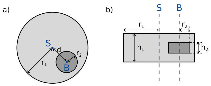
Figure 1: a) side view b) view from above

We denote \(b\) as the distance between the centre of mass \(C\) of the whole system and the symmetry axis \(S\) of the wooden cylinder. In order to determine this distance, we design the following experiment: We place the wooden cylinder on a horizontal base in such a way that it is in a stable equilibrium. Let us now slowly incline the base by an angle \(\Theta\) (see Fig. 2). As a result of the static friction, the wooden cylinder can roll freely without sliding. It will roll down the incline a little bit, but then come to rest in a stable equilibrium after rotating by an angle \(\phi\) which we measure.

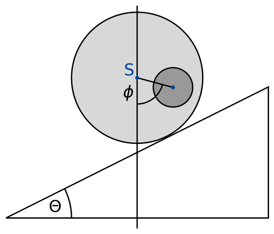
Figure 2: Cylinder on an inclined base.

A.1 — 0.8pt

Find an expression for \(b\) as a function of the quantities (1), the angle \(\phi\) and the tilting angle \(\Theta\) of the base.

From now on, we can assume that the value of \(b\) is known.

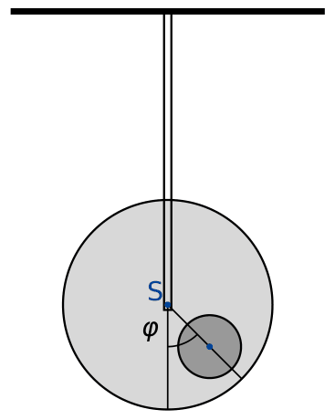
Figure 3: Suspended system.

Next we want to measure the moment of inertia \(I_S\) of the system with respect to the symmetry axis \(S\). To this end, we suspend the wooden cylinder at its symmetry axis from a rigid rod. We then turn it away from its equilibrium position by a small angle \(\varphi\), and let it go. See figure 3 for the setup. We find that \(\varphi\) describes a periodic motion with period \(T\).

A.2 — 0.5pt

Find the equation of motion for \(\varphi\). Express the moment of inertia \(I_S\) of the system around its symmetry axis \(S\) in terms of \(T\), \(b\) and the known quantities (1). You may assume that we are only disturbing the equilibrium position by a small amount so that \(\varphi\) is always very small.

From the measurements in questions A.1 and A.2, we now want to determine the geometry and the position of the metal disk inside the wooden cylinder.

A.3 — 0.4pt

Find an expression for the distance \(d\) as a function of \(b\) and the quantities (1). You may also include \(r_2\) and \(h_2\) as variables in your expression, as they will be calculated in subtask A.5.

A.4 — 0.7pt

Find an expression for the moment of inertia \(I_S\) in terms of \(b\) and the known quantities (1). You may also include \(r_2\) and \(h_2\) as variables in your expression, as they will be calculated in subtask A.5.

A.5 — 1.1pt

Using all the above results, write down an expression for \(h_2\) and \(r_2\) in terms of \(b\), \(T\) and the known quantities (1). You may express \(h_2\) as a function of \(r_2\).

Part B. Rotating Space Station (6.5 points)

Alice is an astronaut living on a space station. The space station is a gigantic wheel of radius \(R\) rotating around its axis, thereby providing artificial gravity for the astronauts. The astronauts live on the inner side of the rim of the wheel. The gravitational attraction of the space station and the curvature of the floor can be ignored.

B.1 — 0.5pt

At what angular frequency \(\omega_{ss}\) does the space station rotate so that the astronauts experience the same gravity \(g_E\) as on the Earth's surface?

Alice and her astronaut friend Bob have an argument. Bob does not believe that they are in fact living in a space station and claims that they are on Earth. Alice wants to prove to Bob that they are living on a rotating space station by using physics. To this end, she attaches a mass \(m\) to a spring with spring constant \(k\) and lets it oscillate. The mass oscillates only in the vertical direction, and cannot move in the horizontal direction.

B.2 — 0.2pt

Assuming that on Earth gravity is constant with acceleration \(g_E\), what would be the angular oscillation frequency \(\omega_E\) that a person on Earth would measure?

B.3 — 0.6pt

What angular oscillation frequency \(\omega\) does Alice measure on the space station?

Alice is convinced that her experiment proves that they are on a rotating space station. Bob remains sceptical. He claims that when taking into account the change in gravity above the surface of the Earth, one finds a similar effect. In the following tasks we investigate whether Bob is right.

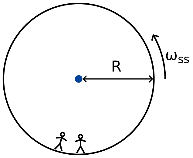
Figure 4: Space station

B.4 — 0.8pt

Derive an expression of the gravity \(g_E(h)\) for small heights \(h\) above the surface of the Earth and compute the oscillation frequency \(\widetilde{\omega}_E\) of the oscillating mass (linear approximation is enough). Denote the radius of the Earth by \(R_E\). Neglect the rotation of Earth.

Indeed, for this space station, Alice does find that the spring pendulum oscillates with the frequency that Bob predicted.

B.5 — 0.3pt

For what radius \(R\) of the space station does the oscillation frequency \(\omega\) match the oscillation frequency \(\widetilde{\omega}_E\) on the Earth? Express your answer in terms of \(R_E\).

Exasperated with Bob's stubbornness, Alice comes up with an experiment to prove her point. To this end she climbs on a tower of height \(H\) over the floor of the space station and drops a mass. This experiment can be understood in the rotating reference frame as well as in an inertial reference frame.

In a uniformly rotating reference frame, the astronauts perceive a fictitious force \(\vec F_C\) called the Coriolis force. The force \(\vec F_C\) acting on an object of mass \(m\) moving at velocity \(\vec v\) in a rotating frame with constant angular frequency \(\vec\omega_{ss}\) is given by

\[ \vec F_C=2m\vec v\times\vec\omega_{ss}. \tag{2} \]

In terms of the scalar quantities you may use

\[ F_C=2mv\omega_{ss}\sin\phi, \tag{3} \]

where \(\phi\) is the angle between the velocity and the axis of rotation. The force is perpendicular to both the velocity \(v\) and the axis of rotation. The sign of the force can be determined from the right-hand rule, but in what follows you may choose it freely.

B.6 — 1.1pt

Calculate the horizontal velocity \(v_x\) and the horizontal displacement \(d_x\) (relative to the base of the tower, in the direction perpendicular to the tower) of the mass at the moment it hits the floor. You may assume that the height \(H\) of the tower is small, so that the acceleration as measured by the astronauts is constant during the fall. Also, you may assume that \(d_x\ll H\).

To get a good result, Alice decides to conduct this experiment from a much taller tower than before. To her surprise, the mass hits the floor at the base of the tower, so that \(d_x=0\).

B.7 — 1.3pt

Find a lower bound for the height of the tower for which it can happen that \(d_x=0\).

Alice is willing to make one last attempt at convincing Bob. She wants to use her spring oscillator to show the effect of the Coriolis force. To this end she changes the original setup: She attaches her spring to a ring which can slide freely on a horizontal rod in the \(x\) direction without any friction. The spring itself oscillates in the \(y\) direction. The rod is parallel to the floor and perpendicular to the axis of rotation of the space station. The \(xy\) plane is thus perpendicular to the axis of rotation, with the \(y\) direction pointing straight towards the center of rotation of the station.

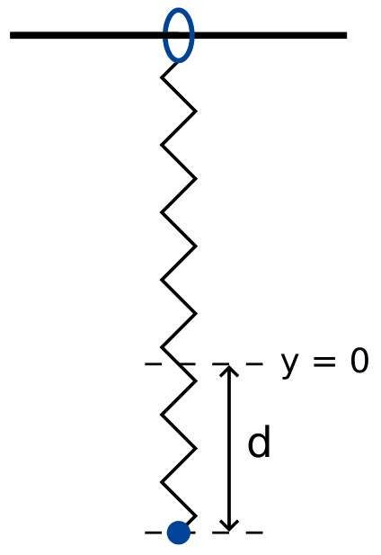
Figure 5: Setup.

B.8 — 1.7pt

Alice pulls the mass a distance \(d\) downwards from the equilibrium point \(x=0\), \(y=0\), and then lets it go (see figure 5).

• Give an algebraic expression of \(x(t)\) and \(y(t)\). You may assume that \(\omega_{ss}d\) is small, and neglect the Coriolis force for motion along the \(y\)-axis.
• Sketch the trajectory \((x(t),y(t))\), marking all important features such as amplitude.

Alice and Bob continue to argue.

General Data Sheet

Speed of light in vacuum	\(c\)	\(=299\,792\,458\ \mathrm{m\cdot s^{-1}}\)
Vacuum permeability (magnetic constant)	\(\mu_0\)	\(=4\pi\times10^{-7}\ \mathrm{kg\cdot m\cdot A^{-2}\cdot s^{-2}}\)
Vacuum permittivity (electrical constant)	\(\varepsilon_0\)	\(=8.854\,187\,817\times10^{-12}\ \mathrm{A^2\cdot s^4\cdot kg^{-1}\cdot m^{-3}}\)
Elementary charge	\(e\)	\(=1.602\,176\,620\,8(98)\times10^{-19}\ \mathrm{A\cdot s}\)
Mass of the electron	\(m_{\mathrm e}\)	\(=9.109\,383\,56(11)\times10^{-31}\ \mathrm{kg}\)
		\(=0.510\,998\,946\,1(31)\ \dfrac{\mathrm{MeV}}{c^2}\)
Mass of the proton	\(m_{\mathrm p}\)	\(=1.672\,621\,898(21)\times10^{-27}\ \mathrm{kg}\)
		\(=938.272\,081\,3(58)\ \dfrac{\mathrm{MeV}}{c^2}\)
Mass of the neutron	\(m_{\mathrm n}\)	\(=1.674\,927\,471(21)\times10^{-27}\ \mathrm{kg}\)
		\(=939.565\,413\,3(58)\ \dfrac{\mathrm{MeV}}{c^2}\)
Unified atomic mass unit	\(u\)	\(=1.660\,539\,040(20)\times10^{-27}\ \mathrm{kg}\)
Rydberg constant	\(R_\infty\)	\(=10\,973\,731.568\,508(65)\ \mathrm{m^{-1}}\)
Universal constant of gravitation	\(G\)	\(=6.674\,08(31)\times10^{-11}\ \mathrm{m^3\cdot kg^{-1}\cdot s^{-2}}\)
Acceleration due to gravity (in Zurich)	\(g\)	\(=9.81\ \mathrm{m\cdot s^{-2}}\)
Planck’s constant	\(h\)	\(=6.626\,070\,040(81)\times10^{-34}\ \mathrm{kg\cdot m^2\cdot s^{-1}}\)
Avogadro number	\(N_A\)	\(=6.022\,140\,857(74)\times10^{23}\ \mathrm{mol^{-1}}\)
Molar gas constant	\(R\)	\(=8.314\,4598(48)\ \mathrm{kg\cdot m^2\cdot s^{-2}\cdot mol^{-1}\cdot K^{-1}}\)
Molar mass constant	\(M_u\)	\(=1\times10^{-3}\ \mathrm{kg\cdot mol^{-1}}\)
Boltzmann constant	\(k_B\)	\(=1.380\,648\,52(79)\times10^{-23}\ \mathrm{kg\cdot m^2\cdot s^{-2}\cdot K^{-1}}\)
Stefan-Boltzmann constant	\(\sigma\)	\(=5.670\,367(13)\times10^{-8}\ \mathrm{kg\cdot s^{-3}\cdot K^{-4}}\)

Official English text of the problem.

Please read the general instructions in the separate envelope before you start this problem.

Introduction

Bistable non-linear semiconducting elements (e.g. thyristors) are widely used in electronics as switches and generators of electromagnetic oscillations. The primary field of applications of thyristors is controlling alternating currents in power electronics, for instance rectification of AC current to DC at the megawatt scale. Bistable elements may also serve as model systems for self-organization phenomena in physics (this topic is covered in part B of the problem), biology (see part C) and other fields of modern nonlinear science.

Goals

To study instabilities and nontrivial dynamics of circuits including elements with non-linear \(I-V\) characteristics. To discover possible applications of such circuits in engineering and in modeling of biological systems.

Part A. Stationary states and instabilities (3 points)

Fig. 1 shows the so-called S-shaped \(I-V\) characteristics of a non-linear element \(X\). In the voltage range between \(U_{\mathrm h}=4.00\ \mathrm V\) (the holding voltage) and \(U_{\mathrm{th}}=10.0\ \mathrm V\) (the threshold voltage) this \(I-V\) characteristics is multivalued. For simplicity, the graph on Fig. 1 is chosen to be piece-wise linear (each branch is a segment of a straight line). In particular, the line in the upper branch touches the origin if it is extended. This approximation gives a good description of real thyristors.

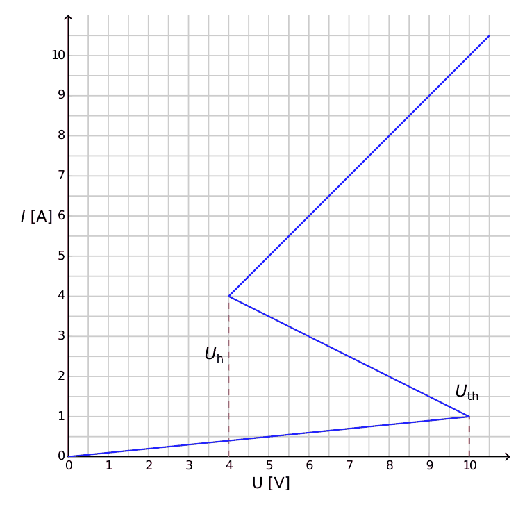
Figure 1: \(I-V\) characteristics of the non-linear element \(X\).

A.1 — 0.4pt

Using the graph, determine the resistance \(R_{\mathrm{on}}\) of the element \(X\) on the upper branch of the \(I-V\) characteristics, and \(R_{\mathrm{off}}\) on the lower branch, respectively. The middle branch is described by the equation

\[ I=I_0-\frac{U}{R_{\mathrm{int}}}. \tag{1} \]

Find the values of the parameters \(I_0\) and \(R_{\mathrm{int}}\).

The element \(X\) is connected in series (see Fig.2) with a resistor \(R\), an inductor \(L\) and an ideal voltage source \(\mathcal E\). One says that the circuit is in a stationary state if the current is constant in time, \(I(t)=\mathrm{const}\).

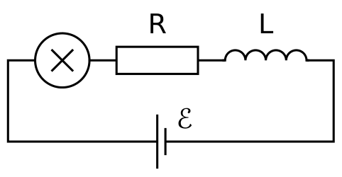
Figure 2: Circuit with element \(X\), resistor \(R\), inductor \(L\) and voltage source \(\mathcal E\).

A.2 — 1pt

What are the possible numbers of stationary states that the circuit of Fig. 2 may have for a fixed value of \(\mathcal E\) and for \(R=3.00\ \Omega\)? How does the answer change for \(R=1.00\ \Omega\)?

A.3 — 0.6pt

Let \(R=3.00\ \Omega\), \(L=1.00\ \mu\mathrm H\) and \(\mathcal E=15.0\ \mathrm V\) in the circuit shown in Fig. 2. Determine the values of the current \(I_{\mathrm{stationary}}\) and the voltage \(V_{\mathrm{stationary}}\) on the non-linear element \(X\) in the stationary state.

The circuit in Fig. 2 is in the stationary state with \(I(t)=I_{\mathrm{stationary}}\). This stationary state is said to be stable if after a small displacement (increase or decrease in the current), the current returns towards the stationary state. And if the system keeps moving away from the stationary state, it is said to be unstable.

A.4 — 1pt

Use numerical values of the question A.3 and study the stability of the stationary state with \(I(t)=I_{\mathrm{stationary}}\). Is it stable or unstable?

Part B. Bistable non-linear elements in physics: radio transmitter (5 points)

We now investigate a new circuit configuration (see Fig. 3). This time, the non-linear element \(X\) is connected in parallel to a capacitor of capacitance \(C=1.00\ \mu\mathrm F\). This block is then connected in series to a resistor of resistance \(R=3.00\ \Omega\) and an ideal constant voltage source of voltage \(\mathcal E=15.0\ \mathrm V\). It turns out that this circuit undergoes oscillations with the non-linear element \(X\) jumping from one branch of the \(I-V\) characteristics to another over the course of one cycle.

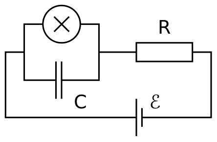
Figure 3: Circuit with element \(X\), capacitor \(C\), resistor \(R\) and voltage source \(\mathcal E\).

B.1 — 1.8pt

Draw the oscillation cycle on the \(I-V\) graph, including its direction (clockwise or anticlockwise). Justify your answer with equations and sketches.

B.2 — 1.9pt

Find expressions for the times \(t_1\) and \(t_2\) that the system spends on each branch of the \(I-V\) graph during the oscillation cycle. Determine their numerical values. Find the numerical value of the oscillation period \(T\) assuming that the time needed for jumps between the branches of the \(I-V\) graph is negligible.

B.3 — 0.7pt

Estimate the average power \(P\) dissipated by the non-linear element over the course of one oscillation. An order of magnitude is sufficient.

The circuit in Fig. 3 is used to build a radio transmitter. For this purpose, the element \(X\) is attached to one end of a linear antenna (a long straight wire) of length \(s\). The other end of the wire is free. In the antenna, an electromagnetic standing wave is formed. The speed of electromagnetic waves along the antenna is the same as in vacuum. The transmitter is using the main harmonic of the system, which has period \(T\) of question B.2.

B.4 — 0.6pt

What is the optimal value of \(s\) assuming that it cannot exceed \(1\ \mathrm{km}\)?

Part C. Bistable non-linear elements in biology: neuristor (2 points)

In this part of the problem, we consider an application of bistable non-linear elements to modeling of biological processes. A neuron in a human brain has the following property: when excited by an external signal, it makes one single oscillation and then returns to its initial state. This feature is called excitability. Due to this property, pulses can propagate in the network of coupled neurons constituting the nerve systems. A semiconductor chip designed to mimic excitability and pulse propagation is called a neuristor (from neuron and transistor).

We attempt to model a simple neuristor using a circuit that includes the non-linear element \(X\) that we investigated previously. To this end, the voltage \(\mathcal E\) in the circuit of Fig. 3 is decreased to the value \(\mathcal E'=12.0\ \mathrm V\). The oscillations stop, and the system reaches its stationary state. Then, the voltage is rapidly increased back to the value \(\mathcal E=15.0\ \mathrm V\), and after a period of time \(\tau\) (with \(\tau<T\)) is set again to the value \(\mathcal E'\) (see Fig. 4). It turns out that there is a certain critical value \(\tau_{\mathrm{crit}}\), and the system shows qualitatively different behavior for \(\tau<\tau_{\mathrm{crit}}\) and for \(\tau>\tau_{\mathrm{crit}}\).

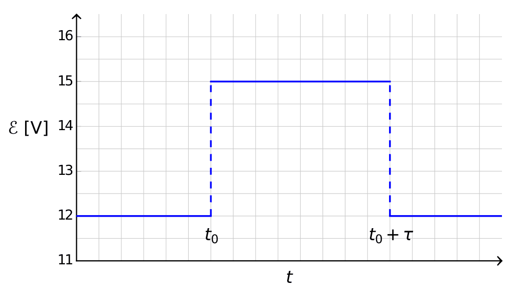
Figure 4: Voltage of the voltage source as a function of time.

C.1 — 1.2pt

Sketch the graphs of the time dependence of the current \(I_X(t)\) on the non-linear element \(X\) for \(\tau<\tau_{\mathrm{crit}}\) and for \(\tau>\tau_{\mathrm{crit}}\).

C.2 — 0.6pt

Find the expression and the numerical value of the critical time \(\tau_{\mathrm{crit}}\) for which the scenario switches.

C.3 — 0.2pt

Is the circuit with \(\tau=1.00\times10^{-6}\ \mathrm s\) a neuristor?

General Data Sheet

Speed of light in vacuum	\(c\)	\(=\)	\(299\,792\,458\ \mathrm{m\cdot s^{-1}}\)
Vacuum permeability (magnetic constant)	\(\mu_0\)	\(=\)	\(4\pi\times10^{-7}\ \mathrm{kg\cdot m\cdot A^{-2}\cdot s^{-2}}\)
Vacuum permittivity (electrical constant)	\(\varepsilon_0\)	\(=\)	\(8.854\,187\,817\times10^{-12}\ \mathrm{A^2\cdot s^4\cdot kg^{-1}\cdot m^{-3}}\)
Elementary charge	\(e\)	\(=\)	\(1.602\,176\,620\,8(98)\times10^{-19}\ \mathrm{A\cdot s}\)
Mass of the electron	\(m_{\mathrm e}\)	\(=\)	\(9.109\,383\,56(11)\times10^{-31}\ \mathrm{kg}\)
		\(=\)	\(0.510\,998\,946\,1(31)\ \dfrac{\mathrm{MeV}}{c^2}\)
Mass of the proton	\(m_{\mathrm p}\)	\(=\)	\(1.672\,621\,898(21)\times10^{-27}\ \mathrm{kg}\)
		\(=\)	\(938.272\,081\,3(58)\ \dfrac{\mathrm{MeV}}{c^2}\)
Mass of the neutron	\(m_{\mathrm n}\)	\(=\)	\(1.674\,927\,471(21)\times10^{-27}\ \mathrm{kg}\)
		\(=\)	\(939.565\,413\,3(58)\ \dfrac{\mathrm{MeV}}{c^2}\)
Unified atomic mass unit	\(u\)	\(=\)	\(1.660\,539\,040(20)\times10^{-27}\ \mathrm{kg}\)
Rydberg constant	\(R_\infty\)	\(=\)	\(10\,973\,731.568\,508(65)\ \mathrm{m^{-1}}\)
Universal constant of gravitation	\(G\)	\(=\)	\(6.674\,08(31)\times10^{-11}\ \mathrm{m^3\cdot kg^{-1}\cdot s^{-2}}\)
Acceleration due to gravity (in Zurich)	\(g\)	\(=\)	\(9.81\ \mathrm{m\cdot s^{-2}}\)
Planck’s constant	\(h\)	\(=\)	\(6.626\,070\,040\,(81)\times10^{-34}\ \mathrm{kg\cdot m^2\cdot s^{-1}}\)
Avogadro number	\(N_{\mathrm A}\)	\(=\)	\(6.022\,140\,857\,(74)\times10^{23}\ \mathrm{mol^{-1}}\)
Molar gas constant	\(R\)	\(=\)	\(8.314\,4598(48)\ \mathrm{kg\cdot m^2\cdot s^{-2}\cdot mol^{-1}\cdot K^{-1}}\)
Molar mass constant	\(M_u\)	\(=\)	\(1\times10^{-3}\ \mathrm{kg\cdot mol^{-1}}\)
Boltzmann constant	\(k_{\mathrm B}\)	\(=\)	\(1.380\,648\,52(79)\times10^{-23}\ \mathrm{kg\cdot m^2\cdot s^{-2}\cdot K^{-1}}\)
Stefan-Boltzmann constant	\(\sigma\)	\(=\)	\(5.670\,367\,(13)\times10^{-8}\ \mathrm{kg\cdot s^{-3}\cdot K^{-4}}\)

Official English text of the problem.

Please read the general instructions in the separate envelope before you start this problem.

In this task, the physics of the particle accelerator LHC (Large Hadron Collider) at CERN is discussed. CERN is the world's largest particle physics laboratory. Its main goal is to get insight into the fundamental laws of nature. Two beams of particles are accelerated to high energies, guided around the accelerator ring by a strong magnetic field and then made to collide with each other. The protons are not spread uniformly around the circumference of the accelerator, but they are clustered in so-called bunches. The resulting particles generated by collisions are observed with large detectors. Some parameters of the LHC can be found in table 1.

LHC ring
Circumference of ring	\(26659\,\mathrm{m}\)
Number of bunches per proton beam	\(2808\)
Number of protons per bunch	\(1.15\times10^{11}\)
Proton beams
Energy of protons	\(7.00\,\mathrm{TeV}\)
Centre of mass energy	\(14.0\,\mathrm{TeV}\)

Table 1: Typical numerical values of relevant LHC parameters.

Particle physicists use convenient units for the energy, momentum and mass: The energy is measured in electron volts [eV]. By definition, \(1\,\mathrm{eV}\) is the amount of energy gained by a particle with elementary charge, \(e\), moved through a potential difference of one volt (\(1\,\mathrm{eV}=1.602\cdot10^{-19}\,\mathrm{kg\,m^2s^{-2}}\)).

The momentum is measured in units of \(\mathrm{eV}/c\) and the mass in units of \(\mathrm{eV}/c^2\), where \(c\) is the speed of light in vacuum. Since \(1\,\mathrm{eV}\) is a very small quantity of energy, particle physicists often use MeV (\(1\,\mathrm{MeV}=10^6\,\mathrm{eV}\)), GeV (\(1\,\mathrm{GeV}=10^9\,\mathrm{eV}\)) or TeV (\(1\,\mathrm{TeV}=10^{12}\,\mathrm{eV}\)).

Part A deals with the acceleration of protons or electrons. Part B is concerned with the identification of particles produced in the collisions at CERN.

Part A. LHC accelerator (6 points)

Acceleration:

Assume that the protons have been accelerated by a voltage \(V\) such that their velocity is very close to the speed of light and neglect any energy loss due to radiation or collisions with other particles.

A.1 — 0.7pt

Find the exact expression for the final velocity \(v\) of the protons as a function of the accelerating voltage \(V\), and physical constants.

A design for a future experiment at CERN plans to use the protons from the LHC and to collide them with electrons which have an energy of \(60.0\,\mathrm{GeV}\).

A.2 — 0.8pt

For particles with high energy and low mass the relative deviation \(\Delta=(c-v)/c\) of the final velocity \(v\) from the speed of light is very small. Find a first order approximation for \(\Delta\) and calculate \(\Delta\) for electrons with an energy of \(60.0\,\mathrm{GeV}\)using the accelerating voltage \(V\) and physical constants.

We now return to the protons in the LHC. Assume that the beam pipe has a circular shape.

A.3 — 1.0pt

Derive an expression for the uniform magnetic flux density \(B\) necessary to keep the proton beam on a circular track. The expression should only contain the energy of the protons \(E\), the circumference \(L\), fundamental constants and numbers. You may use suitable approximations if their effect is smaller than precision given by the least number of significant digits.

Calculate the magnetic flux density \(B\) for a proton energy of \(E=7.00\,\mathrm{TeV}\), neglecting interactions between the protons.

Radiated Power:

An accelerated charged particle radiates energy in the form of electromagnetic waves. The radiated power \(P_{\mathrm{rad}}\) of a charged particle that circulates with a constant angular velocity depends only on its acceleration \(a\), its charge \(q\), the speed of light \(c\) and the permittivity of free space \(\varepsilon_0\).

A.4 — 1.0pt

Use dimensional analysis to find an expression for the radiated power \(P_{\mathrm{rad}}\).

The real formula for the radiated power contains a factor \(1/(6\pi)\); moreover, a full relativistic derivation gives an additional multiplicative factor \(\gamma^4\), with \(\gamma=(1-v^2/c^2)^{-1/2}\).

A.5 — 1.0pt

Calculate \(P_{\mathrm{tot}}\), the total radiated power of the LHC, for a proton energy of \(E=7.00\,\mathrm{TeV}\) (Note table 1). You may use suitable approximations.

Linear Acceleration:

At CERN, protons at rest are accelerated by a linear accelerator of length \(d=30.0\,\mathrm{m}\) through a potential difference of \(V=500\,\mathrm{MV}\). Assume that the electrical field is homogeneous. A linear accelerator consists of two plates as sketched in Figure 1.

A.6 — 1.5pt

Determine the time \(T\) that the protons take to pass through this field.

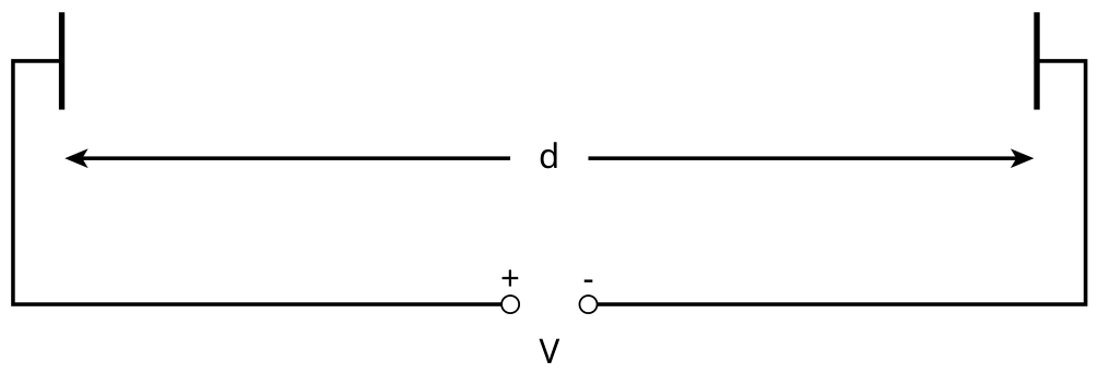
Figure 1: Sketch of an accelerator module.

Part B. Particle Identification (4 points)

Time of flight:

It is important to identify the high energy particles that are generated in the collision in order to interpret the interaction process. A simple method is to measure the time \((t)\) that a particle with known momentum needs to pass a length \(l\) in a so-called Time-of-Flight (ToF) detector. Typical particles which are identified in the detector, together with their masses, are listed in table 2.

Particle	Mass \([\mathrm{MeV}/c^2]\)
Deuteron	\(1876\)
Proton	\(938\)
charged Kaon	\(494\)
charged Pion	\(140\)
Electron	\(0.511\)

Table 2: Particles and their masses.

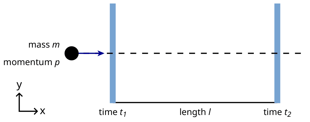
Figure 2: Schematic view of a time-of-flight detector.

B.1 — 0.8pt

Express the particle mass \(m\) in terms of of the momentum \(p\), the flight length \(l\) and the flight time \(t\), assuming that particles have elementary charge \(e\) and travel with velocity close to \(c\) on straight tracks in the ToF detector and that they travel perpendicular to the two detection planes (see figure 2).

B.2 — 0.7pt

Calculate the minimal length \(l\) of a ToF detector that allows to safely distinguish a charged kaon from a charged pion, given both their momenta are measured to be \(1.00\,\mathrm{GeV}/c\). For a good separation it is required that the difference in the time-of-flight is larger than three times the time resolution of the detector. The typical resolution of a ToF detector is \(150\,\mathrm{ps}\) (\(1\,\mathrm{ps}=10^{-12}\,\mathrm{s}\)).

In the following, particles produced in a typical LHC detector are identified in a two stage detector consisting of a tracking detector and a ToF detector. Figure 3 shows the setup in the plane transverse and longitudinal to the proton beams. Both detectors are tubes surrounding the interaction region with the beam passing in the middle of the tubes. The tracking detector measures the trajectory of a charged particle which passes through a magnetic field whose direction is parallel to the proton beams. The radius \(r\) of the trajectory allows one to determine the transverse momentum \(p_{\mathrm{T}}\) of the particle. Since the collision time is known the ToF detector only needs one tube to measure the flight time (time between the collision and the detection in the ToF tube). This ToF tube is situated just outside the tracking chamber. For this task you may assume that all particles created by the collision travel perpendicular to the proton beams, which means that the created particles have no momentum along the direction of the proton beams.

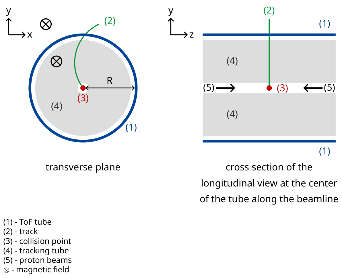
Figure 3 : Experimental setup for particle identification with a tracking chamber and a ToF detector. Both detectors are tubes surrounding the collision point in the middle. Left : transverse view perpendicular to the beamline. Right : longitudinal view parallel to the beam line. The particle is travelling perpendicular to the beam line.

B.3 — 1.7pt

Express the particle mass in terms of the magnetic flux density \(B\), the radius \(R\) of the ToF tube, fundamental constants and the measured quantities: radius \(r\) of the track and time-of-flight \(t\).

We detected four particles and want to identify them. The magnetic flux density in the tracking detector was \(B=0.500\,\mathrm{T}\). The radius \(R\) of the ToF tube was \(3.70\,\mathrm{m}\). Here are the measurements (\(1\,\mathrm{ns}=10^{-9}\,\mathrm{s}\)):

Particle	Radius of the trajectory \(r\) [m]	Time of flight \(t\) [ns]
A	\(5.10\)	\(20\)
B	\(2.94\)	\(14\)
C	\(6.06\)	\(18\)
D	\(2.31\)	\(25\)

B.4 — 0.8pt

Identify the four particles by calculating their mass.

General Data Sheet

Speed of light in vacuum	\(c\)	\(=299\,792\,458\,\mathrm{m\cdot s^{-1}}\)
Vacuum permeability (magnetic constant)	\(\mu_0\)	\(=4\pi\times10^{-7}\,\mathrm{kg\cdot m\cdot A^{-2}\cdot s^{-2}}\)
Vacuum permittivity (electrical constant)	\(\varepsilon_0\)	\(=8.854\,187\,817\times10^{-12}\,\mathrm{A^2\cdot s^4\cdot kg^{-1}\cdot m^{-3}}\)
Elementary charge	\(e\)	\(=1.602\,176\,620\,8(98)\times10^{-19}\,\mathrm{A\cdot s}\)
Mass of the electron	\(m_{\mathrm e}\)	\(=9.109\,383\,56(11)\times10^{-31}\,\mathrm{kg}\)
		\(=0.510\,998\,946\,1(31)\,\dfrac{\mathrm{MeV}}{c^2}\)
Mass of the proton	\(m_{\mathrm p}\)	\(=1.672\,621\,898(21)\times10^{-27}\,\mathrm{kg}\)
		\(=938.272\,081\,3(58)\,\dfrac{\mathrm{MeV}}{c^2}\)
Mass of the neutron	\(m_{\mathrm n}\)	\(=1.674\,927\,471(21)\times10^{-27}\,\mathrm{kg}\)
		\(=939.565\,413\,3(58)\,\dfrac{\mathrm{MeV}}{c^2}\)
Unified atomic mass unit	\(u\)	\(=1.660\,539\,040(20)\times10^{-27}\,\mathrm{kg}\)
Rydberg constant	\(R_\infty\)	\(=10\,973\,731.568\,508(65)\,\mathrm{m^{-1}}\)
Universal constant of gravitation	\(G\)	\(=6.674\,08(31)\times10^{-11}\,\mathrm{m^3\cdot kg^{-1}\cdot s^{-2}}\)
Acceleration due to gravity (in Zurich)	\(g\)	\(=9.81\,\mathrm{m\cdot s^{-2}}\)
Planck’s constant	\(h\)	\(=6.626\,070\,040(81)\times10^{-34}\,\mathrm{kg\cdot m^2\cdot s^{-1}}\)
Avogadro number	\(N_{\mathrm A}\)	\(=6.022\,140\,857(74)\times10^{23}\,\mathrm{mol^{-1}}\)
Molar gas constant	\(R\)	\(=8.314\,4598(48)\,\mathrm{kg\cdot m^2\cdot s^{-2}\cdot mol^{-1}\cdot K^{-1}}\)
Molar mass constant	\(M_{\mathrm u}\)	\(=1\times10^{-3}\,\mathrm{kg\cdot mol^{-1}}\)
Boltzmann constant	\(k_{\mathrm B}\)	\(=1.380\,648\,52(79)\times10^{-23}\,\mathrm{kg\cdot m^2\cdot s^{-2}\cdot K^{-1}}\)
Stefan-Boltzmann constant	\(\sigma\)	\(=5.670\,367(13)\times10^{-8}\,\mathrm{kg\cdot s^{-3}\cdot K^{-4}}\)

Official English text of the problem.

Bitte lesen Sie die allgemeinen Hinweise im separaten Umschlag, bevor Sie mit dieser Aufgabe beginnen.

Teil A. Die verborgene Scheibe (3.5 Punkte)

Wir betrachten einen massiven Holzzylinder mit dem Radius \(r_1\) und der Dicke \(h_1\). An einer Stelle im Inneren des Holzzylinders wurde das Holz durch eine Metallscheibe mit dem Radius \(r_2\) und der Dicke \(h_2\) ersetzt. Die Metallscheibe ist so angeordnet, dass ihre Symmetrieachse \(B\) parallel zur Symmetrieachse \(S\) des Holzzylinders verläuft und sie von der oberen und der unteren Stirnfläche des Holzzylinders jeweils den gleichen Abstand hat. Den Abstand zwischen \(S\) und \(B\) bezeichnen wir mit \(d\). Die Dichte des Holzes beträgt \(\rho_1\), die Dichte des Metalls beträgt \(\rho_2>\rho_1\). Die Gesamtmasse des Holzzylinders mit der darin befindlichen Metallscheibe beträgt \(M\).

In dieser Aufgabe legen wir den Holzzylinder so auf den Boden, dass er frei nach links und rechts rollen kann. Abb. 1 zeigt eine Seitenansicht und eine Draufsicht des Aufbaus.

Ziel dieser Aufgabe ist es, die Größe und die Lage der Metallscheibe zu bestimmen.

Wenn im Folgenden ein Ergebnis durch bekannte Größen ausgedrückt werden soll, dürfen Sie stets annehmen, dass die folgenden Größen bekannt sind:

\[ r_1,\ h_1,\ \rho_1,\ \rho_2,\ M. \tag{1} \]

Ziel ist es, \(r_2\), \(h_2\) und \(d\) durch indirekte Messungen zu bestimmen.

Abbildung 1: a) Seitenansicht b) Draufsicht

Mit \(b\) bezeichnen wir den Abstand zwischen dem Schwerpunkt \(C\) des Gesamtsystems und der Symmetrieachse \(S\) des Holzzylinders. Um diesen Abstand zu bestimmen, entwerfen wir folgendes Experiment: Wir legen den Holzzylinder so auf eine horizontale Unterlage, dass er sich in einem stabilen Gleichgewicht befindet. Nun neigen wir die Unterlage langsam um einen Winkel \(\Theta\) (siehe Abb. 2). Aufgrund der Haftreibung kann der Holzzylinder frei rollen, ohne zu gleiten. Er rollt ein kleines Stück die schiefe Ebene hinab, kommt dann aber in einem stabilen Gleichgewicht zur Ruhe, nachdem er sich um einen Winkel \(\phi\) gedreht hat, den wir messen.

Abbildung 2: Zylinder auf einer geneigten Unterlage.

A.1 — 0.8 Punkte

Bestimmen Sie einen Ausdruck für \(b\) als Funktion der Größen (1), des Winkels \(\phi\) und des Neigungswinkels \(\Theta\) der Unterlage.

Von nun an können wir annehmen, dass der Wert von \(b\) bekannt ist.

Abbildung 3: Aufgehängtes System.

Als Nächstes wollen wir das Trägheitsmoment \(I_S\) des Systems bezüglich der Symmetrieachse \(S\) messen. Dazu hängen wir den Holzzylinder an seiner Symmetrieachse an einer starren Stange auf. Anschließend drehen wir ihn um einen kleinen Winkel \(\varphi\) aus seiner Gleichgewichtslage und lassen ihn los. Abbildung 3 zeigt den Aufbau. Wir stellen fest, dass \(\varphi\) eine periodische Bewegung mit der Periodendauer \(T\) beschreibt.

A.2 — 0.5 Punkte

Bestimmen Sie die Bewegungsgleichung für \(\varphi\). Drücken Sie das Trägheitsmoment \(I_S\) des Systems bezüglich seiner Symmetrieachse \(S\) durch \(T\), \(b\) und die bekannten Größen (1) aus. Sie dürfen annehmen, dass wir das System nur geringfügig aus seiner Gleichgewichtslage auslenken, sodass \(\varphi\) stets sehr klein ist.

Aus den Messungen in den Teilaufgaben A.1 und A.2 wollen wir nun die Geometrie und die Lage der Metallscheibe im Inneren des Holzzylinders bestimmen.

A.3 — 0.4 Punkte

Bestimmen Sie einen Ausdruck für den Abstand \(d\) als Funktion von \(b\) und den Größen (1). Sie dürfen in Ihrem Ausdruck auch \(r_2\) und \(h_2\) als Variablen verwenden, da diese in Teilaufgabe A.5 berechnet werden.

A.4 — 0.7 Punkte

Bestimmen Sie einen Ausdruck für das Trägheitsmoment \(I_S\) in Abhängigkeit von \(b\) und den bekannten Größen (1). Sie dürfen in Ihrem Ausdruck auch \(r_2\) und \(h_2\) als Variablen verwenden, da diese in Teilaufgabe A.5 berechnet werden.

A.5 — 1.1 Punkte

Geben Sie mithilfe aller bisherigen Ergebnisse jeweils einen Ausdruck für \(h_2\) und \(r_2\) in Abhängigkeit von \(b\), \(T\) und den bekannten Größen (1) an. Sie dürfen \(h_2\) als Funktion von \(r_2\) ausdrücken.

Teil B. Rotierende Raumstation (6.5 Punkte)

Alice ist Astronautin und lebt auf einer Raumstation. Die Raumstation ist ein riesiges Rad mit dem Radius \(R\), das sich um seine Achse dreht und dadurch künstliche Schwerkraft für die Astronauten erzeugt. Die Astronauten leben auf der Innenseite des Radkranzes. Die Gravitationsanziehung der Raumstation und die Krümmung des Bodens können vernachlässigt werden.

B.1 — 0.5 Punkte

Mit welcher Winkelgeschwindigkeit \(\omega_{ss}\) dreht sich die Raumstation, damit die Astronauten die gleiche Schwerebeschleunigung \(g_E\) wie auf der Erdoberfläche erfahren?

Alice und ihr Astronautenfreund Bob streiten sich. Bob glaubt nicht, dass sie tatsächlich auf einer Raumstation leben, und behauptet, sie seien auf der Erde. Alice möchte Bob mithilfe der Physik beweisen, dass sie auf einer rotierenden Raumstation leben. Dazu befestigt sie eine Masse \(m\) an einer Feder mit der Federkonstanten \(k\) und lässt sie schwingen. Die Masse schwingt nur in vertikaler Richtung und kann sich nicht in horizontaler Richtung bewegen.

B.2 — 0.2 Punkte

Welche Kreisfrequenz \(\omega_E\) der Schwingung würde eine Person auf der Erde messen, wenn man annimmt, dass dort die Schwerebeschleunigung konstant gleich \(g_E\) ist?

B.3 — 0.6 Punkte

Welche Kreisfrequenz \(\omega\) der Schwingung misst Alice auf der Raumstation?

Alice ist überzeugt, dass ihr Experiment beweist, dass sie sich auf einer rotierenden Raumstation befinden. Bob bleibt skeptisch. Er behauptet, dass man einen ähnlichen Effekt erhält, wenn man die Änderung der Schwerebeschleunigung oberhalb der Erdoberfläche berücksichtigt. In den folgenden Teilaufgaben untersuchen wir, ob Bob recht hat.

Abbildung 4: Raumstation

B.4 — 0.8 Punkte

Leiten Sie einen Ausdruck für die Schwerebeschleunigung \(g_E(h)\) in kleinen Höhen \(h\) über der Erdoberfläche her und berechnen Sie die Kreisfrequenz \(\widetilde{\omega}_E\) der schwingenden Masse (eine lineare Näherung genügt). Bezeichnen Sie den Erdradius mit \(R_E\). Vernachlässigen Sie die Erdrotation.

Tatsächlich stellt Alice bei dieser Raumstation fest, dass das Federpendel mit der von Bob vorhergesagten Frequenz schwingt.

B.5 — 0.3 Punkte

Bei welchem Radius \(R\) der Raumstation stimmt die Kreisfrequenz \(\omega\) mit der Kreisfrequenz \(\widetilde{\omega}_E\) auf der Erde überein? Drücken Sie Ihre Antwort durch \(R_E\) aus.

Verärgert über Bobs Sturheit denkt sich Alice ein Experiment aus, mit dem sie ihre Behauptung beweisen will. Dazu steigt sie auf einen Turm der Höhe \(H\) über dem Boden der Raumstation und lässt eine Masse fallen. Dieses Experiment lässt sich sowohl im rotierenden Bezugssystem als auch in einem Inertialsystem verstehen.

In einem gleichförmig rotierenden Bezugssystem nehmen die Astronauten eine Scheinkraft \(\vec F_C\) wahr, die Corioliskraft genannt wird. Die Kraft \(\vec F_C\), die auf einen Körper der Masse \(m\) wirkt, der sich mit der Geschwindigkeit \(\vec v\) in einem Bezugssystem mit konstanter Winkelgeschwindigkeit \(\vec\omega_{ss}\) bewegt, ist gegeben durch

\[ \vec F_C=2m\vec v\times\vec\omega_{ss}. \tag{2} \]

Für die skalaren Größen dürfen Sie

\[ F_C=2mv\omega_{ss}\sin\phi, \tag{3} \]

verwenden, wobei \(\phi\) der Winkel zwischen der Geschwindigkeit und der Rotationsachse ist. Die Kraft steht sowohl senkrecht auf der Geschwindigkeit \(v\) als auch auf der Rotationsachse. Das Vorzeichen der Kraft lässt sich mit der Rechte-Hand-Regel bestimmen, im Folgenden dürfen Sie es jedoch frei wählen.

B.6 — 1.1 Punkte

Berechnen Sie die horizontale Geschwindigkeit \(v_x\) und die horizontale Verschiebung \(d_x\) (relativ zum Fuß des Turms, in der Richtung senkrecht zum Turm) der Masse in dem Augenblick, in dem sie auf den Boden trifft. Sie dürfen annehmen, dass die Höhe \(H\) des Turms klein ist, sodass die von den Astronauten gemessene Beschleunigung während des Falls konstant ist. Außerdem dürfen Sie annehmen, dass \(d_x\ll H\) gilt.

Um ein gutes Ergebnis zu erhalten, beschließt Alice, dieses Experiment von einem wesentlich höheren Turm als zuvor durchzuführen. Zu ihrer Überraschung trifft die Masse am Fuß des Turms auf den Boden, sodass \(d_x=0\) ist.

B.7 — 1.3 Punkte

Bestimmen Sie eine untere Schranke für die Turmhöhe, bei der \(d_x=0\) auftreten kann.

Alice ist bereit, einen letzten Versuch zu unternehmen, Bob zu überzeugen. Sie möchte mit ihrem Federpendel die Wirkung der Corioliskraft zeigen. Dazu verändert sie den ursprünglichen Aufbau: Sie befestigt ihre Feder an einem Ring, der auf einer horizontalen Stange reibungsfrei in \(x\)-Richtung gleiten kann. Die Feder selbst schwingt in \(y\)-Richtung. Die Stange verläuft parallel zum Boden und senkrecht zur Rotationsachse der Raumstation. Die \(xy\)-Ebene steht somit senkrecht zur Rotationsachse, wobei die \(y\)-Richtung unmittelbar zum Rotationszentrum der Station zeigt.

Abbildung 5: Versuchsaufbau.

B.8 — 1.7 Punkte

Alice zieht die Masse vom Gleichgewichtspunkt \(x=0\), \(y=0\) um eine Strecke \(d\) nach unten und lässt sie dann los (siehe Abbildung 5).

• Geben Sie jeweils einen algebraischen Ausdruck für \(x(t)\) und \(y(t)\) an. Sie dürfen annehmen, dass \(\omega_{ss}d\) klein ist, und die Corioliskraft für die Bewegung entlang der \(y\)-Achse vernachlässigen.
• Skizzieren Sie die Bahnkurve \((x(t),y(t))\) und kennzeichnen Sie alle wichtigen Merkmale, beispielsweise die Amplitude.

Alice und Bob streiten weiter.

Allgemeines Datenblatt

Lichtgeschwindigkeit im Vakuum	\(c\)	\(=299\,792\,458\ \mathrm{m\cdot s^{-1}}\)
Magnetische Feldkonstante (Vakuumpermeabilität)	\(\mu_0\)	\(=4\pi\times10^{-7}\ \mathrm{kg\cdot m\cdot A^{-2}\cdot s^{-2}}\)
Elektrische Feldkonstante (Vakuumpermittivität)	\(\varepsilon_0\)	\(=8.854\,187\,817\times10^{-12}\ \mathrm{A^2\cdot s^4\cdot kg^{-1}\cdot m^{-3}}\)
Elementarladung	\(e\)	\(=1.602\,176\,620\,8(98)\times10^{-19}\ \mathrm{A\cdot s}\)
Elektronenmasse	\(m_{\mathrm e}\)	\(=9.109\,383\,56(11)\times10^{-31}\ \mathrm{kg}\)
		\(=0.510\,998\,946\,1(31)\ \dfrac{\mathrm{MeV}}{c^2}\)
Protonenmasse	\(m_{\mathrm p}\)	\(=1.672\,621\,898(21)\times10^{-27}\ \mathrm{kg}\)
		\(=938.272\,081\,3(58)\ \dfrac{\mathrm{MeV}}{c^2}\)
Neutronenmasse	\(m_{\mathrm n}\)	\(=1.674\,927\,471(21)\times10^{-27}\ \mathrm{kg}\)
		\(=939.565\,413\,3(58)\ \dfrac{\mathrm{MeV}}{c^2}\)
Atomare Masseneinheit	\(u\)	\(=1.660\,539\,040(20)\times10^{-27}\ \mathrm{kg}\)
Rydberg-Konstante	\(R_\infty\)	\(=10\,973\,731.568\,508(65)\ \mathrm{m^{-1}}\)
Universelle Gravitationskonstante	\(G\)	\(=6.674\,08(31)\times10^{-11}\ \mathrm{m^3\cdot kg^{-1}\cdot s^{-2}}\)
Fallbeschleunigung (in Zürich)	\(g\)	\(=9.81\ \mathrm{m\cdot s^{-2}}\)
Plancksches Wirkungsquantum	\(h\)	\(=6.626\,070\,040(81)\times10^{-34}\ \mathrm{kg\cdot m^2\cdot s^{-1}}\)
Avogadro-Konstante	\(N_A\)	\(=6.022\,140\,857(74)\times10^{23}\ \mathrm{mol^{-1}}\)
Molare Gaskonstante	\(R\)	\(=8.314\,4598(48)\ \mathrm{kg\cdot m^2\cdot s^{-2}\cdot mol^{-1}\cdot K^{-1}}\)
Molare Massenkonstante	\(M_u\)	\(=1\times10^{-3}\ \mathrm{kg\cdot mol^{-1}}\)
Boltzmann-Konstante	\(k_B\)	\(=1.380\,648\,52(79)\times10^{-23}\ \mathrm{kg\cdot m^2\cdot s^{-2}\cdot K^{-1}}\)
Stefan-Boltzmann-Konstante	\(\sigma\)	\(=5.670\,367(13)\times10^{-8}\ \mathrm{kg\cdot s^{-3}\cdot K^{-4}}\)

Aufgabentext aus dem offiziellen englischen Text übersetzt.

Bitte lesen Sie die allgemeinen Hinweise im separaten Umschlag, bevor Sie mit dieser Aufgabe beginnen.

Einleitung

Bistabile nichtlineare Halbleiterbauelemente (z. B. Thyristoren) werden in der Elektronik häufig als Schalter und zur Erzeugung elektromagnetischer Schwingungen eingesetzt. Das Hauptanwendungsgebiet von Thyristoren ist die Steuerung von Wechselströmen in der Leistungselektronik, beispielsweise die Gleichrichtung von Wechselstrom zu Gleichstrom im Megawattbereich. Bistabile Bauelemente können auch als Modellsysteme für Selbstorganisationsphänomene in der Physik (dieses Thema wird in Teil B der Aufgabe behandelt), in der Biologie (siehe Teil C) und in anderen Bereichen der modernen nichtlinearen Wissenschaft dienen.

Ziele

Untersuchung von Instabilitäten und nichttrivialer Dynamik in Schaltungen mit Bauelementen mit nichtlinearen \(I-V\)-Kennlinien. Erkundung möglicher Anwendungen solcher Schaltungen in der Technik und bei der Modellierung biologischer Systeme.

Teil A. Stationäre Zustände und Instabilitäten (3 Punkte)

Abb. 1 zeigt die sogenannte S-förmige \(I-V\)-Kennlinie eines nichtlinearen Bauelements \(X\). Im Spannungsbereich zwischen \(U_{\mathrm h}=4.00\ \mathrm V\) (der Haltespannung) und \(U_{\mathrm{th}}=10.0\ \mathrm V\) (der Schwellenspannung) ist diese \(I-V\)-Kennlinie mehrwertig. Der Einfachheit halber ist der Graph in Abb. 1 stückweise linear gewählt (jeder Zweig ist ein Geradenstück). Insbesondere verläuft die Verlängerung des oberen Zweigs durch den Ursprung. Diese Näherung beschreibt reale Thyristoren gut.

Abbildung 1: \(I-V\)-Kennlinie des nichtlinearen Bauelements \(X\).

A.1 — 0.4 Punkte

Bestimmen Sie anhand des Graphen den Widerstand \(R_{\mathrm{on}}\) des Bauelements \(X\) auf dem oberen Zweig der \(I-V\)-Kennlinie sowie \(R_{\mathrm{off}}\) auf dem unteren Zweig. Der mittlere Zweig wird durch folgende Gleichung beschrieben:

\[ I=I_0-\frac{U}{R_{\mathrm{int}}}. \tag{1} \]

Bestimmen Sie die Werte der Parameter \(I_0\) und \(R_{\mathrm{int}}\).

Das Bauelement \(X\) wird mit einem Widerstand \(R\), einer Spule mit der Induktivität \(L\) und einer idealen Spannungsquelle \(\mathcal E\) in Reihe geschaltet (siehe Abb. 2). Man sagt, dass sich die Schaltung in einem stationären Zustand befindet, wenn der Strom zeitlich konstant ist, \(I(t)=\mathrm{const}\).

Abbildung 2: Schaltung mit dem Bauelement \(X\), dem Widerstand \(R\), der Spule mit der Induktivität \(L\) und der Spannungsquelle \(\mathcal E\).

A.2 — 1 Punkt

Welche Anzahlen stationärer Zustände sind für die Schaltung in Abb. 2 bei einem festen Wert von \(\mathcal E\) und für \(R=3.00\ \Omega\) möglich? Wie ändert sich die Antwort für \(R=1.00\ \Omega\)?

A.3 — 0.6 Punkte

Für die Schaltung in Abb. 2 seien \(R=3.00\ \Omega\), \(L=1.00\ \mu\mathrm H\) und \(\mathcal E=15.0\ \mathrm V\). Bestimmen Sie den Strom \(I_{\mathrm{stationary}}\) und die Spannung \(V_{\mathrm{stationary}}\) am nichtlinearen Bauelement \(X\) im stationären Zustand.

Die Schaltung in Abb. 2 befindet sich im stationären Zustand mit \(I(t)=I_{\mathrm{stationary}}\). Dieser stationäre Zustand heißt stabil, wenn der Strom nach einer kleinen Auslenkung (Erhöhung oder Verringerung des Stroms) zum stationären Zustand zurückkehrt. Entfernt sich das System dagegen immer weiter vom stationären Zustand, so heißt dieser instabil.

A.4 — 1 Punkt

Verwenden Sie die Zahlenwerte aus Teilaufgabe A.3 und untersuchen Sie die Stabilität des stationären Zustands mit \(I(t)=I_{\mathrm{stationary}}\). Ist er stabil oder instabil?

Teil B. Bistabile nichtlineare Bauelemente in der Physik: Funksender (5 Punkte)

Wir untersuchen nun eine neue Schaltungsanordnung (siehe Abb. 3). Diesmal ist das nichtlineare Bauelement \(X\) parallel zu einem Kondensator mit der Kapazität \(C=1.00\ \mu\mathrm F\) geschaltet. Diese Parallelschaltung ist wiederum mit einem Widerstand \(R=3.00\ \Omega\) und einer idealen Gleichspannungsquelle mit der Spannung \(\mathcal E=15.0\ \mathrm V\) in Reihe geschaltet. Es zeigt sich, dass in dieser Schaltung Schwingungen auftreten, wobei das nichtlineare Bauelement \(X\) im Verlauf einer Periode von einem Zweig der \(I-V\)-Kennlinie auf einen anderen springt.

Abbildung 3: Schaltung mit dem Bauelement \(X\), dem Kondensator \(C\), dem Widerstand \(R\) und der Spannungsquelle \(\mathcal E\).

B.1 — 1.8 Punkte

Zeichnen Sie den Schwingungszyklus in das \(I-V\)-Diagramm ein und geben Sie seine Umlaufrichtung an (im oder gegen den Uhrzeigersinn). Begründen Sie Ihre Antwort mit Gleichungen und Skizzen.

B.2 — 1.9 Punkte

Bestimmen Sie Ausdrücke für die Zeiten \(t_1\) und \(t_2\), die das System während des Schwingungszyklus auf den einzelnen Zweigen des \(I-V\)-Diagramms verbringt. Berechnen Sie ihre Zahlenwerte. Bestimmen Sie den Zahlenwert der Schwingungsdauer \(T\) unter der Annahme, dass die für die Sprünge zwischen den Zweigen des \(I-V\)-Diagramms benötigte Zeit vernachlässigbar ist.

B.3 — 0.7 Punkte

Schätzen Sie die mittlere Leistung \(P\) ab, die im nichtlinearen Bauelement während einer Schwingung dissipiert wird. Die Angabe der Größenordnung genügt.

Die Schaltung in Abb. 3 wird zum Bau eines Funksenders verwendet. Dazu wird das Bauelement \(X\) an ein Ende einer linearen Antenne (eines langen geraden Drahtes) der Länge \(s\) angeschlossen. Das andere Ende des Drahtes ist frei. In der Antenne bildet sich eine stehende elektromagnetische Welle aus. Die Geschwindigkeit elektromagnetischer Wellen entlang der Antenne ist gleich derjenigen im Vakuum. Der Sender nutzt die Grundschwingung des Systems, deren Periodendauer \(T\) in Teilaufgabe B.2 bestimmt wurde.

B.4 — 0.6 Punkte

Welcher Wert von \(s\) ist optimal, wenn die Länge \(1\ \mathrm{km}\) nicht überschreiten darf?

Teil C. Bistabile nichtlineare Bauelemente in der Biologie: Neuristor (2 Punkte)

In diesem Teil der Aufgabe betrachten wir eine Anwendung bistabiler nichtlinearer Bauelemente zur Modellierung biologischer Prozesse. Ein Neuron im menschlichen Gehirn besitzt folgende Eigenschaft: Wird es durch ein äußeres Signal angeregt, führt es eine einzige Schwingung aus und kehrt anschließend in seinen Ausgangszustand zurück. Diese Eigenschaft wird als Erregbarkeit bezeichnet. Aufgrund dieser Eigenschaft können sich Impulse in dem Netzwerk gekoppelter Neuronen ausbreiten, aus dem das Nervensystem besteht. Ein Halbleiterchip, der Erregbarkeit und Impulsausbreitung nachbilden soll, wird als Neuristor bezeichnet (aus Neuron und Transistor).

Wir versuchen, einen einfachen Neuristor mithilfe einer Schaltung zu modellieren, die das zuvor untersuchte nichtlineare Bauelement \(X\) enthält. Dazu wird die Spannung \(\mathcal E\) in der Schaltung aus Abb. 3 auf den Wert \(\mathcal E'=12.0\ \mathrm V\) verringert. Die Schwingungen hören auf, und das System erreicht seinen stationären Zustand. Anschließend wird die Spannung rasch wieder auf den Wert \(\mathcal E=15.0\ \mathrm V\) erhöht und nach einer Zeitspanne \(\tau\) (mit \(\tau<T\)) erneut auf den Wert \(\mathcal E'\) gesetzt (siehe Abb. 4). Es zeigt sich, dass es einen bestimmten kritischen Wert \(\tau_{\mathrm{crit}}\) gibt und dass das System für \(\tau<\tau_{\mathrm{crit}}\) und für \(\tau>\tau_{\mathrm{crit}}\) qualitativ unterschiedliches Verhalten zeigt.

Abbildung 4: Spannung der Spannungsquelle als Funktion der Zeit.

C.1 — 1.2 Punkte

Skizzieren Sie die zeitlichen Verläufe des Stroms \(I_X(t)\) durch das nichtlineare Bauelement \(X\) für \(\tau<\tau_{\mathrm{crit}}\) und für \(\tau>\tau_{\mathrm{crit}}\).

C.2 — 0.6 Punkte

Bestimmen Sie den Ausdruck und den Zahlenwert der kritischen Zeit \(\tau_{\mathrm{crit}}\), bei der das Verhalten umschlägt.

C.3 — 0.2 Punkte

Ist die Schaltung mit \(\tau=1.00\times10^{-6}\ \mathrm s\) ein Neuristor?

Allgemeines Datenblatt

Lichtgeschwindigkeit im Vakuum	\(c\)	\(=\)	\(299\,792\,458\ \mathrm{m\cdot s^{-1}}\)
Vakuumpermeabilität (magnetische Feldkonstante)	\(\mu_0\)	\(=\)	\(4\pi\times10^{-7}\ \mathrm{kg\cdot m\cdot A^{-2}\cdot s^{-2}}\)
Vakuumpermittivität (elektrische Feldkonstante)	\(\varepsilon_0\)	\(=\)	\(8.854\,187\,817\times10^{-12}\ \mathrm{A^2\cdot s^4\cdot kg^{-1}\cdot m^{-3}}\)
Elementarladung	\(e\)	\(=\)	\(1.602\,176\,620\,8(98)\times10^{-19}\ \mathrm{A\cdot s}\)
Masse des Elektrons	\(m_{\mathrm e}\)	\(=\)	\(9.109\,383\,56(11)\times10^{-31}\ \mathrm{kg}\)
		\(=\)	\(0.510\,998\,946\,1(31)\ \dfrac{\mathrm{MeV}}{c^2}\)
Masse des Protons	\(m_{\mathrm p}\)	\(=\)	\(1.672\,621\,898(21)\times10^{-27}\ \mathrm{kg}\)
		\(=\)	\(938.272\,081\,3(58)\ \dfrac{\mathrm{MeV}}{c^2}\)
Masse des Neutrons	\(m_{\mathrm n}\)	\(=\)	\(1.674\,927\,471(21)\times10^{-27}\ \mathrm{kg}\)
		\(=\)	\(939.565\,413\,3(58)\ \dfrac{\mathrm{MeV}}{c^2}\)
Vereinheitlichte atomare Masseneinheit	\(u\)	\(=\)	\(1.660\,539\,040(20)\times10^{-27}\ \mathrm{kg}\)
Rydberg-Konstante	\(R_\infty\)	\(=\)	\(10\,973\,731.568\,508(65)\ \mathrm{m^{-1}}\)
Universelle Gravitationskonstante	\(G\)	\(=\)	\(6.674\,08(31)\times10^{-11}\ \mathrm{m^3\cdot kg^{-1}\cdot s^{-2}}\)
Erdbeschleunigung (in Zürich)	\(g\)	\(=\)	\(9.81\ \mathrm{m\cdot s^{-2}}\)
Plancksches Wirkungsquantum	\(h\)	\(=\)	\(6.626\,070\,040\,(81)\times10^{-34}\ \mathrm{kg\cdot m^2\cdot s^{-1}}\)
Avogadro-Konstante	\(N_{\mathrm A}\)	\(=\)	\(6.022\,140\,857\,(74)\times10^{23}\ \mathrm{mol^{-1}}\)
Molare Gaskonstante	\(R\)	\(=\)	\(8.314\,4598(48)\ \mathrm{kg\cdot m^2\cdot s^{-2}\cdot mol^{-1}\cdot K^{-1}}\)
Molare Massenkonstante	\(M_u\)	\(=\)	\(1\times10^{-3}\ \mathrm{kg\cdot mol^{-1}}\)
Boltzmann-Konstante	\(k_{\mathrm B}\)	\(=\)	\(1.380\,648\,52(79)\times10^{-23}\ \mathrm{kg\cdot m^2\cdot s^{-2}\cdot K^{-1}}\)
Stefan-Boltzmann-Konstante	\(\sigma\)	\(=\)	\(5.670\,367\,(13)\times10^{-8}\ \mathrm{kg\cdot s^{-3}\cdot K^{-4}}\)

Aufgabentext aus dem offiziellen englischen Text übersetzt.

Bitte lesen Sie die allgemeinen Anweisungen im separaten Umschlag, bevor Sie mit dieser Aufgabe beginnen.

In dieser Aufgabe wird die Physik des Teilchenbeschleunigers LHC (Large Hadron Collider) am CERN behandelt. CERN ist das weltweit größte Labor für Teilchenphysik. Sein Hauptziel ist es, Einblicke in die grundlegenden Naturgesetze zu gewinnen. Zwei Teilchenstrahlen werden auf hohe Energien beschleunigt, durch ein starkes Magnetfeld auf der Kreisbahn des Beschleunigers geführt und anschließend miteinander zur Kollision gebracht. Die Protonen sind nicht gleichmäßig über den Umfang des Beschleunigers verteilt, sondern in sogenannten Teilchenpaketen gebündelt. Die bei den Kollisionen entstehenden Teilchen werden mit großen Detektoren beobachtet. Einige Parameter des LHC sind in Tabelle 1 aufgeführt.

LHC-Ring
Umfang des Rings	\(26659\,\mathrm{m}\)
Anzahl der Teilchenpakete pro Protonenstrahl	\(2808\)
Anzahl der Protonen pro Teilchenpaket	\(1.15\times10^{11}\)
Protonenstrahlen
Energie der Protonen	\(7.00\,\mathrm{TeV}\)
Schwerpunktsenergie	\(14.0\,\mathrm{TeV}\)

Tabelle 1: Typische Zahlenwerte relevanter LHC-Parameter.

Teilchenphysiker verwenden zweckmäßige Einheiten für Energie, Impuls und Masse: Die Energie wird in Elektronenvolt [eV] gemessen. Definitionsgemäß ist \(1\,\mathrm{eV}\) die Energiemenge, die ein Teilchen mit der Elementarladung \(e\) beim Durchlaufen einer Potentialdifferenz von einem Volt gewinnt (\(1\,\mathrm{eV}=1.602\cdot10^{-19}\,\mathrm{kg\,m^2s^{-2}}\)).

Der Impuls wird in Einheiten von \(\mathrm{eV}/c\) und die Masse in Einheiten von \(\mathrm{eV}/c^2\) gemessen, wobei \(c\) die Lichtgeschwindigkeit im Vakuum ist. Da \(1\,\mathrm{eV}\) eine sehr kleine Energiemenge ist, verwenden Teilchenphysiker häufig MeV (\(1\,\mathrm{MeV}=10^6\,\mathrm{eV}\)), GeV (\(1\,\mathrm{GeV}=10^9\,\mathrm{eV}\)) oder TeV (\(1\,\mathrm{TeV}=10^{12}\,\mathrm{eV}\)).

Teil A behandelt die Beschleunigung von Protonen oder Elektronen. Teil B befasst sich mit der Identifizierung von Teilchen, die bei den Kollisionen am CERN entstehen.

Teil A. LHC-Beschleuniger (6 Punkte)

Beschleunigung:

Nehmen Sie an, dass die Protonen durch eine Spannung \(V\) so beschleunigt wurden, dass ihre Geschwindigkeit sehr nahe an der Lichtgeschwindigkeit liegt, und vernachlässigen Sie jeglichen Energieverlust durch Strahlung oder Kollisionen mit anderen Teilchen.

A.1 — 0.7 Punkte

Bestimmen Sie den exakten Ausdruck für die Endgeschwindigkeit \(v\) der Protonen als Funktion der Beschleunigungsspannung \(V\) und physikalischer Konstanten.

Ein Entwurf für ein zukünftiges Experiment am CERN sieht vor, die Protonen aus dem LHC zu verwenden und sie mit Elektronen mit einer Energie von \(60.0\,\mathrm{GeV}\) kollidieren zu lassen.

A.2 — 0.8 Punkte

Für Teilchen mit hoher Energie und geringer Masse ist die relative Abweichung \(\Delta=(c-v)/c\) der Endgeschwindigkeit \(v\) von der Lichtgeschwindigkeit sehr klein. Bestimmen Sie eine Näherung erster Ordnung für \(\Delta\) und berechnen Sie \(\Delta\) für Elektronen mit einer Energie von \(60.0\,\mathrm{GeV}\) mithilfe der Beschleunigungsspannung \(V\) und physikalischer Konstanten.

Wir kehren nun zu den Protonen im LHC zurück. Nehmen Sie an, dass das Strahlrohr kreisförmig ist.

A.3 — 1.0 Punkte

Leiten Sie einen Ausdruck für die homogene magnetische Flussdichte \(B\) her, die erforderlich ist, um den Protonenstrahl auf einer Kreisbahn zu halten. Der Ausdruck soll nur die Energie der Protonen \(E\), den Umfang \(L\), fundamentale Konstanten und Zahlen enthalten. Sie dürfen geeignete Näherungen verwenden, sofern deren Einfluss kleiner ist als die durch die geringste Anzahl signifikanter Stellen vorgegebene Genauigkeit.

Berechnen Sie die magnetische Flussdichte \(B\) für eine Protonenenergie von \(E=7.00\,\mathrm{TeV}\) unter Vernachlässigung der Wechselwirkungen zwischen den Protonen.

Abgestrahlte Leistung:

Ein beschleunigtes geladenes Teilchen strahlt Energie in Form elektromagnetischer Wellen ab. Die abgestrahlte Leistung \(P_{\mathrm{rad}}\) eines geladenen Teilchens, das mit konstanter Winkelgeschwindigkeit umläuft, hängt nur von seiner Beschleunigung \(a\), seiner Ladung \(q\), der Lichtgeschwindigkeit \(c\) und der Permittivität des Vakuums \(\varepsilon_0\) ab.

A.4 — 1.0 Punkte

Bestimmen Sie mithilfe einer Dimensionsanalyse einen Ausdruck für die abgestrahlte Leistung \(P_{\mathrm{rad}}\).

Die tatsächliche Formel für die abgestrahlte Leistung enthält einen Faktor \(1/(6\pi)\); außerdem ergibt eine vollständig relativistische Herleitung einen zusätzlichen multiplikativen Faktor \(\gamma^4\) mit \(\gamma=(1-v^2/c^2)^{-1/2}\).

A.5 — 1.0 Punkte

Berechnen Sie \(P_{\mathrm{tot}}\), die insgesamt abgestrahlte Leistung des LHC, für eine Protonenenergie von \(E=7.00\,\mathrm{TeV}\) (beachten Sie Tabelle 1). Sie dürfen geeignete Näherungen verwenden.

Lineare Beschleunigung:

Am CERN werden anfangs ruhende Protonen in einem Linearbeschleuniger der Länge \(d=30.0\,\mathrm{m}\) durch eine Potentialdifferenz von \(V=500\,\mathrm{MV}\) beschleunigt. Nehmen Sie an, dass das elektrische Feld homogen ist. Ein Linearbeschleuniger besteht aus zwei Platten, wie in Abbildung 1 skizziert.

A.6 — 1.5 Punkte

Bestimmen Sie die Zeit \(T\), die die Protonen benötigen, um dieses Feld zu durchlaufen.

Abbildung 1: Skizze eines Beschleunigermoduls.

Teil B. Teilchenidentifizierung (4 Punkte)

Flugzeit:

Um den Wechselwirkungsprozess zu interpretieren, ist es wichtig, die bei der Kollision erzeugten hochenergetischen Teilchen zu identifizieren. Eine einfache Methode besteht darin, die Zeit \((t)\) zu messen, die ein Teilchen mit bekanntem Impuls benötigt, um eine Strecke \(l\) in einem sogenannten Flugzeitdetektor (Time-of-Flight, ToF) zurückzulegen. Typische Teilchen, die im Detektor identifiziert werden, sind zusammen mit ihren Massen in Tabelle 2 aufgeführt.

Teilchen	Masse \([\mathrm{MeV}/c^2]\)
Deuteron	\(1876\)
Proton	\(938\)
geladenes Kaon	\(494\)
geladenes Pion	\(140\)
Elektron	\(0.511\)

Tabelle 2: Teilchen und ihre Massen.

Abbildung 2: Schematische Darstellung eines Flugzeitdetektors.

B.1 — 0.8 Punkte

Drücken Sie die Teilchenmasse \(m\) durch den Impuls \(p\), die Flugstrecke \(l\) und die Flugzeit \(t\) aus. Nehmen Sie dabei an, dass die Teilchen die Elementarladung \(e\) tragen, sich mit einer Geschwindigkeit nahe \(c\) auf geraden Bahnen im ToF-Detektor bewegen und senkrecht zu den beiden Nachweisebenen fliegen (siehe Abbildung 2).

B.2 — 0.7 Punkte

Berechnen Sie die minimale Länge \(l\) eines ToF-Detektors, mit dem sich ein geladenes Kaon sicher von einem geladenen Pion unterscheiden lässt, wenn für beide ein Impuls von \(1.00\,\mathrm{GeV}/c\) gemessen wird. Für eine gute Trennung muss die Differenz der Flugzeiten größer als das Dreifache der Zeitauflösung des Detektors sein. Die typische Auflösung eines ToF-Detektors beträgt \(150\,\mathrm{ps}\) (\(1\,\mathrm{ps}=10^{-12}\,\mathrm{s}\)).

Im Folgenden werden Teilchen, die in einem typischen LHC-Detektor erzeugt werden, in einem zweistufigen Detektor identifiziert, der aus einem Spurdetektor und einem ToF-Detektor besteht. Abbildung 3 zeigt den Aufbau in der Ebene quer und längs zu den Protonenstrahlen. Beide Detektoren sind Röhren, die den Wechselwirkungsbereich umgeben, wobei der Strahl durch die Mitte der Röhren verläuft. Der Spurdetektor misst die Bahn eines geladenen Teilchens, das ein Magnetfeld durchläuft, dessen Richtung parallel zu den Protonenstrahlen ist. Aus dem Radius \(r\) der Bahn lässt sich der Transversalimpuls \(p_{\mathrm{T}}\) des Teilchens bestimmen. Da der Kollisionszeitpunkt bekannt ist, benötigt der ToF-Detektor nur eine Röhre, um die Flugzeit zu messen (die Zeit zwischen der Kollision und dem Nachweis in der ToF-Röhre). Diese ToF-Röhre befindet sich unmittelbar außerhalb der Spurkammer. Für diese Aufgabe dürfen Sie annehmen, dass sich alle bei der Kollision erzeugten Teilchen senkrecht zu den Protonenstrahlen bewegen, also keinen Impuls entlang der Richtung der Protonenstrahlen besitzen.

Abbildung 3: Versuchsaufbau zur Teilchenidentifizierung mit einer Spurkammer und einem ToF-Detektor. Beide Detektoren sind Röhren, die den Kollisionspunkt in der Mitte umgeben. Links: Querschnitt senkrecht zur Strahlachse. Rechts: Längsschnitt parallel zur Strahlachse. Das Teilchen bewegt sich senkrecht zur Strahlachse.

B.3 — 1.7 Punkte

Drücken Sie die Teilchenmasse durch die magnetische Flussdichte \(B\), den Radius \(R\) der ToF-Röhre, fundamentale Konstanten und die gemessenen Größen aus: den Radius \(r\) der Bahn und die Flugzeit \(t\).

Wir haben vier Teilchen nachgewiesen und möchten sie identifizieren. Die magnetische Flussdichte im Spurdetektor betrug \(B=0.500\,\mathrm{T}\). Der Radius \(R\) der ToF-Röhre betrug \(3.70\,\mathrm{m}\). Hier sind die Messwerte (\(1\,\mathrm{ns}=10^{-9}\,\mathrm{s}\)):

Teilchen	Radius der Bahn \(r\) [m]	Flugzeit \(t\) [ns]
A	\(5.10\)	\(20\)
B	\(2.94\)	\(14\)
C	\(6.06\)	\(18\)
D	\(2.31\)	\(25\)

B.4 — 0.8 Punkte

Identifizieren Sie die vier Teilchen, indem Sie ihre Massen berechnen.

Allgemeines Datenblatt

Lichtgeschwindigkeit im Vakuum	\(c\)	\(=299\,792\,458\,\mathrm{m\cdot s^{-1}}\)
Permeabilität des Vakuums (magnetische Feldkonstante)	\(\mu_0\)	\(=4\pi\times10^{-7}\,\mathrm{kg\cdot m\cdot A^{-2}\cdot s^{-2}}\)
Permittivität des Vakuums (elektrische Feldkonstante)	\(\varepsilon_0\)	\(=8.854\,187\,817\times10^{-12}\,\mathrm{A^2\cdot s^4\cdot kg^{-1}\cdot m^{-3}}\)
Elementarladung	\(e\)	\(=1.602\,176\,620\,8(98)\times10^{-19}\,\mathrm{A\cdot s}\)
Masse des Elektrons	\(m_{\mathrm e}\)	\(=9.109\,383\,56(11)\times10^{-31}\,\mathrm{kg}\)
		\(=0.510\,998\,946\,1(31)\,\dfrac{\mathrm{MeV}}{c^2}\)
Masse des Protons	\(m_{\mathrm p}\)	\(=1.672\,621\,898(21)\times10^{-27}\,\mathrm{kg}\)
		\(=938.272\,081\,3(58)\,\dfrac{\mathrm{MeV}}{c^2}\)
Masse des Neutrons	\(m_{\mathrm n}\)	\(=1.674\,927\,471(21)\times10^{-27}\,\mathrm{kg}\)
		\(=939.565\,413\,3(58)\,\dfrac{\mathrm{MeV}}{c^2}\)
Vereinheitlichte atomare Masseneinheit	\(u\)	\(=1.660\,539\,040(20)\times10^{-27}\,\mathrm{kg}\)
Rydberg-Konstante	\(R_\infty\)	\(=10\,973\,731.568\,508(65)\,\mathrm{m^{-1}}\)
Universelle Gravitationskonstante	\(G\)	\(=6.674\,08(31)\times10^{-11}\,\mathrm{m^3\cdot kg^{-1}\cdot s^{-2}}\)
Fallbeschleunigung (in Zürich)	\(g\)	\(=9.81\,\mathrm{m\cdot s^{-2}}\)
Plancksches Wirkungsquantum	\(h\)	\(=6.626\,070\,040(81)\times10^{-34}\,\mathrm{kg\cdot m^2\cdot s^{-1}}\)
Avogadro-Konstante	\(N_{\mathrm A}\)	\(=6.022\,140\,857(74)\times10^{23}\,\mathrm{mol^{-1}}\)
Molare Gaskonstante	\(R\)	\(=8.314\,4598(48)\,\mathrm{kg\cdot m^2\cdot s^{-2}\cdot mol^{-1}\cdot K^{-1}}\)
Molare Massenkonstante	\(M_{\mathrm u}\)	\(=1\times10^{-3}\,\mathrm{kg\cdot mol^{-1}}\)
Boltzmann-Konstante	\(k_{\mathrm B}\)	\(=1.380\,648\,52(79)\times10^{-23}\,\mathrm{kg\cdot m^2\cdot s^{-2}\cdot K^{-1}}\)
Stefan-Boltzmann-Konstante	\(\sigma\)	\(=5.670\,367(13)\times10^{-8}\,\mathrm{kg\cdot s^{-3}\cdot K^{-4}}\)

Aufgabentext aus dem offiziellen englischen Text übersetzt.

Bu soruya başlamadan önce lütfen ayrı zarftaki genel yönergeleri okuyunuz.

Bölüm A. Gizli Disk (3.5 puan)

Yarıçapı \(r_1\) ve kalınlığı \(h_1\) olan dolu bir ahşap silindir ele alıyoruz. Ahşap silindirin içinde bir yerde, ahşabın yerine yarıçapı \(r_2\) ve kalınlığı \(h_2\) olan metal bir disk yerleştirilmiştir. Metal disk, simetri ekseni \(B\), ahşap silindirin simetri ekseni \(S\)'ye paralel olacak ve ahşap silindirin üst ve alt yüzeylerine eşit uzaklıkta bulunacak şekilde yerleştirilmiştir. \(S\) ile \(B\) arasındaki uzaklığı \(d\) ile gösteriyoruz. Ahşabın yoğunluğu \(\rho_1\), metalin yoğunluğu ise \(\rho_2>\rho_1\)'dir. Ahşap silindir ile içindeki metal diskin toplam kütlesi \(M\)'dir.

Bu soruda ahşap silindiri, sağa ve sola serbestçe yuvarlanabilecek şekilde yere koyuyoruz. Düzeneğin yandan ve üstten görünüşleri için Şekil 1'e bakınız.

Bu sorunun amacı, metal diskin boyutlarını ve konumunu belirlemektir.

Aşağıda, sonucu bilinen nicelikler cinsinden ifade etmeniz istendiğinde, şu niceliklerin bilindiğini her zaman varsayabilirsiniz:

\[ r_1,\ h_1,\ \rho_1,\ \rho_2,\ M. \tag{1} \]

Amaç, dolaylı ölçümler yoluyla \(r_2\), \(h_2\) ve \(d\)'yi belirlemektir.

Şekil 1: a) yandan görünüş b) üstten görünüş

Tüm sistemin kütle merkezi \(C\) ile ahşap silindirin simetri ekseni \(S\) arasındaki uzaklığı \(b\) ile gösteriyoruz. Bu uzaklığı belirlemek için şu deneyi tasarlıyoruz: Ahşap silindiri, kararlı dengede olacak şekilde yatay bir taban üzerine yerleştiriyoruz. Şimdi tabanı yavaşça \(\Theta\) açısı kadar eğelim (bkz. Şekil 2). Statik sürtünme sayesinde ahşap silindir kaymadan serbestçe yuvarlanabilir. Silindir eğim boyunca biraz aşağı yuvarlanacak, ancak daha sonra ölçtüğümüz \(\phi\) açısı kadar dönmüş olarak kararlı bir denge durumunda duracaktır.

Şekil 2: Eğik bir taban üzerindeki silindir.

A.1 — 0.8 puan

\(b\) için, (1)'deki niceliklerin, \(\phi\) açısının ve tabanın eğim açısı \(\Theta\)'nın fonksiyonu olan bir ifade bulunuz.

Bundan sonra \(b\)'nin değerinin bilindiğini varsayabiliriz.

Şekil 3: Asılı sistem.

Şimdi sistemin simetri ekseni \(S\)'ye göre eylemsizlik momenti \(I_S\)'yi ölçmek istiyoruz. Bu amaçla ahşap silindiri, simetri ekseninden rijit bir çubuğa asıyoruz. Ardından denge konumundan küçük bir \(\varphi\) açısı kadar döndürüp serbest bırakıyoruz. Düzenek için Şekil 3'e bakınız. \(\varphi\)'nin, periyodu \(T\) olan periyodik bir hareket yaptığını gözlemliyoruz.

A.2 — 0.5 puan

\(\varphi\) için hareket denklemini bulunuz. Sistemin simetri ekseni \(S\) etrafındaki eylemsizlik momenti \(I_S\)'yi, \(T\), \(b\) ve (1)'deki bilinen nicelikler cinsinden ifade ediniz. Sistemi denge konumundan yalnızca çok az saptırdığımızı ve bu nedenle \(\varphi\)'nin her zaman çok küçük olduğunu varsayabilirsiniz.

Şimdi A.1 ve A.2 sorularındaki ölçümlerden yararlanarak ahşap silindirin içindeki metal diskin geometrisini ve konumunu belirlemek istiyoruz.

A.3 — 0.4 puan

\(d\) uzaklığı için, \(b\) ve (1)'deki niceliklerin fonksiyonu olan bir ifade bulunuz. A.5 alt sorusunda hesaplanacakları için, ifadenize \(r_2\) ve \(h_2\)'yi de değişken olarak dahil edebilirsiniz.

A.4 — 0.7 puan

Eylemsizlik momenti \(I_S\) için, \(b\) ve (1)'deki bilinen nicelikler cinsinden bir ifade bulunuz. A.5 alt sorusunda hesaplanacakları için, ifadenize \(r_2\) ve \(h_2\)'yi de değişken olarak dahil edebilirsiniz.

A.5 — 1.1 puan

Yukarıdaki tüm sonuçları kullanarak \(h_2\) ve \(r_2\) için, \(b\), \(T\) ve (1)'deki bilinen nicelikler cinsinden birer ifade yazınız. \(h_2\)'yi \(r_2\)'nin bir fonksiyonu olarak ifade edebilirsiniz.

Bölüm B. Dönen Uzay İstasyonu (6.5 puan)

Alice, bir uzay istasyonunda yaşayan bir astronottur. Uzay istasyonu, kendi ekseni etrafında dönerek astronotlar için yapay yerçekimi sağlayan, yarıçapı \(R\) olan devasa bir tekerlektir. Astronotlar tekerleğin çemberinin iç yüzeyinde yaşarlar. Uzay istasyonunun kütleçekim etkisi ve zeminin eğriliği ihmal edilebilir.

B.1 — 0.5 puan

Astronotların Dünya yüzeyindekiyle aynı \(g_E\) yerçekimi ivmesini hissetmeleri için uzay istasyonu hangi \(\omega_{ss}\) açısal frekansıyla dönmelidir?

Alice ile astronot arkadaşı Bob tartışırlar. Bob, aslında bir uzay istasyonunda yaşadıklarına inanmaz ve Dünya'da olduklarını iddia eder. Alice, fizikten yararlanarak Bob'a dönen bir uzay istasyonunda yaşadıklarını kanıtlamak ister. Bu amaçla yay sabiti \(k\) olan bir yaya \(m\) kütleli bir cisim bağlar ve salınmasını sağlar. Cisim yalnızca düşey doğrultuda salınır ve yatay doğrultuda hareket edemez.

B.2 — 0.2 puan

Dünya'da yerçekimi ivmesinin sabit ve \(g_E\) olduğunu varsayarsak, Dünya'daki bir kişinin ölçeceği açısal salınım frekansı \(\omega_E\) ne olurdu?

B.3 — 0.6 puan

Alice uzay istasyonunda hangi \(\omega\) açısal salınım frekansını ölçer?

Alice, deneyinin dönen bir uzay istasyonunda olduklarını kanıtladığına emindir. Bob ise şüpheci kalır. Dünya yüzeyinin üzerinde yerçekiminin değişimi dikkate alındığında benzer bir etkinin ortaya çıkacağını iddia eder. Aşağıdaki sorularda Bob'un haklı olup olmadığını araştırıyoruz.

Şekil 4: Uzay istasyonu

B.4 — 0.8 puan

Dünya yüzeyinin üzerindeki küçük \(h\) yükseklikleri için yerçekimi ivmesi \(g_E(h)\)'nin ifadesini türetiniz ve salınan cismin salınım frekansı \(\widetilde{\omega}_E\)'yi hesaplayınız (doğrusal yaklaşım yeterlidir). Dünya'nın yarıçapını \(R_E\) ile gösteriniz. Dünya'nın dönmesini ihmal ediniz.

Gerçekten de Alice, bu uzay istasyonunda yaylı sarkacın Bob'un öngördüğü frekansta salındığını bulur.

B.5 — 0.3 puan

Uzay istasyonunun yarıçapı \(R\) hangi değeri aldığında salınım frekansı \(\omega\), Dünya'daki salınım frekansı \(\widetilde{\omega}_E\) ile aynı olur? Cevabınızı \(R_E\) cinsinden ifade ediniz.

Bob'un inatçılığından bunalan Alice, haklı olduğunu kanıtlamak için bir deney düşünür. Bu amaçla uzay istasyonunun zemininden yüksekliği \(H\) olan bir kuleye tırmanır ve bir cisim bırakır. Bu deney hem dönen referans sisteminde hem de eylemsiz bir referans sisteminde anlaşılabilir.

Düzgün dönen bir referans sisteminde astronotlar, Coriolis kuvveti adı verilen \(\vec F_C\) sanal kuvvetini hissederler. Sabit \(\vec\omega_{ss}\) açısal frekansıyla dönen bir referans sisteminde \(\vec v\) hızıyla hareket eden \(m\) kütleli bir cisme etki eden \(\vec F_C\) kuvveti şu şekilde verilir:

\[ \vec F_C=2m\vec v\times\vec\omega_{ss}. \tag{2} \]

Skaler nicelikler cinsinden şu ifadeyi kullanabilirsiniz:

\[ F_C=2mv\omega_{ss}\sin\phi, \tag{3} \]

Burada \(\phi\), hız ile dönme ekseni arasındaki açıdır. Kuvvet hem \(v\) hızına hem de dönme eksenine diktir. Kuvvetin işareti sağ el kuralıyla belirlenebilir, ancak aşağıdaki sorularda bunu serbestçe seçebilirsiniz.

B.6 — 1.1 puan

Cismin zemine çarptığı andaki yatay hızı \(v_x\)'i ve yatay yer değiştirmesi \(d_x\)'i (kulenin tabanına göre, kuleye dik doğrultuda) hesaplayınız. Kulenin yüksekliği \(H\)'nin küçük olduğunu ve dolayısıyla astronotların ölçtüğü ivmenin düşüş boyunca sabit kaldığını varsayabilirsiniz. Ayrıca \(d_x\ll H\) olduğunu da varsayabilirsiniz.

İyi bir sonuç elde etmek için Alice, bu deneyi öncekinden çok daha yüksek bir kuleden yapmaya karar verir. Şaşırtıcı biçimde cisim, kulenin tabanında zemine çarpar; dolayısıyla \(d_x=0\) olur.

B.7 — 1.3 puan

\(d_x=0\) olmasının mümkün olduğu kule yüksekliği için bir alt sınır bulunuz.

Alice, Bob'u ikna etmek için son bir girişimde bulunmaya isteklidir. Coriolis kuvvetinin etkisini göstermek için yaylı osilatörünü kullanmak ister. Bu amaçla ilk düzeneği değiştirir: Yayını, yatay bir çubuk üzerinde \(x\) doğrultusunda sürtünmesiz olarak serbestçe kayabilen bir halkaya bağlar. Yayın kendisi \(y\) doğrultusunda salınır. Çubuk zemine paralel ve uzay istasyonunun dönme eksenine diktir. Böylece \(xy\) düzlemi dönme eksenine dik olur ve \(y\) doğrultusu doğrudan istasyonun dönme merkezine yönelir.

Şekil 5: Düzenek.

B.8 — 1.7 puan

Alice, cismi \(x=0\), \(y=0\) denge noktasından aşağıya doğru \(d\) kadar çeker ve ardından serbest bırakır (bkz. Şekil 5).

• \(x(t)\) ve \(y(t)\) için cebirsel birer ifade veriniz. \(\omega_{ss}d\)'nin küçük olduğunu varsayabilir ve \(y\) ekseni boyunca harekette Coriolis kuvvetini ihmal edebilirsiniz.
• Genlik gibi tüm önemli özellikleri işaretleyerek \((x(t),y(t))\) yörüngesini çiziniz.

Alice ve Bob tartışmaya devam ederler.

Genel Veri Tablosu

Işığın boşluktaki hızı	\(c\)	\(=299\,792\,458\ \mathrm{m\cdot s^{-1}}\)
Boşluğun manyetik geçirgenliği (manyetik sabit)	\(\mu_0\)	\(=4\pi\times10^{-7}\ \mathrm{kg\cdot m\cdot A^{-2}\cdot s^{-2}}\)
Boşluğun elektriksel geçirgenliği (elektrik sabiti)	\(\varepsilon_0\)	\(=8.854\,187\,817\times10^{-12}\ \mathrm{A^2\cdot s^4\cdot kg^{-1}\cdot m^{-3}}\)
Temel yük	\(e\)	\(=1.602\,176\,620\,8(98)\times10^{-19}\ \mathrm{A\cdot s}\)
Elektronun kütlesi	\(m_{\mathrm e}\)	\(=9.109\,383\,56(11)\times10^{-31}\ \mathrm{kg}\)
		\(=0.510\,998\,946\,1(31)\ \dfrac{\mathrm{MeV}}{c^2}\)
Protonun kütlesi	\(m_{\mathrm p}\)	\(=1.672\,621\,898(21)\times10^{-27}\ \mathrm{kg}\)
		\(=938.272\,081\,3(58)\ \dfrac{\mathrm{MeV}}{c^2}\)
Nötronun kütlesi	\(m_{\mathrm n}\)	\(=1.674\,927\,471(21)\times10^{-27}\ \mathrm{kg}\)
		\(=939.565\,413\,3(58)\ \dfrac{\mathrm{MeV}}{c^2}\)
Birleşik atomik kütle birimi	\(u\)	\(=1.660\,539\,040(20)\times10^{-27}\ \mathrm{kg}\)
Rydberg sabiti	\(R_\infty\)	\(=10\,973\,731.568\,508(65)\ \mathrm{m^{-1}}\)
Evrensel kütleçekim sabiti	\(G\)	\(=6.674\,08(31)\times10^{-11}\ \mathrm{m^3\cdot kg^{-1}\cdot s^{-2}}\)
Yerçekimi ivmesi (Zürih'te)	\(g\)	\(=9.81\ \mathrm{m\cdot s^{-2}}\)
Planck sabiti	\(h\)	\(=6.626\,070\,040(81)\times10^{-34}\ \mathrm{kg\cdot m^2\cdot s^{-1}}\)
Avogadro sayısı	\(N_A\)	\(=6.022\,140\,857(74)\times10^{23}\ \mathrm{mol^{-1}}\)
Molar gaz sabiti	\(R\)	\(=8.314\,4598(48)\ \mathrm{kg\cdot m^2\cdot s^{-2}\cdot mol^{-1}\cdot K^{-1}}\)
Molar kütle sabiti	\(M_u\)	\(=1\times10^{-3}\ \mathrm{kg\cdot mol^{-1}}\)
Boltzmann sabiti	\(k_B\)	\(=1.380\,648\,52(79)\times10^{-23}\ \mathrm{kg\cdot m^2\cdot s^{-2}\cdot K^{-1}}\)
Stefan-Boltzmann sabiti	\(\sigma\)	\(=5.670\,367(13)\times10^{-8}\ \mathrm{kg\cdot s^{-3}\cdot K^{-4}}\)

Soru metni resmi İngilizce metinden çevrilmiştir.

Bu soruya başlamadan önce lütfen ayrı zarfta bulunan genel yönergeleri okuyunuz.

Giriş

İki kararlı durumlu, doğrusal olmayan yarı iletken elemanlar (örneğin tristörler), elektronikte anahtar ve elektromanyetik salınım üreteci olarak yaygın biçimde kullanılır. Tristörlerin başlıca uygulama alanı, güç elektroniğinde alternatif akımların denetlenmesidir; örneğin megawatt ölçeğinde alternatif akımın doğru akıma doğrultulmasıdır. İki kararlı durumlu elemanlar, fizikte (bu konu sorunun B bölümünde ele alınmaktadır), biyolojide (bkz. C bölümü) ve modern doğrusal olmayan bilimin diğer alanlarında özörgütlenme olguları için model sistemler olarak da kullanılabilir.

Amaçlar

Doğrusal olmayan \(I-V\) karakteristiklerine sahip elemanlar içeren devrelerin kararsızlıklarını ve basit olmayan dinamiklerini incelemek. Bu tür devrelerin mühendislikte ve biyolojik sistemlerin modellenmesindeki olası uygulamalarını keşfetmek.

Bölüm A. Durağan durumlar ve kararsızlıklar (3 puan)

Şekil 1, doğrusal olmayan bir \(X\) elemanının S biçimli olarak adlandırılan \(I-V\) karakteristiğini göstermektedir. \(U_{\mathrm h}=4.00\ \mathrm V\) (tutma gerilimi) ile \(U_{\mathrm{th}}=10.0\ \mathrm V\) (eşik gerilimi) arasındaki gerilim aralığında bu \(I-V\) karakteristiği çok değerlidir. Basitlik açısından, Şekil 1'deki grafik parçalı doğrusal olarak seçilmiştir (her dal bir doğru parçasıdır). Özellikle, üst daldaki doğru uzatıldığında orijinden geçer. Bu yaklaşım, gerçek tristörleri iyi bir şekilde betimler.

Şekil 1: Doğrusal olmayan \(X\) elemanının \(I-V\) karakteristiği.

A.1 — 0.4 puan

Grafiği kullanarak \(X\) elemanının \(I-V\) karakteristiğinin üst dalındaki \(R_{\mathrm{on}}\) direncini ve alt dalındaki \(R_{\mathrm{off}}\) direncini belirleyiniz. Orta dal şu denklemle tanımlanmaktadır:

\[ I=I_0-\frac{U}{R_{\mathrm{int}}}. \tag{1} \]

\(I_0\) ve \(R_{\mathrm{int}}\) parametrelerinin değerlerini bulunuz.

\(X\) elemanı, bir \(R\) direnci, bir \(L\) bobini ve ideal bir \(\mathcal E\) gerilim kaynağı ile seri bağlanmıştır (bkz. Şekil 2). Akım zamanla değişmiyorsa, yani \(I(t)=\mathrm{const}\) ise, devrenin durağan durumda olduğu söylenir.

Şekil 2: \(X\) elemanı, \(R\) direnci, \(L\) bobini ve \(\mathcal E\) gerilim kaynağından oluşan devre.

A.2 — 1 puan

Sabit bir \(\mathcal E\) değeri ve \(R=3.00\ \Omega\) için Şekil 2'deki devrenin sahip olabileceği durağan durum sayıları nelerdir? \(R=1.00\ \Omega\) için cevap nasıl değişir?

A.3 — 0.6 puan

Şekil 2'de gösterilen devrede \(R=3.00\ \Omega\), \(L=1.00\ \mu\mathrm H\) ve \(\mathcal E=15.0\ \mathrm V\) olsun. Durağan durumdaki \(I_{\mathrm{stationary}}\) akımının ve doğrusal olmayan \(X\) elemanının uçları arasındaki \(V_{\mathrm{stationary}}\) geriliminin değerlerini belirleyiniz.

Şekil 2'deki devre, \(I(t)=I_{\mathrm{stationary}}\) olan durağan durumdadır. Küçük bir sapmadan (akımda artış veya azalıştan) sonra akım durağan duruma doğru geri dönüyorsa, bu durağan durumun kararlı olduğu söylenir. Sistem durağan durumdan uzaklaşmayı sürdürüyorsa, durumun kararsız olduğu söylenir.

A.4 — 1 puan

A.3 sorusundaki sayısal değerleri kullanarak \(I(t)=I_{\mathrm{stationary}}\) olan durağan durumun kararlılığını inceleyiniz. Bu durum kararlı mıdır, kararsız mıdır?

Bölüm B. Fizikte iki kararlı durumlu, doğrusal olmayan elemanlar: radyo vericisi (5 puan)

Şimdi yeni bir devre düzenini inceleyeceğiz (bkz. Şekil 3). Bu kez doğrusal olmayan \(X\) elemanı, sığası \(C=1.00\ \mu\mathrm F\) olan bir kondansatöre paralel bağlanmıştır. Bu blok daha sonra direnci \(R=3.00\ \Omega\) olan bir dirence ve gerilimi \(\mathcal E=15.0\ \mathrm V\) olan ideal bir sabit gerilim kaynağına seri bağlanmıştır. Bu devrenin, doğrusal olmayan \(X\) elemanının bir çevrim boyunca \(I-V\) karakteristiğinin bir dalından diğerine sıçradığı salınımlar yaptığı görülür.

Şekil 3: \(X\) elemanı, \(C\) kondansatörü, \(R\) direnci ve \(\mathcal E\) gerilim kaynağından oluşan devre.

B.1 — 1.8 puan

Salınım çevrimini, yönünü de (saat yönünde veya saat yönünün tersine) belirterek \(I-V\) grafiği üzerinde çiziniz. Cevabınızı denklemler ve çizimlerle gerekçelendiriniz.

B.2 — 1.9 puan

Sistemin salınım çevrimi sırasında \(I-V\) grafiğinin her bir dalında geçirdiği \(t_1\) ve \(t_2\) süreleri için ifadeler bulunuz. Bunların sayısal değerlerini belirleyiniz. \(I-V\) grafiğinin dalları arasındaki sıçramalar için gereken sürenin ihmal edilebilir olduğunu varsayarak salınım periyodu \(T\)'nin sayısal değerini bulunuz.

B.3 — 0.7 puan

Doğrusal olmayan elemanda bir salınım boyunca harcanan ortalama \(P\) gücünü tahmin ediniz. Büyüklük mertebesini bulmak yeterlidir.

Şekil 3'teki devre bir radyo vericisi yapmak için kullanılmaktadır. Bu amaçla, \(X\) elemanı uzunluğu \(s\) olan doğrusal bir antenin (uzun, düz bir telin) bir ucuna bağlanır. Telin diğer ucu serbesttir. Antende elektromanyetik bir duran dalga oluşur. Anten boyunca elektromanyetik dalgaların hızı, boşluktaki hızlarıyla aynıdır. Verici, sistemin B.2 sorusundaki \(T\) periyoduna sahip temel harmoniğini kullanmaktadır.

B.4 — 0.6 puan

\(1\ \mathrm{km}\)'yi aşamayacağı varsayımıyla \(s\)'nin en uygun değeri nedir?

Bölüm C. Biyolojide iki kararlı durumlu, doğrusal olmayan elemanlar: nöristör (2 puan)

Sorunun bu bölümünde, iki kararlı durumlu, doğrusal olmayan elemanların biyolojik süreçlerin modellenmesine yönelik bir uygulamasını ele alıyoruz. İnsan beynindeki bir nöron şu özelliğe sahiptir: dışarıdan gelen bir sinyalle uyarıldığında tek bir salınım yapar ve ardından başlangıç durumuna döner. Bu özelliğe uyarılabilirlik denir. Bu özellik sayesinde, sinir sistemlerini oluşturan birbirine bağlı nöron ağlarında darbeler yayılabilir. Uyarılabilirliği ve darbe yayılımını taklit etmek üzere tasarlanmış bir yarı iletken yongaya, nöron ve transistör sözcüklerinden türetilen nöristör adı verilir.

Daha önce incelediğimiz doğrusal olmayan \(X\) elemanını içeren bir devre kullanarak basit bir nöristörü modellemeye çalışıyoruz. Bu amaçla, Şekil 3'teki devrede \(\mathcal E\) gerilimi \(\mathcal E'=12.0\ \mathrm V\) değerine düşürülür. Salınımlar durur ve sistem durağan durumuna ulaşır. Ardından gerilim hızla tekrar \(\mathcal E=15.0\ \mathrm V\) değerine yükseltilir ve \(\tau\) süresinin ardından (\(\tau<T\) olmak üzere) yeniden \(\mathcal E'\) değerine ayarlanır (bkz. Şekil 4). Belirli bir \(\tau_{\mathrm{crit}}\) kritik değeri olduğu ve sistemin \(\tau<\tau_{\mathrm{crit}}\) ile \(\tau>\tau_{\mathrm{crit}}\) için niteliksel olarak farklı davranışlar gösterdiği görülür.

Şekil 4: Gerilim kaynağının zamana bağlı gerilimi.

C.1 — 1.2 puan

\(\tau<\tau_{\mathrm{crit}}\) ve \(\tau>\tau_{\mathrm{crit}}\) için doğrusal olmayan \(X\) elemanından geçen \(I_X(t)\) akımının zamana bağlı grafiklerini çiziniz.

C.2 — 0.6 puan

Davranışın değiştiği kritik \(\tau_{\mathrm{crit}}\) süresinin ifadesini ve sayısal değerini bulunuz.

C.3 — 0.2 puan

\(\tau=1.00\times10^{-6}\ \mathrm s\) olan devre bir nöristör müdür?

Genel Veri Tablosu

Işığın boşluktaki hızı	\(c\)	\(=\)	\(299\,792\,458\ \mathrm{m\cdot s^{-1}}\)
Boşluğun manyetik geçirgenliği (manyetik sabit)	\(\mu_0\)	\(=\)	\(4\pi\times10^{-7}\ \mathrm{kg\cdot m\cdot A^{-2}\cdot s^{-2}}\)
Boşluğun elektriksel geçirgenliği (elektrik sabiti)	\(\varepsilon_0\)	\(=\)	\(8.854\,187\,817\times10^{-12}\ \mathrm{A^2\cdot s^4\cdot kg^{-1}\cdot m^{-3}}\)
Temel yük	\(e\)	\(=\)	\(1.602\,176\,620\,8(98)\times10^{-19}\ \mathrm{A\cdot s}\)
Elektronun kütlesi	\(m_{\mathrm e}\)	\(=\)	\(9.109\,383\,56(11)\times10^{-31}\ \mathrm{kg}\)
		\(=\)	\(0.510\,998\,946\,1(31)\ \dfrac{\mathrm{MeV}}{c^2}\)
Protonun kütlesi	\(m_{\mathrm p}\)	\(=\)	\(1.672\,621\,898(21)\times10^{-27}\ \mathrm{kg}\)
		\(=\)	\(938.272\,081\,3(58)\ \dfrac{\mathrm{MeV}}{c^2}\)
Nötronun kütlesi	\(m_{\mathrm n}\)	\(=\)	\(1.674\,927\,471(21)\times10^{-27}\ \mathrm{kg}\)
		\(=\)	\(939.565\,413\,3(58)\ \dfrac{\mathrm{MeV}}{c^2}\)
Birleşik atomik kütle birimi	\(u\)	\(=\)	\(1.660\,539\,040(20)\times10^{-27}\ \mathrm{kg}\)
Rydberg sabiti	\(R_\infty\)	\(=\)	\(10\,973\,731.568\,508(65)\ \mathrm{m^{-1}}\)
Evrensel kütle çekim sabiti	\(G\)	\(=\)	\(6.674\,08(31)\times10^{-11}\ \mathrm{m^3\cdot kg^{-1}\cdot s^{-2}}\)
Yer çekimi ivmesi (Zürih'te)	\(g\)	\(=\)	\(9.81\ \mathrm{m\cdot s^{-2}}\)
Planck sabiti	\(h\)	\(=\)	\(6.626\,070\,040\,(81)\times10^{-34}\ \mathrm{kg\cdot m^2\cdot s^{-1}}\)
Avogadro sayısı	\(N_{\mathrm A}\)	\(=\)	\(6.022\,140\,857\,(74)\times10^{23}\ \mathrm{mol^{-1}}\)
Molar gaz sabiti	\(R\)	\(=\)	\(8.314\,4598(48)\ \mathrm{kg\cdot m^2\cdot s^{-2}\cdot mol^{-1}\cdot K^{-1}}\)
Molar kütle sabiti	\(M_u\)	\(=\)	\(1\times10^{-3}\ \mathrm{kg\cdot mol^{-1}}\)
Boltzmann sabiti	\(k_{\mathrm B}\)	\(=\)	\(1.380\,648\,52(79)\times10^{-23}\ \mathrm{kg\cdot m^2\cdot s^{-2}\cdot K^{-1}}\)
Stefan-Boltzmann sabiti	\(\sigma\)	\(=\)	\(5.670\,367\,(13)\times10^{-8}\ \mathrm{kg\cdot s^{-3}\cdot K^{-4}}\)

Soru metni resmi İngilizce metinden çevrilmiştir.

Bu soruya başlamadan önce lütfen ayrı zarfta bulunan genel yönergeleri okuyunuz.

Bu soruda, CERN'deki LHC (Büyük Hadron Çarpıştırıcısı) parçacık hızlandırıcısının fiziği ele alınmaktadır. CERN, dünyanın en büyük parçacık fiziği laboratuvarıdır. Temel amacı, doğanın temel yasalarını anlamaktır. İki parçacık demeti yüksek enerjilere kadar hızlandırılır, güçlü bir manyetik alanla hızlandırıcı halkası boyunca yönlendirilir ve ardından birbiriyle çarpıştırılır. Protonlar hızlandırıcının çevresi boyunca düzgün dağılmaz; paket adı verilen kümeler hâlinde toplanır. Çarpışmalar sonucunda oluşan parçacıklar büyük dedektörlerle gözlenir. LHC'nin bazı parametreleri tablo 1'de verilmiştir.

LHC halkası
Halkanın çevresi	\(26659\,\mathrm{m}\)
Her proton demetindeki paket sayısı	\(2808\)
Her paketteki proton sayısı	\(1.15\times10^{11}\)
Proton demetleri
Protonların enerjisi	\(7.00\,\mathrm{TeV}\)
Kütle merkezi enerjisi	\(14.0\,\mathrm{TeV}\)

Tablo 1: İlgili LHC parametrelerinin tipik sayısal değerleri.

Parçacık fizikçileri enerji, momentum ve kütle için kullanışlı birimler kullanır: Enerji, elektronvolt [eV] cinsinden ölçülür. Tanım gereği \(1\,\mathrm{eV}\), temel yük \(e\)'ye sahip bir parçacığın bir voltluk potansiyel farkından geçerken kazandığı enerji miktarıdır (\(1\,\mathrm{eV}=1.602\cdot10^{-19}\,\mathrm{kg\,m^2s^{-2}}\)).

Momentum \(\mathrm{eV}/c\), kütle ise \(\mathrm{eV}/c^2\) birimleriyle ölçülür; burada \(c\), ışığın boşluktaki hızıdır. \(1\,\mathrm{eV}\) çok küçük bir enerji miktarı olduğundan, parçacık fizikçileri sıklıkla MeV (\(1\,\mathrm{MeV}=10^6\,\mathrm{eV}\)), GeV (\(1\,\mathrm{GeV}=10^9\,\mathrm{eV}\)) veya TeV (\(1\,\mathrm{TeV}=10^{12}\,\mathrm{eV}\)) kullanır.

Kısım A, protonların veya elektronların hızlandırılmasını ele alır. Kısım B ise CERN'deki çarpışmalarda üretilen parçacıkların tanımlanmasıyla ilgilidir.

Kısım A. LHC hızlandırıcısı (6 puan)

Hızlandırma:

Protonların, hızları ışık hızına çok yakın olacak şekilde bir \(V\) gerilimiyle hızlandırıldığını varsayınız ve ışıma veya diğer parçacıklarla çarpışma nedeniyle oluşan tüm enerji kayıplarını ihmal ediniz.

A.1 — 0.7 puan

Protonların son hızı \(v\)'nin, hızlandırma gerilimi \(V\) ve fiziksel sabitler cinsinden tam ifadesini bulunuz.

CERN'de gelecekte yapılacak bir deney için hazırlanan bir tasarımda, LHC'den gelen protonların kullanılması ve bunların enerjileri \(60.0\,\mathrm{GeV}\) olan elektronlarla çarpıştırılması planlanmaktadır.

A.2 — 0.8 puan

Enerjisi yüksek ve kütlesi küçük parçacıklar için son hız \(v\)'nin ışık hızından bağıl sapması \(\Delta=(c-v)/c\) çok küçüktür. \(\Delta\) için birinci mertebeden bir yaklaşım bulunuz ve hızlandırma gerilimi \(V\) ile fiziksel sabitleri kullanarak, enerjisi \(60.0\,\mathrm{GeV}\) olan elektronlar için \(\Delta\)'yı hesaplayınız.

Şimdi LHC'deki protonlara dönüyoruz. Demet borusunun dairesel olduğunu varsayınız.

A.3 — 1.0 puan

Proton demetini dairesel bir yörüngede tutmak için gereken düzgün manyetik akı yoğunluğu \(B\) için bir ifade türetiniz. Bu ifade yalnızca protonların enerjisi \(E\)'yi, çevre uzunluğu \(L\)'yi, temel sabitleri ve sayıları içermelidir. Etkileri, en az anlamlı basamak sayısının belirlediği hassasiyetten küçük olmak koşuluyla uygun yaklaşımlar kullanabilirsiniz.

Protonlar arasındaki etkileşimleri ihmal ederek, \(E=7.00\,\mathrm{TeV}\) proton enerjisi için manyetik akı yoğunluğu \(B\)'yi hesaplayınız.

Işıma gücü:

İvmelenen yüklü bir parçacık, elektromanyetik dalgalar biçiminde enerji yayar. Sabit açısal hızla dairesel hareket yapan yüklü bir parçacığın ışıma gücü \(P_{\mathrm{rad}}\), yalnızca ivmesi \(a\)'ya, yükü \(q\)'ya, ışık hızı \(c\)'ye ve boşluğun elektriksel geçirgenliği \(\varepsilon_0\)'a bağlıdır.

A.4 — 1.0 puan

Boyut analizini kullanarak ışıma gücü \(P_{\mathrm{rad}}\) için bir ifade bulunuz.

Işıma gücünün gerçek formülü \(1/(6\pi)\) çarpanını içerir; ayrıca, tam bir görelilik hesabı, \(\gamma=(1-v^2/c^2)^{-1/2}\) olmak üzere ek bir \(\gamma^4\) çarpanı verir.

A.5 — 1.0 puan

\(E=7.00\,\mathrm{TeV}\) proton enerjisi için LHC'nin toplam ışıma gücü \(P_{\mathrm{tot}}\)'u hesaplayınız (tablo 1'i dikkate alınız). Uygun yaklaşımlar kullanabilirsiniz.

Doğrusal hızlandırma:

CERN'de, başlangıçta durgun olan protonlar, uzunluğu \(d=30.0\,\mathrm{m}\) olan doğrusal bir hızlandırıcıda \(V=500\,\mathrm{MV}\) potansiyel farkı boyunca hızlandırılır. Elektrik alanının homojen olduğunu varsayınız. Doğrusal bir hızlandırıcı, Şekil 1'de şematik olarak gösterildiği gibi iki levhadan oluşur.

A.6 — 1.5 puan

Protonların bu alanı geçmesi için gereken \(T\) süresini belirleyiniz.

Şekil 1: Bir hızlandırıcı modülünün şeması.

Kısım B. Parçacıkların tanımlanması (4 puan)

Uçuş süresi:

Etkileşim sürecini yorumlayabilmek için çarpışmada oluşan yüksek enerjili parçacıkların tanımlanması önemlidir. Basit bir yöntem, momentumu bilinen bir parçacığın, Uçuş Süresi (ToF) dedektörü adı verilen bir dedektörde \(l\) uzunluğunu katetmesi için gereken süreyi \((t)\) ölçmektir. Dedektörde tanımlanan tipik parçacıklar, kütleleriyle birlikte tablo 2'de listelenmiştir.

Parçacık	Kütle \([\mathrm{MeV}/c^2]\)
Döteron	\(1876\)
Proton	\(938\)
Yüklü kaon	\(494\)
Yüklü pion	\(140\)
Elektron	\(0.511\)

Tablo 2: Parçacıklar ve kütleleri.

Şekil 2: Bir uçuş süresi dedektörünün şematik görünümü.

B.1 — 0.8 puan

Parçacıkların temel yük \(e\)'ye sahip olduğunu, ToF dedektöründe doğrusal yörüngeler boyunca \(c\)'ye yakın hızlarla ilerlediğini ve iki algılama düzlemine dik hareket ettiğini varsayarak (bkz. şekil 2), parçacık kütlesi \(m\)'yi momentum \(p\), uçuş uzunluğu \(l\) ve uçuş süresi \(t\) cinsinden ifade ediniz.

B.2 — 0.7 puan

Her ikisinin de momentumu \(1.00\,\mathrm{GeV}/c\) olarak ölçülen yüklü bir kaonu yüklü bir piondan güvenilir biçimde ayırt etmeyi sağlayan bir ToF dedektörünün en küçük \(l\) uzunluğunu hesaplayınız. İyi bir ayrım için uçuş süreleri arasındaki farkın, dedektörün zaman çözünürlüğünün üç katından büyük olması gerekir. Bir ToF dedektörünün tipik çözünürlüğü \(150\,\mathrm{ps}\)'dir (\(1\,\mathrm{ps}=10^{-12}\,\mathrm{s}\)).

Aşağıda, tipik bir LHC dedektöründe üretilen parçacıklar, bir iz dedektörü ile bir ToF dedektöründen oluşan iki aşamalı bir dedektörde tanımlanmaktadır. Şekil 3, düzeneğin proton demetlerine göre enine ve boyuna düzlemlerdeki görünümlerini göstermektedir. Her iki dedektör de etkileşim bölgesini çevreleyen tüplerden oluşur ve demet bu tüplerin ortasından geçer. İz dedektörü, proton demetlerine paralel yöndeki bir manyetik alandan geçen yüklü bir parçacığın yörüngesini ölçer. Yörüngenin yarıçapı \(r\), parçacığın enine momentumu \(p_{\mathrm{T}}\)'nin belirlenmesini sağlar. Çarpışma anı bilindiğinden, ToF dedektörünün uçuş süresini (çarpışma ile ToF tüpünde algılanma arasındaki süreyi) ölçmek için yalnızca bir tüpe ihtiyacı vardır. Bu ToF tüpü, iz odasının hemen dışında yer alır. Bu soru için, çarpışmada oluşan tüm parçacıkların proton demetlerine dik hareket ettiğini varsayabilirsiniz; başka bir deyişle, oluşan parçacıkların proton demetleri doğrultusunda momentumu yoktur.

Şekil 3: Bir iz odası ve bir ToF dedektörüyle parçacık tanımlamak için kullanılan deney düzeneği. Her iki dedektör de ortadaki çarpışma noktasını çevreleyen tüplerdir. Sol: demet hattına dik enine görünüm. Sağ: demet hattına paralel boyuna görünüm. Parçacık, demet hattına dik hareket etmektedir.

B.3 — 1.7 puan

Parçacık kütlesini, manyetik akı yoğunluğu \(B\), ToF tüpünün yarıçapı \(R\), temel sabitler ve ölçülen büyüklükler olan iz yarıçapı \(r\) ile uçuş süresi \(t\) cinsinden ifade ediniz.

Dört parçacık algıladık ve bunları tanımlamak istiyoruz. İz dedektöründeki manyetik akı yoğunluğu \(B=0.500\,\mathrm{T}\) idi. ToF tüpünün yarıçapı \(R\), \(3.70\,\mathrm{m}\) idi. Ölçümler aşağıdadır (\(1\,\mathrm{ns}=10^{-9}\,\mathrm{s}\)):

Parçacık	Yörüngenin yarıçapı \(r\) [m]	Uçuş süresi \(t\) [ns]
A	\(5.10\)	\(20\)
B	\(2.94\)	\(14\)
C	\(6.06\)	\(18\)
D	\(2.31\)	\(25\)

B.4 — 0.8 puan

Kütlelerini hesaplayarak dört parçacığı tanımlayınız.

Genel veri tablosu

Işığın boşluktaki hızı	\(c\)	\(=299\,792\,458\,\mathrm{m\cdot s^{-1}}\)
Boşluğun manyetik geçirgenliği (manyetik sabit)	\(\mu_0\)	\(=4\pi\times10^{-7}\,\mathrm{kg\cdot m\cdot A^{-2}\cdot s^{-2}}\)
Boşluğun elektriksel geçirgenliği (elektrik sabiti)	\(\varepsilon_0\)	\(=8.854\,187\,817\times10^{-12}\,\mathrm{A^2\cdot s^4\cdot kg^{-1}\cdot m^{-3}}\)
Temel yük	\(e\)	\(=1.602\,176\,620\,8(98)\times10^{-19}\,\mathrm{A\cdot s}\)
Elektronun kütlesi	\(m_{\mathrm e}\)	\(=9.109\,383\,56(11)\times10^{-31}\,\mathrm{kg}\)
		\(=0.510\,998\,946\,1(31)\,\dfrac{\mathrm{MeV}}{c^2}\)
Protonun kütlesi	\(m_{\mathrm p}\)	\(=1.672\,621\,898(21)\times10^{-27}\,\mathrm{kg}\)
		\(=938.272\,081\,3(58)\,\dfrac{\mathrm{MeV}}{c^2}\)
Nötronun kütlesi	\(m_{\mathrm n}\)	\(=1.674\,927\,471(21)\times10^{-27}\,\mathrm{kg}\)
		\(=939.565\,413\,3(58)\,\dfrac{\mathrm{MeV}}{c^2}\)
Birleşik atomik kütle birimi	\(u\)	\(=1.660\,539\,040(20)\times10^{-27}\,\mathrm{kg}\)
Rydberg sabiti	\(R_\infty\)	\(=10\,973\,731.568\,508(65)\,\mathrm{m^{-1}}\)
Evrensel kütle çekim sabiti	\(G\)	\(=6.674\,08(31)\times10^{-11}\,\mathrm{m^3\cdot kg^{-1}\cdot s^{-2}}\)
Yer çekimi ivmesi (Zürih'te)	\(g\)	\(=9.81\,\mathrm{m\cdot s^{-2}}\)
Planck sabiti	\(h\)	\(=6.626\,070\,040(81)\times10^{-34}\,\mathrm{kg\cdot m^2\cdot s^{-1}}\)
Avogadro sayısı	\(N_{\mathrm A}\)	\(=6.022\,140\,857(74)\times10^{23}\,\mathrm{mol^{-1}}\)
Molar gaz sabiti	\(R\)	\(=8.314\,4598(48)\,\mathrm{kg\cdot m^2\cdot s^{-2}\cdot mol^{-1}\cdot K^{-1}}\)
Molar kütle sabiti	\(M_{\mathrm u}\)	\(=1\times10^{-3}\,\mathrm{kg\cdot mol^{-1}}\)
Boltzmann sabiti	\(k_{\mathrm B}\)	\(=1.380\,648\,52(79)\times10^{-23}\,\mathrm{kg\cdot m^2\cdot s^{-2}\cdot K^{-1}}\)
Stefan-Boltzmann sabiti	\(\sigma\)	\(=5.670\,367(13)\times10^{-8}\,\mathrm{kg\cdot s^{-3}\cdot K^{-4}}\)

Soru metni resmi İngilizce metinden çevrilmiştir.

Lea las instrucciones generales que se encuentran en el sobre separado antes de comenzar este problema.

Parte A. El disco oculto (3.5 puntos)

Consideramos un cilindro macizo de madera de radio \(r_1\) y espesor \(h_1\). En algún lugar del interior del cilindro de madera, se ha sustituido la madera por un disco metálico de radio \(r_2\) y espesor \(h_2\). El disco metálico está colocado de modo que su eje de simetría \(B\) es paralelo al eje de simetría \(S\) del cilindro de madera y se encuentra a la misma distancia de las caras superior e inferior del cilindro de madera. Denotamos por \(d\) la distancia entre \(S\) y \(B\). La densidad de la madera es \(\rho_1\) y la del metal es \(\rho_2>\rho_1\). La masa total del cilindro de madera y del disco metálico que contiene es \(M\).

En esta tarea, colocamos el cilindro de madera sobre el suelo de modo que pueda rodar libremente hacia la izquierda y hacia la derecha. En la Fig. 1 se muestran una vista lateral y una vista superior del montaje.

El objetivo de esta tarea es determinar el tamaño y la posición del disco metálico.

En lo que sigue, cuando se le pida expresar el resultado en función de magnitudes conocidas, siempre puede suponer que se conocen las siguientes:

\[ r_1,\ h_1,\ \rho_1,\ \rho_2,\ M. \tag{1} \]

El objetivo es determinar \(r_2\), \(h_2\) y \(d\) mediante medidas indirectas.

Figura 1: a) vista lateral b) vista desde arriba

Denotamos por \(b\) la distancia entre el centro de masas \(C\) del sistema completo y el eje de simetría \(S\) del cilindro de madera. Para determinar esta distancia, diseñamos el siguiente experimento: colocamos el cilindro de madera sobre una base horizontal de modo que se encuentre en equilibrio estable. Inclinamos ahora lentamente la base un ángulo \(\Theta\) (véase la Fig. 2). Debido al rozamiento estático, el cilindro de madera puede rodar libremente sin deslizar. Rodará un poco cuesta abajo, pero después quedará en reposo en un equilibrio estable tras haber girado un ángulo \(\phi\), que medimos.

Figura 2: Cilindro sobre una base inclinada.

A.1 — 0.8pt

Obtenga una expresión para \(b\) en función de las magnitudes (1), del ángulo \(\phi\) y del ángulo de inclinación \(\Theta\) de la base.

A partir de ahora, podemos suponer que se conoce el valor de \(b\).

Figura 3: Sistema suspendido.

A continuación queremos medir el momento de inercia \(I_S\) del sistema respecto al eje de simetría \(S\). Para ello, suspendemos el cilindro de madera por su eje de simetría de una varilla rígida. Después lo giramos un pequeño ángulo \(\varphi\) respecto a su posición de equilibrio y lo soltamos. El montaje se muestra en la figura 3. Observamos que \(\varphi\) describe un movimiento periódico de período \(T\).

A.2 — 0.5pt

Obtenga la ecuación de movimiento de \(\varphi\). Exprese el momento de inercia \(I_S\) del sistema respecto a su eje de simetría \(S\) en función de \(T\), \(b\) y las magnitudes conocidas (1). Puede suponer que solo perturbamos ligeramente la posición de equilibrio, de modo que \(\varphi\) es siempre muy pequeño.

A partir de las medidas de las preguntas A.1 y A.2, queremos determinar ahora la geometría y la posición del disco metálico situado en el interior del cilindro de madera.

A.3 — 0.4pt

Obtenga una expresión para la distancia \(d\) en función de \(b\) y de las magnitudes (1). También puede incluir \(r_2\) y \(h_2\) como variables en su expresión, ya que se calcularán en el apartado A.5.

A.4 — 0.7pt

Obtenga una expresión para el momento de inercia \(I_S\) en función de \(b\) y de las magnitudes conocidas (1). También puede incluir \(r_2\) y \(h_2\) como variables en su expresión, ya que se calcularán en el apartado A.5.

A.5 — 1.1pt

Utilizando todos los resultados anteriores, escriba una expresión para \(h_2\) y \(r_2\) en función de \(b\), \(T\) y de las magnitudes conocidas (1). Puede expresar \(h_2\) en función de \(r_2\).

Parte B. Estación espacial giratoria (6.5 puntos)

Alice es una astronauta que vive en una estación espacial. La estación espacial es una rueda gigantesca de radio \(R\) que gira alrededor de su eje, proporcionando así gravedad artificial a los astronautas. Los astronautas viven en la cara interior del aro de la rueda. Pueden despreciarse la atracción gravitatoria de la estación espacial y la curvatura del suelo.

B.1 — 0.5pt

¿Con qué frecuencia angular \(\omega_{ss}\) debe girar la estación espacial para que los astronautas experimenten la misma gravedad \(g_E\) que en la superficie de la Tierra?

Alice y su amigo astronauta Bob tienen una discusión. Bob no cree que realmente vivan en una estación espacial y afirma que están en la Tierra. Alice quiere demostrarle a Bob, utilizando la física, que viven en una estación espacial giratoria. Para ello, sujeta una masa \(m\) a un muelle de constante elástica \(k\) y la deja oscilar. La masa oscila únicamente en dirección vertical y no puede moverse en dirección horizontal.

B.2 — 0.2pt

Suponiendo que en la Tierra la gravedad es constante, con aceleración \(g_E\), ¿cuál sería la frecuencia angular de oscilación \(\omega_E\) que mediría una persona en la Tierra?

B.3 — 0.6pt

¿Qué frecuencia angular de oscilación \(\omega\) mide Alice en la estación espacial?

Alice está convencida de que su experimento demuestra que están en una estación espacial giratoria. Bob sigue escéptico. Afirma que, al tener en cuenta la variación de la gravedad por encima de la superficie terrestre, se obtiene un efecto similar. En los siguientes apartados investigamos si Bob tiene razón.

Figura 4: Estación espacial

B.4 — 0.8pt

Deduzca una expresión para la gravedad \(g_E(h)\) a pequeñas alturas \(h\) sobre la superficie de la Tierra y calcule la frecuencia de oscilación \(\widetilde{\omega}_E\) de la masa oscilante (basta con una aproximación lineal). Denote por \(R_E\) el radio de la Tierra. Desprecie la rotación terrestre.

En efecto, para esta estación espacial, Alice comprueba que el oscilador de muelle oscila con la frecuencia que Bob había predicho.

B.5 — 0.3pt

¿Para qué radio \(R\) de la estación espacial coincide la frecuencia de oscilación \(\omega\) con la frecuencia de oscilación \(\widetilde{\omega}_E\) en la Tierra? Exprese su respuesta en función de \(R_E\).

Exasperada por la obstinación de Bob, Alice idea un experimento para demostrar que tiene razón. Para ello, sube a una torre de altura \(H\) sobre el suelo de la estación espacial y deja caer una masa. Este experimento puede entenderse tanto en el sistema de referencia giratorio como en un sistema de referencia inercial.

En un sistema de referencia que gira uniformemente, los astronautas perciben una fuerza ficticia \(\vec F_C\) denominada fuerza de Coriolis. La fuerza \(\vec F_C\) que actúa sobre un objeto de masa \(m\) que se mueve con velocidad \(\vec v\) en un sistema de referencia que gira con frecuencia angular constante \(\vec\omega_{ss}\) viene dada por

\[ \vec F_C=2m\vec v\times\vec\omega_{ss}. \tag{2} \]

En términos de las magnitudes escalares, puede utilizar

\[ F_C=2mv\omega_{ss}\sin\phi, \tag{3} \]

donde \(\phi\) es el ángulo entre la velocidad y el eje de rotación. La fuerza es perpendicular tanto a la velocidad \(v\) como al eje de rotación. El signo de la fuerza puede determinarse mediante la regla de la mano derecha, pero en lo que sigue puede elegirlo libremente.

B.6 — 1.1pt

Calcule la velocidad horizontal \(v_x\) y el desplazamiento horizontal \(d_x\) (respecto a la base de la torre, en la dirección perpendicular a ella) de la masa en el instante en que llega al suelo. Puede suponer que la altura \(H\) de la torre es pequeña, de modo que la aceleración medida por los astronautas es constante durante la caída. También puede suponer que \(d_x\ll H\).

Para obtener un buen resultado, Alice decide realizar este experimento desde una torre mucho más alta que la anterior. Para su sorpresa, la masa llega al suelo en la base de la torre, de modo que \(d_x=0\).

B.7 — 1.3pt

Obtenga una cota inferior para la altura de la torre para la cual puede ocurrir que \(d_x=0\).

Alice está dispuesta a hacer un último intento de convencer a Bob. Quiere utilizar su oscilador de muelle para mostrar el efecto de la fuerza de Coriolis. Para ello modifica el montaje original: sujeta el muelle a un anillo que puede deslizar libremente, sin rozamiento, por una varilla horizontal en la dirección \(x\). El muelle oscila en la dirección \(y\). La varilla es paralela al suelo y perpendicular al eje de rotación de la estación espacial. Por tanto, el plano \(xy\) es perpendicular al eje de rotación, y la dirección \(y\) apunta directamente hacia el centro de rotación de la estación.

Figura 5: Montaje.

B.8 — 1.7pt

Alice tira de la masa hacia abajo una distancia \(d\) desde el punto de equilibrio \(x=0\), \(y=0\), y después la suelta (véase la figura 5).

• Dé una expresión algebraica de \(x(t)\) e \(y(t)\). Puede suponer que \(\omega_{ss}d\) es pequeño y despreciar la fuerza de Coriolis para el movimiento a lo largo del eje \(y\).
• Esboce la trayectoria \((x(t),y(t))\), indicando todas las características importantes, como la amplitud.

Alice y Bob siguen discutiendo.

Hoja de datos generales

Velocidad de la luz en el vacío	\(c\)	\(=299\,792\,458\ \mathrm{m\cdot s^{-1}}\)
Permeabilidad del vacío (constante magnética)	\(\mu_0\)	\(=4\pi\times10^{-7}\ \mathrm{kg\cdot m\cdot A^{-2}\cdot s^{-2}}\)
Permitividad del vacío (constante eléctrica)	\(\varepsilon_0\)	\(=8.854\,187\,817\times10^{-12}\ \mathrm{A^2\cdot s^4\cdot kg^{-1}\cdot m^{-3}}\)
Carga elemental	\(e\)	\(=1.602\,176\,620\,8(98)\times10^{-19}\ \mathrm{A\cdot s}\)
Masa del electrón	\(m_{\mathrm e}\)	\(=9.109\,383\,56(11)\times10^{-31}\ \mathrm{kg}\)
		\(=0.510\,998\,946\,1(31)\ \dfrac{\mathrm{MeV}}{c^2}\)
Masa del protón	\(m_{\mathrm p}\)	\(=1.672\,621\,898(21)\times10^{-27}\ \mathrm{kg}\)
		\(=938.272\,081\,3(58)\ \dfrac{\mathrm{MeV}}{c^2}\)
Masa del neutrón	\(m_{\mathrm n}\)	\(=1.674\,927\,471(21)\times10^{-27}\ \mathrm{kg}\)
		\(=939.565\,413\,3(58)\ \dfrac{\mathrm{MeV}}{c^2}\)
Unidad de masa atómica unificada	\(u\)	\(=1.660\,539\,040(20)\times10^{-27}\ \mathrm{kg}\)
Constante de Rydberg	\(R_\infty\)	\(=10\,973\,731.568\,508(65)\ \mathrm{m^{-1}}\)
Constante de gravitación universal	\(G\)	\(=6.674\,08(31)\times10^{-11}\ \mathrm{m^3\cdot kg^{-1}\cdot s^{-2}}\)
Aceleración de la gravedad (en Zúrich)	\(g\)	\(=9.81\ \mathrm{m\cdot s^{-2}}\)
Constante de Planck	\(h\)	\(=6.626\,070\,040(81)\times10^{-34}\ \mathrm{kg\cdot m^2\cdot s^{-1}}\)
Número de Avogadro	\(N_A\)	\(=6.022\,140\,857(74)\times10^{23}\ \mathrm{mol^{-1}}\)
Constante molar de los gases	\(R\)	\(=8.314\,4598(48)\ \mathrm{kg\cdot m^2\cdot s^{-2}\cdot mol^{-1}\cdot K^{-1}}\)
Constante de masa molar	\(M_u\)	\(=1\times10^{-3}\ \mathrm{kg\cdot mol^{-1}}\)
Constante de Boltzmann	\(k_B\)	\(=1.380\,648\,52(79)\times10^{-23}\ \mathrm{kg\cdot m^2\cdot s^{-2}\cdot K^{-1}}\)
Constante de Stefan-Boltzmann	\(\sigma\)	\(=5.670\,367(13)\times10^{-8}\ \mathrm{kg\cdot s^{-3}\cdot K^{-4}}\)

Enunciado traducido del texto oficial en inglés.

Lea las instrucciones generales que se encuentran en el sobre separado antes de comenzar este problema.

Introducción

Los elementos semiconductores no lineales biestables (por ejemplo, los tiristores) se utilizan ampliamente en electrónica como interruptores y generadores de oscilaciones electromagnéticas. El principal campo de aplicación de los tiristores es el control de corrientes alternas en electrónica de potencia, por ejemplo, la rectificación de corriente alterna a corriente continua a escala de megavatios. Los elementos biestables también pueden servir como sistemas modelo de fenómenos de autoorganización en física (este tema se aborda en la parte B del problema), biología (véase la parte C) y otros campos de la ciencia no lineal moderna.

Objetivos

Estudiar las inestabilidades y la dinámica no trivial de circuitos que incluyen elementos con características \(I-V\) no lineales. Descubrir posibles aplicaciones de estos circuitos en ingeniería y en la modelización de sistemas biológicos.

Parte A. Estados estacionarios e inestabilidades (3 puntos)

La Fig. 1 muestra la denominada característica \(I-V\) en forma de S de un elemento no lineal \(X\). En el intervalo de tensiones comprendido entre \(U_{\mathrm h}=4.00\ \mathrm V\) (la tensión de mantenimiento) y \(U_{\mathrm{th}}=10.0\ \mathrm V\) (la tensión umbral), esta característica \(I-V\) es multivaluada. Por simplicidad, se ha elegido que la gráfica de la Fig. 1 sea lineal por tramos (cada rama es un segmento de recta). En particular, la recta de la rama superior pasa por el origen si se prolonga. Esta aproximación describe bien los tiristores reales.

Figura 1: Característica \(I-V\) del elemento no lineal \(X\).

A.1 — 0.4pt

Utilizando la gráfica, determine la resistencia \(R_{\mathrm{on}}\) del elemento \(X\) en la rama superior de la característica \(I-V\), y \(R_{\mathrm{off}}\) en la rama inferior, respectivamente. La rama intermedia se describe mediante la ecuación

\[ I=I_0-\frac{U}{R_{\mathrm{int}}}. \tag{1} \]

Halle los valores de los parámetros \(I_0\) y \(R_{\mathrm{int}}\).

El elemento \(X\) está conectado en serie (véase la Fig. 2) con una resistencia \(R\), una bobina \(L\) y una fuente ideal de tensión \(\mathcal E\). Se dice que el circuito se encuentra en un estado estacionario si la corriente es constante en el tiempo, \(I(t)=\mathrm{const}\).

Figura 2: Circuito con el elemento \(X\), la resistencia \(R\), la bobina \(L\) y la fuente de tensión \(\mathcal E\).

A.2 — 1pt

¿Cuáles son los posibles números de estados estacionarios que puede tener el circuito de la Fig. 2 para un valor fijo de \(\mathcal E\) y para \(R=3.00\ \Omega\)? ¿Cómo cambia la respuesta para \(R=1.00\ \Omega\)?

A.3 — 0.6pt

Sean \(R=3.00\ \Omega\), \(L=1.00\ \mu\mathrm H\) y \(\mathcal E=15.0\ \mathrm V\) en el circuito mostrado en la Fig. 2. Determine los valores de la corriente \(I_{\mathrm{stationary}}\) y de la tensión \(V_{\mathrm{stationary}}\) en el elemento no lineal \(X\) en el estado estacionario.

El circuito de la Fig. 2 se encuentra en el estado estacionario con \(I(t)=I_{\mathrm{stationary}}\). Se dice que este estado estacionario es estable si, tras una pequeña desviación (un aumento o una disminución de la corriente), la corriente vuelve hacia el estado estacionario. Si el sistema sigue alejándose del estado estacionario, se dice que es inestable.

A.4 — 1pt

Utilice los valores numéricos de la pregunta A.3 y estudie la estabilidad del estado estacionario con \(I(t)=I_{\mathrm{stationary}}\). ¿Es estable o inestable?

Parte B. Elementos no lineales biestables en física: transmisor de radio (5 puntos)

Ahora investigamos una nueva configuración del circuito (véase la Fig. 3). Esta vez, el elemento no lineal \(X\) está conectado en paralelo con un condensador de capacidad \(C=1.00\ \mu\mathrm F\). Este conjunto se conecta a su vez en serie con una resistencia de valor \(R=3.00\ \Omega\) y una fuente ideal de tensión constante de valor \(\mathcal E=15.0\ \mathrm V\). Resulta que este circuito presenta oscilaciones en las que el elemento no lineal \(X\) salta de una rama de la característica \(I-V\) a otra a lo largo de un ciclo.

Figura 3: Circuito con el elemento \(X\), el condensador \(C\), la resistencia \(R\) y la fuente de tensión \(\mathcal E\).

B.1 — 1.8pt

Dibuje el ciclo de oscilación en la gráfica \(I-V\), indicando su sentido (horario o antihorario). Justifique su respuesta con ecuaciones y esquemas.

B.2 — 1.9pt

Halle expresiones para los tiempos \(t_1\) y \(t_2\) que el sistema pasa en cada rama de la gráfica \(I-V\) durante el ciclo de oscilación. Determine sus valores numéricos. Halle el valor numérico del período de oscilación \(T\) suponiendo que el tiempo necesario para los saltos entre las ramas de la gráfica \(I-V\) es despreciable.

B.3 — 0.7pt

Estime la potencia media \(P\) disipada por el elemento no lineal a lo largo de una oscilación. Basta con un orden de magnitud.

El circuito de la Fig. 3 se utiliza para construir un transmisor de radio. Para ello, el elemento \(X\) se conecta a un extremo de una antena lineal (un hilo largo y recto) de longitud \(s\). El otro extremo del hilo está libre. En la antena se forma una onda electromagnética estacionaria. La velocidad de las ondas electromagnéticas a lo largo de la antena es la misma que en el vacío. El transmisor utiliza el armónico fundamental del sistema, cuyo período es el \(T\) de la pregunta B.2.

B.4 — 0.6pt

¿Cuál es el valor óptimo de \(s\), suponiendo que no puede superar \(1\ \mathrm{km}\)?

Parte C. Elementos no lineales biestables en biología: neuristor (2 puntos)

En esta parte del problema consideramos una aplicación de los elementos no lineales biestables a la modelización de procesos biológicos. Una neurona del cerebro humano tiene la siguiente propiedad: cuando se excita mediante una señal externa, realiza una única oscilación y después vuelve a su estado inicial. Esta característica se denomina excitabilidad. Gracias a esta propiedad, los pulsos pueden propagarse por la red de neuronas acopladas que constituyen los sistemas nerviosos. Un chip semiconductor diseñado para imitar la excitabilidad y la propagación de pulsos se denomina neuristor (de neurona y transistor).

Intentamos modelizar un neuristor sencillo utilizando un circuito que incluye el elemento no lineal \(X\) que hemos investigado anteriormente. Para ello, la tensión \(\mathcal E\) del circuito de la Fig. 3 se reduce al valor \(\mathcal E'=12.0\ \mathrm V\). Las oscilaciones cesan y el sistema alcanza su estado estacionario. A continuación, la tensión se aumenta rápidamente de nuevo hasta el valor \(\mathcal E=15.0\ \mathrm V\) y, tras un intervalo de tiempo \(\tau\) (con \(\tau<T\)), se fija otra vez en el valor \(\mathcal E'\) (véase la Fig. 4). Resulta que existe un cierto valor crítico \(\tau_{\mathrm{crit}}\), y el sistema presenta comportamientos cualitativamente diferentes para \(\tau<\tau_{\mathrm{crit}}\) y para \(\tau>\tau_{\mathrm{crit}}\).

Figura 4: Tensión de la fuente en función del tiempo.

C.1 — 1.2pt

Esboce las gráficas de la dependencia temporal de la corriente \(I_X(t)\) en el elemento no lineal \(X\) para \(\tau<\tau_{\mathrm{crit}}\) y para \(\tau>\tau_{\mathrm{crit}}\).

C.2 — 0.6pt

Halle la expresión y el valor numérico del tiempo crítico \(\tau_{\mathrm{crit}}\) para el que cambia el comportamiento.

C.3 — 0.2pt

¿Es el circuito con \(\tau=1.00\times10^{-6}\ \mathrm s\) un neuristor?

Hoja general de datos

Velocidad de la luz en el vacío	\(c\)	\(=\)	\(299\,792\,458\ \mathrm{m\cdot s^{-1}}\)
Permeabilidad del vacío (constante magnética)	\(\mu_0\)	\(=\)	\(4\pi\times10^{-7}\ \mathrm{kg\cdot m\cdot A^{-2}\cdot s^{-2}}\)
Permitividad del vacío (constante eléctrica)	\(\varepsilon_0\)	\(=\)	\(8.854\,187\,817\times10^{-12}\ \mathrm{A^2\cdot s^4\cdot kg^{-1}\cdot m^{-3}}\)
Carga elemental	\(e\)	\(=\)	\(1.602\,176\,620\,8(98)\times10^{-19}\ \mathrm{A\cdot s}\)
Masa del electrón	\(m_{\mathrm e}\)	\(=\)	\(9.109\,383\,56(11)\times10^{-31}\ \mathrm{kg}\)
		\(=\)	\(0.510\,998\,946\,1(31)\ \dfrac{\mathrm{MeV}}{c^2}\)
Masa del protón	\(m_{\mathrm p}\)	\(=\)	\(1.672\,621\,898(21)\times10^{-27}\ \mathrm{kg}\)
		\(=\)	\(938.272\,081\,3(58)\ \dfrac{\mathrm{MeV}}{c^2}\)
Masa del neutrón	\(m_{\mathrm n}\)	\(=\)	\(1.674\,927\,471(21)\times10^{-27}\ \mathrm{kg}\)
		\(=\)	\(939.565\,413\,3(58)\ \dfrac{\mathrm{MeV}}{c^2}\)
Unidad de masa atómica unificada	\(u\)	\(=\)	\(1.660\,539\,040(20)\times10^{-27}\ \mathrm{kg}\)
Constante de Rydberg	\(R_\infty\)	\(=\)	\(10\,973\,731.568\,508(65)\ \mathrm{m^{-1}}\)
Constante de gravitación universal	\(G\)	\(=\)	\(6.674\,08(31)\times10^{-11}\ \mathrm{m^3\cdot kg^{-1}\cdot s^{-2}}\)
Aceleración de la gravedad (en Zúrich)	\(g\)	\(=\)	\(9.81\ \mathrm{m\cdot s^{-2}}\)
Constante de Planck	\(h\)	\(=\)	\(6.626\,070\,040\,(81)\times10^{-34}\ \mathrm{kg\cdot m^2\cdot s^{-1}}\)
Número de Avogadro	\(N_{\mathrm A}\)	\(=\)	\(6.022\,140\,857\,(74)\times10^{23}\ \mathrm{mol^{-1}}\)
Constante molar de los gases	\(R\)	\(=\)	\(8.314\,4598(48)\ \mathrm{kg\cdot m^2\cdot s^{-2}\cdot mol^{-1}\cdot K^{-1}}\)
Constante de masa molar	\(M_u\)	\(=\)	\(1\times10^{-3}\ \mathrm{kg\cdot mol^{-1}}\)
Constante de Boltzmann	\(k_{\mathrm B}\)	\(=\)	\(1.380\,648\,52(79)\times10^{-23}\ \mathrm{kg\cdot m^2\cdot s^{-2}\cdot K^{-1}}\)
Constante de Stefan-Boltzmann	\(\sigma\)	\(=\)	\(5.670\,367\,(13)\times10^{-8}\ \mathrm{kg\cdot s^{-3}\cdot K^{-4}}\)

Enunciado traducido del texto oficial en inglés.

Antes de comenzar este problema, lea las instrucciones generales que se encuentran en el sobre aparte.

En este problema se estudia la física del acelerador de partículas LHC (Gran Colisionador de Hadrones) del CERN. El CERN es el mayor laboratorio de física de partículas del mundo. Su principal objetivo es comprender las leyes fundamentales de la naturaleza. Dos haces de partículas se aceleran hasta alcanzar energías elevadas, se guían a lo largo del anillo del acelerador mediante un intenso campo magnético y después se hacen colisionar entre sí. Los protones no se distribuyen uniformemente a lo largo de la circunferencia del acelerador, sino que se agrupan en los llamados paquetes. Las partículas producidas en las colisiones se observan mediante grandes detectores. En la tabla 1 se presentan algunos parámetros del LHC.

Anillo del LHC
Circunferencia del anillo	\(26659\,\mathrm{m}\)
Número de paquetes por haz de protones	\(2808\)
Número de protones por paquete	\(1.15\times10^{11}\)
Haces de protones
Energía de los protones	\(7.00\,\mathrm{TeV}\)
Energía en el sistema del centro de masas	\(14.0\,\mathrm{TeV}\)

Tabla 1: Valores numéricos típicos de los parámetros relevantes del LHC.

Los físicos de partículas utilizan unidades convenientes para la energía, el momento lineal y la masa: la energía se mide en electronvoltios [eV]. Por definición, \(1\,\mathrm{eV}\) es la cantidad de energía que adquiere una partícula con carga elemental, \(e\), al atravesar una diferencia de potencial de un voltio (\(1\,\mathrm{eV}=1.602\cdot10^{-19}\,\mathrm{kg\,m^2s^{-2}}\)).

El momento lineal se mide en unidades de \(\mathrm{eV}/c\) y la masa en unidades de \(\mathrm{eV}/c^2\), donde \(c\) es la velocidad de la luz en el vacío. Dado que \(1\,\mathrm{eV}\) es una cantidad de energía muy pequeña, los físicos de partículas suelen utilizar MeV (\(1\,\mathrm{MeV}=10^6\,\mathrm{eV}\)), GeV (\(1\,\mathrm{GeV}=10^9\,\mathrm{eV}\)) o TeV (\(1\,\mathrm{TeV}=10^{12}\,\mathrm{eV}\)).

La Parte A trata de la aceleración de protones o electrones. La Parte B se ocupa de la identificación de las partículas producidas en las colisiones en el CERN.

Parte A. Acelerador LHC (6 puntos)

Aceleración:

Suponga que los protones se han acelerado mediante una tensión \(V\) de modo que su velocidad es muy próxima a la de la luz, y desprecie cualquier pérdida de energía debida a la radiación o a las colisiones con otras partículas.

A.1 — 0.7pt

Halle la expresión exacta de la velocidad final \(v\) de los protones en función de la tensión de aceleración \(V\) y de las constantes físicas.

El diseño de un futuro experimento en el CERN prevé utilizar los protones del LHC y hacerlos colisionar con electrones de energía \(60.0\,\mathrm{GeV}\).

A.2 — 0.8pt

Para partículas de energía elevada y masa pequeña, la desviación relativa \(\Delta=(c-v)/c\) de la velocidad final \(v\) respecto a la velocidad de la luz es muy pequeña. Halle una aproximación de primer orden para \(\Delta\) y calcule \(\Delta\) para electrones con una energía de \(60.0\,\mathrm{GeV}\) utilizando la tensión de aceleración \(V\) y las constantes físicas.

Volvamos ahora a los protones del LHC. Suponga que el tubo del haz tiene forma circular.

A.3 — 1.0pt

Deduzca una expresión para la densidad de flujo magnético uniforme \(B\) necesaria para mantener el haz de protones en una trayectoria circular. La expresión debe contener únicamente la energía de los protones \(E\), la circunferencia \(L\), constantes fundamentales y números. Puede utilizar aproximaciones adecuadas si su efecto es menor que la precisión correspondiente al menor número de cifras significativas de los datos.

Calcule la densidad de flujo magnético \(B\) para una energía de los protones de \(E=7.00\,\mathrm{TeV}\), despreciando las interacciones entre los protones.

Potencia radiada:

Una partícula cargada acelerada emite energía en forma de ondas electromagnéticas. La potencia radiada \(P_{\mathrm{rad}}\) por una partícula cargada que describe una trayectoria circular con velocidad angular constante depende únicamente de su aceleración \(a\), su carga \(q\), la velocidad de la luz \(c\) y la permitividad del vacío \(\varepsilon_0\).

A.4 — 1.0pt

Utilice el análisis dimensional para hallar una expresión de la potencia radiada \(P_{\mathrm{rad}}\).

La fórmula real de la potencia radiada contiene un factor \(1/(6\pi)\); además, una deducción relativista completa introduce un factor multiplicativo adicional \(\gamma^4\), con \(\gamma=(1-v^2/c^2)^{-1/2}\).

A.5 — 1.0pt

Calcule \(P_{\mathrm{tot}}\), la potencia total radiada por el LHC, para una energía de los protones de \(E=7.00\,\mathrm{TeV}\) (consulte la tabla 1). Puede utilizar aproximaciones adecuadas.

Aceleración lineal:

En el CERN, los protones inicialmente en reposo se aceleran mediante un acelerador lineal de longitud \(d=30.0\,\mathrm{m}\), atravesando una diferencia de potencial de \(V=500\,\mathrm{MV}\). Suponga que el campo eléctrico es homogéneo. Un acelerador lineal consta de dos placas, como se muestra esquemáticamente en la figura 1.

A.6 — 1.5pt

Determine el tiempo \(T\) que tardan los protones en atravesar este campo.

Figura 1: Esquema de un módulo acelerador.

Parte B. Identificación de partículas (4 puntos)

Tiempo de vuelo:

Es importante identificar las partículas de alta energía generadas en la colisión para interpretar el proceso de interacción. Un método sencillo consiste en medir el tiempo \((t)\) que necesita una partícula de momento lineal conocido para recorrer una longitud \(l\) en un detector denominado de tiempo de vuelo (ToF). En la tabla 2 se enumeran algunas partículas típicas identificadas en el detector, junto con sus masas.

Partícula	Masa \([\mathrm{MeV}/c^2]\)
Deuterón	\(1876\)
Protón	\(938\)
Kaón cargado	\(494\)
Pión cargado	\(140\)
Electrón	\(0.511\)

Tabla 2: Partículas y sus masas.

Figura 2: Vista esquemática de un detector de tiempo de vuelo.

B.1 — 0.8pt

Exprese la masa de la partícula \(m\) en función del momento lineal \(p\), la longitud de vuelo \(l\) y el tiempo de vuelo \(t\), suponiendo que las partículas tienen carga elemental \(e\), se desplazan con una velocidad próxima a \(c\) siguiendo trayectorias rectas en el detector ToF y se mueven perpendicularmente a los dos planos de detección (véase la figura 2).

B.2 — 0.7pt

Calcule la longitud mínima \(l\) de un detector ToF que permita distinguir con seguridad un kaón cargado de un pión cargado, si el momento lineal medido de ambos es \(1.00\,\mathrm{GeV}/c\). Para una buena separación, se requiere que la diferencia entre los tiempos de vuelo sea mayor que tres veces la resolución temporal del detector. La resolución típica de un detector ToF es \(150\,\mathrm{ps}\) (\(1\,\mathrm{ps}=10^{-12}\,\mathrm{s}\)).

A continuación, las partículas producidas en un detector típico del LHC se identifican en un detector de dos etapas, compuesto por un detector de trazas y un detector ToF. La figura 3 muestra el montaje en los planos transversal y longitudinal respecto a los haces de protones. Ambos detectores son tubos que rodean la región de interacción, y el haz pasa por el centro de los tubos. El detector de trazas mide la trayectoria de una partícula cargada que atraviesa un campo magnético cuya dirección es paralela a los haces de protones. El radio \(r\) de la trayectoria permite determinar el momento lineal transversal \(p_{\mathrm{T}}\) de la partícula. Como se conoce el instante de la colisión, el detector ToF solo necesita un tubo para medir el tiempo de vuelo (el tiempo transcurrido entre la colisión y la detección en el tubo ToF). Este tubo ToF se sitúa justo fuera de la cámara de trazas. Para este problema puede suponer que todas las partículas creadas en la colisión se desplazan perpendicularmente a los haces de protones, lo que significa que las partículas creadas no tienen momento lineal en la dirección de los haces de protones.

Figura 3: Montaje experimental para la identificación de partículas mediante una cámara de trazas y un detector ToF. Ambos detectores son tubos que rodean el punto de colisión situado en el centro. Izquierda: vista transversal perpendicular a la línea del haz. Derecha: vista longitudinal paralela a la línea del haz. La partícula se desplaza perpendicularmente a la línea del haz.

B.3 — 1.7pt

Exprese la masa de la partícula en función de la densidad de flujo magnético \(B\), el radio \(R\) del tubo ToF, las constantes fundamentales y las magnitudes medidas: el radio \(r\) de la traza y el tiempo de vuelo \(t\).

Hemos detectado cuatro partículas y queremos identificarlas. La densidad de flujo magnético en el detector de trazas era \(B=0.500\,\mathrm{T}\). El radio \(R\) del tubo ToF era \(3.70\,\mathrm{m}\). Estas son las medidas (\(1\,\mathrm{ns}=10^{-9}\,\mathrm{s}\)):

Partícula	Radio de la trayectoria \(r\) [m]	Tiempo de vuelo \(t\) [ns]
A	\(5.10\)	\(20\)
B	\(2.94\)	\(14\)
C	\(6.06\)	\(18\)
D	\(2.31\)	\(25\)

B.4 — 0.8pt

Identifique las cuatro partículas calculando sus masas.

Hoja de datos generales

Velocidad de la luz en el vacío	\(c\)	\(=299\,792\,458\,\mathrm{m\cdot s^{-1}}\)
Permeabilidad del vacío (constante magnética)	\(\mu_0\)	\(=4\pi\times10^{-7}\,\mathrm{kg\cdot m\cdot A^{-2}\cdot s^{-2}}\)
Permitividad del vacío (constante eléctrica)	\(\varepsilon_0\)	\(=8.854\,187\,817\times10^{-12}\,\mathrm{A^2\cdot s^4\cdot kg^{-1}\cdot m^{-3}}\)
Carga elemental	\(e\)	\(=1.602\,176\,620\,8(98)\times10^{-19}\,\mathrm{A\cdot s}\)
Masa del electrón	\(m_{\mathrm e}\)	\(=9.109\,383\,56(11)\times10^{-31}\,\mathrm{kg}\)
		\(=0.510\,998\,946\,1(31)\,\dfrac{\mathrm{MeV}}{c^2}\)
Masa del protón	\(m_{\mathrm p}\)	\(=1.672\,621\,898(21)\times10^{-27}\,\mathrm{kg}\)
		\(=938.272\,081\,3(58)\,\dfrac{\mathrm{MeV}}{c^2}\)
Masa del neutrón	\(m_{\mathrm n}\)	\(=1.674\,927\,471(21)\times10^{-27}\,\mathrm{kg}\)
		\(=939.565\,413\,3(58)\,\dfrac{\mathrm{MeV}}{c^2}\)
Unidad de masa atómica unificada	\(u\)	\(=1.660\,539\,040(20)\times10^{-27}\,\mathrm{kg}\)
Constante de Rydberg	\(R_\infty\)	\(=10\,973\,731.568\,508(65)\,\mathrm{m^{-1}}\)
Constante de gravitación universal	\(G\)	\(=6.674\,08(31)\times10^{-11}\,\mathrm{m^3\cdot kg^{-1}\cdot s^{-2}}\)
Aceleración de la gravedad (en Zúrich)	\(g\)	\(=9.81\,\mathrm{m\cdot s^{-2}}\)
Constante de Planck	\(h\)	\(=6.626\,070\,040(81)\times10^{-34}\,\mathrm{kg\cdot m^2\cdot s^{-1}}\)
Número de Avogadro	\(N_{\mathrm A}\)	\(=6.022\,140\,857(74)\times10^{23}\,\mathrm{mol^{-1}}\)
Constante molar de los gases	\(R\)	\(=8.314\,4598(48)\,\mathrm{kg\cdot m^2\cdot s^{-2}\cdot mol^{-1}\cdot K^{-1}}\)
Constante de masa molar	\(M_{\mathrm u}\)	\(=1\times10^{-3}\,\mathrm{kg\cdot mol^{-1}}\)
Constante de Boltzmann	\(k_{\mathrm B}\)	\(=1.380\,648\,52(79)\times10^{-23}\,\mathrm{kg\cdot m^2\cdot s^{-2}\cdot K^{-1}}\)
Constante de Stefan-Boltzmann	\(\sigma\)	\(=5.670\,367(13)\times10^{-8}\,\mathrm{kg\cdot s^{-3}\cdot K^{-4}}\)

Enunciado traducido del texto oficial en inglés.

开始作答本题之前，请阅读另一个信封中的一般说明。

部分 A. 隐藏的圆盘（3.5 分）

考虑一个半径为 \(r_1\)、厚度为 \(h_1\) 的实心木制圆柱体。在木制圆柱体内部的某处，木材被替换成了一个半径为 \(r_2\)、厚度为 \(h_2\) 的金属圆盘。金属圆盘的对称轴 \(B\) 与木制圆柱体的对称轴 \(S\) 平行，且金属圆盘到木制圆柱体上下两个端面的距离相等。用 \(d\) 表示 \(S\) 与 \(B\) 之间的距离。木材的密度为 \(\rho_1\)，金属的密度为 \(\rho_2>\rho_1\)。木制圆柱体及其内部金属圆盘的总质量为 \(M\)。

在本题中，我们将木制圆柱体放在地面上，使其能够自由地左右滚动。装置的侧视图和俯视图见图 1。

本题的目标是确定金属圆盘的尺寸和位置。

在下文中，当要求用已知量表示结果时，均可认为以下各量已知：

\[ r_1,\ h_1,\ \rho_1,\ \rho_2,\ M. \tag{1} \]

目标是通过间接测量确定 \(r_2\)、\(h_2\) 和 \(d\)。

图 1：a) 侧视图 b) 俯视图

用 \(b\) 表示整个系统的质心 \(C\) 与木制圆柱体的对称轴 \(S\) 之间的距离。为了确定这一距离，我们设计了如下实验：将木制圆柱体放在水平底板上，使其处于稳定平衡状态。然后将底板缓慢倾斜一个角度 \(\Theta\)（见图 2）。由于静摩擦力的作用，木制圆柱体可以自由滚动而不发生滑动。它会沿斜面向下滚动一小段距离，转过角度 \(\phi\) 后静止下来，处于稳定平衡状态；我们测量这一角度。

图 2：倾斜底板上的圆柱体。

A.1 — 0.8 分

求出 \(b\) 的表达式，用式 (1) 中的各量、角度 \(\phi\) 以及底板的倾角 \(\Theta\) 表示。

从现在起，可以认为 \(b\) 的值已知。

图 3：悬挂的系统。

接下来，我们要测量系统绕对称轴 \(S\) 的转动惯量 \(I_S\)。为此，用一根刚性杆在木制圆柱体的对称轴处将其悬挂起来。然后使其偏离平衡位置一个小角度 \(\varphi\)，再将其释放。装置如图 3 所示。我们发现 \(\varphi\) 随时间作周期性变化，周期为 \(T\)。

A.2 — 0.5 分

求出 \(\varphi\) 的运动方程。用 \(T\)、\(b\) 和式 (1) 中的已知量表示系统绕其对称轴 \(S\) 的转动惯量 \(I_S\)。可以假定系统偏离平衡位置的程度很小，因此 \(\varphi\) 始终很小。

现在，我们希望利用 A.1 和 A.2 中的测量结果，确定木制圆柱体内部金属圆盘的几何尺寸和位置。

A.3 — 0.4 分

求出距离 \(d\) 的表达式，用 \(b\) 和式 (1) 中的各量表示。表达式中也可以包含变量 \(r_2\) 和 \(h_2\)，它们将在小题 A.5 中求出。

A.4 — 0.7 分

求出转动惯量 \(I_S\) 的表达式，用 \(b\) 和式 (1) 中的已知量表示。表达式中也可以包含变量 \(r_2\) 和 \(h_2\)，它们将在小题 A.5 中求出。

A.5 — 1.1 分

利用以上所有结果，写出 \(h_2\) 和 \(r_2\) 的表达式，用 \(b\)、\(T\) 和式 (1) 中的已知量表示。可以将 \(h_2\) 表示为 \(r_2\) 的函数。

部分 B. 旋转空间站（6.5 分）

爱丽丝是一名生活在空间站上的宇航员。空间站是一个半径为 \(R\) 的巨型轮状结构，绕自身轴线旋转，从而为宇航员提供人造重力。宇航员生活在轮缘的内侧。空间站自身的引力以及地板的曲率均可忽略。

B.1 — 0.5 分

空间站应以多大的角频率 \(\omega_{ss}\) 旋转，才能使宇航员感受到与地球表面相同的重力加速度 \(g_E\)？

爱丽丝和她的宇航员朋友鲍勃发生了争论。鲍勃不相信他们实际上生活在空间站上，并声称他们在地球上。爱丽丝想利用物理学向鲍勃证明他们生活在一个旋转的空间站上。为此，她将一个质量为 \(m\) 的物体连接到劲度系数为 \(k\) 的弹簧上，并使其振动。物体仅沿竖直方向振动，不能沿水平方向运动。

B.2 — 0.2 分

假设地球上的重力加速度恒为 \(g_E\)，地球上的人测得的振动角频率 \(\omega_E\) 是多少？

B.3 — 0.6 分

爱丽丝在空间站上测得的振动角频率 \(\omega\) 是多少？

爱丽丝确信她的实验证明了他们身处旋转空间站。鲍勃仍然持怀疑态度。他声称，如果考虑地球表面上方重力随高度的变化，也会发现类似的效应。在接下来的小题中，我们将研究鲍勃是否正确。

图 4：空间站

B.4 — 0.8 分

推导地球表面上方较小高度 \(h\) 处的重力加速度 \(g_E(h)\) 的表达式，并计算振动物体的振动角频率 \(\widetilde{\omega}_E\)（采用线性近似即可）。用 \(R_E\) 表示地球半径。忽略地球自转。

对于这个空间站，爱丽丝确实发现弹簧振子的振动频率与鲍勃预言的相同。

B.5 — 0.3 分

当空间站的半径 \(R\) 为多少时，振动角频率 \(\omega\) 与地球上的振动角频率 \(\widetilde{\omega}_E\) 相同？用 \(R_E\) 表示答案。

鲍勃的固执让爱丽丝十分恼火，于是她想出了一个实验来证明自己的观点。为此，她爬上一座高出空间站地板 \(H\) 的塔，并释放一个物体使其下落。这个实验既可以在旋转参考系中理解，也可以在惯性参考系中理解。

在匀速旋转参考系中，宇航员会感受到一种称为科里奥利力的惯性力 \(\vec F_C\)。在角频率恒为 \(\vec\omega_{ss}\) 的旋转参考系中，一个质量为 \(m\)、以速度 \(\vec v\) 运动的物体所受的力 \(\vec F_C\) 为

\[ \vec F_C=2m\vec v\times\vec\omega_{ss}. \tag{2} \]

用标量表示时，可以使用

\[ F_C=2mv\omega_{ss}\sin\phi, \tag{3} \]

其中 \(\phi\) 是速度与转轴之间的夹角。该力既垂直于速度 \(v\)，也垂直于转轴。力的正负号可以由右手定则确定，但在下文中可以自由选择。

B.6 — 1.1 分

计算物体撞击地板瞬间的水平速度 \(v_x\) 和水平位移 \(d_x\)（相对于塔底，沿垂直于塔的方向）。可以假设塔高 \(H\) 很小，因此宇航员测得的加速度在下落过程中保持不变。还可以假设 \(d_x\ll H\)。

为了获得良好的实验结果，爱丽丝决定在一座比之前高得多的塔上进行这个实验。令她惊讶的是，物体在塔底撞击地板，即 \(d_x=0\)。

B.7 — 1.3 分

求出可能出现 \(d_x=0\) 时塔高的一个下界。

爱丽丝愿意再做最后一次尝试来说服鲍勃。她想用弹簧振子展示科里奥利力的效应。为此，她改变了原来的装置：将弹簧连接到一个圆环上，圆环可以沿水平杆的 \(x\) 方向无摩擦地自由滑动。弹簧本身沿 \(y\) 方向振动。杆平行于地板，并垂直于空间站的转轴。因此，\(xy\) 平面垂直于转轴，\(y\) 方向径直指向空间站的旋转中心。

图 5：实验装置。

B.8 — 1.7 分

爱丽丝将物体从平衡位置 \(x=0\)、\(y=0\) 向下拉开距离 \(d\)，然后释放（见图 5）。

• 给出 \(x(t)\) 和 \(y(t)\) 的代数表达式。可以假设 \(\omega_{ss}d\) 很小，并忽略沿 \(y\) 轴方向运动所受的科里奥利力。
• 画出轨迹 \((x(t),y(t))\) 的示意图，标出振幅等所有重要特征。

爱丽丝和鲍勃继续争论着。

通用数据表

真空中的光速	\(c\)	\(=299\,792\,458\ \mathrm{m\cdot s^{-1}}\)
真空磁导率（磁常量）	\(\mu_0\)	\(=4\pi\times10^{-7}\ \mathrm{kg\cdot m\cdot A^{-2}\cdot s^{-2}}\)
真空介电常数（电常量）	\(\varepsilon_0\)	\(=8.854\,187\,817\times10^{-12}\ \mathrm{A^2\cdot s^4\cdot kg^{-1}\cdot m^{-3}}\)
元电荷	\(e\)	\(=1.602\,176\,620\,8(98)\times10^{-19}\ \mathrm{A\cdot s}\)
电子质量	\(m_{\mathrm e}\)	\(=9.109\,383\,56(11)\times10^{-31}\ \mathrm{kg}\)
		\(=0.510\,998\,946\,1(31)\ \dfrac{\mathrm{MeV}}{c^2}\)
质子质量	\(m_{\mathrm p}\)	\(=1.672\,621\,898(21)\times10^{-27}\ \mathrm{kg}\)
		\(=938.272\,081\,3(58)\ \dfrac{\mathrm{MeV}}{c^2}\)
中子质量	\(m_{\mathrm n}\)	\(=1.674\,927\,471(21)\times10^{-27}\ \mathrm{kg}\)
		\(=939.565\,413\,3(58)\ \dfrac{\mathrm{MeV}}{c^2}\)
统一原子质量单位	\(u\)	\(=1.660\,539\,040(20)\times10^{-27}\ \mathrm{kg}\)
里德伯常量	\(R_\infty\)	\(=10\,973\,731.568\,508(65)\ \mathrm{m^{-1}}\)
万有引力常量	\(G\)	\(=6.674\,08(31)\times10^{-11}\ \mathrm{m^3\cdot kg^{-1}\cdot s^{-2}}\)
重力加速度（苏黎世）	\(g\)	\(=9.81\ \mathrm{m\cdot s^{-2}}\)
普朗克常量	\(h\)	\(=6.626\,070\,040(81)\times10^{-34}\ \mathrm{kg\cdot m^2\cdot s^{-1}}\)
阿伏伽德罗常数	\(N_A\)	\(=6.022\,140\,857(74)\times10^{23}\ \mathrm{mol^{-1}}\)
摩尔气体常量	\(R\)	\(=8.314\,4598(48)\ \mathrm{kg\cdot m^2\cdot s^{-2}\cdot mol^{-1}\cdot K^{-1}}\)
摩尔质量常量	\(M_u\)	\(=1\times10^{-3}\ \mathrm{kg\cdot mol^{-1}}\)
玻尔兹曼常量	\(k_B\)	\(=1.380\,648\,52(79)\times10^{-23}\ \mathrm{kg\cdot m^2\cdot s^{-2}\cdot K^{-1}}\)
斯特藩–玻尔兹曼常量	\(\sigma\)	\(=5.670\,367(13)\times10^{-8}\ \mathrm{kg\cdot s^{-3}\cdot K^{-4}}\)

题目译自官方英文原文。

开始解答本题前，请阅读单独信封中的通用说明。

引言

双稳态非线性半导体元件（例如晶闸管）在电子技术中广泛用作开关和电磁振荡发生器。晶闸管的主要应用领域是电力电子技术中的交流电控制，例如在兆瓦功率级别上将交流电整流为直流电。双稳态元件还可作为模型系统，用于研究物理学（本题 B 部分涉及这一主题）、生物学（见 C 部分）以及现代非线性科学其他领域中的自组织现象。

目标

研究含有非线性 \(I-V\) 特性元件的电路的不稳定性和非平凡动力学行为。探索此类电路在工程技术和生物系统建模中的潜在应用。

部分 A. 稳态与不稳定性（3 分）

图 1 给出了非线性元件 \(X\) 的所谓 S 形 \(I-V\) 特性。在 \(U_{\mathrm h}=4.00\ \mathrm V\)（维持电压）与 \(U_{\mathrm{th}}=10.0\ \mathrm V\)（阈值电压）之间的电压范围内，该 \(I-V\) 特性是多值的。为简单起见，图 1 中的曲线取为分段线性形式（每条支线都是一段直线）。特别地，上支线所在直线延长后通过原点。这一近似能够很好地描述实际晶闸管。

图 1：非线性元件 \(X\) 的 \(I-V\) 特性。

A.1 — 0.4 分

利用图像，分别确定元件 \(X\) 在 \(I-V\) 特性上支线上的电阻 \(R_{\mathrm{on}}\) 和下支线上的电阻 \(R_{\mathrm{off}}\)。中间支线由下式描述：

\[ I=I_0-\frac{U}{R_{\mathrm{int}}}. \tag{1} \]

求参数 \(I_0\) 和 \(R_{\mathrm{int}}\) 的值。

将元件 \(X\) 与电阻 \(R\)、电感 \(L\) 和理想电压源 \(\mathcal E\) 串联（见图 2）。若电流不随时间变化，即 \(I(t)=\mathrm{const}\)，则称电路处于稳态。

图 2：由元件 \(X\)、电阻 \(R\)、电感 \(L\) 和电压源 \(\mathcal E\) 组成的电路。

A.2 — 1 分

对于固定的 \(\mathcal E\) 值，当 \(R=3.00\ \Omega\) 时，图 2 中电路的稳态数目可能有哪些？当 \(R=1.00\ \Omega\) 时，答案如何变化？

A.3 — 0.6 分

在图 2 所示电路中，令 \(R=3.00\ \Omega\)、\(L=1.00\ \mu\mathrm H\)、\(\mathcal E=15.0\ \mathrm V\)。求稳态下流过非线性元件 \(X\) 的电流 \(I_{\mathrm{stationary}}\) 和其两端的电压 \(V_{\mathrm{stationary}}\)。

图 2 中的电路处于 \(I(t)=I_{\mathrm{stationary}}\) 的稳态。若受到微小偏离（电流增大或减小）后，电流趋于返回稳态，则称该稳态是稳定的。若系统不断偏离该稳态，则称其是不稳定的。

A.4 — 1 分

使用 A.3 中的数值，研究 \(I(t)=I_{\mathrm{stationary}}\) 这一稳态的稳定性。它是稳定的还是不稳定的？

部分 B. 物理学中的双稳态非线性元件：无线电发射机（5 分）

现在研究一种新的电路结构（见图 3）。这一次，将非线性元件 \(X\) 与电容为 \(C=1.00\ \mu\mathrm F\) 的电容器并联，再将这一并联组合与阻值为 \(R=3.00\ \Omega\) 的电阻以及电压为 \(\mathcal E=15.0\ \mathrm V\) 的理想恒压源串联。该电路会发生振荡，在一个周期内，非线性元件 \(X\) 会从 \(I-V\) 特性的一条支线跳变到另一条支线。

图 3：由元件 \(X\)、电容器 \(C\)、电阻 \(R\) 和电压源 \(\mathcal E\) 组成的电路。

B.1 — 1.8 分

在 \(I-V\) 图上画出振荡循环，并标明其方向（顺时针或逆时针）。用方程和示意图说明你的答案。

B.2 — 1.9 分

求振荡循环中系统在 \(I-V\) 图的各条支线上停留的时间 \(t_1\) 和 \(t_2\) 的表达式，并求出其数值。假设在 \(I-V\) 图的支线之间跳变所需的时间可以忽略，求振荡周期 \(T\) 的数值。

B.3 — 0.7 分

估算一个振荡周期内非线性元件耗散的平均功率 \(P\)。只需给出数量级。

利用图 3 中的电路构建一台无线电发射机。为此，将元件 \(X\) 接到长度为 \(s\) 的线性天线（一根长直导线）的一端。导线的另一端自由。在天线中形成电磁驻波。电磁波沿天线传播的速度与在真空中的速度相同。发射机使用系统的基频，其周期为 B.2 中的 \(T\)。

B.4 — 0.6 分

假设 \(s\) 不能超过 \(1\ \mathrm{km}\)，其最优值是多少？

部分 C. 生物学中的双稳态非线性元件：神经元模拟器（2 分）

在本题这一部分中，我们考虑双稳态非线性元件在生物过程建模中的一种应用。人脑中的神经元具有如下性质：受到外部信号激励时，它产生一次振荡，然后返回初始状态。这一特性称为兴奋性。由于这一性质，脉冲能够在由相互耦合的神经元构成的神经系统网络中传播。用于模拟兴奋性和脉冲传播的半导体芯片称为神经元模拟器（neuristor，该词由 neuron〔神经元〕和 transistor〔晶体管〕组合而成）。

我们尝试用包含先前研究过的非线性元件 \(X\) 的电路，建立一个简单的神经元模拟器模型。为此，将图 3 中电路的电压 \(\mathcal E\) 降至 \(\mathcal E'=12.0\ \mathrm V\)。振荡停止，系统达到稳态。随后，将电压迅速升回 \(\mathcal E=15.0\ \mathrm V\)，经过时间 \(\tau\)（其中 \(\tau<T\)）后，再将其设为 \(\mathcal E'\)（见图 4）。存在某个临界值 \(\tau_{\mathrm{crit}}\)，当 \(\tau<\tau_{\mathrm{crit}}\) 和 \(\tau>\tau_{\mathrm{crit}}\) 时，系统表现出定性不同的行为。

图 4：电压源的电压随时间的变化。

C.1 — 1.2 分

分别画出 \(\tau<\tau_{\mathrm{crit}}\) 和 \(\tau>\tau_{\mathrm{crit}}\) 时流过非线性元件 \(X\) 的电流 \(I_X(t)\) 随时间变化的示意图。

C.2 — 0.6 分

求行为发生转变的临界时间 \(\tau_{\mathrm{crit}}\) 的表达式和数值。

C.3 — 0.2 分

当 \(\tau=1.00\times10^{-6}\ \mathrm s\) 时，该电路是神经元模拟器吗？

通用数据表

真空中的光速	\(c\)	\(=\)	\(299\,792\,458\ \mathrm{m\cdot s^{-1}}\)
真空磁导率（磁常数）	\(\mu_0\)	\(=\)	\(4\pi\times10^{-7}\ \mathrm{kg\cdot m\cdot A^{-2}\cdot s^{-2}}\)
真空介电常数（电常数）	\(\varepsilon_0\)	\(=\)	\(8.854\,187\,817\times10^{-12}\ \mathrm{A^2\cdot s^4\cdot kg^{-1}\cdot m^{-3}}\)
元电荷	\(e\)	\(=\)	\(1.602\,176\,620\,8(98)\times10^{-19}\ \mathrm{A\cdot s}\)
电子质量	\(m_{\mathrm e}\)	\(=\)	\(9.109\,383\,56(11)\times10^{-31}\ \mathrm{kg}\)
		\(=\)	\(0.510\,998\,946\,1(31)\ \dfrac{\mathrm{MeV}}{c^2}\)
质子质量	\(m_{\mathrm p}\)	\(=\)	\(1.672\,621\,898(21)\times10^{-27}\ \mathrm{kg}\)
		\(=\)	\(938.272\,081\,3(58)\ \dfrac{\mathrm{MeV}}{c^2}\)
中子质量	\(m_{\mathrm n}\)	\(=\)	\(1.674\,927\,471(21)\times10^{-27}\ \mathrm{kg}\)
		\(=\)	\(939.565\,413\,3(58)\ \dfrac{\mathrm{MeV}}{c^2}\)
统一原子质量单位	\(u\)	\(=\)	\(1.660\,539\,040(20)\times10^{-27}\ \mathrm{kg}\)
里德伯常数	\(R_\infty\)	\(=\)	\(10\,973\,731.568\,508(65)\ \mathrm{m^{-1}}\)
万有引力常数	\(G\)	\(=\)	\(6.674\,08(31)\times10^{-11}\ \mathrm{m^3\cdot kg^{-1}\cdot s^{-2}}\)
重力加速度（苏黎世）	\(g\)	\(=\)	\(9.81\ \mathrm{m\cdot s^{-2}}\)
普朗克常数	\(h\)	\(=\)	\(6.626\,070\,040\,(81)\times10^{-34}\ \mathrm{kg\cdot m^2\cdot s^{-1}}\)
阿伏伽德罗常数	\(N_{\mathrm A}\)	\(=\)	\(6.022\,140\,857\,(74)\times10^{23}\ \mathrm{mol^{-1}}\)
摩尔气体常数	\(R\)	\(=\)	\(8.314\,4598(48)\ \mathrm{kg\cdot m^2\cdot s^{-2}\cdot mol^{-1}\cdot K^{-1}}\)
摩尔质量常数	\(M_u\)	\(=\)	\(1\times10^{-3}\ \mathrm{kg\cdot mol^{-1}}\)
玻尔兹曼常数	\(k_{\mathrm B}\)	\(=\)	\(1.380\,648\,52(79)\times10^{-23}\ \mathrm{kg\cdot m^2\cdot s^{-2}\cdot K^{-1}}\)
斯特藩–玻尔兹曼常数	\(\sigma\)	\(=\)	\(5.670\,367\,(13)\times10^{-8}\ \mathrm{kg\cdot s^{-3}\cdot K^{-4}}\)

题目译自官方英文原文。

开始作答本题前，请先阅读另一个信封中的总说明。

本题讨论 CERN 的粒子加速器 LHC（大型强子对撞机）所涉及的物理。CERN 是世界上最大的粒子物理实验室，其主要目标是深入了解自然界的基本规律。两束粒子被加速到高能量，在强磁场的引导下沿加速器环运行，然后相互碰撞。质子并非沿加速器的圆周均匀分布，而是聚集成所谓的束团。碰撞产生的粒子由大型探测器观测。表 1 列出了 LHC 的一些参数。

LHC 环
环的周长	\(26659\,\mathrm{m}\)
每束质子束的束团数	\(2808\)
每个束团的质子数	\(1.15\times10^{11}\)
质子束
质子的能量	\(7.00\,\mathrm{TeV}\)
质心能量	\(14.0\,\mathrm{TeV}\)

表 1：LHC 相关参数的典型数值。

粒子物理学家使用便于计算的能量、动量和质量单位：能量以电子伏特 [eV] 为单位。按照定义，\(1\,\mathrm{eV}\) 是一个带有元电荷 \(e\) 的粒子经过一伏特的电势差所获得的能量（\(1\,\mathrm{eV}=1.602\cdot10^{-19}\,\mathrm{kg\,m^2s^{-2}}\)）。

动量以 \(\mathrm{eV}/c\) 为单位，质量以 \(\mathrm{eV}/c^2\) 为单位，其中 \(c\) 为真空中的光速。由于 \(1\,\mathrm{eV}\) 是非常小的能量，粒子物理学家常使用 MeV（\(1\,\mathrm{MeV}=10^6\,\mathrm{eV}\)）、GeV（\(1\,\mathrm{GeV}=10^9\,\mathrm{eV}\)）或 TeV（\(1\,\mathrm{TeV}=10^{12}\,\mathrm{eV}\)）。

部分 A 讨论质子或电子的加速。部分 B 讨论 CERN 的碰撞中所产生粒子的鉴别。

部分 A. LHC 加速器（6 分）

加速：

假设质子已由电压 \(V\) 加速，其速度非常接近光速，并忽略辐射或与其他粒子碰撞所造成的任何能量损失。

A.1 — 0.7 分

求质子的最终速度 \(v\) 关于加速电压 \(V\) 和物理常量的精确表达式。

CERN 的一项未来实验设计计划使用 LHC 中的质子，使它们与能量为 \(60.0\,\mathrm{GeV}\) 的电子碰撞。

A.2 — 0.8 分

对于能量高、质量小的粒子，其最终速度 \(v\) 相对于光速的相对偏差 \(\Delta=(c-v)/c\) 非常小。利用加速电压 \(V\) 和物理常量，求 \(\Delta\) 的一阶近似式，并计算能量为 \(60.0\,\mathrm{GeV}\) 的电子的 \(\Delta\)。

现在回到 LHC 中的质子。假设束流管呈圆形。

A.3 — 1.0 分

推导使质子束保持在圆形轨道上所需的均匀磁感应强度 \(B\) 的表达式。表达式中只能包含质子的能量 \(E\)、周长 \(L\)、基本常量和数值。如果近似带来的影响小于最少有效数字位数所对应的精度，则可采用适当近似。

对于质子能量 \(E=7.00\,\mathrm{TeV}\)，计算磁感应强度 \(B\)，忽略质子之间的相互作用。

辐射功率：

加速运动的带电粒子会以电磁波的形式辐射能量。以恒定角速度做圆周运动的带电粒子的辐射功率 \(P_{\mathrm{rad}}\) 仅取决于其加速度 \(a\)、电荷量 \(q\)、光速 \(c\) 和真空介电常数 \(\varepsilon_0\)。

A.4 — 1.0 分

利用量纲分析求辐射功率 \(P_{\mathrm{rad}}\) 的表达式。

辐射功率的实际公式中含有因子 \(1/(6\pi)\)；此外，完整的相对论推导还给出一个额外的乘法因子 \(\gamma^4\)，其中 \(\gamma=(1-v^2/c^2)^{-1/2}\)。

A.5 — 1.0 分

对于质子能量 \(E=7.00\,\mathrm{TeV}\)，计算 LHC 的总辐射功率 \(P_{\mathrm{tot}}\)（注意表 1）。可以采用适当近似。

直线加速：

在 CERN，静止的质子在长度为 \(d=30.0\,\mathrm{m}\) 的直线加速器中，经电势差 \(V=500\,\mathrm{MV}\) 加速。假设电场均匀。直线加速器由两块极板组成，如图 1 所示。

A.6 — 1.5 分

求质子通过该电场所需的时间 \(T\)。

图 1：加速器模块示意图。

部分 B. 粒子鉴别（4 分）

飞行时间：

为了理解相互作用过程，鉴别碰撞产生的高能粒子十分重要。一种简单方法是：在所谓的飞行时间（ToF）探测器中，测量动量已知的粒子通过长度 \(l\) 所需的时间 \((t)\)。表 2 列出了探测器中通常鉴别的粒子及其质量。

粒子	质量 \([\mathrm{MeV}/c^2]\)
氘核	\(1876\)
质子	\(938\)
带电 K 介子	\(494\)
带电 π 介子	\(140\)
电子	\(0.511\)

表 2：粒子及其质量。

图 2：飞行时间探测器示意图。

B.1 — 0.8 分

用动量 \(p\)、飞行长度 \(l\) 和飞行时间 \(t\) 表示粒子的质量 \(m\)。假设粒子带有元电荷 \(e\)，在 ToF 探测器中以接近 \(c\) 的速度沿直线轨迹运动，且运动方向垂直于两个探测平面（见图 2）。

B.2 — 0.7 分

已测得带电 K 介子与带电 π 介子的动量均为 \(1.00\,\mathrm{GeV}/c\)，计算能够可靠地区分二者的 ToF 探测器的最小长度 \(l\)。为了实现良好的区分，要求飞行时间之差大于探测器时间分辨率的三倍。ToF 探测器的典型时间分辨率为 \(150\,\mathrm{ps}\)（\(1\,\mathrm{ps}=10^{-12}\,\mathrm{s}\)）。

下文使用由径迹探测器和 ToF 探测器组成的两级探测器，鉴别典型 LHC 探测器中产生的粒子。图 3 给出了该装置在垂直于质子束的横截面和平行于质子束的纵截面内的示意图。两个探测器均为围绕相互作用区域的圆筒，束流从圆筒中央穿过。径迹探测器测量带电粒子在磁场中通过时的轨迹，磁场方向平行于质子束。由轨迹半径 \(r\) 可以确定粒子的横向动量 \(p_{\mathrm{T}}\)。由于碰撞时刻已知，ToF 探测器只需一个圆筒即可测量飞行时间（从碰撞到粒子在 ToF 圆筒中被探测到之间的时间）。该 ToF 圆筒位于径迹室的紧外侧。本题中，可假设碰撞产生的所有粒子都沿垂直于质子束的方向运动，也就是说，所产生的粒子沿质子束方向的动量为零。

图 3：利用径迹室和 ToF 探测器进行粒子鉴别的实验装置。两个探测器均为围绕中央碰撞点的圆筒。左图：垂直于束流线的横截面图。右图：平行于束流线的纵截面图。粒子沿垂直于束流线的方向运动。

B.3 — 1.7 分

用磁感应强度 \(B\)、ToF 圆筒的半径 \(R\)、基本常量以及测得的轨迹半径 \(r\) 和飞行时间 \(t\)，表示粒子的质量。

我们探测到了四个粒子，希望鉴别它们。径迹探测器中的磁感应强度为 \(B=0.500\,\mathrm{T}\)。ToF 圆筒的半径为 \(R=3.70\,\mathrm{m}\)。测量结果如下（\(1\,\mathrm{ns}=10^{-9}\,\mathrm{s}\)）：

粒子	轨迹半径 \(r\) [m]	飞行时间 \(t\) [ns]
A	\(5.10\)	\(20\)
B	\(2.94\)	\(14\)
C	\(6.06\)	\(18\)
D	\(2.31\)	\(25\)

B.4 — 0.8 分

通过计算质量，鉴别这四个粒子。

通用数据表

真空中的光速	\(c\)	\(=299\,792\,458\,\mathrm{m\cdot s^{-1}}\)
真空磁导率（磁常量）	\(\mu_0\)	\(=4\pi\times10^{-7}\,\mathrm{kg\cdot m\cdot A^{-2}\cdot s^{-2}}\)
真空介电常数（电常量）	\(\varepsilon_0\)	\(=8.854\,187\,817\times10^{-12}\,\mathrm{A^2\cdot s^4\cdot kg^{-1}\cdot m^{-3}}\)
元电荷	\(e\)	\(=1.602\,176\,620\,8(98)\times10^{-19}\,\mathrm{A\cdot s}\)
电子质量	\(m_{\mathrm e}\)	\(=9.109\,383\,56(11)\times10^{-31}\,\mathrm{kg}\)
		\(=0.510\,998\,946\,1(31)\,\dfrac{\mathrm{MeV}}{c^2}\)
质子质量	\(m_{\mathrm p}\)	\(=1.672\,621\,898(21)\times10^{-27}\,\mathrm{kg}\)
		\(=938.272\,081\,3(58)\,\dfrac{\mathrm{MeV}}{c^2}\)
中子质量	\(m_{\mathrm n}\)	\(=1.674\,927\,471(21)\times10^{-27}\,\mathrm{kg}\)
		\(=939.565\,413\,3(58)\,\dfrac{\mathrm{MeV}}{c^2}\)
统一原子质量单位	\(u\)	\(=1.660\,539\,040(20)\times10^{-27}\,\mathrm{kg}\)
里德伯常量	\(R_\infty\)	\(=10\,973\,731.568\,508(65)\,\mathrm{m^{-1}}\)
万有引力常量	\(G\)	\(=6.674\,08(31)\times10^{-11}\,\mathrm{m^3\cdot kg^{-1}\cdot s^{-2}}\)
重力加速度（苏黎世）	\(g\)	\(=9.81\,\mathrm{m\cdot s^{-2}}\)
普朗克常量	\(h\)	\(=6.626\,070\,040(81)\times10^{-34}\,\mathrm{kg\cdot m^2\cdot s^{-1}}\)
阿伏伽德罗常量	\(N_{\mathrm A}\)	\(=6.022\,140\,857(74)\times10^{23}\,\mathrm{mol^{-1}}\)
摩尔气体常量	\(R\)	\(=8.314\,4598(48)\,\mathrm{kg\cdot m^2\cdot s^{-2}\cdot mol^{-1}\cdot K^{-1}}\)
摩尔质量常量	\(M_{\mathrm u}\)	\(=1\times10^{-3}\,\mathrm{kg\cdot mol^{-1}}\)
玻尔兹曼常量	\(k_{\mathrm B}\)	\(=1.380\,648\,52(79)\times10^{-23}\,\mathrm{kg\cdot m^2\cdot s^{-2}\cdot K^{-1}}\)
斯特藩–玻尔兹曼常量	\(\sigma\)	\(=5.670\,367(13)\times10^{-8}\,\mathrm{kg\cdot s^{-3}\cdot K^{-4}}\)

题目译自官方英文原文。

Прежде чем приступать к этой задаче, прочитайте общие инструкции, находящиеся в отдельном конверте.

Часть A. Скрытый диск (3.5 балла)

Рассмотрим сплошной деревянный цилиндр радиуса \(r_1\) и толщины \(h_1\). В некотором месте внутри деревянного цилиндра дерево заменено металлическим диском радиуса \(r_2\) и толщины \(h_2\). Металлический диск расположен так, что его ось симметрии \(B\) параллельна оси симметрии \(S\) деревянного цилиндра, а расстояния от диска до верхнего и нижнего оснований деревянного цилиндра одинаковы. Обозначим расстояние между \(S\) и \(B\) через \(d\). Плотность дерева равна \(\rho_1\), плотность металла равна \(\rho_2>\rho_1\). Общая масса деревянного цилиндра с находящимся внутри металлическим диском равна \(M\).

В этой задаче мы кладём деревянный цилиндр на опорную поверхность так, чтобы он мог свободно катиться влево и вправо. Вид установки сбоку и сверху показан на рис. 1.

Цель этой задачи — определить размеры и положение металлического диска.

Далее, когда требуется выразить результат через известные величины, всегда можно считать известными следующие величины:

\[ r_1,\ h_1,\ \rho_1,\ \rho_2,\ M. \tag{1} \]

Необходимо определить \(r_2\), \(h_2\) и \(d\) с помощью косвенных измерений.

Рисунок 1: a) вид сбоку b) вид сверху

Обозначим через \(b\) расстояние между центром масс \(C\) всей системы и осью симметрии \(S\) деревянного цилиндра. Чтобы определить это расстояние, проведём следующий опыт: положим деревянный цилиндр на горизонтальную подставку так, чтобы он находился в устойчивом равновесии. Теперь медленно наклоним подставку на угол \(\Theta\) (см. рис. 2). Благодаря трению покоя деревянный цилиндр может свободно катиться без проскальзывания. Он немного скатится вниз по наклонной плоскости, но затем остановится в положении устойчивого равновесия, повернувшись на угол \(\phi\), который мы измеряем.

Рисунок 2: Цилиндр на наклонной подставке.

A.1 — 0.8 балла

Найдите выражение для \(b\) через величины (1), угол \(\phi\) и угол наклона подставки \(\Theta\).

В дальнейшем можно считать значение \(b\) известным.

Рисунок 3: Подвешенная система.

Теперь мы хотим измерить момент инерции \(I_S\) системы относительно оси симметрии \(S\). Для этого подвесим деревянный цилиндр за его ось симметрии на жёстком стержне. Затем отклоним его от положения равновесия на малый угол \(\varphi\) и отпустим. Установка показана на рисунке 3. Мы обнаруживаем, что \(\varphi\) изменяется периодически с периодом \(T\).

A.2 — 0.5 балла

Найдите уравнение движения для \(\varphi\). Выразите момент инерции \(I_S\) системы относительно её оси симметрии \(S\) через \(T\), \(b\) и известные величины (1). Можно считать, что отклонение от положения равновесия мало, так что \(\varphi\) всегда очень мал.

Используя измерения из пунктов A.1 и A.2, теперь мы хотим определить размеры и положение металлического диска внутри деревянного цилиндра.

A.3 — 0.4 балла

Найдите выражение для расстояния \(d\) через \(b\) и величины (1). В выражение можно также включить переменные \(r_2\) и \(h_2\), поскольку они будут вычислены в пункте A.5.

A.4 — 0.7 балла

Найдите выражение для момента инерции \(I_S\) через \(b\) и известные величины (1). В выражение можно также включить переменные \(r_2\) и \(h_2\), поскольку они будут вычислены в пункте A.5.

A.5 — 1.1 балла

Используя все полученные выше результаты, запишите выражения для \(h_2\) и \(r_2\) через \(b\), \(T\) и известные величины (1). Можно выразить \(h_2\) через \(r_2\).

Часть B. Вращающаяся космическая станция (6.5 балла)

Алиса — космонавт, живущий на космической станции. Космическая станция представляет собой гигантское колесо радиуса \(R\), вращающееся вокруг своей оси и тем самым создающее искусственную тяжесть для космонавтов. Космонавты живут на внутренней стороне обода колеса. Гравитационным притяжением космической станции и кривизной пола можно пренебречь.

B.1 — 0.5 балла

С какой угловой скоростью \(\omega_{ss}\) должна вращаться космическая станция, чтобы космонавты ощущали такое же ускорение свободного падения \(g_E\), как на поверхности Земли?

Алиса и её друг-космонавт Боб спорят. Боб не верит, что они действительно живут на космической станции, и утверждает, что они находятся на Земле. Алиса хочет с помощью физики доказать Бобу, что они живут на вращающейся космической станции. Для этого она прикрепляет груз массы \(m\) к пружине жёсткости \(k\) и приводит его в колебательное движение. Груз колеблется только в вертикальном направлении и не может двигаться в горизонтальном направлении.

B.2 — 0.2 балла

Считая, что на Земле ускорение свободного падения постоянно и равно \(g_E\), найдите угловую частоту колебаний \(\omega_E\), которую измерил бы человек на Земле.

B.3 — 0.6 балла

Какую угловую частоту колебаний \(\omega\) измеряет Алиса на космической станции?

Алиса убеждена, что её опыт доказывает, что они находятся на вращающейся космической станции. Боб по-прежнему настроен скептически. Он утверждает, что при учёте изменения ускорения свободного падения с высотой над поверхностью Земли получается аналогичный эффект. В следующих пунктах мы исследуем, прав ли Боб.

Рисунок 4: Космическая станция

B.4 — 0.8 балла

Выведите выражение для ускорения свободного падения \(g_E(h)\) на малых высотах \(h\) над поверхностью Земли и вычислите частоту колебаний \(\widetilde{\omega}_E\) груза (достаточно линейного приближения). Обозначьте радиус Земли через \(R_E\). Пренебрегите вращением Земли.

Действительно, на этой космической станции Алиса обнаруживает, что пружинный маятник колеблется с частотой, предсказанной Бобом.

B.5 — 0.3 балла

При каком радиусе \(R\) космической станции частота колебаний \(\omega\) совпадает с частотой колебаний \(\widetilde{\omega}_E\) на Земле? Выразите ответ через \(R_E\).

Раздражённая упрямством Боба, Алиса придумывает опыт, чтобы доказать свою правоту. Для этого она поднимается на башню высоты \(H\) над полом космической станции и роняет груз. Этот опыт можно рассмотреть как во вращающейся, так и в инерциальной системе отсчёта.

В равномерно вращающейся системе отсчёта космонавты ощущают силу инерции \(\vec F_C\), называемую силой Кориолиса. Сила \(\vec F_C\), действующая на тело массы \(m\), движущееся со скоростью \(\vec v\) в системе отсчёта, вращающейся с постоянной угловой скоростью \(\vec\omega_{ss}\), задаётся выражением

\[ \vec F_C=2m\vec v\times\vec\omega_{ss}. \tag{2} \]

Для модулей величин можно использовать выражение

\[ F_C=2mv\omega_{ss}\sin\phi, \tag{3} \]

где \(\phi\) — угол между скоростью и осью вращения. Сила перпендикулярна как скорости \(v\), так и оси вращения. Знак силы можно определить по правилу правой руки, но далее вы можете выбрать его произвольно.

B.6 — 1.1 балла

Вычислите горизонтальную скорость \(v_x\) и горизонтальное смещение \(d_x\) груза (относительно основания башни, в направлении, перпендикулярном башне) в момент его удара о пол. Можно считать, что высота башни \(H\) мала, так что ускорение, измеряемое космонавтами, остаётся постоянным во время падения. Также можно считать, что \(d_x\ll H\).

Чтобы получить хороший результат, Алиса решает провести этот опыт с гораздо более высокой башни, чем прежде. К её удивлению, груз падает на пол у основания башни, так что \(d_x=0\).

B.7 — 1.3 балла

Найдите нижнюю границу высоты башни, при которой возможно \(d_x=0\).

Алиса готова предпринять последнюю попытку убедить Боба. Она хочет использовать свой пружинный маятник, чтобы показать действие силы Кориолиса. Для этого она изменяет исходную установку: прикрепляет пружину к кольцу, которое может свободно, без трения скользить по горизонтальному стержню в направлении \(x\). Сама пружина совершает колебания в направлении \(y\). Стержень параллелен полу и перпендикулярен оси вращения космической станции. Таким образом, плоскость \(xy\) перпендикулярна оси вращения, а направление \(y\) обращено прямо к центру вращения станции.

Рисунок 5: Установка.

B.8 — 1.7 балла

Алиса оттягивает груз вниз на расстояние \(d\) от положения равновесия \(x=0\), \(y=0\), а затем отпускает его (см. рисунок 5).

• Запишите алгебраические выражения для \(x(t)\) и \(y(t)\). Можно считать, что \(\omega_{ss}d\) мало, и пренебречь силой Кориолиса для движения вдоль оси \(y\).
• Изобразите эскиз траектории \((x(t),y(t))\), отметив все важные особенности, в том числе амплитуду.

Алиса и Боб продолжают спорить.

Общие справочные данные

Скорость света в вакууме	\(c\)	\(=299\,792\,458\ \mathrm{m\cdot s^{-1}}\)
Магнитная проницаемость вакуума (магнитная постоянная)	\(\mu_0\)	\(=4\pi\times10^{-7}\ \mathrm{kg\cdot m\cdot A^{-2}\cdot s^{-2}}\)
Диэлектрическая проницаемость вакуума (электрическая постоянная)	\(\varepsilon_0\)	\(=8.854\,187\,817\times10^{-12}\ \mathrm{A^2\cdot s^4\cdot kg^{-1}\cdot m^{-3}}\)
Элементарный заряд	\(e\)	\(=1.602\,176\,620\,8(98)\times10^{-19}\ \mathrm{A\cdot s}\)
Масса электрона	\(m_{\mathrm e}\)	\(=9.109\,383\,56(11)\times10^{-31}\ \mathrm{kg}\)
		\(=0.510\,998\,946\,1(31)\ \dfrac{\mathrm{MeV}}{c^2}\)
Масса протона	\(m_{\mathrm p}\)	\(=1.672\,621\,898(21)\times10^{-27}\ \mathrm{kg}\)
		\(=938.272\,081\,3(58)\ \dfrac{\mathrm{MeV}}{c^2}\)
Масса нейтрона	\(m_{\mathrm n}\)	\(=1.674\,927\,471(21)\times10^{-27}\ \mathrm{kg}\)
		\(=939.565\,413\,3(58)\ \dfrac{\mathrm{MeV}}{c^2}\)
Унифицированная атомная единица массы	\(u\)	\(=1.660\,539\,040(20)\times10^{-27}\ \mathrm{kg}\)
Постоянная Ридберга	\(R_\infty\)	\(=10\,973\,731.568\,508(65)\ \mathrm{m^{-1}}\)
Гравитационная постоянная	\(G\)	\(=6.674\,08(31)\times10^{-11}\ \mathrm{m^3\cdot kg^{-1}\cdot s^{-2}}\)
Ускорение свободного падения (в Цюрихе)	\(g\)	\(=9.81\ \mathrm{m\cdot s^{-2}}\)
Постоянная Планка	\(h\)	\(=6.626\,070\,040(81)\times10^{-34}\ \mathrm{kg\cdot m^2\cdot s^{-1}}\)
Число Авогадро	\(N_A\)	\(=6.022\,140\,857(74)\times10^{23}\ \mathrm{mol^{-1}}\)
Универсальная газовая постоянная	\(R\)	\(=8.314\,4598(48)\ \mathrm{kg\cdot m^2\cdot s^{-2}\cdot mol^{-1}\cdot K^{-1}}\)
Постоянная молярной массы	\(M_u\)	\(=1\times10^{-3}\ \mathrm{kg\cdot mol^{-1}}\)
Постоянная Больцмана	\(k_B\)	\(=1.380\,648\,52(79)\times10^{-23}\ \mathrm{kg\cdot m^2\cdot s^{-2}\cdot K^{-1}}\)
Постоянная Стефана — Больцмана	\(\sigma\)	\(=5.670\,367(13)\times10^{-8}\ \mathrm{kg\cdot s^{-3}\cdot K^{-4}}\)

Условие переведено с официального английского текста.

Прежде чем приступить к этой задаче, прочитайте общие инструкции, находящиеся в отдельном конверте.

Введение

Бистабильные нелинейные полупроводниковые элементы (например, тиристоры) широко используются в электронике в качестве переключателей и генераторов электромагнитных колебаний. Основная область применения тиристоров — управление переменными токами в силовой электронике, например выпрямление переменного тока в постоянный при мощностях порядка мегаватт. Бистабильные элементы могут также служить модельными системами для изучения явлений самоорганизации в физике (эта тема рассматривается в части B задачи), биологии (см. часть C) и других областях современной нелинейной науки.

Цели

Изучить неустойчивости и нетривиальную динамику цепей, содержащих элементы с нелинейными \(I-V\)-характеристиками. Выявить возможные применения таких цепей в технике и при моделировании биологических систем.

Часть A. Стационарные состояния и неустойчивости (3 балла)

На рис. 1 показана так называемая S-образная \(I-V\)-характеристика нелинейного элемента \(X\). В диапазоне напряжений между \(U_{\mathrm h}=4.00\ \mathrm V\) (напряжение удержания) и \(U_{\mathrm{th}}=10.0\ \mathrm V\) (пороговое напряжение) эта \(I-V\)-характеристика многозначна. Для простоты график на рис. 1 выбран кусочно-линейным (каждая ветвь представляет собой отрезок прямой). В частности, прямая, содержащая верхнюю ветвь, при продолжении проходит через начало координат. Это приближение хорошо описывает реальные тиристоры.

Рисунок 1: \(I-V\)-характеристика нелинейного элемента \(X\).

A.1 — 0.4 балла

Используя график, определите сопротивление \(R_{\mathrm{on}}\) элемента \(X\) на верхней ветви \(I-V\)-характеристики и сопротивление \(R_{\mathrm{off}}\) на нижней ветви соответственно. Средняя ветвь описывается уравнением

\[ I=I_0-\frac{U}{R_{\mathrm{int}}}. \tag{1} \]

Найдите значения параметров \(I_0\) и \(R_{\mathrm{int}}\).

Элемент \(X\) соединён последовательно (см. рис. 2) с резистором \(R\), катушкой индуктивности \(L\) и идеальным источником напряжения \(\mathcal E\). Говорят, что цепь находится в стационарном состоянии, если ток не изменяется со временем, \(I(t)=\mathrm{const}\).

Рисунок 2: Цепь с элементом \(X\), резистором \(R\), катушкой индуктивности \(L\) и источником напряжения \(\mathcal E\).

A.2 — 1 балл

Какое число стационарных состояний может иметь цепь на рис. 2 при фиксированном значении \(\mathcal E\) и \(R=3.00\ \Omega\)? Как изменится ответ при \(R=1.00\ \Omega\)?

A.3 — 0.6 балла

Пусть в цепи, показанной на рис. 2, \(R=3.00\ \Omega\), \(L=1.00\ \mu\mathrm H\) и \(\mathcal E=15.0\ \mathrm V\). Определите значения тока \(I_{\mathrm{stationary}}\) и напряжения \(V_{\mathrm{stationary}}\) на нелинейном элементе \(X\) в стационарном состоянии.

Цепь на рис. 2 находится в стационарном состоянии с \(I(t)=I_{\mathrm{stationary}}\). Это стационарное состояние называют устойчивым, если после небольшого отклонения (увеличения или уменьшения тока) ток возвращается к стационарному значению. Если же система продолжает удаляться от стационарного состояния, его называют неустойчивым.

A.4 — 1 балл

Используя численные значения из вопроса A.3, исследуйте устойчивость стационарного состояния с \(I(t)=I_{\mathrm{stationary}}\). Устойчиво оно или неустойчиво?

Часть B. Бистабильные нелинейные элементы в физике: радиопередатчик (5 баллов)

Теперь исследуем новую конфигурацию цепи (см. рис. 3). На этот раз нелинейный элемент \(X\) подключён параллельно конденсатору ёмкостью \(C=1.00\ \mu\mathrm F\). Этот блок, в свою очередь, соединён последовательно с резистором сопротивлением \(R=3.00\ \Omega\) и идеальным источником постоянного напряжения \(\mathcal E=15.0\ \mathrm V\). Оказывается, в этой цепи возникают колебания, в ходе одного цикла которых нелинейный элемент \(X\) скачком переходит с одной ветви \(I-V\)-характеристики на другую.

Рисунок 3: Цепь с элементом \(X\), конденсатором \(C\), резистором \(R\) и источником напряжения \(\mathcal E\).

B.1 — 1.8 балла

Изобразите цикл колебаний на графике \(I-V\), указав также направление его обхода (по часовой стрелке или против часовой стрелки). Обоснуйте ответ с помощью уравнений и схематических графиков.

B.2 — 1.9 балла

Найдите выражения для промежутков времени \(t_1\) и \(t_2\), которые система проводит на каждой ветви графика \(I-V\) в течение цикла колебаний. Определите их численные значения. Найдите численное значение периода колебаний \(T\), считая время переходов между ветвями графика \(I-V\) пренебрежимо малым.

B.3 — 0.7 балла

Оцените среднюю мощность \(P\), рассеиваемую нелинейным элементом за одно колебание. Достаточно оценки по порядку величины.

Цепь на рис. 3 используется для создания радиопередатчика. Для этого элемент \(X\) подключают к одному концу линейной антенны (длинного прямого провода) длиной \(s\). Другой конец провода свободен. В антенне образуется стоячая электромагнитная волна. Скорость электромагнитных волн вдоль антенны такая же, как в вакууме. Передатчик использует основную гармонику системы, период которой равен \(T\) из вопроса B.2.

B.4 — 0.6 балла

Каково оптимальное значение \(s\), если оно не может превышать \(1\ \mathrm{km}\)?

Часть C. Бистабильные нелинейные элементы в биологии: нейристор (2 балла)

В этой части задачи мы рассматриваем применение бистабильных нелинейных элементов для моделирования биологических процессов. Нейрон человеческого мозга обладает следующим свойством: при возбуждении внешним сигналом он совершает одно-единственное колебание, а затем возвращается в исходное состояние. Это свойство называется возбудимостью. Благодаря ему импульсы могут распространяться по сети связанных нейронов, образующих нервные системы. Полупроводниковая микросхема, предназначенная для воспроизведения возбудимости и распространения импульсов, называется нейристором (от слов «нейрон» и «транзистор»).

Попробуем смоделировать простой нейристор с помощью цепи, содержащей исследованный ранее нелинейный элемент \(X\). Для этого напряжение \(\mathcal E\) в цепи на рис. 3 уменьшают до значения \(\mathcal E'=12.0\ \mathrm V\). Колебания прекращаются, и система достигает стационарного состояния. Затем напряжение быстро увеличивают обратно до значения \(\mathcal E=15.0\ \mathrm V\), а через промежуток времени \(\tau\) (при \(\tau<T\)) вновь устанавливают равным \(\mathcal E'\) (см. рис. 4). Оказывается, существует некоторое критическое значение \(\tau_{\mathrm{crit}}\), и поведение системы качественно различается при \(\tau<\tau_{\mathrm{crit}}\) и при \(\tau>\tau_{\mathrm{crit}}\).

Рисунок 4: Зависимость напряжения источника от времени.

C.1 — 1.2 балла

Схематически изобразите графики зависимости тока \(I_X(t)\) через нелинейный элемент \(X\) от времени для \(\tau<\tau_{\mathrm{crit}}\) и для \(\tau>\tau_{\mathrm{crit}}\).

C.2 — 0.6 балла

Найдите выражение и численное значение критического времени \(\tau_{\mathrm{crit}}\), при котором меняется характер поведения системы.

C.3 — 0.2 балла

Является ли цепь с \(\tau=1.00\times10^{-6}\ \mathrm s\) нейристором?

Общие справочные данные

Скорость света в вакууме	\(c\)	\(=\)	\(299\,792\,458\ \mathrm{m\cdot s^{-1}}\)
Магнитная проницаемость вакуума (магнитная постоянная)	\(\mu_0\)	\(=\)	\(4\pi\times10^{-7}\ \mathrm{kg\cdot m\cdot A^{-2}\cdot s^{-2}}\)
Диэлектрическая проницаемость вакуума (электрическая постоянная)	\(\varepsilon_0\)	\(=\)	\(8.854\,187\,817\times10^{-12}\ \mathrm{A^2\cdot s^4\cdot kg^{-1}\cdot m^{-3}}\)
Элементарный заряд	\(e\)	\(=\)	\(1.602\,176\,620\,8(98)\times10^{-19}\ \mathrm{A\cdot s}\)
Масса электрона	\(m_{\mathrm e}\)	\(=\)	\(9.109\,383\,56(11)\times10^{-31}\ \mathrm{kg}\)
		\(=\)	\(0.510\,998\,946\,1(31)\ \dfrac{\mathrm{MeV}}{c^2}\)
Масса протона	\(m_{\mathrm p}\)	\(=\)	\(1.672\,621\,898(21)\times10^{-27}\ \mathrm{kg}\)
		\(=\)	\(938.272\,081\,3(58)\ \dfrac{\mathrm{MeV}}{c^2}\)
Масса нейтрона	\(m_{\mathrm n}\)	\(=\)	\(1.674\,927\,471(21)\times10^{-27}\ \mathrm{kg}\)
		\(=\)	\(939.565\,413\,3(58)\ \dfrac{\mathrm{MeV}}{c^2}\)
Унифицированная атомная единица массы	\(u\)	\(=\)	\(1.660\,539\,040(20)\times10^{-27}\ \mathrm{kg}\)
Постоянная Ридберга	\(R_\infty\)	\(=\)	\(10\,973\,731.568\,508(65)\ \mathrm{m^{-1}}\)
Гравитационная постоянная	\(G\)	\(=\)	\(6.674\,08(31)\times10^{-11}\ \mathrm{m^3\cdot kg^{-1}\cdot s^{-2}}\)
Ускорение свободного падения (в Цюрихе)	\(g\)	\(=\)	\(9.81\ \mathrm{m\cdot s^{-2}}\)
Постоянная Планка	\(h\)	\(=\)	\(6.626\,070\,040\,(81)\times10^{-34}\ \mathrm{kg\cdot m^2\cdot s^{-1}}\)
Число Авогадро	\(N_{\mathrm A}\)	\(=\)	\(6.022\,140\,857\,(74)\times10^{23}\ \mathrm{mol^{-1}}\)
Универсальная газовая постоянная	\(R\)	\(=\)	\(8.314\,4598(48)\ \mathrm{kg\cdot m^2\cdot s^{-2}\cdot mol^{-1}\cdot K^{-1}}\)
Постоянная молярной массы	\(M_u\)	\(=\)	\(1\times10^{-3}\ \mathrm{kg\cdot mol^{-1}}\)
Постоянная Больцмана	\(k_{\mathrm B}\)	\(=\)	\(1.380\,648\,52(79)\times10^{-23}\ \mathrm{kg\cdot m^2\cdot s^{-2}\cdot K^{-1}}\)
Постоянная Стефана — Больцмана	\(\sigma\)	\(=\)	\(5.670\,367\,(13)\times10^{-8}\ \mathrm{kg\cdot s^{-3}\cdot K^{-4}}\)

Условие переведено с официального английского текста.

Перед тем как приступить к решению этой задачи, прочитайте общие инструкции в отдельном конверте.

В этой задаче рассматривается физика ускорителя частиц LHC (Большого адронного коллайдера) в ЦЕРН. ЦЕРН — крупнейшая в мире лаборатория физики элементарных частиц. Её главная цель — изучение фундаментальных законов природы. Два пучка частиц ускоряют до высоких энергий, направляют по кольцу ускорителя с помощью сильного магнитного поля, а затем сталкивают друг с другом. Протоны распределены по окружности ускорителя не равномерно, а собраны в так называемые сгустки. Частицы, образующиеся при столкновениях, регистрируют с помощью больших детекторов. Некоторые параметры LHC приведены в таблице 1.

Кольцо LHC
Длина окружности кольца	\(26659\,\mathrm{m}\)
Число сгустков в одном протонном пучке	\(2808\)
Число протонов в одном сгустке	\(1.15\times10^{11}\)
Протонные пучки
Энергия протонов	\(7.00\,\mathrm{TeV}\)
Энергия в системе центра масс	\(14.0\,\mathrm{TeV}\)

Таблица 1: Типичные численные значения соответствующих параметров LHC.

В физике элементарных частиц используют удобные единицы энергии, импульса и массы: энергию измеряют в электронвольтах [эВ]. По определению, \(1\,\mathrm{eV}\) — это энергия, которую приобретает частица с элементарным зарядом \(e\), проходя разность потенциалов в один вольт (\(1\,\mathrm{eV}=1.602\cdot10^{-19}\,\mathrm{kg\,m^2s^{-2}}\)).

Импульс измеряют в единицах \(\mathrm{eV}/c\), а массу — в единицах \(\mathrm{eV}/c^2\), где \(c\) — скорость света в вакууме. Поскольку \(1\,\mathrm{eV}\) — очень малая энергия, в физике элементарных частиц часто используют МэВ (\(1\,\mathrm{MeV}=10^6\,\mathrm{eV}\)), ГэВ (\(1\,\mathrm{GeV}=10^9\,\mathrm{eV}\)) или ТэВ (\(1\,\mathrm{TeV}=10^{12}\,\mathrm{eV}\)).

Часть A посвящена ускорению протонов или электронов. В части B рассматривается идентификация частиц, образующихся при столкновениях в ЦЕРН.

Часть A. Ускоритель LHC (6 баллов)

Ускорение:

Предположим, что протоны были ускорены напряжением \(V\) так, что их скорость очень близка к скорости света; пренебрегайте любыми потерями энергии на излучение или столкновения с другими частицами.

A.1 — 0.7 балла

Найдите точное выражение для конечной скорости протонов \(v\) как функции ускоряющего напряжения \(V\) и физических постоянных.

В проекте будущего эксперимента в ЦЕРН планируется использовать протоны из LHC и сталкивать их с электронами, имеющими энергию \(60.0\,\mathrm{GeV}\).

A.2 — 0.8 балла

Для частиц с высокой энергией и малой массой относительное отклонение \(\Delta=(c-v)/c\) конечной скорости \(v\) от скорости света очень мало. Найдите приближение первого порядка для \(\Delta\) и вычислите \(\Delta\) для электронов с энергией \(60.0\,\mathrm{GeV}\), используя ускоряющее напряжение \(V\) и физические постоянные.

Теперь вернёмся к протонам в LHC. Предположим, что вакуумная камера пучка имеет форму окружности.

A.3 — 1.0 балла

Выведите выражение для индукции однородного магнитного поля \(B\), необходимого для удержания протонного пучка на круговой траектории. Выражение должно содержать только энергию протонов \(E\), длину окружности \(L\), фундаментальные постоянные и числа. Можно использовать подходящие приближения, если их влияние меньше точности, определяемой наименьшим числом значащих цифр.

Вычислите магнитную индукцию \(B\) для энергии протонов \(E=7.00\,\mathrm{TeV}\), пренебрегая взаимодействием между протонами.

Мощность излучения:

Ускоренно движущаяся заряженная частица излучает энергию в виде электромагнитных волн. Мощность излучения \(P_{\mathrm{rad}}\) заряженной частицы, движущейся по окружности с постоянной угловой скоростью, зависит только от её ускорения \(a\), её заряда \(q\), скорости света \(c\) и электрической постоянной \(\varepsilon_0\).

A.4 — 1.0 балла

Используя анализ размерностей, найдите выражение для мощности излучения \(P_{\mathrm{rad}}\).

Настоящая формула для мощности излучения содержит множитель \(1/(6\pi)\); кроме того, полный релятивистский вывод даёт дополнительный множитель \(\gamma^4\), где \(\gamma=(1-v^2/c^2)^{-1/2}\).

A.5 — 1.0 балла

Вычислите \(P_{\mathrm{tot}}\), полную мощность излучения LHC, при энергии протонов \(E=7.00\,\mathrm{TeV}\) (обратите внимание на таблицу 1). Можно использовать подходящие приближения.

Линейное ускорение:

В ЦЕРН первоначально покоящиеся протоны ускоряют в линейном ускорителе длиной \(d=30.0\,\mathrm{m}\), пропуская их через разность потенциалов \(V=500\,\mathrm{MV}\). Предположим, что электрическое поле однородно. Линейный ускоритель состоит из двух пластин, как схематически показано на рисунке 1.

A.6 — 1.5 балла

Определите время \(T\), за которое протоны проходят через это поле.

Рисунок 1: Схема ускорительного модуля.

Часть B. Идентификация частиц (4 балла)

Время пролёта:

Для интерпретации процесса взаимодействия важно идентифицировать частицы высокой энергии, образующиеся при столкновении. Простой метод заключается в измерении времени \((t)\), за которое частица с известным импульсом проходит расстояние \(l\) в так называемом времяпролётном детекторе (ToF). Типичные частицы, идентифицируемые в детекторе, и их массы приведены в таблице 2.

Частица	Масса \([\mathrm{MeV}/c^2]\)
Дейтрон	\(1876\)
Протон	\(938\)
Заряженный каон	\(494\)
Заряженный пион	\(140\)
Электрон	\(0.511\)

Таблица 2: Частицы и их массы.

Рисунок 2: Схематическое изображение времяпролётного детектора.

B.1 — 0.8 балла

Выразите массу частицы \(m\) через импульс \(p\), длину пути \(l\) и время пролёта \(t\), предполагая, что частицы имеют элементарный заряд \(e\), движутся в ToF-детекторе со скоростью, близкой к \(c\), по прямолинейным траекториям и перпендикулярно двум плоскостям регистрации (см. рисунок 2).

B.2 — 0.7 балла

Вычислите минимальную длину \(l\) ToF-детектора, позволяющую надёжно отличить заряженный каон от заряженного пиона, если измеренные импульсы обеих частиц равны \(1.00\,\mathrm{GeV}/c\). Для хорошего разделения требуется, чтобы разность времён пролёта превышала утроенное временное разрешение детектора. Типичное временное разрешение ToF-детектора составляет \(150\,\mathrm{ps}\) (\(1\,\mathrm{ps}=10^{-12}\,\mathrm{s}\)).

Далее частицы, образующиеся в типичном детекторе LHC, идентифицируются в двухступенчатом детекторе, состоящем из трекового детектора и ToF-детектора. На рисунке 3 показана установка в плоскостях, поперечной и продольной по отношению к протонным пучкам. Оба детектора представляют собой цилиндрические оболочки, окружающие область взаимодействия; пучок проходит по их оси. Трековый детектор измеряет траекторию заряженной частицы, проходящей через магнитное поле, направленное параллельно протонным пучкам. Радиус \(r\) траектории позволяет определить поперечный импульс \(p_{\mathrm{T}}\) частицы. Поскольку момент столкновения известен, ToF-детектору для измерения времени пролёта (времени между столкновением и регистрацией в цилиндрической оболочке ToF) достаточно одной цилиндрической оболочки. Эта оболочка ToF расположена непосредственно снаружи трековой камеры. В этой задаче можно считать, что все частицы, образующиеся при столкновении, движутся перпендикулярно протонным пучкам, то есть у образовавшихся частиц отсутствует составляющая импульса вдоль направления протонных пучков.

Рисунок 3: Экспериментальная установка для идентификации частиц с помощью трековой камеры и ToF-детектора. Оба детектора представляют собой цилиндрические оболочки, окружающие находящуюся в центре точку столкновения. Слева: поперечный вид, перпендикулярный оси пучка. Справа: продольный вид, параллельный оси пучка. Частица движется перпендикулярно оси пучка.

B.3 — 1.7 балла

Выразите массу частицы через магнитную индукцию \(B\), радиус \(R\) цилиндрической оболочки ToF, фундаментальные постоянные и измеренные величины: радиус трека \(r\) и время пролёта \(t\).

Мы зарегистрировали четыре частицы и хотим их идентифицировать. Магнитная индукция в трековом детекторе составляла \(B=0.500\,\mathrm{T}\). Радиус \(R\) цилиндрической оболочки ToF составлял \(3.70\,\mathrm{m}\). Результаты измерений приведены ниже (\(1\,\mathrm{ns}=10^{-9}\,\mathrm{s}\)):

Частица	Радиус траектории \(r\) [м]	Время пролёта \(t\) [нс]
A	\(5.10\)	\(20\)
B	\(2.94\)	\(14\)
C	\(6.06\)	\(18\)
D	\(2.31\)	\(25\)

B.4 — 0.8 балла

Идентифицируйте эти четыре частицы, вычислив их массы.

Общие справочные данные

Скорость света в вакууме	\(c\)	\(=299\,792\,458\,\mathrm{m\cdot s^{-1}}\)
Магнитная проницаемость вакуума (магнитная постоянная)	\(\mu_0\)	\(=4\pi\times10^{-7}\,\mathrm{kg\cdot m\cdot A^{-2}\cdot s^{-2}}\)
Диэлектрическая проницаемость вакуума (электрическая постоянная)	\(\varepsilon_0\)	\(=8.854\,187\,817\times10^{-12}\,\mathrm{A^2\cdot s^4\cdot kg^{-1}\cdot m^{-3}}\)
Элементарный заряд	\(e\)	\(=1.602\,176\,620\,8(98)\times10^{-19}\,\mathrm{A\cdot s}\)
Масса электрона	\(m_{\mathrm e}\)	\(=9.109\,383\,56(11)\times10^{-31}\,\mathrm{kg}\)
		\(=0.510\,998\,946\,1(31)\,\dfrac{\mathrm{MeV}}{c^2}\)
Масса протона	\(m_{\mathrm p}\)	\(=1.672\,621\,898(21)\times10^{-27}\,\mathrm{kg}\)
		\(=938.272\,081\,3(58)\,\dfrac{\mathrm{MeV}}{c^2}\)
Масса нейтрона	\(m_{\mathrm n}\)	\(=1.674\,927\,471(21)\times10^{-27}\,\mathrm{kg}\)
		\(=939.565\,413\,3(58)\,\dfrac{\mathrm{MeV}}{c^2}\)
Унифицированная атомная единица массы	\(u\)	\(=1.660\,539\,040(20)\times10^{-27}\,\mathrm{kg}\)
Постоянная Ридберга	\(R_\infty\)	\(=10\,973\,731.568\,508(65)\,\mathrm{m^{-1}}\)
Гравитационная постоянная	\(G\)	\(=6.674\,08(31)\times10^{-11}\,\mathrm{m^3\cdot kg^{-1}\cdot s^{-2}}\)
Ускорение свободного падения (в Цюрихе)	\(g\)	\(=9.81\,\mathrm{m\cdot s^{-2}}\)
Постоянная Планка	\(h\)	\(=6.626\,070\,040(81)\times10^{-34}\,\mathrm{kg\cdot m^2\cdot s^{-1}}\)
Число Авогадро	\(N_{\mathrm A}\)	\(=6.022\,140\,857(74)\times10^{23}\,\mathrm{mol^{-1}}\)
Универсальная газовая постоянная	\(R\)	\(=8.314\,4598(48)\,\mathrm{kg\cdot m^2\cdot s^{-2}\cdot mol^{-1}\cdot K^{-1}}\)
Постоянная молярной массы	\(M_{\mathrm u}\)	\(=1\times10^{-3}\,\mathrm{kg\cdot mol^{-1}}\)
Постоянная Больцмана	\(k_{\mathrm B}\)	\(=1.380\,648\,52(79)\times10^{-23}\,\mathrm{kg\cdot m^2\cdot s^{-2}\cdot K^{-1}}\)
Постоянная Стефана — Больцмана	\(\sigma\)	\(=5.670\,367(13)\times10^{-8}\,\mathrm{kg\cdot s^{-3}\cdot K^{-4}}\)

Условие переведено с официального английского текста.

يرجى قراءة التعليمات العامة الموجودة في الظرف المنفصل قبل البدء في هذه المسألة.

الجزء A. القرص المخفي (3.5 نقاط)

نعتبر أسطوانة خشبية مصمتة نصف قطرها \(r_1\) وسماكتها \(h_1\). استُبدل الخشب في موضع ما داخل الأسطوانة الخشبية بقرص معدني نصف قطره \(r_2\) وسماكته \(h_2\). وُضع القرص المعدني بحيث يكون محور تناظره \(B\) موازيًا لمحور تناظر الأسطوانة الخشبية \(S\)، وعلى مسافتين متساويتين من وجهي الأسطوانة الخشبية العلوي والسفلي. نرمز إلى المسافة بين \(S\) و\(B\) بالرمز \(d\). كثافة الخشب هي \(\rho_1\)، وكثافة المعدن هي \(\rho_2>\rho_1\). الكتلة الكلية للأسطوانة الخشبية والقرص المعدني الموجود داخلها هي \(M\).

في هذه المهمة، نضع الأسطوانة الخشبية على الأرض بحيث يمكنها التدحرج بحرية إلى اليسار واليمين. يبيّن الشكل 1 منظرًا جانبيًا ومنظرًا علويًا للترتيب التجريبي.

الهدف من هذه المهمة هو تحديد أبعاد القرص المعدني وموضعه.

فيما يلي، عندما يُطلب التعبير عن النتيجة بدلالة الكميات المعلومة، يمكنك دائمًا افتراض أن الكميات الآتية معلومة:

\[ r_1,\ h_1,\ \rho_1,\ \rho_2,\ M. \tag{1} \]

الهدف هو تحديد \(r_2\) و\(h_2\) و\(d\) عن طريق قياسات غير مباشرة.

الشكل 1: a) منظر جانبي b) منظر من الأعلى

نرمز بالرمز \(b\) إلى المسافة بين مركز كتلة النظام بأكمله \(C\) ومحور تناظر الأسطوانة الخشبية \(S\). لتحديد هذه المسافة، نصمّم التجربة الآتية: نضع الأسطوانة الخشبية على قاعدة أفقية بحيث تكون في حالة اتزان مستقر. ثم نُميل القاعدة ببطء بزاوية \(\Theta\) (انظر الشكل 2). يتيح الاحتكاك السكوني للأسطوانة الخشبية التدحرج بحرية دون انزلاق. وستتدحرج قليلًا إلى أسفل المستوى المائل، ثم تستقر في حالة اتزان مستقر بعد دورانها بزاوية \(\phi\) نقيسها.

الشكل 2: أسطوانة على قاعدة مائلة.

A.1 — 0.8 نقطة

أوجد تعبيرًا لـ \(b\) بدلالة الكميات (1)، والزاوية \(\phi\)، وزاوية ميل القاعدة \(\Theta\).

من الآن فصاعدًا، يمكننا افتراض أن قيمة \(b\) معلومة.

الشكل 3: النظام المعلّق.

نريد بعد ذلك قياس عزم القصور الذاتي \(I_S\) للنظام حول محور التناظر \(S\). لهذا الغرض، نعلّق الأسطوانة الخشبية عند محور تناظرها بقضيب صلب. ثم نديرها بعيدًا عن موضع اتزانها بزاوية صغيرة \(\varphi\)، ونتركها. يبيّن الشكل 3 الترتيب التجريبي. نجد أن \(\varphi\) تصف حركة دورية زمنها الدوري \(T\).

A.2 — 0.5 نقطة

أوجد معادلة الحركة للزاوية \(\varphi\). عبّر عن عزم القصور الذاتي \(I_S\) للنظام حول محور تناظره \(S\) بدلالة \(T\) و\(b\) والكميات المعلومة (1). يمكنك افتراض أننا نُزيح النظام عن موضع اتزانه بمقدار صغير فقط، بحيث تبقى \(\varphi\) صغيرة جدًا دائمًا.

نريد الآن، انطلاقًا من القياسات في السؤالين A.1 وA.2، تحديد أبعاد القرص المعدني وموضعه داخل الأسطوانة الخشبية.

A.3 — 0.4 نقطة

أوجد تعبيرًا للمسافة \(d\) بدلالة \(b\) والكميات (1). يمكنك أيضًا تضمين \(r_2\) و\(h_2\) بوصفهما متغيرين في تعبيرك، إذ سيُحسبان في المهمة الفرعية A.5.

A.4 — 0.7 نقطة

أوجد تعبيرًا لعزم القصور الذاتي \(I_S\) بدلالة \(b\) والكميات المعلومة (1). يمكنك أيضًا تضمين \(r_2\) و\(h_2\) بوصفهما متغيرين في تعبيرك، إذ سيُحسبان في المهمة الفرعية A.5.

A.5 — 1.1 نقطة

باستخدام جميع النتائج السابقة، اكتب تعبيرًا لكل من \(h_2\) و\(r_2\) بدلالة \(b\) و\(T\) والكميات المعلومة (1). يمكنك التعبير عن \(h_2\) بدلالة \(r_2\).

الجزء B. محطة فضائية دوّارة (6.5 نقاط)

أليس رائدة فضاء تعيش على متن محطة فضائية. المحطة الفضائية عجلة عملاقة نصف قطرها \(R\)، تدور حول محورها، فتوفّر بذلك جاذبية اصطناعية لرواد الفضاء. يعيش رواد الفضاء على الجانب الداخلي لطوق العجلة. يمكن إهمال التجاذب الثقالي للمحطة الفضائية وانحناء الأرضية.

B.1 — 0.5 نقطة

بأي تردد زاوي \(\omega_{ss}\) تدور المحطة الفضائية لكي يشعر رواد الفضاء بالجاذبية نفسها \(g_E\) التي يشعرون بها على سطح الأرض؟

يدور جدال بين أليس وصديقها رائد الفضاء بوب. لا يصدّق بوب أنهما يعيشان بالفعل في محطة فضائية، ويدّعي أنهما على الأرض. تريد أليس أن تثبت لبوب، باستخدام الفيزياء، أنهما يعيشان في محطة فضائية دوّارة. لهذا الغرض، تربط كتلة \(m\) بنابض ثابت مرونته \(k\)، وتتركها تتذبذب. تتذبذب الكتلة في الاتجاه الرأسي فقط، ولا يمكنها التحرك في الاتجاه الأفقي.

B.2 — 0.2 نقطة

بافتراض أن الجاذبية على الأرض ثابتة وتسارعها \(g_E\)، ما التردد الزاوي للتذبذب \(\omega_E\) الذي سيقيسه شخص على الأرض؟

B.3 — 0.6 نقطة

ما التردد الزاوي للتذبذب \(\omega\) الذي تقيسه أليس على متن المحطة الفضائية؟

أليس مقتنعة بأن تجربتها تثبت أنهما على متن محطة فضائية دوّارة. لكن بوب لا يزال متشككًا. فهو يدّعي أنه عند أخذ تغيّر الجاذبية فوق سطح الأرض في الحسبان، نجد تأثيرًا مشابهًا. في المهام التالية، نتحقق مما إذا كان بوب محقًا.

الشكل 4: المحطة الفضائية

B.4 — 0.8 نقطة

اشتق تعبيرًا لتسارع الجاذبية \(g_E(h)\) عند ارتفاعات صغيرة \(h\) فوق سطح الأرض، واحسب تردد التذبذب \(\widetilde{\omega}_E\) للكتلة المتذبذبة (يكفي التقريب الخطي). رمز إلى نصف قطر الأرض بالرمز \(R_E\). أهمل دوران الأرض.

بالفعل، تجد أليس، لهذه المحطة الفضائية، أن النواس النابضي يتذبذب بالتردد الذي تنبّأ به بوب.

B.5 — 0.3 نقطة

عند أي نصف قطر \(R\) للمحطة الفضائية يتطابق تردد التذبذب \(\omega\) مع تردد التذبذب \(\widetilde{\omega}_E\) على الأرض؟ عبّر عن إجابتك بدلالة \(R_E\).

تضيق أليس ذرعًا بعناد بوب، فتبتكر تجربة لإثبات وجهة نظرها. لهذا الغرض، تصعد برجًا ارتفاعه \(H\) فوق أرضية المحطة الفضائية، وتُسقط كتلة. يمكن فهم هذه التجربة في الإطار المرجعي الدوّار وكذلك في إطار مرجعي عطالي.

في إطار مرجعي يدور بانتظام، يشعر رواد الفضاء بقوة وهمية \(\vec F_C\) تُسمّى قوة كوريوليس. تُعطى القوة \(\vec F_C\) المؤثرة في جسم كتلته \(m\)، يتحرك بسرعة \(\vec v\) في إطار دوّار ذي تردد زاوي ثابت \(\vec\omega_{ss}\)، بالعلاقة

\[ \vec F_C=2m\vec v\times\vec\omega_{ss}. \tag{2} \]

وبدلالة الكميات القياسية، يمكنك استخدام

\[ F_C=2mv\omega_{ss}\sin\phi, \tag{3} \]

حيث \(\phi\) هي الزاوية بين السرعة ومحور الدوران. تكون القوة عمودية على كل من السرعة \(v\) ومحور الدوران. يمكن تحديد إشارة القوة باستخدام قاعدة اليد اليمنى، ولكن يمكنك فيما يلي اختيارها بحرية.

B.6 — 1.1 نقطة

احسب السرعة الأفقية \(v_x\) والإزاحة الأفقية \(d_x\) (بالنسبة إلى قاعدة البرج، في الاتجاه العمودي على البرج) للكتلة لحظة اصطدامها بالأرضية. يمكنك افتراض أن ارتفاع البرج \(H\) صغير، بحيث يكون التسارع الذي يقيسه رواد الفضاء ثابتًا أثناء السقوط. ويمكنك أيضًا افتراض أن \(d_x\ll H\).

للحصول على نتيجة جيدة، تقرّر أليس إجراء هذه التجربة من برج أعلى بكثير من السابق. ولدهشتها، تصطدم الكتلة بالأرضية عند قاعدة البرج، بحيث يكون \(d_x=0\).

B.7 — 1.3 نقطة

أوجد حدًا أدنى لارتفاع البرج الذي يمكن عنده أن يتحقق \(d_x=0\).

أليس مستعدة لمحاولة أخيرة لإقناع بوب. وهي تريد استخدام مذبذبها النابضي لإظهار تأثير قوة كوريوليس. لهذا الغرض، تغيّر الترتيب الأصلي: تربط نابضها بحلقة يمكنها الانزلاق بحرية على قضيب أفقي في اتجاه \(x\) دون أي احتكاك. ويتذبذب النابض نفسه في اتجاه \(y\). القضيب موازٍ للأرضية وعمودي على محور دوران المحطة الفضائية. ومن ثم فإن المستوى \(xy\) عمودي على محور الدوران، ويتجه الاتجاه \(y\) مباشرة نحو مركز دوران المحطة.

الشكل 5: الترتيب التجريبي.

B.8 — 1.7 نقطة

تسحب أليس الكتلة مسافة \(d\) إلى أسفل من نقطة الاتزان \(x=0\)، \(y=0\)، ثم تتركها (انظر الشكل 5).

• أعطِ تعبيرًا جبريًا لكل من \(x(t)\) و\(y(t)\). يمكنك افتراض أن \(\omega_{ss}d\) صغيرة، وإهمال قوة كوريوليس للحركة على طول المحور \(y\).
• ارسم رسمًا تخطيطيًا للمسار \((x(t),y(t))\)، مع تحديد جميع السمات المهمة، مثل السعة.

تواصل أليس وبوب الجدال.

ورقة البيانات العامة

سرعة الضوء في الفراغ	\(c\)	\(=299\,792\,458\ \mathrm{m\cdot s^{-1}}\)
نفاذية الفراغ (الثابت المغناطيسي)	\(\mu_0\)	\(=4\pi\times10^{-7}\ \mathrm{kg\cdot m\cdot A^{-2}\cdot s^{-2}}\)
سماحية الفراغ (الثابت الكهربائي)	\(\varepsilon_0\)	\(=8.854\,187\,817\times10^{-12}\ \mathrm{A^2\cdot s^4\cdot kg^{-1}\cdot m^{-3}}\)
الشحنة الأولية	\(e\)	\(=1.602\,176\,620\,8(98)\times10^{-19}\ \mathrm{A\cdot s}\)
كتلة الإلكترون	\(m_{\mathrm e}\)	\(=9.109\,383\,56(11)\times10^{-31}\ \mathrm{kg}\)
		\(=0.510\,998\,946\,1(31)\ \dfrac{\mathrm{MeV}}{c^2}\)
كتلة البروتون	\(m_{\mathrm p}\)	\(=1.672\,621\,898(21)\times10^{-27}\ \mathrm{kg}\)
		\(=938.272\,081\,3(58)\ \dfrac{\mathrm{MeV}}{c^2}\)
كتلة النيوترون	\(m_{\mathrm n}\)	\(=1.674\,927\,471(21)\times10^{-27}\ \mathrm{kg}\)
		\(=939.565\,413\,3(58)\ \dfrac{\mathrm{MeV}}{c^2}\)
وحدة الكتلة الذرية الموحدة	\(u\)	\(=1.660\,539\,040(20)\times10^{-27}\ \mathrm{kg}\)
ثابت ريدبرغ	\(R_\infty\)	\(=10\,973\,731.568\,508(65)\ \mathrm{m^{-1}}\)
ثابت الجذب العام	\(G\)	\(=6.674\,08(31)\times10^{-11}\ \mathrm{m^3\cdot kg^{-1}\cdot s^{-2}}\)
تسارع الجاذبية (في زيورخ)	\(g\)	\(=9.81\ \mathrm{m\cdot s^{-2}}\)
ثابت بلانك	\(h\)	\(=6.626\,070\,040(81)\times10^{-34}\ \mathrm{kg\cdot m^2\cdot s^{-1}}\)
عدد أفوغادرو	\(N_A\)	\(=6.022\,140\,857(74)\times10^{23}\ \mathrm{mol^{-1}}\)
ثابت الغاز المولي	\(R\)	\(=8.314\,4598(48)\ \mathrm{kg\cdot m^2\cdot s^{-2}\cdot mol^{-1}\cdot K^{-1}}\)
ثابت الكتلة المولية	\(M_u\)	\(=1\times10^{-3}\ \mathrm{kg\cdot mol^{-1}}\)
ثابت بولتزمان	\(k_B\)	\(=1.380\,648\,52(79)\times10^{-23}\ \mathrm{kg\cdot m^2\cdot s^{-2}\cdot K^{-1}}\)
ثابت ستيفان-بولتزمان	\(\sigma\)	\(=5.670\,367(13)\times10^{-8}\ \mathrm{kg\cdot s^{-3}\cdot K^{-4}}\)

نص المسألة مترجم عن النص الإنجليزي الرسمي.

يرجى قراءة التعليمات العامة الموجودة في الظرف المنفصل قبل البدء بهذه المسألة.

مقدمة

تُستخدم العناصر شبه الموصلة غير الخطية ثنائية الاستقرار (مثل الثايرستورات) على نطاق واسع في الإلكترونيات بوصفها مفاتيح ومولدات للاهتزازات الكهرومغناطيسية. ويتمثل المجال الرئيسي لتطبيقات الثايرستورات في التحكم بالتيارات المتناوبة في إلكترونيات القدرة، مثل تقويم التيار المتناوب إلى تيار مستمر عند مستوى الميغاواط. ويمكن أيضًا أن تُستخدم العناصر ثنائية الاستقرار أنظمةً نموذجية لظواهر التنظيم الذاتي في الفيزياء (يُتناول هذا الموضوع في الجزء B من المسألة)، وعلم الأحياء (انظر الجزء C)، وغيرهما من مجالات علم الظواهر غير الخطية الحديث.

الأهداف

دراسة حالات عدم الاستقرار والديناميكا غير البسيطة للدارات التي تضم عناصر ذات خصائص \(I-V\) غير خطية. واستكشاف التطبيقات الممكنة لهذه الدارات في الهندسة وفي نمذجة الأنظمة البيولوجية.

الجزء A. الحالات المستقرة زمنيًا وعدم الاستقرار (3 نقاط)

يبين الشكل 1 خصائص \(I-V\) لعنصر غير خطي \(X\)، وهي الخصائص التي تُسمى ذات الشكل S. في مجال الجهد بين \(U_{\mathrm h}=4.00\ \mathrm V\) (جهد الإمساك) و\(U_{\mathrm{th}}=10.0\ \mathrm V\) (جهد العتبة)، تكون خصائص \(I-V\) هذه متعددة القيم. وللتبسيط، اختير المنحنى في الشكل 1 خطيًا على أجزاء (كل فرع قطعة من خط مستقيم). وعلى وجه الخصوص، يمر مستقيم الفرع العلوي بنقطة الأصل إذا مُدِّد. ويعطي هذا التقريب وصفًا جيدًا للثايرستورات الحقيقية.

الشكل 1: خصائص \(I-V\) للعنصر غير الخطي \(X\).

A.1 — 0.4 نقطة

باستخدام المنحنى، حدد مقاومة العنصر \(X\)، وهي \(R_{\mathrm{on}}\) على الفرع العلوي من خصائص \(I-V\)، و\(R_{\mathrm{off}}\) على الفرع السفلي، على الترتيب. يوصف الفرع الأوسط بالمعادلة

\[ I=I_0-\frac{U}{R_{\mathrm{int}}}. \tag{1} \]

أوجد قيمتي المعلمتين \(I_0\) و\(R_{\mathrm{int}}\).

يُوصَل العنصر \(X\) على التوالي (انظر الشكل 2) بمقاوم \(R\)، وملف حث \(L\)، ومصدر جهد مثالي \(\mathcal E\). نقول إن الدارة في حالة مستقرة زمنيًا إذا كان التيار ثابتًا مع الزمن، \(I(t)=\mathrm{const}\).

الشكل 2: دارة تضم العنصر \(X\)، والمقاوم \(R\)، وملف الحث \(L\)، ومصدر الجهد \(\mathcal E\).

A.2 — 1 نقطة

ما الأعداد الممكنة للحالات المستقرة زمنيًا التي يمكن أن توجد في دارة الشكل 2 عند قيمة ثابتة لـ\(\mathcal E\)، وعندما تكون \(R=3.00\ \Omega\)؟ وكيف تتغير الإجابة عندما تكون \(R=1.00\ \Omega\)؟

A.3 — 0.6 نقطة

لتكن \(R=3.00\ \Omega\)، و\(L=1.00\ \mu\mathrm H\)، و\(\mathcal E=15.0\ \mathrm V\) في الدارة المبينة في الشكل 2. حدد قيمتي التيار \(I_{\mathrm{stationary}}\) والجهد \(V_{\mathrm{stationary}}\) على العنصر غير الخطي \(X\) في الحالة المستقرة زمنيًا.

الدارة في الشكل 2 في حالة مستقرة زمنيًا يكون فيها \(I(t)=I_{\mathrm{stationary}}\). يُقال إن هذه الحالة مستقرة إزاء الاضطرابات إذا عاد التيار نحوها بعد انحراف صغير (زيادة التيار أو نقصانه). أما إذا استمر النظام في الابتعاد عنها، فيُقال إنها غير مستقرة.

A.4 — 1 نقطة

استخدم القيم العددية الواردة في السؤال A.3، وادرس استقرار الحالة التي يكون فيها \(I(t)=I_{\mathrm{stationary}}\). هل هي مستقرة أم غير مستقرة؟

الجزء B. العناصر غير الخطية ثنائية الاستقرار في الفيزياء: مرسل راديوي (5 نقاط)

ندرس الآن ترتيبًا جديدًا للدارة (انظر الشكل 3). هذه المرة، يُوصَل العنصر غير الخطي \(X\) على التوازي بمكثف سعته \(C=1.00\ \mu\mathrm F\). ثم تُوصَل هذه المجموعة على التوالي بمقاوم مقاومته \(R=3.00\ \Omega\)، ومصدر جهد ثابت مثالي جهده \(\mathcal E=15.0\ \mathrm V\). يتبين أن هذه الدارة تشهد اهتزازات يقفز خلالها العنصر غير الخطي \(X\) من فرع من خصائص \(I-V\) إلى آخر خلال دورة واحدة.

الشكل 3: دارة تضم العنصر \(X\)، والمكثف \(C\)، والمقاوم \(R\)، ومصدر الجهد \(\mathcal E\).

B.1 — 1.8 نقطة

ارسم دورة الاهتزاز على منحنى \(I-V\)، مع بيان اتجاهها (مع عقارب الساعة أو عكسها). علل إجابتك بالمعادلات والرسوم التخطيطية.

B.2 — 1.9 نقطة

أوجد تعبيرين للزمنين \(t_1\) و\(t_2\) اللذين يقضيهما النظام على كل فرع من منحنى \(I-V\) خلال دورة الاهتزاز. حدد قيمتيهما العدديتين. وأوجد القيمة العددية لدور الاهتزاز \(T\)، بافتراض أن الزمن اللازم للقفزات بين فروع منحنى \(I-V\) مهمل.

B.3 — 0.7 نقطة

قدّر القدرة المتوسطة \(P\) التي يبددها العنصر غير الخطي خلال اهتزازة واحدة. يكفي تحديد رتبة المقدار.

تُستخدم الدارة في الشكل 3 لبناء مرسل راديوي. ولهذا الغرض، يُوصَل العنصر \(X\) بأحد طرفي هوائي خطي (سلك مستقيم طويل) طوله \(s\). ويكون الطرف الآخر للسلك حرًا. تتشكل في الهوائي موجة كهرومغناطيسية واقفة. وسرعة الموجات الكهرومغناطيسية على طول الهوائي هي نفسها سرعتها في الفراغ. يستخدم المرسل التوافقية الأساسية للنظام، التي دورها \(T\) الوارد في السؤال B.2.

B.4 — 0.6 نقطة

ما القيمة المثلى لـ\(s\)، بافتراض أنها لا يمكن أن تتجاوز \(1\ \mathrm{km}\)؟

الجزء C. العناصر غير الخطية ثنائية الاستقرار في علم الأحياء: النيورستور (2 نقطة)

في هذا الجزء من المسألة، نتناول تطبيقًا للعناصر غير الخطية ثنائية الاستقرار في نمذجة العمليات البيولوجية. يتمتع العصبون في الدماغ البشري بالخاصية الآتية: عندما تثيره إشارة خارجية، يؤدي اهتزازة واحدة ثم يعود إلى حالته الابتدائية. تُسمى هذه السمة قابلية الاستثارة. وبفضل هذه الخاصية، يمكن للنبضات أن تنتشر في شبكة العصبونات المترابطة التي تشكل الأجهزة العصبية. وتُسمى شريحة شبه موصلة مصممة لمحاكاة قابلية الاستثارة وانتشار النبضات نيورستور (اسم مشتق من العصبون والترانزستور).

نحاول نمذجة نيورستور بسيط باستخدام دارة تضم العنصر غير الخطي \(X\) الذي درسناه سابقًا. ولهذا الغرض، يُخفَّض الجهد \(\mathcal E\) في دارة الشكل 3 إلى القيمة \(\mathcal E'=12.0\ \mathrm V\). تتوقف الاهتزازات، ويصل النظام إلى حالته المستقرة زمنيًا. ثم يُرفَع الجهد سريعًا مجددًا إلى القيمة \(\mathcal E=15.0\ \mathrm V\)، وبعد فترة زمنية \(\tau\) (حيث \(\tau<T\)) يُعاد ضبطه على القيمة \(\mathcal E'\) (انظر الشكل 4). يتبين أن هناك قيمة حرجة معينة \(\tau_{\mathrm{crit}}\)، وأن النظام يُظهر سلوكًا مختلفًا نوعيًا في حالتي \(\tau<\tau_{\mathrm{crit}}\) و\(\tau>\tau_{\mathrm{crit}}\).

الشكل 4: جهد مصدر الجهد بدلالة الزمن.

C.1 — 1.2 نقطة

ارسم تخطيطيًا منحنيي اعتماد التيار \(I_X(t)\) المار في العنصر غير الخطي \(X\) على الزمن في حالتي \(\tau<\tau_{\mathrm{crit}}\) و\(\tau>\tau_{\mathrm{crit}}\).

C.2 — 0.6 نقطة

أوجد التعبير والقيمة العددية للزمن الحرج \(\tau_{\mathrm{crit}}\) الذي يتبدل عنده نمط السلوك.

C.3 — 0.2 نقطة

هل تكون الدارة التي فيها \(\tau=1.00\times10^{-6}\ \mathrm s\) نيورستورًا؟

جدول المعطيات العامة

سرعة الضوء في الفراغ	\(c\)	\(=\)	\(299\,792\,458\ \mathrm{m\cdot s^{-1}}\)
نفاذية الفراغ (الثابت المغناطيسي)	\(\mu_0\)	\(=\)	\(4\pi\times10^{-7}\ \mathrm{kg\cdot m\cdot A^{-2}\cdot s^{-2}}\)
سماحية الفراغ (الثابت الكهربائي)	\(\varepsilon_0\)	\(=\)	\(8.854\,187\,817\times10^{-12}\ \mathrm{A^2\cdot s^4\cdot kg^{-1}\cdot m^{-3}}\)
الشحنة الأولية	\(e\)	\(=\)	\(1.602\,176\,620\,8(98)\times10^{-19}\ \mathrm{A\cdot s}\)
كتلة الإلكترون	\(m_{\mathrm e}\)	\(=\)	\(9.109\,383\,56(11)\times10^{-31}\ \mathrm{kg}\)
		\(=\)	\(0.510\,998\,946\,1(31)\ \dfrac{\mathrm{MeV}}{c^2}\)
كتلة البروتون	\(m_{\mathrm p}\)	\(=\)	\(1.672\,621\,898(21)\times10^{-27}\ \mathrm{kg}\)
		\(=\)	\(938.272\,081\,3(58)\ \dfrac{\mathrm{MeV}}{c^2}\)
كتلة النيوترون	\(m_{\mathrm n}\)	\(=\)	\(1.674\,927\,471(21)\times10^{-27}\ \mathrm{kg}\)
		\(=\)	\(939.565\,413\,3(58)\ \dfrac{\mathrm{MeV}}{c^2}\)
وحدة الكتلة الذرية الموحدة	\(u\)	\(=\)	\(1.660\,539\,040(20)\times10^{-27}\ \mathrm{kg}\)
ثابت ريدبرغ	\(R_\infty\)	\(=\)	\(10\,973\,731.568\,508(65)\ \mathrm{m^{-1}}\)
ثابت الجذب العام	\(G\)	\(=\)	\(6.674\,08(31)\times10^{-11}\ \mathrm{m^3\cdot kg^{-1}\cdot s^{-2}}\)
تسارع الجاذبية (في زيورخ)	\(g\)	\(=\)	\(9.81\ \mathrm{m\cdot s^{-2}}\)
ثابت بلانك	\(h\)	\(=\)	\(6.626\,070\,040\,(81)\times10^{-34}\ \mathrm{kg\cdot m^2\cdot s^{-1}}\)
عدد أفوغادرو	\(N_{\mathrm A}\)	\(=\)	\(6.022\,140\,857\,(74)\times10^{23}\ \mathrm{mol^{-1}}\)
ثابت الغاز المولي	\(R\)	\(=\)	\(8.314\,4598(48)\ \mathrm{kg\cdot m^2\cdot s^{-2}\cdot mol^{-1}\cdot K^{-1}}\)
ثابت الكتلة المولية	\(M_u\)	\(=\)	\(1\times10^{-3}\ \mathrm{kg\cdot mol^{-1}}\)
ثابت بولتزمان	\(k_{\mathrm B}\)	\(=\)	\(1.380\,648\,52(79)\times10^{-23}\ \mathrm{kg\cdot m^2\cdot s^{-2}\cdot K^{-1}}\)
ثابت ستيفان–بولتزمان	\(\sigma\)	\(=\)	\(5.670\,367\,(13)\times10^{-8}\ \mathrm{kg\cdot s^{-3}\cdot K^{-4}}\)

نص المسألة مترجم عن النص الإنجليزي الرسمي.

يرجى قراءة التعليمات العامة الموجودة في الظرف المنفصل قبل البدء في هذه المسألة.

تتناول هذه المسألة فيزياء مسرّع الجسيمات LHC (مصادم الهادرونات الكبير) في سيرن. ويُعدّ سيرن أكبر مختبر لفيزياء الجسيمات في العالم. وهدفه الرئيسي هو التعمّق في فهم القوانين الأساسية للطبيعة. تُسرَّع حزمتان من الجسيمات إلى طاقات عالية، ويوجّههما مجال مغناطيسي قوي حول حلقة المسرّع، ثم تُجعَلان تتصادمان. ولا تتوزّع البروتونات بانتظام على محيط المسرّع، بل تتجمّع فيما يُسمّى عناقيد. وتُرصَد الجسيمات الناتجة عن التصادمات باستخدام كواشف كبيرة. يرد بعض معلمات LHC في الجدول 1.

حلقة LHC
محيط الحلقة	\(26659\,\mathrm{m}\)
عدد العناقيد في كل حزمة بروتونات	\(2808\)
عدد البروتونات في كل عنقود	\(1.15\times10^{11}\)
حزمتا البروتونات
طاقة البروتونات	\(7.00\,\mathrm{TeV}\)
الطاقة في إطار مركز الكتلة	\(14.0\,\mathrm{TeV}\)

الجدول 1: قيم عددية نموذجية لمعلمات LHC ذات الصلة.

يستخدم فيزيائيو الجسيمات وحدات ملائمة للطاقة والزخم والكتلة: تُقاس الطاقة بالإلكترون فولت [eV]. وبحسب التعريف، فإن \(1\,\mathrm{eV}\) هو مقدار الطاقة الذي يكتسبه جسيم يحمل شحنة أولية، \(e\)، عند انتقاله عبر فرق جهد مقداره فولت واحد (\(1\,\mathrm{eV}=1.602\cdot10^{-19}\,\mathrm{kg\,m^2s^{-2}}\)).

يُقاس الزخم بوحدات \(\mathrm{eV}/c\)، والكتلة بوحدات \(\mathrm{eV}/c^2\)، حيث \(c\) هي سرعة الضوء في الفراغ. ولأن \(1\,\mathrm{eV}\) مقدار صغير جدًا من الطاقة، فكثيرًا ما يستخدم فيزيائيو الجسيمات MeV (\(1\,\mathrm{MeV}=10^6\,\mathrm{eV}\)) أو GeV (\(1\,\mathrm{GeV}=10^9\,\mathrm{eV}\)) أو TeV (\(1\,\mathrm{TeV}=10^{12}\,\mathrm{eV}\)).

يتناول الجزء A تسريع البروتونات أو الإلكترونات. ويتعلق الجزء B بالتعرّف على الجسيمات الناتجة عن التصادمات في سيرن.

الجزء A. مسرّع LHC (6 نقاط)

التسريع:

افترض أن البروتونات سُرِّعت بجهد \(V\) بحيث أصبحت سرعتها قريبة جدًا من سرعة الضوء، وأهمل أي فقد للطاقة بسبب الإشعاع أو التصادمات مع جسيمات أخرى.

A.1 — 0.7 نقطة

أوجد التعبير الدقيق للسرعة النهائية \(v\) للبروتونات بدلالة جهد التسريع \(V\) والثوابت الفيزيائية.

يتضمن تصميم تجربة مستقبلية في سيرن استخدام البروتونات من LHC وتصادمها مع إلكترونات طاقتها \(60.0\,\mathrm{GeV}\).

A.2 — 0.8 نقطة

بالنسبة إلى الجسيمات ذات الطاقة العالية والكتلة الصغيرة، يكون الانحراف النسبي \(\Delta=(c-v)/c\) للسرعة النهائية \(v\) عن سرعة الضوء صغيرًا جدًا. أوجد تقريبًا من الرتبة الأولى لـ \(\Delta\)، واحسب \(\Delta\) لإلكترونات طاقتها \(60.0\,\mathrm{GeV}\) باستخدام جهد التسريع \(V\) والثوابت الفيزيائية.

نعود الآن إلى البروتونات في LHC. افترض أن أنبوب الحزمة ذو شكل دائري.

A.3 — 1.0 نقطة

اشتق تعبيرًا لكثافة الفيض المغناطيسي المنتظمة \(B\) اللازمة لإبقاء حزمة البروتونات على مسار دائري. ينبغي أن يقتصر التعبير على طاقة البروتونات \(E\)، والمحيط \(L\)، والثوابت الأساسية والأعداد. يمكنك استخدام تقريبات مناسبة إذا كان تأثيرها أصغر من الدقة التي يحددها أقل عدد من الأرقام المعنوية.

احسب كثافة الفيض المغناطيسي \(B\) عندما تكون طاقة البروتون \(E=7.00\,\mathrm{TeV}\)، مع إهمال التآثرات بين البروتونات.

القدرة الإشعاعية:

يشعّ الجسيم المشحون المتسارع طاقة على هيئة موجات كهرومغناطيسية. وتعتمد القدرة الإشعاعية \(P_{\mathrm{rad}}\) لجسيم مشحون يدور بسرعة زاوية ثابتة فقط على تسارعه \(a\)، وشحنته \(q\)، وسرعة الضوء \(c\)، وسماحية الفراغ \(\varepsilon_0\).

A.4 — 1.0 نقطة

استخدم التحليل البُعدي لإيجاد تعبير للقدرة الإشعاعية \(P_{\mathrm{rad}}\).

تحتوي الصيغة الفعلية للقدرة الإشعاعية على عامل \(1/(6\pi)\)؛ وعلاوة على ذلك، يعطي الاشتقاق النسبي الكامل عامل ضرب إضافيًا \(\gamma^4\)، حيث \(\gamma=(1-v^2/c^2)^{-1/2}\).

A.5 — 1.0 نقطة

احسب \(P_{\mathrm{tot}}\)، القدرة الإشعاعية الكلية لـ LHC، عندما تكون طاقة البروتون \(E=7.00\,\mathrm{TeV}\) (راجع الجدول 1). يمكنك استخدام تقريبات مناسبة.

التسريع الخطي:

في سيرن، تُسرَّع بروتونات ساكنة بواسطة مسرّع خطي طوله \(d=30.0\,\mathrm{m}\) عبر فرق جهد \(V=500\,\mathrm{MV}\). افترض أن المجال الكهربائي متجانس. يتكون المسرّع الخطي من لوحين كما هو موضح في الرسم التخطيطي في الشكل 1.

A.6 — 1.5 نقطة

حدّد الزمن \(T\) الذي تستغرقه البروتونات لعبور هذا المجال.

الشكل 1: رسم تخطيطي لوحدة مسرّع.

الجزء B. التعرّف على الجسيمات (4 نقاط)

زمن الطيران:

من المهم التعرّف على الجسيمات عالية الطاقة التي تتولّد في التصادم من أجل تفسير عملية التآثر. وتتمثل طريقة بسيطة في قياس الزمن \((t)\) الذي يحتاج إليه جسيم معلوم الزخم لقطع طول \(l\) في كاشف يُسمّى كاشف زمن الطيران (ToF). يورد الجدول 2 جسيمات نموذجية يجري التعرّف عليها في الكاشف، مع كتلها.

الجسيم	الكتلة \([\mathrm{MeV}/c^2]\)
الديوترون	\(1876\)
البروتون	\(938\)
الكاون المشحون	\(494\)
البيون المشحون	\(140\)
الإلكترون	\(0.511\)

الجدول 2: الجسيمات وكتلها.

الشكل 2: منظر تخطيطي لكاشف زمن الطيران.

B.1 — 0.8 نقطة

عبّر عن كتلة الجسيم \(m\) بدلالة الزخم \(p\)، وطول مسار الطيران \(l\)، وزمن الطيران \(t\)، بافتراض أن الجسيمات تحمل الشحنة الأولية \(e\)، وتتحرك بسرعة قريبة من \(c\) على مسارات مستقيمة في كاشف ToF، وأنها تتحرك عموديًا على مستويَي الكشف (انظر الشكل 2).

B.2 — 0.7 نقطة

احسب أقل طول \(l\) لكاشف ToF يتيح التمييز بثقة بين كاون مشحون وبيون مشحون، علمًا بأن الزخم المقاس لكل منهما هو \(1.00\,\mathrm{GeV}/c\). ولتحقيق فصل جيد، يُشترط أن يكون الفرق بين زمنَي الطيران أكبر من ثلاثة أمثال الاستبانة الزمنية للكاشف. تبلغ الاستبانة النموذجية لكاشف ToF مقدار \(150\,\mathrm{ps}\) (\(1\,\mathrm{ps}=10^{-12}\,\mathrm{s}\)).

فيما يلي، يجري التعرّف على الجسيمات الناتجة في كاشف نموذجي في LHC باستخدام كاشف ذي مرحلتين، يتكون من كاشف تتبّع وكاشف ToF. يوضّح الشكل 3 ترتيب التجربة في المستويين المستعرض والطولي بالنسبة إلى حزمتَي البروتونات. وكلا الكاشفين أنبوب يحيط بمنطقة التآثر، وتمر الحزمة في وسط الأنبوبين. يقيس كاشف التتبّع مسار جسيم مشحون يمر عبر مجال مغناطيسي اتجاهه موازٍ لحزمتَي البروتونات. ويتيح نصف قطر المسار \(r\) تحديد الزخم المستعرض \(p_{\mathrm{T}}\) للجسيم. ولأن زمن التصادم معلوم، فلا يحتاج كاشف ToF إلا إلى أنبوب واحد لقياس زمن الطيران (الزمن بين التصادم والكشف في أنبوب ToF). يقع أنبوب ToF هذا مباشرةً خارج حجرة التتبّع. في هذه المسألة، يمكنك افتراض أن جميع الجسيمات المتولّدة من التصادم تتحرك عموديًا على حزمتَي البروتونات، أي إن الجسيمات المتولّدة ليس لها زخم على امتداد اتجاه حزمتَي البروتونات.

الشكل 3: ترتيب تجريبي للتعرّف على الجسيمات باستخدام حجرة تتبّع وكاشف ToF. وكلا الكاشفين أنبوب يحيط بنقطة التصادم في الوسط. يسارًا: منظر مستعرض عمودي على خط الحزمة. يمينًا: منظر طولي موازٍ لخط الحزمة. يتحرك الجسيم عموديًا على خط الحزمة.

B.3 — 1.7 نقطة

عبّر عن كتلة الجسيم بدلالة كثافة الفيض المغناطيسي \(B\)، ونصف قطر أنبوب ToF وهو \(R\)، والثوابت الأساسية، والكميات المقاسة: نصف قطر المسار \(r\) وزمن الطيران \(t\).

رصدنا أربعة جسيمات ونريد التعرّف عليها. كانت كثافة الفيض المغناطيسي في كاشف التتبّع \(B=0.500\,\mathrm{T}\). وكان نصف قطر أنبوب ToF وهو \(R\) يساوي \(3.70\,\mathrm{m}\). فيما يلي القياسات (\(1\,\mathrm{ns}=10^{-9}\,\mathrm{s}\)):

الجسيم	نصف قطر المسار \(r\) [m]	زمن الطيران \(t\) [ns]
A	\(5.10\)	\(20\)
B	\(2.94\)	\(14\)
C	\(6.06\)	\(18\)
D	\(2.31\)	\(25\)

B.4 — 0.8 نقطة

تعرّف على الجسيمات الأربعة بحساب كتلها.

ورقة المعطيات العامة

سرعة الضوء في الفراغ	\(c\)	\(=299\,792\,458\,\mathrm{m\cdot s^{-1}}\)
نفاذية الفراغ (الثابت المغناطيسي)	\(\mu_0\)	\(=4\pi\times10^{-7}\,\mathrm{kg\cdot m\cdot A^{-2}\cdot s^{-2}}\)
سماحية الفراغ (الثابت الكهربائي)	\(\varepsilon_0\)	\(=8.854\,187\,817\times10^{-12}\,\mathrm{A^2\cdot s^4\cdot kg^{-1}\cdot m^{-3}}\)
الشحنة الأولية	\(e\)	\(=1.602\,176\,620\,8(98)\times10^{-19}\,\mathrm{A\cdot s}\)
كتلة الإلكترون	\(m_{\mathrm e}\)	\(=9.109\,383\,56(11)\times10^{-31}\,\mathrm{kg}\)
		\(=0.510\,998\,946\,1(31)\,\dfrac{\mathrm{MeV}}{c^2}\)
كتلة البروتون	\(m_{\mathrm p}\)	\(=1.672\,621\,898(21)\times10^{-27}\,\mathrm{kg}\)
		\(=938.272\,081\,3(58)\,\dfrac{\mathrm{MeV}}{c^2}\)
كتلة النيوترون	\(m_{\mathrm n}\)	\(=1.674\,927\,471(21)\times10^{-27}\,\mathrm{kg}\)
		\(=939.565\,413\,3(58)\,\dfrac{\mathrm{MeV}}{c^2}\)
وحدة الكتلة الذرية الموحدة	\(u\)	\(=1.660\,539\,040(20)\times10^{-27}\,\mathrm{kg}\)
ثابت ريدبرغ	\(R_\infty\)	\(=10\,973\,731.568\,508(65)\,\mathrm{m^{-1}}\)
ثابت الجذب العام	\(G\)	\(=6.674\,08(31)\times10^{-11}\,\mathrm{m^3\cdot kg^{-1}\cdot s^{-2}}\)
تسارع الجاذبية (في زيورخ)	\(g\)	\(=9.81\,\mathrm{m\cdot s^{-2}}\)
ثابت بلانك	\(h\)	\(=6.626\,070\,040(81)\times10^{-34}\,\mathrm{kg\cdot m^2\cdot s^{-1}}\)
عدد أفوغادرو	\(N_{\mathrm A}\)	\(=6.022\,140\,857(74)\times10^{23}\,\mathrm{mol^{-1}}\)
ثابت الغاز المولي	\(R\)	\(=8.314\,4598(48)\,\mathrm{kg\cdot m^2\cdot s^{-2}\cdot mol^{-1}\cdot K^{-1}}\)
ثابت الكتلة المولية	\(M_{\mathrm u}\)	\(=1\times10^{-3}\,\mathrm{kg\cdot mol^{-1}}\)
ثابت بولتزمان	\(k_{\mathrm B}\)	\(=1.380\,648\,52(79)\times10^{-23}\,\mathrm{kg\cdot m^2\cdot s^{-2}\cdot K^{-1}}\)
ثابت ستيفان–بولتزمان	\(\sigma\)	\(=5.670\,367(13)\times10^{-8}\,\mathrm{kg\cdot s^{-3}\cdot K^{-4}}\)

نص المسألة مترجم عن النص الإنجليزي الرسمي.