IPhO 2016 · Theory problem 2
Nonlinear Dynamics in Electric Circuits
Please read the general instructions in the separate envelope before you start this problem.
Introduction
Bistable non-linear semiconducting elements (e.g. thyristors) are widely used in electronics as switches and generators of electromagnetic oscillations. The primary field of applications of thyristors is controlling alternating currents in power electronics, for instance rectification of AC current to DC at the megawatt scale. Bistable elements may also serve as model systems for self-organization phenomena in physics (this topic is covered in part B of the problem), biology (see part C) and other fields of modern nonlinear science.
Goals
To study instabilities and nontrivial dynamics of circuits including elements with non-linear \(I-V\) characteristics. To discover possible applications of such circuits in engineering and in modeling of biological systems.
Part A. Stationary states and instabilities (3 points)
Fig. 1 shows the so-called S-shaped \(I-V\) characteristics of a non-linear element \(X\). In the voltage range between \(U_{\mathrm h}=4.00\ \mathrm V\) (the holding voltage) and \(U_{\mathrm{th}}=10.0\ \mathrm V\) (the threshold voltage) this \(I-V\) characteristics is multivalued. For simplicity, the graph on Fig. 1 is chosen to be piece-wise linear (each branch is a segment of a straight line). In particular, the line in the upper branch touches the origin if it is extended. This approximation gives a good description of real thyristors.
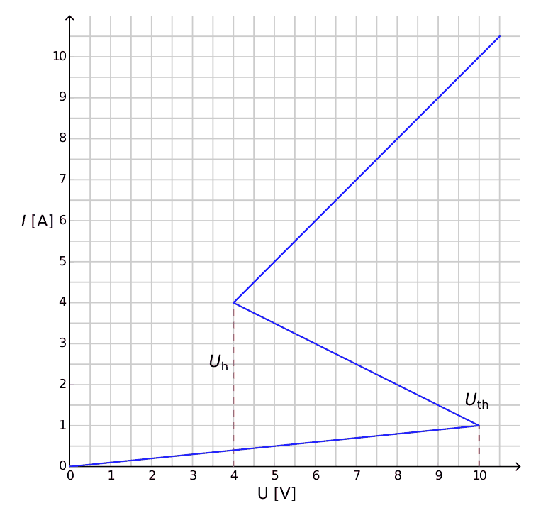
Figure 1: \(I-V\) characteristics of the non-linear element \(X\).
A.1 — 0.4pt
Using the graph, determine the resistance \(R_{\mathrm{on}}\) of the element \(X\) on the upper branch of the \(I-V\) characteristics, and \(R_{\mathrm{off}}\) on the lower branch, respectively. The middle branch is described by the equation
\[ I=I_0-\frac{U}{R_{\mathrm{int}}}. \tag{1} \]
Find the values of the parameters \(I_0\) and \(R_{\mathrm{int}}\).
The element \(X\) is connected in series (see Fig.2) with a resistor \(R\), an inductor \(L\) and an ideal voltage source \(\mathcal E\). One says that the circuit is in a stationary state if the current is constant in time, \(I(t)=\mathrm{const}\).
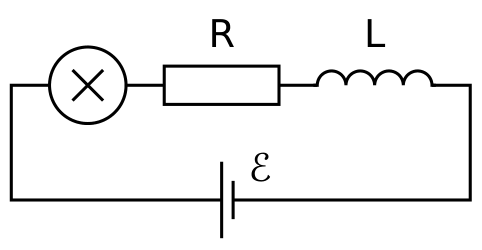
Figure 2: Circuit with element \(X\), resistor \(R\), inductor \(L\) and voltage source \(\mathcal E\).
A.2 — 1pt
What are the possible numbers of stationary states that the circuit of Fig. 2 may have for a fixed value of \(\mathcal E\) and for \(R=3.00\ \Omega\)? How does the answer change for \(R=1.00\ \Omega\)?
A.3 — 0.6pt
Let \(R=3.00\ \Omega\), \(L=1.00\ \mu\mathrm H\) and \(\mathcal E=15.0\ \mathrm V\) in the circuit shown in Fig. 2. Determine the values of the current \(I_{\mathrm{stationary}}\) and the voltage \(V_{\mathrm{stationary}}\) on the non-linear element \(X\) in the stationary state.
The circuit in Fig. 2 is in the stationary state with \(I(t)=I_{\mathrm{stationary}}\). This stationary state is said to be stable if after a small displacement (increase or decrease in the current), the current returns towards the stationary state. And if the system keeps moving away from the stationary state, it is said to be unstable.
A.4 — 1pt
Use numerical values of the question A.3 and study the stability of the stationary state with \(I(t)=I_{\mathrm{stationary}}\). Is it stable or unstable?
Part B. Bistable non-linear elements in physics: radio transmitter (5 points)
We now investigate a new circuit configuration (see Fig. 3). This time, the non-linear element \(X\) is connected in parallel to a capacitor of capacitance \(C=1.00\ \mu\mathrm F\). This block is then connected in series to a resistor of resistance \(R=3.00\ \Omega\) and an ideal constant voltage source of voltage \(\mathcal E=15.0\ \mathrm V\). It turns out that this circuit undergoes oscillations with the non-linear element \(X\) jumping from one branch of the \(I-V\) characteristics to another over the course of one cycle.
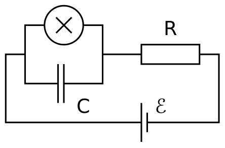
Figure 3: Circuit with element \(X\), capacitor \(C\), resistor \(R\) and voltage source \(\mathcal E\).
B.1 — 1.8pt
Draw the oscillation cycle on the \(I-V\) graph, including its direction (clockwise or anticlockwise). Justify your answer with equations and sketches.
B.2 — 1.9pt
Find expressions for the times \(t_1\) and \(t_2\) that the system spends on each branch of the \(I-V\) graph during the oscillation cycle. Determine their numerical values. Find the numerical value of the oscillation period \(T\) assuming that the time needed for jumps between the branches of the \(I-V\) graph is negligible.
B.3 — 0.7pt
Estimate the average power \(P\) dissipated by the non-linear element over the course of one oscillation. An order of magnitude is sufficient.
The circuit in Fig. 3 is used to build a radio transmitter. For this purpose, the element \(X\) is attached to one end of a linear antenna (a long straight wire) of length \(s\). The other end of the wire is free. In the antenna, an electromagnetic standing wave is formed. The speed of electromagnetic waves along the antenna is the same as in vacuum. The transmitter is using the main harmonic of the system, which has period \(T\) of question B.2.
B.4 — 0.6pt
What is the optimal value of \(s\) assuming that it cannot exceed \(1\ \mathrm{km}\)?
Part C. Bistable non-linear elements in biology: neuristor (2 points)
In this part of the problem, we consider an application of bistable non-linear elements to modeling of biological processes. A neuron in a human brain has the following property: when excited by an external signal, it makes one single oscillation and then returns to its initial state. This feature is called excitability. Due to this property, pulses can propagate in the network of coupled neurons constituting the nerve systems. A semiconductor chip designed to mimic excitability and pulse propagation is called a neuristor (from neuron and transistor).
We attempt to model a simple neuristor using a circuit that includes the non-linear element \(X\) that we investigated previously. To this end, the voltage \(\mathcal E\) in the circuit of Fig. 3 is decreased to the value \(\mathcal E'=12.0\ \mathrm V\). The oscillations stop, and the system reaches its stationary state. Then, the voltage is rapidly increased back to the value \(\mathcal E=15.0\ \mathrm V\), and after a period of time \(\tau\) (with \(\tau<T\)) is set again to the value \(\mathcal E'\) (see Fig. 4). It turns out that there is a certain critical value \(\tau_{\mathrm{crit}}\), and the system shows qualitatively different behavior for \(\tau<\tau_{\mathrm{crit}}\) and for \(\tau>\tau_{\mathrm{crit}}\).
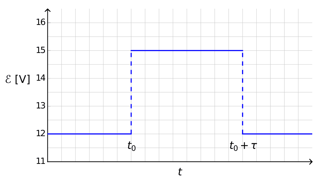
Figure 4: Voltage of the voltage source as a function of time.
C.1 — 1.2pt
Sketch the graphs of the time dependence of the current \(I_X(t)\) on the non-linear element \(X\) for \(\tau<\tau_{\mathrm{crit}}\) and for \(\tau>\tau_{\mathrm{crit}}\).
C.2 — 0.6pt
Find the expression and the numerical value of the critical time \(\tau_{\mathrm{crit}}\) for which the scenario switches.
C.3 — 0.2pt
Is the circuit with \(\tau=1.00\times10^{-6}\ \mathrm s\) a neuristor?
General Data Sheet
| Speed of light in vacuum | \(c\) | \(=\) | \(299\,792\,458\ \mathrm{m\cdot s^{-1}}\) |
| Vacuum permeability (magnetic constant) | \(\mu_0\) | \(=\) | \(4\pi\times10^{-7}\ \mathrm{kg\cdot m\cdot A^{-2}\cdot s^{-2}}\) |
| Vacuum permittivity (electrical constant) | \(\varepsilon_0\) | \(=\) | \(8.854\,187\,817\times10^{-12}\ \mathrm{A^2\cdot s^4\cdot kg^{-1}\cdot m^{-3}}\) |
| Elementary charge | \(e\) | \(=\) | \(1.602\,176\,620\,8(98)\times10^{-19}\ \mathrm{A\cdot s}\) |
| Mass of the electron | \(m_{\mathrm e}\) | \(=\) | \(9.109\,383\,56(11)\times10^{-31}\ \mathrm{kg}\) |
| \(=\) | \(0.510\,998\,946\,1(31)\ \dfrac{\mathrm{MeV}}{c^2}\) | ||
| Mass of the proton | \(m_{\mathrm p}\) | \(=\) | \(1.672\,621\,898(21)\times10^{-27}\ \mathrm{kg}\) |
| \(=\) | \(938.272\,081\,3(58)\ \dfrac{\mathrm{MeV}}{c^2}\) | ||
| Mass of the neutron | \(m_{\mathrm n}\) | \(=\) | \(1.674\,927\,471(21)\times10^{-27}\ \mathrm{kg}\) |
| \(=\) | \(939.565\,413\,3(58)\ \dfrac{\mathrm{MeV}}{c^2}\) | ||
| Unified atomic mass unit | \(u\) | \(=\) | \(1.660\,539\,040(20)\times10^{-27}\ \mathrm{kg}\) |
| Rydberg constant | \(R_\infty\) | \(=\) | \(10\,973\,731.568\,508(65)\ \mathrm{m^{-1}}\) |
| Universal constant of gravitation | \(G\) | \(=\) | \(6.674\,08(31)\times10^{-11}\ \mathrm{m^3\cdot kg^{-1}\cdot s^{-2}}\) |
| Acceleration due to gravity (in Zurich) | \(g\) | \(=\) | \(9.81\ \mathrm{m\cdot s^{-2}}\) |
| Planck’s constant | \(h\) | \(=\) | \(6.626\,070\,040\,(81)\times10^{-34}\ \mathrm{kg\cdot m^2\cdot s^{-1}}\) |
| Avogadro number | \(N_{\mathrm A}\) | \(=\) | \(6.022\,140\,857\,(74)\times10^{23}\ \mathrm{mol^{-1}}\) |
| Molar gas constant | \(R\) | \(=\) | \(8.314\,4598(48)\ \mathrm{kg\cdot m^2\cdot s^{-2}\cdot mol^{-1}\cdot K^{-1}}\) |
| Molar mass constant | \(M_u\) | \(=\) | \(1\times10^{-3}\ \mathrm{kg\cdot mol^{-1}}\) |
| Boltzmann constant | \(k_{\mathrm B}\) | \(=\) | \(1.380\,648\,52(79)\times10^{-23}\ \mathrm{kg\cdot m^2\cdot s^{-2}\cdot K^{-1}}\) |
| Stefan-Boltzmann constant | \(\sigma\) | \(=\) | \(5.670\,367\,(13)\times10^{-8}\ \mathrm{kg\cdot s^{-3}\cdot K^{-4}}\) |
Official English text of the problem.
Answers
- A.1: \(R_{\mathrm{on}}=1.00\ \Omega\), \(R_{\mathrm{off}}=10.0\ \Omega\), \(I_0=6.00\ \mathrm A\), \(R_{\mathrm{int}}=2.00\ \Omega\).
- A.2: For \(R=3.00\ \Omega\), there is one stationary state. For \(R=1.00\ \Omega\), there are three when \(8.00\ \mathrm V<\mathcal E<11.0\ \mathrm V\), two at either endpoint, and one otherwise, for the nonnegative source voltage shown.
- A.3: \(I_{\mathrm{stationary}}=3.00\ \mathrm A\), \(V_{\mathrm{stationary}}=6.00\ \mathrm V\).
- A.4: Stable; small current perturbations decay exponentially with time constant \(1.00\ \mu\mathrm s\).
- B.1: Anticlockwise. In coordinates \((U/\mathrm V,I_X/\mathrm A)\), the cycle is \[ (4,0.4)\rightarrow(10,1)\rightarrow(10,10) \rightarrow(4,4)\rightarrow(4,0.4). \]
- B.2: Defining \(t_1\) on the lower branch and \(t_2\) on the upper branch, \[ t_1=\frac{30}{13}\ln\frac{49}{10}\ \mu\mathrm s=3.67\ \mu\mathrm s, \qquad t_2=\frac34\ln25\ \mu\mathrm s=2.41\ \mu\mathrm s, \] \[ T=6.08\ \mu\mathrm s. \]
- B.3: \(P\) is of order \(10^1\ \mathrm W\). Integration within the ideal model gives \(P=17.3\ \mathrm W\).
- B.4: \(s=cT/4=456\ \mathrm m\).
- C.1: For \(\tau<\tau_{\mathrm{crit}}\), the current makes a small, continuous excursion from \(0.923\ \mathrm A\), remaining below \(1.00\ \mathrm A\), and returns to \(0.923\ \mathrm A\). For \(\tau>\tau_{\mathrm{crit}}\), it produces one large spike: a jump \(1.00\to10.0\ \mathrm A\), decay to \(4.00\ \mathrm A\), a jump to \(0.400\ \mathrm A\), and recovery to \(0.923\ \mathrm A\).
- C.2: \[ \tau_{\mathrm{crit}}=\frac{30}{13}\ln\frac32\ \mu\mathrm s =0.936\ \mu\mathrm s. \]
- C.3: Yes, because \(1.00\ \mu\mathrm s>\tau_{\mathrm{crit}}\), the pulse triggers one complete excursion.
Solution
A.1
The upper branch passes through the origin when extended and through \((U,I)=(4.00\ \mathrm V,4.00\ \mathrm A)\). Hence
\[ R_{\mathrm{on}}=\frac UI=\frac{4.00}{4.00}\ \Omega =\boxed{1.00\ \Omega}. \]
The lower branch passes through the origin and \((10.0\ \mathrm V,1.00\ \mathrm A)\), giving
\[ R_{\mathrm{off}}=\boxed{10.0\ \Omega}. \]
The middle branch joins \((4.00\ \mathrm V,4.00\ \mathrm A)\) to \((10.0\ \mathrm V,1.00\ \mathrm A)\), so
\[ -\frac1{R_{\mathrm{int}}} =\frac{1.00-4.00}{10.0-4.00}\ \frac{\mathrm A}{\mathrm V} =-0.500\ \Omega^{-1}. \]
Therefore
\[ \boxed{R_{\mathrm{int}}=2.00\ \Omega}, \qquad I_0=4.00\ \mathrm A+\frac{4.00\ \mathrm V}{2.00\ \Omega} =\boxed{6.00\ \mathrm A}. \]
Here \(R_{\mathrm{int}}\) is positive; the middle branch’s differential resistance is \(-R_{\mathrm{int}}\).
A.2
Let \(U\) denote the voltage across \(X\). Kirchhoff’s voltage law gives
\[ \mathcal E=RI+U+L\frac{dI}{dt}. \]
In a stationary state,
\[ \mathcal E=RI+U. \]
Thus stationary states are intersections of the characteristic with the load line \(I=(\mathcal E-U)/R\).
Equivalently, using the characteristic as \(U(I)\),
\[ \mathcal E(I)= \begin{cases} (R+10.0\ \Omega)I, &0\le I\le1.00\ \mathrm A,\\[2mm] 12.0\ \mathrm V+(R-2.00\ \Omega)I, &1.00\ \mathrm A\le I\le4.00\ \mathrm A,\\[2mm] (R+1.00\ \Omega)I, &I\ge4.00\ \mathrm A. \end{cases} \]
For \(R=3.00\ \Omega\), all three pieces increase with \(I\). They join continuously at \(\mathcal E=13.0\ \mathrm V\) and \(16.0\ \mathrm V\). Consequently, every nonnegative source voltage has exactly one stationary state.
For \(R=1.00\ \Omega\), the middle piece decreases with \(I\). Its endpoints occur at
\[ \mathcal E(1.00\ \mathrm A)=11.0\ \mathrm V, \qquad \mathcal E(4.00\ \mathrm A)=8.00\ \mathrm V. \]
The number of distinct stationary states is therefore
| Source voltage | Number of stationary states |
|---|---|
| \(0\le\mathcal E<8.00\ \mathrm V\) | 1 |
| \(\mathcal E=8.00\ \mathrm V\) | 2 |
| \(8.00\ \mathrm V<\mathcal E<11.0\ \mathrm V\) | 3 |
| \(\mathcal E=11.0\ \mathrm V\) | 2 |
| \(\mathcal E>11.0\ \mathrm V\) | 1 |
At either boundary, two branch intersections coincide at a corner of the characteristic and count as one state.
A.3
For \(R=3.00\ \Omega\) and \(\mathcal E=15.0\ \mathrm V\), the stationary state lies on the middle branch because \(13.0<15.0<16.0\ \mathrm V\). Hence
\[ 15.0\ \mathrm V =12.0\ \mathrm V+(3.00-2.00)\ \Omega\,I_{\mathrm{stationary}}. \]
Therefore
\[ \boxed{I_{\mathrm{stationary}}=3.00\ \mathrm A}, \]
and
\[ \boxed{ V_{\mathrm{stationary}} =\mathcal E-RI_{\mathrm{stationary}} =6.00\ \mathrm V}. \]
A.4
Write \(I=I_{\mathrm{stationary}}+\delta I\). A sufficiently small perturbation remains on the middle branch, where
\[ U=R_{\mathrm{int}}(I_0-I). \]
Substituting into Kirchhoff’s law and subtracting the stationary equation gives
\[ L\frac{d(\delta I)}{dt} =-(R-R_{\mathrm{int}})\delta I. \]
Thus
\[ \delta I(t)=\delta I(0) \exp\left[-\frac{R-R_{\mathrm{int}}}{L}t\right]. \]
Since \(R-R_{\mathrm{int}}=1.00\ \Omega>0\), the perturbation decays. The stationary state is therefore stable, with relaxation time
\[ \boxed{ \frac{L}{R-R_{\mathrm{int}}} =\frac{1.00\ \mu\mathrm H}{1.00\ \Omega} =1.00\ \mu\mathrm s}. \]
The external resistor’s positive differential resistance exceeds the magnitude of the element’s negative differential resistance.
B.1
The capacitor and \(X\) have the same voltage \(U\). Kirchhoff’s current law gives
\[ \frac{\mathcal E-U}{R}=I_X+C\frac{dU}{dt}, \]
or
\[ C\frac{dU}{dt}=\frac{\mathcal E-U}{R}-I_X(U). \]
On a branch of resistance \(r\), \(I_X=U/r\), so
\[ C\frac{dU}{dt}=\frac{\mathcal E}{R} -\left(\frac1R+\frac1r\right)U. \]
On the lower branch, the voltage towards which the circuit would relax is
\[ U_{\infty,\mathrm{off}} =\frac{\mathcal E R_{\mathrm{off}}}{R+R_{\mathrm{off}}} =\frac{150}{13}\ \mathrm V =11.538\ldots\ \mathrm V. \]
This exceeds \(U_{\mathrm{th}}=10.0\ \mathrm V\). Consequently, throughout the lower-branch part of the cycle, \(dU/dt>0\): the capacitor charges from \(4.00\) to \(10.0\ \mathrm V\).
At \(U_{\mathrm{th}}\), the lower branch ends. The capacitor voltage cannot jump, so \(X\) switches vertically on the \(I-V\) plot:
\[ (U,I_X)=(10.0\ \mathrm V,1.00\ \mathrm A) \longrightarrow(10.0\ \mathrm V,10.0\ \mathrm A). \]
On the upper branch, the corresponding limiting voltage is
\[ U_{\infty,\mathrm{on}} =\frac{\mathcal E R_{\mathrm{on}}}{R+R_{\mathrm{on}}} =3.75\ \mathrm V. \]
This lies below \(U_{\mathrm h}=4.00\ \mathrm V\). Thus \(dU/dt<0\): the capacitor discharges from \(10.0\) to \(4.00\ \mathrm V\). At the holding voltage, the current jumps from \(4.00\) to \(0.400\ \mathrm A\), again at constant voltage.
The requested sketch therefore has these successive segments:
| Segment | Motion in the \(I-V\) plane |
|---|---|
| Lower branch | From \((4.00\ \mathrm V,0.400\ \mathrm A)\) rightwards and slightly upwards to \((10.0\ \mathrm V,1.00\ \mathrm A)\) |
| Threshold switch | Vertically upwards to \((10.0\ \mathrm V,10.0\ \mathrm A)\) |
| Upper branch | Leftwards and downwards to \((4.00\ \mathrm V,4.00\ \mathrm A)\) |
| Holding-voltage switch | Vertically downwards to \((4.00\ \mathrm V,0.400\ \mathrm A)\) |
The direction is anticlockwise.
The middle-branch equilibrium is unstable in this capacitor circuit. Indeed, near \(U=6.00\ \mathrm V\),
\[ C\frac{d(\delta U)}{dt} =\left(\frac1{R_{\mathrm{int}}}-\frac1R\right)\delta U =\frac{\delta U}{6.00\ \Omega}. \]
Voltage perturbations grow, so the middle branch is not a sustained part of the oscillation cycle.
B.2
For a branch of resistance \(r\), define
\[ \theta_r=C\frac{Rr}{R+r}, \qquad U_{\infty,r}=\frac{\mathcal E r}{R+r}. \]
The differential equation from B.1 becomes
\[ \frac{dU}{dt}=\frac{U_{\infty,r}-U}{\theta_r}, \]
with solution
\[ U(t)=U_{\infty,r} +\bigl(U(0)-U_{\infty,r}\bigr)e^{-t/\theta_r}. \]
Define \(t_1\) as the time on the lower branch and \(t_2\) as the time on the upper branch.
For charging from \(U_{\mathrm h}\) to \(U_{\mathrm{th}}\),
\[ \boxed{ t_1=\theta_{\mathrm{off}} \ln\left( \frac{U_{\infty,\mathrm{off}}-U_{\mathrm h}} {U_{\infty,\mathrm{off}}-U_{\mathrm{th}}} \right)}. \]
Here
\[ \theta_{\mathrm{off}} =\frac{30}{13}\ \mu\mathrm s, \]
so
\[ t_1 =\frac{30}{13}\ \mu\mathrm s \ln\left(\frac{150/13-4}{150/13-10}\right) =\frac{30}{13}\ln\frac{49}{10}\ \mu\mathrm s =\boxed{3.67\ \mu\mathrm s}. \]
For discharging from \(U_{\mathrm{th}}\) to \(U_{\mathrm h}\),
\[ \boxed{ t_2=\theta_{\mathrm{on}} \ln\left( \frac{U_{\mathrm{th}}-U_{\infty,\mathrm{on}}} {U_{\mathrm h}-U_{\infty,\mathrm{on}}} \right)}. \]
Since
\[ \theta_{\mathrm{on}}=0.750\ \mu\mathrm s, \]
we obtain
\[ t_2=0.750\ \mu\mathrm s \ln\left(\frac{10.0-3.75}{4.00-3.75}\right) =\frac34\ln25\ \mu\mathrm s =\boxed{2.41\ \mu\mathrm s}. \]
Neglecting the switching durations,
\[ \boxed{T=t_1+t_2=6.08\ \mu\mathrm s}. \]
B.3
On either conducting branch, the instantaneous power dissipated in \(X\) is
\[ p_X=UI_X=\frac{U^2}{r}. \]
We neglect energy dissipated during the ideal instantaneous switches. Using the voltage evolution derived above, the energy dissipated on each branch is
\[ W_{\mathrm{off}} =\frac{\theta_{\mathrm{off}}}{R_{\mathrm{off}}} \int_{U_{\mathrm h}}^{U_{\mathrm{th}}} \frac{U^2}{U_{\infty,\mathrm{off}}-U}\,dU =23.2\ \mu\mathrm J, \]
and
\[ W_{\mathrm{on}} =\frac{\theta_{\mathrm{on}}}{R_{\mathrm{on}}} \int_{U_{\mathrm h}}^{U_{\mathrm{th}}} \frac{U^2}{U-U_{\infty,\mathrm{on}}}\,dU =82.3\ \mu\mathrm J. \]
Thus
\[ P=\frac{W_{\mathrm{off}}+W_{\mathrm{on}}}{T} =\frac{105.5\ \mu\mathrm J}{6.0816\ \mu\mathrm s} =\boxed{17.3\ \mathrm W}. \]
The requested order-of-magnitude estimate is therefore
\[ \boxed{P\sim10^1\ \mathrm W}. \]
B.4
The emitted fundamental has wavelength
\[ \lambda=cT =(299\,792\,458\ \mathrm{m\,s^{-1}}) (6.08162\times10^{-6}\ \mathrm s) =1.82322\times10^3\ \mathrm m. \]
In the ideal antenna model, the free end is a current node, while efficient excitation places a current antinode at the driven end. Their separation is an odd multiple of a quarter wavelength:
\[ s=(2n+1)\frac{\lambda}{4}, \qquad n=0,1,2,\ldots \]
The shortest resonant length is
\[ \boxed{s=\frac{\lambda}{4}=\frac{cT}{4}=456\ \mathrm m}. \]
The next possibility is \(3\lambda/4=1.37\ \mathrm{km}\), which exceeds the limit. Thus the quarter-wave length is the permitted optimum.
C.1
First find the initial stationary state at \(\mathcal E'=12.0\ \mathrm V\). It lies on the lower branch:
\[ I_{\mathrm r}=\frac{\mathcal E'}{R+R_{\mathrm{off}}} =\frac{12}{13}\ \mathrm A =\boxed{0.923\ \mathrm A}, \]
\[ U_{\mathrm r}=R_{\mathrm{off}}I_{\mathrm r} =\frac{120}{13}\ \mathrm V =\boxed{9.23\ \mathrm V}. \]
Let \(u=t-t_0\). Before the pulse, \(I_X=I_{\mathrm r}\). While the source is at \(15.0\ \mathrm V\) and the element remains on the lower branch,
\[ I_X(u) =\frac{\mathcal E}{R+R_{\mathrm{off}}} +\left(I_{\mathrm r} -\frac{\mathcal E}{R+R_{\mathrm{off}}}\right) e^{-u/\theta_{\mathrm{off}}}, \]
or numerically,
\[ I_X(u)=\frac{15-3e^{-u/\theta_{\mathrm{off}}}}{13}\ \mathrm A. \]
The critical duration is the time required for this current to reach \(1.00\ \mathrm A\), corresponding to \(U=U_{\mathrm{th}}\).
For \(\tau<\tau_{\mathrm{crit}}\), the graph is a small continuous bump:
- Before \(t_0\), the current is constant at \(0.923\ \mathrm A\).
- During the pulse, it rises exponentially, with decreasing slope, but remains below \(1.00\ \mathrm A\).
- At \(t_0+\tau\), the current is continuous and its slope changes sign.
- Afterwards it decays exponentially back to \(0.923\ \mathrm A\):
\[ I_X(u)=I_{\mathrm r} +\bigl[I_X(\tau)-I_{\mathrm r}\bigr] e^{-(u-\tau)/\theta_{\mathrm{off}}}, \qquad u\ge\tau. \]
There is no branch switch.
For \(\tau>\tau_{\mathrm{crit}}\), the graph contains one large spike:
- The current initially follows the same gradual rise from \(0.923\) to \(1.00\ \mathrm A\).
- At \(t=t_0+\tau_{\mathrm{crit}}\), it jumps vertically from \(1.00\) to \(10.0\ \mathrm A\).
- It then decreases on the upper branch. While the source remains at \(15.0\ \mathrm V\), \[ I_X(u)=3.75\ \mathrm A +6.25\ \mathrm A\, e^{-(u-\tau_{\mathrm{crit}})/\theta_{\mathrm{on}}}. \]
- On reaching \(4.00\ \mathrm A\), it jumps vertically to \(0.400\ \mathrm A\).
- It subsequently rises on the lower branch and ultimately approaches \(0.923\ \mathrm A\) from below.
If the source returns to \(12.0\ \mathrm V\) while the element is still on the upper branch, the current remains continuous at that instant, but its decay becomes faster. Its subsequent expression is
\[ I_X(u)=3.00\ \mathrm A +\bigl[I_X(\tau)-3.00\ \mathrm A\bigr] e^{-(u-\tau)/\theta_{\mathrm{on}}}. \]
The asymptote \(3.00\ \mathrm A\) lies below the holding current, so the current necessarily reaches \(4.00\ \mathrm A\) and switches off. If this occurs at \(u=u_d\), the following recovery is
\[ I_X(u)=I_{\mathrm r} +\bigl(0.400\ \mathrm A-I_{\mathrm r}\bigr) e^{-(u-u_d)/\theta_{\mathrm{off}}}. \]
For a longer pulse, the upper-to-lower switch can occur before the pulse ends. If the source stays at \(15.0\ \mathrm V\), that switch occurs at
\[ u=\tau_{\mathrm{crit}}+t_2=3.35\ \mu\mathrm s. \]
The current then recovers on the lower branch under the \(15.0\ \mathrm V\) source until \(u=\tau\), after which it approaches the \(12.0\ \mathrm V\) rest state. The source changes produce slope changes, not instantaneous changes in \(I_X\).
There cannot be a second spike during the prescribed pulse: with \(15.0\ \mathrm V\) maintained, the second threshold crossing would occur at \(u=\tau_{\mathrm{crit}}+T>T>\tau\).
C.2
At the critical duration, the capacitor has just charged from \(U_{\mathrm r}\) to \(U_{\mathrm{th}}\):
\[ U_{\mathrm{th}} =U_{\infty,\mathrm{off}} +\bigl(U_{\mathrm r}-U_{\infty,\mathrm{off}}\bigr) e^{-\tau_{\mathrm{crit}}/\theta_{\mathrm{off}}}. \]
Solving,
\[ \boxed{ \tau_{\mathrm{crit}} =\theta_{\mathrm{off}} \ln\left( \frac{U_{\infty,\mathrm{off}}-U_{\mathrm r}} {U_{\infty,\mathrm{off}}-U_{\mathrm{th}}} \right)}. \]
In terms of the circuit parameters,
\[ \boxed{ \tau_{\mathrm{crit}} =\frac{CRR_{\mathrm{off}}}{R+R_{\mathrm{off}}} \ln\left[ \frac{(\mathcal E-\mathcal E')R_{\mathrm{off}}} {\mathcal E R_{\mathrm{off}} -(R+R_{\mathrm{off}})U_{\mathrm{th}}} \right]}. \]
Numerically,
\[ \tau_{\mathrm{crit}} =\frac{30}{13}\ \mu\mathrm s \ln\left( \frac{150/13-120/13}{150/13-10} \right) =\frac{30}{13}\ln\frac32\ \mu\mathrm s. \]
Therefore
\[ \boxed{\tau_{\mathrm{crit}}=0.936\ \mu\mathrm s}. \]
C.3
The specified pulse satisfies
\[ \tau=1.00\ \mu\mathrm s >\tau_{\mathrm{crit}}=0.936\ \mu\mathrm s, \qquad \tau<T. \]
It therefore triggers the switch to the upper branch. The circuit completes one large current excursion and then returns to its original stationary state under the \(12.0\ \mathrm V\) source.
\[ \boxed{\text{Yes, the circuit behaves as a neuristor.}} \]
The solution was checked against the official solution.
IPhO 2016 · Theorieaufgabe 2
Nichtlineare Dynamik in elektrischen Schaltungen
Bitte lesen Sie die allgemeinen Hinweise im separaten Umschlag, bevor Sie mit dieser Aufgabe beginnen.
Einleitung
Bistabile nichtlineare Halbleiterbauelemente (z. B. Thyristoren) werden in der Elektronik häufig als Schalter und zur Erzeugung elektromagnetischer Schwingungen eingesetzt. Das Hauptanwendungsgebiet von Thyristoren ist die Steuerung von Wechselströmen in der Leistungselektronik, beispielsweise die Gleichrichtung von Wechselstrom zu Gleichstrom im Megawattbereich. Bistabile Bauelemente können auch als Modellsysteme für Selbstorganisationsphänomene in der Physik (dieses Thema wird in Teil B der Aufgabe behandelt), in der Biologie (siehe Teil C) und in anderen Bereichen der modernen nichtlinearen Wissenschaft dienen.
Ziele
Untersuchung von Instabilitäten und nichttrivialer Dynamik in Schaltungen mit Bauelementen mit nichtlinearen \(I-V\)-Kennlinien. Erkundung möglicher Anwendungen solcher Schaltungen in der Technik und bei der Modellierung biologischer Systeme.
Teil A. Stationäre Zustände und Instabilitäten (3 Punkte)
Abb. 1 zeigt die sogenannte S-förmige \(I-V\)-Kennlinie eines nichtlinearen Bauelements \(X\). Im Spannungsbereich zwischen \(U_{\mathrm h}=4.00\ \mathrm V\) (der Haltespannung) und \(U_{\mathrm{th}}=10.0\ \mathrm V\) (der Schwellenspannung) ist diese \(I-V\)-Kennlinie mehrwertig. Der Einfachheit halber ist der Graph in Abb. 1 stückweise linear gewählt (jeder Zweig ist ein Geradenstück). Insbesondere verläuft die Verlängerung des oberen Zweigs durch den Ursprung. Diese Näherung beschreibt reale Thyristoren gut.
Abbildung 1: \(I-V\)-Kennlinie des nichtlinearen Bauelements \(X\).
A.1 — 0.4 Punkte
Bestimmen Sie anhand des Graphen den Widerstand \(R_{\mathrm{on}}\) des Bauelements \(X\) auf dem oberen Zweig der \(I-V\)-Kennlinie sowie \(R_{\mathrm{off}}\) auf dem unteren Zweig. Der mittlere Zweig wird durch folgende Gleichung beschrieben:
\[ I=I_0-\frac{U}{R_{\mathrm{int}}}. \tag{1} \]
Bestimmen Sie die Werte der Parameter \(I_0\) und \(R_{\mathrm{int}}\).
Das Bauelement \(X\) wird mit einem Widerstand \(R\), einer Spule mit der Induktivität \(L\) und einer idealen Spannungsquelle \(\mathcal E\) in Reihe geschaltet (siehe Abb. 2). Man sagt, dass sich die Schaltung in einem stationären Zustand befindet, wenn der Strom zeitlich konstant ist, \(I(t)=\mathrm{const}\).
Abbildung 2: Schaltung mit dem Bauelement \(X\), dem Widerstand \(R\), der Spule mit der Induktivität \(L\) und der Spannungsquelle \(\mathcal E\).
A.2 — 1 Punkt
Welche Anzahlen stationärer Zustände sind für die Schaltung in Abb. 2 bei einem festen Wert von \(\mathcal E\) und für \(R=3.00\ \Omega\) möglich? Wie ändert sich die Antwort für \(R=1.00\ \Omega\)?
A.3 — 0.6 Punkte
Für die Schaltung in Abb. 2 seien \(R=3.00\ \Omega\), \(L=1.00\ \mu\mathrm H\) und \(\mathcal E=15.0\ \mathrm V\). Bestimmen Sie den Strom \(I_{\mathrm{stationary}}\) und die Spannung \(V_{\mathrm{stationary}}\) am nichtlinearen Bauelement \(X\) im stationären Zustand.
Die Schaltung in Abb. 2 befindet sich im stationären Zustand mit \(I(t)=I_{\mathrm{stationary}}\). Dieser stationäre Zustand heißt stabil, wenn der Strom nach einer kleinen Auslenkung (Erhöhung oder Verringerung des Stroms) zum stationären Zustand zurückkehrt. Entfernt sich das System dagegen immer weiter vom stationären Zustand, so heißt dieser instabil.
A.4 — 1 Punkt
Verwenden Sie die Zahlenwerte aus Teilaufgabe A.3 und untersuchen Sie die Stabilität des stationären Zustands mit \(I(t)=I_{\mathrm{stationary}}\). Ist er stabil oder instabil?
Teil B. Bistabile nichtlineare Bauelemente in der Physik: Funksender (5 Punkte)
Wir untersuchen nun eine neue Schaltungsanordnung (siehe Abb. 3). Diesmal ist das nichtlineare Bauelement \(X\) parallel zu einem Kondensator mit der Kapazität \(C=1.00\ \mu\mathrm F\) geschaltet. Diese Parallelschaltung ist wiederum mit einem Widerstand \(R=3.00\ \Omega\) und einer idealen Gleichspannungsquelle mit der Spannung \(\mathcal E=15.0\ \mathrm V\) in Reihe geschaltet. Es zeigt sich, dass in dieser Schaltung Schwingungen auftreten, wobei das nichtlineare Bauelement \(X\) im Verlauf einer Periode von einem Zweig der \(I-V\)-Kennlinie auf einen anderen springt.
Abbildung 3: Schaltung mit dem Bauelement \(X\), dem Kondensator \(C\), dem Widerstand \(R\) und der Spannungsquelle \(\mathcal E\).
B.1 — 1.8 Punkte
Zeichnen Sie den Schwingungszyklus in das \(I-V\)-Diagramm ein und geben Sie seine Umlaufrichtung an (im oder gegen den Uhrzeigersinn). Begründen Sie Ihre Antwort mit Gleichungen und Skizzen.
B.2 — 1.9 Punkte
Bestimmen Sie Ausdrücke für die Zeiten \(t_1\) und \(t_2\), die das System während des Schwingungszyklus auf den einzelnen Zweigen des \(I-V\)-Diagramms verbringt. Berechnen Sie ihre Zahlenwerte. Bestimmen Sie den Zahlenwert der Schwingungsdauer \(T\) unter der Annahme, dass die für die Sprünge zwischen den Zweigen des \(I-V\)-Diagramms benötigte Zeit vernachlässigbar ist.
B.3 — 0.7 Punkte
Schätzen Sie die mittlere Leistung \(P\) ab, die im nichtlinearen Bauelement während einer Schwingung dissipiert wird. Die Angabe der Größenordnung genügt.
Die Schaltung in Abb. 3 wird zum Bau eines Funksenders verwendet. Dazu wird das Bauelement \(X\) an ein Ende einer linearen Antenne (eines langen geraden Drahtes) der Länge \(s\) angeschlossen. Das andere Ende des Drahtes ist frei. In der Antenne bildet sich eine stehende elektromagnetische Welle aus. Die Geschwindigkeit elektromagnetischer Wellen entlang der Antenne ist gleich derjenigen im Vakuum. Der Sender nutzt die Grundschwingung des Systems, deren Periodendauer \(T\) in Teilaufgabe B.2 bestimmt wurde.
B.4 — 0.6 Punkte
Welcher Wert von \(s\) ist optimal, wenn die Länge \(1\ \mathrm{km}\) nicht überschreiten darf?
Teil C. Bistabile nichtlineare Bauelemente in der Biologie: Neuristor (2 Punkte)
In diesem Teil der Aufgabe betrachten wir eine Anwendung bistabiler nichtlinearer Bauelemente zur Modellierung biologischer Prozesse. Ein Neuron im menschlichen Gehirn besitzt folgende Eigenschaft: Wird es durch ein äußeres Signal angeregt, führt es eine einzige Schwingung aus und kehrt anschließend in seinen Ausgangszustand zurück. Diese Eigenschaft wird als Erregbarkeit bezeichnet. Aufgrund dieser Eigenschaft können sich Impulse in dem Netzwerk gekoppelter Neuronen ausbreiten, aus dem das Nervensystem besteht. Ein Halbleiterchip, der Erregbarkeit und Impulsausbreitung nachbilden soll, wird als Neuristor bezeichnet (aus Neuron und Transistor).
Wir versuchen, einen einfachen Neuristor mithilfe einer Schaltung zu modellieren, die das zuvor untersuchte nichtlineare Bauelement \(X\) enthält. Dazu wird die Spannung \(\mathcal E\) in der Schaltung aus Abb. 3 auf den Wert \(\mathcal E'=12.0\ \mathrm V\) verringert. Die Schwingungen hören auf, und das System erreicht seinen stationären Zustand. Anschließend wird die Spannung rasch wieder auf den Wert \(\mathcal E=15.0\ \mathrm V\) erhöht und nach einer Zeitspanne \(\tau\) (mit \(\tau<T\)) erneut auf den Wert \(\mathcal E'\) gesetzt (siehe Abb. 4). Es zeigt sich, dass es einen bestimmten kritischen Wert \(\tau_{\mathrm{crit}}\) gibt und dass das System für \(\tau<\tau_{\mathrm{crit}}\) und für \(\tau>\tau_{\mathrm{crit}}\) qualitativ unterschiedliches Verhalten zeigt.
Abbildung 4: Spannung der Spannungsquelle als Funktion der Zeit.
C.1 — 1.2 Punkte
Skizzieren Sie die zeitlichen Verläufe des Stroms \(I_X(t)\) durch das nichtlineare Bauelement \(X\) für \(\tau<\tau_{\mathrm{crit}}\) und für \(\tau>\tau_{\mathrm{crit}}\).
C.2 — 0.6 Punkte
Bestimmen Sie den Ausdruck und den Zahlenwert der kritischen Zeit \(\tau_{\mathrm{crit}}\), bei der das Verhalten umschlägt.
C.3 — 0.2 Punkte
Ist die Schaltung mit \(\tau=1.00\times10^{-6}\ \mathrm s\) ein Neuristor?
Allgemeines Datenblatt
| Lichtgeschwindigkeit im Vakuum | \(c\) | \(=\) | \(299\,792\,458\ \mathrm{m\cdot s^{-1}}\) |
| Vakuumpermeabilität (magnetische Feldkonstante) | \(\mu_0\) | \(=\) | \(4\pi\times10^{-7}\ \mathrm{kg\cdot m\cdot A^{-2}\cdot s^{-2}}\) |
| Vakuumpermittivität (elektrische Feldkonstante) | \(\varepsilon_0\) | \(=\) | \(8.854\,187\,817\times10^{-12}\ \mathrm{A^2\cdot s^4\cdot kg^{-1}\cdot m^{-3}}\) |
| Elementarladung | \(e\) | \(=\) | \(1.602\,176\,620\,8(98)\times10^{-19}\ \mathrm{A\cdot s}\) |
| Masse des Elektrons | \(m_{\mathrm e}\) | \(=\) | \(9.109\,383\,56(11)\times10^{-31}\ \mathrm{kg}\) |
| \(=\) | \(0.510\,998\,946\,1(31)\ \dfrac{\mathrm{MeV}}{c^2}\) | ||
| Masse des Protons | \(m_{\mathrm p}\) | \(=\) | \(1.672\,621\,898(21)\times10^{-27}\ \mathrm{kg}\) |
| \(=\) | \(938.272\,081\,3(58)\ \dfrac{\mathrm{MeV}}{c^2}\) | ||
| Masse des Neutrons | \(m_{\mathrm n}\) | \(=\) | \(1.674\,927\,471(21)\times10^{-27}\ \mathrm{kg}\) |
| \(=\) | \(939.565\,413\,3(58)\ \dfrac{\mathrm{MeV}}{c^2}\) | ||
| Vereinheitlichte atomare Masseneinheit | \(u\) | \(=\) | \(1.660\,539\,040(20)\times10^{-27}\ \mathrm{kg}\) |
| Rydberg-Konstante | \(R_\infty\) | \(=\) | \(10\,973\,731.568\,508(65)\ \mathrm{m^{-1}}\) |
| Universelle Gravitationskonstante | \(G\) | \(=\) | \(6.674\,08(31)\times10^{-11}\ \mathrm{m^3\cdot kg^{-1}\cdot s^{-2}}\) |
| Erdbeschleunigung (in Zürich) | \(g\) | \(=\) | \(9.81\ \mathrm{m\cdot s^{-2}}\) |
| Plancksches Wirkungsquantum | \(h\) | \(=\) | \(6.626\,070\,040\,(81)\times10^{-34}\ \mathrm{kg\cdot m^2\cdot s^{-1}}\) |
| Avogadro-Konstante | \(N_{\mathrm A}\) | \(=\) | \(6.022\,140\,857\,(74)\times10^{23}\ \mathrm{mol^{-1}}\) |
| Molare Gaskonstante | \(R\) | \(=\) | \(8.314\,4598(48)\ \mathrm{kg\cdot m^2\cdot s^{-2}\cdot mol^{-1}\cdot K^{-1}}\) |
| Molare Massenkonstante | \(M_u\) | \(=\) | \(1\times10^{-3}\ \mathrm{kg\cdot mol^{-1}}\) |
| Boltzmann-Konstante | \(k_{\mathrm B}\) | \(=\) | \(1.380\,648\,52(79)\times10^{-23}\ \mathrm{kg\cdot m^2\cdot s^{-2}\cdot K^{-1}}\) |
| Stefan-Boltzmann-Konstante | \(\sigma\) | \(=\) | \(5.670\,367\,(13)\times10^{-8}\ \mathrm{kg\cdot s^{-3}\cdot K^{-4}}\) |
Aufgabentext aus dem offiziellen englischen Text übersetzt.
Antworten
- A.1: \(R_{\mathrm{on}}=1.00\ \Omega\), \(R_{\mathrm{off}}=10.0\ \Omega\), \(I_0=6.00\ \mathrm A\), \(R_{\mathrm{int}}=2.00\ \Omega\).
- A.2: Für \(R=3.00\ \Omega\) gibt es einen stationären Zustand. Für \(R=1.00\ \Omega\) gibt es drei, wenn \(8.00\ \mathrm V<\mathcal E<11.0\ \mathrm V\), zwei an jedem der beiden Randpunkte und einen in allen anderen Fällen, jeweils für die dargestellte nichtnegative Quellenspannung.
- A.3: \(I_{\mathrm{stationary}}=3.00\ \mathrm A\), \(V_{\mathrm{stationary}}=6.00\ \mathrm V\).
- A.4: Stabil; kleine Stromstörungen klingen exponentiell mit der Zeitkonstante \(1.00\ \mu\mathrm s\) ab.
- B.1: Gegen den Uhrzeigersinn. In den Koordinaten \((U/\mathrm V,I_X/\mathrm A)\) lautet der Zyklus \[ (4,0.4)\rightarrow(10,1)\rightarrow(10,10) \rightarrow(4,4)\rightarrow(4,0.4). \]
- B.2: Bezeichnet \(t_1\) die Zeit auf dem unteren Zweig und \(t_2\) die Zeit auf dem oberen Zweig, so gilt \[ t_1=\frac{30}{13}\ln\frac{49}{10}\ \mu\mathrm s=3.67\ \mu\mathrm s, \qquad t_2=\frac34\ln25\ \mu\mathrm s=2.41\ \mu\mathrm s, \] \[ T=6.08\ \mu\mathrm s. \]
- B.3: \(P\) liegt in der Größenordnung \(10^1\ \mathrm W\). Die Integration im idealisierten Modell ergibt \(P=17.3\ \mathrm W\).
- B.4: \(s=cT/4=456\ \mathrm m\).
- C.1: Für \(\tau<\tau_{\mathrm{crit}}\) führt der Strom ausgehend von \(0.923\ \mathrm A\) eine kleine, stetige Auslenkung aus, bleibt dabei unter \(1.00\ \mathrm A\) und kehrt zu \(0.923\ \mathrm A\) zurück. Für \(\tau>\tau_{\mathrm{crit}}\) entsteht eine große Stromspitze: ein Sprung \(1.00\to10.0\ \mathrm A\), ein Abfall auf \(4.00\ \mathrm A\), ein Sprung auf \(0.400\ \mathrm A\) und die Rückkehr zu \(0.923\ \mathrm A\).
- C.2: \[ \tau_{\mathrm{crit}}=\frac{30}{13}\ln\frac32\ \mu\mathrm s =0.936\ \mu\mathrm s. \]
- C.3: Ja, denn \(1.00\ \mu\mathrm s>\tau_{\mathrm{crit}}\), sodass der Impuls eine vollständige Auslenkung auslöst.
Lösung
A.1
Die Verlängerung des oberen Zweigs verläuft durch den Ursprung; außerdem verläuft dieser Zweig durch \((U,I)=(4.00\ \mathrm V,4.00\ \mathrm A)\). Daher gilt
\[ R_{\mathrm{on}}=\frac UI=\frac{4.00}{4.00}\ \Omega =\boxed{1.00\ \Omega}. \]
Der untere Zweig verläuft durch den Ursprung und durch \((10.0\ \mathrm V,1.00\ \mathrm A)\), woraus folgt:
\[ R_{\mathrm{off}}=\boxed{10.0\ \Omega}. \]
Der mittlere Zweig verbindet \((4.00\ \mathrm V,4.00\ \mathrm A)\) mit \((10.0\ \mathrm V,1.00\ \mathrm A)\), also gilt
\[ -\frac1{R_{\mathrm{int}}} =\frac{1.00-4.00}{10.0-4.00}\ \frac{\mathrm A}{\mathrm V} =-0.500\ \Omega^{-1}. \]
Daraus folgt
\[ \boxed{R_{\mathrm{int}}=2.00\ \Omega}, \qquad I_0=4.00\ \mathrm A+\frac{4.00\ \mathrm V}{2.00\ \Omega} =\boxed{6.00\ \mathrm A}. \]
Hier ist \(R_{\mathrm{int}}\) positiv; der differentielle Widerstand des mittleren Zweigs ist \(-R_{\mathrm{int}}\).
A.2
Mit \(U\) sei die Spannung über \(X\) bezeichnet. Die Kirchhoffsche Maschenregel liefert
\[ \mathcal E=RI+U+L\frac{dI}{dt}. \]
Im stationären Zustand gilt
\[ \mathcal E=RI+U. \]
Stationäre Zustände entsprechen somit den Schnittpunkten der Kennlinie mit der Lastgeraden \(I=(\mathcal E-U)/R\).
Gleichwertig lässt sich mit der Kennlinie in der Form \(U(I)\) schreiben:
\[ \mathcal E(I)= \begin{cases} (R+10.0\ \Omega)I, &0\le I\le1.00\ \mathrm A,\\[2mm] 12.0\ \mathrm V+(R-2.00\ \Omega)I, &1.00\ \mathrm A\le I\le4.00\ \mathrm A,\\[2mm] (R+1.00\ \Omega)I, &I\ge4.00\ \mathrm A. \end{cases} \]
Für \(R=3.00\ \Omega\) steigen alle drei Teilstücke mit \(I\) an. Sie schließen bei \(\mathcal E=13.0\ \mathrm V\) und \(16.0\ \mathrm V\) stetig aneinander an. Folglich gibt es für jede nichtnegative Quellenspannung genau einen stationären Zustand.
Für \(R=1.00\ \Omega\) fällt das mittlere Teilstück mit wachsendem \(I\) ab. Seine Endpunkte liegen bei
\[ \mathcal E(1.00\ \mathrm A)=11.0\ \mathrm V, \qquad \mathcal E(4.00\ \mathrm A)=8.00\ \mathrm V. \]
Die Anzahl verschiedener stationärer Zustände beträgt daher
| Quellenspannung | Anzahl stationärer Zustände |
|---|---|
| \(0\le\mathcal E<8.00\ \mathrm V\) | 1 |
| \(\mathcal E=8.00\ \mathrm V\) | 2 |
| \(8.00\ \mathrm V<\mathcal E<11.0\ \mathrm V\) | 3 |
| \(\mathcal E=11.0\ \mathrm V\) | 2 |
| \(\mathcal E>11.0\ \mathrm V\) | 1 |
An jeder der beiden Grenzen fallen zwei Schnittpunkte mit den Zweigen an einem Knick der Kennlinie zusammen und zählen als ein Zustand.
A.3
Für \(R=3.00\ \Omega\) und \(\mathcal E=15.0\ \mathrm V\) liegt der stationäre Zustand auf dem mittleren Zweig, da \(13.0<15.0<16.0\ \mathrm V\). Somit gilt
\[ 15.0\ \mathrm V =12.0\ \mathrm V+(3.00-2.00)\ \Omega\,I_{\mathrm{stationary}}. \]
Daraus folgt
\[ \boxed{I_{\mathrm{stationary}}=3.00\ \mathrm A}, \]
und
\[ \boxed{ V_{\mathrm{stationary}} =\mathcal E-RI_{\mathrm{stationary}} =6.00\ \mathrm V}. \]
A.4
Wir schreiben \(I=I_{\mathrm{stationary}}+\delta I\). Bei einer hinreichend kleinen Störung bleibt das System auf dem mittleren Zweig, auf dem gilt:
\[ U=R_{\mathrm{int}}(I_0-I). \]
Einsetzen in die Kirchhoffsche Maschenregel und Subtrahieren der Gleichung für den stationären Zustand ergibt
\[ L\frac{d(\delta I)}{dt} =-(R-R_{\mathrm{int}})\delta I. \]
Damit gilt
\[ \delta I(t)=\delta I(0) \exp\left[-\frac{R-R_{\mathrm{int}}}{L}t\right]. \]
Da \(R-R_{\mathrm{int}}=1.00\ \Omega>0\), klingt die Störung ab. Der stationäre Zustand ist daher stabil, mit der Relaxationszeit
\[ \boxed{ \frac{L}{R-R_{\mathrm{int}}} =\frac{1.00\ \mu\mathrm H}{1.00\ \Omega} =1.00\ \mu\mathrm s}. \]
Der positive differentielle Widerstand des äußeren Widerstands ist größer als der Betrag des negativen differentiellen Widerstands des Bauelements.
B.1
Am Kondensator und an \(X\) liegt dieselbe Spannung \(U\) an. Die Kirchhoffsche Knotenregel liefert
\[ \frac{\mathcal E-U}{R}=I_X+C\frac{dU}{dt}, \]
oder
\[ C\frac{dU}{dt}=\frac{\mathcal E-U}{R}-I_X(U). \]
Auf einem Zweig mit dem Widerstand \(r\) gilt \(I_X=U/r\), also
\[ C\frac{dU}{dt}=\frac{\mathcal E}{R} -\left(\frac1R+\frac1r\right)U. \]
Auf dem unteren Zweig würde die Schaltung gegen folgende Spannung relaxieren:
\[ U_{\infty,\mathrm{off}} =\frac{\mathcal E R_{\mathrm{off}}}{R+R_{\mathrm{off}}} =\frac{150}{13}\ \mathrm V =11.538\ldots\ \mathrm V. \]
Diese liegt über \(U_{\mathrm{th}}=10.0\ \mathrm V\). Daher gilt während des gesamten Abschnitts des Zyklus auf dem unteren Zweig \(dU/dt>0\): Der Kondensator lädt sich von \(4.00\) auf \(10.0\ \mathrm V\) auf.
Bei \(U_{\mathrm{th}}\) endet der untere Zweig. Die Kondensatorspannung kann sich nicht sprunghaft ändern, daher schaltet \(X\) im \(I-V\)-Diagramm vertikal um:
\[ (U,I_X)=(10.0\ \mathrm V,1.00\ \mathrm A) \longrightarrow(10.0\ \mathrm V,10.0\ \mathrm A). \]
Auf dem oberen Zweig beträgt die entsprechende Grenzspannung
\[ U_{\infty,\mathrm{on}} =\frac{\mathcal E R_{\mathrm{on}}}{R+R_{\mathrm{on}}} =3.75\ \mathrm V. \]
Diese liegt unter \(U_{\mathrm h}=4.00\ \mathrm V\). Somit gilt \(dU/dt<0\): Der Kondensator entlädt sich von \(10.0\) auf \(4.00\ \mathrm V\). Bei der Haltespannung springt der Strom von \(4.00\) auf \(0.400\ \mathrm A\), wiederum bei konstanter Spannung.
Die geforderte Skizze enthält daher nacheinander diese Abschnitte:
| Abschnitt | Bewegung in der \(I-V\)-Ebene |
|---|---|
| Unterer Zweig | Von \((4.00\ \mathrm V,0.400\ \mathrm A)\) nach rechts und leicht aufwärts bis \((10.0\ \mathrm V,1.00\ \mathrm A)\) |
| Umschalten an der Schwellenspannung | Vertikal aufwärts bis \((10.0\ \mathrm V,10.0\ \mathrm A)\) |
| Oberer Zweig | Nach links und abwärts bis \((4.00\ \mathrm V,4.00\ \mathrm A)\) |
| Umschalten an der Haltespannung | Vertikal abwärts bis \((4.00\ \mathrm V,0.400\ \mathrm A)\) |
Die Umlaufrichtung ist gegen den Uhrzeigersinn.
Das Gleichgewicht auf dem mittleren Zweig ist in dieser Kondensatorschaltung instabil. In der Nähe von \(U=6.00\ \mathrm V\) gilt nämlich
\[ C\frac{d(\delta U)}{dt} =\left(\frac1{R_{\mathrm{int}}}-\frac1R\right)\delta U =\frac{\delta U}{6.00\ \Omega}. \]
Spannungsstörungen wachsen an, sodass der mittlere Zweig kein dauerhaft durchlaufener Abschnitt des Schwingungszyklus ist.
B.2
Für einen Zweig mit dem Widerstand \(r\) definieren wir
\[ \theta_r=C\frac{Rr}{R+r}, \qquad U_{\infty,r}=\frac{\mathcal E r}{R+r}. \]
Die Differentialgleichung aus B.1 wird damit zu
\[ \frac{dU}{dt}=\frac{U_{\infty,r}-U}{\theta_r}, \]
mit der Lösung
\[ U(t)=U_{\infty,r} +\bigl(U(0)-U_{\infty,r}\bigr)e^{-t/\theta_r}. \]
Wir bezeichnen mit \(t_1\) die Zeit auf dem unteren Zweig und mit \(t_2\) die Zeit auf dem oberen Zweig.
Für das Aufladen von \(U_{\mathrm h}\) auf \(U_{\mathrm{th}}\) gilt
\[ \boxed{ t_1=\theta_{\mathrm{off}} \ln\left( \frac{U_{\infty,\mathrm{off}}-U_{\mathrm h}} {U_{\infty,\mathrm{off}}-U_{\mathrm{th}}} \right)}. \]
Hier ist
\[ \theta_{\mathrm{off}} =\frac{30}{13}\ \mu\mathrm s, \]
also
\[ t_1 =\frac{30}{13}\ \mu\mathrm s \ln\left(\frac{150/13-4}{150/13-10}\right) =\frac{30}{13}\ln\frac{49}{10}\ \mu\mathrm s =\boxed{3.67\ \mu\mathrm s}. \]
Für das Entladen von \(U_{\mathrm{th}}\) auf \(U_{\mathrm h}\) gilt
\[ \boxed{ t_2=\theta_{\mathrm{on}} \ln\left( \frac{U_{\mathrm{th}}-U_{\infty,\mathrm{on}}} {U_{\mathrm h}-U_{\infty,\mathrm{on}}} \right)}. \]
Wegen
\[ \theta_{\mathrm{on}}=0.750\ \mu\mathrm s, \]
erhalten wir
\[ t_2=0.750\ \mu\mathrm s \ln\left(\frac{10.0-3.75}{4.00-3.75}\right) =\frac34\ln25\ \mu\mathrm s =\boxed{2.41\ \mu\mathrm s}. \]
Unter Vernachlässigung der Umschaltzeiten gilt
\[ \boxed{T=t_1+t_2=6.08\ \mu\mathrm s}. \]
B.3
Auf jedem der beiden leitenden Zweige beträgt die momentan in \(X\) dissipierte Leistung
\[ p_X=UI_X=\frac{U^2}{r}. \]
Wir vernachlässigen die Energie, die während der idealisierten augenblicklichen Umschaltvorgänge dissipiert wird. Mit dem oben hergeleiteten Spannungsverlauf ergibt sich für die auf den einzelnen Zweigen dissipierte Energie
\[ W_{\mathrm{off}} =\frac{\theta_{\mathrm{off}}}{R_{\mathrm{off}}} \int_{U_{\mathrm h}}^{U_{\mathrm{th}}} \frac{U^2}{U_{\infty,\mathrm{off}}-U}\,dU =23.2\ \mu\mathrm J, \]
und
\[ W_{\mathrm{on}} =\frac{\theta_{\mathrm{on}}}{R_{\mathrm{on}}} \int_{U_{\mathrm h}}^{U_{\mathrm{th}}} \frac{U^2}{U-U_{\infty,\mathrm{on}}}\,dU =82.3\ \mu\mathrm J. \]
Somit gilt
\[ P=\frac{W_{\mathrm{off}}+W_{\mathrm{on}}}{T} =\frac{105.5\ \mu\mathrm J}{6.0816\ \mu\mathrm s} =\boxed{17.3\ \mathrm W}. \]
Die geforderte Größenordnung ist daher
\[ \boxed{P\sim10^1\ \mathrm W}. \]
B.4
Die abgestrahlte Grundschwingung hat die Wellenlänge
\[ \lambda=cT =(299\,792\,458\ \mathrm{m\,s^{-1}}) (6.08162\times10^{-6}\ \mathrm s) =1.82322\times10^3\ \mathrm m. \]
Im idealisierten Antennenmodell ist das freie Ende ein Stromknoten, während für eine effiziente Anregung am gespeisten Ende ein Strombauch liegt. Ihr Abstand ist ein ungeradzahliges Vielfaches einer Viertelwellenlänge:
\[ s=(2n+1)\frac{\lambda}{4}, \qquad n=0,1,2,\ldots \]
Die kürzeste Resonanzlänge ist
\[ \boxed{s=\frac{\lambda}{4}=\frac{cT}{4}=456\ \mathrm m}. \]
Die nächste Möglichkeit ist \(3\lambda/4=1.37\ \mathrm{km}\), was die Grenze überschreitet. Somit ist die Viertelwellenlänge das zulässige Optimum.
C.1
Zunächst bestimmen wir den anfänglichen stationären Zustand bei \(\mathcal E'=12.0\ \mathrm V\). Er liegt auf dem unteren Zweig:
\[ I_{\mathrm r}=\frac{\mathcal E'}{R+R_{\mathrm{off}}} =\frac{12}{13}\ \mathrm A =\boxed{0.923\ \mathrm A}, \]
\[ U_{\mathrm r}=R_{\mathrm{off}}I_{\mathrm r} =\frac{120}{13}\ \mathrm V =\boxed{9.23\ \mathrm V}. \]
Es sei \(u=t-t_0\). Vor dem Impuls gilt \(I_X=I_{\mathrm r}\). Solange die Quellenspannung \(15.0\ \mathrm V\) beträgt und das Bauelement auf dem unteren Zweig bleibt, gilt
\[ I_X(u) =\frac{\mathcal E}{R+R_{\mathrm{off}}} +\left(I_{\mathrm r} -\frac{\mathcal E}{R+R_{\mathrm{off}}}\right) e^{-u/\theta_{\mathrm{off}}}, \]
oder mit Zahlenwerten
\[ I_X(u)=\frac{15-3e^{-u/\theta_{\mathrm{off}}}}{13}\ \mathrm A. \]
Die kritische Dauer ist die Zeit, die dieser Strom benötigt, um \(1.00\ \mathrm A\) zu erreichen, entsprechend \(U=U_{\mathrm{th}}\).
Für \(\tau<\tau_{\mathrm{crit}}\) zeigt der Graph eine kleine stetige Erhebung:
- Vor \(t_0\) ist der Strom konstant bei \(0.923\ \mathrm A\).
- Während des Impulses steigt er exponentiell mit abnehmender Steigung an, bleibt jedoch unter \(1.00\ \mathrm A\).
- Bei \(t_0+\tau\) ist der Strom stetig, und seine Steigung wechselt das Vorzeichen.
- Danach fällt er exponentiell auf \(0.923\ \mathrm A\) zurück:
\[ I_X(u)=I_{\mathrm r} +\bigl[I_X(\tau)-I_{\mathrm r}\bigr] e^{-(u-\tau)/\theta_{\mathrm{off}}}, \qquad u\ge\tau. \]
Es findet kein Wechsel des Zweigs statt.
Für \(\tau>\tau_{\mathrm{crit}}\) enthält der Graph eine große Stromspitze:
- Der Strom folgt zunächst demselben allmählichen Anstieg von \(0.923\) auf \(1.00\ \mathrm A\).
- Bei \(t=t_0+\tau_{\mathrm{crit}}\) springt er vertikal von \(1.00\) auf \(10.0\ \mathrm A\).
- Anschließend nimmt er auf dem oberen Zweig ab. Solange die Quellenspannung bei \(15.0\ \mathrm V\) bleibt, gilt \[ I_X(u)=3.75\ \mathrm A +6.25\ \mathrm A\, e^{-(u-\tau_{\mathrm{crit}})/\theta_{\mathrm{on}}}. \]
- Beim Erreichen von \(4.00\ \mathrm A\) springt er vertikal auf \(0.400\ \mathrm A\).
- Danach steigt er auf dem unteren Zweig an und nähert sich schließlich von unten \(0.923\ \mathrm A\).
Kehrt die Quellenspannung auf \(12.0\ \mathrm V\) zurück, während sich das Bauelement noch auf dem oberen Zweig befindet, so bleibt der Strom in diesem Moment stetig, fällt jedoch anschließend schneller ab. Sein weiterer Verlauf lautet
\[ I_X(u)=3.00\ \mathrm A +\bigl[I_X(\tau)-3.00\ \mathrm A\bigr] e^{-(u-\tau)/\theta_{\mathrm{on}}}. \]
Die Asymptote \(3.00\ \mathrm A\) liegt unter dem Haltestrom, sodass der Strom zwangsläufig \(4.00\ \mathrm A\) erreicht und das Bauelement in den ausgeschalteten Zustand wechselt. Geschieht dies bei \(u=u_d\), so lautet der anschließende Rückkehrverlauf
\[ I_X(u)=I_{\mathrm r} +\bigl(0.400\ \mathrm A-I_{\mathrm r}\bigr) e^{-(u-u_d)/\theta_{\mathrm{off}}}. \]
Bei einem längeren Impuls kann der Wechsel vom oberen zum unteren Zweig bereits vor dem Ende des Impulses erfolgen. Bleibt die Quellenspannung bei \(15.0\ \mathrm V\), so erfolgt dieser Wechsel bei
\[ u=\tau_{\mathrm{crit}}+t_2=3.35\ \mu\mathrm s. \]
Der Strom steigt dann auf dem unteren Zweig bei einer Quellenspannung von \(15.0\ \mathrm V\) bis \(u=\tau\) wieder an; danach nähert er sich dem Ruhezustand bei \(12.0\ \mathrm V\). Die Änderungen der Quellenspannung bewirken Änderungen der Steigung, keine augenblicklichen Änderungen von \(I_X\).
Während des vorgegebenen Impulses kann keine zweite Stromspitze auftreten: Bei unverändert beibehaltener Quellenspannung von \(15.0\ \mathrm V\) würde die Schwelle zum zweiten Mal bei \(u=\tau_{\mathrm{crit}}+T>T>\tau\) überschritten.
C.2
Bei der kritischen Dauer hat sich der Kondensator gerade von \(U_{\mathrm r}\) auf \(U_{\mathrm{th}}\) aufgeladen:
\[ U_{\mathrm{th}} =U_{\infty,\mathrm{off}} +\bigl(U_{\mathrm r}-U_{\infty,\mathrm{off}}\bigr) e^{-\tau_{\mathrm{crit}}/\theta_{\mathrm{off}}}. \]
Auflösen ergibt
\[ \boxed{ \tau_{\mathrm{crit}} =\theta_{\mathrm{off}} \ln\left( \frac{U_{\infty,\mathrm{off}}-U_{\mathrm r}} {U_{\infty,\mathrm{off}}-U_{\mathrm{th}}} \right)}. \]
Ausgedrückt durch die Schaltungsparameter gilt
\[ \boxed{ \tau_{\mathrm{crit}} =\frac{CRR_{\mathrm{off}}}{R+R_{\mathrm{off}}} \ln\left[ \frac{(\mathcal E-\mathcal E')R_{\mathrm{off}}} {\mathcal E R_{\mathrm{off}} -(R+R_{\mathrm{off}})U_{\mathrm{th}}} \right]}. \]
Mit Zahlenwerten ergibt sich
\[ \tau_{\mathrm{crit}} =\frac{30}{13}\ \mu\mathrm s \ln\left( \frac{150/13-120/13}{150/13-10} \right) =\frac{30}{13}\ln\frac32\ \mu\mathrm s. \]
Damit ist
\[ \boxed{\tau_{\mathrm{crit}}=0.936\ \mu\mathrm s}. \]
C.3
Der vorgegebene Impuls erfüllt
\[ \tau=1.00\ \mu\mathrm s >\tau_{\mathrm{crit}}=0.936\ \mu\mathrm s, \qquad \tau<T. \]
Er löst daher den Wechsel auf den oberen Zweig aus. Die Schaltung durchläuft eine große Stromauslenkung und kehrt anschließend bei einer Quellenspannung von \(12.0\ \mathrm V\) in ihren ursprünglichen stationären Zustand zurück.
\[ \boxed{\text{Ja, die Schaltung verhält sich wie ein Neuristor.}} \]
Die Lösung wurde mit der offiziellen Lösung abgeglichen.
IPhO 2016 · Teori sorusu 2
Elektrik Devrelerinde Doğrusal Olmayan Dinamik
Bu soruya başlamadan önce lütfen ayrı zarfta bulunan genel yönergeleri okuyunuz.
Giriş
İki kararlı durumlu, doğrusal olmayan yarı iletken elemanlar (örneğin tristörler), elektronikte anahtar ve elektromanyetik salınım üreteci olarak yaygın biçimde kullanılır. Tristörlerin başlıca uygulama alanı, güç elektroniğinde alternatif akımların denetlenmesidir; örneğin megawatt ölçeğinde alternatif akımın doğru akıma doğrultulmasıdır. İki kararlı durumlu elemanlar, fizikte (bu konu sorunun B bölümünde ele alınmaktadır), biyolojide (bkz. C bölümü) ve modern doğrusal olmayan bilimin diğer alanlarında özörgütlenme olguları için model sistemler olarak da kullanılabilir.
Amaçlar
Doğrusal olmayan \(I-V\) karakteristiklerine sahip elemanlar içeren devrelerin kararsızlıklarını ve basit olmayan dinamiklerini incelemek. Bu tür devrelerin mühendislikte ve biyolojik sistemlerin modellenmesindeki olası uygulamalarını keşfetmek.
Bölüm A. Durağan durumlar ve kararsızlıklar (3 puan)
Şekil 1, doğrusal olmayan bir \(X\) elemanının S biçimli olarak adlandırılan \(I-V\) karakteristiğini göstermektedir. \(U_{\mathrm h}=4.00\ \mathrm V\) (tutma gerilimi) ile \(U_{\mathrm{th}}=10.0\ \mathrm V\) (eşik gerilimi) arasındaki gerilim aralığında bu \(I-V\) karakteristiği çok değerlidir. Basitlik açısından, Şekil 1'deki grafik parçalı doğrusal olarak seçilmiştir (her dal bir doğru parçasıdır). Özellikle, üst daldaki doğru uzatıldığında orijinden geçer. Bu yaklaşım, gerçek tristörleri iyi bir şekilde betimler.
Şekil 1: Doğrusal olmayan \(X\) elemanının \(I-V\) karakteristiği.
A.1 — 0.4 puan
Grafiği kullanarak \(X\) elemanının \(I-V\) karakteristiğinin üst dalındaki \(R_{\mathrm{on}}\) direncini ve alt dalındaki \(R_{\mathrm{off}}\) direncini belirleyiniz. Orta dal şu denklemle tanımlanmaktadır:
\[ I=I_0-\frac{U}{R_{\mathrm{int}}}. \tag{1} \]
\(I_0\) ve \(R_{\mathrm{int}}\) parametrelerinin değerlerini bulunuz.
\(X\) elemanı, bir \(R\) direnci, bir \(L\) bobini ve ideal bir \(\mathcal E\) gerilim kaynağı ile seri bağlanmıştır (bkz. Şekil 2). Akım zamanla değişmiyorsa, yani \(I(t)=\mathrm{const}\) ise, devrenin durağan durumda olduğu söylenir.
Şekil 2: \(X\) elemanı, \(R\) direnci, \(L\) bobini ve \(\mathcal E\) gerilim kaynağından oluşan devre.
A.2 — 1 puan
Sabit bir \(\mathcal E\) değeri ve \(R=3.00\ \Omega\) için Şekil 2'deki devrenin sahip olabileceği durağan durum sayıları nelerdir? \(R=1.00\ \Omega\) için cevap nasıl değişir?
A.3 — 0.6 puan
Şekil 2'de gösterilen devrede \(R=3.00\ \Omega\), \(L=1.00\ \mu\mathrm H\) ve \(\mathcal E=15.0\ \mathrm V\) olsun. Durağan durumdaki \(I_{\mathrm{stationary}}\) akımının ve doğrusal olmayan \(X\) elemanının uçları arasındaki \(V_{\mathrm{stationary}}\) geriliminin değerlerini belirleyiniz.
Şekil 2'deki devre, \(I(t)=I_{\mathrm{stationary}}\) olan durağan durumdadır. Küçük bir sapmadan (akımda artış veya azalıştan) sonra akım durağan duruma doğru geri dönüyorsa, bu durağan durumun kararlı olduğu söylenir. Sistem durağan durumdan uzaklaşmayı sürdürüyorsa, durumun kararsız olduğu söylenir.
A.4 — 1 puan
A.3 sorusundaki sayısal değerleri kullanarak \(I(t)=I_{\mathrm{stationary}}\) olan durağan durumun kararlılığını inceleyiniz. Bu durum kararlı mıdır, kararsız mıdır?
Bölüm B. Fizikte iki kararlı durumlu, doğrusal olmayan elemanlar: radyo vericisi (5 puan)
Şimdi yeni bir devre düzenini inceleyeceğiz (bkz. Şekil 3). Bu kez doğrusal olmayan \(X\) elemanı, sığası \(C=1.00\ \mu\mathrm F\) olan bir kondansatöre paralel bağlanmıştır. Bu blok daha sonra direnci \(R=3.00\ \Omega\) olan bir dirence ve gerilimi \(\mathcal E=15.0\ \mathrm V\) olan ideal bir sabit gerilim kaynağına seri bağlanmıştır. Bu devrenin, doğrusal olmayan \(X\) elemanının bir çevrim boyunca \(I-V\) karakteristiğinin bir dalından diğerine sıçradığı salınımlar yaptığı görülür.
Şekil 3: \(X\) elemanı, \(C\) kondansatörü, \(R\) direnci ve \(\mathcal E\) gerilim kaynağından oluşan devre.
B.1 — 1.8 puan
Salınım çevrimini, yönünü de (saat yönünde veya saat yönünün tersine) belirterek \(I-V\) grafiği üzerinde çiziniz. Cevabınızı denklemler ve çizimlerle gerekçelendiriniz.
B.2 — 1.9 puan
Sistemin salınım çevrimi sırasında \(I-V\) grafiğinin her bir dalında geçirdiği \(t_1\) ve \(t_2\) süreleri için ifadeler bulunuz. Bunların sayısal değerlerini belirleyiniz. \(I-V\) grafiğinin dalları arasındaki sıçramalar için gereken sürenin ihmal edilebilir olduğunu varsayarak salınım periyodu \(T\)'nin sayısal değerini bulunuz.
B.3 — 0.7 puan
Doğrusal olmayan elemanda bir salınım boyunca harcanan ortalama \(P\) gücünü tahmin ediniz. Büyüklük mertebesini bulmak yeterlidir.
Şekil 3'teki devre bir radyo vericisi yapmak için kullanılmaktadır. Bu amaçla, \(X\) elemanı uzunluğu \(s\) olan doğrusal bir antenin (uzun, düz bir telin) bir ucuna bağlanır. Telin diğer ucu serbesttir. Antende elektromanyetik bir duran dalga oluşur. Anten boyunca elektromanyetik dalgaların hızı, boşluktaki hızlarıyla aynıdır. Verici, sistemin B.2 sorusundaki \(T\) periyoduna sahip temel harmoniğini kullanmaktadır.
B.4 — 0.6 puan
\(1\ \mathrm{km}\)'yi aşamayacağı varsayımıyla \(s\)'nin en uygun değeri nedir?
Bölüm C. Biyolojide iki kararlı durumlu, doğrusal olmayan elemanlar: nöristör (2 puan)
Sorunun bu bölümünde, iki kararlı durumlu, doğrusal olmayan elemanların biyolojik süreçlerin modellenmesine yönelik bir uygulamasını ele alıyoruz. İnsan beynindeki bir nöron şu özelliğe sahiptir: dışarıdan gelen bir sinyalle uyarıldığında tek bir salınım yapar ve ardından başlangıç durumuna döner. Bu özelliğe uyarılabilirlik denir. Bu özellik sayesinde, sinir sistemlerini oluşturan birbirine bağlı nöron ağlarında darbeler yayılabilir. Uyarılabilirliği ve darbe yayılımını taklit etmek üzere tasarlanmış bir yarı iletken yongaya, nöron ve transistör sözcüklerinden türetilen nöristör adı verilir.
Daha önce incelediğimiz doğrusal olmayan \(X\) elemanını içeren bir devre kullanarak basit bir nöristörü modellemeye çalışıyoruz. Bu amaçla, Şekil 3'teki devrede \(\mathcal E\) gerilimi \(\mathcal E'=12.0\ \mathrm V\) değerine düşürülür. Salınımlar durur ve sistem durağan durumuna ulaşır. Ardından gerilim hızla tekrar \(\mathcal E=15.0\ \mathrm V\) değerine yükseltilir ve \(\tau\) süresinin ardından (\(\tau<T\) olmak üzere) yeniden \(\mathcal E'\) değerine ayarlanır (bkz. Şekil 4). Belirli bir \(\tau_{\mathrm{crit}}\) kritik değeri olduğu ve sistemin \(\tau<\tau_{\mathrm{crit}}\) ile \(\tau>\tau_{\mathrm{crit}}\) için niteliksel olarak farklı davranışlar gösterdiği görülür.
Şekil 4: Gerilim kaynağının zamana bağlı gerilimi.
C.1 — 1.2 puan
\(\tau<\tau_{\mathrm{crit}}\) ve \(\tau>\tau_{\mathrm{crit}}\) için doğrusal olmayan \(X\) elemanından geçen \(I_X(t)\) akımının zamana bağlı grafiklerini çiziniz.
C.2 — 0.6 puan
Davranışın değiştiği kritik \(\tau_{\mathrm{crit}}\) süresinin ifadesini ve sayısal değerini bulunuz.
C.3 — 0.2 puan
\(\tau=1.00\times10^{-6}\ \mathrm s\) olan devre bir nöristör müdür?
Genel Veri Tablosu
| Işığın boşluktaki hızı | \(c\) | \(=\) | \(299\,792\,458\ \mathrm{m\cdot s^{-1}}\) |
| Boşluğun manyetik geçirgenliği (manyetik sabit) | \(\mu_0\) | \(=\) | \(4\pi\times10^{-7}\ \mathrm{kg\cdot m\cdot A^{-2}\cdot s^{-2}}\) |
| Boşluğun elektriksel geçirgenliği (elektrik sabiti) | \(\varepsilon_0\) | \(=\) | \(8.854\,187\,817\times10^{-12}\ \mathrm{A^2\cdot s^4\cdot kg^{-1}\cdot m^{-3}}\) |
| Temel yük | \(e\) | \(=\) | \(1.602\,176\,620\,8(98)\times10^{-19}\ \mathrm{A\cdot s}\) |
| Elektronun kütlesi | \(m_{\mathrm e}\) | \(=\) | \(9.109\,383\,56(11)\times10^{-31}\ \mathrm{kg}\) |
| \(=\) | \(0.510\,998\,946\,1(31)\ \dfrac{\mathrm{MeV}}{c^2}\) | ||
| Protonun kütlesi | \(m_{\mathrm p}\) | \(=\) | \(1.672\,621\,898(21)\times10^{-27}\ \mathrm{kg}\) |
| \(=\) | \(938.272\,081\,3(58)\ \dfrac{\mathrm{MeV}}{c^2}\) | ||
| Nötronun kütlesi | \(m_{\mathrm n}\) | \(=\) | \(1.674\,927\,471(21)\times10^{-27}\ \mathrm{kg}\) |
| \(=\) | \(939.565\,413\,3(58)\ \dfrac{\mathrm{MeV}}{c^2}\) | ||
| Birleşik atomik kütle birimi | \(u\) | \(=\) | \(1.660\,539\,040(20)\times10^{-27}\ \mathrm{kg}\) |
| Rydberg sabiti | \(R_\infty\) | \(=\) | \(10\,973\,731.568\,508(65)\ \mathrm{m^{-1}}\) |
| Evrensel kütle çekim sabiti | \(G\) | \(=\) | \(6.674\,08(31)\times10^{-11}\ \mathrm{m^3\cdot kg^{-1}\cdot s^{-2}}\) |
| Yer çekimi ivmesi (Zürih'te) | \(g\) | \(=\) | \(9.81\ \mathrm{m\cdot s^{-2}}\) |
| Planck sabiti | \(h\) | \(=\) | \(6.626\,070\,040\,(81)\times10^{-34}\ \mathrm{kg\cdot m^2\cdot s^{-1}}\) |
| Avogadro sayısı | \(N_{\mathrm A}\) | \(=\) | \(6.022\,140\,857\,(74)\times10^{23}\ \mathrm{mol^{-1}}\) |
| Molar gaz sabiti | \(R\) | \(=\) | \(8.314\,4598(48)\ \mathrm{kg\cdot m^2\cdot s^{-2}\cdot mol^{-1}\cdot K^{-1}}\) |
| Molar kütle sabiti | \(M_u\) | \(=\) | \(1\times10^{-3}\ \mathrm{kg\cdot mol^{-1}}\) |
| Boltzmann sabiti | \(k_{\mathrm B}\) | \(=\) | \(1.380\,648\,52(79)\times10^{-23}\ \mathrm{kg\cdot m^2\cdot s^{-2}\cdot K^{-1}}\) |
| Stefan-Boltzmann sabiti | \(\sigma\) | \(=\) | \(5.670\,367\,(13)\times10^{-8}\ \mathrm{kg\cdot s^{-3}\cdot K^{-4}}\) |
Soru metni resmi İngilizce metinden çevrilmiştir.
Cevaplar
- A.1: \(R_{\mathrm{on}}=1.00\ \Omega\), \(R_{\mathrm{off}}=10.0\ \Omega\), \(I_0=6.00\ \mathrm A\), \(R_{\mathrm{int}}=2.00\ \Omega\).
- A.2: \(R=3.00\ \Omega\) için bir durağan durum vardır. \(R=1.00\ \Omega\) için, gösterilen negatif olmayan kaynak gerilimlerinde, \(8.00\ \mathrm V<\mathcal E<11.0\ \mathrm V\) olduğunda üç, her iki sınır değerinde iki, diğer durumlarda ise bir durağan durum vardır.
- A.3: \(I_{\mathrm{stationary}}=3.00\ \mathrm A\), \(V_{\mathrm{stationary}}=6.00\ \mathrm V\).
- A.4: Kararlı; akımdaki küçük pertürbasyonlar \(1.00\ \mu\mathrm s\) zaman sabitiyle üstel olarak sönümlenir.
- B.1: Saat yönünün tersine. \((U/\mathrm V,I_X/\mathrm A)\) koordinatlarında çevrim şöyledir: \[ (4,0.4)\rightarrow(10,1)\rightarrow(10,10) \rightarrow(4,4)\rightarrow(4,0.4). \]
- B.2: Alt daldaki süre \(t_1\), üst daldaki süre \(t_2\) olarak tanımlandığında, \[ t_1=\frac{30}{13}\ln\frac{49}{10}\ \mu\mathrm s=3.67\ \mu\mathrm s, \qquad t_2=\frac34\ln25\ \mu\mathrm s=2.41\ \mu\mathrm s, \] \[ T=6.08\ \mu\mathrm s. \]
- B.3: \(P\), \(10^1\ \mathrm W\) mertebesindedir. İdeal modelde integral alınması \(P=17.3\ \mathrm W\) sonucunu verir.
- B.4: \(s=cT/4=456\ \mathrm m\).
- C.1: \(\tau<\tau_{\mathrm{crit}}\) için akım, \(0.923\ \mathrm A\) değerinden küçük ve sürekli bir sapma yapar, \(1.00\ \mathrm A\) değerinin altında kalır ve \(0.923\ \mathrm A\) değerine döner. \(\tau>\tau_{\mathrm{crit}}\) için tek bir büyük sivri darbe oluşturur: \(1.00\to10.0\ \mathrm A\) sıçraması, \(4.00\ \mathrm A\) değerine azalma, \(0.400\ \mathrm A\) değerine sıçrama ve \(0.923\ \mathrm A\) değerine geri dönüş.
- C.2: \[ \tau_{\mathrm{crit}}=\frac{30}{13}\ln\frac32\ \mu\mathrm s =0.936\ \mu\mathrm s. \]
- C.3: Evet, \(1.00\ \mu\mathrm s>\tau_{\mathrm{crit}}\) olduğundan darbe, tam bir sapma ve geri dönüş sürecini tetikler.
Çözüm
A.1
Üst dal, uzatıldığında orijinden ve \((U,I)=(4.00\ \mathrm V,4.00\ \mathrm A)\) noktasından geçer. Dolayısıyla
\[ R_{\mathrm{on}}=\frac UI=\frac{4.00}{4.00}\ \Omega =\boxed{1.00\ \Omega}. \]
Alt dal, orijinden ve \((10.0\ \mathrm V,1.00\ \mathrm A)\) noktasından geçer; buradan
\[ R_{\mathrm{off}}=\boxed{10.0\ \Omega}. \]
Orta dal, \((4.00\ \mathrm V,4.00\ \mathrm A)\) ile \((10.0\ \mathrm V,1.00\ \mathrm A)\) noktalarını birleştirir; bu nedenle
\[ -\frac1{R_{\mathrm{int}}} =\frac{1.00-4.00}{10.0-4.00}\ \frac{\mathrm A}{\mathrm V} =-0.500\ \Omega^{-1}. \]
Böylece
\[ \boxed{R_{\mathrm{int}}=2.00\ \Omega}, \qquad I_0=4.00\ \mathrm A+\frac{4.00\ \mathrm V}{2.00\ \Omega} =\boxed{6.00\ \mathrm A}. \]
Burada \(R_{\mathrm{int}}\) pozitiftir; orta dalın diferansiyel direnci \(-R_{\mathrm{int}}\)'tir.
A.2
\(U\), \(X\)'in uçları arasındaki gerilimi göstersin. Kirchhoff'un gerilim yasası şunu verir:
\[ \mathcal E=RI+U+L\frac{dI}{dt}. \]
Durağan durumda,
\[ \mathcal E=RI+U. \]
Dolayısıyla durağan durumlar, karakteristik eğri ile \(I=(\mathcal E-U)/R\) yük doğrusunun kesişimleridir.
Eşdeğer olarak, karakteristiği \(U(I)\) biçiminde kullanırsak,
\[ \mathcal E(I)= \begin{cases} (R+10.0\ \Omega)I, &0\le I\le1.00\ \mathrm A,\\[2mm] 12.0\ \mathrm V+(R-2.00\ \Omega)I, &1.00\ \mathrm A\le I\le4.00\ \mathrm A,\\[2mm] (R+1.00\ \Omega)I, &I\ge4.00\ \mathrm A. \end{cases} \]
\(R=3.00\ \Omega\) için üç parçanın tümü \(I\) ile artar. Parçalar \(\mathcal E=13.0\ \mathrm V\) ve \(16.0\ \mathrm V\) değerlerinde sürekli biçimde birleşir. Sonuç olarak, negatif olmayan her kaynak gerilimi için tam olarak bir durağan durum vardır.
\(R=1.00\ \Omega\) için orta parça \(I\) ile azalır. Uç noktaları şu değerlerdedir:
\[ \mathcal E(1.00\ \mathrm A)=11.0\ \mathrm V, \qquad \mathcal E(4.00\ \mathrm A)=8.00\ \mathrm V. \]
Dolayısıyla farklı durağan durumların sayısı şöyledir:
| Kaynak gerilimi | Durağan durum sayısı |
|---|---|
| \(0\le\mathcal E<8.00\ \mathrm V\) | 1 |
| \(\mathcal E=8.00\ \mathrm V\) | 2 |
| \(8.00\ \mathrm V<\mathcal E<11.0\ \mathrm V\) | 3 |
| \(\mathcal E=11.0\ \mathrm V\) | 2 |
| \(\mathcal E>11.0\ \mathrm V\) | 1 |
Her iki sınırda da iki dalın yük doğrusu ile kesişimleri, karakteristiğin bir köşe noktasında çakışır ve tek bir durum olarak sayılır.
A.3
\(R=3.00\ \Omega\) ve \(\mathcal E=15.0\ \mathrm V\) için, \(13.0<15.0<16.0\ \mathrm V\) olduğundan durağan durum orta dal üzerinde bulunur. Dolayısıyla
\[ 15.0\ \mathrm V =12.0\ \mathrm V+(3.00-2.00)\ \Omega\,I_{\mathrm{stationary}}. \]
Böylece
\[ \boxed{I_{\mathrm{stationary}}=3.00\ \mathrm A}, \]
ve
\[ \boxed{ V_{\mathrm{stationary}} =\mathcal E-RI_{\mathrm{stationary}} =6.00\ \mathrm V}. \]
A.4
\(I=I_{\mathrm{stationary}}+\delta I\) yazalım. Yeterince küçük bir pertürbasyon, şu bağıntının geçerli olduğu orta dal üzerinde kalır:
\[ U=R_{\mathrm{int}}(I_0-I). \]
Kirchhoff yasasında yerine koyup durağan durum denklemini çıkardığımızda,
\[ L\frac{d(\delta I)}{dt} =-(R-R_{\mathrm{int}})\delta I. \]
Böylece
\[ \delta I(t)=\delta I(0) \exp\left[-\frac{R-R_{\mathrm{int}}}{L}t\right]. \]
\(R-R_{\mathrm{int}}=1.00\ \Omega>0\) olduğundan pertürbasyon sönümlenir. Dolayısıyla durağan durum kararlıdır ve gevşeme süresi şöyledir:
\[ \boxed{ \frac{L}{R-R_{\mathrm{int}}} =\frac{1.00\ \mu\mathrm H}{1.00\ \Omega} =1.00\ \mu\mathrm s}. \]
Dış direncin pozitif diferansiyel direnci, elemanın negatif diferansiyel direncinin mutlak değerinden büyüktür.
B.1
Kondansatörün ve \(X\)'in uçları arasındaki gerilim aynı \(U\) değerindedir. Kirchhoff'un akım yasası şunu verir:
\[ \frac{\mathcal E-U}{R}=I_X+C\frac{dU}{dt}, \]
ya da
\[ C\frac{dU}{dt}=\frac{\mathcal E-U}{R}-I_X(U). \]
Direnci \(r\) olan bir dalda \(I_X=U/r\) olduğundan,
\[ C\frac{dU}{dt}=\frac{\mathcal E}{R} -\left(\frac1R+\frac1r\right)U. \]
Alt dalda, devrenin gevşeyerek yaklaşacağı gerilim şöyledir:
\[ U_{\infty,\mathrm{off}} =\frac{\mathcal E R_{\mathrm{off}}}{R+R_{\mathrm{off}}} =\frac{150}{13}\ \mathrm V =11.538\ldots\ \mathrm V. \]
Bu değer \(U_{\mathrm{th}}=10.0\ \mathrm V\)'u aşar. Sonuç olarak, çevrimin alt daldaki bölümü boyunca \(dU/dt>0\) olur: kondansatör \(4.00\) değerinden \(10.0\ \mathrm V\) değerine kadar şarj olur.
Alt dal \(U_{\mathrm{th}}\) değerinde sona erer. Kondansatör gerilimi sıçrayamayacağı için \(X\), \(I-V\) grafiğinde düşey yönde geçiş yapar:
\[ (U,I_X)=(10.0\ \mathrm V,1.00\ \mathrm A) \longrightarrow(10.0\ \mathrm V,10.0\ \mathrm A). \]
Üst dalda, karşılık gelen sınır gerilimi şöyledir:
\[ U_{\infty,\mathrm{on}} =\frac{\mathcal E R_{\mathrm{on}}}{R+R_{\mathrm{on}}} =3.75\ \mathrm V. \]
Bu değer \(U_{\mathrm h}=4.00\ \mathrm V\)'un altındadır. Dolayısıyla \(dU/dt<0\) olur: kondansatör \(10.0\) değerinden \(4.00\ \mathrm V\) değerine kadar deşarj olur. Tutma geriliminde akım, yine sabit gerilimde, \(4.00\) değerinden \(0.400\ \mathrm A\) değerine sıçrar.
Dolayısıyla istenen çizim, art arda gelen şu parçalardan oluşur:
| Parça | \(I-V\) düzlemindeki hareket |
|---|---|
| Alt dal | \((4.00\ \mathrm V,0.400\ \mathrm A)\) noktasından sağa ve hafifçe yukarı doğru \((10.0\ \mathrm V,1.00\ \mathrm A)\) noktasına |
| Eşik geriliminde geçiş | Düşey olarak yukarı doğru \((10.0\ \mathrm V,10.0\ \mathrm A)\) noktasına |
| Üst dal | Sola ve aşağı doğru \((4.00\ \mathrm V,4.00\ \mathrm A)\) noktasına |
| Tutma geriliminde geçiş | Düşey olarak aşağı doğru \((4.00\ \mathrm V,0.400\ \mathrm A)\) noktasına |
Yön, saat yönünün tersinedir.
Bu kondansatörlü devrede orta daldaki denge kararsızdır. Gerçekten de \(U=6.00\ \mathrm V\) yakınında,
\[ C\frac{d(\delta U)}{dt} =\left(\frac1{R_{\mathrm{int}}}-\frac1R\right)\delta U =\frac{\delta U}{6.00\ \Omega}. \]
Gerilim pertürbasyonları büyür; bu nedenle orta dal, salınım çevriminin üzerinde kalınan bir parçası değildir.
B.2
Direnci \(r\) olan bir dal için şu tanımları yapalım:
\[ \theta_r=C\frac{Rr}{R+r}, \qquad U_{\infty,r}=\frac{\mathcal E r}{R+r}. \]
B.1'deki diferansiyel denklem şu biçimi alır:
\[ \frac{dU}{dt}=\frac{U_{\infty,r}-U}{\theta_r}, \]
ve çözümü şöyledir:
\[ U(t)=U_{\infty,r} +\bigl(U(0)-U_{\infty,r}\bigr)e^{-t/\theta_r}. \]
Alt dalda geçirilen süreyi \(t_1\), üst dalda geçirilen süreyi ise \(t_2\) olarak tanımlayalım.
\(U_{\mathrm h}\) değerinden \(U_{\mathrm{th}}\) değerine şarj olma için,
\[ \boxed{ t_1=\theta_{\mathrm{off}} \ln\left( \frac{U_{\infty,\mathrm{off}}-U_{\mathrm h}} {U_{\infty,\mathrm{off}}-U_{\mathrm{th}}} \right)}. \]
Burada
\[ \theta_{\mathrm{off}} =\frac{30}{13}\ \mu\mathrm s, \]
olduğundan
\[ t_1 =\frac{30}{13}\ \mu\mathrm s \ln\left(\frac{150/13-4}{150/13-10}\right) =\frac{30}{13}\ln\frac{49}{10}\ \mu\mathrm s =\boxed{3.67\ \mu\mathrm s}. \]
\(U_{\mathrm{th}}\) değerinden \(U_{\mathrm h}\) değerine deşarj olma için,
\[ \boxed{ t_2=\theta_{\mathrm{on}} \ln\left( \frac{U_{\mathrm{th}}-U_{\infty,\mathrm{on}}} {U_{\mathrm h}-U_{\infty,\mathrm{on}}} \right)}. \]
Şu bağıntı geçerli olduğundan,
\[ \theta_{\mathrm{on}}=0.750\ \mu\mathrm s, \]
şunu elde ederiz:
\[ t_2=0.750\ \mu\mathrm s \ln\left(\frac{10.0-3.75}{4.00-3.75}\right) =\frac34\ln25\ \mu\mathrm s =\boxed{2.41\ \mu\mathrm s}. \]
Geçiş sürelerini ihmal edersek,
\[ \boxed{T=t_1+t_2=6.08\ \mu\mathrm s}. \]
B.3
İletken dalların her birinde, \(X\)'te harcanan anlık güç şöyledir:
\[ p_X=UI_X=\frac{U^2}{r}. \]
İdeal anlık geçişler sırasında harcanan enerjiyi ihmal ediyoruz. Yukarıda türetilen gerilimin zamana bağlı değişimini kullanırsak, her dalda harcanan enerji şöyledir:
\[ W_{\mathrm{off}} =\frac{\theta_{\mathrm{off}}}{R_{\mathrm{off}}} \int_{U_{\mathrm h}}^{U_{\mathrm{th}}} \frac{U^2}{U_{\infty,\mathrm{off}}-U}\,dU =23.2\ \mu\mathrm J, \]
ve
\[ W_{\mathrm{on}} =\frac{\theta_{\mathrm{on}}}{R_{\mathrm{on}}} \int_{U_{\mathrm h}}^{U_{\mathrm{th}}} \frac{U^2}{U-U_{\infty,\mathrm{on}}}\,dU =82.3\ \mu\mathrm J. \]
Böylece
\[ P=\frac{W_{\mathrm{off}}+W_{\mathrm{on}}}{T} =\frac{105.5\ \mu\mathrm J}{6.0816\ \mu\mathrm s} =\boxed{17.3\ \mathrm W}. \]
Dolayısıyla istenen büyüklük mertebesi tahmini şöyledir:
\[ \boxed{P\sim10^1\ \mathrm W}. \]
B.4
Yayılan temel harmoniğin dalga boyu şöyledir:
\[ \lambda=cT =(299\,792\,458\ \mathrm{m\,s^{-1}}) (6.08162\times10^{-6}\ \mathrm s) =1.82322\times10^3\ \mathrm m. \]
İdeal anten modelinde serbest uç bir akım düğümüdür; verimli uyarım için beslenen uçta bir akım karını bulunur. Aralarındaki uzaklık, çeyrek dalga boyunun tek katıdır:
\[ s=(2n+1)\frac{\lambda}{4}, \qquad n=0,1,2,\ldots \]
Rezonans sağlayan en kısa uzunluk şöyledir:
\[ \boxed{s=\frac{\lambda}{4}=\frac{cT}{4}=456\ \mathrm m}. \]
Bir sonraki olasılık \(3\lambda/4=1.37\ \mathrm{km}\) olup sınırı aşar. Dolayısıyla çeyrek dalga boyu, izin verilen en uygun uzunluktur.
C.1
Önce \(\mathcal E'=12.0\ \mathrm V\) için başlangıçtaki durağan durumu bulalım. Bu durum alt dal üzerindedir:
\[ I_{\mathrm r}=\frac{\mathcal E'}{R+R_{\mathrm{off}}} =\frac{12}{13}\ \mathrm A =\boxed{0.923\ \mathrm A}, \]
\[ U_{\mathrm r}=R_{\mathrm{off}}I_{\mathrm r} =\frac{120}{13}\ \mathrm V =\boxed{9.23\ \mathrm V}. \]
\(u=t-t_0\) olsun. Darbeden önce \(I_X=I_{\mathrm r}\)'dir. Kaynak \(15.0\ \mathrm V\) değerindeyken ve eleman alt dalda kaldığı sürece,
\[ I_X(u) =\frac{\mathcal E}{R+R_{\mathrm{off}}} +\left(I_{\mathrm r} -\frac{\mathcal E}{R+R_{\mathrm{off}}}\right) e^{-u/\theta_{\mathrm{off}}}, \]
ya da sayısal olarak,
\[ I_X(u)=\frac{15-3e^{-u/\theta_{\mathrm{off}}}}{13}\ \mathrm A. \]
Kritik süre, bu akımın \(U=U_{\mathrm{th}}\) değerine karşılık gelen \(1.00\ \mathrm A\) değerine ulaşması için gereken süredir.
\(\tau<\tau_{\mathrm{crit}}\) için grafik, küçük ve sürekli bir tümsek biçimindedir:
- \(t_0\)'dan önce akım \(0.923\ \mathrm A\) değerinde sabittir.
- Darbe sırasında akım, eğimi azalarak üstel biçimde yükselir, ancak \(1.00\ \mathrm A\) değerinin altında kalır.
- \(t_0+\tau\) anında akım süreklidir ve eğimi işaret değiştirir.
- Daha sonra üstel biçimde azalarak yeniden \(0.923\ \mathrm A\) değerine döner:
\[ I_X(u)=I_{\mathrm r} +\bigl[I_X(\tau)-I_{\mathrm r}\bigr] e^{-(u-\tau)/\theta_{\mathrm{off}}}, \qquad u\ge\tau. \]
Dallar arasında geçiş olmaz.
\(\tau>\tau_{\mathrm{crit}}\) için grafik tek bir büyük sivri darbe içerir:
- Akım başlangıçta \(0.923\) değerinden \(1.00\ \mathrm A\) değerine kadar aynı kademeli yükselişi izler.
- \(t=t_0+\tau_{\mathrm{crit}}\) anında \(1.00\) değerinden \(10.0\ \mathrm A\) değerine düşey olarak sıçrar.
- Ardından üst dalda azalır. Kaynak \(15.0\ \mathrm V\) değerinde kaldığı sürece, \[ I_X(u)=3.75\ \mathrm A +6.25\ \mathrm A\, e^{-(u-\tau_{\mathrm{crit}})/\theta_{\mathrm{on}}}. \]
- \(4.00\ \mathrm A\) değerine ulaştığında, düşey olarak \(0.400\ \mathrm A\) değerine sıçrar.
- Daha sonra alt dalda yükselir ve sonunda \(0.923\ \mathrm A\) değerine alttan yaklaşır.
Eleman hâlâ üst daldayken kaynak \(12.0\ \mathrm V\) değerine dönerse, akım o anda sürekli kalır, ancak azalması hızlanır. Bundan sonraki ifadesi şöyledir:
\[ I_X(u)=3.00\ \mathrm A +\bigl[I_X(\tau)-3.00\ \mathrm A\bigr] e^{-(u-\tau)/\theta_{\mathrm{on}}}. \]
\(3.00\ \mathrm A\) asimptotu tutma akımının altında olduğundan akım mutlaka \(4.00\ \mathrm A\) değerine ulaşır ve eleman kesime geçer. Bu, \(u=u_d\) anında gerçekleşirse, ardından gelen geri dönüş şöyledir:
\[ I_X(u)=I_{\mathrm r} +\bigl(0.400\ \mathrm A-I_{\mathrm r}\bigr) e^{-(u-u_d)/\theta_{\mathrm{off}}}. \]
Daha uzun bir darbe için üst daldan alt dala geçiş, darbe sona ermeden gerçekleşebilir. Kaynak \(15.0\ \mathrm V\) değerinde kalırsa bu geçiş şu anda gerçekleşir:
\[ u=\tau_{\mathrm{crit}}+t_2=3.35\ \mu\mathrm s. \]
Akım daha sonra \(u=\tau\) anına kadar \(15.0\ \mathrm V\)'luk kaynak altında alt dalda toparlanır; ardından \(12.0\ \mathrm V\)'luk kaynağa karşılık gelen dinlenim durumuna yaklaşır. Kaynaktaki değişimler, \(I_X\)'te ani değişimlere değil, eğim değişimlerine yol açar.
Verilen darbe süresince ikinci bir sivri darbe oluşamaz: \(15.0\ \mathrm V\) korunursa, eşiğin ikinci kez aşılması \(u=\tau_{\mathrm{crit}}+T>T>\tau\) anında gerçekleşir.
C.2
Kritik sürenin sonunda kondansatör, \(U_{\mathrm r}\) değerinden \(U_{\mathrm{th}}\) değerine henüz şarj olmuştur:
\[ U_{\mathrm{th}} =U_{\infty,\mathrm{off}} +\bigl(U_{\mathrm r}-U_{\infty,\mathrm{off}}\bigr) e^{-\tau_{\mathrm{crit}}/\theta_{\mathrm{off}}}. \]
Çözersek,
\[ \boxed{ \tau_{\mathrm{crit}} =\theta_{\mathrm{off}} \ln\left( \frac{U_{\infty,\mathrm{off}}-U_{\mathrm r}} {U_{\infty,\mathrm{off}}-U_{\mathrm{th}}} \right)}. \]
Devre parametreleri cinsinden,
\[ \boxed{ \tau_{\mathrm{crit}} =\frac{CRR_{\mathrm{off}}}{R+R_{\mathrm{off}}} \ln\left[ \frac{(\mathcal E-\mathcal E')R_{\mathrm{off}}} {\mathcal E R_{\mathrm{off}} -(R+R_{\mathrm{off}})U_{\mathrm{th}}} \right]}. \]
Sayısal olarak,
\[ \tau_{\mathrm{crit}} =\frac{30}{13}\ \mu\mathrm s \ln\left( \frac{150/13-120/13}{150/13-10} \right) =\frac{30}{13}\ln\frac32\ \mu\mathrm s. \]
Dolayısıyla
\[ \boxed{\tau_{\mathrm{crit}}=0.936\ \mu\mathrm s}. \]
C.3
Verilen darbe şu koşulları sağlar:
\[ \tau=1.00\ \mu\mathrm s >\tau_{\mathrm{crit}}=0.936\ \mu\mathrm s, \qquad \tau<T. \]
Dolayısıyla üst dala geçişi tetikler. Devre, akımda tek bir büyük sapma ve geri dönüş sürecini tamamlar, ardından \(12.0\ \mathrm V\)'luk kaynak altında başlangıçtaki durağan durumuna döner.
\[ \boxed{\text{Evet, devre bir nöristör gibi davranır.}} \]
Çözüm, resmi çözümle karşılaştırılarak kontrol edildi.
IPhO 2016 · Problema teórico 2
Dinámica no lineal en circuitos eléctricos
Lea las instrucciones generales que se encuentran en el sobre separado antes de comenzar este problema.
Introducción
Los elementos semiconductores no lineales biestables (por ejemplo, los tiristores) se utilizan ampliamente en electrónica como interruptores y generadores de oscilaciones electromagnéticas. El principal campo de aplicación de los tiristores es el control de corrientes alternas en electrónica de potencia, por ejemplo, la rectificación de corriente alterna a corriente continua a escala de megavatios. Los elementos biestables también pueden servir como sistemas modelo de fenómenos de autoorganización en física (este tema se aborda en la parte B del problema), biología (véase la parte C) y otros campos de la ciencia no lineal moderna.
Objetivos
Estudiar las inestabilidades y la dinámica no trivial de circuitos que incluyen elementos con características \(I-V\) no lineales. Descubrir posibles aplicaciones de estos circuitos en ingeniería y en la modelización de sistemas biológicos.
Parte A. Estados estacionarios e inestabilidades (3 puntos)
La Fig. 1 muestra la denominada característica \(I-V\) en forma de S de un elemento no lineal \(X\). En el intervalo de tensiones comprendido entre \(U_{\mathrm h}=4.00\ \mathrm V\) (la tensión de mantenimiento) y \(U_{\mathrm{th}}=10.0\ \mathrm V\) (la tensión umbral), esta característica \(I-V\) es multivaluada. Por simplicidad, se ha elegido que la gráfica de la Fig. 1 sea lineal por tramos (cada rama es un segmento de recta). En particular, la recta de la rama superior pasa por el origen si se prolonga. Esta aproximación describe bien los tiristores reales.
Figura 1: Característica \(I-V\) del elemento no lineal \(X\).
A.1 — 0.4pt
Utilizando la gráfica, determine la resistencia \(R_{\mathrm{on}}\) del elemento \(X\) en la rama superior de la característica \(I-V\), y \(R_{\mathrm{off}}\) en la rama inferior, respectivamente. La rama intermedia se describe mediante la ecuación
\[ I=I_0-\frac{U}{R_{\mathrm{int}}}. \tag{1} \]
Halle los valores de los parámetros \(I_0\) y \(R_{\mathrm{int}}\).
El elemento \(X\) está conectado en serie (véase la Fig. 2) con una resistencia \(R\), una bobina \(L\) y una fuente ideal de tensión \(\mathcal E\). Se dice que el circuito se encuentra en un estado estacionario si la corriente es constante en el tiempo, \(I(t)=\mathrm{const}\).
Figura 2: Circuito con el elemento \(X\), la resistencia \(R\), la bobina \(L\) y la fuente de tensión \(\mathcal E\).
A.2 — 1pt
¿Cuáles son los posibles números de estados estacionarios que puede tener el circuito de la Fig. 2 para un valor fijo de \(\mathcal E\) y para \(R=3.00\ \Omega\)? ¿Cómo cambia la respuesta para \(R=1.00\ \Omega\)?
A.3 — 0.6pt
Sean \(R=3.00\ \Omega\), \(L=1.00\ \mu\mathrm H\) y \(\mathcal E=15.0\ \mathrm V\) en el circuito mostrado en la Fig. 2. Determine los valores de la corriente \(I_{\mathrm{stationary}}\) y de la tensión \(V_{\mathrm{stationary}}\) en el elemento no lineal \(X\) en el estado estacionario.
El circuito de la Fig. 2 se encuentra en el estado estacionario con \(I(t)=I_{\mathrm{stationary}}\). Se dice que este estado estacionario es estable si, tras una pequeña desviación (un aumento o una disminución de la corriente), la corriente vuelve hacia el estado estacionario. Si el sistema sigue alejándose del estado estacionario, se dice que es inestable.
A.4 — 1pt
Utilice los valores numéricos de la pregunta A.3 y estudie la estabilidad del estado estacionario con \(I(t)=I_{\mathrm{stationary}}\). ¿Es estable o inestable?
Parte B. Elementos no lineales biestables en física: transmisor de radio (5 puntos)
Ahora investigamos una nueva configuración del circuito (véase la Fig. 3). Esta vez, el elemento no lineal \(X\) está conectado en paralelo con un condensador de capacidad \(C=1.00\ \mu\mathrm F\). Este conjunto se conecta a su vez en serie con una resistencia de valor \(R=3.00\ \Omega\) y una fuente ideal de tensión constante de valor \(\mathcal E=15.0\ \mathrm V\). Resulta que este circuito presenta oscilaciones en las que el elemento no lineal \(X\) salta de una rama de la característica \(I-V\) a otra a lo largo de un ciclo.
Figura 3: Circuito con el elemento \(X\), el condensador \(C\), la resistencia \(R\) y la fuente de tensión \(\mathcal E\).
B.1 — 1.8pt
Dibuje el ciclo de oscilación en la gráfica \(I-V\), indicando su sentido (horario o antihorario). Justifique su respuesta con ecuaciones y esquemas.
B.2 — 1.9pt
Halle expresiones para los tiempos \(t_1\) y \(t_2\) que el sistema pasa en cada rama de la gráfica \(I-V\) durante el ciclo de oscilación. Determine sus valores numéricos. Halle el valor numérico del período de oscilación \(T\) suponiendo que el tiempo necesario para los saltos entre las ramas de la gráfica \(I-V\) es despreciable.
B.3 — 0.7pt
Estime la potencia media \(P\) disipada por el elemento no lineal a lo largo de una oscilación. Basta con un orden de magnitud.
El circuito de la Fig. 3 se utiliza para construir un transmisor de radio. Para ello, el elemento \(X\) se conecta a un extremo de una antena lineal (un hilo largo y recto) de longitud \(s\). El otro extremo del hilo está libre. En la antena se forma una onda electromagnética estacionaria. La velocidad de las ondas electromagnéticas a lo largo de la antena es la misma que en el vacío. El transmisor utiliza el armónico fundamental del sistema, cuyo período es el \(T\) de la pregunta B.2.
B.4 — 0.6pt
¿Cuál es el valor óptimo de \(s\), suponiendo que no puede superar \(1\ \mathrm{km}\)?
Parte C. Elementos no lineales biestables en biología: neuristor (2 puntos)
En esta parte del problema consideramos una aplicación de los elementos no lineales biestables a la modelización de procesos biológicos. Una neurona del cerebro humano tiene la siguiente propiedad: cuando se excita mediante una señal externa, realiza una única oscilación y después vuelve a su estado inicial. Esta característica se denomina excitabilidad. Gracias a esta propiedad, los pulsos pueden propagarse por la red de neuronas acopladas que constituyen los sistemas nerviosos. Un chip semiconductor diseñado para imitar la excitabilidad y la propagación de pulsos se denomina neuristor (de neurona y transistor).
Intentamos modelizar un neuristor sencillo utilizando un circuito que incluye el elemento no lineal \(X\) que hemos investigado anteriormente. Para ello, la tensión \(\mathcal E\) del circuito de la Fig. 3 se reduce al valor \(\mathcal E'=12.0\ \mathrm V\). Las oscilaciones cesan y el sistema alcanza su estado estacionario. A continuación, la tensión se aumenta rápidamente de nuevo hasta el valor \(\mathcal E=15.0\ \mathrm V\) y, tras un intervalo de tiempo \(\tau\) (con \(\tau<T\)), se fija otra vez en el valor \(\mathcal E'\) (véase la Fig. 4). Resulta que existe un cierto valor crítico \(\tau_{\mathrm{crit}}\), y el sistema presenta comportamientos cualitativamente diferentes para \(\tau<\tau_{\mathrm{crit}}\) y para \(\tau>\tau_{\mathrm{crit}}\).
Figura 4: Tensión de la fuente en función del tiempo.
C.1 — 1.2pt
Esboce las gráficas de la dependencia temporal de la corriente \(I_X(t)\) en el elemento no lineal \(X\) para \(\tau<\tau_{\mathrm{crit}}\) y para \(\tau>\tau_{\mathrm{crit}}\).
C.2 — 0.6pt
Halle la expresión y el valor numérico del tiempo crítico \(\tau_{\mathrm{crit}}\) para el que cambia el comportamiento.
C.3 — 0.2pt
¿Es el circuito con \(\tau=1.00\times10^{-6}\ \mathrm s\) un neuristor?
Hoja general de datos
| Velocidad de la luz en el vacío | \(c\) | \(=\) | \(299\,792\,458\ \mathrm{m\cdot s^{-1}}\) |
| Permeabilidad del vacío (constante magnética) | \(\mu_0\) | \(=\) | \(4\pi\times10^{-7}\ \mathrm{kg\cdot m\cdot A^{-2}\cdot s^{-2}}\) |
| Permitividad del vacío (constante eléctrica) | \(\varepsilon_0\) | \(=\) | \(8.854\,187\,817\times10^{-12}\ \mathrm{A^2\cdot s^4\cdot kg^{-1}\cdot m^{-3}}\) |
| Carga elemental | \(e\) | \(=\) | \(1.602\,176\,620\,8(98)\times10^{-19}\ \mathrm{A\cdot s}\) |
| Masa del electrón | \(m_{\mathrm e}\) | \(=\) | \(9.109\,383\,56(11)\times10^{-31}\ \mathrm{kg}\) |
| \(=\) | \(0.510\,998\,946\,1(31)\ \dfrac{\mathrm{MeV}}{c^2}\) | ||
| Masa del protón | \(m_{\mathrm p}\) | \(=\) | \(1.672\,621\,898(21)\times10^{-27}\ \mathrm{kg}\) |
| \(=\) | \(938.272\,081\,3(58)\ \dfrac{\mathrm{MeV}}{c^2}\) | ||
| Masa del neutrón | \(m_{\mathrm n}\) | \(=\) | \(1.674\,927\,471(21)\times10^{-27}\ \mathrm{kg}\) |
| \(=\) | \(939.565\,413\,3(58)\ \dfrac{\mathrm{MeV}}{c^2}\) | ||
| Unidad de masa atómica unificada | \(u\) | \(=\) | \(1.660\,539\,040(20)\times10^{-27}\ \mathrm{kg}\) |
| Constante de Rydberg | \(R_\infty\) | \(=\) | \(10\,973\,731.568\,508(65)\ \mathrm{m^{-1}}\) |
| Constante de gravitación universal | \(G\) | \(=\) | \(6.674\,08(31)\times10^{-11}\ \mathrm{m^3\cdot kg^{-1}\cdot s^{-2}}\) |
| Aceleración de la gravedad (en Zúrich) | \(g\) | \(=\) | \(9.81\ \mathrm{m\cdot s^{-2}}\) |
| Constante de Planck | \(h\) | \(=\) | \(6.626\,070\,040\,(81)\times10^{-34}\ \mathrm{kg\cdot m^2\cdot s^{-1}}\) |
| Número de Avogadro | \(N_{\mathrm A}\) | \(=\) | \(6.022\,140\,857\,(74)\times10^{23}\ \mathrm{mol^{-1}}\) |
| Constante molar de los gases | \(R\) | \(=\) | \(8.314\,4598(48)\ \mathrm{kg\cdot m^2\cdot s^{-2}\cdot mol^{-1}\cdot K^{-1}}\) |
| Constante de masa molar | \(M_u\) | \(=\) | \(1\times10^{-3}\ \mathrm{kg\cdot mol^{-1}}\) |
| Constante de Boltzmann | \(k_{\mathrm B}\) | \(=\) | \(1.380\,648\,52(79)\times10^{-23}\ \mathrm{kg\cdot m^2\cdot s^{-2}\cdot K^{-1}}\) |
| Constante de Stefan-Boltzmann | \(\sigma\) | \(=\) | \(5.670\,367\,(13)\times10^{-8}\ \mathrm{kg\cdot s^{-3}\cdot K^{-4}}\) |
Enunciado traducido del texto oficial en inglés.
Respuestas
- A.1: \(R_{\mathrm{on}}=1.00\ \Omega\), \(R_{\mathrm{off}}=10.0\ \Omega\), \(I_0=6.00\ \mathrm A\), \(R_{\mathrm{int}}=2.00\ \Omega\).
- A.2: Para \(R=3.00\ \Omega\), hay un estado estacionario. Para \(R=1.00\ \Omega\), hay tres cuando \(8.00\ \mathrm V<\mathcal E<11.0\ \mathrm V\), dos en cualquiera de los extremos y uno en los demás casos, para la tensión no negativa de la fuente representada.
- A.3: \(I_{\mathrm{stationary}}=3.00\ \mathrm A\), \(V_{\mathrm{stationary}}=6.00\ \mathrm V\).
- A.4: Estable; las pequeñas perturbaciones de corriente decaen exponencialmente con una constante de tiempo de \(1.00\ \mu\mathrm s\).
- B.1: Antihorario. En coordenadas \((U/\mathrm V,I_X/\mathrm A)\), el ciclo es \[ (4,0.4)\rightarrow(10,1)\rightarrow(10,10) \rightarrow(4,4)\rightarrow(4,0.4). \]
- B.2: Definiendo \(t_1\) en la rama inferior y \(t_2\) en la rama superior, \[ t_1=\frac{30}{13}\ln\frac{49}{10}\ \mu\mathrm s=3.67\ \mu\mathrm s, \qquad t_2=\frac34\ln25\ \mu\mathrm s=2.41\ \mu\mathrm s, \] \[ T=6.08\ \mu\mathrm s. \]
- B.3: \(P\) es del orden de \(10^1\ \mathrm W\). La integración dentro del modelo ideal da \(P=17.3\ \mathrm W\).
- B.4: \(s=cT/4=456\ \mathrm m\).
- C.1: Para \(\tau<\tau_{\mathrm{crit}}\), la corriente experimenta una pequeña variación continua desde \(0.923\ \mathrm A\), permanece por debajo de \(1.00\ \mathrm A\) y vuelve a \(0.923\ \mathrm A\). Para \(\tau>\tau_{\mathrm{crit}}\), produce un único pico grande: un salto \(1.00\to10.0\ \mathrm A\), un decaimiento hasta \(4.00\ \mathrm A\), un salto a \(0.400\ \mathrm A\) y una recuperación hasta \(0.923\ \mathrm A\).
- C.2: \[ \tau_{\mathrm{crit}}=\frac{30}{13}\ln\frac32\ \mu\mathrm s =0.936\ \mu\mathrm s. \]
- C.3: Sí, porque \(1.00\ \mu\mathrm s>\tau_{\mathrm{crit}}\), de modo que el pulso desencadena una excursión completa.
Solución
A.1
La rama superior pasa por el origen al prolongarla y por \((U,I)=(4.00\ \mathrm V,4.00\ \mathrm A)\). Por tanto,
\[ R_{\mathrm{on}}=\frac UI=\frac{4.00}{4.00}\ \Omega =\boxed{1.00\ \Omega}. \]
La rama inferior pasa por el origen y por \((10.0\ \mathrm V,1.00\ \mathrm A)\), lo que da
\[ R_{\mathrm{off}}=\boxed{10.0\ \Omega}. \]
La rama intermedia une \((4.00\ \mathrm V,4.00\ \mathrm A)\) con \((10.0\ \mathrm V,1.00\ \mathrm A)\), de modo que
\[ -\frac1{R_{\mathrm{int}}} =\frac{1.00-4.00}{10.0-4.00}\ \frac{\mathrm A}{\mathrm V} =-0.500\ \Omega^{-1}. \]
Por lo tanto,
\[ \boxed{R_{\mathrm{int}}=2.00\ \Omega}, \qquad I_0=4.00\ \mathrm A+\frac{4.00\ \mathrm V}{2.00\ \Omega} =\boxed{6.00\ \mathrm A}. \]
Aquí \(R_{\mathrm{int}}\) es positivo; la resistencia diferencial de la rama intermedia es \(-R_{\mathrm{int}}\).
A.2
Sea \(U\) la tensión entre los terminales de \(X\). La ley de tensiones de Kirchhoff da
\[ \mathcal E=RI+U+L\frac{dI}{dt}. \]
En un estado estacionario,
\[ \mathcal E=RI+U. \]
Así pues, los estados estacionarios son las intersecciones de la característica con la recta de carga \(I=(\mathcal E-U)/R\).
De manera equivalente, utilizando la característica en la forma \(U(I)\),
\[ \mathcal E(I)= \begin{cases} (R+10.0\ \Omega)I, &0\le I\le1.00\ \mathrm A,\\[2mm] 12.0\ \mathrm V+(R-2.00\ \Omega)I, &1.00\ \mathrm A\le I\le4.00\ \mathrm A,\\[2mm] (R+1.00\ \Omega)I, &I\ge4.00\ \mathrm A. \end{cases} \]
Para \(R=3.00\ \Omega\), los tres tramos crecen con \(I\). Se unen de forma continua en \(\mathcal E=13.0\ \mathrm V\) y \(16.0\ \mathrm V\). En consecuencia, cada tensión no negativa de la fuente tiene exactamente un estado estacionario.
Para \(R=1.00\ \Omega\), el tramo intermedio decrece con \(I\). Sus extremos se encuentran en
\[ \mathcal E(1.00\ \mathrm A)=11.0\ \mathrm V, \qquad \mathcal E(4.00\ \mathrm A)=8.00\ \mathrm V. \]
El número de estados estacionarios distintos es, por tanto,
| Tensión de la fuente | Número de estados estacionarios |
|---|---|
| \(0\le\mathcal E<8.00\ \mathrm V\) | 1 |
| \(\mathcal E=8.00\ \mathrm V\) | 2 |
| \(8.00\ \mathrm V<\mathcal E<11.0\ \mathrm V\) | 3 |
| \(\mathcal E=11.0\ \mathrm V\) | 2 |
| \(\mathcal E>11.0\ \mathrm V\) | 1 |
En cualquiera de los límites, dos intersecciones con las ramas coinciden en un vértice de la característica y cuentan como un solo estado.
A.3
Para \(R=3.00\ \Omega\) y \(\mathcal E=15.0\ \mathrm V\), el estado estacionario se encuentra en la rama intermedia porque \(13.0<15.0<16.0\ \mathrm V\). Por tanto,
\[ 15.0\ \mathrm V =12.0\ \mathrm V+(3.00-2.00)\ \Omega\,I_{\mathrm{stationary}}. \]
Por lo tanto,
\[ \boxed{I_{\mathrm{stationary}}=3.00\ \mathrm A}, \]
y
\[ \boxed{ V_{\mathrm{stationary}} =\mathcal E-RI_{\mathrm{stationary}} =6.00\ \mathrm V}. \]
A.4
Escribamos \(I=I_{\mathrm{stationary}}+\delta I\). Una perturbación suficientemente pequeña permanece en la rama intermedia, donde
\[ U=R_{\mathrm{int}}(I_0-I). \]
Al sustituir en la ley de Kirchhoff y restar la ecuación del estado estacionario, se obtiene
\[ L\frac{d(\delta I)}{dt} =-(R-R_{\mathrm{int}})\delta I. \]
Así,
\[ \delta I(t)=\delta I(0) \exp\left[-\frac{R-R_{\mathrm{int}}}{L}t\right]. \]
Como \(R-R_{\mathrm{int}}=1.00\ \Omega>0\), la perturbación decae. Por tanto, el estado estacionario es estable, con un tiempo de relajación
\[ \boxed{ \frac{L}{R-R_{\mathrm{int}}} =\frac{1.00\ \mu\mathrm H}{1.00\ \Omega} =1.00\ \mu\mathrm s}. \]
La resistencia diferencial positiva de la resistencia externa supera el módulo de la resistencia diferencial negativa del elemento.
B.1
El condensador y \(X\) tienen la misma tensión \(U\). La ley de corrientes de Kirchhoff da
\[ \frac{\mathcal E-U}{R}=I_X+C\frac{dU}{dt}, \]
o bien
\[ C\frac{dU}{dt}=\frac{\mathcal E-U}{R}-I_X(U). \]
En una rama de resistencia \(r\), \(I_X=U/r\), de modo que
\[ C\frac{dU}{dt}=\frac{\mathcal E}{R} -\left(\frac1R+\frac1r\right)U. \]
En la rama inferior, la tensión hacia la que se relajaría el circuito es
\[ U_{\infty,\mathrm{off}} =\frac{\mathcal E R_{\mathrm{off}}}{R+R_{\mathrm{off}}} =\frac{150}{13}\ \mathrm V =11.538\ldots\ \mathrm V. \]
Este valor supera \(U_{\mathrm{th}}=10.0\ \mathrm V\). En consecuencia, durante toda la parte del ciclo que transcurre en la rama inferior, \(dU/dt>0\): el condensador se carga desde \(4.00\) hasta \(10.0\ \mathrm V\).
En \(U_{\mathrm{th}}\), la rama inferior termina. La tensión del condensador no puede saltar, por lo que \(X\) conmuta verticalmente en la gráfica \(I-V\):
\[ (U,I_X)=(10.0\ \mathrm V,1.00\ \mathrm A) \longrightarrow(10.0\ \mathrm V,10.0\ \mathrm A). \]
En la rama superior, la tensión límite correspondiente es
\[ U_{\infty,\mathrm{on}} =\frac{\mathcal E R_{\mathrm{on}}}{R+R_{\mathrm{on}}} =3.75\ \mathrm V. \]
Este valor está por debajo de \(U_{\mathrm h}=4.00\ \mathrm V\). Por tanto, \(dU/dt<0\): el condensador se descarga desde \(10.0\) hasta \(4.00\ \mathrm V\). En la tensión de mantenimiento, la corriente salta de \(4.00\) a \(0.400\ \mathrm A\), de nuevo a tensión constante.
El esquema solicitado tiene, por tanto, estos segmentos sucesivos:
| Segmento | Movimiento en el plano \(I-V\) |
|---|---|
| Rama inferior | Desde \((4.00\ \mathrm V,0.400\ \mathrm A)\) hacia la derecha y ligeramente hacia arriba hasta \((10.0\ \mathrm V,1.00\ \mathrm A)\) |
| Conmutación en el umbral | Verticalmente hacia arriba hasta \((10.0\ \mathrm V,10.0\ \mathrm A)\) |
| Rama superior | Hacia la izquierda y hacia abajo hasta \((4.00\ \mathrm V,4.00\ \mathrm A)\) |
| Conmutación en la tensión de mantenimiento | Verticalmente hacia abajo hasta \((4.00\ \mathrm V,0.400\ \mathrm A)\) |
El sentido es antihorario.
El equilibrio en la rama intermedia es inestable en este circuito con condensador. En efecto, cerca de \(U=6.00\ \mathrm V\),
\[ C\frac{d(\delta U)}{dt} =\left(\frac1{R_{\mathrm{int}}}-\frac1R\right)\delta U =\frac{\delta U}{6.00\ \Omega}. \]
Las perturbaciones de tensión crecen, de modo que la rama intermedia no constituye una parte sostenida del ciclo de oscilación.
B.2
Para una rama de resistencia \(r\), definimos
\[ \theta_r=C\frac{Rr}{R+r}, \qquad U_{\infty,r}=\frac{\mathcal E r}{R+r}. \]
La ecuación diferencial de B.1 se convierte en
\[ \frac{dU}{dt}=\frac{U_{\infty,r}-U}{\theta_r}, \]
cuya solución es
\[ U(t)=U_{\infty,r} +\bigl(U(0)-U_{\infty,r}\bigr)e^{-t/\theta_r}. \]
Definimos \(t_1\) como el tiempo en la rama inferior y \(t_2\) como el tiempo en la rama superior.
Para la carga desde \(U_{\mathrm h}\) hasta \(U_{\mathrm{th}}\),
\[ \boxed{ t_1=\theta_{\mathrm{off}} \ln\left( \frac{U_{\infty,\mathrm{off}}-U_{\mathrm h}} {U_{\infty,\mathrm{off}}-U_{\mathrm{th}}} \right)}. \]
Aquí
\[ \theta_{\mathrm{off}} =\frac{30}{13}\ \mu\mathrm s, \]
por lo que
\[ t_1 =\frac{30}{13}\ \mu\mathrm s \ln\left(\frac{150/13-4}{150/13-10}\right) =\frac{30}{13}\ln\frac{49}{10}\ \mu\mathrm s =\boxed{3.67\ \mu\mathrm s}. \]
Para la descarga desde \(U_{\mathrm{th}}\) hasta \(U_{\mathrm h}\),
\[ \boxed{ t_2=\theta_{\mathrm{on}} \ln\left( \frac{U_{\mathrm{th}}-U_{\infty,\mathrm{on}}} {U_{\mathrm h}-U_{\infty,\mathrm{on}}} \right)}. \]
Como
\[ \theta_{\mathrm{on}}=0.750\ \mu\mathrm s, \]
obtenemos
\[ t_2=0.750\ \mu\mathrm s \ln\left(\frac{10.0-3.75}{4.00-3.75}\right) =\frac34\ln25\ \mu\mathrm s =\boxed{2.41\ \mu\mathrm s}. \]
Despreciando las duraciones de las conmutaciones,
\[ \boxed{T=t_1+t_2=6.08\ \mu\mathrm s}. \]
B.3
En cualquiera de las ramas conductoras, la potencia instantánea disipada en \(X\) es
\[ p_X=UI_X=\frac{U^2}{r}. \]
Despreciamos la energía disipada durante las conmutaciones instantáneas ideales. Utilizando la evolución de la tensión deducida anteriormente, la energía disipada en cada rama es
\[ W_{\mathrm{off}} =\frac{\theta_{\mathrm{off}}}{R_{\mathrm{off}}} \int_{U_{\mathrm h}}^{U_{\mathrm{th}}} \frac{U^2}{U_{\infty,\mathrm{off}}-U}\,dU =23.2\ \mu\mathrm J, \]
y
\[ W_{\mathrm{on}} =\frac{\theta_{\mathrm{on}}}{R_{\mathrm{on}}} \int_{U_{\mathrm h}}^{U_{\mathrm{th}}} \frac{U^2}{U-U_{\infty,\mathrm{on}}}\,dU =82.3\ \mu\mathrm J. \]
Así,
\[ P=\frac{W_{\mathrm{off}}+W_{\mathrm{on}}}{T} =\frac{105.5\ \mu\mathrm J}{6.0816\ \mu\mathrm s} =\boxed{17.3\ \mathrm W}. \]
La estimación del orden de magnitud solicitada es, por tanto,
\[ \boxed{P\sim10^1\ \mathrm W}. \]
B.4
El armónico fundamental emitido tiene una longitud de onda
\[ \lambda=cT =(299\,792\,458\ \mathrm{m\,s^{-1}}) (6.08162\times10^{-6}\ \mathrm s) =1.82322\times10^3\ \mathrm m. \]
En el modelo ideal de antena, el extremo libre es un nodo de corriente, mientras que una excitación eficiente sitúa un antinodo de corriente en el extremo alimentado. La separación entre ambos es un múltiplo impar de un cuarto de longitud de onda:
\[ s=(2n+1)\frac{\lambda}{4}, \qquad n=0,1,2,\ldots \]
La longitud resonante más corta es
\[ \boxed{s=\frac{\lambda}{4}=\frac{cT}{4}=456\ \mathrm m}. \]
La siguiente posibilidad es \(3\lambda/4=1.37\ \mathrm{km}\), que supera el límite. Por tanto, la longitud de un cuarto de onda es la opción óptima permitida.
C.1
Primero hallamos el estado estacionario inicial para \(\mathcal E'=12.0\ \mathrm V\). Se encuentra en la rama inferior:
\[ I_{\mathrm r}=\frac{\mathcal E'}{R+R_{\mathrm{off}}} =\frac{12}{13}\ \mathrm A =\boxed{0.923\ \mathrm A}, \]
\[ U_{\mathrm r}=R_{\mathrm{off}}I_{\mathrm r} =\frac{120}{13}\ \mathrm V =\boxed{9.23\ \mathrm V}. \]
Sea \(u=t-t_0\). Antes del pulso, \(I_X=I_{\mathrm r}\). Mientras la fuente está a \(15.0\ \mathrm V\) y el elemento permanece en la rama inferior,
\[ I_X(u) =\frac{\mathcal E}{R+R_{\mathrm{off}}} +\left(I_{\mathrm r} -\frac{\mathcal E}{R+R_{\mathrm{off}}}\right) e^{-u/\theta_{\mathrm{off}}}, \]
o, numéricamente,
\[ I_X(u)=\frac{15-3e^{-u/\theta_{\mathrm{off}}}}{13}\ \mathrm A. \]
La duración crítica es el tiempo necesario para que esta corriente alcance \(1.00\ \mathrm A\), que corresponde a \(U=U_{\mathrm{th}}\).
Para \(\tau<\tau_{\mathrm{crit}}\), la gráfica presenta una pequeña protuberancia continua:
- Antes de \(t_0\), la corriente es constante e igual a \(0.923\ \mathrm A\).
- Durante el pulso, aumenta exponencialmente, con pendiente decreciente, pero permanece por debajo de \(1.00\ \mathrm A\).
- En \(t_0+\tau\), la corriente es continua y su pendiente cambia de signo.
- Después decae exponencialmente hasta volver a \(0.923\ \mathrm A\):
\[ I_X(u)=I_{\mathrm r} +\bigl[I_X(\tau)-I_{\mathrm r}\bigr] e^{-(u-\tau)/\theta_{\mathrm{off}}}, \qquad u\ge\tau. \]
No hay conmutación entre ramas.
Para \(\tau>\tau_{\mathrm{crit}}\), la gráfica contiene un único pico grande:
- La corriente sigue inicialmente el mismo aumento gradual de \(0.923\) a \(1.00\ \mathrm A\).
- En \(t=t_0+\tau_{\mathrm{crit}}\), salta verticalmente de \(1.00\) a \(10.0\ \mathrm A\).
- A continuación disminuye en la rama superior. Mientras la fuente permanece a \(15.0\ \mathrm V\), \[ I_X(u)=3.75\ \mathrm A +6.25\ \mathrm A\, e^{-(u-\tau_{\mathrm{crit}})/\theta_{\mathrm{on}}}. \]
- Al alcanzar \(4.00\ \mathrm A\), salta verticalmente a \(0.400\ \mathrm A\).
- Posteriormente aumenta en la rama inferior y acaba aproximándose a \(0.923\ \mathrm A\) desde abajo.
Si la fuente vuelve a \(12.0\ \mathrm V\) mientras el elemento todavía está en la rama superior, la corriente permanece continua en ese instante, pero su decaimiento se hace más rápido. Su expresión posterior es
\[ I_X(u)=3.00\ \mathrm A +\bigl[I_X(\tau)-3.00\ \mathrm A\bigr] e^{-(u-\tau)/\theta_{\mathrm{on}}}. \]
La asíntota \(3.00\ \mathrm A\) está por debajo de la corriente de mantenimiento, por lo que la corriente necesariamente alcanza \(4.00\ \mathrm A\) y el elemento pasa al estado de baja conducción. Si esto ocurre en \(u=u_d\), la recuperación posterior es
\[ I_X(u)=I_{\mathrm r} +\bigl(0.400\ \mathrm A-I_{\mathrm r}\bigr) e^{-(u-u_d)/\theta_{\mathrm{off}}}. \]
Para un pulso más largo, la conmutación de la rama superior a la inferior puede ocurrir antes de que termine el pulso. Si la fuente permanece a \(15.0\ \mathrm V\), esa conmutación ocurre en
\[ u=\tau_{\mathrm{crit}}+t_2=3.35\ \mu\mathrm s. \]
La corriente se recupera entonces en la rama inferior con la fuente a \(15.0\ \mathrm V\) hasta \(u=\tau\), tras lo cual se aproxima al estado de reposo correspondiente a \(12.0\ \mathrm V\). Los cambios de la fuente producen cambios de pendiente, no cambios instantáneos en \(I_X\).
No puede haber un segundo pico durante el pulso prescrito: manteniendo \(15.0\ \mathrm V\), el segundo cruce del umbral ocurriría en \(u=\tau_{\mathrm{crit}}+T>T>\tau\).
C.2
Al alcanzarse la duración crítica, el condensador acaba de cargarse desde \(U_{\mathrm r}\) hasta \(U_{\mathrm{th}}\):
\[ U_{\mathrm{th}} =U_{\infty,\mathrm{off}} +\bigl(U_{\mathrm r}-U_{\infty,\mathrm{off}}\bigr) e^{-\tau_{\mathrm{crit}}/\theta_{\mathrm{off}}}. \]
Despejando,
\[ \boxed{ \tau_{\mathrm{crit}} =\theta_{\mathrm{off}} \ln\left( \frac{U_{\infty,\mathrm{off}}-U_{\mathrm r}} {U_{\infty,\mathrm{off}}-U_{\mathrm{th}}} \right)}. \]
En función de los parámetros del circuito,
\[ \boxed{ \tau_{\mathrm{crit}} =\frac{CRR_{\mathrm{off}}}{R+R_{\mathrm{off}}} \ln\left[ \frac{(\mathcal E-\mathcal E')R_{\mathrm{off}}} {\mathcal E R_{\mathrm{off}} -(R+R_{\mathrm{off}})U_{\mathrm{th}}} \right]}. \]
Numéricamente,
\[ \tau_{\mathrm{crit}} =\frac{30}{13}\ \mu\mathrm s \ln\left( \frac{150/13-120/13}{150/13-10} \right) =\frac{30}{13}\ln\frac32\ \mu\mathrm s. \]
Por lo tanto,
\[ \boxed{\tau_{\mathrm{crit}}=0.936\ \mu\mathrm s}. \]
C.3
El pulso especificado cumple
\[ \tau=1.00\ \mu\mathrm s >\tau_{\mathrm{crit}}=0.936\ \mu\mathrm s, \qquad \tau<T. \]
Por tanto, desencadena la conmutación a la rama superior. El circuito completa una gran excursión de corriente y después vuelve a su estado estacionario original con la fuente a \(12.0\ \mathrm V\).
\[ \boxed{\text{Sí, el circuito se comporta como un neuristor.}} \]
La solución se comprobó con la solución oficial.
IPhO 2016 · 理论题 2
电路中的非线性动力学
开始解答本题前,请阅读单独信封中的通用说明。
引言
双稳态非线性半导体元件(例如晶闸管)在电子技术中广泛用作开关和电磁振荡发生器。晶闸管的主要应用领域是电力电子技术中的交流电控制,例如在兆瓦功率级别上将交流电整流为直流电。双稳态元件还可作为模型系统,用于研究物理学(本题 B 部分涉及这一主题)、生物学(见 C 部分)以及现代非线性科学其他领域中的自组织现象。
目标
研究含有非线性 \(I-V\) 特性元件的电路的不稳定性和非平凡动力学行为。探索此类电路在工程技术和生物系统建模中的潜在应用。
部分 A. 稳态与不稳定性(3 分)
图 1 给出了非线性元件 \(X\) 的所谓 S 形 \(I-V\) 特性。在 \(U_{\mathrm h}=4.00\ \mathrm V\)(维持电压)与 \(U_{\mathrm{th}}=10.0\ \mathrm V\)(阈值电压)之间的电压范围内,该 \(I-V\) 特性是多值的。为简单起见,图 1 中的曲线取为分段线性形式(每条支线都是一段直线)。特别地,上支线所在直线延长后通过原点。这一近似能够很好地描述实际晶闸管。
图 1:非线性元件 \(X\) 的 \(I-V\) 特性。
A.1 — 0.4 分
利用图像,分别确定元件 \(X\) 在 \(I-V\) 特性上支线上的电阻 \(R_{\mathrm{on}}\) 和下支线上的电阻 \(R_{\mathrm{off}}\)。中间支线由下式描述:
\[ I=I_0-\frac{U}{R_{\mathrm{int}}}. \tag{1} \]
求参数 \(I_0\) 和 \(R_{\mathrm{int}}\) 的值。
将元件 \(X\) 与电阻 \(R\)、电感 \(L\) 和理想电压源 \(\mathcal E\) 串联(见图 2)。若电流不随时间变化,即 \(I(t)=\mathrm{const}\),则称电路处于稳态。
图 2:由元件 \(X\)、电阻 \(R\)、电感 \(L\) 和电压源 \(\mathcal E\) 组成的电路。
A.2 — 1 分
对于固定的 \(\mathcal E\) 值,当 \(R=3.00\ \Omega\) 时,图 2 中电路的稳态数目可能有哪些?当 \(R=1.00\ \Omega\) 时,答案如何变化?
A.3 — 0.6 分
在图 2 所示电路中,令 \(R=3.00\ \Omega\)、\(L=1.00\ \mu\mathrm H\)、\(\mathcal E=15.0\ \mathrm V\)。求稳态下流过非线性元件 \(X\) 的电流 \(I_{\mathrm{stationary}}\) 和其两端的电压 \(V_{\mathrm{stationary}}\)。
图 2 中的电路处于 \(I(t)=I_{\mathrm{stationary}}\) 的稳态。若受到微小偏离(电流增大或减小)后,电流趋于返回稳态,则称该稳态是稳定的。若系统不断偏离该稳态,则称其是不稳定的。
A.4 — 1 分
使用 A.3 中的数值,研究 \(I(t)=I_{\mathrm{stationary}}\) 这一稳态的稳定性。它是稳定的还是不稳定的?
部分 B. 物理学中的双稳态非线性元件:无线电发射机(5 分)
现在研究一种新的电路结构(见图 3)。这一次,将非线性元件 \(X\) 与电容为 \(C=1.00\ \mu\mathrm F\) 的电容器并联,再将这一并联组合与阻值为 \(R=3.00\ \Omega\) 的电阻以及电压为 \(\mathcal E=15.0\ \mathrm V\) 的理想恒压源串联。该电路会发生振荡,在一个周期内,非线性元件 \(X\) 会从 \(I-V\) 特性的一条支线跳变到另一条支线。
图 3:由元件 \(X\)、电容器 \(C\)、电阻 \(R\) 和电压源 \(\mathcal E\) 组成的电路。
B.1 — 1.8 分
在 \(I-V\) 图上画出振荡循环,并标明其方向(顺时针或逆时针)。用方程和示意图说明你的答案。
B.2 — 1.9 分
求振荡循环中系统在 \(I-V\) 图的各条支线上停留的时间 \(t_1\) 和 \(t_2\) 的表达式,并求出其数值。假设在 \(I-V\) 图的支线之间跳变所需的时间可以忽略,求振荡周期 \(T\) 的数值。
B.3 — 0.7 分
估算一个振荡周期内非线性元件耗散的平均功率 \(P\)。只需给出数量级。
利用图 3 中的电路构建一台无线电发射机。为此,将元件 \(X\) 接到长度为 \(s\) 的线性天线(一根长直导线)的一端。导线的另一端自由。在天线中形成电磁驻波。电磁波沿天线传播的速度与在真空中的速度相同。发射机使用系统的基频,其周期为 B.2 中的 \(T\)。
B.4 — 0.6 分
假设 \(s\) 不能超过 \(1\ \mathrm{km}\),其最优值是多少?
部分 C. 生物学中的双稳态非线性元件:神经元模拟器(2 分)
在本题这一部分中,我们考虑双稳态非线性元件在生物过程建模中的一种应用。人脑中的神经元具有如下性质:受到外部信号激励时,它产生一次振荡,然后返回初始状态。这一特性称为兴奋性。由于这一性质,脉冲能够在由相互耦合的神经元构成的神经系统网络中传播。用于模拟兴奋性和脉冲传播的半导体芯片称为神经元模拟器(neuristor,该词由 neuron〔神经元〕和 transistor〔晶体管〕组合而成)。
我们尝试用包含先前研究过的非线性元件 \(X\) 的电路,建立一个简单的神经元模拟器模型。为此,将图 3 中电路的电压 \(\mathcal E\) 降至 \(\mathcal E'=12.0\ \mathrm V\)。振荡停止,系统达到稳态。随后,将电压迅速升回 \(\mathcal E=15.0\ \mathrm V\),经过时间 \(\tau\)(其中 \(\tau<T\))后,再将其设为 \(\mathcal E'\)(见图 4)。存在某个临界值 \(\tau_{\mathrm{crit}}\),当 \(\tau<\tau_{\mathrm{crit}}\) 和 \(\tau>\tau_{\mathrm{crit}}\) 时,系统表现出定性不同的行为。
图 4:电压源的电压随时间的变化。
C.1 — 1.2 分
分别画出 \(\tau<\tau_{\mathrm{crit}}\) 和 \(\tau>\tau_{\mathrm{crit}}\) 时流过非线性元件 \(X\) 的电流 \(I_X(t)\) 随时间变化的示意图。
C.2 — 0.6 分
求行为发生转变的临界时间 \(\tau_{\mathrm{crit}}\) 的表达式和数值。
C.3 — 0.2 分
当 \(\tau=1.00\times10^{-6}\ \mathrm s\) 时,该电路是神经元模拟器吗?
通用数据表
| 真空中的光速 | \(c\) | \(=\) | \(299\,792\,458\ \mathrm{m\cdot s^{-1}}\) |
| 真空磁导率(磁常数) | \(\mu_0\) | \(=\) | \(4\pi\times10^{-7}\ \mathrm{kg\cdot m\cdot A^{-2}\cdot s^{-2}}\) |
| 真空介电常数(电常数) | \(\varepsilon_0\) | \(=\) | \(8.854\,187\,817\times10^{-12}\ \mathrm{A^2\cdot s^4\cdot kg^{-1}\cdot m^{-3}}\) |
| 元电荷 | \(e\) | \(=\) | \(1.602\,176\,620\,8(98)\times10^{-19}\ \mathrm{A\cdot s}\) |
| 电子质量 | \(m_{\mathrm e}\) | \(=\) | \(9.109\,383\,56(11)\times10^{-31}\ \mathrm{kg}\) |
| \(=\) | \(0.510\,998\,946\,1(31)\ \dfrac{\mathrm{MeV}}{c^2}\) | ||
| 质子质量 | \(m_{\mathrm p}\) | \(=\) | \(1.672\,621\,898(21)\times10^{-27}\ \mathrm{kg}\) |
| \(=\) | \(938.272\,081\,3(58)\ \dfrac{\mathrm{MeV}}{c^2}\) | ||
| 中子质量 | \(m_{\mathrm n}\) | \(=\) | \(1.674\,927\,471(21)\times10^{-27}\ \mathrm{kg}\) |
| \(=\) | \(939.565\,413\,3(58)\ \dfrac{\mathrm{MeV}}{c^2}\) | ||
| 统一原子质量单位 | \(u\) | \(=\) | \(1.660\,539\,040(20)\times10^{-27}\ \mathrm{kg}\) |
| 里德伯常数 | \(R_\infty\) | \(=\) | \(10\,973\,731.568\,508(65)\ \mathrm{m^{-1}}\) |
| 万有引力常数 | \(G\) | \(=\) | \(6.674\,08(31)\times10^{-11}\ \mathrm{m^3\cdot kg^{-1}\cdot s^{-2}}\) |
| 重力加速度(苏黎世) | \(g\) | \(=\) | \(9.81\ \mathrm{m\cdot s^{-2}}\) |
| 普朗克常数 | \(h\) | \(=\) | \(6.626\,070\,040\,(81)\times10^{-34}\ \mathrm{kg\cdot m^2\cdot s^{-1}}\) |
| 阿伏伽德罗常数 | \(N_{\mathrm A}\) | \(=\) | \(6.022\,140\,857\,(74)\times10^{23}\ \mathrm{mol^{-1}}\) |
| 摩尔气体常数 | \(R\) | \(=\) | \(8.314\,4598(48)\ \mathrm{kg\cdot m^2\cdot s^{-2}\cdot mol^{-1}\cdot K^{-1}}\) |
| 摩尔质量常数 | \(M_u\) | \(=\) | \(1\times10^{-3}\ \mathrm{kg\cdot mol^{-1}}\) |
| 玻尔兹曼常数 | \(k_{\mathrm B}\) | \(=\) | \(1.380\,648\,52(79)\times10^{-23}\ \mathrm{kg\cdot m^2\cdot s^{-2}\cdot K^{-1}}\) |
| 斯特藩–玻尔兹曼常数 | \(\sigma\) | \(=\) | \(5.670\,367\,(13)\times10^{-8}\ \mathrm{kg\cdot s^{-3}\cdot K^{-4}}\) |
题目译自官方英文原文。
答案
- A.1: \(R_{\mathrm{on}}=1.00\ \Omega\),\(R_{\mathrm{off}}=10.0\ \Omega\),\(I_0=6.00\ \mathrm A\),\(R_{\mathrm{int}}=2.00\ \Omega\)。
- A.2: 当 \(R=3.00\ \Omega\) 时,有一个稳态。当 \(R=1.00\ \Omega\) 时,对于图示的非负电源电压,在 \(8.00\ \mathrm V<\mathcal E<11.0\ \mathrm V\) 时有三个稳态,在两个端点处均有两个稳态,其余情况下有一个稳态。
- A.3: \(I_{\mathrm{stationary}}=3.00\ \mathrm A\),\(V_{\mathrm{stationary}}=6.00\ \mathrm V\)。
- A.4: 稳定;微小电流扰动以时间常数 \(1.00\ \mu\mathrm s\) 随时间指数衰减。
- B.1: 逆时针。在坐标 \((U/\mathrm V,I_X/\mathrm A)\) 中,循环为 \[ (4,0.4)\rightarrow(10,1)\rightarrow(10,10) \rightarrow(4,4)\rightarrow(4,0.4). \]
- B.2: 将下支线上的时间定义为 \(t_1\),上支线上的时间定义为 \(t_2\),则 \[ t_1=\frac{30}{13}\ln\frac{49}{10}\ \mu\mathrm s=3.67\ \mu\mathrm s, \qquad t_2=\frac34\ln25\ \mu\mathrm s=2.41\ \mu\mathrm s, \] \[ T=6.08\ \mu\mathrm s. \]
- B.3: \(P\) 的数量级为 \(10^1\ \mathrm W\)。在理想模型中积分可得 \(P=17.3\ \mathrm W\)。
- B.4: \(s=cT/4=456\ \mathrm m\)。
- C.1: 当 \(\tau<\tau_{\mathrm{crit}}\) 时,电流从 \(0.923\ \mathrm A\) 出发,发生小幅连续偏移,始终低于 \(1.00\ \mathrm A\),随后返回 \(0.923\ \mathrm A\)。当 \(\tau>\tau_{\mathrm{crit}}\) 时,电流产生一个大尖峰:先从 \(1.00\to10.0\ \mathrm A\) 跳变,再衰减至 \(4.00\ \mathrm A\),然后跳变至 \(0.400\ \mathrm A\),最后恢复至 \(0.923\ \mathrm A\)。
- C.2: \[ \tau_{\mathrm{crit}}=\frac{30}{13}\ln\frac32\ \mu\mathrm s =0.936\ \mu\mathrm s. \]
- C.3: 是,因为 \(1.00\ \mu\mathrm s>\tau_{\mathrm{crit}}\),所以该脉冲触发一次完整的偏离与恢复过程。
解答
A.1
上支线延长后通过原点,并通过 \((U,I)=(4.00\ \mathrm V,4.00\ \mathrm A)\)。因此
\[ R_{\mathrm{on}}=\frac UI=\frac{4.00}{4.00}\ \Omega =\boxed{1.00\ \Omega}. \]
下支线通过原点和 \((10.0\ \mathrm V,1.00\ \mathrm A)\),可得
\[ R_{\mathrm{off}}=\boxed{10.0\ \Omega}. \]
中间支线连接 \((4.00\ \mathrm V,4.00\ \mathrm A)\) 和 \((10.0\ \mathrm V,1.00\ \mathrm A)\),因此
\[ -\frac1{R_{\mathrm{int}}} =\frac{1.00-4.00}{10.0-4.00}\ \frac{\mathrm A}{\mathrm V} =-0.500\ \Omega^{-1}. \]
所以
\[ \boxed{R_{\mathrm{int}}=2.00\ \Omega}, \qquad I_0=4.00\ \mathrm A+\frac{4.00\ \mathrm V}{2.00\ \Omega} =\boxed{6.00\ \mathrm A}. \]
这里 \(R_{\mathrm{int}}\) 为正值;中间支线的微分电阻为 \(-R_{\mathrm{int}}\)。
A.2
用 \(U\) 表示 \(X\) 两端的电压。由基尔霍夫电压定律得
\[ \mathcal E=RI+U+L\frac{dI}{dt}. \]
在稳态下,
\[ \mathcal E=RI+U. \]
因此,稳态对应于特性曲线与负载线 \(I=(\mathcal E-U)/R\) 的交点。
等价地,将特性表示为 \(U(I)\),有
\[ \mathcal E(I)= \begin{cases} (R+10.0\ \Omega)I, &0\le I\le1.00\ \mathrm A,\\[2mm] 12.0\ \mathrm V+(R-2.00\ \Omega)I, &1.00\ \mathrm A\le I\le4.00\ \mathrm A,\\[2mm] (R+1.00\ \Omega)I, &I\ge4.00\ \mathrm A. \end{cases} \]
当 \(R=3.00\ \Omega\) 时,三段均随 \(I\) 增大而增大。它们在 \(\mathcal E=13.0\ \mathrm V\) 和 \(16.0\ \mathrm V\) 处连续相接。因此,每个非负电源电压都恰好对应一个稳态。
当 \(R=1.00\ \Omega\) 时,中间一段随 \(I\) 增大而减小。其端点对应于
\[ \mathcal E(1.00\ \mathrm A)=11.0\ \mathrm V, \qquad \mathcal E(4.00\ \mathrm A)=8.00\ \mathrm V. \]
因此,不同稳态的数目为
| 电源电压 | 稳态数目 |
|---|---|
| \(0\le\mathcal E<8.00\ \mathrm V\) | 1 |
| \(\mathcal E=8.00\ \mathrm V\) | 2 |
| \(8.00\ \mathrm V<\mathcal E<11.0\ \mathrm V\) | 3 |
| \(\mathcal E=11.0\ \mathrm V\) | 2 |
| \(\mathcal E>11.0\ \mathrm V\) | 1 |
在两个边界处,与两条支线的交点在特性曲线的折点处重合,计为一个状态。
A.3
当 \(R=3.00\ \Omega\)、\(\mathcal E=15.0\ \mathrm V\) 时,由于 \(13.0<15.0<16.0\ \mathrm V\),稳态位于中间支线上。因此
\[ 15.0\ \mathrm V =12.0\ \mathrm V+(3.00-2.00)\ \Omega\,I_{\mathrm{stationary}}. \]
所以
\[ \boxed{I_{\mathrm{stationary}}=3.00\ \mathrm A}, \]
且
\[ \boxed{ V_{\mathrm{stationary}} =\mathcal E-RI_{\mathrm{stationary}} =6.00\ \mathrm V}. \]
A.4
令 \(I=I_{\mathrm{stationary}}+\delta I\)。足够小的扰动使系统仍位于中间支线上,在该支线上有
\[ U=R_{\mathrm{int}}(I_0-I). \]
代入基尔霍夫定律,并减去稳态方程,得
\[ L\frac{d(\delta I)}{dt} =-(R-R_{\mathrm{int}})\delta I. \]
于是
\[ \delta I(t)=\delta I(0) \exp\left[-\frac{R-R_{\mathrm{int}}}{L}t\right]. \]
由于 \(R-R_{\mathrm{int}}=1.00\ \Omega>0\),扰动衰减。因此,该稳态是稳定的,其弛豫时间为
\[ \boxed{ \frac{L}{R-R_{\mathrm{int}}} =\frac{1.00\ \mu\mathrm H}{1.00\ \Omega} =1.00\ \mu\mathrm s}. \]
外接电阻的正微分电阻大于该元件负微分电阻的绝对值。
B.1
电容器与 \(X\) 两端的电压相同,均为 \(U\)。由基尔霍夫电流定律得
\[ \frac{\mathcal E-U}{R}=I_X+C\frac{dU}{dt}, \]
即
\[ C\frac{dU}{dt}=\frac{\mathcal E-U}{R}-I_X(U). \]
在电阻为 \(r\) 的支线上,\(I_X=U/r\),因此
\[ C\frac{dU}{dt}=\frac{\mathcal E}{R} -\left(\frac1R+\frac1r\right)U. \]
在下支线上,电路弛豫所趋向的电压为
\[ U_{\infty,\mathrm{off}} =\frac{\mathcal E R_{\mathrm{off}}}{R+R_{\mathrm{off}}} =\frac{150}{13}\ \mathrm V =11.538\ldots\ \mathrm V. \]
该值超过 \(U_{\mathrm{th}}=10.0\ \mathrm V\)。因此,在循环的整个下支线阶段,\(dU/dt>0\):电容器从 \(4.00\) 充电至 \(10.0\ \mathrm V\)。
在 \(U_{\mathrm{th}}\) 处,下支线终止。电容器两端的电压不能突变,因此 \(X\) 在 \(I-V\) 图上沿竖直方向跳变:
\[ (U,I_X)=(10.0\ \mathrm V,1.00\ \mathrm A) \longrightarrow(10.0\ \mathrm V,10.0\ \mathrm A). \]
在上支线上,相应的极限电压为
\[ U_{\infty,\mathrm{on}} =\frac{\mathcal E R_{\mathrm{on}}}{R+R_{\mathrm{on}}} =3.75\ \mathrm V. \]
该值低于 \(U_{\mathrm h}=4.00\ \mathrm V\)。因此 \(dU/dt<0\):电容器从 \(10.0\) 放电至 \(4.00\ \mathrm V\)。在维持电压处,电流从 \(4.00\) 跳变至 \(0.400\ \mathrm A\),跳变时电压同样保持不变。
因此,所要求的示意图依次包含以下各段:
| 区段 | 在 \(I-V\) 平面中的运动 |
|---|---|
| 下支线 | 从 \((4.00\ \mathrm V,0.400\ \mathrm A)\) 向右并略向上移动至 \((10.0\ \mathrm V,1.00\ \mathrm A)\) |
| 阈值处的跳变 | 竖直向上至 \((10.0\ \mathrm V,10.0\ \mathrm A)\) |
| 上支线 | 向左下方移动至 \((4.00\ \mathrm V,4.00\ \mathrm A)\) |
| 维持电压处的跳变 | 竖直向下至 \((4.00\ \mathrm V,0.400\ \mathrm A)\) |
方向为逆时针。
在这一含电容器的电路中,中间支线上的平衡态是不稳定的。事实上,在 \(U=6.00\ \mathrm V\) 附近,
\[ C\frac{d(\delta U)}{dt} =\left(\frac1{R_{\mathrm{int}}}-\frac1R\right)\delta U =\frac{\delta U}{6.00\ \Omega}. \]
电压扰动会增大,因此中间支线不构成振荡循环中可持续的一段。
B.2
对于电阻为 \(r\) 的支线,定义
\[ \theta_r=C\frac{Rr}{R+r}, \qquad U_{\infty,r}=\frac{\mathcal E r}{R+r}. \]
B.1 中的微分方程变为
\[ \frac{dU}{dt}=\frac{U_{\infty,r}-U}{\theta_r}, \]
其解为
\[ U(t)=U_{\infty,r} +\bigl(U(0)-U_{\infty,r}\bigr)e^{-t/\theta_r}. \]
将下支线上的时间定义为 \(t_1\),上支线上的时间定义为 \(t_2\)。
从 \(U_{\mathrm h}\) 充电至 \(U_{\mathrm{th}}\) 时,
\[ \boxed{ t_1=\theta_{\mathrm{off}} \ln\left( \frac{U_{\infty,\mathrm{off}}-U_{\mathrm h}} {U_{\infty,\mathrm{off}}-U_{\mathrm{th}}} \right)}. \]
这里
\[ \theta_{\mathrm{off}} =\frac{30}{13}\ \mu\mathrm s, \]
所以
\[ t_1 =\frac{30}{13}\ \mu\mathrm s \ln\left(\frac{150/13-4}{150/13-10}\right) =\frac{30}{13}\ln\frac{49}{10}\ \mu\mathrm s =\boxed{3.67\ \mu\mathrm s}. \]
从 \(U_{\mathrm{th}}\) 放电至 \(U_{\mathrm h}\) 时,
\[ \boxed{ t_2=\theta_{\mathrm{on}} \ln\left( \frac{U_{\mathrm{th}}-U_{\infty,\mathrm{on}}} {U_{\mathrm h}-U_{\infty,\mathrm{on}}} \right)}. \]
由于
\[ \theta_{\mathrm{on}}=0.750\ \mu\mathrm s, \]
得到
\[ t_2=0.750\ \mu\mathrm s \ln\left(\frac{10.0-3.75}{4.00-3.75}\right) =\frac34\ln25\ \mu\mathrm s =\boxed{2.41\ \mu\mathrm s}. \]
忽略跳变所需的时间,
\[ \boxed{T=t_1+t_2=6.08\ \mu\mathrm s}. \]
B.3
在任一导电支线上,\(X\) 中耗散的瞬时功率为
\[ p_X=UI_X=\frac{U^2}{r}. \]
忽略理想瞬时跳变过程中耗散的能量。利用上面推导的电压随时间变化的关系,各支线上耗散的能量为
\[ W_{\mathrm{off}} =\frac{\theta_{\mathrm{off}}}{R_{\mathrm{off}}} \int_{U_{\mathrm h}}^{U_{\mathrm{th}}} \frac{U^2}{U_{\infty,\mathrm{off}}-U}\,dU =23.2\ \mu\mathrm J, \]
以及
\[ W_{\mathrm{on}} =\frac{\theta_{\mathrm{on}}}{R_{\mathrm{on}}} \int_{U_{\mathrm h}}^{U_{\mathrm{th}}} \frac{U^2}{U-U_{\infty,\mathrm{on}}}\,dU =82.3\ \mu\mathrm J. \]
于是
\[ P=\frac{W_{\mathrm{off}}+W_{\mathrm{on}}}{T} =\frac{105.5\ \mu\mathrm J}{6.0816\ \mu\mathrm s} =\boxed{17.3\ \mathrm W}. \]
因此,所要求的数量级估计为
\[ \boxed{P\sim10^1\ \mathrm W}. \]
B.4
发射的基频波的波长为
\[ \lambda=cT =(299\,792\,458\ \mathrm{m\,s^{-1}}) (6.08162\times10^{-6}\ \mathrm s) =1.82322\times10^3\ \mathrm m. \]
在理想天线模型中,自由端为电流波节,而为了高效激励,馈电端应位于电流波腹。两端间距为四分之一波长的奇数倍:
\[ s=(2n+1)\frac{\lambda}{4}, \qquad n=0,1,2,\ldots \]
最短的谐振长度为
\[ \boxed{s=\frac{\lambda}{4}=\frac{cT}{4}=456\ \mathrm m}. \]
下一个可能值为 \(3\lambda/4=1.37\ \mathrm{km}\),超过了限制。因此,四分之一波长是在限制内允许的最优长度。
C.1
先求 \(\mathcal E'=12.0\ \mathrm V\) 时的初始稳态。它位于下支线上:
\[ I_{\mathrm r}=\frac{\mathcal E'}{R+R_{\mathrm{off}}} =\frac{12}{13}\ \mathrm A =\boxed{0.923\ \mathrm A}, \]
\[ U_{\mathrm r}=R_{\mathrm{off}}I_{\mathrm r} =\frac{120}{13}\ \mathrm V =\boxed{9.23\ \mathrm V}. \]
令 \(u=t-t_0\)。脉冲到来前,\(I_X=I_{\mathrm r}\)。当电源电压为 \(15.0\ \mathrm V\),且元件仍位于下支线上时,
\[ I_X(u) =\frac{\mathcal E}{R+R_{\mathrm{off}}} +\left(I_{\mathrm r} -\frac{\mathcal E}{R+R_{\mathrm{off}}}\right) e^{-u/\theta_{\mathrm{off}}}, \]
代入数值为
\[ I_X(u)=\frac{15-3e^{-u/\theta_{\mathrm{off}}}}{13}\ \mathrm A. \]
临界持续时间是这一电流达到 \(1.00\ \mathrm A\) 所需的时间,对应于 \(U=U_{\mathrm{th}}\)。
对于 \(\tau<\tau_{\mathrm{crit}}\),图像呈现一个小幅连续隆起:
- 在 \(t_0\) 之前,电流恒为 \(0.923\ \mathrm A\)。
- 在脉冲期间,电流按指数规律上升,斜率逐渐减小,但始终低于 \(1.00\ \mathrm A\)。
- 在 \(t_0+\tau\) 时刻,电流连续,而其斜率改变符号。
- 随后,电流按指数规律衰减回 \(0.923\ \mathrm A\):
\[ I_X(u)=I_{\mathrm r} +\bigl[I_X(\tau)-I_{\mathrm r}\bigr] e^{-(u-\tau)/\theta_{\mathrm{off}}}, \qquad u\ge\tau. \]
没有发生支线间的跳变。
对于 \(\tau>\tau_{\mathrm{crit}}\),图像包含一个大尖峰:
- 电流起初沿相同的缓慢上升过程,从 \(0.923\) 升至 \(1.00\ \mathrm A\)。
- 在 \(t=t_0+\tau_{\mathrm{crit}}\) 时,电流从 \(1.00\) 竖直跳变至 \(10.0\ \mathrm A\)。
- 随后,电流沿上支线减小。当电源电压仍为 \(15.0\ \mathrm V\) 时, \[ I_X(u)=3.75\ \mathrm A +6.25\ \mathrm A\, e^{-(u-\tau_{\mathrm{crit}})/\theta_{\mathrm{on}}}. \]
- 达到 \(4.00\ \mathrm A\) 时,电流竖直跳变至 \(0.400\ \mathrm A\)。
- 此后,电流沿下支线上升,最终从下方趋近 \(0.923\ \mathrm A\)。
若电源电压恢复为 \(12.0\ \mathrm V\) 时,元件仍位于上支线上,则该时刻电流保持连续,但衰减变快。此后的表达式为
\[ I_X(u)=3.00\ \mathrm A +\bigl[I_X(\tau)-3.00\ \mathrm A\bigr] e^{-(u-\tau)/\theta_{\mathrm{on}}}. \]
渐近值 \(3.00\ \mathrm A\) 低于维持电流,因此电流必然会达到 \(4.00\ \mathrm A\) 并使元件关断。若这一过程发生在 \(u=u_d\),则随后的恢复过程为
\[ I_X(u)=I_{\mathrm r} +\bigl(0.400\ \mathrm A-I_{\mathrm r}\bigr) e^{-(u-u_d)/\theta_{\mathrm{off}}}. \]
对于较长的脉冲,从上支线到下支线的跳变可能在脉冲结束前发生。若电源电压保持为 \(15.0\ \mathrm V\),则这一跳变发生在
\[ u=\tau_{\mathrm{crit}}+t_2=3.35\ \mu\mathrm s. \]
随后,电流在 \(15.0\ \mathrm V\) 电源作用下沿下支线恢复,直至 \(u=\tau\),此后趋近于 \(12.0\ \mathrm V\) 电源下的静息态。电源电压的变化会使斜率改变,而不会使 \(I_X\) 瞬时改变。
在规定的脉冲期间,不可能产生第二个尖峰:若维持 \(15.0\ \mathrm V\),第二次达到阈值的时刻为 \(u=\tau_{\mathrm{crit}}+T>T>\tau\)。
C.2
在临界持续时间结束时,电容器恰好从 \(U_{\mathrm r}\) 充电至 \(U_{\mathrm{th}}\):
\[ U_{\mathrm{th}} =U_{\infty,\mathrm{off}} +\bigl(U_{\mathrm r}-U_{\infty,\mathrm{off}}\bigr) e^{-\tau_{\mathrm{crit}}/\theta_{\mathrm{off}}}. \]
解得
\[ \boxed{ \tau_{\mathrm{crit}} =\theta_{\mathrm{off}} \ln\left( \frac{U_{\infty,\mathrm{off}}-U_{\mathrm r}} {U_{\infty,\mathrm{off}}-U_{\mathrm{th}}} \right)}. \]
用电路参数表示为
\[ \boxed{ \tau_{\mathrm{crit}} =\frac{CRR_{\mathrm{off}}}{R+R_{\mathrm{off}}} \ln\left[ \frac{(\mathcal E-\mathcal E')R_{\mathrm{off}}} {\mathcal E R_{\mathrm{off}} -(R+R_{\mathrm{off}})U_{\mathrm{th}}} \right]}. \]
代入数值,
\[ \tau_{\mathrm{crit}} =\frac{30}{13}\ \mu\mathrm s \ln\left( \frac{150/13-120/13}{150/13-10} \right) =\frac{30}{13}\ln\frac32\ \mu\mathrm s. \]
因此
\[ \boxed{\tau_{\mathrm{crit}}=0.936\ \mu\mathrm s}. \]
C.3
给定脉冲满足
\[ \tau=1.00\ \mu\mathrm s >\tau_{\mathrm{crit}}=0.936\ \mu\mathrm s, \qquad \tau<T. \]
因此,它会触发向上支线的跳变。电路完成一次大幅电流偏离与恢复过程,然后在 \(12.0\ \mathrm V\) 电源作用下返回原来的稳态。
\[ \boxed{\text{是,该电路表现为神经元模拟器。}} \]
解答已与官方解答核对。
IPhO 2016 · Теоретическая задача 2
Нелинейная динамика в электрических цепях
Прежде чем приступить к этой задаче, прочитайте общие инструкции, находящиеся в отдельном конверте.
Введение
Бистабильные нелинейные полупроводниковые элементы (например, тиристоры) широко используются в электронике в качестве переключателей и генераторов электромагнитных колебаний. Основная область применения тиристоров — управление переменными токами в силовой электронике, например выпрямление переменного тока в постоянный при мощностях порядка мегаватт. Бистабильные элементы могут также служить модельными системами для изучения явлений самоорганизации в физике (эта тема рассматривается в части B задачи), биологии (см. часть C) и других областях современной нелинейной науки.
Цели
Изучить неустойчивости и нетривиальную динамику цепей, содержащих элементы с нелинейными \(I-V\)-характеристиками. Выявить возможные применения таких цепей в технике и при моделировании биологических систем.
Часть A. Стационарные состояния и неустойчивости (3 балла)
На рис. 1 показана так называемая S-образная \(I-V\)-характеристика нелинейного элемента \(X\). В диапазоне напряжений между \(U_{\mathrm h}=4.00\ \mathrm V\) (напряжение удержания) и \(U_{\mathrm{th}}=10.0\ \mathrm V\) (пороговое напряжение) эта \(I-V\)-характеристика многозначна. Для простоты график на рис. 1 выбран кусочно-линейным (каждая ветвь представляет собой отрезок прямой). В частности, прямая, содержащая верхнюю ветвь, при продолжении проходит через начало координат. Это приближение хорошо описывает реальные тиристоры.
Рисунок 1: \(I-V\)-характеристика нелинейного элемента \(X\).
A.1 — 0.4 балла
Используя график, определите сопротивление \(R_{\mathrm{on}}\) элемента \(X\) на верхней ветви \(I-V\)-характеристики и сопротивление \(R_{\mathrm{off}}\) на нижней ветви соответственно. Средняя ветвь описывается уравнением
\[ I=I_0-\frac{U}{R_{\mathrm{int}}}. \tag{1} \]
Найдите значения параметров \(I_0\) и \(R_{\mathrm{int}}\).
Элемент \(X\) соединён последовательно (см. рис. 2) с резистором \(R\), катушкой индуктивности \(L\) и идеальным источником напряжения \(\mathcal E\). Говорят, что цепь находится в стационарном состоянии, если ток не изменяется со временем, \(I(t)=\mathrm{const}\).
Рисунок 2: Цепь с элементом \(X\), резистором \(R\), катушкой индуктивности \(L\) и источником напряжения \(\mathcal E\).
A.2 — 1 балл
Какое число стационарных состояний может иметь цепь на рис. 2 при фиксированном значении \(\mathcal E\) и \(R=3.00\ \Omega\)? Как изменится ответ при \(R=1.00\ \Omega\)?
A.3 — 0.6 балла
Пусть в цепи, показанной на рис. 2, \(R=3.00\ \Omega\), \(L=1.00\ \mu\mathrm H\) и \(\mathcal E=15.0\ \mathrm V\). Определите значения тока \(I_{\mathrm{stationary}}\) и напряжения \(V_{\mathrm{stationary}}\) на нелинейном элементе \(X\) в стационарном состоянии.
Цепь на рис. 2 находится в стационарном состоянии с \(I(t)=I_{\mathrm{stationary}}\). Это стационарное состояние называют устойчивым, если после небольшого отклонения (увеличения или уменьшения тока) ток возвращается к стационарному значению. Если же система продолжает удаляться от стационарного состояния, его называют неустойчивым.
A.4 — 1 балл
Используя численные значения из вопроса A.3, исследуйте устойчивость стационарного состояния с \(I(t)=I_{\mathrm{stationary}}\). Устойчиво оно или неустойчиво?
Часть B. Бистабильные нелинейные элементы в физике: радиопередатчик (5 баллов)
Теперь исследуем новую конфигурацию цепи (см. рис. 3). На этот раз нелинейный элемент \(X\) подключён параллельно конденсатору ёмкостью \(C=1.00\ \mu\mathrm F\). Этот блок, в свою очередь, соединён последовательно с резистором сопротивлением \(R=3.00\ \Omega\) и идеальным источником постоянного напряжения \(\mathcal E=15.0\ \mathrm V\). Оказывается, в этой цепи возникают колебания, в ходе одного цикла которых нелинейный элемент \(X\) скачком переходит с одной ветви \(I-V\)-характеристики на другую.
Рисунок 3: Цепь с элементом \(X\), конденсатором \(C\), резистором \(R\) и источником напряжения \(\mathcal E\).
B.1 — 1.8 балла
Изобразите цикл колебаний на графике \(I-V\), указав также направление его обхода (по часовой стрелке или против часовой стрелки). Обоснуйте ответ с помощью уравнений и схематических графиков.
B.2 — 1.9 балла
Найдите выражения для промежутков времени \(t_1\) и \(t_2\), которые система проводит на каждой ветви графика \(I-V\) в течение цикла колебаний. Определите их численные значения. Найдите численное значение периода колебаний \(T\), считая время переходов между ветвями графика \(I-V\) пренебрежимо малым.
B.3 — 0.7 балла
Оцените среднюю мощность \(P\), рассеиваемую нелинейным элементом за одно колебание. Достаточно оценки по порядку величины.
Цепь на рис. 3 используется для создания радиопередатчика. Для этого элемент \(X\) подключают к одному концу линейной антенны (длинного прямого провода) длиной \(s\). Другой конец провода свободен. В антенне образуется стоячая электромагнитная волна. Скорость электромагнитных волн вдоль антенны такая же, как в вакууме. Передатчик использует основную гармонику системы, период которой равен \(T\) из вопроса B.2.
B.4 — 0.6 балла
Каково оптимальное значение \(s\), если оно не может превышать \(1\ \mathrm{km}\)?
Часть C. Бистабильные нелинейные элементы в биологии: нейристор (2 балла)
В этой части задачи мы рассматриваем применение бистабильных нелинейных элементов для моделирования биологических процессов. Нейрон человеческого мозга обладает следующим свойством: при возбуждении внешним сигналом он совершает одно-единственное колебание, а затем возвращается в исходное состояние. Это свойство называется возбудимостью. Благодаря ему импульсы могут распространяться по сети связанных нейронов, образующих нервные системы. Полупроводниковая микросхема, предназначенная для воспроизведения возбудимости и распространения импульсов, называется нейристором (от слов «нейрон» и «транзистор»).
Попробуем смоделировать простой нейристор с помощью цепи, содержащей исследованный ранее нелинейный элемент \(X\). Для этого напряжение \(\mathcal E\) в цепи на рис. 3 уменьшают до значения \(\mathcal E'=12.0\ \mathrm V\). Колебания прекращаются, и система достигает стационарного состояния. Затем напряжение быстро увеличивают обратно до значения \(\mathcal E=15.0\ \mathrm V\), а через промежуток времени \(\tau\) (при \(\tau<T\)) вновь устанавливают равным \(\mathcal E'\) (см. рис. 4). Оказывается, существует некоторое критическое значение \(\tau_{\mathrm{crit}}\), и поведение системы качественно различается при \(\tau<\tau_{\mathrm{crit}}\) и при \(\tau>\tau_{\mathrm{crit}}\).
Рисунок 4: Зависимость напряжения источника от времени.
C.1 — 1.2 балла
Схематически изобразите графики зависимости тока \(I_X(t)\) через нелинейный элемент \(X\) от времени для \(\tau<\tau_{\mathrm{crit}}\) и для \(\tau>\tau_{\mathrm{crit}}\).
C.2 — 0.6 балла
Найдите выражение и численное значение критического времени \(\tau_{\mathrm{crit}}\), при котором меняется характер поведения системы.
C.3 — 0.2 балла
Является ли цепь с \(\tau=1.00\times10^{-6}\ \mathrm s\) нейристором?
Общие справочные данные
| Скорость света в вакууме | \(c\) | \(=\) | \(299\,792\,458\ \mathrm{m\cdot s^{-1}}\) |
| Магнитная проницаемость вакуума (магнитная постоянная) | \(\mu_0\) | \(=\) | \(4\pi\times10^{-7}\ \mathrm{kg\cdot m\cdot A^{-2}\cdot s^{-2}}\) |
| Диэлектрическая проницаемость вакуума (электрическая постоянная) | \(\varepsilon_0\) | \(=\) | \(8.854\,187\,817\times10^{-12}\ \mathrm{A^2\cdot s^4\cdot kg^{-1}\cdot m^{-3}}\) |
| Элементарный заряд | \(e\) | \(=\) | \(1.602\,176\,620\,8(98)\times10^{-19}\ \mathrm{A\cdot s}\) |
| Масса электрона | \(m_{\mathrm e}\) | \(=\) | \(9.109\,383\,56(11)\times10^{-31}\ \mathrm{kg}\) |
| \(=\) | \(0.510\,998\,946\,1(31)\ \dfrac{\mathrm{MeV}}{c^2}\) | ||
| Масса протона | \(m_{\mathrm p}\) | \(=\) | \(1.672\,621\,898(21)\times10^{-27}\ \mathrm{kg}\) |
| \(=\) | \(938.272\,081\,3(58)\ \dfrac{\mathrm{MeV}}{c^2}\) | ||
| Масса нейтрона | \(m_{\mathrm n}\) | \(=\) | \(1.674\,927\,471(21)\times10^{-27}\ \mathrm{kg}\) |
| \(=\) | \(939.565\,413\,3(58)\ \dfrac{\mathrm{MeV}}{c^2}\) | ||
| Унифицированная атомная единица массы | \(u\) | \(=\) | \(1.660\,539\,040(20)\times10^{-27}\ \mathrm{kg}\) |
| Постоянная Ридберга | \(R_\infty\) | \(=\) | \(10\,973\,731.568\,508(65)\ \mathrm{m^{-1}}\) |
| Гравитационная постоянная | \(G\) | \(=\) | \(6.674\,08(31)\times10^{-11}\ \mathrm{m^3\cdot kg^{-1}\cdot s^{-2}}\) |
| Ускорение свободного падения (в Цюрихе) | \(g\) | \(=\) | \(9.81\ \mathrm{m\cdot s^{-2}}\) |
| Постоянная Планка | \(h\) | \(=\) | \(6.626\,070\,040\,(81)\times10^{-34}\ \mathrm{kg\cdot m^2\cdot s^{-1}}\) |
| Число Авогадро | \(N_{\mathrm A}\) | \(=\) | \(6.022\,140\,857\,(74)\times10^{23}\ \mathrm{mol^{-1}}\) |
| Универсальная газовая постоянная | \(R\) | \(=\) | \(8.314\,4598(48)\ \mathrm{kg\cdot m^2\cdot s^{-2}\cdot mol^{-1}\cdot K^{-1}}\) |
| Постоянная молярной массы | \(M_u\) | \(=\) | \(1\times10^{-3}\ \mathrm{kg\cdot mol^{-1}}\) |
| Постоянная Больцмана | \(k_{\mathrm B}\) | \(=\) | \(1.380\,648\,52(79)\times10^{-23}\ \mathrm{kg\cdot m^2\cdot s^{-2}\cdot K^{-1}}\) |
| Постоянная Стефана — Больцмана | \(\sigma\) | \(=\) | \(5.670\,367\,(13)\times10^{-8}\ \mathrm{kg\cdot s^{-3}\cdot K^{-4}}\) |
Условие переведено с официального английского текста.
Ответы
- A.1: \(R_{\mathrm{on}}=1.00\ \Omega\), \(R_{\mathrm{off}}=10.0\ \Omega\), \(I_0=6.00\ \mathrm A\), \(R_{\mathrm{int}}=2.00\ \Omega\).
- A.2: При \(R=3.00\ \Omega\) существует одно стационарное состояние. При \(R=1.00\ \Omega\) их три, если \(8.00\ \mathrm V<\mathcal E<11.0\ \mathrm V\), два на каждой из границ этого интервала и одно в остальных случаях для рассматриваемого неотрицательного напряжения источника.
- A.3: \(I_{\mathrm{stationary}}=3.00\ \mathrm A\), \(V_{\mathrm{stationary}}=6.00\ \mathrm V\).
- A.4: Устойчиво; малые возмущения тока затухают экспоненциально с постоянной времени \(1.00\ \mu\mathrm s\).
- B.1: Против часовой стрелки. В координатах \((U/\mathrm V,I_X/\mathrm A)\) цикл имеет вид \[ (4,0.4)\rightarrow(10,1)\rightarrow(10,10) \rightarrow(4,4)\rightarrow(4,0.4). \]
- B.2: Обозначая через \(t_1\) время на нижней ветви, а через \(t_2\) время на верхней ветви, получаем \[ t_1=\frac{30}{13}\ln\frac{49}{10}\ \mu\mathrm s=3.67\ \mu\mathrm s, \qquad t_2=\frac34\ln25\ \mu\mathrm s=2.41\ \mu\mathrm s, \] \[ T=6.08\ \mu\mathrm s. \]
- B.3: \(P\) имеет порядок \(10^1\ \mathrm W\). Интегрирование в рамках идеальной модели даёт \(P=17.3\ \mathrm W\).
- B.4: \(s=cT/4=456\ \mathrm m\).
- C.1: При \(\tau<\tau_{\mathrm{crit}}\) ток совершает небольшое непрерывное отклонение от \(0.923\ \mathrm A\), оставаясь ниже \(1.00\ \mathrm A\), и возвращается к \(0.923\ \mathrm A\). При \(\tau>\tau_{\mathrm{crit}}\) возникает один большой импульс: скачок \(1.00\to10.0\ \mathrm A\), спад до \(4.00\ \mathrm A\), скачок до \(0.400\ \mathrm A\) и восстановление до \(0.923\ \mathrm A\).
- C.2: \[ \tau_{\mathrm{crit}}=\frac{30}{13}\ln\frac32\ \mu\mathrm s =0.936\ \mu\mathrm s. \]
- C.3: Да: поскольку \(1.00\ \mu\mathrm s>\tau_{\mathrm{crit}}\), импульс вызывает одно полное отклонение с возвратом к исходному состоянию.
Решение
A.1
Верхняя ветвь при продолжении проходит через начало координат и через точку \((U,I)=(4.00\ \mathrm V,4.00\ \mathrm A)\). Следовательно,
\[ R_{\mathrm{on}}=\frac UI=\frac{4.00}{4.00}\ \Omega =\boxed{1.00\ \Omega}. \]
Нижняя ветвь проходит через начало координат и точку \((10.0\ \mathrm V,1.00\ \mathrm A)\), откуда
\[ R_{\mathrm{off}}=\boxed{10.0\ \Omega}. \]
Средняя ветвь соединяет точки \((4.00\ \mathrm V,4.00\ \mathrm A)\) и \((10.0\ \mathrm V,1.00\ \mathrm A)\), поэтому
\[ -\frac1{R_{\mathrm{int}}} =\frac{1.00-4.00}{10.0-4.00}\ \frac{\mathrm A}{\mathrm V} =-0.500\ \Omega^{-1}. \]
Таким образом,
\[ \boxed{R_{\mathrm{int}}=2.00\ \Omega}, \qquad I_0=4.00\ \mathrm A+\frac{4.00\ \mathrm V}{2.00\ \Omega} =\boxed{6.00\ \mathrm A}. \]
Здесь \(R_{\mathrm{int}}\) положительно; дифференциальное сопротивление средней ветви равно \(-R_{\mathrm{int}}\).
A.2
Обозначим через \(U\) напряжение на \(X\). По второму правилу Кирхгофа
\[ \mathcal E=RI+U+L\frac{dI}{dt}. \]
В стационарном состоянии
\[ \mathcal E=RI+U. \]
Таким образом, стационарные состояния соответствуют точкам пересечения характеристики с нагрузочной прямой \(I=(\mathcal E-U)/R\).
Эквивалентным образом, представляя характеристику в виде \(U(I)\), получаем
\[ \mathcal E(I)= \begin{cases} (R+10.0\ \Omega)I, &0\le I\le1.00\ \mathrm A,\\[2mm] 12.0\ \mathrm V+(R-2.00\ \Omega)I, &1.00\ \mathrm A\le I\le4.00\ \mathrm A,\\[2mm] (R+1.00\ \Omega)I, &I\ge4.00\ \mathrm A. \end{cases} \]
При \(R=3.00\ \Omega\) все три участка возрастают с ростом \(I\). Они непрерывно соединяются при \(\mathcal E=13.0\ \mathrm V\) и \(16.0\ \mathrm V\). Следовательно, каждому неотрицательному напряжению источника соответствует ровно одно стационарное состояние.
При \(R=1.00\ \Omega\) средний участок убывает с ростом \(I\). Его концам соответствуют значения
\[ \mathcal E(1.00\ \mathrm A)=11.0\ \mathrm V, \qquad \mathcal E(4.00\ \mathrm A)=8.00\ \mathrm V. \]
Поэтому число различных стационарных состояний равно
| Напряжение источника | Число стационарных состояний |
|---|---|
| \(0\le\mathcal E<8.00\ \mathrm V\) | 1 |
| \(\mathcal E=8.00\ \mathrm V\) | 2 |
| \(8.00\ \mathrm V<\mathcal E<11.0\ \mathrm V\) | 3 |
| \(\mathcal E=11.0\ \mathrm V\) | 2 |
| \(\mathcal E>11.0\ \mathrm V\) | 1 |
На каждой из границ две точки пересечения с ветвями совпадают в точке излома характеристики и считаются одним состоянием.
A.3
При \(R=3.00\ \Omega\) и \(\mathcal E=15.0\ \mathrm V\) стационарное состояние лежит на средней ветви, поскольку \(13.0<15.0<16.0\ \mathrm V\). Следовательно,
\[ 15.0\ \mathrm V =12.0\ \mathrm V+(3.00-2.00)\ \Omega\,I_{\mathrm{stationary}}. \]
Таким образом,
\[ \boxed{I_{\mathrm{stationary}}=3.00\ \mathrm A}, \]
и
\[ \boxed{ V_{\mathrm{stationary}} =\mathcal E-RI_{\mathrm{stationary}} =6.00\ \mathrm V}. \]
A.4
Запишем \(I=I_{\mathrm{stationary}}+\delta I\). При достаточно малом возмущении состояние остаётся на средней ветви, где
\[ U=R_{\mathrm{int}}(I_0-I). \]
Подставляя это выражение в правило Кирхгофа и вычитая уравнение стационарного состояния, получаем
\[ L\frac{d(\delta I)}{dt} =-(R-R_{\mathrm{int}})\delta I. \]
Следовательно,
\[ \delta I(t)=\delta I(0) \exp\left[-\frac{R-R_{\mathrm{int}}}{L}t\right]. \]
Поскольку \(R-R_{\mathrm{int}}=1.00\ \Omega>0\), возмущение затухает. Поэтому стационарное состояние устойчиво, а время релаксации равно
\[ \boxed{ \frac{L}{R-R_{\mathrm{int}}} =\frac{1.00\ \mu\mathrm H}{1.00\ \Omega} =1.00\ \mu\mathrm s}. \]
Положительное дифференциальное сопротивление внешнего резистора превышает модуль отрицательного дифференциального сопротивления элемента.
B.1
Напряжения на конденсаторе и на \(X\) одинаковы и равны \(U\). По первому правилу Кирхгофа
\[ \frac{\mathcal E-U}{R}=I_X+C\frac{dU}{dt}, \]
или
\[ C\frac{dU}{dt}=\frac{\mathcal E-U}{R}-I_X(U). \]
На ветви с сопротивлением \(r\) имеем \(I_X=U/r\), поэтому
\[ C\frac{dU}{dt}=\frac{\mathcal E}{R} -\left(\frac1R+\frac1r\right)U. \]
На нижней ветви напряжение, к которому релаксировала бы цепь, равно
\[ U_{\infty,\mathrm{off}} =\frac{\mathcal E R_{\mathrm{off}}}{R+R_{\mathrm{off}}} =\frac{150}{13}\ \mathrm V =11.538\ldots\ \mathrm V. \]
Оно превышает \(U_{\mathrm{th}}=10.0\ \mathrm V\). Следовательно, на всём участке цикла, соответствующем нижней ветви, \(dU/dt>0\): конденсатор заряжается от \(4.00\) до \(10.0\ \mathrm V\).
При \(U_{\mathrm{th}}\) нижняя ветвь заканчивается. Напряжение на конденсаторе не может измениться скачком, поэтому переход элемента \(X\) на графике \(I-V\) происходит по вертикали:
\[ (U,I_X)=(10.0\ \mathrm V,1.00\ \mathrm A) \longrightarrow(10.0\ \mathrm V,10.0\ \mathrm A). \]
На верхней ветви соответствующее предельное напряжение равно
\[ U_{\infty,\mathrm{on}} =\frac{\mathcal E R_{\mathrm{on}}}{R+R_{\mathrm{on}}} =3.75\ \mathrm V. \]
Оно ниже \(U_{\mathrm h}=4.00\ \mathrm V\). Поэтому \(dU/dt<0\): конденсатор разряжается от \(10.0\) до \(4.00\ \mathrm V\). При напряжении удержания ток скачком изменяется от \(4.00\) до \(0.400\ \mathrm A\), снова при неизменном напряжении.
Таким образом, требуемый схематический график состоит из следующих последовательных участков:
| Участок | Движение на плоскости \(I-V\) |
|---|---|
| Нижняя ветвь | От \((4.00\ \mathrm V,0.400\ \mathrm A)\) вправо и немного вверх до \((10.0\ \mathrm V,1.00\ \mathrm A)\) |
| Переключение при пороговом напряжении | Вертикально вверх до \((10.0\ \mathrm V,10.0\ \mathrm A)\) |
| Верхняя ветвь | Влево и вниз до \((4.00\ \mathrm V,4.00\ \mathrm A)\) |
| Переключение при напряжении удержания | Вертикально вниз до \((4.00\ \mathrm V,0.400\ \mathrm A)\) |
Направление обхода — против часовой стрелки.
В этой цепи с конденсатором равновесие на средней ветви неустойчиво. Действительно, вблизи \(U=6.00\ \mathrm V\)
\[ C\frac{d(\delta U)}{dt} =\left(\frac1{R_{\mathrm{int}}}-\frac1R\right)\delta U =\frac{\delta U}{6.00\ \Omega}. \]
Возмущения напряжения растут, поэтому средняя ветвь не является участком цикла колебаний, на котором система может оставаться.
B.2
Для ветви с сопротивлением \(r\) введём обозначения
\[ \theta_r=C\frac{Rr}{R+r}, \qquad U_{\infty,r}=\frac{\mathcal E r}{R+r}. \]
Дифференциальное уравнение из B.1 принимает вид
\[ \frac{dU}{dt}=\frac{U_{\infty,r}-U}{\theta_r}, \]
и имеет решение
\[ U(t)=U_{\infty,r} +\bigl(U(0)-U_{\infty,r}\bigr)e^{-t/\theta_r}. \]
Обозначим через \(t_1\) время на нижней ветви, а через \(t_2\) — время на верхней ветви.
Для зарядки от \(U_{\mathrm h}\) до \(U_{\mathrm{th}}\)
\[ \boxed{ t_1=\theta_{\mathrm{off}} \ln\left( \frac{U_{\infty,\mathrm{off}}-U_{\mathrm h}} {U_{\infty,\mathrm{off}}-U_{\mathrm{th}}} \right)}. \]
Здесь
\[ \theta_{\mathrm{off}} =\frac{30}{13}\ \mu\mathrm s, \]
поэтому
\[ t_1 =\frac{30}{13}\ \mu\mathrm s \ln\left(\frac{150/13-4}{150/13-10}\right) =\frac{30}{13}\ln\frac{49}{10}\ \mu\mathrm s =\boxed{3.67\ \mu\mathrm s}. \]
Для разрядки от \(U_{\mathrm{th}}\) до \(U_{\mathrm h}\)
\[ \boxed{ t_2=\theta_{\mathrm{on}} \ln\left( \frac{U_{\mathrm{th}}-U_{\infty,\mathrm{on}}} {U_{\mathrm h}-U_{\infty,\mathrm{on}}} \right)}. \]
Поскольку
\[ \theta_{\mathrm{on}}=0.750\ \mu\mathrm s, \]
получаем
\[ t_2=0.750\ \mu\mathrm s \ln\left(\frac{10.0-3.75}{4.00-3.75}\right) =\frac34\ln25\ \mu\mathrm s =\boxed{2.41\ \mu\mathrm s}. \]
Пренебрегая длительностью переключений,
\[ \boxed{T=t_1+t_2=6.08\ \mu\mathrm s}. \]
B.3
На каждой из двух проводящих ветвей мгновенная мощность, рассеиваемая в \(X\), равна
\[ p_X=UI_X=\frac{U^2}{r}. \]
Пренебрежём энергией, рассеиваемой при идеальных мгновенных переключениях. Используя полученную выше зависимость напряжения от времени, найдём энергию, рассеиваемую на каждой ветви:
\[ W_{\mathrm{off}} =\frac{\theta_{\mathrm{off}}}{R_{\mathrm{off}}} \int_{U_{\mathrm h}}^{U_{\mathrm{th}}} \frac{U^2}{U_{\infty,\mathrm{off}}-U}\,dU =23.2\ \mu\mathrm J, \]
и
\[ W_{\mathrm{on}} =\frac{\theta_{\mathrm{on}}}{R_{\mathrm{on}}} \int_{U_{\mathrm h}}^{U_{\mathrm{th}}} \frac{U^2}{U-U_{\infty,\mathrm{on}}}\,dU =82.3\ \mu\mathrm J. \]
Следовательно,
\[ P=\frac{W_{\mathrm{off}}+W_{\mathrm{on}}}{T} =\frac{105.5\ \mu\mathrm J}{6.0816\ \mu\mathrm s} =\boxed{17.3\ \mathrm W}. \]
Таким образом, требуемая оценка по порядку величины составляет
\[ \boxed{P\sim10^1\ \mathrm W}. \]
B.4
Длина волны излучаемой основной гармоники равна
\[ \lambda=cT =(299\,792\,458\ \mathrm{m\,s^{-1}}) (6.08162\times10^{-6}\ \mathrm s) =1.82322\times10^3\ \mathrm m. \]
В идеальной модели антенны свободный конец является узлом тока, а для эффективного возбуждения на подключённом к источнику конце должна находиться пучность тока. Расстояние между ними равно нечётному числу четвертей длины волны:
\[ s=(2n+1)\frac{\lambda}{4}, \qquad n=0,1,2,\ldots \]
Наименьшая резонансная длина равна
\[ \boxed{s=\frac{\lambda}{4}=\frac{cT}{4}=456\ \mathrm m}. \]
Следующее возможное значение — \(3\lambda/4=1.37\ \mathrm{km}\), что превышает ограничение. Поэтому четвертьволновая длина является оптимальной среди допустимых.
C.1
Сначала найдём начальное стационарное состояние при \(\mathcal E'=12.0\ \mathrm V\). Оно лежит на нижней ветви:
\[ I_{\mathrm r}=\frac{\mathcal E'}{R+R_{\mathrm{off}}} =\frac{12}{13}\ \mathrm A =\boxed{0.923\ \mathrm A}, \]
\[ U_{\mathrm r}=R_{\mathrm{off}}I_{\mathrm r} =\frac{120}{13}\ \mathrm V =\boxed{9.23\ \mathrm V}. \]
Пусть \(u=t-t_0\). До импульса \(I_X=I_{\mathrm r}\). Пока напряжение источника равно \(15.0\ \mathrm V\) и элемент остаётся на нижней ветви,
\[ I_X(u) =\frac{\mathcal E}{R+R_{\mathrm{off}}} +\left(I_{\mathrm r} -\frac{\mathcal E}{R+R_{\mathrm{off}}}\right) e^{-u/\theta_{\mathrm{off}}}, \]
или, в численном виде,
\[ I_X(u)=\frac{15-3e^{-u/\theta_{\mathrm{off}}}}{13}\ \mathrm A. \]
Критическая длительность — это время, необходимое для достижения током значения \(1.00\ \mathrm A\), соответствующего \(U=U_{\mathrm{th}}\).
При \(\tau<\tau_{\mathrm{crit}}\) график имеет вид небольшого непрерывного горба:
- До \(t_0\) ток постоянен и равен \(0.923\ \mathrm A\).
- Во время импульса он возрастает по экспоненциальному закону с уменьшающимся наклоном графика, но остаётся ниже \(1.00\ \mathrm A\).
- В момент \(t_0+\tau\) ток непрерывен, а наклон графика меняет знак.
- После этого ток экспоненциально убывает обратно до \(0.923\ \mathrm A\):
\[ I_X(u)=I_{\mathrm r} +\bigl[I_X(\tau)-I_{\mathrm r}\bigr] e^{-(u-\tau)/\theta_{\mathrm{off}}}, \qquad u\ge\tau. \]
Перехода между ветвями не происходит.
При \(\tau>\tau_{\mathrm{crit}}\) график содержит один большой импульс:
- Вначале ток так же постепенно возрастает от \(0.923\) до \(1.00\ \mathrm A\).
- В момент \(t=t_0+\tau_{\mathrm{crit}}\) он скачком переходит по вертикали от \(1.00\) к \(10.0\ \mathrm A\).
- Затем он уменьшается на верхней ветви. Пока напряжение источника остаётся равным \(15.0\ \mathrm V\), \[ I_X(u)=3.75\ \mathrm A +6.25\ \mathrm A\, e^{-(u-\tau_{\mathrm{crit}})/\theta_{\mathrm{on}}}. \]
- Достигнув \(4.00\ \mathrm A\), он скачком переходит по вертикали к \(0.400\ \mathrm A\).
- После этого он возрастает на нижней ветви и в конечном счёте приближается к \(0.923\ \mathrm A\) снизу.
Если напряжение источника возвращается к \(12.0\ \mathrm V\), когда элемент ещё находится на верхней ветви, ток в этот момент остаётся непрерывным, но его спад ускоряется. Его последующая зависимость имеет вид
\[ I_X(u)=3.00\ \mathrm A +\bigl[I_X(\tau)-3.00\ \mathrm A\bigr] e^{-(u-\tau)/\theta_{\mathrm{on}}}. \]
Асимптотическое значение \(3.00\ \mathrm A\) ниже тока удержания, поэтому ток обязательно достигает \(4.00\ \mathrm A\), и элемент выключается. Если это происходит при \(u=u_d\), последующее восстановление описывается выражением
\[ I_X(u)=I_{\mathrm r} +\bigl(0.400\ \mathrm A-I_{\mathrm r}\bigr) e^{-(u-u_d)/\theta_{\mathrm{off}}}. \]
При более длительном импульсе переход с верхней ветви на нижнюю может произойти до окончания импульса. Если напряжение источника остаётся равным \(15.0\ \mathrm V\), этот переход происходит при
\[ u=\tau_{\mathrm{crit}}+t_2=3.35\ \mu\mathrm s. \]
Затем ток восстанавливается на нижней ветви при напряжении источника \(15.0\ \mathrm V\) до момента \(u=\tau\), после чего приближается к состоянию покоя при \(12.0\ \mathrm V\). Изменения напряжения источника вызывают изменения наклона графика, а не мгновенные изменения \(I_X\).
За время заданного импульса второй большой импульс тока возникнуть не может: при сохранении напряжения \(15.0\ \mathrm V\) повторное достижение порога произошло бы при \(u=\tau_{\mathrm{crit}}+T>T>\tau\).
C.2
При критической длительности конденсатор как раз успевает зарядиться от \(U_{\mathrm r}\) до \(U_{\mathrm{th}}\):
\[ U_{\mathrm{th}} =U_{\infty,\mathrm{off}} +\bigl(U_{\mathrm r}-U_{\infty,\mathrm{off}}\bigr) e^{-\tau_{\mathrm{crit}}/\theta_{\mathrm{off}}}. \]
Решая это уравнение, получаем
\[ \boxed{ \tau_{\mathrm{crit}} =\theta_{\mathrm{off}} \ln\left( \frac{U_{\infty,\mathrm{off}}-U_{\mathrm r}} {U_{\infty,\mathrm{off}}-U_{\mathrm{th}}} \right)}. \]
Через параметры цепи это выражается как
\[ \boxed{ \tau_{\mathrm{crit}} =\frac{CRR_{\mathrm{off}}}{R+R_{\mathrm{off}}} \ln\left[ \frac{(\mathcal E-\mathcal E')R_{\mathrm{off}}} {\mathcal E R_{\mathrm{off}} -(R+R_{\mathrm{off}})U_{\mathrm{th}}} \right]}. \]
Численно,
\[ \tau_{\mathrm{crit}} =\frac{30}{13}\ \mu\mathrm s \ln\left( \frac{150/13-120/13}{150/13-10} \right) =\frac{30}{13}\ln\frac32\ \mu\mathrm s. \]
Таким образом,
\[ \boxed{\tau_{\mathrm{crit}}=0.936\ \mu\mathrm s}. \]
C.3
Для заданного импульса выполняются условия
\[ \tau=1.00\ \mu\mathrm s >\tau_{\mathrm{crit}}=0.936\ \mu\mathrm s, \qquad \tau<T. \]
Поэтому он вызывает переход на верхнюю ветвь. Ток в цепи совершает одно большое отклонение, после чего цепь возвращается в исходное стационарное состояние при напряжении источника \(12.0\ \mathrm V\).
\[ \boxed{\text{Да, цепь ведёт себя как нейристор.}} \]
Решение проверено по официальному решению.
IPhO 2016 · مسألة نظرية 2
الديناميكا غير الخطية في الدارات الكهربائية
يرجى قراءة التعليمات العامة الموجودة في الظرف المنفصل قبل البدء بهذه المسألة.
مقدمة
تُستخدم العناصر شبه الموصلة غير الخطية ثنائية الاستقرار (مثل الثايرستورات) على نطاق واسع في الإلكترونيات بوصفها مفاتيح ومولدات للاهتزازات الكهرومغناطيسية. ويتمثل المجال الرئيسي لتطبيقات الثايرستورات في التحكم بالتيارات المتناوبة في إلكترونيات القدرة، مثل تقويم التيار المتناوب إلى تيار مستمر عند مستوى الميغاواط. ويمكن أيضًا أن تُستخدم العناصر ثنائية الاستقرار أنظمةً نموذجية لظواهر التنظيم الذاتي في الفيزياء (يُتناول هذا الموضوع في الجزء B من المسألة)، وعلم الأحياء (انظر الجزء C)، وغيرهما من مجالات علم الظواهر غير الخطية الحديث.
الأهداف
دراسة حالات عدم الاستقرار والديناميكا غير البسيطة للدارات التي تضم عناصر ذات خصائص \(I-V\) غير خطية. واستكشاف التطبيقات الممكنة لهذه الدارات في الهندسة وفي نمذجة الأنظمة البيولوجية.
الجزء A. الحالات المستقرة زمنيًا وعدم الاستقرار (3 نقاط)
يبين الشكل 1 خصائص \(I-V\) لعنصر غير خطي \(X\)، وهي الخصائص التي تُسمى ذات الشكل S. في مجال الجهد بين \(U_{\mathrm h}=4.00\ \mathrm V\) (جهد الإمساك) و\(U_{\mathrm{th}}=10.0\ \mathrm V\) (جهد العتبة)، تكون خصائص \(I-V\) هذه متعددة القيم. وللتبسيط، اختير المنحنى في الشكل 1 خطيًا على أجزاء (كل فرع قطعة من خط مستقيم). وعلى وجه الخصوص، يمر مستقيم الفرع العلوي بنقطة الأصل إذا مُدِّد. ويعطي هذا التقريب وصفًا جيدًا للثايرستورات الحقيقية.
الشكل 1: خصائص \(I-V\) للعنصر غير الخطي \(X\).
A.1 — 0.4 نقطة
باستخدام المنحنى، حدد مقاومة العنصر \(X\)، وهي \(R_{\mathrm{on}}\) على الفرع العلوي من خصائص \(I-V\)، و\(R_{\mathrm{off}}\) على الفرع السفلي، على الترتيب. يوصف الفرع الأوسط بالمعادلة
\[ I=I_0-\frac{U}{R_{\mathrm{int}}}. \tag{1} \]
أوجد قيمتي المعلمتين \(I_0\) و\(R_{\mathrm{int}}\).
يُوصَل العنصر \(X\) على التوالي (انظر الشكل 2) بمقاوم \(R\)، وملف حث \(L\)، ومصدر جهد مثالي \(\mathcal E\). نقول إن الدارة في حالة مستقرة زمنيًا إذا كان التيار ثابتًا مع الزمن، \(I(t)=\mathrm{const}\).
الشكل 2: دارة تضم العنصر \(X\)، والمقاوم \(R\)، وملف الحث \(L\)، ومصدر الجهد \(\mathcal E\).
A.2 — 1 نقطة
ما الأعداد الممكنة للحالات المستقرة زمنيًا التي يمكن أن توجد في دارة الشكل 2 عند قيمة ثابتة لـ\(\mathcal E\)، وعندما تكون \(R=3.00\ \Omega\)؟ وكيف تتغير الإجابة عندما تكون \(R=1.00\ \Omega\)؟
A.3 — 0.6 نقطة
لتكن \(R=3.00\ \Omega\)، و\(L=1.00\ \mu\mathrm H\)، و\(\mathcal E=15.0\ \mathrm V\) في الدارة المبينة في الشكل 2. حدد قيمتي التيار \(I_{\mathrm{stationary}}\) والجهد \(V_{\mathrm{stationary}}\) على العنصر غير الخطي \(X\) في الحالة المستقرة زمنيًا.
الدارة في الشكل 2 في حالة مستقرة زمنيًا يكون فيها \(I(t)=I_{\mathrm{stationary}}\). يُقال إن هذه الحالة مستقرة إزاء الاضطرابات إذا عاد التيار نحوها بعد انحراف صغير (زيادة التيار أو نقصانه). أما إذا استمر النظام في الابتعاد عنها، فيُقال إنها غير مستقرة.
A.4 — 1 نقطة
استخدم القيم العددية الواردة في السؤال A.3، وادرس استقرار الحالة التي يكون فيها \(I(t)=I_{\mathrm{stationary}}\). هل هي مستقرة أم غير مستقرة؟
الجزء B. العناصر غير الخطية ثنائية الاستقرار في الفيزياء: مرسل راديوي (5 نقاط)
ندرس الآن ترتيبًا جديدًا للدارة (انظر الشكل 3). هذه المرة، يُوصَل العنصر غير الخطي \(X\) على التوازي بمكثف سعته \(C=1.00\ \mu\mathrm F\). ثم تُوصَل هذه المجموعة على التوالي بمقاوم مقاومته \(R=3.00\ \Omega\)، ومصدر جهد ثابت مثالي جهده \(\mathcal E=15.0\ \mathrm V\). يتبين أن هذه الدارة تشهد اهتزازات يقفز خلالها العنصر غير الخطي \(X\) من فرع من خصائص \(I-V\) إلى آخر خلال دورة واحدة.
الشكل 3: دارة تضم العنصر \(X\)، والمكثف \(C\)، والمقاوم \(R\)، ومصدر الجهد \(\mathcal E\).
B.1 — 1.8 نقطة
ارسم دورة الاهتزاز على منحنى \(I-V\)، مع بيان اتجاهها (مع عقارب الساعة أو عكسها). علل إجابتك بالمعادلات والرسوم التخطيطية.
B.2 — 1.9 نقطة
أوجد تعبيرين للزمنين \(t_1\) و\(t_2\) اللذين يقضيهما النظام على كل فرع من منحنى \(I-V\) خلال دورة الاهتزاز. حدد قيمتيهما العدديتين. وأوجد القيمة العددية لدور الاهتزاز \(T\)، بافتراض أن الزمن اللازم للقفزات بين فروع منحنى \(I-V\) مهمل.
B.3 — 0.7 نقطة
قدّر القدرة المتوسطة \(P\) التي يبددها العنصر غير الخطي خلال اهتزازة واحدة. يكفي تحديد رتبة المقدار.
تُستخدم الدارة في الشكل 3 لبناء مرسل راديوي. ولهذا الغرض، يُوصَل العنصر \(X\) بأحد طرفي هوائي خطي (سلك مستقيم طويل) طوله \(s\). ويكون الطرف الآخر للسلك حرًا. تتشكل في الهوائي موجة كهرومغناطيسية واقفة. وسرعة الموجات الكهرومغناطيسية على طول الهوائي هي نفسها سرعتها في الفراغ. يستخدم المرسل التوافقية الأساسية للنظام، التي دورها \(T\) الوارد في السؤال B.2.
B.4 — 0.6 نقطة
ما القيمة المثلى لـ\(s\)، بافتراض أنها لا يمكن أن تتجاوز \(1\ \mathrm{km}\)؟
الجزء C. العناصر غير الخطية ثنائية الاستقرار في علم الأحياء: النيورستور (2 نقطة)
في هذا الجزء من المسألة، نتناول تطبيقًا للعناصر غير الخطية ثنائية الاستقرار في نمذجة العمليات البيولوجية. يتمتع العصبون في الدماغ البشري بالخاصية الآتية: عندما تثيره إشارة خارجية، يؤدي اهتزازة واحدة ثم يعود إلى حالته الابتدائية. تُسمى هذه السمة قابلية الاستثارة. وبفضل هذه الخاصية، يمكن للنبضات أن تنتشر في شبكة العصبونات المترابطة التي تشكل الأجهزة العصبية. وتُسمى شريحة شبه موصلة مصممة لمحاكاة قابلية الاستثارة وانتشار النبضات نيورستور (اسم مشتق من العصبون والترانزستور).
نحاول نمذجة نيورستور بسيط باستخدام دارة تضم العنصر غير الخطي \(X\) الذي درسناه سابقًا. ولهذا الغرض، يُخفَّض الجهد \(\mathcal E\) في دارة الشكل 3 إلى القيمة \(\mathcal E'=12.0\ \mathrm V\). تتوقف الاهتزازات، ويصل النظام إلى حالته المستقرة زمنيًا. ثم يُرفَع الجهد سريعًا مجددًا إلى القيمة \(\mathcal E=15.0\ \mathrm V\)، وبعد فترة زمنية \(\tau\) (حيث \(\tau<T\)) يُعاد ضبطه على القيمة \(\mathcal E'\) (انظر الشكل 4). يتبين أن هناك قيمة حرجة معينة \(\tau_{\mathrm{crit}}\)، وأن النظام يُظهر سلوكًا مختلفًا نوعيًا في حالتي \(\tau<\tau_{\mathrm{crit}}\) و\(\tau>\tau_{\mathrm{crit}}\).
الشكل 4: جهد مصدر الجهد بدلالة الزمن.
C.1 — 1.2 نقطة
ارسم تخطيطيًا منحنيي اعتماد التيار \(I_X(t)\) المار في العنصر غير الخطي \(X\) على الزمن في حالتي \(\tau<\tau_{\mathrm{crit}}\) و\(\tau>\tau_{\mathrm{crit}}\).
C.2 — 0.6 نقطة
أوجد التعبير والقيمة العددية للزمن الحرج \(\tau_{\mathrm{crit}}\) الذي يتبدل عنده نمط السلوك.
C.3 — 0.2 نقطة
هل تكون الدارة التي فيها \(\tau=1.00\times10^{-6}\ \mathrm s\) نيورستورًا؟
جدول المعطيات العامة
| سرعة الضوء في الفراغ | \(c\) | \(=\) | \(299\,792\,458\ \mathrm{m\cdot s^{-1}}\) |
| نفاذية الفراغ (الثابت المغناطيسي) | \(\mu_0\) | \(=\) | \(4\pi\times10^{-7}\ \mathrm{kg\cdot m\cdot A^{-2}\cdot s^{-2}}\) |
| سماحية الفراغ (الثابت الكهربائي) | \(\varepsilon_0\) | \(=\) | \(8.854\,187\,817\times10^{-12}\ \mathrm{A^2\cdot s^4\cdot kg^{-1}\cdot m^{-3}}\) |
| الشحنة الأولية | \(e\) | \(=\) | \(1.602\,176\,620\,8(98)\times10^{-19}\ \mathrm{A\cdot s}\) |
| كتلة الإلكترون | \(m_{\mathrm e}\) | \(=\) | \(9.109\,383\,56(11)\times10^{-31}\ \mathrm{kg}\) |
| \(=\) | \(0.510\,998\,946\,1(31)\ \dfrac{\mathrm{MeV}}{c^2}\) | ||
| كتلة البروتون | \(m_{\mathrm p}\) | \(=\) | \(1.672\,621\,898(21)\times10^{-27}\ \mathrm{kg}\) |
| \(=\) | \(938.272\,081\,3(58)\ \dfrac{\mathrm{MeV}}{c^2}\) | ||
| كتلة النيوترون | \(m_{\mathrm n}\) | \(=\) | \(1.674\,927\,471(21)\times10^{-27}\ \mathrm{kg}\) |
| \(=\) | \(939.565\,413\,3(58)\ \dfrac{\mathrm{MeV}}{c^2}\) | ||
| وحدة الكتلة الذرية الموحدة | \(u\) | \(=\) | \(1.660\,539\,040(20)\times10^{-27}\ \mathrm{kg}\) |
| ثابت ريدبرغ | \(R_\infty\) | \(=\) | \(10\,973\,731.568\,508(65)\ \mathrm{m^{-1}}\) |
| ثابت الجذب العام | \(G\) | \(=\) | \(6.674\,08(31)\times10^{-11}\ \mathrm{m^3\cdot kg^{-1}\cdot s^{-2}}\) |
| تسارع الجاذبية (في زيورخ) | \(g\) | \(=\) | \(9.81\ \mathrm{m\cdot s^{-2}}\) |
| ثابت بلانك | \(h\) | \(=\) | \(6.626\,070\,040\,(81)\times10^{-34}\ \mathrm{kg\cdot m^2\cdot s^{-1}}\) |
| عدد أفوغادرو | \(N_{\mathrm A}\) | \(=\) | \(6.022\,140\,857\,(74)\times10^{23}\ \mathrm{mol^{-1}}\) |
| ثابت الغاز المولي | \(R\) | \(=\) | \(8.314\,4598(48)\ \mathrm{kg\cdot m^2\cdot s^{-2}\cdot mol^{-1}\cdot K^{-1}}\) |
| ثابت الكتلة المولية | \(M_u\) | \(=\) | \(1\times10^{-3}\ \mathrm{kg\cdot mol^{-1}}\) |
| ثابت بولتزمان | \(k_{\mathrm B}\) | \(=\) | \(1.380\,648\,52(79)\times10^{-23}\ \mathrm{kg\cdot m^2\cdot s^{-2}\cdot K^{-1}}\) |
| ثابت ستيفان–بولتزمان | \(\sigma\) | \(=\) | \(5.670\,367\,(13)\times10^{-8}\ \mathrm{kg\cdot s^{-3}\cdot K^{-4}}\) |
نص المسألة مترجم عن النص الإنجليزي الرسمي.
الإجابات
- A.1: \(R_{\mathrm{on}}=1.00\ \Omega\)، \(R_{\mathrm{off}}=10.0\ \Omega\)، \(I_0=6.00\ \mathrm A\)، \(R_{\mathrm{int}}=2.00\ \Omega\).
- A.2: عندما تكون \(R=3.00\ \Omega\)، توجد حالة مستقرة زمنيًا واحدة. وعندما تكون \(R=1.00\ \Omega\)، توجد ثلاث حالات إذا كان \(8.00\ \mathrm V<\mathcal E<11.0\ \mathrm V\)، وحالتان عند كل من طرفي المجال، وواحدة فيما عدا ذلك، وذلك لجهد المصدر غير السالب المبين.
- A.3: \(I_{\mathrm{stationary}}=3.00\ \mathrm A\)، \(V_{\mathrm{stationary}}=6.00\ \mathrm V\).
- A.4: مستقرة؛ تضمحل اضطرابات التيار الصغيرة أسيًا بثابت زمني مقداره \(1.00\ \mu\mathrm s\).
- B.1: عكس عقارب الساعة. في الإحداثيات \((U/\mathrm V,I_X/\mathrm A)\)، تكون الدورة \[ (4,0.4)\rightarrow(10,1)\rightarrow(10,10) \rightarrow(4,4)\rightarrow(4,0.4). \]
- B.2: بتعريف \(t_1\) على الفرع السفلي و\(t_2\) على الفرع العلوي، \[ t_1=\frac{30}{13}\ln\frac{49}{10}\ \mu\mathrm s=3.67\ \mu\mathrm s, \qquad t_2=\frac34\ln25\ \mu\mathrm s=2.41\ \mu\mathrm s, \] \[ T=6.08\ \mu\mathrm s. \]
- B.3: \(P\) من رتبة \(10^1\ \mathrm W\). ويعطي التكامل ضمن النموذج المثالي \(P=17.3\ \mathrm W\).
- B.4: \(s=cT/4=456\ \mathrm m\).
- C.1: عندما تكون \(\tau<\tau_{\mathrm{crit}}\)، ينحرف التيار انحرافًا صغيرًا ومتصلًا عن \(0.923\ \mathrm A\)، ويبقى دون \(1.00\ \mathrm A\)، ثم يعود إلى \(0.923\ \mathrm A\). وعندما تكون \(\tau>\tau_{\mathrm{crit}}\)، يُنتج نبضة كبيرة واحدة: قفزة \(1.00\to10.0\ \mathrm A\)، ثم اضمحلالًا إلى \(4.00\ \mathrm A\)، ثم قفزة إلى \(0.400\ \mathrm A\)، ثم عودة إلى \(0.923\ \mathrm A\).
- C.2: \[ \tau_{\mathrm{crit}}=\frac{30}{13}\ln\frac32\ \mu\mathrm s =0.936\ \mu\mathrm s. \]
- C.3: نعم، بما أن \(1.00\ \mu\mathrm s>\tau_{\mathrm{crit}}\)، فتُطلق النبضة انحرافًا كاملًا واحدًا يعقبه الرجوع.
الحل
A.1
يمر الفرع العلوي عند تمديده بنقطة الأصل وبالنقطة \((U,I)=(4.00\ \mathrm V,4.00\ \mathrm A)\). ومن ثم
\[ R_{\mathrm{on}}=\frac UI=\frac{4.00}{4.00}\ \Omega =\boxed{1.00\ \Omega}. \]
يمر الفرع السفلي بنقطة الأصل وبالنقطة \((10.0\ \mathrm V,1.00\ \mathrm A)\)، مما يعطي
\[ R_{\mathrm{off}}=\boxed{10.0\ \Omega}. \]
يصل الفرع الأوسط بين \((4.00\ \mathrm V,4.00\ \mathrm A)\) و\((10.0\ \mathrm V,1.00\ \mathrm A)\)، ولذلك
\[ -\frac1{R_{\mathrm{int}}} =\frac{1.00-4.00}{10.0-4.00}\ \frac{\mathrm A}{\mathrm V} =-0.500\ \Omega^{-1}. \]
إذن
\[ \boxed{R_{\mathrm{int}}=2.00\ \Omega}, \qquad I_0=4.00\ \mathrm A+\frac{4.00\ \mathrm V}{2.00\ \Omega} =\boxed{6.00\ \mathrm A}. \]
هنا تكون \(R_{\mathrm{int}}\) موجبة؛ أما المقاومة التفاضلية للفرع الأوسط فهي \(-R_{\mathrm{int}}\).
A.2
لنرمز بـ\(U\) إلى الجهد بين طرفي \(X\). يعطي قانون كيرشوف للجهد
\[ \mathcal E=RI+U+L\frac{dI}{dt}. \]
في الحالة المستقرة زمنيًا،
\[ \mathcal E=RI+U. \]
إذن الحالات المستقرة زمنيًا هي نقاط تقاطع منحنى الخصائص مع خط الحمل \(I=(\mathcal E-U)/R\).
وبصورة مكافئة، باستخدام منحنى الخصائص على الصورة \(U(I)\)،
\[ \mathcal E(I)= \begin{cases} (R+10.0\ \Omega)I, &0\le I\le1.00\ \mathrm A,\\[2mm] 12.0\ \mathrm V+(R-2.00\ \Omega)I, &1.00\ \mathrm A\le I\le4.00\ \mathrm A,\\[2mm] (R+1.00\ \Omega)I, &I\ge4.00\ \mathrm A. \end{cases} \]
عندما تكون \(R=3.00\ \Omega\)، تتزايد الأجزاء الثلاثة جميعها مع \(I\). وتتصل اتصالًا مستمرًا عند \(\mathcal E=13.0\ \mathrm V\) و\(16.0\ \mathrm V\). وبالتالي، تقابل كل جهد مصدر غير سالب حالة مستقرة زمنيًا واحدة بالضبط.
عندما تكون \(R=1.00\ \Omega\)، يتناقص الجزء الأوسط مع \(I\). ويقع طرفاه عند
\[ \mathcal E(1.00\ \mathrm A)=11.0\ \mathrm V, \qquad \mathcal E(4.00\ \mathrm A)=8.00\ \mathrm V. \]
وعليه، يكون عدد الحالات المستقرة زمنيًا المتميزة
| جهد المصدر | عدد الحالات المستقرة زمنيًا |
|---|---|
| \(0\le\mathcal E<8.00\ \mathrm V\) | 1 |
| \(\mathcal E=8.00\ \mathrm V\) | 2 |
| \(8.00\ \mathrm V<\mathcal E<11.0\ \mathrm V\) | 3 |
| \(\mathcal E=11.0\ \mathrm V\) | 2 |
| \(\mathcal E>11.0\ \mathrm V\) | 1 |
عند كل حد من الحدين، تتطابق نقطتا تقاطع مع فرعين عند زاوية من منحنى الخصائص، وتُحسبان حالة واحدة.
A.3
عندما تكون \(R=3.00\ \Omega\) و\(\mathcal E=15.0\ \mathrm V\)، تقع الحالة المستقرة زمنيًا على الفرع الأوسط، لأن \(13.0<15.0<16.0\ \mathrm V\). ومن ثم
\[ 15.0\ \mathrm V =12.0\ \mathrm V+(3.00-2.00)\ \Omega\,I_{\mathrm{stationary}}. \]
إذن
\[ \boxed{I_{\mathrm{stationary}}=3.00\ \mathrm A}, \]
و
\[ \boxed{ V_{\mathrm{stationary}} =\mathcal E-RI_{\mathrm{stationary}} =6.00\ \mathrm V}. \]
A.4
نكتب \(I=I_{\mathrm{stationary}}+\delta I\). يبقى الاضطراب الصغير بما يكفي على الفرع الأوسط، حيث
\[ U=R_{\mathrm{int}}(I_0-I). \]
بالتعويض في قانون كيرشوف وطرح معادلة الحالة المستقرة زمنيًا، نحصل على
\[ L\frac{d(\delta I)}{dt} =-(R-R_{\mathrm{int}})\delta I. \]
ومن ثم
\[ \delta I(t)=\delta I(0) \exp\left[-\frac{R-R_{\mathrm{int}}}{L}t\right]. \]
بما أن \(R-R_{\mathrm{int}}=1.00\ \Omega>0\)، فإن الاضطراب يضمحل. وعليه، تكون الحالة مستقرة إزاء الاضطرابات، وزمن استرخائها
\[ \boxed{ \frac{L}{R-R_{\mathrm{int}}} =\frac{1.00\ \mu\mathrm H}{1.00\ \Omega} =1.00\ \mu\mathrm s}. \]
تتجاوز المقاومة التفاضلية الموجبة للمقاوم الخارجي مقدار المقاومة التفاضلية السالبة للعنصر.
B.1
للمكثف والعنصر \(X\) الجهد نفسه \(U\). يعطي قانون كيرشوف للتيار
\[ \frac{\mathcal E-U}{R}=I_X+C\frac{dU}{dt}, \]
أو
\[ C\frac{dU}{dt}=\frac{\mathcal E-U}{R}-I_X(U). \]
على فرع مقاومته \(r\)، يكون \(I_X=U/r\)، ومن ثم
\[ C\frac{dU}{dt}=\frac{\mathcal E}{R} -\left(\frac1R+\frac1r\right)U. \]
على الفرع السفلي، يكون الجهد الذي كانت الدارة ستسترخي نحوه
\[ U_{\infty,\mathrm{off}} =\frac{\mathcal E R_{\mathrm{off}}}{R+R_{\mathrm{off}}} =\frac{150}{13}\ \mathrm V =11.538\ldots\ \mathrm V. \]
وهذا يتجاوز \(U_{\mathrm{th}}=10.0\ \mathrm V\). وبالتالي، يكون \(dU/dt>0\) طوال جزء الدورة الواقع على الفرع السفلي: يُشحَن المكثف من \(4.00\) إلى \(10.0\ \mathrm V\).
عند \(U_{\mathrm{th}}\)، ينتهي الفرع السفلي. لا يمكن لجهد المكثف أن يقفز، ولذلك ينتقل \(X\) رأسيًا على مخطط \(I-V\):
\[ (U,I_X)=(10.0\ \mathrm V,1.00\ \mathrm A) \longrightarrow(10.0\ \mathrm V,10.0\ \mathrm A). \]
على الفرع العلوي، يكون الجهد الحدي المقابل
\[ U_{\infty,\mathrm{on}} =\frac{\mathcal E R_{\mathrm{on}}}{R+R_{\mathrm{on}}} =3.75\ \mathrm V. \]
وهذا أقل من \(U_{\mathrm h}=4.00\ \mathrm V\). إذن \(dU/dt<0\): يفرغ المكثف شحنته من \(10.0\) إلى \(4.00\ \mathrm V\). وعند جهد الإمساك، يقفز التيار من \(4.00\) إلى \(0.400\ \mathrm A\)، مع ثبات الجهد مجددًا.
وعليه، يتكون الرسم التخطيطي المطلوب من المقاطع المتعاقبة الآتية:
| المقطع | الحركة في مستوى \(I-V\) |
|---|---|
| الفرع السفلي | من \((4.00\ \mathrm V,0.400\ \mathrm A)\) نحو اليمين وإلى أعلى قليلًا حتى \((10.0\ \mathrm V,1.00\ \mathrm A)\) |
| الانتقال عند العتبة | رأسيًا إلى أعلى حتى \((10.0\ \mathrm V,10.0\ \mathrm A)\) |
| الفرع العلوي | نحو اليسار وإلى أسفل حتى \((4.00\ \mathrm V,4.00\ \mathrm A)\) |
| الانتقال عند جهد الإمساك | رأسيًا إلى أسفل حتى \((4.00\ \mathrm V,0.400\ \mathrm A)\) |
الاتجاه هو عكس عقارب الساعة.
يكون الاتزان على الفرع الأوسط غير مستقر في دارة المكثف هذه. وبالفعل، بالقرب من \(U=6.00\ \mathrm V\)،
\[ C\frac{d(\delta U)}{dt} =\left(\frac1{R_{\mathrm{int}}}-\frac1R\right)\delta U =\frac{\delta U}{6.00\ \Omega}. \]
تنمو اضطرابات الجهد، ولذلك لا يشكل الفرع الأوسط جزءًا مستدامًا من دورة الاهتزاز.
B.2
لفرع مقاومته \(r\)، نعرّف
\[ \theta_r=C\frac{Rr}{R+r}, \qquad U_{\infty,r}=\frac{\mathcal E r}{R+r}. \]
تصبح المعادلة التفاضلية الواردة في B.1
\[ \frac{dU}{dt}=\frac{U_{\infty,r}-U}{\theta_r}, \]
وحلها
\[ U(t)=U_{\infty,r} +\bigl(U(0)-U_{\infty,r}\bigr)e^{-t/\theta_r}. \]
نعرّف \(t_1\) بأنه الزمن على الفرع السفلي، و\(t_2\) بأنه الزمن على الفرع العلوي.
للشحن من \(U_{\mathrm h}\) إلى \(U_{\mathrm{th}}\)،
\[ \boxed{ t_1=\theta_{\mathrm{off}} \ln\left( \frac{U_{\infty,\mathrm{off}}-U_{\mathrm h}} {U_{\infty,\mathrm{off}}-U_{\mathrm{th}}} \right)}. \]
هنا
\[ \theta_{\mathrm{off}} =\frac{30}{13}\ \mu\mathrm s, \]
ومن ثم
\[ t_1 =\frac{30}{13}\ \mu\mathrm s \ln\left(\frac{150/13-4}{150/13-10}\right) =\frac{30}{13}\ln\frac{49}{10}\ \mu\mathrm s =\boxed{3.67\ \mu\mathrm s}. \]
لتفريغ الشحنة من \(U_{\mathrm{th}}\) إلى \(U_{\mathrm h}\)،
\[ \boxed{ t_2=\theta_{\mathrm{on}} \ln\left( \frac{U_{\mathrm{th}}-U_{\infty,\mathrm{on}}} {U_{\mathrm h}-U_{\infty,\mathrm{on}}} \right)}. \]
بما أن
\[ \theta_{\mathrm{on}}=0.750\ \mu\mathrm s, \]
نحصل على
\[ t_2=0.750\ \mu\mathrm s \ln\left(\frac{10.0-3.75}{4.00-3.75}\right) =\frac34\ln25\ \mu\mathrm s =\boxed{2.41\ \mu\mathrm s}. \]
بإهمال مدد الانتقال،
\[ \boxed{T=t_1+t_2=6.08\ \mu\mathrm s}. \]
B.3
على أي من فرعي التوصيل، تكون القدرة اللحظية المبددة في \(X\)
\[ p_X=UI_X=\frac{U^2}{r}. \]
نهمل الطاقة المبددة أثناء الانتقالات اللحظية المثالية. وباستخدام تطور الجهد المشتق أعلاه، تكون الطاقة المبددة على كل فرع
\[ W_{\mathrm{off}} =\frac{\theta_{\mathrm{off}}}{R_{\mathrm{off}}} \int_{U_{\mathrm h}}^{U_{\mathrm{th}}} \frac{U^2}{U_{\infty,\mathrm{off}}-U}\,dU =23.2\ \mu\mathrm J, \]
و
\[ W_{\mathrm{on}} =\frac{\theta_{\mathrm{on}}}{R_{\mathrm{on}}} \int_{U_{\mathrm h}}^{U_{\mathrm{th}}} \frac{U^2}{U-U_{\infty,\mathrm{on}}}\,dU =82.3\ \mu\mathrm J. \]
إذن
\[ P=\frac{W_{\mathrm{off}}+W_{\mathrm{on}}}{T} =\frac{105.5\ \mu\mathrm J}{6.0816\ \mu\mathrm s} =\boxed{17.3\ \mathrm W}. \]
وعليه، يكون تقدير رتبة المقدار المطلوب
\[ \boxed{P\sim10^1\ \mathrm W}. \]
B.4
الطول الموجي للتوافقية الأساسية المنبعثة هو
\[ \lambda=cT =(299\,792\,458\ \mathrm{m\,s^{-1}}) (6.08162\times10^{-6}\ \mathrm s) =1.82322\times10^3\ \mathrm m. \]
في نموذج الهوائي المثالي، يكون الطرف الحر عقدة للتيار، في حين تقتضي الإثارة الفعالة وجود بطن للتيار عند الطرف المغذّى. وتكون المسافة الفاصلة بينهما مضاعفًا فرديًا لربع الطول الموجي:
\[ s=(2n+1)\frac{\lambda}{4}, \qquad n=0,1,2,\ldots \]
أقصر طول رنيني هو
\[ \boxed{s=\frac{\lambda}{4}=\frac{cT}{4}=456\ \mathrm m}. \]
الاحتمال التالي هو \(3\lambda/4=1.37\ \mathrm{km}\)، وهو يتجاوز الحد المسموح. ولذلك، فإن طول ربع الموجة هو الطول الأمثل المسموح به.
C.1
نوجد أولًا الحالة الابتدائية المستقرة زمنيًا عند \(\mathcal E'=12.0\ \mathrm V\). وهي تقع على الفرع السفلي:
\[ I_{\mathrm r}=\frac{\mathcal E'}{R+R_{\mathrm{off}}} =\frac{12}{13}\ \mathrm A =\boxed{0.923\ \mathrm A}, \]
\[ U_{\mathrm r}=R_{\mathrm{off}}I_{\mathrm r} =\frac{120}{13}\ \mathrm V =\boxed{9.23\ \mathrm V}. \]
لتكن \(u=t-t_0\). قبل النبضة، يكون \(I_X=I_{\mathrm r}\). ما دام جهد المصدر عند \(15.0\ \mathrm V\) والعنصر باقيًا على الفرع السفلي،
\[ I_X(u) =\frac{\mathcal E}{R+R_{\mathrm{off}}} +\left(I_{\mathrm r} -\frac{\mathcal E}{R+R_{\mathrm{off}}}\right) e^{-u/\theta_{\mathrm{off}}}, \]
أو عدديًا،
\[ I_X(u)=\frac{15-3e^{-u/\theta_{\mathrm{off}}}}{13}\ \mathrm A. \]
المدة الحرجة هي الزمن اللازم لوصول هذا التيار إلى \(1.00\ \mathrm A\)، وهو ما يقابل \(U=U_{\mathrm{th}}\).
عندما تكون \(\tau<\tau_{\mathrm{crit}}\)، يكون المنحنى نتوءًا صغيرًا متصلًا:
- قبل \(t_0\)، يكون التيار ثابتًا عند \(0.923\ \mathrm A\).
- أثناء النبضة، يرتفع أسيًا بميل متناقص، لكنه يبقى دون \(1.00\ \mathrm A\).
- عند \(t_0+\tau\)، يكون التيار متصلًا ويتغير ميله في الإشارة.
- بعد ذلك يضمحل أسيًا عائدًا إلى \(0.923\ \mathrm A\):
\[ I_X(u)=I_{\mathrm r} +\bigl[I_X(\tau)-I_{\mathrm r}\bigr] e^{-(u-\tau)/\theta_{\mathrm{off}}}, \qquad u\ge\tau. \]
لا يحدث انتقال بين الفروع.
عندما تكون \(\tau>\tau_{\mathrm{crit}}\)، يحتوي المنحنى على نبضة كبيرة واحدة:
- يتبع التيار في البداية الارتفاع التدريجي نفسه من \(0.923\) إلى \(1.00\ \mathrm A\).
- عند \(t=t_0+\tau_{\mathrm{crit}}\)، يقفز رأسيًا من \(1.00\) إلى \(10.0\ \mathrm A\).
- ثم يتناقص على الفرع العلوي. وما دام جهد المصدر باقيًا عند \(15.0\ \mathrm V\)، \[ I_X(u)=3.75\ \mathrm A +6.25\ \mathrm A\, e^{-(u-\tau_{\mathrm{crit}})/\theta_{\mathrm{on}}}. \]
- عند بلوغه \(4.00\ \mathrm A\)، يقفز رأسيًا إلى \(0.400\ \mathrm A\).
- يرتفع بعد ذلك على الفرع السفلي، ويقترب في النهاية من \(0.923\ \mathrm A\) من الأسفل.
إذا عاد جهد المصدر إلى \(12.0\ \mathrm V\) بينما لا يزال العنصر على الفرع العلوي، يبقى التيار متصلًا في تلك اللحظة، لكن اضمحلاله يصبح أسرع. ويكون تعبيره اللاحق
\[ I_X(u)=3.00\ \mathrm A +\bigl[I_X(\tau)-3.00\ \mathrm A\bigr] e^{-(u-\tau)/\theta_{\mathrm{on}}}. \]
تقع القيمة التقاربية \(3.00\ \mathrm A\) دون تيار الإمساك، ولذلك يصل التيار بالضرورة إلى \(4.00\ \mathrm A\)، وينتقل العنصر إلى حالة الإيقاف. وإذا حدث ذلك عند \(u=u_d\)، فإن العودة اللاحقة توصف بالعلاقة
\[ I_X(u)=I_{\mathrm r} +\bigl(0.400\ \mathrm A-I_{\mathrm r}\bigr) e^{-(u-u_d)/\theta_{\mathrm{off}}}. \]
بالنسبة إلى نبضة أطول، يمكن أن يحدث الانتقال من الفرع العلوي إلى السفلي قبل انتهاء النبضة. وإذا بقي جهد المصدر عند \(15.0\ \mathrm V\)، يحدث ذلك الانتقال عند
\[ u=\tau_{\mathrm{crit}}+t_2=3.35\ \mu\mathrm s. \]
ثم يتعافى التيار على الفرع السفلي تحت تأثير مصدر الجهد \(15.0\ \mathrm V\) حتى \(u=\tau\)، وبعد ذلك يقترب من حالة السكون الموافقة لـ\(12.0\ \mathrm V\). تُحدث تغيرات المصدر تغيرات في الميل، ولا تُحدث تغيرات لحظية في \(I_X\).
لا يمكن أن تحدث نبضة ثانية خلال نبضة المصدر المحددة: فإذا استمر الجهد \(15.0\ \mathrm V\)، لحدث العبور الثاني للعتبة عند \(u=\tau_{\mathrm{crit}}+T>T>\tau\).
C.2
عند المدة الحرجة، يكون المكثف قد أتم للتو الشحن من \(U_{\mathrm r}\) إلى \(U_{\mathrm{th}}\):
\[ U_{\mathrm{th}} =U_{\infty,\mathrm{off}} +\bigl(U_{\mathrm r}-U_{\infty,\mathrm{off}}\bigr) e^{-\tau_{\mathrm{crit}}/\theta_{\mathrm{off}}}. \]
بحل المعادلة،
\[ \boxed{ \tau_{\mathrm{crit}} =\theta_{\mathrm{off}} \ln\left( \frac{U_{\infty,\mathrm{off}}-U_{\mathrm r}} {U_{\infty,\mathrm{off}}-U_{\mathrm{th}}} \right)}. \]
بدلالة معلمات الدارة،
\[ \boxed{ \tau_{\mathrm{crit}} =\frac{CRR_{\mathrm{off}}}{R+R_{\mathrm{off}}} \ln\left[ \frac{(\mathcal E-\mathcal E')R_{\mathrm{off}}} {\mathcal E R_{\mathrm{off}} -(R+R_{\mathrm{off}})U_{\mathrm{th}}} \right]}. \]
عدديًا،
\[ \tau_{\mathrm{crit}} =\frac{30}{13}\ \mu\mathrm s \ln\left( \frac{150/13-120/13}{150/13-10} \right) =\frac{30}{13}\ln\frac32\ \mu\mathrm s. \]
إذن
\[ \boxed{\tau_{\mathrm{crit}}=0.936\ \mu\mathrm s}. \]
C.3
تحقق النبضة المحددة
\[ \tau=1.00\ \mu\mathrm s >\tau_{\mathrm{crit}}=0.936\ \mu\mathrm s, \qquad \tau<T. \]
ولذلك تُطلق الانتقال إلى الفرع العلوي. تُتم الدارة انحرافًا كبيرًا واحدًا للتيار يعقبه الرجوع، ثم تعود إلى حالتها الأصلية المستقرة زمنيًا تحت تأثير مصدر الجهد \(12.0\ \mathrm V\).
\[ \boxed{\text{نعم، تتصرف الدارة بوصفها نيورستورًا.}} \]
تمت مراجعة الحل بمقارنته بالحل الرسمي.