Introduction

A meteoroid is a small particle (typically smaller than 1 m) from a comet or an asteroid. A meteoroid that impacts the ground is called a meteorite.

On the night of 17 January 2009 many people near the Baltic Sea saw the glowing trail or fireball of a meteoroid falling through the atmosphere of the Earth. In Sweden a surveillance camera recorded a video of the event, see Fig. 1.1(a). From these pictures and eyewitness accounts it was possible to narrow down the impact area, and six weeks later a meteorite with the mass 0.025 kg was found in the vicinity of the town Maribo in southern Denmark. Measurements on the meteorite, now named Maribo, and its orbit in the sky showed interesting results. Its speed when entering the atmosphere had been exceptionally high. Its age, \(4.567\times10^9\) year, shows that it had been formed shortly after the birth of the solar system. The Maribo meteorite is possibly a part of Comet Encke.

The speed of Maribo

The fireball was moving in westerly direction, heading \(285^\circ\) relative to north, toward the location where the meteorite was subsequently found, as sketched in Fig. 1.1. The meteorite was found at a distance 195 km from the surveillance camera in the direction \(230^\circ\) relative to north.

Part	Question	Points
1.1	Use this and the data in Fig. 1.1 to calculate the average speed of Maribo in the time interval between frames 155 and 161. The curvature of the Earth and the gravitational force on the meteoroid can both be neglected.	1.3

Through the atmosphere and melting?

The friction from the air on a meteoroid moving in the higher atmosphere depends in a complicated way on the shape and velocity of the meteoroid, and on the temperature and density of the atmosphere. As a reasonable approximation the friction force \(F\) in the upper atmosphere is given by the expression \(F=k\rho_{\mathrm{atm}}Av^2\), where \(k\) is a constant, \(\rho_{\mathrm{atm}}\) the density of the atmosphere, \(A\) the projected cross-section area of the meteorite, and \(v\) its speed.

The following simplifying assumptions are made to analyze the meteoroid: The object entering the atmosphere was a sphere of mass \(m_{\mathrm M}=30\ \mathrm{kg}\), radius \(R_{\mathrm M}=0.13\ \mathrm m\), temperature \(T_0=200\ \mathrm K\), and speed \(v_{\mathrm M}=2.91\times10^4\ \mathrm{m/s}\). The density of the atmosphere is constant (its value 40 km above the surface of the Earth), \(\rho_{\mathrm{atm}}=4.1\times10^{-3}\ \mathrm{kg/m^3}\), and the friction coefficient is \(k=0.60\).

Part	Question	Points
1.2a	Estimate how long time after entering the atmosphere it takes the meteoroid to have its speed reduced by 10 % from \(v_{\mathrm M}\) to \(0.90v_{\mathrm M}\). You can neglect the gravitational force on the meteoroid and assume, that it maintains its mass and shape.	0.7
1.2b	Calculate how many times larger the kinetic energy \(E_{\mathrm{kin}}\) of the meteoroid entering the atmosphere is than the energy \(E_{\mathrm{melt}}\) necessary for melting it completely (see data sheet).	0.3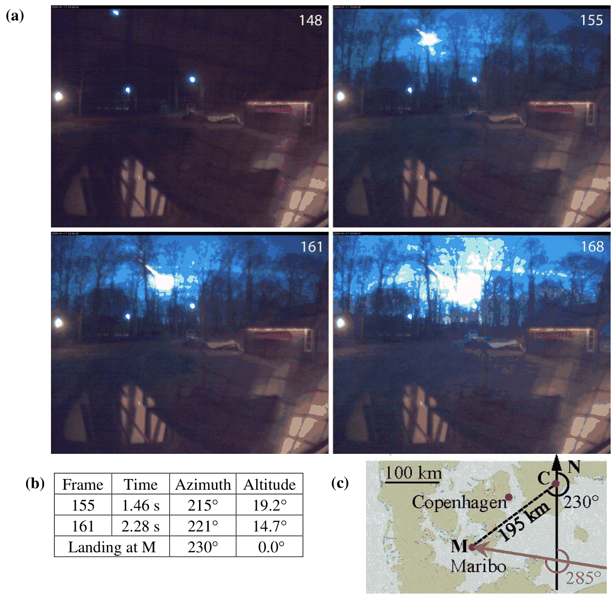

Figure 1.1 (a) Azimuth is the clockwise angular position from north in the horizontal plane, and altitude is the angular position above the horizon. A series of frames recorded by the surveillance camera in Sweden, showing the motion of Maribo as a fireball on its way down through the atmosphere. (b) The data from two frames indicating the time, the direction (azimuth) in degrees, as seen by the camera (C), and the height above the horizon (altitude) in degrees. (c) Sketch of the directions of the path (magenta arrow) of Maribo relative to north (N) and of the landing site (M) in Denmark as seen by the camera (C).

Heating of Maribo during its fall in the atmosphere

When the stony meteoroid Maribo entered the atmosphere at supersonic speed it appeared as a fireball because the surrounding air was glowing. Nevertheless, only the outermost layer of Maribo was heated. Assume that Maribo is a homogenous sphere with density \(\rho_{\mathrm{sm}}\), specific heat capacity \(c_{\mathrm{sm}}\), and thermal conductivity \(k_{\mathrm{sm}}\) (for values see the data sheet). Furthermore, when entering the atmosphere, it had the temperature \(T_0=200\ \mathrm K\). While falling through the atmosphere its surface temperature was constant \(T_{\mathrm s}=1000\ \mathrm K\) due to the air friction, thus gradually heating the interior.

After falling a time \(t\) in the atmosphere, an outer shell of Maribo of thickness \(x\) will have been heated to a temperature significantly larger than \(T_0\). This thickness can be estimated by dimensional analysis as the simple product of powers of the thermodynamic parameters: \(x\approx t^\alpha\rho_{\mathrm{sm}}^\beta c_{\mathrm{sm}}^\gamma k_{\mathrm{sm}}^\delta\).

Part	Question	Points
1.3a	Determine by dimensional (unit) analysis the value of the four powers \(\alpha,\beta,\gamma,\) and \(\delta\).	0.6
1.3b	Calculate the thickness \(x\) after a fall time \(t=5\ \mathrm s\), and determine the ratio \(x/R_{\mathrm M}\).	0.4

The age of a meteorite

The chemical properties of radioactive elements may be different, so during the crystallization of the minerals in a given meteorite, some minerals will have a high content of a specific radioactive element and others a low content. This difference can be used to determine the age of a meteorite by radiometric dating of its radioactive minerals.

As a specific example, we study the isotope \({}^{87}\mathrm{Rb}\) (element no. 37), which decays into the stable isotope \({}^{87}\mathrm{Sr}\) (element no. 38) with a half-life of \(T_{\frac12}=4.9\times10^{10}\) year, relative to the stable isotope \({}^{86}\mathrm{Sr}\). At the time of crystallization the ratio \({}^{87}\mathrm{Sr}/{}^{86}\mathrm{Sr}\) was identical for all minerals, while the ratio \({}^{87}\mathrm{Rb}/{}^{86}\mathrm{Sr}\) was different. As time passes on, the amount of \({}^{87}\mathrm{Rb}\) decreases by decay, while consequently the amount of \({}^{87}\mathrm{Sr}\) increases. As a result, the ratio \({}^{87}\mathrm{Sr}/{}^{86}\mathrm{Sr}\) will be different today. In Fig. 1.2(a), the points on the horizontal line refer to the ratio \({}^{87}\mathrm{Rb}/{}^{86}\mathrm{Sr}\) in different minerals at the time, when they are crystallized.

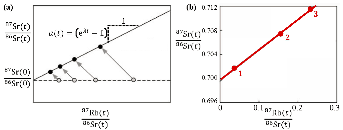
Figure 1.2 (a) The ratio \({}^{87}\mathrm{Sr}/{}^{86}\mathrm{Sr}\) in different minerals at the time \(t=0\) of crystallization (open circles) and at present time (filled circles). (b) The isochron-line for three different mineral samples taken from a meteorite at present time.

Part	Question	Points
1.4a	Write down the decay scheme for the transformation of \({}^{87}_{37}\mathrm{Rb}\) to \({}^{87}_{38}\mathrm{Sr}\).	0.3
1.4b	Show that the present-time ratio \({}^{87}\mathrm{Sr}/{}^{86}\mathrm{Sr}\) plotted versus the present-time ratio \({}^{87}\mathrm{Rb}/{}^{86}\mathrm{Sr}\) in different mineral samples from the same meteorite forms a straight line, the so-called isochron-line, with slope \(a(t)=(e^{\lambda t}-1)\). Here \(t\) is the time since the formation of the minerals, while \(\lambda\) is the decay constant inversely proportional to half-life \(T_{\frac12}\).	0.7
1.4c	Determine the age \(\tau_{\mathrm M}\) of the meteorite using the isochron-line of Fig. 1.2(b).	0.4

Comet Encke, from which Maribo may originate

In its orbit around the Sun, the minimum and maximum distances between comet Encke and the Sun are \(a_{\min}=4.95\times10^{10}\ \mathrm m\) and \(a_{\max}=6.16\times10^{11}\ \mathrm m\), respectively.

Part	Question	Points
1.5	Calculate the orbital period \(t_{\mathrm{Encke}}\) of comet Encke.	0.6

Consequences of an asteroid impact on Earth

65 million years ago Earth was hit by a huge asteroid with density \(\rho_{\mathrm{ast}}=3.0\times10^3\ \mathrm{kg\,m^{-3}}\), radius \(R_{\mathrm{ast}}=5.0\ \mathrm{km}\), and final speed of \(v_{\mathrm{ast}}=2.5\times10^4\ \mathrm{m/s}\). This impact resulted in the extermination of most of the life on Earth and the formation of the enormous Chicxulub Crater. Assume that an identical asteroid would hit Earth today in a completely inelastic collision, and use the fact that the moment of inertia of Earth is 0.83 times that for a homogeneous sphere of the same mass and radius. The moment of inertia of a homogeneous sphere with mass \(M\) and radius \(R\) is \(\frac25MR^2\). Neglect changes in the orbit of the Earth.

Part	Question	Points
1.6a	Let the asteroid hit the North Pole. Find the maximum change in angular orientation of the axis of Earth after the impact.	0.7
1.6b	Let the asteroid hit the Equator in a radial impact. Find the change \(\Delta\tau_{\mathrm{vrt}}\) in the duration of one revolution of Earth after the impact.	0.7
1.6c	Let the asteroid hit the Equator in a tangential impact in the equatorial plane. Find the change \(\Delta\tau_{\mathrm{tan}}\) in the duration of one revolution of Earth after the impact.	0.7

Maximum impact speed

Consider a celestial body, gravitationally bound in the solar system, which impacts the surface of Earth with a speed \(v_{\mathrm{imp}}\). Initially the effect of the gravitational field of the Earth on the body can be neglected. Disregard the friction in the atmosphere, the effect of other celestial bodies, and the rotation of the Earth.

Part	Question	Points
1.7	Calculate \(v_{\mathrm{imp}}^{\max}\), the largest possible value of \(v_{\mathrm{imp}}\).	1.6

Data sheet: Table of physical parameters

Physical parameter	Value
Speed of light in vacuum	\(c=2.998\times10^8\ \mathrm{m\,s^{-1}}\)
Planck's constant over \(2\pi\)	\(\hbar=1.055\times10^{-34}\ \mathrm{J\,s}\)
Gravitational constant	\(G=6.67\times10^{-11}\ \mathrm{m^3\,kg^{-1}\,s^{-2}}\)
Gravitational acceleration	\(g=9.82\ \mathrm{m\,s^{-2}}\)
Elementary charge	\(e=1.602\times10^{-19}\ \mathrm C\)
Electric permittivity of vacuum	\(\epsilon_0=8.854\times10^{-12}\ \mathrm{C^2\,J^{-1}\,m^{-1}}\)
Electron mass	\(m_{\mathrm e}=9.109\times10^{-31}\ \mathrm{kg}\)
Avogadro constant	\(N_{\mathrm A}=6.022\times10^{23}\ \mathrm{mol^{-1}}\)
Boltzmann constant	\(k_{\mathrm B}=1.381\times10^{-23}\ \mathrm{J\,K^{-1}}\)
Stony meteorite, specific heat	\(c_{\mathrm{sm}}=1.2\times10^3\ \mathrm{J\,kg^{-1}\,K^{-1}}\)
Stony meteorite, thermal conductivity	\(k_{\mathrm{sm}}=2.0\ \mathrm{W\,m^{-1}\,K^{-1}}\)
Stony meteorite, density	\(\rho_{\mathrm{sm}}=3.3\times10^3\ \mathrm{kg\,m^{-3}}\)
Stony meteorite, melting point	\(T_{\mathrm{sm}}=1.7\times10^3\ \mathrm K\)
Stony meteorite, specific melting heat	\(L_{\mathrm{sm}}=2.6\times10^5\ \mathrm{J\,kg^{-1}}\)
Silver, molar mass	\(M_{\mathrm{Ag}}=1.079\times10^{-1}\ \mathrm{kg\,mol^{-1}}\)
Silver, density	\(\rho_{\mathrm{Ag}}=1.049\times10^4\ \mathrm{kg\,m^{-3}}\)
Silver, specific heat capacity	\(c_{\mathrm{Ag}}=2.40\times10^2\ \mathrm{J\,kg^{-1}\,K^{-1}}\)
Water, molar mass	\(M_{\mathrm{wa}}=1.801\times10^{-2}\ \mathrm{kg\,mol^{-1}}\)
Water, density	\(\rho_{\mathrm{wa}}=0.998\times10^3\ \mathrm{kg\,m^{-3}}\)
Water, specific heat capacity	\(c_{\mathrm{wa}}=4.181\times10^3\ \mathrm{J\,kg^{-1}\,K^{-1}}\)
Water, heat of vaporization	\(L_{\mathrm{wa}}=2.260\times10^6\ \mathrm{J\,kg^{-1}}\)
Water, boiling temperature	\(T_{100}=100\,^\circ\mathrm C=373.15\ \mathrm K\)
Ice, density of glacier	\(\rho_{\mathrm{ice}}=0.917\times10^3\ \mathrm{kg\,m^{-3}}\)
Steam, specific heat capacity	\(c_{\mathrm{st}}=2.080\times10^3\ \mathrm{J\,kg^{-1}\,K^{-1}}\)
Earth, mass of the	\(m_{\mathrm E}=5.97\times10^{24}\ \mathrm{kg}\)
Earth, radius of the	\(R_{\mathrm E}=6.38\times10^6\ \mathrm m\)
Sun, mass of the	\(m_{\mathrm S}=1.99\times10^{30}\ \mathrm{kg}\)
Sun, radius of the	\(R_{\mathrm S}=6.96\times10^8\ \mathrm m\)
Average Sun-Earth distance	\(a_{\mathrm E}=1.50\times10^{11}\ \mathrm m\)

Official English text of the problem.

Introduction

In this problem we study an efficient process of steam production that has been demonstrated to work experimentally. An aqueous solution of spherical nanometer-sized silver spheres (nanoparticles) with only about \(10^{13}\) particles per liter is illuminated by a focused light beam. A fraction of the light is absorbed by the nanoparticles, which are heated up and generate steam locally around them without heating up the entire water solution. The steam is released from the system in the form of escaping steam bubbles. Not all details of the process are well understood at present, but the core process is known to be absorption of light through the so-called collective electron oscillations of the metallic nanoparticles. The device is known as a plasmonic steam generator.

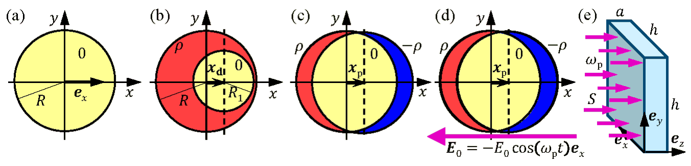
Figure 2.1 (a) A spherical charge-neutral nanoparticle of radius \(R\) placed at the center of the coordinate system. (b) A sphere with a positive homogeneous charge density \(\rho\) (red), and containing a smaller spherical charge-neutral region (0, yellow) of radius \(R_1\), with its center displaced by \(\boldsymbol{x}_{\mathrm d}=x_{\mathrm d}\boldsymbol{e}_x\). (c) The sphere with positive charge density \(\rho\) of the nanoparticle silver ions is fixed in the center of the coordinate system. The center of the spherical region with negative spherical charge density \(-\rho\) (blue) of the electron cloud is displaced by \(\boldsymbol{x}_{\mathrm p}\), where \(x_{\mathrm p}\ll R\). (d) An external homogeneous electric field \(\boldsymbol{E}_0=-E_0\boldsymbol{e}_x\). For time-dependent \(\boldsymbol{E}_0\), the electron cloud moves with velocity \(\boldsymbol{v}=\mathrm d\boldsymbol{x}_{\mathrm p}/\mathrm dt\). (e) The rectangular vessel \((h\times h\times a)\) containing the aqueous solution of nanoparticles illuminated by monochromatic light propagating along the \(z\)-axis with angular frequency \(\omega_{\mathrm p}\) and intensity \(S\).

A single spherical silver nanoparticle

Throughout this problem we consider a spherical silver nanoparticle of radius \(R=10{,}0\ \mathrm{nm}\) and with its center fixed at the origin of the coordinate system, see Fig. 2.1(a). All motions, forces and driving fields are parallel to the horizontal \(x\)-axis (with unit vector \(\boldsymbol{e}_x\)). The nanoparticle contains free (conduction) electrons moving within the whole nanoparticle volume without being bound to any silver atom. Each silver atom is a positive ion that has donated one such free electron.

Part	Question	Points
2.1	Find the following quantities: The volume \(V\) and mass \(M\) of the nanoparticle, the number \(N\) and charge density \(\rho\) of silver ions in the particle, and for the free electrons their concentration \(n\), their total charge \(Q\), and their total mass \(m_0\).	0.7

The electric field in a charge-neutral region inside a charged sphere

For the rest of the problem assume that the relative dielectric permittivity of all materials is \(\varepsilon=1\). Inside a charged sphere of homogeneous charge density \(\rho\) and radius \(R\) is created a small spherical charge-neutral region of radius \(R_1\) by adding the opposite charge density \(-\rho\), with its center displaced by \(\boldsymbol{x}_{\mathrm d}=x_{\mathrm d}\boldsymbol{e}_x\) from the center of the \(R\)-sphere, see Fig. 2.1(b).

Part	Question	Points
2.2	Show that the electric field inside the charge-neutral region is homogenous of the form \(\boldsymbol{E}=A\,(\rho/\varepsilon_0)\,\boldsymbol{x}_{\mathrm d}\), and determine the pre-factor \(A\).	1.2

The restoring force on the displaced electron cloud

In the following, we study the collective motion of the free electrons, and therefore model them as a single negatively charged sphere of homogeneous charge density \(-\rho\) with a center position \(\boldsymbol{x}_{\mathrm p}\), which can move along the \(x\)-axis relative to the center of the positively charged sphere (silver ions) fixed at the origin of the coordinate system, see Fig. 2.1(c). Assume that an external force \(\boldsymbol{F}_{\mathrm{ext}}\) displaces the electron cloud to a new equilibrium position \(\boldsymbol{x}_{\mathrm p}=x_{\mathrm p}\boldsymbol{e}_x\) with \(\lvert x_{\mathrm p}\rvert\ll R\). Except for tiny net charges at opposite ends of the nanoparticle, most of its interior remains charge-neutral.

Part	Question	Points
2.3	Express in terms of \(\boldsymbol{x}_{\mathrm p}\) and \(n\) the following two quantities: The restoring force \(\boldsymbol{F}\) exerted on the electron cloud and the work \(W_{\mathrm{el}}\) done on the electron cloud during displacement.	1.0

The spherical silver nanoparticle in an external constant electric field

A nanoparticle is placed in vacuum and influenced by an external force \(\boldsymbol{F}_{\mathrm{ext}}\) due to an applied static homogeneous electric field \(\boldsymbol{E}_0=-E_0\boldsymbol{e}_x\), which displaces the electron cloud the small distance \(\lvert x_{\mathrm p}\rvert\), where \(\lvert x_{\mathrm p}\rvert\ll R\).

Part	Question	Points
2.4	Find the displacement \(x_{\mathrm p}\) of the electron cloud in terms of \(E_0\) and \(n\), and determine the amount \(-\Delta Q\) of electron charge displaced through the \(yz\)-plane at the center of the nanoparticle in terms of \(n\), \(R\) and \(x_{\mathrm p}\).	0.6

The equivalent capacitance and inductance of the silver nanoparticle

For both a constant and a time-dependent field \(\boldsymbol{E}_0\), the nanoparticle can be modeled as an equivalent electric circuit. The equivalent capacitance can be found by relating the work \(W_{\mathrm{el}}\) done on the separation of charges \(\Delta Q\), to the energy of a capacitor, carrying charge \(\pm\Delta Q\). The charge separation will cause a certain equivalent voltage \(V_0\) across the equivalent capacitor.

Part	Question	Points
2.5a	Express the systems equivalent capacitance \(C\) in terms of \(\varepsilon_0\) and \(R\), and find its value.	0.7
2.5b	For this capacitance, determine in terms of \(E_0\) and \(R\) the equivalent voltage \(V_0\) that should be connected to the equivalent capacitor in order to accumulate the charge \(\Delta Q\).	0.4

For a time-dependent field \(\boldsymbol{E}_0\), the electron cloud moves with velocity \(\boldsymbol{v}=v\boldsymbol{e}_x\), Fig. 2.1(d). It has the kinetic energy \(W_{\mathrm{kin}}\) and forms an electric current \(I\) flowing through the fixed \(yz\)-plane. The kinetic energy of the electron cloud can be attributed to the energy of an equivalent inductor of inductance \(L\) carrying the current \(I\).

Part	Question	Points
2.6a	Express both \(W_{\mathrm{kin}}\) and \(I\) in terms of the velocity \(v\).	0.7
2.6b	Express the equivalent inductance \(L\) in terms of the particle radius \(R\), the electron charge \(e\) and mass \(m_e\), the electron concentration \(n\), and calculate its value.	0.5

The plasmon resonance of the silver nanoparticle

From the above analysis it follows that the motion, arising from displacing the electron cloud from its equilibrium position and then releasing it, can be modeled by an ideal \(LC\)-circuit oscillating at resonance. This dynamical mode of the electron cloud is known as the plasmon resonance, which oscillates at the so-called angular plasmon frequency \(\omega_{\mathrm p}\).

Part	Question	Points
2.7a	Find an expression for the angular plasmon frequency \(\omega_{\mathrm p}\) of the electron cloud in terms of the electron charge \(e\) and mass \(m_e\), the electron density \(n\), and the permittivity \(\varepsilon_0\).	0.5
2.7b	Calculate \(\omega_{\mathrm p}\) in rad/s and the wavelength \(\lambda_{\mathrm p}\) in nm of light in vacuum having angular frequency \(\omega=\omega_{\mathrm p}\).	0.4

The silver nanoparticle illuminated with light at the plasmon frequency

In the rest of the problem, the nanoparticle is illuminated by monochromatic light at the angular plasmon frequency \(\omega_{\mathrm p}\) with the incident intensity \(S=\frac12c\varepsilon_0E_0^2=1.00\ \mathrm{MW\,m^{-2}}\). As the wavelength is large, \(\lambda_{\mathrm p}\gg R\), the nanoparticle can be considered as being placed in a homogeneous harmonically oscillating field \(\boldsymbol{E}_0=-E_0\cos(\omega_{\mathrm p}t)\boldsymbol{e}_x\). Driven by \(\boldsymbol{E}_0\), the center \(\boldsymbol{x}_{\mathrm p}(t)\) of the electron cloud oscillates at the same frequency with velocity \(\boldsymbol{v}=\mathrm d\boldsymbol{x}_{\mathrm p}/\mathrm dt\) and constant amplitude \(x_0\). This oscillating electron motion leads to absorption of light. The energy captured by the particle is either converted into Joule heating inside the particle or re-emitted by the particle as scattered light.

Joule heating is caused by random inelastic collisions, where any given free electron once in a while hits a silver ion and loses its total kinetic energy, which is converted into vibrations of the silver ions (heat). The average time between the collisions is \(\tau\gg1/\omega_{\mathrm p}\), where for silver nanoparticle we use \(\tau=5.24\times10^{-15}\ \mathrm s\).

Part	Question	Points
2.8a	Find an expression for the time-averaged Joule heating power \(P_{\mathrm{heat}}\) in the nanoparticle as well as the time-averaged current squared \(\langle I^2\rangle\), which includes explicitly the time-averaged velocity squared \(\langle v^2\rangle\) of the electron cloud.	1.0
2.8b	Find an expression for the equivalent ohmic resistance \(R_{\mathrm{heat}}\) in an equivalent resistor-model of the nanoparticle having the Joule heating power \(P_{\mathrm{heat}}\) due to the electron cloud current \(I\). Calculate the numerical value of \(R_{\mathrm{heat}}\).	1.0

The incident light beam loses some time-averaged power \(P_{\mathrm{scat}}\) by scattering on the oscillating electron cloud (re-emission). \(P_{\mathrm{scat}}\) depends on the scattering source amplitude \(x_0\), charge \(Q\), angular frequency \(\omega_{\mathrm p}\) and properties of the light (the speed of light \(c\) and permittivity \(\varepsilon_0\) in vacuum). In terms of these four variables, \(P_{\mathrm{scat}}\) is given by \[ P_{\mathrm{scat}}=\frac{Q^2x_0^2\omega_{\mathrm p}^4}{12\pi\varepsilon_0c^3}. \]

Part	Question	Points
2.9	By use of \(P_{\mathrm{scat}}\), find an expression for the equivalent scattering resistance \(R_{\mathrm{scat}}\) (in analogy with \(R_{\mathrm{heat}}\)) in an equivalent resistor-model, and calculate its value.	1.0

The above equivalent circuit elements are combined into an \(LCR\) series circuit model of the silver nanoparticle, which is driven by a harmonically oscillating equivalent voltage \(V=V_0\cos(\omega_{\mathrm p}t)\) determined by the electric field \(\boldsymbol{E}_0\) of the incident light.

Part	Question	Points
2.10a	Derive expressions for the time-averaged power losses \(P_{\mathrm{heat}}\) and \(P_{\mathrm{scat}}\) involving the amplitude \(E_0\) of the electric field in the incident light at the plasmon resonance \(\omega=\omega_{\mathrm p}\).	1.2
2.10b	Calculate the numerical value of \(E_0\), \(P_{\mathrm{heat}}\), and \(P_{\mathrm{scat}}\).	0.3

Steam generation by light

An aqueous solution of silver nanoparticles is prepared with a concentration \(n_{\mathrm{np}}=7.3\times10^{15}\ \mathrm{m^{-3}}\). It is placed inside a rectangular transparent vessel of size \(h\times h\times a=10\times10\times1.0\ \mathrm{cm^3}\) and illuminated by light at the plasmon frequency with the same intensity \(S=1.00\ \mathrm{MW\,m^{-2}}\) at normal incidence as above, see Fig. 2.1(e). The temperature of the water is \(T_{\mathrm{wa}}=20\,^\circ\mathrm C\) and we assume, in fair agreement with observations, that in steady state all Joule heating of the nanoparticle goes to the production of steam of temperature \(T_{\mathrm{st}}=110\,^\circ\mathrm C\), without raising the temperature of the water.

The thermodynamic efficiency \(\eta\) of the plasmonic steam generator is defined by the power ratio \(\eta=P_{\mathrm{st}}/P_{\mathrm{tot}}\), where \(P_{\mathrm{st}}\) is the power going into the production of steam in the entire vessel, while \(P_{\mathrm{tot}}\) is the total power of the incoming light that enters the vessel.

Most of the time any given nanoparticle is surrounded by steam instead of water, and it can thus be described as being in vacuum.

Part	Question	Points
2.11a	Calculate the total mass per second \(\mu_{\mathrm{st}}\) of steam produced by the plasmonic steam generator during illumination by light at the plasmon frequency and intensity \(S\).	0.6
2.11b	Calculate the numerical value of the thermodynamic efficiency \(\eta\) of the plasmonic steam generator.	0.2

Data sheet: Table of physical parameters

Physical parameter	Value
Speed of light in vacuum	\(c=2.998\times10^8\ \mathrm{m\,s^{-1}}\)
Planck's constant over \(2\pi\)	\(\hbar=1.055\times10^{-34}\ \mathrm{J\,s}\)
Gravitational constant	\(G=6.67\times10^{-11}\ \mathrm{m^3\,kg^{-1}\,s^{-2}}\)
Gravitational acceleration	\(g=9.82\ \mathrm{m\,s^{-2}}\)
Elementary charge	\(e=1.602\times10^{-19}\ \mathrm C\)
Electric permittivity of vacuum	\(\varepsilon_0=8.854\times10^{-12}\ \mathrm{C^2\,J^{-1}\,m^{-1}}\)
Electron mass	\(m_e=9.109\times10^{-31}\ \mathrm{kg}\)
Avogadro constant	\(N_A=6.022\times10^{23}\ \mathrm{mol^{-1}}\)
Boltzmann constant	\(k_{\mathrm B}=1.381\times10^{-23}\ \mathrm{J\,K^{-1}}\)
Stony meteorite, specific heat	\(c_{\mathrm{sm}}=1.2\times10^3\ \mathrm{J\,kg^{-1}\,K^{-1}}\)
Stony meteorite, thermal conductivity	\(k_{\mathrm{sm}}=2.0\ \mathrm{W\,m^{-1}\,K^{-1}}\)
Stony meteorite, density	\(\rho_{\mathrm{sm}}=3.3\times10^3\ \mathrm{kg\,m^{-3}}\)
Stony meteorite, melting point	\(T_{\mathrm{sm}}=1.7\times10^3\ \mathrm K\)
Stony meteorite, specific melting heat	\(L_{\mathrm{sm}}=2.6\times10^5\ \mathrm{J\,kg^{-1}}\)
Silver, molar mass	\(M_{\mathrm{Ag}}=1.079\times10^{-1}\ \mathrm{kg\,mol^{-1}}\)
Silver, density	\(\rho_{\mathrm{Ag}}=1.049\times10^4\ \mathrm{kg\,m^{-3}}\)
Silver, specific heat capacity	\(c_{\mathrm{Ag}}=2.40\times10^2\ \mathrm{J\,kg^{-1}\,K^{-1}}\)
Water, molar mass	\(M_{\mathrm{wa}}=1.801\times10^{-2}\ \mathrm{kg\,mol^{-1}}\)
Water, density	\(\rho_{\mathrm{wa}}=0.998\times10^3\ \mathrm{kg\,m^{-3}}\)
Water, specific heat capacity	\(c_{\mathrm{wa}}=4.181\times10^3\ \mathrm{J\,kg^{-1}\,K^{-1}}\)
Water, heat of vaporization	\(L_{\mathrm{wa}}=2.260\times10^6\ \mathrm{J\,kg^{-1}}\)
Water, boiling temperature	\(T_{100}=100\,^\circ\mathrm C=373.15\ \mathrm K\)
Ice, density of glacier	\(\rho_{\mathrm{ice}}=0.917\times10^3\ \mathrm{kg\,m^{-3}}\)
Steam, specific heat capacity	\(c_{\mathrm{st}}=2.080\times10^3\ \mathrm{J\,kg^{-1}\,K^{-1}}\)
Earth, mass of the	\(m_{\mathrm E}=5.97\times10^{24}\ \mathrm{kg}\)
Earth, radius of the	\(R_{\mathrm E}=6.38\times10^6\ \mathrm m\)
Sun, mass of the	\(m_{\mathrm S}=1.99\times10^{30}\ \mathrm{kg}\)
Sun, radius of the	\(R_{\mathrm S}=6.96\times10^8\ \mathrm m\)
Average Sun-Earth distance	\(a_{\mathrm E}=1.50\times10^{11}\ \mathrm m\)

Official English text of the problem.

Introduction

This problem deals with the physics of the Greenlandic ice sheet, the second largest glacier in the world, Fig. 3.1(a). As an idealization, Greenland is modeled as a rectangular island of width \(2L\) and length \(5L\) with the ground at sea level and completely covered by incompressible ice (constant density \(\rho_{\mathrm{ice}}\)), see Fig. 3.1(b). The height profile \(H(x)\) of the ice sheet does not depend on the \(y\)-coordinate and it increases from zero at the coasts \(x=\pm L\) to a maximum height \(H_{\mathrm m}\) along the middle north-south axis (the \(y\)-axis), known as the ice divide, see Fig. 3.1(c).

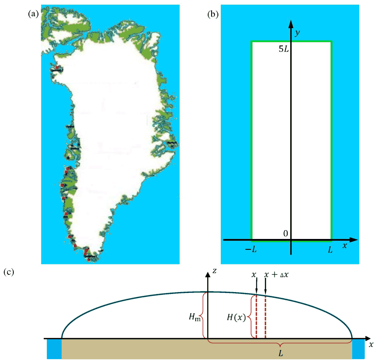
Figure 3.1 (a) A map of Greenland showing the extent of the ice sheet (white), the ice-free, coastal regions (green), and the surrounding ocean (blue). (b) The crude model of the Greenlandic ice sheet as covering a rectangular area in the \(xy\)-plane with side lengths \(2L\) and \(5L\). The ice divide, the line of maximum ice sheet height \(H_{\mathrm m}\) runs along the \(y\)-axis. (c) A vertical cut (\(xz\)-plane) through the ice sheet showing the height profile \(H(x)\) (blue line). \(H(x)\) is independent of the \(y\)-coordinate for \(0<y<5L\), while it drops abruptly to zero at \(y=0\) and \(y=5L\). The \(z\)-axis marks the position of the ice divide. For clarity, the vertical dimensions are expanded compared to the horizontal dimensions. The density \(\rho_{\mathrm{ice}}\) of ice is constant.

Two useful formulas

In this problem you can make use of the integral:

\[ \int_0^1\sqrt{1-x}\,\mathrm dx=\frac23 \]

and the approximation \((1+x)^\alpha\approx1+\alpha x\), valid for \(|\alpha x|\ll1\).

The height profile of the ice sheet

On short time scales the glacier is an incompressible hydrostatic system with fixed height profile \(H(x)\).

3.1

Write down an expression for the pressure \(p(x,z)\) inside the ice sheet as a function of vertical height \(z\) above the ground and distance \(x\) from the ice divide. Neglect the atmospheric pressure.

0.3

Consider a given vertical slab of the ice sheet in equilibrium, covering a small horizontal base area \(\Delta x\Delta y\) between \(x\) and \(x+\Delta x\), see the red dashed lines in Fig. 3.1(c). The size of \(\Delta y\) does not matter. The net horizontal force component \(\Delta F\) on the two vertical sides of the slab, arising from the difference in height on the center-side versus the coastal-side of the slab, is balanced by a friction force \(\Delta F=S_{\mathrm b}\Delta x\Delta y\) from the ground on the base area \(\Delta x\Delta y\), where \(S_{\mathrm b}=100\ \mathrm{kPa}\).

3.2a	For a given value of \(x\), show that in the limit \(\Delta x\rightarrow0\), \(S_{\mathrm b}=kH\,\mathrm dH/\mathrm dx\), and determine \(k\).	0.9
3.2b	Determine an expression for the height profile \(H(x)\) in terms of \(\rho_{\mathrm{ice}}\), \(g\), \(L\), \(S_{\mathrm b}\) and distance \(x\) from the divide. The result will show that the maximum glacier height \(H_{\mathrm m}\) scales with the half-width \(L\) as \(H_{\mathrm m}\propto L^{1/2}\).	0.8
3.2c	Determine the exponent \(\gamma\) with which the total volume \(V_{\mathrm{ice}}\) of the ice sheet scales with the area \(A\) of the rectangular island, \(V_{\mathrm{ice}}\propto A^\gamma\).	0.5

A dynamical ice sheet

On longer time scale, the ice is a viscous incompressible fluid, which by gravity flows from the center part to the coast. In this model, the ice maintains its height profile \(H(x)\) in a steady state, where accumulation of ice due to snowfall in the central region is balanced by melting at the coast. In addition to the ice sheet geometry of Fig. 3.1(b) and (c) make the following model assumptions:

1) Ice flows in the \(xz\)-plane away from the ice divide (the \(y\)-axis). 2) The accumulation rate \(c\) (m/year) in the central region is a constant. 3) Ice can only leave the glacier by melting near the coasts at \(x=\pm L\). 4) The horizontal (\(x\)-)component \(v_x(x)=\mathrm dx/\mathrm dt\) of the ice-flow velocity is independent of \(z\). 5) The vertical (\(z\)-)component \(v_z(z)=\mathrm dz/\mathrm dt\) of the ice-flow velocity is independent of \(x\).

Consider only the central region \(|x|\ll L\) close to the middle of the ice sheet, where height variations of the ice sheet are very small and can be neglected altogether, i.e. \(H(x)\approx H_{\mathrm m}\).

3.3

Use mass conservation to find an expression for the horizontal ice-flow velocity \(v_x(x)\) in terms of \(c\), \(x\), and \(H_{\mathrm m}\).

0.6

From the assumption of incompressibility, i.e. the constant density \(\rho_{\mathrm{ice}}\) of the ice, it follows that mass conservation implies the following restriction on the ice flow velocity components

\[ \frac{\mathrm dv_x}{\mathrm dx}+\frac{\mathrm dv_z}{\mathrm dz}=0. \]

3.4

Write down an expression for the \(z\) dependence of the vertical component \(v_z(z)\) of the ice-flow velocity.

0.6

A small ice particle with the initial surface position \((x_i,H_{\mathrm m})\) will, as time passes, flow as part of the ice sheet along a flow trajectory \(z(x)\) in the vertical \(xz\)-plane.

3.5

Derive an expression for such a flow trajectory \(z(x)\).

0.9

Age and climate indicators in the dynamical ice sheet

Based on the ice-flow velocity components \(v_x(x)\) and \(v_z(z)\), one can estimate the age \(\tau(z)\) of the ice in a specific depth \(H_{\mathrm m}-z\) from the surface of the ice sheet.

3.6

Find an expression for the age \(\tau(z)\) of the ice as a function of height \(z\) above ground, right at the ice divide \(x=0\).

1.0

An ice core drilled in the interior of the Greenlandic ice sheet will penetrate through layers of snow from the past, and the ice core can be analyzed to reveal past climate changes. One of the best indicators is the so-called \(\delta^{18}\mathrm O\), defined as

\[ \delta^{18}\mathrm O =\frac{R_{\mathrm{ice}}-R_{\mathrm{ref}}}{R_{\mathrm{ref}}}\,1000\ \text{‰}, \]

where \(R=[{}^{18}\mathrm O]/[{}^{16}\mathrm O]\) denotes the relative abundance of the two stable isotopes \({}^{18}\mathrm O\) and \({}^{16}\mathrm O\) of oxygen. The reference \(R_{\mathrm{ref}}\) is based on the isotopic composition of the oceans around Equator.

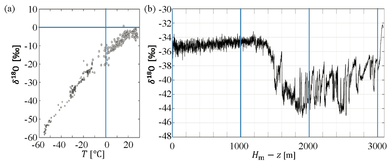
Figure 3.2 (a) Observed relationship between \(\delta^{18}\mathrm O\) in snows versus the mean annual surface temperature \(T\). (b) Measurements of \(\delta^{18}\mathrm O\) versus depth \(H_{\mathrm m}-z\) from the surface, taken from an ice core drilled from surface to bedrock at a specific place along the Greenlandic ice divide where \(H_{\mathrm m}=3060\ \mathrm m\).

Observations from the Greenland ice sheet show that \(\delta^{18}\mathrm O\) in the snow varies approximately linearly with temperature, Fig. 3.2(a). Assuming that this has always been the case, \(\delta^{18}\mathrm O\) retrieved from an ice core at depth \(H_{\mathrm m}-z\) leads to an estimate of the temperature \(T\) near Greenland at the age \(\tau(z)\).

Measurements of \(\delta^{18}\mathrm O\) in a 3060 m long Greenlandic ice core show an abrupt change in \(\delta^{18}\mathrm O\) at a depth of 1492 m, Fig. 3.2(b), marking the end of the last ice age. The ice age began 120,000 years ago, corresponding to a depth of 3040 m, and the current interglacial age began 11,700 years ago, corresponding to a depth of 1492 m. Assume that these two periods can be described by two different accumulation rates, \(c_{\mathrm{ia}}\) (ice age) and \(c_{\mathrm{ig}}\) (interglacial age), respectively. You can assume \(H_{\mathrm m}\) to be constant throughout these 120,000 years.

3.7a	Determine the accumulation rates \(c_{\mathrm{ia}}\) and \(c_{\mathrm{ig}}\).	0.8
3.7b	Use the data in Fig. 3.2 to find the temperature change at the transition from the ice age to the interglacial age.	0.2

Sea level rise from melting of the Greenland ice sheet

A complete melting of the Greenlandic ice sheet will cause a sea level rise in the global ocean. As a crude estimate of this sea level rise, one may simply consider a uniform rise throughout a global ocean with constant area \(A_{\mathrm O}=3.61\times10^{14}\ \mathrm{m^2}\).

3.8

Calculate the average global sea level rise, which would result from a complete melting of the Greenlandic ice sheet, given its present area of \(A_{\mathrm G}=1.71\times10^{12}\ \mathrm{m^2}\) and \(S_{\mathrm b}=100\ \mathrm{kPa}\).

0.6

The massive Greenland ice sheet exerts a gravitational pull on the surrounding ocean. If the ice sheet melts, this local high tide is lost and the sea level will drop close to Greenland, an effect which partially counteracts the sea level rise calculated above.

To estimate the magnitude of this gravitational pull on the water, the Greenlandic ice sheet is now modeled as a point mass located at the ground level and having the total mass of the Greenlandic ice sheet. Copenhagen lies at a distance of 3500 km along the Earth surface from the center of the point mass. One may consider the Earth, without the point mass, to be spherically symmetric and having a global ocean spread out over the entire surface of the Earth of area \(A_{\mathrm E}=5.10\times10^{14}\ \mathrm{m^2}\). All effects of rotation of the Earth may be neglected.

3.9

Within this model, determine the difference \(h_{\mathrm{CPH}}-h_{\mathrm{OPP}}\) between sea levels in Copenhagen (\(h_{\mathrm{CPH}}\)) and diametrically opposite to Greenland (\(h_{\mathrm{OPP}}\)).

1.8

Data sheet: Table of physical parameters

Speed of light in vacuum	\(c=2.998\times10^8\ \mathrm{m\,s^{-1}}\)
Planck's constant over \(2\pi\)	\(\hbar=1.055\times10^{-34}\ \mathrm{J\,s}\)
Gravitational constant	\(G=6.67\times10^{-11}\ \mathrm{m^3\,kg^{-1}\,s^{-2}}\)
Gravitational acceleration	\(g=9.82\ \mathrm{m\,s^{-2}}\)
Elementary charge	\(e=1.602\times10^{-19}\ \mathrm C\)
Dielectric permittivity of vacuum	\(\epsilon_0=8.854\times10^{-12}\ \mathrm{C^2\,J^{-1}\,m^{-1}}\)
Electron mass	\(m_e=9.109\times10^{-31}\ \mathrm{kg}\)
Avogadro constant	\(N_{\mathrm A}=6.022\times10^{23}\ \mathrm{mol^{-1}}\)
Boltzmann constant	\(k_{\mathrm B}=1.381\times10^{-23}\ \mathrm{J\,K^{-1}}\)
Stony meteorite, specific heat	\(c_{\mathrm{sm}}=1.2\times10^3\ \mathrm{J\,kg^{-1}\,K^{-1}}\)
Stony meteorite, thermal conductivity	\(k_{\mathrm{sm}}=2.0\ \mathrm{W\,m^{-1}\,K^{-1}}\)
Stony meteorite, density	\(\rho_{\mathrm{sm}}=3.3\times10^3\ \mathrm{kg\,m^{-3}}\)
Stony meteorite, melting point	\(T_{\mathrm{sm}}=1.7\times10^3\ \mathrm K\)
Stony meteorite, specific melting heat	\(L_{\mathrm{sm}}=2.6\times10^5\ \mathrm{J\,kg^{-1}}\)
Silver, molar mass	\(M_{\mathrm{Ag}}=1.079\times10^{-1}\ \mathrm{kg\,mol^{-1}}\)
Silver, density	\(\rho_{\mathrm{Ag}}=1.049\times10^4\ \mathrm{kg\,m^{-3}}\)
Silver, specific heat capacity	\(c_{\mathrm{Ag}}=2.40\times10^2\ \mathrm{J\,kg^{-1}\,K^{-1}}\)
Water, molar mass	\(M_{\mathrm{wa}}=1.801\times10^{-2}\ \mathrm{kg\,mol^{-1}}\)
Water, density	\(\rho_{\mathrm{wa}}=0.998\times10^3\ \mathrm{kg\,m^{-3}}\)
Water, specific heat capacity	\(c_{\mathrm{wa}}=4.181\times10^3\ \mathrm{J\,kg^{-1}\,K^{-1}}\)
Water, heat of vaporization	\(L_{\mathrm{wa}}=2.260\times10^6\ \mathrm{J\,kg^{-1}}\)
Water, boiling temperature	\(T_{100}=100\,^\circ\mathrm C=373.15\ \mathrm K\)
Ice, density of glacier	\(\rho_{\mathrm{ice}}=0.917\times10^3\ \mathrm{kg\,m^{-3}}\)
Steam, specific heat capacity	\(c_{\mathrm{st}}=2.080\times10^3\ \mathrm{J\,kg^{-1}\,K^{-1}}\)
Earth, mass of the	\(m_{\mathrm E}=5.97\times10^{24}\ \mathrm{kg}\)
Earth, radius of the	\(R_{\mathrm E}=6.38\times10^6\ \mathrm m\)
Sun, mass of the	\(m_{\mathrm S}=1.99\times10^{30}\ \mathrm{kg}\)
Sun, radius of the	\(R_{\mathrm S}=6.96\times10^8\ \mathrm m\)
Average Sun-Earth distance	\(a_{\mathrm E}=1.50\times10^{11}\ \mathrm m\)

Official English text of the problem.

Einleitung

Ein Meteoroid ist ein kleines Teilchen (typischerweise kleiner als 1 m) von einem Kometen oder einem Asteroiden. Ein Meteoroid, der auf dem Erdboden aufschlägt, wird als Meteorit bezeichnet.

In der Nacht des 17. Januar 2009 sahen viele Menschen in der Nähe der Ostsee die Leuchtspur oder den Feuerball eines Meteoroiden, der durch die Erdatmosphäre fiel. In Schweden zeichnete eine Überwachungskamera ein Video des Ereignisses auf, siehe Abb. 1.1(a). Anhand dieser Bilder und von Augenzeugenberichten konnte das Einschlaggebiet eingegrenzt werden, und sechs Wochen später wurde in der Nähe der Stadt Maribo in Süddänemark ein Meteorit mit der Masse 0.025 kg gefunden. Messungen an dem nun Maribo genannten Meteoriten und seiner Bahn am Himmel lieferten interessante Ergebnisse. Seine Geschwindigkeit beim Eintritt in die Atmosphäre war außergewöhnlich hoch gewesen. Sein Alter von \(4.567\times10^9\) Jahren zeigt, dass er kurz nach der Entstehung des Sonnensystems entstanden war. Der Meteorit Maribo ist möglicherweise ein Teil des Kometen Encke.

Die Geschwindigkeit von Maribo

Der Feuerball bewegte sich in westlicher Richtung mit einem Kurs von \(285^\circ\) gegenüber Norden auf den Ort zu, an dem der Meteorit später gefunden wurde, wie in Abb. 1.1 skizziert. Der Meteorit wurde in einer Entfernung von 195 km von der Überwachungskamera in Richtung \(230^\circ\) gegenüber Norden gefunden.

Teil	Frage	Punkte
1.1	Berechnen Sie anhand dieser Angaben und der Daten in Abb. 1.1 die mittlere Geschwindigkeit von Maribo im Zeitintervall zwischen den Einzelbildern 155 und 161. Sowohl die Erdkrümmung als auch die auf den Meteoroiden wirkende Gravitationskraft können vernachlässigt werden.	1.3

Durch die Atmosphäre und dabei schmelzen?

Die Luftreibung an einem Meteoroiden, der sich in der höheren Atmosphäre bewegt, hängt auf komplizierte Weise von seiner Form und Geschwindigkeit sowie von der Temperatur und Dichte der Atmosphäre ab. In guter Näherung ist die Reibungskraft \(F\) in der oberen Atmosphäre durch den Ausdruck \(F=k\rho_{\mathrm{atm}}Av^2\) gegeben, wobei \(k\) eine Konstante, \(\rho_{\mathrm{atm}}\) die Dichte der Atmosphäre, \(A\) die projizierte Querschnittsfläche des Meteoriten und \(v\) seine Geschwindigkeit ist.

Zur Untersuchung des Meteoroiden werden folgende vereinfachende Annahmen getroffen: Das in die Atmosphäre eintretende Objekt war eine Kugel mit der Masse \(m_{\mathrm M}=30\ \mathrm{kg}\), dem Radius \(R_{\mathrm M}=0.13\ \mathrm m\), der Temperatur \(T_0=200\ \mathrm K\) und der Geschwindigkeit \(v_{\mathrm M}=2.91\times10^4\ \mathrm{m/s}\). Die Dichte der Atmosphäre ist konstant (gleich ihrem Wert 40 km über der Erdoberfläche), \(\rho_{\mathrm{atm}}=4.1\times10^{-3}\ \mathrm{kg/m^3}\), und der Reibungskoeffizient beträgt \(k=0.60\).

Teil	Frage	Punkte
1.2a	Schätzen Sie ab, wie lange es nach dem Eintritt in die Atmosphäre dauert, bis die Geschwindigkeit des Meteoroiden um 10 % von \(v_{\mathrm M}\) auf \(0.90v_{\mathrm M}\) abgenommen hat. Sie können die Gravitationskraft auf den Meteoroiden vernachlässigen und annehmen, dass seine Masse und Form unverändert bleiben.	0.7
1.2b	Berechnen Sie, um welchen Faktor die kinetische Energie \(E_{\mathrm{kin}}\) des in die Atmosphäre eintretenden Meteoroiden größer ist als die Energie \(E_{\mathrm{melt}}\), die erforderlich ist, um ihn vollständig zu schmelzen (siehe Datenblatt).	0.3

Abbildung 1.1 (a) Der Azimut ist der in der Horizontalebene im Uhrzeigersinn von Norden aus gemessene Winkel, und die Höhe ist der Winkel über dem Horizont. Eine Folge von Einzelbildern der Überwachungskamera in Schweden zeigt die Bewegung von Maribo als Feuerball auf seinem Weg durch die Atmosphäre nach unten. (b) Die Daten zweier Einzelbilder geben die Zeit, die von der Kamera (C) aus gesehene Richtung (Azimut) in Grad und die Höhe über dem Horizont (Höhenwinkel) in Grad an. (c) Skizze der Richtungen der Bahn (magentafarbener Pfeil) von Maribo gegenüber Norden (N) und des Fundorts (M) in Dänemark, von der Kamera (C) aus gesehen.

Erwärmung von Maribo während seines Falls durch die Atmosphäre

Als der steinerne Meteoroid Maribo mit Überschallgeschwindigkeit in die Atmosphäre eintrat, erschien er als Feuerball, weil die umgebende Luft leuchtete. Dennoch wurde nur die äußerste Schicht von Maribo erwärmt. Nehmen Sie an, dass Maribo eine homogene Kugel mit der Dichte \(\rho_{\mathrm{sm}}\), der spezifischen Wärmekapazität \(c_{\mathrm{sm}}\) und der Wärmeleitfähigkeit \(k_{\mathrm{sm}}\) ist (Werte siehe Datenblatt). Außerdem hatte er beim Eintritt in die Atmosphäre die Temperatur \(T_0=200\ \mathrm K\). Während des Falls durch die Atmosphäre betrug seine Oberflächentemperatur aufgrund der Luftreibung konstant \(T_{\mathrm s}=1000\ \mathrm K\), wodurch sich das Innere allmählich erwärmte.

Nach einer Fallzeit \(t\) in der Atmosphäre wird eine äußere Schale von Maribo mit der Dicke \(x\) auf eine Temperatur erwärmt worden sein, die deutlich über \(T_0\) liegt. Diese Dicke lässt sich durch Dimensionsanalyse als einfaches Produkt von Potenzen der thermodynamischen Parameter abschätzen: \(x\approx t^\alpha\rho_{\mathrm{sm}}^\beta c_{\mathrm{sm}}^\gamma k_{\mathrm{sm}}^\delta\).

Teil	Frage	Punkte
1.3a	Bestimmen Sie durch Dimensionsanalyse (Einheitenanalyse) die Werte der vier Exponenten \(\alpha,\beta,\gamma,\) und \(\delta\).	0.6
1.3b	Berechnen Sie die Dicke \(x\) nach einer Fallzeit \(t=5\ \mathrm s\) und bestimmen Sie das Verhältnis \(x/R_{\mathrm M}\).	0.4

Das Alter eines Meteoriten

Die chemischen Eigenschaften radioaktiver Elemente können unterschiedlich sein. Daher weisen bei der Kristallisation der Minerale in einem bestimmten Meteoriten einige Minerale einen hohen Gehalt an einem bestimmten radioaktiven Element auf, andere dagegen einen niedrigen. Dieser Unterschied kann genutzt werden, um das Alter eines Meteoriten durch radiometrische Datierung seiner radioaktiven Minerale zu bestimmen.

Als konkretes Beispiel untersuchen wir das Isotop \({}^{87}\mathrm{Rb}\) (Ordnungszahl 37), das mit einer Halbwertszeit von \(T_{\frac12}=4.9\times10^{10}\) Jahren in das stabile Isotop \({}^{87}\mathrm{Sr}\) (Ordnungszahl 38) zerfällt, im Verhältnis zum stabilen Isotop \({}^{86}\mathrm{Sr}\). Zum Zeitpunkt der Kristallisation war das Verhältnis \({}^{87}\mathrm{Sr}/{}^{86}\mathrm{Sr}\) für alle Minerale gleich, während das Verhältnis \({}^{87}\mathrm{Rb}/{}^{86}\mathrm{Sr}\) unterschiedlich war. Im Laufe der Zeit nimmt die Menge an \({}^{87}\mathrm{Rb}\) durch Zerfall ab, während infolgedessen die Menge an \({}^{87}\mathrm{Sr}\) zunimmt. Daher ist das Verhältnis \({}^{87}\mathrm{Sr}/{}^{86}\mathrm{Sr}\) heute unterschiedlich. In Abb. 1.2(a) beziehen sich die Punkte auf der horizontalen Linie auf das Verhältnis \({}^{87}\mathrm{Rb}/{}^{86}\mathrm{Sr}\) in verschiedenen Mineralen zum Zeitpunkt ihrer Kristallisation.

Abbildung 1.2 (a) Das Verhältnis \({}^{87}\mathrm{Sr}/{}^{86}\mathrm{Sr}\) in verschiedenen Mineralen zum Zeitpunkt \(t=0\) der Kristallisation (offene Kreise) und zum heutigen Zeitpunkt (ausgefüllte Kreise). (b) Die Isochronengerade für drei verschiedene Mineralproben, die heute einem Meteoriten entnommen wurden.

Teil	Frage	Punkte
1.4a	Geben Sie das Zerfallsschema für die Umwandlung von \({}^{87}_{37}\mathrm{Rb}\) in \({}^{87}_{38}\mathrm{Sr}\) an.	0.3
1.4b	Zeigen Sie, dass die heutigen Verhältnisse \({}^{87}\mathrm{Sr}/{}^{86}\mathrm{Sr}\), aufgetragen gegen die heutigen Verhältnisse \({}^{87}\mathrm{Rb}/{}^{86}\mathrm{Sr}\) in verschiedenen Mineralproben desselben Meteoriten, auf einer Geraden liegen, der sogenannten Isochronengeraden, mit der Steigung \(a(t)=(e^{\lambda t}-1)\). Dabei ist \(t\) die seit der Bildung der Minerale vergangene Zeit, während \(\lambda\) die Zerfallskonstante ist, die umgekehrt proportional zur Halbwertszeit \(T_{\frac12}\) ist.	0.7
1.4c	Bestimmen Sie mithilfe der Isochronengeraden in Abb. 1.2(b) das Alter \(\tau_{\mathrm M}\) des Meteoriten.	0.4

Der Komet Encke, von dem Maribo stammen könnte

Auf seiner Bahn um die Sonne betragen der kleinste und der größte Abstand zwischen dem Kometen Encke und der Sonne \(a_{\min}=4.95\times10^{10}\ \mathrm m\) beziehungsweise \(a_{\max}=6.16\times10^{11}\ \mathrm m\).

Teil	Frage	Punkte
1.5	Berechnen Sie die Umlaufzeit \(t_{\mathrm{Encke}}\) des Kometen Encke.	0.6

Folgen eines Asteroideneinschlags auf der Erde

Vor 65 Millionen Jahren wurde die Erde von einem riesigen Asteroiden mit der Dichte \(\rho_{\mathrm{ast}}=3.0\times10^3\ \mathrm{kg\,m^{-3}}\), dem Radius \(R_{\mathrm{ast}}=5.0\ \mathrm{km}\) und der Endgeschwindigkeit \(v_{\mathrm{ast}}=2.5\times10^4\ \mathrm{m/s}\) getroffen. Dieser Einschlag führte zur Auslöschung des größten Teils des Lebens auf der Erde und zur Entstehung des gewaltigen Chicxulub-Kraters. Nehmen Sie an, dass ein identischer Asteroid heute in einem vollkommen unelastischen Stoß auf die Erde trifft, und nutzen Sie die Tatsache, dass das Trägheitsmoment der Erde das 0.83-Fache des Trägheitsmoments einer homogenen Kugel gleicher Masse und gleichen Radius beträgt. Das Trägheitsmoment einer homogenen Kugel mit der Masse \(M\) und dem Radius \(R\) beträgt \(\frac25MR^2\). Vernachlässigen Sie Änderungen der Erdbahn.

Teil	Frage	Punkte
1.6a	Der Asteroid treffe den Nordpol. Bestimmen Sie die maximale Winkeländerung der Ausrichtung der Erdachse nach dem Einschlag.	0.7
1.6b	Der Asteroid treffe den Äquator bei einem radialen Einschlag. Bestimmen Sie die Änderung \(\Delta\tau_{\mathrm{vrt}}\) der Dauer einer Erdumdrehung nach dem Einschlag.	0.7
1.6c	Der Asteroid treffe den Äquator bei einem tangentialen Einschlag in der Äquatorebene. Bestimmen Sie die Änderung \(\Delta\tau_{\mathrm{tan}}\) der Dauer einer Erdumdrehung nach dem Einschlag.	0.7

Maximale Einschlaggeschwindigkeit

Betrachten Sie einen Himmelskörper, der im Sonnensystem gravitativ gebunden ist und mit einer Geschwindigkeit \(v_{\mathrm{imp}}\) auf die Erdoberfläche trifft. Anfangs kann der Einfluss des Gravitationsfeldes der Erde auf den Körper vernachlässigt werden. Vernachlässigen Sie die Reibung in der Atmosphäre, den Einfluss anderer Himmelskörper und die Erdrotation.

Teil	Frage	Punkte
1.7	Berechnen Sie \(v_{\mathrm{imp}}^{\max}\), den größtmöglichen Wert von \(v_{\mathrm{imp}}\).	1.6

Datenblatt: Tabelle physikalischer Größen

Physikalische Größe	Wert
Lichtgeschwindigkeit im Vakuum	\(c=2.998\times10^8\ \mathrm{m\,s^{-1}}\)
Plancksches Wirkungsquantum dividiert durch \(2\pi\)	\(\hbar=1.055\times10^{-34}\ \mathrm{J\,s}\)
Gravitationskonstante	\(G=6.67\times10^{-11}\ \mathrm{m^3\,kg^{-1}\,s^{-2}}\)
Fallbeschleunigung	\(g=9.82\ \mathrm{m\,s^{-2}}\)
Elementarladung	\(e=1.602\times10^{-19}\ \mathrm C\)
Elektrische Permittivität des Vakuums	\(\epsilon_0=8.854\times10^{-12}\ \mathrm{C^2\,J^{-1}\,m^{-1}}\)
Elektronenmasse	\(m_{\mathrm e}=9.109\times10^{-31}\ \mathrm{kg}\)
Avogadro-Konstante	\(N_{\mathrm A}=6.022\times10^{23}\ \mathrm{mol^{-1}}\)
Boltzmann-Konstante	\(k_{\mathrm B}=1.381\times10^{-23}\ \mathrm{J\,K^{-1}}\)
Steinmeteorit, spezifische Wärmekapazität	\(c_{\mathrm{sm}}=1.2\times10^3\ \mathrm{J\,kg^{-1}\,K^{-1}}\)
Steinmeteorit, Wärmeleitfähigkeit	\(k_{\mathrm{sm}}=2.0\ \mathrm{W\,m^{-1}\,K^{-1}}\)
Steinmeteorit, Dichte	\(\rho_{\mathrm{sm}}=3.3\times10^3\ \mathrm{kg\,m^{-3}}\)
Steinmeteorit, Schmelztemperatur	\(T_{\mathrm{sm}}=1.7\times10^3\ \mathrm K\)
Steinmeteorit, spezifische Schmelzwärme	\(L_{\mathrm{sm}}=2.6\times10^5\ \mathrm{J\,kg^{-1}}\)
Silber, molare Masse	\(M_{\mathrm{Ag}}=1.079\times10^{-1}\ \mathrm{kg\,mol^{-1}}\)
Silber, Dichte	\(\rho_{\mathrm{Ag}}=1.049\times10^4\ \mathrm{kg\,m^{-3}}\)
Silber, spezifische Wärmekapazität	\(c_{\mathrm{Ag}}=2.40\times10^2\ \mathrm{J\,kg^{-1}\,K^{-1}}\)
Wasser, molare Masse	\(M_{\mathrm{wa}}=1.801\times10^{-2}\ \mathrm{kg\,mol^{-1}}\)
Wasser, Dichte	\(\rho_{\mathrm{wa}}=0.998\times10^3\ \mathrm{kg\,m^{-3}}\)
Wasser, spezifische Wärmekapazität	\(c_{\mathrm{wa}}=4.181\times10^3\ \mathrm{J\,kg^{-1}\,K^{-1}}\)
Wasser, Verdampfungswärme	\(L_{\mathrm{wa}}=2.260\times10^6\ \mathrm{J\,kg^{-1}}\)
Wasser, Siedetemperatur	\(T_{100}=100\,^\circ\mathrm C=373.15\ \mathrm K\)
Eis, Dichte von Gletschereis	\(\rho_{\mathrm{ice}}=0.917\times10^3\ \mathrm{kg\,m^{-3}}\)
Wasserdampf, spezifische Wärmekapazität	\(c_{\mathrm{st}}=2.080\times10^3\ \mathrm{J\,kg^{-1}\,K^{-1}}\)
Erde, Masse	\(m_{\mathrm E}=5.97\times10^{24}\ \mathrm{kg}\)
Erde, Radius	\(R_{\mathrm E}=6.38\times10^6\ \mathrm m\)
Sonne, Masse	\(m_{\mathrm S}=1.99\times10^{30}\ \mathrm{kg}\)
Sonne, Radius	\(R_{\mathrm S}=6.96\times10^8\ \mathrm m\)
Mittlerer Abstand Sonne–Erde	\(a_{\mathrm E}=1.50\times10^{11}\ \mathrm m\)

Aufgabentext aus dem offiziellen englischen Text übersetzt.

Einleitung

In dieser Aufgabe untersuchen wir ein effizientes Verfahren zur Dampferzeugung, dessen Funktionsfähigkeit experimentell nachgewiesen wurde. Eine wässrige Lösung aus nanometergroßen Silberkugeln (Nanopartikeln) mit nur etwa \(10^{13}\) Teilchen pro Liter wird mit einem fokussierten Lichtstrahl beleuchtet. Ein Teil des Lichts wird von den Nanopartikeln absorbiert, die sich erwärmen und lokal in ihrer Umgebung Dampf erzeugen, ohne die gesamte wässrige Lösung zu erwärmen. Der Dampf verlässt das System in Form entweichender Dampfblasen. Noch sind nicht alle Einzelheiten des Verfahrens gut verstanden, doch ist bekannt, dass der zentrale Prozess die Absorption von Licht durch die sogenannten kollektiven Elektronenschwingungen der metallischen Nanopartikel ist. Die Vorrichtung wird als plasmonischer Dampferzeuger bezeichnet.

Abbildung 2.1 (a) Ein kugelförmiges, elektrisch neutrales Nanopartikel mit dem Radius \(R\) im Ursprung des Koordinatensystems. (b) Eine Kugel mit einer positiven homogenen Ladungsdichte \(\rho\) (rot), die einen kleineren kugelförmigen, elektrisch neutralen Bereich (0, gelb) mit dem Radius \(R_1\) enthält, dessen Mittelpunkt um \(\boldsymbol{x}_{\mathrm d}=x_{\mathrm d}\boldsymbol{e}_x\) verschoben ist. (c) Die Kugel mit der positiven Ladungsdichte \(\rho\) der Silberionen des Nanopartikels ist im Ursprung des Koordinatensystems fixiert. Der Mittelpunkt des kugelförmigen Bereichs mit der negativen kugelsymmetrischen Ladungsdichte \(-\rho\) (blau) der Elektronenwolke ist um \(\boldsymbol{x}_{\mathrm p}\) verschoben, wobei \(x_{\mathrm p}\ll R\) gilt. (d) Ein äußeres homogenes elektrisches Feld \(\boldsymbol{E}_0=-E_0\boldsymbol{e}_x\). Bei zeitabhängigem \(\boldsymbol{E}_0\) bewegt sich die Elektronenwolke mit der Geschwindigkeit \(\boldsymbol{v}=\mathrm d\boldsymbol{x}_{\mathrm p}/\mathrm dt\). (e) Das quaderförmige Gefäß \((h\times h\times a)\) mit der wässrigen Nanopartikellösung, die mit monochromatischem Licht der Kreisfrequenz \(\omega_{\mathrm p}\) und der Intensität \(S\) beleuchtet wird, das sich entlang der \(z\)-Achse ausbreitet.

Ein einzelnes kugelförmiges Silbernanopartikel

In dieser gesamten Aufgabe betrachten wir ein kugelförmiges Silbernanopartikel mit dem Radius \(R=10{,}0\ \mathrm{nm}\), dessen Mittelpunkt im Ursprung des Koordinatensystems fixiert ist, siehe Abb. 2.1(a). Alle Bewegungen, Kräfte und anregenden Felder sind parallel zur horizontalen \(x\)-Achse (mit dem Einheitsvektor \(\boldsymbol{e}_x\)). Das Nanopartikel enthält freie (Leitungs-)Elektronen, die sich im gesamten Volumen des Nanopartikels bewegen, ohne an ein Silberatom gebunden zu sein. Jedes Silberatom ist ein positives Ion, das ein solches freies Elektron abgegeben hat.

Teil	Frage	Punkte
2.1	Bestimmen Sie die folgenden Größen: das Volumen \(V\) und die Masse \(M\) des Nanopartikels, die Anzahl \(N\) und die Ladungsdichte \(\rho\) der Silberionen im Teilchen sowie für die freien Elektronen ihre Konzentration \(n\), ihre Gesamtladung \(Q\) und ihre Gesamtmasse \(m_0\).	0.7

Das elektrische Feld in einem elektrisch neutralen Bereich innerhalb einer geladenen Kugel

Nehmen Sie für den Rest der Aufgabe an, dass die relative Permittivität aller Materialien \(\varepsilon=1\) beträgt. Innerhalb einer geladenen Kugel mit homogener Ladungsdichte \(\rho\) und Radius \(R\) wird durch Hinzufügen der entgegengesetzten Ladungsdichte \(-\rho\) ein kleiner kugelförmiger, elektrisch neutraler Bereich mit dem Radius \(R_1\) erzeugt, dessen Mittelpunkt gegenüber dem Mittelpunkt der Kugel mit Radius \(R\) um \(\boldsymbol{x}_{\mathrm d}=x_{\mathrm d}\boldsymbol{e}_x\) verschoben ist, siehe Abb. 2.1(b).

Teil	Frage	Punkte
2.2	Zeigen Sie, dass das elektrische Feld innerhalb des elektrisch neutralen Bereichs homogen ist und die Form \(\boldsymbol{E}=A\,(\rho/\varepsilon_0)\,\boldsymbol{x}_{\mathrm d}\) hat, und bestimmen Sie den Vorfaktor \(A\).	1.2

Die Rückstellkraft auf die verschobene Elektronenwolke

Im Folgenden untersuchen wir die kollektive Bewegung der freien Elektronen und modellieren sie daher als eine einzige negativ geladene Kugel mit homogener Ladungsdichte \(-\rho\) und der Mittelpunktposition \(\boldsymbol{x}_{\mathrm p}\), die sich entlang der \(x\)-Achse relativ zum Mittelpunkt der im Ursprung des Koordinatensystems fixierten positiv geladenen Kugel (Silberionen) bewegen kann, siehe Abb. 2.1(c). Nehmen Sie an, dass eine äußere Kraft \(\boldsymbol{F}_{\mathrm{ext}}\) die Elektronenwolke in eine neue Gleichgewichtslage \(\boldsymbol{x}_{\mathrm p}=x_{\mathrm p}\boldsymbol{e}_x\) mit \(\lvert x_{\mathrm p}\rvert\ll R\) verschiebt. Abgesehen von winzigen Nettoladungen an gegenüberliegenden Enden des Nanopartikels bleibt der größte Teil seines Inneren elektrisch neutral.

Teil	Frage	Punkte
2.3	Drücken Sie die folgenden beiden Größen durch \(\boldsymbol{x}_{\mathrm p}\) und \(n\) aus: die auf die Elektronenwolke ausgeübte Rückstellkraft \(\boldsymbol{F}\) und die während der Verschiebung an der Elektronenwolke verrichtete Arbeit \(W_{\mathrm{el}}\).	1.0

Das kugelförmige Silbernanopartikel in einem äußeren konstanten elektrischen Feld

Ein Nanopartikel befindet sich im Vakuum und wird durch eine äußere Kraft \(\boldsymbol{F}_{\mathrm{ext}}\) beeinflusst, die von einem angelegten statischen homogenen elektrischen Feld \(\boldsymbol{E}_0=-E_0\boldsymbol{e}_x\) herrührt. Dieses verschiebt die Elektronenwolke um die kleine Strecke \(\lvert x_{\mathrm p}\rvert\), wobei \(\lvert x_{\mathrm p}\rvert\ll R\) gilt.

Teil	Frage	Punkte
2.4	Bestimmen Sie die Verschiebung \(x_{\mathrm p}\) der Elektronenwolke in Abhängigkeit von \(E_0\) und \(n\) sowie die durch die \(yz\)-Ebene im Mittelpunkt des Nanopartikels verschobene Elektronenladung \(-\Delta Q\) in Abhängigkeit von \(n\), \(R\) und \(x_{\mathrm p}\).	0.6

Die Ersatzkapazität und Ersatzinduktivität des Silbernanopartikels

Sowohl für ein konstantes als auch für ein zeitabhängiges Feld \(\boldsymbol{E}_0\) lässt sich das Nanopartikel durch eine elektrische Ersatzschaltung modellieren. Die Ersatzkapazität lässt sich bestimmen, indem die zur Trennung der Ladungen \(\Delta Q\) verrichtete Arbeit \(W_{\mathrm{el}}\) mit der Energie eines Kondensators in Beziehung gesetzt wird, der die Ladung \(\pm\Delta Q\) trägt. Die Ladungstrennung bewirkt eine bestimmte Ersatzspannung \(V_0\) am Ersatzkondensator.

Teil	Frage	Punkte
2.5a	Drücken Sie die Ersatzkapazität \(C\) des Systems durch \(\varepsilon_0\) und \(R\) aus und bestimmen Sie ihren Wert.	0.7
2.5b	Bestimmen Sie für diese Kapazität in Abhängigkeit von \(E_0\) und \(R\) die Ersatzspannung \(V_0\), die an den Ersatzkondensator angelegt werden muss, damit sich die Ladung \(\Delta Q\) ansammelt.	0.4

Bei einem zeitabhängigen Feld \(\boldsymbol{E}_0\) bewegt sich die Elektronenwolke mit der Geschwindigkeit \(\boldsymbol{v}=v\boldsymbol{e}_x\), Abb. 2.1(d). Sie besitzt die kinetische Energie \(W_{\mathrm{kin}}\) und erzeugt einen elektrischen Strom \(I\), der durch die ortsfeste \(yz\)-Ebene fließt. Die kinetische Energie der Elektronenwolke kann der Energie einer vom Strom \(I\) durchflossenen Ersatzspule mit der Induktivität \(L\) zugeordnet werden.

Teil	Frage	Punkte
2.6a	Drücken Sie sowohl \(W_{\mathrm{kin}}\) als auch \(I\) durch die Geschwindigkeit \(v\) aus.	0.7
2.6b	Drücken Sie die Ersatzinduktivität \(L\) durch den Teilchenradius \(R\), die Elektronenladung \(e\) und die Elektronenmasse \(m_e\) sowie die Elektronenkonzentration \(n\) aus und berechnen Sie ihren Wert.	0.5

Die Plasmonenresonanz des Silbernanopartikels

Aus der obigen Analyse folgt, dass die Bewegung, die entsteht, wenn die Elektronenwolke aus ihrer Gleichgewichtslage verschoben und dann losgelassen wird, durch einen idealen \(LC\)-Schwingkreis beschrieben werden kann, der bei seiner Resonanzfrequenz schwingt. Diese dynamische Schwingungsform der Elektronenwolke wird als Plasmonenresonanz bezeichnet und schwingt mit der sogenannten Plasmonenkreisfrequenz \(\omega_{\mathrm p}\).

Teil	Frage	Punkte
2.7a	Bestimmen Sie einen Ausdruck für die Plasmonenkreisfrequenz \(\omega_{\mathrm p}\) der Elektronenwolke in Abhängigkeit von der Elektronenladung \(e\) und der Elektronenmasse \(m_e\), der Elektronendichte \(n\) und der Permittivität \(\varepsilon_0\).	0.5
2.7b	Berechnen Sie \(\omega_{\mathrm p}\) in rad/s und die Wellenlänge \(\lambda_{\mathrm p}\) in nm von Licht im Vakuum mit der Kreisfrequenz \(\omega=\omega_{\mathrm p}\).	0.4

Das mit Licht bei der Plasmonenfrequenz beleuchtete Silbernanopartikel

Im Rest der Aufgabe wird das Nanopartikel mit monochromatischem Licht bei der Plasmonenkreisfrequenz \(\omega_{\mathrm p}\) und der einfallenden Intensität \(S=\frac12c\varepsilon_0E_0^2=1.00\ \mathrm{MW\,m^{-2}}\) beleuchtet. Da die Wellenlänge groß ist, \(\lambda_{\mathrm p}\gg R\), kann das Nanopartikel als in einem homogenen, harmonisch schwingenden Feld \(\boldsymbol{E}_0=-E_0\cos(\omega_{\mathrm p}t)\boldsymbol{e}_x\) befindlich betrachtet werden. Angetrieben durch \(\boldsymbol{E}_0\) schwingt der Mittelpunkt \(\boldsymbol{x}_{\mathrm p}(t)\) der Elektronenwolke mit derselben Frequenz, der Geschwindigkeit \(\boldsymbol{v}=\mathrm d\boldsymbol{x}_{\mathrm p}/\mathrm dt\) und der konstanten Amplitude \(x_0\). Diese schwingende Elektronenbewegung führt zur Absorption von Licht. Die vom Teilchen aufgenommene Energie wird entweder durch Joulesche Erwärmung im Teilchen in Wärme umgewandelt oder vom Teilchen als Streulicht wieder emittiert.

Die Joulesche Erwärmung wird durch zufällige unelastische Stöße verursacht, bei denen ein beliebiges freies Elektron von Zeit zu Zeit auf ein Silberion trifft und seine gesamte kinetische Energie verliert, die in Schwingungen der Silberionen (Wärme) umgewandelt wird. Die mittlere Zeit zwischen den Stößen beträgt \(\tau\gg1/\omega_{\mathrm p}\), wobei wir für das Silbernanopartikel \(\tau=5.24\times10^{-15}\ \mathrm s\) verwenden.

Teil	Frage	Punkte
2.8a	Bestimmen Sie einen Ausdruck für die zeitlich gemittelte Joulesche Heizleistung \(P_{\mathrm{heat}}\) im Nanopartikel sowie für das zeitlich gemittelte Stromquadrat \(\langle I^2\rangle\), der das zeitlich gemittelte Geschwindigkeitsquadrat \(\langle v^2\rangle\) der Elektronenwolke explizit enthält.	1.0
2.8b	Bestimmen Sie einen Ausdruck für den ohmschen Ersatzwiderstand \(R_{\mathrm{heat}}\) in einem Widerstands-Ersatzmodell des Nanopartikels, in dem der Strom \(I\) der Elektronenwolke die Joulesche Heizleistung \(P_{\mathrm{heat}}\) hervorruft. Berechnen Sie den Zahlenwert von \(R_{\mathrm{heat}}\).	1.0

Der einfallende Lichtstrahl verliert durch Streuung an der schwingenden Elektronenwolke (Reemission) eine zeitlich gemittelte Leistung \(P_{\mathrm{scat}}\). \(P_{\mathrm{scat}}\) hängt von der Amplitude \(x_0\), der Ladung \(Q\) und der Kreisfrequenz \(\omega_{\mathrm p}\) der Streuquelle sowie von den Eigenschaften des Lichts (der Lichtgeschwindigkeit \(c\) und der Permittivität \(\varepsilon_0\) im Vakuum) ab. In Abhängigkeit von diesen vier Variablen ist \(P_{\mathrm{scat}}\) gegeben durch \[ P_{\mathrm{scat}}=\frac{Q^2x_0^2\omega_{\mathrm p}^4}{12\pi\varepsilon_0c^3}. \]

Teil	Frage	Punkte
2.9	Bestimmen Sie mithilfe von \(P_{\mathrm{scat}}\) einen Ausdruck für den Ersatz-Streuwiderstand \(R_{\mathrm{scat}}\) (analog zu \(R_{\mathrm{heat}}\)) in einem Widerstands-Ersatzmodell und berechnen Sie seinen Wert.	1.0

Die obigen Ersatzschaltungselemente werden zu einem \(LCR\)-Reihenschaltungsmodell des Silbernanopartikels zusammengefasst, das durch eine harmonisch schwingende Ersatzspannung \(V=V_0\cos(\omega_{\mathrm p}t)\) angeregt wird, die durch das elektrische Feld \(\boldsymbol{E}_0\) des einfallenden Lichts bestimmt ist.

Teil	Frage	Punkte
2.10a	Leiten Sie Ausdrücke für die zeitlich gemittelten Verlustleistungen \(P_{\mathrm{heat}}\) und \(P_{\mathrm{scat}}\) her, die die Amplitude \(E_0\) des elektrischen Feldes des einfallenden Lichts bei der Plasmonenresonanz \(\omega=\omega_{\mathrm p}\) enthalten.	1.2
2.10b	Berechnen Sie die Zahlenwerte von \(E_0\), \(P_{\mathrm{heat}}\) und \(P_{\mathrm{scat}}\).	0.3

Dampferzeugung durch Licht

Eine wässrige Lösung von Silbernanopartikeln mit einer Konzentration von \(n_{\mathrm{np}}=7.3\times10^{15}\ \mathrm{m^{-3}}\) wird hergestellt. Sie wird in ein quaderförmiges transparentes Gefäß mit den Abmessungen \(h\times h\times a=10\times10\times1.0\ \mathrm{cm^3}\) gefüllt und mit Licht bei der Plasmonenfrequenz und derselben Intensität \(S=1.00\ \mathrm{MW\,m^{-2}}\) wie oben bei senkrechtem Einfall beleuchtet, siehe Abb. 2.1(e). Die Wassertemperatur beträgt \(T_{\mathrm{wa}}=20\,^\circ\mathrm C\), und wir nehmen in recht guter Übereinstimmung mit den Beobachtungen an, dass im stationären Zustand die gesamte Joulesche Wärme des Nanopartikels zur Erzeugung von Dampf mit der Temperatur \(T_{\mathrm{st}}=110\,^\circ\mathrm C\) verwendet wird, ohne die Wassertemperatur zu erhöhen.

Der thermodynamische Wirkungsgrad \(\eta\) des plasmonischen Dampferzeugers ist durch das Leistungsverhältnis \(\eta=P_{\mathrm{st}}/P_{\mathrm{tot}}\) definiert, wobei \(P_{\mathrm{st}}\) die Leistung ist, die im gesamten Gefäß zur Dampferzeugung verwendet wird, während \(P_{\mathrm{tot}}\) die Gesamtleistung des einfallenden Lichts ist, das in das Gefäß eintritt.

Die meiste Zeit ist ein beliebiges Nanopartikel von Dampf statt von Wasser umgeben und kann daher so beschrieben werden, als befände es sich im Vakuum.

Teil	Frage	Punkte
2.11a	Berechnen Sie die gesamte pro Sekunde erzeugte Dampfmasse \(\mu_{\mathrm{st}}\) des plasmonischen Dampferzeugers bei Beleuchtung mit Licht der Plasmonenfrequenz und der Intensität \(S\).	0.6
2.11b	Berechnen Sie den Zahlenwert des thermodynamischen Wirkungsgrads \(\eta\) des plasmonischen Dampferzeugers.	0.2

Datenblatt: Tabelle physikalischer Parameter

Physikalischer Parameter	Wert
Lichtgeschwindigkeit im Vakuum	\(c=2.998\times10^8\ \mathrm{m\,s^{-1}}\)
Plancksches Wirkungsquantum geteilt durch \(2\pi\)	\(\hbar=1.055\times10^{-34}\ \mathrm{J\,s}\)
Gravitationskonstante	\(G=6.67\times10^{-11}\ \mathrm{m^3\,kg^{-1}\,s^{-2}}\)
Fallbeschleunigung	\(g=9.82\ \mathrm{m\,s^{-2}}\)
Elementarladung	\(e=1.602\times10^{-19}\ \mathrm C\)
Elektrische Permittivität des Vakuums	\(\varepsilon_0=8.854\times10^{-12}\ \mathrm{C^2\,J^{-1}\,m^{-1}}\)
Elektronenmasse	\(m_e=9.109\times10^{-31}\ \mathrm{kg}\)
Avogadro-Konstante	\(N_A=6.022\times10^{23}\ \mathrm{mol^{-1}}\)
Boltzmann-Konstante	\(k_{\mathrm B}=1.381\times10^{-23}\ \mathrm{J\,K^{-1}}\)
Steinmeteorit, spezifische Wärmekapazität	\(c_{\mathrm{sm}}=1.2\times10^3\ \mathrm{J\,kg^{-1}\,K^{-1}}\)
Steinmeteorit, Wärmeleitfähigkeit	\(k_{\mathrm{sm}}=2.0\ \mathrm{W\,m^{-1}\,K^{-1}}\)
Steinmeteorit, Dichte	\(\rho_{\mathrm{sm}}=3.3\times10^3\ \mathrm{kg\,m^{-3}}\)
Steinmeteorit, Schmelztemperatur	\(T_{\mathrm{sm}}=1.7\times10^3\ \mathrm K\)
Steinmeteorit, spezifische Schmelzwärme	\(L_{\mathrm{sm}}=2.6\times10^5\ \mathrm{J\,kg^{-1}}\)
Silber, molare Masse	\(M_{\mathrm{Ag}}=1.079\times10^{-1}\ \mathrm{kg\,mol^{-1}}\)
Silber, Dichte	\(\rho_{\mathrm{Ag}}=1.049\times10^4\ \mathrm{kg\,m^{-3}}\)
Silber, spezifische Wärmekapazität	\(c_{\mathrm{Ag}}=2.40\times10^2\ \mathrm{J\,kg^{-1}\,K^{-1}}\)
Wasser, molare Masse	\(M_{\mathrm{wa}}=1.801\times10^{-2}\ \mathrm{kg\,mol^{-1}}\)
Wasser, Dichte	\(\rho_{\mathrm{wa}}=0.998\times10^3\ \mathrm{kg\,m^{-3}}\)
Wasser, spezifische Wärmekapazität	\(c_{\mathrm{wa}}=4.181\times10^3\ \mathrm{J\,kg^{-1}\,K^{-1}}\)
Wasser, spezifische Verdampfungswärme	\(L_{\mathrm{wa}}=2.260\times10^6\ \mathrm{J\,kg^{-1}}\)
Wasser, Siedetemperatur	\(T_{100}=100\,^\circ\mathrm C=373.15\ \mathrm K\)
Eis, Dichte von Gletschereis	\(\rho_{\mathrm{ice}}=0.917\times10^3\ \mathrm{kg\,m^{-3}}\)
Wasserdampf, spezifische Wärmekapazität	\(c_{\mathrm{st}}=2.080\times10^3\ \mathrm{J\,kg^{-1}\,K^{-1}}\)
Masse der Erde	\(m_{\mathrm E}=5.97\times10^{24}\ \mathrm{kg}\)
Radius der Erde	\(R_{\mathrm E}=6.38\times10^6\ \mathrm m\)
Masse der Sonne	\(m_{\mathrm S}=1.99\times10^{30}\ \mathrm{kg}\)
Radius der Sonne	\(R_{\mathrm S}=6.96\times10^8\ \mathrm m\)
Mittlerer Abstand zwischen Sonne und Erde	\(a_{\mathrm E}=1.50\times10^{11}\ \mathrm m\)

Aufgabentext aus dem offiziellen englischen Text übersetzt.

Einleitung

Diese Aufgabe behandelt die Physik des grönländischen Eisschilds, des zweitgrößten Gletschers der Welt, Abb. 3.1(a). Als Idealisierung wird Grönland als rechteckige Insel der Breite \(2L\) und der Länge \(5L\) modelliert, deren Untergrund auf Meereshöhe liegt und vollständig von inkompressiblem Eis (konstante Dichte \(\rho_{\mathrm{ice}}\)) bedeckt ist, siehe Abb. 3.1(b). Das Höhenprofil \(H(x)\) des Eisschilds hängt nicht von der \(y\)-Koordinate ab und steigt von null an den Küsten \(x=\pm L\) bis zu einer maximalen Höhe \(H_{\mathrm m}\) entlang der mittleren Nord-Süd-Achse (der \(y\)-Achse) an, die als Eisscheide bezeichnet wird, siehe Abb. 3.1(c).

Abbildung 3.1 (a) Eine Karte Grönlands mit der Ausdehnung des Eisschilds (weiß), den eisfreien Küstenregionen (grün) und dem umgebenden Ozean (blau). (b) Das grobe Modell des grönländischen Eisschilds, der eine rechteckige Fläche in der \(xy\)-Ebene mit den Seitenlängen \(2L\) und \(5L\) bedeckt. Die Eisscheide, die Linie der maximalen Eisschildhöhe \(H_{\mathrm m}\), verläuft entlang der \(y\)-Achse. (c) Ein vertikaler Schnitt (\(xz\)-Ebene) durch den Eisschild mit dem Höhenprofil \(H(x)\) (blaue Linie). \(H(x)\) ist für \(0<y<5L\) unabhängig von der \(y\)-Koordinate, fällt jedoch bei \(y=0\) und \(y=5L\) abrupt auf null ab. Die \(z\)-Achse kennzeichnet die Lage der Eisscheide. Zur besseren Übersicht sind die vertikalen Abmessungen gegenüber den horizontalen überhöht dargestellt. Die Dichte \(\rho_{\mathrm{ice}}\) des Eises ist konstant.

Zwei nützliche Formeln

In dieser Aufgabe kann das folgende Integral verwendet werden:

\[ \int_0^1\sqrt{1-x}\,\mathrm dx=\frac23 \]

sowie die Näherung \((1+x)^\alpha\approx1+\alpha x\), die für \(|\alpha x|\ll1\) gilt.

Das Höhenprofil des Eisschilds

Auf kurzen Zeitskalen ist der Gletscher ein inkompressibles hydrostatisches System mit festem Höhenprofil \(H(x)\).

3.1

Geben Sie einen Ausdruck für den Druck \(p(x,z)\) innerhalb des Eisschilds als Funktion der vertikalen Höhe \(z\) über dem Untergrund und des Abstands \(x\) von der Eisscheide an. Vernachlässigen Sie den Luftdruck.

0.3

Betrachten Sie eine vertikale Scheibe des Eisschilds im Gleichgewicht, die eine kleine horizontale Grundfläche \(\Delta x\Delta y\) zwischen \(x\) und \(x+\Delta x\) bedeckt, siehe die roten gestrichelten Linien in Abb. 3.1(c). Die Größe von \(\Delta y\) spielt keine Rolle. Die resultierende horizontale Kraftkomponente \(\Delta F\) auf die beiden vertikalen Seitenflächen der Scheibe, die aus dem Höhenunterschied zwischen ihrer dem Zentrum zugewandten und ihrer der Küste zugewandten Seite entsteht, wird durch eine Reibungskraft \(\Delta F=S_{\mathrm b}\Delta x\Delta y\) ausgeglichen, die der Untergrund auf die Grundfläche \(\Delta x\Delta y\) ausübt, wobei \(S_{\mathrm b}=100\ \mathrm{kPa}\) ist.

3.2a	Zeigen Sie für einen gegebenen Wert von \(x\), dass im Grenzfall \(\Delta x\rightarrow0\) die Beziehung \(S_{\mathrm b}=kH\,\mathrm dH/\mathrm dx\) gilt, und bestimmen Sie \(k\).	0.9
3.2b	Bestimmen Sie einen Ausdruck für das Höhenprofil \(H(x)\) in Abhängigkeit von \(\rho_{\mathrm{ice}}\), \(g\), \(L\), \(S_{\mathrm b}\) und dem Abstand \(x\) von der Eisscheide. Das Ergebnis wird zeigen, dass die maximale Gletscherhöhe \(H_{\mathrm m}\) mit der halben Breite \(L\) gemäß \(H_{\mathrm m}\propto L^{1/2}\) skaliert.	0.8
3.2c	Bestimmen Sie den Exponenten \(\gamma\), mit dem das Gesamtvolumen \(V_{\mathrm{ice}}\) des Eisschilds mit der Fläche \(A\) der rechteckigen Insel skaliert, \(V_{\mathrm{ice}}\propto A^\gamma\).	0.5

Ein dynamischer Eisschild

Auf längeren Zeitskalen ist das Eis eine viskose inkompressible Flüssigkeit, die unter dem Einfluss der Schwerkraft vom zentralen Bereich zur Küste fließt. In diesem Modell behält das Eis sein Höhenprofil \(H(x)\) in einem stationären Zustand bei, in dem die Akkumulation von Eis durch Schneefall im zentralen Bereich durch das Abschmelzen an der Küste ausgeglichen wird. Treffen Sie zusätzlich zur Geometrie des Eisschilds aus Abb. 3.1(b) und (c) die folgenden Modellannahmen:

1) Das Eis fließt in der \(xz\)-Ebene von der Eisscheide (der \(y\)-Achse) weg. 2) Die Akkumulationsrate \(c\) (m/Jahr) im zentralen Bereich ist konstant. 3) Das Eis kann den Gletscher nur durch Abschmelzen nahe den Küsten bei \(x=\pm L\) verlassen. 4) Die horizontale (\(x\)-)Komponente \(v_x(x)=\mathrm dx/\mathrm dt\) der Fließgeschwindigkeit des Eises ist unabhängig von \(z\). 5) Die vertikale (\(z\)-)Komponente \(v_z(z)=\mathrm dz/\mathrm dt\) der Fließgeschwindigkeit des Eises ist unabhängig von \(x\).

Betrachten Sie nur den zentralen Bereich \(|x|\ll L\) nahe der Mitte des Eisschilds, in dem die Höhenänderungen des Eisschilds sehr klein sind und vollständig vernachlässigt werden können, d. h. \(H(x)\approx H_{\mathrm m}\).

3.3

Bestimmen Sie mithilfe der Massenerhaltung einen Ausdruck für die horizontale Fließgeschwindigkeit \(v_x(x)\) des Eises in Abhängigkeit von \(c\), \(x\) und \(H_{\mathrm m}\).

0.6

Aus der Annahme der Inkompressibilität, d. h. der konstanten Dichte \(\rho_{\mathrm{ice}}\) des Eises, folgt, dass die Massenerhaltung die folgende Bedingung für die Komponenten der Fließgeschwindigkeit des Eises verlangt:

\[ \frac{\mathrm dv_x}{\mathrm dx}+\frac{\mathrm dv_z}{\mathrm dz}=0. \]

3.4

Geben Sie einen Ausdruck für die \(z\)-Abhängigkeit der vertikalen Komponente \(v_z(z)\) der Fließgeschwindigkeit des Eises an.

0.6

Ein kleines Eisteilchen, das sich anfangs an der Oberfläche an der Position \((x_i,H_{\mathrm m})\) befindet, bewegt sich im Laufe der Zeit als Teil des Eisschilds entlang einer Bahnkurve \(z(x)\) in der vertikalen \(xz\)-Ebene.

3.5

Leiten Sie einen Ausdruck für eine solche Bahnkurve \(z(x)\) her.

0.9

Alter und Klimaindikatoren im dynamischen Eisschild

Anhand der Komponenten \(v_x(x)\) und \(v_z(z)\) der Fließgeschwindigkeit des Eises lässt sich das Alter \(\tau(z)\) des Eises in einer bestimmten Tiefe \(H_{\mathrm m}-z\) unter der Oberfläche des Eisschilds abschätzen.

3.6

Bestimmen Sie einen Ausdruck für das Alter \(\tau(z)\) des Eises als Funktion der Höhe \(z\) über dem Untergrund direkt an der Eisscheide \(x=0\).

1.0

Eine Eiskernbohrung im Inneren des grönländischen Eisschilds durchdringt Schneeschichten aus der Vergangenheit, und der Eiskern kann untersucht werden, um vergangene Klimaveränderungen zu erschließen. Einer der besten Indikatoren ist das sogenannte \(\delta^{18}\mathrm O\), das wie folgt definiert ist:

\[ \delta^{18}\mathrm O =\frac{R_{\mathrm{ice}}-R_{\mathrm{ref}}}{R_{\mathrm{ref}}}\,1000\ \text{‰}, \]

wobei \(R=[{}^{18}\mathrm O]/[{}^{16}\mathrm O]\) das Häufigkeitsverhältnis der beiden stabilen Sauerstoffisotope \({}^{18}\mathrm O\) und \({}^{16}\mathrm O\) bezeichnet. Der Referenzwert \(R_{\mathrm{ref}}\) beruht auf der Isotopenzusammensetzung der Ozeane in der Äquatorregion.

Abbildung 3.2 (a) Beobachteter Zusammenhang zwischen \(\delta^{18}\mathrm O\) im Schnee und der mittleren jährlichen Oberflächentemperatur \(T\). (b) Messwerte von \(\delta^{18}\mathrm O\) in Abhängigkeit von der Tiefe \(H_{\mathrm m}-z\) unter der Oberfläche, gewonnen aus einem Eiskern, der an einer bestimmten Stelle entlang der grönländischen Eisscheide mit \(H_{\mathrm m}=3060\ \mathrm m\) von der Oberfläche bis zum Felsuntergrund erbohrt wurde.

Beobachtungen am grönländischen Eisschild zeigen, dass sich \(\delta^{18}\mathrm O\) im Schnee annähernd linear mit der Temperatur ändert, Abb. 3.2(a). Unter der Annahme, dass dies schon immer der Fall war, ermöglicht das aus einem Eiskern in der Tiefe \(H_{\mathrm m}-z\) bestimmte \(\delta^{18}\mathrm O\) eine Abschätzung der Temperatur \(T\) in der Nähe Grönlands vor \(\tau(z)\) Jahren.

Messungen von \(\delta^{18}\mathrm O\) in einem 3060 m langen grönländischen Eiskern zeigen in einer Tiefe von 1492 m eine abrupte Änderung von \(\delta^{18}\mathrm O\), Abb. 3.2(b), die das Ende der letzten Eiszeit markiert. Die Eiszeit begann vor 120.000 Jahren, was einer Tiefe von 3040 m entspricht, und die gegenwärtige Warmzeit begann vor 11.700 Jahren, was einer Tiefe von 1492 m entspricht. Nehmen Sie an, dass diese beiden Zeiträume durch zwei unterschiedliche Akkumulationsraten, \(c_{\mathrm{ia}}\) (Eiszeit) beziehungsweise \(c_{\mathrm{ig}}\) (Warmzeit), beschrieben werden können. Sie können annehmen, dass \(H_{\mathrm m}\) während dieser gesamten 120.000 Jahre konstant war.

3.7a	Bestimmen Sie die Akkumulationsraten \(c_{\mathrm{ia}}\) und \(c_{\mathrm{ig}}\).	0.8
3.7b	Bestimmen Sie mithilfe der Daten in Abb. 3.2 die Temperaturänderung beim Übergang von der Eiszeit zur Warmzeit.	0.2

Meeresspiegelanstieg durch das Abschmelzen des grönländischen Eisschilds

Ein vollständiges Abschmelzen des grönländischen Eisschilds wird einen Anstieg des Meeresspiegels im Weltmeer verursachen. Als grobe Abschätzung dieses Meeresspiegelanstiegs kann man einfach einen gleichmäßigen Anstieg im gesamten Weltmeer mit konstanter Fläche \(A_{\mathrm O}=3.61\times10^{14}\ \mathrm{m^2}\) betrachten.

3.8

Berechnen Sie den mittleren globalen Meeresspiegelanstieg, der sich aus einem vollständigen Abschmelzen des grönländischen Eisschilds ergeben würde, wenn seine gegenwärtige Fläche \(A_{\mathrm G}=1.71\times10^{12}\ \mathrm{m^2}\) und \(S_{\mathrm b}=100\ \mathrm{kPa}\) gegeben sind.

0.6

Der massereiche grönländische Eisschild übt eine Gravitationsanziehung auf den umgebenden Ozean aus. Wenn der Eisschild schmilzt, entfällt diese lokale Anhebung des Meeresspiegels, und der Meeresspiegel in der Nähe Grönlands sinkt. Dieser Effekt wirkt dem oben berechneten Meeresspiegelanstieg teilweise entgegen.

Um die Größe dieser Gravitationsanziehung auf das Wasser abzuschätzen, wird der grönländische Eisschild nun als Punktmasse auf Höhe des Untergrunds modelliert, deren Masse gleich der Gesamtmasse des grönländischen Eisschilds ist. Kopenhagen liegt entlang der Erdoberfläche in einer Entfernung von 3500 km vom Zentrum der Punktmasse. Die Erde ohne die Punktmasse kann als kugelsymmetrisch betrachtet werden, mit einem globalen Ozean, der die gesamte Erdoberfläche mit der Fläche \(A_{\mathrm E}=5.10\times10^{14}\ \mathrm{m^2}\) bedeckt. Alle Auswirkungen der Erdrotation können vernachlässigt werden.

3.9

Bestimmen Sie im Rahmen dieses Modells die Differenz \(h_{\mathrm{CPH}}-h_{\mathrm{OPP}}\) zwischen dem Meeresspiegel in Kopenhagen (\(h_{\mathrm{CPH}}\)) und dem Meeresspiegel am Grönland diametral gegenüberliegenden Punkt (\(h_{\mathrm{OPP}}\)).

1.8

Datenblatt: Tabelle physikalischer Größen

Lichtgeschwindigkeit im Vakuum	\(c=2.998\times10^8\ \mathrm{m\,s^{-1}}\)
Plancksches Wirkungsquantum geteilt durch \(2\pi\)	\(\hbar=1.055\times10^{-34}\ \mathrm{J\,s}\)
Gravitationskonstante	\(G=6.67\times10^{-11}\ \mathrm{m^3\,kg^{-1}\,s^{-2}}\)
Fallbeschleunigung	\(g=9.82\ \mathrm{m\,s^{-2}}\)
Elementarladung	\(e=1.602\times10^{-19}\ \mathrm C\)
Elektrische Permittivität des Vakuums	\(\epsilon_0=8.854\times10^{-12}\ \mathrm{C^2\,J^{-1}\,m^{-1}}\)
Elektronenmasse	\(m_e=9.109\times10^{-31}\ \mathrm{kg}\)
Avogadro-Konstante	\(N_{\mathrm A}=6.022\times10^{23}\ \mathrm{mol^{-1}}\)
Boltzmann-Konstante	\(k_{\mathrm B}=1.381\times10^{-23}\ \mathrm{J\,K^{-1}}\)
Steinmeteorit, spezifische Wärmekapazität	\(c_{\mathrm{sm}}=1.2\times10^3\ \mathrm{J\,kg^{-1}\,K^{-1}}\)
Steinmeteorit, Wärmeleitfähigkeit	\(k_{\mathrm{sm}}=2.0\ \mathrm{W\,m^{-1}\,K^{-1}}\)
Steinmeteorit, Dichte	\(\rho_{\mathrm{sm}}=3.3\times10^3\ \mathrm{kg\,m^{-3}}\)
Steinmeteorit, Schmelztemperatur	\(T_{\mathrm{sm}}=1.7\times10^3\ \mathrm K\)
Steinmeteorit, spezifische Schmelzwärme	\(L_{\mathrm{sm}}=2.6\times10^5\ \mathrm{J\,kg^{-1}}\)
Silber, molare Masse	\(M_{\mathrm{Ag}}=1.079\times10^{-1}\ \mathrm{kg\,mol^{-1}}\)
Silber, Dichte	\(\rho_{\mathrm{Ag}}=1.049\times10^4\ \mathrm{kg\,m^{-3}}\)
Silber, spezifische Wärmekapazität	\(c_{\mathrm{Ag}}=2.40\times10^2\ \mathrm{J\,kg^{-1}\,K^{-1}}\)
Wasser, molare Masse	\(M_{\mathrm{wa}}=1.801\times10^{-2}\ \mathrm{kg\,mol^{-1}}\)
Wasser, Dichte	\(\rho_{\mathrm{wa}}=0.998\times10^3\ \mathrm{kg\,m^{-3}}\)
Wasser, spezifische Wärmekapazität	\(c_{\mathrm{wa}}=4.181\times10^3\ \mathrm{J\,kg^{-1}\,K^{-1}}\)
Wasser, spezifische Verdampfungswärme	\(L_{\mathrm{wa}}=2.260\times10^6\ \mathrm{J\,kg^{-1}}\)
Wasser, Siedetemperatur	\(T_{100}=100\,^\circ\mathrm C=373.15\ \mathrm K\)
Eis, Dichte von Gletschereis	\(\rho_{\mathrm{ice}}=0.917\times10^3\ \mathrm{kg\,m^{-3}}\)
Wasserdampf, spezifische Wärmekapazität	\(c_{\mathrm{st}}=2.080\times10^3\ \mathrm{J\,kg^{-1}\,K^{-1}}\)
Erde, Masse	\(m_{\mathrm E}=5.97\times10^{24}\ \mathrm{kg}\)
Erde, Radius	\(R_{\mathrm E}=6.38\times10^6\ \mathrm m\)
Sonne, Masse	\(m_{\mathrm S}=1.99\times10^{30}\ \mathrm{kg}\)
Sonne, Radius	\(R_{\mathrm S}=6.96\times10^8\ \mathrm m\)
Mittlerer Abstand zwischen Sonne und Erde	\(a_{\mathrm E}=1.50\times10^{11}\ \mathrm m\)

Aufgabentext aus dem offiziellen englischen Text übersetzt.

Giriş

Meteoroit, bir kuyruklu yıldızdan veya asteroitten gelen küçük bir parçacıktır (genellikle 1 m'den küçüktür). Yere çarpan bir meteoroide gök taşı denir.

17 Ocak 2009 gecesi Baltık Denizi yakınlarında birçok kişi, Dünya atmosferinden geçerek düşen bir meteoroidin ışıklı izini, yani ateş topunu gördü. İsveç'te bir güvenlik kamerası olayın videosunu kaydetti; bkz. Şekil 1.1(a). Bu görüntüler ve görgü tanıklarının anlatımları sayesinde çarpma bölgesi daraltılabildi ve altı hafta sonra Danimarka'nın güneyindeki Maribo kasabası yakınlarında 0.025 kg kütleli bir gök taşı bulundu. Artık Maribo adı verilen gök taşı ve gökyüzündeki yörüngesi üzerinde yapılan ölçümler ilginç sonuçlar ortaya koydu. Atmosfere girerken sürati olağanüstü yüksekti. \(4.567\times10^9\) yıllık yaşı, Güneş sisteminin doğuşundan kısa bir süre sonra oluştuğunu göstermektedir. Maribo gök taşı, Encke Kuyruklu Yıldızı'nın bir parçası olabilir.

Maribo'nun sürati

Ateş topu, Şekil 1.1'de çizildiği gibi, kuzeye göre \(285^\circ\) doğrultusunda batıya doğru, gök taşının daha sonra bulunduğu konuma yönelerek ilerliyordu. Gök taşı, güvenlik kamerasından 195 km uzaklıkta, kuzeye göre \(230^\circ\) doğrultusunda bulundu.

Kısım	Soru	Puan
1.1	Bu bilgileri ve Şekil 1.1'deki verileri kullanarak Maribo'nun 155 ve 161 numaralı kareler arasındaki zaman aralığında ortalama süratini hesaplayınız. Hem Dünya'nın eğriliği hem de meteoroide etki eden kütle çekim kuvveti ihmal edilebilir.	1.3

Atmosferden geçiş ve erime?

Üst atmosferde hareket eden bir meteoroide havanın uyguladığı sürtünme, meteoroidin şekline ve hızına, ayrıca atmosferin sıcaklığına ve yoğunluğuna karmaşık bir biçimde bağlıdır. Makul bir yaklaşımla, üst atmosferdeki sürtünme kuvveti \(F\), \(F=k\rho_{\mathrm{atm}}Av^2\) ifadesiyle verilir; burada \(k\) bir sabit, \(\rho_{\mathrm{atm}}\) atmosferin yoğunluğu, \(A\) gök taşının izdüşüm kesit alanı ve \(v\) süratidir.

Meteoroidi incelemek için şu basitleştirici varsayımlar yapılmaktadır: Atmosfere giren cisim, kütlesi \(m_{\mathrm M}=30\ \mathrm{kg}\), yarıçapı \(R_{\mathrm M}=0.13\ \mathrm m\), sıcaklığı \(T_0=200\ \mathrm K\) ve sürati \(v_{\mathrm M}=2.91\times10^4\ \mathrm{m/s}\) olan bir küreydi. Atmosferin yoğunluğu sabittir (Dünya yüzeyinin 40 km üzerindeki değerindedir), \(\rho_{\mathrm{atm}}=4.1\times10^{-3}\ \mathrm{kg/m^3}\), ve sürtünme katsayısı \(k=0.60\)'tır.

Kısım	Soru	Puan
1.2a	Atmosfere girdikten ne kadar süre sonra meteoroidin süratinin %10 azalarak \(v_{\mathrm M}\)'den \(0.90v_{\mathrm M}\)'ye düşeceğini tahmin ediniz. Meteoroide etki eden kütle çekim kuvvetini ihmal edebilir, kütlesini ve şeklini koruduğunu varsayabilirsiniz.	0.7
1.2b	Atmosfere giren meteoroidin kinetik enerjisinin \(E_{\mathrm{kin}}\), onu tamamen eritmek için gereken enerjinin \(E_{\mathrm{melt}}\) kaç katı olduğunu hesaplayınız (veri çizelgesine bakınız).	0.3

Şekil 1.1 (a) Azimut, yatay düzlemde kuzeyden başlayarak saat yönünde ölçülen açısal konumdur; yükseklik açısı ise ufkun üzerindeki açısal konumdur. İsveç'teki güvenlik kamerasının kaydettiği bir dizi kare, Maribo'nun atmosferden aşağı inerken bir ateş topu olarak hareketini göstermektedir. (b) İki kareye ait veriler; zamanı, kameradan (C) görülen doğrultuyu (azimut) derece cinsinden ve ufkun üzerindeki yüksekliği (yükseklik açısı) derece cinsinden göstermektedir. (c) Maribo'nun izlediği yolun (macenta ok) kuzeye (N) göre doğrultusunun ve Danimarka'daki düşme yerinin (M) kameradan (C) görülen doğrultusunun şematik gösterimi.

Maribo'nun atmosferde düşerken ısınması

Taşsı meteoroit Maribo atmosfere ses üstü süratle girdiğinde, çevresindeki hava ışık yaydığı için bir ateş topu olarak görünüyordu. Buna rağmen Maribo'nun yalnızca en dış katmanı ısındı. Maribo'nun yoğunluğu \(\rho_{\mathrm{sm}}\), öz ısı kapasitesi \(c_{\mathrm{sm}}\) ve ısıl iletkenliği \(k_{\mathrm{sm}}\) olan homojen bir küre olduğunu varsayınız (değerler için veri çizelgesine bakınız). Ayrıca, atmosfere girerken sıcaklığı \(T_0=200\ \mathrm K\) idi. Atmosferden düşerken hava sürtünmesi nedeniyle yüzey sıcaklığı sabit \(T_{\mathrm s}=1000\ \mathrm K\) değerindeydi; böylece iç kısmı giderek ısınıyordu.

Atmosferde \(t\) süresi boyunca düştükten sonra, Maribo'nun \(x\) kalınlığındaki dış kabuğu \(T_0\)'dan belirgin biçimde daha yüksek bir sıcaklığa kadar ısınmış olacaktır. Bu kalınlık, boyut analiziyle termodinamik parametrelerin kuvvetlerinin basit bir çarpımı olarak tahmin edilebilir: \(x\approx t^\alpha\rho_{\mathrm{sm}}^\beta c_{\mathrm{sm}}^\gamma k_{\mathrm{sm}}^\delta\).

Kısım	Soru	Puan
1.3a	Boyut (birim) analiziyle \(\alpha,\beta,\gamma,\) ve \(\delta\) üslerinin değerlerini belirleyiniz.	0.6
1.3b	\(t=5\ \mathrm s\) düşme süresinden sonraki \(x\) kalınlığını hesaplayınız ve \(x/R_{\mathrm M}\) oranını belirleyiniz.	0.4

Bir gök taşının yaşı

Radyoaktif elementlerin kimyasal özellikleri farklı olabilir; bu nedenle belirli bir gök taşındaki mineraller kristalleşirken, bazı mineraller belirli bir radyoaktif elementi yüksek oranda, diğerleri ise düşük oranda içerir. Bu fark, gök taşının radyoaktif minerallerine radyometrik tarihleme uygulanarak yaşını belirlemek için kullanılabilir.

Somut bir örnek olarak, kararlı \({}^{86}\mathrm{Sr}\) izotopunu referans alarak, \(T_{\frac12}=4.9\times10^{10}\) yıl yarı ömürle kararlı \({}^{87}\mathrm{Sr}\) izotopuna (element no. 38) bozunan \({}^{87}\mathrm{Rb}\) izotopunu (element no. 37) inceliyoruz. Kristalleşme anında \({}^{87}\mathrm{Sr}/{}^{86}\mathrm{Sr}\) oranı tüm minerallerde aynıyken, \({}^{87}\mathrm{Rb}/{}^{86}\mathrm{Sr}\) oranı farklıydı. Zaman geçtikçe \({}^{87}\mathrm{Rb}\) miktarı bozunma nedeniyle azalırken, buna bağlı olarak \({}^{87}\mathrm{Sr}\) miktarı artar. Sonuç olarak, \({}^{87}\mathrm{Sr}/{}^{86}\mathrm{Sr}\) oranları bugün farklı olacaktır. Şekil 1.2(a)'da yatay doğru üzerindeki noktalar, farklı minerallerde kristalleştikleri andaki \({}^{87}\mathrm{Rb}/{}^{86}\mathrm{Sr}\) oranını göstermektedir.

Şekil 1.2 (a) Farklı minerallerde kristalleşme anındaki \(t=0\) (boş daireler) ve günümüzdeki (dolu daireler) \({}^{87}\mathrm{Sr}/{}^{86}\mathrm{Sr}\) oranı. (b) Günümüzde bir gök taşından alınan üç farklı mineral örneğinin izokron doğrusu.

Kısım	Soru	Puan
1.4a	\({}^{87}_{37}\mathrm{Rb}\)'nin \({}^{87}_{38}\mathrm{Sr}\)'ye dönüşümünün bozunma şemasını yazınız.	0.3
1.4b	Aynı gök taşından alınan farklı mineral örneklerinde, günümüzdeki \({}^{87}\mathrm{Sr}/{}^{86}\mathrm{Sr}\) oranı günümüzdeki \({}^{87}\mathrm{Rb}/{}^{86}\mathrm{Sr}\) oranına karşı çizildiğinde, eğimi \(a(t)=(e^{\lambda t}-1)\) olan ve izokron doğrusu adı verilen bir doğru oluştuğunu gösteriniz. Burada \(t\), minerallerin oluşumundan bu yana geçen süre, \(\lambda\) ise yarı ömür \(T_{\frac12}\) ile ters orantılı olan bozunma sabitidir.	0.7
1.4c	Şekil 1.2(b)'deki izokron doğrusunu kullanarak gök taşının yaşını \(\tau_{\mathrm M}\) belirleyiniz.	0.4

Maribo'nun kaynağı olabilecek Encke Kuyruklu Yıldızı

Encke Kuyruklu Yıldızı'nın Güneş çevresindeki yörüngesinde, Güneş'e olan en küçük ve en büyük uzaklıkları sırasıyla \(a_{\min}=4.95\times10^{10}\ \mathrm m\) ve \(a_{\max}=6.16\times10^{11}\ \mathrm m\)'dir.

Kısım	Soru	Puan
1.5	Encke Kuyruklu Yıldızı'nın yörünge periyodunu \(t_{\mathrm{Encke}}\) hesaplayınız.	0.6

Bir asteroidin Dünya'ya çarpmasının sonuçları

65 milyon yıl önce Dünya'ya, yoğunluğu \(\rho_{\mathrm{ast}}=3.0\times10^3\ \mathrm{kg\,m^{-3}}\), yarıçapı \(R_{\mathrm{ast}}=5.0\ \mathrm{km}\) ve son sürati \(v_{\mathrm{ast}}=2.5\times10^4\ \mathrm{m/s}\) olan dev bir asteroit çarptı. Bu çarpma, Dünya'daki canlıların çoğunun yok olmasına ve devasa Chicxulub Krateri'nin oluşmasına yol açtı. Özdeş bir asteroidin bugün Dünya'ya tamamen esnek olmayan bir çarpışmayla çarptığını varsayınız ve Dünya'nın eylemsizlik momentinin, aynı kütle ve yarıçapa sahip homojen bir küreninkinin 0.83 katı olduğunu kullanınız. Kütlesi \(M\) ve yarıçapı \(R\) olan homojen bir kürenin eylemsizlik momenti \(\frac25MR^2\)'dir. Dünya'nın yörüngesindeki değişimleri ihmal ediniz.

Kısım	Soru	Puan
1.6a	Asteroit Kuzey Kutbu'na çarpsın. Çarpışmadan sonra Dünya'nın ekseninin açısal yönelimindeki en büyük değişimi bulunuz.	0.7
1.6b	Asteroit Ekvator'a radyal doğrultuda çarpsın. Çarpışmadan sonra Dünya'nın bir tam dönüş süresindeki değişimi \(\Delta\tau_{\mathrm{vrt}}\) bulunuz.	0.7
1.6c	Asteroit Ekvator'a, ekvator düzleminde teğetsel doğrultuda çarpsın. Çarpışmadan sonra Dünya'nın bir tam dönüş süresindeki değişimi \(\Delta\tau_{\mathrm{tan}}\) bulunuz.	0.7

En büyük çarpma sürati

Güneş sistemine kütle çekimiyle bağlı olan ve Dünya yüzeyine \(v_{\mathrm{imp}}\) süratiyle çarpan bir gök cismini ele alınız. Başlangıçta Dünya'nın kütle çekim alanının cisim üzerindeki etkisi ihmal edilebilir. Atmosferdeki sürtünmeyi, diğer gök cisimlerinin etkisini ve Dünya'nın dönmesini ihmal ediniz.

Kısım	Soru	Puan
1.7	\(v_{\mathrm{imp}}\)'nin mümkün olan en büyük değeri \(v_{\mathrm{imp}}^{\max}\)'ı hesaplayınız.	1.6

Veri çizelgesi: Fiziksel parametreler tablosu

Fiziksel parametre	Değer
Işığın boşluktaki sürati	\(c=2.998\times10^8\ \mathrm{m\,s^{-1}}\)
Planck sabitinin \(2\pi\)'ye bölümü	\(\hbar=1.055\times10^{-34}\ \mathrm{J\,s}\)
Kütle çekim sabiti	\(G=6.67\times10^{-11}\ \mathrm{m^3\,kg^{-1}\,s^{-2}}\)
Yer çekimi ivmesi	\(g=9.82\ \mathrm{m\,s^{-2}}\)
Temel yük	\(e=1.602\times10^{-19}\ \mathrm C\)
Boşluğun elektriksel geçirgenliği	\(\epsilon_0=8.854\times10^{-12}\ \mathrm{C^2\,J^{-1}\,m^{-1}}\)
Elektron kütlesi	\(m_{\mathrm e}=9.109\times10^{-31}\ \mathrm{kg}\)
Avogadro sabiti	\(N_{\mathrm A}=6.022\times10^{23}\ \mathrm{mol^{-1}}\)
Boltzmann sabiti	\(k_{\mathrm B}=1.381\times10^{-23}\ \mathrm{J\,K^{-1}}\)
Taşsı gök taşı, öz ısı	\(c_{\mathrm{sm}}=1.2\times10^3\ \mathrm{J\,kg^{-1}\,K^{-1}}\)
Taşsı gök taşı, ısıl iletkenlik	\(k_{\mathrm{sm}}=2.0\ \mathrm{W\,m^{-1}\,K^{-1}}\)
Taşsı gök taşı, yoğunluk	\(\rho_{\mathrm{sm}}=3.3\times10^3\ \mathrm{kg\,m^{-3}}\)
Taşsı gök taşı, erime noktası	\(T_{\mathrm{sm}}=1.7\times10^3\ \mathrm K\)
Taşsı gök taşı, özgül erime ısısı	\(L_{\mathrm{sm}}=2.6\times10^5\ \mathrm{J\,kg^{-1}}\)
Gümüş, molar kütle	\(M_{\mathrm{Ag}}=1.079\times10^{-1}\ \mathrm{kg\,mol^{-1}}\)
Gümüş, yoğunluk	\(\rho_{\mathrm{Ag}}=1.049\times10^4\ \mathrm{kg\,m^{-3}}\)
Gümüş, öz ısı kapasitesi	\(c_{\mathrm{Ag}}=2.40\times10^2\ \mathrm{J\,kg^{-1}\,K^{-1}}\)
Su, molar kütle	\(M_{\mathrm{wa}}=1.801\times10^{-2}\ \mathrm{kg\,mol^{-1}}\)
Su, yoğunluk	\(\rho_{\mathrm{wa}}=0.998\times10^3\ \mathrm{kg\,m^{-3}}\)
Su, öz ısı kapasitesi	\(c_{\mathrm{wa}}=4.181\times10^3\ \mathrm{J\,kg^{-1}\,K^{-1}}\)
Su, buharlaşma ısısı	\(L_{\mathrm{wa}}=2.260\times10^6\ \mathrm{J\,kg^{-1}}\)
Su, kaynama sıcaklığı	\(T_{100}=100\,^\circ\mathrm C=373.15\ \mathrm K\)
Buz, buzul yoğunluğu	\(\rho_{\mathrm{ice}}=0.917\times10^3\ \mathrm{kg\,m^{-3}}\)
Su buharı, öz ısı kapasitesi	\(c_{\mathrm{st}}=2.080\times10^3\ \mathrm{J\,kg^{-1}\,K^{-1}}\)
Dünya'nın kütlesi	\(m_{\mathrm E}=5.97\times10^{24}\ \mathrm{kg}\)
Dünya'nın yarıçapı	\(R_{\mathrm E}=6.38\times10^6\ \mathrm m\)
Güneş'in kütlesi	\(m_{\mathrm S}=1.99\times10^{30}\ \mathrm{kg}\)
Güneş'in yarıçapı	\(R_{\mathrm S}=6.96\times10^8\ \mathrm m\)
Ortalama Güneş-Dünya uzaklığı	\(a_{\mathrm E}=1.50\times10^{11}\ \mathrm m\)

Soru metni resmi İngilizce metinden çevrilmiştir.

Giriş

Bu soruda, çalıştığı deneysel olarak gösterilmiş verimli bir buhar üretim sürecini inceliyoruz. Litre başına yalnızca yaklaşık \(10^{13}\) parçacık içeren, nanometre boyutundaki küresel gümüş parçacıklarının (nanoparçacıkların) sulu çözeltisi, odaklanmış bir ışık demetiyle aydınlatılır. Işığın bir bölümü nanoparçacıklar tarafından soğurulur; ısınan nanoparçacıklar, sulu çözeltinin tamamını ısıtmadan, kendi çevrelerinde yerel olarak buhar üretir. Buhar, sistemden ayrılan buhar kabarcıkları biçiminde dışarı çıkar. Sürecin tüm ayrıntıları günümüzde tam olarak anlaşılmış değildir; ancak temel sürecin, metal nanoparçacıklardaki kolektif elektron salınımları olarak adlandırılan salınımlar yoluyla ışığın soğurulması olduğu bilinmektedir. Bu aygıt, plazmonik buhar üreteci olarak bilinir.

Şekil 2.1 (a) Koordinat sisteminin merkezine yerleştirilmiş, yarıçapı \(R\) olan, elektriksel olarak nötr küresel bir nanoparçacık. (b) Homojen pozitif yük yoğunluğu \(\rho\) olan (kırmızı) ve içinde yarıçapı \(R_1\) olan, merkezi \(\boldsymbol{x}_{\mathrm d}=x_{\mathrm d}\boldsymbol{e}_x\) kadar yer değiştirmiş, elektriksel olarak nötr daha küçük bir küresel bölge (0, sarı) bulunan bir küre. (c) Nanoparçacıktaki gümüş iyonlarının oluşturduğu, pozitif yük yoğunluğu \(\rho\) olan küre, koordinat sisteminin merkezinde sabittir. Elektron bulutunun oluşturduğu, negatif yük yoğunluğu \(-\rho\) olan küresel bölgenin (mavi) merkezi \(\boldsymbol{x}_{\mathrm p}\) kadar yer değiştirmiştir; burada \(x_{\mathrm p}\ll R\)'dir. (d) Homojen bir dış elektrik alan \(\boldsymbol{E}_0=-E_0\boldsymbol{e}_x\). Zamana bağlı \(\boldsymbol{E}_0\) için elektron bulutu \(\boldsymbol{v}=\mathrm d\boldsymbol{x}_{\mathrm p}/\mathrm dt\) hızıyla hareket eder. (e) Nanoparçacıkların sulu çözeltisini içeren, \(z\) ekseni boyunca yayılan, açısal frekansı \(\omega_{\mathrm p}\) ve şiddeti \(S\) olan tek renkli ışıkla aydınlatılan dikdörtgenler prizması biçimindeki kap \((h\times h\times a)\).

Tek bir küresel gümüş nanoparçacık

Bu soru boyunca, yarıçapı \(R=10{,}0\ \mathrm{nm}\) olan ve merkezi koordinat sisteminin başlangıç noktasında sabit tutulan küresel bir gümüş nanoparçacığı ele alıyoruz; bkz. Şekil 2.1(a). Tüm hareketler, kuvvetler ve sürücü alanlar, birim vektörü \(\boldsymbol{e}_x\) olan yatay \(x\) eksenine paraleldir. Nanoparçacık, herhangi bir gümüş atomuna bağlı olmaksızın nanoparçacığın tüm hacmi içinde hareket eden serbest (iletim) elektronları içerir. Her gümüş atomu, böyle bir serbest elektron vermiş olan pozitif bir iyondur.

Kısım	Soru	Puan
2.1	Şu nicelikleri bulunuz: Nanoparçacığın hacmi \(V\) ve kütlesi \(M\), parçacıktaki gümüş iyonlarının sayısı \(N\) ve yük yoğunluğu \(\rho\) ile serbest elektronların sayı yoğunluğu \(n\), toplam yükü \(Q\) ve toplam kütlesi \(m_0\).	0.7

Yüklü bir kürenin içindeki elektriksel olarak nötr bir bölgede elektrik alan

Sorunun geri kalanında, tüm malzemelerin bağıl dielektrik geçirgenliğinin \(\varepsilon=1\) olduğunu varsayınız. Homojen yük yoğunluğu \(\rho\) ve yarıçapı \(R\) olan yüklü bir kürenin içinde, ters işaretli \(-\rho\) yük yoğunluğu eklenerek yarıçapı \(R_1\) olan küçük, elektriksel olarak nötr bir küresel bölge oluşturulur. Bu bölgenin merkezi, \(R\) yarıçaplı kürenin merkezinden \(\boldsymbol{x}_{\mathrm d}=x_{\mathrm d}\boldsymbol{e}_x\) kadar ötelenmiştir; bkz. Şekil 2.1(b).

Kısım	Soru	Puan
2.2	Elektriksel olarak nötr bölgenin içindeki elektrik alanın \(\boldsymbol{E}=A\,(\rho/\varepsilon_0)\,\boldsymbol{x}_{\mathrm d}\) biçiminde homojen olduğunu gösteriniz ve \(A\) katsayısını belirleyiniz.	1.2

Yer değiştirmiş elektron bulutuna etki eden geri çağırıcı kuvvet

Aşağıda serbest elektronların kolektif hareketini inceliyoruz. Bu nedenle elektronları, homojen yük yoğunluğu \(-\rho\) ve merkez konumu \(\boldsymbol{x}_{\mathrm p}\) olan, negatif yüklü tek bir küre olarak modelliyoruz. Bu küre, koordinat sisteminin başlangıç noktasında sabit tutulan pozitif yüklü kürenin (gümüş iyonlarının) merkezine göre \(x\) ekseni boyunca hareket edebilir; bkz. Şekil 2.1(c). Bir dış kuvvetin, \(\boldsymbol{F}_{\mathrm{ext}}\), elektron bulutunu \(\boldsymbol{x}_{\mathrm p}=x_{\mathrm p}\boldsymbol{e}_x\) yeni denge konumuna getirdiğini ve \(\lvert x_{\mathrm p}\rvert\ll R\) olduğunu varsayınız. Nanoparçacığın karşılıklı uçlarındaki çok küçük net yükler dışında, iç kısmının büyük bölümü elektriksel olarak nötr kalır.

Kısım	Soru	Puan
2.3	Şu iki niceliği \(\boldsymbol{x}_{\mathrm p}\) ve \(n\) cinsinden ifade ediniz: Elektron bulutuna etki eden geri çağırıcı kuvvet \(\boldsymbol{F}\) ve yer değiştirme sırasında elektron bulutu üzerinde yapılan iş \(W_{\mathrm{el}}\).	1.0

Sabit bir dış elektrik alan içindeki küresel gümüş nanoparçacık

Bir nanoparçacık boşluğa yerleştirilir ve uygulanan statik, homojen \(\boldsymbol{E}_0=-E_0\boldsymbol{e}_x\) elektrik alanından kaynaklanan bir \(\boldsymbol{F}_{\mathrm{ext}}\) dış kuvvetinin etkisinde kalır. Bu kuvvet, elektron bulutunu \(\lvert x_{\mathrm p}\rvert\) kadar küçük bir mesafe öteler; burada \(\lvert x_{\mathrm p}\rvert\ll R\)'dir.

Kısım	Soru	Puan
2.4	Elektron bulutunun yer değiştirmesi \(x_{\mathrm p}\)'yi \(E_0\) ve \(n\) cinsinden bulunuz. Nanoparçacığın merkezindeki \(yz\) düzleminden geçen elektron yükü miktarı \(-\Delta Q\)'yu \(n\), \(R\) ve \(x_{\mathrm p}\) cinsinden belirleyiniz.	0.6

Gümüş nanoparçacığın eşdeğer kapasitansı ve endüktansı

Hem sabit hem de zamana bağlı \(\boldsymbol{E}_0\) alanı için nanoparçacık, eşdeğer bir elektrik devresi olarak modellenebilir. Eşdeğer kapasitans, \(\Delta Q\) yüklerinin ayrılması için yapılan \(W_{\mathrm{el}}\) işi ile \(\pm\Delta Q\) yükü taşıyan bir kondansatörün enerjisi ilişkilendirilerek bulunabilir. Yüklerin ayrılması, eşdeğer kondansatörün uçları arasında belirli bir \(V_0\) eşdeğer gerilimine yol açar.

Kısım	Soru	Puan
2.5a	Sistemin eşdeğer kapasitansı \(C\)'yi \(\varepsilon_0\) ve \(R\) cinsinden ifade ediniz ve değerini bulunuz.	0.7
2.5b	Bu kapasitans için, \(\Delta Q\) yükünü biriktirmek amacıyla eşdeğer kondansatöre uygulanması gereken \(V_0\) eşdeğer gerilimini \(E_0\) ve \(R\) cinsinden belirleyiniz.	0.4

Zamana bağlı bir \(\boldsymbol{E}_0\) alanı için elektron bulutu \(\boldsymbol{v}=v\boldsymbol{e}_x\) hızıyla hareket eder; Şekil 2.1(d). Bulutun kinetik enerjisi \(W_{\mathrm{kin}}\)'dir ve sabit \(yz\) düzleminden geçen bir \(I\) elektrik akımı oluşturur. Elektron bulutunun kinetik enerjisi, üzerinden \(I\) akımı geçen, endüktansı \(L\) olan eşdeğer bir bobinin enerjisi olarak ele alınabilir.

Kısım	Soru	Puan
2.6a	Hem \(W_{\mathrm{kin}}\)'i hem de \(I\)'yı \(v\) hızı cinsinden ifade ediniz.	0.7
2.6b	Eşdeğer endüktans \(L\)'yi parçacığın yarıçapı \(R\), elektron yükü \(e\) ve kütlesi \(m_e\) ile elektron sayı yoğunluğu \(n\) cinsinden ifade ediniz ve değerini hesaplayınız.	0.5

Gümüş nanoparçacığın plazmon rezonansı

Yukarıdaki analizden, elektron bulutunun denge konumundan uzaklaştırılıp serbest bırakılmasıyla ortaya çıkan hareketin, rezonansta salınan ideal bir \(LC\) devresiyle modellenebileceği sonucu çıkar. Elektron bulutunun bu dinamik modu, plazmon rezonansı olarak bilinir ve açısal plazmon frekansı \(\omega_{\mathrm p}\) olarak adlandırılan frekansta salınır.

Kısım	Soru	Puan
2.7a	Elektron bulutunun açısal plazmon frekansı \(\omega_{\mathrm p}\) için elektron yükü \(e\) ve kütlesi \(m_e\), elektron sayı yoğunluğu \(n\) ve elektriksel geçirgenlik \(\varepsilon_0\) cinsinden bir ifade bulunuz.	0.5
2.7b	\(\omega_{\mathrm p}\)'yi rad/s cinsinden ve boşlukta açısal frekansı \(\omega=\omega_{\mathrm p}\) olan ışığın dalga boyu \(\lambda_{\mathrm p}\)'yi nm cinsinden hesaplayınız.	0.4

Plazmon frekansındaki ışıkla aydınlatılan gümüş nanoparçacık

Sorunun geri kalanında nanoparçacık, açısal plazmon frekansı \(\omega_{\mathrm p}\)'de, gelen ışık şiddeti \(S=\frac12c\varepsilon_0E_0^2=1.00\ \mathrm{MW\,m^{-2}}\) olan tek renkli ışıkla aydınlatılmaktadır. Dalga boyu büyük olduğundan, \(\lambda_{\mathrm p}\gg R\), nanoparçacığın homojen, harmonik olarak salınan bir \(\boldsymbol{E}_0=-E_0\cos(\omega_{\mathrm p}t)\boldsymbol{e}_x\) alanına yerleştirildiği kabul edilebilir. \(\boldsymbol{E}_0\) tarafından sürülen elektron bulutunun merkezi \(\boldsymbol{x}_{\mathrm p}(t)\), aynı frekansta, \(\boldsymbol{v}=\mathrm d\boldsymbol{x}_{\mathrm p}/\mathrm dt\) hızıyla ve sabit \(x_0\) genliğiyle salınır. Elektronların bu salınım hareketi, ışığın soğurulmasına yol açar. Parçacığın aldığı enerji ya parçacık içinde Joule ısınmasına dönüşür ya da parçacık tarafından saçılan ışık olarak yeniden yayılır.

Joule ısınması, rastgele gerçekleşen esnek olmayan çarpışmalardan kaynaklanır. Bu çarpışmalarda herhangi bir serbest elektron zaman zaman bir gümüş iyonuna çarpar ve kinetik enerjisinin tamamını kaybeder; bu enerji gümüş iyonlarının titreşimlerine (ısıya) dönüşür. Çarpışmalar arasındaki ortalama süre \(\tau\gg1/\omega_{\mathrm p}\)'dir; gümüş nanoparçacık için \(\tau=5.24\times10^{-15}\ \mathrm s\) değerini kullanıyoruz.

Kısım	Soru	Puan
2.8a	Nanoparçacıkta zaman ortalamalı Joule ısınma gücü \(P_{\mathrm{heat}}\) ve akımın karesinin zaman ortalaması \(\langle I^2\rangle\) için, elektron bulutunun hızının karesinin zaman ortalamasını \(\langle v^2\rangle\) açıkça içeren ifadeler bulunuz.	1.0
2.8b	Elektron bulutunun \(I\) akımı nedeniyle \(P_{\mathrm{heat}}\) Joule ısınma gücüne sahip nanoparçacığın eşdeğer direnç modelindeki eşdeğer ohmik direnç \(R_{\mathrm{heat}}\) için bir ifade bulunuz. \(R_{\mathrm{heat}}\)'in sayısal değerini hesaplayınız.	1.0

Gelen ışık demeti, salınan elektron bulutundan saçılma (yeniden yayılma) yoluyla zaman ortalamalı \(P_{\mathrm{scat}}\) gücünü kaybeder. \(P_{\mathrm{scat}}\), saçılma kaynağının genliği \(x_0\), yükü \(Q\), açısal frekansı \(\omega_{\mathrm p}\) ve ışığın özelliklerine (ışığın boşluktaki hızı \(c\) ve boşluğun elektriksel geçirgenliği \(\varepsilon_0\)) bağlıdır. Bu dört değişken cinsinden \(P_{\mathrm{scat}}\) şu şekilde verilir: \[ P_{\mathrm{scat}}=\frac{Q^2x_0^2\omega_{\mathrm p}^4}{12\pi\varepsilon_0c^3}. \]

Kısım	Soru	Puan
2.9	\(P_{\mathrm{scat}}\)'ı kullanarak, eşdeğer bir direnç modelindeki eşdeğer saçılma direnci \(R_{\mathrm{scat}}\) için (\(R_{\mathrm{heat}}\)'e benzer biçimde) bir ifade bulunuz ve değerini hesaplayınız.	1.0

Yukarıdaki eşdeğer devre elemanları, gümüş nanoparçacığın bir seri \(LCR\) devre modelinde birleştirilir. Bu devre, gelen ışığın \(\boldsymbol{E}_0\) elektrik alanının belirlediği, harmonik olarak salınan \(V=V_0\cos(\omega_{\mathrm p}t)\) eşdeğer gerilimiyle sürülür.

Kısım	Soru	Puan
2.10a	Plazmon rezonansında, \(\omega=\omega_{\mathrm p}\), gelen ışığın elektrik alanının \(E_0\) genliğini içeren, zaman ortalamalı güç kayıpları \(P_{\mathrm{heat}}\) ve \(P_{\mathrm{scat}}\) için ifadeler türetiniz.	1.2
2.10b	\(E_0\), \(P_{\mathrm{heat}}\) ve \(P_{\mathrm{scat}}\)'ın sayısal değerlerini hesaplayınız.	0.3

Işıkla buhar üretimi

Gümüş nanoparçacıkların, sayı yoğunluğu \(n_{\mathrm{np}}=7.3\times10^{15}\ \mathrm{m^{-3}}\) olan sulu bir çözeltisi hazırlanır. Çözelti, boyutları \(h\times h\times a=10\times10\times1.0\ \mathrm{cm^3}\) olan dikdörtgenler prizması biçimindeki saydam bir kaba konur ve yukarıdakiyle aynı \(S=1.00\ \mathrm{MW\,m^{-2}}\) şiddetinde, plazmon frekansındaki ışıkla dik gelişte aydınlatılır; bkz. Şekil 2.1(e). Suyun sıcaklığı \(T_{\mathrm{wa}}=20\,^\circ\mathrm C\)'dir. Gözlemlerle makul ölçüde uyumlu olarak, kararlı durumda nanoparçacıktaki Joule ısınmasının tamamının, suyun sıcaklığını artırmadan, \(T_{\mathrm{st}}=110\,^\circ\mathrm C\) sıcaklığında buhar üretimine harcandığını varsayıyoruz.

Plazmonik buhar üretecinin termodinamik verimi \(\eta\), \(\eta=P_{\mathrm{st}}/P_{\mathrm{tot}}\) güç oranıyla tanımlanır. Burada \(P_{\mathrm{st}}\), kabın tamamında buhar üretimine harcanan güç; \(P_{\mathrm{tot}}\) ise kaba giren ışığın toplam gücüdür.

Herhangi bir nanoparçacık, zamanın büyük bölümünde su yerine buharla çevrilidir; dolayısıyla boşluktaymış gibi betimlenebilir.

Kısım	Soru	Puan
2.11a	Plazmon frekansında ve \(S\) şiddetindeki ışıkla aydınlatılırken, plazmonik buhar üretecinin saniyede ürettiği toplam buhar kütlesi \(\mu_{\mathrm{st}}\)'yi hesaplayınız.	0.6
2.11b	Plazmonik buhar üretecinin termodinamik verimi \(\eta\)'nın sayısal değerini hesaplayınız.	0.2

Veri sayfası: Fiziksel parametreler tablosu

Fiziksel parametre	Değer
Işığın boşluktaki hızı	\(c=2.998\times10^8\ \mathrm{m\,s^{-1}}\)
Planck sabitinin \(2\pi\)'ye bölümü	\(\hbar=1.055\times10^{-34}\ \mathrm{J\,s}\)
Evrensel kütleçekim sabiti	\(G=6.67\times10^{-11}\ \mathrm{m^3\,kg^{-1}\,s^{-2}}\)
Yerçekimi ivmesi	\(g=9.82\ \mathrm{m\,s^{-2}}\)
Temel yük	\(e=1.602\times10^{-19}\ \mathrm C\)
Boşluğun elektriksel geçirgenliği	\(\varepsilon_0=8.854\times10^{-12}\ \mathrm{C^2\,J^{-1}\,m^{-1}}\)
Elektron kütlesi	\(m_e=9.109\times10^{-31}\ \mathrm{kg}\)
Avogadro sabiti	\(N_A=6.022\times10^{23}\ \mathrm{mol^{-1}}\)
Boltzmann sabiti	\(k_{\mathrm B}=1.381\times10^{-23}\ \mathrm{J\,K^{-1}}\)
Taşsı göktaşının özgül ısısı	\(c_{\mathrm{sm}}=1.2\times10^3\ \mathrm{J\,kg^{-1}\,K^{-1}}\)
Taşsı göktaşının ısıl iletkenliği	\(k_{\mathrm{sm}}=2.0\ \mathrm{W\,m^{-1}\,K^{-1}}\)
Taşsı göktaşının yoğunluğu	\(\rho_{\mathrm{sm}}=3.3\times10^3\ \mathrm{kg\,m^{-3}}\)
Taşsı göktaşının erime noktası	\(T_{\mathrm{sm}}=1.7\times10^3\ \mathrm K\)
Taşsı göktaşının özgül erime ısısı	\(L_{\mathrm{sm}}=2.6\times10^5\ \mathrm{J\,kg^{-1}}\)
Gümüşün molar kütlesi	\(M_{\mathrm{Ag}}=1.079\times10^{-1}\ \mathrm{kg\,mol^{-1}}\)
Gümüşün yoğunluğu	\(\rho_{\mathrm{Ag}}=1.049\times10^4\ \mathrm{kg\,m^{-3}}\)
Gümüşün özgül ısı kapasitesi	\(c_{\mathrm{Ag}}=2.40\times10^2\ \mathrm{J\,kg^{-1}\,K^{-1}}\)
Suyun molar kütlesi	\(M_{\mathrm{wa}}=1.801\times10^{-2}\ \mathrm{kg\,mol^{-1}}\)
Suyun yoğunluğu	\(\rho_{\mathrm{wa}}=0.998\times10^3\ \mathrm{kg\,m^{-3}}\)
Suyun özgül ısı kapasitesi	\(c_{\mathrm{wa}}=4.181\times10^3\ \mathrm{J\,kg^{-1}\,K^{-1}}\)
Suyun buharlaşma ısısı	\(L_{\mathrm{wa}}=2.260\times10^6\ \mathrm{J\,kg^{-1}}\)
Suyun kaynama sıcaklığı	\(T_{100}=100\,^\circ\mathrm C=373.15\ \mathrm K\)
Buzul buzunun yoğunluğu	\(\rho_{\mathrm{ice}}=0.917\times10^3\ \mathrm{kg\,m^{-3}}\)
Buharın özgül ısı kapasitesi	\(c_{\mathrm{st}}=2.080\times10^3\ \mathrm{J\,kg^{-1}\,K^{-1}}\)
Dünya'nın kütlesi	\(m_{\mathrm E}=5.97\times10^{24}\ \mathrm{kg}\)
Dünya'nın yarıçapı	\(R_{\mathrm E}=6.38\times10^6\ \mathrm m\)
Güneş'in kütlesi	\(m_{\mathrm S}=1.99\times10^{30}\ \mathrm{kg}\)
Güneş'in yarıçapı	\(R_{\mathrm S}=6.96\times10^8\ \mathrm m\)
Ortalama Güneş-Dünya uzaklığı	\(a_{\mathrm E}=1.50\times10^{11}\ \mathrm m\)

Soru metni resmi İngilizce metinden çevrilmiştir.

Giriş

Bu soru, dünyanın en büyük ikinci buzulu olan Grönland buz örtüsünün fiziğiyle ilgilidir, Şekil 3.1(a). İdealleştirilmiş bir modelde Grönland, genişliği \(2L\), uzunluğu \(5L\) olan, zemini deniz seviyesinde bulunan ve tamamı sıkıştırılamaz buzla (sabit yoğunluk \(\rho_{\mathrm{ice}}\)) kaplı dikdörtgen bir ada olarak ele alınır; bkz. Şekil 3.1(b). Buz örtüsünün yükseklik profili \(H(x)\), \(y\) koordinatına bağlı değildir ve \(x=\pm L\) kıyılarında sıfırdan başlayarak, buz bölümü çizgisi olarak bilinen ortadaki kuzey-güney ekseni (\(y\) ekseni) boyunca en büyük yüksekliği olan \(H_{\mathrm m}\)'ye ulaşır; bkz. Şekil 3.1(c).

Şekil 3.1 (a) Buz örtüsünün kapladığı alanı (beyaz), buzla kaplı olmayan kıyı bölgelerini (yeşil) ve çevresindeki okyanusu (mavi) gösteren Grönland haritası. (b) Grönland buz örtüsünün, \(xy\) düzleminde kenar uzunlukları \(2L\) ve \(5L\) olan dikdörtgen bir alanı kapladığı kaba model. Buz örtüsünün yüksekliğinin en büyük değeri \(H_{\mathrm m}\)'yi aldığı buz bölümü çizgisi, \(y\) ekseni boyunca uzanır. (c) Buz örtüsünün yükseklik profilini \(H(x)\) (mavi çizgi) gösteren düşey kesit (\(xz\) düzlemi). \(H(x)\), \(0<y<5L\) için \(y\) koordinatından bağımsızdır; \(y=0\) ve \(y=5L\)'de ise aniden sıfıra düşer. \(z\) ekseni, buz bölümü çizgisinin konumunu gösterir. Daha açık görülebilmesi için düşey boyutlar yatay boyutlara göre büyütülmüştür. Buzun yoğunluğu \(\rho_{\mathrm{ice}}\) sabittir.

İki yararlı formül

Bu soruda şu integralden yararlanabilirsiniz:

\[ \int_0^1\sqrt{1-x}\,\mathrm dx=\frac23 \]

ve \((1+x)^\alpha\approx1+\alpha x\) yaklaşımını kullanabilirsiniz; bu yaklaşım \(|\alpha x|\ll1\) için geçerlidir.

Buz örtüsünün yükseklik profili

Kısa zaman ölçeklerinde buzul, yükseklik profili \(H(x)\) sabit olan sıkıştırılamaz bir hidrostatik sistemdir.

3.1

Buz örtüsü içindeki basınç \(p(x,z)\) için, yerden düşey yükseklik \(z\) ve buz bölümü çizgisine uzaklık \(x\)'in fonksiyonu olarak bir ifade yazınız. Atmosfer basıncını ihmal ediniz.

0.3

Buz örtüsünün dengede bulunan ve \(x\) ile \(x+\Delta x\) arasında küçük bir yatay taban alanı \(\Delta x\Delta y\)'yi kaplayan düşey bir dilimini ele alınız; bkz. Şekil 3.1(c)'deki kırmızı kesikli çizgiler. \(\Delta y\)'nin büyüklüğü önemli değildir. Dilimin merkeze bakan tarafı ile kıyıya bakan tarafı arasındaki yükseklik farkından kaynaklanan, iki düşey yüzüne etkiyen net yatay kuvvet bileşeni \(\Delta F\), zeminin \(\Delta x\Delta y\) taban alanına uyguladığı \(\Delta F=S_{\mathrm b}\Delta x\Delta y\) sürtünme kuvvetiyle dengelenir; burada \(S_{\mathrm b}=100\ \mathrm{kPa}\)'dır.

3.2a	Verilen bir \(x\) değeri için, \(\Delta x\rightarrow0\) limitinde \(S_{\mathrm b}=kH\,\mathrm dH/\mathrm dx\) olduğunu gösteriniz ve \(k\)'yı belirleyiniz.	0.9
3.2b	Yükseklik profili \(H(x)\) için \(\rho_{\mathrm{ice}}\), \(g\), \(L\), \(S_{\mathrm b}\) ve buz bölümü çizgisine uzaklık \(x\) cinsinden bir ifade belirleyiniz. Sonuç, en büyük buzul yüksekliği \(H_{\mathrm m}\)'nin yarı genişlik \(L\) ile \(H_{\mathrm m}\propto L^{1/2}\) biçiminde ölçeklendiğini gösterecektir.	0.8
3.2c	Buz örtüsünün toplam hacmi \(V_{\mathrm{ice}}\)'ın dikdörtgen adanın alanı \(A\) ile \(V_{\mathrm{ice}}\propto A^\gamma\) biçiminde ölçeklenmesindeki \(\gamma\) üssünü belirleyiniz.	0.5

Dinamik bir buz örtüsü

Daha uzun zaman ölçeklerinde buz, kütleçekimi etkisiyle orta bölgeden kıyıya doğru akan, viskoz ve sıkıştırılamaz bir akışkandır. Bu modelde buz, orta bölgede kar yağışından kaynaklanan buz birikiminin kıyıdaki erimeyle dengelendiği kararlı durumda yükseklik profilini \(H(x)\) korur. Şekil 3.1(b) ve (c)'deki buz örtüsü geometrisine ek olarak model için aşağıdaki varsayımları yapınız:

1) Buz, \(xz\) düzleminde buz bölümü çizgisinden (\(y\) ekseninden) uzaklaşacak biçimde akar. 2) Orta bölgedeki birikim hızı \(c\) (m/yıl) sabittir. 3) Buz, buzuldan yalnızca \(x=\pm L\) kıyılarının yakınında eriyerek ayrılabilir. 4) Buzun akış hızının yatay (\(x\)) bileşeni \(v_x(x)=\mathrm dx/\mathrm dt\), \(z\)'den bağımsızdır. 5) Buzun akış hızının düşey (\(z\)) bileşeni \(v_z(z)=\mathrm dz/\mathrm dt\), \(x\)'ten bağımsızdır.

Yalnızca buz örtüsünün ortasına yakın, yükseklik değişimlerinin çok küçük olduğu ve tamamen ihmal edilebildiği, yani \(H(x)\approx H_{\mathrm m}\) olan \(|x|\ll L\) merkez bölgesini ele alınız.

3.3

Kütlenin korunumunu kullanarak yatay buz akış hızı \(v_x(x)\) için \(c\), \(x\) ve \(H_{\mathrm m}\) cinsinden bir ifade bulunuz.

0.6

Sıkıştırılamazlık, yani buzun yoğunluğunun \(\rho_{\mathrm{ice}}\) sabit olması varsayımından, kütlenin korunumunun buzun akış hızı bileşenlerine şu kısıtı getirdiği sonucu çıkar:

\[ \frac{\mathrm dv_x}{\mathrm dx}+\frac{\mathrm dv_z}{\mathrm dz}=0. \]

3.4

Buzun akış hızının düşey bileşeni \(v_z(z)\)'nin \(z\)'ye bağımlılığını veren bir ifade yazınız.

0.6

Başlangıçta yüzeyde \((x_i,H_{\mathrm m})\) konumunda bulunan küçük bir buz parçacığı, zaman geçtikçe buz örtüsünün bir parçası olarak düşey \(xz\) düzlemindeki bir akış yörüngesi \(z(x)\) boyunca hareket eder.

3.5

Böyle bir akış yörüngesi \(z(x)\) için bir ifade türetiniz.

0.9

Dinamik buz örtüsünde yaş ve iklim göstergeleri

Buzun akış hızı bileşenleri \(v_x(x)\) ve \(v_z(z)\) kullanılarak, buz örtüsünün yüzeyinden belirli bir \(H_{\mathrm m}-z\) derinliğindeki buzun yaşı \(\tau(z)\) tahmin edilebilir.

3.6

Tam buz bölümü çizgisinde, \(x=0\)'da, buzun yaşı \(\tau(z)\) için yerden yükseklik \(z\)'nin fonksiyonu olarak bir ifade bulunuz.

1.0

Grönland buz örtüsünün iç kesimlerinde sondajla alınan bir buz karotu geçmişten kalan kar katmanlarını içerir ve bu karot analiz edilerek geçmiş iklim değişiklikleri ortaya çıkarılabilir. En iyi göstergelerden biri, şu şekilde tanımlanan \(\delta^{18}\mathrm O\) değeridir:

\[ \delta^{18}\mathrm O =\frac{R_{\mathrm{ice}}-R_{\mathrm{ref}}}{R_{\mathrm{ref}}}\,1000\ \text{‰}, \]

burada \(R=[{}^{18}\mathrm O]/[{}^{16}\mathrm O]\), oksijenin iki kararlı izotopu olan \({}^{18}\mathrm O\) ve \({}^{16}\mathrm O\)'nun göreli bolluğunu belirtir. Referans değeri \(R_{\mathrm{ref}}\), Ekvator çevresindeki okyanusların izotop bileşimine dayanır.

Şekil 3.2 (a) Kardaki \(\delta^{18}\mathrm O\) ile yıllık ortalama yüzey sıcaklığı \(T\) arasında gözlenen ilişki. (b) Grönland buz bölümü çizgisi üzerinde \(H_{\mathrm m}=3060\ \mathrm m\) olan belirli bir yerde yüzeyden ana kayaya kadar sondajla alınmış bir buz karotunda, yüzeyden derinlik \(H_{\mathrm m}-z\)'ye bağlı \(\delta^{18}\mathrm O\) ölçümleri.

Grönland buz örtüsündeki gözlemler, kardaki \(\delta^{18}\mathrm O\)'nun sıcaklıkla yaklaşık olarak doğrusal değiştiğini göstermektedir, Şekil 3.2(a). Bunun her zaman böyle olduğu varsayılırsa, bir buz karotunun \(H_{\mathrm m}-z\) derinliğinden elde edilen \(\delta^{18}\mathrm O\), \(\tau(z)\) yaşına karşılık gelen dönemde Grönland yakınındaki sıcaklık \(T\)'nin tahmin edilmesini sağlar.

Grönland'dan alınan 3060 m uzunluğundaki bir buz karotunda yapılan \(\delta^{18}\mathrm O\) ölçümleri, 1492 m derinlikte \(\delta^{18}\mathrm O\)'da son buzul çağının bitişini gösteren ani bir değişim ortaya koymaktadır, Şekil 3.2(b). Buzul çağı 120,000 yıl önce başlamıştır ve bu, 3040 m derinliğe karşılık gelir; günümüzdeki buzullar arası çağ ise 11,700 yıl önce başlamıştır ve bu, 1492 m derinliğe karşılık gelir. Bu iki dönemin sırasıyla iki farklı birikim hızı, \(c_{\mathrm{ia}}\) (buzul çağı) ve \(c_{\mathrm{ig}}\) (buzullar arası çağ) ile betimlenebildiğini varsayınız. Bu 120,000 yıl boyunca \(H_{\mathrm m}\)'nin sabit kaldığını varsayabilirsiniz.

3.7a	Birikim hızları \(c_{\mathrm{ia}}\) ve \(c_{\mathrm{ig}}\)'yi belirleyiniz.	0.8
3.7b	Buzul çağından buzullar arası çağa geçişteki sıcaklık değişimini bulmak için Şekil 3.2'deki verileri kullanınız.	0.2

Grönland buz örtüsünün erimesinden kaynaklanan deniz seviyesi yükselmesi

Grönland buz örtüsünün tamamen erimesi, dünya okyanuslarında deniz seviyesinin yükselmesine yol açacaktır. Bu deniz seviyesi yükselmesini kabaca tahmin etmek için, alanı sabit ve \(A_{\mathrm O}=3.61\times10^{14}\ \mathrm{m^2}\) olan dünya okyanuslarının tamamında aynı miktarda bir yükselme olduğu düşünülebilir.

3.8

Grönland buz örtüsünün günümüzdeki alanının \(A_{\mathrm G}=1.71\times10^{12}\ \mathrm{m^2}\) ve \(S_{\mathrm b}=100\ \mathrm{kPa}\) olduğu verildiğine göre, buz örtüsünün tamamen erimesi sonucunda dünya genelinde deniz seviyesindeki ortalama yükselmeyi hesaplayınız.

0.6

Grönland'ın büyük kütleli buz örtüsü, çevresindeki okyanusa kütleçekim kuvveti uygular. Buz örtüsü erirse bu yerel su kabarması ortadan kalkar ve Grönland yakınında deniz seviyesi düşer; bu etki, yukarıda hesaplanan deniz seviyesi yükselmesini kısmen dengeler.

Su üzerindeki bu kütleçekim kuvvetinin büyüklüğünü tahmin etmek için Grönland buz örtüsü şimdi zemin seviyesinde bulunan ve Grönland buz örtüsünün toplam kütlesine sahip bir noktasal kütle olarak modellenmektedir. Kopenhag, noktasal kütlenin merkezinden Dünya yüzeyi boyunca 3500 km uzaklıktadır. Noktasal kütle hariç tutulduğunda Dünya'nın küresel simetrik olduğu ve \(A_{\mathrm E}=5.10\times10^{14}\ \mathrm{m^2}\) alanlı tüm yüzeyine yayılmış bir küresel okyanusa sahip olduğu kabul edilebilir. Dünya'nın dönmesinin bütün etkileri ihmal edilebilir.

3.9

Bu model çerçevesinde, Kopenhag'daki deniz seviyesi (\(h_{\mathrm{CPH}}\)) ile Grönland'ın çap doğrultusunda tam karşısındaki deniz seviyesi (\(h_{\mathrm{OPP}}\)) arasındaki \(h_{\mathrm{CPH}}-h_{\mathrm{OPP}}\) farkını belirleyiniz.

1.8

Veri sayfası: Fiziksel parametreler tablosu

Işığın boşluktaki hızı	\(c=2.998\times10^8\ \mathrm{m\,s^{-1}}\)
Planck sabitinin \(2\pi\)'ye bölümü	\(\hbar=1.055\times10^{-34}\ \mathrm{J\,s}\)
Evrensel kütleçekim sabiti	\(G=6.67\times10^{-11}\ \mathrm{m^3\,kg^{-1}\,s^{-2}}\)
Yerçekimi ivmesi	\(g=9.82\ \mathrm{m\,s^{-2}}\)
Temel yük	\(e=1.602\times10^{-19}\ \mathrm C\)
Boşluğun elektriksel geçirgenliği	\(\epsilon_0=8.854\times10^{-12}\ \mathrm{C^2\,J^{-1}\,m^{-1}}\)
Elektron kütlesi	\(m_e=9.109\times10^{-31}\ \mathrm{kg}\)
Avogadro sabiti	\(N_{\mathrm A}=6.022\times10^{23}\ \mathrm{mol^{-1}}\)
Boltzmann sabiti	\(k_{\mathrm B}=1.381\times10^{-23}\ \mathrm{J\,K^{-1}}\)
Taşsı göktaşının özgül ısısı	\(c_{\mathrm{sm}}=1.2\times10^3\ \mathrm{J\,kg^{-1}\,K^{-1}}\)
Taşsı göktaşının ısıl iletkenliği	\(k_{\mathrm{sm}}=2.0\ \mathrm{W\,m^{-1}\,K^{-1}}\)
Taşsı göktaşının yoğunluğu	\(\rho_{\mathrm{sm}}=3.3\times10^3\ \mathrm{kg\,m^{-3}}\)
Taşsı göktaşının erime noktası	\(T_{\mathrm{sm}}=1.7\times10^3\ \mathrm K\)
Taşsı göktaşının özgül erime ısısı	\(L_{\mathrm{sm}}=2.6\times10^5\ \mathrm{J\,kg^{-1}}\)
Gümüşün mol kütlesi	\(M_{\mathrm{Ag}}=1.079\times10^{-1}\ \mathrm{kg\,mol^{-1}}\)
Gümüşün yoğunluğu	\(\rho_{\mathrm{Ag}}=1.049\times10^4\ \mathrm{kg\,m^{-3}}\)
Gümüşün özgül ısı kapasitesi	\(c_{\mathrm{Ag}}=2.40\times10^2\ \mathrm{J\,kg^{-1}\,K^{-1}}\)
Suyun mol kütlesi	\(M_{\mathrm{wa}}=1.801\times10^{-2}\ \mathrm{kg\,mol^{-1}}\)
Suyun yoğunluğu	\(\rho_{\mathrm{wa}}=0.998\times10^3\ \mathrm{kg\,m^{-3}}\)
Suyun özgül ısı kapasitesi	\(c_{\mathrm{wa}}=4.181\times10^3\ \mathrm{J\,kg^{-1}\,K^{-1}}\)
Suyun buharlaşma ısısı	\(L_{\mathrm{wa}}=2.260\times10^6\ \mathrm{J\,kg^{-1}}\)
Suyun kaynama sıcaklığı	\(T_{100}=100\,^\circ\mathrm C=373.15\ \mathrm K\)
Buzul buzunun yoğunluğu	\(\rho_{\mathrm{ice}}=0.917\times10^3\ \mathrm{kg\,m^{-3}}\)
Su buharının özgül ısı kapasitesi	\(c_{\mathrm{st}}=2.080\times10^3\ \mathrm{J\,kg^{-1}\,K^{-1}}\)
Dünya'nın kütlesi	\(m_{\mathrm E}=5.97\times10^{24}\ \mathrm{kg}\)
Dünya'nın yarıçapı	\(R_{\mathrm E}=6.38\times10^6\ \mathrm m\)
Güneş'in kütlesi	\(m_{\mathrm S}=1.99\times10^{30}\ \mathrm{kg}\)
Güneş'in yarıçapı	\(R_{\mathrm S}=6.96\times10^8\ \mathrm m\)
Ortalama Güneş-Dünya uzaklığı	\(a_{\mathrm E}=1.50\times10^{11}\ \mathrm m\)

Soru metni resmi İngilizce metinden çevrilmiştir.

Introducción

Un meteoroide es una pequeña partícula (normalmente de menos de 1 m) procedente de un cometa o de un asteroide. Un meteoroide que impacta contra el suelo se denomina meteorito.

La noche del 17 de enero de 2009, muchas personas cerca del mar Báltico vieron la estela luminosa o bola de fuego de un meteoroide que caía a través de la atmósfera terrestre. En Suecia, una cámara de vigilancia grabó un vídeo del suceso; véase la Fig. 1.1(a). A partir de estas imágenes y de los testimonios de los testigos, fue posible delimitar la zona de impacto y, seis semanas después, se encontró un meteorito de masa 0.025 kg en las proximidades de la localidad de Maribo, en el sur de Dinamarca. Las mediciones del meteorito, ahora denominado Maribo, y de su órbita en el cielo arrojaron resultados interesantes. Su rapidez al entrar en la atmósfera había sido excepcionalmente elevada. Su edad, \(4.567\times10^9\) años, indica que se había formado poco después del nacimiento del sistema solar. Es posible que el meteorito Maribo sea un fragmento del cometa Encke.

La rapidez de Maribo

La bola de fuego se desplazaba hacia el oeste, con un rumbo de \(285^\circ\) respecto al norte, hacia el lugar donde posteriormente se encontró el meteorito, como se representa en la Fig. 1.1. El meteorito se encontró a una distancia de 195 km de la cámara de vigilancia, en la dirección de \(230^\circ\) respecto al norte.

Parte	Pregunta	Puntos
1.1	Utilice esta información y los datos de la Fig. 1.1 para calcular la rapidez media de Maribo en el intervalo de tiempo entre los fotogramas 155 y 161. Se pueden despreciar tanto la curvatura de la Tierra como la fuerza gravitatoria sobre el meteoroide.	1.3

¿Paso por la atmósfera y fusión?

El rozamiento del aire sobre un meteoroide que se desplaza por las capas altas de la atmósfera depende de forma compleja de la forma y la velocidad del meteoroide, así como de la temperatura y la densidad de la atmósfera. Como aproximación razonable, la fuerza de rozamiento \(F\) en la atmósfera superior viene dada por la expresión \(F=k\rho_{\mathrm{atm}}Av^2\), donde \(k\) es una constante, \(\rho_{\mathrm{atm}}\) es la densidad de la atmósfera, \(A\) es el área de la sección transversal proyectada del meteorito y \(v\) es su rapidez.

Para analizar el meteoroide se adoptan las siguientes hipótesis simplificadoras: el objeto que entró en la atmósfera era una esfera de masa \(m_{\mathrm M}=30\ \mathrm{kg}\), radio \(R_{\mathrm M}=0.13\ \mathrm m\), temperatura \(T_0=200\ \mathrm K\) y rapidez \(v_{\mathrm M}=2.91\times10^4\ \mathrm{m/s}\). La densidad de la atmósfera es constante (su valor a 40 km sobre la superficie terrestre), \(\rho_{\mathrm{atm}}=4.1\times10^{-3}\ \mathrm{kg/m^3}\), y el coeficiente de rozamiento es \(k=0.60\).

Parte	Pregunta	Puntos
1.2a	Estime cuánto tiempo tarda el meteoroide, desde su entrada en la atmósfera, en reducir su rapidez un 10 %, de \(v_{\mathrm M}\) a \(0.90v_{\mathrm M}\). Puede despreciar la fuerza gravitatoria sobre el meteoroide y suponer que conserva su masa y su forma.	0.7
1.2b	Calcule cuántas veces mayor es la energía cinética \(E_{\mathrm{kin}}\) del meteoroide al entrar en la atmósfera que la energía \(E_{\mathrm{melt}}\) necesaria para fundirlo por completo (véase la hoja de datos).	0.3

Figura 1.1 (a) El acimut es la posición angular medida en sentido horario desde el norte en el plano horizontal, y la altura angular es la posición angular sobre el horizonte. Secuencia de fotogramas grabados por la cámara de vigilancia en Suecia, que muestra el movimiento de Maribo como una bola de fuego durante su descenso a través de la atmósfera. (b) Datos de dos fotogramas que indican el tiempo, la dirección (acimut) en grados, vista desde la cámara (C), y la altura sobre el horizonte (altura angular) en grados. (c) Esquema de las direcciones de la trayectoria (flecha magenta) de Maribo respecto al norte (N) y del lugar de caída (M) en Dinamarca, visto desde la cámara (C).

Calentamiento de Maribo durante su caída en la atmósfera

Cuando el meteoroide rocoso Maribo entró en la atmósfera a rapidez supersónica, se observó como una bola de fuego porque el aire que lo rodeaba brillaba. Sin embargo, solo se calentó la capa más externa de Maribo. Suponga que Maribo es una esfera homogénea de densidad \(\rho_{\mathrm{sm}}\), capacidad calorífica específica \(c_{\mathrm{sm}}\) y conductividad térmica \(k_{\mathrm{sm}}\) (véanse los valores en la hoja de datos). Además, al entrar en la atmósfera tenía una temperatura \(T_0=200\ \mathrm K\). Durante su caída a través de la atmósfera, su temperatura superficial se mantuvo constante en \(T_{\mathrm s}=1000\ \mathrm K\) debido al rozamiento con el aire, calentando así gradualmente el interior.

Tras caer durante un tiempo \(t\) en la atmósfera, una capa externa de Maribo de espesor \(x\) se habrá calentado hasta una temperatura significativamente superior a \(T_0\). Este espesor puede estimarse mediante análisis dimensional como un simple producto de potencias de los parámetros termodinámicos: \(x\approx t^\alpha\rho_{\mathrm{sm}}^\beta c_{\mathrm{sm}}^\gamma k_{\mathrm{sm}}^\delta\).

Parte	Pregunta	Puntos
1.3a	Determine mediante análisis dimensional (de unidades) el valor de los cuatro exponentes \(\alpha,\beta,\gamma,\) y \(\delta\).	0.6
1.3b	Calcule el espesor \(x\) tras un tiempo de caída \(t=5\ \mathrm s\) y determine la razón \(x/R_{\mathrm M}\).	0.4

La edad de un meteorito

Las propiedades químicas de los elementos radiactivos pueden ser diferentes, de modo que, durante la cristalización de los minerales de un meteorito dado, algunos minerales tendrán un contenido elevado de un determinado elemento radiactivo y otros un contenido bajo. Esta diferencia puede utilizarse para determinar la edad de un meteorito mediante la datación radiométrica de sus minerales radiactivos.

Como ejemplo concreto, estudiamos el isótopo \({}^{87}\mathrm{Rb}\) (elemento n.º 37), que se desintegra en el isótopo estable \({}^{87}\mathrm{Sr}\) (elemento n.º 38) con un período de semidesintegración de \(T_{\frac12}=4.9\times10^{10}\) años, tomando como referencia el isótopo estable \({}^{86}\mathrm{Sr}\). En el momento de la cristalización, la razón \({}^{87}\mathrm{Sr}/{}^{86}\mathrm{Sr}\) era idéntica en todos los minerales, mientras que la razón \({}^{87}\mathrm{Rb}/{}^{86}\mathrm{Sr}\) era diferente. Con el paso del tiempo, la cantidad de \({}^{87}\mathrm{Rb}\) disminuye por desintegración y, en consecuencia, aumenta la cantidad de \({}^{87}\mathrm{Sr}\). Como resultado, la razón \({}^{87}\mathrm{Sr}/{}^{86}\mathrm{Sr}\) será diferente en la actualidad. En la Fig. 1.2(a), los puntos de la línea horizontal corresponden a la razón \({}^{87}\mathrm{Rb}/{}^{86}\mathrm{Sr}\) en distintos minerales en el momento de su cristalización.

Figura 1.2 (a) La razón \({}^{87}\mathrm{Sr}/{}^{86}\mathrm{Sr}\) en distintos minerales en el instante \(t=0\) de cristalización (círculos vacíos) y en la actualidad (círculos rellenos). (b) La recta isócrona de tres muestras minerales diferentes tomadas de un meteorito en la actualidad.

Parte	Pregunta	Puntos
1.4a	Escriba el esquema de desintegración correspondiente a la transformación de \({}^{87}_{37}\mathrm{Rb}\) en \({}^{87}_{38}\mathrm{Sr}\).	0.3
1.4b	Demuestre que, al representar la razón actual \({}^{87}\mathrm{Sr}/{}^{86}\mathrm{Sr}\) frente a la razón actual \({}^{87}\mathrm{Rb}/{}^{86}\mathrm{Sr}\) de distintas muestras minerales del mismo meteorito, se obtiene una línea recta, denominada recta isócrona, de pendiente \(a(t)=(e^{\lambda t}-1)\). Aquí, \(t\) es el tiempo transcurrido desde la formación de los minerales y \(\lambda\) es la constante de desintegración, inversamente proporcional al período de semidesintegración \(T_{\frac12}\).	0.7
1.4c	Determine la edad \(\tau_{\mathrm M}\) del meteorito utilizando la recta isócrona de la Fig. 1.2(b).	0.4

El cometa Encke, del que podría proceder Maribo

En su órbita alrededor del Sol, las distancias mínima y máxima entre el cometa Encke y el Sol son \(a_{\min}=4.95\times10^{10}\ \mathrm m\) y \(a_{\max}=6.16\times10^{11}\ \mathrm m\), respectivamente.

Parte	Pregunta	Puntos
1.5	Calcule el período orbital \(t_{\mathrm{Encke}}\) del cometa Encke.	0.6

Consecuencias del impacto de un asteroide contra la Tierra

Hace 65 millones de años, la Tierra recibió el impacto de un enorme asteroide de densidad \(\rho_{\mathrm{ast}}=3.0\times10^3\ \mathrm{kg\,m^{-3}}\), radio \(R_{\mathrm{ast}}=5.0\ \mathrm{km}\) y rapidez final \(v_{\mathrm{ast}}=2.5\times10^4\ \mathrm{m/s}\). Este impacto provocó la exterminación de la mayor parte de la vida en la Tierra y la formación del enorme cráter de Chicxulub. Suponga que un asteroide idéntico impactara hoy contra la Tierra en una colisión completamente inelástica y utilice el hecho de que el momento de inercia de la Tierra es 0.83 veces el de una esfera homogénea de la misma masa y radio. El momento de inercia de una esfera homogénea de masa \(M\) y radio \(R\) es \(\frac25MR^2\). Desprecie los cambios en la órbita de la Tierra.

Parte	Pregunta	Puntos
1.6a	Suponga que el asteroide impacta en el polo norte. Halle el cambio máximo en la orientación angular del eje de la Tierra tras el impacto.	0.7
1.6b	Suponga que el asteroide impacta en el ecuador de forma radial. Halle el cambio \(\Delta\tau_{\mathrm{vrt}}\) en la duración de una rotación de la Tierra tras el impacto.	0.7
1.6c	Suponga que el asteroide impacta en el ecuador de forma tangencial en el plano ecuatorial. Halle el cambio \(\Delta\tau_{\mathrm{tan}}\) en la duración de una rotación de la Tierra tras el impacto.	0.7

Rapidez máxima de impacto

Considere un cuerpo celeste ligado gravitatoriamente al sistema solar que impacta contra la superficie terrestre con una rapidez \(v_{\mathrm{imp}}\). Inicialmente puede despreciarse el efecto del campo gravitatorio terrestre sobre el cuerpo. Desprecie el rozamiento en la atmósfera, el efecto de otros cuerpos celestes y la rotación de la Tierra.

Parte	Pregunta	Puntos
1.7	Calcule \(v_{\mathrm{imp}}^{\max}\), el mayor valor posible de \(v_{\mathrm{imp}}\).	1.6

Hoja de datos: tabla de parámetros físicos

Parámetro físico	Valor
Rapidez de la luz en el vacío	\(c=2.998\times10^8\ \mathrm{m\,s^{-1}}\)
Constante de Planck dividida por \(2\pi\)	\(\hbar=1.055\times10^{-34}\ \mathrm{J\,s}\)
Constante de gravitación universal	\(G=6.67\times10^{-11}\ \mathrm{m^3\,kg^{-1}\,s^{-2}}\)
Aceleración de la gravedad	\(g=9.82\ \mathrm{m\,s^{-2}}\)
Carga elemental	\(e=1.602\times10^{-19}\ \mathrm C\)
Permitividad eléctrica del vacío	\(\epsilon_0=8.854\times10^{-12}\ \mathrm{C^2\,J^{-1}\,m^{-1}}\)
Masa del electrón	\(m_{\mathrm e}=9.109\times10^{-31}\ \mathrm{kg}\)
Constante de Avogadro	\(N_{\mathrm A}=6.022\times10^{23}\ \mathrm{mol^{-1}}\)
Constante de Boltzmann	\(k_{\mathrm B}=1.381\times10^{-23}\ \mathrm{J\,K^{-1}}\)
Meteorito rocoso, calor específico	\(c_{\mathrm{sm}}=1.2\times10^3\ \mathrm{J\,kg^{-1}\,K^{-1}}\)
Meteorito rocoso, conductividad térmica	\(k_{\mathrm{sm}}=2.0\ \mathrm{W\,m^{-1}\,K^{-1}}\)
Meteorito rocoso, densidad	\(\rho_{\mathrm{sm}}=3.3\times10^3\ \mathrm{kg\,m^{-3}}\)
Meteorito rocoso, punto de fusión	\(T_{\mathrm{sm}}=1.7\times10^3\ \mathrm K\)
Meteorito rocoso, calor latente específico de fusión	\(L_{\mathrm{sm}}=2.6\times10^5\ \mathrm{J\,kg^{-1}}\)
Plata, masa molar	\(M_{\mathrm{Ag}}=1.079\times10^{-1}\ \mathrm{kg\,mol^{-1}}\)
Plata, densidad	\(\rho_{\mathrm{Ag}}=1.049\times10^4\ \mathrm{kg\,m^{-3}}\)
Plata, capacidad calorífica específica	\(c_{\mathrm{Ag}}=2.40\times10^2\ \mathrm{J\,kg^{-1}\,K^{-1}}\)
Agua, masa molar	\(M_{\mathrm{wa}}=1.801\times10^{-2}\ \mathrm{kg\,mol^{-1}}\)
Agua, densidad	\(\rho_{\mathrm{wa}}=0.998\times10^3\ \mathrm{kg\,m^{-3}}\)
Agua, capacidad calorífica específica	\(c_{\mathrm{wa}}=4.181\times10^3\ \mathrm{J\,kg^{-1}\,K^{-1}}\)
Agua, calor de vaporización	\(L_{\mathrm{wa}}=2.260\times10^6\ \mathrm{J\,kg^{-1}}\)
Agua, temperatura de ebullición	\(T_{100}=100\,^\circ\mathrm C=373.15\ \mathrm K\)
Hielo, densidad del hielo glaciar	\(\rho_{\mathrm{ice}}=0.917\times10^3\ \mathrm{kg\,m^{-3}}\)
Vapor de agua, capacidad calorífica específica	\(c_{\mathrm{st}}=2.080\times10^3\ \mathrm{J\,kg^{-1}\,K^{-1}}\)
Tierra, masa	\(m_{\mathrm E}=5.97\times10^{24}\ \mathrm{kg}\)
Tierra, radio	\(R_{\mathrm E}=6.38\times10^6\ \mathrm m\)
Sol, masa	\(m_{\mathrm S}=1.99\times10^{30}\ \mathrm{kg}\)
Sol, radio	\(R_{\mathrm S}=6.96\times10^8\ \mathrm m\)
Distancia media entre el Sol y la Tierra	\(a_{\mathrm E}=1.50\times10^{11}\ \mathrm m\)

Enunciado traducido del texto oficial en inglés.

Introducción

En este problema estudiamos un proceso eficiente de producción de vapor cuyo funcionamiento se ha demostrado experimentalmente. Una disolución acuosa de esferas de plata de tamaño nanométrico (nanopartículas), con tan solo unas \(10^{13}\) partículas por litro, se ilumina con un haz de luz enfocado. Las nanopartículas absorben una fracción de la luz, se calientan y generan vapor localmente a su alrededor sin calentar toda la disolución acuosa. El vapor sale del sistema en forma de burbujas de vapor que escapan. Actualmente no se comprenden bien todos los detalles del proceso, pero se sabe que su mecanismo fundamental es la absorción de luz mediante las llamadas oscilaciones colectivas de los electrones de las nanopartículas metálicas. El dispositivo se conoce como generador plasmónico de vapor.

Figura 2.1 (a) Una nanopartícula esférica eléctricamente neutra de radio \(R\), situada en el centro del sistema de coordenadas. (b) Una esfera con una densidad de carga positiva homogénea \(\rho\) (rojo), que contiene una región esférica más pequeña eléctricamente neutra (0, amarillo) de radio \(R_1\), cuyo centro está desplazado en \(\boldsymbol{x}_{\mathrm d}=x_{\mathrm d}\boldsymbol{e}_x\). (c) La esfera con densidad de carga positiva \(\rho\) de los iones de plata de la nanopartícula está fija en el centro del sistema de coordenadas. El centro de la región esférica con densidad de carga esférica negativa \(-\rho\) (azul) de la nube electrónica está desplazado en \(\boldsymbol{x}_{\mathrm p}\), donde \(x_{\mathrm p}\ll R\). (d) Un campo eléctrico externo homogéneo \(\boldsymbol{E}_0=-E_0\boldsymbol{e}_x\). Para un \(\boldsymbol{E}_0\) dependiente del tiempo, la nube electrónica se mueve con velocidad \(\boldsymbol{v}=\mathrm d\boldsymbol{x}_{\mathrm p}/\mathrm dt\). (e) El recipiente rectangular \((h\times h\times a)\) que contiene la disolución acuosa de nanopartículas iluminada por luz monocromática que se propaga a lo largo del eje \(z\), con frecuencia angular \(\omega_{\mathrm p}\) e intensidad \(S\).

Una única nanopartícula esférica de plata

A lo largo de este problema consideramos una nanopartícula esférica de plata de radio \(R=10{,}0\ \mathrm{nm}\), cuyo centro está fijo en el origen del sistema de coordenadas; véase la Fig. 2.1(a). Todos los movimientos, fuerzas y campos de excitación son paralelos al eje horizontal \(x\) (con vector unitario \(\boldsymbol{e}_x\)). La nanopartícula contiene electrones libres (de conducción) que se mueven por todo su volumen sin estar ligados a ningún átomo de plata. Cada átomo de plata es un ion positivo que ha cedido uno de estos electrones libres.

Parte	Pregunta	Puntos
2.1	Halle las siguientes magnitudes: el volumen \(V\) y la masa \(M\) de la nanopartícula, el número \(N\) y la densidad de carga \(\rho\) de los iones de plata de la partícula y, para los electrones libres, su concentración \(n\), su carga total \(Q\) y su masa total \(m_0\).	0.7

El campo eléctrico en una región eléctricamente neutra dentro de una esfera cargada

Para el resto del problema, suponga que la permitividad dieléctrica relativa de todos los materiales es \(\varepsilon=1\). Dentro de una esfera cargada de densidad de carga homogénea \(\rho\) y radio \(R\), se crea una pequeña región esférica eléctricamente neutra de radio \(R_1\) añadiendo la densidad de carga opuesta \(-\rho\), con su centro desplazado en \(\boldsymbol{x}_{\mathrm d}=x_{\mathrm d}\boldsymbol{e}_x\) respecto al centro de la esfera de radio \(R\); véase la Fig. 2.1(b).

Parte	Pregunta	Puntos
2.2	Demuestre que el campo eléctrico dentro de la región eléctricamente neutra es homogéneo, de la forma \(\boldsymbol{E}=A\,(\rho/\varepsilon_0)\,\boldsymbol{x}_{\mathrm d}\), y determine el factor \(A\).	1.2

La fuerza restauradora sobre la nube electrónica desplazada

A continuación estudiamos el movimiento colectivo de los electrones libres y, por tanto, los modelamos como una única esfera cargada negativamente, de densidad de carga homogénea \(-\rho\), cuyo centro tiene la posición \(\boldsymbol{x}_{\mathrm p}\) y puede moverse a lo largo del eje \(x\) respecto al centro de la esfera cargada positivamente (iones de plata), fijo en el origen del sistema de coordenadas; véase la Fig. 2.1(c). Suponga que una fuerza externa \(\boldsymbol{F}_{\mathrm{ext}}\) desplaza la nube electrónica hasta una nueva posición de equilibrio \(\boldsymbol{x}_{\mathrm p}=x_{\mathrm p}\boldsymbol{e}_x\), con \(\lvert x_{\mathrm p}\rvert\ll R\). Salvo por pequeñas cargas netas en extremos opuestos de la nanopartícula, la mayor parte de su interior permanece eléctricamente neutra.

Parte	Pregunta	Puntos
2.3	Exprese en función de \(\boldsymbol{x}_{\mathrm p}\) y \(n\) las dos magnitudes siguientes: la fuerza restauradora \(\boldsymbol{F}\) ejercida sobre la nube electrónica y el trabajo \(W_{\mathrm{el}}\) realizado sobre ella durante el desplazamiento.	1.0

La nanopartícula esférica de plata en un campo eléctrico externo constante

Se coloca una nanopartícula en el vacío y se somete a una fuerza externa \(\boldsymbol{F}_{\mathrm{ext}}\) debida a un campo eléctrico estático homogéneo aplicado \(\boldsymbol{E}_0=-E_0\boldsymbol{e}_x\), que desplaza la nube electrónica una pequeña distancia \(\lvert x_{\mathrm p}\rvert\), donde \(\lvert x_{\mathrm p}\rvert\ll R\).

Parte	Pregunta	Puntos
2.4	Halle el desplazamiento \(x_{\mathrm p}\) de la nube electrónica en función de \(E_0\) y \(n\), y determine la cantidad \(-\Delta Q\) de carga electrónica desplazada a través del plano \(yz\) en el centro de la nanopartícula en función de \(n\), \(R\) y \(x_{\mathrm p}\).	0.6

La capacidad y la inductancia equivalentes de la nanopartícula de plata

Tanto para un campo \(\boldsymbol{E}_0\) constante como para uno dependiente del tiempo, la nanopartícula puede modelarse mediante un circuito eléctrico equivalente. La capacidad equivalente puede hallarse relacionando el trabajo \(W_{\mathrm{el}}\) realizado para separar las cargas \(\Delta Q\) con la energía de un condensador que almacena una carga \(\pm\Delta Q\). La separación de cargas producirá una determinada tensión equivalente \(V_0\) entre los terminales del condensador equivalente.

Parte	Pregunta	Puntos
2.5a	Exprese la capacidad equivalente \(C\) del sistema en función de \(\varepsilon_0\) y \(R\), y halle su valor.	0.7
2.5b	Para esta capacidad, determine en función de \(E_0\) y \(R\) la tensión equivalente \(V_0\) que debe aplicarse al condensador equivalente para acumular la carga \(\Delta Q\).	0.4

Para un campo \(\boldsymbol{E}_0\) dependiente del tiempo, la nube electrónica se mueve con velocidad \(\boldsymbol{v}=v\boldsymbol{e}_x\), Fig. 2.1(d). Tiene una energía cinética \(W_{\mathrm{kin}}\) y origina una corriente eléctrica \(I\) que atraviesa el plano fijo \(yz\). La energía cinética de la nube electrónica puede atribuirse a la energía de una bobina equivalente de inductancia \(L\) por la que circula la corriente \(I\).

Parte	Pregunta	Puntos
2.6a	Exprese tanto \(W_{\mathrm{kin}}\) como \(I\) en función de la velocidad \(v\).	0.7
2.6b	Exprese la inductancia equivalente \(L\) en función del radio de la partícula \(R\), de la carga \(e\) y la masa \(m_e\) del electrón y de la concentración electrónica \(n\), y calcule su valor.	0.5

La resonancia plasmónica de la nanopartícula de plata

Del análisis anterior se deduce que el movimiento que se produce al desplazar la nube electrónica de su posición de equilibrio y soltarla después puede modelarse mediante un circuito \(LC\) ideal que oscila en resonancia. Este modo dinámico de la nube electrónica se conoce como resonancia plasmónica y oscila a la llamada frecuencia angular plasmónica \(\omega_{\mathrm p}\).

Parte	Pregunta	Puntos
2.7a	Halle una expresión para la frecuencia angular plasmónica \(\omega_{\mathrm p}\) de la nube electrónica en función de la carga \(e\) y la masa \(m_e\) del electrón, de la densidad electrónica \(n\) y de la permitividad \(\varepsilon_0\).	0.5
2.7b	Calcule \(\omega_{\mathrm p}\) en rad/s y la longitud de onda \(\lambda_{\mathrm p}\) en nm de la luz en el vacío con frecuencia angular \(\omega=\omega_{\mathrm p}\).	0.4

La nanopartícula de plata iluminada con luz a la frecuencia plasmónica

En el resto del problema, la nanopartícula se ilumina con luz monocromática a la frecuencia angular plasmónica \(\omega_{\mathrm p}\), con una intensidad incidente \(S=\frac12c\varepsilon_0E_0^2=1.00\ \mathrm{MW\,m^{-2}}\). Como la longitud de onda es grande, \(\lambda_{\mathrm p}\gg R\), puede considerarse que la nanopartícula se encuentra en un campo homogéneo que oscila armónicamente, \(\boldsymbol{E}_0=-E_0\cos(\omega_{\mathrm p}t)\boldsymbol{e}_x\). Bajo la acción de \(\boldsymbol{E}_0\), el centro \(\boldsymbol{x}_{\mathrm p}(t)\) de la nube electrónica oscila a la misma frecuencia, con velocidad \(\boldsymbol{v}=\mathrm d\boldsymbol{x}_{\mathrm p}/\mathrm dt\) y amplitud constante \(x_0\). Este movimiento oscilatorio de los electrones da lugar a la absorción de luz. La energía captada por la partícula se convierte en calor por efecto Joule en su interior o es reemitida por la partícula como luz dispersada.

El calentamiento por efecto Joule se debe a colisiones inelásticas aleatorias, en las que un electrón libre cualquiera choca de vez en cuando con un ion de plata y pierde toda su energía cinética, que se transforma en vibraciones de los iones de plata (calor). El tiempo medio entre colisiones es \(\tau\gg1/\omega_{\mathrm p}\), y para la nanopartícula de plata utilizamos \(\tau=5.24\times10^{-15}\ \mathrm s\).

Parte	Pregunta	Puntos
2.8a	Halle una expresión para la potencia media temporal de calentamiento por efecto Joule \(P_{\mathrm{heat}}\) en la nanopartícula, así como para el valor medio temporal del cuadrado de la corriente \(\langle I^2\rangle\), que incluya explícitamente el valor medio temporal del cuadrado de la velocidad \(\langle v^2\rangle\) de la nube electrónica.	1.0
2.8b	Halle una expresión para la resistencia óhmica equivalente \(R_{\mathrm{heat}}\) en un modelo resistivo equivalente de la nanopartícula cuya potencia de calentamiento por efecto Joule es \(P_{\mathrm{heat}}\), debida a la corriente \(I\) de la nube electrónica. Calcule el valor numérico de \(R_{\mathrm{heat}}\).	1.0

El haz de luz incidente pierde una cierta potencia media temporal \(P_{\mathrm{scat}}\) por dispersión en la nube electrónica oscilante (reemisión). \(P_{\mathrm{scat}}\) depende de la amplitud \(x_0\) de la fuente de dispersión, de la carga \(Q\), de la frecuencia angular \(\omega_{\mathrm p}\) y de las propiedades de la luz (la velocidad de la luz \(c\) y la permitividad \(\varepsilon_0\) en el vacío). En función de estas cuatro variables, \(P_{\mathrm{scat}}\) viene dada por \[ P_{\mathrm{scat}}=\frac{Q^2x_0^2\omega_{\mathrm p}^4}{12\pi\varepsilon_0c^3}. \]

Parte	Pregunta	Puntos
2.9	Utilizando \(P_{\mathrm{scat}}\), halle una expresión para la resistencia equivalente de dispersión \(R_{\mathrm{scat}}\) (por analogía con \(R_{\mathrm{heat}}\)) en un modelo resistivo equivalente, y calcule su valor.	1.0

Los elementos del circuito equivalente anteriores se combinan en un modelo de circuito \(LCR\) en serie de la nanopartícula de plata, excitado por una tensión equivalente que oscila armónicamente, \(V=V_0\cos(\omega_{\mathrm p}t)\), determinada por el campo eléctrico \(\boldsymbol{E}_0\) de la luz incidente.

Parte	Pregunta	Puntos
2.10a	Deduzca expresiones para las pérdidas de potencia medias temporales \(P_{\mathrm{heat}}\) y \(P_{\mathrm{scat}}\) que incluyan la amplitud \(E_0\) del campo eléctrico de la luz incidente en la resonancia plasmónica \(\omega=\omega_{\mathrm p}\).	1.2
2.10b	Calcule el valor numérico de \(E_0\), \(P_{\mathrm{heat}}\) y \(P_{\mathrm{scat}}\).	0.3

Generación de vapor mediante luz

Se prepara una disolución acuosa de nanopartículas de plata con una concentración \(n_{\mathrm{np}}=7.3\times10^{15}\ \mathrm{m^{-3}}\). Se introduce en un recipiente rectangular transparente de dimensiones \(h\times h\times a=10\times10\times1.0\ \mathrm{cm^3}\) y se ilumina con luz a la frecuencia plasmónica, con la misma intensidad \(S=1.00\ \mathrm{MW\,m^{-2}}\) que antes y con incidencia normal; véase la Fig. 2.1(e). La temperatura del agua es \(T_{\mathrm{wa}}=20\,^\circ\mathrm C\) y suponemos, en razonable concordancia con las observaciones, que en régimen estacionario todo el calor generado por efecto Joule en la nanopartícula se destina a producir vapor a una temperatura \(T_{\mathrm{st}}=110\,^\circ\mathrm C\), sin elevar la temperatura del agua.

El rendimiento termodinámico \(\eta\) del generador plasmónico de vapor se define mediante el cociente de potencias \(\eta=P_{\mathrm{st}}/P_{\mathrm{tot}}\), donde \(P_{\mathrm{st}}\) es la potencia destinada a producir vapor en todo el recipiente, mientras que \(P_{\mathrm{tot}}\) es la potencia total de la luz incidente que entra en él.

Durante la mayor parte del tiempo, una nanopartícula cualquiera está rodeada de vapor en lugar de agua, por lo que puede describirse como si estuviera en el vacío.

Parte	Pregunta	Puntos
2.11a	Calcule la masa total por segundo \(\mu_{\mathrm{st}}\) de vapor producido por el generador plasmónico de vapor durante la iluminación con luz a la frecuencia plasmónica y de intensidad \(S\).	0.6
2.11b	Calcule el valor numérico del rendimiento termodinámico \(\eta\) del generador plasmónico de vapor.	0.2

Hoja de datos: tabla de parámetros físicos

Parámetro físico	Valor
Velocidad de la luz en el vacío	\(c=2.998\times10^8\ \mathrm{m\,s^{-1}}\)
Constante de Planck dividida por \(2\pi\)	\(\hbar=1.055\times10^{-34}\ \mathrm{J\,s}\)
Constante de gravitación universal	\(G=6.67\times10^{-11}\ \mathrm{m^3\,kg^{-1}\,s^{-2}}\)
Aceleración de la gravedad	\(g=9.82\ \mathrm{m\,s^{-2}}\)
Carga elemental	\(e=1.602\times10^{-19}\ \mathrm C\)
Permitividad eléctrica del vacío	\(\varepsilon_0=8.854\times10^{-12}\ \mathrm{C^2\,J^{-1}\,m^{-1}}\)
Masa del electrón	\(m_e=9.109\times10^{-31}\ \mathrm{kg}\)
Constante de Avogadro	\(N_A=6.022\times10^{23}\ \mathrm{mol^{-1}}\)
Constante de Boltzmann	\(k_{\mathrm B}=1.381\times10^{-23}\ \mathrm{J\,K^{-1}}\)
Meteorito rocoso, calor específico	\(c_{\mathrm{sm}}=1.2\times10^3\ \mathrm{J\,kg^{-1}\,K^{-1}}\)
Meteorito rocoso, conductividad térmica	\(k_{\mathrm{sm}}=2.0\ \mathrm{W\,m^{-1}\,K^{-1}}\)
Meteorito rocoso, densidad	\(\rho_{\mathrm{sm}}=3.3\times10^3\ \mathrm{kg\,m^{-3}}\)
Meteorito rocoso, punto de fusión	\(T_{\mathrm{sm}}=1.7\times10^3\ \mathrm K\)
Meteorito rocoso, calor específico de fusión	\(L_{\mathrm{sm}}=2.6\times10^5\ \mathrm{J\,kg^{-1}}\)
Plata, masa molar	\(M_{\mathrm{Ag}}=1.079\times10^{-1}\ \mathrm{kg\,mol^{-1}}\)
Plata, densidad	\(\rho_{\mathrm{Ag}}=1.049\times10^4\ \mathrm{kg\,m^{-3}}\)
Plata, capacidad calorífica específica	\(c_{\mathrm{Ag}}=2.40\times10^2\ \mathrm{J\,kg^{-1}\,K^{-1}}\)
Agua, masa molar	\(M_{\mathrm{wa}}=1.801\times10^{-2}\ \mathrm{kg\,mol^{-1}}\)
Agua, densidad	\(\rho_{\mathrm{wa}}=0.998\times10^3\ \mathrm{kg\,m^{-3}}\)
Agua, capacidad calorífica específica	\(c_{\mathrm{wa}}=4.181\times10^3\ \mathrm{J\,kg^{-1}\,K^{-1}}\)
Agua, calor de vaporización	\(L_{\mathrm{wa}}=2.260\times10^6\ \mathrm{J\,kg^{-1}}\)
Agua, temperatura de ebullición	\(T_{100}=100\,^\circ\mathrm C=373.15\ \mathrm K\)
Hielo, densidad del hielo glaciar	\(\rho_{\mathrm{ice}}=0.917\times10^3\ \mathrm{kg\,m^{-3}}\)
Vapor, capacidad calorífica específica	\(c_{\mathrm{st}}=2.080\times10^3\ \mathrm{J\,kg^{-1}\,K^{-1}}\)
Tierra, masa	\(m_{\mathrm E}=5.97\times10^{24}\ \mathrm{kg}\)
Tierra, radio	\(R_{\mathrm E}=6.38\times10^6\ \mathrm m\)
Sol, masa	\(m_{\mathrm S}=1.99\times10^{30}\ \mathrm{kg}\)
Sol, radio	\(R_{\mathrm S}=6.96\times10^8\ \mathrm m\)
Distancia media entre el Sol y la Tierra	\(a_{\mathrm E}=1.50\times10^{11}\ \mathrm m\)

Enunciado traducido del texto oficial en inglés.

Introducción

Este problema trata sobre la física del manto de hielo de Groenlandia, el segundo glaciar más grande del mundo, Fig. 3.1(a). Como idealización, Groenlandia se modela como una isla rectangular de anchura \(2L\) y longitud \(5L\), con el suelo al nivel del mar y completamente cubierta de hielo incompresible (densidad constante \(\rho_{\mathrm{ice}}\)), véase la Fig. 3.1(b). El perfil de altura \(H(x)\) del manto de hielo no depende de la coordenada \(y\) y aumenta desde cero en las costas \(x=\pm L\) hasta una altura máxima \(H_{\mathrm m}\) a lo largo del eje central norte-sur (el eje \(y\)), conocido como la divisoria de hielo, véase la Fig. 3.1(c).

Figura 3.1 (a) Mapa de Groenlandia que muestra la extensión del manto de hielo (blanco), las regiones costeras libres de hielo (verde) y el océano circundante (azul). (b) Modelo simplificado del manto de hielo de Groenlandia que cubre un área rectangular en el plano \(xy\), con lados de longitudes \(2L\) y \(5L\). La divisoria de hielo, la línea de altura máxima del manto de hielo \(H_{\mathrm m}\), discurre a lo largo del eje \(y\). (c) Corte vertical (plano \(xz\)) del manto de hielo que muestra el perfil de altura \(H(x)\) (línea azul). \(H(x)\) es independiente de la coordenada \(y\) para \(0<y<5L\), mientras que desciende bruscamente a cero en \(y=0\) e \(y=5L\). El eje \(z\) marca la posición de la divisoria de hielo. Por claridad, las dimensiones verticales se han ampliado con respecto a las horizontales. La densidad \(\rho_{\mathrm{ice}}\) del hielo es constante.

Dos fórmulas útiles

En este problema se puede utilizar la integral:

\[ \int_0^1\sqrt{1-x}\,\mathrm dx=\frac23 \]

y la aproximación \((1+x)^\alpha\approx1+\alpha x\), válida para \(|\alpha x|\ll1\).

El perfil de altura del manto de hielo

En escalas de tiempo cortas, el glaciar es un sistema hidrostático incompresible con un perfil de altura fijo \(H(x)\).

3.1

Escriba una expresión para la presión \(p(x,z)\) en el interior del manto de hielo en función de la altura vertical \(z\) sobre el suelo y de la distancia \(x\) a la divisoria de hielo. Desprecie la presión atmosférica.

0.3

Considere una porción vertical del manto de hielo en equilibrio, que cubre una pequeña área horizontal de base \(\Delta x\Delta y\) entre \(x\) y \(x+\Delta x\), véanse las líneas rojas discontinuas de la Fig. 3.1(c). El valor de \(\Delta y\) no importa. La componente horizontal neta de la fuerza \(\Delta F\) sobre las dos caras verticales de la porción, debida a la diferencia de altura entre la cara orientada hacia el centro y la orientada hacia la costa, se equilibra con una fuerza de rozamiento \(\Delta F=S_{\mathrm b}\Delta x\Delta y\) ejercida por el suelo sobre el área de base \(\Delta x\Delta y\), donde \(S_{\mathrm b}=100\ \mathrm{kPa}\).

3.2a	Para un valor dado de \(x\), demuestre que, en el límite \(\Delta x\rightarrow0\), \(S_{\mathrm b}=kH\,\mathrm dH/\mathrm dx\), y determine \(k\).	0.9
3.2b	Determine una expresión para el perfil de altura \(H(x)\) en términos de \(\rho_{\mathrm{ice}}\), \(g\), \(L\), \(S_{\mathrm b}\) y la distancia \(x\) a la divisoria. El resultado mostrará que la altura máxima del glaciar \(H_{\mathrm m}\) varía con la semianchura \(L\) según \(H_{\mathrm m}\propto L^{1/2}\).	0.8
3.2c	Determine el exponente \(\gamma\) con el que el volumen total \(V_{\mathrm{ice}}\) del manto de hielo varía con el área \(A\) de la isla rectangular, \(V_{\mathrm{ice}}\propto A^\gamma\).	0.5

Un manto de hielo dinámico

En una escala de tiempo más larga, el hielo es un fluido viscoso incompresible que fluye por gravedad desde la zona central hacia la costa. En este modelo, el hielo mantiene su perfil de altura \(H(x)\) en un estado estacionario, en el que la acumulación de hielo debida a las nevadas en la región central se equilibra con la fusión en la costa. Además de la geometría del manto de hielo de las Figs. 3.1(b) y (c), adopte las siguientes hipótesis del modelo:

1) El hielo fluye en el plano \(xz\) alejándose de la divisoria de hielo (el eje \(y\)). 2) La tasa de acumulación \(c\) (m/año) en la región central es constante. 3) El hielo solo puede salir del glaciar por fusión cerca de las costas en \(x=\pm L\). 4) La componente horizontal (\(x\)) \(v_x(x)=\mathrm dx/\mathrm dt\) de la velocidad de flujo del hielo es independiente de \(z\). 5) La componente vertical (\(z\)) \(v_z(z)=\mathrm dz/\mathrm dt\) de la velocidad de flujo del hielo es independiente de \(x\).

Considere únicamente la región central \(|x|\ll L\), próxima al centro del manto de hielo, donde las variaciones de altura del manto de hielo son muy pequeñas y pueden despreciarse por completo, es decir, \(H(x)\approx H_{\mathrm m}\).

3.3

Utilice la conservación de la masa para hallar una expresión de la velocidad horizontal de flujo del hielo \(v_x(x)\) en términos de \(c\), \(x\) y \(H_{\mathrm m}\).

0.6

De la hipótesis de incompresibilidad, es decir, de la densidad constante \(\rho_{\mathrm{ice}}\) del hielo, se deduce que la conservación de la masa impone la siguiente restricción a las componentes de la velocidad de flujo del hielo

\[ \frac{\mathrm dv_x}{\mathrm dx}+\frac{\mathrm dv_z}{\mathrm dz}=0. \]

3.4

Escriba una expresión para la dependencia con \(z\) de la componente vertical \(v_z(z)\) de la velocidad de flujo del hielo.

0.6

Una pequeña partícula de hielo situada inicialmente en la superficie, en la posición \((x_i,H_{\mathrm m})\), se desplazará con el tiempo como parte del manto de hielo siguiendo una trayectoria de flujo \(z(x)\) en el plano vertical \(xz\).

3.5

Deduzca una expresión para dicha trayectoria de flujo \(z(x)\).

0.9

Edad e indicadores climáticos en el manto de hielo dinámico

A partir de las componentes de la velocidad de flujo del hielo \(v_x(x)\) y \(v_z(z)\), se puede estimar la edad \(\tau(z)\) del hielo a una profundidad determinada \(H_{\mathrm m}-z\) bajo la superficie del manto de hielo.

3.6

Halle una expresión para la edad \(\tau(z)\) del hielo en función de la altura \(z\) sobre el suelo, justo en la divisoria de hielo \(x=0\).

1.0

Un testigo de hielo extraído mediante perforación en el interior del manto de hielo de Groenlandia atravesará capas de nieve del pasado, y su análisis permite revelar cambios climáticos pasados. Uno de los mejores indicadores es el denominado \(\delta^{18}\mathrm O\), definido como

\[ \delta^{18}\mathrm O =\frac{R_{\mathrm{ice}}-R_{\mathrm{ref}}}{R_{\mathrm{ref}}}\,1000\ \text{‰}, \]

donde \(R=[{}^{18}\mathrm O]/[{}^{16}\mathrm O]\) denota la abundancia relativa de los dos isótopos estables \({}^{18}\mathrm O\) y \({}^{16}\mathrm O\) del oxígeno. La referencia \(R_{\mathrm{ref}}\) se basa en la composición isotópica de los océanos alrededor del ecuador.

Figura 3.2 (a) Relación observada entre \(\delta^{18}\mathrm O\) en la nieve y la temperatura media anual de la superficie \(T\). (b) Mediciones de \(\delta^{18}\mathrm O\) en función de la profundidad \(H_{\mathrm m}-z\) bajo la superficie, obtenidas de un testigo de hielo extraído mediante perforación desde la superficie hasta el lecho rocoso en un lugar concreto de la divisoria de hielo de Groenlandia donde \(H_{\mathrm m}=3060\ \mathrm m\).

Las observaciones del manto de hielo de Groenlandia muestran que \(\delta^{18}\mathrm O\) en la nieve varía de forma aproximadamente lineal con la temperatura, Fig. 3.2(a). Suponiendo que siempre haya sido así, el valor de \(\delta^{18}\mathrm O\) obtenido de un testigo de hielo a una profundidad \(H_{\mathrm m}-z\) permite estimar la temperatura \(T\) cerca de Groenlandia en la época correspondiente a la edad \(\tau(z)\).

Las mediciones de \(\delta^{18}\mathrm O\) en un testigo de hielo de Groenlandia de 3060 m de longitud muestran un cambio brusco de \(\delta^{18}\mathrm O\) a una profundidad de 1492 m, Fig. 3.2(b), que marca el final del último período glacial. El período glacial comenzó hace 120 000 años, lo que corresponde a una profundidad de 3040 m, y el período interglacial actual comenzó hace 11 700 años, lo que corresponde a una profundidad de 1492 m. Suponga que estos dos períodos pueden describirse mediante dos tasas de acumulación diferentes, \(c_{\mathrm{ia}}\) (período glacial) y \(c_{\mathrm{ig}}\) (período interglacial), respectivamente. Puede suponer que \(H_{\mathrm m}\) se mantuvo constante durante estos 120 000 años.

3.7a	Determine las tasas de acumulación \(c_{\mathrm{ia}}\) y \(c_{\mathrm{ig}}\).	0.8
3.7b	Utilice los datos de la Fig. 3.2 para hallar el cambio de temperatura en la transición del período glacial al período interglacial.	0.2

Aumento del nivel del mar debido a la fusión del manto de hielo de Groenlandia

La fusión completa del manto de hielo de Groenlandia provocará un aumento del nivel del mar en el océano global. Como estimación aproximada de este aumento del nivel del mar, se puede considerar simplemente una subida uniforme en todo un océano global de área constante \(A_{\mathrm O}=3.61\times10^{14}\ \mathrm{m^2}\).

3.8

Calcule el aumento medio global del nivel del mar que resultaría de la fusión completa del manto de hielo de Groenlandia, dadas su área actual de \(A_{\mathrm G}=1.71\times10^{12}\ \mathrm{m^2}\) y \(S_{\mathrm b}=100\ \mathrm{kPa}\).

0.6

El enorme manto de hielo de Groenlandia ejerce una atracción gravitatoria sobre el océano circundante. Si el manto de hielo se funde, esta elevación local de la marea desaparece y el nivel del mar descenderá cerca de Groenlandia, un efecto que contrarresta parcialmente el aumento del nivel del mar calculado anteriormente.

Para estimar la magnitud de esta atracción gravitatoria sobre el agua, el manto de hielo de Groenlandia se modela ahora como una masa puntual situada al nivel del suelo y cuya masa es la masa total del manto de hielo de Groenlandia. Copenhague se encuentra a una distancia de 3500 km, medida a lo largo de la superficie terrestre, del centro de la masa puntual. Se puede considerar que la Tierra, sin la masa puntual, tiene simetría esférica y un océano global extendido sobre toda su superficie, de área \(A_{\mathrm E}=5.10\times10^{14}\ \mathrm{m^2}\). Se pueden despreciar todos los efectos de la rotación terrestre.

3.9

Dentro de este modelo, determine la diferencia \(h_{\mathrm{CPH}}-h_{\mathrm{OPP}}\) entre los niveles del mar en Copenhague (\(h_{\mathrm{CPH}}\)) y en el punto diametralmente opuesto a Groenlandia (\(h_{\mathrm{OPP}}\)).

1.8

Hoja de datos: tabla de parámetros físicos

Velocidad de la luz en el vacío	\(c=2.998\times10^8\ \mathrm{m\,s^{-1}}\)
Constante de Planck dividida por \(2\pi\)	\(\hbar=1.055\times10^{-34}\ \mathrm{J\,s}\)
Constante de gravitación universal	\(G=6.67\times10^{-11}\ \mathrm{m^3\,kg^{-1}\,s^{-2}}\)
Aceleración de la gravedad	\(g=9.82\ \mathrm{m\,s^{-2}}\)
Carga elemental	\(e=1.602\times10^{-19}\ \mathrm C\)
Permitividad dieléctrica del vacío	\(\epsilon_0=8.854\times10^{-12}\ \mathrm{C^2\,J^{-1}\,m^{-1}}\)
Masa del electrón	\(m_e=9.109\times10^{-31}\ \mathrm{kg}\)
Constante de Avogadro	\(N_{\mathrm A}=6.022\times10^{23}\ \mathrm{mol^{-1}}\)
Constante de Boltzmann	\(k_{\mathrm B}=1.381\times10^{-23}\ \mathrm{J\,K^{-1}}\)
Meteorito rocoso, calor específico	\(c_{\mathrm{sm}}=1.2\times10^3\ \mathrm{J\,kg^{-1}\,K^{-1}}\)
Meteorito rocoso, conductividad térmica	\(k_{\mathrm{sm}}=2.0\ \mathrm{W\,m^{-1}\,K^{-1}}\)
Meteorito rocoso, densidad	\(\rho_{\mathrm{sm}}=3.3\times10^3\ \mathrm{kg\,m^{-3}}\)
Meteorito rocoso, punto de fusión	\(T_{\mathrm{sm}}=1.7\times10^3\ \mathrm K\)
Meteorito rocoso, calor latente específico de fusión	\(L_{\mathrm{sm}}=2.6\times10^5\ \mathrm{J\,kg^{-1}}\)
Plata, masa molar	\(M_{\mathrm{Ag}}=1.079\times10^{-1}\ \mathrm{kg\,mol^{-1}}\)
Plata, densidad	\(\rho_{\mathrm{Ag}}=1.049\times10^4\ \mathrm{kg\,m^{-3}}\)
Plata, capacidad calorífica específica	\(c_{\mathrm{Ag}}=2.40\times10^2\ \mathrm{J\,kg^{-1}\,K^{-1}}\)
Agua, masa molar	\(M_{\mathrm{wa}}=1.801\times10^{-2}\ \mathrm{kg\,mol^{-1}}\)
Agua, densidad	\(\rho_{\mathrm{wa}}=0.998\times10^3\ \mathrm{kg\,m^{-3}}\)
Agua, capacidad calorífica específica	\(c_{\mathrm{wa}}=4.181\times10^3\ \mathrm{J\,kg^{-1}\,K^{-1}}\)
Agua, calor latente de vaporización	\(L_{\mathrm{wa}}=2.260\times10^6\ \mathrm{J\,kg^{-1}}\)
Agua, temperatura de ebullición	\(T_{100}=100\,^\circ\mathrm C=373.15\ \mathrm K\)
Hielo, densidad del hielo glaciar	\(\rho_{\mathrm{ice}}=0.917\times10^3\ \mathrm{kg\,m^{-3}}\)
Vapor de agua, capacidad calorífica específica	\(c_{\mathrm{st}}=2.080\times10^3\ \mathrm{J\,kg^{-1}\,K^{-1}}\)
Tierra, masa	\(m_{\mathrm E}=5.97\times10^{24}\ \mathrm{kg}\)
Tierra, radio	\(R_{\mathrm E}=6.38\times10^6\ \mathrm m\)
Sol, masa	\(m_{\mathrm S}=1.99\times10^{30}\ \mathrm{kg}\)
Sol, radio	\(R_{\mathrm S}=6.96\times10^8\ \mathrm m\)
Distancia media entre el Sol y la Tierra	\(a_{\mathrm E}=1.50\times10^{11}\ \mathrm m\)

Enunciado traducido del texto oficial en inglés.

引言

流星体是来自彗星或小行星的小颗粒（通常小于 1 m）。撞击地面的流星体称为陨石。

2009 年 1 月 17 日夜间，波罗的海附近的许多人看到了一个流星体穿过地球大气层下落时形成的发光轨迹，即火流星。在瑞典，一台监控摄像机记录下了这一事件的视频，见图 1.1(a)。根据这些图像和目击者的描述，人们得以缩小撞击区域的范围。六周后，在丹麦南部马里博镇附近发现了一块质量为 0.025 kg 的陨石。对这块如今被命名为马里博的陨石及其空中轨迹的测量得出了一些有趣的结果。它进入大气层时的速率异常高。它的年龄为 \(4.567\times10^9\) 年，表明它在太阳系诞生后不久就已形成。马里博陨石可能是恩克彗星的一部分。

马里博的速率

火流星向西运动，相对于正北方向的航向角为 \(285^\circ\)，朝向后来发现陨石的地点，如图 1.1 所示。陨石发现地点距监控摄像机 195 km，相对于正北方向的方位角为 \(230^\circ\)。

部分	问题	分值
1.1	利用上述信息和图 1.1 中的数据，计算马里博在第 155 帧到第 161 帧之间这段时间内的平均速率。地球的曲率和流星体所受的引力均可忽略。	1.3

穿过大气层时会熔化吗？

流星体在高层大气中运动时所受的空气摩擦力，以复杂的方式取决于流星体的形状和速度，以及大气的温度和密度。作为合理的近似，高层大气中的摩擦力 \(F\) 可用表达式 \(F=k\rho_{\mathrm{atm}}Av^2\) 给出，其中 \(k\) 为常数，\(\rho_{\mathrm{atm}}\) 为大气密度，\(A\) 为陨石的投影截面积，\(v\) 为其速率。

为分析流星体，作如下简化假设：进入大气层的物体是一个球体，其质量为 \(m_{\mathrm M}=30\ \mathrm{kg}\)，半径为 \(R_{\mathrm M}=0.13\ \mathrm m\)，温度为 \(T_0=200\ \mathrm K\)，速率为 \(v_{\mathrm M}=2.91\times10^4\ \mathrm{m/s}\)。大气密度为常量（取地表上方 40 km 处的数值），\(\rho_{\mathrm{atm}}=4.1\times10^{-3}\ \mathrm{kg/m^3}\)，摩擦系数为 \(k=0.60\)。

部分	问题	分值
1.2a	估算流星体进入大气层后，需要多长时间才能使其速率降低 10 %，即从 \(v_{\mathrm M}\) 降至 \(0.90v_{\mathrm M}\)。可忽略流星体所受的引力，并假设其质量和形状保持不变。	0.7
1.2b	计算流星体进入大气层时的动能 \(E_{\mathrm{kin}}\) 是使其完全熔化所需能量 \(E_{\mathrm{melt}}\) 的多少倍（见数据表）。	0.3

图 1.1 (a) 方位角是在水平面内从正北方向起顺时针量取的角度，高度角是相对于地平线向上量取的角度。瑞典的监控摄像机记录的一系列画面，显示了马里博以火流星的形式穿过大气层下落时的运动。(b) 两帧画面的数据，给出了时间、摄像机（C）所见的方向（方位角，以度为单位），以及高出地平线的角度（高度角，以度为单位）。(c) 示意图，表示摄像机（C）所见的马里博轨迹（品红色箭头）以及丹麦着陆点（M）相对于正北方向（N）的方位。

马里博在大气层下落过程中的受热

当石质流星体马里博以超声速进入大气层时，周围空气发光，使其呈现为火流星。然而，马里博只有最外层被加热。假设马里博是一个均匀球体，密度为 \(\rho_{\mathrm{sm}}\)，比热容为 \(c_{\mathrm{sm}}\)，热导率为 \(k_{\mathrm{sm}}\)（数值见数据表）。此外，它进入大气层时的温度为 \(T_0=200\ \mathrm K\)。在穿过大气层下落的过程中，由于空气摩擦，其表面温度恒为 \(T_{\mathrm s}=1000\ \mathrm K\)，从而使内部逐渐升温。

在大气层中下落时间 \(t\) 后，马里博厚度为 \(x\) 的外壳将被加热到显著高于 \(T_0\) 的温度。可通过量纲分析，将这一厚度估算为各热力学参数幂的简单乘积：\(x\approx t^\alpha\rho_{\mathrm{sm}}^\beta c_{\mathrm{sm}}^\gamma k_{\mathrm{sm}}^\delta\)。

部分	问题	分值
1.3a	利用量纲（单位）分析，确定四个指数 \(\alpha,\beta,\gamma,\) 和 \(\delta\) 的值。	0.6
1.3b	计算下落时间 \(t=5\ \mathrm s\) 后的厚度 \(x\)，并确定比值 \(x/R_{\mathrm M}\)。	0.4

陨石的年龄

放射性元素的化学性质可能不同，因此，在一块陨石中的矿物结晶过程中，某些矿物中的某种放射性元素含量较高，而其他矿物中的含量较低。利用这种差异，可以通过对陨石中放射性矿物进行放射性定年，确定陨石的年龄。

作为一个具体例子，我们研究同位素 \({}^{87}\mathrm{Rb}\)（第 37 号元素），它衰变为稳定同位素 \({}^{87}\mathrm{Sr}\)（第 38 号元素），半衰期为 \(T_{\frac12}=4.9\times10^{10}\) 年，并以稳定同位素 \({}^{86}\mathrm{Sr}\) 为参照。结晶时，所有矿物中的比值 \({}^{87}\mathrm{Sr}/{}^{86}\mathrm{Sr}\) 均相同，而比值 \({}^{87}\mathrm{Rb}/{}^{86}\mathrm{Sr}\) 各不相同。随着时间推移，\({}^{87}\mathrm{Rb}\) 的数量因衰变而减少，\({}^{87}\mathrm{Sr}\) 的数量则相应增加。因此，如今各矿物中的比值 \({}^{87}\mathrm{Sr}/{}^{86}\mathrm{Sr}\) 将有所不同。在图 1.2(a) 中，水平线上的各点对应不同矿物结晶时的比值 \({}^{87}\mathrm{Rb}/{}^{86}\mathrm{Sr}\)。

图 1.2 (a) 不同矿物在结晶时刻 \(t=0\)（空心圆）及当前时刻（实心圆）的比值 \({}^{87}\mathrm{Sr}/{}^{86}\mathrm{Sr}\)。(b) 目前从一块陨石中取得的三种不同矿物样品的等时线。

部分	问题	分值
1.4a	写出 \({}^{87}_{37}\mathrm{Rb}\) 转变为 \({}^{87}_{38}\mathrm{Sr}\) 的衰变方程。	0.3
1.4b	证明：对于同一块陨石中的不同矿物样品，以当前的比值 \({}^{87}\mathrm{Sr}/{}^{86}\mathrm{Sr}\) 为纵坐标、当前的比值 \({}^{87}\mathrm{Rb}/{}^{86}\mathrm{Sr}\) 为横坐标作图，所得各点位于一条直线上，即所谓的等时线，其斜率为 \(a(t)=(e^{\lambda t}-1)\)。其中，\(t\) 为矿物形成以来经过的时间，\(\lambda\) 为衰变常数，与半衰期 \(T_{\frac12}\) 成反比。	0.7
1.4c	利用图 1.2(b) 中的等时线，确定陨石的年龄 \(\tau_{\mathrm M}\)。	0.4

马里博可能来自的恩克彗星

恩克彗星绕太阳运行时，与太阳之间的最小距离和最大距离分别为 \(a_{\min}=4.95\times10^{10}\ \mathrm m\) 和 \(a_{\max}=6.16\times10^{11}\ \mathrm m\)。

部分	问题	分值
1.5	计算恩克彗星的公转周期 \(t_{\mathrm{Encke}}\)。	0.6

小行星撞击地球的后果

6500 万年前，一颗巨大的小行星撞击了地球，其密度为 \(\rho_{\mathrm{ast}}=3.0\times10^3\ \mathrm{kg\,m^{-3}}\)，半径为 \(R_{\mathrm{ast}}=5.0\ \mathrm{km}\)，最终速率为 \(v_{\mathrm{ast}}=2.5\times10^4\ \mathrm{m/s}\)。这次撞击导致地球上大多数生命灭绝，并形成了巨大的希克苏鲁伯陨石坑。假设今天一颗完全相同的小行星以完全非弹性碰撞的方式撞击地球，并利用以下事实：地球的转动惯量是质量和半径均与地球相同的均匀球体的转动惯量的 0.83 倍。质量为 \(M\)、半径为 \(R\) 的均匀球体的转动惯量为 \(\frac25MR^2\)。忽略地球轨道的变化。

部分	问题	分值
1.6a	设小行星撞击北极。求撞击后地轴方向的最大角度变化。	0.7
1.6b	设小行星沿径向撞击赤道。求撞击后地球自转一周所需时间的变化 \(\Delta\tau_{\mathrm{vrt}}\)。	0.7
1.6c	设小行星在赤道平面内沿切向撞击赤道。求撞击后地球自转一周所需时间的变化 \(\Delta\tau_{\mathrm{tan}}\)。	0.7

最大撞击速率

考虑一个受引力束缚在太阳系内的天体，它以速率 \(v_{\mathrm{imp}}\) 撞击地球表面。最初，地球引力场对该天体的影响可以忽略。不考虑大气摩擦、其他天体的影响以及地球自转。

部分	问题	分值
1.7	计算 \(v_{\mathrm{imp}}^{\max}\)，即 \(v_{\mathrm{imp}}\) 的最大可能值。	1.6

数据表：物理参数表

物理参数	数值
真空中的光速	\(c=2.998\times10^8\ \mathrm{m\,s^{-1}}\)
普朗克常量除以 \(2\pi\)	\(\hbar=1.055\times10^{-34}\ \mathrm{J\,s}\)
万有引力常量	\(G=6.67\times10^{-11}\ \mathrm{m^3\,kg^{-1}\,s^{-2}}\)
重力加速度	\(g=9.82\ \mathrm{m\,s^{-2}}\)
元电荷	\(e=1.602\times10^{-19}\ \mathrm C\)
真空介电常数	\(\epsilon_0=8.854\times10^{-12}\ \mathrm{C^2\,J^{-1}\,m^{-1}}\)
电子质量	\(m_{\mathrm e}=9.109\times10^{-31}\ \mathrm{kg}\)
阿伏伽德罗常量	\(N_{\mathrm A}=6.022\times10^{23}\ \mathrm{mol^{-1}}\)
玻尔兹曼常量	\(k_{\mathrm B}=1.381\times10^{-23}\ \mathrm{J\,K^{-1}}\)
石陨石的比热容	\(c_{\mathrm{sm}}=1.2\times10^3\ \mathrm{J\,kg^{-1}\,K^{-1}}\)
石陨石的热导率	\(k_{\mathrm{sm}}=2.0\ \mathrm{W\,m^{-1}\,K^{-1}}\)
石陨石的密度	\(\rho_{\mathrm{sm}}=3.3\times10^3\ \mathrm{kg\,m^{-3}}\)
石陨石的熔点	\(T_{\mathrm{sm}}=1.7\times10^3\ \mathrm K\)
石陨石的比熔化热	\(L_{\mathrm{sm}}=2.6\times10^5\ \mathrm{J\,kg^{-1}}\)
银的摩尔质量	\(M_{\mathrm{Ag}}=1.079\times10^{-1}\ \mathrm{kg\,mol^{-1}}\)
银的密度	\(\rho_{\mathrm{Ag}}=1.049\times10^4\ \mathrm{kg\,m^{-3}}\)
银的比热容	\(c_{\mathrm{Ag}}=2.40\times10^2\ \mathrm{J\,kg^{-1}\,K^{-1}}\)
水的摩尔质量	\(M_{\mathrm{wa}}=1.801\times10^{-2}\ \mathrm{kg\,mol^{-1}}\)
水的密度	\(\rho_{\mathrm{wa}}=0.998\times10^3\ \mathrm{kg\,m^{-3}}\)
水的比热容	\(c_{\mathrm{wa}}=4.181\times10^3\ \mathrm{J\,kg^{-1}\,K^{-1}}\)
水的汽化热	\(L_{\mathrm{wa}}=2.260\times10^6\ \mathrm{J\,kg^{-1}}\)
水的沸点	\(T_{100}=100\,^\circ\mathrm C=373.15\ \mathrm K\)
冰川冰的密度	\(\rho_{\mathrm{ice}}=0.917\times10^3\ \mathrm{kg\,m^{-3}}\)
水蒸气的比热容	\(c_{\mathrm{st}}=2.080\times10^3\ \mathrm{J\,kg^{-1}\,K^{-1}}\)
地球的质量	\(m_{\mathrm E}=5.97\times10^{24}\ \mathrm{kg}\)
地球的半径	\(R_{\mathrm E}=6.38\times10^6\ \mathrm m\)
太阳的质量	\(m_{\mathrm S}=1.99\times10^{30}\ \mathrm{kg}\)
太阳的半径	\(R_{\mathrm S}=6.96\times10^8\ \mathrm m\)
日地平均距离	\(a_{\mathrm E}=1.50\times10^{11}\ \mathrm m\)

题目译自官方英文原文。

引言

本题研究一种已通过实验证实可行的高效蒸汽产生过程。用聚焦光束照射一种含有纳米尺度银球（纳米颗粒）的水溶液，每升溶液中仅含约 \(10^{13}\) 个颗粒。纳米颗粒吸收一部分光，温度升高，并在其周围局部产生蒸汽，而不使整份水溶液升温。蒸汽以逸出的蒸汽泡的形式离开系统。目前，这一过程的所有细节尚未得到充分理解，但已知其核心过程是金属纳米颗粒通过所谓的电子集体振荡吸收光。这种装置称为等离激元蒸汽发生器。

图 2.1 (a) 一个半径为 \(R\) 的电中性球形纳米颗粒，位于坐标系中心。(b) 一个具有均匀正电荷密度 \(\rho\) 的球体（红色），其内部含有一个半径为 \(R_1\) 的较小球形电中性区域（0，黄色），该区域的球心位移为 \(\boldsymbol{x}_{\mathrm d}=x_{\mathrm d}\boldsymbol{e}_x\)。(c) 纳米颗粒中银离子构成的、具有正电荷密度 \(\rho\) 的球体固定在坐标系中心。电子云构成的、具有负电荷密度 \(-\rho\) 的球形区域（蓝色）的中心位移为 \(\boldsymbol{x}_{\mathrm p}\)，其中 \(x_{\mathrm p}\ll R\)。(d) 外加匀强电场 \(\boldsymbol{E}_0=-E_0\boldsymbol{e}_x\)。当 \(\boldsymbol{E}_0\) 随时间变化时，电子云以速度 \(\boldsymbol{v}=\mathrm d\boldsymbol{x}_{\mathrm p}/\mathrm dt\) 运动。(e) 装有纳米颗粒水溶液的长方体容器 \((h\times h\times a)\)，受到沿 \(z\) 轴传播、角频率为 \(\omega_{\mathrm p}\)、光强为 \(S\) 的单色光照射。

单个球形银纳米颗粒

本题始终考虑一个半径为 \(R=10{,}0\ \mathrm{nm}\) 的球形银纳米颗粒，其球心固定在坐标系原点，见图 2.1(a)。所有运动、力和驱动场均平行于水平的 \(x\) 轴（单位矢量为 \(\boldsymbol{e}_x\)）。纳米颗粒中含有自由（传导）电子，它们可以在整个纳米颗粒的体积内运动，而不束缚于任何银原子。每个银原子都贡献了一个这样的自由电子，从而成为正离子。

部分	问题	分值
2.1	求下列各量：纳米颗粒的体积 \(V\) 和质量 \(M\)，颗粒中银离子的数目 \(N\) 和电荷密度 \(\rho\)，以及自由电子的数密度 \(n\)、总电荷量 \(Q\) 和总质量 \(m_0\)。	0.7

带电球体内部电中性区域中的电场

在本题余下部分中，假设所有材料的相对介电常数均为 \(\varepsilon=1\)。在一个电荷密度均匀、为 \(\rho\)，半径为 \(R\) 的带电球体内部，叠加电荷密度为 \(-\rho\) 的反号电荷，形成一个半径为 \(R_1\) 的小球形电中性区域，其球心相对于半径为 \(R\) 的球体中心的位移为 \(\boldsymbol{x}_{\mathrm d}=x_{\mathrm d}\boldsymbol{e}_x\)，见图 2.1(b)。

部分	问题	分值
2.2	证明电中性区域内部的电场是匀强电场，形式为 \(\boldsymbol{E}=A\,(\rho/\varepsilon_0)\,\boldsymbol{x}_{\mathrm d}\)，并确定系数 \(A\)。	1.2

发生位移的电子云所受的回复力

下面研究自由电子的集体运动，因此将它们建模为一个电荷密度均匀、为 \(-\rho\) 的带负电球体，其中心位置为 \(\boldsymbol{x}_{\mathrm p}\)，可沿 \(x\) 轴相对于固定在坐标系原点的带正电球体（银离子）的中心运动，见图 2.1(c)。假设外力 \(\boldsymbol{F}_{\mathrm{ext}}\) 使电子云移动到新的平衡位置 \(\boldsymbol{x}_{\mathrm p}=x_{\mathrm p}\boldsymbol{e}_x\)，其中 \(\lvert x_{\mathrm p}\rvert\ll R\)。除纳米颗粒相对两端的少量净电荷外，其内部大部分区域仍保持电中性。

部分	问题	分值
2.3	用 \(\boldsymbol{x}_{\mathrm p}\) 和 \(n\) 表示以下两个量：电子云所受的回复力 \(\boldsymbol{F}\)，以及在位移过程中对电子云所做的功 \(W_{\mathrm{el}}\)。	1.0

外加恒定电场中的球形银纳米颗粒

将一个纳米颗粒置于真空中，施加静态匀强电场 \(\boldsymbol{E}_0=-E_0\boldsymbol{e}_x\)，使其受到外力 \(\boldsymbol{F}_{\mathrm{ext}}\)，电子云因此移动一小段距离 \(\lvert x_{\mathrm p}\rvert\)，其中 \(\lvert x_{\mathrm p}\rvert\ll R\)。

部分	问题	分值
2.4	用 \(E_0\) 和 \(n\) 表示电子云的位移 \(x_{\mathrm p}\)，并用 \(n\)、\(R\) 和 \(x_{\mathrm p}\) 表示穿过纳米颗粒中心处 \(yz\) 平面的电子电荷量 \(-\Delta Q\)。	0.6

银纳米颗粒的等效电容和电感

无论电场 \(\boldsymbol{E}_0\) 恒定还是随时间变化，都可以用等效电路对纳米颗粒建模。将分离电荷 \(\Delta Q\) 所做的功 \(W_{\mathrm{el}}\) 与带有电荷 \(\pm\Delta Q\) 的电容器的能量联系起来，即可求得等效电容。电荷分离会在等效电容器两端产生一定的等效电压 \(V_0\)。

部分	问题	分值
2.5a	用 \(\varepsilon_0\) 和 \(R\) 表示系统的等效电容 \(C\)，并求出其数值。	0.7
2.5b	对于这一电容，用 \(E_0\) 和 \(R\) 表示为使等效电容器积累电荷 \(\Delta Q\) 而应加在其两端的等效电压 \(V_0\)。	0.4

对于随时间变化的电场 \(\boldsymbol{E}_0\)，电子云以速度 \(\boldsymbol{v}=v\boldsymbol{e}_x\) 运动，见图 2.1(d)。它具有动能 \(W_{\mathrm{kin}}\)，并形成流过固定 \(yz\) 平面的电流 \(I\)。电子云的动能可视为一个电感为 \(L\)、通有电流 \(I\) 的等效电感器的能量。

部分	问题	分值
2.6a	用速度 \(v\) 分别表示 \(W_{\mathrm{kin}}\) 和 \(I\)。	0.7
2.6b	用颗粒半径 \(R\)、电子电荷量 \(e\) 和质量 \(m_e\)、电子数密度 \(n\) 表示等效电感 \(L\)，并计算其数值。	0.5

银纳米颗粒的等离激元共振

由上述分析可知，将电子云移离平衡位置后释放所产生的运动，可用在谐振频率下振荡的理想 \(LC\) 电路来描述。电子云的这种动力学模式称为等离激元共振，其振荡角频率称为等离激元角频率 \(\omega_{\mathrm p}\)。

部分	问题	分值
2.7a	用电子电荷量 \(e\) 和质量 \(m_e\)、电子数密度 \(n\)，以及真空介电常数 \(\varepsilon_0\) 写出电子云的等离激元角频率 \(\omega_{\mathrm p}\) 的表达式。	0.5
2.7b	计算 \(\omega_{\mathrm p}\)（单位为 rad/s），以及真空中角频率为 \(\omega=\omega_{\mathrm p}\) 的光的波长 \(\lambda_{\mathrm p}\)（单位为 nm）。	0.4

受到等离激元频率的光照射的银纳米颗粒

在本题余下部分中，用角频率为等离激元角频率 \(\omega_{\mathrm p}\)、入射光强为 \(S=\frac12c\varepsilon_0E_0^2=1.00\ \mathrm{MW\,m^{-2}}\) 的单色光照射纳米颗粒。由于波长很长，\(\lambda_{\mathrm p}\gg R\)，可认为纳米颗粒处于均匀的简谐振荡电场 \(\boldsymbol{E}_0=-E_0\cos(\omega_{\mathrm p}t)\boldsymbol{e}_x\) 中。在 \(\boldsymbol{E}_0\) 的驱动下，电子云的中心 \(\boldsymbol{x}_{\mathrm p}(t)\) 以相同频率振荡，速度为 \(\boldsymbol{v}=\mathrm d\boldsymbol{x}_{\mathrm p}/\mathrm dt\)，振幅恒为 \(x_0\)。电子的这种振荡运动导致光的吸收。颗粒吸收的能量或者在颗粒内部转化为焦耳热，或者由颗粒以散射光的形式重新发射出去。

焦耳热由随机的非弹性碰撞引起：任意一个自由电子都会不时撞击银离子，并损失其全部动能，这些动能转化为银离子的振动能（热）。两次碰撞之间的平均时间为 \(\tau\gg1/\omega_{\mathrm p}\)，对于银纳米颗粒，取 \(\tau=5.24\times10^{-15}\ \mathrm s\)。

部分	问题	分值
2.8a	求纳米颗粒中焦耳热的时间平均功率 \(P_{\mathrm{heat}}\) 以及电流平方的时间平均值 \(\langle I^2\rangle\) 的表达式，式中应显式包含电子云速度平方的时间平均值 \(\langle v^2\rangle\)。	1.0
2.8b	在纳米颗粒的等效电阻模型中，电子云电流 \(I\) 产生焦耳热功率 \(P_{\mathrm{heat}}\)。求其等效欧姆电阻 \(R_{\mathrm{heat}}\) 的表达式，并计算 \(R_{\mathrm{heat}}\) 的数值。	1.0

入射光束因被振荡的电子云散射（重新发射）而损失一部分时间平均功率 \(P_{\mathrm{scat}}\)。\(P_{\mathrm{scat}}\) 取决于散射源的振幅 \(x_0\)、电荷量 \(Q\)、角频率 \(\omega_{\mathrm p}\) 以及光的性质（真空中的光速 \(c\) 和介电常数 \(\varepsilon_0\)）。用这四个变量表示，\(P_{\mathrm{scat}}\) 为 \[ P_{\mathrm{scat}}=\frac{Q^2x_0^2\omega_{\mathrm p}^4}{12\pi\varepsilon_0c^3}. \]

部分	问题	分值
2.9	利用 \(P_{\mathrm{scat}}\)，求等效电阻模型中的等效散射电阻 \(R_{\mathrm{scat}}\)（与 \(R_{\mathrm{heat}}\) 类似）的表达式，并计算其数值。	1.0

将上述等效电路元件组合成银纳米颗粒的 \(LCR\) 串联电路模型，由入射光的电场 \(\boldsymbol{E}_0\) 所确定的简谐振荡等效电压 \(V=V_0\cos(\omega_{\mathrm p}t)\) 驱动。

部分	问题	分值
2.10a	推导在等离激元共振 \(\omega=\omega_{\mathrm p}\) 时，含有入射光电场振幅 \(E_0\) 的时间平均损耗功率 \(P_{\mathrm{heat}}\) 和 \(P_{\mathrm{scat}}\) 的表达式。	1.2
2.10b	计算 \(E_0\)、\(P_{\mathrm{heat}}\) 和 \(P_{\mathrm{scat}}\) 的数值。	0.3

利用光产生蒸汽

配制银纳米颗粒的水溶液，颗粒数密度为 \(n_{\mathrm{np}}=7.3\times10^{15}\ \mathrm{m^{-3}}\)。将其置于尺寸为 \(h\times h\times a=10\times10\times1.0\ \mathrm{cm^3}\) 的透明长方体容器内，用频率为等离激元频率、光强与前面相同，为 \(S=1.00\ \mathrm{MW\,m^{-2}}\) 的光垂直照射，见图 2.1(e)。水温为 \(T_{\mathrm{wa}}=20\,^\circ\mathrm C\)，并假设在稳态下，纳米颗粒产生的全部焦耳热均用于生成温度为 \(T_{\mathrm{st}}=110\,^\circ\mathrm C\) 的蒸汽，而不使水温升高，这一假设与观测结果相当吻合。

等离激元蒸汽发生器的热力学效率 \(\eta\) 定义为功率之比 \(\eta=P_{\mathrm{st}}/P_{\mathrm{tot}}\)，其中 \(P_{\mathrm{st}}\) 是整个容器内用于产生蒸汽的功率，而 \(P_{\mathrm{tot}}\) 是进入容器的入射光总功率。

大部分时间里，任意一个纳米颗粒周围包裹的是蒸汽而非水，因此可将其描述为处于真空中。

部分	问题	分值
2.11a	计算等离激元蒸汽发生器在频率为等离激元频率、光强为 \(S\) 的光照射下，每秒产生的蒸汽总质量 \(\mu_{\mathrm{st}}\)。	0.6
2.11b	计算等离激元蒸汽发生器的热力学效率 \(\eta\) 的数值。	0.2

数据表：物理参数表

物理参数	数值
真空中的光速	\(c=2.998\times10^8\ \mathrm{m\,s^{-1}}\)
普朗克常量除以 \(2\pi\)	\(\hbar=1.055\times10^{-34}\ \mathrm{J\,s}\)
万有引力常量	\(G=6.67\times10^{-11}\ \mathrm{m^3\,kg^{-1}\,s^{-2}}\)
重力加速度	\(g=9.82\ \mathrm{m\,s^{-2}}\)
元电荷	\(e=1.602\times10^{-19}\ \mathrm C\)
真空介电常数	\(\varepsilon_0=8.854\times10^{-12}\ \mathrm{C^2\,J^{-1}\,m^{-1}}\)
电子质量	\(m_e=9.109\times10^{-31}\ \mathrm{kg}\)
阿伏伽德罗常量	\(N_A=6.022\times10^{23}\ \mathrm{mol^{-1}}\)
玻尔兹曼常量	\(k_{\mathrm B}=1.381\times10^{-23}\ \mathrm{J\,K^{-1}}\)
石陨石的比热容	\(c_{\mathrm{sm}}=1.2\times10^3\ \mathrm{J\,kg^{-1}\,K^{-1}}\)
石陨石的热导率	\(k_{\mathrm{sm}}=2.0\ \mathrm{W\,m^{-1}\,K^{-1}}\)
石陨石的密度	\(\rho_{\mathrm{sm}}=3.3\times10^3\ \mathrm{kg\,m^{-3}}\)
石陨石的熔点	\(T_{\mathrm{sm}}=1.7\times10^3\ \mathrm K\)
石陨石的比熔化热	\(L_{\mathrm{sm}}=2.6\times10^5\ \mathrm{J\,kg^{-1}}\)
银的摩尔质量	\(M_{\mathrm{Ag}}=1.079\times10^{-1}\ \mathrm{kg\,mol^{-1}}\)
银的密度	\(\rho_{\mathrm{Ag}}=1.049\times10^4\ \mathrm{kg\,m^{-3}}\)
银的比热容	\(c_{\mathrm{Ag}}=2.40\times10^2\ \mathrm{J\,kg^{-1}\,K^{-1}}\)
水的摩尔质量	\(M_{\mathrm{wa}}=1.801\times10^{-2}\ \mathrm{kg\,mol^{-1}}\)
水的密度	\(\rho_{\mathrm{wa}}=0.998\times10^3\ \mathrm{kg\,m^{-3}}\)
水的比热容	\(c_{\mathrm{wa}}=4.181\times10^3\ \mathrm{J\,kg^{-1}\,K^{-1}}\)
水的汽化热	\(L_{\mathrm{wa}}=2.260\times10^6\ \mathrm{J\,kg^{-1}}\)
水的沸点	\(T_{100}=100\,^\circ\mathrm C=373.15\ \mathrm K\)
冰川冰的密度	\(\rho_{\mathrm{ice}}=0.917\times10^3\ \mathrm{kg\,m^{-3}}\)
蒸汽的比热容	\(c_{\mathrm{st}}=2.080\times10^3\ \mathrm{J\,kg^{-1}\,K^{-1}}\)
地球的质量	\(m_{\mathrm E}=5.97\times10^{24}\ \mathrm{kg}\)
地球的半径	\(R_{\mathrm E}=6.38\times10^6\ \mathrm m\)
太阳的质量	\(m_{\mathrm S}=1.99\times10^{30}\ \mathrm{kg}\)
太阳的半径	\(R_{\mathrm S}=6.96\times10^8\ \mathrm m\)
日地平均距离	\(a_{\mathrm E}=1.50\times10^{11}\ \mathrm m\)

题目译自官方英文原文。

引言

本题研究格陵兰冰盖的物理性质。它是世界第二大冰川，如图 3.1(a) 所示。作为理想化处理，将格陵兰岛建模为一个宽为 \(2L\)、长为 \(5L\) 的矩形岛屿，其地面位于海平面上，并完全被不可压缩的冰（密度 \(\rho_{\mathrm{ice}}\) 为常量）覆盖，见图 3.1(b)。冰盖的高度剖面 \(H(x)\) 与 \(y\) 坐标无关，从海岸 \(x=\pm L\) 处的零高度逐渐增大，在中央南北轴线（\(y\) 轴）上达到最大高度 \(H_{\mathrm m}\)。这条轴线称为冰分水岭，见图 3.1(c)。

图 3.1 (a) 格陵兰地图，显示了冰盖的范围（白色）、无冰的沿海地区（绿色）和周围的海洋（蓝色）。(b) 格陵兰冰盖的粗略模型：冰盖覆盖 \(xy\) 平面内一个边长为 \(2L\) 和 \(5L\) 的矩形区域。冰分水岭，即冰盖高度达到最大值 \(H_{\mathrm m}\) 的连线，沿 \(y\) 轴延伸。(c) 冰盖的竖直截面（\(xz\) 平面），显示其高度剖面 \(H(x)\)（蓝线）。在 \(0<y<5L\) 范围内，\(H(x)\) 与 \(y\) 坐标无关，而在 \(y=0\) 和 \(y=5L\) 处高度突然降为零。\(z\) 轴标示冰分水岭的位置。为使图示清晰，竖直尺寸相对于水平尺寸作了放大。冰的密度 \(\rho_{\mathrm{ice}}\) 为常量。

两个有用的公式

本题中可以使用以下积分：

\[ \int_0^1\sqrt{1-x}\,\mathrm dx=\frac23 \]

以及在 \(|\alpha x|\ll1\) 时成立的近似式 \((1+x)^\alpha\approx1+\alpha x\)。

冰盖的高度剖面

在较短的时间尺度上，冰川是一个不可压缩的流体静力学系统，具有固定的高度剖面 \(H(x)\)。

3.1

写出冰盖内部压强 \(p(x,z)\) 随离地竖直高度 \(z\) 和距冰分水岭的距离 \(x\) 变化的表达式。忽略大气压强。

0.3

考虑冰盖中处于平衡状态的一块竖直薄片，其底面为位于 \(x\) 与 \(x+\Delta x\) 之间的小水平面积 \(\Delta x\Delta y\)，见图 3.1(c) 中的红色虚线。\(\Delta y\) 的大小无关紧要。由于薄片靠近中心的一侧与靠近海岸的一侧高度不同，两个竖直侧面上的合力具有水平分量 \(\Delta F\)。地面对底面积 \(\Delta x\Delta y\) 施加的摩擦力 \(\Delta F=S_{\mathrm b}\Delta x\Delta y\) 与之平衡，其中 \(S_{\mathrm b}=100\ \mathrm{kPa}\)。

3.2a	对于给定的 \(x\) 值，证明在 \(\Delta x\rightarrow0\) 的极限下，\(S_{\mathrm b}=kH\,\mathrm dH/\mathrm dx\)，并求出 \(k\)。	0.9
3.2b	用 \(\rho_{\mathrm{ice}}\)、\(g\)、\(L\)、\(S_{\mathrm b}\) 以及距冰分水岭的距离 \(x\)，求出高度剖面 \(H(x)\) 的表达式。结果将表明，冰川的最大高度 \(H_{\mathrm m}\) 与半宽 \(L\) 满足标度关系 \(H_{\mathrm m}\propto L^{1/2}\)。	0.8
3.2c	冰盖的总体积 \(V_{\mathrm{ice}}\) 与矩形岛屿的面积 \(A\) 满足标度关系 \(V_{\mathrm{ice}}\propto A^\gamma\)，求指数 \(\gamma\)。	0.5

流动的冰盖

在较长的时间尺度上，冰是一种黏性不可压缩流体，在重力作用下从中央区域流向海岸。在此模型中，冰盖处于稳态，其高度剖面 \(H(x)\) 保持不变，中央区域降雪所导致的冰积累与海岸处的融化相平衡。除采用图 3.1(b) 和 (c) 中的冰盖几何形状外，还作以下模型假设：

1) 冰在 \(xz\) 平面内流动，远离冰分水岭（\(y\) 轴）。 2) 中央区域的积累速率 \(c\)（米/年）为常量。 3) 冰只能通过在 \(x=\pm L\) 处的海岸附近融化而离开冰川。 4) 冰流速度的水平（\(x\) 方向）分量 \(v_x(x)=\mathrm dx/\mathrm dt\) 与 \(z\) 无关。 5) 冰流速度的竖直（\(z\) 方向）分量 \(v_z(z)=\mathrm dz/\mathrm dt\) 与 \(x\) 无关。

只考虑靠近冰盖中部的中央区域 \(|x|\ll L\)，此处冰盖的高度变化很小，可以完全忽略，即 \(H(x)\approx H_{\mathrm m}\)。

3.3

利用质量守恒，用 \(c\)、\(x\) 和 \(H_{\mathrm m}\) 求出水平冰流速度 \(v_x(x)\) 的表达式。

0.6

由不可压缩假设，即冰的密度 \(\rho_{\mathrm{ice}}\) 为常量，可知质量守恒要求冰流速度分量满足以下约束：

\[ \frac{\mathrm dv_x}{\mathrm dx}+\frac{\mathrm dv_z}{\mathrm dz}=0. \]

3.4

写出冰流速度的竖直分量 \(v_z(z)\) 随 \(z\) 变化的表达式。

0.6

一个初始位于表面位置 \((x_i,H_{\mathrm m})\) 的微小冰粒，随着时间推移，将作为冰盖的一部分，沿竖直 \(xz\) 平面内的流动轨迹 \(z(x)\) 运动。

3.5

推导这种流动轨迹 \(z(x)\) 的表达式。

0.9

流动冰盖中的冰龄与气候指标

根据冰流速度分量 \(v_x(x)\) 和 \(v_z(z)\)，可以估算距冰盖表面某一深度 \(H_{\mathrm m}-z\) 处的冰龄 \(\tau(z)\)。

3.6

求出恰好位于冰分水岭 \(x=0\) 处的冰龄 \(\tau(z)\) 随离地高度 \(z\) 变化的表达式。

1.0

在格陵兰冰盖内部钻取的冰芯会穿过过去形成的积雪层，对冰芯进行分析可以揭示过去的气候变化。其中最好的指标之一是所谓的 \(\delta^{18}\mathrm O\)，其定义为

\[ \delta^{18}\mathrm O =\frac{R_{\mathrm{ice}}-R_{\mathrm{ref}}}{R_{\mathrm{ref}}}\,1000\ \text{‰}, \]

其中，\(R=[{}^{18}\mathrm O]/[{}^{16}\mathrm O]\) 表示氧的两种稳定同位素 \({}^{18}\mathrm O\) 与 \({}^{16}\mathrm O\) 的相对丰度比。参考值 \(R_{\mathrm{ref}}\) 以赤道附近海洋的同位素组成为依据。

图 3.2 (a) 观测到的雪中 \(\delta^{18}\mathrm O\) 与年平均地表温度 \(T\) 之间的关系。(b) \(\delta^{18}\mathrm O\) 随距表面深度 \(H_{\mathrm m}-z\) 变化的测量结果，取自沿格陵兰冰分水岭某处从表面一直钻至基岩的冰芯，该处 \(H_{\mathrm m}=3060\ \mathrm m\)。

对格陵兰冰盖的观测表明，雪中的 \(\delta^{18}\mathrm O\) 随温度近似线性变化，如图 3.2(a) 所示。假设这种关系始终成立，则由冰芯深度 \(H_{\mathrm m}-z\) 处获得的 \(\delta^{18}\mathrm O\)，可以估算距今 \(\tau(z)\) 时格陵兰附近的温度 \(T\)。

对一根长 3060 米的格陵兰冰芯进行的 \(\delta^{18}\mathrm O\) 测量表明，在深度 1492 米处，\(\delta^{18}\mathrm O\) 发生突变，如图 3.2(b) 所示，标志着末次冰期的结束。该冰期开始于 120,000 年前，对应深度为 3040 米；当前的间冰期开始于 11,700 年前，对应深度为 1492 米。假设这两个时期可分别用两个不同的积累速率 \(c_{\mathrm{ia}}\)（冰期）和 \(c_{\mathrm{ig}}\)（间冰期）描述。可以假设在这 120,000 年中，\(H_{\mathrm m}\) 始终保持不变。

3.7a	求积累速率 \(c_{\mathrm{ia}}\) 和 \(c_{\mathrm{ig}}\)。	0.8
3.7b	利用图 3.2 中的数据，求从冰期过渡到间冰期时的温度变化。	0.2

格陵兰冰盖融化引起的海平面上升

格陵兰冰盖完全融化将导致全球海洋的海平面上升。为粗略估算海平面上升量，可以简单地认为，面积恒为 \(A_{\mathrm O}=3.61\times10^{14}\ \mathrm{m^2}\) 的全球海洋各处均匀上升。

3.8

已知格陵兰冰盖目前的面积为 \(A_{\mathrm G}=1.71\times10^{12}\ \mathrm{m^2}\)，且 \(S_{\mathrm b}=100\ \mathrm{kPa}\)，计算其完全融化所引起的全球平均海平面上升量。

0.6

质量巨大的格陵兰冰盖对周围海洋施加引力。如果冰盖融化，这种局部的海面隆起将消失，格陵兰附近的海平面会下降，从而部分抵消上面计算的海平面上升。

为了估算这种对海水的引力大小，现在将格陵兰冰盖建模为一个位于地面高度的质点，其质量等于格陵兰冰盖的总质量。哥本哈根沿地球表面距该质点中心的距离为 3500 千米。可以认为，除去该质点后的地球具有球对称性，并且全球海洋覆盖整个地球表面，面积为 \(A_{\mathrm E}=5.10\times10^{14}\ \mathrm{m^2}\)。可以忽略地球自转的所有影响。

3.9

在此模型下，求哥本哈根的海平面（\(h_{\mathrm{CPH}}\)）与格陵兰在地球上的对跖点处的海平面（\(h_{\mathrm{OPP}}\)）之差 \(h_{\mathrm{CPH}}-h_{\mathrm{OPP}}\)。

1.8

数据表：物理参数表

真空中的光速	\(c=2.998\times10^8\ \mathrm{m\,s^{-1}}\)
普朗克常量除以 \(2\pi\)	\(\hbar=1.055\times10^{-34}\ \mathrm{J\,s}\)
万有引力常量	\(G=6.67\times10^{-11}\ \mathrm{m^3\,kg^{-1}\,s^{-2}}\)
重力加速度	\(g=9.82\ \mathrm{m\,s^{-2}}\)
元电荷	\(e=1.602\times10^{-19}\ \mathrm C\)
真空介电常量	\(\epsilon_0=8.854\times10^{-12}\ \mathrm{C^2\,J^{-1}\,m^{-1}}\)
电子质量	\(m_e=9.109\times10^{-31}\ \mathrm{kg}\)
阿伏伽德罗常量	\(N_{\mathrm A}=6.022\times10^{23}\ \mathrm{mol^{-1}}\)
玻尔兹曼常量	\(k_{\mathrm B}=1.381\times10^{-23}\ \mathrm{J\,K^{-1}}\)
石陨石的比热容	\(c_{\mathrm{sm}}=1.2\times10^3\ \mathrm{J\,kg^{-1}\,K^{-1}}\)
石陨石的热导率	\(k_{\mathrm{sm}}=2.0\ \mathrm{W\,m^{-1}\,K^{-1}}\)
石陨石的密度	\(\rho_{\mathrm{sm}}=3.3\times10^3\ \mathrm{kg\,m^{-3}}\)
石陨石的熔点	\(T_{\mathrm{sm}}=1.7\times10^3\ \mathrm K\)
石陨石的比熔化潜热	\(L_{\mathrm{sm}}=2.6\times10^5\ \mathrm{J\,kg^{-1}}\)
银的摩尔质量	\(M_{\mathrm{Ag}}=1.079\times10^{-1}\ \mathrm{kg\,mol^{-1}}\)
银的密度	\(\rho_{\mathrm{Ag}}=1.049\times10^4\ \mathrm{kg\,m^{-3}}\)
银的比热容	\(c_{\mathrm{Ag}}=2.40\times10^2\ \mathrm{J\,kg^{-1}\,K^{-1}}\)
水的摩尔质量	\(M_{\mathrm{wa}}=1.801\times10^{-2}\ \mathrm{kg\,mol^{-1}}\)
水的密度	\(\rho_{\mathrm{wa}}=0.998\times10^3\ \mathrm{kg\,m^{-3}}\)
水的比热容	\(c_{\mathrm{wa}}=4.181\times10^3\ \mathrm{J\,kg^{-1}\,K^{-1}}\)
水的汽化潜热	\(L_{\mathrm{wa}}=2.260\times10^6\ \mathrm{J\,kg^{-1}}\)
水的沸点	\(T_{100}=100\,^\circ\mathrm C=373.15\ \mathrm K\)
冰川冰的密度	\(\rho_{\mathrm{ice}}=0.917\times10^3\ \mathrm{kg\,m^{-3}}\)
水蒸气的比热容	\(c_{\mathrm{st}}=2.080\times10^3\ \mathrm{J\,kg^{-1}\,K^{-1}}\)
地球质量	\(m_{\mathrm E}=5.97\times10^{24}\ \mathrm{kg}\)
地球半径	\(R_{\mathrm E}=6.38\times10^6\ \mathrm m\)
太阳质量	\(m_{\mathrm S}=1.99\times10^{30}\ \mathrm{kg}\)
太阳半径	\(R_{\mathrm S}=6.96\times10^8\ \mathrm m\)
日地平均距离	\(a_{\mathrm E}=1.50\times10^{11}\ \mathrm m\)

题目译自官方英文原文。

Введение

Метеороид — это небольшая частица (обычно размером менее 1 м), происходящая из кометы или астероида. Метеороид, достигший поверхности Земли, называется метеоритом.

В ночь на 17 января 2009 года многие люди вблизи Балтийского моря наблюдали светящийся след, или болид, метеороида, падавшего сквозь атмосферу Земли. В Швеции камера наблюдения записала это событие на видео, см. рис. 1.1(a). По этим кадрам и свидетельствам очевидцев удалось сузить область падения, и через шесть недель в окрестностях города Марибо на юге Дании был найден метеорит массой 0.025 кг. Исследования метеорита, получившего название Марибо, и его небесной орбиты дали интересные результаты. Его скорость при входе в атмосферу была исключительно высокой. Его возраст, \(4.567\times10^9\) лет, показывает, что он образовался вскоре после рождения Солнечной системы. Возможно, метеорит Марибо является частью кометы Энке.

Скорость Марибо

Болид двигался в западном направлении, с курсом \(285^\circ\) относительно севера, к месту, где впоследствии был найден метеорит, как схематически показано на рис. 1.1. Метеорит был найден на расстоянии 195 км от камеры наблюдения в направлении \(230^\circ\) относительно севера.

Часть	Вопрос	Баллы
1.1	Используя эту информацию и данные на рис. 1.1, вычислите среднюю скорость Марибо в промежутке времени между кадрами 155 и 161. Кривизной Земли и силой тяжести, действующей на метеороид, можно пренебречь.	1.3

Полёт через атмосферу и плавление?

Сила сопротивления воздуха, действующая на метеороид, движущийся в высоких слоях атмосферы, сложным образом зависит от формы и скорости метеороида, а также от температуры и плотности атмосферы. В качестве разумного приближения сила сопротивления \(F\) в верхних слоях атмосферы задаётся выражением \(F=k\rho_{\mathrm{atm}}Av^2\), где \(k\) — постоянная, \(\rho_{\mathrm{atm}}\) — плотность атмосферы, \(A\) — площадь поперечного сечения метеорита в проекции на плоскость, перпендикулярную скорости, а \(v\) — его скорость.

Для анализа движения метеороида примем следующие упрощающие предположения. Тело, вошедшее в атмосферу, представляло собой шар массой \(m_{\mathrm M}=30\ \mathrm{kg}\), радиусом \(R_{\mathrm M}=0.13\ \mathrm m\), с температурой \(T_0=200\ \mathrm K\) и скоростью \(v_{\mathrm M}=2.91\times10^4\ \mathrm{m/s}\). Плотность атмосферы постоянна и равна её значению на высоте 40 км над поверхностью Земли: \(\rho_{\mathrm{atm}}=4.1\times10^{-3}\ \mathrm{kg/m^3}\), а коэффициент сопротивления равен \(k=0.60\).

Часть	Вопрос	Баллы
1.2a	Оцените, за какое время после входа в атмосферу скорость метеороида уменьшится на 10 %: от \(v_{\mathrm M}\) до \(0.90v_{\mathrm M}\). Можно пренебречь силой тяжести, действующей на метеороид, и считать, что он сохраняет свою массу и форму.	0.7
1.2b	Вычислите, во сколько раз кинетическая энергия \(E_{\mathrm{kin}}\) метеороида при входе в атмосферу превышает энергию \(E_{\mathrm{melt}}\), необходимую для его полного плавления (см. таблицу справочных данных).	0.3

Рисунок 1.1 (a) Азимут — это угол в горизонтальной плоскости, отсчитываемый по часовой стрелке от направления на север, а угловая высота — угол над горизонтом. Последовательность кадров, снятых камерой наблюдения в Швеции и показывающих движение Марибо в виде болида при его падении сквозь атмосферу. (b) Данные двух кадров: время, направление (азимут) в градусах при наблюдении камерой (C) и высота над горизонтом (угловая высота) в градусах. (c) Схема направлений траектории Марибо (пурпурная стрелка) относительно севера (N) и на место падения (M) в Дании при наблюдении камерой (C).

Нагрев Марибо при падении в атмосфере

Когда каменный метеороид Марибо вошёл в атмосферу со сверхзвуковой скоростью, он наблюдался как болид из-за свечения окружающего воздуха. Тем не менее нагрелся только самый внешний слой Марибо. Считайте, что Марибо — однородный шар с плотностью \(\rho_{\mathrm{sm}}\), удельной теплоёмкостью \(c_{\mathrm{sm}}\) и коэффициентом теплопроводности \(k_{\mathrm{sm}}\) (значения приведены в таблице справочных данных). Кроме того, при входе в атмосферу его температура была равна \(T_0=200\ \mathrm K\). Во время падения сквозь атмосферу из-за трения о воздух температура его поверхности оставалась постоянной и равной \(T_{\mathrm s}=1000\ \mathrm K\), вследствие чего внутренняя область постепенно нагревалась.

После падения в атмосфере в течение времени \(t\) внешний слой Марибо толщиной \(x\) нагреется до температуры, значительно превышающей \(T_0\). Эту толщину можно оценить методом анализа размерностей как простое произведение степеней термодинамических параметров: \(x\approx t^\alpha\rho_{\mathrm{sm}}^\beta c_{\mathrm{sm}}^\gamma k_{\mathrm{sm}}^\delta\).

Часть	Вопрос	Баллы
1.3a	Методом анализа размерностей (единиц измерения) определите значения четырёх показателей степени \(\alpha,\beta,\gamma,\) и \(\delta\).	0.6
1.3b	Вычислите толщину \(x\) после падения в течение времени \(t=5\ \mathrm s\) и определите отношение \(x/R_{\mathrm M}\).	0.4

Возраст метеорита

Химические свойства радиоактивных элементов могут различаться, поэтому при кристаллизации минералов в данном метеорите одни минералы будут иметь высокое содержание определённого радиоактивного элемента, а другие — низкое. Это различие можно использовать для определения возраста метеорита методом радиометрического датирования его радиоактивных минералов.

В качестве конкретного примера рассмотрим изотоп \({}^{87}\mathrm{Rb}\) (элемент № 37), который распадается с образованием стабильного изотопа \({}^{87}\mathrm{Sr}\) (элемент № 38) с периодом полураспада \(T_{\frac12}=4.9\times10^{10}\) лет, используя стабильный изотоп \({}^{86}\mathrm{Sr}\) в качестве эталона. В момент кристаллизации отношение \({}^{87}\mathrm{Sr}/{}^{86}\mathrm{Sr}\) было одинаковым для всех минералов, тогда как отношение \({}^{87}\mathrm{Rb}/{}^{86}\mathrm{Sr}\) различалось. С течением времени количество \({}^{87}\mathrm{Rb}\) уменьшается вследствие распада, а количество \({}^{87}\mathrm{Sr}\) соответственно увеличивается. В результате к настоящему времени отношение \({}^{87}\mathrm{Sr}/{}^{86}\mathrm{Sr}\) будет различным. На рис. 1.2(a) точки на горизонтальной прямой соответствуют отношению \({}^{87}\mathrm{Rb}/{}^{86}\mathrm{Sr}\) в различных минералах в момент их кристаллизации.

Рисунок 1.2 (a) Отношение \({}^{87}\mathrm{Sr}/{}^{86}\mathrm{Sr}\) в различных минералах в момент кристаллизации \(t=0\) (незакрашенные кружки) и в настоящее время (закрашенные кружки). (b) Изохрона для трёх различных образцов минералов, взятых из метеорита в настоящее время.

Часть	Вопрос	Баллы
1.4a	Запишите схему распада при превращении \({}^{87}_{37}\mathrm{Rb}\) в \({}^{87}_{38}\mathrm{Sr}\).	0.3
1.4b	Покажите, что график зависимости современного отношения \({}^{87}\mathrm{Sr}/{}^{86}\mathrm{Sr}\) от современного отношения \({}^{87}\mathrm{Rb}/{}^{86}\mathrm{Sr}\) в различных образцах минералов из одного и того же метеорита представляет собой прямую, так называемую изохрону, с угловым коэффициентом \(a(t)=(e^{\lambda t}-1)\). Здесь \(t\) — время, прошедшее с момента образования минералов, а \(\lambda\) — постоянная распада, обратно пропорциональная периоду полураспада \(T_{\frac12}\).	0.7
1.4c	Определите возраст \(\tau_{\mathrm M}\) метеорита, используя изохрону на рис. 1.2(b).	0.4

Комета Энке, от которой, возможно, происходит Марибо

При движении кометы Энке по орбите вокруг Солнца минимальное и максимальное расстояния между ней и Солнцем равны соответственно \(a_{\min}=4.95\times10^{10}\ \mathrm m\) и \(a_{\max}=6.16\times10^{11}\ \mathrm m\).

Часть	Вопрос	Баллы
1.5	Вычислите период обращения \(t_{\mathrm{Encke}}\) кометы Энке по орбите.	0.6

Последствия столкновения астероида с Землёй

65 миллионов лет назад с Землёй столкнулся огромный астероид плотностью \(\rho_{\mathrm{ast}}=3.0\times10^3\ \mathrm{kg\,m^{-3}}\), радиусом \(R_{\mathrm{ast}}=5.0\ \mathrm{km}\) и конечной скоростью \(v_{\mathrm{ast}}=2.5\times10^4\ \mathrm{m/s}\). Этот удар привёл к гибели большей части жизни на Земле и образованию огромного кратера Чиксулуб. Предположите, что такой же астероид столкнулся бы с Землёй сегодня, причём столкновение было бы абсолютно неупругим, и используйте тот факт, что момент инерции Земли составляет 0.83 от момента инерции однородного шара той же массы и радиуса. Момент инерции однородного шара массой \(M\) и радиусом \(R\) равен \(\frac25MR^2\). Изменениями орбиты Земли пренебрегите.

Часть	Вопрос	Баллы
1.6a	Пусть астероид ударит в Северный полюс. Найдите максимальное изменение угловой ориентации оси Земли после удара.	0.7
1.6b	Пусть астероид ударит в экватор в радиальном направлении. Найдите изменение \(\Delta\tau_{\mathrm{vrt}}\) продолжительности одного оборота Земли после удара.	0.7
1.6c	Пусть астероид ударит в экватор по касательной в экваториальной плоскости. Найдите изменение \(\Delta\tau_{\mathrm{tan}}\) продолжительности одного оборота Земли после удара.	0.7

Максимальная скорость столкновения

Рассмотрим небесное тело, гравитационно связанное с Солнечной системой, которое сталкивается с поверхностью Земли со скоростью \(v_{\mathrm{imp}}\). Вначале влиянием гравитационного поля Земли на тело можно пренебречь. Не учитывайте трение в атмосфере, влияние других небесных тел и вращение Земли.

Часть	Вопрос	Баллы
1.7	Вычислите \(v_{\mathrm{imp}}^{\max}\) — наибольшее возможное значение \(v_{\mathrm{imp}}\).	1.6

Справочные данные: таблица физических параметров

Физический параметр	Значение
Скорость света в вакууме	\(c=2.998\times10^8\ \mathrm{m\,s^{-1}}\)
Постоянная Планка, делённая на \(2\pi\)	\(\hbar=1.055\times10^{-34}\ \mathrm{J\,s}\)
Гравитационная постоянная	\(G=6.67\times10^{-11}\ \mathrm{m^3\,kg^{-1}\,s^{-2}}\)
Ускорение свободного падения	\(g=9.82\ \mathrm{m\,s^{-2}}\)
Элементарный заряд	\(e=1.602\times10^{-19}\ \mathrm C\)
Электрическая постоянная	\(\epsilon_0=8.854\times10^{-12}\ \mathrm{C^2\,J^{-1}\,m^{-1}}\)
Масса электрона	\(m_{\mathrm e}=9.109\times10^{-31}\ \mathrm{kg}\)
Постоянная Авогадро	\(N_{\mathrm A}=6.022\times10^{23}\ \mathrm{mol^{-1}}\)
Постоянная Больцмана	\(k_{\mathrm B}=1.381\times10^{-23}\ \mathrm{J\,K^{-1}}\)
Удельная теплоёмкость каменного метеорита	\(c_{\mathrm{sm}}=1.2\times10^3\ \mathrm{J\,kg^{-1}\,K^{-1}}\)
Коэффициент теплопроводности каменного метеорита	\(k_{\mathrm{sm}}=2.0\ \mathrm{W\,m^{-1}\,K^{-1}}\)
Плотность каменного метеорита	\(\rho_{\mathrm{sm}}=3.3\times10^3\ \mathrm{kg\,m^{-3}}\)
Температура плавления каменного метеорита	\(T_{\mathrm{sm}}=1.7\times10^3\ \mathrm K\)
Удельная теплота плавления каменного метеорита	\(L_{\mathrm{sm}}=2.6\times10^5\ \mathrm{J\,kg^{-1}}\)
Молярная масса серебра	\(M_{\mathrm{Ag}}=1.079\times10^{-1}\ \mathrm{kg\,mol^{-1}}\)
Плотность серебра	\(\rho_{\mathrm{Ag}}=1.049\times10^4\ \mathrm{kg\,m^{-3}}\)
Удельная теплоёмкость серебра	\(c_{\mathrm{Ag}}=2.40\times10^2\ \mathrm{J\,kg^{-1}\,K^{-1}}\)
Молярная масса воды	\(M_{\mathrm{wa}}=1.801\times10^{-2}\ \mathrm{kg\,mol^{-1}}\)
Плотность воды	\(\rho_{\mathrm{wa}}=0.998\times10^3\ \mathrm{kg\,m^{-3}}\)
Удельная теплоёмкость воды	\(c_{\mathrm{wa}}=4.181\times10^3\ \mathrm{J\,kg^{-1}\,K^{-1}}\)
Удельная теплота парообразования воды	\(L_{\mathrm{wa}}=2.260\times10^6\ \mathrm{J\,kg^{-1}}\)
Температура кипения воды	\(T_{100}=100\,^\circ\mathrm C=373.15\ \mathrm K\)
Плотность ледникового льда	\(\rho_{\mathrm{ice}}=0.917\times10^3\ \mathrm{kg\,m^{-3}}\)
Удельная теплоёмкость водяного пара	\(c_{\mathrm{st}}=2.080\times10^3\ \mathrm{J\,kg^{-1}\,K^{-1}}\)
Масса Земли	\(m_{\mathrm E}=5.97\times10^{24}\ \mathrm{kg}\)
Радиус Земли	\(R_{\mathrm E}=6.38\times10^6\ \mathrm m\)
Масса Солнца	\(m_{\mathrm S}=1.99\times10^{30}\ \mathrm{kg}\)
Радиус Солнца	\(R_{\mathrm S}=6.96\times10^8\ \mathrm m\)
Среднее расстояние от Солнца до Земли	\(a_{\mathrm E}=1.50\times10^{11}\ \mathrm m\)

Условие переведено с официального английского текста.

Введение

В этой задаче мы изучим эффективный процесс получения пара, работоспособность которого была продемонстрирована экспериментально. Водный раствор сферических частиц серебра нанометрового размера (наночастиц), содержащий всего около \(10^{13}\) частиц на литр, освещается сфокусированным световым пучком. Часть света поглощается наночастицами, которые нагреваются и локально образуют вокруг себя пар без нагревания всего водного раствора. Пар выводится из системы в виде выходящих пузырьков пара. В настоящее время не все детали этого процесса хорошо изучены, однако известно, что в его основе лежит поглощение света посредством так называемых коллективных колебаний электронов металлических наночастиц. Такое устройство называется плазмонным парогенератором.

Рисунок 2.1 (a) Сферическая электронейтральная наночастица радиуса \(R\), расположенная в начале координат. (b) Шар с однородной положительной плотностью заряда \(\rho\) (красный), содержащий меньшую сферическую электронейтральную область (0, жёлтая) радиуса \(R_1\), центр которой смещён на \(\boldsymbol{x}_{\mathrm d}=x_{\mathrm d}\boldsymbol{e}_x\). (c) Шар с положительной плотностью заряда \(\rho\), образованный ионами серебра наночастицы, закреплён в начале координат. Центр сферической области электронного облака с отрицательной сферически симметричной плотностью заряда \(-\rho\) (синяя) смещён на \(\boldsymbol{x}_{\mathrm p}\), где \(x_{\mathrm p}\ll R\). (d) Внешнее однородное электрическое поле \(\boldsymbol{E}_0=-E_0\boldsymbol{e}_x\). При зависящем от времени \(\boldsymbol{E}_0\) электронное облако движется со скоростью \(\boldsymbol{v}=\mathrm d\boldsymbol{x}_{\mathrm p}/\mathrm dt\). (e) Прямоугольный сосуд \((h\times h\times a)\), содержащий водный раствор наночастиц, который освещается монохроматическим светом, распространяющимся вдоль оси \(z\), с угловой частотой \(\omega_{\mathrm p}\) и интенсивностью \(S\).

Одиночная сферическая наночастица серебра

Во всей задаче мы рассматриваем сферическую наночастицу серебра радиуса \(R=10{,}0\ \mathrm{nm}\), центр которой закреплён в начале координат, см. рис. 2.1(a). Все перемещения, силы и возбуждающие поля параллельны горизонтальной оси \(x\) (с единичным вектором \(\boldsymbol{e}_x\)). Наночастица содержит свободные электроны (электроны проводимости), которые движутся по всему её объёму, не будучи связанными с каким-либо атомом серебра. Каждый атом серебра представляет собой положительный ион, отдавший один такой свободный электрон.

Часть	Вопрос	Баллы
2.1	Найдите следующие величины: объём \(V\) и массу \(M\) наночастицы, число \(N\) и плотность заряда \(\rho\) ионов серебра в частице, а для свободных электронов — их концентрацию \(n\), полный заряд \(Q\) и полную массу \(m_0\).	0.7

Электрическое поле в электронейтральной области внутри заряженного шара

В оставшейся части задачи считайте, что относительная диэлектрическая проницаемость всех материалов равна \(\varepsilon=1\). Внутри заряженного шара с однородной плотностью заряда \(\rho\) и радиусом \(R\) путём добавления противоположной плотности заряда \(-\rho\) создана небольшая сферическая электронейтральная область радиуса \(R_1\), центр которой смещён на \(\boldsymbol{x}_{\mathrm d}=x_{\mathrm d}\boldsymbol{e}_x\) относительно центра шара радиуса \(R\), см. рис. 2.1(b).

Часть	Вопрос	Баллы
2.2	Покажите, что электрическое поле внутри электронейтральной области однородно и имеет вид \(\boldsymbol{E}=A\,(\rho/\varepsilon_0)\,\boldsymbol{x}_{\mathrm d}\), и определите коэффициент \(A\).	1.2

Возвращающая сила, действующая на смещённое электронное облако

Далее мы изучаем коллективное движение свободных электронов и поэтому моделируем их единым отрицательно заряженным шаром с однородной плотностью заряда \(-\rho\) и положением центра \(\boldsymbol{x}_{\mathrm p}\), который может двигаться вдоль оси \(x\) относительно центра положительно заряженного шара (ионов серебра), закреплённого в начале координат, см. рис. 2.1(c). Предположим, что внешняя сила \(\boldsymbol{F}_{\mathrm{ext}}\) смещает электронное облако в новое положение равновесия \(\boldsymbol{x}_{\mathrm p}=x_{\mathrm p}\boldsymbol{e}_x\), причём \(\lvert x_{\mathrm p}\rvert\ll R\). За исключением малых нескомпенсированных зарядов на противоположных краях наночастицы, большая часть её внутреннего объёма остаётся электронейтральной.

Часть	Вопрос	Баллы
2.3	Выразите через \(\boldsymbol{x}_{\mathrm p}\) и \(n\) следующие две величины: возвращающую силу \(\boldsymbol{F}\), действующую на электронное облако, и работу \(W_{\mathrm{el}}\), совершённую над электронным облаком при его смещении.	1.0

Сферическая наночастица серебра во внешнем постоянном электрическом поле

Наночастица находится в вакууме и испытывает действие внешней силы \(\boldsymbol{F}_{\mathrm{ext}}\), обусловленной приложенным постоянным однородным электрическим полем \(\boldsymbol{E}_0=-E_0\boldsymbol{e}_x\), которое смещает электронное облако на малое расстояние \(\lvert x_{\mathrm p}\rvert\), где \(\lvert x_{\mathrm p}\rvert\ll R\).

Часть	Вопрос	Баллы
2.4	Найдите смещение \(x_{\mathrm p}\) электронного облака через \(E_0\) и \(n\) и определите величину \(-\Delta Q\) электронного заряда, перенесённого через плоскость \(yz\), проходящую через центр наночастицы, через \(n\), \(R\) и \(x_{\mathrm p}\).	0.6

Эквивалентные ёмкость и индуктивность наночастицы серебра

Как для постоянного, так и для зависящего от времени поля \(\boldsymbol{E}_0\) наночастицу можно моделировать эквивалентной электрической цепью. Эквивалентную ёмкость можно найти, сопоставив работу \(W_{\mathrm{el}}\), затраченную на разделение зарядов \(\Delta Q\), с энергией конденсатора, несущего заряды \(\pm\Delta Q\). Разделение зарядов создаёт определённое эквивалентное напряжение \(V_0\) на эквивалентном конденсаторе.

Часть	Вопрос	Баллы
2.5a	Выразите эквивалентную ёмкость системы \(C\) через \(\varepsilon_0\) и \(R\) и найдите её значение.	0.7
2.5b	Для этой ёмкости определите через \(E_0\) и \(R\) эквивалентное напряжение \(V_0\), которое следует приложить к эквивалентному конденсатору, чтобы накопить заряд \(\Delta Q\).	0.4

При зависящем от времени поле \(\boldsymbol{E}_0\) электронное облако движется со скоростью \(\boldsymbol{v}=v\boldsymbol{e}_x\), рис. 2.1(d). Оно обладает кинетической энергией \(W_{\mathrm{kin}}\) и создаёт электрический ток \(I\), протекающий через неподвижную плоскость \(yz\). Кинетическую энергию электронного облака можно сопоставить с энергией эквивалентной катушки индуктивности \(L\), по которой протекает ток \(I\).

Часть	Вопрос	Баллы
2.6a	Выразите \(W_{\mathrm{kin}}\) и \(I\) через скорость \(v\).	0.7
2.6b	Выразите эквивалентную индуктивность \(L\) через радиус частицы \(R\), заряд \(e\) и массу \(m_e\) электрона, концентрацию электронов \(n\) и вычислите её значение.	0.5

Плазмонный резонанс наночастицы серебра

Из приведённого выше анализа следует, что движение, возникающее после смещения электронного облака из положения равновесия и последующего его освобождения, можно моделировать идеальным \(LC\)-контуром, совершающим колебания на резонансной частоте. Этот динамический режим электронного облака известен как плазмонный резонанс; колебания происходят на так называемой угловой плазмонной частоте \(\omega_{\mathrm p}\).

Часть	Вопрос	Баллы
2.7a	Найдите выражение для угловой плазмонной частоты \(\omega_{\mathrm p}\) электронного облака через заряд \(e\) и массу \(m_e\) электрона, концентрацию электронов \(n\) и диэлектрическую проницаемость вакуума \(\varepsilon_0\).	0.5
2.7b	Вычислите \(\omega_{\mathrm p}\) в рад/с и длину волны \(\lambda_{\mathrm p}\) в нм для света в вакууме с угловой частотой \(\omega=\omega_{\mathrm p}\).	0.4

Наночастица серебра, освещённая светом на плазмонной частоте

В оставшейся части задачи наночастица освещается монохроматическим светом на угловой плазмонной частоте \(\omega_{\mathrm p}\) с интенсивностью падающего света \(S=\frac12c\varepsilon_0E_0^2=1.00\ \mathrm{MW\,m^{-2}}\). Поскольку длина волны велика, \(\lambda_{\mathrm p}\gg R\), можно считать, что наночастица находится в однородном гармонически изменяющемся поле \(\boldsymbol{E}_0=-E_0\cos(\omega_{\mathrm p}t)\boldsymbol{e}_x\). Под действием \(\boldsymbol{E}_0\) центр \(\boldsymbol{x}_{\mathrm p}(t)\) электронного облака колеблется с той же частотой, со скоростью \(\boldsymbol{v}=\mathrm d\boldsymbol{x}_{\mathrm p}/\mathrm dt\) и постоянной амплитудой \(x_0\). Это колебательное движение электронов приводит к поглощению света. Энергия, захваченная частицей, либо превращается в джоулево тепло внутри частицы, либо переизлучается частицей в виде рассеянного света.

Джоулево тепловыделение обусловлено случайными неупругими столкновениями, при которых каждый свободный электрон время от времени сталкивается с ионом серебра и теряет всю свою кинетическую энергию, которая превращается в энергию колебаний ионов серебра (тепло). Среднее время между столкновениями равно \(\tau\gg1/\omega_{\mathrm p}\); для наночастицы серебра будем использовать \(\tau=5.24\times10^{-15}\ \mathrm s\).

Часть	Вопрос	Баллы
2.8a	Найдите выражения для усреднённой по времени мощности джоулева тепловыделения \(P_{\mathrm{heat}}\) в наночастице, а также для среднего по времени квадрата тока \(\langle I^2\rangle\), явно содержащие средний по времени квадрат скорости \(\langle v^2\rangle\) электронного облака.	1.0
2.8b	Найдите выражение для эквивалентного омического сопротивления \(R_{\mathrm{heat}}\) в модели наночастицы в виде эквивалентного резистора с мощностью джоулева тепловыделения \(P_{\mathrm{heat}}\), обусловленного током электронного облака \(I\). Вычислите численное значение \(R_{\mathrm{heat}}\).	1.0

Падающий световой пучок теряет некоторую среднюю по времени мощность \(P_{\mathrm{scat}}\) вследствие рассеяния на колеблющемся электронном облаке (переизлучения). \(P_{\mathrm{scat}}\) зависит от амплитуды \(x_0\), заряда \(Q\) и угловой частоты \(\omega_{\mathrm p}\) источника рассеяния, а также от свойств света (скорости света \(c\) и диэлектрической проницаемости \(\varepsilon_0\) в вакууме). Через эти четыре переменные \(P_{\mathrm{scat}}\) выражается как \[ P_{\mathrm{scat}}=\frac{Q^2x_0^2\omega_{\mathrm p}^4}{12\pi\varepsilon_0c^3}. \]

Часть	Вопрос	Баллы
2.9	Используя \(P_{\mathrm{scat}}\), найдите выражение для эквивалентного сопротивления рассеяния \(R_{\mathrm{scat}}\) (по аналогии с \(R_{\mathrm{heat}}\)) в модели эквивалентного резистора и вычислите его значение.	1.0

Приведённые выше элементы эквивалентной цепи объединяются в последовательный \(LCR\)-контур, моделирующий наночастицу серебра, который возбуждается гармонически изменяющимся эквивалентным напряжением \(V=V_0\cos(\omega_{\mathrm p}t)\), определяемым электрическим полем \(\boldsymbol{E}_0\) падающего света.

Часть	Вопрос	Баллы
2.10a	Выведите выражения для средних по времени мощностей потерь \(P_{\mathrm{heat}}\) и \(P_{\mathrm{scat}}\), содержащие амплитуду \(E_0\) электрического поля падающего света при плазмонном резонансе \(\omega=\omega_{\mathrm p}\).	1.2
2.10b	Вычислите численные значения \(E_0\), \(P_{\mathrm{heat}}\) и \(P_{\mathrm{scat}}\).	0.3

Получение пара с помощью света

Приготовлен водный раствор наночастиц серебра с концентрацией \(n_{\mathrm{np}}=7.3\times10^{15}\ \mathrm{m^{-3}}\). Он помещён в прямоугольный прозрачный сосуд размером \(h\times h\times a=10\times10\times1.0\ \mathrm{cm^3}\) и освещается светом на плазмонной частоте с той же интенсивностью \(S=1.00\ \mathrm{MW\,m^{-2}}\), что и выше, при нормальном падении, см. рис. 2.1(e). Температура воды равна \(T_{\mathrm{wa}}=20\,^\circ\mathrm C\), и мы предполагаем, в удовлетворительном согласии с наблюдениями, что в стационарном режиме всё джоулево тепло наночастицы идёт на получение пара с температурой \(T_{\mathrm{st}}=110\,^\circ\mathrm C\), не повышая температуру воды.

Термодинамический КПД \(\eta\) плазмонного парогенератора определяется отношением мощностей \(\eta=P_{\mathrm{st}}/P_{\mathrm{tot}}\), где \(P_{\mathrm{st}}\) — мощность, идущая на получение пара во всём сосуде, а \(P_{\mathrm{tot}}\) — полная мощность падающего света, входящего в сосуд.

Большую часть времени каждая наночастица окружена паром, а не водой, поэтому её можно описывать как находящуюся в вакууме.

Часть	Вопрос	Баллы
2.11a	Вычислите полную массу пара в секунду \(\mu_{\mathrm{st}}\), производимого плазмонным парогенератором при освещении светом на плазмонной частоте с интенсивностью \(S\).	0.6
2.11b	Вычислите численное значение термодинамического КПД \(\eta\) плазмонного парогенератора.	0.2

Справочные данные: таблица физических параметров

Физический параметр	Значение
Скорость света в вакууме	\(c=2.998\times10^8\ \mathrm{m\,s^{-1}}\)
Постоянная Планка, делённая на \(2\pi\)	\(\hbar=1.055\times10^{-34}\ \mathrm{J\,s}\)
Гравитационная постоянная	\(G=6.67\times10^{-11}\ \mathrm{m^3\,kg^{-1}\,s^{-2}}\)
Ускорение свободного падения	\(g=9.82\ \mathrm{m\,s^{-2}}\)
Элементарный заряд	\(e=1.602\times10^{-19}\ \mathrm C\)
Диэлектрическая проницаемость вакуума	\(\varepsilon_0=8.854\times10^{-12}\ \mathrm{C^2\,J^{-1}\,m^{-1}}\)
Масса электрона	\(m_e=9.109\times10^{-31}\ \mathrm{kg}\)
Постоянная Авогадро	\(N_A=6.022\times10^{23}\ \mathrm{mol^{-1}}\)
Постоянная Больцмана	\(k_{\mathrm B}=1.381\times10^{-23}\ \mathrm{J\,K^{-1}}\)
Каменный метеорит, удельная теплоёмкость	\(c_{\mathrm{sm}}=1.2\times10^3\ \mathrm{J\,kg^{-1}\,K^{-1}}\)
Каменный метеорит, теплопроводность	\(k_{\mathrm{sm}}=2.0\ \mathrm{W\,m^{-1}\,K^{-1}}\)
Каменный метеорит, плотность	\(\rho_{\mathrm{sm}}=3.3\times10^3\ \mathrm{kg\,m^{-3}}\)
Каменный метеорит, температура плавления	\(T_{\mathrm{sm}}=1.7\times10^3\ \mathrm K\)
Каменный метеорит, удельная теплота плавления	\(L_{\mathrm{sm}}=2.6\times10^5\ \mathrm{J\,kg^{-1}}\)
Серебро, молярная масса	\(M_{\mathrm{Ag}}=1.079\times10^{-1}\ \mathrm{kg\,mol^{-1}}\)
Серебро, плотность	\(\rho_{\mathrm{Ag}}=1.049\times10^4\ \mathrm{kg\,m^{-3}}\)
Серебро, удельная теплоёмкость	\(c_{\mathrm{Ag}}=2.40\times10^2\ \mathrm{J\,kg^{-1}\,K^{-1}}\)
Вода, молярная масса	\(M_{\mathrm{wa}}=1.801\times10^{-2}\ \mathrm{kg\,mol^{-1}}\)
Вода, плотность	\(\rho_{\mathrm{wa}}=0.998\times10^3\ \mathrm{kg\,m^{-3}}\)
Вода, удельная теплоёмкость	\(c_{\mathrm{wa}}=4.181\times10^3\ \mathrm{J\,kg^{-1}\,K^{-1}}\)
Вода, удельная теплота парообразования	\(L_{\mathrm{wa}}=2.260\times10^6\ \mathrm{J\,kg^{-1}}\)
Вода, температура кипения	\(T_{100}=100\,^\circ\mathrm C=373.15\ \mathrm K\)
Лёд, плотность ледникового льда	\(\rho_{\mathrm{ice}}=0.917\times10^3\ \mathrm{kg\,m^{-3}}\)
Пар, удельная теплоёмкость	\(c_{\mathrm{st}}=2.080\times10^3\ \mathrm{J\,kg^{-1}\,K^{-1}}\)
Земля, масса	\(m_{\mathrm E}=5.97\times10^{24}\ \mathrm{kg}\)
Земля, радиус	\(R_{\mathrm E}=6.38\times10^6\ \mathrm m\)
Солнце, масса	\(m_{\mathrm S}=1.99\times10^{30}\ \mathrm{kg}\)
Солнце, радиус	\(R_{\mathrm S}=6.96\times10^8\ \mathrm m\)
Среднее расстояние от Солнца до Земли	\(a_{\mathrm E}=1.50\times10^{11}\ \mathrm m\)

Условие переведено с официального английского текста.

Введение

Эта задача посвящена физике Гренландского ледникового щита — второго по величине ледника в мире, рис. 3.1(a). В идеализированной модели Гренландия представляет собой прямоугольный остров шириной \(2L\) и длиной \(5L\), поверхность суши которого находится на уровне моря и полностью покрыта несжимаемым льдом (с постоянной плотностью \(\rho_{\mathrm{ice}}\)), см. рис. 3.1(b). Профиль высоты \(H(x)\) ледникового щита не зависит от координаты \(y\); высота увеличивается от нуля у берегов \(x=\pm L\) до максимальной высоты \(H_{\mathrm m}\) вдоль центральной оси, направленной с севера на юг (оси \(y\)), которая называется ледоразделом, см. рис. 3.1(c).

Рисунок 3.1 (a) Карта Гренландии, на которой показаны ледниковый щит (белым), свободные ото льда прибрежные области (зелёным) и окружающий океан (синим). (b) Упрощённая модель Гренландского ледникового щита, покрывающего прямоугольную область в плоскости \(xy\) со сторонами \(2L\) и \(5L\). Ледораздел — линия максимальной высоты ледникового щита \(H_{\mathrm m}\) — проходит вдоль оси \(y\). (c) Вертикальный разрез (плоскость \(xz\)) ледникового щита, показывающий профиль высоты \(H(x)\) (синяя линия). \(H(x)\) не зависит от координаты \(y\) при \(0<y<5L\), но резко падает до нуля при \(y=0\) и \(y=5L\). Ось \(z\) отмечает положение ледораздела. Для наглядности вертикальные размеры увеличены по сравнению с горизонтальными. Плотность льда \(\rho_{\mathrm{ice}}\) постоянна.

Две полезные формулы

В этой задаче можно воспользоваться интегралом:

\[ \int_0^1\sqrt{1-x}\,\mathrm dx=\frac23 \]

и приближением \((1+x)^\alpha\approx1+\alpha x\), справедливым при \(|\alpha x|\ll1\).

Профиль высоты ледникового щита

На малых временны́х масштабах ледник представляет собой несжимаемую гидростатическую систему с неизменным профилем высоты \(H(x)\).

3.1

Запишите выражение для давления \(p(x,z)\) внутри ледникового щита как функции высоты \(z\) над поверхностью суши и расстояния \(x\) от ледораздела. Пренебрегите атмосферным давлением.

0.3

Рассмотрим находящийся в равновесии вертикальный слой ледникового щита с малой площадью горизонтального основания \(\Delta x\Delta y\), расположенный между \(x\) и \(x+\Delta x\), см. красные штриховые линии на рис. 3.1(c). Величина \(\Delta y\) не имеет значения. Результирующая горизонтальная составляющая силы \(\Delta F\), действующей на две вертикальные грани слоя и возникающей из-за разницы высот со стороны центра и со стороны берега, уравновешивается силой трения \(\Delta F=S_{\mathrm b}\Delta x\Delta y\), действующей со стороны грунта на основание площадью \(\Delta x\Delta y\), где \(S_{\mathrm b}=100\ \mathrm{kPa}\).

3.2a	Для заданного значения \(x\) покажите, что в пределе \(\Delta x\rightarrow0\) выполняется \(S_{\mathrm b}=kH\,\mathrm dH/\mathrm dx\), и определите \(k\).	0.9
3.2b	Найдите выражение для профиля высоты \(H(x)\) через \(\rho_{\mathrm{ice}}\), \(g\), \(L\), \(S_{\mathrm b}\) и расстояние \(x\) от ледораздела. Полученный результат покажет, что максимальная высота ледника \(H_{\mathrm m}\) зависит от его полуширины \(L\) по закону \(H_{\mathrm m}\propto L^{1/2}\).	0.8
3.2c	Определите показатель степени \(\gamma\) в зависимости полного объёма \(V_{\mathrm{ice}}\) ледникового щита от площади \(A\) прямоугольного острова, \(V_{\mathrm{ice}}\propto A^\gamma\).	0.5

Динамика ледникового щита

На больших временны́х масштабах лёд представляет собой вязкую несжимаемую жидкость, которая под действием силы тяжести течёт из центральной части к берегу. В этой модели лёд сохраняет профиль высоты \(H(x)\) в стационарном состоянии, при котором накопление льда вследствие снегопадов в центральной области уравновешивается таянием у берега. В дополнение к геометрии ледникового щита, показанной на рис. 3.1(b) и (c), примите следующие модельные предположения:

1) Лёд течёт в плоскости \(xz\) в направлении от ледораздела (оси \(y\)). 2) Скорость накопления \(c\) (м/год) в центральной области постоянна. 3) Лёд может покидать ледник только за счёт таяния вблизи берегов при \(x=\pm L\). 4) Горизонтальная (\(x\)-)составляющая \(v_x(x)=\mathrm dx/\mathrm dt\) скорости течения льда не зависит от \(z\). 5) Вертикальная (\(z\)-)составляющая \(v_z(z)=\mathrm dz/\mathrm dt\) скорости течения льда не зависит от \(x\).

Рассматривайте только центральную область \(|x|\ll L\) вблизи середины ледникового щита, где изменения его высоты очень малы и ими можно полностью пренебречь, т. е. \(H(x)\approx H_{\mathrm m}\).

3.3

Используя закон сохранения массы, найдите выражение для горизонтальной скорости течения льда \(v_x(x)\) через \(c\), \(x\) и \(H_{\mathrm m}\).

0.6

Из предположения о несжимаемости, т. е. о постоянстве плотности льда \(\rho_{\mathrm{ice}}\), следует, что закон сохранения массы накладывает следующее ограничение на составляющие скорости течения льда

\[ \frac{\mathrm dv_x}{\mathrm dx}+\frac{\mathrm dv_z}{\mathrm dz}=0. \]

3.4

Запишите выражение для зависимости вертикальной составляющей \(v_z(z)\) скорости течения льда от \(z\).

0.6

Малая частица льда, первоначально находившаяся на поверхности в точке \((x_i,H_{\mathrm m})\), с течением времени будет перемещаться вместе с ледниковым щитом вдоль траектории \(z(x)\) в вертикальной плоскости \(xz\).

3.5

Выведите выражение для такой траектории течения \(z(x)\).

0.9

Возраст льда и климатические индикаторы в движущемся ледниковом щите

По составляющим скорости течения льда \(v_x(x)\) и \(v_z(z)\) можно оценить возраст \(\tau(z)\) льда на определённой глубине \(H_{\mathrm m}-z\) от поверхности ледникового щита.

3.6

Найдите выражение для возраста льда \(\tau(z)\) как функции высоты \(z\) над грунтом непосредственно на ледоразделе \(x=0\).

1.0

Ледяной керн, полученный при бурении во внутренней части Гренландского ледникового щита, проходит через слои снега, выпавшего в прошлом; анализ керна позволяет выявить прошлые изменения климата. Одним из лучших индикаторов является так называемая величина \(\delta^{18}\mathrm O\), определяемая как

\[ \delta^{18}\mathrm O =\frac{R_{\mathrm{ice}}-R_{\mathrm{ref}}}{R_{\mathrm{ref}}}\,1000\ \text{‰}, \]

где \(R=[{}^{18}\mathrm O]/[{}^{16}\mathrm O]\) обозначает отношение содержаний двух стабильных изотопов кислорода \({}^{18}\mathrm O\) и \({}^{16}\mathrm O\). Эталонное значение \(R_{\mathrm{ref}}\) основано на изотопном составе океанов вблизи экватора.

Рисунок 3.2 (a) Наблюдаемая зависимость \(\delta^{18}\mathrm O\) в снеге от среднегодовой температуры поверхности \(T\). (b) Измеренные значения \(\delta^{18}\mathrm O\) в зависимости от глубины \(H_{\mathrm m}-z\) от поверхности для ледяного керна, полученного бурением от поверхности до коренного ложа в определённой точке Гренландского ледораздела, где \(H_{\mathrm m}=3060\ \mathrm m\).

Наблюдения на Гренландском ледниковом щите показывают, что \(\delta^{18}\mathrm O\) в снеге изменяется с температурой приблизительно линейно, рис. 3.2(a). Если предположить, что так было всегда, то значение \(\delta^{18}\mathrm O\), полученное из ледяного керна на глубине \(H_{\mathrm m}-z\), позволяет оценить температуру \(T\) вблизи Гренландии \(\tau(z)\) лет назад.

Измерения \(\delta^{18}\mathrm O\) в гренландском ледяном керне длиной 3060 м показывают резкое изменение \(\delta^{18}\mathrm O\) на глубине 1492 м, рис. 3.2(b), отмечающее конец последнего ледникового периода. Ледниковый период начался 120 000 лет назад, что соответствует глубине 3040 м, а нынешний межледниковый период начался 11 700 лет назад, что соответствует глубине 1492 м. Предположите, что эти два периода можно описать двумя различными скоростями накопления: \(c_{\mathrm{ia}}\) (ледниковый период) и \(c_{\mathrm{ig}}\) (межледниковый период) соответственно. Можно считать \(H_{\mathrm m}\) постоянной на протяжении этих 120 000 лет.

3.7a	Определите скорости накопления \(c_{\mathrm{ia}}\) и \(c_{\mathrm{ig}}\).	0.8
3.7b	Используя данные рис. 3.2, найдите изменение температуры при переходе от ледникового периода к межледниковому.	0.2

Повышение уровня моря вследствие таяния Гренландского ледникового щита

Полное таяние Гренландского ледникового щита приведёт к повышению уровня Мирового океана. Для грубой оценки этого повышения можно просто рассмотреть равномерный подъём уровня Мирового океана с постоянной площадью \(A_{\mathrm O}=3.61\times10^{14}\ \mathrm{m^2}\).

3.8

Рассчитайте среднее повышение уровня Мирового океана, которое произошло бы при полном таянии Гренландского ледникового щита, если его нынешняя площадь равна \(A_{\mathrm G}=1.71\times10^{12}\ \mathrm{m^2}\), а \(S_{\mathrm b}=100\ \mathrm{kPa}\).

0.6

Массивный Гренландский ледниковый щит гравитационно притягивает воду окружающего океана. Если ледниковый щит растает, это локальное приливное повышение исчезнет и уровень моря вблизи Гренландии понизится; данный эффект частично компенсирует рассчитанное выше повышение уровня моря.

Чтобы оценить величину этого гравитационного притяжения воды, теперь представим Гренландский ледниковый щит точечной массой, расположенной на уровне грунта и равной полной массе Гренландского ледникового щита. Копенгаген расположен на расстоянии 3500 км по поверхности Земли от центра этой точечной массы. Землю без точечной массы можно считать сферически симметричной, а Мировой океан — покрывающим всю поверхность Земли площадью \(A_{\mathrm E}=5.10\times10^{14}\ \mathrm{m^2}\). Всеми эффектами вращения Земли можно пренебречь.

3.9

В рамках этой модели определите разность \(h_{\mathrm{CPH}}-h_{\mathrm{OPP}}\) между уровнями моря в Копенгагене (\(h_{\mathrm{CPH}}\)) и в точке, диаметрально противоположной Гренландии (\(h_{\mathrm{OPP}}\)).

1.8

Справочные данные: таблица физических параметров

Скорость света в вакууме	\(c=2.998\times10^8\ \mathrm{m\,s^{-1}}\)
Постоянная Планка, делённая на \(2\pi\)	\(\hbar=1.055\times10^{-34}\ \mathrm{J\,s}\)
Гравитационная постоянная	\(G=6.67\times10^{-11}\ \mathrm{m^3\,kg^{-1}\,s^{-2}}\)
Ускорение свободного падения	\(g=9.82\ \mathrm{m\,s^{-2}}\)
Элементарный заряд	\(e=1.602\times10^{-19}\ \mathrm C\)
Электрическая постоянная	\(\epsilon_0=8.854\times10^{-12}\ \mathrm{C^2\,J^{-1}\,m^{-1}}\)
Масса электрона	\(m_e=9.109\times10^{-31}\ \mathrm{kg}\)
Постоянная Авогадро	\(N_{\mathrm A}=6.022\times10^{23}\ \mathrm{mol^{-1}}\)
Постоянная Больцмана	\(k_{\mathrm B}=1.381\times10^{-23}\ \mathrm{J\,K^{-1}}\)
Каменный метеорит, удельная теплоёмкость	\(c_{\mathrm{sm}}=1.2\times10^3\ \mathrm{J\,kg^{-1}\,K^{-1}}\)
Каменный метеорит, теплопроводность	\(k_{\mathrm{sm}}=2.0\ \mathrm{W\,m^{-1}\,K^{-1}}\)
Каменный метеорит, плотность	\(\rho_{\mathrm{sm}}=3.3\times10^3\ \mathrm{kg\,m^{-3}}\)
Каменный метеорит, температура плавления	\(T_{\mathrm{sm}}=1.7\times10^3\ \mathrm K\)
Каменный метеорит, удельная теплота плавления	\(L_{\mathrm{sm}}=2.6\times10^5\ \mathrm{J\,kg^{-1}}\)
Серебро, молярная масса	\(M_{\mathrm{Ag}}=1.079\times10^{-1}\ \mathrm{kg\,mol^{-1}}\)
Серебро, плотность	\(\rho_{\mathrm{Ag}}=1.049\times10^4\ \mathrm{kg\,m^{-3}}\)
Серебро, удельная теплоёмкость	\(c_{\mathrm{Ag}}=2.40\times10^2\ \mathrm{J\,kg^{-1}\,K^{-1}}\)
Вода, молярная масса	\(M_{\mathrm{wa}}=1.801\times10^{-2}\ \mathrm{kg\,mol^{-1}}\)
Вода, плотность	\(\rho_{\mathrm{wa}}=0.998\times10^3\ \mathrm{kg\,m^{-3}}\)
Вода, удельная теплоёмкость	\(c_{\mathrm{wa}}=4.181\times10^3\ \mathrm{J\,kg^{-1}\,K^{-1}}\)
Вода, удельная теплота парообразования	\(L_{\mathrm{wa}}=2.260\times10^6\ \mathrm{J\,kg^{-1}}\)
Вода, температура кипения	\(T_{100}=100\,^\circ\mathrm C=373.15\ \mathrm K\)
Лёд, плотность ледникового льда	\(\rho_{\mathrm{ice}}=0.917\times10^3\ \mathrm{kg\,m^{-3}}\)
Пар, удельная теплоёмкость	\(c_{\mathrm{st}}=2.080\times10^3\ \mathrm{J\,kg^{-1}\,K^{-1}}\)
Земля, масса	\(m_{\mathrm E}=5.97\times10^{24}\ \mathrm{kg}\)
Земля, радиус	\(R_{\mathrm E}=6.38\times10^6\ \mathrm m\)
Солнце, масса	\(m_{\mathrm S}=1.99\times10^{30}\ \mathrm{kg}\)
Солнце, радиус	\(R_{\mathrm S}=6.96\times10^8\ \mathrm m\)
Среднее расстояние от Солнца до Земли	\(a_{\mathrm E}=1.50\times10^{11}\ \mathrm m\)

Условие переведено с официального английского текста.

مقدمة

الجُسيم النيزكي هو جسيم صغير (عادةً أصغر من 1 m) مصدره مذنّب أو كويكب. ويُسمّى الجسيم النيزكي الذي يصطدم بالأرض نيزكًا.

في ليلة 17 يناير 2009، رأى كثير من الناس بالقرب من بحر البلطيق المسار المتوهّج، أو الكرة النارية، لجسيم نيزكي يسقط عبر الغلاف الجوي للأرض. وفي السويد، سجّلت كاميرا مراقبة مقطع فيديو للحدث، انظر الشكل 1.1(a). ومن هذه الصور وروايات شهود العيان، أمكن تضييق نطاق منطقة الاصطدام، وبعد ستة أسابيع عُثر على نيزك كتلته 0.025 kg بالقرب من بلدة ماريبو في جنوب الدنمارك. وأظهرت القياسات التي أُجريت على النيزك، الذي سُمّي الآن ماريبو، وعلى مداره في السماء نتائج مثيرة للاهتمام. فقد كانت سرعته عند دخوله الغلاف الجوي عاليةً على نحو استثنائي. ويُظهر عمره، البالغ \(4.567\times10^9\) سنة، أنه تكوّن بعد نشأة المجموعة الشمسية بوقت قصير. ومن المحتمل أن يكون نيزك ماريبو جزءًا من المذنّب إنكه.

سرعة ماريبو

كانت الكرة النارية تتحرك باتجاه الغرب، بزاوية \(285^\circ\) بالنسبة إلى الشمال، نحو الموقع الذي عُثر فيه لاحقًا على النيزك، كما هو موضّح تخطيطيًا في الشكل 1.1. وقد عُثر على النيزك على مسافة 195 km من كاميرا المراقبة، في الاتجاه \(230^\circ\) بالنسبة إلى الشمال.

الجزء	السؤال	الدرجات
1.1	استخدم هذه المعلومات والبيانات الواردة في الشكل 1.1 لحساب متوسط سرعة ماريبو في الفترة الزمنية بين الإطارين 155 و161. يمكن إهمال كلٍّ من انحناء الأرض وقوة الجاذبية المؤثّرة في الجسيم النيزكي.	1.3

عبر الغلاف الجوي، وهل ينصهر؟

يعتمد احتكاك الهواء بجسيم نيزكي يتحرك في الطبقات العليا من الغلاف الجوي اعتمادًا معقّدًا على شكل الجسيم النيزكي وسرعته، وعلى درجة حرارة الغلاف الجوي وكثافته. وكتقريب معقول، تُعطى قوة الاحتكاك \(F\) في الطبقات العليا من الغلاف الجوي بالعلاقة \(F=k\rho_{\mathrm{atm}}Av^2\)، حيث \(k\) ثابت، و\(\rho_{\mathrm{atm}}\) كثافة الغلاف الجوي، و\(A\) مساحة المقطع العرضي المسقَط للنيزك، و\(v\) سرعته.

تُعتمد الافتراضات التبسيطية الآتية لتحليل الجسيم النيزكي: كان الجسم الداخل إلى الغلاف الجوي كرةً كتلتها \(m_{\mathrm M}=30\ \mathrm{kg}\)، ونصف قطرها \(R_{\mathrm M}=0.13\ \mathrm m\)، ودرجة حرارتها \(T_0=200\ \mathrm K\)، وسرعتها \(v_{\mathrm M}=2.91\times10^4\ \mathrm{m/s}\). وكثافة الغلاف الجوي ثابتة (وتساوي قيمتها على ارتفاع 40 km فوق سطح الأرض)، \(\rho_{\mathrm{atm}}=4.1\times10^{-3}\ \mathrm{kg/m^3}\)، ومعامل الاحتكاك هو \(k=0.60\).

الجزء	السؤال	الدرجات
1.2a	قدّر الزمن اللازم بعد دخول الجسيم النيزكي الغلاف الجوي حتى تنخفض سرعته بنسبة 10 % من \(v_{\mathrm M}\) إلى \(0.90v_{\mathrm M}\). يمكنك إهمال قوة الجاذبية المؤثّرة في الجسيم النيزكي وافتراض أنه يحتفظ بكتلته وشكله.	0.7
1.2b	احسب عدد المرات التي تتجاوز بها الطاقة الحركية \(E_{\mathrm{kin}}\) للجسيم النيزكي عند دخوله الغلاف الجوي الطاقة \(E_{\mathrm{melt}}\) اللازمة لصهره بالكامل (انظر ورقة البيانات).	0.3

الشكل 1.1 (a) السمت هو الموضع الزاوي المقاس في اتجاه عقارب الساعة بدءًا من الشمال في المستوى الأفقي، والارتفاع هو الموضع الزاوي فوق الأفق. سلسلة من الإطارات التي سجّلتها كاميرا المراقبة في السويد، تُظهر حركة ماريبو بوصفه كرةً نارية أثناء هبوطه عبر الغلاف الجوي. (b) بيانات من إطارين تبيّن الزمن والاتجاه (السمت) بالدرجات، كما تراه الكاميرا (C)، والارتفاع فوق الأفق (زاوية الارتفاع) بالدرجات. (c) رسم تخطيطي لاتجاه مسار ماريبو (السهم الأرجواني) بالنسبة إلى الشمال (N)، واتجاه موقع سقوطه (M) في الدنمارك كما تراه الكاميرا (C).

تسخّن ماريبو أثناء سقوطه في الغلاف الجوي

عندما دخل الجسيم النيزكي الصخري ماريبو الغلاف الجوي بسرعة تفوق سرعة الصوت، ظهر ككرة نارية لأن الهواء المحيط به كان متوهّجًا. ومع ذلك، لم تسخن إلا الطبقة الخارجية القصوى من ماريبو. افترض أن ماريبو كرة متجانسة كثافتها \(\rho_{\mathrm{sm}}\)، وسعتها الحرارية النوعية \(c_{\mathrm{sm}}\)، وموصليتها الحرارية \(k_{\mathrm{sm}}\) (للقيم، انظر ورقة البيانات). وافترض أيضًا أن درجة حرارته عند دخول الغلاف الجوي كانت \(T_0=200\ \mathrm K\). وأثناء سقوطه عبر الغلاف الجوي، كانت درجة حرارة سطحه ثابتة عند \(T_{\mathrm s}=1000\ \mathrm K\) بفعل الاحتكاك بالهواء، ممّا أدّى إلى تسخين داخله تدريجيًا.

بعد سقوط ماريبو مدةً زمنية \(t\) في الغلاف الجوي، تكون قشرة خارجية منه سُمكها \(x\) قد سُخّنت إلى درجة حرارة أعلى بكثير من \(T_0\). ويمكن تقدير هذا السُّمك بالتحليل البُعدي على صورة حاصل ضرب بسيط لقوى المعاملات الديناميكية الحرارية: \(x\approx t^\alpha\rho_{\mathrm{sm}}^\beta c_{\mathrm{sm}}^\gamma k_{\mathrm{sm}}^\delta\).

الجزء	السؤال	الدرجات
1.3a	حدّد بالتحليل البُعدي (تحليل الوحدات) قيم الأسس الأربعة \(\alpha,\beta,\gamma,\) و\(\delta\).	0.6
1.3b	احسب السُّمك \(x\) بعد زمن سقوط \(t=5\ \mathrm s\)، وحدّد النسبة \(x/R_{\mathrm M}\).	0.4

عمر النيزك

قد تختلف الخواص الكيميائية للعناصر المشعّة، لذا فإن بعض المعادن، أثناء تبلور المعادن في نيزك معيّن، تحتوي على نسبة عالية من عنصر مشعّ محدّد، بينما تحتوي معادن أخرى على نسبة منخفضة منه. ويمكن استخدام هذا الاختلاف لتحديد عمر النيزك بالتأريخ الإشعاعي لمعادنه المشعّة.

كمثال محدّد، ندرس النظير \({}^{87}\mathrm{Rb}\) (العنصر رقم 37)، الذي يضمحلّ إلى النظير المستقر \({}^{87}\mathrm{Sr}\) (العنصر رقم 38) بعمر نصف مقداره \(T_{\frac12}=4.9\times10^{10}\) سنة، وذلك بالنسبة إلى النظير المستقر \({}^{86}\mathrm{Sr}\). عند التبلور، كانت النسبة \({}^{87}\mathrm{Sr}/{}^{86}\mathrm{Sr}\) متطابقة في جميع المعادن، بينما كانت النسبة \({}^{87}\mathrm{Rb}/{}^{86}\mathrm{Sr}\) مختلفة. ومع مرور الزمن، تتناقص كمية \({}^{87}\mathrm{Rb}\) بفعل الاضمحلال، وتزداد تبعًا لذلك كمية \({}^{87}\mathrm{Sr}\). ونتيجةً لذلك، تكون النسبة \({}^{87}\mathrm{Sr}/{}^{86}\mathrm{Sr}\) مختلفة اليوم. في الشكل 1.2(a)، تشير النقاط الواقعة على الخط الأفقي إلى النسبة \({}^{87}\mathrm{Rb}/{}^{86}\mathrm{Sr}\) في معادن مختلفة عند تبلورها.

الشكل 1.2 (a) النسبة \({}^{87}\mathrm{Sr}/{}^{86}\mathrm{Sr}\) في معادن مختلفة عند زمن التبلور \(t=0\) (الدوائر الفارغة) وفي الوقت الحاضر (الدوائر المصمتة). (b) خط تساوي العمر لثلاث عينات معدنية مختلفة مأخوذة من نيزك في الوقت الحاضر.

الجزء	السؤال	الدرجات
1.4a	اكتب مخطّط الاضمحلال لتحوّل \({}^{87}_{37}\mathrm{Rb}\) إلى \({}^{87}_{38}\mathrm{Sr}\).	0.3
1.4b	بيّن أن تمثيل النسبة الحالية \({}^{87}\mathrm{Sr}/{}^{86}\mathrm{Sr}\) بدلالة النسبة الحالية \({}^{87}\mathrm{Rb}/{}^{86}\mathrm{Sr}\) في عينات معدنية مختلفة من النيزك نفسه يعطي خطًا مستقيمًا، يُسمّى خط تساوي العمر، وميله \(a(t)=(e^{\lambda t}-1)\). هنا \(t\) هو الزمن المنقضي منذ تكوّن المعادن، و\(\lambda\) هو ثابت الاضمحلال الذي يتناسب عكسيًا مع عمر النصف \(T_{\frac12}\).	0.7
1.4c	حدّد عمر النيزك \(\tau_{\mathrm M}\) باستخدام خط تساوي العمر في الشكل 1.2(b).	0.4

المذنّب إنكه، الذي قد يكون مصدر ماريبو

في مدار المذنّب إنكه حول الشمس، تبلغ المسافتان الدنيا والعظمى بينه وبين الشمس \(a_{\min}=4.95\times10^{10}\ \mathrm m\) و\(a_{\max}=6.16\times10^{11}\ \mathrm m\)، على الترتيب.

الجزء	السؤال	الدرجات
1.5	احسب الزمن الدوري المداري \(t_{\mathrm{Encke}}\) للمذنّب إنكه.	0.6

عواقب اصطدام كويكب بالأرض

قبل 65 مليون سنة، اصطدم بالأرض كويكب ضخم كثافته \(\rho_{\mathrm{ast}}=3.0\times10^3\ \mathrm{kg\,m^{-3}}\)، ونصف قطره \(R_{\mathrm{ast}}=5.0\ \mathrm{km}\)، وسرعته النهائية \(v_{\mathrm{ast}}=2.5\times10^4\ \mathrm{m/s}\). وأدّى هذا الاصطدام إلى انقراض معظم أشكال الحياة على الأرض وتكوّن فوهة تشيكشولوب الهائلة. افترض أن كويكبًا مماثلًا يصطدم بالأرض اليوم اصطدامًا عديم المرونة تمامًا، واستخدم حقيقة أن عزم القصور الذاتي للأرض يساوي 0.83 من عزم القصور الذاتي لكرة متجانسة لها الكتلة ونصف القطر نفسيهما. وعزم القصور الذاتي لكرة متجانسة كتلتها \(M\) ونصف قطرها \(R\) هو \(\frac25MR^2\). أهمل التغيّرات في مدار الأرض.

الجزء	السؤال	الدرجات
1.6a	ليصطدم الكويكب بالقطب الشمالي. أوجد أقصى تغيّر في الاتجاه الزاوي لمحور الأرض بعد الاصطدام.	0.7
1.6b	ليصطدم الكويكب بخط الاستواء اصطدامًا شعاعيًا. أوجد التغيّر \(\Delta\tau_{\mathrm{vrt}}\) في مدة دورة واحدة للأرض بعد الاصطدام.	0.7
1.6c	ليصطدم الكويكب بخط الاستواء اصطدامًا مماسيًا في المستوى الاستوائي. أوجد التغيّر \(\Delta\tau_{\mathrm{tan}}\) في مدة دورة واحدة للأرض بعد الاصطدام.	0.7

أقصى سرعة اصطدام

اعتبر جسمًا سماويًا مرتبطًا بالجاذبية ضمن المجموعة الشمسية، يصطدم بسطح الأرض بسرعة \(v_{\mathrm{imp}}\). في البداية، يمكن إهمال تأثير مجال جاذبية الأرض في الجسم. أهمل الاحتكاك في الغلاف الجوي، وتأثير الأجرام السماوية الأخرى، ودوران الأرض.

الجزء	السؤال	الدرجات
1.7	احسب \(v_{\mathrm{imp}}^{\max}\)، وهي أكبر قيمة ممكنة لـ\(v_{\mathrm{imp}}\).	1.6

ورقة البيانات: جدول المعاملات الفيزيائية

المعامل الفيزيائي	القيمة
سرعة الضوء في الفراغ	\(c=2.998\times10^8\ \mathrm{m\,s^{-1}}\)
ثابت بلانك مقسومًا على \(2\pi\)	\(\hbar=1.055\times10^{-34}\ \mathrm{J\,s}\)
ثابت الجاذبية	\(G=6.67\times10^{-11}\ \mathrm{m^3\,kg^{-1}\,s^{-2}}\)
تسارع الجاذبية	\(g=9.82\ \mathrm{m\,s^{-2}}\)
الشحنة الأولية	\(e=1.602\times10^{-19}\ \mathrm C\)
السماحية الكهربائية للفراغ	\(\epsilon_0=8.854\times10^{-12}\ \mathrm{C^2\,J^{-1}\,m^{-1}}\)
كتلة الإلكترون	\(m_{\mathrm e}=9.109\times10^{-31}\ \mathrm{kg}\)
ثابت أفوغادرو	\(N_{\mathrm A}=6.022\times10^{23}\ \mathrm{mol^{-1}}\)
ثابت بولتزمان	\(k_{\mathrm B}=1.381\times10^{-23}\ \mathrm{J\,K^{-1}}\)
النيزك الصخري، الحرارة النوعية	\(c_{\mathrm{sm}}=1.2\times10^3\ \mathrm{J\,kg^{-1}\,K^{-1}}\)
النيزك الصخري، الموصلية الحرارية	\(k_{\mathrm{sm}}=2.0\ \mathrm{W\,m^{-1}\,K^{-1}}\)
النيزك الصخري، الكثافة	\(\rho_{\mathrm{sm}}=3.3\times10^3\ \mathrm{kg\,m^{-3}}\)
النيزك الصخري، درجة الانصهار	\(T_{\mathrm{sm}}=1.7\times10^3\ \mathrm K\)
النيزك الصخري، الحرارة النوعية للانصهار	\(L_{\mathrm{sm}}=2.6\times10^5\ \mathrm{J\,kg^{-1}}\)
الفضة، الكتلة المولية	\(M_{\mathrm{Ag}}=1.079\times10^{-1}\ \mathrm{kg\,mol^{-1}}\)
الفضة، الكثافة	\(\rho_{\mathrm{Ag}}=1.049\times10^4\ \mathrm{kg\,m^{-3}}\)
الفضة، السعة الحرارية النوعية	\(c_{\mathrm{Ag}}=2.40\times10^2\ \mathrm{J\,kg^{-1}\,K^{-1}}\)
الماء، الكتلة المولية	\(M_{\mathrm{wa}}=1.801\times10^{-2}\ \mathrm{kg\,mol^{-1}}\)
الماء، الكثافة	\(\rho_{\mathrm{wa}}=0.998\times10^3\ \mathrm{kg\,m^{-3}}\)
الماء، السعة الحرارية النوعية	\(c_{\mathrm{wa}}=4.181\times10^3\ \mathrm{J\,kg^{-1}\,K^{-1}}\)
الماء، حرارة التبخّر	\(L_{\mathrm{wa}}=2.260\times10^6\ \mathrm{J\,kg^{-1}}\)
الماء، درجة الغليان	\(T_{100}=100\,^\circ\mathrm C=373.15\ \mathrm K\)
الجليد، كثافة الجليد النهري	\(\rho_{\mathrm{ice}}=0.917\times10^3\ \mathrm{kg\,m^{-3}}\)
البخار، السعة الحرارية النوعية	\(c_{\mathrm{st}}=2.080\times10^3\ \mathrm{J\,kg^{-1}\,K^{-1}}\)
كتلة الأرض	\(m_{\mathrm E}=5.97\times10^{24}\ \mathrm{kg}\)
نصف قطر الأرض	\(R_{\mathrm E}=6.38\times10^6\ \mathrm m\)
كتلة الشمس	\(m_{\mathrm S}=1.99\times10^{30}\ \mathrm{kg}\)
نصف قطر الشمس	\(R_{\mathrm S}=6.96\times10^8\ \mathrm m\)
متوسط المسافة بين الشمس والأرض	\(a_{\mathrm E}=1.50\times10^{11}\ \mathrm m\)

نص المسألة مترجم عن النص الإنجليزي الرسمي.

مقدمة

ندرس في هذه المسألة عملية فعّالة لإنتاج البخار ثبت نجاحها تجريبيًا. يُضاء محلول مائي يحتوي على جسيمات فضة كروية ذات أبعاد نانومترية (جسيمات نانوية)، بتركيز لا يتجاوز نحو \(10^{13}\) جسيمًا في اللتر، بحزمة ضوئية مركّزة. تمتص الجسيمات النانوية جزءًا من الضوء، فتسخن وتولّد البخار موضعيًا حولها دون تسخين المحلول المائي بأكمله. ويغادر البخار النظام على هيئة فقاعات بخار متصاعدة. ليست جميع تفاصيل هذه العملية مفهومة جيدًا في الوقت الحاضر، لكن من المعروف أن عمليتها الأساسية هي امتصاص الضوء من خلال ما يُسمّى الاهتزازات الجماعية للإلكترونات في الجسيمات النانوية المعدنية. ويُعرف هذا الجهاز باسم مولّد البخار البلازموني.

الشكل 2.1 (a) جسيم نانوي كروي متعادل الشحنة نصف قطره \(R\)، موضوع في مركز جهاز الإحداثيات. (b) كرة ذات كثافة شحنة موجبة متجانسة \(\rho\) (بالأحمر)، تحتوي على منطقة كروية أصغر متعادلة الشحنة (0، بالأصفر) نصف قطرها \(R_1\)، ومركزها مزاح بمقدار \(\boldsymbol{x}_{\mathrm d}=x_{\mathrm d}\boldsymbol{e}_x\). (c) الكرة ذات كثافة الشحنة الموجبة \(\rho\) لأيونات الفضة في الجسيم النانوي ثابتة في مركز جهاز الإحداثيات. مركز المنطقة الكروية ذات كثافة الشحنة الكروية السالبة \(-\rho\) (بالأزرق) للسحابة الإلكترونية مزاح بمقدار \(\boldsymbol{x}_{\mathrm p}\)، حيث \(x_{\mathrm p}\ll R\). (d) مجال كهربائي خارجي متجانس \(\boldsymbol{E}_0=-E_0\boldsymbol{e}_x\). عندما يكون \(\boldsymbol{E}_0\) متغيرًا مع الزمن، تتحرك السحابة الإلكترونية بسرعة \(\boldsymbol{v}=\mathrm d\boldsymbol{x}_{\mathrm p}/\mathrm dt\). (e) الوعاء المستطيل \((h\times h\times a)\) الذي يحتوي على المحلول المائي للجسيمات النانوية، والمضاء بضوء أحادي اللون ينتشر على امتداد المحور \(z\) بتردد زاوي \(\omega_{\mathrm p}\) وشدة \(S\).

جسيم فضة نانوي كروي منفرد

نعتبر طوال هذه المسألة جسيم فضة نانويًا كرويًا نصف قطره \(R=10{,}0\ \mathrm{nm}\)، ومركزه ثابت عند مبدأ جهاز الإحداثيات، انظر الشكل 2.1(a). جميع الحركات والقوى والمجالات المحرِّكة موازية للمحور الأفقي \(x\) (ذي متجه الوحدة \(\boldsymbol{e}_x\)). يحتوي الجسيم النانوي على إلكترونات حرة (إلكترونات توصيل) تتحرك داخل كامل حجم الجسيم النانوي دون أن تكون مرتبطة بأي ذرة فضة. وكل ذرة فضة هي أيون موجب منح إلكترونًا حرًا واحدًا من هذه الإلكترونات.

الجزء	السؤال	الدرجات
2.1	أوجد الكميات الآتية: حجم الجسيم النانوي \(V\) وكتلته \(M\)، وعدد أيونات الفضة \(N\) وكثافة شحنتها \(\rho\) في الجسيم، وللإلكترونات الحرة تركيزها \(n\)، وشحنتها الكلية \(Q\)، وكتلتها الكلية \(m_0\).	0.7

المجال الكهربائي في منطقة متعادلة الشحنة داخل كرة مشحونة

افترض في بقية المسألة أن السماحية الكهربائية النسبية لجميع المواد هي \(\varepsilon=1\). تُنشأ داخل كرة مشحونة ذات كثافة شحنة متجانسة \(\rho\) ونصف قطر \(R\) منطقة كروية صغيرة متعادلة الشحنة نصف قطرها \(R_1\)، بإضافة كثافة الشحنة المعاكسة \(-\rho\)، ويكون مركزها مزاحًا بمقدار \(\boldsymbol{x}_{\mathrm d}=x_{\mathrm d}\boldsymbol{e}_x\) عن مركز الكرة ذات نصف القطر \(R\)، انظر الشكل 2.1(b).

الجزء	السؤال	الدرجات
2.2	بيّن أن المجال الكهربائي داخل المنطقة المتعادلة الشحنة متجانس ويأخذ الصورة \(\boldsymbol{E}=A\,(\rho/\varepsilon_0)\,\boldsymbol{x}_{\mathrm d}\)، وحدّد المعامل \(A\).	1.2

قوة الإرجاع المؤثرة في السحابة الإلكترونية المزاحة

ندرس فيما يلي الحركة الجماعية للإلكترونات الحرة، ولذلك نمثّلها بكرة واحدة سالبة الشحنة ذات كثافة شحنة متجانسة \(-\rho\)، وموضع مركزها \(\boldsymbol{x}_{\mathrm p}\)، ويمكنها التحرك على امتداد المحور \(x\) بالنسبة إلى مركز الكرة موجبة الشحنة (أيونات الفضة) الثابت عند مبدأ جهاز الإحداثيات، انظر الشكل 2.1(c). افترض أن قوة خارجية \(\boldsymbol{F}_{\mathrm{ext}}\) تزيح السحابة الإلكترونية إلى موضع اتزان جديد \(\boldsymbol{x}_{\mathrm p}=x_{\mathrm p}\boldsymbol{e}_x\)، مع \(\lvert x_{\mathrm p}\rvert\ll R\). باستثناء شحنات صافية ضئيلة عند طرفين متقابلين من الجسيم النانوي، يبقى معظم داخله متعادل الشحنة.

الجزء	السؤال	الدرجات
2.3	عبّر بدلالة \(\boldsymbol{x}_{\mathrm p}\) و\(n\) عن الكميتين الآتيتين: قوة الإرجاع \(\boldsymbol{F}\) المؤثرة في السحابة الإلكترونية، والشغل \(W_{\mathrm{el}}\) المبذول على السحابة الإلكترونية أثناء الإزاحة.	1.0

جسيم الفضة النانوي الكروي في مجال كهربائي خارجي ثابت

يوضع جسيم نانوي في الفراغ، ويتأثر بقوة خارجية \(\boldsymbol{F}_{\mathrm{ext}}\) ناتجة عن تطبيق مجال كهربائي ساكن متجانس \(\boldsymbol{E}_0=-E_0\boldsymbol{e}_x\)، يزيح السحابة الإلكترونية مسافة صغيرة \(\lvert x_{\mathrm p}\rvert\)، حيث \(\lvert x_{\mathrm p}\rvert\ll R\).

الجزء	السؤال	الدرجات
2.4	أوجد إزاحة السحابة الإلكترونية \(x_{\mathrm p}\) بدلالة \(E_0\) و\(n\)، وحدّد مقدار الشحنة الإلكترونية \(-\Delta Q\) التي تعبر المستوى \(yz\) عند مركز الجسيم النانوي بدلالة \(n\) و\(R\) و\(x_{\mathrm p}\).	0.6

السعة الكهربائية والمحاثة المكافئتان لجسيم الفضة النانوي

يمكن تمثيل الجسيم النانوي بدائرة كهربائية مكافئة، سواء أكان المجال \(\boldsymbol{E}_0\) ثابتًا أم متغيرًا مع الزمن. ويمكن إيجاد السعة المكافئة بربط الشغل \(W_{\mathrm{el}}\) المبذول لفصل الشحنات \(\Delta Q\) بطاقة مكثّف يحمل شحنة \(\pm\Delta Q\). ويؤدي فصل الشحنات إلى فرق جهد مكافئ معيّن \(V_0\) بين طرفي المكثّف المكافئ.

الجزء	السؤال	الدرجات
2.5a	عبّر عن السعة المكافئة للنظام \(C\) بدلالة \(\varepsilon_0\) و\(R\)، وأوجد قيمتها.	0.7
2.5b	لهذه السعة، حدّد بدلالة \(E_0\) و\(R\) فرق الجهد المكافئ \(V_0\) الذي ينبغي تطبيقه بين طرفي المكثّف المكافئ لتجميع الشحنة \(\Delta Q\).	0.4

عندما يكون المجال \(\boldsymbol{E}_0\) متغيرًا مع الزمن، تتحرك السحابة الإلكترونية بسرعة \(\boldsymbol{v}=v\boldsymbol{e}_x\)، الشكل 2.1(d). وتكون لها طاقة حركية \(W_{\mathrm{kin}}\)، وتشكّل تيارًا كهربائيًا \(I\) يمر عبر المستوى الثابت \(yz\). ويمكن إسناد الطاقة الحركية للسحابة الإلكترونية إلى طاقة ملف مكافئ محاثته \(L\) ويمر فيه التيار \(I\).

الجزء	السؤال	الدرجات
2.6a	عبّر عن كلٍّ من \(W_{\mathrm{kin}}\) و\(I\) بدلالة السرعة \(v\).	0.7
2.6b	عبّر عن المحاثة المكافئة \(L\) بدلالة نصف قطر الجسيم \(R\)، وشحنة الإلكترون \(e\) وكتلته \(m_e\)، وتركيز الإلكترونات \(n\)، واحسب قيمتها.	0.5

الرنين البلازموني لجسيم الفضة النانوي

يترتب على التحليل السابق أن الحركة الناشئة عن إزاحة السحابة الإلكترونية عن موضع اتزانها ثم إطلاقها يمكن تمثيلها بدائرة مثالية من نوع \(LC\) تتذبذب عند الرنين. ويُعرف هذا النمط الديناميكي للسحابة الإلكترونية باسم الرنين البلازموني، وهو يتذبذب عند ما يُسمّى التردد البلازموني الزاوي \(\omega_{\mathrm p}\).

الجزء	السؤال	الدرجات
2.7a	أوجد تعبيرًا للتردد البلازموني الزاوي \(\omega_{\mathrm p}\) للسحابة الإلكترونية بدلالة شحنة الإلكترون \(e\) وكتلته \(m_e\)، وكثافة الإلكترونات \(n\)، والسماحية \(\varepsilon_0\).	0.5
2.7b	احسب \(\omega_{\mathrm p}\) بوحدة rad/s، والطول الموجي \(\lambda_{\mathrm p}\) بوحدة nm لضوء في الفراغ تردده الزاوي \(\omega=\omega_{\mathrm p}\).	0.4

جسيم الفضة النانوي المضاء بضوء عند التردد البلازموني

في بقية المسألة، يُضاء الجسيم النانوي بضوء أحادي اللون عند التردد البلازموني الزاوي \(\omega_{\mathrm p}\)، وبشدة ساقطة \(S=\frac12c\varepsilon_0E_0^2=1.00\ \mathrm{MW\,m^{-2}}\). ولأن الطول الموجي كبير، \(\lambda_{\mathrm p}\gg R\)، يمكن اعتبار الجسيم النانوي موضوعًا في مجال متجانس متذبذب توافقياً \(\boldsymbol{E}_0=-E_0\cos(\omega_{\mathrm p}t)\boldsymbol{e}_x\). وبفعل المجال المحرِّك \(\boldsymbol{E}_0\)، يتذبذب مركز السحابة الإلكترونية \(\boldsymbol{x}_{\mathrm p}(t)\) بالتردد نفسه، بسرعة \(\boldsymbol{v}=\mathrm d\boldsymbol{x}_{\mathrm p}/\mathrm dt\) وسعة ثابتة \(x_0\). تؤدي هذه الحركة التذبذبية للإلكترونات إلى امتصاص الضوء. وتتحول الطاقة التي يلتقطها الجسيم إما إلى تسخين جول داخل الجسيم، أو يعيد الجسيم إصدارها على هيئة ضوء متشتت.

ينشأ تسخين جول عن تصادمات عشوائية غير مرنة، يصطدم فيها أي إلكترون حر من حين إلى آخر بأيون فضة، ويفقد كامل طاقته الحركية التي تتحول إلى اهتزازات لأيونات الفضة (حرارة). ومتوسط الزمن بين التصادمات هو \(\tau\gg1/\omega_{\mathrm p}\)، ونستخدم لجسيم الفضة النانوي القيمة \(\tau=5.24\times10^{-15}\ \mathrm s\).

الجزء	السؤال	الدرجات
2.8a	أوجد تعبيرًا للمتوسط الزمني لقدرة تسخين جول \(P_{\mathrm{heat}}\) في الجسيم النانوي، وكذلك للمتوسط الزمني لمربع التيار \(\langle I^2\rangle\)، يتضمن صراحةً المتوسط الزمني لمربع سرعة السحابة الإلكترونية \(\langle v^2\rangle\).	1.0
2.8b	أوجد تعبيرًا للمقاومة الأومية المكافئة \(R_{\mathrm{heat}}\) في نموذج مقاومة مكافئ للجسيم النانوي، تكون فيه قدرة تسخين جول \(P_{\mathrm{heat}}\) ناتجة عن تيار السحابة الإلكترونية \(I\). احسب القيمة العددية للمقاومة \(R_{\mathrm{heat}}\).	1.0

تفقد الحزمة الضوئية الساقطة قدرةً متوسطها الزمني \(P_{\mathrm{scat}}\) بسبب التشتت على السحابة الإلكترونية المتذبذبة (إعادة الإصدار). تعتمد \(P_{\mathrm{scat}}\) على سعة مصدر التشتت \(x_0\)، وشحنته \(Q\)، وتردده الزاوي \(\omega_{\mathrm p}\)، وخصائص الضوء (سرعة الضوء \(c\) والسماحية \(\varepsilon_0\) في الفراغ). وبدلالة هذه المتغيرات الأربعة، تُعطى \(P_{\mathrm{scat}}\) بالعلاقة \[ P_{\mathrm{scat}}=\frac{Q^2x_0^2\omega_{\mathrm p}^4}{12\pi\varepsilon_0c^3}. \]

الجزء	السؤال	الدرجات
2.9	باستخدام \(P_{\mathrm{scat}}\)، أوجد تعبيرًا لمقاومة التشتت المكافئة \(R_{\mathrm{scat}}\) (على غرار \(R_{\mathrm{heat}}\)) في نموذج مقاومة مكافئ، واحسب قيمتها.	1.0

تُجمع عناصر الدائرة المكافئة السابقة في نموذج دائرة \(LCR\) متصلة على التوالي لجسيم الفضة النانوي، تُقاد بفرق جهد مكافئ متذبذب توافقياً \(V=V_0\cos(\omega_{\mathrm p}t)\)، يحدّده المجال الكهربائي \(\boldsymbol{E}_0\) للضوء الساقط.

الجزء	السؤال	الدرجات
2.10a	اشتق تعبيرين للمتوسطين الزمنيين لقدرتَي الفقد \(P_{\mathrm{heat}}\) و\(P_{\mathrm{scat}}\)، يتضمنان سعة المجال الكهربائي \(E_0\) في الضوء الساقط عند الرنين البلازموني \(\omega=\omega_{\mathrm p}\).	1.2
2.10b	احسب القيم العددية لكلٍّ من \(E_0\) و\(P_{\mathrm{heat}}\) و\(P_{\mathrm{scat}}\).	0.3

توليد البخار بالضوء

يُحضّر محلول مائي لجسيمات فضة نانوية بتركيز \(n_{\mathrm{np}}=7.3\times10^{15}\ \mathrm{m^{-3}}\). ويوضع داخل وعاء مستطيل شفاف أبعاده \(h\times h\times a=10\times10\times1.0\ \mathrm{cm^3}\)، ويُضاء بضوء عند التردد البلازموني، وبالشدة نفسها \(S=1.00\ \mathrm{MW\,m^{-2}}\) عند سقوط عمودي كما سبق، انظر الشكل 2.1(e). درجة حرارة الماء هي \(T_{\mathrm{wa}}=20\,^\circ\mathrm C\)، ونفترض، بما يتفق مع المشاهدات بدرجة معقولة، أن كامل تسخين جول للجسيم النانوي يُستهلك في الحالة المستقرة في إنتاج بخار درجة حرارته \(T_{\mathrm{st}}=110\,^\circ\mathrm C\)، دون رفع درجة حرارة الماء.

تُعرَّف الكفاءة الديناميكية الحرارية \(\eta\) لمولّد البخار البلازموني بنسبة القدرتين \(\eta=P_{\mathrm{st}}/P_{\mathrm{tot}}\)، حيث \(P_{\mathrm{st}}\) هي القدرة المستهلكة في إنتاج البخار في الوعاء بأكمله، بينما \(P_{\mathrm{tot}}\) هي القدرة الكلية للضوء الساقط الذي يدخل الوعاء.

يكون أي جسيم نانوي محاطًا بالبخار بدلًا من الماء معظم الوقت، ولذلك يمكن وصفه بأنه موجود في الفراغ.

الجزء	السؤال	الدرجات
2.11a	احسب الكتلة الكلية في الثانية \(\mu_{\mathrm{st}}\) للبخار الذي ينتجه مولّد البخار البلازموني أثناء إضاءته بضوء عند التردد البلازموني وبشدة \(S\).	0.6
2.11b	احسب القيمة العددية للكفاءة الديناميكية الحرارية \(\eta\) لمولّد البخار البلازموني.	0.2

ورقة البيانات: جدول المعلمات الفيزيائية

المعلمة الفيزيائية	القيمة
سرعة الضوء في الفراغ	\(c=2.998\times10^8\ \mathrm{m\,s^{-1}}\)
ثابت بلانك مقسومًا على \(2\pi\)	\(\hbar=1.055\times10^{-34}\ \mathrm{J\,s}\)
ثابت الجاذبية	\(G=6.67\times10^{-11}\ \mathrm{m^3\,kg^{-1}\,s^{-2}}\)
تسارع الجاذبية	\(g=9.82\ \mathrm{m\,s^{-2}}\)
الشحنة الأولية	\(e=1.602\times10^{-19}\ \mathrm C\)
السماحية الكهربائية للفراغ	\(\varepsilon_0=8.854\times10^{-12}\ \mathrm{C^2\,J^{-1}\,m^{-1}}\)
كتلة الإلكترون	\(m_e=9.109\times10^{-31}\ \mathrm{kg}\)
ثابت أفوغادرو	\(N_A=6.022\times10^{23}\ \mathrm{mol^{-1}}\)
ثابت بولتزمان	\(k_{\mathrm B}=1.381\times10^{-23}\ \mathrm{J\,K^{-1}}\)
الحرارة النوعية للنيزك الحجري	\(c_{\mathrm{sm}}=1.2\times10^3\ \mathrm{J\,kg^{-1}\,K^{-1}}\)
الموصلية الحرارية للنيزك الحجري	\(k_{\mathrm{sm}}=2.0\ \mathrm{W\,m^{-1}\,K^{-1}}\)
كثافة النيزك الحجري	\(\rho_{\mathrm{sm}}=3.3\times10^3\ \mathrm{kg\,m^{-3}}\)
درجة انصهار النيزك الحجري	\(T_{\mathrm{sm}}=1.7\times10^3\ \mathrm K\)
الحرارة النوعية للانصهار للنيزك الحجري	\(L_{\mathrm{sm}}=2.6\times10^5\ \mathrm{J\,kg^{-1}}\)
الكتلة المولية للفضة	\(M_{\mathrm{Ag}}=1.079\times10^{-1}\ \mathrm{kg\,mol^{-1}}\)
كثافة الفضة	\(\rho_{\mathrm{Ag}}=1.049\times10^4\ \mathrm{kg\,m^{-3}}\)
السعة الحرارية النوعية للفضة	\(c_{\mathrm{Ag}}=2.40\times10^2\ \mathrm{J\,kg^{-1}\,K^{-1}}\)
الكتلة المولية للماء	\(M_{\mathrm{wa}}=1.801\times10^{-2}\ \mathrm{kg\,mol^{-1}}\)
كثافة الماء	\(\rho_{\mathrm{wa}}=0.998\times10^3\ \mathrm{kg\,m^{-3}}\)
السعة الحرارية النوعية للماء	\(c_{\mathrm{wa}}=4.181\times10^3\ \mathrm{J\,kg^{-1}\,K^{-1}}\)
حرارة تبخر الماء	\(L_{\mathrm{wa}}=2.260\times10^6\ \mathrm{J\,kg^{-1}}\)
درجة غليان الماء	\(T_{100}=100\,^\circ\mathrm C=373.15\ \mathrm K\)
كثافة جليد النهر الجليدي	\(\rho_{\mathrm{ice}}=0.917\times10^3\ \mathrm{kg\,m^{-3}}\)
السعة الحرارية النوعية للبخار	\(c_{\mathrm{st}}=2.080\times10^3\ \mathrm{J\,kg^{-1}\,K^{-1}}\)
كتلة الأرض	\(m_{\mathrm E}=5.97\times10^{24}\ \mathrm{kg}\)
نصف قطر الأرض	\(R_{\mathrm E}=6.38\times10^6\ \mathrm m\)
كتلة الشمس	\(m_{\mathrm S}=1.99\times10^{30}\ \mathrm{kg}\)
نصف قطر الشمس	\(R_{\mathrm S}=6.96\times10^8\ \mathrm m\)
متوسط المسافة بين الشمس والأرض	\(a_{\mathrm E}=1.50\times10^{11}\ \mathrm m\)

نص المسألة مترجم عن النص الإنجليزي الرسمي.

مقدمة

تتناول هذه المسألة فيزياء الغطاء الجليدي في غرينلاند، وهو ثاني أكبر نهر جليدي في العالم، الشكل 3.1(a). وفي نموذج مثالي، تُمثَّل غرينلاند بجزيرة مستطيلة عرضها \(2L\) وطولها \(5L\)، تقع أرضها عند مستوى سطح البحر ويغطيها بالكامل جليد غير قابل للانضغاط (ذو كثافة ثابتة \(\rho_{\mathrm{ice}}\))، انظر الشكل 3.1(b). لا يعتمد منحنى ارتفاع الغطاء الجليدي \(H(x)\) على الإحداثي \(y\)، ويزداد الارتفاع من الصفر عند الساحلين \(x=\pm L\) إلى ارتفاع أعظمي \(H_{\mathrm m}\) على امتداد المحور الأوسط الممتد من الشمال إلى الجنوب (المحور \(y\))، والمعروف باسم خط تقسيم الجليد، انظر الشكل 3.1(c).

الشكل 3.1 (a) خريطة لغرينلاند تُبيّن امتداد الغطاء الجليدي (بالأبيض)، والمناطق الساحلية الخالية من الجليد (بالأخضر)، والمحيط المحيط بها (بالأزرق). (b) النموذج التقريبي للغطاء الجليدي في غرينلاند بوصفه يغطي مساحة مستطيلة في المستوى \(xy\)، طولا ضلعيها \(2L\) و\(5L\). يمتد خط تقسيم الجليد، وهو خط الارتفاع الأعظمي للغطاء الجليدي \(H_{\mathrm m}\)، على طول المحور \(y\). (c) مقطع رأسي (المستوى \(xz\)) عبر الغطاء الجليدي يُبيّن منحنى الارتفاع \(H(x)\) (الخط الأزرق). لا يعتمد \(H(x)\) على الإحداثي \(y\) عندما \(0<y<5L\)، بينما يهبط فجأة إلى الصفر عند \(y=0\) و\(y=5L\). يحدد المحور \(z\) موضع خط تقسيم الجليد. وللتوضيح، كُبّرت الأبعاد الرأسية مقارنة بالأبعاد الأفقية. كثافة الجليد \(\rho_{\mathrm{ice}}\) ثابتة.

صيغتان مفيدتان

يمكنك في هذه المسألة الاستعانة بالتكامل:

\[ \int_0^1\sqrt{1-x}\,\mathrm dx=\frac23 \]

وبالتقريب \((1+x)^\alpha\approx1+\alpha x\)، الصالح عندما \(|\alpha x|\ll1\).

منحنى ارتفاع الغطاء الجليدي

على المقاييس الزمنية القصيرة، يكون النهر الجليدي نظامًا هيدروستاتيكيًا غير قابل للانضغاط ذا منحنى ارتفاع ثابت \(H(x)\).

3.1

اكتب تعبيرًا للضغط \(p(x,z)\) داخل الغطاء الجليدي بدلالة الارتفاع الرأسي \(z\) فوق الأرض والمسافة \(x\) من خط تقسيم الجليد. أهمل الضغط الجوي.

0.3

اعتبر شريحة رأسية معينة من الغطاء الجليدي في حالة اتزان، تغطي مساحة قاعدة أفقية صغيرة \(\Delta x\Delta y\) بين \(x\) و\(x+\Delta x\)، انظر الخطوط الحمراء المتقطعة في الشكل 3.1(c). لا يهم مقدار \(\Delta y\). تتوازن المركبة الأفقية المحصلة للقوة \(\Delta F\) المؤثرة على الجانبين الرأسيين للشريحة، والناشئة عن اختلاف الارتفاع بين جانب الشريحة المواجه للمركز وجانبها المواجه للساحل، مع قوة احتكاك \(\Delta F=S_{\mathrm b}\Delta x\Delta y\) تؤثر بها الأرض على مساحة القاعدة \(\Delta x\Delta y\)، حيث \(S_{\mathrm b}=100\ \mathrm{kPa}\).

3.2a	لقيمة معينة من \(x\)، بيّن أنه في النهاية \(\Delta x\rightarrow0\)، تكون \(S_{\mathrm b}=kH\,\mathrm dH/\mathrm dx\)، وحدد \(k\).	0.9
3.2b	أوجد تعبيرًا لمنحنى الارتفاع \(H(x)\) بدلالة \(\rho_{\mathrm{ice}}\) و\(g\) و\(L\) و\(S_{\mathrm b}\) والمسافة \(x\) من خط التقسيم. ستُظهر النتيجة أن الارتفاع الأعظمي للنهر الجليدي \(H_{\mathrm m}\) يتناسب مع نصف العرض \(L\) وفق العلاقة \(H_{\mathrm m}\propto L^{1/2}\).	0.8
3.2c	حدد الأس \(\gamma\) الذي يصف تناسب الحجم الكلي \(V_{\mathrm{ice}}\) للغطاء الجليدي مع مساحة الجزيرة المستطيلة \(A\)، وفق العلاقة \(V_{\mathrm{ice}}\propto A^\gamma\).	0.5

غطاء جليدي متحرك

على مقياس زمني أطول، يكون الجليد مائعًا لزجًا غير قابل للانضغاط، يتدفق بفعل الجاذبية من الجزء المركزي إلى الساحل. وفي هذا النموذج، يحافظ الجليد على منحنى ارتفاعه \(H(x)\) في حالة مستقرة، يتوازن فيها تراكم الجليد الناتج عن تساقط الثلوج في المنطقة المركزية مع الانصهار عند الساحل. بالإضافة إلى هندسة الغطاء الجليدي المبينة في الشكلين 3.1(b) و(c)، اعتمد الافتراضات التالية للنموذج:

1) يتدفق الجليد في المستوى \(xz\) مبتعدًا عن خط تقسيم الجليد (المحور \(y\)). 2) معدل التراكم \(c\) (متر/سنة) في المنطقة المركزية ثابت. 3) لا يمكن للجليد مغادرة النهر الجليدي إلا بالانصهار قرب الساحلين عند \(x=\pm L\). 4) المركبة الأفقية (في اتجاه \(x\)) \(v_x(x)=\mathrm dx/\mathrm dt\) لسرعة تدفق الجليد لا تعتمد على \(z\). 5) المركبة الرأسية (في اتجاه \(z\)) \(v_z(z)=\mathrm dz/\mathrm dt\) لسرعة تدفق الجليد لا تعتمد على \(x\).

اعتبر فقط المنطقة المركزية \(|x|\ll L\) القريبة من وسط الغطاء الجليدي، حيث تكون تغيرات ارتفاع الغطاء الجليدي صغيرة جدًا ويمكن إهمالها كليًا، أي \(H(x)\approx H_{\mathrm m}\).

3.3

استخدم انحفاظ الكتلة لإيجاد تعبير لسرعة تدفق الجليد الأفقية \(v_x(x)\) بدلالة \(c\) و\(x\) و\(H_{\mathrm m}\).

0.6

يترتب على افتراض عدم قابلية الانضغاط، أي ثبات كثافة الجليد \(\rho_{\mathrm{ice}}\)، أن انحفاظ الكتلة يفرض القيد التالي على مركبتي سرعة تدفق الجليد

\[ \frac{\mathrm dv_x}{\mathrm dx}+\frac{\mathrm dv_z}{\mathrm dz}=0. \]

3.4

اكتب تعبيرًا يصف اعتماد المركبة الرأسية \(v_z(z)\) لسرعة تدفق الجليد على \(z\).

0.6

مع مرور الزمن، يتدفق جسيم جليدي صغير يقع ابتداءً عند الموضع السطحي \((x_i,H_{\mathrm m})\)، بوصفه جزءًا من الغطاء الجليدي، على طول مسار تدفق \(z(x)\) في المستوى الرأسي \(xz\).

3.5

اشتق تعبيرًا لمسار التدفق هذا \(z(x)\).

0.9

العمر والمؤشرات المناخية في الغطاء الجليدي المتحرك

استنادًا إلى مركبتي سرعة تدفق الجليد \(v_x(x)\) و\(v_z(z)\)، يمكن تقدير عمر الجليد \(\tau(z)\) عند عمق معين \(H_{\mathrm m}-z\) تحت سطح الغطاء الجليدي.

3.6

أوجد تعبيرًا لعمر الجليد \(\tau(z)\) بدلالة الارتفاع \(z\) فوق الأرض، عند خط تقسيم الجليد مباشرةً \(x=0\).

1.0

تخترق اللُّبابة الجليدية المستخرجة بالحفر في داخل الغطاء الجليدي في غرينلاند طبقات من الثلوج تعود إلى الماضي، ويمكن تحليل هذه اللُّبابة للكشف عن التغيرات المناخية الماضية. ومن أفضل المؤشرات ما يسمى \(\delta^{18}\mathrm O\)، والمُعرَّف بالعلاقة

\[ \delta^{18}\mathrm O =\frac{R_{\mathrm{ice}}-R_{\mathrm{ref}}}{R_{\mathrm{ref}}}\,1000\ \text{‰}, \]

حيث ترمز \(R=[{}^{18}\mathrm O]/[{}^{16}\mathrm O]\) إلى الوفرة النسبية لنظيري الأكسجين المستقرين \({}^{18}\mathrm O\) و\({}^{16}\mathrm O\). وتستند القيمة المرجعية \(R_{\mathrm{ref}}\) إلى التركيب النظائري للمحيطات حول خط الاستواء.

الشكل 3.2 (a) العلاقة المرصودة بين \(\delta^{18}\mathrm O\) في الثلوج ومتوسط درجة حرارة السطح السنوي \(T\). (b) قياسات \(\delta^{18}\mathrm O\) بدلالة العمق \(H_{\mathrm m}-z\) تحت السطح، مأخوذة من لُبابة جليدية استُخرجت بالحفر من السطح حتى الصخر القاعدي في موضع معين على امتداد خط تقسيم الجليد في غرينلاند، حيث \(H_{\mathrm m}=3060\ \mathrm m\).

تُظهر أرصاد الغطاء الجليدي في غرينلاند أن \(\delta^{18}\mathrm O\) في الثلج يتغير تقريبًا بصورة خطية مع درجة الحرارة، الشكل 3.2(a). وبافتراض أن هذا كان صحيحًا دائمًا، فإن \(\delta^{18}\mathrm O\) المستخلص من لُبابة جليدية عند العمق \(H_{\mathrm m}-z\) يتيح تقدير درجة الحرارة \(T\) قرب غرينلاند عند العمر \(\tau(z)\).

تُظهر قياسات \(\delta^{18}\mathrm O\) في لُبابة جليدية من غرينلاند طولها 3060 مترًا تغيرًا مفاجئًا في \(\delta^{18}\mathrm O\) عند عمق 1492 مترًا، الشكل 3.2(b)، يشير إلى نهاية العصر الجليدي الأخير. بدأ العصر الجليدي قبل 120,000 سنة، وهو ما يقابل عمقًا قدره 3040 مترًا، وبدأت الفترة الحالية بين الجليديين قبل 11,700 سنة، وهو ما يقابل عمقًا قدره 1492 مترًا. افترض أنه يمكن وصف هاتين الفترتين بمعدلي تراكم مختلفين، هما \(c_{\mathrm{ia}}\) (العصر الجليدي) و\(c_{\mathrm{ig}}\) (الفترة بين الجليديين)، على الترتيب. يمكنك افتراض ثبات \(H_{\mathrm m}\) طوال هذه السنوات البالغ عددها 120,000 سنة.

3.7a	حدد معدلي التراكم \(c_{\mathrm{ia}}\) و\(c_{\mathrm{ig}}\).	0.8
3.7b	استخدم بيانات الشكل 3.2 لإيجاد التغير في درجة الحرارة عند الانتقال من العصر الجليدي إلى الفترة بين الجليديين.	0.2

ارتفاع مستوى سطح البحر الناتج عن انصهار الغطاء الجليدي في غرينلاند

سيؤدي الانصهار الكامل للغطاء الجليدي في غرينلاند إلى ارتفاع مستوى سطح البحر في المحيط العالمي. وكتقدير تقريبي لهذا الارتفاع، يمكن ببساطة اعتبار ارتفاع منتظم في جميع أنحاء محيط عالمي ذي مساحة ثابتة \(A_{\mathrm O}=3.61\times10^{14}\ \mathrm{m^2}\).

3.8

احسب متوسط ارتفاع مستوى سطح البحر عالميًا الذي سينتج عن الانصهار الكامل للغطاء الجليدي في غرينلاند، علمًا بأن مساحته الحالية \(A_{\mathrm G}=1.71\times10^{12}\ \mathrm{m^2}\) وأن \(S_{\mathrm b}=100\ \mathrm{kPa}\).

0.6

يمارس الغطاء الجليدي الضخم في غرينلاند جذبًا ثقاليًا على المحيط المحيط به. وإذا انصهر الغطاء الجليدي، يزول هذا المد المحلي وينخفض مستوى سطح البحر بالقرب من غرينلاند، وهو تأثير يعاكس جزئيًا ارتفاع مستوى سطح البحر المحسوب أعلاه.

لتقدير مقدار هذا الجذب الثقالي المؤثر على الماء، يُمثَّل الغطاء الجليدي في غرينلاند الآن بكتلة نقطية تقع عند مستوى الأرض وتساوي كتلتها الكتلة الكلية للغطاء الجليدي في غرينلاند. تقع كوبنهاغن على مسافة 3500 كيلومتر على امتداد سطح الأرض من مركز الكتلة النقطية. ويمكن اعتبار الأرض، دون الكتلة النقطية، متناظرة كرويًا ولها محيط عالمي منتشر على سطحها بأكمله، ذي مساحة \(A_{\mathrm E}=5.10\times10^{14}\ \mathrm{m^2}\). ويمكن إهمال جميع تأثيرات دوران الأرض.

3.9

ضمن هذا النموذج، حدد الفرق \(h_{\mathrm{CPH}}-h_{\mathrm{OPP}}\) بين مستوى سطح البحر في كوبنهاغن (\(h_{\mathrm{CPH}}\)) ومستواه عند النقطة المقابلة لغرينلاند قطريًا (\(h_{\mathrm{OPP}}\)).

1.8

ورقة البيانات: جدول المعلمات الفيزيائية

سرعة الضوء في الفراغ	\(c=2.998\times10^8\ \mathrm{m\,s^{-1}}\)
ثابت بلانك مقسومًا على \(2\pi\)	\(\hbar=1.055\times10^{-34}\ \mathrm{J\,s}\)
ثابت الجذب العام	\(G=6.67\times10^{-11}\ \mathrm{m^3\,kg^{-1}\,s^{-2}}\)
تسارع الجاذبية	\(g=9.82\ \mathrm{m\,s^{-2}}\)
الشحنة الأولية	\(e=1.602\times10^{-19}\ \mathrm C\)
السماحية الكهربائية للفراغ	\(\epsilon_0=8.854\times10^{-12}\ \mathrm{C^2\,J^{-1}\,m^{-1}}\)
كتلة الإلكترون	\(m_e=9.109\times10^{-31}\ \mathrm{kg}\)
ثابت أفوغادرو	\(N_{\mathrm A}=6.022\times10^{23}\ \mathrm{mol^{-1}}\)
ثابت بولتزمان	\(k_{\mathrm B}=1.381\times10^{-23}\ \mathrm{J\,K^{-1}}\)
نيزك حجري، الحرارة النوعية	\(c_{\mathrm{sm}}=1.2\times10^3\ \mathrm{J\,kg^{-1}\,K^{-1}}\)
نيزك حجري، الموصلية الحرارية	\(k_{\mathrm{sm}}=2.0\ \mathrm{W\,m^{-1}\,K^{-1}}\)
نيزك حجري، الكثافة	\(\rho_{\mathrm{sm}}=3.3\times10^3\ \mathrm{kg\,m^{-3}}\)
نيزك حجري، درجة الانصهار	\(T_{\mathrm{sm}}=1.7\times10^3\ \mathrm K\)
نيزك حجري، الحرارة النوعية للانصهار	\(L_{\mathrm{sm}}=2.6\times10^5\ \mathrm{J\,kg^{-1}}\)
الفضة، الكتلة المولية	\(M_{\mathrm{Ag}}=1.079\times10^{-1}\ \mathrm{kg\,mol^{-1}}\)
الفضة، الكثافة	\(\rho_{\mathrm{Ag}}=1.049\times10^4\ \mathrm{kg\,m^{-3}}\)
الفضة، السعة الحرارية النوعية	\(c_{\mathrm{Ag}}=2.40\times10^2\ \mathrm{J\,kg^{-1}\,K^{-1}}\)
الماء، الكتلة المولية	\(M_{\mathrm{wa}}=1.801\times10^{-2}\ \mathrm{kg\,mol^{-1}}\)
الماء، الكثافة	\(\rho_{\mathrm{wa}}=0.998\times10^3\ \mathrm{kg\,m^{-3}}\)
الماء، السعة الحرارية النوعية	\(c_{\mathrm{wa}}=4.181\times10^3\ \mathrm{J\,kg^{-1}\,K^{-1}}\)
الماء، حرارة التبخر	\(L_{\mathrm{wa}}=2.260\times10^6\ \mathrm{J\,kg^{-1}}\)
الماء، درجة الغليان	\(T_{100}=100\,^\circ\mathrm C=373.15\ \mathrm K\)
الجليد، كثافة النهر الجليدي	\(\rho_{\mathrm{ice}}=0.917\times10^3\ \mathrm{kg\,m^{-3}}\)
البخار، السعة الحرارية النوعية	\(c_{\mathrm{st}}=2.080\times10^3\ \mathrm{J\,kg^{-1}\,K^{-1}}\)
الأرض، الكتلة	\(m_{\mathrm E}=5.97\times10^{24}\ \mathrm{kg}\)
الأرض، نصف القطر	\(R_{\mathrm E}=6.38\times10^6\ \mathrm m\)
الشمس، الكتلة	\(m_{\mathrm S}=1.99\times10^{30}\ \mathrm{kg}\)
الشمس، نصف القطر	\(R_{\mathrm S}=6.96\times10^8\ \mathrm m\)
متوسط المسافة بين الشمس والأرض	\(a_{\mathrm E}=1.50\times10^{11}\ \mathrm m\)

نص المسألة مترجم عن النص الإنجليزي الرسمي.