IPhO 2013 · Theory problem 2
Plasmonic Steam Generator
Introduction
In this problem we study an efficient process of steam production that has been demonstrated to work experimentally. An aqueous solution of spherical nanometer-sized silver spheres (nanoparticles) with only about \(10^{13}\) particles per liter is illuminated by a focused light beam. A fraction of the light is absorbed by the nanoparticles, which are heated up and generate steam locally around them without heating up the entire water solution. The steam is released from the system in the form of escaping steam bubbles. Not all details of the process are well understood at present, but the core process is known to be absorption of light through the so-called collective electron oscillations of the metallic nanoparticles. The device is known as a plasmonic steam generator.
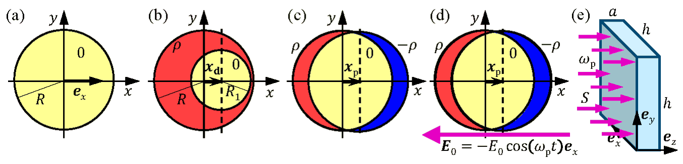
Figure 2.1 (a) A spherical charge-neutral nanoparticle of radius \(R\) placed at the center of the coordinate system. (b) A sphere with a positive homogeneous charge density \(\rho\) (red), and containing a smaller spherical charge-neutral region (0, yellow) of radius \(R_1\), with its center displaced by \(\boldsymbol{x}_{\mathrm d}=x_{\mathrm d}\boldsymbol{e}_x\). (c) The sphere with positive charge density \(\rho\) of the nanoparticle silver ions is fixed in the center of the coordinate system. The center of the spherical region with negative spherical charge density \(-\rho\) (blue) of the electron cloud is displaced by \(\boldsymbol{x}_{\mathrm p}\), where \(x_{\mathrm p}\ll R\). (d) An external homogeneous electric field \(\boldsymbol{E}_0=-E_0\boldsymbol{e}_x\). For time-dependent \(\boldsymbol{E}_0\), the electron cloud moves with velocity \(\boldsymbol{v}=\mathrm d\boldsymbol{x}_{\mathrm p}/\mathrm dt\). (e) The rectangular vessel \((h\times h\times a)\) containing the aqueous solution of nanoparticles illuminated by monochromatic light propagating along the \(z\)-axis with angular frequency \(\omega_{\mathrm p}\) and intensity \(S\).
A single spherical silver nanoparticle
Throughout this problem we consider a spherical silver nanoparticle of radius \(R=10{,}0\ \mathrm{nm}\) and with its center fixed at the origin of the coordinate system, see Fig. 2.1(a). All motions, forces and driving fields are parallel to the horizontal \(x\)-axis (with unit vector \(\boldsymbol{e}_x\)). The nanoparticle contains free (conduction) electrons moving within the whole nanoparticle volume without being bound to any silver atom. Each silver atom is a positive ion that has donated one such free electron.
| Part | Question | Points |
|---|---|---|
| 2.1 | Find the following quantities: The volume \(V\) and mass \(M\) of the nanoparticle, the number \(N\) and charge density \(\rho\) of silver ions in the particle, and for the free electrons their concentration \(n\), their total charge \(Q\), and their total mass \(m_0\). | 0.7 |
The electric field in a charge-neutral region inside a charged sphere
For the rest of the problem assume that the relative dielectric permittivity of all materials is \(\varepsilon=1\). Inside a charged sphere of homogeneous charge density \(\rho\) and radius \(R\) is created a small spherical charge-neutral region of radius \(R_1\) by adding the opposite charge density \(-\rho\), with its center displaced by \(\boldsymbol{x}_{\mathrm d}=x_{\mathrm d}\boldsymbol{e}_x\) from the center of the \(R\)-sphere, see Fig. 2.1(b).
| Part | Question | Points |
|---|---|---|
| 2.2 | Show that the electric field inside the charge-neutral region is homogenous of the form \(\boldsymbol{E}=A\,(\rho/\varepsilon_0)\,\boldsymbol{x}_{\mathrm d}\), and determine the pre-factor \(A\). | 1.2 |
The restoring force on the displaced electron cloud
In the following, we study the collective motion of the free electrons, and therefore model them as a single negatively charged sphere of homogeneous charge density \(-\rho\) with a center position \(\boldsymbol{x}_{\mathrm p}\), which can move along the \(x\)-axis relative to the center of the positively charged sphere (silver ions) fixed at the origin of the coordinate system, see Fig. 2.1(c). Assume that an external force \(\boldsymbol{F}_{\mathrm{ext}}\) displaces the electron cloud to a new equilibrium position \(\boldsymbol{x}_{\mathrm p}=x_{\mathrm p}\boldsymbol{e}_x\) with \(\lvert x_{\mathrm p}\rvert\ll R\). Except for tiny net charges at opposite ends of the nanoparticle, most of its interior remains charge-neutral.
| Part | Question | Points |
|---|---|---|
| 2.3 | Express in terms of \(\boldsymbol{x}_{\mathrm p}\) and \(n\) the following two quantities: The restoring force \(\boldsymbol{F}\) exerted on the electron cloud and the work \(W_{\mathrm{el}}\) done on the electron cloud during displacement. | 1.0 |
The spherical silver nanoparticle in an external constant electric field
A nanoparticle is placed in vacuum and influenced by an external force \(\boldsymbol{F}_{\mathrm{ext}}\) due to an applied static homogeneous electric field \(\boldsymbol{E}_0=-E_0\boldsymbol{e}_x\), which displaces the electron cloud the small distance \(\lvert x_{\mathrm p}\rvert\), where \(\lvert x_{\mathrm p}\rvert\ll R\).
| Part | Question | Points |
|---|---|---|
| 2.4 | Find the displacement \(x_{\mathrm p}\) of the electron cloud in terms of \(E_0\) and \(n\), and determine the amount \(-\Delta Q\) of electron charge displaced through the \(yz\)-plane at the center of the nanoparticle in terms of \(n\), \(R\) and \(x_{\mathrm p}\). | 0.6 |
The equivalent capacitance and inductance of the silver nanoparticle
For both a constant and a time-dependent field \(\boldsymbol{E}_0\), the nanoparticle can be modeled as an equivalent electric circuit. The equivalent capacitance can be found by relating the work \(W_{\mathrm{el}}\) done on the separation of charges \(\Delta Q\), to the energy of a capacitor, carrying charge \(\pm\Delta Q\). The charge separation will cause a certain equivalent voltage \(V_0\) across the equivalent capacitor.
| Part | Question | Points |
|---|---|---|
| 2.5a | Express the systems equivalent capacitance \(C\) in terms of \(\varepsilon_0\) and \(R\), and find its value. | 0.7 |
| 2.5b | For this capacitance, determine in terms of \(E_0\) and \(R\) the equivalent voltage \(V_0\) that should be connected to the equivalent capacitor in order to accumulate the charge \(\Delta Q\). | 0.4 |
For a time-dependent field \(\boldsymbol{E}_0\), the electron cloud moves with velocity \(\boldsymbol{v}=v\boldsymbol{e}_x\), Fig. 2.1(d). It has the kinetic energy \(W_{\mathrm{kin}}\) and forms an electric current \(I\) flowing through the fixed \(yz\)-plane. The kinetic energy of the electron cloud can be attributed to the energy of an equivalent inductor of inductance \(L\) carrying the current \(I\).
| Part | Question | Points |
|---|---|---|
| 2.6a | Express both \(W_{\mathrm{kin}}\) and \(I\) in terms of the velocity \(v\). | 0.7 |
| 2.6b | Express the equivalent inductance \(L\) in terms of the particle radius \(R\), the electron charge \(e\) and mass \(m_e\), the electron concentration \(n\), and calculate its value. | 0.5 |
The plasmon resonance of the silver nanoparticle
From the above analysis it follows that the motion, arising from displacing the electron cloud from its equilibrium position and then releasing it, can be modeled by an ideal \(LC\)-circuit oscillating at resonance. This dynamical mode of the electron cloud is known as the plasmon resonance, which oscillates at the so-called angular plasmon frequency \(\omega_{\mathrm p}\).
| Part | Question | Points |
|---|---|---|
| 2.7a | Find an expression for the angular plasmon frequency \(\omega_{\mathrm p}\) of the electron cloud in terms of the electron charge \(e\) and mass \(m_e\), the electron density \(n\), and the permittivity \(\varepsilon_0\). | 0.5 |
| 2.7b | Calculate \(\omega_{\mathrm p}\) in rad/s and the wavelength \(\lambda_{\mathrm p}\) in nm of light in vacuum having angular frequency \(\omega=\omega_{\mathrm p}\). | 0.4 |
The silver nanoparticle illuminated with light at the plasmon frequency
In the rest of the problem, the nanoparticle is illuminated by monochromatic light at the angular plasmon frequency \(\omega_{\mathrm p}\) with the incident intensity \(S=\frac12c\varepsilon_0E_0^2=1.00\ \mathrm{MW\,m^{-2}}\). As the wavelength is large, \(\lambda_{\mathrm p}\gg R\), the nanoparticle can be considered as being placed in a homogeneous harmonically oscillating field \(\boldsymbol{E}_0=-E_0\cos(\omega_{\mathrm p}t)\boldsymbol{e}_x\). Driven by \(\boldsymbol{E}_0\), the center \(\boldsymbol{x}_{\mathrm p}(t)\) of the electron cloud oscillates at the same frequency with velocity \(\boldsymbol{v}=\mathrm d\boldsymbol{x}_{\mathrm p}/\mathrm dt\) and constant amplitude \(x_0\). This oscillating electron motion leads to absorption of light. The energy captured by the particle is either converted into Joule heating inside the particle or re-emitted by the particle as scattered light.
Joule heating is caused by random inelastic collisions, where any given free electron once in a while hits a silver ion and loses its total kinetic energy, which is converted into vibrations of the silver ions (heat). The average time between the collisions is \(\tau\gg1/\omega_{\mathrm p}\), where for silver nanoparticle we use \(\tau=5.24\times10^{-15}\ \mathrm s\).
| Part | Question | Points |
|---|---|---|
| 2.8a | Find an expression for the time-averaged Joule heating power \(P_{\mathrm{heat}}\) in the nanoparticle as well as the time-averaged current squared \(\langle I^2\rangle\), which includes explicitly the time-averaged velocity squared \(\langle v^2\rangle\) of the electron cloud. | 1.0 |
| 2.8b | Find an expression for the equivalent ohmic resistance \(R_{\mathrm{heat}}\) in an equivalent resistor-model of the nanoparticle having the Joule heating power \(P_{\mathrm{heat}}\) due to the electron cloud current \(I\). Calculate the numerical value of \(R_{\mathrm{heat}}\). | 1.0 |
The incident light beam loses some time-averaged power \(P_{\mathrm{scat}}\) by scattering on the oscillating electron cloud (re-emission). \(P_{\mathrm{scat}}\) depends on the scattering source amplitude \(x_0\), charge \(Q\), angular frequency \(\omega_{\mathrm p}\) and properties of the light (the speed of light \(c\) and permittivity \(\varepsilon_0\) in vacuum). In terms of these four variables, \(P_{\mathrm{scat}}\) is given by \[ P_{\mathrm{scat}}=\frac{Q^2x_0^2\omega_{\mathrm p}^4}{12\pi\varepsilon_0c^3}. \]
| Part | Question | Points |
|---|---|---|
| 2.9 | By use of \(P_{\mathrm{scat}}\), find an expression for the equivalent scattering resistance \(R_{\mathrm{scat}}\) (in analogy with \(R_{\mathrm{heat}}\)) in an equivalent resistor-model, and calculate its value. | 1.0 |
The above equivalent circuit elements are combined into an \(LCR\) series circuit model of the silver nanoparticle, which is driven by a harmonically oscillating equivalent voltage \(V=V_0\cos(\omega_{\mathrm p}t)\) determined by the electric field \(\boldsymbol{E}_0\) of the incident light.
| Part | Question | Points |
|---|---|---|
| 2.10a | Derive expressions for the time-averaged power losses \(P_{\mathrm{heat}}\) and \(P_{\mathrm{scat}}\) involving the amplitude \(E_0\) of the electric field in the incident light at the plasmon resonance \(\omega=\omega_{\mathrm p}\). | 1.2 |
| 2.10b | Calculate the numerical value of \(E_0\), \(P_{\mathrm{heat}}\), and \(P_{\mathrm{scat}}\). | 0.3 |
Steam generation by light
An aqueous solution of silver nanoparticles is prepared with a concentration \(n_{\mathrm{np}}=7.3\times10^{15}\ \mathrm{m^{-3}}\). It is placed inside a rectangular transparent vessel of size \(h\times h\times a=10\times10\times1.0\ \mathrm{cm^3}\) and illuminated by light at the plasmon frequency with the same intensity \(S=1.00\ \mathrm{MW\,m^{-2}}\) at normal incidence as above, see Fig. 2.1(e). The temperature of the water is \(T_{\mathrm{wa}}=20\,^\circ\mathrm C\) and we assume, in fair agreement with observations, that in steady state all Joule heating of the nanoparticle goes to the production of steam of temperature \(T_{\mathrm{st}}=110\,^\circ\mathrm C\), without raising the temperature of the water.
The thermodynamic efficiency \(\eta\) of the plasmonic steam generator is defined by the power ratio \(\eta=P_{\mathrm{st}}/P_{\mathrm{tot}}\), where \(P_{\mathrm{st}}\) is the power going into the production of steam in the entire vessel, while \(P_{\mathrm{tot}}\) is the total power of the incoming light that enters the vessel.
Most of the time any given nanoparticle is surrounded by steam instead of water, and it can thus be described as being in vacuum.
| Part | Question | Points |
|---|---|---|
| 2.11a | Calculate the total mass per second \(\mu_{\mathrm{st}}\) of steam produced by the plasmonic steam generator during illumination by light at the plasmon frequency and intensity \(S\). | 0.6 |
| 2.11b | Calculate the numerical value of the thermodynamic efficiency \(\eta\) of the plasmonic steam generator. | 0.2 |
Data sheet: Table of physical parameters
| Physical parameter | Value |
|---|---|
| Speed of light in vacuum | \(c=2.998\times10^8\ \mathrm{m\,s^{-1}}\) |
| Planck's constant over \(2\pi\) | \(\hbar=1.055\times10^{-34}\ \mathrm{J\,s}\) |
| Gravitational constant | \(G=6.67\times10^{-11}\ \mathrm{m^3\,kg^{-1}\,s^{-2}}\) |
| Gravitational acceleration | \(g=9.82\ \mathrm{m\,s^{-2}}\) |
| Elementary charge | \(e=1.602\times10^{-19}\ \mathrm C\) |
| Electric permittivity of vacuum | \(\varepsilon_0=8.854\times10^{-12}\ \mathrm{C^2\,J^{-1}\,m^{-1}}\) |
| Electron mass | \(m_e=9.109\times10^{-31}\ \mathrm{kg}\) |
| Avogadro constant | \(N_A=6.022\times10^{23}\ \mathrm{mol^{-1}}\) |
| Boltzmann constant | \(k_{\mathrm B}=1.381\times10^{-23}\ \mathrm{J\,K^{-1}}\) |
| Stony meteorite, specific heat | \(c_{\mathrm{sm}}=1.2\times10^3\ \mathrm{J\,kg^{-1}\,K^{-1}}\) |
| Stony meteorite, thermal conductivity | \(k_{\mathrm{sm}}=2.0\ \mathrm{W\,m^{-1}\,K^{-1}}\) |
| Stony meteorite, density | \(\rho_{\mathrm{sm}}=3.3\times10^3\ \mathrm{kg\,m^{-3}}\) |
| Stony meteorite, melting point | \(T_{\mathrm{sm}}=1.7\times10^3\ \mathrm K\) |
| Stony meteorite, specific melting heat | \(L_{\mathrm{sm}}=2.6\times10^5\ \mathrm{J\,kg^{-1}}\) |
| Silver, molar mass | \(M_{\mathrm{Ag}}=1.079\times10^{-1}\ \mathrm{kg\,mol^{-1}}\) |
| Silver, density | \(\rho_{\mathrm{Ag}}=1.049\times10^4\ \mathrm{kg\,m^{-3}}\) |
| Silver, specific heat capacity | \(c_{\mathrm{Ag}}=2.40\times10^2\ \mathrm{J\,kg^{-1}\,K^{-1}}\) |
| Water, molar mass | \(M_{\mathrm{wa}}=1.801\times10^{-2}\ \mathrm{kg\,mol^{-1}}\) |
| Water, density | \(\rho_{\mathrm{wa}}=0.998\times10^3\ \mathrm{kg\,m^{-3}}\) |
| Water, specific heat capacity | \(c_{\mathrm{wa}}=4.181\times10^3\ \mathrm{J\,kg^{-1}\,K^{-1}}\) |
| Water, heat of vaporization | \(L_{\mathrm{wa}}=2.260\times10^6\ \mathrm{J\,kg^{-1}}\) |
| Water, boiling temperature | \(T_{100}=100\,^\circ\mathrm C=373.15\ \mathrm K\) |
| Ice, density of glacier | \(\rho_{\mathrm{ice}}=0.917\times10^3\ \mathrm{kg\,m^{-3}}\) |
| Steam, specific heat capacity | \(c_{\mathrm{st}}=2.080\times10^3\ \mathrm{J\,kg^{-1}\,K^{-1}}\) |
| Earth, mass of the | \(m_{\mathrm E}=5.97\times10^{24}\ \mathrm{kg}\) |
| Earth, radius of the | \(R_{\mathrm E}=6.38\times10^6\ \mathrm m\) |
| Sun, mass of the | \(m_{\mathrm S}=1.99\times10^{30}\ \mathrm{kg}\) |
| Sun, radius of the | \(R_{\mathrm S}=6.96\times10^8\ \mathrm m\) |
| Average Sun-Earth distance | \(a_{\mathrm E}=1.50\times10^{11}\ \mathrm m\) |
Official English text of the problem.
Answers
Here \(e>0\), \(Q<0\), and \(W_{\mathrm{el}}\) denotes the positive work supplied to separate the charges. Choose the circuit-current direction so that \(I=\mathrm d(\Delta Q)/\mathrm dt\), positive when the electrons move in \(+x\).
-
2.1 \[ \begin{gathered} V=4.19\times10^{-24}\ \mathrm{m^3},\qquad M=4.39\times10^{-20}\ \mathrm{kg},\\ N=2.45\times10^5,\qquad \rho=+9.38\times10^9\ \mathrm{C\,m^{-3}},\\ n=5.85\times10^{28}\ \mathrm{m^{-3}},\qquad Q=-3.93\times10^{-14}\ \mathrm C,\qquad m_0=2.23\times10^{-25}\ \mathrm{kg}. \end{gathered} \]
-
2.2 \[ \boldsymbol E=\frac{\rho}{3\varepsilon_0}\boldsymbol x_{\mathrm d}, \qquad \boxed{A=\frac13}. \]
-
2.3 \[ \boldsymbol F=-\frac{4\pi n^2e^2R^3}{9\varepsilon_0}\boldsymbol x_{\mathrm p}, \qquad W_{\mathrm{el}}=\frac{2\pi n^2e^2R^3}{9\varepsilon_0}x_{\mathrm p}^2. \]
-
2.4 \[ x_{\mathrm p}=\frac{3\varepsilon_0E_0}{ne}, \qquad -\Delta Q=-ne\pi R^2x_{\mathrm p}. \]
-
2.5a \[ C=\frac94\pi\varepsilon_0R =6.26\times10^{-19}\ \mathrm F. \]
-
2.5b \[ V_0=\frac43RE_0. \]
-
2.6a \[ W_{\mathrm{kin}}=\frac12m_0v^2=\frac{2\pi}{3}nm_eR^3v^2, \qquad I=ne\pi R^2v. \]
-
2.6b \[ L=\frac{4m_e}{3\pi ne^2R} =2.57\times10^{-14}\ \mathrm H. \]
-
2.7a \[ \omega_{\mathrm p}=\sqrt{\frac{ne^2}{3\varepsilon_0m_e}}. \]
-
2.7b \[ \omega_{\mathrm p}=7.88\times10^{15}\ \mathrm{rad\,s^{-1}}, \qquad \lambda_{\mathrm p}=239\ \mathrm{nm}. \]
-
2.8a \[ P_{\mathrm{heat}}=\frac{m_0}{2\tau}\langle v^2\rangle, \qquad \langle I^2\rangle=(ne\pi R^2)^2\langle v^2\rangle. \]
-
2.8b \[ R_{\mathrm{heat}}=\frac{L}{2\tau} =\frac{2m_e}{3\pi ne^2R\tau} =2.46\ \Omega. \]
-
2.9 \[ R_{\mathrm{scat}}=\frac{8R^2\omega_{\mathrm p}^2} {27\pi\varepsilon_0c^3} =2.45\ \Omega. \]
-
2.10a \[ P_{\mathrm{heat}}= \frac{8R^2E_0^2}{9} \frac{R_{\mathrm{heat}}}{(R_{\mathrm{heat}}+R_{\mathrm{scat}})^2}, \qquad P_{\mathrm{scat}}= \frac{8R^2E_0^2}{9} \frac{R_{\mathrm{scat}}}{(R_{\mathrm{heat}}+R_{\mathrm{scat}})^2}. \]
-
2.10b \[ E_0=2.74\times10^4\ \mathrm{V\,m^{-1}}, \qquad P_{\mathrm{heat}}=6.82\times10^{-9}\ \mathrm W, \qquad P_{\mathrm{scat}}=6.82\times10^{-9}\ \mathrm W. \]
-
2.11a, using uniform illumination throughout the vessel: \[ \mu_{\mathrm{st}}\simeq1.9\times10^{-3}\ \mathrm{kg\,s^{-1}} =1.9\ \mathrm{g\,s^{-1}}. \]
-
2.11b, with the same approximation: \[ \eta\simeq0.50=50\%. \]
Solution
All electrostatic and circuit results below use the prescribed rigid, uniformly charged electron-cloud model. Displacement-dependent results retain the leading terms for \(\lvert x_{\mathrm p}\rvert/R\ll1\).
2.1
The particle is a sphere, so \[ V=\frac{4\pi R^3}{3} =\frac{4\pi}{3}(1.00\times10^{-8})^3 =4.19\times10^{-24}\ \mathrm{m^3}. \] Its mass is \[ M=\rho_{\mathrm{Ag}}V =4.39\times10^{-20}\ \mathrm{kg}. \]
The number of silver atoms, and hence of singly charged silver ions, is \[ N=\frac{M}{M_{\mathrm{Ag}}}N_A =2.45\times10^5. \] There is one conduction electron per ion. Thus \[ n=\frac{N}{V} =\frac{\rho_{\mathrm{Ag}}N_A}{M_{\mathrm{Ag}}} =5.85\times10^{28}\ \mathrm{m^{-3}}. \]
The positive ionic charge density is \[ \rho=ne=+9.38\times10^9\ \mathrm{C\,m^{-3}}. \] For the electrons, \[ Q=-Ne=-3.93\times10^{-14}\ \mathrm C, \qquad m_0=Nm_e=2.23\times10^{-25}\ \mathrm{kg}. \]
2.2
Apply Gauss's law to a concentric Gaussian sphere of radius \(r\) inside a uniformly charged sphere: \[ E(r)\,4\pi r^2 =\frac{\rho(4\pi r^3/3)}{\varepsilon_0}. \] Consequently, the interior field is \[ \boldsymbol E_+(\boldsymbol r) =\frac{\rho}{3\varepsilon_0}\boldsymbol r. \]
The neutral region is formed by superposing a sphere of charge density \(-\rho\), centered at \(\boldsymbol x_{\mathrm d}\). At a point inside this smaller sphere its field is \[ \boldsymbol E_-(\boldsymbol r) =-\frac{\rho}{3\varepsilon_0} (\boldsymbol r-\boldsymbol x_{\mathrm d}). \] Adding the two fields gives \[ \boldsymbol E =\boldsymbol E_++\boldsymbol E_- =\frac{\rho}{3\varepsilon_0}\boldsymbol x_{\mathrm d}. \] The position \(\boldsymbol r\) cancels, so the field is homogeneous and \[ \boxed{A=\frac13}. \]
2.3
The displaced electron cloud has charge density \(-ne\), while the fixed ions have charge density \(+ne\). By 2.2, the field in their overlapping, neutral interior is \[ \boldsymbol E_{\mathrm{int}} =\frac{ne}{3\varepsilon_0}\boldsymbol x_{\mathrm p}. \] To first order in displacement this field gives the restoring force on the cloud: \[ \boldsymbol F=Q\boldsymbol E_{\mathrm{int}} =-\frac{Nne^2}{3\varepsilon_0}\boldsymbol x_{\mathrm p}. \] The small nonoverlapping regions only affect higher-order terms. With \(N=4\pi nR^3/3\), \[ \boxed{\boldsymbol F =-\frac{4\pi n^2e^2R^3}{9\varepsilon_0}\boldsymbol x_{\mathrm p}}. \]
Define the effective spring constant \[ k=\frac{Nne^2}{3\varepsilon_0}. \] The work supplied in a quasistatic displacement from zero to \(x_{\mathrm p}\) is \[ W_{\mathrm{el}} =-\int_0^{x_{\mathrm p}}F_x(x)\,\mathrm dx =\int_0^{x_{\mathrm p}}kx\,\mathrm dx =\frac12kx_{\mathrm p}^2. \] Therefore \[ \boxed{W_{\mathrm{el}} =\frac{Nne^2}{6\varepsilon_0}x_{\mathrm p}^2 =\frac{2\pi n^2e^2R^3}{9\varepsilon_0}x_{\mathrm p}^2}. \] This is the stored electrostatic energy used in 2.5. The work done by the restoring force itself is \(-W_{\mathrm{el}}\).
2.4
The external field points in \(-x\), so the force on the negative electron cloud points in \(+x\): \[ \boldsymbol F_{\mathrm{ext}} =Q\boldsymbol E_0 =NeE_0\boldsymbol e_x. \] At equilibrium, \[ NeE_0-\frac{Nne^2}{3\varepsilon_0}x_{\mathrm p}=0. \] Hence \[ \boxed{x_{\mathrm p}=\frac{3\varepsilon_0E_0}{ne}}. \]
For a small translation \(x_{\mathrm p}\), the volume of electron cloud transported through the central plane is, to leading order, \[ \Delta V=\pi R^2x_{\mathrm p}. \] Multiplying by its charge density gives \[ \boxed{-\Delta Q=-ne\pi R^2x_{\mathrm p}}. \] Thus the positive charge-separation variable is \[ \Delta Q=ne\pi R^2x_{\mathrm p} =3\pi\varepsilon_0R^2E_0. \]
2.5a
Equate the electrostatic energy to the energy of the equivalent capacitor: \[ W_{\mathrm{el}}=\frac{(\Delta Q)^2}{2C}. \] Using the results above, \[ C= \frac{(ne\pi R^2x_{\mathrm p})^2} {2\left(2\pi n^2e^2R^3x_{\mathrm p}^2/(9\varepsilon_0)\right)} =\frac94\pi\varepsilon_0R. \] Therefore \[ \boxed{C=6.26\times10^{-19}\ \mathrm F}. \]
2.5b
The equivalent voltage is \[ V_0=\frac{\Delta Q}{C}. \] Substitution yields \[ V_0= \frac{3\pi\varepsilon_0R^2E_0} {(9/4)\pi\varepsilon_0R}, \] so \[ \boxed{V_0=\frac43RE_0}. \]
2.6a
All \(N\) electrons participate in the collective motion. Their kinetic energy is \[ \boxed{ W_{\mathrm{kin}}=\frac12Nm_ev^2 =\frac12m_0v^2 =\frac{2\pi}{3}nm_eR^3v^2}. \]
Differentiating the charge-separation relation gives \[ \boxed{ I=\frac{\mathrm d(\Delta Q)}{\mathrm dt} =ne\pi R^2v}. \] Here positive circuit current corresponds to conventional current in the \(-x\) direction. If conventional current through the plane were instead defined positive in \(+x\), it would be \(I_x=-ne\pi R^2v\). The energy and resistance results depend on \(I^2\), so this orientation choice does not affect them.
2.6b
Identify the kinetic energy with the energy of the equivalent inductor: \[ \frac12LI^2=\frac12m_0v^2. \] It follows that \[ L=\frac{m_0}{(ne\pi R^2)^2}. \] Using \(m_0=(4\pi R^3/3)nm_e\), \[ \boxed{L=\frac{4m_e}{3\pi ne^2R} =2.57\times10^{-14}\ \mathrm H}. \]
2.7a
For a freely oscillating ideal \(LC\) circuit, \[ L\frac{\mathrm d^2(\Delta Q)}{\mathrm dt^2} +\frac{\Delta Q}{C}=0, \] so \[ \omega_{\mathrm p}^2=\frac1{LC}. \] Since \[ LC= \frac{4m_e}{3\pi ne^2R} \frac{9\pi\varepsilon_0R}{4} =\frac{3\varepsilon_0m_e}{ne^2}, \] we obtain \[ \boxed{\omega_{\mathrm p} =\sqrt{\frac{ne^2}{3\varepsilon_0m_e}}}. \] The same result follows directly from \(\omega_{\mathrm p}^2=k/m_0\).
2.7b
Substitution of the given constants gives \[ \boxed{\omega_{\mathrm p} =7.88\times10^{15}\ \mathrm{rad\,s^{-1}}}. \] Because \(\omega=2\pi c/\lambda\), \[ \lambda_{\mathrm p}=\frac{2\pi c}{\omega_{\mathrm p}} =2.39\times10^{-7}\ \mathrm m. \] Thus \[ \boxed{\lambda_{\mathrm p}=239\ \mathrm{nm}}. \]
2.8a
In the stated collision model, each electron loses its entire collective kinetic energy in a collision. Its time-averaged energy loss per collision is \[ \frac12m_e\langle v^2\rangle. \] There are, on average, \(N/\tau\) collisions per second among all electrons. Random collision times allow us to use the cycle-averaged kinetic energy, giving \[ \boxed{ P_{\mathrm{heat}} =\frac{Nm_e}{2\tau}\langle v^2\rangle =\frac{m_0}{2\tau}\langle v^2\rangle}. \]
From the current–velocity relation, \[ \boxed{\langle I^2\rangle =(ne\pi R^2)^2\langle v^2\rangle}. \]
2.8b
The equivalent resistance is defined by \[ P_{\mathrm{heat}}=R_{\mathrm{heat}}\langle I^2\rangle. \] Consequently, \[ R_{\mathrm{heat}} =\frac{m_0}{2\tau(ne\pi R^2)^2} =\frac{L}{2\tau}. \] Thus \[ \boxed{ R_{\mathrm{heat}} =\frac{2m_e}{3\pi ne^2R\tau} =2.46\ \Omega}. \]
The factor \(1/2\) follows from the kinetic energy \(\frac12m_ev^2\) lost per collision in the specific model given in the problem.
2.9
For harmonic motion of amplitude \(x_0\), \[ x_{\mathrm p}(t)=x_0\cos(\omega_{\mathrm p}t+\phi), \] and hence \[ \langle v^2\rangle=\frac12\omega_{\mathrm p}^2x_0^2. \] Therefore \[ \langle I^2\rangle =\frac12(ne\pi R^2)^2\omega_{\mathrm p}^2x_0^2. \]
Define the scattering resistance by \[ P_{\mathrm{scat}}=R_{\mathrm{scat}}\langle I^2\rangle. \] Using the supplied radiation formula, \[ R_{\mathrm{scat}} = \frac{Q^2x_0^2\omega_{\mathrm p}^4} {12\pi\varepsilon_0c^3} \frac{2}{(ne\pi R^2)^2\omega_{\mathrm p}^2x_0^2}. \] Since \[ Q=-\frac43\pi R^3ne, \qquad \frac{Q^2}{(ne\pi R^2)^2}=\frac{16R^2}{9}, \] we obtain \[ \boxed{ R_{\mathrm{scat}} =\frac{8R^2\omega_{\mathrm p}^2} {27\pi\varepsilon_0c^3} =2.45\ \Omega}. \] Equivalently, \[ R_{\mathrm{scat}} =\frac{8ne^2R^2}{81\pi\varepsilon_0^2m_ec^3}. \]
2.10a
Both heating and scattering remove energy from the same oscillating current. Their equivalent resistances therefore add in the series circuit: \[ R_\Sigma=R_{\mathrm{heat}}+R_{\mathrm{scat}}. \]
At \(\omega=\omega_{\mathrm p}=1/\sqrt{LC}\), the inductive and capacitive reactances cancel: \[ \omega_{\mathrm p}L-\frac1{\omega_{\mathrm p}C}=0. \] Thus the current is in phase with the driving voltage and has amplitude \[ I_0=\frac{V_0}{R_\Sigma} =\frac{4RE_0}{3R_\Sigma}. \] For a sinusoidal current, \[ \langle I^2\rangle=\frac{I_0^2}{2} =\frac{8R^2E_0^2}{9R_\Sigma^2}. \] The two average powers are therefore \[ \boxed{ P_{\mathrm{heat}}= \frac{8R^2E_0^2}{9} \frac{R_{\mathrm{heat}}} {(R_{\mathrm{heat}}+R_{\mathrm{scat}})^2}} \] and \[ \boxed{ P_{\mathrm{scat}}= \frac{8R^2E_0^2}{9} \frac{R_{\mathrm{scat}}} {(R_{\mathrm{heat}}+R_{\mathrm{scat}})^2}}. \]
2.10b
From the specified incident intensity, \[ S=\frac12c\varepsilon_0E_0^2, \] so \[ E_0=\sqrt{\frac{2S}{c\varepsilon_0}} =\sqrt{\frac{2(1.00\times10^6)} {(2.998\times10^8)(8.854\times10^{-12})}}. \] Thus \[ \boxed{E_0=2.74\times10^4\ \mathrm{V\,m^{-1}}}. \]
Using unrounded intermediate values, \[ V_0=3.66\times10^{-4}\ \mathrm V, \qquad R_\Sigma=4.910\ \Omega, \qquad I_0=7.45\times10^{-5}\ \mathrm A. \] Consequently, \[ \boxed{P_{\mathrm{heat}}=6.82\times10^{-9}\ \mathrm W}, \qquad \boxed{P_{\mathrm{scat}}=6.82\times10^{-9}\ \mathrm W}. \] Their near equality follows from the near equality of the two resistances.
The displacement amplitude can also be checked: \[ x_0=\frac{I_0}{ne\pi R^2\omega_{\mathrm p}} =3.21\times10^{-15}\ \mathrm m, \] so \(x_0/R=3.21\times10^{-7}\ll1\). Also, \(\omega_{\mathrm p}\tau=41.3\), consistent with the assumed separation of oscillation and collision timescales.
2.11a
Apply the per-particle heating power from 2.10 throughout the illuminated volume. This uses uniform illumination and does not introduce an additional model for attenuation or multiple scattering.
The vessel volume is \[ V_{\mathrm{vessel}}=h^2a =(0.10)^2(0.010) =1.0\times10^{-4}\ \mathrm{m^3}. \] It contains \[ N_{\mathrm{np}}=n_{\mathrm{np}}h^2a =7.3\times10^{11} \] nanoparticles. All their Joule heating is assumed to produce steam, so \[ P_{\mathrm{st}}=N_{\mathrm{np}}P_{\mathrm{heat}} =4.98\times10^3\ \mathrm W. \]
Each kilogram that becomes steam must first be heated from \(20^\circ\mathrm C\) to \(100^\circ\mathrm C\), then vaporized, and finally heated to \(110^\circ\mathrm C\). The required energy per unit mass is \[ q_{\mathrm{st}} =c_{\mathrm{wa}}(T_{100}-T_{\mathrm{wa}}) +L_{\mathrm{wa}} +c_{\mathrm{st}}(T_{\mathrm{st}}-T_{100}). \] Numerically, \[ \begin{aligned} q_{\mathrm{st}} &=(4.181\times10^3)(80) +2.260\times10^6 +(2.080\times10^3)(10)\\ &=2.61528\times10^6\ \mathrm{J\,kg^{-1}}. \end{aligned} \] The bulk water remaining at \(20^\circ\mathrm C\) does not eliminate the heating required for the portion that evaporates.
Energy conservation gives \[ \mu_{\mathrm{st}}q_{\mathrm{st}}=P_{\mathrm{st}}. \] Thus \[ \mu_{\mathrm{st}} =\frac{n_{\mathrm{np}}h^2aP_{\mathrm{heat}}} {c_{\mathrm{wa}}(T_{100}-T_{\mathrm{wa}}) +L_{\mathrm{wa}} +c_{\mathrm{st}}(T_{\mathrm{st}}-T_{100})} =1.904\times10^{-3}\ \mathrm{kg\,s^{-1}}. \] To the precision of the vessel and concentration data, \[ \boxed{\mu_{\mathrm{st}}\simeq1.9\ \mathrm{g\,s^{-1}}}. \]
2.11b
The beam enters normally through the face of area \(h^2\), so \[ P_{\mathrm{tot}}=Sh^2 =(1.00\times10^6)(0.10)^2 =1.00\times10^4\ \mathrm W. \] Therefore \[ \eta=\frac{P_{\mathrm{st}}}{P_{\mathrm{tot}}} =\frac{n_{\mathrm{np}}h^2aP_{\mathrm{heat}}}{Sh^2} =\frac{n_{\mathrm{np}}aP_{\mathrm{heat}}}{S}. \] Numerically, \[ \eta=0.4979, \] or, with sensible rounding, \[ \boxed{\eta\simeq0.50=50\%}. \]
The solution was checked against the official solution.
IPhO 2013 · Theorieaufgabe 2
Plasmonischer Dampferzeuger
Einleitung
In dieser Aufgabe untersuchen wir ein effizientes Verfahren zur Dampferzeugung, dessen Funktionsfähigkeit experimentell nachgewiesen wurde. Eine wässrige Lösung aus nanometergroßen Silberkugeln (Nanopartikeln) mit nur etwa \(10^{13}\) Teilchen pro Liter wird mit einem fokussierten Lichtstrahl beleuchtet. Ein Teil des Lichts wird von den Nanopartikeln absorbiert, die sich erwärmen und lokal in ihrer Umgebung Dampf erzeugen, ohne die gesamte wässrige Lösung zu erwärmen. Der Dampf verlässt das System in Form entweichender Dampfblasen. Noch sind nicht alle Einzelheiten des Verfahrens gut verstanden, doch ist bekannt, dass der zentrale Prozess die Absorption von Licht durch die sogenannten kollektiven Elektronenschwingungen der metallischen Nanopartikel ist. Die Vorrichtung wird als plasmonischer Dampferzeuger bezeichnet.
Abbildung 2.1 (a) Ein kugelförmiges, elektrisch neutrales Nanopartikel mit dem Radius \(R\) im Ursprung des Koordinatensystems. (b) Eine Kugel mit einer positiven homogenen Ladungsdichte \(\rho\) (rot), die einen kleineren kugelförmigen, elektrisch neutralen Bereich (0, gelb) mit dem Radius \(R_1\) enthält, dessen Mittelpunkt um \(\boldsymbol{x}_{\mathrm d}=x_{\mathrm d}\boldsymbol{e}_x\) verschoben ist. (c) Die Kugel mit der positiven Ladungsdichte \(\rho\) der Silberionen des Nanopartikels ist im Ursprung des Koordinatensystems fixiert. Der Mittelpunkt des kugelförmigen Bereichs mit der negativen kugelsymmetrischen Ladungsdichte \(-\rho\) (blau) der Elektronenwolke ist um \(\boldsymbol{x}_{\mathrm p}\) verschoben, wobei \(x_{\mathrm p}\ll R\) gilt. (d) Ein äußeres homogenes elektrisches Feld \(\boldsymbol{E}_0=-E_0\boldsymbol{e}_x\). Bei zeitabhängigem \(\boldsymbol{E}_0\) bewegt sich die Elektronenwolke mit der Geschwindigkeit \(\boldsymbol{v}=\mathrm d\boldsymbol{x}_{\mathrm p}/\mathrm dt\). (e) Das quaderförmige Gefäß \((h\times h\times a)\) mit der wässrigen Nanopartikellösung, die mit monochromatischem Licht der Kreisfrequenz \(\omega_{\mathrm p}\) und der Intensität \(S\) beleuchtet wird, das sich entlang der \(z\)-Achse ausbreitet.
Ein einzelnes kugelförmiges Silbernanopartikel
In dieser gesamten Aufgabe betrachten wir ein kugelförmiges Silbernanopartikel mit dem Radius \(R=10{,}0\ \mathrm{nm}\), dessen Mittelpunkt im Ursprung des Koordinatensystems fixiert ist, siehe Abb. 2.1(a). Alle Bewegungen, Kräfte und anregenden Felder sind parallel zur horizontalen \(x\)-Achse (mit dem Einheitsvektor \(\boldsymbol{e}_x\)). Das Nanopartikel enthält freie (Leitungs-)Elektronen, die sich im gesamten Volumen des Nanopartikels bewegen, ohne an ein Silberatom gebunden zu sein. Jedes Silberatom ist ein positives Ion, das ein solches freies Elektron abgegeben hat.
| Teil | Frage | Punkte |
|---|---|---|
| 2.1 | Bestimmen Sie die folgenden Größen: das Volumen \(V\) und die Masse \(M\) des Nanopartikels, die Anzahl \(N\) und die Ladungsdichte \(\rho\) der Silberionen im Teilchen sowie für die freien Elektronen ihre Konzentration \(n\), ihre Gesamtladung \(Q\) und ihre Gesamtmasse \(m_0\). | 0.7 |
Das elektrische Feld in einem elektrisch neutralen Bereich innerhalb einer geladenen Kugel
Nehmen Sie für den Rest der Aufgabe an, dass die relative Permittivität aller Materialien \(\varepsilon=1\) beträgt. Innerhalb einer geladenen Kugel mit homogener Ladungsdichte \(\rho\) und Radius \(R\) wird durch Hinzufügen der entgegengesetzten Ladungsdichte \(-\rho\) ein kleiner kugelförmiger, elektrisch neutraler Bereich mit dem Radius \(R_1\) erzeugt, dessen Mittelpunkt gegenüber dem Mittelpunkt der Kugel mit Radius \(R\) um \(\boldsymbol{x}_{\mathrm d}=x_{\mathrm d}\boldsymbol{e}_x\) verschoben ist, siehe Abb. 2.1(b).
| Teil | Frage | Punkte |
|---|---|---|
| 2.2 | Zeigen Sie, dass das elektrische Feld innerhalb des elektrisch neutralen Bereichs homogen ist und die Form \(\boldsymbol{E}=A\,(\rho/\varepsilon_0)\,\boldsymbol{x}_{\mathrm d}\) hat, und bestimmen Sie den Vorfaktor \(A\). | 1.2 |
Die Rückstellkraft auf die verschobene Elektronenwolke
Im Folgenden untersuchen wir die kollektive Bewegung der freien Elektronen und modellieren sie daher als eine einzige negativ geladene Kugel mit homogener Ladungsdichte \(-\rho\) und der Mittelpunktposition \(\boldsymbol{x}_{\mathrm p}\), die sich entlang der \(x\)-Achse relativ zum Mittelpunkt der im Ursprung des Koordinatensystems fixierten positiv geladenen Kugel (Silberionen) bewegen kann, siehe Abb. 2.1(c). Nehmen Sie an, dass eine äußere Kraft \(\boldsymbol{F}_{\mathrm{ext}}\) die Elektronenwolke in eine neue Gleichgewichtslage \(\boldsymbol{x}_{\mathrm p}=x_{\mathrm p}\boldsymbol{e}_x\) mit \(\lvert x_{\mathrm p}\rvert\ll R\) verschiebt. Abgesehen von winzigen Nettoladungen an gegenüberliegenden Enden des Nanopartikels bleibt der größte Teil seines Inneren elektrisch neutral.
| Teil | Frage | Punkte |
|---|---|---|
| 2.3 | Drücken Sie die folgenden beiden Größen durch \(\boldsymbol{x}_{\mathrm p}\) und \(n\) aus: die auf die Elektronenwolke ausgeübte Rückstellkraft \(\boldsymbol{F}\) und die während der Verschiebung an der Elektronenwolke verrichtete Arbeit \(W_{\mathrm{el}}\). | 1.0 |
Das kugelförmige Silbernanopartikel in einem äußeren konstanten elektrischen Feld
Ein Nanopartikel befindet sich im Vakuum und wird durch eine äußere Kraft \(\boldsymbol{F}_{\mathrm{ext}}\) beeinflusst, die von einem angelegten statischen homogenen elektrischen Feld \(\boldsymbol{E}_0=-E_0\boldsymbol{e}_x\) herrührt. Dieses verschiebt die Elektronenwolke um die kleine Strecke \(\lvert x_{\mathrm p}\rvert\), wobei \(\lvert x_{\mathrm p}\rvert\ll R\) gilt.
| Teil | Frage | Punkte |
|---|---|---|
| 2.4 | Bestimmen Sie die Verschiebung \(x_{\mathrm p}\) der Elektronenwolke in Abhängigkeit von \(E_0\) und \(n\) sowie die durch die \(yz\)-Ebene im Mittelpunkt des Nanopartikels verschobene Elektronenladung \(-\Delta Q\) in Abhängigkeit von \(n\), \(R\) und \(x_{\mathrm p}\). | 0.6 |
Die Ersatzkapazität und Ersatzinduktivität des Silbernanopartikels
Sowohl für ein konstantes als auch für ein zeitabhängiges Feld \(\boldsymbol{E}_0\) lässt sich das Nanopartikel durch eine elektrische Ersatzschaltung modellieren. Die Ersatzkapazität lässt sich bestimmen, indem die zur Trennung der Ladungen \(\Delta Q\) verrichtete Arbeit \(W_{\mathrm{el}}\) mit der Energie eines Kondensators in Beziehung gesetzt wird, der die Ladung \(\pm\Delta Q\) trägt. Die Ladungstrennung bewirkt eine bestimmte Ersatzspannung \(V_0\) am Ersatzkondensator.
| Teil | Frage | Punkte |
|---|---|---|
| 2.5a | Drücken Sie die Ersatzkapazität \(C\) des Systems durch \(\varepsilon_0\) und \(R\) aus und bestimmen Sie ihren Wert. | 0.7 |
| 2.5b | Bestimmen Sie für diese Kapazität in Abhängigkeit von \(E_0\) und \(R\) die Ersatzspannung \(V_0\), die an den Ersatzkondensator angelegt werden muss, damit sich die Ladung \(\Delta Q\) ansammelt. | 0.4 |
Bei einem zeitabhängigen Feld \(\boldsymbol{E}_0\) bewegt sich die Elektronenwolke mit der Geschwindigkeit \(\boldsymbol{v}=v\boldsymbol{e}_x\), Abb. 2.1(d). Sie besitzt die kinetische Energie \(W_{\mathrm{kin}}\) und erzeugt einen elektrischen Strom \(I\), der durch die ortsfeste \(yz\)-Ebene fließt. Die kinetische Energie der Elektronenwolke kann der Energie einer vom Strom \(I\) durchflossenen Ersatzspule mit der Induktivität \(L\) zugeordnet werden.
| Teil | Frage | Punkte |
|---|---|---|
| 2.6a | Drücken Sie sowohl \(W_{\mathrm{kin}}\) als auch \(I\) durch die Geschwindigkeit \(v\) aus. | 0.7 |
| 2.6b | Drücken Sie die Ersatzinduktivität \(L\) durch den Teilchenradius \(R\), die Elektronenladung \(e\) und die Elektronenmasse \(m_e\) sowie die Elektronenkonzentration \(n\) aus und berechnen Sie ihren Wert. | 0.5 |
Die Plasmonenresonanz des Silbernanopartikels
Aus der obigen Analyse folgt, dass die Bewegung, die entsteht, wenn die Elektronenwolke aus ihrer Gleichgewichtslage verschoben und dann losgelassen wird, durch einen idealen \(LC\)-Schwingkreis beschrieben werden kann, der bei seiner Resonanzfrequenz schwingt. Diese dynamische Schwingungsform der Elektronenwolke wird als Plasmonenresonanz bezeichnet und schwingt mit der sogenannten Plasmonenkreisfrequenz \(\omega_{\mathrm p}\).
| Teil | Frage | Punkte |
|---|---|---|
| 2.7a | Bestimmen Sie einen Ausdruck für die Plasmonenkreisfrequenz \(\omega_{\mathrm p}\) der Elektronenwolke in Abhängigkeit von der Elektronenladung \(e\) und der Elektronenmasse \(m_e\), der Elektronendichte \(n\) und der Permittivität \(\varepsilon_0\). | 0.5 |
| 2.7b | Berechnen Sie \(\omega_{\mathrm p}\) in rad/s und die Wellenlänge \(\lambda_{\mathrm p}\) in nm von Licht im Vakuum mit der Kreisfrequenz \(\omega=\omega_{\mathrm p}\). | 0.4 |
Das mit Licht bei der Plasmonenfrequenz beleuchtete Silbernanopartikel
Im Rest der Aufgabe wird das Nanopartikel mit monochromatischem Licht bei der Plasmonenkreisfrequenz \(\omega_{\mathrm p}\) und der einfallenden Intensität \(S=\frac12c\varepsilon_0E_0^2=1.00\ \mathrm{MW\,m^{-2}}\) beleuchtet. Da die Wellenlänge groß ist, \(\lambda_{\mathrm p}\gg R\), kann das Nanopartikel als in einem homogenen, harmonisch schwingenden Feld \(\boldsymbol{E}_0=-E_0\cos(\omega_{\mathrm p}t)\boldsymbol{e}_x\) befindlich betrachtet werden. Angetrieben durch \(\boldsymbol{E}_0\) schwingt der Mittelpunkt \(\boldsymbol{x}_{\mathrm p}(t)\) der Elektronenwolke mit derselben Frequenz, der Geschwindigkeit \(\boldsymbol{v}=\mathrm d\boldsymbol{x}_{\mathrm p}/\mathrm dt\) und der konstanten Amplitude \(x_0\). Diese schwingende Elektronenbewegung führt zur Absorption von Licht. Die vom Teilchen aufgenommene Energie wird entweder durch Joulesche Erwärmung im Teilchen in Wärme umgewandelt oder vom Teilchen als Streulicht wieder emittiert.
Die Joulesche Erwärmung wird durch zufällige unelastische Stöße verursacht, bei denen ein beliebiges freies Elektron von Zeit zu Zeit auf ein Silberion trifft und seine gesamte kinetische Energie verliert, die in Schwingungen der Silberionen (Wärme) umgewandelt wird. Die mittlere Zeit zwischen den Stößen beträgt \(\tau\gg1/\omega_{\mathrm p}\), wobei wir für das Silbernanopartikel \(\tau=5.24\times10^{-15}\ \mathrm s\) verwenden.
| Teil | Frage | Punkte |
|---|---|---|
| 2.8a | Bestimmen Sie einen Ausdruck für die zeitlich gemittelte Joulesche Heizleistung \(P_{\mathrm{heat}}\) im Nanopartikel sowie für das zeitlich gemittelte Stromquadrat \(\langle I^2\rangle\), der das zeitlich gemittelte Geschwindigkeitsquadrat \(\langle v^2\rangle\) der Elektronenwolke explizit enthält. | 1.0 |
| 2.8b | Bestimmen Sie einen Ausdruck für den ohmschen Ersatzwiderstand \(R_{\mathrm{heat}}\) in einem Widerstands-Ersatzmodell des Nanopartikels, in dem der Strom \(I\) der Elektronenwolke die Joulesche Heizleistung \(P_{\mathrm{heat}}\) hervorruft. Berechnen Sie den Zahlenwert von \(R_{\mathrm{heat}}\). | 1.0 |
Der einfallende Lichtstrahl verliert durch Streuung an der schwingenden Elektronenwolke (Reemission) eine zeitlich gemittelte Leistung \(P_{\mathrm{scat}}\). \(P_{\mathrm{scat}}\) hängt von der Amplitude \(x_0\), der Ladung \(Q\) und der Kreisfrequenz \(\omega_{\mathrm p}\) der Streuquelle sowie von den Eigenschaften des Lichts (der Lichtgeschwindigkeit \(c\) und der Permittivität \(\varepsilon_0\) im Vakuum) ab. In Abhängigkeit von diesen vier Variablen ist \(P_{\mathrm{scat}}\) gegeben durch \[ P_{\mathrm{scat}}=\frac{Q^2x_0^2\omega_{\mathrm p}^4}{12\pi\varepsilon_0c^3}. \]
| Teil | Frage | Punkte |
|---|---|---|
| 2.9 | Bestimmen Sie mithilfe von \(P_{\mathrm{scat}}\) einen Ausdruck für den Ersatz-Streuwiderstand \(R_{\mathrm{scat}}\) (analog zu \(R_{\mathrm{heat}}\)) in einem Widerstands-Ersatzmodell und berechnen Sie seinen Wert. | 1.0 |
Die obigen Ersatzschaltungselemente werden zu einem \(LCR\)-Reihenschaltungsmodell des Silbernanopartikels zusammengefasst, das durch eine harmonisch schwingende Ersatzspannung \(V=V_0\cos(\omega_{\mathrm p}t)\) angeregt wird, die durch das elektrische Feld \(\boldsymbol{E}_0\) des einfallenden Lichts bestimmt ist.
| Teil | Frage | Punkte |
|---|---|---|
| 2.10a | Leiten Sie Ausdrücke für die zeitlich gemittelten Verlustleistungen \(P_{\mathrm{heat}}\) und \(P_{\mathrm{scat}}\) her, die die Amplitude \(E_0\) des elektrischen Feldes des einfallenden Lichts bei der Plasmonenresonanz \(\omega=\omega_{\mathrm p}\) enthalten. | 1.2 |
| 2.10b | Berechnen Sie die Zahlenwerte von \(E_0\), \(P_{\mathrm{heat}}\) und \(P_{\mathrm{scat}}\). | 0.3 |
Dampferzeugung durch Licht
Eine wässrige Lösung von Silbernanopartikeln mit einer Konzentration von \(n_{\mathrm{np}}=7.3\times10^{15}\ \mathrm{m^{-3}}\) wird hergestellt. Sie wird in ein quaderförmiges transparentes Gefäß mit den Abmessungen \(h\times h\times a=10\times10\times1.0\ \mathrm{cm^3}\) gefüllt und mit Licht bei der Plasmonenfrequenz und derselben Intensität \(S=1.00\ \mathrm{MW\,m^{-2}}\) wie oben bei senkrechtem Einfall beleuchtet, siehe Abb. 2.1(e). Die Wassertemperatur beträgt \(T_{\mathrm{wa}}=20\,^\circ\mathrm C\), und wir nehmen in recht guter Übereinstimmung mit den Beobachtungen an, dass im stationären Zustand die gesamte Joulesche Wärme des Nanopartikels zur Erzeugung von Dampf mit der Temperatur \(T_{\mathrm{st}}=110\,^\circ\mathrm C\) verwendet wird, ohne die Wassertemperatur zu erhöhen.
Der thermodynamische Wirkungsgrad \(\eta\) des plasmonischen Dampferzeugers ist durch das Leistungsverhältnis \(\eta=P_{\mathrm{st}}/P_{\mathrm{tot}}\) definiert, wobei \(P_{\mathrm{st}}\) die Leistung ist, die im gesamten Gefäß zur Dampferzeugung verwendet wird, während \(P_{\mathrm{tot}}\) die Gesamtleistung des einfallenden Lichts ist, das in das Gefäß eintritt.
Die meiste Zeit ist ein beliebiges Nanopartikel von Dampf statt von Wasser umgeben und kann daher so beschrieben werden, als befände es sich im Vakuum.
| Teil | Frage | Punkte |
|---|---|---|
| 2.11a | Berechnen Sie die gesamte pro Sekunde erzeugte Dampfmasse \(\mu_{\mathrm{st}}\) des plasmonischen Dampferzeugers bei Beleuchtung mit Licht der Plasmonenfrequenz und der Intensität \(S\). | 0.6 |
| 2.11b | Berechnen Sie den Zahlenwert des thermodynamischen Wirkungsgrads \(\eta\) des plasmonischen Dampferzeugers. | 0.2 |
Datenblatt: Tabelle physikalischer Parameter
| Physikalischer Parameter | Wert |
|---|---|
| Lichtgeschwindigkeit im Vakuum | \(c=2.998\times10^8\ \mathrm{m\,s^{-1}}\) |
| Plancksches Wirkungsquantum geteilt durch \(2\pi\) | \(\hbar=1.055\times10^{-34}\ \mathrm{J\,s}\) |
| Gravitationskonstante | \(G=6.67\times10^{-11}\ \mathrm{m^3\,kg^{-1}\,s^{-2}}\) |
| Fallbeschleunigung | \(g=9.82\ \mathrm{m\,s^{-2}}\) |
| Elementarladung | \(e=1.602\times10^{-19}\ \mathrm C\) |
| Elektrische Permittivität des Vakuums | \(\varepsilon_0=8.854\times10^{-12}\ \mathrm{C^2\,J^{-1}\,m^{-1}}\) |
| Elektronenmasse | \(m_e=9.109\times10^{-31}\ \mathrm{kg}\) |
| Avogadro-Konstante | \(N_A=6.022\times10^{23}\ \mathrm{mol^{-1}}\) |
| Boltzmann-Konstante | \(k_{\mathrm B}=1.381\times10^{-23}\ \mathrm{J\,K^{-1}}\) |
| Steinmeteorit, spezifische Wärmekapazität | \(c_{\mathrm{sm}}=1.2\times10^3\ \mathrm{J\,kg^{-1}\,K^{-1}}\) |
| Steinmeteorit, Wärmeleitfähigkeit | \(k_{\mathrm{sm}}=2.0\ \mathrm{W\,m^{-1}\,K^{-1}}\) |
| Steinmeteorit, Dichte | \(\rho_{\mathrm{sm}}=3.3\times10^3\ \mathrm{kg\,m^{-3}}\) |
| Steinmeteorit, Schmelztemperatur | \(T_{\mathrm{sm}}=1.7\times10^3\ \mathrm K\) |
| Steinmeteorit, spezifische Schmelzwärme | \(L_{\mathrm{sm}}=2.6\times10^5\ \mathrm{J\,kg^{-1}}\) |
| Silber, molare Masse | \(M_{\mathrm{Ag}}=1.079\times10^{-1}\ \mathrm{kg\,mol^{-1}}\) |
| Silber, Dichte | \(\rho_{\mathrm{Ag}}=1.049\times10^4\ \mathrm{kg\,m^{-3}}\) |
| Silber, spezifische Wärmekapazität | \(c_{\mathrm{Ag}}=2.40\times10^2\ \mathrm{J\,kg^{-1}\,K^{-1}}\) |
| Wasser, molare Masse | \(M_{\mathrm{wa}}=1.801\times10^{-2}\ \mathrm{kg\,mol^{-1}}\) |
| Wasser, Dichte | \(\rho_{\mathrm{wa}}=0.998\times10^3\ \mathrm{kg\,m^{-3}}\) |
| Wasser, spezifische Wärmekapazität | \(c_{\mathrm{wa}}=4.181\times10^3\ \mathrm{J\,kg^{-1}\,K^{-1}}\) |
| Wasser, spezifische Verdampfungswärme | \(L_{\mathrm{wa}}=2.260\times10^6\ \mathrm{J\,kg^{-1}}\) |
| Wasser, Siedetemperatur | \(T_{100}=100\,^\circ\mathrm C=373.15\ \mathrm K\) |
| Eis, Dichte von Gletschereis | \(\rho_{\mathrm{ice}}=0.917\times10^3\ \mathrm{kg\,m^{-3}}\) |
| Wasserdampf, spezifische Wärmekapazität | \(c_{\mathrm{st}}=2.080\times10^3\ \mathrm{J\,kg^{-1}\,K^{-1}}\) |
| Masse der Erde | \(m_{\mathrm E}=5.97\times10^{24}\ \mathrm{kg}\) |
| Radius der Erde | \(R_{\mathrm E}=6.38\times10^6\ \mathrm m\) |
| Masse der Sonne | \(m_{\mathrm S}=1.99\times10^{30}\ \mathrm{kg}\) |
| Radius der Sonne | \(R_{\mathrm S}=6.96\times10^8\ \mathrm m\) |
| Mittlerer Abstand zwischen Sonne und Erde | \(a_{\mathrm E}=1.50\times10^{11}\ \mathrm m\) |
Aufgabentext aus dem offiziellen englischen Text übersetzt.
Antworten
Hier gelten \(e>0\) und \(Q<0\), und \(W_{\mathrm{el}}\) bezeichnet die positive Arbeit, die zur Ladungstrennung zugeführt wird. Wählen Sie die Stromrichtung im Ersatzschaltkreis so, dass \(I=\mathrm d(\Delta Q)/\mathrm dt\) gilt, positiv, wenn sich die Elektronen in \(+x\)-Richtung bewegen.
-
2.1 \[ \begin{gathered} V=4.19\times10^{-24}\ \mathrm{m^3},\qquad M=4.39\times10^{-20}\ \mathrm{kg},\\ N=2.45\times10^5,\qquad \rho=+9.38\times10^9\ \mathrm{C\,m^{-3}},\\ n=5.85\times10^{28}\ \mathrm{m^{-3}},\qquad Q=-3.93\times10^{-14}\ \mathrm C,\qquad m_0=2.23\times10^{-25}\ \mathrm{kg}. \end{gathered} \]
-
2.2 \[ \boldsymbol E=\frac{\rho}{3\varepsilon_0}\boldsymbol x_{\mathrm d}, \qquad \boxed{A=\frac13}. \]
-
2.3 \[ \boldsymbol F=-\frac{4\pi n^2e^2R^3}{9\varepsilon_0}\boldsymbol x_{\mathrm p}, \qquad W_{\mathrm{el}}=\frac{2\pi n^2e^2R^3}{9\varepsilon_0}x_{\mathrm p}^2. \]
-
2.4 \[ x_{\mathrm p}=\frac{3\varepsilon_0E_0}{ne}, \qquad -\Delta Q=-ne\pi R^2x_{\mathrm p}. \]
-
2.5a \[ C=\frac94\pi\varepsilon_0R =6.26\times10^{-19}\ \mathrm F. \]
-
2.5b \[ V_0=\frac43RE_0. \]
-
2.6a \[ W_{\mathrm{kin}}=\frac12m_0v^2=\frac{2\pi}{3}nm_eR^3v^2, \qquad I=ne\pi R^2v. \]
-
2.6b \[ L=\frac{4m_e}{3\pi ne^2R} =2.57\times10^{-14}\ \mathrm H. \]
-
2.7a \[ \omega_{\mathrm p}=\sqrt{\frac{ne^2}{3\varepsilon_0m_e}}. \]
-
2.7b \[ \omega_{\mathrm p}=7.88\times10^{15}\ \mathrm{rad\,s^{-1}}, \qquad \lambda_{\mathrm p}=239\ \mathrm{nm}. \]
-
2.8a \[ P_{\mathrm{heat}}=\frac{m_0}{2\tau}\langle v^2\rangle, \qquad \langle I^2\rangle=(ne\pi R^2)^2\langle v^2\rangle. \]
-
2.8b \[ R_{\mathrm{heat}}=\frac{L}{2\tau} =\frac{2m_e}{3\pi ne^2R\tau} =2.46\ \Omega. \]
-
2.9 \[ R_{\mathrm{scat}}=\frac{8R^2\omega_{\mathrm p}^2} {27\pi\varepsilon_0c^3} =2.45\ \Omega. \]
-
2.10a \[ P_{\mathrm{heat}}= \frac{8R^2E_0^2}{9} \frac{R_{\mathrm{heat}}}{(R_{\mathrm{heat}}+R_{\mathrm{scat}})^2}, \qquad P_{\mathrm{scat}}= \frac{8R^2E_0^2}{9} \frac{R_{\mathrm{scat}}}{(R_{\mathrm{heat}}+R_{\mathrm{scat}})^2}. \]
-
2.10b \[ E_0=2.74\times10^4\ \mathrm{V\,m^{-1}}, \qquad P_{\mathrm{heat}}=6.82\times10^{-9}\ \mathrm W, \qquad P_{\mathrm{scat}}=6.82\times10^{-9}\ \mathrm W. \]
-
2.11a, bei gleichmäßiger Beleuchtung im gesamten Gefäß: \[ \mu_{\mathrm{st}}\simeq1.9\times10^{-3}\ \mathrm{kg\,s^{-1}} =1.9\ \mathrm{g\,s^{-1}}. \]
-
2.11b, mit derselben Näherung: \[ \eta\simeq0.50=50\%. \]
Lösung
Alle nachfolgenden Ergebnisse zur Elektrostatik und zur Ersatzschaltung beruhen auf dem vorgegebenen Modell einer starren, gleichmäßig geladenen Elektronenwolke. Bei verschiebungsabhängigen Ergebnissen werden die führenden Terme für \(\lvert x_{\mathrm p}\rvert/R\ll1\) beibehalten.
2.1
Das Teilchen ist eine Kugel, also gilt \[ V=\frac{4\pi R^3}{3} =\frac{4\pi}{3}(1.00\times10^{-8})^3 =4.19\times10^{-24}\ \mathrm{m^3}. \] Seine Masse beträgt \[ M=\rho_{\mathrm{Ag}}V =4.39\times10^{-20}\ \mathrm{kg}. \]
Die Anzahl der Silberatome und damit der einfach geladenen Silberionen beträgt \[ N=\frac{M}{M_{\mathrm{Ag}}}N_A =2.45\times10^5. \] Pro Ion gibt es ein Leitungselektron. Somit gilt \[ n=\frac{N}{V} =\frac{\rho_{\mathrm{Ag}}N_A}{M_{\mathrm{Ag}}} =5.85\times10^{28}\ \mathrm{m^{-3}}. \]
Die positive Ladungsdichte der Ionen beträgt \[ \rho=ne=+9.38\times10^9\ \mathrm{C\,m^{-3}}. \] Für die Elektronen gilt \[ Q=-Ne=-3.93\times10^{-14}\ \mathrm C, \qquad m_0=Nm_e=2.23\times10^{-25}\ \mathrm{kg}. \]
2.2
Wir wenden das gaußsche Gesetz auf eine konzentrische gaußsche Kugelfläche mit dem Radius \(r\) innerhalb einer gleichmäßig geladenen Kugel an: \[ E(r)\,4\pi r^2 =\frac{\rho(4\pi r^3/3)}{\varepsilon_0}. \] Folglich lautet das Feld im Inneren \[ \boldsymbol E_+(\boldsymbol r) =\frac{\rho}{3\varepsilon_0}\boldsymbol r. \]
Der neutrale Bereich entsteht durch Überlagerung mit einer Kugel der Ladungsdichte \(-\rho\), deren Mittelpunkt bei \(\boldsymbol x_{\mathrm d}\) liegt. An einem Punkt innerhalb dieser kleineren Kugel lautet ihr Feld \[ \boldsymbol E_-(\boldsymbol r) =-\frac{\rho}{3\varepsilon_0} (\boldsymbol r-\boldsymbol x_{\mathrm d}). \] Die Addition der beiden Felder ergibt \[ \boldsymbol E =\boldsymbol E_++\boldsymbol E_- =\frac{\rho}{3\varepsilon_0}\boldsymbol x_{\mathrm d}. \] Die Ortsabhängigkeit \(\boldsymbol r\) hebt sich auf, daher ist das Feld homogen, und es gilt \[ \boxed{A=\frac13}. \]
2.3
Die verschobene Elektronenwolke hat die Ladungsdichte \(-ne\), während die ortsfesten Ionen die Ladungsdichte \(+ne\) haben. Nach 2.2 lautet das Feld in ihrem überlappenden, neutralen Innenbereich \[ \boldsymbol E_{\mathrm{int}} =\frac{ne}{3\varepsilon_0}\boldsymbol x_{\mathrm p}. \] In erster Ordnung der Verschiebung ergibt dieses Feld die Rückstellkraft auf die Wolke: \[ \boldsymbol F=Q\boldsymbol E_{\mathrm{int}} =-\frac{Nne^2}{3\varepsilon_0}\boldsymbol x_{\mathrm p}. \] Die kleinen nicht überlappenden Bereiche beeinflussen nur Terme höherer Ordnung. Mit \(N=4\pi nR^3/3\) gilt \[ \boxed{\boldsymbol F =-\frac{4\pi n^2e^2R^3}{9\varepsilon_0}\boldsymbol x_{\mathrm p}}. \]
Wir definieren die effektive Federkonstante \[ k=\frac{Nne^2}{3\varepsilon_0}. \] Die bei einer quasistatischen Verschiebung von null bis \(x_{\mathrm p}\) zugeführte Arbeit beträgt \[ W_{\mathrm{el}} =-\int_0^{x_{\mathrm p}}F_x(x)\,\mathrm dx =\int_0^{x_{\mathrm p}}kx\,\mathrm dx =\frac12kx_{\mathrm p}^2. \] Daher gilt \[ \boxed{W_{\mathrm{el}} =\frac{Nne^2}{6\varepsilon_0}x_{\mathrm p}^2 =\frac{2\pi n^2e^2R^3}{9\varepsilon_0}x_{\mathrm p}^2}. \] Dies ist die gespeicherte elektrostatische Energie, die in 2.5 verwendet wird. Die von der Rückstellkraft selbst verrichtete Arbeit beträgt \(-W_{\mathrm{el}}\).
2.4
Das äußere Feld zeigt in \(-x\)-Richtung, daher zeigt die Kraft auf die negative Elektronenwolke in \(+x\)-Richtung: \[ \boldsymbol F_{\mathrm{ext}} =Q\boldsymbol E_0 =NeE_0\boldsymbol e_x. \] Im Gleichgewicht gilt \[ NeE_0-\frac{Nne^2}{3\varepsilon_0}x_{\mathrm p}=0. \] Daraus folgt \[ \boxed{x_{\mathrm p}=\frac{3\varepsilon_0E_0}{ne}}. \]
Bei einer kleinen Verschiebung \(x_{\mathrm p}\) beträgt das durch die Mittelebene transportierte Volumen der Elektronenwolke in führender Ordnung \[ \Delta V=\pi R^2x_{\mathrm p}. \] Multiplikation mit ihrer Ladungsdichte ergibt \[ \boxed{-\Delta Q=-ne\pi R^2x_{\mathrm p}}. \] Somit lautet die positive Ladungstrennungsvariable \[ \Delta Q=ne\pi R^2x_{\mathrm p} =3\pi\varepsilon_0R^2E_0. \]
2.5a
Wir setzen die elektrostatische Energie gleich der Energie des Ersatzkondensators: \[ W_{\mathrm{el}}=\frac{(\Delta Q)^2}{2C}. \] Mit den obigen Ergebnissen gilt \[ C= \frac{(ne\pi R^2x_{\mathrm p})^2} {2\left(2\pi n^2e^2R^3x_{\mathrm p}^2/(9\varepsilon_0)\right)} =\frac94\pi\varepsilon_0R. \] Daher ist \[ \boxed{C=6.26\times10^{-19}\ \mathrm F}. \]
2.5b
Die Ersatzspannung beträgt \[ V_0=\frac{\Delta Q}{C}. \] Einsetzen ergibt \[ V_0= \frac{3\pi\varepsilon_0R^2E_0} {(9/4)\pi\varepsilon_0R}, \] also \[ \boxed{V_0=\frac43RE_0}. \]
2.6a
Alle \(N\) Elektronen nehmen an der kollektiven Bewegung teil. Ihre kinetische Energie beträgt \[ \boxed{ W_{\mathrm{kin}}=\frac12Nm_ev^2 =\frac12m_0v^2 =\frac{2\pi}{3}nm_eR^3v^2}. \]
Durch Differenzieren der Beziehung für die Ladungstrennung ergibt sich \[ \boxed{ I=\frac{\mathrm d(\Delta Q)}{\mathrm dt} =ne\pi R^2v}. \] Hier entspricht ein positiver Strom im Ersatzschaltkreis einem Strom in technischer Stromrichtung in \(-x\)-Richtung. Würde der Strom durch die Ebene stattdessen in \(+x\)-Richtung als positiv definiert, so wäre er \(I_x=-ne\pi R^2v\). Die Ergebnisse für Energie und Widerstand hängen von \(I^2\) ab, sodass diese Wahl der Orientierung sie nicht beeinflusst.
2.6b
Wir identifizieren die kinetische Energie mit der Energie der Ersatzspule: \[ \frac12LI^2=\frac12m_0v^2. \] Daraus folgt \[ L=\frac{m_0}{(ne\pi R^2)^2}. \] Mit \(m_0=(4\pi R^3/3)nm_e\) gilt \[ \boxed{L=\frac{4m_e}{3\pi ne^2R} =2.57\times10^{-14}\ \mathrm H}. \]
2.7a
Für einen frei schwingenden idealen \(LC\)-Schwingkreis gilt \[ L\frac{\mathrm d^2(\Delta Q)}{\mathrm dt^2} +\frac{\Delta Q}{C}=0, \] also \[ \omega_{\mathrm p}^2=\frac1{LC}. \] Wegen \[ LC= \frac{4m_e}{3\pi ne^2R} \frac{9\pi\varepsilon_0R}{4} =\frac{3\varepsilon_0m_e}{ne^2}, \] erhalten wir \[ \boxed{\omega_{\mathrm p} =\sqrt{\frac{ne^2}{3\varepsilon_0m_e}}}. \] Dasselbe Ergebnis folgt unmittelbar aus \(\omega_{\mathrm p}^2=k/m_0\).
2.7b
Einsetzen der gegebenen Konstanten ergibt \[ \boxed{\omega_{\mathrm p} =7.88\times10^{15}\ \mathrm{rad\,s^{-1}}}. \] Wegen \(\omega=2\pi c/\lambda\) gilt \[ \lambda_{\mathrm p}=\frac{2\pi c}{\omega_{\mathrm p}} =2.39\times10^{-7}\ \mathrm m. \] Somit ist \[ \boxed{\lambda_{\mathrm p}=239\ \mathrm{nm}}. \]
2.8a
Im vorgegebenen Stoßmodell verliert jedes Elektron bei einem Stoß seine gesamte kinetische Energie der kollektiven Bewegung. Sein zeitlich gemittelter Energieverlust pro Stoß beträgt \[ \frac12m_e\langle v^2\rangle. \] Über alle Elektronen gemittelt treten \(N/\tau\) Stöße pro Sekunde auf. Die zufälligen Stoßzeitpunkte erlauben es, die über eine Periode gemittelte kinetische Energie zu verwenden, sodass \[ \boxed{ P_{\mathrm{heat}} =\frac{Nm_e}{2\tau}\langle v^2\rangle =\frac{m_0}{2\tau}\langle v^2\rangle}. \]
Aus der Beziehung zwischen Strom und Geschwindigkeit folgt \[ \boxed{\langle I^2\rangle =(ne\pi R^2)^2\langle v^2\rangle}. \]
2.8b
Der Ersatzwiderstand ist definiert durch \[ P_{\mathrm{heat}}=R_{\mathrm{heat}}\langle I^2\rangle. \] Folglich gilt \[ R_{\mathrm{heat}} =\frac{m_0}{2\tau(ne\pi R^2)^2} =\frac{L}{2\tau}. \] Somit ist \[ \boxed{ R_{\mathrm{heat}} =\frac{2m_e}{3\pi ne^2R\tau} =2.46\ \Omega}. \]
Der Faktor \(1/2\) folgt aus der kinetischen Energie \(\frac12m_ev^2\), die im konkret in der Aufgabe vorgegebenen Modell pro Stoß verloren geht.
2.9
Für eine harmonische Bewegung mit der Amplitude \(x_0\) gilt \[ x_{\mathrm p}(t)=x_0\cos(\omega_{\mathrm p}t+\phi), \] und damit \[ \langle v^2\rangle=\frac12\omega_{\mathrm p}^2x_0^2. \] Daher gilt \[ \langle I^2\rangle =\frac12(ne\pi R^2)^2\omega_{\mathrm p}^2x_0^2. \]
Wir definieren den Streuwiderstand durch \[ P_{\mathrm{scat}}=R_{\mathrm{scat}}\langle I^2\rangle. \] Mit der angegebenen Strahlungsformel ergibt sich \[ R_{\mathrm{scat}} = \frac{Q^2x_0^2\omega_{\mathrm p}^4} {12\pi\varepsilon_0c^3} \frac{2}{(ne\pi R^2)^2\omega_{\mathrm p}^2x_0^2}. \] Wegen \[ Q=-\frac43\pi R^3ne, \qquad \frac{Q^2}{(ne\pi R^2)^2}=\frac{16R^2}{9}, \] erhalten wir \[ \boxed{ R_{\mathrm{scat}} =\frac{8R^2\omega_{\mathrm p}^2} {27\pi\varepsilon_0c^3} =2.45\ \Omega}. \] Äquivalent dazu gilt \[ R_{\mathrm{scat}} =\frac{8ne^2R^2}{81\pi\varepsilon_0^2m_ec^3}. \]
2.10a
Sowohl Erwärmung als auch Streuung entziehen demselben schwingenden Strom Energie. Ihre Ersatzwiderstände addieren sich daher in der Reihenschaltung: \[ R_\Sigma=R_{\mathrm{heat}}+R_{\mathrm{scat}}. \]
Bei \(\omega=\omega_{\mathrm p}=1/\sqrt{LC}\) heben sich der induktive und der kapazitive Blindwiderstand auf: \[ \omega_{\mathrm p}L-\frac1{\omega_{\mathrm p}C}=0. \] Somit ist der Strom in Phase mit der anregenden Spannung und hat die Amplitude \[ I_0=\frac{V_0}{R_\Sigma} =\frac{4RE_0}{3R_\Sigma}. \] Für einen sinusförmigen Strom gilt \[ \langle I^2\rangle=\frac{I_0^2}{2} =\frac{8R^2E_0^2}{9R_\Sigma^2}. \] Die beiden mittleren Leistungen betragen daher \[ \boxed{ P_{\mathrm{heat}}= \frac{8R^2E_0^2}{9} \frac{R_{\mathrm{heat}}} {(R_{\mathrm{heat}}+R_{\mathrm{scat}})^2}} \] und \[ \boxed{ P_{\mathrm{scat}}= \frac{8R^2E_0^2}{9} \frac{R_{\mathrm{scat}}} {(R_{\mathrm{heat}}+R_{\mathrm{scat}})^2}}. \]
2.10b
Aus der angegebenen einfallenden Intensität folgt \[ S=\frac12c\varepsilon_0E_0^2, \] also \[ E_0=\sqrt{\frac{2S}{c\varepsilon_0}} =\sqrt{\frac{2(1.00\times10^6)} {(2.998\times10^8)(8.854\times10^{-12})}}. \] Somit gilt \[ \boxed{E_0=2.74\times10^4\ \mathrm{V\,m^{-1}}}. \]
Mit ungerundeten Zwischenwerten ergibt sich \[ V_0=3.66\times10^{-4}\ \mathrm V, \qquad R_\Sigma=4.910\ \Omega, \qquad I_0=7.45\times10^{-5}\ \mathrm A. \] Folglich gilt \[ \boxed{P_{\mathrm{heat}}=6.82\times10^{-9}\ \mathrm W}, \qquad \boxed{P_{\mathrm{scat}}=6.82\times10^{-9}\ \mathrm W}. \] Ihre annähernde Gleichheit folgt aus der annähernden Gleichheit der beiden Widerstände.
Auch die Verschiebungsamplitude lässt sich überprüfen: \[ x_0=\frac{I_0}{ne\pi R^2\omega_{\mathrm p}} =3.21\times10^{-15}\ \mathrm m, \] also gilt \(x_0/R=3.21\times10^{-7}\ll1\). Außerdem ist \(\omega_{\mathrm p}\tau=41.3\), im Einklang mit der angenommenen Trennung der Zeitskalen von Schwingung und Stößen.
2.11a
Wir verwenden die Heizleistung pro Teilchen aus 2.10 im gesamten beleuchteten Volumen. Dabei wird von gleichmäßiger Beleuchtung ausgegangen und kein zusätzliches Modell für Abschwächung oder Mehrfachstreuung eingeführt.
Das Gefäßvolumen beträgt \[ V_{\mathrm{vessel}}=h^2a =(0.10)^2(0.010) =1.0\times10^{-4}\ \mathrm{m^3}. \] Es enthält \[ N_{\mathrm{np}}=n_{\mathrm{np}}h^2a =7.3\times10^{11} \] Nanopartikel. Es wird angenommen, dass ihre gesamte Joulesche Wärme Dampf erzeugt, also gilt \[ P_{\mathrm{st}}=N_{\mathrm{np}}P_{\mathrm{heat}} =4.98\times10^3\ \mathrm W. \]
Jedes Kilogramm, das zu Dampf wird, muss zunächst von \(20^\circ\mathrm C\) auf \(100^\circ\mathrm C\) erwärmt, dann verdampft und schließlich auf \(110^\circ\mathrm C\) erhitzt werden. Die erforderliche Energie pro Masseneinheit beträgt \[ q_{\mathrm{st}} =c_{\mathrm{wa}}(T_{100}-T_{\mathrm{wa}}) +L_{\mathrm{wa}} +c_{\mathrm{st}}(T_{\mathrm{st}}-T_{100}). \] Numerisch ergibt sich \[ \begin{aligned} q_{\mathrm{st}} &=(4.181\times10^3)(80) +2.260\times10^6 +(2.080\times10^3)(10)\\ &=2.61528\times10^6\ \mathrm{J\,kg^{-1}}. \end{aligned} \] Dass das übrige Wasser bei \(20^\circ\mathrm C\) bleibt, macht die Erwärmung des verdampfenden Anteils nicht überflüssig.
Die Energieerhaltung liefert \[ \mu_{\mathrm{st}}q_{\mathrm{st}}=P_{\mathrm{st}}. \] Somit gilt \[ \mu_{\mathrm{st}} =\frac{n_{\mathrm{np}}h^2aP_{\mathrm{heat}}} {c_{\mathrm{wa}}(T_{100}-T_{\mathrm{wa}}) +L_{\mathrm{wa}} +c_{\mathrm{st}}(T_{\mathrm{st}}-T_{100})} =1.904\times10^{-3}\ \mathrm{kg\,s^{-1}}. \] Mit der Genauigkeit der Gefäß- und Konzentrationsangaben ergibt sich \[ \boxed{\mu_{\mathrm{st}}\simeq1.9\ \mathrm{g\,s^{-1}}}. \]
2.11b
Der Strahl tritt senkrecht durch die Seitenfläche mit dem Flächeninhalt \(h^2\) ein, also gilt \[ P_{\mathrm{tot}}=Sh^2 =(1.00\times10^6)(0.10)^2 =1.00\times10^4\ \mathrm W. \] Daher ist \[ \eta=\frac{P_{\mathrm{st}}}{P_{\mathrm{tot}}} =\frac{n_{\mathrm{np}}h^2aP_{\mathrm{heat}}}{Sh^2} =\frac{n_{\mathrm{np}}aP_{\mathrm{heat}}}{S}. \] Numerisch ergibt sich \[ \eta=0.4979, \] oder, sinnvoll gerundet, \[ \boxed{\eta\simeq0.50=50\%}. \]
Die Lösung wurde mit der offiziellen Lösung abgeglichen.
IPhO 2013 · Teori sorusu 2
Plazmonik Buhar Üreteci
Giriş
Bu soruda, çalıştığı deneysel olarak gösterilmiş verimli bir buhar üretim sürecini inceliyoruz. Litre başına yalnızca yaklaşık \(10^{13}\) parçacık içeren, nanometre boyutundaki küresel gümüş parçacıklarının (nanoparçacıkların) sulu çözeltisi, odaklanmış bir ışık demetiyle aydınlatılır. Işığın bir bölümü nanoparçacıklar tarafından soğurulur; ısınan nanoparçacıklar, sulu çözeltinin tamamını ısıtmadan, kendi çevrelerinde yerel olarak buhar üretir. Buhar, sistemden ayrılan buhar kabarcıkları biçiminde dışarı çıkar. Sürecin tüm ayrıntıları günümüzde tam olarak anlaşılmış değildir; ancak temel sürecin, metal nanoparçacıklardaki kolektif elektron salınımları olarak adlandırılan salınımlar yoluyla ışığın soğurulması olduğu bilinmektedir. Bu aygıt, plazmonik buhar üreteci olarak bilinir.
Şekil 2.1 (a) Koordinat sisteminin merkezine yerleştirilmiş, yarıçapı \(R\) olan, elektriksel olarak nötr küresel bir nanoparçacık. (b) Homojen pozitif yük yoğunluğu \(\rho\) olan (kırmızı) ve içinde yarıçapı \(R_1\) olan, merkezi \(\boldsymbol{x}_{\mathrm d}=x_{\mathrm d}\boldsymbol{e}_x\) kadar yer değiştirmiş, elektriksel olarak nötr daha küçük bir küresel bölge (0, sarı) bulunan bir küre. (c) Nanoparçacıktaki gümüş iyonlarının oluşturduğu, pozitif yük yoğunluğu \(\rho\) olan küre, koordinat sisteminin merkezinde sabittir. Elektron bulutunun oluşturduğu, negatif yük yoğunluğu \(-\rho\) olan küresel bölgenin (mavi) merkezi \(\boldsymbol{x}_{\mathrm p}\) kadar yer değiştirmiştir; burada \(x_{\mathrm p}\ll R\)'dir. (d) Homojen bir dış elektrik alan \(\boldsymbol{E}_0=-E_0\boldsymbol{e}_x\). Zamana bağlı \(\boldsymbol{E}_0\) için elektron bulutu \(\boldsymbol{v}=\mathrm d\boldsymbol{x}_{\mathrm p}/\mathrm dt\) hızıyla hareket eder. (e) Nanoparçacıkların sulu çözeltisini içeren, \(z\) ekseni boyunca yayılan, açısal frekansı \(\omega_{\mathrm p}\) ve şiddeti \(S\) olan tek renkli ışıkla aydınlatılan dikdörtgenler prizması biçimindeki kap \((h\times h\times a)\).
Tek bir küresel gümüş nanoparçacık
Bu soru boyunca, yarıçapı \(R=10{,}0\ \mathrm{nm}\) olan ve merkezi koordinat sisteminin başlangıç noktasında sabit tutulan küresel bir gümüş nanoparçacığı ele alıyoruz; bkz. Şekil 2.1(a). Tüm hareketler, kuvvetler ve sürücü alanlar, birim vektörü \(\boldsymbol{e}_x\) olan yatay \(x\) eksenine paraleldir. Nanoparçacık, herhangi bir gümüş atomuna bağlı olmaksızın nanoparçacığın tüm hacmi içinde hareket eden serbest (iletim) elektronları içerir. Her gümüş atomu, böyle bir serbest elektron vermiş olan pozitif bir iyondur.
| Kısım | Soru | Puan |
|---|---|---|
| 2.1 | Şu nicelikleri bulunuz: Nanoparçacığın hacmi \(V\) ve kütlesi \(M\), parçacıktaki gümüş iyonlarının sayısı \(N\) ve yük yoğunluğu \(\rho\) ile serbest elektronların sayı yoğunluğu \(n\), toplam yükü \(Q\) ve toplam kütlesi \(m_0\). | 0.7 |
Yüklü bir kürenin içindeki elektriksel olarak nötr bir bölgede elektrik alan
Sorunun geri kalanında, tüm malzemelerin bağıl dielektrik geçirgenliğinin \(\varepsilon=1\) olduğunu varsayınız. Homojen yük yoğunluğu \(\rho\) ve yarıçapı \(R\) olan yüklü bir kürenin içinde, ters işaretli \(-\rho\) yük yoğunluğu eklenerek yarıçapı \(R_1\) olan küçük, elektriksel olarak nötr bir küresel bölge oluşturulur. Bu bölgenin merkezi, \(R\) yarıçaplı kürenin merkezinden \(\boldsymbol{x}_{\mathrm d}=x_{\mathrm d}\boldsymbol{e}_x\) kadar ötelenmiştir; bkz. Şekil 2.1(b).
| Kısım | Soru | Puan |
|---|---|---|
| 2.2 | Elektriksel olarak nötr bölgenin içindeki elektrik alanın \(\boldsymbol{E}=A\,(\rho/\varepsilon_0)\,\boldsymbol{x}_{\mathrm d}\) biçiminde homojen olduğunu gösteriniz ve \(A\) katsayısını belirleyiniz. | 1.2 |
Yer değiştirmiş elektron bulutuna etki eden geri çağırıcı kuvvet
Aşağıda serbest elektronların kolektif hareketini inceliyoruz. Bu nedenle elektronları, homojen yük yoğunluğu \(-\rho\) ve merkez konumu \(\boldsymbol{x}_{\mathrm p}\) olan, negatif yüklü tek bir küre olarak modelliyoruz. Bu küre, koordinat sisteminin başlangıç noktasında sabit tutulan pozitif yüklü kürenin (gümüş iyonlarının) merkezine göre \(x\) ekseni boyunca hareket edebilir; bkz. Şekil 2.1(c). Bir dış kuvvetin, \(\boldsymbol{F}_{\mathrm{ext}}\), elektron bulutunu \(\boldsymbol{x}_{\mathrm p}=x_{\mathrm p}\boldsymbol{e}_x\) yeni denge konumuna getirdiğini ve \(\lvert x_{\mathrm p}\rvert\ll R\) olduğunu varsayınız. Nanoparçacığın karşılıklı uçlarındaki çok küçük net yükler dışında, iç kısmının büyük bölümü elektriksel olarak nötr kalır.
| Kısım | Soru | Puan |
|---|---|---|
| 2.3 | Şu iki niceliği \(\boldsymbol{x}_{\mathrm p}\) ve \(n\) cinsinden ifade ediniz: Elektron bulutuna etki eden geri çağırıcı kuvvet \(\boldsymbol{F}\) ve yer değiştirme sırasında elektron bulutu üzerinde yapılan iş \(W_{\mathrm{el}}\). | 1.0 |
Sabit bir dış elektrik alan içindeki küresel gümüş nanoparçacık
Bir nanoparçacık boşluğa yerleştirilir ve uygulanan statik, homojen \(\boldsymbol{E}_0=-E_0\boldsymbol{e}_x\) elektrik alanından kaynaklanan bir \(\boldsymbol{F}_{\mathrm{ext}}\) dış kuvvetinin etkisinde kalır. Bu kuvvet, elektron bulutunu \(\lvert x_{\mathrm p}\rvert\) kadar küçük bir mesafe öteler; burada \(\lvert x_{\mathrm p}\rvert\ll R\)'dir.
| Kısım | Soru | Puan |
|---|---|---|
| 2.4 | Elektron bulutunun yer değiştirmesi \(x_{\mathrm p}\)'yi \(E_0\) ve \(n\) cinsinden bulunuz. Nanoparçacığın merkezindeki \(yz\) düzleminden geçen elektron yükü miktarı \(-\Delta Q\)'yu \(n\), \(R\) ve \(x_{\mathrm p}\) cinsinden belirleyiniz. | 0.6 |
Gümüş nanoparçacığın eşdeğer kapasitansı ve endüktansı
Hem sabit hem de zamana bağlı \(\boldsymbol{E}_0\) alanı için nanoparçacık, eşdeğer bir elektrik devresi olarak modellenebilir. Eşdeğer kapasitans, \(\Delta Q\) yüklerinin ayrılması için yapılan \(W_{\mathrm{el}}\) işi ile \(\pm\Delta Q\) yükü taşıyan bir kondansatörün enerjisi ilişkilendirilerek bulunabilir. Yüklerin ayrılması, eşdeğer kondansatörün uçları arasında belirli bir \(V_0\) eşdeğer gerilimine yol açar.
| Kısım | Soru | Puan |
|---|---|---|
| 2.5a | Sistemin eşdeğer kapasitansı \(C\)'yi \(\varepsilon_0\) ve \(R\) cinsinden ifade ediniz ve değerini bulunuz. | 0.7 |
| 2.5b | Bu kapasitans için, \(\Delta Q\) yükünü biriktirmek amacıyla eşdeğer kondansatöre uygulanması gereken \(V_0\) eşdeğer gerilimini \(E_0\) ve \(R\) cinsinden belirleyiniz. | 0.4 |
Zamana bağlı bir \(\boldsymbol{E}_0\) alanı için elektron bulutu \(\boldsymbol{v}=v\boldsymbol{e}_x\) hızıyla hareket eder; Şekil 2.1(d). Bulutun kinetik enerjisi \(W_{\mathrm{kin}}\)'dir ve sabit \(yz\) düzleminden geçen bir \(I\) elektrik akımı oluşturur. Elektron bulutunun kinetik enerjisi, üzerinden \(I\) akımı geçen, endüktansı \(L\) olan eşdeğer bir bobinin enerjisi olarak ele alınabilir.
| Kısım | Soru | Puan |
|---|---|---|
| 2.6a | Hem \(W_{\mathrm{kin}}\)'i hem de \(I\)'yı \(v\) hızı cinsinden ifade ediniz. | 0.7 |
| 2.6b | Eşdeğer endüktans \(L\)'yi parçacığın yarıçapı \(R\), elektron yükü \(e\) ve kütlesi \(m_e\) ile elektron sayı yoğunluğu \(n\) cinsinden ifade ediniz ve değerini hesaplayınız. | 0.5 |
Gümüş nanoparçacığın plazmon rezonansı
Yukarıdaki analizden, elektron bulutunun denge konumundan uzaklaştırılıp serbest bırakılmasıyla ortaya çıkan hareketin, rezonansta salınan ideal bir \(LC\) devresiyle modellenebileceği sonucu çıkar. Elektron bulutunun bu dinamik modu, plazmon rezonansı olarak bilinir ve açısal plazmon frekansı \(\omega_{\mathrm p}\) olarak adlandırılan frekansta salınır.
| Kısım | Soru | Puan |
|---|---|---|
| 2.7a | Elektron bulutunun açısal plazmon frekansı \(\omega_{\mathrm p}\) için elektron yükü \(e\) ve kütlesi \(m_e\), elektron sayı yoğunluğu \(n\) ve elektriksel geçirgenlik \(\varepsilon_0\) cinsinden bir ifade bulunuz. | 0.5 |
| 2.7b | \(\omega_{\mathrm p}\)'yi rad/s cinsinden ve boşlukta açısal frekansı \(\omega=\omega_{\mathrm p}\) olan ışığın dalga boyu \(\lambda_{\mathrm p}\)'yi nm cinsinden hesaplayınız. | 0.4 |
Plazmon frekansındaki ışıkla aydınlatılan gümüş nanoparçacık
Sorunun geri kalanında nanoparçacık, açısal plazmon frekansı \(\omega_{\mathrm p}\)'de, gelen ışık şiddeti \(S=\frac12c\varepsilon_0E_0^2=1.00\ \mathrm{MW\,m^{-2}}\) olan tek renkli ışıkla aydınlatılmaktadır. Dalga boyu büyük olduğundan, \(\lambda_{\mathrm p}\gg R\), nanoparçacığın homojen, harmonik olarak salınan bir \(\boldsymbol{E}_0=-E_0\cos(\omega_{\mathrm p}t)\boldsymbol{e}_x\) alanına yerleştirildiği kabul edilebilir. \(\boldsymbol{E}_0\) tarafından sürülen elektron bulutunun merkezi \(\boldsymbol{x}_{\mathrm p}(t)\), aynı frekansta, \(\boldsymbol{v}=\mathrm d\boldsymbol{x}_{\mathrm p}/\mathrm dt\) hızıyla ve sabit \(x_0\) genliğiyle salınır. Elektronların bu salınım hareketi, ışığın soğurulmasına yol açar. Parçacığın aldığı enerji ya parçacık içinde Joule ısınmasına dönüşür ya da parçacık tarafından saçılan ışık olarak yeniden yayılır.
Joule ısınması, rastgele gerçekleşen esnek olmayan çarpışmalardan kaynaklanır. Bu çarpışmalarda herhangi bir serbest elektron zaman zaman bir gümüş iyonuna çarpar ve kinetik enerjisinin tamamını kaybeder; bu enerji gümüş iyonlarının titreşimlerine (ısıya) dönüşür. Çarpışmalar arasındaki ortalama süre \(\tau\gg1/\omega_{\mathrm p}\)'dir; gümüş nanoparçacık için \(\tau=5.24\times10^{-15}\ \mathrm s\) değerini kullanıyoruz.
| Kısım | Soru | Puan |
|---|---|---|
| 2.8a | Nanoparçacıkta zaman ortalamalı Joule ısınma gücü \(P_{\mathrm{heat}}\) ve akımın karesinin zaman ortalaması \(\langle I^2\rangle\) için, elektron bulutunun hızının karesinin zaman ortalamasını \(\langle v^2\rangle\) açıkça içeren ifadeler bulunuz. | 1.0 |
| 2.8b | Elektron bulutunun \(I\) akımı nedeniyle \(P_{\mathrm{heat}}\) Joule ısınma gücüne sahip nanoparçacığın eşdeğer direnç modelindeki eşdeğer ohmik direnç \(R_{\mathrm{heat}}\) için bir ifade bulunuz. \(R_{\mathrm{heat}}\)'in sayısal değerini hesaplayınız. | 1.0 |
Gelen ışık demeti, salınan elektron bulutundan saçılma (yeniden yayılma) yoluyla zaman ortalamalı \(P_{\mathrm{scat}}\) gücünü kaybeder. \(P_{\mathrm{scat}}\), saçılma kaynağının genliği \(x_0\), yükü \(Q\), açısal frekansı \(\omega_{\mathrm p}\) ve ışığın özelliklerine (ışığın boşluktaki hızı \(c\) ve boşluğun elektriksel geçirgenliği \(\varepsilon_0\)) bağlıdır. Bu dört değişken cinsinden \(P_{\mathrm{scat}}\) şu şekilde verilir: \[ P_{\mathrm{scat}}=\frac{Q^2x_0^2\omega_{\mathrm p}^4}{12\pi\varepsilon_0c^3}. \]
| Kısım | Soru | Puan |
|---|---|---|
| 2.9 | \(P_{\mathrm{scat}}\)'ı kullanarak, eşdeğer bir direnç modelindeki eşdeğer saçılma direnci \(R_{\mathrm{scat}}\) için (\(R_{\mathrm{heat}}\)'e benzer biçimde) bir ifade bulunuz ve değerini hesaplayınız. | 1.0 |
Yukarıdaki eşdeğer devre elemanları, gümüş nanoparçacığın bir seri \(LCR\) devre modelinde birleştirilir. Bu devre, gelen ışığın \(\boldsymbol{E}_0\) elektrik alanının belirlediği, harmonik olarak salınan \(V=V_0\cos(\omega_{\mathrm p}t)\) eşdeğer gerilimiyle sürülür.
| Kısım | Soru | Puan |
|---|---|---|
| 2.10a | Plazmon rezonansında, \(\omega=\omega_{\mathrm p}\), gelen ışığın elektrik alanının \(E_0\) genliğini içeren, zaman ortalamalı güç kayıpları \(P_{\mathrm{heat}}\) ve \(P_{\mathrm{scat}}\) için ifadeler türetiniz. | 1.2 |
| 2.10b | \(E_0\), \(P_{\mathrm{heat}}\) ve \(P_{\mathrm{scat}}\)'ın sayısal değerlerini hesaplayınız. | 0.3 |
Işıkla buhar üretimi
Gümüş nanoparçacıkların, sayı yoğunluğu \(n_{\mathrm{np}}=7.3\times10^{15}\ \mathrm{m^{-3}}\) olan sulu bir çözeltisi hazırlanır. Çözelti, boyutları \(h\times h\times a=10\times10\times1.0\ \mathrm{cm^3}\) olan dikdörtgenler prizması biçimindeki saydam bir kaba konur ve yukarıdakiyle aynı \(S=1.00\ \mathrm{MW\,m^{-2}}\) şiddetinde, plazmon frekansındaki ışıkla dik gelişte aydınlatılır; bkz. Şekil 2.1(e). Suyun sıcaklığı \(T_{\mathrm{wa}}=20\,^\circ\mathrm C\)'dir. Gözlemlerle makul ölçüde uyumlu olarak, kararlı durumda nanoparçacıktaki Joule ısınmasının tamamının, suyun sıcaklığını artırmadan, \(T_{\mathrm{st}}=110\,^\circ\mathrm C\) sıcaklığında buhar üretimine harcandığını varsayıyoruz.
Plazmonik buhar üretecinin termodinamik verimi \(\eta\), \(\eta=P_{\mathrm{st}}/P_{\mathrm{tot}}\) güç oranıyla tanımlanır. Burada \(P_{\mathrm{st}}\), kabın tamamında buhar üretimine harcanan güç; \(P_{\mathrm{tot}}\) ise kaba giren ışığın toplam gücüdür.
Herhangi bir nanoparçacık, zamanın büyük bölümünde su yerine buharla çevrilidir; dolayısıyla boşluktaymış gibi betimlenebilir.
| Kısım | Soru | Puan |
|---|---|---|
| 2.11a | Plazmon frekansında ve \(S\) şiddetindeki ışıkla aydınlatılırken, plazmonik buhar üretecinin saniyede ürettiği toplam buhar kütlesi \(\mu_{\mathrm{st}}\)'yi hesaplayınız. | 0.6 |
| 2.11b | Plazmonik buhar üretecinin termodinamik verimi \(\eta\)'nın sayısal değerini hesaplayınız. | 0.2 |
Veri sayfası: Fiziksel parametreler tablosu
| Fiziksel parametre | Değer |
|---|---|
| Işığın boşluktaki hızı | \(c=2.998\times10^8\ \mathrm{m\,s^{-1}}\) |
| Planck sabitinin \(2\pi\)'ye bölümü | \(\hbar=1.055\times10^{-34}\ \mathrm{J\,s}\) |
| Evrensel kütleçekim sabiti | \(G=6.67\times10^{-11}\ \mathrm{m^3\,kg^{-1}\,s^{-2}}\) |
| Yerçekimi ivmesi | \(g=9.82\ \mathrm{m\,s^{-2}}\) |
| Temel yük | \(e=1.602\times10^{-19}\ \mathrm C\) |
| Boşluğun elektriksel geçirgenliği | \(\varepsilon_0=8.854\times10^{-12}\ \mathrm{C^2\,J^{-1}\,m^{-1}}\) |
| Elektron kütlesi | \(m_e=9.109\times10^{-31}\ \mathrm{kg}\) |
| Avogadro sabiti | \(N_A=6.022\times10^{23}\ \mathrm{mol^{-1}}\) |
| Boltzmann sabiti | \(k_{\mathrm B}=1.381\times10^{-23}\ \mathrm{J\,K^{-1}}\) |
| Taşsı göktaşının özgül ısısı | \(c_{\mathrm{sm}}=1.2\times10^3\ \mathrm{J\,kg^{-1}\,K^{-1}}\) |
| Taşsı göktaşının ısıl iletkenliği | \(k_{\mathrm{sm}}=2.0\ \mathrm{W\,m^{-1}\,K^{-1}}\) |
| Taşsı göktaşının yoğunluğu | \(\rho_{\mathrm{sm}}=3.3\times10^3\ \mathrm{kg\,m^{-3}}\) |
| Taşsı göktaşının erime noktası | \(T_{\mathrm{sm}}=1.7\times10^3\ \mathrm K\) |
| Taşsı göktaşının özgül erime ısısı | \(L_{\mathrm{sm}}=2.6\times10^5\ \mathrm{J\,kg^{-1}}\) |
| Gümüşün molar kütlesi | \(M_{\mathrm{Ag}}=1.079\times10^{-1}\ \mathrm{kg\,mol^{-1}}\) |
| Gümüşün yoğunluğu | \(\rho_{\mathrm{Ag}}=1.049\times10^4\ \mathrm{kg\,m^{-3}}\) |
| Gümüşün özgül ısı kapasitesi | \(c_{\mathrm{Ag}}=2.40\times10^2\ \mathrm{J\,kg^{-1}\,K^{-1}}\) |
| Suyun molar kütlesi | \(M_{\mathrm{wa}}=1.801\times10^{-2}\ \mathrm{kg\,mol^{-1}}\) |
| Suyun yoğunluğu | \(\rho_{\mathrm{wa}}=0.998\times10^3\ \mathrm{kg\,m^{-3}}\) |
| Suyun özgül ısı kapasitesi | \(c_{\mathrm{wa}}=4.181\times10^3\ \mathrm{J\,kg^{-1}\,K^{-1}}\) |
| Suyun buharlaşma ısısı | \(L_{\mathrm{wa}}=2.260\times10^6\ \mathrm{J\,kg^{-1}}\) |
| Suyun kaynama sıcaklığı | \(T_{100}=100\,^\circ\mathrm C=373.15\ \mathrm K\) |
| Buzul buzunun yoğunluğu | \(\rho_{\mathrm{ice}}=0.917\times10^3\ \mathrm{kg\,m^{-3}}\) |
| Buharın özgül ısı kapasitesi | \(c_{\mathrm{st}}=2.080\times10^3\ \mathrm{J\,kg^{-1}\,K^{-1}}\) |
| Dünya'nın kütlesi | \(m_{\mathrm E}=5.97\times10^{24}\ \mathrm{kg}\) |
| Dünya'nın yarıçapı | \(R_{\mathrm E}=6.38\times10^6\ \mathrm m\) |
| Güneş'in kütlesi | \(m_{\mathrm S}=1.99\times10^{30}\ \mathrm{kg}\) |
| Güneş'in yarıçapı | \(R_{\mathrm S}=6.96\times10^8\ \mathrm m\) |
| Ortalama Güneş-Dünya uzaklığı | \(a_{\mathrm E}=1.50\times10^{11}\ \mathrm m\) |
Soru metni resmi İngilizce metinden çevrilmiştir.
Cevaplar
Burada \(e>0\), \(Q<0\)'dır ve \(W_{\mathrm{el}}\), yükleri ayırmak için dışarıdan yapılan pozitif işi gösterir. Devre akımının yönünü, \(I=\mathrm d(\Delta Q)/\mathrm dt\) olacak ve elektronlar \(+x\) yönünde hareket ettiğinde pozitif olacak şekilde seçiniz.
-
2.1 \[ \begin{gathered} V=4.19\times10^{-24}\ \mathrm{m^3},\qquad M=4.39\times10^{-20}\ \mathrm{kg},\\ N=2.45\times10^5,\qquad \rho=+9.38\times10^9\ \mathrm{C\,m^{-3}},\\ n=5.85\times10^{28}\ \mathrm{m^{-3}},\qquad Q=-3.93\times10^{-14}\ \mathrm C,\qquad m_0=2.23\times10^{-25}\ \mathrm{kg}. \end{gathered} \]
-
2.2 \[ \boldsymbol E=\frac{\rho}{3\varepsilon_0}\boldsymbol x_{\mathrm d}, \qquad \boxed{A=\frac13}. \]
-
2.3 \[ \boldsymbol F=-\frac{4\pi n^2e^2R^3}{9\varepsilon_0}\boldsymbol x_{\mathrm p}, \qquad W_{\mathrm{el}}=\frac{2\pi n^2e^2R^3}{9\varepsilon_0}x_{\mathrm p}^2. \]
-
2.4 \[ x_{\mathrm p}=\frac{3\varepsilon_0E_0}{ne}, \qquad -\Delta Q=-ne\pi R^2x_{\mathrm p}. \]
-
2.5a \[ C=\frac94\pi\varepsilon_0R =6.26\times10^{-19}\ \mathrm F. \]
-
2.5b \[ V_0=\frac43RE_0. \]
-
2.6a \[ W_{\mathrm{kin}}=\frac12m_0v^2=\frac{2\pi}{3}nm_eR^3v^2, \qquad I=ne\pi R^2v. \]
-
2.6b \[ L=\frac{4m_e}{3\pi ne^2R} =2.57\times10^{-14}\ \mathrm H. \]
-
2.7a \[ \omega_{\mathrm p}=\sqrt{\frac{ne^2}{3\varepsilon_0m_e}}. \]
-
2.7b \[ \omega_{\mathrm p}=7.88\times10^{15}\ \mathrm{rad\,s^{-1}}, \qquad \lambda_{\mathrm p}=239\ \mathrm{nm}. \]
-
2.8a \[ P_{\mathrm{heat}}=\frac{m_0}{2\tau}\langle v^2\rangle, \qquad \langle I^2\rangle=(ne\pi R^2)^2\langle v^2\rangle. \]
-
2.8b \[ R_{\mathrm{heat}}=\frac{L}{2\tau} =\frac{2m_e}{3\pi ne^2R\tau} =2.46\ \Omega. \]
-
2.9 \[ R_{\mathrm{scat}}=\frac{8R^2\omega_{\mathrm p}^2} {27\pi\varepsilon_0c^3} =2.45\ \Omega. \]
-
2.10a \[ P_{\mathrm{heat}}= \frac{8R^2E_0^2}{9} \frac{R_{\mathrm{heat}}}{(R_{\mathrm{heat}}+R_{\mathrm{scat}})^2}, \qquad P_{\mathrm{scat}}= \frac{8R^2E_0^2}{9} \frac{R_{\mathrm{scat}}}{(R_{\mathrm{heat}}+R_{\mathrm{scat}})^2}. \]
-
2.10b \[ E_0=2.74\times10^4\ \mathrm{V\,m^{-1}}, \qquad P_{\mathrm{heat}}=6.82\times10^{-9}\ \mathrm W, \qquad P_{\mathrm{scat}}=6.82\times10^{-9}\ \mathrm W. \]
-
2.11a, kabın tamamında düzgün aydınlatma kullanıldığında: \[ \mu_{\mathrm{st}}\simeq1.9\times10^{-3}\ \mathrm{kg\,s^{-1}} =1.9\ \mathrm{g\,s^{-1}}. \]
-
2.11b, aynı yaklaşımla: \[ \eta\simeq0.50=50\%. \]
Çözüm
Aşağıdaki tüm elektrostatik ve devre sonuçlarında, belirtilen rijit, düzgün yüklü elektron bulutu modeli kullanılır. Yer değiştirmeye bağlı sonuçlarda, \(\lvert x_{\mathrm p}\rvert/R\ll1\) için başat terimler tutulur.
2.1
Parçacık bir küredir; dolayısıyla \[ V=\frac{4\pi R^3}{3} =\frac{4\pi}{3}(1.00\times10^{-8})^3 =4.19\times10^{-24}\ \mathrm{m^3}. \] Kütlesi \[ M=\rho_{\mathrm{Ag}}V =4.39\times10^{-20}\ \mathrm{kg}. \]
Gümüş atomlarının, dolayısıyla tek yüklü gümüş iyonlarının sayısı \[ N=\frac{M}{M_{\mathrm{Ag}}}N_A =2.45\times10^5. \] İyon başına bir iletim elektronu vardır. Böylece \[ n=\frac{N}{V} =\frac{\rho_{\mathrm{Ag}}N_A}{M_{\mathrm{Ag}}} =5.85\times10^{28}\ \mathrm{m^{-3}}. \]
Pozitif iyonik yük yoğunluğu \[ \rho=ne=+9.38\times10^9\ \mathrm{C\,m^{-3}}. \] Elektronlar için \[ Q=-Ne=-3.93\times10^{-14}\ \mathrm C, \qquad m_0=Nm_e=2.23\times10^{-25}\ \mathrm{kg}. \]
2.2
Düzgün yüklü bir kürenin içindeki, onunla eş merkezli ve yarıçapı \(r\) olan küresel Gauss yüzeyine Gauss yasasını uygulayalım: \[ E(r)\,4\pi r^2 =\frac{\rho(4\pi r^3/3)}{\varepsilon_0}. \] Buna göre iç bölgedeki alan \[ \boldsymbol E_+(\boldsymbol r) =\frac{\rho}{3\varepsilon_0}\boldsymbol r. \]
Nötr bölge, merkezi \(\boldsymbol x_{\mathrm d}\)'de olan, yük yoğunluğu \(-\rho\) olan bir kürenin üst üste bindirilmesiyle oluşturulur. Bu küçük kürenin içindeki bir noktada oluşturduğu alan \[ \boldsymbol E_-(\boldsymbol r) =-\frac{\rho}{3\varepsilon_0} (\boldsymbol r-\boldsymbol x_{\mathrm d}). \] İki alan toplandığında \[ \boldsymbol E =\boldsymbol E_++\boldsymbol E_- =\frac{\rho}{3\varepsilon_0}\boldsymbol x_{\mathrm d}. \] \(\boldsymbol r\) konumuna bağlı terimler birbirini götürür; dolayısıyla alan homojendir ve \[ \boxed{A=\frac13}. \]
2.3
Yer değiştirmiş elektron bulutunun yük yoğunluğu \(-ne\), sabit iyonların yük yoğunluğu ise \(+ne\)'dir. 2.2'ye göre, bunların örtüşen nötr iç bölgesindeki alan \[ \boldsymbol E_{\mathrm{int}} =\frac{ne}{3\varepsilon_0}\boldsymbol x_{\mathrm p}. \] Yer değiştirmede birinci mertebeye kadar, bu alan buluta etki eden geri çağırıcı kuvveti verir: \[ \boldsymbol F=Q\boldsymbol E_{\mathrm{int}} =-\frac{Nne^2}{3\varepsilon_0}\boldsymbol x_{\mathrm p}. \] Örtüşmeyen küçük bölgeler yalnızca daha yüksek mertebeli terimleri etkiler. \(N=4\pi nR^3/3\) kullanılarak \[ \boxed{\boldsymbol F =-\frac{4\pi n^2e^2R^3}{9\varepsilon_0}\boldsymbol x_{\mathrm p}}. \]
Etkin yay sabitini şöyle tanımlayalım: \[ k=\frac{Nne^2}{3\varepsilon_0}. \] Sıfırdan \(x_{\mathrm p}\)'ye kadar yarı statik bir yer değiştirmede dışarıdan yapılan iş \[ W_{\mathrm{el}} =-\int_0^{x_{\mathrm p}}F_x(x)\,\mathrm dx =\int_0^{x_{\mathrm p}}kx\,\mathrm dx =\frac12kx_{\mathrm p}^2. \] Dolayısıyla \[ \boxed{W_{\mathrm{el}} =\frac{Nne^2}{6\varepsilon_0}x_{\mathrm p}^2 =\frac{2\pi n^2e^2R^3}{9\varepsilon_0}x_{\mathrm p}^2}. \] Bu, 2.5'te kullanılan depolanmış elektrostatik enerjidir. Geri çağırıcı kuvvetin kendisinin yaptığı iş \(-W_{\mathrm{el}}\)'dir.
2.4
Dış alan \(-x\) yönündedir; dolayısıyla negatif elektron bulutuna etki eden kuvvet \(+x\) yönündedir: \[ \boldsymbol F_{\mathrm{ext}} =Q\boldsymbol E_0 =NeE_0\boldsymbol e_x. \] Dengede \[ NeE_0-\frac{Nne^2}{3\varepsilon_0}x_{\mathrm p}=0. \] Böylece \[ \boxed{x_{\mathrm p}=\frac{3\varepsilon_0E_0}{ne}}. \]
Küçük bir \(x_{\mathrm p}\) ötelemesi için, merkez düzleminden geçen elektron bulutunun hacmi başat mertebede \[ \Delta V=\pi R^2x_{\mathrm p}. \] Yük yoğunluğuyla çarpıldığında \[ \boxed{-\Delta Q=-ne\pi R^2x_{\mathrm p}}. \] Böylece pozitif yük ayrışması değişkeni \[ \Delta Q=ne\pi R^2x_{\mathrm p} =3\pi\varepsilon_0R^2E_0. \]
2.5a
Elektrostatik enerjiyi eşdeğer kondansatörün enerjisine eşitleyelim: \[ W_{\mathrm{el}}=\frac{(\Delta Q)^2}{2C}. \] Yukarıdaki sonuçları kullanarak \[ C= \frac{(ne\pi R^2x_{\mathrm p})^2} {2\left(2\pi n^2e^2R^3x_{\mathrm p}^2/(9\varepsilon_0)\right)} =\frac94\pi\varepsilon_0R. \] Dolayısıyla \[ \boxed{C=6.26\times10^{-19}\ \mathrm F}. \]
2.5b
Eşdeğer gerilim \[ V_0=\frac{\Delta Q}{C}. \] Yerine koyma işlemiyle \[ V_0= \frac{3\pi\varepsilon_0R^2E_0} {(9/4)\pi\varepsilon_0R}, \] böylece \[ \boxed{V_0=\frac43RE_0}. \]
2.6a
\(N\) elektronun tümü kolektif harekete katılır. Bunların kinetik enerjisi \[ \boxed{ W_{\mathrm{kin}}=\frac12Nm_ev^2 =\frac12m_0v^2 =\frac{2\pi}{3}nm_eR^3v^2}. \]
Yük ayrışması bağıntısının türevi alındığında \[ \boxed{ I=\frac{\mathrm d(\Delta Q)}{\mathrm dt} =ne\pi R^2v}. \] Burada pozitif devre akımı, \(-x\) yönündeki konvansiyonel akıma karşılık gelir. Bunun yerine düzlemden geçen konvansiyonel akım \(+x\) yönünde pozitif tanımlansaydı, \(I_x=-ne\pi R^2v\) olurdu. Enerji ve direnç sonuçları \(I^2\)'ye bağlı olduğundan, bu yön seçimi onları etkilemez.
2.6b
Kinetik enerjiyi eşdeğer bobinin enerjisiyle özdeşleştirelim: \[ \frac12LI^2=\frac12m_0v^2. \] Buradan \[ L=\frac{m_0}{(ne\pi R^2)^2}. \] \(m_0=(4\pi R^3/3)nm_e\) kullanılarak \[ \boxed{L=\frac{4m_e}{3\pi ne^2R} =2.57\times10^{-14}\ \mathrm H}. \]
2.7a
Serbestçe salınan ideal bir \(LC\) devresi için \[ L\frac{\mathrm d^2(\Delta Q)}{\mathrm dt^2} +\frac{\Delta Q}{C}=0, \] böylece \[ \omega_{\mathrm p}^2=\frac1{LC}. \] Şu bağıntıdan \[ LC= \frac{4m_e}{3\pi ne^2R} \frac{9\pi\varepsilon_0R}{4} =\frac{3\varepsilon_0m_e}{ne^2}, \] şunu elde ederiz: \[ \boxed{\omega_{\mathrm p} =\sqrt{\frac{ne^2}{3\varepsilon_0m_e}}}. \] Aynı sonuç doğrudan \(\omega_{\mathrm p}^2=k/m_0\) bağıntısından da elde edilir.
2.7b
Verilen sabitler yerine konduğunda \[ \boxed{\omega_{\mathrm p} =7.88\times10^{15}\ \mathrm{rad\,s^{-1}}}. \] \(\omega=2\pi c/\lambda\) olduğundan \[ \lambda_{\mathrm p}=\frac{2\pi c}{\omega_{\mathrm p}} =2.39\times10^{-7}\ \mathrm m. \] Böylece \[ \boxed{\lambda_{\mathrm p}=239\ \mathrm{nm}}. \]
2.8a
Belirtilen çarpışma modelinde, her elektron bir çarpışmada kolektif harekete ait kinetik enerjisinin tamamını kaybeder. Çarpışma başına zaman ortalamalı enerji kaybı \[ \frac12m_e\langle v^2\rangle. \] Tüm elektronlar arasında saniyede ortalama \(N/\tau\) çarpışma gerçekleşir. Çarpışma zamanlarının rastgele olması, bir periyot üzerinden ortalaması alınmış kinetik enerjiyi kullanmamıza olanak verir; böylece \[ \boxed{ P_{\mathrm{heat}} =\frac{Nm_e}{2\tau}\langle v^2\rangle =\frac{m_0}{2\tau}\langle v^2\rangle}. \]
Akım-hız bağıntısından \[ \boxed{\langle I^2\rangle =(ne\pi R^2)^2\langle v^2\rangle}. \]
2.8b
Eşdeğer direnç şu bağıntıyla tanımlanır: \[ P_{\mathrm{heat}}=R_{\mathrm{heat}}\langle I^2\rangle. \] Buna göre \[ R_{\mathrm{heat}} =\frac{m_0}{2\tau(ne\pi R^2)^2} =\frac{L}{2\tau}. \] Böylece \[ \boxed{ R_{\mathrm{heat}} =\frac{2m_e}{3\pi ne^2R\tau} =2.46\ \Omega}. \]
\(1/2\) çarpanı, soruda verilen özel modelde çarpışma başına kaybedilen \(\frac12m_ev^2\) kinetik enerjisinden kaynaklanır.
2.9
Genliği \(x_0\) olan harmonik hareket için \[ x_{\mathrm p}(t)=x_0\cos(\omega_{\mathrm p}t+\phi), \] ve dolayısıyla \[ \langle v^2\rangle=\frac12\omega_{\mathrm p}^2x_0^2. \] Bu nedenle \[ \langle I^2\rangle =\frac12(ne\pi R^2)^2\omega_{\mathrm p}^2x_0^2. \]
Saçılma direncini şu bağıntıyla tanımlayalım: \[ P_{\mathrm{scat}}=R_{\mathrm{scat}}\langle I^2\rangle. \] Verilen ışınım formülünü kullanarak \[ R_{\mathrm{scat}} = \frac{Q^2x_0^2\omega_{\mathrm p}^4} {12\pi\varepsilon_0c^3} \frac{2}{(ne\pi R^2)^2\omega_{\mathrm p}^2x_0^2}. \] Şu bağıntılardan \[ Q=-\frac43\pi R^3ne, \qquad \frac{Q^2}{(ne\pi R^2)^2}=\frac{16R^2}{9}, \] şunu elde ederiz: \[ \boxed{ R_{\mathrm{scat}} =\frac{8R^2\omega_{\mathrm p}^2} {27\pi\varepsilon_0c^3} =2.45\ \Omega}. \] Eşdeğer biçimde \[ R_{\mathrm{scat}} =\frac{8ne^2R^2}{81\pi\varepsilon_0^2m_ec^3}. \]
2.10a
Hem ısınma hem de saçılma, aynı salınımlı akımdan enerji uzaklaştırır. Bu nedenle eşdeğer dirençleri seri devrede toplanır: \[ R_\Sigma=R_{\mathrm{heat}}+R_{\mathrm{scat}}. \]
\(\omega=\omega_{\mathrm p}=1/\sqrt{LC}\) olduğunda endüktif ve kapasitif reaktanslar birbirini götürür: \[ \omega_{\mathrm p}L-\frac1{\omega_{\mathrm p}C}=0. \] Böylece akım, sürücü gerilimle aynı fazdadır ve genliği \[ I_0=\frac{V_0}{R_\Sigma} =\frac{4RE_0}{3R_\Sigma}. \] Sinüzoidal bir akım için \[ \langle I^2\rangle=\frac{I_0^2}{2} =\frac{8R^2E_0^2}{9R_\Sigma^2}. \] Dolayısıyla iki ortalama güç \[ \boxed{ P_{\mathrm{heat}}= \frac{8R^2E_0^2}{9} \frac{R_{\mathrm{heat}}} {(R_{\mathrm{heat}}+R_{\mathrm{scat}})^2}} \] ve \[ \boxed{ P_{\mathrm{scat}}= \frac{8R^2E_0^2}{9} \frac{R_{\mathrm{scat}}} {(R_{\mathrm{heat}}+R_{\mathrm{scat}})^2}}. \]
2.10b
Belirtilen gelen ışık şiddetinden \[ S=\frac12c\varepsilon_0E_0^2, \] böylece \[ E_0=\sqrt{\frac{2S}{c\varepsilon_0}} =\sqrt{\frac{2(1.00\times10^6)} {(2.998\times10^8)(8.854\times10^{-12})}}. \] Buna göre \[ \boxed{E_0=2.74\times10^4\ \mathrm{V\,m^{-1}}}. \]
Yuvarlanmamış ara değerler kullanılarak \[ V_0=3.66\times10^{-4}\ \mathrm V, \qquad R_\Sigma=4.910\ \Omega, \qquad I_0=7.45\times10^{-5}\ \mathrm A. \] Dolayısıyla \[ \boxed{P_{\mathrm{heat}}=6.82\times10^{-9}\ \mathrm W}, \qquad \boxed{P_{\mathrm{scat}}=6.82\times10^{-9}\ \mathrm W}. \] Bunların neredeyse eşit olması, iki direncin neredeyse eşit olmasından kaynaklanır.
Yer değiştirme genliği de kontrol edilebilir: \[ x_0=\frac{I_0}{ne\pi R^2\omega_{\mathrm p}} =3.21\times10^{-15}\ \mathrm m, \] dolayısıyla \(x_0/R=3.21\times10^{-7}\ll1\). Ayrıca \(\omega_{\mathrm p}\tau=41.3\) olup bu, salınım ve çarpışma zaman ölçeklerinin birbirinden ayrık olduğu varsayımıyla tutarlıdır.
2.11a
2.10'daki parçacık başına ısınma gücünü aydınlatılan hacmin tamamına uygulayalım. Burada düzgün aydınlatma kabul edilir; zayıflama veya çoklu saçılma için ek bir model kullanılmaz.
Kabın hacmi \[ V_{\mathrm{vessel}}=h^2a =(0.10)^2(0.010) =1.0\times10^{-4}\ \mathrm{m^3}. \] Kapta \[ N_{\mathrm{np}}=n_{\mathrm{np}}h^2a =7.3\times10^{11} \] nanoparçacık bulunur. Bunlardaki Joule ısınmasının tamamının buhar ürettiği varsayılır; dolayısıyla \[ P_{\mathrm{st}}=N_{\mathrm{np}}P_{\mathrm{heat}} =4.98\times10^3\ \mathrm W. \]
Buhara dönüşen her kilogram, önce \(20^\circ\mathrm C\)'den \(100^\circ\mathrm C\)'ye ısıtılmalı, sonra buharlaştırılmalı ve son olarak \(110^\circ\mathrm C\)'ye ısıtılmalıdır. Birim kütle başına gerekli enerji \[ q_{\mathrm{st}} =c_{\mathrm{wa}}(T_{100}-T_{\mathrm{wa}}) +L_{\mathrm{wa}} +c_{\mathrm{st}}(T_{\mathrm{st}}-T_{100}). \] Sayısal olarak \[ \begin{aligned} q_{\mathrm{st}} &=(4.181\times10^3)(80) +2.260\times10^6 +(2.080\times10^3)(10)\\ &=2.61528\times10^6\ \mathrm{J\,kg^{-1}}. \end{aligned} \] Suyun geri kalanının \(20^\circ\mathrm C\)'de kalması, buharlaşan kısmın ısıtılması gereğini ortadan kaldırmaz.
Enerjinin korunumu \[ \mu_{\mathrm{st}}q_{\mathrm{st}}=P_{\mathrm{st}}. \] Böylece \[ \mu_{\mathrm{st}} =\frac{n_{\mathrm{np}}h^2aP_{\mathrm{heat}}} {c_{\mathrm{wa}}(T_{100}-T_{\mathrm{wa}}) +L_{\mathrm{wa}} +c_{\mathrm{st}}(T_{\mathrm{st}}-T_{100})} =1.904\times10^{-3}\ \mathrm{kg\,s^{-1}}. \] Kabın boyutları ve sayı yoğunluğu verilerinin duyarlılığına göre \[ \boxed{\mu_{\mathrm{st}}\simeq1.9\ \mathrm{g\,s^{-1}}}. \]
2.11b
Demet, alanı \(h^2\) olan yüzeyden dik olarak girer; dolayısıyla \[ P_{\mathrm{tot}}=Sh^2 =(1.00\times10^6)(0.10)^2 =1.00\times10^4\ \mathrm W. \] Bu nedenle \[ \eta=\frac{P_{\mathrm{st}}}{P_{\mathrm{tot}}} =\frac{n_{\mathrm{np}}h^2aP_{\mathrm{heat}}}{Sh^2} =\frac{n_{\mathrm{np}}aP_{\mathrm{heat}}}{S}. \] Sayısal olarak \[ \eta=0.4979, \] ya da uygun biçimde yuvarlandığında \[ \boxed{\eta\simeq0.50=50\%}. \]
Çözüm, resmi çözümle karşılaştırılarak kontrol edildi.
IPhO 2013 · Problema teórico 2
Generador plasmónico de vapor
Introducción
En este problema estudiamos un proceso eficiente de producción de vapor cuyo funcionamiento se ha demostrado experimentalmente. Una disolución acuosa de esferas de plata de tamaño nanométrico (nanopartículas), con tan solo unas \(10^{13}\) partículas por litro, se ilumina con un haz de luz enfocado. Las nanopartículas absorben una fracción de la luz, se calientan y generan vapor localmente a su alrededor sin calentar toda la disolución acuosa. El vapor sale del sistema en forma de burbujas de vapor que escapan. Actualmente no se comprenden bien todos los detalles del proceso, pero se sabe que su mecanismo fundamental es la absorción de luz mediante las llamadas oscilaciones colectivas de los electrones de las nanopartículas metálicas. El dispositivo se conoce como generador plasmónico de vapor.
Figura 2.1 (a) Una nanopartícula esférica eléctricamente neutra de radio \(R\), situada en el centro del sistema de coordenadas. (b) Una esfera con una densidad de carga positiva homogénea \(\rho\) (rojo), que contiene una región esférica más pequeña eléctricamente neutra (0, amarillo) de radio \(R_1\), cuyo centro está desplazado en \(\boldsymbol{x}_{\mathrm d}=x_{\mathrm d}\boldsymbol{e}_x\). (c) La esfera con densidad de carga positiva \(\rho\) de los iones de plata de la nanopartícula está fija en el centro del sistema de coordenadas. El centro de la región esférica con densidad de carga esférica negativa \(-\rho\) (azul) de la nube electrónica está desplazado en \(\boldsymbol{x}_{\mathrm p}\), donde \(x_{\mathrm p}\ll R\). (d) Un campo eléctrico externo homogéneo \(\boldsymbol{E}_0=-E_0\boldsymbol{e}_x\). Para un \(\boldsymbol{E}_0\) dependiente del tiempo, la nube electrónica se mueve con velocidad \(\boldsymbol{v}=\mathrm d\boldsymbol{x}_{\mathrm p}/\mathrm dt\). (e) El recipiente rectangular \((h\times h\times a)\) que contiene la disolución acuosa de nanopartículas iluminada por luz monocromática que se propaga a lo largo del eje \(z\), con frecuencia angular \(\omega_{\mathrm p}\) e intensidad \(S\).
Una única nanopartícula esférica de plata
A lo largo de este problema consideramos una nanopartícula esférica de plata de radio \(R=10{,}0\ \mathrm{nm}\), cuyo centro está fijo en el origen del sistema de coordenadas; véase la Fig. 2.1(a). Todos los movimientos, fuerzas y campos de excitación son paralelos al eje horizontal \(x\) (con vector unitario \(\boldsymbol{e}_x\)). La nanopartícula contiene electrones libres (de conducción) que se mueven por todo su volumen sin estar ligados a ningún átomo de plata. Cada átomo de plata es un ion positivo que ha cedido uno de estos electrones libres.
| Parte | Pregunta | Puntos |
|---|---|---|
| 2.1 | Halle las siguientes magnitudes: el volumen \(V\) y la masa \(M\) de la nanopartícula, el número \(N\) y la densidad de carga \(\rho\) de los iones de plata de la partícula y, para los electrones libres, su concentración \(n\), su carga total \(Q\) y su masa total \(m_0\). | 0.7 |
El campo eléctrico en una región eléctricamente neutra dentro de una esfera cargada
Para el resto del problema, suponga que la permitividad dieléctrica relativa de todos los materiales es \(\varepsilon=1\). Dentro de una esfera cargada de densidad de carga homogénea \(\rho\) y radio \(R\), se crea una pequeña región esférica eléctricamente neutra de radio \(R_1\) añadiendo la densidad de carga opuesta \(-\rho\), con su centro desplazado en \(\boldsymbol{x}_{\mathrm d}=x_{\mathrm d}\boldsymbol{e}_x\) respecto al centro de la esfera de radio \(R\); véase la Fig. 2.1(b).
| Parte | Pregunta | Puntos |
|---|---|---|
| 2.2 | Demuestre que el campo eléctrico dentro de la región eléctricamente neutra es homogéneo, de la forma \(\boldsymbol{E}=A\,(\rho/\varepsilon_0)\,\boldsymbol{x}_{\mathrm d}\), y determine el factor \(A\). | 1.2 |
La fuerza restauradora sobre la nube electrónica desplazada
A continuación estudiamos el movimiento colectivo de los electrones libres y, por tanto, los modelamos como una única esfera cargada negativamente, de densidad de carga homogénea \(-\rho\), cuyo centro tiene la posición \(\boldsymbol{x}_{\mathrm p}\) y puede moverse a lo largo del eje \(x\) respecto al centro de la esfera cargada positivamente (iones de plata), fijo en el origen del sistema de coordenadas; véase la Fig. 2.1(c). Suponga que una fuerza externa \(\boldsymbol{F}_{\mathrm{ext}}\) desplaza la nube electrónica hasta una nueva posición de equilibrio \(\boldsymbol{x}_{\mathrm p}=x_{\mathrm p}\boldsymbol{e}_x\), con \(\lvert x_{\mathrm p}\rvert\ll R\). Salvo por pequeñas cargas netas en extremos opuestos de la nanopartícula, la mayor parte de su interior permanece eléctricamente neutra.
| Parte | Pregunta | Puntos |
|---|---|---|
| 2.3 | Exprese en función de \(\boldsymbol{x}_{\mathrm p}\) y \(n\) las dos magnitudes siguientes: la fuerza restauradora \(\boldsymbol{F}\) ejercida sobre la nube electrónica y el trabajo \(W_{\mathrm{el}}\) realizado sobre ella durante el desplazamiento. | 1.0 |
La nanopartícula esférica de plata en un campo eléctrico externo constante
Se coloca una nanopartícula en el vacío y se somete a una fuerza externa \(\boldsymbol{F}_{\mathrm{ext}}\) debida a un campo eléctrico estático homogéneo aplicado \(\boldsymbol{E}_0=-E_0\boldsymbol{e}_x\), que desplaza la nube electrónica una pequeña distancia \(\lvert x_{\mathrm p}\rvert\), donde \(\lvert x_{\mathrm p}\rvert\ll R\).
| Parte | Pregunta | Puntos |
|---|---|---|
| 2.4 | Halle el desplazamiento \(x_{\mathrm p}\) de la nube electrónica en función de \(E_0\) y \(n\), y determine la cantidad \(-\Delta Q\) de carga electrónica desplazada a través del plano \(yz\) en el centro de la nanopartícula en función de \(n\), \(R\) y \(x_{\mathrm p}\). | 0.6 |
La capacidad y la inductancia equivalentes de la nanopartícula de plata
Tanto para un campo \(\boldsymbol{E}_0\) constante como para uno dependiente del tiempo, la nanopartícula puede modelarse mediante un circuito eléctrico equivalente. La capacidad equivalente puede hallarse relacionando el trabajo \(W_{\mathrm{el}}\) realizado para separar las cargas \(\Delta Q\) con la energía de un condensador que almacena una carga \(\pm\Delta Q\). La separación de cargas producirá una determinada tensión equivalente \(V_0\) entre los terminales del condensador equivalente.
| Parte | Pregunta | Puntos |
|---|---|---|
| 2.5a | Exprese la capacidad equivalente \(C\) del sistema en función de \(\varepsilon_0\) y \(R\), y halle su valor. | 0.7 |
| 2.5b | Para esta capacidad, determine en función de \(E_0\) y \(R\) la tensión equivalente \(V_0\) que debe aplicarse al condensador equivalente para acumular la carga \(\Delta Q\). | 0.4 |
Para un campo \(\boldsymbol{E}_0\) dependiente del tiempo, la nube electrónica se mueve con velocidad \(\boldsymbol{v}=v\boldsymbol{e}_x\), Fig. 2.1(d). Tiene una energía cinética \(W_{\mathrm{kin}}\) y origina una corriente eléctrica \(I\) que atraviesa el plano fijo \(yz\). La energía cinética de la nube electrónica puede atribuirse a la energía de una bobina equivalente de inductancia \(L\) por la que circula la corriente \(I\).
| Parte | Pregunta | Puntos |
|---|---|---|
| 2.6a | Exprese tanto \(W_{\mathrm{kin}}\) como \(I\) en función de la velocidad \(v\). | 0.7 |
| 2.6b | Exprese la inductancia equivalente \(L\) en función del radio de la partícula \(R\), de la carga \(e\) y la masa \(m_e\) del electrón y de la concentración electrónica \(n\), y calcule su valor. | 0.5 |
La resonancia plasmónica de la nanopartícula de plata
Del análisis anterior se deduce que el movimiento que se produce al desplazar la nube electrónica de su posición de equilibrio y soltarla después puede modelarse mediante un circuito \(LC\) ideal que oscila en resonancia. Este modo dinámico de la nube electrónica se conoce como resonancia plasmónica y oscila a la llamada frecuencia angular plasmónica \(\omega_{\mathrm p}\).
| Parte | Pregunta | Puntos |
|---|---|---|
| 2.7a | Halle una expresión para la frecuencia angular plasmónica \(\omega_{\mathrm p}\) de la nube electrónica en función de la carga \(e\) y la masa \(m_e\) del electrón, de la densidad electrónica \(n\) y de la permitividad \(\varepsilon_0\). | 0.5 |
| 2.7b | Calcule \(\omega_{\mathrm p}\) en rad/s y la longitud de onda \(\lambda_{\mathrm p}\) en nm de la luz en el vacío con frecuencia angular \(\omega=\omega_{\mathrm p}\). | 0.4 |
La nanopartícula de plata iluminada con luz a la frecuencia plasmónica
En el resto del problema, la nanopartícula se ilumina con luz monocromática a la frecuencia angular plasmónica \(\omega_{\mathrm p}\), con una intensidad incidente \(S=\frac12c\varepsilon_0E_0^2=1.00\ \mathrm{MW\,m^{-2}}\). Como la longitud de onda es grande, \(\lambda_{\mathrm p}\gg R\), puede considerarse que la nanopartícula se encuentra en un campo homogéneo que oscila armónicamente, \(\boldsymbol{E}_0=-E_0\cos(\omega_{\mathrm p}t)\boldsymbol{e}_x\). Bajo la acción de \(\boldsymbol{E}_0\), el centro \(\boldsymbol{x}_{\mathrm p}(t)\) de la nube electrónica oscila a la misma frecuencia, con velocidad \(\boldsymbol{v}=\mathrm d\boldsymbol{x}_{\mathrm p}/\mathrm dt\) y amplitud constante \(x_0\). Este movimiento oscilatorio de los electrones da lugar a la absorción de luz. La energía captada por la partícula se convierte en calor por efecto Joule en su interior o es reemitida por la partícula como luz dispersada.
El calentamiento por efecto Joule se debe a colisiones inelásticas aleatorias, en las que un electrón libre cualquiera choca de vez en cuando con un ion de plata y pierde toda su energía cinética, que se transforma en vibraciones de los iones de plata (calor). El tiempo medio entre colisiones es \(\tau\gg1/\omega_{\mathrm p}\), y para la nanopartícula de plata utilizamos \(\tau=5.24\times10^{-15}\ \mathrm s\).
| Parte | Pregunta | Puntos |
|---|---|---|
| 2.8a | Halle una expresión para la potencia media temporal de calentamiento por efecto Joule \(P_{\mathrm{heat}}\) en la nanopartícula, así como para el valor medio temporal del cuadrado de la corriente \(\langle I^2\rangle\), que incluya explícitamente el valor medio temporal del cuadrado de la velocidad \(\langle v^2\rangle\) de la nube electrónica. | 1.0 |
| 2.8b | Halle una expresión para la resistencia óhmica equivalente \(R_{\mathrm{heat}}\) en un modelo resistivo equivalente de la nanopartícula cuya potencia de calentamiento por efecto Joule es \(P_{\mathrm{heat}}\), debida a la corriente \(I\) de la nube electrónica. Calcule el valor numérico de \(R_{\mathrm{heat}}\). | 1.0 |
El haz de luz incidente pierde una cierta potencia media temporal \(P_{\mathrm{scat}}\) por dispersión en la nube electrónica oscilante (reemisión). \(P_{\mathrm{scat}}\) depende de la amplitud \(x_0\) de la fuente de dispersión, de la carga \(Q\), de la frecuencia angular \(\omega_{\mathrm p}\) y de las propiedades de la luz (la velocidad de la luz \(c\) y la permitividad \(\varepsilon_0\) en el vacío). En función de estas cuatro variables, \(P_{\mathrm{scat}}\) viene dada por \[ P_{\mathrm{scat}}=\frac{Q^2x_0^2\omega_{\mathrm p}^4}{12\pi\varepsilon_0c^3}. \]
| Parte | Pregunta | Puntos |
|---|---|---|
| 2.9 | Utilizando \(P_{\mathrm{scat}}\), halle una expresión para la resistencia equivalente de dispersión \(R_{\mathrm{scat}}\) (por analogía con \(R_{\mathrm{heat}}\)) en un modelo resistivo equivalente, y calcule su valor. | 1.0 |
Los elementos del circuito equivalente anteriores se combinan en un modelo de circuito \(LCR\) en serie de la nanopartícula de plata, excitado por una tensión equivalente que oscila armónicamente, \(V=V_0\cos(\omega_{\mathrm p}t)\), determinada por el campo eléctrico \(\boldsymbol{E}_0\) de la luz incidente.
| Parte | Pregunta | Puntos |
|---|---|---|
| 2.10a | Deduzca expresiones para las pérdidas de potencia medias temporales \(P_{\mathrm{heat}}\) y \(P_{\mathrm{scat}}\) que incluyan la amplitud \(E_0\) del campo eléctrico de la luz incidente en la resonancia plasmónica \(\omega=\omega_{\mathrm p}\). | 1.2 |
| 2.10b | Calcule el valor numérico de \(E_0\), \(P_{\mathrm{heat}}\) y \(P_{\mathrm{scat}}\). | 0.3 |
Generación de vapor mediante luz
Se prepara una disolución acuosa de nanopartículas de plata con una concentración \(n_{\mathrm{np}}=7.3\times10^{15}\ \mathrm{m^{-3}}\). Se introduce en un recipiente rectangular transparente de dimensiones \(h\times h\times a=10\times10\times1.0\ \mathrm{cm^3}\) y se ilumina con luz a la frecuencia plasmónica, con la misma intensidad \(S=1.00\ \mathrm{MW\,m^{-2}}\) que antes y con incidencia normal; véase la Fig. 2.1(e). La temperatura del agua es \(T_{\mathrm{wa}}=20\,^\circ\mathrm C\) y suponemos, en razonable concordancia con las observaciones, que en régimen estacionario todo el calor generado por efecto Joule en la nanopartícula se destina a producir vapor a una temperatura \(T_{\mathrm{st}}=110\,^\circ\mathrm C\), sin elevar la temperatura del agua.
El rendimiento termodinámico \(\eta\) del generador plasmónico de vapor se define mediante el cociente de potencias \(\eta=P_{\mathrm{st}}/P_{\mathrm{tot}}\), donde \(P_{\mathrm{st}}\) es la potencia destinada a producir vapor en todo el recipiente, mientras que \(P_{\mathrm{tot}}\) es la potencia total de la luz incidente que entra en él.
Durante la mayor parte del tiempo, una nanopartícula cualquiera está rodeada de vapor en lugar de agua, por lo que puede describirse como si estuviera en el vacío.
| Parte | Pregunta | Puntos |
|---|---|---|
| 2.11a | Calcule la masa total por segundo \(\mu_{\mathrm{st}}\) de vapor producido por el generador plasmónico de vapor durante la iluminación con luz a la frecuencia plasmónica y de intensidad \(S\). | 0.6 |
| 2.11b | Calcule el valor numérico del rendimiento termodinámico \(\eta\) del generador plasmónico de vapor. | 0.2 |
Hoja de datos: tabla de parámetros físicos
| Parámetro físico | Valor |
|---|---|
| Velocidad de la luz en el vacío | \(c=2.998\times10^8\ \mathrm{m\,s^{-1}}\) |
| Constante de Planck dividida por \(2\pi\) | \(\hbar=1.055\times10^{-34}\ \mathrm{J\,s}\) |
| Constante de gravitación universal | \(G=6.67\times10^{-11}\ \mathrm{m^3\,kg^{-1}\,s^{-2}}\) |
| Aceleración de la gravedad | \(g=9.82\ \mathrm{m\,s^{-2}}\) |
| Carga elemental | \(e=1.602\times10^{-19}\ \mathrm C\) |
| Permitividad eléctrica del vacío | \(\varepsilon_0=8.854\times10^{-12}\ \mathrm{C^2\,J^{-1}\,m^{-1}}\) |
| Masa del electrón | \(m_e=9.109\times10^{-31}\ \mathrm{kg}\) |
| Constante de Avogadro | \(N_A=6.022\times10^{23}\ \mathrm{mol^{-1}}\) |
| Constante de Boltzmann | \(k_{\mathrm B}=1.381\times10^{-23}\ \mathrm{J\,K^{-1}}\) |
| Meteorito rocoso, calor específico | \(c_{\mathrm{sm}}=1.2\times10^3\ \mathrm{J\,kg^{-1}\,K^{-1}}\) |
| Meteorito rocoso, conductividad térmica | \(k_{\mathrm{sm}}=2.0\ \mathrm{W\,m^{-1}\,K^{-1}}\) |
| Meteorito rocoso, densidad | \(\rho_{\mathrm{sm}}=3.3\times10^3\ \mathrm{kg\,m^{-3}}\) |
| Meteorito rocoso, punto de fusión | \(T_{\mathrm{sm}}=1.7\times10^3\ \mathrm K\) |
| Meteorito rocoso, calor específico de fusión | \(L_{\mathrm{sm}}=2.6\times10^5\ \mathrm{J\,kg^{-1}}\) |
| Plata, masa molar | \(M_{\mathrm{Ag}}=1.079\times10^{-1}\ \mathrm{kg\,mol^{-1}}\) |
| Plata, densidad | \(\rho_{\mathrm{Ag}}=1.049\times10^4\ \mathrm{kg\,m^{-3}}\) |
| Plata, capacidad calorífica específica | \(c_{\mathrm{Ag}}=2.40\times10^2\ \mathrm{J\,kg^{-1}\,K^{-1}}\) |
| Agua, masa molar | \(M_{\mathrm{wa}}=1.801\times10^{-2}\ \mathrm{kg\,mol^{-1}}\) |
| Agua, densidad | \(\rho_{\mathrm{wa}}=0.998\times10^3\ \mathrm{kg\,m^{-3}}\) |
| Agua, capacidad calorífica específica | \(c_{\mathrm{wa}}=4.181\times10^3\ \mathrm{J\,kg^{-1}\,K^{-1}}\) |
| Agua, calor de vaporización | \(L_{\mathrm{wa}}=2.260\times10^6\ \mathrm{J\,kg^{-1}}\) |
| Agua, temperatura de ebullición | \(T_{100}=100\,^\circ\mathrm C=373.15\ \mathrm K\) |
| Hielo, densidad del hielo glaciar | \(\rho_{\mathrm{ice}}=0.917\times10^3\ \mathrm{kg\,m^{-3}}\) |
| Vapor, capacidad calorífica específica | \(c_{\mathrm{st}}=2.080\times10^3\ \mathrm{J\,kg^{-1}\,K^{-1}}\) |
| Tierra, masa | \(m_{\mathrm E}=5.97\times10^{24}\ \mathrm{kg}\) |
| Tierra, radio | \(R_{\mathrm E}=6.38\times10^6\ \mathrm m\) |
| Sol, masa | \(m_{\mathrm S}=1.99\times10^{30}\ \mathrm{kg}\) |
| Sol, radio | \(R_{\mathrm S}=6.96\times10^8\ \mathrm m\) |
| Distancia media entre el Sol y la Tierra | \(a_{\mathrm E}=1.50\times10^{11}\ \mathrm m\) |
Enunciado traducido del texto oficial en inglés.
Respuestas
Aquí \(e>0\), \(Q<0\), y \(W_{\mathrm{el}}\) denota el trabajo positivo suministrado para separar las cargas. Se elige el sentido de la corriente del circuito de modo que \(I=\mathrm d(\Delta Q)/\mathrm dt\), positivo cuando los electrones se mueven en \(+x\).
-
2.1 \[ \begin{gathered} V=4.19\times10^{-24}\ \mathrm{m^3},\qquad M=4.39\times10^{-20}\ \mathrm{kg},\\ N=2.45\times10^5,\qquad \rho=+9.38\times10^9\ \mathrm{C\,m^{-3}},\\ n=5.85\times10^{28}\ \mathrm{m^{-3}},\qquad Q=-3.93\times10^{-14}\ \mathrm C,\qquad m_0=2.23\times10^{-25}\ \mathrm{kg}. \end{gathered} \]
-
2.2 \[ \boldsymbol E=\frac{\rho}{3\varepsilon_0}\boldsymbol x_{\mathrm d}, \qquad \boxed{A=\frac13}. \]
-
2.3 \[ \boldsymbol F=-\frac{4\pi n^2e^2R^3}{9\varepsilon_0}\boldsymbol x_{\mathrm p}, \qquad W_{\mathrm{el}}=\frac{2\pi n^2e^2R^3}{9\varepsilon_0}x_{\mathrm p}^2. \]
-
2.4 \[ x_{\mathrm p}=\frac{3\varepsilon_0E_0}{ne}, \qquad -\Delta Q=-ne\pi R^2x_{\mathrm p}. \]
-
2.5a \[ C=\frac94\pi\varepsilon_0R =6.26\times10^{-19}\ \mathrm F. \]
-
2.5b \[ V_0=\frac43RE_0. \]
-
2.6a \[ W_{\mathrm{kin}}=\frac12m_0v^2=\frac{2\pi}{3}nm_eR^3v^2, \qquad I=ne\pi R^2v. \]
-
2.6b \[ L=\frac{4m_e}{3\pi ne^2R} =2.57\times10^{-14}\ \mathrm H. \]
-
2.7a \[ \omega_{\mathrm p}=\sqrt{\frac{ne^2}{3\varepsilon_0m_e}}. \]
-
2.7b \[ \omega_{\mathrm p}=7.88\times10^{15}\ \mathrm{rad\,s^{-1}}, \qquad \lambda_{\mathrm p}=239\ \mathrm{nm}. \]
-
2.8a \[ P_{\mathrm{heat}}=\frac{m_0}{2\tau}\langle v^2\rangle, \qquad \langle I^2\rangle=(ne\pi R^2)^2\langle v^2\rangle. \]
-
2.8b \[ R_{\mathrm{heat}}=\frac{L}{2\tau} =\frac{2m_e}{3\pi ne^2R\tau} =2.46\ \Omega. \]
-
2.9 \[ R_{\mathrm{scat}}=\frac{8R^2\omega_{\mathrm p}^2} {27\pi\varepsilon_0c^3} =2.45\ \Omega. \]
-
2.10a \[ P_{\mathrm{heat}}= \frac{8R^2E_0^2}{9} \frac{R_{\mathrm{heat}}}{(R_{\mathrm{heat}}+R_{\mathrm{scat}})^2}, \qquad P_{\mathrm{scat}}= \frac{8R^2E_0^2}{9} \frac{R_{\mathrm{scat}}}{(R_{\mathrm{heat}}+R_{\mathrm{scat}})^2}. \]
-
2.10b \[ E_0=2.74\times10^4\ \mathrm{V\,m^{-1}}, \qquad P_{\mathrm{heat}}=6.82\times10^{-9}\ \mathrm W, \qquad P_{\mathrm{scat}}=6.82\times10^{-9}\ \mathrm W. \]
-
2.11a, utilizando iluminación uniforme en todo el recipiente: \[ \mu_{\mathrm{st}}\simeq1.9\times10^{-3}\ \mathrm{kg\,s^{-1}} =1.9\ \mathrm{g\,s^{-1}}. \]
-
2.11b, con la misma aproximación: \[ \eta\simeq0.50=50\%. \]
Solución
Todos los resultados electrostáticos y de circuitos que siguen utilizan el modelo prescrito de nube electrónica rígida y uniformemente cargada. Los resultados que dependen del desplazamiento conservan los términos dominantes para \(\lvert x_{\mathrm p}\rvert/R\ll1\).
2.1
La partícula es una esfera, por lo que \[ V=\frac{4\pi R^3}{3} =\frac{4\pi}{3}(1.00\times10^{-8})^3 =4.19\times10^{-24}\ \mathrm{m^3}. \] Su masa es \[ M=\rho_{\mathrm{Ag}}V =4.39\times10^{-20}\ \mathrm{kg}. \]
El número de átomos de plata y, por tanto, de iones de plata con una sola carga positiva es \[ N=\frac{M}{M_{\mathrm{Ag}}}N_A =2.45\times10^5. \] Hay un electrón de conducción por ion. Por tanto, \[ n=\frac{N}{V} =\frac{\rho_{\mathrm{Ag}}N_A}{M_{\mathrm{Ag}}} =5.85\times10^{28}\ \mathrm{m^{-3}}. \]
La densidad de carga iónica positiva es \[ \rho=ne=+9.38\times10^9\ \mathrm{C\,m^{-3}}. \] Para los electrones, \[ Q=-Ne=-3.93\times10^{-14}\ \mathrm C, \qquad m_0=Nm_e=2.23\times10^{-25}\ \mathrm{kg}. \]
2.2
Aplicamos la ley de Gauss a una superficie gaussiana esférica concéntrica de radio \(r\) situada dentro de una esfera uniformemente cargada: \[ E(r)\,4\pi r^2 =\frac{\rho(4\pi r^3/3)}{\varepsilon_0}. \] Por consiguiente, el campo interior es \[ \boldsymbol E_+(\boldsymbol r) =\frac{\rho}{3\varepsilon_0}\boldsymbol r. \]
La región neutra se forma superponiendo una esfera de densidad de carga \(-\rho\), centrada en \(\boldsymbol x_{\mathrm d}\). En un punto situado dentro de esta esfera más pequeña, su campo es \[ \boldsymbol E_-(\boldsymbol r) =-\frac{\rho}{3\varepsilon_0} (\boldsymbol r-\boldsymbol x_{\mathrm d}). \] Al sumar los dos campos se obtiene \[ \boldsymbol E =\boldsymbol E_++\boldsymbol E_- =\frac{\rho}{3\varepsilon_0}\boldsymbol x_{\mathrm d}. \] La posición \(\boldsymbol r\) se cancela, por lo que el campo es homogéneo y \[ \boxed{A=\frac13}. \]
2.3
La nube electrónica desplazada tiene una densidad de carga \(-ne\), mientras que los iones fijos tienen una densidad de carga \(+ne\). Según 2.2, el campo en la región interior neutra donde se superponen es \[ \boldsymbol E_{\mathrm{int}} =\frac{ne}{3\varepsilon_0}\boldsymbol x_{\mathrm p}. \] A primer orden en el desplazamiento, este campo proporciona la fuerza restauradora sobre la nube: \[ \boldsymbol F=Q\boldsymbol E_{\mathrm{int}} =-\frac{Nne^2}{3\varepsilon_0}\boldsymbol x_{\mathrm p}. \] Las pequeñas regiones que no se superponen solo afectan a términos de orden superior. Con \(N=4\pi nR^3/3\), \[ \boxed{\boldsymbol F =-\frac{4\pi n^2e^2R^3}{9\varepsilon_0}\boldsymbol x_{\mathrm p}}. \]
Definimos la constante elástica efectiva \[ k=\frac{Nne^2}{3\varepsilon_0}. \] El trabajo suministrado en un desplazamiento cuasiestático desde cero hasta \(x_{\mathrm p}\) es \[ W_{\mathrm{el}} =-\int_0^{x_{\mathrm p}}F_x(x)\,\mathrm dx =\int_0^{x_{\mathrm p}}kx\,\mathrm dx =\frac12kx_{\mathrm p}^2. \] Por tanto, \[ \boxed{W_{\mathrm{el}} =\frac{Nne^2}{6\varepsilon_0}x_{\mathrm p}^2 =\frac{2\pi n^2e^2R^3}{9\varepsilon_0}x_{\mathrm p}^2}. \] Esta es la energía electrostática almacenada que se utiliza en 2.5. El trabajo realizado por la propia fuerza restauradora es \(-W_{\mathrm{el}}\).
2.4
El campo externo apunta en \(-x\), por lo que la fuerza sobre la nube electrónica negativa apunta en \(+x\): \[ \boldsymbol F_{\mathrm{ext}} =Q\boldsymbol E_0 =NeE_0\boldsymbol e_x. \] En el equilibrio, \[ NeE_0-\frac{Nne^2}{3\varepsilon_0}x_{\mathrm p}=0. \] De aquí, \[ \boxed{x_{\mathrm p}=\frac{3\varepsilon_0E_0}{ne}}. \]
Para una pequeña traslación \(x_{\mathrm p}\), el volumen de nube electrónica transportado a través del plano central es, al orden dominante, \[ \Delta V=\pi R^2x_{\mathrm p}. \] Al multiplicarlo por su densidad de carga se obtiene \[ \boxed{-\Delta Q=-ne\pi R^2x_{\mathrm p}}. \] Por tanto, la variable positiva de separación de cargas es \[ \Delta Q=ne\pi R^2x_{\mathrm p} =3\pi\varepsilon_0R^2E_0. \]
2.5a
Igualamos la energía electrostática a la energía del condensador equivalente: \[ W_{\mathrm{el}}=\frac{(\Delta Q)^2}{2C}. \] Utilizando los resultados anteriores, \[ C= \frac{(ne\pi R^2x_{\mathrm p})^2} {2\left(2\pi n^2e^2R^3x_{\mathrm p}^2/(9\varepsilon_0)\right)} =\frac94\pi\varepsilon_0R. \] Por tanto, \[ \boxed{C=6.26\times10^{-19}\ \mathrm F}. \]
2.5b
La tensión equivalente es \[ V_0=\frac{\Delta Q}{C}. \] Al sustituir se obtiene \[ V_0= \frac{3\pi\varepsilon_0R^2E_0} {(9/4)\pi\varepsilon_0R}, \] por lo que \[ \boxed{V_0=\frac43RE_0}. \]
2.6a
Los \(N\) electrones participan en el movimiento colectivo. Su energía cinética es \[ \boxed{ W_{\mathrm{kin}}=\frac12Nm_ev^2 =\frac12m_0v^2 =\frac{2\pi}{3}nm_eR^3v^2}. \]
Al derivar la relación de separación de cargas se obtiene \[ \boxed{ I=\frac{\mathrm d(\Delta Q)}{\mathrm dt} =ne\pi R^2v}. \] Aquí, una corriente positiva en el circuito corresponde a una corriente convencional en el sentido \(-x\). Si, en cambio, se definiera como positiva la corriente convencional a través del plano en el sentido \(+x\), sería \(I_x=-ne\pi R^2v\). Los resultados de energía y resistencia dependen de \(I^2\), por lo que esta elección de orientación no los afecta.
2.6b
Identificamos la energía cinética con la energía de la bobina equivalente: \[ \frac12LI^2=\frac12m_0v^2. \] Se deduce que \[ L=\frac{m_0}{(ne\pi R^2)^2}. \] Utilizando \(m_0=(4\pi R^3/3)nm_e\), \[ \boxed{L=\frac{4m_e}{3\pi ne^2R} =2.57\times10^{-14}\ \mathrm H}. \]
2.7a
Para un circuito \(LC\) ideal que oscila libremente, \[ L\frac{\mathrm d^2(\Delta Q)}{\mathrm dt^2} +\frac{\Delta Q}{C}=0, \] por lo que \[ \omega_{\mathrm p}^2=\frac1{LC}. \] Como \[ LC= \frac{4m_e}{3\pi ne^2R} \frac{9\pi\varepsilon_0R}{4} =\frac{3\varepsilon_0m_e}{ne^2}, \] obtenemos \[ \boxed{\omega_{\mathrm p} =\sqrt{\frac{ne^2}{3\varepsilon_0m_e}}}. \] El mismo resultado se deduce directamente de \(\omega_{\mathrm p}^2=k/m_0\).
2.7b
Al sustituir las constantes dadas se obtiene \[ \boxed{\omega_{\mathrm p} =7.88\times10^{15}\ \mathrm{rad\,s^{-1}}}. \] Como \(\omega=2\pi c/\lambda\), \[ \lambda_{\mathrm p}=\frac{2\pi c}{\omega_{\mathrm p}} =2.39\times10^{-7}\ \mathrm m. \] Por tanto, \[ \boxed{\lambda_{\mathrm p}=239\ \mathrm{nm}}. \]
2.8a
En el modelo de colisiones indicado, cada electrón pierde en una colisión toda su energía cinética asociada al movimiento colectivo. Su pérdida de energía media temporal por colisión es \[ \frac12m_e\langle v^2\rangle. \] Entre todos los electrones se producen, en promedio, \(N/\tau\) colisiones por segundo. La aleatoriedad de los instantes de colisión permite utilizar la energía cinética promediada sobre un ciclo, lo que da \[ \boxed{ P_{\mathrm{heat}} =\frac{Nm_e}{2\tau}\langle v^2\rangle =\frac{m_0}{2\tau}\langle v^2\rangle}. \]
De la relación entre corriente y velocidad, \[ \boxed{\langle I^2\rangle =(ne\pi R^2)^2\langle v^2\rangle}. \]
2.8b
La resistencia equivalente se define mediante \[ P_{\mathrm{heat}}=R_{\mathrm{heat}}\langle I^2\rangle. \] Por consiguiente, \[ R_{\mathrm{heat}} =\frac{m_0}{2\tau(ne\pi R^2)^2} =\frac{L}{2\tau}. \] Por tanto, \[ \boxed{ R_{\mathrm{heat}} =\frac{2m_e}{3\pi ne^2R\tau} =2.46\ \Omega}. \]
El factor \(1/2\) se debe a la energía cinética \(\frac12m_ev^2\) perdida por colisión en el modelo específico dado en el problema.
2.9
Para un movimiento armónico de amplitud \(x_0\), \[ x_{\mathrm p}(t)=x_0\cos(\omega_{\mathrm p}t+\phi), \] y, por tanto, \[ \langle v^2\rangle=\frac12\omega_{\mathrm p}^2x_0^2. \] Así, \[ \langle I^2\rangle =\frac12(ne\pi R^2)^2\omega_{\mathrm p}^2x_0^2. \]
Definimos la resistencia de dispersión mediante \[ P_{\mathrm{scat}}=R_{\mathrm{scat}}\langle I^2\rangle. \] Utilizando la fórmula de radiación proporcionada, \[ R_{\mathrm{scat}} = \frac{Q^2x_0^2\omega_{\mathrm p}^4} {12\pi\varepsilon_0c^3} \frac{2}{(ne\pi R^2)^2\omega_{\mathrm p}^2x_0^2}. \] Como \[ Q=-\frac43\pi R^3ne, \qquad \frac{Q^2}{(ne\pi R^2)^2}=\frac{16R^2}{9}, \] obtenemos \[ \boxed{ R_{\mathrm{scat}} =\frac{8R^2\omega_{\mathrm p}^2} {27\pi\varepsilon_0c^3} =2.45\ \Omega}. \] De forma equivalente, \[ R_{\mathrm{scat}} =\frac{8ne^2R^2}{81\pi\varepsilon_0^2m_ec^3}. \]
2.10a
Tanto el calentamiento como la dispersión extraen energía de la misma corriente oscilante. Por tanto, sus resistencias equivalentes se suman en el circuito en serie: \[ R_\Sigma=R_{\mathrm{heat}}+R_{\mathrm{scat}}. \]
Para \(\omega=\omega_{\mathrm p}=1/\sqrt{LC}\), las reactancias inductiva y capacitiva se cancelan: \[ \omega_{\mathrm p}L-\frac1{\omega_{\mathrm p}C}=0. \] Así, la corriente está en fase con la tensión de excitación y tiene una amplitud \[ I_0=\frac{V_0}{R_\Sigma} =\frac{4RE_0}{3R_\Sigma}. \] Para una corriente sinusoidal, \[ \langle I^2\rangle=\frac{I_0^2}{2} =\frac{8R^2E_0^2}{9R_\Sigma^2}. \] Por tanto, las dos potencias medias son \[ \boxed{ P_{\mathrm{heat}}= \frac{8R^2E_0^2}{9} \frac{R_{\mathrm{heat}}} {(R_{\mathrm{heat}}+R_{\mathrm{scat}})^2}} \] y \[ \boxed{ P_{\mathrm{scat}}= \frac{8R^2E_0^2}{9} \frac{R_{\mathrm{scat}}} {(R_{\mathrm{heat}}+R_{\mathrm{scat}})^2}}. \]
2.10b
A partir de la intensidad incidente especificada, \[ S=\frac12c\varepsilon_0E_0^2, \] se obtiene \[ E_0=\sqrt{\frac{2S}{c\varepsilon_0}} =\sqrt{\frac{2(1.00\times10^6)} {(2.998\times10^8)(8.854\times10^{-12})}}. \] Por tanto, \[ \boxed{E_0=2.74\times10^4\ \mathrm{V\,m^{-1}}}. \]
Utilizando valores intermedios sin redondear, \[ V_0=3.66\times10^{-4}\ \mathrm V, \qquad R_\Sigma=4.910\ \Omega, \qquad I_0=7.45\times10^{-5}\ \mathrm A. \] Por consiguiente, \[ \boxed{P_{\mathrm{heat}}=6.82\times10^{-9}\ \mathrm W}, \qquad \boxed{P_{\mathrm{scat}}=6.82\times10^{-9}\ \mathrm W}. \] Su casi igualdad se debe a la casi igualdad de las dos resistencias.
También puede comprobarse la amplitud del desplazamiento: \[ x_0=\frac{I_0}{ne\pi R^2\omega_{\mathrm p}} =3.21\times10^{-15}\ \mathrm m, \] por lo que \(x_0/R=3.21\times10^{-7}\ll1\). Además, \(\omega_{\mathrm p}\tau=41.3\), en concordancia con la separación supuesta entre las escalas temporales de oscilación y de colisión.
2.11a
Aplicamos la potencia de calentamiento por partícula de 2.10 a todo el volumen iluminado. Esto supone una iluminación uniforme y no introduce un modelo adicional de atenuación ni de dispersión múltiple.
El volumen del recipiente es \[ V_{\mathrm{vessel}}=h^2a =(0.10)^2(0.010) =1.0\times10^{-4}\ \mathrm{m^3}. \] Contiene \[ N_{\mathrm{np}}=n_{\mathrm{np}}h^2a =7.3\times10^{11} \] nanopartículas. Se supone que todo su calor generado por efecto Joule produce vapor, por lo que \[ P_{\mathrm{st}}=N_{\mathrm{np}}P_{\mathrm{heat}} =4.98\times10^3\ \mathrm W. \]
Cada kilogramo que se convierte en vapor debe calentarse primero desde \(20^\circ\mathrm C\) hasta \(100^\circ\mathrm C\), vaporizarse después y, finalmente, calentarse hasta \(110^\circ\mathrm C\). La energía necesaria por unidad de masa es \[ q_{\mathrm{st}} =c_{\mathrm{wa}}(T_{100}-T_{\mathrm{wa}}) +L_{\mathrm{wa}} +c_{\mathrm{st}}(T_{\mathrm{st}}-T_{100}). \] Numéricamente, \[ \begin{aligned} q_{\mathrm{st}} &=(4.181\times10^3)(80) +2.260\times10^6 +(2.080\times10^3)(10)\\ &=2.61528\times10^6\ \mathrm{J\,kg^{-1}}. \end{aligned} \] Que la masa de agua restante permanezca a \(20^\circ\mathrm C\) no elimina el calentamiento necesario de la porción que se evapora.
La conservación de la energía da \[ \mu_{\mathrm{st}}q_{\mathrm{st}}=P_{\mathrm{st}}. \] Por tanto, \[ \mu_{\mathrm{st}} =\frac{n_{\mathrm{np}}h^2aP_{\mathrm{heat}}} {c_{\mathrm{wa}}(T_{100}-T_{\mathrm{wa}}) +L_{\mathrm{wa}} +c_{\mathrm{st}}(T_{\mathrm{st}}-T_{100})} =1.904\times10^{-3}\ \mathrm{kg\,s^{-1}}. \] Con la precisión de los datos del recipiente y de la concentración, \[ \boxed{\mu_{\mathrm{st}}\simeq1.9\ \mathrm{g\,s^{-1}}}. \]
2.11b
El haz entra perpendicularmente por la cara de área \(h^2\), por lo que \[ P_{\mathrm{tot}}=Sh^2 =(1.00\times10^6)(0.10)^2 =1.00\times10^4\ \mathrm W. \] Por tanto, \[ \eta=\frac{P_{\mathrm{st}}}{P_{\mathrm{tot}}} =\frac{n_{\mathrm{np}}h^2aP_{\mathrm{heat}}}{Sh^2} =\frac{n_{\mathrm{np}}aP_{\mathrm{heat}}}{S}. \] Numéricamente, \[ \eta=0.4979, \] o, con un redondeo adecuado, \[ \boxed{\eta\simeq0.50=50\%}. \]
La solución se comprobó con la solución oficial.
IPhO 2013 · 理论题 2
等离激元蒸汽发生器
引言
本题研究一种已通过实验证实可行的高效蒸汽产生过程。用聚焦光束照射一种含有纳米尺度银球(纳米颗粒)的水溶液,每升溶液中仅含约 \(10^{13}\) 个颗粒。纳米颗粒吸收一部分光,温度升高,并在其周围局部产生蒸汽,而不使整份水溶液升温。蒸汽以逸出的蒸汽泡的形式离开系统。目前,这一过程的所有细节尚未得到充分理解,但已知其核心过程是金属纳米颗粒通过所谓的电子集体振荡吸收光。这种装置称为等离激元蒸汽发生器。
图 2.1 (a) 一个半径为 \(R\) 的电中性球形纳米颗粒,位于坐标系中心。(b) 一个具有均匀正电荷密度 \(\rho\) 的球体(红色),其内部含有一个半径为 \(R_1\) 的较小球形电中性区域(0,黄色),该区域的球心位移为 \(\boldsymbol{x}_{\mathrm d}=x_{\mathrm d}\boldsymbol{e}_x\)。(c) 纳米颗粒中银离子构成的、具有正电荷密度 \(\rho\) 的球体固定在坐标系中心。电子云构成的、具有负电荷密度 \(-\rho\) 的球形区域(蓝色)的中心位移为 \(\boldsymbol{x}_{\mathrm p}\),其中 \(x_{\mathrm p}\ll R\)。(d) 外加匀强电场 \(\boldsymbol{E}_0=-E_0\boldsymbol{e}_x\)。当 \(\boldsymbol{E}_0\) 随时间变化时,电子云以速度 \(\boldsymbol{v}=\mathrm d\boldsymbol{x}_{\mathrm p}/\mathrm dt\) 运动。(e) 装有纳米颗粒水溶液的长方体容器 \((h\times h\times a)\),受到沿 \(z\) 轴传播、角频率为 \(\omega_{\mathrm p}\)、光强为 \(S\) 的单色光照射。
单个球形银纳米颗粒
本题始终考虑一个半径为 \(R=10{,}0\ \mathrm{nm}\) 的球形银纳米颗粒,其球心固定在坐标系原点,见图 2.1(a)。所有运动、力和驱动场均平行于水平的 \(x\) 轴(单位矢量为 \(\boldsymbol{e}_x\))。纳米颗粒中含有自由(传导)电子,它们可以在整个纳米颗粒的体积内运动,而不束缚于任何银原子。每个银原子都贡献了一个这样的自由电子,从而成为正离子。
| 部分 | 问题 | 分值 |
|---|---|---|
| 2.1 | 求下列各量:纳米颗粒的体积 \(V\) 和质量 \(M\),颗粒中银离子的数目 \(N\) 和电荷密度 \(\rho\),以及自由电子的数密度 \(n\)、总电荷量 \(Q\) 和总质量 \(m_0\)。 | 0.7 |
带电球体内部电中性区域中的电场
在本题余下部分中,假设所有材料的相对介电常数均为 \(\varepsilon=1\)。在一个电荷密度均匀、为 \(\rho\),半径为 \(R\) 的带电球体内部,叠加电荷密度为 \(-\rho\) 的反号电荷,形成一个半径为 \(R_1\) 的小球形电中性区域,其球心相对于半径为 \(R\) 的球体中心的位移为 \(\boldsymbol{x}_{\mathrm d}=x_{\mathrm d}\boldsymbol{e}_x\),见图 2.1(b)。
| 部分 | 问题 | 分值 |
|---|---|---|
| 2.2 | 证明电中性区域内部的电场是匀强电场,形式为 \(\boldsymbol{E}=A\,(\rho/\varepsilon_0)\,\boldsymbol{x}_{\mathrm d}\),并确定系数 \(A\)。 | 1.2 |
发生位移的电子云所受的回复力
下面研究自由电子的集体运动,因此将它们建模为一个电荷密度均匀、为 \(-\rho\) 的带负电球体,其中心位置为 \(\boldsymbol{x}_{\mathrm p}\),可沿 \(x\) 轴相对于固定在坐标系原点的带正电球体(银离子)的中心运动,见图 2.1(c)。假设外力 \(\boldsymbol{F}_{\mathrm{ext}}\) 使电子云移动到新的平衡位置 \(\boldsymbol{x}_{\mathrm p}=x_{\mathrm p}\boldsymbol{e}_x\),其中 \(\lvert x_{\mathrm p}\rvert\ll R\)。除纳米颗粒相对两端的少量净电荷外,其内部大部分区域仍保持电中性。
| 部分 | 问题 | 分值 |
|---|---|---|
| 2.3 | 用 \(\boldsymbol{x}_{\mathrm p}\) 和 \(n\) 表示以下两个量:电子云所受的回复力 \(\boldsymbol{F}\),以及在位移过程中对电子云所做的功 \(W_{\mathrm{el}}\)。 | 1.0 |
外加恒定电场中的球形银纳米颗粒
将一个纳米颗粒置于真空中,施加静态匀强电场 \(\boldsymbol{E}_0=-E_0\boldsymbol{e}_x\),使其受到外力 \(\boldsymbol{F}_{\mathrm{ext}}\),电子云因此移动一小段距离 \(\lvert x_{\mathrm p}\rvert\),其中 \(\lvert x_{\mathrm p}\rvert\ll R\)。
| 部分 | 问题 | 分值 |
|---|---|---|
| 2.4 | 用 \(E_0\) 和 \(n\) 表示电子云的位移 \(x_{\mathrm p}\),并用 \(n\)、\(R\) 和 \(x_{\mathrm p}\) 表示穿过纳米颗粒中心处 \(yz\) 平面的电子电荷量 \(-\Delta Q\)。 | 0.6 |
银纳米颗粒的等效电容和电感
无论电场 \(\boldsymbol{E}_0\) 恒定还是随时间变化,都可以用等效电路对纳米颗粒建模。将分离电荷 \(\Delta Q\) 所做的功 \(W_{\mathrm{el}}\) 与带有电荷 \(\pm\Delta Q\) 的电容器的能量联系起来,即可求得等效电容。电荷分离会在等效电容器两端产生一定的等效电压 \(V_0\)。
| 部分 | 问题 | 分值 |
|---|---|---|
| 2.5a | 用 \(\varepsilon_0\) 和 \(R\) 表示系统的等效电容 \(C\),并求出其数值。 | 0.7 |
| 2.5b | 对于这一电容,用 \(E_0\) 和 \(R\) 表示为使等效电容器积累电荷 \(\Delta Q\) 而应加在其两端的等效电压 \(V_0\)。 | 0.4 |
对于随时间变化的电场 \(\boldsymbol{E}_0\),电子云以速度 \(\boldsymbol{v}=v\boldsymbol{e}_x\) 运动,见图 2.1(d)。它具有动能 \(W_{\mathrm{kin}}\),并形成流过固定 \(yz\) 平面的电流 \(I\)。电子云的动能可视为一个电感为 \(L\)、通有电流 \(I\) 的等效电感器的能量。
| 部分 | 问题 | 分值 |
|---|---|---|
| 2.6a | 用速度 \(v\) 分别表示 \(W_{\mathrm{kin}}\) 和 \(I\)。 | 0.7 |
| 2.6b | 用颗粒半径 \(R\)、电子电荷量 \(e\) 和质量 \(m_e\)、电子数密度 \(n\) 表示等效电感 \(L\),并计算其数值。 | 0.5 |
银纳米颗粒的等离激元共振
由上述分析可知,将电子云移离平衡位置后释放所产生的运动,可用在谐振频率下振荡的理想 \(LC\) 电路来描述。电子云的这种动力学模式称为等离激元共振,其振荡角频率称为等离激元角频率 \(\omega_{\mathrm p}\)。
| 部分 | 问题 | 分值 |
|---|---|---|
| 2.7a | 用电子电荷量 \(e\) 和质量 \(m_e\)、电子数密度 \(n\),以及真空介电常数 \(\varepsilon_0\) 写出电子云的等离激元角频率 \(\omega_{\mathrm p}\) 的表达式。 | 0.5 |
| 2.7b | 计算 \(\omega_{\mathrm p}\)(单位为 rad/s),以及真空中角频率为 \(\omega=\omega_{\mathrm p}\) 的光的波长 \(\lambda_{\mathrm p}\)(单位为 nm)。 | 0.4 |
受到等离激元频率的光照射的银纳米颗粒
在本题余下部分中,用角频率为等离激元角频率 \(\omega_{\mathrm p}\)、入射光强为 \(S=\frac12c\varepsilon_0E_0^2=1.00\ \mathrm{MW\,m^{-2}}\) 的单色光照射纳米颗粒。由于波长很长,\(\lambda_{\mathrm p}\gg R\),可认为纳米颗粒处于均匀的简谐振荡电场 \(\boldsymbol{E}_0=-E_0\cos(\omega_{\mathrm p}t)\boldsymbol{e}_x\) 中。在 \(\boldsymbol{E}_0\) 的驱动下,电子云的中心 \(\boldsymbol{x}_{\mathrm p}(t)\) 以相同频率振荡,速度为 \(\boldsymbol{v}=\mathrm d\boldsymbol{x}_{\mathrm p}/\mathrm dt\),振幅恒为 \(x_0\)。电子的这种振荡运动导致光的吸收。颗粒吸收的能量或者在颗粒内部转化为焦耳热,或者由颗粒以散射光的形式重新发射出去。
焦耳热由随机的非弹性碰撞引起:任意一个自由电子都会不时撞击银离子,并损失其全部动能,这些动能转化为银离子的振动能(热)。两次碰撞之间的平均时间为 \(\tau\gg1/\omega_{\mathrm p}\),对于银纳米颗粒,取 \(\tau=5.24\times10^{-15}\ \mathrm s\)。
| 部分 | 问题 | 分值 |
|---|---|---|
| 2.8a | 求纳米颗粒中焦耳热的时间平均功率 \(P_{\mathrm{heat}}\) 以及电流平方的时间平均值 \(\langle I^2\rangle\) 的表达式,式中应显式包含电子云速度平方的时间平均值 \(\langle v^2\rangle\)。 | 1.0 |
| 2.8b | 在纳米颗粒的等效电阻模型中,电子云电流 \(I\) 产生焦耳热功率 \(P_{\mathrm{heat}}\)。求其等效欧姆电阻 \(R_{\mathrm{heat}}\) 的表达式,并计算 \(R_{\mathrm{heat}}\) 的数值。 | 1.0 |
入射光束因被振荡的电子云散射(重新发射)而损失一部分时间平均功率 \(P_{\mathrm{scat}}\)。\(P_{\mathrm{scat}}\) 取决于散射源的振幅 \(x_0\)、电荷量 \(Q\)、角频率 \(\omega_{\mathrm p}\) 以及光的性质(真空中的光速 \(c\) 和介电常数 \(\varepsilon_0\))。用这四个变量表示,\(P_{\mathrm{scat}}\) 为 \[ P_{\mathrm{scat}}=\frac{Q^2x_0^2\omega_{\mathrm p}^4}{12\pi\varepsilon_0c^3}. \]
| 部分 | 问题 | 分值 |
|---|---|---|
| 2.9 | 利用 \(P_{\mathrm{scat}}\),求等效电阻模型中的等效散射电阻 \(R_{\mathrm{scat}}\)(与 \(R_{\mathrm{heat}}\) 类似)的表达式,并计算其数值。 | 1.0 |
将上述等效电路元件组合成银纳米颗粒的 \(LCR\) 串联电路模型,由入射光的电场 \(\boldsymbol{E}_0\) 所确定的简谐振荡等效电压 \(V=V_0\cos(\omega_{\mathrm p}t)\) 驱动。
| 部分 | 问题 | 分值 |
|---|---|---|
| 2.10a | 推导在等离激元共振 \(\omega=\omega_{\mathrm p}\) 时,含有入射光电场振幅 \(E_0\) 的时间平均损耗功率 \(P_{\mathrm{heat}}\) 和 \(P_{\mathrm{scat}}\) 的表达式。 | 1.2 |
| 2.10b | 计算 \(E_0\)、\(P_{\mathrm{heat}}\) 和 \(P_{\mathrm{scat}}\) 的数值。 | 0.3 |
利用光产生蒸汽
配制银纳米颗粒的水溶液,颗粒数密度为 \(n_{\mathrm{np}}=7.3\times10^{15}\ \mathrm{m^{-3}}\)。将其置于尺寸为 \(h\times h\times a=10\times10\times1.0\ \mathrm{cm^3}\) 的透明长方体容器内,用频率为等离激元频率、光强与前面相同,为 \(S=1.00\ \mathrm{MW\,m^{-2}}\) 的光垂直照射,见图 2.1(e)。水温为 \(T_{\mathrm{wa}}=20\,^\circ\mathrm C\),并假设在稳态下,纳米颗粒产生的全部焦耳热均用于生成温度为 \(T_{\mathrm{st}}=110\,^\circ\mathrm C\) 的蒸汽,而不使水温升高,这一假设与观测结果相当吻合。
等离激元蒸汽发生器的热力学效率 \(\eta\) 定义为功率之比 \(\eta=P_{\mathrm{st}}/P_{\mathrm{tot}}\),其中 \(P_{\mathrm{st}}\) 是整个容器内用于产生蒸汽的功率,而 \(P_{\mathrm{tot}}\) 是进入容器的入射光总功率。
大部分时间里,任意一个纳米颗粒周围包裹的是蒸汽而非水,因此可将其描述为处于真空中。
| 部分 | 问题 | 分值 |
|---|---|---|
| 2.11a | 计算等离激元蒸汽发生器在频率为等离激元频率、光强为 \(S\) 的光照射下,每秒产生的蒸汽总质量 \(\mu_{\mathrm{st}}\)。 | 0.6 |
| 2.11b | 计算等离激元蒸汽发生器的热力学效率 \(\eta\) 的数值。 | 0.2 |
数据表:物理参数表
| 物理参数 | 数值 |
|---|---|
| 真空中的光速 | \(c=2.998\times10^8\ \mathrm{m\,s^{-1}}\) |
| 普朗克常量除以 \(2\pi\) | \(\hbar=1.055\times10^{-34}\ \mathrm{J\,s}\) |
| 万有引力常量 | \(G=6.67\times10^{-11}\ \mathrm{m^3\,kg^{-1}\,s^{-2}}\) |
| 重力加速度 | \(g=9.82\ \mathrm{m\,s^{-2}}\) |
| 元电荷 | \(e=1.602\times10^{-19}\ \mathrm C\) |
| 真空介电常数 | \(\varepsilon_0=8.854\times10^{-12}\ \mathrm{C^2\,J^{-1}\,m^{-1}}\) |
| 电子质量 | \(m_e=9.109\times10^{-31}\ \mathrm{kg}\) |
| 阿伏伽德罗常量 | \(N_A=6.022\times10^{23}\ \mathrm{mol^{-1}}\) |
| 玻尔兹曼常量 | \(k_{\mathrm B}=1.381\times10^{-23}\ \mathrm{J\,K^{-1}}\) |
| 石陨石的比热容 | \(c_{\mathrm{sm}}=1.2\times10^3\ \mathrm{J\,kg^{-1}\,K^{-1}}\) |
| 石陨石的热导率 | \(k_{\mathrm{sm}}=2.0\ \mathrm{W\,m^{-1}\,K^{-1}}\) |
| 石陨石的密度 | \(\rho_{\mathrm{sm}}=3.3\times10^3\ \mathrm{kg\,m^{-3}}\) |
| 石陨石的熔点 | \(T_{\mathrm{sm}}=1.7\times10^3\ \mathrm K\) |
| 石陨石的比熔化热 | \(L_{\mathrm{sm}}=2.6\times10^5\ \mathrm{J\,kg^{-1}}\) |
| 银的摩尔质量 | \(M_{\mathrm{Ag}}=1.079\times10^{-1}\ \mathrm{kg\,mol^{-1}}\) |
| 银的密度 | \(\rho_{\mathrm{Ag}}=1.049\times10^4\ \mathrm{kg\,m^{-3}}\) |
| 银的比热容 | \(c_{\mathrm{Ag}}=2.40\times10^2\ \mathrm{J\,kg^{-1}\,K^{-1}}\) |
| 水的摩尔质量 | \(M_{\mathrm{wa}}=1.801\times10^{-2}\ \mathrm{kg\,mol^{-1}}\) |
| 水的密度 | \(\rho_{\mathrm{wa}}=0.998\times10^3\ \mathrm{kg\,m^{-3}}\) |
| 水的比热容 | \(c_{\mathrm{wa}}=4.181\times10^3\ \mathrm{J\,kg^{-1}\,K^{-1}}\) |
| 水的汽化热 | \(L_{\mathrm{wa}}=2.260\times10^6\ \mathrm{J\,kg^{-1}}\) |
| 水的沸点 | \(T_{100}=100\,^\circ\mathrm C=373.15\ \mathrm K\) |
| 冰川冰的密度 | \(\rho_{\mathrm{ice}}=0.917\times10^3\ \mathrm{kg\,m^{-3}}\) |
| 蒸汽的比热容 | \(c_{\mathrm{st}}=2.080\times10^3\ \mathrm{J\,kg^{-1}\,K^{-1}}\) |
| 地球的质量 | \(m_{\mathrm E}=5.97\times10^{24}\ \mathrm{kg}\) |
| 地球的半径 | \(R_{\mathrm E}=6.38\times10^6\ \mathrm m\) |
| 太阳的质量 | \(m_{\mathrm S}=1.99\times10^{30}\ \mathrm{kg}\) |
| 太阳的半径 | \(R_{\mathrm S}=6.96\times10^8\ \mathrm m\) |
| 日地平均距离 | \(a_{\mathrm E}=1.50\times10^{11}\ \mathrm m\) |
题目译自官方英文原文。
答案
这里 \(e>0\)、\(Q<0\),且 \(W_{\mathrm{el}}\) 表示为分离电荷而从外部提供的正功。选取电路电流的方向,使得 \(I=\mathrm d(\Delta Q)/\mathrm dt\),当电子沿 \(+x\) 方向运动时,电流为正。
-
2.1 \[ \begin{gathered} V=4.19\times10^{-24}\ \mathrm{m^3},\qquad M=4.39\times10^{-20}\ \mathrm{kg},\\ N=2.45\times10^5,\qquad \rho=+9.38\times10^9\ \mathrm{C\,m^{-3}},\\ n=5.85\times10^{28}\ \mathrm{m^{-3}},\qquad Q=-3.93\times10^{-14}\ \mathrm C,\qquad m_0=2.23\times10^{-25}\ \mathrm{kg}. \end{gathered} \]
-
2.2 \[ \boldsymbol E=\frac{\rho}{3\varepsilon_0}\boldsymbol x_{\mathrm d}, \qquad \boxed{A=\frac13}. \]
-
2.3 \[ \boldsymbol F=-\frac{4\pi n^2e^2R^3}{9\varepsilon_0}\boldsymbol x_{\mathrm p}, \qquad W_{\mathrm{el}}=\frac{2\pi n^2e^2R^3}{9\varepsilon_0}x_{\mathrm p}^2. \]
-
2.4 \[ x_{\mathrm p}=\frac{3\varepsilon_0E_0}{ne}, \qquad -\Delta Q=-ne\pi R^2x_{\mathrm p}. \]
-
2.5a \[ C=\frac94\pi\varepsilon_0R =6.26\times10^{-19}\ \mathrm F. \]
-
2.5b \[ V_0=\frac43RE_0. \]
-
2.6a \[ W_{\mathrm{kin}}=\frac12m_0v^2=\frac{2\pi}{3}nm_eR^3v^2, \qquad I=ne\pi R^2v. \]
-
2.6b \[ L=\frac{4m_e}{3\pi ne^2R} =2.57\times10^{-14}\ \mathrm H. \]
-
2.7a \[ \omega_{\mathrm p}=\sqrt{\frac{ne^2}{3\varepsilon_0m_e}}. \]
-
2.7b \[ \omega_{\mathrm p}=7.88\times10^{15}\ \mathrm{rad\,s^{-1}}, \qquad \lambda_{\mathrm p}=239\ \mathrm{nm}. \]
-
2.8a \[ P_{\mathrm{heat}}=\frac{m_0}{2\tau}\langle v^2\rangle, \qquad \langle I^2\rangle=(ne\pi R^2)^2\langle v^2\rangle. \]
-
2.8b \[ R_{\mathrm{heat}}=\frac{L}{2\tau} =\frac{2m_e}{3\pi ne^2R\tau} =2.46\ \Omega. \]
-
2.9 \[ R_{\mathrm{scat}}=\frac{8R^2\omega_{\mathrm p}^2} {27\pi\varepsilon_0c^3} =2.45\ \Omega. \]
-
2.10a \[ P_{\mathrm{heat}}= \frac{8R^2E_0^2}{9} \frac{R_{\mathrm{heat}}}{(R_{\mathrm{heat}}+R_{\mathrm{scat}})^2}, \qquad P_{\mathrm{scat}}= \frac{8R^2E_0^2}{9} \frac{R_{\mathrm{scat}}}{(R_{\mathrm{heat}}+R_{\mathrm{scat}})^2}. \]
-
2.10b \[ E_0=2.74\times10^4\ \mathrm{V\,m^{-1}}, \qquad P_{\mathrm{heat}}=6.82\times10^{-9}\ \mathrm W, \qquad P_{\mathrm{scat}}=6.82\times10^{-9}\ \mathrm W. \]
-
2.11a,采用整个容器内光照均匀的假设: \[ \mu_{\mathrm{st}}\simeq1.9\times10^{-3}\ \mathrm{kg\,s^{-1}} =1.9\ \mathrm{g\,s^{-1}}. \]
-
2.11b,采用同样的近似: \[ \eta\simeq0.50=50\%. \]
解答
以下所有静电学和电路结果均采用题目规定的刚性、均匀带电电子云模型。与位移有关的结果仅保留 \(\lvert x_{\mathrm p}\rvert/R\ll1\) 时的最低阶项。
2.1
颗粒是球体,因此 \[ V=\frac{4\pi R^3}{3} =\frac{4\pi}{3}(1.00\times10^{-8})^3 =4.19\times10^{-24}\ \mathrm{m^3}. \] 其质量为 \[ M=\rho_{\mathrm{Ag}}V =4.39\times10^{-20}\ \mathrm{kg}. \]
银原子的数目,也就是带一个单位正电荷的银离子的数目,为 \[ N=\frac{M}{M_{\mathrm{Ag}}}N_A =2.45\times10^5. \] 每个离子对应一个传导电子。因此 \[ n=\frac{N}{V} =\frac{\rho_{\mathrm{Ag}}N_A}{M_{\mathrm{Ag}}} =5.85\times10^{28}\ \mathrm{m^{-3}}. \]
离子的正电荷密度为 \[ \rho=ne=+9.38\times10^9\ \mathrm{C\,m^{-3}}. \] 对于电子, \[ Q=-Ne=-3.93\times10^{-14}\ \mathrm C, \qquad m_0=Nm_e=2.23\times10^{-25}\ \mathrm{kg}. \]
2.2
在均匀带电球体内,取半径为 \(r\) 的同心高斯球面,应用高斯定律: \[ E(r)\,4\pi r^2 =\frac{\rho(4\pi r^3/3)}{\varepsilon_0}. \] 因此,球体内部的电场为 \[ \boldsymbol E_+(\boldsymbol r) =\frac{\rho}{3\varepsilon_0}\boldsymbol r. \]
叠加一个电荷密度为 \(-\rho\)、中心位于 \(\boldsymbol x_{\mathrm d}\) 的球体,即形成电中性区域。在这个较小球体内的一点,其电场为 \[ \boldsymbol E_-(\boldsymbol r) =-\frac{\rho}{3\varepsilon_0} (\boldsymbol r-\boldsymbol x_{\mathrm d}). \] 将两个电场相加,得到 \[ \boldsymbol E =\boldsymbol E_++\boldsymbol E_- =\frac{\rho}{3\varepsilon_0}\boldsymbol x_{\mathrm d}. \] 位置 \(\boldsymbol r\) 消去,因此电场均匀,且 \[ \boxed{A=\frac13}. \]
2.3
发生位移的电子云的电荷密度为 \(-ne\),而固定离子的电荷密度为 \(+ne\)。由 2.2,它们重叠的电中性内部区域中的电场为 \[ \boldsymbol E_{\mathrm{int}} =\frac{ne}{3\varepsilon_0}\boldsymbol x_{\mathrm p}. \] 保留位移的一阶项,该电场给出电子云所受的回复力: \[ \boldsymbol F=Q\boldsymbol E_{\mathrm{int}} =-\frac{Nne^2}{3\varepsilon_0}\boldsymbol x_{\mathrm p}. \] 小的非重叠区域仅影响更高阶项。利用 \(N=4\pi nR^3/3\), \[ \boxed{\boldsymbol F =-\frac{4\pi n^2e^2R^3}{9\varepsilon_0}\boldsymbol x_{\mathrm p}}. \]
定义等效劲度系数 \[ k=\frac{Nne^2}{3\varepsilon_0}. \] 从零准静态移动至 \(x_{\mathrm p}\) 时,外界提供的功为 \[ W_{\mathrm{el}} =-\int_0^{x_{\mathrm p}}F_x(x)\,\mathrm dx =\int_0^{x_{\mathrm p}}kx\,\mathrm dx =\frac12kx_{\mathrm p}^2. \] 因此 \[ \boxed{W_{\mathrm{el}} =\frac{Nne^2}{6\varepsilon_0}x_{\mathrm p}^2 =\frac{2\pi n^2e^2R^3}{9\varepsilon_0}x_{\mathrm p}^2}. \] 这就是 2.5 中使用的储存的静电能。回复力本身所做的功为 \(-W_{\mathrm{el}}\)。
2.4
外电场指向 \(-x\) 方向,因此带负电的电子云所受的力指向 \(+x\) 方向: \[ \boldsymbol F_{\mathrm{ext}} =Q\boldsymbol E_0 =NeE_0\boldsymbol e_x. \] 在平衡时, \[ NeE_0-\frac{Nne^2}{3\varepsilon_0}x_{\mathrm p}=0. \] 所以 \[ \boxed{x_{\mathrm p}=\frac{3\varepsilon_0E_0}{ne}}. \]
对于小的平移 \(x_{\mathrm p}\),穿过中心平面的电子云体积在最低阶近似下为 \[ \Delta V=\pi R^2x_{\mathrm p}. \] 乘以其电荷密度,得到 \[ \boxed{-\Delta Q=-ne\pi R^2x_{\mathrm p}}. \] 因此,取正值的电荷分离变量为 \[ \Delta Q=ne\pi R^2x_{\mathrm p} =3\pi\varepsilon_0R^2E_0. \]
2.5a
令静电能等于等效电容器的能量: \[ W_{\mathrm{el}}=\frac{(\Delta Q)^2}{2C}. \] 利用上述结果, \[ C= \frac{(ne\pi R^2x_{\mathrm p})^2} {2\left(2\pi n^2e^2R^3x_{\mathrm p}^2/(9\varepsilon_0)\right)} =\frac94\pi\varepsilon_0R. \] 因此 \[ \boxed{C=6.26\times10^{-19}\ \mathrm F}. \]
2.5b
等效电压为 \[ V_0=\frac{\Delta Q}{C}. \] 代入得到 \[ V_0= \frac{3\pi\varepsilon_0R^2E_0} {(9/4)\pi\varepsilon_0R}, \] 所以 \[ \boxed{V_0=\frac43RE_0}. \]
2.6a
全部 \(N\) 个电子都参与集体运动。它们的动能为 \[ \boxed{ W_{\mathrm{kin}}=\frac12Nm_ev^2 =\frac12m_0v^2 =\frac{2\pi}{3}nm_eR^3v^2}. \]
对电荷分离关系求导,得到 \[ \boxed{ I=\frac{\mathrm d(\Delta Q)}{\mathrm dt} =ne\pi R^2v}. \] 这里,正的电路电流对应于沿 \(-x\) 方向的常规电流。如果将穿过该平面的常规电流改为定义沿 \(+x\) 方向为正,则有 \(I_x=-ne\pi R^2v\)。能量和电阻的结果取决于 \(I^2\),因此方向的这一选取不会影响这些结果。
2.6b
将动能视为等效电感器的能量: \[ \frac12LI^2=\frac12m_0v^2. \] 于是 \[ L=\frac{m_0}{(ne\pi R^2)^2}. \] 利用 \(m_0=(4\pi R^3/3)nm_e\), \[ \boxed{L=\frac{4m_e}{3\pi ne^2R} =2.57\times10^{-14}\ \mathrm H}. \]
2.7a
对于自由振荡的理想 \(LC\) 电路, \[ L\frac{\mathrm d^2(\Delta Q)}{\mathrm dt^2} +\frac{\Delta Q}{C}=0, \] 所以 \[ \omega_{\mathrm p}^2=\frac1{LC}. \] 由于 \[ LC= \frac{4m_e}{3\pi ne^2R} \frac{9\pi\varepsilon_0R}{4} =\frac{3\varepsilon_0m_e}{ne^2}, \] 得到 \[ \boxed{\omega_{\mathrm p} =\sqrt{\frac{ne^2}{3\varepsilon_0m_e}}}. \] 由 \(\omega_{\mathrm p}^2=k/m_0\) 也可直接得到相同结果。
2.7b
代入给定常量,得到 \[ \boxed{\omega_{\mathrm p} =7.88\times10^{15}\ \mathrm{rad\,s^{-1}}}. \] 由于 \(\omega=2\pi c/\lambda\), \[ \lambda_{\mathrm p}=\frac{2\pi c}{\omega_{\mathrm p}} =2.39\times10^{-7}\ \mathrm m. \] 因此 \[ \boxed{\lambda_{\mathrm p}=239\ \mathrm{nm}}. \]
2.8a
在题设的碰撞模型中,每个电子在一次碰撞中损失其全部集体运动动能。每次碰撞中能量损失的时间平均值为 \[ \frac12m_e\langle v^2\rangle. \] 所有电子平均每秒共发生 \(N/\tau\) 次碰撞。由于碰撞时刻是随机的,可以采用一个周期内的平均动能,从而得到 \[ \boxed{ P_{\mathrm{heat}} =\frac{Nm_e}{2\tau}\langle v^2\rangle =\frac{m_0}{2\tau}\langle v^2\rangle}. \]
由电流与速度的关系, \[ \boxed{\langle I^2\rangle =(ne\pi R^2)^2\langle v^2\rangle}. \]
2.8b
等效电阻由下式定义: \[ P_{\mathrm{heat}}=R_{\mathrm{heat}}\langle I^2\rangle. \] 因此, \[ R_{\mathrm{heat}} =\frac{m_0}{2\tau(ne\pi R^2)^2} =\frac{L}{2\tau}. \] 于是 \[ \boxed{ R_{\mathrm{heat}} =\frac{2m_e}{3\pi ne^2R\tau} =2.46\ \Omega}. \]
因子 \(1/2\) 来自题目所给特定模型中每次碰撞损失的动能 \(\frac12m_ev^2\)。
2.9
对于振幅为 \(x_0\) 的简谐运动, \[ x_{\mathrm p}(t)=x_0\cos(\omega_{\mathrm p}t+\phi), \] 因而 \[ \langle v^2\rangle=\frac12\omega_{\mathrm p}^2x_0^2. \] 因此 \[ \langle I^2\rangle =\frac12(ne\pi R^2)^2\omega_{\mathrm p}^2x_0^2. \]
通过下式定义散射电阻: \[ P_{\mathrm{scat}}=R_{\mathrm{scat}}\langle I^2\rangle. \] 利用给定的辐射公式, \[ R_{\mathrm{scat}} = \frac{Q^2x_0^2\omega_{\mathrm p}^4} {12\pi\varepsilon_0c^3} \frac{2}{(ne\pi R^2)^2\omega_{\mathrm p}^2x_0^2}. \] 由于 \[ Q=-\frac43\pi R^3ne, \qquad \frac{Q^2}{(ne\pi R^2)^2}=\frac{16R^2}{9}, \] 得到 \[ \boxed{ R_{\mathrm{scat}} =\frac{8R^2\omega_{\mathrm p}^2} {27\pi\varepsilon_0c^3} =2.45\ \Omega}. \] 等价地, \[ R_{\mathrm{scat}} =\frac{8ne^2R^2}{81\pi\varepsilon_0^2m_ec^3}. \]
2.10a
发热和散射都从同一振荡电流中带走能量。因此,它们的等效电阻在串联电路中相加: \[ R_\Sigma=R_{\mathrm{heat}}+R_{\mathrm{scat}}. \]
当 \(\omega=\omega_{\mathrm p}=1/\sqrt{LC}\) 时,感抗与容抗相互抵消: \[ \omega_{\mathrm p}L-\frac1{\omega_{\mathrm p}C}=0. \] 因此,电流与驱动电压同相,振幅为 \[ I_0=\frac{V_0}{R_\Sigma} =\frac{4RE_0}{3R_\Sigma}. \] 对于正弦电流, \[ \langle I^2\rangle=\frac{I_0^2}{2} =\frac{8R^2E_0^2}{9R_\Sigma^2}. \] 因此,两种平均功率分别为 \[ \boxed{ P_{\mathrm{heat}}= \frac{8R^2E_0^2}{9} \frac{R_{\mathrm{heat}}} {(R_{\mathrm{heat}}+R_{\mathrm{scat}})^2}} \] 和 \[ \boxed{ P_{\mathrm{scat}}= \frac{8R^2E_0^2}{9} \frac{R_{\mathrm{scat}}} {(R_{\mathrm{heat}}+R_{\mathrm{scat}})^2}}. \]
2.10b
由给定的入射光强, \[ S=\frac12c\varepsilon_0E_0^2, \] 所以 \[ E_0=\sqrt{\frac{2S}{c\varepsilon_0}} =\sqrt{\frac{2(1.00\times10^6)} {(2.998\times10^8)(8.854\times10^{-12})}}. \] 因此 \[ \boxed{E_0=2.74\times10^4\ \mathrm{V\,m^{-1}}}. \]
使用未经舍入的中间值, \[ V_0=3.66\times10^{-4}\ \mathrm V, \qquad R_\Sigma=4.910\ \Omega, \qquad I_0=7.45\times10^{-5}\ \mathrm A. \] 因此, \[ \boxed{P_{\mathrm{heat}}=6.82\times10^{-9}\ \mathrm W}, \qquad \boxed{P_{\mathrm{scat}}=6.82\times10^{-9}\ \mathrm W}. \] 两者近乎相等,是因为两个电阻近乎相等。
还可以检验位移振幅: \[ x_0=\frac{I_0}{ne\pi R^2\omega_{\mathrm p}} =3.21\times10^{-15}\ \mathrm m, \] 所以 \(x_0/R=3.21\times10^{-7}\ll1\)。此外,\(\omega_{\mathrm p}\tau=41.3\),与振荡和碰撞时间尺度相互分离的假设一致。
2.11a
将 2.10 中每个颗粒的发热功率应用于整个受光照的体积。这里采用均匀光照的假设,不另行引入衰减或多重散射模型。
容器的体积为 \[ V_{\mathrm{vessel}}=h^2a =(0.10)^2(0.010) =1.0\times10^{-4}\ \mathrm{m^3}. \] 其中含有 \[ N_{\mathrm{np}}=n_{\mathrm{np}}h^2a =7.3\times10^{11} \] 个纳米颗粒。假设它们产生的全部焦耳热都用于生成蒸汽,因此 \[ P_{\mathrm{st}}=N_{\mathrm{np}}P_{\mathrm{heat}} =4.98\times10^3\ \mathrm W. \]
每千克变成蒸汽的水都必须先从 \(20^\circ\mathrm C\) 加热至 \(100^\circ\mathrm C\),然后汽化,最后加热至 \(110^\circ\mathrm C\)。单位质量所需的能量为 \[ q_{\mathrm{st}} =c_{\mathrm{wa}}(T_{100}-T_{\mathrm{wa}}) +L_{\mathrm{wa}} +c_{\mathrm{st}}(T_{\mathrm{st}}-T_{100}). \] 代入数值, \[ \begin{aligned} q_{\mathrm{st}} &=(4.181\times10^3)(80) +2.260\times10^6 +(2.080\times10^3)(10)\\ &=2.61528\times10^6\ \mathrm{J\,kg^{-1}}. \end{aligned} \] 主体水温保持在 \(20^\circ\mathrm C\),并不意味着可以省去对蒸发部分加热所需的能量。
由能量守恒, \[ \mu_{\mathrm{st}}q_{\mathrm{st}}=P_{\mathrm{st}}. \] 因此 \[ \mu_{\mathrm{st}} =\frac{n_{\mathrm{np}}h^2aP_{\mathrm{heat}}} {c_{\mathrm{wa}}(T_{100}-T_{\mathrm{wa}}) +L_{\mathrm{wa}} +c_{\mathrm{st}}(T_{\mathrm{st}}-T_{100})} =1.904\times10^{-3}\ \mathrm{kg\,s^{-1}}. \] 按容器尺寸和数密度数据的精度, \[ \boxed{\mu_{\mathrm{st}}\simeq1.9\ \mathrm{g\,s^{-1}}}. \]
2.11b
光束垂直入射到面积为 \(h^2\) 的表面,因此 \[ P_{\mathrm{tot}}=Sh^2 =(1.00\times10^6)(0.10)^2 =1.00\times10^4\ \mathrm W. \] 因此 \[ \eta=\frac{P_{\mathrm{st}}}{P_{\mathrm{tot}}} =\frac{n_{\mathrm{np}}h^2aP_{\mathrm{heat}}}{Sh^2} =\frac{n_{\mathrm{np}}aP_{\mathrm{heat}}}{S}. \] 代入数值, \[ \eta=0.4979, \] 或作合理舍入, \[ \boxed{\eta\simeq0.50=50\%}. \]
解答已与官方解答核对。
IPhO 2013 · Теоретическая задача 2
Плазмонный парогенератор
Введение
В этой задаче мы изучим эффективный процесс получения пара, работоспособность которого была продемонстрирована экспериментально. Водный раствор сферических частиц серебра нанометрового размера (наночастиц), содержащий всего около \(10^{13}\) частиц на литр, освещается сфокусированным световым пучком. Часть света поглощается наночастицами, которые нагреваются и локально образуют вокруг себя пар без нагревания всего водного раствора. Пар выводится из системы в виде выходящих пузырьков пара. В настоящее время не все детали этого процесса хорошо изучены, однако известно, что в его основе лежит поглощение света посредством так называемых коллективных колебаний электронов металлических наночастиц. Такое устройство называется плазмонным парогенератором.
Рисунок 2.1 (a) Сферическая электронейтральная наночастица радиуса \(R\), расположенная в начале координат. (b) Шар с однородной положительной плотностью заряда \(\rho\) (красный), содержащий меньшую сферическую электронейтральную область (0, жёлтая) радиуса \(R_1\), центр которой смещён на \(\boldsymbol{x}_{\mathrm d}=x_{\mathrm d}\boldsymbol{e}_x\). (c) Шар с положительной плотностью заряда \(\rho\), образованный ионами серебра наночастицы, закреплён в начале координат. Центр сферической области электронного облака с отрицательной сферически симметричной плотностью заряда \(-\rho\) (синяя) смещён на \(\boldsymbol{x}_{\mathrm p}\), где \(x_{\mathrm p}\ll R\). (d) Внешнее однородное электрическое поле \(\boldsymbol{E}_0=-E_0\boldsymbol{e}_x\). При зависящем от времени \(\boldsymbol{E}_0\) электронное облако движется со скоростью \(\boldsymbol{v}=\mathrm d\boldsymbol{x}_{\mathrm p}/\mathrm dt\). (e) Прямоугольный сосуд \((h\times h\times a)\), содержащий водный раствор наночастиц, который освещается монохроматическим светом, распространяющимся вдоль оси \(z\), с угловой частотой \(\omega_{\mathrm p}\) и интенсивностью \(S\).
Одиночная сферическая наночастица серебра
Во всей задаче мы рассматриваем сферическую наночастицу серебра радиуса \(R=10{,}0\ \mathrm{nm}\), центр которой закреплён в начале координат, см. рис. 2.1(a). Все перемещения, силы и возбуждающие поля параллельны горизонтальной оси \(x\) (с единичным вектором \(\boldsymbol{e}_x\)). Наночастица содержит свободные электроны (электроны проводимости), которые движутся по всему её объёму, не будучи связанными с каким-либо атомом серебра. Каждый атом серебра представляет собой положительный ион, отдавший один такой свободный электрон.
| Часть | Вопрос | Баллы |
|---|---|---|
| 2.1 | Найдите следующие величины: объём \(V\) и массу \(M\) наночастицы, число \(N\) и плотность заряда \(\rho\) ионов серебра в частице, а для свободных электронов — их концентрацию \(n\), полный заряд \(Q\) и полную массу \(m_0\). | 0.7 |
Электрическое поле в электронейтральной области внутри заряженного шара
В оставшейся части задачи считайте, что относительная диэлектрическая проницаемость всех материалов равна \(\varepsilon=1\). Внутри заряженного шара с однородной плотностью заряда \(\rho\) и радиусом \(R\) путём добавления противоположной плотности заряда \(-\rho\) создана небольшая сферическая электронейтральная область радиуса \(R_1\), центр которой смещён на \(\boldsymbol{x}_{\mathrm d}=x_{\mathrm d}\boldsymbol{e}_x\) относительно центра шара радиуса \(R\), см. рис. 2.1(b).
| Часть | Вопрос | Баллы |
|---|---|---|
| 2.2 | Покажите, что электрическое поле внутри электронейтральной области однородно и имеет вид \(\boldsymbol{E}=A\,(\rho/\varepsilon_0)\,\boldsymbol{x}_{\mathrm d}\), и определите коэффициент \(A\). | 1.2 |
Возвращающая сила, действующая на смещённое электронное облако
Далее мы изучаем коллективное движение свободных электронов и поэтому моделируем их единым отрицательно заряженным шаром с однородной плотностью заряда \(-\rho\) и положением центра \(\boldsymbol{x}_{\mathrm p}\), который может двигаться вдоль оси \(x\) относительно центра положительно заряженного шара (ионов серебра), закреплённого в начале координат, см. рис. 2.1(c). Предположим, что внешняя сила \(\boldsymbol{F}_{\mathrm{ext}}\) смещает электронное облако в новое положение равновесия \(\boldsymbol{x}_{\mathrm p}=x_{\mathrm p}\boldsymbol{e}_x\), причём \(\lvert x_{\mathrm p}\rvert\ll R\). За исключением малых нескомпенсированных зарядов на противоположных краях наночастицы, большая часть её внутреннего объёма остаётся электронейтральной.
| Часть | Вопрос | Баллы |
|---|---|---|
| 2.3 | Выразите через \(\boldsymbol{x}_{\mathrm p}\) и \(n\) следующие две величины: возвращающую силу \(\boldsymbol{F}\), действующую на электронное облако, и работу \(W_{\mathrm{el}}\), совершённую над электронным облаком при его смещении. | 1.0 |
Сферическая наночастица серебра во внешнем постоянном электрическом поле
Наночастица находится в вакууме и испытывает действие внешней силы \(\boldsymbol{F}_{\mathrm{ext}}\), обусловленной приложенным постоянным однородным электрическим полем \(\boldsymbol{E}_0=-E_0\boldsymbol{e}_x\), которое смещает электронное облако на малое расстояние \(\lvert x_{\mathrm p}\rvert\), где \(\lvert x_{\mathrm p}\rvert\ll R\).
| Часть | Вопрос | Баллы |
|---|---|---|
| 2.4 | Найдите смещение \(x_{\mathrm p}\) электронного облака через \(E_0\) и \(n\) и определите величину \(-\Delta Q\) электронного заряда, перенесённого через плоскость \(yz\), проходящую через центр наночастицы, через \(n\), \(R\) и \(x_{\mathrm p}\). | 0.6 |
Эквивалентные ёмкость и индуктивность наночастицы серебра
Как для постоянного, так и для зависящего от времени поля \(\boldsymbol{E}_0\) наночастицу можно моделировать эквивалентной электрической цепью. Эквивалентную ёмкость можно найти, сопоставив работу \(W_{\mathrm{el}}\), затраченную на разделение зарядов \(\Delta Q\), с энергией конденсатора, несущего заряды \(\pm\Delta Q\). Разделение зарядов создаёт определённое эквивалентное напряжение \(V_0\) на эквивалентном конденсаторе.
| Часть | Вопрос | Баллы |
|---|---|---|
| 2.5a | Выразите эквивалентную ёмкость системы \(C\) через \(\varepsilon_0\) и \(R\) и найдите её значение. | 0.7 |
| 2.5b | Для этой ёмкости определите через \(E_0\) и \(R\) эквивалентное напряжение \(V_0\), которое следует приложить к эквивалентному конденсатору, чтобы накопить заряд \(\Delta Q\). | 0.4 |
При зависящем от времени поле \(\boldsymbol{E}_0\) электронное облако движется со скоростью \(\boldsymbol{v}=v\boldsymbol{e}_x\), рис. 2.1(d). Оно обладает кинетической энергией \(W_{\mathrm{kin}}\) и создаёт электрический ток \(I\), протекающий через неподвижную плоскость \(yz\). Кинетическую энергию электронного облака можно сопоставить с энергией эквивалентной катушки индуктивности \(L\), по которой протекает ток \(I\).
| Часть | Вопрос | Баллы |
|---|---|---|
| 2.6a | Выразите \(W_{\mathrm{kin}}\) и \(I\) через скорость \(v\). | 0.7 |
| 2.6b | Выразите эквивалентную индуктивность \(L\) через радиус частицы \(R\), заряд \(e\) и массу \(m_e\) электрона, концентрацию электронов \(n\) и вычислите её значение. | 0.5 |
Плазмонный резонанс наночастицы серебра
Из приведённого выше анализа следует, что движение, возникающее после смещения электронного облака из положения равновесия и последующего его освобождения, можно моделировать идеальным \(LC\)-контуром, совершающим колебания на резонансной частоте. Этот динамический режим электронного облака известен как плазмонный резонанс; колебания происходят на так называемой угловой плазмонной частоте \(\omega_{\mathrm p}\).
| Часть | Вопрос | Баллы |
|---|---|---|
| 2.7a | Найдите выражение для угловой плазмонной частоты \(\omega_{\mathrm p}\) электронного облака через заряд \(e\) и массу \(m_e\) электрона, концентрацию электронов \(n\) и диэлектрическую проницаемость вакуума \(\varepsilon_0\). | 0.5 |
| 2.7b | Вычислите \(\omega_{\mathrm p}\) в рад/с и длину волны \(\lambda_{\mathrm p}\) в нм для света в вакууме с угловой частотой \(\omega=\omega_{\mathrm p}\). | 0.4 |
Наночастица серебра, освещённая светом на плазмонной частоте
В оставшейся части задачи наночастица освещается монохроматическим светом на угловой плазмонной частоте \(\omega_{\mathrm p}\) с интенсивностью падающего света \(S=\frac12c\varepsilon_0E_0^2=1.00\ \mathrm{MW\,m^{-2}}\). Поскольку длина волны велика, \(\lambda_{\mathrm p}\gg R\), можно считать, что наночастица находится в однородном гармонически изменяющемся поле \(\boldsymbol{E}_0=-E_0\cos(\omega_{\mathrm p}t)\boldsymbol{e}_x\). Под действием \(\boldsymbol{E}_0\) центр \(\boldsymbol{x}_{\mathrm p}(t)\) электронного облака колеблется с той же частотой, со скоростью \(\boldsymbol{v}=\mathrm d\boldsymbol{x}_{\mathrm p}/\mathrm dt\) и постоянной амплитудой \(x_0\). Это колебательное движение электронов приводит к поглощению света. Энергия, захваченная частицей, либо превращается в джоулево тепло внутри частицы, либо переизлучается частицей в виде рассеянного света.
Джоулево тепловыделение обусловлено случайными неупругими столкновениями, при которых каждый свободный электрон время от времени сталкивается с ионом серебра и теряет всю свою кинетическую энергию, которая превращается в энергию колебаний ионов серебра (тепло). Среднее время между столкновениями равно \(\tau\gg1/\omega_{\mathrm p}\); для наночастицы серебра будем использовать \(\tau=5.24\times10^{-15}\ \mathrm s\).
| Часть | Вопрос | Баллы |
|---|---|---|
| 2.8a | Найдите выражения для усреднённой по времени мощности джоулева тепловыделения \(P_{\mathrm{heat}}\) в наночастице, а также для среднего по времени квадрата тока \(\langle I^2\rangle\), явно содержащие средний по времени квадрат скорости \(\langle v^2\rangle\) электронного облака. | 1.0 |
| 2.8b | Найдите выражение для эквивалентного омического сопротивления \(R_{\mathrm{heat}}\) в модели наночастицы в виде эквивалентного резистора с мощностью джоулева тепловыделения \(P_{\mathrm{heat}}\), обусловленного током электронного облака \(I\). Вычислите численное значение \(R_{\mathrm{heat}}\). | 1.0 |
Падающий световой пучок теряет некоторую среднюю по времени мощность \(P_{\mathrm{scat}}\) вследствие рассеяния на колеблющемся электронном облаке (переизлучения). \(P_{\mathrm{scat}}\) зависит от амплитуды \(x_0\), заряда \(Q\) и угловой частоты \(\omega_{\mathrm p}\) источника рассеяния, а также от свойств света (скорости света \(c\) и диэлектрической проницаемости \(\varepsilon_0\) в вакууме). Через эти четыре переменные \(P_{\mathrm{scat}}\) выражается как \[ P_{\mathrm{scat}}=\frac{Q^2x_0^2\omega_{\mathrm p}^4}{12\pi\varepsilon_0c^3}. \]
| Часть | Вопрос | Баллы |
|---|---|---|
| 2.9 | Используя \(P_{\mathrm{scat}}\), найдите выражение для эквивалентного сопротивления рассеяния \(R_{\mathrm{scat}}\) (по аналогии с \(R_{\mathrm{heat}}\)) в модели эквивалентного резистора и вычислите его значение. | 1.0 |
Приведённые выше элементы эквивалентной цепи объединяются в последовательный \(LCR\)-контур, моделирующий наночастицу серебра, который возбуждается гармонически изменяющимся эквивалентным напряжением \(V=V_0\cos(\omega_{\mathrm p}t)\), определяемым электрическим полем \(\boldsymbol{E}_0\) падающего света.
| Часть | Вопрос | Баллы |
|---|---|---|
| 2.10a | Выведите выражения для средних по времени мощностей потерь \(P_{\mathrm{heat}}\) и \(P_{\mathrm{scat}}\), содержащие амплитуду \(E_0\) электрического поля падающего света при плазмонном резонансе \(\omega=\omega_{\mathrm p}\). | 1.2 |
| 2.10b | Вычислите численные значения \(E_0\), \(P_{\mathrm{heat}}\) и \(P_{\mathrm{scat}}\). | 0.3 |
Получение пара с помощью света
Приготовлен водный раствор наночастиц серебра с концентрацией \(n_{\mathrm{np}}=7.3\times10^{15}\ \mathrm{m^{-3}}\). Он помещён в прямоугольный прозрачный сосуд размером \(h\times h\times a=10\times10\times1.0\ \mathrm{cm^3}\) и освещается светом на плазмонной частоте с той же интенсивностью \(S=1.00\ \mathrm{MW\,m^{-2}}\), что и выше, при нормальном падении, см. рис. 2.1(e). Температура воды равна \(T_{\mathrm{wa}}=20\,^\circ\mathrm C\), и мы предполагаем, в удовлетворительном согласии с наблюдениями, что в стационарном режиме всё джоулево тепло наночастицы идёт на получение пара с температурой \(T_{\mathrm{st}}=110\,^\circ\mathrm C\), не повышая температуру воды.
Термодинамический КПД \(\eta\) плазмонного парогенератора определяется отношением мощностей \(\eta=P_{\mathrm{st}}/P_{\mathrm{tot}}\), где \(P_{\mathrm{st}}\) — мощность, идущая на получение пара во всём сосуде, а \(P_{\mathrm{tot}}\) — полная мощность падающего света, входящего в сосуд.
Большую часть времени каждая наночастица окружена паром, а не водой, поэтому её можно описывать как находящуюся в вакууме.
| Часть | Вопрос | Баллы |
|---|---|---|
| 2.11a | Вычислите полную массу пара в секунду \(\mu_{\mathrm{st}}\), производимого плазмонным парогенератором при освещении светом на плазмонной частоте с интенсивностью \(S\). | 0.6 |
| 2.11b | Вычислите численное значение термодинамического КПД \(\eta\) плазмонного парогенератора. | 0.2 |
Справочные данные: таблица физических параметров
| Физический параметр | Значение |
|---|---|
| Скорость света в вакууме | \(c=2.998\times10^8\ \mathrm{m\,s^{-1}}\) |
| Постоянная Планка, делённая на \(2\pi\) | \(\hbar=1.055\times10^{-34}\ \mathrm{J\,s}\) |
| Гравитационная постоянная | \(G=6.67\times10^{-11}\ \mathrm{m^3\,kg^{-1}\,s^{-2}}\) |
| Ускорение свободного падения | \(g=9.82\ \mathrm{m\,s^{-2}}\) |
| Элементарный заряд | \(e=1.602\times10^{-19}\ \mathrm C\) |
| Диэлектрическая проницаемость вакуума | \(\varepsilon_0=8.854\times10^{-12}\ \mathrm{C^2\,J^{-1}\,m^{-1}}\) |
| Масса электрона | \(m_e=9.109\times10^{-31}\ \mathrm{kg}\) |
| Постоянная Авогадро | \(N_A=6.022\times10^{23}\ \mathrm{mol^{-1}}\) |
| Постоянная Больцмана | \(k_{\mathrm B}=1.381\times10^{-23}\ \mathrm{J\,K^{-1}}\) |
| Каменный метеорит, удельная теплоёмкость | \(c_{\mathrm{sm}}=1.2\times10^3\ \mathrm{J\,kg^{-1}\,K^{-1}}\) |
| Каменный метеорит, теплопроводность | \(k_{\mathrm{sm}}=2.0\ \mathrm{W\,m^{-1}\,K^{-1}}\) |
| Каменный метеорит, плотность | \(\rho_{\mathrm{sm}}=3.3\times10^3\ \mathrm{kg\,m^{-3}}\) |
| Каменный метеорит, температура плавления | \(T_{\mathrm{sm}}=1.7\times10^3\ \mathrm K\) |
| Каменный метеорит, удельная теплота плавления | \(L_{\mathrm{sm}}=2.6\times10^5\ \mathrm{J\,kg^{-1}}\) |
| Серебро, молярная масса | \(M_{\mathrm{Ag}}=1.079\times10^{-1}\ \mathrm{kg\,mol^{-1}}\) |
| Серебро, плотность | \(\rho_{\mathrm{Ag}}=1.049\times10^4\ \mathrm{kg\,m^{-3}}\) |
| Серебро, удельная теплоёмкость | \(c_{\mathrm{Ag}}=2.40\times10^2\ \mathrm{J\,kg^{-1}\,K^{-1}}\) |
| Вода, молярная масса | \(M_{\mathrm{wa}}=1.801\times10^{-2}\ \mathrm{kg\,mol^{-1}}\) |
| Вода, плотность | \(\rho_{\mathrm{wa}}=0.998\times10^3\ \mathrm{kg\,m^{-3}}\) |
| Вода, удельная теплоёмкость | \(c_{\mathrm{wa}}=4.181\times10^3\ \mathrm{J\,kg^{-1}\,K^{-1}}\) |
| Вода, удельная теплота парообразования | \(L_{\mathrm{wa}}=2.260\times10^6\ \mathrm{J\,kg^{-1}}\) |
| Вода, температура кипения | \(T_{100}=100\,^\circ\mathrm C=373.15\ \mathrm K\) |
| Лёд, плотность ледникового льда | \(\rho_{\mathrm{ice}}=0.917\times10^3\ \mathrm{kg\,m^{-3}}\) |
| Пар, удельная теплоёмкость | \(c_{\mathrm{st}}=2.080\times10^3\ \mathrm{J\,kg^{-1}\,K^{-1}}\) |
| Земля, масса | \(m_{\mathrm E}=5.97\times10^{24}\ \mathrm{kg}\) |
| Земля, радиус | \(R_{\mathrm E}=6.38\times10^6\ \mathrm m\) |
| Солнце, масса | \(m_{\mathrm S}=1.99\times10^{30}\ \mathrm{kg}\) |
| Солнце, радиус | \(R_{\mathrm S}=6.96\times10^8\ \mathrm m\) |
| Среднее расстояние от Солнца до Земли | \(a_{\mathrm E}=1.50\times10^{11}\ \mathrm m\) |
Условие переведено с официального английского текста.
Ответы
Здесь \(e>0\), \(Q<0\), а \(W_{\mathrm{el}}\) обозначает положительную работу, затраченную на разделение зарядов. Выберем направление тока в цепи так, чтобы \(I=\mathrm d(\Delta Q)/\mathrm dt\), причём ток положителен, когда электроны движутся в направлении \(+x\).
-
2.1 \[ \begin{gathered} V=4.19\times10^{-24}\ \mathrm{m^3},\qquad M=4.39\times10^{-20}\ \mathrm{kg},\\ N=2.45\times10^5,\qquad \rho=+9.38\times10^9\ \mathrm{C\,m^{-3}},\\ n=5.85\times10^{28}\ \mathrm{m^{-3}},\qquad Q=-3.93\times10^{-14}\ \mathrm C,\qquad m_0=2.23\times10^{-25}\ \mathrm{kg}. \end{gathered} \]
-
2.2 \[ \boldsymbol E=\frac{\rho}{3\varepsilon_0}\boldsymbol x_{\mathrm d}, \qquad \boxed{A=\frac13}. \]
-
2.3 \[ \boldsymbol F=-\frac{4\pi n^2e^2R^3}{9\varepsilon_0}\boldsymbol x_{\mathrm p}, \qquad W_{\mathrm{el}}=\frac{2\pi n^2e^2R^3}{9\varepsilon_0}x_{\mathrm p}^2. \]
-
2.4 \[ x_{\mathrm p}=\frac{3\varepsilon_0E_0}{ne}, \qquad -\Delta Q=-ne\pi R^2x_{\mathrm p}. \]
-
2.5a \[ C=\frac94\pi\varepsilon_0R =6.26\times10^{-19}\ \mathrm F. \]
-
2.5b \[ V_0=\frac43RE_0. \]
-
2.6a \[ W_{\mathrm{kin}}=\frac12m_0v^2=\frac{2\pi}{3}nm_eR^3v^2, \qquad I=ne\pi R^2v. \]
-
2.6b \[ L=\frac{4m_e}{3\pi ne^2R} =2.57\times10^{-14}\ \mathrm H. \]
-
2.7a \[ \omega_{\mathrm p}=\sqrt{\frac{ne^2}{3\varepsilon_0m_e}}. \]
-
2.7b \[ \omega_{\mathrm p}=7.88\times10^{15}\ \mathrm{rad\,s^{-1}}, \qquad \lambda_{\mathrm p}=239\ \mathrm{nm}. \]
-
2.8a \[ P_{\mathrm{heat}}=\frac{m_0}{2\tau}\langle v^2\rangle, \qquad \langle I^2\rangle=(ne\pi R^2)^2\langle v^2\rangle. \]
-
2.8b \[ R_{\mathrm{heat}}=\frac{L}{2\tau} =\frac{2m_e}{3\pi ne^2R\tau} =2.46\ \Omega. \]
-
2.9 \[ R_{\mathrm{scat}}=\frac{8R^2\omega_{\mathrm p}^2} {27\pi\varepsilon_0c^3} =2.45\ \Omega. \]
-
2.10a \[ P_{\mathrm{heat}}= \frac{8R^2E_0^2}{9} \frac{R_{\mathrm{heat}}}{(R_{\mathrm{heat}}+R_{\mathrm{scat}})^2}, \qquad P_{\mathrm{scat}}= \frac{8R^2E_0^2}{9} \frac{R_{\mathrm{scat}}}{(R_{\mathrm{heat}}+R_{\mathrm{scat}})^2}. \]
-
2.10b \[ E_0=2.74\times10^4\ \mathrm{V\,m^{-1}}, \qquad P_{\mathrm{heat}}=6.82\times10^{-9}\ \mathrm W, \qquad P_{\mathrm{scat}}=6.82\times10^{-9}\ \mathrm W. \]
-
2.11a, при равномерном освещении по всему объёму сосуда: \[ \mu_{\mathrm{st}}\simeq1.9\times10^{-3}\ \mathrm{kg\,s^{-1}} =1.9\ \mathrm{g\,s^{-1}}. \]
-
2.11b, в том же приближении: \[ \eta\simeq0.50=50\%. \]
Решение
Все приведённые ниже результаты электростатического анализа и анализа цепи получены в рамках заданной модели жёсткого, равномерно заряженного электронного облака. В результатах, зависящих от смещения, сохранены главные члены при \(\lvert x_{\mathrm p}\rvert/R\ll1\).
2.1
Частица имеет форму шара, поэтому \[ V=\frac{4\pi R^3}{3} =\frac{4\pi}{3}(1.00\times10^{-8})^3 =4.19\times10^{-24}\ \mathrm{m^3}. \] Её масса равна \[ M=\rho_{\mathrm{Ag}}V =4.39\times10^{-20}\ \mathrm{kg}. \]
Число атомов серебра, а значит, и однозарядных ионов серебра равно \[ N=\frac{M}{M_{\mathrm{Ag}}}N_A =2.45\times10^5. \] На каждый ион приходится один электрон проводимости. Таким образом, \[ n=\frac{N}{V} =\frac{\rho_{\mathrm{Ag}}N_A}{M_{\mathrm{Ag}}} =5.85\times10^{28}\ \mathrm{m^{-3}}. \]
Плотность положительного заряда ионов равна \[ \rho=ne=+9.38\times10^9\ \mathrm{C\,m^{-3}}. \] Для электронов \[ Q=-Ne=-3.93\times10^{-14}\ \mathrm C, \qquad m_0=Nm_e=2.23\times10^{-25}\ \mathrm{kg}. \]
2.2
Применим теорему Гаусса к концентрической сферической гауссовой поверхности радиуса \(r\) внутри равномерно заряженного шара: \[ E(r)\,4\pi r^2 =\frac{\rho(4\pi r^3/3)}{\varepsilon_0}. \] Следовательно, поле внутри шара равно \[ \boldsymbol E_+(\boldsymbol r) =\frac{\rho}{3\varepsilon_0}\boldsymbol r. \]
Нейтральная область образуется наложением шара с плотностью заряда \(-\rho\), центр которого находится в точке \(\boldsymbol x_{\mathrm d}\). В точке внутри этого меньшего шара его поле равно \[ \boldsymbol E_-(\boldsymbol r) =-\frac{\rho}{3\varepsilon_0} (\boldsymbol r-\boldsymbol x_{\mathrm d}). \] Сложение двух полей даёт \[ \boldsymbol E =\boldsymbol E_++\boldsymbol E_- =\frac{\rho}{3\varepsilon_0}\boldsymbol x_{\mathrm d}. \] Зависимость от положения \(\boldsymbol r\) сокращается, поэтому поле однородно и \[ \boxed{A=\frac13}. \]
2.3
Смещённое электронное облако имеет плотность заряда \(-ne\), а неподвижные ионы — плотность заряда \(+ne\). Согласно 2.2, поле в их общей нейтральной внутренней области равно \[ \boldsymbol E_{\mathrm{int}} =\frac{ne}{3\varepsilon_0}\boldsymbol x_{\mathrm p}. \] В первом порядке по смещению это поле создаёт возвращающую силу, действующую на облако: \[ \boldsymbol F=Q\boldsymbol E_{\mathrm{int}} =-\frac{Nne^2}{3\varepsilon_0}\boldsymbol x_{\mathrm p}. \] Малые неперекрывающиеся области влияют лишь на члены более высоких порядков. С учётом \(N=4\pi nR^3/3\), \[ \boxed{\boldsymbol F =-\frac{4\pi n^2e^2R^3}{9\varepsilon_0}\boldsymbol x_{\mathrm p}}. \]
Определим эффективный коэффициент жёсткости \[ k=\frac{Nne^2}{3\varepsilon_0}. \] Работа, затраченная при квазистатическом смещении от нуля до \(x_{\mathrm p}\), равна \[ W_{\mathrm{el}} =-\int_0^{x_{\mathrm p}}F_x(x)\,\mathrm dx =\int_0^{x_{\mathrm p}}kx\,\mathrm dx =\frac12kx_{\mathrm p}^2. \] Следовательно, \[ \boxed{W_{\mathrm{el}} =\frac{Nne^2}{6\varepsilon_0}x_{\mathrm p}^2 =\frac{2\pi n^2e^2R^3}{9\varepsilon_0}x_{\mathrm p}^2}. \] Это запасённая электростатическая энергия, используемая в 2.5. Работа самой возвращающей силы равна \(-W_{\mathrm{el}}\).
2.4
Внешнее поле направлено вдоль \(-x\), поэтому сила, действующая на отрицательно заряженное электронное облако, направлена вдоль \(+x\): \[ \boldsymbol F_{\mathrm{ext}} =Q\boldsymbol E_0 =NeE_0\boldsymbol e_x. \] В равновесии \[ NeE_0-\frac{Nne^2}{3\varepsilon_0}x_{\mathrm p}=0. \] Отсюда \[ \boxed{x_{\mathrm p}=\frac{3\varepsilon_0E_0}{ne}}. \]
При малом поступательном смещении \(x_{\mathrm p}\) объём электронного облака, перенесённый через центральную плоскость, в главном порядке равен \[ \Delta V=\pi R^2x_{\mathrm p}. \] Умножение на плотность его заряда даёт \[ \boxed{-\Delta Q=-ne\pi R^2x_{\mathrm p}}. \] Таким образом, положительная величина, характеризующая разделение зарядов, равна \[ \Delta Q=ne\pi R^2x_{\mathrm p} =3\pi\varepsilon_0R^2E_0. \]
2.5a
Приравняем электростатическую энергию к энергии эквивалентного конденсатора: \[ W_{\mathrm{el}}=\frac{(\Delta Q)^2}{2C}. \] Используя полученные выше результаты, \[ C= \frac{(ne\pi R^2x_{\mathrm p})^2} {2\left(2\pi n^2e^2R^3x_{\mathrm p}^2/(9\varepsilon_0)\right)} =\frac94\pi\varepsilon_0R. \] Следовательно, \[ \boxed{C=6.26\times10^{-19}\ \mathrm F}. \]
2.5b
Эквивалентное напряжение равно \[ V_0=\frac{\Delta Q}{C}. \] Подстановка даёт \[ V_0= \frac{3\pi\varepsilon_0R^2E_0} {(9/4)\pi\varepsilon_0R}, \] поэтому \[ \boxed{V_0=\frac43RE_0}. \]
2.6a
Все \(N\) электронов участвуют в коллективном движении. Их кинетическая энергия равна \[ \boxed{ W_{\mathrm{kin}}=\frac12Nm_ev^2 =\frac12m_0v^2 =\frac{2\pi}{3}nm_eR^3v^2}. \]
Дифференцирование соотношения для разделения зарядов даёт \[ \boxed{ I=\frac{\mathrm d(\Delta Q)}{\mathrm dt} =ne\pi R^2v}. \] Здесь положительный ток в цепи соответствует условному направлению тока вдоль \(-x\). Если бы положительным условным направлением тока через плоскость было выбрано направление \(+x\), то было бы \(I_x=-ne\pi R^2v\). Результаты для энергии и сопротивления зависят от \(I^2\), поэтому выбор направления на них не влияет.
2.6b
Сопоставим кинетическую энергию с энергией эквивалентной катушки индуктивности: \[ \frac12LI^2=\frac12m_0v^2. \] Отсюда следует, что \[ L=\frac{m_0}{(ne\pi R^2)^2}. \] Используя \(m_0=(4\pi R^3/3)nm_e\), \[ \boxed{L=\frac{4m_e}{3\pi ne^2R} =2.57\times10^{-14}\ \mathrm H}. \]
2.7a
Для свободных колебаний идеального \(LC\)-контура \[ L\frac{\mathrm d^2(\Delta Q)}{\mathrm dt^2} +\frac{\Delta Q}{C}=0, \] поэтому \[ \omega_{\mathrm p}^2=\frac1{LC}. \] Поскольку \[ LC= \frac{4m_e}{3\pi ne^2R} \frac{9\pi\varepsilon_0R}{4} =\frac{3\varepsilon_0m_e}{ne^2}, \] получаем \[ \boxed{\omega_{\mathrm p} =\sqrt{\frac{ne^2}{3\varepsilon_0m_e}}}. \] Тот же результат непосредственно следует из \(\omega_{\mathrm p}^2=k/m_0\).
2.7b
Подстановка заданных постоянных даёт \[ \boxed{\omega_{\mathrm p} =7.88\times10^{15}\ \mathrm{rad\,s^{-1}}}. \] Поскольку \(\omega=2\pi c/\lambda\), \[ \lambda_{\mathrm p}=\frac{2\pi c}{\omega_{\mathrm p}} =2.39\times10^{-7}\ \mathrm m. \] Таким образом, \[ \boxed{\lambda_{\mathrm p}=239\ \mathrm{nm}}. \]
2.8a
В заданной модели столкновений каждый электрон при столкновении теряет всю свою кинетическую энергию коллективного движения. Его средняя по времени потеря энергии за одно столкновение равна \[ \frac12m_e\langle v^2\rangle. \] В среднем среди всех электронов происходит \(N/\tau\) столкновений в секунду. Случайность моментов столкновений позволяет использовать усреднённую за период кинетическую энергию, что даёт \[ \boxed{ P_{\mathrm{heat}} =\frac{Nm_e}{2\tau}\langle v^2\rangle =\frac{m_0}{2\tau}\langle v^2\rangle}. \]
Из соотношения между током и скоростью \[ \boxed{\langle I^2\rangle =(ne\pi R^2)^2\langle v^2\rangle}. \]
2.8b
Эквивалентное сопротивление определяется соотношением \[ P_{\mathrm{heat}}=R_{\mathrm{heat}}\langle I^2\rangle. \] Следовательно, \[ R_{\mathrm{heat}} =\frac{m_0}{2\tau(ne\pi R^2)^2} =\frac{L}{2\tau}. \] Таким образом, \[ \boxed{ R_{\mathrm{heat}} =\frac{2m_e}{3\pi ne^2R\tau} =2.46\ \Omega}. \]
Множитель \(1/2\) возникает из выражения для кинетической энергии \(\frac12m_ev^2\), теряемой при каждом столкновении в конкретной модели, заданной в условии.
2.9
Для гармонического движения с амплитудой \(x_0\) \[ x_{\mathrm p}(t)=x_0\cos(\omega_{\mathrm p}t+\phi), \] и, следовательно, \[ \langle v^2\rangle=\frac12\omega_{\mathrm p}^2x_0^2. \] Поэтому \[ \langle I^2\rangle =\frac12(ne\pi R^2)^2\omega_{\mathrm p}^2x_0^2. \]
Определим сопротивление рассеяния соотношением \[ P_{\mathrm{scat}}=R_{\mathrm{scat}}\langle I^2\rangle. \] Используя приведённую формулу излучения, \[ R_{\mathrm{scat}} = \frac{Q^2x_0^2\omega_{\mathrm p}^4} {12\pi\varepsilon_0c^3} \frac{2}{(ne\pi R^2)^2\omega_{\mathrm p}^2x_0^2}. \] Поскольку \[ Q=-\frac43\pi R^3ne, \qquad \frac{Q^2}{(ne\pi R^2)^2}=\frac{16R^2}{9}, \] получаем \[ \boxed{ R_{\mathrm{scat}} =\frac{8R^2\omega_{\mathrm p}^2} {27\pi\varepsilon_0c^3} =2.45\ \Omega}. \] Эквивалентная запись: \[ R_{\mathrm{scat}} =\frac{8ne^2R^2}{81\pi\varepsilon_0^2m_ec^3}. \]
2.10a
И тепловыделение, и рассеяние отбирают энергию у одного и того же колеблющегося тока. Поэтому их эквивалентные сопротивления складываются в последовательной цепи: \[ R_\Sigma=R_{\mathrm{heat}}+R_{\mathrm{scat}}. \]
При \(\omega=\omega_{\mathrm p}=1/\sqrt{LC}\) индуктивное и ёмкостное реактивные сопротивления компенсируют друг друга: \[ \omega_{\mathrm p}L-\frac1{\omega_{\mathrm p}C}=0. \] Таким образом, ток совпадает по фазе с возбуждающим напряжением и имеет амплитуду \[ I_0=\frac{V_0}{R_\Sigma} =\frac{4RE_0}{3R_\Sigma}. \] Для синусоидального тока \[ \langle I^2\rangle=\frac{I_0^2}{2} =\frac{8R^2E_0^2}{9R_\Sigma^2}. \] Следовательно, две средние мощности равны \[ \boxed{ P_{\mathrm{heat}}= \frac{8R^2E_0^2}{9} \frac{R_{\mathrm{heat}}} {(R_{\mathrm{heat}}+R_{\mathrm{scat}})^2}} \] и \[ \boxed{ P_{\mathrm{scat}}= \frac{8R^2E_0^2}{9} \frac{R_{\mathrm{scat}}} {(R_{\mathrm{heat}}+R_{\mathrm{scat}})^2}}. \]
2.10b
Из заданной интенсивности падающего света \[ S=\frac12c\varepsilon_0E_0^2, \] поэтому \[ E_0=\sqrt{\frac{2S}{c\varepsilon_0}} =\sqrt{\frac{2(1.00\times10^6)} {(2.998\times10^8)(8.854\times10^{-12})}}. \] Таким образом, \[ \boxed{E_0=2.74\times10^4\ \mathrm{V\,m^{-1}}}. \]
Используя неокруглённые промежуточные значения, \[ V_0=3.66\times10^{-4}\ \mathrm V, \qquad R_\Sigma=4.910\ \Omega, \qquad I_0=7.45\times10^{-5}\ \mathrm A. \] Следовательно, \[ \boxed{P_{\mathrm{heat}}=6.82\times10^{-9}\ \mathrm W}, \qquad \boxed{P_{\mathrm{scat}}=6.82\times10^{-9}\ \mathrm W}. \] Их приближённое равенство следует из приближённого равенства двух сопротивлений.
Можно также проверить амплитуду смещения: \[ x_0=\frac{I_0}{ne\pi R^2\omega_{\mathrm p}} =3.21\times10^{-15}\ \mathrm m, \] так что \(x_0/R=3.21\times10^{-7}\ll1\). Кроме того, \(\omega_{\mathrm p}\tau=41.3\), что согласуется с предполагаемым разделением характерных времён колебаний и столкновений.
2.11a
Применим мощность тепловыделения одной частицы из 2.10 ко всему освещённому объёму. При этом используется предположение о равномерном освещении и не вводится дополнительная модель ослабления света или многократного рассеяния.
Объём сосуда равен \[ V_{\mathrm{vessel}}=h^2a =(0.10)^2(0.010) =1.0\times10^{-4}\ \mathrm{m^3}. \] Он содержит \[ N_{\mathrm{np}}=n_{\mathrm{np}}h^2a =7.3\times10^{11} \] наночастиц. Предполагается, что всё выделяемое ими джоулево тепло идёт на получение пара, поэтому \[ P_{\mathrm{st}}=N_{\mathrm{np}}P_{\mathrm{heat}} =4.98\times10^3\ \mathrm W. \]
Каждый килограмм воды, превращающийся в пар, сначала должен быть нагрет от \(20^\circ\mathrm C\) до \(100^\circ\mathrm C\), затем испарён и, наконец, нагрет до \(110^\circ\mathrm C\). Необходимая энергия на единицу массы равна \[ q_{\mathrm{st}} =c_{\mathrm{wa}}(T_{100}-T_{\mathrm{wa}}) +L_{\mathrm{wa}} +c_{\mathrm{st}}(T_{\mathrm{st}}-T_{100}). \] Численно \[ \begin{aligned} q_{\mathrm{st}} &=(4.181\times10^3)(80) +2.260\times10^6 +(2.080\times10^3)(10)\\ &=2.61528\times10^6\ \mathrm{J\,kg^{-1}}. \end{aligned} \] То, что основная масса воды остаётся при \(20^\circ\mathrm C\), не устраняет необходимости нагревать ту часть воды, которая испаряется.
Закон сохранения энергии даёт \[ \mu_{\mathrm{st}}q_{\mathrm{st}}=P_{\mathrm{st}}. \] Таким образом, \[ \mu_{\mathrm{st}} =\frac{n_{\mathrm{np}}h^2aP_{\mathrm{heat}}} {c_{\mathrm{wa}}(T_{100}-T_{\mathrm{wa}}) +L_{\mathrm{wa}} +c_{\mathrm{st}}(T_{\mathrm{st}}-T_{100})} =1.904\times10^{-3}\ \mathrm{kg\,s^{-1}}. \] С точностью, соответствующей данным о размерах сосуда и концентрации, \[ \boxed{\mu_{\mathrm{st}}\simeq1.9\ \mathrm{g\,s^{-1}}}. \]
2.11b
Пучок входит перпендикулярно грани площадью \(h^2\), поэтому \[ P_{\mathrm{tot}}=Sh^2 =(1.00\times10^6)(0.10)^2 =1.00\times10^4\ \mathrm W. \] Следовательно, \[ \eta=\frac{P_{\mathrm{st}}}{P_{\mathrm{tot}}} =\frac{n_{\mathrm{np}}h^2aP_{\mathrm{heat}}}{Sh^2} =\frac{n_{\mathrm{np}}aP_{\mathrm{heat}}}{S}. \] Численно \[ \eta=0.4979, \] или, с разумным округлением, \[ \boxed{\eta\simeq0.50=50\%}. \]
Решение проверено по официальному решению.
IPhO 2013 · مسألة نظرية 2
مولّد البخار البلازموني
مقدمة
ندرس في هذه المسألة عملية فعّالة لإنتاج البخار ثبت نجاحها تجريبيًا. يُضاء محلول مائي يحتوي على جسيمات فضة كروية ذات أبعاد نانومترية (جسيمات نانوية)، بتركيز لا يتجاوز نحو \(10^{13}\) جسيمًا في اللتر، بحزمة ضوئية مركّزة. تمتص الجسيمات النانوية جزءًا من الضوء، فتسخن وتولّد البخار موضعيًا حولها دون تسخين المحلول المائي بأكمله. ويغادر البخار النظام على هيئة فقاعات بخار متصاعدة. ليست جميع تفاصيل هذه العملية مفهومة جيدًا في الوقت الحاضر، لكن من المعروف أن عمليتها الأساسية هي امتصاص الضوء من خلال ما يُسمّى الاهتزازات الجماعية للإلكترونات في الجسيمات النانوية المعدنية. ويُعرف هذا الجهاز باسم مولّد البخار البلازموني.
الشكل 2.1 (a) جسيم نانوي كروي متعادل الشحنة نصف قطره \(R\)، موضوع في مركز جهاز الإحداثيات. (b) كرة ذات كثافة شحنة موجبة متجانسة \(\rho\) (بالأحمر)، تحتوي على منطقة كروية أصغر متعادلة الشحنة (0، بالأصفر) نصف قطرها \(R_1\)، ومركزها مزاح بمقدار \(\boldsymbol{x}_{\mathrm d}=x_{\mathrm d}\boldsymbol{e}_x\). (c) الكرة ذات كثافة الشحنة الموجبة \(\rho\) لأيونات الفضة في الجسيم النانوي ثابتة في مركز جهاز الإحداثيات. مركز المنطقة الكروية ذات كثافة الشحنة الكروية السالبة \(-\rho\) (بالأزرق) للسحابة الإلكترونية مزاح بمقدار \(\boldsymbol{x}_{\mathrm p}\)، حيث \(x_{\mathrm p}\ll R\). (d) مجال كهربائي خارجي متجانس \(\boldsymbol{E}_0=-E_0\boldsymbol{e}_x\). عندما يكون \(\boldsymbol{E}_0\) متغيرًا مع الزمن، تتحرك السحابة الإلكترونية بسرعة \(\boldsymbol{v}=\mathrm d\boldsymbol{x}_{\mathrm p}/\mathrm dt\). (e) الوعاء المستطيل \((h\times h\times a)\) الذي يحتوي على المحلول المائي للجسيمات النانوية، والمضاء بضوء أحادي اللون ينتشر على امتداد المحور \(z\) بتردد زاوي \(\omega_{\mathrm p}\) وشدة \(S\).
جسيم فضة نانوي كروي منفرد
نعتبر طوال هذه المسألة جسيم فضة نانويًا كرويًا نصف قطره \(R=10{,}0\ \mathrm{nm}\)، ومركزه ثابت عند مبدأ جهاز الإحداثيات، انظر الشكل 2.1(a). جميع الحركات والقوى والمجالات المحرِّكة موازية للمحور الأفقي \(x\) (ذي متجه الوحدة \(\boldsymbol{e}_x\)). يحتوي الجسيم النانوي على إلكترونات حرة (إلكترونات توصيل) تتحرك داخل كامل حجم الجسيم النانوي دون أن تكون مرتبطة بأي ذرة فضة. وكل ذرة فضة هي أيون موجب منح إلكترونًا حرًا واحدًا من هذه الإلكترونات.
| الجزء | السؤال | الدرجات |
|---|---|---|
| 2.1 | أوجد الكميات الآتية: حجم الجسيم النانوي \(V\) وكتلته \(M\)، وعدد أيونات الفضة \(N\) وكثافة شحنتها \(\rho\) في الجسيم، وللإلكترونات الحرة تركيزها \(n\)، وشحنتها الكلية \(Q\)، وكتلتها الكلية \(m_0\). | 0.7 |
المجال الكهربائي في منطقة متعادلة الشحنة داخل كرة مشحونة
افترض في بقية المسألة أن السماحية الكهربائية النسبية لجميع المواد هي \(\varepsilon=1\). تُنشأ داخل كرة مشحونة ذات كثافة شحنة متجانسة \(\rho\) ونصف قطر \(R\) منطقة كروية صغيرة متعادلة الشحنة نصف قطرها \(R_1\)، بإضافة كثافة الشحنة المعاكسة \(-\rho\)، ويكون مركزها مزاحًا بمقدار \(\boldsymbol{x}_{\mathrm d}=x_{\mathrm d}\boldsymbol{e}_x\) عن مركز الكرة ذات نصف القطر \(R\)، انظر الشكل 2.1(b).
| الجزء | السؤال | الدرجات |
|---|---|---|
| 2.2 | بيّن أن المجال الكهربائي داخل المنطقة المتعادلة الشحنة متجانس ويأخذ الصورة \(\boldsymbol{E}=A\,(\rho/\varepsilon_0)\,\boldsymbol{x}_{\mathrm d}\)، وحدّد المعامل \(A\). | 1.2 |
قوة الإرجاع المؤثرة في السحابة الإلكترونية المزاحة
ندرس فيما يلي الحركة الجماعية للإلكترونات الحرة، ولذلك نمثّلها بكرة واحدة سالبة الشحنة ذات كثافة شحنة متجانسة \(-\rho\)، وموضع مركزها \(\boldsymbol{x}_{\mathrm p}\)، ويمكنها التحرك على امتداد المحور \(x\) بالنسبة إلى مركز الكرة موجبة الشحنة (أيونات الفضة) الثابت عند مبدأ جهاز الإحداثيات، انظر الشكل 2.1(c). افترض أن قوة خارجية \(\boldsymbol{F}_{\mathrm{ext}}\) تزيح السحابة الإلكترونية إلى موضع اتزان جديد \(\boldsymbol{x}_{\mathrm p}=x_{\mathrm p}\boldsymbol{e}_x\)، مع \(\lvert x_{\mathrm p}\rvert\ll R\). باستثناء شحنات صافية ضئيلة عند طرفين متقابلين من الجسيم النانوي، يبقى معظم داخله متعادل الشحنة.
| الجزء | السؤال | الدرجات |
|---|---|---|
| 2.3 | عبّر بدلالة \(\boldsymbol{x}_{\mathrm p}\) و\(n\) عن الكميتين الآتيتين: قوة الإرجاع \(\boldsymbol{F}\) المؤثرة في السحابة الإلكترونية، والشغل \(W_{\mathrm{el}}\) المبذول على السحابة الإلكترونية أثناء الإزاحة. | 1.0 |
جسيم الفضة النانوي الكروي في مجال كهربائي خارجي ثابت
يوضع جسيم نانوي في الفراغ، ويتأثر بقوة خارجية \(\boldsymbol{F}_{\mathrm{ext}}\) ناتجة عن تطبيق مجال كهربائي ساكن متجانس \(\boldsymbol{E}_0=-E_0\boldsymbol{e}_x\)، يزيح السحابة الإلكترونية مسافة صغيرة \(\lvert x_{\mathrm p}\rvert\)، حيث \(\lvert x_{\mathrm p}\rvert\ll R\).
| الجزء | السؤال | الدرجات |
|---|---|---|
| 2.4 | أوجد إزاحة السحابة الإلكترونية \(x_{\mathrm p}\) بدلالة \(E_0\) و\(n\)، وحدّد مقدار الشحنة الإلكترونية \(-\Delta Q\) التي تعبر المستوى \(yz\) عند مركز الجسيم النانوي بدلالة \(n\) و\(R\) و\(x_{\mathrm p}\). | 0.6 |
السعة الكهربائية والمحاثة المكافئتان لجسيم الفضة النانوي
يمكن تمثيل الجسيم النانوي بدائرة كهربائية مكافئة، سواء أكان المجال \(\boldsymbol{E}_0\) ثابتًا أم متغيرًا مع الزمن. ويمكن إيجاد السعة المكافئة بربط الشغل \(W_{\mathrm{el}}\) المبذول لفصل الشحنات \(\Delta Q\) بطاقة مكثّف يحمل شحنة \(\pm\Delta Q\). ويؤدي فصل الشحنات إلى فرق جهد مكافئ معيّن \(V_0\) بين طرفي المكثّف المكافئ.
| الجزء | السؤال | الدرجات |
|---|---|---|
| 2.5a | عبّر عن السعة المكافئة للنظام \(C\) بدلالة \(\varepsilon_0\) و\(R\)، وأوجد قيمتها. | 0.7 |
| 2.5b | لهذه السعة، حدّد بدلالة \(E_0\) و\(R\) فرق الجهد المكافئ \(V_0\) الذي ينبغي تطبيقه بين طرفي المكثّف المكافئ لتجميع الشحنة \(\Delta Q\). | 0.4 |
عندما يكون المجال \(\boldsymbol{E}_0\) متغيرًا مع الزمن، تتحرك السحابة الإلكترونية بسرعة \(\boldsymbol{v}=v\boldsymbol{e}_x\)، الشكل 2.1(d). وتكون لها طاقة حركية \(W_{\mathrm{kin}}\)، وتشكّل تيارًا كهربائيًا \(I\) يمر عبر المستوى الثابت \(yz\). ويمكن إسناد الطاقة الحركية للسحابة الإلكترونية إلى طاقة ملف مكافئ محاثته \(L\) ويمر فيه التيار \(I\).
| الجزء | السؤال | الدرجات |
|---|---|---|
| 2.6a | عبّر عن كلٍّ من \(W_{\mathrm{kin}}\) و\(I\) بدلالة السرعة \(v\). | 0.7 |
| 2.6b | عبّر عن المحاثة المكافئة \(L\) بدلالة نصف قطر الجسيم \(R\)، وشحنة الإلكترون \(e\) وكتلته \(m_e\)، وتركيز الإلكترونات \(n\)، واحسب قيمتها. | 0.5 |
الرنين البلازموني لجسيم الفضة النانوي
يترتب على التحليل السابق أن الحركة الناشئة عن إزاحة السحابة الإلكترونية عن موضع اتزانها ثم إطلاقها يمكن تمثيلها بدائرة مثالية من نوع \(LC\) تتذبذب عند الرنين. ويُعرف هذا النمط الديناميكي للسحابة الإلكترونية باسم الرنين البلازموني، وهو يتذبذب عند ما يُسمّى التردد البلازموني الزاوي \(\omega_{\mathrm p}\).
| الجزء | السؤال | الدرجات |
|---|---|---|
| 2.7a | أوجد تعبيرًا للتردد البلازموني الزاوي \(\omega_{\mathrm p}\) للسحابة الإلكترونية بدلالة شحنة الإلكترون \(e\) وكتلته \(m_e\)، وكثافة الإلكترونات \(n\)، والسماحية \(\varepsilon_0\). | 0.5 |
| 2.7b | احسب \(\omega_{\mathrm p}\) بوحدة rad/s، والطول الموجي \(\lambda_{\mathrm p}\) بوحدة nm لضوء في الفراغ تردده الزاوي \(\omega=\omega_{\mathrm p}\). | 0.4 |
جسيم الفضة النانوي المضاء بضوء عند التردد البلازموني
في بقية المسألة، يُضاء الجسيم النانوي بضوء أحادي اللون عند التردد البلازموني الزاوي \(\omega_{\mathrm p}\)، وبشدة ساقطة \(S=\frac12c\varepsilon_0E_0^2=1.00\ \mathrm{MW\,m^{-2}}\). ولأن الطول الموجي كبير، \(\lambda_{\mathrm p}\gg R\)، يمكن اعتبار الجسيم النانوي موضوعًا في مجال متجانس متذبذب توافقياً \(\boldsymbol{E}_0=-E_0\cos(\omega_{\mathrm p}t)\boldsymbol{e}_x\). وبفعل المجال المحرِّك \(\boldsymbol{E}_0\)، يتذبذب مركز السحابة الإلكترونية \(\boldsymbol{x}_{\mathrm p}(t)\) بالتردد نفسه، بسرعة \(\boldsymbol{v}=\mathrm d\boldsymbol{x}_{\mathrm p}/\mathrm dt\) وسعة ثابتة \(x_0\). تؤدي هذه الحركة التذبذبية للإلكترونات إلى امتصاص الضوء. وتتحول الطاقة التي يلتقطها الجسيم إما إلى تسخين جول داخل الجسيم، أو يعيد الجسيم إصدارها على هيئة ضوء متشتت.
ينشأ تسخين جول عن تصادمات عشوائية غير مرنة، يصطدم فيها أي إلكترون حر من حين إلى آخر بأيون فضة، ويفقد كامل طاقته الحركية التي تتحول إلى اهتزازات لأيونات الفضة (حرارة). ومتوسط الزمن بين التصادمات هو \(\tau\gg1/\omega_{\mathrm p}\)، ونستخدم لجسيم الفضة النانوي القيمة \(\tau=5.24\times10^{-15}\ \mathrm s\).
| الجزء | السؤال | الدرجات |
|---|---|---|
| 2.8a | أوجد تعبيرًا للمتوسط الزمني لقدرة تسخين جول \(P_{\mathrm{heat}}\) في الجسيم النانوي، وكذلك للمتوسط الزمني لمربع التيار \(\langle I^2\rangle\)، يتضمن صراحةً المتوسط الزمني لمربع سرعة السحابة الإلكترونية \(\langle v^2\rangle\). | 1.0 |
| 2.8b | أوجد تعبيرًا للمقاومة الأومية المكافئة \(R_{\mathrm{heat}}\) في نموذج مقاومة مكافئ للجسيم النانوي، تكون فيه قدرة تسخين جول \(P_{\mathrm{heat}}\) ناتجة عن تيار السحابة الإلكترونية \(I\). احسب القيمة العددية للمقاومة \(R_{\mathrm{heat}}\). | 1.0 |
تفقد الحزمة الضوئية الساقطة قدرةً متوسطها الزمني \(P_{\mathrm{scat}}\) بسبب التشتت على السحابة الإلكترونية المتذبذبة (إعادة الإصدار). تعتمد \(P_{\mathrm{scat}}\) على سعة مصدر التشتت \(x_0\)، وشحنته \(Q\)، وتردده الزاوي \(\omega_{\mathrm p}\)، وخصائص الضوء (سرعة الضوء \(c\) والسماحية \(\varepsilon_0\) في الفراغ). وبدلالة هذه المتغيرات الأربعة، تُعطى \(P_{\mathrm{scat}}\) بالعلاقة \[ P_{\mathrm{scat}}=\frac{Q^2x_0^2\omega_{\mathrm p}^4}{12\pi\varepsilon_0c^3}. \]
| الجزء | السؤال | الدرجات |
|---|---|---|
| 2.9 | باستخدام \(P_{\mathrm{scat}}\)، أوجد تعبيرًا لمقاومة التشتت المكافئة \(R_{\mathrm{scat}}\) (على غرار \(R_{\mathrm{heat}}\)) في نموذج مقاومة مكافئ، واحسب قيمتها. | 1.0 |
تُجمع عناصر الدائرة المكافئة السابقة في نموذج دائرة \(LCR\) متصلة على التوالي لجسيم الفضة النانوي، تُقاد بفرق جهد مكافئ متذبذب توافقياً \(V=V_0\cos(\omega_{\mathrm p}t)\)، يحدّده المجال الكهربائي \(\boldsymbol{E}_0\) للضوء الساقط.
| الجزء | السؤال | الدرجات |
|---|---|---|
| 2.10a | اشتق تعبيرين للمتوسطين الزمنيين لقدرتَي الفقد \(P_{\mathrm{heat}}\) و\(P_{\mathrm{scat}}\)، يتضمنان سعة المجال الكهربائي \(E_0\) في الضوء الساقط عند الرنين البلازموني \(\omega=\omega_{\mathrm p}\). | 1.2 |
| 2.10b | احسب القيم العددية لكلٍّ من \(E_0\) و\(P_{\mathrm{heat}}\) و\(P_{\mathrm{scat}}\). | 0.3 |
توليد البخار بالضوء
يُحضّر محلول مائي لجسيمات فضة نانوية بتركيز \(n_{\mathrm{np}}=7.3\times10^{15}\ \mathrm{m^{-3}}\). ويوضع داخل وعاء مستطيل شفاف أبعاده \(h\times h\times a=10\times10\times1.0\ \mathrm{cm^3}\)، ويُضاء بضوء عند التردد البلازموني، وبالشدة نفسها \(S=1.00\ \mathrm{MW\,m^{-2}}\) عند سقوط عمودي كما سبق، انظر الشكل 2.1(e). درجة حرارة الماء هي \(T_{\mathrm{wa}}=20\,^\circ\mathrm C\)، ونفترض، بما يتفق مع المشاهدات بدرجة معقولة، أن كامل تسخين جول للجسيم النانوي يُستهلك في الحالة المستقرة في إنتاج بخار درجة حرارته \(T_{\mathrm{st}}=110\,^\circ\mathrm C\)، دون رفع درجة حرارة الماء.
تُعرَّف الكفاءة الديناميكية الحرارية \(\eta\) لمولّد البخار البلازموني بنسبة القدرتين \(\eta=P_{\mathrm{st}}/P_{\mathrm{tot}}\)، حيث \(P_{\mathrm{st}}\) هي القدرة المستهلكة في إنتاج البخار في الوعاء بأكمله، بينما \(P_{\mathrm{tot}}\) هي القدرة الكلية للضوء الساقط الذي يدخل الوعاء.
يكون أي جسيم نانوي محاطًا بالبخار بدلًا من الماء معظم الوقت، ولذلك يمكن وصفه بأنه موجود في الفراغ.
| الجزء | السؤال | الدرجات |
|---|---|---|
| 2.11a | احسب الكتلة الكلية في الثانية \(\mu_{\mathrm{st}}\) للبخار الذي ينتجه مولّد البخار البلازموني أثناء إضاءته بضوء عند التردد البلازموني وبشدة \(S\). | 0.6 |
| 2.11b | احسب القيمة العددية للكفاءة الديناميكية الحرارية \(\eta\) لمولّد البخار البلازموني. | 0.2 |
ورقة البيانات: جدول المعلمات الفيزيائية
| المعلمة الفيزيائية | القيمة |
|---|---|
| سرعة الضوء في الفراغ | \(c=2.998\times10^8\ \mathrm{m\,s^{-1}}\) |
| ثابت بلانك مقسومًا على \(2\pi\) | \(\hbar=1.055\times10^{-34}\ \mathrm{J\,s}\) |
| ثابت الجاذبية | \(G=6.67\times10^{-11}\ \mathrm{m^3\,kg^{-1}\,s^{-2}}\) |
| تسارع الجاذبية | \(g=9.82\ \mathrm{m\,s^{-2}}\) |
| الشحنة الأولية | \(e=1.602\times10^{-19}\ \mathrm C\) |
| السماحية الكهربائية للفراغ | \(\varepsilon_0=8.854\times10^{-12}\ \mathrm{C^2\,J^{-1}\,m^{-1}}\) |
| كتلة الإلكترون | \(m_e=9.109\times10^{-31}\ \mathrm{kg}\) |
| ثابت أفوغادرو | \(N_A=6.022\times10^{23}\ \mathrm{mol^{-1}}\) |
| ثابت بولتزمان | \(k_{\mathrm B}=1.381\times10^{-23}\ \mathrm{J\,K^{-1}}\) |
| الحرارة النوعية للنيزك الحجري | \(c_{\mathrm{sm}}=1.2\times10^3\ \mathrm{J\,kg^{-1}\,K^{-1}}\) |
| الموصلية الحرارية للنيزك الحجري | \(k_{\mathrm{sm}}=2.0\ \mathrm{W\,m^{-1}\,K^{-1}}\) |
| كثافة النيزك الحجري | \(\rho_{\mathrm{sm}}=3.3\times10^3\ \mathrm{kg\,m^{-3}}\) |
| درجة انصهار النيزك الحجري | \(T_{\mathrm{sm}}=1.7\times10^3\ \mathrm K\) |
| الحرارة النوعية للانصهار للنيزك الحجري | \(L_{\mathrm{sm}}=2.6\times10^5\ \mathrm{J\,kg^{-1}}\) |
| الكتلة المولية للفضة | \(M_{\mathrm{Ag}}=1.079\times10^{-1}\ \mathrm{kg\,mol^{-1}}\) |
| كثافة الفضة | \(\rho_{\mathrm{Ag}}=1.049\times10^4\ \mathrm{kg\,m^{-3}}\) |
| السعة الحرارية النوعية للفضة | \(c_{\mathrm{Ag}}=2.40\times10^2\ \mathrm{J\,kg^{-1}\,K^{-1}}\) |
| الكتلة المولية للماء | \(M_{\mathrm{wa}}=1.801\times10^{-2}\ \mathrm{kg\,mol^{-1}}\) |
| كثافة الماء | \(\rho_{\mathrm{wa}}=0.998\times10^3\ \mathrm{kg\,m^{-3}}\) |
| السعة الحرارية النوعية للماء | \(c_{\mathrm{wa}}=4.181\times10^3\ \mathrm{J\,kg^{-1}\,K^{-1}}\) |
| حرارة تبخر الماء | \(L_{\mathrm{wa}}=2.260\times10^6\ \mathrm{J\,kg^{-1}}\) |
| درجة غليان الماء | \(T_{100}=100\,^\circ\mathrm C=373.15\ \mathrm K\) |
| كثافة جليد النهر الجليدي | \(\rho_{\mathrm{ice}}=0.917\times10^3\ \mathrm{kg\,m^{-3}}\) |
| السعة الحرارية النوعية للبخار | \(c_{\mathrm{st}}=2.080\times10^3\ \mathrm{J\,kg^{-1}\,K^{-1}}\) |
| كتلة الأرض | \(m_{\mathrm E}=5.97\times10^{24}\ \mathrm{kg}\) |
| نصف قطر الأرض | \(R_{\mathrm E}=6.38\times10^6\ \mathrm m\) |
| كتلة الشمس | \(m_{\mathrm S}=1.99\times10^{30}\ \mathrm{kg}\) |
| نصف قطر الشمس | \(R_{\mathrm S}=6.96\times10^8\ \mathrm m\) |
| متوسط المسافة بين الشمس والأرض | \(a_{\mathrm E}=1.50\times10^{11}\ \mathrm m\) |
نص المسألة مترجم عن النص الإنجليزي الرسمي.
الإجابات
هنا \(e>0\) و\(Q<0\)، ويرمز \(W_{\mathrm{el}}\) إلى الشغل الموجب المبذول لفصل الشحنات. اختر اتجاه تيار الدائرة بحيث يكون \(I=\mathrm d(\Delta Q)/\mathrm dt\)، ويكون موجبًا عندما تتحرك الإلكترونات في اتجاه \(+x\).
-
2.1 \[ \begin{gathered} V=4.19\times10^{-24}\ \mathrm{m^3},\qquad M=4.39\times10^{-20}\ \mathrm{kg},\\ N=2.45\times10^5,\qquad \rho=+9.38\times10^9\ \mathrm{C\,m^{-3}},\\ n=5.85\times10^{28}\ \mathrm{m^{-3}},\qquad Q=-3.93\times10^{-14}\ \mathrm C,\qquad m_0=2.23\times10^{-25}\ \mathrm{kg}. \end{gathered} \]
-
2.2 \[ \boldsymbol E=\frac{\rho}{3\varepsilon_0}\boldsymbol x_{\mathrm d}, \qquad \boxed{A=\frac13}. \]
-
2.3 \[ \boldsymbol F=-\frac{4\pi n^2e^2R^3}{9\varepsilon_0}\boldsymbol x_{\mathrm p}, \qquad W_{\mathrm{el}}=\frac{2\pi n^2e^2R^3}{9\varepsilon_0}x_{\mathrm p}^2. \]
-
2.4 \[ x_{\mathrm p}=\frac{3\varepsilon_0E_0}{ne}, \qquad -\Delta Q=-ne\pi R^2x_{\mathrm p}. \]
-
2.5a \[ C=\frac94\pi\varepsilon_0R =6.26\times10^{-19}\ \mathrm F. \]
-
2.5b \[ V_0=\frac43RE_0. \]
-
2.6a \[ W_{\mathrm{kin}}=\frac12m_0v^2=\frac{2\pi}{3}nm_eR^3v^2, \qquad I=ne\pi R^2v. \]
-
2.6b \[ L=\frac{4m_e}{3\pi ne^2R} =2.57\times10^{-14}\ \mathrm H. \]
-
2.7a \[ \omega_{\mathrm p}=\sqrt{\frac{ne^2}{3\varepsilon_0m_e}}. \]
-
2.7b \[ \omega_{\mathrm p}=7.88\times10^{15}\ \mathrm{rad\,s^{-1}}, \qquad \lambda_{\mathrm p}=239\ \mathrm{nm}. \]
-
2.8a \[ P_{\mathrm{heat}}=\frac{m_0}{2\tau}\langle v^2\rangle, \qquad \langle I^2\rangle=(ne\pi R^2)^2\langle v^2\rangle. \]
-
2.8b \[ R_{\mathrm{heat}}=\frac{L}{2\tau} =\frac{2m_e}{3\pi ne^2R\tau} =2.46\ \Omega. \]
-
2.9 \[ R_{\mathrm{scat}}=\frac{8R^2\omega_{\mathrm p}^2} {27\pi\varepsilon_0c^3} =2.45\ \Omega. \]
-
2.10a \[ P_{\mathrm{heat}}= \frac{8R^2E_0^2}{9} \frac{R_{\mathrm{heat}}}{(R_{\mathrm{heat}}+R_{\mathrm{scat}})^2}, \qquad P_{\mathrm{scat}}= \frac{8R^2E_0^2}{9} \frac{R_{\mathrm{scat}}}{(R_{\mathrm{heat}}+R_{\mathrm{scat}})^2}. \]
-
2.10b \[ E_0=2.74\times10^4\ \mathrm{V\,m^{-1}}, \qquad P_{\mathrm{heat}}=6.82\times10^{-9}\ \mathrm W, \qquad P_{\mathrm{scat}}=6.82\times10^{-9}\ \mathrm W. \]
-
2.11a، باستخدام إضاءة منتظمة في كامل الوعاء: \[ \mu_{\mathrm{st}}\simeq1.9\times10^{-3}\ \mathrm{kg\,s^{-1}} =1.9\ \mathrm{g\,s^{-1}}. \]
-
2.11b، بالتقريب نفسه: \[ \eta\simeq0.50=50\%. \]
الحل
تستخدم جميع النتائج الكهروستاتيكية ونتائج الدائرة أدناه النموذج المفروض للسحابة الإلكترونية الصلبة المشحونة بانتظام. وتحتفظ النتائج المعتمدة على الإزاحة بالحدود الرائدة عندما \(\lvert x_{\mathrm p}\rvert/R\ll1\).
2.1
الجسيم كرة، ولذلك \[ V=\frac{4\pi R^3}{3} =\frac{4\pi}{3}(1.00\times10^{-8})^3 =4.19\times10^{-24}\ \mathrm{m^3}. \] وكتلته هي \[ M=\rho_{\mathrm{Ag}}V =4.39\times10^{-20}\ \mathrm{kg}. \]
عدد ذرات الفضة، ومن ثم عدد أيونات الفضة أحادية الشحنة، هو \[ N=\frac{M}{M_{\mathrm{Ag}}}N_A =2.45\times10^5. \] يوجد إلكترون توصيل واحد لكل أيون. ومن ثم \[ n=\frac{N}{V} =\frac{\rho_{\mathrm{Ag}}N_A}{M_{\mathrm{Ag}}} =5.85\times10^{28}\ \mathrm{m^{-3}}. \]
كثافة الشحنة الأيونية الموجبة هي \[ \rho=ne=+9.38\times10^9\ \mathrm{C\,m^{-3}}. \] أما للإلكترونات، \[ Q=-Ne=-3.93\times10^{-14}\ \mathrm C, \qquad m_0=Nm_e=2.23\times10^{-25}\ \mathrm{kg}. \]
2.2
نطبّق قانون غاوس على سطح غاوسي كروي متحد المركز نصف قطره \(r\)، داخل كرة مشحونة بانتظام: \[ E(r)\,4\pi r^2 =\frac{\rho(4\pi r^3/3)}{\varepsilon_0}. \] وعليه، فإن المجال الداخلي هو \[ \boldsymbol E_+(\boldsymbol r) =\frac{\rho}{3\varepsilon_0}\boldsymbol r. \]
تتكوّن المنطقة المتعادلة بتراكب كرة كثافة شحنتها \(-\rho\)، ومركزها عند \(\boldsymbol x_{\mathrm d}\). وعند نقطة داخل هذه الكرة الأصغر، يكون مجالها \[ \boldsymbol E_-(\boldsymbol r) =-\frac{\rho}{3\varepsilon_0} (\boldsymbol r-\boldsymbol x_{\mathrm d}). \] يعطي جمع المجالين \[ \boldsymbol E =\boldsymbol E_++\boldsymbol E_- =\frac{\rho}{3\varepsilon_0}\boldsymbol x_{\mathrm d}. \] يُلغى الاعتماد على الموضع \(\boldsymbol r\)، ولذلك يكون المجال متجانسًا، ويكون \[ \boxed{A=\frac13}. \]
2.3
كثافة شحنة السحابة الإلكترونية المزاحة هي \(-ne\)، بينما كثافة شحنة الأيونات الثابتة هي \(+ne\). وفقًا للجزء 2.2، يكون المجال في المنطقة الداخلية المتعادلة التي تتداخلان فيها \[ \boldsymbol E_{\mathrm{int}} =\frac{ne}{3\varepsilon_0}\boldsymbol x_{\mathrm p}. \] إلى الرتبة الأولى في الإزاحة، يعطي هذا المجال قوة الإرجاع المؤثرة في السحابة: \[ \boldsymbol F=Q\boldsymbol E_{\mathrm{int}} =-\frac{Nne^2}{3\varepsilon_0}\boldsymbol x_{\mathrm p}. \] لا تؤثر المناطق الصغيرة غير المتداخلة إلا في حدود الرتب الأعلى. وباستخدام \(N=4\pi nR^3/3\)، \[ \boxed{\boldsymbol F =-\frac{4\pi n^2e^2R^3}{9\varepsilon_0}\boldsymbol x_{\mathrm p}}. \]
نعرّف ثابت النابض الفعّال \[ k=\frac{Nne^2}{3\varepsilon_0}. \] الشغل المبذول في إزاحة شبه ساكنة من الصفر إلى \(x_{\mathrm p}\) هو \[ W_{\mathrm{el}} =-\int_0^{x_{\mathrm p}}F_x(x)\,\mathrm dx =\int_0^{x_{\mathrm p}}kx\,\mathrm dx =\frac12kx_{\mathrm p}^2. \] لذلك \[ \boxed{W_{\mathrm{el}} =\frac{Nne^2}{6\varepsilon_0}x_{\mathrm p}^2 =\frac{2\pi n^2e^2R^3}{9\varepsilon_0}x_{\mathrm p}^2}. \] هذه هي الطاقة الكهروستاتيكية المخزّنة المستخدمة في الجزء 2.5. أما الشغل الذي تبذله قوة الإرجاع نفسها فهو \(-W_{\mathrm{el}}\).
2.4
يتجه المجال الخارجي في اتجاه \(-x\)، ولذلك تتجه القوة المؤثرة في السحابة الإلكترونية السالبة في اتجاه \(+x\): \[ \boldsymbol F_{\mathrm{ext}} =Q\boldsymbol E_0 =NeE_0\boldsymbol e_x. \] عند الاتزان، \[ NeE_0-\frac{Nne^2}{3\varepsilon_0}x_{\mathrm p}=0. \] ومن ثم \[ \boxed{x_{\mathrm p}=\frac{3\varepsilon_0E_0}{ne}}. \]
عند انتقال صغير \(x_{\mathrm p}\)، يكون حجم السحابة الإلكترونية المنقول عبر المستوى المركزي، إلى الرتبة الرائدة، \[ \Delta V=\pi R^2x_{\mathrm p}. \] وبضربه في كثافة شحنتها نحصل على \[ \boxed{-\Delta Q=-ne\pi R^2x_{\mathrm p}}. \] إذن متغير فصل الشحنة الموجب هو \[ \Delta Q=ne\pi R^2x_{\mathrm p} =3\pi\varepsilon_0R^2E_0. \]
2.5a
نساوي الطاقة الكهروستاتيكية بطاقة المكثّف المكافئ: \[ W_{\mathrm{el}}=\frac{(\Delta Q)^2}{2C}. \] وباستخدام النتائج السابقة، \[ C= \frac{(ne\pi R^2x_{\mathrm p})^2} {2\left(2\pi n^2e^2R^3x_{\mathrm p}^2/(9\varepsilon_0)\right)} =\frac94\pi\varepsilon_0R. \] لذلك \[ \boxed{C=6.26\times10^{-19}\ \mathrm F}. \]
2.5b
فرق الجهد المكافئ هو \[ V_0=\frac{\Delta Q}{C}. \] بالتعويض نحصل على \[ V_0= \frac{3\pi\varepsilon_0R^2E_0} {(9/4)\pi\varepsilon_0R}, \] ومن ثم \[ \boxed{V_0=\frac43RE_0}. \]
2.6a
تشارك الإلكترونات جميعها، وعددها \(N\)، في الحركة الجماعية. وطاقتها الحركية هي \[ \boxed{ W_{\mathrm{kin}}=\frac12Nm_ev^2 =\frac12m_0v^2 =\frac{2\pi}{3}nm_eR^3v^2}. \]
باشتقاق علاقة فصل الشحنة نحصل على \[ \boxed{ I=\frac{\mathrm d(\Delta Q)}{\mathrm dt} =ne\pi R^2v}. \] هنا يقابل تيار الدائرة الموجب تيارًا اصطلاحيًا في اتجاه \(-x\). ولو عُرّف التيار الاصطلاحي عبر المستوى على أنه موجب في اتجاه \(+x\) بدلًا من ذلك، لكان \(I_x=-ne\pi R^2v\). وتعتمد نتائج الطاقة والمقاومة على \(I^2\)، ولذلك لا يؤثر فيها هذا الاختيار للاتجاه.
2.6b
نساوي الطاقة الحركية بطاقة الملف المكافئ: \[ \frac12LI^2=\frac12m_0v^2. \] وينتج عن ذلك \[ L=\frac{m_0}{(ne\pi R^2)^2}. \] وباستخدام \(m_0=(4\pi R^3/3)nm_e\)، \[ \boxed{L=\frac{4m_e}{3\pi ne^2R} =2.57\times10^{-14}\ \mathrm H}. \]
2.7a
لدائرة مثالية من نوع \(LC\) تتذبذب بحرية، \[ L\frac{\mathrm d^2(\Delta Q)}{\mathrm dt^2} +\frac{\Delta Q}{C}=0, \] ومن ثم \[ \omega_{\mathrm p}^2=\frac1{LC}. \] وبما أن \[ LC= \frac{4m_e}{3\pi ne^2R} \frac{9\pi\varepsilon_0R}{4} =\frac{3\varepsilon_0m_e}{ne^2}, \] نحصل على \[ \boxed{\omega_{\mathrm p} =\sqrt{\frac{ne^2}{3\varepsilon_0m_e}}}. \] وتنتج النتيجة نفسها مباشرةً من \(\omega_{\mathrm p}^2=k/m_0\).
2.7b
بالتعويض بالثوابت المعطاة نحصل على \[ \boxed{\omega_{\mathrm p} =7.88\times10^{15}\ \mathrm{rad\,s^{-1}}}. \] ولأن \(\omega=2\pi c/\lambda\)، \[ \lambda_{\mathrm p}=\frac{2\pi c}{\omega_{\mathrm p}} =2.39\times10^{-7}\ \mathrm m. \] إذن \[ \boxed{\lambda_{\mathrm p}=239\ \mathrm{nm}}. \]
2.8a
في نموذج التصادم المذكور، يفقد كل إلكترون كامل طاقته الحركية الجماعية في التصادم. والمتوسط الزمني للطاقة التي يفقدها في كل تصادم هو \[ \frac12m_e\langle v^2\rangle. \] يحدث في المتوسط \(N/\tau\) تصادمًا في الثانية بين جميع الإلكترونات. وتسمح لنا عشوائية أزمنة التصادم باستخدام متوسط الطاقة الحركية على دورة كاملة، فنحصل على \[ \boxed{ P_{\mathrm{heat}} =\frac{Nm_e}{2\tau}\langle v^2\rangle =\frac{m_0}{2\tau}\langle v^2\rangle}. \]
ومن العلاقة بين التيار والسرعة، \[ \boxed{\langle I^2\rangle =(ne\pi R^2)^2\langle v^2\rangle}. \]
2.8b
تُعرَّف المقاومة المكافئة بالعلاقة \[ P_{\mathrm{heat}}=R_{\mathrm{heat}}\langle I^2\rangle. \] وعليه، \[ R_{\mathrm{heat}} =\frac{m_0}{2\tau(ne\pi R^2)^2} =\frac{L}{2\tau}. \] إذن \[ \boxed{ R_{\mathrm{heat}} =\frac{2m_e}{3\pi ne^2R\tau} =2.46\ \Omega}. \]
ينشأ العامل \(1/2\) من الطاقة الحركية \(\frac12m_ev^2\) المفقودة في كل تصادم، وفق النموذج المحدّد المعطى في المسألة.
2.9
لحركة توافقية سعتها \(x_0\)، \[ x_{\mathrm p}(t)=x_0\cos(\omega_{\mathrm p}t+\phi), \] ومن ثم \[ \langle v^2\rangle=\frac12\omega_{\mathrm p}^2x_0^2. \] لذلك \[ \langle I^2\rangle =\frac12(ne\pi R^2)^2\omega_{\mathrm p}^2x_0^2. \]
نعرّف مقاومة التشتت بالعلاقة \[ P_{\mathrm{scat}}=R_{\mathrm{scat}}\langle I^2\rangle. \] وباستخدام صيغة الإشعاع المعطاة، \[ R_{\mathrm{scat}} = \frac{Q^2x_0^2\omega_{\mathrm p}^4} {12\pi\varepsilon_0c^3} \frac{2}{(ne\pi R^2)^2\omega_{\mathrm p}^2x_0^2}. \] وبما أن \[ Q=-\frac43\pi R^3ne, \qquad \frac{Q^2}{(ne\pi R^2)^2}=\frac{16R^2}{9}, \] نحصل على \[ \boxed{ R_{\mathrm{scat}} =\frac{8R^2\omega_{\mathrm p}^2} {27\pi\varepsilon_0c^3} =2.45\ \Omega}. \] وبصورة مكافئة، \[ R_{\mathrm{scat}} =\frac{8ne^2R^2}{81\pi\varepsilon_0^2m_ec^3}. \]
2.10a
يسحب كلٌّ من التسخين والتشتت طاقةً من التيار المتذبذب نفسه. ولذلك تُجمع مقاومتاهما المكافئتان في الدائرة المتصلة على التوالي: \[ R_\Sigma=R_{\mathrm{heat}}+R_{\mathrm{scat}}. \]
عند \(\omega=\omega_{\mathrm p}=1/\sqrt{LC}\)، تتلاشى المفاعلتان الحثية والسعوية إحداهما بالأخرى: \[ \omega_{\mathrm p}L-\frac1{\omega_{\mathrm p}C}=0. \] ومن ثم يكون التيار متفقًا في الطور مع فرق الجهد المحرِّك، وتكون سعته \[ I_0=\frac{V_0}{R_\Sigma} =\frac{4RE_0}{3R_\Sigma}. \] ولتيار جيبي، \[ \langle I^2\rangle=\frac{I_0^2}{2} =\frac{8R^2E_0^2}{9R_\Sigma^2}. \] لذلك يكون متوسطا القدرتين \[ \boxed{ P_{\mathrm{heat}}= \frac{8R^2E_0^2}{9} \frac{R_{\mathrm{heat}}} {(R_{\mathrm{heat}}+R_{\mathrm{scat}})^2}} \] و \[ \boxed{ P_{\mathrm{scat}}= \frac{8R^2E_0^2}{9} \frac{R_{\mathrm{scat}}} {(R_{\mathrm{heat}}+R_{\mathrm{scat}})^2}}. \]
2.10b
من الشدة الساقطة المحدّدة، \[ S=\frac12c\varepsilon_0E_0^2, \] ومن ثم \[ E_0=\sqrt{\frac{2S}{c\varepsilon_0}} =\sqrt{\frac{2(1.00\times10^6)} {(2.998\times10^8)(8.854\times10^{-12})}}. \] إذن \[ \boxed{E_0=2.74\times10^4\ \mathrm{V\,m^{-1}}}. \]
باستخدام قيم وسيطة غير مقرّبة، \[ V_0=3.66\times10^{-4}\ \mathrm V, \qquad R_\Sigma=4.910\ \Omega, \qquad I_0=7.45\times10^{-5}\ \mathrm A. \] وعليه، \[ \boxed{P_{\mathrm{heat}}=6.82\times10^{-9}\ \mathrm W}, \qquad \boxed{P_{\mathrm{scat}}=6.82\times10^{-9}\ \mathrm W}. \] ينشأ تقاربهما الشديد من التقارب الشديد بين المقاومتين.
ويمكن أيضًا التحقق من سعة الإزاحة: \[ x_0=\frac{I_0}{ne\pi R^2\omega_{\mathrm p}} =3.21\times10^{-15}\ \mathrm m, \] ومن ثم \(x_0/R=3.21\times10^{-7}\ll1\). كذلك، \(\omega_{\mathrm p}\tau=41.3\)، بما يتفق مع الفصل المفترض بين المقياسين الزمنيين للتذبذب والتصادمات.
2.11a
نطبّق قدرة التسخين لكل جسيم من الجزء 2.10 على كامل الحجم المضاء. ويستخدم ذلك افتراض الإضاءة المنتظمة، ولا يُدخل نموذجًا إضافيًا للتوهين أو التشتت المتعدد.
حجم الوعاء هو \[ V_{\mathrm{vessel}}=h^2a =(0.10)^2(0.010) =1.0\times10^{-4}\ \mathrm{m^3}. \] وهو يحتوي على \[ N_{\mathrm{np}}=n_{\mathrm{np}}h^2a =7.3\times10^{11} \] جسيمًا نانويًا. ونفترض أن كامل تسخين جول فيها يُستخدم لإنتاج البخار، ومن ثم \[ P_{\mathrm{st}}=N_{\mathrm{np}}P_{\mathrm{heat}} =4.98\times10^3\ \mathrm W. \]
يجب أولًا تسخين كل كيلوغرام يتحول إلى بخار من \(20^\circ\mathrm C\) إلى \(100^\circ\mathrm C\)، ثم تبخيره، وأخيرًا تسخينه إلى \(110^\circ\mathrm C\). والطاقة المطلوبة لكل وحدة كتلة هي \[ q_{\mathrm{st}} =c_{\mathrm{wa}}(T_{100}-T_{\mathrm{wa}}) +L_{\mathrm{wa}} +c_{\mathrm{st}}(T_{\mathrm{st}}-T_{100}). \] عدديًا، \[ \begin{aligned} q_{\mathrm{st}} &=(4.181\times10^3)(80) +2.260\times10^6 +(2.080\times10^3)(10)\\ &=2.61528\times10^6\ \mathrm{J\,kg^{-1}}. \end{aligned} \] إن بقاء كتلة الماء عند \(20^\circ\mathrm C\) لا يلغي التسخين اللازم للجزء الذي يتبخر.
يعطي حفظ الطاقة \[ \mu_{\mathrm{st}}q_{\mathrm{st}}=P_{\mathrm{st}}. \] إذن \[ \mu_{\mathrm{st}} =\frac{n_{\mathrm{np}}h^2aP_{\mathrm{heat}}} {c_{\mathrm{wa}}(T_{100}-T_{\mathrm{wa}}) +L_{\mathrm{wa}} +c_{\mathrm{st}}(T_{\mathrm{st}}-T_{100})} =1.904\times10^{-3}\ \mathrm{kg\,s^{-1}}. \] وبالدقة التي تتيحها بيانات الوعاء والتركيز، \[ \boxed{\mu_{\mathrm{st}}\simeq1.9\ \mathrm{g\,s^{-1}}}. \]
2.11b
تدخل الحزمة عموديًا عبر الوجه ذي المساحة \(h^2\)، ولذلك \[ P_{\mathrm{tot}}=Sh^2 =(1.00\times10^6)(0.10)^2 =1.00\times10^4\ \mathrm W. \] لذلك \[ \eta=\frac{P_{\mathrm{st}}}{P_{\mathrm{tot}}} =\frac{n_{\mathrm{np}}h^2aP_{\mathrm{heat}}}{Sh^2} =\frac{n_{\mathrm{np}}aP_{\mathrm{heat}}}{S}. \] عدديًا، \[ \eta=0.4979, \] أو، بالتقريب المناسب، \[ \boxed{\eta\simeq0.50=50\%}. \]
تمت مراجعة الحل بمقارنته بالحل الرسمي.