IPhO 2013 · Theory problem 3
The Greenlandic Ice Sheet
Introduction
This problem deals with the physics of the Greenlandic ice sheet, the second largest glacier in the world, Fig. 3.1(a). As an idealization, Greenland is modeled as a rectangular island of width \(2L\) and length \(5L\) with the ground at sea level and completely covered by incompressible ice (constant density \(\rho_{\mathrm{ice}}\)), see Fig. 3.1(b). The height profile \(H(x)\) of the ice sheet does not depend on the \(y\)-coordinate and it increases from zero at the coasts \(x=\pm L\) to a maximum height \(H_{\mathrm m}\) along the middle north-south axis (the \(y\)-axis), known as the ice divide, see Fig. 3.1(c).
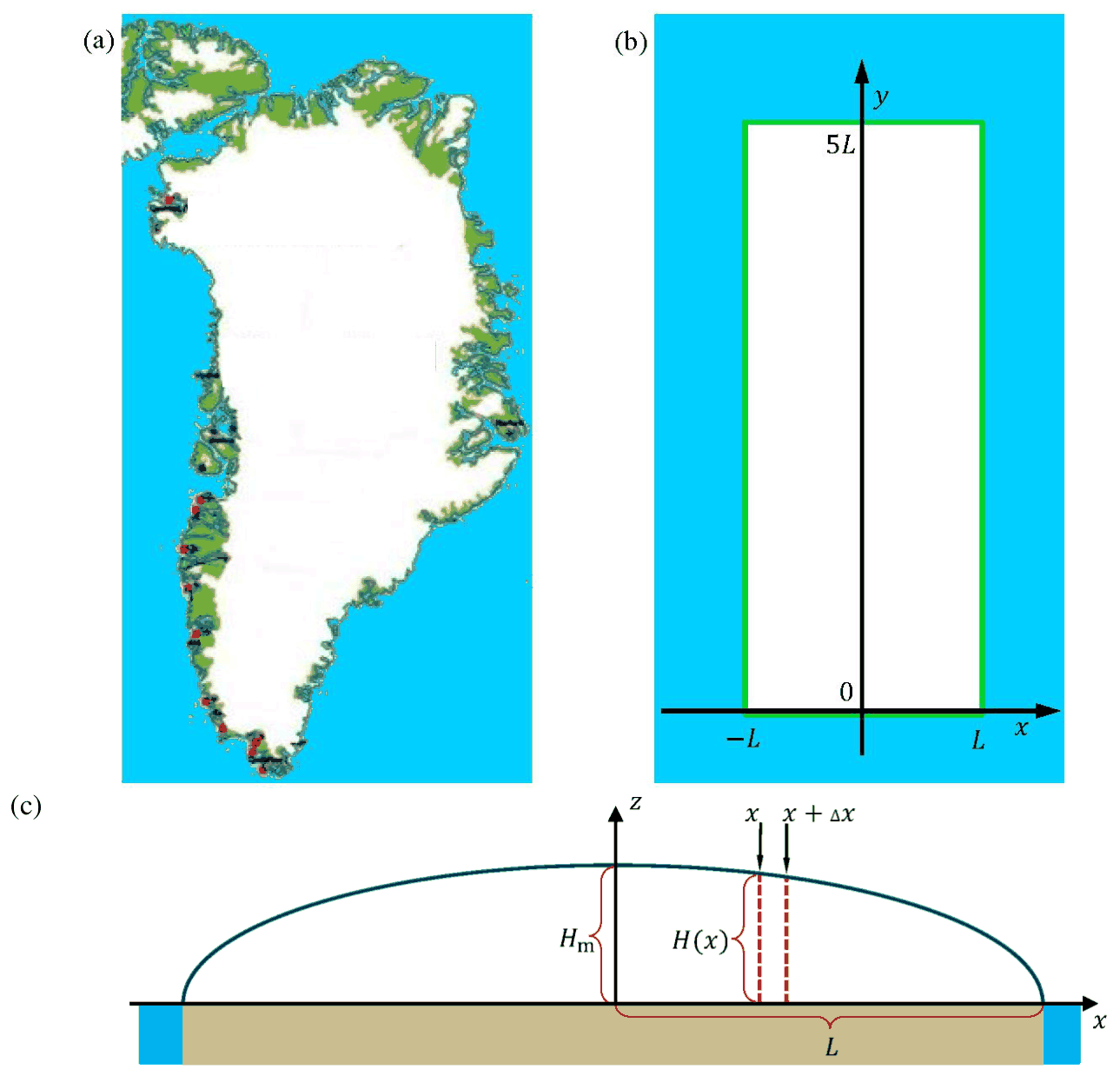
Figure 3.1 (a) A map of Greenland showing the extent of the ice sheet (white), the ice-free, coastal regions (green), and the surrounding ocean (blue). (b) The crude model of the Greenlandic ice sheet as covering a rectangular area in the \(xy\)-plane with side lengths \(2L\) and \(5L\). The ice divide, the line of maximum ice sheet height \(H_{\mathrm m}\) runs along the \(y\)-axis. (c) A vertical cut (\(xz\)-plane) through the ice sheet showing the height profile \(H(x)\) (blue line). \(H(x)\) is independent of the \(y\)-coordinate for \(0<y<5L\), while it drops abruptly to zero at \(y=0\) and \(y=5L\). The \(z\)-axis marks the position of the ice divide. For clarity, the vertical dimensions are expanded compared to the horizontal dimensions. The density \(\rho_{\mathrm{ice}}\) of ice is constant.
Two useful formulas
In this problem you can make use of the integral:
\[ \int_0^1\sqrt{1-x}\,\mathrm dx=\frac23 \]
and the approximation \((1+x)^\alpha\approx1+\alpha x\), valid for \(|\alpha x|\ll1\).
The height profile of the ice sheet
On short time scales the glacier is an incompressible hydrostatic system with fixed height profile \(H(x)\).
| 3.1 | Write down an expression for the pressure \(p(x,z)\) inside the ice sheet as a function of vertical height \(z\) above the ground and distance \(x\) from the ice divide. Neglect the atmospheric pressure. | 0.3 |
Consider a given vertical slab of the ice sheet in equilibrium, covering a small horizontal base area \(\Delta x\Delta y\) between \(x\) and \(x+\Delta x\), see the red dashed lines in Fig. 3.1(c). The size of \(\Delta y\) does not matter. The net horizontal force component \(\Delta F\) on the two vertical sides of the slab, arising from the difference in height on the center-side versus the coastal-side of the slab, is balanced by a friction force \(\Delta F=S_{\mathrm b}\Delta x\Delta y\) from the ground on the base area \(\Delta x\Delta y\), where \(S_{\mathrm b}=100\ \mathrm{kPa}\).
| 3.2a | For a given value of \(x\), show that in the limit \(\Delta x\rightarrow0\), \(S_{\mathrm b}=kH\,\mathrm dH/\mathrm dx\), and determine \(k\). | 0.9 |
| 3.2b | Determine an expression for the height profile \(H(x)\) in terms of \(\rho_{\mathrm{ice}}\), \(g\), \(L\), \(S_{\mathrm b}\) and distance \(x\) from the divide. The result will show that the maximum glacier height \(H_{\mathrm m}\) scales with the half-width \(L\) as \(H_{\mathrm m}\propto L^{1/2}\). | 0.8 |
| 3.2c | Determine the exponent \(\gamma\) with which the total volume \(V_{\mathrm{ice}}\) of the ice sheet scales with the area \(A\) of the rectangular island, \(V_{\mathrm{ice}}\propto A^\gamma\). | 0.5 |
A dynamical ice sheet
On longer time scale, the ice is a viscous incompressible fluid, which by gravity flows from the center part to the coast. In this model, the ice maintains its height profile \(H(x)\) in a steady state, where accumulation of ice due to snowfall in the central region is balanced by melting at the coast. In addition to the ice sheet geometry of Fig. 3.1(b) and (c) make the following model assumptions:
1) Ice flows in the \(xz\)-plane away from the ice divide (the \(y\)-axis). 2) The accumulation rate \(c\) (m/year) in the central region is a constant. 3) Ice can only leave the glacier by melting near the coasts at \(x=\pm L\). 4) The horizontal (\(x\)-)component \(v_x(x)=\mathrm dx/\mathrm dt\) of the ice-flow velocity is independent of \(z\). 5) The vertical (\(z\)-)component \(v_z(z)=\mathrm dz/\mathrm dt\) of the ice-flow velocity is independent of \(x\).
Consider only the central region \(|x|\ll L\) close to the middle of the ice sheet, where height variations of the ice sheet are very small and can be neglected altogether, i.e. \(H(x)\approx H_{\mathrm m}\).
| 3.3 | Use mass conservation to find an expression for the horizontal ice-flow velocity \(v_x(x)\) in terms of \(c\), \(x\), and \(H_{\mathrm m}\). | 0.6 |
From the assumption of incompressibility, i.e. the constant density \(\rho_{\mathrm{ice}}\) of the ice, it follows that mass conservation implies the following restriction on the ice flow velocity components
\[ \frac{\mathrm dv_x}{\mathrm dx}+\frac{\mathrm dv_z}{\mathrm dz}=0. \]
| 3.4 | Write down an expression for the \(z\) dependence of the vertical component \(v_z(z)\) of the ice-flow velocity. | 0.6 |
A small ice particle with the initial surface position \((x_i,H_{\mathrm m})\) will, as time passes, flow as part of the ice sheet along a flow trajectory \(z(x)\) in the vertical \(xz\)-plane.
| 3.5 | Derive an expression for such a flow trajectory \(z(x)\). | 0.9 |
Age and climate indicators in the dynamical ice sheet
Based on the ice-flow velocity components \(v_x(x)\) and \(v_z(z)\), one can estimate the age \(\tau(z)\) of the ice in a specific depth \(H_{\mathrm m}-z\) from the surface of the ice sheet.
| 3.6 | Find an expression for the age \(\tau(z)\) of the ice as a function of height \(z\) above ground, right at the ice divide \(x=0\). | 1.0 |
An ice core drilled in the interior of the Greenlandic ice sheet will penetrate through layers of snow from the past, and the ice core can be analyzed to reveal past climate changes. One of the best indicators is the so-called \(\delta^{18}\mathrm O\), defined as
\[ \delta^{18}\mathrm O =\frac{R_{\mathrm{ice}}-R_{\mathrm{ref}}}{R_{\mathrm{ref}}}\,1000\ \text{‰}, \]
where \(R=[{}^{18}\mathrm O]/[{}^{16}\mathrm O]\) denotes the relative abundance of the two stable isotopes \({}^{18}\mathrm O\) and \({}^{16}\mathrm O\) of oxygen. The reference \(R_{\mathrm{ref}}\) is based on the isotopic composition of the oceans around Equator.
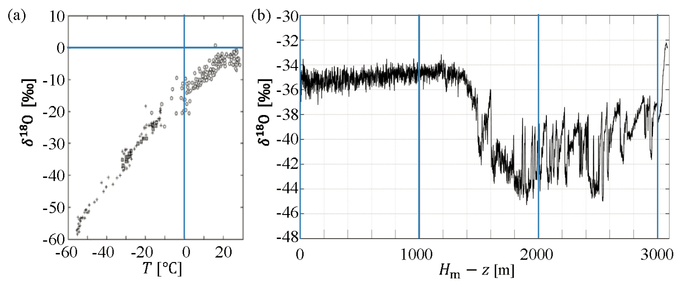
Figure 3.2 (a) Observed relationship between \(\delta^{18}\mathrm O\) in snows versus the mean annual surface temperature \(T\). (b) Measurements of \(\delta^{18}\mathrm O\) versus depth \(H_{\mathrm m}-z\) from the surface, taken from an ice core drilled from surface to bedrock at a specific place along the Greenlandic ice divide where \(H_{\mathrm m}=3060\ \mathrm m\).
Observations from the Greenland ice sheet show that \(\delta^{18}\mathrm O\) in the snow varies approximately linearly with temperature, Fig. 3.2(a). Assuming that this has always been the case, \(\delta^{18}\mathrm O\) retrieved from an ice core at depth \(H_{\mathrm m}-z\) leads to an estimate of the temperature \(T\) near Greenland at the age \(\tau(z)\).
Measurements of \(\delta^{18}\mathrm O\) in a 3060 m long Greenlandic ice core show an abrupt change in \(\delta^{18}\mathrm O\) at a depth of 1492 m, Fig. 3.2(b), marking the end of the last ice age. The ice age began 120,000 years ago, corresponding to a depth of 3040 m, and the current interglacial age began 11,700 years ago, corresponding to a depth of 1492 m. Assume that these two periods can be described by two different accumulation rates, \(c_{\mathrm{ia}}\) (ice age) and \(c_{\mathrm{ig}}\) (interglacial age), respectively. You can assume \(H_{\mathrm m}\) to be constant throughout these 120,000 years.
| 3.7a | Determine the accumulation rates \(c_{\mathrm{ia}}\) and \(c_{\mathrm{ig}}\). | 0.8 |
| 3.7b | Use the data in Fig. 3.2 to find the temperature change at the transition from the ice age to the interglacial age. | 0.2 |
Sea level rise from melting of the Greenland ice sheet
A complete melting of the Greenlandic ice sheet will cause a sea level rise in the global ocean. As a crude estimate of this sea level rise, one may simply consider a uniform rise throughout a global ocean with constant area \(A_{\mathrm O}=3.61\times10^{14}\ \mathrm{m^2}\).
| 3.8 | Calculate the average global sea level rise, which would result from a complete melting of the Greenlandic ice sheet, given its present area of \(A_{\mathrm G}=1.71\times10^{12}\ \mathrm{m^2}\) and \(S_{\mathrm b}=100\ \mathrm{kPa}\). | 0.6 |
The massive Greenland ice sheet exerts a gravitational pull on the surrounding ocean. If the ice sheet melts, this local high tide is lost and the sea level will drop close to Greenland, an effect which partially counteracts the sea level rise calculated above.
To estimate the magnitude of this gravitational pull on the water, the Greenlandic ice sheet is now modeled as a point mass located at the ground level and having the total mass of the Greenlandic ice sheet. Copenhagen lies at a distance of 3500 km along the Earth surface from the center of the point mass. One may consider the Earth, without the point mass, to be spherically symmetric and having a global ocean spread out over the entire surface of the Earth of area \(A_{\mathrm E}=5.10\times10^{14}\ \mathrm{m^2}\). All effects of rotation of the Earth may be neglected.
| 3.9 | Within this model, determine the difference \(h_{\mathrm{CPH}}-h_{\mathrm{OPP}}\) between sea levels in Copenhagen (\(h_{\mathrm{CPH}}\)) and diametrically opposite to Greenland (\(h_{\mathrm{OPP}}\)). | 1.8 |
Data sheet: Table of physical parameters
| Speed of light in vacuum | \(c=2.998\times10^8\ \mathrm{m\,s^{-1}}\) |
| Planck's constant over \(2\pi\) | \(\hbar=1.055\times10^{-34}\ \mathrm{J\,s}\) |
| Gravitational constant | \(G=6.67\times10^{-11}\ \mathrm{m^3\,kg^{-1}\,s^{-2}}\) |
| Gravitational acceleration | \(g=9.82\ \mathrm{m\,s^{-2}}\) |
| Elementary charge | \(e=1.602\times10^{-19}\ \mathrm C\) |
| Dielectric permittivity of vacuum | \(\epsilon_0=8.854\times10^{-12}\ \mathrm{C^2\,J^{-1}\,m^{-1}}\) |
| Electron mass | \(m_e=9.109\times10^{-31}\ \mathrm{kg}\) |
| Avogadro constant | \(N_{\mathrm A}=6.022\times10^{23}\ \mathrm{mol^{-1}}\) |
| Boltzmann constant | \(k_{\mathrm B}=1.381\times10^{-23}\ \mathrm{J\,K^{-1}}\) |
| Stony meteorite, specific heat | \(c_{\mathrm{sm}}=1.2\times10^3\ \mathrm{J\,kg^{-1}\,K^{-1}}\) |
| Stony meteorite, thermal conductivity | \(k_{\mathrm{sm}}=2.0\ \mathrm{W\,m^{-1}\,K^{-1}}\) |
| Stony meteorite, density | \(\rho_{\mathrm{sm}}=3.3\times10^3\ \mathrm{kg\,m^{-3}}\) |
| Stony meteorite, melting point | \(T_{\mathrm{sm}}=1.7\times10^3\ \mathrm K\) |
| Stony meteorite, specific melting heat | \(L_{\mathrm{sm}}=2.6\times10^5\ \mathrm{J\,kg^{-1}}\) |
| Silver, molar mass | \(M_{\mathrm{Ag}}=1.079\times10^{-1}\ \mathrm{kg\,mol^{-1}}\) |
| Silver, density | \(\rho_{\mathrm{Ag}}=1.049\times10^4\ \mathrm{kg\,m^{-3}}\) |
| Silver, specific heat capacity | \(c_{\mathrm{Ag}}=2.40\times10^2\ \mathrm{J\,kg^{-1}\,K^{-1}}\) |
| Water, molar mass | \(M_{\mathrm{wa}}=1.801\times10^{-2}\ \mathrm{kg\,mol^{-1}}\) |
| Water, density | \(\rho_{\mathrm{wa}}=0.998\times10^3\ \mathrm{kg\,m^{-3}}\) |
| Water, specific heat capacity | \(c_{\mathrm{wa}}=4.181\times10^3\ \mathrm{J\,kg^{-1}\,K^{-1}}\) |
| Water, heat of vaporization | \(L_{\mathrm{wa}}=2.260\times10^6\ \mathrm{J\,kg^{-1}}\) |
| Water, boiling temperature | \(T_{100}=100\,^\circ\mathrm C=373.15\ \mathrm K\) |
| Ice, density of glacier | \(\rho_{\mathrm{ice}}=0.917\times10^3\ \mathrm{kg\,m^{-3}}\) |
| Steam, specific heat capacity | \(c_{\mathrm{st}}=2.080\times10^3\ \mathrm{J\,kg^{-1}\,K^{-1}}\) |
| Earth, mass of the | \(m_{\mathrm E}=5.97\times10^{24}\ \mathrm{kg}\) |
| Earth, radius of the | \(R_{\mathrm E}=6.38\times10^6\ \mathrm m\) |
| Sun, mass of the | \(m_{\mathrm S}=1.99\times10^{30}\ \mathrm{kg}\) |
| Sun, radius of the | \(R_{\mathrm S}=6.96\times10^8\ \mathrm m\) |
| Average Sun-Earth distance | \(a_{\mathrm E}=1.50\times10^{11}\ \mathrm m\) |
Official English text of the problem.
Answers
- 3.1: \(\displaystyle p(x,z)=\rho_{\mathrm{ice}}g[H(x)-z]\), for \(0\le z\le H(x)\).
- 3.2a: \(\displaystyle S_{\mathrm b}=-\rho_{\mathrm{ice}}gH\frac{\mathrm dH}{\mathrm dx}\), so \(\boxed{k=-\rho_{\mathrm{ice}}g}\) on the \(x>0\) half.
- 3.2b: \(\displaystyle \boxed{H(x)=\sqrt{\frac{2S_{\mathrm b}}{\rho_{\mathrm{ice}}g}(L-|x|)}}\), with \(\displaystyle H_{\mathrm m}=\sqrt{\frac{2S_{\mathrm b}L}{\rho_{\mathrm{ice}}g}}\).
- 3.2c: \(\boxed{\gamma=\tfrac54}\); specifically, \(\displaystyle V_{\mathrm{ice}}=\frac23 AH_{\mathrm m}\).
- 3.3: \(\displaystyle \boxed{v_x(x)=\frac{c}{H_{\mathrm m}}x}\).
- 3.4: \(\displaystyle \boxed{v_z(z)=-\frac{c}{H_{\mathrm m}}z}\).
- 3.5: \(\displaystyle \boxed{z(x)=H_{\mathrm m}\frac{x_i}{x}}\) for \(x_i\ne0\). For \(x_i=0\), the trajectory is vertical along \(x=0\).
- 3.6: \(\displaystyle \boxed{\tau(z)=\frac{H_{\mathrm m}}c\ln\!\frac{H_{\mathrm m}}z}\).
- 3.7a: \(\displaystyle \boxed{c_{\mathrm{ia}}=0.123\ \mathrm{m/year},\qquad c_{\mathrm{ig}}=0.175\ \mathrm{m/year}}\).
- 3.7b: \(\boxed{\Delta T\approx+10\ \mathrm K}\), approximately \(10\,^\circ\mathrm C\) of warming.
- 3.8: \(\boxed{\Delta h_{\mathrm{mean}}\approx8.8\ \mathrm m}\).
- 3.9: \(\displaystyle \boxed{h_{\mathrm{CPH}}-h_{\mathrm{OPP}}\approx4.5\ \mathrm m}\), with Copenhagen higher.
Solution
3.1
Hydrostatic balance in the vertical direction gives
\[ \frac{\partial p}{\partial z}=-\rho_{\mathrm{ice}}g. \]
The pressure at the surface is zero when atmospheric pressure is neglected:
\[ p(x,H(x))=0. \]
Integrating downward from the surface therefore gives
\[ \boxed{p(x,z)=\rho_{\mathrm{ice}}g[H(x)-z]}. \]
3.2a
Consider the right-hand half of the ice sheet, \(x>0\). The pressure force on a vertical face of height \(H(x)\) and width \(\Delta y\) is
\[ F(x)=\Delta y\int_0^{H(x)} \rho_{\mathrm{ice}}g[H(x)-z]\,\mathrm dz =\frac12\rho_{\mathrm{ice}}gH(x)^2\Delta y. \]
The force on the center-side face acts toward increasing \(x\), while that on the coastal-side face acts toward decreasing \(x\). Their resultant is
\[ \Delta F =\frac12\rho_{\mathrm{ice}}g \left[H(x)^2-H(x+\Delta x)^2\right]\Delta y. \]
To first order in \(\Delta x\),
\[ \Delta F =-\rho_{\mathrm{ice}}gH(x)\frac{\mathrm dH}{\mathrm dx} \,\Delta x\Delta y. \]
Balancing this outward force against the basal friction \(S_{\mathrm b}\Delta x\Delta y\) yields
\[ \boxed{S_{\mathrm b} =-\rho_{\mathrm{ice}}gH\frac{\mathrm dH}{\mathrm dx}}, \qquad \boxed{k=-\rho_{\mathrm{ice}}g}. \]
The derivative is negative on this half, so \(S_{\mathrm b}>0\), as required. On either half, the corresponding magnitude relation is \(S_{\mathrm b}=\rho_{\mathrm{ice}}gH|\mathrm dH/\mathrm dx|\).
3.2b
On \(0\le x\le L\), the result above can be written
\[ \frac{\mathrm d(H^2)}{\mathrm dx} =-\frac{2S_{\mathrm b}}{\rho_{\mathrm{ice}}g}. \]
Using the coastal boundary condition \(H(L)=0\),
\[ H(x)^2=\frac{2S_{\mathrm b}}{\rho_{\mathrm{ice}}g}(L-x). \]
Reflection about the ice divide gives the complete profile:
\[ \boxed{ H(x)=\sqrt{\frac{2S_{\mathrm b}}{\rho_{\mathrm{ice}}g}(L-|x|)} },\qquad -L\le x\le L. \]
At the divide,
\[ \boxed{ H_{\mathrm m}=\sqrt{\frac{2S_{\mathrm b}L}{\rho_{\mathrm{ice}}g}} }, \]
so \(H_{\mathrm m}\propto L^{1/2}\) when the basal friction, density, and gravitational acceleration are fixed.
3.2c
The island area is
\[ A=(2L)(5L)=10L^2. \]
Since the profile is independent of \(y\), the ice volume is
\[ V_{\mathrm{ice}} =5L\int_{-L}^{L}H(x)\,\mathrm dx =10L H_{\mathrm m}\int_0^L \sqrt{1-\frac{x}{L}}\,\mathrm dx. \]
With \(u=x/L\), the supplied integral gives
\[ V_{\mathrm{ice}} =10L^2H_{\mathrm m}\int_0^1\sqrt{1-u}\,\mathrm du =\frac{20}{3}L^2H_{\mathrm m} =\boxed{\frac23 AH_{\mathrm m}}. \]
Thus
\[ V_{\mathrm{ice}}\propto L^{2+1/2} =L^{5/2} \propto A^{5/4}, \]
and
\[ \boxed{\gamma=\frac54}. \]
3.3
Take a central control volume between the divide and a position \(x>0\), with width \(\Delta y\). In steady state, the accumulation over its surface must equal its horizontal outflow.
The accumulated mass per unit time is
\[ \dot m_{\mathrm{in}} =\rho_{\mathrm{ice}}cx\Delta y. \]
There is no horizontal flow through the divide by symmetry. Since \(v_x\) is independent of height, the outflow through the face at \(x\) is
\[ \dot m_{\mathrm{out}} =\rho_{\mathrm{ice}}v_x(x)H_{\mathrm m}\Delta y. \]
Equating these gives
\[ \boxed{v_x(x)=\frac{c}{H_{\mathrm m}}x}. \]
The same signed expression applies for \(x<0\), where the flow is toward negative \(x\). This result uses the central-region approximation \(H(x)\approx H_{\mathrm m}\).
3.4
Incompressibility requires
\[ \frac{\mathrm dv_z}{\mathrm dz} =-\frac{\mathrm dv_x}{\mathrm dx} =-\frac{c}{H_{\mathrm m}}. \]
Integration gives
\[ v_z(z)=-\frac{c}{H_{\mathrm m}}z+C. \]
There is no flow through the ground, so \(v_z(0)=0\), implying \(C=0\). Therefore,
\[ \boxed{v_z(z)=-\frac{c}{H_{\mathrm m}}z}. \]
In particular, \(v_z(H_{\mathrm m})=-c\): downward motion at the surface balances the addition of new ice.
3.5
For a particle with \(x_i\ne0\), its trajectory satisfies
\[ \frac{\mathrm dz}{\mathrm dx} =\frac{\mathrm dz/\mathrm dt}{\mathrm dx/\mathrm dt} =\frac{v_z}{v_x} =-\frac zx. \]
Separating variables and applying the initial condition \(z(x_i)=H_{\mathrm m}\),
\[ \int_{H_{\mathrm m}}^z\frac{\mathrm dz'}{z'} =-\int_{x_i}^x\frac{\mathrm dx'}{x'}, \]
so
\[ \ln\frac{z}{H_{\mathrm m}} =-\ln\left|\frac{x}{x_i}\right|. \]
The particle remains on its original side of the divide; hence \(x/x_i>0\), and
\[ \boxed{xz=x_iH_{\mathrm m}}, \qquad \boxed{z(x)=H_{\mathrm m}\frac{x_i}{x}}. \]
The trajectory is a branch of a rectangular hyperbola, along which the particle moves outward and downward. Equivalently,
\[ x(t)=x_i e^{ct/H_{\mathrm m}}, \qquad z(t)=H_{\mathrm m}e^{-ct/H_{\mathrm m}}. \]
For \(x_i=0\), the particle remains at \(x=0\) and descends vertically according to the same expression for \(z(t)\). These trajectories apply while the particle remains in the central region.
3.6
At the ice divide, the horizontal velocity vanishes. The age is the elapsed time since the particle was deposited at \(z=H_{\mathrm m}\):
\[ \tau(z)=\int_{H_{\mathrm m}}^z\frac{\mathrm dz'}{v_z(z')} =-\frac{H_{\mathrm m}}c \int_{H_{\mathrm m}}^z\frac{\mathrm dz'}{z'}. \]
Therefore,
\[ \boxed{\tau(z)=\frac{H_{\mathrm m}}c \ln\frac{H_{\mathrm m}}z}. \]
This is zero at the surface and increases with depth. In this idealized model, it diverges as \(z\to0\), because the vertical velocity approaches zero at the bed.
3.7a
For this ice core, \(H_{\mathrm m}=3060\ \mathrm m\). The present heights above the bed of the two dated layers are
\[ z_1=3060-1492=1568\ \mathrm m, \]
\[ z_2=3060-3040=20\ \mathrm m. \]
The transition layer has experienced only the \(11\,700\) years of interglacial flow. Thus
\[ \ln\frac{3060}{1568} =\frac{c_{\mathrm{ig}}(11\,700\ \mathrm{year})}{3060\ \mathrm m}, \]
giving
\[ \boxed{ c_{\mathrm{ig}} =\frac{3060}{11\,700} \ln\frac{3060}{1568} =0.175\ \mathrm{m/year} }. \]
For the older layer, the accumulation rate changed during its descent. With constant \(H_{\mathrm m}\),
\[ \frac{\mathrm d\ln z}{\mathrm dt} =-\frac{c(t)}{H_{\mathrm m}}. \]
It experienced ice-age flow for
\[ 120\,000-11\,700=108\,300\ \mathrm{years}, \]
followed by interglacial flow for \(11\,700\) years. Consequently,
\[ \ln\frac{3060}{20} =\frac{ c_{\mathrm{ia}}(108\,300\ \mathrm{year}) +c_{\mathrm{ig}}(11\,700\ \mathrm{year}) }{3060\ \mathrm m}. \]
Subtracting the equation for the transition layer eliminates the interglacial contribution:
\[ \ln\frac{1568}{20} =\frac{c_{\mathrm{ia}}(108\,300\ \mathrm{year})}{3060\ \mathrm m}. \]
Hence
\[ \boxed{ c_{\mathrm{ia}} =\frac{3060}{108\,300} \ln\frac{1568}{20} =0.123\ \mathrm{m/year} }. \]
Accounting for the interglacial compression of the older ice is essential.
3.7b
Figure 3.2(b) gives representative isotope values of approximately
\[ \delta_{\mathrm{ia}}^{18}\mathrm O\approx-42\ \text{‰}, \qquad \delta_{\mathrm{ig}}^{18}\mathrm O\approx-35\ \text{‰}. \]
Thus the transition corresponds to an increase of roughly \(7\ \text{‰}\).
The approximately linear trend in Fig. 3.2(a), in the relevant temperature range, has slope about
\[ \frac{\Delta(\delta^{18}\mathrm O)}{\Delta T} \approx0.7\ \text{‰}\,\mathrm{K^{-1}}. \]
Therefore,
\[ \Delta T \approx\frac{7\ \text{‰}} {0.7\ \text{‰}\,\mathrm{K^{-1}}} \approx10\ \mathrm K. \]
The change is a warming:
\[ \boxed{T_{\mathrm{ig}}-T_{\mathrm{ia}}\approx+10\ \mathrm K}. \]
The precision is limited by the graphical readings.
3.8
Use the island geometry and height profile to determine the present model volume. Since \(A_{\mathrm G}=10L^2\),
\[ L=\sqrt{\frac{A_{\mathrm G}}{10}} =\sqrt{\frac{1.71\times10^{12}}{10}} =4.14\times10^5\ \mathrm m. \]
The maximum height predicted by the model is
\[ H_{\mathrm m} =\sqrt{\frac{2S_{\mathrm b}L}{\rho_{\mathrm{ice}}g}} =\sqrt{ \frac{2(1.00\times10^5)(4.1352\times10^5)} {(917)(9.82)} } =3.03\times10^3\ \mathrm m. \]
Using part 3.2c,
\[ V_{\mathrm{ice}} =\frac23 A_{\mathrm G}H_{\mathrm m} =3.45\times10^{15}\ \mathrm{m^3}. \]
Melting conserves mass, so the resulting water volume is
\[ V_{\mathrm{water}} =\frac{\rho_{\mathrm{ice}}}{\rho_{\mathrm{wa}}}V_{\mathrm{ice}}. \]
Spreading this water uniformly over the constant ocean area gives
\[ \Delta h_{\mathrm{mean}} =\frac{V_{\mathrm{water}}}{A_{\mathrm O}} =\frac{\rho_{\mathrm{ice}}}{\rho_{\mathrm{wa}}} \frac{2A_{\mathrm G}H_{\mathrm m}}{3A_{\mathrm O}}. \]
Numerically,
\[ \Delta h_{\mathrm{mean}} =\frac{917}{998} \frac{3.4548\times10^{15}}{3.61\times10^{14}} =8.79\ \mathrm m. \]
Thus
\[ \boxed{\Delta h_{\mathrm{mean}}\approx8.8\ \mathrm m}. \]
3.9
An ocean at rest has an equipotential free surface. We therefore compare the gravitational potentials at Copenhagen and at the point opposite Greenland.
The point mass representing the ice sheet is
\[ M=\rho_{\mathrm{ice}}V_{\mathrm{ice}} =(917)(3.4548\times10^{15}) =3.17\times10^{18}\ \mathrm{kg}. \]
Let \(R\) denote Earth’s radius and \(h\) a small sea-surface displacement from a reference sphere. Earth’s contribution to the gravitational potential per unit mass is
\[ \Phi_{\mathrm E}(R+h) =-\frac{Gm_{\mathrm E}}{R+h} \approx-\frac{Gm_{\mathrm E}}R+gh, \]
where \(h\ll R\). The ice mass contributes
\[ \Phi_{\mathrm{ice}}=-\frac{GM}{d}, \]
with \(d\) the straight-line distance to the ice mass.
To first order, \(d\) can be evaluated on the reference sphere: changes of a few metres are negligible compared with distances of millions of metres. Equal surface potentials therefore require
\[ gh_{\mathrm{CPH}}-\frac{GM}{d_{\mathrm{CPH}}} = gh_{\mathrm{OPP}}-\frac{GM}{d_{\mathrm{OPP}}}. \]
Thus
\[ h_{\mathrm{CPH}}-h_{\mathrm{OPP}} =\frac{GM}{g} \left(\frac1{d_{\mathrm{CPH}}} -\frac1{d_{\mathrm{OPP}}}\right). \]
The given \(3500\ \mathrm{km}\) is an arc length \(s\), so the central angle and chord distance are
\[ \theta=\frac{s}{R}, \qquad d_{\mathrm{CPH}}=2R\sin\frac{\theta}{2} =2R\sin\frac{s}{2R}. \]
At the opposite point,
\[ d_{\mathrm{OPP}}=2R. \]
Consequently,
\[ \boxed{ h_{\mathrm{CPH}}-h_{\mathrm{OPP}} =\frac{GM}{2gR} \left[ \frac1{\sin(s/(2R))}-1 \right] }. \]
The stated Earth area gives \(R=\sqrt{A_{\mathrm E}/(4\pi)}\approx6.37\times10^6\ \mathrm m\), consistent with the supplied radius. Using \(R=6.38\times10^6\ \mathrm m\),
\[ \theta=0.5486, \qquad d_{\mathrm{CPH}}=3.456\times10^6\ \mathrm m, \qquad d_{\mathrm{OPP}}=1.276\times10^7\ \mathrm m. \]
Hence
\[ h_{\mathrm{CPH}}-h_{\mathrm{OPP}} = \frac{(6.67\times10^{-11})(3.168\times10^{18})}{9.82} \left( \frac1{3.456\times10^6} -\frac1{1.276\times10^7} \right) =4.54\ \mathrm m. \]
Therefore,
\[ \boxed{h_{\mathrm{CPH}}-h_{\mathrm{OPP}}\approx4.5\ \mathrm m}. \]
The positive sign means that Greenland’s gravitational attraction raises the equilibrium ocean surface at Copenhagen relative to the opposite side of Earth. Any common offset needed to conserve ocean volume cancels from this difference.
The solution was checked against the official solution.
IPhO 2013 · Theorieaufgabe 3
Der grönländische Eisschild
Einleitung
Diese Aufgabe behandelt die Physik des grönländischen Eisschilds, des zweitgrößten Gletschers der Welt, Abb. 3.1(a). Als Idealisierung wird Grönland als rechteckige Insel der Breite \(2L\) und der Länge \(5L\) modelliert, deren Untergrund auf Meereshöhe liegt und vollständig von inkompressiblem Eis (konstante Dichte \(\rho_{\mathrm{ice}}\)) bedeckt ist, siehe Abb. 3.1(b). Das Höhenprofil \(H(x)\) des Eisschilds hängt nicht von der \(y\)-Koordinate ab und steigt von null an den Küsten \(x=\pm L\) bis zu einer maximalen Höhe \(H_{\mathrm m}\) entlang der mittleren Nord-Süd-Achse (der \(y\)-Achse) an, die als Eisscheide bezeichnet wird, siehe Abb. 3.1(c).
Abbildung 3.1 (a) Eine Karte Grönlands mit der Ausdehnung des Eisschilds (weiß), den eisfreien Küstenregionen (grün) und dem umgebenden Ozean (blau). (b) Das grobe Modell des grönländischen Eisschilds, der eine rechteckige Fläche in der \(xy\)-Ebene mit den Seitenlängen \(2L\) und \(5L\) bedeckt. Die Eisscheide, die Linie der maximalen Eisschildhöhe \(H_{\mathrm m}\), verläuft entlang der \(y\)-Achse. (c) Ein vertikaler Schnitt (\(xz\)-Ebene) durch den Eisschild mit dem Höhenprofil \(H(x)\) (blaue Linie). \(H(x)\) ist für \(0<y<5L\) unabhängig von der \(y\)-Koordinate, fällt jedoch bei \(y=0\) und \(y=5L\) abrupt auf null ab. Die \(z\)-Achse kennzeichnet die Lage der Eisscheide. Zur besseren Übersicht sind die vertikalen Abmessungen gegenüber den horizontalen überhöht dargestellt. Die Dichte \(\rho_{\mathrm{ice}}\) des Eises ist konstant.
Zwei nützliche Formeln
In dieser Aufgabe kann das folgende Integral verwendet werden:
\[ \int_0^1\sqrt{1-x}\,\mathrm dx=\frac23 \]
sowie die Näherung \((1+x)^\alpha\approx1+\alpha x\), die für \(|\alpha x|\ll1\) gilt.
Das Höhenprofil des Eisschilds
Auf kurzen Zeitskalen ist der Gletscher ein inkompressibles hydrostatisches System mit festem Höhenprofil \(H(x)\).
| 3.1 | Geben Sie einen Ausdruck für den Druck \(p(x,z)\) innerhalb des Eisschilds als Funktion der vertikalen Höhe \(z\) über dem Untergrund und des Abstands \(x\) von der Eisscheide an. Vernachlässigen Sie den Luftdruck. | 0.3 |
Betrachten Sie eine vertikale Scheibe des Eisschilds im Gleichgewicht, die eine kleine horizontale Grundfläche \(\Delta x\Delta y\) zwischen \(x\) und \(x+\Delta x\) bedeckt, siehe die roten gestrichelten Linien in Abb. 3.1(c). Die Größe von \(\Delta y\) spielt keine Rolle. Die resultierende horizontale Kraftkomponente \(\Delta F\) auf die beiden vertikalen Seitenflächen der Scheibe, die aus dem Höhenunterschied zwischen ihrer dem Zentrum zugewandten und ihrer der Küste zugewandten Seite entsteht, wird durch eine Reibungskraft \(\Delta F=S_{\mathrm b}\Delta x\Delta y\) ausgeglichen, die der Untergrund auf die Grundfläche \(\Delta x\Delta y\) ausübt, wobei \(S_{\mathrm b}=100\ \mathrm{kPa}\) ist.
| 3.2a | Zeigen Sie für einen gegebenen Wert von \(x\), dass im Grenzfall \(\Delta x\rightarrow0\) die Beziehung \(S_{\mathrm b}=kH\,\mathrm dH/\mathrm dx\) gilt, und bestimmen Sie \(k\). | 0.9 |
| 3.2b | Bestimmen Sie einen Ausdruck für das Höhenprofil \(H(x)\) in Abhängigkeit von \(\rho_{\mathrm{ice}}\), \(g\), \(L\), \(S_{\mathrm b}\) und dem Abstand \(x\) von der Eisscheide. Das Ergebnis wird zeigen, dass die maximale Gletscherhöhe \(H_{\mathrm m}\) mit der halben Breite \(L\) gemäß \(H_{\mathrm m}\propto L^{1/2}\) skaliert. | 0.8 |
| 3.2c | Bestimmen Sie den Exponenten \(\gamma\), mit dem das Gesamtvolumen \(V_{\mathrm{ice}}\) des Eisschilds mit der Fläche \(A\) der rechteckigen Insel skaliert, \(V_{\mathrm{ice}}\propto A^\gamma\). | 0.5 |
Ein dynamischer Eisschild
Auf längeren Zeitskalen ist das Eis eine viskose inkompressible Flüssigkeit, die unter dem Einfluss der Schwerkraft vom zentralen Bereich zur Küste fließt. In diesem Modell behält das Eis sein Höhenprofil \(H(x)\) in einem stationären Zustand bei, in dem die Akkumulation von Eis durch Schneefall im zentralen Bereich durch das Abschmelzen an der Küste ausgeglichen wird. Treffen Sie zusätzlich zur Geometrie des Eisschilds aus Abb. 3.1(b) und (c) die folgenden Modellannahmen:
1) Das Eis fließt in der \(xz\)-Ebene von der Eisscheide (der \(y\)-Achse) weg. 2) Die Akkumulationsrate \(c\) (m/Jahr) im zentralen Bereich ist konstant. 3) Das Eis kann den Gletscher nur durch Abschmelzen nahe den Küsten bei \(x=\pm L\) verlassen. 4) Die horizontale (\(x\)-)Komponente \(v_x(x)=\mathrm dx/\mathrm dt\) der Fließgeschwindigkeit des Eises ist unabhängig von \(z\). 5) Die vertikale (\(z\)-)Komponente \(v_z(z)=\mathrm dz/\mathrm dt\) der Fließgeschwindigkeit des Eises ist unabhängig von \(x\).
Betrachten Sie nur den zentralen Bereich \(|x|\ll L\) nahe der Mitte des Eisschilds, in dem die Höhenänderungen des Eisschilds sehr klein sind und vollständig vernachlässigt werden können, d. h. \(H(x)\approx H_{\mathrm m}\).
| 3.3 | Bestimmen Sie mithilfe der Massenerhaltung einen Ausdruck für die horizontale Fließgeschwindigkeit \(v_x(x)\) des Eises in Abhängigkeit von \(c\), \(x\) und \(H_{\mathrm m}\). | 0.6 |
Aus der Annahme der Inkompressibilität, d. h. der konstanten Dichte \(\rho_{\mathrm{ice}}\) des Eises, folgt, dass die Massenerhaltung die folgende Bedingung für die Komponenten der Fließgeschwindigkeit des Eises verlangt:
\[ \frac{\mathrm dv_x}{\mathrm dx}+\frac{\mathrm dv_z}{\mathrm dz}=0. \]
| 3.4 | Geben Sie einen Ausdruck für die \(z\)-Abhängigkeit der vertikalen Komponente \(v_z(z)\) der Fließgeschwindigkeit des Eises an. | 0.6 |
Ein kleines Eisteilchen, das sich anfangs an der Oberfläche an der Position \((x_i,H_{\mathrm m})\) befindet, bewegt sich im Laufe der Zeit als Teil des Eisschilds entlang einer Bahnkurve \(z(x)\) in der vertikalen \(xz\)-Ebene.
| 3.5 | Leiten Sie einen Ausdruck für eine solche Bahnkurve \(z(x)\) her. | 0.9 |
Alter und Klimaindikatoren im dynamischen Eisschild
Anhand der Komponenten \(v_x(x)\) und \(v_z(z)\) der Fließgeschwindigkeit des Eises lässt sich das Alter \(\tau(z)\) des Eises in einer bestimmten Tiefe \(H_{\mathrm m}-z\) unter der Oberfläche des Eisschilds abschätzen.
| 3.6 | Bestimmen Sie einen Ausdruck für das Alter \(\tau(z)\) des Eises als Funktion der Höhe \(z\) über dem Untergrund direkt an der Eisscheide \(x=0\). | 1.0 |
Eine Eiskernbohrung im Inneren des grönländischen Eisschilds durchdringt Schneeschichten aus der Vergangenheit, und der Eiskern kann untersucht werden, um vergangene Klimaveränderungen zu erschließen. Einer der besten Indikatoren ist das sogenannte \(\delta^{18}\mathrm O\), das wie folgt definiert ist:
\[ \delta^{18}\mathrm O =\frac{R_{\mathrm{ice}}-R_{\mathrm{ref}}}{R_{\mathrm{ref}}}\,1000\ \text{‰}, \]
wobei \(R=[{}^{18}\mathrm O]/[{}^{16}\mathrm O]\) das Häufigkeitsverhältnis der beiden stabilen Sauerstoffisotope \({}^{18}\mathrm O\) und \({}^{16}\mathrm O\) bezeichnet. Der Referenzwert \(R_{\mathrm{ref}}\) beruht auf der Isotopenzusammensetzung der Ozeane in der Äquatorregion.
Abbildung 3.2 (a) Beobachteter Zusammenhang zwischen \(\delta^{18}\mathrm O\) im Schnee und der mittleren jährlichen Oberflächentemperatur \(T\). (b) Messwerte von \(\delta^{18}\mathrm O\) in Abhängigkeit von der Tiefe \(H_{\mathrm m}-z\) unter der Oberfläche, gewonnen aus einem Eiskern, der an einer bestimmten Stelle entlang der grönländischen Eisscheide mit \(H_{\mathrm m}=3060\ \mathrm m\) von der Oberfläche bis zum Felsuntergrund erbohrt wurde.
Beobachtungen am grönländischen Eisschild zeigen, dass sich \(\delta^{18}\mathrm O\) im Schnee annähernd linear mit der Temperatur ändert, Abb. 3.2(a). Unter der Annahme, dass dies schon immer der Fall war, ermöglicht das aus einem Eiskern in der Tiefe \(H_{\mathrm m}-z\) bestimmte \(\delta^{18}\mathrm O\) eine Abschätzung der Temperatur \(T\) in der Nähe Grönlands vor \(\tau(z)\) Jahren.
Messungen von \(\delta^{18}\mathrm O\) in einem 3060 m langen grönländischen Eiskern zeigen in einer Tiefe von 1492 m eine abrupte Änderung von \(\delta^{18}\mathrm O\), Abb. 3.2(b), die das Ende der letzten Eiszeit markiert. Die Eiszeit begann vor 120.000 Jahren, was einer Tiefe von 3040 m entspricht, und die gegenwärtige Warmzeit begann vor 11.700 Jahren, was einer Tiefe von 1492 m entspricht. Nehmen Sie an, dass diese beiden Zeiträume durch zwei unterschiedliche Akkumulationsraten, \(c_{\mathrm{ia}}\) (Eiszeit) beziehungsweise \(c_{\mathrm{ig}}\) (Warmzeit), beschrieben werden können. Sie können annehmen, dass \(H_{\mathrm m}\) während dieser gesamten 120.000 Jahre konstant war.
| 3.7a | Bestimmen Sie die Akkumulationsraten \(c_{\mathrm{ia}}\) und \(c_{\mathrm{ig}}\). | 0.8 |
| 3.7b | Bestimmen Sie mithilfe der Daten in Abb. 3.2 die Temperaturänderung beim Übergang von der Eiszeit zur Warmzeit. | 0.2 |
Meeresspiegelanstieg durch das Abschmelzen des grönländischen Eisschilds
Ein vollständiges Abschmelzen des grönländischen Eisschilds wird einen Anstieg des Meeresspiegels im Weltmeer verursachen. Als grobe Abschätzung dieses Meeresspiegelanstiegs kann man einfach einen gleichmäßigen Anstieg im gesamten Weltmeer mit konstanter Fläche \(A_{\mathrm O}=3.61\times10^{14}\ \mathrm{m^2}\) betrachten.
| 3.8 | Berechnen Sie den mittleren globalen Meeresspiegelanstieg, der sich aus einem vollständigen Abschmelzen des grönländischen Eisschilds ergeben würde, wenn seine gegenwärtige Fläche \(A_{\mathrm G}=1.71\times10^{12}\ \mathrm{m^2}\) und \(S_{\mathrm b}=100\ \mathrm{kPa}\) gegeben sind. | 0.6 |
Der massereiche grönländische Eisschild übt eine Gravitationsanziehung auf den umgebenden Ozean aus. Wenn der Eisschild schmilzt, entfällt diese lokale Anhebung des Meeresspiegels, und der Meeresspiegel in der Nähe Grönlands sinkt. Dieser Effekt wirkt dem oben berechneten Meeresspiegelanstieg teilweise entgegen.
Um die Größe dieser Gravitationsanziehung auf das Wasser abzuschätzen, wird der grönländische Eisschild nun als Punktmasse auf Höhe des Untergrunds modelliert, deren Masse gleich der Gesamtmasse des grönländischen Eisschilds ist. Kopenhagen liegt entlang der Erdoberfläche in einer Entfernung von 3500 km vom Zentrum der Punktmasse. Die Erde ohne die Punktmasse kann als kugelsymmetrisch betrachtet werden, mit einem globalen Ozean, der die gesamte Erdoberfläche mit der Fläche \(A_{\mathrm E}=5.10\times10^{14}\ \mathrm{m^2}\) bedeckt. Alle Auswirkungen der Erdrotation können vernachlässigt werden.
| 3.9 | Bestimmen Sie im Rahmen dieses Modells die Differenz \(h_{\mathrm{CPH}}-h_{\mathrm{OPP}}\) zwischen dem Meeresspiegel in Kopenhagen (\(h_{\mathrm{CPH}}\)) und dem Meeresspiegel am Grönland diametral gegenüberliegenden Punkt (\(h_{\mathrm{OPP}}\)). | 1.8 |
Datenblatt: Tabelle physikalischer Größen
| Lichtgeschwindigkeit im Vakuum | \(c=2.998\times10^8\ \mathrm{m\,s^{-1}}\) |
| Plancksches Wirkungsquantum geteilt durch \(2\pi\) | \(\hbar=1.055\times10^{-34}\ \mathrm{J\,s}\) |
| Gravitationskonstante | \(G=6.67\times10^{-11}\ \mathrm{m^3\,kg^{-1}\,s^{-2}}\) |
| Fallbeschleunigung | \(g=9.82\ \mathrm{m\,s^{-2}}\) |
| Elementarladung | \(e=1.602\times10^{-19}\ \mathrm C\) |
| Elektrische Permittivität des Vakuums | \(\epsilon_0=8.854\times10^{-12}\ \mathrm{C^2\,J^{-1}\,m^{-1}}\) |
| Elektronenmasse | \(m_e=9.109\times10^{-31}\ \mathrm{kg}\) |
| Avogadro-Konstante | \(N_{\mathrm A}=6.022\times10^{23}\ \mathrm{mol^{-1}}\) |
| Boltzmann-Konstante | \(k_{\mathrm B}=1.381\times10^{-23}\ \mathrm{J\,K^{-1}}\) |
| Steinmeteorit, spezifische Wärmekapazität | \(c_{\mathrm{sm}}=1.2\times10^3\ \mathrm{J\,kg^{-1}\,K^{-1}}\) |
| Steinmeteorit, Wärmeleitfähigkeit | \(k_{\mathrm{sm}}=2.0\ \mathrm{W\,m^{-1}\,K^{-1}}\) |
| Steinmeteorit, Dichte | \(\rho_{\mathrm{sm}}=3.3\times10^3\ \mathrm{kg\,m^{-3}}\) |
| Steinmeteorit, Schmelztemperatur | \(T_{\mathrm{sm}}=1.7\times10^3\ \mathrm K\) |
| Steinmeteorit, spezifische Schmelzwärme | \(L_{\mathrm{sm}}=2.6\times10^5\ \mathrm{J\,kg^{-1}}\) |
| Silber, molare Masse | \(M_{\mathrm{Ag}}=1.079\times10^{-1}\ \mathrm{kg\,mol^{-1}}\) |
| Silber, Dichte | \(\rho_{\mathrm{Ag}}=1.049\times10^4\ \mathrm{kg\,m^{-3}}\) |
| Silber, spezifische Wärmekapazität | \(c_{\mathrm{Ag}}=2.40\times10^2\ \mathrm{J\,kg^{-1}\,K^{-1}}\) |
| Wasser, molare Masse | \(M_{\mathrm{wa}}=1.801\times10^{-2}\ \mathrm{kg\,mol^{-1}}\) |
| Wasser, Dichte | \(\rho_{\mathrm{wa}}=0.998\times10^3\ \mathrm{kg\,m^{-3}}\) |
| Wasser, spezifische Wärmekapazität | \(c_{\mathrm{wa}}=4.181\times10^3\ \mathrm{J\,kg^{-1}\,K^{-1}}\) |
| Wasser, spezifische Verdampfungswärme | \(L_{\mathrm{wa}}=2.260\times10^6\ \mathrm{J\,kg^{-1}}\) |
| Wasser, Siedetemperatur | \(T_{100}=100\,^\circ\mathrm C=373.15\ \mathrm K\) |
| Eis, Dichte von Gletschereis | \(\rho_{\mathrm{ice}}=0.917\times10^3\ \mathrm{kg\,m^{-3}}\) |
| Wasserdampf, spezifische Wärmekapazität | \(c_{\mathrm{st}}=2.080\times10^3\ \mathrm{J\,kg^{-1}\,K^{-1}}\) |
| Erde, Masse | \(m_{\mathrm E}=5.97\times10^{24}\ \mathrm{kg}\) |
| Erde, Radius | \(R_{\mathrm E}=6.38\times10^6\ \mathrm m\) |
| Sonne, Masse | \(m_{\mathrm S}=1.99\times10^{30}\ \mathrm{kg}\) |
| Sonne, Radius | \(R_{\mathrm S}=6.96\times10^8\ \mathrm m\) |
| Mittlerer Abstand zwischen Sonne und Erde | \(a_{\mathrm E}=1.50\times10^{11}\ \mathrm m\) |
Aufgabentext aus dem offiziellen englischen Text übersetzt.
Antworten
- 3.1: \(\displaystyle p(x,z)=\rho_{\mathrm{ice}}g[H(x)-z]\), für \(0\le z\le H(x)\).
- 3.2a: \(\displaystyle S_{\mathrm b}=-\rho_{\mathrm{ice}}gH\frac{\mathrm dH}{\mathrm dx}\), also \(\boxed{k=-\rho_{\mathrm{ice}}g}\) auf der Hälfte \(x>0\).
- 3.2b: \(\displaystyle \boxed{H(x)=\sqrt{\frac{2S_{\mathrm b}}{\rho_{\mathrm{ice}}g}(L-|x|)}}\), mit \(\displaystyle H_{\mathrm m}=\sqrt{\frac{2S_{\mathrm b}L}{\rho_{\mathrm{ice}}g}}\).
- 3.2c: \(\boxed{\gamma=\tfrac54}\); genauer gilt \(\displaystyle V_{\mathrm{ice}}=\frac23 AH_{\mathrm m}\).
- 3.3: \(\displaystyle \boxed{v_x(x)=\frac{c}{H_{\mathrm m}}x}\).
- 3.4: \(\displaystyle \boxed{v_z(z)=-\frac{c}{H_{\mathrm m}}z}\).
- 3.5: \(\displaystyle \boxed{z(x)=H_{\mathrm m}\frac{x_i}{x}}\) für \(x_i\ne0\). Für \(x_i=0\) verläuft die Bahn vertikal entlang \(x=0\).
- 3.6: \(\displaystyle \boxed{\tau(z)=\frac{H_{\mathrm m}}c\ln\!\frac{H_{\mathrm m}}z}\).
- 3.7a: \(\displaystyle \boxed{c_{\mathrm{ia}}=0.123\ \mathrm{m/year},\qquad c_{\mathrm{ig}}=0.175\ \mathrm{m/year}}\).
- 3.7b: \(\boxed{\Delta T\approx+10\ \mathrm K}\), eine Erwärmung um ungefähr \(10\,^\circ\mathrm C\).
- 3.8: \(\boxed{\Delta h_{\mathrm{mean}}\approx8.8\ \mathrm m}\).
- 3.9: \(\displaystyle \boxed{h_{\mathrm{CPH}}-h_{\mathrm{OPP}}\approx4.5\ \mathrm m}\), wobei der Meeresspiegel in Kopenhagen höher liegt.
Lösung
3.1
Das hydrostatische Gleichgewicht in vertikaler Richtung ergibt
\[ \frac{\partial p}{\partial z}=-\rho_{\mathrm{ice}}g. \]
Bei Vernachlässigung des Luftdrucks ist der Druck an der Oberfläche null:
\[ p(x,H(x))=0. \]
Die Integration von der Oberfläche nach unten liefert daher
\[ \boxed{p(x,z)=\rho_{\mathrm{ice}}g[H(x)-z]}. \]
3.2a
Betrachten Sie die rechte Hälfte des Eisschilds, \(x>0\). Die Druckkraft auf eine vertikale Seitenfläche der Höhe \(H(x)\) und der Breite \(\Delta y\) beträgt
\[ F(x)=\Delta y\int_0^{H(x)} \rho_{\mathrm{ice}}g[H(x)-z]\,\mathrm dz =\frac12\rho_{\mathrm{ice}}gH(x)^2\Delta y. \]
Die Kraft auf die dem Zentrum zugewandte Seitenfläche wirkt in Richtung zunehmender \(x\), während die Kraft auf die der Küste zugewandte Seitenfläche in Richtung abnehmender \(x\) wirkt. Ihre Resultierende ist
\[ \Delta F =\frac12\rho_{\mathrm{ice}}g \left[H(x)^2-H(x+\Delta x)^2\right]\Delta y. \]
In erster Ordnung in \(\Delta x\) gilt
\[ \Delta F =-\rho_{\mathrm{ice}}gH(x)\frac{\mathrm dH}{\mathrm dx} \,\Delta x\Delta y. \]
Das Gleichgewicht zwischen dieser nach außen gerichteten Kraft und der Reibung am Untergrund \(S_{\mathrm b}\Delta x\Delta y\) liefert
\[ \boxed{S_{\mathrm b} =-\rho_{\mathrm{ice}}gH\frac{\mathrm dH}{\mathrm dx}}, \qquad \boxed{k=-\rho_{\mathrm{ice}}g}. \]
Auf dieser Hälfte ist die Ableitung negativ, sodass wie gefordert \(S_{\mathrm b}>0\) ist. Auf beiden Hälften gilt für die Beträge die entsprechende Beziehung \(S_{\mathrm b}=\rho_{\mathrm{ice}}gH|\mathrm dH/\mathrm dx|\).
3.2b
Für \(0\le x\le L\) lässt sich das obige Ergebnis schreiben als
\[ \frac{\mathrm d(H^2)}{\mathrm dx} =-\frac{2S_{\mathrm b}}{\rho_{\mathrm{ice}}g}. \]
Mit der Randbedingung \(H(L)=0\) an der Küste folgt
\[ H(x)^2=\frac{2S_{\mathrm b}}{\rho_{\mathrm{ice}}g}(L-x). \]
Spiegelung an der Eisscheide ergibt das vollständige Profil:
\[ \boxed{ H(x)=\sqrt{\frac{2S_{\mathrm b}}{\rho_{\mathrm{ice}}g}(L-|x|)} },\qquad -L\le x\le L. \]
An der Eisscheide gilt
\[ \boxed{ H_{\mathrm m}=\sqrt{\frac{2S_{\mathrm b}L}{\rho_{\mathrm{ice}}g}} }, \]
also \(H_{\mathrm m}\propto L^{1/2}\), wenn die Reibung am Untergrund, die Dichte und die Fallbeschleunigung konstant sind.
3.2c
Die Fläche der Insel beträgt
\[ A=(2L)(5L)=10L^2. \]
Da das Profil unabhängig von \(y\) ist, beträgt das Eisvolumen
\[ V_{\mathrm{ice}} =5L\int_{-L}^{L}H(x)\,\mathrm dx =10L H_{\mathrm m}\int_0^L \sqrt{1-\frac{x}{L}}\,\mathrm dx. \]
Mit \(u=x/L\) liefert das angegebene Integral
\[ V_{\mathrm{ice}} =10L^2H_{\mathrm m}\int_0^1\sqrt{1-u}\,\mathrm du =\frac{20}{3}L^2H_{\mathrm m} =\boxed{\frac23 AH_{\mathrm m}}. \]
Somit gilt
\[ V_{\mathrm{ice}}\propto L^{2+1/2} =L^{5/2} \propto A^{5/4}, \]
und
\[ \boxed{\gamma=\frac54}. \]
3.3
Betrachten Sie im zentralen Bereich ein Kontrollvolumen zwischen der Eisscheide und einer Position \(x>0\) mit der Breite \(\Delta y\). Im stationären Zustand muss die Akkumulation auf seiner Oberfläche gleich seinem horizontalen Abfluss sein.
Die pro Zeiteinheit akkumulierte Masse beträgt
\[ \dot m_{\mathrm{in}} =\rho_{\mathrm{ice}}cx\Delta y. \]
Aus Symmetriegründen gibt es keinen horizontalen Fluss durch die Eisscheide. Da \(v_x\) unabhängig von der Höhe ist, beträgt der Massenabfluss durch die Seitenfläche bei \(x\)
\[ \dot m_{\mathrm{out}} =\rho_{\mathrm{ice}}v_x(x)H_{\mathrm m}\Delta y. \]
Gleichsetzen ergibt
\[ \boxed{v_x(x)=\frac{c}{H_{\mathrm m}}x}. \]
Derselbe vorzeichenbehaftete Ausdruck gilt für \(x<0\), wo der Fluss in Richtung negativer \(x\) erfolgt. Dieses Ergebnis verwendet die Näherung \(H(x)\approx H_{\mathrm m}\) für den zentralen Bereich.
3.4
Die Inkompressibilität erfordert
\[ \frac{\mathrm dv_z}{\mathrm dz} =-\frac{\mathrm dv_x}{\mathrm dx} =-\frac{c}{H_{\mathrm m}}. \]
Integration ergibt
\[ v_z(z)=-\frac{c}{H_{\mathrm m}}z+C. \]
Durch den Untergrund findet kein Fluss statt, daher ist \(v_z(0)=0\), woraus \(C=0\) folgt. Somit gilt
\[ \boxed{v_z(z)=-\frac{c}{H_{\mathrm m}}z}. \]
Insbesondere gilt \(v_z(H_{\mathrm m})=-c\): Die Abwärtsbewegung an der Oberfläche gleicht die Zufuhr von neuem Eis aus.
3.5
Für ein Teilchen mit \(x_i\ne0\) erfüllt seine Bahnkurve die Beziehung
\[ \frac{\mathrm dz}{\mathrm dx} =\frac{\mathrm dz/\mathrm dt}{\mathrm dx/\mathrm dt} =\frac{v_z}{v_x} =-\frac zx. \]
Durch Trennung der Variablen und Anwendung der Anfangsbedingung \(z(x_i)=H_{\mathrm m}\) folgt
\[ \int_{H_{\mathrm m}}^z\frac{\mathrm dz'}{z'} =-\int_{x_i}^x\frac{\mathrm dx'}{x'}, \]
also
\[ \ln\frac{z}{H_{\mathrm m}} =-\ln\left|\frac{x}{x_i}\right|. \]
Das Teilchen bleibt auf seiner ursprünglichen Seite der Eisscheide; daher ist \(x/x_i>0\), und es gilt
\[ \boxed{xz=x_iH_{\mathrm m}}, \qquad \boxed{z(x)=H_{\mathrm m}\frac{x_i}{x}}. \]
Die Bahnkurve ist ein Ast einer gleichseitigen Hyperbel, entlang dessen sich das Teilchen nach außen und nach unten bewegt. Gleichwertig gilt
\[ x(t)=x_i e^{ct/H_{\mathrm m}}, \qquad z(t)=H_{\mathrm m}e^{-ct/H_{\mathrm m}}. \]
Für \(x_i=0\) bleibt das Teilchen bei \(x=0\) und sinkt gemäß demselben Ausdruck für \(z(t)\) vertikal ab. Diese Bahnkurven gelten, solange das Teilchen im zentralen Bereich bleibt.
3.6
An der Eisscheide verschwindet die horizontale Geschwindigkeit. Das Alter ist die Zeit, die seit der Ablagerung des Teilchens bei \(z=H_{\mathrm m}\) vergangen ist:
\[ \tau(z)=\int_{H_{\mathrm m}}^z\frac{\mathrm dz'}{v_z(z')} =-\frac{H_{\mathrm m}}c \int_{H_{\mathrm m}}^z\frac{\mathrm dz'}{z'}. \]
Daher gilt
\[ \boxed{\tau(z)=\frac{H_{\mathrm m}}c \ln\frac{H_{\mathrm m}}z}. \]
An der Oberfläche ist dieses Alter null, und es nimmt mit der Tiefe zu. In diesem idealisierten Modell divergiert es für \(z\to0\), weil die vertikale Geschwindigkeit am Gletscherbett gegen null geht.
3.7a
Für diesen Eiskern gilt \(H_{\mathrm m}=3060\ \mathrm m\). Die gegenwärtigen Höhen der beiden datierten Schichten über dem Gletscherbett betragen
\[ z_1=3060-1492=1568\ \mathrm m, \]
\[ z_2=3060-3040=20\ \mathrm m. \]
Die Übergangsschicht hat nur die \(11\,700\) Jahre des Eisflusses während der Warmzeit durchlaufen. Somit gilt
\[ \ln\frac{3060}{1568} =\frac{c_{\mathrm{ig}}(11\,700\ \mathrm{year})}{3060\ \mathrm m}, \]
woraus folgt
\[ \boxed{ c_{\mathrm{ig}} =\frac{3060}{11\,700} \ln\frac{3060}{1568} =0.175\ \mathrm{m/year} }. \]
Für die ältere Schicht änderte sich die Akkumulationsrate während ihres Absinkens. Bei konstantem \(H_{\mathrm m}\) gilt
\[ \frac{\mathrm d\ln z}{\mathrm dt} =-\frac{c(t)}{H_{\mathrm m}}. \]
Sie war dem Eisfluss während der Eiszeit über einen Zeitraum von
\[ 120\,000-11\,700=108\,300\ \mathrm{years}, \]
ausgesetzt, gefolgt von \(11\,700\) Jahren Eisfluss während der Warmzeit. Folglich gilt
\[ \ln\frac{3060}{20} =\frac{ c_{\mathrm{ia}}(108\,300\ \mathrm{year}) +c_{\mathrm{ig}}(11\,700\ \mathrm{year}) }{3060\ \mathrm m}. \]
Durch Subtraktion der Gleichung für die Übergangsschicht entfällt der Beitrag der Warmzeit:
\[ \ln\frac{1568}{20} =\frac{c_{\mathrm{ia}}(108\,300\ \mathrm{year})}{3060\ \mathrm m}. \]
Damit ergibt sich
\[ \boxed{ c_{\mathrm{ia}} =\frac{3060}{108\,300} \ln\frac{1568}{20} =0.123\ \mathrm{m/year} }. \]
Die Kompression des älteren Eises während der Warmzeit muss unbedingt berücksichtigt werden.
3.7b
Abbildung 3.2(b) liefert repräsentative Isotopenwerte von ungefähr
\[ \delta_{\mathrm{ia}}^{18}\mathrm O\approx-42\ \text{‰}, \qquad \delta_{\mathrm{ig}}^{18}\mathrm O\approx-35\ \text{‰}. \]
Der Übergang entspricht somit einem Anstieg um etwa \(7\ \text{‰}\).
Der annähernd lineare Verlauf in Abb. 3.2(a) hat im relevanten Temperaturbereich eine Steigung von etwa
\[ \frac{\Delta(\delta^{18}\mathrm O)}{\Delta T} \approx0.7\ \text{‰}\,\mathrm{K^{-1}}. \]
Daher gilt
\[ \Delta T \approx\frac{7\ \text{‰}} {0.7\ \text{‰}\,\mathrm{K^{-1}}} \approx10\ \mathrm K. \]
Die Änderung ist eine Erwärmung:
\[ \boxed{T_{\mathrm{ig}}-T_{\mathrm{ia}}\approx+10\ \mathrm K}. \]
Die Genauigkeit ist durch das Ablesen aus den Diagrammen begrenzt.
3.8
Mithilfe der Inselgeometrie und des Höhenprofils lässt sich das gegenwärtige Volumen im Modell bestimmen. Da \(A_{\mathrm G}=10L^2\) gilt, folgt
\[ L=\sqrt{\frac{A_{\mathrm G}}{10}} =\sqrt{\frac{1.71\times10^{12}}{10}} =4.14\times10^5\ \mathrm m. \]
Die vom Modell vorhergesagte maximale Höhe beträgt
\[ H_{\mathrm m} =\sqrt{\frac{2S_{\mathrm b}L}{\rho_{\mathrm{ice}}g}} =\sqrt{ \frac{2(1.00\times10^5)(4.1352\times10^5)} {(917)(9.82)} } =3.03\times10^3\ \mathrm m. \]
Mit Teil 3.2c folgt
\[ V_{\mathrm{ice}} =\frac23 A_{\mathrm G}H_{\mathrm m} =3.45\times10^{15}\ \mathrm{m^3}. \]
Beim Schmelzen bleibt die Masse erhalten, sodass das entstehende Wasservolumen beträgt:
\[ V_{\mathrm{water}} =\frac{\rho_{\mathrm{ice}}}{\rho_{\mathrm{wa}}}V_{\mathrm{ice}}. \]
Wird dieses Wasser gleichmäßig über die konstante Ozeanfläche verteilt, ergibt sich
\[ \Delta h_{\mathrm{mean}} =\frac{V_{\mathrm{water}}}{A_{\mathrm O}} =\frac{\rho_{\mathrm{ice}}}{\rho_{\mathrm{wa}}} \frac{2A_{\mathrm G}H_{\mathrm m}}{3A_{\mathrm O}}. \]
Numerisch ergibt sich
\[ \Delta h_{\mathrm{mean}} =\frac{917}{998} \frac{3.4548\times10^{15}}{3.61\times10^{14}} =8.79\ \mathrm m. \]
Somit gilt
\[ \boxed{\Delta h_{\mathrm{mean}}\approx8.8\ \mathrm m}. \]
3.9
Die freie Oberfläche eines ruhenden Ozeans ist eine Äquipotentialfläche. Daher vergleichen wir die Gravitationspotentiale in Kopenhagen und am Grönland gegenüberliegenden Punkt.
Die Punktmasse, die den Eisschild repräsentiert, beträgt
\[ M=\rho_{\mathrm{ice}}V_{\mathrm{ice}} =(917)(3.4548\times10^{15}) =3.17\times10^{18}\ \mathrm{kg}. \]
Sei \(R\) der Erdradius und \(h\) eine kleine Verschiebung der Meeresoberfläche gegenüber einer Referenzkugel. Der Beitrag der Erde zum Gravitationspotential pro Masseneinheit ist
\[ \Phi_{\mathrm E}(R+h) =-\frac{Gm_{\mathrm E}}{R+h} \approx-\frac{Gm_{\mathrm E}}R+gh, \]
wobei \(h\ll R\) gilt. Die Eismasse liefert den Beitrag
\[ \Phi_{\mathrm{ice}}=-\frac{GM}{d}, \]
wobei \(d\) der geradlinige Abstand zur Eismasse ist.
In erster Ordnung kann \(d\) auf der Referenzkugel berechnet werden: Änderungen um wenige Meter sind gegenüber Entfernungen von Millionen Metern vernachlässigbar. Gleiche Potentiale an der Oberfläche erfordern daher
\[ gh_{\mathrm{CPH}}-\frac{GM}{d_{\mathrm{CPH}}} = gh_{\mathrm{OPP}}-\frac{GM}{d_{\mathrm{OPP}}}. \]
Somit gilt
\[ h_{\mathrm{CPH}}-h_{\mathrm{OPP}} =\frac{GM}{g} \left(\frac1{d_{\mathrm{CPH}}} -\frac1{d_{\mathrm{OPP}}}\right). \]
Die angegebenen \(3500\ \mathrm{km}\) sind eine Bogenlänge \(s\), sodass sich für den Mittelpunktswinkel und die Sehnenlänge ergibt:
\[ \theta=\frac{s}{R}, \qquad d_{\mathrm{CPH}}=2R\sin\frac{\theta}{2} =2R\sin\frac{s}{2R}. \]
Am gegenüberliegenden Punkt gilt
\[ d_{\mathrm{OPP}}=2R. \]
Folglich gilt
\[ \boxed{ h_{\mathrm{CPH}}-h_{\mathrm{OPP}} =\frac{GM}{2gR} \left[ \frac1{\sin(s/(2R))}-1 \right] }. \]
Aus der angegebenen Erdoberfläche folgt \(R=\sqrt{A_{\mathrm E}/(4\pi)}\approx6.37\times10^6\ \mathrm m\), in Übereinstimmung mit dem angegebenen Radius. Mit \(R=6.38\times10^6\ \mathrm m\) ergibt sich
\[ \theta=0.5486, \qquad d_{\mathrm{CPH}}=3.456\times10^6\ \mathrm m, \qquad d_{\mathrm{OPP}}=1.276\times10^7\ \mathrm m. \]
Damit folgt
\[ h_{\mathrm{CPH}}-h_{\mathrm{OPP}} = \frac{(6.67\times10^{-11})(3.168\times10^{18})}{9.82} \left( \frac1{3.456\times10^6} -\frac1{1.276\times10^7} \right) =4.54\ \mathrm m. \]
Daher gilt
\[ \boxed{h_{\mathrm{CPH}}-h_{\mathrm{OPP}}\approx4.5\ \mathrm m}. \]
Das positive Vorzeichen bedeutet, dass die Gravitationsanziehung Grönlands die Meeresoberfläche im Gleichgewicht bei Kopenhagen gegenüber der gegenüberliegenden Seite der Erde anhebt. Eine gemeinsame Höhenverschiebung, die zur Erhaltung des Ozeanvolumens erforderlich ist, fällt aus dieser Differenz heraus.
Die Lösung wurde mit der offiziellen Lösung abgeglichen.
IPhO 2013 · Teori sorusu 3
Grönland Buz Örtüsü
Giriş
Bu soru, dünyanın en büyük ikinci buzulu olan Grönland buz örtüsünün fiziğiyle ilgilidir, Şekil 3.1(a). İdealleştirilmiş bir modelde Grönland, genişliği \(2L\), uzunluğu \(5L\) olan, zemini deniz seviyesinde bulunan ve tamamı sıkıştırılamaz buzla (sabit yoğunluk \(\rho_{\mathrm{ice}}\)) kaplı dikdörtgen bir ada olarak ele alınır; bkz. Şekil 3.1(b). Buz örtüsünün yükseklik profili \(H(x)\), \(y\) koordinatına bağlı değildir ve \(x=\pm L\) kıyılarında sıfırdan başlayarak, buz bölümü çizgisi olarak bilinen ortadaki kuzey-güney ekseni (\(y\) ekseni) boyunca en büyük yüksekliği olan \(H_{\mathrm m}\)'ye ulaşır; bkz. Şekil 3.1(c).
Şekil 3.1 (a) Buz örtüsünün kapladığı alanı (beyaz), buzla kaplı olmayan kıyı bölgelerini (yeşil) ve çevresindeki okyanusu (mavi) gösteren Grönland haritası. (b) Grönland buz örtüsünün, \(xy\) düzleminde kenar uzunlukları \(2L\) ve \(5L\) olan dikdörtgen bir alanı kapladığı kaba model. Buz örtüsünün yüksekliğinin en büyük değeri \(H_{\mathrm m}\)'yi aldığı buz bölümü çizgisi, \(y\) ekseni boyunca uzanır. (c) Buz örtüsünün yükseklik profilini \(H(x)\) (mavi çizgi) gösteren düşey kesit (\(xz\) düzlemi). \(H(x)\), \(0<y<5L\) için \(y\) koordinatından bağımsızdır; \(y=0\) ve \(y=5L\)'de ise aniden sıfıra düşer. \(z\) ekseni, buz bölümü çizgisinin konumunu gösterir. Daha açık görülebilmesi için düşey boyutlar yatay boyutlara göre büyütülmüştür. Buzun yoğunluğu \(\rho_{\mathrm{ice}}\) sabittir.
İki yararlı formül
Bu soruda şu integralden yararlanabilirsiniz:
\[ \int_0^1\sqrt{1-x}\,\mathrm dx=\frac23 \]
ve \((1+x)^\alpha\approx1+\alpha x\) yaklaşımını kullanabilirsiniz; bu yaklaşım \(|\alpha x|\ll1\) için geçerlidir.
Buz örtüsünün yükseklik profili
Kısa zaman ölçeklerinde buzul, yükseklik profili \(H(x)\) sabit olan sıkıştırılamaz bir hidrostatik sistemdir.
| 3.1 | Buz örtüsü içindeki basınç \(p(x,z)\) için, yerden düşey yükseklik \(z\) ve buz bölümü çizgisine uzaklık \(x\)'in fonksiyonu olarak bir ifade yazınız. Atmosfer basıncını ihmal ediniz. | 0.3 |
Buz örtüsünün dengede bulunan ve \(x\) ile \(x+\Delta x\) arasında küçük bir yatay taban alanı \(\Delta x\Delta y\)'yi kaplayan düşey bir dilimini ele alınız; bkz. Şekil 3.1(c)'deki kırmızı kesikli çizgiler. \(\Delta y\)'nin büyüklüğü önemli değildir. Dilimin merkeze bakan tarafı ile kıyıya bakan tarafı arasındaki yükseklik farkından kaynaklanan, iki düşey yüzüne etkiyen net yatay kuvvet bileşeni \(\Delta F\), zeminin \(\Delta x\Delta y\) taban alanına uyguladığı \(\Delta F=S_{\mathrm b}\Delta x\Delta y\) sürtünme kuvvetiyle dengelenir; burada \(S_{\mathrm b}=100\ \mathrm{kPa}\)'dır.
| 3.2a | Verilen bir \(x\) değeri için, \(\Delta x\rightarrow0\) limitinde \(S_{\mathrm b}=kH\,\mathrm dH/\mathrm dx\) olduğunu gösteriniz ve \(k\)'yı belirleyiniz. | 0.9 |
| 3.2b | Yükseklik profili \(H(x)\) için \(\rho_{\mathrm{ice}}\), \(g\), \(L\), \(S_{\mathrm b}\) ve buz bölümü çizgisine uzaklık \(x\) cinsinden bir ifade belirleyiniz. Sonuç, en büyük buzul yüksekliği \(H_{\mathrm m}\)'nin yarı genişlik \(L\) ile \(H_{\mathrm m}\propto L^{1/2}\) biçiminde ölçeklendiğini gösterecektir. | 0.8 |
| 3.2c | Buz örtüsünün toplam hacmi \(V_{\mathrm{ice}}\)'ın dikdörtgen adanın alanı \(A\) ile \(V_{\mathrm{ice}}\propto A^\gamma\) biçiminde ölçeklenmesindeki \(\gamma\) üssünü belirleyiniz. | 0.5 |
Dinamik bir buz örtüsü
Daha uzun zaman ölçeklerinde buz, kütleçekimi etkisiyle orta bölgeden kıyıya doğru akan, viskoz ve sıkıştırılamaz bir akışkandır. Bu modelde buz, orta bölgede kar yağışından kaynaklanan buz birikiminin kıyıdaki erimeyle dengelendiği kararlı durumda yükseklik profilini \(H(x)\) korur. Şekil 3.1(b) ve (c)'deki buz örtüsü geometrisine ek olarak model için aşağıdaki varsayımları yapınız:
1) Buz, \(xz\) düzleminde buz bölümü çizgisinden (\(y\) ekseninden) uzaklaşacak biçimde akar. 2) Orta bölgedeki birikim hızı \(c\) (m/yıl) sabittir. 3) Buz, buzuldan yalnızca \(x=\pm L\) kıyılarının yakınında eriyerek ayrılabilir. 4) Buzun akış hızının yatay (\(x\)) bileşeni \(v_x(x)=\mathrm dx/\mathrm dt\), \(z\)'den bağımsızdır. 5) Buzun akış hızının düşey (\(z\)) bileşeni \(v_z(z)=\mathrm dz/\mathrm dt\), \(x\)'ten bağımsızdır.
Yalnızca buz örtüsünün ortasına yakın, yükseklik değişimlerinin çok küçük olduğu ve tamamen ihmal edilebildiği, yani \(H(x)\approx H_{\mathrm m}\) olan \(|x|\ll L\) merkez bölgesini ele alınız.
| 3.3 | Kütlenin korunumunu kullanarak yatay buz akış hızı \(v_x(x)\) için \(c\), \(x\) ve \(H_{\mathrm m}\) cinsinden bir ifade bulunuz. | 0.6 |
Sıkıştırılamazlık, yani buzun yoğunluğunun \(\rho_{\mathrm{ice}}\) sabit olması varsayımından, kütlenin korunumunun buzun akış hızı bileşenlerine şu kısıtı getirdiği sonucu çıkar:
\[ \frac{\mathrm dv_x}{\mathrm dx}+\frac{\mathrm dv_z}{\mathrm dz}=0. \]
| 3.4 | Buzun akış hızının düşey bileşeni \(v_z(z)\)'nin \(z\)'ye bağımlılığını veren bir ifade yazınız. | 0.6 |
Başlangıçta yüzeyde \((x_i,H_{\mathrm m})\) konumunda bulunan küçük bir buz parçacığı, zaman geçtikçe buz örtüsünün bir parçası olarak düşey \(xz\) düzlemindeki bir akış yörüngesi \(z(x)\) boyunca hareket eder.
| 3.5 | Böyle bir akış yörüngesi \(z(x)\) için bir ifade türetiniz. | 0.9 |
Dinamik buz örtüsünde yaş ve iklim göstergeleri
Buzun akış hızı bileşenleri \(v_x(x)\) ve \(v_z(z)\) kullanılarak, buz örtüsünün yüzeyinden belirli bir \(H_{\mathrm m}-z\) derinliğindeki buzun yaşı \(\tau(z)\) tahmin edilebilir.
| 3.6 | Tam buz bölümü çizgisinde, \(x=0\)'da, buzun yaşı \(\tau(z)\) için yerden yükseklik \(z\)'nin fonksiyonu olarak bir ifade bulunuz. | 1.0 |
Grönland buz örtüsünün iç kesimlerinde sondajla alınan bir buz karotu geçmişten kalan kar katmanlarını içerir ve bu karot analiz edilerek geçmiş iklim değişiklikleri ortaya çıkarılabilir. En iyi göstergelerden biri, şu şekilde tanımlanan \(\delta^{18}\mathrm O\) değeridir:
\[ \delta^{18}\mathrm O =\frac{R_{\mathrm{ice}}-R_{\mathrm{ref}}}{R_{\mathrm{ref}}}\,1000\ \text{‰}, \]
burada \(R=[{}^{18}\mathrm O]/[{}^{16}\mathrm O]\), oksijenin iki kararlı izotopu olan \({}^{18}\mathrm O\) ve \({}^{16}\mathrm O\)'nun göreli bolluğunu belirtir. Referans değeri \(R_{\mathrm{ref}}\), Ekvator çevresindeki okyanusların izotop bileşimine dayanır.
Şekil 3.2 (a) Kardaki \(\delta^{18}\mathrm O\) ile yıllık ortalama yüzey sıcaklığı \(T\) arasında gözlenen ilişki. (b) Grönland buz bölümü çizgisi üzerinde \(H_{\mathrm m}=3060\ \mathrm m\) olan belirli bir yerde yüzeyden ana kayaya kadar sondajla alınmış bir buz karotunda, yüzeyden derinlik \(H_{\mathrm m}-z\)'ye bağlı \(\delta^{18}\mathrm O\) ölçümleri.
Grönland buz örtüsündeki gözlemler, kardaki \(\delta^{18}\mathrm O\)'nun sıcaklıkla yaklaşık olarak doğrusal değiştiğini göstermektedir, Şekil 3.2(a). Bunun her zaman böyle olduğu varsayılırsa, bir buz karotunun \(H_{\mathrm m}-z\) derinliğinden elde edilen \(\delta^{18}\mathrm O\), \(\tau(z)\) yaşına karşılık gelen dönemde Grönland yakınındaki sıcaklık \(T\)'nin tahmin edilmesini sağlar.
Grönland'dan alınan 3060 m uzunluğundaki bir buz karotunda yapılan \(\delta^{18}\mathrm O\) ölçümleri, 1492 m derinlikte \(\delta^{18}\mathrm O\)'da son buzul çağının bitişini gösteren ani bir değişim ortaya koymaktadır, Şekil 3.2(b). Buzul çağı 120,000 yıl önce başlamıştır ve bu, 3040 m derinliğe karşılık gelir; günümüzdeki buzullar arası çağ ise 11,700 yıl önce başlamıştır ve bu, 1492 m derinliğe karşılık gelir. Bu iki dönemin sırasıyla iki farklı birikim hızı, \(c_{\mathrm{ia}}\) (buzul çağı) ve \(c_{\mathrm{ig}}\) (buzullar arası çağ) ile betimlenebildiğini varsayınız. Bu 120,000 yıl boyunca \(H_{\mathrm m}\)'nin sabit kaldığını varsayabilirsiniz.
| 3.7a | Birikim hızları \(c_{\mathrm{ia}}\) ve \(c_{\mathrm{ig}}\)'yi belirleyiniz. | 0.8 |
| 3.7b | Buzul çağından buzullar arası çağa geçişteki sıcaklık değişimini bulmak için Şekil 3.2'deki verileri kullanınız. | 0.2 |
Grönland buz örtüsünün erimesinden kaynaklanan deniz seviyesi yükselmesi
Grönland buz örtüsünün tamamen erimesi, dünya okyanuslarında deniz seviyesinin yükselmesine yol açacaktır. Bu deniz seviyesi yükselmesini kabaca tahmin etmek için, alanı sabit ve \(A_{\mathrm O}=3.61\times10^{14}\ \mathrm{m^2}\) olan dünya okyanuslarının tamamında aynı miktarda bir yükselme olduğu düşünülebilir.
| 3.8 | Grönland buz örtüsünün günümüzdeki alanının \(A_{\mathrm G}=1.71\times10^{12}\ \mathrm{m^2}\) ve \(S_{\mathrm b}=100\ \mathrm{kPa}\) olduğu verildiğine göre, buz örtüsünün tamamen erimesi sonucunda dünya genelinde deniz seviyesindeki ortalama yükselmeyi hesaplayınız. | 0.6 |
Grönland'ın büyük kütleli buz örtüsü, çevresindeki okyanusa kütleçekim kuvveti uygular. Buz örtüsü erirse bu yerel su kabarması ortadan kalkar ve Grönland yakınında deniz seviyesi düşer; bu etki, yukarıda hesaplanan deniz seviyesi yükselmesini kısmen dengeler.
Su üzerindeki bu kütleçekim kuvvetinin büyüklüğünü tahmin etmek için Grönland buz örtüsü şimdi zemin seviyesinde bulunan ve Grönland buz örtüsünün toplam kütlesine sahip bir noktasal kütle olarak modellenmektedir. Kopenhag, noktasal kütlenin merkezinden Dünya yüzeyi boyunca 3500 km uzaklıktadır. Noktasal kütle hariç tutulduğunda Dünya'nın küresel simetrik olduğu ve \(A_{\mathrm E}=5.10\times10^{14}\ \mathrm{m^2}\) alanlı tüm yüzeyine yayılmış bir küresel okyanusa sahip olduğu kabul edilebilir. Dünya'nın dönmesinin bütün etkileri ihmal edilebilir.
| 3.9 | Bu model çerçevesinde, Kopenhag'daki deniz seviyesi (\(h_{\mathrm{CPH}}\)) ile Grönland'ın çap doğrultusunda tam karşısındaki deniz seviyesi (\(h_{\mathrm{OPP}}\)) arasındaki \(h_{\mathrm{CPH}}-h_{\mathrm{OPP}}\) farkını belirleyiniz. | 1.8 |
Veri sayfası: Fiziksel parametreler tablosu
| Işığın boşluktaki hızı | \(c=2.998\times10^8\ \mathrm{m\,s^{-1}}\) |
| Planck sabitinin \(2\pi\)'ye bölümü | \(\hbar=1.055\times10^{-34}\ \mathrm{J\,s}\) |
| Evrensel kütleçekim sabiti | \(G=6.67\times10^{-11}\ \mathrm{m^3\,kg^{-1}\,s^{-2}}\) |
| Yerçekimi ivmesi | \(g=9.82\ \mathrm{m\,s^{-2}}\) |
| Temel yük | \(e=1.602\times10^{-19}\ \mathrm C\) |
| Boşluğun elektriksel geçirgenliği | \(\epsilon_0=8.854\times10^{-12}\ \mathrm{C^2\,J^{-1}\,m^{-1}}\) |
| Elektron kütlesi | \(m_e=9.109\times10^{-31}\ \mathrm{kg}\) |
| Avogadro sabiti | \(N_{\mathrm A}=6.022\times10^{23}\ \mathrm{mol^{-1}}\) |
| Boltzmann sabiti | \(k_{\mathrm B}=1.381\times10^{-23}\ \mathrm{J\,K^{-1}}\) |
| Taşsı göktaşının özgül ısısı | \(c_{\mathrm{sm}}=1.2\times10^3\ \mathrm{J\,kg^{-1}\,K^{-1}}\) |
| Taşsı göktaşının ısıl iletkenliği | \(k_{\mathrm{sm}}=2.0\ \mathrm{W\,m^{-1}\,K^{-1}}\) |
| Taşsı göktaşının yoğunluğu | \(\rho_{\mathrm{sm}}=3.3\times10^3\ \mathrm{kg\,m^{-3}}\) |
| Taşsı göktaşının erime noktası | \(T_{\mathrm{sm}}=1.7\times10^3\ \mathrm K\) |
| Taşsı göktaşının özgül erime ısısı | \(L_{\mathrm{sm}}=2.6\times10^5\ \mathrm{J\,kg^{-1}}\) |
| Gümüşün mol kütlesi | \(M_{\mathrm{Ag}}=1.079\times10^{-1}\ \mathrm{kg\,mol^{-1}}\) |
| Gümüşün yoğunluğu | \(\rho_{\mathrm{Ag}}=1.049\times10^4\ \mathrm{kg\,m^{-3}}\) |
| Gümüşün özgül ısı kapasitesi | \(c_{\mathrm{Ag}}=2.40\times10^2\ \mathrm{J\,kg^{-1}\,K^{-1}}\) |
| Suyun mol kütlesi | \(M_{\mathrm{wa}}=1.801\times10^{-2}\ \mathrm{kg\,mol^{-1}}\) |
| Suyun yoğunluğu | \(\rho_{\mathrm{wa}}=0.998\times10^3\ \mathrm{kg\,m^{-3}}\) |
| Suyun özgül ısı kapasitesi | \(c_{\mathrm{wa}}=4.181\times10^3\ \mathrm{J\,kg^{-1}\,K^{-1}}\) |
| Suyun buharlaşma ısısı | \(L_{\mathrm{wa}}=2.260\times10^6\ \mathrm{J\,kg^{-1}}\) |
| Suyun kaynama sıcaklığı | \(T_{100}=100\,^\circ\mathrm C=373.15\ \mathrm K\) |
| Buzul buzunun yoğunluğu | \(\rho_{\mathrm{ice}}=0.917\times10^3\ \mathrm{kg\,m^{-3}}\) |
| Su buharının özgül ısı kapasitesi | \(c_{\mathrm{st}}=2.080\times10^3\ \mathrm{J\,kg^{-1}\,K^{-1}}\) |
| Dünya'nın kütlesi | \(m_{\mathrm E}=5.97\times10^{24}\ \mathrm{kg}\) |
| Dünya'nın yarıçapı | \(R_{\mathrm E}=6.38\times10^6\ \mathrm m\) |
| Güneş'in kütlesi | \(m_{\mathrm S}=1.99\times10^{30}\ \mathrm{kg}\) |
| Güneş'in yarıçapı | \(R_{\mathrm S}=6.96\times10^8\ \mathrm m\) |
| Ortalama Güneş-Dünya uzaklığı | \(a_{\mathrm E}=1.50\times10^{11}\ \mathrm m\) |
Soru metni resmi İngilizce metinden çevrilmiştir.
Cevaplar
- 3.1: \(\displaystyle p(x,z)=\rho_{\mathrm{ice}}g[H(x)-z]\), \(0\le z\le H(x)\) için.
- 3.2a: \(\displaystyle S_{\mathrm b}=-\rho_{\mathrm{ice}}gH\frac{\mathrm dH}{\mathrm dx}\), dolayısıyla \(\boxed{k=-\rho_{\mathrm{ice}}g}\), \(x>0\) yarısında.
- 3.2b: \(\displaystyle \boxed{H(x)=\sqrt{\frac{2S_{\mathrm b}}{\rho_{\mathrm{ice}}g}(L-|x|)}}\), burada \(\displaystyle H_{\mathrm m}=\sqrt{\frac{2S_{\mathrm b}L}{\rho_{\mathrm{ice}}g}}\).
- 3.2c: \(\boxed{\gamma=\tfrac54}\); daha açık olarak, \(\displaystyle V_{\mathrm{ice}}=\frac23 AH_{\mathrm m}\).
- 3.3: \(\displaystyle \boxed{v_x(x)=\frac{c}{H_{\mathrm m}}x}\).
- 3.4: \(\displaystyle \boxed{v_z(z)=-\frac{c}{H_{\mathrm m}}z}\).
- 3.5: \(\displaystyle \boxed{z(x)=H_{\mathrm m}\frac{x_i}{x}}\), \(x_i\ne0\) için. \(x_i=0\) için yörünge \(x=0\) boyunca düşeydir.
- 3.6: \(\displaystyle \boxed{\tau(z)=\frac{H_{\mathrm m}}c\ln\!\frac{H_{\mathrm m}}z}\).
- 3.7a: \(\displaystyle \boxed{c_{\mathrm{ia}}=0.123\ \mathrm{m/year},\qquad c_{\mathrm{ig}}=0.175\ \mathrm{m/year}}\).
- 3.7b: \(\boxed{\Delta T\approx+10\ \mathrm K}\), yaklaşık \(10\,^\circ\mathrm C\) ısınma.
- 3.8: \(\boxed{\Delta h_{\mathrm{mean}}\approx8.8\ \mathrm m}\).
- 3.9: \(\displaystyle \boxed{h_{\mathrm{CPH}}-h_{\mathrm{OPP}}\approx4.5\ \mathrm m}\), Kopenhag'daki seviye daha yüksektir.
Çözüm
3.1
Düşey yöndeki hidrostatik denge şu eşitliği verir:
\[ \frac{\partial p}{\partial z}=-\rho_{\mathrm{ice}}g. \]
Atmosfer basıncı ihmal edildiğinde yüzeydeki basınç sıfırdır:
\[ p(x,H(x))=0. \]
Dolayısıyla yüzeyden aşağıya doğru integral alınırsa
\[ \boxed{p(x,z)=\rho_{\mathrm{ice}}g[H(x)-z]}. \]
3.2a
Buz örtüsünün sağ yarısını, \(x>0\) bölgesini ele alalım. Yüksekliği \(H(x)\), genişliği \(\Delta y\) olan düşey bir yüze etkiyen basınç kuvveti
\[ F(x)=\Delta y\int_0^{H(x)} \rho_{\mathrm{ice}}g[H(x)-z]\,\mathrm dz =\frac12\rho_{\mathrm{ice}}gH(x)^2\Delta y. \]
Merkeze bakan yüzdeki kuvvet artan \(x\) yönünde, kıyıya bakan yüzdeki kuvvet ise azalan \(x\) yönünde etkir. Bu kuvvetlerin bileşkesi
\[ \Delta F =\frac12\rho_{\mathrm{ice}}g \left[H(x)^2-H(x+\Delta x)^2\right]\Delta y. \]
\(\Delta x\)'e göre birinci mertebede,
\[ \Delta F =-\rho_{\mathrm{ice}}gH(x)\frac{\mathrm dH}{\mathrm dx} \,\Delta x\Delta y. \]
Dışa doğru yönelmiş bu kuvveti taban sürtünmesi \(S_{\mathrm b}\Delta x\Delta y\) ile dengelediğimizde
\[ \boxed{S_{\mathrm b} =-\rho_{\mathrm{ice}}gH\frac{\mathrm dH}{\mathrm dx}}, \qquad \boxed{k=-\rho_{\mathrm{ice}}g}. \]
Bu yarıda türev negatiftir; dolayısıyla gerektiği gibi \(S_{\mathrm b}>0\) olur. Her iki yarı için de büyüklükler arasındaki karşılık gelen bağıntı \(S_{\mathrm b}=\rho_{\mathrm{ice}}gH|\mathrm dH/\mathrm dx|\)'tir.
3.2b
\(0\le x\le L\) aralığında yukarıdaki sonuç şu şekilde yazılabilir:
\[ \frac{\mathrm d(H^2)}{\mathrm dx} =-\frac{2S_{\mathrm b}}{\rho_{\mathrm{ice}}g}. \]
Kıyıdaki \(H(L)=0\) sınır koşulu kullanılırsa
\[ H(x)^2=\frac{2S_{\mathrm b}}{\rho_{\mathrm{ice}}g}(L-x). \]
Buz bölümü çizgisine göre yansıtma, profilin tamamını verir:
\[ \boxed{ H(x)=\sqrt{\frac{2S_{\mathrm b}}{\rho_{\mathrm{ice}}g}(L-|x|)} },\qquad -L\le x\le L. \]
Buz bölümü çizgisinde,
\[ \boxed{ H_{\mathrm m}=\sqrt{\frac{2S_{\mathrm b}L}{\rho_{\mathrm{ice}}g}} }, \]
dolayısıyla taban sürtünmesi, yoğunluk ve yerçekimi ivmesi sabit olduğunda \(H_{\mathrm m}\propto L^{1/2}\) olur.
3.2c
Adanın alanı
\[ A=(2L)(5L)=10L^2. \]
Profil \(y\)'den bağımsız olduğundan buzun hacmi
\[ V_{\mathrm{ice}} =5L\int_{-L}^{L}H(x)\,\mathrm dx =10L H_{\mathrm m}\int_0^L \sqrt{1-\frac{x}{L}}\,\mathrm dx. \]
\(u=x/L\) dönüşümüyle, verilen integralden
\[ V_{\mathrm{ice}} =10L^2H_{\mathrm m}\int_0^1\sqrt{1-u}\,\mathrm du =\frac{20}{3}L^2H_{\mathrm m} =\boxed{\frac23 AH_{\mathrm m}}. \]
Böylece
\[ V_{\mathrm{ice}}\propto L^{2+1/2} =L^{5/2} \propto A^{5/4}, \]
ve
\[ \boxed{\gamma=\frac54}. \]
3.3
Merkez bölgesinde, buz bölümü çizgisi ile \(x>0\) konumu arasında genişliği \(\Delta y\) olan bir kontrol hacmi ele alalım. Kararlı durumda yüzeydeki birikim, yatay yöndeki dışarı akışa eşit olmalıdır.
Birim zamanda biriken kütle
\[ \dot m_{\mathrm{in}} =\rho_{\mathrm{ice}}cx\Delta y. \]
Simetri gereği buz bölümü çizgisinden yatay akış yoktur. \(v_x\) yükseklikten bağımsız olduğundan, \(x\) konumundaki yüzden dışarıya kütle akış hızı
\[ \dot m_{\mathrm{out}} =\rho_{\mathrm{ice}}v_x(x)H_{\mathrm m}\Delta y. \]
Bunlar eşitlenirse
\[ \boxed{v_x(x)=\frac{c}{H_{\mathrm m}}x}. \]
Aynı işaretli ifade, akışın negatif \(x\) yönünde olduğu \(x<0\) bölgesinde de geçerlidir. Bu sonuç, merkez bölgesi için \(H(x)\approx H_{\mathrm m}\) yaklaşımını kullanır.
3.4
Sıkıştırılamazlık şu koşulu gerektirir:
\[ \frac{\mathrm dv_z}{\mathrm dz} =-\frac{\mathrm dv_x}{\mathrm dx} =-\frac{c}{H_{\mathrm m}}. \]
İntegral alındığında
\[ v_z(z)=-\frac{c}{H_{\mathrm m}}z+C. \]
Zeminden akış olmadığından \(v_z(0)=0\)'dır; buradan \(C=0\) bulunur. Dolayısıyla,
\[ \boxed{v_z(z)=-\frac{c}{H_{\mathrm m}}z}. \]
Özel olarak, \(v_z(H_{\mathrm m})=-c\): yüzeydeki aşağı yönlü hareket, yeni buz eklenmesini dengeler.
3.5
\(x_i\ne0\) olan bir parçacığın yörüngesi şu eşitliği sağlar:
\[ \frac{\mathrm dz}{\mathrm dx} =\frac{\mathrm dz/\mathrm dt}{\mathrm dx/\mathrm dt} =\frac{v_z}{v_x} =-\frac zx. \]
Değişkenler ayrılıp \(z(x_i)=H_{\mathrm m}\) başlangıç koşulu uygulanırsa
\[ \int_{H_{\mathrm m}}^z\frac{\mathrm dz'}{z'} =-\int_{x_i}^x\frac{\mathrm dx'}{x'}, \]
dolayısıyla
\[ \ln\frac{z}{H_{\mathrm m}} =-\ln\left|\frac{x}{x_i}\right|. \]
Parçacık, buz bölümü çizgisinin başlangıçta bulunduğu tarafında kalır; bu nedenle \(x/x_i>0\) olur ve
\[ \boxed{xz=x_iH_{\mathrm m}}, \qquad \boxed{z(x)=H_{\mathrm m}\frac{x_i}{x}}. \]
Yörünge, parçacığın dışa ve aşağıya doğru hareket ettiği bir eşkenar hiperbol koludur. Eşdeğer olarak,
\[ x(t)=x_i e^{ct/H_{\mathrm m}}, \qquad z(t)=H_{\mathrm m}e^{-ct/H_{\mathrm m}}. \]
\(x_i=0\) için parçacık \(x=0\)'da kalır ve aynı \(z(t)\) ifadesine göre düşey olarak alçalır. Bu yörüngeler, parçacık merkez bölgesinde kaldığı sürece geçerlidir.
3.6
Buz bölümü çizgisinde yatay hız sıfırdır. Yaş, parçacığın \(z=H_{\mathrm m}\)'de birikmesinden bu yana geçen süredir:
\[ \tau(z)=\int_{H_{\mathrm m}}^z\frac{\mathrm dz'}{v_z(z')} =-\frac{H_{\mathrm m}}c \int_{H_{\mathrm m}}^z\frac{\mathrm dz'}{z'}. \]
Dolayısıyla,
\[ \boxed{\tau(z)=\frac{H_{\mathrm m}}c \ln\frac{H_{\mathrm m}}z}. \]
Bu değer yüzeyde sıfırdır ve derinlikle artar. Bu idealleştirilmiş modelde, tabanda düşey hız sıfıra yaklaştığından \(z\to0\) iken yaş sonsuza gider.
3.7a
Bu buz karotu için \(H_{\mathrm m}=3060\ \mathrm m\)'dir. Yaşları belirlenmiş iki katmanın günümüzde tabandan yükseklikleri
\[ z_1=3060-1492=1568\ \mathrm m, \]
\[ z_2=3060-3040=20\ \mathrm m. \]
Geçiş katmanı yalnızca \(11\,700\) yıllık buzullar arası dönemin akışına maruz kalmıştır. Dolayısıyla
\[ \ln\frac{3060}{1568} =\frac{c_{\mathrm{ig}}(11\,700\ \mathrm{year})}{3060\ \mathrm m}, \]
buradan
\[ \boxed{ c_{\mathrm{ig}} =\frac{3060}{11\,700} \ln\frac{3060}{1568} =0.175\ \mathrm{m/year} }. \]
Daha yaşlı katmanın alçalması sırasında birikim hızı değişmiştir. \(H_{\mathrm m}\) sabit olduğunda,
\[ \frac{\mathrm d\ln z}{\mathrm dt} =-\frac{c(t)}{H_{\mathrm m}}. \]
Bu katman, buzul çağı akışına
\[ 120\,000-11\,700=108\,300\ \mathrm{years}, \]
süreyle, ardından da \(11\,700\) yıl boyunca buzullar arası dönemin akışına maruz kalmıştır. Sonuç olarak,
\[ \ln\frac{3060}{20} =\frac{ c_{\mathrm{ia}}(108\,300\ \mathrm{year}) +c_{\mathrm{ig}}(11\,700\ \mathrm{year}) }{3060\ \mathrm m}. \]
Geçiş katmanına ait denklem çıkarıldığında buzullar arası dönemin katkısı elenir:
\[ \ln\frac{1568}{20} =\frac{c_{\mathrm{ia}}(108\,300\ \mathrm{year})}{3060\ \mathrm m}. \]
Böylece
\[ \boxed{ c_{\mathrm{ia}} =\frac{3060}{108\,300} \ln\frac{1568}{20} =0.123\ \mathrm{m/year} }. \]
Daha yaşlı buzun buzullar arası dönemde uğradığı sıkışmayı hesaba katmak zorunludur.
3.7b
Şekil 3.2(b), temsili izotop değerlerini yaklaşık olarak şöyle verir:
\[ \delta_{\mathrm{ia}}^{18}\mathrm O\approx-42\ \text{‰}, \qquad \delta_{\mathrm{ig}}^{18}\mathrm O\approx-35\ \text{‰}. \]
Dolayısıyla geçiş, yaklaşık \(7\ \text{‰}\)'lik bir artışa karşılık gelir.
Şekil 3.2(a)'daki yaklaşık doğrusal eğilimin ilgili sıcaklık aralığındaki eğimi yaklaşık olarak
\[ \frac{\Delta(\delta^{18}\mathrm O)}{\Delta T} \approx0.7\ \text{‰}\,\mathrm{K^{-1}}. \]
Dolayısıyla,
\[ \Delta T \approx\frac{7\ \text{‰}} {0.7\ \text{‰}\,\mathrm{K^{-1}}} \approx10\ \mathrm K. \]
Bu değişim bir ısınmadır:
\[ \boxed{T_{\mathrm{ig}}-T_{\mathrm{ia}}\approx+10\ \mathrm K}. \]
Hassasiyet, grafikten okunan değerlerin hassasiyetiyle sınırlıdır.
3.8
Modelin günümüzdeki hacmini belirlemek için adanın geometrisini ve yükseklik profilini kullanalım. \(A_{\mathrm G}=10L^2\) olduğundan,
\[ L=\sqrt{\frac{A_{\mathrm G}}{10}} =\sqrt{\frac{1.71\times10^{12}}{10}} =4.14\times10^5\ \mathrm m. \]
Modelin öngördüğü en büyük yükseklik
\[ H_{\mathrm m} =\sqrt{\frac{2S_{\mathrm b}L}{\rho_{\mathrm{ice}}g}} =\sqrt{ \frac{2(1.00\times10^5)(4.1352\times10^5)} {(917)(9.82)} } =3.03\times10^3\ \mathrm m. \]
3.2c kısmı kullanılırsa
\[ V_{\mathrm{ice}} =\frac23 A_{\mathrm G}H_{\mathrm m} =3.45\times10^{15}\ \mathrm{m^3}. \]
Erime sırasında kütle korunduğundan, oluşan suyun hacmi
\[ V_{\mathrm{water}} =\frac{\rho_{\mathrm{ice}}}{\rho_{\mathrm{wa}}}V_{\mathrm{ice}}. \]
Bu su, sabit okyanus alanına düzgün biçimde yayıldığında
\[ \Delta h_{\mathrm{mean}} =\frac{V_{\mathrm{water}}}{A_{\mathrm O}} =\frac{\rho_{\mathrm{ice}}}{\rho_{\mathrm{wa}}} \frac{2A_{\mathrm G}H_{\mathrm m}}{3A_{\mathrm O}}. \]
Sayısal olarak,
\[ \Delta h_{\mathrm{mean}} =\frac{917}{998} \frac{3.4548\times10^{15}}{3.61\times10^{14}} =8.79\ \mathrm m. \]
Böylece
\[ \boxed{\Delta h_{\mathrm{mean}}\approx8.8\ \mathrm m}. \]
3.9
Durgun bir okyanusun serbest yüzeyi eşpotansiyeldir. Bu nedenle Kopenhag'daki ve Grönland'ın tam karşısındaki noktadaki kütleçekim potansiyellerini karşılaştırırız.
Buz örtüsünü temsil eden noktasal kütle
\[ M=\rho_{\mathrm{ice}}V_{\mathrm{ice}} =(917)(3.4548\times10^{15}) =3.17\times10^{18}\ \mathrm{kg}. \]
\(R\), Dünya'nın yarıçapını; \(h\) ise deniz yüzeyinin bir referans küresine göre küçük yer değiştirmesini göstersin. Dünya'nın birim kütle başına kütleçekim potansiyeline katkısı
\[ \Phi_{\mathrm E}(R+h) =-\frac{Gm_{\mathrm E}}{R+h} \approx-\frac{Gm_{\mathrm E}}R+gh, \]
burada \(h\ll R\)'dir. Buz kütlesinin katkısı
\[ \Phi_{\mathrm{ice}}=-\frac{GM}{d}, \]
burada \(d\), buz kütlesine olan doğrusal uzaklıktır.
Birinci mertebede \(d\), referans küresi üzerinde hesaplanabilir: birkaç metrelik değişimler, milyonlarca metrelik uzaklıkların yanında ihmal edilebilir. Bu nedenle yüzey potansiyellerinin eşitliği şu koşulu gerektirir:
\[ gh_{\mathrm{CPH}}-\frac{GM}{d_{\mathrm{CPH}}} = gh_{\mathrm{OPP}}-\frac{GM}{d_{\mathrm{OPP}}}. \]
Böylece
\[ h_{\mathrm{CPH}}-h_{\mathrm{OPP}} =\frac{GM}{g} \left(\frac1{d_{\mathrm{CPH}}} -\frac1{d_{\mathrm{OPP}}}\right). \]
Verilen \(3500\ \mathrm{km}\), \(s\) yay uzunluğudur; dolayısıyla merkez açı ve kiriş uzunluğu
\[ \theta=\frac{s}{R}, \qquad d_{\mathrm{CPH}}=2R\sin\frac{\theta}{2} =2R\sin\frac{s}{2R}. \]
Tam karşıdaki noktada,
\[ d_{\mathrm{OPP}}=2R. \]
Sonuç olarak,
\[ \boxed{ h_{\mathrm{CPH}}-h_{\mathrm{OPP}} =\frac{GM}{2gR} \left[ \frac1{\sin(s/(2R))}-1 \right] }. \]
Verilen Dünya yüzey alanından \(R=\sqrt{A_{\mathrm E}/(4\pi)}\approx6.37\times10^6\ \mathrm m\) bulunur; bu, verilen yarıçapla uyumludur. \(R=6.38\times10^6\ \mathrm m\) kullanıldığında,
\[ \theta=0.5486, \qquad d_{\mathrm{CPH}}=3.456\times10^6\ \mathrm m, \qquad d_{\mathrm{OPP}}=1.276\times10^7\ \mathrm m. \]
Böylece
\[ h_{\mathrm{CPH}}-h_{\mathrm{OPP}} = \frac{(6.67\times10^{-11})(3.168\times10^{18})}{9.82} \left( \frac1{3.456\times10^6} -\frac1{1.276\times10^7} \right) =4.54\ \mathrm m. \]
Dolayısıyla,
\[ \boxed{h_{\mathrm{CPH}}-h_{\mathrm{OPP}}\approx4.5\ \mathrm m}. \]
Pozitif işaret, Grönland'ın kütleçekiminin Kopenhag'daki denge okyanus yüzeyini Dünya'nın karşı tarafına göre yükselttiği anlamına gelir. Okyanus hacmini korumak için gereken ortak bir seviye kayması bu farkta birbirini götürür.
Çözüm, resmi çözümle karşılaştırılarak kontrol edildi.
IPhO 2013 · Problema teórico 3
El manto de hielo de Groenlandia
Introducción
Este problema trata sobre la física del manto de hielo de Groenlandia, el segundo glaciar más grande del mundo, Fig. 3.1(a). Como idealización, Groenlandia se modela como una isla rectangular de anchura \(2L\) y longitud \(5L\), con el suelo al nivel del mar y completamente cubierta de hielo incompresible (densidad constante \(\rho_{\mathrm{ice}}\)), véase la Fig. 3.1(b). El perfil de altura \(H(x)\) del manto de hielo no depende de la coordenada \(y\) y aumenta desde cero en las costas \(x=\pm L\) hasta una altura máxima \(H_{\mathrm m}\) a lo largo del eje central norte-sur (el eje \(y\)), conocido como la divisoria de hielo, véase la Fig. 3.1(c).
Figura 3.1 (a) Mapa de Groenlandia que muestra la extensión del manto de hielo (blanco), las regiones costeras libres de hielo (verde) y el océano circundante (azul). (b) Modelo simplificado del manto de hielo de Groenlandia que cubre un área rectangular en el plano \(xy\), con lados de longitudes \(2L\) y \(5L\). La divisoria de hielo, la línea de altura máxima del manto de hielo \(H_{\mathrm m}\), discurre a lo largo del eje \(y\). (c) Corte vertical (plano \(xz\)) del manto de hielo que muestra el perfil de altura \(H(x)\) (línea azul). \(H(x)\) es independiente de la coordenada \(y\) para \(0<y<5L\), mientras que desciende bruscamente a cero en \(y=0\) e \(y=5L\). El eje \(z\) marca la posición de la divisoria de hielo. Por claridad, las dimensiones verticales se han ampliado con respecto a las horizontales. La densidad \(\rho_{\mathrm{ice}}\) del hielo es constante.
Dos fórmulas útiles
En este problema se puede utilizar la integral:
\[ \int_0^1\sqrt{1-x}\,\mathrm dx=\frac23 \]
y la aproximación \((1+x)^\alpha\approx1+\alpha x\), válida para \(|\alpha x|\ll1\).
El perfil de altura del manto de hielo
En escalas de tiempo cortas, el glaciar es un sistema hidrostático incompresible con un perfil de altura fijo \(H(x)\).
| 3.1 | Escriba una expresión para la presión \(p(x,z)\) en el interior del manto de hielo en función de la altura vertical \(z\) sobre el suelo y de la distancia \(x\) a la divisoria de hielo. Desprecie la presión atmosférica. | 0.3 |
Considere una porción vertical del manto de hielo en equilibrio, que cubre una pequeña área horizontal de base \(\Delta x\Delta y\) entre \(x\) y \(x+\Delta x\), véanse las líneas rojas discontinuas de la Fig. 3.1(c). El valor de \(\Delta y\) no importa. La componente horizontal neta de la fuerza \(\Delta F\) sobre las dos caras verticales de la porción, debida a la diferencia de altura entre la cara orientada hacia el centro y la orientada hacia la costa, se equilibra con una fuerza de rozamiento \(\Delta F=S_{\mathrm b}\Delta x\Delta y\) ejercida por el suelo sobre el área de base \(\Delta x\Delta y\), donde \(S_{\mathrm b}=100\ \mathrm{kPa}\).
| 3.2a | Para un valor dado de \(x\), demuestre que, en el límite \(\Delta x\rightarrow0\), \(S_{\mathrm b}=kH\,\mathrm dH/\mathrm dx\), y determine \(k\). | 0.9 |
| 3.2b | Determine una expresión para el perfil de altura \(H(x)\) en términos de \(\rho_{\mathrm{ice}}\), \(g\), \(L\), \(S_{\mathrm b}\) y la distancia \(x\) a la divisoria. El resultado mostrará que la altura máxima del glaciar \(H_{\mathrm m}\) varía con la semianchura \(L\) según \(H_{\mathrm m}\propto L^{1/2}\). | 0.8 |
| 3.2c | Determine el exponente \(\gamma\) con el que el volumen total \(V_{\mathrm{ice}}\) del manto de hielo varía con el área \(A\) de la isla rectangular, \(V_{\mathrm{ice}}\propto A^\gamma\). | 0.5 |
Un manto de hielo dinámico
En una escala de tiempo más larga, el hielo es un fluido viscoso incompresible que fluye por gravedad desde la zona central hacia la costa. En este modelo, el hielo mantiene su perfil de altura \(H(x)\) en un estado estacionario, en el que la acumulación de hielo debida a las nevadas en la región central se equilibra con la fusión en la costa. Además de la geometría del manto de hielo de las Figs. 3.1(b) y (c), adopte las siguientes hipótesis del modelo:
1) El hielo fluye en el plano \(xz\) alejándose de la divisoria de hielo (el eje \(y\)). 2) La tasa de acumulación \(c\) (m/año) en la región central es constante. 3) El hielo solo puede salir del glaciar por fusión cerca de las costas en \(x=\pm L\). 4) La componente horizontal (\(x\)) \(v_x(x)=\mathrm dx/\mathrm dt\) de la velocidad de flujo del hielo es independiente de \(z\). 5) La componente vertical (\(z\)) \(v_z(z)=\mathrm dz/\mathrm dt\) de la velocidad de flujo del hielo es independiente de \(x\).
Considere únicamente la región central \(|x|\ll L\), próxima al centro del manto de hielo, donde las variaciones de altura del manto de hielo son muy pequeñas y pueden despreciarse por completo, es decir, \(H(x)\approx H_{\mathrm m}\).
| 3.3 | Utilice la conservación de la masa para hallar una expresión de la velocidad horizontal de flujo del hielo \(v_x(x)\) en términos de \(c\), \(x\) y \(H_{\mathrm m}\). | 0.6 |
De la hipótesis de incompresibilidad, es decir, de la densidad constante \(\rho_{\mathrm{ice}}\) del hielo, se deduce que la conservación de la masa impone la siguiente restricción a las componentes de la velocidad de flujo del hielo
\[ \frac{\mathrm dv_x}{\mathrm dx}+\frac{\mathrm dv_z}{\mathrm dz}=0. \]
| 3.4 | Escriba una expresión para la dependencia con \(z\) de la componente vertical \(v_z(z)\) de la velocidad de flujo del hielo. | 0.6 |
Una pequeña partícula de hielo situada inicialmente en la superficie, en la posición \((x_i,H_{\mathrm m})\), se desplazará con el tiempo como parte del manto de hielo siguiendo una trayectoria de flujo \(z(x)\) en el plano vertical \(xz\).
| 3.5 | Deduzca una expresión para dicha trayectoria de flujo \(z(x)\). | 0.9 |
Edad e indicadores climáticos en el manto de hielo dinámico
A partir de las componentes de la velocidad de flujo del hielo \(v_x(x)\) y \(v_z(z)\), se puede estimar la edad \(\tau(z)\) del hielo a una profundidad determinada \(H_{\mathrm m}-z\) bajo la superficie del manto de hielo.
| 3.6 | Halle una expresión para la edad \(\tau(z)\) del hielo en función de la altura \(z\) sobre el suelo, justo en la divisoria de hielo \(x=0\). | 1.0 |
Un testigo de hielo extraído mediante perforación en el interior del manto de hielo de Groenlandia atravesará capas de nieve del pasado, y su análisis permite revelar cambios climáticos pasados. Uno de los mejores indicadores es el denominado \(\delta^{18}\mathrm O\), definido como
\[ \delta^{18}\mathrm O =\frac{R_{\mathrm{ice}}-R_{\mathrm{ref}}}{R_{\mathrm{ref}}}\,1000\ \text{‰}, \]
donde \(R=[{}^{18}\mathrm O]/[{}^{16}\mathrm O]\) denota la abundancia relativa de los dos isótopos estables \({}^{18}\mathrm O\) y \({}^{16}\mathrm O\) del oxígeno. La referencia \(R_{\mathrm{ref}}\) se basa en la composición isotópica de los océanos alrededor del ecuador.
Figura 3.2 (a) Relación observada entre \(\delta^{18}\mathrm O\) en la nieve y la temperatura media anual de la superficie \(T\). (b) Mediciones de \(\delta^{18}\mathrm O\) en función de la profundidad \(H_{\mathrm m}-z\) bajo la superficie, obtenidas de un testigo de hielo extraído mediante perforación desde la superficie hasta el lecho rocoso en un lugar concreto de la divisoria de hielo de Groenlandia donde \(H_{\mathrm m}=3060\ \mathrm m\).
Las observaciones del manto de hielo de Groenlandia muestran que \(\delta^{18}\mathrm O\) en la nieve varía de forma aproximadamente lineal con la temperatura, Fig. 3.2(a). Suponiendo que siempre haya sido así, el valor de \(\delta^{18}\mathrm O\) obtenido de un testigo de hielo a una profundidad \(H_{\mathrm m}-z\) permite estimar la temperatura \(T\) cerca de Groenlandia en la época correspondiente a la edad \(\tau(z)\).
Las mediciones de \(\delta^{18}\mathrm O\) en un testigo de hielo de Groenlandia de 3060 m de longitud muestran un cambio brusco de \(\delta^{18}\mathrm O\) a una profundidad de 1492 m, Fig. 3.2(b), que marca el final del último período glacial. El período glacial comenzó hace 120 000 años, lo que corresponde a una profundidad de 3040 m, y el período interglacial actual comenzó hace 11 700 años, lo que corresponde a una profundidad de 1492 m. Suponga que estos dos períodos pueden describirse mediante dos tasas de acumulación diferentes, \(c_{\mathrm{ia}}\) (período glacial) y \(c_{\mathrm{ig}}\) (período interglacial), respectivamente. Puede suponer que \(H_{\mathrm m}\) se mantuvo constante durante estos 120 000 años.
| 3.7a | Determine las tasas de acumulación \(c_{\mathrm{ia}}\) y \(c_{\mathrm{ig}}\). | 0.8 |
| 3.7b | Utilice los datos de la Fig. 3.2 para hallar el cambio de temperatura en la transición del período glacial al período interglacial. | 0.2 |
Aumento del nivel del mar debido a la fusión del manto de hielo de Groenlandia
La fusión completa del manto de hielo de Groenlandia provocará un aumento del nivel del mar en el océano global. Como estimación aproximada de este aumento del nivel del mar, se puede considerar simplemente una subida uniforme en todo un océano global de área constante \(A_{\mathrm O}=3.61\times10^{14}\ \mathrm{m^2}\).
| 3.8 | Calcule el aumento medio global del nivel del mar que resultaría de la fusión completa del manto de hielo de Groenlandia, dadas su área actual de \(A_{\mathrm G}=1.71\times10^{12}\ \mathrm{m^2}\) y \(S_{\mathrm b}=100\ \mathrm{kPa}\). | 0.6 |
El enorme manto de hielo de Groenlandia ejerce una atracción gravitatoria sobre el océano circundante. Si el manto de hielo se funde, esta elevación local de la marea desaparece y el nivel del mar descenderá cerca de Groenlandia, un efecto que contrarresta parcialmente el aumento del nivel del mar calculado anteriormente.
Para estimar la magnitud de esta atracción gravitatoria sobre el agua, el manto de hielo de Groenlandia se modela ahora como una masa puntual situada al nivel del suelo y cuya masa es la masa total del manto de hielo de Groenlandia. Copenhague se encuentra a una distancia de 3500 km, medida a lo largo de la superficie terrestre, del centro de la masa puntual. Se puede considerar que la Tierra, sin la masa puntual, tiene simetría esférica y un océano global extendido sobre toda su superficie, de área \(A_{\mathrm E}=5.10\times10^{14}\ \mathrm{m^2}\). Se pueden despreciar todos los efectos de la rotación terrestre.
| 3.9 | Dentro de este modelo, determine la diferencia \(h_{\mathrm{CPH}}-h_{\mathrm{OPP}}\) entre los niveles del mar en Copenhague (\(h_{\mathrm{CPH}}\)) y en el punto diametralmente opuesto a Groenlandia (\(h_{\mathrm{OPP}}\)). | 1.8 |
Hoja de datos: tabla de parámetros físicos
| Velocidad de la luz en el vacío | \(c=2.998\times10^8\ \mathrm{m\,s^{-1}}\) |
| Constante de Planck dividida por \(2\pi\) | \(\hbar=1.055\times10^{-34}\ \mathrm{J\,s}\) |
| Constante de gravitación universal | \(G=6.67\times10^{-11}\ \mathrm{m^3\,kg^{-1}\,s^{-2}}\) |
| Aceleración de la gravedad | \(g=9.82\ \mathrm{m\,s^{-2}}\) |
| Carga elemental | \(e=1.602\times10^{-19}\ \mathrm C\) |
| Permitividad dieléctrica del vacío | \(\epsilon_0=8.854\times10^{-12}\ \mathrm{C^2\,J^{-1}\,m^{-1}}\) |
| Masa del electrón | \(m_e=9.109\times10^{-31}\ \mathrm{kg}\) |
| Constante de Avogadro | \(N_{\mathrm A}=6.022\times10^{23}\ \mathrm{mol^{-1}}\) |
| Constante de Boltzmann | \(k_{\mathrm B}=1.381\times10^{-23}\ \mathrm{J\,K^{-1}}\) |
| Meteorito rocoso, calor específico | \(c_{\mathrm{sm}}=1.2\times10^3\ \mathrm{J\,kg^{-1}\,K^{-1}}\) |
| Meteorito rocoso, conductividad térmica | \(k_{\mathrm{sm}}=2.0\ \mathrm{W\,m^{-1}\,K^{-1}}\) |
| Meteorito rocoso, densidad | \(\rho_{\mathrm{sm}}=3.3\times10^3\ \mathrm{kg\,m^{-3}}\) |
| Meteorito rocoso, punto de fusión | \(T_{\mathrm{sm}}=1.7\times10^3\ \mathrm K\) |
| Meteorito rocoso, calor latente específico de fusión | \(L_{\mathrm{sm}}=2.6\times10^5\ \mathrm{J\,kg^{-1}}\) |
| Plata, masa molar | \(M_{\mathrm{Ag}}=1.079\times10^{-1}\ \mathrm{kg\,mol^{-1}}\) |
| Plata, densidad | \(\rho_{\mathrm{Ag}}=1.049\times10^4\ \mathrm{kg\,m^{-3}}\) |
| Plata, capacidad calorífica específica | \(c_{\mathrm{Ag}}=2.40\times10^2\ \mathrm{J\,kg^{-1}\,K^{-1}}\) |
| Agua, masa molar | \(M_{\mathrm{wa}}=1.801\times10^{-2}\ \mathrm{kg\,mol^{-1}}\) |
| Agua, densidad | \(\rho_{\mathrm{wa}}=0.998\times10^3\ \mathrm{kg\,m^{-3}}\) |
| Agua, capacidad calorífica específica | \(c_{\mathrm{wa}}=4.181\times10^3\ \mathrm{J\,kg^{-1}\,K^{-1}}\) |
| Agua, calor latente de vaporización | \(L_{\mathrm{wa}}=2.260\times10^6\ \mathrm{J\,kg^{-1}}\) |
| Agua, temperatura de ebullición | \(T_{100}=100\,^\circ\mathrm C=373.15\ \mathrm K\) |
| Hielo, densidad del hielo glaciar | \(\rho_{\mathrm{ice}}=0.917\times10^3\ \mathrm{kg\,m^{-3}}\) |
| Vapor de agua, capacidad calorífica específica | \(c_{\mathrm{st}}=2.080\times10^3\ \mathrm{J\,kg^{-1}\,K^{-1}}\) |
| Tierra, masa | \(m_{\mathrm E}=5.97\times10^{24}\ \mathrm{kg}\) |
| Tierra, radio | \(R_{\mathrm E}=6.38\times10^6\ \mathrm m\) |
| Sol, masa | \(m_{\mathrm S}=1.99\times10^{30}\ \mathrm{kg}\) |
| Sol, radio | \(R_{\mathrm S}=6.96\times10^8\ \mathrm m\) |
| Distancia media entre el Sol y la Tierra | \(a_{\mathrm E}=1.50\times10^{11}\ \mathrm m\) |
Enunciado traducido del texto oficial en inglés.
Respuestas
- 3.1: \(\displaystyle p(x,z)=\rho_{\mathrm{ice}}g[H(x)-z]\), para \(0\le z\le H(x)\).
- 3.2a: \(\displaystyle S_{\mathrm b}=-\rho_{\mathrm{ice}}gH\frac{\mathrm dH}{\mathrm dx}\), por lo que \(\boxed{k=-\rho_{\mathrm{ice}}g}\) en la mitad \(x>0\).
- 3.2b: \(\displaystyle \boxed{H(x)=\sqrt{\frac{2S_{\mathrm b}}{\rho_{\mathrm{ice}}g}(L-|x|)}}\), con \(\displaystyle H_{\mathrm m}=\sqrt{\frac{2S_{\mathrm b}L}{\rho_{\mathrm{ice}}g}}\).
- 3.2c: \(\boxed{\gamma=\tfrac54}\); en concreto, \(\displaystyle V_{\mathrm{ice}}=\frac23 AH_{\mathrm m}\).
- 3.3: \(\displaystyle \boxed{v_x(x)=\frac{c}{H_{\mathrm m}}x}\).
- 3.4: \(\displaystyle \boxed{v_z(z)=-\frac{c}{H_{\mathrm m}}z}\).
- 3.5: \(\displaystyle \boxed{z(x)=H_{\mathrm m}\frac{x_i}{x}}\) para \(x_i\ne0\). Para \(x_i=0\), la trayectoria es vertical a lo largo de \(x=0\).
- 3.6: \(\displaystyle \boxed{\tau(z)=\frac{H_{\mathrm m}}c\ln\!\frac{H_{\mathrm m}}z}\).
- 3.7a: \(\displaystyle \boxed{c_{\mathrm{ia}}=0.123\ \mathrm{m/year},\qquad c_{\mathrm{ig}}=0.175\ \mathrm{m/year}}\).
- 3.7b: \(\boxed{\Delta T\approx+10\ \mathrm K}\), un calentamiento de aproximadamente \(10\,^\circ\mathrm C\).
- 3.8: \(\boxed{\Delta h_{\mathrm{mean}}\approx8.8\ \mathrm m}\).
- 3.9: \(\displaystyle \boxed{h_{\mathrm{CPH}}-h_{\mathrm{OPP}}\approx4.5\ \mathrm m}\), con un nivel más alto en Copenhague.
Solución
3.1
El equilibrio hidrostático en la dirección vertical da
\[ \frac{\partial p}{\partial z}=-\rho_{\mathrm{ice}}g. \]
La presión en la superficie es cero cuando se desprecia la presión atmosférica:
\[ p(x,H(x))=0. \]
Por tanto, al integrar hacia abajo desde la superficie se obtiene
\[ \boxed{p(x,z)=\rho_{\mathrm{ice}}g[H(x)-z]}. \]
3.2a
Considérese la mitad derecha del manto de hielo, \(x>0\). La fuerza de presión sobre una cara vertical de altura \(H(x)\) y anchura \(\Delta y\) es
\[ F(x)=\Delta y\int_0^{H(x)} \rho_{\mathrm{ice}}g[H(x)-z]\,\mathrm dz =\frac12\rho_{\mathrm{ice}}gH(x)^2\Delta y. \]
La fuerza sobre la cara orientada hacia el centro actúa en el sentido de \(x\) creciente, mientras que la fuerza sobre la cara orientada hacia la costa actúa en el sentido de \(x\) decreciente. Su resultante es
\[ \Delta F =\frac12\rho_{\mathrm{ice}}g \left[H(x)^2-H(x+\Delta x)^2\right]\Delta y. \]
A primer orden en \(\Delta x\),
\[ \Delta F =-\rho_{\mathrm{ice}}gH(x)\frac{\mathrm dH}{\mathrm dx} \,\Delta x\Delta y. \]
Al equilibrar esta fuerza dirigida hacia el exterior con el rozamiento basal \(S_{\mathrm b}\Delta x\Delta y\), se obtiene
\[ \boxed{S_{\mathrm b} =-\rho_{\mathrm{ice}}gH\frac{\mathrm dH}{\mathrm dx}}, \qquad \boxed{k=-\rho_{\mathrm{ice}}g}. \]
La derivada es negativa en esta mitad, por lo que \(S_{\mathrm b}>0\), como corresponde. En cualquiera de las dos mitades, la relación correspondiente entre los módulos es \(S_{\mathrm b}=\rho_{\mathrm{ice}}gH|\mathrm dH/\mathrm dx|\).
3.2b
En \(0\le x\le L\), el resultado anterior puede escribirse como
\[ \frac{\mathrm d(H^2)}{\mathrm dx} =-\frac{2S_{\mathrm b}}{\rho_{\mathrm{ice}}g}. \]
Utilizando la condición de contorno en la costa \(H(L)=0\),
\[ H(x)^2=\frac{2S_{\mathrm b}}{\rho_{\mathrm{ice}}g}(L-x). \]
La reflexión respecto a la divisoria de hielo da el perfil completo:
\[ \boxed{ H(x)=\sqrt{\frac{2S_{\mathrm b}}{\rho_{\mathrm{ice}}g}(L-|x|)} },\qquad -L\le x\le L. \]
En la divisoria,
\[ \boxed{ H_{\mathrm m}=\sqrt{\frac{2S_{\mathrm b}L}{\rho_{\mathrm{ice}}g}} }, \]
por lo que \(H_{\mathrm m}\propto L^{1/2}\) cuando el rozamiento basal, la densidad y la aceleración de la gravedad se mantienen fijos.
3.2c
El área de la isla es
\[ A=(2L)(5L)=10L^2. \]
Como el perfil es independiente de \(y\), el volumen de hielo es
\[ V_{\mathrm{ice}} =5L\int_{-L}^{L}H(x)\,\mathrm dx =10L H_{\mathrm m}\int_0^L \sqrt{1-\frac{x}{L}}\,\mathrm dx. \]
Con \(u=x/L\), la integral proporcionada da
\[ V_{\mathrm{ice}} =10L^2H_{\mathrm m}\int_0^1\sqrt{1-u}\,\mathrm du =\frac{20}{3}L^2H_{\mathrm m} =\boxed{\frac23 AH_{\mathrm m}}. \]
Así,
\[ V_{\mathrm{ice}}\propto L^{2+1/2} =L^{5/2} \propto A^{5/4}, \]
y
\[ \boxed{\gamma=\frac54}. \]
3.3
Tomemos un volumen de control central entre la divisoria y una posición \(x>0\), con anchura \(\Delta y\). En estado estacionario, la acumulación sobre su superficie debe ser igual al flujo horizontal saliente.
La masa acumulada por unidad de tiempo es
\[ \dot m_{\mathrm{in}} =\rho_{\mathrm{ice}}cx\Delta y. \]
Por simetría, no hay flujo horizontal a través de la divisoria. Como \(v_x\) es independiente de la altura, el flujo saliente a través de la cara situada en \(x\) es
\[ \dot m_{\mathrm{out}} =\rho_{\mathrm{ice}}v_x(x)H_{\mathrm m}\Delta y. \]
Al igualarlos se obtiene
\[ \boxed{v_x(x)=\frac{c}{H_{\mathrm m}}x}. \]
La misma expresión, con su signo, se aplica para \(x<0\), donde el flujo se dirige hacia valores negativos de \(x\). Este resultado utiliza la aproximación de la región central \(H(x)\approx H_{\mathrm m}\).
3.4
La incompresibilidad exige
\[ \frac{\mathrm dv_z}{\mathrm dz} =-\frac{\mathrm dv_x}{\mathrm dx} =-\frac{c}{H_{\mathrm m}}. \]
La integración da
\[ v_z(z)=-\frac{c}{H_{\mathrm m}}z+C. \]
No hay flujo a través del suelo, por lo que \(v_z(0)=0\), lo que implica \(C=0\). Por tanto,
\[ \boxed{v_z(z)=-\frac{c}{H_{\mathrm m}}z}. \]
En particular, \(v_z(H_{\mathrm m})=-c\): el movimiento descendente en la superficie compensa la incorporación de hielo nuevo.
3.5
Para una partícula con \(x_i\ne0\), su trayectoria satisface
\[ \frac{\mathrm dz}{\mathrm dx} =\frac{\mathrm dz/\mathrm dt}{\mathrm dx/\mathrm dt} =\frac{v_z}{v_x} =-\frac zx. \]
Separando variables y aplicando la condición inicial \(z(x_i)=H_{\mathrm m}\),
\[ \int_{H_{\mathrm m}}^z\frac{\mathrm dz'}{z'} =-\int_{x_i}^x\frac{\mathrm dx'}{x'}, \]
por lo que
\[ \ln\frac{z}{H_{\mathrm m}} =-\ln\left|\frac{x}{x_i}\right|. \]
La partícula permanece en el lado de la divisoria en el que se encontraba inicialmente; por tanto, \(x/x_i>0\), y
\[ \boxed{xz=x_iH_{\mathrm m}}, \qquad \boxed{z(x)=H_{\mathrm m}\frac{x_i}{x}}. \]
La trayectoria es una rama de una hipérbola equilátera, a lo largo de la cual la partícula se desplaza hacia el exterior y hacia abajo. De forma equivalente,
\[ x(t)=x_i e^{ct/H_{\mathrm m}}, \qquad z(t)=H_{\mathrm m}e^{-ct/H_{\mathrm m}}. \]
Para \(x_i=0\), la partícula permanece en \(x=0\) y desciende verticalmente según la misma expresión para \(z(t)\). Estas trayectorias son válidas mientras la partícula permanezca en la región central.
3.6
En la divisoria de hielo, la velocidad horizontal se anula. La edad es el tiempo transcurrido desde que la partícula se depositó en \(z=H_{\mathrm m}\):
\[ \tau(z)=\int_{H_{\mathrm m}}^z\frac{\mathrm dz'}{v_z(z')} =-\frac{H_{\mathrm m}}c \int_{H_{\mathrm m}}^z\frac{\mathrm dz'}{z'}. \]
Por tanto,
\[ \boxed{\tau(z)=\frac{H_{\mathrm m}}c \ln\frac{H_{\mathrm m}}z}. \]
Esta edad es cero en la superficie y aumenta con la profundidad. En este modelo idealizado, diverge cuando \(z\to0\), porque la velocidad vertical tiende a cero en el lecho.
3.7a
Para este testigo de hielo, \(H_{\mathrm m}=3060\ \mathrm m\). Las alturas actuales sobre el lecho de las dos capas datadas son
\[ z_1=3060-1492=1568\ \mathrm m, \]
\[ z_2=3060-3040=20\ \mathrm m. \]
La capa de transición solo ha experimentado los \(11\,700\) años de flujo interglacial. Así,
\[ \ln\frac{3060}{1568} =\frac{c_{\mathrm{ig}}(11\,700\ \mathrm{year})}{3060\ \mathrm m}, \]
lo que da
\[ \boxed{ c_{\mathrm{ig}} =\frac{3060}{11\,700} \ln\frac{3060}{1568} =0.175\ \mathrm{m/year} }. \]
Para la capa más antigua, la tasa de acumulación cambió durante su descenso. Con \(H_{\mathrm m}\) constante,
\[ \frac{\mathrm d\ln z}{\mathrm dt} =-\frac{c(t)}{H_{\mathrm m}}. \]
Experimentó flujo glacial durante
\[ 120\,000-11\,700=108\,300\ \mathrm{years}, \]
seguido de flujo interglacial durante \(11\,700\) años. En consecuencia,
\[ \ln\frac{3060}{20} =\frac{ c_{\mathrm{ia}}(108\,300\ \mathrm{year}) +c_{\mathrm{ig}}(11\,700\ \mathrm{year}) }{3060\ \mathrm m}. \]
Al restar la ecuación de la capa de transición se elimina la contribución interglacial:
\[ \ln\frac{1568}{20} =\frac{c_{\mathrm{ia}}(108\,300\ \mathrm{year})}{3060\ \mathrm m}. \]
Por tanto,
\[ \boxed{ c_{\mathrm{ia}} =\frac{3060}{108\,300} \ln\frac{1568}{20} =0.123\ \mathrm{m/year} }. \]
Es esencial tener en cuenta la compresión del hielo más antiguo durante el período interglacial.
3.7b
La Figura 3.2(b) da valores isotópicos representativos de aproximadamente
\[ \delta_{\mathrm{ia}}^{18}\mathrm O\approx-42\ \text{‰}, \qquad \delta_{\mathrm{ig}}^{18}\mathrm O\approx-35\ \text{‰}. \]
Así, la transición corresponde a un aumento de unos \(7\ \text{‰}\).
La tendencia aproximadamente lineal de la Fig. 3.2(a), en el intervalo de temperaturas pertinente, tiene una pendiente de aproximadamente
\[ \frac{\Delta(\delta^{18}\mathrm O)}{\Delta T} \approx0.7\ \text{‰}\,\mathrm{K^{-1}}. \]
Por tanto,
\[ \Delta T \approx\frac{7\ \text{‰}} {0.7\ \text{‰}\,\mathrm{K^{-1}}} \approx10\ \mathrm K. \]
El cambio es un calentamiento:
\[ \boxed{T_{\mathrm{ig}}-T_{\mathrm{ia}}\approx+10\ \mathrm K}. \]
La precisión está limitada por las lecturas de las gráficas.
3.8
Utilizamos la geometría de la isla y el perfil de altura para determinar el volumen actual según el modelo. Como \(A_{\mathrm G}=10L^2\),
\[ L=\sqrt{\frac{A_{\mathrm G}}{10}} =\sqrt{\frac{1.71\times10^{12}}{10}} =4.14\times10^5\ \mathrm m. \]
La altura máxima que predice el modelo es
\[ H_{\mathrm m} =\sqrt{\frac{2S_{\mathrm b}L}{\rho_{\mathrm{ice}}g}} =\sqrt{ \frac{2(1.00\times10^5)(4.1352\times10^5)} {(917)(9.82)} } =3.03\times10^3\ \mathrm m. \]
Utilizando el apartado 3.2c,
\[ V_{\mathrm{ice}} =\frac23 A_{\mathrm G}H_{\mathrm m} =3.45\times10^{15}\ \mathrm{m^3}. \]
La fusión conserva la masa, por lo que el volumen de agua resultante es
\[ V_{\mathrm{water}} =\frac{\rho_{\mathrm{ice}}}{\rho_{\mathrm{wa}}}V_{\mathrm{ice}}. \]
Al distribuir esta agua uniformemente sobre el área constante del océano se obtiene
\[ \Delta h_{\mathrm{mean}} =\frac{V_{\mathrm{water}}}{A_{\mathrm O}} =\frac{\rho_{\mathrm{ice}}}{\rho_{\mathrm{wa}}} \frac{2A_{\mathrm G}H_{\mathrm m}}{3A_{\mathrm O}}. \]
Numéricamente,
\[ \Delta h_{\mathrm{mean}} =\frac{917}{998} \frac{3.4548\times10^{15}}{3.61\times10^{14}} =8.79\ \mathrm m. \]
Así,
\[ \boxed{\Delta h_{\mathrm{mean}}\approx8.8\ \mathrm m}. \]
3.9
Un océano en reposo tiene una superficie libre equipotencial. Por ello, comparamos los potenciales gravitatorios en Copenhague y en el punto opuesto a Groenlandia.
La masa puntual que representa el manto de hielo es
\[ M=\rho_{\mathrm{ice}}V_{\mathrm{ice}} =(917)(3.4548\times10^{15}) =3.17\times10^{18}\ \mathrm{kg}. \]
Sea \(R\) el radio terrestre y \(h\) un pequeño desplazamiento de la superficie del mar respecto a una esfera de referencia. La contribución de la Tierra al potencial gravitatorio por unidad de masa es
\[ \Phi_{\mathrm E}(R+h) =-\frac{Gm_{\mathrm E}}{R+h} \approx-\frac{Gm_{\mathrm E}}R+gh, \]
donde \(h\ll R\). La masa de hielo contribuye con
\[ \Phi_{\mathrm{ice}}=-\frac{GM}{d}, \]
siendo \(d\) la distancia en línea recta a la masa de hielo.
A primer orden, \(d\) puede evaluarse sobre la esfera de referencia: los cambios de unos pocos metros son despreciables frente a distancias de millones de metros. Por tanto, la igualdad de los potenciales en la superficie exige
\[ gh_{\mathrm{CPH}}-\frac{GM}{d_{\mathrm{CPH}}} = gh_{\mathrm{OPP}}-\frac{GM}{d_{\mathrm{OPP}}}. \]
Así,
\[ h_{\mathrm{CPH}}-h_{\mathrm{OPP}} =\frac{GM}{g} \left(\frac1{d_{\mathrm{CPH}}} -\frac1{d_{\mathrm{OPP}}}\right). \]
La distancia dada de \(3500\ \mathrm{km}\) es una longitud de arco \(s\), por lo que el ángulo central y la distancia medida a lo largo de la cuerda son
\[ \theta=\frac{s}{R}, \qquad d_{\mathrm{CPH}}=2R\sin\frac{\theta}{2} =2R\sin\frac{s}{2R}. \]
En el punto opuesto,
\[ d_{\mathrm{OPP}}=2R. \]
En consecuencia,
\[ \boxed{ h_{\mathrm{CPH}}-h_{\mathrm{OPP}} =\frac{GM}{2gR} \left[ \frac1{\sin(s/(2R))}-1 \right] }. \]
El área terrestre indicada da \(R=\sqrt{A_{\mathrm E}/(4\pi)}\approx6.37\times10^6\ \mathrm m\), coherente con el radio proporcionado. Utilizando \(R=6.38\times10^6\ \mathrm m\),
\[ \theta=0.5486, \qquad d_{\mathrm{CPH}}=3.456\times10^6\ \mathrm m, \qquad d_{\mathrm{OPP}}=1.276\times10^7\ \mathrm m. \]
Por tanto,
\[ h_{\mathrm{CPH}}-h_{\mathrm{OPP}} = \frac{(6.67\times10^{-11})(3.168\times10^{18})}{9.82} \left( \frac1{3.456\times10^6} -\frac1{1.276\times10^7} \right) =4.54\ \mathrm m. \]
Por consiguiente,
\[ \boxed{h_{\mathrm{CPH}}-h_{\mathrm{OPP}}\approx4.5\ \mathrm m}. \]
El signo positivo significa que la atracción gravitatoria de Groenlandia eleva la superficie oceánica de equilibrio en Copenhague respecto al lado opuesto de la Tierra. Cualquier desplazamiento común necesario para conservar el volumen del océano se cancela en esta diferencia.
La solución se comprobó con la solución oficial.
IPhO 2013 · 理论题 3
格陵兰冰盖
引言
本题研究格陵兰冰盖的物理性质。它是世界第二大冰川,如图 3.1(a) 所示。作为理想化处理,将格陵兰岛建模为一个宽为 \(2L\)、长为 \(5L\) 的矩形岛屿,其地面位于海平面上,并完全被不可压缩的冰(密度 \(\rho_{\mathrm{ice}}\) 为常量)覆盖,见图 3.1(b)。冰盖的高度剖面 \(H(x)\) 与 \(y\) 坐标无关,从海岸 \(x=\pm L\) 处的零高度逐渐增大,在中央南北轴线(\(y\) 轴)上达到最大高度 \(H_{\mathrm m}\)。这条轴线称为冰分水岭,见图 3.1(c)。
图 3.1 (a) 格陵兰地图,显示了冰盖的范围(白色)、无冰的沿海地区(绿色)和周围的海洋(蓝色)。(b) 格陵兰冰盖的粗略模型:冰盖覆盖 \(xy\) 平面内一个边长为 \(2L\) 和 \(5L\) 的矩形区域。冰分水岭,即冰盖高度达到最大值 \(H_{\mathrm m}\) 的连线,沿 \(y\) 轴延伸。(c) 冰盖的竖直截面(\(xz\) 平面),显示其高度剖面 \(H(x)\)(蓝线)。在 \(0<y<5L\) 范围内,\(H(x)\) 与 \(y\) 坐标无关,而在 \(y=0\) 和 \(y=5L\) 处高度突然降为零。\(z\) 轴标示冰分水岭的位置。为使图示清晰,竖直尺寸相对于水平尺寸作了放大。冰的密度 \(\rho_{\mathrm{ice}}\) 为常量。
两个有用的公式
本题中可以使用以下积分:
\[ \int_0^1\sqrt{1-x}\,\mathrm dx=\frac23 \]
以及在 \(|\alpha x|\ll1\) 时成立的近似式 \((1+x)^\alpha\approx1+\alpha x\)。
冰盖的高度剖面
在较短的时间尺度上,冰川是一个不可压缩的流体静力学系统,具有固定的高度剖面 \(H(x)\)。
| 3.1 | 写出冰盖内部压强 \(p(x,z)\) 随离地竖直高度 \(z\) 和距冰分水岭的距离 \(x\) 变化的表达式。忽略大气压强。 | 0.3 |
考虑冰盖中处于平衡状态的一块竖直薄片,其底面为位于 \(x\) 与 \(x+\Delta x\) 之间的小水平面积 \(\Delta x\Delta y\),见图 3.1(c) 中的红色虚线。\(\Delta y\) 的大小无关紧要。由于薄片靠近中心的一侧与靠近海岸的一侧高度不同,两个竖直侧面上的合力具有水平分量 \(\Delta F\)。地面对底面积 \(\Delta x\Delta y\) 施加的摩擦力 \(\Delta F=S_{\mathrm b}\Delta x\Delta y\) 与之平衡,其中 \(S_{\mathrm b}=100\ \mathrm{kPa}\)。
| 3.2a | 对于给定的 \(x\) 值,证明在 \(\Delta x\rightarrow0\) 的极限下,\(S_{\mathrm b}=kH\,\mathrm dH/\mathrm dx\),并求出 \(k\)。 | 0.9 |
| 3.2b | 用 \(\rho_{\mathrm{ice}}\)、\(g\)、\(L\)、\(S_{\mathrm b}\) 以及距冰分水岭的距离 \(x\),求出高度剖面 \(H(x)\) 的表达式。结果将表明,冰川的最大高度 \(H_{\mathrm m}\) 与半宽 \(L\) 满足标度关系 \(H_{\mathrm m}\propto L^{1/2}\)。 | 0.8 |
| 3.2c | 冰盖的总体积 \(V_{\mathrm{ice}}\) 与矩形岛屿的面积 \(A\) 满足标度关系 \(V_{\mathrm{ice}}\propto A^\gamma\),求指数 \(\gamma\)。 | 0.5 |
流动的冰盖
在较长的时间尺度上,冰是一种黏性不可压缩流体,在重力作用下从中央区域流向海岸。在此模型中,冰盖处于稳态,其高度剖面 \(H(x)\) 保持不变,中央区域降雪所导致的冰积累与海岸处的融化相平衡。除采用图 3.1(b) 和 (c) 中的冰盖几何形状外,还作以下模型假设:
1) 冰在 \(xz\) 平面内流动,远离冰分水岭(\(y\) 轴)。 2) 中央区域的积累速率 \(c\)(米/年)为常量。 3) 冰只能通过在 \(x=\pm L\) 处的海岸附近融化而离开冰川。 4) 冰流速度的水平(\(x\) 方向)分量 \(v_x(x)=\mathrm dx/\mathrm dt\) 与 \(z\) 无关。 5) 冰流速度的竖直(\(z\) 方向)分量 \(v_z(z)=\mathrm dz/\mathrm dt\) 与 \(x\) 无关。
只考虑靠近冰盖中部的中央区域 \(|x|\ll L\),此处冰盖的高度变化很小,可以完全忽略,即 \(H(x)\approx H_{\mathrm m}\)。
| 3.3 | 利用质量守恒,用 \(c\)、\(x\) 和 \(H_{\mathrm m}\) 求出水平冰流速度 \(v_x(x)\) 的表达式。 | 0.6 |
由不可压缩假设,即冰的密度 \(\rho_{\mathrm{ice}}\) 为常量,可知质量守恒要求冰流速度分量满足以下约束:
\[ \frac{\mathrm dv_x}{\mathrm dx}+\frac{\mathrm dv_z}{\mathrm dz}=0. \]
| 3.4 | 写出冰流速度的竖直分量 \(v_z(z)\) 随 \(z\) 变化的表达式。 | 0.6 |
一个初始位于表面位置 \((x_i,H_{\mathrm m})\) 的微小冰粒,随着时间推移,将作为冰盖的一部分,沿竖直 \(xz\) 平面内的流动轨迹 \(z(x)\) 运动。
| 3.5 | 推导这种流动轨迹 \(z(x)\) 的表达式。 | 0.9 |
流动冰盖中的冰龄与气候指标
根据冰流速度分量 \(v_x(x)\) 和 \(v_z(z)\),可以估算距冰盖表面某一深度 \(H_{\mathrm m}-z\) 处的冰龄 \(\tau(z)\)。
| 3.6 | 求出恰好位于冰分水岭 \(x=0\) 处的冰龄 \(\tau(z)\) 随离地高度 \(z\) 变化的表达式。 | 1.0 |
在格陵兰冰盖内部钻取的冰芯会穿过过去形成的积雪层,对冰芯进行分析可以揭示过去的气候变化。其中最好的指标之一是所谓的 \(\delta^{18}\mathrm O\),其定义为
\[ \delta^{18}\mathrm O =\frac{R_{\mathrm{ice}}-R_{\mathrm{ref}}}{R_{\mathrm{ref}}}\,1000\ \text{‰}, \]
其中,\(R=[{}^{18}\mathrm O]/[{}^{16}\mathrm O]\) 表示氧的两种稳定同位素 \({}^{18}\mathrm O\) 与 \({}^{16}\mathrm O\) 的相对丰度比。参考值 \(R_{\mathrm{ref}}\) 以赤道附近海洋的同位素组成为依据。
图 3.2 (a) 观测到的雪中 \(\delta^{18}\mathrm O\) 与年平均地表温度 \(T\) 之间的关系。(b) \(\delta^{18}\mathrm O\) 随距表面深度 \(H_{\mathrm m}-z\) 变化的测量结果,取自沿格陵兰冰分水岭某处从表面一直钻至基岩的冰芯,该处 \(H_{\mathrm m}=3060\ \mathrm m\)。
对格陵兰冰盖的观测表明,雪中的 \(\delta^{18}\mathrm O\) 随温度近似线性变化,如图 3.2(a) 所示。假设这种关系始终成立,则由冰芯深度 \(H_{\mathrm m}-z\) 处获得的 \(\delta^{18}\mathrm O\),可以估算距今 \(\tau(z)\) 时格陵兰附近的温度 \(T\)。
对一根长 3060 米的格陵兰冰芯进行的 \(\delta^{18}\mathrm O\) 测量表明,在深度 1492 米处,\(\delta^{18}\mathrm O\) 发生突变,如图 3.2(b) 所示,标志着末次冰期的结束。该冰期开始于 120,000 年前,对应深度为 3040 米;当前的间冰期开始于 11,700 年前,对应深度为 1492 米。假设这两个时期可分别用两个不同的积累速率 \(c_{\mathrm{ia}}\)(冰期)和 \(c_{\mathrm{ig}}\)(间冰期)描述。可以假设在这 120,000 年中,\(H_{\mathrm m}\) 始终保持不变。
| 3.7a | 求积累速率 \(c_{\mathrm{ia}}\) 和 \(c_{\mathrm{ig}}\)。 | 0.8 |
| 3.7b | 利用图 3.2 中的数据,求从冰期过渡到间冰期时的温度变化。 | 0.2 |
格陵兰冰盖融化引起的海平面上升
格陵兰冰盖完全融化将导致全球海洋的海平面上升。为粗略估算海平面上升量,可以简单地认为,面积恒为 \(A_{\mathrm O}=3.61\times10^{14}\ \mathrm{m^2}\) 的全球海洋各处均匀上升。
| 3.8 | 已知格陵兰冰盖目前的面积为 \(A_{\mathrm G}=1.71\times10^{12}\ \mathrm{m^2}\),且 \(S_{\mathrm b}=100\ \mathrm{kPa}\),计算其完全融化所引起的全球平均海平面上升量。 | 0.6 |
质量巨大的格陵兰冰盖对周围海洋施加引力。如果冰盖融化,这种局部的海面隆起将消失,格陵兰附近的海平面会下降,从而部分抵消上面计算的海平面上升。
为了估算这种对海水的引力大小,现在将格陵兰冰盖建模为一个位于地面高度的质点,其质量等于格陵兰冰盖的总质量。哥本哈根沿地球表面距该质点中心的距离为 3500 千米。可以认为,除去该质点后的地球具有球对称性,并且全球海洋覆盖整个地球表面,面积为 \(A_{\mathrm E}=5.10\times10^{14}\ \mathrm{m^2}\)。可以忽略地球自转的所有影响。
| 3.9 | 在此模型下,求哥本哈根的海平面(\(h_{\mathrm{CPH}}\))与格陵兰在地球上的对跖点处的海平面(\(h_{\mathrm{OPP}}\))之差 \(h_{\mathrm{CPH}}-h_{\mathrm{OPP}}\)。 | 1.8 |
数据表:物理参数表
| 真空中的光速 | \(c=2.998\times10^8\ \mathrm{m\,s^{-1}}\) |
| 普朗克常量除以 \(2\pi\) | \(\hbar=1.055\times10^{-34}\ \mathrm{J\,s}\) |
| 万有引力常量 | \(G=6.67\times10^{-11}\ \mathrm{m^3\,kg^{-1}\,s^{-2}}\) |
| 重力加速度 | \(g=9.82\ \mathrm{m\,s^{-2}}\) |
| 元电荷 | \(e=1.602\times10^{-19}\ \mathrm C\) |
| 真空介电常量 | \(\epsilon_0=8.854\times10^{-12}\ \mathrm{C^2\,J^{-1}\,m^{-1}}\) |
| 电子质量 | \(m_e=9.109\times10^{-31}\ \mathrm{kg}\) |
| 阿伏伽德罗常量 | \(N_{\mathrm A}=6.022\times10^{23}\ \mathrm{mol^{-1}}\) |
| 玻尔兹曼常量 | \(k_{\mathrm B}=1.381\times10^{-23}\ \mathrm{J\,K^{-1}}\) |
| 石陨石的比热容 | \(c_{\mathrm{sm}}=1.2\times10^3\ \mathrm{J\,kg^{-1}\,K^{-1}}\) |
| 石陨石的热导率 | \(k_{\mathrm{sm}}=2.0\ \mathrm{W\,m^{-1}\,K^{-1}}\) |
| 石陨石的密度 | \(\rho_{\mathrm{sm}}=3.3\times10^3\ \mathrm{kg\,m^{-3}}\) |
| 石陨石的熔点 | \(T_{\mathrm{sm}}=1.7\times10^3\ \mathrm K\) |
| 石陨石的比熔化潜热 | \(L_{\mathrm{sm}}=2.6\times10^5\ \mathrm{J\,kg^{-1}}\) |
| 银的摩尔质量 | \(M_{\mathrm{Ag}}=1.079\times10^{-1}\ \mathrm{kg\,mol^{-1}}\) |
| 银的密度 | \(\rho_{\mathrm{Ag}}=1.049\times10^4\ \mathrm{kg\,m^{-3}}\) |
| 银的比热容 | \(c_{\mathrm{Ag}}=2.40\times10^2\ \mathrm{J\,kg^{-1}\,K^{-1}}\) |
| 水的摩尔质量 | \(M_{\mathrm{wa}}=1.801\times10^{-2}\ \mathrm{kg\,mol^{-1}}\) |
| 水的密度 | \(\rho_{\mathrm{wa}}=0.998\times10^3\ \mathrm{kg\,m^{-3}}\) |
| 水的比热容 | \(c_{\mathrm{wa}}=4.181\times10^3\ \mathrm{J\,kg^{-1}\,K^{-1}}\) |
| 水的汽化潜热 | \(L_{\mathrm{wa}}=2.260\times10^6\ \mathrm{J\,kg^{-1}}\) |
| 水的沸点 | \(T_{100}=100\,^\circ\mathrm C=373.15\ \mathrm K\) |
| 冰川冰的密度 | \(\rho_{\mathrm{ice}}=0.917\times10^3\ \mathrm{kg\,m^{-3}}\) |
| 水蒸气的比热容 | \(c_{\mathrm{st}}=2.080\times10^3\ \mathrm{J\,kg^{-1}\,K^{-1}}\) |
| 地球质量 | \(m_{\mathrm E}=5.97\times10^{24}\ \mathrm{kg}\) |
| 地球半径 | \(R_{\mathrm E}=6.38\times10^6\ \mathrm m\) |
| 太阳质量 | \(m_{\mathrm S}=1.99\times10^{30}\ \mathrm{kg}\) |
| 太阳半径 | \(R_{\mathrm S}=6.96\times10^8\ \mathrm m\) |
| 日地平均距离 | \(a_{\mathrm E}=1.50\times10^{11}\ \mathrm m\) |
题目译自官方英文原文。
答案
- 3.1: \(\displaystyle p(x,z)=\rho_{\mathrm{ice}}g[H(x)-z]\),适用于 \(0\le z\le H(x)\)。
- 3.2a: \(\displaystyle S_{\mathrm b}=-\rho_{\mathrm{ice}}gH\frac{\mathrm dH}{\mathrm dx}\),因此 \(\boxed{k=-\rho_{\mathrm{ice}}g}\),适用于 \(x>0\) 的半侧。
- 3.2b: \(\displaystyle \boxed{H(x)=\sqrt{\frac{2S_{\mathrm b}}{\rho_{\mathrm{ice}}g}(L-|x|)}}\),其中 \(\displaystyle H_{\mathrm m}=\sqrt{\frac{2S_{\mathrm b}L}{\rho_{\mathrm{ice}}g}}\)。
- 3.2c: \(\boxed{\gamma=\tfrac54}\);具体地,\(\displaystyle V_{\mathrm{ice}}=\frac23 AH_{\mathrm m}\)。
- 3.3: \(\displaystyle \boxed{v_x(x)=\frac{c}{H_{\mathrm m}}x}\)。
- 3.4: \(\displaystyle \boxed{v_z(z)=-\frac{c}{H_{\mathrm m}}z}\)。
- 3.5: \(\displaystyle \boxed{z(x)=H_{\mathrm m}\frac{x_i}{x}}\),适用于 \(x_i\ne0\)。当 \(x_i=0\) 时,轨迹为沿 \(x=0\) 的竖直线。
- 3.6: \(\displaystyle \boxed{\tau(z)=\frac{H_{\mathrm m}}c\ln\!\frac{H_{\mathrm m}}z}\)。
- 3.7a: \(\displaystyle \boxed{c_{\mathrm{ia}}=0.123\ \mathrm{m/year},\qquad c_{\mathrm{ig}}=0.175\ \mathrm{m/year}}\)。
- 3.7b: \(\boxed{\Delta T\approx+10\ \mathrm K}\),即升温约 \(10\,^\circ\mathrm C\)。
- 3.8: \(\boxed{\Delta h_{\mathrm{mean}}\approx8.8\ \mathrm m}\)。
- 3.9: \(\displaystyle \boxed{h_{\mathrm{CPH}}-h_{\mathrm{OPP}}\approx4.5\ \mathrm m}\),哥本哈根处较高。
解答
3.1
竖直方向的流体静力平衡给出
\[ \frac{\partial p}{\partial z}=-\rho_{\mathrm{ice}}g. \]
忽略大气压强时,表面处的压强为零:
\[ p(x,H(x))=0. \]
因此,从表面向下积分可得
\[ \boxed{p(x,z)=\rho_{\mathrm{ice}}g[H(x)-z]}. \]
3.2a
考虑冰盖的右半侧,即 \(x>0\)。作用在高度为 \(H(x)\)、宽度为 \(\Delta y\) 的竖直面上的压力为
\[ F(x)=\Delta y\int_0^{H(x)} \rho_{\mathrm{ice}}g[H(x)-z]\,\mathrm dz =\frac12\rho_{\mathrm{ice}}gH(x)^2\Delta y. \]
靠近中心一侧面上的力指向 \(x\) 增大的方向,而靠近海岸一侧面上的力指向 \(x\) 减小的方向。两者的合力为
\[ \Delta F =\frac12\rho_{\mathrm{ice}}g \left[H(x)^2-H(x+\Delta x)^2\right]\Delta y. \]
保留到 \(\Delta x\) 的一阶项,
\[ \Delta F =-\rho_{\mathrm{ice}}gH(x)\frac{\mathrm dH}{\mathrm dx} \,\Delta x\Delta y. \]
此向外的力与底部摩擦力 \(S_{\mathrm b}\Delta x\Delta y\) 平衡,得到
\[ \boxed{S_{\mathrm b} =-\rho_{\mathrm{ice}}gH\frac{\mathrm dH}{\mathrm dx}}, \qquad \boxed{k=-\rho_{\mathrm{ice}}g}. \]
这一半侧的导数为负,因此 \(S_{\mathrm b}>0\),符合要求。在任意一半侧,相应的大小关系均为 \(S_{\mathrm b}=\rho_{\mathrm{ice}}gH|\mathrm dH/\mathrm dx|\)。
3.2b
在 \(0\le x\le L\) 范围内,上述结果可写为
\[ \frac{\mathrm d(H^2)}{\mathrm dx} =-\frac{2S_{\mathrm b}}{\rho_{\mathrm{ice}}g}. \]
利用海岸处的边界条件 \(H(L)=0\),
\[ H(x)^2=\frac{2S_{\mathrm b}}{\rho_{\mathrm{ice}}g}(L-x). \]
关于冰分水岭作镜像反射,即得完整的高度剖面:
\[ \boxed{ H(x)=\sqrt{\frac{2S_{\mathrm b}}{\rho_{\mathrm{ice}}g}(L-|x|)} },\qquad -L\le x\le L. \]
在冰分水岭处,
\[ \boxed{ H_{\mathrm m}=\sqrt{\frac{2S_{\mathrm b}L}{\rho_{\mathrm{ice}}g}} }, \]
因此,当底部摩擦力、密度和重力加速度固定时,\(H_{\mathrm m}\propto L^{1/2}\)。
3.2c
岛屿面积为
\[ A=(2L)(5L)=10L^2. \]
由于高度剖面与 \(y\) 无关,冰的体积为
\[ V_{\mathrm{ice}} =5L\int_{-L}^{L}H(x)\,\mathrm dx =10L H_{\mathrm m}\int_0^L \sqrt{1-\frac{x}{L}}\,\mathrm dx. \]
令 \(u=x/L\),利用题目给出的积分可得
\[ V_{\mathrm{ice}} =10L^2H_{\mathrm m}\int_0^1\sqrt{1-u}\,\mathrm du =\frac{20}{3}L^2H_{\mathrm m} =\boxed{\frac23 AH_{\mathrm m}}. \]
因此
\[ V_{\mathrm{ice}}\propto L^{2+1/2} =L^{5/2} \propto A^{5/4}, \]
从而
\[ \boxed{\gamma=\frac54}. \]
3.3
在中央区域内,取冰分水岭与位置 \(x>0\) 之间、宽度为 \(\Delta y\) 的控制体。在稳态下,其表面的积累量必须等于水平流出量。
单位时间内积累的质量为
\[ \dot m_{\mathrm{in}} =\rho_{\mathrm{ice}}cx\Delta y. \]
由对称性可知,没有水平流动穿过冰分水岭。由于 \(v_x\) 与高度无关,通过 \(x\) 处截面的流出质量流率为
\[ \dot m_{\mathrm{out}} =\rho_{\mathrm{ice}}v_x(x)H_{\mathrm m}\Delta y. \]
令两者相等可得
\[ \boxed{v_x(x)=\frac{c}{H_{\mathrm m}}x}. \]
同一个带符号的表达式也适用于 \(x<0\),此处流动沿 \(x\) 负方向。该结果采用了中央区域近似 \(H(x)\approx H_{\mathrm m}\)。
3.4
不可压缩性要求
\[ \frac{\mathrm dv_z}{\mathrm dz} =-\frac{\mathrm dv_x}{\mathrm dx} =-\frac{c}{H_{\mathrm m}}. \]
积分得
\[ v_z(z)=-\frac{c}{H_{\mathrm m}}z+C. \]
没有流动穿过地面,因此 \(v_z(0)=0\),这意味着 \(C=0\)。于是,
\[ \boxed{v_z(z)=-\frac{c}{H_{\mathrm m}}z}. \]
特别地,\(v_z(H_{\mathrm m})=-c\):表面处的向下运动与新冰的加入相平衡。
3.5
对于 \(x_i\ne0\) 的冰粒,其轨迹满足
\[ \frac{\mathrm dz}{\mathrm dx} =\frac{\mathrm dz/\mathrm dt}{\mathrm dx/\mathrm dt} =\frac{v_z}{v_x} =-\frac zx. \]
分离变量并应用初始条件 \(z(x_i)=H_{\mathrm m}\),
\[ \int_{H_{\mathrm m}}^z\frac{\mathrm dz'}{z'} =-\int_{x_i}^x\frac{\mathrm dx'}{x'}, \]
因此
\[ \ln\frac{z}{H_{\mathrm m}} =-\ln\left|\frac{x}{x_i}\right|. \]
冰粒始终位于冰分水岭原来的一侧,故 \(x/x_i>0\),于是
\[ \boxed{xz=x_iH_{\mathrm m}}, \qquad \boxed{z(x)=H_{\mathrm m}\frac{x_i}{x}}. \]
轨迹为等轴双曲线的一支,冰粒沿此轨迹向外、向下运动。等价地,
\[ x(t)=x_i e^{ct/H_{\mathrm m}}, \qquad z(t)=H_{\mathrm m}e^{-ct/H_{\mathrm m}}. \]
当 \(x_i=0\) 时,冰粒始终位于 \(x=0\),并按照相同的 \(z(t)\) 表达式竖直下降。这些轨迹适用于冰粒仍处在中央区域内的阶段。
3.6
在冰分水岭处,水平速度为零。冰龄就是冰粒自沉积在 \(z=H_{\mathrm m}\) 处以来经过的时间:
\[ \tau(z)=\int_{H_{\mathrm m}}^z\frac{\mathrm dz'}{v_z(z')} =-\frac{H_{\mathrm m}}c \int_{H_{\mathrm m}}^z\frac{\mathrm dz'}{z'}. \]
因此,
\[ \boxed{\tau(z)=\frac{H_{\mathrm m}}c \ln\frac{H_{\mathrm m}}z}. \]
表面处的冰龄为零,并随深度增加而增大。在此理想化模型中,当 \(z\to0\) 时,冰龄发散,因为在冰床处竖直速度趋于零。
3.7a
对于这根冰芯,\(H_{\mathrm m}=3060\ \mathrm m\)。两个已确定年代的冰层目前在冰床以上的高度分别为
\[ z_1=3060-1492=1568\ \mathrm m, \]
\[ z_2=3060-3040=20\ \mathrm m. \]
过渡层仅经历了 \(11\,700\) 年的间冰期流动。因此
\[ \ln\frac{3060}{1568} =\frac{c_{\mathrm{ig}}(11\,700\ \mathrm{year})}{3060\ \mathrm m}, \]
得到
\[ \boxed{ c_{\mathrm{ig}} =\frac{3060}{11\,700} \ln\frac{3060}{1568} =0.175\ \mathrm{m/year} }. \]
对于较老的冰层,积累速率在其下降过程中发生过变化。由于 \(H_{\mathrm m}\) 为常量,
\[ \frac{\mathrm d\ln z}{\mathrm dt} =-\frac{c(t)}{H_{\mathrm m}}. \]
它经历的冰期流动时间为
\[ 120\,000-11\,700=108\,300\ \mathrm{years}, \]
随后又经历了 \(11\,700\) 年的间冰期流动。因此,
\[ \ln\frac{3060}{20} =\frac{ c_{\mathrm{ia}}(108\,300\ \mathrm{year}) +c_{\mathrm{ig}}(11\,700\ \mathrm{year}) }{3060\ \mathrm m}. \]
减去过渡层所满足的方程,消去间冰期的贡献:
\[ \ln\frac{1568}{20} =\frac{c_{\mathrm{ia}}(108\,300\ \mathrm{year})}{3060\ \mathrm m}. \]
故
\[ \boxed{ c_{\mathrm{ia}} =\frac{3060}{108\,300} \ln\frac{1568}{20} =0.123\ \mathrm{m/year} }. \]
必须考虑较老的冰在间冰期受到的压缩。
3.7b
图 3.2(b) 给出的代表性同位素值约为
\[ \delta_{\mathrm{ia}}^{18}\mathrm O\approx-42\ \text{‰}, \qquad \delta_{\mathrm{ig}}^{18}\mathrm O\approx-35\ \text{‰}. \]
因此,该过渡对应于约 \(7\ \text{‰}\) 的增加。
图 3.2(a) 在相关温度范围内呈近似线性变化,其斜率约为
\[ \frac{\Delta(\delta^{18}\mathrm O)}{\Delta T} \approx0.7\ \text{‰}\,\mathrm{K^{-1}}. \]
因此,
\[ \Delta T \approx\frac{7\ \text{‰}} {0.7\ \text{‰}\,\mathrm{K^{-1}}} \approx10\ \mathrm K. \]
这一变化为升温:
\[ \boxed{T_{\mathrm{ig}}-T_{\mathrm{ia}}\approx+10\ \mathrm K}. \]
精度受图上读数的限制。
3.8
利用岛屿的几何形状和高度剖面求出模型中目前的体积。由于 \(A_{\mathrm G}=10L^2\),
\[ L=\sqrt{\frac{A_{\mathrm G}}{10}} =\sqrt{\frac{1.71\times10^{12}}{10}} =4.14\times10^5\ \mathrm m. \]
模型预测的最大高度为
\[ H_{\mathrm m} =\sqrt{\frac{2S_{\mathrm b}L}{\rho_{\mathrm{ice}}g}} =\sqrt{ \frac{2(1.00\times10^5)(4.1352\times10^5)} {(917)(9.82)} } =3.03\times10^3\ \mathrm m. \]
利用 3.2c 小题的结果,
\[ V_{\mathrm{ice}} =\frac23 A_{\mathrm G}H_{\mathrm m} =3.45\times10^{15}\ \mathrm{m^3}. \]
融化过程质量守恒,因此所得水的体积为
\[ V_{\mathrm{water}} =\frac{\rho_{\mathrm{ice}}}{\rho_{\mathrm{wa}}}V_{\mathrm{ice}}. \]
将这些水均匀分布在面积恒定的海洋上,得到
\[ \Delta h_{\mathrm{mean}} =\frac{V_{\mathrm{water}}}{A_{\mathrm O}} =\frac{\rho_{\mathrm{ice}}}{\rho_{\mathrm{wa}}} \frac{2A_{\mathrm G}H_{\mathrm m}}{3A_{\mathrm O}}. \]
代入数值得
\[ \Delta h_{\mathrm{mean}} =\frac{917}{998} \frac{3.4548\times10^{15}}{3.61\times10^{14}} =8.79\ \mathrm m. \]
因此
\[ \boxed{\Delta h_{\mathrm{mean}}\approx8.8\ \mathrm m}. \]
3.9
静止海洋的自由表面是等势面。因此,我们比较哥本哈根与格陵兰对跖点处的引力势。
代表冰盖的质点质量为
\[ M=\rho_{\mathrm{ice}}V_{\mathrm{ice}} =(917)(3.4548\times10^{15}) =3.17\times10^{18}\ \mathrm{kg}. \]
设 \(R\) 为地球半径,\(h\) 为海面相对于参考球面的微小位移。地球对单位质量引力势的贡献为
\[ \Phi_{\mathrm E}(R+h) =-\frac{Gm_{\mathrm E}}{R+h} \approx-\frac{Gm_{\mathrm E}}R+gh, \]
其中 \(h\ll R\)。冰盖质量的贡献为
\[ \Phi_{\mathrm{ice}}=-\frac{GM}{d}, \]
其中 \(d\) 是到冰盖质点的直线距离。
在一阶近似下,可以在参考球面上计算 \(d\):与数百万米的距离相比,几米的变化可以忽略。因此,表面引力势相等要求
\[ gh_{\mathrm{CPH}}-\frac{GM}{d_{\mathrm{CPH}}} = gh_{\mathrm{OPP}}-\frac{GM}{d_{\mathrm{OPP}}}. \]
于是
\[ h_{\mathrm{CPH}}-h_{\mathrm{OPP}} =\frac{GM}{g} \left(\frac1{d_{\mathrm{CPH}}} -\frac1{d_{\mathrm{OPP}}}\right). \]
给定的 \(3500\ \mathrm{km}\) 是弧长 \(s\),因此地心角和弦长为
\[ \theta=\frac{s}{R}, \qquad d_{\mathrm{CPH}}=2R\sin\frac{\theta}{2} =2R\sin\frac{s}{2R}. \]
在对跖点处,
\[ d_{\mathrm{OPP}}=2R. \]
因此,
\[ \boxed{ h_{\mathrm{CPH}}-h_{\mathrm{OPP}} =\frac{GM}{2gR} \left[ \frac1{\sin(s/(2R))}-1 \right] }. \]
由题目给出的地球表面积可得 \(R=\sqrt{A_{\mathrm E}/(4\pi)}\approx6.37\times10^6\ \mathrm m\),与所给半径一致。取 \(R=6.38\times10^6\ \mathrm m\),
\[ \theta=0.5486, \qquad d_{\mathrm{CPH}}=3.456\times10^6\ \mathrm m, \qquad d_{\mathrm{OPP}}=1.276\times10^7\ \mathrm m. \]
故
\[ h_{\mathrm{CPH}}-h_{\mathrm{OPP}} = \frac{(6.67\times10^{-11})(3.168\times10^{18})}{9.82} \left( \frac1{3.456\times10^6} -\frac1{1.276\times10^7} \right) =4.54\ \mathrm m. \]
因此,
\[ \boxed{h_{\mathrm{CPH}}-h_{\mathrm{OPP}}\approx4.5\ \mathrm m}. \]
正号表示,格陵兰的引力使哥本哈根处的平衡海面相对于地球另一侧升高。为保持海洋体积守恒而需要的任何共同高度偏移,都会在这一差值中抵消。
解答已与官方解答核对。
IPhO 2013 · Теоретическая задача 3
Гренландский ледниковый щит
Введение
Эта задача посвящена физике Гренландского ледникового щита — второго по величине ледника в мире, рис. 3.1(a). В идеализированной модели Гренландия представляет собой прямоугольный остров шириной \(2L\) и длиной \(5L\), поверхность суши которого находится на уровне моря и полностью покрыта несжимаемым льдом (с постоянной плотностью \(\rho_{\mathrm{ice}}\)), см. рис. 3.1(b). Профиль высоты \(H(x)\) ледникового щита не зависит от координаты \(y\); высота увеличивается от нуля у берегов \(x=\pm L\) до максимальной высоты \(H_{\mathrm m}\) вдоль центральной оси, направленной с севера на юг (оси \(y\)), которая называется ледоразделом, см. рис. 3.1(c).
Рисунок 3.1 (a) Карта Гренландии, на которой показаны ледниковый щит (белым), свободные ото льда прибрежные области (зелёным) и окружающий океан (синим). (b) Упрощённая модель Гренландского ледникового щита, покрывающего прямоугольную область в плоскости \(xy\) со сторонами \(2L\) и \(5L\). Ледораздел — линия максимальной высоты ледникового щита \(H_{\mathrm m}\) — проходит вдоль оси \(y\). (c) Вертикальный разрез (плоскость \(xz\)) ледникового щита, показывающий профиль высоты \(H(x)\) (синяя линия). \(H(x)\) не зависит от координаты \(y\) при \(0<y<5L\), но резко падает до нуля при \(y=0\) и \(y=5L\). Ось \(z\) отмечает положение ледораздела. Для наглядности вертикальные размеры увеличены по сравнению с горизонтальными. Плотность льда \(\rho_{\mathrm{ice}}\) постоянна.
Две полезные формулы
В этой задаче можно воспользоваться интегралом:
\[ \int_0^1\sqrt{1-x}\,\mathrm dx=\frac23 \]
и приближением \((1+x)^\alpha\approx1+\alpha x\), справедливым при \(|\alpha x|\ll1\).
Профиль высоты ледникового щита
На малых временны́х масштабах ледник представляет собой несжимаемую гидростатическую систему с неизменным профилем высоты \(H(x)\).
| 3.1 | Запишите выражение для давления \(p(x,z)\) внутри ледникового щита как функции высоты \(z\) над поверхностью суши и расстояния \(x\) от ледораздела. Пренебрегите атмосферным давлением. | 0.3 |
Рассмотрим находящийся в равновесии вертикальный слой ледникового щита с малой площадью горизонтального основания \(\Delta x\Delta y\), расположенный между \(x\) и \(x+\Delta x\), см. красные штриховые линии на рис. 3.1(c). Величина \(\Delta y\) не имеет значения. Результирующая горизонтальная составляющая силы \(\Delta F\), действующей на две вертикальные грани слоя и возникающей из-за разницы высот со стороны центра и со стороны берега, уравновешивается силой трения \(\Delta F=S_{\mathrm b}\Delta x\Delta y\), действующей со стороны грунта на основание площадью \(\Delta x\Delta y\), где \(S_{\mathrm b}=100\ \mathrm{kPa}\).
| 3.2a | Для заданного значения \(x\) покажите, что в пределе \(\Delta x\rightarrow0\) выполняется \(S_{\mathrm b}=kH\,\mathrm dH/\mathrm dx\), и определите \(k\). | 0.9 |
| 3.2b | Найдите выражение для профиля высоты \(H(x)\) через \(\rho_{\mathrm{ice}}\), \(g\), \(L\), \(S_{\mathrm b}\) и расстояние \(x\) от ледораздела. Полученный результат покажет, что максимальная высота ледника \(H_{\mathrm m}\) зависит от его полуширины \(L\) по закону \(H_{\mathrm m}\propto L^{1/2}\). | 0.8 |
| 3.2c | Определите показатель степени \(\gamma\) в зависимости полного объёма \(V_{\mathrm{ice}}\) ледникового щита от площади \(A\) прямоугольного острова, \(V_{\mathrm{ice}}\propto A^\gamma\). | 0.5 |
Динамика ледникового щита
На больших временны́х масштабах лёд представляет собой вязкую несжимаемую жидкость, которая под действием силы тяжести течёт из центральной части к берегу. В этой модели лёд сохраняет профиль высоты \(H(x)\) в стационарном состоянии, при котором накопление льда вследствие снегопадов в центральной области уравновешивается таянием у берега. В дополнение к геометрии ледникового щита, показанной на рис. 3.1(b) и (c), примите следующие модельные предположения:
1) Лёд течёт в плоскости \(xz\) в направлении от ледораздела (оси \(y\)). 2) Скорость накопления \(c\) (м/год) в центральной области постоянна. 3) Лёд может покидать ледник только за счёт таяния вблизи берегов при \(x=\pm L\). 4) Горизонтальная (\(x\)-)составляющая \(v_x(x)=\mathrm dx/\mathrm dt\) скорости течения льда не зависит от \(z\). 5) Вертикальная (\(z\)-)составляющая \(v_z(z)=\mathrm dz/\mathrm dt\) скорости течения льда не зависит от \(x\).
Рассматривайте только центральную область \(|x|\ll L\) вблизи середины ледникового щита, где изменения его высоты очень малы и ими можно полностью пренебречь, т. е. \(H(x)\approx H_{\mathrm m}\).
| 3.3 | Используя закон сохранения массы, найдите выражение для горизонтальной скорости течения льда \(v_x(x)\) через \(c\), \(x\) и \(H_{\mathrm m}\). | 0.6 |
Из предположения о несжимаемости, т. е. о постоянстве плотности льда \(\rho_{\mathrm{ice}}\), следует, что закон сохранения массы накладывает следующее ограничение на составляющие скорости течения льда
\[ \frac{\mathrm dv_x}{\mathrm dx}+\frac{\mathrm dv_z}{\mathrm dz}=0. \]
| 3.4 | Запишите выражение для зависимости вертикальной составляющей \(v_z(z)\) скорости течения льда от \(z\). | 0.6 |
Малая частица льда, первоначально находившаяся на поверхности в точке \((x_i,H_{\mathrm m})\), с течением времени будет перемещаться вместе с ледниковым щитом вдоль траектории \(z(x)\) в вертикальной плоскости \(xz\).
| 3.5 | Выведите выражение для такой траектории течения \(z(x)\). | 0.9 |
Возраст льда и климатические индикаторы в движущемся ледниковом щите
По составляющим скорости течения льда \(v_x(x)\) и \(v_z(z)\) можно оценить возраст \(\tau(z)\) льда на определённой глубине \(H_{\mathrm m}-z\) от поверхности ледникового щита.
| 3.6 | Найдите выражение для возраста льда \(\tau(z)\) как функции высоты \(z\) над грунтом непосредственно на ледоразделе \(x=0\). | 1.0 |
Ледяной керн, полученный при бурении во внутренней части Гренландского ледникового щита, проходит через слои снега, выпавшего в прошлом; анализ керна позволяет выявить прошлые изменения климата. Одним из лучших индикаторов является так называемая величина \(\delta^{18}\mathrm O\), определяемая как
\[ \delta^{18}\mathrm O =\frac{R_{\mathrm{ice}}-R_{\mathrm{ref}}}{R_{\mathrm{ref}}}\,1000\ \text{‰}, \]
где \(R=[{}^{18}\mathrm O]/[{}^{16}\mathrm O]\) обозначает отношение содержаний двух стабильных изотопов кислорода \({}^{18}\mathrm O\) и \({}^{16}\mathrm O\). Эталонное значение \(R_{\mathrm{ref}}\) основано на изотопном составе океанов вблизи экватора.
Рисунок 3.2 (a) Наблюдаемая зависимость \(\delta^{18}\mathrm O\) в снеге от среднегодовой температуры поверхности \(T\). (b) Измеренные значения \(\delta^{18}\mathrm O\) в зависимости от глубины \(H_{\mathrm m}-z\) от поверхности для ледяного керна, полученного бурением от поверхности до коренного ложа в определённой точке Гренландского ледораздела, где \(H_{\mathrm m}=3060\ \mathrm m\).
Наблюдения на Гренландском ледниковом щите показывают, что \(\delta^{18}\mathrm O\) в снеге изменяется с температурой приблизительно линейно, рис. 3.2(a). Если предположить, что так было всегда, то значение \(\delta^{18}\mathrm O\), полученное из ледяного керна на глубине \(H_{\mathrm m}-z\), позволяет оценить температуру \(T\) вблизи Гренландии \(\tau(z)\) лет назад.
Измерения \(\delta^{18}\mathrm O\) в гренландском ледяном керне длиной 3060 м показывают резкое изменение \(\delta^{18}\mathrm O\) на глубине 1492 м, рис. 3.2(b), отмечающее конец последнего ледникового периода. Ледниковый период начался 120 000 лет назад, что соответствует глубине 3040 м, а нынешний межледниковый период начался 11 700 лет назад, что соответствует глубине 1492 м. Предположите, что эти два периода можно описать двумя различными скоростями накопления: \(c_{\mathrm{ia}}\) (ледниковый период) и \(c_{\mathrm{ig}}\) (межледниковый период) соответственно. Можно считать \(H_{\mathrm m}\) постоянной на протяжении этих 120 000 лет.
| 3.7a | Определите скорости накопления \(c_{\mathrm{ia}}\) и \(c_{\mathrm{ig}}\). | 0.8 |
| 3.7b | Используя данные рис. 3.2, найдите изменение температуры при переходе от ледникового периода к межледниковому. | 0.2 |
Повышение уровня моря вследствие таяния Гренландского ледникового щита
Полное таяние Гренландского ледникового щита приведёт к повышению уровня Мирового океана. Для грубой оценки этого повышения можно просто рассмотреть равномерный подъём уровня Мирового океана с постоянной площадью \(A_{\mathrm O}=3.61\times10^{14}\ \mathrm{m^2}\).
| 3.8 | Рассчитайте среднее повышение уровня Мирового океана, которое произошло бы при полном таянии Гренландского ледникового щита, если его нынешняя площадь равна \(A_{\mathrm G}=1.71\times10^{12}\ \mathrm{m^2}\), а \(S_{\mathrm b}=100\ \mathrm{kPa}\). | 0.6 |
Массивный Гренландский ледниковый щит гравитационно притягивает воду окружающего океана. Если ледниковый щит растает, это локальное приливное повышение исчезнет и уровень моря вблизи Гренландии понизится; данный эффект частично компенсирует рассчитанное выше повышение уровня моря.
Чтобы оценить величину этого гравитационного притяжения воды, теперь представим Гренландский ледниковый щит точечной массой, расположенной на уровне грунта и равной полной массе Гренландского ледникового щита. Копенгаген расположен на расстоянии 3500 км по поверхности Земли от центра этой точечной массы. Землю без точечной массы можно считать сферически симметричной, а Мировой океан — покрывающим всю поверхность Земли площадью \(A_{\mathrm E}=5.10\times10^{14}\ \mathrm{m^2}\). Всеми эффектами вращения Земли можно пренебречь.
| 3.9 | В рамках этой модели определите разность \(h_{\mathrm{CPH}}-h_{\mathrm{OPP}}\) между уровнями моря в Копенгагене (\(h_{\mathrm{CPH}}\)) и в точке, диаметрально противоположной Гренландии (\(h_{\mathrm{OPP}}\)). | 1.8 |
Справочные данные: таблица физических параметров
| Скорость света в вакууме | \(c=2.998\times10^8\ \mathrm{m\,s^{-1}}\) |
| Постоянная Планка, делённая на \(2\pi\) | \(\hbar=1.055\times10^{-34}\ \mathrm{J\,s}\) |
| Гравитационная постоянная | \(G=6.67\times10^{-11}\ \mathrm{m^3\,kg^{-1}\,s^{-2}}\) |
| Ускорение свободного падения | \(g=9.82\ \mathrm{m\,s^{-2}}\) |
| Элементарный заряд | \(e=1.602\times10^{-19}\ \mathrm C\) |
| Электрическая постоянная | \(\epsilon_0=8.854\times10^{-12}\ \mathrm{C^2\,J^{-1}\,m^{-1}}\) |
| Масса электрона | \(m_e=9.109\times10^{-31}\ \mathrm{kg}\) |
| Постоянная Авогадро | \(N_{\mathrm A}=6.022\times10^{23}\ \mathrm{mol^{-1}}\) |
| Постоянная Больцмана | \(k_{\mathrm B}=1.381\times10^{-23}\ \mathrm{J\,K^{-1}}\) |
| Каменный метеорит, удельная теплоёмкость | \(c_{\mathrm{sm}}=1.2\times10^3\ \mathrm{J\,kg^{-1}\,K^{-1}}\) |
| Каменный метеорит, теплопроводность | \(k_{\mathrm{sm}}=2.0\ \mathrm{W\,m^{-1}\,K^{-1}}\) |
| Каменный метеорит, плотность | \(\rho_{\mathrm{sm}}=3.3\times10^3\ \mathrm{kg\,m^{-3}}\) |
| Каменный метеорит, температура плавления | \(T_{\mathrm{sm}}=1.7\times10^3\ \mathrm K\) |
| Каменный метеорит, удельная теплота плавления | \(L_{\mathrm{sm}}=2.6\times10^5\ \mathrm{J\,kg^{-1}}\) |
| Серебро, молярная масса | \(M_{\mathrm{Ag}}=1.079\times10^{-1}\ \mathrm{kg\,mol^{-1}}\) |
| Серебро, плотность | \(\rho_{\mathrm{Ag}}=1.049\times10^4\ \mathrm{kg\,m^{-3}}\) |
| Серебро, удельная теплоёмкость | \(c_{\mathrm{Ag}}=2.40\times10^2\ \mathrm{J\,kg^{-1}\,K^{-1}}\) |
| Вода, молярная масса | \(M_{\mathrm{wa}}=1.801\times10^{-2}\ \mathrm{kg\,mol^{-1}}\) |
| Вода, плотность | \(\rho_{\mathrm{wa}}=0.998\times10^3\ \mathrm{kg\,m^{-3}}\) |
| Вода, удельная теплоёмкость | \(c_{\mathrm{wa}}=4.181\times10^3\ \mathrm{J\,kg^{-1}\,K^{-1}}\) |
| Вода, удельная теплота парообразования | \(L_{\mathrm{wa}}=2.260\times10^6\ \mathrm{J\,kg^{-1}}\) |
| Вода, температура кипения | \(T_{100}=100\,^\circ\mathrm C=373.15\ \mathrm K\) |
| Лёд, плотность ледникового льда | \(\rho_{\mathrm{ice}}=0.917\times10^3\ \mathrm{kg\,m^{-3}}\) |
| Пар, удельная теплоёмкость | \(c_{\mathrm{st}}=2.080\times10^3\ \mathrm{J\,kg^{-1}\,K^{-1}}\) |
| Земля, масса | \(m_{\mathrm E}=5.97\times10^{24}\ \mathrm{kg}\) |
| Земля, радиус | \(R_{\mathrm E}=6.38\times10^6\ \mathrm m\) |
| Солнце, масса | \(m_{\mathrm S}=1.99\times10^{30}\ \mathrm{kg}\) |
| Солнце, радиус | \(R_{\mathrm S}=6.96\times10^8\ \mathrm m\) |
| Среднее расстояние от Солнца до Земли | \(a_{\mathrm E}=1.50\times10^{11}\ \mathrm m\) |
Условие переведено с официального английского текста.
Ответы
- 3.1: \(\displaystyle p(x,z)=\rho_{\mathrm{ice}}g[H(x)-z]\), при \(0\le z\le H(x)\).
- 3.2a: \(\displaystyle S_{\mathrm b}=-\rho_{\mathrm{ice}}gH\frac{\mathrm dH}{\mathrm dx}\), поэтому \(\boxed{k=-\rho_{\mathrm{ice}}g}\) на половине \(x>0\).
- 3.2b: \(\displaystyle \boxed{H(x)=\sqrt{\frac{2S_{\mathrm b}}{\rho_{\mathrm{ice}}g}(L-|x|)}}\), где \(\displaystyle H_{\mathrm m}=\sqrt{\frac{2S_{\mathrm b}L}{\rho_{\mathrm{ice}}g}}\).
- 3.2c: \(\boxed{\gamma=\tfrac54}\); в частности, \(\displaystyle V_{\mathrm{ice}}=\frac23 AH_{\mathrm m}\).
- 3.3: \(\displaystyle \boxed{v_x(x)=\frac{c}{H_{\mathrm m}}x}\).
- 3.4: \(\displaystyle \boxed{v_z(z)=-\frac{c}{H_{\mathrm m}}z}\).
- 3.5: \(\displaystyle \boxed{z(x)=H_{\mathrm m}\frac{x_i}{x}}\) при \(x_i\ne0\). При \(x_i=0\) траектория вертикальна и проходит вдоль \(x=0\).
- 3.6: \(\displaystyle \boxed{\tau(z)=\frac{H_{\mathrm m}}c\ln\!\frac{H_{\mathrm m}}z}\).
- 3.7a: \(\displaystyle \boxed{c_{\mathrm{ia}}=0.123\ \mathrm{m/year},\qquad c_{\mathrm{ig}}=0.175\ \mathrm{m/year}}\).
- 3.7b: \(\boxed{\Delta T\approx+10\ \mathrm K}\), потепление приблизительно на \(10\,^\circ\mathrm C\).
- 3.8: \(\boxed{\Delta h_{\mathrm{mean}}\approx8.8\ \mathrm m}\).
- 3.9: \(\displaystyle \boxed{h_{\mathrm{CPH}}-h_{\mathrm{OPP}}\approx4.5\ \mathrm m}\), причём в Копенгагене уровень выше.
Решение
3.1
Условие гидростатического равновесия в вертикальном направлении даёт
\[ \frac{\partial p}{\partial z}=-\rho_{\mathrm{ice}}g. \]
Если пренебречь атмосферным давлением, давление на поверхности равно нулю:
\[ p(x,H(x))=0. \]
Поэтому интегрирование вниз от поверхности даёт
\[ \boxed{p(x,z)=\rho_{\mathrm{ice}}g[H(x)-z]}. \]
3.2a
Рассмотрим правую половину ледникового щита, \(x>0\). Сила давления на вертикальную грань высотой \(H(x)\) и шириной \(\Delta y\) равна
\[ F(x)=\Delta y\int_0^{H(x)} \rho_{\mathrm{ice}}g[H(x)-z]\,\mathrm dz =\frac12\rho_{\mathrm{ice}}gH(x)^2\Delta y. \]
Сила на грани со стороны центра направлена в сторону увеличения \(x\), а на грани со стороны берега — в сторону уменьшения \(x\). Их равнодействующая равна
\[ \Delta F =\frac12\rho_{\mathrm{ice}}g \left[H(x)^2-H(x+\Delta x)^2\right]\Delta y. \]
В первом порядке по \(\Delta x\)
\[ \Delta F =-\rho_{\mathrm{ice}}gH(x)\frac{\mathrm dH}{\mathrm dx} \,\Delta x\Delta y. \]
Приравнивая эту направленную наружу силу силе трения о ложе \(S_{\mathrm b}\Delta x\Delta y\), получаем
\[ \boxed{S_{\mathrm b} =-\rho_{\mathrm{ice}}gH\frac{\mathrm dH}{\mathrm dx}}, \qquad \boxed{k=-\rho_{\mathrm{ice}}g}. \]
На этой половине производная отрицательна, поэтому \(S_{\mathrm b}>0\), как и требуется. На любой из половин соответствующее соотношение для модулей имеет вид \(S_{\mathrm b}=\rho_{\mathrm{ice}}gH|\mathrm dH/\mathrm dx|\).
3.2b
При \(0\le x\le L\) полученный выше результат можно записать как
\[ \frac{\mathrm d(H^2)}{\mathrm dx} =-\frac{2S_{\mathrm b}}{\rho_{\mathrm{ice}}g}. \]
Используя граничное условие на берегу \(H(L)=0\), получаем
\[ H(x)^2=\frac{2S_{\mathrm b}}{\rho_{\mathrm{ice}}g}(L-x). \]
Отражение относительно ледораздела даёт полный профиль:
\[ \boxed{ H(x)=\sqrt{\frac{2S_{\mathrm b}}{\rho_{\mathrm{ice}}g}(L-|x|)} },\qquad -L\le x\le L. \]
На ледоразделе
\[ \boxed{ H_{\mathrm m}=\sqrt{\frac{2S_{\mathrm b}L}{\rho_{\mathrm{ice}}g}} }, \]
так что \(H_{\mathrm m}\propto L^{1/2}\) при неизменных трении о ложе, плотности и ускорении свободного падения.
3.2c
Площадь острова равна
\[ A=(2L)(5L)=10L^2. \]
Поскольку профиль не зависит от \(y\), объём льда равен
\[ V_{\mathrm{ice}} =5L\int_{-L}^{L}H(x)\,\mathrm dx =10L H_{\mathrm m}\int_0^L \sqrt{1-\frac{x}{L}}\,\mathrm dx. \]
С заменой \(u=x/L\) приведённый в условии интеграл даёт
\[ V_{\mathrm{ice}} =10L^2H_{\mathrm m}\int_0^1\sqrt{1-u}\,\mathrm du =\frac{20}{3}L^2H_{\mathrm m} =\boxed{\frac23 AH_{\mathrm m}}. \]
Таким образом,
\[ V_{\mathrm{ice}}\propto L^{2+1/2} =L^{5/2} \propto A^{5/4}, \]
и
\[ \boxed{\gamma=\frac54}. \]
3.3
Выделим в центральной области контрольный объём между ледоразделом и точкой \(x>0\), шириной \(\Delta y\). В стационарном состоянии накопление на его поверхности должно равняться горизонтальному оттоку.
Масса, накапливающаяся в единицу времени, равна
\[ \dot m_{\mathrm{in}} =\rho_{\mathrm{ice}}cx\Delta y. \]
В силу симметрии горизонтального течения через ледораздел нет. Поскольку \(v_x\) не зависит от высоты, отток через грань в точке \(x\) равен
\[ \dot m_{\mathrm{out}} =\rho_{\mathrm{ice}}v_x(x)H_{\mathrm m}\Delta y. \]
Приравнивая эти величины, получаем
\[ \boxed{v_x(x)=\frac{c}{H_{\mathrm m}}x}. \]
То же выражение с учётом знака справедливо при \(x<0\), где течение направлено в сторону отрицательных \(x\). Этот результат получен в приближении центральной области \(H(x)\approx H_{\mathrm m}\).
3.4
Условие несжимаемости требует
\[ \frac{\mathrm dv_z}{\mathrm dz} =-\frac{\mathrm dv_x}{\mathrm dx} =-\frac{c}{H_{\mathrm m}}. \]
Интегрирование даёт
\[ v_z(z)=-\frac{c}{H_{\mathrm m}}z+C. \]
Через грунт течения нет, поэтому \(v_z(0)=0\), откуда \(C=0\). Следовательно,
\[ \boxed{v_z(z)=-\frac{c}{H_{\mathrm m}}z}. \]
В частности, \(v_z(H_{\mathrm m})=-c\): движение вниз на поверхности уравновешивает поступление нового льда.
3.5
Для частицы с \(x_i\ne0\) траектория удовлетворяет уравнению
\[ \frac{\mathrm dz}{\mathrm dx} =\frac{\mathrm dz/\mathrm dt}{\mathrm dx/\mathrm dt} =\frac{v_z}{v_x} =-\frac zx. \]
Разделяя переменные и учитывая начальное условие \(z(x_i)=H_{\mathrm m}\), получаем
\[ \int_{H_{\mathrm m}}^z\frac{\mathrm dz'}{z'} =-\int_{x_i}^x\frac{\mathrm dx'}{x'}, \]
так что
\[ \ln\frac{z}{H_{\mathrm m}} =-\ln\left|\frac{x}{x_i}\right|. \]
Частица остаётся на той же стороне ледораздела, где находилась первоначально; следовательно, \(x/x_i>0\), и
\[ \boxed{xz=x_iH_{\mathrm m}}, \qquad \boxed{z(x)=H_{\mathrm m}\frac{x_i}{x}}. \]
Траектория представляет собой ветвь равносторонней гиперболы, вдоль которой частица движется наружу и вниз. Эквивалентная запись:
\[ x(t)=x_i e^{ct/H_{\mathrm m}}, \qquad z(t)=H_{\mathrm m}e^{-ct/H_{\mathrm m}}. \]
При \(x_i=0\) частица остаётся при \(x=0\) и опускается вертикально в соответствии с тем же выражением для \(z(t)\). Эти траектории применимы, пока частица остаётся в центральной области.
3.6
На ледоразделе горизонтальная скорость равна нулю. Возраст — это время, прошедшее с момента отложения частицы при \(z=H_{\mathrm m}\):
\[ \tau(z)=\int_{H_{\mathrm m}}^z\frac{\mathrm dz'}{v_z(z')} =-\frac{H_{\mathrm m}}c \int_{H_{\mathrm m}}^z\frac{\mathrm dz'}{z'}. \]
Следовательно,
\[ \boxed{\tau(z)=\frac{H_{\mathrm m}}c \ln\frac{H_{\mathrm m}}z}. \]
На поверхности возраст равен нулю и увеличивается с глубиной. В этой идеализированной модели он стремится к бесконечности при \(z\to0\), поскольку вертикальная скорость у ложа стремится к нулю.
3.7a
Для данного ледяного керна \(H_{\mathrm m}=3060\ \mathrm m\). Нынешние высоты двух датированных слоёв над ложем равны
\[ z_1=3060-1492=1568\ \mathrm m, \]
\[ z_2=3060-3040=20\ \mathrm m. \]
Переходный слой подвергался течению только в течение \(11\,700\) лет межледникового периода. Поэтому
\[ \ln\frac{3060}{1568} =\frac{c_{\mathrm{ig}}(11\,700\ \mathrm{year})}{3060\ \mathrm m}, \]
откуда
\[ \boxed{ c_{\mathrm{ig}} =\frac{3060}{11\,700} \ln\frac{3060}{1568} =0.175\ \mathrm{m/year} }. \]
Для более древнего слоя скорость накопления изменилась в процессе его опускания. При постоянной \(H_{\mathrm m}\)
\[ \frac{\mathrm d\ln z}{\mathrm dt} =-\frac{c(t)}{H_{\mathrm m}}. \]
Он подвергался течению в условиях ледникового периода в течение
\[ 120\,000-11\,700=108\,300\ \mathrm{years}, \]
а затем — течению в условиях межледникового периода в течение \(11\,700\) лет. Следовательно,
\[ \ln\frac{3060}{20} =\frac{ c_{\mathrm{ia}}(108\,300\ \mathrm{year}) +c_{\mathrm{ig}}(11\,700\ \mathrm{year}) }{3060\ \mathrm m}. \]
Вычитание уравнения для переходного слоя исключает вклад межледникового периода:
\[ \ln\frac{1568}{20} =\frac{c_{\mathrm{ia}}(108\,300\ \mathrm{year})}{3060\ \mathrm m}. \]
Отсюда
\[ \boxed{ c_{\mathrm{ia}} =\frac{3060}{108\,300} \ln\frac{1568}{20} =0.123\ \mathrm{m/year} }. \]
Необходимо учитывать сжатие более древнего льда в течение межледникового периода.
3.7b
На рис. 3.2(b) характерные значения изотопного показателя приблизительно равны
\[ \delta_{\mathrm{ia}}^{18}\mathrm O\approx-42\ \text{‰}, \qquad \delta_{\mathrm{ig}}^{18}\mathrm O\approx-35\ \text{‰}. \]
Таким образом, переходу соответствует увеличение примерно на \(7\ \text{‰}\).
Приблизительно линейная зависимость на рис. 3.2(a) в соответствующем диапазоне температур имеет наклон около
\[ \frac{\Delta(\delta^{18}\mathrm O)}{\Delta T} \approx0.7\ \text{‰}\,\mathrm{K^{-1}}. \]
Следовательно,
\[ \Delta T \approx\frac{7\ \text{‰}} {0.7\ \text{‰}\,\mathrm{K^{-1}}} \approx10\ \mathrm K. \]
Изменение представляет собой потепление:
\[ \boxed{T_{\mathrm{ig}}-T_{\mathrm{ia}}\approx+10\ \mathrm K}. \]
Точность ограничена считыванием значений с графиков.
3.8
Используем геометрию острова и профиль высоты для определения нынешнего объёма льда в модели. Поскольку \(A_{\mathrm G}=10L^2\),
\[ L=\sqrt{\frac{A_{\mathrm G}}{10}} =\sqrt{\frac{1.71\times10^{12}}{10}} =4.14\times10^5\ \mathrm m. \]
Максимальная высота, предсказываемая моделью, равна
\[ H_{\mathrm m} =\sqrt{\frac{2S_{\mathrm b}L}{\rho_{\mathrm{ice}}g}} =\sqrt{ \frac{2(1.00\times10^5)(4.1352\times10^5)} {(917)(9.82)} } =3.03\times10^3\ \mathrm m. \]
Используя пункт 3.2c, получаем
\[ V_{\mathrm{ice}} =\frac23 A_{\mathrm G}H_{\mathrm m} =3.45\times10^{15}\ \mathrm{m^3}. \]
При таянии масса сохраняется, поэтому объём образующейся воды равен
\[ V_{\mathrm{water}} =\frac{\rho_{\mathrm{ice}}}{\rho_{\mathrm{wa}}}V_{\mathrm{ice}}. \]
Равномерное распределение этой воды по постоянной площади океана даёт
\[ \Delta h_{\mathrm{mean}} =\frac{V_{\mathrm{water}}}{A_{\mathrm O}} =\frac{\rho_{\mathrm{ice}}}{\rho_{\mathrm{wa}}} \frac{2A_{\mathrm G}H_{\mathrm m}}{3A_{\mathrm O}}. \]
Численно
\[ \Delta h_{\mathrm{mean}} =\frac{917}{998} \frac{3.4548\times10^{15}}{3.61\times10^{14}} =8.79\ \mathrm m. \]
Таким образом,
\[ \boxed{\Delta h_{\mathrm{mean}}\approx8.8\ \mathrm m}. \]
3.9
Свободная поверхность покоящегося океана является эквипотенциальной. Поэтому сравним гравитационные потенциалы в Копенгагене и в точке, противоположной Гренландии.
Точечная масса, представляющая ледниковый щит, равна
\[ M=\rho_{\mathrm{ice}}V_{\mathrm{ice}} =(917)(3.4548\times10^{15}) =3.17\times10^{18}\ \mathrm{kg}. \]
Пусть \(R\) обозначает радиус Земли, а \(h\) — малое смещение поверхности моря относительно опорной сферы. Вклад Земли в гравитационный потенциал на единицу массы равен
\[ \Phi_{\mathrm E}(R+h) =-\frac{Gm_{\mathrm E}}{R+h} \approx-\frac{Gm_{\mathrm E}}R+gh, \]
где \(h\ll R\). Масса льда даёт вклад
\[ \Phi_{\mathrm{ice}}=-\frac{GM}{d}, \]
где \(d\) — расстояние по прямой до массы льда.
В первом порядке \(d\) можно вычислять на опорной сфере: изменения на несколько метров пренебрежимо малы по сравнению с расстояниями в миллионы метров. Поэтому равенство потенциалов на поверхности требует
\[ gh_{\mathrm{CPH}}-\frac{GM}{d_{\mathrm{CPH}}} = gh_{\mathrm{OPP}}-\frac{GM}{d_{\mathrm{OPP}}}. \]
Таким образом,
\[ h_{\mathrm{CPH}}-h_{\mathrm{OPP}} =\frac{GM}{g} \left(\frac1{d_{\mathrm{CPH}}} -\frac1{d_{\mathrm{OPP}}}\right). \]
Указанное расстояние \(3500\ \mathrm{km}\) является длиной дуги \(s\), поэтому центральный угол и длина хорды равны
\[ \theta=\frac{s}{R}, \qquad d_{\mathrm{CPH}}=2R\sin\frac{\theta}{2} =2R\sin\frac{s}{2R}. \]
В противоположной точке
\[ d_{\mathrm{OPP}}=2R. \]
Следовательно,
\[ \boxed{ h_{\mathrm{CPH}}-h_{\mathrm{OPP}} =\frac{GM}{2gR} \left[ \frac1{\sin(s/(2R))}-1 \right] }. \]
Из указанной площади Земли следует \(R=\sqrt{A_{\mathrm E}/(4\pi)}\approx6.37\times10^6\ \mathrm m\), что согласуется с приведённым радиусом. Используя \(R=6.38\times10^6\ \mathrm m\), получаем
\[ \theta=0.5486, \qquad d_{\mathrm{CPH}}=3.456\times10^6\ \mathrm m, \qquad d_{\mathrm{OPP}}=1.276\times10^7\ \mathrm m. \]
Отсюда
\[ h_{\mathrm{CPH}}-h_{\mathrm{OPP}} = \frac{(6.67\times10^{-11})(3.168\times10^{18})}{9.82} \left( \frac1{3.456\times10^6} -\frac1{1.276\times10^7} \right) =4.54\ \mathrm m. \]
Следовательно,
\[ \boxed{h_{\mathrm{CPH}}-h_{\mathrm{OPP}}\approx4.5\ \mathrm m}. \]
Положительный знак означает, что гравитационное притяжение Гренландии повышает равновесную поверхность океана в Копенгагене относительно противоположной стороны Земли. Любое общее смещение, необходимое для сохранения объёма океана, сокращается в этой разности.
Решение проверено по официальному решению.
IPhO 2013 · مسألة نظرية 3
الغطاء الجليدي في غرينلاند
مقدمة
تتناول هذه المسألة فيزياء الغطاء الجليدي في غرينلاند، وهو ثاني أكبر نهر جليدي في العالم، الشكل 3.1(a). وفي نموذج مثالي، تُمثَّل غرينلاند بجزيرة مستطيلة عرضها \(2L\) وطولها \(5L\)، تقع أرضها عند مستوى سطح البحر ويغطيها بالكامل جليد غير قابل للانضغاط (ذو كثافة ثابتة \(\rho_{\mathrm{ice}}\))، انظر الشكل 3.1(b). لا يعتمد منحنى ارتفاع الغطاء الجليدي \(H(x)\) على الإحداثي \(y\)، ويزداد الارتفاع من الصفر عند الساحلين \(x=\pm L\) إلى ارتفاع أعظمي \(H_{\mathrm m}\) على امتداد المحور الأوسط الممتد من الشمال إلى الجنوب (المحور \(y\))، والمعروف باسم خط تقسيم الجليد، انظر الشكل 3.1(c).
الشكل 3.1 (a) خريطة لغرينلاند تُبيّن امتداد الغطاء الجليدي (بالأبيض)، والمناطق الساحلية الخالية من الجليد (بالأخضر)، والمحيط المحيط بها (بالأزرق). (b) النموذج التقريبي للغطاء الجليدي في غرينلاند بوصفه يغطي مساحة مستطيلة في المستوى \(xy\)، طولا ضلعيها \(2L\) و\(5L\). يمتد خط تقسيم الجليد، وهو خط الارتفاع الأعظمي للغطاء الجليدي \(H_{\mathrm m}\)، على طول المحور \(y\). (c) مقطع رأسي (المستوى \(xz\)) عبر الغطاء الجليدي يُبيّن منحنى الارتفاع \(H(x)\) (الخط الأزرق). لا يعتمد \(H(x)\) على الإحداثي \(y\) عندما \(0<y<5L\)، بينما يهبط فجأة إلى الصفر عند \(y=0\) و\(y=5L\). يحدد المحور \(z\) موضع خط تقسيم الجليد. وللتوضيح، كُبّرت الأبعاد الرأسية مقارنة بالأبعاد الأفقية. كثافة الجليد \(\rho_{\mathrm{ice}}\) ثابتة.
صيغتان مفيدتان
يمكنك في هذه المسألة الاستعانة بالتكامل:
\[ \int_0^1\sqrt{1-x}\,\mathrm dx=\frac23 \]
وبالتقريب \((1+x)^\alpha\approx1+\alpha x\)، الصالح عندما \(|\alpha x|\ll1\).
منحنى ارتفاع الغطاء الجليدي
على المقاييس الزمنية القصيرة، يكون النهر الجليدي نظامًا هيدروستاتيكيًا غير قابل للانضغاط ذا منحنى ارتفاع ثابت \(H(x)\).
| 3.1 | اكتب تعبيرًا للضغط \(p(x,z)\) داخل الغطاء الجليدي بدلالة الارتفاع الرأسي \(z\) فوق الأرض والمسافة \(x\) من خط تقسيم الجليد. أهمل الضغط الجوي. | 0.3 |
اعتبر شريحة رأسية معينة من الغطاء الجليدي في حالة اتزان، تغطي مساحة قاعدة أفقية صغيرة \(\Delta x\Delta y\) بين \(x\) و\(x+\Delta x\)، انظر الخطوط الحمراء المتقطعة في الشكل 3.1(c). لا يهم مقدار \(\Delta y\). تتوازن المركبة الأفقية المحصلة للقوة \(\Delta F\) المؤثرة على الجانبين الرأسيين للشريحة، والناشئة عن اختلاف الارتفاع بين جانب الشريحة المواجه للمركز وجانبها المواجه للساحل، مع قوة احتكاك \(\Delta F=S_{\mathrm b}\Delta x\Delta y\) تؤثر بها الأرض على مساحة القاعدة \(\Delta x\Delta y\)، حيث \(S_{\mathrm b}=100\ \mathrm{kPa}\).
| 3.2a | لقيمة معينة من \(x\)، بيّن أنه في النهاية \(\Delta x\rightarrow0\)، تكون \(S_{\mathrm b}=kH\,\mathrm dH/\mathrm dx\)، وحدد \(k\). | 0.9 |
| 3.2b | أوجد تعبيرًا لمنحنى الارتفاع \(H(x)\) بدلالة \(\rho_{\mathrm{ice}}\) و\(g\) و\(L\) و\(S_{\mathrm b}\) والمسافة \(x\) من خط التقسيم. ستُظهر النتيجة أن الارتفاع الأعظمي للنهر الجليدي \(H_{\mathrm m}\) يتناسب مع نصف العرض \(L\) وفق العلاقة \(H_{\mathrm m}\propto L^{1/2}\). | 0.8 |
| 3.2c | حدد الأس \(\gamma\) الذي يصف تناسب الحجم الكلي \(V_{\mathrm{ice}}\) للغطاء الجليدي مع مساحة الجزيرة المستطيلة \(A\)، وفق العلاقة \(V_{\mathrm{ice}}\propto A^\gamma\). | 0.5 |
غطاء جليدي متحرك
على مقياس زمني أطول، يكون الجليد مائعًا لزجًا غير قابل للانضغاط، يتدفق بفعل الجاذبية من الجزء المركزي إلى الساحل. وفي هذا النموذج، يحافظ الجليد على منحنى ارتفاعه \(H(x)\) في حالة مستقرة، يتوازن فيها تراكم الجليد الناتج عن تساقط الثلوج في المنطقة المركزية مع الانصهار عند الساحل. بالإضافة إلى هندسة الغطاء الجليدي المبينة في الشكلين 3.1(b) و(c)، اعتمد الافتراضات التالية للنموذج:
1) يتدفق الجليد في المستوى \(xz\) مبتعدًا عن خط تقسيم الجليد (المحور \(y\)). 2) معدل التراكم \(c\) (متر/سنة) في المنطقة المركزية ثابت. 3) لا يمكن للجليد مغادرة النهر الجليدي إلا بالانصهار قرب الساحلين عند \(x=\pm L\). 4) المركبة الأفقية (في اتجاه \(x\)) \(v_x(x)=\mathrm dx/\mathrm dt\) لسرعة تدفق الجليد لا تعتمد على \(z\). 5) المركبة الرأسية (في اتجاه \(z\)) \(v_z(z)=\mathrm dz/\mathrm dt\) لسرعة تدفق الجليد لا تعتمد على \(x\).
اعتبر فقط المنطقة المركزية \(|x|\ll L\) القريبة من وسط الغطاء الجليدي، حيث تكون تغيرات ارتفاع الغطاء الجليدي صغيرة جدًا ويمكن إهمالها كليًا، أي \(H(x)\approx H_{\mathrm m}\).
| 3.3 | استخدم انحفاظ الكتلة لإيجاد تعبير لسرعة تدفق الجليد الأفقية \(v_x(x)\) بدلالة \(c\) و\(x\) و\(H_{\mathrm m}\). | 0.6 |
يترتب على افتراض عدم قابلية الانضغاط، أي ثبات كثافة الجليد \(\rho_{\mathrm{ice}}\)، أن انحفاظ الكتلة يفرض القيد التالي على مركبتي سرعة تدفق الجليد
\[ \frac{\mathrm dv_x}{\mathrm dx}+\frac{\mathrm dv_z}{\mathrm dz}=0. \]
| 3.4 | اكتب تعبيرًا يصف اعتماد المركبة الرأسية \(v_z(z)\) لسرعة تدفق الجليد على \(z\). | 0.6 |
مع مرور الزمن، يتدفق جسيم جليدي صغير يقع ابتداءً عند الموضع السطحي \((x_i,H_{\mathrm m})\)، بوصفه جزءًا من الغطاء الجليدي، على طول مسار تدفق \(z(x)\) في المستوى الرأسي \(xz\).
| 3.5 | اشتق تعبيرًا لمسار التدفق هذا \(z(x)\). | 0.9 |
العمر والمؤشرات المناخية في الغطاء الجليدي المتحرك
استنادًا إلى مركبتي سرعة تدفق الجليد \(v_x(x)\) و\(v_z(z)\)، يمكن تقدير عمر الجليد \(\tau(z)\) عند عمق معين \(H_{\mathrm m}-z\) تحت سطح الغطاء الجليدي.
| 3.6 | أوجد تعبيرًا لعمر الجليد \(\tau(z)\) بدلالة الارتفاع \(z\) فوق الأرض، عند خط تقسيم الجليد مباشرةً \(x=0\). | 1.0 |
تخترق اللُّبابة الجليدية المستخرجة بالحفر في داخل الغطاء الجليدي في غرينلاند طبقات من الثلوج تعود إلى الماضي، ويمكن تحليل هذه اللُّبابة للكشف عن التغيرات المناخية الماضية. ومن أفضل المؤشرات ما يسمى \(\delta^{18}\mathrm O\)، والمُعرَّف بالعلاقة
\[ \delta^{18}\mathrm O =\frac{R_{\mathrm{ice}}-R_{\mathrm{ref}}}{R_{\mathrm{ref}}}\,1000\ \text{‰}, \]
حيث ترمز \(R=[{}^{18}\mathrm O]/[{}^{16}\mathrm O]\) إلى الوفرة النسبية لنظيري الأكسجين المستقرين \({}^{18}\mathrm O\) و\({}^{16}\mathrm O\). وتستند القيمة المرجعية \(R_{\mathrm{ref}}\) إلى التركيب النظائري للمحيطات حول خط الاستواء.
الشكل 3.2 (a) العلاقة المرصودة بين \(\delta^{18}\mathrm O\) في الثلوج ومتوسط درجة حرارة السطح السنوي \(T\). (b) قياسات \(\delta^{18}\mathrm O\) بدلالة العمق \(H_{\mathrm m}-z\) تحت السطح، مأخوذة من لُبابة جليدية استُخرجت بالحفر من السطح حتى الصخر القاعدي في موضع معين على امتداد خط تقسيم الجليد في غرينلاند، حيث \(H_{\mathrm m}=3060\ \mathrm m\).
تُظهر أرصاد الغطاء الجليدي في غرينلاند أن \(\delta^{18}\mathrm O\) في الثلج يتغير تقريبًا بصورة خطية مع درجة الحرارة، الشكل 3.2(a). وبافتراض أن هذا كان صحيحًا دائمًا، فإن \(\delta^{18}\mathrm O\) المستخلص من لُبابة جليدية عند العمق \(H_{\mathrm m}-z\) يتيح تقدير درجة الحرارة \(T\) قرب غرينلاند عند العمر \(\tau(z)\).
تُظهر قياسات \(\delta^{18}\mathrm O\) في لُبابة جليدية من غرينلاند طولها 3060 مترًا تغيرًا مفاجئًا في \(\delta^{18}\mathrm O\) عند عمق 1492 مترًا، الشكل 3.2(b)، يشير إلى نهاية العصر الجليدي الأخير. بدأ العصر الجليدي قبل 120,000 سنة، وهو ما يقابل عمقًا قدره 3040 مترًا، وبدأت الفترة الحالية بين الجليديين قبل 11,700 سنة، وهو ما يقابل عمقًا قدره 1492 مترًا. افترض أنه يمكن وصف هاتين الفترتين بمعدلي تراكم مختلفين، هما \(c_{\mathrm{ia}}\) (العصر الجليدي) و\(c_{\mathrm{ig}}\) (الفترة بين الجليديين)، على الترتيب. يمكنك افتراض ثبات \(H_{\mathrm m}\) طوال هذه السنوات البالغ عددها 120,000 سنة.
| 3.7a | حدد معدلي التراكم \(c_{\mathrm{ia}}\) و\(c_{\mathrm{ig}}\). | 0.8 |
| 3.7b | استخدم بيانات الشكل 3.2 لإيجاد التغير في درجة الحرارة عند الانتقال من العصر الجليدي إلى الفترة بين الجليديين. | 0.2 |
ارتفاع مستوى سطح البحر الناتج عن انصهار الغطاء الجليدي في غرينلاند
سيؤدي الانصهار الكامل للغطاء الجليدي في غرينلاند إلى ارتفاع مستوى سطح البحر في المحيط العالمي. وكتقدير تقريبي لهذا الارتفاع، يمكن ببساطة اعتبار ارتفاع منتظم في جميع أنحاء محيط عالمي ذي مساحة ثابتة \(A_{\mathrm O}=3.61\times10^{14}\ \mathrm{m^2}\).
| 3.8 | احسب متوسط ارتفاع مستوى سطح البحر عالميًا الذي سينتج عن الانصهار الكامل للغطاء الجليدي في غرينلاند، علمًا بأن مساحته الحالية \(A_{\mathrm G}=1.71\times10^{12}\ \mathrm{m^2}\) وأن \(S_{\mathrm b}=100\ \mathrm{kPa}\). | 0.6 |
يمارس الغطاء الجليدي الضخم في غرينلاند جذبًا ثقاليًا على المحيط المحيط به. وإذا انصهر الغطاء الجليدي، يزول هذا المد المحلي وينخفض مستوى سطح البحر بالقرب من غرينلاند، وهو تأثير يعاكس جزئيًا ارتفاع مستوى سطح البحر المحسوب أعلاه.
لتقدير مقدار هذا الجذب الثقالي المؤثر على الماء، يُمثَّل الغطاء الجليدي في غرينلاند الآن بكتلة نقطية تقع عند مستوى الأرض وتساوي كتلتها الكتلة الكلية للغطاء الجليدي في غرينلاند. تقع كوبنهاغن على مسافة 3500 كيلومتر على امتداد سطح الأرض من مركز الكتلة النقطية. ويمكن اعتبار الأرض، دون الكتلة النقطية، متناظرة كرويًا ولها محيط عالمي منتشر على سطحها بأكمله، ذي مساحة \(A_{\mathrm E}=5.10\times10^{14}\ \mathrm{m^2}\). ويمكن إهمال جميع تأثيرات دوران الأرض.
| 3.9 | ضمن هذا النموذج، حدد الفرق \(h_{\mathrm{CPH}}-h_{\mathrm{OPP}}\) بين مستوى سطح البحر في كوبنهاغن (\(h_{\mathrm{CPH}}\)) ومستواه عند النقطة المقابلة لغرينلاند قطريًا (\(h_{\mathrm{OPP}}\)). | 1.8 |
ورقة البيانات: جدول المعلمات الفيزيائية
| سرعة الضوء في الفراغ | \(c=2.998\times10^8\ \mathrm{m\,s^{-1}}\) |
| ثابت بلانك مقسومًا على \(2\pi\) | \(\hbar=1.055\times10^{-34}\ \mathrm{J\,s}\) |
| ثابت الجذب العام | \(G=6.67\times10^{-11}\ \mathrm{m^3\,kg^{-1}\,s^{-2}}\) |
| تسارع الجاذبية | \(g=9.82\ \mathrm{m\,s^{-2}}\) |
| الشحنة الأولية | \(e=1.602\times10^{-19}\ \mathrm C\) |
| السماحية الكهربائية للفراغ | \(\epsilon_0=8.854\times10^{-12}\ \mathrm{C^2\,J^{-1}\,m^{-1}}\) |
| كتلة الإلكترون | \(m_e=9.109\times10^{-31}\ \mathrm{kg}\) |
| ثابت أفوغادرو | \(N_{\mathrm A}=6.022\times10^{23}\ \mathrm{mol^{-1}}\) |
| ثابت بولتزمان | \(k_{\mathrm B}=1.381\times10^{-23}\ \mathrm{J\,K^{-1}}\) |
| نيزك حجري، الحرارة النوعية | \(c_{\mathrm{sm}}=1.2\times10^3\ \mathrm{J\,kg^{-1}\,K^{-1}}\) |
| نيزك حجري، الموصلية الحرارية | \(k_{\mathrm{sm}}=2.0\ \mathrm{W\,m^{-1}\,K^{-1}}\) |
| نيزك حجري، الكثافة | \(\rho_{\mathrm{sm}}=3.3\times10^3\ \mathrm{kg\,m^{-3}}\) |
| نيزك حجري، درجة الانصهار | \(T_{\mathrm{sm}}=1.7\times10^3\ \mathrm K\) |
| نيزك حجري، الحرارة النوعية للانصهار | \(L_{\mathrm{sm}}=2.6\times10^5\ \mathrm{J\,kg^{-1}}\) |
| الفضة، الكتلة المولية | \(M_{\mathrm{Ag}}=1.079\times10^{-1}\ \mathrm{kg\,mol^{-1}}\) |
| الفضة، الكثافة | \(\rho_{\mathrm{Ag}}=1.049\times10^4\ \mathrm{kg\,m^{-3}}\) |
| الفضة، السعة الحرارية النوعية | \(c_{\mathrm{Ag}}=2.40\times10^2\ \mathrm{J\,kg^{-1}\,K^{-1}}\) |
| الماء، الكتلة المولية | \(M_{\mathrm{wa}}=1.801\times10^{-2}\ \mathrm{kg\,mol^{-1}}\) |
| الماء، الكثافة | \(\rho_{\mathrm{wa}}=0.998\times10^3\ \mathrm{kg\,m^{-3}}\) |
| الماء، السعة الحرارية النوعية | \(c_{\mathrm{wa}}=4.181\times10^3\ \mathrm{J\,kg^{-1}\,K^{-1}}\) |
| الماء، حرارة التبخر | \(L_{\mathrm{wa}}=2.260\times10^6\ \mathrm{J\,kg^{-1}}\) |
| الماء، درجة الغليان | \(T_{100}=100\,^\circ\mathrm C=373.15\ \mathrm K\) |
| الجليد، كثافة النهر الجليدي | \(\rho_{\mathrm{ice}}=0.917\times10^3\ \mathrm{kg\,m^{-3}}\) |
| البخار، السعة الحرارية النوعية | \(c_{\mathrm{st}}=2.080\times10^3\ \mathrm{J\,kg^{-1}\,K^{-1}}\) |
| الأرض، الكتلة | \(m_{\mathrm E}=5.97\times10^{24}\ \mathrm{kg}\) |
| الأرض، نصف القطر | \(R_{\mathrm E}=6.38\times10^6\ \mathrm m\) |
| الشمس، الكتلة | \(m_{\mathrm S}=1.99\times10^{30}\ \mathrm{kg}\) |
| الشمس، نصف القطر | \(R_{\mathrm S}=6.96\times10^8\ \mathrm m\) |
| متوسط المسافة بين الشمس والأرض | \(a_{\mathrm E}=1.50\times10^{11}\ \mathrm m\) |
نص المسألة مترجم عن النص الإنجليزي الرسمي.
الإجابات
- 3.1: \(\displaystyle p(x,z)=\rho_{\mathrm{ice}}g[H(x)-z]\)، عندما \(0\le z\le H(x)\).
- 3.2a: \(\displaystyle S_{\mathrm b}=-\rho_{\mathrm{ice}}gH\frac{\mathrm dH}{\mathrm dx}\)، ومن ثم \(\boxed{k=-\rho_{\mathrm{ice}}g}\) في النصف \(x>0\).
- 3.2b: \(\displaystyle \boxed{H(x)=\sqrt{\frac{2S_{\mathrm b}}{\rho_{\mathrm{ice}}g}(L-|x|)}}\)، حيث \(\displaystyle H_{\mathrm m}=\sqrt{\frac{2S_{\mathrm b}L}{\rho_{\mathrm{ice}}g}}\).
- 3.2c: \(\boxed{\gamma=\tfrac54}\)؛ وتحديدًا، \(\displaystyle V_{\mathrm{ice}}=\frac23 AH_{\mathrm m}\).
- 3.3: \(\displaystyle \boxed{v_x(x)=\frac{c}{H_{\mathrm m}}x}\).
- 3.4: \(\displaystyle \boxed{v_z(z)=-\frac{c}{H_{\mathrm m}}z}\).
- 3.5: \(\displaystyle \boxed{z(x)=H_{\mathrm m}\frac{x_i}{x}}\) عندما \(x_i\ne0\). وعندما \(x_i=0\)، يكون المسار رأسيًا على امتداد \(x=0\).
- 3.6: \(\displaystyle \boxed{\tau(z)=\frac{H_{\mathrm m}}c\ln\!\frac{H_{\mathrm m}}z}\).
- 3.7a: \(\displaystyle \boxed{c_{\mathrm{ia}}=0.123\ \mathrm{m/year},\qquad c_{\mathrm{ig}}=0.175\ \mathrm{m/year}}\).
- 3.7b: \(\boxed{\Delta T\approx+10\ \mathrm K}\)، أي احترار بنحو \(10\,^\circ\mathrm C\).
- 3.8: \(\boxed{\Delta h_{\mathrm{mean}}\approx8.8\ \mathrm m}\).
- 3.9: \(\displaystyle \boxed{h_{\mathrm{CPH}}-h_{\mathrm{OPP}}\approx4.5\ \mathrm m}\)، ويكون المستوى أعلى في كوبنهاغن.
الحل
3.1
يعطي الاتزان الهيدروستاتيكي في الاتجاه الرأسي
\[ \frac{\partial p}{\partial z}=-\rho_{\mathrm{ice}}g. \]
يكون الضغط عند السطح صفرًا عند إهمال الضغط الجوي:
\[ p(x,H(x))=0. \]
ومن ثم يعطي التكامل نزولًا من السطح
\[ \boxed{p(x,z)=\rho_{\mathrm{ice}}g[H(x)-z]}. \]
3.2a
اعتبر النصف الأيمن من الغطاء الجليدي، \(x>0\). قوة الضغط المؤثرة على وجه رأسي ارتفاعه \(H(x)\) وعرضه \(\Delta y\) هي
\[ F(x)=\Delta y\int_0^{H(x)} \rho_{\mathrm{ice}}g[H(x)-z]\,\mathrm dz =\frac12\rho_{\mathrm{ice}}gH(x)^2\Delta y. \]
تؤثر القوة على الوجه المواجه للمركز في اتجاه تزايد \(x\)، بينما تؤثر القوة على الوجه المواجه للساحل في اتجاه تناقص \(x\). وتكون محصلتهما
\[ \Delta F =\frac12\rho_{\mathrm{ice}}g \left[H(x)^2-H(x+\Delta x)^2\right]\Delta y. \]
إلى الرتبة الأولى في \(\Delta x\)،
\[ \Delta F =-\rho_{\mathrm{ice}}gH(x)\frac{\mathrm dH}{\mathrm dx} \,\Delta x\Delta y. \]
بموازنة هذه القوة المتجهة إلى الخارج مع الاحتكاك القاعدي \(S_{\mathrm b}\Delta x\Delta y\)، نحصل على
\[ \boxed{S_{\mathrm b} =-\rho_{\mathrm{ice}}gH\frac{\mathrm dH}{\mathrm dx}}, \qquad \boxed{k=-\rho_{\mathrm{ice}}g}. \]
المشتقة سالبة في هذا النصف، ولذلك \(S_{\mathrm b}>0\)، كما هو مطلوب. وفي أي من النصفين، تكون العلاقة المناظرة بين المقادير هي \(S_{\mathrm b}=\rho_{\mathrm{ice}}gH|\mathrm dH/\mathrm dx|\).
3.2b
في المجال \(0\le x\le L\)، يمكن كتابة النتيجة السابقة على الصورة
\[ \frac{\mathrm d(H^2)}{\mathrm dx} =-\frac{2S_{\mathrm b}}{\rho_{\mathrm{ice}}g}. \]
باستخدام الشرط الحدي عند الساحل \(H(L)=0\)،
\[ H(x)^2=\frac{2S_{\mathrm b}}{\rho_{\mathrm{ice}}g}(L-x). \]
يعطي الانعكاس حول خط تقسيم الجليد منحنى الارتفاع الكامل:
\[ \boxed{ H(x)=\sqrt{\frac{2S_{\mathrm b}}{\rho_{\mathrm{ice}}g}(L-|x|)} },\qquad -L\le x\le L. \]
عند خط التقسيم،
\[ \boxed{ H_{\mathrm m}=\sqrt{\frac{2S_{\mathrm b}L}{\rho_{\mathrm{ice}}g}} }, \]
ومن ثم \(H_{\mathrm m}\propto L^{1/2}\) عندما يكون الاحتكاك القاعدي والكثافة وتسارع الجاذبية ثوابت.
3.2c
مساحة الجزيرة هي
\[ A=(2L)(5L)=10L^2. \]
بما أن منحنى الارتفاع لا يعتمد على \(y\)، فإن حجم الجليد هو
\[ V_{\mathrm{ice}} =5L\int_{-L}^{L}H(x)\,\mathrm dx =10L H_{\mathrm m}\int_0^L \sqrt{1-\frac{x}{L}}\,\mathrm dx. \]
بوضع \(u=x/L\)، يعطي التكامل المعطى
\[ V_{\mathrm{ice}} =10L^2H_{\mathrm m}\int_0^1\sqrt{1-u}\,\mathrm du =\frac{20}{3}L^2H_{\mathrm m} =\boxed{\frac23 AH_{\mathrm m}}. \]
إذن
\[ V_{\mathrm{ice}}\propto L^{2+1/2} =L^{5/2} \propto A^{5/4}, \]
و
\[ \boxed{\gamma=\frac54}. \]
3.3
نأخذ حجم تحكم مركزيًا بين خط التقسيم وموضع \(x>0\)، بعرض \(\Delta y\). في الحالة المستقرة، يجب أن يساوي التراكم على سطحه التدفق الأفقي الخارج منه.
الكتلة المتراكمة في وحدة الزمن هي
\[ \dot m_{\mathrm{in}} =\rho_{\mathrm{ice}}cx\Delta y. \]
بفعل التناظر، لا يوجد تدفق أفقي عبر خط التقسيم. وبما أن \(v_x\) لا تعتمد على الارتفاع، فإن التدفق الخارج عبر الوجه عند \(x\) هو
\[ \dot m_{\mathrm{out}} =\rho_{\mathrm{ice}}v_x(x)H_{\mathrm m}\Delta y. \]
بمساواة هذين المقدارين نحصل على
\[ \boxed{v_x(x)=\frac{c}{H_{\mathrm m}}x}. \]
ينطبق التعبير نفسه بإشارته عندما \(x<0\)، حيث يكون التدفق في اتجاه \(x\) السالب. تستخدم هذه النتيجة تقريب المنطقة المركزية \(H(x)\approx H_{\mathrm m}\).
3.4
تقتضي عدم قابلية الانضغاط أن
\[ \frac{\mathrm dv_z}{\mathrm dz} =-\frac{\mathrm dv_x}{\mathrm dx} =-\frac{c}{H_{\mathrm m}}. \]
يعطي التكامل
\[ v_z(z)=-\frac{c}{H_{\mathrm m}}z+C. \]
لا يوجد تدفق عبر الأرض، ولذلك \(v_z(0)=0\)، مما يعني أن \(C=0\). ومن ثم،
\[ \boxed{v_z(z)=-\frac{c}{H_{\mathrm m}}z}. \]
وبوجه خاص، \(v_z(H_{\mathrm m})=-c\): توازن الحركة نحو الأسفل عند السطح إضافة الجليد الجديد.
3.5
لجسيم يحقق \(x_i\ne0\)، يحقق مساره
\[ \frac{\mathrm dz}{\mathrm dx} =\frac{\mathrm dz/\mathrm dt}{\mathrm dx/\mathrm dt} =\frac{v_z}{v_x} =-\frac zx. \]
بفصل المتغيرات وتطبيق الشرط الابتدائي \(z(x_i)=H_{\mathrm m}\)،
\[ \int_{H_{\mathrm m}}^z\frac{\mathrm dz'}{z'} =-\int_{x_i}^x\frac{\mathrm dx'}{x'}, \]
ومن ثم
\[ \ln\frac{z}{H_{\mathrm m}} =-\ln\left|\frac{x}{x_i}\right|. \]
يبقى الجسيم في جانبه الأصلي من خط التقسيم؛ ولذلك \(x/x_i>0\)، و
\[ \boxed{xz=x_iH_{\mathrm m}}, \qquad \boxed{z(x)=H_{\mathrm m}\frac{x_i}{x}}. \]
المسار فرع من قطع زائد قائم، يتحرك الجسيم على امتداده إلى الخارج وإلى الأسفل. وبصورة مكافئة،
\[ x(t)=x_i e^{ct/H_{\mathrm m}}, \qquad z(t)=H_{\mathrm m}e^{-ct/H_{\mathrm m}}. \]
عندما \(x_i=0\)، يبقى الجسيم عند \(x=0\) ويهبط رأسيًا وفق التعبير نفسه لـ \(z(t)\). تنطبق هذه المسارات ما دام الجسيم في المنطقة المركزية.
3.6
عند خط تقسيم الجليد، تنعدم السرعة الأفقية. العمر هو الزمن المنقضي منذ ترسّب الجسيم عند \(z=H_{\mathrm m}\):
\[ \tau(z)=\int_{H_{\mathrm m}}^z\frac{\mathrm dz'}{v_z(z')} =-\frac{H_{\mathrm m}}c \int_{H_{\mathrm m}}^z\frac{\mathrm dz'}{z'}. \]
لذلك،
\[ \boxed{\tau(z)=\frac{H_{\mathrm m}}c \ln\frac{H_{\mathrm m}}z}. \]
يساوي هذا العمر صفرًا عند السطح ويزداد مع العمق. وفي هذا النموذج المثالي، يتباعد عندما \(z\to0\)، لأن السرعة الرأسية تقترب من الصفر عند القاعدة.
3.7a
لهذه اللُّبابة الجليدية، \(H_{\mathrm m}=3060\ \mathrm m\). الارتفاعان الحاليان فوق القاعدة للطبقتين اللتين حُدد عمرهما هما
\[ z_1=3060-1492=1568\ \mathrm m, \]
\[ z_2=3060-3040=20\ \mathrm m. \]
لم تتعرض الطبقة الانتقالية إلا للتدفق خلال الفترة بين الجليديين البالغة \(11\,700\) سنة. ومن ثم
\[ \ln\frac{3060}{1568} =\frac{c_{\mathrm{ig}}(11\,700\ \mathrm{year})}{3060\ \mathrm m}, \]
مما يعطي
\[ \boxed{ c_{\mathrm{ig}} =\frac{3060}{11\,700} \ln\frac{3060}{1568} =0.175\ \mathrm{m/year} }. \]
أما الطبقة الأقدم، فقد تغير معدل التراكم أثناء هبوطها. ومع ثبات \(H_{\mathrm m}\)،
\[ \frac{\mathrm d\ln z}{\mathrm dt} =-\frac{c(t)}{H_{\mathrm m}}. \]
تعرضت هذه الطبقة للتدفق في العصر الجليدي مدة
\[ 120\,000-11\,700=108\,300\ \mathrm{years}, \]
تلاها تدفق خلال الفترة بين الجليديين مدة \(11\,700\) سنة. وبالتالي،
\[ \ln\frac{3060}{20} =\frac{ c_{\mathrm{ia}}(108\,300\ \mathrm{year}) +c_{\mathrm{ig}}(11\,700\ \mathrm{year}) }{3060\ \mathrm m}. \]
بطرح معادلة الطبقة الانتقالية، تُحذف مساهمة الفترة بين الجليديين:
\[ \ln\frac{1568}{20} =\frac{c_{\mathrm{ia}}(108\,300\ \mathrm{year})}{3060\ \mathrm m}. \]
وعليه
\[ \boxed{ c_{\mathrm{ia}} =\frac{3060}{108\,300} \ln\frac{1568}{20} =0.123\ \mathrm{m/year} }. \]
من الضروري أخذ انضغاط الجليد الأقدم خلال الفترة بين الجليديين في الحسبان.
3.7b
يعطي الشكل 3.2(b) قيمًا نظائرية تمثيلية تقارب
\[ \delta_{\mathrm{ia}}^{18}\mathrm O\approx-42\ \text{‰}, \qquad \delta_{\mathrm{ig}}^{18}\mathrm O\approx-35\ \text{‰}. \]
إذن يقابل الانتقال زيادة بنحو \(7\ \text{‰}\).
للمنحى الخطي تقريبًا في الشكل 3.2(a)، ضمن مجال درجات الحرارة المعني، ميل يقارب
\[ \frac{\Delta(\delta^{18}\mathrm O)}{\Delta T} \approx0.7\ \text{‰}\,\mathrm{K^{-1}}. \]
لذلك،
\[ \Delta T \approx\frac{7\ \text{‰}} {0.7\ \text{‰}\,\mathrm{K^{-1}}} \approx10\ \mathrm K. \]
يتمثل التغير في احترار:
\[ \boxed{T_{\mathrm{ig}}-T_{\mathrm{ia}}\approx+10\ \mathrm K}. \]
تحد القراءات البيانية من الدقة.
3.8
نستخدم هندسة الجزيرة ومنحنى الارتفاع لتحديد الحجم الحالي وفق النموذج. بما أن \(A_{\mathrm G}=10L^2\)،
\[ L=\sqrt{\frac{A_{\mathrm G}}{10}} =\sqrt{\frac{1.71\times10^{12}}{10}} =4.14\times10^5\ \mathrm m. \]
الارتفاع الأعظمي الذي يتنبأ به النموذج هو
\[ H_{\mathrm m} =\sqrt{\frac{2S_{\mathrm b}L}{\rho_{\mathrm{ice}}g}} =\sqrt{ \frac{2(1.00\times10^5)(4.1352\times10^5)} {(917)(9.82)} } =3.03\times10^3\ \mathrm m. \]
باستخدام الجزء 3.2c،
\[ V_{\mathrm{ice}} =\frac23 A_{\mathrm G}H_{\mathrm m} =3.45\times10^{15}\ \mathrm{m^3}. \]
يحفظ الانصهار الكتلة، ولذلك يكون حجم الماء الناتج
\[ V_{\mathrm{water}} =\frac{\rho_{\mathrm{ice}}}{\rho_{\mathrm{wa}}}V_{\mathrm{ice}}. \]
يؤدي توزيع هذا الماء بانتظام على مساحة المحيط الثابتة إلى
\[ \Delta h_{\mathrm{mean}} =\frac{V_{\mathrm{water}}}{A_{\mathrm O}} =\frac{\rho_{\mathrm{ice}}}{\rho_{\mathrm{wa}}} \frac{2A_{\mathrm G}H_{\mathrm m}}{3A_{\mathrm O}}. \]
عدديًا،
\[ \Delta h_{\mathrm{mean}} =\frac{917}{998} \frac{3.4548\times10^{15}}{3.61\times10^{14}} =8.79\ \mathrm m. \]
إذن
\[ \boxed{\Delta h_{\mathrm{mean}}\approx8.8\ \mathrm m}. \]
3.9
يكون السطح الحر لمحيط ساكن سطحًا متساوي الجهد. ولذلك نقارن جهدي الجاذبية عند كوبنهاغن وعند النقطة المقابلة لغرينلاند.
الكتلة النقطية التي تمثل الغطاء الجليدي هي
\[ M=\rho_{\mathrm{ice}}V_{\mathrm{ice}} =(917)(3.4548\times10^{15}) =3.17\times10^{18}\ \mathrm{kg}. \]
لنرمز بـ \(R\) إلى نصف قطر الأرض وبـ \(h\) إلى إزاحة صغيرة لسطح البحر عن كرة مرجعية. مساهمة الأرض في جهد الجاذبية لكل وحدة كتلة هي
\[ \Phi_{\mathrm E}(R+h) =-\frac{Gm_{\mathrm E}}{R+h} \approx-\frac{Gm_{\mathrm E}}R+gh, \]
حيث \(h\ll R\). وتساهم كتلة الجليد بالجهد
\[ \Phi_{\mathrm{ice}}=-\frac{GM}{d}, \]
حيث \(d\) هي المسافة المستقيمة إلى كتلة الجليد.
إلى الرتبة الأولى، يمكن حساب \(d\) على الكرة المرجعية: فالتغيرات البالغة بضعة أمتار مهملة مقارنة بمسافات تبلغ ملايين الأمتار. ولذلك يقتضي تساوي جهدي السطح أن
\[ gh_{\mathrm{CPH}}-\frac{GM}{d_{\mathrm{CPH}}} = gh_{\mathrm{OPP}}-\frac{GM}{d_{\mathrm{OPP}}}. \]
إذن
\[ h_{\mathrm{CPH}}-h_{\mathrm{OPP}} =\frac{GM}{g} \left(\frac1{d_{\mathrm{CPH}}} -\frac1{d_{\mathrm{OPP}}}\right). \]
المسافة المعطاة \(3500\ \mathrm{km}\) هي طول قوس \(s\)، ولذلك تكون الزاوية المركزية والمسافة الوترية
\[ \theta=\frac{s}{R}, \qquad d_{\mathrm{CPH}}=2R\sin\frac{\theta}{2} =2R\sin\frac{s}{2R}. \]
عند النقطة المقابلة،
\[ d_{\mathrm{OPP}}=2R. \]
وبالتالي،
\[ \boxed{ h_{\mathrm{CPH}}-h_{\mathrm{OPP}} =\frac{GM}{2gR} \left[ \frac1{\sin(s/(2R))}-1 \right] }. \]
تعطي مساحة الأرض المذكورة \(R=\sqrt{A_{\mathrm E}/(4\pi)}\approx6.37\times10^6\ \mathrm m\)، بما يتفق مع نصف القطر المعطى. باستخدام \(R=6.38\times10^6\ \mathrm m\)،
\[ \theta=0.5486, \qquad d_{\mathrm{CPH}}=3.456\times10^6\ \mathrm m, \qquad d_{\mathrm{OPP}}=1.276\times10^7\ \mathrm m. \]
وعليه
\[ h_{\mathrm{CPH}}-h_{\mathrm{OPP}} = \frac{(6.67\times10^{-11})(3.168\times10^{18})}{9.82} \left( \frac1{3.456\times10^6} -\frac1{1.276\times10^7} \right) =4.54\ \mathrm m. \]
لذلك،
\[ \boxed{h_{\mathrm{CPH}}-h_{\mathrm{OPP}}\approx4.5\ \mathrm m}. \]
تعني الإشارة الموجبة أن جذب غرينلاند الثقالي يرفع سطح المحيط المتزن عند كوبنهاغن بالنسبة إلى الجانب المقابل من الأرض. وأي إزاحة مشتركة لازمة للحفاظ على حجم المحيط تُلغى عند حساب هذا الفرق.
تمت مراجعة الحل بمقارنته بالحل الرسمي.