Th 1 AN ILL FATED SATELLITE

The most frequent orbital manoeuvres performed by spacecraft consist of velocity variations along the direction of flight, namely accelerations to reach higher orbits or brakings done to initiate re-entering in the atmosphere. In this problem we will study the orbital variations when the engine thrust is applied in a radial direction.

To obtain numerical values use: Earth radius \(R_T=6.37\cdot10^6\ \mathrm{m}\), Earth surface gravity \(g=9.81\ \mathrm{m/s^2}\), and take the length of the sidereal day to be \(T_0=24.0\ \mathrm{h}\).

We consider a geosynchronous\(^{1}\) communications satellite of mass \(m\) placed in an equatorial circular orbit of radius \(r_0\). These satellites have an “apogee engine” which provides the tangential thrusts needed to reach the final orbit.

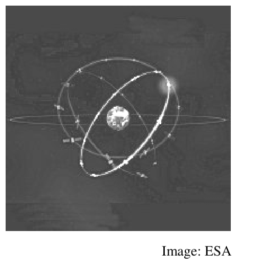
Image: ESA

Marks are indicated at the beginning of each subquestion, in parenthesis.

Question 1

1.1 (0.3) Compute the numerical value of \(r_0\).

1.2 (0.3+0.1) Give the analytical expression of the velocity \(v_0\) of the satellite as a function of \(g\), \(R_T\), and \(r_0\), and calculate its numerical value.

1.3 (0.4+0.4) Obtain the expressions of its angular momentum \(L_0\) and mechanical energy \(E_0\), as functions of \(v_0\), \(m\), \(g\) and \(R_T\).

Once this geosynchronous circular orbit has been reached (see Figure F-1), the satellite has been stabilised in the desired location, and is being readied to do its work, an error by the ground controllers causes the apogee engine to be fired again. The thrust happens to be directed towards the Earth and, despite the quick reaction of the ground crew to shut the engine off, an unwanted velocity variation \(\Delta v\) is imparted on the satellite. We characterize this boost by the parameter \(\beta=\Delta v/v_0\). The duration of the engine burn is always negligible with respect to any other orbital times, so that it can be considered as instantaneous.

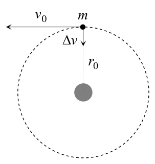
F-1

Question 2

Suppose \(\beta<1\).

2.1 (0.4+0.5) Determine the parameters of the new orbit\(^{2}\), semi-latus-rectum \(l\) and eccentricity \(\varepsilon\), in terms of \(r_0\) and \(\beta\).

2.2 (1.0) Calculate the angle \(\alpha\) between the major axis of the new orbit and the position vector at the accidental misfire.

2.3 (1.0+0.2) Give the analytical expressions of the perigee \(r_{\min}\) and apogee \(r_{\max}\) distances to the Earth centre, as functions of \(r_0\) and \(\beta\), and calculate their numerical values for \(\beta=1/4\).

2.4 (0.5+0.2) Determine the period of the new orbit, \(T\), as a function of \(T_0\) and \(\beta\), and calculate its numerical value for \(\beta=1/4\).

\(^{1}\) Its revolution period is \(T_0\).

\(^{2}\) See the “hint”.

Question 3

3.1 (0.5) Calculate the minimum boost parameter, \(\beta_{\mathrm{esc}}\), needed for the satellite to escape Earth gravity.

3.2 (1.0) Determine in this case the closest approach of the satellite to the Earth centre in the new trajectory, \(r'_{\min}\), as a function of \(r_0\).

Question 4

Suppose \(\beta>\beta_{\mathrm{esc}}\).

4.1 (1.0) Determine the residual velocity at the infinity, \(v_\infty\), as a function of \(v_0\) and \(\beta\).

4.2 (1.0) Obtain the “impact parameter” \(b\) of the asymptotic escape direction in terms of \(r_0\) and \(\beta\). (See Figure F-2).

4.3 (1.0+0.2) Determine the angle \(\phi\) of the asymptotic escape direction in terms of \(\beta\). Calculate its numerical value for \(\beta=\dfrac{3}{2}\beta_{\mathrm{esc}}\).

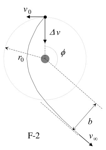
F-2

HINT

Under the action of central forces obeying the inverse-square law, bodies follow trajectories described by ellipses, parabolas or hyperbolas. In the approximation \(m\ll M\) the gravitating mass \(M\) is at one of the focuses. Taking the origin at this focus, the general polar equation of these curves can be written as (see Figure F-3)

\[ r(\theta)=\frac{l}{1-\varepsilon\cos\theta} \]

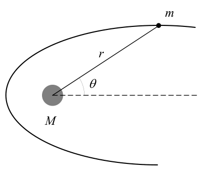
F-3

where \(l\) is a positive constant named the semi-latus-rectum and \(\varepsilon\) is the eccentricity of the curve. In terms of constants of motion:

\[ l=\frac{L^2}{GMm^2} \qquad\text{and}\qquad \varepsilon= \left(1+\frac{2EL^2}{G^2M^2m^3}\right)^{1/2} \]

where \(G\) is the Newton constant, \(L\) is the modulus of the angular momentum of the orbiting mass, with respect to the origin, and \(E\) is its mechanical energy, with zero potential energy at infinity.

We may have the following cases:

i) If \(0\leq\varepsilon<1\), the curve is an ellipse (circumference for \(\varepsilon=0\)).

ii) If \(\varepsilon=1\), the curve is a parabola.

iii) If \(\varepsilon>1\), the curve is a hyperbola.

Official English text of the problem.

Th 2 ABSOLUTE MEASUREMENTS OF ELECTRICAL QUANTITIES

The technological and scientific transformations underwent during the XIX century produced a compelling need of universally accepted standards for the electrical quantities. It was thought the new absolute units should only rely on the standards of length, mass and time established after the French Revolution. An intensive experimental work to settle the values of these units was developed from 1861 until 1912. We propose here three case studies.

Marks are indicated at the beginning of each subquestion, in parenthesis.

Determination of the ohm (Kelvin)

A closed circular coil of \(N\) turns, radius \(a\) and total resistance \(R\) is rotated with uniform angular velocity \(\omega\) about a vertical diameter in a horizontal magnetic field \(\vec B_0=B_0\vec i\).

1. (0.5+1.0) Compute the electromotive force \(\mathcal E\) induced in the coil, and also the mean power\({}^{1}\) \(\langle P\rangle\) required for maintaining the coil in motion. Neglect the coil self inductance.

A small magnetic needle is placed at the center of the coil, as shown in Figure F-1. It is free to turn slowly around the Z axis in a horizontal plane, but it cannot follow the rapid rotation of the coil.

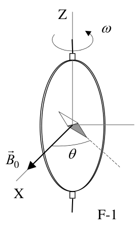
F-1

2. (2.0) Once the stationary regime is reached, the needle will set at a direction making a small angle \(\theta\) with \(\vec B_0\). Compute the resistance \(R\) of the coil in terms of this angle and the other parameters of the system.

Lord Kelvin used this method in the 1860s to set the absolute standard for the ohm. To avoid the rotating coil, Lorenz devised an alternative method used by Lord Rayleigh and Ms. Sidgwick, that we analyze in the next paragraphs.

Determination of the ohm (Rayleigh, Sidgwick).

The experimental setup is shown in Figure F-2. It consists of two identical metal disks D and D' of radius \(b\) mounted on the conducting shaft SS'. A motor rotates the set at an angular velocity \(\omega\), which can be adjusted for measuring \(R\). Two identical coils C and C' (of radius \(a\) and with \(N\) turns each) surround the disks. They are connected in such a form that the current \(I\) flows through them in opposite directions. The whole apparatus serves to measure the resistance \(R\).

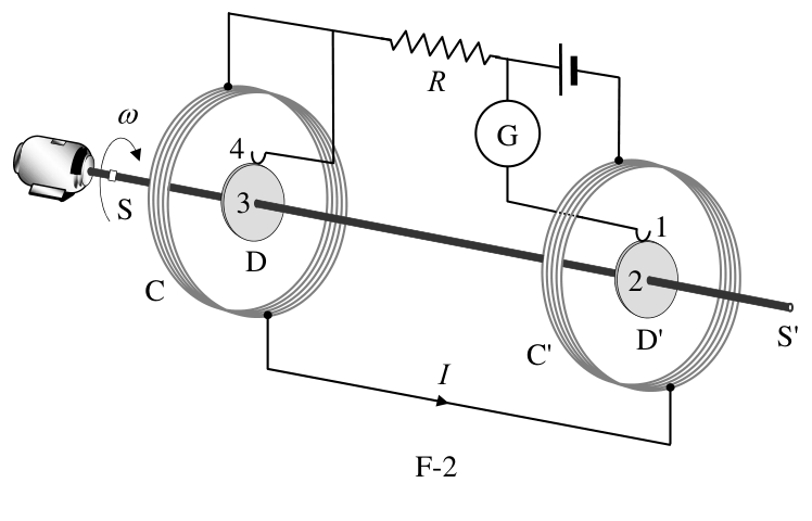
F-2

\({}^{1}\) The mean value \(\langle X\rangle\) of a quantity \(X(t)\) in a periodic system of period \(T\) is \[ \langle X\rangle=\frac{1}{T}\int_0^T X(t)\,dt. \]

You may need one or more of these integrals: \[ \int_0^{2\pi}\sin x\,dx =\int_0^{2\pi}\cos x\,dx =\int_0^{2\pi}\sin x\cos x\,dx=0, \] \[ \int_0^{2\pi}\sin^2x\,dx =\int_0^{2\pi}\cos^2x\,dx=\pi, \qquad \text{and later}\qquad \int x^n\,dx=\frac{1}{n+1}x^{n+1}. \]

3. (2.0) Assume that the current \(I\) flowing through the coils C and C' creates a uniform magnetic field \(B\) around D and D', equal to the one at the centre of the coil. Compute\({}^{1}\) the electromotive force \(\mathcal E\) induced between the rims 1 and 4, assuming that the distance between the coils is much larger than the radius of the coils and that \(a\gg b\).

The disks are connected to the circuit by brush contacts at their rims 1 and 4. The galvanometer G detects the flow of current through the circuit 1-2-3-4.

4. (0.5) The resistance \(R\) is measured when G reads zero. Give \(R\) in terms of the physical parameters of the system.

Determination of the ampere

Passing a current through two conductors and measuring the force between them provides an absolute determination of the current itself. The “Current Balance” designed by Lord Kelvin in 1882 exploits this method. It consists of six identical single turn coils \(C_1\ldots C_6\) of radius \(a\), connected in series. As shown in Figure F-3, the fixed coils \(C_1\), \(C_3\), \(C_4\), and \(C_6\) are on two horizontal planes separated by a small distance \(2h\). The coils \(C_2\) and \(C_5\) are carried on balance arms of length \(d\), and they are, in equilibrium, equidistant from both planes.

The current \(I\) flows through the various coils in such a direction that the magnetic force on \(C_2\) is upwards while that on \(C_5\) is downwards. A mass \(m\) at a distance \(x\) from the fulcrum O is required to restore the balance to the equilibrium position described above when the current flows through the circuit.

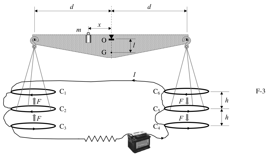
F-3

5. (1.0) Compute the force \(F\) on \(C_2\) due to the magnetic interaction with \(C_1\). For simplicity assume that the force per unit length is the one corresponding to two long, straight wires carrying parallel currents.

6. (1.0) The current \(I\) is measured when the balance is in equilibrium. Give the value of \(I\) in terms of the physical parameters of the system. The dimensions of the apparatus are such that we can neglect the mutual effects of the coils on the left and on the right.

Let \(M\) be the mass of the balance (except for \(m\) and the hanging parts), G its centre of mass and \(l\) the distance \(\overline{OG}\).

7. (2.0) The balance equilibrium is stable against deviations producing small changes \(\delta z\) in the height of \(C_2\) and \(-\delta z\) in \(C_5\). Compute\({}^{2}\) the maximum value \(\delta z_{\max}\) so that the balance still returns towards the equilibrium position when it is released.

\({}^{2}\) Consider that the coils centres remain approximately aligned.

Use the approximations \[ \frac{1}{1\pm\beta}\approx1\mp\beta+\beta^2 \qquad\text{or}\qquad \frac{1}{1\pm\beta^2}\approx1\mp\beta^2 \] for \(\beta\ll1\), and \(\sin\theta\approx\tan\theta\) for small \(\theta\).

Official English text of the problem.

Th 3 NEUTRONS IN A GRAVITATIONAL FIELD

In the familiar classical world, an elastic bouncing ball on the Earth’s surface is an ideal example for perpetual motion. The ball is trapped: it can not go below the surface or above its turning point. It will remain bounded in this state, turning down and bouncing up once and again, forever. Only air drag or inelastic bounces could stop the process and will be ignored in the following.

A group of physicists from the Institute Laue - Langevin in Grenoble reported\(^{1}\) in 2002 experimental evidence on the behaviour of neutrons in the gravitational field of the Earth. In the experiment, neutrons moving to the right were allowed to fall towards a horizontal crystal surface acting as a neutron mirror, where they bounced back elastically up to the initial height once and again.

The setup of the experiment is sketched in Figure F-1. It consists of the opening W, the neutron mirror M (at height \(z = 0\)), the neutron absorber A (at height \(z = H\) and with length \(L\)) and the neutron detector D. The beam of neutrons flies with constant horizontal velocity component \(v_x\) from W to D through the cavity between A and M. All the neutrons that reach the surface of A are absorbed and disappear from the experiment. Those that reach the surface of M are reflected elastically. The detector D counts the transmission rate \(N(H)\), that is, the total number of neutrons that reach D per unit time.

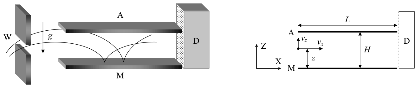
F-1

Marks are indicated at the beginning of each subquestion, in parenthesis.

The neutrons enter the cavity with a wide range of positive and negative vertical velocities, \(v_z\). Once in the cavity, they fly between the mirror below and the absorber above.

1. (1.5) Compute classically the range of vertical velocities \(v_z(z)\) of the neutrons that, entering at a height \(z\), can arrive at the detector D. Assume that \(L\) is much larger than any other length in the problem.

2. (1.5) Calculate classically the minimum length \(L_c\) of the cavity to ensure that all neutrons outside the previous velocity range, regardless of the values of \(z\), are absorbed by A. Use \(v_x = 10\ \mathrm{m\,s^{-1}}\) and \(H = 50\ \mu\mathrm{m}\).

The neutron transmission rate \(N(H)\) is measured at D. We expect that it increases monotonically with \(H\).

3. (2.5) Compute the classical rate \(N_c(H)\) assuming that neutrons arrive at the cavity with vertical velocity \(v_z\) and at height \(z\), being all the values of \(v_z\) and \(z\) equally probable. Give the answer in terms of \(\rho\), the constant number of neutrons per unit time, per unit vertical velocity, per unit height, that enter the cavity with vertical velocity \(v_z\) and at height \(z\).

\(^{1}\) V. V. Nesvizhevsky et al. “Quantum states of neutrons in the Earth’s gravitational field.” Nature, 415 (2002) 297. Phys Rev D 67, 102002 (2003).

The experimental results obtained by the Grenoble group disagree with the above classical predictions, showing instead that the value of \(N(H)\) experiences sharp increases when \(H\) crosses some critical heights \(H_1\), \(H_2\) ... (Figure F-2 shows a sketch). In other words, the experiment showed that the vertical motion of neutrons bouncing on the mirror is quantized. In the language that Bohr and Sommerfeld used to obtain the energy levels of the hydrogen atom, this can be written as: “The action \(S\) of these neutrons along the vertical direction is an integer multiple of the Planck action constant \(h\)”. Here \(S\) is given by

\[ S=\int p_z(z)\,dz=nh,\qquad n=1,2,3\ldots \qquad\text{(Bohr-Sommerfeld quantization rule)} \]

where \(p_z\) is the vertical component of the classical momentum, and the integral covers a whole bouncing cycle. Only neutrons with these values of \(S\) are allowed in the cavity.

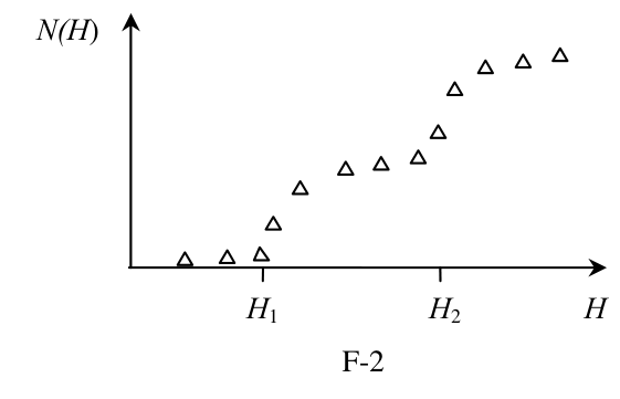
F-2

4. (2.5) Compute the turning heights \(H_n\) and energy levels \(E_n\) (associated to the vertical motion) using the Bohr-Sommerfeld quantization condition. Give the numerical result for \(H_1\) in \(\mu\mathrm{m}\) and for \(E_1\) in eV.

The uniform initial distribution \(\rho\) of neutrons at the entrance changes, during the flight through a long cavity, into the step-like distribution detected at D (see Figure F-2). From now on, we consider for simplicity the case of a long cavity with \(H < H_2\). Classically, all neutrons with energies in the range considered in question 1 were allowed through it, while quantum mechanically only neutrons in the energy level \(E_1\) are permitted. According to the time-energy Heisenberg uncertainty principle, this reshuffling requires a minimum time of flight. The uncertainty of the vertical motion energy will be significant if the cavity length is small. This phenomenon will give rise to the widening of the energy levels.

5. (2.0) Estimate the minimum time of flight \(t_q\) and the minimum length \(L_q\) of the cavity needed to observe the first sharp increase in the number of neutrons at D. Use \(v_x = 10\ \mathrm{m\,s^{-1}}\).

Data:

Quantity	Value
Planck action constant	\(h = 6.63\cdot10^{-34}\ \mathrm{J\,s}\)
Speed of light in vacuum	\(c = 3.00\cdot10^8\ \mathrm{m\,s^{-1}}\)
Elementary charge	\(e = 1.60\cdot10^{-19}\ \mathrm{C}\)
Neutron mass	\(M = 1.67\cdot10^{-27}\ \mathrm{kg}\)
Acceleration of gravity on Earth	\(g = 9.81\ \mathrm{m\,s^{-2}}\)

If necessary, use the expression:

\[ \int(1-x)^{1/2}\,dx=-\frac{2(1-x)^{3/2}}{3} \]

Official English text of the problem.

Th 1 EIN VOM PECH VERFOLGTER SATELLIT

Die häufigsten Bahnmanöver von Raumfahrzeugen bestehen in Geschwindigkeitsänderungen entlang der Flugrichtung, nämlich in Beschleunigungen zum Erreichen höherer Umlaufbahnen oder in Bremsmanövern zum Einleiten des Wiedereintritts in die Atmosphäre. In dieser Aufgabe untersuchen wir die Bahnänderungen, wenn der Triebwerksschub in radialer Richtung wirkt.

Verwenden Sie zur Berechnung der Zahlenwerte den Erdradius \(R_T=6.37\cdot10^6\ \mathrm{m}\), die Fallbeschleunigung an der Erdoberfläche \(g=9.81\ \mathrm{m/s^2}\), und setzen Sie die Dauer des siderischen Tages mit \(T_0=24.0\ \mathrm{h}\) an.

Wir betrachten einen geosynchronen\(^{1}\) Kommunikationssatelliten der Masse \(m\) auf einer äquatorialen Kreisbahn mit dem Radius \(r_0\). Diese Satelliten verfügen über ein „Apogäumstriebwerk“, das den zum Erreichen der endgültigen Umlaufbahn erforderlichen tangentialen Schub liefert.

Bild: ESA

Die Punktzahlen stehen jeweils zu Beginn jeder Teilaufgabe in Klammern.

Frage 1

1.1 (0.3) Berechnen Sie den Zahlenwert von \(r_0\).

1.2 (0.3+0.1) Geben Sie den analytischen Ausdruck für die Geschwindigkeit \(v_0\) des Satelliten als Funktion von \(g\), \(R_T\) und \(r_0\) an und berechnen Sie ihren Zahlenwert.

1.3 (0.4+0.4) Leiten Sie die Ausdrücke für seinen Drehimpuls \(L_0\) und seine mechanische Energie \(E_0\) als Funktionen von \(v_0\), \(m\), \(g\) und \(R_T\) her.

Nachdem diese geosynchrone Kreisbahn erreicht ist (siehe Abbildung F-1), der Satellit an der gewünschten Position stabilisiert wurde und auf seinen Einsatz vorbereitet wird, führt ein Fehler des Kontrollpersonals am Boden dazu, dass das Apogäumstriebwerk erneut gezündet wird. Der Schub ist dabei zur Erde hin gerichtet, und trotz der schnellen Reaktion der Bodenmannschaft, die das Triebwerk abschaltet, erfährt der Satellit eine unerwünschte Geschwindigkeitsänderung \(\Delta v\). Wir charakterisieren diesen Antriebsstoß durch den Parameter \(\beta=\Delta v/v_0\). Die Brenndauer des Triebwerks ist gegenüber allen anderen für die Bahnbewegung relevanten Zeiten stets vernachlässigbar, sodass der Antriebsstoß als momentan betrachtet werden kann.

F-1

Frage 2

Es sei \(\beta<1\).

2.1 (0.4+0.5) Bestimmen Sie die Parameter der neuen Bahn\(^{2}\), den Halbparameter \(l\) und die Exzentrizität \(\varepsilon\), in Abhängigkeit von \(r_0\) und \(\beta\).

2.2 (1.0) Berechnen Sie den Winkel \(\alpha\) zwischen der großen Achse der neuen Bahn und dem Ortsvektor zum Zeitpunkt der versehentlichen Zündung.

2.3 (1.0+0.2) Geben Sie die analytischen Ausdrücke für die Abstände des Perigäums \(r_{\min}\) und des Apogäums \(r_{\max}\) vom Erdmittelpunkt als Funktionen von \(r_0\) und \(\beta\) an und berechnen Sie ihre Zahlenwerte für \(\beta=1/4\).

2.4 (0.5+0.2) Bestimmen Sie die Umlaufzeit der neuen Bahn, \(T\), als Funktion von \(T_0\) und \(\beta\) und berechnen Sie ihren Zahlenwert für \(\beta=1/4\).

\(^{1}\) Ihre Umlaufzeit beträgt \(T_0\).

\(^{2}\) Siehe den „Hinweis“.

Frage 3

3.1 (0.5) Berechnen Sie den minimalen Antriebsstoßparameter \(\beta_{\mathrm{esc}}\), der erforderlich ist, damit der Satellit dem Schwerefeld der Erde entkommt.

3.2 (1.0) Bestimmen Sie für diesen Fall den kleinsten Abstand des Satelliten vom Erdmittelpunkt auf der neuen Bahn, \(r'_{\min}\), als Funktion von \(r_0\).

Frage 4

Es sei \(\beta>\beta_{\mathrm{esc}}\).

4.1 (1.0) Bestimmen Sie die Restgeschwindigkeit im Unendlichen, \(v_\infty\), als Funktion von \(v_0\) und \(\beta\).

4.2 (1.0) Leiten Sie den „Stoßparameter“ \(b\) der asymptotischen Fluchtrichtung in Abhängigkeit von \(r_0\) und \(\beta\) her. (Siehe Abbildung F-2).

4.3 (1.0+0.2) Bestimmen Sie den Winkel \(\phi\) der asymptotischen Fluchtrichtung in Abhängigkeit von \(\beta\). Berechnen Sie seinen Zahlenwert für \(\beta=\dfrac{3}{2}\beta_{\mathrm{esc}}\).

F-2

HINWEIS

Unter der Wirkung von Zentralkräften, die dem inversen Quadratgesetz folgen, bewegen sich Körper auf Bahnen, die durch Ellipsen, Parabeln oder Hyperbeln beschrieben werden. In der Näherung \(m\ll M\) befindet sich die gravitierende Masse \(M\) in einem der Brennpunkte. Legt man den Ursprung in diesen Brennpunkt, so lässt sich die allgemeine Polargleichung dieser Kurven folgendermaßen schreiben (siehe Abbildung F-3):

\[ r(\theta)=\frac{l}{1-\varepsilon\cos\theta} \]

F-3

Dabei ist \(l\) eine positive Konstante, die als Halbparameter bezeichnet wird, und \(\varepsilon\) ist die Exzentrizität der Kurve. In Abhängigkeit von den Erhaltungsgrößen gilt:

\[ l=\frac{L^2}{GMm^2} \qquad\text{und}\qquad \varepsilon= \left(1+\frac{2EL^2}{G^2M^2m^3}\right)^{1/2} \]

Dabei ist \(G\) die Newtonsche Gravitationskonstante, \(L\) der Betrag des Drehimpulses der umlaufenden Masse bezüglich des Ursprungs und \(E\) ihre mechanische Energie, wobei die potenzielle Energie im Unendlichen gleich null ist.

Folgende Fälle sind möglich:

i) Für \(0\leq\varepsilon<1\) ist die Kurve eine Ellipse (für \(\varepsilon=0\) eine Kreislinie).

ii) Für \(\varepsilon=1\) ist die Kurve eine Parabel.

iii) Für \(\varepsilon>1\) ist die Kurve eine Hyperbel.

Aufgabentext aus dem offiziellen englischen Text übersetzt.

Th 2 ABSOLUTMESSUNGEN ELEKTRISCHER GRÖSSEN

Die technologischen und wissenschaftlichen Umwälzungen im XIX. Jahrhundert führten zu einem dringenden Bedarf an allgemein anerkannten Normalen für die elektrischen Größen. Die neuen absoluten Einheiten sollten, so die damalige Vorstellung, ausschließlich auf den nach der Französischen Revolution festgelegten Normalen für Länge, Masse und Zeit beruhen. Von 1861 bis 1912 wurden umfangreiche experimentelle Arbeiten durchgeführt, um die Werte dieser Einheiten festzulegen. Wir stellen hier drei Fallstudien vor.

Die Punktzahlen stehen jeweils zu Beginn jeder Teilaufgabe in Klammern.

Bestimmung des Ohms (Kelvin)

Eine geschlossene kreisförmige Spule mit \(N\) Windungen, dem Radius \(a\) und dem Gesamtwiderstand \(R\) wird mit konstanter Winkelgeschwindigkeit \(\omega\) um einen vertikalen Durchmesser in einem horizontalen Magnetfeld \(\vec B_0=B_0\vec i\) gedreht.

1. (0.5+1.0) Berechnen Sie die in der Spule induzierte elektromotorische Kraft \(\mathcal E\) sowie die mittlere Leistung\({}^{1}\) \(\langle P\rangle\), die erforderlich ist, um die Spule in Bewegung zu halten. Vernachlässigen Sie die Selbstinduktivität der Spule.

Eine kleine Magnetnadel wird wie in Abbildung F-1 im Mittelpunkt der Spule angebracht. Sie kann sich in einer horizontalen Ebene frei und langsam um die Z-Achse drehen, der schnellen Drehung der Spule jedoch nicht folgen.

F-1

2. (2.0) Sobald der stationäre Zustand erreicht ist, stellt sich die Nadel in einer Richtung ein, die mit \(\vec B_0\) einen kleinen Winkel \(\theta\) bildet. Berechnen Sie den Widerstand \(R\) der Spule in Abhängigkeit von diesem Winkel und den anderen Parametern des Systems.

Lord Kelvin verwendete diese Methode in den 1860er-Jahren, um das absolute Normal für das Ohm festzulegen. Um die rotierende Spule zu vermeiden, entwickelte Lorenz eine alternative Methode, die von Lord Rayleigh und Frau Sidgwick angewandt wurde und die wir in den folgenden Absätzen untersuchen.

Bestimmung des Ohms (Rayleigh, Sidgwick).

Der Versuchsaufbau ist in Abbildung F-2 dargestellt. Er besteht aus zwei identischen Metallscheiben D und D' mit dem Radius \(b\), die auf der leitenden Welle SS' montiert sind. Ein Motor versetzt die Anordnung in eine Drehung mit der Winkelgeschwindigkeit \(\omega\), die zur Messung von \(R\) eingestellt werden kann. Zwei identische Spulen C und C' (mit dem Radius \(a\) und jeweils \(N\) Windungen) umgeben die Scheiben. Sie sind so verschaltet, dass der Strom \(I\) sie in entgegengesetzten Richtungen durchfließt. Die gesamte Apparatur dient zur Messung des Widerstands \(R\).

F-2

\({}^{1}\) Der Mittelwert \(\langle X\rangle\) einer Größe \(X(t)\) in einem periodischen System mit der Periodendauer \(T\) ist \[ \langle X\rangle=\frac{1}{T}\int_0^T X(t)\,dt. \]

Sie benötigen möglicherweise eines oder mehrere der folgenden Integrale: \[ \int_0^{2\pi}\sin x\,dx =\int_0^{2\pi}\cos x\,dx =\int_0^{2\pi}\sin x\cos x\,dx=0, \] \[ \int_0^{2\pi}\sin^2x\,dx =\int_0^{2\pi}\cos^2x\,dx=\pi, \qquad \text{und später}\qquad \int x^n\,dx=\frac{1}{n+1}x^{n+1}. \]

3. (2.0) Nehmen Sie an, dass der durch die Spulen C und C' fließende Strom \(I\) im Bereich von D und D' ein homogenes Magnetfeld \(B\) erzeugt, das gleich dem Feld im Mittelpunkt der jeweiligen Spule ist. Berechnen Sie\({}^{1}\) die zwischen den Rändern 1 und 4 induzierte elektromotorische Kraft \(\mathcal E\) unter der Annahme, dass der Abstand zwischen den Spulen viel größer als ihr Radius ist und dass \(a\gg b\) gilt.

Die Scheiben sind über Bürstenkontakte an ihren Rändern 1 und 4 mit dem Stromkreis verbunden. Das Galvanometer G weist einen Stromfluss durch den Stromkreis 1-2-3-4 nach.

4. (0.5) Der Widerstand \(R\) wird gemessen, wenn G null anzeigt. Geben Sie \(R\) in Abhängigkeit von den physikalischen Parametern des Systems an.

Bestimmung des Amperes

Indem man einen Strom durch zwei Leiter fließen lässt und die Kraft zwischen ihnen misst, kann man den Strom selbst absolut bestimmen. Die 1882 von Lord Kelvin entworfene „Stromwaage“ nutzt diese Methode. Sie besteht aus sechs identischen Spulen \(C_1\ldots C_6\) mit jeweils einer Windung und dem Radius \(a\), die in Reihe geschaltet sind. Wie in Abbildung F-3 gezeigt, liegen die feststehenden Spulen \(C_1\), \(C_3\), \(C_4\) und \(C_6\) in zwei horizontalen Ebenen mit dem kleinen Abstand \(2h\). Die Spulen \(C_2\) und \(C_5\) werden von Waagearmen der Länge \(d\) getragen und haben im Gleichgewicht von beiden Ebenen denselben Abstand.

Der Strom \(I\) fließt durch die verschiedenen Spulen jeweils in einer solchen Richtung, dass die magnetische Kraft auf \(C_2\) nach oben und diejenige auf \(C_5\) nach unten gerichtet ist. Eine Masse \(m\) im Abstand \(x\) vom Drehpunkt O ist erforderlich, um die Waage wieder in die oben beschriebene Gleichgewichtslage zu bringen, wenn der Strom durch den Stromkreis fließt.

F-3

5. (1.0) Berechnen Sie die Kraft \(F\) auf \(C_2\) aufgrund der magnetischen Wechselwirkung mit \(C_1\). Nehmen Sie der Einfachheit halber an, dass die Kraft pro Längeneinheit derjenigen zwischen zwei langen, geraden Drähten mit gleichgerichteten Strömen entspricht.

6. (1.0) Der Strom \(I\) wird gemessen, wenn sich die Waage im Gleichgewicht befindet. Geben Sie den Wert von \(I\) in Abhängigkeit von den physikalischen Parametern des Systems an. Die Abmessungen der Apparatur sind so gewählt, dass die gegenseitigen Einflüsse der Spulen auf der linken und auf der rechten Seite vernachlässigt werden können.

Es seien \(M\) die Masse der Waage (ohne \(m\) und die aufgehängten Teile), G ihr Schwerpunkt und \(l\) der Abstand \(\overline{OG}\).

7. (2.0) Das Gleichgewicht der Waage ist stabil gegenüber Auslenkungen, die kleine Höhenänderungen \(\delta z\) von \(C_2\) und \(-\delta z\) von \(C_5\) bewirken. Berechnen Sie\({}^{2}\) den maximalen Wert \(\delta z_{\max}\), bei dem sich die Waage nach dem Loslassen noch in Richtung ihrer Gleichgewichtslage zurückbewegt.

\({}^{2}\) Nehmen Sie an, dass die Spulenmittelpunkte näherungsweise auf einer gemeinsamen Achse bleiben.

Verwenden Sie die Näherungen \[ \frac{1}{1\pm\beta}\approx1\mp\beta+\beta^2 \qquad\text{oder}\qquad \frac{1}{1\pm\beta^2}\approx1\mp\beta^2 \] für \(\beta\ll1\) sowie \(\sin\theta\approx\tan\theta\) für kleine \(\theta\).

Aufgabentext aus dem offiziellen englischen Text übersetzt.

Th 3 NEUTRONEN IM GRAVITATIONSFELD

In der vertrauten klassischen Welt ist ein elastisch auf der Erdoberfläche hüpfender Ball ein ideales Beispiel für eine unaufhörliche Bewegung. Der Ball ist eingeschlossen: Er kann weder unter die Oberfläche noch über seinen Umkehrpunkt gelangen. Er bleibt in diesem Zustand räumlich begrenzt und wird immer wieder nach unten umkehren und nach oben zurückprallen, bis in alle Ewigkeit. Nur Luftwiderstand oder unelastische Stöße könnten den Vorgang zum Stillstand bringen; sie werden im Folgenden vernachlässigt.

Eine Gruppe von Physikern des Instituts Laue - Langevin in Grenoble berichtete\(^{1}\) im Jahr 2002 über experimentelle Nachweise zum Verhalten von Neutronen im Gravitationsfeld der Erde. Im Experiment ließ man nach rechts fliegende Neutronen auf eine horizontale Kristalloberfläche fallen, die als Neutronenspiegel wirkte und an der sie immer wieder elastisch bis zur ursprünglichen Höhe zurückprallten.

Der Versuchsaufbau ist in Abbildung F-1 skizziert. Er besteht aus der Öffnung W, dem Neutronenspiegel M (auf der Höhe \(z = 0\)), dem Neutronenabsorber A (auf der Höhe \(z = H\) und mit der Länge \(L\)) und dem Neutronendetektor D. Der Neutronenstrahl fliegt mit einer konstanten horizontalen Geschwindigkeitskomponente \(v_x\) von W nach D durch den Hohlraum zwischen A und M. Alle Neutronen, die die Oberfläche von A erreichen, werden absorbiert und scheiden aus dem Experiment aus. Diejenigen, die die Oberfläche von M erreichen, werden elastisch reflektiert. Der Detektor D misst die Transmissionsrate \(N(H)\), also die Gesamtzahl der Neutronen, die D pro Zeiteinheit erreichen.

F-1

Die Punktzahlen sind am Anfang jeder Teilaufgabe in Klammern angegeben.

Die Neutronen treten mit einem breiten Spektrum positiver und negativer vertikaler Geschwindigkeiten \(v_z\) in den Hohlraum ein. Im Hohlraum fliegen sie zwischen dem Spiegel unten und dem Absorber oben.

1. (1.5) Berechnen Sie klassisch den Bereich der vertikalen Geschwindigkeiten \(v_z(z)\) der Neutronen, die beim Eintritt auf einer Höhe \(z\) den Detektor D erreichen können. Nehmen Sie an, dass \(L\) wesentlich größer als jede andere Länge in dieser Aufgabe ist.

2. (1.5) Berechnen Sie klassisch die Mindestlänge \(L_c\) des Hohlraums, die sicherstellt, dass alle Neutronen außerhalb des zuvor bestimmten Geschwindigkeitsbereichs unabhängig vom Wert von \(z\) durch A absorbiert werden. Verwenden Sie \(v_x = 10\ \mathrm{m\,s^{-1}}\) und \(H = 50\ \mu\mathrm{m}\).

Die Neutronentransmissionsrate \(N(H)\) wird bei D gemessen. Wir erwarten, dass sie mit \(H\) monoton zunimmt.

3. (2.5) Berechnen Sie die klassische Rate \(N_c(H)\) unter der Annahme, dass Neutronen mit einer vertikalen Geschwindigkeit \(v_z\) auf einer Höhe \(z\) am Hohlraum eintreffen, wobei alle Werte von \(v_z\) und \(z\) gleich wahrscheinlich sind. Geben Sie das Ergebnis in Abhängigkeit von \(\rho\) an, der konstanten Anzahl von Neutronen pro Zeiteinheit, pro Einheit der vertikalen Geschwindigkeit und pro Höheneinheit, die mit der vertikalen Geschwindigkeit \(v_z\) auf der Höhe \(z\) in den Hohlraum eintreten.

\(^{1}\) V. V. Nesvizhevsky et al. „Quantenzustände von Neutronen im Gravitationsfeld der Erde.“ Nature, 415 (2002) 297. Phys Rev D 67, 102002 (2003).

Die experimentellen Ergebnisse der Gruppe aus Grenoble stimmen nicht mit den obigen klassischen Vorhersagen überein. Sie zeigen stattdessen, dass der Wert von \(N(H)\) sprunghaft ansteigt, wenn \(H\) bestimmte kritische Höhen \(H_1\), \(H_2\) ... überschreitet (Abbildung F-2 zeigt eine Skizze). Mit anderen Worten zeigte das Experiment, dass die vertikale Bewegung der am Spiegel zurückprallenden Neutronen quantisiert ist. In der Sprache, die Bohr und Sommerfeld zur Bestimmung der Energieniveaus des Wasserstoffatoms verwendeten, lässt sich dies so ausdrücken: „Die Wirkung \(S\) dieser Neutronen in vertikaler Richtung ist ein ganzzahliges Vielfaches des planckschen Wirkungsquantums \(h\).“ Dabei ist \(S\) gegeben durch

\[ S=\int p_z(z)\,dz=nh,\qquad n=1,2,3\ldots \qquad\text{(Bohr-Sommerfeld-Quantisierungsregel)} \]

wobei \(p_z\) die vertikale Komponente des klassischen Impulses ist und sich das Integral über einen vollständigen Zyklus der Hüpfbewegung erstreckt. Nur Neutronen mit diesen Werten von \(S\) sind im Hohlraum erlaubt.

F-2

4. (2.5) Berechnen Sie die Umkehrhöhen \(H_n\) und die (zur vertikalen Bewegung gehörenden) Energieniveaus \(E_n\) mithilfe der Bohr-Sommerfeld-Quantisierungsbedingung. Geben Sie das numerische Ergebnis für \(H_1\) in \(\mu\mathrm{m}\) und für \(E_1\) in eV an.

Die anfänglich gleichförmige Verteilung \(\rho\) der Neutronen am Eingang geht während des Flugs durch einen langen Hohlraum in die bei D nachgewiesene stufenförmige Verteilung über (siehe Abbildung F-2). Von nun an betrachten wir der Einfachheit halber den Fall eines langen Hohlraums mit \(H < H_2\). Klassisch konnten alle Neutronen mit Energien in dem in Aufgabe 1 betrachteten Bereich den Hohlraum durchqueren, während quantenmechanisch nur Neutronen im Energieniveau \(E_1\) erlaubt sind. Nach der Energie-Zeit-Unschärferelation von Heisenberg erfordert diese Umverteilung eine Mindestflugzeit. Bei geringer Hohlraumlänge ist die Unschärfe der Energie der vertikalen Bewegung beträchtlich. Dieses Phänomen führt zu einer Verbreiterung der Energieniveaus.

5. (2.0) Schätzen Sie die Mindestflugzeit \(t_q\) und die Mindestlänge \(L_q\) des Hohlraums ab, die erforderlich sind, um den ersten sprunghaften Anstieg der Neutronenzahl bei D zu beobachten. Verwenden Sie \(v_x = 10\ \mathrm{m\,s^{-1}}\).

Gegebene Größen:

Größe	Wert
Plancksches Wirkungsquantum	\(h = 6.63\cdot10^{-34}\ \mathrm{J\,s}\)
Lichtgeschwindigkeit im Vakuum	\(c = 3.00\cdot10^8\ \mathrm{m\,s^{-1}}\)
Elementarladung	\(e = 1.60\cdot10^{-19}\ \mathrm{C}\)
Neutronenmasse	\(M = 1.67\cdot10^{-27}\ \mathrm{kg}\)
Erdbeschleunigung	\(g = 9.81\ \mathrm{m\,s^{-2}}\)

Verwenden Sie bei Bedarf den Ausdruck:

\[ \int(1-x)^{1/2}\,dx=-\frac{2(1-x)^{3/2}}{3} \]

Aufgabentext aus dem offiziellen englischen Text übersetzt.

Th 1 TALİHSİZ BİR UYDU

Uzay araçlarının en sık gerçekleştirdiği yörünge manevraları, uçuş doğrultusunda yapılan hız değişikliklerinden, yani daha yüksek yörüngelere ulaşmak için hızlanmalardan veya atmosfere yeniden girişi başlatmak için yavaşlamalardan oluşur. Bu soruda, motorun itme kuvveti radyal doğrultuda uygulandığında meydana gelen yörünge değişikliklerini inceleyeceğiz.

Sayısal değerleri elde etmek için Dünya'nın yarıçapını \(R_T=6.37\cdot10^6\ \mathrm{m}\), Dünya yüzeyindeki yerçekimi ivmesini \(g=9.81\ \mathrm{m/s^2}\) ve yıldız gününün süresini \(T_0=24.0\ \mathrm{h}\) olarak alınız.

Ekvator düzleminde, yarıçapı \(r_0\) olan dairesel bir yörüngeye yerleştirilmiş, kütlesi \(m\) olan yer eşzamanlı\(^{1}\) bir haberleşme uydusunu ele alıyoruz. Bu uydularda, son yörüngeye ulaşmak için gereken teğetsel itme kuvvetlerini sağlayan bir “yeröte motoru” bulunur.

Görsel: ESA

Puanlar her alt sorunun başında parantez içinde belirtilmiştir.

Soru 1

1.1 (0.3) \(r_0\)'ın sayısal değerini hesaplayınız.

1.2 (0.3+0.1) Uydunun \(v_0\) hızının analitik ifadesini \(g\), \(R_T\) ve \(r_0\) cinsinden veriniz ve sayısal değerini hesaplayınız.

1.3 (0.4+0.4) Uydunun açısal momentumu \(L_0\) ve mekanik enerjisi \(E_0\) için ifadeleri \(v_0\), \(m\), \(g\) ve \(R_T\) cinsinden elde ediniz.

Bu yer eşzamanlı dairesel yörüngeye ulaşıldıktan (bkz. Şekil F-1), uydu istenen konumda kararlı hâle getirildikten sonra, görevine hazırlanırken yer kontrol ekibinin bir hatası nedeniyle yeröte motoru yeniden ateşlenir. İtme kuvveti Dünya'ya doğru yönelmiştir ve yer ekibinin motoru kapatmak için hızla müdahale etmesine rağmen uyduya istenmeyen bir \(\Delta v\) hız değişimi kazandırılır. Bu hız değişimini \(\beta=\Delta v/v_0\) parametresiyle tanımlıyoruz. Motorun yanma süresi, yörünge hareketine ilişkin diğer tüm sürelere kıyasla her zaman ihmal edilebilecek kadar kısadır; dolayısıyla ateşleme anlık kabul edilebilir.

F-1

Soru 2

\(\beta<1\) olduğunu varsayınız.

2.1 (0.4+0.5) Yeni yörüngenin\(^{2}\) parametreleri olan yarı dik kiriş uzunluğu \(l\) ve dışmerkezlik \(\varepsilon\)'yi \(r_0\) ve \(\beta\) cinsinden belirleyiniz.

2.2 (1.0) Yeni yörüngenin büyük ekseni ile yanlışlıkla ateşleme anındaki konum vektörü arasındaki \(\alpha\) açısını hesaplayınız.

2.3 (1.0+0.2) Yerberi ve yeröte noktalarının Dünya'nın merkezine uzaklıkları olan \(r_{\min}\) ve \(r_{\max}\)'ın analitik ifadelerini \(r_0\) ve \(\beta\) cinsinden veriniz ve \(\beta=1/4\) için sayısal değerlerini hesaplayınız.

2.4 (0.5+0.2) Yeni yörüngenin periyodu \(T\)'yi \(T_0\) ve \(\beta\) cinsinden belirleyiniz ve \(\beta=1/4\) için sayısal değerini hesaplayınız.

\(^{1}\) Dolanım periyodu \(T_0\)'dır.

\(^{2}\) “İpucu”na bakınız.

Soru 3

3.1 (0.5) Uydunun Dünya'nın kütleçekiminden kurtulması için gereken en küçük hız değişimi parametresi \(\beta_{\mathrm{esc}}\)'yi hesaplayınız.

3.2 (1.0) Bu durumda uydunun yeni yörüngesinde Dünya'nın merkezine en yakın olduğu uzaklığı, \(r'_{\min}\)'ı, \(r_0\) cinsinden belirleyiniz.

Soru 4

\(\beta>\beta_{\mathrm{esc}}\) olduğunu varsayınız.

4.1 (1.0) Sonsuzdaki artık hız \(v_\infty\)'yi \(v_0\) ve \(\beta\) cinsinden belirleyiniz.

4.2 (1.0) Asimptotik kaçış doğrultusunun “çarpma parametresi” \(b\)'yi \(r_0\) ve \(\beta\) cinsinden elde ediniz. (Bkz. Şekil F-2).

4.3 (1.0+0.2) Asimptotik kaçış yönünün \(\phi\) açısını \(\beta\) cinsinden belirleyiniz. \(\beta=\dfrac{3}{2}\beta_{\mathrm{esc}}\) için sayısal değerini hesaplayınız.

F-2

İPUCU

Ters kare yasasına uyan merkezî kuvvetlerin etkisi altında cisimler elips, parabol veya hiperbol biçiminde yörüngeler izler. \(m\ll M\) yaklaşımında, çekim kaynağı olan \(M\) kütlesi odaklardan birinde bulunur. Başlangıç noktası bu odakta alındığında, bu eğrilerin genel kutupsal denklemi şöyle yazılabilir (bkz. Şekil F-3):

\[ r(\theta)=\frac{l}{1-\varepsilon\cos\theta} \]

F-3

Burada \(l\), yarı dik kiriş uzunluğu adı verilen pozitif bir sabit, \(\varepsilon\) ise eğrinin dışmerkezliğidir. Hareket sabitleri cinsinden:

\[ l=\frac{L^2}{GMm^2} \qquad\text{ve}\qquad \varepsilon= \left(1+\frac{2EL^2}{G^2M^2m^3}\right)^{1/2} \]

Burada \(G\) Newton'un kütleçekim sabiti, \(L\) yörüngede dolanan kütlenin başlangıç noktasına göre açısal momentumunun büyüklüğü ve \(E\), potansiyel enerji sonsuzda sıfır alınmak üzere mekanik enerjisidir.

Şu durumlar söz konusu olabilir:

i) \(0\leq\varepsilon<1\) ise eğri bir elipstir (\(\varepsilon=0\) için çemberdir).

ii) \(\varepsilon=1\) ise eğri bir paraboldür.

iii) \(\varepsilon>1\) ise eğri bir hiperboldür.

Soru metni resmi İngilizce metinden çevrilmiştir.

Th 2 ELEKTRİKSEL BÜYÜKLÜKLERİN MUTLAK ÖLÇÜMLERİ

XIX. yüzyılda yaşanan teknolojik ve bilimsel dönüşümler, elektriksel büyüklükler için evrensel olarak kabul gören standartlara duyulan ihtiyacı zorunlu hâle getirdi. Yeni mutlak birimlerin yalnızca Fransız Devrimi'nden sonra belirlenen uzunluk, kütle ve zaman standartlarına dayanması gerektiği düşünülüyordu. Bu birimlerin değerlerini belirlemek için 1861'den 1912'ye kadar yoğun deneysel çalışmalar yürütüldü. Burada üç örnek inceleme sunuyoruz.

Puanlar, her alt sorunun başında parantez içinde belirtilmiştir.

Ohmun belirlenmesi (Kelvin)

Sarım sayısı \(N\), yarıçapı \(a\) ve toplam direnci \(R\) olan kapalı dairesel bir bobin, yatay bir \(\vec B_0=B_0\vec i\) manyetik alanı içinde, düşey bir çapı etrafında sabit \(\omega\) açısal hızıyla döndürülmektedir.

1. (0.5+1.0) Bobinde indüklenen \(\mathcal E\) elektromotor kuvvetini ve bobinin hareketini sürdürmek için gereken ortalama gücü\({}^{1}\) \(\langle P\rangle\) hesaplayınız. Bobinin özindüktansını ihmal ediniz.

Şekil F-1'de gösterildiği gibi, bobinin merkezine küçük bir mıknatıs iğnesi yerleştirilmiştir. İğne, yatay bir düzlemde Z ekseni etrafında yavaşça serbestçe dönebilir, ancak bobinin hızlı dönüşünü izleyemez.

F-1

2. (2.0) Kararlı rejime ulaşıldığında iğne, \(\vec B_0\) ile küçük bir \(\theta\) açısı yapan bir doğrultuya yerleşir. Bobinin \(R\) direncini bu açı ve sistemin diğer parametreleri cinsinden hesaplayınız.

Lord Kelvin, 1860'larda ohmun mutlak standardını belirlemek için bu yöntemi kullandı. Dönen bobine gerek kalmaması için Lorenz, Lord Rayleigh ve Bayan Sidgwick tarafından kullanılan alternatif bir yöntem geliştirdi; bu yöntemi sonraki paragraflarda inceleyeceğiz.

Ohmun belirlenmesi (Rayleigh, Sidgwick).

Deney düzeneği Şekil F-2'de gösterilmiştir. Düzenek, iletken SS' miline takılı, yarıçapları \(b\) olan özdeş iki metal diskten, D ve D' disklerinden oluşur. Bir motor, bu sistemi \(R\)'yi ölçmek için ayarlanabilen \(\omega\) açısal hızıyla döndürür. Özdeş iki bobin, C ve C' (her birinin yarıçapı \(a\) ve sarım sayısı \(N\)), diskleri çevreler. Bobinler, \(I\) akımı içlerinden zıt yönlerde geçecek biçimde bağlanmıştır. Düzeneğin tamamı \(R\) direncini ölçmek için kullanılır.

F-2

\({}^{1}\) Periyodu \(T\) olan periyodik bir sistemde, \(X(t)\) büyüklüğünün ortalama değeri \(\langle X\rangle\) şöyledir: \[ \langle X\rangle=\frac{1}{T}\int_0^T X(t)\,dt. \]

Şu integrallerden birine veya birkaçına ihtiyaç duyabilirsiniz: \[ \int_0^{2\pi}\sin x\,dx =\int_0^{2\pi}\cos x\,dx =\int_0^{2\pi}\sin x\cos x\,dx=0, \] \[ \int_0^{2\pi}\sin^2x\,dx =\int_0^{2\pi}\cos^2x\,dx=\pi, \qquad \text{ve ileride}\qquad \int x^n\,dx=\frac{1}{n+1}x^{n+1}. \]

3. (2.0) C ve C' bobinlerinden geçen \(I\) akımının, D ve D' çevresinde bobin merkezindeki alana eşit, düzgün bir \(B\) manyetik alanı oluşturduğunu varsayınız. Bobinler arasındaki uzaklığın bobinlerin yarıçapından çok daha büyük olduğunu ve \(a\gg b\) koşulunun sağlandığını varsayarak, 1 ve 4 kenarları arasında indüklenen \(\mathcal E\) elektromotor kuvvetini hesaplayınız\({}^{1}\).

Diskler, 1 ve 4 kenarlarındaki fırça temaslarıyla devreye bağlanmıştır. G galvanometresi, 1-2-3-4 devresinden geçen akımı algılar.

4. (0.5) \(R\) direnci, G sıfırı gösterdiğinde ölçülür. \(R\)'yi sistemin fiziksel parametreleri cinsinden veriniz.

Amperin belirlenmesi

İki iletkenden akım geçirip aralarındaki kuvveti ölçmek, akımın kendisinin mutlak olarak belirlenmesini sağlar. Lord Kelvin'in 1882'de tasarladığı “Akım Terazisi” bu yöntemden yararlanır. Seri bağlanmış, yarıçapları \(a\) olan, özdeş ve tek sarımlı altı bobinden, \(C_1\ldots C_6\)'dan oluşur. Şekil F-3'te gösterildiği gibi, sabit \(C_1\), \(C_3\), \(C_4\) ve \(C_6\) bobinleri, aralarında küçük bir \(2h\) uzaklığı bulunan iki yatay düzlem üzerindedir. \(C_2\) ve \(C_5\) bobinleri, uzunluğu \(d\) olan terazi kollarında taşınır ve dengedeyken her iki düzleme eşit uzaklıktadır.

\(I\) akımı, çeşitli bobinlerden, \(C_2\) üzerindeki manyetik kuvvet yukarı, \(C_5\) üzerindeki ise aşağı yönde olacak biçimde geçer. Devreden akım geçtiğinde teraziyi yukarıda açıklanan denge konumuna geri getirmek için, O destek noktasından \(x\) uzaklığa \(m\) kütlesi yerleştirilmesi gerekir.

F-3

5. (1.0) \(C_1\) ile manyetik etkileşiminden dolayı \(C_2\) üzerine etkiyen \(F\) kuvvetini hesaplayınız. Basitlik için, birim uzunluk başına kuvvetin paralel akımlar taşıyan iki uzun, düz tel arasındaki kuvvetle aynı olduğunu varsayınız.

6. (1.0) \(I\) akımı, terazi dengedeyken ölçülür. \(I\)'nın değerini sistemin fiziksel parametreleri cinsinden veriniz. Düzeneğin boyutları, soldaki ve sağdaki bobinlerin birbirlerine etkilerini ihmal edebileceğimiz şekildedir.

\(M\), terazinin kütlesi (\(m\) ve asılı parçalar hariç), G kütle merkezi ve \(l\), \(\overline{OG}\) uzaklığı olsun.

7. (2.0) Terazinin dengesi, \(C_2\)'nin yüksekliğinde küçük \(\delta z\), \(C_5\)'inkinde ise \(-\delta z\) değişimleri oluşturan sapmalara karşı kararlıdır. Terazi serbest bırakıldığında hâlâ denge konumuna doğru dönecek şekilde, \(\delta z_{\max}\) en büyük değerini hesaplayınız\({}^{2}\).

\({}^{2}\) Bobin merkezlerinin yaklaşık olarak aynı hizada kaldığını kabul ediniz.

\(\beta\ll1\) için \[ \frac{1}{1\pm\beta}\approx1\mp\beta+\beta^2 \qquad\text{veya}\qquad \frac{1}{1\pm\beta^2}\approx1\mp\beta^2 \] yaklaşımlarını ve küçük \(\theta\) için \(\sin\theta\approx\tan\theta\) yaklaşımını kullanınız.

Soru metni resmi İngilizce metinden çevrilmiştir.

Th 3 KÜTLEÇEKİM ALANINDA NÖTRONLAR

Alışık olduğumuz klasik dünyada, Dünya'nın yüzeyinde esnek olarak sıçrayan bir top, sürekli hareket için ideal bir örnektir. Top hapsolmuştur: yüzeyin altına inemez veya dönüş noktasının üzerine çıkamaz. Bu durumda sınırlı bir bölgede kalacak, tekrar tekrar aşağı dönüp yukarı sıçrayarak bunu sonsuza dek sürdürecektir. Süreci yalnızca hava direnci veya esnek olmayan çarpmalar durdurabilir; bunlar aşağıda göz ardı edilecektir.

Grenoble'daki Institute Laue - Langevin'den bir grup fizikçi, 2002 yılında nötronların Dünya'nın kütleçekim alanındaki davranışına ilişkin deneysel kanıtlar bildirdi\(^{1}\). Deneyde, sağa doğru hareket eden nötronların, nötron aynası görevi gören yatay bir kristal yüzeye doğru düşmelerine izin verildi; nötronlar bu yüzeyden esnek olarak yansıyıp tekrar tekrar başlangıç yüksekliklerine kadar yükseldiler.

Deney düzeneği Şekil F-1'de şematik olarak gösterilmiştir. Düzenek, W açıklığından, M nötron aynasından (\(z = 0\) yüksekliğinde), A nötron soğurucusundan (\(z = H\) yüksekliğinde ve \(L\) uzunluğunda) ve D nötron dedektöründen oluşur. Nötron demeti, A ile M arasındaki boşluktan geçerek W'den D'ye sabit yatay hız bileşeni \(v_x\) ile ilerler. A'nın yüzeyine ulaşan tüm nötronlar soğurulur ve deneyden çıkar. M'nin yüzeyine ulaşanlar ise esnek olarak yansır. D dedektörü, geçiş hızını \(N(H)\), yani birim zamanda D'ye ulaşan toplam nötron sayısını ölçer.

F-1

Her alt sorunun başında, parantez içinde puanı belirtilmiştir.

Nötronlar boşluğa, geniş bir aralıktaki pozitif ve negatif düşey hızlarla, \(v_z\), girer. Boşluğa girdikten sonra alttaki ayna ile üstteki soğurucu arasında hareket ederler.

1. (1.5) Boşluğa \(z\) yüksekliğinde girip D dedektörüne ulaşabilen nötronların düşey hız aralığını \(v_z(z)\) klasik olarak hesaplayınız. \(L\)'nin sorudaki diğer tüm uzunluklardan çok daha büyük olduğunu varsayınız.

2. (1.5) Önceki hız aralığının dışında kalan tüm nötronların, \(z\) değerlerinden bağımsız olarak, A tarafından soğurulmasını sağlayacak en küçük boşluk uzunluğunu \(L_c\) klasik olarak hesaplayınız. \(v_x = 10\ \mathrm{m\,s^{-1}}\) ve \(H = 50\ \mu\mathrm{m}\) kullanınız.

Nötron geçiş hızı \(N(H)\), D'de ölçülür. Bunun \(H\) ile monoton olarak artmasını bekleriz.

3. (2.5) Nötronların boşluğa \(v_z\) düşey hızıyla ve \(z\) yüksekliğinde geldiğini, tüm \(v_z\) ve \(z\) değerlerinin eşit olasılıklı olduğunu varsayarak klasik geçiş hızını \(N_c(H)\) hesaplayınız. Yanıtınızı, boşluğa \(v_z\) düşey hızıyla ve \(z\) yüksekliğinde giren nötronların birim zaman, birim düşey hız ve birim yükseklik başına sabit sayısı olan \(\rho\) cinsinden veriniz.

\(^{1}\) V. V. Nesvizhevsky ve diğerleri. “Dünya'nın kütleçekim alanında nötronların kuantum durumları.” Nature, 415 (2002) 297. Phys Rev D 67, 102002 (2003).

Grenoble grubunun elde ettiği deneysel sonuçlar, yukarıdaki klasik öngörülerle uyuşmamaktadır; bunun yerine, \(H\) bazı kritik yükseklikleri, \(H_1\), \(H_2\) ... geçtiğinde \(N(H)\) değerinin keskin artışlar gösterdiğini ortaya koymaktadır (Şekil F-2'de şematik bir gösterim verilmiştir). Başka bir deyişle deney, ayna üzerinde sıçrayan nötronların düşey hareketinin kuantumlanmış olduğunu göstermiştir. Bohr ve Sommerfeld'in hidrojen atomunun enerji düzeylerini elde etmek için kullandıkları dille bu şöyle ifade edilebilir: “Bu nötronların düşey doğrultudaki eylemi \(S\), Planck eylem sabiti \(h\)'nin bir tam sayı katıdır.” Burada \(S\) şöyle verilir:

\[ S=\int p_z(z)\,dz=nh,\qquad n=1,2,3\ldots \qquad\text{(Bohr-Sommerfeld kuantumlama kuralı)} \]

Burada \(p_z\), klasik momentumun düşey bileşenidir ve integral tam bir sıçrama çevrimini kapsar. Boşlukta yalnızca bu \(S\) değerlerine sahip nötronlara izin verilir.

F-2

4. (2.5) Bohr-Sommerfeld kuantumlama koşulunu kullanarak dönüş yüksekliklerini \(H_n\) ve (düşey hareketle ilişkili) enerji düzeylerini \(E_n\) hesaplayınız. \(H_1\) için sayısal sonucu \(\mu\mathrm{m}\), \(E_1\) için ise eV cinsinden veriniz.

Nötronların girişteki düzgün başlangıç dağılımı \(\rho\), uzun bir boşluk boyunca uçuş sırasında, D'de algılanan basamaklı dağılıma dönüşür (bkz. Şekil F-2). Bundan sonra, basitlik için \(H < H_2\) olan uzun bir boşluk durumunu ele alacağız. Klasik olarak, enerjileri 1. soruda ele alınan aralıkta bulunan tüm nötronların boşluktan geçmesine izin verilirken, kuantum mekaniğine göre yalnızca \(E_1\) enerji düzeyindeki nötronlara izin verilir. Heisenberg'in zaman-enerji belirsizlik ilkesine göre, bu yeniden düzenlenme için bir en küçük uçuş süresi gereklidir. Boşluğun uzunluğu küçükse düşey hareketin enerjisindeki belirsizlik önemli olacaktır. Bu olgu, enerji düzeylerinin genişlemesine yol açacaktır.

5. (2.0) D'deki nötron sayısında ilk keskin artışı gözlemlemek için gereken en küçük uçuş süresini \(t_q\) ve en küçük boşluk uzunluğunu \(L_q\) tahmin ediniz. \(v_x = 10\ \mathrm{m\,s^{-1}}\) kullanınız.

Veriler:

Nicelik	Değer
Planck eylem sabiti	\(h = 6.63\cdot10^{-34}\ \mathrm{J\,s}\)
Işığın boşluktaki hızı	\(c = 3.00\cdot10^8\ \mathrm{m\,s^{-1}}\)
Temel yük	\(e = 1.60\cdot10^{-19}\ \mathrm{C}\)
Nötron kütlesi	\(M = 1.67\cdot10^{-27}\ \mathrm{kg}\)
Dünya'daki yerçekimi ivmesi	\(g = 9.81\ \mathrm{m\,s^{-2}}\)

Gerekirse şu ifadeyi kullanınız:

\[ \int(1-x)^{1/2}\,dx=-\frac{2(1-x)^{3/2}}{3} \]

Soru metni resmi İngilizce metinden çevrilmiştir.

Th 1 UN SATÉLITE DESAFORTUNADO

Las maniobras orbitales más frecuentes que realizan las naves espaciales consisten en variaciones de velocidad en la dirección de vuelo, es decir, aceleraciones para alcanzar órbitas más altas o frenados para iniciar la reentrada en la atmósfera. En este problema estudiaremos las variaciones orbitales cuando el empuje del motor se aplica en una dirección radial.

Para obtener valores numéricos, utilice: radio terrestre \(R_T=6.37\cdot10^6\ \mathrm{m}\), aceleración de la gravedad en la superficie terrestre \(g=9.81\ \mathrm{m/s^2}\), y tome como duración del día sidéreo \(T_0=24.0\ \mathrm{h}\).

Consideramos un satélite de comunicaciones geosíncrono\(^{1}\) de masa \(m\), situado en una órbita circular ecuatorial de radio \(r_0\). Estos satélites disponen de un «motor de apogeo» que proporciona los empujes tangenciales necesarios para alcanzar la órbita definitiva.

Imagen: ESA

La puntuación se indica entre paréntesis al principio de cada apartado.

Pregunta 1

1.1 (0.3) Calcule el valor numérico de \(r_0\).

1.2 (0.3+0.1) Dé la expresión analítica de la velocidad \(v_0\) del satélite en función de \(g\), \(R_T\) y \(r_0\), y calcule su valor numérico.

1.3 (0.4+0.4) Obtenga las expresiones de su momento angular \(L_0\) y de su energía mecánica \(E_0\), en función de \(v_0\), \(m\), \(g\) y \(R_T\).

Una vez alcanzada esta órbita circular geosíncrona (véase la figura F-1), cuando el satélite ya se ha estabilizado en la posición deseada y se está preparando para realizar su trabajo, un error de los controladores en tierra provoca un nuevo encendido del motor de apogeo. El empuje resulta estar dirigido hacia la Tierra y, a pesar de la rápida reacción del equipo en tierra para apagar el motor, se comunica al satélite una variación de velocidad no deseada \(\Delta v\). Caracterizamos este impulso mediante el parámetro \(\beta=\Delta v/v_0\). La duración del encendido del motor es siempre despreciable frente a cualquier otro tiempo orbital, por lo que puede considerarse instantáneo.

F-1

Pregunta 2

Suponga que \(\beta<1\).

2.1 (0.4+0.5) Determine los parámetros de la nueva órbita\(^{2}\), el semilado recto \(l\) y la excentricidad \(\varepsilon\), en función de \(r_0\) y \(\beta\).

2.2 (1.0) Calcule el ángulo \(\alpha\) entre el eje mayor de la nueva órbita y el vector de posición en el instante del encendido accidental.

2.3 (1.0+0.2) Dé las expresiones analíticas de las distancias del perigeo \(r_{\min}\) y del apogeo \(r_{\max}\) al centro de la Tierra, en función de \(r_0\) y \(\beta\), y calcule sus valores numéricos para \(\beta=1/4\).

2.4 (0.5+0.2) Determine el período de la nueva órbita, \(T\), en función de \(T_0\) y \(\beta\), y calcule su valor numérico para \(\beta=1/4\).

\(^{1}\) Su período de revolución es \(T_0\).

\(^{2}\) Véase la «indicación».

Pregunta 3

3.1 (0.5) Calcule el parámetro mínimo de impulso, \(\beta_{\mathrm{esc}}\), necesario para que el satélite escape de la gravedad terrestre.

3.2 (1.0) Determine, en este caso, la distancia mínima del satélite al centro de la Tierra en la nueva trayectoria, \(r'_{\min}\), en función de \(r_0\).

Pregunta 4

Suponga que \(\beta>\beta_{\mathrm{esc}}\).

4.1 (1.0) Determine la velocidad residual en el infinito, \(v_\infty\), en función de \(v_0\) y \(\beta\).

4.2 (1.0) Obtenga el «parámetro de impacto» \(b\) de la dirección asintótica de escape en función de \(r_0\) y \(\beta\). (Véase la figura F-2).

4.3 (1.0+0.2) Determine el ángulo \(\phi\) de la dirección asintótica de escape en función de \(\beta\). Calcule su valor numérico para \(\beta=\dfrac{3}{2}\beta_{\mathrm{esc}}\).

F-2

INDICACIÓN

Bajo la acción de fuerzas centrales que obedecen la ley del inverso del cuadrado, los cuerpos siguen trayectorias descritas por elipses, parábolas o hipérbolas. En la aproximación \(m\ll M\), la masa gravitatoria \(M\) se encuentra en uno de los focos. Tomando el origen en este foco, la ecuación polar general de estas curvas puede escribirse como (véase la figura F-3)

\[ r(\theta)=\frac{l}{1-\varepsilon\cos\theta} \]

F-3

donde \(l\) es una constante positiva denominada semilado recto y \(\varepsilon\) es la excentricidad de la curva. En función de las constantes del movimiento:

\[ l=\frac{L^2}{GMm^2} \qquad\text{y}\qquad \varepsilon= \left(1+\frac{2EL^2}{G^2M^2m^3}\right)^{1/2} \]

donde \(G\) es la constante de gravitación de Newton, \(L\) es el módulo del momento angular de la masa en órbita respecto al origen, y \(E\) es su energía mecánica, tomando la energía potencial igual a cero en el infinito.

Pueden darse los siguientes casos:

i) Si \(0\leq\varepsilon<1\), la curva es una elipse (una circunferencia para \(\varepsilon=0\)).

ii) Si \(\varepsilon=1\), la curva es una parábola.

iii) Si \(\varepsilon>1\), la curva es una hipérbola.

Enunciado traducido del texto oficial en inglés.

Th 2 MEDIDAS ABSOLUTAS DE MAGNITUDES ELÉCTRICAS

Las transformaciones tecnológicas y científicas que tuvieron lugar durante el siglo XIX generaron una necesidad imperiosa de patrones universalmente aceptados para las magnitudes eléctricas. Se consideraba que las nuevas unidades absolutas debían basarse únicamente en los patrones de longitud, masa y tiempo establecidos tras la Revolución francesa. Entre 1861 y 1912 se llevó a cabo una intensa labor experimental para fijar los valores de estas unidades. Aquí proponemos tres casos de estudio.

Las puntuaciones se indican entre paréntesis al comienzo de cada apartado.

Determinación del ohmio (Kelvin)

Una bobina circular cerrada de \(N\) espiras, radio \(a\) y resistencia total \(R\) gira con velocidad angular uniforme \(\omega\) alrededor de un diámetro vertical en un campo magnético horizontal \(\vec B_0=B_0\vec i\).

1. (0.5+1.0) Calcule la fuerza electromotriz \(\mathcal E\) inducida en la bobina, así como la potencia media\({}^{1}\) \(\langle P\rangle\) necesaria para mantenerla en movimiento. Desprecie la autoinductancia de la bobina.

En el centro de la bobina se coloca una pequeña aguja magnética, como se muestra en la figura F-1. Puede girar libremente y de forma lenta alrededor del eje Z en un plano horizontal, pero no puede seguir la rápida rotación de la bobina.

F-1

2. (2.0) Una vez alcanzado el régimen estacionario, la aguja se orientará en una dirección que forma un pequeño ángulo \(\theta\) con \(\vec B_0\). Calcule la resistencia \(R\) de la bobina en función de este ángulo y de los demás parámetros del sistema.

Lord Kelvin utilizó este método en la década de 1860 para establecer el patrón absoluto del ohmio. Para evitar la bobina giratoria, Lorenz ideó un método alternativo que utilizaron Lord Rayleigh y la Sra. Sidgwick, y que analizamos en los párrafos siguientes.

Determinación del ohmio (Rayleigh, Sidgwick).

El montaje experimental se muestra en la figura F-2. Consta de dos discos metálicos idénticos D y D' de radio \(b\), montados sobre el eje conductor SS'. Un motor hace girar el conjunto con una velocidad angular \(\omega\), que puede ajustarse para medir \(R\). Dos bobinas idénticas C y C' (de radio \(a\) y con \(N\) espiras cada una) rodean los discos. Están conectadas de tal forma que la corriente \(I\) circula por ellas en sentidos opuestos. El aparato completo sirve para medir la resistencia \(R\).

F-2

\({}^{1}\) El valor medio \(\langle X\rangle\) de una magnitud \(X(t)\) en un sistema periódico de período \(T\) es \[ \langle X\rangle=\frac{1}{T}\int_0^T X(t)\,dt. \]

Puede necesitar una o varias de estas integrales: \[ \int_0^{2\pi}\sin x\,dx =\int_0^{2\pi}\cos x\,dx =\int_0^{2\pi}\sin x\cos x\,dx=0, \] \[ \int_0^{2\pi}\sin^2x\,dx =\int_0^{2\pi}\cos^2x\,dx=\pi, \qquad \text{y más adelante}\qquad \int x^n\,dx=\frac{1}{n+1}x^{n+1}. \]

3. (2.0) Suponga que la corriente \(I\) que circula por las bobinas C y C' crea un campo magnético uniforme \(B\) en torno a D y D', igual al del centro de la bobina. Calcule\({}^{1}\) la fuerza electromotriz \(\mathcal E\) inducida entre los bordes 1 y 4, suponiendo que la distancia entre las bobinas es mucho mayor que su radio y que \(a\gg b\).

Los discos están conectados al circuito mediante contactos de escobilla en sus bordes 1 y 4. El galvanómetro G detecta el paso de corriente por el circuito 1-2-3-4.

4. (0.5) La resistencia \(R\) se mide cuando G indica cero. Exprese \(R\) en función de los parámetros físicos del sistema.

Determinación del amperio

Hacer pasar una corriente por dos conductores y medir la fuerza entre ellos permite determinar de forma absoluta la propia corriente. La «balanza de corriente» diseñada por Lord Kelvin en 1882 utiliza este método. Consta de seis bobinas idénticas de una sola espira \(C_1\ldots C_6\), de radio \(a\), conectadas en serie. Como se muestra en la figura F-3, las bobinas fijas \(C_1\), \(C_3\), \(C_4\) y \(C_6\) se encuentran en dos planos horizontales separados por una pequeña distancia \(2h\). Las bobinas \(C_2\) y \(C_5\) están suspendidas de los brazos de la balanza, de longitud \(d\), y, en equilibrio, se encuentran a la misma distancia de ambos planos.

La corriente \(I\) circula por las distintas bobinas en un sentido tal que la fuerza magnética sobre \(C_2\) está dirigida hacia arriba, mientras que la fuerza sobre \(C_5\) está dirigida hacia abajo. Se necesita una masa \(m\) a una distancia \(x\) del punto de apoyo O para devolver la balanza a la posición de equilibrio descrita anteriormente cuando circula corriente por el circuito.

F-3

5. (1.0) Calcule la fuerza \(F\) sobre \(C_2\) debida a la interacción magnética con \(C_1\). Para simplificar, suponga que la fuerza por unidad de longitud es la correspondiente a dos hilos largos y rectilíneos por los que circulan corrientes paralelas.

6. (1.0) La corriente \(I\) se mide cuando la balanza está en equilibrio. Exprese el valor de \(I\) en función de los parámetros físicos del sistema. Las dimensiones del aparato son tales que podemos despreciar los efectos mutuos entre las bobinas de la izquierda y las de la derecha.

Sean \(M\) la masa de la balanza (excluyendo \(m\) y las partes suspendidas), G su centro de masas y \(l\) la distancia \(\overline{OG}\).

7. (2.0) El equilibrio de la balanza es estable frente a desviaciones que producen pequeños cambios \(\delta z\) en la altura de \(C_2\) y \(-\delta z\) en la de \(C_5\). Calcule\({}^{2}\) el valor máximo \(\delta z_{\max}\) para el que la balanza sigue regresando hacia la posición de equilibrio al soltarla.

\({}^{2}\) Considere que los centros de las bobinas permanecen aproximadamente alineados.

Utilice las aproximaciones \[ \frac{1}{1\pm\beta}\approx1\mp\beta+\beta^2 \qquad\text{o}\qquad \frac{1}{1\pm\beta^2}\approx1\mp\beta^2 \] para \(\beta\ll1\), y \(\sin\theta\approx\tan\theta\) para \(\theta\) pequeño.

Enunciado traducido del texto oficial en inglés.

Th 3 NEUTRONES EN UN CAMPO GRAVITATORIO

En el mundo clásico que nos resulta familiar, una pelota que rebota elásticamente sobre la superficie terrestre es un ejemplo ideal de movimiento perpetuo. La pelota está confinada: no puede descender por debajo de la superficie ni ascender por encima de su punto de retorno. Permanecerá confinada en este estado, descendiendo y rebotando hacia arriba una y otra vez, para siempre. Solo la resistencia del aire o los rebotes inelásticos podrían detener el proceso, y ambos se ignorarán en lo que sigue.

Un grupo de físicos del Instituto Laue - Langevin de Grenoble publicó\(^{1}\) en 2002 pruebas experimentales sobre el comportamiento de los neutrones en el campo gravitatorio de la Tierra. En el experimento, se dejaba que unos neutrones que se desplazaban hacia la derecha cayeran hacia una superficie cristalina horizontal que actuaba como espejo de neutrones, donde rebotaban elásticamente hasta alcanzar la altura inicial una y otra vez.

El montaje experimental se representa esquemáticamente en la Figura F-1. Consta de la abertura W, el espejo de neutrones M (a la altura \(z = 0\)), el absorbedor de neutrones A (a la altura \(z = H\) y de longitud \(L\)) y el detector de neutrones D. El haz de neutrones se desplaza con una componente horizontal constante de la velocidad \(v_x\) desde W hasta D a través de la cavidad entre A y M. Todos los neutrones que alcanzan la superficie de A son absorbidos y desaparecen del experimento. Los que alcanzan la superficie de M se reflejan elásticamente. El detector D mide la tasa de transmisión \(N(H)\), es decir, el número total de neutrones que llegan a D por unidad de tiempo.

F-1

La puntuación se indica entre paréntesis al comienzo de cada apartado.

Los neutrones entran en la cavidad con un amplio intervalo de velocidades verticales positivas y negativas, \(v_z\). Una vez dentro de la cavidad, se desplazan entre el espejo situado debajo y el absorbedor situado encima.

1. (1.5) Calcule, según la mecánica clásica, el intervalo de velocidades verticales \(v_z(z)\) de los neutrones que, al entrar a una altura \(z\), pueden llegar al detector D. Suponga que \(L\) es mucho mayor que cualquier otra longitud del problema.

2. (1.5) Calcule, según la mecánica clásica, la longitud mínima \(L_c\) de la cavidad necesaria para garantizar que todos los neutrones cuyas velocidades queden fuera del intervalo anterior, independientemente de los valores de \(z\), sean absorbidos por A. Utilice \(v_x = 10\ \mathrm{m\,s^{-1}}\) y \(H = 50\ \mu\mathrm{m}\).

La tasa de transmisión de neutrones \(N(H)\) se mide en D. Se espera que aumente monótonamente con \(H\).

3. (2.5) Calcule la tasa clásica \(N_c(H)\) suponiendo que los neutrones llegan a la cavidad con velocidad vertical \(v_z\) y a una altura \(z\), siendo todos los valores de \(v_z\) y \(z\) igualmente probables. Exprese la respuesta en función de \(\rho\), el número constante de neutrones por unidad de tiempo, por unidad de velocidad vertical y por unidad de altura que entran en la cavidad con velocidad vertical \(v_z\) y a una altura \(z\).

\(^{1}\) V. V. Nesvizhevsky et al. «Estados cuánticos de neutrones en el campo gravitatorio de la Tierra». Nature, 415 (2002) 297. Phys Rev D 67, 102002 (2003).

Los resultados experimentales obtenidos por el grupo de Grenoble discrepan de las predicciones clásicas anteriores y muestran, en cambio, que el valor de \(N(H)\) experimenta aumentos bruscos cuando \(H\) supera ciertas alturas críticas \(H_1\), \(H_2\) ... (la Figura F-2 muestra un esquema). En otras palabras, el experimento mostró que el movimiento vertical de los neutrones que rebotan sobre el espejo está cuantizado. En el lenguaje que Bohr y Sommerfeld utilizaron para obtener los niveles de energía del átomo de hidrógeno, esto puede escribirse así: «La acción \(S\) de estos neutrones a lo largo de la dirección vertical es un múltiplo entero de la constante de acción de Planck \(h\)». Aquí, \(S\) viene dada por

\[ S=\int p_z(z)\,dz=nh,\qquad n=1,2,3\ldots \qquad\text{(regla de cuantización de Bohr-Sommerfeld)} \]

donde \(p_z\) es la componente vertical de la cantidad de movimiento clásica, y la integral abarca un ciclo completo de rebote. Solo se permiten en la cavidad neutrones con estos valores de \(S\).

F-2

4. (2.5) Calcule las alturas de retorno \(H_n\) y los niveles de energía \(E_n\) (asociados al movimiento vertical) utilizando la condición de cuantización de Bohr-Sommerfeld. Dé el resultado numérico de \(H_1\) en \(\mu\mathrm{m}\) y de \(E_1\) en eV.

La distribución inicial uniforme \(\rho\) de neutrones a la entrada se transforma, durante el vuelo a través de una cavidad larga, en la distribución escalonada detectada en D (véase la Figura F-2). A partir de ahora, consideraremos por simplicidad el caso de una cavidad larga con \(H < H_2\). Clásicamente, todos los neutrones con energías dentro del intervalo considerado en la pregunta 1 podían atravesarla, mientras que, según la mecánica cuántica, solo se permiten neutrones en el nivel de energía \(E_1\). Según el principio de incertidumbre de Heisenberg entre tiempo y energía, esta redistribución requiere un tiempo de vuelo mínimo. La incertidumbre de la energía del movimiento vertical será significativa si la longitud de la cavidad es pequeña. Este fenómeno dará lugar al ensanchamiento de los niveles de energía.

5. (2.0) Estime el tiempo de vuelo mínimo \(t_q\) y la longitud mínima \(L_q\) de la cavidad necesarios para observar el primer aumento brusco en el número de neutrones en D. Utilice \(v_x = 10\ \mathrm{m\,s^{-1}}\).

Datos:

Magnitud	Valor
Constante de acción de Planck	\(h = 6.63\cdot10^{-34}\ \mathrm{J\,s}\)
Velocidad de la luz en el vacío	\(c = 3.00\cdot10^8\ \mathrm{m\,s^{-1}}\)
Carga elemental	\(e = 1.60\cdot10^{-19}\ \mathrm{C}\)
Masa del neutrón	\(M = 1.67\cdot10^{-27}\ \mathrm{kg}\)
Aceleración de la gravedad en la Tierra	\(g = 9.81\ \mathrm{m\,s^{-2}}\)

Si es necesario, utilice la expresión:

\[ \int(1-x)^{1/2}\,dx=-\frac{2(1-x)^{3/2}}{3} \]

Enunciado traducido del texto oficial en inglés.

Th 1 一颗命运多舛的卫星

航天器最常进行的轨道机动是沿飞行方向改变速度，即通过加速进入更高的轨道，或通过制动开始重返大气层。本题将研究沿径向施加发动机推力时轨道的变化。

计算数值时请使用：地球半径 \(R_T=6.37\cdot10^6\ \mathrm{m}\)，地球表面的重力加速度 \(g=9.81\ \mathrm{m/s^2}\)，并取恒星日的长度为 \(T_0=24.0\ \mathrm{h}\)。

考虑一颗质量为 \(m\) 的地球同步\(^{1}\)通信卫星，它位于半径为 \(r_0\) 的赤道圆轨道上。这类卫星配备有“远地点发动机”，用于提供到达最终轨道所需的切向推力。

图片：ESA

各小问的分值在该小问开头的括号内标出。

问题 1

1.1 (0.3) 计算 \(r_0\) 的数值。

1.2 (0.3+0.1) 给出卫星速度 \(v_0\) 关于 \(g\)、\(R_T\) 和 \(r_0\) 的解析表达式，并计算其数值。

1.3 (0.4+0.4) 求出卫星的角动量 \(L_0\) 和机械能 \(E_0\) 关于 \(v_0\)、\(m\)、\(g\) 和 \(R_T\) 的表达式。

卫星到达这一地球同步圆轨道后（见图 F-1），已在预定位置稳定下来，正准备开始工作。此时，地面控制人员的一次失误导致远地点发动机再次点火。推力恰好指向地球，尽管地面人员迅速作出反应并关闭了发动机，卫星仍获得了一个非预期的速度变化量 \(\Delta v\)。我们用参数 \(\beta=\Delta v/v_0\) 表征此次推进。与其他任何轨道运动时间尺度相比，发动机点火持续时间始终可以忽略不计，因此可将其视为瞬时过程。

F-1

问题 2

设 \(\beta<1\)。

2.1 (0.4+0.5) 用 \(r_0\) 和 \(\beta\) 表示新轨道\(^{2}\)的参数：半通径 \(l\) 和离心率 \(\varepsilon\)。

2.2 (1.0) 计算新轨道的长轴与意外点火时的位置矢量之间的夹角 \(\alpha\)。

2.3 (1.0+0.2) 给出近地点和远地点到地心的距离 \(r_{\min}\) 和 \(r_{\max}\) 关于 \(r_0\) 和 \(\beta\) 的解析表达式，并计算 \(\beta=1/4\) 时的数值。

2.4 (0.5+0.2) 求出新轨道的周期 \(T\) 关于 \(T_0\) 和 \(\beta\) 的表达式，并计算 \(\beta=1/4\) 时的数值。

\(^{1}\) 其公转周期为 \(T_0\)。

\(^{2}\) 见“提示”。

问题 3

3.1 (0.5) 计算卫星逃逸地球引力所需的最小推进参数 \(\beta_{\mathrm{esc}}\)。

3.2 (1.0) 求出在此情况下卫星沿新轨迹运动时到地心的最小距离 \(r'_{\min}\)，用 \(r_0\) 表示。

问题 4

设 \(\beta>\beta_{\mathrm{esc}}\)。

4.1 (1.0) 求出无穷远处的剩余速度 \(v_\infty\) 关于 \(v_0\) 和 \(\beta\) 的表达式。

4.2 (1.0) 用 \(r_0\) 和 \(\beta\) 表示渐近逃逸方向的“碰撞参数” \(b\)。（见图 F-2）。

4.3 (1.0+0.2) 求出渐近逃逸方向的角度 \(\phi\) 关于 \(\beta\) 的表达式。计算 \(\beta=\dfrac{3}{2}\beta_{\mathrm{esc}}\) 时的数值。

F-2

提示

在遵循平方反比定律的有心力作用下，物体沿椭圆、抛物线或双曲线轨迹运动。在 \(m\ll M\) 的近似下，产生引力的质量为 \(M\) 的物体位于其中一个焦点处。以该焦点为原点，这些曲线的一般极坐标方程可写为（见图 F-3）

\[ r(\theta)=\frac{l}{1-\varepsilon\cos\theta} \]

F-3

其中，\(l\) 是称为半通径的正常数，\(\varepsilon\) 是曲线的离心率。用运动常量表示为：

\[ l=\frac{L^2}{GMm^2} \qquad\text{和}\qquad \varepsilon= \left(1+\frac{2EL^2}{G^2M^2m^3}\right)^{1/2} \]

其中，\(G\) 是牛顿引力常量，\(L\) 是绕行物体相对于原点的角动量大小，\(E\) 是其机械能，并取无穷远处的势能为零。

可能出现以下情况：

i) 若 \(0\leq\varepsilon<1\)，曲线为椭圆（\(\varepsilon=0\) 时为圆）。

ii) 若 \(\varepsilon=1\)，曲线为抛物线。

iii) 若 \(\varepsilon>1\)，曲线为双曲线。

题目译自官方英文原文。

Th 2 电学量的绝对测量

19 世纪的技术与科学变革，使人们迫切需要为电学量建立普遍认可的标准。当时人们认为，新的绝对单位应当仅依赖于法国大革命后确立的长度、质量和时间标准。从 1861 年到 1912 年，人们开展了大量实验工作，以确定这些单位的量值。这里我们提出三个研究实例。

各小题的分值在题首括号内标明。

欧姆的测定（开尔文）

一个由 \(N\) 匝组成、半径为 \(a\)、总电阻为 \(R\) 的闭合圆形线圈，在水平磁场 \(\vec B_0=B_0\vec i\) 中绕一条竖直直径以恒定角速度 \(\omega\) 转动。

1. (0.5+1.0) 计算线圈中产生的感应电动势 \(\mathcal E\)，以及维持线圈运动所需的平均功率\({}^{1}\) \(\langle P\rangle\)。忽略线圈的自感。

在线圈中心放置一根小磁针，如图 F-1 所示。它可以在水平面内绕 Z 轴缓慢自由转动，但无法跟随线圈的快速转动。

F-1

2. (2.0) 达到稳态后，磁针将停在与 \(\vec B_0\) 成一个小角度 \(\theta\) 的方向上。用该角度及系统的其他参数表示线圈的电阻 \(R\)。

开尔文勋爵在 19 世纪 60 年代用这种方法确立了欧姆的绝对标准。为避免使用旋转线圈，洛伦兹设计了另一种方法，瑞利勋爵和西奇威克女士采用了这一方法。我们将在下文中分析它。

欧姆的测定（瑞利、西奇威克）。

实验装置如图 F-2 所示。两个相同的金属圆盘 D 和 D' 安装在导电转轴 SS' 上，圆盘半径均为 \(b\)。电动机带动整套装置以角速度 \(\omega\) 转动，调节该角速度即可测量 \(R\)。两个相同的线圈 C 和 C'（半径均为 \(a\)，各有 \(N\) 匝）分别环绕两个圆盘。它们的连接方式使电流 \(I\) 沿相反方向流过两个线圈。整套装置用于测量电阻 \(R\)。

F-2

\({}^{1}\) 在周期为 \(T\) 的周期系统中，物理量 \(X(t)\) 的平均值 \(\langle X\rangle\) 为 \[ \langle X\rangle=\frac{1}{T}\int_0^T X(t)\,dt. \]

你可能需要用到下列积分中的一个或多个： \[ \int_0^{2\pi}\sin x\,dx =\int_0^{2\pi}\cos x\,dx =\int_0^{2\pi}\sin x\cos x\,dx=0, \] \[ \int_0^{2\pi}\sin^2x\,dx =\int_0^{2\pi}\cos^2x\,dx=\pi, \qquad \text{以及稍后会用到的}\qquad \int x^n\,dx=\frac{1}{n+1}x^{n+1}. \]

3. (2.0) 假设流过线圈 C 和 C' 的电流 \(I\) 在 D 和 D' 附近产生均匀磁场 \(B\)，其大小等于线圈中心处的磁场。假设两线圈间的距离远大于线圈半径，且 \(a\gg b\)，计算\({}^{1}\) 圆盘边缘 1 和 4 之间产生的感应电动势 \(\mathcal E\)。

圆盘通过位于边缘 1 和 4 处的电刷接入电路。检流计 G 用于检测电路 1-2-3-4 中是否有电流流过。

4. (0.5) 当 G 的读数为零时，即可测得电阻 \(R\)。用系统的物理参数表示 \(R\)。

安培的测定

让电流通过两个导体，并测量它们之间的作用力，就能对电流本身进行绝对测量。开尔文勋爵于 1882 年设计的“电流天平”利用了这一方法。它由六个相同的单匝线圈 \(C_1\ldots C_6\) 串联而成，各线圈的半径均为 \(a\)。如图 F-3 所示，固定线圈 \(C_1\)、\(C_3\)、\(C_4\) 和 \(C_6\) 位于两个相距很近的水平面内，两平面的间距为 \(2h\)。线圈 \(C_2\) 和 \(C_5\) 由长度为 \(d\) 的天平臂承载；平衡时，它们到两个平面的距离相等。

电流 \(I\) 在各线圈中的流向使 \(C_2\) 所受磁力向上，而 \(C_5\) 所受磁力向下。电流通过电路时，需要在距支点 O 为 \(x\) 的位置放置质量为 \(m\) 的物体，使天平恢复到上述平衡位置。

F-3

5. (1.0) 计算 \(C_1\) 对 \(C_2\) 的磁相互作用力 \(F\)。为简便起见，假设单位长度所受的力等于两根载有平行电流的长直导线之间单位长度所受的力。

6. (1.0) 当天平处于平衡状态时，即可测得电流 \(I\)。用系统的物理参数表示 \(I\) 的值。装置的尺寸使我们可以忽略左右两侧线圈之间的相互作用。

设 \(M\) 为天平的质量（不包括 \(m\) 和悬挂部分），G 为其质心，\(l\) 为距离 \(\overline{OG}\)。

7. (2.0) 对于使 \(C_2\) 的高度发生微小变化 \(\delta z\)、使 \(C_5\) 的高度发生微小变化 \(-\delta z\) 的偏移，天平的平衡是稳定的。计算\({}^{2}\) 天平释放后仍能向平衡位置返回时，\(\delta z\) 的最大值 \(\delta z_{\max}\)。

\({}^{2}\) 认为各线圈的中心仍近似对齐。

使用近似式 \[ \frac{1}{1\pm\beta}\approx1\mp\beta+\beta^2 \qquad\text{或}\qquad \frac{1}{1\pm\beta^2}\approx1\mp\beta^2 \] 其中 \(\beta\ll1\)；对于小角度 \(\theta\)，使用 \(\sin\theta\approx\tan\theta\)。

题目译自官方英文原文。

Th 3 引力场中的中子

在我们熟悉的经典世界中，一个在地球表面弹性跳动的小球是永恒运动的理想例子。小球被束缚着：它既不能进入地表以下，也不能越过其转向点。它将始终处于这一束缚状态，一次又一次地转而下落、反弹上升，永不停息。只有空气阻力或非弹性碰撞才能使这一过程停止，以下将忽略这些因素。

格勒诺布尔劳厄–朗之万研究所的一组物理学家于 2002 年报告了中子在地球引力场中运动行为的实验证据\(^{1}\)。在实验中，向右运动的中子向一块水平晶体表面下落，该表面充当中子反射镜；中子在其上发生弹性反弹，一次又一次地回到初始高度。

实验装置如图 F-1 所示。它由开口 W、中子反射镜 M（位于高度 \(z = 0\) 处）、中子吸收体 A（位于高度 \(z = H\) 处，长度为 \(L\)）和中子探测器 D 组成。中子束以恒定的水平速度分量 \(v_x\) 从 W 出发，穿过 A 与 M 之间的腔体，到达 D。所有到达 A 表面的中子都会被吸收，从实验中消失。到达 M 表面的中子则发生弹性反射。探测器 D 测量透射计数率 \(N(H)\)，即单位时间内到达 D 的中子总数。

F-1

各小问的分值在该小问开头的括号中给出。

进入腔体的中子具有范围很广的正、负竖直速度 \(v_z\)。进入腔体后，它们在下方的反射镜与上方的吸收体之间飞行。

1. (1.5) 用经典力学计算：在高度 \(z\) 处进入腔体并能到达探测器 D 的中子，其竖直速度 \(v_z(z)\) 的取值范围。假设 \(L\) 远大于本题中的其他任何长度。

2. (1.5) 用经典力学计算腔体的最小长度 \(L_c\)，使竖直速度不在上述范围内的所有中子，无论其 \(z\) 值如何，都能被 A 吸收。取 \(v_x = 10\ \mathrm{m\,s^{-1}}\) 和 \(H = 50\ \mu\mathrm{m}\)。

在 D 处测量中子的透射计数率 \(N(H)\)。我们预期它随 \(H\) 单调增加。

3. (2.5) 假设中子以竖直速度 \(v_z\) 在高度 \(z\) 处到达腔体，且 \(v_z\) 和 \(z\) 的所有取值都等可能，计算经典透射计数率 \(N_c(H)\)。答案用常量 \(\rho\) 表示，它表示以竖直速度 \(v_z\) 在高度 \(z\) 处进入腔体的中子，在单位时间、单位竖直速度区间和单位高度区间内的数目。

\(^{1}\) V. V. Nesvizhevsky 等，“地球引力场中中子的量子态”。Nature, 415 (2002) 297. Phys Rev D 67, 102002 (2003).

格勒诺布尔小组获得的实验结果与上述经典预言不符，而是表明，当 \(H\) 越过某些临界高度 \(H_1\)、\(H_2\) ……时，\(N(H)\) 的值会急剧增加（图 F-2 给出了示意图）。换言之，实验表明，在反射镜上反弹的中子，其竖直运动是量子化的。用玻尔和索末菲求取氢原子能级时所采用的语言，可以表述为：“这些中子沿竖直方向的作用量 \(S\) 是普朗克作用量常数 \(h\) 的整数倍。”这里，\(S\) 由下式给出：

\[ S=\int p_z(z)\,dz=nh,\qquad n=1,2,3\ldots \qquad\text{(Bohr-Sommerfeld 量子化规则)} \]

其中，\(p_z\) 是经典动量的竖直分量，积分涵盖一个完整的反弹周期。只有具有这些 \(S\) 值的中子才允许存在于腔体中。

F-2

4. (2.5) 利用玻尔–索末菲量子化条件，计算转向高度 \(H_n\) 及（与竖直运动相对应的）能级 \(E_n\)。给出 \(H_1\) 以 \(\mu\mathrm{m}\) 为单位的数值，以及 \(E_1\) 以 eV 为单位的数值。

中子在入口处的均匀初始分布 \(\rho\)，在穿过长腔体的飞行过程中，转变为 D 处探测到的阶梯状分布（见图 F-2）。从现在起，为简单起见，我们考虑 \(H < H_2\) 的长腔体情形。经典力学允许能量处于第 1 问所考虑范围内的所有中子通过，而量子力学只允许处于能级 \(E_1\) 的中子通过。根据海森堡时间—能量不确定性原理，这种重新分布需要一个最短飞行时间。如果腔体长度很短，竖直运动能量的不确定度就会很显著。这一现象将导致能级展宽。

5. (2.0) 估算在 D 处观察到中子数第一次急剧增加所需的最短飞行时间 \(t_q\) 和腔体的最小长度 \(L_q\)。取 \(v_x = 10\ \mathrm{m\,s^{-1}}\)。

数据：

物理量	数值
普朗克作用量常数	\(h = 6.63\cdot10^{-34}\ \mathrm{J\,s}\)
真空中的光速	\(c = 3.00\cdot10^8\ \mathrm{m\,s^{-1}}\)
元电荷	\(e = 1.60\cdot10^{-19}\ \mathrm{C}\)
中子质量	\(M = 1.67\cdot10^{-27}\ \mathrm{kg}\)
地球上的重力加速度	\(g = 9.81\ \mathrm{m\,s^{-2}}\)

如有需要，可使用以下表达式：

\[ \int(1-x)^{1/2}\,dx=-\frac{2(1-x)^{3/2}}{3} \]

题目译自官方英文原文。

Th 1 ЗЛОПОЛУЧНЫЙ СПУТНИК

Наиболее часто выполняемые космическими аппаратами орбитальные манёвры заключаются в изменении скорости вдоль направления полёта: разгоне для перехода на более высокие орбиты или торможении для начала входа в атмосферу. В этой задаче мы исследуем изменения орбиты при действии тяги двигателя в радиальном направлении.

Для численных расчётов используйте следующие значения: радиус Земли \(R_T=6.37\cdot10^6\ \mathrm{m}\), ускорение свободного падения у поверхности Земли \(g=9.81\ \mathrm{m/s^2}\); продолжительность звёздных суток примите равной \(T_0=24.0\ \mathrm{h}\).

Рассмотрим геосинхронный\(^{1}\) спутник связи массой \(m\), находящийся на экваториальной круговой орбите радиусом \(r_0\). Такие спутники оснащены «апогейным двигателем», который создаёт тангенциальную тягу, необходимую для выхода на конечную орбиту.

Изображение: ESA

В начале каждого подпункта в скобках указано количество баллов.

Вопрос 1

1.1 (0.3) Вычислите численное значение \(r_0\).

1.2 (0.3+0.1) Получите аналитическое выражение для скорости \(v_0\) спутника через \(g\), \(R_T\) и \(r_0\) и вычислите её численное значение.

1.3 (0.4+0.4) Получите выражения для его момента импульса \(L_0\) и механической энергии \(E_0\) через \(v_0\), \(m\), \(g\) и \(R_T\).

После выхода на эту геосинхронную круговую орбиту (см. рисунок F-1), когда спутник уже стабилизирован в требуемом положении и готовится приступить к работе, ошибка наземных операторов приводит к повторному включению апогейного двигателя. Оказывается, что тяга направлена к Земле, и, несмотря на быструю реакцию наземного персонала, отключившего двигатель, спутник получает нежелательное приращение скорости \(\Delta v\). Будем характеризовать этот импульс параметром \(\beta=\Delta v/v_0\). Продолжительность работы двигателя всегда пренебрежимо мала по сравнению с любыми другими характерными временами орбитального движения, поэтому его включение можно считать мгновенным.

F-1

Вопрос 2

Предположим, что \(\beta<1\).

2.1 (0.4+0.5) Определите параметры новой орбиты\(^{2}\) — фокальный параметр \(l\) и эксцентриситет \(\varepsilon\) — через \(r_0\) и \(\beta\).

2.2 (1.0) Вычислите угол \(\alpha\) между большой осью новой орбиты и радиус-вектором в момент случайного включения двигателя.

2.3 (1.0+0.2) Получите аналитические выражения для расстояний от центра Земли до перигея \(r_{\min}\) и апогея \(r_{\max}\) через \(r_0\) и \(\beta\) и вычислите их численные значения при \(\beta=1/4\).

2.4 (0.5+0.2) Определите период движения по новой орбите \(T\) через \(T_0\) и \(\beta\) и вычислите его численное значение при \(\beta=1/4\).

\(^{1}\) Период его обращения равен \(T_0\).

\(^{2}\) См. «подсказку».

Вопрос 3

3.1 (0.5) Вычислите минимальное значение параметра импульса \(\beta_{\mathrm{esc}}\), необходимое для ухода спутника из гравитационного поля Земли.

3.2 (1.0) Определите для этого случая наименьшее расстояние спутника от центра Земли на новой траектории \(r'_{\min}\) через \(r_0\).

Вопрос 4

Предположим, что \(\beta>\beta_{\mathrm{esc}}\).

4.1 (1.0) Определите остаточную скорость на бесконечности \(v_\infty\) через \(v_0\) и \(\beta\).

4.2 (1.0) Получите выражение для «прицельного параметра» \(b\) асимптотического направления ухода через \(r_0\) и \(\beta\). (См. рисунок F-2).

4.3 (1.0+0.2) Определите угол \(\phi\), задающий асимптотическое направление ухода, через \(\beta\). Вычислите его численное значение при \(\beta=\dfrac{3}{2}\beta_{\mathrm{esc}}\).

F-2

ПОДСКАЗКА

Под действием центральных сил, подчиняющихся закону обратных квадратов, тела движутся по траекториям, представляющим собой эллипсы, параболы или гиперболы. В приближении \(m\ll M\) притягивающая масса \(M\) находится в одном из фокусов. Если поместить начало координат в этот фокус, общее уравнение этих кривых в полярных координатах можно записать в виде (см. рисунок F-3)

\[ r(\theta)=\frac{l}{1-\varepsilon\cos\theta} \]

F-3

где \(l\) — положительная постоянная, называемая фокальным параметром, а \(\varepsilon\) — эксцентриситет кривой. Через интегралы движения они выражаются следующим образом:

\[ l=\frac{L^2}{GMm^2} \qquad\text{и}\qquad \varepsilon= \left(1+\frac{2EL^2}{G^2M^2m^3}\right)^{1/2} \]

где \(G\) — гравитационная постоянная Ньютона, \(L\) — модуль момента импульса движущегося по орбите тела относительно начала координат, а \(E\) — его механическая энергия; потенциальная энергия на бесконечности принята равной нулю.

Возможны следующие случаи:

i) Если \(0\leq\varepsilon<1\), кривая является эллипсом (окружностью при \(\varepsilon=0\)).

ii) Если \(\varepsilon=1\), кривая является параболой.

iii) Если \(\varepsilon>1\), кривая является гиперболой.

Условие переведено с официального английского текста.

Th 2 АБСОЛЮТНЫЕ ИЗМЕРЕНИЯ ЭЛЕКТРИЧЕСКИХ ВЕЛИЧИН

Технические и научные преобразования XIX века вызвали настоятельную потребность в общепринятых эталонах электрических величин. Предполагалось, что новые абсолютные единицы должны опираться только на эталоны длины, массы и времени, установленные после Французской революции. С 1861 по 1912 год велась интенсивная экспериментальная работа по установлению значений этих единиц. Здесь мы предлагаем рассмотреть три конкретных примера.

В начале каждого вопроса в скобках указано количество баллов.

Определение ома (Кельвин)

Замкнутая круглая катушка из \(N\) витков радиусом \(a\) и полным сопротивлением \(R\) вращается с постоянной угловой скоростью \(\omega\) вокруг вертикального диаметра в горизонтальном магнитном поле \(\vec B_0=B_0\vec i\).

1. (0.5+1.0) Вычислите электродвижущую силу \(\mathcal E\), индуцируемую в катушке, а также среднюю мощность\({}^{1}\) \(\langle P\rangle\), необходимую для поддержания вращения катушки. Пренебрегите самоиндукцией катушки.

В центре катушки помещена небольшая магнитная стрелка, как показано на рисунке F-1. Она может свободно и медленно поворачиваться вокруг оси Z в горизонтальной плоскости, но не может следовать за быстрым вращением катушки.

F-1

2. (2.0) После установления стационарного режима стрелка расположится в направлении, составляющем малый угол \(\theta\) с \(\vec B_0\). Вычислите сопротивление \(R\) катушки через этот угол и другие параметры системы.

Лорд Кельвин использовал этот метод в 1860-х годах для установления абсолютного эталона ома. Чтобы обойтись без вращающейся катушки, Лоренц разработал альтернативный метод, которым воспользовались лорд Рэлей и госпожа Сиджвик; этот метод мы рассмотрим далее.

Определение ома (Рэлей, Сиджвик).

Экспериментальная установка показана на рисунке F-2. Она состоит из двух одинаковых металлических дисков D и D' радиусом \(b\), закреплённых на проводящем валу SS'. Двигатель вращает эту систему с угловой скоростью \(\omega\), которую можно регулировать при измерении \(R\). Две одинаковые катушки C и C' (радиусом \(a\), каждая из \(N\) витков) окружают диски. Они соединены так, что ток \(I\) течёт в них в противоположных направлениях. Вся установка служит для измерения сопротивления \(R\).

F-2

\({}^{1}\) Среднее значение \(\langle X\rangle\) величины \(X(t)\) в периодической системе с периодом \(T\) равно \[ \langle X\rangle=\frac{1}{T}\int_0^T X(t)\,dt. \]

Вам могут понадобиться один или несколько из следующих интегралов: \[ \int_0^{2\pi}\sin x\,dx =\int_0^{2\pi}\cos x\,dx =\int_0^{2\pi}\sin x\cos x\,dx=0, \] \[ \int_0^{2\pi}\sin^2x\,dx =\int_0^{2\pi}\cos^2x\,dx=\pi, \qquad \text{а далее}\qquad \int x^n\,dx=\frac{1}{n+1}x^{n+1}. \]

3. (2.0) Предположим, что ток \(I\), текущий через катушки C и C', создаёт в области дисков D и D' однородное магнитное поле \(B\), равное полю в центре катушки. Вычислите\({}^{1}\) электродвижущую силу \(\mathcal E\), возникающую между краями дисков в точках 1 и 4, считая, что расстояние между катушками намного больше их радиуса и что \(a\gg b\).

Диски подключены к цепи с помощью щёточных контактов на их краях в точках 1 и 4. Гальванометр G обнаруживает протекание тока по цепи 1-2-3-4.

4. (0.5) Сопротивление \(R\) измеряют, когда G показывает нуль. Выразите \(R\) через физические параметры системы.

Определение ампера

Пропускание тока через два проводника и измерение силы между ними позволяет выполнить абсолютное измерение самого тока. На этом методе основаны «токовые весы», разработанные лордом Кельвином в 1882 году. Они состоят из шести одинаковых одновитковых катушек \(C_1\ldots C_6\) радиусом \(a\), соединённых последовательно. Как показано на рисунке F-3, неподвижные катушки \(C_1\), \(C_3\), \(C_4\) и \(C_6\) расположены в двух горизонтальных плоскостях, разделённых небольшим расстоянием \(2h\). Катушки \(C_2\) и \(C_5\) подвешены к плечам коромысла весов длиной \(d\) и в состоянии равновесия находятся на одинаковом расстоянии от обеих плоскостей.

Ток \(I\) течёт через катушки в таких направлениях, что магнитная сила, действующая на \(C_2\), направлена вверх, а действующая на \(C_5\) — вниз. Чтобы при протекании тока по цепи вернуть весы в описанное выше положение равновесия, необходимо поместить груз массой \(m\) на расстоянии \(x\) от точки опоры O.

F-3

5. (1.0) Вычислите силу \(F\), действующую на \(C_2\) вследствие магнитного взаимодействия с \(C_1\). Для простоты считайте, что сила, приходящаяся на единицу длины, равна соответствующей силе для двух длинных прямолинейных проводов с параллельными токами.

6. (1.0) Ток \(I\) измеряют, когда весы находятся в равновесии. Выразите значение \(I\) через физические параметры системы. Размеры установки таковы, что взаимным влиянием катушек слева и справа можно пренебречь.

Пусть \(M\) — масса весов (без груза \(m\) и подвешенных частей), G — их центр масс, а \(l\) — расстояние \(\overline{OG}\).

7. (2.0) Равновесие весов устойчиво относительно отклонений, вызывающих малые изменения высоты \(C_2\) на \(\delta z\) и \(C_5\) на \(-\delta z\). Вычислите\({}^{2}\) максимальное значение \(\delta z_{\max}\), при котором весы после освобождения ещё начинают возвращаться к положению равновесия.

\({}^{2}\) Считайте, что центры катушек остаются приблизительно на одной прямой.

Используйте приближения \[ \frac{1}{1\pm\beta}\approx1\mp\beta+\beta^2 \qquad\text{или}\qquad \frac{1}{1\pm\beta^2}\approx1\mp\beta^2 \] при \(\beta\ll1\), а также \(\sin\theta\approx\tan\theta\) при малых \(\theta\).

Условие переведено с официального английского текста.

Th 3 НЕЙТРОНЫ В ГРАВИТАЦИОННОМ ПОЛЕ

В привычном нам классическом мире мяч, упруго отскакивающий от поверхности Земли, служит идеальным примером вечного движения. Мяч оказывается заперт: он не может опуститься ниже поверхности или подняться выше точки поворота. Он будет вечно оставаться в этом ограниченном пространстве, раз за разом опускаясь и отскакивая вверх. Остановить этот процесс могли бы лишь сопротивление воздуха или неупругие удары, которыми далее мы будем пренебрегать.

В 2002 году группа физиков из Института Лауэ — Ланжевена в Гренобле сообщила\(^{1}\) об экспериментальных данных о поведении нейтронов в гравитационном поле Земли. В эксперименте нейтроны, движущиеся вправо, падали на горизонтальную поверхность кристалла, служившую нейтронным зеркалом, и раз за разом упруго отскакивали от неё до первоначальной высоты.

Схема экспериментальной установки показана на рисунке F-1. Она состоит из отверстия W, нейтронного зеркала M (на высоте \(z = 0\)), поглотителя нейтронов A (на высоте \(z = H\), длиной \(L\)) и детектора нейтронов D. Пучок нейтронов летит с постоянной горизонтальной составляющей скорости \(v_x\) от W к D через полость между A и M. Все нейтроны, достигающие поверхности A, поглощаются и выбывают из эксперимента. Нейтроны, достигающие поверхности M, отражаются упруго. Детектор D измеряет интенсивность прошедшего потока \(N(H)\), то есть общее число нейтронов, достигающих D за единицу времени.

F-1

В начале каждого пункта в скобках указано число баллов.

Нейтроны входят в полость с широким диапазоном положительных и отрицательных вертикальных скоростей \(v_z\). Оказавшись в полости, они летят между зеркалом снизу и поглотителем сверху.

1. (1.5) Вычислите в рамках классической механики диапазон вертикальных скоростей \(v_z(z)\) нейтронов, которые, входя на высоте \(z\), могут достичь детектора D. Считайте, что \(L\) намного больше любого другого размера в задаче.

2. (1.5) Вычислите в рамках классической механики минимальную длину \(L_c\) полости, при которой все нейтроны со скоростями вне найденного выше диапазона, независимо от значений \(z\), поглощаются поглотителем A. Используйте \(v_x = 10\ \mathrm{m\,s^{-1}}\) и \(H = 50\ \mu\mathrm{m}\).

Интенсивность прошедшего потока нейтронов \(N(H)\) измеряется детектором D. Ожидается, что она монотонно возрастает с \(H\).

3. (2.5) Вычислите классическую интенсивность \(N_c(H)\), считая, что нейтроны входят в полость с вертикальной скоростью \(v_z\) на высоте \(z\), причём все значения \(v_z\) и \(z\) равновероятны. Выразите ответ через \(\rho\) — постоянное число нейтронов, входящих в полость с вертикальной скоростью \(v_z\) на высоте \(z\), в расчёте на единицу времени, единицу вертикальной скорости и единицу высоты.

\(^{1}\) В. В. Несвижевский и др. «Квантовые состояния нейтронов в гравитационном поле Земли». Nature, 415 (2002) 297. Phys Rev D 67, 102002 (2003).

Экспериментальные результаты, полученные гренобльской группой, расходятся с приведёнными выше классическими предсказаниями: вместо этого значение \(N(H)\) резко возрастает, когда \(H\) проходит через некоторые критические высоты \(H_1\), \(H_2\) ... (схематически это показано на рисунке F-2). Иными словами, эксперимент показал, что вертикальное движение нейтронов, отскакивающих от зеркала, квантовано. На языке, который Бор и Зоммерфельд использовали для получения уровней энергии атома водорода, это можно записать так: «Действие \(S\) этих нейтронов при движении в вертикальном направлении кратно постоянной действия Планка \(h\)». Здесь \(S\) определяется выражением

\[ S=\int p_z(z)\,dz=nh,\qquad n=1,2,3\ldots \qquad\text{(правило квантования Бора — Зоммерфельда)} \]

где \(p_z\) — вертикальная составляющая классического импульса, а интеграл берётся по полному циклу движения между последовательными отскоками. В полости могут находиться только нейтроны с такими значениями \(S\).

F-2

4. (2.5) Вычислите высоты точек поворота \(H_n\) и уровни энергии \(E_n\) (связанные с вертикальным движением), используя условие квантования Бора — Зоммерфельда. Приведите численный результат для \(H_1\) в \(\mu\mathrm{m}\) и для \(E_1\) в эВ.

Начальное равномерное распределение \(\rho\) нейтронов на входе в процессе пролёта через длинную полость превращается в ступенчатое распределение, регистрируемое детектором D (см. рисунок F-2). Далее для простоты рассматривается длинная полость с \(H < H_2\). С классической точки зрения через неё могли проходить все нейтроны с энергиями в диапазоне, рассмотренном в пункте 1, тогда как с квантово-механической точки зрения допускаются только нейтроны на уровне энергии \(E_1\). Согласно соотношению неопределённостей Гейзенберга для энергии и времени, такое перераспределение требует некоторого минимального времени пролёта. Если длина полости мала, неопределённость энергии вертикального движения будет значительной. Это явление приводит к уширению уровней энергии.

5. (2.0) Оцените минимальное время пролёта \(t_q\) и минимальную длину \(L_q\) полости, необходимые для наблюдения первого резкого увеличения числа нейтронов, регистрируемых детектором D. Используйте \(v_x = 10\ \mathrm{m\,s^{-1}}\).

Данные:

Величина	Значение
Постоянная действия Планка	\(h = 6.63\cdot10^{-34}\ \mathrm{J\,s}\)
Скорость света в вакууме	\(c = 3.00\cdot10^8\ \mathrm{m\,s^{-1}}\)
Элементарный заряд	\(e = 1.60\cdot10^{-19}\ \mathrm{C}\)
Масса нейтрона	\(M = 1.67\cdot10^{-27}\ \mathrm{kg}\)
Ускорение свободного падения на Земле	\(g = 9.81\ \mathrm{m\,s^{-2}}\)

При необходимости используйте выражение:

\[ \int(1-x)^{1/2}\,dx=-\frac{2(1-x)^{3/2}}{3} \]

Условие переведено с официального английского текста.

Th 1 قمر صناعي سيئ الحظ

تتمثل المناورات المدارية الأكثر شيوعًا التي تنفذها المركبات الفضائية في تغييرات السرعة على امتداد اتجاه الطيران، أي التسارع للوصول إلى مدارات أعلى أو الكبح لبدء العودة إلى الغلاف الجوي. سندرس في هذه المسألة التغيرات المدارية عندما يُطبَّق دفع المحرك في اتجاه شعاعي.

للحصول على القيم العددية، استخدم: نصف قطر الأرض \(R_T=6.37\cdot10^6\ \mathrm{m}\)، وتسارع الجاذبية على سطح الأرض \(g=9.81\ \mathrm{m/s^2}\)، واعتبر طول اليوم النجمي \(T_0=24.0\ \mathrm{h}\).

نعتبر قمرًا صناعيًا للاتصالات متزامنًا مع دوران الأرض\(^{1}\)، كتلته \(m\)، موضوعًا في مدار دائري استوائي نصف قطره \(r_0\). تحتوي هذه الأقمار الصناعية على «محرك الأوج» الذي يوفر الدفعات المماسية اللازمة للوصول إلى المدار النهائي.

الصورة: وكالة الفضاء الأوروبية

تُبيَّن الدرجات في بداية كل سؤال فرعي، بين قوسين.

السؤال 1

1.1 (0.3) احسب القيمة العددية لـ \(r_0\).

1.2 (0.3+0.1) أعطِ التعبير التحليلي لسرعة القمر الصناعي \(v_0\) بدلالة \(g\)، و\(R_T\)، و\(r_0\)، واحسب قيمتها العددية.

1.3 (0.4+0.4) أوجد تعبيري زخمه الزاوي \(L_0\) وطاقته الميكانيكية \(E_0\)، بدلالة \(v_0\)، و\(m\)، و\(g\)، و\(R_T\).

بعد الوصول إلى هذا المدار الدائري المتزامن مع دوران الأرض (انظر الشكل F-1)، وتثبيت القمر الصناعي في الموقع المطلوب، وأثناء تجهيزه لأداء عمله، يتسبب خطأ من مراقبي التحكم الأرضي في تشغيل محرك الأوج مرة أخرى. ويتصادف أن يكون الدفع موجَّهًا نحو الأرض، وعلى الرغم من استجابة الفريق الأرضي السريعة لإيقاف المحرك، يكتسب القمر الصناعي تغيرًا غير مرغوب فيه في السرعة مقداره \(\Delta v\). نميّز هذه الدفعة بالمعامل \(\beta=\Delta v/v_0\). تكون مدة تشغيل المحرك دائمًا مهملة مقارنة بأي أزمنة مدارية أخرى، بحيث يمكن اعتبارها لحظية.

F-1

السؤال 2

افترض أن \(\beta<1\).

2.1 (0.4+0.5) حدِّد معاملي المدار الجديد\(^{2}\)، وهما نصف الوتر البؤري العمودي \(l\) والاختلاف المركزي \(\varepsilon\)، بدلالة \(r_0\) و\(\beta\).

2.2 (1.0) احسب الزاوية \(\alpha\) بين المحور الأكبر للمدار الجديد ومتجه الموضع عند التشغيل العرضي الخاطئ للمحرك.

2.3 (1.0+0.2) أعطِ التعبيرين التحليليين لبُعدي الحضيض \(r_{\min}\) والأوج \(r_{\max}\) عن مركز الأرض، بدلالة \(r_0\) و\(\beta\)، واحسب قيمتيهما العدديتين عندما \(\beta=1/4\).

2.4 (0.5+0.2) حدِّد الزمن الدوري للمدار الجديد، \(T\)، بدلالة \(T_0\) و\(\beta\)، واحسب قيمته العددية عندما \(\beta=1/4\).

\(^{1}\) زمن دورانه هو \(T_0\).

\(^{2}\) انظر «التلميح».

السؤال 3

3.1 (0.5) احسب الحد الأدنى لمعامل الدفعة، \(\beta_{\mathrm{esc}}\)، اللازم لإفلات القمر الصناعي من جاذبية الأرض.

3.2 (1.0) حدِّد في هذه الحالة أقرب مسافة يصل إليها القمر الصناعي من مركز الأرض على المسار الجديد، \(r'_{\min}\)، بدلالة \(r_0\).

السؤال 4

افترض أن \(\beta>\beta_{\mathrm{esc}}\).

4.1 (1.0) حدِّد السرعة المتبقية عند اللانهاية، \(v_\infty\)، بدلالة \(v_0\) و\(\beta\).

4.2 (1.0) أوجد «معامل التصادم» \(b\) لاتجاه الإفلات التقاربي بدلالة \(r_0\) و\(\beta\). (انظر الشكل F-2).

4.3 (1.0+0.2) حدِّد الزاوية \(\phi\) لاتجاه الإفلات التقاربي بدلالة \(\beta\). احسب قيمتها العددية عندما \(\beta=\dfrac{3}{2}\beta_{\mathrm{esc}}\).

F-2

تلميح

تحت تأثير قوى مركزية تخضع لقانون التربيع العكسي، تتبع الأجسام مسارات على شكل قطوع ناقصة أو مكافئة أو زائدة. في التقريب \(m\ll M\)، تقع الكتلة الجاذبة \(M\) عند إحدى البؤرتين. وباتخاذ هذه البؤرة مبدأً للإحداثيات، يمكن كتابة المعادلة القطبية العامة لهذه المنحنيات على الصورة الآتية (انظر الشكل F-3)

\[ r(\theta)=\frac{l}{1-\varepsilon\cos\theta} \]

F-3

حيث \(l\) ثابت موجب يُسمَّى نصف الوتر البؤري العمودي، و\(\varepsilon\) هو الاختلاف المركزي للمنحنى. وبدلالة ثوابت الحركة:

\[ l=\frac{L^2}{GMm^2} \qquad\text{و}\qquad \varepsilon= \left(1+\frac{2EL^2}{G^2M^2m^3}\right)^{1/2} \]

حيث \(G\) ثابت نيوتن للجاذبية، و\(L\) مقدار الزخم الزاوي للكتلة التي تدور في المدار بالنسبة إلى مبدأ الإحداثيات، و\(E\) طاقتها الميكانيكية، مع اتخاذ طاقة الوضع صفرًا عند اللانهاية.

يمكن أن تكون لدينا الحالات الآتية:

i) إذا كان \(0\leq\varepsilon<1\)، فالمنحنى قطع ناقص (دائرة عندما \(\varepsilon=0\)).

ii) إذا كان \(\varepsilon=1\)، فالمنحنى قطع مكافئ.

iii) إذا كان \(\varepsilon>1\)، فالمنحنى قطع زائد.

نص المسألة مترجم عن النص الإنجليزي الرسمي.

Th 2 القياسات المطلقة للكميات الكهربائية

أوجدت التحولات التكنولوجية والعلمية التي شهدها القرن التاسع عشر حاجة ملحّة إلى معايير للكميات الكهربائية تحظى بقبول عالمي. وكان يُعتقد أن الوحدات المطلقة الجديدة ينبغي أن تعتمد حصراً على معايير الطول والكتلة والزمن التي أُرسيت بعد الثورة الفرنسية. وقد أُجريت أعمال تجريبية مكثفة لتحديد قيم هذه الوحدات في الفترة من 1861 إلى 1912. ونطرح هنا ثلاث دراسات لحالات محددة.

تُبيَّن الدرجات في بداية كل سؤال فرعي، بين قوسين.

تعيين الأوم (كلفن)

يُدار ملف دائري مغلق عدد لفاته \(N\)، ونصف قطره \(a\)، ومقاومته الكلية \(R\)، بسرعة زاوية منتظمة \(\omega\) حول قطر رأسي في مجال مغناطيسي أفقي \(\vec B_0=B_0\vec i\).

1. (0.5+1.0) احسب القوة الدافعة الكهربائية \(\mathcal E\) المستحثة في الملف، وكذلك متوسط القدرة\({}^{1}\) \(\langle P\rangle\) اللازمة لإبقاء الملف في حالة حركة. أهمل الحث الذاتي للملف.

توضع إبرة مغناطيسية صغيرة عند مركز الملف، كما هو موضح في الشكل F-1. ويمكنها الدوران ببطء بحرية حول المحور Z في مستوى أفقي، لكنها لا تستطيع مجاراة دوران الملف السريع.

F-1

2. (2.0) بعد بلوغ الحالة المستقرة، تستقر الإبرة في اتجاه يصنع زاوية صغيرة \(\theta\) مع \(\vec B_0\). احسب مقاومة الملف \(R\) بدلالة هذه الزاوية وسائر معلمات النظام.

استخدم اللورد كلفن هذه الطريقة في ستينيات القرن التاسع عشر لإرساء المعيار المطلق للأوم. وللاستغناء عن الملف الدوار، ابتكر لورنتس طريقة بديلة استخدمها اللورد رايلي والسيدة سيدجويك، ونحللها في الفقرات التالية.

تعيين الأوم (رايلي، سيدجويك).

يُبيَّن التركيب التجريبي في الشكل F-2. ويتكون من قرصين معدنيين متماثلين D وD' نصف قطر كل منهما \(b\)، مثبتين على المحور الموصل SS'. يدير محرك هذه المجموعة بسرعة زاوية \(\omega\) يمكن ضبطها لقياس \(R\). ويحيط بالقرصين ملفان متماثلان C وC' (نصف قطر كل منهما \(a\)، وعدد لفات كل منهما \(N\)). وهما موصولان بحيث يسري فيهما التيار \(I\) في اتجاهين متعاكسين. ويُستخدم الجهاز بأكمله لقياس المقاومة \(R\).

F-2

\({}^{1}\) تُعرَّف القيمة المتوسطة \(\langle X\rangle\) لكمية \(X(t)\) في نظام دوري زمنه الدوري \(T\) بالعلاقة \[ \langle X\rangle=\frac{1}{T}\int_0^T X(t)\,dt. \]

قد تحتاج إلى واحد أو أكثر من التكاملات التالية: \[ \int_0^{2\pi}\sin x\,dx =\int_0^{2\pi}\cos x\,dx =\int_0^{2\pi}\sin x\cos x\,dx=0, \] \[ \int_0^{2\pi}\sin^2x\,dx =\int_0^{2\pi}\cos^2x\,dx=\pi, \qquad \text{ولاحقاً}\qquad \int x^n\,dx=\frac{1}{n+1}x^{n+1}. \]

3. (2.0) افترض أن التيار \(I\) المار في الملفين C وC' يولّد مجالاً مغناطيسياً منتظماً \(B\) حول D وD'، مساوياً للمجال عند مركز الملف. احسب\({}^{1}\) القوة الدافعة الكهربائية \(\mathcal E\) المستحثة بين الحافتين 1 و4، بافتراض أن المسافة بين الملفين أكبر بكثير من نصف قطرهما وأن \(a\gg b\).

يُوصَل القرصان بالدائرة بواسطة تلامسات فرشية عند حافتيهما 1 و4. ويكشف الجلفانومتر G عن مرور التيار في الدائرة 1-2-3-4.

4. (0.5) تُقاس المقاومة \(R\) عندما تكون قراءة G صفراً. أوجد \(R\) بدلالة المعلمات الفيزيائية للنظام.

تعيين الأمبير

يتيح تمرير تيار في موصلين وقياس القوة بينهما تعييناً مطلقاً للتيار نفسه. ويعتمد «ميزان التيار» الذي صممه اللورد كلفن في عام 1882 على هذه الطريقة. ويتكون من ستة ملفات متماثلة أحادية اللفة \(C_1\ldots C_6\)، نصف قطر كل منها \(a\)، موصولة على التوالي. وكما هو موضح في الشكل F-3، تقع الملفات الثابتة \(C_1\) و\(C_3\) و\(C_4\) و\(C_6\) في مستويين أفقيين تفصل بينهما مسافة صغيرة \(2h\). ويحمل ذراعا الميزان، اللذان طول كل منهما \(d\)، الملفين \(C_2\) و\(C_5\)، وهما عند الاتزان على مسافتين متساويتين من المستويين.

يسري التيار \(I\) في الملفات المختلفة باتجاه يجعل القوة المغناطيسية المؤثرة في \(C_2\) متجهة إلى أعلى، بينما تكون القوة المؤثرة في \(C_5\) متجهة إلى أسفل. وتلزم كتلة \(m\) على مسافة \(x\) من نقطة الارتكاز O لإعادة الميزان إلى وضع الاتزان الموصوف أعلاه عند مرور التيار في الدائرة.

F-3

5. (1.0) احسب القوة \(F\) المؤثرة في \(C_2\) نتيجة التفاعل المغناطيسي مع \(C_1\). للتبسيط، افترض أن القوة لكل وحدة طول تساوي تلك الخاصة بسلكين طويلين مستقيمين يحملان تيارين متوازيين.

6. (1.0) يُقاس التيار \(I\) عندما يكون الميزان في حالة اتزان. أوجد قيمة \(I\) بدلالة المعلمات الفيزيائية للنظام. أبعاد الجهاز بحيث يمكننا إهمال التأثيرات المتبادلة بين الملفات الموجودة على اليسار وتلك الموجودة على اليمين.

لتكن \(M\) كتلة الميزان (باستثناء \(m\) والأجزاء المعلقة)، وG مركز كتلته، و\(l\) المسافة \(\overline{OG}\).

7. (2.0) يكون اتزان الميزان مستقراً إزاء الانحرافات التي تُحدث تغيرات صغيرة \(\delta z\) في ارتفاع \(C_2\) و\(-\delta z\) في ارتفاع \(C_5\). احسب\({}^{2}\) القيمة العظمى \(\delta z_{\max}\) التي يظل الميزان عندها يعود نحو وضع الاتزان عندما يُترك حراً.

\({}^{2}\) اعتبر أن مراكز الملفات تبقى على استقامة واحدة تقريباً.

استخدم التقريبين \[ \frac{1}{1\pm\beta}\approx1\mp\beta+\beta^2 \qquad\text{أو}\qquad \frac{1}{1\pm\beta^2}\approx1\mp\beta^2 \] عندما يكون \(\beta\ll1\)، والتقريب \(\sin\theta\approx\tan\theta\) للزوايا الصغيرة \(\theta\).

نص المسألة مترجم عن النص الإنجليزي الرسمي.

Th 3 النيوترونات في مجال الجاذبية

في العالم الكلاسيكي المألوف، تُعدّ كرة ترتد ارتدادًا مرنًا على سطح الأرض مثالًا مثاليًا للحركة الدائمة. فالكرة محصورة: لا يمكنها أن تهبط إلى ما دون السطح أو أن ترتفع فوق نقطة انقلاب حركتها. وستبقى محصورة في هذه الحالة، فتنعكس حركتها إلى أسفل ثم ترتد إلى أعلى مرة بعد أخرى، إلى الأبد. ولا يمكن أن يوقف هذه العملية إلا مقاومة الهواء أو الارتدادات غير المرنة، وسنهمل كليهما فيما يأتي.

أعلنت مجموعة من الفيزيائيين من معهد لاو - لانجفان في غرونوبل في عام 2002 عن أدلة تجريبية على سلوك النيوترونات في مجال جاذبية الأرض\(^{1}\). في التجربة، سُمح لنيوترونات تتحرك نحو اليمين بالسقوط نحو سطح بلوري أفقي يعمل مرآةً للنيوترونات، فكانت ترتد عنه ارتدادًا مرنًا إلى الارتفاع الابتدائي مرة بعد أخرى.

يوضح الشكل F-1 مخطط ترتيب التجربة. وهو يتكون من الفتحة W، ومرآة النيوترونات M (عند الارتفاع \(z = 0\))، وماصّ النيوترونات A (عند الارتفاع \(z = H\) وبطول \(L\))، وكاشف النيوترونات D. تنتقل حزمة النيوترونات بمركبة سرعة أفقية ثابتة \(v_x\) من W إلى D عبر التجويف الواقع بين A وM. تُمتص جميع النيوترونات التي تصل إلى سطح A وتختفي من التجربة. أما تلك التي تصل إلى سطح M فتنعكس انعكاسًا مرنًا. يقيس الكاشف D معدل النفاذ \(N(H)\)، أي العدد الكلي للنيوترونات التي تصل إلى D في وحدة الزمن.

F-1

تُبيَّن الدرجات في بداية كل سؤال فرعي، بين قوسين.

تدخل النيوترونات التجويف بسرعات رأسية \(v_z\) تغطي نطاقًا واسعًا من القيم الموجبة والسالبة. وما إن تدخل التجويف حتى تتحرك بين المرآة في الأسفل والماصّ في الأعلى.

1. (1.5) احسب وفق الميكانيكا الكلاسيكية نطاق السرعات الرأسية \(v_z(z)\) للنيوترونات التي تدخل عند ارتفاع \(z\) ويمكنها الوصول إلى الكاشف D. افترض أن \(L\) أكبر بكثير من أي طول آخر في المسألة.

2. (1.5) احسب وفق الميكانيكا الكلاسيكية الطول الأدنى \(L_c\) للتجويف الذي يضمن أن يمتص A جميع النيوترونات الواقعة خارج نطاق السرعات السابق، بصرف النظر عن قيم \(z\). استخدم \(v_x = 10\ \mathrm{m\,s^{-1}}\) و\(H = 50\ \mu\mathrm{m}\).

يُقاس معدل نفاذ النيوترونات \(N(H)\) عند D. ونتوقع أن يزداد رتيبًا مع \(H\).

3. (2.5) احسب معدل النفاذ الكلاسيكي \(N_c(H)\) بافتراض أن النيوترونات تصل إلى التجويف بسرعة رأسية \(v_z\) وعند ارتفاع \(z\)، وأن جميع قيم \(v_z\) و\(z\) متساوية الاحتمال. أعطِ الإجابة بدلالة \(\rho\)، وهو العدد الثابت للنيوترونات، لكل وحدة زمن ولكل وحدة سرعة رأسية ولكل وحدة ارتفاع، التي تدخل التجويف بسرعة رأسية \(v_z\) وعند ارتفاع \(z\).

\(^{1}\) V. V. Nesvizhevsky وآخرون. «الحالات الكمومية للنيوترونات في مجال جاذبية الأرض». Nature, 415 (2002) 297. Phys Rev D 67, 102002 (2003).

تختلف النتائج التجريبية التي حصلت عليها مجموعة غرونوبل عن التنبؤات الكلاسيكية السابقة، إذ تُظهر بدلًا من ذلك أن قيمة \(N(H)\) تشهد زيادات حادة عندما تتجاوز \(H\) بعض الارتفاعات الحرجة \(H_1\)، \(H_2\) ... (يعرض الشكل F-2 رسمًا تخطيطيًا لذلك). وبعبارة أخرى، أظهرت التجربة أن الحركة الرأسية للنيوترونات المرتدة عن المرآة مكمّاة. وبلغة بور وسومرفلد التي استخدماها للحصول على مستويات طاقة ذرة الهيدروجين، يمكن كتابة ذلك كما يأتي: «الفعل \(S\) لهذه النيوترونات في الاتجاه الرأسي يساوي مضاعفًا صحيحًا لثابت بلانك للفعل \(h\)». وهنا يُعطى \(S\) بالعلاقة

\[ S=\int p_z(z)\,dz=nh,\qquad n=1,2,3\ldots \qquad\text{(قاعدة بور-سومرفلد للتكميم)} \]

حيث \(p_z\) هو المركبة الرأسية للزخم الكلاسيكي، ويشمل التكامل دورة ارتداد كاملة. ولا يُسمح في التجويف إلا بالنيوترونات التي لها هذه القيم من \(S\).

F-2

4. (2.5) احسب ارتفاعات انقلاب الحركة \(H_n\) ومستويات الطاقة \(E_n\) (المرتبطة بالحركة الرأسية) باستخدام شرط بور-سومرفلد للتكميم. أعطِ النتيجة العددية لـ\(H_1\) بوحدة \(\mu\mathrm{m}\) ولـ\(E_1\) بوحدة eV.

يتحول التوزيع الابتدائي المنتظم \(\rho\) للنيوترونات عند المدخل، أثناء انتقالها عبر تجويف طويل، إلى التوزيع المتدرج الذي يُرصد عند D (انظر الشكل F-2). من الآن فصاعدًا، ندرس للتبسيط حالة تجويف طويل يحقق \(H < H_2\). وفق الميكانيكا الكلاسيكية، كان يُسمح لجميع النيوترونات ذات الطاقات الواقعة ضمن النطاق المدروس في السؤال 1 بالمرور عبره، بينما لا يُسمح وفق ميكانيكا الكم إلا بالنيوترونات في مستوى الطاقة \(E_1\). وبحسب مبدأ هايزنبرغ لعدم اليقين بين الزمن والطاقة، تتطلب إعادة التوزيع هذه زمن عبور أدنى. وسيكون عدم اليقين في طاقة الحركة الرأسية ملحوظًا إذا كان طول التجويف صغيرًا. وتؤدي هذه الظاهرة إلى اتساع مستويات الطاقة.

5. (2.0) قدّر زمن العبور الأدنى \(t_q\) والطول الأدنى \(L_q\) للتجويف اللازمين لرصد أول زيادة حادة في عدد النيوترونات عند D. استخدم \(v_x = 10\ \mathrm{m\,s^{-1}}\).

المعطيات:

الكمية	القيمة
ثابت بلانك للفعل	\(h = 6.63\cdot10^{-34}\ \mathrm{J\,s}\)
سرعة الضوء في الفراغ	\(c = 3.00\cdot10^8\ \mathrm{m\,s^{-1}}\)
الشحنة الأولية	\(e = 1.60\cdot10^{-19}\ \mathrm{C}\)
كتلة النيوترون	\(M = 1.67\cdot10^{-27}\ \mathrm{kg}\)
تسارع الجاذبية على الأرض	\(g = 9.81\ \mathrm{m\,s^{-2}}\)

استخدم، عند الحاجة، العلاقة:

\[ \int(1-x)^{1/2}\,dx=-\frac{2(1-x)^{3/2}}{3} \]

نص المسألة مترجم عن النص الإنجليزي الرسمي.