IPhO 2005 · Theory problem 2
Absolute Measurements of Electrical Quantities
Th 2 ABSOLUTE MEASUREMENTS OF ELECTRICAL QUANTITIES
The technological and scientific transformations underwent during the XIX century produced a compelling need of universally accepted standards for the electrical quantities. It was thought the new absolute units should only rely on the standards of length, mass and time established after the French Revolution. An intensive experimental work to settle the values of these units was developed from 1861 until 1912. We propose here three case studies.
Marks are indicated at the beginning of each subquestion, in parenthesis.
Determination of the ohm (Kelvin)
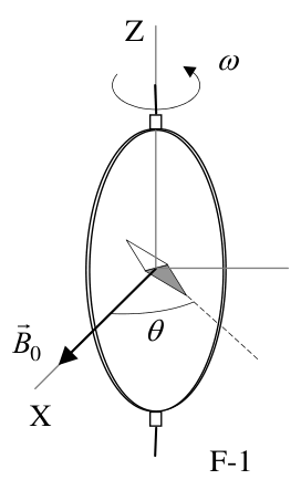
A closed circular coil of \(N\) turns, radius \(a\) and total resistance \(R\) is rotated with uniform angular velocity \(\omega\) about a vertical diameter in a horizontal magnetic field \(\vec B_0=B_0\vec i\).
1. (0.5+1.0) Compute the electromotive force \(\mathcal E\) induced in the coil, and also the mean power\({}^{1}\) \(\langle P\rangle\) required for maintaining the coil in motion. Neglect the coil self inductance.
A small magnetic needle is placed at the center of the coil, as shown in Figure F-1. It is free to turn slowly around the Z axis in a horizontal plane, but it cannot follow the rapid rotation of the coil.
F-1
2. (2.0) Once the stationary regime is reached, the needle will set at a direction making a small angle \(\theta\) with \(\vec B_0\). Compute the resistance \(R\) of the coil in terms of this angle and the other parameters of the system.
Lord Kelvin used this method in the 1860s to set the absolute standard for the ohm. To avoid the rotating coil, Lorenz devised an alternative method used by Lord Rayleigh and Ms. Sidgwick, that we analyze in the next paragraphs.
Determination of the ohm (Rayleigh, Sidgwick).
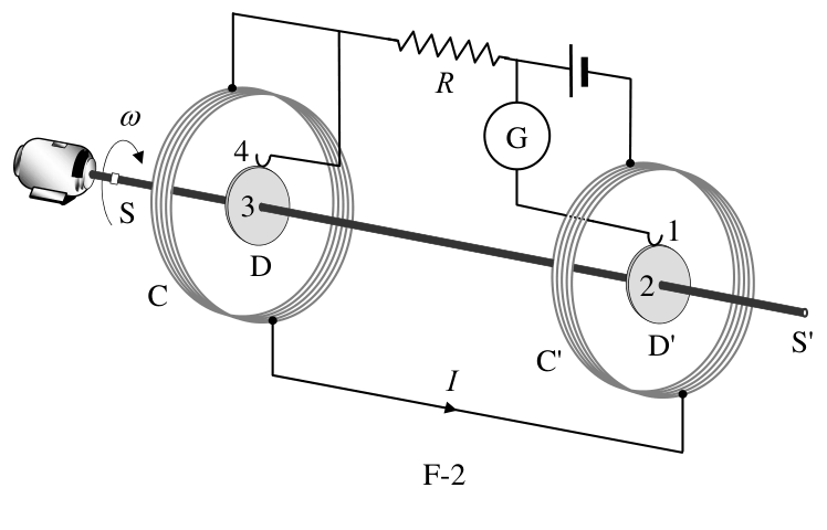
The experimental setup is shown in Figure F-2. It consists of two identical metal disks D and D' of radius \(b\) mounted on the conducting shaft SS'. A motor rotates the set at an angular velocity \(\omega\), which can be adjusted for measuring \(R\). Two identical coils C and C' (of radius \(a\) and with \(N\) turns each) surround the disks. They are connected in such a form that the current \(I\) flows through them in opposite directions. The whole apparatus serves to measure the resistance \(R\).
F-2
\({}^{1}\) The mean value \(\langle X\rangle\) of a quantity \(X(t)\) in a periodic system of period \(T\) is \[ \langle X\rangle=\frac{1}{T}\int_0^T X(t)\,dt. \]
You may need one or more of these integrals: \[ \int_0^{2\pi}\sin x\,dx =\int_0^{2\pi}\cos x\,dx =\int_0^{2\pi}\sin x\cos x\,dx=0, \] \[ \int_0^{2\pi}\sin^2x\,dx =\int_0^{2\pi}\cos^2x\,dx=\pi, \qquad \text{and later}\qquad \int x^n\,dx=\frac{1}{n+1}x^{n+1}. \]
3. (2.0) Assume that the current \(I\) flowing through the coils C and C' creates a uniform magnetic field \(B\) around D and D', equal to the one at the centre of the coil. Compute\({}^{1}\) the electromotive force \(\mathcal E\) induced between the rims 1 and 4, assuming that the distance between the coils is much larger than the radius of the coils and that \(a\gg b\).
The disks are connected to the circuit by brush contacts at their rims 1 and 4. The galvanometer G detects the flow of current through the circuit 1-2-3-4.
4. (0.5) The resistance \(R\) is measured when G reads zero. Give \(R\) in terms of the physical parameters of the system.
Determination of the ampere
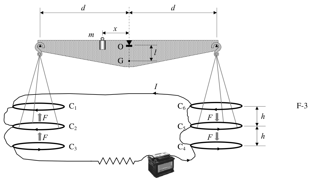
Passing a current through two conductors and measuring the force between them provides an absolute determination of the current itself. The “Current Balance” designed by Lord Kelvin in 1882 exploits this method. It consists of six identical single turn coils \(C_1\ldots C_6\) of radius \(a\), connected in series. As shown in Figure F-3, the fixed coils \(C_1\), \(C_3\), \(C_4\), and \(C_6\) are on two horizontal planes separated by a small distance \(2h\). The coils \(C_2\) and \(C_5\) are carried on balance arms of length \(d\), and they are, in equilibrium, equidistant from both planes.
The current \(I\) flows through the various coils in such a direction that the magnetic force on \(C_2\) is upwards while that on \(C_5\) is downwards. A mass \(m\) at a distance \(x\) from the fulcrum O is required to restore the balance to the equilibrium position described above when the current flows through the circuit.
F-3
5. (1.0) Compute the force \(F\) on \(C_2\) due to the magnetic interaction with \(C_1\). For simplicity assume that the force per unit length is the one corresponding to two long, straight wires carrying parallel currents.
6. (1.0) The current \(I\) is measured when the balance is in equilibrium. Give the value of \(I\) in terms of the physical parameters of the system. The dimensions of the apparatus are such that we can neglect the mutual effects of the coils on the left and on the right.
Let \(M\) be the mass of the balance (except for \(m\) and the hanging parts), G its centre of mass and \(l\) the distance \(\overline{OG}\).
7. (2.0) The balance equilibrium is stable against deviations producing small changes \(\delta z\) in the height of \(C_2\) and \(-\delta z\) in \(C_5\). Compute\({}^{2}\) the maximum value \(\delta z_{\max}\) so that the balance still returns towards the equilibrium position when it is released.
\({}^{2}\) Consider that the coils centres remain approximately aligned.
Use the approximations \[ \frac{1}{1\pm\beta}\approx1\mp\beta+\beta^2 \qquad\text{or}\qquad \frac{1}{1\pm\beta^2}\approx1\mp\beta^2 \] for \(\beta\ll1\), and \(\sin\theta\approx\tan\theta\) for small \(\theta\).
Official English text of the problem.
Answers
Here \(\mu_0\) is the permeability of free space and \(g\) is gravitational acceleration. No numerical parameter values are supplied, so the answers are symbolic.
-
Taking the coil normal parallel to \(\vec B_0\) at \(t=0\), \[ \boxed{\mathcal E(t)=N\pi a^2B_0\omega\sin(\omega t)}, \qquad \boxed{\langle P\rangle=\frac{N^2\pi^2a^4B_0^2\omega^2}{2R}}. \]
-
\[ \boxed{R=\frac{\mu_0\pi N^2a\omega}{4\tan\theta} \approx\frac{\mu_0\pi N^2a\omega}{4\theta}}, \] with \(\theta\) in radians.
-
The magnitude of the emf between the rims is \[ \boxed{|\mathcal E_{14}|=B\omega b^2 =\frac{\mu_0NI\omega b^2}{2a}}. \]
-
\[ \boxed{R=\frac{\mu_0N\omega b^2}{2a}}. \]
-
\[ \boxed{F=\frac{\mu_0aI^2}{h}}, \qquad\text{directed upwards.} \]
-
\[ \boxed{I=\sqrt{\frac{mgxh}{4\mu_0ad}}}. \]
-
To the order of the prescribed small-displacement approximation, \[ \boxed{\delta z_{\max}\approx \frac{Ml h^2}{mxd} =\frac{Mglh^3}{4\mu_0aI^2d^2}}. \] A positive displacement returns towards equilibrium when \(0<\delta z<\delta z_{\max}\); equality is the limiting boundary.
Solution
1. Induced emf and mean mechanical power
Let \(A=\pi a^2\). Choose the positive normal to the coil as \[ \hat n(t)=\cos(\omega t)\,\hat i+\sin(\omega t)\,\hat j, \] so that it is parallel to the applied field at \(t=0\).
The magnetic flux linkage through the \(N\) turns is \[ \Lambda(t)=NAB_0\cos(\omega t). \] Faraday’s law therefore gives \[ \mathcal E(t)=-\frac{d\Lambda}{dt} =NAB_0\omega\sin(\omega t), \] or \[ \boxed{\mathcal E(t)=N\pi a^2B_0\omega\sin(\omega t)}. \] A different initial orientation changes only the phase.
Since self inductance is neglected, the instantaneous current is \[ i(t)=\frac{\mathcal E(t)}{R}. \] At constant angular speed, the mechanical power supplied against the magnetic braking torque equals the Joule heating: \[ P(t)=i^2(t)R =\frac{N^2A^2B_0^2\omega^2}{R}\sin^2(\omega t). \] Using \(\langle\sin^2(\omega t)\rangle=\tfrac12\), \[ \boxed{\langle P\rangle =\frac{N^2\pi^2a^4B_0^2\omega^2}{2R}}. \]
2. Resistance from the magnetic needle’s deflection
The field at the centre of a circular \(N\)-turn coil is \[ \vec B_{\mathrm c}(t)=\frac{\mu_0Ni(t)}{2a}\hat n(t). \] Substituting the current found in part 1 and writing \(\phi=\omega t\), \[ \vec B_{\mathrm c}(t) =\frac{\mu_0N^2\pi aB_0\omega}{2R} \left( \sin\phi\cos\phi\,\hat i+\sin^2\phi\,\hat j \right). \]
The needle changes direction negligibly during one coil revolution. Consequently, its mean torque is its magnetic moment crossed with the vector average of the total field. Since \[ \langle\sin\phi\cos\phi\rangle=0, \qquad \langle\sin^2\phi\rangle=\frac12, \] the coil’s mean field is \[ \langle\vec B_{\mathrm c}\rangle =\frac{\mu_0N^2\pi aB_0\omega}{4R}\hat j. \] It is perpendicular to the applied field.
The stationary needle aligns with \[ \langle\vec B_{\mathrm{total}}\rangle =B_0\hat i+ \frac{\mu_0N^2\pi aB_0\omega}{4R}\hat j. \] Thus \[ \tan\theta =\frac{\langle B_{\mathrm c,y}\rangle}{B_0} =\frac{\mu_0N^2\pi a\omega}{4R}, \] giving \[ \boxed{R=\frac{\mu_0\pi N^2a\omega}{4\tan\theta}}. \] For the specified small angle, \[ \boxed{R\approx\frac{\mu_0\pi N^2a\omega}{4\theta}}. \]
3. Emf between the rotating disks’ rims
The magnetic field at the centre of either surrounding coil has magnitude \[ B=\frac{\mu_0NI}{2a}. \] The large separation of the coils allows their mutual field contributions to be neglected. The condition \(a\gg b\) permits this central field to be treated as uniform across each disk.
At radius \(r\), a disk element moves with tangential speed \[ v=\omega r. \] In an axial magnetic field, the magnetic force per unit charge, \(\vec v\times\vec B\), is radial. Hence the magnitude of the motional emf from the hub to the rim of one disk is \[ \mathcal E_{\mathrm d} =\int_0^b B\omega r\,dr =\frac12B\omega b^2. \]
The disks rotate in the same sense but their magnetic fields are opposite. Their rim-to-hub emfs therefore have opposite signs. Since the hubs are joined by the conducting shaft, the rim-to-rim emfs add in magnitude: \[ |\mathcal E_{14}|=2\mathcal E_{\mathrm d}=B\omega b^2. \] Thus \[ \boxed{|\mathcal E_{14}|=\frac{\mu_0NI\omega b^2}{2a}}. \] The polarity is determined by the direction of \(\vec\omega\) relative to the axial field in each disk.
4. Resistance at galvanometer null
When the galvanometer reads zero, no current flows through the disk–shaft–galvanometer branch. There is therefore no resistive voltage drop along that branch.
The disk emf balances the voltage \(IR\) across the resistance: \[ IR=|\mathcal E_{14}| =\frac{\mu_0NI\omega b^2}{2a}. \] Cancelling the nonzero current, \[ \boxed{R=\frac{\mu_0N\omega b^2}{2a}}. \]
5. Force between \(C_1\) and \(C_2\)
For two long parallel wires separated by \(h\), each carrying current \(I\), the magnetic force per unit length is \[ f=\frac{\mu_0I^2}{2\pi h}. \] Using the prescribed approximation, this applies locally around the circumference \(2\pi a\) of the coils. The force is therefore \[ F=f(2\pi a) =\frac{\mu_0I^2}{2\pi h}(2\pi a), \] so \[ \boxed{F=\frac{\mu_0aI^2}{h}}. \]
The currents in \(C_1\) and \(C_2\) circulate in the same direction, so the interaction is attractive. Since \(C_1\) is above \(C_2\), the force on \(C_2\) is upwards.
6. Current from the balance equilibrium
The upper coil \(C_1\) attracts \(C_2\) upwards, while the lower coil \(C_3\), carrying the opposite current, repels it upwards. Each contributes the force found in part 5. Thus the total upward force on \(C_2\) is \(2F\).
Similarly, the total force on \(C_5\) is \(2F\) downwards. These two forces produce torques in the same rotational sense: \[ \tau_{\mathrm{mag}}=(2F)d+(2F)d=4Fd. \]
The added mass provides the opposing torque \(mgx\). At equilibrium, \[ mgx=4Fd=\frac{4\mu_0aI^2d}{h}. \] Consequently, \[ \boxed{I=\sqrt{\frac{mgxh}{4\mu_0ad}}}. \]
7. Maximum displacement that produces a restoring torque
Write \(z=\delta z\), positive when \(C_2\) rises and \(C_5\) falls. Let \(\alpha\) be the corresponding tilt of the balance, so that \[ z=d\sin\alpha. \] We retain the assumed alignment of the coil centres and treat the current as fixed.
Define \[ K=\mu_0aI^2. \] After the displacement, the separations between \(C_2\) and its upper and lower fixed coils are \(h-z\) and \(h+z\). Both magnetic forces remain upwards, so their sum is \[ F_{\mathrm L}(z) =\frac{K}{h-z}+\frac{K}{h+z} =\frac{2Kh}{h^2-z^2}. \] On the right, the two separations are interchanged; the total downward force has the same magnitude.
Taking positive torque to mean a tendency to increase \(z\), the total magnetic torque is \[ \tau_{\mathrm{mag}} =2d\cos\alpha\,F_{\mathrm L}(z) =\frac{4Khd}{h^2-z^2}\cos\alpha. \]
The added mass supplies the opposing torque \[ \tau_m=-mgx\cos\alpha. \] Because the balance’s centre of mass lies a distance \(l\) below its fulcrum, its weight supplies the restoring torque \[ \tau_M=-Mgl\sin\alpha. \] The equal weights of the hanging parts cancel in the torque balance.
Hence the net torque is \[ \tau(z) =\left(\frac{4Khd}{h^2-z^2}-mgx\right)\cos\alpha -Mgl\sin\alpha. \] From the equilibrium condition in part 6, \[ mgx=\frac{4Kd}{h}. \] Substitution gives \[ \tau(z) =mgx\frac{z^2}{h^2-z^2}\cos\alpha -Mgl\sin\alpha. \]
For small tilt, \(\cos\alpha>0\), so the torque has the same sign as \[ \frac{\tau(z)}{\cos\alpha} =mgx\frac{z^2}{h^2-z^2}-Mgl\tan\alpha. \] Using the prescribed approximations, \[ \frac{z^2}{h^2-z^2}\approx\frac{z^2}{h^2}, \qquad \tan\alpha\approx\sin\alpha=\frac{z}{d}, \] we obtain \[ \frac{\tau(z)}{\cos\alpha} \approx \frac{mgx}{h^2}z^2-\frac{Mgl}{d}z. \]
For \(z>0\), the balance initially moves back towards equilibrium if \(\tau(z)<0\). Therefore \[ \frac{mgx}{h^2}z<\frac{Mgl}{d}, \] or \[ z<\frac{Ml h^2}{mxd}. \] The limiting displacement is thus \[ \boxed{\delta z_{\max}\approx\frac{Ml h^2}{mxd}}. \] Using the equilibrium relation once more, \[ \boxed{\delta z_{\max}\approx \frac{Mglh^3}{4\mu_0aI^2d^2}}. \]
At this boundary the net torque vanishes to the retained order; a larger positive displacement produces a torque away from equilibrium. For a negative small displacement, both terms in the approximate torque point towards increasing \(z\), initially returning the balance towards equilibrium.
The stated limit is the leading small-displacement result, requiring \(\delta z_{\max}\ll h\) and \(\delta z_{\max}\ll d\) for quantitative use of the approximations.
The solution was checked against the official solution.
IPhO 2005 · Theorieaufgabe 2
Absolutmessungen elektrischer Größen
Th 2 ABSOLUTMESSUNGEN ELEKTRISCHER GRÖSSEN
Die technologischen und wissenschaftlichen Umwälzungen im XIX. Jahrhundert führten zu einem dringenden Bedarf an allgemein anerkannten Normalen für die elektrischen Größen. Die neuen absoluten Einheiten sollten, so die damalige Vorstellung, ausschließlich auf den nach der Französischen Revolution festgelegten Normalen für Länge, Masse und Zeit beruhen. Von 1861 bis 1912 wurden umfangreiche experimentelle Arbeiten durchgeführt, um die Werte dieser Einheiten festzulegen. Wir stellen hier drei Fallstudien vor.
Die Punktzahlen stehen jeweils zu Beginn jeder Teilaufgabe in Klammern.
Bestimmung des Ohms (Kelvin)
Eine geschlossene kreisförmige Spule mit \(N\) Windungen, dem Radius \(a\) und dem Gesamtwiderstand \(R\) wird mit konstanter Winkelgeschwindigkeit \(\omega\) um einen vertikalen Durchmesser in einem horizontalen Magnetfeld \(\vec B_0=B_0\vec i\) gedreht.
1. (0.5+1.0) Berechnen Sie die in der Spule induzierte elektromotorische Kraft \(\mathcal E\) sowie die mittlere Leistung\({}^{1}\) \(\langle P\rangle\), die erforderlich ist, um die Spule in Bewegung zu halten. Vernachlässigen Sie die Selbstinduktivität der Spule.
Eine kleine Magnetnadel wird wie in Abbildung F-1 im Mittelpunkt der Spule angebracht. Sie kann sich in einer horizontalen Ebene frei und langsam um die Z-Achse drehen, der schnellen Drehung der Spule jedoch nicht folgen.
F-1
2. (2.0) Sobald der stationäre Zustand erreicht ist, stellt sich die Nadel in einer Richtung ein, die mit \(\vec B_0\) einen kleinen Winkel \(\theta\) bildet. Berechnen Sie den Widerstand \(R\) der Spule in Abhängigkeit von diesem Winkel und den anderen Parametern des Systems.
Lord Kelvin verwendete diese Methode in den 1860er-Jahren, um das absolute Normal für das Ohm festzulegen. Um die rotierende Spule zu vermeiden, entwickelte Lorenz eine alternative Methode, die von Lord Rayleigh und Frau Sidgwick angewandt wurde und die wir in den folgenden Absätzen untersuchen.
Bestimmung des Ohms (Rayleigh, Sidgwick).
Der Versuchsaufbau ist in Abbildung F-2 dargestellt. Er besteht aus zwei identischen Metallscheiben D und D' mit dem Radius \(b\), die auf der leitenden Welle SS' montiert sind. Ein Motor versetzt die Anordnung in eine Drehung mit der Winkelgeschwindigkeit \(\omega\), die zur Messung von \(R\) eingestellt werden kann. Zwei identische Spulen C und C' (mit dem Radius \(a\) und jeweils \(N\) Windungen) umgeben die Scheiben. Sie sind so verschaltet, dass der Strom \(I\) sie in entgegengesetzten Richtungen durchfließt. Die gesamte Apparatur dient zur Messung des Widerstands \(R\).
F-2
\({}^{1}\) Der Mittelwert \(\langle X\rangle\) einer Größe \(X(t)\) in einem periodischen System mit der Periodendauer \(T\) ist \[ \langle X\rangle=\frac{1}{T}\int_0^T X(t)\,dt. \]
Sie benötigen möglicherweise eines oder mehrere der folgenden Integrale: \[ \int_0^{2\pi}\sin x\,dx =\int_0^{2\pi}\cos x\,dx =\int_0^{2\pi}\sin x\cos x\,dx=0, \] \[ \int_0^{2\pi}\sin^2x\,dx =\int_0^{2\pi}\cos^2x\,dx=\pi, \qquad \text{und später}\qquad \int x^n\,dx=\frac{1}{n+1}x^{n+1}. \]
3. (2.0) Nehmen Sie an, dass der durch die Spulen C und C' fließende Strom \(I\) im Bereich von D und D' ein homogenes Magnetfeld \(B\) erzeugt, das gleich dem Feld im Mittelpunkt der jeweiligen Spule ist. Berechnen Sie\({}^{1}\) die zwischen den Rändern 1 und 4 induzierte elektromotorische Kraft \(\mathcal E\) unter der Annahme, dass der Abstand zwischen den Spulen viel größer als ihr Radius ist und dass \(a\gg b\) gilt.
Die Scheiben sind über Bürstenkontakte an ihren Rändern 1 und 4 mit dem Stromkreis verbunden. Das Galvanometer G weist einen Stromfluss durch den Stromkreis 1-2-3-4 nach.
4. (0.5) Der Widerstand \(R\) wird gemessen, wenn G null anzeigt. Geben Sie \(R\) in Abhängigkeit von den physikalischen Parametern des Systems an.
Bestimmung des Amperes
Indem man einen Strom durch zwei Leiter fließen lässt und die Kraft zwischen ihnen misst, kann man den Strom selbst absolut bestimmen. Die 1882 von Lord Kelvin entworfene „Stromwaage“ nutzt diese Methode. Sie besteht aus sechs identischen Spulen \(C_1\ldots C_6\) mit jeweils einer Windung und dem Radius \(a\), die in Reihe geschaltet sind. Wie in Abbildung F-3 gezeigt, liegen die feststehenden Spulen \(C_1\), \(C_3\), \(C_4\) und \(C_6\) in zwei horizontalen Ebenen mit dem kleinen Abstand \(2h\). Die Spulen \(C_2\) und \(C_5\) werden von Waagearmen der Länge \(d\) getragen und haben im Gleichgewicht von beiden Ebenen denselben Abstand.
Der Strom \(I\) fließt durch die verschiedenen Spulen jeweils in einer solchen Richtung, dass die magnetische Kraft auf \(C_2\) nach oben und diejenige auf \(C_5\) nach unten gerichtet ist. Eine Masse \(m\) im Abstand \(x\) vom Drehpunkt O ist erforderlich, um die Waage wieder in die oben beschriebene Gleichgewichtslage zu bringen, wenn der Strom durch den Stromkreis fließt.
F-3
5. (1.0) Berechnen Sie die Kraft \(F\) auf \(C_2\) aufgrund der magnetischen Wechselwirkung mit \(C_1\). Nehmen Sie der Einfachheit halber an, dass die Kraft pro Längeneinheit derjenigen zwischen zwei langen, geraden Drähten mit gleichgerichteten Strömen entspricht.
6. (1.0) Der Strom \(I\) wird gemessen, wenn sich die Waage im Gleichgewicht befindet. Geben Sie den Wert von \(I\) in Abhängigkeit von den physikalischen Parametern des Systems an. Die Abmessungen der Apparatur sind so gewählt, dass die gegenseitigen Einflüsse der Spulen auf der linken und auf der rechten Seite vernachlässigt werden können.
Es seien \(M\) die Masse der Waage (ohne \(m\) und die aufgehängten Teile), G ihr Schwerpunkt und \(l\) der Abstand \(\overline{OG}\).
7. (2.0) Das Gleichgewicht der Waage ist stabil gegenüber Auslenkungen, die kleine Höhenänderungen \(\delta z\) von \(C_2\) und \(-\delta z\) von \(C_5\) bewirken. Berechnen Sie\({}^{2}\) den maximalen Wert \(\delta z_{\max}\), bei dem sich die Waage nach dem Loslassen noch in Richtung ihrer Gleichgewichtslage zurückbewegt.
\({}^{2}\) Nehmen Sie an, dass die Spulenmittelpunkte näherungsweise auf einer gemeinsamen Achse bleiben.
Verwenden Sie die Näherungen \[ \frac{1}{1\pm\beta}\approx1\mp\beta+\beta^2 \qquad\text{oder}\qquad \frac{1}{1\pm\beta^2}\approx1\mp\beta^2 \] für \(\beta\ll1\) sowie \(\sin\theta\approx\tan\theta\) für kleine \(\theta\).
Aufgabentext aus dem offiziellen englischen Text übersetzt.
Antworten
Hier bezeichnet \(\mu_0\) die magnetische Feldkonstante und \(g\) die Fallbeschleunigung. Da keine Zahlenwerte für die Parameter angegeben sind, werden die Antworten in symbolischer Form angegeben.
-
Wählt man die Spulennormale bei \(t=0\) parallel zu \(\vec B_0\), so gilt \[ \boxed{\mathcal E(t)=N\pi a^2B_0\omega\sin(\omega t)}, \qquad \boxed{\langle P\rangle=\frac{N^2\pi^2a^4B_0^2\omega^2}{2R}}. \]
-
\[ \boxed{R=\frac{\mu_0\pi N^2a\omega}{4\tan\theta} \approx\frac{\mu_0\pi N^2a\omega}{4\theta}}, \] wobei \(\theta\) im Bogenmaß angegeben wird.
-
Der Betrag der elektromotorischen Kraft zwischen den Rändern ist \[ \boxed{|\mathcal E_{14}|=B\omega b^2 =\frac{\mu_0NI\omega b^2}{2a}}. \]
-
\[ \boxed{R=\frac{\mu_0N\omega b^2}{2a}}. \]
-
\[ \boxed{F=\frac{\mu_0aI^2}{h}}, \qquad\text{nach oben gerichtet.} \]
-
\[ \boxed{I=\sqrt{\frac{mgxh}{4\mu_0ad}}}. \]
-
Bis zur Ordnung der vorgegebenen Näherung für kleine Auslenkungen gilt \[ \boxed{\delta z_{\max}\approx \frac{Ml h^2}{mxd} =\frac{Mglh^3}{4\mu_0aI^2d^2}}. \] Bei einer positiven Auslenkung bewegt sich die Waage in Richtung des Gleichgewichts zurück, wenn \(0<\delta z<\delta z_{\max}\); Gleichheit kennzeichnet den Grenzfall.
Lösung
1. Induzierte elektromotorische Kraft und mittlere mechanische Leistung
Es sei \(A=\pi a^2\). Wir wählen die positive Spulennormale als \[ \hat n(t)=\cos(\omega t)\,\hat i+\sin(\omega t)\,\hat j, \] sodass sie bei \(t=0\) parallel zum angelegten Feld ist.
Die magnetische Flussverkettung der \(N\) Windungen ist \[ \Lambda(t)=NAB_0\cos(\omega t). \] Aus dem Faradayschen Induktionsgesetz folgt daher \[ \mathcal E(t)=-\frac{d\Lambda}{dt} =NAB_0\omega\sin(\omega t), \] also \[ \boxed{\mathcal E(t)=N\pi a^2B_0\omega\sin(\omega t)}. \] Eine andere Anfangsausrichtung ändert lediglich die Phase.
Da die Selbstinduktivität vernachlässigt wird, ist der momentane Strom \[ i(t)=\frac{\mathcal E(t)}{R}. \] Bei konstanter Winkelgeschwindigkeit ist die gegen das magnetische Bremsmoment aufgebrachte mechanische Leistung gleich der Jouleschen Wärmeleistung: \[ P(t)=i^2(t)R =\frac{N^2A^2B_0^2\omega^2}{R}\sin^2(\omega t). \] Mit \(\langle\sin^2(\omega t)\rangle=\tfrac12\) ergibt sich \[ \boxed{\langle P\rangle =\frac{N^2\pi^2a^4B_0^2\omega^2}{2R}}. \]
2. Widerstand aus der Ablenkung der Magnetnadel
Das Feld im Mittelpunkt einer kreisförmigen Spule mit \(N\) Windungen ist \[ \vec B_{\mathrm c}(t)=\frac{\mu_0Ni(t)}{2a}\hat n(t). \] Setzt man den in Teil 1 bestimmten Strom ein und schreibt \(\phi=\omega t\), so erhält man \[ \vec B_{\mathrm c}(t) =\frac{\mu_0N^2\pi aB_0\omega}{2R} \left( \sin\phi\cos\phi\,\hat i+\sin^2\phi\,\hat j \right). \]
Während einer Umdrehung der Spule ändert die Nadel ihre Richtung nur vernachlässigbar wenig. Ihr mittleres Drehmoment ist daher das Kreuzprodukt ihres magnetischen Moments mit dem Vektormittelwert des Gesamtfeldes. Wegen \[ \langle\sin\phi\cos\phi\rangle=0, \qquad \langle\sin^2\phi\rangle=\frac12, \] ist das mittlere Feld der Spule \[ \langle\vec B_{\mathrm c}\rangle =\frac{\mu_0N^2\pi aB_0\omega}{4R}\hat j. \] Es steht senkrecht zum angelegten Feld.
Im stationären Zustand richtet sich die Nadel entlang \[ \langle\vec B_{\mathrm{total}}\rangle =B_0\hat i+ \frac{\mu_0N^2\pi aB_0\omega}{4R}\hat j \] aus. Somit gilt \[ \tan\theta =\frac{\langle B_{\mathrm c,y}\rangle}{B_0} =\frac{\mu_0N^2\pi a\omega}{4R}, \] woraus folgt: \[ \boxed{R=\frac{\mu_0\pi N^2a\omega}{4\tan\theta}}. \] Für den vorgegebenen kleinen Winkel gilt \[ \boxed{R\approx\frac{\mu_0\pi N^2a\omega}{4\theta}}. \]
3. Elektromotorische Kraft zwischen den Rändern der rotierenden Scheiben
Das Magnetfeld im Mittelpunkt jeder der umgebenden Spulen hat den Betrag \[ B=\frac{\mu_0NI}{2a}. \] Aufgrund des großen Abstands der Spulen können ihre gegenseitigen Feldbeiträge vernachlässigt werden. Die Bedingung \(a\gg b\) erlaubt es, dieses Feld im Mittelpunkt über die gesamte jeweilige Scheibe als homogen anzusehen.
Im Abstand \(r\) von der Achse bewegt sich ein Scheibenelement mit der Tangentialgeschwindigkeit \[ v=\omega r. \] In einem axialen Magnetfeld ist die magnetische Kraft pro Ladungseinheit, \(\vec v\times\vec B\), radial gerichtet. Daher beträgt die durch Bewegung induzierte elektromotorische Kraft von der Nabe bis zum Rand einer Scheibe \[ \mathcal E_{\mathrm d} =\int_0^b B\omega r\,dr =\frac12B\omega b^2. \]
Die Scheiben drehen sich im selben Drehsinn, ihre Magnetfelder sind jedoch entgegengesetzt gerichtet. Die elektromotorischen Kräfte zwischen Rand und Nabe haben daher entgegengesetzte Vorzeichen. Da die Naben durch die leitende Welle verbunden sind, addieren sich die Beträge der elektromotorischen Kräfte zwischen den beiden Rändern: \[ |\mathcal E_{14}|=2\mathcal E_{\mathrm d}=B\omega b^2. \] Somit gilt \[ \boxed{|\mathcal E_{14}|=\frac{\mu_0NI\omega b^2}{2a}}. \] Die Polarität wird durch die Richtung von \(\vec\omega\) relativ zum axialen Feld in der jeweiligen Scheibe bestimmt.
4. Widerstand beim Nullabgleich des Galvanometers
Wenn das Galvanometer null anzeigt, fließt durch den Zweig aus Scheiben, Welle und Galvanometer kein Strom. Entlang dieses Zweigs tritt daher kein ohmscher Spannungsabfall auf.
Die elektromotorische Kraft der Scheiben gleicht die Spannung \(IR\) am Widerstand aus: \[ IR=|\mathcal E_{14}| =\frac{\mu_0NI\omega b^2}{2a}. \] Durch Kürzen des von null verschiedenen Stroms erhält man \[ \boxed{R=\frac{\mu_0N\omega b^2}{2a}}. \]
5. Kraft zwischen \(C_1\) und \(C_2\)
Für zwei lange parallele Drähte im Abstand \(h\), die jeweils den Strom \(I\) führen, beträgt die magnetische Kraft pro Längeneinheit \[ f=\frac{\mu_0I^2}{2\pi h}. \] In der vorgegebenen Näherung gilt dies lokal entlang des Umfangs \(2\pi a\) der Spulen. Die Kraft ist daher \[ F=f(2\pi a) =\frac{\mu_0I^2}{2\pi h}(2\pi a), \] also \[ \boxed{F=\frac{\mu_0aI^2}{h}}. \]
Die Ströme in \(C_1\) und \(C_2\) fließen im selben Umlaufsinn, sodass die Wechselwirkung anziehend ist. Da \(C_1\) oberhalb von \(C_2\) liegt, ist die Kraft auf \(C_2\) nach oben gerichtet.
6. Strom aus dem Gleichgewicht der Waage
Die obere Spule \(C_1\) zieht \(C_2\) nach oben an, während die untere Spule \(C_3\), deren Strom in entgegengesetzter Richtung fließt, sie nach oben abstößt. Jede trägt die in Teil 5 bestimmte Kraft bei. Die gesamte nach oben gerichtete Kraft auf \(C_2\) beträgt somit \(2F\).
Entsprechend beträgt die Gesamtkraft auf \(C_5\) ebenfalls \(2F\) und ist nach unten gerichtet. Diese beiden Kräfte erzeugen Drehmomente im selben Drehsinn: \[ \tau_{\mathrm{mag}}=(2F)d+(2F)d=4Fd. \]
Die zusätzliche Masse erzeugt das entgegengesetzte Drehmoment \(mgx\). Im Gleichgewicht gilt \[ mgx=4Fd=\frac{4\mu_0aI^2d}{h}. \] Folglich ist \[ \boxed{I=\sqrt{\frac{mgxh}{4\mu_0ad}}}. \]
7. Maximale Auslenkung, bei der ein rückstellendes Drehmoment auftritt
Wir schreiben \(z=\delta z\), wobei das Vorzeichen positiv ist, wenn \(C_2\) steigt und \(C_5\) sinkt. Es sei \(\alpha\) der zugehörige Neigungswinkel der Waage, sodass \[ z=d\sin\alpha. \] Wir behalten die angenommene Ausrichtung der Spulenmittelpunkte auf einer gemeinsamen Achse bei und behandeln den Strom als konstant.
Wir definieren \[ K=\mu_0aI^2. \] Nach der Auslenkung betragen die Abstände zwischen \(C_2\) und der oberen beziehungsweise unteren feststehenden Spule \(h-z\) und \(h+z\). Beide magnetischen Kräfte bleiben nach oben gerichtet, sodass ihre Summe \[ F_{\mathrm L}(z) =\frac{K}{h-z}+\frac{K}{h+z} =\frac{2Kh}{h^2-z^2} \] beträgt. Auf der rechten Seite sind die beiden Abstände vertauscht; die gesamte nach unten gerichtete Kraft hat denselben Betrag.
Wenn ein positives Drehmoment eine Tendenz zur Vergrößerung von \(z\) bezeichnet, ist das gesamte magnetische Drehmoment \[ \tau_{\mathrm{mag}} =2d\cos\alpha\,F_{\mathrm L}(z) =\frac{4Khd}{h^2-z^2}\cos\alpha. \]
Die zusätzliche Masse liefert das entgegengesetzte Drehmoment \[ \tau_m=-mgx\cos\alpha. \] Da der Schwerpunkt der Waage im Abstand \(l\) unterhalb ihres Drehpunkts liegt, liefert ihre Gewichtskraft das rückstellende Drehmoment \[ \tau_M=-Mgl\sin\alpha. \] Die gleichen Gewichtskräfte der aufgehängten Teile heben sich in der Drehmomentbilanz auf.
Das resultierende Drehmoment ist somit \[ \tau(z) =\left(\frac{4Khd}{h^2-z^2}-mgx\right)\cos\alpha -Mgl\sin\alpha. \] Aus der Gleichgewichtsbedingung in Teil 6 folgt \[ mgx=\frac{4Kd}{h}. \] Einsetzen ergibt \[ \tau(z) =mgx\frac{z^2}{h^2-z^2}\cos\alpha -Mgl\sin\alpha. \]
Für kleine Neigungswinkel gilt \(\cos\alpha>0\), sodass das Drehmoment dasselbe Vorzeichen hat wie \[ \frac{\tau(z)}{\cos\alpha} =mgx\frac{z^2}{h^2-z^2}-Mgl\tan\alpha. \] Mit den vorgegebenen Näherungen \[ \frac{z^2}{h^2-z^2}\approx\frac{z^2}{h^2}, \qquad \tan\alpha\approx\sin\alpha=\frac{z}{d}, \] erhalten wir \[ \frac{\tau(z)}{\cos\alpha} \approx \frac{mgx}{h^2}z^2-\frac{Mgl}{d}z. \]
Für \(z>0\) bewegt sich die Waage zunächst in Richtung des Gleichgewichts zurück, wenn \(\tau(z)<0\) gilt. Daher muss \[ \frac{mgx}{h^2}z<\frac{Mgl}{d}, \] also \[ z<\frac{Ml h^2}{mxd} \] gelten. Die Grenzauslenkung ist somit \[ \boxed{\delta z_{\max}\approx\frac{Ml h^2}{mxd}}. \] Mit der Gleichgewichtsbeziehung erhält man erneut \[ \boxed{\delta z_{\max}\approx \frac{Mglh^3}{4\mu_0aI^2d^2}}. \]
An dieser Grenze verschwindet das resultierende Drehmoment bis zur berücksichtigten Ordnung; eine größere positive Auslenkung erzeugt ein Drehmoment, das von der Gleichgewichtslage wegführt. Bei einer kleinen negativen Auslenkung wirken beide Terme des näherungsweisen Drehmoments in Richtung zunehmender \(z\), sodass sich die Waage zunächst in Richtung des Gleichgewichts zurückbewegt.
Der angegebene Grenzwert ist das Ergebnis in führender Ordnung für kleine Auslenkungen; für eine quantitative Anwendung der Näherungen müssen \(\delta z_{\max}\ll h\) und \(\delta z_{\max}\ll d\) gelten.
Die Lösung wurde mit der offiziellen Lösung abgeglichen.
IPhO 2005 · Teori sorusu 2
Elektriksel Büyüklüklerin Mutlak Ölçümleri
Th 2 ELEKTRİKSEL BÜYÜKLÜKLERİN MUTLAK ÖLÇÜMLERİ
XIX. yüzyılda yaşanan teknolojik ve bilimsel dönüşümler, elektriksel büyüklükler için evrensel olarak kabul gören standartlara duyulan ihtiyacı zorunlu hâle getirdi. Yeni mutlak birimlerin yalnızca Fransız Devrimi'nden sonra belirlenen uzunluk, kütle ve zaman standartlarına dayanması gerektiği düşünülüyordu. Bu birimlerin değerlerini belirlemek için 1861'den 1912'ye kadar yoğun deneysel çalışmalar yürütüldü. Burada üç örnek inceleme sunuyoruz.
Puanlar, her alt sorunun başında parantez içinde belirtilmiştir.
Ohmun belirlenmesi (Kelvin)
Sarım sayısı \(N\), yarıçapı \(a\) ve toplam direnci \(R\) olan kapalı dairesel bir bobin, yatay bir \(\vec B_0=B_0\vec i\) manyetik alanı içinde, düşey bir çapı etrafında sabit \(\omega\) açısal hızıyla döndürülmektedir.
1. (0.5+1.0) Bobinde indüklenen \(\mathcal E\) elektromotor kuvvetini ve bobinin hareketini sürdürmek için gereken ortalama gücü\({}^{1}\) \(\langle P\rangle\) hesaplayınız. Bobinin özindüktansını ihmal ediniz.
Şekil F-1'de gösterildiği gibi, bobinin merkezine küçük bir mıknatıs iğnesi yerleştirilmiştir. İğne, yatay bir düzlemde Z ekseni etrafında yavaşça serbestçe dönebilir, ancak bobinin hızlı dönüşünü izleyemez.
F-1
2. (2.0) Kararlı rejime ulaşıldığında iğne, \(\vec B_0\) ile küçük bir \(\theta\) açısı yapan bir doğrultuya yerleşir. Bobinin \(R\) direncini bu açı ve sistemin diğer parametreleri cinsinden hesaplayınız.
Lord Kelvin, 1860'larda ohmun mutlak standardını belirlemek için bu yöntemi kullandı. Dönen bobine gerek kalmaması için Lorenz, Lord Rayleigh ve Bayan Sidgwick tarafından kullanılan alternatif bir yöntem geliştirdi; bu yöntemi sonraki paragraflarda inceleyeceğiz.
Ohmun belirlenmesi (Rayleigh, Sidgwick).
Deney düzeneği Şekil F-2'de gösterilmiştir. Düzenek, iletken SS' miline takılı, yarıçapları \(b\) olan özdeş iki metal diskten, D ve D' disklerinden oluşur. Bir motor, bu sistemi \(R\)'yi ölçmek için ayarlanabilen \(\omega\) açısal hızıyla döndürür. Özdeş iki bobin, C ve C' (her birinin yarıçapı \(a\) ve sarım sayısı \(N\)), diskleri çevreler. Bobinler, \(I\) akımı içlerinden zıt yönlerde geçecek biçimde bağlanmıştır. Düzeneğin tamamı \(R\) direncini ölçmek için kullanılır.
F-2
\({}^{1}\) Periyodu \(T\) olan periyodik bir sistemde, \(X(t)\) büyüklüğünün ortalama değeri \(\langle X\rangle\) şöyledir: \[ \langle X\rangle=\frac{1}{T}\int_0^T X(t)\,dt. \]
Şu integrallerden birine veya birkaçına ihtiyaç duyabilirsiniz: \[ \int_0^{2\pi}\sin x\,dx =\int_0^{2\pi}\cos x\,dx =\int_0^{2\pi}\sin x\cos x\,dx=0, \] \[ \int_0^{2\pi}\sin^2x\,dx =\int_0^{2\pi}\cos^2x\,dx=\pi, \qquad \text{ve ileride}\qquad \int x^n\,dx=\frac{1}{n+1}x^{n+1}. \]
3. (2.0) C ve C' bobinlerinden geçen \(I\) akımının, D ve D' çevresinde bobin merkezindeki alana eşit, düzgün bir \(B\) manyetik alanı oluşturduğunu varsayınız. Bobinler arasındaki uzaklığın bobinlerin yarıçapından çok daha büyük olduğunu ve \(a\gg b\) koşulunun sağlandığını varsayarak, 1 ve 4 kenarları arasında indüklenen \(\mathcal E\) elektromotor kuvvetini hesaplayınız\({}^{1}\).
Diskler, 1 ve 4 kenarlarındaki fırça temaslarıyla devreye bağlanmıştır. G galvanometresi, 1-2-3-4 devresinden geçen akımı algılar.
4. (0.5) \(R\) direnci, G sıfırı gösterdiğinde ölçülür. \(R\)'yi sistemin fiziksel parametreleri cinsinden veriniz.
Amperin belirlenmesi
İki iletkenden akım geçirip aralarındaki kuvveti ölçmek, akımın kendisinin mutlak olarak belirlenmesini sağlar. Lord Kelvin'in 1882'de tasarladığı “Akım Terazisi” bu yöntemden yararlanır. Seri bağlanmış, yarıçapları \(a\) olan, özdeş ve tek sarımlı altı bobinden, \(C_1\ldots C_6\)'dan oluşur. Şekil F-3'te gösterildiği gibi, sabit \(C_1\), \(C_3\), \(C_4\) ve \(C_6\) bobinleri, aralarında küçük bir \(2h\) uzaklığı bulunan iki yatay düzlem üzerindedir. \(C_2\) ve \(C_5\) bobinleri, uzunluğu \(d\) olan terazi kollarında taşınır ve dengedeyken her iki düzleme eşit uzaklıktadır.
\(I\) akımı, çeşitli bobinlerden, \(C_2\) üzerindeki manyetik kuvvet yukarı, \(C_5\) üzerindeki ise aşağı yönde olacak biçimde geçer. Devreden akım geçtiğinde teraziyi yukarıda açıklanan denge konumuna geri getirmek için, O destek noktasından \(x\) uzaklığa \(m\) kütlesi yerleştirilmesi gerekir.
F-3
5. (1.0) \(C_1\) ile manyetik etkileşiminden dolayı \(C_2\) üzerine etkiyen \(F\) kuvvetini hesaplayınız. Basitlik için, birim uzunluk başına kuvvetin paralel akımlar taşıyan iki uzun, düz tel arasındaki kuvvetle aynı olduğunu varsayınız.
6. (1.0) \(I\) akımı, terazi dengedeyken ölçülür. \(I\)'nın değerini sistemin fiziksel parametreleri cinsinden veriniz. Düzeneğin boyutları, soldaki ve sağdaki bobinlerin birbirlerine etkilerini ihmal edebileceğimiz şekildedir.
\(M\), terazinin kütlesi (\(m\) ve asılı parçalar hariç), G kütle merkezi ve \(l\), \(\overline{OG}\) uzaklığı olsun.
7. (2.0) Terazinin dengesi, \(C_2\)'nin yüksekliğinde küçük \(\delta z\), \(C_5\)'inkinde ise \(-\delta z\) değişimleri oluşturan sapmalara karşı kararlıdır. Terazi serbest bırakıldığında hâlâ denge konumuna doğru dönecek şekilde, \(\delta z_{\max}\) en büyük değerini hesaplayınız\({}^{2}\).
\({}^{2}\) Bobin merkezlerinin yaklaşık olarak aynı hizada kaldığını kabul ediniz.
\(\beta\ll1\) için \[ \frac{1}{1\pm\beta}\approx1\mp\beta+\beta^2 \qquad\text{veya}\qquad \frac{1}{1\pm\beta^2}\approx1\mp\beta^2 \] yaklaşımlarını ve küçük \(\theta\) için \(\sin\theta\approx\tan\theta\) yaklaşımını kullanınız.
Soru metni resmi İngilizce metinden çevrilmiştir.
Cevaplar
Burada \(\mu_0\) boşluğun manyetik geçirgenliği, \(g\) ise yerçekimi ivmesidir. Parametrelerin sayısal değerleri verilmediği için cevaplar semboliktir.
-
\(t=0\) anında bobinin normalini \(\vec B_0\)'a paralel alırsak, \[ \boxed{\mathcal E(t)=N\pi a^2B_0\omega\sin(\omega t)}, \qquad \boxed{\langle P\rangle=\frac{N^2\pi^2a^4B_0^2\omega^2}{2R}}. \]
-
\[ \boxed{R=\frac{\mu_0\pi N^2a\omega}{4\tan\theta} \approx\frac{\mu_0\pi N^2a\omega}{4\theta}}, \] burada \(\theta\) radyan cinsindendir.
-
Kenarlar arasındaki elektromotor kuvvetin büyüklüğü \[ \boxed{|\mathcal E_{14}|=B\omega b^2 =\frac{\mu_0NI\omega b^2}{2a}}. \]
-
\[ \boxed{R=\frac{\mu_0N\omega b^2}{2a}}. \]
-
\[ \boxed{F=\frac{\mu_0aI^2}{h}}, \qquad\text{yukarı yönlüdür.} \]
-
\[ \boxed{I=\sqrt{\frac{mgxh}{4\mu_0ad}}}. \]
-
Verilen küçük yer değiştirme yaklaşımının mertebesinde, \[ \boxed{\delta z_{\max}\approx \frac{Ml h^2}{mxd} =\frac{Mglh^3}{4\mu_0aI^2d^2}}. \] Pozitif bir yer değiştirme için, \(0<\delta z<\delta z_{\max}\) olduğunda dengeye doğru geri dönüş gerçekleşir; eşitlik sınır durumudur.
Çözüm
1. İndüklenen elektromotor kuvvet ve ortalama mekanik güç
\(A=\pi a^2\) olsun. Bobinin pozitif normalini \[ \hat n(t)=\cos(\omega t)\,\hat i+\sin(\omega t)\,\hat j, \] olarak seçelim; böylece \(t=0\) anında uygulanan alana paralel olur.
\(N\) sarımdan geçen toplam manyetik akı \[ \Lambda(t)=NAB_0\cos(\omega t). \] Dolayısıyla Faraday yasası \[ \mathcal E(t)=-\frac{d\Lambda}{dt} =NAB_0\omega\sin(\omega t), \] ya da \[ \boxed{\mathcal E(t)=N\pi a^2B_0\omega\sin(\omega t)}. \] sonucunu verir. Başlangıç yöneliminin farklı olması yalnızca fazı değiştirir.
Özindüktans ihmal edildiğinden anlık akım \[ i(t)=\frac{\mathcal E(t)}{R}. \] Sabit açısal süratte, manyetik frenleme torkuna karşı sağlanan mekanik güç, Joule ısınmasının gücüne eşittir: \[ P(t)=i^2(t)R =\frac{N^2A^2B_0^2\omega^2}{R}\sin^2(\omega t). \] \(\langle\sin^2(\omega t)\rangle=\tfrac12\) kullanılırsa, \[ \boxed{\langle P\rangle =\frac{N^2\pi^2a^4B_0^2\omega^2}{2R}}. \]
2. Mıknatıs iğnesinin sapmasından direncin bulunması
\(N\) sarımlı dairesel bir bobinin merkezindeki alan \[ \vec B_{\mathrm c}(t)=\frac{\mu_0Ni(t)}{2a}\hat n(t). \] 1. kısımda bulunan akımı yerine koyup \(\phi=\omega t\) yazarsak, \[ \vec B_{\mathrm c}(t) =\frac{\mu_0N^2\pi aB_0\omega}{2R} \left( \sin\phi\cos\phi\,\hat i+\sin^2\phi\,\hat j \right). \]
Bobinin bir tam dönüşü sırasında iğnenin yönündeki değişim ihmal edilebilir. Bu nedenle iğne üzerindeki ortalama tork, manyetik momentinin toplam alanın vektörel ortalaması ile vektörel çarpımıdır. \[ \langle\sin\phi\cos\phi\rangle=0, \qquad \langle\sin^2\phi\rangle=\frac12, \] olduğundan bobinin ortalama alanı \[ \langle\vec B_{\mathrm c}\rangle =\frac{\mu_0N^2\pi aB_0\omega}{4R}\hat j. \] Bu alan, uygulanan alana diktir.
Durağan iğne, \[ \langle\vec B_{\mathrm{total}}\rangle =B_0\hat i+ \frac{\mu_0N^2\pi aB_0\omega}{4R}\hat j. \] doğrultusunda hizalanır. Böylece \[ \tan\theta =\frac{\langle B_{\mathrm c,y}\rangle}{B_0} =\frac{\mu_0N^2\pi a\omega}{4R}, \] ve buradan \[ \boxed{R=\frac{\mu_0\pi N^2a\omega}{4\tan\theta}}. \] Belirtilen küçük açı için, \[ \boxed{R\approx\frac{\mu_0\pi N^2a\omega}{4\theta}}. \]
3. Dönen disklerin kenarları arasındaki elektromotor kuvvet
Diskleri çevreleyen bobinlerden herhangi birinin merkezindeki manyetik alanın büyüklüğü \[ B=\frac{\mu_0NI}{2a}. \] Bobinlerin birbirinden çok uzakta olması, birbirlerinin alanlarına yaptıkları katkıların ihmal edilmesini sağlar. \(a\gg b\) koşulu, merkezdeki bu alanın her bir disk boyunca düzgün kabul edilmesine olanak tanır.
\(r\) yarıçapındaki bir disk elemanı, \[ v=\omega r. \] teğetsel süratiyle hareket eder. Eksenel bir manyetik alanda, birim yük başına manyetik kuvvet olan \(\vec v\times\vec B\) radyal yöndedir. Dolayısıyla bir diskin göbeğinden kenarına kadar oluşan hareket elektromotor kuvvetinin büyüklüğü \[ \mathcal E_{\mathrm d} =\int_0^b B\omega r\,dr =\frac12B\omega b^2. \]
Diskler aynı yönde döner, ancak manyetik alanları zıttır. Bu nedenle kenarlarından göbeklerine doğru elektromotor kuvvetleri zıt işaretlidir. Göbekler iletken mille birbirine bağlı olduğundan, kenardan kenara elektromotor kuvvetler büyüklükçe toplanır: \[ |\mathcal E_{14}|=2\mathcal E_{\mathrm d}=B\omega b^2. \] Böylece \[ \boxed{|\mathcal E_{14}|=\frac{\mu_0NI\omega b^2}{2a}}. \] Kutupluluk, \(\vec\omega\)'nın her bir diskteki eksenel alana göre yönüyle belirlenir.
4. Galvanometrenin sıfır gösterdiği durumda direnç
Galvanometre sıfır gösterdiğinde disk–mil–galvanometre kolundan akım geçmez. Dolayısıyla bu kol boyunca dirençten kaynaklanan bir gerilim düşümü yoktur.
Disklerin elektromotor kuvveti, direnç üzerindeki \(IR\) gerilimini dengeler: \[ IR=|\mathcal E_{14}| =\frac{\mu_0NI\omega b^2}{2a}. \] Sıfırdan farklı olan akımı sadeleştirirsek, \[ \boxed{R=\frac{\mu_0N\omega b^2}{2a}}. \]
5. \(C_1\) ile \(C_2\) arasındaki kuvvet
Aralarında \(h\) uzaklığı bulunan ve her birinden \(I\) akımı geçen iki uzun paralel tel için, birim uzunluk başına manyetik kuvvet \[ f=\frac{\mu_0I^2}{2\pi h}. \] Verilen yaklaşım kullanıldığında bu ifade, bobinlerin \(2\pi a\) çevresi boyunca yerel olarak geçerlidir. Dolayısıyla kuvvet \[ F=f(2\pi a) =\frac{\mu_0I^2}{2\pi h}(2\pi a), \] ve böylece \[ \boxed{F=\frac{\mu_0aI^2}{h}}. \]
\(C_1\) ve \(C_2\)'deki akımlar aynı yönde dolandığından etkileşim çekicidir. \(C_1\), \(C_2\)'nin üzerinde olduğundan \(C_2\) üzerindeki kuvvet yukarı yönlüdür.
6. Terazinin dengesinden akımın bulunması
Üstteki \(C_1\) bobini \(C_2\)'yi yukarı doğru çekerken, zıt yönde akım taşıyan alttaki \(C_3\) bobini onu yukarı doğru iter. Her biri, 5. kısımda bulunan kuvvet kadar katkıda bulunur. Dolayısıyla \(C_2\) üzerindeki toplam yukarı yönlü kuvvet \(2F\)'dir.
Benzer şekilde, \(C_5\) üzerindeki toplam kuvvet aşağı yönlü \(2F\)'dir. Bu iki kuvvet aynı dönme yönünde torklar oluşturur: \[ \tau_{\mathrm{mag}}=(2F)d+(2F)d=4Fd. \]
Eklenen kütle, zıt yönlü \(mgx\) torkunu sağlar. Dengede, \[ mgx=4Fd=\frac{4\mu_0aI^2d}{h}. \] Sonuç olarak, \[ \boxed{I=\sqrt{\frac{mgxh}{4\mu_0ad}}}. \]
7. Geri çağırıcı tork oluşturan en büyük yer değiştirme
\(z=\delta z\) yazalım; \(C_2\) yükselip \(C_5\) alçaldığında bu büyüklük pozitif olsun. Terazinin buna karşılık gelen eğim açısı \(\alpha\) olsun; böylece \[ z=d\sin\alpha. \] Bobin merkezlerinin aynı hizada olduğu varsayımını koruyor ve akımı sabit kabul ediyoruz.
Şu tanımı yapalım: \[ K=\mu_0aI^2. \] Yer değiştirmeden sonra \(C_2\) ile üstündeki ve altındaki sabit bobinler arasındaki uzaklıklar \(h-z\) ve \(h+z\) olur. Her iki manyetik kuvvet de yukarı yönlü kalır; dolayısıyla toplamları \[ F_{\mathrm L}(z) =\frac{K}{h-z}+\frac{K}{h+z} =\frac{2Kh}{h^2-z^2}. \] Sağ tarafta iki uzaklık yer değiştirir; toplam aşağı yönlü kuvvet aynı büyüklüktedir.
Pozitif torku \(z\)'yi artırma eğilimi olarak alırsak, toplam manyetik tork \[ \tau_{\mathrm{mag}} =2d\cos\alpha\,F_{\mathrm L}(z) =\frac{4Khd}{h^2-z^2}\cos\alpha. \]
Eklenen kütle, zıt yönlü şu torku sağlar: \[ \tau_m=-mgx\cos\alpha. \] Terazinin kütle merkezi, destek noktasının \(l\) kadar altında bulunduğundan, ağırlığı şu geri çağırıcı torku sağlar: \[ \tau_M=-Mgl\sin\alpha. \] Asılı parçaların eşit ağırlıkları tork dengesinde birbirini götürür.
Dolayısıyla net tork \[ \tau(z) =\left(\frac{4Khd}{h^2-z^2}-mgx\right)\cos\alpha -Mgl\sin\alpha. \] 6. kısımdaki denge koşulundan, \[ mgx=\frac{4Kd}{h}. \] Yerine koyarsak, \[ \tau(z) =mgx\frac{z^2}{h^2-z^2}\cos\alpha -Mgl\sin\alpha. \]
Küçük eğim için \(\cos\alpha>0\) olduğundan, tork şu ifadeyle aynı işarete sahiptir: \[ \frac{\tau(z)}{\cos\alpha} =mgx\frac{z^2}{h^2-z^2}-Mgl\tan\alpha. \] Verilen yaklaşımları kullanarak, \[ \frac{z^2}{h^2-z^2}\approx\frac{z^2}{h^2}, \qquad \tan\alpha\approx\sin\alpha=\frac{z}{d}, \] şunu elde ederiz: \[ \frac{\tau(z)}{\cos\alpha} \approx \frac{mgx}{h^2}z^2-\frac{Mgl}{d}z. \]
\(z>0\) için, \(\tau(z)<0\) ise terazi başlangıçta dengeye doğru geri hareket eder. Bu nedenle \[ \frac{mgx}{h^2}z<\frac{Mgl}{d}, \] ya da \[ z<\frac{Ml h^2}{mxd}. \] Dolayısıyla sınır yer değiştirmesi \[ \boxed{\delta z_{\max}\approx\frac{Ml h^2}{mxd}}. \] Denge bağıntısını bir kez daha kullanırsak, \[ \boxed{\delta z_{\max}\approx \frac{Mglh^3}{4\mu_0aI^2d^2}}. \]
Bu sınırda net tork, korunan mertebede sıfır olur; daha büyük pozitif bir yer değiştirme, dengeden uzaklaştıran bir tork oluşturur. Küçük, negatif bir yer değiştirme için yaklaşık torktaki her iki terim de \(z\)'yi artırma yönündedir ve başlangıçta teraziyi dengeye doğru geri döndürür.
Belirtilen sınır, küçük yer değiştirme yaklaşımının başat mertebedeki sonucudur; yaklaşımların nicel olarak kullanılabilmesi için \(\delta z_{\max}\ll h\) ve \(\delta z_{\max}\ll d\) koşullarını gerektirir.
Çözüm, resmi çözümle karşılaştırılarak kontrol edildi.
IPhO 2005 · Problema teórico 2
Medidas absolutas de magnitudes eléctricas
Th 2 MEDIDAS ABSOLUTAS DE MAGNITUDES ELÉCTRICAS
Las transformaciones tecnológicas y científicas que tuvieron lugar durante el siglo XIX generaron una necesidad imperiosa de patrones universalmente aceptados para las magnitudes eléctricas. Se consideraba que las nuevas unidades absolutas debían basarse únicamente en los patrones de longitud, masa y tiempo establecidos tras la Revolución francesa. Entre 1861 y 1912 se llevó a cabo una intensa labor experimental para fijar los valores de estas unidades. Aquí proponemos tres casos de estudio.
Las puntuaciones se indican entre paréntesis al comienzo de cada apartado.
Determinación del ohmio (Kelvin)
Una bobina circular cerrada de \(N\) espiras, radio \(a\) y resistencia total \(R\) gira con velocidad angular uniforme \(\omega\) alrededor de un diámetro vertical en un campo magnético horizontal \(\vec B_0=B_0\vec i\).
1. (0.5+1.0) Calcule la fuerza electromotriz \(\mathcal E\) inducida en la bobina, así como la potencia media\({}^{1}\) \(\langle P\rangle\) necesaria para mantenerla en movimiento. Desprecie la autoinductancia de la bobina.
En el centro de la bobina se coloca una pequeña aguja magnética, como se muestra en la figura F-1. Puede girar libremente y de forma lenta alrededor del eje Z en un plano horizontal, pero no puede seguir la rápida rotación de la bobina.
F-1
2. (2.0) Una vez alcanzado el régimen estacionario, la aguja se orientará en una dirección que forma un pequeño ángulo \(\theta\) con \(\vec B_0\). Calcule la resistencia \(R\) de la bobina en función de este ángulo y de los demás parámetros del sistema.
Lord Kelvin utilizó este método en la década de 1860 para establecer el patrón absoluto del ohmio. Para evitar la bobina giratoria, Lorenz ideó un método alternativo que utilizaron Lord Rayleigh y la Sra. Sidgwick, y que analizamos en los párrafos siguientes.
Determinación del ohmio (Rayleigh, Sidgwick).
El montaje experimental se muestra en la figura F-2. Consta de dos discos metálicos idénticos D y D' de radio \(b\), montados sobre el eje conductor SS'. Un motor hace girar el conjunto con una velocidad angular \(\omega\), que puede ajustarse para medir \(R\). Dos bobinas idénticas C y C' (de radio \(a\) y con \(N\) espiras cada una) rodean los discos. Están conectadas de tal forma que la corriente \(I\) circula por ellas en sentidos opuestos. El aparato completo sirve para medir la resistencia \(R\).
F-2
\({}^{1}\) El valor medio \(\langle X\rangle\) de una magnitud \(X(t)\) en un sistema periódico de período \(T\) es \[ \langle X\rangle=\frac{1}{T}\int_0^T X(t)\,dt. \]
Puede necesitar una o varias de estas integrales: \[ \int_0^{2\pi}\sin x\,dx =\int_0^{2\pi}\cos x\,dx =\int_0^{2\pi}\sin x\cos x\,dx=0, \] \[ \int_0^{2\pi}\sin^2x\,dx =\int_0^{2\pi}\cos^2x\,dx=\pi, \qquad \text{y más adelante}\qquad \int x^n\,dx=\frac{1}{n+1}x^{n+1}. \]
3. (2.0) Suponga que la corriente \(I\) que circula por las bobinas C y C' crea un campo magnético uniforme \(B\) en torno a D y D', igual al del centro de la bobina. Calcule\({}^{1}\) la fuerza electromotriz \(\mathcal E\) inducida entre los bordes 1 y 4, suponiendo que la distancia entre las bobinas es mucho mayor que su radio y que \(a\gg b\).
Los discos están conectados al circuito mediante contactos de escobilla en sus bordes 1 y 4. El galvanómetro G detecta el paso de corriente por el circuito 1-2-3-4.
4. (0.5) La resistencia \(R\) se mide cuando G indica cero. Exprese \(R\) en función de los parámetros físicos del sistema.
Determinación del amperio
Hacer pasar una corriente por dos conductores y medir la fuerza entre ellos permite determinar de forma absoluta la propia corriente. La «balanza de corriente» diseñada por Lord Kelvin en 1882 utiliza este método. Consta de seis bobinas idénticas de una sola espira \(C_1\ldots C_6\), de radio \(a\), conectadas en serie. Como se muestra en la figura F-3, las bobinas fijas \(C_1\), \(C_3\), \(C_4\) y \(C_6\) se encuentran en dos planos horizontales separados por una pequeña distancia \(2h\). Las bobinas \(C_2\) y \(C_5\) están suspendidas de los brazos de la balanza, de longitud \(d\), y, en equilibrio, se encuentran a la misma distancia de ambos planos.
La corriente \(I\) circula por las distintas bobinas en un sentido tal que la fuerza magnética sobre \(C_2\) está dirigida hacia arriba, mientras que la fuerza sobre \(C_5\) está dirigida hacia abajo. Se necesita una masa \(m\) a una distancia \(x\) del punto de apoyo O para devolver la balanza a la posición de equilibrio descrita anteriormente cuando circula corriente por el circuito.
F-3
5. (1.0) Calcule la fuerza \(F\) sobre \(C_2\) debida a la interacción magnética con \(C_1\). Para simplificar, suponga que la fuerza por unidad de longitud es la correspondiente a dos hilos largos y rectilíneos por los que circulan corrientes paralelas.
6. (1.0) La corriente \(I\) se mide cuando la balanza está en equilibrio. Exprese el valor de \(I\) en función de los parámetros físicos del sistema. Las dimensiones del aparato son tales que podemos despreciar los efectos mutuos entre las bobinas de la izquierda y las de la derecha.
Sean \(M\) la masa de la balanza (excluyendo \(m\) y las partes suspendidas), G su centro de masas y \(l\) la distancia \(\overline{OG}\).
7. (2.0) El equilibrio de la balanza es estable frente a desviaciones que producen pequeños cambios \(\delta z\) en la altura de \(C_2\) y \(-\delta z\) en la de \(C_5\). Calcule\({}^{2}\) el valor máximo \(\delta z_{\max}\) para el que la balanza sigue regresando hacia la posición de equilibrio al soltarla.
\({}^{2}\) Considere que los centros de las bobinas permanecen aproximadamente alineados.
Utilice las aproximaciones \[ \frac{1}{1\pm\beta}\approx1\mp\beta+\beta^2 \qquad\text{o}\qquad \frac{1}{1\pm\beta^2}\approx1\mp\beta^2 \] para \(\beta\ll1\), y \(\sin\theta\approx\tan\theta\) para \(\theta\) pequeño.
Enunciado traducido del texto oficial en inglés.
Respuestas
Aquí \(\mu_0\) es la permeabilidad del vacío y \(g\) es la aceleración de la gravedad. No se proporcionan valores numéricos de los parámetros, por lo que las respuestas son simbólicas.
-
Tomando la normal a la bobina paralela a \(\vec B_0\) en \(t=0\), \[ \boxed{\mathcal E(t)=N\pi a^2B_0\omega\sin(\omega t)}, \qquad \boxed{\langle P\rangle=\frac{N^2\pi^2a^4B_0^2\omega^2}{2R}}. \]
-
\[ \boxed{R=\frac{\mu_0\pi N^2a\omega}{4\tan\theta} \approx\frac{\mu_0\pi N^2a\omega}{4\theta}}, \] con \(\theta\) en radianes.
-
El módulo de la fem entre los bordes es \[ \boxed{|\mathcal E_{14}|=B\omega b^2 =\frac{\mu_0NI\omega b^2}{2a}}. \]
-
\[ \boxed{R=\frac{\mu_0N\omega b^2}{2a}}. \]
-
\[ \boxed{F=\frac{\mu_0aI^2}{h}}, \qquad\text{dirigida hacia arriba.} \]
-
\[ \boxed{I=\sqrt{\frac{mgxh}{4\mu_0ad}}}. \]
-
Hasta el orden de la aproximación de pequeños desplazamientos indicada, \[ \boxed{\delta z_{\max}\approx \frac{Ml h^2}{mxd} =\frac{Mglh^3}{4\mu_0aI^2d^2}}. \] Un desplazamiento positivo da lugar a un retorno hacia el equilibrio cuando \(0<\delta z<\delta z_{\max}\); la igualdad corresponde al límite.
Solución
1. Fem inducida y potencia mecánica media
Sea \(A=\pi a^2\). Elegimos la normal positiva a la bobina como \[ \hat n(t)=\cos(\omega t)\,\hat i+\sin(\omega t)\,\hat j, \] de modo que sea paralela al campo aplicado en \(t=0\).
El flujo magnético concatenado con las \(N\) espiras es \[ \Lambda(t)=NAB_0\cos(\omega t). \] Por tanto, la ley de Faraday da \[ \mathcal E(t)=-\frac{d\Lambda}{dt} =NAB_0\omega\sin(\omega t), \] o bien \[ \boxed{\mathcal E(t)=N\pi a^2B_0\omega\sin(\omega t)}. \] Una orientación inicial diferente solo cambia la fase.
Como se desprecia la autoinductancia, la corriente instantánea es \[ i(t)=\frac{\mathcal E(t)}{R}. \] A velocidad angular constante, la potencia mecánica suministrada para vencer el par de frenado magnético es igual a la potencia disipada por efecto Joule: \[ P(t)=i^2(t)R =\frac{N^2A^2B_0^2\omega^2}{R}\sin^2(\omega t). \] Utilizando \(\langle\sin^2(\omega t)\rangle=\tfrac12\), \[ \boxed{\langle P\rangle =\frac{N^2\pi^2a^4B_0^2\omega^2}{2R}}. \]
2. Resistencia a partir de la desviación de la aguja magnética
El campo en el centro de una bobina circular de \(N\) espiras es \[ \vec B_{\mathrm c}(t)=\frac{\mu_0Ni(t)}{2a}\hat n(t). \] Sustituyendo la corriente obtenida en el apartado 1 y escribiendo \(\phi=\omega t\), \[ \vec B_{\mathrm c}(t) =\frac{\mu_0N^2\pi aB_0\omega}{2R} \left( \sin\phi\cos\phi\,\hat i+\sin^2\phi\,\hat j \right). \]
La dirección de la aguja cambia de forma despreciable durante una vuelta de la bobina. En consecuencia, el momento de fuerza medio que actúa sobre ella es el producto vectorial de su momento magnético por el promedio vectorial del campo total. Como \[ \langle\sin\phi\cos\phi\rangle=0, \qquad \langle\sin^2\phi\rangle=\frac12, \] el campo medio de la bobina es \[ \langle\vec B_{\mathrm c}\rangle =\frac{\mu_0N^2\pi aB_0\omega}{4R}\hat j. \] Es perpendicular al campo aplicado.
La aguja en régimen estacionario se alinea con \[ \langle\vec B_{\mathrm{total}}\rangle =B_0\hat i+ \frac{\mu_0N^2\pi aB_0\omega}{4R}\hat j. \] Así, \[ \tan\theta =\frac{\langle B_{\mathrm c,y}\rangle}{B_0} =\frac{\mu_0N^2\pi a\omega}{4R}, \] de donde se obtiene \[ \boxed{R=\frac{\mu_0\pi N^2a\omega}{4\tan\theta}}. \] Para el ángulo pequeño especificado, \[ \boxed{R\approx\frac{\mu_0\pi N^2a\omega}{4\theta}}. \]
3. Fem entre los bordes de los discos giratorios
El campo magnético en el centro de cualquiera de las bobinas que rodean los discos tiene módulo \[ B=\frac{\mu_0NI}{2a}. \] La gran separación entre las bobinas permite despreciar sus contribuciones mutuas al campo. La condición \(a\gg b\) permite tratar este campo central como uniforme en toda la superficie de cada disco.
A una distancia radial \(r\), un elemento del disco se mueve con rapidez tangencial \[ v=\omega r. \] En un campo magnético axial, la fuerza magnética por unidad de carga, \(\vec v\times\vec B\), es radial. Por tanto, el módulo de la fem de movimiento desde el centro hasta el borde de un disco es \[ \mathcal E_{\mathrm d} =\int_0^b B\omega r\,dr =\frac12B\omega b^2. \]
Los discos giran en el mismo sentido, pero sus campos magnéticos son opuestos. Por ello, sus fem del borde al centro tienen signos opuestos. Como los centros están unidos por el eje conductor, las fem entre los bordes se suman en módulo: \[ |\mathcal E_{14}|=2\mathcal E_{\mathrm d}=B\omega b^2. \] Así, \[ \boxed{|\mathcal E_{14}|=\frac{\mu_0NI\omega b^2}{2a}}. \] La polaridad viene determinada por la dirección de \(\vec\omega\) con respecto al campo axial en cada disco.
4. Resistencia cuando el galvanómetro indica cero
Cuando el galvanómetro indica cero, no circula corriente por la rama disco–eje–galvanómetro. Por tanto, no hay caída de tensión resistiva a lo largo de esa rama.
La fem de los discos compensa la tensión \(IR\) en los extremos de la resistencia: \[ IR=|\mathcal E_{14}| =\frac{\mu_0NI\omega b^2}{2a}. \] Cancelando la corriente no nula, \[ \boxed{R=\frac{\mu_0N\omega b^2}{2a}}. \]
5. Fuerza entre \(C_1\) y \(C_2\)
Para dos hilos largos y paralelos separados por \(h\), por cada uno de los cuales circula una corriente \(I\), la fuerza magnética por unidad de longitud es \[ f=\frac{\mu_0I^2}{2\pi h}. \] Según la aproximación indicada, esta expresión se aplica localmente a lo largo de la circunferencia \(2\pi a\) de las bobinas. Por tanto, la fuerza es \[ F=f(2\pi a) =\frac{\mu_0I^2}{2\pi h}(2\pi a), \] de modo que \[ \boxed{F=\frac{\mu_0aI^2}{h}}. \]
Las corrientes en \(C_1\) y \(C_2\) circulan en el mismo sentido, por lo que la interacción es atractiva. Como \(C_1\) está por encima de \(C_2\), la fuerza sobre \(C_2\) está dirigida hacia arriba.
6. Corriente a partir del equilibrio de la balanza
La bobina superior \(C_1\) atrae a \(C_2\) hacia arriba, mientras que la bobina inferior \(C_3\), por la que circula corriente en sentido opuesto, la repele hacia arriba. Cada una aporta la fuerza obtenida en el apartado 5. Por tanto, la fuerza total hacia arriba sobre \(C_2\) es \(2F\).
De forma análoga, la fuerza total sobre \(C_5\) es \(2F\) hacia abajo. Estas dos fuerzas producen momentos de fuerza en el mismo sentido de giro: \[ \tau_{\mathrm{mag}}=(2F)d+(2F)d=4Fd. \]
La masa añadida proporciona el momento de fuerza opuesto \(mgx\). En equilibrio, \[ mgx=4Fd=\frac{4\mu_0aI^2d}{h}. \] En consecuencia, \[ \boxed{I=\sqrt{\frac{mgxh}{4\mu_0ad}}}. \]
7. Desplazamiento máximo que produce un momento de fuerza restaurador
Escribimos \(z=\delta z\), positivo cuando \(C_2\) sube y \(C_5\) baja. Sea \(\alpha\) la inclinación correspondiente de la balanza, de modo que \[ z=d\sin\alpha. \] Mantenemos la hipótesis de alineación de los centros de las bobinas y consideramos fija la corriente.
Definimos \[ K=\mu_0aI^2. \] Tras el desplazamiento, las separaciones entre \(C_2\) y sus bobinas fijas superior e inferior son \(h-z\) y \(h+z\). Ambas fuerzas magnéticas siguen dirigidas hacia arriba, por lo que su suma es \[ F_{\mathrm L}(z) =\frac{K}{h-z}+\frac{K}{h+z} =\frac{2Kh}{h^2-z^2}. \] A la derecha, las dos separaciones se intercambian; la fuerza total hacia abajo tiene el mismo módulo.
Tomando como positivo el momento de fuerza que tiende a aumentar \(z\), el momento de fuerza magnético total es \[ \tau_{\mathrm{mag}} =2d\cos\alpha\,F_{\mathrm L}(z) =\frac{4Khd}{h^2-z^2}\cos\alpha. \]
La masa añadida proporciona el momento de fuerza opuesto \[ \tau_m=-mgx\cos\alpha. \] Como el centro de masas de la balanza se encuentra a una distancia \(l\) por debajo de su punto de apoyo, su peso proporciona el momento de fuerza restaurador \[ \tau_M=-Mgl\sin\alpha. \] Los pesos iguales de las partes suspendidas se cancelan en el balance de momentos de fuerza.
Por tanto, el momento de fuerza neto es \[ \tau(z) =\left(\frac{4Khd}{h^2-z^2}-mgx\right)\cos\alpha -Mgl\sin\alpha. \] De la condición de equilibrio del apartado 6, \[ mgx=\frac{4Kd}{h}. \] Al sustituir se obtiene \[ \tau(z) =mgx\frac{z^2}{h^2-z^2}\cos\alpha -Mgl\sin\alpha. \]
Para inclinaciones pequeñas, \(\cos\alpha>0\), por lo que el momento de fuerza tiene el mismo signo que \[ \frac{\tau(z)}{\cos\alpha} =mgx\frac{z^2}{h^2-z^2}-Mgl\tan\alpha. \] Utilizando las aproximaciones indicadas, \[ \frac{z^2}{h^2-z^2}\approx\frac{z^2}{h^2}, \qquad \tan\alpha\approx\sin\alpha=\frac{z}{d}, \] obtenemos \[ \frac{\tau(z)}{\cos\alpha} \approx \frac{mgx}{h^2}z^2-\frac{Mgl}{d}z. \]
Para \(z>0\), la balanza se mueve inicialmente de vuelta hacia el equilibrio si \(\tau(z)<0\). Por tanto, \[ \frac{mgx}{h^2}z<\frac{Mgl}{d}, \] o bien \[ z<\frac{Ml h^2}{mxd}. \] El desplazamiento límite es, por tanto, \[ \boxed{\delta z_{\max}\approx\frac{Ml h^2}{mxd}}. \] Utilizando una vez más la relación de equilibrio, \[ \boxed{\delta z_{\max}\approx \frac{Mglh^3}{4\mu_0aI^2d^2}}. \]
En este límite, el momento de fuerza neto se anula hasta el orden retenido; un desplazamiento positivo mayor produce un momento de fuerza que aleja la balanza del equilibrio. Para un pequeño desplazamiento negativo, ambos términos del momento de fuerza aproximado apuntan en el sentido de aumento de \(z\), haciendo que la balanza regrese inicialmente hacia el equilibrio.
El límite indicado es el resultado de orden dominante para pequeños desplazamientos, y requiere \(\delta z_{\max}\ll h\) y \(\delta z_{\max}\ll d\) para utilizar cuantitativamente las aproximaciones.
La solución se comprobó con la solución oficial.
IPhO 2005 · 理论题 2
电学量的绝对测量
Th 2 电学量的绝对测量
19 世纪的技术与科学变革,使人们迫切需要为电学量建立普遍认可的标准。当时人们认为,新的绝对单位应当仅依赖于法国大革命后确立的长度、质量和时间标准。从 1861 年到 1912 年,人们开展了大量实验工作,以确定这些单位的量值。这里我们提出三个研究实例。
各小题的分值在题首括号内标明。
欧姆的测定(开尔文)
一个由 \(N\) 匝组成、半径为 \(a\)、总电阻为 \(R\) 的闭合圆形线圈,在水平磁场 \(\vec B_0=B_0\vec i\) 中绕一条竖直直径以恒定角速度 \(\omega\) 转动。
1. (0.5+1.0) 计算线圈中产生的感应电动势 \(\mathcal E\),以及维持线圈运动所需的平均功率\({}^{1}\) \(\langle P\rangle\)。忽略线圈的自感。
在线圈中心放置一根小磁针,如图 F-1 所示。它可以在水平面内绕 Z 轴缓慢自由转动,但无法跟随线圈的快速转动。
F-1
2. (2.0) 达到稳态后,磁针将停在与 \(\vec B_0\) 成一个小角度 \(\theta\) 的方向上。用该角度及系统的其他参数表示线圈的电阻 \(R\)。
开尔文勋爵在 19 世纪 60 年代用这种方法确立了欧姆的绝对标准。为避免使用旋转线圈,洛伦兹设计了另一种方法,瑞利勋爵和西奇威克女士采用了这一方法。我们将在下文中分析它。
欧姆的测定(瑞利、西奇威克)。
实验装置如图 F-2 所示。两个相同的金属圆盘 D 和 D' 安装在导电转轴 SS' 上,圆盘半径均为 \(b\)。电动机带动整套装置以角速度 \(\omega\) 转动,调节该角速度即可测量 \(R\)。两个相同的线圈 C 和 C'(半径均为 \(a\),各有 \(N\) 匝)分别环绕两个圆盘。它们的连接方式使电流 \(I\) 沿相反方向流过两个线圈。整套装置用于测量电阻 \(R\)。
F-2
\({}^{1}\) 在周期为 \(T\) 的周期系统中,物理量 \(X(t)\) 的平均值 \(\langle X\rangle\) 为 \[ \langle X\rangle=\frac{1}{T}\int_0^T X(t)\,dt. \]
你可能需要用到下列积分中的一个或多个: \[ \int_0^{2\pi}\sin x\,dx =\int_0^{2\pi}\cos x\,dx =\int_0^{2\pi}\sin x\cos x\,dx=0, \] \[ \int_0^{2\pi}\sin^2x\,dx =\int_0^{2\pi}\cos^2x\,dx=\pi, \qquad \text{以及稍后会用到的}\qquad \int x^n\,dx=\frac{1}{n+1}x^{n+1}. \]
3. (2.0) 假设流过线圈 C 和 C' 的电流 \(I\) 在 D 和 D' 附近产生均匀磁场 \(B\),其大小等于线圈中心处的磁场。假设两线圈间的距离远大于线圈半径,且 \(a\gg b\),计算\({}^{1}\) 圆盘边缘 1 和 4 之间产生的感应电动势 \(\mathcal E\)。
圆盘通过位于边缘 1 和 4 处的电刷接入电路。检流计 G 用于检测电路 1-2-3-4 中是否有电流流过。
4. (0.5) 当 G 的读数为零时,即可测得电阻 \(R\)。用系统的物理参数表示 \(R\)。
安培的测定
让电流通过两个导体,并测量它们之间的作用力,就能对电流本身进行绝对测量。开尔文勋爵于 1882 年设计的“电流天平”利用了这一方法。它由六个相同的单匝线圈 \(C_1\ldots C_6\) 串联而成,各线圈的半径均为 \(a\)。如图 F-3 所示,固定线圈 \(C_1\)、\(C_3\)、\(C_4\) 和 \(C_6\) 位于两个相距很近的水平面内,两平面的间距为 \(2h\)。线圈 \(C_2\) 和 \(C_5\) 由长度为 \(d\) 的天平臂承载;平衡时,它们到两个平面的距离相等。
电流 \(I\) 在各线圈中的流向使 \(C_2\) 所受磁力向上,而 \(C_5\) 所受磁力向下。电流通过电路时,需要在距支点 O 为 \(x\) 的位置放置质量为 \(m\) 的物体,使天平恢复到上述平衡位置。
F-3
5. (1.0) 计算 \(C_1\) 对 \(C_2\) 的磁相互作用力 \(F\)。为简便起见,假设单位长度所受的力等于两根载有平行电流的长直导线之间单位长度所受的力。
6. (1.0) 当天平处于平衡状态时,即可测得电流 \(I\)。用系统的物理参数表示 \(I\) 的值。装置的尺寸使我们可以忽略左右两侧线圈之间的相互作用。
设 \(M\) 为天平的质量(不包括 \(m\) 和悬挂部分),G 为其质心,\(l\) 为距离 \(\overline{OG}\)。
7. (2.0) 对于使 \(C_2\) 的高度发生微小变化 \(\delta z\)、使 \(C_5\) 的高度发生微小变化 \(-\delta z\) 的偏移,天平的平衡是稳定的。计算\({}^{2}\) 天平释放后仍能向平衡位置返回时,\(\delta z\) 的最大值 \(\delta z_{\max}\)。
\({}^{2}\) 认为各线圈的中心仍近似对齐。
使用近似式 \[ \frac{1}{1\pm\beta}\approx1\mp\beta+\beta^2 \qquad\text{或}\qquad \frac{1}{1\pm\beta^2}\approx1\mp\beta^2 \] 其中 \(\beta\ll1\);对于小角度 \(\theta\),使用 \(\sin\theta\approx\tan\theta\)。
题目译自官方英文原文。
答案
这里,\(\mu_0\) 为真空磁导率,\(g\) 为重力加速度。题目未给出参数的数值,因此答案均以符号表示。
-
取 \(t=0\) 时线圈的法线与 \(\vec B_0\) 平行, \[ \boxed{\mathcal E(t)=N\pi a^2B_0\omega\sin(\omega t)}, \qquad \boxed{\langle P\rangle=\frac{N^2\pi^2a^4B_0^2\omega^2}{2R}}. \]
-
\[ \boxed{R=\frac{\mu_0\pi N^2a\omega}{4\tan\theta} \approx\frac{\mu_0\pi N^2a\omega}{4\theta}}, \] 其中 \(\theta\) 以弧度为单位。
-
两圆盘边缘之间的电动势大小为 \[ \boxed{|\mathcal E_{14}|=B\omega b^2 =\frac{\mu_0NI\omega b^2}{2a}}. \]
-
\[ \boxed{R=\frac{\mu_0N\omega b^2}{2a}}. \]
-
\[ \boxed{F=\frac{\mu_0aI^2}{h}}, \qquad\text{方向向上。} \]
-
\[ \boxed{I=\sqrt{\frac{mgxh}{4\mu_0ad}}}. \]
-
在题目所规定的小位移近似所保留的阶次内, \[ \boxed{\delta z_{\max}\approx \frac{Ml h^2}{mxd} =\frac{Mglh^3}{4\mu_0aI^2d^2}}. \] 当正位移满足 \(0<\delta z<\delta z_{\max}\) 时,天平向平衡位置返回;等号对应临界边界。
解答
1. 感应电动势与平均机械功率
令 \(A=\pi a^2\)。选取线圈的正法线方向为 \[ \hat n(t)=\cos(\omega t)\,\hat i+\sin(\omega t)\,\hat j, \] 使其在 \(t=0\) 时与外加磁场平行。
穿过 \(N\) 匝线圈的磁链为 \[ \Lambda(t)=NAB_0\cos(\omega t). \] 因此,由法拉第电磁感应定律得 \[ \mathcal E(t)=-\frac{d\Lambda}{dt} =NAB_0\omega\sin(\omega t), \] 即 \[ \boxed{\mathcal E(t)=N\pi a^2B_0\omega\sin(\omega t)}. \] 初始取向不同只会改变相位。
由于忽略自感,瞬时电流为 \[ i(t)=\frac{\mathcal E(t)}{R}. \] 在角速度恒定时,为克服磁制动力矩而提供的机械功率等于焦耳热功率: \[ P(t)=i^2(t)R =\frac{N^2A^2B_0^2\omega^2}{R}\sin^2(\omega t). \] 利用 \(\langle\sin^2(\omega t)\rangle=\tfrac12\),得 \[ \boxed{\langle P\rangle =\frac{N^2\pi^2a^4B_0^2\omega^2}{2R}}. \]
2. 由磁针偏转求电阻
\(N\) 匝圆形线圈中心处的磁场为 \[ \vec B_{\mathrm c}(t)=\frac{\mu_0Ni(t)}{2a}\hat n(t). \] 代入第 1 小题求得的电流,并记 \(\phi=\omega t\),得 \[ \vec B_{\mathrm c}(t) =\frac{\mu_0N^2\pi aB_0\omega}{2R} \left( \sin\phi\cos\phi\,\hat i+\sin^2\phi\,\hat j \right). \]
在线圈转动一周的时间内,磁针方向的变化可以忽略。因此,磁针所受的平均力矩等于其磁矩与总磁场的矢量平均值的叉积。由于 \[ \langle\sin\phi\cos\phi\rangle=0, \qquad \langle\sin^2\phi\rangle=\frac12, \] 线圈产生的平均磁场为 \[ \langle\vec B_{\mathrm c}\rangle =\frac{\mu_0N^2\pi aB_0\omega}{4R}\hat j. \] 它与外加磁场垂直。
稳态下,磁针沿下列磁场的方向排列: \[ \langle\vec B_{\mathrm{total}}\rangle =B_0\hat i+ \frac{\mu_0N^2\pi aB_0\omega}{4R}\hat j. \] 因此 \[ \tan\theta =\frac{\langle B_{\mathrm c,y}\rangle}{B_0} =\frac{\mu_0N^2\pi a\omega}{4R}, \] 从而得到 \[ \boxed{R=\frac{\mu_0\pi N^2a\omega}{4\tan\theta}}. \] 对于题目给定的小角度, \[ \boxed{R\approx\frac{\mu_0\pi N^2a\omega}{4\theta}}. \]
3. 旋转圆盘边缘之间的电动势
任一环绕圆盘的线圈在其中心产生的磁场大小为 \[ B=\frac{\mu_0NI}{2a}. \] 两线圈相距很远,因此可以忽略它们在彼此位置处产生的磁场。条件 \(a\gg b\) 使我们可以将每个圆盘范围内的磁场视为均匀磁场,其值等于中心处的磁场。
在半径 \(r\) 处,圆盘微元运动的切向速率为 \[ v=\omega r. \] 在轴向磁场中,单位电荷所受的磁力 \(\vec v\times\vec B\) 沿径向。因此,一个圆盘从中心到边缘的动生电动势大小为 \[ \mathcal E_{\mathrm d} =\int_0^b B\omega r\,dr =\frac12B\omega b^2. \]
两个圆盘的转动方向相同,但它们所处的磁场方向相反。因此,它们从边缘到中心的电动势符号相反。由于两个圆盘的中心由导电转轴连接,两边缘之间的电动势大小等于两个电动势大小之和: \[ |\mathcal E_{14}|=2\mathcal E_{\mathrm d}=B\omega b^2. \] 因此 \[ \boxed{|\mathcal E_{14}|=\frac{\mu_0NI\omega b^2}{2a}}. \] 电动势的极性由 \(\vec\omega\) 相对于各圆盘内轴向磁场的方向决定。
4. 检流计示零时的电阻
当检流计读数为零时,圆盘—转轴—检流计支路中没有电流流过。因此,该支路上没有电阻性电压降。
圆盘产生的电动势与电阻两端的电压 \(IR\) 相平衡: \[ IR=|\mathcal E_{14}| =\frac{\mu_0NI\omega b^2}{2a}. \] 约去非零电流,得 \[ \boxed{R=\frac{\mu_0N\omega b^2}{2a}}. \]
5. \(C_1\) 与 \(C_2\) 之间的作用力
对于两根相距 \(h\)、各自通有电流 \(I\) 的平行长直导线,单位长度所受的磁力为 \[ f=\frac{\mu_0I^2}{2\pi h}. \] 根据题目规定的近似,这一关系局部适用于线圈周长 \(2\pi a\) 上的各处。因此,作用力为 \[ F=f(2\pi a) =\frac{\mu_0I^2}{2\pi h}(2\pi a), \] 所以 \[ \boxed{F=\frac{\mu_0aI^2}{h}}. \]
\(C_1\) 和 \(C_2\) 中电流的环绕方向相同,因此相互吸引。由于 \(C_1\) 位于 \(C_2\) 上方,\(C_2\) 所受的力向上。
6. 由天平平衡求电流
上方线圈 \(C_1\) 对 \(C_2\) 施加向上的吸引力,而下方线圈 \(C_3\) 中的电流方向相反,对 \(C_2\) 施加向上的排斥力。两者施加的力均为第 5 小题求得的力。因此,\(C_2\) 所受向上的合力为 \(2F\)。
类似地,\(C_5\) 所受的合力为 \(2F\),方向向下。这两个力产生的力矩具有相同的转动方向: \[ \tau_{\mathrm{mag}}=(2F)d+(2F)d=4Fd. \]
添加的物体提供反向力矩 \(mgx\)。平衡时, \[ mgx=4Fd=\frac{4\mu_0aI^2d}{h}. \] 因此, \[ \boxed{I=\sqrt{\frac{mgxh}{4\mu_0ad}}}. \]
7. 能产生回复力矩的最大位移
记 \(z=\delta z\),并规定 \(C_2\) 上升、\(C_5\) 下降时为正。设 \(\alpha\) 为天平相应的倾角,则 \[ z=d\sin\alpha. \] 我们保留各线圈中心对齐的假设,并认为电流保持不变。
定义 \[ K=\mu_0aI^2. \] 发生位移后,\(C_2\) 与其上、下固定线圈之间的距离分别为 \(h-z\) 和 \(h+z\)。两个磁力仍然都向上,因此它们的合力为 \[ F_{\mathrm L}(z) =\frac{K}{h-z}+\frac{K}{h+z} =\frac{2Kh}{h^2-z^2}. \] 在右侧,两个间距对调;向下的合力大小相同。
规定使 \(z\) 有增大趋势的力矩为正,则总磁力矩为 \[ \tau_{\mathrm{mag}} =2d\cos\alpha\,F_{\mathrm L}(z) =\frac{4Khd}{h^2-z^2}\cos\alpha. \]
添加的物体提供反向力矩 \[ \tau_m=-mgx\cos\alpha. \] 由于天平的质心位于支点下方距离 \(l\) 处,其重力提供回复力矩 \[ \tau_M=-Mgl\sin\alpha. \] 悬挂部分的重力相等,在力矩平衡中相互抵消。
因此,合力矩为 \[ \tau(z) =\left(\frac{4Khd}{h^2-z^2}-mgx\right)\cos\alpha -Mgl\sin\alpha. \] 由第 6 小题中的平衡条件, \[ mgx=\frac{4Kd}{h}. \] 代入得 \[ \tau(z) =mgx\frac{z^2}{h^2-z^2}\cos\alpha -Mgl\sin\alpha. \]
倾角很小时,\(\cos\alpha>0\),因此力矩与下式同号: \[ \frac{\tau(z)}{\cos\alpha} =mgx\frac{z^2}{h^2-z^2}-Mgl\tan\alpha. \] 使用题目规定的近似, \[ \frac{z^2}{h^2-z^2}\approx\frac{z^2}{h^2}, \qquad \tan\alpha\approx\sin\alpha=\frac{z}{d}, \] 得到 \[ \frac{\tau(z)}{\cos\alpha} \approx \frac{mgx}{h^2}z^2-\frac{Mgl}{d}z. \]
对于 \(z>0\),若 \(\tau(z)<0\),天平释放后起初将向平衡位置运动。因此 \[ \frac{mgx}{h^2}z<\frac{Mgl}{d}, \] 即 \[ z<\frac{Ml h^2}{mxd}. \] 因此,临界位移为 \[ \boxed{\delta z_{\max}\approx\frac{Ml h^2}{mxd}}. \] 再次利用平衡关系,得 \[ \boxed{\delta z_{\max}\approx \frac{Mglh^3}{4\mu_0aI^2d^2}}. \]
在这一边界处,合力矩在所保留的阶次内为零;更大的正位移会产生使天平偏离平衡位置的力矩。对于负的小位移,近似力矩中的两项都指向使 \(z\) 增大的方向,因此天平起初会向平衡位置返回。
上述极限是小位移下的首阶结果;要定量使用这些近似,需满足 \(\delta z_{\max}\ll h\) 和 \(\delta z_{\max}\ll d\)。
解答已与官方解答核对。
IPhO 2005 · Теоретическая задача 2
Абсолютные измерения электрических величин
Th 2 АБСОЛЮТНЫЕ ИЗМЕРЕНИЯ ЭЛЕКТРИЧЕСКИХ ВЕЛИЧИН
Технические и научные преобразования XIX века вызвали настоятельную потребность в общепринятых эталонах электрических величин. Предполагалось, что новые абсолютные единицы должны опираться только на эталоны длины, массы и времени, установленные после Французской революции. С 1861 по 1912 год велась интенсивная экспериментальная работа по установлению значений этих единиц. Здесь мы предлагаем рассмотреть три конкретных примера.
В начале каждого вопроса в скобках указано количество баллов.
Определение ома (Кельвин)
Замкнутая круглая катушка из \(N\) витков радиусом \(a\) и полным сопротивлением \(R\) вращается с постоянной угловой скоростью \(\omega\) вокруг вертикального диаметра в горизонтальном магнитном поле \(\vec B_0=B_0\vec i\).
1. (0.5+1.0) Вычислите электродвижущую силу \(\mathcal E\), индуцируемую в катушке, а также среднюю мощность\({}^{1}\) \(\langle P\rangle\), необходимую для поддержания вращения катушки. Пренебрегите самоиндукцией катушки.
В центре катушки помещена небольшая магнитная стрелка, как показано на рисунке F-1. Она может свободно и медленно поворачиваться вокруг оси Z в горизонтальной плоскости, но не может следовать за быстрым вращением катушки.
F-1
2. (2.0) После установления стационарного режима стрелка расположится в направлении, составляющем малый угол \(\theta\) с \(\vec B_0\). Вычислите сопротивление \(R\) катушки через этот угол и другие параметры системы.
Лорд Кельвин использовал этот метод в 1860-х годах для установления абсолютного эталона ома. Чтобы обойтись без вращающейся катушки, Лоренц разработал альтернативный метод, которым воспользовались лорд Рэлей и госпожа Сиджвик; этот метод мы рассмотрим далее.
Определение ома (Рэлей, Сиджвик).
Экспериментальная установка показана на рисунке F-2. Она состоит из двух одинаковых металлических дисков D и D' радиусом \(b\), закреплённых на проводящем валу SS'. Двигатель вращает эту систему с угловой скоростью \(\omega\), которую можно регулировать при измерении \(R\). Две одинаковые катушки C и C' (радиусом \(a\), каждая из \(N\) витков) окружают диски. Они соединены так, что ток \(I\) течёт в них в противоположных направлениях. Вся установка служит для измерения сопротивления \(R\).
F-2
\({}^{1}\) Среднее значение \(\langle X\rangle\) величины \(X(t)\) в периодической системе с периодом \(T\) равно \[ \langle X\rangle=\frac{1}{T}\int_0^T X(t)\,dt. \]
Вам могут понадобиться один или несколько из следующих интегралов: \[ \int_0^{2\pi}\sin x\,dx =\int_0^{2\pi}\cos x\,dx =\int_0^{2\pi}\sin x\cos x\,dx=0, \] \[ \int_0^{2\pi}\sin^2x\,dx =\int_0^{2\pi}\cos^2x\,dx=\pi, \qquad \text{а далее}\qquad \int x^n\,dx=\frac{1}{n+1}x^{n+1}. \]
3. (2.0) Предположим, что ток \(I\), текущий через катушки C и C', создаёт в области дисков D и D' однородное магнитное поле \(B\), равное полю в центре катушки. Вычислите\({}^{1}\) электродвижущую силу \(\mathcal E\), возникающую между краями дисков в точках 1 и 4, считая, что расстояние между катушками намного больше их радиуса и что \(a\gg b\).
Диски подключены к цепи с помощью щёточных контактов на их краях в точках 1 и 4. Гальванометр G обнаруживает протекание тока по цепи 1-2-3-4.
4. (0.5) Сопротивление \(R\) измеряют, когда G показывает нуль. Выразите \(R\) через физические параметры системы.
Определение ампера
Пропускание тока через два проводника и измерение силы между ними позволяет выполнить абсолютное измерение самого тока. На этом методе основаны «токовые весы», разработанные лордом Кельвином в 1882 году. Они состоят из шести одинаковых одновитковых катушек \(C_1\ldots C_6\) радиусом \(a\), соединённых последовательно. Как показано на рисунке F-3, неподвижные катушки \(C_1\), \(C_3\), \(C_4\) и \(C_6\) расположены в двух горизонтальных плоскостях, разделённых небольшим расстоянием \(2h\). Катушки \(C_2\) и \(C_5\) подвешены к плечам коромысла весов длиной \(d\) и в состоянии равновесия находятся на одинаковом расстоянии от обеих плоскостей.
Ток \(I\) течёт через катушки в таких направлениях, что магнитная сила, действующая на \(C_2\), направлена вверх, а действующая на \(C_5\) — вниз. Чтобы при протекании тока по цепи вернуть весы в описанное выше положение равновесия, необходимо поместить груз массой \(m\) на расстоянии \(x\) от точки опоры O.
F-3
5. (1.0) Вычислите силу \(F\), действующую на \(C_2\) вследствие магнитного взаимодействия с \(C_1\). Для простоты считайте, что сила, приходящаяся на единицу длины, равна соответствующей силе для двух длинных прямолинейных проводов с параллельными токами.
6. (1.0) Ток \(I\) измеряют, когда весы находятся в равновесии. Выразите значение \(I\) через физические параметры системы. Размеры установки таковы, что взаимным влиянием катушек слева и справа можно пренебречь.
Пусть \(M\) — масса весов (без груза \(m\) и подвешенных частей), G — их центр масс, а \(l\) — расстояние \(\overline{OG}\).
7. (2.0) Равновесие весов устойчиво относительно отклонений, вызывающих малые изменения высоты \(C_2\) на \(\delta z\) и \(C_5\) на \(-\delta z\). Вычислите\({}^{2}\) максимальное значение \(\delta z_{\max}\), при котором весы после освобождения ещё начинают возвращаться к положению равновесия.
\({}^{2}\) Считайте, что центры катушек остаются приблизительно на одной прямой.
Используйте приближения \[ \frac{1}{1\pm\beta}\approx1\mp\beta+\beta^2 \qquad\text{или}\qquad \frac{1}{1\pm\beta^2}\approx1\mp\beta^2 \] при \(\beta\ll1\), а также \(\sin\theta\approx\tan\theta\) при малых \(\theta\).
Условие переведено с официального английского текста.
Ответы
Здесь \(\mu_0\) — магнитная постоянная, а \(g\) — ускорение свободного падения. Численные значения параметров не заданы, поэтому ответы приведены в буквенном виде.
-
Выбирая нормаль к катушке параллельной \(\vec B_0\) при \(t=0\), получаем \[ \boxed{\mathcal E(t)=N\pi a^2B_0\omega\sin(\omega t)}, \qquad \boxed{\langle P\rangle=\frac{N^2\pi^2a^4B_0^2\omega^2}{2R}}. \]
-
\[ \boxed{R=\frac{\mu_0\pi N^2a\omega}{4\tan\theta} \approx\frac{\mu_0\pi N^2a\omega}{4\theta}}, \] где \(\theta\) выражен в радианах.
-
Модуль ЭДС между краями дисков равен \[ \boxed{|\mathcal E_{14}|=B\omega b^2 =\frac{\mu_0NI\omega b^2}{2a}}. \]
-
\[ \boxed{R=\frac{\mu_0N\omega b^2}{2a}}. \]
-
\[ \boxed{F=\frac{\mu_0aI^2}{h}}, \qquad\text{направлена вверх.} \]
-
\[ \boxed{I=\sqrt{\frac{mgxh}{4\mu_0ad}}}. \]
-
С точностью до порядка, учитываемого в заданном приближении малых смещений, \[ \boxed{\delta z_{\max}\approx \frac{Ml h^2}{mxd} =\frac{Mglh^3}{4\mu_0aI^2d^2}}. \] При положительном смещении весы начинают возвращаться к равновесию, если \(0<\delta z<\delta z_{\max}\); равенство соответствует предельной границе.
Решение
1. Индуцированная ЭДС и средняя механическая мощность
Пусть \(A=\pi a^2\). Выберем положительную нормаль к катушке в виде \[ \hat n(t)=\cos(\omega t)\,\hat i+\sin(\omega t)\,\hat j, \] так что при \(t=0\) она параллельна внешнему полю.
Потокосцепление с \(N\) витками равно \[ \Lambda(t)=NAB_0\cos(\omega t). \] Поэтому закон Фарадея даёт \[ \mathcal E(t)=-\frac{d\Lambda}{dt} =NAB_0\omega\sin(\omega t), \] или \[ \boxed{\mathcal E(t)=N\pi a^2B_0\omega\sin(\omega t)}. \] Другая начальная ориентация изменяет только фазу.
Поскольку самоиндукцией пренебрегаем, мгновенный ток равен \[ i(t)=\frac{\mathcal E(t)}{R}. \] При постоянной угловой скорости механическая мощность, затрачиваемая на преодоление тормозящего момента магнитных сил, равна мощности джоулева тепловыделения: \[ P(t)=i^2(t)R =\frac{N^2A^2B_0^2\omega^2}{R}\sin^2(\omega t). \] Используя \(\langle\sin^2(\omega t)\rangle=\tfrac12\), получаем \[ \boxed{\langle P\rangle =\frac{N^2\pi^2a^4B_0^2\omega^2}{2R}}. \]
2. Сопротивление по отклонению магнитной стрелки
Поле в центре круглой катушки из \(N\) витков равно \[ \vec B_{\mathrm c}(t)=\frac{\mu_0Ni(t)}{2a}\hat n(t). \] Подставляя ток, найденный в пункте 1, и обозначая \(\phi=\omega t\), получаем \[ \vec B_{\mathrm c}(t) =\frac{\mu_0N^2\pi aB_0\omega}{2R} \left( \sin\phi\cos\phi\,\hat i+\sin^2\phi\,\hat j \right). \]
За один оборот катушки направление стрелки изменяется пренебрежимо мало. Следовательно, средний момент сил, действующий на неё, равен векторному произведению её магнитного момента на среднее значение вектора полного поля. Поскольку \[ \langle\sin\phi\cos\phi\rangle=0, \qquad \langle\sin^2\phi\rangle=\frac12, \] среднее поле катушки равно \[ \langle\vec B_{\mathrm c}\rangle =\frac{\mu_0N^2\pi aB_0\omega}{4R}\hat j. \] Оно перпендикулярно внешнему полю.
В стационарном состоянии стрелка устанавливается вдоль \[ \langle\vec B_{\mathrm{total}}\rangle =B_0\hat i+ \frac{\mu_0N^2\pi aB_0\omega}{4R}\hat j. \] Таким образом, \[ \tan\theta =\frac{\langle B_{\mathrm c,y}\rangle}{B_0} =\frac{\mu_0N^2\pi a\omega}{4R}, \] откуда \[ \boxed{R=\frac{\mu_0\pi N^2a\omega}{4\tan\theta}}. \] Для указанного малого угла \[ \boxed{R\approx\frac{\mu_0\pi N^2a\omega}{4\theta}}. \]
3. ЭДС между краями вращающихся дисков
Модуль магнитного поля в центре каждой из окружающих диски катушек равен \[ B=\frac{\mu_0NI}{2a}. \] Большое расстояние между катушками позволяет пренебречь вкладом каждой из них в поле у другой. Условие \(a\gg b\) позволяет считать поле во всех точках каждого диска однородным и равным полю в центре.
На расстоянии \(r\) от оси элемент диска движется с тангенциальной скоростью \[ v=\omega r. \] В магнитном поле, направленном вдоль оси, магнитная сила, приходящаяся на единицу заряда, \(\vec v\times\vec B\), направлена по радиусу. Поэтому модуль ЭДС движения от центра до края одного диска равен \[ \mathcal E_{\mathrm d} =\int_0^b B\omega r\,dr =\frac12B\omega b^2. \]
Диски вращаются в одном направлении, но магнитные поля в них противоположны. Поэтому их ЭДС, отсчитываемые от края к центру, имеют противоположные знаки. Поскольку центры дисков соединены проводящим валом, при переходе от края одного диска к краю другого модули ЭДС складываются: \[ |\mathcal E_{14}|=2\mathcal E_{\mathrm d}=B\omega b^2. \] Таким образом, \[ \boxed{|\mathcal E_{14}|=\frac{\mu_0NI\omega b^2}{2a}}. \] Полярность определяется направлением \(\vec\omega\) относительно осевого поля в каждом диске.
4. Сопротивление при нулевом показании гальванометра
Когда гальванометр показывает нуль, ток через ветвь, содержащую диски, вал и гальванометр, не течёт. Поэтому омическое падение напряжения вдоль этой ветви отсутствует.
ЭДС дисков уравновешивает напряжение \(IR\) на сопротивлении: \[ IR=|\mathcal E_{14}| =\frac{\mu_0NI\omega b^2}{2a}. \] Сокращая ненулевой ток, получаем \[ \boxed{R=\frac{\mu_0N\omega b^2}{2a}}. \]
5. Сила между \(C_1\) и \(C_2\)
Для двух длинных параллельных проводов, находящихся на расстоянии \(h\) друг от друга и несущих ток \(I\) каждый, магнитная сила на единицу длины равна \[ f=\frac{\mu_0I^2}{2\pi h}. \] В заданном приближении это выражение применимо локально вдоль всей окружности катушек длиной \(2\pi a\). Поэтому сила равна \[ F=f(2\pi a) =\frac{\mu_0I^2}{2\pi h}(2\pi a), \] так что \[ \boxed{F=\frac{\mu_0aI^2}{h}}. \]
Токи в \(C_1\) и \(C_2\) текут по окружностям в одном направлении, поэтому катушки притягиваются. Поскольку \(C_1\) расположена выше \(C_2\), сила, действующая на \(C_2\), направлена вверх.
6. Ток из условия равновесия весов
Верхняя катушка \(C_1\) притягивает \(C_2\) вверх, а нижняя катушка \(C_3\), ток в которой течёт в противоположном направлении, отталкивает её вверх. Каждая создаёт силу, найденную в пункте 5. Таким образом, полная направленная вверх сила, действующая на \(C_2\), равна \(2F\).
Аналогично полная сила, действующая на \(C_5\), равна \(2F\) и направлена вниз. Эти две силы создают моменты одного направления вращения: \[ \tau_{\mathrm{mag}}=(2F)d+(2F)d=4Fd. \]
Добавленный груз создаёт противоположно направленный момент \(mgx\). В равновесии \[ mgx=4Fd=\frac{4\mu_0aI^2d}{h}. \] Следовательно, \[ \boxed{I=\sqrt{\frac{mgxh}{4\mu_0ad}}}. \]
7. Максимальное смещение, при котором момент сил является возвращающим
Обозначим \(z=\delta z\), считая его положительным, когда \(C_2\) поднимается, а \(C_5\) опускается. Пусть \(\alpha\) — соответствующий угол наклона коромысла весов, так что \[ z=d\sin\alpha. \] Сохраним предположение о расположении центров катушек на одной прямой и будем считать ток постоянным.
Введём обозначение \[ K=\mu_0aI^2. \] После смещения расстояния между \(C_2\) и её верхней и нижней неподвижными катушками равны \(h-z\) и \(h+z\). Обе магнитные силы по-прежнему направлены вверх, поэтому их сумма равна \[ F_{\mathrm L}(z) =\frac{K}{h-z}+\frac{K}{h+z} =\frac{2Kh}{h^2-z^2}. \] Справа эти два расстояния меняются местами; полная направленная вниз сила имеет тот же модуль.
Считая положительным момент, стремящийся увеличить \(z\), получаем полный момент магнитных сил \[ \tau_{\mathrm{mag}} =2d\cos\alpha\,F_{\mathrm L}(z) =\frac{4Khd}{h^2-z^2}\cos\alpha. \]
Добавленный груз создаёт противоположно направленный момент \[ \tau_m=-mgx\cos\alpha. \] Поскольку центр масс весов расположен на расстоянии \(l\) ниже точки опоры, сила тяжести весов создаёт возвращающий момент \[ \tau_M=-Mgl\sin\alpha. \] Моменты одинаковых сил тяжести подвешенных частей взаимно компенсируются.
Следовательно, результирующий момент равен \[ \tau(z) =\left(\frac{4Khd}{h^2-z^2}-mgx\right)\cos\alpha -Mgl\sin\alpha. \] Из условия равновесия в пункте 6 \[ mgx=\frac{4Kd}{h}. \] Подстановка даёт \[ \tau(z) =mgx\frac{z^2}{h^2-z^2}\cos\alpha -Mgl\sin\alpha. \]
При малом наклоне \(\cos\alpha>0\), поэтому момент имеет тот же знак, что и \[ \frac{\tau(z)}{\cos\alpha} =mgx\frac{z^2}{h^2-z^2}-Mgl\tan\alpha. \] Используя заданные приближения, \[ \frac{z^2}{h^2-z^2}\approx\frac{z^2}{h^2}, \qquad \tan\alpha\approx\sin\alpha=\frac{z}{d}, \] получаем \[ \frac{\tau(z)}{\cos\alpha} \approx \frac{mgx}{h^2}z^2-\frac{Mgl}{d}z. \]
При \(z>0\) весы начинают двигаться обратно к равновесию, если \(\tau(z)<0\). Поэтому \[ \frac{mgx}{h^2}z<\frac{Mgl}{d}, \] или \[ z<\frac{Ml h^2}{mxd}. \] Таким образом, предельное смещение равно \[ \boxed{\delta z_{\max}\approx\frac{Ml h^2}{mxd}}. \] Ещё раз используя соотношение равновесия, получаем \[ \boxed{\delta z_{\max}\approx \frac{Mglh^3}{4\mu_0aI^2d^2}}. \]
На этой границе результирующий момент обращается в нуль с точностью до учитываемого порядка; при большем положительном смещении возникает момент, уводящий весы от равновесия. При отрицательном малом смещении оба слагаемых приближённого выражения для момента направлены в сторону увеличения \(z\), так что первоначально весы возвращаются к равновесию.
Указанная граница представляет собой результат в главном порядке по малому смещению; для количественного применения приближений необходимо выполнение условий \(\delta z_{\max}\ll h\) и \(\delta z_{\max}\ll d\).
Решение проверено по официальному решению.
IPhO 2005 · مسألة نظرية 2
القياسات المطلقة للكميات الكهربائية
Th 2 القياسات المطلقة للكميات الكهربائية
أوجدت التحولات التكنولوجية والعلمية التي شهدها القرن التاسع عشر حاجة ملحّة إلى معايير للكميات الكهربائية تحظى بقبول عالمي. وكان يُعتقد أن الوحدات المطلقة الجديدة ينبغي أن تعتمد حصراً على معايير الطول والكتلة والزمن التي أُرسيت بعد الثورة الفرنسية. وقد أُجريت أعمال تجريبية مكثفة لتحديد قيم هذه الوحدات في الفترة من 1861 إلى 1912. ونطرح هنا ثلاث دراسات لحالات محددة.
تُبيَّن الدرجات في بداية كل سؤال فرعي، بين قوسين.
تعيين الأوم (كلفن)
يُدار ملف دائري مغلق عدد لفاته \(N\)، ونصف قطره \(a\)، ومقاومته الكلية \(R\)، بسرعة زاوية منتظمة \(\omega\) حول قطر رأسي في مجال مغناطيسي أفقي \(\vec B_0=B_0\vec i\).
1. (0.5+1.0) احسب القوة الدافعة الكهربائية \(\mathcal E\) المستحثة في الملف، وكذلك متوسط القدرة\({}^{1}\) \(\langle P\rangle\) اللازمة لإبقاء الملف في حالة حركة. أهمل الحث الذاتي للملف.
توضع إبرة مغناطيسية صغيرة عند مركز الملف، كما هو موضح في الشكل F-1. ويمكنها الدوران ببطء بحرية حول المحور Z في مستوى أفقي، لكنها لا تستطيع مجاراة دوران الملف السريع.
F-1
2. (2.0) بعد بلوغ الحالة المستقرة، تستقر الإبرة في اتجاه يصنع زاوية صغيرة \(\theta\) مع \(\vec B_0\). احسب مقاومة الملف \(R\) بدلالة هذه الزاوية وسائر معلمات النظام.
استخدم اللورد كلفن هذه الطريقة في ستينيات القرن التاسع عشر لإرساء المعيار المطلق للأوم. وللاستغناء عن الملف الدوار، ابتكر لورنتس طريقة بديلة استخدمها اللورد رايلي والسيدة سيدجويك، ونحللها في الفقرات التالية.
تعيين الأوم (رايلي، سيدجويك).
يُبيَّن التركيب التجريبي في الشكل F-2. ويتكون من قرصين معدنيين متماثلين D وD' نصف قطر كل منهما \(b\)، مثبتين على المحور الموصل SS'. يدير محرك هذه المجموعة بسرعة زاوية \(\omega\) يمكن ضبطها لقياس \(R\). ويحيط بالقرصين ملفان متماثلان C وC' (نصف قطر كل منهما \(a\)، وعدد لفات كل منهما \(N\)). وهما موصولان بحيث يسري فيهما التيار \(I\) في اتجاهين متعاكسين. ويُستخدم الجهاز بأكمله لقياس المقاومة \(R\).
F-2
\({}^{1}\) تُعرَّف القيمة المتوسطة \(\langle X\rangle\) لكمية \(X(t)\) في نظام دوري زمنه الدوري \(T\) بالعلاقة \[ \langle X\rangle=\frac{1}{T}\int_0^T X(t)\,dt. \]
قد تحتاج إلى واحد أو أكثر من التكاملات التالية: \[ \int_0^{2\pi}\sin x\,dx =\int_0^{2\pi}\cos x\,dx =\int_0^{2\pi}\sin x\cos x\,dx=0, \] \[ \int_0^{2\pi}\sin^2x\,dx =\int_0^{2\pi}\cos^2x\,dx=\pi, \qquad \text{ولاحقاً}\qquad \int x^n\,dx=\frac{1}{n+1}x^{n+1}. \]
3. (2.0) افترض أن التيار \(I\) المار في الملفين C وC' يولّد مجالاً مغناطيسياً منتظماً \(B\) حول D وD'، مساوياً للمجال عند مركز الملف. احسب\({}^{1}\) القوة الدافعة الكهربائية \(\mathcal E\) المستحثة بين الحافتين 1 و4، بافتراض أن المسافة بين الملفين أكبر بكثير من نصف قطرهما وأن \(a\gg b\).
يُوصَل القرصان بالدائرة بواسطة تلامسات فرشية عند حافتيهما 1 و4. ويكشف الجلفانومتر G عن مرور التيار في الدائرة 1-2-3-4.
4. (0.5) تُقاس المقاومة \(R\) عندما تكون قراءة G صفراً. أوجد \(R\) بدلالة المعلمات الفيزيائية للنظام.
تعيين الأمبير
يتيح تمرير تيار في موصلين وقياس القوة بينهما تعييناً مطلقاً للتيار نفسه. ويعتمد «ميزان التيار» الذي صممه اللورد كلفن في عام 1882 على هذه الطريقة. ويتكون من ستة ملفات متماثلة أحادية اللفة \(C_1\ldots C_6\)، نصف قطر كل منها \(a\)، موصولة على التوالي. وكما هو موضح في الشكل F-3، تقع الملفات الثابتة \(C_1\) و\(C_3\) و\(C_4\) و\(C_6\) في مستويين أفقيين تفصل بينهما مسافة صغيرة \(2h\). ويحمل ذراعا الميزان، اللذان طول كل منهما \(d\)، الملفين \(C_2\) و\(C_5\)، وهما عند الاتزان على مسافتين متساويتين من المستويين.
يسري التيار \(I\) في الملفات المختلفة باتجاه يجعل القوة المغناطيسية المؤثرة في \(C_2\) متجهة إلى أعلى، بينما تكون القوة المؤثرة في \(C_5\) متجهة إلى أسفل. وتلزم كتلة \(m\) على مسافة \(x\) من نقطة الارتكاز O لإعادة الميزان إلى وضع الاتزان الموصوف أعلاه عند مرور التيار في الدائرة.
F-3
5. (1.0) احسب القوة \(F\) المؤثرة في \(C_2\) نتيجة التفاعل المغناطيسي مع \(C_1\). للتبسيط، افترض أن القوة لكل وحدة طول تساوي تلك الخاصة بسلكين طويلين مستقيمين يحملان تيارين متوازيين.
6. (1.0) يُقاس التيار \(I\) عندما يكون الميزان في حالة اتزان. أوجد قيمة \(I\) بدلالة المعلمات الفيزيائية للنظام. أبعاد الجهاز بحيث يمكننا إهمال التأثيرات المتبادلة بين الملفات الموجودة على اليسار وتلك الموجودة على اليمين.
لتكن \(M\) كتلة الميزان (باستثناء \(m\) والأجزاء المعلقة)، وG مركز كتلته، و\(l\) المسافة \(\overline{OG}\).
7. (2.0) يكون اتزان الميزان مستقراً إزاء الانحرافات التي تُحدث تغيرات صغيرة \(\delta z\) في ارتفاع \(C_2\) و\(-\delta z\) في ارتفاع \(C_5\). احسب\({}^{2}\) القيمة العظمى \(\delta z_{\max}\) التي يظل الميزان عندها يعود نحو وضع الاتزان عندما يُترك حراً.
\({}^{2}\) اعتبر أن مراكز الملفات تبقى على استقامة واحدة تقريباً.
استخدم التقريبين \[ \frac{1}{1\pm\beta}\approx1\mp\beta+\beta^2 \qquad\text{أو}\qquad \frac{1}{1\pm\beta^2}\approx1\mp\beta^2 \] عندما يكون \(\beta\ll1\)، والتقريب \(\sin\theta\approx\tan\theta\) للزوايا الصغيرة \(\theta\).
نص المسألة مترجم عن النص الإنجليزي الرسمي.
الإجابات
هنا تمثل \(\mu_0\) نفاذية الفراغ، ويمثل \(g\) تسارع الجاذبية. لم تُعطَ قيم عددية للمعلمات، لذا فإن الإجابات رمزية.
-
باختيار العمودي على الملف موازياً لـ \(\vec B_0\) عند \(t=0\)، \[ \boxed{\mathcal E(t)=N\pi a^2B_0\omega\sin(\omega t)}, \qquad \boxed{\langle P\rangle=\frac{N^2\pi^2a^4B_0^2\omega^2}{2R}}. \]
-
\[ \boxed{R=\frac{\mu_0\pi N^2a\omega}{4\tan\theta} \approx\frac{\mu_0\pi N^2a\omega}{4\theta}}, \] حيث تُقاس \(\theta\) بالراديان.
-
مقدار القوة الدافعة الكهربائية بين الحافتين هو \[ \boxed{|\mathcal E_{14}|=B\omega b^2 =\frac{\mu_0NI\omega b^2}{2a}}. \]
-
\[ \boxed{R=\frac{\mu_0N\omega b^2}{2a}}. \]
-
\[ \boxed{F=\frac{\mu_0aI^2}{h}}, \qquad\text{متجهة إلى أعلى.} \]
-
\[ \boxed{I=\sqrt{\frac{mgxh}{4\mu_0ad}}}. \]
-
ضمن رتبة تقريب الإزاحة الصغيرة المحدد، \[ \boxed{\delta z_{\max}\approx \frac{Ml h^2}{mxd} =\frac{Mglh^3}{4\mu_0aI^2d^2}}. \] تؤدي الإزاحة الموجبة إلى عودة نحو الاتزان عندما يكون \(0<\delta z<\delta z_{\max}\)؛ وتمثل المساواة الحالة الحدية.
الحل
1. القوة الدافعة الكهربائية المستحثة ومتوسط القدرة الميكانيكية
لتكن \(A=\pi a^2\). نختار العمودي الموجب على الملف على الصورة \[ \hat n(t)=\cos(\omega t)\,\hat i+\sin(\omega t)\,\hat j, \] بحيث يكون موازياً للمجال المطبق عند \(t=0\).
الفيض المغناطيسي الكلي المرتبط باللفات الـ \(N\) هو \[ \Lambda(t)=NAB_0\cos(\omega t). \] ومن ثم يعطي قانون فاراداي \[ \mathcal E(t)=-\frac{d\Lambda}{dt} =NAB_0\omega\sin(\omega t), \] أو \[ \boxed{\mathcal E(t)=N\pi a^2B_0\omega\sin(\omega t)}. \] ولا يغيّر اختيار اتجاه ابتدائي مختلف إلا الطور.
بما أننا نهمل الحث الذاتي، فإن التيار اللحظي هو \[ i(t)=\frac{\mathcal E(t)}{R}. \] عند ثبات السرعة الزاوية، تساوي القدرة الميكانيكية المبذولة ضد عزم الكبح المغناطيسي معدل توليد حرارة جول: \[ P(t)=i^2(t)R =\frac{N^2A^2B_0^2\omega^2}{R}\sin^2(\omega t). \] وباستخدام \(\langle\sin^2(\omega t)\rangle=\tfrac12\)، \[ \boxed{\langle P\rangle =\frac{N^2\pi^2a^4B_0^2\omega^2}{2R}}. \]
2. المقاومة من انحراف الإبرة المغناطيسية
المجال عند مركز ملف دائري ذي \(N\) لفة هو \[ \vec B_{\mathrm c}(t)=\frac{\mu_0Ni(t)}{2a}\hat n(t). \] بالتعويض عن التيار الذي أوجدناه في الجزء 1، وكتابة \(\phi=\omega t\)، \[ \vec B_{\mathrm c}(t) =\frac{\mu_0N^2\pi aB_0\omega}{2R} \left( \sin\phi\cos\phi\,\hat i+\sin^2\phi\,\hat j \right). \]
يتغير اتجاه الإبرة بمقدار مهمل خلال دورة واحدة للملف. ولذلك فإن متوسط عزم القوة المؤثر فيها يساوي حاصل الضرب الاتجاهي لعزمها المغناطيسي في المتوسط المتجهي للمجال الكلي. وبما أن \[ \langle\sin\phi\cos\phi\rangle=0, \qquad \langle\sin^2\phi\rangle=\frac12, \] فإن متوسط مجال الملف هو \[ \langle\vec B_{\mathrm c}\rangle =\frac{\mu_0N^2\pi aB_0\omega}{4R}\hat j. \] وهو عمودي على المجال المطبق.
تصطف الإبرة المستقرة مع \[ \langle\vec B_{\mathrm{total}}\rangle =B_0\hat i+ \frac{\mu_0N^2\pi aB_0\omega}{4R}\hat j. \] ومن ثم \[ \tan\theta =\frac{\langle B_{\mathrm c,y}\rangle}{B_0} =\frac{\mu_0N^2\pi a\omega}{4R}, \] فنحصل على \[ \boxed{R=\frac{\mu_0\pi N^2a\omega}{4\tan\theta}}. \] وللزاوية الصغيرة المحددة، \[ \boxed{R\approx\frac{\mu_0\pi N^2a\omega}{4\theta}}. \]
3. القوة الدافعة الكهربائية بين حافتي القرصين الدوارين
مقدار المجال المغناطيسي عند مركز أي من الملفين المحيطين هو \[ B=\frac{\mu_0NI}{2a}. \] يسمح التباعد الكبير بين الملفين بإهمال مساهمة مجال كل منهما عند الآخر. ويسمح الشرط \(a\gg b\) باعتبار هذا المجال المركزي منتظماً على امتداد كل قرص.
عند نصف القطر \(r\)، يتحرك عنصر من القرص بسرعة مماسية \[ v=\omega r. \] في مجال مغناطيسي محوري، تكون القوة المغناطيسية لكل وحدة شحنة، \(\vec v\times\vec B\)، شعاعية الاتجاه. ومن ثم فإن مقدار القوة الدافعة الكهربائية الحركية من مركز أحد القرصين إلى حافته هو \[ \mathcal E_{\mathrm d} =\int_0^b B\omega r\,dr =\frac12B\omega b^2. \]
يدور القرصان في الاتجاه نفسه، لكن مجاليهما المغناطيسيين متعاكسان. ولذلك فإن قوتيهما الدافعتين الكهربائيتين بين الحافة والمركز متعاكستان في الإشارة. وبما أن المركزين موصولان بالمحور الموصل، فإن مقداري القوتين الدافعتين الكهربائيتين يتجمعان بين الحافتين: \[ |\mathcal E_{14}|=2\mathcal E_{\mathrm d}=B\omega b^2. \] ومن ثم \[ \boxed{|\mathcal E_{14}|=\frac{\mu_0NI\omega b^2}{2a}}. \] تتحدد القطبية باتجاه \(\vec\omega\) بالنسبة إلى المجال المحوري في كل قرص.
4. المقاومة عند انعدام قراءة الجلفانومتر
عندما تكون قراءة الجلفانومتر صفراً، لا يمر تيار في فرع القرص–المحور–الجلفانومتر. ولذلك لا يحدث هبوط في الجهد بسبب المقاومة على امتداد هذا الفرع.
توازن القوة الدافعة الكهربائية للقرصين الجهد \(IR\) بين طرفي المقاومة: \[ IR=|\mathcal E_{14}| =\frac{\mu_0NI\omega b^2}{2a}. \] وباختزال التيار غير الصفري، \[ \boxed{R=\frac{\mu_0N\omega b^2}{2a}}. \]
5. القوة بين \(C_1\) و\(C_2\)
لسلكين طويلين متوازيين تفصل بينهما مسافة \(h\)، ويمر في كل منهما تيار \(I\)، تكون القوة المغناطيسية لكل وحدة طول \[ f=\frac{\mu_0I^2}{2\pi h}. \] وفقاً للتقريب المحدد، تنطبق هذه العلاقة محلياً على امتداد محيط الملفين \(2\pi a\). ولذلك تكون القوة \[ F=f(2\pi a) =\frac{\mu_0I^2}{2\pi h}(2\pi a), \] ومن ثم \[ \boxed{F=\frac{\mu_0aI^2}{h}}. \]
يسري التياران في \(C_1\) و\(C_2\) في الاتجاه الدوراني نفسه، لذا يكون التفاعل تجاذبياً. وبما أن \(C_1\) يقع فوق \(C_2\)، فإن القوة المؤثرة في \(C_2\) تتجه إلى أعلى.
6. التيار من اتزان الميزان
يجذب الملف العلوي \(C_1\) الملف \(C_2\) إلى أعلى، بينما يدفعه الملف السفلي \(C_3\)، الذي يحمل تياراً معاكساً، إلى أعلى بالتنافر. ويسهم كل منهما بالقوة التي أوجدناها في الجزء 5. ومن ثم فإن القوة الكلية المتجهة إلى أعلى والمؤثرة في \(C_2\) هي \(2F\).
وبالمثل، تكون القوة الكلية المؤثرة في \(C_5\) مساوية لـ \(2F\) ومتجهة إلى أسفل. وتنتج هاتان القوتان عزمين في الاتجاه الدوراني نفسه: \[ \tau_{\mathrm{mag}}=(2F)d+(2F)d=4Fd. \]
تولّد الكتلة المضافة العزم المعاكس \(mgx\). وعند الاتزان، \[ mgx=4Fd=\frac{4\mu_0aI^2d}{h}. \] وبالتالي، \[ \boxed{I=\sqrt{\frac{mgxh}{4\mu_0ad}}}. \]
7. الإزاحة العظمى التي تولّد عزم إرجاع
نكتب \(z=\delta z\)، وتكون موجبة عندما يرتفع \(C_2\) وينخفض \(C_5\). ولتكن \(\alpha\) زاوية ميل الميزان الموافقة، بحيث \[ z=d\sin\alpha. \] نُبقي على افتراض بقاء مراكز الملفات على استقامة واحدة، ونعتبر التيار ثابتاً.
نعرّف \[ K=\mu_0aI^2. \] بعد الإزاحة، تصبح المسافتان بين \(C_2\) والملفين الثابتين العلوي والسفلي \(h-z\) و\(h+z\). وتبقى القوتان المغناطيسيتان متجهتين إلى أعلى، لذا فإن مجموعهما هو \[ F_{\mathrm L}(z) =\frac{K}{h-z}+\frac{K}{h+z} =\frac{2Kh}{h^2-z^2}. \] وعلى اليمين، تتبادل المسافتان قيمتيهما؛ ويكون للقوة الكلية المتجهة إلى أسفل المقدار نفسه.
باعتبار العزم الموجب هو الذي يميل إلى زيادة \(z\)، يكون العزم المغناطيسي الكلي \[ \tau_{\mathrm{mag}} =2d\cos\alpha\,F_{\mathrm L}(z) =\frac{4Khd}{h^2-z^2}\cos\alpha. \]
تولّد الكتلة المضافة العزم المعاكس \[ \tau_m=-mgx\cos\alpha. \] ولأن مركز كتلة الميزان يقع على مسافة \(l\) أسفل نقطة ارتكازه، فإن وزنه يولّد عزم الإرجاع \[ \tau_M=-Mgl\sin\alpha. \] وتُلغي أوزان الأجزاء المعلقة المتساوية بعضها بعضاً في اتزان العزوم.
ومن ثم فإن العزم المحصل هو \[ \tau(z) =\left(\frac{4Khd}{h^2-z^2}-mgx\right)\cos\alpha -Mgl\sin\alpha. \] ومن شرط الاتزان في الجزء 6، \[ mgx=\frac{4Kd}{h}. \] بالتعويض نحصل على \[ \tau(z) =mgx\frac{z^2}{h^2-z^2}\cos\alpha -Mgl\sin\alpha. \]
للميل الصغير، يكون \(\cos\alpha>0\)، لذا تكون إشارة العزم هي إشارة المقدار \[ \frac{\tau(z)}{\cos\alpha} =mgx\frac{z^2}{h^2-z^2}-Mgl\tan\alpha. \] وباستخدام التقريبات المحددة، \[ \frac{z^2}{h^2-z^2}\approx\frac{z^2}{h^2}, \qquad \tan\alpha\approx\sin\alpha=\frac{z}{d}, \] نحصل على \[ \frac{\tau(z)}{\cos\alpha} \approx \frac{mgx}{h^2}z^2-\frac{Mgl}{d}z. \]
عندما يكون \(z>0\)، يبدأ الميزان بالتحرك عائداً نحو الاتزان إذا كان \(\tau(z)<0\). ولذلك \[ \frac{mgx}{h^2}z<\frac{Mgl}{d}, \] أو \[ z<\frac{Ml h^2}{mxd}. \] ومن ثم فإن الإزاحة الحدية هي \[ \boxed{\delta z_{\max}\approx\frac{Ml h^2}{mxd}}. \] وباستخدام علاقة الاتزان مرة أخرى، \[ \boxed{\delta z_{\max}\approx \frac{Mglh^3}{4\mu_0aI^2d^2}}. \]
عند هذا الحد ينعدم العزم المحصل ضمن الرتبة المحتفظ بها؛ وتولّد إزاحة موجبة أكبر عزماً يُبعد الميزان عن الاتزان. أما عند إزاحة سالبة صغيرة، فإن كلا الحدين في العزم التقريبي يتجه نحو زيادة \(z\)، فيبدأ الميزان بالعودة نحو الاتزان.
الحد المذكور هو نتيجة الرتبة الأولى غير المنعدمة في تقريب الإزاحة الصغيرة، ويتطلب \(\delta z_{\max}\ll h\) و\(\delta z_{\max}\ll d\) للاستخدام الكمي للتقريبات.
تمت مراجعة الحل بمقارنته بالحل الرسمي.