IPhO 2019 · Theory problem 2
The Physics of a Microwave Oven
This question discusses the generation of microwave radiation in a microwave oven, and its use to heat up food. The microwave radiation is generated in a device called “magnetron”. Part A concerns the operation of the magnetron, while part B deals with the absorption of microwave radiation in food.
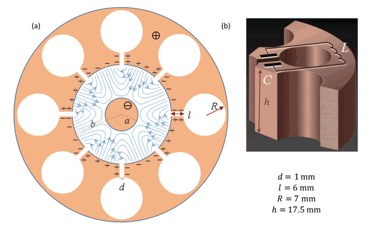
Figure 1
Part A: The structure and operation of a magnetron (6.6 points)
A magnetron is a device for the generation of microwave radiation, either in pulses (for radar applications), or continuously (e.g., in a microwave oven). The magnetron has a mode of self-amplifying oscillations. Supplying the magnetron with static (non-alternating) voltage quickly excites this mode. The microwave radiation thus created is transmitted out of the magnetron.
A typical microwave oven magnetron consists of a solid copper cylindrical cathode (with radius \(a\)) and a surrounding anode (with radius \(b\)). The latter has the shape of a thick cylindrical shell into which cylindrical cavities are drilled. These cavities are known as “resonators”. One of the resonators is coupled to an antenna which will transmit the microwave energy out; we will ignore the antenna in the following. All internal spaces are in vacuum. We will consider a typical magnetron with eight resonators, as depicted in Figure 1(a). The three-dimensional structure of a single resonator is shown in Figure 1(b). As indicated there, each of the eight cavities behaves as an inductor-capacitor (LC) resonator, with operating frequency \(f=2.45\,\mathrm{GHz}\).
A static uniform magnetic field is applied along the magnetron's longitudinal axis, pointing out of the page in Figure 1(a). In addition, a constant voltage is applied between the anode (positive potential) and the cathode (negative potential). Electrons emitted from the cathode reach the anode and charge it, such that they excite an oscillation mode in which the sign of the charge is opposite between every two adjacent resonators. The oscillation of the cavities amplify these oscillations.
The process described above creates an alternating electric field with the aforementioned frequency \(f=2.45\,\mathrm{GHz}\) (blue lines in Figure 1(a); the static field is not plotted) in the space between the cathode and the anode, in addition to the static field caused by the applied constant voltage. In the steady state, the typical amplitude of the alternating electric field between the anode and the cathode is approximately \(\frac13\) of the static electric field there. The electron motion in the space between the cathode and the anode is affected by both the static and the alternating parts of the field. This causes electrons that reach the anode to transfer about \(80\%\) of the energy they acquire from the static field into the alternating field. A minority of the ejected electrons returns to the cathode and releases additional electrons, further amplifying the alternating field.
Each resonator can be thought of as a capacitor and an inductor, see Figure 1(b). The capacitance mainly arises from the planar parts of the resonator surface, while the inductance stems from the cylindrical part. Assume that the current in the resonator flows uniformly very close to the surface of its cylindrical cavity, and that the strength of the magnetic field generated by this current is \(0.6\) times that of an ideal infinite solenoid. The various lengths defining the resonator geometry are given in Figure 1(b). The vacuum permittivity and permeability are \(\varepsilon_0=8.85\cdot10^{-12}\,\mathrm{F/m}\) and \(\mu_0=4\pi\cdot10^{-7}\,\mathrm{H/m}\), respectively.
A.1 — 0.4pt
Use the above data to estimate the frequency \(f_{\mathrm{est}}\) of a single resonator. (Your result may differ from the actual value, \(f=2.45\,\mathrm{GHz}\). Use the actual value in the remainder of the question.)
Task A.2 below does not deal with the magnetron itself, but helps to introduce some of the relevant physics. Consider an electron moving in free space under the influence of a uniform electric field directed along the negative \(y\) axis, \(\vec E=-E_0\hat y\), and a uniform magnetic field directed along the positive \(z\) axis, \(\vec B=B_0\hat z\) (\(E_0\) and \(B_0\) are positive; \(\hat x,\hat y,\hat z\) are unit vectors oriented in the conventional manner). Let us denote the electron velocity at time \(t\) by \(\vec u(t)\). The drift velocity \(\vec u_D\) of the electron is defined as its average velocity. We denote by \(m\) and \(-e\) the mass and charge of the electron, respectively.
A.2 — 1.5pt
In each of the following two cases, find \(\vec u_D\). In addition, draw in the Answer Sheet the electron's trajectory (in the lab frame) during the time interval \(0<t<\frac{4\pi m}{eB_0}\) if:
- at \(t=0\) the electron velocity is \(\vec u(0)=(3E_0/B_0)\hat x\),
- at \(t=0\) the electron velocity is \(\vec u(0)=-(3E_0/B_0)\hat x\).
We now resume our discussion of the magnetron. The distance between the cathode and the anode is \(15\,\mathrm{mm}\). Assume that, due to the aforementioned energy loss to the alternating fields, the maximal kinetic energy of each electron does not exceed \(K_{\max}=800\,\mathrm{eV}\). The static magnetic field strength is \(B_0=0.3\,\mathrm T\). The electron mass and charge are \(m=9.1\cdot10^{-31}\,\mathrm{kg}\) and \(-e=-1.6\cdot10^{-19}\,\mathrm C\), respectively.
A.3 — 0.4pt
Numerically estimate the maximal radius \(r\) of the electron motion trajectory in the reference frame in which this motion is approximately circular, considering this reference frame as approximately inertial.
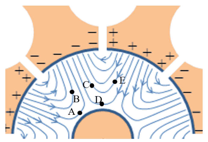
Figure 2
A.4 — 1.2pt
Figure 2 depicts the alternating electric field lines between the anode and the cathode at a given moment in time (the static field is not plotted). Indicate in the Answer Sheet which of the electrons positioned at A,B,C,D and E will drift towards the anode, which will drift towards the cathode and which will drift at a direction perpendicular to the radius at that moment.
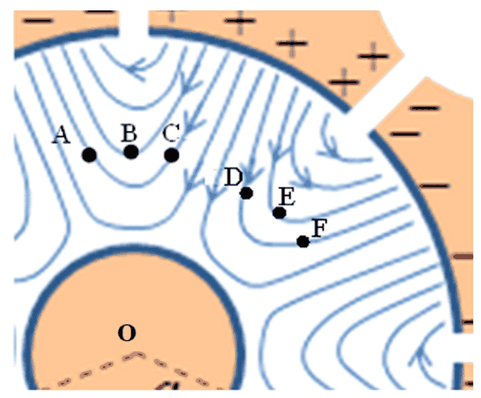
Figure 3
Figure 3 depicts the alternating electric field lines between the anode and the cathode (the static field is not plotted) at a given moment in time. The positions of six electrons at that moment are denoted by A, B, C, D, E and F. All electrons are at the same distance from the cathode.
A.5 — 1.2pt
Consider the situation shown in Figure 3. For each of the six electron pairs AB, AC, BC, DE, DF, EF, indicate in the Answer Sheet whether their drift will cause the angle between their position vectors (measured from the cathode’s center O) to increase or decrease at that moment.
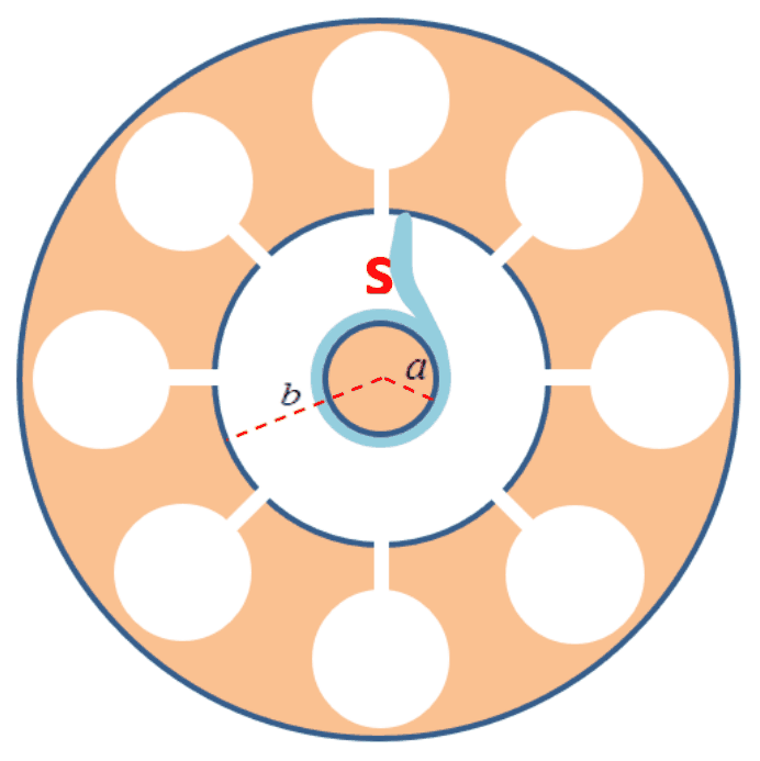
Figure 4
The pattern you have discovered in Task A.5 acts as a focusing mechanism, concentrating the electrons in the space between the cathode and anode into spokes. Figure 4 depicts one such spoke, denoted by S.
A.6 — 0.8pt
Depict in the Answer Sheet the other spokes at that moment. Indicate by arrows their direction of rotation, and calculate their average angular velocity \(\omega_s\).
Make the approximation that the total electric field half-way between the cathode and the anode is equal to its average static value along a radial line from the cathode to the anode, and that the spokes are approximately radial in that region. The cathode and anode radii (\(a\) and \(b\), respectively) are defined in Figure 4.
A.7 — 1.1pt
Find an approximate expression for the static voltage \(V_0\) required for operating the magnetron in the manner described. (The expression you will find gives an approximation for the minimal value required for the magnetron operation; the optimal voltage is somewhat higher.)
Part B: The interaction of microwave radiation with water molecules (3.4 points)
This part deals with the usage of microwave radiation (radiated by the magnetron antenna into the food chamber) for cooking, that is, heating up a lossy dielectric material such as water, either pure or salty (which is our model for, say, soup).
An electric dipole is a configuration of two equal and opposite electric charges \(q\) and \(-q\) a small distance \(d\) apart. The electric dipole vector points from the negative to the positive charge, and its magnitude is \(p=qd\).
A time-dependent electric field \(\vec E(t)=E(t)\hat x\) is applied on a single dipole of moment \(\vec p(t)\) with constant magnitude \(p_0=|\vec p(t)|\). The angle between the dipole and the electric field is \(\theta(t)\).
B.1 — 0.5pt
Write expressions for both the magnitude of the torque \(\tau(t)\) applied by the electric field on the dipole and the power \(H_i(t)\) delivered by the field to the dipole, in terms of \(p_0\), \(E(t)\), \(\theta(t)\) and their derivatives.
Water molecules are polar, hence can be treated as electric dipoles. Due to the strong hydrogen bonds between water molecules in liquid water, one cannot treat them as independent dipoles. Rather, one should refer to the polarization vector \(\vec P(t)\), which is the dipole moment density (average dipole moment per unit volume of an ensemble of water molecules). The polarization \(\vec P(t)\) is parallel to the local applied alternating electric field (of the microwave radiation), \(\vec E(t)\), and oscillates in time with an amplitude that is proportional to the amplitude of the local alternating electric field, but with a phase lag \(\delta\).
The local alternating electric field at a given location inside the water is \(\vec E(t)=E_0\sin(\omega t)\hat x\), where \(\omega=2\pi f\), giving rise to polarization \(\vec P(t)=\beta\varepsilon_0E_0\sin(\omega t-\delta)\hat x\), where the dimensionless constant \(\beta\) is a property of water.
B.2 — 0.5pt
Find an expression for the time-averaged power \(\langle H(t)\rangle\) per unit volume absorbed by the water.
The time-average for a time dependent periodic variable \(f(t)\) over its period \(T\) is defined as:
\[ \langle f(t)\rangle=\frac1T\int_{t_0}^{t_0+T}f(t)\,\mathrm dt. \tag{1} \]
Let us now consider the propagation of the radiation through the water. The relative dielectric constant of water (at the electromagnetic field frequency) is \(\varepsilon_r\), and the corresponding index of refraction of water is \(n=\sqrt{\varepsilon_r}\). The momentary energy density of the electric field is given by \(\frac12\varepsilon_r\varepsilon_0E^2\). The time-averaged energy density of the electric and magnetic fields are equal.
B.3 — 1.1pt
Let us denote the time-averaged radiation energy flux density by \(I(z)\) (average radiation power flow per unit area). Here \(z\) is the depth of penetration into the water, and the radiation propagates in the \(z\) direction. Find an expression for the dependence of the flux density \(I(z)\) on \(z\). The flux density at the water surface, \(I(0)\), may appear in your result.
The phase lag \(\delta\) is the result of the interaction between the water molecules. It depends on the dimensionless dielectric loss coefficient \(\varepsilon_\ell\) and the relative dielectric constant \(\varepsilon_r\) (both of which depend on the radiation angular frequency \(\omega\) and the temperature) via the relation \(\tan\delta=\varepsilon_\ell/\varepsilon_r\). When \(\delta\) is small enough, the electric field at penetration depth \(z\) into the water is given by:
\[ \vec E(z,t)=\vec E_0e^{-\frac12nk_0z\tan\delta} \sin(nk_0z-\omega t) \tag{2} \]
where \(k_0=\omega/c\) and \(c=3.0\cdot10^8\,\mathrm{m/s}\) is the speed of light in vacuum.
B.4 — 0.6pt
Employ the approximation \(\tan\delta\approx\sin\delta\) and find an expression for the coefficient \(\beta\) defined in Task B.2 in terms of the other parameters.
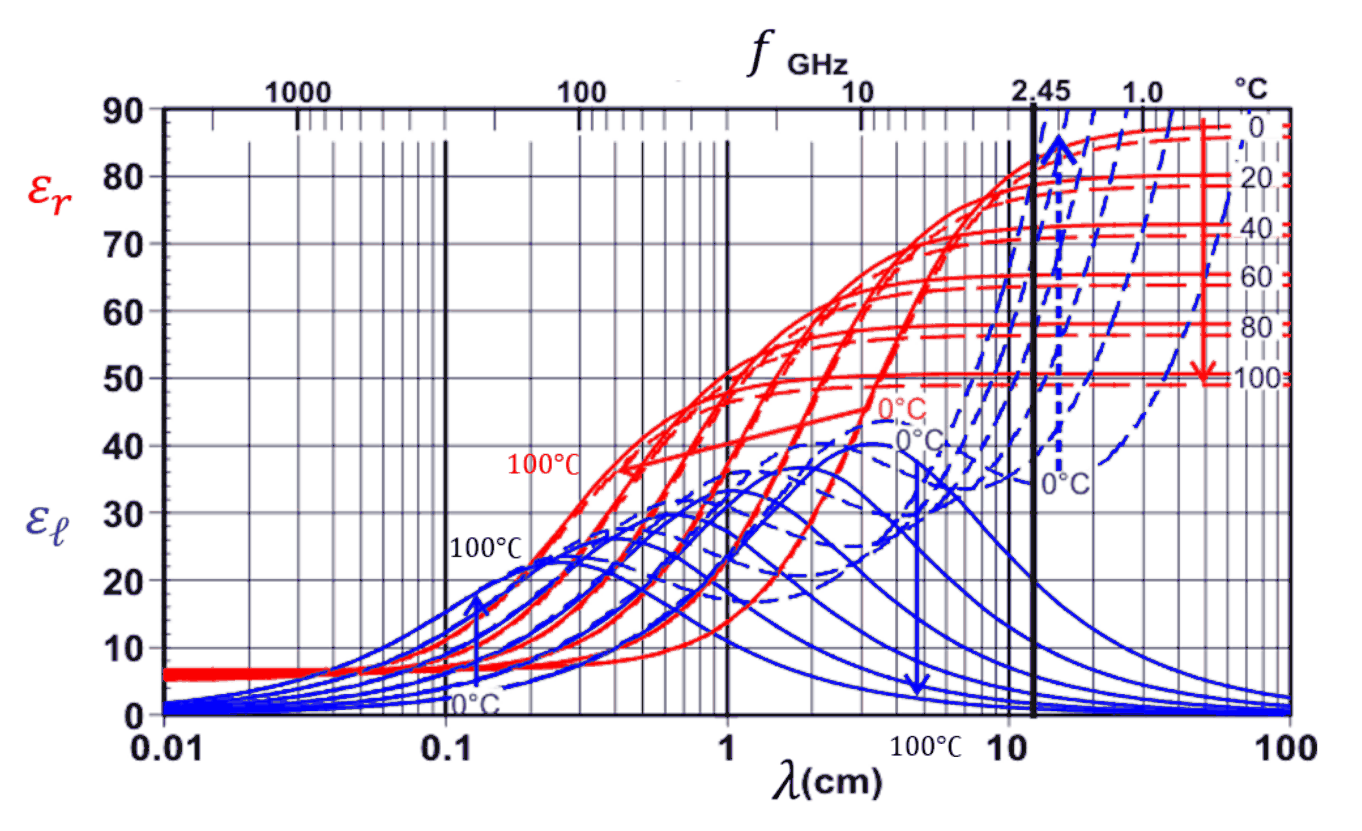
Figure 5. The arrows indicate the variation with temperature across the curves from \(0^\circ\mathrm C\) to \(100^\circ\mathrm C\).
Figure 5 depicts \(\varepsilon_\ell\) (blue) and \(\varepsilon_r\) (red) for both pure water (solid lines) and a dilute solution of salt in water (dashed lines) as functions of wavelength or frequency, at several different temperatures. The angular frequency \(\omega=2\pi\cdot2.45\cdot10^9\,\mathrm{s^{-1}}\) is indicated by a bold vertical line. Below we will consider microwave radiation at this frequency only.
B.5 — 0.7pt
Use Figure 5 to address the following questions:
- For water at \(20^\circ\mathrm C\), find the penetration depth \(z_{1/2}\) at which the power per unit volume is reduced to half of its value at \(z=0\).
- Indicate in the Answer Sheet whether the penetration depth of the microwave radiation into water increases, decreases or remains the same with temperature.
- Indicate in the Answer Sheet whether the penetration depth of the microwave radiation into soup (dilute salt solution) increases, decreases or remains the same with temperature.
Official English text of the problem.
Answers
-
A.1: \(C\simeq0.93\,\mathrm{pF}\), \(L\simeq6.6\,\mathrm{nH}\), giving \[ \boxed{f_{\mathrm{est}}\simeq2.03\,\mathrm{GHz}.} \]
-
A.2: In both cases, \[ \boxed{\vec u_D=-\frac{E_0}{B_0}\hat x.} \] Put \(\omega_c=eB_0/m\), \(\ell=mE_0/(eB_0^2)\), and \(s=\omega_ct\). With the initial position at the origin, the requested trajectories are \[ \boxed{\frac{(x,y)_1}{\ell}=(-s+4\sin s,\;4[1-\cos s]),} \] \[ \boxed{\frac{(x,y)_2}{\ell}=(-s-2\sin s,\;-2[1-\cos s]),} \qquad 0<s<4\pi. \] They are looping trochoids drifting left, with counterclockwise gyration.
-
A.3: \[ \boxed{r_{\max}\simeq3.2\times10^{-4}\,\mathrm m=0.32\,\mathrm{mm}.} \]
-
A.4: My reading of the field-line tangents is A and B toward the cathode; C, D and E toward the anode; none exactly perpendicular to the radius. The diagram-reading uncertainty is noted below.
-
A.5: AB, AC and BC decrease; DE, DF and EF increase.
-
A.6: There are four spokes, separated by \(90^\circ\). Add copies of S rotated by \(90^\circ\), \(180^\circ\), and \(270^\circ\). They rotate counterclockwise, with \[ \boxed{\omega_s=\frac{2\pi f}{4}=3.85\times10^9\,\mathrm{rad\,s^{-1}}.} \]
-
A.7: \[ \boxed{V_0\simeq\frac{B_0\omega_s}{2}(b^2-a^2) =\frac{\pi fB_0}{4}(b^2-a^2).} \]
-
B.1: For field magnitude \(|E|\) and the angle between the dipole and the instantaneous field, \[ \boxed{\tau=p_0|E|\sin\theta,\qquad H_i=-p_0|E|\sin\theta\,\dot\theta.} \] The convention-independent power formula is \(H_i=\vec E\cdot\dot{\vec p}\).
-
B.2: \[ \boxed{\langle H\rangle=\frac12\beta\varepsilon_0\omega E_0^2\sin\delta.} \]
-
B.3: \[ \boxed{I(z)=I(0)\exp\!\left[-\frac{\beta\omega\sin\delta}{nc}\,z\right].} \]
-
B.4: \[ \boxed{\beta\simeq n^2=\varepsilon_r.} \]
-
B.5:
1. \[ \boxed{z_{1/2}=\frac{c\sqrt{\varepsilon_r}\ln2}{\omega\varepsilon_\ell} \simeq1.2\,\mathrm{cm}} \] from approximate graph readings \(\varepsilon_r\simeq78\), \(\varepsilon_\ell\simeq10\).
2. The penetration depth in pure water increases with temperature.
3. The penetration depth in soup decreases with temperature.
Solution
A.1
The approximately parallel conducting faces forming the slot have area \(hl\) and separation \(d\). Neglecting fringing, their capacitance is
\[ C\simeq\frac{\varepsilon_0hl}{d}. \]
Using the dimensions in Figure 1,
\[ C=\frac{(8.85\times10^{-12})(17.5\times10^{-3})(6\times10^{-3})} {1\times10^{-3}} =9.29\times10^{-13}\,\mathrm F. \]
Let \(I\) be the total current circulating around the cylindrical cavity. Its uniform distribution over height \(h\) gives an effective surface current density \(I/h\). An ideal infinite solenoid with this surface current would produce \(\mu_0I/h\). Applying the specified correction,
\[ B\simeq0.6\frac{\mu_0 I}{h}. \]
Approximating the flux through the cavity by \(B\pi R^2\),
\[ L=\frac{\Phi}{I} \simeq0.6\frac{\mu_0\pi R^2}{h} =6.63\times10^{-9}\,\mathrm H. \]
Thus
\[ f_{\mathrm{est}}=\frac{1}{2\pi\sqrt{LC}} =\frac{1}{2\pi} \sqrt{\frac{d}{0.6\mu_0\varepsilon_0\pi R^2l}} \simeq2.03\times10^9\,\mathrm{Hz}. \]
The height cancels because \(C\propto h\) and \(L\propto h^{-1}\). The estimate is approximate because the resonator is represented by idealized lumped capacitance and inductance.
A.2
The electron obeys the Lorentz-force equation,
\[ m\frac{\mathrm d\vec u}{\mathrm dt} =-e(\vec E+\vec u\times\vec B). \]
For the stated fields, its components are
\[ \dot u_x=-\omega_cu_y,\qquad \dot u_y=\omega_c\left(u_x+\frac{E_0}{B_0}\right), \qquad \omega_c=\frac{eB_0}{m}. \]
Define \(v_D=E_0/B_0\). A constant velocity \(-v_D\hat x\) makes the electric and magnetic forces cancel. More generally,
\[ \vec u_D=\frac{\vec E\times\vec B}{B_0^2} =-v_D\hat x. \]
In the frame translating with this velocity, the remaining velocity rotates uniformly. For \(u_y(0)=0\),
\[ u_x=-v_D+A\cos(\omega_ct),\qquad u_y=A\sin(\omega_ct), \]
where \(A=u_x(0)+v_D\). The oscillatory terms average to zero, so both initial conditions give the same drift.
Taking \(x(0)=y(0)=0\), integration gives
\[ x=-v_Dt+\frac{A}{\omega_c}\sin(\omega_ct), \qquad y=\frac{A}{\omega_c}[1-\cos(\omega_ct)]. \]
For case 1, \(A=4v_D\); for case 2, \(A=-2v_D\). This gives the parametric trajectories stated in the answers.
For a precise sketch, use \(\ell=v_D/\omega_c\). The following points describe the first cyclotron period:
| \(s=\omega_ct\) | Case 1: \((x/\ell,y/\ell)\) | Case 2: \((x/\ell,y/\ell)\) |
|---|---|---|
| \(0\) | \((0,0)\) | \((0,0)\) |
| \(\pi/2\) | \((4-\pi/2,4)\) | \((-2-\pi/2,-2)\) |
| \(\pi\) | \((-\pi,8)\) | \((-\pi,-4)\) |
| \(3\pi/2\) | \((-4-3\pi/2,4)\) | \((2-3\pi/2,-2)\) |
| \(2\pi\) | \((-2\pi,0)\) | \((-2\pi,0)\) |
Repeat this curve translated by \(-2\pi\ell\) in \(x\) to obtain the second period.
In case 1, the electron initially moves right and bends upward; the entire curve lies in \(0\le y\le8\ell\). In case 2, it initially moves left and bends downward; the curve lies in \(-4\ell\le y\le0\). Both end at \((-4\pi\ell,0)\) after the specified interval. Their gyration is counterclockwise, and neither trajectory has cusps because its velocity never vanishes.
A.3
In the approximately inertial local drift frame, the electric force is approximately cancelled by the magnetic force associated with the frame velocity. The remaining motion is approximately circular:
\[ \frac{mv_\perp^2}{r}=ev_\perp B_0, \qquad r=\frac{mv_\perp}{eB_0}. \]
Using the full kinetic-energy bound as an upper estimate for the gyration energy,
\[ v_\perp\lesssim\sqrt{\frac{2K_{\max}}m}. \]
Here
\[ K_{\max}=800(1.6\times10^{-19}) =1.28\times10^{-16}\,\mathrm J, \]
so
\[ v_{\max}\simeq1.68\times10^7\,\mathrm{m\,s^{-1}}, \]
and
\[ r_{\max}\simeq \frac{\sqrt{2mK_{\max}}}{eB_0} = \frac{\sqrt{2(9.1\times10^{-31})(1.28\times10^{-16})}} {(1.6\times10^{-19})(0.3)} =3.18\times10^{-4}\,\mathrm m. \]
Thus \(r_{\max}\simeq0.32\,\mathrm{mm}\), much smaller than the \(15\,\mathrm{mm}\) gap. This supports treating the gyration as a small motion superposed on the drift of its centre.
A.4
Let \(\hat r\) point radially outward and \(\hat\phi\) counterclockwise. With the magnetic field pointing out of the page,
\[ \vec E=E_r\hat r+E_\phi\hat\phi \]
gives
\[ \vec u_D=\frac{\vec E\times\vec B}{B_0^2} =\frac{E_\phi}{B_0}\hat r-\frac{E_r}{B_0}\hat\phi. \]
Therefore:
- \(E_\phi>0\) produces drift toward the anode.
- \(E_\phi<0\) produces drift toward the cathode.
- \(E_\phi=0\) produces drift perpendicular to the radius.
The static electric field is radial, so it contributes only azimuthal drift. The radial classification is determined entirely by the tangential component of the plotted alternating field.
My reading of the local tangents gives:
| Electron | Tangential alternating-field component | Radial drift |
|---|---|---|
| A | Clockwise | Toward cathode |
| B | Clockwise | Toward cathode |
| C | Counterclockwise | Toward anode |
| D | Counterclockwise | Toward anode |
| E | Counterclockwise | Toward anode |
These classifications concern the radial component; the electrons also have azimuthal drift. The tangents are read from a schematic figure, so these classifications carry some reading uncertainty.
A.5
At a common distance \(\rho\) from the cathode centre,
\[ \dot\phi=\frac{u_\phi}{\rho} =-\frac{E_r}{B_0\rho}. \]
The static field is radially inward and gives all six electrons the same counterclockwise angular velocity at that radius. Thus only differences in the radial component of the alternating field affect their instantaneous angular separations.
For A, B and C, Figure 3 shows the radial alternating-field component changing from outward at A, through approximately zero at B, to inward at C. Consequently,
\[ \dot\phi_A<\dot\phi_B<\dot\phi_C. \]
Their positions are ordered \(\phi_A>\phi_B>\phi_C\). The electron behind therefore moves faster than the one ahead, so all three separations decrease:
\[ \frac{\mathrm d}{\mathrm dt}(\phi_A-\phi_B)<0,\quad \frac{\mathrm d}{\mathrm dt}(\phi_A-\phi_C)<0,\quad \frac{\mathrm d}{\mathrm dt}(\phi_B-\phi_C)<0. \]
For D, E and F, the radial alternating-field component changes in the opposite way: inward at D, approximately zero at E, and outward at F. Hence
\[ \dot\phi_D>\dot\phi_E>\dot\phi_F. \]
Since \(\phi_D>\phi_E>\phi_F\), all three separations increase.
| Pair | Change of angular separation |
|---|---|
| AB | Decreases |
| AC | Decreases |
| BC | Decreases |
| DE | Increases |
| DF | Increases |
| EF | Increases |
A.6
Adjacent resonators have opposite oscillation phases. Thus, at a given instant, alternate angular regions focus electrons while the intervening regions spread them apart. Eight resonators therefore produce four spokes.
The drawing should contain three additional copies of S, obtained by rotations of \(90^\circ\), \(180^\circ\), and \(270^\circ\) about the cathode centre. Their shapes should have the same sense of curvature.
The static field points inward. Its drift is
\[ (-\hat r)\times\hat z=+\hat\phi, \]
so the spokes rotate counterclockwise.
After half an oscillation period, the resonator polarities reverse. A spoke must advance to the next resonator position, an angle \(2\pi/8=\pi/4\). Therefore
\[ \omega_s=\frac{\pi/4}{T/2} =\frac{\pi}{2T} =\frac{2\pi f}{4}. \]
Using \(f=2.45\times10^9\,\mathrm{Hz}\),
\[ \boxed{\omega_s=3.85\times10^9\,\mathrm{rad\,s^{-1}}.} \]
Equivalently, the spokes make \(6.125\times10^8\) revolutions per second.
A.7
Under the prescribed approximation, the field magnitude at the midpoint of the gap is
\[ E_{\mathrm{mid}}\simeq\frac{V_0}{b-a}. \]
The midpoint radius is
\[ \rho_{\mathrm{mid}}=\frac{a+b}{2}. \]
The electron drift there must have the tangential speed of the spoke:
\[ \frac{E_{\mathrm{mid}}}{B_0} \simeq\omega_s\rho_{\mathrm{mid}}. \]
Consequently,
\[ \frac{V_0}{B_0(b-a)} \simeq\omega_s\frac{a+b}{2}, \]
which yields
\[ \boxed{ V_0\simeq\frac{B_0\omega_s}{2}(b^2-a^2) =\frac{\pi fB_0}{4}(b^2-a^2). } \]
With the given \(B_0\) and \(f\), this can also be written
\[ V_0\simeq (5.77\times10^8\,\mathrm{V\,m^{-2}})(b^2-a^2), \]
with \(a\) and \(b\) measured in metres.
B.1
The forces on the two charges form a couple. The torque is
\[ \vec\tau=\vec p\times\vec E. \]
Thus, for \(\theta\) defined as the angle between the dipole and the instantaneous field,
\[ \boxed{\tau=p_0|E|\sin\theta.} \]
The torque tends to reduce this angle. Its signed component conjugate to \(\theta\) is therefore \(-p_0|E|\sin\theta\), giving the mechanical power
\[ \boxed{H_i=-p_0|E|\sin\theta\,\dot\theta.} \]
In particular, an aligning dipole has \(\dot\theta<0\), so the field delivers positive power.
The result can be derived without an angular convention. If \(\vec r_+\) and \(\vec r_-\) are the charge positions,
\[ H_i=q\vec E\cdot\dot{\vec r}_+ -q\vec E\cdot\dot{\vec r}_- =\vec E\cdot\frac{\mathrm d}{\mathrm dt} \big[q(\vec r_+-\vec r_-)\big]. \]
Hence
\[ \boxed{H_i=\vec E\cdot\dot{\vec p}.} \]
If instead \(\theta\) is measured from the fixed positive \(x\) axis and \(E(t)\) is a signed component, this becomes
\[ H_i=E(t)\frac{\mathrm d}{\mathrm dt}(p_0\cos\theta) =-p_0E(t)\sin\theta\,\dot\theta. \]
There is no \(\dot E\) term in the mechanical power delivered to the dipole.
B.2
Summing the single-dipole power over unit volume gives
\[ H(t)=\vec E(t)\cdot\frac{\mathrm d\vec P}{\mathrm dt}. \]
The given polarization has derivative
\[ \frac{\mathrm d\vec P}{\mathrm dt} =\beta\varepsilon_0E_0\omega \cos(\omega t-\delta)\hat x. \]
Therefore
\[ H(t)=\beta\varepsilon_0\omega E_0^2 \sin(\omega t)\cos(\omega t-\delta). \]
Using
\[ \cos(\omega t-\delta) =\cos(\omega t)\cos\delta+\sin(\omega t)\sin\delta, \]
and the period averages
\[ \langle\sin(\omega t)\cos(\omega t)\rangle=0, \qquad \langle\sin^2(\omega t)\rangle=\frac12, \]
we obtain
\[ \boxed{\langle H\rangle =\frac12\beta\varepsilon_0\omega E_0^2\sin\delta.} \]
For a positive phase lag, the mean absorbed power is positive.
B.3
Let \(\mathcal E(z)\) denote the local electric-field amplitude. The average electric energy density is
\[ \langle u_E\rangle =\frac12\varepsilon_r\varepsilon_0\langle E^2\rangle =\frac14\varepsilon_r\varepsilon_0\mathcal E^2. \]
The average magnetic energy density is equal to this, so
\[ \langle u\rangle =\frac12\varepsilon_r\varepsilon_0\mathcal E^2. \]
Using the propagation speed \(c/n\) in the problem's dielectric-wave model,
\[ I(z)=\frac cn\langle u\rangle =\frac12nc\varepsilon_0\mathcal E^2(z), \]
where \(n^2=\varepsilon_r\).
Conservation of energy for a thin layer of thickness \(\mathrm dz\) gives
\[ -\frac{\mathrm dI}{\mathrm dz}=\langle H\rangle. \]
Substituting the result of B.2 and eliminating \(\mathcal E^2\),
\[ -\frac{\mathrm dI}{\mathrm dz} =\frac12\beta\varepsilon_0\omega\mathcal E^2\sin\delta =\frac{\beta\omega\sin\delta}{nc}I. \]
For a homogeneous medium at fixed temperature, the coefficient is constant. Integration gives
\[ \boxed{ I(z)=I(0)\exp\!\left[-\frac{\beta\omega\sin\delta}{nc}z\right]. } \]
The attenuation coefficient for power is therefore
\[ \alpha=\frac{\beta\omega\sin\delta}{nc}. \]
B.4
Equation (2) gives an electric-field amplitude proportional to
\[ e^{-\frac12nk_0z\tan\delta}. \]
Since intensity is proportional to the square of this amplitude,
\[ I(z)=I(0)e^{-nk_0z\tan\delta}. \]
Comparison with B.3, using \(k_0=\omega/c\), gives
\[ \frac{\beta\omega\sin\delta}{nc} =\frac{n\omega}{c}\tan\delta. \]
Thus
\[ \beta\sin\delta=n^2\tan\delta. \]
Within the requested approximation \(\tan\delta\simeq\sin\delta\),
\[ \boxed{\beta\simeq n^2=\varepsilon_r.} \]
This result follows within the dielectric and small-loss approximations specified in the problem.
B.5
Using the supplied relation \(\tan\delta=\varepsilon_\ell/\varepsilon_r\), the power attenuation coefficient is
\[ \alpha=nk_0\tan\delta =\frac{\omega}{c} \frac{\varepsilon_\ell}{\sqrt{\varepsilon_r}}. \]
At uniform temperature, the local absorbed power per unit volume is proportional to the local intensity:
\[ \langle H(z)\rangle=\alpha I(z). \]
It therefore has the same exponential dependence,
\[ \frac{\langle H(z)\rangle}{\langle H(0)\rangle} =e^{-\alpha z}. \]
1. Half-power depth at \(20^\circ\mathrm C\).
The condition \(e^{-\alpha z_{1/2}}=1/2\) gives
\[ z_{1/2}=\frac{\ln2}{\alpha} =\frac{c\sqrt{\varepsilon_r}\ln2}{\omega\varepsilon_\ell}. \]
At the marked frequency, the solid curves for \(20^\circ\mathrm C\) give approximately
\[ \varepsilon_r\simeq78,\qquad \varepsilon_\ell\simeq10. \]
Consequently,
\[ z_{1/2}\simeq \frac{(3.0\times10^8)\sqrt{78}\ln2} {(2\pi)(2.45\times10^9)(10)} =1.19\times10^{-2}\,\mathrm m. \]
Thus the graph supports a half-power depth of approximately
\[ \boxed{z_{1/2}\simeq1.2\,\mathrm{cm}.} \]
This is the half-power depth; the field-amplitude decay has an exponent smaller by a factor of two.
2. Pure water as temperature increases.
At fixed frequency,
\[ z_{1/2}\propto\frac{\sqrt{\varepsilon_r}}{\varepsilon_\ell}. \]
The solid blue curves show a substantial decrease of \(\varepsilon_\ell\) with temperature. The decrease of \(\sqrt{\varepsilon_r}\) is much smaller in relative terms. Therefore the ratio increases:
\[ \boxed{\text{The penetration depth in pure water increases with temperature.}} \]
3. Soup as temperature increases.
At the same frequency, the dashed blue curves show increasing dielectric loss with increasing temperature, while the dashed red curves show decreasing \(\varepsilon_r\). Both changes reduce \(\sqrt{\varepsilon_r}/\varepsilon_\ell\). Therefore
\[ \boxed{\text{The penetration depth in soup decreases with temperature.}} \]
The solution was checked against the official solution.
IPhO 2019 · Theorieaufgabe 2
Die Physik eines Mikrowellenherds
Diese Aufgabe behandelt die Erzeugung von Mikrowellenstrahlung in einem Mikrowellenherd und ihre Verwendung zum Erwärmen von Speisen. Die Mikrowellenstrahlung wird in einer Vorrichtung erzeugt, die als „Magnetron“ bezeichnet wird. Teil A befasst sich mit der Funktionsweise des Magnetrons, während Teil B die Absorption von Mikrowellenstrahlung in Speisen behandelt.
Abbildung 1
Teil A: Aufbau und Funktionsweise eines Magnetrons (6.6 Punkte)
Ein Magnetron ist eine Vorrichtung zur Erzeugung von Mikrowellenstrahlung, entweder in Pulsen (für Radaranwendungen) oder kontinuierlich (z. B. in einem Mikrowellenherd). Das Magnetron besitzt eine sich selbst verstärkende Schwingungsmode. Wird an das Magnetron eine statische Spannung (keine Wechselspannung) angelegt, so wird diese Mode rasch angeregt. Die so erzeugte Mikrowellenstrahlung wird aus dem Magnetron ausgekoppelt.
Das Magnetron eines typischen Mikrowellenherds besteht aus einer massiven zylindrischen Kupferkathode (mit dem Radius \(a\)) und einer sie umgebenden Anode (mit dem Radius \(b\)). Letztere hat die Form eines dickwandigen Hohlzylinders, in den zylindrische Hohlräume gebohrt sind. Diese Hohlräume werden als „Resonatoren“ bezeichnet. Einer der Resonatoren ist an eine Antenne gekoppelt, die die Mikrowellenenergie nach außen überträgt; im Folgenden vernachlässigen wir die Antenne. Alle Innenräume sind evakuiert. Wir betrachten ein typisches Magnetron mit acht Resonatoren, wie es in Abbildung 1(a) dargestellt ist. Die dreidimensionale Struktur eines einzelnen Resonators ist in Abbildung 1(b) gezeigt. Wie dort angedeutet, verhält sich jeder der acht Hohlräume wie ein LC-Schwingkreis aus einer Induktivität und einer Kapazität, mit der Betriebsfrequenz \(f=2.45\,\mathrm{GHz}\).
Entlang der Längsachse des Magnetrons wird ein statisches homogenes Magnetfeld angelegt, das in Abbildung 1(a) aus der Zeichenebene herauszeigt. Zusätzlich wird zwischen der Anode (positives Potenzial) und der Kathode (negatives Potenzial) eine konstante Spannung angelegt. Von der Kathode emittierte Elektronen erreichen die Anode und laden sie auf, sodass sie eine Schwingungsmode anregen, bei der die Ladungen benachbarter Resonatoren jeweils entgegengesetzte Vorzeichen haben. Die Schwingungen der Hohlräume verstärken diese Schwingungen.
Der oben beschriebene Vorgang erzeugt im Raum zwischen Kathode und Anode zusätzlich zu dem durch die angelegte konstante Spannung verursachten statischen Feld ein elektrisches Wechselfeld mit der bereits genannten Frequenz \(f=2.45\,\mathrm{GHz}\) (blaue Linien in Abbildung 1(a); das statische Feld ist nicht eingezeichnet). Im stationären Zustand beträgt die typische Amplitude des elektrischen Wechselfelds zwischen Anode und Kathode ungefähr \(\frac13\) des dortigen statischen elektrischen Felds. Die Bewegung der Elektronen im Raum zwischen Kathode und Anode wird sowohl durch den statischen als auch durch den zeitlich wechselnden Anteil des Felds beeinflusst. Dies bewirkt, dass Elektronen, die die Anode erreichen, etwa \(80\%\) der Energie, die sie aus dem statischen Feld aufnehmen, auf das Wechselfeld übertragen. Ein kleinerer Teil der emittierten Elektronen kehrt zur Kathode zurück und löst weitere Elektronen heraus, wodurch das Wechselfeld weiter verstärkt wird.
Jeder Resonator kann als Kondensator und Spule aufgefasst werden, siehe Abbildung 1(b). Die Kapazität ergibt sich hauptsächlich aus den ebenen Teilen der Resonatoroberfläche, während die Induktivität vom zylindrischen Teil herrührt. Nehmen Sie an, dass der Strom im Resonator gleichmäßig verteilt unmittelbar an der Oberfläche seines zylindrischen Hohlraums fließt und dass der Betrag des von diesem Strom erzeugten Magnetfelds das \(0.6\)-Fache desjenigen einer idealen unendlich langen Spule beträgt. Die verschiedenen Längen, die die Geometrie des Resonators festlegen, sind in Abbildung 1(b) angegeben. Die Permittivität und die Permeabilität des Vakuums betragen \(\varepsilon_0=8.85\cdot10^{-12}\,\mathrm{F/m}\) bzw. \(\mu_0=4\pi\cdot10^{-7}\,\mathrm{H/m}\).
A.1 — 0.4 Punkte
Schätzen Sie anhand der obigen Angaben die Frequenz \(f_{\mathrm{est}}\) eines einzelnen Resonators ab. (Ihr Ergebnis kann vom tatsächlichen Wert \(f=2.45\,\mathrm{GHz}\) abweichen. Verwenden Sie im weiteren Verlauf der Aufgabe den tatsächlichen Wert.)
Die folgende Teilaufgabe A.2 behandelt nicht das Magnetron selbst, dient jedoch dazu, einige der relevanten physikalischen Zusammenhänge einzuführen. Betrachten Sie ein Elektron, das sich im freien Raum unter dem Einfluss eines homogenen elektrischen Felds in Richtung der negativen \(y\)-Achse, \(\vec E=-E_0\hat y\), und eines homogenen Magnetfelds in Richtung der positiven \(z\)-Achse, \(\vec B=B_0\hat z\), bewegt (\(E_0\) und \(B_0\) sind positiv; \(\hat x,\hat y,\hat z\) sind in der üblichen Weise orientierte Einheitsvektoren). Wir bezeichnen die Geschwindigkeit des Elektrons zum Zeitpunkt \(t\) mit \(\vec u(t)\). Die Driftgeschwindigkeit \(\vec u_D\) des Elektrons ist als seine mittlere Geschwindigkeit definiert. Mit \(m\) und \(-e\) bezeichnen wir die Masse bzw. die Ladung des Elektrons.
A.2 — 1.5 Punkte
Bestimmen Sie in jedem der folgenden beiden Fälle \(\vec u_D\). Zeichnen Sie außerdem auf dem Antwortblatt die Bahn des Elektrons (im Laborsystem) während des Zeitintervalls \(0<t<\frac{4\pi m}{eB_0}\), wenn:
- zum Zeitpunkt \(t=0\) die Geschwindigkeit des Elektrons \(\vec u(0)=(3E_0/B_0)\hat x\) beträgt,
- zum Zeitpunkt \(t=0\) die Geschwindigkeit des Elektrons \(\vec u(0)=-(3E_0/B_0)\hat x\) beträgt.
Wir kehren nun zur Betrachtung des Magnetrons zurück. Der Abstand zwischen Kathode und Anode beträgt \(15\,\mathrm{mm}\). Nehmen Sie an, dass aufgrund der oben erwähnten Energieabgabe an die Wechselfelder die maximale kinetische Energie jedes Elektrons den Wert \(K_{\max}=800\,\mathrm{eV}\) nicht überschreitet. Der Betrag des statischen Magnetfelds beträgt \(B_0=0.3\,\mathrm T\). Masse und Ladung des Elektrons sind \(m=9.1\cdot10^{-31}\,\mathrm{kg}\) bzw. \(-e=-1.6\cdot10^{-19}\,\mathrm C\).
A.3 — 0.4 Punkte
Schätzen Sie den maximalen Radius \(r\) der Elektronenbahn in dem Bezugssystem, in dem diese Bewegung näherungsweise kreisförmig ist, numerisch ab. Betrachten Sie dieses Bezugssystem dabei näherungsweise als Inertialsystem.
Abbildung 2
A.4 — 1.2 Punkte
Abbildung 2 zeigt die Feldlinien des elektrischen Wechselfelds zwischen Anode und Kathode zu einem bestimmten Zeitpunkt (das statische Feld ist nicht eingezeichnet). Geben Sie auf dem Antwortblatt an, welche der Elektronen an den Positionen A, B, C, D und E zu diesem Zeitpunkt zur Anode, welche zur Kathode und welche in einer Richtung senkrecht zum Radius driften.
Abbildung 3
Abbildung 3 zeigt die Feldlinien des elektrischen Wechselfelds zwischen Anode und Kathode (das statische Feld ist nicht eingezeichnet) zu einem bestimmten Zeitpunkt. Die Positionen von sechs Elektronen zu diesem Zeitpunkt sind mit A, B, C, D, E und F bezeichnet. Alle Elektronen haben denselben Abstand von der Kathode.
A.5 — 1.2 Punkte
Betrachten Sie die in Abbildung 3 gezeigte Situation. Geben Sie für jedes der sechs Elektronenpaare AB, AC, BC, DE, DF, EF auf dem Antwortblatt an, ob sich der Winkel zwischen ihren Ortsvektoren (gemessen vom Mittelpunkt O der Kathode aus) durch ihre Drift zu diesem Zeitpunkt vergrößert oder verkleinert.
Abbildung 4
Das in Teilaufgabe A.5 entdeckte Muster wirkt als Fokussierungsmechanismus, der die Elektronen im Raum zwischen Kathode und Anode in Speichen konzentriert. Abbildung 4 zeigt eine solche Speiche, die mit S bezeichnet ist.
A.6 — 0.8 Punkte
Zeichnen Sie auf dem Antwortblatt die übrigen Speichen zu diesem Zeitpunkt ein. Geben Sie ihre Drehrichtung durch Pfeile an und berechnen Sie ihre mittlere Winkelgeschwindigkeit \(\omega_s\).
Nehmen Sie näherungsweise an, dass das gesamte elektrische Feld auf halbem Weg zwischen Kathode und Anode gleich seinem mittleren statischen Wert entlang einer radialen Linie von der Kathode zur Anode ist und dass die Speichen in diesem Bereich näherungsweise radial verlaufen. Die Radien der Kathode und der Anode (\(a\) bzw. \(b\)) sind in Abbildung 4 definiert.
A.7 — 1.1 Punkte
Bestimmen Sie einen Näherungsausdruck für die statische Spannung \(V_0\), die erforderlich ist, um das Magnetron in der beschriebenen Weise zu betreiben. (Der von Ihnen gefundene Ausdruck liefert eine Näherung für den zum Betrieb des Magnetrons erforderlichen Mindestwert; die optimale Spannung liegt etwas höher.)
Teil B: Die Wechselwirkung von Mikrowellenstrahlung mit Wassermolekülen (3.4 Punkte)
Dieser Teil behandelt die Verwendung von Mikrowellenstrahlung (die von der Antenne des Magnetrons in den Garraum abgestrahlt wird) zum Garen, also zum Erwärmen eines verlustbehafteten dielektrischen Materials wie Wasser, entweder rein oder salzhaltig (was beispielsweise als Modell für Suppe dient).
Ein elektrischer Dipol ist eine Anordnung zweier betragsgleicher, entgegengesetzter elektrischer Ladungen \(q\) und \(-q\), die einen kleinen Abstand \(d\) voneinander haben. Der elektrische Dipolvektor zeigt von der negativen zur positiven Ladung, und sein Betrag ist \(p=qd\).
Auf einen einzelnen Dipol mit dem Moment \(\vec p(t)\) und dem konstanten Betrag \(p_0=|\vec p(t)|\) wirkt ein zeitabhängiges elektrisches Feld \(\vec E(t)=E(t)\hat x\). Der Winkel zwischen dem Dipol und dem elektrischen Feld ist \(\theta(t)\).
B.1 — 0.5 Punkte
Geben Sie Ausdrücke sowohl für den Betrag des Drehmoments \(\tau(t)\), das das elektrische Feld auf den Dipol ausübt, als auch für die Leistung \(H_i(t)\), die das Feld auf den Dipol überträgt, in Abhängigkeit von \(p_0\), \(E(t)\), \(\theta(t)\) und ihren Ableitungen an.
Wassermoleküle sind polar und können daher als elektrische Dipole behandelt werden. Aufgrund der starken Wasserstoffbrückenbindungen zwischen Wassermolekülen in flüssigem Wasser kann man sie nicht als unabhängige Dipole behandeln. Stattdessen sollte man den Polarisationsvektor \(\vec P(t)\) betrachten, der die Dipolmomentdichte darstellt (das mittlere Dipolmoment pro Volumeneinheit eines Ensembles von Wassermolekülen). Die Polarisation \(\vec P(t)\) ist parallel zum lokal angelegten elektrischen Wechselfeld (der Mikrowellenstrahlung), \(\vec E(t)\), und schwingt zeitlich mit einer Amplitude, die proportional zur Amplitude des lokalen elektrischen Wechselfelds ist, jedoch mit einer Phasenverzögerung \(\delta\).
Das lokale elektrische Wechselfeld an einem bestimmten Ort im Wasser lautet \(\vec E(t)=E_0\sin(\omega t)\hat x\), wobei \(\omega=2\pi f\). Es erzeugt die Polarisation \(\vec P(t)=\beta\varepsilon_0E_0\sin(\omega t-\delta)\hat x\), wobei die dimensionslose Konstante \(\beta\) eine Eigenschaft des Wassers ist.
B.2 — 0.5 Punkte
Bestimmen Sie einen Ausdruck für die vom Wasser absorbierte zeitlich gemittelte Leistung \(\langle H(t)\rangle\) pro Volumeneinheit.
Der zeitliche Mittelwert einer zeitabhängigen periodischen Größe \(f(t)\) über ihre Periode \(T\) ist definiert als:
\[ \langle f(t)\rangle=\frac1T\int_{t_0}^{t_0+T}f(t)\,\mathrm dt. \tag{1} \]
Betrachten wir nun die Ausbreitung der Strahlung durch das Wasser. Die relative Dielektrizitätskonstante des Wassers (bei der Frequenz des elektromagnetischen Felds) beträgt \(\varepsilon_r\), und der zugehörige Brechungsindex des Wassers ist \(n=\sqrt{\varepsilon_r}\). Die momentane Energiedichte des elektrischen Felds ist durch \(\frac12\varepsilon_r\varepsilon_0E^2\) gegeben. Die zeitlich gemittelten Energiedichten des elektrischen und des magnetischen Felds sind gleich.
B.3 — 1.1 Punkte
Wir bezeichnen die zeitlich gemittelte Energieflussdichte der Strahlung mit \(I(z)\) (mittlere Strahlungsleistung pro Flächeneinheit). Dabei ist \(z\) die Eindringtiefe in das Wasser, und die Strahlung breitet sich in \(z\)-Richtung aus. Bestimmen Sie einen Ausdruck für die Abhängigkeit der Flussdichte \(I(z)\) von \(z\). Die Flussdichte an der Wasseroberfläche, \(I(0)\), darf in Ihrem Ergebnis vorkommen.
Die Phasenverzögerung \(\delta\) entsteht durch die Wechselwirkung zwischen den Wassermolekülen. Sie hängt über die Beziehung \(\tan\delta=\varepsilon_\ell/\varepsilon_r\) vom dimensionslosen dielektrischen Verlustkoeffizienten \(\varepsilon_\ell\) und von der relativen Dielektrizitätskonstante \(\varepsilon_r\) ab (die beide von der Kreisfrequenz \(\omega\) der Strahlung und von der Temperatur abhängen). Wenn \(\delta\) hinreichend klein ist, ist das elektrische Feld in der Eindringtiefe \(z\) im Wasser gegeben durch:
\[ \vec E(z,t)=\vec E_0e^{-\frac12nk_0z\tan\delta} \sin(nk_0z-\omega t) \tag{2} \]
wobei \(k_0=\omega/c\) gilt und \(c=3.0\cdot10^8\,\mathrm{m/s}\) die Lichtgeschwindigkeit im Vakuum ist.
B.4 — 0.6 Punkte
Verwenden Sie die Näherung \(\tan\delta\approx\sin\delta\) und bestimmen Sie einen Ausdruck für den in Teilaufgabe B.2 definierten Koeffizienten \(\beta\) in Abhängigkeit von den übrigen Parametern.
Abbildung 5. Die Pfeile geben die Änderung entlang der Kurvenscharen mit der Temperatur von \(0^\circ\mathrm C\) bis \(100^\circ\mathrm C\) an.
Abbildung 5 zeigt \(\varepsilon_\ell\) (blau) und \(\varepsilon_r\) (rot) sowohl für reines Wasser (durchgezogene Linien) als auch für eine verdünnte Salzlösung in Wasser (gestrichelte Linien) als Funktionen der Wellenlänge oder der Frequenz bei mehreren verschiedenen Temperaturen. Die Kreisfrequenz \(\omega=2\pi\cdot2.45\cdot10^9\,\mathrm{s^{-1}}\) ist durch eine dicke senkrechte Linie markiert. Im Folgenden betrachten wir ausschließlich Mikrowellenstrahlung dieser Frequenz.
B.5 — 0.7 Punkte
Beantworten Sie anhand von Abbildung 5 die folgenden Fragen:
- Bestimmen Sie für Wasser bei \(20^\circ\mathrm C\) die Eindringtiefe \(z_{1/2}\), bei der die Leistung pro Volumeneinheit auf die Hälfte ihres Werts bei \(z=0\) gesunken ist.
- Geben Sie auf dem Antwortblatt an, ob die Eindringtiefe der Mikrowellenstrahlung in Wasser mit der Temperatur zunimmt, abnimmt oder gleich bleibt.
- Geben Sie auf dem Antwortblatt an, ob die Eindringtiefe der Mikrowellenstrahlung in Suppe (verdünnte Salzlösung) mit der Temperatur zunimmt, abnimmt oder gleich bleibt.
Aufgabentext aus dem offiziellen englischen Text übersetzt.
Antworten
-
A.1: \(C\simeq0.93\,\mathrm{pF}\), \(L\simeq6.6\,\mathrm{nH}\), woraus folgt: \[ \boxed{f_{\mathrm{est}}\simeq2.03\,\mathrm{GHz}.} \]
-
A.2: In beiden Fällen gilt \[ \boxed{\vec u_D=-\frac{E_0}{B_0}\hat x.} \] Setzen wir \(\omega_c=eB_0/m\), \(\ell=mE_0/(eB_0^2)\) und \(s=\omega_ct\). Liegt die Anfangsposition im Ursprung, so lauten die gesuchten Bahnen \[ \boxed{\frac{(x,y)_1}{\ell}=(-s+4\sin s,\;4[1-\cos s]),} \] \[ \boxed{\frac{(x,y)_2}{\ell}=(-s-2\sin s,\;-2[1-\cos s]),} \qquad 0<s<4\pi. \] Es handelt sich um schleifenförmige Trochoiden, die nach links driften und deren Gyration gegen den Uhrzeigersinn erfolgt.
-
A.3: \[ \boxed{r_{\max}\simeq3.2\times10^{-4}\,\mathrm m=0.32\,\mathrm{mm}.} \]
-
A.4: Nach meiner Ablesung der Feldlinientangenten gilt: A und B zur Kathode; C, D und E zur Anode; keines genau senkrecht zum Radius. Auf die Unsicherheit beim Ablesen der Abbildung wird weiter unten hingewiesen.
-
A.5: AB, AC und BC nehmen ab; DE, DF und EF nehmen zu.
-
A.6: Es gibt vier Speichen mit einem Winkelabstand von \(90^\circ\). Ergänzen Sie um \(90^\circ\), \(180^\circ\) und \(270^\circ\) gedrehte Kopien von S. Sie rotieren gegen den Uhrzeigersinn, mit \[ \boxed{\omega_s=\frac{2\pi f}{4}=3.85\times10^9\,\mathrm{rad\,s^{-1}}.} \]
-
A.7: \[ \boxed{V_0\simeq\frac{B_0\omega_s}{2}(b^2-a^2) =\frac{\pi fB_0}{4}(b^2-a^2).} \]
-
B.1: Für den Feldbetrag \(|E|\) und den Winkel zwischen dem Dipol und dem momentanen Feld gilt \[ \boxed{\tau=p_0|E|\sin\theta,\qquad H_i=-p_0|E|\sin\theta\,\dot\theta.} \] Die von der Konvention unabhängige Leistungsformel lautet \(H_i=\vec E\cdot\dot{\vec p}\).
-
B.2: \[ \boxed{\langle H\rangle=\frac12\beta\varepsilon_0\omega E_0^2\sin\delta.} \]
-
B.3: \[ \boxed{I(z)=I(0)\exp\!\left[-\frac{\beta\omega\sin\delta}{nc}\,z\right].} \]
-
B.4: \[ \boxed{\beta\simeq n^2=\varepsilon_r.} \]
-
B.5:
1. \[ \boxed{z_{1/2}=\frac{c\sqrt{\varepsilon_r}\ln2}{\omega\varepsilon_\ell} \simeq1.2\,\mathrm{cm}} \] aus den näherungsweise abgelesenen Werten \(\varepsilon_r\simeq78\), \(\varepsilon_\ell\simeq10\).
2. Die Eindringtiefe in reinem Wasser nimmt mit der Temperatur zu.
3. Die Eindringtiefe in Suppe nimmt mit der Temperatur ab.
Lösung
A.1
Die näherungsweise parallelen leitenden Flächen, die den Spalt bilden, haben die Fläche \(hl\) und den Abstand \(d\). Unter Vernachlässigung der Randfelder beträgt ihre Kapazität
\[ C\simeq\frac{\varepsilon_0hl}{d}. \]
Mit den Abmessungen aus Abbildung 1 ergibt sich
\[ C=\frac{(8.85\times10^{-12})(17.5\times10^{-3})(6\times10^{-3})} {1\times10^{-3}} =9.29\times10^{-13}\,\mathrm F. \]
Sei \(I\) der gesamte Strom, der um den zylindrischen Hohlraum fließt. Seine gleichmäßige Verteilung über die Höhe \(h\) ergibt eine effektive Flächenstromdichte \(I/h\). Eine ideale unendlich lange Spule mit diesem Oberflächenstrom würde \(\mu_0I/h\) erzeugen. Unter Anwendung der angegebenen Korrektur gilt
\[ B\simeq0.6\frac{\mu_0 I}{h}. \]
Nähert man den Fluss durch den Hohlraum durch \(B\pi R^2\) an, so erhält man
\[ L=\frac{\Phi}{I} \simeq0.6\frac{\mu_0\pi R^2}{h} =6.63\times10^{-9}\,\mathrm H. \]
Damit folgt
\[ f_{\mathrm{est}}=\frac{1}{2\pi\sqrt{LC}} =\frac{1}{2\pi} \sqrt{\frac{d}{0.6\mu_0\varepsilon_0\pi R^2l}} \simeq2.03\times10^9\,\mathrm{Hz}. \]
Die Höhe kürzt sich heraus, da \(C\propto h\) und \(L\propto h^{-1}\) gelten. Die Abschätzung ist nur näherungsweise gültig, da der Resonator durch idealisierte konzentrierte Kapazität und Induktivität beschrieben wird.
A.2
Für das Elektron gilt die Bewegungsgleichung mit der Lorentzkraft,
\[ m\frac{\mathrm d\vec u}{\mathrm dt} =-e(\vec E+\vec u\times\vec B). \]
Für die angegebenen Felder lauten ihre Komponenten
\[ \dot u_x=-\omega_cu_y,\qquad \dot u_y=\omega_c\left(u_x+\frac{E_0}{B_0}\right), \qquad \omega_c=\frac{eB_0}{m}. \]
Definieren wir \(v_D=E_0/B_0\). Bei einer konstanten Geschwindigkeit \(-v_D\hat x\) heben sich die elektrische und die magnetische Kraft auf. Allgemeiner gilt
\[ \vec u_D=\frac{\vec E\times\vec B}{B_0^2} =-v_D\hat x. \]
Im Bezugssystem, das sich mit dieser Geschwindigkeit translatorisch bewegt, rotiert der verbleibende Geschwindigkeitsvektor gleichförmig. Für \(u_y(0)=0\) gilt
\[ u_x=-v_D+A\cos(\omega_ct),\qquad u_y=A\sin(\omega_ct), \]
wobei \(A=u_x(0)+v_D\). Die schwingenden Terme haben den Mittelwert null, sodass beide Anfangsbedingungen dieselbe Drift ergeben.
Mit \(x(0)=y(0)=0\) liefert die Integration
\[ x=-v_Dt+\frac{A}{\omega_c}\sin(\omega_ct), \qquad y=\frac{A}{\omega_c}[1-\cos(\omega_ct)]. \]
Für Fall 1 gilt \(A=4v_D\); für Fall 2 gilt \(A=-2v_D\). Daraus ergeben sich die in den Antworten angegebenen parametrischen Bahnen.
Verwenden Sie für eine genaue Skizze \(\ell=v_D/\omega_c\). Die folgenden Punkte beschreiben die erste Zyklotronperiode:
| \(s=\omega_ct\) | Fall 1: \((x/\ell,y/\ell)\) | Fall 2: \((x/\ell,y/\ell)\) |
|---|---|---|
| \(0\) | \((0,0)\) | \((0,0)\) |
| \(\pi/2\) | \((4-\pi/2,4)\) | \((-2-\pi/2,-2)\) |
| \(\pi\) | \((-\pi,8)\) | \((-\pi,-4)\) |
| \(3\pi/2\) | \((-4-3\pi/2,4)\) | \((2-3\pi/2,-2)\) |
| \(2\pi\) | \((-2\pi,0)\) | \((-2\pi,0)\) |
Wiederholen Sie diese Kurve um \(-2\pi\ell\) in \(x\)-Richtung verschoben, um die zweite Periode zu erhalten.
In Fall 1 bewegt sich das Elektron zunächst nach rechts und wird nach oben abgelenkt; die gesamte Kurve liegt in \(0\le y\le8\ell\). In Fall 2 bewegt es sich zunächst nach links und wird nach unten abgelenkt; die Kurve liegt in \(-4\ell\le y\le0\). Beide enden nach dem angegebenen Intervall bei \((-4\pi\ell,0)\). Ihre Gyration erfolgt gegen den Uhrzeigersinn, und keine der beiden Bahnen besitzt Spitzen, da ihre Geschwindigkeit niemals verschwindet.
A.3
Im lokalen Driftbezugssystem, das näherungsweise ein Inertialsystem ist, wird die elektrische Kraft durch die mit der Geschwindigkeit des Bezugssystems verbundene magnetische Kraft näherungsweise aufgehoben. Die verbleibende Bewegung ist näherungsweise kreisförmig:
\[ \frac{mv_\perp^2}{r}=ev_\perp B_0, \qquad r=\frac{mv_\perp}{eB_0}. \]
Verwendet man die gesamte obere Schranke der kinetischen Energie als obere Abschätzung für die Gyrationsenergie, so gilt
\[ v_\perp\lesssim\sqrt{\frac{2K_{\max}}m}. \]
Hier ist
\[ K_{\max}=800(1.6\times10^{-19}) =1.28\times10^{-16}\,\mathrm J, \]
also
\[ v_{\max}\simeq1.68\times10^7\,\mathrm{m\,s^{-1}}, \]
und
\[ r_{\max}\simeq \frac{\sqrt{2mK_{\max}}}{eB_0} = \frac{\sqrt{2(9.1\times10^{-31})(1.28\times10^{-16})}} {(1.6\times10^{-19})(0.3)} =3.18\times10^{-4}\,\mathrm m. \]
Somit ist \(r_{\max}\simeq0.32\,\mathrm{mm}\), also viel kleiner als die Spaltbreite von \(15\,\mathrm{mm}\). Dies rechtfertigt es, die Gyration als kleine Bewegung zu behandeln, die der Drift ihres Mittelpunkts überlagert ist.
A.4
Sei \(\hat r\) radial nach außen und \(\hat\phi\) gegen den Uhrzeigersinn gerichtet. Für ein aus der Zeichenebene herausgerichtetes Magnetfeld ergibt
\[ \vec E=E_r\hat r+E_\phi\hat\phi \]
die Driftgeschwindigkeit
\[ \vec u_D=\frac{\vec E\times\vec B}{B_0^2} =\frac{E_\phi}{B_0}\hat r-\frac{E_r}{B_0}\hat\phi. \]
Daraus folgt:
- \(E_\phi>0\) bewirkt eine Drift zur Anode.
- \(E_\phi<0\) bewirkt eine Drift zur Kathode.
- \(E_\phi=0\) bewirkt eine Drift senkrecht zum Radius.
Das statische elektrische Feld ist radial und trägt daher nur zur azimutalen Drift bei. Die Einordnung der radialen Drift wird vollständig durch die tangentiale Komponente des eingezeichneten Wechselfelds bestimmt.
Meine Ablesung der lokalen Tangenten ergibt:
| Elektron | Tangentiale Komponente des Wechselfelds | Radiale Drift |
|---|---|---|
| A | Im Uhrzeigersinn | Zur Kathode |
| B | Im Uhrzeigersinn | Zur Kathode |
| C | Gegen den Uhrzeigersinn | Zur Anode |
| D | Gegen den Uhrzeigersinn | Zur Anode |
| E | Gegen den Uhrzeigersinn | Zur Anode |
Diese Einordnungen beziehen sich auf die radiale Komponente; die Elektronen weisen außerdem eine azimutale Drift auf. Die Tangenten werden aus einer schematischen Abbildung abgelesen; diese Einordnungen sind daher mit einer gewissen Ableseunsicherheit behaftet.
A.5
Bei einem gemeinsamen Abstand \(\rho\) vom Kathodenmittelpunkt gilt
\[ \dot\phi=\frac{u_\phi}{\rho} =-\frac{E_r}{B_0\rho}. \]
Das statische Feld ist radial nach innen gerichtet und verleiht allen sechs Elektronen bei diesem Radius dieselbe Winkelgeschwindigkeit gegen den Uhrzeigersinn. Daher beeinflussen nur Unterschiede in der radialen Komponente des Wechselfelds ihre momentanen Winkelabstände.
Für A, B und C zeigt Abbildung 3, dass sich die radiale Komponente des Wechselfelds von einer nach außen gerichteten Komponente bei A über einen Wert von ungefähr null bei B zu einer nach innen gerichteten Komponente bei C ändert. Folglich gilt
\[ \dot\phi_A<\dot\phi_B<\dot\phi_C. \]
Ihre Positionen sind gemäß \(\phi_A>\phi_B>\phi_C\) angeordnet. Das jeweils hintere Elektron bewegt sich daher schneller als das vordere, sodass alle drei Abstände abnehmen:
\[ \frac{\mathrm d}{\mathrm dt}(\phi_A-\phi_B)<0,\quad \frac{\mathrm d}{\mathrm dt}(\phi_A-\phi_C)<0,\quad \frac{\mathrm d}{\mathrm dt}(\phi_B-\phi_C)<0. \]
Für D, E und F ändert sich die radiale Komponente des Wechselfelds in umgekehrter Weise: bei D nach innen gerichtet, bei E ungefähr null und bei F nach außen gerichtet. Daher gilt
\[ \dot\phi_D>\dot\phi_E>\dot\phi_F. \]
Da \(\phi_D>\phi_E>\phi_F\) gilt, nehmen alle drei Abstände zu.
| Paar | Änderung des Winkelabstands |
|---|---|
| AB | Nimmt ab |
| AC | Nimmt ab |
| BC | Nimmt ab |
| DE | Nimmt zu |
| DF | Nimmt zu |
| EF | Nimmt zu |
A.6
Benachbarte Resonatoren schwingen gegenphasig. Daher fokussieren zu einem bestimmten Zeitpunkt abwechselnde Winkelbereiche die Elektronen, während die dazwischenliegenden Bereiche sie auseinandertreiben. Acht Resonatoren erzeugen somit vier Speichen.
Die Zeichnung sollte drei zusätzliche Kopien von S enthalten, die durch Drehungen um \(90^\circ\), \(180^\circ\) und \(270^\circ\) um den Kathodenmittelpunkt entstehen. Ihre Formen sollten denselben Krümmungssinn aufweisen.
Das statische Feld zeigt nach innen. Die zugehörige Drift ist
\[ (-\hat r)\times\hat z=+\hat\phi, \]
also rotieren die Speichen gegen den Uhrzeigersinn.
Nach einer halben Schwingungsperiode kehren sich die Polaritäten der Resonatoren um. Eine Speiche muss sich bis zur Position des nächsten Resonators weiterbewegen, also um den Winkel \(2\pi/8=\pi/4\). Daher gilt
\[ \omega_s=\frac{\pi/4}{T/2} =\frac{\pi}{2T} =\frac{2\pi f}{4}. \]
Mit \(f=2.45\times10^9\,\mathrm{Hz}\) folgt
\[ \boxed{\omega_s=3.85\times10^9\,\mathrm{rad\,s^{-1}}.} \]
Gleichbedeutend damit führen die Speichen \(6.125\times10^8\) Umdrehungen pro Sekunde aus.
A.7
Unter der vorgegebenen Näherung beträgt der Feldbetrag in der Mitte des Spalts
\[ E_{\mathrm{mid}}\simeq\frac{V_0}{b-a}. \]
Der Radius in der Mitte des Spalts ist
\[ \rho_{\mathrm{mid}}=\frac{a+b}{2}. \]
Die Drift der Elektronen muss dort dieselbe Tangentialgeschwindigkeit wie die Speiche haben:
\[ \frac{E_{\mathrm{mid}}}{B_0} \simeq\omega_s\rho_{\mathrm{mid}}. \]
Folglich gilt
\[ \frac{V_0}{B_0(b-a)} \simeq\omega_s\frac{a+b}{2}, \]
woraus sich ergibt:
\[ \boxed{ V_0\simeq\frac{B_0\omega_s}{2}(b^2-a^2) =\frac{\pi fB_0}{4}(b^2-a^2). } \]
Mit den gegebenen Werten von \(B_0\) und \(f\) lässt sich dies auch schreiben als
\[ V_0\simeq (5.77\times10^8\,\mathrm{V\,m^{-2}})(b^2-a^2), \]
wobei \(a\) und \(b\) in Metern gemessen werden.
B.1
Die Kräfte auf die beiden Ladungen bilden ein Kräftepaar. Das Drehmoment lautet
\[ \vec\tau=\vec p\times\vec E. \]
Wenn \(\theta\) als Winkel zwischen dem Dipol und dem momentanen Feld definiert ist, gilt somit
\[ \boxed{\tau=p_0|E|\sin\theta.} \]
Das Drehmoment wirkt darauf hin, diesen Winkel zu verkleinern. Seine vorzeichenbehaftete, zu \(\theta\) konjugierte Komponente ist daher \(-p_0|E|\sin\theta\), woraus sich die mechanische Leistung ergibt:
\[ \boxed{H_i=-p_0|E|\sin\theta\,\dot\theta.} \]
Insbesondere gilt für einen Dipol, der sich am Feld ausrichtet, \(\dot\theta<0\), sodass das Feld eine positive Leistung überträgt.
Das Ergebnis lässt sich ohne eine Winkelkonvention herleiten. Sind \(\vec r_+\) und \(\vec r_-\) die Positionen der Ladungen, so gilt
\[ H_i=q\vec E\cdot\dot{\vec r}_+ -q\vec E\cdot\dot{\vec r}_- =\vec E\cdot\frac{\mathrm d}{\mathrm dt} \big[q(\vec r_+-\vec r_-)\big]. \]
Daher gilt
\[ \boxed{H_i=\vec E\cdot\dot{\vec p}.} \]
Wird \(\theta\) stattdessen von der festen positiven \(x\)-Achse aus gemessen und ist \(E(t)\) eine vorzeichenbehaftete Komponente, so wird daraus
\[ H_i=E(t)\frac{\mathrm d}{\mathrm dt}(p_0\cos\theta) =-p_0E(t)\sin\theta\,\dot\theta. \]
In der auf den Dipol übertragenen mechanischen Leistung tritt kein Term mit \(\dot E\) auf.
B.2
Die Summation der Leistung der einzelnen Dipole über eine Volumeneinheit ergibt
\[ H(t)=\vec E(t)\cdot\frac{\mathrm d\vec P}{\mathrm dt}. \]
Die Ableitung der gegebenen Polarisation lautet
\[ \frac{\mathrm d\vec P}{\mathrm dt} =\beta\varepsilon_0E_0\omega \cos(\omega t-\delta)\hat x. \]
Daher gilt
\[ H(t)=\beta\varepsilon_0\omega E_0^2 \sin(\omega t)\cos(\omega t-\delta). \]
Mit
\[ \cos(\omega t-\delta) =\cos(\omega t)\cos\delta+\sin(\omega t)\sin\delta, \]
und den Mittelwerten über eine Periode
\[ \langle\sin(\omega t)\cos(\omega t)\rangle=0, \qquad \langle\sin^2(\omega t)\rangle=\frac12, \]
erhalten wir
\[ \boxed{\langle H\rangle =\frac12\beta\varepsilon_0\omega E_0^2\sin\delta.} \]
Bei einer positiven Phasenverzögerung ist die mittlere absorbierte Leistung positiv.
B.3
Sei \(\mathcal E(z)\) die lokale Amplitude des elektrischen Felds. Die mittlere elektrische Energiedichte beträgt
\[ \langle u_E\rangle =\frac12\varepsilon_r\varepsilon_0\langle E^2\rangle =\frac14\varepsilon_r\varepsilon_0\mathcal E^2. \]
Die mittlere magnetische Energiedichte ist ebenso groß, also gilt
\[ \langle u\rangle =\frac12\varepsilon_r\varepsilon_0\mathcal E^2. \]
Mit der Ausbreitungsgeschwindigkeit \(c/n\) im Modell der Aufgabe für Wellen in einem Dielektrikum folgt
\[ I(z)=\frac cn\langle u\rangle =\frac12nc\varepsilon_0\mathcal E^2(z), \]
wobei \(n^2=\varepsilon_r\) gilt.
Die Energieerhaltung für eine dünne Schicht der Dicke \(\mathrm dz\) ergibt
\[ -\frac{\mathrm dI}{\mathrm dz}=\langle H\rangle. \]
Setzt man das Ergebnis aus B.2 ein und eliminiert \(\mathcal E^2\), so erhält man
\[ -\frac{\mathrm dI}{\mathrm dz} =\frac12\beta\varepsilon_0\omega\mathcal E^2\sin\delta =\frac{\beta\omega\sin\delta}{nc}I. \]
Für ein homogenes Medium bei fester Temperatur ist der Koeffizient konstant. Die Integration ergibt
\[ \boxed{ I(z)=I(0)\exp\!\left[-\frac{\beta\omega\sin\delta}{nc}z\right]. } \]
Der Abschwächungskoeffizient für die Leistung beträgt daher
\[ \alpha=\frac{\beta\omega\sin\delta}{nc}. \]
B.4
Gleichung (2) liefert eine Amplitude des elektrischen Felds, die proportional ist zu
\[ e^{-\frac12nk_0z\tan\delta}. \]
Da die Intensität proportional zum Quadrat dieser Amplitude ist, gilt
\[ I(z)=I(0)e^{-nk_0z\tan\delta}. \]
Der Vergleich mit B.3 unter Verwendung von \(k_0=\omega/c\) ergibt
\[ \frac{\beta\omega\sin\delta}{nc} =\frac{n\omega}{c}\tan\delta. \]
Somit gilt
\[ \beta\sin\delta=n^2\tan\delta. \]
Im Rahmen der geforderten Näherung \(\tan\delta\simeq\sin\delta\) folgt
\[ \boxed{\beta\simeq n^2=\varepsilon_r.} \]
Dieses Ergebnis gilt im Rahmen der in der Aufgabe vorgegebenen Näherungen für das Dielektrikum und für kleine Verluste.
B.5
Mit der angegebenen Beziehung \(\tan\delta=\varepsilon_\ell/\varepsilon_r\) lautet der Abschwächungskoeffizient für die Leistung
\[ \alpha=nk_0\tan\delta =\frac{\omega}{c} \frac{\varepsilon_\ell}{\sqrt{\varepsilon_r}}. \]
Bei einheitlicher Temperatur ist die lokal absorbierte Leistung pro Volumeneinheit proportional zur lokalen Intensität:
\[ \langle H(z)\rangle=\alpha I(z). \]
Sie weist daher dieselbe exponentielle Abhängigkeit auf,
\[ \frac{\langle H(z)\rangle}{\langle H(0)\rangle} =e^{-\alpha z}. \]
1. Halbwertstiefe der Leistung bei \(20^\circ\mathrm C\).
Die Bedingung \(e^{-\alpha z_{1/2}}=1/2\) ergibt
\[ z_{1/2}=\frac{\ln2}{\alpha} =\frac{c\sqrt{\varepsilon_r}\ln2}{\omega\varepsilon_\ell}. \]
Bei der markierten Frequenz liefern die durchgezogenen Kurven für \(20^\circ\mathrm C\) näherungsweise
\[ \varepsilon_r\simeq78,\qquad \varepsilon_\ell\simeq10. \]
Folglich gilt
\[ z_{1/2}\simeq \frac{(3.0\times10^8)\sqrt{78}\ln2} {(2\pi)(2.45\times10^9)(10)} =1.19\times10^{-2}\,\mathrm m. \]
Damit ergibt sich aus dem Diagramm eine Halbwertstiefe der Leistung von ungefähr
\[ \boxed{z_{1/2}\simeq1.2\,\mathrm{cm}.} \]
Dies ist die Halbwertstiefe der Leistung; der Exponent für die Abnahme der Feldamplitude ist um einen Faktor zwei kleiner.
2. Reines Wasser bei steigender Temperatur.
Bei fester Frequenz gilt
\[ z_{1/2}\propto\frac{\sqrt{\varepsilon_r}}{\varepsilon_\ell}. \]
Die durchgezogenen blauen Kurven zeigen eine deutliche Abnahme von \(\varepsilon_\ell\) mit der Temperatur. Die relative Abnahme von \(\sqrt{\varepsilon_r}\) ist wesentlich geringer. Daher nimmt das Verhältnis zu:
\[ \boxed{\text{Die Eindringtiefe in reinem Wasser nimmt mit der Temperatur zu.}} \]
3. Suppe bei steigender Temperatur.
Bei derselben Frequenz zeigen die gestrichelten blauen Kurven zunehmende dielektrische Verluste bei steigender Temperatur, während die gestrichelten roten Kurven eine Abnahme von \(\varepsilon_r\) zeigen. Beide Änderungen verringern \(\sqrt{\varepsilon_r}/\varepsilon_\ell\). Daher gilt
\[ \boxed{\text{Die Eindringtiefe in Suppe nimmt mit der Temperatur ab.}} \]
Die Lösung wurde mit der offiziellen Lösung abgeglichen.
IPhO 2019 · Teori sorusu 2
Mikrodalga Fırının Fiziği
Bu soru, bir mikrodalga fırında mikrodalga ışınımının üretilmesini ve yiyecekleri ısıtmak için kullanılmasını ele almaktadır. Mikrodalga ışınımı, “magnetron” adı verilen bir aygıtta üretilir. Bölüm A magnetronun çalışmasıyla, bölüm B ise mikrodalga ışınımının yiyeceklerde soğurulmasıyla ilgilidir.
Şekil 1
Bölüm A: Magnetronun yapısı ve çalışması (6.6 puan)
Magnetron, mikrodalga ışınımını darbeler hâlinde (radar uygulamaları için) veya sürekli olarak (örneğin bir mikrodalga fırında) üreten bir aygıttır. Magnetronun kendi kendini güçlendiren bir salınım modu vardır. Magnetrona statik (alternatif olmayan) gerilim uygulanması, bu modu hızla uyarır. Böylece oluşan mikrodalga ışınımı magnetronun dışına aktarılır.
Tipik bir mikrodalga fırın magnetronu, içi dolu bakır bir silindirik katottan (yarıçapı \(a\)) ve onu çevreleyen bir anottan (yarıçapı \(b\)) oluşur. Anot, içine silindirik oyuklar açılmış kalın bir silindirik kabuk biçimindedir. Bu oyuklara “rezonatör” denir. Rezonatörlerden biri, mikrodalga enerjisini dışarıya aktaracak bir antene bağlanmıştır; aşağıda anteni göz ardı edeceğiz. İçteki tüm boşluklar vakumdadır. Şekil 1(a)'da gösterildiği gibi, sekiz rezonatörlü tipik bir magnetronu ele alacağız. Tek bir rezonatörün üç boyutlu yapısı Şekil 1(b)'de gösterilmiştir. Burada belirtildiği üzere, sekiz oyuğun her biri, çalışma frekansı \(f=2.45\,\mathrm{GHz}\) olan bir bobin-kondansatör (LC) rezonatörü gibi davranır.
Magnetronun boyuna ekseni boyunca, Şekil 1(a)'da sayfa düzleminden dışarıya doğru yönelen statik ve düzgün bir manyetik alan uygulanır. Ayrıca, anot (pozitif potansiyel) ile katot (negatif potansiyel) arasına sabit bir gerilim uygulanır. Katottan yayılan elektronlar anoda ulaşarak onu yükler ve komşu her iki rezonatörde yükün işaretinin zıt olduğu bir salınım modunu uyarır. Oyukların salınımı bu salınımları güçlendirir.
Yukarıda açıklanan süreç, katot ile anot arasındaki bölgede, uygulanan sabit gerilimin oluşturduğu statik alana ek olarak, yukarıda belirtilen \(f=2.45\,\mathrm{GHz}\) frekansında alternatif bir elektrik alan oluşturur (Şekil 1(a)'daki mavi çizgiler; statik alan çizilmemiştir). Kararlı durumda, anot ile katot arasındaki alternatif elektrik alanın tipik genliği, buradaki statik elektrik alanın yaklaşık \(\frac13\)'üdür. Katot ile anot arasındaki elektron hareketi, alanın hem statik hem de alternatif bileşenlerinden etkilenir. Bunun sonucunda anoda ulaşan elektronlar, statik alandan kazandıkları enerjinin yaklaşık \(80\%\)'ini alternatif alana aktarır. Yayılan elektronların küçük bir bölümü katoda geri dönerek ek elektronlar koparır ve alternatif alanı daha da güçlendirir.
Her rezonatör bir kondansatör ve bir bobin olarak düşünülebilir; bkz. Şekil 1(b). Sığa esas olarak rezonatör yüzeyinin düzlemsel kısımlarından, indüktans ise silindirik kısmından kaynaklanır. Rezonatördeki akımın, silindirik oyuğun yüzeyine çok yakın bir bölgede düzgün dağılımla aktığını ve bu akımın oluşturduğu manyetik alanın büyüklüğünün ideal bir sonsuz solenoidinkinin \(0.6\) katı olduğunu varsayın. Rezonatör geometrisini tanımlayan çeşitli uzunluklar Şekil 1(b)'de verilmiştir. Boşluğun elektriksel ve manyetik geçirgenlikleri sırasıyla \(\varepsilon_0=8.85\cdot10^{-12}\,\mathrm{F/m}\) ve \(\mu_0=4\pi\cdot10^{-7}\,\mathrm{H/m}\)'dir.
A.1 — 0.4 puan
Yukarıdaki verileri kullanarak tek bir rezonatörün \(f_{\mathrm{est}}\) frekansını tahmin edin. (Sonucunuz gerçek değer olan \(f=2.45\,\mathrm{GHz}\)'den farklı olabilir. Sorunun geri kalanında gerçek değeri kullanın.)
Aşağıdaki A.2 sorusu doğrudan magnetronla ilgili değildir; ancak ilgili bazı fiziksel kavramları tanıtmaya yardımcı olur. Serbest uzayda, negatif \(y\) ekseni yönündeki düzgün bir elektrik alanın, \(\vec E=-E_0\hat y\), ve pozitif \(z\) ekseni yönündeki düzgün bir manyetik alanın, \(\vec B=B_0\hat z\), etkisi altında hareket eden bir elektron düşünün (\(E_0\) ve \(B_0\) pozitiftir; \(\hat x,\hat y,\hat z\) alışılmış biçimde yönlendirilmiş birim vektörlerdir). Elektronun \(t\) anındaki hızını \(\vec u(t)\) ile gösterelim. Elektronun sürüklenme hızı \(\vec u_D\), ortalama hızı olarak tanımlanır. Elektronun kütlesini ve yükünü sırasıyla \(m\) ve \(-e\) ile gösteriyoruz.
A.2 — 1.5 puan
Aşağıdaki iki durumun her birinde \(\vec u_D\)'yi bulun. Ayrıca, aşağıdaki başlangıç koşulları için \(0<t<\frac{4\pi m}{eB_0}\) zaman aralığında elektronun yörüngesini (laboratuvar referans sisteminde) Cevap Kâğıdı'na çizin:
- \(t=0\) anında elektronun hızı \(\vec u(0)=(3E_0/B_0)\hat x\),
- \(t=0\) anında elektronun hızı \(\vec u(0)=-(3E_0/B_0)\hat x\).
Şimdi magnetronu incelemeye geri dönelim. Katot ile anot arasındaki uzaklık \(15\,\mathrm{mm}\)'dir. Yukarıda belirtilen, alternatif alanlara enerji kaybı nedeniyle her bir elektronun en büyük kinetik enerjisinin \(K_{\max}=800\,\mathrm{eV}\)'u aşmadığını varsayın. Statik manyetik alanın büyüklüğü \(B_0=0.3\,\mathrm T\)'dır. Elektronun kütlesi ve yükü sırasıyla \(m=9.1\cdot10^{-31}\,\mathrm{kg}\) ve \(-e=-1.6\cdot10^{-19}\,\mathrm C\)'dur.
A.3 — 0.4 puan
Elektron hareketinin yaklaşık olarak dairesel olduğu referans sisteminde, bu referans sistemini yaklaşık olarak eylemsiz kabul ederek, elektron yörüngesinin en büyük \(r\) yarıçapını sayısal olarak tahmin edin.
Şekil 2
A.4 — 1.2 puan
Şekil 2, belirli bir anda anot ile katot arasındaki alternatif elektrik alan çizgilerini göstermektedir (statik alan çizilmemiştir). A, B, C, D ve E konumlarındaki elektronlardan hangilerinin o anda anoda doğru, hangilerinin katoda doğru, hangilerinin ise yarıçapa dik yönde sürükleneceğini Cevap Kâğıdı'nda belirtin.
Şekil 3
Şekil 3, belirli bir anda anot ile katot arasındaki alternatif elektrik alan çizgilerini göstermektedir (statik alan çizilmemiştir). Altı elektronun o andaki konumları A, B, C, D, E ve F ile gösterilmiştir. Elektronların tümü katottan aynı uzaklıktadır.
A.5 — 1.2 puan
Şekil 3'te gösterilen durumu ele alın. AB, AC, BC, DE, DF, EF elektron çiftlerinin her biri için, sürüklenmelerinin o anda konum vektörleri (katodun O merkezinden ölçülen) arasındaki açıyı artıracağını mı yoksa azaltacağını mı Cevap Kâğıdı'nda belirtin.
Şekil 4
A.5 sorusunda bulduğunuz davranış, katot ile anot arasındaki elektronları tekerlek kolları biçiminde yoğunlaştıran bir odaklama mekanizması olarak işlev görür. Şekil 4, S ile gösterilen böyle bir kolu betimlemektedir.
A.6 — 0.8 puan
O andaki diğer kolları Cevap Kâğıdı'na çizin. Dönme yönlerini oklarla belirtin ve ortalama açısal hızlarını, \(\omega_s\), hesaplayın.
Katot ile anot arasındaki orta noktada toplam elektrik alanın, katottan anoda uzanan radyal bir çizgi boyunca statik alanın ortalama değerine eşit olduğu ve kolların bu bölgede yaklaşık olarak radyal olduğu yaklaşımını yapın. Katot ve anot yarıçapları (sırasıyla \(a\) ve \(b\)) Şekil 4'te tanımlanmıştır.
A.7 — 1.1 puan
Magnetronun açıklanan biçimde çalışması için gereken statik gerilim \(V_0\) için yaklaşık bir ifade bulun. (Bulacağınız ifade, magnetronun çalışması için gereken en küçük değerin bir yaklaşımını verir; en uygun gerilim biraz daha yüksektir.)
Bölüm B: Mikrodalga ışınımının su molekülleriyle etkileşimi (3.4 puan)
Bu bölüm, mikrodalga ışınımının (magnetron anteninden yiyecek haznesine yayılan) pişirme amacıyla kullanılmasını, yani saf veya tuzlu su gibi kayıplı bir dielektrik malzemenin ısıtılmasını ele almaktadır (tuzlu suyu, örneğin çorba için model olarak kullanıyoruz).
Elektrik dipolü, aralarında küçük bir \(d\) uzaklığı bulunan eşit büyüklükte ve zıt işaretli \(q\) ve \(-q\) elektrik yüklerinden oluşan bir düzendir. Elektrik dipol vektörü negatif yükten pozitif yüke doğru yönelir ve büyüklüğü \(p=qd\)'dir.
Momenti \(\vec p(t)\), sabit büyüklüğü \(p_0=|\vec p(t)|\) olan tek bir dipole, zamana bağlı bir \(\vec E(t)=E(t)\hat x\) elektrik alanı uygulanır. Dipol ile elektrik alan arasındaki açı \(\theta(t)\)'dir.
B.1 — 0.5 puan
Elektrik alanın dipole uyguladığı torkun büyüklüğü \(\tau(t)\) ve alanın dipole aktardığı güç \(H_i(t)\) için \(p_0\), \(E(t)\), \(\theta(t)\) ve bunların türevleri cinsinden ifadeler yazın.
Su molekülleri polardır; dolayısıyla elektrik dipolleri olarak ele alınabilirler. Sıvı sudaki su molekülleri arasındaki güçlü hidrojen bağları nedeniyle bunlar bağımsız dipoller olarak ele alınamaz. Bunun yerine, dipol momenti yoğunluğu (bir su molekülleri topluluğunun birim hacim başına ortalama dipol momenti) olan \(\vec P(t)\) kutuplanma vektörü kullanılmalıdır. \(\vec P(t)\) kutuplanması, yerel olarak uygulanan alternatif elektrik alana (mikrodalga ışınımının alanı) \(\vec E(t)\) paraleldir ve yerel alternatif elektrik alanın genliğiyle orantılı bir genlikle, ancak \(\delta\) kadar faz gecikmesiyle zaman içinde salınır.
Suyun içindeki belirli bir konumda yerel alternatif elektrik alan \(\vec E(t)=E_0\sin(\omega t)\hat x\) olup, burada \(\omega=2\pi f\)'dir; bu alan \(\vec P(t)=\beta\varepsilon_0E_0\sin(\omega t-\delta)\hat x\) kutuplanmasına yol açar; boyutsuz \(\beta\) sabiti suyun bir özelliğidir.
B.2 — 0.5 puan
Suyun birim hacim başına soğurduğu gücün zaman ortalaması \(\langle H(t)\rangle\) için bir ifade bulun.
Zamana bağlı periyodik bir \(f(t)\) değişkeninin \(T\) periyodu boyunca zaman ortalaması şöyle tanımlanır:
\[ \langle f(t)\rangle=\frac1T\int_{t_0}^{t_0+T}f(t)\,\mathrm dt. \tag{1} \]
Şimdi ışınımın su içinde yayılmasını ele alalım. Suyun bağıl dielektrik sabiti (elektromanyetik alanın frekansında) \(\varepsilon_r\), buna karşılık gelen kırılma indisi ise \(n=\sqrt{\varepsilon_r}\)'dir. Elektrik alanın anlık enerji yoğunluğu \(\frac12\varepsilon_r\varepsilon_0E^2\) ile verilir. Elektrik ve manyetik alanların zaman ortalamalı enerji yoğunlukları eşittir.
B.3 — 1.1 puan
Zaman ortalamalı ışınım enerjisi akı yoğunluğunu \(I(z)\) ile gösterelim (birim alan başına ortalama ışınım gücü akışı). Burada \(z\), suya nüfuz etme derinliğidir ve ışınım \(z\) yönünde yayılır. \(I(z)\) akı yoğunluğunun \(z\)'ye bağımlılığı için bir ifade bulun. Sonucunuzda su yüzeyindeki akı yoğunluğu \(I(0)\) yer alabilir.
Faz gecikmesi \(\delta\), su molekülleri arasındaki etkileşimin sonucudur. Boyutsuz dielektrik kayıp katsayısı \(\varepsilon_\ell\) ve bağıl dielektrik sabiti \(\varepsilon_r\)'ye (her ikisi de ışınımın açısal frekansına \(\omega\) ve sıcaklığa bağlıdır), \(\tan\delta=\varepsilon_\ell/\varepsilon_r\) bağıntısıyla bağlıdır. \(\delta\) yeterince küçük olduğunda, suya nüfuz etme derinliği \(z\)'de elektrik alan şöyle verilir:
\[ \vec E(z,t)=\vec E_0e^{-\frac12nk_0z\tan\delta} \sin(nk_0z-\omega t) \tag{2} \]
Burada \(k_0=\omega/c\) ve \(c=3.0\cdot10^8\,\mathrm{m/s}\) ışığın boşluktaki hızıdır.
B.4 — 0.6 puan
\(\tan\delta\approx\sin\delta\) yaklaşımını kullanın ve B.2 sorusunda tanımlanan \(\beta\) katsayısı için diğer parametreler cinsinden bir ifade bulun.
Şekil 5. Oklar, eğriler boyunca sıcaklığın \(0^\circ\mathrm C\)'den \(100^\circ\mathrm C\)'ye değişimini göstermektedir.
Şekil 5, farklı sıcaklıklarda hem saf su (sürekli çizgiler) hem de suda seyreltik tuz çözeltisi (kesikli çizgiler) için \(\varepsilon_\ell\) (mavi) ve \(\varepsilon_r\)'yi (kırmızı), dalga boyunun veya frekansın fonksiyonları olarak göstermektedir. \(\omega=2\pi\cdot2.45\cdot10^9\,\mathrm{s^{-1}}\) açısal frekansı kalın bir düşey çizgiyle belirtilmiştir. Aşağıda yalnızca bu frekanstaki mikrodalga ışınımını ele alacağız.
B.5 — 0.7 puan
Aşağıdaki soruları yanıtlamak için Şekil 5'i kullanın:
- \(20^\circ\mathrm C\)'deki su için, birim hacim başına gücün \(z=0\)'daki değerinin yarısına düştüğü nüfuz etme derinliği \(z_{1/2}\)'yi bulun.
- Mikrodalga ışınımının suya nüfuz etme derinliğinin sıcaklıkla arttığını mı, azaldığını mı yoksa aynı kaldığını mı Cevap Kâğıdı'nda belirtin.
- Mikrodalga ışınımının çorbaya (seyreltik tuz çözeltisi) nüfuz etme derinliğinin sıcaklıkla arttığını mı, azaldığını mı yoksa aynı kaldığını mı Cevap Kâğıdı'nda belirtin.
Soru metni resmi İngilizce metinden çevrilmiştir.
Cevaplar
-
A.1: \(C\simeq0.93\,\mathrm{pF}\), \(L\simeq6.6\,\mathrm{nH}\), buradan \[ \boxed{f_{\mathrm{est}}\simeq2.03\,\mathrm{GHz}.} \]
-
A.2: Her iki durumda da, \[ \boxed{\vec u_D=-\frac{E_0}{B_0}\hat x.} \] \(\omega_c=eB_0/m\), \(\ell=mE_0/(eB_0^2)\) ve \(s=\omega_ct\) olarak alın. Başlangıç konumu orijinde olduğunda, istenen yörüngeler \[ \boxed{\frac{(x,y)_1}{\ell}=(-s+4\sin s,\;4[1-\cos s]),} \] \[ \boxed{\frac{(x,y)_2}{\ell}=(-s-2\sin s,\;-2[1-\cos s]),} \qquad 0<s<4\pi. \] şeklindedir. Bunlar, sola sürüklenen ve saat yönünün tersine dolanan ilmekli trokoitlerdir.
-
A.3: \[ \boxed{r_{\max}\simeq3.2\times10^{-4}\,\mathrm m=0.32\,\mathrm{mm}.} \]
-
A.4: Alan çizgilerinin teğetlerini okuyuşuma göre A ve B katoda doğru; C, D ve E anoda doğru sürüklenir; hiçbiri tam olarak yarıçapa dik yönde sürüklenmez. Şekli okumaya ilişkin belirsizlik aşağıda belirtilmiştir.
-
A.5: AB, AC ve BC azalır; DE, DF ve EF artar.
-
A.6: Aralarında \(90^\circ\) bulunan dört kol vardır. S'nin \(90^\circ\), \(180^\circ\) ve \(270^\circ\) döndürülmüş kopyalarını ekleyin. Kollar saat yönünün tersine döner ve \[ \boxed{\omega_s=\frac{2\pi f}{4}=3.85\times10^9\,\mathrm{rad\,s^{-1}}.} \]
-
A.7: \[ \boxed{V_0\simeq\frac{B_0\omega_s}{2}(b^2-a^2) =\frac{\pi fB_0}{4}(b^2-a^2).} \]
-
B.1: Alan büyüklüğü \(|E|\) ve dipol ile anlık alan arasındaki açı için, \[ \boxed{\tau=p_0|E|\sin\theta,\qquad H_i=-p_0|E|\sin\theta\,\dot\theta.} \] Seçilen uzlaşımdan bağımsız güç formülü \(H_i=\vec E\cdot\dot{\vec p}\)'dir.
-
B.2: \[ \boxed{\langle H\rangle=\frac12\beta\varepsilon_0\omega E_0^2\sin\delta.} \]
-
B.3: \[ \boxed{I(z)=I(0)\exp\!\left[-\frac{\beta\omega\sin\delta}{nc}\,z\right].} \]
-
B.4: \[ \boxed{\beta\simeq n^2=\varepsilon_r.} \]
-
B.5:
1. \[ \boxed{z_{1/2}=\frac{c\sqrt{\varepsilon_r}\ln2}{\omega\varepsilon_\ell} \simeq1.2\,\mathrm{cm}} \] sonucu, grafikten yaklaşık olarak okunan \(\varepsilon_r\simeq78\), \(\varepsilon_\ell\simeq10\) değerlerinden elde edilir.
2. Saf suda nüfuz etme derinliği sıcaklıkla artar.
3. Çorbada nüfuz etme derinliği sıcaklıkla azalır.
Çözüm
A.1
Yarığı oluşturan, yaklaşık olarak paralel iletken yüzeylerin alanı \(hl\), aralarındaki uzaklık ise \(d\)'dir. Kenar etkileri ihmal edildiğinde sığaları
\[ C\simeq\frac{\varepsilon_0hl}{d}. \]
Şekil 1'deki boyutlar kullanılırsa,
\[ C=\frac{(8.85\times10^{-12})(17.5\times10^{-3})(6\times10^{-3})} {1\times10^{-3}} =9.29\times10^{-13}\,\mathrm F. \]
Silindirik oyuğun çevresinde dolaşan toplam akım \(I\) olsun. Bu akımın \(h\) yüksekliği boyunca düzgün dağılımı, \(I/h\) etkin yüzey akım yoğunluğunu verir. Bu yüzey akımına sahip ideal bir sonsuz solenoid, \(\mu_0I/h\) büyüklüğünde alan üretirdi. Belirtilen düzeltme uygulandığında,
\[ B\simeq0.6\frac{\mu_0 I}{h}. \]
Oyuktan geçen akı \(B\pi R^2\) ile yaklaşık olarak ifade edilirse,
\[ L=\frac{\Phi}{I} \simeq0.6\frac{\mu_0\pi R^2}{h} =6.63\times10^{-9}\,\mathrm H. \]
Böylece
\[ f_{\mathrm{est}}=\frac{1}{2\pi\sqrt{LC}} =\frac{1}{2\pi} \sqrt{\frac{d}{0.6\mu_0\varepsilon_0\pi R^2l}} \simeq2.03\times10^9\,\mathrm{Hz}. \]
\(C\propto h\) ve \(L\propto h^{-1}\) olduğundan yükseklik sadeleşir. Rezonatör, idealleştirilmiş toplu sığa ve indüktans elemanlarıyla temsil edildiği için bu tahmin yaklaşık bir değerdir.
A.2
Elektron, Lorentz kuvveti denklemine uyar:
\[ m\frac{\mathrm d\vec u}{\mathrm dt} =-e(\vec E+\vec u\times\vec B). \]
Verilen alanlar için bu denklemin bileşenleri
\[ \dot u_x=-\omega_cu_y,\qquad \dot u_y=\omega_c\left(u_x+\frac{E_0}{B_0}\right), \qquad \omega_c=\frac{eB_0}{m}. \]
\(v_D=E_0/B_0\) tanımını yapalım. Sabit \(-v_D\hat x\) hızı, elektriksel ve manyetik kuvvetlerin birbirini dengelemesini sağlar. Daha genel olarak,
\[ \vec u_D=\frac{\vec E\times\vec B}{B_0^2} =-v_D\hat x. \]
Bu hızla ötelenen referans sisteminde, geriye kalan hız vektörü düzgün olarak döner. \(u_y(0)=0\) için,
\[ u_x=-v_D+A\cos(\omega_ct),\qquad u_y=A\sin(\omega_ct), \]
burada \(A=u_x(0)+v_D\)'dir. Salınımlı terimlerin ortalaması sıfırdır; dolayısıyla her iki başlangıç koşulu da aynı sürüklenmeyi verir.
\(x(0)=y(0)=0\) alınarak integral alındığında
\[ x=-v_Dt+\frac{A}{\omega_c}\sin(\omega_ct), \qquad y=\frac{A}{\omega_c}[1-\cos(\omega_ct)]. \]
- durum için \(A=4v_D\); 2. durum için \(A=-2v_D\)'dir. Buradan cevaplarda belirtilen parametrik yörüngeler elde edilir.
Hassas bir çizim için \(\ell=v_D/\omega_c\) kullanın. Aşağıdaki noktalar ilk siklotron periyodunu betimler:
| \(s=\omega_ct\) | 1. durum: \((x/\ell,y/\ell)\) | 2. durum: \((x/\ell,y/\ell)\) |
|---|---|---|
| \(0\) | \((0,0)\) | \((0,0)\) |
| \(\pi/2\) | \((4-\pi/2,4)\) | \((-2-\pi/2,-2)\) |
| \(\pi\) | \((-\pi,8)\) | \((-\pi,-4)\) |
| \(3\pi/2\) | \((-4-3\pi/2,4)\) | \((2-3\pi/2,-2)\) |
| \(2\pi\) | \((-2\pi,0)\) | \((-2\pi,0)\) |
İkinci periyodu elde etmek için bu eğriyi \(x\) yönünde \(-2\pi\ell\) kadar öteleyerek tekrarlayın.
- durumda elektron başlangıçta sağa hareket eder ve yukarı doğru kıvrılır; eğrinin tamamı \(0\le y\le8\ell\) aralığında kalır. 2. durumda başlangıçta sola hareket eder ve aşağı doğru kıvrılır; eğri \(-4\ell\le y\le0\) aralığında kalır. Belirtilen zaman aralığının sonunda her ikisi de \((-4\pi\ell,0)\) noktasına ulaşır. Dolanmaları saat yönünün tersinedir ve hızları hiçbir zaman sıfır olmadığı için yörüngelerin hiçbirinde sivri dönüş noktası yoktur.
A.3
Yaklaşık olarak eylemsiz olan yerel sürüklenme referans sisteminde, elektriksel kuvvet, referans sisteminin hızına karşılık gelen manyetik kuvvet tarafından yaklaşık olarak dengelenir. Geriye kalan hareket yaklaşık olarak daireseldir:
\[ \frac{mv_\perp^2}{r}=ev_\perp B_0, \qquad r=\frac{mv_\perp}{eB_0}. \]
Kinetik enerji sınırının tamamını dolanma enerjisi için bir üst tahmin olarak kullanırsak,
\[ v_\perp\lesssim\sqrt{\frac{2K_{\max}}m}. \]
Burada
\[ K_{\max}=800(1.6\times10^{-19}) =1.28\times10^{-16}\,\mathrm J, \]
dolayısıyla
\[ v_{\max}\simeq1.68\times10^7\,\mathrm{m\,s^{-1}}, \]
ve
\[ r_{\max}\simeq \frac{\sqrt{2mK_{\max}}}{eB_0} = \frac{\sqrt{2(9.1\times10^{-31})(1.28\times10^{-16})}} {(1.6\times10^{-19})(0.3)} =3.18\times10^{-4}\,\mathrm m. \]
Böylece \(r_{\max}\simeq0.32\,\mathrm{mm}\) bulunur; bu, \(15\,\mathrm{mm}\)'lik aralıktan çok daha küçüktür. Bu sonuç, dolanmanın, merkezinin sürüklenmesine eklenen küçük bir hareket olarak ele alınmasını destekler.
A.4
\(\hat r\) radyal olarak dışarıya, \(\hat\phi\) ise saat yönünün tersine yönelsin. Manyetik alan sayfa düzleminden dışarıya yönelmişken,
\[ \vec E=E_r\hat r+E_\phi\hat\phi \]
alanı
\[ \vec u_D=\frac{\vec E\times\vec B}{B_0^2} =\frac{E_\phi}{B_0}\hat r-\frac{E_r}{B_0}\hat\phi. \]
sonucunu verir. Dolayısıyla:
- \(E_\phi>0\), anoda doğru sürüklenme oluşturur.
- \(E_\phi<0\), katoda doğru sürüklenme oluşturur.
- \(E_\phi=0\), yarıçapa dik sürüklenme oluşturur.
Statik elektrik alan radyaldir; bu nedenle yalnızca azimutal sürüklenmeye katkıda bulunur. Radyal sınıflandırma bütünüyle, çizilmiş olan alternatif alanın teğetsel bileşeni tarafından belirlenir.
Yerel teğetleri okuyuşuma göre:
| Elektron | Alternatif alanın teğetsel bileşeni | Radyal sürüklenme |
|---|---|---|
| A | Saat yönünde | Katoda doğru |
| B | Saat yönünde | Katoda doğru |
| C | Saat yönünün tersine | Anoda doğru |
| D | Saat yönünün tersine | Anoda doğru |
| E | Saat yönünün tersine | Anoda doğru |
Bu sınıflandırmalar radyal bileşenle ilgilidir; elektronların azimutal sürüklenmesi de vardır. Teğetler şematik bir şekilden okunduğu için bu sınıflandırmalar bir miktar okuma belirsizliği taşır.
A.5
Katot merkezinden aynı \(\rho\) uzaklığında,
\[ \dot\phi=\frac{u_\phi}{\rho} =-\frac{E_r}{B_0\rho}. \]
Statik alan radyal olarak içeriye yönelir ve bu yarıçapta altı elektronun tümüne saat yönünün tersine aynı açısal hızı kazandırır. Dolayısıyla anlık açısal ayrımlarını yalnızca alternatif alanın radyal bileşenindeki farklılıklar etkiler.
A, B ve C için Şekil 3, alternatif alanın radyal bileşeninin A'da dışarıya doğru olmaktan, B'de yaklaşık sıfır üzerinden geçerek C'de içeriye doğru olacak biçimde değiştiğini gösterir. Sonuç olarak,
\[ \dot\phi_A<\dot\phi_B<\dot\phi_C. \]
Konumları \(\phi_A>\phi_B>\phi_C\) biçiminde sıralanmıştır. Dolayısıyla arkadaki elektron öndekinden daha hızlı hareket eder ve üç açısal ayrımın tümü azalır:
\[ \frac{\mathrm d}{\mathrm dt}(\phi_A-\phi_B)<0,\quad \frac{\mathrm d}{\mathrm dt}(\phi_A-\phi_C)<0,\quad \frac{\mathrm d}{\mathrm dt}(\phi_B-\phi_C)<0. \]
D, E ve F için alternatif alanın radyal bileşeni ters biçimde değişir: D'de içeriye doğru, E'de yaklaşık sıfır ve F'de dışarıya doğrudur. Bu nedenle
\[ \dot\phi_D>\dot\phi_E>\dot\phi_F. \]
\(\phi_D>\phi_E>\phi_F\) olduğundan üç açısal ayrımın tümü artar.
| Çift | Açısal ayrımın değişimi |
|---|---|
| AB | Azalır |
| AC | Azalır |
| BC | Azalır |
| DE | Artar |
| DF | Artar |
| EF | Artar |
A.6
Komşu rezonatörlerin salınım fazları zıttır. Dolayısıyla belirli bir anda, birer atlayarak sıralanan açısal bölgeler elektronları odaklarken aradaki bölgeler onları birbirinden uzaklaştırır. Bu nedenle sekiz rezonatör dört kol oluşturur.
Çizimde, S'nin katot merkezi etrafında \(90^\circ\), \(180^\circ\) ve \(270^\circ\) döndürülmesiyle elde edilen üç ek kopyası bulunmalıdır. Bunların biçimleri aynı kıvrılma yönüne sahip olmalıdır.
Statik alan içeriye yönelir. Oluşturduğu sürüklenme
\[ (-\hat r)\times\hat z=+\hat\phi, \]
olduğundan kollar saat yönünün tersine döner.
Yarım salınım periyodu sonra rezonatörlerin kutupları tersine döner. Bir kol, bir sonraki rezonatörün konumuna, yani \(2\pi/8=\pi/4\) açısı kadar ilerlemelidir. Dolayısıyla
\[ \omega_s=\frac{\pi/4}{T/2} =\frac{\pi}{2T} =\frac{2\pi f}{4}. \]
\(f=2.45\times10^9\,\mathrm{Hz}\) kullanılarak,
\[ \boxed{\omega_s=3.85\times10^9\,\mathrm{rad\,s^{-1}}.} \]
Eşdeğer olarak, kollar saniyede \(6.125\times10^8\) tur atar.
A.7
Belirtilen yaklaşım altında, aralığın orta noktasındaki alan büyüklüğü
\[ E_{\mathrm{mid}}\simeq\frac{V_0}{b-a}. \]
Orta noktanın yarıçapı
\[ \rho_{\mathrm{mid}}=\frac{a+b}{2}. \]
Buradaki elektron sürüklenmesi, kolun teğetsel hızına sahip olmalıdır:
\[ \frac{E_{\mathrm{mid}}}{B_0} \simeq\omega_s\rho_{\mathrm{mid}}. \]
Sonuç olarak,
\[ \frac{V_0}{B_0(b-a)} \simeq\omega_s\frac{a+b}{2}, \]
buradan
\[ \boxed{ V_0\simeq\frac{B_0\omega_s}{2}(b^2-a^2) =\frac{\pi fB_0}{4}(b^2-a^2). } \]
elde edilir. Verilen \(B_0\) ve \(f\) değerleriyle bu ifade ayrıca
\[ V_0\simeq (5.77\times10^8\,\mathrm{V\,m^{-2}})(b^2-a^2), \]
şeklinde yazılabilir; burada \(a\) ve \(b\) metre cinsinden ölçülür.
B.1
İki yüke etki eden kuvvetler bir kuvvet çifti oluşturur. Tork
\[ \vec\tau=\vec p\times\vec E. \]
Böylece, \(\theta\) dipol ile anlık alan arasındaki açı olarak tanımlandığında,
\[ \boxed{\tau=p_0|E|\sin\theta.} \]
Tork bu açıyı azaltma eğilimindedir. Bu nedenle \(\theta\)'ya eşlenik işaretli bileşeni \(-p_0|E|\sin\theta\)'dır ve mekanik güç
\[ \boxed{H_i=-p_0|E|\sin\theta\,\dot\theta.} \]
olarak elde edilir. Özellikle, alanla hizalanmakta olan bir dipol için \(\dot\theta<0\)'dır; dolayısıyla alan pozitif güç aktarır.
Bu sonuç, açıya ilişkin bir uzlaşım seçilmeden de türetilebilir. Yüklerin konumları \(\vec r_+\) ve \(\vec r_-\) ise,
\[ H_i=q\vec E\cdot\dot{\vec r}_+ -q\vec E\cdot\dot{\vec r}_- =\vec E\cdot\frac{\mathrm d}{\mathrm dt} \big[q(\vec r_+-\vec r_-)\big]. \]
Dolayısıyla
\[ \boxed{H_i=\vec E\cdot\dot{\vec p}.} \]
Bunun yerine \(\theta\) sabit pozitif \(x\) ekseninden ölçülür ve \(E(t)\) işaretli bir bileşen olarak alınırsa, bu ifade
\[ H_i=E(t)\frac{\mathrm d}{\mathrm dt}(p_0\cos\theta) =-p_0E(t)\sin\theta\,\dot\theta. \]
hâline gelir. Dipole aktarılan mekanik güçte \(\dot E\) terimi yoktur.
B.2
Tek dipole aktarılan gücü birim hacim üzerinden toplamak
\[ H(t)=\vec E(t)\cdot\frac{\mathrm d\vec P}{\mathrm dt}. \]
sonucunu verir. Verilen kutuplanmanın türevi
\[ \frac{\mathrm d\vec P}{\mathrm dt} =\beta\varepsilon_0E_0\omega \cos(\omega t-\delta)\hat x. \]
Dolayısıyla
\[ H(t)=\beta\varepsilon_0\omega E_0^2 \sin(\omega t)\cos(\omega t-\delta). \]
Şu özdeşliği
\[ \cos(\omega t-\delta) =\cos(\omega t)\cos\delta+\sin(\omega t)\sin\delta, \]
ve periyot ortalamalarını
\[ \langle\sin(\omega t)\cos(\omega t)\rangle=0, \qquad \langle\sin^2(\omega t)\rangle=\frac12, \]
kullanarak
\[ \boxed{\langle H\rangle =\frac12\beta\varepsilon_0\omega E_0^2\sin\delta.} \]
elde ederiz. Pozitif bir faz gecikmesi için soğurulan ortalama güç pozitiftir.
B.3
Yerel elektrik alan genliğini \(\mathcal E(z)\) ile gösterelim. Ortalama elektriksel enerji yoğunluğu
\[ \langle u_E\rangle =\frac12\varepsilon_r\varepsilon_0\langle E^2\rangle =\frac14\varepsilon_r\varepsilon_0\mathcal E^2. \]
Ortalama manyetik enerji yoğunluğu buna eşittir; dolayısıyla
\[ \langle u\rangle =\frac12\varepsilon_r\varepsilon_0\mathcal E^2. \]
Sorudaki dielektrik dalga modelinde yayılma hızı \(c/n\) kullanılarak,
\[ I(z)=\frac cn\langle u\rangle =\frac12nc\varepsilon_0\mathcal E^2(z), \]
burada \(n^2=\varepsilon_r\)'dir.
Kalınlığı \(\mathrm dz\) olan ince bir tabaka için enerjinin korunumu
\[ -\frac{\mathrm dI}{\mathrm dz}=\langle H\rangle. \]
sonucunu verir. B.2'nin sonucu yerine konulup \(\mathcal E^2\) elenirse,
\[ -\frac{\mathrm dI}{\mathrm dz} =\frac12\beta\varepsilon_0\omega\mathcal E^2\sin\delta =\frac{\beta\omega\sin\delta}{nc}I. \]
Sabit sıcaklıktaki homojen bir ortam için katsayı sabittir. İntegral alınarak
\[ \boxed{ I(z)=I(0)\exp\!\left[-\frac{\beta\omega\sin\delta}{nc}z\right]. } \]
elde edilir. Dolayısıyla güç için zayıflama katsayısı
\[ \alpha=\frac{\beta\omega\sin\delta}{nc}. \]
B.4
Denklem (2), elektrik alan genliğinin
\[ e^{-\frac12nk_0z\tan\delta}. \]
ile orantılı olduğunu verir. Şiddet bu genliğin karesiyle orantılı olduğundan,
\[ I(z)=I(0)e^{-nk_0z\tan\delta}. \]
\(k_0=\omega/c\) kullanılarak B.3 ile karşılaştırıldığında,
\[ \frac{\beta\omega\sin\delta}{nc} =\frac{n\omega}{c}\tan\delta. \]
Böylece
\[ \beta\sin\delta=n^2\tan\delta. \]
İstenen \(\tan\delta\simeq\sin\delta\) yaklaşımı altında,
\[ \boxed{\beta\simeq n^2=\varepsilon_r.} \]
Bu sonuç, soruda belirtilen dielektrik ve küçük kayıp yaklaşımları çerçevesinde elde edilir.
B.5
Verilen \(\tan\delta=\varepsilon_\ell/\varepsilon_r\) bağıntısı kullanıldığında, güç zayıflama katsayısı
\[ \alpha=nk_0\tan\delta =\frac{\omega}{c} \frac{\varepsilon_\ell}{\sqrt{\varepsilon_r}}. \]
Sıcaklık her yerde aynı olduğunda, birim hacim başına yerel soğurulan güç, yerel şiddetle orantılıdır:
\[ \langle H(z)\rangle=\alpha I(z). \]
Dolayısıyla aynı üstel bağımlılığa sahiptir:
\[ \frac{\langle H(z)\rangle}{\langle H(0)\rangle} =e^{-\alpha z}. \]
1. \(20^\circ\mathrm C\)'de yarı güç derinliği.
\(e^{-\alpha z_{1/2}}=1/2\) koşulu
\[ z_{1/2}=\frac{\ln2}{\alpha} =\frac{c\sqrt{\varepsilon_r}\ln2}{\omega\varepsilon_\ell}. \]
sonucunu verir. İşaretlenen frekansta, \(20^\circ\mathrm C\) için sürekli eğriler yaklaşık olarak
\[ \varepsilon_r\simeq78,\qquad \varepsilon_\ell\simeq10. \]
değerlerini verir. Sonuç olarak,
\[ z_{1/2}\simeq \frac{(3.0\times10^8)\sqrt{78}\ln2} {(2\pi)(2.45\times10^9)(10)} =1.19\times10^{-2}\,\mathrm m. \]
Böylece grafik, yaklaşık olarak şu yarı güç derinliğini destekler:
\[ \boxed{z_{1/2}\simeq1.2\,\mathrm{cm}.} \]
Bu, yarı güç derinliğidir; alan genliğinin azalmasındaki üs bunun yarısı kadardır.
2. Sıcaklık artarken saf su.
Sabit frekansta,
\[ z_{1/2}\propto\frac{\sqrt{\varepsilon_r}}{\varepsilon_\ell}. \]
Sürekli mavi eğriler, \(\varepsilon_\ell\)'nin sıcaklıkla önemli ölçüde azaldığını gösterir. \(\sqrt{\varepsilon_r}\)'deki azalma oransal olarak çok daha küçüktür. Dolayısıyla oran artar:
\[ \boxed{\text{Saf suda nüfuz etme derinliği sıcaklıkla artar.}} \]
3. Sıcaklık artarken çorba.
Aynı frekansta, kesikli mavi eğriler sıcaklık arttıkça dielektrik kaybının arttığını, kesikli kırmızı eğriler ise \(\varepsilon_r\)'nin azaldığını gösterir. Her iki değişim de \(\sqrt{\varepsilon_r}/\varepsilon_\ell\) oranını azaltır. Dolayısıyla
\[ \boxed{\text{Çorbada nüfuz etme derinliği sıcaklıkla azalır.}} \]
Çözüm, resmi çözümle karşılaştırılarak kontrol edildi.
IPhO 2019 · Problema teórico 2
La física de un horno microondas
Este problema trata sobre la generación de radiación de microondas en un horno microondas y su uso para calentar alimentos. La radiación de microondas se genera en un dispositivo llamado «magnetrón». La Parte A trata sobre el funcionamiento del magnetrón, mientras que la Parte B aborda la absorción de la radiación de microondas en los alimentos.
Figura 1
Parte A: Estructura y funcionamiento de un magnetrón (6.6 puntos)
Un magnetrón es un dispositivo que genera radiación de microondas, ya sea en pulsos (para aplicaciones de radar) o de forma continua (por ejemplo, en un horno microondas). El magnetrón posee un modo de oscilaciones que se autoamplifican. Al alimentar el magnetrón con una tensión estática (no alterna), este modo se excita rápidamente. La radiación de microondas así creada se transmite al exterior del magnetrón.
Un magnetrón típico de un horno microondas consta de un cátodo cilíndrico macizo de cobre (de radio \(a\)) y un ánodo que lo rodea (de radio \(b\)). Este último tiene la forma de una envoltura cilíndrica gruesa en la que se perforan cavidades cilíndricas. Estas cavidades se denominan «resonadores». Uno de los resonadores está acoplado a una antena que transmitirá la energía de microondas al exterior; en lo que sigue ignoraremos la antena. Todos los espacios internos se encuentran en el vacío. Consideraremos un magnetrón típico con ocho resonadores, como se muestra en la Figura 1(a). La estructura tridimensional de un solo resonador se muestra en la Figura 1(b). Como se indica en ella, cada una de las ocho cavidades se comporta como un resonador de bobina y condensador (LC), con una frecuencia de funcionamiento \(f=2.45\,\mathrm{GHz}\).
Se aplica un campo magnético estático y uniforme a lo largo del eje longitudinal del magnetrón, dirigido hacia fuera de la página en la Figura 1(a). Además, se aplica una tensión constante entre el ánodo (potencial positivo) y el cátodo (potencial negativo). Los electrones emitidos por el cátodo llegan al ánodo y lo cargan, de modo que excitan un modo de oscilación en el que el signo de la carga es opuesto en cada par de resonadores adyacentes. La oscilación de las cavidades amplifica estas oscilaciones.
El proceso descrito anteriormente crea un campo eléctrico alterno con la frecuencia antes mencionada \(f=2.45\,\mathrm{GHz}\) (líneas azules en la Figura 1(a); no se representa el campo estático) en el espacio entre el cátodo y el ánodo, además del campo estático causado por la tensión constante aplicada. En régimen estacionario, la amplitud típica del campo eléctrico alterno entre el ánodo y el cátodo es aproximadamente \(\frac13\) del campo eléctrico estático en esa región. El movimiento de los electrones en el espacio entre el cátodo y el ánodo se ve afectado tanto por la parte estática como por la parte alterna del campo. Esto hace que los electrones que llegan al ánodo transfieran al campo alterno aproximadamente el \(80\%\) de la energía que adquieren del campo estático. Una minoría de los electrones emitidos regresa al cátodo y libera electrones adicionales, lo que amplifica aún más el campo alterno.
Cada resonador puede considerarse como un condensador y una bobina; véase la Figura 1(b). La capacitancia procede principalmente de las partes planas de la superficie del resonador, mientras que la inductancia se debe a la parte cilíndrica. Suponga que la corriente en el resonador fluye uniformemente muy cerca de la superficie de su cavidad cilíndrica, y que la magnitud del campo magnético generado por esta corriente es \(0.6\) veces la de un solenoide ideal infinito. Las distintas longitudes que definen la geometría del resonador se indican en la Figura 1(b). La permitividad y la permeabilidad del vacío son \(\varepsilon_0=8.85\cdot10^{-12}\,\mathrm{F/m}\) y \(\mu_0=4\pi\cdot10^{-7}\,\mathrm{H/m}\), respectivamente.
A.1 — 0.4pt
Utilice los datos anteriores para estimar la frecuencia \(f_{\mathrm{est}}\) de un solo resonador. (Su resultado puede diferir del valor real, \(f=2.45\,\mathrm{GHz}\). Utilice el valor real en el resto del problema.)
El apartado A.2 que sigue no trata sobre el magnetrón en sí, sino que ayuda a introducir algunos de los conceptos físicos pertinentes. Considere un electrón que se mueve en el espacio libre bajo la influencia de un campo eléctrico uniforme dirigido a lo largo del eje \(y\) negativo, \(\vec E=-E_0\hat y\), y de un campo magnético uniforme dirigido a lo largo del eje \(z\) positivo, \(\vec B=B_0\hat z\) (\(E_0\) y \(B_0\) son positivos; \(\hat x,\hat y,\hat z\) son vectores unitarios orientados de la manera convencional). Denotemos la velocidad del electrón en el instante \(t\) por \(\vec u(t)\). La velocidad de deriva \(\vec u_D\) del electrón se define como su velocidad media. Denotamos por \(m\) y \(-e\) la masa y la carga del electrón, respectivamente.
A.2 — 1.5pt
En cada uno de los dos casos siguientes, halle \(\vec u_D\). Además, dibuje en la Hoja de Respuestas la trayectoria del electrón (en el sistema de referencia del laboratorio) durante el intervalo de tiempo \(0<t<\frac{4\pi m}{eB_0}\) si:
- en \(t=0\) la velocidad del electrón es \(\vec u(0)=(3E_0/B_0)\hat x\),
- en \(t=0\) la velocidad del electrón es \(\vec u(0)=-(3E_0/B_0)\hat x\).
Retomemos ahora el análisis del magnetrón. La distancia entre el cátodo y el ánodo es \(15\,\mathrm{mm}\). Suponga que, debido a la pérdida de energía hacia los campos alternos antes mencionada, la energía cinética máxima de cada electrón no supera \(K_{\max}=800\,\mathrm{eV}\). La magnitud del campo magnético estático es \(B_0=0.3\,\mathrm T\). La masa y la carga del electrón son \(m=9.1\cdot10^{-31}\,\mathrm{kg}\) y \(-e=-1.6\cdot10^{-19}\,\mathrm C\), respectivamente.
A.3 — 0.4pt
Estime numéricamente el radio máximo \(r\) de la trayectoria del electrón en el sistema de referencia en el que este movimiento es aproximadamente circular, considerando dicho sistema de referencia como aproximadamente inercial.
Figura 2
A.4 — 1.2pt
La Figura 2 representa las líneas del campo eléctrico alterno entre el ánodo y el cátodo en un instante dado (no se representa el campo estático). Indique en la Hoja de Respuestas cuáles de los electrones situados en A,B,C,D y E tendrán una deriva hacia el ánodo, cuáles hacia el cátodo y cuáles en una dirección perpendicular al radio en ese instante.
Figura 3
La Figura 3 representa las líneas del campo eléctrico alterno entre el ánodo y el cátodo (no se representa el campo estático) en un instante dado. Las posiciones de seis electrones en ese instante se denotan por A, B, C, D, E y F. Todos los electrones se encuentran a la misma distancia del cátodo.
A.5 — 1.2pt
Considere la situación que se muestra en la Figura 3. Para cada uno de los seis pares de electrones AB, AC, BC, DE, DF, EF, indique en la Hoja de Respuestas si su deriva hará que el ángulo entre sus vectores de posición (medidos desde el centro O del cátodo) aumente o disminuya en ese instante.
Figura 4
El patrón que ha descubierto en el apartado A.5 actúa como un mecanismo de enfoque, concentrando los electrones del espacio entre el cátodo y el ánodo en haces radiales. La Figura 4 representa uno de estos haces, denotado por S.
A.6 — 0.8pt
Represente en la Hoja de Respuestas los demás haces radiales en ese instante. Indique mediante flechas su sentido de rotación y calcule su velocidad angular media \(\omega_s\).
Adopte la aproximación de que el campo eléctrico total a mitad de camino entre el cátodo y el ánodo es igual a su valor estático medio a lo largo de una línea radial desde el cátodo hasta el ánodo, y de que los haces son aproximadamente radiales en esa región. Los radios del cátodo y del ánodo (\(a\) y \(b\), respectivamente) se definen en la Figura 4.
A.7 — 1.1pt
Halle una expresión aproximada para la tensión estática \(V_0\) necesaria para que el magnetrón funcione de la manera descrita. (La expresión que obtendrá proporciona una aproximación al valor mínimo necesario para el funcionamiento del magnetrón; la tensión óptima es algo mayor.)
Parte B: Interacción de la radiación de microondas con las moléculas de agua (3.4 puntos)
Esta parte trata sobre el uso de la radiación de microondas (emitida por la antena del magnetrón hacia la cámara de cocción) para cocinar, es decir, para calentar un material dieléctrico con pérdidas como el agua, ya sea pura o salada (que es nuestro modelo para, por ejemplo, una sopa).
Un dipolo eléctrico es una configuración de dos cargas eléctricas iguales y opuestas \(q\) y \(-q\), separadas por una pequeña distancia \(d\). El vector dipolar eléctrico apunta desde la carga negativa hacia la positiva, y su magnitud es \(p=qd\).
Se aplica un campo eléctrico dependiente del tiempo \(\vec E(t)=E(t)\hat x\) a un único dipolo de momento \(\vec p(t)\) con magnitud constante \(p_0=|\vec p(t)|\). El ángulo entre el dipolo y el campo eléctrico es \(\theta(t)\).
B.1 — 0.5pt
Escriba expresiones tanto para la magnitud del momento de fuerzas \(\tau(t)\) que el campo eléctrico ejerce sobre el dipolo como para la potencia \(H_i(t)\) que el campo entrega al dipolo, en función de \(p_0\), \(E(t)\), \(\theta(t)\) y sus derivadas.
Las moléculas de agua son polares, por lo que pueden tratarse como dipolos eléctricos. Debido a los fuertes enlaces de hidrógeno entre las moléculas de agua en el agua líquida, no es posible tratarlas como dipolos independientes. En su lugar, debe utilizarse el vector de polarización \(\vec P(t)\), que es la densidad de momento dipolar (momento dipolar medio por unidad de volumen de un conjunto de moléculas de agua). La polarización \(\vec P(t)\) es paralela al campo eléctrico alterno local aplicado (de la radiación de microondas), \(\vec E(t)\), y oscila en el tiempo con una amplitud proporcional a la amplitud del campo eléctrico alterno local, pero con un retraso de fase \(\delta\).
El campo eléctrico alterno local en un punto dado del interior del agua es \(\vec E(t)=E_0\sin(\omega t)\hat x\), donde \(\omega=2\pi f\), y da lugar a una polarización \(\vec P(t)=\beta\varepsilon_0E_0\sin(\omega t-\delta)\hat x\), donde la constante adimensional \(\beta\) es una propiedad del agua.
B.2 — 0.5pt
Halle una expresión para la potencia media temporal \(\langle H(t)\rangle\) absorbida por el agua por unidad de volumen.
El promedio temporal de una variable periódica dependiente del tiempo \(f(t)\) a lo largo de su período \(T\) se define como:
\[ \langle f(t)\rangle=\frac1T\int_{t_0}^{t_0+T}f(t)\,\mathrm dt. \tag{1} \]
Consideremos ahora la propagación de la radiación a través del agua. La constante dieléctrica relativa del agua (a la frecuencia del campo electromagnético) es \(\varepsilon_r\), y el índice de refracción correspondiente del agua es \(n=\sqrt{\varepsilon_r}\). La densidad de energía instantánea del campo eléctrico viene dada por \(\frac12\varepsilon_r\varepsilon_0E^2\). Las densidades de energía medias temporales de los campos eléctrico y magnético son iguales.
B.3 — 1.1pt
Denotemos la densidad de flujo de energía de la radiación promediada en el tiempo por \(I(z)\) (flujo medio de potencia de radiación por unidad de área). Aquí \(z\) es la profundidad de penetración en el agua, y la radiación se propaga en la dirección \(z\). Halle una expresión para la dependencia de la densidad de flujo \(I(z)\) con \(z\). La densidad de flujo en la superficie del agua, \(I(0)\), puede aparecer en su resultado.
El retraso de fase \(\delta\) es consecuencia de la interacción entre las moléculas de agua. Depende del coeficiente adimensional de pérdidas dieléctricas \(\varepsilon_\ell\) y de la constante dieléctrica relativa \(\varepsilon_r\) (ambos dependientes de la frecuencia angular de la radiación \(\omega\) y de la temperatura) mediante la relación \(\tan\delta=\varepsilon_\ell/\varepsilon_r\). Cuando \(\delta\) es suficientemente pequeño, el campo eléctrico a una profundidad de penetración \(z\) en el agua viene dado por:
\[ \vec E(z,t)=\vec E_0e^{-\frac12nk_0z\tan\delta} \sin(nk_0z-\omega t) \tag{2} \]
donde \(k_0=\omega/c\) y \(c=3.0\cdot10^8\,\mathrm{m/s}\) es la velocidad de la luz en el vacío.
B.4 — 0.6pt
Emplee la aproximación \(\tan\delta\approx\sin\delta\) y halle una expresión para el coeficiente \(\beta\) definido en el apartado B.2 en función de los demás parámetros.
Figura 5. Las flechas indican la variación con la temperatura a través de las curvas desde \(0^\circ\mathrm C\) hasta \(100^\circ\mathrm C\).
La Figura 5 representa \(\varepsilon_\ell\) (azul) y \(\varepsilon_r\) (rojo), tanto para agua pura (líneas continuas) como para una disolución diluida de sal en agua (líneas discontinuas), en función de la longitud de onda o de la frecuencia, a varias temperaturas diferentes. La frecuencia angular \(\omega=2\pi\cdot2.45\cdot10^9\,\mathrm{s^{-1}}\) está indicada mediante una línea vertical gruesa. A continuación consideraremos únicamente radiación de microondas a esta frecuencia.
B.5 — 0.7pt
Utilice la Figura 5 para responder a las siguientes preguntas:
- Para agua a \(20^\circ\mathrm C\), halle la profundidad de penetración \(z_{1/2}\) a la que la potencia por unidad de volumen se reduce a la mitad de su valor en \(z=0\).
- Indique en la Hoja de Respuestas si la profundidad de penetración de la radiación de microondas en el agua aumenta, disminuye o permanece igual con la temperatura.
- Indique en la Hoja de Respuestas si la profundidad de penetración de la radiación de microondas en la sopa (disolución diluida de sal) aumenta, disminuye o permanece igual con la temperatura.
Enunciado traducido del texto oficial en inglés.
Respuestas
-
A.1: \(C\simeq0.93\,\mathrm{pF}\), \(L\simeq6.6\,\mathrm{nH}\), lo que da \[ \boxed{f_{\mathrm{est}}\simeq2.03\,\mathrm{GHz}.} \]
-
A.2: En ambos casos, \[ \boxed{\vec u_D=-\frac{E_0}{B_0}\hat x.} \] Definamos \(\omega_c=eB_0/m\), \(\ell=mE_0/(eB_0^2)\) y \(s=\omega_ct\). Con la posición inicial en el origen, las trayectorias solicitadas son \[ \boxed{\frac{(x,y)_1}{\ell}=(-s+4\sin s,\;4[1-\cos s]),} \] \[ \boxed{\frac{(x,y)_2}{\ell}=(-s-2\sin s,\;-2[1-\cos s]),} \qquad 0<s<4\pi. \] Son trocoides con bucles que derivan hacia la izquierda, con un movimiento de giro en sentido antihorario.
-
A.3: \[ \boxed{r_{\max}\simeq3.2\times10^{-4}\,\mathrm m=0.32\,\mathrm{mm}.} \]
-
A.4: Mi interpretación de las tangentes a las líneas de campo es A y B hacia el cátodo; C, D y E hacia el ánodo; ninguno exactamente perpendicular al radio. La incertidumbre de la interpretación del diagrama se señala más adelante.
-
A.5: AB, AC y BC disminuyen; DE, DF y EF aumentan.
-
A.6: Hay cuatro haces radiales, separados por \(90^\circ\). Añada copias de S giradas \(90^\circ\), \(180^\circ\) y \(270^\circ\). Giran en sentido antihorario, con \[ \boxed{\omega_s=\frac{2\pi f}{4}=3.85\times10^9\,\mathrm{rad\,s^{-1}}.} \]
-
A.7: \[ \boxed{V_0\simeq\frac{B_0\omega_s}{2}(b^2-a^2) =\frac{\pi fB_0}{4}(b^2-a^2).} \]
-
B.1: Para una magnitud del campo \(|E|\) y el ángulo entre el dipolo y el campo instantáneo, \[ \boxed{\tau=p_0|E|\sin\theta,\qquad H_i=-p_0|E|\sin\theta\,\dot\theta.} \] La fórmula de la potencia independiente de la convención es \(H_i=\vec E\cdot\dot{\vec p}\).
-
B.2: \[ \boxed{\langle H\rangle=\frac12\beta\varepsilon_0\omega E_0^2\sin\delta.} \]
-
B.3: \[ \boxed{I(z)=I(0)\exp\!\left[-\frac{\beta\omega\sin\delta}{nc}\,z\right].} \]
-
B.4: \[ \boxed{\beta\simeq n^2=\varepsilon_r.} \]
-
B.5:
1. \[ \boxed{z_{1/2}=\frac{c\sqrt{\varepsilon_r}\ln2}{\omega\varepsilon_\ell} \simeq1.2\,\mathrm{cm}} \] a partir de las lecturas aproximadas de la gráfica \(\varepsilon_r\simeq78\), \(\varepsilon_\ell\simeq10\).
2. La profundidad de penetración en el agua pura aumenta con la temperatura.
3. La profundidad de penetración en la sopa disminuye con la temperatura.
Solución
A.1
Las caras conductoras aproximadamente paralelas que forman la ranura tienen un área \(hl\) y una separación \(d\). Despreciando los efectos de borde, su capacitancia es
\[ C\simeq\frac{\varepsilon_0hl}{d}. \]
Utilizando las dimensiones de la Figura 1,
\[ C=\frac{(8.85\times10^{-12})(17.5\times10^{-3})(6\times10^{-3})} {1\times10^{-3}} =9.29\times10^{-13}\,\mathrm F. \]
Sea \(I\) la corriente total que circula alrededor de la cavidad cilíndrica. Su distribución uniforme a lo largo de la altura \(h\) da una densidad superficial de corriente efectiva \(I/h\). Un solenoide ideal infinito con esta corriente superficial produciría \(\mu_0I/h\). Aplicando la corrección especificada,
\[ B\simeq0.6\frac{\mu_0 I}{h}. \]
Aproximando el flujo a través de la cavidad por \(B\pi R^2\),
\[ L=\frac{\Phi}{I} \simeq0.6\frac{\mu_0\pi R^2}{h} =6.63\times10^{-9}\,\mathrm H. \]
Por tanto,
\[ f_{\mathrm{est}}=\frac{1}{2\pi\sqrt{LC}} =\frac{1}{2\pi} \sqrt{\frac{d}{0.6\mu_0\varepsilon_0\pi R^2l}} \simeq2.03\times10^9\,\mathrm{Hz}. \]
La altura se cancela porque \(C\propto h\) y \(L\propto h^{-1}\). La estimación es aproximada porque el resonador se representa mediante una capacitancia y una inductancia concentradas e idealizadas.
A.2
El electrón obedece la ecuación de la fuerza de Lorentz,
\[ m\frac{\mathrm d\vec u}{\mathrm dt} =-e(\vec E+\vec u\times\vec B). \]
Para los campos indicados, sus componentes son
\[ \dot u_x=-\omega_cu_y,\qquad \dot u_y=\omega_c\left(u_x+\frac{E_0}{B_0}\right), \qquad \omega_c=\frac{eB_0}{m}. \]
Definamos \(v_D=E_0/B_0\). Una velocidad constante \(-v_D\hat x\) hace que las fuerzas eléctrica y magnética se cancelen. De forma más general,
\[ \vec u_D=\frac{\vec E\times\vec B}{B_0^2} =-v_D\hat x. \]
En el sistema de referencia que se traslada con esta velocidad, la velocidad restante gira uniformemente. Para \(u_y(0)=0\),
\[ u_x=-v_D+A\cos(\omega_ct),\qquad u_y=A\sin(\omega_ct), \]
donde \(A=u_x(0)+v_D\). Los términos oscilatorios tienen promedio nulo, por lo que ambas condiciones iniciales dan la misma deriva.
Tomando \(x(0)=y(0)=0\), la integración da
\[ x=-v_Dt+\frac{A}{\omega_c}\sin(\omega_ct), \qquad y=\frac{A}{\omega_c}[1-\cos(\omega_ct)]. \]
Para el caso 1, \(A=4v_D\); para el caso 2, \(A=-2v_D\). Esto da las trayectorias paramétricas indicadas en las respuestas.
Para un dibujo preciso, utilice \(\ell=v_D/\omega_c\). Los siguientes puntos describen el primer período ciclotrónico:
| \(s=\omega_ct\) | Caso 1: \((x/\ell,y/\ell)\) | Caso 2: \((x/\ell,y/\ell)\) |
|---|---|---|
| \(0\) | \((0,0)\) | \((0,0)\) |
| \(\pi/2\) | \((4-\pi/2,4)\) | \((-2-\pi/2,-2)\) |
| \(\pi\) | \((-\pi,8)\) | \((-\pi,-4)\) |
| \(3\pi/2\) | \((-4-3\pi/2,4)\) | \((2-3\pi/2,-2)\) |
| \(2\pi\) | \((-2\pi,0)\) | \((-2\pi,0)\) |
Repita esta curva trasladada \(-2\pi\ell\) en \(x\) para obtener el segundo período.
En el caso 1, el electrón se mueve inicialmente hacia la derecha y se curva hacia arriba; toda la curva se encuentra en \(0\le y\le8\ell\). En el caso 2, se mueve inicialmente hacia la izquierda y se curva hacia abajo; la curva se encuentra en \(-4\ell\le y\le0\). Ambos terminan en \((-4\pi\ell,0)\) tras el intervalo especificado. Su movimiento de giro es antihorario, y ninguna de las trayectorias tiene cúspides porque su velocidad nunca se anula.
A.3
En el sistema de referencia local de deriva, aproximadamente inercial, la fuerza eléctrica queda aproximadamente cancelada por la fuerza magnética asociada a la velocidad del sistema de referencia. El movimiento restante es aproximadamente circular:
\[ \frac{mv_\perp^2}{r}=ev_\perp B_0, \qquad r=\frac{mv_\perp}{eB_0}. \]
Utilizando la cota total de energía cinética como estimación superior de la energía de giro,
\[ v_\perp\lesssim\sqrt{\frac{2K_{\max}}m}. \]
Aquí,
\[ K_{\max}=800(1.6\times10^{-19}) =1.28\times10^{-16}\,\mathrm J, \]
por lo que
\[ v_{\max}\simeq1.68\times10^7\,\mathrm{m\,s^{-1}}, \]
y
\[ r_{\max}\simeq \frac{\sqrt{2mK_{\max}}}{eB_0} = \frac{\sqrt{2(9.1\times10^{-31})(1.28\times10^{-16})}} {(1.6\times10^{-19})(0.3)} =3.18\times10^{-4}\,\mathrm m. \]
Por tanto, \(r_{\max}\simeq0.32\,\mathrm{mm}\), mucho menor que la separación de \(15\,\mathrm{mm}\). Esto justifica tratar el giro como un pequeño movimiento superpuesto a la deriva de su centro.
A.4
Sea \(\hat r\) el vector unitario radial hacia fuera y \(\hat\phi\) el vector unitario azimutal en sentido antihorario. Con el campo magnético dirigido hacia fuera de la página,
\[ \vec E=E_r\hat r+E_\phi\hat\phi \]
da
\[ \vec u_D=\frac{\vec E\times\vec B}{B_0^2} =\frac{E_\phi}{B_0}\hat r-\frac{E_r}{B_0}\hat\phi. \]
Por tanto:
- \(E_\phi>0\) produce una deriva hacia el ánodo.
- \(E_\phi<0\) produce una deriva hacia el cátodo.
- \(E_\phi=0\) produce una deriva perpendicular al radio.
El campo eléctrico estático es radial, por lo que solo contribuye a la deriva azimutal. La clasificación radial queda determinada por completo por la componente tangencial del campo alterno representado.
Mi interpretación de las tangentes locales da:
| Electrón | Componente tangencial del campo alterno | Deriva radial |
|---|---|---|
| A | Sentido horario | Hacia el cátodo |
| B | Sentido horario | Hacia el cátodo |
| C | Sentido antihorario | Hacia el ánodo |
| D | Sentido antihorario | Hacia el ánodo |
| E | Sentido antihorario | Hacia el ánodo |
Estas clasificaciones se refieren a la componente radial; los electrones también tienen deriva azimutal. Las tangentes se leen en un esquema, por lo que estas clasificaciones conllevan cierta incertidumbre de lectura.
A.5
A una distancia común \(\rho\) del centro del cátodo,
\[ \dot\phi=\frac{u_\phi}{\rho} =-\frac{E_r}{B_0\rho}. \]
El campo estático es radial hacia dentro y proporciona a los seis electrones la misma velocidad angular antihoraria a ese radio. Por tanto, solo las diferencias en la componente radial del campo alterno afectan a sus separaciones angulares instantáneas.
Para A, B y C, la Figura 3 muestra que la componente radial del campo alterno cambia de dirigida hacia fuera en A, pasando por aproximadamente cero en B, a dirigida hacia dentro en C. En consecuencia,
\[ \dot\phi_A<\dot\phi_B<\dot\phi_C. \]
Sus posiciones están ordenadas como \(\phi_A>\phi_B>\phi_C\). Por tanto, el electrón que va detrás se mueve más deprisa que el que va delante, de modo que las tres separaciones disminuyen:
\[ \frac{\mathrm d}{\mathrm dt}(\phi_A-\phi_B)<0,\quad \frac{\mathrm d}{\mathrm dt}(\phi_A-\phi_C)<0,\quad \frac{\mathrm d}{\mathrm dt}(\phi_B-\phi_C)<0. \]
Para D, E y F, la componente radial del campo alterno cambia de manera opuesta: hacia dentro en D, aproximadamente cero en E y hacia fuera en F. Así,
\[ \dot\phi_D>\dot\phi_E>\dot\phi_F. \]
Como \(\phi_D>\phi_E>\phi_F\), las tres separaciones aumentan.
| Par | Cambio de la separación angular |
|---|---|
| AB | Disminuye |
| AC | Disminuye |
| BC | Disminuye |
| DE | Aumenta |
| DF | Aumenta |
| EF | Aumenta |
A.6
Los resonadores adyacentes tienen fases de oscilación opuestas. Por tanto, en un instante dado, regiones angulares alternas concentran los electrones, mientras que las regiones intermedias los dispersan. Así, ocho resonadores producen cuatro haces radiales.
El dibujo debe contener tres copias adicionales de S, obtenidas mediante rotaciones de \(90^\circ\), \(180^\circ\) y \(270^\circ\) alrededor del centro del cátodo. Sus formas deben tener el mismo sentido de curvatura.
El campo estático apunta hacia dentro. Su deriva es
\[ (-\hat r)\times\hat z=+\hat\phi, \]
por lo que los haces giran en sentido antihorario.
Tras medio período de oscilación, las polaridades de los resonadores se invierten. Un haz debe avanzar hasta la posición del siguiente resonador, un ángulo \(2\pi/8=\pi/4\). Por tanto,
\[ \omega_s=\frac{\pi/4}{T/2} =\frac{\pi}{2T} =\frac{2\pi f}{4}. \]
Utilizando \(f=2.45\times10^9\,\mathrm{Hz}\),
\[ \boxed{\omega_s=3.85\times10^9\,\mathrm{rad\,s^{-1}}.} \]
Equivalentemente, los haces realizan \(6.125\times10^8\) revoluciones por segundo.
A.7
Bajo la aproximación indicada, la magnitud del campo en el punto medio del espacio entre los electrodos es
\[ E_{\mathrm{mid}}\simeq\frac{V_0}{b-a}. \]
El radio del punto medio es
\[ \rho_{\mathrm{mid}}=\frac{a+b}{2}. \]
La deriva de los electrones allí debe tener la rapidez tangencial del haz:
\[ \frac{E_{\mathrm{mid}}}{B_0} \simeq\omega_s\rho_{\mathrm{mid}}. \]
En consecuencia,
\[ \frac{V_0}{B_0(b-a)} \simeq\omega_s\frac{a+b}{2}, \]
lo que da
\[ \boxed{ V_0\simeq\frac{B_0\omega_s}{2}(b^2-a^2) =\frac{\pi fB_0}{4}(b^2-a^2). } \]
Con los valores dados de \(B_0\) y \(f\), esto también puede escribirse como
\[ V_0\simeq (5.77\times10^8\,\mathrm{V\,m^{-2}})(b^2-a^2), \]
con \(a\) y \(b\) medidos en metros.
B.1
Las fuerzas sobre las dos cargas forman un par. El momento de fuerzas es
\[ \vec\tau=\vec p\times\vec E. \]
Así, si \(\theta\) se define como el ángulo entre el dipolo y el campo instantáneo,
\[ \boxed{\tau=p_0|E|\sin\theta.} \]
El momento de fuerzas tiende a reducir este ángulo. Su componente con signo conjugada a \(\theta\) es, por tanto, \(-p_0|E|\sin\theta\), lo que da la potencia mecánica
\[ \boxed{H_i=-p_0|E|\sin\theta\,\dot\theta.} \]
En particular, un dipolo que se está alineando tiene \(\dot\theta<0\), por lo que el campo entrega una potencia positiva.
El resultado puede deducirse sin adoptar una convención angular. Si \(\vec r_+\) y \(\vec r_-\) son las posiciones de las cargas,
\[ H_i=q\vec E\cdot\dot{\vec r}_+ -q\vec E\cdot\dot{\vec r}_- =\vec E\cdot\frac{\mathrm d}{\mathrm dt} \big[q(\vec r_+-\vec r_-)\big]. \]
Por tanto,
\[ \boxed{H_i=\vec E\cdot\dot{\vec p}.} \]
Si, en cambio, \(\theta\) se mide desde el semieje positivo fijo \(x\) y \(E(t)\) es una componente con signo, esto se convierte en
\[ H_i=E(t)\frac{\mathrm d}{\mathrm dt}(p_0\cos\theta) =-p_0E(t)\sin\theta\,\dot\theta. \]
No hay ningún término \(\dot E\) en la potencia mecánica entregada al dipolo.
B.2
Sumando la potencia de cada dipolo en una unidad de volumen se obtiene
\[ H(t)=\vec E(t)\cdot\frac{\mathrm d\vec P}{\mathrm dt}. \]
La polarización dada tiene como derivada
\[ \frac{\mathrm d\vec P}{\mathrm dt} =\beta\varepsilon_0E_0\omega \cos(\omega t-\delta)\hat x. \]
Por tanto,
\[ H(t)=\beta\varepsilon_0\omega E_0^2 \sin(\omega t)\cos(\omega t-\delta). \]
Utilizando
\[ \cos(\omega t-\delta) =\cos(\omega t)\cos\delta+\sin(\omega t)\sin\delta, \]
y los promedios a lo largo de un período
\[ \langle\sin(\omega t)\cos(\omega t)\rangle=0, \qquad \langle\sin^2(\omega t)\rangle=\frac12, \]
obtenemos
\[ \boxed{\langle H\rangle =\frac12\beta\varepsilon_0\omega E_0^2\sin\delta.} \]
Para un retraso de fase positivo, la potencia media absorbida es positiva.
B.3
Sea \(\mathcal E(z)\) la amplitud local del campo eléctrico. La densidad media de energía eléctrica es
\[ \langle u_E\rangle =\frac12\varepsilon_r\varepsilon_0\langle E^2\rangle =\frac14\varepsilon_r\varepsilon_0\mathcal E^2. \]
La densidad media de energía magnética es igual a esta, por lo que
\[ \langle u\rangle =\frac12\varepsilon_r\varepsilon_0\mathcal E^2. \]
Utilizando la velocidad de propagación \(c/n\) en el modelo de ondas en un dieléctrico del problema,
\[ I(z)=\frac cn\langle u\rangle =\frac12nc\varepsilon_0\mathcal E^2(z), \]
donde \(n^2=\varepsilon_r\).
La conservación de la energía para una capa delgada de espesor \(\mathrm dz\) da
\[ -\frac{\mathrm dI}{\mathrm dz}=\langle H\rangle. \]
Sustituyendo el resultado de B.2 y eliminando \(\mathcal E^2\),
\[ -\frac{\mathrm dI}{\mathrm dz} =\frac12\beta\varepsilon_0\omega\mathcal E^2\sin\delta =\frac{\beta\omega\sin\delta}{nc}I. \]
Para un medio homogéneo a temperatura fija, el coeficiente es constante. La integración da
\[ \boxed{ I(z)=I(0)\exp\!\left[-\frac{\beta\omega\sin\delta}{nc}z\right]. } \]
El coeficiente de atenuación de la potencia es, por tanto,
\[ \alpha=\frac{\beta\omega\sin\delta}{nc}. \]
B.4
La ecuación (2) da una amplitud del campo eléctrico proporcional a
\[ e^{-\frac12nk_0z\tan\delta}. \]
Como la intensidad es proporcional al cuadrado de esta amplitud,
\[ I(z)=I(0)e^{-nk_0z\tan\delta}. \]
La comparación con B.3, utilizando \(k_0=\omega/c\), da
\[ \frac{\beta\omega\sin\delta}{nc} =\frac{n\omega}{c}\tan\delta. \]
Así,
\[ \beta\sin\delta=n^2\tan\delta. \]
Dentro de la aproximación solicitada \(\tan\delta\simeq\sin\delta\),
\[ \boxed{\beta\simeq n^2=\varepsilon_r.} \]
Este resultado se obtiene dentro de las aproximaciones de dieléctrico y de pérdidas pequeñas especificadas en el problema.
B.5
Utilizando la relación proporcionada \(\tan\delta=\varepsilon_\ell/\varepsilon_r\), el coeficiente de atenuación de la potencia es
\[ \alpha=nk_0\tan\delta =\frac{\omega}{c} \frac{\varepsilon_\ell}{\sqrt{\varepsilon_r}}. \]
A temperatura uniforme, la potencia local absorbida por unidad de volumen es proporcional a la intensidad local:
\[ \langle H(z)\rangle=\alpha I(z). \]
Por tanto, tiene la misma dependencia exponencial,
\[ \frac{\langle H(z)\rangle}{\langle H(0)\rangle} =e^{-\alpha z}. \]
1. Profundidad de reducción de la potencia a la mitad a \(20^\circ\mathrm C\).
La condición \(e^{-\alpha z_{1/2}}=1/2\) da
\[ z_{1/2}=\frac{\ln2}{\alpha} =\frac{c\sqrt{\varepsilon_r}\ln2}{\omega\varepsilon_\ell}. \]
A la frecuencia señalada, las curvas continuas para \(20^\circ\mathrm C\) dan aproximadamente
\[ \varepsilon_r\simeq78,\qquad \varepsilon_\ell\simeq10. \]
En consecuencia,
\[ z_{1/2}\simeq \frac{(3.0\times10^8)\sqrt{78}\ln2} {(2\pi)(2.45\times10^9)(10)} =1.19\times10^{-2}\,\mathrm m. \]
Por tanto, la gráfica indica una profundidad de reducción de la potencia a la mitad de aproximadamente
\[ \boxed{z_{1/2}\simeq1.2\,\mathrm{cm}.} \]
Esta es la profundidad de reducción de la potencia a la mitad; el decaimiento de la amplitud del campo tiene un exponente menor en un factor de dos.
2. Agua pura al aumentar la temperatura.
A frecuencia fija,
\[ z_{1/2}\propto\frac{\sqrt{\varepsilon_r}}{\varepsilon_\ell}. \]
Las curvas azules continuas muestran una disminución considerable de \(\varepsilon_\ell\) con la temperatura. La disminución de \(\sqrt{\varepsilon_r}\) es mucho menor en términos relativos. Por tanto, el cociente aumenta:
\[ \boxed{\text{La profundidad de penetración en el agua pura aumenta con la temperatura.}} \]
3. Sopa al aumentar la temperatura.
A la misma frecuencia, las curvas azules discontinuas muestran que las pérdidas dieléctricas aumentan al aumentar la temperatura, mientras que las curvas rojas discontinuas muestran una disminución de \(\varepsilon_r\). Ambos cambios reducen \(\sqrt{\varepsilon_r}/\varepsilon_\ell\). Por tanto,
\[ \boxed{\text{La profundidad de penetración en la sopa disminuye con la temperatura.}} \]
La solución se comprobó con la solución oficial.
IPhO 2019 · 理论题 2
微波炉的物理原理
本题讨论微波炉中微波辐射的产生,以及利用微波辐射加热食物的过程。微波辐射由一种称为“磁控管”的装置产生。A 部分讨论磁控管的工作原理,B 部分讨论食物对微波辐射的吸收。
图 1
部分 A: 磁控管的结构与工作原理(6.6 分)
磁控管是一种产生微波辐射的装置,既可以产生脉冲辐射(用于雷达),也可以产生连续辐射(例如用于微波炉)。磁控管具有一种自放大的振荡模式。给磁控管施加静态(非交变)电压,就能迅速激发这一模式。由此产生的微波辐射被传输到磁控管外。
典型的微波炉磁控管由实心铜圆柱形阴极(半径为 \(a\))和环绕它的阳极(半径为 \(b\))组成。阳极呈厚圆柱壳形,其中钻有圆柱形空腔。这些空腔称为“谐振腔”。其中一个谐振腔与天线耦合,天线将微波能量传输出去;以下讨论中我们忽略天线。所有内部空间均为真空。我们考虑一个具有八个谐振腔的典型磁控管,如图 1(a) 所示。单个谐振腔的三维结构如图 1(b) 所示。如图所示,八个空腔中的每一个都相当于一个电感–电容(LC)谐振器,其工作频率为 \(f=2.45\,\mathrm{GHz}\)。
沿磁控管的纵轴施加一个静态匀强磁场,在图 1(a) 中其方向垂直纸面向外。此外,在阳极(正电势)与阴极(负电势)之间施加恒定电压。从阴极发射的电子到达阳极并使其带电,从而激发一种振荡模式,在该模式下,每两个相邻谐振腔的电荷符号相反。空腔的振荡使这些振荡得到放大。
上述过程在阴极与阳极之间的空间中产生频率为前述 \(f=2.45\,\mathrm{GHz}\) 的交变电场(图 1(a) 中的蓝线;图中未画出静电场),它叠加在外加恒定电压所产生的静电场上。在稳态下,阳极与阴极之间交变电场的典型振幅约为该处静电场的 \(\frac13\)。阴极与阳极之间空间中的电子运动同时受到电场的静态部分和交变部分的影响。这使得到达阳极的电子将其从静电场获得的能量的约 \(80\%\) 转移给交变电场。少数发射出的电子返回阴极,释放出更多电子,从而进一步放大交变电场。
每个谐振腔都可以看作一个电容器和一个电感器,见图 1(b)。电容主要来自谐振腔表面的平面部分,而电感则来自圆柱面部分。假设谐振腔中的电流在紧贴其圆柱形空腔表面处均匀流动,且该电流产生的磁场大小为理想无限长螺线管磁场大小的 \(0.6\) 倍。确定谐振腔几何形状的各个长度在图 1(b) 中给出。真空介电常数和真空磁导率分别为 \(\varepsilon_0=8.85\cdot10^{-12}\,\mathrm{F/m}\) 和 \(\mu_0=4\pi\cdot10^{-7}\,\mathrm{H/m}\)。
A.1 — 0.4 分
利用上述数据估算单个谐振腔的频率 \(f_{\mathrm{est}}\)。(你的结果可能与实际值 \(f=2.45\,\mathrm{GHz}\) 不同。在本题其余部分中,请使用实际值。)
下面的任务 A.2 不涉及磁控管本身,而是帮助引入一些相关的物理知识。考虑一个电子在自由空间中运动,受到沿 \(y\) 轴负方向的匀强电场 \(\vec E=-E_0\hat y\) 和沿 \(z\) 轴正方向的匀强磁场 \(\vec B=B_0\hat z\) 的作用(\(E_0\) 和 \(B_0\) 均为正数;\(\hat x,\hat y,\hat z\) 是按通常方式定向的单位矢量)。用 \(\vec u(t)\) 表示电子在时刻 \(t\) 的速度。电子的漂移速度 \(\vec u_D\) 定义为其平均速度。分别用 \(m\) 和 \(-e\) 表示电子的质量和电荷。
A.2 — 1.5 分
对于以下两种情况,分别求出 \(\vec u_D\)。此外,在答题纸上画出电子在时间间隔 \(0<t<\frac{4\pi m}{eB_0}\) 内的轨迹(在实验室参考系中),条件分别为:
- 在 \(t=0\) 时,电子的速度为 \(\vec u(0)=(3E_0/B_0)\hat x\),
- 在 \(t=0\) 时,电子的速度为 \(\vec u(0)=-(3E_0/B_0)\hat x\)。
现在我们继续讨论磁控管。阴极与阳极之间的距离为 \(15\,\mathrm{mm}\)。假设由于前述向交变场的能量损失,每个电子的最大动能不超过 \(K_{\max}=800\,\mathrm{eV}\)。静磁场的大小为 \(B_0=0.3\,\mathrm T\)。电子的质量和电荷分别为 \(m=9.1\cdot10^{-31}\,\mathrm{kg}\) 和 \(-e=-1.6\cdot10^{-19}\,\mathrm C\)。
A.3 — 0.4 分
在电子运动近似为圆周运动的参考系中,估算电子运动轨迹的最大半径 \(r\) 的数值,并将该参考系视为近似惯性系。
图 2
A.4 — 1.2 分
图 2 描绘了某一时刻阳极与阴极之间的交变电场线(图中未画出静电场)。在答题纸上指出,位于 A、B、C、D 和 E 的电子中,哪些在该时刻向阳极漂移,哪些向阴极漂移,哪些沿垂直于半径的方向漂移。
图 3
图 3 描绘了某一时刻阳极与阴极之间的交变电场线(图中未画出静电场)。六个电子在该时刻的位置分别用 A、B、C、D、E 和 F 表示。所有电子到阴极的距离均相同。
A.5 — 1.2 分
考虑图 3 所示的情形。对于六对电子 AB、AC、BC、DE、DF、EF,分别在答题纸上指出,其漂移会使它们的位置矢量(以阴极中心 O 为起点)之间的夹角在该时刻增大还是减小。
图 4
你在任务 A.5 中发现的规律构成了一种聚焦机制,使阴极与阳极之间空间中的电子集中成辐条状。图 4 描绘了其中一条辐条,记为 S。
A.6 — 0.8 分
在答题纸上画出该时刻的其他辐条。用箭头标出它们的旋转方向,并计算其平均角速度 \(\omega_s\)。
作如下近似:阴极与阳极之间中点处的总电场等于沿阴极到阳极的一条径向线上的静电场平均值,并且辐条在该区域内近似沿径向。阴极和阳极的半径(分别为 \(a\) 和 \(b\))在图 4 中定义。
A.7 — 1.1 分
求出使磁控管按上述方式工作所需的静态电压 \(V_0\) 的近似表达式。(你求出的表达式给出了磁控管工作所需最小电压的近似值;最佳电压略高于此值。)
部分 B: 微波辐射与水分子的相互作用(3.4 分)
本部分讨论利用微波辐射(由磁控管天线辐射到食物腔内)进行烹饪,也就是加热有损耗的电介质材料,例如纯水或盐水(后者可作为汤等食物的模型)。
电偶极子由两个相距很小距离 \(d\)、电荷量大小相等且符号相反的电荷 \(q\) 和 \(-q\) 构成。电偶极矩矢量由负电荷指向正电荷,其大小为 \(p=qd\)。
一个随时间变化的电场 \(\vec E(t)=E(t)\hat x\) 作用于单个偶极子,其偶极矩为 \(\vec p(t)\),大小恒为 \(p_0=|\vec p(t)|\)。偶极矩与电场之间的夹角为 \(\theta(t)\)。
B.1 — 0.5 分
用 \(p_0\)、\(E(t)\)、\(\theta(t)\) 及其导数,写出电场作用于偶极子的力矩大小 \(\tau(t)\) 以及电场向偶极子传递能量的功率 \(H_i(t)\) 的表达式。
水分子具有极性,因此可以视为电偶极子。由于液态水中水分子之间存在很强的氢键,不能将它们视为相互独立的偶极子。而应使用极化强度矢量 \(\vec P(t)\),它是偶极矩密度(水分子集合中单位体积的平均偶极矩)。极化强度 \(\vec P(t)\) 平行于局部外加交变电场(微波辐射的电场)\(\vec E(t)\),并随时间振荡,其振幅与局部交变电场的振幅成正比,但相位滞后 \(\delta\)。
水中某一位置的局部交变电场为 \(\vec E(t)=E_0\sin(\omega t)\hat x\),其中 \(\omega=2\pi f\),它产生的极化强度为 \(\vec P(t)=\beta\varepsilon_0E_0\sin(\omega t-\delta)\hat x\),其中无量纲常数 \(\beta\) 是水的一项性质。
B.2 — 0.5 分
求水在单位体积内吸收的时间平均功率 \(\langle H(t)\rangle\) 的表达式。
随时间变化的周期变量 \(f(t)\) 在其周期 \(T\) 内的时间平均值定义为:
\[ \langle f(t)\rangle=\frac1T\int_{t_0}^{t_0+T}f(t)\,\mathrm dt. \tag{1} \]
现在考虑辐射在水中的传播。水的相对介电常数(在该电磁场频率下)为 \(\varepsilon_r\),对应的水的折射率为 \(n=\sqrt{\varepsilon_r}\)。电场的瞬时能量密度为 \(\frac12\varepsilon_r\varepsilon_0E^2\)。电场和磁场的时间平均能量密度相等。
B.3 — 1.1 分
用 \(I(z)\) 表示时间平均辐射能流密度(通过单位面积的平均辐射功率)。这里 \(z\) 是辐射进入水中的穿透深度,辐射沿 \(z\) 方向传播。求能流密度 \(I(z)\) 随 \(z\) 变化的表达式。结果中可以包含水面处的能流密度 \(I(0)\)。
相位滞后 \(\delta\) 是水分子间相互作用的结果。它通过关系 \(\tan\delta=\varepsilon_\ell/\varepsilon_r\) 取决于无量纲介电损耗系数 \(\varepsilon_\ell\) 和相对介电常数 \(\varepsilon_r\)(两者均取决于辐射角频率 \(\omega\) 和温度)。当 \(\delta\) 足够小时,水中穿透深度 \(z\) 处的电场为:
\[ \vec E(z,t)=\vec E_0e^{-\frac12nk_0z\tan\delta} \sin(nk_0z-\omega t) \tag{2} \]
其中 \(k_0=\omega/c\),\(c=3.0\cdot10^8\,\mathrm{m/s}\) 为真空中的光速。
B.4 — 0.6 分
采用近似 \(\tan\delta\approx\sin\delta\),用其他参数表示任务 B.2 中定义的系数 \(\beta\)。
图 5。箭头表示各曲线随温度从 \(0^\circ\mathrm C\) 到 \(100^\circ\mathrm C\) 的变化方向。
图 5 给出了在几个不同温度下,纯水(实线)和稀盐水溶液(虚线)的 \(\varepsilon_\ell\)(蓝色)和 \(\varepsilon_r\)(红色)随波长或频率的变化关系。粗竖线标出了角频率 \(\omega=2\pi\cdot2.45\cdot10^9\,\mathrm{s^{-1}}\)。以下仅考虑这一频率的微波辐射。
B.5 — 0.7 分
利用图 5 回答以下问题:
- 对于 \(20^\circ\mathrm C\) 的水,求单位体积吸收功率降至 \(z=0\) 处数值一半时的穿透深度 \(z_{1/2}\)。
- 在答题纸上指出,微波辐射在水中的穿透深度随温度升高是增大、减小还是保持不变。
- 在答题纸上指出,微波辐射在汤(稀盐溶液)中的穿透深度随温度升高是增大、减小还是保持不变。
题目译自官方英文原文。
答案
-
A.1: \(C\simeq0.93\,\mathrm{pF}\),\(L\simeq6.6\,\mathrm{nH}\),由此得到 \[ \boxed{f_{\mathrm{est}}\simeq2.03\,\mathrm{GHz}.} \]
-
A.2: 两种情况下均有 \[ \boxed{\vec u_D=-\frac{E_0}{B_0}\hat x.} \] 令 \(\omega_c=eB_0/m\)、\(\ell=mE_0/(eB_0^2)\)、\(s=\omega_ct\)。取初始位置为原点,则所求轨迹为 \[ \boxed{\frac{(x,y)_1}{\ell}=(-s+4\sin s,\;4[1-\cos s]),} \] \[ \boxed{\frac{(x,y)_2}{\ell}=(-s-2\sin s,\;-2[1-\cos s]),} \qquad 0<s<4\pi. \] 它们是向左漂移、带有环圈的长幅摆线,回旋方向为逆时针。
-
A.3: \[ \boxed{r_{\max}\simeq3.2\times10^{-4}\,\mathrm m=0.32\,\mathrm{mm}.} \]
-
A.4: 我对电场线切线方向的判读结果是:A 和 B 向阴极漂移;C、D 和 E 向阳极漂移;没有电子的漂移方向恰好垂直于半径。下文会说明读图的不确定性。
-
A.5: AB、AC 和 BC 的夹角减小;DE、DF 和 EF 的夹角增大。
-
A.6: 共有四条辐条,彼此相隔 \(90^\circ\)。补画将 S 分别旋转 \(90^\circ\)、\(180^\circ\) 和 \(270^\circ\) 后得到的辐条。它们沿逆时针方向旋转,角速度为 \[ \boxed{\omega_s=\frac{2\pi f}{4}=3.85\times10^9\,\mathrm{rad\,s^{-1}}.} \]
-
A.7: \[ \boxed{V_0\simeq\frac{B_0\omega_s}{2}(b^2-a^2) =\frac{\pi fB_0}{4}(b^2-a^2).} \]
-
B.1: 以 \(|E|\) 表示电场大小,并以偶极矩与瞬时电场之间的夹角作为角度,有 \[ \boxed{\tau=p_0|E|\sin\theta,\qquad H_i=-p_0|E|\sin\theta\,\dot\theta.} \] 不依赖于约定的功率公式为 \(H_i=\vec E\cdot\dot{\vec p}\)。
-
B.2: \[ \boxed{\langle H\rangle=\frac12\beta\varepsilon_0\omega E_0^2\sin\delta.} \]
-
B.3: \[ \boxed{I(z)=I(0)\exp\!\left[-\frac{\beta\omega\sin\delta}{nc}\,z\right].} \]
-
B.4: \[ \boxed{\beta\simeq n^2=\varepsilon_r.} \]
-
B.5:
1. \[ \boxed{z_{1/2}=\frac{c\sqrt{\varepsilon_r}\ln2}{\omega\varepsilon_\ell} \simeq1.2\,\mathrm{cm}} \] 其中采用了从图中读出的近似值 \(\varepsilon_r\simeq78\)、\(\varepsilon_\ell\simeq10\)。
2. 纯水中的穿透深度随温度升高而增大。
3. 汤中的穿透深度随温度升高而减小。
解答
A.1
构成狭缝的两个近似平行导电面的面积为 \(hl\),间距为 \(d\)。忽略边缘效应,其电容为
\[ C\simeq\frac{\varepsilon_0hl}{d}. \]
使用图 1 中的尺寸,
\[ C=\frac{(8.85\times10^{-12})(17.5\times10^{-3})(6\times10^{-3})} {1\times10^{-3}} =9.29\times10^{-13}\,\mathrm F. \]
设 \(I\) 为绕圆柱形空腔流动的总电流。电流沿高度 \(h\) 均匀分布,因此等效面电流密度为 \(I/h\)。具有这一面电流的理想无限长螺线管会产生 \(\mu_0I/h\) 的磁场。应用题目指定的修正,
\[ B\simeq0.6\frac{\mu_0 I}{h}. \]
将穿过空腔的磁通量近似为 \(B\pi R^2\),则
\[ L=\frac{\Phi}{I} \simeq0.6\frac{\mu_0\pi R^2}{h} =6.63\times10^{-9}\,\mathrm H. \]
因此
\[ f_{\mathrm{est}}=\frac{1}{2\pi\sqrt{LC}} =\frac{1}{2\pi} \sqrt{\frac{d}{0.6\mu_0\varepsilon_0\pi R^2l}} \simeq2.03\times10^9\,\mathrm{Hz}. \]
由于 \(C\propto h\) 且 \(L\propto h^{-1}\),高度被约去。这个估算是近似的,因为我们用理想化的集总电容和电感来表示谐振腔。
A.2
电子遵循洛伦兹力方程,
\[ m\frac{\mathrm d\vec u}{\mathrm dt} =-e(\vec E+\vec u\times\vec B). \]
对于题目给定的场,其分量形式为
\[ \dot u_x=-\omega_cu_y,\qquad \dot u_y=\omega_c\left(u_x+\frac{E_0}{B_0}\right), \qquad \omega_c=\frac{eB_0}{m}. \]
定义 \(v_D=E_0/B_0\)。恒定速度 \(-v_D\hat x\) 使电场力与磁场力相互抵消。更一般地,
\[ \vec u_D=\frac{\vec E\times\vec B}{B_0^2} =-v_D\hat x. \]
在以此速度平移的参考系中,剩余的速度矢量匀速转动。对于 \(u_y(0)=0\),
\[ u_x=-v_D+A\cos(\omega_ct),\qquad u_y=A\sin(\omega_ct), \]
其中 \(A=u_x(0)+v_D\)。振荡项的平均值为零,因此两种初始条件给出相同的漂移速度。
取 \(x(0)=y(0)=0\),积分得到
\[ x=-v_Dt+\frac{A}{\omega_c}\sin(\omega_ct), \qquad y=\frac{A}{\omega_c}[1-\cos(\omega_ct)]. \]
对于情况 1,\(A=4v_D\);对于情况 2,\(A=-2v_D\)。由此得到答案中给出的轨迹参数方程。
为了准确作图,使用 \(\ell=v_D/\omega_c\)。下列各点描述了第一个回旋周期:
| \(s=\omega_ct\) | 情况 1: \((x/\ell,y/\ell)\) | 情况 2: \((x/\ell,y/\ell)\) |
|---|---|---|
| \(0\) | \((0,0)\) | \((0,0)\) |
| \(\pi/2\) | \((4-\pi/2,4)\) | \((-2-\pi/2,-2)\) |
| \(\pi\) | \((-\pi,8)\) | \((-\pi,-4)\) |
| \(3\pi/2\) | \((-4-3\pi/2,4)\) | \((2-3\pi/2,-2)\) |
| \(2\pi\) | \((-2\pi,0)\) | \((-2\pi,0)\) |
将这条曲线沿 \(x\) 方向平移 \(-2\pi\ell\) 后重复,即得到第二个周期的轨迹。
在情况 1 中,电子最初向右运动并向上弯曲;整条曲线位于 \(0\le y\le8\ell\) 内。在情况 2 中,电子最初向左运动并向下弯曲;曲线位于 \(-4\ell\le y\le0\) 内。在指定时间间隔结束后,两者都到达 \((-4\pi\ell,0)\)。它们的回旋方向均为逆时针,且由于速度始终不为零,两条轨迹都没有尖点。
A.3
在近似惯性的局部漂移参考系中,电场力近似被与参考系速度相对应的磁场力抵消。剩余运动近似为圆周运动:
\[ \frac{mv_\perp^2}{r}=ev_\perp B_0, \qquad r=\frac{mv_\perp}{eB_0}. \]
将全部动能的上限用作回旋运动能量的上限估计,
\[ v_\perp\lesssim\sqrt{\frac{2K_{\max}}m}. \]
这里
\[ K_{\max}=800(1.6\times10^{-19}) =1.28\times10^{-16}\,\mathrm J, \]
因此
\[ v_{\max}\simeq1.68\times10^7\,\mathrm{m\,s^{-1}}, \]
并且
\[ r_{\max}\simeq \frac{\sqrt{2mK_{\max}}}{eB_0} = \frac{\sqrt{2(9.1\times10^{-31})(1.28\times10^{-16})}} {(1.6\times10^{-19})(0.3)} =3.18\times10^{-4}\,\mathrm m. \]
所以 \(r_{\max}\simeq0.32\,\mathrm{mm}\),远小于 \(15\,\mathrm{mm}\) 的间隙。这支持将回旋视为叠加在其中心漂移之上的小尺度运动。
A.4
令 \(\hat r\) 沿径向向外,\(\hat\phi\) 沿逆时针方向。当磁场垂直纸面向外时,
\[ \vec E=E_r\hat r+E_\phi\hat\phi \]
给出
\[ \vec u_D=\frac{\vec E\times\vec B}{B_0^2} =\frac{E_\phi}{B_0}\hat r-\frac{E_r}{B_0}\hat\phi. \]
因此:
- \(E_\phi>0\) 产生朝向阳极的漂移。
- \(E_\phi<0\) 产生朝向阴极的漂移。
- \(E_\phi=0\) 产生垂直于半径的漂移。
静电场沿径向,因此仅对方位角方向的漂移有贡献。径向漂移的分类完全由图示交变电场的切向分量决定。
我对局部切线方向的判读结果如下:
| 电子 | 交变电场的切向分量 | 径向漂移 |
|---|---|---|
| A | 顺时针 | 朝向阴极 |
| B | 顺时针 | 朝向阴极 |
| C | 逆时针 | 朝向阳极 |
| D | 逆时针 | 朝向阳极 |
| E | 逆时针 | 朝向阳极 |
这些分类针对的是径向分量;电子也有方位角方向的漂移。切线方向是从示意图中读取的,因此这些分类存在一定的判读不确定性。
A.5
在距阴极中心相同的距离 \(\rho\) 处,
\[ \dot\phi=\frac{u_\phi}{\rho} =-\frac{E_r}{B_0\rho}. \]
静电场沿径向向内,使六个电子在该半径处具有相同的逆时针角速度。因此,只有交变电场径向分量的差异才会影响它们的瞬时角间距。
对于 A、B 和 C,图 3 显示交变电场的径向分量从 A 处向外,经 B 处近似为零,变为 C 处向内。因此,
\[ \dot\phi_A<\dot\phi_B<\dot\phi_C. \]
它们的位置满足 \(\phi_A>\phi_B>\phi_C\)。因此,后方电子比前方电子运动得更快,三个角间距都减小:
\[ \frac{\mathrm d}{\mathrm dt}(\phi_A-\phi_B)<0,\quad \frac{\mathrm d}{\mathrm dt}(\phi_A-\phi_C)<0,\quad \frac{\mathrm d}{\mathrm dt}(\phi_B-\phi_C)<0. \]
对于 D、E 和 F,交变电场径向分量的变化方式相反:D 处向内,E 处近似为零,F 处向外。因此
\[ \dot\phi_D>\dot\phi_E>\dot\phi_F. \]
由于 \(\phi_D>\phi_E>\phi_F\),三个角间距都增大。
| 电子对 | 角间距的变化 |
|---|---|
| AB | 减小 |
| AC | 减小 |
| BC | 减小 |
| DE | 增大 |
| DF | 增大 |
| EF | 增大 |
A.6
相邻谐振腔的振荡相位相反。因此,在给定时刻,相隔的角向区域使电子聚焦,而其间的区域使电子分散。所以八个谐振腔产生四条辐条。
图中应补画三条与 S 相同的辐条,它们由 S 绕阴极中心分别旋转 \(90^\circ\)、\(180^\circ\) 和 \(270^\circ\) 得到。它们的形状应具有相同的弯曲方向。
静电场指向内侧。它产生的漂移方向为
\[ (-\hat r)\times\hat z=+\hat\phi, \]
因此辐条沿逆时针方向旋转。
经过半个振荡周期后,谐振腔的极性反转。一条辐条必须前进至下一个谐振腔的位置,即转过角度 \(2\pi/8=\pi/4\)。因此
\[ \omega_s=\frac{\pi/4}{T/2} =\frac{\pi}{2T} =\frac{2\pi f}{4}. \]
使用 \(f=2.45\times10^9\,\mathrm{Hz}\),
\[ \boxed{\omega_s=3.85\times10^9\,\mathrm{rad\,s^{-1}}.} \]
等价地,辐条每秒旋转 \(6.125\times10^8\) 圈。
A.7
在题目指定的近似下,间隙中点处的电场大小为
\[ E_{\mathrm{mid}}\simeq\frac{V_0}{b-a}. \]
中点处的半径为
\[ \rho_{\mathrm{mid}}=\frac{a+b}{2}. \]
该处电子的漂移速度必须等于辐条的切向速度:
\[ \frac{E_{\mathrm{mid}}}{B_0} \simeq\omega_s\rho_{\mathrm{mid}}. \]
因此,
\[ \frac{V_0}{B_0(b-a)} \simeq\omega_s\frac{a+b}{2}, \]
由此得到
\[ \boxed{ V_0\simeq\frac{B_0\omega_s}{2}(b^2-a^2) =\frac{\pi fB_0}{4}(b^2-a^2). } \]
代入给定的 \(B_0\) 和 \(f\),也可写为
\[ V_0\simeq (5.77\times10^8\,\mathrm{V\,m^{-2}})(b^2-a^2), \]
其中 \(a\) 和 \(b\) 以米为单位。
B.1
两个电荷所受的力构成力偶。力矩为
\[ \vec\tau=\vec p\times\vec E. \]
因此,将 \(\theta\) 定义为偶极矩与瞬时电场之间的夹角时,
\[ \boxed{\tau=p_0|E|\sin\theta.} \]
力矩使该夹角趋于减小。因此,与 \(\theta\) 共轭的带符号力矩分量为 \(-p_0|E|\sin\theta\),从而得到机械功率
\[ \boxed{H_i=-p_0|E|\sin\theta\,\dot\theta.} \]
特别地,趋向与电场对齐的偶极子满足 \(\dot\theta<0\),因此电场传递的功率为正。
无需约定角度的定义也能推导出这一结果。若 \(\vec r_+\) 和 \(\vec r_-\) 为两个电荷的位置,则
\[ H_i=q\vec E\cdot\dot{\vec r}_+ -q\vec E\cdot\dot{\vec r}_- =\vec E\cdot\frac{\mathrm d}{\mathrm dt} \big[q(\vec r_+-\vec r_-)\big]. \]
因此
\[ \boxed{H_i=\vec E\cdot\dot{\vec p}.} \]
如果改为从固定的 \(x\) 轴正方向量取 \(\theta\),并令 \(E(t)\) 表示带符号的分量,则上式变为
\[ H_i=E(t)\frac{\mathrm d}{\mathrm dt}(p_0\cos\theta) =-p_0E(t)\sin\theta\,\dot\theta. \]
传递给偶极子的机械功率中没有 \(\dot E\) 项。
B.2
将单位体积内各个偶极子的功率相加,得到
\[ H(t)=\vec E(t)\cdot\frac{\mathrm d\vec P}{\mathrm dt}. \]
给定极化强度的导数为
\[ \frac{\mathrm d\vec P}{\mathrm dt} =\beta\varepsilon_0E_0\omega \cos(\omega t-\delta)\hat x. \]
因此
\[ H(t)=\beta\varepsilon_0\omega E_0^2 \sin(\omega t)\cos(\omega t-\delta). \]
利用
\[ \cos(\omega t-\delta) =\cos(\omega t)\cos\delta+\sin(\omega t)\sin\delta, \]
以及周期平均值
\[ \langle\sin(\omega t)\cos(\omega t)\rangle=0, \qquad \langle\sin^2(\omega t)\rangle=\frac12, \]
得到
\[ \boxed{\langle H\rangle =\frac12\beta\varepsilon_0\omega E_0^2\sin\delta.} \]
当相位滞后为正时,平均吸收功率为正。
B.3
用 \(\mathcal E(z)\) 表示局部电场振幅。平均电场能量密度为
\[ \langle u_E\rangle =\frac12\varepsilon_r\varepsilon_0\langle E^2\rangle =\frac14\varepsilon_r\varepsilon_0\mathcal E^2. \]
平均磁场能量密度与其相等,因此
\[ \langle u\rangle =\frac12\varepsilon_r\varepsilon_0\mathcal E^2. \]
采用题目中电介质波动模型的传播速度 \(c/n\),
\[ I(z)=\frac cn\langle u\rangle =\frac12nc\varepsilon_0\mathcal E^2(z), \]
其中 \(n^2=\varepsilon_r\)。
对厚度为 \(\mathrm dz\) 的薄层应用能量守恒,得到
\[ -\frac{\mathrm dI}{\mathrm dz}=\langle H\rangle. \]
代入 B.2 的结果并消去 \(\mathcal E^2\),
\[ -\frac{\mathrm dI}{\mathrm dz} =\frac12\beta\varepsilon_0\omega\mathcal E^2\sin\delta =\frac{\beta\omega\sin\delta}{nc}I. \]
对于温度固定的均匀介质,该系数为常数。积分得到
\[ \boxed{ I(z)=I(0)\exp\!\left[-\frac{\beta\omega\sin\delta}{nc}z\right]. } \]
因此,功率的衰减系数为
\[ \alpha=\frac{\beta\omega\sin\delta}{nc}. \]
B.4
式 (2) 给出的电场振幅正比于
\[ e^{-\frac12nk_0z\tan\delta}. \]
由于强度正比于该振幅的平方,
\[ I(z)=I(0)e^{-nk_0z\tan\delta}. \]
与 B.3 比较,并使用 \(k_0=\omega/c\),得到
\[ \frac{\beta\omega\sin\delta}{nc} =\frac{n\omega}{c}\tan\delta. \]
因此
\[ \beta\sin\delta=n^2\tan\delta. \]
在所要求的近似 \(\tan\delta\simeq\sin\delta\) 下,
\[ \boxed{\beta\simeq n^2=\varepsilon_r.} \]
这一结果是在题目指定的电介质近似和小损耗近似下得到的。
B.5
利用给定关系 \(\tan\delta=\varepsilon_\ell/\varepsilon_r\),功率衰减系数为
\[ \alpha=nk_0\tan\delta =\frac{\omega}{c} \frac{\varepsilon_\ell}{\sqrt{\varepsilon_r}}. \]
在温度均匀时,单位体积内的局部吸收功率正比于局部强度:
\[ \langle H(z)\rangle=\alpha I(z). \]
因此,它具有相同的指数变化关系,
\[ \frac{\langle H(z)\rangle}{\langle H(0)\rangle} =e^{-\alpha z}. \]
1. \(20^\circ\mathrm C\) 时的半功率深度。
由条件 \(e^{-\alpha z_{1/2}}=1/2\) 得到
\[ z_{1/2}=\frac{\ln2}{\alpha} =\frac{c\sqrt{\varepsilon_r}\ln2}{\omega\varepsilon_\ell}. \]
在标出的频率处,从 \(20^\circ\mathrm C\) 对应的实线读出的近似值为
\[ \varepsilon_r\simeq78,\qquad \varepsilon_\ell\simeq10. \]
因此,
\[ z_{1/2}\simeq \frac{(3.0\times10^8)\sqrt{78}\ln2} {(2\pi)(2.45\times10^9)(10)} =1.19\times10^{-2}\,\mathrm m. \]
因此,根据图像得到的半功率深度约为
\[ \boxed{z_{1/2}\simeq1.2\,\mathrm{cm}.} \]
这是半功率深度;电场振幅衰减的指数只有功率衰减指数的一半。
2. 温度升高时的纯水。
在频率固定时,
\[ z_{1/2}\propto\frac{\sqrt{\varepsilon_r}}{\varepsilon_\ell}. \]
蓝色实线表明,\(\varepsilon_\ell\) 随温度升高而显著减小。相比之下,\(\sqrt{\varepsilon_r}\) 的相对减小幅度小得多。因此,这一比值增大:
\[ \boxed{\text{纯水中的穿透深度随温度升高而增大。}} \]
3. 温度升高时的汤。
在相同频率下,蓝色虚线表明介电损耗随温度升高而增大,而红色虚线表明 \(\varepsilon_r\) 减小。这两种变化都会使 \(\sqrt{\varepsilon_r}/\varepsilon_\ell\) 减小。因此
\[ \boxed{\text{汤中的穿透深度随温度升高而减小。}} \]
解答已与官方解答核对。
IPhO 2019 · Теоретическая задача 2
Физика микроволновой печи
В этой задаче рассматриваются генерация микроволнового излучения в микроволновой печи и его использование для нагревания пищи. Микроволновое излучение генерируется в устройстве, называемом «магнетрон». Часть A посвящена работе магнетрона, а часть B — поглощению микроволнового излучения пищей.
Рисунок 1
Часть A: Устройство и работа магнетрона (6.6 балла)
Магнетрон — это устройство для генерации микроволнового излучения в импульсном режиме (для радиолокации) или непрерывно (например, в микроволновой печи). В магнетроне существует режим самовозбуждающихся колебаний. Подача на магнетрон постоянного (не переменного) напряжения быстро возбуждает этот режим. Возникающее при этом микроволновое излучение выводится из магнетрона.
Типичный магнетрон микроволновой печи состоит из сплошного медного цилиндрического катода (радиуса \(a\)) и окружающего его анода (радиуса \(b\)). Анод имеет форму толстой цилиндрической оболочки, в которой высверлены цилиндрические полости. Эти полости называются «резонаторами». Один из резонаторов связан с антенной, которая выводит микроволновую энергию наружу; далее мы не будем учитывать антенну. Во всех внутренних полостях создан вакуум. Мы рассмотрим типичный магнетрон с восемью резонаторами, изображённый на рисунке 1(a). Объёмное строение одного резонатора показано на рисунке 1(b). Как указано на рисунке, каждая из восьми полостей ведёт себя как колебательный LC-контур, состоящий из индуктивности и ёмкости, с рабочей частотой \(f=2.45\,\mathrm{GHz}\).
Вдоль продольной оси магнетрона приложено постоянное однородное магнитное поле, направленное на рисунке 1(a) из плоскости страницы к читателю. Кроме того, между анодом (положительный потенциал) и катодом (отрицательный потенциал) приложено постоянное напряжение. Электроны, испускаемые катодом, достигают анода и заряжают его, возбуждая моду колебаний, в которой знаки зарядов любых двух соседних резонаторов противоположны. Колебания в полостях усиливают эти колебания.
Описанный выше процесс создаёт в пространстве между катодом и анодом переменное электрическое поле с указанной частотой \(f=2.45\,\mathrm{GHz}\) (синие линии на рисунке 1(a); постоянное поле не показано), в дополнение к постоянному полю, обусловленному приложенным постоянным напряжением. В установившемся режиме характерная амплитуда переменного электрического поля между анодом и катодом составляет приблизительно \(\frac13\) постоянного электрического поля в этой области. На движение электронов в пространстве между катодом и анодом влияют как постоянная, так и переменная составляющие поля. В результате электроны, достигающие анода, передают переменному полю около \(80\%\) энергии, полученной ими от постоянного поля. Небольшая доля испущенных электронов возвращается на катод и выбивает дополнительные электроны, ещё больше усиливая переменное поле.
Каждый резонатор можно представить как конденсатор и катушку индуктивности, см. рисунок 1(b). Ёмкость в основном обусловлена плоскими участками поверхности резонатора, а индуктивность — цилиндрическим участком. Считайте, что ток в резонаторе распределён равномерно и течёт в непосредственной близости от поверхности его цилиндрической полости, а магнитная индукция создаваемого этим током поля составляет \(0.6\) от магнитной индукции поля идеального бесконечного соленоида. Размеры, определяющие геометрию резонатора, приведены на рисунке 1(b). Электрическая и магнитная постоянные равны соответственно \(\varepsilon_0=8.85\cdot10^{-12}\,\mathrm{F/m}\) и \(\mu_0=4\pi\cdot10^{-7}\,\mathrm{H/m}\).
A.1 — 0.4 балла
Используя приведённые выше данные, оцените частоту \(f_{\mathrm{est}}\) одного резонатора. (Ваш результат может отличаться от действительного значения \(f=2.45\,\mathrm{GHz}\). В оставшейся части задачи используйте действительное значение.)
Следующий пункт A.2 не относится непосредственно к магнетрону, но помогает познакомиться с некоторыми необходимыми физическими представлениями. Рассмотрим электрон, движущийся в свободном пространстве под действием однородного электрического поля, направленного вдоль отрицательного направления оси \(y\), \(\vec E=-E_0\hat y\), и однородного магнитного поля, направленного вдоль положительного направления оси \(z\), \(\vec B=B_0\hat z\) (\(E_0\) и \(B_0\) положительны; \(\hat x,\hat y,\hat z\) — единичные векторы, ориентированные обычным образом). Обозначим скорость электрона в момент времени \(t\) через \(\vec u(t)\). Скорость дрейфа электрона \(\vec u_D\) определяется как его средняя скорость. Обозначим массу и заряд электрона через \(m\) и \(-e\) соответственно.
A.2 — 1.5 балла
В каждом из следующих двух случаев найдите \(\vec u_D\). Кроме того, изобразите в бланке ответов траекторию электрона (в лабораторной системе отсчёта) за промежуток времени \(0<t<\frac{4\pi m}{eB_0}\), если:
- при \(t=0\) скорость электрона равна \(\vec u(0)=(3E_0/B_0)\hat x\),
- при \(t=0\) скорость электрона равна \(\vec u(0)=-(3E_0/B_0)\hat x\).
Теперь вернёмся к обсуждению магнетрона. Расстояние между катодом и анодом равно \(15\,\mathrm{mm}\). Считайте, что вследствие упомянутой выше передачи энергии переменным полям максимальная кинетическая энергия каждого электрона не превышает \(K_{\max}=800\,\mathrm{eV}\). Индукция постоянного магнитного поля равна \(B_0=0.3\,\mathrm T\). Масса и заряд электрона равны соответственно \(m=9.1\cdot10^{-31}\,\mathrm{kg}\) и \(-e=-1.6\cdot10^{-19}\,\mathrm C\).
A.3 — 0.4 балла
Численно оцените максимальный радиус \(r\) траектории движения электрона в системе отсчёта, в которой это движение приблизительно круговое, считая эту систему отсчёта приближённо инерциальной.
Рисунок 2
A.4 — 1.2 балла
На рисунке 2 изображены силовые линии переменного электрического поля между анодом и катодом в некоторый момент времени (постоянное поле не показано). Укажите в бланке ответов, какие из электронов, находящихся в точках A,B,C,D и E, будут в этот момент дрейфовать к аноду, какие — к катоду, а какие — в направлении, перпендикулярном радиусу.
Рисунок 3
На рисунке 3 изображены силовые линии переменного электрического поля между анодом и катодом (постоянное поле не показано) в некоторый момент времени. Положения шести электронов в этот момент обозначены буквами A, B, C, D, E и F. Все электроны находятся на одинаковом расстоянии от катода.
A.5 — 1.2 балла
Рассмотрите ситуацию, показанную на рисунке 3. Для каждой из шести пар электронов AB, AC, BC, DE, DF, EF укажите в бланке ответов, будет ли их дрейф в этот момент приводить к увеличению или уменьшению угла между их радиус-векторами (отсчитываемыми от центра катода O).
Рисунок 4
Закономерность, обнаруженная вами в пункте A.5, действует как механизм фокусировки, собирающий электроны в пространстве между катодом и анодом в спицы. На рисунке 4 показана одна такая спица, обозначенная S.
A.6 — 0.8 балла
Изобразите в бланке ответов остальные спицы в этот момент. Укажите стрелками направление их вращения и вычислите их среднюю угловую скорость \(\omega_s\).
Примите приближение, согласно которому полное электрическое поле посередине между катодом и анодом равно среднему значению постоянного поля вдоль радиальной линии от катода до анода, а спицы в этой области направлены приблизительно радиально. Радиусы катода и анода (\(a\) и \(b\) соответственно) определены на рисунке 4.
A.7 — 1.1 балла
Найдите приближённое выражение для постоянного напряжения \(V_0\), необходимого для работы магнетрона описанным образом. (Полученное вами выражение даёт приближение для минимального значения, необходимого для работы магнетрона; оптимальное напряжение несколько выше.)
Часть B: Взаимодействие микроволнового излучения с молекулами воды (3.4 балла)
Эта часть посвящена использованию микроволнового излучения (поступающего от антенны магнетрона в камеру с пищей) для приготовления пищи, то есть для нагревания диэлектрика с потерями, такого как чистая или солёная вода (которая служит нам моделью, например, супа).
Электрический диполь — это система из двух равных по величине и противоположных по знаку электрических зарядов \(q\) и \(-q\), находящихся на небольшом расстоянии \(d\) друг от друга. Вектор электрического дипольного момента направлен от отрицательного заряда к положительному, а его модуль равен \(p=qd\).
На отдельный диполь с моментом \(\vec p(t)\) постоянного модуля \(p_0=|\vec p(t)|\) действует зависящее от времени электрическое поле \(\vec E(t)=E(t)\hat x\). Угол между диполем и электрическим полем равен \(\theta(t)\).
B.1 — 0.5 балла
Запишите выражения для модуля момента сил \(\tau(t)\), действующего со стороны электрического поля на диполь, и для мощности \(H_i(t)\), передаваемой полем диполю, через \(p_0\), \(E(t)\), \(\theta(t)\) и их производные.
Молекулы воды полярны, поэтому их можно рассматривать как электрические диполи. Из-за сильных водородных связей между молекулами в жидкой воде их нельзя считать независимыми диполями. Вместо этого следует использовать вектор поляризации \(\vec P(t)\), представляющий собой плотность дипольного момента (средний дипольный момент единицы объёма совокупности молекул воды). Поляризация \(\vec P(t)\) параллельна локальному приложенному переменному электрическому полю (микроволнового излучения) \(\vec E(t)\) и колеблется во времени с амплитудой, пропорциональной амплитуде локального переменного электрического поля, но с отставанием по фазе \(\delta\).
Локальное переменное электрическое поле в заданной точке внутри воды равно \(\vec E(t)=E_0\sin(\omega t)\hat x\), где \(\omega=2\pi f\), и создаёт поляризацию \(\vec P(t)=\beta\varepsilon_0E_0\sin(\omega t-\delta)\hat x\), где безразмерная постоянная \(\beta\) характеризует свойства воды.
B.2 — 0.5 балла
Найдите выражение для усреднённой по времени мощности \(\langle H(t)\rangle\), поглощаемой единицей объёма воды.
Среднее по времени значение зависящей от времени периодической величины \(f(t)\) за её период \(T\) определяется как:
\[ \langle f(t)\rangle=\frac1T\int_{t_0}^{t_0+T}f(t)\,\mathrm dt. \tag{1} \]
Рассмотрим теперь распространение излучения в воде. Относительная диэлектрическая проницаемость воды (на частоте электромагнитного поля) равна \(\varepsilon_r\), а соответствующий показатель преломления воды равен \(n=\sqrt{\varepsilon_r}\). Мгновенная плотность энергии электрического поля задаётся выражением \(\frac12\varepsilon_r\varepsilon_0E^2\). Усреднённые по времени плотности энергии электрического и магнитного полей равны.
B.3 — 1.1 балла
Обозначим усреднённую по времени плотность потока энергии излучения через \(I(z)\) (средняя мощность излучения, проходящего через единицу площади). Здесь \(z\) — глубина проникновения в воду, а излучение распространяется в направлении \(z\). Найдите выражение для зависимости плотности потока \(I(z)\) от \(z\). В ваш результат может входить плотность потока на поверхности воды \(I(0)\).
Отставание по фазе \(\delta\) возникает вследствие взаимодействия молекул воды. Оно зависит от безразмерного коэффициента диэлектрических потерь \(\varepsilon_\ell\) и относительной диэлектрической проницаемости \(\varepsilon_r\) (обе величины зависят от угловой частоты излучения \(\omega\) и температуры) согласно соотношению \(\tan\delta=\varepsilon_\ell/\varepsilon_r\). При достаточно малом \(\delta\) электрическое поле на глубине проникновения \(z\) в воду задаётся выражением:
\[ \vec E(z,t)=\vec E_0e^{-\frac12nk_0z\tan\delta} \sin(nk_0z-\omega t) \tag{2} \]
где \(k_0=\omega/c\), а \(c=3.0\cdot10^8\,\mathrm{m/s}\) — скорость света в вакууме.
B.4 — 0.6 балла
Используя приближение \(\tan\delta\approx\sin\delta\), найдите выражение для коэффициента \(\beta\), определённого в пункте B.2, через остальные параметры.
Рисунок 5. Стрелки указывают направление изменения температуры от \(0^\circ\mathrm C\) до \(100^\circ\mathrm C\) при переходе между кривыми.
На рисунке 5 показаны \(\varepsilon_\ell\) (синим) и \(\varepsilon_r\) (красным) для чистой воды (сплошные линии) и разбавленного раствора соли в воде (штриховые линии) в зависимости от длины волны или частоты при нескольких различных температурах. Угловая частота \(\omega=2\pi\cdot2.45\cdot10^9\,\mathrm{s^{-1}}\) отмечена жирной вертикальной линией. Далее будем рассматривать микроволновое излучение только этой частоты.
B.5 — 0.7 балла
Используя рисунок 5, ответьте на следующие вопросы:
- Для воды при \(20^\circ\mathrm C\) найдите глубину проникновения \(z_{1/2}\), на которой мощность, поглощаемая единицей объёма, уменьшается вдвое по сравнению с её значением при \(z=0\).
- Укажите в бланке ответов, увеличивается, уменьшается или остаётся неизменной глубина проникновения микроволнового излучения в воду с повышением температуры.
- Укажите в бланке ответов, увеличивается, уменьшается или остаётся неизменной глубина проникновения микроволнового излучения в суп (разбавленный раствор соли) с повышением температуры.
Условие переведено с официального английского текста.
Ответы
-
A.1: \(C\simeq0.93\,\mathrm{pF}\), \(L\simeq6.6\,\mathrm{nH}\), откуда \[ \boxed{f_{\mathrm{est}}\simeq2.03\,\mathrm{GHz}.} \]
-
A.2: В обоих случаях \[ \boxed{\vec u_D=-\frac{E_0}{B_0}\hat x.} \] Положим \(\omega_c=eB_0/m\), \(\ell=mE_0/(eB_0^2)\) и \(s=\omega_ct\). Если начальное положение находится в начале координат, искомые траектории имеют вид \[ \boxed{\frac{(x,y)_1}{\ell}=(-s+4\sin s,\;4[1-\cos s]),} \] \[ \boxed{\frac{(x,y)_2}{\ell}=(-s-2\sin s,\;-2[1-\cos s]),} \qquad 0<s<4\pi. \] Это петлеобразные трохоиды, дрейфующие влево, с вращением против часовой стрелки.
-
A.3: \[ \boxed{r_{\max}\simeq3.2\times10^{-4}\,\mathrm m=0.32\,\mathrm{mm}.} \]
-
A.4: Согласно моему прочтению направлений касательных к силовым линиям, A и B движутся к катоду; C, D и E — к аноду; ни один не движется строго перпендикулярно радиусу. Неопределённость прочтения рисунка отмечена ниже.
-
A.5: AB, AC и BC уменьшаются; DE, DF и EF увеличиваются.
-
A.6: Имеются четыре спицы, разделённые углами \(90^\circ\). Добавьте копии S, повёрнутые на \(90^\circ\), \(180^\circ\) и \(270^\circ\). Они вращаются против часовой стрелки с угловой скоростью \[ \boxed{\omega_s=\frac{2\pi f}{4}=3.85\times10^9\,\mathrm{rad\,s^{-1}}.} \]
-
A.7: \[ \boxed{V_0\simeq\frac{B_0\omega_s}{2}(b^2-a^2) =\frac{\pi fB_0}{4}(b^2-a^2).} \]
-
B.1: Для модуля поля \(|E|\) и угла между диполем и мгновенным направлением поля \[ \boxed{\tau=p_0|E|\sin\theta,\qquad H_i=-p_0|E|\sin\theta\,\dot\theta.} \] Формула мощности, не зависящая от выбора соглашения об угле, имеет вид \(H_i=\vec E\cdot\dot{\vec p}\).
-
B.2: \[ \boxed{\langle H\rangle=\frac12\beta\varepsilon_0\omega E_0^2\sin\delta.} \]
-
B.3: \[ \boxed{I(z)=I(0)\exp\!\left[-\frac{\beta\omega\sin\delta}{nc}\,z\right].} \]
-
B.4: \[ \boxed{\beta\simeq n^2=\varepsilon_r.} \]
-
B.5:
1. \[ \boxed{z_{1/2}=\frac{c\sqrt{\varepsilon_r}\ln2}{\omega\varepsilon_\ell} \simeq1.2\,\mathrm{cm}} \] по приближённым значениям, считанным с графика: \(\varepsilon_r\simeq78\), \(\varepsilon_\ell\simeq10\).
2. Глубина проникновения в чистую воду увеличивается с повышением температуры.
3. Глубина проникновения в суп уменьшается с повышением температуры.
Решение
A.1
Приблизительно параллельные проводящие грани, образующие щель, имеют площадь \(hl\) и находятся на расстоянии \(d\) друг от друга. Пренебрегая краевыми эффектами, их ёмкость можно записать как
\[ C\simeq\frac{\varepsilon_0hl}{d}. \]
Используя размеры на рисунке 1, получаем
\[ C=\frac{(8.85\times10^{-12})(17.5\times10^{-3})(6\times10^{-3})} {1\times10^{-3}} =9.29\times10^{-13}\,\mathrm F. \]
Пусть \(I\) — полный ток, циркулирующий вокруг цилиндрической полости. Его равномерное распределение по высоте \(h\) даёт эффективную поверхностную плотность тока \(I/h\). Идеальный бесконечный соленоид с таким поверхностным током создавал бы поле \(\mu_0I/h\). Вводя указанную поправку, получаем
\[ B\simeq0.6\frac{\mu_0 I}{h}. \]
Приближённо выражая поток через полость как \(B\pi R^2\), получаем
\[ L=\frac{\Phi}{I} \simeq0.6\frac{\mu_0\pi R^2}{h} =6.63\times10^{-9}\,\mathrm H. \]
Таким образом,
\[ f_{\mathrm{est}}=\frac{1}{2\pi\sqrt{LC}} =\frac{1}{2\pi} \sqrt{\frac{d}{0.6\mu_0\varepsilon_0\pi R^2l}} \simeq2.03\times10^9\,\mathrm{Hz}. \]
Высота сокращается, поскольку \(C\propto h\) и \(L\propto h^{-1}\). Оценка приближённая, так как резонатор представлен идеализированными сосредоточенными ёмкостью и индуктивностью.
A.2
Движение электрона описывается уравнением с силой Лоренца:
\[ m\frac{\mathrm d\vec u}{\mathrm dt} =-e(\vec E+\vec u\times\vec B). \]
Для заданных полей его проекции имеют вид
\[ \dot u_x=-\omega_cu_y,\qquad \dot u_y=\omega_c\left(u_x+\frac{E_0}{B_0}\right), \qquad \omega_c=\frac{eB_0}{m}. \]
Обозначим \(v_D=E_0/B_0\). При постоянной скорости \(-v_D\hat x\) электрическая и магнитная силы взаимно компенсируются. В более общем виде
\[ \vec u_D=\frac{\vec E\times\vec B}{B_0^2} =-v_D\hat x. \]
В системе отсчёта, поступательно движущейся с этой скоростью, оставшаяся составляющая скорости равномерно вращается. При \(u_y(0)=0\)
\[ u_x=-v_D+A\cos(\omega_ct),\qquad u_y=A\sin(\omega_ct), \]
где \(A=u_x(0)+v_D\). Средние значения колебательных слагаемых равны нулю, поэтому оба начальных условия дают один и тот же дрейф.
Полагая \(x(0)=y(0)=0\), после интегрирования получаем
\[ x=-v_Dt+\frac{A}{\omega_c}\sin(\omega_ct), \qquad y=\frac{A}{\omega_c}[1-\cos(\omega_ct)]. \]
В случае 1 \(A=4v_D\); в случае 2 \(A=-2v_D\). Это даёт параметрические уравнения траекторий, приведённые в ответах.
Для точного построения используйте \(\ell=v_D/\omega_c\). Следующие точки описывают первый циклотронный период:
| \(s=\omega_ct\) | Случай 1: \((x/\ell,y/\ell)\) | Случай 2: \((x/\ell,y/\ell)\) |
|---|---|---|
| \(0\) | \((0,0)\) | \((0,0)\) |
| \(\pi/2\) | \((4-\pi/2,4)\) | \((-2-\pi/2,-2)\) |
| \(\pi\) | \((-\pi,8)\) | \((-\pi,-4)\) |
| \(3\pi/2\) | \((-4-3\pi/2,4)\) | \((2-3\pi/2,-2)\) |
| \(2\pi\) | \((-2\pi,0)\) | \((-2\pi,0)\) |
Чтобы получить второй период, повторите эту кривую, сдвинув её на \(-2\pi\ell\) по оси \(x\).
В случае 1 электрон первоначально движется вправо, а затем отклоняется вверх; вся кривая лежит в области \(0\le y\le8\ell\). В случае 2 он первоначально движется влево, а затем отклоняется вниз; кривая лежит в области \(-4\ell\le y\le0\). По окончании указанного промежутка обе траектории заканчиваются в точке \((-4\pi\ell,0)\). Вращение происходит против часовой стрелки, и ни одна из траекторий не имеет точек возврата, поскольку скорость нигде не обращается в нуль.
A.3
В приближённо инерциальной локальной системе дрейфа электрическая сила приблизительно компенсируется магнитной силой, связанной со скоростью этой системы отсчёта. Оставшееся движение приблизительно круговое:
\[ \frac{mv_\perp^2}{r}=ev_\perp B_0, \qquad r=\frac{mv_\perp}{eB_0}. \]
Используя ограничение на полную кинетическую энергию как верхнюю оценку энергии вращения, получаем
\[ v_\perp\lesssim\sqrt{\frac{2K_{\max}}m}. \]
Здесь
\[ K_{\max}=800(1.6\times10^{-19}) =1.28\times10^{-16}\,\mathrm J, \]
так что
\[ v_{\max}\simeq1.68\times10^7\,\mathrm{m\,s^{-1}}, \]
и
\[ r_{\max}\simeq \frac{\sqrt{2mK_{\max}}}{eB_0} = \frac{\sqrt{2(9.1\times10^{-31})(1.28\times10^{-16})}} {(1.6\times10^{-19})(0.3)} =3.18\times10^{-4}\,\mathrm m. \]
Таким образом, \(r_{\max}\simeq0.32\,\mathrm{mm}\), что намного меньше зазора \(15\,\mathrm{mm}\). Это обосновывает представление вращения как малого движения, наложенного на дрейф его центра.
A.4
Пусть \(\hat r\) направлен радиально наружу, а \(\hat\phi\) — против часовой стрелки. При магнитном поле, направленном из плоскости страницы к читателю,
\[ \vec E=E_r\hat r+E_\phi\hat\phi \]
даёт
\[ \vec u_D=\frac{\vec E\times\vec B}{B_0^2} =\frac{E_\phi}{B_0}\hat r-\frac{E_r}{B_0}\hat\phi. \]
Следовательно:
- \(E_\phi>0\) вызывает дрейф к аноду.
- \(E_\phi<0\) вызывает дрейф к катоду.
- \(E_\phi=0\) вызывает дрейф перпендикулярно радиусу.
Постоянное электрическое поле радиально, поэтому оно вносит вклад только в азимутальный дрейф. Радиальное направление дрейфа полностью определяется тангенциальной составляющей изображённого переменного поля.
Моё прочтение направлений локальных касательных даёт:
| Электрон | Тангенциальная составляющая переменного поля | Радиальный дрейф |
|---|---|---|
| A | По часовой стрелке | К катоду |
| B | По часовой стрелке | К катоду |
| C | Против часовой стрелки | К аноду |
| D | Против часовой стрелки | К аноду |
| E | Против часовой стрелки | К аноду |
Эта классификация относится к радиальной составляющей; электроны также испытывают азимутальный дрейф. Касательные определяются по схематическому рисунку, поэтому эта классификация содержит некоторую неопределённость прочтения.
A.5
На одинаковом расстоянии \(\rho\) от центра катода
\[ \dot\phi=\frac{u_\phi}{\rho} =-\frac{E_r}{B_0\rho}. \]
Постоянное поле направлено радиально внутрь и сообщает всем шести электронам на этом радиусе одинаковую угловую скорость против часовой стрелки. Поэтому на мгновенное изменение угловых расстояний между ними влияют только различия радиальной составляющей переменного поля.
Для A, B и C на рисунке 3 радиальная составляющая переменного поля меняется от направленной наружу в A через приблизительно нулевую в B до направленной внутрь в C. Следовательно,
\[ \dot\phi_A<\dot\phi_B<\dot\phi_C. \]
Их положения упорядочены как \(\phi_A>\phi_B>\phi_C\). Поэтому электрон, находящийся позади, движется быстрее находящегося впереди, и все три угловых расстояния уменьшаются:
\[ \frac{\mathrm d}{\mathrm dt}(\phi_A-\phi_B)<0,\quad \frac{\mathrm d}{\mathrm dt}(\phi_A-\phi_C)<0,\quad \frac{\mathrm d}{\mathrm dt}(\phi_B-\phi_C)<0. \]
Для D, E и F радиальная составляющая переменного поля меняется противоположным образом: она направлена внутрь в D, приблизительно равна нулю в E и направлена наружу в F. Поэтому
\[ \dot\phi_D>\dot\phi_E>\dot\phi_F. \]
Поскольку \(\phi_D>\phi_E>\phi_F\), все три угловых расстояния увеличиваются.
| Пара | Изменение углового расстояния |
|---|---|
| AB | Уменьшается |
| AC | Уменьшается |
| BC | Уменьшается |
| DE | Увеличивается |
| DF | Увеличивается |
| EF | Увеличивается |
A.6
Соседние резонаторы колеблются в противофазе. Поэтому в данный момент времени в чередующихся угловых областях электроны фокусируются, а в промежутках между ними — расходятся. Таким образом, восемь резонаторов создают четыре спицы.
На рисунок следует добавить три копии S, полученные поворотами на \(90^\circ\), \(180^\circ\) и \(270^\circ\) вокруг центра катода. Их изгиб должен быть направлен в ту же сторону.
Постоянное поле направлено внутрь. Создаваемый им дрейф имеет направление
\[ (-\hat r)\times\hat z=+\hat\phi, \]
поэтому спицы вращаются против часовой стрелки.
Через половину периода колебаний полярности резонаторов меняются на противоположные. Спица должна переместиться к положению следующего резонатора, то есть на угол \(2\pi/8=\pi/4\). Следовательно,
\[ \omega_s=\frac{\pi/4}{T/2} =\frac{\pi}{2T} =\frac{2\pi f}{4}. \]
Используя \(f=2.45\times10^9\,\mathrm{Hz}\), получаем
\[ \boxed{\omega_s=3.85\times10^9\,\mathrm{rad\,s^{-1}}.} \]
Иными словами, спицы совершают \(6.125\times10^8\) оборотов в секунду.
A.7
В рамках предписанного приближения модуль поля в середине зазора равен
\[ E_{\mathrm{mid}}\simeq\frac{V_0}{b-a}. \]
Радиус середины зазора равен
\[ \rho_{\mathrm{mid}}=\frac{a+b}{2}. \]
Скорость дрейфа электронов там должна совпадать с тангенциальной скоростью спицы:
\[ \frac{E_{\mathrm{mid}}}{B_0} \simeq\omega_s\rho_{\mathrm{mid}}. \]
Следовательно,
\[ \frac{V_0}{B_0(b-a)} \simeq\omega_s\frac{a+b}{2}, \]
откуда
\[ \boxed{ V_0\simeq\frac{B_0\omega_s}{2}(b^2-a^2) =\frac{\pi fB_0}{4}(b^2-a^2). } \]
При заданных \(B_0\) и \(f\) это также можно записать в виде
\[ V_0\simeq (5.77\times10^8\,\mathrm{V\,m^{-2}})(b^2-a^2), \]
где \(a\) и \(b\) выражены в метрах.
B.1
Силы, действующие на два заряда, образуют пару. Момент сил равен
\[ \vec\tau=\vec p\times\vec E. \]
Таким образом, если \(\theta\) определён как угол между диполем и мгновенным направлением поля,
\[ \boxed{\tau=p_0|E|\sin\theta.} \]
Момент сил стремится уменьшить этот угол. Поэтому его знаковая компонента, сопряжённая с \(\theta\), равна \(-p_0|E|\sin\theta\), что даёт механическую мощность
\[ \boxed{H_i=-p_0|E|\sin\theta\,\dot\theta.} \]
В частности, для диполя, поворачивающегося по направлению поля, \(\dot\theta<0\), поэтому передаваемая полем мощность положительна.
Результат можно вывести независимо от соглашения об отсчёте угла. Если \(\vec r_+\) и \(\vec r_-\) — положения зарядов, то
\[ H_i=q\vec E\cdot\dot{\vec r}_+ -q\vec E\cdot\dot{\vec r}_- =\vec E\cdot\frac{\mathrm d}{\mathrm dt} \big[q(\vec r_+-\vec r_-)\big]. \]
Следовательно,
\[ \boxed{H_i=\vec E\cdot\dot{\vec p}.} \]
Если же \(\theta\) отсчитывается от фиксированного положительного направления оси \(x\), а \(E(t)\) — проекция поля с учётом знака, это выражение принимает вид
\[ H_i=E(t)\frac{\mathrm d}{\mathrm dt}(p_0\cos\theta) =-p_0E(t)\sin\theta\,\dot\theta. \]
В механической мощности, передаваемой диполю, нет слагаемого с \(\dot E\).
B.2
Суммирование мощности для отдельных диполей в единице объёма даёт
\[ H(t)=\vec E(t)\cdot\frac{\mathrm d\vec P}{\mathrm dt}. \]
Производная заданной поляризации равна
\[ \frac{\mathrm d\vec P}{\mathrm dt} =\beta\varepsilon_0E_0\omega \cos(\omega t-\delta)\hat x. \]
Поэтому
\[ H(t)=\beta\varepsilon_0\omega E_0^2 \sin(\omega t)\cos(\omega t-\delta). \]
Используя
\[ \cos(\omega t-\delta) =\cos(\omega t)\cos\delta+\sin(\omega t)\sin\delta, \]
и средние за период значения
\[ \langle\sin(\omega t)\cos(\omega t)\rangle=0, \qquad \langle\sin^2(\omega t)\rangle=\frac12, \]
получаем
\[ \boxed{\langle H\rangle =\frac12\beta\varepsilon_0\omega E_0^2\sin\delta.} \]
При положительном отставании по фазе средняя поглощаемая мощность положительна.
B.3
Обозначим локальную амплитуду электрического поля через \(\mathcal E(z)\). Средняя плотность энергии электрического поля равна
\[ \langle u_E\rangle =\frac12\varepsilon_r\varepsilon_0\langle E^2\rangle =\frac14\varepsilon_r\varepsilon_0\mathcal E^2. \]
Средняя плотность энергии магнитного поля равна этой величине, поэтому
\[ \langle u\rangle =\frac12\varepsilon_r\varepsilon_0\mathcal E^2. \]
Используя скорость распространения \(c/n\) в принятой в задаче модели волны в диэлектрике, получаем
\[ I(z)=\frac cn\langle u\rangle =\frac12nc\varepsilon_0\mathcal E^2(z), \]
где \(n^2=\varepsilon_r\).
Закон сохранения энергии для тонкого слоя толщины \(\mathrm dz\) даёт
\[ -\frac{\mathrm dI}{\mathrm dz}=\langle H\rangle. \]
Подставляя результат B.2 и исключая \(\mathcal E^2\), получаем
\[ -\frac{\mathrm dI}{\mathrm dz} =\frac12\beta\varepsilon_0\omega\mathcal E^2\sin\delta =\frac{\beta\omega\sin\delta}{nc}I. \]
Для однородной среды при фиксированной температуре коэффициент постоянен. Интегрирование даёт
\[ \boxed{ I(z)=I(0)\exp\!\left[-\frac{\beta\omega\sin\delta}{nc}z\right]. } \]
Следовательно, коэффициент ослабления по мощности равен
\[ \alpha=\frac{\beta\omega\sin\delta}{nc}. \]
B.4
Согласно уравнению (2), амплитуда электрического поля пропорциональна
\[ e^{-\frac12nk_0z\tan\delta}. \]
Поскольку интенсивность пропорциональна квадрату этой амплитуды,
\[ I(z)=I(0)e^{-nk_0z\tan\delta}. \]
Сравнение с B.3 с учётом \(k_0=\omega/c\) даёт
\[ \frac{\beta\omega\sin\delta}{nc} =\frac{n\omega}{c}\tan\delta. \]
Таким образом,
\[ \beta\sin\delta=n^2\tan\delta. \]
В рамках требуемого приближения \(\tan\delta\simeq\sin\delta\)
\[ \boxed{\beta\simeq n^2=\varepsilon_r.} \]
Этот результат следует в рамках указанных в задаче приближений для диэлектрика и малых потерь.
B.5
Используя данное соотношение \(\tan\delta=\varepsilon_\ell/\varepsilon_r\), получаем коэффициент ослабления по мощности:
\[ \alpha=nk_0\tan\delta =\frac{\omega}{c} \frac{\varepsilon_\ell}{\sqrt{\varepsilon_r}}. \]
При однородной температуре локальная мощность, поглощаемая единицей объёма, пропорциональна локальной интенсивности:
\[ \langle H(z)\rangle=\alpha I(z). \]
Поэтому она имеет ту же экспоненциальную зависимость:
\[ \frac{\langle H(z)\rangle}{\langle H(0)\rangle} =e^{-\alpha z}. \]
1. Глубина половинного ослабления мощности при \(20^\circ\mathrm C\).
Условие \(e^{-\alpha z_{1/2}}=1/2\) даёт
\[ z_{1/2}=\frac{\ln2}{\alpha} =\frac{c\sqrt{\varepsilon_r}\ln2}{\omega\varepsilon_\ell}. \]
На отмеченной частоте сплошные кривые для \(20^\circ\mathrm C\) дают приблизительно
\[ \varepsilon_r\simeq78,\qquad \varepsilon_\ell\simeq10. \]
Следовательно,
\[ z_{1/2}\simeq \frac{(3.0\times10^8)\sqrt{78}\ln2} {(2\pi)(2.45\times10^9)(10)} =1.19\times10^{-2}\,\mathrm m. \]
Таким образом, график даёт глубину половинного ослабления мощности приблизительно
\[ \boxed{z_{1/2}\simeq1.2\,\mathrm{cm}.} \]
Это глубина половинного ослабления мощности; показатель экспоненты при затухании амплитуды поля вдвое меньше.
2. Чистая вода при повышении температуры.
При фиксированной частоте
\[ z_{1/2}\propto\frac{\sqrt{\varepsilon_r}}{\varepsilon_\ell}. \]
Сплошные синие кривые показывают значительное уменьшение \(\varepsilon_\ell\) с повышением температуры. Относительное уменьшение \(\sqrt{\varepsilon_r}\) гораздо меньше. Поэтому отношение увеличивается:
\[ \boxed{\text{Глубина проникновения в чистую воду увеличивается с повышением температуры.}} \]
3. Суп при повышении температуры.
На той же частоте штриховые синие кривые показывают рост диэлектрических потерь с повышением температуры, а штриховые красные кривые — уменьшение \(\varepsilon_r\). Оба изменения уменьшают \(\sqrt{\varepsilon_r}/\varepsilon_\ell\). Следовательно,
\[ \boxed{\text{Глубина проникновения в суп уменьшается с повышением температуры.}} \]
Решение проверено по официальному решению.
IPhO 2019 · مسألة نظرية 2
فيزياء فرن الميكروويف
تتناول هذه المسألة توليد إشعاع الموجات الميكروية في فرن الميكروويف، واستخدامه في تسخين الطعام. يُولَّد إشعاع الموجات الميكروية في جهاز يُسمّى «المغنطرون». يتناول الجزء A عمل المغنطرون، بينما يتناول الجزء B امتصاص إشعاع الموجات الميكروية في الطعام.
الشكل 1
الجزء A: بنية المغنطرون وعمله (6.6 نقاط)
المغنطرون جهاز لتوليد إشعاع الموجات الميكروية، إما على هيئة نبضات (لتطبيقات الرادار)، وإما بصورة مستمرة (كما في فرن الميكروويف مثلًا). للمغنطرون نمط من التذبذبات ذاتية التضخيم. ويؤدي تزويد المغنطرون بفرق جهد ثابت (غير متناوب) إلى إثارة هذا النمط سريعًا. ثم يُنقَل إشعاع الموجات الميكروية المتولد بهذه الطريقة إلى خارج المغنطرون.
يتكوّن المغنطرون النموذجي لفرن الميكروويف من مهبط أسطواني مصمت من النحاس (نصف قطره \(a\)) ومصعد يحيط به (نصف قطره \(b\)). ويتخذ المصعد شكل غلاف أسطواني سميك حُفرت فيه تجاويف أسطوانية. تُعرف هذه التجاويف باسم «الرنانات». ويقترن أحد الرنانات بهوائي ينقل طاقة الموجات الميكروية إلى الخارج؛ وسنهمل الهوائي فيما يأتي. جميع الحيّزات الداخلية مفرَّغة من الهواء. سننظر في مغنطرون نموذجي ذي ثمانية رنانات، كما هو موضّح في الشكل 1(a). وتُعرض البنية ثلاثية الأبعاد لرنان واحد في الشكل 1(b). وكما هو مبيّن هناك، يسلك كلٌّ من التجاويف الثمانية سلوك رنان مكوَّن من محث ومكثف (LC)، بتردد تشغيل \(f=2.45\,\mathrm{GHz}\).
يُطبَّق مجال مغناطيسي ثابت ومنتظم على امتداد المحور الطولي للمغنطرون، ويتجه إلى خارج الصفحة في الشكل 1(a). ويُطبَّق أيضًا فرق جهد ثابت بين المصعد (ذي الجهد الموجب) والمهبط (ذي الجهد السالب). تصل الإلكترونات المنبعثة من المهبط إلى المصعد وتشحنه، بحيث تثير نمط تذبذب تكون فيه إشارة الشحنة متعاكسة بين كل رنانين متجاورين. وتُضخِّم تذبذبات التجاويف هذه التذبذبات.
تولِّد العملية الموصوفة أعلاه مجالًا كهربائيًا متناوبًا بالتردد المذكور آنفًا \(f=2.45\,\mathrm{GHz}\) (الخطوط الزرقاء في الشكل 1(a)؛ لم يُرسَم المجال الثابت) في الحيّز بين المهبط والمصعد، إضافةً إلى المجال الثابت الناشئ عن فرق الجهد الثابت المطبَّق. وفي الحالة المستقرة، تبلغ السعة النموذجية للمجال الكهربائي المتناوب بين المصعد والمهبط نحو \(\frac13\) المجال الكهربائي الثابت هناك. تتأثر حركة الإلكترونات في الحيّز بين المهبط والمصعد بكلٍّ من الجزأين الثابت والمتناوب للمجال. ويؤدي ذلك إلى أن تنقل الإلكترونات التي تصل إلى المصعد نحو \(80\%\) من الطاقة التي تكتسبها من المجال الثابت إلى المجال المتناوب. وتعود أقلية من الإلكترونات المنبعثة إلى المهبط وتحرِّر إلكترونات إضافية، مما يزيد من تضخيم المجال المتناوب.
يمكن اعتبار كل رنان مكثفًا ومحثًا، انظر الشكل 1(b). تنشأ السعة الكهربائية أساسًا من الأجزاء المستوية لسطح الرنان، بينما ينشأ الحث الذاتي من الجزء الأسطواني. افترض أن التيار في الرنان يسري بانتظام على مقربة شديدة من سطح تجويفه الأسطواني، وأن شدة المجال المغناطيسي الذي يولّده هذا التيار تساوي \(0.6\) من شدة مجال ملف لولبي مثالي لانهائي الطول. تُعطى الأطوال المختلفة المحدِّدة لهندسة الرنان في الشكل 1(b). سماحية الفراغ ونفاذيته هما \(\varepsilon_0=8.85\cdot10^{-12}\,\mathrm{F/m}\) و\(\mu_0=4\pi\cdot10^{-7}\,\mathrm{H/m}\)، على الترتيب.
A.1 — 0.4 نقطة
استخدم المعطيات السابقة لتقدير تردد رنان واحد \(f_{\mathrm{est}}\). (قد تختلف نتيجتك عن القيمة الفعلية، \(f=2.45\,\mathrm{GHz}\). استخدم القيمة الفعلية في بقية المسألة.)
لا يتناول المطلوب A.2 أدناه المغنطرون نفسه، لكنه يساعد على تقديم بعض الفيزياء ذات الصلة. انظر في إلكترون يتحرك في الفضاء الحر تحت تأثير مجال كهربائي منتظم باتجاه المحور \(y\) السالب، \(\vec E=-E_0\hat y\)، ومجال مغناطيسي منتظم باتجاه المحور \(z\) الموجب، \(\vec B=B_0\hat z\) (كلٌّ من \(E_0\) و\(B_0\) موجب؛ و\(\hat x,\hat y,\hat z\) متجهات وحدة موجَّهة بالطريقة الاصطلاحية المعتادة). لنرمز إلى سرعة الإلكترون عند الزمن \(t\) بالمتجه \(\vec u(t)\). تُعرَّف سرعة انجراف الإلكترون \(\vec u_D\) بأنها متوسط سرعته المتجهة. ونرمز بــ \(m\) و\(-e\) إلى كتلة الإلكترون وشحنته، على الترتيب.
A.2 — 1.5 نقطة
أوجد \(\vec u_D\) في كلٍّ من الحالتين التاليتين. وارسم أيضًا في ورقة الإجابة مسار الإلكترون (في الإطار المرجعي للمختبر) خلال الفترة الزمنية \(0<t<\frac{4\pi m}{eB_0}\) إذا كانت:
- سرعة الإلكترون عند \(t=0\) هي \(\vec u(0)=(3E_0/B_0)\hat x\)،
- سرعة الإلكترون عند \(t=0\) هي \(\vec u(0)=-(3E_0/B_0)\hat x\).
نعود الآن إلى مناقشة المغنطرون. المسافة بين المهبط والمصعد هي \(15\,\mathrm{mm}\). افترض أن الطاقة الحركية العظمى لكل إلكترون، بسبب فقدان الطاقة إلى المجالات المتناوبة المذكور آنفًا، لا تتجاوز \(K_{\max}=800\,\mathrm{eV}\). شدة المجال المغناطيسي الثابت هي \(B_0=0.3\,\mathrm T\). وكتلة الإلكترون وشحنته هما \(m=9.1\cdot10^{-31}\,\mathrm{kg}\) و\(-e=-1.6\cdot10^{-19}\,\mathrm C\)، على الترتيب.
A.3 — 0.4 نقطة
قدِّر عدديًا نصف القطر الأعظمي \(r\) لمسار حركة الإلكترون في الإطار المرجعي الذي تكون فيه هذه الحركة دائرية تقريبًا، مع اعتبار هذا الإطار قصوريًا تقريبًا.
الشكل 2
A.4 — 1.2 نقطة
يوضّح الشكل 2 خطوط المجال الكهربائي المتناوب بين المصعد والمهبط عند لحظة زمنية معيّنة (لم يُرسَم المجال الثابت). حدِّد في ورقة الإجابة أيّ الإلكترونات الموجودة في المواضع A,B,C,D وE سينجرف نحو المصعد، وأيّها سينجرف نحو المهبط، وأيّها سينجرف في اتجاه عمودي على نصف القطر عند تلك اللحظة.
الشكل 3
يوضّح الشكل 3 خطوط المجال الكهربائي المتناوب بين المصعد والمهبط (لم يُرسَم المجال الثابت) عند لحظة زمنية معيّنة. يُرمَز إلى مواضع ستة إلكترونات عند تلك اللحظة بالحروف A وB وC وD وE وF. تقع جميع الإلكترونات على المسافة نفسها من المهبط.
A.5 — 1.2 نقطة
انظر في الحالة الموضّحة في الشكل 3. لكل زوج من أزواج الإلكترونات الستة AB وAC وBC وDE وDF وEF، حدِّد في ورقة الإجابة ما إذا كان انجرافهما سيؤدي إلى زيادة الزاوية بين متجهي موضعيهما (المقيسين من مركز المهبط O) أو نقصانها عند تلك اللحظة.
الشكل 4
يعمل النمط الذي اكتشفته في المطلوب A.5 بوصفه آلية تركيز، إذ يجمع الإلكترونات في الحيّز بين المهبط والمصعد في أذرع شعاعية. يوضّح الشكل 4 أحد هذه الأذرع، ويُرمَز إليه بالحرف S.
A.6 — 0.8 نقطة
ارسم في ورقة الإجابة الأذرع الشعاعية الأخرى عند تلك اللحظة. وبيِّن اتجاه دورانها بأسهم، واحسب متوسط سرعتها الزاوية \(\omega_s\).
افترض، على سبيل التقريب، أن المجال الكهربائي الكلي في منتصف المسافة بين المهبط والمصعد يساوي متوسط قيمته الثابتة على طول خط شعاعي من المهبط إلى المصعد، وأن الأذرع تتجه شعاعيًا تقريبًا في تلك المنطقة. يُعرَّف نصفا قطر المهبط والمصعد (\(a\) و\(b\)، على الترتيب) في الشكل 4.
A.7 — 1.1 نقطة
أوجد تعبيرًا تقريبيًا لفرق الجهد الثابت \(V_0\) اللازم لتشغيل المغنطرون بالطريقة الموصوفة. (يعطي التعبير الذي ستجده تقريبًا للقيمة الدنيا اللازمة لعمل المغنطرون؛ أما فرق الجهد الأمثل فأعلى قليلًا.)
الجزء B: تفاعل إشعاع الموجات الميكروية مع جزيئات الماء (3.4 نقاط)
يتناول هذا الجزء استخدام إشعاع الموجات الميكروية (الذي يبثّه هوائي المغنطرون إلى حجرة الطعام) للطهو، أي لتسخين مادة عازلة كهربائيًا ذات فقد، مثل الماء، سواء أكان نقيًا أم مالحًا (وهو نموذجنا للحساء مثلًا).
ثنائي القطب الكهربائي ترتيب يتكوّن من شحنتين كهربائيتين متساويتين مقدارًا ومتعاكستين إشارةً، \(q\) و\(-q\)، تفصل بينهما مسافة صغيرة \(d\). يتجه متجه ثنائي القطب الكهربائي من الشحنة السالبة إلى الشحنة الموجبة، ومقداره \(p=qd\).
يُطبَّق مجال كهربائي تابع للزمن \(\vec E(t)=E(t)\hat x\) على ثنائي قطب واحد عزمه \(\vec p(t)\) ومقداره الثابت \(p_0=|\vec p(t)|\). الزاوية بين ثنائي القطب والمجال الكهربائي هي \(\theta(t)\).
B.1 — 0.5 نقطة
اكتب تعبيرين لكلٍّ من مقدار عزم القوة \(\tau(t)\) الذي يؤثر به المجال الكهربائي في ثنائي القطب، والقدرة \(H_i(t)\) التي ينقلها المجال إلى ثنائي القطب، بدلالة \(p_0\) و\(E(t)\) و\(\theta(t)\) ومشتقاتها.
جزيئات الماء قطبية، ولذلك يمكن معاملتها بوصفها ثنائيات أقطاب كهربائية. وبسبب الروابط الهيدروجينية القوية بين جزيئات الماء في الماء السائل، لا يمكن معاملتها بوصفها ثنائيات أقطاب مستقلة. بل ينبغي الرجوع إلى متجه الاستقطاب \(\vec P(t)\)، الذي يمثّل كثافة العزم ثنائي القطب (متوسط العزم ثنائي القطب لكل وحدة حجم من مجموعة من جزيئات الماء). يكون الاستقطاب \(\vec P(t)\) موازيًا للمجال الكهربائي المتناوب المحلي المطبَّق (الناشئ عن إشعاع الموجات الميكروية)، \(\vec E(t)\)، ويتذبذب مع الزمن بسعة تتناسب مع سعة المجال الكهربائي المتناوب المحلي، ولكن بتأخر في الطور مقداره \(\delta\).
المجال الكهربائي المتناوب المحلي عند موضع معيّن داخل الماء هو \(\vec E(t)=E_0\sin(\omega t)\hat x\)، حيث \(\omega=2\pi f\)، وينشأ عنه استقطاب \(\vec P(t)=\beta\varepsilon_0E_0\sin(\omega t-\delta)\hat x\)، حيث الثابت العديم الأبعاد \(\beta\) خاصية للماء.
B.2 — 0.5 نقطة
أوجد تعبيرًا للمتوسط الزمني للقدرة \(\langle H(t)\rangle\) التي يمتصها الماء لكل وحدة حجم.
يُعرَّف المتوسط الزمني لمتغير دوري تابع للزمن \(f(t)\) على مدى دورته \(T\) كما يأتي:
\[ \langle f(t)\rangle=\frac1T\int_{t_0}^{t_0+T}f(t)\,\mathrm dt. \tag{1} \]
لننظر الآن في انتشار الإشعاع عبر الماء. ثابت العزل الكهربائي النسبي للماء (عند تردد المجال الكهرومغناطيسي) هو \(\varepsilon_r\)، ومعامل انكسار الماء الموافق هو \(n=\sqrt{\varepsilon_r}\). تُعطى كثافة الطاقة اللحظية للمجال الكهربائي بالعلاقة \(\frac12\varepsilon_r\varepsilon_0E^2\). ويتساوى المتوسط الزمني لكثافة طاقة المجال الكهربائي مع نظيره للمجال المغناطيسي.
B.3 — 1.1 نقطة
لنرمز إلى المتوسط الزمني لكثافة تدفق طاقة الإشعاع بالرمز \(I(z)\) (متوسط القدرة الإشعاعية المارة لكل وحدة مساحة). هنا يمثّل \(z\) عمق الاختراق في الماء، وينتشر الإشعاع في الاتجاه \(z\). أوجد تعبيرًا لاعتماد كثافة التدفق \(I(z)\) على \(z\). يمكن أن تتضمن نتيجتك كثافة التدفق عند سطح الماء، \(I(0)\).
ينشأ التأخر في الطور \(\delta\) عن التفاعل بين جزيئات الماء. وهو يعتمد على معامل الفقد العازل العديم الأبعاد \(\varepsilon_\ell\) وثابت العزل الكهربائي النسبي \(\varepsilon_r\) (وكلاهما يعتمد على التردد الزاوي للإشعاع \(\omega\) ودرجة الحرارة) وفق العلاقة \(\tan\delta=\varepsilon_\ell/\varepsilon_r\). عندما يكون \(\delta\) صغيرًا بما يكفي، يُعطى المجال الكهربائي عند عمق اختراق \(z\) في الماء بالعلاقة:
\[ \vec E(z,t)=\vec E_0e^{-\frac12nk_0z\tan\delta} \sin(nk_0z-\omega t) \tag{2} \]
حيث \(k_0=\omega/c\)، و\(c=3.0\cdot10^8\,\mathrm{m/s}\) هي سرعة الضوء في الفراغ.
B.4 — 0.6 نقطة
استخدم التقريب \(\tan\delta\approx\sin\delta\)، وأوجد تعبيرًا للمعامل \(\beta\) المعرَّف في المطلوب B.2 بدلالة المعلمات الأخرى.
الشكل 5. تشير الأسهم إلى التغير مع درجة الحرارة عبر المنحنيات من \(0^\circ\mathrm C\) إلى \(100^\circ\mathrm C\).
يوضّح الشكل 5 كلًّا من \(\varepsilon_\ell\) (بالأزرق) و\(\varepsilon_r\) (بالأحمر) لكلٍّ من الماء النقي (خطوط متصلة) ومحلول مخفف من الملح في الماء (خطوط متقطعة)، بوصفهما دالتين في الطول الموجي أو التردد، عند عدة درجات حرارة مختلفة. يُشار إلى التردد الزاوي \(\omega=2\pi\cdot2.45\cdot10^9\,\mathrm{s^{-1}}\) بخط رأسي سميك. وفيما يأتي سننظر فقط في إشعاع الموجات الميكروية عند هذا التردد.
B.5 — 0.7 نقطة
استخدم الشكل 5 للإجابة عن الأسئلة الآتية:
- للماء عند \(20^\circ\mathrm C\)، أوجد عمق الاختراق \(z_{1/2}\) الذي تنخفض عنده القدرة لكل وحدة حجم إلى نصف قيمتها عند \(z=0\).
- حدِّد في ورقة الإجابة ما إذا كان عمق اختراق إشعاع الموجات الميكروية في الماء يزداد أو ينقص أو يبقى ثابتًا مع ارتفاع درجة الحرارة.
- حدِّد في ورقة الإجابة ما إذا كان عمق اختراق إشعاع الموجات الميكروية في الحساء (محلول ملحي مخفف) يزداد أو ينقص أو يبقى ثابتًا مع ارتفاع درجة الحرارة.
نص المسألة مترجم عن النص الإنجليزي الرسمي.
الإجابات
-
A.1: \(C\simeq0.93\,\mathrm{pF}\)، \(L\simeq6.6\,\mathrm{nH}\)، مما يعطي \[ \boxed{f_{\mathrm{est}}\simeq2.03\,\mathrm{GHz}.} \]
-
A.2: في كلتا الحالتين، \[ \boxed{\vec u_D=-\frac{E_0}{B_0}\hat x.} \] ضع \(\omega_c=eB_0/m\)، و\(\ell=mE_0/(eB_0^2)\)، و\(s=\omega_ct\). إذا كان الموضع الابتدائي عند نقطة الأصل، فإن المسارين المطلوبين هما \[ \boxed{\frac{(x,y)_1}{\ell}=(-s+4\sin s,\;4[1-\cos s]),} \] \[ \boxed{\frac{(x,y)_2}{\ell}=(-s-2\sin s,\;-2[1-\cos s]),} \qquad 0<s<4\pi. \] وهما منحنيان تروكويديان ذوا حلقات ينجرفان إلى اليسار، مع دوران عكس اتجاه عقارب الساعة.
-
A.3: \[ \boxed{r_{\max}\simeq3.2\times10^{-4}\,\mathrm m=0.32\,\mathrm{mm}.} \]
-
A.4: بحسب قراءتي لمماسات خطوط المجال، يتجه A وB نحو المهبط؛ ويتجه C وD وE نحو المصعد؛ ولا يتجه أيٌّ منها عموديًا تمامًا على نصف القطر. يُشار أدناه إلى عدم اليقين في قراءة الرسم.
-
A.5: تتناقص الزوايا بين AB وAC وBC؛ وتتزايد الزوايا بين DE وDF وEF.
-
A.6: توجد أربعة أذرع شعاعية، يفصل بينها \(90^\circ\). أضف نسخًا من S مدوَّرة بمقدار \(90^\circ\) و\(180^\circ\) و\(270^\circ\). وهي تدور عكس اتجاه عقارب الساعة، بسرعة زاوية \[ \boxed{\omega_s=\frac{2\pi f}{4}=3.85\times10^9\,\mathrm{rad\,s^{-1}}.} \]
-
A.7: \[ \boxed{V_0\simeq\frac{B_0\omega_s}{2}(b^2-a^2) =\frac{\pi fB_0}{4}(b^2-a^2).} \]
-
B.1: لمقدار المجال \(|E|\) والزاوية بين ثنائي القطب والمجال اللحظي، \[ \boxed{\tau=p_0|E|\sin\theta,\qquad H_i=-p_0|E|\sin\theta\,\dot\theta.} \] صيغة القدرة المستقلة عن الاصطلاح المختار هي \(H_i=\vec E\cdot\dot{\vec p}\).
-
B.2: \[ \boxed{\langle H\rangle=\frac12\beta\varepsilon_0\omega E_0^2\sin\delta.} \]
-
B.3: \[ \boxed{I(z)=I(0)\exp\!\left[-\frac{\beta\omega\sin\delta}{nc}\,z\right].} \]
-
B.4: \[ \boxed{\beta\simeq n^2=\varepsilon_r.} \]
-
B.5:
1. \[ \boxed{z_{1/2}=\frac{c\sqrt{\varepsilon_r}\ln2}{\omega\varepsilon_\ell} \simeq1.2\,\mathrm{cm}} \] من القراءتين التقريبيتين للرسم البياني \(\varepsilon_r\simeq78\)، و\(\varepsilon_\ell\simeq10\).
2. عمق الاختراق في الماء النقي يزداد مع ارتفاع درجة الحرارة.
3. عمق الاختراق في الحساء ينقص مع ارتفاع درجة الحرارة.
الحل
A.1
للوجهين الموصلين المتوازيين تقريبًا اللذين يشكّلان الشق مساحة \(hl\)، وتفصل بينهما مسافة \(d\). بإهمال تأثير الحواف، تكون سعتهما الكهربائية
\[ C\simeq\frac{\varepsilon_0hl}{d}. \]
باستخدام الأبعاد في الشكل 1،
\[ C=\frac{(8.85\times10^{-12})(17.5\times10^{-3})(6\times10^{-3})} {1\times10^{-3}} =9.29\times10^{-13}\,\mathrm F. \]
ليكن \(I\) التيار الكلي الذي يسري حول التجويف الأسطواني. يعطي توزيعه المنتظم على الارتفاع \(h\) كثافة تيار سطحي فعالة \(I/h\). ويولِّد ملف لولبي مثالي لانهائي الطول بهذا التيار السطحي مجالًا مقداره \(\mu_0I/h\). بتطبيق التصحيح المحدَّد،
\[ B\simeq0.6\frac{\mu_0 I}{h}. \]
بتقريب التدفق عبر التجويف إلى \(B\pi R^2\)،
\[ L=\frac{\Phi}{I} \simeq0.6\frac{\mu_0\pi R^2}{h} =6.63\times10^{-9}\,\mathrm H. \]
إذن
\[ f_{\mathrm{est}}=\frac{1}{2\pi\sqrt{LC}} =\frac{1}{2\pi} \sqrt{\frac{d}{0.6\mu_0\varepsilon_0\pi R^2l}} \simeq2.03\times10^9\,\mathrm{Hz}. \]
يُختزَل الارتفاع لأن \(C\propto h\) و\(L\propto h^{-1}\). وهذا التقدير تقريبي لأن الرنان يُمثَّل بسعة كهربائية وحث ذاتي مركَّزين ومثاليين.
A.2
يخضع الإلكترون لمعادلة قوة لورنتز،
\[ m\frac{\mathrm d\vec u}{\mathrm dt} =-e(\vec E+\vec u\times\vec B). \]
بالنسبة إلى المجالين المعطيين، تكون مركّباتها
\[ \dot u_x=-\omega_cu_y,\qquad \dot u_y=\omega_c\left(u_x+\frac{E_0}{B_0}\right), \qquad \omega_c=\frac{eB_0}{m}. \]
عرِّف \(v_D=E_0/B_0\). تجعل السرعة الثابتة \(-v_D\hat x\) القوتين الكهربائية والمغناطيسية تتلاشيان. وبصورة أعم،
\[ \vec u_D=\frac{\vec E\times\vec B}{B_0^2} =-v_D\hat x. \]
في الإطار المتحرك حركة انتقالية بهذه السرعة، يدور متجه السرعة المتبقية بانتظام. عندما يكون \(u_y(0)=0\)،
\[ u_x=-v_D+A\cos(\omega_ct),\qquad u_y=A\sin(\omega_ct), \]
حيث \(A=u_x(0)+v_D\). متوسط الحدود المتذبذبة يساوي صفرًا، ولذلك يعطي كلا الشرطين الابتدائيين الانجراف نفسه.
بأخذ \(x(0)=y(0)=0\)، يعطي التكامل
\[ x=-v_Dt+\frac{A}{\omega_c}\sin(\omega_ct), \qquad y=\frac{A}{\omega_c}[1-\cos(\omega_ct)]. \]
في الحالة 1، \(A=4v_D\)؛ وفي الحالة 2، \(A=-2v_D\). وهذا يعطي التمثيلين البارامتريين للمسارين الواردين في الإجابات.
لرسم دقيق، استخدم \(\ell=v_D/\omega_c\). تصف النقاط الآتية الدورة السيكلوترونية الأولى:
| \(s=\omega_ct\) | الحالة 1: \((x/\ell,y/\ell)\) | الحالة 2: \((x/\ell,y/\ell)\) |
|---|---|---|
| \(0\) | \((0,0)\) | \((0,0)\) |
| \(\pi/2\) | \((4-\pi/2,4)\) | \((-2-\pi/2,-2)\) |
| \(\pi\) | \((-\pi,8)\) | \((-\pi,-4)\) |
| \(3\pi/2\) | \((-4-3\pi/2,4)\) | \((2-3\pi/2,-2)\) |
| \(2\pi\) | \((-2\pi,0)\) | \((-2\pi,0)\) |
كرِّر هذا المنحنى بعد إزاحته بمقدار \(-2\pi\ell\) في الاتجاه \(x\) للحصول على الدورة الثانية.
في الحالة 1، يتحرك الإلكترون في البداية إلى اليمين وينحني نحو الأعلى؛ ويقع المنحنى بأكمله في المجال \(0\le y\le8\ell\). وفي الحالة 2، يتحرك في البداية إلى اليسار وينحني نحو الأسفل؛ ويقع المنحنى في المجال \(-4\ell\le y\le0\). ينتهي كلاهما عند \((-4\pi\ell,0)\) بعد الفترة المحدَّدة. ويكون دورانهما عكس اتجاه عقارب الساعة، ولا يحتوي أيٌّ من المسارين على نقاط مدببة لأن سرعته لا تنعدم أبدًا.
A.3
في إطار الانجراف المحلي القصوري تقريبًا، تتلاشى القوة الكهربائية تقريبًا مع القوة المغناطيسية المرتبطة بسرعة الإطار. وتكون الحركة المتبقية دائرية تقريبًا:
\[ \frac{mv_\perp^2}{r}=ev_\perp B_0, \qquad r=\frac{mv_\perp}{eB_0}. \]
باستخدام الحد الأعلى للطاقة الحركية بأكمله تقديرًا أعلى لطاقة الدوران،
\[ v_\perp\lesssim\sqrt{\frac{2K_{\max}}m}. \]
هنا
\[ K_{\max}=800(1.6\times10^{-19}) =1.28\times10^{-16}\,\mathrm J, \]
ومن ثم
\[ v_{\max}\simeq1.68\times10^7\,\mathrm{m\,s^{-1}}, \]
و
\[ r_{\max}\simeq \frac{\sqrt{2mK_{\max}}}{eB_0} = \frac{\sqrt{2(9.1\times10^{-31})(1.28\times10^{-16})}} {(1.6\times10^{-19})(0.3)} =3.18\times10^{-4}\,\mathrm m. \]
إذن \(r_{\max}\simeq0.32\,\mathrm{mm}\)، وهو أصغر بكثير من عرض الفجوة البالغ \(15\,\mathrm{mm}\). وهذا يدعم معاملة الدوران بوصفه حركة صغيرة متراكبة مع انجراف مركزه.
A.4
ليكن \(\hat r\) متجهًا شعاعيًا نحو الخارج، و\(\hat\phi\) متجهًا عكس اتجاه عقارب الساعة. عندما يتجه المجال المغناطيسي إلى خارج الصفحة، فإن
\[ \vec E=E_r\hat r+E_\phi\hat\phi \]
يعطي
\[ \vec u_D=\frac{\vec E\times\vec B}{B_0^2} =\frac{E_\phi}{B_0}\hat r-\frac{E_r}{B_0}\hat\phi. \]
وعليه:
- تؤدي \(E_\phi>0\) إلى انجراف نحو المصعد.
- تؤدي \(E_\phi<0\) إلى انجراف نحو المهبط.
- تؤدي \(E_\phi=0\) إلى انجراف عمودي على نصف القطر.
المجال الكهربائي الثابت شعاعي، ولذلك لا يسهم إلا في انجراف سمتي. وتتحدد فئة الانجراف الشعاعي بالكامل بالمركّبة المماسية للمجال المتناوب المرسوم.
تعطي قراءتي للمماسات المحلية ما يأتي:
| الإلكترون | المركّبة المماسية للمجال المتناوب | الانجراف الشعاعي |
|---|---|---|
| A | في اتجاه عقارب الساعة | نحو المهبط |
| B | في اتجاه عقارب الساعة | نحو المهبط |
| C | عكس اتجاه عقارب الساعة | نحو المصعد |
| D | عكس اتجاه عقارب الساعة | نحو المصعد |
| E | عكس اتجاه عقارب الساعة | نحو المصعد |
تتعلق هذه التصنيفات بالمركّبة الشعاعية؛ وللإلكترونات انجراف سمتي أيضًا. وتُقرأ المماسات من رسم تخطيطي، ولذلك تنطوي هذه التصنيفات على قدر من عدم اليقين في القراءة.
A.5
عند مسافة مشتركة \(\rho\) من مركز المهبط،
\[ \dot\phi=\frac{u_\phi}{\rho} =-\frac{E_r}{B_0\rho}. \]
يتجه المجال الثابت شعاعيًا نحو الداخل، ويمنح الإلكترونات الستة جميعها السرعة الزاوية نفسها عكس اتجاه عقارب الساعة عند نصف القطر ذاك. ولذلك لا تؤثر في فروق الزوايا اللحظية بينها إلا الاختلافات في المركّبة الشعاعية للمجال المتناوب.
بالنسبة إلى A وB وC، يبيّن الشكل 3 أن المركّبة الشعاعية للمجال المتناوب تتغير من الاتجاه نحو الخارج عند A، مرورًا بقيمة تساوي صفرًا تقريبًا عند B، إلى الاتجاه نحو الداخل عند C. وبناءً على ذلك،
\[ \dot\phi_A<\dot\phi_B<\dot\phi_C. \]
مواضعها مرتَّبة وفق \(\phi_A>\phi_B>\phi_C\). لذلك يتحرك الإلكترون المتأخر أسرع من الإلكترون المتقدم، فتتناقص فروق الزوايا الثلاثة جميعها:
\[ \frac{\mathrm d}{\mathrm dt}(\phi_A-\phi_B)<0,\quad \frac{\mathrm d}{\mathrm dt}(\phi_A-\phi_C)<0,\quad \frac{\mathrm d}{\mathrm dt}(\phi_B-\phi_C)<0. \]
أما بالنسبة إلى D وE وF، فتتغير المركّبة الشعاعية للمجال المتناوب على النحو المعاكس: نحو الداخل عند D، وصفر تقريبًا عند E، ونحو الخارج عند F. ومن ثم
\[ \dot\phi_D>\dot\phi_E>\dot\phi_F. \]
وبما أن \(\phi_D>\phi_E>\phi_F\)، فإن فروق الزوايا الثلاثة جميعها تتزايد.
| الزوج | تغيّر فرق الزاوية |
|---|---|
| AB | يتناقص |
| AC | يتناقص |
| BC | يتناقص |
| DE | يتزايد |
| DF | يتزايد |
| EF | يتزايد |
A.6
للرنانات المتجاورة أطوار تذبذب متعاكسة. لذلك، عند لحظة معيّنة، تركّز المناطق الزاوية المتناوبة الإلكترونات، بينما تفرّقها المناطق الواقعة بينها. وهكذا تولّد الرنانات الثمانية أربعة أذرع شعاعية.
ينبغي أن يحتوي الرسم على ثلاث نسخ إضافية من S، نحصل عليها بتدويرات مقدارها \(90^\circ\) و\(180^\circ\) و\(270^\circ\) حول مركز المهبط. ويجب أن يكون لأشكالها اتجاه الانحناء نفسه.
يتجه المجال الثابت نحو الداخل. ويكون انجرافه وفق
\[ (-\hat r)\times\hat z=+\hat\phi, \]
فتدور الأذرع عكس اتجاه عقارب الساعة.
بعد نصف دورة تذبذب، تنعكس قطبيات الرنانات. يجب أن يتقدم الذراع إلى موضع الرنان التالي، بزاوية \(2\pi/8=\pi/4\). لذلك
\[ \omega_s=\frac{\pi/4}{T/2} =\frac{\pi}{2T} =\frac{2\pi f}{4}. \]
باستخدام \(f=2.45\times10^9\,\mathrm{Hz}\)،
\[ \boxed{\omega_s=3.85\times10^9\,\mathrm{rad\,s^{-1}}.} \]
وبصورة مكافئة، تتمّ الأذرع \(6.125\times10^8\) دورة في الثانية.
A.7
وفق التقريب المفروض، يكون مقدار المجال عند منتصف الفجوة
\[ E_{\mathrm{mid}}\simeq\frac{V_0}{b-a}. \]
نصف قطر نقطة المنتصف هو
\[ \rho_{\mathrm{mid}}=\frac{a+b}{2}. \]
يجب أن تكون سرعة انجراف الإلكترون هناك مساوية للسرعة المماسية للذراع:
\[ \frac{E_{\mathrm{mid}}}{B_0} \simeq\omega_s\rho_{\mathrm{mid}}. \]
وبناءً على ذلك،
\[ \frac{V_0}{B_0(b-a)} \simeq\omega_s\frac{a+b}{2}, \]
مما يعطي
\[ \boxed{ V_0\simeq\frac{B_0\omega_s}{2}(b^2-a^2) =\frac{\pi fB_0}{4}(b^2-a^2). } \]
باستخدام القيمتين المعطاتين لـ \(B_0\) و\(f\)، يمكن كتابة ذلك أيضًا على الصورة
\[ V_0\simeq (5.77\times10^8\,\mathrm{V\,m^{-2}})(b^2-a^2), \]
حيث يُقاس \(a\) و\(b\) بالأمتار.
B.1
تشكّل القوتان المؤثرتان في الشحنتين ازدواجًا. وعزم القوة هو
\[ \vec\tau=\vec p\times\vec E. \]
إذن، عندما تُعرَّف \(\theta\) بأنها الزاوية بين ثنائي القطب والمجال اللحظي،
\[ \boxed{\tau=p_0|E|\sin\theta.} \]
يميل عزم القوة إلى تقليل هذه الزاوية. لذلك تكون مركّبته ذات الإشارة والمقترنة بالزاوية \(\theta\) هي \(-p_0|E|\sin\theta\)، مما يعطي القدرة الميكانيكية
\[ \boxed{H_i=-p_0|E|\sin\theta\,\dot\theta.} \]
وعلى وجه الخصوص، فإن ثنائي القطب الذي يتجه إلى الاصطفاف مع المجال يحقق \(\dot\theta<0\)، ولذلك ينقل المجال إليه قدرة موجبة.
يمكن اشتقاق النتيجة دون اعتماد اصطلاح للزاوية. إذا كان \(\vec r_+\) و\(\vec r_-\) موضعي الشحنتين،
\[ H_i=q\vec E\cdot\dot{\vec r}_+ -q\vec E\cdot\dot{\vec r}_- =\vec E\cdot\frac{\mathrm d}{\mathrm dt} \big[q(\vec r_+-\vec r_-)\big]. \]
ومن ثم
\[ \boxed{H_i=\vec E\cdot\dot{\vec p}.} \]
أما إذا قِيست \(\theta\) من المحور \(x\) الموجب الثابت وكان \(E(t)\) مركّبة ذات إشارة، فتصبح هذه العلاقة
\[ H_i=E(t)\frac{\mathrm d}{\mathrm dt}(p_0\cos\theta) =-p_0E(t)\sin\theta\,\dot\theta. \]
لا يوجد حدٌّ يتضمن \(\dot E\) في القدرة الميكانيكية المنقولة إلى ثنائي القطب.
B.2
بجمع قدرة ثنائي القطب الواحد على وحدة الحجم، نحصل على
\[ H(t)=\vec E(t)\cdot\frac{\mathrm d\vec P}{\mathrm dt}. \]
مشتقة الاستقطاب المعطى هي
\[ \frac{\mathrm d\vec P}{\mathrm dt} =\beta\varepsilon_0E_0\omega \cos(\omega t-\delta)\hat x. \]
لذلك
\[ H(t)=\beta\varepsilon_0\omega E_0^2 \sin(\omega t)\cos(\omega t-\delta). \]
باستخدام
\[ \cos(\omega t-\delta) =\cos(\omega t)\cos\delta+\sin(\omega t)\sin\delta, \]
والمتوسطين على مدى دورة
\[ \langle\sin(\omega t)\cos(\omega t)\rangle=0, \qquad \langle\sin^2(\omega t)\rangle=\frac12, \]
نحصل على
\[ \boxed{\langle H\rangle =\frac12\beta\varepsilon_0\omega E_0^2\sin\delta.} \]
عندما يكون التأخر في الطور موجبًا، يكون متوسط القدرة الممتصة موجبًا.
B.3
لنرمز إلى سعة المجال الكهربائي المحلية بالرمز \(\mathcal E(z)\). متوسط كثافة الطاقة الكهربائية هو
\[ \langle u_E\rangle =\frac12\varepsilon_r\varepsilon_0\langle E^2\rangle =\frac14\varepsilon_r\varepsilon_0\mathcal E^2. \]
متوسط كثافة الطاقة المغناطيسية يساوي هذه القيمة، ومن ثم
\[ \langle u\rangle =\frac12\varepsilon_r\varepsilon_0\mathcal E^2. \]
باستخدام سرعة الانتشار \(c/n\) في نموذج الموجة في العازل المعتمد في المسألة،
\[ I(z)=\frac cn\langle u\rangle =\frac12nc\varepsilon_0\mathcal E^2(z), \]
حيث \(n^2=\varepsilon_r\).
يعطي انحفاظ الطاقة في طبقة رقيقة سمكها \(\mathrm dz\)
\[ -\frac{\mathrm dI}{\mathrm dz}=\langle H\rangle. \]
بالتعويض بنتيجة B.2 وحذف \(\mathcal E^2\)،
\[ -\frac{\mathrm dI}{\mathrm dz} =\frac12\beta\varepsilon_0\omega\mathcal E^2\sin\delta =\frac{\beta\omega\sin\delta}{nc}I. \]
في وسط متجانس عند درجة حرارة ثابتة، يكون المعامل ثابتًا. يعطي التكامل
\[ \boxed{ I(z)=I(0)\exp\!\left[-\frac{\beta\omega\sin\delta}{nc}z\right]. } \]
ومن ثم فإن معامل توهين القدرة هو
\[ \alpha=\frac{\beta\omega\sin\delta}{nc}. \]
B.4
تعطي المعادلة (2) سعة للمجال الكهربائي تتناسب مع
\[ e^{-\frac12nk_0z\tan\delta}. \]
بما أن الشدة تتناسب مع مربع هذه السعة،
\[ I(z)=I(0)e^{-nk_0z\tan\delta}. \]
بالمقارنة مع B.3، واستخدام \(k_0=\omega/c\)، نحصل على
\[ \frac{\beta\omega\sin\delta}{nc} =\frac{n\omega}{c}\tan\delta. \]
إذن
\[ \beta\sin\delta=n^2\tan\delta. \]
ضمن التقريب المطلوب \(\tan\delta\simeq\sin\delta\)،
\[ \boxed{\beta\simeq n^2=\varepsilon_r.} \]
تنتج هذه النتيجة ضمن تقريبي العازل والفقد الصغير المحدَّدين في المسألة.
B.5
باستخدام العلاقة المعطاة \(\tan\delta=\varepsilon_\ell/\varepsilon_r\)، يكون معامل توهين القدرة
\[ \alpha=nk_0\tan\delta =\frac{\omega}{c} \frac{\varepsilon_\ell}{\sqrt{\varepsilon_r}}. \]
عند درجة حرارة موحّدة، تتناسب القدرة الممتصة محليًا لكل وحدة حجم مع الشدة المحلية:
\[ \langle H(z)\rangle=\alpha I(z). \]
ولذلك يكون لها الاعتماد الأُسّي نفسه،
\[ \frac{\langle H(z)\rangle}{\langle H(0)\rangle} =e^{-\alpha z}. \]
1. عمق نصف القدرة عند \(20^\circ\mathrm C\).
يعطي الشرط \(e^{-\alpha z_{1/2}}=1/2\)
\[ z_{1/2}=\frac{\ln2}{\alpha} =\frac{c\sqrt{\varepsilon_r}\ln2}{\omega\varepsilon_\ell}. \]
عند التردد المحدَّد، تعطي المنحنيات المتصلة الخاصة بدرجة حرارة \(20^\circ\mathrm C\) تقريبًا
\[ \varepsilon_r\simeq78,\qquad \varepsilon_\ell\simeq10. \]
وبناءً على ذلك،
\[ z_{1/2}\simeq \frac{(3.0\times10^8)\sqrt{78}\ln2} {(2\pi)(2.45\times10^9)(10)} =1.19\times10^{-2}\,\mathrm m. \]
إذن يؤيد الرسم البياني عمقًا لنصف القدرة يقارب
\[ \boxed{z_{1/2}\simeq1.2\,\mathrm{cm}.} \]
هذا هو عمق نصف القدرة؛ أما تناقص سعة المجال فأُسّه أصغر بعامل مقداره اثنان.
2. الماء النقي مع ارتفاع درجة الحرارة.
عند تردد ثابت،
\[ z_{1/2}\propto\frac{\sqrt{\varepsilon_r}}{\varepsilon_\ell}. \]
تبيّن المنحنيات الزرقاء المتصلة انخفاضًا كبيرًا في \(\varepsilon_\ell\) مع ارتفاع درجة الحرارة. أما انخفاض \(\sqrt{\varepsilon_r}\) فأصغر بكثير من حيث النسبة. ولذلك تزداد النسبة:
\[ \boxed{\text{يزداد عمق الاختراق في الماء النقي مع ارتفاع درجة الحرارة.}} \]
3. الحساء مع ارتفاع درجة الحرارة.
عند التردد نفسه، تبيّن المنحنيات الزرقاء المتقطعة ازدياد الفقد العازل مع ارتفاع درجة الحرارة، بينما تبيّن المنحنيات الحمراء المتقطعة انخفاض \(\varepsilon_r\). ويقلّل كلا التغيرين من \(\sqrt{\varepsilon_r}/\varepsilon_\ell\). لذلك
\[ \boxed{\text{ينقص عمق الاختراق في الحساء مع ارتفاع درجة الحرارة.}} \]
تمت مراجعة الحل بمقارنته بالحل الرسمي.