IPhO 2017 · Theory problem 2
Earthquake, Volcano and Tsunami
Indonesia is the supermarket of natural hazards. Almost all of the natural hazards have occurred in Indonesia, such as volcano eruptions, earthquakes and tsunami.
A. Merapi Volcano Eruption
Merapi volcano in Yogyakarta is one of the most active volcano in Java. Pyroclastic flows are well-known eruption characteristics of the volcano. The pyroclastic flow is a hot mixture of gas and rock which travels away from a volcano. In October 26th, 2010, Merapi showed his explosive character by producing an ash plume that reached 12 km altitude (Fig. 1) and pyroclastic currents displacing more than 20,000 people around the volcano.
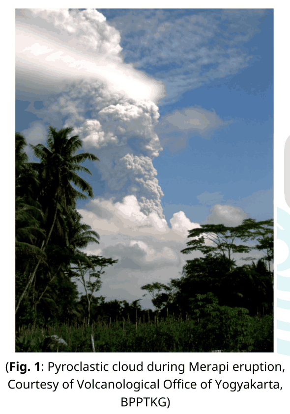
(Fig. 1: Pyroclastic cloud during Merapi eruption, Courtesy of Volcanological Office of Yogyakarta, BPPTKG)
Let us look at the causes of the largest eruption of Merapi in 2010. It is known by geophysicists that the influence of the external water into the magma plays an important role to the explosive behavior of volcanic eruptions (hydro magmatic eruptions). Let’s assume that we dealt with a volcano as a system that consists of mixture of magmatic particles and water. The volcano vents structures and atmosphere are being boundary of the system. The explosive eruption is considered to be happening in two stages, (1) an instantaneous magma-water interaction, and (2) a system expansion. In the first stage, a mass of magma (\(m_m\)) at an absolute temperature (\(T_m\)) mixes with a mass of external water (\(m_w\)) at an absolute temperature (\(T_w\)). The thermal equilibrium is reached almost instantaneously. This interaction can be perceived as a nearly-constant volume process. Latent heat of evaporation of water and latent heat of melting of magma can be neglected.
| A.1 | Find the equilibrium temperature at the first stage in terms of the masses and heat capacity per unit mass of water \(c_{Vw}\) and magma \(c_{Vm}\). | 0.5 pt. |
| A.2 | Determine its equilibrium pressure at the first stage by assuming that the mixture can be modeled as ideal gas. Assume that the volume per unit mole of the mixture is \(v_e\). | 0.3 pt. |
The system expansion (the second stage) can occur through several possibilities, one of which is thermal detonation. Although such process is quite complicated, we can empirically measure the relative velocity of the erupted mixture. The velocity of gas during the eruption depend on the pressure \(p\), the total mass \(m\) and the volume \(V\) of the mixture in the conduit of a volcano.
| A.3 | Express the velocity of gas during the eruption in terms of \(p\), \(m\), and \(V\) up to a proportional constant \(\kappa\). | 0.5 pt. |
The observed pressure is around the order of 100 MPa. This makes the eruption (relative) velocity can be as large as ballistic velocity.
B. The Yogyakarta Earthquake
The 2006 Yogyakarta earthquake of magnitude \(M_w=6.4\), which destroyed many buildings in the Bantul and Yogyakarta area, occurred at 05:54:00.00 local time or 22:54:00.00 UTC. The earthquake was caused by a sudden displacement of the Opak fault segment (see Fig. 2). The hypocenter was located 15 km below the surface.
The seismic wave that propagates on the earth crust can be recorded using seismometer. The diagram from seismometer is called seismogram (Fig. 2 and 3, Lower graph). These seismograms represent the vertical ground velocity as a function of time recorded by the seismic station at Gamping Station Yogyakarta (YOGI) (Fig. 2) and Denpasar, Bali (DNP) (Fig. 3). In general, seismic wave consists of three wave types: the longitudinal or primary (\(P\)-wave), the transversal or secondary (\(S\)-wave), and the surface wave. The \(P\)-wave and \(S\)-wave travel in the subsurface while the surface wave travels along the Earth surface. Seismic waves traveling through subsurfaces to the stations can be divided into those that propagate in a straight line, those that are reflected by a layer’s boundary, and those that are refracted into the next layer. The longitudinal wave or the primary wave has the highest velocity, while the surface wave has the lowest velocity, around 60% of the \(P\)-wave.
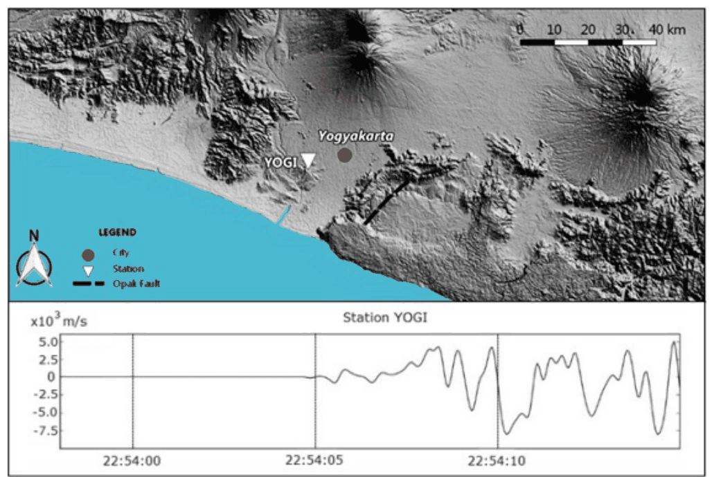
(Fig. 2: The maps location of YOGI)
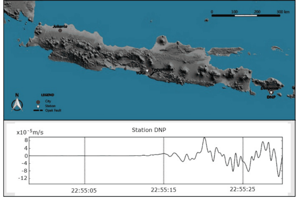
(Fig. 3: The maps location of DNP (Denpasar))
The distance between the epicenter (the projection of hypocenter on the Earth surface) and the YOGI and DNP stations respectively are 22.5 km and 500 km. The depth of the Earth crust layer in Java, Indonesia, is 30 km. Beneath the Earth’s crust is the Earth’s mantle layer. Just like other wave phenomena, seismic wave also satisfies the Snell’s law. The seismic wave can also be reflected by the mantle layer. In this problem we assume that the earth curvature is neglected.
| B.1 | Fig. 2 shows the seismogram at the YOGI station. Use the data to find the velocity of the \(P\)-wave in the Earth crust. | 0.5 pt. |
| B.2 | Find the travel time of the direct \(P\) wave and reflected wave due to the Yogyakarta earthquake that arrived at the DNP station in Denpasar. | 0.6 pt. |
By assuming that the Earth is composed of only two layers: the crust and the mantle, the primary wave propagates in the crust and in the mantle with different constant velocities. The velocity in the mantle is faster than in the crust. Note that \(P\)-wave refracted into the mantle at the right angle (\(90^\circ\)) is being partly refracted back into the crust along its entire path of propagation along the crust-mantle boundary.
| B.3 | Find the velocity of the \(P\)-wave in the mantle. | 1.2 pt. |
For a more realistic Earth structure, the crust can be divided into a number of thin layers so that the velocity of seismic wave is a function of the depth \(z\) according to \(v(z)=v_0+az\) where \(a\) is a constant and the hypocenter is approximated on the surface. In this model, the wave ray is curving.
| B.4 | Let us define the ray parameter \(p=\sin\theta(z)/v(z)\), where \(\theta(z)\) is the angle between the ray and the normal. Suppose a seismic wave arrives to the station with ray parameter \(p\); express the distance to the hypocenter in terms of \(p\), \(v_0\), and \(a\). Assume that the hypocenter is very close to the ground surface. | 1.4 pt. |
| B.5 | Find the travel time \(T\) from hypocenter to any station, in form of integral over \(z\). | 1.0 pt. |
The earth consists of a stack of homogeneous layers with the velocity of each layer is \(v_i\) and the thickness of \(\delta z_i\).
| B.6 | From the result of the previous problem, approximate the travel time (\(T\)) from the hypocenter to DNP station by assuming that the crust consists of only three discretized layers, \((i=1,2,3)\), characterized by \(v_1=6.65\) km/sec, \(v_2=6.97\) km/sec, \(v_3=6.99\) km/sec, \(p=0.143\) sec/km, \(\delta z_1=6.0\) km, \(\delta z_2=9.0\) km, \(\delta z_3=15\) km. | 1.0 pt. |
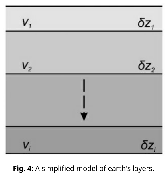
Fig. 4: A simplified model of earth’s layers.
C. Java Tsunami
The 2006 Pangandaran earthquake and tsunami occurred on July 17 at 15:19:27 local time off the coast of west and central Java. During the earthquake where the epicenter fault is on the ocean floor, the fault may be displaced producing a remarkably large water wave called tsunami. In other words, a tsunami is a shallow-water wave which is initiated by a tiny amplitude, but with an extremely large wavelength. Consider a sudden fault causing a lifting of some ocean floor as shown in Fig. 5. Assume that the energy of the earthquake is transformed to the potential energy of this raised ocean water. For simple model we approximate that the raised water has a geometry of a box with its area of \(\lambda L/2\) (where \(L\gg\lambda\)) and height of \(h\).
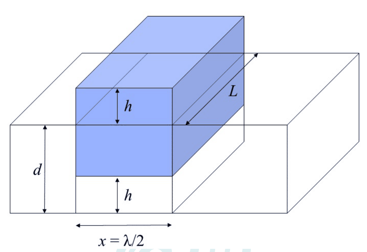
Fig. 5: Illustration for the tsunami wave \(d\) is the depth of the ocean.
| C.1 | Find the potential energy stored in the raised ocean water due to the earthquake with respect to ocean surface. Assume that the density of sea water is \(\rho\). | 0.5 pt. |
| C.2 | Find the speed of tsunami wave up to dimensionless factor. | 1.2 pt. |
| C.3 | Using energy argument, determine the amplitude of the tsunami wave as a function of the depth, assuming that the depth varies slowly and also knowing that at a depth of \(d_0\) the amplitude is \(A_0\). | 1.3 pt. |
Official English text of the problem.
Answers
The seismogram readings used below are approximately \(5\,\mathrm{s}\) after the earthquake at YOGI and \(72\,\mathrm{s}\) at DNP. Let \(v_c\) and \(v_m\) denote the crust and mantle speeds.
- A.1: \(\displaystyle T_e=\frac{m_m c_{Vm}T_m+m_w c_{Vw}T_w}{m_m c_{Vm}+m_w c_{Vw}}\).
- A.2: \(\displaystyle p_e=\frac{RT_e}{v_e}\).
- A.3: \(\displaystyle u=\kappa\sqrt{\frac{pV}{m}}\).
- B.1: \(\displaystyle v_c\simeq5.4\,\mathrm{km\,s^{-1}}\).
- B.2: \(\displaystyle t_{\rm direct}\simeq92.5\,\mathrm{s},\qquad t_{\rm reflected}\simeq92.8\,\mathrm{s}\), both approximately \(93\,\mathrm{s}\) at the precision of the graph.
- B.3: \(\displaystyle v_m\simeq7.6\,\mathrm{km\,s^{-1}}\).
- B.4: \(\displaystyle X=\frac{2}{ap}\sqrt{1-p^2v_0^2}\), assuming \(a>0\) and \(0<pv_0<1\).
- B.5: \(\displaystyle T=2\int_0^{z_t}\frac{dz}{v(z)\sqrt{1-p^2v(z)^2}},\qquad z_t=\frac{p^{-1}-v_0}{a}\).
- B.6: Direct discretization gives \(\displaystyle T\simeq1.84\times10^2\,\mathrm{s}\). This layer sum has a geometric inconsistency with the stated \(500\,\mathrm{km}\) offset, explained below.
- C.1: \(\displaystyle U=\frac14\rho g\lambda Lh^2\).
- C.2: \(\displaystyle c=C\sqrt{gd}\), where \(C\) is dimensionless; linear shallow-water theory gives \(C=1\).
- C.3: \(\displaystyle A(d)=A_0\left(\frac{d_0}{d}\right)^{1/4}\).
Solution
A.1 — Equilibrium temperature
During the rapid mixing, take heat exchange with the surroundings and boundary work to be negligible. Neglecting the specified latent heats and treating the heat capacities as constant, conservation of internal energy gives
\[ m_m c_{Vm}(T_e-T_m)+m_w c_{Vw}(T_e-T_w)=0. \]
Thus
\[ \boxed{ T_e=\frac{m_m c_{Vm}T_m+m_w c_{Vw}T_w} {m_m c_{Vm}+m_w c_{Vw}} }. \]
This is the initial-temperature average weighted by the two heat capacities.
A.2 — Equilibrium pressure
For \(n\) moles of the ideal-gas mixture,
\[ p_eV=nRT_e. \]
Since its molar volume is \(v_e=V/n\),
\[ \boxed{ p_e=\frac{RT_e}{v_e} =\frac{R}{v_e} \frac{m_m c_{Vm}T_m+m_w c_{Vw}T_w} {m_m c_{Vm}+m_w c_{Vw}} }. \]
Here \(R\) is the universal gas constant.
A.3 — Eruption velocity
Assume, as specified, that the velocity depends only on \(p,m,V\). Write
\[ u=\kappa p^\alpha m^\beta V^\gamma. \]
Using
\[ [p]=ML^{-1}T^{-2},\qquad [m]=M,\qquad [V]=L^3, \]
dimensional consistency requires
\[ \alpha+\beta=0,\qquad -\alpha+3\gamma=1,\qquad -2\alpha=-1. \]
Therefore
\[ \alpha=\frac12,\qquad \beta=-\frac12,\qquad \gamma=\frac12, \]
and
\[ \boxed{u=\kappa\sqrt{\frac{pV}{m}}}. \]
Equivalently, \(u=\kappa\sqrt{p/\rho_{\rm mix}}\), where \(\rho_{\rm mix}=m/V\). Dimensional analysis does not determine \(\kappa\).
B.1 — \(P\)-wave speed in the crust
Let the source depth be \(z_s=15\,\mathrm{km}\). The horizontal distance to YOGI is \(22.5\,\mathrm{km}\), so the direct source-to-station distance is
\[ s_Y=\sqrt{22.5^2+15^2} =27.04\,\mathrm{km}. \]
The first visible departure from the baseline in Fig. 2 is approximately at 22:54:05 UTC. Relative to the earthquake time 22:54:00, this gives
\[ t_Y\simeq5\,\mathrm{s}. \]
Hence
\[ \boxed{ v_c=\frac{s_Y}{t_Y} \simeq\frac{27.04}{5} \simeq5.4\,\mathrm{km\,s^{-1}} }. \]
The numerical calculations below retain \(5.4083\,\mathrm{km\,s^{-1}}\) internally, although the graph does not justify that many significant figures.
B.2 — Direct and reflected travel times to DNP
Write the horizontal source-to-DNP distance as \(X=500\,\mathrm{km}\), and the crust thickness as \(H=30\,\mathrm{km}\).
For the direct wave,
\[ s_{\rm direct}=\sqrt{X^2+z_s^2}, \]
so
\[ \boxed{ t_{\rm direct} =\frac{\sqrt{500^2+15^2}}{v_c} \simeq92.5\,\mathrm{s} }. \]
For reflection at the horizontal crust–mantle boundary, reflect the source across the plane \(z=H\). Its image is at depth
\[ z_{\rm image}=2H-z_s=45\,\mathrm{km}. \]
Unfolding the reflected ray gives a straight line from this image to DNP. Consequently,
\[ s_{\rm reflected}=\sqrt{X^2+(2H-z_s)^2}, \]
and
\[ \boxed{ t_{\rm reflected} =\frac{\sqrt{500^2+45^2}}{v_c} \simeq92.8\,\mathrm{s} }. \]
Both travel times are about \(93\,\mathrm{s}\); their calculated difference is approximately \(0.33\,\mathrm{s}\).
B.3 — \(P\)-wave speed in the mantle
The first departure from the flat baseline in Fig. 3 is approximately at 22:55:12 UTC, giving
\[ t_D\simeq72\,\mathrm{s}. \]
This precedes the direct and reflected crustal arrivals calculated above. We identify it with the critically refracted wave that travels along the mantle boundary and radiates back into the crust.
Let \(\theta_c\) be the critical angle measured from the vertical. Snell’s law gives
\[ \frac{\sin\theta_c}{v_c}=\frac{1}{v_m}, \qquad \sin\theta_c=\frac{v_c}{v_m}. \]
The downward crustal leg spans depth \(H-z_s\), and the upward leg spans depth \(H\). Their combined vertical displacement in magnitude is
\[ K=(H-z_s)+H=2H-z_s=45\,\mathrm{km}. \]
Their combined length and horizontal projection are therefore
\[ s_{\rm crust}=\frac{K}{\cos\theta_c}, \qquad X_{\rm crust}=K\tan\theta_c. \]
The distance travelled along the mantle boundary is
\[ X_{\rm mantle}=X-K\tan\theta_c. \]
Thus
\[ t_D= \frac{K}{v_c\cos\theta_c} +\frac{X-K\tan\theta_c}{v_m}. \]
Using \(\sin\theta_c=v_c/v_m\), this simplifies to
\[ \boxed{ t_D=\frac{X}{v_m} +\frac{K}{v_c}\sqrt{1-\frac{v_c^2}{v_m^2}} }. \]
Substituting the graph reading,
\[ 72= \frac{500}{v_m} +\frac{45}{5.4083} \sqrt{1-\left(\frac{5.4083}{v_m}\right)^2}, \]
with distances in kilometres and speeds in kilometres per second. Solving gives
\[ v_m\simeq7.554\,\mathrm{km\,s^{-1}}, \]
or, at appropriate precision,
\[ \boxed{v_m\simeq7.6\,\mathrm{km\,s^{-1}}}. \]
As a check, \(\theta_c\simeq45.7^\circ\), and the mantle segment is approximately \(454\,\mathrm{km}\) long. The crustal legs take about \(11.9\,\mathrm{s}\), and the mantle segment about \(60.1\,\mathrm{s}\).
B.4 — Distance for the continuously varying velocity
Take \(z\) positive downward and \(x\) horizontal. Snell’s law across the thin horizontal layers implies that
\[ p=\frac{\sin\theta(z)}{v(z)} \]
is constant along a ray. Therefore
\[ \sin\theta(z)=pv(z), \qquad \cos\theta(z)=\sqrt{1-p^2v(z)^2}. \]
On the downward leg,
\[ \frac{dx}{dz} =\tan\theta(z) =\frac{pv(z)}{\sqrt{1-p^2v(z)^2}}. \]
For a returning ray in a medium with \(a>0\), the deepest point occurs where the ray becomes horizontal:
\[ pv(z_t)=1. \]
Since \(v(z)=v_0+az\),
\[ \boxed{z_t=\frac{p^{-1}-v_0}{a}}. \]
With both source and receiver approximated as lying on the surface, the downward and upward portions are symmetric. The horizontal distance is
\[ X=2\int_0^{z_t} \frac{p(v_0+az)} {\sqrt{1-p^2(v_0+az)^2}}\,dz. \]
Set \(u=p(v_0+az)\), so \(du=pa\,dz\). Then
\[ X=\frac{2}{ap}\int_{pv_0}^{1} \frac{u}{\sqrt{1-u^2}}\,du. \]
Since the antiderivative is \(-\sqrt{1-u^2}\),
\[ \boxed{ X=\frac{2}{ap}\sqrt{1-p^2v_0^2} =\frac{2}{a}\sqrt{\frac{1}{p^2}-v_0^2} }. \]
The returning-ray solution requires \(0<pv_0<1\).
B.5 — Travel-time integral
A ray segment of length \(ds\) takes time
\[ dt=\frac{ds}{v(z)}. \]
Since \(\lvert dz\rvert=ds\cos\theta(z)\),
\[ dt= \frac{\lvert dz\rvert} {v(z)\sqrt{1-p^2v(z)^2}}. \]
Including both the downward and upward legs gives
\[ \boxed{ T=2\int_0^{z_t} \frac{dz}{v(z)\sqrt{1-p^2v(z)^2}} }. \]
For the linear velocity profile, this is
\[ \boxed{ T= 2\int_0^{(p^{-1}-v_0)/a} \frac{dz} {(v_0+az)\sqrt{1-p^2(v_0+az)^2}} }. \]
The singularity at the turning point is integrable. Evaluating the integral also gives
\[ T=\frac{2}{a} \ln\!\left( \frac{1+\sqrt{1-p^2v_0^2}}{pv_0} \right). \]
An equivalent form, useful for examining the numerical approximation in B.6, follows by subtracting \(pX\):
\[ \begin{aligned} T-pX &= 2\int_0^{z_t} \left[ \frac{1}{v\sqrt{1-p^2v^2}} -\frac{p^2v}{\sqrt{1-p^2v^2}} \right]dz\\ &= 2\int_0^{z_t}\sqrt{\frac{1}{v(z)^2}-p^2}\,dz. \end{aligned} \]
Hence, for a geometrically consistent ray,
\[ \boxed{ T=pX+2\int_0^{z_t}\sqrt{\frac{1}{v(z)^2}-p^2}\,dz }. \]
B.6 — Three-layer approximation
Retaining the surface-source approximation from B.4–B.5, discretize the first travel-time integral:
\[ \boxed{ T\approx 2\sum_{i=1}^{3} \frac{\delta z_i} {v_i\sqrt{1-p^2v_i^2}} }. \]
The factor of two accounts for passage through each layer on the downward and upward legs.
Using the numbers exactly as printed gives:
| Layer \(i\) | \(pv_i\) | Two-leg contribution \(\displaystyle \frac{2\delta z_i}{v_i\sqrt{1-p^2v_i^2}}\) |
|---|---|---|
| 1 | 0.95095 | \(5.833\,\mathrm{s}\) |
| 2 | 0.99671 | \(31.863\,\mathrm{s}\) |
| 3 | 0.99957 | \(146.366\,\mathrm{s}\) |
Thus the direct layer quadrature gives
\[ \boxed{ T\approx184.06\,\mathrm{s} \simeq1.84\times10^2\,\mathrm{s} }. \]
There is a consistency limitation in interpreting this number as the travel time to DNP. The horizontal distance of the same discrete ray would be
\[ X_{\rm layers} = 2\sum_{i=1}^{3} \frac{\delta z_i\,pv_i} {\sqrt{1-p^2v_i^2}} \simeq1280.9\,\mathrm{km}, \]
which differs substantially from \(500\,\mathrm{km}\).
If instead one inserts the prescribed \(500\,\mathrm{km}\) offset into the second form of B.5 and approximates its integral, one obtains the formal estimate
\[ \begin{aligned} T &\approx p(500) +2\sum_{i=1}^{3}\delta z_i \sqrt{\frac{1}{v_i^2}-p^2}\\ &=71.5+0.8934\\ &\approx72.39\,\mathrm{s}. \end{aligned} \]
The two continuum formulas are equivalent, but these coarse approximations fail to preserve their required distance relation. Thus \(184\,\mathrm{s}\) is the direct travel-time layer sum; \(72.4\,\mathrm{s}\) is a fixed-offset estimate. They cannot both describe the same literal three-layer ray with the supplied parameters.
C.1 — Potential energy of the raised water
Let the horizontal area of the raised box be
\[ S=\frac{\lambda L}{2}. \]
Taking the undisturbed ocean surface as zero gravitational potential, a horizontal slab of thickness \(dz\) at height \(z\) has mass \(\rho S\,dz\). Consequently,
\[ U=\int_0^h \rho Sgz\,dz =\frac12\rho Sgh^2. \]
Therefore
\[ \boxed{U=\frac14\rho g\lambda Lh^2}. \]
Equivalently, the water above the original surface has mass \(\rho Sh\), with its centre of mass at height \(h/2\).
C.2 — Tsunami speed
Use the shallow-water, small-amplitude approximations
\[ \lambda\gg d,\qquad h\ll d. \]
The horizontal fluid velocity is then approximately uniform through the depth, and the vertical pressure distribution is approximately hydrostatic.
Let \(\eta(x,t)\) be the surface displacement and \(u(x,t)\) the horizontal fluid velocity. Conservation of water volume, linearized about depth \(d\), gives
\[ \frac{\partial\eta}{\partial t} +d\frac{\partial u}{\partial x}=0. \]
The horizontal pressure gradient is \(\rho g\,\partial\eta/\partial x\). Newton’s second law therefore gives
\[ \frac{\partial u}{\partial t} =-g\frac{\partial\eta}{\partial x}. \]
Differentiating the first equation with respect to time and substituting the second,
\[ \frac{\partial^2\eta}{\partial t^2} =gd\frac{\partial^2\eta}{\partial x^2}. \]
This is the wave equation, so
\[ \boxed{c=\sqrt{gd}}. \]
At the level requested in the question,
\[ \boxed{c=C\sqrt{gd}}, \]
with a dimensionless factor \(C\); the stated linear shallow-water assumptions give \(C=1\). The density cancels because it multiplies both inertia and the gravitational restoring force.
C.3 — Amplitude as the depth changes
Assume slow depth variation, negligible reflection and dissipation, and constant wavefront width. Since \(L\gg\lambda\), the wave can be treated locally as a plane wave.
For a sinusoidal surface displacement of amplitude \(A\),
\[ \eta=A\cos(kx-\omega t), \qquad \langle\eta^2\rangle=\frac{A^2}{2}. \]
The mean gravitational potential energy per unit horizontal area is
\[ \overline{\mathcal E}_{\rm pot} =\frac12\rho g\langle\eta^2\rangle =\frac14\rho gA^2. \]
For a progressive shallow-water wave, continuity gives
\[ u=\frac{c}{d}\eta. \]
Its mean kinetic energy per unit horizontal area is therefore
\[ \overline{\mathcal E}_{\rm kin} =\frac12\rho d\langle u^2\rangle =\frac{\rho c^2A^2}{4d} =\frac14\rho gA^2. \]
Thus the total mean energy density is
\[ \overline{\mathcal E}=\frac12\rho gA^2. \]
Shallow-water waves are nondispersive, so their group velocity equals \(c=\sqrt{gd}\). Conservation of energy flux per unit wavefront width gives
\[ \overline{\mathcal E}\,c=\text{constant}, \]
or
\[ A^2\sqrt d=\text{constant}. \]
Using the reference amplitude \(A_0\) at depth \(d_0\),
\[ A^2\sqrt d=A_0^2\sqrt{d_0}. \]
Therefore
\[ \boxed{ A(d)=A_0\left(\frac{d_0}{d}\right)^{1/4} }. \]
This is Green’s law. Its validity requires small amplitude relative to depth and sufficiently slow depth variation; it does not describe the eventual breaking of the wave.
The solution was checked against the official solution.
IPhO 2017 · Theorieaufgabe 2
Erdbeben, Vulkan und Tsunami
Indonesien ist der Supermarkt der Naturgefahren. Fast alle Arten von Naturereignissen mit Gefahrenpotenzial sind in Indonesien bereits aufgetreten, darunter Vulkanausbrüche, Erdbeben und Tsunamis.
A. Ausbruch des Vulkans Merapi
Der Vulkan Merapi in Yogyakarta ist einer der aktivsten Vulkane auf Java. Pyroklastische Ströme sind ein bekanntes Merkmal seiner Ausbrüche. Ein pyroklastischer Strom ist ein heißes Gemisch aus Gas und Gestein, das sich von einem Vulkan wegbewegt. Am 26. Oktober 2010 zeigte der Merapi seinen explosiven Charakter: Er erzeugte eine Aschewolke, die eine Höhe von 12 km erreichte (Abb. 1), sowie pyroklastische Ströme, die mehr als 20.000 Menschen in der Umgebung des Vulkans zur Flucht zwangen.
(Abb. 1: Pyroklastische Wolke während des Merapi-Ausbruchs, mit freundlicher Genehmigung des Vulkanologischen Amtes von Yogyakarta, BPPTKG)
Betrachten wir die Ursachen des größten Ausbruchs des Merapi im Jahr 2010. Geophysikern ist bekannt, dass das Eindringen von Wasser von außen in das Magma eine wichtige Rolle für das explosive Verhalten von Vulkanausbrüchen spielt (hydromagmatische Eruptionen). Wir nehmen an, dass wir den Vulkan als ein System behandeln, das aus einem Gemisch aus Magmapartikeln und Wasser besteht. Die Strukturen der Vulkanschlote und die Atmosphäre bilden die Grenze des Systems. Der explosive Ausbruch wird als Vorgang in zwei Phasen betrachtet: (1) eine augenblickliche Wechselwirkung zwischen Magma und Wasser und (2) eine Expansion des Systems. In der ersten Phase vermischt sich eine Magmamasse (\(m_m\)) bei einer absoluten Temperatur (\(T_m\)) mit einer Masse von außen zugeführten Wassers (\(m_w\)) bei einer absoluten Temperatur (\(T_w\)). Das thermische Gleichgewicht wird nahezu augenblicklich erreicht. Diese Wechselwirkung kann als Prozess bei nahezu konstantem Volumen betrachtet werden. Die latente Verdampfungswärme des Wassers und die latente Schmelzwärme des Magmas können vernachlässigt werden.
| A.1 | Bestimmen Sie die Gleichgewichtstemperatur in der ersten Phase in Abhängigkeit von den Massen und den spezifischen Wärmekapazitäten des Wassers \(c_{Vw}\) und des Magmas \(c_{Vm}\). | 0.5 Pkt. |
| A.2 | Bestimmen Sie den Gleichgewichtsdruck in der ersten Phase unter der Annahme, dass das Gemisch als ideales Gas modelliert werden kann. Nehmen Sie an, dass das molare Volumen des Gemischs \(v_e\) beträgt. | 0.3 Pkt. |
Die Expansion des Systems (die zweite Phase) kann auf verschiedene Arten erfolgen, darunter durch thermische Detonation. Obwohl ein solcher Prozess recht kompliziert ist, können wir die Relativgeschwindigkeit des ausgestoßenen Gemischs empirisch messen. Die Geschwindigkeit des Gases während des Ausbruchs hängt vom Druck \(p\), der Gesamtmasse \(m\) und dem Volumen \(V\) des Gemischs im Förderschlot eines Vulkans ab.
| A.3 | Drücken Sie die Geschwindigkeit des Gases während des Ausbruchs bis auf eine Proportionalitätskonstante \(\kappa\) durch \(p\), \(m\) und \(V\) aus. | 0.5 Pkt. |
Der beobachtete Druck liegt in der Größenordnung von 100 MPa. Dadurch kann die (relative) Eruptionsgeschwindigkeit die Größenordnung ballistischer Geschwindigkeiten erreichen.
B. Das Erdbeben von Yogyakarta
Das Erdbeben von Yogyakarta im Jahr 2006 mit der Magnitude \(M_w=6.4\), das viele Gebäude in der Region Bantul und Yogyakarta zerstörte, ereignete sich um 05:54:00.00 Uhr Ortszeit bzw. um 22:54:00.00 Uhr UTC. Es wurde durch eine plötzliche Verschiebung des Opak-Verwerfungssegments verursacht (siehe Abb. 2). Das Hypozentrum lag 15 km unter der Oberfläche.
Die sich in der Erdkruste ausbreitenden seismischen Wellen können mit einem Seismometer aufgezeichnet werden. Die Aufzeichnung eines Seismometers wird als Seismogramm bezeichnet (Abb. 2 und 3, jeweils unteres Diagramm). Diese Seismogramme zeigen die vertikale Bodengeschwindigkeit als Funktion der Zeit, aufgezeichnet an der seismischen Station Gamping in Yogyakarta (YOGI) (Abb. 2) und in Denpasar auf Bali (DNP) (Abb. 3). Im Allgemeinen bestehen seismische Wellen aus drei Wellentypen: der Longitudinal- oder Primärwelle (\(P\)-Welle), der Transversal- oder Sekundärwelle (\(S\)-Welle) und der Oberflächenwelle. Die \(P\)-Welle und die \(S\)-Welle breiten sich im Untergrund aus, während sich die Oberflächenwelle entlang der Erdoberfläche ausbreitet. Seismische Wellen, die durch den Untergrund zu den Stationen gelangen, lassen sich in solche unterteilen, die sich geradlinig ausbreiten, solche, die an einer Schichtgrenze reflektiert werden, und solche, die in die nächste Schicht gebrochen werden. Die Longitudinal- oder Primärwelle besitzt die höchste Geschwindigkeit, während die Oberflächenwelle die niedrigste Geschwindigkeit besitzt, etwa 60% der Geschwindigkeit der \(P\)-Welle.
(Abb. 2: Karten mit der Lage von YOGI)
(Abb. 3: Karten mit der Lage von DNP (Denpasar))
Die Entfernungen zwischen dem Epizentrum (der Projektion des Hypozentrums auf die Erdoberfläche) und den Stationen YOGI bzw. DNP betragen 22.5 km bzw. 500 km. Die Mächtigkeit der Erdkruste auf Java in Indonesien beträgt 30 km. Unter der Erdkruste liegt der Erdmantel. Wie andere Wellenphänomene gehorchen auch seismische Wellen dem Snelliusschen Brechungsgesetz. Seismische Wellen können auch an der Mantelschicht reflektiert werden. In dieser Aufgabe wird die Erdkrümmung vernachlässigt.
| B.1 | Abb. 2 zeigt das Seismogramm an der Station YOGI. Bestimmen Sie mithilfe dieser Daten die Geschwindigkeit der \(P\)-Welle in der Erdkruste. | 0.5 Pkt. |
| B.2 | Bestimmen Sie die Laufzeit der direkten \(P\)-Welle und der reflektierten Welle des Erdbebens von Yogyakarta zur Station DNP in Denpasar. | 0.6 Pkt. |
Unter der Annahme, dass die Erde nur aus zwei Schichten besteht, der Kruste und dem Mantel, breitet sich die Primärwelle in der Kruste und im Mantel mit unterschiedlichen konstanten Geschwindigkeiten aus. Die Geschwindigkeit im Mantel ist größer als diejenige in der Kruste. Beachten Sie, dass eine unter einem rechten Winkel (\(90^\circ\)) in den Mantel gebrochene \(P\)-Welle entlang ihres gesamten Ausbreitungsweges an der Kruste-Mantel-Grenze teilweise zurück in die Kruste gebrochen wird.
| B.3 | Bestimmen Sie die Geschwindigkeit der \(P\)-Welle im Mantel. | 1.2 Pkt. |
Für einen realistischeren Aufbau der Erde kann die Kruste in eine Reihe dünner Schichten unterteilt werden, sodass die Geschwindigkeit der seismischen Welle gemäß \(v(z)=v_0+az\) von der Tiefe \(z\) abhängt, wobei \(a\) eine Konstante ist und das Hypozentrum näherungsweise an der Oberfläche liegt. In diesem Modell verläuft der Wellenstrahl gekrümmt.
| B.4 | Wir definieren den Strahlparameter \(p=\sin\theta(z)/v(z)\), wobei \(\theta(z)\) der Winkel zwischen dem Strahl und der Normalen ist. Eine seismische Welle erreiche die Station mit dem Strahlparameter \(p\); drücken Sie die Entfernung zum Hypozentrum durch \(p\), \(v_0\) und \(a\) aus. Nehmen Sie an, dass das Hypozentrum sehr nahe an der Erdoberfläche liegt. | 1.4 Pkt. |
| B.5 | Bestimmen Sie die Laufzeit \(T\) vom Hypozentrum zu einer beliebigen Station in Form eines Integrals über \(z\). | 1.0 Pkt. |
Die Erde besteht aus einem Stapel homogener Schichten, wobei jede Schicht die Geschwindigkeit \(v_i\) und die Dicke \(\delta z_i\) besitzt.
| B.6 | Nähern Sie mithilfe des Ergebnisses der vorherigen Teilaufgabe die Laufzeit (\(T\)) vom Hypozentrum zur Station DNP an. Nehmen Sie dazu an, dass die Kruste nur aus drei diskretisierten Schichten \((i=1,2,3)\) besteht, die durch \(v_1=6.65\) km/sec, \(v_2=6.97\) km/sec, \(v_3=6.99\) km/sec, \(p=0.143\) sec/km, \(\delta z_1=6.0\) km, \(\delta z_2=9.0\) km, \(\delta z_3=15\) km charakterisiert sind. | 1.0 Pkt. |
Abb. 4: Ein vereinfachtes Modell der Erdschichten.
C. Tsunami auf Java
Das Erdbeben und der Tsunami von Pangandaran im Jahr 2006 ereigneten sich am 17. Juli um 15:19:27 Uhr Ortszeit vor der Küste von West- und Zentraljava. Bei einem Erdbeben, dessen epizentrale Verwerfung am Meeresboden liegt, kann eine Verschiebung an der Verwerfung eine außergewöhnlich große Wasserwelle erzeugen, die als Tsunami bezeichnet wird. Mit anderen Worten: Ein Tsunami ist eine Flachwasserwelle, die mit einer winzigen Amplitude, aber einer extrem großen Wellenlänge beginnt. Betrachten Sie eine plötzliche Verwerfungsbewegung, durch die ein Teil des Meeresbodens angehoben wird, wie in Abb. 5 gezeigt. Nehmen Sie an, dass die Energie des Erdbebens in die potenzielle Energie dieses angehobenen Meerwassers umgewandelt wird. In einem einfachen Modell nähern wir das angehobene Wasser durch einen Quader mit der Grundfläche \(\lambda L/2\) (wobei \(L\gg\lambda\)) und der Höhe \(h\) an.
Abb. 5: Veranschaulichung der Tsunamiwelle; \(d\) ist die Meerestiefe.
| C.1 | Bestimmen Sie die potenzielle Energie, die im durch das Erdbeben angehobenen Meerwasser gespeichert ist, bezogen auf die Meeresoberfläche. Nehmen Sie an, dass die Dichte des Meerwassers \(\rho\) beträgt. | 0.5 Pkt. |
| C.2 | Bestimmen Sie die Geschwindigkeit der Tsunamiwelle bis auf einen dimensionslosen Faktor. | 1.2 Pkt. |
| C.3 | Bestimmen Sie mithilfe einer Energiebetrachtung die Amplitude der Tsunamiwelle als Funktion der Tiefe. Nehmen Sie an, dass sich die Tiefe langsam ändert und dass die Amplitude bei einer Tiefe von \(d_0\) den Wert \(A_0\) hat. | 1.3 Pkt. |
Aufgabentext aus dem offiziellen englischen Text übersetzt.
Antworten
Die im Folgenden verwendeten Ablesewerte aus den Seismogrammen liegen etwa \(5\,\mathrm{s}\) nach dem Erdbeben bei YOGI und \(72\,\mathrm{s}\) bei DNP. Mit \(v_c\) und \(v_m\) werden die Geschwindigkeiten in Kruste und Mantel bezeichnet.
- A.1: \(\displaystyle T_e=\frac{m_m c_{Vm}T_m+m_w c_{Vw}T_w}{m_m c_{Vm}+m_w c_{Vw}}\).
- A.2: \(\displaystyle p_e=\frac{RT_e}{v_e}\).
- A.3: \(\displaystyle u=\kappa\sqrt{\frac{pV}{m}}\).
- B.1: \(\displaystyle v_c\simeq5.4\,\mathrm{km\,s^{-1}}\).
- B.2: \(\displaystyle t_{\rm direct}\simeq92.5\,\mathrm{s},\qquad t_{\rm reflected}\simeq92.8\,\mathrm{s}\), beide bei der Genauigkeit des Diagramms ungefähr \(93\,\mathrm{s}\).
- B.3: \(\displaystyle v_m\simeq7.6\,\mathrm{km\,s^{-1}}\).
- B.4: \(\displaystyle X=\frac{2}{ap}\sqrt{1-p^2v_0^2}\), unter den Annahmen \(a>0\) und \(0<pv_0<1\).
- B.5: \(\displaystyle T=2\int_0^{z_t}\frac{dz}{v(z)\sqrt{1-p^2v(z)^2}},\qquad z_t=\frac{p^{-1}-v_0}{a}\).
- B.6: Die direkte Diskretisierung ergibt \(\displaystyle T\simeq1.84\times10^2\,\mathrm{s}\). Diese Schichtsumme weist eine geometrische Unvereinbarkeit mit der angegebenen horizontalen Entfernung von \(500\,\mathrm{km}\) auf, die weiter unten erläutert wird.
- C.1: \(\displaystyle U=\frac14\rho g\lambda Lh^2\).
- C.2: \(\displaystyle c=C\sqrt{gd}\), wobei \(C\) dimensionslos ist; die lineare Flachwassertheorie ergibt \(C=1\).
- C.3: \(\displaystyle A(d)=A_0\left(\frac{d_0}{d}\right)^{1/4}\).
Lösung
A.1 — Gleichgewichtstemperatur
Während der schnellen Vermischung werden der Wärmeaustausch mit der Umgebung und die Volumenarbeit als vernachlässigbar angenommen. Wenn die angegebenen latenten Wärmen vernachlässigt und die Wärmekapazitäten als konstant behandelt werden, ergibt die Erhaltung der inneren Energie
\[ m_m c_{Vm}(T_e-T_m)+m_w c_{Vw}(T_e-T_w)=0. \]
Somit gilt
\[ \boxed{ T_e=\frac{m_m c_{Vm}T_m+m_w c_{Vw}T_w} {m_m c_{Vm}+m_w c_{Vw}} }. \]
Dies ist der mit den beiden Wärmekapazitäten gewichtete Mittelwert der Anfangstemperaturen.
A.2 — Gleichgewichtsdruck
Für \(n\) Mol des idealen Gasgemischs gilt
\[ p_eV=nRT_e. \]
Da sein molares Volumen \(v_e=V/n\) ist, gilt
\[ \boxed{ p_e=\frac{RT_e}{v_e} =\frac{R}{v_e} \frac{m_m c_{Vm}T_m+m_w c_{Vw}T_w} {m_m c_{Vm}+m_w c_{Vw}} }. \]
Hier ist \(R\) die universelle Gaskonstante.
A.3 — Eruptionsgeschwindigkeit
Wie vorgegeben nehmen wir an, dass die Geschwindigkeit nur von \(p,m,V\) abhängt. Wir setzen an:
\[ u=\kappa p^\alpha m^\beta V^\gamma. \]
Mit
\[ [p]=ML^{-1}T^{-2},\qquad [m]=M,\qquad [V]=L^3, \]
verlangt die Dimensionskonsistenz
\[ \alpha+\beta=0,\qquad -\alpha+3\gamma=1,\qquad -2\alpha=-1. \]
Daraus folgt
\[ \alpha=\frac12,\qquad \beta=-\frac12,\qquad \gamma=\frac12, \]
und
\[ \boxed{u=\kappa\sqrt{\frac{pV}{m}}}. \]
Gleichwertig ist \(u=\kappa\sqrt{p/\rho_{\rm mix}}\), wobei \(\rho_{\rm mix}=m/V\). Die Dimensionsanalyse bestimmt \(\kappa\) nicht.
B.1 — Geschwindigkeit der \(P\)-Welle in der Kruste
Die Herdtiefe sei \(z_s=15\,\mathrm{km}\). Die horizontale Entfernung zu YOGI beträgt \(22.5\,\mathrm{km}\), sodass für die direkte Entfernung vom Herd zur Station gilt:
\[ s_Y=\sqrt{22.5^2+15^2} =27.04\,\mathrm{km}. \]
Die erste sichtbare Abweichung von der Grundlinie in Abb. 2 liegt ungefähr bei 22:54:05 Uhr UTC. Bezogen auf den Zeitpunkt des Erdbebens um 22:54:00 Uhr ergibt dies
\[ t_Y\simeq5\,\mathrm{s}. \]
Damit folgt
\[ \boxed{ v_c=\frac{s_Y}{t_Y} \simeq\frac{27.04}{5} \simeq5.4\,\mathrm{km\,s^{-1}} }. \]
In den folgenden numerischen Berechnungen wird intern mit \(5.4083\,\mathrm{km\,s^{-1}}\) weitergerechnet, obwohl das Diagramm nicht so viele signifikante Stellen rechtfertigt.
B.2 — Laufzeiten der direkten und der reflektierten Welle zu DNP
Wir bezeichnen die horizontale Entfernung vom Herd zu DNP mit \(X=500\,\mathrm{km}\) und die Krustenmächtigkeit mit \(H=30\,\mathrm{km}\).
Für die direkte Welle gilt
\[ s_{\rm direct}=\sqrt{X^2+z_s^2}, \]
also
\[ \boxed{ t_{\rm direct} =\frac{\sqrt{500^2+15^2}}{v_c} \simeq92.5\,\mathrm{s} }. \]
Für die Reflexion an der horizontalen Kruste-Mantel-Grenze spiegeln wir den Herd an der Ebene \(z=H\). Sein Spiegelbild liegt in der Tiefe
\[ z_{\rm image}=2H-z_s=45\,\mathrm{km}. \]
Durch Aufklappen des reflektierten Strahls entsteht eine gerade Linie von diesem Spiegelbild zu DNP. Folglich gilt
\[ s_{\rm reflected}=\sqrt{X^2+(2H-z_s)^2}, \]
und
\[ \boxed{ t_{\rm reflected} =\frac{\sqrt{500^2+45^2}}{v_c} \simeq92.8\,\mathrm{s} }. \]
Beide Laufzeiten betragen etwa \(93\,\mathrm{s}\); ihre berechnete Differenz beträgt ungefähr \(0.33\,\mathrm{s}\).
B.3 — Geschwindigkeit der \(P\)-Welle im Mantel
Die erste Abweichung von der flachen Grundlinie in Abb. 3 liegt ungefähr bei 22:55:12 Uhr UTC. Daraus ergibt sich
\[ t_D\simeq72\,\mathrm{s}. \]
Dieser Zeitpunkt liegt vor den oben berechneten Ankunftszeiten der direkten und der reflektierten Krustenwelle. Wir ordnen ihn der kritisch gebrochenen Welle zu, die sich entlang der Mantelgrenze ausbreitet und dabei zurück in die Kruste abstrahlt.
Es sei \(\theta_c\) der von der Vertikalen aus gemessene Grenzwinkel. Das Snelliussche Brechungsgesetz ergibt
\[ \frac{\sin\theta_c}{v_c}=\frac{1}{v_m}, \qquad \sin\theta_c=\frac{v_c}{v_m}. \]
Der abwärts gerichtete Strahlabschnitt in der Kruste überbrückt den Tiefenunterschied \(H-z_s\), der aufwärts gerichtete Abschnitt den Tiefenunterschied \(H\). Die Summe der Beträge ihrer vertikalen Verschiebungen ist
\[ K=(H-z_s)+H=2H-z_s=45\,\mathrm{km}. \]
Ihre Gesamtlänge und ihre gesamte horizontale Projektion betragen daher
\[ s_{\rm crust}=\frac{K}{\cos\theta_c}, \qquad X_{\rm crust}=K\tan\theta_c. \]
Die entlang der Mantelgrenze zurückgelegte Strecke ist
\[ X_{\rm mantle}=X-K\tan\theta_c. \]
Somit gilt
\[ t_D= \frac{K}{v_c\cos\theta_c} +\frac{X-K\tan\theta_c}{v_m}. \]
Mit \(\sin\theta_c=v_c/v_m\) vereinfacht sich dies zu
\[ \boxed{ t_D=\frac{X}{v_m} +\frac{K}{v_c}\sqrt{1-\frac{v_c^2}{v_m^2}} }. \]
Einsetzen des aus dem Diagramm abgelesenen Wertes ergibt
\[ 72= \frac{500}{v_m} +\frac{45}{5.4083} \sqrt{1-\left(\frac{5.4083}{v_m}\right)^2}, \]
wobei Entfernungen in Kilometern und Geschwindigkeiten in Kilometern pro Sekunde angegeben werden. Die Lösung lautet
\[ v_m\simeq7.554\,\mathrm{km\,s^{-1}}, \]
oder mit angemessener Genauigkeit
\[ \boxed{v_m\simeq7.6\,\mathrm{km\,s^{-1}}}. \]
Zur Kontrolle: \(\theta_c\simeq45.7^\circ\), und der Mantelabschnitt ist ungefähr \(454\,\mathrm{km}\) lang. Die Krustenabschnitte benötigen etwa \(11.9\,\mathrm{s}\), der Mantelabschnitt etwa \(60.1\,\mathrm{s}\).
B.4 — Entfernung bei kontinuierlich veränderlicher Geschwindigkeit
Wir wählen \(z\) nach unten positiv und \(x\) horizontal. Aus dem Snelliusschen Brechungsgesetz an den dünnen horizontalen Schichten folgt, dass
\[ p=\frac{\sin\theta(z)}{v(z)} \]
entlang eines Strahls konstant ist. Daher gilt
\[ \sin\theta(z)=pv(z), \qquad \cos\theta(z)=\sqrt{1-p^2v(z)^2}. \]
Auf dem abwärts gerichteten Abschnitt gilt
\[ \frac{dx}{dz} =\tan\theta(z) =\frac{pv(z)}{\sqrt{1-p^2v(z)^2}}. \]
Für einen zur Oberfläche zurückkehrenden Strahl in einem Medium mit \(a>0\) liegt der tiefste Punkt dort, wo der Strahl horizontal verläuft:
\[ pv(z_t)=1. \]
Da \(v(z)=v_0+az\), folgt
\[ \boxed{z_t=\frac{p^{-1}-v_0}{a}}. \]
Wenn sowohl Quelle als auch Empfänger näherungsweise an der Oberfläche liegen, sind die abwärts und aufwärts gerichteten Abschnitte symmetrisch. Die horizontale Entfernung ist
\[ X=2\int_0^{z_t} \frac{p(v_0+az)} {\sqrt{1-p^2(v_0+az)^2}}\,dz. \]
Wir setzen \(u=p(v_0+az)\), sodass \(du=pa\,dz\). Dann gilt
\[ X=\frac{2}{ap}\int_{pv_0}^{1} \frac{u}{\sqrt{1-u^2}}\,du. \]
Da die Stammfunktion \(-\sqrt{1-u^2}\) ist, folgt
\[ \boxed{ X=\frac{2}{ap}\sqrt{1-p^2v_0^2} =\frac{2}{a}\sqrt{\frac{1}{p^2}-v_0^2} }. \]
Die Lösung für einen zurückkehrenden Strahl erfordert \(0<pv_0<1\).
B.5 — Laufzeitintegral
Für einen Strahlabschnitt der Länge \(ds\) gilt für die benötigte Zeit
\[ dt=\frac{ds}{v(z)}. \]
Wegen \(\lvert dz\rvert=ds\cos\theta(z)\) gilt
\[ dt= \frac{\lvert dz\rvert} {v(z)\sqrt{1-p^2v(z)^2}}. \]
Unter Berücksichtigung sowohl des abwärts als auch des aufwärts gerichteten Abschnitts ergibt sich
\[ \boxed{ T=2\int_0^{z_t} \frac{dz}{v(z)\sqrt{1-p^2v(z)^2}} }. \]
Für das lineare Geschwindigkeitsprofil lautet dies
\[ \boxed{ T= 2\int_0^{(p^{-1}-v_0)/a} \frac{dz} {(v_0+az)\sqrt{1-p^2(v_0+az)^2}} }. \]
Die Singularität am Umkehrpunkt ist integrierbar. Die Auswertung des Integrals ergibt außerdem
\[ T=\frac{2}{a} \ln\!\left( \frac{1+\sqrt{1-p^2v_0^2}}{pv_0} \right). \]
Eine äquivalente Form, die zur Untersuchung der numerischen Näherung in B.6 nützlich ist, ergibt sich durch Subtraktion von \(pX\):
\[ \begin{aligned} T-pX &= 2\int_0^{z_t} \left[ \frac{1}{v\sqrt{1-p^2v^2}} -\frac{p^2v}{\sqrt{1-p^2v^2}} \right]dz\\ &= 2\int_0^{z_t}\sqrt{\frac{1}{v(z)^2}-p^2}\,dz. \end{aligned} \]
Für einen geometrisch konsistenten Strahl gilt somit
\[ \boxed{ T=pX+2\int_0^{z_t}\sqrt{\frac{1}{v(z)^2}-p^2}\,dz }. \]
B.6 — Dreischichtnäherung
Wir behalten die Näherung einer Quelle an der Oberfläche aus B.4–B.5 bei und diskretisieren das erste Laufzeitintegral:
\[ \boxed{ T\approx 2\sum_{i=1}^{3} \frac{\delta z_i} {v_i\sqrt{1-p^2v_i^2}} }. \]
Der Faktor zwei berücksichtigt, dass jede Schicht auf dem abwärts und dem aufwärts gerichteten Abschnitt durchlaufen wird.
Bei Verwendung der Zahlen genau wie angegeben ergibt sich:
| Schicht \(i\) | \(pv_i\) | Beitrag beider Strahlabschnitte \(\displaystyle \frac{2\delta z_i}{v_i\sqrt{1-p^2v_i^2}}\) |
|---|---|---|
| 1 | 0.95095 | \(5.833\,\mathrm{s}\) |
| 2 | 0.99671 | \(31.863\,\mathrm{s}\) |
| 3 | 0.99957 | \(146.366\,\mathrm{s}\) |
Die direkte schichtweise Quadratur ergibt somit
\[ \boxed{ T\approx184.06\,\mathrm{s} \simeq1.84\times10^2\,\mathrm{s} }. \]
Die Interpretation dieses Wertes als Laufzeit zu DNP ist durch ein Konsistenzproblem eingeschränkt. Die horizontale Entfernung desselben diskreten Strahls wäre
\[ X_{\rm layers} = 2\sum_{i=1}^{3} \frac{\delta z_i\,pv_i} {\sqrt{1-p^2v_i^2}} \simeq1280.9\,\mathrm{km}, \]
was erheblich von \(500\,\mathrm{km}\) abweicht.
Setzt man stattdessen die vorgegebene horizontale Entfernung von \(500\,\mathrm{km}\) in die zweite Form aus B.5 ein und nähert deren Integral an, erhält man die formale Abschätzung
\[ \begin{aligned} T &\approx p(500) +2\sum_{i=1}^{3}\delta z_i \sqrt{\frac{1}{v_i^2}-p^2}\\ &=71.5+0.8934\\ &\approx72.39\,\mathrm{s}. \end{aligned} \]
Die beiden Formeln für das kontinuierliche Medium sind äquivalent, aber diese groben Näherungen bewahren die dafür erforderliche Beziehung zur Entfernung nicht. Somit ist \(184\,\mathrm{s}\) die direkte Schichtsumme für die Laufzeit; \(72.4\,\mathrm{s}\) ist eine Abschätzung bei fest vorgegebener horizontaler Entfernung. Beide können mit den angegebenen Parametern nicht denselben tatsächlich durch drei Schichten verlaufenden Strahl beschreiben.
C.1 — Potenzielle Energie des angehobenen Wassers
Die horizontale Grundfläche des angehobenen Quaders sei
\[ S=\frac{\lambda L}{2}. \]
Wählt man die ungestörte Meeresoberfläche als Nullniveau des Gravitationspotenzials, so besitzt eine horizontale Schicht der Dicke \(dz\) in der Höhe \(z\) die Masse \(\rho S\,dz\). Folglich gilt
\[ U=\int_0^h \rho Sgz\,dz =\frac12\rho Sgh^2. \]
Daraus folgt
\[ \boxed{U=\frac14\rho g\lambda Lh^2}. \]
Gleichwertig lässt sich feststellen, dass das Wasser oberhalb der ursprünglichen Oberfläche die Masse \(\rho Sh\) besitzt und sein Schwerpunkt in der Höhe \(h/2\) liegt.
C.2 — Tsunamigeschwindigkeit
Wir verwenden die Näherungen für flaches Wasser und kleine Amplituden
\[ \lambda\gg d,\qquad h\ll d. \]
Die horizontale Strömungsgeschwindigkeit ist dann über die gesamte Tiefe näherungsweise gleich, und die vertikale Druckverteilung ist näherungsweise hydrostatisch.
Es seien \(\eta(x,t)\) die Auslenkung der Oberfläche und \(u(x,t)\) die horizontale Strömungsgeschwindigkeit. Die Erhaltung des Wasservolumens ergibt nach Linearisierung um die Tiefe \(d\)
\[ \frac{\partial\eta}{\partial t} +d\frac{\partial u}{\partial x}=0. \]
Der horizontale Druckgradient beträgt \(\rho g\,\partial\eta/\partial x\). Das zweite Newtonsche Gesetz ergibt daher
\[ \frac{\partial u}{\partial t} =-g\frac{\partial\eta}{\partial x}. \]
Durch Ableiten der ersten Gleichung nach der Zeit und Einsetzen der zweiten erhält man
\[ \frac{\partial^2\eta}{\partial t^2} =gd\frac{\partial^2\eta}{\partial x^2}. \]
Dies ist die Wellengleichung, also gilt
\[ \boxed{c=\sqrt{gd}}. \]
In der in der Aufgabenstellung verlangten Form lautet das Ergebnis
\[ \boxed{c=C\sqrt{gd}}, \]
mit einem dimensionslosen Faktor \(C\); die angegebenen Annahmen der linearen Flachwassertheorie ergeben \(C=1\). Die Dichte kürzt sich heraus, weil sie sowohl in die Trägheit als auch in die gravitative Rückstellkraft als Faktor eingeht.
C.3 — Amplitude bei veränderlicher Tiefe
Wir nehmen eine langsame Änderung der Tiefe, vernachlässigbare Reflexion und Dissipation sowie eine konstante Breite der Wellenfront an. Da \(L\gg\lambda\), kann die Welle lokal als ebene Welle behandelt werden.
Für eine sinusförmige Oberflächenauslenkung mit der Amplitude \(A\) gilt
\[ \eta=A\cos(kx-\omega t), \qquad \langle\eta^2\rangle=\frac{A^2}{2}. \]
Die mittlere potenzielle Energie im Schwerefeld pro horizontaler Flächeneinheit ist
\[ \overline{\mathcal E}_{\rm pot} =\frac12\rho g\langle\eta^2\rangle =\frac14\rho gA^2. \]
Für eine fortschreitende Flachwasserwelle ergibt die Kontinuitätsgleichung
\[ u=\frac{c}{d}\eta. \]
Ihre mittlere kinetische Energie pro horizontaler Flächeneinheit beträgt daher
\[ \overline{\mathcal E}_{\rm kin} =\frac12\rho d\langle u^2\rangle =\frac{\rho c^2A^2}{4d} =\frac14\rho gA^2. \]
Somit ist die gesamte mittlere Energiedichte
\[ \overline{\mathcal E}=\frac12\rho gA^2. \]
Flachwasserwellen sind dispersionsfrei, sodass ihre Gruppengeschwindigkeit gleich \(c=\sqrt{gd}\) ist. Aus der Erhaltung des Energieflusses pro Breiteneinheit der Wellenfront folgt
\[ \overline{\mathcal E}\,c=\text{konstant}, \]
oder
\[ A^2\sqrt d=\text{konstant}. \]
Mit der Referenzamplitude \(A_0\) bei der Tiefe \(d_0\) gilt
\[ A^2\sqrt d=A_0^2\sqrt{d_0}. \]
Daher folgt
\[ \boxed{ A(d)=A_0\left(\frac{d_0}{d}\right)^{1/4} }. \]
Dies ist das Greensche Gesetz. Seine Gültigkeit setzt eine im Vergleich zur Tiefe kleine Amplitude und eine hinreichend langsame Änderung der Tiefe voraus; es beschreibt nicht das spätere Brechen der Welle.
Die Lösung wurde mit der offiziellen Lösung abgeglichen.
IPhO 2017 · Teori sorusu 2
Deprem, Yanardağ ve Tsunami
Endonezya, doğal tehlikelerin süpermarketidir. Yanardağ patlamaları, depremler ve tsunamiler gibi doğal tehlikelerin hemen hemen tümü Endonezya'da meydana gelmiştir.
A. Merapi Yanardağı'nın Patlaması
Yogyakarta'daki Merapi Yanardağı, Java'nın en etkin yanardağlarından biridir. Piroklastik akıntılar, bu yanardağın iyi bilinen püskürme özelliklerindendir. Piroklastik akıntı, bir yanardağdan uzaklaşarak ilerleyen sıcak bir gaz ve kaya karışımıdır. 26 Ekim 2010'da Merapi, 12 km yüksekliğe ulaşan bir kül sütunu (Şek. 1) ve yanardağın çevresindeki 20,000'den fazla insanı yerinden eden piroklastik akıntılar oluşturarak patlayıcı karakterini göstermiştir.
(Şek. 1: Merapi patlaması sırasında piroklastik bulut; Yogyakarta Volkanoloji Ofisi, BPPTKG'nin izniyle)
Merapi'nin 2010'daki en büyük patlamasının nedenlerine bakalım. Dışarıdan gelen suyun magmaya etkisinin, volkanik püskürmelerin patlayıcı davranışında (hidromagmatik püskürmeler) önemli bir rol oynadığı jeofizikçilerce bilinmektedir. Yanardağı, magmatik parçacıklar ve su karışımından oluşan bir sistem olarak ele aldığımızı varsayalım. Yanardağın püskürme ağzını oluşturan yapılar ve atmosfer, sistemin sınırını oluşturmaktadır. Patlayıcı püskürmenin iki aşamada gerçekleştiği kabul edilir: (1) ani bir magma-su etkileşimi ve (2) sistemin genleşmesi. İlk aşamada, mutlak sıcaklığı (\(T_m\)) olan bir magma kütlesi (\(m_m\)), mutlak sıcaklığı (\(T_w\)) olan dış kaynaklı bir su kütlesiyle (\(m_w\)) karışır. Isıl dengeye neredeyse anında ulaşılır. Bu etkileşim, hacmin yaklaşık olarak sabit kaldığı bir süreç olarak düşünülebilir. Suyun buharlaşma gizli ısısı ve magmanın erime gizli ısısı ihmal edilebilir.
| A.1 | İlk aşamadaki denge sıcaklığını, kütleler ile suyun \(c_{Vw}\) ve magmanın \(c_{Vm}\) birim kütle başına ısı kapasiteleri cinsinden bulunuz. | 0.5 puan |
| A.2 | Karışımın ideal gaz olarak modellenebildiğini varsayarak ilk aşamadaki denge basıncını belirleyiniz. Karışımın mol başına hacminin \(v_e\) olduğunu varsayınız. | 0.3 puan |
Sistemin genleşmesi (ikinci aşama) çeşitli yollarla gerçekleşebilir; bunlardan biri ısıl detonasyondur. Böyle bir süreç oldukça karmaşık olsa da püsküren karışımın bağıl hızını deneysel olarak ölçebiliriz. Püskürme sırasındaki gaz hızı, yanardağ bacasındaki karışımın basıncına \(p\), toplam kütlesine \(m\) ve hacmine \(V\) bağlıdır.
| A.3 | Püskürme sırasındaki gaz hızını, bir \(\kappa\) orantı sabitine kadar, \(p\), \(m\) ve \(V\) cinsinden ifade ediniz. | 0.5 puan |
Gözlenen basınç 100 MPa mertebesindedir. Bu nedenle püskürmenin (bağıl) hızı, balistik hız kadar büyük olabilir.
B. Yogyakarta Depremi
Bantul ve Yogyakarta bölgesindeki birçok binayı yıkan, \(M_w=6.4\) büyüklüğündeki 2006 Yogyakarta depremi, yerel saatle 05:54:00.00'da, yani UTC ile 22:54:00.00'da meydana gelmiştir. Depreme, Opak fay segmentinin ani bir yer değiştirmesi neden olmuştur (bkz. Şek. 2). İç merkez, yüzeyin 15 km altında bulunuyordu.
Yer kabuğunda yayılan sismik dalga, sismometre kullanılarak kaydedilebilir. Sismometreden elde edilen grafiğe sismogram denir (Şek. 2 ve 3, alttaki grafik). Bu sismogramlar, Yogyakarta'daki Gamping İstasyonu (YOGI) (Şek. 2) ve Bali'deki Denpasar (DNP) (Şek. 3) sismik istasyonlarınca kaydedilen düşey yer hızını zamanın fonksiyonu olarak göstermektedir. Genel olarak sismik dalgalar üç dalga türünden oluşur: boyuna veya birincil dalga (\(P\) dalgası), enine veya ikincil dalga (\(S\) dalgası) ve yüzey dalgası. \(P\) ve \(S\) dalgaları yer altında ilerlerken yüzey dalgası Yer yüzeyi boyunca ilerler. Yer altından istasyonlara ulaşan sismik dalgalar; doğrusal olarak yayılanlar, bir katman sınırından yansıyanlar ve bir sonraki katmana kırılarak geçenler olarak ayrılabilir. Boyuna dalga veya birincil dalga en yüksek hıza sahipken yüzey dalgası, \(P\) dalgasının hızının yaklaşık %60'ı kadar olan en düşük hıza sahiptir.
(Şek. 2: YOGI'nin haritadaki konumu)
(Şek. 3: DNP'nin (Denpasar) haritadaki konumu)
Dış merkez (iç merkezin Yer yüzeyindeki izdüşümü) ile YOGI ve DNP istasyonları arasındaki uzaklıklar sırasıyla 22.5 km ve 500 km'dir. Endonezya'nın Java bölgesinde yer kabuğu katmanının derinliği 30 km'dir. Yer kabuğunun altında Yer'in manto katmanı bulunur. Diğer dalga olaylarında olduğu gibi sismik dalgalar da Snell yasasına uyar. Sismik dalga, manto katmanından da yansıyabilir. Bu soruda Yer'in eğriliğinin ihmal edildiğini varsayıyoruz.
| B.1 | Şek. 2, YOGI istasyonundaki sismogramı göstermektedir. Verileri kullanarak \(P\) dalgasının yer kabuğundaki hızını bulunuz. | 0.5 puan |
| B.2 | Yogyakarta depremi nedeniyle Denpasar'daki DNP istasyonuna ulaşan doğrudan \(P\) dalgasının ve yansıyan dalganın yayılma sürelerini bulunuz. | 0.6 puan |
Yer'in yalnızca iki katmandan, kabuk ve mantodan oluştuğu varsayıldığında birincil dalga, kabukta ve mantoda birbirinden farklı sabit hızlarla yayılır. Mantodaki hız, kabuktakinden büyüktür. Mantoya dik açıyla (\(90^\circ\)) kırılarak geçen \(P\) dalgasının, kabuk-manto sınırı boyunca ilerlediği yolun tamamında kısmen tekrar kabuğa kırılarak geçtiğine dikkat ediniz.
| B.3 | \(P\) dalgasının mantodaki hızını bulunuz. | 1.2 puan |
Daha gerçekçi bir Yer yapısı için kabuk, sismik dalganın hızı \(v(z)=v_0+az\) bağıntısına göre derinliğin \(z\) bir fonksiyonu olacak biçimde çok sayıda ince katmana ayrılabilir; burada \(a\) bir sabittir ve iç merkezin yaklaşık olarak yüzeyde bulunduğu kabul edilir. Bu modelde dalga ışını eğrilir.
| B.4 | Işın parametresini \(p=\sin\theta(z)/v(z)\) olarak tanımlayalım; burada \(\theta(z)\), ışın ile normal arasındaki açıdır. Bir sismik dalganın istasyona \(p\) ışın parametresiyle ulaştığını varsayınız; iç merkeze olan uzaklığı \(p\), \(v_0\) ve \(a\) cinsinden ifade ediniz. İç merkezin yer yüzeyine çok yakın olduğunu varsayınız. | 1.4 puan |
| B.5 | İç merkezden herhangi bir istasyona yayılma süresini \(T\), \(z\) üzerinden bir integral biçiminde bulunuz. | 1.0 puan |
Yer, her bir katmanın hızının \(v_i\), kalınlığının ise \(\delta z_i\) olduğu, üst üste dizilmiş homojen katmanlardan oluşmaktadır.
| B.6 | Önceki sorunun sonucundan yararlanarak, iç merkezden DNP istasyonuna yayılma süresini (\(T\)) yaklaşık olarak hesaplayınız; kabuğun yalnızca üç ayrık katmandan, \((i=1,2,3)\), oluştuğunu ve bu katmanların \(v_1=6.65\) km/sec, \(v_2=6.97\) km/sec, \(v_3=6.99\) km/sec, \(p=0.143\) sec/km, \(\delta z_1=6.0\) km, \(\delta z_2=9.0\) km, \(\delta z_3=15\) km ile tanımlandığını varsayınız. | 1.0 puan |
Şek. 4: Yer'in katmanlarının basitleştirilmiş bir modeli.
C. Java Tsunamisi
2006 Pangandaran depremi ve tsunamisi, 17 Temmuz'da yerel saatle 15:19:27'de, Java'nın batı ve orta kesimlerinin açıklarında meydana gelmiştir. Dış merkezdeki fayın okyanus tabanında bulunduğu bir deprem sırasında fay yer değiştirerek tsunami adı verilen, son derece büyük bir su dalgası oluşturabilir. Başka bir deyişle tsunami, çok küçük bir genlikle ancak son derece büyük bir dalga boyuyla başlayan bir sığ su dalgasıdır. Şek. 5'te gösterildiği gibi, okyanus tabanının bir kısmının yükselmesine neden olan ani bir fay hareketini ele alınız. Depremin enerjisinin, yükselen bu okyanus suyunun potansiyel enerjisine dönüştüğünü varsayınız. Basit bir model için yükselen suyun, taban alanı \(\lambda L/2\) (burada \(L\gg\lambda\)) ve yüksekliği \(h\) olan bir dikdörtgenler prizması geometrisine sahip olduğunu yaklaşık olarak kabul ediyoruz.
Şek. 5: Tsunami dalgasının gösterimi; \(d\), okyanusun derinliğidir.
| C.1 | Deprem nedeniyle yükselen okyanus suyunda, okyanus yüzeyine göre depolanan potansiyel enerjiyi bulunuz. Deniz suyunun yoğunluğunun \(\rho\) olduğunu varsayınız. | 0.5 puan |
| C.2 | Tsunami dalgasının hızını boyutsuz bir çarpana kadar bulunuz. | 1.2 puan |
| C.3 | Derinliğin yavaş değiştiğini varsayarak ve \(d_0\) derinliğindeki genliğin \(A_0\) olduğunu bilerek, enerjiye dayalı bir akıl yürütmeyle tsunami dalgasının genliğini derinliğin fonksiyonu olarak belirleyiniz. | 1.3 puan |
Soru metni resmi İngilizce metinden çevrilmiştir.
Cevaplar
Aşağıda kullanılan sismogram okumaları, depremden sonra YOGI için yaklaşık \(5\,\mathrm{s}\), DNP için ise \(72\,\mathrm{s}\)'dir. \(v_c\) ve \(v_m\), kabuktaki ve mantodaki hızları göstersin.
- A.1: \(\displaystyle T_e=\frac{m_m c_{Vm}T_m+m_w c_{Vw}T_w}{m_m c_{Vm}+m_w c_{Vw}}\).
- A.2: \(\displaystyle p_e=\frac{RT_e}{v_e}\).
- A.3: \(\displaystyle u=\kappa\sqrt{\frac{pV}{m}}\).
- B.1: \(\displaystyle v_c\simeq5.4\,\mathrm{km\,s^{-1}}\).
- B.2: \(\displaystyle t_{\rm direct}\simeq92.5\,\mathrm{s},\qquad t_{\rm reflected}\simeq92.8\,\mathrm{s}\); grafiğin duyarlılığı düzeyinde her ikisi de yaklaşık \(93\,\mathrm{s}\)'dir.
- B.3: \(\displaystyle v_m\simeq7.6\,\mathrm{km\,s^{-1}}\).
- B.4: \(\displaystyle X=\frac{2}{ap}\sqrt{1-p^2v_0^2}\); \(a>0\) ve \(0<pv_0<1\) varsayılmıştır.
- B.5: \(\displaystyle T=2\int_0^{z_t}\frac{dz}{v(z)\sqrt{1-p^2v(z)^2}},\qquad z_t=\frac{p^{-1}-v_0}{a}\).
- B.6: Doğrudan ayrıklaştırma \(\displaystyle T\simeq1.84\times10^2\,\mathrm{s}\) sonucunu verir. Bu katman toplamı, belirtilen \(500\,\mathrm{km}\) yatay uzaklıkla geometrik olarak tutarsızdır; bu durum aşağıda açıklanmıştır.
- C.1: \(\displaystyle U=\frac14\rho g\lambda Lh^2\).
- C.2: \(\displaystyle c=C\sqrt{gd}\); burada \(C\) boyutsuzdur; doğrusal sığ su kuramı \(C=1\) verir.
- C.3: \(\displaystyle A(d)=A_0\left(\frac{d_0}{d}\right)^{1/4}\).
Çözüm
A.1 — Denge sıcaklığı
Hızlı karışma sırasında çevreyle ısı alışverişinin ve sınır işinin ihmal edilebilir olduğunu kabul edelim. Belirtilen gizli ısıları ihmal edip ısı kapasitelerini sabit alırsak iç enerjinin korunumu
\[ m_m c_{Vm}(T_e-T_m)+m_w c_{Vw}(T_e-T_w)=0. \]
bağıntısını verir. Böylece
\[ \boxed{ T_e=\frac{m_m c_{Vm}T_m+m_w c_{Vw}T_w} {m_m c_{Vm}+m_w c_{Vw}} }. \]
Bu, başlangıç sıcaklıklarının iki ısı kapasitesiyle ağırlıklandırılmış ortalamasıdır.
A.2 — Denge basıncı
İdeal gaz karışımının \(n\) molü için
\[ p_eV=nRT_e. \]
Molar hacmi \(v_e=V/n\) olduğundan
\[ \boxed{ p_e=\frac{RT_e}{v_e} =\frac{R}{v_e} \frac{m_m c_{Vm}T_m+m_w c_{Vw}T_w} {m_m c_{Vm}+m_w c_{Vw}} }. \]
Burada \(R\), evrensel gaz sabitidir.
A.3 — Püskürme hızı
Belirtildiği gibi hızın yalnızca \(p,m,V\)'ye bağlı olduğunu varsayalım. Şöyle yazalım:
\[ u=\kappa p^\alpha m^\beta V^\gamma. \]
Şu boyutları kullanırsak
\[ [p]=ML^{-1}T^{-2},\qquad [m]=M,\qquad [V]=L^3, \]
boyutsal tutarlılık şu koşulları gerektirir:
\[ \alpha+\beta=0,\qquad -\alpha+3\gamma=1,\qquad -2\alpha=-1. \]
Dolayısıyla
\[ \alpha=\frac12,\qquad \beta=-\frac12,\qquad \gamma=\frac12, \]
ve
\[ \boxed{u=\kappa\sqrt{\frac{pV}{m}}}. \]
Eşdeğer olarak, \(u=\kappa\sqrt{p/\rho_{\rm mix}}\); burada \(\rho_{\rm mix}=m/V\)'dir. Boyut analizi \(\kappa\)'yı belirlemez.
B.1 — \(P\) dalgasının kabuktaki hızı
Kaynak derinliği \(z_s=15\,\mathrm{km}\) olsun. YOGI'ye yatay uzaklık \(22.5\,\mathrm{km}\) olduğundan kaynaktan istasyona doğrudan uzaklık
\[ s_Y=\sqrt{22.5^2+15^2} =27.04\,\mathrm{km}. \]
Şek. 2'de taban çizgisinden görülebilen ilk sapma, yaklaşık UTC 22:54:05'te gerçekleşir. Deprem zamanı 22:54:00'a göre bu,
\[ t_Y\simeq5\,\mathrm{s}. \]
sonucunu verir. Böylece
\[ \boxed{ v_c=\frac{s_Y}{t_Y} \simeq\frac{27.04}{5} \simeq5.4\,\mathrm{km\,s^{-1}} }. \]
Grafik bu kadar çok anlamlı basamağı desteklemese de aşağıdaki sayısal hesaplamaların ara işlemlerinde \(5.4083\,\mathrm{km\,s^{-1}}\) değeri korunmuştur.
B.2 — DNP'ye doğrudan ve yansıyarak yayılma süreleri
Kaynaktan DNP'ye yatay uzaklığı \(X=500\,\mathrm{km}\), kabuk kalınlığını ise \(H=30\,\mathrm{km}\) olarak yazalım.
Doğrudan dalga için
\[ s_{\rm direct}=\sqrt{X^2+z_s^2}, \]
dolayısıyla
\[ \boxed{ t_{\rm direct} =\frac{\sqrt{500^2+15^2}}{v_c} \simeq92.5\,\mathrm{s} }. \]
Yatay kabuk–manto sınırındaki yansımayı ele almak için kaynağın \(z=H\) düzlemine göre simetriğini alalım. Görüntüsünün derinliği
\[ z_{\rm image}=2H-z_s=45\,\mathrm{km}. \]
Yansıyan ışın yolu açıldığında bu görüntüden DNP'ye uzanan bir doğru elde edilir. Sonuç olarak
\[ s_{\rm reflected}=\sqrt{X^2+(2H-z_s)^2}, \]
ve
\[ \boxed{ t_{\rm reflected} =\frac{\sqrt{500^2+45^2}}{v_c} \simeq92.8\,\mathrm{s} }. \]
Her iki yayılma süresi de yaklaşık \(93\,\mathrm{s}\)'dir; hesaplanan farkları yaklaşık \(0.33\,\mathrm{s}\)'dir.
B.3 — \(P\) dalgasının mantodaki hızı
Şek. 3'te düz taban çizgisinden ilk sapma, yaklaşık UTC 22:55:12'de gerçekleşir ve
\[ t_D\simeq72\,\mathrm{s}. \]
sonucunu verir. Bu, kabukta ilerleyen doğrudan ve yansıyan dalgalar için yukarıda hesaplanan varışlardan öncedir. Bu varışı, manto sınırı boyunca ilerleyip kabuğa geri yayılan, kritik kırılmaya uğramış dalgayla ilişkilendiriyoruz.
\(\theta_c\), düşeyden ölçülen kritik açı olsun. Snell yasası
\[ \frac{\sin\theta_c}{v_c}=\frac{1}{v_m}, \qquad \sin\theta_c=\frac{v_c}{v_m}. \]
bağıntılarını verir. Kabukta aşağı doğru ilerleyen yol parçası \(H-z_s\), yukarı doğru ilerleyen yol parçası ise \(H\) derinlik aralığını kat eder. Düşey yer değiştirmelerinin büyüklükleri toplamı
\[ K=(H-z_s)+H=2H-z_s=45\,\mathrm{km}. \]
Dolayısıyla toplam uzunlukları ve yatay izdüşümleri
\[ s_{\rm crust}=\frac{K}{\cos\theta_c}, \qquad X_{\rm crust}=K\tan\theta_c. \]
Manto sınırı boyunca alınan yol
\[ X_{\rm mantle}=X-K\tan\theta_c. \]
Böylece
\[ t_D= \frac{K}{v_c\cos\theta_c} +\frac{X-K\tan\theta_c}{v_m}. \]
\(\sin\theta_c=v_c/v_m\) kullanıldığında bu ifade
\[ \boxed{ t_D=\frac{X}{v_m} +\frac{K}{v_c}\sqrt{1-\frac{v_c^2}{v_m^2}} }. \]
biçimine sadeleşir. Grafikten okunan değer yerine konulduğunda
\[ 72= \frac{500}{v_m} +\frac{45}{5.4083} \sqrt{1-\left(\frac{5.4083}{v_m}\right)^2}, \]
elde edilir; burada uzaklıklar kilometre, hızlar ise kilometre/saniye cinsindendir. Denklem çözüldüğünde
\[ v_m\simeq7.554\,\mathrm{km\,s^{-1}}, \]
veya uygun duyarlılıkla
\[ \boxed{v_m\simeq7.6\,\mathrm{km\,s^{-1}}}. \]
Kontrol amacıyla, \(\theta_c\simeq45.7^\circ\) bulunur ve mantodaki yol parçası yaklaşık \(454\,\mathrm{km}\) uzunluğundadır. Kabuktaki yol parçalarının kat edilmesi yaklaşık \(11.9\,\mathrm{s}\), mantodaki yol parçasının kat edilmesi ise yaklaşık \(60.1\,\mathrm{s}\) sürer.
B.4 — Sürekli değişen hız için uzaklık
\(z\) eksenini aşağıya doğru pozitif, \(x\) eksenini yatay alalım. İnce yatay katmanlar arasında Snell yasası,
\[ p=\frac{\sin\theta(z)}{v(z)} \]
ifadesinin bir ışın boyunca sabit olduğunu gösterir. Dolayısıyla
\[ \sin\theta(z)=pv(z), \qquad \cos\theta(z)=\sqrt{1-p^2v(z)^2}. \]
Aşağı doğru ilerleyen yol parçasında
\[ \frac{dx}{dz} =\tan\theta(z) =\frac{pv(z)}{\sqrt{1-p^2v(z)^2}}. \]
\(a>0\) olan bir ortamda geri dönen bir ışın için en derin noktaya, ışının yatay hâle geldiği yerde ulaşılır:
\[ pv(z_t)=1. \]
\(v(z)=v_0+az\) olduğundan
\[ \boxed{z_t=\frac{p^{-1}-v_0}{a}}. \]
Hem kaynağın hem de alıcının yaklaşık olarak yüzeyde bulunduğu kabul edildiğinde, aşağı ve yukarı ilerleyen kısımlar simetriktir. Yatay uzaklık
\[ X=2\int_0^{z_t} \frac{p(v_0+az)} {\sqrt{1-p^2(v_0+az)^2}}\,dz. \]
\(u=p(v_0+az)\) değişken dönüşümünü yapalım; böylece \(du=pa\,dz\) olur. O hâlde
\[ X=\frac{2}{ap}\int_{pv_0}^{1} \frac{u}{\sqrt{1-u^2}}\,du. \]
Belirsiz integral \(-\sqrt{1-u^2}\) olduğundan
\[ \boxed{ X=\frac{2}{ap}\sqrt{1-p^2v_0^2} =\frac{2}{a}\sqrt{\frac{1}{p^2}-v_0^2} }. \]
Geri dönen ışın çözümü, \(0<pv_0<1\) koşulunu gerektirir.
B.5 — Yayılma süresi integrali
\(ds\) uzunluğundaki bir ışın parçasının kat edilmesi için geçen süre
\[ dt=\frac{ds}{v(z)}. \]
\(\lvert dz\rvert=ds\cos\theta(z)\) olduğundan
\[ dt= \frac{\lvert dz\rvert} {v(z)\sqrt{1-p^2v(z)^2}}. \]
Hem aşağı hem yukarı ilerleyen yol parçaları hesaba katıldığında
\[ \boxed{ T=2\int_0^{z_t} \frac{dz}{v(z)\sqrt{1-p^2v(z)^2}} }. \]
Doğrusal hız profili için bu ifade
\[ \boxed{ T= 2\int_0^{(p^{-1}-v_0)/a} \frac{dz} {(v_0+az)\sqrt{1-p^2(v_0+az)^2}} }. \]
Dönüş noktasındaki tekillik integrallenebilirdir. İntegralin hesaplanması ayrıca
\[ T=\frac{2}{a} \ln\!\left( \frac{1+\sqrt{1-p^2v_0^2}}{pv_0} \right). \]
sonucunu verir. B.6'daki sayısal yaklaşımı incelemek için kullanışlı olan eşdeğer bir biçim, \(pX\) çıkarılarak elde edilir:
\[ \begin{aligned} T-pX &= 2\int_0^{z_t} \left[ \frac{1}{v\sqrt{1-p^2v^2}} -\frac{p^2v}{\sqrt{1-p^2v^2}} \right]dz\\ &= 2\int_0^{z_t}\sqrt{\frac{1}{v(z)^2}-p^2}\,dz. \end{aligned} \]
Dolayısıyla geometrik olarak tutarlı bir ışın için
\[ \boxed{ T=pX+2\int_0^{z_t}\sqrt{\frac{1}{v(z)^2}-p^2}\,dz }. \]
B.6 — Üç katmanlı yaklaşım
B.4–B.5'teki yüzeyde bulunan kaynak yaklaşımını koruyarak ilk yayılma süresi integralini ayrıklaştıralım:
\[ \boxed{ T\approx 2\sum_{i=1}^{3} \frac{\delta z_i} {v_i\sqrt{1-p^2v_i^2}} }. \]
İki çarpanı, her katmanın hem aşağı hem yukarı ilerleyen yol boyunca geçilmesini hesaba katar.
Sayılar tam olarak verildiği biçimde kullanıldığında şu sonuçlar elde edilir:
| Katman \(i\) | \(pv_i\) | İki yol parçasının katkısı \(\displaystyle \frac{2\delta z_i}{v_i\sqrt{1-p^2v_i^2}}\) |
|---|---|---|
| 1 | 0.95095 | \(5.833\,\mathrm{s}\) |
| 2 | 0.99671 | \(31.863\,\mathrm{s}\) |
| 3 | 0.99957 | \(146.366\,\mathrm{s}\) |
Böylece katmanlar üzerinden doğrudan sayısal integrasyon
\[ \boxed{ T\approx184.06\,\mathrm{s} \simeq1.84\times10^2\,\mathrm{s} }. \]
sonucunu verir. Bu sayının DNP'ye yayılma süresi olarak yorumlanmasında bir tutarlılık sınırlaması vardır. Aynı ayrık ışının yatay uzaklığı
\[ X_{\rm layers} = 2\sum_{i=1}^{3} \frac{\delta z_i\,pv_i} {\sqrt{1-p^2v_i^2}} \simeq1280.9\,\mathrm{km}, \]
olurdu; bu da \(500\,\mathrm{km}\)'den önemli ölçüde farklıdır.
Bunun yerine, B.5'in ikinci biçimine verilen \(500\,\mathrm{km}\) yatay uzaklık konulup integrali yaklaşık olarak hesaplanırsa, biçimsel olarak şu tahmin elde edilir:
\[ \begin{aligned} T &\approx p(500) +2\sum_{i=1}^{3}\delta z_i \sqrt{\frac{1}{v_i^2}-p^2}\\ &=71.5+0.8934\\ &\approx72.39\,\mathrm{s}. \end{aligned} \]
Sürekli ortam için elde edilen iki formül eşdeğerdir; ancak bu kaba yaklaşımlar, formüllerin gerektirdiği uzaklık bağıntısını koruyamaz. Dolayısıyla \(184\,\mathrm{s}\), yayılma süresinin doğrudan katman toplamıdır; \(72.4\,\mathrm{s}\) ise yatay uzaklığın sabit tutulduğu bir tahmindir. Verilen parametrelerle, bu iki değer aynı gerçek üç katmanlı ışını betimleyemez.
C.1 — Yükselen suyun potansiyel enerjisi
Yükselen su prizmasının yatay alanı
\[ S=\frac{\lambda L}{2}. \]
olsun. Bozulmamış okyanus yüzeyindeki kütleçekim potansiyelini sıfır alırsak, \(z\) yüksekliğindeki \(dz\) kalınlıklı yatay bir dilimin kütlesi \(\rho S\,dz\) olur. Sonuç olarak
\[ U=\int_0^h \rho Sgz\,dz =\frac12\rho Sgh^2. \]
Dolayısıyla
\[ \boxed{U=\frac14\rho g\lambda Lh^2}. \]
Eşdeğer olarak, başlangıçtaki yüzeyin üzerindeki suyun kütlesi \(\rho Sh\), kütle merkezinin yüksekliği ise \(h/2\)'dir.
C.2 — Tsunami hızı
Sığ su ve küçük genlik yaklaşımlarını kullanalım:
\[ \lambda\gg d,\qquad h\ll d. \]
Bu durumda yatay akışkan hızı derinlik boyunca yaklaşık olarak sabittir ve düşey basınç dağılımı yaklaşık olarak hidrostatiktir.
\(\eta(x,t)\) yüzeyin yer değiştirmesi, \(u(x,t)\) ise yatay akışkan hızı olsun. Suyun hacminin korunumu, \(d\) derinliği çevresinde doğrusallaştırıldığında
\[ \frac{\partial\eta}{\partial t} +d\frac{\partial u}{\partial x}=0. \]
bağıntısını verir. Yatay basınç gradyanı \(\rho g\,\partial\eta/\partial x\)'tir. Dolayısıyla Newton'un ikinci yasası
\[ \frac{\partial u}{\partial t} =-g\frac{\partial\eta}{\partial x}. \]
bağıntısını verir. İlk denklemin zamana göre türevi alınıp ikinci denklem yerine konulduğunda
\[ \frac{\partial^2\eta}{\partial t^2} =gd\frac{\partial^2\eta}{\partial x^2}. \]
Bu, dalga denklemidir; dolayısıyla
\[ \boxed{c=\sqrt{gd}}. \]
Soruda istenen düzeyde
\[ \boxed{c=C\sqrt{gd}}, \]
burada \(C\) boyutsuz bir çarpandır; belirtilen doğrusal sığ su varsayımları \(C=1\) verir. Yoğunluk, hem eylemsizliğin hem de kütleçekimden kaynaklanan geri çağırıcı kuvvetin çarpanı olduğundan sadeleşir.
C.3 — Derinlik değişirken genlik
Derinliğin yavaş değiştiğini, yansıma ve enerji kayıplarının ihmal edilebilir olduğunu ve dalga cephesi genişliğinin sabit kaldığını varsayalım. \(L\gg\lambda\) olduğundan dalga, yerel olarak düzlem dalga kabul edilebilir.
Genliği \(A\) olan sinüzoidal bir yüzey yer değiştirmesi için
\[ \eta=A\cos(kx-\omega t), \qquad \langle\eta^2\rangle=\frac{A^2}{2}. \]
Birim yatay alan başına ortalama kütleçekim potansiyel enerjisi
\[ \overline{\mathcal E}_{\rm pot} =\frac12\rho g\langle\eta^2\rangle =\frac14\rho gA^2. \]
İlerleyen bir sığ su dalgası için süreklilik,
\[ u=\frac{c}{d}\eta. \]
bağıntısını verir. Dolayısıyla birim yatay alan başına ortalama kinetik enerjisi
\[ \overline{\mathcal E}_{\rm kin} =\frac12\rho d\langle u^2\rangle =\frac{\rho c^2A^2}{4d} =\frac14\rho gA^2. \]
Böylece toplam ortalama enerji yoğunluğu
\[ \overline{\mathcal E}=\frac12\rho gA^2. \]
Sığ su dalgaları dispersif değildir; dolayısıyla grup hızları \(c=\sqrt{gd}\)'ye eşittir. Birim dalga cephesi genişliği başına enerji akısının korunumu
\[ \overline{\mathcal E}\,c=\text{sabit}, \]
veya
\[ A^2\sqrt d=\text{sabit}. \]
bağıntısını verir. \(d_0\) derinliğindeki referans genlik \(A_0\) kullanıldığında
\[ A^2\sqrt d=A_0^2\sqrt{d_0}. \]
Dolayısıyla
\[ \boxed{ A(d)=A_0\left(\frac{d_0}{d}\right)^{1/4} }. \]
Bu, Green yasasıdır. Geçerliliği, genliğin derinliğe göre küçük olmasını ve derinliğin yeterince yavaş değişmesini gerektirir; dalganın sonunda kırılmasını betimlemez.
Çözüm, resmi çözümle karşılaştırılarak kontrol edildi.
IPhO 2017 · Problema teórico 2
Terremoto, volcán y tsunami
Indonesia es el supermercado de los peligros naturales. En Indonesia se han producido casi todos los tipos de peligros naturales, como erupciones volcánicas, terremotos y tsunamis.
A. Erupción del volcán Merapi
El volcán Merapi, en Yogyakarta, es uno de los volcanes más activos de Java. Los flujos piroclásticos son una característica bien conocida de sus erupciones. Un flujo piroclástico es una mezcla caliente de gas y roca que se desplaza alejándose de un volcán. El 26 de octubre de 2010, el Merapi mostró su carácter explosivo al producir una columna de ceniza que alcanzó los 12 km de altitud (Fig. 1) y corrientes piroclásticas que obligaron a desplazarse a más de 20,000 personas de los alrededores del volcán.
(Fig. 1: Nube piroclástica durante la erupción del Merapi, cortesía de la Oficina Vulcanológica de Yogyakarta, BPPTKG)
Examinemos las causas de la mayor erupción del Merapi en 2010. Los geofísicos saben que la entrada de agua externa en el magma desempeña un papel importante en el comportamiento explosivo de las erupciones volcánicas (erupciones hidromagmáticas). Supongamos que tratamos el volcán como un sistema que consiste en una mezcla de partículas magmáticas y agua. Las estructuras de los conductos volcánicos y la atmósfera constituyen los límites del sistema. Se considera que la erupción explosiva ocurre en dos etapas: (1) una interacción instantánea entre magma y agua, y (2) una expansión del sistema. En la primera etapa, una masa de magma (\(m_m\)) a una temperatura absoluta (\(T_m\)) se mezcla con una masa de agua externa (\(m_w\)) a una temperatura absoluta (\(T_w\)). El equilibrio térmico se alcanza casi instantáneamente. Esta interacción puede considerarse un proceso a volumen casi constante. Pueden despreciarse el calor latente de vaporización del agua y el calor latente de fusión del magma.
| A.1 | Halle la temperatura de equilibrio en la primera etapa en función de las masas y de las capacidades caloríficas por unidad de masa del agua \(c_{Vw}\) y del magma \(c_{Vm}\). | 0.5 pt. |
| A.2 | Determine la presión de equilibrio en la primera etapa suponiendo que la mezcla puede modelarse como un gas ideal. Suponga que el volumen por mol de la mezcla es \(v_e\). | 0.3 pt. |
La expansión del sistema (la segunda etapa) puede producirse mediante varios mecanismos, uno de los cuales es la detonación térmica. Aunque este proceso es bastante complicado, podemos medir empíricamente la velocidad relativa de la mezcla expulsada. La velocidad del gas durante la erupción depende de la presión \(p\), la masa total \(m\) y el volumen \(V\) de la mezcla en el conducto de un volcán.
| A.3 | Exprese la velocidad del gas durante la erupción en función de \(p\), \(m\) y \(V\), salvo una constante de proporcionalidad \(\kappa\). | 0.5 pt. |
La presión observada es del orden de 100 MPa. Esto permite que la velocidad (relativa) de la erupción llegue a ser tan grande como una velocidad balística.
B. El terremoto de Yogyakarta
El terremoto de Yogyakarta de 2006, de magnitud \(M_w=6.4\), que destruyó numerosos edificios en las zonas de Bantul y Yogyakarta, ocurrió a las 05:54:00.00 hora local, o 22:54:00.00 UTC. El terremoto fue causado por un desplazamiento repentino del segmento de la falla de Opak (véase la Fig. 2). El hipocentro se encontraba a 15 km bajo la superficie.
La onda sísmica que se propaga por la corteza terrestre puede registrarse mediante un sismómetro. El diagrama obtenido con un sismómetro se denomina sismograma (Fig. 2 y 3, gráfico inferior). Estos sismogramas representan la velocidad vertical del suelo en función del tiempo, registrada por las estaciones sísmicas de Gamping, Yogyakarta (YOGI) (Fig. 2), y de Denpasar, Bali (DNP) (Fig. 3). En general, las ondas sísmicas comprenden tres tipos: las longitudinales o primarias (ondas \(P\)), las transversales o secundarias (ondas \(S\)) y las superficiales. Las ondas \(P\) y \(S\) se propagan por el subsuelo, mientras que las ondas superficiales se propagan a lo largo de la superficie terrestre. Las ondas sísmicas que viajan por el subsuelo hasta las estaciones pueden dividirse en las que se propagan en línea recta, las que se reflejan en el límite de una capa y las que se refractan hacia la capa siguiente. La onda longitudinal o primaria tiene la mayor velocidad, mientras que la onda superficial tiene la menor, alrededor del 60% de la de la onda \(P\).
(Fig. 2: Mapas de ubicación de YOGI)
(Fig. 3: Mapas de ubicación de DNP (Denpasar))
Las distancias entre el epicentro (la proyección del hipocentro sobre la superficie terrestre) y las estaciones YOGI y DNP son, respectivamente, 22.5 km y 500 km. El espesor de la corteza terrestre en Java, Indonesia, es de 30 km. Debajo de la corteza terrestre se encuentra el manto terrestre. Al igual que otros fenómenos ondulatorios, las ondas sísmicas también satisfacen la ley de Snell. Las ondas sísmicas también pueden reflejarse en la capa del manto. En este problema se desprecia la curvatura terrestre.
| B.1 | La Fig. 2 muestra el sismograma de la estación YOGI. Utilice los datos para hallar la velocidad de la onda \(P\) en la corteza terrestre. | 0.5 pt. |
| B.2 | Halle los tiempos de recorrido de la onda \(P\) directa y de la onda reflejada debidas al terremoto de Yogyakarta que llegaron a la estación DNP en Denpasar. | 0.6 pt. |
Suponiendo que la Tierra está compuesta únicamente por dos capas, la corteza y el manto, la onda primaria se propaga en ellas con velocidades constantes diferentes. La velocidad en el manto es mayor que en la corteza. Observe que la onda \(P\) que se refracta hacia el manto formando un ángulo recto (\(90^\circ\)) se refracta parcialmente de nuevo hacia la corteza a lo largo de toda su trayectoria de propagación por el límite entre la corteza y el manto.
| B.3 | Halle la velocidad de la onda \(P\) en el manto. | 1.2 pt. |
Para representar una estructura terrestre más realista, la corteza puede dividirse en varias capas delgadas, de modo que la velocidad de la onda sísmica sea una función de la profundidad \(z\), según \(v(z)=v_0+az\), donde \(a\) es una constante, y se aproxima la posición del hipocentro situándolo en la superficie. En este modelo, el rayo de la onda se curva.
| B.4 | Definamos el parámetro del rayo \(p=\sin\theta(z)/v(z)\), donde \(\theta(z)\) es el ángulo entre el rayo y la normal. Suponga que una onda sísmica llega a la estación con un parámetro del rayo \(p\); exprese la distancia al hipocentro en función de \(p\), \(v_0\) y \(a\). Suponga que el hipocentro se encuentra muy cerca de la superficie del suelo. | 1.4 pt. |
| B.5 | Halle el tiempo de recorrido \(T\) desde el hipocentro hasta cualquier estación, en forma de una integral respecto de \(z\). | 1.0 pt. |
La Tierra consiste en un conjunto de capas homogéneas superpuestas, cada una con una velocidad \(v_i\) y un espesor \(\delta z_i\).
| B.6 | A partir del resultado del apartado anterior, aproxime el tiempo de recorrido (\(T\)) desde el hipocentro hasta la estación DNP suponiendo que la corteza consta de solo tres capas discretas, \((i=1,2,3)\), caracterizadas por \(v_1=6.65\) km/sec, \(v_2=6.97\) km/sec, \(v_3=6.99\) km/sec, \(p=0.143\) sec/km, \(\delta z_1=6.0\) km, \(\delta z_2=9.0\) km, \(\delta z_3=15\) km. | 1.0 pt. |
Fig. 4: Modelo simplificado de las capas de la Tierra.
C. Tsunami de Java
El terremoto y tsunami de Pangandaran de 2006 ocurrieron el 17 de julio a las 15:19:27 hora local, frente a las costas occidental y central de Java. Durante un terremoto cuya falla epicentral se encuentra en el fondo oceánico, la falla puede desplazarse y producir una ola extraordinariamente grande llamada tsunami. En otras palabras, un tsunami es una onda de aguas someras que se inicia con una amplitud diminuta, pero con una longitud de onda extremadamente grande. Considere un movimiento repentino de una falla que provoca la elevación de una parte del fondo oceánico, como se muestra en la Fig. 5. Suponga que la energía del terremoto se transforma en la energía potencial de esta agua oceánica elevada. Para un modelo sencillo, aproximamos el agua elevada mediante un bloque rectangular cuya área es \(\lambda L/2\) (donde \(L\gg\lambda\)) y cuya altura es \(h\).
Fig. 5: Ilustración de la onda del tsunami; \(d\) es la profundidad del océano.
| C.1 | Halle la energía potencial almacenada en el agua oceánica elevada debido al terremoto, con respecto a la superficie del océano. Suponga que la densidad del agua de mar es \(\rho\). | 0.5 pt. |
| C.2 | Halle la velocidad de la onda del tsunami salvo un factor adimensional. | 1.2 pt. |
| C.3 | Mediante un argumento energético, determine la amplitud de la onda del tsunami en función de la profundidad, suponiendo que esta varía lentamente y sabiendo que, a una profundidad \(d_0\), la amplitud es \(A_0\). | 1.3 pt. |
Enunciado traducido del texto oficial en inglés.
Respuestas
Las lecturas de los sismogramas utilizadas a continuación corresponden aproximadamente a \(5\,\mathrm{s}\) después del terremoto en YOGI y a \(72\,\mathrm{s}\) en DNP. Sean \(v_c\) y \(v_m\) las velocidades en la corteza y en el manto.
- A.1: \(\displaystyle T_e=\frac{m_m c_{Vm}T_m+m_w c_{Vw}T_w}{m_m c_{Vm}+m_w c_{Vw}}\).
- A.2: \(\displaystyle p_e=\frac{RT_e}{v_e}\).
- A.3: \(\displaystyle u=\kappa\sqrt{\frac{pV}{m}}\).
- B.1: \(\displaystyle v_c\simeq5.4\,\mathrm{km\,s^{-1}}\).
- B.2: \(\displaystyle t_{\rm direct}\simeq92.5\,\mathrm{s},\qquad t_{\rm reflected}\simeq92.8\,\mathrm{s}\), ambos aproximadamente \(93\,\mathrm{s}\) con la precisión del gráfico.
- B.3: \(\displaystyle v_m\simeq7.6\,\mathrm{km\,s^{-1}}\).
- B.4: \(\displaystyle X=\frac{2}{ap}\sqrt{1-p^2v_0^2}\), suponiendo \(a>0\) y \(0<pv_0<1\).
- B.5: \(\displaystyle T=2\int_0^{z_t}\frac{dz}{v(z)\sqrt{1-p^2v(z)^2}},\qquad z_t=\frac{p^{-1}-v_0}{a}\).
- B.6: La discretización directa da \(\displaystyle T\simeq1.84\times10^2\,\mathrm{s}\). Esta suma por capas presenta una inconsistencia geométrica con la distancia horizontal indicada de \(500\,\mathrm{km}\), que se explica más adelante.
- C.1: \(\displaystyle U=\frac14\rho g\lambda Lh^2\).
- C.2: \(\displaystyle c=C\sqrt{gd}\), donde \(C\) es adimensional; la teoría lineal de aguas someras da \(C=1\).
- C.3: \(\displaystyle A(d)=A_0\left(\frac{d_0}{d}\right)^{1/4}\).
Solución
A.1 — Temperatura de equilibrio
Durante la mezcla rápida, considere despreciables el intercambio de calor con el entorno y el trabajo realizado en la frontera del sistema. Despreciando los calores latentes indicados y tratando las capacidades caloríficas como constantes, la conservación de la energía interna da
\[ m_m c_{Vm}(T_e-T_m)+m_w c_{Vw}(T_e-T_w)=0. \]
Por tanto,
\[ \boxed{ T_e=\frac{m_m c_{Vm}T_m+m_w c_{Vw}T_w} {m_m c_{Vm}+m_w c_{Vw}} }. \]
Esta es la media de las temperaturas iniciales ponderada por las dos capacidades caloríficas.
A.2 — Presión de equilibrio
Para \(n\) moles de la mezcla de gases ideales,
\[ p_eV=nRT_e. \]
Como su volumen molar es \(v_e=V/n\),
\[ \boxed{ p_e=\frac{RT_e}{v_e} =\frac{R}{v_e} \frac{m_m c_{Vm}T_m+m_w c_{Vw}T_w} {m_m c_{Vm}+m_w c_{Vw}} }. \]
Aquí \(R\) es la constante universal de los gases.
A.3 — Velocidad de erupción
Suponga, como se indica, que la velocidad depende únicamente de \(p,m,V\). Escribimos
\[ u=\kappa p^\alpha m^\beta V^\gamma. \]
Utilizando
\[ [p]=ML^{-1}T^{-2},\qquad [m]=M,\qquad [V]=L^3, \]
la coherencia dimensional exige
\[ \alpha+\beta=0,\qquad -\alpha+3\gamma=1,\qquad -2\alpha=-1. \]
Por tanto,
\[ \alpha=\frac12,\qquad \beta=-\frac12,\qquad \gamma=\frac12, \]
y
\[ \boxed{u=\kappa\sqrt{\frac{pV}{m}}}. \]
Equivalentemente, \(u=\kappa\sqrt{p/\rho_{\rm mix}}\), donde \(\rho_{\rm mix}=m/V\). El análisis dimensional no determina \(\kappa\).
B.1 — Velocidad de la onda \(P\) en la corteza
Sea \(z_s=15\,\mathrm{km}\) la profundidad de la fuente. La distancia horizontal a YOGI es \(22.5\,\mathrm{km}\), por lo que la distancia directa entre la fuente y la estación es
\[ s_Y=\sqrt{22.5^2+15^2} =27.04\,\mathrm{km}. \]
La primera desviación visible respecto de la línea de base en la Fig. 2 se produce aproximadamente a las 22:54:05 UTC. Con respecto a la hora del terremoto, 22:54:00, esto da
\[ t_Y\simeq5\,\mathrm{s}. \]
Por consiguiente,
\[ \boxed{ v_c=\frac{s_Y}{t_Y} \simeq\frac{27.04}{5} \simeq5.4\,\mathrm{km\,s^{-1}} }. \]
Los cálculos numéricos siguientes conservan internamente \(5.4083\,\mathrm{km\,s^{-1}}\), aunque el gráfico no justifica tantas cifras significativas.
B.2 — Tiempos de recorrido directo y reflejado hasta DNP
Denotemos la distancia horizontal entre la fuente y DNP por \(X=500\,\mathrm{km}\), y el espesor de la corteza por \(H=30\,\mathrm{km}\).
Para la onda directa,
\[ s_{\rm direct}=\sqrt{X^2+z_s^2}, \]
de modo que
\[ \boxed{ t_{\rm direct} =\frac{\sqrt{500^2+15^2}}{v_c} \simeq92.5\,\mathrm{s} }. \]
Para la reflexión en el límite horizontal entre corteza y manto, reflejamos la fuente respecto del plano \(z=H\). Su imagen se encuentra a una profundidad
\[ z_{\rm image}=2H-z_s=45\,\mathrm{km}. \]
Al desplegar el rayo reflejado se obtiene una línea recta desde esta imagen hasta DNP. En consecuencia,
\[ s_{\rm reflected}=\sqrt{X^2+(2H-z_s)^2}, \]
y
\[ \boxed{ t_{\rm reflected} =\frac{\sqrt{500^2+45^2}}{v_c} \simeq92.8\,\mathrm{s} }. \]
Ambos tiempos de recorrido son de unos \(93\,\mathrm{s}\); su diferencia calculada es aproximadamente \(0.33\,\mathrm{s}\).
B.3 — Velocidad de la onda \(P\) en el manto
La primera desviación respecto de la línea de base plana en la Fig. 3 se produce aproximadamente a las 22:55:12 UTC, lo que da
\[ t_D\simeq72\,\mathrm{s}. \]
Esta llegada precede a las llegadas directa y reflejada por la corteza calculadas anteriormente. La identificamos con la onda refractada críticamente que viaja a lo largo del límite del manto e irradia de nuevo hacia la corteza.
Sea \(\theta_c\) el ángulo crítico medido desde la vertical. La ley de Snell da
\[ \frac{\sin\theta_c}{v_c}=\frac{1}{v_m}, \qquad \sin\theta_c=\frac{v_c}{v_m}. \]
El tramo descendente en la corteza abarca una profundidad \(H-z_s\), y el tramo ascendente abarca una profundidad \(H\). La suma de las magnitudes de sus desplazamientos verticales es
\[ K=(H-z_s)+H=2H-z_s=45\,\mathrm{km}. \]
Por tanto, su longitud total y su proyección horizontal total son
\[ s_{\rm crust}=\frac{K}{\cos\theta_c}, \qquad X_{\rm crust}=K\tan\theta_c. \]
La distancia recorrida a lo largo del límite del manto es
\[ X_{\rm mantle}=X-K\tan\theta_c. \]
Así,
\[ t_D= \frac{K}{v_c\cos\theta_c} +\frac{X-K\tan\theta_c}{v_m}. \]
Utilizando \(\sin\theta_c=v_c/v_m\), esto se simplifica a
\[ \boxed{ t_D=\frac{X}{v_m} +\frac{K}{v_c}\sqrt{1-\frac{v_c^2}{v_m^2}} }. \]
Sustituyendo la lectura del gráfico,
\[ 72= \frac{500}{v_m} +\frac{45}{5.4083} \sqrt{1-\left(\frac{5.4083}{v_m}\right)^2}, \]
con las distancias en kilómetros y las velocidades en kilómetros por segundo. Al resolver se obtiene
\[ v_m\simeq7.554\,\mathrm{km\,s^{-1}}, \]
o, con la precisión adecuada,
\[ \boxed{v_m\simeq7.6\,\mathrm{km\,s^{-1}}}. \]
Como comprobación, \(\theta_c\simeq45.7^\circ\), y el tramo en el manto tiene aproximadamente \(454\,\mathrm{km}\) de longitud. Los tramos en la corteza requieren unos \(11.9\,\mathrm{s}\), y el tramo en el manto unos \(60.1\,\mathrm{s}\).
B.4 — Distancia para una velocidad que varía continuamente
Tomemos \(z\) positiva hacia abajo y \(x\) horizontal. La ley de Snell aplicada entre las capas horizontales delgadas implica que
\[ p=\frac{\sin\theta(z)}{v(z)} \]
es constante a lo largo de un rayo. Por tanto,
\[ \sin\theta(z)=pv(z), \qquad \cos\theta(z)=\sqrt{1-p^2v(z)^2}. \]
En el tramo descendente,
\[ \frac{dx}{dz} =\tan\theta(z) =\frac{pv(z)}{\sqrt{1-p^2v(z)^2}}. \]
Para un rayo que regresa a la superficie en un medio con \(a>0\), el punto más profundo se alcanza donde el rayo se vuelve horizontal:
\[ pv(z_t)=1. \]
Como \(v(z)=v_0+az\),
\[ \boxed{z_t=\frac{p^{-1}-v_0}{a}}. \]
Aproximando tanto la fuente como el receptor por puntos situados en la superficie, los tramos descendente y ascendente son simétricos. La distancia horizontal es
\[ X=2\int_0^{z_t} \frac{p(v_0+az)} {\sqrt{1-p^2(v_0+az)^2}}\,dz. \]
Hagamos \(u=p(v_0+az)\), de modo que \(du=pa\,dz\). Entonces
\[ X=\frac{2}{ap}\int_{pv_0}^{1} \frac{u}{\sqrt{1-u^2}}\,du. \]
Como una primitiva es \(-\sqrt{1-u^2}\),
\[ \boxed{ X=\frac{2}{ap}\sqrt{1-p^2v_0^2} =\frac{2}{a}\sqrt{\frac{1}{p^2}-v_0^2} }. \]
La solución para un rayo que regresa a la superficie requiere \(0<pv_0<1\).
B.5 — Integral del tiempo de recorrido
Un segmento de rayo de longitud \(ds\) requiere un tiempo
\[ dt=\frac{ds}{v(z)}. \]
Como \(\lvert dz\rvert=ds\cos\theta(z)\),
\[ dt= \frac{\lvert dz\rvert} {v(z)\sqrt{1-p^2v(z)^2}}. \]
Incluyendo tanto el tramo descendente como el ascendente se obtiene
\[ \boxed{ T=2\int_0^{z_t} \frac{dz}{v(z)\sqrt{1-p^2v(z)^2}} }. \]
Para el perfil lineal de velocidad, esto es
\[ \boxed{ T= 2\int_0^{(p^{-1}-v_0)/a} \frac{dz} {(v_0+az)\sqrt{1-p^2(v_0+az)^2}} }. \]
La singularidad en el punto de retorno es integrable. Al evaluar la integral también se obtiene
\[ T=\frac{2}{a} \ln\!\left( \frac{1+\sqrt{1-p^2v_0^2}}{pv_0} \right). \]
Una forma equivalente, útil para examinar la aproximación numérica de B.6, se obtiene restando \(pX\):
\[ \begin{aligned} T-pX &= 2\int_0^{z_t} \left[ \frac{1}{v\sqrt{1-p^2v^2}} -\frac{p^2v}{\sqrt{1-p^2v^2}} \right]dz\\ &= 2\int_0^{z_t}\sqrt{\frac{1}{v(z)^2}-p^2}\,dz. \end{aligned} \]
Por consiguiente, para un rayo geométricamente consistente,
\[ \boxed{ T=pX+2\int_0^{z_t}\sqrt{\frac{1}{v(z)^2}-p^2}\,dz }. \]
B.6 — Aproximación de tres capas
Manteniendo la aproximación de una fuente en la superficie de B.4–B.5, discretizamos la primera integral del tiempo de recorrido:
\[ \boxed{ T\approx 2\sum_{i=1}^{3} \frac{\delta z_i} {v_i\sqrt{1-p^2v_i^2}} }. \]
El factor dos tiene en cuenta el paso por cada capa en los tramos descendente y ascendente.
Utilizando los números exactamente como aparecen en el enunciado se obtiene:
| Capa \(i\) | \(pv_i\) | Contribución de ambos tramos \(\displaystyle \frac{2\delta z_i}{v_i\sqrt{1-p^2v_i^2}}\) |
|---|---|---|
| 1 | 0.95095 | \(5.833\,\mathrm{s}\) |
| 2 | 0.99671 | \(31.863\,\mathrm{s}\) |
| 3 | 0.99957 | \(146.366\,\mathrm{s}\) |
Así, la cuadratura directa por capas da
\[ \boxed{ T\approx184.06\,\mathrm{s} \simeq1.84\times10^2\,\mathrm{s} }. \]
Existe una limitación de consistencia al interpretar este número como el tiempo de recorrido hasta DNP. La distancia horizontal del mismo rayo discreto sería
\[ X_{\rm layers} = 2\sum_{i=1}^{3} \frac{\delta z_i\,pv_i} {\sqrt{1-p^2v_i^2}} \simeq1280.9\,\mathrm{km}, \]
lo que difiere considerablemente de \(500\,\mathrm{km}\).
Si, en cambio, se introduce la distancia horizontal prescrita de \(500\,\mathrm{km}\) en la segunda forma de B.5 y se aproxima su integral, se obtiene la estimación formal
\[ \begin{aligned} T &\approx p(500) +2\sum_{i=1}^{3}\delta z_i \sqrt{\frac{1}{v_i^2}-p^2}\\ &=71.5+0.8934\\ &\approx72.39\,\mathrm{s}. \end{aligned} \]
Las dos fórmulas del modelo continuo son equivalentes, pero estas aproximaciones poco refinadas no conservan la relación de distancia que requieren. Por tanto, \(184\,\mathrm{s}\) es la suma directa por capas del tiempo de recorrido; \(72.4\,\mathrm{s}\) es una estimación con distancia horizontal fija. Ambas no pueden describir el mismo rayo en un modelo literal de tres capas con los parámetros proporcionados.
C.1 — Energía potencial del agua elevada
Sea el área horizontal del bloque elevado
\[ S=\frac{\lambda L}{2}. \]
Tomando la superficie no perturbada del océano como nivel de potencial gravitatorio nulo, una lámina horizontal de espesor \(dz\) a una altura \(z\) tiene una masa \(\rho S\,dz\). En consecuencia,
\[ U=\int_0^h \rho Sgz\,dz =\frac12\rho Sgh^2. \]
Por tanto,
\[ \boxed{U=\frac14\rho g\lambda Lh^2}. \]
Equivalentemente, el agua por encima de la superficie original tiene una masa \(\rho Sh\), con su centro de masas a una altura \(h/2\).
C.2 — Velocidad del tsunami
Utilizamos las aproximaciones de aguas someras y amplitud pequeña
\[ \lambda\gg d,\qquad h\ll d. \]
La velocidad horizontal del fluido es entonces aproximadamente uniforme en toda la profundidad, y la distribución vertical de presión es aproximadamente hidrostática.
Sean \(\eta(x,t)\) el desplazamiento de la superficie y \(u(x,t)\) la velocidad horizontal del fluido. La conservación del volumen de agua, linealizada alrededor de la profundidad \(d\), da
\[ \frac{\partial\eta}{\partial t} +d\frac{\partial u}{\partial x}=0. \]
El gradiente horizontal de presión es \(\rho g\,\partial\eta/\partial x\). Por tanto, la segunda ley de Newton da
\[ \frac{\partial u}{\partial t} =-g\frac{\partial\eta}{\partial x}. \]
Derivando la primera ecuación respecto del tiempo y sustituyendo la segunda,
\[ \frac{\partial^2\eta}{\partial t^2} =gd\frac{\partial^2\eta}{\partial x^2}. \]
Esta es la ecuación de ondas, de modo que
\[ \boxed{c=\sqrt{gd}}. \]
Con el nivel de detalle solicitado en la pregunta,
\[ \boxed{c=C\sqrt{gd}}, \]
con un factor adimensional \(C\); las hipótesis lineales de aguas someras indicadas dan \(C=1\). La densidad se cancela porque multiplica tanto a la inercia como a la fuerza restauradora gravitatoria.
C.3 — Amplitud al variar la profundidad
Suponga una variación lenta de la profundidad, reflexión y disipación despreciables, y una anchura constante del frente de onda. Como \(L\gg\lambda\), la onda puede tratarse localmente como una onda plana.
Para un desplazamiento sinusoidal de la superficie de amplitud \(A\),
\[ \eta=A\cos(kx-\omega t), \qquad \langle\eta^2\rangle=\frac{A^2}{2}. \]
La energía potencial gravitatoria media por unidad de área horizontal es
\[ \overline{\mathcal E}_{\rm pot} =\frac12\rho g\langle\eta^2\rangle =\frac14\rho gA^2. \]
Para una onda progresiva en aguas someras, la continuidad da
\[ u=\frac{c}{d}\eta. \]
Por tanto, su energía cinética media por unidad de área horizontal es
\[ \overline{\mathcal E}_{\rm kin} =\frac12\rho d\langle u^2\rangle =\frac{\rho c^2A^2}{4d} =\frac14\rho gA^2. \]
Así, la densidad media de energía total es
\[ \overline{\mathcal E}=\frac12\rho gA^2. \]
Las ondas de aguas someras no son dispersivas, por lo que su velocidad de grupo es igual a \(c=\sqrt{gd}\). La conservación del flujo de energía por unidad de anchura del frente de onda da
\[ \overline{\mathcal E}\,c=\text{constante}, \]
o
\[ A^2\sqrt d=\text{constante}. \]
Utilizando la amplitud de referencia \(A_0\) a la profundidad \(d_0\),
\[ A^2\sqrt d=A_0^2\sqrt{d_0}. \]
Por tanto,
\[ \boxed{ A(d)=A_0\left(\frac{d_0}{d}\right)^{1/4} }. \]
Esta es la ley de Green. Su validez requiere una amplitud pequeña con respecto a la profundidad y una variación suficientemente lenta de esta; no describe la rotura final de la ola.
La solución se comprobó con la solución oficial.
IPhO 2017 · 理论题 2
地震、火山与海啸
印度尼西亚堪称自然灾害的“超市”。几乎所有类型的自然灾害都曾在印度尼西亚发生,例如火山喷发、地震和海啸。
A. 默拉皮火山喷发
位于日惹的默拉皮火山是爪哇岛最活跃的火山之一。火山碎屑流是这座火山广为人知的喷发特征。火山碎屑流是从火山向外流动的高温气体与岩石混合物。2010 年 10 月 26 日,默拉皮火山展现了其爆炸性喷发的特性,喷出的火山灰柱高达 12 km(图 1),产生的火山碎屑流迫使火山周围超过 20,000 人撤离家园。
(图 1:默拉皮火山喷发时的火山碎屑云,图片由日惹火山观测机构 BPPTKG 提供)
下面考察默拉皮火山 2010 年最大规模喷发的成因。地球物理学家知道,外部水进入岩浆所产生的影响对火山喷发的爆炸性行为(水汽岩浆喷发)起着重要作用。假设我们将火山视为由岩浆颗粒和水的混合物组成的系统。火山喷口结构和大气构成该系统的边界。将爆炸性喷发视为分两个阶段发生:(1) 瞬时的岩浆与水相互作用,以及 (2) 系统膨胀。在第一阶段,质量为(\(m_m\))、绝对温度为(\(T_m\))的岩浆与质量为(\(m_w\))、绝对温度为(\(T_w\))的外部水混合。热平衡几乎瞬间建立。这一相互作用可视为近似等容过程。水的汽化潜热和岩浆的熔化潜热均可忽略。
| A.1 | 用水和岩浆的质量以及它们的单位质量热容 \(c_{Vw}\) 和 \(c_{Vm}\) 表示第一阶段的平衡温度。 | 0.5 分 |
| A.2 | 假设可将混合物视为理想气体,求第一阶段的平衡压强。设混合物的摩尔体积为 \(v_e\)。 | 0.3 分 |
系统膨胀(第二阶段)可能通过多种方式发生,其中一种是热爆轰。虽然这一过程相当复杂,但我们可以通过实验测量喷出混合物的相对速度。喷发过程中气体的速度取决于火山通道内混合物的压强 \(p\)、总质量 \(m\) 和体积 \(V\)。
| A.3 | 用 \(p\)、\(m\) 和 \(V\) 表示喷发过程中气体的速度,允许含有一个比例常数 \(\kappa\)。 | 0.5 分 |
观测到的压强约为 100 MPa 量级。这使得喷发的(相对)速度可达到弹道速度的大小。
B. 日惹地震
2006 年日惹地震的震级为 \(M_w=6.4\),摧毁了班图尔和日惹地区的许多建筑物,发生时间为当地时间 05:54:00.00,即 UTC 时间 22:54:00.00。这次地震由奥帕克断层段的突然错动引起(见图 2)。震源位于地表以下 15 km 处。
在地壳中传播的地震波可用地震仪记录。地震仪记录的图形称为地震图(图 2 和图 3 的下图)。这些地震图表示日惹的甘平地震台(YOGI)(图 2)和巴厘岛登巴萨地震台(DNP)(图 3)记录的地面竖直速度随时间的变化。一般而言,地震波包括三种波:纵波或初至波(\(P\) 波)、横波或次至波(\(S\) 波),以及面波。\(P\) 波和 \(S\) 波在地下传播,而面波沿地球表面传播。在地下传播并到达台站的地震波可分为沿直线传播的波、在层间界面上反射的波,以及折射进入下一层的波。纵波或初至波的速度最高,而面波的速度最低,约为 \(P\) 波速度的 60%。
(图 2:YOGI 的位置图)
(图 3:DNP(登巴萨)的位置图)
震中(震源在地球表面的投影)到 YOGI 和 DNP 台站的距离分别为 22.5 km 和 500 km。印度尼西亚爪哇岛的地壳厚度为 30 km。地壳之下是地幔。与其他波动现象一样,地震波也遵循斯涅尔定律。地震波也可被地幔层反射。本题中忽略地球曲率。
| B.1 | 图 2 给出了 YOGI 台站的地震图。利用这些数据求 \(P\) 波在地壳中的速度。 | 0.5 分 |
| B.2 | 求日惹地震产生的直达 \(P\) 波和反射波到达登巴萨 DNP 台站的传播时间。 | 0.6 分 |
假设地球仅由地壳和地幔两层组成,初至波在地壳和地幔中以不同的恒定速度传播。地幔中的速度比地壳中的速度大。注意,以直角(\(90^\circ\))折射进入地幔的 \(P\) 波,在沿地壳与地幔界面传播的整个路径上,均有一部分折射回地壳。
| B.3 | 求 \(P\) 波在地幔中的速度。 | 1.2 分 |
在更接近实际的地球结构模型中,可将地壳分成许多薄层,使地震波速度成为深度 \(z\) 的函数,即 \(v(z)=v_0+az\),其中 \(a\) 为常数,并将震源近似视为位于地表。在这一模型中,波射线是弯曲的。
| B.4 | 定义射线参数 \(p=\sin\theta(z)/v(z)\),其中 \(\theta(z)\) 为射线与法线之间的夹角。设某地震波以射线参数 \(p\) 到达台站;用 \(p\)、\(v_0\) 和 \(a\) 表示台站到震源的距离。假设震源非常靠近地表。 | 1.4 分 |
| B.5 | 以对 \(z\) 积分的形式,求从震源到任意台站的传播时间 \(T\)。 | 1.0 分 |
地球由一系列均匀层叠加而成,各层的波速为 \(v_i\),厚度为 \(\delta z_i\)。
| B.6 | 利用上一问的结果,近似计算从震源到 DNP 台站的传播时间(\(T\))。假设地壳仅由三个离散层 \((i=1,2,3)\) 组成,其参数为 \(v_1=6.65\) km/sec、\(v_2=6.97\) km/sec、\(v_3=6.99\) km/sec、\(p=0.143\) sec/km、\(\delta z_1=6.0\) km、\(\delta z_2=9.0\) km、\(\delta z_3=15\) km。 | 1.0 分 |
图 4:地球分层结构的简化模型。
C. 爪哇海啸
2006 年庞岸达兰地震和海啸发生于 7 月 17 日当地时间 15:19:27,地点位于爪哇岛西部和中部沿岸外海。当地震的震中断层位于海底时,断层可能发生错动,产生称为海啸的巨大水波。换言之,海啸是一种起初振幅很小、但波长极大的浅水波。考虑图 5 所示的断层突然错动,导致部分海底抬升的情形。假设地震能量转化为被抬升海水的势能。在简化模型中,将抬升的水体近似视为底面积为 \(\lambda L/2\)(其中 \(L\gg\lambda\))、高度为 \(h\) 的长方体。
图 5:海啸波示意图,\(d\) 为海洋深度。
| C.1 | 求因地震而抬升的海水相对于海面的势能。设海水密度为 \(\rho\)。 | 0.5 分 |
| C.2 | 求海啸波的速度,允许含有一个无量纲因子。 | 1.2 分 |
| C.3 | 利用能量分析,确定海啸波振幅随水深变化的函数关系。假设水深缓慢变化,并已知水深为 \(d_0\) 时振幅为 \(A_0\)。 | 1.3 分 |
题目译自官方英文原文。
答案
以下采用的地震图读数为:YOGI 台站在地震发生后约 \(5\,\mathrm{s}\) 收到波,DNP 台站在约 \(72\,\mathrm{s}\) 后收到波。用 \(v_c\) 和 \(v_m\) 分别表示地壳和地幔中的波速。
- A.1: \(\displaystyle T_e=\frac{m_m c_{Vm}T_m+m_w c_{Vw}T_w}{m_m c_{Vm}+m_w c_{Vw}}\)。
- A.2: \(\displaystyle p_e=\frac{RT_e}{v_e}\)。
- A.3: \(\displaystyle u=\kappa\sqrt{\frac{pV}{m}}\)。
- B.1: \(\displaystyle v_c\simeq5.4\,\mathrm{km\,s^{-1}}\)。
- B.2: \(\displaystyle t_{\rm direct}\simeq92.5\,\mathrm{s},\qquad t_{\rm reflected}\simeq92.8\,\mathrm{s}\),按图的精度,两者均约为 \(93\,\mathrm{s}\)。
- B.3: \(\displaystyle v_m\simeq7.6\,\mathrm{km\,s^{-1}}\)。
- B.4: \(\displaystyle X=\frac{2}{ap}\sqrt{1-p^2v_0^2}\),假设 \(a>0\) 且 \(0<pv_0<1\)。
- B.5: \(\displaystyle T=2\int_0^{z_t}\frac{dz}{v(z)\sqrt{1-p^2v(z)^2}},\qquad z_t=\frac{p^{-1}-v_0}{a}\)。
- B.6: 直接离散化得到 \(\displaystyle T\simeq1.84\times10^2\,\mathrm{s}\)。这一分层求和结果与题给的 \(500\,\mathrm{km}\) 水平距离在几何上不一致,下文将作解释。
- C.1: \(\displaystyle U=\frac14\rho g\lambda Lh^2\)。
- C.2: \(\displaystyle c=C\sqrt{gd}\),其中 \(C\) 为无量纲因子;线性浅水波理论给出 \(C=1\)。
- C.3: \(\displaystyle A(d)=A_0\left(\frac{d_0}{d}\right)^{1/4}\)。
解答
A.1 — 平衡温度
在快速混合过程中,认为与外界的热交换以及边界功均可忽略。忽略题中指定的潜热,并将热容视为常数,由内能守恒可得
\[ m_m c_{Vm}(T_e-T_m)+m_w c_{Vw}(T_e-T_w)=0. \]
因此
\[ \boxed{ T_e=\frac{m_m c_{Vm}T_m+m_w c_{Vw}T_w} {m_m c_{Vm}+m_w c_{Vw}} }. \]
这是以两部分物质的热容为权重,对初始温度求得的加权平均值。
A.2 — 平衡压强
对于 \(n\) 摩尔理想气体混合物,
\[ p_eV=nRT_e. \]
由于其摩尔体积为 \(v_e=V/n\),
\[ \boxed{ p_e=\frac{RT_e}{v_e} =\frac{R}{v_e} \frac{m_m c_{Vm}T_m+m_w c_{Vw}T_w} {m_m c_{Vm}+m_w c_{Vw}} }. \]
这里 \(R\) 为普适气体常数。
A.3 — 喷发速度
按题意,假设速度仅取决于 \(p,m,V\)。令
\[ u=\kappa p^\alpha m^\beta V^\gamma. \]
利用
\[ [p]=ML^{-1}T^{-2},\qquad [m]=M,\qquad [V]=L^3, \]
量纲一致性要求
\[ \alpha+\beta=0,\qquad -\alpha+3\gamma=1,\qquad -2\alpha=-1. \]
因此
\[ \alpha=\frac12,\qquad \beta=-\frac12,\qquad \gamma=\frac12, \]
从而
\[ \boxed{u=\kappa\sqrt{\frac{pV}{m}}}. \]
等价地,\(u=\kappa\sqrt{p/\rho_{\rm mix}}\),其中 \(\rho_{\rm mix}=m/V\)。量纲分析无法确定 \(\kappa\)。
B.1 — 地壳中的 \(P\) 波速度
设震源深度为 \(z_s=15\,\mathrm{km}\)。到 YOGI 的水平距离为 \(22.5\,\mathrm{km}\),因此震源到台站的直线距离为
\[ s_Y=\sqrt{22.5^2+15^2} =27.04\,\mathrm{km}. \]
图 2 中首次可见的偏离基线发生在 UTC 时间约 22:54:05。相对于地震发生时间 22:54:00,可得
\[ t_Y\simeq5\,\mathrm{s}. \]
所以
\[ \boxed{ v_c=\frac{s_Y}{t_Y} \simeq\frac{27.04}{5} \simeq5.4\,\mathrm{km\,s^{-1}} }. \]
以下数值计算在中间步骤中保留 \(5.4083\,\mathrm{km\,s^{-1}}\),尽管图的精度并不足以支持如此多的有效数字。
B.2 — 到达 DNP 的直达波和反射波的传播时间
将震源到 DNP 的水平距离记为 \(X=500\,\mathrm{km}\),地壳厚度记为 \(H=30\,\mathrm{km}\)。
对于直达波,
\[ s_{\rm direct}=\sqrt{X^2+z_s^2}, \]
所以
\[ \boxed{ t_{\rm direct} =\frac{\sqrt{500^2+15^2}}{v_c} \simeq92.5\,\mathrm{s} }. \]
对于水平地壳—地幔界面上的反射,作震源关于平面 \(z=H\) 的镜像。其像的深度为
\[ z_{\rm image}=2H-z_s=45\,\mathrm{km}. \]
将反射射线展开,便得到从该像点到 DNP 的直线。因此,
\[ s_{\rm reflected}=\sqrt{X^2+(2H-z_s)^2}, \]
从而
\[ \boxed{ t_{\rm reflected} =\frac{\sqrt{500^2+45^2}}{v_c} \simeq92.8\,\mathrm{s} }. \]
两种传播时间都约为 \(93\,\mathrm{s}\);计算所得的时间差约为 \(0.33\,\mathrm{s}\)。
B.3 — 地幔中的 \(P\) 波速度
图 3 中首次偏离平直基线的时刻约为 UTC 时间 22:55:12,因此
\[ t_D\simeq72\,\mathrm{s}. \]
这一到时早于上文计算的地壳中直达波和反射波的到时。我们将其认定为沿地幔界面传播并向地壳中辐射的临界折射波。
设 \(\theta_c\) 为相对于竖直方向测量的临界角。由斯涅尔定律可得
\[ \frac{\sin\theta_c}{v_c}=\frac{1}{v_m}, \qquad \sin\theta_c=\frac{v_c}{v_m}. \]
地壳中的下行段跨越深度 \(H-z_s\),上行段跨越深度 \(H\)。两段竖直位移的大小之和为
\[ K=(H-z_s)+H=2H-z_s=45\,\mathrm{km}. \]
因此,它们的总长度和水平投影之和为
\[ s_{\rm crust}=\frac{K}{\cos\theta_c}, \qquad X_{\rm crust}=K\tan\theta_c. \]
沿地幔界面传播的距离为
\[ X_{\rm mantle}=X-K\tan\theta_c. \]
于是
\[ t_D= \frac{K}{v_c\cos\theta_c} +\frac{X-K\tan\theta_c}{v_m}. \]
利用 \(\sin\theta_c=v_c/v_m\),可将其简化为
\[ \boxed{ t_D=\frac{X}{v_m} +\frac{K}{v_c}\sqrt{1-\frac{v_c^2}{v_m^2}} }. \]
代入从图中读取的数值,
\[ 72= \frac{500}{v_m} +\frac{45}{5.4083} \sqrt{1-\left(\frac{5.4083}{v_m}\right)^2}, \]
其中距离以千米计,速度以千米每秒计。解得
\[ v_m\simeq7.554\,\mathrm{km\,s^{-1}}, \]
或者,按适当精度表示为
\[ \boxed{v_m\simeq7.6\,\mathrm{km\,s^{-1}}}. \]
作为检验,\(\theta_c\simeq45.7^\circ\),地幔段长约 \(454\,\mathrm{km}\)。地壳中的两段共耗时约 \(11.9\,\mathrm{s}\),地幔段耗时约 \(60.1\,\mathrm{s}\)。
B.4 — 速度连续变化时的距离
取 \(z\) 轴竖直向下为正,\(x\) 轴沿水平方向。各水平薄层之间的斯涅尔定律表明
\[ p=\frac{\sin\theta(z)}{v(z)} \]
沿同一条射线保持不变。因此
\[ \sin\theta(z)=pv(z), \qquad \cos\theta(z)=\sqrt{1-p^2v(z)^2}. \]
在下行段,
\[ \frac{dx}{dz} =\tan\theta(z) =\frac{pv(z)}{\sqrt{1-p^2v(z)^2}}. \]
对于 \(a>0\) 的介质中返回地表的射线,最深点位于射线变为水平的位置:
\[ pv(z_t)=1. \]
由于 \(v(z)=v_0+az\),
\[ \boxed{z_t=\frac{p^{-1}-v_0}{a}}. \]
将震源和接收点均近似视为位于地表时,下行部分与上行部分对称。水平距离为
\[ X=2\int_0^{z_t} \frac{p(v_0+az)} {\sqrt{1-p^2(v_0+az)^2}}\,dz. \]
令 \(u=p(v_0+az)\),则 \(du=pa\,dz\)。于是
\[ X=\frac{2}{ap}\int_{pv_0}^{1} \frac{u}{\sqrt{1-u^2}}\,du. \]
由于原函数为 \(-\sqrt{1-u^2}\),
\[ \boxed{ X=\frac{2}{ap}\sqrt{1-p^2v_0^2} =\frac{2}{a}\sqrt{\frac{1}{p^2}-v_0^2} }. \]
返回地表的射线解要求 \(0<pv_0<1\)。
B.5 — 传播时间积分
长度为 \(ds\) 的射线段所需时间为
\[ dt=\frac{ds}{v(z)}. \]
由于 \(\lvert dz\rvert=ds\cos\theta(z)\),
\[ dt= \frac{\lvert dz\rvert} {v(z)\sqrt{1-p^2v(z)^2}}. \]
计入下行段和上行段,得到
\[ \boxed{ T=2\int_0^{z_t} \frac{dz}{v(z)\sqrt{1-p^2v(z)^2}} }. \]
对于速度随深度线性变化的情况,此式为
\[ \boxed{ T= 2\int_0^{(p^{-1}-v_0)/a} \frac{dz} {(v_0+az)\sqrt{1-p^2(v_0+az)^2}} }. \]
转向点处的奇点是可积的。计算该积分还可得到
\[ T=\frac{2}{a} \ln\!\left( \frac{1+\sqrt{1-p^2v_0^2}}{pv_0} \right). \]
减去 \(pX\),可得到一种等价形式,便于考察 B.6 中的数值近似:
\[ \begin{aligned} T-pX &= 2\int_0^{z_t} \left[ \frac{1}{v\sqrt{1-p^2v^2}} -\frac{p^2v}{\sqrt{1-p^2v^2}} \right]dz\\ &= 2\int_0^{z_t}\sqrt{\frac{1}{v(z)^2}-p^2}\,dz. \end{aligned} \]
因此,对于几何关系自洽的射线,
\[ \boxed{ T=pX+2\int_0^{z_t}\sqrt{\frac{1}{v(z)^2}-p^2}\,dz }. \]
B.6 — 三层近似
沿用 B.4–B.5 中震源位于地表的近似,将第一个传播时间积分离散化:
\[ \boxed{ T\approx 2\sum_{i=1}^{3} \frac{\delta z_i} {v_i\sqrt{1-p^2v_i^2}} }. \]
因子 2 计入了下行段和上行段各穿过每一层一次。
严格使用题中印出的数值,得到:
| 层 \(i\) | \(pv_i\) | 下行与上行两段的时间贡献 \(\displaystyle \frac{2\delta z_i}{v_i\sqrt{1-p^2v_i^2}}\) |
|---|---|---|
| 1 | 0.95095 | \(5.833\,\mathrm{s}\) |
| 2 | 0.99671 | \(31.863\,\mathrm{s}\) |
| 3 | 0.99957 | \(146.366\,\mathrm{s}\) |
因此,直接进行分层数值积分可得
\[ \boxed{ T\approx184.06\,\mathrm{s} \simeq1.84\times10^2\,\mathrm{s} }. \]
将这一数值解释为到达 DNP 的传播时间时,存在一致性方面的限制。同一条离散射线的水平距离应为
\[ X_{\rm layers} = 2\sum_{i=1}^{3} \frac{\delta z_i\,pv_i} {\sqrt{1-p^2v_i^2}} \simeq1280.9\,\mathrm{km}, \]
这与 \(500\,\mathrm{km}\) 相差很大。
如果改为将题给的 \(500\,\mathrm{km}\) 水平距离代入 B.5 的第二种形式,并近似计算其中的积分,则得到形式上的估计值
\[ \begin{aligned} T &\approx p(500) +2\sum_{i=1}^{3}\delta z_i \sqrt{\frac{1}{v_i^2}-p^2}\\ &=71.5+0.8934\\ &\approx72.39\,\mathrm{s}. \end{aligned} \]
连续介质中的这两个公式是等价的,但这些粗略近似未能保持它们所要求的距离关系。因此,\(184\,\mathrm{s}\) 是直接对各层传播时间求和的结果;\(72.4\,\mathrm{s}\) 是固定水平距离下的估计值。对于给定参数,它们不可能同时描述同一条严格按三层模型传播的射线。
C.1 — 抬升水体的势能
设被抬升的长方体水体的水平面积为
\[ S=\frac{\lambda L}{2}. \]
以未受扰动的海面为重力势能零点,高度 \(z\) 处厚度为 \(dz\) 的水平薄层质量为 \(\rho S\,dz\)。因此,
\[ U=\int_0^h \rho Sgz\,dz =\frac12\rho Sgh^2. \]
所以
\[ \boxed{U=\frac14\rho g\lambda Lh^2}. \]
等价地,原海面以上的水体质量为 \(\rho Sh\),其质心位于高度 \(h/2\) 处。
C.2 — 海啸速度
采用浅水、小振幅近似
\[ \lambda\gg d,\qquad h\ll d. \]
此时流体的水平速度在整个水深范围内近似均匀,竖直方向上的压强分布近似为静水压分布。
设 \(\eta(x,t)\) 为水面的位移,\(u(x,t)\) 为流体的水平速度。将水体积守恒方程在水深 \(d\) 附近线性化,得到
\[ \frac{\partial\eta}{\partial t} +d\frac{\partial u}{\partial x}=0. \]
水平压强梯度为 \(\rho g\,\partial\eta/\partial x\)。因此由牛顿第二定律得
\[ \frac{\partial u}{\partial t} =-g\frac{\partial\eta}{\partial x}. \]
对第一个方程关于时间求导,并代入第二个方程,
\[ \frac{\partial^2\eta}{\partial t^2} =gd\frac{\partial^2\eta}{\partial x^2}. \]
这是波动方程,因此
\[ \boxed{c=\sqrt{gd}}. \]
按题目要求的精确程度,
\[ \boxed{c=C\sqrt{gd}}, \]
其中 \(C\) 为无量纲因子;上述线性浅水波假设给出 \(C=1\)。密度同时作为因子出现在惯性项和重力回复力项中,因此相互约去。
C.3 — 水深变化时的振幅
假设水深缓慢变化,反射和耗散可忽略,且波前宽度保持不变。由于 \(L\gg\lambda\),可将该波在局部视为平面波。
对于振幅为 \(A\) 的正弦水面位移,
\[ \eta=A\cos(kx-\omega t), \qquad \langle\eta^2\rangle=\frac{A^2}{2}. \]
单位水平面积的平均重力势能为
\[ \overline{\mathcal E}_{\rm pot} =\frac12\rho g\langle\eta^2\rangle =\frac14\rho gA^2. \]
对于行进的浅水波,由连续性方程可得
\[ u=\frac{c}{d}\eta. \]
因此,其单位水平面积的平均动能为
\[ \overline{\mathcal E}_{\rm kin} =\frac12\rho d\langle u^2\rangle =\frac{\rho c^2A^2}{4d} =\frac14\rho gA^2. \]
所以总平均能量密度为
\[ \overline{\mathcal E}=\frac12\rho gA^2. \]
浅水波没有色散,因此其群速度等于 \(c=\sqrt{gd}\)。单位波前宽度的能流守恒给出
\[ \overline{\mathcal E}\,c=\text{常数}, \]
即
\[ A^2\sqrt d=\text{常数}. \]
利用深度 \(d_0\) 处的参考振幅 \(A_0\),
\[ A^2\sqrt d=A_0^2\sqrt{d_0}. \]
因此
\[ \boxed{ A(d)=A_0\left(\frac{d_0}{d}\right)^{1/4} }. \]
这就是格林定律。其适用条件是振幅相对于水深很小,且水深变化足够缓慢;它不能描述波最终发生的破碎。
解答已与官方解答核对。
IPhO 2017 · Теоретическая задача 2
Землетрясение, вулкан и цунами
Индонезия — настоящий супермаркет природных катастроф. В Индонезии происходили почти все виды природных катастроф, в том числе извержения вулканов, землетрясения и цунами.
A. Извержение вулкана Мерапи
Вулкан Мерапи в Джокьякарте — один из самых активных вулканов Явы. Характерной особенностью его извержений являются пирокластические потоки. Пирокластический поток представляет собой горячую смесь газа и обломков горных пород, движущуюся от вулкана. 26 октября 2010 года Мерапи проявил свой взрывной характер, выбросив столб пепла, достигший высоты 12 км (рис. 1), и породив пирокластические потоки, из-за которых более 20 000 жителей окрестностей вулкана были вынуждены покинуть свои дома.
(Рис. 1: Пирокластическое облако во время извержения Мерапи. Предоставлено Вулканологической службой Джокьякарты, BPPTKG)
Рассмотрим причины крупнейшего извержения Мерапи в 2010 году. Геофизикам известно, что поступление внешней воды в магму играет важную роль во взрывном характере вулканических извержений (гидромагматических извержений). Будем рассматривать вулкан как систему, состоящую из смеси частиц магмы и воды. Стенки вулканических каналов и атмосфера образуют границу системы. Считается, что взрывное извержение происходит в две стадии: (1) мгновенное взаимодействие магмы и воды и (2) расширение системы. На первой стадии масса магмы (\(m_m\)) при абсолютной температуре (\(T_m\)) смешивается с массой внешней воды (\(m_w\)) при абсолютной температуре (\(T_w\)). Тепловое равновесие устанавливается практически мгновенно. Это взаимодействие можно рассматривать как процесс при почти постоянном объёме. Удельной теплотой испарения воды и удельной теплотой плавления магмы можно пренебречь.
| A.1 | Найдите равновесную температуру на первой стадии через массы и удельные теплоёмкости воды \(c_{Vw}\) и магмы \(c_{Vm}\). | 0.5 балла |
| A.2 | Определите равновесное давление на первой стадии, предполагая, что смесь можно описать моделью идеального газа. Считайте, что молярный объём смеси равен \(v_e\). | 0.3 балла |
Расширение системы (вторая стадия) может происходить по нескольким сценариям, один из которых — тепловая детонация. Хотя этот процесс довольно сложен, относительную скорость извергаемой смеси можно измерить экспериментально. Скорость газа при извержении зависит от давления \(p\), полной массы \(m\) и объёма \(V\) смеси в канале вулкана.
| A.3 | Выразите скорость газа при извержении через \(p\), \(m\) и \(V\) с точностью до коэффициента пропорциональности \(\kappa\). | 0.5 балла |
Наблюдаемое давление составляет величину порядка 100 МПа. Поэтому (относительная) скорость извержения может достигать баллистической скорости.
B. Землетрясение в Джокьякарте
Землетрясение 2006 года в Джокьякарте магнитудой \(M_w=6.4\), разрушившее множество зданий в районах Бантул и Джокьякарта, произошло в 05:54:00.00 по местному времени, или в 22:54:00.00 UTC. Землетрясение было вызвано внезапным смещением участка разлома Опак (см. рис. 2). Гипоцентр находился на глубине 15 км под поверхностью.
Сейсмическую волну, распространяющуюся в земной коре, можно зарегистрировать с помощью сейсмометра. Запись сейсмометра называется сейсмограммой (нижние графики на рис. 2 и 3). Эти сейсмограммы показывают зависимость вертикальной скорости грунта от времени, зарегистрированную сейсмическими станциями Гампинг в Джокьякарте (YOGI) (рис. 2) и Денпасар на Бали (DNP) (рис. 3). В общем случае различают три типа сейсмических волн: продольные, или первичные (\(P\)-волны), поперечные, или вторичные (\(S\)-волны), и поверхностные волны. \(P\)-волны и \(S\)-волны распространяются в недрах Земли, а поверхностные волны — вдоль её поверхности. Сейсмические волны, проходящие через недра к станциям, можно разделить на распространяющиеся по прямой, отражающиеся от границы слоя и преломляющиеся в следующий слой. Продольная, или первичная, волна имеет наибольшую скорость, а поверхностная — наименьшую, составляющую около 60% скорости \(P\)-волны.
(Рис. 2: Карта расположения YOGI)
(Рис. 3: Карта расположения DNP (Денпасар))
Расстояния от эпицентра (проекции гипоцентра на поверхность Земли) до станций YOGI и DNP равны соответственно 22.5 км и 500 км. Толщина земной коры на Яве, Индонезия, составляет 30 км. Под земной корой находится слой мантии Земли. Как и другие волны, сейсмические волны подчиняются закону Снеллиуса. Сейсмическая волна также может отражаться от слоя мантии. В этой задаче кривизной Земли пренебрегаем.
| B.1 | На рис. 2 приведена сейсмограмма станции YOGI. Используя эти данные, найдите скорость \(P\)-волны в земной коре. | 0.5 балла |
| B.2 | Найдите время распространения прямой \(P\)-волны и отражённой волны, возникших при землетрясении в Джокьякарте и достигших станции DNP в Денпасаре. | 0.6 балла |
Предположим, что Земля состоит только из двух слоёв: коры и мантии; первичная волна распространяется в коре и мантии с различными постоянными скоростями. Скорость в мантии больше скорости в коре. Обратите внимание, что \(P\)-волна, преломившаяся в мантию под прямым углом (\(90^\circ\)), частично преломляется обратно в кору на всём пути своего распространения вдоль границы коры и мантии.
| B.3 | Найдите скорость \(P\)-волны в мантии. | 1.2 балла |
Для более реалистичного описания строения Земли кору можно разделить на множество тонких слоёв так, чтобы скорость сейсмической волны зависела от глубины \(z\) по закону \(v(z)=v_0+az\), где \(a\) — постоянная, а гипоцентр приближённо считался расположенным на поверхности. В этой модели волновой луч искривляется.
| B.4 | Определим лучевой параметр \(p=\sin\theta(z)/v(z)\), где \(\theta(z)\) — угол между лучом и нормалью. Пусть на станцию приходит сейсмическая волна с лучевым параметром \(p\); выразите расстояние до гипоцентра через \(p\), \(v_0\) и \(a\). Считайте, что гипоцентр расположен очень близко к поверхности Земли. | 1.4 балла |
| B.5 | Найдите время распространения \(T\) от гипоцентра до произвольной станции в виде интеграла по \(z\). | 1.0 балла |
Земля состоит из последовательности однородных слоёв, скорость в каждом из которых равна \(v_i\), а толщина — \(\delta z_i\).
| B.6 | Используя результат предыдущего пункта, приближённо вычислите время распространения (\(T\)) от гипоцентра до станции DNP, считая, что кора состоит только из трёх дискретных слоёв, \((i=1,2,3)\), с параметрами \(v_1=6.65\) км/с, \(v_2=6.97\) км/с, \(v_3=6.99\) км/с, \(p=0.143\) с/км, \(\delta z_1=6.0\) км, \(\delta z_2=9.0\) км, \(\delta z_3=15\) км. | 1.0 балла |
Рис. 4: Упрощённая модель слоёв Земли.
C. Цунами на Яве
Землетрясение и цунами 2006 года в Пангандаране произошли 17 июля в 15:19:27 по местному времени у побережья западной и центральной Явы. При землетрясении, у которого разлом в области эпицентра находится на океанском дне, смещение по разлому может породить чрезвычайно большую водяную волну, называемую цунами. Иными словами, цунами — это волна на мелкой воде, которая первоначально имеет малую амплитуду, но чрезвычайно большую длину волны. Рассмотрим внезапное смещение по разлому, вызывающее поднятие части океанского дна, как показано на рис. 5. Предположим, что энергия землетрясения превращается в потенциальную энергию поднятой океанской воды. В простой модели приближённо считаем, что поднятая вода имеет форму прямоугольного параллелепипеда с площадью основания \(\lambda L/2\) (где \(L\gg\lambda\)) и высотой \(h\).
Рис. 5: Иллюстрация волны цунами; \(d\) — глубина океана.
| C.1 | Найдите потенциальную энергию океанской воды, поднятой в результате землетрясения, относительно поверхности океана. Считайте, что плотность морской воды равна \(\rho\). | 0.5 балла |
| C.2 | Найдите скорость волны цунами с точностью до безразмерного множителя. | 1.2 балла |
| C.3 | Используя энергетические соображения, определите амплитуду волны цунами как функцию глубины, предполагая, что глубина изменяется медленно, и зная, что на глубине \(d_0\) амплитуда равна \(A_0\). | 1.3 балла |
Условие переведено с официального английского текста.
Ответы
Используемые ниже отсчёты по сейсмограммам составляют приблизительно \(5\,\mathrm{s}\) после землетрясения на станции YOGI и \(72\,\mathrm{s}\) на станции DNP. Обозначим скорости в коре и мантии через \(v_c\) и \(v_m\).
- A.1: \(\displaystyle T_e=\frac{m_m c_{Vm}T_m+m_w c_{Vw}T_w}{m_m c_{Vm}+m_w c_{Vw}}\).
- A.2: \(\displaystyle p_e=\frac{RT_e}{v_e}\).
- A.3: \(\displaystyle u=\kappa\sqrt{\frac{pV}{m}}\).
- B.1: \(\displaystyle v_c\simeq5.4\,\mathrm{km\,s^{-1}}\).
- B.2: \(\displaystyle t_{\rm direct}\simeq92.5\,\mathrm{s},\qquad t_{\rm reflected}\simeq92.8\,\mathrm{s}\), оба значения приблизительно равны \(93\,\mathrm{s}\) в пределах точности графика.
- B.3: \(\displaystyle v_m\simeq7.6\,\mathrm{km\,s^{-1}}\).
- B.4: \(\displaystyle X=\frac{2}{ap}\sqrt{1-p^2v_0^2}\), при условии \(a>0\) и \(0<pv_0<1\).
- B.5: \(\displaystyle T=2\int_0^{z_t}\frac{dz}{v(z)\sqrt{1-p^2v(z)^2}},\qquad z_t=\frac{p^{-1}-v_0}{a}\).
- B.6: Непосредственная дискретизация даёт \(\displaystyle T\simeq1.84\times10^2\,\mathrm{s}\). Эта сумма по слоям геометрически не согласуется с заданным горизонтальным расстоянием \(500\,\mathrm{km}\), как объясняется ниже.
- C.1: \(\displaystyle U=\frac14\rho g\lambda Lh^2\).
- C.2: \(\displaystyle c=C\sqrt{gd}\), где \(C\) — безразмерный множитель; линейная теория мелкой воды даёт \(C=1\).
- C.3: \(\displaystyle A(d)=A_0\left(\frac{d_0}{d}\right)^{1/4}\).
Решение
A.1 — Равновесная температура
При быстром смешивании будем пренебрегать теплообменом с окружающей средой и работой при перемещении границы системы. Пренебрегая указанными теплотами фазовых переходов и считая теплоёмкости постоянными, из закона сохранения внутренней энергии получаем
\[ m_m c_{Vm}(T_e-T_m)+m_w c_{Vw}(T_e-T_w)=0. \]
Следовательно,
\[ \boxed{ T_e=\frac{m_m c_{Vm}T_m+m_w c_{Vw}T_w} {m_m c_{Vm}+m_w c_{Vw}} }. \]
Это среднее начальных температур с весами, равными теплоёмкостям двух компонентов.
A.2 — Равновесное давление
Для \(n\) молей смеси идеальных газов
\[ p_eV=nRT_e. \]
Поскольку её молярный объём равен \(v_e=V/n\),
\[ \boxed{ p_e=\frac{RT_e}{v_e} =\frac{R}{v_e} \frac{m_m c_{Vm}T_m+m_w c_{Vw}T_w} {m_m c_{Vm}+m_w c_{Vw}} }. \]
Здесь \(R\) — универсальная газовая постоянная.
A.3 — Скорость извержения
Предположим, как указано в условии, что скорость зависит только от \(p,m,V\). Запишем
\[ u=\kappa p^\alpha m^\beta V^\gamma. \]
Используя
\[ [p]=ML^{-1}T^{-2},\qquad [m]=M,\qquad [V]=L^3, \]
из условия согласованности размерностей получаем
\[ \alpha+\beta=0,\qquad -\alpha+3\gamma=1,\qquad -2\alpha=-1. \]
Поэтому
\[ \alpha=\frac12,\qquad \beta=-\frac12,\qquad \gamma=\frac12, \]
и
\[ \boxed{u=\kappa\sqrt{\frac{pV}{m}}}. \]
Эквивалентная запись: \(u=\kappa\sqrt{p/\rho_{\rm mix}}\), где \(\rho_{\rm mix}=m/V\). Анализ размерностей не определяет \(\kappa\).
B.1 — Скорость \(P\)-волны в коре
Пусть глубина источника равна \(z_s=15\,\mathrm{km}\). Горизонтальное расстояние до YOGI составляет \(22.5\,\mathrm{km}\), поэтому расстояние по прямой от источника до станции равно
\[ s_Y=\sqrt{22.5^2+15^2} =27.04\,\mathrm{km}. \]
Первое видимое отклонение от базовой линии на рис. 2 наблюдается приблизительно в 22:54:05 UTC. Относительно момента землетрясения 22:54:00 это даёт
\[ t_Y\simeq5\,\mathrm{s}. \]
Следовательно,
\[ \boxed{ v_c=\frac{s_Y}{t_Y} \simeq\frac{27.04}{5} \simeq5.4\,\mathrm{km\,s^{-1}} }. \]
В приведённых ниже численных расчётах для промежуточных вычислений сохраняется значение \(5.4083\,\mathrm{km\,s^{-1}}\), хотя график не позволяет обосновать такое количество значащих цифр.
B.2 — Время распространения прямой и отражённой волн до DNP
Обозначим горизонтальное расстояние от источника до DNP через \(X=500\,\mathrm{km}\), а толщину коры — через \(H=30\,\mathrm{km}\).
Для прямой волны
\[ s_{\rm direct}=\sqrt{X^2+z_s^2}, \]
поэтому
\[ \boxed{ t_{\rm direct} =\frac{\sqrt{500^2+15^2}}{v_c} \simeq92.5\,\mathrm{s} }. \]
Для отражения от горизонтальной границы коры и мантии зеркально отразим источник относительно плоскости \(z=H\). Его изображение находится на глубине
\[ z_{\rm image}=2H-z_s=45\,\mathrm{km}. \]
При разворачивании отражённого луча получается прямая линия от этого изображения до DNP. Следовательно,
\[ s_{\rm reflected}=\sqrt{X^2+(2H-z_s)^2}, \]
и
\[ \boxed{ t_{\rm reflected} =\frac{\sqrt{500^2+45^2}}{v_c} \simeq92.8\,\mathrm{s} }. \]
Оба времени распространения составляют около \(93\,\mathrm{s}\); их вычисленная разность приблизительно равна \(0.33\,\mathrm{s}\).
B.3 — Скорость \(P\)-волны в мантии
Первое отклонение от горизонтальной базовой линии на рис. 3 наблюдается приблизительно в 22:55:12 UTC, что даёт
\[ t_D\simeq72\,\mathrm{s}. \]
Это раньше рассчитанных выше моментов прихода прямой и отражённой волн, распространяющихся в коре. Отождествим этот сигнал с критически преломлённой волной, которая распространяется вдоль границы мантии и излучается обратно в кору.
Пусть \(\theta_c\) — критический угол, отсчитываемый от вертикали. Закон Снеллиуса даёт
\[ \frac{\sin\theta_c}{v_c}=\frac{1}{v_m}, \qquad \sin\theta_c=\frac{v_c}{v_m}. \]
На нисходящем участке луча в коре изменение глубины равно \(H-z_s\), а на восходящем — \(H\). Сумма модулей вертикальных перемещений составляет
\[ K=(H-z_s)+H=2H-z_s=45\,\mathrm{km}. \]
Поэтому суммарная длина этих участков и их горизонтальная проекция равны
\[ s_{\rm crust}=\frac{K}{\cos\theta_c}, \qquad X_{\rm crust}=K\tan\theta_c. \]
Расстояние, пройденное вдоль границы мантии, равно
\[ X_{\rm mantle}=X-K\tan\theta_c. \]
Таким образом,
\[ t_D= \frac{K}{v_c\cos\theta_c} +\frac{X-K\tan\theta_c}{v_m}. \]
С учётом \(\sin\theta_c=v_c/v_m\) это выражение упрощается до
\[ \boxed{ t_D=\frac{X}{v_m} +\frac{K}{v_c}\sqrt{1-\frac{v_c^2}{v_m^2}} }. \]
Подставляя значение, считанное с графика, получаем
\[ 72= \frac{500}{v_m} +\frac{45}{5.4083} \sqrt{1-\left(\frac{5.4083}{v_m}\right)^2}, \]
где расстояния выражены в километрах, а скорости — в километрах в секунду. Решение даёт
\[ v_m\simeq7.554\,\mathrm{km\,s^{-1}}, \]
или, с надлежащей точностью,
\[ \boxed{v_m\simeq7.6\,\mathrm{km\,s^{-1}}}. \]
Для проверки: \(\theta_c\simeq45.7^\circ\), а длина участка вдоль мантии составляет приблизительно \(454\,\mathrm{km}\). Прохождение участков в коре занимает около \(11.9\,\mathrm{s}\), а участка вдоль мантии — около \(60.1\,\mathrm{s}\).
B.4 — Расстояние при непрерывно изменяющейся скорости
Направим ось \(z\) вниз, а ось \(x\) — горизонтально. Из закона Снеллиуса для тонких горизонтальных слоёв следует, что величина
\[ p=\frac{\sin\theta(z)}{v(z)} \]
постоянна вдоль луча. Поэтому
\[ \sin\theta(z)=pv(z), \qquad \cos\theta(z)=\sqrt{1-p^2v(z)^2}. \]
На нисходящем участке
\[ \frac{dx}{dz} =\tan\theta(z) =\frac{pv(z)}{\sqrt{1-p^2v(z)^2}}. \]
Для возвращающегося к поверхности луча в среде с \(a>0\) наибольшая глубина достигается там, где луч становится горизонтальным:
\[ pv(z_t)=1. \]
Поскольку \(v(z)=v_0+az\),
\[ \boxed{z_t=\frac{p^{-1}-v_0}{a}}. \]
Если и источник, и приёмник приближённо считать расположенными на поверхности, нисходящая и восходящая части луча симметричны. Горизонтальное расстояние равно
\[ X=2\int_0^{z_t} \frac{p(v_0+az)} {\sqrt{1-p^2(v_0+az)^2}}\,dz. \]
Положим \(u=p(v_0+az)\), тогда \(du=pa\,dz\). Получаем
\[ X=\frac{2}{ap}\int_{pv_0}^{1} \frac{u}{\sqrt{1-u^2}}\,du. \]
Поскольку первообразная равна \(-\sqrt{1-u^2}\),
\[ \boxed{ X=\frac{2}{ap}\sqrt{1-p^2v_0^2} =\frac{2}{a}\sqrt{\frac{1}{p^2}-v_0^2} }. \]
Для существования решения с возвращающимся лучом необходимо \(0<pv_0<1\).
B.5 — Интеграл для времени распространения
Прохождение участка луча длиной \(ds\) занимает время
\[ dt=\frac{ds}{v(z)}. \]
Поскольку \(\lvert dz\rvert=ds\cos\theta(z)\),
\[ dt= \frac{\lvert dz\rvert} {v(z)\sqrt{1-p^2v(z)^2}}. \]
Учитывая как нисходящий, так и восходящий участки, получаем
\[ \boxed{ T=2\int_0^{z_t} \frac{dz}{v(z)\sqrt{1-p^2v(z)^2}} }. \]
Для линейного профиля скорости это выражение принимает вид
\[ \boxed{ T= 2\int_0^{(p^{-1}-v_0)/a} \frac{dz} {(v_0+az)\sqrt{1-p^2(v_0+az)^2}} }. \]
Особенность в точке поворота интегрируема. Вычисление интеграла также даёт
\[ T=\frac{2}{a} \ln\!\left( \frac{1+\sqrt{1-p^2v_0^2}}{pv_0} \right). \]
Эквивалентная форма, полезная для анализа численного приближения в B.6, получается вычитанием \(pX\):
\[ \begin{aligned} T-pX &= 2\int_0^{z_t} \left[ \frac{1}{v\sqrt{1-p^2v^2}} -\frac{p^2v}{\sqrt{1-p^2v^2}} \right]dz\\ &= 2\int_0^{z_t}\sqrt{\frac{1}{v(z)^2}-p^2}\,dz. \end{aligned} \]
Следовательно, для геометрически согласованного луча
\[ \boxed{ T=pX+2\int_0^{z_t}\sqrt{\frac{1}{v(z)^2}-p^2}\,dz }. \]
B.6 — Трёхслойное приближение
Сохраняя приближение расположенного на поверхности источника из B.4–B.5, дискретизируем первый интеграл для времени распространения:
\[ \boxed{ T\approx 2\sum_{i=1}^{3} \frac{\delta z_i} {v_i\sqrt{1-p^2v_i^2}} }. \]
Множитель два учитывает прохождение каждого слоя на нисходящем и восходящем участках луча.
Используя числа в точности в том виде, в котором они приведены в условии, получаем:
| Слой \(i\) | \(pv_i\) | Вклад двух участков \(\displaystyle \frac{2\delta z_i}{v_i\sqrt{1-p^2v_i^2}}\) |
|---|---|---|
| 1 | 0.95095 | \(5.833\,\mathrm{s}\) |
| 2 | 0.99671 | \(31.863\,\mathrm{s}\) |
| 3 | 0.99957 | \(146.366\,\mathrm{s}\) |
Таким образом, непосредственное суммирование по слоям даёт
\[ \boxed{ T\approx184.06\,\mathrm{s} \simeq1.84\times10^2\,\mathrm{s} }. \]
Интерпретация этого числа как времени распространения до DNP ограничена несогласованностью геометрии. Горизонтальное расстояние для того же дискретного луча составило бы
\[ X_{\rm layers} = 2\sum_{i=1}^{3} \frac{\delta z_i\,pv_i} {\sqrt{1-p^2v_i^2}} \simeq1280.9\,\mathrm{km}, \]
что существенно отличается от \(500\,\mathrm{km}\).
Если вместо этого подставить заданное горизонтальное расстояние \(500\,\mathrm{km}\) во вторую форму выражения из B.5 и приближённо вычислить её интеграл, получится формальная оценка
\[ \begin{aligned} T &\approx p(500) +2\sum_{i=1}^{3}\delta z_i \sqrt{\frac{1}{v_i^2}-p^2}\\ &=71.5+0.8934\\ &\approx72.39\,\mathrm{s}. \end{aligned} \]
Две формулы для непрерывной среды эквивалентны, однако эти грубые приближения не сохраняют необходимое соотношение для расстояния. Таким образом, \(184\,\mathrm{s}\) — результат непосредственного суммирования времени распространения по слоям, а \(72.4\,\mathrm{s}\) — оценка при фиксированном горизонтальном расстоянии. Оба значения не могут описывать один и тот же луч в буквальной трёхслойной модели с заданными параметрами.
C.1 — Потенциальная энергия поднятой воды
Пусть горизонтальная площадь основания поднятого параллелепипеда равна
\[ S=\frac{\lambda L}{2}. \]
Примем невозмущённую поверхность океана за нулевой уровень гравитационного потенциала. Тогда горизонтальный слой толщиной \(dz\) на высоте \(z\) имеет массу \(\rho S\,dz\). Следовательно,
\[ U=\int_0^h \rho Sgz\,dz =\frac12\rho Sgh^2. \]
Поэтому
\[ \boxed{U=\frac14\rho g\lambda Lh^2}. \]
Эквивалентное рассуждение: вода над исходной поверхностью имеет массу \(\rho Sh\), а её центр масс находится на высоте \(h/2\).
C.2 — Скорость цунами
Используем приближения мелкой воды и малой амплитуды:
\[ \lambda\gg d,\qquad h\ll d. \]
Тогда горизонтальная скорость жидкости приблизительно одинакова по всей глубине, а вертикальное распределение давления приближённо является гидростатическим.
Пусть \(\eta(x,t)\) — смещение поверхности, а \(u(x,t)\) — горизонтальная скорость жидкости. Закон сохранения объёма воды, линеаризованный относительно глубины \(d\), даёт
\[ \frac{\partial\eta}{\partial t} +d\frac{\partial u}{\partial x}=0. \]
Горизонтальный градиент давления равен \(\rho g\,\partial\eta/\partial x\). Поэтому второй закон Ньютона даёт
\[ \frac{\partial u}{\partial t} =-g\frac{\partial\eta}{\partial x}. \]
Дифференцируя первое уравнение по времени и подставляя второе, получаем
\[ \frac{\partial^2\eta}{\partial t^2} =gd\frac{\partial^2\eta}{\partial x^2}. \]
Это волновое уравнение, поэтому
\[ \boxed{c=\sqrt{gd}}. \]
С точностью, требуемой в условии,
\[ \boxed{c=C\sqrt{gd}}, \]
где \(C\) — безразмерный множитель; приведённые предположения линейной теории мелкой воды дают \(C=1\). Плотность сокращается, поскольку она входит множителем как в инерционный член, так и в возвращающую силу тяжести.
C.3 — Амплитуда при изменении глубины
Предположим, что глубина меняется медленно, отражением и диссипацией можно пренебречь, а ширина волнового фронта постоянна. Поскольку \(L\gg\lambda\), волну можно локально считать плоской.
Для синусоидального смещения поверхности с амплитудой \(A\)
\[ \eta=A\cos(kx-\omega t), \qquad \langle\eta^2\rangle=\frac{A^2}{2}. \]
Средняя гравитационная потенциальная энергия на единицу горизонтальной площади равна
\[ \overline{\mathcal E}_{\rm pot} =\frac12\rho g\langle\eta^2\rangle =\frac14\rho gA^2. \]
Для бегущей волны на мелкой воде уравнение непрерывности даёт
\[ u=\frac{c}{d}\eta. \]
Поэтому её средняя кинетическая энергия на единицу горизонтальной площади равна
\[ \overline{\mathcal E}_{\rm kin} =\frac12\rho d\langle u^2\rangle =\frac{\rho c^2A^2}{4d} =\frac14\rho gA^2. \]
Таким образом, полная средняя плотность энергии равна
\[ \overline{\mathcal E}=\frac12\rho gA^2. \]
Волны на мелкой воде не обладают дисперсией, поэтому их групповая скорость равна \(c=\sqrt{gd}\). Из сохранения потока энергии на единицу ширины волнового фронта следует
\[ \overline{\mathcal E}\,c=\text{постоянная}, \]
или
\[ A^2\sqrt d=\text{постоянная}. \]
Используя опорную амплитуду \(A_0\) на глубине \(d_0\), получаем
\[ A^2\sqrt d=A_0^2\sqrt{d_0}. \]
Следовательно,
\[ \boxed{ A(d)=A_0\left(\frac{d_0}{d}\right)^{1/4} }. \]
Это закон Грина. Для его применимости необходимы малая по сравнению с глубиной амплитуда и достаточно медленное изменение глубины; он не описывает последующее обрушение волны.
Решение проверено по официальному решению.
IPhO 2017 · مسألة نظرية 2
الزلزال والبركان والتسونامي
إندونيسيا سوق شاملة للأخطار الطبيعية. فقد شهدت تقريبًا جميع أنواع الأخطار الطبيعية، مثل الثورانات البركانية والزلازل والتسونامي.
A. ثوران بركان ميرابي
يُعد بركان ميرابي في يوغياكارتا أحد أكثر البراكين نشاطًا في جاوة. وتُعد تدفقات الفتات البركاني من السمات المعروفة لثورانه. وتدفق الفتات البركاني هو مزيج ساخن من الغاز والصخور يتحرك مبتعدًا عن البركان. في 26 أكتوبر 2010، أظهر ميرابي طابعه الانفجاري بإنتاج عمود من الرماد بلغ ارتفاعه 12 km (الشكل 1)، وتيارات من الفتات البركاني أدت إلى نزوح أكثر من 20,000 شخص من محيط البركان.
(الشكل 1: سحابة من الفتات البركاني أثناء ثوران ميرابي، بإذن من مكتب علم البراكين في يوغياكارتا، BPPTKG)
لننظر في أسباب أكبر ثوران لميرابي في عام 2010. يعرف علماء الجيوفيزياء أن تأثير دخول المياه الخارجية إلى الصهارة يؤدي دورًا مهمًا في السلوك الانفجاري للثورانات البركانية (الثورانات المائية الصهارية). لنفترض أننا نتعامل مع بركان بوصفه نظامًا يتكون من مزيج من جسيمات الصهارة والماء. وتشكل بُنى فوهات البركان والغلاف الجوي حدود النظام. نعتبر أن الثوران الانفجاري يحدث على مرحلتين: (1) تفاعل لحظي بين الصهارة والماء، و(2) تمدد النظام. في المرحلة الأولى، تمتزج كتلة من الصهارة (\(m_m\)) عند درجة حرارة مطلقة (\(T_m\)) بكتلة من المياه الخارجية (\(m_w\)) عند درجة حرارة مطلقة (\(T_w\)). ويُبلَغ الاتزان الحراري بصورة شبه لحظية. ويمكن اعتبار هذا التفاعل عملية تجري عند حجم شبه ثابت. ويمكن إهمال الحرارة الكامنة لتبخر الماء والحرارة الكامنة لانصهار الصهارة.
| A.1 | أوجد درجة حرارة الاتزان في المرحلة الأولى بدلالة الكتل والسعة الحرارية لكل وحدة كتلة للماء \(c_{Vw}\) وللصهارة \(c_{Vm}\). | 0.5 نقطة |
| A.2 | حدد ضغط الاتزان في المرحلة الأولى بافتراض إمكان نمذجة المزيج بوصفه غازًا مثاليًا. افترض أن الحجم لكل مول من المزيج هو \(v_e\). | 0.3 نقطة |
يمكن أن يحدث تمدد النظام (المرحلة الثانية) بطرائق عدة، إحداها التفجير الحراري. وعلى الرغم من أن هذه العملية معقدة إلى حد كبير، فإننا نستطيع قياس السرعة النسبية للمزيج المقذوف تجريبيًا. تعتمد سرعة الغاز أثناء الثوران على الضغط \(p\)، والكتلة الكلية \(m\)، والحجم \(V\) للمزيج في قناة البركان.
| A.3 | عبّر عن سرعة الغاز أثناء الثوران بدلالة \(p\)، و\(m\)، و\(V\)، إلى حد ثابت تناسب \(\kappa\). | 0.5 نقطة |
الضغط المرصود من رتبة 100 MPa تقريبًا. وهذا يتيح لسرعة الثوران (النسبية) أن تبلغ مقدار السرعة الباليستية.
B. زلزال يوغياكارتا
وقع زلزال يوغياكارتا عام 2006، الذي بلغت قوته \(M_w=6.4\) ودمر مباني كثيرة في منطقتي بانتول ويوغياكارتا، عند الساعة 05:54:00.00 بالتوقيت المحلي، أو 22:54:00.00 بالتوقيت العالمي المنسق UTC. ونجم الزلزال عن إزاحة مفاجئة لقطاع من صدع أوباك (انظر الشكل 2). وكانت بؤرة الزلزال على عمق 15 km تحت السطح.
يمكن تسجيل الموجة الزلزالية التي تنتشر في القشرة الأرضية باستخدام مقياس الزلازل. ويُسمى المخطط الناتج عن مقياس الزلازل سجلًا زلزاليًا (الشكلان 2 و3، الرسم السفلي). تمثل هذه السجلات الزلزالية السرعة الرأسية للأرض بدلالة الزمن، كما سجلتها محطة الرصد الزلزالي في غامبينغ، يوغياكارتا (YOGI) (الشكل 2)، ومحطة دينباسار، بالي (DNP) (الشكل 3). وبوجه عام، تتكون الموجات الزلزالية من ثلاثة أنواع: الموجة الطولية أو الأولية (موجة \(P\))، والموجة المستعرضة أو الثانوية (موجة \(S\))، والموجة السطحية. تنتقل موجتا \(P\) و\(S\) تحت السطح، بينما تنتقل الموجة السطحية على امتداد سطح الأرض. ويمكن تقسيم الموجات الزلزالية التي تنتقل تحت السطح إلى المحطات إلى موجات تنتشر في خط مستقيم، وموجات تنعكس عند الحد الفاصل لطبقة، وموجات تنكسر إلى الطبقة التالية. وللموجة الطولية أو الأولية أعلى سرعة، بينما للموجة السطحية أدنى سرعة، وتبلغ نحو 60% من سرعة موجة \(P\).
(الشكل 2: خرائط موقع YOGI)
(الشكل 3: خرائط موقع DNP (دينباسار))
المسافتان بين المركز السطحي للزلزال (إسقاط البؤرة على سطح الأرض) ومحطتي YOGI وDNP هما، على الترتيب، 22.5 km و500 km. ويبلغ عمق طبقة القشرة الأرضية في جاوة، إندونيسيا، 30 km. وتقع طبقة الوشاح الأرضي تحت القشرة الأرضية. وكغيرها من الظواهر الموجية، تخضع الموجة الزلزالية أيضًا لقانون سنيل. ويمكن كذلك أن تنعكس الموجة الزلزالية عن طبقة الوشاح. في هذه المسألة نفترض إهمال انحناء الأرض.
| B.1 | يبين الشكل 2 السجل الزلزالي في محطة YOGI. استخدم البيانات لإيجاد سرعة موجة \(P\) في القشرة الأرضية. | 0.5 نقطة |
| B.2 | أوجد زمن انتقال موجة \(P\) المباشرة والموجة المنعكسة الناجمتين عن زلزال يوغياكارتا والواصلتين إلى محطة DNP في دينباسار. | 0.6 نقطة |
بافتراض أن الأرض تتكون من طبقتين فقط، هما القشرة والوشاح، تنتشر الموجة الأولية في القشرة وفي الوشاح بسرعتين ثابتتين مختلفتين. وتكون السرعة في الوشاح أكبر منها في القشرة. لاحظ أن موجة \(P\) التي تنكسر إلى الوشاح بزاوية قائمة (\(90^\circ\)) ينكسر جزء منها عائدًا إلى القشرة على امتداد مسار انتشارها كله على الحد الفاصل بين القشرة والوشاح.
| B.3 | أوجد سرعة موجة \(P\) في الوشاح. | 1.2 نقطة |
لتمثيل بنية الأرض بصورة أكثر واقعية، يمكن تقسيم القشرة إلى عدد من الطبقات الرقيقة، بحيث تكون سرعة الموجة الزلزالية دالة في العمق \(z\) وفق العلاقة \(v(z)=v_0+az\)، حيث \(a\) ثابت، ونقرب موضع بؤرة الزلزال باعتباره على السطح. في هذا النموذج يكون الشعاع الموجي منحنيًا.
| B.4 | لنعرّف معامل الشعاع \(p=\sin\theta(z)/v(z)\)، حيث \(\theta(z)\) هي الزاوية بين الشعاع والعمود على السطح. افترض أن موجة زلزالية تصل إلى المحطة بمعامل شعاع \(p\)؛ عبّر عن المسافة إلى بؤرة الزلزال بدلالة \(p\)، و\(v_0\)، و\(a\). افترض أن البؤرة قريبة جدًا من سطح الأرض. | 1.4 نقطة |
| B.5 | أوجد زمن الانتقال \(T\) من بؤرة الزلزال إلى أي محطة، على صورة تكامل بالنسبة إلى \(z\). | 1.0 نقطة |
تتكون الأرض من طبقات متجانسة متراكبة، سرعة الموجة في كل منها هي \(v_i\)، وسماكتها \(\delta z_i\).
| B.6 | انطلاقًا من نتيجة المسألة السابقة، قرّب زمن الانتقال (\(T\)) من بؤرة الزلزال إلى محطة DNP بافتراض أن القشرة تتكون من ثلاث طبقات متقطعة فقط، \((i=1,2,3)\)، تتصف بالقيم \(v_1=6.65\ \mathrm{km/sec}\)، و\(v_2=6.97\ \mathrm{km/sec}\)، و\(v_3=6.99\ \mathrm{km/sec}\)، و\(p=0.143\ \mathrm{sec/km}\)، و\(\delta z_1=6.0\ \mathrm{km}\)، و\(\delta z_2=9.0\ \mathrm{km}\)، و\(\delta z_3=15\ \mathrm{km}\). | 1.0 نقطة |
الشكل 4: نموذج مبسط لطبقات الأرض.
C. تسونامي جاوة
وقع زلزال بانغانداران والتسونامي المصاحب له عام 2006 في 17 يوليو عند الساعة 15:19:27 بالتوقيت المحلي، قبالة ساحل غرب جاوة ووسطها. أثناء الزلزال الذي يقع فيه الصدع عند المركز السطحي على قاع المحيط، قد تحدث إزاحة على الصدع فتنتج موجة مائية ضخمة جدًا تسمى تسونامي. وبعبارة أخرى، فإن التسونامي موجة مياه ضحلة تبدأ بسعة ضئيلة، ولكن بطول موجي هائل. تأمل حركة مفاجئة لصدع تسبب ارتفاع جزء من قاع المحيط كما في الشكل 5. افترض أن طاقة الزلزال تتحول إلى طاقة وضع مياه المحيط المرتفعة هذه. وفي نموذج مبسط، نقرب شكل المياه المرتفعة بمتوازي مستطيلات مساحة قاعدته \(\lambda L/2\) (حيث \(L\gg\lambda\)) وارتفاعه \(h\).
الشكل 5: رسم توضيحي لموجة التسونامي؛ \(d\) هو عمق المحيط.
| C.1 | أوجد طاقة الوضع المختزنة في مياه المحيط التي ارتفعت بفعل الزلزال، بالنسبة إلى سطح المحيط. افترض أن كثافة مياه البحر هي \(\rho\). | 0.5 نقطة |
| C.2 | أوجد سرعة موجة التسونامي إلى حد عامل عديم الأبعاد. | 1.2 نقطة |
| C.3 | باستخدام حجة قائمة على الطاقة، حدد سعة موجة التسونامي بدلالة العمق، بافتراض أن العمق يتغير ببطء، ومع العلم بأن السعة عند العمق \(d_0\) هي \(A_0\). | 1.3 نقطة |
نص المسألة مترجم عن النص الإنجليزي الرسمي.
الإجابات
قراءات السجل الزلزالي المستخدمة أدناه هي نحو \(5\,\mathrm{s}\) بعد الزلزال في YOGI و\(72\,\mathrm{s}\) في DNP. ليرمز \(v_c\) و\(v_m\) إلى سرعتي الموجة في القشرة والوشاح.
- A.1: \(\displaystyle T_e=\frac{m_m c_{Vm}T_m+m_w c_{Vw}T_w}{m_m c_{Vm}+m_w c_{Vw}}\).
- A.2: \(\displaystyle p_e=\frac{RT_e}{v_e}\).
- A.3: \(\displaystyle u=\kappa\sqrt{\frac{pV}{m}}\).
- B.1: \(\displaystyle v_c\simeq5.4\,\mathrm{km\,s^{-1}}\).
- B.2: \(\displaystyle t_{\rm direct}\simeq92.5\,\mathrm{s},\qquad t_{\rm reflected}\simeq92.8\,\mathrm{s}\)، وكلاهما يساوي تقريبًا \(93\,\mathrm{s}\) ضمن دقة الرسم البياني.
- B.3: \(\displaystyle v_m\simeq7.6\,\mathrm{km\,s^{-1}}\).
- B.4: \(\displaystyle X=\frac{2}{ap}\sqrt{1-p^2v_0^2}\)، بافتراض \(a>0\) و\(0<pv_0<1\).
- B.5: \(\displaystyle T=2\int_0^{z_t}\frac{dz}{v(z)\sqrt{1-p^2v(z)^2}},\qquad z_t=\frac{p^{-1}-v_0}{a}\).
- B.6: يعطي التقريب المتقطع المباشر \(\displaystyle T\simeq1.84\times10^2\,\mathrm{s}\). لا يتسق هذا المجموع على الطبقات هندسيًا مع المسافة الأفقية المعطاة البالغة \(500\,\mathrm{km}\)، كما هو موضح أدناه.
- C.1: \(\displaystyle U=\frac14\rho g\lambda Lh^2\).
- C.2: \(\displaystyle c=C\sqrt{gd}\)، حيث \(C\) عديم الأبعاد؛ وتعطي النظرية الخطية لموجات المياه الضحلة \(C=1\).
- C.3: \(\displaystyle A(d)=A_0\left(\frac{d_0}{d}\right)^{1/4}\).
الحل
A.1 — درجة حرارة الاتزان
أثناء المزج السريع، نعتبر تبادل الحرارة مع الوسط المحيط والشغل المبذول عند الحدود مهملين. وبإهمال الحرارة الكامنة المذكورة واعتبار السعات الحرارية ثابتة، يعطي انحفاظ الطاقة الداخلية
\[ m_m c_{Vm}(T_e-T_m)+m_w c_{Vw}(T_e-T_w)=0. \]
ومن ثم
\[ \boxed{ T_e=\frac{m_m c_{Vm}T_m+m_w c_{Vw}T_w} {m_m c_{Vm}+m_w c_{Vw}} }. \]
هذا هو متوسط درجتي الحرارة الابتدائيتين المرجح بالسعتين الحراريتين.
A.2 — ضغط الاتزان
لعدد \(n\) من مولات مزيج الغاز المثالي،
\[ p_eV=nRT_e. \]
وبما أن حجمه المولي هو \(v_e=V/n\)،
\[ \boxed{ p_e=\frac{RT_e}{v_e} =\frac{R}{v_e} \frac{m_m c_{Vm}T_m+m_w c_{Vw}T_w} {m_m c_{Vm}+m_w c_{Vw}} }. \]
هنا \(R\) هو ثابت الغازات العام.
A.3 — سرعة الثوران
نفترض، وفق المعطيات، أن السرعة تعتمد فقط على \(p,m,V\). نكتب
\[ u=\kappa p^\alpha m^\beta V^\gamma. \]
باستخدام
\[ [p]=ML^{-1}T^{-2},\qquad [m]=M,\qquad [V]=L^3, \]
يقتضي التجانس البُعدي
\[ \alpha+\beta=0,\qquad -\alpha+3\gamma=1,\qquad -2\alpha=-1. \]
وعليه
\[ \alpha=\frac12,\qquad \beta=-\frac12,\qquad \gamma=\frac12, \]
و
\[ \boxed{u=\kappa\sqrt{\frac{pV}{m}}}. \]
وبصورة مكافئة، \(u=\kappa\sqrt{p/\rho_{\rm mix}}\)، حيث \(\rho_{\rm mix}=m/V\). لا يحدد التحليل البُعدي قيمة \(\kappa\).
B.1 — سرعة موجة \(P\) في القشرة
ليكن عمق المصدر \(z_s=15\,\mathrm{km}\). المسافة الأفقية إلى YOGI هي \(22.5\,\mathrm{km}\)، ولذلك فإن المسافة المباشرة من المصدر إلى المحطة هي
\[ s_Y=\sqrt{22.5^2+15^2} =27.04\,\mathrm{km}. \]
يظهر أول انحراف مرئي عن خط الأساس في الشكل 2 عند نحو الساعة 22:54:05 UTC. وبالنسبة إلى وقت الزلزال 22:54:00، يعطي ذلك
\[ t_Y\simeq5\,\mathrm{s}. \]
ومن ثم
\[ \boxed{ v_c=\frac{s_Y}{t_Y} \simeq\frac{27.04}{5} \simeq5.4\,\mathrm{km\,s^{-1}} }. \]
تحتفظ الحسابات العددية أدناه داخليًا بالقيمة \(5.4083\,\mathrm{km\,s^{-1}}\)، مع أن الرسم البياني لا يبرر هذا العدد من الأرقام المعنوية.
B.2 — زمنا الانتقال المباشر والمنعكس إلى DNP
نكتب المسافة الأفقية من المصدر إلى DNP على الصورة \(X=500\,\mathrm{km}\)، وسماكة القشرة على الصورة \(H=30\,\mathrm{km}\).
للموجة المباشرة،
\[ s_{\rm direct}=\sqrt{X^2+z_s^2}, \]
إذن
\[ \boxed{ t_{\rm direct} =\frac{\sqrt{500^2+15^2}}{v_c} \simeq92.5\,\mathrm{s} }. \]
بالنسبة إلى الانعكاس عند الحد الأفقي الفاصل بين القشرة والوشاح، نعكس المصدر حول المستوى \(z=H\). وتقع صورته على عمق
\[ z_{\rm image}=2H-z_s=45\,\mathrm{km}. \]
بفرد مسار الشعاع المنعكس نحصل على خط مستقيم من هذه الصورة إلى DNP. وبناءً على ذلك،
\[ s_{\rm reflected}=\sqrt{X^2+(2H-z_s)^2}, \]
و
\[ \boxed{ t_{\rm reflected} =\frac{\sqrt{500^2+45^2}}{v_c} \simeq92.8\,\mathrm{s} }. \]
كلا زمني الانتقال يساوي نحو \(93\,\mathrm{s}\)؛ والفرق المحسوب بينهما يساوي تقريبًا \(0.33\,\mathrm{s}\).
B.3 — سرعة موجة \(P\) في الوشاح
يقع أول انحراف عن خط الأساس المستوي في الشكل 3 عند نحو الساعة 22:55:12 UTC، مما يعطي
\[ t_D\simeq72\,\mathrm{s}. \]
يسبق هذا وصول الموجتين القشريتين المباشرة والمنعكسة المحسوب أعلاه. وننسبه إلى الموجة المنكسرة انكسارًا حرجًا، التي تنتقل على امتداد حد الوشاح وتشع عائدة إلى القشرة.
لتكن \(\theta_c\) الزاوية الحرجة المقيسة من الاتجاه الرأسي. يعطي قانون سنيل
\[ \frac{\sin\theta_c}{v_c}=\frac{1}{v_m}, \qquad \sin\theta_c=\frac{v_c}{v_m}. \]
يمتد الجزء الهابط في القشرة عبر عمق \(H-z_s\)، ويمتد الجزء الصاعد عبر عمق \(H\). ومجموع مقداري إزاحتيهما الرأسيتين هو
\[ K=(H-z_s)+H=2H-z_s=45\,\mathrm{km}. \]
ولذلك فإن مجموع طوليهما ومجموع إسقاطيهما الأفقيين هما
\[ s_{\rm crust}=\frac{K}{\cos\theta_c}, \qquad X_{\rm crust}=K\tan\theta_c. \]
المسافة المقطوعة على امتداد حد الوشاح هي
\[ X_{\rm mantle}=X-K\tan\theta_c. \]
إذن
\[ t_D= \frac{K}{v_c\cos\theta_c} +\frac{X-K\tan\theta_c}{v_m}. \]
وباستخدام \(\sin\theta_c=v_c/v_m\)، تُبسَّط هذه العلاقة إلى
\[ \boxed{ t_D=\frac{X}{v_m} +\frac{K}{v_c}\sqrt{1-\frac{v_c^2}{v_m^2}} }. \]
بالتعويض بقراءة الرسم البياني،
\[ 72= \frac{500}{v_m} +\frac{45}{5.4083} \sqrt{1-\left(\frac{5.4083}{v_m}\right)^2}, \]
حيث المسافات بالكيلومترات والسرعات بالكيلومترات في الثانية. وبالحل نحصل على
\[ v_m\simeq7.554\,\mathrm{km\,s^{-1}}, \]
أو، بالدقة المناسبة،
\[ \boxed{v_m\simeq7.6\,\mathrm{km\,s^{-1}}}. \]
للتحقق، نجد أن \(\theta_c\simeq45.7^\circ\)، وأن طول الجزء الواقع على حد الوشاح يساوي تقريبًا \(454\,\mathrm{km}\). ويستغرق الجزآن القشريان نحو \(11.9\,\mathrm{s}\)، والجزء الواقع على حد الوشاح نحو \(60.1\,\mathrm{s}\).
B.4 — المسافة في حالة السرعة المتغيرة باستمرار
نأخذ \(z\) موجبًا نحو الأسفل و\(x\) أفقيًا. يقتضي قانون سنيل عبر الطبقات الأفقية الرقيقة أن يكون
\[ p=\frac{\sin\theta(z)}{v(z)} \]
ثابتًا على امتداد الشعاع. ومن ثم
\[ \sin\theta(z)=pv(z), \qquad \cos\theta(z)=\sqrt{1-p^2v(z)^2}. \]
على الجزء الهابط،
\[ \frac{dx}{dz} =\tan\theta(z) =\frac{pv(z)}{\sqrt{1-p^2v(z)^2}}. \]
بالنسبة إلى شعاع عائد في وسط فيه \(a>0\)، تقع أعمق نقطة حيث يصبح الشعاع أفقيًا:
\[ pv(z_t)=1. \]
وبما أن \(v(z)=v_0+az\)،
\[ \boxed{z_t=\frac{p^{-1}-v_0}{a}}. \]
عند تقريب موضعي المصدر والمستقبِل باعتبارهما على السطح، يكون الجزآن الهابط والصاعد متناظرين. والمسافة الأفقية هي
\[ X=2\int_0^{z_t} \frac{p(v_0+az)} {\sqrt{1-p^2(v_0+az)^2}}\,dz. \]
نضع \(u=p(v_0+az)\)، فيكون \(du=pa\,dz\). وعندئذ
\[ X=\frac{2}{ap}\int_{pv_0}^{1} \frac{u}{\sqrt{1-u^2}}\,du. \]
وبما أن الدالة الأصلية هي \(-\sqrt{1-u^2}\)،
\[ \boxed{ X=\frac{2}{ap}\sqrt{1-p^2v_0^2} =\frac{2}{a}\sqrt{\frac{1}{p^2}-v_0^2} }. \]
يتطلب حل الشعاع العائد تحقق \(0<pv_0<1\).
B.5 — تكامل زمن الانتقال
يستغرق قطع جزء من الشعاع طوله \(ds\) زمنًا
\[ dt=\frac{ds}{v(z)}. \]
وبما أن \(\lvert dz\rvert=ds\cos\theta(z)\)،
\[ dt= \frac{\lvert dz\rvert} {v(z)\sqrt{1-p^2v(z)^2}}. \]
بإدراج الجزأين الهابط والصاعد نحصل على
\[ \boxed{ T=2\int_0^{z_t} \frac{dz}{v(z)\sqrt{1-p^2v(z)^2}} }. \]
في حالة التوزيع الخطي للسرعة، تصبح العلاقة
\[ \boxed{ T= 2\int_0^{(p^{-1}-v_0)/a} \frac{dz} {(v_0+az)\sqrt{1-p^2(v_0+az)^2}} }. \]
التفرد عند نقطة التحول قابل للتكامل. ويعطي حساب التكامل أيضًا
\[ T=\frac{2}{a} \ln\!\left( \frac{1+\sqrt{1-p^2v_0^2}}{pv_0} \right). \]
نحصل، بطرح \(pX\)، على صيغة مكافئة مفيدة لفحص التقريب العددي في B.6:
\[ \begin{aligned} T-pX &= 2\int_0^{z_t} \left[ \frac{1}{v\sqrt{1-p^2v^2}} -\frac{p^2v}{\sqrt{1-p^2v^2}} \right]dz\\ &= 2\int_0^{z_t}\sqrt{\frac{1}{v(z)^2}-p^2}\,dz. \end{aligned} \]
وعليه، لشعاع متسق هندسيًا،
\[ \boxed{ T=pX+2\int_0^{z_t}\sqrt{\frac{1}{v(z)^2}-p^2}\,dz }. \]
B.6 — تقريب الطبقات الثلاث
مع الإبقاء على تقريب المصدر السطحي من B.4–B.5، نحوّل تكامل زمن الانتقال الأول إلى مجموع متقطع:
\[ \boxed{ T\approx 2\sum_{i=1}^{3} \frac{\delta z_i} {v_i\sqrt{1-p^2v_i^2}} }. \]
يمثل العامل اثنان المرور عبر كل طبقة في الجزأين الهابط والصاعد.
باستخدام الأعداد كما وردت تمامًا نحصل على:
| الطبقة \(i\) | \(pv_i\) | مساهمة الجزأين \(\displaystyle \frac{2\delta z_i}{v_i\sqrt{1-p^2v_i^2}}\) |
|---|---|---|
| 1 | 0.95095 | \(5.833\,\mathrm{s}\) |
| 2 | 0.99671 | \(31.863\,\mathrm{s}\) |
| 3 | 0.99957 | \(146.366\,\mathrm{s}\) |
إذن يعطي التكامل العددي المباشر على الطبقات
\[ \boxed{ T\approx184.06\,\mathrm{s} \simeq1.84\times10^2\,\mathrm{s} }. \]
ثمة قيد يتعلق بالاتساق عند تفسير هذا العدد بوصفه زمن الانتقال إلى DNP. فالمسافة الأفقية للشعاع المتقطع نفسه ستكون
\[ X_{\rm layers} = 2\sum_{i=1}^{3} \frac{\delta z_i\,pv_i} {\sqrt{1-p^2v_i^2}} \simeq1280.9\,\mathrm{km}, \]
وهي تختلف اختلافًا كبيرًا عن \(500\,\mathrm{km}\).
أما إذا عوضنا بدلًا من ذلك بالمسافة الأفقية المعطاة \(500\,\mathrm{km}\) في الصيغة الثانية من B.5 وقرّبنا تكاملها، فنحصل على التقدير الشكلي
\[ \begin{aligned} T &\approx p(500) +2\sum_{i=1}^{3}\delta z_i \sqrt{\frac{1}{v_i^2}-p^2}\\ &=71.5+0.8934\\ &\approx72.39\,\mathrm{s}. \end{aligned} \]
الصيغتان في النموذج المتصل متكافئتان، لكن هذين التقريبين الخشنين لا يحافظان على علاقة المسافة التي يتطلبها هذا التكافؤ. ومن ثم فإن \(184\,\mathrm{s}\) هو المجموع المباشر لزمن الانتقال عبر الطبقات؛ أما \(72.4\,\mathrm{s}\) فهو تقدير عند مسافة أفقية ثابتة. ولا يمكن لكليهما وصف الشعاع نفسه في نموذج الطبقات الثلاث بحرفيته وبالمعاملات المعطاة.
C.1 — طاقة وضع المياه المرتفعة
لتكن المساحة الأفقية لمتوازي المستطيلات المرتفع
\[ S=\frac{\lambda L}{2}. \]
باتخاذ سطح المحيط غير المضطرب مرجعًا صفريًا لجهد الجاذبية، تكون كتلة شريحة أفقية سماكتها \(dz\) عند الارتفاع \(z\) هي \(\rho S\,dz\). وبناءً على ذلك،
\[ U=\int_0^h \rho Sgz\,dz =\frac12\rho Sgh^2. \]
وعليه
\[ \boxed{U=\frac14\rho g\lambda Lh^2}. \]
وبصورة مكافئة، كتلة الماء فوق السطح الأصلي هي \(\rho Sh\)، ويقع مركز كتلته عند الارتفاع \(h/2\).
C.2 — سرعة التسونامي
نستخدم تقريبي المياه الضحلة والسعة الصغيرة
\[ \lambda\gg d,\qquad h\ll d. \]
عندئذ تكون سرعة المائع الأفقية منتظمة تقريبًا عبر العمق، ويكون توزيع الضغط الرأسي هيدروستاتيكيًا تقريبًا.
لتكن \(\eta(x,t)\) إزاحة السطح و\(u(x,t)\) سرعة المائع الأفقية. يعطي انحفاظ حجم الماء، بعد خطّيته حول العمق \(d\)،
\[ \frac{\partial\eta}{\partial t} +d\frac{\partial u}{\partial x}=0. \]
تدرج الضغط الأفقي هو \(\rho g\,\partial\eta/\partial x\). ولذلك يعطي قانون نيوتن الثاني
\[ \frac{\partial u}{\partial t} =-g\frac{\partial\eta}{\partial x}. \]
باشتقاق المعادلة الأولى بالنسبة إلى الزمن والتعويض بالثانية،
\[ \frac{\partial^2\eta}{\partial t^2} =gd\frac{\partial^2\eta}{\partial x^2}. \]
هذه هي معادلة الموجة، ولذلك
\[ \boxed{c=\sqrt{gd}}. \]
وعند مستوى التفصيل المطلوب في السؤال،
\[ \boxed{c=C\sqrt{gd}}, \]
حيث \(C\) عامل عديم الأبعاد؛ وتعطي الافتراضات الخطية المذكورة للمياه الضحلة \(C=1\). تُختزل الكثافة لأنها تضرب كلًا من القصور الذاتي وقوة الإرجاع الثقالية.
C.3 — السعة مع تغير العمق
نفترض تغيرًا بطيئًا في العمق، وانعكاسًا وتبددًا مهملين، وعرضًا ثابتًا لجبهة الموجة. وبما أن \(L\gg\lambda\)، يمكن التعامل مع الموجة محليًا بوصفها موجة مستوية.
لإزاحة سطح جيبية سعتها \(A\)،
\[ \eta=A\cos(kx-\omega t), \qquad \langle\eta^2\rangle=\frac{A^2}{2}. \]
متوسط طاقة الوضع الثقالية لكل وحدة مساحة أفقية هو
\[ \overline{\mathcal E}_{\rm pot} =\frac12\rho g\langle\eta^2\rangle =\frac14\rho gA^2. \]
لموجة مياه ضحلة تقدمية، تعطي معادلة الاستمرارية
\[ u=\frac{c}{d}\eta. \]
ولذلك فإن متوسط طاقتها الحركية لكل وحدة مساحة أفقية هو
\[ \overline{\mathcal E}_{\rm kin} =\frac12\rho d\langle u^2\rangle =\frac{\rho c^2A^2}{4d} =\frac14\rho gA^2. \]
إذن يكون متوسط كثافة الطاقة الكلية
\[ \overline{\mathcal E}=\frac12\rho gA^2. \]
موجات المياه الضحلة غير تشتتية، ولذلك تساوي سرعة مجموعتها \(c=\sqrt{gd}\). يعطي انحفاظ فيض الطاقة لكل وحدة عرض من جبهة الموجة
\[ \overline{\mathcal E}\,c=\text{ثابت}, \]
أو
\[ A^2\sqrt d=\text{ثابت}. \]
باستخدام السعة المرجعية \(A_0\) عند العمق \(d_0\)،
\[ A^2\sqrt d=A_0^2\sqrt{d_0}. \]
وعليه
\[ \boxed{ A(d)=A_0\left(\frac{d_0}{d}\right)^{1/4} }. \]
هذا هو قانون غرين. وتتطلب صحته أن تكون السعة صغيرة مقارنة بالعمق، وأن يكون تغير العمق بطيئًا بما يكفي؛ وهو لا يصف تكسر الموجة في نهاية المطاف.
تمت مراجعة الحل بمقارنته بالحل الرسمي.