IPhO 2017 · Theory problem 3
Cosmic Inflation
Due to the relative movement of galaxies observed from the earth, the wavelength of visible spectrum of a particular galaxy differs from its original wavelength, which is known as the electromagnetic Doppler effect. One expects, for a collection of galaxies, to a random distributions of wavelength shifts: some positive (red shift) and some negative (blue shift). However, observations show that all, except for a nearby group of galaxies, are red shifted. This must be true even if the observation take place on different point in the universe. As a conclusion, our universe must be expanding. On the other hand local irregularity of the universe can be neglected on scales of more than 100 Mpc, in which 1 pc = 3.26 light-years. Averaged over large scales, the clumpy distribution of galaxies becomes more and more isotropic (independent of direction) and homogeneous (independent of position). Therefore we can assume the universe as a matter having a uniform mass density \(\rho\) and is expanding.
A. Expansion of Universe
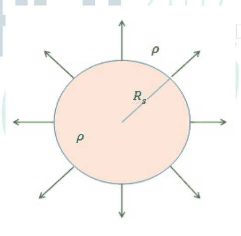
For a simple model of our universe, let us consider an expanding uniform-density sphere embedded in a medium of a much larger sphere with the same density. Let say at some time, the radius of the smaller sphere is \(R_s\). To express the expansion of the sphere, the time dependency of the radius \(R(t)\) can be expressed by scale factor \(a(t)\), that is \(R(t)=a(t)R_s\).
Using Newton’s law of gravity to evaluate velocity of a mass element on the sphere boundary according the model of our universe, one can obtain a set of Friedmann equations:
\[ \left(\frac{\dot a}{a}\right)^2 =A_1\rho(t)-\frac{kc^2}{R_s^2a^2(t)} \tag{1} \]
where \(k\) a dimensionless constant, and \(c\) is velocity of light.
| Part | Question | Points |
|---|---|---|
| A.1 | Determine the constant \(A_1\) in the equation (1) | 1.3 pt. |
The discussion so far is non-relativistic. But in fact, it can be extended to a relativistic system by reinterpreting \(\rho(t)c^2\) as total energy density (excluding the gravitational potential energy). In this relativistic system derives the 2nd Friedmann equation:
\[ \dot\rho+A_2\left(\rho+\left(\frac{p}{c^2}\right)\right)\frac{\dot a}{a}=0 \tag{2} \]
using the 1st law thermodynamics of an adiabatic system, where \(p\) denotes the pressure on the sphere.
| Part | Question | Points |
|---|---|---|
| A.2 | Determine the constants \(A_2\) in the equation (2) | 0.9 pt. |
To solve Eqs. (1) and (2), one should assume a relation \(p=p(\rho)\), such as \(p(t)/c^2=w\rho(t)\), where \(w\) is a constant. There is also a factor \(H=\dot a/a\) being called Hubble parameter. The present values of parameters are usually symbolized by subscript 0 such as \(t_0,\rho_0,H_0,a_0\) and so on. For simplicity, we take \(a_0=1\).
Universe is believed to start from a big explosion called Big-Bang that produces radiation of relativistic particles. During its expansion, the universe is cooling down and the particles in it become non-relativistic. However, the recent observations clarify that the present universe is dominated by cosmological constant energy density. For the case of photon, as the universe is expanding, the photon’s wavelength expands proportionally to the scale factor.
| Part | Question | Points |
|---|---|---|
| A.3 | For each of the following three cases determine the resulting value of \(w\): (i) a universe filled only with radiation (i.e. photon energy), (ii) a universe filled only with non-relativistic matter and (iii) a universe with constant energy density. | 1.2 pt. |
| A.4 | In the case of \(k=0\), find \(a(t)\) for each case of (i) to (iii) being mentioned in A.3. Use the initial condition \(a(t=0)=0\) for case (i) and (ii), and use the condition \(a_0=1\) for case (iii). | 1.2 pt. |
Constant \(k\) in Eq. (1) refers to classification of spatial geometry of the universe. Its value can be \(k=+1\) for positive-curvature universe (closed), \(k=0\) for flat universe (infinite), and \(k=-1\) for negative-curvature universe (open, infinite). Let define a density ratio \(\Omega=\rho/\rho_c\), where \(\rho_cc^2=H^2/A_1\) is critical energy density. Note that \(A_1\) is obtained from problem A.1.
| Part | Question | Points |
|---|---|---|
| A.5 | Express \(k\) in Eq.(1) in terms of \(\Omega\), \(H\), \(a\) and \(R_0\). | 0.1 pt. |
| A.6 | Find a range for \(\Omega\) that corresponds to each value of \(k=+1\), \(k=0\) and \(k=-1\). | 0.3 pt. |
B. Motivation To Introduce Inflation Phase and Its General Conditions
The observation of cosmic microwave background radiation (CMB) suggests that our present universe is approximately flat. The problem is that if this is true the present universe should start from exactly flat early universe, otherwise any deviation from the flatness will eventually grow over time and spoil the present flatness.
| Part | Question | Points |
|---|---|---|
| B.1 | Find \((\Omega(t)-1)\) as a function of time for the universe when it is dominated by radiation or non-relativistic matter (see problem A.3). | 0.5 pt. |
To solve the problem, at some early time in its history, the universe should undergo a constant energy density domination period which leads to an exponential expansion so called inflation period.
| Part | Question | Points |
|---|---|---|
| B.2 | For this constant energy density domination period, find \((\Omega(t)-1)\) as a function of time. Assume that \((\Omega(t)-1)\ll1\). | 0.3 pt. |
| B.3 | Show that condition for inflation implies several following conditions: negative pressure, accelerated expansion \((\ddot a>0)\), and decreasing Hubble radius \((d(aH)^{-1}/dt<0)\). | 0.9 pt. |
| B.4 | Show that the condition of decreasing Hubble radius can be expressed in terms of parameter \(\epsilon=-\dot H/H^2\) as \(\epsilon<1\). | 0.2 pt. |
Inflation occurs as long as \(\epsilon<1\) and then ends when \(\epsilon=1\). We can define e-folding number \(N\), such that \(dN=d\ln a=Hdt\) and \(N=0\) at the end of inflation.
C. Inflation Generated by Homogenously Distributed Matter
As an example of simple physical system that can generate period of inflation is a universe dominated by homogenously distributed matter. This kind of matter is called inflaton and can be characterized by a function \(\phi(t)\).
The dynamical equation of the matter can be expressed as
\[ \ddot\phi+3H\dot\phi=-V', \tag{3} \]
where \(V=V(\phi)\) is a potential function and \(V'=\frac{\partial V}{\partial\phi}\). The Hubble parameter satisfies
\[ H^2=\frac{1}{3M_{pl}^2}\left[\frac12\dot\phi^2+V\right]. \tag{4} \]
with \(M_{pl}\) is a constant called the reduced Planck mass. Inflation phase occurs during domination of potential energy \(V\) over kinetic energy \(\dot\phi^2/2\) for sufficient time such that \(\ddot\phi\) term in equation (3) can be neglected. This condition is called slow-roll approximation.
The quantities \(\epsilon\) and \(\eta_V=\delta+\epsilon\), where \(\delta=-\ddot\phi/(H\dot\phi)\), are called ‘slow-roll’ parameters.
| Part | Question | Points |
|---|---|---|
| C.1 | Estimate parameter \(\epsilon\), parameter \(\eta_V\), \(dN/d\phi\) in terms of potential \(V(\phi)\) and its first and second derivative (\(V'\) and \(V''\)). | 1.7 pt. |
D. Inflation with A Simple Potential
Predictions of any inflation model should be compared to observational constraints from CMB as follow \(n_s=0.968\pm0.006\) and \(r<0.12\), where \(r=16\epsilon\) and \(n_s=1+2\eta_V-6\epsilon\) are evaluated at \(\phi=\phi_{start}\) for inflation model being generated by a dominant matter. Assume that potential of matter takes a simple form \(V(\phi)=\Lambda^4\left(\frac{\phi}{M_{pl}}\right)^n\) where \(n\) is any integer and \(\Lambda\) is a constant.
| Part | Question | Points |
|---|---|---|
| D.1 | Calculate \(\phi_{end}\) at the end of inflation. | 0.5 pt. |
| D.2 | Express \(r\) and \(n_s\) in terms of e-folding number \(N\) and integer \(n\). Estimate the value of \(n\) that is closest to observational values \(r\) and \(n_s\). Take \(N=60\) in your calculation. | 0.9 pt. |
Official English text of the problem.
Answers
The results below use the dimensionally consistent critical density \(\rho_c=H^2/A_1\). Write \(\Delta=\Omega-1\). For D.2, let \(\mathcal N=\ln(a_{\mathrm{end}}/a_{\mathrm{start}})=-N_{\mathrm{start}}>0\); the requested 60 e-folds means \(\mathcal N=60\).
-
A.1: \(\displaystyle \boxed{A_1=\frac{8\pi G}{3}}\).
-
A.2: \(\boxed{A_2=3}\).
-
A.3: \(\boxed{w_{\mathrm{radiation}}=\tfrac13,\quad w_{\mathrm{matter}}=0,\quad w_{\mathrm{constant\ density}}=-1}\).
-
A.4: On the expanding branch, \[ \boxed{ \begin{aligned} \text{(i)}\quad a(t)&=(2H_0t)^{1/2}=(t/t_0)^{1/2},\\ \text{(ii)}\quad a(t)&=\left(\tfrac32H_0t\right)^{2/3}=(t/t_0)^{2/3},\\ \text{(iii)}\quad a(t)&=e^{H_0(t-t_0)}. \end{aligned}} \] Here \(H_0^2=8\pi G\rho_0/3\), with \(H_0t_0=1/2\) in (i) and \(2/3\) in (ii).
-
A.5: \(\displaystyle \boxed{k=(\Omega-1)\left(\frac{aHR_0}{c}\right)^2}\).
-
A.6: \(\boxed{k=+1:\Omega>1;\quad k=0:\Omega=1;\quad k=-1:\Omega<1}\). For nonnegative density, the last range is \(0\leq\Omega<1\).
-
B.1: To leading order near flatness, relative to a reference time \(t_*\), \[ \boxed{ \Delta(t)\simeq \begin{cases} \Delta_*(t/t_*),&\text{radiation},\\ \Delta_*(t/t_*)^{2/3},&\text{non-relativistic matter}. \end{cases}} \]
-
B.2: With \(H_\Lambda=\sqrt{8\pi G\rho_\Lambda/3}\), \[ \boxed{\Delta(t)\simeq\Delta_i e^{-2H_\Lambda(t-t_i)}}. \]
-
B.3: Constant density gives \[ \boxed{p=-\rho c^2<0,\qquad \frac{\ddot a}{a}=\frac{8\pi G\rho}{3}>0,\qquad \frac{d}{dt}(aH)^{-1}<0.} \] More generally, accelerated expansion requires \(p<-\rho c^2/3\).
-
B.4: \[ \boxed{\frac{d}{dt}(aH)^{-1}=\frac{\epsilon-1}{a}<0 \quad\Longleftrightarrow\quad \epsilon<1.} \]
-
C.1: In the slow-roll approximation, \[ \boxed{ \epsilon\simeq\frac{M_{pl}^2}{2}\left(\frac{V'}{V}\right)^2,\qquad \eta_V\simeq M_{pl}^2\frac{V''}{V},\qquad \frac{dN}{d\phi}\simeq-\frac{V}{M_{pl}^2V'}.} \]
-
D.1: For \(n>0\), on the positive-field branch, \[ \boxed{\phi_{\mathrm{end}}\simeq\frac{n}{\sqrt2}M_{pl}}. \] The formal threshold is \(\lvert\phi\rvert\simeq |n|M_{pl}/\sqrt2\). Nonpositive \(n\) does not give the assumed end of slow-roll inflation in this model.
-
D.2: \[ \boxed{ r\simeq\frac{16n}{4\mathcal N+n},\qquad n_s\simeq1-\frac{2(n+2)}{4\mathcal N+n}.} \] Equivalently, the denominators are \(n-4N_{\mathrm{start}}\) in the statement’s signed convention. At \(\mathcal N=60\), \[ \begin{array}{c|cc} n&r&n_s\\ \hline 1&0.0664&0.9751\\ 2&0.1322&0.9669 \end{array} \] If \(r<0.12\) is enforced, \(n=1\) is the closest positive-integer choice. No positive integer satisfies both quoted observational bounds.
Solution
A.1
Consider a mass element on the boundary of a comoving sphere of radius \(R=aR_s\). By Newton’s shell theorem, its acceleration depends only on the enclosed mass, \[ M=\frac{4\pi}{3}\rho R^3. \] In the non-relativistic model, this enclosed mass is constant. Newton’s equation is \[ \ddot R=-\frac{GM}{R^2}. \] Multiplying by \(\dot R\) and integrating gives the conserved specific mechanical energy \[ \frac12\dot R^2-\frac{GM}{R}=\mathcal E. \] Therefore \[ \left(\frac{\dot R}{R}\right)^2 =\frac{2GM}{R^3}+\frac{2\mathcal E}{R^2} =\frac{8\pi G}{3}\rho+\frac{2\mathcal E}{a^2R_s^2}. \] Since \(\dot R/R=\dot a/a\), comparison with (1), identifying \(2\mathcal E=-kc^2\), yields \[ \boxed{A_1=\frac{8\pi G}{3}}. \]
A.2
Let the physical volume of the sphere be \[ \mathcal V=\frac{4\pi}{3}(aR_s)^3. \] Its total internal energy is \(U=\rho c^2\mathcal V\). The first law for an adiabatic system gives \[ dU=-p\,d\mathcal V. \] Thus \[ c^2\mathcal V\,d\rho+(\rho c^2+p)\,d\mathcal V=0. \] Using \(\dot{\mathcal V}/\mathcal V=3\dot a/a\), \[ \dot\rho+3\left(\rho+\frac{p}{c^2}\right)\frac{\dot a}{a}=0. \] Hence \[ \boxed{A_2=3}. \]
A.3
For constant \(w\), the continuity equation becomes \[ \frac{\dot\rho}{\rho}=-3(1+w)\frac{\dot a}{a}, \] so, using \(a_0=1\), \[ \boxed{\rho=\rho_0a^{-3(1+w)}}. \]
For radiation, the photon number density decreases as \(a^{-3}\). Each photon has energy \(hc/\lambda\), and the given wavelength scaling \(\lambda\propto a\) makes its energy proportional to \(a^{-1}\). Therefore \[ \rho c^2\propto a^{-4}, \] which gives \[ 3(1+w)=4,\qquad \boxed{w=\frac13}. \]
For non-relativistic matter, the energy is dominated by approximately constant rest energy per particle. The number density decreases as \(a^{-3}\), giving \[ \rho\propto a^{-3},\qquad \boxed{w=0}. \] This is the pressureless-matter approximation.
For constant energy density, \(\dot\rho=0\). In an expanding universe, the continuity equation requires \[ \rho+\frac{p}{c^2}=0, \] and hence \[ \boxed{w=-1}. \]
A.4
For \(k=0\), \[ H^2=\frac{8\pi G}{3}\rho =H_0^2a^{-3(1+w)}. \] Choosing the expanding branch, \[ \dot a=H_0a^{1-\frac32(1+w)}. \]
For \(w\neq-1\), integration with \(a(0)=0\) gives \[ a^{\frac32(1+w)} =\frac32(1+w)H_0t. \]
Consequently, for radiation, \[ \boxed{a(t)=(2H_0t)^{1/2}}. \] The normalization \(a(t_0)=1\) implies \(2H_0t_0=1\), so \[ a(t)=\left(\frac{t}{t_0}\right)^{1/2}. \]
For non-relativistic matter, \[ \boxed{a(t)=\left(\frac32H_0t\right)^{2/3}}. \] Here \(3H_0t_0/2=1\), giving \[ a(t)=\left(\frac{t}{t_0}\right)^{2/3}. \]
For constant energy density, \(H=H_0\) is constant. Integrating \(\dot a/a=H_0\) and imposing \(a(t_0)=1\), \[ \boxed{a(t)=e^{H_0(t-t_0)}}. \]
A.5
Setting \(k=0\) in (1) determines the critical mass-equivalent density: \[ \rho_c=\frac{H^2}{A_1}=\frac{3H^2}{8\pi G}. \] Thus the printed definition \(\rho_cc^2=H^2/A_1\) is dimensionally inconsistent. The corresponding critical energy density is \[ \rho_cc^2=\frac{H^2c^2}{A_1}. \]
Using the consistent definition, \[ \Omega=\frac{A_1\rho}{H^2}. \] Divide (1) by \(H^2\): \[ 1=\Omega-\frac{kc^2}{a^2R_s^2H^2}. \] Since \(a_0=1\), the present radius is \(R_0=R_s\). Therefore \[ \boxed{k=(\Omega-1)\frac{a^2H^2R_0^2}{c^2}}. \]
A.6
The factor multiplying \(\Omega-1\) in A.5 is positive. Hence \(k\) and \(\Omega-1\) have the same sign:
| Spatial curvature | Density ratio |
|---|---|
| \(k=+1\), closed | \(\Omega>1\) |
| \(k=0\), flat | \(\Omega=1\) |
| \(k=-1\), open | \(\Omega<1\) |
With nonnegative energy density, the open-universe range is \(0\leq\Omega<1\).
B.1
From A.5, \[ \Delta(t)\equiv\Omega(t)-1 =\frac{kc^2}{R_0^2a^2H^2} =\frac{kc^2}{R_0^2\dot a^2}. \] This identity is exact.
To study a small departure from flatness, evaluate \(\dot a\) using the flat-universe solutions of A.4 to leading order. If \[ a\propto t^\alpha, \] then \[ \dot a^2\propto t^{2\alpha-2}, \qquad \Delta\propto t^{2-2\alpha}. \]
During radiation domination, \(\alpha=1/2\), so \[ \boxed{\Delta(t)\simeq\Delta_*\frac{t}{t_*}}. \]
During matter domination, \(\alpha=2/3\), so \[ \boxed{\Delta(t)\simeq\Delta_*\left(\frac{t}{t_*}\right)^{2/3}}. \]
Thus the magnitude of any small, nonzero departure from flatness grows during either era. These power laws apply while curvature remains a small correction to the expansion.
B.2
Let the constant density be \(\rho_\Lambda\), and define \[ H_\Lambda^2=\frac{8\pi G}{3}\rho_\Lambda. \] For \(|\Omega-1|\ll1\), the curvature contribution to (1) is small, so \[ H\simeq H_\Lambda,\qquad a(t)\simeq a_i e^{H_\Lambda(t-t_i)}. \] Substitution into \[ \Delta=\frac{kc^2}{R_0^2a^2H^2} \] gives \[ \boxed{\Delta(t)\simeq\Delta_i e^{-2H_\Lambda(t-t_i)}}. \] Inflation therefore suppresses departures from flatness exponentially.
B.3
Differentiate (1), and use the continuity equation: \[ 2H\dot H =A_1\dot\rho+\frac{2kc^2H}{R_0^2a^2}, \] so \[ \dot H =-\frac{3A_1}{2}\left(\rho+\frac{p}{c^2}\right) +\frac{kc^2}{R_0^2a^2}. \] Adding \(H^2\) from (1) eliminates the curvature term: \[ \frac{\ddot a}{a} =\dot H+H^2 =-\frac{A_1}{2}\left(\rho+\frac{3p}{c^2}\right). \] Using A.1, \[ \boxed{\frac{\ddot a}{a} =-\frac{4\pi G}{3}\left(\rho+\frac{3p}{c^2}\right)}. \]
For positive density, accelerated expansion requires \[ \boxed{p<-\frac13\rho c^2}, \] which in particular requires negative pressure.
For the constant-density period considered here, A.3 gives \(p=-\rho c^2\). Hence \[ \frac{\ddot a}{a}=\frac{8\pi G}{3}\rho>0. \]
Finally, \(aH=\dot a\), so \[ \frac{d}{dt}(aH)^{-1} =\frac{d}{dt}\frac1{\dot a} =-\frac{\ddot a}{\dot a^2}<0. \] This proves all three requested properties.
The radius appearing in this condition is the comoving Hubble radius, \(c/(aH)\); the constant \(c\) does not affect the derivative’s sign.
B.4
Direct differentiation gives \[ \frac{d}{dt}(aH)^{-1} =-\frac{\dot aH+a\dot H}{a^2H^2} =-\frac1a\left(1+\frac{\dot H}{H^2}\right). \] Since \(\epsilon=-\dot H/H^2\), \[ \boxed{\frac{d}{dt}(aH)^{-1}=\frac{\epsilon-1}{a}}. \] Because \(a>0\), the radius decreases exactly when \[ \boxed{\epsilon<1}. \] Equivalently, \[ \frac{\ddot a}{a}=H^2(1-\epsilon). \]
C.1
First differentiate (4): \[ 2H\dot H =\frac{1}{3M_{pl}^2} \left(\dot\phi\,\ddot\phi+V'\dot\phi\right). \] Equation (3) gives \(\ddot\phi+V'=-3H\dot\phi\), so \[ 2H\dot H=-\frac{H\dot\phi^2}{M_{pl}^2}. \] Thus \[ \boxed{\dot H=-\frac{\dot\phi^2}{2M_{pl}^2}}, \qquad \epsilon=\frac{\dot\phi^2}{2M_{pl}^2H^2}. \]
The slow-roll assumptions give \[ H^2\simeq\frac{V}{3M_{pl}^2}, \qquad 3H\dot\phi\simeq-V'. \] Substituting these into \(\epsilon\), \[ \epsilon \simeq\frac{V'^2}{18M_{pl}^2H^4} =\boxed{\frac{M_{pl}^2}{2}\left(\frac{V'}{V}\right)^2}. \]
To obtain \(\eta_V\), differentiate the slow-roll field equation: \[ 3\dot H\dot\phi+3H\ddot\phi\simeq-V''\dot\phi. \] Dividing by \(3H^2\dot\phi\), \[ \frac{\dot H}{H^2}+\frac{\ddot\phi}{H\dot\phi} \simeq-\frac{V''}{3H^2}. \] The left side is \(-\epsilon-\delta\). Therefore \[ \eta_V=\delta+\epsilon \simeq\frac{V''}{3H^2} =\boxed{M_{pl}^2\frac{V''}{V}}. \]
Finally, using the statement’s definition \(dN=Hdt\), \[ \frac{dN}{d\phi} =\frac{H}{\dot\phi} \simeq-\frac{3H^2}{V'} =\boxed{-\frac{V}{M_{pl}^2V'}}. \] This expression applies along a rolling, monotonic field trajectory.
D.1
For \[ V(\phi)=\Lambda^4\left(\frac{\phi}{M_{pl}}\right)^n, \] the derivative ratios are \[ \frac{V'}{V}=\frac n\phi, \qquad \frac{V''}{V}=\frac{n(n-1)}{\phi^2}. \] Consequently, \[ \epsilon\simeq\frac{n^2M_{pl}^2}{2\phi^2}. \] Extrapolating this slow-roll expression to the end condition \(\epsilon=1\) gives \[ |\phi_{\mathrm{end}}|\simeq\frac{|n|}{\sqrt2}M_{pl}. \]
For \(n>0\), take the positive-field branch. The field rolls toward smaller \(\phi\), so \(\epsilon\) increases and reaches unity at \[ \boxed{\phi_{\mathrm{end}}\simeq\frac n{\sqrt2}M_{pl}}. \] The field has the same units as \(M_{pl}\).
The statement permits any integer \(n\), but the assumed exit restricts the relevant cases:
- For \(n=0\), the potential is constant and \(\epsilon\simeq0\); this model provides no slow-roll exit.
- For \(n<0\) and \(\phi>0\), \(V'<0\), so \(\dot\phi\simeq-V'/(3H)>0\). Thus \(\epsilon\propto\phi^{-2}\) decreases. The formal \(\epsilon=1\) threshold is an entry into inflation.
The end-field result is an estimate because slow roll ceases to be a controlled approximation as \(\epsilon\) approaches unity.
D.2
For the monomial potential, C.1 gives \[ \frac{dN}{d\phi}\simeq-\frac{\phi}{nM_{pl}^2}. \] Integrating from the end of inflation, where \(N=0\), \[ N(\phi)\simeq-\frac{\phi^2-\phi_{\mathrm{end}}^2}{2nM_{pl}^2}. \]
For \(n>0\), the initial field is larger than the final field, so the statement’s \(N_{\mathrm{start}}\) is negative. Define the positive duration \[ \mathcal N\equiv-N_{\mathrm{start}} =\ln\frac{a_{\mathrm{end}}}{a_{\mathrm{start}}}. \] Then \[ \phi_{\mathrm{start}}^2 \simeq\phi_{\mathrm{end}}^2+2nM_{pl}^2\mathcal N =\frac n2(4\mathcal N+n)M_{pl}^2. \]
The slow-roll parameters at the start are therefore \[ \epsilon_{\mathrm{start}} \simeq\frac{n}{4\mathcal N+n}, \qquad \eta_{V,\mathrm{start}} \simeq\frac{2(n-1)}{4\mathcal N+n}. \] Thus \[ \boxed{r\simeq\frac{16n}{4\mathcal N+n}} \] and \[ \boxed{ n_s\simeq 1+\frac{4(n-1)-6n}{4\mathcal N+n} =1-\frac{2(n+2)}{4\mathcal N+n}}. \]
In the statement’s signed convention these become \[ r\simeq\frac{16n}{n-4N_{\mathrm{start}}}, \qquad n_s\simeq1-\frac{2(n+2)}{n-4N_{\mathrm{start}}}. \] For \(\mathcal N\gg n\), the familiar leading forms are \[ r\simeq\frac{4n}{\mathcal N}, \qquad n_s\simeq1-\frac{n+2}{2\mathcal N}. \]
Interpreting the requested \(N=60\) as a positive duration \(\mathcal N=60\), the tensor bound gives \[ \frac{16n}{240+n}<0.12 \quad\Longrightarrow\quad n<\frac{28.8}{15.88}\simeq1.814. \] Therefore the only positive integer satisfying this bound is \(n=1\).
The numerical predictions, all dimensionless, are:
| \(n\) | \(r\) | \(n_s\) | Comparison with the stated constraints |
|---|---|---|---|
| 1 | 0.0664 | 0.9751 | Satisfies \(r<0.12\); \(n_s\) is slightly above \(0.974\) |
| 2 | 0.1322 | 0.9669 | Satisfies the quoted \(n_s\) interval; exceeds the \(r\) bound |
| 3 | 0.1975 | 0.9588 | Outside both quoted bounds |
Hence \[ \boxed{n=1\quad\text{if the tensor upper bound is enforced}.} \] Its predicted spectral index is about \(0.0011\) above the upper edge of the quoted interval. The integer \(n=2\) is closer to the central spectral index, but violates the tensor bound. No positive integer satisfies both quoted bounds simultaneously.
The solution was checked against the official solution. Where this solution differs from the official solution, the official solution contains an error or a misprint.
IPhO 2017 · Theorieaufgabe 3
Kosmische Inflation
Aufgrund der von der Erde aus beobachteten Relativbewegung der Galaxien weichen die Wellenlängen im sichtbaren Spektrum einer bestimmten Galaxie von ihren ursprünglichen Wellenlängen ab; dies ist als elektromagnetischer Dopplereffekt bekannt. Für eine Ansammlung von Galaxien würde man eine zufällige Verteilung der Wellenlängenverschiebungen erwarten: einige positiv (Rotverschiebung) und einige negativ (Blauverschiebung). Beobachtungen zeigen jedoch, dass alle Galaxien mit Ausnahme einer nahe gelegenen Gruppe rotverschoben sind. Dies muss auch dann gelten, wenn die Beobachtung von einem anderen Punkt im Universum aus erfolgt. Daraus folgt, dass sich unser Universum ausdehnen muss. Andererseits können lokale Unregelmäßigkeiten des Universums auf Skalen von mehr als 100 Mpc vernachlässigt werden, wobei 1 pc = 3.26 Lichtjahre ist. Über große Skalen gemittelt wird die klumpige Verteilung der Galaxien zunehmend isotrop (richtungsunabhängig) und homogen (ortsunabhängig). Daher können wir das Universum als sich ausdehnende Materie mit einer einheitlichen Massendichte \(\rho\) auffassen.
A. Expansion des Universums
Als einfaches Modell unseres Universums betrachten wir eine expandierende Kugel mit homogener Dichte, die in das Medium einer viel größeren Kugel gleicher Dichte eingebettet ist. Zu einem bestimmten Zeitpunkt sei der Radius der kleineren Kugel \(R_s\). Zur Beschreibung der Expansion der Kugel kann die Zeitabhängigkeit des Radius \(R(t)\) durch den Skalenfaktor \(a(t)\) ausgedrückt werden, also \(R(t)=a(t)R_s\).
Wendet man das Newtonsche Gravitationsgesetz an, um gemäß unserem Modell des Universums die Geschwindigkeit eines Massenelements auf der Kugeloberfläche zu bestimmen, erhält man einen Satz von Friedmann-Gleichungen:
\[ \left(\frac{\dot a}{a}\right)^2 =A_1\rho(t)-\frac{kc^2}{R_s^2a^2(t)} \tag{1} \]
wobei \(k\) eine dimensionslose Konstante und \(c\) die Lichtgeschwindigkeit ist.
| Teil | Frage | Punkte |
|---|---|---|
| A.1 | Bestimmen Sie die Konstante \(A_1\) in Gleichung (1). | 1.3 Pkt. |
Die bisherige Betrachtung ist nichtrelativistisch. Sie lässt sich jedoch auf ein relativistisches System erweitern, indem \(\rho(t)c^2\) als gesamte Energiedichte (ohne die potenzielle Gravitationsenergie) interpretiert wird. In diesem relativistischen System ergibt sich die zweite Friedmann-Gleichung:
\[ \dot\rho+A_2\left(\rho+\left(\frac{p}{c^2}\right)\right)\frac{\dot a}{a}=0 \tag{2} \]
unter Verwendung des ersten Hauptsatzes der Thermodynamik für ein adiabatisches System, wobei \(p\) den auf die Kugel wirkenden Druck bezeichnet.
| Teil | Frage | Punkte |
|---|---|---|
| A.2 | Bestimmen Sie die Konstante \(A_2\) in Gleichung (2). | 0.9 Pkt. |
Um die Gleichungen (1) und (2) zu lösen, muss man eine Beziehung \(p=p(\rho)\) annehmen, beispielsweise \(p(t)/c^2=w\rho(t)\), wobei \(w\) eine Konstante ist. Außerdem gibt es die Größe \(H=\dot a/a\), die als Hubble-Parameter bezeichnet wird. Die heutigen Werte der Parameter werden üblicherweise mit dem Index 0 gekennzeichnet, etwa \(t_0,\rho_0,H_0,a_0\) und so weiter. Der Einfachheit halber setzen wir \(a_0=1\).
Man geht davon aus, dass das Universum mit einer gewaltigen Explosion, dem Urknall, begann, bei der Strahlung aus relativistischen Teilchen entstand. Während seiner Expansion kühlt das Universum ab, und die darin enthaltenen Teilchen werden nichtrelativistisch. Neuere Beobachtungen zeigen jedoch, dass das heutige Universum von der Energiedichte der kosmologischen Konstante dominiert wird. Bei Photonen wächst die Wellenlänge während der Expansion des Universums proportional zum Skalenfaktor.
| Teil | Frage | Punkte |
|---|---|---|
| A.3 | Bestimmen Sie für jeden der folgenden drei Fälle den resultierenden Wert von \(w\): (i) ein Universum, das ausschließlich mit Strahlung (d. h. Photonenenergie) gefüllt ist, (ii) ein Universum, das ausschließlich mit nichtrelativistischer Materie gefüllt ist, und (iii) ein Universum mit konstanter Energiedichte. | 1.2 Pkt. |
| A.4 | Bestimmen Sie für \(k=0\) die Funktion \(a(t)\) für jeden der in A.3 genannten Fälle (i) bis (iii). Verwenden Sie für die Fälle (i) und (ii) die Anfangsbedingung \(a(t=0)=0\) und für Fall (iii) die Bedingung \(a_0=1\). | 1.2 Pkt. |
Die Konstante \(k\) in Gl. (1) dient der Klassifizierung der räumlichen Geometrie des Universums. Ihr Wert kann \(k=+1\) für ein Universum mit positiver Krümmung (geschlossen), \(k=0\) für ein flaches Universum (unendlich) und \(k=-1\) für ein Universum mit negativer Krümmung (offen, unendlich) sein. Wir definieren das Dichteverhältnis \(\Omega=\rho/\rho_c\), wobei \(\rho_cc^2=H^2/A_1\) die kritische Energiedichte ist. Beachten Sie, dass \(A_1\) aus Aufgabe A.1 bekannt ist.
| Teil | Frage | Punkte |
|---|---|---|
| A.5 | Drücken Sie \(k\) in Gl. (1) durch \(\Omega\), \(H\), \(a\) und \(R_0\) aus. | 0.1 Pkt. |
| A.6 | Bestimmen Sie jeweils den Wertebereich von \(\Omega\), der den Werten \(k=+1\), \(k=0\) und \(k=-1\) entspricht. | 0.3 Pkt. |
B. Motivation für die Einführung einer Inflationsphase und ihre allgemeinen Bedingungen
Die Beobachtung der kosmischen Mikrowellenhintergrundstrahlung (CMB) legt nahe, dass unser heutiges Universum annähernd flach ist. Das Problem besteht darin, dass in diesem Fall das heutige Universum aus einem exakt flachen frühen Universum hervorgegangen sein müsste; andernfalls würde jede Abweichung von der Flachheit im Laufe der Zeit anwachsen und die heutige Flachheit zunichtemachen.
| Teil | Frage | Punkte |
|---|---|---|
| B.1 | Bestimmen Sie \((\Omega(t)-1)\) als Funktion der Zeit für ein Universum, das von Strahlung oder nichtrelativistischer Materie dominiert wird (siehe Aufgabe A.3). | 0.5 Pkt. |
Zur Lösung dieses Problems sollte das Universum zu einem frühen Zeitpunkt seiner Geschichte eine Phase durchlaufen haben, in der eine konstante Energiedichte dominiert. Diese führt zu einer exponentiellen Expansion, der sogenannten Inflationsphase.
| Teil | Frage | Punkte |
|---|---|---|
| B.2 | Bestimmen Sie für diese Phase, in der eine konstante Energiedichte dominiert, \((\Omega(t)-1)\) als Funktion der Zeit. Nehmen Sie an, dass \((\Omega(t)-1)\ll1\). | 0.3 Pkt. |
| B.3 | Zeigen Sie, dass die Inflationsbedingung die folgenden Bedingungen nach sich zieht: negativer Druck, beschleunigte Expansion \((\ddot a>0)\) und abnehmender Hubble-Radius \((d(aH)^{-1}/dt<0)\). | 0.9 Pkt. |
| B.4 | Zeigen Sie, dass sich die Bedingung eines abnehmenden Hubble-Radius mithilfe des Parameters \(\epsilon=-\dot H/H^2\) als \(\epsilon<1\) ausdrücken lässt. | 0.2 Pkt. |
Inflation findet statt, solange \(\epsilon<1\), und endet, wenn \(\epsilon=1\). Wir können die Anzahl der e-Faltungen \(N\) definieren, sodass \(dN=d\ln a=Hdt\) gilt und \(N=0\) am Ende der Inflation ist.
C. Durch homogen verteilte Materie erzeugte Inflation
Ein Beispiel für ein einfaches physikalisches System, das eine Inflationsphase erzeugen kann, ist ein Universum, das von homogen verteilter Materie dominiert wird. Diese Art von Materie wird Inflaton genannt und lässt sich durch eine Funktion \(\phi(t)\) charakterisieren.
Die Bewegungsgleichung der Materie lässt sich schreiben als
\[ \ddot\phi+3H\dot\phi=-V', \tag{3} \]
wobei \(V=V(\phi)\) eine Potenzialfunktion und \(V'=\frac{\partial V}{\partial\phi}\) ist. Der Hubble-Parameter erfüllt
\[ H^2=\frac{1}{3M_{pl}^2}\left[\frac12\dot\phi^2+V\right]. \tag{4} \]
Dabei ist \(M_{pl}\) eine Konstante, die als reduzierte Planck-Masse bezeichnet wird. Die Inflationsphase tritt auf, wenn die potenzielle Energie \(V\) hinreichend lange gegenüber der kinetischen Energie \(\dot\phi^2/2\) dominiert, sodass der Term \(\ddot\phi\) in Gleichung (3) vernachlässigt werden kann. Diese Bedingung wird als Slow-Roll-Näherung bezeichnet.
Die Größen \(\epsilon\) und \(\eta_V=\delta+\epsilon\), wobei \(\delta=-\ddot\phi/(H\dot\phi)\), heißen „Slow-Roll-Parameter“.
| Teil | Frage | Punkte |
|---|---|---|
| C.1 | Schätzen Sie den Parameter \(\epsilon\), den Parameter \(\eta_V\) und \(dN/d\phi\) in Abhängigkeit vom Potenzial \(V(\phi)\) und dessen erster und zweiter Ableitung (\(V'\) und \(V''\)) ab. | 1.7 Pkt. |
D. Inflation mit einem einfachen Potenzial
Die Vorhersagen jedes Inflationsmodells sollten mit den folgenden, aus CMB-Beobachtungen abgeleiteten Einschränkungen verglichen werden: \(n_s=0.968\pm0.006\) und \(r<0.12\). Dabei werden \(r=16\epsilon\) und \(n_s=1+2\eta_V-6\epsilon\) für ein durch eine dominierende Materiekomponente erzeugtes Inflationsmodell bei \(\phi=\phi_{start}\) ausgewertet. Nehmen Sie an, dass das Potenzial der Materie die einfache Form \(V(\phi)=\Lambda^4\left(\frac{\phi}{M_{pl}}\right)^n\) hat, wobei \(n\) eine beliebige ganze Zahl und \(\Lambda\) eine Konstante ist.
| Teil | Frage | Punkte |
|---|---|---|
| D.1 | Berechnen Sie \(\phi_{end}\) am Ende der Inflation. | 0.5 Pkt. |
| D.2 | Drücken Sie \(r\) und \(n_s\) durch die Anzahl der e-Faltungen \(N\) und die ganze Zahl \(n\) aus. Schätzen Sie den Wert von \(n\) ab, der den beobachteten Werten von \(r\) und \(n_s\) am nächsten kommt. Verwenden Sie in Ihrer Rechnung \(N=60\). | 0.9 Pkt. |
Aufgabentext aus dem offiziellen englischen Text übersetzt.
Antworten
Die folgenden Ergebnisse verwenden die dimensionskonsistente kritische Dichte \(\rho_c=H^2/A_1\). Wir schreiben \(\Delta=\Omega-1\). Für D.2 sei \(\mathcal N=\ln(a_{\mathrm{end}}/a_{\mathrm{start}})=-N_{\mathrm{start}}>0\); die geforderten 60 e-Faltungen bedeuten \(\mathcal N=60\).
-
A.1: \(\displaystyle \boxed{A_1=\frac{8\pi G}{3}}\).
-
A.2: \(\boxed{A_2=3}\).
-
A.3: \(\boxed{w_{\mathrm{radiation}}=\tfrac13,\quad w_{\mathrm{matter}}=0,\quad w_{\mathrm{constant\ density}}=-1}\).
-
A.4: Auf dem expandierenden Lösungszweig gilt \[ \boxed{ \begin{aligned} \text{(i)}\quad a(t)&=(2H_0t)^{1/2}=(t/t_0)^{1/2},\\ \text{(ii)}\quad a(t)&=\left(\tfrac32H_0t\right)^{2/3}=(t/t_0)^{2/3},\\ \text{(iii)}\quad a(t)&=e^{H_0(t-t_0)}. \end{aligned}} \] Hier ist \(H_0^2=8\pi G\rho_0/3\), mit \(H_0t_0=1/2\) in (i) und \(2/3\) in (ii).
-
A.5: \(\displaystyle \boxed{k=(\Omega-1)\left(\frac{aHR_0}{c}\right)^2}\).
-
A.6: \(\boxed{k=+1:\Omega>1;\quad k=0:\Omega=1;\quad k=-1:\Omega<1}\). Für nichtnegative Dichte lautet der letzte Wertebereich \(0\leq\Omega<1\).
-
B.1: In führender Ordnung nahe der Flachheit gilt, bezogen auf einen Referenzzeitpunkt \(t_*\), \[ \boxed{ \Delta(t)\simeq \begin{cases} \Delta_*(t/t_*),&\text{Strahlung},\\ \Delta_*(t/t_*)^{2/3},&\text{nichtrelativistische Materie}. \end{cases}} \]
-
B.2: Mit \(H_\Lambda=\sqrt{8\pi G\rho_\Lambda/3}\) gilt \[ \boxed{\Delta(t)\simeq\Delta_i e^{-2H_\Lambda(t-t_i)}}. \]
-
B.3: Konstante Dichte ergibt \[ \boxed{p=-\rho c^2<0,\qquad \frac{\ddot a}{a}=\frac{8\pi G\rho}{3}>0,\qquad \frac{d}{dt}(aH)^{-1}<0.} \] Allgemeiner erfordert beschleunigte Expansion \(p<-\rho c^2/3\).
-
B.4: \[ \boxed{\frac{d}{dt}(aH)^{-1}=\frac{\epsilon-1}{a}<0 \quad\Longleftrightarrow\quad \epsilon<1.} \]
-
C.1: In der Slow-Roll-Näherung gilt \[ \boxed{ \epsilon\simeq\frac{M_{pl}^2}{2}\left(\frac{V'}{V}\right)^2,\qquad \eta_V\simeq M_{pl}^2\frac{V''}{V},\qquad \frac{dN}{d\phi}\simeq-\frac{V}{M_{pl}^2V'}.} \]
-
D.1: Für \(n>0\) gilt auf dem Lösungszweig mit positivem Feld \[ \boxed{\phi_{\mathrm{end}}\simeq\frac{n}{\sqrt2}M_{pl}}. \] Der formale Schwellenwert ist \(\lvert\phi\rvert\simeq |n|M_{pl}/\sqrt2\). Für nichtpositives \(n\) ergibt sich in diesem Modell nicht das angenommene Ende der Slow-Roll-Inflation.
-
D.2: \[ \boxed{ r\simeq\frac{16n}{4\mathcal N+n},\qquad n_s\simeq1-\frac{2(n+2)}{4\mathcal N+n}.} \] In der vorzeichenbehafteten Konvention der Aufgabenstellung lauten die Nenner äquivalent \(n-4N_{\mathrm{start}}\). Für \(\mathcal N=60\) gilt \[ \begin{array}{c|cc} n&r&n_s\\ \hline 1&0.0664&0.9751\\ 2&0.1322&0.9669 \end{array} \] Wenn \(r<0.12\) eingehalten werden muss, ist \(n=1\) die am nächsten liegende positive ganze Zahl. Keine positive ganze Zahl erfüllt beide angegebenen Beobachtungsgrenzen.
Lösung
A.1
Wir betrachten ein Massenelement auf der Oberfläche einer mitbewegten Kugel mit Radius \(R=aR_s\). Nach dem Newtonschen Schalentheorem hängt seine Beschleunigung nur von der eingeschlossenen Masse ab, \[ M=\frac{4\pi}{3}\rho R^3. \] Im nichtrelativistischen Modell ist diese eingeschlossene Masse konstant. Die Newtonsche Bewegungsgleichung lautet \[ \ddot R=-\frac{GM}{R^2}. \] Multiplikation mit \(\dot R\) und Integration liefern die erhaltene spezifische mechanische Energie \[ \frac12\dot R^2-\frac{GM}{R}=\mathcal E. \] Daher gilt \[ \left(\frac{\dot R}{R}\right)^2 =\frac{2GM}{R^3}+\frac{2\mathcal E}{R^2} =\frac{8\pi G}{3}\rho+\frac{2\mathcal E}{a^2R_s^2}. \] Wegen \(\dot R/R=\dot a/a\) ergibt der Vergleich mit (1) unter der Zuordnung \(2\mathcal E=-kc^2\) \[ \boxed{A_1=\frac{8\pi G}{3}}. \]
A.2
Das physikalische Volumen der Kugel sei \[ \mathcal V=\frac{4\pi}{3}(aR_s)^3. \] Ihre gesamte innere Energie ist \(U=\rho c^2\mathcal V\). Der erste Hauptsatz für ein adiabatisches System liefert \[ dU=-p\,d\mathcal V. \] Somit gilt \[ c^2\mathcal V\,d\rho+(\rho c^2+p)\,d\mathcal V=0. \] Mit \(\dot{\mathcal V}/\mathcal V=3\dot a/a\) folgt \[ \dot\rho+3\left(\rho+\frac{p}{c^2}\right)\frac{\dot a}{a}=0. \] Also ist \[ \boxed{A_2=3}. \]
A.3
Für konstantes \(w\) wird die Kontinuitätsgleichung zu \[ \frac{\dot\rho}{\rho}=-3(1+w)\frac{\dot a}{a}, \] sodass mit \(a_0=1\) folgt: \[ \boxed{\rho=\rho_0a^{-3(1+w)}}. \]
Bei Strahlung nimmt die Photonenzahldichte wie \(a^{-3}\) ab. Jedes Photon besitzt die Energie \(hc/\lambda\), und aufgrund der gegebenen Skalierung der Wellenlänge \(\lambda\propto a\) ist seine Energie proportional zu \(a^{-1}\). Daher gilt \[ \rho c^2\propto a^{-4}, \] woraus folgt: \[ 3(1+w)=4,\qquad \boxed{w=\frac13}. \]
Bei nichtrelativistischer Materie wird die Energie von der annähernd konstanten Ruheenergie pro Teilchen dominiert. Die Teilchenzahldichte nimmt wie \(a^{-3}\) ab, sodass \[ \rho\propto a^{-3},\qquad \boxed{w=0}. \] Dies ist die Näherung druckloser Materie.
Für konstante Energiedichte gilt \(\dot\rho=0\). In einem expandierenden Universum erfordert die Kontinuitätsgleichung \[ \rho+\frac{p}{c^2}=0, \] und somit \[ \boxed{w=-1}. \]
A.4
Für \(k=0\) gilt \[ H^2=\frac{8\pi G}{3}\rho =H_0^2a^{-3(1+w)}. \] Wählen wir den expandierenden Lösungszweig, so ist \[ \dot a=H_0a^{1-\frac32(1+w)}. \]
Für \(w\neq-1\) liefert die Integration mit \(a(0)=0\) \[ a^{\frac32(1+w)} =\frac32(1+w)H_0t. \]
Folglich gilt für Strahlung \[ \boxed{a(t)=(2H_0t)^{1/2}}. \] Die Normierung \(a(t_0)=1\) impliziert \(2H_0t_0=1\), also \[ a(t)=\left(\frac{t}{t_0}\right)^{1/2}. \]
Für nichtrelativistische Materie gilt \[ \boxed{a(t)=\left(\frac32H_0t\right)^{2/3}}. \] Hier ist \(3H_0t_0/2=1\), woraus folgt: \[ a(t)=\left(\frac{t}{t_0}\right)^{2/3}. \]
Bei konstanter Energiedichte ist \(H=H_0\) konstant. Integration von \(\dot a/a=H_0\) unter der Bedingung \(a(t_0)=1\) ergibt \[ \boxed{a(t)=e^{H_0(t-t_0)}}. \]
A.5
Setzt man \(k=0\) in (1), erhält man die kritische massenäquivalente Dichte: \[ \rho_c=\frac{H^2}{A_1}=\frac{3H^2}{8\pi G}. \] Die abgedruckte Definition \(\rho_cc^2=H^2/A_1\) ist daher dimensionswidrig. Die entsprechende kritische Energiedichte ist \[ \rho_cc^2=\frac{H^2c^2}{A_1}. \]
Mit der konsistenten Definition gilt \[ \Omega=\frac{A_1\rho}{H^2}. \] Wir dividieren (1) durch \(H^2\): \[ 1=\Omega-\frac{kc^2}{a^2R_s^2H^2}. \] Da \(a_0=1\), ist der heutige Radius \(R_0=R_s\). Daher gilt \[ \boxed{k=(\Omega-1)\frac{a^2H^2R_0^2}{c^2}}. \]
A.6
Der Faktor, mit dem \(\Omega-1\) in A.5 multipliziert wird, ist positiv. Daher haben \(k\) und \(\Omega-1\) dasselbe Vorzeichen:
| Räumliche Krümmung | Dichteverhältnis |
|---|---|
| \(k=+1\), geschlossen | \(\Omega>1\) |
| \(k=0\), flach | \(\Omega=1\) |
| \(k=-1\), offen | \(\Omega<1\) |
Bei nichtnegativer Energiedichte lautet der Wertebereich für ein offenes Universum \(0\leq\Omega<1\).
B.1
Aus A.5 folgt \[ \Delta(t)\equiv\Omega(t)-1 =\frac{kc^2}{R_0^2a^2H^2} =\frac{kc^2}{R_0^2\dot a^2}. \] Diese Identität ist exakt.
Um eine kleine Abweichung von der Flachheit zu untersuchen, bestimmen wir \(\dot a\) in führender Ordnung mithilfe der Lösungen für ein flaches Universum aus A.4. Wenn \[ a\propto t^\alpha, \] dann gilt \[ \dot a^2\propto t^{2\alpha-2}, \qquad \Delta\propto t^{2-2\alpha}. \]
Während der Strahlungsdominanz ist \(\alpha=1/2\), also \[ \boxed{\Delta(t)\simeq\Delta_*\frac{t}{t_*}}. \]
Während der Materiedominanz ist \(\alpha=2/3\), also \[ \boxed{\Delta(t)\simeq\Delta_*\left(\frac{t}{t_*}\right)^{2/3}}. \]
Somit wächst der Betrag jeder kleinen, von null verschiedenen Abweichung von der Flachheit in beiden Epochen. Diese Potenzgesetze gelten, solange die Krümmung nur eine kleine Korrektur zur Expansion beiträgt.
B.2
Die konstante Dichte sei \(\rho_\Lambda\), und wir definieren \[ H_\Lambda^2=\frac{8\pi G}{3}\rho_\Lambda. \] Für \(|\Omega-1|\ll1\) ist der Krümmungsbeitrag zu (1) klein, sodass \[ H\simeq H_\Lambda,\qquad a(t)\simeq a_i e^{H_\Lambda(t-t_i)}. \] Einsetzen in \[ \Delta=\frac{kc^2}{R_0^2a^2H^2} \] ergibt \[ \boxed{\Delta(t)\simeq\Delta_i e^{-2H_\Lambda(t-t_i)}}. \] Die Inflation unterdrückt Abweichungen von der Flachheit daher exponentiell.
B.3
Wir differenzieren (1) und verwenden die Kontinuitätsgleichung: \[ 2H\dot H =A_1\dot\rho+\frac{2kc^2H}{R_0^2a^2}, \] also \[ \dot H =-\frac{3A_1}{2}\left(\rho+\frac{p}{c^2}\right) +\frac{kc^2}{R_0^2a^2}. \] Durch Addition von \(H^2\) aus (1) wird der Krümmungsterm eliminiert: \[ \frac{\ddot a}{a} =\dot H+H^2 =-\frac{A_1}{2}\left(\rho+\frac{3p}{c^2}\right). \] Mit A.1 folgt \[ \boxed{\frac{\ddot a}{a} =-\frac{4\pi G}{3}\left(\rho+\frac{3p}{c^2}\right)}. \]
Für positive Dichte erfordert beschleunigte Expansion \[ \boxed{p<-\frac13\rho c^2}, \] was insbesondere einen negativen Druck voraussetzt.
Für die hier betrachtete Phase konstanter Dichte ergibt A.3 \(p=-\rho c^2\). Daher gilt \[ \frac{\ddot a}{a}=\frac{8\pi G}{3}\rho>0. \]
Schließlich ist \(aH=\dot a\), also \[ \frac{d}{dt}(aH)^{-1} =\frac{d}{dt}\frac1{\dot a} =-\frac{\ddot a}{\dot a^2}<0. \] Damit sind alle drei geforderten Eigenschaften bewiesen.
Der in dieser Bedingung auftretende Radius ist der mitbewegte Hubble-Radius \(c/(aH)\); die Konstante \(c\) beeinflusst das Vorzeichen der Ableitung nicht.
B.4
Direktes Differenzieren ergibt \[ \frac{d}{dt}(aH)^{-1} =-\frac{\dot aH+a\dot H}{a^2H^2} =-\frac1a\left(1+\frac{\dot H}{H^2}\right). \] Wegen \(\epsilon=-\dot H/H^2\) gilt \[ \boxed{\frac{d}{dt}(aH)^{-1}=\frac{\epsilon-1}{a}}. \] Da \(a>0\), nimmt der Radius genau dann ab, wenn \[ \boxed{\epsilon<1}. \] Äquivalent dazu gilt \[ \frac{\ddot a}{a}=H^2(1-\epsilon). \]
C.1
Zunächst differenzieren wir (4): \[ 2H\dot H =\frac{1}{3M_{pl}^2} \left(\dot\phi\,\ddot\phi+V'\dot\phi\right). \] Gleichung (3) liefert \(\ddot\phi+V'=-3H\dot\phi\), also \[ 2H\dot H=-\frac{H\dot\phi^2}{M_{pl}^2}. \] Somit gilt \[ \boxed{\dot H=-\frac{\dot\phi^2}{2M_{pl}^2}}, \qquad \epsilon=\frac{\dot\phi^2}{2M_{pl}^2H^2}. \]
Die Slow-Roll-Annahmen liefern \[ H^2\simeq\frac{V}{3M_{pl}^2}, \qquad 3H\dot\phi\simeq-V'. \] Setzt man dies in \(\epsilon\) ein, erhält man \[ \epsilon \simeq\frac{V'^2}{18M_{pl}^2H^4} =\boxed{\frac{M_{pl}^2}{2}\left(\frac{V'}{V}\right)^2}. \]
Um \(\eta_V\) zu erhalten, differenzieren wir die Slow-Roll-Feldgleichung: \[ 3\dot H\dot\phi+3H\ddot\phi\simeq-V''\dot\phi. \] Division durch \(3H^2\dot\phi\) ergibt \[ \frac{\dot H}{H^2}+\frac{\ddot\phi}{H\dot\phi} \simeq-\frac{V''}{3H^2}. \] Die linke Seite ist \(-\epsilon-\delta\). Daher gilt \[ \eta_V=\delta+\epsilon \simeq\frac{V''}{3H^2} =\boxed{M_{pl}^2\frac{V''}{V}}. \]
Schließlich ergibt sich mit der Definition \(dN=Hdt\) aus der Aufgabenstellung \[ \frac{dN}{d\phi} =\frac{H}{\dot\phi} \simeq-\frac{3H^2}{V'} =\boxed{-\frac{V}{M_{pl}^2V'}}. \] Dieser Ausdruck gilt entlang einer monotonen Feldtrajektorie, auf der das Feld das Potenzial hinabrollt.
D.1
Für \[ V(\phi)=\Lambda^4\left(\frac{\phi}{M_{pl}}\right)^n, \] lauten die Ableitungsverhältnisse \[ \frac{V'}{V}=\frac n\phi, \qquad \frac{V''}{V}=\frac{n(n-1)}{\phi^2}. \] Folglich gilt \[ \epsilon\simeq\frac{n^2M_{pl}^2}{2\phi^2}. \] Extrapoliert man diesen Slow-Roll-Ausdruck bis zur Endbedingung \(\epsilon=1\), erhält man \[ |\phi_{\mathrm{end}}|\simeq\frac{|n|}{\sqrt2}M_{pl}. \]
Für \(n>0\) wählen wir den Lösungszweig mit positivem Feld. Das Feld rollt zu kleineren \(\phi\), sodass \(\epsilon\) zunimmt und den Wert eins erreicht bei \[ \boxed{\phi_{\mathrm{end}}\simeq\frac n{\sqrt2}M_{pl}}. \] Das Feld hat dieselben Einheiten wie \(M_{pl}\).
Die Aufgabenstellung lässt jede ganze Zahl \(n\) zu, doch das angenommene Ende der Inflation schränkt die relevanten Fälle ein:
- Für \(n=0\) ist das Potenzial konstant und \(\epsilon\simeq0\); dieses Modell liefert kein Ende der Slow-Roll-Inflation.
- Für \(n<0\) und \(\phi>0\) ist \(V'<0\), also \(\dot\phi\simeq-V'/(3H)>0\). Somit nimmt \(\epsilon\propto\phi^{-2}\) ab. Der formale Schwellenwert \(\epsilon=1\) kennzeichnet einen Eintritt in die Inflation.
Das Ergebnis für den Feldwert am Ende ist eine Abschätzung, da Slow Roll keine kontrollierte Näherung mehr ist, wenn sich \(\epsilon\) dem Wert eins nähert.
D.2
Für das Monompotenzial ergibt C.1 \[ \frac{dN}{d\phi}\simeq-\frac{\phi}{nM_{pl}^2}. \] Integration vom Ende der Inflation aus, wo \(N=0\) gilt, liefert \[ N(\phi)\simeq-\frac{\phi^2-\phi_{\mathrm{end}}^2}{2nM_{pl}^2}. \]
Für \(n>0\) ist der anfängliche Feldwert größer als der abschließende, sodass \(N_{\mathrm{start}}\) gemäß der Aufgabenstellung negativ ist. Wir definieren die positive Dauer \[ \mathcal N\equiv-N_{\mathrm{start}} =\ln\frac{a_{\mathrm{end}}}{a_{\mathrm{start}}}. \] Dann gilt \[ \phi_{\mathrm{start}}^2 \simeq\phi_{\mathrm{end}}^2+2nM_{pl}^2\mathcal N =\frac n2(4\mathcal N+n)M_{pl}^2. \]
Die Slow-Roll-Parameter zu Beginn sind daher \[ \epsilon_{\mathrm{start}} \simeq\frac{n}{4\mathcal N+n}, \qquad \eta_{V,\mathrm{start}} \simeq\frac{2(n-1)}{4\mathcal N+n}. \] Somit gilt \[ \boxed{r\simeq\frac{16n}{4\mathcal N+n}} \] und \[ \boxed{ n_s\simeq 1+\frac{4(n-1)-6n}{4\mathcal N+n} =1-\frac{2(n+2)}{4\mathcal N+n}}. \]
In der vorzeichenbehafteten Konvention der Aufgabenstellung lauten diese Ausdrücke \[ r\simeq\frac{16n}{n-4N_{\mathrm{start}}}, \qquad n_s\simeq1-\frac{2(n+2)}{n-4N_{\mathrm{start}}}. \] Für \(\mathcal N\gg n\) ergeben sich die bekannten Formen in führender Ordnung \[ r\simeq\frac{4n}{\mathcal N}, \qquad n_s\simeq1-\frac{n+2}{2\mathcal N}. \]
Interpretiert man das geforderte \(N=60\) als positive Dauer \(\mathcal N=60\), liefert die Tensorgrenze \[ \frac{16n}{240+n}<0.12 \quad\Longrightarrow\quad n<\frac{28.8}{15.88}\simeq1.814. \] Die einzige positive ganze Zahl, die diese Grenze einhält, ist daher \(n=1\).
Die numerischen Vorhersagen, die alle dimensionslos sind, lauten:
| \(n\) | \(r\) | \(n_s\) | Vergleich mit den angegebenen Einschränkungen |
|---|---|---|---|
| 1 | 0.0664 | 0.9751 | Erfüllt \(r<0.12\); \(n_s\) liegt geringfügig über \(0.974\) |
| 2 | 0.1322 | 0.9669 | Liegt im angegebenen \(n_s\)-Intervall; überschreitet die Grenze für \(r\) |
| 3 | 0.1975 | 0.9588 | Außerhalb beider angegebenen Grenzen |
Somit gilt \[ \boxed{n=1\quad\text{wenn die Tensorobergrenze eingehalten werden muss}.} \] Der vorhergesagte Spektralindex liegt etwa \(0.0011\) über dem oberen Rand des angegebenen Intervalls. Die ganze Zahl \(n=2\) liegt näher am zentralen Wert des Spektralindex, verletzt jedoch die Tensorgrenze. Keine positive ganze Zahl erfüllt beide angegebenen Grenzen gleichzeitig.
Die Lösung wurde mit der offiziellen Lösung abgeglichen. Wo diese Lösung von der offiziellen Lösung abweicht, enthält die offizielle Lösung einen Fehler oder Druckfehler.
IPhO 2017 · Teori sorusu 3
Kozmik Enflasyon
Dünya'dan gözlenen gökadaların göreli hareketi nedeniyle, belirli bir gökadanın görünür tayfındaki dalga boyları özgün dalga boylarından farklıdır; buna elektromanyetik Doppler etkisi denir. Bir gökada topluluğu için dalga boyu kaymalarının rastgele dağılması beklenir: bazıları pozitif (kırmızıya kayma), bazıları ise negatif (maviye kayma) olur. Ancak gözlemler, yakındaki bir gökada grubu dışında tüm gökadaların kırmızıya kaydığını göstermektedir. Gözlemler evrenin farklı bir noktasından yapılsa da bunun geçerli olması gerekir. Buradan, evrenimizin genişliyor olması gerektiği sonucuna varılır. Öte yandan evrenin yerel düzensizlikleri, 100 Mpc'den büyük ölçeklerde ihmal edilebilir; burada 1 pc = 3.26 ışık yılıdır. Büyük ölçeklerde ortalaması alındığında, gökadaların kümeli dağılımı giderek daha izotropik (yönden bağımsız) ve homojen (konumdan bağımsız) hâle gelir. Dolayısıyla evreni, düzgün bir \(\rho\) kütle yoğunluğuna sahip, genişleyen bir madde dağılımı olarak kabul edebiliriz.
A. Evrenin Genişlemesi
Evrenimizin basit bir modeli olarak, aynı yoğunluğa sahip çok daha büyük bir kürenin oluşturduğu ortamın içinde bulunan, düzgün yoğunluklu ve genişleyen bir küreyi ele alalım. Belirli bir anda küçük kürenin yarıçapı \(R_s\) olsun. Kürenin genişlemesini ifade etmek için, yarıçapın zamana bağımlılığı \(R(t)\), \(a(t)\) ölçek çarpanı ile, yani \(R(t)=a(t)R_s\) biçiminde ifade edilebilir.
Evren modelimize göre küre sınırındaki bir kütle elemanının hızını hesaplamak için Newton'un kütle çekim yasası kullanılarak bir dizi Friedmann denklemi elde edilebilir:
\[ \left(\frac{\dot a}{a}\right)^2 =A_1\rho(t)-\frac{kc^2}{R_s^2a^2(t)} \tag{1} \]
Burada \(k\) boyutsuz bir sabit, \(c\) ise ışık hızıdır.
| Kısım | Soru | Puan |
|---|---|---|
| A.1 | (1) denklemindeki \(A_1\) sabitini belirleyiniz. | 1.3 puan |
Buraya kadarki inceleme göreli değildir. Ancak gerçekte, \(\rho(t)c^2\) toplam enerji yoğunluğu (kütle çekim potansiyel enerjisi hariç) olarak yeniden yorumlanarak göreli bir sisteme genişletilebilir. Bu göreli sistemde ikinci Friedmann denklemi
\[ \dot\rho+A_2\left(\rho+\left(\frac{p}{c^2}\right)\right)\frac{\dot a}{a}=0 \tag{2} \]
adyabatik bir sistem için termodinamiğin birinci yasası kullanılarak türetilir; burada \(p\), küre üzerindeki basıncı gösterir.
| Kısım | Soru | Puan |
|---|---|---|
| A.2 | (2) denklemindeki \(A_2\) sabitini belirleyiniz. | 0.9 puan |
(1) ve (2) denklemlerini çözmek için, \(w\) bir sabit olmak üzere \(p(t)/c^2=w\rho(t)\) gibi bir \(p=p(\rho)\) bağıntısı varsayılmalıdır. Ayrıca Hubble parametresi olarak adlandırılan \(H=\dot a/a\) çarpanı vardır. Parametrelerin günümüzdeki değerleri genellikle \(t_0,\rho_0,H_0,a_0\) vb. biçiminde 0 alt indisiyle gösterilir. Basitlik için \(a_0=1\) alıyoruz.
Evrenin, göreli parçacıklardan oluşan ışınımı üreten ve Büyük Patlama adı verilen büyük bir patlamayla başladığı düşünülmektedir. Genişlerken evren soğur ve içindeki parçacıklar göreli olmayan hâle gelir. Bununla birlikte, yakın tarihli gözlemler günümüzdeki evrende kozmolojik sabitin enerji yoğunluğunun baskın olduğunu ortaya koymaktadır. Fotonlar söz konusu olduğunda, evren genişledikçe fotonun dalga boyu ölçek çarpanıyla orantılı olarak artar.
| Kısım | Soru | Puan |
|---|---|---|
| A.3 | Aşağıdaki üç durumun her biri için ortaya çıkan \(w\) değerini belirleyiniz: (i) yalnızca ışınımla (yani foton enerjisiyle) dolu bir evren, (ii) yalnızca göreli olmayan maddeyle dolu bir evren ve (iii) enerji yoğunluğu sabit olan bir evren. | 1.2 puan |
| A.4 | \(k=0\) durumunda, A.3'te belirtilen (i) ile (iii) arasındaki durumların her biri için \(a(t)\)'yi bulunuz. (i) ve (ii) durumları için \(a(t=0)=0\) başlangıç koşulunu, (iii) durumu için ise \(a_0=1\) koşulunu kullanınız. | 1.2 puan |
(1) denklemindeki \(k\) sabiti, evrenin uzaysal geometrisinin sınıflandırılmasıyla ilgilidir. Değeri, pozitif eğrilikli bir evren (kapalı) için \(k=+1\), düz bir evren (sonsuz) için \(k=0\) ve negatif eğrilikli bir evren (açık, sonsuz) için \(k=-1\) olabilir. \(\Omega=\rho/\rho_c\) yoğunluk oranını tanımlayalım; burada \(\rho_cc^2=H^2/A_1\) kritik enerji yoğunluğudur. \(A_1\)'in A.1 sorusundan elde edildiğine dikkat ediniz.
| Kısım | Soru | Puan |
|---|---|---|
| A.5 | (1) denklemindeki \(k\)'yi \(\Omega\), \(H\), \(a\) ve \(R_0\) cinsinden ifade ediniz. | 0.1 puan |
| A.6 | \(k=+1\), \(k=0\) ve \(k=-1\) değerlerinin her birine karşılık gelen \(\Omega\) aralığını bulunuz. | 0.3 puan |
B. Enflasyon Evresinin Öne Sürülme Gerekçesi ve Genel Koşulları
Kozmik mikrodalga arka plan ışınımı (CMB) gözlemleri, günümüzdeki evrenimizin yaklaşık olarak düz olduğunu düşündürmektedir. Sorun şudur: Bu doğruysa, günümüzdeki evrenin başlangıçtaki erken evreni tam olarak düz olmalıdır; aksi hâlde düzlükten herhangi bir sapma zamanla büyüyerek günümüzdeki düzlüğü bozacaktır.
| Kısım | Soru | Puan |
|---|---|---|
| B.1 | Işınımın veya göreli olmayan maddenin baskın olduğu evren için \((\Omega(t)-1)\)'i zamanın bir fonksiyonu olarak bulunuz (A.3 sorusuna bakınız). | 0.5 puan |
Bu sorunu çözmek için evren, tarihinin erken bir döneminde, enflasyon dönemi adı verilen üstel bir genişlemeye yol açan, sabit enerji yoğunluğunun baskın olduğu bir dönemden geçmelidir.
| Kısım | Soru | Puan |
|---|---|---|
| B.2 | Sabit enerji yoğunluğunun baskın olduğu bu dönem için \((\Omega(t)-1)\)'i zamanın bir fonksiyonu olarak bulunuz. \((\Omega(t)-1)\ll1\) olduğunu varsayınız. | 0.3 puan |
| B.3 | Enflasyon koşulunun şu koşulları gerektirdiğini gösteriniz: negatif basınç, ivmeli genişleme \((\ddot a>0)\) ve azalan Hubble yarıçapı \((d(aH)^{-1}/dt<0)\). | 0.9 puan |
| B.4 | Azalan Hubble yarıçapı koşulunun, \(\epsilon=-\dot H/H^2\) parametresi cinsinden \(\epsilon<1\) olarak ifade edilebileceğini gösteriniz. | 0.2 puan |
Enflasyon, \(\epsilon<1\) olduğu sürece gerçekleşir ve \(\epsilon=1\) olduğunda sona erer. \(dN=d\ln a=Hdt\) olacak ve enflasyonun sonunda \(N=0\) olacak şekilde \(N\) e-katlanma sayısını tanımlayabiliriz.
C. Homojen Dağılmış Maddenin Oluşturduğu Enflasyon
Bir enflasyon dönemi oluşturabilen basit bir fiziksel sisteme örnek, homojen dağılmış maddenin baskın olduğu bir evrendir. Bu tür maddeye inflaton denir ve bu madde bir \(\phi(t)\) fonksiyonuyla betimlenebilir.
Maddenin dinamik denklemi şöyle ifade edilebilir:
\[ \ddot\phi+3H\dot\phi=-V', \tag{3} \]
Burada \(V=V(\phi)\) bir potansiyel fonksiyonu ve \(V'=\frac{\partial V}{\partial\phi}\)'dir. Hubble parametresi şu bağıntıyı sağlar:
\[ H^2=\frac{1}{3M_{pl}^2}\left[\frac12\dot\phi^2+V\right]. \tag{4} \]
Burada \(M_{pl}\), indirgenmiş Planck kütlesi adı verilen bir sabittir. Enflasyon evresi, \(V\) potansiyel enerjisinin \(\dot\phi^2/2\) kinetik enerjisine, (3) denklemindeki \(\ddot\phi\) teriminin ihmal edilebilmesini sağlayacak kadar uzun süre baskın olması sırasında gerçekleşir. Bu koşula yavaş yuvarlanma yaklaşımı denir.
\(\delta=-\ddot\phi/(H\dot\phi)\) olmak üzere, \(\epsilon\) ve \(\eta_V=\delta+\epsilon\) niceliklerine ‘yavaş yuvarlanma’ parametreleri denir.
| Kısım | Soru | Puan |
|---|---|---|
| C.1 | \(\epsilon\) parametresini, \(\eta_V\) parametresini ve \(dN/d\phi\)'yi \(V(\phi)\) potansiyeli ile onun birinci ve ikinci türevleri (\(V'\) ve \(V''\)) cinsinden yaklaşık olarak hesaplayınız. | 1.7 puan |
D. Basit Bir Potansiyelle Enflasyon
Herhangi bir enflasyon modelinin öngörüleri, CMB'den elde edilen şu gözlemsel kısıtlarla karşılaştırılmalıdır: \(n_s=0.968\pm0.006\) ve \(r<0.12\). Burada, baskın bir maddenin oluşturduğu enflasyon modeli için \(r=16\epsilon\) ve \(n_s=1+2\eta_V-6\epsilon\), \(\phi=\phi_{start}\) değerinde hesaplanır. Maddenin potansiyelinin \(V(\phi)=\Lambda^4\left(\frac{\phi}{M_{pl}}\right)^n\) basit biçiminde olduğunu varsayınız; burada \(n\) herhangi bir tam sayı, \(\Lambda\) ise bir sabittir.
| Kısım | Soru | Puan |
|---|---|---|
| D.1 | Enflasyonun sonundaki \(\phi_{end}\)'i hesaplayınız. | 0.5 puan |
| D.2 | \(r\) ve \(n_s\)'yi \(N\) e-katlanma sayısı ve \(n\) tam sayısı cinsinden ifade ediniz. Gözlemsel \(r\) ve \(n_s\) değerlerine en yakın sonucu veren \(n\) değerini tahmin ediniz. Hesabınızda \(N=60\) alınız. | 0.9 puan |
Soru metni resmi İngilizce metinden çevrilmiştir.
Cevaplar
Aşağıdaki sonuçlarda boyutsal olarak tutarlı olan \(\rho_c=H^2/A_1\) kritik yoğunluğu kullanılmıştır. \(\Delta=\Omega-1\) yazalım. D.2 için \(\mathcal N=\ln(a_{\mathrm{end}}/a_{\mathrm{start}})=-N_{\mathrm{start}}>0\) olsun; istenen 60 e-katlanma, \(\mathcal N=60\) anlamına gelir.
-
A.1: \(\displaystyle \boxed{A_1=\frac{8\pi G}{3}}\).
-
A.2: \(\boxed{A_2=3}\).
-
A.3: \(\boxed{w_{\mathrm{radiation}}=\tfrac13,\quad w_{\mathrm{matter}}=0,\quad w_{\mathrm{constant\ density}}=-1}\).
-
A.4: Genişleyen çözüm dalında, \[ \boxed{ \begin{aligned} \text{(i)}\quad a(t)&=(2H_0t)^{1/2}=(t/t_0)^{1/2},\\ \text{(ii)}\quad a(t)&=\left(\tfrac32H_0t\right)^{2/3}=(t/t_0)^{2/3},\\ \text{(iii)}\quad a(t)&=e^{H_0(t-t_0)}. \end{aligned}} \] Burada \(H_0^2=8\pi G\rho_0/3\) olup (i)'de \(H_0t_0=1/2\), (ii)'de ise \(2/3\)'tür.
-
A.5: \(\displaystyle \boxed{k=(\Omega-1)\left(\frac{aHR_0}{c}\right)^2}\).
-
A.6: \(\boxed{k=+1:\Omega>1;\quad k=0:\Omega=1;\quad k=-1:\Omega<1}\). Negatif olmayan yoğunluk için son aralık \(0\leq\Omega<1\)'dir.
-
B.1: Düzlüğe yakın durumda başat mertebede, bir \(t_*\) referans zamanına göre, \[ \boxed{ \Delta(t)\simeq \begin{cases} \Delta_*(t/t_*),&\text{ışınım},\\ \Delta_*(t/t_*)^{2/3},&\text{göreli olmayan madde}. \end{cases}} \]
-
B.2: \(H_\Lambda=\sqrt{8\pi G\rho_\Lambda/3}\) olmak üzere, \[ \boxed{\Delta(t)\simeq\Delta_i e^{-2H_\Lambda(t-t_i)}}. \]
-
B.3: Sabit yoğunluk şu sonuçları verir: \[ \boxed{p=-\rho c^2<0,\qquad \frac{\ddot a}{a}=\frac{8\pi G\rho}{3}>0,\qquad \frac{d}{dt}(aH)^{-1}<0.} \] Daha genel olarak, ivmeli genişleme \(p<-\rho c^2/3\) koşulunu gerektirir.
-
B.4: \[ \boxed{\frac{d}{dt}(aH)^{-1}=\frac{\epsilon-1}{a}<0 \quad\Longleftrightarrow\quad \epsilon<1.} \]
-
C.1: Yavaş yuvarlanma yaklaşımında, \[ \boxed{ \epsilon\simeq\frac{M_{pl}^2}{2}\left(\frac{V'}{V}\right)^2,\qquad \eta_V\simeq M_{pl}^2\frac{V''}{V},\qquad \frac{dN}{d\phi}\simeq-\frac{V}{M_{pl}^2V'}.} \]
-
D.1: \(n>0\) için, alanın pozitif olduğu çözüm dalında, \[ \boxed{\phi_{\mathrm{end}}\simeq\frac{n}{\sqrt2}M_{pl}}. \] Biçimsel eşik \(\lvert\phi\rvert\simeq |n|M_{pl}/\sqrt2\)'dir. Pozitif olmayan \(n\), bu modelde yavaş yuvarlanma enflasyonunun varsayılan biçimde sona ermesini sağlamaz.
-
D.2: \[ \boxed{ r\simeq\frac{16n}{4\mathcal N+n},\qquad n_s\simeq1-\frac{2(n+2)}{4\mathcal N+n}.} \] Eşdeğer olarak, soru metnindeki işaretli tanım kullanıldığında paydalar \(n-4N_{\mathrm{start}}\) olur. \(\mathcal N=60\) için, \[ \begin{array}{c|cc} n&r&n_s\\ \hline 1&0.0664&0.9751\\ 2&0.1322&0.9669 \end{array} \] \(r<0.12\) koşulu uygulanırsa, en yakın pozitif tam sayı seçimi \(n=1\)'dir. Hiçbir pozitif tam sayı, verilen iki gözlemsel sınırı birden sağlamaz.
Çözüm
A.1
Yarıçapı \(R=aR_s\) olan, evrenin genişlemesiyle birlikte hareket eden bir kürenin sınırındaki bir kütle elemanını ele alalım. Newton'un küresel kabuk teoremine göre, bu elemanın ivmesi yalnızca kürenin içinde kalan kütleye bağlıdır: \[ M=\frac{4\pi}{3}\rho R^3. \] Göreli olmayan modelde, içeride kalan bu kütle sabittir. Newton denklemi şöyledir: \[ \ddot R=-\frac{GM}{R^2}. \] \(\dot R\) ile çarpıp integral alındığında, korunan birim kütle başına mekanik enerji elde edilir: \[ \frac12\dot R^2-\frac{GM}{R}=\mathcal E. \] Dolayısıyla \[ \left(\frac{\dot R}{R}\right)^2 =\frac{2GM}{R^3}+\frac{2\mathcal E}{R^2} =\frac{8\pi G}{3}\rho+\frac{2\mathcal E}{a^2R_s^2}. \] \(\dot R/R=\dot a/a\) olduğundan, \(2\mathcal E=-kc^2\) eşleştirmesi yapılarak (1) ile karşılaştırıldığında şu sonuç elde edilir: \[ \boxed{A_1=\frac{8\pi G}{3}}. \]
A.2
Kürenin fiziksel hacmi şöyle olsun: \[ \mathcal V=\frac{4\pi}{3}(aR_s)^3. \] Toplam iç enerjisi \(U=\rho c^2\mathcal V\)'dir. Adyabatik bir sistem için birinci yasa şu bağıntıyı verir: \[ dU=-p\,d\mathcal V. \] Böylece \[ c^2\mathcal V\,d\rho+(\rho c^2+p)\,d\mathcal V=0. \] \(\dot{\mathcal V}/\mathcal V=3\dot a/a\) kullanıldığında, \[ \dot\rho+3\left(\rho+\frac{p}{c^2}\right)\frac{\dot a}{a}=0. \] Buradan \[ \boxed{A_2=3}. \]
A.3
Sabit \(w\) için süreklilik denklemi şu hâle gelir: \[ \frac{\dot\rho}{\rho}=-3(1+w)\frac{\dot a}{a}, \] Dolayısıyla \(a_0=1\) kullanılarak, \[ \boxed{\rho=\rho_0a^{-3(1+w)}}. \]
Işınım için foton sayı yoğunluğu \(a^{-3}\) ile orantılı olarak azalır. Her fotonun enerjisi \(hc/\lambda\)'dır ve verilen \(\lambda\propto a\) dalga boyu ölçeklenmesi, enerjisini \(a^{-1}\) ile orantılı kılar. Dolayısıyla \[ \rho c^2\propto a^{-4}, \] ve buradan \[ 3(1+w)=4,\qquad \boxed{w=\frac13}. \]
Göreli olmayan madde için enerjiye baskın katkı, parçacık başına yaklaşık sabit olan durgunluk enerjisinden gelir. Sayı yoğunluğu \(a^{-3}\) ile orantılı olarak azalır ve şu sonuç elde edilir: \[ \rho\propto a^{-3},\qquad \boxed{w=0}. \] Bu, basınçsız madde yaklaşımıdır.
Sabit enerji yoğunluğu için \(\dot\rho=0\)'dır. Genişleyen bir evrende süreklilik denklemi şu koşulu gerektirir: \[ \rho+\frac{p}{c^2}=0, \] ve dolayısıyla \[ \boxed{w=-1}. \]
A.4
\(k=0\) için, \[ H^2=\frac{8\pi G}{3}\rho =H_0^2a^{-3(1+w)}. \] Genişleyen çözüm dalı seçildiğinde, \[ \dot a=H_0a^{1-\frac32(1+w)}. \]
\(w\neq-1\) için, \(a(0)=0\) koşuluyla integral alınırsa \[ a^{\frac32(1+w)} =\frac32(1+w)H_0t. \]
Sonuç olarak, ışınım için, \[ \boxed{a(t)=(2H_0t)^{1/2}}. \] \(a(t_0)=1\) normalizasyonu \(2H_0t_0=1\) sonucunu verir; dolayısıyla \[ a(t)=\left(\frac{t}{t_0}\right)^{1/2}. \]
Göreli olmayan madde için, \[ \boxed{a(t)=\left(\frac32H_0t\right)^{2/3}}. \] Burada \(3H_0t_0/2=1\) olduğundan, \[ a(t)=\left(\frac{t}{t_0}\right)^{2/3}. \]
Sabit enerji yoğunluğu için \(H=H_0\) sabittir. \(\dot a/a=H_0\)'ın integrali alınıp \(a(t_0)=1\) koşulu uygulandığında, \[ \boxed{a(t)=e^{H_0(t-t_0)}}. \]
A.5
(1)'de \(k=0\) alınması, kritik kütle eşdeğeri yoğunluğunu belirler: \[ \rho_c=\frac{H^2}{A_1}=\frac{3H^2}{8\pi G}. \] Dolayısıyla basılı metindeki \(\rho_cc^2=H^2/A_1\) tanımı boyutsal olarak tutarsızdır. Buna karşılık gelen kritik enerji yoğunluğu şöyledir: \[ \rho_cc^2=\frac{H^2c^2}{A_1}. \]
Tutarlı tanım kullanıldığında, \[ \Omega=\frac{A_1\rho}{H^2}. \] (1)'i \(H^2\)'ye bölelim: \[ 1=\Omega-\frac{kc^2}{a^2R_s^2H^2}. \] \(a_0=1\) olduğundan, günümüzdeki yarıçap \(R_0=R_s\)'dir. Dolayısıyla \[ \boxed{k=(\Omega-1)\frac{a^2H^2R_0^2}{c^2}}. \]
A.6
A.5'te \(\Omega-1\)'in önündeki çarpan pozitiftir. Bu nedenle \(k\) ve \(\Omega-1\) aynı işarete sahiptir:
| Uzaysal eğrilik | Yoğunluk oranı |
|---|---|
| \(k=+1\), kapalı | \(\Omega>1\) |
| \(k=0\), düz | \(\Omega=1\) |
| \(k=-1\), açık | \(\Omega<1\) |
Enerji yoğunluğu negatif değilse, açık evrene karşılık gelen aralık \(0\leq\Omega<1\)'dir.
B.1
A.5'ten, \[ \Delta(t)\equiv\Omega(t)-1 =\frac{kc^2}{R_0^2a^2H^2} =\frac{kc^2}{R_0^2\dot a^2}. \] Bu özdeşlik kesindir.
Düzlükten küçük bir sapmayı incelemek için, \(\dot a\)'yı başat mertebede A.4'teki düz evren çözümlerini kullanarak hesaplayalım. Eğer \[ a\propto t^\alpha, \] ise \[ \dot a^2\propto t^{2\alpha-2}, \qquad \Delta\propto t^{2-2\alpha}. \]
Işınımın baskın olduğu dönemde \(\alpha=1/2\)'dir; dolayısıyla \[ \boxed{\Delta(t)\simeq\Delta_*\frac{t}{t_*}}. \]
Maddenin baskın olduğu dönemde \(\alpha=2/3\)'tür; dolayısıyla \[ \boxed{\Delta(t)\simeq\Delta_*\left(\frac{t}{t_*}\right)^{2/3}}. \]
Böylece, düzlükten küçük ve sıfırdan farklı herhangi bir sapmanın büyüklüğü her iki dönemde de artar. Bu kuvvet yasaları, eğrilik genişlemeye küçük bir düzeltme olarak kaldığı sürece geçerlidir.
B.2
Sabit yoğunluk \(\rho_\Lambda\) olsun ve şu tanımı yapalım: \[ H_\Lambda^2=\frac{8\pi G}{3}\rho_\Lambda. \] \(|\Omega-1|\ll1\) için eğriliğin (1)'e katkısı küçüktür; dolayısıyla \[ H\simeq H_\Lambda,\qquad a(t)\simeq a_i e^{H_\Lambda(t-t_i)}. \] Bu ifadeler \[ \Delta=\frac{kc^2}{R_0^2a^2H^2} \] bağıntısında yerine konduğunda \[ \boxed{\Delta(t)\simeq\Delta_i e^{-2H_\Lambda(t-t_i)}}. \] Dolayısıyla enflasyon, düzlükten sapmaları üstel olarak bastırır.
B.3
(1)'in türevini alıp süreklilik denklemini kullanalım: \[ 2H\dot H =A_1\dot\rho+\frac{2kc^2H}{R_0^2a^2}, \] böylece \[ \dot H =-\frac{3A_1}{2}\left(\rho+\frac{p}{c^2}\right) +\frac{kc^2}{R_0^2a^2}. \] (1)'deki \(H^2\) eklendiğinde eğrilik terimi yok olur: \[ \frac{\ddot a}{a} =\dot H+H^2 =-\frac{A_1}{2}\left(\rho+\frac{3p}{c^2}\right). \] A.1 kullanılarak, \[ \boxed{\frac{\ddot a}{a} =-\frac{4\pi G}{3}\left(\rho+\frac{3p}{c^2}\right)}. \]
Pozitif yoğunluk için ivmeli genişleme şu koşulu gerektirir: \[ \boxed{p<-\frac13\rho c^2}, \] bu da özellikle basıncın negatif olmasını gerektirir.
Burada ele alınan sabit yoğunluklu dönem için A.3, \(p=-\rho c^2\) sonucunu verir. Dolayısıyla \[ \frac{\ddot a}{a}=\frac{8\pi G}{3}\rho>0. \]
Son olarak, \(aH=\dot a\) olduğundan, \[ \frac{d}{dt}(aH)^{-1} =\frac{d}{dt}\frac1{\dot a} =-\frac{\ddot a}{\dot a^2}<0. \] Böylece istenen üç özelliğin tümü kanıtlanmış olur.
Bu koşulda yer alan yarıçap, eş hareketli Hubble yarıçapı \(c/(aH)\)'dır; \(c\) sabiti türevin işaretini etkilemez.
B.4
Doğrudan türev alındığında, \[ \frac{d}{dt}(aH)^{-1} =-\frac{\dot aH+a\dot H}{a^2H^2} =-\frac1a\left(1+\frac{\dot H}{H^2}\right). \] \(\epsilon=-\dot H/H^2\) olduğundan, \[ \boxed{\frac{d}{dt}(aH)^{-1}=\frac{\epsilon-1}{a}}. \] \(a>0\) olduğu için, yarıçapın azalması için gerek ve yeter koşul şudur: \[ \boxed{\epsilon<1}. \] Eşdeğer olarak, \[ \frac{\ddot a}{a}=H^2(1-\epsilon). \]
C.1
Önce (4)'ün türevini alalım: \[ 2H\dot H =\frac{1}{3M_{pl}^2} \left(\dot\phi\,\ddot\phi+V'\dot\phi\right). \] (3) denklemi \(\ddot\phi+V'=-3H\dot\phi\) sonucunu verir; dolayısıyla \[ 2H\dot H=-\frac{H\dot\phi^2}{M_{pl}^2}. \] Böylece \[ \boxed{\dot H=-\frac{\dot\phi^2}{2M_{pl}^2}}, \qquad \epsilon=\frac{\dot\phi^2}{2M_{pl}^2H^2}. \]
Yavaş yuvarlanma varsayımları şu bağıntıları verir: \[ H^2\simeq\frac{V}{3M_{pl}^2}, \qquad 3H\dot\phi\simeq-V'. \] Bunlar \(\epsilon\)'da yerine konduğunda, \[ \epsilon \simeq\frac{V'^2}{18M_{pl}^2H^4} =\boxed{\frac{M_{pl}^2}{2}\left(\frac{V'}{V}\right)^2}. \]
\(\eta_V\)'yi elde etmek için yavaş yuvarlanma alan denkleminin türevini alalım: \[ 3\dot H\dot\phi+3H\ddot\phi\simeq-V''\dot\phi. \] \(3H^2\dot\phi\)'ye bölersek, \[ \frac{\dot H}{H^2}+\frac{\ddot\phi}{H\dot\phi} \simeq-\frac{V''}{3H^2}. \] Sol taraf \(-\epsilon-\delta\)'dır. Dolayısıyla \[ \eta_V=\delta+\epsilon \simeq\frac{V''}{3H^2} =\boxed{M_{pl}^2\frac{V''}{V}}. \]
Son olarak, soru metnindeki \(dN=Hdt\) tanımı kullanıldığında, \[ \frac{dN}{d\phi} =\frac{H}{\dot\phi} \simeq-\frac{3H^2}{V'} =\boxed{-\frac{V}{M_{pl}^2V'}}. \] Bu ifade, yuvarlanan alanın monoton bir yörüngesi boyunca geçerlidir.
D.1
\[ V(\phi)=\Lambda^4\left(\frac{\phi}{M_{pl}}\right)^n, \] için türev oranları şöyledir: \[ \frac{V'}{V}=\frac n\phi, \qquad \frac{V''}{V}=\frac{n(n-1)}{\phi^2}. \] Sonuç olarak, \[ \epsilon\simeq\frac{n^2M_{pl}^2}{2\phi^2}. \] Bu yavaş yuvarlanma ifadesi \(\epsilon=1\) bitiş koşuluna kadar uzatıldığında, \[ |\phi_{\mathrm{end}}|\simeq\frac{|n|}{\sqrt2}M_{pl}. \]
\(n>0\) için alanın pozitif olduğu çözüm dalını alalım. Alan, daha küçük \(\phi\) değerlerine doğru yuvarlanır; dolayısıyla \(\epsilon\) artar ve şu değerde bire ulaşır: \[ \boxed{\phi_{\mathrm{end}}\simeq\frac n{\sqrt2}M_{pl}}. \] Alanın birimi \(M_{pl}\) ile aynıdır.
Soru metni herhangi bir \(n\) tam sayısına izin verir, ancak varsayılan sona eriş, ilgili durumları sınırlar:
- \(n=0\) için potansiyel sabittir ve \(\epsilon\simeq0\)'dır; bu model yavaş yuvarlanmadan çıkış sağlamaz.
- \(n<0\) ve \(\phi>0\) için \(V'<0\)'dır; dolayısıyla \(\dot\phi\simeq-V'/(3H)>0\). Böylece \(\epsilon\propto\phi^{-2}\) azalır. Biçimsel \(\epsilon=1\) eşiği, enflasyona girişi ifade eder.
Enflasyonun sonundaki alan değeri için elde edilen sonuç yaklaşık bir değerdir; çünkü \(\epsilon\) bire yaklaştıkça yavaş yuvarlanma, kontrollü bir yaklaşım olmaktan çıkar.
D.2
Tek terimli potansiyel için C.1 şu sonucu verir: \[ \frac{dN}{d\phi}\simeq-\frac{\phi}{nM_{pl}^2}. \] \(N=0\) olan enflasyon sonundan başlayarak integral alındığında, \[ N(\phi)\simeq-\frac{\phi^2-\phi_{\mathrm{end}}^2}{2nM_{pl}^2}. \]
\(n>0\) için başlangıçtaki alan değeri son değerden büyüktür; dolayısıyla soru metnindeki \(N_{\mathrm{start}}\) negatiftir. Pozitif süreyi şöyle tanımlayalım: \[ \mathcal N\equiv-N_{\mathrm{start}} =\ln\frac{a_{\mathrm{end}}}{a_{\mathrm{start}}}. \] O hâlde \[ \phi_{\mathrm{start}}^2 \simeq\phi_{\mathrm{end}}^2+2nM_{pl}^2\mathcal N =\frac n2(4\mathcal N+n)M_{pl}^2. \]
Dolayısıyla başlangıçtaki yavaş yuvarlanma parametreleri şöyledir: \[ \epsilon_{\mathrm{start}} \simeq\frac{n}{4\mathcal N+n}, \qquad \eta_{V,\mathrm{start}} \simeq\frac{2(n-1)}{4\mathcal N+n}. \] Böylece \[ \boxed{r\simeq\frac{16n}{4\mathcal N+n}} \] ve \[ \boxed{ n_s\simeq 1+\frac{4(n-1)-6n}{4\mathcal N+n} =1-\frac{2(n+2)}{4\mathcal N+n}}. \]
Soru metnindeki işaretli tanımla bunlar şu hâle gelir: \[ r\simeq\frac{16n}{n-4N_{\mathrm{start}}}, \qquad n_s\simeq1-\frac{2(n+2)}{n-4N_{\mathrm{start}}}. \] \(\mathcal N\gg n\) için bilinen başat biçimler şöyledir: \[ r\simeq\frac{4n}{\mathcal N}, \qquad n_s\simeq1-\frac{n+2}{2\mathcal N}. \]
İstenen \(N=60\) değeri, \(\mathcal N=60\) pozitif süresi olarak yorumlandığında, tensör sınırı şu sonucu verir: \[ \frac{16n}{240+n}<0.12 \quad\Longrightarrow\quad n<\frac{28.8}{15.88}\simeq1.814. \] Dolayısıyla bu sınırı sağlayan tek pozitif tam sayı \(n=1\)'dir.
Tümü boyutsuz olan sayısal öngörüler şöyledir:
| \(n\) | \(r\) | \(n_s\) | Verilen kısıtlarla karşılaştırma |
|---|---|---|---|
| 1 | 0.0664 | 0.9751 | \(r<0.12\) koşulunu sağlar; \(n_s\), \(0.974\)'ün biraz üzerindedir |
| 2 | 0.1322 | 0.9669 | Verilen \(n_s\) aralığını sağlar; \(r\) sınırını aşar |
| 3 | 0.1975 | 0.9588 | Verilen her iki sınırın dışındadır |
Buradan \[ \boxed{n=1\quad\text{tensör üst sınırı uygulanırsa}.} \] Bu seçimin öngördüğü tayfsal indis, verilen aralığın üst sınırından yaklaşık \(0.0011\) daha büyüktür. \(n=2\) tam sayısı tayfsal indisin merkez değerine daha yakındır, ancak tensör sınırını ihlal eder. Hiçbir pozitif tam sayı, verilen iki sınırı aynı anda sağlamaz.
Çözüm, resmi çözümle karşılaştırılarak kontrol edildi. Bu çözümün resmi çözümden ayrıldığı yerlerde resmi çözümde bir hata ya da baskı hatası vardır.
IPhO 2017 · Problema teórico 3
Inflación cósmica
Debido al movimiento relativo de las galaxias observado desde la Tierra, la longitud de onda del espectro visible de una galaxia determinada difiere de su longitud de onda original, fenómeno conocido como efecto Doppler electromagnético. Para un conjunto de galaxias, cabría esperar una distribución aleatoria de los desplazamientos de longitud de onda: algunos positivos (corrimiento al rojo) y otros negativos (corrimiento al azul). Sin embargo, las observaciones muestran que todas, salvo un grupo de galaxias cercanas, presentan corrimiento al rojo. Esto debe cumplirse incluso si la observación se realiza desde un punto distinto del universo. Se concluye, por tanto, que nuestro universo debe estar expandiéndose. Por otra parte, las irregularidades locales del universo pueden despreciarse a escalas superiores a 100 Mpc, donde 1 pc = 3.26 años luz. Al promediar sobre grandes escalas, la distribución de galaxias en agrupaciones se vuelve cada vez más isótropa (independiente de la dirección) y homogénea (independiente de la posición). Por tanto, podemos considerar el universo como materia con una densidad de masa uniforme \(\rho\) que se está expandiendo.
A. Expansión del universo
Como modelo sencillo de nuestro universo, consideremos una esfera en expansión de densidad uniforme, inmersa en el medio de una esfera mucho mayor con la misma densidad. Supongamos que, en cierto instante, el radio de la esfera menor es \(R_s\). Para describir la expansión de la esfera, la dependencia temporal del radio \(R(t)\) puede expresarse mediante el factor de escala \(a(t)\), es decir, \(R(t)=a(t)R_s\).
Utilizando la ley de gravitación de Newton para calcular la velocidad de un elemento de masa situado en la superficie de la esfera según este modelo de nuestro universo, se puede obtener un conjunto de ecuaciones de Friedmann:
\[ \left(\frac{\dot a}{a}\right)^2 =A_1\rho(t)-\frac{kc^2}{R_s^2a^2(t)} \tag{1} \]
donde \(k\) es una constante adimensional y \(c\) es la velocidad de la luz.
| Parte | Pregunta | Puntos |
|---|---|---|
| A.1 | Determine la constante \(A_1\) en la ecuación (1) | 1.3 pt. |
Hasta aquí, el tratamiento es no relativista. Sin embargo, puede extenderse a un sistema relativista reinterpretando \(\rho(t)c^2\) como la densidad total de energía (excluida la energía potencial gravitatoria). En este sistema relativista se obtiene la segunda ecuación de Friedmann:
\[ \dot\rho+A_2\left(\rho+\left(\frac{p}{c^2}\right)\right)\frac{\dot a}{a}=0 \tag{2} \]
utilizando el primer principio de la termodinámica para un sistema adiabático, donde \(p\) representa la presión sobre la esfera.
| Parte | Pregunta | Puntos |
|---|---|---|
| A.2 | Determine la constante \(A_2\) en la ecuación (2) | 0.9 pt. |
Para resolver las ecs. (1) y (2), debe suponerse una relación \(p=p(\rho)\), como \(p(t)/c^2=w\rho(t)\), donde \(w\) es una constante. También se define el factor \(H=\dot a/a\), denominado parámetro de Hubble. Los valores actuales de los parámetros suelen indicarse mediante el subíndice 0, como \(t_0,\rho_0,H_0,a_0\), etc. Por simplicidad, tomamos \(a_0=1\).
Se cree que el universo comenzó con una gran explosión, denominada Big Bang, que produjo radiación de partículas relativistas. Durante su expansión, el universo se enfría y las partículas que contiene se vuelven no relativistas. Sin embargo, las observaciones recientes ponen de manifiesto que el universo actual está dominado por la densidad de energía de la constante cosmológica. En el caso de los fotones, a medida que el universo se expande, su longitud de onda aumenta proporcionalmente al factor de escala.
| Parte | Pregunta | Puntos |
|---|---|---|
| A.3 | Para cada uno de los tres casos siguientes, determine el valor resultante de \(w\): (i) un universo que contiene únicamente radiación (es decir, energía de fotones), (ii) un universo que contiene únicamente materia no relativista y (iii) un universo con densidad de energía constante. | 1.2 pt. |
| A.4 | En el caso de \(k=0\), halle \(a(t)\) para cada uno de los casos (i) a (iii) mencionados en A.3. Utilice la condición inicial \(a(t=0)=0\) para los casos (i) y (ii), y la condición \(a_0=1\) para el caso (iii). | 1.2 pt. |
La constante \(k\) de la ec. (1) corresponde a la clasificación de la geometría espacial del universo. Su valor puede ser \(k=+1\) para un universo de curvatura positiva (cerrado), \(k=0\) para un universo plano (infinito) y \(k=-1\) para un universo de curvatura negativa (abierto, infinito). Definamos el cociente de densidades \(\Omega=\rho/\rho_c\), donde \(\rho_cc^2=H^2/A_1\) es la densidad crítica de energía. Obsérvese que \(A_1\) se obtiene en el apartado A.1.
| Parte | Pregunta | Puntos |
|---|---|---|
| A.5 | Exprese \(k\) en la ec. (1) en función de \(\Omega\), \(H\), \(a\) y \(R_0\). | 0.1 pt. |
| A.6 | Halle el intervalo de \(\Omega\) que corresponde a cada valor de \(k=+1\), \(k=0\) y \(k=-1\). | 0.3 pt. |
B. Motivación para introducir una fase de inflación y sus condiciones generales
La observación de la radiación cósmica de fondo de microondas (CMB) sugiere que nuestro universo actual es aproximadamente plano. El problema es que, si esto es cierto, el universo actual debería haber partido de un universo temprano exactamente plano; de lo contrario, cualquier desviación de la planitud acabaría creciendo con el tiempo y destruiría la planitud actual.
| Parte | Pregunta | Puntos |
|---|---|---|
| B.1 | Halle \((\Omega(t)-1)\) en función del tiempo para un universo dominado por radiación o por materia no relativista (véase el apartado A.3). | 0.5 pt. |
Para resolver este problema, en algún momento temprano de su historia el universo debería atravesar un período dominado por una densidad de energía constante, que da lugar a una expansión exponencial denominada período de inflación.
| Parte | Pregunta | Puntos |
|---|---|---|
| B.2 | Para este período dominado por una densidad de energía constante, halle \((\Omega(t)-1)\) en función del tiempo. Suponga que \((\Omega(t)-1)\ll1\). | 0.3 pt. |
| B.3 | Demuestre que la condición de inflación implica las siguientes condiciones: presión negativa, expansión acelerada \((\ddot a>0)\) y disminución del radio de Hubble \((d(aH)^{-1}/dt<0)\). | 0.9 pt. |
| B.4 | Demuestre que la condición de disminución del radio de Hubble puede expresarse en función del parámetro \(\epsilon=-\dot H/H^2\) como \(\epsilon<1\). | 0.2 pt. |
La inflación tiene lugar mientras \(\epsilon<1\) y termina cuando \(\epsilon=1\). Podemos definir el número de e-folds \(N\), de modo que \(dN=d\ln a=Hdt\) y \(N=0\) al final de la inflación.
C. Inflación generada por materia distribuida homogéneamente
Un ejemplo de sistema físico sencillo capaz de generar un período de inflación es un universo dominado por materia distribuida homogéneamente. Este tipo de materia se denomina inflatón y puede caracterizarse mediante una función \(\phi(t)\).
La ecuación dinámica de esta materia puede expresarse como
\[ \ddot\phi+3H\dot\phi=-V', \tag{3} \]
donde \(V=V(\phi)\) es una función potencial y \(V'=\frac{\partial V}{\partial\phi}\). El parámetro de Hubble satisface
\[ H^2=\frac{1}{3M_{pl}^2}\left[\frac12\dot\phi^2+V\right]. \tag{4} \]
donde \(M_{pl}\) es una constante denominada masa de Planck reducida. La fase de inflación tiene lugar cuando la energía potencial \(V\) domina sobre la energía cinética \(\dot\phi^2/2\) durante un tiempo suficiente para que el término \(\ddot\phi\) de la ecuación (3) pueda despreciarse. Esta condición se denomina aproximación de rodadura lenta.
Las magnitudes \(\epsilon\) y \(\eta_V=\delta+\epsilon\), donde \(\delta=-\ddot\phi/(H\dot\phi)\), se denominan parámetros de «rodadura lenta».
| Parte | Pregunta | Puntos |
|---|---|---|
| C.1 | Estime el parámetro \(\epsilon\), el parámetro \(\eta_V\) y \(dN/d\phi\) en función del potencial \(V(\phi)\) y de sus derivadas primera y segunda (\(V'\) y \(V''\)). | 1.7 pt. |
D. Inflación con un potencial sencillo
Las predicciones de cualquier modelo de inflación deben compararse con las siguientes restricciones observacionales del CMB: \(n_s=0.968\pm0.006\) y \(r<0.12\), donde \(r=16\epsilon\) y \(n_s=1+2\eta_V-6\epsilon\) se evalúan en \(\phi=\phi_{start}\) para un modelo de inflación generado por una materia dominante. Suponga que el potencial de la materia tiene la forma sencilla \(V(\phi)=\Lambda^4\left(\frac{\phi}{M_{pl}}\right)^n\), donde \(n\) es un entero cualquiera y \(\Lambda\) es una constante.
| Parte | Pregunta | Puntos |
|---|---|---|
| D.1 | Calcule \(\phi_{end}\) al final de la inflación. | 0.5 pt. |
| D.2 | Exprese \(r\) y \(n_s\) en función del número de e-folds \(N\) y del entero \(n\). Estime el valor de \(n\) que más se aproxima a los valores observacionales de \(r\) y \(n_s\). Tome \(N=60\) en sus cálculos. | 0.9 pt. |
Enunciado traducido del texto oficial en inglés.
Respuestas
Los resultados siguientes utilizan la densidad crítica dimensionalmente coherente \(\rho_c=H^2/A_1\). Escribamos \(\Delta=\Omega-1\). Para D.2, sea \(\mathcal N=\ln(a_{\mathrm{end}}/a_{\mathrm{start}})=-N_{\mathrm{start}}>0\); los 60 e-folds solicitados significan \(\mathcal N=60\).
-
A.1: \(\displaystyle \boxed{A_1=\frac{8\pi G}{3}}\).
-
A.2: \(\boxed{A_2=3}\).
-
A.3: \(\boxed{w_{\mathrm{radiation}}=\tfrac13,\quad w_{\mathrm{matter}}=0,\quad w_{\mathrm{constant\ density}}=-1}\).
-
A.4: En la rama de expansión, \[ \boxed{ \begin{aligned} \text{(i)}\quad a(t)&=(2H_0t)^{1/2}=(t/t_0)^{1/2},\\ \text{(ii)}\quad a(t)&=\left(\tfrac32H_0t\right)^{2/3}=(t/t_0)^{2/3},\\ \text{(iii)}\quad a(t)&=e^{H_0(t-t_0)}. \end{aligned}} \] Aquí \(H_0^2=8\pi G\rho_0/3\), con \(H_0t_0=1/2\) en (i) y \(2/3\) en (ii).
-
A.5: \(\displaystyle \boxed{k=(\Omega-1)\left(\frac{aHR_0}{c}\right)^2}\).
-
A.6: \(\boxed{k=+1:\Omega>1;\quad k=0:\Omega=1;\quad k=-1:\Omega<1}\). Para una densidad no negativa, el último intervalo es \(0\leq\Omega<1\).
-
B.1: A orden dominante cerca de la planitud, respecto a un instante de referencia \(t_*\), \[ \boxed{ \Delta(t)\simeq \begin{cases} \Delta_*(t/t_*),&\text{radiación},\\ \Delta_*(t/t_*)^{2/3},&\text{materia no relativista}. \end{cases}} \]
-
B.2: Con \(H_\Lambda=\sqrt{8\pi G\rho_\Lambda/3}\), \[ \boxed{\Delta(t)\simeq\Delta_i e^{-2H_\Lambda(t-t_i)}}. \]
-
B.3: La densidad constante da \[ \boxed{p=-\rho c^2<0,\qquad \frac{\ddot a}{a}=\frac{8\pi G\rho}{3}>0,\qquad \frac{d}{dt}(aH)^{-1}<0.} \] En general, la expansión acelerada requiere \(p<-\rho c^2/3\).
-
B.4: \[ \boxed{\frac{d}{dt}(aH)^{-1}=\frac{\epsilon-1}{a}<0 \quad\Longleftrightarrow\quad \epsilon<1.} \]
-
C.1: En la aproximación de rodadura lenta, \[ \boxed{ \epsilon\simeq\frac{M_{pl}^2}{2}\left(\frac{V'}{V}\right)^2,\qquad \eta_V\simeq M_{pl}^2\frac{V''}{V},\qquad \frac{dN}{d\phi}\simeq-\frac{V}{M_{pl}^2V'}.} \]
-
D.1: Para \(n>0\), en la rama de campo positivo, \[ \boxed{\phi_{\mathrm{end}}\simeq\frac{n}{\sqrt2}M_{pl}}. \] El umbral formal es \(\lvert\phi\rvert\simeq |n|M_{pl}/\sqrt2\). Los valores no positivos de \(n\) no dan lugar al final supuesto de la inflación de rodadura lenta en este modelo.
-
D.2: \[ \boxed{ r\simeq\frac{16n}{4\mathcal N+n},\qquad n_s\simeq1-\frac{2(n+2)}{4\mathcal N+n}.} \] De forma equivalente, los denominadores son \(n-4N_{\mathrm{start}}\) en la convención con signo del enunciado. Para \(\mathcal N=60\), \[ \begin{array}{c|cc} n&r&n_s\\ \hline 1&0.0664&0.9751\\ 2&0.1322&0.9669 \end{array} \] Si se exige \(r<0.12\), \(n=1\) es la opción entera positiva más cercana. Ningún entero positivo satisface ambas restricciones observacionales citadas.
Solución
A.1
Consideremos un elemento de masa en la superficie de una esfera comóvil de radio \(R=aR_s\). Según el teorema de las capas esféricas de Newton, su aceleración depende únicamente de la masa encerrada, \[ M=\frac{4\pi}{3}\rho R^3. \] En el modelo no relativista, esta masa encerrada es constante. La ecuación de Newton es \[ \ddot R=-\frac{GM}{R^2}. \] Multiplicando por \(\dot R\) e integrando se obtiene la energía mecánica específica conservada \[ \frac12\dot R^2-\frac{GM}{R}=\mathcal E. \] Por tanto, \[ \left(\frac{\dot R}{R}\right)^2 =\frac{2GM}{R^3}+\frac{2\mathcal E}{R^2} =\frac{8\pi G}{3}\rho+\frac{2\mathcal E}{a^2R_s^2}. \] Puesto que \(\dot R/R=\dot a/a\), la comparación con (1), identificando \(2\mathcal E=-kc^2\), da \[ \boxed{A_1=\frac{8\pi G}{3}}. \]
A.2
Sea el volumen físico de la esfera \[ \mathcal V=\frac{4\pi}{3}(aR_s)^3. \] Su energía interna total es \(U=\rho c^2\mathcal V\). El primer principio para un sistema adiabático da \[ dU=-p\,d\mathcal V. \] Así, \[ c^2\mathcal V\,d\rho+(\rho c^2+p)\,d\mathcal V=0. \] Utilizando \(\dot{\mathcal V}/\mathcal V=3\dot a/a\), \[ \dot\rho+3\left(\rho+\frac{p}{c^2}\right)\frac{\dot a}{a}=0. \] Por consiguiente, \[ \boxed{A_2=3}. \]
A.3
Para \(w\) constante, la ecuación de continuidad se convierte en \[ \frac{\dot\rho}{\rho}=-3(1+w)\frac{\dot a}{a}, \] por lo que, utilizando \(a_0=1\), \[ \boxed{\rho=\rho_0a^{-3(1+w)}}. \]
Para la radiación, la densidad numérica de fotones disminuye como \(a^{-3}\). Cada fotón tiene una energía \(hc/\lambda\), y la dependencia dada de la longitud de onda, \(\lambda\propto a\), hace que su energía sea proporcional a \(a^{-1}\). Por tanto, \[ \rho c^2\propto a^{-4}, \] lo que da \[ 3(1+w)=4,\qquad \boxed{w=\frac13}. \]
Para la materia no relativista, la energía está dominada por la energía en reposo por partícula, aproximadamente constante. La densidad numérica disminuye como \(a^{-3}\), lo que da \[ \rho\propto a^{-3},\qquad \boxed{w=0}. \] Esta es la aproximación de materia sin presión.
Para una densidad de energía constante, \(\dot\rho=0\). En un universo en expansión, la ecuación de continuidad exige \[ \rho+\frac{p}{c^2}=0, \] y, por consiguiente, \[ \boxed{w=-1}. \]
A.4
Para \(k=0\), \[ H^2=\frac{8\pi G}{3}\rho =H_0^2a^{-3(1+w)}. \] Eligiendo la rama de expansión, \[ \dot a=H_0a^{1-\frac32(1+w)}. \]
Para \(w\neq-1\), la integración con \(a(0)=0\) da \[ a^{\frac32(1+w)} =\frac32(1+w)H_0t. \]
En consecuencia, para la radiación, \[ \boxed{a(t)=(2H_0t)^{1/2}}. \] La normalización \(a(t_0)=1\) implica \(2H_0t_0=1\), de modo que \[ a(t)=\left(\frac{t}{t_0}\right)^{1/2}. \]
Para la materia no relativista, \[ \boxed{a(t)=\left(\frac32H_0t\right)^{2/3}}. \] Aquí \(3H_0t_0/2=1\), lo que da \[ a(t)=\left(\frac{t}{t_0}\right)^{2/3}. \]
Para una densidad de energía constante, \(H=H_0\) es constante. Integrando \(\dot a/a=H_0\) e imponiendo \(a(t_0)=1\), \[ \boxed{a(t)=e^{H_0(t-t_0)}}. \]
A.5
Al hacer \(k=0\) en (1), se determina la densidad equivalente de masa crítica: \[ \rho_c=\frac{H^2}{A_1}=\frac{3H^2}{8\pi G}. \] Por tanto, la definición impresa \(\rho_cc^2=H^2/A_1\) es dimensionalmente incoherente. La densidad crítica de energía correspondiente es \[ \rho_cc^2=\frac{H^2c^2}{A_1}. \]
Utilizando la definición coherente, \[ \Omega=\frac{A_1\rho}{H^2}. \] Dividimos (1) por \(H^2\): \[ 1=\Omega-\frac{kc^2}{a^2R_s^2H^2}. \] Puesto que \(a_0=1\), el radio actual es \(R_0=R_s\). Por tanto, \[ \boxed{k=(\Omega-1)\frac{a^2H^2R_0^2}{c^2}}. \]
A.6
El factor que multiplica a \(\Omega-1\) en A.5 es positivo. Por consiguiente, \(k\) y \(\Omega-1\) tienen el mismo signo:
| Curvatura espacial | Cociente de densidades |
|---|---|
| \(k=+1\), cerrado | \(\Omega>1\) |
| \(k=0\), plano | \(\Omega=1\) |
| \(k=-1\), abierto | \(\Omega<1\) |
Con una densidad de energía no negativa, el intervalo correspondiente a un universo abierto es \(0\leq\Omega<1\).
B.1
A partir de A.5, \[ \Delta(t)\equiv\Omega(t)-1 =\frac{kc^2}{R_0^2a^2H^2} =\frac{kc^2}{R_0^2\dot a^2}. \] Esta identidad es exacta.
Para estudiar una pequeña desviación de la planitud, evaluamos \(\dot a\) utilizando las soluciones de universo plano de A.4 a orden dominante. Si \[ a\propto t^\alpha, \] entonces \[ \dot a^2\propto t^{2\alpha-2}, \qquad \Delta\propto t^{2-2\alpha}. \]
Durante la era dominada por la radiación, \(\alpha=1/2\), por lo que \[ \boxed{\Delta(t)\simeq\Delta_*\frac{t}{t_*}}. \]
Durante la era dominada por la materia, \(\alpha=2/3\), por lo que \[ \boxed{\Delta(t)\simeq\Delta_*\left(\frac{t}{t_*}\right)^{2/3}}. \]
Así, la magnitud de cualquier desviación pequeña y no nula de la planitud crece durante cualquiera de las dos eras. Estas leyes de potencias son válidas mientras la curvatura siga siendo una pequeña corrección a la expansión.
B.2
Sea \(\rho_\Lambda\) la densidad constante, y definamos \[ H_\Lambda^2=\frac{8\pi G}{3}\rho_\Lambda. \] Para \(|\Omega-1|\ll1\), la contribución de la curvatura a (1) es pequeña, de modo que \[ H\simeq H_\Lambda,\qquad a(t)\simeq a_i e^{H_\Lambda(t-t_i)}. \] Al sustituir en \[ \Delta=\frac{kc^2}{R_0^2a^2H^2} \] se obtiene \[ \boxed{\Delta(t)\simeq\Delta_i e^{-2H_\Lambda(t-t_i)}}. \] Por tanto, la inflación suprime exponencialmente las desviaciones de la planitud.
B.3
Derivamos (1) y utilizamos la ecuación de continuidad: \[ 2H\dot H =A_1\dot\rho+\frac{2kc^2H}{R_0^2a^2}, \] de modo que \[ \dot H =-\frac{3A_1}{2}\left(\rho+\frac{p}{c^2}\right) +\frac{kc^2}{R_0^2a^2}. \] Al sumar \(H^2\) de (1), se elimina el término de curvatura: \[ \frac{\ddot a}{a} =\dot H+H^2 =-\frac{A_1}{2}\left(\rho+\frac{3p}{c^2}\right). \] Utilizando A.1, \[ \boxed{\frac{\ddot a}{a} =-\frac{4\pi G}{3}\left(\rho+\frac{3p}{c^2}\right)}. \]
Para una densidad positiva, la expansión acelerada requiere \[ \boxed{p<-\frac13\rho c^2}, \] lo que, en particular, exige una presión negativa.
Para el período de densidad constante considerado aquí, A.3 da \(p=-\rho c^2\). Por consiguiente, \[ \frac{\ddot a}{a}=\frac{8\pi G}{3}\rho>0. \]
Por último, \(aH=\dot a\), de modo que \[ \frac{d}{dt}(aH)^{-1} =\frac{d}{dt}\frac1{\dot a} =-\frac{\ddot a}{\dot a^2}<0. \] Esto demuestra las tres propiedades solicitadas.
El radio que aparece en esta condición es el radio de Hubble comóvil, \(c/(aH)\); la constante \(c\) no afecta al signo de la derivada.
B.4
La derivación directa da \[ \frac{d}{dt}(aH)^{-1} =-\frac{\dot aH+a\dot H}{a^2H^2} =-\frac1a\left(1+\frac{\dot H}{H^2}\right). \] Puesto que \(\epsilon=-\dot H/H^2\), \[ \boxed{\frac{d}{dt}(aH)^{-1}=\frac{\epsilon-1}{a}}. \] Como \(a>0\), el radio disminuye exactamente cuando \[ \boxed{\epsilon<1}. \] De forma equivalente, \[ \frac{\ddot a}{a}=H^2(1-\epsilon). \]
C.1
Primero derivamos (4): \[ 2H\dot H =\frac{1}{3M_{pl}^2} \left(\dot\phi\,\ddot\phi+V'\dot\phi\right). \] La ecuación (3) da \(\ddot\phi+V'=-3H\dot\phi\), de modo que \[ 2H\dot H=-\frac{H\dot\phi^2}{M_{pl}^2}. \] Así, \[ \boxed{\dot H=-\frac{\dot\phi^2}{2M_{pl}^2}}, \qquad \epsilon=\frac{\dot\phi^2}{2M_{pl}^2H^2}. \]
Las hipótesis de rodadura lenta dan \[ H^2\simeq\frac{V}{3M_{pl}^2}, \qquad 3H\dot\phi\simeq-V'. \] Sustituyendo estas expresiones en \(\epsilon\), \[ \epsilon \simeq\frac{V'^2}{18M_{pl}^2H^4} =\boxed{\frac{M_{pl}^2}{2}\left(\frac{V'}{V}\right)^2}. \]
Para obtener \(\eta_V\), derivamos la ecuación del campo en la aproximación de rodadura lenta: \[ 3\dot H\dot\phi+3H\ddot\phi\simeq-V''\dot\phi. \] Dividiendo por \(3H^2\dot\phi\), \[ \frac{\dot H}{H^2}+\frac{\ddot\phi}{H\dot\phi} \simeq-\frac{V''}{3H^2}. \] El miembro izquierdo es \(-\epsilon-\delta\). Por tanto, \[ \eta_V=\delta+\epsilon \simeq\frac{V''}{3H^2} =\boxed{M_{pl}^2\frac{V''}{V}}. \]
Por último, utilizando la definición del enunciado \(dN=Hdt\), \[ \frac{dN}{d\phi} =\frac{H}{\dot\phi} \simeq-\frac{3H^2}{V'} =\boxed{-\frac{V}{M_{pl}^2V'}}. \] Esta expresión es válida a lo largo de una trayectoria de evolución monótona del campo.
D.1
Para \[ V(\phi)=\Lambda^4\left(\frac{\phi}{M_{pl}}\right)^n, \] los cocientes de las derivadas son \[ \frac{V'}{V}=\frac n\phi, \qquad \frac{V''}{V}=\frac{n(n-1)}{\phi^2}. \] En consecuencia, \[ \epsilon\simeq\frac{n^2M_{pl}^2}{2\phi^2}. \] Extrapolando esta expresión de rodadura lenta hasta la condición final \(\epsilon=1\), se obtiene \[ |\phi_{\mathrm{end}}|\simeq\frac{|n|}{\sqrt2}M_{pl}. \]
Para \(n>0\), tomamos la rama de campo positivo. El campo evoluciona hacia valores menores de \(\phi\), por lo que \(\epsilon\) aumenta y alcanza la unidad en \[ \boxed{\phi_{\mathrm{end}}\simeq\frac n{\sqrt2}M_{pl}}. \] El campo tiene las mismas unidades que \(M_{pl}\).
El enunciado permite cualquier entero \(n\), pero la salida supuesta restringe los casos pertinentes:
- Para \(n=0\), el potencial es constante y \(\epsilon\simeq0\); este modelo no proporciona una salida de la inflación de rodadura lenta.
- Para \(n<0\) y \(\phi>0\), \(V'<0\), por lo que \(\dot\phi\simeq-V'/(3H)>0\). Así, \(\epsilon\propto\phi^{-2}\) disminuye. El umbral formal \(\epsilon=1\) corresponde a una entrada en la inflación.
El resultado para el campo al final de la inflación es una estimación, porque la rodadura lenta deja de ser una aproximación controlada cuando \(\epsilon\) se acerca a la unidad.
D.2
Para el potencial monomial, C.1 da \[ \frac{dN}{d\phi}\simeq-\frac{\phi}{nM_{pl}^2}. \] Integrando desde el final de la inflación, donde \(N=0\), \[ N(\phi)\simeq-\frac{\phi^2-\phi_{\mathrm{end}}^2}{2nM_{pl}^2}. \]
Para \(n>0\), el campo inicial es mayor que el campo final, de modo que el \(N_{\mathrm{start}}\) del enunciado es negativo. Definimos la duración positiva \[ \mathcal N\equiv-N_{\mathrm{start}} =\ln\frac{a_{\mathrm{end}}}{a_{\mathrm{start}}}. \] Entonces \[ \phi_{\mathrm{start}}^2 \simeq\phi_{\mathrm{end}}^2+2nM_{pl}^2\mathcal N =\frac n2(4\mathcal N+n)M_{pl}^2. \]
Los parámetros de rodadura lenta al inicio son, por tanto, \[ \epsilon_{\mathrm{start}} \simeq\frac{n}{4\mathcal N+n}, \qquad \eta_{V,\mathrm{start}} \simeq\frac{2(n-1)}{4\mathcal N+n}. \] Así, \[ \boxed{r\simeq\frac{16n}{4\mathcal N+n}} \] y \[ \boxed{ n_s\simeq 1+\frac{4(n-1)-6n}{4\mathcal N+n} =1-\frac{2(n+2)}{4\mathcal N+n}}. \]
En la convención con signo del enunciado, estas expresiones se convierten en \[ r\simeq\frac{16n}{n-4N_{\mathrm{start}}}, \qquad n_s\simeq1-\frac{2(n+2)}{n-4N_{\mathrm{start}}}. \] Para \(\mathcal N\gg n\), las formas habituales a orden dominante son \[ r\simeq\frac{4n}{\mathcal N}, \qquad n_s\simeq1-\frac{n+2}{2\mathcal N}. \]
Interpretando el \(N=60\) solicitado como una duración positiva \(\mathcal N=60\), la cota tensorial da \[ \frac{16n}{240+n}<0.12 \quad\Longrightarrow\quad n<\frac{28.8}{15.88}\simeq1.814. \] Por tanto, el único entero positivo que satisface esta cota es \(n=1\).
Las predicciones numéricas, todas adimensionales, son:
| \(n\) | \(r\) | \(n_s\) | Comparación con las restricciones indicadas |
|---|---|---|---|
| 1 | 0.0664 | 0.9751 | Satisface \(r<0.12\); \(n_s\) está ligeramente por encima de \(0.974\) |
| 2 | 0.1322 | 0.9669 | Satisface el intervalo citado de \(n_s\); supera la cota de \(r\) |
| 3 | 0.1975 | 0.9588 | Fuera de ambas restricciones citadas |
Por consiguiente, \[ \boxed{n=1\quad\text{si se exige la cota superior tensorial}.} \] El índice espectral predicho está aproximadamente \(0.0011\) por encima del extremo superior del intervalo citado. El entero \(n=2\) se aproxima más al valor central del índice espectral, pero viola la cota tensorial. Ningún entero positivo satisface simultáneamente ambas restricciones citadas.
La solución se comprobó con la solución oficial. Donde esta solución difiere de la solución oficial, la solución oficial contiene un error o una errata.
IPhO 2017 · 理论题 3
宇宙暴胀
由于从地球上观测到的星系相对运动,某个星系的可见光谱波长会偏离其原始波长,这称为电磁多普勒效应。对于一群星系,人们预期波长偏移应呈随机分布:有些为正(红移),有些为负(蓝移)。然而,观测表明,除附近的一群星系外,所有星系都发生了红移。即使在宇宙中的其他位置进行观测,这一结论也应成立。因此,我们的宇宙必定正在膨胀。另一方面,在超过 100 Mpc 的尺度上,可以忽略宇宙的局部不规则性,其中 1 pc = 3.26 光年。在大尺度上取平均后,星系的成团分布变得越来越各向同性(与方向无关)且均匀(与位置无关)。因此,我们可以将宇宙视为质量密度为 \(\rho\) 的均匀物质,并认为它正在膨胀。
A. 宇宙的膨胀
作为宇宙的一个简单模型,我们考虑一个正在膨胀的均匀密度球体,它嵌在一个密度相同、体积大得多的球体介质中。设在某一时刻,较小球体的半径为 \(R_s\)。为了描述球体的膨胀,可以用尺度因子 \(a(t)\) 表示半径 \(R(t)\) 随时间的变化,即 \(R(t)=a(t)R_s\)。
根据这一宇宙模型,利用牛顿万有引力定律求球体边界上一个质量元的速度,可以得到一组弗里德曼方程:
\[ \left(\frac{\dot a}{a}\right)^2 =A_1\rho(t)-\frac{kc^2}{R_s^2a^2(t)} \tag{1} \]
其中,\(k\) 是一个无量纲常数,\(c\) 是光速。
| 部分 | 问题 | 分值 |
|---|---|---|
| A.1 | 求方程 (1) 中的常数 \(A_1\)。 | 1.3 分 |
以上讨论是非相对论性的。但实际上,只要将 \(\rho(t)c^2\) 重新解释为总能量密度(不包括引力势能),就可以将其推广到相对论性系统。对于这一相对论性系统,利用绝热系统的热力学第一定律可导出第二个弗里德曼方程:
\[ \dot\rho+A_2\left(\rho+\left(\frac{p}{c^2}\right)\right)\frac{\dot a}{a}=0 \tag{2} \]
其中,\(p\) 表示球体所受的压强。
| 部分 | 问题 | 分值 |
|---|---|---|
| A.2 | 求方程 (2) 中的常数 \(A_2\)。 | 0.9 分 |
要求解方程 (1) 和 (2),应假设一个关系 \(p=p(\rho)\),例如 \(p(t)/c^2=w\rho(t)\),其中 \(w\) 是常数。另外,\(H=\dot a/a\) 称为哈勃参数。各参数的当前值通常用下标 0 表示,例如 \(t_0,\rho_0,H_0,a_0\) 等。为简单起见,取 \(a_0=1\)。
人们认为,宇宙始于一次称为“大爆炸”的剧烈爆炸,它产生了由相对论性粒子组成的辐射。在膨胀过程中,宇宙逐渐冷却,其中的粒子变为非相对论性粒子。然而,近期观测表明,当前宇宙由宇宙学常数的能量密度主导。对于光子,随着宇宙膨胀,其波长按与尺度因子成正比的方式增大。
| 部分 | 问题 | 分值 |
|---|---|---|
| A.3 | 分别求以下三种情况中 \(w\) 的值:(i) 仅充满辐射(即光子能量)的宇宙,(ii) 仅充满非相对论性物质的宇宙,以及 (iii) 能量密度恒定的宇宙。 | 1.2 分 |
| A.4 | 在 \(k=0\) 的情况下,分别求 A.3 中 (i) 至 (iii) 各种情况的 \(a(t)\)。对情况 (i) 和 (ii),使用初始条件 \(a(t=0)=0\);对情况 (iii),使用条件 \(a_0=1\)。 | 1.2 分 |
方程 (1) 中的常数 \(k\) 对应于宇宙空间几何的分类。对于正曲率宇宙(闭合),其值为 \(k=+1\);对于平直宇宙(无限),其值为 \(k=0\);对于负曲率宇宙(开放、无限),其值为 \(k=-1\)。定义密度比 \(\Omega=\rho/\rho_c\),其中 \(\rho_cc^2=H^2/A_1\) 是临界能量密度。注意,\(A_1\) 由问题 A.1 求得。
| 部分 | 问题 | 分值 |
|---|---|---|
| A.5 | 用 \(\Omega\)、\(H\)、\(a\) 和 \(R_0\) 表示方程 (1) 中的 \(k\)。 | 0.1 分 |
| A.6 | 分别求与 \(k=+1\)、\(k=0\) 和 \(k=-1\) 对应的 \(\Omega\) 的取值范围。 | 0.3 分 |
B. 引入暴胀阶段的动机及其一般条件
宇宙微波背景辐射(CMB)的观测表明,当前宇宙近似平直。问题在于,如果确实如此,当前宇宙就应起源于一个完全平直的早期宇宙,否则任何对平直性的偏离最终都会随时间增长,破坏当前的平直性。
| 部分 | 问题 | 分值 |
|---|---|---|
| B.1 | 对于由辐射或非相对论性物质主导的宇宙(见问题 A.3),求 \((\Omega(t)-1)\) 随时间的变化关系。 | 0.5 分 |
为解决这一问题,宇宙应在其历史的某个早期时刻经历一个由恒定能量密度主导的时期,从而产生指数膨胀,这一时期称为暴胀期。
| 部分 | 问题 | 分值 |
|---|---|---|
| B.2 | 对于这一恒定能量密度主导的时期,求 \((\Omega(t)-1)\) 随时间的变化关系。假设 \((\Omega(t)-1)\ll1\)。 | 0.3 分 |
| B.3 | 证明,暴胀条件意味着以下几个条件成立:负压强、加速膨胀 \((\ddot a>0)\),以及哈勃半径减小 \((d(aH)^{-1}/dt<0)\)。 | 0.9 分 |
| B.4 | 证明,哈勃半径减小的条件可以用参数 \(\epsilon=-\dot H/H^2\) 表示为 \(\epsilon<1\)。 | 0.2 分 |
只要 \(\epsilon<1\),暴胀就会持续;当 \(\epsilon=1\) 时,暴胀结束。可以定义 e 折叠数 \(N\),使得 \(dN=d\ln a=Hdt\),并在暴胀结束时取 \(N=0\)。
C. 由均匀分布的物质产生的暴胀
能够产生暴胀期的一个简单物理系统的例子,是由均匀分布的物质主导的宇宙。这种物质称为暴胀子,可用函数 \(\phi(t)\) 描述。
这种物质的动力学方程可表示为
\[ \ddot\phi+3H\dot\phi=-V', \tag{3} \]
其中,\(V=V(\phi)\) 是势函数,\(V'=\frac{\partial V}{\partial\phi}\)。哈勃参数满足
\[ H^2=\frac{1}{3M_{pl}^2}\left[\frac12\dot\phi^2+V\right]. \tag{4} \]
其中,\(M_{pl}\) 是一个常数,称为约化普朗克质量。当势能 \(V\) 相对于动能 \(\dot\phi^2/2\) 占主导地位并持续足够长的时间,使方程 (3) 中的 \(\ddot\phi\) 项可以忽略时,就会出现暴胀阶段。这一条件称为慢滚近似。
\(\epsilon\) 和 \(\eta_V=\delta+\epsilon\) 称为“慢滚”参数,其中 \(\delta=-\ddot\phi/(H\dot\phi)\)。
| 部分 | 问题 | 分值 |
|---|---|---|
| C.1 | 用势 \(V(\phi)\) 及其一阶、二阶导数(\(V'\) 和 \(V''\))估算参数 \(\epsilon\)、参数 \(\eta_V\) 以及 \(dN/d\phi\)。 | 1.7 分 |
D. 简单势下的暴胀
任何暴胀模型的预言都应与以下来自 CMB 的观测约束进行比较:\(n_s=0.968\pm0.006\) 和 \(r<0.12\)。对于由一种占主导地位的物质产生的暴胀模型,其中的 \(r=16\epsilon\) 和 \(n_s=1+2\eta_V-6\epsilon\) 均在 \(\phi=\phi_{start}\) 处取值。假设物质的势具有简单形式 \(V(\phi)=\Lambda^4\left(\frac{\phi}{M_{pl}}\right)^n\),其中 \(n\) 为任意整数,\(\Lambda\) 为常数。
| 部分 | 问题 | 分值 |
|---|---|---|
| D.1 | 计算暴胀结束时的 \(\phi_{end}\)。 | 0.5 分 |
| D.2 | 用 e 折叠数 \(N\) 和整数 \(n\) 表示 \(r\) 和 \(n_s\)。估算使结果最接近 \(r\) 和 \(n_s\) 观测值的 \(n\) 值。计算时取 \(N=60\)。 | 0.9 分 |
题目译自官方英文原文。
答案
以下结果采用量纲一致的临界密度 \(\rho_c=H^2/A_1\)。记 \(\Delta=\Omega-1\)。对于 D.2,令 \(\mathcal N=\ln(a_{\mathrm{end}}/a_{\mathrm{start}})=-N_{\mathrm{start}}>0\);题目要求的 60 个 e 折叠意味着 \(\mathcal N=60\)。
-
A.1: \(\displaystyle \boxed{A_1=\frac{8\pi G}{3}}\)。
-
A.2: \(\boxed{A_2=3}\)。
-
A.3: \(\boxed{w_{\mathrm{radiation}}=\tfrac13,\quad w_{\mathrm{matter}}=0,\quad w_{\mathrm{constant\ density}}=-1}\)。
-
A.4: 在膨胀分支上, \[ \boxed{ \begin{aligned} \text{(i)}\quad a(t)&=(2H_0t)^{1/2}=(t/t_0)^{1/2},\\ \text{(ii)}\quad a(t)&=\left(\tfrac32H_0t\right)^{2/3}=(t/t_0)^{2/3},\\ \text{(iii)}\quad a(t)&=e^{H_0(t-t_0)}. \end{aligned}} \] 这里 \(H_0^2=8\pi G\rho_0/3\),其中 (i) 中有 \(H_0t_0=1/2\),(ii) 中为 \(2/3\)。
-
A.5: \(\displaystyle \boxed{k=(\Omega-1)\left(\frac{aHR_0}{c}\right)^2}\)。
-
A.6: \(\boxed{k=+1:\Omega>1;\quad k=0:\Omega=1;\quad k=-1:\Omega<1}\)。对于非负密度,最后一个范围为 \(0\leq\Omega<1\)。
-
B.1: 在接近平直的情况下,取最低阶近似,相对于参考时刻 \(t_*\), \[ \boxed{ \Delta(t)\simeq \begin{cases} \Delta_*(t/t_*),&\text{辐射},\\ \Delta_*(t/t_*)^{2/3},&\text{非相对论性物质}. \end{cases}} \]
-
B.2: 令 \(H_\Lambda=\sqrt{8\pi G\rho_\Lambda/3}\),则 \[ \boxed{\Delta(t)\simeq\Delta_i e^{-2H_\Lambda(t-t_i)}}. \]
-
B.3: 恒定密度给出 \[ \boxed{p=-\rho c^2<0,\qquad \frac{\ddot a}{a}=\frac{8\pi G\rho}{3}>0,\qquad \frac{d}{dt}(aH)^{-1}<0.} \] 更一般地,加速膨胀要求 \(p<-\rho c^2/3\)。
-
B.4: \[ \boxed{\frac{d}{dt}(aH)^{-1}=\frac{\epsilon-1}{a}<0 \quad\Longleftrightarrow\quad \epsilon<1.} \]
-
C.1: 在慢滚近似下, \[ \boxed{ \epsilon\simeq\frac{M_{pl}^2}{2}\left(\frac{V'}{V}\right)^2,\qquad \eta_V\simeq M_{pl}^2\frac{V''}{V},\qquad \frac{dN}{d\phi}\simeq-\frac{V}{M_{pl}^2V'}.} \]
-
D.1: 对于 \(n>0\),在场取正值的分支上, \[ \boxed{\phi_{\mathrm{end}}\simeq\frac{n}{\sqrt2}M_{pl}}. \] 形式上的阈值为 \(\lvert\phi\rvert\simeq |n|M_{pl}/\sqrt2\)。在此模型中,非正的 \(n\) 无法给出所假设的慢滚暴胀结束过程。
-
D.2: \[ \boxed{ r\simeq\frac{16n}{4\mathcal N+n},\qquad n_s\simeq1-\frac{2(n+2)}{4\mathcal N+n}.} \] 等价地,按照题目中带符号的约定,分母为 \(n-4N_{\mathrm{start}}\)。当 \(\mathcal N=60\) 时, \[ \begin{array}{c|cc} n&r&n_s\\ \hline 1&0.0664&0.9751\\ 2&0.1322&0.9669 \end{array} \] 若严格要求 \(r<0.12\),则 \(n=1\) 是最接近观测值的正整数选择。没有任何正整数能同时满足所给的两个观测约束。
解答
A.1
考虑半径为 \(R=aR_s\) 的共动球体边界上的一个质量元。根据牛顿球壳定理,其加速度仅取决于球内包围的质量, \[ M=\frac{4\pi}{3}\rho R^3. \] 在非相对论性模型中,这一包围质量保持不变。牛顿运动方程为 \[ \ddot R=-\frac{GM}{R^2}. \] 两边乘以 \(\dot R\) 并积分,得到守恒的单位质量机械能 \[ \frac12\dot R^2-\frac{GM}{R}=\mathcal E. \] 因此 \[ \left(\frac{\dot R}{R}\right)^2 =\frac{2GM}{R^3}+\frac{2\mathcal E}{R^2} =\frac{8\pi G}{3}\rho+\frac{2\mathcal E}{a^2R_s^2}. \] 由于 \(\dot R/R=\dot a/a\),与式 (1) 比较,并令 \(2\mathcal E=-kc^2\),得到 \[ \boxed{A_1=\frac{8\pi G}{3}}. \]
A.2
设球体的物理体积为 \[ \mathcal V=\frac{4\pi}{3}(aR_s)^3. \] 其总内能为 \(U=\rho c^2\mathcal V\)。绝热系统的热力学第一定律给出 \[ dU=-p\,d\mathcal V. \] 因此 \[ c^2\mathcal V\,d\rho+(\rho c^2+p)\,d\mathcal V=0. \] 利用 \(\dot{\mathcal V}/\mathcal V=3\dot a/a\), \[ \dot\rho+3\left(\rho+\frac{p}{c^2}\right)\frac{\dot a}{a}=0. \] 故 \[ \boxed{A_2=3}. \]
A.3
对于常数 \(w\),连续性方程变为 \[ \frac{\dot\rho}{\rho}=-3(1+w)\frac{\dot a}{a}, \] 因此,利用 \(a_0=1\), \[ \boxed{\rho=\rho_0a^{-3(1+w)}}. \]
对于辐射,光子数密度按 \(a^{-3}\) 减小。每个光子的能量为 \(hc/\lambda\),题目给出的波长标度关系 \(\lambda\propto a\) 使其能量正比于 \(a^{-1}\)。因此 \[ \rho c^2\propto a^{-4}, \] 由此得到 \[ 3(1+w)=4,\qquad \boxed{w=\frac13}. \]
对于非相对论性物质,能量主要来自每个粒子近似不变的静能。粒子数密度按 \(a^{-3}\) 减小,因而 \[ \rho\propto a^{-3},\qquad \boxed{w=0}. \] 这就是无压物质近似。
对于恒定能量密度,\(\dot\rho=0\)。在膨胀宇宙中,连续性方程要求 \[ \rho+\frac{p}{c^2}=0, \] 因此 \[ \boxed{w=-1}. \]
A.4
对于 \(k=0\), \[ H^2=\frac{8\pi G}{3}\rho =H_0^2a^{-3(1+w)}. \] 选择膨胀分支, \[ \dot a=H_0a^{1-\frac32(1+w)}. \]
对于 \(w\neq-1\),用 \(a(0)=0\) 积分得到 \[ a^{\frac32(1+w)} =\frac32(1+w)H_0t. \]
于是,对于辐射, \[ \boxed{a(t)=(2H_0t)^{1/2}}. \] 归一化条件 \(a(t_0)=1\) 意味着 \(2H_0t_0=1\),因此 \[ a(t)=\left(\frac{t}{t_0}\right)^{1/2}. \]
对于非相对论性物质, \[ \boxed{a(t)=\left(\frac32H_0t\right)^{2/3}}. \] 这里 \(3H_0t_0/2=1\),从而 \[ a(t)=\left(\frac{t}{t_0}\right)^{2/3}. \]
对于恒定能量密度,\(H=H_0\) 为常数。对 \(\dot a/a=H_0\) 积分,并施加条件 \(a(t_0)=1\), \[ \boxed{a(t)=e^{H_0(t-t_0)}}. \]
A.5
在式 (1) 中令 \(k=0\),即可确定临界等效质量密度: \[ \rho_c=\frac{H^2}{A_1}=\frac{3H^2}{8\pi G}. \] 因此,题目印出的定义 \(\rho_cc^2=H^2/A_1\) 在量纲上不一致。相应的临界能量密度为 \[ \rho_cc^2=\frac{H^2c^2}{A_1}. \]
采用量纲一致的定义, \[ \Omega=\frac{A_1\rho}{H^2}. \] 将式 (1) 除以 \(H^2\): \[ 1=\Omega-\frac{kc^2}{a^2R_s^2H^2}. \] 由于 \(a_0=1\),当前半径为 \(R_0=R_s\)。因此 \[ \boxed{k=(\Omega-1)\frac{a^2H^2R_0^2}{c^2}}. \]
A.6
A.5 中乘在 \(\Omega-1\) 前的因子为正。因此,\(k\) 与 \(\Omega-1\) 同号:
| 空间曲率 | 密度比 |
|---|---|
| \(k=+1\),闭合 | \(\Omega>1\) |
| \(k=0\),平直 | \(\Omega=1\) |
| \(k=-1\),开放 | \(\Omega<1\) |
当能量密度非负时,开放宇宙的范围为 \(0\leq\Omega<1\)。
B.1
由 A.5, \[ \Delta(t)\equiv\Omega(t)-1 =\frac{kc^2}{R_0^2a^2H^2} =\frac{kc^2}{R_0^2\dot a^2}. \] 这一恒等式是精确的。
为研究对平直性的微小偏离,在最低阶近似下用 A.4 的平直宇宙解计算 \(\dot a\)。若 \[ a\propto t^\alpha, \] 则 \[ \dot a^2\propto t^{2\alpha-2}, \qquad \Delta\propto t^{2-2\alpha}. \]
在辐射主导时期,\(\alpha=1/2\),所以 \[ \boxed{\Delta(t)\simeq\Delta_*\frac{t}{t_*}}. \]
在物质主导时期,\(\alpha=2/3\),所以 \[ \boxed{\Delta(t)\simeq\Delta_*\left(\frac{t}{t_*}\right)^{2/3}}. \]
因此,在这两个时期中,任何微小但非零的平直性偏离,其大小都会增长。这些幂律关系适用于曲率对膨胀的影响仍只是微小修正的阶段。
B.2
设恒定密度为 \(\rho_\Lambda\),并定义 \[ H_\Lambda^2=\frac{8\pi G}{3}\rho_\Lambda. \] 对于 \(|\Omega-1|\ll1\),式 (1) 中曲率的贡献很小,因此 \[ H\simeq H_\Lambda,\qquad a(t)\simeq a_i e^{H_\Lambda(t-t_i)}. \] 将其代入 \[ \Delta=\frac{kc^2}{R_0^2a^2H^2} \] 得到 \[ \boxed{\Delta(t)\simeq\Delta_i e^{-2H_\Lambda(t-t_i)}}. \] 因此,暴胀以指数方式抑制对平直性的偏离。
B.3
对式 (1) 求导,并利用连续性方程: \[ 2H\dot H =A_1\dot\rho+\frac{2kc^2H}{R_0^2a^2}, \] 所以 \[ \dot H =-\frac{3A_1}{2}\left(\rho+\frac{p}{c^2}\right) +\frac{kc^2}{R_0^2a^2}. \] 加上式 (1) 给出的 \(H^2\),消去曲率项: \[ \frac{\ddot a}{a} =\dot H+H^2 =-\frac{A_1}{2}\left(\rho+\frac{3p}{c^2}\right). \] 利用 A.1, \[ \boxed{\frac{\ddot a}{a} =-\frac{4\pi G}{3}\left(\rho+\frac{3p}{c^2}\right)}. \]
对于正密度,加速膨胀要求 \[ \boxed{p<-\frac13\rho c^2}, \] 这尤其要求压强为负。
对于这里考虑的恒定密度时期,A.3 给出 \(p=-\rho c^2\)。因此 \[ \frac{\ddot a}{a}=\frac{8\pi G}{3}\rho>0. \]
最后,\(aH=\dot a\),所以 \[ \frac{d}{dt}(aH)^{-1} =\frac{d}{dt}\frac1{\dot a} =-\frac{\ddot a}{\dot a^2}<0. \] 这就证明了题目要求的全部三个性质。
这一条件中出现的半径是共动哈勃半径 \(c/(aH)\);常数 \(c\) 不影响导数的符号。
B.4
直接求导得到 \[ \frac{d}{dt}(aH)^{-1} =-\frac{\dot aH+a\dot H}{a^2H^2} =-\frac1a\left(1+\frac{\dot H}{H^2}\right). \] 由于 \(\epsilon=-\dot H/H^2\), \[ \boxed{\frac{d}{dt}(aH)^{-1}=\frac{\epsilon-1}{a}}. \] 因为 \(a>0\),半径减小当且仅当 \[ \boxed{\epsilon<1}. \] 等价地, \[ \frac{\ddot a}{a}=H^2(1-\epsilon). \]
C.1
首先对式 (4) 求导: \[ 2H\dot H =\frac{1}{3M_{pl}^2} \left(\dot\phi\,\ddot\phi+V'\dot\phi\right). \] 方程 (3) 给出 \(\ddot\phi+V'=-3H\dot\phi\),所以 \[ 2H\dot H=-\frac{H\dot\phi^2}{M_{pl}^2}. \] 因此 \[ \boxed{\dot H=-\frac{\dot\phi^2}{2M_{pl}^2}}, \qquad \epsilon=\frac{\dot\phi^2}{2M_{pl}^2H^2}. \]
慢滚假设给出 \[ H^2\simeq\frac{V}{3M_{pl}^2}, \qquad 3H\dot\phi\simeq-V'. \] 将这些关系代入 \(\epsilon\), \[ \epsilon \simeq\frac{V'^2}{18M_{pl}^2H^4} =\boxed{\frac{M_{pl}^2}{2}\left(\frac{V'}{V}\right)^2}. \]
为求 \(\eta_V\),对慢滚场方程求导: \[ 3\dot H\dot\phi+3H\ddot\phi\simeq-V''\dot\phi. \] 两边除以 \(3H^2\dot\phi\), \[ \frac{\dot H}{H^2}+\frac{\ddot\phi}{H\dot\phi} \simeq-\frac{V''}{3H^2}. \] 左边为 \(-\epsilon-\delta\)。因此 \[ \eta_V=\delta+\epsilon \simeq\frac{V''}{3H^2} =\boxed{M_{pl}^2\frac{V''}{V}}. \]
最后,利用题目中的定义 \(dN=Hdt\), \[ \frac{dN}{d\phi} =\frac{H}{\dot\phi} \simeq-\frac{3H^2}{V'} =\boxed{-\frac{V}{M_{pl}^2V'}}. \] 这一表达式适用于场单调滚动的演化轨迹。
D.1
对于 \[ V(\phi)=\Lambda^4\left(\frac{\phi}{M_{pl}}\right)^n, \] 导数与势的比值为 \[ \frac{V'}{V}=\frac n\phi, \qquad \frac{V''}{V}=\frac{n(n-1)}{\phi^2}. \] 因此, \[ \epsilon\simeq\frac{n^2M_{pl}^2}{2\phi^2}. \] 将这一慢滚表达式外推至结束条件 \(\epsilon=1\),得到 \[ |\phi_{\mathrm{end}}|\simeq\frac{|n|}{\sqrt2}M_{pl}. \]
对于 \(n>0\),取场为正值的分支。场向较小的 \(\phi\) 滚动,因此 \(\epsilon\) 增大,并在下式所示的场值处达到 1: \[ \boxed{\phi_{\mathrm{end}}\simeq\frac n{\sqrt2}M_{pl}}. \] 场与 \(M_{pl}\) 具有相同的单位。
题目允许 \(n\) 为任意整数,但所假设的暴胀退出过程限制了相关情况:
- 对于 \(n=0\),势为常数,且 \(\epsilon\simeq0\);这一模型无法使宇宙退出慢滚暴胀。
- 对于 \(n<0\) 且 \(\phi>0\),有 \(V'<0\),因此 \(\dot\phi\simeq-V'/(3H)>0\)。于是 \(\epsilon\propto\phi^{-2}\) 减小。形式上的 \(\epsilon=1\) 阈值对应于进入暴胀。
暴胀结束时的场值只是估算值,因为当 \(\epsilon\) 接近 1 时,慢滚近似不再是误差可控的近似。
D.2
对于单项式势,C.1 给出 \[ \frac{dN}{d\phi}\simeq-\frac{\phi}{nM_{pl}^2}. \] 从暴胀结束时的 \(N=0\) 开始积分, \[ N(\phi)\simeq-\frac{\phi^2-\phi_{\mathrm{end}}^2}{2nM_{pl}^2}. \]
对于 \(n>0\),初始场值大于最终场值,因此题目中的 \(N_{\mathrm{start}}\) 为负。定义正的持续量 \[ \mathcal N\equiv-N_{\mathrm{start}} =\ln\frac{a_{\mathrm{end}}}{a_{\mathrm{start}}}. \] 则 \[ \phi_{\mathrm{start}}^2 \simeq\phi_{\mathrm{end}}^2+2nM_{pl}^2\mathcal N =\frac n2(4\mathcal N+n)M_{pl}^2. \]
因此,开始时的慢滚参数为 \[ \epsilon_{\mathrm{start}} \simeq\frac{n}{4\mathcal N+n}, \qquad \eta_{V,\mathrm{start}} \simeq\frac{2(n-1)}{4\mathcal N+n}. \] 于是 \[ \boxed{r\simeq\frac{16n}{4\mathcal N+n}} \] 以及 \[ \boxed{ n_s\simeq 1+\frac{4(n-1)-6n}{4\mathcal N+n} =1-\frac{2(n+2)}{4\mathcal N+n}}. \]
按照题目中带符号的约定,这些表达式变为 \[ r\simeq\frac{16n}{n-4N_{\mathrm{start}}}, \qquad n_s\simeq1-\frac{2(n+2)}{n-4N_{\mathrm{start}}}. \] 对于 \(\mathcal N\gg n\),熟知的最低阶形式为 \[ r\simeq\frac{4n}{\mathcal N}, \qquad n_s\simeq1-\frac{n+2}{2\mathcal N}. \]
将题目要求的 \(N=60\) 理解为正的持续量 \(\mathcal N=60\),张量约束给出 \[ \frac{16n}{240+n}<0.12 \quad\Longrightarrow\quad n<\frac{28.8}{15.88}\simeq1.814. \] 因此,满足这一约束的唯一正整数为 \(n=1\)。
数值预言如下,所有数值均无量纲:
| \(n\) | \(r\) | \(n_s\) | 与所给约束的比较 |
|---|---|---|---|
| 1 | 0.0664 | 0.9751 | 满足 \(r<0.12\);\(n_s\) 略高于 \(0.974\) |
| 2 | 0.1322 | 0.9669 | 满足所给的 \(n_s\) 区间;超出 \(r\) 的上限 |
| 3 | 0.1975 | 0.9588 | 均不满足所给的两个约束 |
因此 \[ \boxed{n=1\quad\text{若严格要求满足张量上限}.} \] 其预言的谱指数比所给区间的上边界约高 \(0.0011\)。整数 \(n=2\) 对应的谱指数更接近中心值,但违反了张量约束。没有任何正整数能同时满足所给的两个约束。
解答已与官方解答核对。本解答与官方解答不同之处,均为官方解答中的错误或印刷错误。
IPhO 2017 · Теоретическая задача 3
Космологическая инфляция
Из-за относительного движения галактик, наблюдаемого с Земли, длина волны видимого излучения отдельной галактики отличается от исходной длины волны; это явление известно как электромагнитный эффект Доплера. Для совокупности галактик можно было бы ожидать случайного распределения сдвигов длины волны: часть из них была бы положительной (красное смещение), а часть — отрицательной (синее смещение). Однако наблюдения показывают, что все галактики, за исключением одной близкой группы, имеют красное смещение. Это должно оставаться верным и при наблюдении из других точек Вселенной. Следовательно, наша Вселенная должна расширяться. С другой стороны, локальными неоднородностями Вселенной можно пренебречь на масштабах более 100 Мпк, где 1 пк = 3.26 светового года. При усреднении по большим масштабам неоднородное распределение галактик становится всё более изотропным (не зависящим от направления) и однородным (не зависящим от положения). Поэтому можно считать, что Вселенная заполнена веществом с однородной плотностью массы \(\rho\) и расширяется.
A. Расширение Вселенной
В качестве простой модели нашей Вселенной рассмотрим расширяющийся шар однородной плотности, находящийся внутри гораздо большего шара с той же плотностью. Пусть в некоторый момент времени радиус меньшего шара равен \(R_s\). Для описания расширения шара зависимость радиуса \(R(t)\) от времени можно выразить через масштабный фактор \(a(t)\), то есть \(R(t)=a(t)R_s\).
Используя закон всемирного тяготения Ньютона для определения скорости элемента массы на границе шара в этой модели Вселенной, можно получить систему уравнений Фридмана:
\[ \left(\frac{\dot a}{a}\right)^2 =A_1\rho(t)-\frac{kc^2}{R_s^2a^2(t)} \tag{1} \]
где \(k\) — безразмерная постоянная, а \(c\) — скорость света.
| Часть | Вопрос | Баллы |
|---|---|---|
| A.1 | Определите постоянную \(A_1\) в уравнении (1). | 1.3 балла |
До сих пор рассмотрение было нерелятивистским. Однако его можно распространить и на релятивистскую систему, понимая под \(\rho(t)c^2\) полную плотность энергии (без учёта гравитационной потенциальной энергии). Для такой релятивистской системы второе уравнение Фридмана
\[ \dot\rho+A_2\left(\rho+\left(\frac{p}{c^2}\right)\right)\frac{\dot a}{a}=0 \tag{2} \]
выводится с помощью первого начала термодинамики для адиабатической системы, где \(p\) обозначает давление на шар.
| Часть | Вопрос | Баллы |
|---|---|---|
| A.2 | Определите постоянную \(A_2\) в уравнении (2). | 0.9 балла |
Для решения уравнений (1) и (2) необходимо задать зависимость \(p=p(\rho)\), например \(p(t)/c^2=w\rho(t)\), где \(w\) — постоянная. Вводится также величина \(H=\dot a/a\), называемая параметром Хаббла. Современные значения параметров обычно обозначают нижним индексом 0, например \(t_0,\rho_0,H_0,a_0\) и так далее. Для простоты примем \(a_0=1\).
Считается, что Вселенная возникла в результате мощного взрыва, называемого Большим взрывом, породившего излучение релятивистских частиц. По мере расширения Вселенная охлаждается, и находящиеся в ней частицы становятся нерелятивистскими. Однако недавние наблюдения показывают, что в современной Вселенной преобладает плотность энергии, связанная с космологической постоянной. При расширении Вселенной длина волны фотона увеличивается пропорционально масштабному фактору.
| Часть | Вопрос | Баллы |
|---|---|---|
| A.3 | Для каждого из следующих трёх случаев определите значение \(w\): (i) Вселенная, заполненная только излучением (то есть энергией фотонов), (ii) Вселенная, заполненная только нерелятивистским веществом, и (iii) Вселенная с постоянной плотностью энергии. | 1.2 балла |
| A.4 | При \(k=0\) найдите \(a(t)\) для каждого из случаев (i)–(iii), указанных в A.3. Для случаев (i) и (ii) используйте начальное условие \(a(t=0)=0\), а для случая (iii) — условие \(a_0=1\). | 1.2 балла |
Постоянная \(k\) в уравнении (1) определяет тип пространственной геометрии Вселенной. Она может принимать значения \(k=+1\) для Вселенной с положительной кривизной (замкнутой), \(k=0\) для плоской Вселенной (бесконечной) и \(k=-1\) для Вселенной с отрицательной кривизной (открытой, бесконечной). Введём отношение плотностей \(\Omega=\rho/\rho_c\), где \(\rho_cc^2=H^2/A_1\) — критическая плотность энергии. Обратите внимание, что \(A_1\) определяется в задании A.1.
| Часть | Вопрос | Баллы |
|---|---|---|
| A.5 | Выразите \(k\) в уравнении (1) через \(\Omega\), \(H\), \(a\) и \(R_0\). | 0.1 балла |
| A.6 | Найдите диапазон значений \(\Omega\), соответствующий каждому из значений \(k=+1\), \(k=0\) и \(k=-1\). | 0.3 балла |
B. Причины введения стадии инфляции и её общие условия
Наблюдения космического микроволнового фонового излучения (CMB) свидетельствуют о том, что современная Вселенная приблизительно плоская. Проблема состоит в том, что в таком случае ранняя Вселенная должна была быть в точности плоской: иначе любое отклонение от плоской геометрии со временем увеличивалось бы и нарушило бы наблюдаемую сегодня плоскостность.
| Часть | Вопрос | Баллы |
|---|---|---|
| B.1 | Найдите \((\Omega(t)-1)\) как функцию времени для Вселенной, в которой преобладает излучение или нерелятивистское вещество (см. задание A.3). | 0.5 балла |
Для решения этой проблемы Вселенная на некотором раннем этапе своей истории должна была пройти период преобладания постоянной плотности энергии, приводящий к экспоненциальному расширению, — так называемый период инфляции.
| Часть | Вопрос | Баллы |
|---|---|---|
| B.2 | Для этого периода преобладания постоянной плотности энергии найдите \((\Omega(t)-1)\) как функцию времени. Считайте, что \((\Omega(t)-1)\ll1\). | 0.3 балла |
| B.3 | Покажите, что условие инфляции влечёт следующие условия: отрицательное давление, ускоренное расширение \((\ddot a>0)\) и уменьшение радиуса Хаббла \((d(aH)^{-1}/dt<0)\). | 0.9 балла |
| B.4 | Покажите, что условие уменьшения радиуса Хаббла можно выразить через параметр \(\epsilon=-\dot H/H^2\) в виде \(\epsilon<1\). | 0.2 балла |
Инфляция продолжается, пока \(\epsilon<1\), и заканчивается при \(\epsilon=1\). Можно определить число e-кратных увеличений масштабного фактора \(N\) так, что \(dN=d\ln a=Hdt\), причём \(N=0\) в конце инфляции.
C. Инфляция, порождаемая однородно распределённым веществом
Примером простой физической системы, способной породить период инфляции, служит Вселенная, в которой преобладает однородно распределённое вещество. Такое вещество называют инфлатоном и описывают функцией \(\phi(t)\).
Уравнение динамики этого вещества можно записать в виде
\[ \ddot\phi+3H\dot\phi=-V', \tag{3} \]
где \(V=V(\phi)\) — потенциальная функция и \(V'=\frac{\partial V}{\partial\phi}\). Параметр Хаббла удовлетворяет уравнению
\[ H^2=\frac{1}{3M_{pl}^2}\left[\frac12\dot\phi^2+V\right]. \tag{4} \]
Здесь \(M_{pl}\) — постоянная, называемая приведённой планковской массой. Стадия инфляции возникает, когда потенциальная энергия \(V\) преобладает над кинетической энергией \(\dot\phi^2/2\) достаточно долго, чтобы членом \(\ddot\phi\) в уравнении (3) можно было пренебречь. Это условие называют приближением медленного скатывания.
Величины \(\epsilon\) и \(\eta_V=\delta+\epsilon\), где \(\delta=-\ddot\phi/(H\dot\phi)\), называются параметрами медленного скатывания.
| Часть | Вопрос | Баллы |
|---|---|---|
| C.1 | Оцените параметр \(\epsilon\), параметр \(\eta_V\) и \(dN/d\phi\) через потенциал \(V(\phi)\) и его первую и вторую производные (\(V'\) и \(V''\)). | 1.7 балла |
D. Инфляция с простым потенциалом
Предсказания любой инфляционной модели следует сравнивать со следующими наблюдательными ограничениями, полученными по CMB: \(n_s=0.968\pm0.006\) и \(r<0.12\), где \(r=16\epsilon\) и \(n_s=1+2\eta_V-6\epsilon\) вычисляются при \(\phi=\phi_{start}\) для инфляционной модели, порождаемой преобладающим веществом. Предположим, что потенциал вещества имеет простой вид \(V(\phi)=\Lambda^4\left(\frac{\phi}{M_{pl}}\right)^n\), где \(n\) — любое целое число, а \(\Lambda\) — постоянная.
| Часть | Вопрос | Баллы |
|---|---|---|
| D.1 | Вычислите \(\phi_{end}\) в конце инфляции. | 0.5 балла |
| D.2 | Выразите \(r\) и \(n_s\) через число e-кратных увеличений \(N\) и целое число \(n\). Оцените значение \(n\), при котором значения \(r\) и \(n_s\) наиболее близки к наблюдаемым. В расчёте примите \(N=60\). | 0.9 балла |
Условие переведено с официального английского текста.
Ответы
В приведённых ниже результатах используется размерностно согласованная критическая плотность \(\rho_c=H^2/A_1\). Обозначим \(\Delta=\Omega-1\). Для D.2 положим \(\mathcal N=\ln(a_{\mathrm{end}}/a_{\mathrm{start}})=-N_{\mathrm{start}}>0\); требуемые 60 e-кратных увеличений означают \(\mathcal N=60\).
-
A.1: \(\displaystyle \boxed{A_1=\frac{8\pi G}{3}}\).
-
A.2: \(\boxed{A_2=3}\).
-
A.3: \(\boxed{w_{\mathrm{radiation}}=\tfrac13,\quad w_{\mathrm{matter}}=0,\quad w_{\mathrm{constant\ density}}=-1}\).
-
A.4: На расширяющейся ветви решения \[ \boxed{ \begin{aligned} \text{(i)}\quad a(t)&=(2H_0t)^{1/2}=(t/t_0)^{1/2},\\ \text{(ii)}\quad a(t)&=\left(\tfrac32H_0t\right)^{2/3}=(t/t_0)^{2/3},\\ \text{(iii)}\quad a(t)&=e^{H_0(t-t_0)}. \end{aligned}} \] Здесь \(H_0^2=8\pi G\rho_0/3\), причём \(H_0t_0=1/2\) в случае (i) и \(2/3\) в случае (ii).
-
A.5: \(\displaystyle \boxed{k=(\Omega-1)\left(\frac{aHR_0}{c}\right)^2}\).
-
A.6: \(\boxed{k=+1:\Omega>1;\quad k=0:\Omega=1;\quad k=-1:\Omega<1}\). Для неотрицательной плотности последний диапазон имеет вид \(0\leq\Omega<1\).
-
B.1: В ведущем порядке вблизи плоской геометрии, относительно опорного момента времени \(t_*\), \[ \boxed{ \Delta(t)\simeq \begin{cases} \Delta_*(t/t_*),&\text{излучение},\\ \Delta_*(t/t_*)^{2/3},&\text{нерелятивистское вещество}. \end{cases}} \]
-
B.2: При \(H_\Lambda=\sqrt{8\pi G\rho_\Lambda/3}\) \[ \boxed{\Delta(t)\simeq\Delta_i e^{-2H_\Lambda(t-t_i)}}. \]
-
B.3: Постоянная плотность даёт \[ \boxed{p=-\rho c^2<0,\qquad \frac{\ddot a}{a}=\frac{8\pi G\rho}{3}>0,\qquad \frac{d}{dt}(aH)^{-1}<0.} \] В более общем случае для ускоренного расширения необходимо \(p<-\rho c^2/3\).
-
B.4: \[ \boxed{\frac{d}{dt}(aH)^{-1}=\frac{\epsilon-1}{a}<0 \quad\Longleftrightarrow\quad \epsilon<1.} \]
-
C.1: В приближении медленного скатывания \[ \boxed{ \epsilon\simeq\frac{M_{pl}^2}{2}\left(\frac{V'}{V}\right)^2,\qquad \eta_V\simeq M_{pl}^2\frac{V''}{V},\qquad \frac{dN}{d\phi}\simeq-\frac{V}{M_{pl}^2V'}.} \]
-
D.1: Для \(n>0\), на ветви с положительным полем, \[ \boxed{\phi_{\mathrm{end}}\simeq\frac{n}{\sqrt2}M_{pl}}. \] Формальное пороговое значение равно \(\lvert\phi\rvert\simeq |n|M_{pl}/\sqrt2\). Неположительные \(n\) не приводят в этой модели к предполагаемому завершению инфляции в режиме медленного скатывания.
-
D.2: \[ \boxed{ r\simeq\frac{16n}{4\mathcal N+n},\qquad n_s\simeq1-\frac{2(n+2)}{4\mathcal N+n}.} \] Эквивалентно, при принятом в условии соглашении о знаке знаменатели имеют вид \(n-4N_{\mathrm{start}}\). При \(\mathcal N=60\) \[ \begin{array}{c|cc} n&r&n_s\\ \hline 1&0.0664&0.9751\\ 2&0.1322&0.9669 \end{array} \] Если требуется выполнение \(r<0.12\), ближайшим положительным целым значением является \(n=1\). Ни одно положительное целое число не удовлетворяет обоим приведённым наблюдательным ограничениям.
Решение
A.1
Рассмотрим элемент массы на границе сопутствующего шара радиуса \(R=aR_s\). По теореме Ньютона о сферическом слое его ускорение зависит только от массы, заключённой внутри шара, \[ M=\frac{4\pi}{3}\rho R^3. \] В нерелятивистской модели эта масса постоянна. Уравнение Ньютона имеет вид \[ \ddot R=-\frac{GM}{R^2}. \] Умножая на \(\dot R\) и интегрируя, получаем сохраняющуюся удельную механическую энергию \[ \frac12\dot R^2-\frac{GM}{R}=\mathcal E. \] Следовательно, \[ \left(\frac{\dot R}{R}\right)^2 =\frac{2GM}{R^3}+\frac{2\mathcal E}{R^2} =\frac{8\pi G}{3}\rho+\frac{2\mathcal E}{a^2R_s^2}. \] Поскольку \(\dot R/R=\dot a/a\), сравнение с (1) при отождествлении \(2\mathcal E=-kc^2\) даёт \[ \boxed{A_1=\frac{8\pi G}{3}}. \]
A.2
Пусть физический объём шара равен \[ \mathcal V=\frac{4\pi}{3}(aR_s)^3. \] Его полная внутренняя энергия равна \(U=\rho c^2\mathcal V\). Первое начало термодинамики для адиабатической системы даёт \[ dU=-p\,d\mathcal V. \] Таким образом, \[ c^2\mathcal V\,d\rho+(\rho c^2+p)\,d\mathcal V=0. \] Используя \(\dot{\mathcal V}/\mathcal V=3\dot a/a\), получаем \[ \dot\rho+3\left(\rho+\frac{p}{c^2}\right)\frac{\dot a}{a}=0. \] Следовательно, \[ \boxed{A_2=3}. \]
A.3
При постоянном \(w\) уравнение непрерывности принимает вид \[ \frac{\dot\rho}{\rho}=-3(1+w)\frac{\dot a}{a}, \] откуда с учётом \(a_0=1\) \[ \boxed{\rho=\rho_0a^{-3(1+w)}}. \]
Для излучения концентрация фотонов уменьшается как \(a^{-3}\). Каждый фотон обладает энергией \(hc/\lambda\), а заданная зависимость длины волны \(\lambda\propto a\) означает, что его энергия пропорциональна \(a^{-1}\). Поэтому \[ \rho c^2\propto a^{-4}, \] что даёт \[ 3(1+w)=4,\qquad \boxed{w=\frac13}. \]
Для нерелятивистского вещества основной вклад в энергию вносит приблизительно постоянная энергия покоя каждой частицы. Концентрация частиц уменьшается как \(a^{-3}\), поэтому \[ \rho\propto a^{-3},\qquad \boxed{w=0}. \] Это приближение вещества с нулевым давлением.
При постоянной плотности энергии \(\dot\rho=0\). В расширяющейся Вселенной уравнение непрерывности требует \[ \rho+\frac{p}{c^2}=0, \] и, следовательно, \[ \boxed{w=-1}. \]
A.4
При \(k=0\) \[ H^2=\frac{8\pi G}{3}\rho =H_0^2a^{-3(1+w)}. \] Выбирая расширяющуюся ветвь решения, получаем \[ \dot a=H_0a^{1-\frac32(1+w)}. \]
Для \(w\neq-1\) интегрирование с условием \(a(0)=0\) даёт \[ a^{\frac32(1+w)} =\frac32(1+w)H_0t. \]
Следовательно, для излучения \[ \boxed{a(t)=(2H_0t)^{1/2}}. \] Нормировка \(a(t_0)=1\) означает \(2H_0t_0=1\), так что \[ a(t)=\left(\frac{t}{t_0}\right)^{1/2}. \]
Для нерелятивистского вещества \[ \boxed{a(t)=\left(\frac32H_0t\right)^{2/3}}. \] Здесь \(3H_0t_0/2=1\), откуда \[ a(t)=\left(\frac{t}{t_0}\right)^{2/3}. \]
При постоянной плотности энергии \(H=H_0\) постоянно. Интегрируя \(\dot a/a=H_0\) и накладывая условие \(a(t_0)=1\), получаем \[ \boxed{a(t)=e^{H_0(t-t_0)}}. \]
A.5
Подстановка \(k=0\) в (1) определяет критическую плотность, выраженную в единицах массы: \[ \rho_c=\frac{H^2}{A_1}=\frac{3H^2}{8\pi G}. \] Таким образом, приведённое в условии определение \(\rho_cc^2=H^2/A_1\) размерностно несогласованно. Соответствующая критическая плотность энергии равна \[ \rho_cc^2=\frac{H^2c^2}{A_1}. \]
Используя согласованное определение, получаем \[ \Omega=\frac{A_1\rho}{H^2}. \] Разделим (1) на \(H^2\): \[ 1=\Omega-\frac{kc^2}{a^2R_s^2H^2}. \] Поскольку \(a_0=1\), современный радиус равен \(R_0=R_s\). Поэтому \[ \boxed{k=(\Omega-1)\frac{a^2H^2R_0^2}{c^2}}. \]
A.6
Множитель при \(\Omega-1\) в A.5 положителен. Следовательно, \(k\) и \(\Omega-1\) имеют одинаковый знак:
| Пространственная кривизна | Отношение плотностей |
|---|---|
| \(k=+1\), замкнутая Вселенная | \(\Omega>1\) |
| \(k=0\), плоская Вселенная | \(\Omega=1\) |
| \(k=-1\), открытая Вселенная | \(\Omega<1\) |
При неотрицательной плотности энергии диапазон для открытой Вселенной имеет вид \(0\leq\Omega<1\).
B.1
Из A.5 \[ \Delta(t)\equiv\Omega(t)-1 =\frac{kc^2}{R_0^2a^2H^2} =\frac{kc^2}{R_0^2\dot a^2}. \] Это точное тождество.
Чтобы исследовать малое отклонение от плоской геометрии, вычислим \(\dot a\) в ведущем порядке, используя решения для плоской Вселенной из A.4. Если \[ a\propto t^\alpha, \] то \[ \dot a^2\propto t^{2\alpha-2}, \qquad \Delta\propto t^{2-2\alpha}. \]
В эпоху преобладания излучения \(\alpha=1/2\), поэтому \[ \boxed{\Delta(t)\simeq\Delta_*\frac{t}{t_*}}. \]
В эпоху преобладания вещества \(\alpha=2/3\), поэтому \[ \boxed{\Delta(t)\simeq\Delta_*\left(\frac{t}{t_*}\right)^{2/3}}. \]
Таким образом, величина любого малого ненулевого отклонения от плоской геометрии растёт в обе эпохи. Эти степенные законы применимы, пока кривизна остаётся малой поправкой к расширению.
B.2
Обозначим постоянную плотность через \(\rho_\Lambda\) и определим \[ H_\Lambda^2=\frac{8\pi G}{3}\rho_\Lambda. \] При \(|\Omega-1|\ll1\) вклад кривизны в (1) мал, поэтому \[ H\simeq H_\Lambda,\qquad a(t)\simeq a_i e^{H_\Lambda(t-t_i)}. \] Подстановка в \[ \Delta=\frac{kc^2}{R_0^2a^2H^2} \] даёт \[ \boxed{\Delta(t)\simeq\Delta_i e^{-2H_\Lambda(t-t_i)}}. \] Следовательно, инфляция экспоненциально подавляет отклонения от плоской геометрии.
B.3
Продифференцируем (1) и воспользуемся уравнением непрерывности: \[ 2H\dot H =A_1\dot\rho+\frac{2kc^2H}{R_0^2a^2}, \] откуда \[ \dot H =-\frac{3A_1}{2}\left(\rho+\frac{p}{c^2}\right) +\frac{kc^2}{R_0^2a^2}. \] Прибавляя \(H^2\) из (1), исключаем член с кривизной: \[ \frac{\ddot a}{a} =\dot H+H^2 =-\frac{A_1}{2}\left(\rho+\frac{3p}{c^2}\right). \] Используя A.1, получаем \[ \boxed{\frac{\ddot a}{a} =-\frac{4\pi G}{3}\left(\rho+\frac{3p}{c^2}\right)}. \]
При положительной плотности для ускоренного расширения необходимо \[ \boxed{p<-\frac13\rho c^2}, \] что, в частности, требует отрицательного давления.
Для рассматриваемого здесь периода постоянной плотности A.3 даёт \(p=-\rho c^2\). Следовательно, \[ \frac{\ddot a}{a}=\frac{8\pi G}{3}\rho>0. \]
Наконец, \(aH=\dot a\), поэтому \[ \frac{d}{dt}(aH)^{-1} =\frac{d}{dt}\frac1{\dot a} =-\frac{\ddot a}{\dot a^2}<0. \] Тем самым доказаны все три требуемых свойства.
Радиус, фигурирующий в этом условии, — это сопутствующий радиус Хаббла \(c/(aH)\); постоянная \(c\) не влияет на знак производной.
B.4
Непосредственное дифференцирование даёт \[ \frac{d}{dt}(aH)^{-1} =-\frac{\dot aH+a\dot H}{a^2H^2} =-\frac1a\left(1+\frac{\dot H}{H^2}\right). \] Поскольку \(\epsilon=-\dot H/H^2\), \[ \boxed{\frac{d}{dt}(aH)^{-1}=\frac{\epsilon-1}{a}}. \] Так как \(a>0\), радиус уменьшается тогда и только тогда, когда \[ \boxed{\epsilon<1}. \] Эквивалентно, \[ \frac{\ddot a}{a}=H^2(1-\epsilon). \]
C.1
Сначала продифференцируем (4): \[ 2H\dot H =\frac{1}{3M_{pl}^2} \left(\dot\phi\,\ddot\phi+V'\dot\phi\right). \] Уравнение (3) даёт \(\ddot\phi+V'=-3H\dot\phi\), поэтому \[ 2H\dot H=-\frac{H\dot\phi^2}{M_{pl}^2}. \] Таким образом, \[ \boxed{\dot H=-\frac{\dot\phi^2}{2M_{pl}^2}}, \qquad \epsilon=\frac{\dot\phi^2}{2M_{pl}^2H^2}. \]
Предположения приближения медленного скатывания дают \[ H^2\simeq\frac{V}{3M_{pl}^2}, \qquad 3H\dot\phi\simeq-V'. \] Подставляя эти выражения в \(\epsilon\), получаем \[ \epsilon \simeq\frac{V'^2}{18M_{pl}^2H^4} =\boxed{\frac{M_{pl}^2}{2}\left(\frac{V'}{V}\right)^2}. \]
Чтобы получить \(\eta_V\), продифференцируем уравнение поля в приближении медленного скатывания: \[ 3\dot H\dot\phi+3H\ddot\phi\simeq-V''\dot\phi. \] Деля на \(3H^2\dot\phi\), получаем \[ \frac{\dot H}{H^2}+\frac{\ddot\phi}{H\dot\phi} \simeq-\frac{V''}{3H^2}. \] Левая часть равна \(-\epsilon-\delta\). Поэтому \[ \eta_V=\delta+\epsilon \simeq\frac{V''}{3H^2} =\boxed{M_{pl}^2\frac{V''}{V}}. \]
Наконец, используя данное в условии определение \(dN=Hdt\), получаем \[ \frac{dN}{d\phi} =\frac{H}{\dot\phi} \simeq-\frac{3H^2}{V'} =\boxed{-\frac{V}{M_{pl}^2V'}}. \] Это выражение применимо вдоль траектории монотонно скатывающегося поля.
D.1
Для \[ V(\phi)=\Lambda^4\left(\frac{\phi}{M_{pl}}\right)^n, \] отношения производных к потенциалу равны \[ \frac{V'}{V}=\frac n\phi, \qquad \frac{V''}{V}=\frac{n(n-1)}{\phi^2}. \] Следовательно, \[ \epsilon\simeq\frac{n^2M_{pl}^2}{2\phi^2}. \] Экстраполяция этого выражения, полученного в приближении медленного скатывания, до условия завершения \(\epsilon=1\) даёт \[ |\phi_{\mathrm{end}}|\simeq\frac{|n|}{\sqrt2}M_{pl}. \]
При \(n>0\) выберем ветвь с положительным полем. Поле скатывается в сторону меньших \(\phi\), поэтому \(\epsilon\) увеличивается и достигает единицы при \[ \boxed{\phi_{\mathrm{end}}\simeq\frac n{\sqrt2}M_{pl}}. \] Поле имеет те же единицы измерения, что и \(M_{pl}\).
Условие допускает любое целое \(n\), однако предполагаемый выход из инфляции ограничивает рассматриваемые случаи:
- При \(n=0\) потенциал постоянен и \(\epsilon\simeq0\); эта модель не обеспечивает выхода из режима медленного скатывания.
- При \(n<0\) и \(\phi>0\) имеем \(V'<0\), поэтому \(\dot\phi\simeq-V'/(3H)>0\). Следовательно, \(\epsilon\propto\phi^{-2}\) уменьшается. Формальный порог \(\epsilon=1\) соответствует входу в инфляцию.
Полученное значение поля в конце инфляции является оценкой, поскольку при приближении \(\epsilon\) к единице медленное скатывание перестаёт быть контролируемым приближением.
D.2
Для степенного потенциала C.1 даёт \[ \frac{dN}{d\phi}\simeq-\frac{\phi}{nM_{pl}^2}. \] Интегрируя от конца инфляции, где \(N=0\), получаем \[ N(\phi)\simeq-\frac{\phi^2-\phi_{\mathrm{end}}^2}{2nM_{pl}^2}. \]
При \(n>0\) начальное значение поля больше конечного, поэтому введённое в условии \(N_{\mathrm{start}}\) отрицательно. Определим положительную длительность \[ \mathcal N\equiv-N_{\mathrm{start}} =\ln\frac{a_{\mathrm{end}}}{a_{\mathrm{start}}}. \] Тогда \[ \phi_{\mathrm{start}}^2 \simeq\phi_{\mathrm{end}}^2+2nM_{pl}^2\mathcal N =\frac n2(4\mathcal N+n)M_{pl}^2. \]
Таким образом, параметры медленного скатывания в начале равны \[ \epsilon_{\mathrm{start}} \simeq\frac{n}{4\mathcal N+n}, \qquad \eta_{V,\mathrm{start}} \simeq\frac{2(n-1)}{4\mathcal N+n}. \] Следовательно, \[ \boxed{r\simeq\frac{16n}{4\mathcal N+n}} \] и \[ \boxed{ n_s\simeq 1+\frac{4(n-1)-6n}{4\mathcal N+n} =1-\frac{2(n+2)}{4\mathcal N+n}}. \]
При принятом в условии соглашении о знаке эти выражения принимают вид \[ r\simeq\frac{16n}{n-4N_{\mathrm{start}}}, \qquad n_s\simeq1-\frac{2(n+2)}{n-4N_{\mathrm{start}}}. \] При \(\mathcal N\gg n\) получаются известные выражения ведущего порядка: \[ r\simeq\frac{4n}{\mathcal N}, \qquad n_s\simeq1-\frac{n+2}{2\mathcal N}. \]
Интерпретируя заданное \(N=60\) как положительную длительность \(\mathcal N=60\), из ограничения на тензорные возмущения получаем \[ \frac{16n}{240+n}<0.12 \quad\Longrightarrow\quad n<\frac{28.8}{15.88}\simeq1.814. \] Следовательно, единственное положительное целое число, удовлетворяющее этому ограничению, — \(n=1\).
Численные предсказания, все безразмерные, таковы:
| \(n\) | \(r\) | \(n_s\) | Сравнение с указанными ограничениями |
|---|---|---|---|
| 1 | 0.0664 | 0.9751 | Удовлетворяет \(r<0.12\); \(n_s\) немного выше \(0.974\) |
| 2 | 0.1322 | 0.9669 | Удовлетворяет указанному интервалу \(n_s\); превышает ограничение на \(r\) |
| 3 | 0.1975 | 0.9588 | За пределами обоих указанных ограничений |
Следовательно, \[ \boxed{n=1\quad\text{если требуется соблюдение верхней границы для тензорных возмущений}.} \] Предсказываемый при этом спектральный индекс примерно на \(0.0011\) выше верхней границы указанного интервала. Целое число \(n=2\) даёт значение спектрального индекса, более близкое к центральному, но нарушает ограничение на тензорные возмущения. Ни одно положительное целое число не удовлетворяет обоим указанным ограничениям одновременно.
Решение проверено по официальному решению. Там, где это решение расходится с официальным, в официальном решении есть ошибка или опечатка.
IPhO 2017 · مسألة نظرية 3
التضخم الكوني
بسبب الحركة النسبية للمجرات التي تُرصد من الأرض، يختلف الطول الموجي للطيف المرئي لمجرة معينة عن طوله الموجي الأصلي، وهو ما يُعرف بتأثير دوبلر الكهرومغناطيسي. ومن المتوقع، بالنسبة إلى مجموعة من المجرات، أن تتوزع إزاحات الأطوال الموجية عشوائيًا: بعضها موجب (انزياح نحو الأحمر) وبعضها سالب (انزياح نحو الأزرق). غير أن الأرصاد تُظهر أن جميع المجرات، باستثناء مجموعة قريبة منها، منزاحة نحو الأحمر. ولا بد أن يكون هذا صحيحًا حتى لو أُجريت الأرصاد من نقطة أخرى في الكون. ونستنتج من ذلك أن كوننا لا بد أن يكون متمددًا. ومن ناحية أخرى، يمكن إهمال عدم انتظام الكون محليًا على مقاييس تتجاوز 100 Mpc، حيث 1 pc = 3.26 سنة ضوئية. وعند أخذ المتوسط على مقاييس كبيرة، يصبح التوزيع المتكتل للمجرات أكثر فأكثر تماثلًا في جميع الاتجاهات (مستقلًا عن الاتجاه) وتجانسًا (مستقلًا عن الموضع). ولذلك يمكننا افتراض أن الكون مادة ذات كثافة كتلية منتظمة \(\rho\) وأنه يتمدد.
A. تمدد الكون
لبناء نموذج بسيط لكوننا، لننظر في كرة متمددة ذات كثافة منتظمة، تقع داخل وسط تشكله كرة أكبر منها بكثير ولها الكثافة نفسها. لنفترض أن نصف قطر الكرة الأصغر عند لحظة ما هو \(R_s\). وللتعبير عن تمدد الكرة، يمكن التعبير عن اعتماد نصف القطر \(R(t)\) على الزمن بواسطة عامل المقياس \(a(t)\)، أي إن \(R(t)=a(t)R_s\).
باستخدام قانون نيوتن للجاذبية لحساب سرعة عنصر كتلي على سطح الكرة وفقًا لنموذج كوننا، يمكن الحصول على مجموعة من معادلات فريدمان:
\[ \left(\frac{\dot a}{a}\right)^2 =A_1\rho(t)-\frac{kc^2}{R_s^2a^2(t)} \tag{1} \]
حيث \(k\) ثابت عديم الأبعاد، و\(c\) سرعة الضوء.
| الجزء | السؤال | الدرجات |
|---|---|---|
| A.1 | أوجد الثابت \(A_1\) في المعادلة (1) | 1.3 درجة |
المناقشة حتى الآن غير نسبية. لكنها في الواقع قابلة للتعميم إلى نظام نسبي بإعادة تفسير \(\rho(t)c^2\) على أنها كثافة الطاقة الكلية (باستثناء طاقة الوضع الثقالية). وفي هذا النظام النسبي تُشتق معادلة فريدمان الثانية:
\[ \dot\rho+A_2\left(\rho+\left(\frac{p}{c^2}\right)\right)\frac{\dot a}{a}=0 \tag{2} \]
باستخدام القانون الأول للديناميكا الحرارية لنظام كظومي، حيث يرمز \(p\) إلى الضغط على الكرة.
| الجزء | السؤال | الدرجات |
|---|---|---|
| A.2 | أوجد الثابت \(A_2\) في المعادلة (2) | 0.9 درجة |
لحل المعادلتين (1) و(2)، ينبغي افتراض علاقة \(p=p(\rho)\)، مثل \(p(t)/c^2=w\rho(t)\)، حيث \(w\) ثابت. ويوجد أيضًا عامل \(H=\dot a/a\) يُسمى معامل هابل. ويُرمز عادةً إلى القيم الحالية للمعاملات بدليل سفلي 0، مثل \(t_0,\rho_0,H_0,a_0\) وهكذا. وللتبسيط، نأخذ \(a_0=1\).
يُعتقد أن الكون بدأ بانفجار عظيم يُسمى الانفجار العظيم، نتج عنه إشعاع من جسيمات نسبية. وفي أثناء تمدده، يبرد الكون وتصبح الجسيمات فيه غير نسبية. غير أن الأرصاد الحديثة توضح أن كثافة طاقة الثابت الكوني تهيمن على الكون الحالي. وفي حالة الفوتون، يتمدد طوله الموجي تناسبًا مع عامل المقياس مع تمدد الكون.
| الجزء | السؤال | الدرجات |
|---|---|---|
| A.3 | أوجد قيمة \(w\) الناتجة في كل من الحالات الثلاث الآتية: (i) كون لا يحتوي إلا على الإشعاع (أي طاقة الفوتونات)، و(ii) كون لا يحتوي إلا على مادة غير نسبية، و(iii) كون ذو كثافة طاقة ثابتة. | 1.2 درجة |
| A.4 | في حالة \(k=0\)، أوجد \(a(t)\) لكل حالة من الحالات (i) إلى (iii) المذكورة في A.3. استخدم الشرط الابتدائي \(a(t=0)=0\) للحالتين (i) و(ii)، واستخدم الشرط \(a_0=1\) للحالة (iii). | 1.2 درجة |
يشير الثابت \(k\) في المعادلة (1) إلى تصنيف الهندسة المكانية للكون. ويمكن أن تكون قيمته \(k=+1\) لكون ذي انحناء موجب (مغلق)، أو \(k=0\) لكون مسطح (لانهائي)، أو \(k=-1\) لكون ذي انحناء سالب (مفتوح، لانهائي). لنعرّف نسبة الكثافة \(\Omega=\rho/\rho_c\)، حيث \(\rho_cc^2=H^2/A_1\) هي كثافة الطاقة الحرجة. لاحظ أن \(A_1\) يُستخرج من المسألة A.1.
| الجزء | السؤال | الدرجات |
|---|---|---|
| A.5 | عبّر عن \(k\) في المعادلة (1) بدلالة \(\Omega\) و\(H\) و\(a\) و\(R_0\). | 0.1 درجة |
| A.6 | أوجد مجال \(\Omega\) الموافق لكل قيمة من القيم \(k=+1\) و\(k=0\) و\(k=-1\). | 0.3 درجة |
B. الدافع إلى إدخال مرحلة التضخم وشروطها العامة
تشير أرصاد إشعاع الخلفية الكونية الميكروي (CMB) إلى أن كوننا الحالي مسطح تقريبًا. وتكمن المشكلة في أنه، إذا صح ذلك، فلا بد أن يكون الكون الحالي قد بدأ من كون مبكر مسطح تمامًا، وإلا فإن أي انحراف عن التسطيح سينمو في نهاية المطاف بمرور الزمن ويُفسد التسطيح الحالي.
| الجزء | السؤال | الدرجات |
|---|---|---|
| B.1 | أوجد \((\Omega(t)-1)\) بدلالة الزمن للكون حين يهيمن عليه الإشعاع أو المادة غير النسبية (انظر المسألة A.3). | 0.5 درجة |
لحل المشكلة، ينبغي أن يمر الكون، في وقت مبكر من تاريخه، بفترة تهيمن فيها كثافة طاقة ثابتة، مما يؤدي إلى تمدد أُسّي يُسمى فترة التضخم.
| الجزء | السؤال | الدرجات |
|---|---|---|
| B.2 | لهذه الفترة التي تهيمن فيها كثافة طاقة ثابتة، أوجد \((\Omega(t)-1)\) بدلالة الزمن. افترض أن \((\Omega(t)-1)\ll1\). | 0.3 درجة |
| B.3 | بيّن أن شرط التضخم يستلزم الشروط الآتية: ضغطًا سالبًا، وتمددًا متسارعًا \((\ddot a>0)\)، وتناقص نصف قطر هابل \((d(aH)^{-1}/dt<0)\). | 0.9 درجة |
| B.4 | بيّن أن شرط تناقص نصف قطر هابل يمكن التعبير عنه بدلالة المعامل \(\epsilon=-\dot H/H^2\) على الصورة \(\epsilon<1\). | 0.2 درجة |
يحدث التضخم ما دام \(\epsilon<1\)، ثم ينتهي عندما \(\epsilon=1\). ويمكننا تعريف عدد الطيات الأُسّية \(N\)، بحيث \(dN=d\ln a=Hdt\) و\(N=0\) عند نهاية التضخم.
C. التضخم الناشئ عن مادة موزعة توزيعًا متجانسًا
من أمثلة الأنظمة الفيزيائية البسيطة القادرة على توليد فترة تضخم كونٌ تهيمن عليه مادة موزعة توزيعًا متجانسًا. ويُسمى هذا النوع من المادة الإنفلاتون، ويمكن وصفه بدالة \(\phi(t)\).
يمكن التعبير عن المعادلة الديناميكية للمادة على الصورة
\[ \ddot\phi+3H\dot\phi=-V', \tag{3} \]
حيث \(V=V(\phi)\) دالة طاقة وضع، و\(V'=\frac{\partial V}{\partial\phi}\). ويحقق معامل هابل
\[ H^2=\frac{1}{3M_{pl}^2}\left[\frac12\dot\phi^2+V\right]. \tag{4} \]
حيث \(M_{pl}\) ثابت يُسمى كتلة بلانك المختزلة. تحدث مرحلة التضخم عندما تهيمن طاقة الوضع \(V\) على الطاقة الحركية \(\dot\phi^2/2\) مدة كافية بحيث يمكن إهمال الحد \(\ddot\phi\) في المعادلة (3). ويُسمى هذا الشرط تقريب التدحرج البطيء.
تُسمى الكميتان \(\epsilon\) و\(\eta_V=\delta+\epsilon\)، حيث \(\delta=-\ddot\phi/(H\dot\phi)\)، معاملي «التدحرج البطيء».
| الجزء | السؤال | الدرجات |
|---|---|---|
| C.1 | قدّر المعامل \(\epsilon\)، والمعامل \(\eta_V\)، و\(dN/d\phi\) بدلالة طاقة الوضع \(V(\phi)\) ومشتقتيها الأولى والثانية (\(V'\) و\(V''\)). | 1.7 درجة |
D. التضخم مع طاقة وضع بسيطة
ينبغي مقارنة تنبؤات أي نموذج للتضخم بالقيود الرصدية المستمدة من CMB، وهي \(n_s=0.968\pm0.006\) و\(r<0.12\)، حيث تُحسب \(r=16\epsilon\) و\(n_s=1+2\eta_V-6\epsilon\) عند \(\phi=\phi_{start}\) لنموذج تضخم تولّده مادة مهيمنة. افترض أن طاقة وضع المادة تتخذ الصورة البسيطة \(V(\phi)=\Lambda^4\left(\frac{\phi}{M_{pl}}\right)^n\)، حيث \(n\) عدد صحيح كيفي و\(\Lambda\) ثابت.
| الجزء | السؤال | الدرجات |
|---|---|---|
| D.1 | احسب \(\phi_{end}\) عند نهاية التضخم. | 0.5 درجة |
| D.2 | عبّر عن \(r\) و\(n_s\) بدلالة عدد الطيات الأُسّية \(N\) والعدد الصحيح \(n\). قدّر قيمة \(n\) التي تعطي أقرب توافق مع القيم الرصدية لـ\(r\) و\(n_s\). خذ \(N=60\) في حسابك. | 0.9 درجة |
نص المسألة مترجم عن النص الإنجليزي الرسمي.
الإجابات
تستخدم النتائج أدناه الكثافة الحرجة المتسقة بُعديًا \(\rho_c=H^2/A_1\). لنكتب \(\Delta=\Omega-1\). وفي D.2، لتكن \(\mathcal N=\ln(a_{\mathrm{end}}/a_{\mathrm{start}})=-N_{\mathrm{start}}>0\)؛ إذ تعني الطيات الأُسّية الستون المطلوبة \(\mathcal N=60\).
-
A.1: \(\displaystyle \boxed{A_1=\frac{8\pi G}{3}}\).
-
A.2: \(\boxed{A_2=3}\).
-
A.3: \(\boxed{w_{\mathrm{radiation}}=\tfrac13,\quad w_{\mathrm{matter}}=0,\quad w_{\mathrm{constant\ density}}=-1}\).
-
A.4: على فرع التمدد، \[ \boxed{ \begin{aligned} \text{(i)}\quad a(t)&=(2H_0t)^{1/2}=(t/t_0)^{1/2},\\ \text{(ii)}\quad a(t)&=\left(\tfrac32H_0t\right)^{2/3}=(t/t_0)^{2/3},\\ \text{(iii)}\quad a(t)&=e^{H_0(t-t_0)}. \end{aligned}} \] هنا \(H_0^2=8\pi G\rho_0/3\)، مع \(H_0t_0=1/2\) في (i) و\(2/3\) في (ii).
-
A.5: \(\displaystyle \boxed{k=(\Omega-1)\left(\frac{aHR_0}{c}\right)^2}\).
-
A.6: \(\boxed{k=+1:\Omega>1;\quad k=0:\Omega=1;\quad k=-1:\Omega<1}\). وللكثافة غير السالبة، يكون المجال الأخير \(0\leq\Omega<1\).
-
B.1: إلى الرتبة الرائدة بالقرب من التسطيح، وبالنسبة إلى زمن مرجعي \(t_*\)، \[ \boxed{ \Delta(t)\simeq \begin{cases} \Delta_*(t/t_*),&\text{الإشعاع},\\ \Delta_*(t/t_*)^{2/3},&\text{المادة غير النسبية}. \end{cases}} \]
-
B.2: مع \(H_\Lambda=\sqrt{8\pi G\rho_\Lambda/3}\)، \[ \boxed{\Delta(t)\simeq\Delta_i e^{-2H_\Lambda(t-t_i)}}. \]
-
B.3: تعطي الكثافة الثابتة \[ \boxed{p=-\rho c^2<0,\qquad \frac{\ddot a}{a}=\frac{8\pi G\rho}{3}>0,\qquad \frac{d}{dt}(aH)^{-1}<0.} \] وبصورة أعم، يتطلب التمدد المتسارع \(p<-\rho c^2/3\).
-
B.4: \[ \boxed{\frac{d}{dt}(aH)^{-1}=\frac{\epsilon-1}{a}<0 \quad\Longleftrightarrow\quad \epsilon<1.} \]
-
C.1: في تقريب التدحرج البطيء، \[ \boxed{ \epsilon\simeq\frac{M_{pl}^2}{2}\left(\frac{V'}{V}\right)^2,\qquad \eta_V\simeq M_{pl}^2\frac{V''}{V},\qquad \frac{dN}{d\phi}\simeq-\frac{V}{M_{pl}^2V'}.} \]
-
D.1: عندما \(n>0\)، وعلى فرع الحقل الموجب، \[ \boxed{\phi_{\mathrm{end}}\simeq\frac{n}{\sqrt2}M_{pl}}. \] العتبة الشكلية هي \(\lvert\phi\rvert\simeq |n|M_{pl}/\sqrt2\). ولا تعطي قيم \(n\) غير الموجبة النهاية المفترضة لتضخم التدحرج البطيء في هذا النموذج.
-
D.2: \[ \boxed{ r\simeq\frac{16n}{4\mathcal N+n},\qquad n_s\simeq1-\frac{2(n+2)}{4\mathcal N+n}.} \] وبصورة مكافئة، تكون المقامات \(n-4N_{\mathrm{start}}\) وفق اصطلاح الإشارة في نص المسألة. وعند \(\mathcal N=60\)، \[ \begin{array}{c|cc} n&r&n_s\\ \hline 1&0.0664&0.9751\\ 2&0.1322&0.9669 \end{array} \] إذا فُرض القيد \(r<0.12\)، فإن \(n=1\) هو أقرب اختيار من الأعداد الصحيحة الموجبة. ولا يوجد عدد صحيح موجب يحقق كلا القيدين الرصديين المذكورين.
الحل
A.1
لننظر في عنصر كتلي على سطح كرة مسايرة للتمدد نصف قطرها \(R=aR_s\). وفقًا لمبرهنة القشرة لنيوتن، يعتمد تسارعه على الكتلة المحصورة داخلها فقط، \[ M=\frac{4\pi}{3}\rho R^3. \] في النموذج غير النسبي، تكون هذه الكتلة المحصورة ثابتة. ومعادلة نيوتن هي \[ \ddot R=-\frac{GM}{R^2}. \] بالضرب في \(\dot R\) والتكامل، نحصل على الطاقة الميكانيكية النوعية المحفوظة \[ \frac12\dot R^2-\frac{GM}{R}=\mathcal E. \] ومن ثم \[ \left(\frac{\dot R}{R}\right)^2 =\frac{2GM}{R^3}+\frac{2\mathcal E}{R^2} =\frac{8\pi G}{3}\rho+\frac{2\mathcal E}{a^2R_s^2}. \] بما أن \(\dot R/R=\dot a/a\)، فإن المقارنة مع (1)، مع وضع \(2\mathcal E=-kc^2\)، تعطي \[ \boxed{A_1=\frac{8\pi G}{3}}. \]
A.2
ليكن الحجم الفيزيائي للكرة \[ \mathcal V=\frac{4\pi}{3}(aR_s)^3. \] طاقتها الداخلية الكلية هي \(U=\rho c^2\mathcal V\). ويعطي القانون الأول لنظام كظومي \[ dU=-p\,d\mathcal V. \] إذن \[ c^2\mathcal V\,d\rho+(\rho c^2+p)\,d\mathcal V=0. \] وباستخدام \(\dot{\mathcal V}/\mathcal V=3\dot a/a\)، \[ \dot\rho+3\left(\rho+\frac{p}{c^2}\right)\frac{\dot a}{a}=0. \] ومن ثم \[ \boxed{A_2=3}. \]
A.3
عندما يكون \(w\) ثابتًا، تصبح معادلة الاستمرارية \[ \frac{\dot\rho}{\rho}=-3(1+w)\frac{\dot a}{a}, \] ولذلك، باستخدام \(a_0=1\)، \[ \boxed{\rho=\rho_0a^{-3(1+w)}}. \]
بالنسبة إلى الإشعاع، تتناقص الكثافة العددية للفوتونات وفق \(a^{-3}\). ولكل فوتون طاقة \(hc/\lambda\)، وتجعل علاقة تناسب الطول الموجي المعطاة \(\lambda\propto a\) طاقته متناسبة مع \(a^{-1}\). ومن ثم \[ \rho c^2\propto a^{-4}, \] وهو ما يعطي \[ 3(1+w)=4,\qquad \boxed{w=\frac13}. \]
بالنسبة إلى المادة غير النسبية، تهيمن على الطاقة طاقةُ السكون لكل جسيم، وهي ثابتة تقريبًا. وتتناقص الكثافة العددية وفق \(a^{-3}\)، مما يعطي \[ \rho\propto a^{-3},\qquad \boxed{w=0}. \] هذا هو تقريب المادة عديمة الضغط.
بالنسبة إلى كثافة الطاقة الثابتة، \(\dot\rho=0\). وفي كون متمدد، تتطلب معادلة الاستمرارية \[ \rho+\frac{p}{c^2}=0, \] ومن ثم \[ \boxed{w=-1}. \]
A.4
عندما \(k=0\)، \[ H^2=\frac{8\pi G}{3}\rho =H_0^2a^{-3(1+w)}. \] وباختيار فرع التمدد، \[ \dot a=H_0a^{1-\frac32(1+w)}. \]
عندما \(w\neq-1\)، يعطي التكامل مع \(a(0)=0\) \[ a^{\frac32(1+w)} =\frac32(1+w)H_0t. \]
وعليه، بالنسبة إلى الإشعاع، \[ \boxed{a(t)=(2H_0t)^{1/2}}. \] يستلزم التطبيع \(a(t_0)=1\) أن \(2H_0t_0=1\)، ولذلك \[ a(t)=\left(\frac{t}{t_0}\right)^{1/2}. \]
بالنسبة إلى المادة غير النسبية، \[ \boxed{a(t)=\left(\frac32H_0t\right)^{2/3}}. \] هنا \(3H_0t_0/2=1\)، مما يعطي \[ a(t)=\left(\frac{t}{t_0}\right)^{2/3}. \]
بالنسبة إلى كثافة الطاقة الثابتة، يكون \(H=H_0\) ثابتًا. وبالتكامل لـ\(\dot a/a=H_0\) وفرض \(a(t_0)=1\)، \[ \boxed{a(t)=e^{H_0(t-t_0)}}. \]
A.5
بوضع \(k=0\) في (1)، تتحدد الكثافة الكتلية المكافئة الحرجة: \[ \rho_c=\frac{H^2}{A_1}=\frac{3H^2}{8\pi G}. \] لذلك فإن التعريف المطبوع \(\rho_cc^2=H^2/A_1\) غير متسق بُعديًا. وكثافة الطاقة الحرجة المقابلة هي \[ \rho_cc^2=\frac{H^2c^2}{A_1}. \]
وباستخدام التعريف المتسق، \[ \Omega=\frac{A_1\rho}{H^2}. \] نقسم (1) على \(H^2\): \[ 1=\Omega-\frac{kc^2}{a^2R_s^2H^2}. \] بما أن \(a_0=1\)، فإن نصف القطر الحالي هو \(R_0=R_s\). ومن ثم \[ \boxed{k=(\Omega-1)\frac{a^2H^2R_0^2}{c^2}}. \]
A.6
العامل المضروب في \(\Omega-1\) في A.5 موجب. ولذلك فإن \(k\) و\(\Omega-1\) لهما الإشارة نفسها:
| الانحناء المكاني | نسبة الكثافة |
|---|---|
| \(k=+1\)، مغلق | \(\Omega>1\) |
| \(k=0\)، مسطح | \(\Omega=1\) |
| \(k=-1\)، مفتوح | \(\Omega<1\) |
عندما تكون كثافة الطاقة غير سالبة، يكون مجال الكون المفتوح \(0\leq\Omega<1\).
B.1
من A.5، \[ \Delta(t)\equiv\Omega(t)-1 =\frac{kc^2}{R_0^2a^2H^2} =\frac{kc^2}{R_0^2\dot a^2}. \] هذه المتطابقة دقيقة.
لدراسة انحراف صغير عن التسطيح، نحسب \(\dot a\) باستخدام حلول الكون المسطح في A.4 إلى الرتبة الرائدة. إذا كان \[ a\propto t^\alpha, \] فإن \[ \dot a^2\propto t^{2\alpha-2}, \qquad \Delta\propto t^{2-2\alpha}. \]
في أثناء هيمنة الإشعاع، \(\alpha=1/2\)، ولذلك \[ \boxed{\Delta(t)\simeq\Delta_*\frac{t}{t_*}}. \]
في أثناء هيمنة المادة، \(\alpha=2/3\)، ولذلك \[ \boxed{\Delta(t)\simeq\Delta_*\left(\frac{t}{t_*}\right)^{2/3}}. \]
وهكذا ينمو مقدار أي انحراف صغير غير صفري عن التسطيح في كلتا الحقبتين. وتنطبق قوانين القوى هذه ما دام الانحناء لا يمثل إلا تصحيحًا صغيرًا للتمدد.
B.2
لتكن الكثافة الثابتة \(\rho_\Lambda\)، ولنعرّف \[ H_\Lambda^2=\frac{8\pi G}{3}\rho_\Lambda. \] عندما \(|\Omega-1|\ll1\)، تكون مساهمة الانحناء في (1) صغيرة، ولذلك \[ H\simeq H_\Lambda,\qquad a(t)\simeq a_i e^{H_\Lambda(t-t_i)}. \] وبالتعويض في \[ \Delta=\frac{kc^2}{R_0^2a^2H^2} \] نحصل على \[ \boxed{\Delta(t)\simeq\Delta_i e^{-2H_\Lambda(t-t_i)}}. \] إذن يخمد التضخم الانحرافات عن التسطيح أُسّيًا.
B.3
نشتق (1)، ونستخدم معادلة الاستمرارية: \[ 2H\dot H =A_1\dot\rho+\frac{2kc^2H}{R_0^2a^2}, \] ومن ثم \[ \dot H =-\frac{3A_1}{2}\left(\rho+\frac{p}{c^2}\right) +\frac{kc^2}{R_0^2a^2}. \] بإضافة \(H^2\) من (1)، يُحذف حد الانحناء: \[ \frac{\ddot a}{a} =\dot H+H^2 =-\frac{A_1}{2}\left(\rho+\frac{3p}{c^2}\right). \] وباستخدام A.1، \[ \boxed{\frac{\ddot a}{a} =-\frac{4\pi G}{3}\left(\rho+\frac{3p}{c^2}\right)}. \]
للكثافة الموجبة، يتطلب التمدد المتسارع \[ \boxed{p<-\frac13\rho c^2}, \] وهو ما يتطلب، على وجه الخصوص، ضغطًا سالبًا.
لفترة الكثافة الثابتة المدروسة هنا، تعطي A.3 أن \(p=-\rho c^2\). ومن ثم \[ \frac{\ddot a}{a}=\frac{8\pi G}{3}\rho>0. \]
وأخيرًا، \(aH=\dot a\)، ولذلك \[ \frac{d}{dt}(aH)^{-1} =\frac{d}{dt}\frac1{\dot a} =-\frac{\ddot a}{\dot a^2}<0. \] وهذا يثبت الخصائص الثلاث المطلوبة جميعها.
نصف القطر الوارد في هذا الشرط هو نصف قطر هابل المساير للتمدد، \(c/(aH)\)؛ ولا يؤثر الثابت \(c\) في إشارة المشتقة.
B.4
يعطي الاشتقاق المباشر \[ \frac{d}{dt}(aH)^{-1} =-\frac{\dot aH+a\dot H}{a^2H^2} =-\frac1a\left(1+\frac{\dot H}{H^2}\right). \] بما أن \(\epsilon=-\dot H/H^2\)، \[ \boxed{\frac{d}{dt}(aH)^{-1}=\frac{\epsilon-1}{a}}. \] ولأن \(a>0\)، يتناقص نصف القطر إذا وفقط إذا \[ \boxed{\epsilon<1}. \] وبصورة مكافئة، \[ \frac{\ddot a}{a}=H^2(1-\epsilon). \]
C.1
نشتق أولًا (4): \[ 2H\dot H =\frac{1}{3M_{pl}^2} \left(\dot\phi\,\ddot\phi+V'\dot\phi\right). \] تعطي المعادلة (3) أن \(\ddot\phi+V'=-3H\dot\phi\)، ولذلك \[ 2H\dot H=-\frac{H\dot\phi^2}{M_{pl}^2}. \] إذن \[ \boxed{\dot H=-\frac{\dot\phi^2}{2M_{pl}^2}}, \qquad \epsilon=\frac{\dot\phi^2}{2M_{pl}^2H^2}. \]
تعطي افتراضات التدحرج البطيء \[ H^2\simeq\frac{V}{3M_{pl}^2}, \qquad 3H\dot\phi\simeq-V'. \] وبالتعويض بهاتين العلاقتين في \(\epsilon\)، \[ \epsilon \simeq\frac{V'^2}{18M_{pl}^2H^4} =\boxed{\frac{M_{pl}^2}{2}\left(\frac{V'}{V}\right)^2}. \]
للحصول على \(\eta_V\)، نشتق معادلة الحقل في تقريب التدحرج البطيء: \[ 3\dot H\dot\phi+3H\ddot\phi\simeq-V''\dot\phi. \] وبالقسمة على \(3H^2\dot\phi\)، \[ \frac{\dot H}{H^2}+\frac{\ddot\phi}{H\dot\phi} \simeq-\frac{V''}{3H^2}. \] الطرف الأيسر هو \(-\epsilon-\delta\). ومن ثم \[ \eta_V=\delta+\epsilon \simeq\frac{V''}{3H^2} =\boxed{M_{pl}^2\frac{V''}{V}}. \]
وأخيرًا، باستخدام التعريف الوارد في نص المسألة \(dN=Hdt\)، \[ \frac{dN}{d\phi} =\frac{H}{\dot\phi} \simeq-\frac{3H^2}{V'} =\boxed{-\frac{V}{M_{pl}^2V'}}. \] تنطبق هذه العبارة على طول مسار حقل متدحرج يتغير تغيرًا رتيبًا.
D.1
من أجل \[ V(\phi)=\Lambda^4\left(\frac{\phi}{M_{pl}}\right)^n, \] تكون نسب المشتقات \[ \frac{V'}{V}=\frac n\phi, \qquad \frac{V''}{V}=\frac{n(n-1)}{\phi^2}. \] وعليه، \[ \epsilon\simeq\frac{n^2M_{pl}^2}{2\phi^2}. \] باستقراء عبارة التدحرج البطيء هذه حتى شرط النهاية \(\epsilon=1\)، نحصل على \[ |\phi_{\mathrm{end}}|\simeq\frac{|n|}{\sqrt2}M_{pl}. \]
عندما \(n>0\)، نأخذ فرع الحقل الموجب. يتدحرج الحقل نحو قيم أصغر لـ\(\phi\)، ولذلك تزداد \(\epsilon\) وتبلغ الواحد عند \[ \boxed{\phi_{\mathrm{end}}\simeq\frac n{\sqrt2}M_{pl}}. \] للحقل الوحدات نفسها التي لـ\(M_{pl}\).
يسمح نص المسألة بأي عدد صحيح \(n\)، لكن الخروج المفترض من التضخم يقيد الحالات ذات الصلة:
- عندما \(n=0\)، تكون طاقة الوضع ثابتة و\(\epsilon\simeq0\)؛ ولا يوفر هذا النموذج خروجًا من تضخم التدحرج البطيء.
- عندما \(n<0\) و\(\phi>0\)، تكون \(V'<0\)، ولذلك \(\dot\phi\simeq-V'/(3H)>0\). ومن ثم تتناقص \(\epsilon\propto\phi^{-2}\). وتمثل العتبة الشكلية \(\epsilon=1\) دخولًا في التضخم.
نتيجة قيمة الحقل عند النهاية تقديرية، لأن التدحرج البطيء لا يعود تقريبًا مضبوطًا حين تقترب \(\epsilon\) من الواحد.
D.2
لطاقة الوضع الأحادية الحد، تعطي C.1 \[ \frac{dN}{d\phi}\simeq-\frac{\phi}{nM_{pl}^2}. \] وبالتكامل انطلاقًا من نهاية التضخم، حيث \(N=0\)، \[ N(\phi)\simeq-\frac{\phi^2-\phi_{\mathrm{end}}^2}{2nM_{pl}^2}. \]
عندما \(n>0\)، تكون قيمة الحقل الابتدائية أكبر من قيمته النهائية، ولذلك تكون \(N_{\mathrm{start}}\) في نص المسألة سالبة. نعرّف المدة الموجبة \[ \mathcal N\equiv-N_{\mathrm{start}} =\ln\frac{a_{\mathrm{end}}}{a_{\mathrm{start}}}. \] عندئذ \[ \phi_{\mathrm{start}}^2 \simeq\phi_{\mathrm{end}}^2+2nM_{pl}^2\mathcal N =\frac n2(4\mathcal N+n)M_{pl}^2. \]
إذن معاملا التدحرج البطيء عند البداية هما \[ \epsilon_{\mathrm{start}} \simeq\frac{n}{4\mathcal N+n}, \qquad \eta_{V,\mathrm{start}} \simeq\frac{2(n-1)}{4\mathcal N+n}. \] ومن ثم \[ \boxed{r\simeq\frac{16n}{4\mathcal N+n}} \] و \[ \boxed{ n_s\simeq 1+\frac{4(n-1)-6n}{4\mathcal N+n} =1-\frac{2(n+2)}{4\mathcal N+n}}. \]
وفق اصطلاح الإشارة في نص المسألة، تصبح هاتان العلاقتان \[ r\simeq\frac{16n}{n-4N_{\mathrm{start}}}, \qquad n_s\simeq1-\frac{2(n+2)}{n-4N_{\mathrm{start}}}. \] عندما \(\mathcal N\gg n\)، تكون الصيغ المألوفة إلى الرتبة الرائدة \[ r\simeq\frac{4n}{\mathcal N}, \qquad n_s\simeq1-\frac{n+2}{2\mathcal N}. \]
بتفسير القيمة المطلوبة \(N=60\) على أنها مدة موجبة \(\mathcal N=60\)، يعطي القيد على النسبة الموترية \[ \frac{16n}{240+n}<0.12 \quad\Longrightarrow\quad n<\frac{28.8}{15.88}\simeq1.814. \] ولذلك فإن العدد الصحيح الموجب الوحيد الذي يحقق هذا القيد هو \(n=1\).
التنبؤات العددية، وجميعها عديمة الأبعاد، هي:
| \(n\) | \(r\) | \(n_s\) | المقارنة بالقيود المذكورة |
|---|---|---|---|
| 1 | 0.0664 | 0.9751 | يحقق \(r<0.12\)؛ و\(n_s\) أعلى قليلًا من \(0.974\) |
| 2 | 0.1322 | 0.9669 | يحقق المجال المذكور لـ\(n_s\)؛ ويتجاوز القيد على \(r\) |
| 3 | 0.1975 | 0.9588 | خارج كلا القيدين المذكورين |
ومن ثم \[ \boxed{n=1\quad\text{إذا فُرض الحد الأعلى للنسبة الموترية}.} \] مؤشره الطيفي المتوقع أعلى بنحو \(0.0011\) من الطرف العلوي للمجال المذكور. والعدد الصحيح \(n=2\) أقرب إلى القيمة المركزية للمؤشر الطيفي، لكنه يخالف القيد على النسبة الموترية. لا يوجد عدد صحيح موجب يحقق كلا القيدين المذكورين في آن واحد.
تمت مراجعة الحل بمقارنته بالحل الرسمي. حيثما يختلف هذا الحل عن الحل الرسمي، يحتوي الحل الرسمي على خطأ أو خطأ مطبعي.