IPhO 2015 · Theory problem 2
The Extremum Principle
A The Extremum Principle in Mechanics
Consider a horizontal frictionless \(x-y\) plane shown in Fig. 1. It is divided into two regions, I and II, by a line AB satisfying the equation \(x=x_1\). The potential energy of a point particle of mass \(m\) in region I is \(V=0\) while it is \(V=V_0\) in region II. The particle is sent from the origin O with speed \(v_1\) along a line making an angle \(\theta_1\) with the \(x\)-axis. It reaches point P in region II traveling with speed \(v_2\) along a line that makes an angle \(\theta_2\) with the \(x\)-axis. Ignore gravity and relativistic effects in this entire task T-2 (all parts).
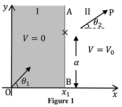
Figure 1
| A1 | Obtain an expression for \(v_2\) in terms of \(m\), \(v_1\) and \(V_0\). | 0.2 |
| A2 | Express \(v_2\) in terms of \(v_1\), \(\theta_1\) and \(\theta_2\). | 0.3 |
We define a quantity called action \(A=m\int v(s)ds\), where \(ds\) is the infinitesimal length along the trajectory of a particle of mass \(m\) moving with speed \(v(s)\). The integral is taken over the path. As an example, for a particle moving with constant speed \(v\) on a circular path of radius \(R\), the action \(A\) for one revolution will be \(2\pi mRv\). For a particle with constant energy \(E\), it can be shown that of all the possible trajectories between two fixed points, the actual trajectory is the one on which \(A\) defined above is an extremum (minimum or maximum). Historically this is known as the Principle of Least Action (PLA).
| A3 | PLA implies that the trajectory of a particle moving between two fixed points in a region of constant potential will be a straight line. Let the two fixed points O and P in Fig. 1 have coordinates \((0,0)\) and \((x_0,y_0)\) respectively and the boundary point where the particle transits from region I to region II have coordinates \((x_1,\alpha)\). Note that \(x_1\) is fixed and the action depends on the coordinate \(\alpha\) only. State the expression for the action \(A(\alpha)\). Use PLA to obtain the relationship between \(v_1/v_2\) and these coordinates. | 1.0 |
B The Extremum Principle in Optics
A light ray travels from medium I to medium II with refractive indices \(n_1\) and \(n_2\) respectively. The two media are separated by a line parallel to the \(x\)-axis. The light ray makes an angle \(i_1\) with the \(y\)-axis in medium I and \(i_2\) in medium II (see Fig. 2). To obtain the trajectory of the ray, we make use of another extremum (minimum or maximum) principle known as Fermat’s principle of least time.
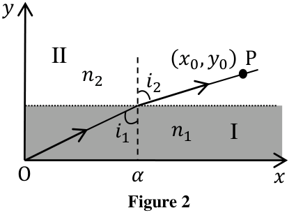
Figure 2
| B1 | The principle states that between two fixed points, a light ray moves along a path such that time taken between the two points is an extremum. Derive the relation between \(\sin i_1\) and \(\sin i_2\) on the basis of Fermat’s principle. | 0.5 |
Shown in Fig. 3 is a schematic sketch of the path of a laser beam incident horizontally on a solution of sugar in which the concentration of sugar decreases with height. As a consequence, the refractive index of the solution also decreases with height.
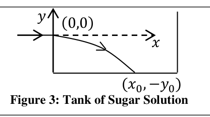
Figure 3: Tank of Sugar Solution
| B2 | Assume that the refractive index \(n(y)\) depends only on \(y\). Use the equation obtained in B1 to obtain the expression for the slope \(dy/dx\) of the beam’s path in terms of refractive index \(n_0\) at \(y=0\) and \(n(y)\). | 1.5 |
| B3 | The laser beam is directed horizontally from the origin \((0,0)\) into the sugar solution at a height \(y_0\) from the bottom of the tank as shown in figure 3. Take \(n(y)=n_0-ky\) where \(n_0\) and \(k\) are positive constants. Obtain an expression for \(x\) in terms of \(y\) and related quantities for the actual trajectory of the laser beam. | 1.2 |
\(^{1}\) Manoj Harbola (IIT-Kanpur) and Vijay A. Singh (ex-National Coordinator, Science Olympiads) were the principal authors of this problem. The contributions of the Academic Committee, Academic Development Group and the International Board are gratefully acknowledged.
| You may use: \(\int\sec\theta\,d\theta=\ln(\sec\theta+\tan\theta)+\text{constant}\), where \(\sec\theta=1/\cos\theta\) or \(\displaystyle\int\frac{dx}{\sqrt{x^2-1}}=\ln\!\left(x+\sqrt{x^2-1}\right)+\text{constant}\) |
||
| B4 | Obtain the value of \(x_0\), the point where the beam meets the bottom of the tank. Take \(y_0=10.0\ \mathrm{cm}\), \(n_0=1.50\), \(k=0.050\ \mathrm{cm^{-1}}\) (\(1\ \mathrm{cm}=10^{-2}\ \mathrm{m}\)). | 0.8 |
C The Extremum Principle and the Wave Nature of Matter
We now explore the connection between the PLA and the wave nature of a moving particle. For this we assume that a particle moving from O to P can take all possible trajectories and we will seek a trajectory that depends on the constructive interference of de Broglie waves.
| C1 | As the particle moves along its trajectory by an infinitesimal distance \(\Delta s\), relate the change \(\Delta\varphi\) in the phase of its de Broglie wave to the change \(\Delta A\) in the action and the Planck constant. | 0.6 |
| C2 | Recall the problem from part A where the particle traverses from O to P (see Fig. 4). Let an opaque partition be placed at the boundary AB between the two regions. There is a small opening CD of width \(d\) in AB such that \(d\ll(x_0-x_1)\) and \(d\ll x_1\). Consider two extreme paths OCP and ODP such that OCP lies on the classical trajectory discussed in part A. Obtain the phase difference \(\Delta\varphi_{CD}\) between the two paths to first order. |
1.2 |
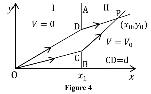
Figure 4
D Matter Wave Interference
Consider an electron gun at O which directs a collimated beam of electrons to a narrow slit at F in the opaque partition \(\mathrm{A_1B_1}\) at \(x=x_1\) such that OFP is a straight line. P is a point on the screen at \(x=x_0\) (see Fig. 5). The speed in I is \(v_1=2.0000\times10^7\ \mathrm{m\,s^{-1}}\) and \(\theta=10.0000^\circ\). The potential in II is such that speed \(v_2=1.9900\times10^7\ \mathrm{m\,s^{-1}}\). The distance \(x_0-x_1\) is \(250.00\ \mathrm{mm}\) (\(1\mathrm{mm}=10^{-3}\mathrm{m}\)). Ignore electron-electron interaction.
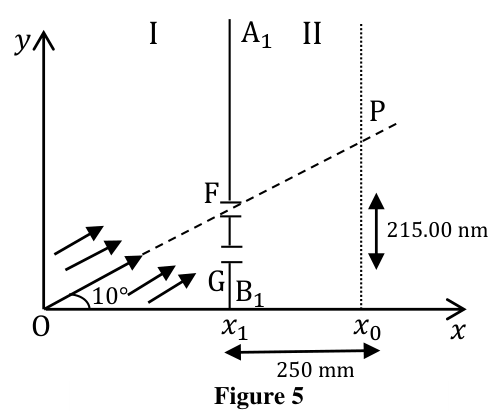
Figure 5
| D1 | If the electrons at O have been accelerated from rest, calculate the accelerating potential \(U_1\). | 0.3 |
| D2 | Another identical slit G is made in the partition \(\mathrm{A_1B_1}\) at a distance of \(215.00\ \mathrm{nm}\) (\(1\mathrm{nm}=10^{-9}\mathrm{m}\)) below slit F (Fig. 5). If the phase difference between de Broglie waves arriving at P through the slits F and G is \(2\pi\beta\), calculate \(\beta\). | 0.8 |
| D3 | What is the smallest distance \(\Delta y\) from P at which null (zero) electron detection maybe expected on the screen? [Note: you may find the approximation \(\sin(\theta+\Delta\theta)\approx\sin\theta+\Delta\theta\cos\theta\) useful] | 1.2 |
| D4 | The beam has a square cross section of \(500\mathrm{nm}\times500\mathrm{nm}\) and the setup is \(2\ \mathrm{m}\) long. What should be the minimum flux density \(I_{\min}\) (number of electrons per unit normal area per unit time) if, on an average, there is at least one electron in the setup at a given time? | 0.4 |
Official English text of the problem.
Answers
- A1: \(\displaystyle v_2=\sqrt{v_1^2-\frac{2V_0}{m}}\).
- A2: \(\displaystyle v_2=v_1\frac{\sin\theta_1}{\sin\theta_2}\).
- A3:
\[ A(\alpha)=m v_1\sqrt{x_1^2+\alpha^2} +m v_2\sqrt{(x_0-x_1)^2+(y_0-\alpha)^2}, \] \[ \frac{v_1}{v_2} =\frac{(y_0-\alpha)\sqrt{x_1^2+\alpha^2}} {\alpha\sqrt{(x_0-x_1)^2+(y_0-\alpha)^2}}. \] - B1: \(\displaystyle n_1\sin i_1=n_2\sin i_2\).
- B2: \(\displaystyle \frac{dy}{dx}=-\sqrt{\frac{n(y)^2}{n_0^2}-1}\).
- B3:
\[ x(y)=\frac{n_0}{k}\ln\!\left[ \frac{n_0-ky+\sqrt{(n_0-ky)^2-n_0^2}}{n_0} \right]. \] Equivalently, \(\displaystyle y(x)=\frac{n_0}{k}\left[1-\cosh\!\left(\frac{kx}{n_0}\right)\right]\). - B4: \(\displaystyle x_0=23.86\ldots\ \mathrm{cm}\approx24\ \mathrm{cm}\).
- C1: \(\displaystyle \Delta\varphi=\frac{2\pi}{h}\Delta A=\frac{\Delta A}{\hbar}\).
- C2: \(\displaystyle \Delta\varphi_{CD}=0\) to first order in \(d\); the leading correction is quadratic.
- D1: \(\displaystyle U_1\approx1.14\times10^3\ \mathrm{V}\).
- D2: \(\displaystyle \beta=\frac{m_e d(v_1-v_2)\sin\theta}{h}\approx5.13\).
- D3: \(\displaystyle \Delta y\approx1.6\times10^{-5}\ \mathrm{m}=16\ \mu\mathrm{m}\), below P.
- D4: \(\displaystyle I_{\min}\approx4\times10^{19}\ \mathrm{m^{-2}\,s^{-1}}\).
Solution
For the numerical electron calculations, use \[ m_e=9.1093837\times10^{-31}\ \mathrm{kg},\qquad e=1.602176634\times10^{-19}\ \mathrm{C},\qquad h=6.62607015\times10^{-34}\ \mathrm{J\,s}, \] where \(e\) is the magnitude of the electron charge.
A1
The potential is time independent, so mechanical energy is conserved: \[ \frac12 mv_1^2=\frac12 mv_2^2+V_0. \] Therefore, \[ \boxed{v_2=\sqrt{v_1^2-\frac{2V_0}{m}}}. \] The problem assumes that the particle is transmitted into region II.
A2
The potential depends only on \(x\), so the force has no \(y\)-component. Consequently, the momentum parallel to the boundary is conserved: \[ mv_1\sin\theta_1=mv_2\sin\theta_2. \] Thus, \[ \boxed{v_2=v_1\frac{\sin\theta_1}{\sin\theta_2}}. \]
A3
Let the boundary crossing point be \(Q=(x_1,\alpha)\). The two straight segments have lengths \[ L_1=\sqrt{x_1^2+\alpha^2},\qquad L_2=\sqrt{(x_0-x_1)^2+(y_0-\alpha)^2}. \] At fixed total energy, the speeds in the two regions are fixed. Hence \[ \boxed{A(\alpha)=m(v_1L_1+v_2L_2)}. \]
The actual trajectory satisfies \[ \frac{dA}{d\alpha} =m\left[ v_1\frac{\alpha}{L_1} -v_2\frac{y_0-\alpha}{L_2} \right]=0. \] Therefore, \[ \boxed{ \frac{v_1}{v_2} =\frac{(y_0-\alpha)L_1}{\alpha L_2} =\frac{(y_0-\alpha)\sqrt{x_1^2+\alpha^2}} {\alpha\sqrt{(x_0-x_1)^2+(y_0-\alpha)^2}} }. \]
Since \(\alpha/L_1=\sin\theta_1\) and \((y_0-\alpha)/L_2=\sin\theta_2\), this reproduces A2. Moreover, \[ \frac{d^2A}{d\alpha^2} =m\left[ \frac{v_1x_1^2}{L_1^3} +\frac{v_2(x_0-x_1)^2}{L_2^3} \right]>0, \] so this stationary action is a minimum.
B1
Write the horizontal interface as \(y=b\), and let the ray cross it at \((\alpha,b)\). The speed of light in medium \(j\) is \(c/n_j\). Its travel time from O to P is therefore \[ T(\alpha)=\frac{n_1}{c}\sqrt{\alpha^2+b^2} +\frac{n_2}{c}\sqrt{(x_0-\alpha)^2+(y_0-b)^2}. \]
Fermat’s principle requires \(dT/d\alpha=0\): \[ n_1\frac{\alpha}{\sqrt{\alpha^2+b^2}} =n_2\frac{x_0-\alpha} {\sqrt{(x_0-\alpha)^2+(y_0-b)^2}}. \] Because the angles are measured from the interface normal, the two geometric ratios are \(\sin i_1\) and \(\sin i_2\). Thus \[ \boxed{n_1\sin i_1=n_2\sin i_2}, \qquad \boxed{\frac{\sin i_1}{\sin i_2}=\frac{n_2}{n_1}}. \]
B2
Regard the liquid as a succession of thin horizontal layers. Applying B1 between adjacent layers shows that \[ n(y)\sin i(y)=\text{constant}. \] The initial ray is horizontal, so \(i(0)=90^\circ\), giving \[ n(y)\sin i(y)=n_0. \]
For a ray traveling towards increasing \(x\), \[ \sin i=\frac{dx}{ds} =\frac{1}{\sqrt{1+(dy/dx)^2}}. \] Consequently, \[ \frac{n(y)}{\sqrt{1+(dy/dx)^2}}=n_0, \] and hence \[ \left(\frac{dy}{dx}\right)^2=\frac{n(y)^2}{n_0^2}-1. \]
The ray bends towards the larger refractive index, which is downward. Choosing the negative slope, \[ \boxed{\frac{dy}{dx} =-\sqrt{\frac{n(y)^2}{n_0^2}-1}}. \]
B3
Substitute \(n(y)=n_0-ky\): \[ \frac{dx}{dy} =-\frac{n_0}{\sqrt{(n_0-ky)^2-n_0^2}}. \] Integrating from the entry point \((0,0)\), \[ x=-n_0\int_0^y \frac{d\eta}{\sqrt{(n_0-k\eta)^2-n_0^2}}. \]
With \(u=(n_0-k\eta)/n_0\), this becomes \[ x=\frac{n_0}{k} \int_1^{(n_0-ky)/n_0}\frac{du}{\sqrt{u^2-1}}. \] Using the supplied integral, \[ \boxed{ x(y)=\frac{n_0}{k} \ln\!\left[ \frac{n_0-ky+\sqrt{(n_0-ky)^2-n_0^2}}{n_0} \right] }. \] This is the branch with \(x\ge0\) and \(-y_0\le y\le0\).
Equivalently, \[ \frac{kx}{n_0} =\operatorname{arcosh}\!\left(1-\frac{ky}{n_0}\right), \] so \[ \boxed{ y(x)=\frac{n_0}{k} \left[1-\cosh\!\left(\frac{kx}{n_0}\right)\right] }. \] It passes through the origin with a horizontal tangent and curves increasingly downward.
B4
At the bottom, \(y=-y_0\). Therefore, \[ x_0=\frac{n_0}{k} \operatorname{arcosh}\!\left(1+\frac{ky_0}{n_0}\right). \] Using centimetres consistently, \[ \frac{n_0}{k}=30.0\ \mathrm{cm}, \qquad 1+\frac{ky_0}{n_0} =1+\frac{0.050(10.0)}{1.50}=\frac43. \] Thus \[ x_0=30.0\ln\!\left(\frac{4+\sqrt7}{3}\right)\ \mathrm{cm} =23.86096\ldots\ \mathrm{cm}. \] Hence \[ \boxed{x_0\approx24\ \mathrm{cm}=0.24\ \mathrm{m}}. \]
C1
The de Broglie wavelength is \[ \lambda=\frac{h}{p}=\frac{h}{mv}. \] The spatial phase accumulated over an infinitesimal distance is \[ \Delta\varphi=\frac{2\pi}{\lambda}\Delta s =\frac{2\pi}{h}mv\,\Delta s. \] Since \(\Delta A=mv\,\Delta s\), \[ \boxed{\Delta\varphi=\frac{2\pi}{h}\Delta A =\frac{\Delta A}{\hbar}}. \] For stationary waves of the same energy, the common temporal phase cancels when comparing paths at the same observation time.
C2
Let C have coordinate \((x_1,\alpha)\), so D has coordinate \((x_1,\alpha+d)\). To first order, \[ OD-OC=d\sin\theta_1+O(d^2), \] while \[ DP-CP=-d\sin\theta_2+O(d^2). \] Therefore, \[ A_{ODP}-A_{OCP} =md\left(v_1\sin\theta_1-v_2\sin\theta_2\right)+O(d^2). \]
Because OCP is the classical trajectory, A2 gives \[ v_1\sin\theta_1=v_2\sin\theta_2. \] Using C1, \[ \Delta\varphi_{CD} =\frac{2\pi md}{h} \left(v_1\sin\theta_1-v_2\sin\theta_2\right)+O(d^2). \] Thus \[ \boxed{\Delta\varphi_{CD}=0\quad\text{to first order in }d}. \]
The phase difference is generally nonzero at second order. Stationary action makes neighboring paths have the same phase to first order.
D1
Acceleration from rest through a potential difference of magnitude \(U_1\) gives \[ eU_1=\frac12m_ev_1^2. \] Hence \[ U_1=\frac{m_ev_1^2}{2e} =1137.126\ldots\ \mathrm{V}, \] or \[ \boxed{U_1\approx1.14\times10^3\ \mathrm{V}}. \]
D2
Let \[ d=215.00\times10^{-9}\ \mathrm{m}, \qquad L=x_0-x_1=0.25000\ \mathrm{m}. \] We treat the incident collimated beam as a coherent plane wave and use the far-field path-length differences to first order in the slit separation.
Since F is above G, the incident phase difference is \[ \varphi_F^{\mathrm{in}}-\varphi_G^{\mathrm{in}} =\frac{m_ev_1}{\hbar}d\sin\theta. \] At P, which lies on the straight continuation of OF, \[ FP-GP\simeq-d\sin\theta. \] Propagation in region II therefore contributes \[ -\frac{m_ev_2}{\hbar}d\sin\theta. \]
Taking the total phase difference as the phase through F minus that through G, \[ 2\pi\beta =\frac{m_ed}{\hbar}(v_1-v_2)\sin\theta. \] Thus \[ \boxed{\beta=\frac{m_ed(v_1-v_2)\sin\theta}{h}}. \] Numerically, \[ \beta=5.132650\ldots, \qquad \boxed{\beta\approx5.13}. \] This is the unreduced phase difference in cycles; modulo one cycle it is \(0.132650\ldots\).
D3
For identical slits with equal amplitudes, destructive interference occurs when the phase difference is an odd multiple of \(\pi\), or a half-integer number of cycles.
Let the outgoing direction towards a nearby screen point be \(\theta+\delta\theta\). The incident phase difference remains fixed, while the propagation phase changes. The phase difference in cycles becomes \[ b(\delta\theta) =\frac{m_ed}{h} \left[v_1\sin\theta-v_2\sin(\theta+\delta\theta)\right]. \] Using the given small-angle expansion, \[ b(\delta\theta) \simeq\beta-\frac{m_ev_2d}{h}\cos\theta\,\delta\theta. \]
The neighboring half-integers are \(4.5\) and \(5.5\). Their distances from \(\beta\) are \[ \beta-4.5=0.632650\ldots, \qquad 5.5-\beta=0.367350\ldots. \] The nearest minimum therefore has \(b=5.5\), giving \[ \delta\theta =-\frac{h(5.5-\beta)}{m_ev_2d\cos\theta}. \] The negative sign means the minimum lies below P.
The signed displacement on the vertical screen is \[ \delta y =L\left[\tan(\theta+\delta\theta)-\tan\theta\right] \simeq\frac{L}{\cos^2\theta}\delta\theta. \] Thus its magnitude is \[ \boxed{ \Delta y =\frac{hL(5.5-\beta)} {m_ev_2d\cos^3\theta} }. \]
Numerically, \[ \frac{hL}{m_ev_2d\cos^3\theta} =44.5001\ldots\ \mu\mathrm{m}, \] so the leading-order result is \[ \Delta y=(44.5001\ldots)(0.3673499\ldots)\ \mu\mathrm{m} =16.3471\ldots\ \mu\mathrm{m}. \] Therefore, \[ \boxed{\Delta y\approx16\ \mu\mathrm{m},\quad\text{below P}}. \]
The small-angle and far-field approximations are appropriate here: \(|\delta\theta|\simeq6.34\times10^{-5}\ \mathrm{rad}\), and \(d/L=8.60\times10^{-7}\). The quoted result neglects higher-order path-length corrections.
D4
The beam’s normal cross-sectional area is \[ S=(500\times10^{-9})^2 =2.50\times10^{-13}\ \mathrm{m^2}. \] For a \(2\ \mathrm{m}\) flight distance, using \(v\simeq2.0\times10^7\ \mathrm{m\,s^{-1}}\), the transit time is \[ \tau\simeq\frac{2}{2.0\times10^7} =1.0\times10^{-7}\ \mathrm{s}. \]
If the flux density is \(I\), the number entering per unit time is \(IS\). In steady operation, the average number in the apparatus is \[ \overline N=IS\tau. \] The minimum flux corresponds to \(\overline N=1\): \[ I_{\min}=\frac{1}{S\tau}. \] Therefore, \[ \boxed{ I_{\min}\simeq \frac{1}{(2.50\times10^{-13})(1.0\times10^{-7})} =4\times10^{19}\ \mathrm{m^{-2}\,s^{-1}} }. \]
More precisely, \(\tau=\ell_1/v_1+\ell_2/v_2\), where \(\ell_1+\ell_2\) is the flight distance. The two speeds differ by only \(0.5\%\), so replacing them by the common approximate speed does not affect the quoted precision.
The solution was checked against the official solution.
IPhO 2015 · Theorieaufgabe 2
Das Extremalprinzip
A Das Extremalprinzip in der Mechanik
Betrachten Sie die in Abb. 1 dargestellte horizontale, reibungsfreie \(x-y\)-Ebene. Sie wird durch eine Gerade AB mit der Gleichung \(x=x_1\) in zwei Bereiche I und II unterteilt. Die potenzielle Energie eines punktförmigen Teilchens der Masse \(m\) beträgt im Bereich I \(V=0\) und im Bereich II \(V=V_0\). Das Teilchen wird vom Ursprung O mit der Geschwindigkeit \(v_1\) entlang einer Geraden ausgesandt, die mit der \(x\)-Achse den Winkel \(\theta_1\) bildet. Es erreicht den Punkt P im Bereich II mit der Geschwindigkeit \(v_2\) entlang einer Geraden, die mit der \(x\)-Achse den Winkel \(\theta_2\) bildet. Vernachlässigen Sie in der gesamten Aufgabe T-2 (in allen Teilen) die Gravitation und relativistische Effekte.
Abbildung 1
| A1 | Bestimmen Sie einen Ausdruck für \(v_2\) in Abhängigkeit von \(m\), \(v_1\) und \(V_0\). | 0.2 |
| A2 | Drücken Sie \(v_2\) durch \(v_1\), \(\theta_1\) und \(\theta_2\) aus. | 0.3 |
Wir definieren eine Größe namens Wirkung \(A=m\int v(s)ds\), wobei \(ds\) die infinitesimale Länge entlang der Bahn eines Teilchens der Masse \(m\) ist, das sich mit der Geschwindigkeit \(v(s)\) bewegt. Das Integral wird entlang der Bahn gebildet. Beispielsweise beträgt für ein Teilchen, das sich mit konstanter Geschwindigkeit \(v\) auf einer Kreisbahn mit dem Radius \(R\) bewegt, die Wirkung \(A\) für einen Umlauf \(2\pi mRv\). Für ein Teilchen mit konstanter Energie \(E\) lässt sich zeigen, dass von allen möglichen Bahnen zwischen zwei festen Punkten die tatsächliche Bahn diejenige ist, auf der das oben definierte \(A\) ein Extremum (Minimum oder Maximum) annimmt. Historisch ist dies als Prinzip der kleinsten Wirkung (PLA) bekannt.
| A3 | Aus dem PLA folgt, dass die Bahn eines Teilchens, das sich zwischen zwei festen Punkten in einem Bereich mit konstantem Potenzial bewegt, eine Gerade ist. Die beiden festen Punkte O und P in Abb. 1 sollen die Koordinaten \((0,0)\) bzw. \((x_0,y_0)\) haben, und der Grenzpunkt, an dem das Teilchen von Bereich I in Bereich II übertritt, soll die Koordinaten \((x_1,\alpha)\) haben. Beachten Sie, dass \(x_1\) fest ist und die Wirkung nur von der Koordinate \(\alpha\) abhängt. Geben Sie den Ausdruck für die Wirkung \(A(\alpha)\) an. Leiten Sie mithilfe des PLA den Zusammenhang zwischen \(v_1/v_2\) und diesen Koordinaten her. | 1.0 |
B Das Extremalprinzip in der Optik
Ein Lichtstrahl läuft von Medium I in Medium II mit den jeweiligen Brechungsindizes \(n_1\) und \(n_2\). Die beiden Medien sind durch eine zur \(x\)-Achse parallele Gerade getrennt. Der Lichtstrahl bildet mit der \(y\)-Achse im Medium I den Winkel \(i_1\) und im Medium II den Winkel \(i_2\) (siehe Abb. 2). Um die Bahn des Strahls zu bestimmen, verwenden wir ein weiteres Extremalprinzip (Minimum oder Maximum), das als Fermatsches Prinzip der kürzesten Zeit bekannt ist.
Abbildung 2
| B1 | Das Prinzip besagt, dass sich ein Lichtstrahl zwischen zwei festen Punkten auf einem Weg bewegt, für den die zwischen den beiden Punkten benötigte Zeit ein Extremum annimmt. Leiten Sie auf Grundlage des Fermatschen Prinzips den Zusammenhang zwischen \(\sin i_1\) und \(\sin i_2\) her. | 0.5 |
Abb. 3 zeigt eine schematische Skizze der Bahn eines Laserstrahls, der horizontal in eine Zuckerlösung einfällt, deren Zuckerkonzentration mit der Höhe abnimmt. Infolgedessen nimmt auch der Brechungsindex der Lösung mit der Höhe ab.
Abbildung 3: Behälter mit Zuckerlösung
| B2 | Nehmen Sie an, dass der Brechungsindex \(n(y)\) nur von \(y\) abhängt. Leiten Sie mithilfe der in B1 erhaltenen Gleichung einen Ausdruck für die Steigung \(dy/dx\) der Strahlbahn in Abhängigkeit vom Brechungsindex \(n_0\) bei \(y=0\) und von \(n(y)\) her. | 1.5 |
| B3 | Der Laserstrahl wird vom Ursprung \((0,0)\) aus horizontal in die Zuckerlösung gerichtet, und zwar in einer Höhe \(y_0\) über dem Boden des Behälters, wie in Abbildung 3 dargestellt. Setzen Sie \(n(y)=n_0-ky\), wobei \(n_0\) und \(k\) positive Konstanten sind. Bestimmen Sie für die tatsächliche Bahn des Laserstrahls einen Ausdruck für \(x\) in Abhängigkeit von \(y\) und den zugehörigen Größen. | 1.2 |
\(^{1}\) Manoj Harbola (IIT-Kanpur) und Vijay A. Singh (ehemaliger nationaler Koordinator der Wissenschaftsolympiaden) waren die Hauptautoren dieser Aufgabe. Den Beiträgen des Akademischen Komitees, der Akademischen Entwicklungsgruppe und des Internationalen Gremiums gilt unser Dank.
| Sie dürfen verwenden: \(\int\sec\theta\,d\theta=\ln(\sec\theta+\tan\theta)+\text{Konstante}\), wobei \(\sec\theta=1/\cos\theta\), oder \(\displaystyle\int\frac{dx}{\sqrt{x^2-1}}=\ln\!\left(x+\sqrt{x^2-1}\right)+\text{Konstante}\) |
||
| B4 | Bestimmen Sie den Wert von \(x_0\), der Stelle, an der der Strahl auf den Boden des Behälters trifft. Verwenden Sie \(y_0=10.0\ \mathrm{cm}\), \(n_0=1.50\), \(k=0.050\ \mathrm{cm^{-1}}\) (\(1\ \mathrm{cm}=10^{-2}\ \mathrm{m}\)). | 0.8 |
C Das Extremalprinzip und die Wellennatur der Materie
Wir untersuchen nun den Zusammenhang zwischen dem PLA und der Wellennatur eines bewegten Teilchens. Dazu nehmen wir an, dass ein Teilchen, das sich von O nach P bewegt, alle möglichen Bahnen nehmen kann, und suchen eine Bahn, die sich aus der konstruktiven Interferenz von De-Broglie-Wellen ergibt.
| C1 | Während sich das Teilchen entlang seiner Bahn um eine infinitesimale Strecke \(\Delta s\) bewegt, stellen Sie den Zusammenhang zwischen der Änderung \(\Delta\varphi\) der Phase seiner De-Broglie-Welle, der Änderung \(\Delta A\) der Wirkung und der Planck-Konstanten her. | 0.6 |
| C2 | Betrachten Sie erneut die Aufgabe aus Teil A, in der sich das Teilchen von O nach P bewegt (siehe Abb. 4). An der Grenze AB zwischen den beiden Bereichen werde eine undurchlässige Trennwand angebracht. In AB befindet sich eine kleine Öffnung CD der Breite \(d\), wobei \(d\ll(x_0-x_1)\) und \(d\ll x_1\) gelten. Betrachten Sie die beiden äußersten Wege OCP und ODP, wobei OCP auf der in Teil A behandelten klassischen Bahn liegt. Bestimmen Sie die Phasendifferenz \(\Delta\varphi_{CD}\) zwischen den beiden Wegen in erster Ordnung. |
1.2 |
Abbildung 4
D Interferenz von Materiewellen
Betrachten Sie eine Elektronenkanone bei O, die einen kollimierten Elektronenstrahl auf einen schmalen Spalt bei F in der undurchlässigen Trennwand \(\mathrm{A_1B_1}\) bei \(x=x_1\) richtet, sodass OFP eine Gerade ist. P ist ein Punkt auf dem Schirm bei \(x=x_0\) (siehe Abb. 5). Die Geschwindigkeit in I beträgt \(v_1=2.0000\times10^7\ \mathrm{m\,s^{-1}}\), und es gilt \(\theta=10.0000^\circ\). Das Potenzial in II ist so gewählt, dass die Geschwindigkeit \(v_2=1.9900\times10^7\ \mathrm{m\,s^{-1}}\) beträgt. Der Abstand \(x_0-x_1\) beträgt \(250.00\ \mathrm{mm}\) (\(1\mathrm{mm}=10^{-3}\mathrm{m}\)). Vernachlässigen Sie die Wechselwirkung zwischen den Elektronen.
Abbildung 5
| D1 | Wenn die Elektronen bei O aus der Ruhe beschleunigt wurden, berechnen Sie die Beschleunigungsspannung \(U_1\). | 0.3 |
| D2 | In der Trennwand \(\mathrm{A_1B_1}\) wird ein weiterer identischer Spalt G im Abstand von \(215.00\ \mathrm{nm}\) (\(1\mathrm{nm}=10^{-9}\mathrm{m}\)) unterhalb des Spalts F angebracht (Abb. 5). Wenn die Phasendifferenz zwischen den durch die Spalte F und G bei P eintreffenden De-Broglie-Wellen \(2\pi\beta\) beträgt, berechnen Sie \(\beta\). | 0.8 |
| D3 | In welchem kleinsten Abstand \(\Delta y\) von P ist auf dem Schirm zu erwarten, dass keine Elektronen nachgewiesen werden (Nachweisrate null)? [Hinweis: Die Näherung \(\sin(\theta+\Delta\theta)\approx\sin\theta+\Delta\theta\cos\theta\) kann hilfreich sein.] | 1.2 |
| D4 | Der Strahl hat einen quadratischen Querschnitt von \(500\mathrm{nm}\times500\mathrm{nm}\), und die Anordnung ist \(2\ \mathrm{m}\) lang. Wie groß muss die minimale Flussdichte \(I_{\min}\) (Anzahl der Elektronen pro Flächeneinheit senkrecht zur Strahlrichtung und pro Zeiteinheit) sein, damit sich zu einem gegebenen Zeitpunkt im Mittel mindestens ein Elektron in der Anordnung befindet? | 0.4 |
Aufgabentext aus dem offiziellen englischen Text übersetzt.
Antworten
- A1: \(\displaystyle v_2=\sqrt{v_1^2-\frac{2V_0}{m}}\).
- A2: \(\displaystyle v_2=v_1\frac{\sin\theta_1}{\sin\theta_2}\).
- A3:
\[ A(\alpha)=m v_1\sqrt{x_1^2+\alpha^2} +m v_2\sqrt{(x_0-x_1)^2+(y_0-\alpha)^2}, \] \[ \frac{v_1}{v_2} =\frac{(y_0-\alpha)\sqrt{x_1^2+\alpha^2}} {\alpha\sqrt{(x_0-x_1)^2+(y_0-\alpha)^2}}. \] - B1: \(\displaystyle n_1\sin i_1=n_2\sin i_2\).
- B2: \(\displaystyle \frac{dy}{dx}=-\sqrt{\frac{n(y)^2}{n_0^2}-1}\).
- B3:
\[ x(y)=\frac{n_0}{k}\ln\!\left[ \frac{n_0-ky+\sqrt{(n_0-ky)^2-n_0^2}}{n_0} \right]. \] Gleichwertig dazu ist \(\displaystyle y(x)=\frac{n_0}{k}\left[1-\cosh\!\left(\frac{kx}{n_0}\right)\right]\). - B4: \(\displaystyle x_0=23.86\ldots\ \mathrm{cm}\approx24\ \mathrm{cm}\).
- C1: \(\displaystyle \Delta\varphi=\frac{2\pi}{h}\Delta A=\frac{\Delta A}{\hbar}\).
- C2: \(\displaystyle \Delta\varphi_{CD}=0\) in erster Ordnung in \(d\); die führende Korrektur ist quadratisch.
- D1: \(\displaystyle U_1\approx1.14\times10^3\ \mathrm{V}\).
- D2: \(\displaystyle \beta=\frac{m_e d(v_1-v_2)\sin\theta}{h}\approx5.13\).
- D3: \(\displaystyle \Delta y\approx1.6\times10^{-5}\ \mathrm{m}=16\ \mu\mathrm{m}\), unterhalb von P.
- D4: \(\displaystyle I_{\min}\approx4\times10^{19}\ \mathrm{m^{-2}\,s^{-1}}\).
Lösung
Für die numerischen Berechnungen zu den Elektronen verwenden wir \[ m_e=9.1093837\times10^{-31}\ \mathrm{kg},\qquad e=1.602176634\times10^{-19}\ \mathrm{C},\qquad h=6.62607015\times10^{-34}\ \mathrm{J\,s}, \] wobei \(e\) der Betrag der Elektronenladung ist.
A1
Das Potenzial ist zeitunabhängig, daher bleibt die mechanische Energie erhalten: \[ \frac12 mv_1^2=\frac12 mv_2^2+V_0. \] Daraus folgt \[ \boxed{v_2=\sqrt{v_1^2-\frac{2V_0}{m}}}. \] Die Aufgabe setzt voraus, dass das Teilchen in den Bereich II übertritt.
A2
Das Potenzial hängt nur von \(x\) ab, daher besitzt die Kraft keine \(y\)-Komponente. Folglich bleibt der Impuls parallel zur Grenze erhalten: \[ mv_1\sin\theta_1=mv_2\sin\theta_2. \] Somit gilt \[ \boxed{v_2=v_1\frac{\sin\theta_1}{\sin\theta_2}}. \]
A3
Der Punkt des Grenzübertritts sei \(Q=(x_1,\alpha)\). Die beiden geraden Teilstrecken haben die Längen \[ L_1=\sqrt{x_1^2+\alpha^2},\qquad L_2=\sqrt{(x_0-x_1)^2+(y_0-\alpha)^2}. \] Bei fester Gesamtenergie sind die Geschwindigkeiten in den beiden Bereichen festgelegt. Daher gilt \[ \boxed{A(\alpha)=m(v_1L_1+v_2L_2)}. \]
Die tatsächliche Bahn erfüllt \[ \frac{dA}{d\alpha} =m\left[ v_1\frac{\alpha}{L_1} -v_2\frac{y_0-\alpha}{L_2} \right]=0. \] Daraus folgt \[ \boxed{ \frac{v_1}{v_2} =\frac{(y_0-\alpha)L_1}{\alpha L_2} =\frac{(y_0-\alpha)\sqrt{x_1^2+\alpha^2}} {\alpha\sqrt{(x_0-x_1)^2+(y_0-\alpha)^2}} }. \]
Da \(\alpha/L_1=\sin\theta_1\) und \((y_0-\alpha)/L_2=\sin\theta_2\) gelten, ergibt sich wieder A2. Außerdem ist \[ \frac{d^2A}{d\alpha^2} =m\left[ \frac{v_1x_1^2}{L_1^3} +\frac{v_2(x_0-x_1)^2}{L_2^3} \right]>0, \] sodass diese stationäre Wirkung ein Minimum ist.
B1
Wir beschreiben die horizontale Grenzfläche durch \(y=b\) und nehmen an, dass der Strahl sie bei \((\alpha,b)\) durchquert. Die Lichtgeschwindigkeit im Medium \(j\) ist \(c/n_j\). Seine Laufzeit von O nach P beträgt daher \[ T(\alpha)=\frac{n_1}{c}\sqrt{\alpha^2+b^2} +\frac{n_2}{c}\sqrt{(x_0-\alpha)^2+(y_0-b)^2}. \]
Das Fermatsche Prinzip verlangt \(dT/d\alpha=0\): \[ n_1\frac{\alpha}{\sqrt{\alpha^2+b^2}} =n_2\frac{x_0-\alpha} {\sqrt{(x_0-\alpha)^2+(y_0-b)^2}}. \] Da die Winkel gegenüber der Grenzflächennormalen gemessen werden, sind die beiden geometrischen Verhältnisse \(\sin i_1\) und \(\sin i_2\). Somit gilt \[ \boxed{n_1\sin i_1=n_2\sin i_2}, \qquad \boxed{\frac{\sin i_1}{\sin i_2}=\frac{n_2}{n_1}}. \]
B2
Wir betrachten die Flüssigkeit als eine Folge dünner horizontaler Schichten. Die Anwendung von B1 auf benachbarte Schichten zeigt, dass \[ n(y)\sin i(y)=\text{konstant}. \] Der Strahl verläuft anfangs horizontal, also ist \(i(0)=90^\circ\), woraus folgt: \[ n(y)\sin i(y)=n_0. \]
Für einen Strahl, der sich in Richtung zunehmender \(x\) bewegt, gilt \[ \sin i=\frac{dx}{ds} =\frac{1}{\sqrt{1+(dy/dx)^2}}. \] Folglich ist \[ \frac{n(y)}{\sqrt{1+(dy/dx)^2}}=n_0, \] und damit \[ \left(\frac{dy}{dx}\right)^2=\frac{n(y)^2}{n_0^2}-1. \]
Der Strahl wird zum größeren Brechungsindex hin gekrümmt, also nach unten. Mit der Wahl der negativen Steigung ergibt sich \[ \boxed{\frac{dy}{dx} =-\sqrt{\frac{n(y)^2}{n_0^2}-1}}. \]
B3
Wir setzen \(n(y)=n_0-ky\) ein: \[ \frac{dx}{dy} =-\frac{n_0}{\sqrt{(n_0-ky)^2-n_0^2}}. \] Integration vom Eintrittspunkt \((0,0)\) aus ergibt \[ x=-n_0\int_0^y \frac{d\eta}{\sqrt{(n_0-k\eta)^2-n_0^2}}. \]
Mit \(u=(n_0-k\eta)/n_0\) wird daraus \[ x=\frac{n_0}{k} \int_1^{(n_0-ky)/n_0}\frac{du}{\sqrt{u^2-1}}. \] Mit dem angegebenen Integral erhalten wir \[ \boxed{ x(y)=\frac{n_0}{k} \ln\!\left[ \frac{n_0-ky+\sqrt{(n_0-ky)^2-n_0^2}}{n_0} \right] }. \] Dies ist der Zweig mit \(x\ge0\) und \(-y_0\le y\le0\).
Gleichwertig dazu ist \[ \frac{kx}{n_0} =\operatorname{arcosh}\!\left(1-\frac{ky}{n_0}\right), \] also \[ \boxed{ y(x)=\frac{n_0}{k} \left[1-\cosh\!\left(\frac{kx}{n_0}\right)\right] }. \] Die Bahn geht mit einer horizontalen Tangente durch den Ursprung und krümmt sich zunehmend nach unten.
B4
Am Boden gilt \(y=-y_0\). Daher ist \[ x_0=\frac{n_0}{k} \operatorname{arcosh}\!\left(1+\frac{ky_0}{n_0}\right). \] Bei durchgängiger Verwendung von Zentimetern gilt \[ \frac{n_0}{k}=30.0\ \mathrm{cm}, \qquad 1+\frac{ky_0}{n_0} =1+\frac{0.050(10.0)}{1.50}=\frac43. \] Somit ergibt sich \[ x_0=30.0\ln\!\left(\frac{4+\sqrt7}{3}\right)\ \mathrm{cm} =23.86096\ldots\ \mathrm{cm}. \] Damit ist \[ \boxed{x_0\approx24\ \mathrm{cm}=0.24\ \mathrm{m}}. \]
C1
Die De-Broglie-Wellenlänge beträgt \[ \lambda=\frac{h}{p}=\frac{h}{mv}. \] Die über eine infinitesimale Strecke angesammelte räumliche Phase ist \[ \Delta\varphi=\frac{2\pi}{\lambda}\Delta s =\frac{2\pi}{h}mv\,\Delta s. \] Da \(\Delta A=mv\,\Delta s\) gilt, folgt \[ \boxed{\Delta\varphi=\frac{2\pi}{h}\Delta A =\frac{\Delta A}{\hbar}}. \] Für stationäre Wellen gleicher Energie fällt die gemeinsame zeitliche Phase beim Vergleich der Wege zur selben Beobachtungszeit weg.
C2
C habe die Koordinaten \((x_1,\alpha)\), sodass D die Koordinaten \((x_1,\alpha+d)\) hat. In erster Ordnung gilt \[ OD-OC=d\sin\theta_1+O(d^2), \] während \[ DP-CP=-d\sin\theta_2+O(d^2). \] Daher ist \[ A_{ODP}-A_{OCP} =md\left(v_1\sin\theta_1-v_2\sin\theta_2\right)+O(d^2). \]
Da OCP die klassische Bahn ist, liefert A2 \[ v_1\sin\theta_1=v_2\sin\theta_2. \] Mit C1 erhalten wir \[ \Delta\varphi_{CD} =\frac{2\pi md}{h} \left(v_1\sin\theta_1-v_2\sin\theta_2\right)+O(d^2). \] Somit gilt \[ \boxed{\Delta\varphi_{CD}=0\quad\text{in erster Ordnung in }d}. \]
In zweiter Ordnung ist die Phasendifferenz im Allgemeinen von null verschieden. Die Stationarität der Wirkung bewirkt, dass benachbarte Wege in erster Ordnung dieselbe Phase haben.
D1
Die Beschleunigung aus der Ruhe durch eine Potenzialdifferenz vom Betrag \(U_1\) ergibt \[ eU_1=\frac12m_ev_1^2. \] Daher ist \[ U_1=\frac{m_ev_1^2}{2e} =1137.126\ldots\ \mathrm{V}, \] oder \[ \boxed{U_1\approx1.14\times10^3\ \mathrm{V}}. \]
D2
Es sei \[ d=215.00\times10^{-9}\ \mathrm{m}, \qquad L=x_0-x_1=0.25000\ \mathrm{m}. \] Wir behandeln den einfallenden kollimierten Strahl als kohärente ebene Welle und verwenden die Weglängendifferenzen im Fernfeld in erster Ordnung im Spaltabstand.
Da F oberhalb von G liegt, beträgt die Phasendifferenz der einfallenden Welle \[ \varphi_F^{\mathrm{in}}-\varphi_G^{\mathrm{in}} =\frac{m_ev_1}{\hbar}d\sin\theta. \] Für P, das auf der geradlinigen Verlängerung von OF liegt, gilt \[ FP-GP\simeq-d\sin\theta. \] Der Beitrag der Ausbreitung im Bereich II beträgt daher \[ -\frac{m_ev_2}{\hbar}d\sin\theta. \]
Definieren wir die gesamte Phasendifferenz als die Phase durch F minus die Phase durch G, so gilt \[ 2\pi\beta =\frac{m_ed}{\hbar}(v_1-v_2)\sin\theta. \] Somit ist \[ \boxed{\beta=\frac{m_ed(v_1-v_2)\sin\theta}{h}}. \] Numerisch ergibt sich \[ \beta=5.132650\ldots, \qquad \boxed{\beta\approx5.13}. \] Dies ist die unreduzierte Phasendifferenz in Einheiten einer vollen Schwingung; modulo einer vollen Schwingung beträgt sie \(0.132650\ldots\).
D3
Bei identischen Spalten mit gleichen Amplituden tritt destruktive Interferenz auf, wenn die Phasendifferenz ein ungeradzahliges Vielfaches von \(\pi\) oder eine halbzahlige Anzahl voller Schwingungen ist.
Die Ausbreitungsrichtung zu einem benachbarten Schirmpunkt sei \(\theta+\delta\theta\). Die Phasendifferenz der einfallenden Welle bleibt unverändert, während sich die Ausbreitungsphase ändert. Die Phasendifferenz in Einheiten einer vollen Schwingung wird zu \[ b(\delta\theta) =\frac{m_ed}{h} \left[v_1\sin\theta-v_2\sin(\theta+\delta\theta)\right]. \] Mit der angegebenen Entwicklung für kleine Winkel ergibt sich \[ b(\delta\theta) \simeq\beta-\frac{m_ev_2d}{h}\cos\theta\,\delta\theta. \]
Die benachbarten Halbzahlen sind \(4.5\) und \(5.5\). Ihre Abstände von \(\beta\) betragen \[ \beta-4.5=0.632650\ldots, \qquad 5.5-\beta=0.367350\ldots. \] Das nächstgelegene Minimum hat daher \(b=5.5\), woraus folgt: \[ \delta\theta =-\frac{h(5.5-\beta)}{m_ev_2d\cos\theta}. \] Das negative Vorzeichen bedeutet, dass das Minimum unterhalb von P liegt.
Die vorzeichenbehaftete Verschiebung auf dem vertikalen Schirm ist \[ \delta y =L\left[\tan(\theta+\delta\theta)-\tan\theta\right] \simeq\frac{L}{\cos^2\theta}\delta\theta. \] Ihr Betrag ist somit \[ \boxed{ \Delta y =\frac{hL(5.5-\beta)} {m_ev_2d\cos^3\theta} }. \]
Numerisch ergibt sich \[ \frac{hL}{m_ev_2d\cos^3\theta} =44.5001\ldots\ \mu\mathrm{m}, \] sodass das Ergebnis in führender Ordnung lautet: \[ \Delta y=(44.5001\ldots)(0.3673499\ldots)\ \mu\mathrm{m} =16.3471\ldots\ \mu\mathrm{m}. \] Daher gilt \[ \boxed{\Delta y\approx16\ \mu\mathrm{m},\quad\text{unterhalb von P}}. \]
Die Kleinwinkel- und Fernfeldnäherungen sind hier angemessen: \(|\delta\theta|\simeq6.34\times10^{-5}\ \mathrm{rad}\), und \(d/L=8.60\times10^{-7}\). Das angegebene Ergebnis vernachlässigt Korrekturen höherer Ordnung der Weglängen.
D4
Die Querschnittsfläche des Strahls senkrecht zur Strahlrichtung beträgt \[ S=(500\times10^{-9})^2 =2.50\times10^{-13}\ \mathrm{m^2}. \] Für eine Flugstrecke von \(2\ \mathrm{m}\) beträgt die Durchflugzeit mit \(v\simeq2.0\times10^7\ \mathrm{m\,s^{-1}}\) \[ \tau\simeq\frac{2}{2.0\times10^7} =1.0\times10^{-7}\ \mathrm{s}. \]
Bei einer Flussdichte \(I\) ist die pro Zeiteinheit eintretende Anzahl \(IS\). Im stationären Betrieb beträgt die mittlere Anzahl in der Apparatur \[ \overline N=IS\tau. \] Der minimale Fluss entspricht \(\overline N=1\): \[ I_{\min}=\frac{1}{S\tau}. \] Daher gilt \[ \boxed{ I_{\min}\simeq \frac{1}{(2.50\times10^{-13})(1.0\times10^{-7})} =4\times10^{19}\ \mathrm{m^{-2}\,s^{-1}} }. \]
Genauer gilt \(\tau=\ell_1/v_1+\ell_2/v_2\), wobei \(\ell_1+\ell_2\) die Flugstrecke ist. Die beiden Geschwindigkeiten unterscheiden sich nur um \(0.5\%\), sodass ihre Ersetzung durch die gemeinsame Näherungsgeschwindigkeit die angegebene Genauigkeit nicht beeinflusst.
Die Lösung wurde mit der offiziellen Lösung abgeglichen.
IPhO 2015 · Teori sorusu 2
Ekstremum İlkesi
A Mekanikte Ekstremum İlkesi
Şekil 1'de gösterilen yatay, sürtünmesiz bir \(x-y\) düzlemini ele alın. Bu düzlem, \(x=x_1\) denklemini sağlayan AB doğrusu ile I ve II olmak üzere iki bölgeye ayrılmıştır. Kütlesi \(m\) olan noktasal bir parçacığın potansiyel enerjisi I bölgesinde \(V=0\), II bölgesinde ise \(V=V_0\)'dır. Parçacık, O başlangıç noktasından \(x\) ekseniyle \(\theta_1\) açısı yapan bir doğru boyunca \(v_1\) süratiyle gönderilir. II bölgesindeki P noktasına, \(x\) ekseniyle \(\theta_2\) açısı yapan bir doğru boyunca \(v_2\) süratiyle hareket ederek ulaşır. Bu T-2 sorusunun tamamında (tüm kısımlarında) kütleçekimini ve görelilik etkilerini ihmal edin.
Şekil 1
| A1 | \(v_2\) için \(m\), \(v_1\) ve \(V_0\) cinsinden bir ifade elde edin. | 0.2 |
| A2 | \(v_2\)'yi \(v_1\), \(\theta_1\) ve \(\theta_2\) cinsinden ifade edin. | 0.3 |
Eylem adı verilen bir niceliği \(A=m\int v(s)ds\) olarak tanımlıyoruz; burada \(ds\), \(v(s)\) süratiyle hareket eden \(m\) kütleli bir parçacığın yörüngesi boyunca sonsuz küçük uzunluk elemanıdır. İntegral, izlenen yol boyunca alınır. Örneğin, yarıçapı \(R\) olan çembersel bir yörüngede sabit \(v\) süratiyle hareket eden bir parçacığın bir tam turdaki eylemi \(A\), \(2\pi mRv\) olur. Enerjisi sabit ve \(E\) olan bir parçacık için, iki sabit nokta arasındaki tüm olası yörüngeler arasında gerçek yörüngenin, yukarıda tanımlanan \(A\)'nın bir ekstremum (minimum veya maksimum) olduğu yörünge olduğu gösterilebilir. Bu, tarihsel olarak En Küçük Eylem İlkesi (PLA) adıyla bilinir.
| A3 | PLA, potansiyelin sabit olduğu bir bölgede iki sabit nokta arasında hareket eden bir parçacığın yörüngesinin düz bir doğru olacağını ifade eder. Şekil 1'deki iki sabit nokta O ve P'nin koordinatları sırasıyla \((0,0)\) ve \((x_0,y_0)\), parçacığın I bölgesinden II bölgesine geçtiği sınır noktasının koordinatları ise \((x_1,\alpha)\) olsun. \(x_1\)'in sabit olduğuna ve eylemin yalnızca \(\alpha\) koordinatına bağlı olduğuna dikkat edin. Eylem \(A(\alpha)\) için ifadeyi yazın. PLA'yı kullanarak \(v_1/v_2\) ile bu koordinatlar arasındaki bağıntıyı elde edin. | 1.0 |
B Optikte Ekstremum İlkesi
Bir ışık ışını, kırılma indisleri sırasıyla \(n_1\) ve \(n_2\) olan I ortamından II ortamına geçer. İki ortam, \(x\) eksenine paralel bir doğru ile ayrılmıştır. Işık ışını, \(y\) ekseniyle I ortamında \(i_1\), II ortamında ise \(i_2\) açısı yapar (bkz. Şekil 2). Işının yörüngesini elde etmek için, Fermat'nın en kısa süre ilkesi olarak bilinen başka bir ekstremum (minimum veya maksimum) ilkesinden yararlanırız.
Şekil 2
| B1 | Bu ilkeye göre bir ışık ışını, iki sabit nokta arasında, bu iki nokta arasındaki yolculuk süresinin bir ekstremum olduğu yolu izler. Fermat ilkesinden hareketle \(\sin i_1\) ile \(\sin i_2\) arasındaki bağıntıyı türetin. | 0.5 |
Şekil 3'te, şeker derişiminin yükseklikle azaldığı bir şeker çözeltisine yatay olarak giren lazer demetinin izlediği yol şematik olarak gösterilmiştir. Bunun sonucunda çözeltinin kırılma indisi de yükseklikle azalır.
Şekil 3: Şeker Çözeltisi Tankı
| B2 | Kırılma indisi \(n(y)\)'nin yalnızca \(y\)'ye bağlı olduğunu varsayın. B1'de elde edilen denklemi kullanarak demetin izlediği yolun eğimi \(dy/dx\) için, \(y=0\)'daki kırılma indisi \(n_0\) ve \(n(y)\) cinsinden bir ifade elde edin. | 1.5 |
| B3 | Lazer demeti, Şekil 3'te gösterildiği gibi tankın tabanından \(y_0\) yüksekliğindeki \((0,0)\) başlangıç noktasından şeker çözeltisine yatay olarak yönlendirilir. \(n_0\) ve \(k\) pozitif sabitler olmak üzere \(n(y)=n_0-ky\) alın. Lazer demetinin gerçek yörüngesi için \(x\)'in \(y\) ve ilgili nicelikler cinsinden bir ifadesini elde edin. | 1.2 |
\(^{1}\) Bu sorunun başlıca yazarları Manoj Harbola (IIT-Kanpur) ve Vijay A. Singh'dir (eski Bilim Olimpiyatları Ulusal Koordinatörü). Akademik Komite, Akademik Geliştirme Grubu ve Uluslararası Kurulun katkılarına teşekkür ederiz.
| Şu integralleri kullanabilirsiniz: \(\int\sec\theta\,d\theta=\ln(\sec\theta+\tan\theta)+\text{sabit}\), burada \(\sec\theta=1/\cos\theta\), veya \(\displaystyle\int\frac{dx}{\sqrt{x^2-1}}=\ln\!\left(x+\sqrt{x^2-1}\right)+\text{sabit}\) |
||
| B4 | Demetin tankın tabanına ulaştığı noktanın \(x_0\) değerini bulun. \(y_0=10.0\ \mathrm{cm}\), \(n_0=1.50\), \(k=0.050\ \mathrm{cm^{-1}}\) (\(1\ \mathrm{cm}=10^{-2}\ \mathrm{m}\)) alın. | 0.8 |
C Ekstremum İlkesi ve Maddenin Dalga Doğası
Şimdi PLA ile hareket eden bir parçacığın dalga doğası arasındaki bağlantıyı inceleyeceğiz. Bunun için O'dan P'ye hareket eden bir parçacığın olası tüm yörüngeleri izleyebileceğini varsayacak ve de Broglie dalgalarının yapıcı girişimine dayanan bir yörünge arayacağız.
| C1 | Parçacık yörüngesi boyunca sonsuz küçük bir \(\Delta s\) mesafesi kadar ilerlerken, de Broglie dalgasının fazındaki \(\Delta\varphi\) değişimini, eylemdeki \(\Delta A\) değişimi ve Planck sabiti ile ilişkilendirin. | 0.6 |
| C2 | Parçacığın O'dan P'ye ilerlediği A kısmındaki soruyu hatırlayın (bkz. Şekil 4). İki bölge arasındaki AB sınırına geçirimsiz bir bölme yerleştirilsin. AB üzerinde, \(d\ll(x_0-x_1)\) ve \(d\ll x_1\) koşullarını sağlayan \(d\) genişliğinde küçük bir CD açıklığı vardır. OCP, A kısmında ele alınan klasik yörünge üzerinde olacak şekilde, iki uç yol olan OCP ve ODP'yi ele alın. İki yol arasındaki \(\Delta\varphi_{CD}\) faz farkını birinci mertebede elde edin. |
1.2 |
Şekil 4
D Madde Dalgalarının Girişimi
O noktasında bulunan ve kolime edilmiş bir elektron demetini, \(x=x_1\)'deki geçirimsiz \(\mathrm{A_1B_1}\) bölmesinde F noktasında bulunan dar bir yarığa, OFP düz bir doğru oluşturacak şekilde yönlendiren bir elektron tabancasını ele alın. P, \(x=x_0\)'daki ekran üzerinde bir noktadır (bkz. Şekil 5). I bölgesindeki sürat \(v_1=2.0000\times10^7\ \mathrm{m\,s^{-1}}\) ve \(\theta=10.0000^\circ\)'dir. II bölgesindeki potansiyel, sürat \(v_2=1.9900\times10^7\ \mathrm{m\,s^{-1}}\) olacak şekildedir. \(x_0-x_1\) uzaklığı \(250.00\ \mathrm{mm}\)'dir (\(1\mathrm{mm}=10^{-3}\mathrm{m}\)). Elektron-elektron etkileşimini ihmal edin.
Şekil 5
| D1 | O'daki elektronlar durgun hâlden hızlandırılmışsa, hızlandırıcı potansiyel \(U_1\)'i hesaplayın. | 0.3 |
| D2 | \(\mathrm{A_1B_1}\) bölmesinde, F yarığının \(215.00\ \mathrm{nm}\) (\(1\mathrm{nm}=10^{-9}\mathrm{m}\)) aşağısında özdeş bir G yarığı daha açılır (Şekil 5). F ve G yarıklarından geçerek P'ye ulaşan de Broglie dalgaları arasındaki faz farkı \(2\pi\beta\) ise \(\beta\)'yı hesaplayın. | 0.8 |
| D3 | Ekranda elektron algılanma olasılığının sıfır olması beklenen noktanın P'ye olan en küçük \(\Delta y\) uzaklığı nedir? [Not: \(\sin(\theta+\Delta\theta)\approx\sin\theta+\Delta\theta\cos\theta\) yaklaşımını yararlı bulabilirsiniz.] | 1.2 |
| D4 | Demet, \(500\mathrm{nm}\times500\mathrm{nm}\) boyutlarında kare bir kesite sahiptir ve düzenek \(2\ \mathrm{m}\) uzunluğundadır. Herhangi bir anda düzenekte ortalama olarak en az bir elektron bulunması için gereken en küçük akı yoğunluğu \(I_{\min}\) (birim dik kesit alanından birim zamanda geçen elektron sayısı) ne olmalıdır? | 0.4 |
Soru metni resmi İngilizce metinden çevrilmiştir.
Cevaplar
- A1: \(\displaystyle v_2=\sqrt{v_1^2-\frac{2V_0}{m}}\).
- A2: \(\displaystyle v_2=v_1\frac{\sin\theta_1}{\sin\theta_2}\).
- A3:
\[ A(\alpha)=m v_1\sqrt{x_1^2+\alpha^2} +m v_2\sqrt{(x_0-x_1)^2+(y_0-\alpha)^2}, \] \[ \frac{v_1}{v_2} =\frac{(y_0-\alpha)\sqrt{x_1^2+\alpha^2}} {\alpha\sqrt{(x_0-x_1)^2+(y_0-\alpha)^2}}. \] - B1: \(\displaystyle n_1\sin i_1=n_2\sin i_2\).
- B2: \(\displaystyle \frac{dy}{dx}=-\sqrt{\frac{n(y)^2}{n_0^2}-1}\).
- B3:
\[ x(y)=\frac{n_0}{k}\ln\!\left[ \frac{n_0-ky+\sqrt{(n_0-ky)^2-n_0^2}}{n_0} \right]. \] Eşdeğer olarak, \(\displaystyle y(x)=\frac{n_0}{k}\left[1-\cosh\!\left(\frac{kx}{n_0}\right)\right]\). - B4: \(\displaystyle x_0=23.86\ldots\ \mathrm{cm}\approx24\ \mathrm{cm}\).
- C1: \(\displaystyle \Delta\varphi=\frac{2\pi}{h}\Delta A=\frac{\Delta A}{\hbar}\).
- C2: \(\displaystyle \Delta\varphi_{CD}=0\), \(d\)'ye göre birinci mertebede geçerlidir; ilk düzeltme ikinci derecedendir.
- D1: \(\displaystyle U_1\approx1.14\times10^3\ \mathrm{V}\).
- D2: \(\displaystyle \beta=\frac{m_e d(v_1-v_2)\sin\theta}{h}\approx5.13\).
- D3: \(\displaystyle \Delta y\approx1.6\times10^{-5}\ \mathrm{m}=16\ \mu\mathrm{m}\), P'nin aşağısında.
- D4: \(\displaystyle I_{\min}\approx4\times10^{19}\ \mathrm{m^{-2}\,s^{-1}}\).
Çözüm
Elektronlarla ilgili sayısal hesaplamalarda \[ m_e=9.1093837\times10^{-31}\ \mathrm{kg},\qquad e=1.602176634\times10^{-19}\ \mathrm{C},\qquad h=6.62607015\times10^{-34}\ \mathrm{J\,s}, \] değerlerini kullanın; burada \(e\), elektron yükünün büyüklüğüdür.
A1
Potansiyel zamandan bağımsızdır; dolayısıyla mekanik enerji korunur: \[ \frac12 mv_1^2=\frac12 mv_2^2+V_0. \] Böylece, \[ \boxed{v_2=\sqrt{v_1^2-\frac{2V_0}{m}}}. \] Soruda parçacığın II bölgesine geçtiği varsayılmaktadır.
A2
Potansiyel yalnızca \(x\)'e bağlı olduğundan kuvvetin \(y\) bileşeni yoktur. Bu nedenle sınır yüzeyine paralel momentum korunur: \[ mv_1\sin\theta_1=mv_2\sin\theta_2. \] Dolayısıyla, \[ \boxed{v_2=v_1\frac{\sin\theta_1}{\sin\theta_2}}. \]
A3
Sınırı geçiş noktası \(Q=(x_1,\alpha)\) olsun. İki doğru parçasının uzunlukları \[ L_1=\sqrt{x_1^2+\alpha^2},\qquad L_2=\sqrt{(x_0-x_1)^2+(y_0-\alpha)^2}. \] şeklindedir. Toplam enerji sabitken iki bölgedeki süratler de sabittir. Bu nedenle \[ \boxed{A(\alpha)=m(v_1L_1+v_2L_2)}. \]
Gerçek yörünge \[ \frac{dA}{d\alpha} =m\left[ v_1\frac{\alpha}{L_1} -v_2\frac{y_0-\alpha}{L_2} \right]=0. \] koşulunu sağlar. Böylece, \[ \boxed{ \frac{v_1}{v_2} =\frac{(y_0-\alpha)L_1}{\alpha L_2} =\frac{(y_0-\alpha)\sqrt{x_1^2+\alpha^2}} {\alpha\sqrt{(x_0-x_1)^2+(y_0-\alpha)^2}} }. \]
\(\alpha/L_1=\sin\theta_1\) ve \((y_0-\alpha)/L_2=\sin\theta_2\) olduğundan A2'deki sonuç yeniden elde edilir. Ayrıca, \[ \frac{d^2A}{d\alpha^2} =m\left[ \frac{v_1x_1^2}{L_1^3} +\frac{v_2(x_0-x_1)^2}{L_2^3} \right]>0, \] olduğundan eylemin bu durağan değeri bir minimumdur.
B1
Yatay ara yüzeyi \(y=b\) olarak yazalım ve ışının bu ara yüzeyi \((\alpha,b)\) noktasında geçtiğini varsayalım. Işığın \(j\) ortamındaki sürati \(c/n_j\)'dir. Dolayısıyla O'dan P'ye yolculuk süresi \[ T(\alpha)=\frac{n_1}{c}\sqrt{\alpha^2+b^2} +\frac{n_2}{c}\sqrt{(x_0-\alpha)^2+(y_0-b)^2}. \] olur.
Fermat ilkesi \(dT/d\alpha=0\) olmasını gerektirir: \[ n_1\frac{\alpha}{\sqrt{\alpha^2+b^2}} =n_2\frac{x_0-\alpha} {\sqrt{(x_0-\alpha)^2+(y_0-b)^2}}. \] Açılar ara yüzeyin normalinden ölçüldüğü için bu iki geometrik oran \(\sin i_1\) ve \(\sin i_2\)'dir. Dolayısıyla \[ \boxed{n_1\sin i_1=n_2\sin i_2}, \qquad \boxed{\frac{\sin i_1}{\sin i_2}=\frac{n_2}{n_1}}. \]
B2
Sıvıyı art arda gelen ince yatay katmanlar olarak düşünelim. B1'in komşu katmanlar arasında uygulanması, \[ n(y)\sin i(y)=\text{sabit}. \] olduğunu gösterir. Başlangıçtaki ışın yatay olduğundan \(i(0)=90^\circ\)'dir ve \[ n(y)\sin i(y)=n_0. \] elde edilir.
Artan \(x\) yönünde ilerleyen bir ışın için, \[ \sin i=\frac{dx}{ds} =\frac{1}{\sqrt{1+(dy/dx)^2}}. \] Bunun sonucunda, \[ \frac{n(y)}{\sqrt{1+(dy/dx)^2}}=n_0, \] ve dolayısıyla \[ \left(\frac{dy}{dx}\right)^2=\frac{n(y)^2}{n_0^2}-1. \]
Işın, kırılma indisinin daha büyük olduğu yöne, yani aşağıya doğru bükülür. Negatif eğimi seçersek, \[ \boxed{\frac{dy}{dx} =-\sqrt{\frac{n(y)^2}{n_0^2}-1}}. \]
B3
\(n(y)=n_0-ky\) yerine konursa: \[ \frac{dx}{dy} =-\frac{n_0}{\sqrt{(n_0-ky)^2-n_0^2}}. \] Giriş noktası \((0,0)\)'dan itibaren integral alındığında, \[ x=-n_0\int_0^y \frac{d\eta}{\sqrt{(n_0-k\eta)^2-n_0^2}}. \]
\(u=(n_0-k\eta)/n_0\) dönüşümüyle bu ifade \[ x=\frac{n_0}{k} \int_1^{(n_0-ky)/n_0}\frac{du}{\sqrt{u^2-1}}. \] hâline gelir. Verilen integral kullanılarak, \[ \boxed{ x(y)=\frac{n_0}{k} \ln\!\left[ \frac{n_0-ky+\sqrt{(n_0-ky)^2-n_0^2}}{n_0} \right] }. \] Bu, \(x\ge0\) ve \(-y_0\le y\le0\) koşullarını sağlayan daldır.
Eşdeğer olarak, \[ \frac{kx}{n_0} =\operatorname{arcosh}\!\left(1-\frac{ky}{n_0}\right), \] dolayısıyla \[ \boxed{ y(x)=\frac{n_0}{k} \left[1-\cosh\!\left(\frac{kx}{n_0}\right)\right] }. \] Bu eğri, başlangıç noktasından yatay bir teğetle geçer ve aşağıya doğru giderek daha fazla kıvrılır.
B4
Tabanda \(y=-y_0\)'dır. Böylece, \[ x_0=\frac{n_0}{k} \operatorname{arcosh}\!\left(1+\frac{ky_0}{n_0}\right). \] Uzunluklar tutarlı biçimde santimetre cinsinden kullanılırsa, \[ \frac{n_0}{k}=30.0\ \mathrm{cm}, \qquad 1+\frac{ky_0}{n_0} =1+\frac{0.050(10.0)}{1.50}=\frac43. \] Dolayısıyla \[ x_0=30.0\ln\!\left(\frac{4+\sqrt7}{3}\right)\ \mathrm{cm} =23.86096\ldots\ \mathrm{cm}. \] Böylece \[ \boxed{x_0\approx24\ \mathrm{cm}=0.24\ \mathrm{m}}. \]
C1
de Broglie dalga boyu \[ \lambda=\frac{h}{p}=\frac{h}{mv}. \] şeklindedir. Sonsuz küçük bir mesafe boyunca biriken uzaysal faz \[ \Delta\varphi=\frac{2\pi}{\lambda}\Delta s =\frac{2\pi}{h}mv\,\Delta s. \] olur. \(\Delta A=mv\,\Delta s\) olduğundan, \[ \boxed{\Delta\varphi=\frac{2\pi}{h}\Delta A =\frac{\Delta A}{\hbar}}. \] Aynı enerjiye sahip durağan dalgalar için, yollar aynı gözlem anında karşılaştırıldığında ortak zamansal faz birbirini götürür.
C2
C'nin koordinatı \((x_1,\alpha)\) olsun; bu durumda D'nin koordinatı \((x_1,\alpha+d)\)'dir. Birinci mertebede, \[ OD-OC=d\sin\theta_1+O(d^2), \] iken \[ DP-CP=-d\sin\theta_2+O(d^2). \] Böylece, \[ A_{ODP}-A_{OCP} =md\left(v_1\sin\theta_1-v_2\sin\theta_2\right)+O(d^2). \]
OCP klasik yörünge olduğundan A2'ye göre \[ v_1\sin\theta_1=v_2\sin\theta_2. \] C1 kullanılarak, \[ \Delta\varphi_{CD} =\frac{2\pi md}{h} \left(v_1\sin\theta_1-v_2\sin\theta_2\right)+O(d^2). \] Dolayısıyla \[ \boxed{\Delta\varphi_{CD}=0\quad\text{birinci mertebede; açılım değişkeni: }d}. \]
Faz farkı ikinci mertebede genellikle sıfırdan farklıdır. Eylemin durağan olması, komşu yolların birinci mertebede aynı faza sahip olmasını sağlar.
D1
Elektronların büyüklüğü \(U_1\) olan bir potansiyel farkıyla durgun hâlden hızlandırılması \[ eU_1=\frac12m_ev_1^2. \] bağıntısını verir. Böylece \[ U_1=\frac{m_ev_1^2}{2e} =1137.126\ldots\ \mathrm{V}, \] veya \[ \boxed{U_1\approx1.14\times10^3\ \mathrm{V}}. \]
D2
Şu tanımları yapalım: \[ d=215.00\times10^{-9}\ \mathrm{m}, \qquad L=x_0-x_1=0.25000\ \mathrm{m}. \] Gelen kolime edilmiş demeti eşevreli bir düzlem dalga olarak ele alır ve uzak alan yol uzunluğu farklarını, yarıklar arası uzaklığın birinci mertebesinde kullanırız.
F, G'nin yukarısında olduğundan, gelen dalganın faz farkı \[ \varphi_F^{\mathrm{in}}-\varphi_G^{\mathrm{in}} =\frac{m_ev_1}{\hbar}d\sin\theta. \] olur. OF'nin doğrusal uzantısı üzerinde bulunan P'de, \[ FP-GP\simeq-d\sin\theta. \] Dolayısıyla II bölgesindeki yayılımın katkısı \[ -\frac{m_ev_2}{\hbar}d\sin\theta. \] olur.
Toplam faz farkını, F'den geçen dalganın fazından G'den geçen dalganın fazı çıkarılacak şekilde alırsak, \[ 2\pi\beta =\frac{m_ed}{\hbar}(v_1-v_2)\sin\theta. \] Dolayısıyla \[ \boxed{\beta=\frac{m_ed(v_1-v_2)\sin\theta}{h}}. \] Sayısal olarak, \[ \beta=5.132650\ldots, \qquad \boxed{\beta\approx5.13}. \] Bu, çevrim cinsinden ifade edilen, indirgenmemiş faz farkıdır; bir çevrime göre modülosu \(0.132650\ldots\)'dır.
D3
Genlikleri eşit olan özdeş yarıklar için yıkıcı girişim, faz farkı \(\pi\)'nin tek katı, yani çevrim cinsinden bir yarım tam sayı olduğunda oluşur.
Ekrandaki yakın bir noktaya doğru çıkış yönü \(\theta+\delta\theta\) olsun. Gelen dalganın faz farkı sabit kalırken yayılım fazı değişir. Çevrim cinsinden faz farkı \[ b(\delta\theta) =\frac{m_ed}{h} \left[v_1\sin\theta-v_2\sin(\theta+\delta\theta)\right]. \] olur. Verilen küçük açı açılımını kullanırsak, \[ b(\delta\theta) \simeq\beta-\frac{m_ev_2d}{h}\cos\theta\,\delta\theta. \]
Komşu yarım tam sayılar \(4.5\) ve \(5.5\)'tir. Bunların \(\beta\)'ya uzaklıkları \[ \beta-4.5=0.632650\ldots, \qquad 5.5-\beta=0.367350\ldots. \] şeklindedir. Dolayısıyla en yakın minimumda \(b=5.5\) olur ve \[ \delta\theta =-\frac{h(5.5-\beta)}{m_ev_2d\cos\theta}. \] elde edilir. Negatif işaret, minimumun P'nin aşağısında bulunduğunu gösterir.
Düşey ekrandaki işaretli yer değiştirme \[ \delta y =L\left[\tan(\theta+\delta\theta)-\tan\theta\right] \simeq\frac{L}{\cos^2\theta}\delta\theta. \] olur. Dolayısıyla bunun büyüklüğü \[ \boxed{ \Delta y =\frac{hL(5.5-\beta)} {m_ev_2d\cos^3\theta} }. \] şeklindedir.
Sayısal olarak, \[ \frac{hL}{m_ev_2d\cos^3\theta} =44.5001\ldots\ \mu\mathrm{m}, \] olduğundan en düşük mertebedeki sonuç \[ \Delta y=(44.5001\ldots)(0.3673499\ldots)\ \mu\mathrm{m} =16.3471\ldots\ \mu\mathrm{m}. \] olur. Böylece, \[ \boxed{\Delta y\approx16\ \mu\mathrm{m},\quad\text{P'nin aşağısında}}. \]
Küçük açı ve uzak alan yaklaşımları burada uygundur: \(|\delta\theta|\simeq6.34\times10^{-5}\ \mathrm{rad}\) ve \(d/L=8.60\times10^{-7}\). Verilen sonuçta yol uzunluğunun daha yüksek mertebeli düzeltmeleri ihmal edilmiştir.
D4
Demetin dik kesit alanı \[ S=(500\times10^{-9})^2 =2.50\times10^{-13}\ \mathrm{m^2}. \] olur. \(2\ \mathrm{m}\)'lik bir uçuş mesafesi için, \(v\simeq2.0\times10^7\ \mathrm{m\,s^{-1}}\) kullanıldığında geçiş süresi \[ \tau\simeq\frac{2}{2.0\times10^7} =1.0\times10^{-7}\ \mathrm{s}. \] olur.
Akı yoğunluğu \(I\) ise birim zamanda giren elektron sayısı \(IS\)'dir. Kararlı çalışma durumunda düzenekteki ortalama elektron sayısı \[ \overline N=IS\tau. \] olur. En küçük akı, \(\overline N=1\) durumuna karşılık gelir: \[ I_{\min}=\frac{1}{S\tau}. \] Böylece, \[ \boxed{ I_{\min}\simeq \frac{1}{(2.50\times10^{-13})(1.0\times10^{-7})} =4\times10^{19}\ \mathrm{m^{-2}\,s^{-1}} }. \]
Daha kesin olarak, \(\tau=\ell_1/v_1+\ell_2/v_2\)'dir; burada \(\ell_1+\ell_2\) uçuş mesafesidir. İki sürat arasındaki fark yalnızca \(0.5\%\) olduğundan bunların yerine ortak bir yaklaşık sürat kullanılması, verilen sonucun hassasiyetini etkilemez.
Çözüm, resmi çözümle karşılaştırılarak kontrol edildi.
IPhO 2015 · Problema teórico 2
El principio de extremo
A El principio de extremo en mecánica
Considere el plano horizontal \(x-y\) sin rozamiento que se muestra en la Fig. 1. Una recta AB de ecuación \(x=x_1\) lo divide en dos regiones, I y II. La energía potencial de una partícula puntual de masa \(m\) en la región I es \(V=0\), mientras que en la región II es \(V=V_0\). La partícula se lanza desde el origen O con rapidez \(v_1\) siguiendo una recta que forma un ángulo \(\theta_1\) con el eje \(x\). Llega al punto P de la región II con rapidez \(v_2\), siguiendo una recta que forma un ángulo \(\theta_2\) con el eje \(x\). Desprecie la gravedad y los efectos relativistas en todo este problema T-2 (en todos sus apartados).
Figura 1
| A1 | Obtenga una expresión para \(v_2\) en función de \(m\), \(v_1\) y \(V_0\). | 0.2 |
| A2 | Exprese \(v_2\) en función de \(v_1\), \(\theta_1\) y \(\theta_2\). | 0.3 |
Definimos una magnitud denominada acción \(A=m\int v(s)ds\), donde \(ds\) es la longitud infinitesimal a lo largo de la trayectoria de una partícula de masa \(m\) que se mueve con rapidez \(v(s)\). La integral se calcula a lo largo de la trayectoria. Por ejemplo, para una partícula que se mueve con rapidez constante \(v\) en una trayectoria circular de radio \(R\), la acción \(A\) correspondiente a una vuelta será \(2\pi mRv\). Para una partícula con energía constante \(E\), puede demostrarse que, de todas las trayectorias posibles entre dos puntos fijos, la trayectoria real es aquella para la cual la \(A\) definida anteriormente es un extremo (mínimo o máximo). Históricamente, esto se conoce como el principio de mínima acción (PLA).
| A3 | El PLA implica que la trayectoria de una partícula que se mueve entre dos puntos fijos en una región de potencial constante será una línea recta. Sean \((0,0)\) y \((x_0,y_0)\) las coordenadas de los dos puntos fijos O y P de la Fig. 1, respectivamente, y \((x_1,\alpha)\) las coordenadas del punto de la frontera por el que la partícula pasa de la región I a la región II. Observe que \(x_1\) es fijo y que la acción depende únicamente de la coordenada \(\alpha\). Escriba la expresión de la acción \(A(\alpha)\). Utilice el PLA para obtener la relación entre \(v_1/v_2\) y estas coordenadas. | 1.0 |
B El principio de extremo en óptica
Un rayo de luz pasa del medio I al medio II, cuyos índices de refracción son \(n_1\) y \(n_2\), respectivamente. Los dos medios están separados por una recta paralela al eje \(x\). El rayo de luz forma un ángulo \(i_1\) con el eje \(y\) en el medio I y un ángulo \(i_2\) en el medio II (véase la Fig. 2). Para obtener la trayectoria del rayo, utilizamos otro principio de extremo (mínimo o máximo), conocido como el principio de tiempo mínimo de Fermat.
Figura 2
| B1 | El principio establece que, entre dos puntos fijos, un rayo de luz sigue una trayectoria tal que el tiempo empleado en recorrerla entre ambos puntos es un extremo. Deduzca la relación entre \(\sin i_1\) y \(\sin i_2\) a partir del principio de Fermat. | 0.5 |
La Fig. 3 muestra un esquema de la trayectoria de un haz láser que incide horizontalmente sobre una disolución de azúcar cuya concentración disminuye con la altura. En consecuencia, el índice de refracción de la disolución también disminuye con la altura.
Figura 3: Depósito de disolución de azúcar
| B2 | Suponga que el índice de refracción \(n(y)\) depende únicamente de \(y\). Utilice la ecuación obtenida en B1 para obtener la expresión de la pendiente \(dy/dx\) de la trayectoria del haz en función del índice de refracción \(n_0\) en \(y=0\) y de \(n(y)\). | 1.5 |
| B3 | El haz láser se dirige horizontalmente desde el origen \((0,0)\) hacia el interior de la disolución de azúcar, a una altura \(y_0\) sobre el fondo del depósito, como se muestra en la figura 3. Tome \(n(y)=n_0-ky\), donde \(n_0\) y \(k\) son constantes positivas. Obtenga una expresión de \(x\) en función de \(y\) y de las magnitudes pertinentes para la trayectoria real del haz láser. | 1.2 |
\(^{1}\) Manoj Harbola (IIT-Kanpur) y Vijay A. Singh (excoordinador nacional de las Olimpiadas de Ciencias) fueron los autores principales de este problema. Se agradecen las contribuciones del Comité Académico, del Grupo de Desarrollo Académico y del Consejo Internacional.
| Puede utilizar: \(\int\sec\theta\,d\theta=\ln(\sec\theta+\tan\theta)+\text{constante}\), donde \(\sec\theta=1/\cos\theta\) o \(\displaystyle\int\frac{dx}{\sqrt{x^2-1}}=\ln\!\left(x+\sqrt{x^2-1}\right)+\text{constante}\) |
||
| B4 | Obtenga el valor de \(x_0\), el punto en el que el haz alcanza el fondo del depósito. Tome \(y_0=10.0\ \mathrm{cm}\), \(n_0=1.50\), \(k=0.050\ \mathrm{cm^{-1}}\) (\(1\ \mathrm{cm}=10^{-2}\ \mathrm{m}\)). | 0.8 |
C El principio de extremo y la naturaleza ondulatoria de la materia
A continuación exploramos la conexión entre el PLA y la naturaleza ondulatoria de una partícula en movimiento. Para ello suponemos que una partícula que se mueve de O a P puede seguir todas las trayectorias posibles y buscaremos una trayectoria que dependa de la interferencia constructiva de las ondas de de Broglie.
| C1 | Cuando la partícula recorre una distancia infinitesimal \(\Delta s\) a lo largo de su trayectoria, relacione el cambio \(\Delta\varphi\) de la fase de su onda de de Broglie con el cambio \(\Delta A\) de la acción y con la constante de Planck. | 0.6 |
| C2 | Recuerde el problema de la parte A, en el que la partícula se desplaza de O a P (véase la Fig. 4). Se coloca una barrera opaca en la frontera AB entre las dos regiones. En AB hay una pequeña abertura CD de anchura \(d\), tal que \(d\ll(x_0-x_1)\) y \(d\ll x_1\). Considere las dos trayectorias extremas OCP y ODP, de modo que OCP coincida con la trayectoria clásica estudiada en la parte A. Obtenga la diferencia de fase \(\Delta\varphi_{CD}\) entre ambas trayectorias a primer orden. |
1.2 |
Figura 4
D Interferencia de ondas de materia
Considere un cañón de electrones situado en O que dirige un haz colimado de electrones hacia una rendija estrecha situada en F, en la barrera opaca \(\mathrm{A_1B_1}\), en \(x=x_1\), de modo que OFP sea una línea recta. P es un punto de la pantalla situada en \(x=x_0\) (véase la Fig. 5). La rapidez en I es \(v_1=2.0000\times10^7\ \mathrm{m\,s^{-1}}\) y \(\theta=10.0000^\circ\). El potencial en II es tal que la rapidez es \(v_2=1.9900\times10^7\ \mathrm{m\,s^{-1}}\). La distancia \(x_0-x_1\) es \(250.00\ \mathrm{mm}\) (\(1\mathrm{mm}=10^{-3}\mathrm{m}\)). Desprecie la interacción entre electrones.
Figura 5
| D1 | Si los electrones en O se han acelerado desde el reposo, calcule el potencial acelerador \(U_1\). | 0.3 |
| D2 | Se practica otra rendija idéntica G en la barrera \(\mathrm{A_1B_1}\), a una distancia de \(215.00\ \mathrm{nm}\) (\(1\mathrm{nm}=10^{-9}\mathrm{m}\)) por debajo de la rendija F (Fig. 5). Si la diferencia de fase entre las ondas de de Broglie que llegan a P a través de las rendijas F y G es \(2\pi\beta\), calcule \(\beta\). | 0.8 |
| D3 | ¿Cuál es la distancia mínima \(\Delta y\) desde P a la que cabe esperar una detección nula (cero) de electrones en la pantalla? [Nota: puede resultar útil la aproximación \(\sin(\theta+\Delta\theta)\approx\sin\theta+\Delta\theta\cos\theta\)] | 1.2 |
| D4 | El haz tiene una sección transversal cuadrada de \(500\mathrm{nm}\times500\mathrm{nm}\) y el montaje tiene una longitud de \(2\ \mathrm{m}\). ¿Cuál debe ser la densidad de flujo mínima \(I_{\min}\) (número de electrones por unidad de área normal y por unidad de tiempo) para que, en promedio, haya al menos un electrón en el montaje en un instante dado? | 0.4 |
Enunciado traducido del texto oficial en inglés.
Respuestas
- A1: \(\displaystyle v_2=\sqrt{v_1^2-\frac{2V_0}{m}}\).
- A2: \(\displaystyle v_2=v_1\frac{\sin\theta_1}{\sin\theta_2}\).
- A3:
\[ A(\alpha)=m v_1\sqrt{x_1^2+\alpha^2} +m v_2\sqrt{(x_0-x_1)^2+(y_0-\alpha)^2}, \] \[ \frac{v_1}{v_2} =\frac{(y_0-\alpha)\sqrt{x_1^2+\alpha^2}} {\alpha\sqrt{(x_0-x_1)^2+(y_0-\alpha)^2}}. \] - B1: \(\displaystyle n_1\sin i_1=n_2\sin i_2\).
- B2: \(\displaystyle \frac{dy}{dx}=-\sqrt{\frac{n(y)^2}{n_0^2}-1}\).
- B3:
\[ x(y)=\frac{n_0}{k}\ln\!\left[ \frac{n_0-ky+\sqrt{(n_0-ky)^2-n_0^2}}{n_0} \right]. \] De forma equivalente, \(\displaystyle y(x)=\frac{n_0}{k}\left[1-\cosh\!\left(\frac{kx}{n_0}\right)\right]\). - B4: \(\displaystyle x_0=23.86\ldots\ \mathrm{cm}\approx24\ \mathrm{cm}\).
- C1: \(\displaystyle \Delta\varphi=\frac{2\pi}{h}\Delta A=\frac{\Delta A}{\hbar}\).
- C2: \(\displaystyle \Delta\varphi_{CD}=0\) a primer orden en \(d\); la corrección dominante es cuadrática.
- D1: \(\displaystyle U_1\approx1.14\times10^3\ \mathrm{V}\).
- D2: \(\displaystyle \beta=\frac{m_e d(v_1-v_2)\sin\theta}{h}\approx5.13\).
- D3: \(\displaystyle \Delta y\approx1.6\times10^{-5}\ \mathrm{m}=16\ \mu\mathrm{m}\), por debajo de P.
- D4: \(\displaystyle I_{\min}\approx4\times10^{19}\ \mathrm{m^{-2}\,s^{-1}}\).
Solución
Para los cálculos numéricos relativos a los electrones, utilice \[ m_e=9.1093837\times10^{-31}\ \mathrm{kg},\qquad e=1.602176634\times10^{-19}\ \mathrm{C},\qquad h=6.62607015\times10^{-34}\ \mathrm{J\,s}, \] donde \(e\) es el módulo de la carga del electrón.
A1
El potencial no depende del tiempo, por lo que se conserva la energía mecánica: \[ \frac12 mv_1^2=\frac12 mv_2^2+V_0. \] Por tanto, \[ \boxed{v_2=\sqrt{v_1^2-\frac{2V_0}{m}}}. \] El problema supone que la partícula se transmite a la región II.
A2
El potencial depende únicamente de \(x\), por lo que la fuerza no tiene componente \(y\). En consecuencia, se conserva la componente del momento lineal paralela a la frontera: \[ mv_1\sin\theta_1=mv_2\sin\theta_2. \] Así, \[ \boxed{v_2=v_1\frac{\sin\theta_1}{\sin\theta_2}}. \]
A3
Sea \(Q=(x_1,\alpha)\) el punto de cruce de la frontera. Los dos segmentos rectos tienen longitudes \[ L_1=\sqrt{x_1^2+\alpha^2},\qquad L_2=\sqrt{(x_0-x_1)^2+(y_0-\alpha)^2}. \] Para una energía total fija, las rapideces en ambas regiones son fijas. Por consiguiente, \[ \boxed{A(\alpha)=m(v_1L_1+v_2L_2)}. \]
La trayectoria real satisface \[ \frac{dA}{d\alpha} =m\left[ v_1\frac{\alpha}{L_1} -v_2\frac{y_0-\alpha}{L_2} \right]=0. \] Por tanto, \[ \boxed{ \frac{v_1}{v_2} =\frac{(y_0-\alpha)L_1}{\alpha L_2} =\frac{(y_0-\alpha)\sqrt{x_1^2+\alpha^2}} {\alpha\sqrt{(x_0-x_1)^2+(y_0-\alpha)^2}} }. \]
Como \(\alpha/L_1=\sin\theta_1\) y \((y_0-\alpha)/L_2=\sin\theta_2\), se recupera el resultado de A2. Además, \[ \frac{d^2A}{d\alpha^2} =m\left[ \frac{v_1x_1^2}{L_1^3} +\frac{v_2(x_0-x_1)^2}{L_2^3} \right]>0, \] por lo que esta acción estacionaria es un mínimo.
B1
Escribamos la interfaz horizontal como \(y=b\) y supongamos que el rayo la cruza en \((\alpha,b)\). La rapidez de la luz en el medio \(j\) es \(c/n_j\). Por tanto, su tiempo de recorrido de O a P es \[ T(\alpha)=\frac{n_1}{c}\sqrt{\alpha^2+b^2} +\frac{n_2}{c}\sqrt{(x_0-\alpha)^2+(y_0-b)^2}. \]
El principio de Fermat exige que \(dT/d\alpha=0\): \[ n_1\frac{\alpha}{\sqrt{\alpha^2+b^2}} =n_2\frac{x_0-\alpha} {\sqrt{(x_0-\alpha)^2+(y_0-b)^2}}. \] Como los ángulos se miden respecto de la normal a la interfaz, los dos cocientes geométricos son \(\sin i_1\) y \(\sin i_2\). Así, \[ \boxed{n_1\sin i_1=n_2\sin i_2}, \qquad \boxed{\frac{\sin i_1}{\sin i_2}=\frac{n_2}{n_1}}. \]
B2
Considere el líquido como una sucesión de capas horizontales delgadas. Al aplicar B1 entre capas adyacentes se obtiene \[ n(y)\sin i(y)=\text{constante}. \] El rayo inicial es horizontal, por lo que \(i(0)=90^\circ\), lo que da \[ n(y)\sin i(y)=n_0. \]
Para un rayo que se propaga en el sentido de \(x\) creciente, \[ \sin i=\frac{dx}{ds} =\frac{1}{\sqrt{1+(dy/dx)^2}}. \] En consecuencia, \[ \frac{n(y)}{\sqrt{1+(dy/dx)^2}}=n_0, \] y, por tanto, \[ \left(\frac{dy}{dx}\right)^2=\frac{n(y)^2}{n_0^2}-1. \]
El rayo se curva hacia donde el índice de refracción es mayor, es decir, hacia abajo. Eligiendo la pendiente negativa, \[ \boxed{\frac{dy}{dx} =-\sqrt{\frac{n(y)^2}{n_0^2}-1}}. \]
B3
Sustituimos \(n(y)=n_0-ky\): \[ \frac{dx}{dy} =-\frac{n_0}{\sqrt{(n_0-ky)^2-n_0^2}}. \] Integrando desde el punto de entrada \((0,0)\), \[ x=-n_0\int_0^y \frac{d\eta}{\sqrt{(n_0-k\eta)^2-n_0^2}}. \]
Con \(u=(n_0-k\eta)/n_0\), esto se convierte en \[ x=\frac{n_0}{k} \int_1^{(n_0-ky)/n_0}\frac{du}{\sqrt{u^2-1}}. \] Utilizando la integral proporcionada, \[ \boxed{ x(y)=\frac{n_0}{k} \ln\!\left[ \frac{n_0-ky+\sqrt{(n_0-ky)^2-n_0^2}}{n_0} \right] }. \] Esta es la rama con \(x\ge0\) y \(-y_0\le y\le0\).
De forma equivalente, \[ \frac{kx}{n_0} =\operatorname{arcosh}\!\left(1-\frac{ky}{n_0}\right), \] por lo que \[ \boxed{ y(x)=\frac{n_0}{k} \left[1-\cosh\!\left(\frac{kx}{n_0}\right)\right] }. \] Pasa por el origen con tangente horizontal y se curva cada vez más hacia abajo.
B4
En el fondo, \(y=-y_0\). Por tanto, \[ x_0=\frac{n_0}{k} \operatorname{arcosh}\!\left(1+\frac{ky_0}{n_0}\right). \] Utilizando centímetros de forma coherente, \[ \frac{n_0}{k}=30.0\ \mathrm{cm}, \qquad 1+\frac{ky_0}{n_0} =1+\frac{0.050(10.0)}{1.50}=\frac43. \] Así, \[ x_0=30.0\ln\!\left(\frac{4+\sqrt7}{3}\right)\ \mathrm{cm} =23.86096\ldots\ \mathrm{cm}. \] Por consiguiente, \[ \boxed{x_0\approx24\ \mathrm{cm}=0.24\ \mathrm{m}}. \]
C1
La longitud de onda de de Broglie es \[ \lambda=\frac{h}{p}=\frac{h}{mv}. \] La fase espacial acumulada a lo largo de una distancia infinitesimal es \[ \Delta\varphi=\frac{2\pi}{\lambda}\Delta s =\frac{2\pi}{h}mv\,\Delta s. \] Como \(\Delta A=mv\,\Delta s\), \[ \boxed{\Delta\varphi=\frac{2\pi}{h}\Delta A =\frac{\Delta A}{\hbar}}. \] Para ondas estacionarias de la misma energía, la fase temporal común se cancela al comparar trayectorias en el mismo instante de observación.
C2
Sea \((x_1,\alpha)\) la coordenada de C, de modo que D tiene coordenada \((x_1,\alpha+d)\). A primer orden, \[ OD-OC=d\sin\theta_1+O(d^2), \] mientras que \[ DP-CP=-d\sin\theta_2+O(d^2). \] Por tanto, \[ A_{ODP}-A_{OCP} =md\left(v_1\sin\theta_1-v_2\sin\theta_2\right)+O(d^2). \]
Como OCP es la trayectoria clásica, A2 da \[ v_1\sin\theta_1=v_2\sin\theta_2. \] Utilizando C1, \[ \Delta\varphi_{CD} =\frac{2\pi md}{h} \left(v_1\sin\theta_1-v_2\sin\theta_2\right)+O(d^2). \] Así, \[ \boxed{\Delta\varphi_{CD}=0\quad\text{a primer orden en }d}. \]
La diferencia de fase es, en general, distinta de cero a segundo orden. La acción estacionaria hace que las trayectorias vecinas tengan la misma fase a primer orden.
D1
La aceleración desde el reposo a través de una diferencia de potencial de módulo \(U_1\) da \[ eU_1=\frac12m_ev_1^2. \] Por consiguiente, \[ U_1=\frac{m_ev_1^2}{2e} =1137.126\ldots\ \mathrm{V}, \] o bien \[ \boxed{U_1\approx1.14\times10^3\ \mathrm{V}}. \]
D2
Sean \[ d=215.00\times10^{-9}\ \mathrm{m}, \qquad L=x_0-x_1=0.25000\ \mathrm{m}. \] Tratamos el haz colimado incidente como una onda plana coherente y utilizamos las diferencias de longitud de recorrido en campo lejano a primer orden en la separación entre rendijas.
Como F está por encima de G, la diferencia de fase incidente es \[ \varphi_F^{\mathrm{in}}-\varphi_G^{\mathrm{in}} =\frac{m_ev_1}{\hbar}d\sin\theta. \] En P, que se encuentra en la prolongación rectilínea de OF, \[ FP-GP\simeq-d\sin\theta. \] Por tanto, la propagación en la región II aporta \[ -\frac{m_ev_2}{\hbar}d\sin\theta. \]
Tomando como diferencia de fase total la fase a través de F menos la fase a través de G, \[ 2\pi\beta =\frac{m_ed}{\hbar}(v_1-v_2)\sin\theta. \] Así, \[ \boxed{\beta=\frac{m_ed(v_1-v_2)\sin\theta}{h}}. \] Numéricamente, \[ \beta=5.132650\ldots, \qquad \boxed{\beta\approx5.13}. \] Esta es la diferencia de fase sin reducir, expresada en ciclos; módulo un ciclo es \(0.132650\ldots\).
D3
Para rendijas idénticas con amplitudes iguales, la interferencia destructiva se produce cuando la diferencia de fase es un múltiplo impar de \(\pi\), o un número semientero de ciclos.
Sea \(\theta+\delta\theta\) la dirección de salida hacia un punto cercano de la pantalla. La diferencia de fase incidente permanece fija, mientras que cambia la fase de propagación. La diferencia de fase en ciclos pasa a ser \[ b(\delta\theta) =\frac{m_ed}{h} \left[v_1\sin\theta-v_2\sin(\theta+\delta\theta)\right]. \] Utilizando el desarrollo para ángulos pequeños proporcionado, \[ b(\delta\theta) \simeq\beta-\frac{m_ev_2d}{h}\cos\theta\,\delta\theta. \]
Los semienteros vecinos son \(4.5\) y \(5.5\). Sus distancias a \(\beta\) son \[ \beta-4.5=0.632650\ldots, \qquad 5.5-\beta=0.367350\ldots. \] Por tanto, el mínimo más cercano corresponde a \(b=5.5\), lo que da \[ \delta\theta =-\frac{h(5.5-\beta)}{m_ev_2d\cos\theta}. \] El signo negativo significa que el mínimo está por debajo de P.
El desplazamiento con signo sobre la pantalla vertical es \[ \delta y =L\left[\tan(\theta+\delta\theta)-\tan\theta\right] \simeq\frac{L}{\cos^2\theta}\delta\theta. \] Así, su módulo es \[ \boxed{ \Delta y =\frac{hL(5.5-\beta)} {m_ev_2d\cos^3\theta} }. \]
Numéricamente, \[ \frac{hL}{m_ev_2d\cos^3\theta} =44.5001\ldots\ \mu\mathrm{m}, \] por lo que el resultado al orden dominante es \[ \Delta y=(44.5001\ldots)(0.3673499\ldots)\ \mu\mathrm{m} =16.3471\ldots\ \mu\mathrm{m}. \] Por tanto, \[ \boxed{\Delta y\approx16\ \mu\mathrm{m},\quad\text{por debajo de P}}. \]
Las aproximaciones de ángulos pequeños y de campo lejano son adecuadas aquí: \(|\delta\theta|\simeq6.34\times10^{-5}\ \mathrm{rad}\), y \(d/L=8.60\times10^{-7}\). El resultado indicado desprecia las correcciones de orden superior en la longitud de recorrido.
D4
El área de la sección transversal normal del haz es \[ S=(500\times10^{-9})^2 =2.50\times10^{-13}\ \mathrm{m^2}. \] Para una distancia de vuelo de \(2\ \mathrm{m}\), utilizando \(v\simeq2.0\times10^7\ \mathrm{m\,s^{-1}}\), el tiempo de tránsito es \[ \tau\simeq\frac{2}{2.0\times10^7} =1.0\times10^{-7}\ \mathrm{s}. \]
Si la densidad de flujo es \(I\), el número de electrones que entran por unidad de tiempo es \(IS\). En régimen estacionario, el número medio de electrones en el aparato es \[ \overline N=IS\tau. \] El flujo mínimo corresponde a \(\overline N=1\): \[ I_{\min}=\frac{1}{S\tau}. \] Por tanto, \[ \boxed{ I_{\min}\simeq \frac{1}{(2.50\times10^{-13})(1.0\times10^{-7})} =4\times10^{19}\ \mathrm{m^{-2}\,s^{-1}} }. \]
Más precisamente, \(\tau=\ell_1/v_1+\ell_2/v_2\), donde \(\ell_1+\ell_2\) es la distancia de vuelo. Las dos rapideces difieren únicamente en un \(0.5\%\), por lo que sustituirlas por la rapidez aproximada común no afecta a la precisión indicada.
La solución se comprobó con la solución oficial.
IPhO 2015 · 理论题 2
极值原理
A 力学中的极值原理
考虑图 1 所示的水平无摩擦 \(x-y\) 平面。满足方程 \(x=x_1\) 的直线 AB 将其分为 I 和 II 两个区域。质量为 \(m\) 的质点在区域 I 中的势能为 \(V=0\),在区域 II 中的势能为 \(V=V_0\)。质点从原点 O 出发,以速率 \(v_1\) 沿与 \(x\) 轴成 \(\theta_1\) 角的直线运动。它到达区域 II 中的 P 点时,以速率 \(v_2\) 沿与 \(x\) 轴成 \(\theta_2\) 角的直线运动。在整个 T-2 题(所有部分)中,忽略重力和相对论效应。
图 1
| A1 | 用 \(m\)、\(v_1\) 和 \(V_0\) 表示 \(v_2\)。 | 0.2 |
| A2 | 用 \(v_1\)、\(\theta_1\) 和 \(\theta_2\) 表示 \(v_2\)。 | 0.3 |
我们定义一个称为作用量的物理量 \(A=m\int v(s)ds\),其中,\(ds\) 是沿质量为 \(m\)、以速率 \(v(s)\) 运动的质点轨迹的无穷小长度。积分沿路径进行。例如,对于以恒定速率 \(v\) 沿半径为 \(R\) 的圆周运动的质点,转动一周的作用量 \(A\) 为 \(2\pi mRv\)。对于能量 \(E\) 保持不变的质点,可以证明,在连接两个固定点的所有可能轨迹中,实际轨迹使上述定义的 \(A\) 取极值(极小值或极大值)。这一原理在历史上被称为最小作用量原理(PLA)。
| A3 | 根据 PLA,在势能恒定的区域中,质点在两个固定点之间运动的轨迹是一条直线。设图 1 中两个固定点 O 和 P 的坐标分别为 \((0,0)\) 和 \((x_0,y_0)\),质点从区域 I 进入区域 II 时经过的边界点坐标为 \((x_1,\alpha)\)。注意,\(x_1\) 固定,作用量仅取决于坐标 \(\alpha\)。写出作用量 \(A(\alpha)\) 的表达式。利用 PLA 求出 \(v_1/v_2\) 与这些坐标之间的关系。 | 1.0 |
B 光学中的极值原理
一条光线从介质 I 进入介质 II,两种介质的折射率分别为 \(n_1\) 和 \(n_2\)。两种介质由一条平行于 \(x\) 轴的直线分隔。光线在介质 I 中与 \(y\) 轴成 \(i_1\) 角,在介质 II 中与 \(y\) 轴成 \(i_2\) 角(见图 2)。为求出光线的轨迹,我们采用另一种极值(极小值或极大值)原理,即费马最短时间原理。
图 2
| B1 | 该原理指出,光线在两个固定点之间沿着使传播时间取极值的路径传播。根据费马原理,推导 \(\sin i_1\) 与 \(\sin i_2\) 之间的关系。 | 0.5 |
图 3 示意了一束水平入射到糖溶液中的激光的传播路径,其中糖的浓度随高度增加而减小。因此,溶液的折射率也随高度增加而减小。
图 3:糖溶液槽
| B2 | 假设折射率 \(n(y)\) 仅取决于 \(y\)。利用 B1 中得到的方程,用 \(y=0\) 处的折射率 \(n_0\) 和 \(n(y)\) 表示光束路径的斜率 \(dy/dx\)。 | 1.5 |
| B3 | 如图 3 所示,激光束从原点 \((0,0)\) 沿水平方向射入糖溶液,入射点距槽底的高度为 \(y_0\)。取 \(n(y)=n_0-ky\),其中 \(n_0\) 和 \(k\) 为正常量。对于激光束的实际轨迹,求出用 \(y\) 和相关物理量表示 \(x\) 的表达式。 | 1.2 |
\(^{1}\) Manoj Harbola(IIT-Kanpur)和 Vijay A. Singh(前科学奥林匹克竞赛全国协调员)是本题的主要命题人。谨向学术委员会、学术发展小组和国际委员会所作的贡献表示感谢。
| 可以使用:\(\int\sec\theta\,d\theta=\ln(\sec\theta+\tan\theta)+\text{常数}\),其中 \(\sec\theta=1/\cos\theta\),或 \(\displaystyle\int\frac{dx}{\sqrt{x^2-1}}=\ln\!\left(x+\sqrt{x^2-1}\right)+\text{常数}\) |
||
| B4 | 求光束与槽底相交处的 \(x_0\) 值。取 \(y_0=10.0\ \mathrm{cm}\)、\(n_0=1.50\)、\(k=0.050\ \mathrm{cm^{-1}}\)(\(1\ \mathrm{cm}=10^{-2}\ \mathrm{m}\))。 | 0.8 |
C 极值原理与物质的波动性
现在,我们探究 PLA 与运动粒子的波动性之间的联系。为此,假设粒子从 O 到 P 可以经过所有可能的轨迹,并依据德布罗意波的相长干涉来寻找一条轨迹。
| C1 | 当粒子沿轨迹移动无穷小距离 \(\Delta s\) 时,写出其德布罗意波的相位变化 \(\Delta\varphi\) 与作用量变化 \(\Delta A\) 及普朗克常量之间的关系。 | 0.6 |
| C2 | 回顾 A 部分中粒子从 O 运动到 P 的问题(见图 4)。在两个区域的边界 AB 处放置一块不透明隔板。AB 上有一个宽度为 \(d\) 的小孔 CD,满足 \(d\ll(x_0-x_1)\) 且 \(d\ll x_1\)。 考虑两条位于小孔两端的路径 OCP 和 ODP,其中 OCP 位于 A 部分讨论的经典轨迹上。求两条路径之间的相位差 \(\Delta\varphi_{CD}\),保留至一阶。 |
1.2 |
图 4
D 物质波干涉
考虑位于 O 点的电子枪,它将一束准直电子束射向位于 \(x=x_1\) 处的不透明隔板 \(\mathrm{A_1B_1}\) 上 F 点处的窄缝,且 OFP 为一条直线。P 是位于 \(x=x_0\) 处的屏幕上的一点(见图 5)。区域 I 中的速率为 \(v_1=2.0000\times10^7\ \mathrm{m\,s^{-1}}\),且 \(\theta=10.0000^\circ\)。区域 II 中的电势使电子的速率为 \(v_2=1.9900\times10^7\ \mathrm{m\,s^{-1}}\)。距离 \(x_0-x_1\) 为 \(250.00\ \mathrm{mm}\)(\(1\mathrm{mm}=10^{-3}\mathrm{m}\))。忽略电子之间的相互作用。
图 5
| D1 | 若 O 点处的电子是从静止开始加速的,计算加速电压 \(U_1\)。 | 0.3 |
| D2 | 在隔板 \(\mathrm{A_1B_1}\) 上,在窄缝 F 下方 \(215.00\ \mathrm{nm}\)(\(1\mathrm{nm}=10^{-9}\mathrm{m}\))处开出另一条相同的窄缝 G(图 5)。若通过窄缝 F 和 G 到达 P 点的德布罗意波之间的相位差为 \(2\pi\beta\),计算 \(\beta\)。 | 0.8 |
| D3 | 屏幕上预计探测不到电子(探测概率为零)的位置与 P 点之间的最小距离 \(\Delta y\) 是多少?[注意:近似式 \(\sin(\theta+\Delta\theta)\approx\sin\theta+\Delta\theta\cos\theta\) 可能有用。] | 1.2 |
| D4 | 电子束具有 \(500\mathrm{nm}\times500\mathrm{nm}\) 的正方形横截面,装置长 \(2\ \mathrm{m}\)。若要使装置内在任意时刻平均至少有一个电子,最小通量密度 \(I_{\min}\)(单位时间内通过垂直于束流方向的单位面积的电子数)应为多少? | 0.4 |
题目译自官方英文原文。
答案
- A1: \(\displaystyle v_2=\sqrt{v_1^2-\frac{2V_0}{m}}\)。
- A2: \(\displaystyle v_2=v_1\frac{\sin\theta_1}{\sin\theta_2}\)。
- A3:
\[ A(\alpha)=m v_1\sqrt{x_1^2+\alpha^2} +m v_2\sqrt{(x_0-x_1)^2+(y_0-\alpha)^2}, \] \[ \frac{v_1}{v_2} =\frac{(y_0-\alpha)\sqrt{x_1^2+\alpha^2}} {\alpha\sqrt{(x_0-x_1)^2+(y_0-\alpha)^2}}. \] - B1: \(\displaystyle n_1\sin i_1=n_2\sin i_2\)。
- B2: \(\displaystyle \frac{dy}{dx}=-\sqrt{\frac{n(y)^2}{n_0^2}-1}\)。
- B3:
\[ x(y)=\frac{n_0}{k}\ln\!\left[ \frac{n_0-ky+\sqrt{(n_0-ky)^2-n_0^2}}{n_0} \right]. \] 等价地,\(\displaystyle y(x)=\frac{n_0}{k}\left[1-\cosh\!\left(\frac{kx}{n_0}\right)\right]\)。 - B4: \(\displaystyle x_0=23.86\ldots\ \mathrm{cm}\approx24\ \mathrm{cm}\)。
- C1: \(\displaystyle \Delta\varphi=\frac{2\pi}{h}\Delta A=\frac{\Delta A}{\hbar}\)。
- C2: 保留至 \(d\) 的一阶时,\(\displaystyle \Delta\varphi_{CD}=0\);最低阶修正为二次项。
- D1: \(\displaystyle U_1\approx1.14\times10^3\ \mathrm{V}\)。
- D2: \(\displaystyle \beta=\frac{m_e d(v_1-v_2)\sin\theta}{h}\approx5.13\)。
- D3: \(\displaystyle \Delta y\approx1.6\times10^{-5}\ \mathrm{m}=16\ \mu\mathrm{m}\),位于 P 下方。
- D4: \(\displaystyle I_{\min}\approx4\times10^{19}\ \mathrm{m^{-2}\,s^{-1}}\)。
解答
在有关电子的数值计算中,使用 \[ m_e=9.1093837\times10^{-31}\ \mathrm{kg},\qquad e=1.602176634\times10^{-19}\ \mathrm{C},\qquad h=6.62607015\times10^{-34}\ \mathrm{J\,s}, \] 其中 \(e\) 为电子电荷量的大小。
A1
势能不随时间变化,因此机械能守恒: \[ \frac12 mv_1^2=\frac12 mv_2^2+V_0. \] 因此, \[ \boxed{v_2=\sqrt{v_1^2-\frac{2V_0}{m}}}. \] 题目假设粒子能够透射进入区域 II。
A2
势能仅取决于 \(x\),因此力没有 \(y\) 分量。所以,平行于边界的动量分量守恒: \[ mv_1\sin\theta_1=mv_2\sin\theta_2. \] 于是, \[ \boxed{v_2=v_1\frac{\sin\theta_1}{\sin\theta_2}}. \]
A3
设穿过边界的点为 \(Q=(x_1,\alpha)\)。两段直线的长度为 \[ L_1=\sqrt{x_1^2+\alpha^2},\qquad L_2=\sqrt{(x_0-x_1)^2+(y_0-\alpha)^2}. \] 总能量固定时,两个区域中的速率各自固定。因此 \[ \boxed{A(\alpha)=m(v_1L_1+v_2L_2)}. \]
实际轨迹满足 \[ \frac{dA}{d\alpha} =m\left[ v_1\frac{\alpha}{L_1} -v_2\frac{y_0-\alpha}{L_2} \right]=0. \] 因此, \[ \boxed{ \frac{v_1}{v_2} =\frac{(y_0-\alpha)L_1}{\alpha L_2} =\frac{(y_0-\alpha)\sqrt{x_1^2+\alpha^2}} {\alpha\sqrt{(x_0-x_1)^2+(y_0-\alpha)^2}} }. \]
由于 \(\alpha/L_1=\sin\theta_1\) 且 \((y_0-\alpha)/L_2=\sin\theta_2\),这就再次得到了 A2 的结果。此外, \[ \frac{d^2A}{d\alpha^2} =m\left[ \frac{v_1x_1^2}{L_1^3} +\frac{v_2(x_0-x_1)^2}{L_2^3} \right]>0, \] 因此,这一驻定作用量是极小值。
B1
将水平界面写为 \(y=b\),设光线在 \((\alpha,b)\) 处穿过界面。光在介质 \(j\) 中的速率为 \(c/n_j\)。因此,从 O 到 P 的传播时间为 \[ T(\alpha)=\frac{n_1}{c}\sqrt{\alpha^2+b^2} +\frac{n_2}{c}\sqrt{(x_0-\alpha)^2+(y_0-b)^2}. \]
费马原理要求 \(dT/d\alpha=0\): \[ n_1\frac{\alpha}{\sqrt{\alpha^2+b^2}} =n_2\frac{x_0-\alpha} {\sqrt{(x_0-\alpha)^2+(y_0-b)^2}}. \] 由于角度是相对于界面法线测量的,这两个几何比值分别为 \(\sin i_1\) 和 \(\sin i_2\)。于是 \[ \boxed{n_1\sin i_1=n_2\sin i_2}, \qquad \boxed{\frac{\sin i_1}{\sin i_2}=\frac{n_2}{n_1}}. \]
B2
将液体视为一系列水平薄层。在相邻薄层之间应用 B1 的结果可得 \[ n(y)\sin i(y)=\text{常数}. \] 初始光线沿水平方向,因此 \(i(0)=90^\circ\),从而 \[ n(y)\sin i(y)=n_0. \]
对于沿 \(x\) 增大方向传播的光线, \[ \sin i=\frac{dx}{ds} =\frac{1}{\sqrt{1+(dy/dx)^2}}. \] 因此, \[ \frac{n(y)}{\sqrt{1+(dy/dx)^2}}=n_0, \] 进而 \[ \left(\frac{dy}{dx}\right)^2=\frac{n(y)^2}{n_0^2}-1. \]
光线向折射率较大的方向弯曲,即向下弯曲。选取负斜率,得到 \[ \boxed{\frac{dy}{dx} =-\sqrt{\frac{n(y)^2}{n_0^2}-1}}. \]
B3
代入 \(n(y)=n_0-ky\): \[ \frac{dx}{dy} =-\frac{n_0}{\sqrt{(n_0-ky)^2-n_0^2}}. \] 从入射点 \((0,0)\) 开始积分, \[ x=-n_0\int_0^y \frac{d\eta}{\sqrt{(n_0-k\eta)^2-n_0^2}}. \]
令 \(u=(n_0-k\eta)/n_0\),则上式变为 \[ x=\frac{n_0}{k} \int_1^{(n_0-ky)/n_0}\frac{du}{\sqrt{u^2-1}}. \] 利用题目给出的积分公式, \[ \boxed{ x(y)=\frac{n_0}{k} \ln\!\left[ \frac{n_0-ky+\sqrt{(n_0-ky)^2-n_0^2}}{n_0} \right] }. \] 这是满足 \(x\ge0\) 且 \(-y_0\le y\le0\) 的分支。
等价地, \[ \frac{kx}{n_0} =\operatorname{arcosh}\!\left(1-\frac{ky}{n_0}\right), \] 所以 \[ \boxed{ y(x)=\frac{n_0}{k} \left[1-\cosh\!\left(\frac{kx}{n_0}\right)\right] }. \] 该曲线经过原点,在原点处的切线水平,并且向下弯曲的程度逐渐增大。
B4
在槽底,\(y=-y_0\)。因此, \[ x_0=\frac{n_0}{k} \operatorname{arcosh}\!\left(1+\frac{ky_0}{n_0}\right). \] 统一使用厘米为长度单位, \[ \frac{n_0}{k}=30.0\ \mathrm{cm}, \qquad 1+\frac{ky_0}{n_0} =1+\frac{0.050(10.0)}{1.50}=\frac43. \] 于是 \[ x_0=30.0\ln\!\left(\frac{4+\sqrt7}{3}\right)\ \mathrm{cm} =23.86096\ldots\ \mathrm{cm}. \] 因此 \[ \boxed{x_0\approx24\ \mathrm{cm}=0.24\ \mathrm{m}}. \]
C1
德布罗意波长为 \[ \lambda=\frac{h}{p}=\frac{h}{mv}. \] 经过无穷小距离所积累的空间相位为 \[ \Delta\varphi=\frac{2\pi}{\lambda}\Delta s =\frac{2\pi}{h}mv\,\Delta s. \] 由于 \(\Delta A=mv\,\Delta s\), \[ \boxed{\Delta\varphi=\frac{2\pi}{h}\Delta A =\frac{\Delta A}{\hbar}}. \] 对于能量相同的定态波,在同一观测时刻比较不同路径时,共同的时间相位相互抵消。
C2
设 C 的坐标为 \((x_1,\alpha)\),则 D 的坐标为 \((x_1,\alpha+d)\)。保留至一阶, \[ OD-OC=d\sin\theta_1+O(d^2), \] 而 \[ DP-CP=-d\sin\theta_2+O(d^2). \] 因此, \[ A_{ODP}-A_{OCP} =md\left(v_1\sin\theta_1-v_2\sin\theta_2\right)+O(d^2). \]
由于 OCP 是经典轨迹,由 A2 得 \[ v_1\sin\theta_1=v_2\sin\theta_2. \] 利用 C1, \[ \Delta\varphi_{CD} =\frac{2\pi md}{h} \left(v_1\sin\theta_1-v_2\sin\theta_2\right)+O(d^2). \] 于是 \[ \boxed{\Delta\varphi_{CD}=0\quad\text{取一阶近似,展开变量为 }d}. \]
相位差的二阶项一般不为零。作用量的驻定性使相邻路径在一阶近似下具有相同的相位。
D1
电子从静止开始经过大小为 \(U_1\) 的电势差加速,满足 \[ eU_1=\frac12m_ev_1^2. \] 因此 \[ U_1=\frac{m_ev_1^2}{2e} =1137.126\ldots\ \mathrm{V}, \] 即 \[ \boxed{U_1\approx1.14\times10^3\ \mathrm{V}}. \]
D2
令 \[ d=215.00\times10^{-9}\ \mathrm{m}, \qquad L=x_0-x_1=0.25000\ \mathrm{m}. \] 将入射准直电子束视为相干平面波,并使用远场路径长度差,保留至缝间距的一阶。
由于 F 位于 G 上方,入射相位差为 \[ \varphi_F^{\mathrm{in}}-\varphi_G^{\mathrm{in}} =\frac{m_ev_1}{\hbar}d\sin\theta. \] 在位于 OF 直线延长线上的 P 点, \[ FP-GP\simeq-d\sin\theta. \] 因此,在区域 II 中的传播对相位差的贡献为 \[ -\frac{m_ev_2}{\hbar}d\sin\theta. \]
取总相位差为经 F 的相位减去经 G 的相位, \[ 2\pi\beta =\frac{m_ed}{\hbar}(v_1-v_2)\sin\theta. \] 于是 \[ \boxed{\beta=\frac{m_ed(v_1-v_2)\sin\theta}{h}}. \] 数值上, \[ \beta=5.132650\ldots, \qquad \boxed{\beta\approx5.13}. \] 这是以周期为单位、未经取模的相位差;对一个周期取模后为 \(0.132650\ldots\)。
D3
对于振幅相等的相同双缝,当相位差为 \(\pi\) 的奇数倍,即半整数个周期时,发生相消干涉。
设朝向屏幕上邻近点的出射方向为 \(\theta+\delta\theta\)。入射相位差保持不变,而传播相位发生变化。以周期为单位的相位差变为 \[ b(\delta\theta) =\frac{m_ed}{h} \left[v_1\sin\theta-v_2\sin(\theta+\delta\theta)\right]. \] 利用给定的小角度展开式, \[ b(\delta\theta) \simeq\beta-\frac{m_ev_2d}{h}\cos\theta\,\delta\theta. \]
相邻的半整数为 \(4.5\) 和 \(5.5\)。它们与 \(\beta\) 的距离为 \[ \beta-4.5=0.632650\ldots, \qquad 5.5-\beta=0.367350\ldots. \] 因此,最近的极小值对应于 \(b=5.5\),从而 \[ \delta\theta =-\frac{h(5.5-\beta)}{m_ev_2d\cos\theta}. \] 负号表示该极小值位于 P 下方。
在竖直屏幕上的有符号位移为 \[ \delta y =L\left[\tan(\theta+\delta\theta)-\tan\theta\right] \simeq\frac{L}{\cos^2\theta}\delta\theta. \] 因此,其大小为 \[ \boxed{ \Delta y =\frac{hL(5.5-\beta)} {m_ev_2d\cos^3\theta} }. \]
数值上, \[ \frac{hL}{m_ev_2d\cos^3\theta} =44.5001\ldots\ \mu\mathrm{m}, \] 因此,最低阶结果为 \[ \Delta y=(44.5001\ldots)(0.3673499\ldots)\ \mu\mathrm{m} =16.3471\ldots\ \mu\mathrm{m}. \] 因此, \[ \boxed{\Delta y\approx16\ \mu\mathrm{m},\quad\text{位于 P 下方}}. \]
小角度近似和远场近似在此处适用:\(|\delta\theta|\simeq6.34\times10^{-5}\ \mathrm{rad}\),且 \(d/L=8.60\times10^{-7}\)。上述结果忽略了路径长度的高阶修正。
D4
垂直于电子束方向的横截面积为 \[ S=(500\times10^{-9})^2 =2.50\times10^{-13}\ \mathrm{m^2}. \] 对于 \(2\ \mathrm{m}\) 的飞行距离,取 \(v\simeq2.0\times10^7\ \mathrm{m\,s^{-1}}\),通过装置所需的时间为 \[ \tau\simeq\frac{2}{2.0\times10^7} =1.0\times10^{-7}\ \mathrm{s}. \]
若通量密度为 \(I\),则单位时间内进入的电子数为 \(IS\)。在稳定运行状态下,装置内的平均电子数为 \[ \overline N=IS\tau. \] 最小通量对应于 \(\overline N=1\): \[ I_{\min}=\frac{1}{S\tau}. \] 因此, \[ \boxed{ I_{\min}\simeq \frac{1}{(2.50\times10^{-13})(1.0\times10^{-7})} =4\times10^{19}\ \mathrm{m^{-2}\,s^{-1}} }. \]
更精确地,\(\tau=\ell_1/v_1+\ell_2/v_2\),其中 \(\ell_1+\ell_2\) 为飞行距离。两个速率仅相差 \(0.5\%\),因此用同一个近似速率替代它们,不会影响所给结果的精度。
解答已与官方解答核对。
IPhO 2015 · Теоретическая задача 2
Принцип экстремума
A Принцип экстремума в механике
Рассмотрим горизонтальную плоскость \(x-y\) без трения, показанную на рис. 1. Прямая AB, заданная уравнением \(x=x_1\), делит её на две области: I и II. Потенциальная энергия материальной точки массой \(m\) в области I равна \(V=0\), а в области II — \(V=V_0\). Частица вылетает из начала координат O со скоростью \(v_1\) вдоль прямой, составляющей угол \(\theta_1\) с осью \(x\). Она достигает точки P в области II, двигаясь со скоростью \(v_2\) вдоль прямой, составляющей угол \(\theta_2\) с осью \(x\). Во всей задаче T-2 (во всех частях) пренебрегайте силой тяжести и релятивистскими эффектами.
Рисунок 1
| A1 | Получите выражение для \(v_2\) через \(m\), \(v_1\) и \(V_0\). | 0.2 |
| A2 | Выразите \(v_2\) через \(v_1\), \(\theta_1\) и \(\theta_2\). | 0.3 |
Определим величину, называемую действием, \(A=m\int v(s)ds\), где \(ds\) — бесконечно малый элемент длины траектории частицы массой \(m\), движущейся со скоростью \(v(s)\). Интеграл берётся вдоль траектории. Например, для частицы, движущейся с постоянной скоростью \(v\) по окружности радиуса \(R\), действие \(A\) за один оборот равно \(2\pi mRv\). Можно показать, что для частицы с постоянной энергией \(E\) из всех возможных траекторий между двумя фиксированными точками действительной является та, на которой определённое выше действие \(A\) имеет экстремум (минимум или максимум). Исторически это утверждение известно как принцип наименьшего действия (PLA).
| A3 | Из PLA следует, что траектория частицы, движущейся между двумя фиксированными точками в области постоянной потенциальной энергии, является прямой линией. Пусть две фиксированные точки O и P на рис. 1 имеют координаты \((0,0)\) и \((x_0,y_0)\) соответственно, а точка на границе, в которой частица переходит из области I в область II, имеет координаты \((x_1,\alpha)\). Обратите внимание, что \(x_1\) фиксировано и действие зависит только от координаты \(\alpha\). Запишите выражение для действия \(A(\alpha)\). Используя PLA, получите связь между \(v_1/v_2\) и этими координатами. | 1.0 |
B Принцип экстремума в оптике
Световой луч переходит из среды I в среду II с показателями преломления \(n_1\) и \(n_2\) соответственно. Эти две среды разделены прямой, параллельной оси \(x\). Световой луч составляет угол \(i_1\) с осью \(y\) в среде I и угол \(i_2\) в среде II (см. рис. 2). Чтобы найти траекторию луча, воспользуемся другим принципом экстремума (минимума или максимума), известным как принцип наименьшего времени Ферма.
Рисунок 2
| B1 | Этот принцип гласит, что между двумя фиксированными точками световой луч распространяется по такому пути, для которого время прохождения между этими точками имеет экстремум. На основе принципа Ферма выведите соотношение между \(\sin i_1\) и \(\sin i_2\). | 0.5 |
На рис. 3 схематически показана траектория лазерного луча, горизонтально падающего на раствор сахара, в котором концентрация сахара уменьшается с высотой. Вследствие этого показатель преломления раствора также уменьшается с высотой.
Рисунок 3: Сосуд с раствором сахара
| B2 | Предположим, что показатель преломления \(n(y)\) зависит только от \(y\). Используя уравнение, полученное в B1, найдите выражение для наклона \(dy/dx\) траектории луча через показатель преломления \(n_0\) при \(y=0\) и \(n(y)\). | 1.5 |
| B3 | Лазерный луч направлен горизонтально из начала координат \((0,0)\) в раствор сахара на высоте \(y_0\) от дна сосуда, как показано на рисунке 3. Примите \(n(y)=n_0-ky\), где \(n_0\) и \(k\) — положительные постоянные. Получите выражение для \(x\) через \(y\) и соответствующие величины для действительной траектории лазерного луча. | 1.2 |
\(^{1}\) Основными авторами этой задачи были Манодж Харбола (Индийский технологический институт в Канпуре) и Виджай А. Сингх (бывший национальный координатор научных олимпиад). Авторы с благодарностью отмечают вклад Академического комитета, Группы академического развития и Международного совета.
| Вы можете использовать: \(\int\sec\theta\,d\theta=\ln(\sec\theta+\tan\theta)+\text{постоянная}\), где \(\sec\theta=1/\cos\theta\), или \(\displaystyle\int\frac{dx}{\sqrt{x^2-1}}=\ln\!\left(x+\sqrt{x^2-1}\right)+\text{постоянная}\) |
||
| B4 | Найдите значение \(x_0\) — координаты точки, в которой луч достигает дна сосуда. Примите \(y_0=10.0\ \mathrm{cm}\), \(n_0=1.50\), \(k=0.050\ \mathrm{cm^{-1}}\) (\(1\ \mathrm{cm}=10^{-2}\ \mathrm{m}\)). | 0.8 |
C Принцип экстремума и волновая природа материи
Теперь исследуем связь между PLA и волновой природой движущейся частицы. Для этого предположим, что частица, движущаяся из O в P, может проходить по всем возможным траекториям, и будем искать траекторию, определяемую конструктивной интерференцией волн де Бройля.
| C1 | При перемещении частицы вдоль её траектории на бесконечно малое расстояние \(\Delta s\) установите связь между изменением \(\Delta\varphi\) фазы её волны де Бройля, изменением \(\Delta A\) действия и постоянной Планка. | 0.6 |
| C2 | Вернёмся к задаче из части A, в которой частица движется из O в P (см. рис. 4). Пусть на границе AB между двумя областями установлена непрозрачная перегородка. В AB имеется небольшое отверстие CD шириной \(d\), причём \(d\ll(x_0-x_1)\) и \(d\ll x_1\). Рассмотрим два крайних пути OCP и ODP, причём OCP совпадает с классической траекторией, рассмотренной в части A. Найдите разность фаз \(\Delta\varphi_{CD}\) между этими двумя путями в первом порядке. |
1.2 |
Рисунок 4
D Интерференция волн материи
Рассмотрим электронную пушку в точке O, направляющую коллимированный пучок электронов на узкую щель в точке F непрозрачной перегородки \(\mathrm{A_1B_1}\), расположенной при \(x=x_1\), так что OFP — прямая линия. P — точка на экране, расположенном при \(x=x_0\) (см. рис. 5). Скорость в области I равна \(v_1=2.0000\times10^7\ \mathrm{m\,s^{-1}}\), а \(\theta=10.0000^\circ\). Потенциал в области II таков, что скорость равна \(v_2=1.9900\times10^7\ \mathrm{m\,s^{-1}}\). Расстояние \(x_0-x_1\) равно \(250.00\ \mathrm{mm}\) (\(1\mathrm{mm}=10^{-3}\mathrm{m}\)). Пренебрегайте взаимодействием электронов друг с другом.
Рисунок 5
| D1 | Если электроны в точке O были ускорены из состояния покоя, вычислите ускоряющее напряжение \(U_1\). | 0.3 |
| D2 | В перегородке \(\mathrm{A_1B_1}\) сделана ещё одна такая же щель G на расстоянии \(215.00\ \mathrm{nm}\) (\(1\mathrm{nm}=10^{-9}\mathrm{m}\)) ниже щели F (рис. 5). Если разность фаз волн де Бройля, приходящих в точку P через щели F и G, равна \(2\pi\beta\), вычислите \(\beta\). | 0.8 |
| D3 | На каком наименьшем расстоянии \(\Delta y\) от P на экране можно ожидать нулевую вероятность регистрации электронов? [Примечание: вам может пригодиться приближение \(\sin(\theta+\Delta\theta)\approx\sin\theta+\Delta\theta\cos\theta\)] | 1.2 |
| D4 | Пучок имеет квадратное поперечное сечение \(500\mathrm{nm}\times500\mathrm{nm}\), а длина установки равна \(2\ \mathrm{m}\). Какова должна быть минимальная плотность потока \(I_{\min}\) (число электронов на единицу площади, перпендикулярной пучку, в единицу времени), чтобы в данный момент времени в установке находился в среднем хотя бы один электрон? | 0.4 |
Условие переведено с официального английского текста.
Ответы
- A1: \(\displaystyle v_2=\sqrt{v_1^2-\frac{2V_0}{m}}\).
- A2: \(\displaystyle v_2=v_1\frac{\sin\theta_1}{\sin\theta_2}\).
- A3:
\[ A(\alpha)=m v_1\sqrt{x_1^2+\alpha^2} +m v_2\sqrt{(x_0-x_1)^2+(y_0-\alpha)^2}, \] \[ \frac{v_1}{v_2} =\frac{(y_0-\alpha)\sqrt{x_1^2+\alpha^2}} {\alpha\sqrt{(x_0-x_1)^2+(y_0-\alpha)^2}}. \] - B1: \(\displaystyle n_1\sin i_1=n_2\sin i_2\).
- B2: \(\displaystyle \frac{dy}{dx}=-\sqrt{\frac{n(y)^2}{n_0^2}-1}\).
- B3:
\[ x(y)=\frac{n_0}{k}\ln\!\left[ \frac{n_0-ky+\sqrt{(n_0-ky)^2-n_0^2}}{n_0} \right]. \] Эквивалентная запись: \(\displaystyle y(x)=\frac{n_0}{k}\left[1-\cosh\!\left(\frac{kx}{n_0}\right)\right]\). - B4: \(\displaystyle x_0=23.86\ldots\ \mathrm{cm}\approx24\ \mathrm{cm}\).
- C1: \(\displaystyle \Delta\varphi=\frac{2\pi}{h}\Delta A=\frac{\Delta A}{\hbar}\).
- C2: \(\displaystyle \Delta\varphi_{CD}=0\) в первом порядке по \(d\); главная поправка квадратична.
- D1: \(\displaystyle U_1\approx1.14\times10^3\ \mathrm{V}\).
- D2: \(\displaystyle \beta=\frac{m_e d(v_1-v_2)\sin\theta}{h}\approx5.13\).
- D3: \(\displaystyle \Delta y\approx1.6\times10^{-5}\ \mathrm{m}=16\ \mu\mathrm{m}\), ниже P.
- D4: \(\displaystyle I_{\min}\approx4\times10^{19}\ \mathrm{m^{-2}\,s^{-1}}\).
Решение
Для численных расчётов, связанных с электронами, используем \[ m_e=9.1093837\times10^{-31}\ \mathrm{kg},\qquad e=1.602176634\times10^{-19}\ \mathrm{C},\qquad h=6.62607015\times10^{-34}\ \mathrm{J\,s}, \] где \(e\) — модуль заряда электрона.
A1
Потенциальная энергия не зависит от времени, поэтому механическая энергия сохраняется: \[ \frac12 mv_1^2=\frac12 mv_2^2+V_0. \] Следовательно, \[ \boxed{v_2=\sqrt{v_1^2-\frac{2V_0}{m}}}. \] В задаче предполагается, что частица проходит в область II.
A2
Потенциальная энергия зависит только от \(x\), поэтому у силы нет составляющей вдоль \(y\). Следовательно, составляющая импульса, параллельная границе, сохраняется: \[ mv_1\sin\theta_1=mv_2\sin\theta_2. \] Таким образом, \[ \boxed{v_2=v_1\frac{\sin\theta_1}{\sin\theta_2}}. \]
A3
Обозначим точку пересечения границы через \(Q=(x_1,\alpha)\). Длины двух прямолинейных отрезков равны \[ L_1=\sqrt{x_1^2+\alpha^2},\qquad L_2=\sqrt{(x_0-x_1)^2+(y_0-\alpha)^2}. \] При фиксированной полной энергии скорости в обеих областях фиксированы. Поэтому \[ \boxed{A(\alpha)=m(v_1L_1+v_2L_2)}. \]
Действительная траектория удовлетворяет условию \[ \frac{dA}{d\alpha} =m\left[ v_1\frac{\alpha}{L_1} -v_2\frac{y_0-\alpha}{L_2} \right]=0. \] Следовательно, \[ \boxed{ \frac{v_1}{v_2} =\frac{(y_0-\alpha)L_1}{\alpha L_2} =\frac{(y_0-\alpha)\sqrt{x_1^2+\alpha^2}} {\alpha\sqrt{(x_0-x_1)^2+(y_0-\alpha)^2}} }. \]
Поскольку \(\alpha/L_1=\sin\theta_1\) и \((y_0-\alpha)/L_2=\sin\theta_2\), это воспроизводит результат A2. Кроме того, \[ \frac{d^2A}{d\alpha^2} =m\left[ \frac{v_1x_1^2}{L_1^3} +\frac{v_2(x_0-x_1)^2}{L_2^3} \right]>0, \] так что это стационарное значение действия является минимумом.
B1
Запишем уравнение горизонтальной границы раздела как \(y=b\) и предположим, что луч пересекает её в точке \((\alpha,b)\). Скорость света в среде \(j\) равна \(c/n_j\). Поэтому время его прохождения из O в P равно \[ T(\alpha)=\frac{n_1}{c}\sqrt{\alpha^2+b^2} +\frac{n_2}{c}\sqrt{(x_0-\alpha)^2+(y_0-b)^2}. \]
Принцип Ферма требует выполнения условия \(dT/d\alpha=0\): \[ n_1\frac{\alpha}{\sqrt{\alpha^2+b^2}} =n_2\frac{x_0-\alpha} {\sqrt{(x_0-\alpha)^2+(y_0-b)^2}}. \] Поскольку углы отсчитываются от нормали к границе раздела, эти два геометрических отношения равны \(\sin i_1\) и \(\sin i_2\). Таким образом, \[ \boxed{n_1\sin i_1=n_2\sin i_2}, \qquad \boxed{\frac{\sin i_1}{\sin i_2}=\frac{n_2}{n_1}}. \]
B2
Представим жидкость как последовательность тонких горизонтальных слоёв. Применение B1 к соседним слоям показывает, что \[ n(y)\sin i(y)=\text{постоянная}. \] Первоначально луч горизонтален, поэтому \(i(0)=90^\circ\), откуда \[ n(y)\sin i(y)=n_0. \]
Для луча, распространяющегося в сторону увеличения \(x\), \[ \sin i=\frac{dx}{ds} =\frac{1}{\sqrt{1+(dy/dx)^2}}. \] Следовательно, \[ \frac{n(y)}{\sqrt{1+(dy/dx)^2}}=n_0, \] откуда \[ \left(\frac{dy}{dx}\right)^2=\frac{n(y)^2}{n_0^2}-1. \]
Луч изгибается в сторону большего показателя преломления, то есть вниз. Выбирая отрицательный наклон, получаем \[ \boxed{\frac{dy}{dx} =-\sqrt{\frac{n(y)^2}{n_0^2}-1}}. \]
B3
Подставим \(n(y)=n_0-ky\): \[ \frac{dx}{dy} =-\frac{n_0}{\sqrt{(n_0-ky)^2-n_0^2}}. \] Интегрируя от точки входа \((0,0)\), получаем \[ x=-n_0\int_0^y \frac{d\eta}{\sqrt{(n_0-k\eta)^2-n_0^2}}. \]
При замене \(u=(n_0-k\eta)/n_0\) это выражение принимает вид \[ x=\frac{n_0}{k} \int_1^{(n_0-ky)/n_0}\frac{du}{\sqrt{u^2-1}}. \] Используя приведённый в условии интеграл, получаем \[ \boxed{ x(y)=\frac{n_0}{k} \ln\!\left[ \frac{n_0-ky+\sqrt{(n_0-ky)^2-n_0^2}}{n_0} \right] }. \] Это ветвь, для которой \(x\ge0\) и \(-y_0\le y\le0\).
Эквивалентная запись: \[ \frac{kx}{n_0} =\operatorname{arcosh}\!\left(1-\frac{ky}{n_0}\right), \] так что \[ \boxed{ y(x)=\frac{n_0}{k} \left[1-\cosh\!\left(\frac{kx}{n_0}\right)\right] }. \] Траектория проходит через начало координат с горизонтальной касательной и всё сильнее изгибается вниз.
B4
На дне \(y=-y_0\). Следовательно, \[ x_0=\frac{n_0}{k} \operatorname{arcosh}\!\left(1+\frac{ky_0}{n_0}\right). \] Выражая все длины в сантиметрах, получаем \[ \frac{n_0}{k}=30.0\ \mathrm{cm}, \qquad 1+\frac{ky_0}{n_0} =1+\frac{0.050(10.0)}{1.50}=\frac43. \] Таким образом, \[ x_0=30.0\ln\!\left(\frac{4+\sqrt7}{3}\right)\ \mathrm{cm} =23.86096\ldots\ \mathrm{cm}. \] Отсюда \[ \boxed{x_0\approx24\ \mathrm{cm}=0.24\ \mathrm{m}}. \]
C1
Длина волны де Бройля равна \[ \lambda=\frac{h}{p}=\frac{h}{mv}. \] Набег пространственной фазы на бесконечно малом расстоянии равен \[ \Delta\varphi=\frac{2\pi}{\lambda}\Delta s =\frac{2\pi}{h}mv\,\Delta s. \] Поскольку \(\Delta A=mv\,\Delta s\), \[ \boxed{\Delta\varphi=\frac{2\pi}{h}\Delta A =\frac{\Delta A}{\hbar}}. \] Для стационарных волн с одинаковой энергией общая временная фаза сокращается при сравнении путей в один и тот же момент наблюдения.
C2
Пусть C имеет координаты \((x_1,\alpha)\), тогда D имеет координаты \((x_1,\alpha+d)\). В первом порядке \[ OD-OC=d\sin\theta_1+O(d^2), \] а \[ DP-CP=-d\sin\theta_2+O(d^2). \] Следовательно, \[ A_{ODP}-A_{OCP} =md\left(v_1\sin\theta_1-v_2\sin\theta_2\right)+O(d^2). \]
Поскольку OCP — классическая траектория, из A2 следует \[ v_1\sin\theta_1=v_2\sin\theta_2. \] Используя C1, получаем \[ \Delta\varphi_{CD} =\frac{2\pi md}{h} \left(v_1\sin\theta_1-v_2\sin\theta_2\right)+O(d^2). \] Таким образом, \[ \boxed{\Delta\varphi_{CD}=0\quad\text{в первом порядке по }d}. \]
Во втором порядке разность фаз в общем случае ненулевая. Стационарность действия обеспечивает совпадение фаз для соседних путей в первом порядке.
D1
При ускорении из состояния покоя разностью потенциалов с модулем \(U_1\) получаем \[ eU_1=\frac12m_ev_1^2. \] Отсюда \[ U_1=\frac{m_ev_1^2}{2e} =1137.126\ldots\ \mathrm{V}, \] или \[ \boxed{U_1\approx1.14\times10^3\ \mathrm{V}}. \]
D2
Пусть \[ d=215.00\times10^{-9}\ \mathrm{m}, \qquad L=x_0-x_1=0.25000\ \mathrm{m}. \] Будем рассматривать падающий коллимированный пучок как когерентную плоскую волну и использовать разности длин путей в дальней зоне в первом порядке по расстоянию между щелями.
Поскольку F находится выше G, разность фаз падающей волны равна \[ \varphi_F^{\mathrm{in}}-\varphi_G^{\mathrm{in}} =\frac{m_ev_1}{\hbar}d\sin\theta. \] В точке P, лежащей на прямолинейном продолжении OF, \[ FP-GP\simeq-d\sin\theta. \] Поэтому распространение в области II даёт вклад \[ -\frac{m_ev_2}{\hbar}d\sin\theta. \]
Определяя полную разность фаз как фазу волны, прошедшей через F, минус фазу волны, прошедшей через G, получаем \[ 2\pi\beta =\frac{m_ed}{\hbar}(v_1-v_2)\sin\theta. \] Таким образом, \[ \boxed{\beta=\frac{m_ed(v_1-v_2)\sin\theta}{h}}. \] Численно \[ \beta=5.132650\ldots, \qquad \boxed{\beta\approx5.13}. \] Это полная разность фаз, выраженная в числе периодов; по модулю одного периода она равна \(0.132650\ldots\).
D3
Для одинаковых щелей с равными амплитудами деструктивная интерференция возникает, когда разность фаз равна нечётному кратному \(\pi\), то есть полуцелому числу периодов.
Пусть направление выходящей волны к соседней точке экрана задаётся углом \(\theta+\delta\theta\). Разность фаз падающей волны остаётся неизменной, а фаза, набегаемая при распространении, изменяется. Разность фаз в числе периодов становится равной \[ b(\delta\theta) =\frac{m_ed}{h} \left[v_1\sin\theta-v_2\sin(\theta+\delta\theta)\right]. \] Используя данное в условии разложение для малого угла, получаем \[ b(\delta\theta) \simeq\beta-\frac{m_ev_2d}{h}\cos\theta\,\delta\theta. \]
Соседние полуцелые числа — \(4.5\) и \(5.5\). Их расстояния от \(\beta\) равны \[ \beta-4.5=0.632650\ldots, \qquad 5.5-\beta=0.367350\ldots. \] Поэтому ближайшему минимуму соответствует \(b=5.5\), откуда \[ \delta\theta =-\frac{h(5.5-\beta)}{m_ev_2d\cos\theta}. \] Отрицательный знак означает, что минимум находится ниже P.
Смещение на вертикальном экране с учётом знака равно \[ \delta y =L\left[\tan(\theta+\delta\theta)-\tan\theta\right] \simeq\frac{L}{\cos^2\theta}\delta\theta. \] Таким образом, его модуль равен \[ \boxed{ \Delta y =\frac{hL(5.5-\beta)} {m_ev_2d\cos^3\theta} }. \]
Численно \[ \frac{hL}{m_ev_2d\cos^3\theta} =44.5001\ldots\ \mu\mathrm{m}, \] поэтому результат в главном порядке имеет вид \[ \Delta y=(44.5001\ldots)(0.3673499\ldots)\ \mu\mathrm{m} =16.3471\ldots\ \mu\mathrm{m}. \] Следовательно, \[ \boxed{\Delta y\approx16\ \mu\mathrm{m},\quad\text{ниже P}}. \]
Приближения малого угла и дальней зоны здесь применимы: \(|\delta\theta|\simeq6.34\times10^{-5}\ \mathrm{rad}\), а \(d/L=8.60\times10^{-7}\). В приведённом результате не учитываются поправки высших порядков к длинам путей.
D4
Площадь поперечного сечения пучка, перпендикулярного его направлению, равна \[ S=(500\times10^{-9})^2 =2.50\times10^{-13}\ \mathrm{m^2}. \] Для длины пролёта \(2\ \mathrm{m}\), используя \(v\simeq2.0\times10^7\ \mathrm{m\,s^{-1}}\), получаем время пролёта \[ \tau\simeq\frac{2}{2.0\times10^7} =1.0\times10^{-7}\ \mathrm{s}. \]
Если плотность потока равна \(I\), то число электронов, входящих в установку в единицу времени, равно \(IS\). В стационарном режиме среднее число электронов в установке равно \[ \overline N=IS\tau. \] Минимальный поток соответствует \(\overline N=1\): \[ I_{\min}=\frac{1}{S\tau}. \] Следовательно, \[ \boxed{ I_{\min}\simeq \frac{1}{(2.50\times10^{-13})(1.0\times10^{-7})} =4\times10^{19}\ \mathrm{m^{-2}\,s^{-1}} }. \]
Более точно, \(\tau=\ell_1/v_1+\ell_2/v_2\), где \(\ell_1+\ell_2\) — длина пролёта. Две скорости отличаются всего на \(0.5\%\), поэтому замена их общим приближённым значением скорости не влияет на указанную точность.
Решение проверено по официальному решению.
IPhO 2015 · مسألة نظرية 2
مبدأ القيمة القصوى أو الدنيا
A مبدأ القيمة القصوى أو الدنيا في الميكانيكا
اعتبر المستوى الأفقي العديم الاحتكاك \(x-y\) المبين في الشكل 1. يقسمه المستقيم AB، الذي يحقق المعادلة \(x=x_1\)، إلى منطقتين، I وII. طاقة الوضع لجسيم نقطي كتلته \(m\) في المنطقة I هي \(V=0\)، بينما هي \(V=V_0\) في المنطقة II. يُطلق الجسيم من نقطة الأصل O بسرعة \(v_1\) على امتداد مستقيم يصنع زاوية \(\theta_1\) مع المحور \(x\). ويصل إلى النقطة P في المنطقة II متحركًا بسرعة \(v_2\) على امتداد مستقيم يصنع زاوية \(\theta_2\) مع المحور \(x\). أهمل الجاذبية والتأثيرات النسبية في هذه المهمة T-2 بأكملها (بجميع أجزائها).
الشكل 1
| A1 | أوجد تعبيرًا عن \(v_2\) بدلالة \(m\) و\(v_1\) و\(V_0\). | 0.2 |
| A2 | عبّر عن \(v_2\) بدلالة \(v_1\) و\(\theta_1\) و\(\theta_2\). | 0.3 |
نعرّف كمية تسمى الفعل، \(A=m\int v(s)ds\)، حيث \(ds\) طول متناهٍ في الصغر على امتداد مسار جسيم كتلته \(m\) يتحرك بسرعة \(v(s)\). ويُجرى التكامل على المسار. فعلى سبيل المثال، لجسيم يتحرك بسرعة ثابتة \(v\) على مسار دائري نصف قطره \(R\)، يكون الفعل \(A\) لدورة واحدة مساويًا لـ \(2\pi mRv\). ويمكن إثبات أنه، لجسيم طاقته ثابتة \(E\)، يكون المسار الفعلي من بين جميع المسارات الممكنة بين نقطتين ثابتتين هو المسار الذي يأخذ عليه \(A\)، المعرّف أعلاه، قيمة قصوى أو دنيا. ويُعرف هذا تاريخيًا باسم مبدأ الفعل الأقل (PLA).
| A3 | يقتضي مبدأ PLA أن يكون مسار جسيم يتحرك بين نقطتين ثابتتين في منطقة ذات طاقة وضع ثابتة خطًا مستقيمًا. لتكن إحداثيات النقطتين الثابتتين O وP في الشكل 1 هي \((0,0)\) و\((x_0,y_0)\) على الترتيب، ولتكن إحداثيات نقطة الحد الفاصل التي ينتقل عندها الجسيم من المنطقة I إلى المنطقة II هي \((x_1,\alpha)\). لاحظ أن \(x_1\) ثابت، وأن الفعل يعتمد على الإحداثي \(\alpha\) فقط. اكتب التعبير عن الفعل \(A(\alpha)\). واستخدم مبدأ PLA لإيجاد العلاقة بين \(v_1/v_2\) وهذه الإحداثيات. | 1.0 |
B مبدأ القيمة القصوى أو الدنيا في البصريات
ينتقل شعاع ضوئي من الوسط I إلى الوسط II، ومعاملا انكسارهما هما \(n_1\) و\(n_2\) على الترتيب. يفصل بين الوسطين مستقيم موازٍ للمحور \(x\). يصنع الشعاع الضوئي زاوية \(i_1\) مع المحور \(y\) في الوسط I وزاوية \(i_2\) في الوسط II (انظر الشكل 2). ولإيجاد مسار الشعاع، نستخدم مبدأ آخر للقيمة القصوى أو الدنيا يُعرف بمبدأ فيرما للزمن الأقل.
الشكل 2
| B1 | ينص المبدأ على أن الشعاع الضوئي يتحرك بين نقطتين ثابتتين على مسار يكون الزمن المستغرق لقطع المسافة بينهما عليه ذا قيمة قصوى أو دنيا. اشتق العلاقة بين \(\sin i_1\) و\(\sin i_2\) استنادًا إلى مبدأ فيرما. | 0.5 |
يبين الشكل 3 رسمًا تخطيطيًا لمسار حزمة ليزر تسقط أفقيًا على محلول سكري يتناقص فيه تركيز السكر مع الارتفاع. ونتيجة لذلك، يتناقص معامل انكسار المحلول أيضًا مع الارتفاع.
الشكل 3: حوض المحلول السكري
| B2 | افترض أن معامل الانكسار \(n(y)\) يعتمد على \(y\) فقط. استخدم المعادلة التي حصلت عليها في B1 لإيجاد التعبير عن ميل مسار الحزمة \(dy/dx\) بدلالة معامل الانكسار \(n_0\) عند \(y=0\) و\(n(y)\). | 1.5 |
| B3 | تُوجَّه حزمة الليزر أفقيًا من نقطة الأصل \((0,0)\) إلى داخل المحلول السكري على ارتفاع \(y_0\) من قاع الحوض، كما هو مبين في الشكل 3. خذ \(n(y)=n_0-ky\)، حيث \(n_0\) و\(k\) ثابتان موجبان. أوجد تعبيرًا عن \(x\) بدلالة \(y\) والكميات ذات الصلة للمسار الفعلي لحزمة الليزر. | 1.2 |
\(^{1}\) كان مانوج هاربولا (IIT-Kanpur) وفيجاي أ. سينغ (المنسق الوطني السابق للأولمبيادات العلمية) المؤلفين الرئيسيين لهذه المسألة. ونتقدم بالشكر والتقدير إلى اللجنة الأكاديمية ومجموعة التطوير الأكاديمي والمجلس الدولي على إسهاماتهم.
| يمكنك استخدام: \(\int\sec\theta\,d\theta=\ln(\sec\theta+\tan\theta)+\text{ثابت}\)، حيث \(\sec\theta=1/\cos\theta\)، أو \(\displaystyle\int\frac{dx}{\sqrt{x^2-1}}=\ln\!\left(x+\sqrt{x^2-1}\right)+\text{ثابت}\) |
||
| B4 | أوجد قيمة \(x_0\)، وهي النقطة التي تلتقي عندها الحزمة بقاع الحوض. خذ \(y_0=10.0\ \mathrm{cm}\)، و\(n_0=1.50\)، و\(k=0.050\ \mathrm{cm^{-1}}\) (\(1\ \mathrm{cm}=10^{-2}\ \mathrm{m}\)). | 0.8 |
C مبدأ القيمة القصوى أو الدنيا والطبيعة الموجية للمادة
نستكشف الآن الصلة بين مبدأ PLA والطبيعة الموجية لجسيم متحرك. ولهذا نفترض أن الجسيم المتحرك من O إلى P يمكنه سلوك جميع المسارات الممكنة، وسنبحث عن مسار يعتمد على التداخل البنّاء لموجات دي برولي.
| C1 | عندما يتحرك الجسيم على امتداد مساره مسافة متناهية في الصغر \(\Delta s\)، اربط التغير \(\Delta\varphi\) في طور موجة دي برولي الخاصة به بالتغير \(\Delta A\) في الفعل وثابت بلانك. | 0.6 |
| C2 | تذكّر المسألة الواردة في الجزء A، التي ينتقل فيها الجسيم من O إلى P (انظر الشكل 4). ليُوضع حاجز معتم عند الحد الفاصل AB بين المنطقتين. توجد في AB فتحة صغيرة CD عرضها \(d\)، بحيث \(d\ll(x_0-x_1)\) و\(d\ll x_1\). اعتبر المسارين الطرفيين OCP وODP، بحيث يقع OCP على المسار الكلاسيكي الذي نوقش في الجزء A. أوجد فرق الطور \(\Delta\varphi_{CD}\) بين المسارين حتى الرتبة الأولى. |
1.2 |
الشكل 4
D تداخل موجات المادة
اعتبر مدفع إلكترونات عند O يوجّه حزمة متوازية من الإلكترونات نحو شق ضيق عند F في الحاجز المعتم \(\mathrm{A_1B_1}\) عند \(x=x_1\)، بحيث يكون OFP خطًا مستقيمًا. تقع النقطة P على الشاشة عند \(x=x_0\) (انظر الشكل 5). السرعة في I هي \(v_1=2.0000\times10^7\ \mathrm{m\,s^{-1}}\)، و\(\theta=10.0000^\circ\). والجهد في II بحيث تكون السرعة \(v_2=1.9900\times10^7\ \mathrm{m\,s^{-1}}\). المسافة \(x_0-x_1\) هي \(250.00\ \mathrm{mm}\) (\(1\mathrm{mm}=10^{-3}\mathrm{m}\)). أهمل التآثر بين الإلكترونات.
الشكل 5
| D1 | إذا كانت الإلكترونات عند O قد سُرّعت انطلاقًا من السكون، فاحسب جهد التسريع \(U_1\). | 0.3 |
| D2 | يُفتح شق آخر مماثل G في الحاجز \(\mathrm{A_1B_1}\) على مسافة \(215.00\ \mathrm{nm}\) (\(1\mathrm{nm}=10^{-9}\mathrm{m}\)) أسفل الشق F (الشكل 5). إذا كان فرق الطور بين موجات دي برولي الواصلة إلى P عبر الشقين F وG هو \(2\pi\beta\)، فاحسب \(\beta\). | 0.8 |
| D3 | ما أصغر مسافة \(\Delta y\) من P يمكن عندها توقع انعدام كشف الإلكترونات (أي أن يكون الكشف صفرًا) على الشاشة؟ [ملاحظة: قد تجد التقريب \(\sin(\theta+\Delta\theta)\approx\sin\theta+\Delta\theta\cos\theta\) مفيدًا] | 1.2 |
| D4 | للحزمة مقطع عرضي مربع أبعاده \(500\mathrm{nm}\times500\mathrm{nm}\)، ويبلغ طول المنظومة \(2\ \mathrm{m}\). ما الحد الأدنى لكثافة الفيض \(I_{\min}\) (عدد الإلكترونات لكل وحدة مساحة عمودية على الحزمة في وحدة الزمن)، إذا كان يوجد، في المتوسط، إلكترون واحد على الأقل في المنظومة في أي لحظة؟ | 0.4 |
نص المسألة مترجم عن النص الإنجليزي الرسمي.
الإجابات
- A1: \(\displaystyle v_2=\sqrt{v_1^2-\frac{2V_0}{m}}\).
- A2: \(\displaystyle v_2=v_1\frac{\sin\theta_1}{\sin\theta_2}\).
- A3:
\[ A(\alpha)=m v_1\sqrt{x_1^2+\alpha^2} +m v_2\sqrt{(x_0-x_1)^2+(y_0-\alpha)^2}, \] \[ \frac{v_1}{v_2} =\frac{(y_0-\alpha)\sqrt{x_1^2+\alpha^2}} {\alpha\sqrt{(x_0-x_1)^2+(y_0-\alpha)^2}}. \] - B1: \(\displaystyle n_1\sin i_1=n_2\sin i_2\).
- B2: \(\displaystyle \frac{dy}{dx}=-\sqrt{\frac{n(y)^2}{n_0^2}-1}\).
- B3:
\[ x(y)=\frac{n_0}{k}\ln\!\left[ \frac{n_0-ky+\sqrt{(n_0-ky)^2-n_0^2}}{n_0} \right]. \] وبصورة مكافئة، \(\displaystyle y(x)=\frac{n_0}{k}\left[1-\cosh\!\left(\frac{kx}{n_0}\right)\right]\). - B4: \(\displaystyle x_0=23.86\ldots\ \mathrm{cm}\approx24\ \mathrm{cm}\).
- C1: \(\displaystyle \Delta\varphi=\frac{2\pi}{h}\Delta A=\frac{\Delta A}{\hbar}\).
- C2: \(\displaystyle \Delta\varphi_{CD}=0\) حتى الرتبة الأولى في \(d\)؛ والتصحيح الرئيس تربيعي.
- D1: \(\displaystyle U_1\approx1.14\times10^3\ \mathrm{V}\).
- D2: \(\displaystyle \beta=\frac{m_e d(v_1-v_2)\sin\theta}{h}\approx5.13\).
- D3: \(\displaystyle \Delta y\approx1.6\times10^{-5}\ \mathrm{m}=16\ \mu\mathrm{m}\)، أسفل P.
- D4: \(\displaystyle I_{\min}\approx4\times10^{19}\ \mathrm{m^{-2}\,s^{-1}}\).
الحل
للحسابات العددية الخاصة بالإلكترونات، استخدم \[ m_e=9.1093837\times10^{-31}\ \mathrm{kg},\qquad e=1.602176634\times10^{-19}\ \mathrm{C},\qquad h=6.62607015\times10^{-34}\ \mathrm{J\,s}, \] حيث \(e\) هو مقدار شحنة الإلكترون.
A1
طاقة الوضع مستقلة عن الزمن، لذا فإن الطاقة الميكانيكية محفوظة: \[ \frac12 mv_1^2=\frac12 mv_2^2+V_0. \] ومن ثم، \[ \boxed{v_2=\sqrt{v_1^2-\frac{2V_0}{m}}}. \] تفترض المسألة أن الجسيم ينفذ إلى المنطقة II.
A2
تعتمد طاقة الوضع على \(x\) فقط، لذا لا توجد للقوة مركبة في اتجاه \(y\). وبناءً على ذلك، تُحفظ كمية الحركة الموازية للحد الفاصل: \[ mv_1\sin\theta_1=mv_2\sin\theta_2. \] إذن، \[ \boxed{v_2=v_1\frac{\sin\theta_1}{\sin\theta_2}}. \]
A3
لتكن نقطة عبور الحد الفاصل هي \(Q=(x_1,\alpha)\). طولا القطعتين المستقيمتين هما \[ L_1=\sqrt{x_1^2+\alpha^2},\qquad L_2=\sqrt{(x_0-x_1)^2+(y_0-\alpha)^2}. \] عند ثبات الطاقة الكلية، تكون السرعتان في المنطقتين ثابتتين. ومن ثم \[ \boxed{A(\alpha)=m(v_1L_1+v_2L_2)}. \]
يحقق المسار الفعلي \[ \frac{dA}{d\alpha} =m\left[ v_1\frac{\alpha}{L_1} -v_2\frac{y_0-\alpha}{L_2} \right]=0. \] ومن ثم، \[ \boxed{ \frac{v_1}{v_2} =\frac{(y_0-\alpha)L_1}{\alpha L_2} =\frac{(y_0-\alpha)\sqrt{x_1^2+\alpha^2}} {\alpha\sqrt{(x_0-x_1)^2+(y_0-\alpha)^2}} }. \]
بما أن \(\alpha/L_1=\sin\theta_1\) و\((y_0-\alpha)/L_2=\sin\theta_2\)، فإن هذا يعيد إنتاج نتيجة A2. علاوة على ذلك، \[ \frac{d^2A}{d\alpha^2} =m\left[ \frac{v_1x_1^2}{L_1^3} +\frac{v_2(x_0-x_1)^2}{L_2^3} \right]>0, \] لذا فإن هذه القيمة الساكنة للفعل هي قيمة دنيا.
B1
لنكتب معادلة السطح الفاصل الأفقي على الصورة \(y=b\)، ولنفترض أن الشعاع يعبره عند \((\alpha,b)\). سرعة الضوء في الوسط \(j\) هي \(c/n_j\). ولذلك فإن زمن انتقاله من O إلى P هو \[ T(\alpha)=\frac{n_1}{c}\sqrt{\alpha^2+b^2} +\frac{n_2}{c}\sqrt{(x_0-\alpha)^2+(y_0-b)^2}. \]
يتطلب مبدأ فيرما أن يكون \(dT/d\alpha=0\): \[ n_1\frac{\alpha}{\sqrt{\alpha^2+b^2}} =n_2\frac{x_0-\alpha} {\sqrt{(x_0-\alpha)^2+(y_0-b)^2}}. \] لأن الزاويتين تُقاسان من العمود على السطح الفاصل، فإن النسبتين الهندسيتين هما \(\sin i_1\) و\(\sin i_2\). إذن \[ \boxed{n_1\sin i_1=n_2\sin i_2}, \qquad \boxed{\frac{\sin i_1}{\sin i_2}=\frac{n_2}{n_1}}. \]
B2
اعتبر السائل تتابعًا من طبقات أفقية رقيقة. يبين تطبيق B1 بين الطبقات المتجاورة أن \[ n(y)\sin i(y)=\text{ثابت}. \] الشعاع الابتدائي أفقي، لذا فإن \(i(0)=90^\circ\)، وهو ما يعطي \[ n(y)\sin i(y)=n_0. \]
لشعاع يتحرك في اتجاه تزايد \(x\)، \[ \sin i=\frac{dx}{ds} =\frac{1}{\sqrt{1+(dy/dx)^2}}. \] وبناءً على ذلك، \[ \frac{n(y)}{\sqrt{1+(dy/dx)^2}}=n_0, \] ومن ثم \[ \left(\frac{dy}{dx}\right)^2=\frac{n(y)^2}{n_0^2}-1. \]
ينحني الشعاع نحو معامل الانكسار الأكبر، أي إلى الأسفل. وباختيار الميل السالب، \[ \boxed{\frac{dy}{dx} =-\sqrt{\frac{n(y)^2}{n_0^2}-1}}. \]
B3
نعوّض \(n(y)=n_0-ky\): \[ \frac{dx}{dy} =-\frac{n_0}{\sqrt{(n_0-ky)^2-n_0^2}}. \] بالتكامل من نقطة الدخول \((0,0)\)، \[ x=-n_0\int_0^y \frac{d\eta}{\sqrt{(n_0-k\eta)^2-n_0^2}}. \]
بوضع \(u=(n_0-k\eta)/n_0\)، يصبح ذلك \[ x=\frac{n_0}{k} \int_1^{(n_0-ky)/n_0}\frac{du}{\sqrt{u^2-1}}. \] وباستخدام التكامل المعطى، \[ \boxed{ x(y)=\frac{n_0}{k} \ln\!\left[ \frac{n_0-ky+\sqrt{(n_0-ky)^2-n_0^2}}{n_0} \right] }. \] هذا هو الفرع الذي يحقق \(x\ge0\) و\(-y_0\le y\le0\).
وبصورة مكافئة، \[ \frac{kx}{n_0} =\operatorname{arcosh}\!\left(1-\frac{ky}{n_0}\right), \] ومن ثم \[ \boxed{ y(x)=\frac{n_0}{k} \left[1-\cosh\!\left(\frac{kx}{n_0}\right)\right] }. \] يمر هذا المسار بنقطة الأصل بمماس أفقي، ويتزايد انحناؤه نحو الأسفل.
B4
عند القاع، \(y=-y_0\). ومن ثم، \[ x_0=\frac{n_0}{k} \operatorname{arcosh}\!\left(1+\frac{ky_0}{n_0}\right). \] باستخدام السنتيمترات على نحو متسق، \[ \frac{n_0}{k}=30.0\ \mathrm{cm}, \qquad 1+\frac{ky_0}{n_0} =1+\frac{0.050(10.0)}{1.50}=\frac43. \] إذن \[ x_0=30.0\ln\!\left(\frac{4+\sqrt7}{3}\right)\ \mathrm{cm} =23.86096\ldots\ \mathrm{cm}. \] ومن ثم \[ \boxed{x_0\approx24\ \mathrm{cm}=0.24\ \mathrm{m}}. \]
C1
طول موجة دي برولي هو \[ \lambda=\frac{h}{p}=\frac{h}{mv}. \] الطور المكاني المتراكم على مسافة متناهية في الصغر هو \[ \Delta\varphi=\frac{2\pi}{\lambda}\Delta s =\frac{2\pi}{h}mv\,\Delta s. \] بما أن \(\Delta A=mv\,\Delta s\)، \[ \boxed{\Delta\varphi=\frac{2\pi}{h}\Delta A =\frac{\Delta A}{\hbar}}. \] بالنسبة إلى الموجات المستقرة ذات الطاقة نفسها، يُلغى الطور الزمني المشترك عند مقارنة المسارات في زمن الرصد نفسه.
C2
لتكن إحداثيات C هي \((x_1,\alpha)\)، فتكون إحداثيات D هي \((x_1,\alpha+d)\). حتى الرتبة الأولى، \[ OD-OC=d\sin\theta_1+O(d^2), \] بينما \[ DP-CP=-d\sin\theta_2+O(d^2). \] ومن ثم، \[ A_{ODP}-A_{OCP} =md\left(v_1\sin\theta_1-v_2\sin\theta_2\right)+O(d^2). \]
لأن OCP هو المسار الكلاسيكي، فإن A2 تعطي \[ v_1\sin\theta_1=v_2\sin\theta_2. \] وباستخدام C1، \[ \Delta\varphi_{CD} =\frac{2\pi md}{h} \left(v_1\sin\theta_1-v_2\sin\theta_2\right)+O(d^2). \] إذن \[ \boxed{\Delta\varphi_{CD}=0\quad\text{حتى الرتبة الأولى في }d}. \]
يكون فرق الطور عمومًا غير صفري عند الرتبة الثانية. ويجعل سكون الفعل المسارات المتجاورة ذات طور واحد حتى الرتبة الأولى.
D1
التسريع من السكون عبر فرق جهد مقداره \(U_1\) يعطي \[ eU_1=\frac12m_ev_1^2. \] ومن ثم \[ U_1=\frac{m_ev_1^2}{2e} =1137.126\ldots\ \mathrm{V}, \] أو \[ \boxed{U_1\approx1.14\times10^3\ \mathrm{V}}. \]
D2
ليكن \[ d=215.00\times10^{-9}\ \mathrm{m}, \qquad L=x_0-x_1=0.25000\ \mathrm{m}. \] نتعامل مع الحزمة الساقطة المتوازية بوصفها موجة مستوية مترابطة، ونستخدم فروق أطوال المسارات في المجال البعيد حتى الرتبة الأولى في المسافة الفاصلة بين الشقين.
بما أن F يقع أعلى G، فإن فرق طور الموجة الساقطة هو \[ \varphi_F^{\mathrm{in}}-\varphi_G^{\mathrm{in}} =\frac{m_ev_1}{\hbar}d\sin\theta. \] عند P، التي تقع على الامتداد المستقيم لـ OF، \[ FP-GP\simeq-d\sin\theta. \] لذلك يسهم الانتشار في المنطقة II بمقدار \[ -\frac{m_ev_2}{\hbar}d\sin\theta. \]
بأخذ فرق الطور الكلي على أنه الطور عبر F مطروحًا منه الطور عبر G، \[ 2\pi\beta =\frac{m_ed}{\hbar}(v_1-v_2)\sin\theta. \] إذن \[ \boxed{\beta=\frac{m_ed(v_1-v_2)\sin\theta}{h}}. \] عدديًا، \[ \beta=5.132650\ldots, \qquad \boxed{\beta\approx5.13}. \] هذا هو فرق الطور غير المختزل مقيسًا بالدورات؛ أما باقيه بترديد دورة واحدة فهو \(0.132650\ldots\).
D3
لشقين متماثلين ذوي سعتين متساويتين، يحدث التداخل الهدّام عندما يكون فرق الطور مضاعفًا فرديًا لـ \(\pi\)، أو عددًا نصف صحيح من الدورات.
ليكن اتجاه الخروج نحو نقطة قريبة على الشاشة هو \(\theta+\delta\theta\). يظل فرق طور الموجة الساقطة ثابتًا، بينما يتغير طور الانتشار. ويصبح فرق الطور مقيسًا بالدورات \[ b(\delta\theta) =\frac{m_ed}{h} \left[v_1\sin\theta-v_2\sin(\theta+\delta\theta)\right]. \] باستخدام التوسع المعطى للزوايا الصغيرة، \[ b(\delta\theta) \simeq\beta-\frac{m_ev_2d}{h}\cos\theta\,\delta\theta. \]
العددان نصف الصحيحان المجاوران هما \(4.5\) و\(5.5\). وبُعداهما عن \(\beta\) هما \[ \beta-4.5=0.632650\ldots, \qquad 5.5-\beta=0.367350\ldots. \] لذلك يتحقق أقرب حد أدنى عند \(b=5.5\)، وهو ما يعطي \[ \delta\theta =-\frac{h(5.5-\beta)}{m_ev_2d\cos\theta}. \] تعني الإشارة السالبة أن الحد الأدنى يقع أسفل P.
الإزاحة ذات الإشارة على الشاشة الرأسية هي \[ \delta y =L\left[\tan(\theta+\delta\theta)-\tan\theta\right] \simeq\frac{L}{\cos^2\theta}\delta\theta. \] إذن مقدارها هو \[ \boxed{ \Delta y =\frac{hL(5.5-\beta)} {m_ev_2d\cos^3\theta} }. \]
عدديًا، \[ \frac{hL}{m_ev_2d\cos^3\theta} =44.5001\ldots\ \mu\mathrm{m}, \] لذا فإن النتيجة في الرتبة الرئيسة هي \[ \Delta y=(44.5001\ldots)(0.3673499\ldots)\ \mu\mathrm{m} =16.3471\ldots\ \mu\mathrm{m}. \] ومن ثم، \[ \boxed{\Delta y\approx16\ \mu\mathrm{m},\quad\text{أسفل P}}. \]
تقريبا الزوايا الصغيرة والمجال البعيد مناسبان هنا: \(|\delta\theta|\simeq6.34\times10^{-5}\ \mathrm{rad}\)، و\(d/L=8.60\times10^{-7}\). وتهمل النتيجة المذكورة تصحيحات أطوال المسارات من الرتب الأعلى.
D4
مساحة المقطع العرضي العمودي على الحزمة هي \[ S=(500\times10^{-9})^2 =2.50\times10^{-13}\ \mathrm{m^2}. \] لمسافة طيران قدرها \(2\ \mathrm{m}\)، وباستخدام \(v\simeq2.0\times10^7\ \mathrm{m\,s^{-1}}\)، يكون زمن العبور \[ \tau\simeq\frac{2}{2.0\times10^7} =1.0\times10^{-7}\ \mathrm{s}. \]
إذا كانت كثافة الفيض هي \(I\)، فإن عدد الإلكترونات الداخلة في وحدة الزمن هو \(IS\). وفي التشغيل المستقر، يكون متوسط عدد الإلكترونات في الجهاز \[ \overline N=IS\tau. \] يقابل الحد الأدنى للفيض الحالة \(\overline N=1\): \[ I_{\min}=\frac{1}{S\tau}. \] ومن ثم، \[ \boxed{ I_{\min}\simeq \frac{1}{(2.50\times10^{-13})(1.0\times10^{-7})} =4\times10^{19}\ \mathrm{m^{-2}\,s^{-1}} }. \]
وبصورة أدق، \(\tau=\ell_1/v_1+\ell_2/v_2\)، حيث \(\ell_1+\ell_2\) هي مسافة الطيران. لا تختلف السرعتان إلا بنسبة \(0.5\%\)، لذا فإن استبدالهما بالسرعة التقريبية المشتركة لا يؤثر في الدقة المذكورة.
تمت مراجعة الحل بمقارنته بالحل الرسمي.