IPhO 2009 · Theory problem 2
Doppler Laser Cooling and Optical Molasses
The purpose of this problem is to develop a simple theory to understand the so-called “laser cooling” and “optical molasses” phenomena. This refers to the cooling of a beam of neutral atoms, typically alkaline, by counterpropagating laser beams with the same frequency. This is part of the Physics Nobel Prize awarded to S. Chu, P. Phillips and C. Cohen-Tannoudji in 1997.
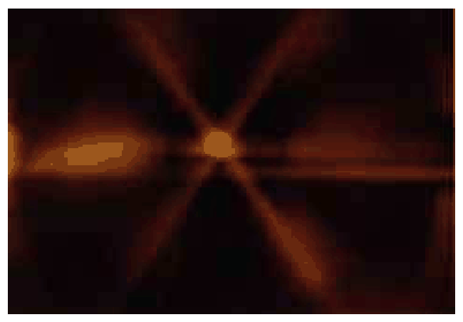
The image above shows sodium atoms (the bright spot in the center) trapped at the intersection of three orthogonal pairs of opposing laser beams. The trapping region is called “optical molasses” because the dissipative optical force resembles the viscous drag on a body moving through molasses.
In this problem you will analyze the basic phenomenon of the interaction between a photon incident on an atom and the basis of the dissipative mechanism in one dimension.
PART I: BASICS OF LASER COOLING
Consider an atom of mass \(m\) moving in the \(+x\) direction with velocity \(v\). For simplicity, we shall consider the problem to be one-dimensional, namely, we shall ignore the \(y\) and \(z\) directions (see figure 1). The atom has two internal energy levels. The energy of the lowest state is considered to be zero and the energy of the excited state to be \(\hbar\omega_0\), where \(\hbar=h/2\pi\). The atom is initially in the lowest state. A laser beam with frequency \(\omega_L\) in the laboratory is directed in the \(-x\) direction and it is incident on the atom. Quantum mechanically the laser is composed of a large number of photons, each with energy \(\hbar\omega_L\) and momentum \(-\hbar q\). A photon can be absorbed by the atom and later spontaneously emitted; this emission can occur with equal probabilities along the \(+x\) and \(-x\) directions. Since the atom moves at non-relativistic speeds, \(v/c\ll1\) (with \(c\) the speed of light) keep terms up to first order in this quantity only. Consider also \(\hbar q/mv\ll1\), namely, that the momentum of the atom is much larger than the momentum of a single photon. In writing your answers, keep only corrections linear in either of the above quantities.
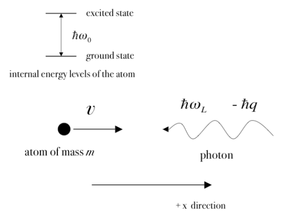
Fig.1 Sketch of an atom of mass \(m\) with velocity \(v\) in the \(+x\) direction, colliding with a photon with energy \(\hbar\omega_L\) and momentum \(-\hbar q\). The atom has two internal states with energy difference \(\hbar\omega_0\).
Assume that the laser frequency \(\omega_L\) is tuned such that, as seen by the moving atom, it is in resonance with the internal transition of the atom. Answer the following questions:
1. Absorption.
| 1a | Write down the resonance condition for the absorption of the photon. | 0.2 |
| 1b | Write down the momentum \(p_{at}\) of the atom after absorption, as seen in the laboratory. | 0.2 |
| 1c | Write down the total energy \(\varepsilon_{at}\) of the atom after absorption, as seen in the laboratory. | 0.2 |
2. Spontaneous emission of a photon in the \(-x\) direction.
At some time after the absorption of the incident photon, the atom may emit a photon in the \(-x\) direction.
| 2a | Write down the energy of the emitted photon, \(\varepsilon_{ph}\), after the emission process in the \(-x\) direction, as seen in the laboratory. | 0.2 |
| 2b | Write down the momentum of the emitted photon \(p_{ph}\), after the emission process in the \(-x\) direction, as seen in the laboratory. | 0.2 |
| 2c | Write down the momentum of the atom \(p_{at}\), after the emission process in the \(-x\) direction, as seen in the laboratory. | 0.2 |
| 2d | Write down the total energy of the atom \(\varepsilon_{at}\), after the emission process in the \(-x\) direction, as seen in the laboratory. | 0.2 |
3. Spontaneous emission of a photon in the \(+x\) direction.
At some time after the absorption of the incident photon, the atom may instead emit a photon in the \(+x\) direction.
| 3a | Write down the energy of the emitted photon, \(\varepsilon_{ph}\), after the emission process in the \(+x\) direction, as seen in the laboratory. | 0.2 |
| 3b | Write down the momentum of the emitted photon \(p_{ph}\), after the emission process in the \(+x\) direction, as seen in the laboratory. | 0.2 |
| 3c | Write down the momentum of the atom \(p_{at}\), after the emission process in the \(+x\) direction, as seen in the laboratory. | 0.2 |
| 3d | Write down the total energy of the atom \(\varepsilon_{at}\), after the emission process in the \(+x\) direction, as seen in the laboratory. | 0.2 |
4. Average emission after the absorption.
The spontaneous emission of a photon in the \(-x\) or in the \(+x\) directions occurs with the same probability. Taking this into account, answer the following questions.
| 4a | Write down the average energy of an emitted photon, \(\varepsilon_{ph}\), after the emission process. | 0.2 |
| 4b | Write down the average momentum of an emitted photon \(p_{ph}\), after the emission process. | 0.2 |
| 4c | Write down the average total energy of the atom \(\varepsilon_{at}\), after the emission process. | 0.2 |
| 4d | Write down the average momentum of the atom \(p_{at}\), after the emission process. | 0.2 |
5. Energy and momentum transfer.
Assuming a complete one-photon absorption-emission process only, as described above, there is a net average momentum and energy transfer between the laser radiation and the atom.
| 5a | Write down the average energy change \(\Delta\varepsilon\) of the atom after a complete one-photon absorption-emission process. | 0.2 |
| 5b | Write down the average momentum change \(\Delta p\) of the atom after a complete one-photon absorption-emission process. | 0.2 |
6. Energy and momentum transfer by a laser beam along the \(+x\) direction.
Consider now that a laser beam of frequency \(\omega'_L\) is incident on the atom along the \(+x\) direction, while the atom moves also in the \(+x\) direction with velocity \(v\). Assuming a resonance condition between the internal transition of the atom and the laser beam, as seen by the atom, answer the following questions:
| 6a | Write down the average energy change \(\Delta\varepsilon\) of the atom after a complete one-photon absorption-emission process. | 0.3 |
| 6b | Write down the average momentum change \(\Delta p\) of the atom after a complete one-photon absorption-emission process. | 0.3 |
PART II: DISSIPATION AND THE FUNDAMENTALS OF OPTICAL MOLASSES
Nature, however, imposes an inherent uncertainty in quantum processes. Thus, the fact that the atom can spontaneously emit a photon in a finite time after absorption, gives as a result that the resonance condition does not have to be obeyed exactly as in the discussion above. That is, the frequency of the laser beams \(\omega_L\) and \(\omega'_L\) may have any value and the absorption-emission process can still occur. These will happen with different (quantum) probabilities and, as one should expect, the maximum probability is found at the exact resonance condition. On the average, the time elapsed between a single process of absorption and emission is called the lifetime of the excited energy level of the atom and it is denoted by \(\Gamma^{-1}\).
Consider a collection of \(N\) atoms at rest in the laboratory frame of reference, and a laser beam of frequency \(\omega_L\) incident on them. The atoms absorb and emit continuously such that there is, on average, \(N_{exc}\) atoms in the excited state (and therefore, \(N-N_{exc}\) atoms in the ground state). A quantum mechanical calculation yields the following result:
\[ N_{exc} = N\frac{\Omega_R^2} {(\omega_0-\omega_L)^2+\dfrac{\Gamma^2}{4}+2\Omega_R^2} \]
where \(\omega_0\) is the resonance frequency of the atomic transition and \(\Omega_R\) is the so-called Rabi frequency; \(\Omega_R^2\) is proportional to the intensity of the laser beam. As mentioned above, you can see that this number is different from zero even if the resonance frequency \(\omega_0\) is different from the frequency of the laser beam \(\omega_L\). An alternative way of expressing the previous result is that the number of absorption-emission processes per unit of time is \(N_{exc}\Gamma\).
Consider the physical situation depicted in Figure 2, in which two counter propagating laser beams with the same but arbitrary frequency \(\omega_L\) are incident on a gas of \(N\) atoms that move in the \(+x\) direction with velocity \(v\).
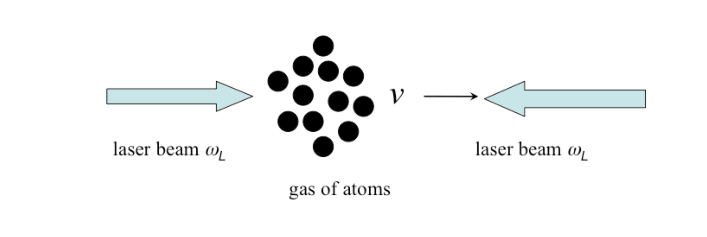
Figure 2. Two counter propagating laser beams with the same but arbitrary frequency \(\omega_L\) are incident on a gas of \(N\) atoms that move in the \(+x\) direction with velocity \(v\).
7. Force on the atomic beam by the lasers.
| 7a | With the information found so far, find the force that the lasers exert on the atomic beam. You should assume that \(mv\gg\hbar q\). | 1.5 |
8. Low velocity limit.
Assume now that the velocity of the atoms is small enough such that you can expand the force up to first order in \(v\).
| 8a | Find an expression for the force found in Question (7a), in this limit. | 1.5 |
Using this result, you can find the conditions for speeding up, slowing down, or no effect at all on the atoms by the laser radiation.
| 8b | Write down the condition to obtain a positive force (speeding up the atoms). | 0.25 |
| 8c | Write down the condition to obtain a zero force. | 0.25 |
| 8d | Write down the condition to obtain a negative force (slowing down the atoms). | 0.25 |
| 8e | Consider now that the atoms are moving with a velocity \(-v\) (in the \(-x\) direction). Write down the condition to obtain a slowing down force on the atoms. | 0.25 |
9. Optical molasses.
In the case of a negative force, one obtains a frictional dissipative force. Assume that initially, at \(t=0\), the gas of atoms has velocity \(v_0\).
| 9a | In the limit of low velocities, find the velocity of the atoms after the laser beams have been on for a time \(\tau\). | 1.5 |
| 9b | Assume now that the gas of atoms is in thermal equilibrium at a temperature \(T_0\). Find the temperature \(T\) after the laser beams have been on for a time \(\tau\). | 0.5 |
This model does not allow you to go to arbitrarily low temperatures.
Official English text of the problem.
Answers
Define \[ \beta=\frac vc,\qquad q=\frac{\omega_L}{c},\qquad q'=\frac{\omega'_L}{c},\qquad K=\frac12mv^2. \] For Part II, define \[ \Delta=\omega_0-\omega_L,\qquad D=\Delta^2+\frac{\Gamma^2}{4}+2\Omega_R^2,\qquad \alpha=\frac{4\hbar q^2\Gamma\Omega_R^2\Delta}{D^2}. \] The two beams are taken to have the same \(\Omega_R\).
Photon quantities below retain their first Doppler correction. Atomic quantities retain the leading recoil correction, omitting products of \(v/c\) and \(\hbar q/(mv)\). The small momentum corrections before this truncation are displayed in the solution. Atomic energies omit the constant rest energy.
- 1a: \(\displaystyle \omega_L(1+\beta)=\omega_0\), equivalently \(\omega_L+qv=\omega_0\).
- 1b: \(\displaystyle p_{at}=mv-\hbar q.\)
- 1c: \(\displaystyle \varepsilon_{at}=K+\hbar\omega_L=K+\hbar\omega_0-\hbar qv.\)
- 2a: \(\displaystyle \varepsilon_{ph}=\hbar\omega_0(1-\beta)\simeq\hbar\omega_L.\)
- 2b: \(\displaystyle p_{ph}=-\frac{\hbar\omega_0}{c}(1-\beta)\simeq-\hbar q.\)
- 2c: \(\displaystyle p_{at}=mv.\)
- 2d: \(\displaystyle \varepsilon_{at}=K.\)
- 3a: \(\displaystyle \varepsilon_{ph}=\hbar\omega_0(1+\beta)\simeq\hbar\omega_L(1+2\beta).\)
- 3b: \(\displaystyle p_{ph}=\frac{\hbar\omega_0}{c}(1+\beta)\simeq\hbar q(1+2\beta).\)
- 3c: \(\displaystyle p_{at}\simeq mv-2\hbar q.\)
- 3d: \(\displaystyle \varepsilon_{at}\simeq K-2\hbar qv.\)
- 4a: \(\displaystyle \langle\varepsilon_{ph}\rangle=\hbar\omega_0.\)
- 4b: \(\displaystyle \langle p_{ph}\rangle=\frac{\hbar\omega_0v}{c^2}\simeq\hbar q\beta.\)
- 4c: \(\displaystyle \langle\varepsilon_{at}\rangle\simeq K-\hbar qv.\)
- 4d: \(\displaystyle \langle p_{at}\rangle\simeq mv-\hbar q.\)
- 5a: \(\displaystyle \Delta\varepsilon=-\frac{\hbar\omega_0v}{c}\simeq-\hbar qv.\)
- 5b: \(\displaystyle \Delta p\simeq-\hbar q.\)
- 6a: \(\displaystyle \Delta\varepsilon=+\frac{\hbar\omega_0v}{c}\simeq+\hbar q'v.\)
- 6b: \(\displaystyle \Delta p\simeq+\hbar q'.\)
- 7a: \[ \boxed{ F(v)=N\hbar q\Gamma\Omega_R^2 \left[ \frac{1}{(\Delta+qv)^2+\Gamma^2/4+2\Omega_R^2} - \frac{1}{(\Delta-qv)^2+\Gamma^2/4+2\Omega_R^2} \right]. } \]
- 8a: \[ \boxed{F(v)\simeq-N\alpha v =-\frac{4N\hbar q^2\Gamma\Omega_R^2(\omega_0-\omega_L)} {\left[(\omega_0-\omega_L)^2+\Gamma^2/4+2\Omega_R^2\right]^2}\,v.} \]
- 8b: \(\displaystyle \omega_L>\omega_0.\)
- 8c: \(\displaystyle \omega_L=\omega_0.\)
- 8d: \(\displaystyle \omega_L<\omega_0.\)
- 8e: \(\displaystyle \omega_L<\omega_0\); the force then points in \(+x\).
- 9a: \(\displaystyle \boxed{v(\tau)=v_0e^{-\alpha\tau/m}}\), with \(\alpha>0\).
- 9b: \(\displaystyle \boxed{T(\tau)=T_0e^{-2\alpha\tau/m}}\).
Solution
The photon energy–momentum relation gives \[ \hbar\omega_L=c\hbar q,\qquad q=\frac{\omega_L}{c}. \] Write the two small parameters as \[ \beta=\frac vc\ll1,\qquad \eta=\frac{\hbar q}{mv}\ll1. \]
The recoil energy \((\hbar q)^2/(2m)\) is quadratic in \(\eta\) relative to the initial atomic kinetic energy, so it is omitted. The change in atomic velocity following absorption is \(-\hbar q/m\); its contribution to a Doppler factor is \[ \frac{\hbar q}{mc}=\eta\beta, \] which is also omitted.
Thus, when calculating emitted photon frequencies, the emitting atom can be assigned velocity \(v\). Momentum corrections of order \(\hbar q\beta=mv\,\eta\beta\) are shown where useful, but omitted from the leading atomic recoil results.
1a. Resonance condition
For a photon propagating in \(-x\), the frequency measured by an atom moving in \(+x\) is, to first order, \[ \omega_{\mathrm{atom}} =\omega_L-\mathbf{k}\cdot\mathbf{v} =\omega_L+qv. \] Resonance requires this frequency to equal \(\omega_0\): \[ \boxed{\omega_L+qv=\omega_0}, \qquad \boxed{\omega_L\left(1+\frac vc\right)=\omega_0}. \]
This also follows from conservation of energy: \[ \frac12mv^2+\hbar\omega_L = \frac{(mv-\hbar q)^2}{2m}+\hbar\omega_0. \] Discarding the recoil energy gives the same condition.
1b. Atomic momentum after absorption
Conservation of momentum gives \[ \boxed{p_{at}=mv-\hbar q}. \]
1c. Atomic energy after absorption
The atom acquires the incident photon’s energy: \[ \boxed{\varepsilon_{at}=\frac12mv^2+\hbar\omega_L}. \] Equivalently, adding its kinetic and internal energies, \[ \varepsilon_{at} = \frac{(mv-\hbar q)^2}{2m}+\hbar\omega_0 \simeq \boxed{\frac12mv^2-\hbar qv+\hbar\omega_0}. \] The resonance condition makes these expressions equal to the retained order.
For the emission questions, let \(s=+1\) denote a photon emitted in \(+x\), and \(s=-1\) a photon emitted in \(-x\). Neglecting recoil in the transition frequency, its energy in the emitting atom’s rest frame is \(\hbar\omega_0\). The first-order Doppler transformation gives \[ \varepsilon_{ph}^{(s)} =\hbar\omega_0(1+s\beta), \qquad p_{ph}^{(s)} =s\frac{\hbar\omega_0}{c}(1+s\beta). \]
2a. Photon energy for emission in \(-x\)
Taking \(s=-1\), \[ \boxed{\varepsilon_{ph}^{(-)} =\hbar\omega_0(1-\beta)}. \] Since \[ \omega_L=\frac{\omega_0}{1+\beta} \simeq\omega_0(1-\beta), \] this is \[ \boxed{\varepsilon_{ph}^{(-)}\simeq\hbar\omega_L}. \]
2b. Photon momentum for emission in \(-x\)
Using \(p_{ph}=-\varepsilon_{ph}/c\), \[ \boxed{p_{ph}^{(-)} =-\frac{\hbar\omega_0}{c}(1-\beta) \simeq-\hbar q}. \]
2c. Atomic momentum after emission in \(-x\)
Conservation of momentum over the complete process gives \[ p_{at}^{(-)} =mv-\hbar q-p_{ph}^{(-)} \simeq mv-\hbar q+\hbar q. \] Therefore \[ \boxed{p_{at}^{(-)}=mv}. \]
2d. Atomic energy after emission in \(-x\)
The emitted photon carries away the energy supplied by the absorbed photon: \[ \varepsilon_{at}^{(-)} =K+\hbar\omega_L-\varepsilon_{ph}^{(-)} \simeq K. \] Thus \[ \boxed{\varepsilon_{at}^{(-)}=\frac12mv^2}. \]
3a. Photon energy for emission in \(+x\)
For \(s=+1\), \[ \boxed{\varepsilon_{ph}^{(+)} =\hbar\omega_0(1+\beta)}. \] Using \(\omega_0=\omega_L(1+\beta)\), \[ \boxed{\varepsilon_{ph}^{(+)} \simeq\hbar\omega_L(1+2\beta)}. \]
3b. Photon momentum for emission in \(+x\)
The momentum is positive: \[ \boxed{p_{ph}^{(+)} =\frac{\hbar\omega_0}{c}(1+\beta) \simeq\hbar q(1+2\beta)}. \]
3c. Atomic momentum after emission in \(+x\)
Momentum conservation, retaining the photon’s Doppler correction temporarily, gives \[ p_{at}^{(+)} =mv-\hbar q-\hbar q(1+2\beta) =mv-2\hbar q-2\hbar q\beta. \] The last term is of relative order \(\eta\beta\) in the atomic momentum. With that mixed correction omitted, \[ \boxed{p_{at}^{(+)}\simeq mv-2\hbar q}. \]
3d. Atomic energy after emission in \(+x\)
The atom returns to its ground state. Conservation of energy gives \[ \begin{aligned} \varepsilon_{at}^{(+)} &=K+\hbar\omega_L-\hbar\omega_0(1+\beta)\\ &\simeq K+\hbar\omega_0(1-\beta) -\hbar\omega_0(1+\beta)\\ &=K-2\hbar\omega_0\beta. \end{aligned} \] At the retained atomic accuracy, \[ \boxed{\varepsilon_{at}^{(+)} \simeq\frac12mv^2-2\hbar qv}. \]
This also follows by expanding \[ \frac{(mv-2\hbar q)^2}{2m} = K-2\hbar qv+\frac{2\hbar^2q^2}{m} \] and discarding the quadratic recoil term.
4a. Average emitted photon energy
The two directions have equal probability: \[ \begin{aligned} \langle\varepsilon_{ph}\rangle &=\frac12\hbar\omega_0(1-\beta) +\frac12\hbar\omega_0(1+\beta)\\ &=\boxed{\hbar\omega_0}. \end{aligned} \]
4b. Average emitted photon momentum
Averaging the signed momenta, \[ \begin{aligned} \langle p_{ph}\rangle &=\frac12\left[ -\frac{\hbar\omega_0}{c}(1-\beta) +\frac{\hbar\omega_0}{c}(1+\beta) \right]\\ &=\boxed{\frac{\hbar\omega_0v}{c^2}} \simeq\boxed{\hbar q\beta}. \end{aligned} \]
Although the directions are equally probable, the two photon energies differ in the laboratory. Their mean laboratory momentum is consequently small and positive.
Relative to the atomic momentum, this mean is of order \[ \frac{\langle p_{ph}\rangle}{mv}\simeq\eta\beta. \] It is therefore omitted in the leading atomic momentum changes below.
4c. Average atomic energy
Using the results of 2d and 3d, \[ \langle\varepsilon_{at}\rangle =\frac12K+\frac12(K-2\hbar qv). \] Hence \[ \boxed{\langle\varepsilon_{at}\rangle \simeq K-\hbar qv}. \]
Equivalently, \[ \langle\varepsilon_{at}\rangle =K+\hbar\omega_L-\hbar\omega_0. \]
4d. Average atomic momentum
Before discarding the mixed correction, momentum conservation gives \[ \langle p_{at}\rangle =mv-\hbar q-\langle p_{ph}\rangle =mv-\hbar q-\frac{\hbar\omega_0v}{c^2}. \] Thus, to the requested leading atomic recoil order, \[ \boxed{\langle p_{at}\rangle\simeq mv-\hbar q}. \]
5a. Average atomic energy change
Subtracting the initial energy, \[ \Delta\varepsilon =\langle\varepsilon_{at}\rangle-K =\hbar(\omega_L-\omega_0). \] The resonance condition yields \[ \boxed{\Delta\varepsilon =-\frac{\hbar\omega_0v}{c} \simeq-\hbar qv}. \]
The emitted photon has, on average, more energy than the absorbed photon. That difference comes from the atom’s kinetic energy.
5b. Average atomic momentum change
Subtracting the initial momentum from 4d gives \[ \boxed{\Delta p\simeq-\hbar q}. \] The smaller correction before truncation is \[ -\langle p_{ph}\rangle =-\frac{\hbar\omega_0v}{c^2}. \] At leading recoil order, the energy and momentum changes obey \[ \Delta\varepsilon\simeq v\,\Delta p. \]
6a. Energy change for a laser propagating in \(+x\)
The atom now moves away from the incident light. The resonance condition is \[ \omega'_L\left(1-\frac vc\right)=\omega_0, \] so \[ \omega'_L\simeq\omega_0(1+\beta). \]
The mean emitted photon energy remains \(\hbar\omega_0\). Therefore \[ \Delta\varepsilon =\hbar(\omega'_L-\omega_0) =\boxed{\frac{\hbar\omega_0v}{c}} \simeq\boxed{\hbar q'v}, \qquad q'=\frac{\omega'_L}{c}. \] The atom gains kinetic energy.
6b. Momentum change for a laser propagating in \(+x\)
The absorbed photon supplies momentum \(+\hbar q'\). Consequently, \[ \Delta p =\hbar q'-\frac{\hbar\omega_0v}{c^2} \simeq\boxed{+\hbar q'}. \] The omitted second term is again a mixed Doppler–recoil correction in the atomic momentum.
7a. Force from the two laser beams
Use the supplied scattering law separately for the two beams, taking their intensities, and hence their Rabi frequencies, to be equal.
Let \(+\) label the beam propagating in \(+x\), and \(-\) the beam propagating in \(-x\). The frequencies seen by the moving atoms are \[ \omega_{\mathrm{atom},+}=\omega_L-qv, \qquad \omega_{\mathrm{atom},-}=\omega_L+qv. \] Thus their detunings from the atomic transition are \[ \omega_0-\omega_{\mathrm{atom},+}=\Delta+qv, \qquad \omega_0-\omega_{\mathrm{atom},-}=\Delta-qv. \]
The total numbers of scattering events per unit time are \[ R_+(v) = \frac{N\Gamma\Omega_R^2} {(\Delta+qv)^2+\Gamma^2/4+2\Omega_R^2}, \] \[ R_-(v) = \frac{N\Gamma\Omega_R^2} {(\Delta-qv)^2+\Gamma^2/4+2\Omega_R^2}. \]
At leading recoil order, each event transfers \(+\hbar q\) or \(-\hbar q\), respectively. Therefore \[ F(v)=\hbar qR_+(v)-\hbar qR_-(v), \] giving \[ \boxed{ F(v)=N\hbar q\Gamma\Omega_R^2 \left[ \frac{1}{(\Delta+qv)^2+\Gamma^2/4+2\Omega_R^2} - \frac{1}{(\Delta-qv)^2+\Gamma^2/4+2\Omega_R^2} \right]. } \]
This is the force on all \(N\) atoms. The force on one atom is \(F/N\).
The Doppler shift \(qv\) is retained in the scattering probabilities: it can be significant compared with the transition linewidth even when \(v/c\) is very small.
8a. Low-velocity expansion
Put \[ D=\Delta^2+\frac{\Gamma^2}{4}+2\Omega_R^2. \] For sufficiently small \(qv\), \[ \frac{1}{(\Delta\pm qv)^2+\Gamma^2/4+2\Omega_R^2} \simeq \frac1D\mp\frac{2\Delta qv}{D^2}. \] For example, \(|qv|\ll\sqrt D\) is a sufficient small-velocity condition.
Subtracting the two expansions, \[ F(v) \simeq N\hbar q\Gamma\Omega_R^2 \left(-\frac{4\Delta qv}{D^2}\right). \] Hence \[ \boxed{F(v)\simeq-N\alpha v}, \qquad \boxed{\alpha=\frac{4\hbar q^2\Gamma\Omega_R^2\Delta}{D^2}}. \]
The coefficient \(\alpha\) has units of mass per time, so \(\alpha v\) has units of force.
8b. Positive force
For \(v>0\), all factors in \(\alpha\) except \(\Delta\) are positive. A positive force requires \[ \Delta<0. \] Therefore \[ \boxed{\omega_L>\omega_0}. \] This is blue detuning.
8c. Zero force
For nonzero intensity and a moving atom, the detuning condition is \[ \Delta=0, \] or \[ \boxed{\omega_L=\omega_0}. \] The two scattering rates are then equal. Independently, symmetry also gives zero force at \(v=0\).
8d. Negative force
For \(v>0\), a negative force requires \(\alpha>0\), hence \[ \boxed{\omega_L<\omega_0}. \] This is red detuning. The counterpropagating beam is Doppler shifted closer to resonance and is scattered more strongly.
8e. Slowing atoms moving in \(-x\)
For velocity \(-v\), with \(v>0\), \[ F(-v)=+N\alpha v. \] Slowing requires a force in \(+x\), so again \(\alpha>0\). Thus \[ \boxed{\omega_L<\omega_0}. \]
Red detuning produces a force opposing motion in either direction.
9a. Velocity after time \(\tau\)
For red detuning, \(\alpha>0\). The gas has total mass \(Nm\), so Newton’s second law gives \[ Nm\frac{dv}{dt}=-N\alpha v. \] The factor \(N\) cancels: \[ \frac{dv}{dt}=-\frac{\alpha}{m}v. \] Integrating with \(v(0)=v_0\), \[ \boxed{v(\tau)=v_0e^{-\alpha\tau/m}}. \]
Explicitly, \[ \boxed{ v(\tau)=v_0 \exp\!\left[ -\frac{4\hbar q^2\Gamma\Omega_R^2(\omega_0-\omega_L)\tau} {m\left[(\omega_0-\omega_L)^2+\Gamma^2/4+2\Omega_R^2\right]^2} \right]. } \]
The velocity decay time is \(m/\alpha\).
9b. Temperature after time \(\tau\)
In this deterministic friction model, each atomic velocity is multiplied by \[ e^{-\alpha\tau/m}. \] Therefore the variance of the velocities is multiplied by \[ e^{-2\alpha\tau/m}. \]
For one-dimensional thermal motion, \[ m\left\langle (v-\langle v\rangle)^2\right\rangle=k_BT. \] Consequently, \[ \boxed{T(\tau)=T_0e^{-2\alpha\tau/m}}. \]
Explicitly, \[ \boxed{ T(\tau)=T_0 \exp\!\left[ -\frac{8\hbar q^2\Gamma\Omega_R^2(\omega_0-\omega_L)\tau} {m\left[(\omega_0-\omega_L)^2+\Gamma^2/4+2\Omega_R^2\right]^2} \right]. } \]
This exponential cannot be extrapolated to arbitrarily low temperatures. The calculation omitted quadratic recoil contributions and the fluctuations caused by random scattering events. In particular, the assumption \(mv\gg\hbar q\), applied to a typical thermal speed, requires \[ k_BT\gg\frac{(\hbar q)^2}{m}. \] As the atoms cool, the terms omitted from this model become relevant.
The solution was checked against the official solution. Where this solution differs from the official solution, the official solution contains an error or a misprint.
IPhO 2009 · Theorieaufgabe 2
Doppler-Laserkühlung und optische Melasse
Ziel dieser Aufgabe ist es, eine einfache Theorie zum Verständnis der sogenannten „Laserkühlung“ und „optischen Melasse“ zu entwickeln. Dabei geht es um die Kühlung eines Strahls neutraler Atome, typischerweise Alkaliatome, durch gegenläufige Laserstrahlen gleicher Frequenz. Dies ist Teil der Arbeiten, für die S. Chu, P. Phillips und C. Cohen-Tannoudji 1997 den Nobelpreis für Physik erhielten.
Das obige Bild zeigt Natriumatome (den hellen Fleck in der Mitte), die am Schnittpunkt dreier zueinander senkrechter Paare gegenläufiger Laserstrahlen eingefangen sind. Der Bereich, in dem die Atome eingefangen sind, wird als „optische Melasse“ bezeichnet, weil die dissipative optische Kraft der viskosen Widerstandskraft auf einen Körper ähnelt, der sich durch Melasse bewegt.
In dieser Aufgabe untersuchen Sie das grundlegende Phänomen der Wechselwirkung zwischen einem auf ein Atom treffenden Photon und dem Atom sowie die Grundlage des dissipativen Mechanismus in einer Dimension.
TEIL I: GRUNDLAGEN DER LASERKÜHLUNG
Betrachten Sie ein Atom der Masse \(m\), das sich mit der Geschwindigkeit \(v\) in \(+x\)-Richtung bewegt. Der Einfachheit halber betrachten wir das Problem als eindimensional, vernachlässigen also die \(y\)- und \(z\)-Richtungen (siehe Abbildung 1). Das Atom besitzt zwei innere Energieniveaus. Die Energie des niedrigsten Zustands wird gleich null gesetzt, die Energie des angeregten Zustands gleich \(\hbar\omega_0\), wobei \(\hbar=h/2\pi\). Das Atom befindet sich anfangs im niedrigsten Zustand. Ein Laserstrahl mit der Frequenz \(\omega_L\) im Laborsystem ist in \(-x\)-Richtung gerichtet und trifft auf das Atom. Quantenmechanisch besteht der Laserstrahl aus einer großen Anzahl von Photonen, die jeweils die Energie \(\hbar\omega_L\) und den Impuls \(-\hbar q\) besitzen. Ein Photon kann vom Atom absorbiert und später spontan emittiert werden; diese Emission kann mit gleicher Wahrscheinlichkeit in \(+x\)- oder \(-x\)-Richtung erfolgen. Da sich das Atom mit nichtrelativistischen Geschwindigkeiten bewegt, \(v/c\ll1\) (wobei \(c\) die Lichtgeschwindigkeit ist), berücksichtigen Sie nur Terme bis zur ersten Ordnung in dieser Größe. Nehmen Sie außerdem \(\hbar q/mv\ll1\) an, also dass der Impuls des Atoms viel größer als der Impuls eines einzelnen Photons ist. Behalten Sie in Ihren Antworten nur Korrekturen bei, die in einer der beiden obigen Größen linear sind.
Abb.1 Skizze eines Atoms der Masse \(m\) mit der Geschwindigkeit \(v\) in \(+x\)-Richtung, das mit einem Photon der Energie \(\hbar\omega_L\) und des Impulses \(-\hbar q\) zusammenstößt. Das Atom besitzt zwei innere Zustände mit der Energiedifferenz \(\hbar\omega_0\).
Nehmen Sie an, dass die Laserfrequenz \(\omega_L\) so abgestimmt ist, dass sie aus Sicht des bewegten Atoms mit dessen innerem Übergang in Resonanz ist. Beantworten Sie die folgenden Fragen:
1. Absorption.
| 1a | Geben Sie die Resonanzbedingung für die Absorption des Photons an. | 0.2 |
| 1b | Geben Sie den Impuls \(p_{at}\) des Atoms nach der Absorption im Laborsystem an. | 0.2 |
| 1c | Geben Sie die Gesamtenergie \(\varepsilon_{at}\) des Atoms nach der Absorption im Laborsystem an. | 0.2 |
2. Spontane Emission eines Photons in \(-x\)-Richtung.
Einige Zeit nach der Absorption des einfallenden Photons kann das Atom ein Photon in \(-x\)-Richtung emittieren.
| 2a | Geben Sie die Energie des emittierten Photons, \(\varepsilon_{ph}\), nach dem Emissionsvorgang in \(-x\)-Richtung im Laborsystem an. | 0.2 |
| 2b | Geben Sie den Impuls des emittierten Photons \(p_{ph}\) nach dem Emissionsvorgang in \(-x\)-Richtung im Laborsystem an. | 0.2 |
| 2c | Geben Sie den Impuls des Atoms \(p_{at}\) nach dem Emissionsvorgang in \(-x\)-Richtung im Laborsystem an. | 0.2 |
| 2d | Geben Sie die Gesamtenergie des Atoms \(\varepsilon_{at}\) nach dem Emissionsvorgang in \(-x\)-Richtung im Laborsystem an. | 0.2 |
3. Spontane Emission eines Photons in \(+x\)-Richtung.
Einige Zeit nach der Absorption des einfallenden Photons kann das Atom stattdessen ein Photon in \(+x\)-Richtung emittieren.
| 3a | Geben Sie die Energie des emittierten Photons, \(\varepsilon_{ph}\), nach dem Emissionsvorgang in \(+x\)-Richtung im Laborsystem an. | 0.2 |
| 3b | Geben Sie den Impuls des emittierten Photons \(p_{ph}\) nach dem Emissionsvorgang in \(+x\)-Richtung im Laborsystem an. | 0.2 |
| 3c | Geben Sie den Impuls des Atoms \(p_{at}\) nach dem Emissionsvorgang in \(+x\)-Richtung im Laborsystem an. | 0.2 |
| 3d | Geben Sie die Gesamtenergie des Atoms \(\varepsilon_{at}\) nach dem Emissionsvorgang in \(+x\)-Richtung im Laborsystem an. | 0.2 |
4. Mittelwerte der Emission nach der Absorption.
Die spontane Emission eines Photons in \(-x\)- oder \(+x\)-Richtung erfolgt mit gleicher Wahrscheinlichkeit. Beantworten Sie unter Berücksichtigung dieser Tatsache die folgenden Fragen.
| 4a | Geben Sie die mittlere Energie eines emittierten Photons, \(\varepsilon_{ph}\), nach dem Emissionsvorgang an. | 0.2 |
| 4b | Geben Sie den mittleren Impuls eines emittierten Photons \(p_{ph}\) nach dem Emissionsvorgang an. | 0.2 |
| 4c | Geben Sie die mittlere Gesamtenergie des Atoms \(\varepsilon_{at}\) nach dem Emissionsvorgang an. | 0.2 |
| 4d | Geben Sie den mittleren Impuls des Atoms \(p_{at}\) nach dem Emissionsvorgang an. | 0.2 |
5. Energie- und Impulsübertragung.
Betrachtet man nur einen vollständigen Absorptions-Emissions-Prozess eines einzelnen Photons wie oben beschrieben, so ergibt sich im Mittel eine Nettoübertragung von Impuls und Energie zwischen der Laserstrahlung und dem Atom.
| 5a | Geben Sie die mittlere Energieänderung \(\Delta\varepsilon\) des Atoms nach einem vollständigen Absorptions-Emissions-Prozess eines einzelnen Photons an. | 0.2 |
| 5b | Geben Sie die mittlere Impulsänderung \(\Delta p\) des Atoms nach einem vollständigen Absorptions-Emissions-Prozess eines einzelnen Photons an. | 0.2 |
6. Energie- und Impulsübertragung durch einen Laserstrahl in \(+x\)-Richtung.
Betrachten Sie nun einen Laserstrahl der Frequenz \(\omega'_L\), der in \(+x\)-Richtung auf das Atom trifft, während sich das Atom ebenfalls mit der Geschwindigkeit \(v\) in \(+x\)-Richtung bewegt. Beantworten Sie die folgenden Fragen unter der Annahme, dass aus Sicht des Atoms die Resonanzbedingung zwischen seinem inneren Übergang und dem Laserstrahl erfüllt ist:
| 6a | Geben Sie die mittlere Energieänderung \(\Delta\varepsilon\) des Atoms nach einem vollständigen Absorptions-Emissions-Prozess eines einzelnen Photons an. | 0.3 |
| 6b | Geben Sie die mittlere Impulsänderung \(\Delta p\) des Atoms nach einem vollständigen Absorptions-Emissions-Prozess eines einzelnen Photons an. | 0.3 |
TEIL II: DISSIPATION UND GRUNDLAGEN DER OPTISCHEN MELASSE
Die Natur bringt jedoch eine inhärente Unschärfe in Quantenprozessen mit sich. So hat die Tatsache, dass das Atom ein Photon innerhalb einer endlichen Zeit nach der Absorption spontan emittieren kann, zur Folge, dass die Resonanzbedingung nicht wie in der obigen Betrachtung exakt erfüllt sein muss. Das heißt, die Frequenzen der Laserstrahlen \(\omega_L\) und \(\omega'_L\) können beliebige Werte annehmen, und der Absorptions-Emissions-Prozess kann dennoch stattfinden. Diese Prozesse treten mit unterschiedlichen (quantenmechanischen) Wahrscheinlichkeiten auf, wobei erwartungsgemäß die größte Wahrscheinlichkeit bei exakter Erfüllung der Resonanzbedingung vorliegt. Die im Mittel zwischen der Absorption und der Emission bei einem einzelnen Prozess verstrichene Zeit heißt Lebensdauer des angeregten Energieniveaus des Atoms und wird mit \(\Gamma^{-1}\) bezeichnet.
Betrachten Sie eine Ansammlung von \(N\) Atomen, die im Laborsystem ruhen, und einen auf sie einfallenden Laserstrahl der Frequenz \(\omega_L\). Die Atome absorbieren und emittieren fortlaufend, sodass sich im Mittel \(N_{exc}\) Atome im angeregten Zustand befinden (und somit \(N-N_{exc}\) Atome im Grundzustand). Eine quantenmechanische Rechnung liefert das folgende Ergebnis:
\[ N_{exc} = N\frac{\Omega_R^2} {(\omega_0-\omega_L)^2+\dfrac{\Gamma^2}{4}+2\Omega_R^2} \]
Dabei ist \(\omega_0\) die Resonanzfrequenz des atomaren Übergangs und \(\Omega_R\) die sogenannte Rabi-Frequenz; \(\Omega_R^2\) ist proportional zur Intensität des Laserstrahls. Wie oben erwähnt, erkennen Sie, dass diese Zahl auch dann von null verschieden ist, wenn die Resonanzfrequenz \(\omega_0\) von der Frequenz des Laserstrahls \(\omega_L\) abweicht. Das vorherige Ergebnis lässt sich auch so ausdrücken, dass die Anzahl der Absorptions-Emissions-Prozesse pro Zeiteinheit \(N_{exc}\Gamma\) beträgt.
Betrachten Sie die in Abbildung 2 dargestellte physikalische Situation, in der zwei gegenläufige Laserstrahlen mit gleicher, aber beliebiger Frequenz \(\omega_L\) auf ein Gas aus \(N\) Atomen treffen, die sich mit der Geschwindigkeit \(v\) in \(+x\)-Richtung bewegen.
Abbildung 2. Zwei gegenläufige Laserstrahlen mit gleicher, aber beliebiger Frequenz \(\omega_L\) treffen auf ein Gas aus \(N\) Atomen, die sich mit der Geschwindigkeit \(v\) in \(+x\)-Richtung bewegen.
7. Kraft der Laser auf den Atomstrahl.
| 7a | Bestimmen Sie mithilfe der bisher gewonnenen Erkenntnisse die Kraft, welche die Laser auf den Atomstrahl ausüben. Nehmen Sie dabei \(mv\gg\hbar q\) an. | 1.5 |
8. Grenzfall kleiner Geschwindigkeiten.
Nehmen Sie nun an, dass die Geschwindigkeit der Atome so klein ist, dass Sie die Kraft bis zur ersten Ordnung in \(v\) entwickeln können.
| 8a | Bestimmen Sie in diesem Grenzfall einen Ausdruck für die in Frage (7a) ermittelte Kraft. | 1.5 |
Mithilfe dieses Ergebnisses können Sie die Bedingungen bestimmen, unter denen die Laserstrahlung die Atome beschleunigt, abbremst oder überhaupt nicht beeinflusst.
| 8b | Geben Sie die Bedingung für eine positive Kraft an (Beschleunigung der Atome). | 0.25 |
| 8c | Geben Sie die Bedingung für eine verschwindende Kraft an. | 0.25 |
| 8d | Geben Sie die Bedingung für eine negative Kraft an (Abbremsung der Atome). | 0.25 |
| 8e | Betrachten Sie nun Atome, die sich mit der Geschwindigkeit \(-v\) (in \(-x\)-Richtung) bewegen. Geben Sie die Bedingung für eine die Atome abbremsende Kraft an. | 0.25 |
9. Optische Melasse.
Im Fall einer negativen Kraft erhält man eine dissipative Reibungskraft. Nehmen Sie an, dass das Gas aus Atomen anfangs, bei \(t=0\), die Geschwindigkeit \(v_0\) besitzt.
| 9a | Bestimmen Sie im Grenzfall kleiner Geschwindigkeiten die Geschwindigkeit der Atome, nachdem die Laserstrahlen für eine Zeit \(\tau\) eingeschaltet waren. | 1.5 |
| 9b | Nehmen Sie nun an, dass sich das Gas aus Atomen bei einer Temperatur \(T_0\) im thermischen Gleichgewicht befindet. Bestimmen Sie die Temperatur \(T\), nachdem die Laserstrahlen für eine Zeit \(\tau\) eingeschaltet waren. | 0.5 |
Dieses Modell erlaubt es nicht, beliebig niedrige Temperaturen zu erreichen.
Aufgabentext aus dem offiziellen englischen Text übersetzt.
Antworten
Wir definieren \[ \beta=\frac vc,\qquad q=\frac{\omega_L}{c},\qquad q'=\frac{\omega'_L}{c},\qquad K=\frac12mv^2. \] Für Teil II definieren wir \[ \Delta=\omega_0-\omega_L,\qquad D=\Delta^2+\frac{\Gamma^2}{4}+2\Omega_R^2,\qquad \alpha=\frac{4\hbar q^2\Gamma\Omega_R^2\Delta}{D^2}. \] Für die beiden Strahlen wird derselbe Wert von \(\Omega_R\) angenommen.
Bei den nachfolgenden Photonengrößen wird die erste Doppler-Korrektur beibehalten. Bei den atomaren Größen wird die führende Rückstoßkorrektur beibehalten, während Produkte aus \(v/c\) und \(\hbar q/(mv)\) vernachlässigt werden. Die kleinen Impulskorrekturen vor dieser Beschränkung werden in der Lösung angegeben. Bei den atomaren Energien wird die konstante Ruheenergie weggelassen.
- 1a: \(\displaystyle \omega_L(1+\beta)=\omega_0\), äquivalent dazu \(\omega_L+qv=\omega_0\).
- 1b: \(\displaystyle p_{at}=mv-\hbar q.\)
- 1c: \(\displaystyle \varepsilon_{at}=K+\hbar\omega_L=K+\hbar\omega_0-\hbar qv.\)
- 2a: \(\displaystyle \varepsilon_{ph}=\hbar\omega_0(1-\beta)\simeq\hbar\omega_L.\)
- 2b: \(\displaystyle p_{ph}=-\frac{\hbar\omega_0}{c}(1-\beta)\simeq-\hbar q.\)
- 2c: \(\displaystyle p_{at}=mv.\)
- 2d: \(\displaystyle \varepsilon_{at}=K.\)
- 3a: \(\displaystyle \varepsilon_{ph}=\hbar\omega_0(1+\beta)\simeq\hbar\omega_L(1+2\beta).\)
- 3b: \(\displaystyle p_{ph}=\frac{\hbar\omega_0}{c}(1+\beta)\simeq\hbar q(1+2\beta).\)
- 3c: \(\displaystyle p_{at}\simeq mv-2\hbar q.\)
- 3d: \(\displaystyle \varepsilon_{at}\simeq K-2\hbar qv.\)
- 4a: \(\displaystyle \langle\varepsilon_{ph}\rangle=\hbar\omega_0.\)
- 4b: \(\displaystyle \langle p_{ph}\rangle=\frac{\hbar\omega_0v}{c^2}\simeq\hbar q\beta.\)
- 4c: \(\displaystyle \langle\varepsilon_{at}\rangle\simeq K-\hbar qv.\)
- 4d: \(\displaystyle \langle p_{at}\rangle\simeq mv-\hbar q.\)
- 5a: \(\displaystyle \Delta\varepsilon=-\frac{\hbar\omega_0v}{c}\simeq-\hbar qv.\)
- 5b: \(\displaystyle \Delta p\simeq-\hbar q.\)
- 6a: \(\displaystyle \Delta\varepsilon=+\frac{\hbar\omega_0v}{c}\simeq+\hbar q'v.\)
- 6b: \(\displaystyle \Delta p\simeq+\hbar q'.\)
- 7a: \[ \boxed{ F(v)=N\hbar q\Gamma\Omega_R^2 \left[ \frac{1}{(\Delta+qv)^2+\Gamma^2/4+2\Omega_R^2} - \frac{1}{(\Delta-qv)^2+\Gamma^2/4+2\Omega_R^2} \right]. } \]
- 8a: \[ \boxed{F(v)\simeq-N\alpha v =-\frac{4N\hbar q^2\Gamma\Omega_R^2(\omega_0-\omega_L)} {\left[(\omega_0-\omega_L)^2+\Gamma^2/4+2\Omega_R^2\right]^2}\,v.} \]
- 8b: \(\displaystyle \omega_L>\omega_0.\)
- 8c: \(\displaystyle \omega_L=\omega_0.\)
- 8d: \(\displaystyle \omega_L<\omega_0.\)
- 8e: \(\displaystyle \omega_L<\omega_0\); die Kraft zeigt dann in \(+x\)-Richtung.
- 9a: \(\displaystyle \boxed{v(\tau)=v_0e^{-\alpha\tau/m}}\), mit \(\alpha>0\).
- 9b: \(\displaystyle \boxed{T(\tau)=T_0e^{-2\alpha\tau/m}}\).
Lösung
Aus der Energie-Impuls-Beziehung des Photons folgt \[ \hbar\omega_L=c\hbar q,\qquad q=\frac{\omega_L}{c}. \] Wir schreiben die beiden kleinen Parameter als \[ \beta=\frac vc\ll1,\qquad \eta=\frac{\hbar q}{mv}\ll1. \]
Die Rückstoßenergie \((\hbar q)^2/(2m)\) ist relativ zur anfänglichen kinetischen Energie des Atoms quadratisch in \(\eta\) und wird daher vernachlässigt. Die Änderung der Atomgeschwindigkeit infolge der Absorption beträgt \(-\hbar q/m\); ihr Beitrag zu einem Doppler-Faktor ist \[ \frac{\hbar q}{mc}=\eta\beta, \] und wird ebenfalls vernachlässigt.
Bei der Berechnung der Frequenzen emittierter Photonen kann dem emittierenden Atom somit die Geschwindigkeit \(v\) zugeordnet werden. Impulskorrekturen der Ordnung \(\hbar q\beta=mv\,\eta\beta\) werden angegeben, wo dies hilfreich ist, in den Ergebnissen für den führenden atomaren Rückstoß jedoch weggelassen.
1a. Resonanzbedingung
Für ein Photon, das sich in \(-x\)-Richtung ausbreitet, ist die von einem in \(+x\)-Richtung bewegten Atom gemessene Frequenz in erster Ordnung \[ \omega_{\mathrm{atom}} =\omega_L-\mathbf{k}\cdot\mathbf{v} =\omega_L+qv. \] Resonanz erfordert, dass diese Frequenz gleich \(\omega_0\) ist: \[ \boxed{\omega_L+qv=\omega_0}, \qquad \boxed{\omega_L\left(1+\frac vc\right)=\omega_0}. \]
Dies folgt auch aus der Energieerhaltung: \[ \frac12mv^2+\hbar\omega_L = \frac{(mv-\hbar q)^2}{2m}+\hbar\omega_0. \] Vernachlässigt man die Rückstoßenergie, erhält man dieselbe Bedingung.
1b. Impuls des Atoms nach der Absorption
Aus der Impulserhaltung folgt \[ \boxed{p_{at}=mv-\hbar q}. \]
1c. Energie des Atoms nach der Absorption
Das Atom nimmt die Energie des einfallenden Photons auf: \[ \boxed{\varepsilon_{at}=\frac12mv^2+\hbar\omega_L}. \] Gleichwertig ergibt sich durch Addition seiner kinetischen und inneren Energie \[ \varepsilon_{at} = \frac{(mv-\hbar q)^2}{2m}+\hbar\omega_0 \simeq \boxed{\frac12mv^2-\hbar qv+\hbar\omega_0}. \] Aufgrund der Resonanzbedingung sind diese Ausdrücke bis zur berücksichtigten Ordnung gleich.
Für die Fragen zur Emission bezeichne \(s=+1\) ein in \(+x\)-Richtung emittiertes Photon und \(s=-1\) ein in \(-x\)-Richtung emittiertes Photon. Vernachlässigt man den Rückstoß in der Übergangsfrequenz, so ist seine Energie im Ruhesystem des emittierenden Atoms \(\hbar\omega_0\). Die Doppler-Transformation erster Ordnung ergibt \[ \varepsilon_{ph}^{(s)} =\hbar\omega_0(1+s\beta), \qquad p_{ph}^{(s)} =s\frac{\hbar\omega_0}{c}(1+s\beta). \]
2a. Photonenenergie bei Emission in \(-x\)-Richtung
Mit \(s=-1\) folgt \[ \boxed{\varepsilon_{ph}^{(-)} =\hbar\omega_0(1-\beta)}. \] Da \[ \omega_L=\frac{\omega_0}{1+\beta} \simeq\omega_0(1-\beta), \] ergibt sich \[ \boxed{\varepsilon_{ph}^{(-)}\simeq\hbar\omega_L}. \]
2b. Photonenimpuls bei Emission in \(-x\)-Richtung
Mit \(p_{ph}=-\varepsilon_{ph}/c\) folgt \[ \boxed{p_{ph}^{(-)} =-\frac{\hbar\omega_0}{c}(1-\beta) \simeq-\hbar q}. \]
2c. Impuls des Atoms nach der Emission in \(-x\)-Richtung
Die Impulserhaltung für den vollständigen Prozess ergibt \[ p_{at}^{(-)} =mv-\hbar q-p_{ph}^{(-)} \simeq mv-\hbar q+\hbar q. \] Daher gilt \[ \boxed{p_{at}^{(-)}=mv}. \]
2d. Energie des Atoms nach der Emission in \(-x\)-Richtung
Das emittierte Photon trägt die Energie fort, die das absorbierte Photon zugeführt hat: \[ \varepsilon_{at}^{(-)} =K+\hbar\omega_L-\varepsilon_{ph}^{(-)} \simeq K. \] Somit gilt \[ \boxed{\varepsilon_{at}^{(-)}=\frac12mv^2}. \]
3a. Photonenenergie bei Emission in \(+x\)-Richtung
Für \(s=+1\) gilt \[ \boxed{\varepsilon_{ph}^{(+)} =\hbar\omega_0(1+\beta)}. \] Mit \(\omega_0=\omega_L(1+\beta)\) folgt \[ \boxed{\varepsilon_{ph}^{(+)} \simeq\hbar\omega_L(1+2\beta)}. \]
3b. Photonenimpuls bei Emission in \(+x\)-Richtung
Der Impuls ist positiv: \[ \boxed{p_{ph}^{(+)} =\frac{\hbar\omega_0}{c}(1+\beta) \simeq\hbar q(1+2\beta)}. \]
3c. Impuls des Atoms nach der Emission in \(+x\)-Richtung
Die Impulserhaltung ergibt, wenn die Doppler-Korrektur des Photons vorübergehend beibehalten wird, \[ p_{at}^{(+)} =mv-\hbar q-\hbar q(1+2\beta) =mv-2\hbar q-2\hbar q\beta. \] Der letzte Term hat im atomaren Impuls die relative Ordnung \(\eta\beta\). Unter Vernachlässigung dieser gemischten Korrektur folgt \[ \boxed{p_{at}^{(+)}\simeq mv-2\hbar q}. \]
3d. Energie des Atoms nach der Emission in \(+x\)-Richtung
Das Atom kehrt in seinen Grundzustand zurück. Die Energieerhaltung ergibt \[ \begin{aligned} \varepsilon_{at}^{(+)} &=K+\hbar\omega_L-\hbar\omega_0(1+\beta)\\ &\simeq K+\hbar\omega_0(1-\beta) -\hbar\omega_0(1+\beta)\\ &=K-2\hbar\omega_0\beta. \end{aligned} \] Mit der für die atomaren Größen beibehaltenen Genauigkeit gilt \[ \boxed{\varepsilon_{at}^{(+)} \simeq\frac12mv^2-2\hbar qv}. \]
Dies folgt auch durch Ausmultiplizieren von \[ \frac{(mv-2\hbar q)^2}{2m} = K-2\hbar qv+\frac{2\hbar^2q^2}{m} \] und Vernachlässigen des quadratischen Rückstoßterms.
4a. Mittlere Energie des emittierten Photons
Die beiden Richtungen sind gleich wahrscheinlich: \[ \begin{aligned} \langle\varepsilon_{ph}\rangle &=\frac12\hbar\omega_0(1-\beta) +\frac12\hbar\omega_0(1+\beta)\\ &=\boxed{\hbar\omega_0}. \end{aligned} \]
4b. Mittlerer Impuls des emittierten Photons
Die Mittelung der vorzeichenbehafteten Impulse ergibt \[ \begin{aligned} \langle p_{ph}\rangle &=\frac12\left[ -\frac{\hbar\omega_0}{c}(1-\beta) +\frac{\hbar\omega_0}{c}(1+\beta) \right]\\ &=\boxed{\frac{\hbar\omega_0v}{c^2}} \simeq\boxed{\hbar q\beta}. \end{aligned} \]
Obwohl die Richtungen gleich wahrscheinlich sind, unterscheiden sich die beiden Photonenenergien im Laborsystem. Ihr mittlerer Impuls im Laborsystem ist daher klein und positiv.
Relativ zum Impuls des Atoms hat dieser Mittelwert die Ordnung \[ \frac{\langle p_{ph}\rangle}{mv}\simeq\eta\beta. \] Er wird deshalb bei den nachfolgenden führenden Änderungen des atomaren Impulses vernachlässigt.
4c. Mittlere Energie des Atoms
Mit den Ergebnissen aus 2d und 3d gilt \[ \langle\varepsilon_{at}\rangle =\frac12K+\frac12(K-2\hbar qv). \] Daraus folgt \[ \boxed{\langle\varepsilon_{at}\rangle \simeq K-\hbar qv}. \]
Gleichwertig gilt \[ \langle\varepsilon_{at}\rangle =K+\hbar\omega_L-\hbar\omega_0. \]
4d. Mittlerer Impuls des Atoms
Vor dem Vernachlässigen der gemischten Korrektur ergibt die Impulserhaltung \[ \langle p_{at}\rangle =mv-\hbar q-\langle p_{ph}\rangle =mv-\hbar q-\frac{\hbar\omega_0v}{c^2}. \] Somit gilt in der geforderten führenden Ordnung des atomaren Rückstoßes \[ \boxed{\langle p_{at}\rangle\simeq mv-\hbar q}. \]
5a. Mittlere Energieänderung des Atoms
Durch Subtraktion der Anfangsenergie ergibt sich \[ \Delta\varepsilon =\langle\varepsilon_{at}\rangle-K =\hbar(\omega_L-\omega_0). \] Die Resonanzbedingung liefert \[ \boxed{\Delta\varepsilon =-\frac{\hbar\omega_0v}{c} \simeq-\hbar qv}. \]
Das emittierte Photon hat im Mittel mehr Energie als das absorbierte Photon. Diese Differenz stammt aus der kinetischen Energie des Atoms.
5b. Mittlere Impulsänderung des Atoms
Subtraktion des Anfangsimpulses vom Ergebnis aus 4d ergibt \[ \boxed{\Delta p\simeq-\hbar q}. \] Die kleinere Korrektur vor der Beschränkung auf die führende Ordnung lautet \[ -\langle p_{ph}\rangle =-\frac{\hbar\omega_0v}{c^2}. \] In führender Rückstoßordnung erfüllen die Energie- und Impulsänderungen die Beziehung \[ \Delta\varepsilon\simeq v\,\Delta p. \]
6a. Energieänderung für einen in \(+x\)-Richtung laufenden Laserstrahl
Das Atom bewegt sich nun vom einfallenden Licht weg. Die Resonanzbedingung lautet \[ \omega'_L\left(1-\frac vc\right)=\omega_0, \] also \[ \omega'_L\simeq\omega_0(1+\beta). \]
Die mittlere Energie des emittierten Photons bleibt \(\hbar\omega_0\). Daher gilt \[ \Delta\varepsilon =\hbar(\omega'_L-\omega_0) =\boxed{\frac{\hbar\omega_0v}{c}} \simeq\boxed{\hbar q'v}, \qquad q'=\frac{\omega'_L}{c}. \] Das Atom gewinnt kinetische Energie.
6b. Impulsänderung für einen in \(+x\)-Richtung laufenden Laserstrahl
Das absorbierte Photon führt den Impuls \(+\hbar q'\) zu. Folglich gilt \[ \Delta p =\hbar q'-\frac{\hbar\omega_0v}{c^2} \simeq\boxed{+\hbar q'}. \] Der vernachlässigte zweite Term ist wiederum eine gemischte Doppler-Rückstoßkorrektur des atomaren Impulses.
7a. Kraft durch die beiden Laserstrahlen
Wir wenden das angegebene Streugesetz getrennt auf die beiden Strahlen an und nehmen an, dass ihre Intensitäten und damit ihre Rabi-Frequenzen gleich sind.
Mit \(+\) bezeichnen wir den in \(+x\)-Richtung laufenden Strahl und mit \(-\) den in \(-x\)-Richtung laufenden Strahl. Die von den bewegten Atomen wahrgenommenen Frequenzen sind \[ \omega_{\mathrm{atom},+}=\omega_L-qv, \qquad \omega_{\mathrm{atom},-}=\omega_L+qv. \] Ihre Verstimmungen gegenüber dem atomaren Übergang sind somit \[ \omega_0-\omega_{\mathrm{atom},+}=\Delta+qv, \qquad \omega_0-\omega_{\mathrm{atom},-}=\Delta-qv. \]
Die Gesamtzahlen der Streuereignisse pro Zeiteinheit betragen \[ R_+(v) = \frac{N\Gamma\Omega_R^2} {(\Delta+qv)^2+\Gamma^2/4+2\Omega_R^2}, \] \[ R_-(v) = \frac{N\Gamma\Omega_R^2} {(\Delta-qv)^2+\Gamma^2/4+2\Omega_R^2}. \]
In führender Rückstoßordnung überträgt jedes Ereignis den Impuls \(+\hbar q\) beziehungsweise \(-\hbar q\). Daher gilt \[ F(v)=\hbar qR_+(v)-\hbar qR_-(v), \] woraus folgt \[ \boxed{ F(v)=N\hbar q\Gamma\Omega_R^2 \left[ \frac{1}{(\Delta+qv)^2+\Gamma^2/4+2\Omega_R^2} - \frac{1}{(\Delta-qv)^2+\Gamma^2/4+2\Omega_R^2} \right]. } \]
Dies ist die Kraft auf alle \(N\) Atome. Die Kraft auf ein einzelnes Atom ist \(F/N\).
Die Doppler-Verschiebung \(qv\) wird in den Streuwahrscheinlichkeiten beibehalten: Sie kann im Vergleich zur Linienbreite des Übergangs bedeutend sein, selbst wenn \(v/c\) sehr klein ist.
8a. Entwicklung für kleine Geschwindigkeiten
Wir setzen \[ D=\Delta^2+\frac{\Gamma^2}{4}+2\Omega_R^2. \] Für hinreichend kleines \(qv\) gilt \[ \frac{1}{(\Delta\pm qv)^2+\Gamma^2/4+2\Omega_R^2} \simeq \frac1D\mp\frac{2\Delta qv}{D^2}. \] Beispielsweise ist \(|qv|\ll\sqrt D\) eine hinreichende Bedingung für kleine Geschwindigkeiten.
Subtrahieren der beiden Entwicklungen ergibt \[ F(v) \simeq N\hbar q\Gamma\Omega_R^2 \left(-\frac{4\Delta qv}{D^2}\right). \] Daraus folgt \[ \boxed{F(v)\simeq-N\alpha v}, \qquad \boxed{\alpha=\frac{4\hbar q^2\Gamma\Omega_R^2\Delta}{D^2}}. \]
Der Koeffizient \(\alpha\) hat die Einheit Masse pro Zeit, sodass \(\alpha v\) die Einheit einer Kraft hat.
8b. Positive Kraft
Für \(v>0\) sind alle Faktoren in \(\alpha\) außer \(\Delta\) positiv. Eine positive Kraft erfordert \[ \Delta<0. \] Daher gilt \[ \boxed{\omega_L>\omega_0}. \] Dies ist eine Blauverstimmung.
8c. Verschwindende Kraft
Für eine von null verschiedene Intensität und ein bewegtes Atom lautet die Bedingung an die Verstimmung \[ \Delta=0, \] oder \[ \boxed{\omega_L=\omega_0}. \] Die beiden Streuraten sind dann gleich. Unabhängig davon ergibt sich aus der Symmetrie auch bei \(v=0\) eine verschwindende Kraft.
8d. Negative Kraft
Für \(v>0\) erfordert eine negative Kraft \(\alpha>0\), also \[ \boxed{\omega_L<\omega_0}. \] Dies ist eine Rotverstimmung. Der entgegenlaufende Strahl wird durch den Doppler-Effekt näher an die Resonanz verschoben und stärker gestreut.
8e. Abbremsen von Atomen, die sich in \(-x\)-Richtung bewegen
Für die Geschwindigkeit \(-v\) mit \(v>0\) gilt \[ F(-v)=+N\alpha v. \] Das Abbremsen erfordert eine Kraft in \(+x\)-Richtung, also wiederum \(\alpha>0\). Somit gilt \[ \boxed{\omega_L<\omega_0}. \]
Eine Rotverstimmung erzeugt eine Kraft, die der Bewegung in beiden Richtungen entgegenwirkt.
9a. Geschwindigkeit nach der Zeit \(\tau\)
Bei Rotverstimmung gilt \(\alpha>0\). Das Gas hat die Gesamtmasse \(Nm\), sodass das zweite Newtonsche Gesetz ergibt \[ Nm\frac{dv}{dt}=-N\alpha v. \] Der Faktor \(N\) kürzt sich heraus: \[ \frac{dv}{dt}=-\frac{\alpha}{m}v. \] Integration mit \(v(0)=v_0\) ergibt \[ \boxed{v(\tau)=v_0e^{-\alpha\tau/m}}. \]
Explizit gilt \[ \boxed{ v(\tau)=v_0 \exp\!\left[ -\frac{4\hbar q^2\Gamma\Omega_R^2(\omega_0-\omega_L)\tau} {m\left[(\omega_0-\omega_L)^2+\Gamma^2/4+2\Omega_R^2\right]^2} \right]. } \]
Die Abklingzeit der Geschwindigkeit beträgt \(m/\alpha\).
9b. Temperatur nach der Zeit \(\tau\)
In diesem deterministischen Reibungsmodell wird jede Atomgeschwindigkeit mit folgendem Faktor multipliziert: \[ e^{-\alpha\tau/m}. \] Daher wird die Varianz der Geschwindigkeiten mit folgendem Faktor multipliziert: \[ e^{-2\alpha\tau/m}. \]
Für eine eindimensionale thermische Bewegung gilt \[ m\left\langle (v-\langle v\rangle)^2\right\rangle=k_BT. \] Folglich gilt \[ \boxed{T(\tau)=T_0e^{-2\alpha\tau/m}}. \]
Explizit gilt \[ \boxed{ T(\tau)=T_0 \exp\!\left[ -\frac{8\hbar q^2\Gamma\Omega_R^2(\omega_0-\omega_L)\tau} {m\left[(\omega_0-\omega_L)^2+\Gamma^2/4+2\Omega_R^2\right]^2} \right]. } \]
Dieser exponentielle Verlauf kann nicht zu beliebig niedrigen Temperaturen extrapoliert werden. In der Rechnung wurden quadratische Rückstoßbeiträge und die durch zufällige Streuereignisse verursachten Fluktuationen vernachlässigt. Insbesondere erfordert die Annahme \(mv\gg\hbar q\), angewandt auf eine typische thermische Geschwindigkeit, \[ k_BT\gg\frac{(\hbar q)^2}{m}. \] Wenn die Atome abkühlen, werden die in diesem Modell vernachlässigten Terme relevant.
Die Lösung wurde mit der offiziellen Lösung abgeglichen. Wo diese Lösung von der offiziellen Lösung abweicht, enthält die offizielle Lösung einen Fehler oder Druckfehler.
IPhO 2009 · Teori sorusu 2
Doppler Lazer Soğutması ve Optik Melas
Bu sorunun amacı, “lazer soğutması” ve “optik melas” olarak adlandırılan olguları anlamak için basit bir kuram geliştirmektir. Burada söz konusu olan, genellikle alkali elementlerden oluşan nötr atom demetinin, aynı frekansta ve zıt yönlerde ilerleyen lazer demetleriyle soğutulmasıdır. Bu çalışma, 1997 yılında S. Chu, P. Phillips ve C. Cohen-Tannoudji'ye verilen Nobel Fizik Ödülü'nün konuları arasındadır.
Yukarıdaki görüntü, birbirine dik üç çift karşıt yönlü lazer demetinin kesişiminde tuzaklanmış sodyum atomlarını (merkezdeki parlak nokta) göstermektedir. Tuzaklama bölgesine “optik melas” adı verilir; çünkü enerji yitimine yol açan optik kuvvet, melas içinde hareket eden bir cisme etki eden viskoz sürükleme kuvvetine benzer.
Bu soruda, bir atoma gelen fotonun atomla etkileşiminin temelini ve bir boyutta enerji yitimi mekanizmasının dayanağını inceleyeceksiniz.
BÖLÜM I: LAZER SOĞUTMASININ TEMELLERİ
\(+x\) yönünde \(v\) hızıyla hareket eden, kütlesi \(m\) olan bir atom düşünün. Basitlik için sorunu bir boyutlu ele alacağız; yani \(y\) ve \(z\) yönlerini göz ardı edeceğiz (bkz. şekil 1). Atomun iki iç enerji düzeyi vardır. En düşük enerjili durumun enerjisi sıfır, uyarılmış durumun enerjisi ise \(\hbar\omega_0\) olarak alınır; burada \(\hbar=h/2\pi\)'dir. Atom başlangıçta en düşük enerjili durumdadır. Laboratuvarda frekansı \(\omega_L\) olan bir lazer demeti \(-x\) yönünde ilerleyerek atoma gelir. Kuantum mekaniği açısından lazer, her biri \(\hbar\omega_L\) enerjisine ve \(-\hbar q\) momentumuna sahip çok sayıda fotondan oluşur. Atom bir fotonu soğurabilir ve daha sonra kendiliğinden bir foton yayabilir; bu yayım \(+x\) ve \(-x\) yönlerinde eşit olasılıklarla gerçekleşebilir. Atom göreli olmayan hızlarda hareket ettiğinden, \(v/c\ll1\) olduğundan (\(c\) ışık hızıdır), bu niceliğe göre yalnızca birinci mertebeye kadar olan terimleri tutun. Ayrıca \(\hbar q/mv\ll1\) olduğunu, yani atomun momentumunun tek bir fotonun momentumundan çok daha büyük olduğunu kabul edin. Cevaplarınızı yazarken, yukarıdaki niceliklerin her birine göre yalnızca doğrusal düzeltmeleri tutun.
Şekil 1. \(+x\) yönünde \(v\) hızıyla hareket eden, kütlesi \(m\) olan bir atomun, enerjisi \(\hbar\omega_L\) ve momentumu \(-\hbar q\) olan bir fotonla çarpışmasının şematik gösterimi. Atomun, aralarındaki enerji farkı \(\hbar\omega_0\) olan iki iç durumu vardır.
Lazer frekansı \(\omega_L\)'nin, hareketli atomun gördüğü haliyle atomun iç geçişiyle rezonansta olacak şekilde ayarlandığını varsayın. Aşağıdaki soruları cevaplayın:
1. Soğurma.
| 1a | Fotonun soğurulması için rezonans koşulunu yazın. | 0.2 |
| 1b | Soğurmadan sonra atomun laboratuvardan gözlenen \(p_{at}\) momentumunu yazın. | 0.2 |
| 1c | Soğurmadan sonra atomun laboratuvardan gözlenen toplam \(\varepsilon_{at}\) enerjisini yazın. | 0.2 |
2. \(-x\) yönünde kendiliğinden foton yayımı.
Gelen fotonun soğurulmasından bir süre sonra atom, \(-x\) yönünde bir foton yayabilir.
| 2a | \(-x\) yönündeki yayım sürecinden sonra yayılan fotonun laboratuvardan gözlenen \(\varepsilon_{ph}\) enerjisini yazın. | 0.2 |
| 2b | \(-x\) yönündeki yayım sürecinden sonra yayılan fotonun laboratuvardan gözlenen \(p_{ph}\) momentumunu yazın. | 0.2 |
| 2c | \(-x\) yönündeki yayım sürecinden sonra atomun laboratuvardan gözlenen \(p_{at}\) momentumunu yazın. | 0.2 |
| 2d | \(-x\) yönündeki yayım sürecinden sonra atomun laboratuvardan gözlenen toplam \(\varepsilon_{at}\) enerjisini yazın. | 0.2 |
3. \(+x\) yönünde kendiliğinden foton yayımı.
Gelen fotonun soğurulmasından bir süre sonra atom, bunun yerine \(+x\) yönünde bir foton yayabilir.
| 3a | \(+x\) yönündeki yayım sürecinden sonra yayılan fotonun laboratuvardan gözlenen \(\varepsilon_{ph}\) enerjisini yazın. | 0.2 |
| 3b | \(+x\) yönündeki yayım sürecinden sonra yayılan fotonun laboratuvardan gözlenen \(p_{ph}\) momentumunu yazın. | 0.2 |
| 3c | \(+x\) yönündeki yayım sürecinden sonra atomun laboratuvardan gözlenen \(p_{at}\) momentumunu yazın. | 0.2 |
| 3d | \(+x\) yönündeki yayım sürecinden sonra atomun laboratuvardan gözlenen toplam \(\varepsilon_{at}\) enerjisini yazın. | 0.2 |
4. Soğurmadan sonraki yayımın ortalamaları.
Bir fotonun \(-x\) veya \(+x\) yönlerinde kendiliğinden yayılması aynı olasılıkla gerçekleşir. Bunu dikkate alarak aşağıdaki soruları cevaplayın.
| 4a | Yayım sürecinden sonra yayılan bir fotonun ortalama \(\varepsilon_{ph}\) enerjisini yazın. | 0.2 |
| 4b | Yayım sürecinden sonra yayılan bir fotonun ortalama \(p_{ph}\) momentumunu yazın. | 0.2 |
| 4c | Yayım sürecinden sonra atomun ortalama toplam \(\varepsilon_{at}\) enerjisini yazın. | 0.2 |
| 4d | Yayım sürecinden sonra atomun ortalama \(p_{at}\) momentumunu yazın. | 0.2 |
5. Enerji ve momentum aktarımı.
Yalnızca yukarıda açıklanan tek fotonluk tam bir soğurma–yayım sürecini ele aldığımızda, lazer ışınımı ile atom arasında net bir ortalama momentum ve enerji aktarımı vardır.
| 5a | Tek fotonluk tam bir soğurma–yayım sürecinden sonra atomun ortalama \(\Delta\varepsilon\) enerji değişimini yazın. | 0.2 |
| 5b | Tek fotonluk tam bir soğurma–yayım sürecinden sonra atomun ortalama \(\Delta p\) momentum değişimini yazın. | 0.2 |
6. \(+x\) yönündeki bir lazer demetinin enerji ve momentum aktarımı.
Şimdi, frekansı \(\omega'_L\) olan bir lazer demetinin atoma \(+x\) yönünde geldiğini ve atomun da \(+x\) yönünde \(v\) hızıyla hareket ettiğini düşünün. Atomun gördüğü haliyle, atomun iç geçişi ile lazer demeti arasında rezonans koşulunun sağlandığını varsayarak aşağıdaki soruları cevaplayın:
| 6a | Tek fotonluk tam bir soğurma–yayım sürecinden sonra atomun ortalama \(\Delta\varepsilon\) enerji değişimini yazın. | 0.3 |
| 6b | Tek fotonluk tam bir soğurma–yayım sürecinden sonra atomun ortalama \(\Delta p\) momentum değişimini yazın. | 0.3 |
BÖLÜM II: ENERJİ YİTİMİ VE OPTİK MELASIN TEMELLERİ
Ancak doğa, kuantum süreçlerinde özünde bir belirsizlik barındırır. Dolayısıyla atomun soğurmadan sonra sonlu bir süre içinde kendiliğinden bir foton yayabilmesi, rezonans koşulunun yukarıdaki tartışmada olduğu gibi tam olarak sağlanmasının gerekmemesi sonucunu doğurur. Yani lazer demetlerinin \(\omega_L\) ve \(\omega'_L\) frekansları herhangi bir değer alabilir ve soğurma–yayım süreci yine de gerçekleşebilir. Bu süreçler farklı (kuantum) olasılıklarla gerçekleşir ve bekleneceği gibi en yüksek olasılık, tam rezonans koşulunda elde edilir. Tek bir soğurma ve yayım sürecinde soğurma ile yayım arasında geçen ortalama süreye, atomun uyarılmış enerji düzeyinin ömrü denir ve bu süre \(\Gamma^{-1}\) ile gösterilir.
Laboratuvar referans sisteminde durgun olan \(N\) atomdan oluşan bir topluluk ve bunların üzerine gelen, frekansı \(\omega_L\) olan bir lazer demeti düşünün. Atomlar sürekli olarak soğurma ve yayım yapar; böylece ortalama olarak \(N_{exc}\) atom uyarılmış durumda (dolayısıyla \(N-N_{exc}\) atom da temel durumda) bulunur. Kuantum mekaniksel bir hesaplama şu sonucu verir:
\[ N_{exc} = N\frac{\Omega_R^2} {(\omega_0-\omega_L)^2+\dfrac{\Gamma^2}{4}+2\Omega_R^2} \]
Burada \(\omega_0\), atomik geçişin rezonans frekansı, \(\Omega_R\) ise Rabi frekansı olarak adlandırılan niceliktir; \(\Omega_R^2\), lazer demetinin şiddetiyle orantılıdır. Yukarıda belirtildiği gibi, rezonans frekansı \(\omega_0\), lazer demetinin \(\omega_L\) frekansından farklı olsa bile bu sayının sıfırdan farklı olduğunu görebilirsiniz. Önceki sonucu ifade etmenin başka bir yolu da birim zamandaki soğurma–yayım süreçlerinin sayısının \(N_{exc}\Gamma\) olduğunu söylemektir.
Şekil 2'de gösterilen fiziksel durumu ele alın: aynı fakat keyfî \(\omega_L\) frekansına sahip, zıt yönlerde ilerleyen iki lazer demeti, \(+x\) yönünde \(v\) hızıyla hareket eden \(N\) atomdan oluşan bir gazın üzerine gelmektedir.
Şekil 2. Aynı fakat keyfî \(\omega_L\) frekansına sahip, zıt yönlerde ilerleyen iki lazer demeti, \(+x\) yönünde \(v\) hızıyla hareket eden \(N\) atomdan oluşan bir gazın üzerine gelmektedir.
7. Lazerlerin atom demetine uyguladığı kuvvet.
| 7a | Şimdiye kadar elde edilen bilgileri kullanarak lazerlerin atom demetine uyguladığı kuvveti bulun. \(mv\gg\hbar q\) olduğunu varsaymalısınız. | 1.5 |
8. Düşük hız sınırı.
Şimdi atomların hızının, kuvveti \(v\)'ye göre birinci mertebeye kadar açabileceğiniz kadar küçük olduğunu varsayın.
| 8a | (7a) sorusunda bulunan kuvvet için bu sınırda bir ifade bulun. | 1.5 |
Bu sonucu kullanarak lazer ışınımının atomları hızlandırma, yavaşlatma veya atomlar üzerinde hiçbir etki oluşturmama koşullarını bulabilirsiniz.
| 8b | Pozitif bir kuvvet elde etme (atomları hızlandırma) koşulunu yazın. | 0.25 |
| 8c | Sıfır kuvvet elde etme koşulunu yazın. | 0.25 |
| 8d | Negatif bir kuvvet elde etme (atomları yavaşlatma) koşulunu yazın. | 0.25 |
| 8e | Şimdi atomların \(-v\) hızıyla (\(-x\) yönünde) hareket ettiğini düşünün. Atomları yavaşlatan bir kuvvet elde etme koşulunu yazın. | 0.25 |
9. Optik melas.
Negatif kuvvet durumunda, sürtünme niteliğinde, enerji yitimine yol açan bir kuvvet elde edilir. Başlangıçta, \(t=0\) anında, atom gazının hızının \(v_0\) olduğunu varsayın.
| 9a | Düşük hız sınırında, lazer demetleri \(\tau\) süresi boyunca açık kaldıktan sonra atomların hızını bulun. | 1.5 |
| 9b | Şimdi atom gazının \(T_0\) sıcaklığında ısıl dengede olduğunu varsayın. Lazer demetleri \(\tau\) süresi boyunca açık kaldıktan sonraki \(T\) sıcaklığını bulun. | 0.5 |
Bu model, keyfî derecede düşük sıcaklıklara ulaşmanıza izin vermez.
Soru metni resmi İngilizce metinden çevrilmiştir.
Cevaplar
Şu tanımları yapalım: \[ \beta=\frac vc,\qquad q=\frac{\omega_L}{c},\qquad q'=\frac{\omega'_L}{c},\qquad K=\frac12mv^2. \] Bölüm II için şu tanımları yapalım: \[ \Delta=\omega_0-\omega_L,\qquad D=\Delta^2+\frac{\Gamma^2}{4}+2\Omega_R^2,\qquad \alpha=\frac{4\hbar q^2\Gamma\Omega_R^2\Delta}{D^2}. \] İki demetin aynı \(\Omega_R\) değerine sahip olduğu kabul edilir.
Aşağıdaki foton niceliklerinde ilk Doppler düzeltmesi tutulmuştur. Atom niceliklerinde başat geri tepme düzeltmesi tutulmuş, \(v/c\) ile \(\hbar q/(mv)\)'nin çarpımları ihmal edilmiştir. Bu kesme işleminden önceki küçük momentum düzeltmeleri çözümde gösterilmiştir. Atom enerjilerinde sabit durgunluk enerjisi yer almamaktadır.
- 1a: \(\displaystyle \omega_L(1+\beta)=\omega_0\), eşdeğer olarak \(\omega_L+qv=\omega_0\).
- 1b: \(\displaystyle p_{at}=mv-\hbar q.\)
- 1c: \(\displaystyle \varepsilon_{at}=K+\hbar\omega_L=K+\hbar\omega_0-\hbar qv.\)
- 2a: \(\displaystyle \varepsilon_{ph}=\hbar\omega_0(1-\beta)\simeq\hbar\omega_L.\)
- 2b: \(\displaystyle p_{ph}=-\frac{\hbar\omega_0}{c}(1-\beta)\simeq-\hbar q.\)
- 2c: \(\displaystyle p_{at}=mv.\)
- 2d: \(\displaystyle \varepsilon_{at}=K.\)
- 3a: \(\displaystyle \varepsilon_{ph}=\hbar\omega_0(1+\beta)\simeq\hbar\omega_L(1+2\beta).\)
- 3b: \(\displaystyle p_{ph}=\frac{\hbar\omega_0}{c}(1+\beta)\simeq\hbar q(1+2\beta).\)
- 3c: \(\displaystyle p_{at}\simeq mv-2\hbar q.\)
- 3d: \(\displaystyle \varepsilon_{at}\simeq K-2\hbar qv.\)
- 4a: \(\displaystyle \langle\varepsilon_{ph}\rangle=\hbar\omega_0.\)
- 4b: \(\displaystyle \langle p_{ph}\rangle=\frac{\hbar\omega_0v}{c^2}\simeq\hbar q\beta.\)
- 4c: \(\displaystyle \langle\varepsilon_{at}\rangle\simeq K-\hbar qv.\)
- 4d: \(\displaystyle \langle p_{at}\rangle\simeq mv-\hbar q.\)
- 5a: \(\displaystyle \Delta\varepsilon=-\frac{\hbar\omega_0v}{c}\simeq-\hbar qv.\)
- 5b: \(\displaystyle \Delta p\simeq-\hbar q.\)
- 6a: \(\displaystyle \Delta\varepsilon=+\frac{\hbar\omega_0v}{c}\simeq+\hbar q'v.\)
- 6b: \(\displaystyle \Delta p\simeq+\hbar q'.\)
- 7a: \[ \boxed{ F(v)=N\hbar q\Gamma\Omega_R^2 \left[ \frac{1}{(\Delta+qv)^2+\Gamma^2/4+2\Omega_R^2} - \frac{1}{(\Delta-qv)^2+\Gamma^2/4+2\Omega_R^2} \right]. } \]
- 8a: \[ \boxed{F(v)\simeq-N\alpha v =-\frac{4N\hbar q^2\Gamma\Omega_R^2(\omega_0-\omega_L)} {\left[(\omega_0-\omega_L)^2+\Gamma^2/4+2\Omega_R^2\right]^2}\,v.} \]
- 8b: \(\displaystyle \omega_L>\omega_0.\)
- 8c: \(\displaystyle \omega_L=\omega_0.\)
- 8d: \(\displaystyle \omega_L<\omega_0.\)
- 8e: \(\displaystyle \omega_L<\omega_0\); bu durumda kuvvet \(+x\) yönündedir.
- 9a: \(\displaystyle \boxed{v(\tau)=v_0e^{-\alpha\tau/m}}\), burada \(\alpha>0\)'dır.
- 9b: \(\displaystyle \boxed{T(\tau)=T_0e^{-2\alpha\tau/m}}\).
Çözüm
Fotonun enerji–momentum bağıntısı şunu verir: \[ \hbar\omega_L=c\hbar q,\qquad q=\frac{\omega_L}{c}. \] İki küçük parametreyi şöyle yazalım: \[ \beta=\frac vc\ll1,\qquad \eta=\frac{\hbar q}{mv}\ll1. \]
\((\hbar q)^2/(2m)\) geri tepme enerjisi, atomun başlangıçtaki kinetik enerjisine göre \(\eta\)'nın ikinci mertebesindedir; bu nedenle ihmal edilir. Soğurmanın ardından atomun hızındaki değişim \(-\hbar q/m\)'dir; bunun Doppler çarpanına katkısı \[ \frac{\hbar q}{mc}=\eta\beta, \] olup bu da ihmal edilir.
Dolayısıyla yayılan fotonların frekansları hesaplanırken, yayımı yapan atomun hızı \(v\) alınabilir. \(\hbar q\beta=mv\,\eta\beta\) mertebesindeki momentum düzeltmeleri, yararlı oldukları yerlerde gösterilmiş, ancak atomun geri tepmesine ilişkin başat sonuçlarda ihmal edilmiştir.
1a. Rezonans koşulu
\(-x\) yönünde ilerleyen bir foton için, \(+x\) yönünde hareket eden bir atomun ölçtüğü frekans birinci mertebede şöyledir: \[ \omega_{\mathrm{atom}} =\omega_L-\mathbf{k}\cdot\mathbf{v} =\omega_L+qv. \] Rezonans için bu frekansın \(\omega_0\)'a eşit olması gerekir: \[ \boxed{\omega_L+qv=\omega_0}, \qquad \boxed{\omega_L\left(1+\frac vc\right)=\omega_0}. \]
Bu sonuç enerjinin korunumundan da elde edilir: \[ \frac12mv^2+\hbar\omega_L = \frac{(mv-\hbar q)^2}{2m}+\hbar\omega_0. \] Geri tepme enerjisi ihmal edildiğinde aynı koşul elde edilir.
1b. Soğurmadan sonra atomun momentumu
Momentumun korunumu şunu verir: \[ \boxed{p_{at}=mv-\hbar q}. \]
1c. Soğurmadan sonra atomun enerjisi
Atom, gelen fotonun enerjisini kazanır: \[ \boxed{\varepsilon_{at}=\frac12mv^2+\hbar\omega_L}. \] Eşdeğer olarak, kinetik ve iç enerjileri toplanırsa \[ \varepsilon_{at} = \frac{(mv-\hbar q)^2}{2m}+\hbar\omega_0 \simeq \boxed{\frac12mv^2-\hbar qv+\hbar\omega_0}. \] Rezonans koşulu, tutulan mertebede bu ifadelerin eşit olmasını sağlar.
Yayımla ilgili sorular için \(s=+1\), \(+x\) yönünde yayılan bir fotonu; \(s=-1\) ise \(-x\) yönünde yayılan bir fotonu göstersin. Geçiş frekansındaki geri tepme etkisi ihmal edildiğinde, fotonun yayımı yapan atomun durgunluk sistemindeki enerjisi \(\hbar\omega_0\)'dır. Birinci mertebeden Doppler dönüşümü şunu verir: \[ \varepsilon_{ph}^{(s)} =\hbar\omega_0(1+s\beta), \qquad p_{ph}^{(s)} =s\frac{\hbar\omega_0}{c}(1+s\beta). \]
2a. \(-x\) yönündeki yayımda fotonun enerjisi
\(s=-1\) alınırsa \[ \boxed{\varepsilon_{ph}^{(-)} =\hbar\omega_0(1-\beta)}. \] Şu bağıntı geçerli olduğundan, \[ \omega_L=\frac{\omega_0}{1+\beta} \simeq\omega_0(1-\beta), \] bu ifade şöyle olur: \[ \boxed{\varepsilon_{ph}^{(-)}\simeq\hbar\omega_L}. \]
2b. \(-x\) yönündeki yayımda fotonun momentumu
\(p_{ph}=-\varepsilon_{ph}/c\) kullanılarak \[ \boxed{p_{ph}^{(-)} =-\frac{\hbar\omega_0}{c}(1-\beta) \simeq-\hbar q}. \]
2c. \(-x\) yönündeki yayımdan sonra atomun momentumu
Sürecin tamamı boyunca momentumun korunumu şunu verir: \[ p_{at}^{(-)} =mv-\hbar q-p_{ph}^{(-)} \simeq mv-\hbar q+\hbar q. \] Dolayısıyla \[ \boxed{p_{at}^{(-)}=mv}. \]
2d. \(-x\) yönündeki yayımdan sonra atomun enerjisi
Yayılan foton, soğurulan fotonun sağladığı enerjiyi beraberinde götürür: \[ \varepsilon_{at}^{(-)} =K+\hbar\omega_L-\varepsilon_{ph}^{(-)} \simeq K. \] Böylece \[ \boxed{\varepsilon_{at}^{(-)}=\frac12mv^2}. \]
3a. \(+x\) yönündeki yayımda fotonun enerjisi
\(s=+1\) için \[ \boxed{\varepsilon_{ph}^{(+)} =\hbar\omega_0(1+\beta)}. \] \(\omega_0=\omega_L(1+\beta)\) kullanılarak \[ \boxed{\varepsilon_{ph}^{(+)} \simeq\hbar\omega_L(1+2\beta)}. \]
3b. \(+x\) yönündeki yayımda fotonun momentumu
Momentum pozitiftir: \[ \boxed{p_{ph}^{(+)} =\frac{\hbar\omega_0}{c}(1+\beta) \simeq\hbar q(1+2\beta)}. \]
3c. \(+x\) yönündeki yayımdan sonra atomun momentumu
Fotonun Doppler düzeltmesi geçici olarak tutulduğunda, momentumun korunumu şunu verir: \[ p_{at}^{(+)} =mv-\hbar q-\hbar q(1+2\beta) =mv-2\hbar q-2\hbar q\beta. \] Son terim, atomun momentumunda göreli olarak \(\eta\beta\) mertebesindedir. Bu karma düzeltme ihmal edildiğinde \[ \boxed{p_{at}^{(+)}\simeq mv-2\hbar q}. \]
3d. \(+x\) yönündeki yayımdan sonra atomun enerjisi
Atom temel durumuna döner. Enerjinin korunumu şunu verir: \[ \begin{aligned} \varepsilon_{at}^{(+)} &=K+\hbar\omega_L-\hbar\omega_0(1+\beta)\\ &\simeq K+\hbar\omega_0(1-\beta) -\hbar\omega_0(1+\beta)\\ &=K-2\hbar\omega_0\beta. \end{aligned} \] Atom nicelikleri için tutulan doğruluk düzeyinde \[ \boxed{\varepsilon_{at}^{(+)} \simeq\frac12mv^2-2\hbar qv}. \]
Bu sonuç, şu açılım yapılıp \[ \frac{(mv-2\hbar q)^2}{2m} = K-2\hbar qv+\frac{2\hbar^2q^2}{m} \] ikinci dereceden geri tepme terimi ihmal edilerek de elde edilir.
4a. Yayılan fotonun ortalama enerjisi
İki yön eşit olasılıklıdır: \[ \begin{aligned} \langle\varepsilon_{ph}\rangle &=\frac12\hbar\omega_0(1-\beta) +\frac12\hbar\omega_0(1+\beta)\\ &=\boxed{\hbar\omega_0}. \end{aligned} \]
4b. Yayılan fotonun ortalama momentumu
Momentumların işaretleri dikkate alınarak ortalama alındığında \[ \begin{aligned} \langle p_{ph}\rangle &=\frac12\left[ -\frac{\hbar\omega_0}{c}(1-\beta) +\frac{\hbar\omega_0}{c}(1+\beta) \right]\\ &=\boxed{\frac{\hbar\omega_0v}{c^2}} \simeq\boxed{\hbar q\beta}. \end{aligned} \]
Yönler eşit olasılıklı olsa da iki fotonun laboratuvardaki enerjileri farklıdır. Dolayısıyla laboratuvardaki ortalama momentumları küçük ve pozitiftir.
Atomun momentumuna göre bu ortalama şu mertebededir: \[ \frac{\langle p_{ph}\rangle}{mv}\simeq\eta\beta. \] Bu nedenle aşağıdaki başat atom momentumu değişimlerinde ihmal edilir.
4c. Atomun ortalama enerjisi
2d ve 3d'nin sonuçları kullanılarak \[ \langle\varepsilon_{at}\rangle =\frac12K+\frac12(K-2\hbar qv). \] Böylece \[ \boxed{\langle\varepsilon_{at}\rangle \simeq K-\hbar qv}. \]
Eşdeğer olarak, \[ \langle\varepsilon_{at}\rangle =K+\hbar\omega_L-\hbar\omega_0. \]
4d. Atomun ortalama momentumu
Karma düzeltme ihmal edilmeden önce, momentumun korunumu şunu verir: \[ \langle p_{at}\rangle =mv-\hbar q-\langle p_{ph}\rangle =mv-\hbar q-\frac{\hbar\omega_0v}{c^2}. \] Dolayısıyla istenen başat atomik geri tepme mertebesinde \[ \boxed{\langle p_{at}\rangle\simeq mv-\hbar q}. \]
5a. Atomun ortalama enerji değişimi
Başlangıç enerjisi çıkarıldığında \[ \Delta\varepsilon =\langle\varepsilon_{at}\rangle-K =\hbar(\omega_L-\omega_0). \] Rezonans koşulu şunu verir: \[ \boxed{\Delta\varepsilon =-\frac{\hbar\omega_0v}{c} \simeq-\hbar qv}. \]
Yayılan foton, ortalama olarak soğurulan fotondan daha fazla enerjiye sahiptir. Bu fark, atomun kinetik enerjisinden karşılanır.
5b. Atomun ortalama momentum değişimi
4d'den başlangıç momentumu çıkarıldığında \[ \boxed{\Delta p\simeq-\hbar q}. \] Kesme işleminden önceki daha küçük düzeltme şöyledir: \[ -\langle p_{ph}\rangle =-\frac{\hbar\omega_0v}{c^2}. \] Başat geri tepme mertebesinde, enerji ve momentum değişimleri şu bağıntıyı sağlar: \[ \Delta\varepsilon\simeq v\,\Delta p. \]
6a. \(+x\) yönünde ilerleyen bir lazer için enerji değişimi
Atom artık gelen ışıktan uzaklaşmaktadır. Rezonans koşulu \[ \omega'_L\left(1-\frac vc\right)=\omega_0, \] olduğundan \[ \omega'_L\simeq\omega_0(1+\beta). \]
Yayılan fotonun ortalama enerjisi yine \(\hbar\omega_0\)'dır. Dolayısıyla \[ \Delta\varepsilon =\hbar(\omega'_L-\omega_0) =\boxed{\frac{\hbar\omega_0v}{c}} \simeq\boxed{\hbar q'v}, \qquad q'=\frac{\omega'_L}{c}. \] Atom kinetik enerji kazanır.
6b. \(+x\) yönünde ilerleyen bir lazer için momentum değişimi
Soğurulan foton \(+\hbar q'\) momentumu sağlar. Sonuç olarak, \[ \Delta p =\hbar q'-\frac{\hbar\omega_0v}{c^2} \simeq\boxed{+\hbar q'}. \] İhmal edilen ikinci terim, yine atomun momentumundaki karma bir Doppler–geri tepme düzeltmesidir.
7a. İki lazer demetinden kaynaklanan kuvvet
Verilen saçılma yasasını, demetlerin şiddetlerini ve dolayısıyla Rabi frekanslarını eşit alarak, iki demet için ayrı ayrı kullanın.
\(+\) işareti \(+x\) yönünde ilerleyen demeti, \(-\) işareti ise \(-x\) yönünde ilerleyen demeti göstersin. Hareketli atomların gördüğü frekanslar şöyledir: \[ \omega_{\mathrm{atom},+}=\omega_L-qv, \qquad \omega_{\mathrm{atom},-}=\omega_L+qv. \] Dolayısıyla atomik geçişten frekans sapmaları şöyledir: \[ \omega_0-\omega_{\mathrm{atom},+}=\Delta+qv, \qquad \omega_0-\omega_{\mathrm{atom},-}=\Delta-qv. \]
Birim zamandaki toplam saçılma olayı sayıları şöyledir: \[ R_+(v) = \frac{N\Gamma\Omega_R^2} {(\Delta+qv)^2+\Gamma^2/4+2\Omega_R^2}, \] \[ R_-(v) = \frac{N\Gamma\Omega_R^2} {(\Delta-qv)^2+\Gamma^2/4+2\Omega_R^2}. \]
Başat geri tepme mertebesinde her olay, sırasıyla \(+\hbar q\) veya \(-\hbar q\) momentumu aktarır. Dolayısıyla \[ F(v)=\hbar qR_+(v)-\hbar qR_-(v), \] ve buradan \[ \boxed{ F(v)=N\hbar q\Gamma\Omega_R^2 \left[ \frac{1}{(\Delta+qv)^2+\Gamma^2/4+2\Omega_R^2} - \frac{1}{(\Delta-qv)^2+\Gamma^2/4+2\Omega_R^2} \right]. } \]
Bu, \(N\) atomun tümüne etki eden kuvvettir. Tek bir atoma etki eden kuvvet \(F/N\)'dir.
Saçılma olasılıklarında \(qv\) Doppler kayması tutulur: \(v/c\) çok küçük olduğunda bile bu kayma, geçişin çizgi genişliğiyle karşılaştırıldığında önemli olabilir.
8a. Düşük hız açılımı
Şu tanımı yapalım: \[ D=\Delta^2+\frac{\Gamma^2}{4}+2\Omega_R^2. \] Yeterince küçük \(qv\) için \[ \frac{1}{(\Delta\pm qv)^2+\Gamma^2/4+2\Omega_R^2} \simeq \frac1D\mp\frac{2\Delta qv}{D^2}. \] Örneğin \(|qv|\ll\sqrt D\), yeterli bir düşük hız koşuludur.
İki açılım birbirinden çıkarıldığında \[ F(v) \simeq N\hbar q\Gamma\Omega_R^2 \left(-\frac{4\Delta qv}{D^2}\right). \] Böylece \[ \boxed{F(v)\simeq-N\alpha v}, \qquad \boxed{\alpha=\frac{4\hbar q^2\Gamma\Omega_R^2\Delta}{D^2}}. \]
\(\alpha\) katsayısının birimi kütle bölü zamandır; dolayısıyla \(\alpha v\)'nin birimi kuvvettir.
8b. Pozitif kuvvet
\(v>0\) için \(\alpha\)'daki \(\Delta\) dışındaki tüm çarpanlar pozitiftir. Pozitif kuvvet için \[ \Delta<0. \] Dolayısıyla \[ \boxed{\omega_L>\omega_0}. \] Bu, frekansın rezonansa göre maviye ayarlanmasıdır.
8c. Sıfır kuvvet
Sıfırdan farklı şiddet ve hareketli bir atom için frekans sapması koşulu \[ \Delta=0, \] veya \[ \boxed{\omega_L=\omega_0}. \] Bu durumda iki saçılma hızı eşittir. Bundan bağımsız olarak, simetri de \(v=0\) için sıfır kuvvet verir.
8d. Negatif kuvvet
\(v>0\) için negatif kuvvet, \(\alpha>0\) olmasını gerektirir; dolayısıyla \[ \boxed{\omega_L<\omega_0}. \] Bu, frekansın rezonansa göre kırmızıya ayarlanmasıdır. Atomların hareketine zıt yönde ilerleyen demetin frekansı Doppler etkisiyle rezonansa yaklaşır ve bu demet daha güçlü saçılır.
8e. \(-x\) yönünde hareket eden atomların yavaşlatılması
\(v>0\) olmak üzere \(-v\) hızı için \[ F(-v)=+N\alpha v. \] Yavaşlatma, \(+x\) yönünde bir kuvvet gerektirir; dolayısıyla yine \(\alpha>0\) olmalıdır. Böylece \[ \boxed{\omega_L<\omega_0}. \]
Frekansın rezonansa göre kırmızıya ayarlanması, her iki yöndeki harekete de karşı koyan bir kuvvet üretir.
9a. \(\tau\) süresi sonraki hız
Frekans rezonansa göre kırmızıya ayarlandığında \(\alpha>0\)'dır. Gazın toplam kütlesi \(Nm\) olduğundan Newton'un ikinci yasası şunu verir: \[ Nm\frac{dv}{dt}=-N\alpha v. \] \(N\) çarpanı sadeleşir: \[ \frac{dv}{dt}=-\frac{\alpha}{m}v. \] \(v(0)=v_0\) başlangıç koşuluyla integral alınırsa \[ \boxed{v(\tau)=v_0e^{-\alpha\tau/m}}. \]
Açık biçimiyle, \[ \boxed{ v(\tau)=v_0 \exp\!\left[ -\frac{4\hbar q^2\Gamma\Omega_R^2(\omega_0-\omega_L)\tau} {m\left[(\omega_0-\omega_L)^2+\Gamma^2/4+2\Omega_R^2\right]^2} \right]. } \]
Hızın sönüm zaman sabiti \(m/\alpha\)'dır.
9b. \(\tau\) süresi sonraki sıcaklık
Bu deterministik sürtünme modelinde, her atomun hızı şu çarpanla çarpılır: \[ e^{-\alpha\tau/m}. \] Dolayısıyla hızların varyansı şu çarpanla çarpılır: \[ e^{-2\alpha\tau/m}. \]
Bir boyutlu ısıl hareket için \[ m\left\langle (v-\langle v\rangle)^2\right\rangle=k_BT. \] Sonuç olarak, \[ \boxed{T(\tau)=T_0e^{-2\alpha\tau/m}}. \]
Açık biçimiyle, \[ \boxed{ T(\tau)=T_0 \exp\!\left[ -\frac{8\hbar q^2\Gamma\Omega_R^2(\omega_0-\omega_L)\tau} {m\left[(\omega_0-\omega_L)^2+\Gamma^2/4+2\Omega_R^2\right]^2} \right]. } \]
Bu üstel bağıntı, keyfî derecede düşük sıcaklıklara ekstrapole edilemez. Hesaplamada, ikinci dereceden geri tepme katkıları ve rastgele saçılma olaylarının yol açtığı dalgalanmalar ihmal edilmiştir. Özellikle, tipik bir ısıl hıza uygulanan \(mv\gg\hbar q\) varsayımı şu koşulu gerektirir: \[ k_BT\gg\frac{(\hbar q)^2}{m}. \] Atomlar soğudukça bu modelde ihmal edilen terimler önem kazanır.
Çözüm, resmi çözümle karşılaştırılarak kontrol edildi. Bu çözümün resmi çözümden ayrıldığı yerlerde resmi çözümde bir hata ya da baskı hatası vardır.
IPhO 2009 · Problema teórico 2
Enfriamiento Doppler por láser y melaza óptica
El propósito de este problema es desarrollar una teoría sencilla para comprender los fenómenos denominados «enfriamiento por láser» y «melaza óptica». Se trata del enfriamiento de un haz de átomos neutros, generalmente alcalinos, mediante haces láser que se propagan en sentidos opuestos con la misma frecuencia. Este tema forma parte de los trabajos por los que se concedió el Premio Nobel de Física a S. Chu, P. Phillips y C. Cohen-Tannoudji en 1997.
La imagen anterior muestra átomos de sodio (el punto brillante en el centro) atrapados en la intersección de tres pares ortogonales de haces láser opuestos. La región de atrapamiento se denomina «melaza óptica» porque la fuerza óptica disipativa se asemeja a la resistencia viscosa que experimenta un cuerpo al moverse a través de la melaza.
En este problema analizará el fenómeno básico de la interacción entre un fotón que incide sobre un átomo y el fundamento del mecanismo disipativo en una dimensión.
PARTE I: FUNDAMENTOS DEL ENFRIAMIENTO POR LÁSER
Considere un átomo de masa \(m\) que se mueve en la dirección \(+x\) con velocidad \(v\). Por simplicidad, consideraremos que el problema es unidimensional, es decir, ignoraremos las direcciones \(y\) y \(z\) (véase la figura 1). El átomo tiene dos niveles de energía interna. Se toma como cero la energía del estado de menor energía y como \(\hbar\omega_0\) la energía del estado excitado, donde \(\hbar=h/2\pi\). El átomo se encuentra inicialmente en el estado de menor energía. Un haz láser de frecuencia \(\omega_L\) en el laboratorio se dirige en la dirección \(-x\) e incide sobre el átomo. Desde el punto de vista de la mecánica cuántica, el láser está compuesto por un gran número de fotones, cada uno con energía \(\hbar\omega_L\) y momento lineal \(-\hbar q\). El átomo puede absorber un fotón y emitirlo espontáneamente más tarde; esta emisión puede producirse con igual probabilidad en las direcciones \(+x\) y \(-x\). Puesto que el átomo se mueve a velocidades no relativistas, \(v/c\ll1\) (siendo \(c\) la velocidad de la luz), conserve únicamente los términos hasta primer orden en esta cantidad. Considere también que \(\hbar q/mv\ll1\), es decir, que el momento lineal del átomo es mucho mayor que el de un solo fotón. Al escribir sus respuestas, conserve únicamente las correcciones lineales en cualquiera de las dos cantidades anteriores.
Fig.1 Esquema de un átomo de masa \(m\) con velocidad \(v\) en la dirección \(+x\), que colisiona con un fotón de energía \(\hbar\omega_L\) y momento lineal \(-\hbar q\). El átomo tiene dos estados internos con una diferencia de energía \(\hbar\omega_0\).
Suponga que la frecuencia del láser \(\omega_L\) está ajustada de manera que, vista por el átomo en movimiento, está en resonancia con la transición interna del átomo. Responda a las siguientes preguntas:
1. Absorción.
| 1a | Escriba la condición de resonancia para la absorción del fotón. | 0.2 |
| 1b | Escriba el momento lineal \(p_{at}\) del átomo después de la absorción, observado en el laboratorio. | 0.2 |
| 1c | Escriba la energía total \(\varepsilon_{at}\) del átomo después de la absorción, observada en el laboratorio. | 0.2 |
2. Emisión espontánea de un fotón en la dirección \(-x\).
En algún instante posterior a la absorción del fotón incidente, el átomo puede emitir un fotón en la dirección \(-x\).
| 2a | Escriba la energía del fotón emitido, \(\varepsilon_{ph}\), después del proceso de emisión en la dirección \(-x\), observada en el laboratorio. | 0.2 |
| 2b | Escriba el momento lineal del fotón emitido \(p_{ph}\), después del proceso de emisión en la dirección \(-x\), observado en el laboratorio. | 0.2 |
| 2c | Escriba el momento lineal del átomo \(p_{at}\), después del proceso de emisión en la dirección \(-x\), observado en el laboratorio. | 0.2 |
| 2d | Escriba la energía total del átomo \(\varepsilon_{at}\), después del proceso de emisión en la dirección \(-x\), observada en el laboratorio. | 0.2 |
3. Emisión espontánea de un fotón en la dirección \(+x\).
En algún instante posterior a la absorción del fotón incidente, el átomo puede, en cambio, emitir un fotón en la dirección \(+x\).
| 3a | Escriba la energía del fotón emitido, \(\varepsilon_{ph}\), después del proceso de emisión en la dirección \(+x\), observada en el laboratorio. | 0.2 |
| 3b | Escriba el momento lineal del fotón emitido \(p_{ph}\), después del proceso de emisión en la dirección \(+x\), observado en el laboratorio. | 0.2 |
| 3c | Escriba el momento lineal del átomo \(p_{at}\), después del proceso de emisión en la dirección \(+x\), observado en el laboratorio. | 0.2 |
| 3d | Escriba la energía total del átomo \(\varepsilon_{at}\), después del proceso de emisión en la dirección \(+x\), observada en el laboratorio. | 0.2 |
4. Valores medios de la emisión después de la absorción.
La emisión espontánea de un fotón en las direcciones \(-x\) o \(+x\) ocurre con la misma probabilidad. Teniendo esto en cuenta, responda a las siguientes preguntas.
| 4a | Escriba la energía media de un fotón emitido, \(\varepsilon_{ph}\), después del proceso de emisión. | 0.2 |
| 4b | Escriba el momento lineal medio de un fotón emitido \(p_{ph}\), después del proceso de emisión. | 0.2 |
| 4c | Escriba la energía total media del átomo \(\varepsilon_{at}\), después del proceso de emisión. | 0.2 |
| 4d | Escriba el momento lineal medio del átomo \(p_{at}\), después del proceso de emisión. | 0.2 |
5. Transferencia de energía y momento lineal.
Suponiendo únicamente un proceso completo de absorción y emisión de un solo fotón, como el descrito anteriormente, existe una transferencia media neta de momento lineal y energía entre la radiación láser y el átomo.
| 5a | Escriba la variación media de energía \(\Delta\varepsilon\) del átomo después de un proceso completo de absorción y emisión de un solo fotón. | 0.2 |
| 5b | Escriba la variación media de momento lineal \(\Delta p\) del átomo después de un proceso completo de absorción y emisión de un solo fotón. | 0.2 |
6. Transferencia de energía y momento lineal por un haz láser en la dirección \(+x\).
Considere ahora que un haz láser de frecuencia \(\omega'_L\) incide sobre el átomo en la dirección \(+x\), mientras que el átomo también se mueve en la dirección \(+x\) con velocidad \(v\). Suponiendo que se cumple una condición de resonancia entre la transición interna del átomo y el haz láser, tal como lo observa el átomo, responda a las siguientes preguntas:
| 6a | Escriba la variación media de energía \(\Delta\varepsilon\) del átomo después de un proceso completo de absorción y emisión de un solo fotón. | 0.3 |
| 6b | Escriba la variación media de momento lineal \(\Delta p\) del átomo después de un proceso completo de absorción y emisión de un solo fotón. | 0.3 |
PARTE II: DISIPACIÓN Y FUNDAMENTOS DE LA MELAZA ÓPTICA
Sin embargo, la naturaleza impone una incertidumbre inherente a los procesos cuánticos. Así, el hecho de que el átomo pueda emitir espontáneamente un fotón en un tiempo finito después de la absorción tiene como consecuencia que la condición de resonancia no deba cumplirse exactamente como en la discusión anterior. Es decir, las frecuencias de los haces láser \(\omega_L\) y \(\omega'_L\) pueden tener cualquier valor y el proceso de absorción y emisión puede seguir ocurriendo. Estos procesos ocurrirán con distintas probabilidades (cuánticas) y, como cabe esperar, la probabilidad máxima se alcanza cuando se cumple exactamente la condición de resonancia. El tiempo medio transcurrido entre la absorción y la emisión en un único proceso se denomina tiempo de vida del nivel de energía excitado del átomo y se representa por \(\Gamma^{-1}\).
Considere un conjunto de \(N\) átomos en reposo en el sistema de referencia del laboratorio y un haz láser de frecuencia \(\omega_L\) que incide sobre ellos. Los átomos absorben y emiten continuamente, de modo que hay, en promedio, \(N_{exc}\) átomos en el estado excitado (y, por tanto, \(N-N_{exc}\) átomos en el estado fundamental). Un cálculo de mecánica cuántica proporciona el siguiente resultado:
\[ N_{exc} = N\frac{\Omega_R^2} {(\omega_0-\omega_L)^2+\dfrac{\Gamma^2}{4}+2\Omega_R^2} \]
donde \(\omega_0\) es la frecuencia de resonancia de la transición atómica y \(\Omega_R\) es la denominada frecuencia de Rabi; \(\Omega_R^2\) es proporcional a la intensidad del haz láser. Como se ha mencionado antes, puede observarse que este número es distinto de cero incluso si la frecuencia de resonancia \(\omega_0\) es diferente de la frecuencia del haz láser \(\omega_L\). Una forma alternativa de expresar el resultado anterior es que el número de procesos de absorción y emisión por unidad de tiempo es \(N_{exc}\Gamma\).
Considere la situación física representada en la figura 2, en la que dos haces láser que se propagan en sentidos opuestos con la misma frecuencia \(\omega_L\), pero arbitraria, inciden sobre un gas de \(N\) átomos que se mueven en la dirección \(+x\) con velocidad \(v\).
Figura 2. Dos haces láser que se propagan en sentidos opuestos con la misma frecuencia \(\omega_L\), pero arbitraria, inciden sobre un gas de \(N\) átomos que se mueven en la dirección \(+x\) con velocidad \(v\).
7. Fuerza ejercida por los láseres sobre el haz atómico.
| 7a | Con la información obtenida hasta ahora, determine la fuerza que los láseres ejercen sobre el haz atómico. Debe suponer que \(mv\gg\hbar q\). | 1.5 |
8. Límite de bajas velocidades.
Suponga ahora que la velocidad de los átomos es lo suficientemente pequeña como para poder desarrollar la fuerza hasta primer orden en \(v\).
| 8a | Obtenga una expresión para la fuerza hallada en la pregunta (7a), en este límite. | 1.5 |
Utilizando este resultado, puede determinar las condiciones para que la radiación láser aumente la rapidez de los átomos, la disminuya o no tenga ningún efecto sobre ellos.
| 8b | Escriba la condición para obtener una fuerza positiva (que aumente la rapidez de los átomos). | 0.25 |
| 8c | Escriba la condición para obtener una fuerza nula. | 0.25 |
| 8d | Escriba la condición para obtener una fuerza negativa (que frene los átomos). | 0.25 |
| 8e | Considere ahora que los átomos se mueven con una velocidad \(-v\) (en la dirección \(-x\)). Escriba la condición para obtener una fuerza que frene los átomos. | 0.25 |
9. Melaza óptica.
En el caso de una fuerza negativa, se obtiene una fuerza disipativa de rozamiento. Suponga que inicialmente, en \(t=0\), el gas de átomos tiene una velocidad \(v_0\).
| 9a | En el límite de bajas velocidades, determine la velocidad de los átomos después de que los haces láser hayan estado encendidos durante un tiempo \(\tau\). | 1.5 |
| 9b | Suponga ahora que el gas de átomos está en equilibrio térmico a una temperatura \(T_0\). Determine la temperatura \(T\) después de que los haces láser hayan estado encendidos durante un tiempo \(\tau\). | 0.5 |
Este modelo no permite alcanzar temperaturas arbitrariamente bajas.
Enunciado traducido del texto oficial en inglés.
Respuestas
Definamos \[ \beta=\frac vc,\qquad q=\frac{\omega_L}{c},\qquad q'=\frac{\omega'_L}{c},\qquad K=\frac12mv^2. \] Para la Parte II, definamos \[ \Delta=\omega_0-\omega_L,\qquad D=\Delta^2+\frac{\Gamma^2}{4}+2\Omega_R^2,\qquad \alpha=\frac{4\hbar q^2\Gamma\Omega_R^2\Delta}{D^2}. \] Se supone que los dos haces tienen la misma \(\Omega_R\).
Las magnitudes de los fotones que se indican a continuación conservan su primera corrección Doppler. Las magnitudes atómicas conservan la corrección de retroceso de orden más bajo, omitiendo los productos de \(v/c\) y \(\hbar q/(mv)\). Las pequeñas correcciones del momento lineal anteriores a este truncamiento se muestran en la solución. Las energías atómicas omiten la energía en reposo constante.
- 1a: \(\displaystyle \omega_L(1+\beta)=\omega_0\), equivalentemente \(\omega_L+qv=\omega_0\).
- 1b: \(\displaystyle p_{at}=mv-\hbar q.\)
- 1c: \(\displaystyle \varepsilon_{at}=K+\hbar\omega_L=K+\hbar\omega_0-\hbar qv.\)
- 2a: \(\displaystyle \varepsilon_{ph}=\hbar\omega_0(1-\beta)\simeq\hbar\omega_L.\)
- 2b: \(\displaystyle p_{ph}=-\frac{\hbar\omega_0}{c}(1-\beta)\simeq-\hbar q.\)
- 2c: \(\displaystyle p_{at}=mv.\)
- 2d: \(\displaystyle \varepsilon_{at}=K.\)
- 3a: \(\displaystyle \varepsilon_{ph}=\hbar\omega_0(1+\beta)\simeq\hbar\omega_L(1+2\beta).\)
- 3b: \(\displaystyle p_{ph}=\frac{\hbar\omega_0}{c}(1+\beta)\simeq\hbar q(1+2\beta).\)
- 3c: \(\displaystyle p_{at}\simeq mv-2\hbar q.\)
- 3d: \(\displaystyle \varepsilon_{at}\simeq K-2\hbar qv.\)
- 4a: \(\displaystyle \langle\varepsilon_{ph}\rangle=\hbar\omega_0.\)
- 4b: \(\displaystyle \langle p_{ph}\rangle=\frac{\hbar\omega_0v}{c^2}\simeq\hbar q\beta.\)
- 4c: \(\displaystyle \langle\varepsilon_{at}\rangle\simeq K-\hbar qv.\)
- 4d: \(\displaystyle \langle p_{at}\rangle\simeq mv-\hbar q.\)
- 5a: \(\displaystyle \Delta\varepsilon=-\frac{\hbar\omega_0v}{c}\simeq-\hbar qv.\)
- 5b: \(\displaystyle \Delta p\simeq-\hbar q.\)
- 6a: \(\displaystyle \Delta\varepsilon=+\frac{\hbar\omega_0v}{c}\simeq+\hbar q'v.\)
- 6b: \(\displaystyle \Delta p\simeq+\hbar q'.\)
- 7a: \[ \boxed{ F(v)=N\hbar q\Gamma\Omega_R^2 \left[ \frac{1}{(\Delta+qv)^2+\Gamma^2/4+2\Omega_R^2} - \frac{1}{(\Delta-qv)^2+\Gamma^2/4+2\Omega_R^2} \right]. } \]
- 8a: \[ \boxed{F(v)\simeq-N\alpha v =-\frac{4N\hbar q^2\Gamma\Omega_R^2(\omega_0-\omega_L)} {\left[(\omega_0-\omega_L)^2+\Gamma^2/4+2\Omega_R^2\right]^2}\,v.} \]
- 8b: \(\displaystyle \omega_L>\omega_0.\)
- 8c: \(\displaystyle \omega_L=\omega_0.\)
- 8d: \(\displaystyle \omega_L<\omega_0.\)
- 8e: \(\displaystyle \omega_L<\omega_0\); la fuerza apunta entonces en la dirección \(+x\).
- 9a: \(\displaystyle \boxed{v(\tau)=v_0e^{-\alpha\tau/m}}\), con \(\alpha>0\).
- 9b: \(\displaystyle \boxed{T(\tau)=T_0e^{-2\alpha\tau/m}}\).
Solución
La relación entre la energía y el momento lineal del fotón da \[ \hbar\omega_L=c\hbar q,\qquad q=\frac{\omega_L}{c}. \] Escribamos los dos parámetros pequeños como \[ \beta=\frac vc\ll1,\qquad \eta=\frac{\hbar q}{mv}\ll1. \]
La energía de retroceso \((\hbar q)^2/(2m)\) es cuadrática en \(\eta\) respecto a la energía cinética atómica inicial, por lo que se omite. La variación de la velocidad atómica tras la absorción es \(-\hbar q/m\); su contribución a un factor Doppler es \[ \frac{\hbar q}{mc}=\eta\beta, \] que también se omite.
Por tanto, al calcular las frecuencias de los fotones emitidos, se puede asignar al átomo emisor la velocidad \(v\). Las correcciones del momento lineal de orden \(\hbar q\beta=mv\,\eta\beta\) se muestran cuando resultan útiles, pero se omiten en los resultados de retroceso atómico de orden más bajo.
1a. Condición de resonancia
Para un fotón que se propaga en \(-x\), la frecuencia medida por un átomo que se mueve en \(+x\) es, a primer orden, \[ \omega_{\mathrm{atom}} =\omega_L-\mathbf{k}\cdot\mathbf{v} =\omega_L+qv. \] La resonancia exige que esta frecuencia sea igual a \(\omega_0\): \[ \boxed{\omega_L+qv=\omega_0}, \qquad \boxed{\omega_L\left(1+\frac vc\right)=\omega_0}. \]
Esto también se deduce de la conservación de la energía: \[ \frac12mv^2+\hbar\omega_L = \frac{(mv-\hbar q)^2}{2m}+\hbar\omega_0. \] Al descartar la energía de retroceso se obtiene la misma condición.
1b. Momento lineal atómico después de la absorción
La conservación del momento lineal da \[ \boxed{p_{at}=mv-\hbar q}. \]
1c. Energía atómica después de la absorción
El átomo adquiere la energía del fotón incidente: \[ \boxed{\varepsilon_{at}=\frac12mv^2+\hbar\omega_L}. \] Equivalentemente, sumando sus energías cinética e interna, \[ \varepsilon_{at} = \frac{(mv-\hbar q)^2}{2m}+\hbar\omega_0 \simeq \boxed{\frac12mv^2-\hbar qv+\hbar\omega_0}. \] La condición de resonancia hace que estas expresiones sean iguales al orden conservado.
Para las preguntas sobre la emisión, sea \(s=+1\) la etiqueta de un fotón emitido en \(+x\), y \(s=-1\) la de un fotón emitido en \(-x\). Despreciando el retroceso en la frecuencia de transición, su energía en el sistema de reposo del átomo emisor es \(\hbar\omega_0\). La transformación Doppler de primer orden da \[ \varepsilon_{ph}^{(s)} =\hbar\omega_0(1+s\beta), \qquad p_{ph}^{(s)} =s\frac{\hbar\omega_0}{c}(1+s\beta). \]
2a. Energía del fotón para la emisión en \(-x\)
Tomando \(s=-1\), \[ \boxed{\varepsilon_{ph}^{(-)} =\hbar\omega_0(1-\beta)}. \] Puesto que \[ \omega_L=\frac{\omega_0}{1+\beta} \simeq\omega_0(1-\beta), \] esto es \[ \boxed{\varepsilon_{ph}^{(-)}\simeq\hbar\omega_L}. \]
2b. Momento lineal del fotón para la emisión en \(-x\)
Utilizando \(p_{ph}=-\varepsilon_{ph}/c\), \[ \boxed{p_{ph}^{(-)} =-\frac{\hbar\omega_0}{c}(1-\beta) \simeq-\hbar q}. \]
2c. Momento lineal atómico después de la emisión en \(-x\)
La conservación del momento lineal en el proceso completo da \[ p_{at}^{(-)} =mv-\hbar q-p_{ph}^{(-)} \simeq mv-\hbar q+\hbar q. \] Por tanto, \[ \boxed{p_{at}^{(-)}=mv}. \]
2d. Energía atómica después de la emisión en \(-x\)
El fotón emitido se lleva la energía suministrada por el fotón absorbido: \[ \varepsilon_{at}^{(-)} =K+\hbar\omega_L-\varepsilon_{ph}^{(-)} \simeq K. \] Así, \[ \boxed{\varepsilon_{at}^{(-)}=\frac12mv^2}. \]
3a. Energía del fotón para la emisión en \(+x\)
Para \(s=+1\), \[ \boxed{\varepsilon_{ph}^{(+)} =\hbar\omega_0(1+\beta)}. \] Utilizando \(\omega_0=\omega_L(1+\beta)\), \[ \boxed{\varepsilon_{ph}^{(+)} \simeq\hbar\omega_L(1+2\beta)}. \]
3b. Momento lineal del fotón para la emisión en \(+x\)
El momento lineal es positivo: \[ \boxed{p_{ph}^{(+)} =\frac{\hbar\omega_0}{c}(1+\beta) \simeq\hbar q(1+2\beta)}. \]
3c. Momento lineal atómico después de la emisión en \(+x\)
La conservación del momento lineal, manteniendo temporalmente la corrección Doppler del fotón, da \[ p_{at}^{(+)} =mv-\hbar q-\hbar q(1+2\beta) =mv-2\hbar q-2\hbar q\beta. \] El último término es de orden relativo \(\eta\beta\) en el momento lineal atómico. Omitiendo esa corrección mixta, \[ \boxed{p_{at}^{(+)}\simeq mv-2\hbar q}. \]
3d. Energía atómica después de la emisión en \(+x\)
El átomo vuelve a su estado fundamental. La conservación de la energía da \[ \begin{aligned} \varepsilon_{at}^{(+)} &=K+\hbar\omega_L-\hbar\omega_0(1+\beta)\\ &\simeq K+\hbar\omega_0(1-\beta) -\hbar\omega_0(1+\beta)\\ &=K-2\hbar\omega_0\beta. \end{aligned} \] Con la precisión conservada para las magnitudes atómicas, \[ \boxed{\varepsilon_{at}^{(+)} \simeq\frac12mv^2-2\hbar qv}. \]
Esto también se obtiene desarrollando \[ \frac{(mv-2\hbar q)^2}{2m} = K-2\hbar qv+\frac{2\hbar^2q^2}{m} \] y descartando el término cuadrático de retroceso.
4a. Energía media del fotón emitido
Las dos direcciones tienen igual probabilidad: \[ \begin{aligned} \langle\varepsilon_{ph}\rangle &=\frac12\hbar\omega_0(1-\beta) +\frac12\hbar\omega_0(1+\beta)\\ &=\boxed{\hbar\omega_0}. \end{aligned} \]
4b. Momento lineal medio del fotón emitido
Promediando los momentos lineales con sus signos, \[ \begin{aligned} \langle p_{ph}\rangle &=\frac12\left[ -\frac{\hbar\omega_0}{c}(1-\beta) +\frac{\hbar\omega_0}{c}(1+\beta) \right]\\ &=\boxed{\frac{\hbar\omega_0v}{c^2}} \simeq\boxed{\hbar q\beta}. \end{aligned} \]
Aunque las direcciones son igualmente probables, las energías de los dos fotones difieren en el laboratorio. En consecuencia, su momento lineal medio en el laboratorio es pequeño y positivo.
Respecto al momento lineal atómico, este valor medio es de orden \[ \frac{\langle p_{ph}\rangle}{mv}\simeq\eta\beta. \] Por tanto, se omite en las variaciones del momento lineal atómico de orden más bajo que se presentan a continuación.
4c. Energía atómica media
Utilizando los resultados de 2d y 3d, \[ \langle\varepsilon_{at}\rangle =\frac12K+\frac12(K-2\hbar qv). \] Por consiguiente, \[ \boxed{\langle\varepsilon_{at}\rangle \simeq K-\hbar qv}. \]
Equivalentemente, \[ \langle\varepsilon_{at}\rangle =K+\hbar\omega_L-\hbar\omega_0. \]
4d. Momento lineal atómico medio
Antes de descartar la corrección mixta, la conservación del momento lineal da \[ \langle p_{at}\rangle =mv-\hbar q-\langle p_{ph}\rangle =mv-\hbar q-\frac{\hbar\omega_0v}{c^2}. \] Así, al orden más bajo del retroceso atómico solicitado, \[ \boxed{\langle p_{at}\rangle\simeq mv-\hbar q}. \]
5a. Variación media de la energía atómica
Restando la energía inicial, \[ \Delta\varepsilon =\langle\varepsilon_{at}\rangle-K =\hbar(\omega_L-\omega_0). \] La condición de resonancia proporciona \[ \boxed{\Delta\varepsilon =-\frac{\hbar\omega_0v}{c} \simeq-\hbar qv}. \]
El fotón emitido tiene, en promedio, más energía que el fotón absorbido. Esa diferencia procede de la energía cinética del átomo.
5b. Variación media del momento lineal atómico
Restando el momento lineal inicial del resultado de 4d se obtiene \[ \boxed{\Delta p\simeq-\hbar q}. \] La corrección más pequeña anterior al truncamiento es \[ -\langle p_{ph}\rangle =-\frac{\hbar\omega_0v}{c^2}. \] Al orden más bajo del retroceso, las variaciones de energía y momento lineal cumplen \[ \Delta\varepsilon\simeq v\,\Delta p. \]
6a. Variación de energía para un láser que se propaga en \(+x\)
Ahora el átomo se aleja de la luz incidente. La condición de resonancia es \[ \omega'_L\left(1-\frac vc\right)=\omega_0, \] de modo que \[ \omega'_L\simeq\omega_0(1+\beta). \]
La energía media del fotón emitido sigue siendo \(\hbar\omega_0\). Por tanto, \[ \Delta\varepsilon =\hbar(\omega'_L-\omega_0) =\boxed{\frac{\hbar\omega_0v}{c}} \simeq\boxed{\hbar q'v}, \qquad q'=\frac{\omega'_L}{c}. \] El átomo gana energía cinética.
6b. Variación del momento lineal para un láser que se propaga en \(+x\)
El fotón absorbido aporta un momento lineal \(+\hbar q'\). En consecuencia, \[ \Delta p =\hbar q'-\frac{\hbar\omega_0v}{c^2} \simeq\boxed{+\hbar q'}. \] El segundo término omitido es, de nuevo, una corrección mixta de Doppler y retroceso en el momento lineal atómico.
7a. Fuerza debida a los dos haces láser
Utilizamos la ley de dispersión proporcionada por separado para cada haz, suponiendo que sus intensidades y, por tanto, sus frecuencias de Rabi son iguales.
Sea \(+\) la etiqueta del haz que se propaga en \(+x\), y \(-\) la del haz que se propaga en \(-x\). Las frecuencias observadas por los átomos en movimiento son \[ \omega_{\mathrm{atom},+}=\omega_L-qv, \qquad \omega_{\mathrm{atom},-}=\omega_L+qv. \] Por tanto, sus desintonizaciones respecto a la transición atómica son \[ \omega_0-\omega_{\mathrm{atom},+}=\Delta+qv, \qquad \omega_0-\omega_{\mathrm{atom},-}=\Delta-qv. \]
Los números totales de sucesos de dispersión por unidad de tiempo son \[ R_+(v) = \frac{N\Gamma\Omega_R^2} {(\Delta+qv)^2+\Gamma^2/4+2\Omega_R^2}, \] \[ R_-(v) = \frac{N\Gamma\Omega_R^2} {(\Delta-qv)^2+\Gamma^2/4+2\Omega_R^2}. \]
Al orden más bajo del retroceso, cada suceso transfiere \(+\hbar q\) o \(-\hbar q\), respectivamente. Por tanto, \[ F(v)=\hbar qR_+(v)-\hbar qR_-(v), \] lo que da \[ \boxed{ F(v)=N\hbar q\Gamma\Omega_R^2 \left[ \frac{1}{(\Delta+qv)^2+\Gamma^2/4+2\Omega_R^2} - \frac{1}{(\Delta-qv)^2+\Gamma^2/4+2\Omega_R^2} \right]. } \]
Esta es la fuerza sobre el conjunto de los \(N\) átomos. La fuerza sobre un átomo es \(F/N\).
El desplazamiento Doppler \(qv\) se conserva en las probabilidades de dispersión: puede ser significativo en comparación con la anchura de línea de la transición incluso cuando \(v/c\) es muy pequeño.
8a. Desarrollo para bajas velocidades
Definamos \[ D=\Delta^2+\frac{\Gamma^2}{4}+2\Omega_R^2. \] Para \(qv\) suficientemente pequeño, \[ \frac{1}{(\Delta\pm qv)^2+\Gamma^2/4+2\Omega_R^2} \simeq \frac1D\mp\frac{2\Delta qv}{D^2}. \] Por ejemplo, \(|qv|\ll\sqrt D\) es una condición suficiente de baja velocidad.
Restando los dos desarrollos, \[ F(v) \simeq N\hbar q\Gamma\Omega_R^2 \left(-\frac{4\Delta qv}{D^2}\right). \] Por consiguiente, \[ \boxed{F(v)\simeq-N\alpha v}, \qquad \boxed{\alpha=\frac{4\hbar q^2\Gamma\Omega_R^2\Delta}{D^2}}. \]
El coeficiente \(\alpha\) tiene unidades de masa por unidad de tiempo, por lo que \(\alpha v\) tiene unidades de fuerza.
8b. Fuerza positiva
Para \(v>0\), todos los factores de \(\alpha\), salvo \(\Delta\), son positivos. Una fuerza positiva requiere \[ \Delta<0. \] Por tanto, \[ \boxed{\omega_L>\omega_0}. \] Esto es una desintonización hacia el azul.
8c. Fuerza nula
Para una intensidad no nula y un átomo en movimiento, la condición de desintonización es \[ \Delta=0, \] o bien \[ \boxed{\omega_L=\omega_0}. \] Las dos tasas de dispersión son entonces iguales. Independientemente de ello, la simetría también da una fuerza nula cuando \(v=0\).
8d. Fuerza negativa
Para \(v>0\), una fuerza negativa requiere \(\alpha>0\), por lo que \[ \boxed{\omega_L<\omega_0}. \] Esto es una desintonización hacia el rojo. El efecto Doppler acerca a la resonancia la frecuencia del haz que se propaga en sentido opuesto al movimiento, y este se dispersa con mayor intensidad.
8e. Frenado de los átomos que se mueven en \(-x\)
Para una velocidad \(-v\), con \(v>0\), \[ F(-v)=+N\alpha v. \] El frenado requiere una fuerza en \(+x\), de modo que, de nuevo, \(\alpha>0\). Así, \[ \boxed{\omega_L<\omega_0}. \]
La desintonización hacia el rojo produce una fuerza que se opone al movimiento en cualquiera de los dos sentidos.
9a. Velocidad después de un tiempo \(\tau\)
Para una desintonización hacia el rojo, \(\alpha>0\). El gas tiene una masa total \(Nm\), por lo que la segunda ley de Newton da \[ Nm\frac{dv}{dt}=-N\alpha v. \] El factor \(N\) se cancela: \[ \frac{dv}{dt}=-\frac{\alpha}{m}v. \] Integrando con \(v(0)=v_0\), \[ \boxed{v(\tau)=v_0e^{-\alpha\tau/m}}. \]
Explícitamente, \[ \boxed{ v(\tau)=v_0 \exp\!\left[ -\frac{4\hbar q^2\Gamma\Omega_R^2(\omega_0-\omega_L)\tau} {m\left[(\omega_0-\omega_L)^2+\Gamma^2/4+2\Omega_R^2\right]^2} \right]. } \]
El tiempo característico de decaimiento de la velocidad es \(m/\alpha\).
9b. Temperatura después de un tiempo \(\tau\)
En este modelo determinista de rozamiento, cada velocidad atómica se multiplica por \[ e^{-\alpha\tau/m}. \] Por tanto, la varianza de las velocidades se multiplica por \[ e^{-2\alpha\tau/m}. \]
Para el movimiento térmico unidimensional, \[ m\left\langle (v-\langle v\rangle)^2\right\rangle=k_BT. \] En consecuencia, \[ \boxed{T(\tau)=T_0e^{-2\alpha\tau/m}}. \]
Explícitamente, \[ \boxed{ T(\tau)=T_0 \exp\!\left[ -\frac{8\hbar q^2\Gamma\Omega_R^2(\omega_0-\omega_L)\tau} {m\left[(\omega_0-\omega_L)^2+\Gamma^2/4+2\Omega_R^2\right]^2} \right]. } \]
Esta exponencial no puede extrapolarse a temperaturas arbitrariamente bajas. En el cálculo se han omitido las contribuciones cuadráticas del retroceso y las fluctuaciones causadas por los sucesos aleatorios de dispersión. En particular, la hipótesis \(mv\gg\hbar q\), aplicada a una rapidez térmica típica, requiere \[ k_BT\gg\frac{(\hbar q)^2}{m}. \] A medida que los átomos se enfrían, los términos omitidos en este modelo se vuelven relevantes.
La solución se comprobó con la solución oficial. Donde esta solución difiere de la solución oficial, la solución oficial contiene un error o una errata.
IPhO 2009 · 理论题 2
多普勒激光冷却与光学黏胶
本题旨在建立一个简单的理论,以理解所谓的“激光冷却”和“光学黏胶”现象。这是指利用频率相同、传播方向相反的激光束来冷却一束中性原子,通常是碱金属原子。这是朱棣文、菲利普斯和科恩-塔努吉获得 1997 年诺贝尔物理学奖的部分研究内容。
上图展示了被俘获在三对相互正交、相向传播的激光束交汇处的钠原子(中心的亮斑)。这一俘获区域被称为“光学黏胶”,因为耗散性的光学力类似于物体在糖浆中运动时所受到的黏滞阻力。
在本题中,你将分析光子入射到原子上时相互作用的基本现象,以及一维情况下耗散机制的基础。
第 I 部分:激光冷却基础
考虑一个质量为 \(m\)、以速度 \(v\) 沿 \(+x\) 方向运动的原子。为简单起见,我们将问题视为一维问题,即忽略 \(y\) 和 \(z\) 方向(见图 1)。原子具有两个内部能级。最低能态的能量取为零,激发态的能量为 \(\hbar\omega_0\),其中 \(\hbar=h/2\pi\)。原子初始处于最低能态。一束在实验室中频率为 \(\omega_L\) 的激光沿 \(-x\) 方向传播,并入射到原子上。从量子力学的角度看,激光由大量光子组成,每个光子的能量为 \(\hbar\omega_L\),动量为 \(-\hbar q\)。原子可以吸收一个光子,随后自发发射一个光子;沿 \(+x\) 和 \(-x\) 方向发射的概率相等。由于原子以非相对论速度运动,\(v/c\ll1\)(其中 \(c\) 为光速),只保留这一量的一阶项。还应考虑 \(\hbar q/mv\ll1\),即原子的动量远大于单个光子的动量。作答时,只保留上述两个量各自的线性修正。
图 1. 一个质量为 \(m\)、以速度 \(v\) 沿 \(+x\) 方向运动的原子与一个能量为 \(\hbar\omega_L\)、动量为 \(-\hbar q\) 的光子碰撞的示意图。原子具有两个内部态,能量差为 \(\hbar\omega_0\)。
假设激光频率 \(\omega_L\) 已调节到使运动原子所观测到的激光与原子的内部跃迁共振。回答下列问题:
1. 吸收。
| 1a | 写出吸收光子的共振条件。 | 0.2 |
| 1b | 写出在实验室中观测到的原子吸收光子后的动量 \(p_{at}\)。 | 0.2 |
| 1c | 写出在实验室中观测到的原子吸收光子后的总能量 \(\varepsilon_{at}\)。 | 0.2 |
2. 沿 \(-x\) 方向自发发射光子。
在吸收入射光子后的某一时刻,原子可能沿 \(-x\) 方向发射一个光子。
| 2a | 写出沿 \(-x\) 方向发射过程结束后,在实验室中观测到的所发射光子的能量 \(\varepsilon_{ph}\)。 | 0.2 |
| 2b | 写出沿 \(-x\) 方向发射过程结束后,在实验室中观测到的所发射光子的动量 \(p_{ph}\)。 | 0.2 |
| 2c | 写出沿 \(-x\) 方向发射过程结束后,在实验室中观测到的原子的动量 \(p_{at}\)。 | 0.2 |
| 2d | 写出沿 \(-x\) 方向发射过程结束后,在实验室中观测到的原子的总能量 \(\varepsilon_{at}\)。 | 0.2 |
3. 沿 \(+x\) 方向自发发射光子。
在吸收入射光子后的某一时刻,原子也可能改为沿 \(+x\) 方向发射一个光子。
| 3a | 写出沿 \(+x\) 方向发射过程结束后,在实验室中观测到的所发射光子的能量 \(\varepsilon_{ph}\)。 | 0.2 |
| 3b | 写出沿 \(+x\) 方向发射过程结束后,在实验室中观测到的所发射光子的动量 \(p_{ph}\)。 | 0.2 |
| 3c | 写出沿 \(+x\) 方向发射过程结束后,在实验室中观测到的原子的动量 \(p_{at}\)。 | 0.2 |
| 3d | 写出沿 \(+x\) 方向发射过程结束后,在实验室中观测到的原子的总能量 \(\varepsilon_{at}\)。 | 0.2 |
4. 吸收后发射过程的平均值。
沿 \(-x\) 或 \(+x\) 方向自发发射光子的概率相等。考虑这一点,回答下列问题。
| 4a | 写出发射过程结束后,所发射光子的平均能量 \(\varepsilon_{ph}\)。 | 0.2 |
| 4b | 写出发射过程结束后,所发射光子的平均动量 \(p_{ph}\)。 | 0.2 |
| 4c | 写出发射过程结束后,原子的平均总能量 \(\varepsilon_{at}\)。 | 0.2 |
| 4d | 写出发射过程结束后,原子的平均动量 \(p_{at}\)。 | 0.2 |
5. 能量和动量的传递。
假设只发生一次上述完整的单光子吸收—发射过程,激光辐射与原子之间将发生净的平均动量和能量传递。
| 5a | 写出一次完整的单光子吸收—发射过程后,原子的平均能量变化 \(\Delta\varepsilon\)。 | 0.2 |
| 5b | 写出一次完整的单光子吸收—发射过程后,原子的平均动量变化 \(\Delta p\)。 | 0.2 |
6. 沿 \(+x\) 方向传播的激光束所引起的能量和动量传递。
现在考虑一束频率为 \(\omega'_L\) 的激光沿 \(+x\) 方向入射到原子上,而原子也以速度 \(v\) 沿 \(+x\) 方向运动。假设在原子看来,原子的内部跃迁与激光束满足共振条件,回答下列问题:
| 6a | 写出一次完整的单光子吸收—发射过程后,原子的平均能量变化 \(\Delta\varepsilon\)。 | 0.3 |
| 6b | 写出一次完整的单光子吸收—发射过程后,原子的平均动量变化 \(\Delta p\)。 | 0.3 |
第 II 部分:耗散与光学黏胶的基本原理
然而,自然界中的量子过程具有内禀的不确定性。因此,原子在吸收光子后的有限时间内能够自发发射光子这一事实,意味着不必像上述讨论那样严格满足共振条件。也就是说,激光束的频率 \(\omega_L\) 和 \(\omega'_L\) 可以取任意值,吸收—发射过程仍然能够发生。这些过程发生的(量子)概率各不相同,而且正如所预期的那样,在严格满足共振条件时概率最大。一次吸收与发射之间经历的平均时间称为原子激发能级的寿命,记为 \(\Gamma^{-1}\)。
考虑在实验室参考系中静止的 \(N\) 个原子,以及入射到这些原子上的一束频率为 \(\omega_L\) 的激光。原子不断吸收和发射光子,使得平均有 \(N_{exc}\) 个原子处于激发态(因而有 \(N-N_{exc}\) 个原子处于基态)。量子力学计算给出以下结果:
\[ N_{exc} = N\frac{\Omega_R^2} {(\omega_0-\omega_L)^2+\dfrac{\Gamma^2}{4}+2\Omega_R^2} \]
其中,\(\omega_0\) 为原子跃迁的共振频率,\(\Omega_R\) 为所谓的拉比频率;\(\Omega_R^2\) 与激光束的强度成正比。正如上文所述,可以看出,即使共振频率 \(\omega_0\) 不同于激光束的频率 \(\omega_L\),这一数目仍不为零。上述结果也可以表述为:单位时间内发生的吸收—发射过程数为 \(N_{exc}\Gamma\)。
考虑图 2 所示的物理情形:两束传播方向相反、频率相同但可取任意值 \(\omega_L\) 的激光,入射到由 \(N\) 个以速度 \(v\) 沿 \(+x\) 方向运动的原子组成的气体上。
图 2. 两束传播方向相反、频率相同但可取任意值 \(\omega_L\) 的激光,入射到由 \(N\) 个以速度 \(v\) 沿 \(+x\) 方向运动的原子组成的气体上。
7. 激光对原子束施加的力。
| 7a | 利用目前得到的信息,求激光对原子束施加的力。应假设 \(mv\gg\hbar q\)。 | 1.5 |
8. 低速极限。
现在假设原子的速度足够小,可以将力展开到 \(v\) 的一阶。
| 8a | 求第 (7a) 问所得的力在此极限下的表达式。 | 1.5 |
利用这一结果,可以求出激光辐射使原子加速、减速或完全不产生影响的条件。
| 8b | 写出获得正向力(使原子加速)的条件。 | 0.25 |
| 8c | 写出力为零的条件。 | 0.25 |
| 8d | 写出获得负向力(使原子减速)的条件。 | 0.25 |
| 8e | 现在考虑原子以速度 \(-v\)(沿 \(-x\) 方向)运动。写出使原子受到减速力的条件。 | 0.25 |
9. 光学黏胶。
在力为负的情况下,得到的是摩擦性的耗散力。假设初始时刻 \(t=0\),原子气体的速度为 \(v_0\)。
| 9a | 在低速极限下,求激光束开启时间 \(\tau\) 后原子的速度。 | 1.5 |
| 9b | 现在假设原子气体处于温度为 \(T_0\) 的热平衡状态。求激光束开启时间 \(\tau\) 后的温度 \(T\)。 | 0.5 |
这一模型不能使温度降至任意低。
题目译自官方英文原文。
答案
定义 \[ \beta=\frac vc,\qquad q=\frac{\omega_L}{c},\qquad q'=\frac{\omega'_L}{c},\qquad K=\frac12mv^2. \] 对于第 II 部分,定义 \[ \Delta=\omega_0-\omega_L,\qquad D=\Delta^2+\frac{\Gamma^2}{4}+2\Omega_R^2,\qquad \alpha=\frac{4\hbar q^2\Gamma\Omega_R^2\Delta}{D^2}. \] 取两束激光的 \(\Omega_R\) 相同。
下面的光子物理量保留其一阶多普勒修正。原子物理量保留最低阶反冲修正,略去 \(v/c\) 与 \(\hbar q/(mv)\) 的乘积。解答中列出了这一截断之前的小动量修正。原子能量略去了恒定的静止能量。
- 1a: \(\displaystyle \omega_L(1+\beta)=\omega_0\),等价地,\(\omega_L+qv=\omega_0\)。
- 1b: \(\displaystyle p_{at}=mv-\hbar q.\)
- 1c: \(\displaystyle \varepsilon_{at}=K+\hbar\omega_L=K+\hbar\omega_0-\hbar qv.\)
- 2a: \(\displaystyle \varepsilon_{ph}=\hbar\omega_0(1-\beta)\simeq\hbar\omega_L.\)
- 2b: \(\displaystyle p_{ph}=-\frac{\hbar\omega_0}{c}(1-\beta)\simeq-\hbar q.\)
- 2c: \(\displaystyle p_{at}=mv.\)
- 2d: \(\displaystyle \varepsilon_{at}=K.\)
- 3a: \(\displaystyle \varepsilon_{ph}=\hbar\omega_0(1+\beta)\simeq\hbar\omega_L(1+2\beta).\)
- 3b: \(\displaystyle p_{ph}=\frac{\hbar\omega_0}{c}(1+\beta)\simeq\hbar q(1+2\beta).\)
- 3c: \(\displaystyle p_{at}\simeq mv-2\hbar q.\)
- 3d: \(\displaystyle \varepsilon_{at}\simeq K-2\hbar qv.\)
- 4a: \(\displaystyle \langle\varepsilon_{ph}\rangle=\hbar\omega_0.\)
- 4b: \(\displaystyle \langle p_{ph}\rangle=\frac{\hbar\omega_0v}{c^2}\simeq\hbar q\beta.\)
- 4c: \(\displaystyle \langle\varepsilon_{at}\rangle\simeq K-\hbar qv.\)
- 4d: \(\displaystyle \langle p_{at}\rangle\simeq mv-\hbar q.\)
- 5a: \(\displaystyle \Delta\varepsilon=-\frac{\hbar\omega_0v}{c}\simeq-\hbar qv.\)
- 5b: \(\displaystyle \Delta p\simeq-\hbar q.\)
- 6a: \(\displaystyle \Delta\varepsilon=+\frac{\hbar\omega_0v}{c}\simeq+\hbar q'v.\)
- 6b: \(\displaystyle \Delta p\simeq+\hbar q'.\)
- 7a: \[ \boxed{ F(v)=N\hbar q\Gamma\Omega_R^2 \left[ \frac{1}{(\Delta+qv)^2+\Gamma^2/4+2\Omega_R^2} - \frac{1}{(\Delta-qv)^2+\Gamma^2/4+2\Omega_R^2} \right]. } \]
- 8a: \[ \boxed{F(v)\simeq-N\alpha v =-\frac{4N\hbar q^2\Gamma\Omega_R^2(\omega_0-\omega_L)} {\left[(\omega_0-\omega_L)^2+\Gamma^2/4+2\Omega_R^2\right]^2}\,v.} \]
- 8b: \(\displaystyle \omega_L>\omega_0.\)
- 8c: \(\displaystyle \omega_L=\omega_0.\)
- 8d: \(\displaystyle \omega_L<\omega_0.\)
- 8e: \(\displaystyle \omega_L<\omega_0\);此时力指向 \(+x\) 方向。
- 9a: \(\displaystyle \boxed{v(\tau)=v_0e^{-\alpha\tau/m}}\),其中 \(\alpha>0\)。
- 9b: \(\displaystyle \boxed{T(\tau)=T_0e^{-2\alpha\tau/m}}\)。
解答
光子的能量—动量关系给出 \[ \hbar\omega_L=c\hbar q,\qquad q=\frac{\omega_L}{c}. \] 将两个小参数写为 \[ \beta=\frac vc\ll1,\qquad \eta=\frac{\hbar q}{mv}\ll1. \]
反冲能量 \((\hbar q)^2/(2m)\) 相对于原子初始动能是 \(\eta\) 的二阶量,因此略去。吸收后原子速度的变化为 \(-\hbar q/m\);它对多普勒因子的贡献为 \[ \frac{\hbar q}{mc}=\eta\beta, \] 这一项也略去。
因此,在计算所发射光子的频率时,可以将发射光子的原子速度取为 \(v\)。在有助于说明问题的地方,会列出 \(\hbar q\beta=mv\,\eta\beta\) 阶的动量修正,但在最低阶原子反冲结果中将其略去。
1a. 共振条件
对于沿 \(-x\) 方向传播的光子,沿 \(+x\) 方向运动的原子测得的频率在一阶近似下为 \[ \omega_{\mathrm{atom}} =\omega_L-\mathbf{k}\cdot\mathbf{v} =\omega_L+qv. \] 共振要求此频率等于 \(\omega_0\): \[ \boxed{\omega_L+qv=\omega_0}, \qquad \boxed{\omega_L\left(1+\frac vc\right)=\omega_0}. \]
这也可以由能量守恒得到: \[ \frac12mv^2+\hbar\omega_L = \frac{(mv-\hbar q)^2}{2m}+\hbar\omega_0. \] 略去反冲能量便得到相同的条件。
1b. 吸收后原子的动量
由动量守恒得 \[ \boxed{p_{at}=mv-\hbar q}. \]
1c. 吸收后原子的能量
原子获得入射光子的能量: \[ \boxed{\varepsilon_{at}=\frac12mv^2+\hbar\omega_L}. \] 等价地,将其动能和内部能量相加,得到 \[ \varepsilon_{at} = \frac{(mv-\hbar q)^2}{2m}+\hbar\omega_0 \simeq \boxed{\frac12mv^2-\hbar qv+\hbar\omega_0}. \] 共振条件使这些表达式在所保留的阶数内相等。
对于发射过程的各问,令 \(s=+1\) 表示沿 \(+x\) 方向发射的光子,\(s=-1\) 表示沿 \(-x\) 方向发射的光子。忽略反冲对跃迁频率的影响,光子在发射原子的静止参考系中的能量为 \(\hbar\omega_0\)。一阶多普勒变换给出 \[ \varepsilon_{ph}^{(s)} =\hbar\omega_0(1+s\beta), \qquad p_{ph}^{(s)} =s\frac{\hbar\omega_0}{c}(1+s\beta). \]
2a. 沿 \(-x\) 方向发射时的光子能量
取 \(s=-1\), \[ \boxed{\varepsilon_{ph}^{(-)} =\hbar\omega_0(1-\beta)}. \] 由于 \[ \omega_L=\frac{\omega_0}{1+\beta} \simeq\omega_0(1-\beta), \] 因此有 \[ \boxed{\varepsilon_{ph}^{(-)}\simeq\hbar\omega_L}. \]
2b. 沿 \(-x\) 方向发射时的光子动量
利用 \(p_{ph}=-\varepsilon_{ph}/c\),得 \[ \boxed{p_{ph}^{(-)} =-\frac{\hbar\omega_0}{c}(1-\beta) \simeq-\hbar q}. \]
2c. 沿 \(-x\) 方向发射后原子的动量
由整个过程的动量守恒得 \[ p_{at}^{(-)} =mv-\hbar q-p_{ph}^{(-)} \simeq mv-\hbar q+\hbar q. \] 因此 \[ \boxed{p_{at}^{(-)}=mv}. \]
2d. 沿 \(-x\) 方向发射后原子的能量
发射的光子带走了所吸收光子提供的能量: \[ \varepsilon_{at}^{(-)} =K+\hbar\omega_L-\varepsilon_{ph}^{(-)} \simeq K. \] 于是 \[ \boxed{\varepsilon_{at}^{(-)}=\frac12mv^2}. \]
3a. 沿 \(+x\) 方向发射时的光子能量
对于 \(s=+1\), \[ \boxed{\varepsilon_{ph}^{(+)} =\hbar\omega_0(1+\beta)}. \] 利用 \(\omega_0=\omega_L(1+\beta)\),得 \[ \boxed{\varepsilon_{ph}^{(+)} \simeq\hbar\omega_L(1+2\beta)}. \]
3b. 沿 \(+x\) 方向发射时的光子动量
动量为正: \[ \boxed{p_{ph}^{(+)} =\frac{\hbar\omega_0}{c}(1+\beta) \simeq\hbar q(1+2\beta)}. \]
3c. 沿 \(+x\) 方向发射后原子的动量
暂时保留光子的多普勒修正,由动量守恒得 \[ p_{at}^{(+)} =mv-\hbar q-\hbar q(1+2\beta) =mv-2\hbar q-2\hbar q\beta. \] 最后一项相对于原子动量是 \(\eta\beta\) 阶的。略去这一混合修正,得 \[ \boxed{p_{at}^{(+)}\simeq mv-2\hbar q}. \]
3d. 沿 \(+x\) 方向发射后原子的能量
原子回到基态。由能量守恒得 \[ \begin{aligned} \varepsilon_{at}^{(+)} &=K+\hbar\omega_L-\hbar\omega_0(1+\beta)\\ &\simeq K+\hbar\omega_0(1-\beta) -\hbar\omega_0(1+\beta)\\ &=K-2\hbar\omega_0\beta. \end{aligned} \] 在原子物理量所保留的精度下, \[ \boxed{\varepsilon_{at}^{(+)} \simeq\frac12mv^2-2\hbar qv}. \]
也可以通过展开 \[ \frac{(mv-2\hbar q)^2}{2m} = K-2\hbar qv+\frac{2\hbar^2q^2}{m} \] 并略去二阶反冲项,得到这一结果。
4a. 所发射光子的平均能量
两个方向的概率相等: \[ \begin{aligned} \langle\varepsilon_{ph}\rangle &=\frac12\hbar\omega_0(1-\beta) +\frac12\hbar\omega_0(1+\beta)\\ &=\boxed{\hbar\omega_0}. \end{aligned} \]
4b. 所发射光子的平均动量
对带符号的动量取平均, \[ \begin{aligned} \langle p_{ph}\rangle &=\frac12\left[ -\frac{\hbar\omega_0}{c}(1-\beta) +\frac{\hbar\omega_0}{c}(1+\beta) \right]\\ &=\boxed{\frac{\hbar\omega_0v}{c^2}} \simeq\boxed{\hbar q\beta}. \end{aligned} \]
虽然两个方向的概率相等,但在实验室中,两个光子的能量不同。因此,它们在实验室中的平均动量是一个很小的正值。
这一平均值相对于原子动量的阶数为 \[ \frac{\langle p_{ph}\rangle}{mv}\simeq\eta\beta. \] 因此,在下面的最低阶原子动量变化中将其略去。
4c. 原子的平均能量
利用 2d 和 3d 的结果, \[ \langle\varepsilon_{at}\rangle =\frac12K+\frac12(K-2\hbar qv). \] 因此 \[ \boxed{\langle\varepsilon_{at}\rangle \simeq K-\hbar qv}. \]
等价地, \[ \langle\varepsilon_{at}\rangle =K+\hbar\omega_L-\hbar\omega_0. \]
4d. 原子的平均动量
在略去混合修正之前,由动量守恒得 \[ \langle p_{at}\rangle =mv-\hbar q-\langle p_{ph}\rangle =mv-\hbar q-\frac{\hbar\omega_0v}{c^2}. \] 因此,在题目要求的最低阶原子反冲近似下, \[ \boxed{\langle p_{at}\rangle\simeq mv-\hbar q}. \]
5a. 原子的平均能量变化
减去初始能量, \[ \Delta\varepsilon =\langle\varepsilon_{at}\rangle-K =\hbar(\omega_L-\omega_0). \] 由共振条件得 \[ \boxed{\Delta\varepsilon =-\frac{\hbar\omega_0v}{c} \simeq-\hbar qv}. \]
所发射光子的平均能量大于所吸收光子的能量。两者的差值来自原子的动能。
5b. 原子的平均动量变化
从 4d 的结果中减去初始动量,得 \[ \boxed{\Delta p\simeq-\hbar q}. \] 截断之前较小的修正为 \[ -\langle p_{ph}\rangle =-\frac{\hbar\omega_0v}{c^2}. \] 在最低阶反冲近似下,能量和动量的变化满足 \[ \Delta\varepsilon\simeq v\,\Delta p. \]
6a. 激光沿 \(+x\) 方向传播时的能量变化
此时原子沿远离入射光的方向运动。共振条件为 \[ \omega'_L\left(1-\frac vc\right)=\omega_0, \] 所以 \[ \omega'_L\simeq\omega_0(1+\beta). \]
所发射光子的平均能量仍为 \(\hbar\omega_0\)。因此 \[ \Delta\varepsilon =\hbar(\omega'_L-\omega_0) =\boxed{\frac{\hbar\omega_0v}{c}} \simeq\boxed{\hbar q'v}, \qquad q'=\frac{\omega'_L}{c}. \] 原子的动能增加。
6b. 激光沿 \(+x\) 方向传播时的动量变化
所吸收的光子提供动量 \(+\hbar q'\)。因此, \[ \Delta p =\hbar q'-\frac{\hbar\omega_0v}{c^2} \simeq\boxed{+\hbar q'}. \] 所略去的第二项仍是原子动量中的多普勒—反冲混合修正。
7a. 两束激光产生的力
对两束激光分别使用给定的散射规律,取它们的强度相等,因而拉比频率也相等。
用 \(+\) 标记沿 \(+x\) 方向传播的光束,用 \(-\) 标记沿 \(-x\) 方向传播的光束。运动原子观测到的频率为 \[ \omega_{\mathrm{atom},+}=\omega_L-qv, \qquad \omega_{\mathrm{atom},-}=\omega_L+qv. \] 因此,它们相对于原子跃迁的失谐量为 \[ \omega_0-\omega_{\mathrm{atom},+}=\Delta+qv, \qquad \omega_0-\omega_{\mathrm{atom},-}=\Delta-qv. \]
单位时间内散射事件的总数分别为 \[ R_+(v) = \frac{N\Gamma\Omega_R^2} {(\Delta+qv)^2+\Gamma^2/4+2\Omega_R^2}, \] \[ R_-(v) = \frac{N\Gamma\Omega_R^2} {(\Delta-qv)^2+\Gamma^2/4+2\Omega_R^2}. \]
在最低阶反冲近似下,每次事件分别传递动量 \(+\hbar q\) 或 \(-\hbar q\)。因此 \[ F(v)=\hbar qR_+(v)-\hbar qR_-(v), \] 得到 \[ \boxed{ F(v)=N\hbar q\Gamma\Omega_R^2 \left[ \frac{1}{(\Delta+qv)^2+\Gamma^2/4+2\Omega_R^2} - \frac{1}{(\Delta-qv)^2+\Gamma^2/4+2\Omega_R^2} \right]. } \]
这是全部 \(N\) 个原子受到的力。单个原子受到的力为 \(F/N\)。
散射概率中保留了多普勒频移 \(qv\):即使 \(v/c\) 很小,它与跃迁线宽相比仍可能不可忽略。
8a. 低速展开
令 \[ D=\Delta^2+\frac{\Gamma^2}{4}+2\Omega_R^2. \] 对于足够小的 \(qv\), \[ \frac{1}{(\Delta\pm qv)^2+\Gamma^2/4+2\Omega_R^2} \simeq \frac1D\mp\frac{2\Delta qv}{D^2}. \] 例如,\(|qv|\ll\sqrt D\) 就是速度足够小的一个充分条件。
将两个展开式相减, \[ F(v) \simeq N\hbar q\Gamma\Omega_R^2 \left(-\frac{4\Delta qv}{D^2}\right). \] 因此 \[ \boxed{F(v)\simeq-N\alpha v}, \qquad \boxed{\alpha=\frac{4\hbar q^2\Gamma\Omega_R^2\Delta}{D^2}}. \]
系数 \(\alpha\) 的单位为质量除以时间,因此 \(\alpha v\) 具有力的单位。
8b. 正向力
对于 \(v>0\),\(\alpha\) 中除 \(\Delta\) 之外的所有因子均为正。力为正要求 \[ \Delta<0. \] 因此 \[ \boxed{\omega_L>\omega_0}. \] 这称为蓝失谐。
8c. 零力
对于非零光强和运动的原子,失谐条件为 \[ \Delta=0, \] 即 \[ \boxed{\omega_L=\omega_0}. \] 此时两个散射速率相等。此外,由对称性可知,\(v=0\) 时力也为零。
8d. 负向力
对于 \(v>0\),力为负要求 \(\alpha>0\),因此 \[ \boxed{\omega_L<\omega_0}. \] 这称为红失谐。与原子相向传播的光束由于多普勒频移而更接近共振,因而受到更强的散射。
8e. 使沿 \(-x\) 方向运动的原子减速
对于速度 \(-v\),其中 \(v>0\), \[ F(-v)=+N\alpha v. \] 减速要求力沿 \(+x\) 方向,因此同样需要 \(\alpha>0\)。于是 \[ \boxed{\omega_L<\omega_0}. \]
红失谐产生的力在原子沿任一方向运动时都与其运动方向相反。
9a. 时间 \(\tau\) 后的速度
对于红失谐,\(\alpha>0\)。气体的总质量为 \(Nm\),因此牛顿第二定律给出 \[ Nm\frac{dv}{dt}=-N\alpha v. \] 约去因子 \(N\): \[ \frac{dv}{dt}=-\frac{\alpha}{m}v. \] 结合 \(v(0)=v_0\) 积分,得 \[ \boxed{v(\tau)=v_0e^{-\alpha\tau/m}}. \]
显式写出为 \[ \boxed{ v(\tau)=v_0 \exp\!\left[ -\frac{4\hbar q^2\Gamma\Omega_R^2(\omega_0-\omega_L)\tau} {m\left[(\omega_0-\omega_L)^2+\Gamma^2/4+2\Omega_R^2\right]^2} \right]. } \]
速度衰减的时间常数为 \(m/\alpha\)。
9b. 时间 \(\tau\) 后的温度
在这一确定性摩擦模型中,每个原子的速度都乘以 \[ e^{-\alpha\tau/m}. \] 因此,速度的方差乘以 \[ e^{-2\alpha\tau/m}. \]
对于一维热运动, \[ m\left\langle (v-\langle v\rangle)^2\right\rangle=k_BT. \] 因此, \[ \boxed{T(\tau)=T_0e^{-2\alpha\tau/m}}. \]
显式写出为 \[ \boxed{ T(\tau)=T_0 \exp\!\left[ -\frac{8\hbar q^2\Gamma\Omega_R^2(\omega_0-\omega_L)\tau} {m\left[(\omega_0-\omega_L)^2+\Gamma^2/4+2\Omega_R^2\right]^2} \right]. } \]
这一指数关系不能外推到任意低温。计算中略去了二阶反冲贡献以及随机散射事件引起的涨落。特别地,将假设 \(mv\gg\hbar q\) 应用于典型热运动速率时,要求 \[ k_BT\gg\frac{(\hbar q)^2}{m}. \] 随着原子冷却,这一模型中被略去的项将变得不可忽略。
解答已与官方解答核对。本解答与官方解答不同之处,均为官方解答中的错误或印刷错误。
IPhO 2009 · Теоретическая задача 2
Доплеровское лазерное охлаждение и оптическая патока
Цель этой задачи — построить простую теорию, позволяющую понять явления так называемого «лазерного охлаждения» и «оптической патоки». Речь идёт об охлаждении пучка нейтральных атомов, обычно атомов щелочных металлов, встречными лазерными пучками одинаковой частоты. Эти исследования входят в число работ, за которые С. Чу, У. Филлипс и К. Коэн-Таннуджи были удостоены Нобелевской премии по физике в 1997 году.
На изображении выше показаны атомы натрия (яркое пятно в центре), удерживаемые на пересечении трёх взаимно перпендикулярных пар встречных лазерных пучков. Область удержания называется «оптической патокой», поскольку диссипативная оптическая сила напоминает силу вязкого сопротивления, действующую на тело, движущееся в патоке.
В этой задаче вы рассмотрите основные особенности взаимодействия фотона с атомом, на который он падает, и основы механизма диссипации в одномерном случае.
ЧАСТЬ I: ОСНОВЫ ЛАЗЕРНОГО ОХЛАЖДЕНИЯ
Рассмотрим атом массой \(m\), движущийся в направлении \(+x\) со скоростью \(v\). Для простоты будем считать задачу одномерной, то есть не будем учитывать направления \(y\) и \(z\) (см. рисунок 1). Атом имеет два внутренних энергетических уровня. Энергию основного состояния примем равной нулю, а энергию возбуждённого состояния — равной \(\hbar\omega_0\), где \(\hbar=h/2\pi\). Первоначально атом находится в основном состоянии. Лазерный пучок с частотой \(\omega_L\) в лабораторной системе отсчёта направлен вдоль \(-x\) и падает на атом. С квантово-механической точки зрения лазерное излучение состоит из большого числа фотонов, каждый из которых имеет энергию \(\hbar\omega_L\) и импульс \(-\hbar q\). Фотон может быть поглощён атомом, после чего атом может спонтанно испустить фотон; испускание может происходить с равными вероятностями в направлениях \(+x\) и \(-x\). Поскольку атом движется с нерелятивистской скоростью, \(v/c\ll1\) (где \(c\) — скорость света), сохраняйте только члены не выше первого порядка по этой величине. Считайте также, что \(\hbar q/mv\ll1\), то есть импульс атома намного больше импульса одного фотона. Записывая ответы, сохраняйте только поправки, линейные по каждой из указанных выше величин.
Рис. 1. Схема столкновения атома массой \(m\), движущегося со скоростью \(v\) в направлении \(+x\), с фотоном, имеющим энергию \(\hbar\omega_L\) и импульс \(-\hbar q\). Атом имеет два внутренних состояния с разностью энергий \(\hbar\omega_0\).
Предположим, что частота лазера \(\omega_L\) настроена так, что в системе отсчёта движущегося атома излучение находится в резонансе с внутренним переходом атома. Ответьте на следующие вопросы:
1. Поглощение.
| 1a | Запишите условие резонанса для поглощения фотона. | 0.2 |
| 1b | Запишите импульс \(p_{at}\) атома после поглощения в лабораторной системе отсчёта. | 0.2 |
| 1c | Запишите полную энергию \(\varepsilon_{at}\) атома после поглощения в лабораторной системе отсчёта. | 0.2 |
2. Спонтанное испускание фотона в направлении \(-x\).
Через некоторое время после поглощения падающего фотона атом может испустить фотон в направлении \(-x\).
| 2a | Запишите энергию испущенного фотона \(\varepsilon_{ph}\) после процесса испускания в направлении \(-x\) в лабораторной системе отсчёта. | 0.2 |
| 2b | Запишите импульс испущенного фотона \(p_{ph}\) после процесса испускания в направлении \(-x\) в лабораторной системе отсчёта. | 0.2 |
| 2c | Запишите импульс атома \(p_{at}\) после процесса испускания в направлении \(-x\) в лабораторной системе отсчёта. | 0.2 |
| 2d | Запишите полную энергию атома \(\varepsilon_{at}\) после процесса испускания в направлении \(-x\) в лабораторной системе отсчёта. | 0.2 |
3. Спонтанное испускание фотона в направлении \(+x\).
Через некоторое время после поглощения падающего фотона атом может вместо этого испустить фотон в направлении \(+x\).
| 3a | Запишите энергию испущенного фотона \(\varepsilon_{ph}\) после процесса испускания в направлении \(+x\) в лабораторной системе отсчёта. | 0.2 |
| 3b | Запишите импульс испущенного фотона \(p_{ph}\) после процесса испускания в направлении \(+x\) в лабораторной системе отсчёта. | 0.2 |
| 3c | Запишите импульс атома \(p_{at}\) после процесса испускания в направлении \(+x\) в лабораторной системе отсчёта. | 0.2 |
| 3d | Запишите полную энергию атома \(\varepsilon_{at}\) после процесса испускания в направлении \(+x\) в лабораторной системе отсчёта. | 0.2 |
4. Усреднение по испусканию после поглощения.
Спонтанное испускание фотона в направлениях \(-x\) и \(+x\) происходит с одинаковой вероятностью. Учитывая это, ответьте на следующие вопросы.
| 4a | Запишите среднюю энергию испущенного фотона \(\varepsilon_{ph}\) после процесса испускания. | 0.2 |
| 4b | Запишите средний импульс испущенного фотона \(p_{ph}\) после процесса испускания. | 0.2 |
| 4c | Запишите среднюю полную энергию атома \(\varepsilon_{at}\) после процесса испускания. | 0.2 |
| 4d | Запишите средний импульс атома \(p_{at}\) после процесса испускания. | 0.2 |
5. Передача энергии и импульса.
Если рассматривать только полный однофотонный процесс поглощения–испускания, описанный выше, то в среднем между лазерным излучением и атомом происходит результирующий обмен импульсом и энергией.
| 5a | Запишите среднее изменение энергии \(\Delta\varepsilon\) атома после полного однофотонного процесса поглощения–испускания. | 0.2 |
| 5b | Запишите среднее изменение импульса \(\Delta p\) атома после полного однофотонного процесса поглощения–испускания. | 0.2 |
6. Передача энергии и импульса лазерным пучком, направленным вдоль \(+x\).
Теперь рассмотрим лазерный пучок с частотой \(\omega'_L\), падающий на атом в направлении \(+x\), при этом атом также движется в направлении \(+x\) со скоростью \(v\). Предполагая, что в системе отсчёта атома выполняется условие резонанса между его внутренним переходом и лазерным излучением, ответьте на следующие вопросы:
| 6a | Запишите среднее изменение энергии \(\Delta\varepsilon\) атома после полного однофотонного процесса поглощения–испускания. | 0.3 |
| 6b | Запишите среднее изменение импульса \(\Delta p\) атома после полного однофотонного процесса поглощения–испускания. | 0.3 |
ЧАСТЬ II: ДИССИПАЦИЯ И ОСНОВЫ ОПТИЧЕСКОЙ ПАТОКИ
Однако квантовым процессам присуща неопределённость, обусловленная самой природой. Поэтому тот факт, что атом может спонтанно испустить фотон через конечное время после поглощения, приводит к тому, что условие резонанса не обязано выполняться точно, как предполагалось выше. То есть частоты лазерных пучков \(\omega_L\) и \(\omega'_L\) могут принимать любые значения, и процесс поглощения–испускания всё равно может происходить. Такие процессы будут происходить с различными (квантовыми) вероятностями, причём, как и следовало ожидать, максимальная вероятность достигается при точном выполнении условия резонанса. Среднее время, проходящее между поглощением и испусканием в одном процессе, называется временем жизни возбуждённого энергетического уровня атома и обозначается \(\Gamma^{-1}\).
Рассмотрим совокупность из \(N\) атомов, покоящихся в лабораторной системе отсчёта, и падающий на них лазерный пучок с частотой \(\omega_L\). Атомы непрерывно поглощают и испускают фотоны, так что в среднем в возбуждённом состоянии находится \(N_{exc}\) атомов (и, следовательно, в основном состоянии находится \(N-N_{exc}\) атомов). Квантово-механический расчёт даёт следующий результат:
\[ N_{exc} = N\frac{\Omega_R^2} {(\omega_0-\omega_L)^2+\dfrac{\Gamma^2}{4}+2\Omega_R^2} \]
где \(\omega_0\) — резонансная частота атомного перехода, а \(\Omega_R\) — так называемая частота Раби; \(\Omega_R^2\) пропорциональна интенсивности лазерного пучка. Как отмечалось выше, видно, что это число отлично от нуля даже тогда, когда резонансная частота \(\omega_0\) отличается от частоты лазерного пучка \(\omega_L\). Предыдущий результат можно также выразить следующим образом: число процессов поглощения–испускания в единицу времени равно \(N_{exc}\Gamma\).
Рассмотрим физическую ситуацию, изображённую на рисунке 2: два встречных лазерных пучка с одинаковой, но произвольной частотой \(\omega_L\) падают на газ из \(N\) атомов, движущихся в направлении \(+x\) со скоростью \(v\).
Рисунок 2. Два встречных лазерных пучка с одинаковой, но произвольной частотой \(\omega_L\) падают на газ из \(N\) атомов, движущихся в направлении \(+x\) со скоростью \(v\).
7. Сила, действующая на атомный пучок со стороны лазеров.
| 7a | Используя полученные к этому моменту сведения, найдите силу, с которой лазеры действуют на атомный пучок. Считайте, что \(mv\gg\hbar q\). | 1.5 |
8. Предел малых скоростей.
Теперь предположим, что скорость атомов достаточно мала, чтобы можно было разложить силу до первого порядка по \(v\).
| 8a | Найдите выражение для силы из вопроса (7a) в этом пределе. | 1.5 |
Используя этот результат, можно найти условия, при которых лазерное излучение ускоряет атомы, замедляет их или вовсе не влияет на их движение.
| 8b | Запишите условие, при котором сила положительна (атомы ускоряются). | 0.25 |
| 8c | Запишите условие, при котором сила равна нулю. | 0.25 |
| 8d | Запишите условие, при котором сила отрицательна (атомы замедляются). | 0.25 |
| 8e | Теперь рассмотрим атомы, движущиеся со скоростью \(-v\) (в направлении \(-x\)). Запишите условие, при котором на атомы действует замедляющая сила. | 0.25 |
9. Оптическая патока.
В случае отрицательной силы возникает диссипативная сила трения. Предположим, что первоначально, при \(t=0\), газ атомов имеет скорость \(v_0\).
| 9a | В пределе малых скоростей найдите скорость атомов после того, как лазерные пучки действовали в течение времени \(\tau\). | 1.5 |
| 9b | Теперь предположим, что газ атомов находится в тепловом равновесии при температуре \(T_0\). Найдите температуру \(T\) после того, как лазерные пучки действовали в течение времени \(\tau\). | 0.5 |
Эта модель не позволяет достичь сколь угодно низких температур.
Условие переведено с официального английского текста.
Ответы
Введём обозначения \[ \beta=\frac vc,\qquad q=\frac{\omega_L}{c},\qquad q'=\frac{\omega'_L}{c},\qquad K=\frac12mv^2. \] Для части II введём обозначения \[ \Delta=\omega_0-\omega_L,\qquad D=\Delta^2+\frac{\Gamma^2}{4}+2\Omega_R^2,\qquad \alpha=\frac{4\hbar q^2\Gamma\Omega_R^2\Delta}{D^2}. \] Для обоих пучков принимается одинаковое значение \(\Omega_R\).
В приведённых ниже величинах для фотонов сохранена первая доплеровская поправка. В величинах для атомов сохранена ведущая поправка на отдачу, а произведения \(v/c\) и \(\hbar q/(mv)\) опущены. Малые поправки к импульсу до этого усечения приведены в решении. В энергиях атомов не учитывается постоянная энергия покоя.
- 1a: \(\displaystyle \omega_L(1+\beta)=\omega_0\), или, что эквивалентно, \(\omega_L+qv=\omega_0\).
- 1b: \(\displaystyle p_{at}=mv-\hbar q.\)
- 1c: \(\displaystyle \varepsilon_{at}=K+\hbar\omega_L=K+\hbar\omega_0-\hbar qv.\)
- 2a: \(\displaystyle \varepsilon_{ph}=\hbar\omega_0(1-\beta)\simeq\hbar\omega_L.\)
- 2b: \(\displaystyle p_{ph}=-\frac{\hbar\omega_0}{c}(1-\beta)\simeq-\hbar q.\)
- 2c: \(\displaystyle p_{at}=mv.\)
- 2d: \(\displaystyle \varepsilon_{at}=K.\)
- 3a: \(\displaystyle \varepsilon_{ph}=\hbar\omega_0(1+\beta)\simeq\hbar\omega_L(1+2\beta).\)
- 3b: \(\displaystyle p_{ph}=\frac{\hbar\omega_0}{c}(1+\beta)\simeq\hbar q(1+2\beta).\)
- 3c: \(\displaystyle p_{at}\simeq mv-2\hbar q.\)
- 3d: \(\displaystyle \varepsilon_{at}\simeq K-2\hbar qv.\)
- 4a: \(\displaystyle \langle\varepsilon_{ph}\rangle=\hbar\omega_0.\)
- 4b: \(\displaystyle \langle p_{ph}\rangle=\frac{\hbar\omega_0v}{c^2}\simeq\hbar q\beta.\)
- 4c: \(\displaystyle \langle\varepsilon_{at}\rangle\simeq K-\hbar qv.\)
- 4d: \(\displaystyle \langle p_{at}\rangle\simeq mv-\hbar q.\)
- 5a: \(\displaystyle \Delta\varepsilon=-\frac{\hbar\omega_0v}{c}\simeq-\hbar qv.\)
- 5b: \(\displaystyle \Delta p\simeq-\hbar q.\)
- 6a: \(\displaystyle \Delta\varepsilon=+\frac{\hbar\omega_0v}{c}\simeq+\hbar q'v.\)
- 6b: \(\displaystyle \Delta p\simeq+\hbar q'.\)
- 7a: \[ \boxed{ F(v)=N\hbar q\Gamma\Omega_R^2 \left[ \frac{1}{(\Delta+qv)^2+\Gamma^2/4+2\Omega_R^2} - \frac{1}{(\Delta-qv)^2+\Gamma^2/4+2\Omega_R^2} \right]. } \]
- 8a: \[ \boxed{F(v)\simeq-N\alpha v =-\frac{4N\hbar q^2\Gamma\Omega_R^2(\omega_0-\omega_L)} {\left[(\omega_0-\omega_L)^2+\Gamma^2/4+2\Omega_R^2\right]^2}\,v.} \]
- 8b: \(\displaystyle \omega_L>\omega_0.\)
- 8c: \(\displaystyle \omega_L=\omega_0.\)
- 8d: \(\displaystyle \omega_L<\omega_0.\)
- 8e: \(\displaystyle \omega_L<\omega_0\); сила при этом направлена вдоль \(+x\).
- 9a: \(\displaystyle \boxed{v(\tau)=v_0e^{-\alpha\tau/m}}\), где \(\alpha>0\).
- 9b: \(\displaystyle \boxed{T(\tau)=T_0e^{-2\alpha\tau/m}}\).
Решение
Связь между энергией и импульсом фотона даёт \[ \hbar\omega_L=c\hbar q,\qquad q=\frac{\omega_L}{c}. \] Обозначим два малых параметра следующим образом: \[ \beta=\frac vc\ll1,\qquad \eta=\frac{\hbar q}{mv}\ll1. \]
Энергия отдачи \((\hbar q)^2/(2m)\) имеет второй порядок по \(\eta\) относительно начальной кинетической энергии атома, поэтому ею пренебрегаем. Изменение скорости атома после поглощения равно \(-\hbar q/m\); его вклад в доплеровский множитель составляет \[ \frac{\hbar q}{mc}=\eta\beta, \] и им также пренебрегаем.
Таким образом, при вычислении частот испущенных фотонов можно считать скорость испускающего атома равной \(v\). Поправки к импульсу порядка \(\hbar q\beta=mv\,\eta\beta\) приведены там, где это полезно, но опущены в результатах для атома, учитывающих лишь ведущий порядок отдачи.
1a. Условие резонанса
Для фотона, распространяющегося в направлении \(-x\), частота, измеренная атомом, движущимся в направлении \(+x\), в первом порядке равна \[ \omega_{\mathrm{atom}} =\omega_L-\mathbf{k}\cdot\mathbf{v} =\omega_L+qv. \] Для резонанса необходимо, чтобы эта частота была равна \(\omega_0\): \[ \boxed{\omega_L+qv=\omega_0}, \qquad \boxed{\omega_L\left(1+\frac vc\right)=\omega_0}. \]
Это также следует из закона сохранения энергии: \[ \frac12mv^2+\hbar\omega_L = \frac{(mv-\hbar q)^2}{2m}+\hbar\omega_0. \] Пренебрегая энергией отдачи, получаем то же условие.
1b. Импульс атома после поглощения
Закон сохранения импульса даёт \[ \boxed{p_{at}=mv-\hbar q}. \]
1c. Энергия атома после поглощения
Атом получает энергию падающего фотона: \[ \boxed{\varepsilon_{at}=\frac12mv^2+\hbar\omega_L}. \] Эквивалентное выражение получается при сложении его кинетической и внутренней энергий: \[ \varepsilon_{at} = \frac{(mv-\hbar q)^2}{2m}+\hbar\omega_0 \simeq \boxed{\frac12mv^2-\hbar qv+\hbar\omega_0}. \] В силу условия резонанса эти выражения совпадают с точностью до сохраняемых членов.
В вопросах об испускании обозначим через \(s=+1\) случай фотона, испущенного в направлении \(+x\), а через \(s=-1\) — фотона, испущенного в направлении \(-x\). Если пренебречь отдачей при определении частоты перехода, энергия фотона в системе покоя испускающего атома равна \(\hbar\omega_0\). Доплеровское преобразование в первом порядке даёт \[ \varepsilon_{ph}^{(s)} =\hbar\omega_0(1+s\beta), \qquad p_{ph}^{(s)} =s\frac{\hbar\omega_0}{c}(1+s\beta). \]
2a. Энергия фотона при испускании в направлении \(-x\)
Полагая \(s=-1\), получаем \[ \boxed{\varepsilon_{ph}^{(-)} =\hbar\omega_0(1-\beta)}. \] Поскольку \[ \omega_L=\frac{\omega_0}{1+\beta} \simeq\omega_0(1-\beta), \] это выражение принимает вид \[ \boxed{\varepsilon_{ph}^{(-)}\simeq\hbar\omega_L}. \]
2b. Импульс фотона при испускании в направлении \(-x\)
Используя \(p_{ph}=-\varepsilon_{ph}/c\), получаем \[ \boxed{p_{ph}^{(-)} =-\frac{\hbar\omega_0}{c}(1-\beta) \simeq-\hbar q}. \]
2c. Импульс атома после испускания в направлении \(-x\)
Закон сохранения импульса для полного процесса даёт \[ p_{at}^{(-)} =mv-\hbar q-p_{ph}^{(-)} \simeq mv-\hbar q+\hbar q. \] Следовательно, \[ \boxed{p_{at}^{(-)}=mv}. \]
2d. Энергия атома после испускания в направлении \(-x\)
Испущенный фотон уносит энергию, переданную поглощённым фотоном: \[ \varepsilon_{at}^{(-)} =K+\hbar\omega_L-\varepsilon_{ph}^{(-)} \simeq K. \] Таким образом, \[ \boxed{\varepsilon_{at}^{(-)}=\frac12mv^2}. \]
3a. Энергия фотона при испускании в направлении \(+x\)
При \(s=+1\) \[ \boxed{\varepsilon_{ph}^{(+)} =\hbar\omega_0(1+\beta)}. \] Используя \(\omega_0=\omega_L(1+\beta)\), получаем \[ \boxed{\varepsilon_{ph}^{(+)} \simeq\hbar\omega_L(1+2\beta)}. \]
3b. Импульс фотона при испускании в направлении \(+x\)
Импульс положителен: \[ \boxed{p_{ph}^{(+)} =\frac{\hbar\omega_0}{c}(1+\beta) \simeq\hbar q(1+2\beta)}. \]
3c. Импульс атома после испускания в направлении \(+x\)
Временно сохраняя доплеровскую поправку к импульсу фотона, из закона сохранения импульса получаем \[ p_{at}^{(+)} =mv-\hbar q-\hbar q(1+2\beta) =mv-2\hbar q-2\hbar q\beta. \] Последний член имеет относительный порядок \(\eta\beta\) в импульсе атома. Опуская эту смешанную поправку, получаем \[ \boxed{p_{at}^{(+)}\simeq mv-2\hbar q}. \]
3d. Энергия атома после испускания в направлении \(+x\)
Атом возвращается в основное состояние. Закон сохранения энергии даёт \[ \begin{aligned} \varepsilon_{at}^{(+)} &=K+\hbar\omega_L-\hbar\omega_0(1+\beta)\\ &\simeq K+\hbar\omega_0(1-\beta) -\hbar\omega_0(1+\beta)\\ &=K-2\hbar\omega_0\beta. \end{aligned} \] С принятой точностью для величин, относящихся к атому, \[ \boxed{\varepsilon_{at}^{(+)} \simeq\frac12mv^2-2\hbar qv}. \]
Это также следует из разложения \[ \frac{(mv-2\hbar q)^2}{2m} = K-2\hbar qv+\frac{2\hbar^2q^2}{m} \] после отбрасывания квадратичного члена отдачи.
4a. Средняя энергия испущенного фотона
Оба направления равновероятны: \[ \begin{aligned} \langle\varepsilon_{ph}\rangle &=\frac12\hbar\omega_0(1-\beta) +\frac12\hbar\omega_0(1+\beta)\\ &=\boxed{\hbar\omega_0}. \end{aligned} \]
4b. Средний импульс испущенного фотона
Усредняя импульсы с учётом их знаков, получаем \[ \begin{aligned} \langle p_{ph}\rangle &=\frac12\left[ -\frac{\hbar\omega_0}{c}(1-\beta) +\frac{\hbar\omega_0}{c}(1+\beta) \right]\\ &=\boxed{\frac{\hbar\omega_0v}{c^2}} \simeq\boxed{\hbar q\beta}. \end{aligned} \]
Хотя направления равновероятны, энергии двух фотонов в лабораторной системе отсчёта различаются. Поэтому их средний импульс в лабораторной системе отсчёта мал и положителен.
По отношению к импульсу атома это среднее имеет порядок \[ \frac{\langle p_{ph}\rangle}{mv}\simeq\eta\beta. \] Поэтому ниже им пренебрегают при вычислении изменений импульса атома в ведущем порядке.
4c. Средняя энергия атома
Используя результаты 2d и 3d, получаем \[ \langle\varepsilon_{at}\rangle =\frac12K+\frac12(K-2\hbar qv). \] Отсюда \[ \boxed{\langle\varepsilon_{at}\rangle \simeq K-\hbar qv}. \]
Эквивалентная запись: \[ \langle\varepsilon_{at}\rangle =K+\hbar\omega_L-\hbar\omega_0. \]
4d. Средний импульс атома
До отбрасывания смешанной поправки закон сохранения импульса даёт \[ \langle p_{at}\rangle =mv-\hbar q-\langle p_{ph}\rangle =mv-\hbar q-\frac{\hbar\omega_0v}{c^2}. \] Таким образом, в требуемом ведущем порядке отдачи атома \[ \boxed{\langle p_{at}\rangle\simeq mv-\hbar q}. \]
5a. Среднее изменение энергии атома
Вычитая начальную энергию, получаем \[ \Delta\varepsilon =\langle\varepsilon_{at}\rangle-K =\hbar(\omega_L-\omega_0). \] Условие резонанса даёт \[ \boxed{\Delta\varepsilon =-\frac{\hbar\omega_0v}{c} \simeq-\hbar qv}. \]
Испущенный фотон в среднем имеет большую энергию, чем поглощённый. Эта разность обеспечивается за счёт кинетической энергии атома.
5b. Среднее изменение импульса атома
Вычитая начальный импульс из результата 4d, получаем \[ \boxed{\Delta p\simeq-\hbar q}. \] Меньшая поправка до усечения имеет вид \[ -\langle p_{ph}\rangle =-\frac{\hbar\omega_0v}{c^2}. \] В ведущем порядке отдачи изменения энергии и импульса удовлетворяют соотношению \[ \Delta\varepsilon\simeq v\,\Delta p. \]
6a. Изменение энергии для лазерного излучения, распространяющегося в направлении \(+x\)
Теперь атом удаляется от падающего света. Условие резонанса имеет вид \[ \omega'_L\left(1-\frac vc\right)=\omega_0, \] так что \[ \omega'_L\simeq\omega_0(1+\beta). \]
Средняя энергия испущенного фотона по-прежнему равна \(\hbar\omega_0\). Следовательно, \[ \Delta\varepsilon =\hbar(\omega'_L-\omega_0) =\boxed{\frac{\hbar\omega_0v}{c}} \simeq\boxed{\hbar q'v}, \qquad q'=\frac{\omega'_L}{c}. \] Кинетическая энергия атома увеличивается.
6b. Изменение импульса для лазерного излучения, распространяющегося в направлении \(+x\)
Поглощённый фотон передаёт импульс \(+\hbar q'\). Следовательно, \[ \Delta p =\hbar q'-\frac{\hbar\omega_0v}{c^2} \simeq\boxed{+\hbar q'}. \] Опущенный второй член снова представляет собой смешанную доплеровскую поправку и поправку на отдачу в импульсе атома.
7a. Сила со стороны двух лазерных пучков
Применим приведённый закон рассеяния отдельно к каждому из двух пучков, считая их интенсивности, а следовательно, и частоты Раби одинаковыми.
Обозначим знаком \(+\) пучок, распространяющийся в направлении \(+x\), а знаком \(-\) — пучок, распространяющийся в направлении \(-x\). Частоты в системе отсчёта движущихся атомов равны \[ \omega_{\mathrm{atom},+}=\omega_L-qv, \qquad \omega_{\mathrm{atom},-}=\omega_L+qv. \] Таким образом, их расстройки относительно частоты атомного перехода равны \[ \omega_0-\omega_{\mathrm{atom},+}=\Delta+qv, \qquad \omega_0-\omega_{\mathrm{atom},-}=\Delta-qv. \]
Полные числа актов рассеяния в единицу времени равны \[ R_+(v) = \frac{N\Gamma\Omega_R^2} {(\Delta+qv)^2+\Gamma^2/4+2\Omega_R^2}, \] \[ R_-(v) = \frac{N\Gamma\Omega_R^2} {(\Delta-qv)^2+\Gamma^2/4+2\Omega_R^2}. \]
В ведущем порядке отдачи каждый акт передаёт импульс \(+\hbar q\) или \(-\hbar q\) соответственно. Поэтому \[ F(v)=\hbar qR_+(v)-\hbar qR_-(v), \] откуда \[ \boxed{ F(v)=N\hbar q\Gamma\Omega_R^2 \left[ \frac{1}{(\Delta+qv)^2+\Gamma^2/4+2\Omega_R^2} - \frac{1}{(\Delta-qv)^2+\Gamma^2/4+2\Omega_R^2} \right]. } \]
Это сила, действующая на все \(N\) атомов. Сила, действующая на один атом, равна \(F/N\).
Доплеровский сдвиг \(qv\) сохраняется в вероятностях рассеяния: он может быть существенным по сравнению с шириной линии перехода даже при очень малом \(v/c\).
8a. Разложение при малых скоростях
Положим \[ D=\Delta^2+\frac{\Gamma^2}{4}+2\Omega_R^2. \] При достаточно малом \(qv\) \[ \frac{1}{(\Delta\pm qv)^2+\Gamma^2/4+2\Omega_R^2} \simeq \frac1D\mp\frac{2\Delta qv}{D^2}. \] Например, \(|qv|\ll\sqrt D\) — достаточное условие малости скорости.
Вычитая два разложения, получаем \[ F(v) \simeq N\hbar q\Gamma\Omega_R^2 \left(-\frac{4\Delta qv}{D^2}\right). \] Отсюда \[ \boxed{F(v)\simeq-N\alpha v}, \qquad \boxed{\alpha=\frac{4\hbar q^2\Gamma\Omega_R^2\Delta}{D^2}}. \]
Коэффициент \(\alpha\) имеет размерность массы, делённой на время, поэтому \(\alpha v\) имеет размерность силы.
8b. Положительная сила
При \(v>0\) все множители в \(\alpha\), кроме \(\Delta\), положительны. Для положительной силы необходимо \[ \Delta<0. \] Следовательно, \[ \boxed{\omega_L>\omega_0}. \] Это синяя расстройка.
8c. Нулевая сила
При ненулевой интенсивности и движущемся атоме условие на расстройку имеет вид \[ \Delta=0, \] или \[ \boxed{\omega_L=\omega_0}. \] Тогда частоты актов рассеяния для двух пучков равны. Независимо от этого, из симметрии также следует, что при \(v=0\) сила равна нулю.
8d. Отрицательная сила
При \(v>0\) для отрицательной силы необходимо \(\alpha>0\), следовательно, \[ \boxed{\omega_L<\omega_0}. \] Это красная расстройка. Доплеровский сдвиг приближает частоту встречного пучка к резонансу, и этот пучок рассеивается сильнее.
8e. Замедление атомов, движущихся в направлении \(-x\)
Для скорости \(-v\), где \(v>0\), \[ F(-v)=+N\alpha v. \] Для замедления необходима сила, направленная вдоль \(+x\), поэтому снова требуется \(\alpha>0\). Таким образом, \[ \boxed{\omega_L<\omega_0}. \]
Красная расстройка создаёт силу, направленную против движения в любом из двух направлений.
9a. Скорость через время \(\tau\)
При красной расстройке \(\alpha>0\). Полная масса газа равна \(Nm\), поэтому второй закон Ньютона даёт \[ Nm\frac{dv}{dt}=-N\alpha v. \] Множитель \(N\) сокращается: \[ \frac{dv}{dt}=-\frac{\alpha}{m}v. \] Интегрируя с начальным условием \(v(0)=v_0\), получаем \[ \boxed{v(\tau)=v_0e^{-\alpha\tau/m}}. \]
В явном виде: \[ \boxed{ v(\tau)=v_0 \exp\!\left[ -\frac{4\hbar q^2\Gamma\Omega_R^2(\omega_0-\omega_L)\tau} {m\left[(\omega_0-\omega_L)^2+\Gamma^2/4+2\Omega_R^2\right]^2} \right]. } \]
Характерное время затухания скорости равно \(m/\alpha\).
9b. Температура через время \(\tau\)
В этой детерминированной модели трения скорость каждого атома умножается на \[ e^{-\alpha\tau/m}. \] Поэтому дисперсия скоростей умножается на \[ e^{-2\alpha\tau/m}. \]
Для одномерного теплового движения \[ m\left\langle (v-\langle v\rangle)^2\right\rangle=k_BT. \] Следовательно, \[ \boxed{T(\tau)=T_0e^{-2\alpha\tau/m}}. \]
В явном виде: \[ \boxed{ T(\tau)=T_0 \exp\!\left[ -\frac{8\hbar q^2\Gamma\Omega_R^2(\omega_0-\omega_L)\tau} {m\left[(\omega_0-\omega_L)^2+\Gamma^2/4+2\Omega_R^2\right]^2} \right]. } \]
Этот экспоненциальный закон нельзя экстраполировать до сколь угодно низких температур. В расчёте были опущены квадратичные вклады отдачи и флуктуации, обусловленные случайными актами рассеяния. В частности, предположение \(mv\gg\hbar q\), применённое к характерной тепловой скорости, требует \[ k_BT\gg\frac{(\hbar q)^2}{m}. \] По мере охлаждения атомов члены, опущенные в этой модели, становятся существенными.
Решение проверено по официальному решению. Там, где это решение расходится с официальным, в официальном решении есть ошибка или опечатка.
IPhO 2009 · مسألة نظرية 2
التبريد بالليزر بتأثير دوبلر والدبس البصري
الهدف من هذه المسألة هو تطوير نظرية بسيطة لفهم الظاهرتين المعروفتين باسم «التبريد بالليزر» و«الدبس البصري». ويُقصد بذلك تبريد حزمة من الذرات المتعادلة، التي تكون عادةً من الفلزات القلوية، بواسطة حزم ليزر متعاكسة الانتشار ذات التردد نفسه. وهذا جزء من العمل الذي مُنحت عليه جائزة نوبل في الفيزياء لكل من ستيفن تشو وويليام فيليبس وكلود كوهين تانوجي في عام 1997.
تُظهر الصورة أعلاه ذرات الصوديوم (البقعة المضيئة في الوسط) المحتجزة عند تقاطع ثلاثة أزواج متعامدة من حزم الليزر المتقابلة. وتُسمّى منطقة الاحتجاز «الدبس البصري» لأن القوة البصرية المبدِّدة تشبه قوة المقاومة اللزجة المؤثرة في جسم يتحرك عبر الدبس.
ستحلّل في هذه المسألة الظاهرة الأساسية لتفاعل فوتون ساقط على ذرة، وأساس آلية التبديد في بُعد واحد.
الجزء I: أساسيات التبريد بالليزر
اعتبر ذرة كتلتها \(m\) تتحرك في الاتجاه \(+x\) بسرعة \(v\). وللتبسيط، سنعتبر المسألة أحادية البُعد، أي إننا سنهمل الاتجاهين \(y\) و\(z\) (انظر الشكل 1). للذرة مستويان داخليان للطاقة. تُعتبر طاقة الحالة الدنيا مساوية للصفر، وطاقة الحالة المثارة مساوية لـ \(\hbar\omega_0\)، حيث \(\hbar=h/2\pi\). تكون الذرة في البداية في الحالة الدنيا. تُوجَّه حزمة ليزر ذات تردد \(\omega_L\) في المختبر في الاتجاه \(-x\)، وتسقط على الذرة. من منظور ميكانيكا الكم، يتكوّن الليزر من عدد كبير من الفوتونات، طاقة كل منها \(\hbar\omega_L\) وزخمه \(-\hbar q\). يمكن أن تمتص الذرة فوتونًا ثم تبعثه تلقائيًا لاحقًا؛ ويمكن أن يحدث هذا الانبعاث باحتمالين متساويين في الاتجاهين \(+x\) و\(-x\). وبما أن الذرة تتحرك بسرعات غير نسبية، فإن \(v/c\ll1\) (حيث \(c\) سرعة الضوء)، لذا احتفظ فقط بالحدود حتى الرتبة الأولى في هذه الكمية. واعتبر أيضًا أن \(\hbar q/mv\ll1\)، أي إن زخم الذرة أكبر بكثير من زخم فوتون واحد. وعند كتابة إجاباتك، احتفظ فقط بالتصحيحات الخطية في أيٍّ من الكميتين المذكورتين أعلاه.
الشكل 1. رسم تخطيطي لذرة كتلتها \(m\) وسرعتها \(v\) في الاتجاه \(+x\)، تتصادم مع فوتون طاقته \(\hbar\omega_L\) وزخمه \(-\hbar q\). للذرة حالتان داخليتان فرق الطاقة بينهما \(\hbar\omega_0\).
افترض أن تردد الليزر \(\omega_L\) مضبوط بحيث يكون، كما تراه الذرة المتحركة، في حالة رنين مع الانتقال الداخلي للذرة. أجب عن الأسئلة الآتية:
1. الامتصاص.
| 1a | اكتب شرط الرنين لامتصاص الفوتون. | 0.2 |
| 1b | اكتب زخم الذرة \(p_{at}\) بعد الامتصاص، كما يُقاس في المختبر. | 0.2 |
| 1c | اكتب الطاقة الكلية للذرة \(\varepsilon_{at}\) بعد الامتصاص، كما تُقاس في المختبر. | 0.2 |
2. الانبعاث التلقائي لفوتون في الاتجاه \(-x\).
في وقتٍ ما بعد امتصاص الفوتون الساقط، قد تبعث الذرة فوتونًا في الاتجاه \(-x\).
| 2a | اكتب طاقة الفوتون المنبعث، \(\varepsilon_{ph}\)، بعد عملية الانبعاث في الاتجاه \(-x\)، كما تُقاس في المختبر. | 0.2 |
| 2b | اكتب زخم الفوتون المنبعث \(p_{ph}\)، بعد عملية الانبعاث في الاتجاه \(-x\)، كما يُقاس في المختبر. | 0.2 |
| 2c | اكتب زخم الذرة \(p_{at}\)، بعد عملية الانبعاث في الاتجاه \(-x\)، كما يُقاس في المختبر. | 0.2 |
| 2d | اكتب الطاقة الكلية للذرة \(\varepsilon_{at}\)، بعد عملية الانبعاث في الاتجاه \(-x\)، كما تُقاس في المختبر. | 0.2 |
3. الانبعاث التلقائي لفوتون في الاتجاه \(+x\).
في وقتٍ ما بعد امتصاص الفوتون الساقط، قد تبعث الذرة بدلًا من ذلك فوتونًا في الاتجاه \(+x\).
| 3a | اكتب طاقة الفوتون المنبعث، \(\varepsilon_{ph}\)، بعد عملية الانبعاث في الاتجاه \(+x\)، كما تُقاس في المختبر. | 0.2 |
| 3b | اكتب زخم الفوتون المنبعث \(p_{ph}\)، بعد عملية الانبعاث في الاتجاه \(+x\)، كما يُقاس في المختبر. | 0.2 |
| 3c | اكتب زخم الذرة \(p_{at}\)، بعد عملية الانبعاث في الاتجاه \(+x\)، كما يُقاس في المختبر. | 0.2 |
| 3d | اكتب الطاقة الكلية للذرة \(\varepsilon_{at}\)، بعد عملية الانبعاث في الاتجاه \(+x\)، كما تُقاس في المختبر. | 0.2 |
4. متوسطات الانبعاث بعد الامتصاص.
يحدث الانبعاث التلقائي لفوتون في الاتجاه \(-x\) أو في الاتجاه \(+x\) بالاحتمال نفسه. مع أخذ ذلك في الحسبان، أجب عن الأسئلة الآتية.
| 4a | اكتب متوسط طاقة الفوتون المنبعث، \(\varepsilon_{ph}\)، بعد عملية الانبعاث. | 0.2 |
| 4b | اكتب متوسط زخم الفوتون المنبعث \(p_{ph}\)، بعد عملية الانبعاث. | 0.2 |
| 4c | اكتب متوسط الطاقة الكلية للذرة \(\varepsilon_{at}\)، بعد عملية الانبعاث. | 0.2 |
| 4d | اكتب متوسط زخم الذرة \(p_{at}\)، بعد عملية الانبعاث. | 0.2 |
5. انتقال الطاقة والزخم.
بافتراض حدوث عملية كاملة واحدة فقط لامتصاص فوتون واحد ثم انبعاثه، كما وُصفت أعلاه، يكون هناك متوسط انتقال صافٍ للزخم والطاقة بين إشعاع الليزر والذرة.
| 5a | اكتب متوسط التغير في طاقة الذرة \(\Delta\varepsilon\) بعد عملية كاملة لامتصاص فوتون واحد ثم انبعاثه. | 0.2 |
| 5b | اكتب متوسط التغير في زخم الذرة \(\Delta p\) بعد عملية كاملة لامتصاص فوتون واحد ثم انبعاثه. | 0.2 |
6. انتقال الطاقة والزخم بواسطة حزمة ليزر في الاتجاه \(+x\).
اعتبر الآن أن حزمة ليزر ذات تردد \(\omega'_L\) تسقط على الذرة في الاتجاه \(+x\)، بينما تتحرك الذرة أيضًا في الاتجاه \(+x\) بسرعة \(v\). بافتراض تحقق شرط الرنين بين الانتقال الداخلي للذرة وحزمة الليزر، كما تراه الذرة، أجب عن الأسئلة الآتية:
| 6a | اكتب متوسط التغير في طاقة الذرة \(\Delta\varepsilon\) بعد عملية كاملة لامتصاص فوتون واحد ثم انبعاثه. | 0.3 |
| 6b | اكتب متوسط التغير في زخم الذرة \(\Delta p\) بعد عملية كاملة لامتصاص فوتون واحد ثم انبعاثه. | 0.3 |
الجزء II: التبديد وأسس الدبس البصري
إلا أن الطبيعة تفرض عدم يقين متأصلًا في العمليات الكمومية. وهكذا، فإن قدرة الذرة على أن تبعث فوتونًا تلقائيًا خلال زمن محدود بعد الامتصاص تعني أن شرط الرنين لا يلزم أن يتحقق تمامًا كما في المناقشة أعلاه. أي إن ترددي حزمتي الليزر \(\omega_L\) و\(\omega'_L\) يمكن أن يأخذا أي قيمة، ومع ذلك يمكن أن تحدث عملية الامتصاص والانبعاث. وتحدث هذه العمليات باحتمالات (كمومية) مختلفة، وكما يُتوقَّع، يكون الاحتمال أعظميًا عند تحقق شرط الرنين تمامًا. ويُسمّى متوسط الزمن المنقضي بين الامتصاص والانبعاث في عملية واحدة عمر مستوى الطاقة المثار للذرة، ويُرمز إليه بـ \(\Gamma^{-1}\).
اعتبر مجموعة من \(N\) ذرة ساكنة في الإطار المرجعي للمختبر، وحزمة ليزر ذات تردد \(\omega_L\) تسقط عليها. تمتص الذرات وتبعث باستمرار بحيث يوجد، في المتوسط، \(N_{exc}\) ذرة في الحالة المثارة (ومن ثمّ \(N-N_{exc}\) ذرة في الحالة الأرضية). ويعطي حساب وفق ميكانيكا الكم النتيجة الآتية:
\[ N_{exc} = N\frac{\Omega_R^2} {(\omega_0-\omega_L)^2+\dfrac{\Gamma^2}{4}+2\Omega_R^2} \]
حيث \(\omega_0\) هو تردد رنين الانتقال الذري، و\(\Omega_R\) هو ما يُسمّى تردد رابي؛ وتتناسب \(\Omega_R^2\) مع شدة حزمة الليزر. وكما ذُكر أعلاه، يمكنك أن ترى أن هذا العدد يختلف عن الصفر حتى إذا اختلف تردد الرنين \(\omega_0\) عن تردد حزمة الليزر \(\omega_L\). ويمكن التعبير عن النتيجة السابقة بطريقة أخرى، وهي أن عدد عمليات الامتصاص والانبعاث في وحدة الزمن يساوي \(N_{exc}\Gamma\).
اعتبر الحالة الفيزيائية المبيّنة في الشكل 2، حيث تسقط حزمتا ليزر متعاكستا الانتشار لهما التردد نفسه، ولكنه اعتباطي، \(\omega_L\)، على غاز من \(N\) ذرة تتحرك في الاتجاه \(+x\) بسرعة \(v\).
الشكل 2. تسقط حزمتا ليزر متعاكستا الانتشار لهما التردد نفسه، ولكنه اعتباطي، \(\omega_L\)، على غاز من \(N\) ذرة تتحرك في الاتجاه \(+x\) بسرعة \(v\).
7. القوة التي يؤثر بها الليزران في الحزمة الذرية.
| 7a | باستخدام المعلومات التي حصلت عليها حتى الآن، أوجد القوة التي يؤثر بها الليزران في الحزمة الذرية. عليك افتراض أن \(mv\gg\hbar q\). | 1.5 |
8. حد السرعات الصغيرة.
افترض الآن أن سرعة الذرات صغيرة بما يكفي لتتمكن من توسيع القوة حتى الرتبة الأولى في \(v\).
| 8a | أوجد تعبيرًا للقوة التي وجدتها في السؤال (7a)، في هذا الحد. | 1.5 |
باستخدام هذه النتيجة، يمكنك إيجاد الشروط التي يؤدي فيها إشعاع الليزر إلى زيادة سرعة الذرات أو إبطائها أو عدم التأثير فيها إطلاقًا.
| 8b | اكتب شرط الحصول على قوة موجبة (تزيد سرعة الذرات). | 0.25 |
| 8c | اكتب شرط الحصول على قوة معدومة. | 0.25 |
| 8d | اكتب شرط الحصول على قوة سالبة (تبطئ الذرات). | 0.25 |
| 8e | اعتبر الآن أن الذرات تتحرك بسرعة \(-v\) (في الاتجاه \(-x\)). اكتب شرط الحصول على قوة تُبطئ الذرات. | 0.25 |
9. الدبس البصري.
في حالة القوة السالبة، نحصل على قوة احتكاك مبدِّدة. افترض أن غاز الذرات تكون له في البداية، عند \(t=0\)، سرعة \(v_0\).
| 9a | في حد السرعات الصغيرة، أوجد سرعة الذرات بعد تشغيل حزمتي الليزر لمدة \(\tau\). | 1.5 |
| 9b | افترض الآن أن غاز الذرات في اتزان حراري عند درجة حرارة \(T_0\). أوجد درجة الحرارة \(T\) بعد تشغيل حزمتي الليزر لمدة \(\tau\). | 0.5 |
لا يتيح لك هذا النموذج الوصول إلى درجات حرارة منخفضة كيفما تشاء.
نص المسألة مترجم عن النص الإنجليزي الرسمي.
الإجابات
نعرّف \[ \beta=\frac vc,\qquad q=\frac{\omega_L}{c},\qquad q'=\frac{\omega'_L}{c},\qquad K=\frac12mv^2. \] وللجزء II، نعرّف \[ \Delta=\omega_0-\omega_L,\qquad D=\Delta^2+\frac{\Gamma^2}{4}+2\Omega_R^2,\qquad \alpha=\frac{4\hbar q^2\Gamma\Omega_R^2\Delta}{D^2}. \] نعتبر أن للحزمتين القيمة نفسها لـ \(\Omega_R\).
تحتفظ الكميات المتعلقة بالفوتونات أدناه بتصحيح دوبلر الأول. وتحتفظ الكميات المتعلقة بالذرة بتصحيح الارتداد من الرتبة الأولى، مع إهمال حواصل ضرب \(v/c\) و\(\hbar q/(mv)\). وتُعرض في الحل تصحيحات الزخم الصغيرة قبل هذا القطع. وتُهمل طاقات الذرة طاقة السكون الثابتة.
- 1a: \(\displaystyle \omega_L(1+\beta)=\omega_0\)، أو بصورة مكافئة \(\omega_L+qv=\omega_0\).
- 1b: \(\displaystyle p_{at}=mv-\hbar q.\)
- 1c: \(\displaystyle \varepsilon_{at}=K+\hbar\omega_L=K+\hbar\omega_0-\hbar qv.\)
- 2a: \(\displaystyle \varepsilon_{ph}=\hbar\omega_0(1-\beta)\simeq\hbar\omega_L.\)
- 2b: \(\displaystyle p_{ph}=-\frac{\hbar\omega_0}{c}(1-\beta)\simeq-\hbar q.\)
- 2c: \(\displaystyle p_{at}=mv.\)
- 2d: \(\displaystyle \varepsilon_{at}=K.\)
- 3a: \(\displaystyle \varepsilon_{ph}=\hbar\omega_0(1+\beta)\simeq\hbar\omega_L(1+2\beta).\)
- 3b: \(\displaystyle p_{ph}=\frac{\hbar\omega_0}{c}(1+\beta)\simeq\hbar q(1+2\beta).\)
- 3c: \(\displaystyle p_{at}\simeq mv-2\hbar q.\)
- 3d: \(\displaystyle \varepsilon_{at}\simeq K-2\hbar qv.\)
- 4a: \(\displaystyle \langle\varepsilon_{ph}\rangle=\hbar\omega_0.\)
- 4b: \(\displaystyle \langle p_{ph}\rangle=\frac{\hbar\omega_0v}{c^2}\simeq\hbar q\beta.\)
- 4c: \(\displaystyle \langle\varepsilon_{at}\rangle\simeq K-\hbar qv.\)
- 4d: \(\displaystyle \langle p_{at}\rangle\simeq mv-\hbar q.\)
- 5a: \(\displaystyle \Delta\varepsilon=-\frac{\hbar\omega_0v}{c}\simeq-\hbar qv.\)
- 5b: \(\displaystyle \Delta p\simeq-\hbar q.\)
- 6a: \(\displaystyle \Delta\varepsilon=+\frac{\hbar\omega_0v}{c}\simeq+\hbar q'v.\)
- 6b: \(\displaystyle \Delta p\simeq+\hbar q'.\)
- 7a: \[ \boxed{ F(v)=N\hbar q\Gamma\Omega_R^2 \left[ \frac{1}{(\Delta+qv)^2+\Gamma^2/4+2\Omega_R^2} - \frac{1}{(\Delta-qv)^2+\Gamma^2/4+2\Omega_R^2} \right]. } \]
- 8a: \[ \boxed{F(v)\simeq-N\alpha v =-\frac{4N\hbar q^2\Gamma\Omega_R^2(\omega_0-\omega_L)} {\left[(\omega_0-\omega_L)^2+\Gamma^2/4+2\Omega_R^2\right]^2}\,v.} \]
- 8b: \(\displaystyle \omega_L>\omega_0.\)
- 8c: \(\displaystyle \omega_L=\omega_0.\)
- 8d: \(\displaystyle \omega_L<\omega_0.\)
- 8e: \(\displaystyle \omega_L<\omega_0\)؛ وتكون القوة حينئذٍ في الاتجاه \(+x\).
- 9a: \(\displaystyle \boxed{v(\tau)=v_0e^{-\alpha\tau/m}}\)، حيث \(\alpha>0\).
- 9b: \(\displaystyle \boxed{T(\tau)=T_0e^{-2\alpha\tau/m}}\).
الحل
تعطي علاقة الطاقة بالزخم للفوتون \[ \hbar\omega_L=c\hbar q,\qquad q=\frac{\omega_L}{c}. \] نكتب المعلمتين الصغيرتين على الصورة \[ \beta=\frac vc\ll1,\qquad \eta=\frac{\hbar q}{mv}\ll1. \]
طاقة الارتداد \((\hbar q)^2/(2m)\) من الرتبة الثانية في \(\eta\) بالنسبة إلى الطاقة الحركية الابتدائية للذرة، لذا تُهمل. والتغير في سرعة الذرة عقب الامتصاص هو \(-\hbar q/m\)؛ وإسهامه في عامل دوبلر هو \[ \frac{\hbar q}{mc}=\eta\beta, \] وهو يُهمل أيضًا.
وعليه، عند حساب ترددات الفوتونات المنبعثة، يمكن إسناد السرعة \(v\) إلى الذرة الباعثة. وتُعرض تصحيحات الزخم من الرتبة \(\hbar q\beta=mv\,\eta\beta\) حيث يكون ذلك مفيدًا، لكنها تُهمل في نتائج ارتداد الذرة من الرتبة الأولى.
1a. شرط الرنين
بالنسبة إلى فوتون ينتشر في الاتجاه \(-x\)، يكون التردد الذي تقيسه ذرة تتحرك في الاتجاه \(+x\)، حتى الرتبة الأولى، \[ \omega_{\mathrm{atom}} =\omega_L-\mathbf{k}\cdot\mathbf{v} =\omega_L+qv. \] يتطلب الرنين أن يساوي هذا التردد \(\omega_0\): \[ \boxed{\omega_L+qv=\omega_0}, \qquad \boxed{\omega_L\left(1+\frac vc\right)=\omega_0}. \]
ويمكن الحصول على ذلك أيضًا من حفظ الطاقة: \[ \frac12mv^2+\hbar\omega_L = \frac{(mv-\hbar q)^2}{2m}+\hbar\omega_0. \] يؤدي إهمال طاقة الارتداد إلى الشرط نفسه.
1b. زخم الذرة بعد الامتصاص
يعطي حفظ الزخم \[ \boxed{p_{at}=mv-\hbar q}. \]
1c. طاقة الذرة بعد الامتصاص
تكتسب الذرة طاقة الفوتون الساقط: \[ \boxed{\varepsilon_{at}=\frac12mv^2+\hbar\omega_L}. \] وبصورة مكافئة، بجمع طاقتيها الحركية والداخلية، \[ \varepsilon_{at} = \frac{(mv-\hbar q)^2}{2m}+\hbar\omega_0 \simeq \boxed{\frac12mv^2-\hbar qv+\hbar\omega_0}. \] يجعل شرط الرنين هذين التعبيرين متساويين حتى الرتبة المحتفَظ بها.
في أسئلة الانبعاث، ليرمز \(s=+1\) إلى فوتون منبعث في الاتجاه \(+x\)، و\(s=-1\) إلى فوتون منبعث في الاتجاه \(-x\). بإهمال الارتداد في تردد الانتقال، تكون طاقته في إطار سكون الذرة الباعثة \(\hbar\omega_0\). ويعطي تحويل دوبلر من الرتبة الأولى \[ \varepsilon_{ph}^{(s)} =\hbar\omega_0(1+s\beta), \qquad p_{ph}^{(s)} =s\frac{\hbar\omega_0}{c}(1+s\beta). \]
2a. طاقة الفوتون عند الانبعاث في الاتجاه \(-x\)
بوضع \(s=-1\)، \[ \boxed{\varepsilon_{ph}^{(-)} =\hbar\omega_0(1-\beta)}. \] وبما أن \[ \omega_L=\frac{\omega_0}{1+\beta} \simeq\omega_0(1-\beta), \] فإن ذلك يعطي \[ \boxed{\varepsilon_{ph}^{(-)}\simeq\hbar\omega_L}. \]
2b. زخم الفوتون عند الانبعاث في الاتجاه \(-x\)
باستخدام \(p_{ph}=-\varepsilon_{ph}/c\)، \[ \boxed{p_{ph}^{(-)} =-\frac{\hbar\omega_0}{c}(1-\beta) \simeq-\hbar q}. \]
2c. زخم الذرة بعد الانبعاث في الاتجاه \(-x\)
يعطي حفظ الزخم خلال العملية الكاملة \[ p_{at}^{(-)} =mv-\hbar q-p_{ph}^{(-)} \simeq mv-\hbar q+\hbar q. \] ومن ثمّ \[ \boxed{p_{at}^{(-)}=mv}. \]
2d. طاقة الذرة بعد الانبعاث في الاتجاه \(-x\)
يحمل الفوتون المنبعث الطاقة التي قدّمها الفوتون الممتص: \[ \varepsilon_{at}^{(-)} =K+\hbar\omega_L-\varepsilon_{ph}^{(-)} \simeq K. \] إذن \[ \boxed{\varepsilon_{at}^{(-)}=\frac12mv^2}. \]
3a. طاقة الفوتون عند الانبعاث في الاتجاه \(+x\)
عند \(s=+1\)، \[ \boxed{\varepsilon_{ph}^{(+)} =\hbar\omega_0(1+\beta)}. \] وباستخدام \(\omega_0=\omega_L(1+\beta)\)، \[ \boxed{\varepsilon_{ph}^{(+)} \simeq\hbar\omega_L(1+2\beta)}. \]
3b. زخم الفوتون عند الانبعاث في الاتجاه \(+x\)
الزخم موجب: \[ \boxed{p_{ph}^{(+)} =\frac{\hbar\omega_0}{c}(1+\beta) \simeq\hbar q(1+2\beta)}. \]
3c. زخم الذرة بعد الانبعاث في الاتجاه \(+x\)
يعطي حفظ الزخم، مع الاحتفاظ مؤقتًا بتصحيح دوبلر للفوتون، \[ p_{at}^{(+)} =mv-\hbar q-\hbar q(1+2\beta) =mv-2\hbar q-2\hbar q\beta. \] الحد الأخير من الرتبة النسبية \(\eta\beta\) في زخم الذرة. وبإهمال هذا التصحيح المختلط، \[ \boxed{p_{at}^{(+)}\simeq mv-2\hbar q}. \]
3d. طاقة الذرة بعد الانبعاث في الاتجاه \(+x\)
تعود الذرة إلى حالتها الأرضية. ويعطي حفظ الطاقة \[ \begin{aligned} \varepsilon_{at}^{(+)} &=K+\hbar\omega_L-\hbar\omega_0(1+\beta)\\ &\simeq K+\hbar\omega_0(1-\beta) -\hbar\omega_0(1+\beta)\\ &=K-2\hbar\omega_0\beta. \end{aligned} \] ضمن الدقة المحتفَظ بها للكميات الذرية، \[ \boxed{\varepsilon_{at}^{(+)} \simeq\frac12mv^2-2\hbar qv}. \]
ويمكن الحصول على ذلك أيضًا بتوسيع \[ \frac{(mv-2\hbar q)^2}{2m} = K-2\hbar qv+\frac{2\hbar^2q^2}{m} \] وإهمال حد الارتداد التربيعي.
4a. متوسط طاقة الفوتون المنبعث
للجهتين احتمالان متساويان: \[ \begin{aligned} \langle\varepsilon_{ph}\rangle &=\frac12\hbar\omega_0(1-\beta) +\frac12\hbar\omega_0(1+\beta)\\ &=\boxed{\hbar\omega_0}. \end{aligned} \]
4b. متوسط زخم الفوتون المنبعث
بأخذ متوسط الزخمين مع مراعاة إشارتيهما، \[ \begin{aligned} \langle p_{ph}\rangle &=\frac12\left[ -\frac{\hbar\omega_0}{c}(1-\beta) +\frac{\hbar\omega_0}{c}(1+\beta) \right]\\ &=\boxed{\frac{\hbar\omega_0v}{c^2}} \simeq\boxed{\hbar q\beta}. \end{aligned} \]
على الرغم من تساوي احتمالي الاتجاهين، تختلف طاقتا الفوتونين في المختبر. ولذلك يكون متوسط زخمهما في المختبر صغيرًا وموجبًا.
وبالنسبة إلى زخم الذرة، يكون هذا المتوسط من الرتبة \[ \frac{\langle p_{ph}\rangle}{mv}\simeq\eta\beta. \] لذلك يُهمل في تغيرات زخم الذرة من الرتبة الأولى أدناه.
4c. متوسط طاقة الذرة
باستخدام نتيجتي 2d و3d، \[ \langle\varepsilon_{at}\rangle =\frac12K+\frac12(K-2\hbar qv). \] ومن ثمّ \[ \boxed{\langle\varepsilon_{at}\rangle \simeq K-\hbar qv}. \]
وبصورة مكافئة، \[ \langle\varepsilon_{at}\rangle =K+\hbar\omega_L-\hbar\omega_0. \]
4d. متوسط زخم الذرة
قبل إهمال التصحيح المختلط، يعطي حفظ الزخم \[ \langle p_{at}\rangle =mv-\hbar q-\langle p_{ph}\rangle =mv-\hbar q-\frac{\hbar\omega_0v}{c^2}. \] إذن، حتى الرتبة الأولى المطلوبة لارتداد الذرة، \[ \boxed{\langle p_{at}\rangle\simeq mv-\hbar q}. \]
5a. متوسط التغير في طاقة الذرة
بطرح الطاقة الابتدائية، \[ \Delta\varepsilon =\langle\varepsilon_{at}\rangle-K =\hbar(\omega_L-\omega_0). \] يعطي شرط الرنين \[ \boxed{\Delta\varepsilon =-\frac{\hbar\omega_0v}{c} \simeq-\hbar qv}. \]
تكون طاقة الفوتون المنبعث، في المتوسط، أكبر من طاقة الفوتون الممتص. ويأتي هذا الفرق من الطاقة الحركية للذرة.
5b. متوسط التغير في زخم الذرة
بطرح الزخم الابتدائي من نتيجة 4d نحصل على \[ \boxed{\Delta p\simeq-\hbar q}. \] والتصحيح الأصغر قبل القطع هو \[ -\langle p_{ph}\rangle =-\frac{\hbar\omega_0v}{c^2}. \] حتى الرتبة الأولى للارتداد، يحقق تغيرا الطاقة والزخم العلاقة \[ \Delta\varepsilon\simeq v\,\Delta p. \]
6a. تغير الطاقة لليزر ينتشر في الاتجاه \(+x\)
تتحرك الذرة الآن مبتعدةً عن الضوء الساقط. وشرط الرنين هو \[ \omega'_L\left(1-\frac vc\right)=\omega_0, \] ومن ثمّ \[ \omega'_L\simeq\omega_0(1+\beta). \]
يبقى متوسط طاقة الفوتون المنبعث \(\hbar\omega_0\). لذلك \[ \Delta\varepsilon =\hbar(\omega'_L-\omega_0) =\boxed{\frac{\hbar\omega_0v}{c}} \simeq\boxed{\hbar q'v}, \qquad q'=\frac{\omega'_L}{c}. \] تكتسب الذرة طاقة حركية.
6b. تغير الزخم لليزر ينتشر في الاتجاه \(+x\)
يقدّم الفوتون الممتص زخمًا مقداره \(+\hbar q'\). وبالتالي، \[ \Delta p =\hbar q'-\frac{\hbar\omega_0v}{c^2} \simeq\boxed{+\hbar q'}. \] الحد الثاني المُهمَل هو، مرة أخرى، تصحيح مختلط من دوبلر والارتداد في زخم الذرة.
7a. القوة الناتجة عن حزمتي الليزر
نستخدم قانون التشتت المعطى لكل حزمة على حدة، مع اعتبار شدتيهما، ومن ثمّ ترددي رابي لهما، متساويتين.
لنرمز بـ \(+\) إلى الحزمة المنتشرة في الاتجاه \(+x\)، وبـ \(-\) إلى الحزمة المنتشرة في الاتجاه \(-x\). الترددان اللذان تراهما الذرات المتحركة هما \[ \omega_{\mathrm{atom},+}=\omega_L-qv, \qquad \omega_{\mathrm{atom},-}=\omega_L+qv. \] ومن ثمّ يكون انحرافاهما عن تردد الانتقال الذري \[ \omega_0-\omega_{\mathrm{atom},+}=\Delta+qv, \qquad \omega_0-\omega_{\mathrm{atom},-}=\Delta-qv. \]
العددان الكليان لأحداث التشتت في وحدة الزمن هما \[ R_+(v) = \frac{N\Gamma\Omega_R^2} {(\Delta+qv)^2+\Gamma^2/4+2\Omega_R^2}, \] \[ R_-(v) = \frac{N\Gamma\Omega_R^2} {(\Delta-qv)^2+\Gamma^2/4+2\Omega_R^2}. \]
حتى الرتبة الأولى للارتداد، ينقل كل حدث زخمًا مقداره \(+\hbar q\) أو \(-\hbar q\)، على الترتيب. لذلك \[ F(v)=\hbar qR_+(v)-\hbar qR_-(v), \] مما يعطي \[ \boxed{ F(v)=N\hbar q\Gamma\Omega_R^2 \left[ \frac{1}{(\Delta+qv)^2+\Gamma^2/4+2\Omega_R^2} - \frac{1}{(\Delta-qv)^2+\Gamma^2/4+2\Omega_R^2} \right]. } \]
هذه هي القوة المؤثرة في جميع الذرات البالغ عددها \(N\). أما القوة المؤثرة في ذرة واحدة فهي \(F/N\).
يُحتفظ بإزاحة دوبلر \(qv\) في احتمالات التشتت؛ فقد تكون كبيرة مقارنة بعرض خط الانتقال حتى عندما تكون \(v/c\) صغيرة جدًا.
8a. التوسيع عند السرعات الصغيرة
نضع \[ D=\Delta^2+\frac{\Gamma^2}{4}+2\Omega_R^2. \] عندما تكون \(qv\) صغيرة بما يكفي، \[ \frac{1}{(\Delta\pm qv)^2+\Gamma^2/4+2\Omega_R^2} \simeq \frac1D\mp\frac{2\Delta qv}{D^2}. \] على سبيل المثال، يُعدّ \(|qv|\ll\sqrt D\) شرطًا كافيًا لصغر السرعة.
بطرح التوسيعين، \[ F(v) \simeq N\hbar q\Gamma\Omega_R^2 \left(-\frac{4\Delta qv}{D^2}\right). \] ومن ثمّ \[ \boxed{F(v)\simeq-N\alpha v}, \qquad \boxed{\alpha=\frac{4\hbar q^2\Gamma\Omega_R^2\Delta}{D^2}}. \]
للمعامل \(\alpha\) وحدات كتلة مقسومة على زمن، لذا تكون لـ \(\alpha v\) وحدات قوة.
8b. القوة الموجبة
عندما \(v>0\)، تكون جميع العوامل في \(\alpha\) موجبة باستثناء \(\Delta\). وتتطلب القوة الموجبة \[ \Delta<0. \] لذلك \[ \boxed{\omega_L>\omega_0}. \] هذا هو الانحراف نحو الأزرق.
8c. القوة المعدومة
لشدة غير معدومة وذرة متحركة، يكون شرط الانحراف عن الرنين \[ \Delta=0, \] أو \[ \boxed{\omega_L=\omega_0}. \] يكون معدلا التشتت حينئذٍ متساويين. وبصورة مستقلة، يقتضي التناظر أيضًا انعدام القوة عند \(v=0\).
8d. القوة السالبة
عندما \(v>0\)، تتطلب القوة السالبة أن يكون \(\alpha>0\)، ومن ثمّ \[ \boxed{\omega_L<\omega_0}. \] هذا هو الانحراف نحو الأحمر. تجعل إزاحة دوبلر الحزمة المنتشرة عكس اتجاه الحركة أقرب إلى الرنين، فتتشتت بدرجة أكبر.
8e. إبطاء الذرات المتحركة في الاتجاه \(-x\)
عند السرعة \(-v\)، حيث \(v>0\)، \[ F(-v)=+N\alpha v. \] يتطلب الإبطاء قوة في الاتجاه \(+x\)، لذا يلزم مرة أخرى أن يكون \(\alpha>0\). وعليه \[ \boxed{\omega_L<\omega_0}. \]
يُنتج الانحراف نحو الأحمر قوة تعاكس الحركة في أيٍّ من الاتجاهين.
9a. السرعة بعد زمن \(\tau\)
عند الانحراف نحو الأحمر، يكون \(\alpha>0\). الكتلة الكلية للغاز هي \(Nm\)، لذا يعطي قانون نيوتن الثاني \[ Nm\frac{dv}{dt}=-N\alpha v. \] يُختزل العامل \(N\): \[ \frac{dv}{dt}=-\frac{\alpha}{m}v. \] بالتكامل مع الشرط \(v(0)=v_0\)، \[ \boxed{v(\tau)=v_0e^{-\alpha\tau/m}}. \]
وبصورة صريحة، \[ \boxed{ v(\tau)=v_0 \exp\!\left[ -\frac{4\hbar q^2\Gamma\Omega_R^2(\omega_0-\omega_L)\tau} {m\left[(\omega_0-\omega_L)^2+\Gamma^2/4+2\Omega_R^2\right]^2} \right]. } \]
ثابت الزمن لتناقص السرعة هو \(m/\alpha\).
9b. درجة الحرارة بعد زمن \(\tau\)
في نموذج الاحتكاك الحتمي هذا، تُضرب سرعة كل ذرة في \[ e^{-\alpha\tau/m}. \] لذلك يُضرب تباين السرعات في \[ e^{-2\alpha\tau/m}. \]
للحركة الحرارية أحادية البُعد، \[ m\left\langle (v-\langle v\rangle)^2\right\rangle=k_BT. \] وبالتالي، \[ \boxed{T(\tau)=T_0e^{-2\alpha\tau/m}}. \]
وبصورة صريحة، \[ \boxed{ T(\tau)=T_0 \exp\!\left[ -\frac{8\hbar q^2\Gamma\Omega_R^2(\omega_0-\omega_L)\tau} {m\left[(\omega_0-\omega_L)^2+\Gamma^2/4+2\Omega_R^2\right]^2} \right]. } \]
لا يمكن استقراء هذا السلوك الأُسّي إلى درجات حرارة منخفضة كيفما نشاء. فقد أهمل الحساب إسهامات الارتداد التربيعية والتقلبات الناتجة عن أحداث التشتت العشوائية. وعلى وجه الخصوص، يتطلب الافتراض \(mv\gg\hbar q\)، عند تطبيقه على سرعة حرارية نموذجية، \[ k_BT\gg\frac{(\hbar q)^2}{m}. \] ومع تبريد الذرات، تصبح الحدود المُهمَلة في هذا النموذج ذات أهمية.
تمت مراجعة الحل بمقارنته بالحل الرسمي. حيثما يختلف هذا الحل عن الحل الرسمي، يحتوي الحل الرسمي على خطأ أو خطأ مطبعي.