IPhO 1990 · Theory problem 2
Electric experiments in the magnetosphere of the earth
In May 1991 the spaceship Atlantis will be placed in orbit around the earth. We shall assume that this orbit will be circular and that it lies in the earth's equatorial plane.
At some predetermined moment the spaceship will release a satellite S, which is attached to a conducting rod of length \(L\). We suppose that the rod is rigid, has negligible mass, and is covered by an electrical insulator. We also neglect all friction. Let \(\alpha\) be the angle that the rod makes to the line between the Atlantis and the centre of the earth. (see Fig. 1).
S also lies in the equatorial plane.
Assume that the mass of the satellite is much smaller than that of the Atlantis, and that \(L\) is much smaller than the radius of the orbit.
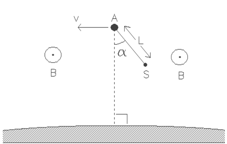
Figure 1 The spaceship Atlantis (A) with a satellite (S) in an orbit around the earth. The orbit lies in the earth’s equatorial plane. The magnetic field (B) is perpendicular to the diagram and is directed towards the reader.
\(\mathrm{a}_1\) - Deduce for which value(s) of \(\alpha\) the configuration of the spaceship and satellite remain unchanged (with respect to the earth)? In other words, for which value(s) of \(\alpha\) is \(\alpha\) constant?
\(\mathrm{a}_2\) - Discuss the stability of the equilibrium for each case.
Suppose that, at a given moment, the rod deviates from the stable configuration by a small angle. The system will begin to swing like a pendulum.
b - Express the period of the swinging in terms of the period of revolution of the system around the earth.
In Fig. 1 the magnetic field of the earth is perpendicular to the diagram and is directed towards the reader. Due to the orbital velocity of the rod, a potential difference arises between its ends. The environment (the magnetosphere) is a rarefied, ionised gas with a very good electrical conductivity. Contact with the ionised gas is made by means of electrodes in A (the Atlantis) and S (the satellite). As a consequence of the motion, a current, \(I\), flows through the rod.
\(\mathrm{c}_1\) - In which direction does the current flow through the rod? (Take \(\alpha=0\))
Data:
| - the period of the orbit | \(T=5{,}4\cdot10^3\ \mathrm{s}\) |
| - the length of the rod | \(L=2{,}0\cdot10^4\ \mathrm{m}\) |
| - magnetic field strength of the eart at the height of the satellite | \(B=5{,}0\cdot10^{-5}\ \mathrm{Wb.m^{-2}}\) |
| - the mass of the shuttle Atlantis | \(m=1{,}0\cdot10^5\ \mathrm{kg}\) |
Next, a current source inside the shuttle is included in the circuit, which maintains a net direct current of 0.1 A in the opposite direction.
\(\mathrm{c}_2\) - How long must this current be maintained to change the altitude of the orbit by 10 m.
Assume that \(\alpha\) remains zero. Ignore all contributions from currents in the magnetosphere.
- Does the altitude decrease or increase?
Official English text of the problem.
Answers
- a₁: The rod must be radial or tangential. To leading order in \(L/R\), the directed angles are \[ \boxed{\alpha=0,\ \frac{\pi}{2},\ \pi,\ \frac{3\pi}{2}\pmod{2\pi}}. \]
- a₂: The radial equilibria, \(\alpha=0,\pi\), are stable. The tangential equilibria, \(\alpha=\pi/2,3\pi/2\), are unstable.
- b: The small-oscillation period is \[ \boxed{T_{\mathrm{swing}}=\frac{T}{\sqrt3}\simeq3.1\times10^3\ \mathrm{s}}. \]
- c₁: Conventional current flows from the satellite S to Atlantis A.
- c₂: The altitude increases, and the required time, in the circular-orbit approximation, is \[ \boxed{t=\frac{\pi m\,\Delta h}{IBLT} \simeq5.8\times10^3\ \mathrm{s}\simeq1.6\ \mathrm{h}}. \]
Solution
a₁ — Equilibrium orientations
Let \(R\) be the orbital radius of Atlantis, \(\mu=GM_{\mathrm E}\), and \[ \Omega=\frac{2\pi}{T}. \] Since Atlantis follows a circular orbit, \[ \Omega^2=\frac{\mu}{R^3}. \] The satellite’s much smaller mass allows us to neglect its effect on Atlantis’s motion.
Use a frame centred on Atlantis and rotating with the orbit. Let \(\mathbf e_x\) point towards the earth’s centre, and let \(\mathbf e_y\) point to the right in Fig. 1. The satellite’s displacement from Atlantis is \[ \boldsymbol{\rho} =L\cos\alpha\,\mathbf e_x+L\sin\alpha\,\mathbf e_y. \]
For a general small displacement \(x\mathbf e_x+y\mathbf e_y\), expansion of the earth’s gravitational field to first order in \(L/R\) gives \[ \mathbf g_S-\mathbf g_A =\frac{\mu}{R^3} \left(2x\,\mathbf e_x-y\,\mathbf e_y\right). \] The additional centrifugal acceleration is \[ \Omega^2\left(x\,\mathbf e_x+y\,\mathbf e_y\right). \] Their sum is therefore \[ \mathbf a_{\mathrm{eff}}=3\Omega^2x\,\mathbf e_x. \]
The unit vector perpendicular to the rod, in the direction of increasing \(\alpha\), is \[ \mathbf e_\alpha=-\sin\alpha\,\mathbf e_x+\cos\alpha\,\mathbf e_y. \] The rod’s force acts along the rod. The Coriolis force also acts along the rod, because the relative velocity \(L\dot\alpha\,\mathbf e_\alpha\) is perpendicular to it. Neither contributes to the tangential equation.
Consequently, \[ L\ddot\alpha =\mathbf a_{\mathrm{eff}}\cdot\mathbf e_\alpha =-3\Omega^2L\sin\alpha\cos\alpha, \] or \[ \boxed{\ddot\alpha+3\Omega^2\sin\alpha\cos\alpha=0}. \]
A constant angle requires \[ \sin\alpha\cos\alpha=0, \] so \[ \boxed{\alpha=\frac{n\pi}{2},\qquad n\in\mathbb Z}. \] Thus the rod is either radial or tangential. These angles use the stated approximation \(L\ll R\).
a₂ — Stability
Write \[ \alpha=\alpha_0+\delta,\qquad |\delta|\ll1, \] where \(\alpha_0\) is an equilibrium angle. Linearizing the equation of motion gives \[ \ddot\delta+3\Omega^2\cos(2\alpha_0)\,\delta=0. \]
For the radial configurations, \(\alpha_0=0,\pi\), \[ \ddot\delta+3\Omega^2\delta=0. \] The acceleration restores the rod towards equilibrium, so both radial configurations are stable.
For the tangential configurations, \(\alpha_0=\pi/2,3\pi/2\), \[ \ddot\delta-3\Omega^2\delta=0. \] This equation admits an exponentially growing displacement, \[ \delta\propto e^{\sqrt3\,\Omega t}, \] so both tangential configurations are unstable.
b — Period of small oscillations
Near either stable equilibrium, the equation found above is that of simple harmonic motion: \[ \ddot\delta+\omega_{\mathrm{swing}}^2\delta=0, \qquad \omega_{\mathrm{swing}}=\sqrt3\,\Omega. \] Hence \[ \boxed{T_{\mathrm{swing}} =\frac{2\pi}{\sqrt3\,\Omega} =\frac{T}{\sqrt3}}. \] Using the given orbital period, \[ T_{\mathrm{swing}} =\frac{5.4\times10^3}{\sqrt3}\ \mathrm{s} \simeq\boxed{3.1\times10^3\ \mathrm{s}}. \]
c₁ — Direction of the induced current
The magnetic force on a positive charge moving with the rod is \[ \mathbf F_B=q\,\mathbf v\times\mathbf B. \] In Fig. 1, \(\mathbf v\) points left and \(\mathbf B\) points out of the page. Therefore \(\mathbf v\times\mathbf B\) points upwards.
For \(\alpha=0\), S lies below A. The motional emf therefore drives positive charges along the rod from S towards A: \[ \boxed{\text{Conventional current flows from S to A.}} \]
c₂ — Time required and direction of altitude change
The current source reverses the current, so it flows from A to S, downwards in the figure. The magnetic force on the rod is \[ \mathbf F=I\,\boldsymbol{\ell}\times\mathbf B, \] where \(\boldsymbol{\ell}\) points along the current. Downwards crossed with out of the page points left, along the orbital velocity.
Since the rod is perpendicular to the field, \[ F=IBL =(0.1)(5.0\times10^{-5})(2.0\times10^4) =\boxed{0.10\ \mathrm N}. \] This forward force supplies energy to the orbit.
Treat the weak thrust as producing a gradual change of a nearly circular orbit. The total orbiting mass is approximately the given shuttle mass \(m\). For a circular orbit, \[ v^2=\frac{\mu}{R}, \] and the total mechanical energy is \[ E=\frac12mv^2-\frac{\mu m}{R} =-\frac{\mu m}{2R}. \] The magnetic force supplies power \(Fv\), so \[ Fv=\frac{dE}{dt} =\frac{\mu m}{2R^2}\frac{dR}{dt}. \] Substituting \(v=\Omega R\) and \(\mu=\Omega^2R^3\), \[ F\Omega R =\frac{m\Omega^2R}{2}\frac{dR}{dt}, \] which gives \[ \boxed{\frac{dR}{dt}=\frac{2F}{m\Omega} =\frac{FT}{\pi m}}. \]
The change of altitude equals the change of orbital radius. Over a rise of only \(10\ \mathrm m\), we may treat \(B\), \(F\), and \(T\) as constant. Thus \[ t=\frac{\pi m\,\Delta h}{FT} =\frac{\pi m\,\Delta h}{IBLT}. \] Numerically, \[ t= \frac{\pi(1.0\times10^5)(10)} {(0.10)(5.4\times10^3)} \ \mathrm s =5.82\times10^3\ \mathrm s. \] Therefore, \[ \boxed{t\simeq5.8\times10^3\ \mathrm s \simeq97\ \mathrm{min}\simeq1.6\ \mathrm h}. \]
Because the force adds orbital energy, \(E\) becomes less negative and \(R\) increases: \[ \boxed{\text{The altitude increases by }10\ \mathrm m.} \]
The solution was checked against the official solution.
IPhO 1990 · Theorieaufgabe 2
Elektrische Experimente in der Magnetosphäre der Erde
Im Mai 1991 wird das Raumschiff Atlantis in eine Umlaufbahn um die Erde gebracht werden. Wir nehmen an, dass diese Umlaufbahn kreisförmig ist und in der Äquatorebene der Erde liegt.
Zu einem vorher festgelegten Zeitpunkt wird das Raumschiff einen Satelliten S aussetzen, der an einem leitenden Stab der Länge \(L\) befestigt ist. Wir nehmen an, dass der Stab starr ist, eine vernachlässigbare Masse hat und mit einem elektrischen Isolator überzogen ist. Außerdem vernachlässigen wir jegliche Reibung. Es sei \(\alpha\) der Winkel, den der Stab mit der Verbindungslinie zwischen Atlantis und dem Erdmittelpunkt bildet. (Siehe Abb. 1.)
S befindet sich ebenfalls in der Äquatorebene.
Nehmen Sie an, dass die Masse des Satelliten viel kleiner als die der Atlantis ist und dass \(L\) viel kleiner als der Radius der Umlaufbahn ist.
Abbildung 1 Das Raumschiff Atlantis (A) mit einem Satelliten (S) auf einer Umlaufbahn um die Erde. Die Umlaufbahn liegt in der Äquatorebene der Erde. Das Magnetfeld (B) steht senkrecht zur Zeichenebene und ist auf den Leser zu gerichtet.
\(\mathrm{a}_1\) - Leiten Sie her, für welche Werte von \(\alpha\) die Anordnung von Raumschiff und Satellit (bezüglich der Erde) unverändert bleibt. Mit anderen Worten: Für welche Werte von \(\alpha\) ist \(\alpha\) konstant?
\(\mathrm{a}_2\) - Untersuchen Sie für jeden Fall die Stabilität des Gleichgewichts.
Nehmen Sie an, dass der Stab zu einem bestimmten Zeitpunkt um einen kleinen Winkel von der stabilen Anordnung abweicht. Das System beginnt dann wie ein Pendel zu schwingen.
b - Drücken Sie die Schwingungsdauer durch die Umlaufdauer des Systems um die Erde aus.
In Abb. 1 steht das Magnetfeld der Erde senkrecht zur Zeichenebene und ist auf den Leser zu gerichtet. Aufgrund der Bahngeschwindigkeit des Stabes entsteht zwischen seinen Enden eine Potentialdifferenz. Die Umgebung (die Magnetosphäre) ist ein verdünntes, ionisiertes Gas mit sehr guter elektrischer Leitfähigkeit. Der Kontakt mit dem ionisierten Gas wird durch Elektroden in A (Atlantis) und S (Satellit) hergestellt. Infolge der Bewegung fließt ein Strom \(I\) durch den Stab.
\(\mathrm{c}_1\) - In welche Richtung fließt der Strom durch den Stab? (Setzen Sie \(\alpha=0\).)
Gegebene Werte:
| - Umlaufdauer | \(T=5{,}4\cdot10^3\ \mathrm{s}\) |
| - Länge des Stabes | \(L=2{,}0\cdot10^4\ \mathrm{m}\) |
| - magnetische Flussdichte der Erde in der Höhe des Satelliten | \(B=5{,}0\cdot10^{-5}\ \mathrm{Wb.m^{-2}}\) |
| - Masse der Raumfähre Atlantis | \(m=1{,}0\cdot10^5\ \mathrm{kg}\) |
Nun wird eine Stromquelle im Inneren der Raumfähre in den Stromkreis eingefügt, die einen resultierenden Gleichstrom von 0.1 A in entgegengesetzter Richtung aufrechterhält.
\(\mathrm{c}_2\) - Wie lange muss dieser Strom aufrechterhalten werden, um die Höhe der Umlaufbahn um 10 m zu verändern?
Nehmen Sie an, dass \(\alpha\) null bleibt. Vernachlässigen Sie alle Beiträge von Strömen in der Magnetosphäre.
- Nimmt die Höhe ab oder zu?
Aufgabentext aus dem offiziellen englischen Text übersetzt.
Antworten
- a₁: Der Stab muss radial oder tangential ausgerichtet sein. In führender Ordnung in \(L/R\) sind die gerichteten Winkel \[ \boxed{\alpha=0,\ \frac{\pi}{2},\ \pi,\ \frac{3\pi}{2}\pmod{2\pi}}. \]
- a₂: Die radialen Gleichgewichtslagen \(\alpha=0,\pi\) sind stabil. Die tangentialen Gleichgewichtslagen \(\alpha=\pi/2,3\pi/2\) sind instabil.
- b: Die Schwingungsdauer bei kleinen Auslenkungen ist \[ \boxed{T_{\mathrm{swing}}=\frac{T}{\sqrt3}\simeq3.1\times10^3\ \mathrm{s}}. \]
- c₁: Der Strom fließt in technischer Stromrichtung vom Satelliten S zur Atlantis A.
- c₂: Die Höhe nimmt zu, und die erforderliche Zeit beträgt in der Näherung einer Kreisbahn \[ \boxed{t=\frac{\pi m\,\Delta h}{IBLT} \simeq5.8\times10^3\ \mathrm{s}\simeq1.6\ \mathrm{h}}. \]
Lösung
a₁ — Gleichgewichtsausrichtungen
Es seien \(R\) der Bahnradius der Atlantis, \(\mu=GM_{\mathrm E}\) und \[ \Omega=\frac{2\pi}{T}. \] Da Atlantis einer Kreisbahn folgt, gilt \[ \Omega^2=\frac{\mu}{R^3}. \] Wegen der viel kleineren Masse des Satelliten können wir seinen Einfluss auf die Bewegung der Atlantis vernachlässigen.
Wir verwenden ein Bezugssystem mit Ursprung in Atlantis, das mit der Umlaufbewegung rotiert. Dabei zeige \(\mathbf e_x\) zum Erdmittelpunkt und \(\mathbf e_y\) in Abb. 1 nach rechts. Der Ortsvektor des Satelliten relativ zur Atlantis ist \[ \boldsymbol{\rho} =L\cos\alpha\,\mathbf e_x+L\sin\alpha\,\mathbf e_y. \]
Für eine allgemeine kleine Verschiebung \(x\mathbf e_x+y\mathbf e_y\) ergibt die Entwicklung des Gravitationsfeldes der Erde bis zur ersten Ordnung in \(L/R\) \[ \mathbf g_S-\mathbf g_A =\frac{\mu}{R^3} \left(2x\,\mathbf e_x-y\,\mathbf e_y\right). \] Die zusätzliche Zentrifugalbeschleunigung ist \[ \Omega^2\left(x\,\mathbf e_x+y\,\mathbf e_y\right). \] Ihre Summe ist daher \[ \mathbf a_{\mathrm{eff}}=3\Omega^2x\,\mathbf e_x. \]
Der Einheitsvektor senkrecht zum Stab in Richtung zunehmenden \(\alpha\) ist \[ \mathbf e_\alpha=-\sin\alpha\,\mathbf e_x+\cos\alpha\,\mathbf e_y. \] Die vom Stab ausgeübte Kraft wirkt entlang des Stabes. Auch die Corioliskraft wirkt entlang des Stabes, da die Relativgeschwindigkeit \(L\dot\alpha\,\mathbf e_\alpha\) senkrecht zu ihm steht. Keine der beiden Kräfte trägt zur tangentialen Bewegungsgleichung bei.
Folglich gilt \[ L\ddot\alpha =\mathbf a_{\mathrm{eff}}\cdot\mathbf e_\alpha =-3\Omega^2L\sin\alpha\cos\alpha, \] oder \[ \boxed{\ddot\alpha+3\Omega^2\sin\alpha\cos\alpha=0}. \]
Ein konstanter Winkel erfordert \[ \sin\alpha\cos\alpha=0, \] also \[ \boxed{\alpha=\frac{n\pi}{2},\qquad n\in\mathbb Z}. \] Der Stab ist somit entweder radial oder tangential ausgerichtet. Diese Winkel gelten in der angegebenen Näherung \(L\ll R\).
a₂ — Stabilität
Wir setzen \[ \alpha=\alpha_0+\delta,\qquad |\delta|\ll1, \] wobei \(\alpha_0\) ein Gleichgewichtswinkel ist. Die Linearisierung der Bewegungsgleichung ergibt \[ \ddot\delta+3\Omega^2\cos(2\alpha_0)\,\delta=0. \]
Für die radialen Anordnungen \(\alpha_0=0,\pi\) gilt \[ \ddot\delta+3\Omega^2\delta=0. \] Die Beschleunigung führt den Stab zur Gleichgewichtslage zurück, daher sind beide radialen Anordnungen stabil.
Für die tangentialen Anordnungen \(\alpha_0=\pi/2,3\pi/2\) gilt \[ \ddot\delta-3\Omega^2\delta=0. \] Diese Gleichung lässt eine exponentiell anwachsende Auslenkung zu, \[ \delta\propto e^{\sqrt3\,\Omega t}, \] also sind beide tangentialen Anordnungen instabil.
b — Schwingungsdauer kleiner Schwingungen
In der Nähe jeder der beiden stabilen Gleichgewichtslagen ist die oben gefundene Gleichung die einer harmonischen Schwingung: \[ \ddot\delta+\omega_{\mathrm{swing}}^2\delta=0, \qquad \omega_{\mathrm{swing}}=\sqrt3\,\Omega. \] Daher gilt \[ \boxed{T_{\mathrm{swing}} =\frac{2\pi}{\sqrt3\,\Omega} =\frac{T}{\sqrt3}}. \] Mit der gegebenen Umlaufdauer ergibt sich \[ T_{\mathrm{swing}} =\frac{5.4\times10^3}{\sqrt3}\ \mathrm{s} \simeq\boxed{3.1\times10^3\ \mathrm{s}}. \]
c₁ — Richtung des induzierten Stroms
Die magnetische Kraft auf eine positive Ladung, die sich mit dem Stab bewegt, ist \[ \mathbf F_B=q\,\mathbf v\times\mathbf B. \] In Abb. 1 zeigt \(\mathbf v\) nach links und \(\mathbf B\) aus der Zeichenebene heraus. Daher zeigt \(\mathbf v\times\mathbf B\) nach oben.
Für \(\alpha=0\) liegt S unterhalb von A. Die Bewegungsinduktionsspannung treibt daher positive Ladungen entlang des Stabes von S nach A: \[ \boxed{\text{Der Strom fließt in technischer Stromrichtung von S nach A.}} \]
c₂ — Erforderliche Zeit und Richtung der Höhenänderung
Die Stromquelle kehrt den Strom um, sodass er von A nach S fließt, in der Abbildung nach unten. Die magnetische Kraft auf den Stab ist \[ \mathbf F=I\,\boldsymbol{\ell}\times\mathbf B, \] wobei \(\boldsymbol{\ell}\) in Stromrichtung zeigt. Das Kreuzprodukt eines nach unten gerichteten Vektors mit einem aus der Zeichenebene heraus gerichteten Vektor zeigt nach links, in Richtung der Bahngeschwindigkeit.
Da der Stab senkrecht zum Feld steht, gilt \[ F=IBL =(0.1)(5.0\times10^{-5})(2.0\times10^4) =\boxed{0.10\ \mathrm N}. \] Diese vorwärts gerichtete Kraft führt der Bahnbewegung Energie zu.
Wir betrachten den schwachen Schub als Ursache einer allmählichen Änderung einer nahezu kreisförmigen Umlaufbahn. Die gesamte umlaufende Masse entspricht näherungsweise der gegebenen Masse \(m\) der Raumfähre. Für eine Kreisbahn gilt \[ v^2=\frac{\mu}{R}, \] und die gesamte mechanische Energie ist \[ E=\frac12mv^2-\frac{\mu m}{R} =-\frac{\mu m}{2R}. \] Die magnetische Kraft führt die Leistung \(Fv\) zu, also gilt \[ Fv=\frac{dE}{dt} =\frac{\mu m}{2R^2}\frac{dR}{dt}. \] Durch Einsetzen von \(v=\Omega R\) und \(\mu=\Omega^2R^3\) ergibt sich \[ F\Omega R =\frac{m\Omega^2R}{2}\frac{dR}{dt}, \] woraus folgt \[ \boxed{\frac{dR}{dt}=\frac{2F}{m\Omega} =\frac{FT}{\pi m}}. \]
Die Höhenänderung ist gleich der Änderung des Bahnradius. Bei einem Anstieg um nur \(10\ \mathrm m\) können wir \(B\), \(F\) und \(T\) als konstant behandeln. Somit gilt \[ t=\frac{\pi m\,\Delta h}{FT} =\frac{\pi m\,\Delta h}{IBLT}. \] Numerisch ergibt sich \[ t= \frac{\pi(1.0\times10^5)(10)} {(0.10)(5.4\times10^3)} \ \mathrm s =5.82\times10^3\ \mathrm s. \] Damit gilt \[ \boxed{t\simeq5.8\times10^3\ \mathrm s \simeq97\ \mathrm{min}\simeq1.6\ \mathrm h}. \]
Da die Kraft der Bahnbewegung Energie zuführt, wird \(E\) weniger negativ und \(R\) nimmt zu: \[ \boxed{\text{Die Höhe steigt um }10\ \mathrm m.} \]
Die Lösung wurde mit der offiziellen Lösung abgeglichen.
IPhO 1990 · Teori sorusu 2
Dünya'nın manyetosferinde elektrik deneyleri
Mayıs 1991'de Atlantis uzay aracı Dünya çevresinde bir yörüngeye yerleştirilecektir. Bu yörüngenin dairesel olduğunu ve Dünya'nın ekvator düzleminde bulunduğunu varsayacağız.
Önceden belirlenmiş bir anda uzay aracı, uzunluğu \(L\) olan iletken bir çubuğa bağlı S uydusunu serbest bırakacaktır. Çubuğun rijit olduğunu, kütlesinin ihmal edilebilir olduğunu ve elektriksel bir yalıtkanla kaplı olduğunu varsayıyoruz. Ayrıca tüm sürtünmeleri ihmal ediyoruz. Çubuğun Atlantis ile Dünya'nın merkezini birleştiren doğruyla yaptığı açı \(\alpha\) olsun. (Bkz. Şekil 1).
S de ekvator düzleminde bulunmaktadır.
Uydunun kütlesinin Atlantis'in kütlesinden çok küçük olduğunu ve \(L\)'nin yörünge yarıçapından çok küçük olduğunu varsayın.
Şekil 1 Dünya çevresindeki bir yörüngede, bir uydu (S) ile birlikte Atlantis uzay aracı (A). Yörünge Dünya'nın ekvator düzlemindedir. Manyetik alan (B) şekil düzlemine diktir ve okuyucuya doğru yönelmiştir.
\(\mathrm{a}_1\) - \(\alpha\)'nın hangi değerinde (veya değerlerinde) uzay aracı ve uydunun düzeninin (Dünya'ya göre) değişmeden kaldığını türetin. Başka bir deyişle, \(\alpha\)'nın hangi değerinde (veya değerlerinde) \(\alpha\) sabit kalır?
\(\mathrm{a}_2\) - Her bir durum için dengenin kararlılığını tartışın.
Belirli bir anda çubuğun kararlı konumundan küçük bir açı kadar saptığını varsayın. Sistem bir sarkaç gibi salınmaya başlayacaktır.
b - Salınım periyodunu, sistemin Dünya çevresindeki dolanım periyodu cinsinden ifade edin.
Şekil 1'de Dünya'nın manyetik alanı şekil düzlemine diktir ve okuyucuya doğru yönelmiştir. Çubuğun yörüngesel hızı nedeniyle uçları arasında bir potansiyel farkı oluşur. Ortam (manyetosfer), elektrik iletkenliği çok iyi olan seyrek, iyonlaşmış bir gazdır. İyonlaşmış gazla temas, A'daki (Atlantis) ve S'deki (uydu) elektrotlar aracılığıyla sağlanır. Hareketin bir sonucu olarak çubuktan \(I\) akımı geçer.
\(\mathrm{c}_1\) - Akım çubuktan hangi yönde geçer? (\(\alpha=0\) alın.)
Veriler:
| - yörünge periyodu | \(T=5{,}4\cdot10^3\ \mathrm{s}\) |
| - çubuğun uzunluğu | \(L=2{,}0\cdot10^4\ \mathrm{m}\) |
| - uydunun bulunduğu yükseklikte Dünya'nın manyetik alanının büyüklüğü | \(B=5{,}0\cdot10^{-5}\ \mathrm{Wb.m^{-2}}\) |
| - Atlantis mekiğinin kütlesi | \(m=1{,}0\cdot10^5\ \mathrm{kg}\) |
Ardından, mekiğin içindeki bir akım kaynağı devreye dahil edilerek ters yönde 0.1 A büyüklüğünde net bir doğru akım sağlanır.
\(\mathrm{c}_2\) - Yörüngenin yüksekliğini 10 m değiştirmek için bu akım ne kadar süreyle sürdürülmelidir?
\(\alpha\)'nın sıfır olarak kaldığını varsayın. Manyetosferdeki akımların tüm katkılarını ihmal edin.
- Yükseklik azalır mı, artar mı?
Soru metni resmi İngilizce metinden çevrilmiştir.
Cevaplar
- a₁: Çubuk radyal veya teğetsel olmalıdır. \(L/R\)'nin başat mertebesinde yönlü açılar \[ \boxed{\alpha=0,\ \frac{\pi}{2},\ \pi,\ \frac{3\pi}{2}\pmod{2\pi}}. \]
- a₂: Radyal denge konumları, \(\alpha=0,\pi\), kararlıdır. Teğetsel denge konumları, \(\alpha=\pi/2,3\pi/2\), kararsızdır.
- b: Küçük salınımların periyodu \[ \boxed{T_{\mathrm{swing}}=\frac{T}{\sqrt3}\simeq3.1\times10^3\ \mathrm{s}}. \]
- c₁: Konvansiyonel akım S uydusundan Atlantis A'ya doğru akar.
- c₂: Yükseklik artar ve dairesel yörünge yaklaşımında gereken süre \[ \boxed{t=\frac{\pi m\,\Delta h}{IBLT} \simeq5.8\times10^3\ \mathrm{s}\simeq1.6\ \mathrm{h}}. \]
Çözüm
a₁ — Denge yönelimleri
Atlantis'in yörünge yarıçapı \(R\), \(\mu=GM_{\mathrm E}\) ve \[ \Omega=\frac{2\pi}{T}. \] olsun. Atlantis dairesel bir yörüngede hareket ettiğinden, \[ \Omega^2=\frac{\mu}{R^3}. \] Uydunun kütlesinin çok daha küçük olması, Atlantis'in hareketi üzerindeki etkisini ihmal etmemize olanak tanır.
Merkezi Atlantis'te olan ve yörüngeyle birlikte dönen bir referans sistemi kullanalım. \(\mathbf e_x\) Dünya'nın merkezine doğru, \(\mathbf e_y\) ise Şekil 1'de sağa doğru yönelsin. Uydunun Atlantis'e göre yer değiştirmesi \[ \boldsymbol{\rho} =L\cos\alpha\,\mathbf e_x+L\sin\alpha\,\mathbf e_y. \]
Genel bir küçük \(x\mathbf e_x+y\mathbf e_y\) yer değiştirmesi için Dünya'nın kütle çekim alanını \(L/R\)'de birinci mertebeye kadar açarsak \[ \mathbf g_S-\mathbf g_A =\frac{\mu}{R^3} \left(2x\,\mathbf e_x-y\,\mathbf e_y\right). \] Ek merkezkaç ivmesi \[ \Omega^2\left(x\,\mathbf e_x+y\,\mathbf e_y\right). \] Dolayısıyla bunların toplamı \[ \mathbf a_{\mathrm{eff}}=3\Omega^2x\,\mathbf e_x. \]
Çubuğa dik, \(\alpha\)'nın artış yönündeki birim vektör \[ \mathbf e_\alpha=-\sin\alpha\,\mathbf e_x+\cos\alpha\,\mathbf e_y. \] Çubuğun uyguladığı kuvvet çubuk boyunca etkir. Bağıl hız \(L\dot\alpha\,\mathbf e_\alpha\) çubuğa dik olduğundan, Coriolis kuvveti de çubuk boyunca etkir. Bu kuvvetlerin hiçbiri teğetsel hareket denklemine katkıda bulunmaz.
Sonuç olarak, \[ L\ddot\alpha =\mathbf a_{\mathrm{eff}}\cdot\mathbf e_\alpha =-3\Omega^2L\sin\alpha\cos\alpha, \] veya \[ \boxed{\ddot\alpha+3\Omega^2\sin\alpha\cos\alpha=0}. \]
Açının sabit olması için \[ \sin\alpha\cos\alpha=0, \] olmalıdır; dolayısıyla \[ \boxed{\alpha=\frac{n\pi}{2},\qquad n\in\mathbb Z}. \] Böylece çubuk ya radyal ya da teğetseldir. Bu açılar, belirtilen \(L\ll R\) yaklaşımı kullanılarak elde edilmiştir.
a₂ — Kararlılık
\[ \alpha=\alpha_0+\delta,\qquad |\delta|\ll1, \] yazalım; burada \(\alpha_0\) bir denge açısıdır. Hareket denklemini doğrusallaştırırsak \[ \ddot\delta+3\Omega^2\cos(2\alpha_0)\,\delta=0. \]
Radyal konumlar, \(\alpha_0=0,\pi\), için \[ \ddot\delta+3\Omega^2\delta=0. \] İvme çubuğu dengeye doğru geri döndürür; dolayısıyla her iki radyal konum da kararlıdır.
Teğetsel konumlar, \(\alpha_0=\pi/2,3\pi/2\), için \[ \ddot\delta-3\Omega^2\delta=0. \] Bu denklem, üstel olarak büyüyen bir yer değiştirme çözümüne sahiptir: \[ \delta\propto e^{\sqrt3\,\Omega t}, \] dolayısıyla her iki teğetsel konum da kararsızdır.
b — Küçük salınımların periyodu
Her iki kararlı denge konumunun yakınında, yukarıda bulunan denklem basit harmonik hareket denklemidir: \[ \ddot\delta+\omega_{\mathrm{swing}}^2\delta=0, \qquad \omega_{\mathrm{swing}}=\sqrt3\,\Omega. \] Buradan \[ \boxed{T_{\mathrm{swing}} =\frac{2\pi}{\sqrt3\,\Omega} =\frac{T}{\sqrt3}}. \] Verilen yörünge periyodunu kullanırsak \[ T_{\mathrm{swing}} =\frac{5.4\times10^3}{\sqrt3}\ \mathrm{s} \simeq\boxed{3.1\times10^3\ \mathrm{s}}. \]
c₁ — İndüklenen akımın yönü
Çubukla birlikte hareket eden pozitif bir yüke etkiyen manyetik kuvvet \[ \mathbf F_B=q\,\mathbf v\times\mathbf B. \] Şekil 1'de \(\mathbf v\) sola, \(\mathbf B\) ise sayfa düzleminden dışarıya yönelmiştir. Dolayısıyla \(\mathbf v\times\mathbf B\) yukarıya yönelmiştir.
\(\alpha=0\) için S, A'nın altında bulunur. Bu nedenle hareketten kaynaklanan elektromotor kuvvet, pozitif yükleri çubuk boyunca S'den A'ya doğru sürükler: \[ \boxed{\text{Konvansiyonel akım S'den A'ya doğru akar.}} \]
c₂ — Gereken süre ve yükseklik değişiminin yönü
Akım kaynağı akımın yönünü tersine çevirir; böylece akım A'dan S'ye, şekilde aşağıya doğru akar. Çubuğa etkiyen manyetik kuvvet \[ \mathbf F=I\,\boldsymbol{\ell}\times\mathbf B, \] şeklindedir; burada \(\boldsymbol{\ell}\) akım yönünde uzanır. Aşağı yön ile sayfa düzleminden dışarı yönün vektörel çarpımı, yörüngesel hız yönünde sola yönelir.
Çubuk alana dik olduğundan, \[ F=IBL =(0.1)(5.0\times10^{-5})(2.0\times10^4) =\boxed{0.10\ \mathrm N}. \] İleri yöndeki bu kuvvet yörüngeye enerji sağlar.
Zayıf itki kuvvetinin, yaklaşık olarak dairesel olan bir yörüngede yavaş bir değişim oluşturduğunu kabul edelim. Yörüngede dolanan toplam kütle, yaklaşık olarak verilen mekik kütlesi \(m\)'dir. Dairesel bir yörünge için \[ v^2=\frac{\mu}{R}, \] ve toplam mekanik enerji \[ E=\frac12mv^2-\frac{\mu m}{R} =-\frac{\mu m}{2R}. \] Manyetik kuvvet \(Fv\) gücünü sağladığından, \[ Fv=\frac{dE}{dt} =\frac{\mu m}{2R^2}\frac{dR}{dt}. \] \(v=\Omega R\) ve \(\mu=\Omega^2R^3\) yerine konulduğunda, \[ F\Omega R =\frac{m\Omega^2R}{2}\frac{dR}{dt}, \] buradan \[ \boxed{\frac{dR}{dt}=\frac{2F}{m\Omega} =\frac{FT}{\pi m}}. \]
Yükseklik değişimi, yörünge yarıçapının değişimine eşittir. Yalnızca \(10\ \mathrm m\)'lik bir yükselme boyunca \(B\), \(F\) ve \(T\)'yi sabit kabul edebiliriz. Böylece \[ t=\frac{\pi m\,\Delta h}{FT} =\frac{\pi m\,\Delta h}{IBLT}. \] Sayısal olarak, \[ t= \frac{\pi(1.0\times10^5)(10)} {(0.10)(5.4\times10^3)} \ \mathrm s =5.82\times10^3\ \mathrm s. \] Dolayısıyla, \[ \boxed{t\simeq5.8\times10^3\ \mathrm s \simeq97\ \mathrm{min}\simeq1.6\ \mathrm h}. \]
Kuvvet yörünge enerjisini artırdığından, \(E\) daha az negatif olur ve \(R\) artar: \[ \boxed{\text{Yükseklikteki artış }10\ \mathrm m.} \]
Çözüm, resmi çözümle karşılaştırılarak kontrol edildi.
IPhO 1990 · Problema teórico 2
Experimentos eléctricos en la magnetosfera de la Tierra
En mayo de 1991, la nave espacial Atlantis se pondrá en órbita alrededor de la Tierra. Supondremos que esta órbita será circular y que estará situada en el plano ecuatorial terrestre.
En un momento predeterminado, la nave espacial liberará un satélite S, unido a una varilla conductora de longitud \(L\). Suponemos que la varilla es rígida, tiene una masa despreciable y está recubierta de un aislante eléctrico. También despreciamos todo rozamiento. Sea \(\alpha\) el ángulo que forma la varilla con la línea que une el Atlantis con el centro de la Tierra (véase la Fig. 1).
S también se encuentra en el plano ecuatorial.
Suponga que la masa del satélite es mucho menor que la del Atlantis y que \(L\) es mucho menor que el radio de la órbita.
Figura 1 La nave espacial Atlantis (A) con un satélite (S) en una órbita alrededor de la Tierra. La órbita está situada en el plano ecuatorial terrestre. El campo magnético (B) es perpendicular al dibujo y está dirigido hacia el lector.
\(\mathrm{a}_1\) - Deduzca para qué valor(es) de \(\alpha\) permanece invariable la configuración de la nave espacial y el satélite (con respecto a la Tierra). En otras palabras, ¿para qué valor(es) de \(\alpha\) es constante \(\alpha\)?
\(\mathrm{a}_2\) - Analice la estabilidad del equilibrio en cada caso.
Suponga que, en un momento dado, la varilla se desvía de la configuración estable un ángulo pequeño. El sistema comenzará a oscilar como un péndulo.
b - Exprese el período de oscilación en función del período de revolución del sistema alrededor de la Tierra.
En la Fig. 1, el campo magnético terrestre es perpendicular al dibujo y está dirigido hacia el lector. Debido a la velocidad orbital de la varilla, aparece una diferencia de potencial entre sus extremos. El medio circundante (la magnetosfera) es un gas enrarecido e ionizado con una conductividad eléctrica muy elevada. El contacto con el gas ionizado se establece mediante electrodos en A (el Atlantis) y S (el satélite). Como consecuencia del movimiento, circula por la varilla una corriente \(I\).
\(\mathrm{c}_1\) - ¿En qué sentido circula la corriente por la varilla? (Tome \(\alpha=0\))
Datos:
| - período de la órbita | \(T=5{,}4\cdot10^3\ \mathrm{s}\) |
| - longitud de la varilla | \(L=2{,}0\cdot10^4\ \mathrm{m}\) |
| - intensidad del campo magnético terrestre a la altura del satélite | \(B=5{,}0\cdot10^{-5}\ \mathrm{Wb.m^{-2}}\) |
| - masa del transbordador Atlantis | \(m=1{,}0\cdot10^5\ \mathrm{kg}\) |
A continuación, se incorpora al circuito una fuente de corriente situada en el interior del transbordador, que mantiene una corriente continua neta de 0.1 A en el sentido opuesto.
\(\mathrm{c}_2\) - ¿Durante cuánto tiempo debe mantenerse esta corriente para modificar la altitud de la órbita en 10 m?
Suponga que \(\alpha\) permanece igual a cero. Desprecie todas las contribuciones de las corrientes en la magnetosfera.
- ¿Disminuye o aumenta la altitud?
Enunciado traducido del texto oficial en inglés.
Respuestas
- a₁: La varilla debe ser radial o tangencial. Al orden dominante en \(L/R\), los ángulos orientados son \[ \boxed{\alpha=0,\ \frac{\pi}{2},\ \pi,\ \frac{3\pi}{2}\pmod{2\pi}}. \]
- a₂: Los equilibrios radiales, \(\alpha=0,\pi\), son estables. Los equilibrios tangenciales, \(\alpha=\pi/2,3\pi/2\), son inestables.
- b: El período de las pequeñas oscilaciones es \[ \boxed{T_{\mathrm{swing}}=\frac{T}{\sqrt3}\simeq3.1\times10^3\ \mathrm{s}}. \]
- c₁: La corriente convencional circula desde el satélite S hacia el Atlantis A.
- c₂: La altitud aumenta, y el tiempo necesario, en la aproximación de órbita circular, es \[ \boxed{t=\frac{\pi m\,\Delta h}{IBLT} \simeq5.8\times10^3\ \mathrm{s}\simeq1.6\ \mathrm{h}}. \]
Solución
a₁ — Orientaciones de equilibrio
Sea \(R\) el radio orbital del Atlantis, \(\mu=GM_{\mathrm E}\), y \[ \Omega=\frac{2\pi}{T}. \] Como el Atlantis sigue una órbita circular, \[ \Omega^2=\frac{\mu}{R^3}. \] La masa mucho menor del satélite permite despreciar su efecto sobre el movimiento del Atlantis.
Utilicemos un sistema de referencia centrado en el Atlantis y que gira con la órbita. Sea \(\mathbf e_x\) un vector dirigido hacia el centro de la Tierra y \(\mathbf e_y\) un vector dirigido hacia la derecha en la Fig. 1. El desplazamiento del satélite respecto al Atlantis es \[ \boldsymbol{\rho} =L\cos\alpha\,\mathbf e_x+L\sin\alpha\,\mathbf e_y. \]
Para un desplazamiento pequeño general \(x\mathbf e_x+y\mathbf e_y\), el desarrollo del campo gravitatorio terrestre a primer orden en \(L/R\) da \[ \mathbf g_S-\mathbf g_A =\frac{\mu}{R^3} \left(2x\,\mathbf e_x-y\,\mathbf e_y\right). \] La aceleración centrífuga adicional es \[ \Omega^2\left(x\,\mathbf e_x+y\,\mathbf e_y\right). \] Por tanto, su suma es \[ \mathbf a_{\mathrm{eff}}=3\Omega^2x\,\mathbf e_x. \]
El vector unitario perpendicular a la varilla, en el sentido de aumento de \(\alpha\), es \[ \mathbf e_\alpha=-\sin\alpha\,\mathbf e_x+\cos\alpha\,\mathbf e_y. \] La fuerza de la varilla actúa a lo largo de esta. La fuerza de Coriolis también actúa a lo largo de la varilla, porque la velocidad relativa \(L\dot\alpha\,\mathbf e_\alpha\) es perpendicular a ella. Ninguna de las dos contribuye a la ecuación tangencial.
En consecuencia, \[ L\ddot\alpha =\mathbf a_{\mathrm{eff}}\cdot\mathbf e_\alpha =-3\Omega^2L\sin\alpha\cos\alpha, \] o bien \[ \boxed{\ddot\alpha+3\Omega^2\sin\alpha\cos\alpha=0}. \]
Para que el ángulo sea constante, se requiere \[ \sin\alpha\cos\alpha=0, \] por lo que \[ \boxed{\alpha=\frac{n\pi}{2},\qquad n\in\mathbb Z}. \] Así pues, la varilla es radial o tangencial. Estos ángulos se obtienen utilizando la aproximación indicada \(L\ll R\).
a₂ — Estabilidad
Escribamos \[ \alpha=\alpha_0+\delta,\qquad |\delta|\ll1, \] donde \(\alpha_0\) es un ángulo de equilibrio. Al linealizar la ecuación de movimiento se obtiene \[ \ddot\delta+3\Omega^2\cos(2\alpha_0)\,\delta=0. \]
Para las configuraciones radiales, \(\alpha_0=0,\pi\), \[ \ddot\delta+3\Omega^2\delta=0. \] La aceleración hace que la varilla vuelva hacia el equilibrio, por lo que ambas configuraciones radiales son estables.
Para las configuraciones tangenciales, \(\alpha_0=\pi/2,3\pi/2\), \[ \ddot\delta-3\Omega^2\delta=0. \] Esta ecuación admite un desplazamiento que crece exponencialmente, \[ \delta\propto e^{\sqrt3\,\Omega t}, \] por lo que ambas configuraciones tangenciales son inestables.
b — Período de las pequeñas oscilaciones
Cerca de cualquiera de los dos equilibrios estables, la ecuación obtenida anteriormente es la de un movimiento armónico simple: \[ \ddot\delta+\omega_{\mathrm{swing}}^2\delta=0, \qquad \omega_{\mathrm{swing}}=\sqrt3\,\Omega. \] Por tanto, \[ \boxed{T_{\mathrm{swing}} =\frac{2\pi}{\sqrt3\,\Omega} =\frac{T}{\sqrt3}}. \] Utilizando el período orbital dado, \[ T_{\mathrm{swing}} =\frac{5.4\times10^3}{\sqrt3}\ \mathrm{s} \simeq\boxed{3.1\times10^3\ \mathrm{s}}. \]
c₁ — Sentido de la corriente inducida
La fuerza magnética sobre una carga positiva que se mueve con la varilla es \[ \mathbf F_B=q\,\mathbf v\times\mathbf B. \] En la Fig. 1, \(\mathbf v\) apunta hacia la izquierda y \(\mathbf B\) sale del plano de la página. Por tanto, \(\mathbf v\times\mathbf B\) apunta hacia arriba.
Para \(\alpha=0\), S está situado debajo de A. Por tanto, la fuerza electromotriz de movimiento impulsa las cargas positivas a lo largo de la varilla desde S hacia A: \[ \boxed{\text{La corriente convencional circula de S a A.}} \]
c₂ — Tiempo necesario y sentido del cambio de altitud
La fuente de corriente invierte el sentido de la corriente, de modo que esta circula de A a S, hacia abajo en la figura. La fuerza magnética sobre la varilla es \[ \mathbf F=I\,\boldsymbol{\ell}\times\mathbf B, \] donde \(\boldsymbol{\ell}\) apunta en el sentido de la corriente. El producto vectorial de un vector dirigido hacia abajo por otro que sale del plano de la página apunta hacia la izquierda, en el sentido de la velocidad orbital.
Como la varilla es perpendicular al campo, \[ F=IBL =(0.1)(5.0\times10^{-5})(2.0\times10^4) =\boxed{0.10\ \mathrm N}. \] Esta fuerza hacia delante aporta energía a la órbita.
Consideremos que el débil empuje produce una variación gradual de una órbita casi circular. La masa total en órbita es aproximadamente la masa dada del transbordador \(m\). Para una órbita circular, \[ v^2=\frac{\mu}{R}, \] y la energía mecánica total es \[ E=\frac12mv^2-\frac{\mu m}{R} =-\frac{\mu m}{2R}. \] La fuerza magnética suministra una potencia \(Fv\), por lo que \[ Fv=\frac{dE}{dt} =\frac{\mu m}{2R^2}\frac{dR}{dt}. \] Sustituyendo \(v=\Omega R\) y \(\mu=\Omega^2R^3\), \[ F\Omega R =\frac{m\Omega^2R}{2}\frac{dR}{dt}, \] se obtiene \[ \boxed{\frac{dR}{dt}=\frac{2F}{m\Omega} =\frac{FT}{\pi m}}. \]
La variación de altitud es igual a la variación del radio orbital. Durante un ascenso de solo \(10\ \mathrm m\), podemos considerar constantes \(B\), \(F\) y \(T\). Así, \[ t=\frac{\pi m\,\Delta h}{FT} =\frac{\pi m\,\Delta h}{IBLT}. \] Numéricamente, \[ t= \frac{\pi(1.0\times10^5)(10)} {(0.10)(5.4\times10^3)} \ \mathrm s =5.82\times10^3\ \mathrm s. \] Por tanto, \[ \boxed{t\simeq5.8\times10^3\ \mathrm s \simeq97\ \mathrm{min}\simeq1.6\ \mathrm h}. \]
Como la fuerza aumenta la energía orbital, \(E\) se hace menos negativa y \(R\) aumenta: \[ \boxed{\text{La altitud aumenta en }10\ \mathrm m.} \]
La solución se comprobó con la solución oficial.
IPhO 1990 · 理论题 2
地球磁层中的电学实验
1991 年 5 月,亚特兰蒂斯号航天飞机将进入环绕地球的轨道。我们假定该轨道为圆形,且位于地球赤道平面内。
在某个预定时刻,航天飞机将释放一颗卫星 S,卫星连接在一根长度为 \(L\) 的导电杆上。假设该杆是刚性的,质量可忽略不计,表面包覆着电绝缘材料。我们还忽略一切摩擦。设 \(\alpha\) 为杆与亚特兰蒂斯号和地心之间连线的夹角。(见图 1)。
S 也位于赤道平面内。
假设卫星的质量远小于亚特兰蒂斯号的质量,且 \(L\) 远小于轨道半径。
图 1 携带卫星(S)的亚特兰蒂斯号航天飞机(A)在环绕地球的轨道上运行。轨道位于地球赤道平面内。磁场(B)垂直于图面,方向指向读者。
\(\mathrm{a}_1\) - 推导当 \(\alpha\) 取何值时,航天飞机与卫星的构型(相对于地球)保持不变?换言之,当 \(\alpha\) 取何值时,\(\alpha\) 为常量?
\(\mathrm{a}_2\) - 讨论每种情况下平衡的稳定性。
假设在某一时刻,杆偏离稳定构型一个小角度。系统将开始像摆一样摆动。
b - 用系统绕地球公转的周期表示摆动周期。
在图 1 中,地球磁场垂直于图面,方向指向读者。由于杆具有轨道速度,其两端会产生电势差。周围环境(磁层)是一种稀薄的电离气体,具有很好的导电性。通过 A(亚特兰蒂斯号)和 S(卫星)上的电极与电离气体接触。由于这一运动,电流 \(I\) 流过杆。
\(\mathrm{c}_1\) - 电流沿杆向哪个方向流动?(取 \(\alpha=0\))
数据:
| - 轨道周期 | \(T=5{,}4\cdot10^3\ \mathrm{s}\) |
| - 杆的长度 | \(L=2{,}0\cdot10^4\ \mathrm{m}\) |
| - 卫星所在高度处的地球磁感应强度 | \(B=5{,}0\cdot10^{-5}\ \mathrm{Wb.m^{-2}}\) |
| - 亚特兰蒂斯号航天飞机的质量 | \(m=1{,}0\cdot10^5\ \mathrm{kg}\) |
接着,将航天飞机内部的一个电流源接入电路,使电路中维持方向相反、大小为 0.1 A 的净直流电流。
\(\mathrm{c}_2\) - 为使轨道高度改变 10 m,这一电流必须维持多长时间?
假设 \(\alpha\) 始终为零。忽略磁层中电流的一切影响。
- 高度是降低还是升高?
题目译自官方英文原文。
答案
- a₁: 杆必须沿径向或切向。在 \(L/R\) 的首阶近似下,有向角为 \[ \boxed{\alpha=0,\ \frac{\pi}{2},\ \pi,\ \frac{3\pi}{2}\pmod{2\pi}}. \]
- a₂: 径向平衡位置 \(\alpha=0,\pi\) 是稳定的。切向平衡位置 \(\alpha=\pi/2,3\pi/2\) 是不稳定的。
- b: 小振动周期为 \[ \boxed{T_{\mathrm{swing}}=\frac{T}{\sqrt3}\simeq3.1\times10^3\ \mathrm{s}}. \]
- c₁: 约定的电流方向为从卫星 S 流向亚特兰蒂斯号 A。
- c₂: 高度升高,在圆轨道近似下,所需时间为 \[ \boxed{t=\frac{\pi m\,\Delta h}{IBLT} \simeq5.8\times10^3\ \mathrm{s}\simeq1.6\ \mathrm{h}}. \]
解答
a₁ — 平衡取向
设亚特兰蒂斯号的轨道半径为 \(R\),\(\mu=GM_{\mathrm E}\),且 \[ \Omega=\frac{2\pi}{T}. \] 由于亚特兰蒂斯号沿圆轨道运行, \[ \Omega^2=\frac{\mu}{R^3}. \] 卫星的质量小得多,因此可以忽略它对亚特兰蒂斯号运动的影响。
采用以亚特兰蒂斯号为原点、随轨道运动旋转的参考系。令 \(\mathbf e_x\) 指向地心,\(\mathbf e_y\) 指向图 1 中的右方。卫星相对于亚特兰蒂斯号的位移为 \[ \boldsymbol{\rho} =L\cos\alpha\,\mathbf e_x+L\sin\alpha\,\mathbf e_y. \]
对于一般的小位移 \(x\mathbf e_x+y\mathbf e_y\),将地球引力场按 \(L/R\) 展开至一阶,得到 \[ \mathbf g_S-\mathbf g_A =\frac{\mu}{R^3} \left(2x\,\mathbf e_x-y\,\mathbf e_y\right). \] 附加的离心加速度为 \[ \Omega^2\left(x\,\mathbf e_x+y\,\mathbf e_y\right). \] 因此,两者之和为 \[ \mathbf a_{\mathrm{eff}}=3\Omega^2x\,\mathbf e_x. \]
垂直于杆且指向 \(\alpha\) 增大方向的单位矢量为 \[ \mathbf e_\alpha=-\sin\alpha\,\mathbf e_x+\cos\alpha\,\mathbf e_y. \] 杆的作用力沿杆方向。科里奥利力也沿杆方向,因为相对速度 \(L\dot\alpha\,\mathbf e_\alpha\) 垂直于杆。这两个力都不对切向运动方程作出贡献。
因此, \[ L\ddot\alpha =\mathbf a_{\mathrm{eff}}\cdot\mathbf e_\alpha =-3\Omega^2L\sin\alpha\cos\alpha, \] 即 \[ \boxed{\ddot\alpha+3\Omega^2\sin\alpha\cos\alpha=0}. \]
角度保持不变要求 \[ \sin\alpha\cos\alpha=0, \] 所以 \[ \boxed{\alpha=\frac{n\pi}{2},\qquad n\in\mathbb Z}. \] 因此,杆沿径向或切向。这些角度是在题设近似 \(L\ll R\) 下得到的。
a₂ — 稳定性
令 \[ \alpha=\alpha_0+\delta,\qquad |\delta|\ll1, \] 其中 \(\alpha_0\) 为平衡角。将运动方程线性化,得到 \[ \ddot\delta+3\Omega^2\cos(2\alpha_0)\,\delta=0. \]
对于径向构型,\(\alpha_0=0,\pi\), \[ \ddot\delta+3\Omega^2\delta=0. \] 加速度使杆返回平衡位置,因此两种径向构型都是稳定的。
对于切向构型,\(\alpha_0=\pi/2,3\pi/2\), \[ \ddot\delta-3\Omega^2\delta=0. \] 该方程具有位移随时间指数增长的解, \[ \delta\propto e^{\sqrt3\,\Omega t}, \] 因此两种切向构型都是不稳定的。
b — 小振动周期
在任一稳定平衡位置附近,上面得到的方程都是简谐运动方程: \[ \ddot\delta+\omega_{\mathrm{swing}}^2\delta=0, \qquad \omega_{\mathrm{swing}}=\sqrt3\,\Omega. \] 因此 \[ \boxed{T_{\mathrm{swing}} =\frac{2\pi}{\sqrt3\,\Omega} =\frac{T}{\sqrt3}}. \] 代入给定的轨道周期, \[ T_{\mathrm{swing}} =\frac{5.4\times10^3}{\sqrt3}\ \mathrm{s} \simeq\boxed{3.1\times10^3\ \mathrm{s}}. \]
c₁ — 感应电流的方向
随杆一起运动的正电荷所受的磁场力为 \[ \mathbf F_B=q\,\mathbf v\times\mathbf B. \] 在图 1 中,\(\mathbf v\) 指向左方,\(\mathbf B\) 指向纸外。因此,\(\mathbf v\times\mathbf B\) 指向上方。
当 \(\alpha=0\) 时,S 位于 A 下方。因此,动生电动势驱使正电荷沿杆从 S 流向 A: \[ \boxed{\text{约定的电流方向为从 S 流向 A。}} \]
c₂ — 所需时间与高度变化的方向
电流源使电流反向,因此电流从 A 流向 S,在图中向下。杆所受的磁场力为 \[ \mathbf F=I\,\boldsymbol{\ell}\times\mathbf B, \] 其中 \(\boldsymbol{\ell}\) 指向电流方向。向下的矢量与指向纸外的矢量作叉积,结果指向左方,即轨道速度的方向。
由于杆与磁场垂直, \[ F=IBL =(0.1)(5.0\times10^{-5})(2.0\times10^4) =\boxed{0.10\ \mathrm N}. \] 这一向前的力为轨道运动提供能量。
将微弱推力的作用视为使近圆轨道缓慢变化。绕轨道运动的总质量近似等于给定的航天飞机质量 \(m\)。对于圆轨道, \[ v^2=\frac{\mu}{R}, \] 总机械能为 \[ E=\frac12mv^2-\frac{\mu m}{R} =-\frac{\mu m}{2R}. \] 磁场力提供的功率为 \(Fv\),所以 \[ Fv=\frac{dE}{dt} =\frac{\mu m}{2R^2}\frac{dR}{dt}. \] 代入 \(v=\Omega R\) 和 \(\mu=\Omega^2R^3\), \[ F\Omega R =\frac{m\Omega^2R}{2}\frac{dR}{dt}, \] 得到 \[ \boxed{\frac{dR}{dt}=\frac{2F}{m\Omega} =\frac{FT}{\pi m}}. \]
高度的变化等于轨道半径的变化。在仅升高 \(10\ \mathrm m\) 的过程中,可以将 \(B\)、\(F\) 和 \(T\) 视为常量。因此 \[ t=\frac{\pi m\,\Delta h}{FT} =\frac{\pi m\,\Delta h}{IBLT}. \] 代入数值得 \[ t= \frac{\pi(1.0\times10^5)(10)} {(0.10)(5.4\times10^3)} \ \mathrm s =5.82\times10^3\ \mathrm s. \] 因此, \[ \boxed{t\simeq5.8\times10^3\ \mathrm s \simeq97\ \mathrm{min}\simeq1.6\ \mathrm h}. \]
由于该力增加了轨道能量,\(E\) 的负值绝对值减小,\(R\) 增大: \[ \boxed{\text{高度升高 }10\ \mathrm m.} \]
解答已与官方解答核对。
IPhO 1990 · Теоретическая задача 2
Электрические эксперименты в магнитосфере Земли
В мае 1991 года космический корабль «Атлантис» будет выведен на орбиту вокруг Земли. Будем считать, что эта орбита круговая и лежит в экваториальной плоскости Земли.
В некоторый заранее заданный момент космический корабль выпустит спутник S, прикреплённый к проводящему стержню длиной \(L\). Предположим, что стержень жёсткий, имеет пренебрежимо малую массу и покрыт электроизоляционным материалом. Будем также пренебрегать всяким трением. Обозначим через \(\alpha\) угол между стержнем и прямой, соединяющей «Атлантис» с центром Земли (см. рис. 1).
Спутник S также находится в экваториальной плоскости.
Считайте, что масса спутника намного меньше массы «Атлантиса», а \(L\) намного меньше радиуса орбиты.
Рисунок 1. Космический корабль «Атлантис» (A) со спутником (S) на орбите вокруг Земли. Орбита лежит в экваториальной плоскости Земли. Магнитное поле (B) перпендикулярно плоскости рисунка и направлено к читателю.
\(\mathrm{a}_1\) - Определите, при каких значениях \(\alpha\) конфигурация космического корабля и спутника остаётся неизменной (относительно Земли)? Иными словами, при каких значениях \(\alpha\) угол \(\alpha\) остаётся постоянным?
\(\mathrm{a}_2\) - Исследуйте устойчивость равновесия в каждом случае.
Предположим, что в некоторый момент стержень отклоняется от устойчивого положения на малый угол. Система начнёт колебаться подобно маятнику.
b - Выразите период колебаний через период обращения системы вокруг Земли.
На рис. 1 магнитное поле Земли перпендикулярно плоскости рисунка и направлено к читателю. Вследствие движения стержня по орбите между его концами возникает разность потенциалов. Окружающая среда (магнитосфера) представляет собой разреженный ионизованный газ с очень высокой электропроводностью. Контакт с ионизованным газом осуществляется с помощью электродов в A («Атлантисе») и S (спутнике). В результате движения по стержню протекает ток \(I\).
\(\mathrm{c}_1\) - В каком направлении течёт ток по стержню? (Примите \(\alpha=0\))
Данные:
| - период обращения по орбите | \(T=5{,}4\cdot10^3\ \mathrm{s}\) |
| - длина стержня | \(L=2{,}0\cdot10^4\ \mathrm{m}\) |
| - магнитная индукция поля Земли на высоте спутника | \(B=5{,}0\cdot10^{-5}\ \mathrm{Wb.m^{-2}}\) |
| - масса шаттла «Атлантис» | \(m=1{,}0\cdot10^5\ \mathrm{kg}\) |
Затем в цепь включают находящийся внутри шаттла источник тока, который поддерживает результирующий постоянный ток силой 0.1 А в противоположном направлении.
\(\mathrm{c}_2\) - Как долго необходимо поддерживать этот ток, чтобы изменить высоту орбиты на 10 м?
Считайте, что \(\alpha\) остаётся равным нулю. Пренебрегайте всеми воздействиями токов в магнитосфере.
- Уменьшается или увеличивается высота орбиты?
Условие переведено с официального английского текста.
Ответы
- a₁: Стержень должен быть направлен радиально или по касательной. В ведущем порядке по \(L/R\) ориентированные углы равны \[ \boxed{\alpha=0,\ \frac{\pi}{2},\ \pi,\ \frac{3\pi}{2}\pmod{2\pi}}. \]
- a₂: Радиальные положения равновесия, \(\alpha=0,\pi\), устойчивы. Касательные положения равновесия, \(\alpha=\pi/2,3\pi/2\), неустойчивы.
- b: Период малых колебаний равен \[ \boxed{T_{\mathrm{swing}}=\frac{T}{\sqrt3}\simeq3.1\times10^3\ \mathrm{s}}. \]
- c₁: Ток в условно принятом направлении течёт от спутника S к «Атлантису» A.
- c₂: Высота увеличивается, а необходимое время в приближении круговой орбиты равно \[ \boxed{t=\frac{\pi m\,\Delta h}{IBLT} \simeq5.8\times10^3\ \mathrm{s}\simeq1.6\ \mathrm{h}}. \]
Решение
a₁ — Равновесные ориентации
Пусть \(R\) — радиус орбиты «Атлантиса», \(\mu=GM_{\mathrm E}\), а \[ \Omega=\frac{2\pi}{T}. \] Поскольку «Атлантис» движется по круговой орбите, \[ \Omega^2=\frac{\mu}{R^3}. \] Значительно меньшая масса спутника позволяет пренебречь его влиянием на движение «Атлантиса».
Воспользуемся системой отсчёта с началом на «Атлантисе», вращающейся вместе с его движением по орбите. Пусть \(\mathbf e_x\) направлен к центру Земли, а \(\mathbf e_y\) — вправо на рис. 1. Радиус-вектор спутника относительно «Атлантиса» равен \[ \boldsymbol{\rho} =L\cos\alpha\,\mathbf e_x+L\sin\alpha\,\mathbf e_y. \]
Для произвольного малого смещения \(x\mathbf e_x+y\mathbf e_y\) разложение гравитационного поля Земли до первого порядка по \(L/R\) даёт \[ \mathbf g_S-\mathbf g_A =\frac{\mu}{R^3} \left(2x\,\mathbf e_x-y\,\mathbf e_y\right). \] Дополнительное центробежное ускорение равно \[ \Omega^2\left(x\,\mathbf e_x+y\,\mathbf e_y\right). \] Следовательно, их сумма равна \[ \mathbf a_{\mathrm{eff}}=3\Omega^2x\,\mathbf e_x. \]
Единичный вектор, перпендикулярный стержню и направленный в сторону увеличения \(\alpha\), имеет вид \[ \mathbf e_\alpha=-\sin\alpha\,\mathbf e_x+\cos\alpha\,\mathbf e_y. \] Сила со стороны стержня направлена вдоль него. Сила Кориолиса также направлена вдоль стержня, поскольку относительная скорость \(L\dot\alpha\,\mathbf e_\alpha\) перпендикулярна ему. Ни одна из этих сил не даёт вклада в уравнение движения в касательном направлении.
Следовательно, \[ L\ddot\alpha =\mathbf a_{\mathrm{eff}}\cdot\mathbf e_\alpha =-3\Omega^2L\sin\alpha\cos\alpha, \] или \[ \boxed{\ddot\alpha+3\Omega^2\sin\alpha\cos\alpha=0}. \]
Для постоянства угла необходимо, чтобы \[ \sin\alpha\cos\alpha=0, \] откуда \[ \boxed{\alpha=\frac{n\pi}{2},\qquad n\in\mathbb Z}. \] Таким образом, стержень направлен либо радиально, либо по касательной. Эти значения углов получены в указанном приближении \(L\ll R\).
a₂ — Устойчивость
Запишем \[ \alpha=\alpha_0+\delta,\qquad |\delta|\ll1, \] где \(\alpha_0\) — равновесное значение угла. Линеаризация уравнения движения даёт \[ \ddot\delta+3\Omega^2\cos(2\alpha_0)\,\delta=0. \]
Для радиальных конфигураций, \(\alpha_0=0,\pi\), \[ \ddot\delta+3\Omega^2\delta=0. \] Ускорение возвращает стержень к положению равновесия, поэтому обе радиальные конфигурации устойчивы.
Для касательных конфигураций, \(\alpha_0=\pi/2,3\pi/2\), \[ \ddot\delta-3\Omega^2\delta=0. \] Это уравнение допускает экспоненциально растущее отклонение, \[ \delta\propto e^{\sqrt3\,\Omega t}, \] поэтому обе касательные конфигурации неустойчивы.
b — Период малых колебаний
Вблизи каждого из устойчивых положений равновесия полученное выше уравнение является уравнением гармонических колебаний: \[ \ddot\delta+\omega_{\mathrm{swing}}^2\delta=0, \qquad \omega_{\mathrm{swing}}=\sqrt3\,\Omega. \] Отсюда \[ \boxed{T_{\mathrm{swing}} =\frac{2\pi}{\sqrt3\,\Omega} =\frac{T}{\sqrt3}}. \] Подставляя заданный период обращения по орбите, получаем \[ T_{\mathrm{swing}} =\frac{5.4\times10^3}{\sqrt3}\ \mathrm{s} \simeq\boxed{3.1\times10^3\ \mathrm{s}}. \]
c₁ — Направление индукционного тока
Магнитная сила, действующая на положительный заряд, движущийся вместе со стержнем, равна \[ \mathbf F_B=q\,\mathbf v\times\mathbf B. \] На рис. 1 вектор \(\mathbf v\) направлен влево, а \(\mathbf B\) — из плоскости рисунка к читателю. Поэтому \(\mathbf v\times\mathbf B\) направлен вверх.
При \(\alpha=0\) спутник S находится ниже A. Следовательно, ЭДС движения перемещает положительные заряды вдоль стержня от S к A: \[ \boxed{\text{Ток в условно принятом направлении течёт от S к A.}} \]
c₂ — Необходимое время и направление изменения высоты
Источник тока меняет направление тока на противоположное, так что ток течёт от A к S, вниз на рисунке. Магнитная сила, действующая на стержень, равна \[ \mathbf F=I\,\boldsymbol{\ell}\times\mathbf B, \] где \(\boldsymbol{\ell}\) направлен по току. Векторное произведение вектора, направленного вниз, на вектор, направленный из плоскости рисунка к читателю, направлено влево, вдоль орбитальной скорости.
Поскольку стержень перпендикулярен полю, \[ F=IBL =(0.1)(5.0\times10^{-5})(2.0\times10^4) =\boxed{0.10\ \mathrm N}. \] Эта направленная вперёд сила увеличивает энергию орбитального движения.
Будем считать, что слабая тяга вызывает постепенное изменение почти круговой орбиты. Полная масса системы, движущейся по орбите, приблизительно равна заданной массе шаттла \(m\). Для круговой орбиты \[ v^2=\frac{\mu}{R}, \] а полная механическая энергия равна \[ E=\frac12mv^2-\frac{\mu m}{R} =-\frac{\mu m}{2R}. \] Мощность магнитной силы равна \(Fv\), поэтому \[ Fv=\frac{dE}{dt} =\frac{\mu m}{2R^2}\frac{dR}{dt}. \] Подставляя \(v=\Omega R\) и \(\mu=\Omega^2R^3\), получаем \[ F\Omega R =\frac{m\Omega^2R}{2}\frac{dR}{dt}, \] откуда \[ \boxed{\frac{dR}{dt}=\frac{2F}{m\Omega} =\frac{FT}{\pi m}}. \]
Изменение высоты равно изменению радиуса орбиты. При подъёме всего на \(10\ \mathrm m\) величины \(B\), \(F\) и \(T\) можно считать постоянными. Таким образом, \[ t=\frac{\pi m\,\Delta h}{FT} =\frac{\pi m\,\Delta h}{IBLT}. \] Численно \[ t= \frac{\pi(1.0\times10^5)(10)} {(0.10)(5.4\times10^3)} \ \mathrm s =5.82\times10^3\ \mathrm s. \] Следовательно, \[ \boxed{t\simeq5.8\times10^3\ \mathrm s \simeq97\ \mathrm{min}\simeq1.6\ \mathrm h}. \]
Поскольку сила увеличивает энергию орбитального движения, \(E\) становится менее отрицательной, а \(R\) увеличивается: \[ \boxed{\text{Высота увеличивается на }10\ \mathrm m.} \]
Решение проверено по официальному решению.
IPhO 1990 · مسألة نظرية 2
تجارب كهربائية في الغلاف المغناطيسي للأرض
في مايو 1991، ستوضع المركبة الفضائية أتلانتس في مدار حول الأرض. سنفترض أن هذا المدار دائري وأنه يقع في المستوى الاستوائي للأرض.
في لحظة محددة مسبقًا، ستطلق المركبة الفضائية قمرًا صناعيًا S، موصولًا بقضيب موصل طوله \(L\). نفترض أن القضيب صلب، وكتلته مهملة، ومغطى بعازل كهربائي. ونهمل أيضًا جميع أشكال الاحتكاك. لتكن \(\alpha\) الزاوية التي يصنعها القضيب مع الخط الواصل بين أتلانتس ومركز الأرض. (انظر الشكل 1).
يقع S أيضًا في المستوى الاستوائي.
افترض أن كتلة القمر الصناعي أصغر بكثير من كتلة أتلانتس، وأن \(L\) أصغر بكثير من نصف قطر المدار.
الشكل 1 المركبة الفضائية أتلانتس (A) مع قمر صناعي (S) في مدار حول الأرض. يقع المدار في المستوى الاستوائي للأرض. المجال المغناطيسي (B) عمودي على مستوى الرسم ومتجه نحو القارئ.
\(\mathrm{a}_1\) - استنتج عند أي قيمة أو قيم للزاوية \(\alpha\) يبقى وضع المركبة الفضائية والقمر الصناعي دون تغير (بالنسبة إلى الأرض)؟ وبعبارة أخرى، عند أي قيمة أو قيم للزاوية \(\alpha\) تظل \(\alpha\) ثابتة؟
\(\mathrm{a}_2\) - ناقش استقرار الاتزان في كل حالة.
افترض أن القضيب ينحرف في لحظة معينة عن الوضع المستقر بزاوية صغيرة. سيبدأ النظام بالتأرجح مثل البندول.
b - عبّر عن زمن دورة التأرجح بدلالة زمن دورة النظام حول الأرض.
في الشكل 1، يكون المجال المغناطيسي للأرض عموديًا على مستوى الرسم ومتجهًا نحو القارئ. وبسبب السرعة المدارية للقضيب، ينشأ فرق جهد بين طرفيه. والوسط المحيط (الغلاف المغناطيسي) غاز مخلخل متأين ذو موصلية كهربائية جيدة جدًا. يتحقق التلامس مع الغاز المتأين بواسطة قطبين كهربائيين في A (أتلانتس) وS (القمر الصناعي). ونتيجة للحركة، يسري تيار \(I\) عبر القضيب.
\(\mathrm{c}_1\) - في أي اتجاه يسري التيار عبر القضيب؟ (خذ \(\alpha=0\))
المعطيات:
| - زمن الدورة المدارية | \(T=5{,}4\cdot10^3\ \mathrm{s}\) |
| - طول القضيب | \(L=2{,}0\cdot10^4\ \mathrm{m}\) |
| - شدة المجال المغناطيسي للأرض عند ارتفاع القمر الصناعي | \(B=5{,}0\cdot10^{-5}\ \mathrm{Wb.m^{-2}}\) |
| - كتلة المكوك أتلانتس | \(m=1{,}0\cdot10^5\ \mathrm{kg}\) |
بعد ذلك، يُدرج في الدارة مصدر تيار داخل المكوك، يحافظ على تيار مستمر صافٍ مقداره 0.1 أمبير في الاتجاه المعاكس.
\(\mathrm{c}_2\) - ما المدة التي يجب خلالها الإبقاء على هذا التيار لتغيير ارتفاع المدار بمقدار 10 أمتار؟
افترض أن \(\alpha\) تظل صفرًا. أهمل جميع إسهامات التيارات في الغلاف المغناطيسي.
- هل ينخفض الارتفاع أم يزداد؟
نص المسألة مترجم عن النص الإنجليزي الرسمي.
الإجابات
- a₁: يجب أن يكون القضيب شعاعيًا أو مماسيًا. إلى الرتبة الرئيسية في \(L/R\)، تكون الزوايا الموجّهة \[ \boxed{\alpha=0,\ \frac{\pi}{2},\ \pi,\ \frac{3\pi}{2}\pmod{2\pi}}. \]
- a₂: وضعا الاتزان الشعاعيان، \(\alpha=0,\pi\)، مستقران. ووضعا الاتزان المماسيان، \(\alpha=\pi/2,3\pi/2\)، غير مستقرين.
- b: زمن دورة الاهتزازات الصغيرة هو \[ \boxed{T_{\mathrm{swing}}=\frac{T}{\sqrt3}\simeq3.1\times10^3\ \mathrm{s}}. \]
- c₁: يسري التيار الاصطلاحي من القمر الصناعي S إلى أتلانتس A.
- c₂: يزداد الارتفاع، والزمن اللازم، في تقريب المدار الدائري، هو \[ \boxed{t=\frac{\pi m\,\Delta h}{IBLT} \simeq5.8\times10^3\ \mathrm{s}\simeq1.6\ \mathrm{h}}. \]
الحل
a₁ — اتجاهات الاتزان
ليكن \(R\) نصف قطر مدار أتلانتس، ولتكن \(\mu=GM_{\mathrm E}\)، و \[ \Omega=\frac{2\pi}{T}. \] بما أن أتلانتس تتبع مدارًا دائريًا، فإن \[ \Omega^2=\frac{\mu}{R^3}. \] تتيح لنا كتلة القمر الصناعي الأصغر بكثير إهمال تأثيره في حركة أتلانتس.
نستخدم إطارًا مرجعيًا مركزه أتلانتس ويدور مع المدار. ليكن \(\mathbf e_x\) متجهًا نحو مركز الأرض، وليكن \(\mathbf e_y\) متجهًا إلى اليمين في الشكل 1. إزاحة القمر الصناعي عن أتلانتس هي \[ \boldsymbol{\rho} =L\cos\alpha\,\mathbf e_x+L\sin\alpha\,\mathbf e_y. \]
لإزاحة صغيرة عامة \(x\mathbf e_x+y\mathbf e_y\)، يعطي نشر مجال الجاذبية الأرضية إلى الرتبة الأولى في \(L/R\) \[ \mathbf g_S-\mathbf g_A =\frac{\mu}{R^3} \left(2x\,\mathbf e_x-y\,\mathbf e_y\right). \] التسارع الإضافي الناتج عن القوة الطاردة المركزية هو \[ \Omega^2\left(x\,\mathbf e_x+y\,\mathbf e_y\right). \] ومن ثم فإن مجموعهما هو \[ \mathbf a_{\mathrm{eff}}=3\Omega^2x\,\mathbf e_x. \]
متجه الوحدة العمودي على القضيب، في اتجاه تزايد \(\alpha\)، هو \[ \mathbf e_\alpha=-\sin\alpha\,\mathbf e_x+\cos\alpha\,\mathbf e_y. \] تؤثر قوة القضيب على امتداد القضيب. وتؤثر قوة كوريوليس أيضًا على امتداد القضيب، لأن السرعة النسبية \(L\dot\alpha\,\mathbf e_\alpha\) عمودية عليه. ولا تسهم أي منهما في معادلة الحركة المماسية.
وبالتالي، \[ L\ddot\alpha =\mathbf a_{\mathrm{eff}}\cdot\mathbf e_\alpha =-3\Omega^2L\sin\alpha\cos\alpha, \] أو \[ \boxed{\ddot\alpha+3\Omega^2\sin\alpha\cos\alpha=0}. \]
يتطلب ثبات الزاوية أن يكون \[ \sin\alpha\cos\alpha=0, \] إذن \[ \boxed{\alpha=\frac{n\pi}{2},\qquad n\in\mathbb Z}. \] وعليه يكون القضيب إما شعاعيًا وإما مماسيًا. تعتمد هذه الزوايا على التقريب المذكور \(L\ll R\).
a₂ — الاستقرار
نكتب \[ \alpha=\alpha_0+\delta,\qquad |\delta|\ll1, \] حيث \(\alpha_0\) زاوية اتزان. وبأخذ التقريب الخطي لمعادلة الحركة نحصل على \[ \ddot\delta+3\Omega^2\cos(2\alpha_0)\,\delta=0. \]
للوضعين الشعاعيين، \(\alpha_0=0,\pi\)، \[ \ddot\delta+3\Omega^2\delta=0. \] يعيد التسارع القضيب نحو الاتزان، لذا فإن كلا الوضعين الشعاعيين مستقر.
للوضعين المماسيين، \(\alpha_0=\pi/2,3\pi/2\)، \[ \ddot\delta-3\Omega^2\delta=0. \] تقبل هذه المعادلة إزاحة تنمو أسيًا، \[ \delta\propto e^{\sqrt3\,\Omega t}, \] لذا فإن كلا الوضعين المماسيين غير مستقر.
b — زمن دورة الاهتزازات الصغيرة
بالقرب من أي من وضعي الاتزان المستقرين، تكون المعادلة التي وجدناها أعلاه معادلة حركة توافقية بسيطة: \[ \ddot\delta+\omega_{\mathrm{swing}}^2\delta=0, \qquad \omega_{\mathrm{swing}}=\sqrt3\,\Omega. \] ومن ثم \[ \boxed{T_{\mathrm{swing}} =\frac{2\pi}{\sqrt3\,\Omega} =\frac{T}{\sqrt3}}. \] باستخدام زمن الدورة المدارية المعطى، \[ T_{\mathrm{swing}} =\frac{5.4\times10^3}{\sqrt3}\ \mathrm{s} \simeq\boxed{3.1\times10^3\ \mathrm{s}}. \]
c₁ — اتجاه التيار المستحث
القوة المغناطيسية المؤثرة في شحنة موجبة تتحرك مع القضيب هي \[ \mathbf F_B=q\,\mathbf v\times\mathbf B. \] في الشكل 1، تتجه \(\mathbf v\) إلى اليسار وتتجه \(\mathbf B\) إلى خارج الصفحة. لذلك يتجه \(\mathbf v\times\mathbf B\) إلى الأعلى.
عندما تكون \(\alpha=0\)، يقع S أسفل A. ومن ثم تدفع القوة الدافعة الكهربائية الحركية الشحنات الموجبة على طول القضيب من S نحو A: \[ \boxed{\text{يسري التيار الاصطلاحي من S إلى A.}} \]
c₂ — الزمن اللازم واتجاه تغير الارتفاع
يعكس مصدر التيار اتجاه التيار، فيسري من A إلى S، أي إلى الأسفل في الشكل. القوة المغناطيسية المؤثرة في القضيب هي \[ \mathbf F=I\,\boldsymbol{\ell}\times\mathbf B, \] حيث يتجه \(\boldsymbol{\ell}\) في اتجاه التيار. ويشير حاصل الضرب الاتجاهي لاتجاه إلى الأسفل في اتجاه إلى خارج الصفحة إلى اليسار، أي في اتجاه السرعة المدارية.
بما أن القضيب عمودي على المجال، فإن \[ F=IBL =(0.1)(5.0\times10^{-5})(2.0\times10^4) =\boxed{0.10\ \mathrm N}. \] تزوّد هذه القوة المتجهة إلى الأمام المدار بالطاقة.
نعتبر أن قوة الدفع الضعيفة تُحدث تغيرًا تدريجيًا في مدار شبه دائري. وتساوي الكتلة الكلية التي تدور في المدار تقريبًا كتلة المكوك المعطاة \(m\). للمدار الدائري، \[ v^2=\frac{\mu}{R}, \] والطاقة الميكانيكية الكلية هي \[ E=\frac12mv^2-\frac{\mu m}{R} =-\frac{\mu m}{2R}. \] تزوّد القوة المغناطيسية النظام بقدرة \(Fv\)، لذا \[ Fv=\frac{dE}{dt} =\frac{\mu m}{2R^2}\frac{dR}{dt}. \] بالتعويض عن \(v=\Omega R\) و\(\mu=\Omega^2R^3\)، \[ F\Omega R =\frac{m\Omega^2R}{2}\frac{dR}{dt}, \] فنحصل على \[ \boxed{\frac{dR}{dt}=\frac{2F}{m\Omega} =\frac{FT}{\pi m}}. \]
يساوي التغير في الارتفاع التغير في نصف قطر المدار. وخلال زيادة في الارتفاع مقدارها \(10\ \mathrm m\) فقط، يمكننا اعتبار \(B\) و\(F\) و\(T\) ثوابت. ومن ثم \[ t=\frac{\pi m\,\Delta h}{FT} =\frac{\pi m\,\Delta h}{IBLT}. \] عدديًا، \[ t= \frac{\pi(1.0\times10^5)(10)} {(0.10)(5.4\times10^3)} \ \mathrm s =5.82\times10^3\ \mathrm s. \] إذن، \[ \boxed{t\simeq5.8\times10^3\ \mathrm s \simeq97\ \mathrm{min}\simeq1.6\ \mathrm h}. \]
لأن القوة تضيف طاقة مدارية، تصبح \(E\) أقل سلبية ويزداد \(R\): \[ \boxed{\text{يزداد الارتفاع بمقدار }10\ \mathrm m.} \]
تمت مراجعة الحل بمقارنته بالحل الرسمي.