IPhO 1984 · Theory problem 2
Seiching of lake water
In certain lakes there is a strange phenomenon called “seiching” which is an oscillation of the water. Lakes in which you can see this phenomenon are normally long compared with the depth and also narrow. It is natural to see waves in a lake but not something like the seiching, where the entire water volume oscillates, like the coffee in a cup that you carry to a waiting guest.
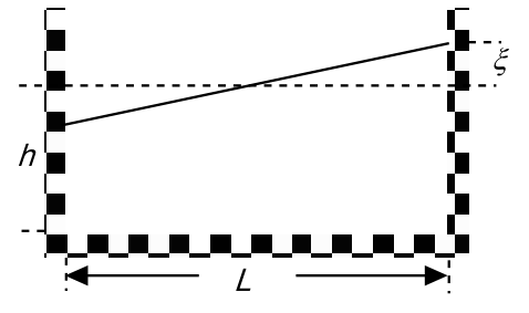
In order to create a model of the seiching we look at water in a rectangular container. The length of the container is \(L\) and the depth of the water is \(h\). Assume that the surface of the water to begin with makes a small angle with the horizontal. The seiching will then start, and we assume that the water surface continues to be plane but oscillates around an axis in the horizontal plane and located in the middle of the container.
Create a model of the movement of the water and derive a formula for the oscillation period \(T\). The starting conditions are given in figure above. Assume that \(\xi \ll h\). The table below shows experimental oscillation periods for different water depths in two containers of different lengths. Check in some reasonable way how well the formula that you have derived agrees with the experimental data. Give your opinion on the quality of your model.
Table 1. \(L = 479\ \mathrm{mm}\)
| \(h/\mathrm{mm}\) | 30 | 50 | 69 | 88 | 107 | 124 | 142 |
|---|---|---|---|---|---|---|---|
| \(T/\mathrm{s}\) | 1.78 | 1.40 | 1.18 | 1.08 | 1.00 | 0.91 | 0.82 |
Table 2. \(L = 143\ \mathrm{mm}\)
| \(h/\mathrm{mm}\) | 31 | 38 | 58 | 67 | 124 |
|---|---|---|---|---|---|
| \(T/\mathrm{s}\) | 0.52 | 0.52 | 0.43 | 0.35 | 0.28 |
The graph below shows results from measurements in lake Vättern in Sweden. This lake has a length of 123 km and a mean depth of 50 m. What is the time scale in the graph?
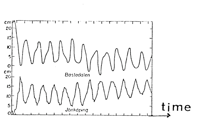
The water surface level in Bastudalen (northern end of lake Vättern) and Jönköping (southern end).
Official English text of the problem.
Answers
Problem 2 has no numbered subparts or printed point values. Its requests are answered in their printed order.
-
2 — Motion and period: A simple model using the centre of mass and hydrostatic end-wall forces gives harmonic oscillations with \[ \boxed{T_0=\frac{\pi L}{\sqrt{3gh}}.} \] An energy model accounting for the variation of horizontal flow speed gives the refined estimate \[ \boxed{T_1=\frac{2\pi L}{\sqrt{10gh}} \simeq1.987\,\frac{L}{\sqrt{gh}}.} \]
-
2 — Experimental comparison and quality: \(T_0\) underestimates the measured periods by \(10.0\)–\(15.2\%\) in the longer container and \(8.6\)–\(20.0\%\) in the shorter one. The model captures the approximate scaling \(T\propto L/\sqrt h\). The energy estimate agrees more closely: its largest discrepancies are \(7.1\%\) and \(12.4\%\), respectively. Both models have limited validity when the depth becomes comparable with the length.
-
2 — Lake Vättern: \(T_0\simeq2.8\ \mathrm h\), while \(T_1\simeq3.1\ \mathrm h\). Thus the graph shows approximately three hours per oscillation, or two hours per horizontal tick interval, with about a day and a half represented overall.
Solution
2 — Model of the motion and oscillation period
Let the container have width \(b\), and let the water density be \(\rho\). Measure \(x\) horizontally from the middle of the container. Write the surface height above the bottom as
\[ H(x,t)=h+\eta(x,t),\qquad \eta(x,t)=\frac{2q(t)x}{L}, \qquad -\frac L2\leq x\leq\frac L2. \]
Thus the depths at the left and right ends are \(h-q\) and \(h+q\), respectively. Initially \(q=\xi\).
We neglect viscosity, damping and surface tension. For a long, shallow container, vertical accelerations can initially be neglected and the pressure approximated as hydrostatic. Small amplitude, \(|q|\ll h\), allows a linear oscillation model.
The total mass is
\[ M=\rho bLh, \]
since the volume above the mean surface equals the missing volume below it. The horizontal coordinate \(X\) of the centre of mass is
\[ \begin{aligned} X &=\frac{\rho b}{M} \int_{-L/2}^{L/2}xH(x,t)\,dx\\ &=\frac{1}{Lh}\frac{2q}{L} \int_{-L/2}^{L/2}x^2\,dx\\ &=\boxed{\frac{Lq}{6h}}. \end{aligned} \]
The hydrostatic force exerted by an end wall on water of depth \(H\) has magnitude
\[ b\int_0^H \rho g(H-z)\,dz =\frac12\rho gbH^2. \]
Consequently, the net horizontal force on the water is
\[ \begin{aligned} F_x &=\frac12\rho gb\left[(h-q)^2-(h+q)^2\right]\\ &=-2\rho gbhq. \end{aligned} \]
The force is restoring: when the water is higher on the right, it acts towards the left. Newton’s second law gives
\[ M\ddot X=F_x, \]
or
\[ \rho bLh\frac{L}{6h}\ddot q=-2\rho gbhq. \]
Therefore,
\[ \boxed{\ddot q+\frac{12gh}{L^2}q=0}. \]
This is simple harmonic motion, with
\[ \omega_0=\frac{\sqrt{12gh}}{L}, \qquad \boxed{T_0=\frac{2\pi}{\omega_0} =\frac{\pi L}{\sqrt{3gh}}}. \]
If the illustrated configuration is released from rest,
\[ q(t)=\xi\cos(\omega_0t), \qquad \eta(x,t)=\frac{2\xi x}{L}\cos(\omega_0t). \]
The two ends therefore oscillate in opposite phase. The period is independent of the small amplitude, the width and the density.
An energy estimate accounting for the flow speed
The planar surface is an approximation to the actual motion. We can assess the effect of resolving the internal flow by constructing an energy model.
Assume that the horizontal velocity \(u(x,t)\) is approximately uniform over the depth. Conservation of volume, linearized about the depth \(h\), requires
\[ \frac{\partial\eta}{\partial t} +h\frac{\partial u}{\partial x}=0. \]
Using \(\eta=2qx/L\) and imposing zero horizontal flow through both end walls gives
\[ \boxed{ u(x,t)=\frac{\dot q}{Lh} \left(\frac{L^2}{4}-x^2\right). } \]
The horizontal speed is greatest at the middle and vanishes at the walls. In the shallow-water approximation, the kinetic energy of vertical motion is small compared with that of horizontal motion. Thus
\[ \begin{aligned} K &=\frac12\rho bh \int_{-L/2}^{L/2}u^2\,dx\\ &=\boxed{\frac{\rho bL^3}{60h}\dot q^{\,2}}. \end{aligned} \]
The increase in gravitational potential energy above that of a horizontal surface is
\[ \begin{aligned} U &=\frac{\rho gb}{2} \int_{-L/2}^{L/2}\left[(h+\eta)^2-h^2\right]dx\\ &=\frac{\rho gb}{2}\int_{-L/2}^{L/2}\eta^2\,dx\\ &=\boxed{\frac{\rho gbL}{6}q^2}, \end{aligned} \]
where the term proportional to \(\int\eta\,dx\) vanishes by volume conservation.
Conserving \(K+U\) now gives
\[ \ddot q+\frac{10gh}{L^2}q=0, \]
and hence
\[ \boxed{ T_1=\frac{2\pi L}{\sqrt{10gh}} =\sqrt{\frac65}\,T_0. } \]
This estimate is about \(9.5\%\) longer than the simple centre-of-mass result.
The differing coefficients reflect the approximate descriptions of the motion: the first model uses hydrostatic end forces, while the second uses the energy of a volume-conserving trial flow. The actual free surface generally departs from a plane, so neither coefficient should be regarded as an exact hydrodynamic result.
2 — Comparison with the measurements and quality of the model
Using \(g=9.81\ \mathrm{m\,s^{-2}}\), the predicted periods are:
For \(L=479\ \mathrm{mm}\):
| \(h\) (mm) | Measured \(T\) (s) | \(T_0\) (s) | \(T_1\) (s) |
|---|---|---|---|
| 30 | 1.78 | 1.60 | 1.75 |
| 50 | 1.40 | 1.24 | 1.36 |
| 69 | 1.18 | 1.06 | 1.16 |
| 88 | 1.08 | 0.935 | 1.02 |
| 107 | 1.00 | 0.848 | 0.929 |
| 124 | 0.91 | 0.788 | 0.863 |
| 142 | 0.82 | 0.736 | 0.806 |
For \(L=143\ \mathrm{mm}\):
| \(h\) (mm) | Measured \(T\) (s) | \(T_0\) (s) | \(T_1\) (s) |
|---|---|---|---|
| 31 | 0.52 | 0.470 | 0.515 |
| 38 | 0.52 | 0.425 | 0.465 |
| 58 | 0.43 | 0.344 | 0.377 |
| 67 | 0.35 | 0.320 | 0.350 |
| 124 | 0.28 | 0.235 | 0.258 |
For a quantitative comparison, define the relative discrepancy as
\[ \varepsilon= \frac{T_{\mathrm{model}}-T_{\mathrm{measured}}} {T_{\mathrm{measured}}}. \]
The simple model gives periods systematically below the observations: by \(10.0\)–\(15.2\%\) in the longer container and \(8.6\)–\(20.0\%\) in the shorter one. The energy estimate reduces the maximum absolute discrepancies to \(7.1\%\) and \(12.4\%\).
The approximate scaling can also be checked through the dimensionless quantity
\[ C=\frac{T\sqrt{gh}}{L}. \]
The experimental values range from approximately \(2.02\) to \(2.14\) in the longer container and \(1.98\) to \(2.27\) in the shorter one. These are reasonably close to a common constant. The two model predictions are
\[ C_0=\frac{\pi}{\sqrt3}\simeq1.814, \qquad C_1=\frac{2\pi}{\sqrt{10}}\simeq1.987. \]
Thus the models provide a useful description of the scale and parameter dependence, and resolving the flow speed improves agreement with these data.
Their validity nevertheless has limits. The ratios \(h/L\) range from \(0.063\) to \(0.30\) in the longer container and from \(0.22\) to \(0.87\) in the shorter one. In particular, the deepest measurements in the shorter container fall outside a reliable shallow-water approximation. Vertical motion and departures from the assumed planar surface then matter. No experimental uncertainties are supplied, so the table establishes numerical agreement rather than a statistical validation.
2 — Time scale of the lake measurements
For lake Vättern,
\[ L=1.23\times10^5\ \mathrm m, \qquad h=50\ \mathrm m, \]
giving
\[ \sqrt{gh}\simeq22.1\ \mathrm{m\,s^{-1}}. \]
The simple model predicts
\[ T_0= \frac{\pi(1.23\times10^5)} {\sqrt{3(9.81)(50)}} \simeq1.01\times10^4\ \mathrm s =\boxed{2.8\ \mathrm h}. \]
The energy estimate gives
\[ T_1= \frac{2\pi(1.23\times10^5)} {\sqrt{10(9.81)(50)}} \simeq1.10\times10^4\ \mathrm s =\boxed{3.1\ \mathrm h}. \]
Accordingly, successive peaks in either trace are separated by approximately three hours.
In the reproduced graph, a complete oscillation occupies approximately \(1.5\) horizontal tick intervals. Therefore,
\[ \text{time per tick interval} \approx\frac{3\ \mathrm h}{1.5} \approx\boxed{2\ \mathrm h}. \]
There are roughly twelve oscillations across the record, corresponding to approximately \(36\ \mathrm h\), or a day and a half. The two traces are approximately in opposite phase, as expected for oscillations at opposite ends of the lake.
The solution was checked against the official solution.
IPhO 1984 · Theorieaufgabe 2
Seiches in Seen
In manchen Seen tritt ein merkwürdiges Phänomen auf, das als „Seiche“ bezeichnet wird und eine Schwingung des Wassers darstellt. Seen, in denen man dieses Phänomen beobachten kann, sind gewöhnlich im Verhältnis zu ihrer Tiefe lang und außerdem schmal. Wellen in einem See sind ein vertrauter Anblick, nicht aber eine Erscheinung wie eine Seiche, bei der das gesamte Wasservolumen schwingt, ähnlich wie der Kaffee in einer Tasse, die man zu einem wartenden Gast trägt.
Um ein Modell für die Seiche zu entwickeln, betrachten wir Wasser in einem rechteckigen Behälter. Die Länge des Behälters beträgt \(L\), die Wassertiefe \(h\). Nehmen Sie an, dass die Wasseroberfläche zu Beginn einen kleinen Winkel mit der Horizontalen bildet. Daraufhin setzt die Seiche ein, und wir nehmen an, dass die Wasseroberfläche eben bleibt, jedoch um eine Achse schwingt, die in der horizontalen Ebene in der Mitte des Behälters liegt.
Entwickeln Sie ein Modell für die Bewegung des Wassers und leiten Sie eine Formel für die Schwingungsdauer \(T\) her. Die Anfangsbedingungen sind in der obigen Abbildung dargestellt. Nehmen Sie an, dass \(\xi \ll h\). Die folgende Tabelle zeigt experimentell bestimmte Schwingungsdauern für verschiedene Wassertiefen in zwei Behältern unterschiedlicher Länge. Überprüfen Sie auf geeignete Weise, wie gut die von Ihnen hergeleitete Formel mit den experimentellen Daten übereinstimmt. Beurteilen Sie die Güte Ihres Modells.
Tabelle 1. \(L = 479\ \mathrm{mm}\)
| \(h/\mathrm{mm}\) | 30 | 50 | 69 | 88 | 107 | 124 | 142 |
|---|---|---|---|---|---|---|---|
| \(T/\mathrm{s}\) | 1.78 | 1.40 | 1.18 | 1.08 | 1.00 | 0.91 | 0.82 |
Tabelle 2. \(L = 143\ \mathrm{mm}\)
| \(h/\mathrm{mm}\) | 31 | 38 | 58 | 67 | 124 |
|---|---|---|---|---|---|
| \(T/\mathrm{s}\) | 0.52 | 0.52 | 0.43 | 0.35 | 0.28 |
Das folgende Diagramm zeigt Messergebnisse vom Vätternsee in Schweden. Dieser See hat eine Länge von 123 km und eine mittlere Tiefe von 50 m. Welche Zeitskala hat das Diagramm?
Der Wasserstand in Bastudalen (am Nordende des Vätternsees) und Jönköping (am Südende).
Aufgabentext aus dem offiziellen englischen Text übersetzt.
Antworten
Aufgabe 2 enthält weder nummerierte Teilaufgaben noch gedruckte Punktangaben. Die Fragen werden in der Reihenfolge beantwortet, in der sie abgedruckt sind.
-
2 — Bewegung und Schwingungsdauer: Ein einfaches Modell, das den Schwerpunkt und die hydrostatischen Kräfte an den Stirnwänden verwendet, ergibt harmonische Schwingungen mit \[ \boxed{T_0=\frac{\pi L}{\sqrt{3gh}}.} \] Ein Energiemodell, das die räumliche Änderung der horizontalen Strömungsgeschwindigkeit berücksichtigt, liefert die verfeinerte Abschätzung \[ \boxed{T_1=\frac{2\pi L}{\sqrt{10gh}} \simeq1.987\,\frac{L}{\sqrt{gh}}.} \]
-
2 — Vergleich mit dem Experiment und Güte: \(T_0\) unterschätzt die gemessenen Schwingungsdauern im längeren Behälter um \(10.0\)–\(15.2\%\) und im kürzeren um \(8.6\)–\(20.0\%\). Das Modell erfasst näherungsweise das Skalierungsverhalten \(T\propto L/\sqrt h\). Die Energieabschätzung stimmt besser mit den Messwerten überein: Ihre größten Abweichungen betragen \(7.1\%\) beziehungsweise \(12.4\%\). Beide Modelle sind nur eingeschränkt gültig, wenn die Tiefe mit der Länge vergleichbar wird.
-
2 — Vätternsee: \(T_0\simeq2.8\ \mathrm h\), während \(T_1\simeq3.1\ \mathrm h\). Das Diagramm zeigt somit ungefähr drei Stunden pro Schwingung oder zwei Stunden pro horizontalem Teilstrichabstand, wobei insgesamt etwa eineinhalb Tage dargestellt sind.
Lösung
2 — Modell der Bewegung und Schwingungsdauer
Der Behälter habe die Breite \(b\), und die Dichte des Wassers sei \(\rho\). Die horizontale Koordinate \(x\) wird von der Mitte des Behälters aus gemessen. Wir schreiben die Höhe der Wasseroberfläche über dem Boden als
\[ H(x,t)=h+\eta(x,t),\qquad \eta(x,t)=\frac{2q(t)x}{L}, \qquad -\frac L2\leq x\leq\frac L2. \]
Damit betragen die Wassertiefen am linken und rechten Ende \(h-q\) beziehungsweise \(h+q\). Zu Beginn gilt \(q=\xi\).
Wir vernachlässigen Viskosität, Dämpfung und Oberflächenspannung. Für einen langen, flachen Behälter können vertikale Beschleunigungen zunächst vernachlässigt und der Druck als näherungsweise hydrostatisch angenommen werden. Die kleine Amplitude, \(|q|\ll h\), ermöglicht ein lineares Schwingungsmodell.
Die Gesamtmasse beträgt
\[ M=\rho bLh, \]
da das Volumen oberhalb der mittleren Wasseroberfläche gleich dem darunter fehlenden Volumen ist. Die horizontale Koordinate \(X\) des Schwerpunkts lautet
\[ \begin{aligned} X &=\frac{\rho b}{M} \int_{-L/2}^{L/2}xH(x,t)\,dx\\ &=\frac{1}{Lh}\frac{2q}{L} \int_{-L/2}^{L/2}x^2\,dx\\ &=\boxed{\frac{Lq}{6h}}. \end{aligned} \]
Die hydrostatische Kraft, die eine Stirnwand auf Wasser der Tiefe \(H\) ausübt, hat den Betrag
\[ b\int_0^H \rho g(H-z)\,dz =\frac12\rho gbH^2. \]
Folglich ist die resultierende horizontale Kraft auf das Wasser
\[ \begin{aligned} F_x &=\frac12\rho gb\left[(h-q)^2-(h+q)^2\right]\\ &=-2\rho gbhq. \end{aligned} \]
Die Kraft ist rücktreibend: Wenn das Wasser rechts höher steht, wirkt sie nach links. Das zweite Newtonsche Gesetz ergibt
\[ M\ddot X=F_x, \]
oder
\[ \rho bLh\frac{L}{6h}\ddot q=-2\rho gbhq. \]
Somit gilt
\[ \boxed{\ddot q+\frac{12gh}{L^2}q=0}. \]
Dies ist eine harmonische Schwingung mit
\[ \omega_0=\frac{\sqrt{12gh}}{L}, \qquad \boxed{T_0=\frac{2\pi}{\omega_0} =\frac{\pi L}{\sqrt{3gh}}}. \]
Wird das Wasser aus der dargestellten Anordnung ohne Anfangsgeschwindigkeit freigegeben, so gilt
\[ q(t)=\xi\cos(\omega_0t), \qquad \eta(x,t)=\frac{2\xi x}{L}\cos(\omega_0t). \]
Die beiden Enden schwingen daher gegenphasig. Die Schwingungsdauer ist unabhängig von der kleinen Amplitude, der Breite und der Dichte.
Eine Energieabschätzung unter Berücksichtigung der Strömungsgeschwindigkeit
Die ebene Oberfläche ist eine Näherung für die tatsächliche Bewegung. Wir können den Einfluss einer genaueren Beschreibung der inneren Strömung abschätzen, indem wir ein Energiemodell aufstellen.
Wir nehmen an, dass die horizontale Geschwindigkeit \(u(x,t)\) über die Tiefe näherungsweise konstant ist. Die um die Tiefe \(h\) linearisierte Volumenerhaltung verlangt
\[ \frac{\partial\eta}{\partial t} +h\frac{\partial u}{\partial x}=0. \]
Mit \(\eta=2qx/L\) und der Bedingung, dass durch beide Stirnwände keine horizontale Strömung erfolgt, ergibt sich
\[ \boxed{ u(x,t)=\frac{\dot q}{Lh} \left(\frac{L^2}{4}-x^2\right). } \]
Die horizontale Geschwindigkeit ist in der Mitte am größten und verschwindet an den Wänden. In der Flachwassernäherung ist die kinetische Energie der vertikalen Bewegung klein gegenüber derjenigen der horizontalen Bewegung. Daher gilt
\[ \begin{aligned} K &=\frac12\rho bh \int_{-L/2}^{L/2}u^2\,dx\\ &=\boxed{\frac{\rho bL^3}{60h}\dot q^{\,2}}. \end{aligned} \]
Die Zunahme der potenziellen Energie im Schwerefeld gegenüber derjenigen bei horizontaler Wasseroberfläche beträgt
\[ \begin{aligned} U &=\frac{\rho gb}{2} \int_{-L/2}^{L/2}\left[(h+\eta)^2-h^2\right]dx\\ &=\frac{\rho gb}{2}\int_{-L/2}^{L/2}\eta^2\,dx\\ &=\boxed{\frac{\rho gbL}{6}q^2}, \end{aligned} \]
wobei der zu \(\int\eta\,dx\) proportionale Term aufgrund der Volumenerhaltung verschwindet.
Aus der Erhaltung von \(K+U\) folgt nun
\[ \ddot q+\frac{10gh}{L^2}q=0, \]
und damit
\[ \boxed{ T_1=\frac{2\pi L}{\sqrt{10gh}} =\sqrt{\frac65}\,T_0. } \]
Diese Abschätzung ergibt eine um etwa \(9.5\%\) längere Schwingungsdauer als das einfache Schwerpunktmodell.
Die unterschiedlichen Koeffizienten spiegeln die näherungsweisen Beschreibungen der Bewegung wider: Das erste Modell verwendet hydrostatische Kräfte an den Stirnwänden, während das zweite die Energie eines volumenerhaltenden Strömungsansatzes verwendet. Die tatsächliche freie Oberfläche weicht im Allgemeinen von einer Ebene ab, sodass keiner der beiden Koeffizienten als exaktes hydrodynamisches Ergebnis angesehen werden sollte.
2 — Vergleich mit den Messungen und Güte des Modells
Mit \(g=9.81\ \mathrm{m\,s^{-2}}\) ergeben sich die folgenden vorhergesagten Schwingungsdauern:
Für \(L=479\ \mathrm{mm}\):
| \(h\) (mm) | Gemessenes \(T\) (s) | \(T_0\) (s) | \(T_1\) (s) |
|---|---|---|---|
| 30 | 1.78 | 1.60 | 1.75 |
| 50 | 1.40 | 1.24 | 1.36 |
| 69 | 1.18 | 1.06 | 1.16 |
| 88 | 1.08 | 0.935 | 1.02 |
| 107 | 1.00 | 0.848 | 0.929 |
| 124 | 0.91 | 0.788 | 0.863 |
| 142 | 0.82 | 0.736 | 0.806 |
Für \(L=143\ \mathrm{mm}\):
| \(h\) (mm) | Gemessenes \(T\) (s) | \(T_0\) (s) | \(T_1\) (s) |
|---|---|---|---|
| 31 | 0.52 | 0.470 | 0.515 |
| 38 | 0.52 | 0.425 | 0.465 |
| 58 | 0.43 | 0.344 | 0.377 |
| 67 | 0.35 | 0.320 | 0.350 |
| 124 | 0.28 | 0.235 | 0.258 |
Für einen quantitativen Vergleich definieren wir die relative Abweichung als
\[ \varepsilon= \frac{T_{\mathrm{model}}-T_{\mathrm{measured}}} {T_{\mathrm{measured}}}. \]
Das einfache Modell liefert Schwingungsdauern, die systematisch unter den beobachteten Werten liegen: im längeren Behälter um \(10.0\)–\(15.2\%\) und im kürzeren um \(8.6\)–\(20.0\%\). Die Energieabschätzung verringert die maximalen absoluten Abweichungen auf \(7.1\%\) und \(12.4\%\).
Das näherungsweise Skalierungsverhalten lässt sich auch anhand der folgenden dimensionslosen Größe überprüfen:
\[ C=\frac{T\sqrt{gh}}{L}. \]
Die experimentellen Werte liegen im längeren Behälter ungefähr zwischen \(2.02\) und \(2.14\) und im kürzeren zwischen \(1.98\) und \(2.27\). Sie liegen damit recht nahe an einer gemeinsamen Konstante. Die beiden Modellvorhersagen lauten
\[ C_0=\frac{\pi}{\sqrt3}\simeq1.814, \qquad C_1=\frac{2\pi}{\sqrt{10}}\simeq1.987. \]
Die Modelle liefern somit eine nützliche Beschreibung der Größenordnung und der Parameterabhängigkeit, und eine genauere Berücksichtigung der Strömungsgeschwindigkeit verbessert die Übereinstimmung mit diesen Daten.
Ihre Gültigkeit ist dennoch begrenzt. Die Verhältnisse \(h/L\) reichen im längeren Behälter von \(0.063\) bis \(0.30\) und im kürzeren von \(0.22\) bis \(0.87\). Insbesondere liegen die Messungen bei den größten Tiefen im kürzeren Behälter außerhalb des Bereichs, in dem die Flachwassernäherung zuverlässig ist. Vertikale Bewegungen und Abweichungen von der angenommenen ebenen Oberfläche spielen dann eine Rolle. Es sind keine experimentellen Unsicherheiten angegeben, sodass die Tabelle eine numerische Übereinstimmung, jedoch keine statistische Validierung belegt.
2 — Zeitskala der Messungen am See
Für den Vätternsee gilt
\[ L=1.23\times10^5\ \mathrm m, \qquad h=50\ \mathrm m, \]
Damit ergibt sich
\[ \sqrt{gh}\simeq22.1\ \mathrm{m\,s^{-1}}. \]
Das einfache Modell sagt voraus:
\[ T_0= \frac{\pi(1.23\times10^5)} {\sqrt{3(9.81)(50)}} \simeq1.01\times10^4\ \mathrm s =\boxed{2.8\ \mathrm h}. \]
Die Energieabschätzung liefert
\[ T_1= \frac{2\pi(1.23\times10^5)} {\sqrt{10(9.81)(50)}} \simeq1.10\times10^4\ \mathrm s =\boxed{3.1\ \mathrm h}. \]
Dementsprechend liegen aufeinanderfolgende Maxima jeder der beiden Kurven ungefähr drei Stunden auseinander.
Im wiedergegebenen Diagramm erstreckt sich eine vollständige Schwingung über ungefähr \(1.5\) horizontale Teilstrichabstände. Daher gilt
\[ \text{Zeit pro Teilstrichabstand} \approx\frac{3\ \mathrm h}{1.5} \approx\boxed{2\ \mathrm h}. \]
Die Aufzeichnung umfasst etwa zwölf Schwingungen, was ungefähr \(36\ \mathrm h\) oder eineinhalb Tagen entspricht. Die beiden Kurven sind annähernd gegenphasig, wie es für Schwingungen an gegenüberliegenden Enden des Sees zu erwarten ist.
Die Lösung wurde mit der offiziellen Lösung abgeglichen.
IPhO 1984 · Teori sorusu 2
Göl suyunun seş salınımı
Bazı göllerde, suyun salınım yaptığı ve “seş” adı verilen ilginç bir olay görülür. Bu olayın gözlenebildiği göller genellikle derinliklerine göre uzun ve aynı zamanda dardır. Bir gölde dalgalar görmek doğaldır; ancak bekleyen bir misafire götürdüğünüz fincandaki kahve gibi suyun tüm hacminin salındığı seş benzeri bir olay görmek alışıldık değildir.
Seş olayını modellemek için dikdörtgen bir kaptaki suyu ele alıyoruz. Kabın uzunluğu \(L\), suyun derinliği ise \(h\)'dir. Başlangıçta su yüzeyinin yatayla küçük bir açı yaptığını varsayın. Bu durumda seş salınımı başlayacaktır; su yüzeyinin düzlemsel kalmaya devam ettiğini, ancak yatay düzlemde bulunan ve kabın ortasından geçen bir eksen etrafında salındığını varsayıyoruz.
Suyun hareketi için bir model oluşturun ve salınım periyodu \(T\) için bir formül türetin. Başlangıç koşulları yukarıdaki şekilde verilmiştir. \(\xi \ll h\) olduğunu varsayın. Aşağıdaki tabloda, farklı uzunluklardaki iki kapta farklı su derinlikleri için deneysel salınım periyotları verilmiştir. Türettiğiniz formülün deneysel verilerle ne kadar iyi uyuştuğunu uygun bir yöntemle kontrol edin. Modelinizin niteliği hakkındaki görüşünüzü belirtin.
Tablo 1. \(L = 479\ \mathrm{mm}\)
| \(h/\mathrm{mm}\) | 30 | 50 | 69 | 88 | 107 | 124 | 142 |
|---|---|---|---|---|---|---|---|
| \(T/\mathrm{s}\) | 1.78 | 1.40 | 1.18 | 1.08 | 1.00 | 0.91 | 0.82 |
Tablo 2. \(L = 143\ \mathrm{mm}\)
| \(h/\mathrm{mm}\) | 31 | 38 | 58 | 67 | 124 |
|---|---|---|---|---|---|
| \(T/\mathrm{s}\) | 0.52 | 0.52 | 0.43 | 0.35 | 0.28 |
Aşağıdaki grafik, İsveç'teki Vättern Gölü'nde yapılan ölçümlerin sonuçlarını göstermektedir. Bu gölün uzunluğu 123 km, ortalama derinliği ise 50 m'dir. Grafikteki zaman ölçeği nedir?
Bastudalen'de (Vättern Gölü'nün kuzey ucu) ve Jönköping'de (güney ucu) su yüzeyinin seviyesi.
Soru metni resmi İngilizce metinden çevrilmiştir.
Cevaplar
2. soruda numaralandırılmış alt kısımlar veya belirtilmiş puan değerleri yoktur. İstenenler, soruda verildikleri sırayla yanıtlanmıştır.
-
2 — Hareket ve periyot: Kütle merkezini ve uç duvarların uyguladığı hidrostatik kuvvetleri kullanan basit bir model, periyodu \[ \boxed{T_0=\frac{\pi L}{\sqrt{3gh}}.} \] olan harmonik salınımlar verir. Yatay akış süratinin değişimini hesaba katan bir enerji modeli ise daha gelişmiş bir tahmin verir: \[ \boxed{T_1=\frac{2\pi L}{\sqrt{10gh}} \simeq1.987\,\frac{L}{\sqrt{gh}}.} \]
-
2 — Deneysel karşılaştırma ve modelin niteliği: \(T_0\), ölçülen periyotlardan uzun kapta \(10.0\)–\(15.2\%\), kısa kapta ise \(8.6\)–\(20.0\%\) daha küçüktür. Model, yaklaşık \(T\propto L/\sqrt h\) ölçekleme ilişkisini yansıtır. Enerji tahmini daha iyi uyuşur: en büyük sapmalar sırasıyla \(7.1\%\) ve \(12.4\%\)'tür. Derinlik uzunlukla karşılaştırılabilir hâle geldiğinde her iki modelin de geçerliliği sınırlıdır.
-
2 — Vättern Gölü: \(T_0\simeq2.8\ \mathrm h\), buna karşılık \(T_1\simeq3.1\ \mathrm h\) olur. Dolayısıyla grafikte her salınım yaklaşık üç saate, diğer bir deyişle yatay eksendeki her işaret aralığı iki saate karşılık gelir; grafiğin tamamı yaklaşık bir buçuk günü temsil eder.
Çözüm
2 — Hareket modeli ve salınım periyodu
Kabın genişliği \(b\), suyun yoğunluğu ise \(\rho\) olsun. \(x\) koordinatını kabın ortasından başlayarak yatay doğrultuda ölçelim. Yüzeyin tabandan yüksekliğini şöyle yazalım:
\[ H(x,t)=h+\eta(x,t),\qquad \eta(x,t)=\frac{2q(t)x}{L}, \qquad -\frac L2\leq x\leq\frac L2. \]
Böylece sol ve sağ uçlardaki derinlikler sırasıyla \(h-q\) ve \(h+q\) olur. Başlangıçta \(q=\xi\)'dir.
Viskoziteyi, sönümü ve yüzey gerilimini ihmal ediyoruz. Uzun ve sığ bir kap için ilk yaklaşımda düşey ivmeler ihmal edilebilir ve basınç hidrostatik olarak alınabilir. Küçük genlik, \(|q|\ll h\), doğrusal bir salınım modeli kurmaya olanak tanır.
Toplam kütle
\[ M=\rho bLh, \]
olur; çünkü ortalama yüzeyin üzerindeki hacim, bu yüzeyin altında eksilen hacme eşittir. Kütle merkezinin yatay koordinatı \(X\) şöyledir:
\[ \begin{aligned} X &=\frac{\rho b}{M} \int_{-L/2}^{L/2}xH(x,t)\,dx\\ &=\frac{1}{Lh}\frac{2q}{L} \int_{-L/2}^{L/2}x^2\,dx\\ &=\boxed{\frac{Lq}{6h}}. \end{aligned} \]
Bir uç duvarın derinliği \(H\) olan suya uyguladığı hidrostatik kuvvetin büyüklüğü
\[ b\int_0^H \rho g(H-z)\,dz =\frac12\rho gbH^2. \]
olur. Dolayısıyla suya etki eden net yatay kuvvet
\[ \begin{aligned} F_x &=\frac12\rho gb\left[(h-q)^2-(h+q)^2\right]\\ &=-2\rho gbhq. \end{aligned} \]
olur. Bu kuvvet geri çağırıcıdır: su sağ tarafta daha yüksek olduğunda kuvvet sola doğru etki eder. Newton'un ikinci yasası
\[ M\ddot X=F_x, \]
ya da
\[ \rho bLh\frac{L}{6h}\ddot q=-2\rho gbhq. \]
bağıntısını verir. Dolayısıyla,
\[ \boxed{\ddot q+\frac{12gh}{L^2}q=0}. \]
Bu, açısal frekansı ve periyodu
\[ \omega_0=\frac{\sqrt{12gh}}{L}, \qquad \boxed{T_0=\frac{2\pi}{\omega_0} =\frac{\pi L}{\sqrt{3gh}}}. \]
olan basit harmonik harekettir.
Şekilde gösterilen durumdan ilk hızsız olarak serbest bırakılırsa,
\[ q(t)=\xi\cos(\omega_0t), \qquad \eta(x,t)=\frac{2\xi x}{L}\cos(\omega_0t). \]
Dolayısıyla iki uç zıt fazda salınır. Periyot, küçük genliğin değerinden, genişlikten ve yoğunluktan bağımsızdır.
Akış süratini hesaba katan bir enerji tahmini
Düzlemsel yüzey, gerçek harekete ilişkin bir yaklaşımdır. Bir enerji modeli kurarak iç akışın ayrıntılarını hesaba katmanın etkisini değerlendirebiliriz.
Yatay hız \(u(x,t)\)'nin derinlik boyunca yaklaşık olarak sabit olduğunu varsayalım. \(h\) derinliği etrafında doğrusallaştırılan hacim korunumu,
\[ \frac{\partial\eta}{\partial t} +h\frac{\partial u}{\partial x}=0. \]
koşulunu gerektirir.
\(\eta=2qx/L\) bağıntısı kullanılıp her iki uç duvardan geçen yatay akışın sıfır olması koşulu uygulandığında
\[ \boxed{ u(x,t)=\frac{\dot q}{Lh} \left(\frac{L^2}{4}-x^2\right). } \]
elde edilir.
Yatay sürat ortada en büyüktür ve duvarlarda sıfır olur. Sığ su yaklaşımında düşey hareketin kinetik enerjisi, yatay hareketinkine göre küçüktür. Dolayısıyla
\[ \begin{aligned} K &=\frac12\rho bh \int_{-L/2}^{L/2}u^2\,dx\\ &=\boxed{\frac{\rho bL^3}{60h}\dot q^{\,2}}. \end{aligned} \]
Yerçekimi potansiyel enerjisinin, yüzeyin yatay olduğu durumdakine göre artışı
\[ \begin{aligned} U &=\frac{\rho gb}{2} \int_{-L/2}^{L/2}\left[(h+\eta)^2-h^2\right]dx\\ &=\frac{\rho gb}{2}\int_{-L/2}^{L/2}\eta^2\,dx\\ &=\boxed{\frac{\rho gbL}{6}q^2}, \end{aligned} \]
olur; burada \(\int\eta\,dx\) ile orantılı terim, hacim korunumundan dolayı sıfırdır.
Şimdi \(K+U\)'nun korunumu
\[ \ddot q+\frac{10gh}{L^2}q=0, \]
ve dolayısıyla
\[ \boxed{ T_1=\frac{2\pi L}{\sqrt{10gh}} =\sqrt{\frac65}\,T_0. } \]
sonucunu verir.
Bu tahmin, basit kütle merkezi sonucundan yaklaşık \(9.5\%\) daha uzundur.
Katsayıların farklı olması, hareketin yaklaşık betimlemelerini yansıtır: ilk model uçlardaki hidrostatik kuvvetleri kullanırken, ikincisi hacmi koruyan bir deneme akışının enerjisini kullanır. Gerçek serbest yüzey genellikle düzlemsellikten sapar; bu nedenle katsayıların hiçbiri kesin bir hidrodinamik sonuç olarak görülmemelidir.
2 — Ölçümlerle karşılaştırma ve modelin niteliği
\(g=9.81\ \mathrm{m\,s^{-2}}\) kullanıldığında, öngörülen periyotlar şöyledir:
\(L=479\ \mathrm{mm}\) için:
| \(h\) (mm) | Ölçülen \(T\) (s) | \(T_0\) (s) | \(T_1\) (s) |
|---|---|---|---|
| 30 | 1.78 | 1.60 | 1.75 |
| 50 | 1.40 | 1.24 | 1.36 |
| 69 | 1.18 | 1.06 | 1.16 |
| 88 | 1.08 | 0.935 | 1.02 |
| 107 | 1.00 | 0.848 | 0.929 |
| 124 | 0.91 | 0.788 | 0.863 |
| 142 | 0.82 | 0.736 | 0.806 |
\(L=143\ \mathrm{mm}\) için:
| \(h\) (mm) | Ölçülen \(T\) (s) | \(T_0\) (s) | \(T_1\) (s) |
|---|---|---|---|
| 31 | 0.52 | 0.470 | 0.515 |
| 38 | 0.52 | 0.425 | 0.465 |
| 58 | 0.43 | 0.344 | 0.377 |
| 67 | 0.35 | 0.320 | 0.350 |
| 124 | 0.28 | 0.235 | 0.258 |
Nicel bir karşılaştırma için bağıl sapmayı şöyle tanımlayalım:
\[ \varepsilon= \frac{T_{\mathrm{model}}-T_{\mathrm{measured}}} {T_{\mathrm{measured}}}. \]
Basit model, gözlemlerden sistematik olarak daha düşük periyotlar verir: uzun kapta \(10.0\)–\(15.2\%\), kısa kapta ise \(8.6\)–\(20.0\%\) oranında. Enerji tahmini, en büyük mutlak sapmaları \(7.1\%\) ve \(12.4\%\)'e indirir.
Yaklaşık ölçekleme ilişkisi, boyutsuz
\[ C=\frac{T\sqrt{gh}}{L}. \]
niceliği aracılığıyla da kontrol edilebilir.
Deneysel değerler uzun kapta yaklaşık \(2.02\) ile \(2.14\), kısa kapta ise \(1.98\) ile \(2.27\) arasında değişir. Bunlar ortak bir sabite makul ölçüde yakındır. İki modelin öngörüleri şöyledir:
\[ C_0=\frac{\pi}{\sqrt3}\simeq1.814, \qquad C_1=\frac{2\pi}{\sqrt{10}}\simeq1.987. \]
Dolayısıyla modeller, büyüklük ölçeğini ve parametrelere bağımlılığı yararlı biçimde betimler; akış süratinin ayrıntılarını hesaba katmak da bu verilerle uyumu iyileştirir.
Bununla birlikte geçerliliklerinin sınırları vardır. \(h/L\) oranları uzun kapta \(0.063\) ile \(0.30\), kısa kapta ise \(0.22\) ile \(0.87\) arasında değişir. Özellikle kısa kaptaki en derin suyla yapılan ölçümler, sığ su yaklaşımının güvenilir olduğu aralığın dışında kalır. Bu durumda düşey hareket ve varsayılan düzlemsel yüzeyden sapmalar önem kazanır. Deneysel belirsizlikler verilmediğinden tablo, istatistiksel bir doğrulama değil, sayısal uyum ortaya koyar.
2 — Göl ölçümlerinin zaman ölçeği
Vättern Gölü için,
\[ L=1.23\times10^5\ \mathrm m, \qquad h=50\ \mathrm m, \]
olduğundan
\[ \sqrt{gh}\simeq22.1\ \mathrm{m\,s^{-1}}. \]
elde edilir.
Basit modelin öngörüsü şöyledir:
\[ T_0= \frac{\pi(1.23\times10^5)} {\sqrt{3(9.81)(50)}} \simeq1.01\times10^4\ \mathrm s =\boxed{2.8\ \mathrm h}. \]
Enerji tahmini ise şu sonucu verir:
\[ T_1= \frac{2\pi(1.23\times10^5)} {\sqrt{10(9.81)(50)}} \simeq1.10\times10^4\ \mathrm s =\boxed{3.1\ \mathrm h}. \]
Buna göre, her iki eğriden herhangi birindeki ardışık tepeler arasında yaklaşık üç saat vardır.
Verilen grafikte tam bir salınım, yatay eksendeki yaklaşık \(1.5\) işaret aralığını kaplar. Dolayısıyla,
\[ \text{işaret aralığı başına süre} \approx\frac{3\ \mathrm h}{1.5} \approx\boxed{2\ \mathrm h}. \]
Kayıt boyunca yaklaşık on iki salınım vardır; bu da yaklaşık \(36\ \mathrm h\), yani bir buçuk güne karşılık gelir. Gölün karşı uçlarındaki salınımlar için beklendiği gibi, iki eğri yaklaşık olarak zıt fazdadır.
Çözüm, resmi çözümle karşılaştırılarak kontrol edildi.
IPhO 1984 · Problema teórico 2
Seiches en el agua de un lago
En ciertos lagos se produce un extraño fenómeno llamado «seiche», que consiste en una oscilación del agua. Los lagos en los que se puede observar este fenómeno suelen ser largos en comparación con su profundidad y, además, estrechos. Es normal observar olas en un lago, pero no algo como un seiche, en el que oscila todo el volumen de agua, como el café en una taza que se lleva a un invitado que está esperando.
Para elaborar un modelo del seiche, consideramos el agua contenida en un recipiente rectangular. La longitud del recipiente es \(L\) y la profundidad del agua es \(h\). Supongamos que, inicialmente, la superficie del agua forma un ángulo pequeño con la horizontal. Entonces comenzará el seiche, y suponemos que la superficie del agua sigue siendo plana, pero oscila alrededor de un eje situado en el plano horizontal y en el centro del recipiente.
Elabore un modelo del movimiento del agua y deduzca una fórmula para el período de oscilación \(T\). Las condiciones iniciales se muestran en la figura anterior. Suponga que \(\xi \ll h\). La tabla siguiente muestra los períodos de oscilación experimentales para distintas profundidades de agua en dos recipientes de diferente longitud. Compruebe, de alguna manera razonable, en qué medida la fórmula deducida concuerda con los datos experimentales. Exprese su opinión sobre la calidad de su modelo.
Tabla 1. \(L = 479\ \mathrm{mm}\)
| \(h/\mathrm{mm}\) | 30 | 50 | 69 | 88 | 107 | 124 | 142 |
|---|---|---|---|---|---|---|---|
| \(T/\mathrm{s}\) | 1.78 | 1.40 | 1.18 | 1.08 | 1.00 | 0.91 | 0.82 |
Tabla 2. \(L = 143\ \mathrm{mm}\)
| \(h/\mathrm{mm}\) | 31 | 38 | 58 | 67 | 124 |
|---|---|---|---|---|---|
| \(T/\mathrm{s}\) | 0.52 | 0.52 | 0.43 | 0.35 | 0.28 |
El gráfico siguiente muestra los resultados de mediciones realizadas en el lago Vättern, en Suecia. Este lago tiene una longitud de 123 km y una profundidad media de 50 m. ¿Cuál es la escala temporal del gráfico?
El nivel de la superficie del agua en Bastudalen (extremo norte del lago Vättern) y Jönköping (extremo sur).
Enunciado traducido del texto oficial en inglés.
Respuestas
El problema 2 no tiene apartados numerados ni puntuaciones indicadas. Sus preguntas se responden en el orden en que aparecen.
-
2 — Movimiento y período: Un modelo sencillo que utiliza el centro de masas y las fuerzas hidrostáticas en las paredes de los extremos da lugar a oscilaciones armónicas con \[ \boxed{T_0=\frac{\pi L}{\sqrt{3gh}}.} \] Un modelo energético que tiene en cuenta la variación de la velocidad del flujo horizontal proporciona la estimación más precisa \[ \boxed{T_1=\frac{2\pi L}{\sqrt{10gh}} \simeq1.987\,\frac{L}{\sqrt{gh}}.} \]
-
2 — Comparación experimental y calidad: \(T_0\) subestima los períodos medidos entre un \(10.0\)–\(15.2\%\) en el recipiente más largo y entre un \(8.6\)–\(20.0\%\) en el más corto. El modelo reproduce la ley de escala aproximada \(T\propto L/\sqrt h\). La estimación energética presenta una concordancia mayor: sus discrepancias máximas son del \(7.1\%\) y del \(12.4\%\), respectivamente. Ambos modelos tienen una validez limitada cuando la profundidad se vuelve comparable con la longitud.
-
2 — Lago Vättern: \(T_0\simeq2.8\ \mathrm h\), mientras que \(T_1\simeq3.1\ \mathrm h\). Por tanto, el gráfico muestra aproximadamente tres horas por oscilación, o dos horas por intervalo entre marcas del eje horizontal, y representa en total alrededor de un día y medio.
Solución
2 — Modelo del movimiento y período de oscilación
Sea \(b\) la anchura del recipiente y \(\rho\) la densidad del agua. Medimos \(x\) horizontalmente desde el centro del recipiente. Escribimos la altura de la superficie sobre el fondo como
\[ H(x,t)=h+\eta(x,t),\qquad \eta(x,t)=\frac{2q(t)x}{L}, \qquad -\frac L2\leq x\leq\frac L2. \]
Así, las profundidades en los extremos izquierdo y derecho son \(h-q\) y \(h+q\), respectivamente. Inicialmente, \(q=\xi\).
Despreciamos la viscosidad, el amortiguamiento y la tensión superficial. Para un recipiente largo y poco profundo, se pueden despreciar inicialmente las aceleraciones verticales y aproximar la presión por la hidrostática. Una amplitud pequeña, \(|q|\ll h\), permite utilizar un modelo de oscilación lineal.
La masa total es
\[ M=\rho bLh, \]
ya que el volumen por encima de la superficie media es igual al volumen que falta por debajo de ella. La coordenada horizontal \(X\) del centro de masas es
\[ \begin{aligned} X &=\frac{\rho b}{M} \int_{-L/2}^{L/2}xH(x,t)\,dx\\ &=\frac{1}{Lh}\frac{2q}{L} \int_{-L/2}^{L/2}x^2\,dx\\ &=\boxed{\frac{Lq}{6h}}. \end{aligned} \]
La fuerza hidrostática que ejerce una pared de un extremo sobre el agua de profundidad \(H\) tiene un módulo
\[ b\int_0^H \rho g(H-z)\,dz =\frac12\rho gbH^2. \]
Por consiguiente, la fuerza horizontal neta sobre el agua es
\[ \begin{aligned} F_x &=\frac12\rho gb\left[(h-q)^2-(h+q)^2\right]\\ &=-2\rho gbhq. \end{aligned} \]
La fuerza es restauradora: cuando el agua está más alta a la derecha, actúa hacia la izquierda. La segunda ley de Newton da
\[ M\ddot X=F_x, \]
o bien
\[ \rho bLh\frac{L}{6h}\ddot q=-2\rho gbhq. \]
Por tanto,
\[ \boxed{\ddot q+\frac{12gh}{L^2}q=0}. \]
Este es un movimiento armónico simple, con
\[ \omega_0=\frac{\sqrt{12gh}}{L}, \qquad \boxed{T_0=\frac{2\pi}{\omega_0} =\frac{\pi L}{\sqrt{3gh}}}. \]
Si se deja evolucionar desde el reposo la configuración ilustrada,
\[ q(t)=\xi\cos(\omega_0t), \qquad \eta(x,t)=\frac{2\xi x}{L}\cos(\omega_0t). \]
Por tanto, los dos extremos oscilan en oposición de fase. El período es independiente de la pequeña amplitud, de la anchura y de la densidad.
Una estimación energética que tiene en cuenta la velocidad del flujo
La superficie plana es una aproximación al movimiento real. Podemos evaluar el efecto de describir el flujo interno construyendo un modelo energético.
Supongamos que la velocidad horizontal \(u(x,t)\) es aproximadamente uniforme a lo largo de la profundidad. La conservación del volumen, linealizada en torno a la profundidad \(h\), exige
\[ \frac{\partial\eta}{\partial t} +h\frac{\partial u}{\partial x}=0. \]
Utilizando \(\eta=2qx/L\) e imponiendo un flujo horizontal nulo a través de ambas paredes de los extremos, se obtiene
\[ \boxed{ u(x,t)=\frac{\dot q}{Lh} \left(\frac{L^2}{4}-x^2\right). } \]
La rapidez horizontal es máxima en el centro y se anula en las paredes. En la aproximación de aguas someras, la energía cinética del movimiento vertical es pequeña en comparación con la del movimiento horizontal. Así,
\[ \begin{aligned} K &=\frac12\rho bh \int_{-L/2}^{L/2}u^2\,dx\\ &=\boxed{\frac{\rho bL^3}{60h}\dot q^{\,2}}. \end{aligned} \]
El aumento de la energía potencial gravitatoria respecto a la de una superficie horizontal es
\[ \begin{aligned} U &=\frac{\rho gb}{2} \int_{-L/2}^{L/2}\left[(h+\eta)^2-h^2\right]dx\\ &=\frac{\rho gb}{2}\int_{-L/2}^{L/2}\eta^2\,dx\\ &=\boxed{\frac{\rho gbL}{6}q^2}, \end{aligned} \]
donde el término proporcional a \(\int\eta\,dx\) se anula por la conservación del volumen.
La conservación de \(K+U\) da ahora
\[ \ddot q+\frac{10gh}{L^2}q=0, \]
y, por tanto,
\[ \boxed{ T_1=\frac{2\pi L}{\sqrt{10gh}} =\sqrt{\frac65}\,T_0. } \]
Esta estimación es aproximadamente un \(9.5\%\) mayor que el resultado del modelo sencillo del centro de masas.
Los distintos coeficientes reflejan las descripciones aproximadas del movimiento: el primer modelo utiliza las fuerzas hidrostáticas en los extremos, mientras que el segundo utiliza la energía de un flujo de prueba que conserva el volumen. La superficie libre real generalmente se aparta de un plano, por lo que ninguno de los coeficientes debe considerarse un resultado hidrodinámico exacto.
2 — Comparación con las mediciones y calidad del modelo
Utilizando \(g=9.81\ \mathrm{m\,s^{-2}}\), los períodos previstos son:
Para \(L=479\ \mathrm{mm}\):
| \(h\) (mm) | \(T\) medido (s) | \(T_0\) (s) | \(T_1\) (s) |
|---|---|---|---|
| 30 | 1.78 | 1.60 | 1.75 |
| 50 | 1.40 | 1.24 | 1.36 |
| 69 | 1.18 | 1.06 | 1.16 |
| 88 | 1.08 | 0.935 | 1.02 |
| 107 | 1.00 | 0.848 | 0.929 |
| 124 | 0.91 | 0.788 | 0.863 |
| 142 | 0.82 | 0.736 | 0.806 |
Para \(L=143\ \mathrm{mm}\):
| \(h\) (mm) | \(T\) medido (s) | \(T_0\) (s) | \(T_1\) (s) |
|---|---|---|---|
| 31 | 0.52 | 0.470 | 0.515 |
| 38 | 0.52 | 0.425 | 0.465 |
| 58 | 0.43 | 0.344 | 0.377 |
| 67 | 0.35 | 0.320 | 0.350 |
| 124 | 0.28 | 0.235 | 0.258 |
Para realizar una comparación cuantitativa, definimos la discrepancia relativa como
\[ \varepsilon= \frac{T_{\mathrm{model}}-T_{\mathrm{measured}}} {T_{\mathrm{measured}}}. \]
El modelo sencillo da períodos sistemáticamente inferiores a los observados: entre un \(10.0\)–\(15.2\%\) en el recipiente más largo y entre un \(8.6\)–\(20.0\%\) en el más corto. La estimación energética reduce las discrepancias absolutas máximas al \(7.1\%\) y al \(12.4\%\).
La ley de escala aproximada también se puede comprobar mediante la magnitud adimensional
\[ C=\frac{T\sqrt{gh}}{L}. \]
Los valores experimentales varían aproximadamente entre \(2.02\) y \(2.14\) en el recipiente más largo, y entre \(1.98\) y \(2.27\) en el más corto. Estos valores son razonablemente próximos a una constante común. Las predicciones de los dos modelos son
\[ C_0=\frac{\pi}{\sqrt3}\simeq1.814, \qquad C_1=\frac{2\pi}{\sqrt{10}}\simeq1.987. \]
Por tanto, los modelos proporcionan una descripción útil de la escala y de la dependencia respecto a los parámetros, y describir la velocidad del flujo mejora la concordancia con estos datos.
No obstante, su validez tiene límites. Las razones \(h/L\) varían entre \(0.063\) y \(0.30\) en el recipiente más largo, y entre \(0.22\) y \(0.87\) en el más corto. En particular, las mediciones con mayor profundidad en el recipiente más corto quedan fuera del ámbito de validez de la aproximación de aguas someras. En ese caso, el movimiento vertical y las desviaciones respecto a la superficie plana supuesta son importantes. No se proporcionan incertidumbres experimentales, por lo que la tabla establece una concordancia numérica, más que una validación estadística.
2 — Escala temporal de las mediciones en el lago
Para el lago Vättern,
\[ L=1.23\times10^5\ \mathrm m, \qquad h=50\ \mathrm m, \]
lo que da
\[ \sqrt{gh}\simeq22.1\ \mathrm{m\,s^{-1}}. \]
El modelo sencillo predice
\[ T_0= \frac{\pi(1.23\times10^5)} {\sqrt{3(9.81)(50)}} \simeq1.01\times10^4\ \mathrm s =\boxed{2.8\ \mathrm h}. \]
La estimación energética da
\[ T_1= \frac{2\pi(1.23\times10^5)} {\sqrt{10(9.81)(50)}} \simeq1.10\times10^4\ \mathrm s =\boxed{3.1\ \mathrm h}. \]
En consecuencia, los máximos sucesivos de cualquiera de las dos curvas están separados por aproximadamente tres horas.
En el gráfico reproducido, una oscilación completa ocupa aproximadamente \(1.5\) intervalos entre marcas del eje horizontal. Por tanto,
\[ \text{tiempo por intervalo entre marcas} \approx\frac{3\ \mathrm h}{1.5} \approx\boxed{2\ \mathrm h}. \]
El registro abarca aproximadamente doce oscilaciones, que corresponden a unas \(36\ \mathrm h\), o un día y medio. Las dos curvas están aproximadamente en oposición de fase, como cabe esperar de las oscilaciones en extremos opuestos del lago.
La solución se comprobó con la solución oficial.
IPhO 1984 · 理论题 2
湖水的假潮
某些湖泊中会出现一种称为“假潮”的奇特现象,即湖水的振荡。能观察到这种现象的湖泊通常长度远大于水深,而且湖面狭窄。在湖中看到波浪是很自然的,但假潮却不同:整个湖水都在振荡,就像你端着一杯咖啡走向等候的客人时,杯中的咖啡那样。
为了建立假潮的模型,我们考察矩形容器中的水。容器的长度为 \(L\),水深为 \(h\)。假设水面最初与水平面成一个小角度。随后水便开始发生假潮振荡,我们假定水面始终保持为平面,但绕一条位于水平面内、通过容器中部的轴振荡。
建立水运动的模型,并推导振荡周期 \(T\) 的公式。初始条件如上图所示。假设 \(\xi \ll h\)。下表给出了两个不同长度的容器中,不同水深所对应的实验振荡周期。用某种合理的方法检验你所推导的公式与实验数据的符合程度。评价你的模型的优劣。
表 1. \(L = 479\ \mathrm{mm}\)
| \(h/\mathrm{mm}\) | 30 | 50 | 69 | 88 | 107 | 124 | 142 |
|---|---|---|---|---|---|---|---|
| \(T/\mathrm{s}\) | 1.78 | 1.40 | 1.18 | 1.08 | 1.00 | 0.91 | 0.82 |
表 2. \(L = 143\ \mathrm{mm}\)
| \(h/\mathrm{mm}\) | 31 | 38 | 58 | 67 | 124 |
|---|---|---|---|---|---|
| \(T/\mathrm{s}\) | 0.52 | 0.52 | 0.43 | 0.35 | 0.28 |
下图给出了瑞典韦特恩湖的测量结果。该湖长 123 km,平均水深为 50 m。图中的时间尺度是多少?
巴斯图达伦(韦特恩湖北端)和延雪平(南端)的水位。
题目译自官方英文原文。
答案
题目 2 没有编号的小问,也没有标注分值。以下按照题目中的顺序回答各项要求。
-
2 — 运动与周期: 利用质心和端壁静水压力建立的简单模型给出简谐振荡,其周期为 \[ \boxed{T_0=\frac{\pi L}{\sqrt{3gh}}.} \] 考虑水平流速变化的能量模型给出改进的估计 \[ \boxed{T_1=\frac{2\pi L}{\sqrt{10gh}} \simeq1.987\,\frac{L}{\sqrt{gh}}.} \]
-
2 — 与实验的比较及模型评价: 在较长的容器中,\(T_0\) 比实测周期低 \(10.0\)–\(15.2\%\);在较短的容器中,低 \(8.6\)–\(20.0\%\)。该模型反映了近似的标度关系 \(T\propto L/\sqrt h\)。能量估计与实验更为接近:两种容器中的最大偏差分别为 \(7.1\%\) 和 \(12.4\%\)。当水深与长度相当时,两种模型的适用性都受到限制。
-
2 — 韦特恩湖: \(T_0\simeq2.8\ \mathrm h\),而 \(T_1\simeq3.1\ \mathrm h\)。因此,图中每次振荡约为三小时,或者说,横轴每个刻度间隔为两小时,整段记录约为一天半。
解答
2 — 运动模型与振荡周期
设容器宽度为 \(b\),水的密度为 \(\rho\)。以容器中点为原点,沿水平方向取坐标 \(x\)。将水面距容器底部的高度写为
\[ H(x,t)=h+\eta(x,t),\qquad \eta(x,t)=\frac{2q(t)x}{L}, \qquad -\frac L2\leq x\leq\frac L2. \]
因此,左、右两端的水深分别为 \(h-q\) 和 \(h+q\)。初始时 \(q=\xi\)。
忽略黏性、阻尼和表面张力。对于长而浅的容器,首先可以忽略竖直加速度,并将压强近似视为静水压强。小振幅条件 \(|q|\ll h\) 使我们能够采用线性振荡模型。
水的总质量为
\[ M=\rho bLh, \]
因为平均水面以上的水体积等于其下方缺少的水体积。质心的水平坐标 \(X\) 为
\[ \begin{aligned} X &=\frac{\rho b}{M} \int_{-L/2}^{L/2}xH(x,t)\,dx\\ &=\frac{1}{Lh}\frac{2q}{L} \int_{-L/2}^{L/2}x^2\,dx\\ &=\boxed{\frac{Lq}{6h}}. \end{aligned} \]
端壁对深度为 \(H\) 的水施加的静水压力大小为
\[ b\int_0^H \rho g(H-z)\,dz =\frac12\rho gbH^2. \]
因此,水所受的水平合力为
\[ \begin{aligned} F_x &=\frac12\rho gb\left[(h-q)^2-(h+q)^2\right]\\ &=-2\rho gbhq. \end{aligned} \]
该力为回复力:当右侧水面较高时,力指向左侧。由牛顿第二定律得
\[ M\ddot X=F_x, \]
即
\[ \rho bLh\frac{L}{6h}\ddot q=-2\rho gbhq. \]
因此,
\[ \boxed{\ddot q+\frac{12gh}{L^2}q=0}. \]
这是简谐运动,其角频率和周期为
\[ \omega_0=\frac{\sqrt{12gh}}{L}, \qquad \boxed{T_0=\frac{2\pi}{\omega_0} =\frac{\pi L}{\sqrt{3gh}}}. \]
若水从图示状态由静止释放,则
\[ q(t)=\xi\cos(\omega_0t), \qquad \eta(x,t)=\frac{2\xi x}{L}\cos(\omega_0t). \]
因此,两端以相反的相位振荡。周期与小振幅的大小、容器宽度及水的密度无关。
考虑流速的能量估计
平面水面只是对实际运动的一种近似。我们可以构建能量模型,评估计入内部流动分布的影响。
假设水平速度 \(u(x,t)\) 沿水深方向近似均匀。将体积守恒关系在水深 \(h\) 附近线性化,要求
\[ \frac{\partial\eta}{\partial t} +h\frac{\partial u}{\partial x}=0. \]
利用 \(\eta=2qx/L\),并施加两端壁处水平均无水流穿过的条件,得到
\[ \boxed{ u(x,t)=\frac{\dot q}{Lh} \left(\frac{L^2}{4}-x^2\right). } \]
水平流速在中部最大,在端壁处为零。在浅水近似下,竖直运动的动能远小于水平运动的动能。因此
\[ \begin{aligned} K &=\frac12\rho bh \int_{-L/2}^{L/2}u^2\,dx\\ &=\boxed{\frac{\rho bL^3}{60h}\dot q^{\,2}}. \end{aligned} \]
相对于水面水平时,重力势能的增加量为
\[ \begin{aligned} U &=\frac{\rho gb}{2} \int_{-L/2}^{L/2}\left[(h+\eta)^2-h^2\right]dx\\ &=\frac{\rho gb}{2}\int_{-L/2}^{L/2}\eta^2\,dx\\ &=\boxed{\frac{\rho gbL}{6}q^2}, \end{aligned} \]
其中,与 \(\int\eta\,dx\) 成正比的项由体积守恒而为零。
由 \(K+U\) 守恒,现在得到
\[ \ddot q+\frac{10gh}{L^2}q=0, \]
从而
\[ \boxed{ T_1=\frac{2\pi L}{\sqrt{10gh}} =\sqrt{\frac65}\,T_0. } \]
这一估计比简单质心模型的结果约长 \(9.5\%\)。
系数的差异反映了两种模型对运动的近似描述不同:第一个模型使用端壁处的静水压力,第二个模型则使用满足体积守恒的试探流场的能量。实际自由液面通常会偏离平面,因此这两个系数都不应被视为精确的流体动力学结果。
2 — 与测量结果的比较及模型评价
取 \(g=9.81\ \mathrm{m\,s^{-2}}\),预测周期如下:
对于 \(L=479\ \mathrm{mm}\):
| \(h\) (mm) | 实测 \(T\) (s) | \(T_0\) (s) | \(T_1\) (s) |
|---|---|---|---|
| 30 | 1.78 | 1.60 | 1.75 |
| 50 | 1.40 | 1.24 | 1.36 |
| 69 | 1.18 | 1.06 | 1.16 |
| 88 | 1.08 | 0.935 | 1.02 |
| 107 | 1.00 | 0.848 | 0.929 |
| 124 | 0.91 | 0.788 | 0.863 |
| 142 | 0.82 | 0.736 | 0.806 |
对于 \(L=143\ \mathrm{mm}\):
| \(h\) (mm) | 实测 \(T\) (s) | \(T_0\) (s) | \(T_1\) (s) |
|---|---|---|---|
| 31 | 0.52 | 0.470 | 0.515 |
| 38 | 0.52 | 0.425 | 0.465 |
| 58 | 0.43 | 0.344 | 0.377 |
| 67 | 0.35 | 0.320 | 0.350 |
| 124 | 0.28 | 0.235 | 0.258 |
为进行定量比较,将相对偏差定义为
\[ \varepsilon= \frac{T_{\mathrm{model}}-T_{\mathrm{measured}}} {T_{\mathrm{measured}}}. \]
简单模型给出的周期系统性地低于观测值:在较长的容器中低 \(10.0\)–\(15.2\%\),在较短的容器中低 \(8.6\)–\(20.0\%\)。能量估计将偏差绝对值的最大值分别降至 \(7.1\%\) 和 \(12.4\%\)。
也可以通过无量纲量来检验近似的标度关系:
\[ C=\frac{T\sqrt{gh}}{L}. \]
较长容器中的实验值约在 \(2.02\) 至 \(2.14\) 之间,较短容器中的实验值约在 \(1.98\) 至 \(2.27\) 之间。这些值与同一个常数相当接近。两个模型的预测值为
\[ C_0=\frac{\pi}{\sqrt3}\simeq1.814, \qquad C_1=\frac{2\pi}{\sqrt{10}}\simeq1.987. \]
因此,这些模型有效地描述了周期的量级及其对参数的依赖关系,而计入流速分布后,与这些数据的符合程度有所改善。
不过,它们的适用性仍有限制。较长容器中的比值 \(h/L\) 从 \(0.063\) 到 \(0.30\),较短容器中则从 \(0.22\) 到 \(0.87\)。尤其是较短容器中水深最大的那些测量条件,已经超出了浅水近似的可靠适用范围。此时,竖直运动以及水面对所假定平面的偏离就变得重要。题目未给出实验不确定度,因此表格说明的是数值上的符合程度,而非统计意义上的验证。
2 — 湖泊测量结果的时间尺度
对于韦特恩湖,
\[ L=1.23\times10^5\ \mathrm m, \qquad h=50\ \mathrm m, \]
由此得到
\[ \sqrt{gh}\simeq22.1\ \mathrm{m\,s^{-1}}. \]
简单模型预测
\[ T_0= \frac{\pi(1.23\times10^5)} {\sqrt{3(9.81)(50)}} \simeq1.01\times10^4\ \mathrm s =\boxed{2.8\ \mathrm h}. \]
能量估计给出
\[ T_1= \frac{2\pi(1.23\times10^5)} {\sqrt{10(9.81)(50)}} \simeq1.10\times10^4\ \mathrm s =\boxed{3.1\ \mathrm h}. \]
因此,任一曲线中相邻峰值之间的时间间隔约为三小时。
在所给图中,一次完整振荡约占横轴的 \(1.5\) 个刻度间隔。因此,
\[ \text{每个刻度间隔对应的时间} \approx\frac{3\ \mathrm h}{1.5} \approx\boxed{2\ \mathrm h}. \]
整段记录中约有十二次振荡,对应约 \(36\ \mathrm h\),即一天半。两条曲线的相位近似相反,这与湖泊两端振荡的预期相符。
解答已与官方解答核对。
IPhO 1984 · Теоретическая задача 2
Сейши в озере
В некоторых озёрах наблюдается необычное явление, называемое «сейшами», — колебания воды. Озёра, в которых можно наблюдать это явление, обычно имеют большую длину по сравнению с глубиной и при этом узки. Волны на озере — привычное явление, но сейши выглядят необычно: при них колеблется весь объём воды, подобно кофе в чашке, которую вы несёте ожидающему гостю.
Чтобы построить модель сейш, рассмотрим воду в прямоугольном сосуде. Длина сосуда равна \(L\), а глубина воды — \(h\). Предположим, что в начальный момент поверхность воды составляет небольшой угол с горизонтом. Затем начнутся сейши; будем считать, что поверхность воды остаётся плоской, но колеблется вокруг оси, лежащей в горизонтальной плоскости и проходящей через середину сосуда.
Постройте модель движения воды и выведите формулу для периода колебаний \(T\). Начальные условия показаны на рисунке выше. Считайте, что \(\xi \ll h\). В приведённых ниже таблицах указаны экспериментальные периоды колебаний при различных глубинах воды в двух сосудах разной длины. Проверьте каким-либо разумным способом, насколько хорошо выведенная вами формула согласуется с экспериментальными данными. Оцените качество своей модели.
Таблица 1. \(L = 479\ \mathrm{mm}\)
| \(h/\mathrm{mm}\) | 30 | 50 | 69 | 88 | 107 | 124 | 142 |
|---|---|---|---|---|---|---|---|
| \(T/\mathrm{s}\) | 1.78 | 1.40 | 1.18 | 1.08 | 1.00 | 0.91 | 0.82 |
Таблица 2. \(L = 143\ \mathrm{mm}\)
| \(h/\mathrm{mm}\) | 31 | 38 | 58 | 67 | 124 |
|---|---|---|---|---|---|
| \(T/\mathrm{s}\) | 0.52 | 0.52 | 0.43 | 0.35 | 0.28 |
На графике ниже представлены результаты измерений на озере Веттерн в Швеции. Длина этого озера составляет 123 км, а средняя глубина — 50 м. Каков масштаб времени на графике?
Уровень поверхности воды в Бастудалене (северная оконечность озера Веттерн) и Йёнчёпинге (южная оконечность).
Условие переведено с официального английского текста.
Ответы
В задаче 2 нет пронумерованных подпунктов или указаний на количество баллов. Ответы на её вопросы приведены в порядке их появления в условии.
-
2 — Движение и период: Простая модель, использующая положение центра масс и гидростатические силы со стороны торцевых стенок, даёт гармонические колебания с периодом \[ \boxed{T_0=\frac{\pi L}{\sqrt{3gh}}.} \] Энергетическая модель, учитывающая изменение горизонтальной скорости течения вдоль сосуда, даёт уточнённую оценку \[ \boxed{T_1=\frac{2\pi L}{\sqrt{10gh}} \simeq1.987\,\frac{L}{\sqrt{gh}}.} \]
-
2 — Сравнение с экспериментом и качество модели: \(T_0\) меньше измеренных периодов на \(10.0\)–\(15.2\%\) в более длинном сосуде и на \(8.6\)–\(20.0\%\) в более коротком. Модель воспроизводит приближённую зависимость \(T\propto L/\sqrt h\). Энергетическая оценка лучше согласуется с данными: наибольшие расхождения составляют соответственно \(7.1\%\) и \(12.4\%\). Обе модели имеют ограниченную применимость, когда глубина становится сравнимой с длиной.
-
2 — Озеро Веттерн: \(T_0\simeq2.8\ \mathrm h\), тогда как \(T_1\simeq3.1\ \mathrm h\). Таким образом, на графике одному колебанию соответствуют приблизительно три часа, а одному интервалу между делениями горизонтальной оси — два часа; всего на нём представлено около полутора суток.
Решение
2 — Модель движения и период колебаний
Пусть ширина сосуда равна \(b\), а плотность воды — \(\rho\). Будем отсчитывать горизонтальную координату \(x\) от середины сосуда. Запишем высоту поверхности над дном в виде
\[ H(x,t)=h+\eta(x,t),\qquad \eta(x,t)=\frac{2q(t)x}{L}, \qquad -\frac L2\leq x\leq\frac L2. \]
Таким образом, глубины у левого и правого торцов равны соответственно \(h-q\) и \(h+q\). В начальный момент \(q=\xi\).
Пренебрежём вязкостью, затуханием и поверхностным натяжением. Для длинного неглубокого сосуда в первом приближении можно пренебречь вертикальными ускорениями и считать давление гидростатическим. Малая амплитуда, \(|q|\ll h\), позволяет использовать линейную модель колебаний.
Полная масса равна
\[ M=\rho bLh, \]
поскольку объём воды над средним уровнем поверхности равен недостающему объёму под ним. Горизонтальная координата \(X\) центра масс равна
\[ \begin{aligned} X &=\frac{\rho b}{M} \int_{-L/2}^{L/2}xH(x,t)\,dx\\ &=\frac{1}{Lh}\frac{2q}{L} \int_{-L/2}^{L/2}x^2\,dx\\ &=\boxed{\frac{Lq}{6h}}. \end{aligned} \]
Гидростатическая сила, с которой торцевая стенка действует на воду при глубине \(H\), имеет модуль
\[ b\int_0^H \rho g(H-z)\,dz =\frac12\rho gbH^2. \]
Следовательно, результирующая горизонтальная сила, действующая на воду, равна
\[ \begin{aligned} F_x &=\frac12\rho gb\left[(h-q)^2-(h+q)^2\right]\\ &=-2\rho gbhq. \end{aligned} \]
Эта сила является возвращающей: когда уровень воды справа выше, она направлена влево. По второму закону Ньютона
\[ M\ddot X=F_x, \]
или
\[ \rho bLh\frac{L}{6h}\ddot q=-2\rho gbhq. \]
Поэтому
\[ \boxed{\ddot q+\frac{12gh}{L^2}q=0}. \]
Это уравнение гармонических колебаний, для которых
\[ \omega_0=\frac{\sqrt{12gh}}{L}, \qquad \boxed{T_0=\frac{2\pi}{\omega_0} =\frac{\pi L}{\sqrt{3gh}}}. \]
Если воду отпустить из состояния покоя в показанной на рисунке конфигурации, то
\[ q(t)=\xi\cos(\omega_0t), \qquad \eta(x,t)=\frac{2\xi x}{L}\cos(\omega_0t). \]
Таким образом, уровни воды у двух торцов колеблются в противофазе. Период не зависит от малой амплитуды, ширины сосуда и плотности воды.
Энергетическая оценка с учётом скорости течения
Предположение о плоской поверхности является приближённым описанием реального движения. Построив энергетическую модель, можно оценить, как влияет учёт распределения скоростей внутри жидкости.
Предположим, что горизонтальная скорость \(u(x,t)\) приблизительно одинакова по всей глубине. Закон сохранения объёма, линеаризованный относительно глубины \(h\), требует выполнения условия
\[ \frac{\partial\eta}{\partial t} +h\frac{\partial u}{\partial x}=0. \]
Используя \(\eta=2qx/L\) и налагая условие отсутствия горизонтального потока через обе торцевые стенки, получаем
\[ \boxed{ u(x,t)=\frac{\dot q}{Lh} \left(\frac{L^2}{4}-x^2\right). } \]
Горизонтальная скорость максимальна в середине сосуда и обращается в нуль у стенок. В приближении мелкой воды кинетическая энергия вертикального движения мала по сравнению с кинетической энергией горизонтального движения. Поэтому
\[ \begin{aligned} K &=\frac12\rho bh \int_{-L/2}^{L/2}u^2\,dx\\ &=\boxed{\frac{\rho bL^3}{60h}\dot q^{\,2}}. \end{aligned} \]
Приращение потенциальной энергии в поле тяжести относительно состояния с горизонтальной поверхностью равно
\[ \begin{aligned} U &=\frac{\rho gb}{2} \int_{-L/2}^{L/2}\left[(h+\eta)^2-h^2\right]dx\\ &=\frac{\rho gb}{2}\int_{-L/2}^{L/2}\eta^2\,dx\\ &=\boxed{\frac{\rho gbL}{6}q^2}, \end{aligned} \]
где член, пропорциональный \(\int\eta\,dx\), обращается в нуль вследствие сохранения объёма.
Теперь из сохранения \(K+U\) получаем
\[ \ddot q+\frac{10gh}{L^2}q=0, \]
и, следовательно,
\[ \boxed{ T_1=\frac{2\pi L}{\sqrt{10gh}} =\sqrt{\frac65}\,T_0. } \]
Эта оценка периода примерно на \(9.5\%\) больше результата простой модели, основанной на движении центра масс.
Различие коэффициентов отражает приближённый характер описания движения: первая модель использует гидростатические силы со стороны торцевых стенок, а вторая — энергию пробного поля скоростей течения, удовлетворяющего закону сохранения объёма. В действительности свободная поверхность, вообще говоря, отклоняется от плоскости, поэтому ни один из коэффициентов не следует считать точным результатом гидродинамики.
2 — Сравнение с измерениями и качество модели
При \(g=9.81\ \mathrm{m\,s^{-2}}\) предсказанные периоды равны:
Для \(L=479\ \mathrm{mm}\):
| \(h\) (мм) | Измеренный \(T\) (с) | \(T_0\) (с) | \(T_1\) (с) |
|---|---|---|---|
| 30 | 1.78 | 1.60 | 1.75 |
| 50 | 1.40 | 1.24 | 1.36 |
| 69 | 1.18 | 1.06 | 1.16 |
| 88 | 1.08 | 0.935 | 1.02 |
| 107 | 1.00 | 0.848 | 0.929 |
| 124 | 0.91 | 0.788 | 0.863 |
| 142 | 0.82 | 0.736 | 0.806 |
Для \(L=143\ \mathrm{mm}\):
| \(h\) (мм) | Измеренный \(T\) (с) | \(T_0\) (с) | \(T_1\) (с) |
|---|---|---|---|
| 31 | 0.52 | 0.470 | 0.515 |
| 38 | 0.52 | 0.425 | 0.465 |
| 58 | 0.43 | 0.344 | 0.377 |
| 67 | 0.35 | 0.320 | 0.350 |
| 124 | 0.28 | 0.235 | 0.258 |
Для количественного сравнения определим относительное расхождение как
\[ \varepsilon= \frac{T_{\mathrm{model}}-T_{\mathrm{measured}}} {T_{\mathrm{measured}}}. \]
Простая модель даёт периоды, систематически меньшие наблюдаемых: на \(10.0\)–\(15.2\%\) в более длинном сосуде и на \(8.6\)–\(20.0\%\) в более коротком. Энергетическая оценка уменьшает максимальные абсолютные значения расхождений до \(7.1\%\) и \(12.4\%\).
Приближённую зависимость можно также проверить с помощью безразмерной величины
\[ C=\frac{T\sqrt{gh}}{L}. \]
Экспериментальные значения лежат приблизительно в диапазоне от \(2.02\) до \(2.14\) для более длинного сосуда и от \(1.98\) до \(2.27\) для более короткого. Эти значения достаточно близки к общей постоянной. Две модели предсказывают
\[ C_0=\frac{\pi}{\sqrt3}\simeq1.814, \qquad C_1=\frac{2\pi}{\sqrt{10}}\simeq1.987. \]
Таким образом, модели позволяют достаточно хорошо описать характерную величину периода и его зависимость от параметров, а учёт распределения скорости течения улучшает согласие с этими данными.
Тем не менее их применимость ограниченна. Отношения \(h/L\) лежат в диапазоне от \(0.063\) до \(0.30\) для более длинного сосуда и от \(0.22\) до \(0.87\) для более короткого. В частности, измерения при наибольших глубинах в более коротком сосуде выходят за пределы надёжной применимости приближения мелкой воды. В этих условиях становятся существенными вертикальное движение и отклонения поверхности от предполагаемой плоскости. Экспериментальные погрешности не указаны, поэтому таблица устанавливает численное согласие, но не обеспечивает статистической проверки модели.
2 — Масштаб времени озёрных измерений
Для озера Веттерн
\[ L=1.23\times10^5\ \mathrm m, \qquad h=50\ \mathrm m, \]
откуда
\[ \sqrt{gh}\simeq22.1\ \mathrm{m\,s^{-1}}. \]
Простая модель предсказывает
\[ T_0= \frac{\pi(1.23\times10^5)} {\sqrt{3(9.81)(50)}} \simeq1.01\times10^4\ \mathrm s =\boxed{2.8\ \mathrm h}. \]
Энергетическая оценка даёт
\[ T_1= \frac{2\pi(1.23\times10^5)} {\sqrt{10(9.81)(50)}} \simeq1.10\times10^4\ \mathrm s =\boxed{3.1\ \mathrm h}. \]
Следовательно, последовательные максимумы каждой из кривых разделены промежутком времени приблизительно в три часа.
На приведённом графике одно полное колебание занимает приблизительно \(1.5\) интервала между делениями горизонтальной оси. Поэтому
\[ \text{время на один интервал между делениями} \approx\frac{3\ \mathrm h}{1.5} \approx\boxed{2\ \mathrm h}. \]
На всей записи укладывается примерно двенадцать колебаний, что соответствует приблизительно \(36\ \mathrm h\), или полутора суткам. Две кривые находятся приблизительно в противофазе, как и следует ожидать для колебаний у противоположных концов озера.
Решение проверено по официальному решению.
IPhO 1984 · مسألة نظرية 2
التذبذب القائم لمياه البحيرات
تحدث في بعض البحيرات ظاهرة غريبة تسمى «التذبذب القائم»، وهي تذبذب للمياه. وتكون البحيرات التي يمكن مشاهدة هذه الظاهرة فيها طويلة عادةً مقارنة بعمقها، وضيقة أيضًا. ومن الطبيعي أن نرى أمواجًا في بحيرة، لكن ليس ظاهرة كالتذبذب القائم، حيث يتذبذب حجم الماء بأكمله، كما تتذبذب القهوة في فنجان تحمله إلى ضيف ينتظر.
لبناء نموذج للتذبذب القائم، ننظر إلى الماء في وعاء مستطيل. طول الوعاء هو \(L\)، وعمق الماء هو \(h\). افترض أن سطح الماء يصنع في البداية زاوية صغيرة مع الأفقي. عندئذ يبدأ التذبذب القائم، ونفترض أن سطح الماء يظل مستويًا، لكنه يتذبذب حول محور يقع في المستوى الأفقي وفي منتصف الوعاء.
أنشئ نموذجًا لحركة الماء، واشتق صيغة لدور التذبذب \(T\). الشروط الابتدائية مبينة في الشكل أعلاه. افترض أن \(\xi \ll h\). يبين الجدول أدناه أدوار التذبذب المقيسة تجريبيًا لأعماق مختلفة للماء في وعاءين مختلفي الطول. تحقق بطريقة معقولة من مدى توافق الصيغة التي اشتققتها مع البيانات التجريبية. وأبدِ رأيك في جودة نموذجك.
الجدول 1. \(L = 479\ \mathrm{mm}\)
| \(h/\mathrm{mm}\) | 30 | 50 | 69 | 88 | 107 | 124 | 142 |
|---|---|---|---|---|---|---|---|
| \(T/\mathrm{s}\) | 1.78 | 1.40 | 1.18 | 1.08 | 1.00 | 0.91 | 0.82 |
الجدول 2. \(L = 143\ \mathrm{mm}\)
| \(h/\mathrm{mm}\) | 31 | 38 | 58 | 67 | 124 |
|---|---|---|---|---|---|
| \(T/\mathrm{s}\) | 0.52 | 0.52 | 0.43 | 0.35 | 0.28 |
يبين الرسم البياني أدناه نتائج قياسات أُجريت في بحيرة فاترن في السويد. يبلغ طول هذه البحيرة 123 km، ومتوسط عمقها 50 m. ما مقياس الزمن في الرسم البياني؟
منسوب سطح الماء في باستودالن (الطرف الشمالي لبحيرة فاترن) ويونشوبينغ (الطرف الجنوبي).
نص المسألة مترجم عن النص الإنجليزي الرسمي.
الإجابات
ليس للمسألة 2 أجزاء فرعية مرقمة أو درجات مطبوعة. وتُجاب مطالبها بحسب ترتيب ورودها في النص.
-
2 — الحركة والدور: يعطي نموذج بسيط يستخدم مركز الكتلة والقوى الهيدروستاتيكية المؤثرة من الجدارين الطرفيين تذبذبات توافقية دورها \[ \boxed{T_0=\frac{\pi L}{\sqrt{3gh}}.} \] ويعطي نموذج قائم على الطاقة، يأخذ في الحسبان تغير سرعة الجريان الأفقي، التقدير المحسَّن \[ \boxed{T_1=\frac{2\pi L}{\sqrt{10gh}} \simeq1.987\,\frac{L}{\sqrt{gh}}.} \]
-
2 — المقارنة التجريبية والجودة: يعطي \(T_0\) أدوارًا أقل من المقيسة بنسبة \(10.0\)–\(15.2\%\) في الوعاء الأطول، وبنسبة \(8.6\)–\(20.0\%\) في الوعاء الأقصر. ويصف النموذج علاقة التناسب التقريبية \(T\propto L/\sqrt h\). أما تقدير الطاقة فيتفق مع القياسات بدرجة أكبر: إذ تبلغ أكبر فروقه النسبية \(7.1\%\) و\(12.4\%\)، على الترتيب. وتكون صلاحية كلا النموذجين محدودة عندما يصبح العمق مقاربًا للطول.
-
2 — بحيرة فاترن: \(T_0\simeq2.8\ \mathrm h\)، بينما \(T_1\simeq3.1\ \mathrm h\). ومن ثم يمثل الرسم البياني نحو ثلاث ساعات لكل تذبذب، أو ساعتين لكل فاصل بين علامتي تدريج أفقيتين متتاليتين، ويمثل إجمالًا نحو يوم ونصف.
الحل
2 — نموذج الحركة ودور التذبذب
ليكن عرض الوعاء \(b\)، وكثافة الماء \(\rho\). نقيس \(x\) أفقيًا من منتصف الوعاء. ونكتب ارتفاع السطح عن القاع على الصورة
\[ H(x,t)=h+\eta(x,t),\qquad \eta(x,t)=\frac{2q(t)x}{L}, \qquad -\frac L2\leq x\leq\frac L2. \]
إذن عمقا الماء عند الطرفين الأيسر والأيمن هما \(h-q\) و\(h+q\)، على الترتيب. وفي البداية يكون \(q=\xi\).
نهمل اللزوجة والتخميد والتوتر السطحي. وفي وعاء طويل قليل العمق، يمكن في البداية إهمال التسارعات الرأسية وتقريب الضغط بضغط هيدروستاتيكي. وتتيح السعة الصغيرة، \(|q|\ll h\)، استخدام نموذج خطي للتذبذب.
الكتلة الكلية هي
\[ M=\rho bLh, \]
لأن الحجم الواقع فوق السطح المتوسط يساوي الحجم الناقص تحته. والإحداثي الأفقي \(X\) لمركز الكتلة هو
\[ \begin{aligned} X &=\frac{\rho b}{M} \int_{-L/2}^{L/2}xH(x,t)\,dx\\ &=\frac{1}{Lh}\frac{2q}{L} \int_{-L/2}^{L/2}x^2\,dx\\ &=\boxed{\frac{Lq}{6h}}. \end{aligned} \]
مقدار القوة الهيدروستاتيكية التي يؤثر بها جدار طرفي في ماء عمقه \(H\) هو
\[ b\int_0^H \rho g(H-z)\,dz =\frac12\rho gbH^2. \]
وبالتالي، فإن محصلة القوى الأفقية المؤثرة في الماء هي
\[ \begin{aligned} F_x &=\frac12\rho gb\left[(h-q)^2-(h+q)^2\right]\\ &=-2\rho gbhq. \end{aligned} \]
هذه قوة إرجاع: فعندما يرتفع الماء أكثر على اليمين، تؤثر نحو اليسار. ويعطي قانون نيوتن الثاني
\[ M\ddot X=F_x, \]
أي
\[ \rho bLh\frac{L}{6h}\ddot q=-2\rho gbhq. \]
ومن ثم،
\[ \boxed{\ddot q+\frac{12gh}{L^2}q=0}. \]
هذه حركة توافقية بسيطة، حيث
\[ \omega_0=\frac{\sqrt{12gh}}{L}, \qquad \boxed{T_0=\frac{2\pi}{\omega_0} =\frac{\pi L}{\sqrt{3gh}}}. \]
إذا تُرك الماء ليتحرك من السكون انطلاقًا من الوضع المبين، فإن
\[ q(t)=\xi\cos(\omega_0t), \qquad \eta(x,t)=\frac{2\xi x}{L}\cos(\omega_0t). \]
إذن يتذبذب الطرفان بطورين متعاكسين. ولا يعتمد الدور على السعة الصغيرة أو العرض أو الكثافة.
تقدير قائم على الطاقة يأخذ سرعة الجريان في الحسبان
يمثل السطح المستوي تقريبًا للحركة الفعلية. ويمكننا تقييم أثر وصف الجريان الداخلي تفصيليًا ببناء نموذج قائم على الطاقة.
نفترض أن السرعة الأفقية \(u(x,t)\) منتظمة تقريبًا على امتداد العمق. ويتطلب انحفاظ الحجم، بعد تقريب معادلته خطيًا حول العمق \(h\)، أن يكون
\[ \frac{\partial\eta}{\partial t} +h\frac{\partial u}{\partial x}=0. \]
باستخدام \(\eta=2qx/L\) وفرض انعدام الجريان الأفقي عبر كلا الجدارين الطرفيين، نحصل على
\[ \boxed{ u(x,t)=\frac{\dot q}{Lh} \left(\frac{L^2}{4}-x^2\right). } \]
تكون السرعة الأفقية أعظمية عند المنتصف، وتنعدم عند الجدارين. وفي تقريب المياه الضحلة، تكون الطاقة الحركية للحركة الرأسية صغيرة مقارنة بالطاقة الحركية للحركة الأفقية. ومن ثم
\[ \begin{aligned} K &=\frac12\rho bh \int_{-L/2}^{L/2}u^2\,dx\\ &=\boxed{\frac{\rho bL^3}{60h}\dot q^{\,2}}. \end{aligned} \]
الزيادة في طاقة الوضع الثقالية مقارنة بحالة السطح الأفقي هي
\[ \begin{aligned} U &=\frac{\rho gb}{2} \int_{-L/2}^{L/2}\left[(h+\eta)^2-h^2\right]dx\\ &=\frac{\rho gb}{2}\int_{-L/2}^{L/2}\eta^2\,dx\\ &=\boxed{\frac{\rho gbL}{6}q^2}, \end{aligned} \]
حيث ينعدم الحد المتناسب مع \(\int\eta\,dx\) بفعل انحفاظ الحجم.
يعطي انحفاظ \(K+U\) الآن
\[ \ddot q+\frac{10gh}{L^2}q=0, \]
وبالتالي
\[ \boxed{ T_1=\frac{2\pi L}{\sqrt{10gh}} =\sqrt{\frac65}\,T_0. } \]
هذا التقدير أطول بنحو \(9.5\%\) من نتيجة نموذج مركز الكتلة البسيط.
يعكس اختلاف المعاملين الطبيعة التقريبية لوصف الحركة: يستخدم النموذج الأول القوى الهيدروستاتيكية عند الطرفين، بينما يستخدم الثاني طاقة جريان مفترض يحافظ على الحجم. وينحرف السطح الحر الفعلي عمومًا عن المستوى، لذا لا ينبغي اعتبار أي من المعاملين نتيجة هيدروديناميكية دقيقة.
2 — المقارنة مع القياسات وجودة النموذج
باستخدام \(g=9.81\ \mathrm{m\,s^{-2}}\)، تكون الأدوار المتوقعة كما يلي:
عند \(L=479\ \mathrm{mm}\):
| \(h\) (mm) | \(T\) المقيس (s) | \(T_0\) (s) | \(T_1\) (s) |
|---|---|---|---|
| 30 | 1.78 | 1.60 | 1.75 |
| 50 | 1.40 | 1.24 | 1.36 |
| 69 | 1.18 | 1.06 | 1.16 |
| 88 | 1.08 | 0.935 | 1.02 |
| 107 | 1.00 | 0.848 | 0.929 |
| 124 | 0.91 | 0.788 | 0.863 |
| 142 | 0.82 | 0.736 | 0.806 |
عند \(L=143\ \mathrm{mm}\):
| \(h\) (mm) | \(T\) المقيس (s) | \(T_0\) (s) | \(T_1\) (s) |
|---|---|---|---|
| 31 | 0.52 | 0.470 | 0.515 |
| 38 | 0.52 | 0.425 | 0.465 |
| 58 | 0.43 | 0.344 | 0.377 |
| 67 | 0.35 | 0.320 | 0.350 |
| 124 | 0.28 | 0.235 | 0.258 |
لإجراء مقارنة كمية، نعرّف الفرق النسبي على النحو الآتي
\[ \varepsilon= \frac{T_{\mathrm{model}}-T_{\mathrm{measured}}} {T_{\mathrm{measured}}}. \]
يعطي النموذج البسيط أدوارًا أقل من القيم المرصودة بصورة منتظمة: بنسبة \(10.0\)–\(15.2\%\) في الوعاء الأطول، وبنسبة \(8.6\)–\(20.0\%\) في الوعاء الأقصر. ويخفض تقدير الطاقة القيم العظمى المطلقة للفروق النسبية إلى \(7.1\%\) و\(12.4\%\).
يمكن أيضًا التحقق من علاقة التناسب التقريبية باستخدام الكمية اللابعدية
\[ C=\frac{T\sqrt{gh}}{L}. \]
تتراوح القيم التجريبية تقريبًا بين \(2.02\) و\(2.14\) في الوعاء الأطول، وبين \(1.98\) و\(2.27\) في الوعاء الأقصر. وهذه القيم قريبة بدرجة معقولة من ثابت مشترك. وتنبؤا النموذجين هما
\[ C_0=\frac{\pi}{\sqrt3}\simeq1.814, \qquad C_1=\frac{2\pi}{\sqrt{10}}\simeq1.987. \]
وهكذا يقدم النموذجان وصفًا مفيدًا للمقدار وللاعتماد على المعلمات، كما أن وصف سرعة الجريان تفصيليًا يحسن التوافق مع هذه البيانات.
ومع ذلك، فإن لصلاحيتهما حدودًا. تتراوح النسب \(h/L\) بين \(0.063\) و\(0.30\) في الوعاء الأطول، وبين \(0.22\) و\(0.87\) في الوعاء الأقصر. وعلى وجه الخصوص، تقع القياسات عند أكبر الأعماق في الوعاء الأقصر خارج نطاق موثوقية تقريب المياه الضحلة. وعندئذ تصبح الحركة الرأسية والانحرافات عن السطح المستوي المفترض ذات أهمية. ولم تُعطَ قيم لعدم اليقين التجريبي، لذا يثبت الجدول توافقًا عدديًا ولا يمثل تحققًا إحصائيًا من صحة النموذج.
2 — مقياس الزمن لقياسات البحيرة
لبحيرة فاترن،
\[ L=1.23\times10^5\ \mathrm m, \qquad h=50\ \mathrm m, \]
مما يعطي
\[ \sqrt{gh}\simeq22.1\ \mathrm{m\,s^{-1}}. \]
يتنبأ النموذج البسيط بأن
\[ T_0= \frac{\pi(1.23\times10^5)} {\sqrt{3(9.81)(50)}} \simeq1.01\times10^4\ \mathrm s =\boxed{2.8\ \mathrm h}. \]
ويعطي تقدير الطاقة
\[ T_1= \frac{2\pi(1.23\times10^5)} {\sqrt{10(9.81)(50)}} \simeq1.10\times10^4\ \mathrm s =\boxed{3.1\ \mathrm h}. \]
وعليه، تفصل بين القمم المتتالية في أي من المنحنيين نحو ثلاث ساعات.
في الرسم البياني المعروض، يشغل التذبذب الكامل نحو \(1.5\) فاصل بين علامات التدريج الأفقية. ولذلك،
\[ \text{الزمن لكل فاصل تدريج} \approx\frac{3\ \mathrm h}{1.5} \approx\boxed{2\ \mathrm h}. \]
يوجد نحو اثني عشر تذبذبًا على امتداد التسجيل، وهو ما يقابل نحو \(36\ \mathrm h\)، أي يومًا ونصفًا. والمنحنيان متعاكسان في الطور تقريبًا، كما هو متوقع للتذبذبات عند طرفي البحيرة المتقابلين.
تمت مراجعة الحل بمقارنته بالحل الرسمي.