IPhO 2026 · Theory problem 3
Chasing the absolute zero
QUESTION T3 [10 pts]. Chasing the absolute zero
A refrigeration cycle must be carried out by a system with characteristics appropriate for the temperatures to be achieved. One hundred years ago, in 1926, the chemist William Giauque and, independently, the physicist Peter Debye proposed paramagnetic salts as ideal systems for lowering temperatures far below 1 K. Indeed, beginning in the following decade, temperatures as low as 0.0044 K were achieved (Wander de Haas and Gerrit Wiersma, 1935, Leiden Cryogenic Laboratories). In this question, the paramagnetic Carnot refrigeration cycle is studied.
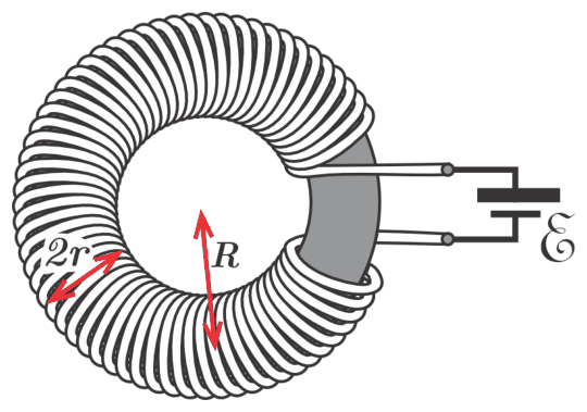
Fig. 3a.
Consider a torus with mean radius \(R\) and inner radius \(r\) made of a homogeneous, isotropic paramagnetic material, around which an insulated conducting wire is wound, with its ends connected to an external voltage source (emf), as shown in figure 3a. The resistance of the wire is so low that energy losses due to the heating of the wire can be neglected. The winding is dense, with \(N\) turns in total, and it is assumed that \(r\ll R\), so that the fields \(\vec H\) and \(\vec B\) and the magnetization \(\vec M\) have approximately constant magnitudes throughout the torus. Let \(V\) and \(A\) be the volume and the cross-section area of the torus. Hereinafter, the abbreviation Pm-T is used to refer to the paramagnetic torus.
In paramagnetic materials, \(\vec M\) is parallel to \(\vec H\) and the following relation holds:
\[ \vec B=\mu_0\vec H+\mu_0\vec M. \]
Energy transfer sign convention: in this problem, Work (\(W\)) and Heat (\(Q\)) are considered positive when they flow into the system, and negative when they flow out.
T3-A [1.0 pts]. Work in the Pm-T
Hint: in magnetic materials, \(\displaystyle\oint_C\vec H\cdot d\vec\ell=I_C\), where \(I_C\) is the net free current passing through the area bounded by the closed curve \(C\).
T3-A1 [0.2 pts]. Let \(H\) be the magnitude of \(\vec H\) in the torus. Write \(H\) in terms of \(N\), \(A\), \(V\) and the instantaneous electric current \(I\) in the wire.
T3-A2 [0.6 pts]. Let \(dW_{emf}\) be the work that the external voltage source performs to change the magnitude of \(\vec B\) by \(dB\). Write \(dW_{emf}\) in terms of \(V\), \(H\), and \(dB\).
T3-A3 [0.2 pts]. The total work done by the voltage source, \(dW_{emf}\), can be divided in two parts: the work that would be performed to change the magnetic field if the toroid had a vacuum core, \(dW_{vac}\), and the work done on the paramagnetic material itself, \(dW\). Write \(dW\) in terms of \(\mu_0\), \(H\), \(V\) and \(dM\).
T3-B [3.0 pts]. Heat and temperature in the Pm-T
The following table compares two thermodynamic systems: the ideal gas and the Pm-T. Use this information and your answer to question T3-A3 to solve the following questions. This information will also be used in part C. If you did not find an answer for \(dW\) in question T3-A3, you may use \(dW=\alpha V\mu_0H\,dM\) where \(\alpha\) is a number. The volume \(V\) of the paramagnetic torus is constant, so that there is no work due to pressure. Below, \(T\) is the temperature in all instances.
| IDEAL GAS | PARAMAGNETIC TORUS |
|---|---|
| State functions: \(P,V\) and temperature \(T\) | State functions: \(H,M\) and temperature \(T\) |
| Constants: \(R,\gamma\) and number of moles \(n\) | Constants: \(K,\lambda\) and number of moles \(n\) |
| Equation of state: \(PV=nRT\) | Equation of state: \(TMV=nKH\) |
| Heat capacity at constant \(V\): \(C_V=nR/(\gamma-1)\) | Heat capacity at constant \(M\): \(C_M=n\lambda/T^2\) |
| Internal energy \(U\) in any process satisfies \(dU=C_V\,dT\) | Internal energy \(U\) in any process satisfies \(dU=C_M\,dT\) |
\(K\) and \(\lambda\) are constants given by the material in the torus. You may use the equations provided in the table directly without proving them.
T3-B1 [1.5 pts]. If the magnitude of \(\vec H\) changes from \(H_i\) to \(H_f\) at a constant temperature \(T\), an energy \(Q\) is transferred between the Pm-T and its environment. Write \(Q\) in terms of \(\mu_0\), \(n\), \(V\), \(K\), \(H_i\), \(H_f\), and \(T\).
T3-B2 [1.5 pts]. If the magnitude of \(\vec H\) changes adiabatically from \(H_i\) to \(H_f\), the temperature of the Pm-T changes from \(T_i\) to \(T_f\). Write \(\Delta T=T_f-T_i\) in terms of \(\mu_0\), \(V\), \(n\), \(K\), \(\lambda\), \(H_i\), \(H_f\), and \(T_i\).
T3-C [6.0 pts]. Carnot refrigerator of the Pm-T
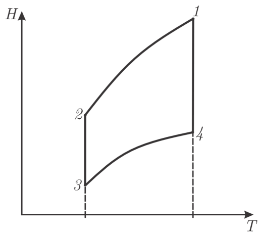
Fig.3b.
The \(H\) vs. \(T\) diagram of the Carnot refrigeration cycle \(1\to2\to3\to4\to1\) performed by the Pm-T is shown in figure 3b. In this cycle, let:
- \(T_h\): temperature of the hot reservoir
- \(T_c\): temperature of the cold reservoir
- \(Q_h\): absolute value of the heat transferred to the hot reservoir
- \(Q_c\): absolute value of the heat absorbed from the cold reservoir
T3-C1 [0.2 pts]. Mark \(T_h\) and \(T_c\) on the \(T\) axis of the \(H\) vs. \(T\) diagram. Also label the processes in which the transfers of \(Q_h\) and \(Q_c\) occur, respectively.
T3-C2 [1.5 pts]. Let \(M_1\), \(M_2\), \(M_3\), and \(M_4\) be the magnitudes of \(\vec M\) at the vertices of this cycle. Write \(M_1\) in terms of \(M_2\), \(M_3\), and \(M_4\).
T3-C3 [0.8 pts]. Suppose that to cool 1.00 L of liquid helium initially at 1.00 K, we utilize a 2.0 moles Pm-T made of potassium chromate. For this material, \(K=1.87\times10^{-6}\ \mathrm{K\cdot m^3/mol}\), its density is \(2730\ \mathrm{kg/m^3}\) and its molar mass is \(0.19\ \mathrm{kg/mole}\). The Pm-T performs a Carnot refrigeration cycle with \(H_1=411624\ \mathrm{A/m}\), \(H_2=311306\ \mathrm{A/m}\), \(H_3=204618\ \mathrm{A/m}\) and \(H_4=240446\ \mathrm{A/m}\). After one operating cycle, calculate the final temperature of the liquid helium. Assume that for the liquid helium both the specific heat capacity \(c=100\ \mathrm{J/(kg\cdot K)}\) and the density \(\rho=130\ \mathrm{kg/m^3}\) remain constant.
T3-C4 [2.0 pts]. In order to continuously lower the temperature of a body with constant heat capacity \(C_c\), Carnot cycles are allowed to occur over time in such a way that the power \(P\) transferred to the refrigerator remains constant. It is then assumed that the temperature \(T_h\) of the hot reservoir remains constant and that in each operating cycle the temperature \(T_c\) of the cooled body decreases by \(dT_c\), satisfying the relation \(dQ_c/dQ_h=T_c/T_h\). If at \(t=0\) we have \(T_c=T_0\), determine the time \(t\) that the Carnot refrigerator must operate for the cooled body to reach a temperature \(T<T_0\). Express your answer in terms of \(C_c\), \(T_h\), \(P\), \(T_0\) and \(T\).
T3-C5 [1.5 pts]. The efficiency of a refrigerator is quantified by its coefficient of performance \(\mathrm{COP}=Q_c/W\). Determine the overall COP of the refrigerator of question T3-C4 with all the cycles performed until time \(t\). Write your answer in terms of \(T_0\) and \(T_h\) and \(T\).
Physical Constants
Reference values for selected physical constants.
| Constant | Notation | Value | Units |
|---|---|---|---|
| Speed of light in vacuum | \(c\) | \(2.99792458\times10^8\) | \(\mathrm{m\cdot s^{-1}}\) |
| Planck constant | \(h\) | \(4.135667696\ldots\times10^{-15}\) | \(\mathrm{eV\cdot s}\) |
| Reduced Planck constant | \(\hbar=h/2\pi\) | \(6.582119569\ldots\times10^{-16}\) | \(\mathrm{eV\cdot s}\) |
| Avogadro number | \(N_A\) | \(6.02214076\times10^{23}\) | \(\mathrm{mol^{-1}}\) |
| Boltzmann constant | \(k_B\) | \(8.617333262\times10^{-5}\) | \(\mathrm{eV\cdot K^{-1}}\) |
| Ideal gas constant | \(R\) | \(8.31446261815324\) | \(\mathrm{kg\cdot m^2\cdot s^{-2}\cdot mol^{-1}\cdot K^{-1}}\) |
| Elementary charge | \(e\) | \(1.602176634\times10^{-19}\) | \(\mathrm{A\cdot s}\) |
| Universal gravitational constant | \(G\) | \(6.67430(15)\times10^{-11}\) | \(\mathrm{m^3\cdot kg^{-1}\cdot s^{-2}}\) |
| Stefan Boltzmann constant | \(\sigma\) | \(5.670374419\times10^{-8}\) | \(\mathrm{kg\cdot s^{-3}\cdot K^{-4}}\) |
| Vacuum permeability | \(\mu_0\) | \(1.25663706127(20)\times10^{-6}\) | \(\mathrm{kg\cdot m\cdot A^{-2}\cdot s^{-2}}\) |
| Vacuum permittivity | \(\varepsilon_0\) | \(8.8541878188(14)\times10^{-12}\) | \(\mathrm{A^2\cdot s^4\cdot kg^{-1}\cdot m^{-3}}\) |
| Mass of the electron | \(m_e\) | \(5.1099895069(16)\times10^5\) | \(\mathrm{eV}/c^2\) |
| Mass of the proton | \(m_p\) | \(9.3827208943(29)\times10^8\) | \(\mathrm{eV}/c^2\) |
| Atomic mass units | \(\mathrm{amu}\) | \(9.3149410372(29)\times10^8\) | \(\mathrm{eV}/c^2\) |
Official English text of the problem.
Answers
-
T3-A1: \[ \boxed{H=\frac{NAI}{V}}. \]
-
T3-A2: \[ \boxed{dW_{emf}=VH\,dB}. \]
-
T3-A3: \[ \boxed{dW=\mu_0VH\,dM},\qquad \alpha=1. \]
-
T3-B1: \[ \boxed{Q=\frac{\mu_0nK}{2T}\left(H_i^2-H_f^2\right)}. \]
-
T3-B2: \[ \boxed{\Delta T =T_i\left[ \sqrt{\frac{\lambda+\mu_0KH_f^2} {\lambda+\mu_0KH_i^2}}-1 \right]}. \]
-
T3-C1: The left vertical line, through states \(2,3\), is at \(T_c\); the right vertical line, through states \(1,4\), is at \(T_h\). Heat \(Q_c\) is absorbed during \(2\to3\), and heat \(Q_h\) is rejected during \(4\to1\).
-
T3-C2: \[ \boxed{M_1=\sqrt{M_2^2+M_4^2-M_3^2}}. \]
-
T3-C3: Using \(T_c\simeq1.00\ \mathrm K\) for the cold stroke, \[ \boxed{T_{\mathrm{He},f}\simeq0.990\ \mathrm K}. \] This is a small-cooling estimate that takes the cold isotherm at the initial helium temperature; it uses only the cold stroke \(2\to3\) (see the note at the end of the T3-C3 solution).
-
T3-C4: \[ \boxed{t=\frac{C_c}{P} \left[T_h\ln\!\left(\frac{T_0}{T}\right)-(T_0-T)\right]}. \]
-
T3-C5: \[ \boxed{\mathrm{COP}_{\mathrm{overall}} =\frac{T_0-T} {T_h\ln(T_0/T)-(T_0-T)}}. \]
Solution
We use the prescribed sign convention throughout: \[ dU=dQ+dW, \] where heat and work are positive when supplied to the paramagnetic material. The magnetic processes are treated quasistatically, with the uniform-field approximation \(r\ll R\) and negligible resistive losses.
T3-A1
Choose an Amperian circle of radius \(R\) inside the torus. It links all \(N\) turns, so the enclosed free current is \(NI\). Thus, \[ H(2\pi R)=NI. \] Since the torus volume is \(V=(2\pi R)A\), \[ \boxed{H=\frac{NI}{2\pi R}=\frac{NAI}{V}}. \]
T3-A2
The magnetic flux through each turn is approximately \[ \Phi=AB. \] Faraday’s law gives an induced emf \(-NA\,dB/dt\). With negligible resistance, the applied source emf balances this: \[ \mathcal E=NA\frac{dB}{dt}. \] The electrical work supplied in time \(dt\) is therefore \[ dW_{emf}=\mathcal E I\,dt=NAI\,dB. \] Using \(NAI=VH\) from A1, \[ \boxed{dW_{emf}=VH\,dB}. \]
This expression also gives the correct sign when the source receives energy during a decrease of the field.
T3-A3
Because the fields and magnetization are parallel, \[ dB=\mu_0\,dH+\mu_0\,dM. \] Consequently, \[ dW_{emf} =\mu_0VH\,dH+\mu_0VH\,dM. \]
For a vacuum core, \(B=\mu_0H\), so the work associated with the same change of \(H\) is \[ dW_{vac}=\mu_0VH\,dH =d\!\left(\frac{\mu_0VH^2}{2}\right). \] Subtracting this vacuum-field contribution leaves the work on the material: \[ \boxed{dW=dW_{emf}-dW_{vac}=\mu_0VH\,dM}. \] Thus the fallback coefficient is \(\alpha=1\).
T3-B1
The given internal-energy relation implies that an isothermal process has \[ dU=\frac{n\lambda}{T^2}\,dT=0. \] The first law then gives \[ dQ=-dW=-\mu_0VH\,dM. \]
At constant \(T\), the equation of state yields \[ M=\frac{nKH}{VT}, \qquad dM=\frac{nK}{VT}\,dH. \] Hence \[ Q=-\frac{\mu_0nK}{T}\int_{H_i}^{H_f}H\,dH, \] and therefore \[ \boxed{Q=\frac{\mu_0nK}{2T}(H_i^2-H_f^2)}. \]
The volume cancels. Isothermal demagnetization, \(H_f<H_i\), absorbs heat; isothermal magnetization releases heat.
T3-B2
An adiabatic process has \(dQ=0\), so \[ \frac{n\lambda}{T^2}\,dT=\mu_0VH\,dM. \] Now both \(H\) and \(T\) vary. Differentiating the equation of state gives \[ dM=\frac{nK}{V} \left(\frac{dH}{T}-\frac{H}{T^2}\,dT\right). \] Substitution into the first law gives \[ \frac{n\lambda}{T^2}\,dT =\mu_0nK \left(\frac{H}{T}\,dH-\frac{H^2}{T^2}\,dT\right). \] Thus \[ (\lambda+\mu_0KH^2)\,dT =\mu_0KHT\,dH, \] or \[ \frac{dT}{T} =\frac{\mu_0KH}{\lambda+\mu_0KH^2}\,dH. \]
Integrating between the initial and final states, \[ \ln\frac{T_f}{T_i} =\frac12\ln \frac{\lambda+\mu_0KH_f^2} {\lambda+\mu_0KH_i^2}. \] Therefore, \[ T_f=T_i \sqrt{\frac{\lambda+\mu_0KH_f^2} {\lambda+\mu_0KH_i^2}}, \] and \[ \boxed{\Delta T =T_i\left[ \sqrt{\frac{\lambda+\mu_0KH_f^2} {\lambda+\mu_0KH_i^2}}-1 \right]}. \]
For positive \(K\) and heat capacity, decreasing \(H\) decreases \(T\): this is adiabatic demagnetization.
An equivalent form, useful below, is the adiabatic invariant \[ \boxed{\frac{\lambda+\mu_0KH^2}{T^2} =\text{constant along an adiabat}}. \]
T3-C1
The horizontal coordinate is temperature. Therefore:
- Label the left dashed projection, beneath states \(2\) and \(3\), \(T_c\).
- Label the right dashed projection, beneath states \(1\) and \(4\), \(T_h\).
On \(2\to3\), the field decreases at constant \(T_c\). By B1, the torus absorbs heat, so place \(Q_c\), directed into the torus, beside this downward vertical stroke.
On \(4\to1\), the field increases at constant \(T_h\). The torus releases heat, so place \(Q_h\), directed out of the torus, beside this upward vertical stroke.
The remaining strokes are \(1\to2\), adiabatic cooling, and \(3\to4\), adiabatic heating.
T3-C2
Substitute \[ H=\frac{VTM}{nK} \] into the adiabatic invariant from B2: \[ \frac{\lambda}{T^2} +\frac{\mu_0V^2}{n^2K}M^2 =\text{constant}. \]
For the adiabat \(1\to2\), \[ \frac{\mu_0V^2}{n^2K}(M_1^2-M_2^2) =\lambda\left(\frac1{T_c^2}-\frac1{T_h^2}\right). \] For the adiabat \(3\to4\), \[ \frac{\mu_0V^2}{n^2K}(M_4^2-M_3^2) =\lambda\left(\frac1{T_c^2}-\frac1{T_h^2}\right). \] Their right-hand sides are identical, so \[ M_1^2-M_2^2=M_4^2-M_3^2. \] Since the \(M_j\) are magnitudes, the positive root is required: \[ \boxed{M_1=\sqrt{M_2^2+M_4^2-M_3^2}}. \]
T3-C3
For the one-cycle estimate, take the cold-stroke temperature as approximately the initial helium temperature: \[ T_c\simeq1.00\ \mathrm K. \] The heat absorbed during \(2\to3\) is \[ Q_c=\frac{\mu_0nK}{2T_c}(H_2^2-H_3^2). \] Using the supplied values, \[ Q_c= \frac{ (1.25663706127\times10^{-6})(2.0)(1.87\times10^{-6}) }{ 2(1.00) } \left(311306^2-204618^2\right)\ \mathrm J, \] which gives \[ Q_c=0.1293459\ldots\ \mathrm J\simeq0.13\ \mathrm J. \]
The helium mass and heat capacity are \[ m_{\mathrm{He}} =\rho V_{\mathrm{He}} =(130)(1.00\times10^{-3}) =0.130\ \mathrm{kg}, \] \[ C_{\mathrm{He}}=m_{\mathrm{He}}c =(0.130)(100)=13.0\ \mathrm{J\,K^{-1}}. \] Energy conservation for the helium gives \[ C_{\mathrm{He}}(T_{\mathrm{He},f}-1.00\ \mathrm K)=-Q_c. \] Thus \[ T_{\mathrm{He},f} =1.00\ \mathrm K-\frac{0.1293459\ldots\ \mathrm J} {13.0\ \mathrm{J\,K^{-1}}} =0.9900503\ldots\ \mathrm K, \] or \[ \boxed{T_{\mathrm{He},f}\simeq0.990\ \mathrm K}. \]
The estimated temperature decrease is approximately \(1\%\), supporting the small-change approximation for this numerical estimate. The material volume cancels from \(Q_c\), so its density and molar mass are unnecessary here. For an exact cycle the four given fields are not fully consistent: with \(M=nKH/(VT)\) on the two isotherms, the relation of T3-C2 requires \(T_h/T_c=\sqrt{(H_1^2-H_4^2)/(H_2^2-H_3^2)}\approx1.42\), and the adiabats \(1\to2\) and \(3\to4\) then hold only with \(\lambda\approx-0.062\ \mathrm{J\,K\,mol^{-1}}\), that is, a negative heat capacity \(C_M=n\lambda/T^2\). The estimate above uses only the cold stroke and does not depend on \(\lambda\).
T3-C4
Let \(dT_c<0\) denote the actual temperature change of the cooled body. The positive heat extracted from it is \[ dQ_c=-C_c\,dT_c. \] The specified Carnot relation gives \[ dQ_h=\frac{T_h}{T_c}\,dQ_c. \] Since the refrigerator returns to its original state after each cycle, its net internal-energy change vanishes. The required work is therefore \[ dW=dQ_h-dQ_c =\left(\frac{T_h}{T_c}-1\right)dQ_c. \] With constant input power, \[ P\,dt=dW =-C_c\left(\frac{T_h}{T_c}-1\right)dT_c. \]
Integrating from \(T_c=T_0\) at \(t=0\) to \(T_c=T\), \[ Pt=-C_c\int_{T_0}^{T} \left(\frac{T_h}{T_c}-1\right)dT_c. \] Hence \[ Pt=C_c \left[ T_h\ln\!\left(\frac{T_0}{T}\right)+T-T_0 \right], \] and \[ \boxed{ t=\frac{C_c}{P} \left[ T_h\ln\!\left(\frac{T_0}{T}\right)-(T_0-T) \right]}. \]
For \(0<T<T_0<T_h\), this time is positive. Moreover, \[ T\to0^+\quad\Longrightarrow\quad t\to\infty. \] Within the stated model, reaching absolute zero requires an infinite operating time.
T3-C5
The total heat extracted from the cooled body is \[ Q_{c,\mathrm{total}}=C_c(T_0-T). \] The total work supplied is \[ W_{\mathrm{total}}=Pt =C_c\left[ T_h\ln\!\left(\frac{T_0}{T}\right)-(T_0-T) \right]. \] Therefore, \[ \boxed{ \mathrm{COP}_{\mathrm{overall}} =\frac{Q_{c,\mathrm{total}}}{W_{\mathrm{total}}} =\frac{T_0-T} {T_h\ln(T_0/T)-(T_0-T)} }. \]
As a check, for an infinitesimal temperature decrease, \[ \lim_{T\to T_0^-}\mathrm{COP}_{\mathrm{overall}} =\frac{T_0}{T_h-T_0}, \] which is the usual Carnot refrigerator COP at cold temperature \(T_0\).
The solution was checked against the official solution.
IPhO 2026 · Theorieaufgabe 3
Auf der Jagd nach dem absoluten Nullpunkt
AUFGABE T3 [10 Punkte]. Auf der Jagd nach dem absoluten Nullpunkt
Ein Kältekreisprozess muss mit einem System durchgeführt werden, dessen Eigenschaften für die zu erreichenden Temperaturen geeignet sind. Vor hundert Jahren, im Jahr 1926, schlugen der Chemiker William Giauque und unabhängig von ihm der Physiker Peter Debye paramagnetische Salze als ideale Systeme vor, um Temperaturen weit unter 1 K zu erreichen. Tatsächlich wurden ab dem folgenden Jahrzehnt Temperaturen bis hinab zu 0.0044 K erreicht (Wander de Haas und Gerrit Wiersma, 1935, Leiden Cryogenic Laboratories). In dieser Aufgabe wird der paramagnetische Carnot-Kältekreisprozess untersucht.
Abb. 3a.
Betrachten Sie einen Torus mit mittlerem Radius \(R\) und Innenradius \(r\) aus einem homogenen, isotropen paramagnetischen Material, um den ein isolierter leitender Draht gewickelt ist. Seine Enden sind an eine externe Spannungsquelle (EMK) angeschlossen, wie in Abbildung 3a gezeigt. Der Widerstand des Drahtes ist so gering, dass Energieverluste durch die Erwärmung des Drahtes vernachlässigt werden können. Die Wicklung ist dicht und umfasst insgesamt \(N\) Windungen. Es wird angenommen, dass \(r\ll R\), sodass die Beträge der Felder \(\vec H\) und \(\vec B\) sowie der Magnetisierung \(\vec M\) im gesamten Torus näherungsweise konstant sind. \(V\) und \(A\) bezeichnen das Volumen und die Querschnittsfläche des Torus. Im Folgenden wird der paramagnetische Torus mit Pm-T abgekürzt.
In paramagnetischen Materialien ist \(\vec M\) parallel zu \(\vec H\), und es gilt die folgende Beziehung:
\[ \vec B=\mu_0\vec H+\mu_0\vec M. \]
Vorzeichenkonvention für die Energieübertragung: In dieser Aufgabe werden Arbeit (\(W\)) und Wärme (\(Q\)) als positiv betrachtet, wenn sie dem System zugeführt werden, und als negativ, wenn sie vom System abgegeben werden.
T3-A [1.0 Punkte]. Arbeit im Pm-T
Hinweis: In magnetischen Materialien gilt \(\displaystyle\oint_C\vec H\cdot d\vec\ell=I_C\), wobei \(I_C\) der gesamte vorzeichenbehaftete freie Strom durch die von der geschlossenen Kurve \(C\) begrenzte Fläche ist.
T3-A1 [0.2 Punkte]. \(H\) sei der Betrag von \(\vec H\) im Torus. Drücken Sie \(H\) durch \(N\), \(A\), \(V\) und die momentane elektrische Stromstärke \(I\) im Draht aus.
T3-A2 [0.6 Punkte]. \(dW_{emf}\) sei die Arbeit, welche die externe Spannungsquelle verrichtet, um den Betrag von \(\vec B\) um \(dB\) zu ändern. Drücken Sie \(dW_{emf}\) durch \(V\), \(H\) und \(dB\) aus.
T3-A3 [0.2 Punkte]. Die gesamte von der Spannungsquelle verrichtete Arbeit \(dW_{emf}\) lässt sich in zwei Anteile aufteilen: die Arbeit \(dW_{vac}\), die zur Änderung des Magnetfeldes verrichtet würde, wenn der Ringkern aus Vakuum bestünde, und die am paramagnetischen Material selbst verrichtete Arbeit \(dW\). Drücken Sie \(dW\) durch \(\mu_0\), \(H\), \(V\) und \(dM\) aus.
T3-B [3.0 Punkte]. Wärme und Temperatur im Pm-T
Die folgende Tabelle vergleicht zwei thermodynamische Systeme: das ideale Gas und den Pm-T. Verwenden Sie diese Informationen und Ihre Antwort auf Frage T3-A3, um die folgenden Fragen zu lösen. Diese Informationen werden auch in Teil C verwendet. Falls Sie in Frage T3-A3 keinen Ausdruck für \(dW\) gefunden haben, dürfen Sie \(dW=\alpha V\mu_0H\,dM\) verwenden, wobei \(\alpha\) eine Zahl ist. Das Volumen \(V\) des paramagnetischen Torus ist konstant, sodass keine Druckarbeit verrichtet wird. Im Folgenden bezeichnet \(T\) stets die Temperatur.
| IDEALES GAS | PARAMAGNETISCHER TORUS |
|---|---|
| Zustandsgrößen: \(P,V\) und Temperatur \(T\) | Zustandsgrößen: \(H,M\) und Temperatur \(T\) |
| Konstanten: \(R,\gamma\) und Stoffmenge \(n\) | Konstanten: \(K,\lambda\) und Stoffmenge \(n\) |
| Zustandsgleichung: \(PV=nRT\) | Zustandsgleichung: \(TMV=nKH\) |
| Wärmekapazität bei konstantem \(V\): \(C_V=nR/(\gamma-1)\) | Wärmekapazität bei konstantem \(M\): \(C_M=n\lambda/T^2\) |
| Für die innere Energie \(U\) gilt bei jedem Prozess \(dU=C_V\,dT\) | Für die innere Energie \(U\) gilt bei jedem Prozess \(dU=C_M\,dT\) |
\(K\) und \(\lambda\) sind Konstanten, die durch das Material im Torus bestimmt werden. Sie dürfen die in der Tabelle angegebenen Gleichungen ohne Beweis direkt verwenden.
T3-B1 [1.5 Punkte]. Wenn sich der Betrag von \(\vec H\) bei konstanter Temperatur \(T\) von \(H_i\) auf \(H_f\) ändert, wird zwischen dem Pm-T und seiner Umgebung eine Energie \(Q\) übertragen. Drücken Sie \(Q\) durch \(\mu_0\), \(n\), \(V\), \(K\), \(H_i\), \(H_f\) und \(T\) aus.
T3-B2 [1.5 Punkte]. Wenn sich der Betrag von \(\vec H\) adiabatisch von \(H_i\) auf \(H_f\) ändert, ändert sich die Temperatur des Pm-T von \(T_i\) auf \(T_f\). Drücken Sie \(\Delta T=T_f-T_i\) durch \(\mu_0\), \(V\), \(n\), \(K\), \(\lambda\), \(H_i\), \(H_f\) und \(T_i\) aus.
T3-C [6.0 Punkte]. Carnot-Kältemaschine mit dem Pm-T
Abb. 3b.
Das \(H\)-\(T\)-Diagramm des vom Pm-T durchlaufenen Carnot-Kältekreisprozesses \(1\to2\to3\to4\to1\) ist in Abbildung 3b dargestellt. In diesem Kreisprozess bezeichnen:
- \(T_h\): die Temperatur des warmen Reservoirs
- \(T_c\): die Temperatur des kalten Reservoirs
- \(Q_h\): den Betrag der an das warme Reservoir abgegebenen Wärme
- \(Q_c\): den Betrag der aus dem kalten Reservoir aufgenommenen Wärme
T3-C1 [0.2 Punkte]. Markieren Sie \(T_h\) und \(T_c\) auf der \(T\)-Achse des \(H\)-\(T\)-Diagramms. Kennzeichnen Sie außerdem die Prozesse, bei denen jeweils die Wärmeübertragungen \(Q_h\) und \(Q_c\) stattfinden.
T3-C2 [1.5 Punkte]. \(M_1\), \(M_2\), \(M_3\) und \(M_4\) seien die Beträge von \(\vec M\) an den Eckpunkten dieses Kreisprozesses. Drücken Sie \(M_1\) durch \(M_2\), \(M_3\) und \(M_4\) aus.
T3-C3 [0.8 Punkte]. Nehmen Sie an, dass wir zur Kühlung von 1.00 L flüssigem Helium mit einer Anfangstemperatur von 1.00 K einen Pm-T aus 2.0 mol Kaliumchromat verwenden. Für dieses Material gilt \(K=1.87\times10^{-6}\ \mathrm{K\cdot m^3/mol}\), seine Dichte beträgt \(2730\ \mathrm{kg/m^3}\) und seine molare Masse \(0.19\ \mathrm{kg/mole}\). Der Pm-T durchläuft einen Carnot-Kältekreisprozess mit \(H_1=411624\ \mathrm{A/m}\), \(H_2=311306\ \mathrm{A/m}\), \(H_3=204618\ \mathrm{A/m}\) und \(H_4=240446\ \mathrm{A/m}\). Berechnen Sie die Endtemperatur des flüssigen Heliums nach einem Betriebszyklus. Nehmen Sie an, dass beim flüssigen Helium sowohl die spezifische Wärmekapazität \(c=100\ \mathrm{J/(kg\cdot K)}\) als auch die Dichte \(\rho=130\ \mathrm{kg/m^3}\) konstant bleiben.
T3-C4 [2.0 Punkte]. Um die Temperatur eines Körpers mit konstanter Wärmekapazität \(C_c\) kontinuierlich zu senken, werden im Laufe der Zeit Carnot-Kreisprozesse so durchgeführt, dass die der Kältemaschine zugeführte Leistung \(P\) konstant bleibt. Dabei wird angenommen, dass die Temperatur \(T_h\) des warmen Reservoirs konstant bleibt und dass die Temperatur \(T_c\) des gekühlten Körpers in jedem Betriebszyklus um \(dT_c\) abnimmt, wobei die Beziehung \(dQ_c/dQ_h=T_c/T_h\) erfüllt ist. Wenn bei \(t=0\) gilt \(T_c=T_0\), bestimmen Sie die Zeit \(t\), während der die Carnot-Kältemaschine betrieben werden muss, damit der gekühlte Körper eine Temperatur \(T<T_0\) erreicht. Drücken Sie Ihre Antwort durch \(C_c\), \(T_h\), \(P\), \(T_0\) und \(T\) aus.
T3-C5 [1.5 Punkte]. Die Effizienz einer Kältemaschine wird durch ihre Leistungszahl \(\mathrm{COP}=Q_c/W\) beschrieben. Bestimmen Sie die Gesamtleistungszahl der Kältemaschine aus Frage T3-C4 unter Berücksichtigung aller bis zum Zeitpunkt \(t\) durchgeführten Kreisprozesse. Drücken Sie Ihre Antwort durch \(T_0\), \(T_h\) und \(T\) aus.
Physikalische Konstanten
Referenzwerte ausgewählter physikalischer Konstanten.
| Konstante | Symbol | Wert | Einheiten |
|---|---|---|---|
| Lichtgeschwindigkeit im Vakuum | \(c\) | \(2.99792458\times10^8\) | \(\mathrm{m\cdot s^{-1}}\) |
| Planck-Konstante | \(h\) | \(4.135667696\ldots\times10^{-15}\) | \(\mathrm{eV\cdot s}\) |
| Reduzierte Planck-Konstante | \(\hbar=h/2\pi\) | \(6.582119569\ldots\times10^{-16}\) | \(\mathrm{eV\cdot s}\) |
| Avogadro-Konstante | \(N_A\) | \(6.02214076\times10^{23}\) | \(\mathrm{mol^{-1}}\) |
| Boltzmann-Konstante | \(k_B\) | \(8.617333262\times10^{-5}\) | \(\mathrm{eV\cdot K^{-1}}\) |
| Universelle Gaskonstante | \(R\) | \(8.31446261815324\) | \(\mathrm{kg\cdot m^2\cdot s^{-2}\cdot mol^{-1}\cdot K^{-1}}\) |
| Elementarladung | \(e\) | \(1.602176634\times10^{-19}\) | \(\mathrm{A\cdot s}\) |
| Universelle Gravitationskonstante | \(G\) | \(6.67430(15)\times10^{-11}\) | \(\mathrm{m^3\cdot kg^{-1}\cdot s^{-2}}\) |
| Stefan-Boltzmann-Konstante | \(\sigma\) | \(5.670374419\times10^{-8}\) | \(\mathrm{kg\cdot s^{-3}\cdot K^{-4}}\) |
| Magnetische Feldkonstante | \(\mu_0\) | \(1.25663706127(20)\times10^{-6}\) | \(\mathrm{kg\cdot m\cdot A^{-2}\cdot s^{-2}}\) |
| Elektrische Feldkonstante | \(\varepsilon_0\) | \(8.8541878188(14)\times10^{-12}\) | \(\mathrm{A^2\cdot s^4\cdot kg^{-1}\cdot m^{-3}}\) |
| Elektronenmasse | \(m_e\) | \(5.1099895069(16)\times10^5\) | \(\mathrm{eV}/c^2\) |
| Protonenmasse | \(m_p\) | \(9.3827208943(29)\times10^8\) | \(\mathrm{eV}/c^2\) |
| Atomare Masseneinheiten | \(\mathrm{amu}\) | \(9.3149410372(29)\times10^8\) | \(\mathrm{eV}/c^2\) |
Aufgabentext aus dem offiziellen englischen Text übersetzt.
Antworten
-
T3-A1: \[ \boxed{H=\frac{NAI}{V}}. \]
-
T3-A2: \[ \boxed{dW_{emf}=VH\,dB}. \]
-
T3-A3: \[ \boxed{dW=\mu_0VH\,dM},\qquad \alpha=1. \]
-
T3-B1: \[ \boxed{Q=\frac{\mu_0nK}{2T}\left(H_i^2-H_f^2\right)}. \]
-
T3-B2: \[ \boxed{\Delta T =T_i\left[ \sqrt{\frac{\lambda+\mu_0KH_f^2} {\lambda+\mu_0KH_i^2}}-1 \right]}. \]
-
T3-C1: Die linke senkrechte Linie durch die Zustände \(2,3\) liegt bei \(T_c\); die rechte senkrechte Linie durch die Zustände \(1,4\) liegt bei \(T_h\). Während \(2\to3\) wird die Wärme \(Q_c\) aufgenommen, und während \(4\to1\) wird die Wärme \(Q_h\) abgegeben.
-
T3-C2: \[ \boxed{M_1=\sqrt{M_2^2+M_4^2-M_3^2}}. \]
-
T3-C3: Mit \(T_c\simeq1.00\ \mathrm K\) für den kalten Prozessabschnitt ergibt sich \[ \boxed{T_{\mathrm{He},f}\simeq0.990\ \mathrm K}. \] Dies ist eine Abschätzung für eine geringe Abkühlung, bei der für die kalte Isotherme die Anfangstemperatur des Heliums angenommen wird; sie verwendet nur den kalten Prozessabschnitt \(2\to3\) (siehe den Hinweis am Ende der Lösung zu T3-C3).
-
T3-C4: \[ \boxed{t=\frac{C_c}{P} \left[T_h\ln\!\left(\frac{T_0}{T}\right)-(T_0-T)\right]}. \]
-
T3-C5: \[ \boxed{\mathrm{COP}_{\mathrm{overall}} =\frac{T_0-T} {T_h\ln(T_0/T)-(T_0-T)}}. \]
Lösung
Wir verwenden durchgehend die vorgegebene Vorzeichenkonvention: \[ dU=dQ+dW, \] wobei Wärme und Arbeit positiv sind, wenn sie dem paramagnetischen Material zugeführt werden. Die magnetischen Prozesse werden quasistatisch behandelt, mit der Näherung eines homogenen Feldes für \(r\ll R\) und vernachlässigbaren ohmschen Verlusten.
T3-A1
Wir wählen einen ampereschen Integrationsweg in Form eines Kreises mit Radius \(R\) innerhalb des Torus. Er umfasst alle \(N\) Windungen, sodass der eingeschlossene freie Strom \(NI\) beträgt. Somit gilt \[ H(2\pi R)=NI. \] Da das Torusvolumen \(V=(2\pi R)A\) beträgt, folgt \[ \boxed{H=\frac{NI}{2\pi R}=\frac{NAI}{V}}. \]
T3-A2
Der magnetische Fluss durch jede Windung beträgt näherungsweise \[ \Phi=AB. \] Das faradaysche Induktionsgesetz liefert eine induzierte EMK von \(-NA\,dB/dt\). Bei vernachlässigbarem Widerstand gleicht die angelegte Quellenspannung diese aus: \[ \mathcal E=NA\frac{dB}{dt}. \] Die während der Zeit \(dt\) zugeführte elektrische Arbeit beträgt daher \[ dW_{emf}=\mathcal E I\,dt=NAI\,dB. \] Mit \(NAI=VH\) aus A1 folgt \[ \boxed{dW_{emf}=VH\,dB}. \]
Dieser Ausdruck liefert auch dann das richtige Vorzeichen, wenn die Quelle während einer Abnahme des Feldes Energie aufnimmt.
T3-A3
Da die Felder und die Magnetisierung parallel sind, gilt \[ dB=\mu_0\,dH+\mu_0\,dM. \] Folglich ist \[ dW_{emf} =\mu_0VH\,dH+\mu_0VH\,dM. \]
Für einen Vakuumkern gilt \(B=\mu_0H\), sodass für die mit derselben Änderung von \(H\) verbundene Arbeit gilt \[ dW_{vac}=\mu_0VH\,dH =d\!\left(\frac{\mu_0VH^2}{2}\right). \]
Subtrahiert man diesen Beitrag des Vakuumfeldes, verbleibt die am Material verrichtete Arbeit: \[ \boxed{dW=dW_{emf}-dW_{vac}=\mu_0VH\,dM}. \] Damit ist der als Ersatz vorgesehene Koeffizient \(\alpha=1\).
T3-B1
Aus der gegebenen Beziehung für die innere Energie folgt für einen isothermen Prozess \[ dU=\frac{n\lambda}{T^2}\,dT=0. \] Der erste Hauptsatz liefert dann \[ dQ=-dW=-\mu_0VH\,dM. \]
Bei konstantem \(T\) ergibt die Zustandsgleichung \[ M=\frac{nKH}{VT}, \qquad dM=\frac{nK}{VT}\,dH. \] Daraus folgt \[ Q=-\frac{\mu_0nK}{T}\int_{H_i}^{H_f}H\,dH, \] und somit \[ \boxed{Q=\frac{\mu_0nK}{2T}(H_i^2-H_f^2)}. \]
Das Volumen kürzt sich heraus. Bei isothermer Entmagnetisierung, \(H_f<H_i\), wird Wärme aufgenommen; bei isothermer Magnetisierung wird Wärme abgegeben.
T3-B2
Für einen adiabatischen Prozess gilt \(dQ=0\), also \[ \frac{n\lambda}{T^2}\,dT=\mu_0VH\,dM. \] Nun ändern sich sowohl \(H\) als auch \(T\). Durch Differenzieren der Zustandsgleichung erhält man \[ dM=\frac{nK}{V} \left(\frac{dH}{T}-\frac{H}{T^2}\,dT\right). \] Einsetzen in den ersten Hauptsatz ergibt \[ \frac{n\lambda}{T^2}\,dT =\mu_0nK \left(\frac{H}{T}\,dH-\frac{H^2}{T^2}\,dT\right). \] Somit gilt \[ (\lambda+\mu_0KH^2)\,dT =\mu_0KHT\,dH, \] oder \[ \frac{dT}{T} =\frac{\mu_0KH}{\lambda+\mu_0KH^2}\,dH. \]
Integration zwischen Anfangs- und Endzustand liefert \[ \ln\frac{T_f}{T_i} =\frac12\ln \frac{\lambda+\mu_0KH_f^2} {\lambda+\mu_0KH_i^2}. \] Daher ist \[ T_f=T_i \sqrt{\frac{\lambda+\mu_0KH_f^2} {\lambda+\mu_0KH_i^2}}, \] und \[ \boxed{\Delta T =T_i\left[ \sqrt{\frac{\lambda+\mu_0KH_f^2} {\lambda+\mu_0KH_i^2}}-1 \right]}. \]
Bei positivem \(K\) und positiver Wärmekapazität führt eine Abnahme von \(H\) zu einer Abnahme von \(T\): Dies ist die adiabatische Entmagnetisierung.
Eine äquivalente, im Folgenden nützliche Form ist die adiabatische Invariante \[ \boxed{\frac{\lambda+\mu_0KH^2}{T^2} =\text{konstant entlang einer Adiabate}}. \]
T3-C1
Die horizontale Koordinate ist die Temperatur. Daher:
- Beschriften Sie die linke gestrichelte Projektion unterhalb der Zustände \(2\) und \(3\) mit \(T_c\).
- Beschriften Sie die rechte gestrichelte Projektion unterhalb der Zustände \(1\) und \(4\) mit \(T_h\).
Bei \(2\to3\) nimmt das Feld bei konstantem \(T_c\) ab. Nach B1 nimmt der Torus Wärme auf; tragen Sie daher neben diesem senkrecht nach unten verlaufenden Prozessabschnitt \(Q_c\) mit einer in den Torus gerichteten Richtung ein.
Bei \(4\to1\) nimmt das Feld bei konstantem \(T_h\) zu. Der Torus gibt Wärme ab; tragen Sie daher neben diesem senkrecht nach oben verlaufenden Prozessabschnitt \(Q_h\) mit einer aus dem Torus heraus gerichteten Richtung ein.
Die übrigen Prozessabschnitte sind \(1\to2\), adiabatische Abkühlung, und \(3\to4\), adiabatische Erwärmung.
T3-C2
Setzen wir \[ H=\frac{VTM}{nK} \] in die adiabatische Invariante aus B2 ein: \[ \frac{\lambda}{T^2} +\frac{\mu_0V^2}{n^2K}M^2 =\text{konstant}. \]
Für die Adiabate \(1\to2\) gilt \[ \frac{\mu_0V^2}{n^2K}(M_1^2-M_2^2) =\lambda\left(\frac1{T_c^2}-\frac1{T_h^2}\right). \] Für die Adiabate \(3\to4\) gilt \[ \frac{\mu_0V^2}{n^2K}(M_4^2-M_3^2) =\lambda\left(\frac1{T_c^2}-\frac1{T_h^2}\right). \] Ihre rechten Seiten sind identisch, sodass \[ M_1^2-M_2^2=M_4^2-M_3^2. \] Da die \(M_j\) Beträge sind, ist die positive Wurzel zu wählen: \[ \boxed{M_1=\sqrt{M_2^2+M_4^2-M_3^2}}. \]
T3-C3
Für die Abschätzung über einen Kreisprozess setzen wir die Temperatur des kalten Prozessabschnitts näherungsweise gleich der Anfangstemperatur des Heliums: \[ T_c\simeq1.00\ \mathrm K. \] Die während \(2\to3\) aufgenommene Wärme beträgt \[ Q_c=\frac{\mu_0nK}{2T_c}(H_2^2-H_3^2). \] Mit den angegebenen Werten ergibt sich \[ Q_c= \frac{ (1.25663706127\times10^{-6})(2.0)(1.87\times10^{-6}) }{ 2(1.00) } \left(311306^2-204618^2\right)\ \mathrm J, \] woraus folgt \[ Q_c=0.1293459\ldots\ \mathrm J\simeq0.13\ \mathrm J. \]
Die Masse und die Wärmekapazität des Heliums betragen \[ m_{\mathrm{He}} =\rho V_{\mathrm{He}} =(130)(1.00\times10^{-3}) =0.130\ \mathrm{kg}, \] \[ C_{\mathrm{He}}=m_{\mathrm{He}}c =(0.130)(100)=13.0\ \mathrm{J\,K^{-1}}. \] Die Energieerhaltung für das Helium liefert \[ C_{\mathrm{He}}(T_{\mathrm{He},f}-1.00\ \mathrm K)=-Q_c. \] Somit gilt \[ T_{\mathrm{He},f} =1.00\ \mathrm K-\frac{0.1293459\ldots\ \mathrm J} {13.0\ \mathrm{J\,K^{-1}}} =0.9900503\ldots\ \mathrm K, \] oder \[ \boxed{T_{\mathrm{He},f}\simeq0.990\ \mathrm K}. \]
Die geschätzte Temperaturabnahme beträgt etwa \(1\%\), was die Näherung einer kleinen Änderung für diese numerische Abschätzung stützt. Das Materialvolumen kürzt sich aus \(Q_c\) heraus, sodass seine Dichte und molare Masse hier nicht benötigt werden. Für einen exakten Kreisprozess sind die vier gegebenen Feldstärken nicht vollständig konsistent: Mit \(M=nKH/(VT)\) auf den beiden Isothermen erfordert die Beziehung aus T3-C2 \(T_h/T_c=\sqrt{(H_1^2-H_4^2)/(H_2^2-H_3^2)}\approx1.42\), und die Adiabaten \(1\to2\) und \(3\to4\) sind dann nur mit \(\lambda\approx-0.062\ \mathrm{J\,K\,mol^{-1}}\) erfüllbar, also mit einer negativen Wärmekapazität \(C_M=n\lambda/T^2\). Die obige Abschätzung verwendet nur den kalten Prozessabschnitt und hängt nicht von \(\lambda\) ab.
T3-C4
\(dT_c<0\) bezeichne die tatsächliche Temperaturänderung des gekühlten Körpers. Die ihm entzogene, positiv gezählte Wärme beträgt \[ dQ_c=-C_c\,dT_c. \] Die vorgegebene Carnot-Beziehung liefert \[ dQ_h=\frac{T_h}{T_c}\,dQ_c. \] Da die Kältemaschine nach jedem Kreisprozess in ihren ursprünglichen Zustand zurückkehrt, verschwindet die Nettoänderung ihrer inneren Energie. Die erforderliche Arbeit beträgt daher \[ dW=dQ_h-dQ_c =\left(\frac{T_h}{T_c}-1\right)dQ_c. \] Bei konstanter zugeführter Leistung gilt \[ P\,dt=dW =-C_c\left(\frac{T_h}{T_c}-1\right)dT_c. \]
Durch Integration von \(T_c=T_0\) bei \(t=0\) bis \(T_c=T\) erhält man \[ Pt=-C_c\int_{T_0}^{T} \left(\frac{T_h}{T_c}-1\right)dT_c. \] Daraus folgt \[ Pt=C_c \left[ T_h\ln\!\left(\frac{T_0}{T}\right)+T-T_0 \right], \] und \[ \boxed{ t=\frac{C_c}{P} \left[ T_h\ln\!\left(\frac{T_0}{T}\right)-(T_0-T) \right]}. \]
Für \(0<T<T_0<T_h\) ist diese Zeit positiv. Außerdem gilt \[ T\to0^+\quad\Longrightarrow\quad t\to\infty. \] Im Rahmen des angegebenen Modells erfordert das Erreichen des absoluten Nullpunkts eine unendlich lange Betriebszeit.
T3-C5
Die dem gekühlten Körper insgesamt entzogene Wärme beträgt \[ Q_{c,\mathrm{total}}=C_c(T_0-T). \] Die insgesamt zugeführte Arbeit beträgt \[ W_{\mathrm{total}}=Pt =C_c\left[ T_h\ln\!\left(\frac{T_0}{T}\right)-(T_0-T) \right]. \] Daher gilt \[ \boxed{ \mathrm{COP}_{\mathrm{overall}} =\frac{Q_{c,\mathrm{total}}}{W_{\mathrm{total}}} =\frac{T_0-T} {T_h\ln(T_0/T)-(T_0-T)} }. \]
Zur Kontrolle ergibt sich für eine infinitesimale Temperaturabnahme \[ \lim_{T\to T_0^-}\mathrm{COP}_{\mathrm{overall}} =\frac{T_0}{T_h-T_0}, \] was der üblichen Leistungszahl einer Carnot-Kältemaschine bei der kalten Temperatur \(T_0\) entspricht.
Die Lösung wurde mit der offiziellen Lösung abgeglichen.
IPhO 2026 · Teori sorusu 3
Mutlak sıfırın peşinde
SORU T3 [10 puan]. Mutlak sıfırın peşinde
Bir soğutma çevrimi, ulaşılmak istenen sıcaklıklara uygun özelliklere sahip bir sistemle gerçekleştirilmelidir. Yüz yıl önce, 1926'da, kimyager William Giauque ve ondan bağımsız olarak fizikçi Peter Debye, sıcaklıkları 1 K'nin çok altına düşürmek için ideal sistemler olarak paramanyetik tuzları önerdiler. Nitekim, izleyen on yıldan itibaren 0.0044 K kadar düşük sıcaklıklara ulaşıldı (Wander de Haas ve Gerrit Wiersma, 1935, Leiden Kriyojeni Laboratuvarları). Bu soruda, paramanyetik Carnot soğutma çevrimi incelenmektedir.
Şekil 3a.
Şekil 3a'da gösterildiği gibi, homojen ve izotrop bir paramanyetik malzemeden yapılmış, ortalama yarıçapı \(R\) ve iç yarıçapı \(r\) olan bir torus düşünün. Torusun etrafına yalıtılmış bir iletken tel sarılmış ve telin uçları harici bir gerilim kaynağına (emk) bağlanmıştır. Telin direnci, telin ısınmasından kaynaklanan enerji kayıplarının ihmal edilebileceği kadar küçüktür. Toplam \(N\) sarımlı sargı sık sarılmıştır ve \(r\ll R\) olduğu varsayılmaktadır; dolayısıyla \(\vec H\) ve \(\vec B\) alanları ile \(\vec M\) mıknatıslanmasının büyüklükleri torusun her yerinde yaklaşık olarak sabittir. Torusun hacmi \(V\), kesit alanı ise \(A\) olsun. Bundan sonra paramanyetik torusu belirtmek için Pm-T kısaltması kullanılacaktır.
Paramanyetik malzemelerde \(\vec M\), \(\vec H\)'ye paraleldir ve aşağıdaki bağıntı geçerlidir:
\[ \vec B=\mu_0\vec H+\mu_0\vec M. \]
Enerji aktarımı için işaret kuralı: bu soruda iş (\(W\)) ve ısı (\(Q\)), sisteme aktarıldıklarında pozitif, sistemden dışarı aktarıldıklarında negatif kabul edilir.
T3-A [1.0 puan]. Pm-T'de iş
İpucu: manyetik malzemelerde, \(\displaystyle\oint_C\vec H\cdot d\vec\ell=I_C\) olup burada \(I_C\), kapalı \(C\) eğrisinin sınırladığı alandan geçen net serbest akımdır.
T3-A1 [0.2 puan]. Torustaki \(\vec H\)'nin büyüklüğü \(H\) olsun. \(H\)'yi \(N\), \(A\), \(V\) ve teldeki anlık elektrik akımı \(I\) cinsinden yazın.
T3-A2 [0.6 puan]. Harici gerilim kaynağının \(\vec B\)'nin büyüklüğünü \(dB\) kadar değiştirmek için yaptığı iş \(dW_{emf}\) olsun. \(dW_{emf}\)'yi \(V\), \(H\) ve \(dB\) cinsinden yazın.
T3-A3 [0.2 puan]. Gerilim kaynağının yaptığı toplam iş \(dW_{emf}\) iki kısma ayrılabilir: toroidin çekirdeği boşluk olsaydı manyetik alanı değiştirmek için yapılacak iş \(dW_{vac}\) ve paramanyetik malzemenin kendisi üzerinde yapılan iş \(dW\). \(dW\)'yi \(\mu_0\), \(H\), \(V\) ve \(dM\) cinsinden yazın.
T3-B [3.0 puan]. Pm-T'de ısı ve sıcaklık
Aşağıdaki tabloda iki termodinamik sistem karşılaştırılmaktadır: ideal gaz ve Pm-T. Aşağıdaki soruları çözmek için bu bilgileri ve T3-A3 sorusuna verdiğiniz cevabı kullanın. Bu bilgiler C bölümünde de kullanılacaktır. T3-A3 sorusunda \(dW\) için bir cevap bulamadıysanız, \(\alpha\) bir sayı olmak üzere \(dW=\alpha V\mu_0H\,dM\) ifadesini kullanabilirsiniz. Paramanyetik torusun hacmi \(V\) sabittir; dolayısıyla basınçtan kaynaklanan bir iş yoktur. Aşağıda \(T\), her durumda sıcaklığı göstermektedir.
| İDEAL GAZ | PARAMANYETİK TORUS |
|---|---|
| Durum fonksiyonları: \(P,V\) ve sıcaklık \(T\) | Durum fonksiyonları: \(H,M\) ve sıcaklık \(T\) |
| Sabitler: \(R,\gamma\) ve mol sayısı \(n\) | Sabitler: \(K,\lambda\) ve mol sayısı \(n\) |
| Durum denklemi: \(PV=nRT\) | Durum denklemi: \(TMV=nKH\) |
| Sabit \(V\)'de ısı kapasitesi: \(C_V=nR/(\gamma-1)\) | Sabit \(M\)'de ısı kapasitesi: \(C_M=n\lambda/T^2\) |
| İç enerji \(U\), her süreçte \(dU=C_V\,dT\) bağıntısını sağlar | İç enerji \(U\), her süreçte \(dU=C_M\,dT\) bağıntısını sağlar |
\(K\) ve \(\lambda\), torustaki malzemenin belirlediği sabitlerdir. Tabloda verilen denklemleri kanıtlamadan doğrudan kullanabilirsiniz.
T3-B1 [1.5 puan]. \(\vec H\)'nin büyüklüğü sabit \(T\) sıcaklığında \(H_i\)'den \(H_f\)'ye değişirse Pm-T ile çevresi arasında \(Q\) enerjisi aktarılır. \(Q\)'yu \(\mu_0\), \(n\), \(V\), \(K\), \(H_i\), \(H_f\) ve \(T\) cinsinden yazın.
T3-B2 [1.5 puan]. \(\vec H\)'nin büyüklüğü adyabatik olarak \(H_i\)'den \(H_f\)'ye değişirse Pm-T'nin sıcaklığı \(T_i\)'den \(T_f\)'ye değişir. \(\Delta T=T_f-T_i\)'yi \(\mu_0\), \(V\), \(n\), \(K\), \(\lambda\), \(H_i\), \(H_f\) ve \(T_i\) cinsinden yazın.
T3-C [6.0 puan]. Pm-T ile çalışan Carnot soğutucusu
Şekil 3b.
Pm-T'nin gerçekleştirdiği \(1\to2\to3\to4\to1\) Carnot soğutma çevriminin \(H\)–\(T\) diyagramı şekil 3b'de gösterilmiştir. Bu çevrimde aşağıdaki tanımları kullanalım:
- \(T_h\): sıcak ısı deposunun sıcaklığı
- \(T_c\): soğuk ısı deposunun sıcaklığı
- \(Q_h\): sıcak ısı deposuna aktarılan ısının mutlak değeri
- \(Q_c\): soğuk ısı deposundan alınan ısının mutlak değeri
T3-C1 [0.2 puan]. \(H\)–\(T\) diyagramının \(T\) ekseninde \(T_h\) ve \(T_c\)'yi işaretleyin. Ayrıca sırasıyla \(Q_h\) ve \(Q_c\) aktarımlarının gerçekleştiği süreçleri de etiketleyin.
T3-C2 [1.5 puan]. Bu çevrimin köşe noktalarında \(\vec M\)'nin büyüklükleri \(M_1\), \(M_2\), \(M_3\) ve \(M_4\) olsun. \(M_1\)'i \(M_2\), \(M_3\) ve \(M_4\) cinsinden yazın.
T3-C3 [0.8 puan]. Başlangıçta 1.00 K sıcaklığındaki 1.00 L sıvı helyumu soğutmak için potasyum kromattan yapılmış 2.0 mollük bir Pm-T kullandığımızı varsayın. Bu malzeme için \(K=1.87\times10^{-6}\ \mathrm{K\cdot m^3/mol}\), yoğunluk \(2730\ \mathrm{kg/m^3}\) ve molar kütle \(0.19\ \mathrm{kg/mole}\)'dür. Pm-T, \(H_1=411624\ \mathrm{A/m}\), \(H_2=311306\ \mathrm{A/m}\), \(H_3=204618\ \mathrm{A/m}\) ve \(H_4=240446\ \mathrm{A/m}\) değerleriyle bir Carnot soğutma çevrimi gerçekleştirir. Bir çalışma çevriminden sonra sıvı helyumun son sıcaklığını hesaplayın. Sıvı helyumun hem özgül ısı kapasitesinin \(c=100\ \mathrm{J/(kg\cdot K)}\) hem de yoğunluğunun \(\rho=130\ \mathrm{kg/m^3}\) sabit kaldığını varsayın.
T3-C4 [2.0 puan]. Isı kapasitesi \(C_c\) sabit olan bir cismin sıcaklığını sürekli düşürmek amacıyla, soğutucuya aktarılan \(P\) gücü sabit kalacak şekilde zaman içinde Carnot çevrimleri gerçekleştirilir. Sıcak ısı deposunun \(T_h\) sıcaklığının sabit kaldığı ve her çalışma çevriminde soğutulan cismin \(T_c\) sıcaklığının \(dT_c\) kadar azaldığı, bu sırada \(dQ_c/dQ_h=T_c/T_h\) bağıntısının sağlandığı varsayılmaktadır. \(t=0\) anında \(T_c=T_0\) ise soğutulan cismin \(T<T_0\) sıcaklığına ulaşması için Carnot soğutucusunun çalışması gereken \(t\) süresini belirleyin. Cevabınızı \(C_c\), \(T_h\), \(P\), \(T_0\) ve \(T\) cinsinden ifade edin.
T3-C5 [1.5 puan]. Bir soğutucunun verimliliği, performans katsayısı \(\mathrm{COP}=Q_c/W\) ile nicelendirilir. T3-C4 sorusundaki soğutucunun \(t\) anına kadar gerçekleştirilen tüm çevrimleri için toplam COP değerini belirleyin. Cevabınızı \(T_0\), \(T_h\) ve \(T\) cinsinden yazın.
Fiziksel Sabitler
Seçilmiş fiziksel sabitler için referans değerler.
| Sabit | Gösterim | Değer | Birimler |
|---|---|---|---|
| Işığın boşluktaki hızı | \(c\) | \(2.99792458\times10^8\) | \(\mathrm{m\cdot s^{-1}}\) |
| Planck sabiti | \(h\) | \(4.135667696\ldots\times10^{-15}\) | \(\mathrm{eV\cdot s}\) |
| İndirgenmiş Planck sabiti | \(\hbar=h/2\pi\) | \(6.582119569\ldots\times10^{-16}\) | \(\mathrm{eV\cdot s}\) |
| Avogadro sayısı | \(N_A\) | \(6.02214076\times10^{23}\) | \(\mathrm{mol^{-1}}\) |
| Boltzmann sabiti | \(k_B\) | \(8.617333262\times10^{-5}\) | \(\mathrm{eV\cdot K^{-1}}\) |
| İdeal gaz sabiti | \(R\) | \(8.31446261815324\) | \(\mathrm{kg\cdot m^2\cdot s^{-2}\cdot mol^{-1}\cdot K^{-1}}\) |
| Temel yük | \(e\) | \(1.602176634\times10^{-19}\) | \(\mathrm{A\cdot s}\) |
| Evrensel kütle çekimi sabiti | \(G\) | \(6.67430(15)\times10^{-11}\) | \(\mathrm{m^3\cdot kg^{-1}\cdot s^{-2}}\) |
| Stefan–Boltzmann sabiti | \(\sigma\) | \(5.670374419\times10^{-8}\) | \(\mathrm{kg\cdot s^{-3}\cdot K^{-4}}\) |
| Boşluğun manyetik geçirgenliği | \(\mu_0\) | \(1.25663706127(20)\times10^{-6}\) | \(\mathrm{kg\cdot m\cdot A^{-2}\cdot s^{-2}}\) |
| Boşluğun elektriksel geçirgenliği | \(\varepsilon_0\) | \(8.8541878188(14)\times10^{-12}\) | \(\mathrm{A^2\cdot s^4\cdot kg^{-1}\cdot m^{-3}}\) |
| Elektronun kütlesi | \(m_e\) | \(5.1099895069(16)\times10^5\) | \(\mathrm{eV}/c^2\) |
| Protonun kütlesi | \(m_p\) | \(9.3827208943(29)\times10^8\) | \(\mathrm{eV}/c^2\) |
| Atomik kütle birimleri | \(\mathrm{amu}\) | \(9.3149410372(29)\times10^8\) | \(\mathrm{eV}/c^2\) |
Soru metni resmi İngilizce metinden çevrilmiştir.
Cevaplar
-
T3-A1: \[ \boxed{H=\frac{NAI}{V}}. \]
-
T3-A2: \[ \boxed{dW_{emf}=VH\,dB}. \]
-
T3-A3: \[ \boxed{dW=\mu_0VH\,dM},\qquad \alpha=1. \]
-
T3-B1: \[ \boxed{Q=\frac{\mu_0nK}{2T}\left(H_i^2-H_f^2\right)}. \]
-
T3-B2: \[ \boxed{\Delta T =T_i\left[ \sqrt{\frac{\lambda+\mu_0KH_f^2} {\lambda+\mu_0KH_i^2}}-1 \right]}. \]
-
T3-C1: \(2,3\) durumlarından geçen soldaki düşey doğru \(T_c\) sıcaklığındadır; \(1,4\) durumlarından geçen sağdaki düşey doğru ise \(T_h\) sıcaklığındadır. \(2\to3\) sırasında \(Q_c\) ısısı alınır, \(4\to1\) sırasında ise \(Q_h\) ısısı dışarı verilir.
-
T3-C2: \[ \boxed{M_1=\sqrt{M_2^2+M_4^2-M_3^2}}. \]
-
T3-C3: Soğuk aşama için \(T_c\simeq1.00\ \mathrm K\) kullanıldığında, \[ \boxed{T_{\mathrm{He},f}\simeq0.990\ \mathrm K}. \] Bu, küçük bir soğumaya dayanan bir tahmindir; soğuk izoterm helyumun başlangıç sıcaklığında alınmış ve yalnızca soğuk aşama \(2\to3\) kullanılmıştır (T3-C3 çözümünün sonundaki nota bakın).
-
T3-C4: \[ \boxed{t=\frac{C_c}{P} \left[T_h\ln\!\left(\frac{T_0}{T}\right)-(T_0-T)\right]}. \]
-
T3-C5: \[ \boxed{\mathrm{COP}_{\mathrm{overall}} =\frac{T_0-T} {T_h\ln(T_0/T)-(T_0-T)}}. \]
Çözüm
Çözüm boyunca belirtilen işaret kuralını kullanıyoruz: \[ dU=dQ+dW, \] burada ısı ve iş, paramanyetik malzemeye aktarıldıklarında pozitiftir. Manyetik süreçler, \(r\ll R\) düzgün alan yaklaşımı ve ihmal edilebilir direnç kayıpları altında kuazistatik olarak ele alınmaktadır.
T3-A1
Torusun içinde yarıçapı \(R\) olan bir Ampère çemberi seçin. Bu çember, \(N\) sarımın tümünü çevreler; dolayısıyla çevrelediği serbest akım \(NI\)'dır. Böylece, \[ H(2\pi R)=NI. \] Torusun hacmi \(V=(2\pi R)A\) olduğundan, \[ \boxed{H=\frac{NI}{2\pi R}=\frac{NAI}{V}}. \]
T3-A2
Her sarımdan geçen manyetik akı yaklaşık olarak \[ \Phi=AB. \] Faraday yasası, indüklenen emk'yi \(-NA\,dB/dt\) olarak verir. Direnç ihmal edilebildiğinde, uygulanan kaynak emk'si bunu dengeler: \[ \mathcal E=NA\frac{dB}{dt}. \] Dolayısıyla \(dt\) süresinde sağlanan elektriksel iş \[ dW_{emf}=\mathcal E I\,dt=NAI\,dB. \] A1'deki \(NAI=VH\) bağıntısı kullanılarak, \[ \boxed{dW_{emf}=VH\,dB}. \]
Bu ifade, alan azalırken kaynak enerji aldığında da doğru işareti verir.
T3-A3
Alanlar ve mıknatıslanma paralel olduğundan, \[ dB=\mu_0\,dH+\mu_0\,dM. \] Bunun sonucunda, \[ dW_{emf} =\mu_0VH\,dH+\mu_0VH\,dM. \]
Boşluk çekirdek için \(B=\mu_0H\) olduğundan, \(H\)'nin aynı değişimine karşılık gelen iş \[ dW_{vac}=\mu_0VH\,dH =d\!\left(\frac{\mu_0VH^2}{2}\right). \] Boşluktaki alana ait bu katkı çıkarıldığında, malzeme üzerinde yapılan iş kalır: \[ \boxed{dW=dW_{emf}-dW_{vac}=\mu_0VH\,dM}. \] Dolayısıyla, alternatif olarak verilen ifadedeki katsayı \(\alpha=1\)'dir.
T3-B1
Verilen iç enerji bağıntısı, izotermal bir süreçte \[ dU=\frac{n\lambda}{T^2}\,dT=0. \] olduğunu gösterir. Bu durumda birinci yasa \[ dQ=-dW=-\mu_0VH\,dM. \] bağıntısını verir.
Sabit \(T\)'de durum denkleminden \[ M=\frac{nKH}{VT}, \qquad dM=\frac{nK}{VT}\,dH. \] elde edilir. Böylece \[ Q=-\frac{\mu_0nK}{T}\int_{H_i}^{H_f}H\,dH, \] ve dolayısıyla \[ \boxed{Q=\frac{\mu_0nK}{2T}(H_i^2-H_f^2)}. \]
Hacim sadeleşir. İzotermal demanyetizasyon, \(H_f<H_i\), sırasında ısı alınır; izotermal mıknatıslanma sırasında ısı açığa çıkar.
T3-B2
Adyabatik bir süreçte \(dQ=0\) olduğundan, \[ \frac{n\lambda}{T^2}\,dT=\mu_0VH\,dM. \] Artık hem \(H\) hem de \(T\) değişmektedir. Durum denkleminin diferansiyeli alınırsa \[ dM=\frac{nK}{V} \left(\frac{dH}{T}-\frac{H}{T^2}\,dT\right). \] elde edilir. Birinci yasada yerine konulduğunda \[ \frac{n\lambda}{T^2}\,dT =\mu_0nK \left(\frac{H}{T}\,dH-\frac{H^2}{T^2}\,dT\right). \] bulunur. Böylece \[ (\lambda+\mu_0KH^2)\,dT =\mu_0KHT\,dH, \] veya \[ \frac{dT}{T} =\frac{\mu_0KH}{\lambda+\mu_0KH^2}\,dH. \]
Başlangıç ve son durumlar arasında integral alınırsa, \[ \ln\frac{T_f}{T_i} =\frac12\ln \frac{\lambda+\mu_0KH_f^2} {\lambda+\mu_0KH_i^2}. \] Dolayısıyla, \[ T_f=T_i \sqrt{\frac{\lambda+\mu_0KH_f^2} {\lambda+\mu_0KH_i^2}}, \] ve \[ \boxed{\Delta T =T_i\left[ \sqrt{\frac{\lambda+\mu_0KH_f^2} {\lambda+\mu_0KH_i^2}}-1 \right]}. \]
\(K\) ve ısı kapasitesi pozitif olduğunda, \(H\)'nin azalması \(T\)'yi azaltır: bu, adyabatik demanyetizasyondur.
Aşağıda yararlı olacak eşdeğer bir biçim, şu adyabatik değişmezdir: \[ \boxed{\frac{\lambda+\mu_0KH^2}{T^2} =\text{bir adyabat boyunca sabit}}. \]
T3-C1
Yatay koordinat sıcaklıktır. Bu nedenle:
- \(2\) ve \(3\) durumlarının altındaki, kesikli çizgiyle gösterilen soldaki izdüşümü \(T_c\) olarak etiketleyin.
- \(1\) ve \(4\) durumlarının altındaki, kesikli çizgiyle gösterilen sağdaki izdüşümü \(T_h\) olarak etiketleyin.
\(2\to3\) sürecinde alan, sabit \(T_c\) sıcaklığında azalır. B1'e göre torus ısı alır; bu nedenle aşağı yönlü bu düşey aşamanın yanına, torusun içine doğru yönelmiş \(Q_c\)'yi yerleştirin.
\(4\to1\) sürecinde alan, sabit \(T_h\) sıcaklığında artar. Torus ısı verir; bu nedenle yukarı yönlü bu düşey aşamanın yanına, torustan dışarı doğru yönelmiş \(Q_h\)'yi yerleştirin.
Kalan aşamalar, adyabatik soğuma olan \(1\to2\) ve adyabatik ısınma olan \(3\to4\)'tür.
T3-C2
\[ H=\frac{VTM}{nK} \] ifadesini B2'deki adyabatik değişmezde yerine koyun: \[ \frac{\lambda}{T^2} +\frac{\mu_0V^2}{n^2K}M^2 =\text{sabit}. \]
\(1\to2\) adyabatı için, \[ \frac{\mu_0V^2}{n^2K}(M_1^2-M_2^2) =\lambda\left(\frac1{T_c^2}-\frac1{T_h^2}\right). \] \(3\to4\) adyabatı için, \[ \frac{\mu_0V^2}{n^2K}(M_4^2-M_3^2) =\lambda\left(\frac1{T_c^2}-\frac1{T_h^2}\right). \] Sağ tarafları aynı olduğundan, \[ M_1^2-M_2^2=M_4^2-M_3^2. \] \(M_j\) değerleri büyüklük olduğundan pozitif kök alınmalıdır: \[ \boxed{M_1=\sqrt{M_2^2+M_4^2-M_3^2}}. \]
T3-C3
Tek çevrimlik tahmin için, soğuk aşamanın sıcaklığını yaklaşık olarak helyumun başlangıç sıcaklığına eşit alın: \[ T_c\simeq1.00\ \mathrm K. \] \(2\to3\) sırasında alınan ısı \[ Q_c=\frac{\mu_0nK}{2T_c}(H_2^2-H_3^2). \] Verilen değerler kullanıldığında, \[ Q_c= \frac{ (1.25663706127\times10^{-6})(2.0)(1.87\times10^{-6}) }{ 2(1.00) } \left(311306^2-204618^2\right)\ \mathrm J, \] buradan \[ Q_c=0.1293459\ldots\ \mathrm J\simeq0.13\ \mathrm J. \] elde edilir.
Helyumun kütlesi ve ısı kapasitesi \[ m_{\mathrm{He}} =\rho V_{\mathrm{He}} =(130)(1.00\times10^{-3}) =0.130\ \mathrm{kg}, \] \[ C_{\mathrm{He}}=m_{\mathrm{He}}c =(0.130)(100)=13.0\ \mathrm{J\,K^{-1}}. \] Helyum için enerjinin korunumu \[ C_{\mathrm{He}}(T_{\mathrm{He},f}-1.00\ \mathrm K)=-Q_c. \] bağıntısını verir. Böylece \[ T_{\mathrm{He},f} =1.00\ \mathrm K-\frac{0.1293459\ldots\ \mathrm J} {13.0\ \mathrm{J\,K^{-1}}} =0.9900503\ldots\ \mathrm K, \] veya \[ \boxed{T_{\mathrm{He},f}\simeq0.990\ \mathrm K}. \]
Tahmin edilen sıcaklık düşüşü yaklaşık \(1\%\) olup bu sayısal tahminde küçük değişim yaklaşımının kullanılmasını destekler. Malzemenin hacmi \(Q_c\) ifadesinde sadeleştiğinden, yoğunluğu ve molar kütlesi burada gerekli değildir. Tam bir çevrim için verilen dört alan değeri tam olarak tutarlı değildir: iki izotermde \(M=nKH/(VT)\) kullanıldığında T3-C2'deki bağıntı \(T_h/T_c=\sqrt{(H_1^2-H_4^2)/(H_2^2-H_3^2)}\approx1.42\) olmasını gerektirir ve bu durumda \(1\to2\) ile \(3\to4\) adyabatları ancak \(\lambda\approx-0.062\ \mathrm{J\,K\,mol^{-1}}\) ile, yani \(C_M=n\lambda/T^2\) ısı kapasitesi negatif olduğunda sağlanabilir. Yukarıdaki tahmin yalnızca soğuk aşamayı kullanır ve \(\lambda\)'ya bağlı değildir.
T3-C4
\(dT_c<0\), soğutulan cismin gerçek sıcaklık değişimini göstersin. Cisimden çekilen pozitif ısı \[ dQ_c=-C_c\,dT_c. \] Belirtilen Carnot bağıntısı \[ dQ_h=\frac{T_h}{T_c}\,dQ_c. \] sonucunu verir. Soğutucu her çevrimden sonra başlangıç durumuna döndüğünden, net iç enerji değişimi sıfırdır. Dolayısıyla gerekli iş \[ dW=dQ_h-dQ_c =\left(\frac{T_h}{T_c}-1\right)dQ_c. \] Sabit giriş gücüyle, \[ P\,dt=dW =-C_c\left(\frac{T_h}{T_c}-1\right)dT_c. \]
\(t=0\) anındaki \(T_c=T_0\)'dan \(T_c=T\)'ye integral alınırsa, \[ Pt=-C_c\int_{T_0}^{T} \left(\frac{T_h}{T_c}-1\right)dT_c. \] Böylece \[ Pt=C_c \left[ T_h\ln\!\left(\frac{T_0}{T}\right)+T-T_0 \right], \] ve \[ \boxed{ t=\frac{C_c}{P} \left[ T_h\ln\!\left(\frac{T_0}{T}\right)-(T_0-T) \right]}. \]
\(0<T<T_0<T_h\) için bu süre pozitiftir. Ayrıca, \[ T\to0^+\quad\Longrightarrow\quad t\to\infty. \] Belirtilen model kapsamında, mutlak sıfıra ulaşmak sonsuz bir çalışma süresi gerektirir.
T3-C5
Soğutulan cisimden çekilen toplam ısı \[ Q_{c,\mathrm{total}}=C_c(T_0-T). \] Sağlanan toplam iş \[ W_{\mathrm{total}}=Pt =C_c\left[ T_h\ln\!\left(\frac{T_0}{T}\right)-(T_0-T) \right]. \] Dolayısıyla, \[ \boxed{ \mathrm{COP}_{\mathrm{overall}} =\frac{Q_{c,\mathrm{total}}}{W_{\mathrm{total}}} =\frac{T_0-T} {T_h\ln(T_0/T)-(T_0-T)} }. \]
Bir kontrol olarak, sonsuz küçük bir sıcaklık düşüşü için, \[ \lim_{T\to T_0^-}\mathrm{COP}_{\mathrm{overall}} =\frac{T_0}{T_h-T_0}, \] bu da soğuk taraf sıcaklığı \(T_0\) olan Carnot soğutucusunun bilinen COP değeridir.
Çözüm, resmi çözümle karşılaştırılarak kontrol edildi.
IPhO 2026 · Problema teórico 3
En busca del cero absoluto
PREGUNTA T3 [10 pts]. En busca del cero absoluto
Un ciclo de refrigeración debe realizarse mediante un sistema cuyas características sean adecuadas para las temperaturas que se pretenden alcanzar. Hace cien años, en 1926, el químico William Giauque y, de manera independiente, el físico Peter Debye propusieron las sales paramagnéticas como sistemas ideales para reducir la temperatura muy por debajo de 1 K. En efecto, a partir de la década siguiente se alcanzaron temperaturas tan bajas como 0.0044 K (Wander de Haas y Gerrit Wiersma, 1935, Laboratorios Criogénicos de Leiden). En esta pregunta se estudia el ciclo de refrigeración de Carnot paramagnético.
Fig. 3a.
Considere un toro de radio medio \(R\) y radio interior \(r\), hecho de un material paramagnético homogéneo e isótropo, alrededor del cual se enrolla un hilo conductor aislado, cuyos extremos están conectados a una fuente externa de tensión (fem), como se muestra en la figura 3a. La resistencia del hilo es tan baja que pueden despreciarse las pérdidas de energía debidas a su calentamiento. El devanado es denso, con un total de \(N\) espiras, y se supone que \(r\ll R\), de modo que los campos \(\vec H\) y \(\vec B\) y la magnetización \(\vec M\) tienen módulos aproximadamente constantes en todo el toro. Sean \(V\) y \(A\) el volumen y el área de la sección transversal del toro. En adelante se utiliza la abreviatura Pm-T para referirse al toro paramagnético.
En los materiales paramagnéticos, \(\vec M\) es paralela a \(\vec H\) y se cumple la siguiente relación:
\[ \vec B=\mu_0\vec H+\mu_0\vec M. \]
Convenio de signos para la transferencia de energía: en este problema, el trabajo (\(W\)) y el calor (\(Q\)) se consideran positivos cuando entran en el sistema y negativos cuando salen de él.
T3-A [1.0 pts]. Trabajo en el Pm-T
Indicación: en los materiales magnéticos, \(\displaystyle\oint_C\vec H\cdot d\vec\ell=I_C\), donde \(I_C\) es la corriente libre neta que atraviesa el área delimitada por la curva cerrada \(C\).
T3-A1 [0.2 pts]. Sea \(H\) el módulo de \(\vec H\) en el toro. Exprese \(H\) en función de \(N\), \(A\), \(V\) y la corriente eléctrica instantánea \(I\) en el hilo.
T3-A2 [0.6 pts]. Sea \(dW_{emf}\) el trabajo que realiza la fuente externa de tensión para modificar el módulo de \(\vec B\) en \(dB\). Exprese \(dW_{emf}\) en función de \(V\), \(H\) y \(dB\).
T3-A3 [0.2 pts]. El trabajo total realizado por la fuente de tensión, \(dW_{emf}\), puede dividirse en dos partes: el trabajo que se realizaría para modificar el campo magnético si el toroide tuviera un núcleo vacío, \(dW_{vac}\), y el trabajo realizado sobre el propio material paramagnético, \(dW\). Exprese \(dW\) en función de \(\mu_0\), \(H\), \(V\) y \(dM\).
T3-B [3.0 pts]. Calor y temperatura en el Pm-T
La siguiente tabla compara dos sistemas termodinámicos: el gas ideal y el Pm-T. Utilice esta información y su respuesta a la pregunta T3-A3 para resolver las siguientes preguntas. Esta información también se utilizará en la parte C. Si no encontró una expresión para \(dW\) en la pregunta T3-A3, puede utilizar \(dW=\alpha V\mu_0H\,dM\), donde \(\alpha\) es un número. El volumen \(V\) del toro paramagnético es constante, por lo que no hay trabajo debido a la presión. A continuación, \(T\) representa la temperatura en todos los casos.
| GAS IDEAL | TORO PARAMAGNÉTICO |
|---|---|
| Funciones de estado: \(P,V\) y temperatura \(T\) | Funciones de estado: \(H,M\) y temperatura \(T\) |
| Constantes: \(R,\gamma\) y número de moles \(n\) | Constantes: \(K,\lambda\) y número de moles \(n\) |
| Ecuación de estado: \(PV=nRT\) | Ecuación de estado: \(TMV=nKH\) |
| Capacidad calorífica a \(V\) constante: \(C_V=nR/(\gamma-1)\) | Capacidad calorífica a \(M\) constante: \(C_M=n\lambda/T^2\) |
| La energía interna \(U\) satisface \(dU=C_V\,dT\) en cualquier proceso | La energía interna \(U\) satisface \(dU=C_M\,dT\) en cualquier proceso |
\(K\) y \(\lambda\) son constantes determinadas por el material del toro. Puede utilizar directamente las ecuaciones proporcionadas en la tabla sin demostrarlas.
T3-B1 [1.5 pts]. Si el módulo de \(\vec H\) cambia de \(H_i\) a \(H_f\) a una temperatura constante \(T\), se transfiere una energía \(Q\) entre el Pm-T y su entorno. Exprese \(Q\) en función de \(\mu_0\), \(n\), \(V\), \(K\), \(H_i\), \(H_f\) y \(T\).
T3-B2 [1.5 pts]. Si el módulo de \(\vec H\) cambia adiabáticamente de \(H_i\) a \(H_f\), la temperatura del Pm-T cambia de \(T_i\) a \(T_f\). Exprese \(\Delta T=T_f-T_i\) en función de \(\mu_0\), \(V\), \(n\), \(K\), \(\lambda\), \(H_i\), \(H_f\) y \(T_i\).
T3-C [6.0 pts]. Refrigerador de Carnot del Pm-T
Fig.3b.
El diagrama de \(H\) frente a \(T\) del ciclo de refrigeración de Carnot \(1\to2\to3\to4\to1\) realizado por el Pm-T se muestra en la figura 3b. En este ciclo, sean:
- \(T_h\): temperatura del foco caliente
- \(T_c\): temperatura del foco frío
- \(Q_h\): valor absoluto del calor transferido al foco caliente
- \(Q_c\): valor absoluto del calor absorbido del foco frío
T3-C1 [0.2 pts]. Marque \(T_h\) y \(T_c\) en el eje \(T\) del diagrama de \(H\) frente a \(T\). Indique también los procesos en los que se producen las transferencias de \(Q_h\) y \(Q_c\), respectivamente.
T3-C2 [1.5 pts]. Sean \(M_1\), \(M_2\), \(M_3\) y \(M_4\) los módulos de \(\vec M\) en los vértices de este ciclo. Exprese \(M_1\) en función de \(M_2\), \(M_3\) y \(M_4\).
T3-C3 [0.8 pts]. Suponga que, para enfriar 1.00 L de helio líquido inicialmente a 1.00 K, utilizamos un Pm-T de 2.0 moles hecho de cromato de potasio. Para este material, \(K=1.87\times10^{-6}\ \mathrm{K\cdot m^3/mol}\), su densidad es \(2730\ \mathrm{kg/m^3}\) y su masa molar es \(0.19\ \mathrm{kg/mole}\). El Pm-T realiza un ciclo de refrigeración de Carnot con \(H_1=411624\ \mathrm{A/m}\), \(H_2=311306\ \mathrm{A/m}\), \(H_3=204618\ \mathrm{A/m}\) y \(H_4=240446\ \mathrm{A/m}\). Tras un ciclo de funcionamiento, calcule la temperatura final del helio líquido. Suponga que, para el helio líquido, tanto el calor específico \(c=100\ \mathrm{J/(kg\cdot K)}\) como la densidad \(\rho=130\ \mathrm{kg/m^3}\) permanecen constantes.
T3-C4 [2.0 pts]. Para reducir continuamente la temperatura de un cuerpo de capacidad calorífica constante \(C_c\), se realizan ciclos de Carnot a lo largo del tiempo de tal manera que la potencia \(P\) transferida al refrigerador permanece constante. Se supone entonces que la temperatura \(T_h\) del foco caliente permanece constante y que, en cada ciclo de funcionamiento, la temperatura \(T_c\) del cuerpo enfriado disminuye en \(dT_c\), satisfaciendo la relación \(dQ_c/dQ_h=T_c/T_h\). Si en \(t=0\) tenemos \(T_c=T_0\), determine el tiempo \(t\) durante el cual debe funcionar el refrigerador de Carnot para que el cuerpo enfriado alcance una temperatura \(T<T_0\). Exprese su respuesta en función de \(C_c\), \(T_h\), \(P\), \(T_0\) y \(T\).
T3-C5 [1.5 pts]. La eficiencia de un refrigerador se cuantifica mediante su coeficiente de rendimiento \(\mathrm{COP}=Q_c/W\). Determine el COP global del refrigerador de la pregunta T3-C4 considerando todos los ciclos realizados hasta el instante \(t\). Exprese su respuesta en función de \(T_0\), \(T_h\) y \(T\).
Constantes físicas
Valores de referencia de algunas constantes físicas.
| Constante | Notación | Valor | Unidades |
|---|---|---|---|
| Velocidad de la luz en el vacío | \(c\) | \(2.99792458\times10^8\) | \(\mathrm{m\cdot s^{-1}}\) |
| Constante de Planck | \(h\) | \(4.135667696\ldots\times10^{-15}\) | \(\mathrm{eV\cdot s}\) |
| Constante reducida de Planck | \(\hbar=h/2\pi\) | \(6.582119569\ldots\times10^{-16}\) | \(\mathrm{eV\cdot s}\) |
| Número de Avogadro | \(N_A\) | \(6.02214076\times10^{23}\) | \(\mathrm{mol^{-1}}\) |
| Constante de Boltzmann | \(k_B\) | \(8.617333262\times10^{-5}\) | \(\mathrm{eV\cdot K^{-1}}\) |
| Constante de los gases ideales | \(R\) | \(8.31446261815324\) | \(\mathrm{kg\cdot m^2\cdot s^{-2}\cdot mol^{-1}\cdot K^{-1}}\) |
| Carga elemental | \(e\) | \(1.602176634\times10^{-19}\) | \(\mathrm{A\cdot s}\) |
| Constante de gravitación universal | \(G\) | \(6.67430(15)\times10^{-11}\) | \(\mathrm{m^3\cdot kg^{-1}\cdot s^{-2}}\) |
| Constante de Stefan-Boltzmann | \(\sigma\) | \(5.670374419\times10^{-8}\) | \(\mathrm{kg\cdot s^{-3}\cdot K^{-4}}\) |
| Permeabilidad del vacío | \(\mu_0\) | \(1.25663706127(20)\times10^{-6}\) | \(\mathrm{kg\cdot m\cdot A^{-2}\cdot s^{-2}}\) |
| Permitividad del vacío | \(\varepsilon_0\) | \(8.8541878188(14)\times10^{-12}\) | \(\mathrm{A^2\cdot s^4\cdot kg^{-1}\cdot m^{-3}}\) |
| Masa del electrón | \(m_e\) | \(5.1099895069(16)\times10^5\) | \(\mathrm{eV}/c^2\) |
| Masa del protón | \(m_p\) | \(9.3827208943(29)\times10^8\) | \(\mathrm{eV}/c^2\) |
| Unidades de masa atómica | \(\mathrm{amu}\) | \(9.3149410372(29)\times10^8\) | \(\mathrm{eV}/c^2\) |
Enunciado traducido del texto oficial en inglés.
Respuestas
-
T3-A1: \[ \boxed{H=\frac{NAI}{V}}. \]
-
T3-A2: \[ \boxed{dW_{emf}=VH\,dB}. \]
-
T3-A3: \[ \boxed{dW=\mu_0VH\,dM},\qquad \alpha=1. \]
-
T3-B1: \[ \boxed{Q=\frac{\mu_0nK}{2T}\left(H_i^2-H_f^2\right)}. \]
-
T3-B2: \[ \boxed{\Delta T =T_i\left[ \sqrt{\frac{\lambda+\mu_0KH_f^2} {\lambda+\mu_0KH_i^2}}-1 \right]}. \]
-
T3-C1: La línea vertical izquierda, que pasa por los estados \(2,3\), está a \(T_c\); la línea vertical derecha, que pasa por los estados \(1,4\), está a \(T_h\). El calor \(Q_c\) se absorbe durante \(2\to3\), y el calor \(Q_h\) se cede durante \(4\to1\).
-
T3-C2: \[ \boxed{M_1=\sqrt{M_2^2+M_4^2-M_3^2}}. \]
-
T3-C3: Utilizando \(T_c\simeq1.00\ \mathrm K\) para la etapa fría, \[ \boxed{T_{\mathrm{He},f}\simeq0.990\ \mathrm K}. \] Esta estimación supone un enfriamiento pequeño y toma la isoterma fría a la temperatura inicial del helio; solo utiliza la etapa fría \(2\to3\) (véase la nota al final de la solución de T3-C3).
-
T3-C4: \[ \boxed{t=\frac{C_c}{P} \left[T_h\ln\!\left(\frac{T_0}{T}\right)-(T_0-T)\right]}. \]
-
T3-C5: \[ \boxed{\mathrm{COP}_{\mathrm{overall}} =\frac{T_0-T} {T_h\ln(T_0/T)-(T_0-T)}}. \]
Solución
Utilizamos en todo momento el convenio de signos indicado: \[ dU=dQ+dW, \] donde el calor y el trabajo son positivos cuando se suministran al material paramagnético. Los procesos magnéticos se tratan como cuasiestáticos, con la aproximación de campo uniforme \(r\ll R\) y pérdidas resistivas despreciables.
T3-A1
Elijamos una circunferencia amperiana de radio \(R\) dentro del toro. Enlaza las \(N\) espiras, por lo que la corriente libre encerrada es \(NI\). Así, \[ H(2\pi R)=NI. \] Como el volumen del toro es \(V=(2\pi R)A\), \[ \boxed{H=\frac{NI}{2\pi R}=\frac{NAI}{V}}. \]
T3-A2
El flujo magnético a través de cada espira es aproximadamente \[ \Phi=AB. \] La ley de Faraday da una fem inducida \(-NA\,dB/dt\). Si la resistencia es despreciable, la fem aplicada por la fuente la compensa: \[ \mathcal E=NA\frac{dB}{dt}. \] Por tanto, el trabajo eléctrico suministrado en el tiempo \(dt\) es \[ dW_{emf}=\mathcal E I\,dt=NAI\,dB. \] Utilizando \(NAI=VH\), obtenido en A1, \[ \boxed{dW_{emf}=VH\,dB}. \]
Esta expresión también da el signo correcto cuando la fuente recibe energía durante una disminución del campo.
T3-A3
Como los campos y la magnetización son paralelos, \[ dB=\mu_0\,dH+\mu_0\,dM. \] En consecuencia, \[ dW_{emf} =\mu_0VH\,dH+\mu_0VH\,dM. \]
Para un núcleo vacío, \(B=\mu_0H\), de modo que el trabajo asociado al mismo cambio de \(H\) es \[ dW_{vac}=\mu_0VH\,dH =d\!\left(\frac{\mu_0VH^2}{2}\right). \] Al restar esta contribución del campo en el vacío, queda el trabajo sobre el material: \[ \boxed{dW=dW_{emf}-dW_{vac}=\mu_0VH\,dM}. \] Por tanto, el coeficiente de la expresión alternativa es \(\alpha=1\).
T3-B1
La relación dada para la energía interna implica que, en un proceso isotermo, \[ dU=\frac{n\lambda}{T^2}\,dT=0. \] La primera ley da entonces \[ dQ=-dW=-\mu_0VH\,dM. \]
A \(T\) constante, la ecuación de estado proporciona \[ M=\frac{nKH}{VT}, \qquad dM=\frac{nK}{VT}\,dH. \] Así, \[ Q=-\frac{\mu_0nK}{T}\int_{H_i}^{H_f}H\,dH, \] y, por tanto, \[ \boxed{Q=\frac{\mu_0nK}{2T}(H_i^2-H_f^2)}. \]
El volumen se cancela. La desmagnetización isoterma, \(H_f<H_i\), absorbe calor; la magnetización isoterma libera calor.
T3-B2
En un proceso adiabático se cumple \(dQ=0\), de modo que \[ \frac{n\lambda}{T^2}\,dT=\mu_0VH\,dM. \] Ahora varían tanto \(H\) como \(T\). Al diferenciar la ecuación de estado se obtiene \[ dM=\frac{nK}{V} \left(\frac{dH}{T}-\frac{H}{T^2}\,dT\right). \] Al sustituir en la primera ley se obtiene \[ \frac{n\lambda}{T^2}\,dT =\mu_0nK \left(\frac{H}{T}\,dH-\frac{H^2}{T^2}\,dT\right). \] Así, \[ (\lambda+\mu_0KH^2)\,dT =\mu_0KHT\,dH, \] o bien \[ \frac{dT}{T} =\frac{\mu_0KH}{\lambda+\mu_0KH^2}\,dH. \]
Integrando entre los estados inicial y final, \[ \ln\frac{T_f}{T_i} =\frac12\ln \frac{\lambda+\mu_0KH_f^2} {\lambda+\mu_0KH_i^2}. \] Por tanto, \[ T_f=T_i \sqrt{\frac{\lambda+\mu_0KH_f^2} {\lambda+\mu_0KH_i^2}}, \] y \[ \boxed{\Delta T =T_i\left[ \sqrt{\frac{\lambda+\mu_0KH_f^2} {\lambda+\mu_0KH_i^2}}-1 \right]}. \]
Para \(K\) y capacidad calorífica positivas, una disminución de \(H\) reduce \(T\): esto es la desmagnetización adiabática.
Una forma equivalente, que será útil más adelante, es el invariante adiabático \[ \boxed{\frac{\lambda+\mu_0KH^2}{T^2} =\text{constante a lo largo de una adiabática}}. \]
T3-C1
La coordenada horizontal es la temperatura. Por tanto:
- Marque con \(T_c\) la proyección discontinua izquierda, situada debajo de los estados \(2\) y \(3\).
- Marque con \(T_h\) la proyección discontinua derecha, situada debajo de los estados \(1\) y \(4\).
En \(2\to3\), el campo disminuye a \(T_c\) constante. Según B1, el toro absorbe calor, por lo que se debe colocar \(Q_c\), dirigido hacia el interior del toro, junto a esta etapa vertical descendente.
En \(4\to1\), el campo aumenta a \(T_h\) constante. El toro libera calor, por lo que se debe colocar \(Q_h\), dirigido hacia el exterior del toro, junto a esta etapa vertical ascendente.
Las etapas restantes son \(1\to2\), enfriamiento adiabático, y \(3\to4\), calentamiento adiabático.
T3-C2
Sustituimos \[ H=\frac{VTM}{nK} \] en el invariante adiabático de B2: \[ \frac{\lambda}{T^2} +\frac{\mu_0V^2}{n^2K}M^2 =\text{constante}. \]
Para la adiabática \(1\to2\), \[ \frac{\mu_0V^2}{n^2K}(M_1^2-M_2^2) =\lambda\left(\frac1{T_c^2}-\frac1{T_h^2}\right). \] Para la adiabática \(3\to4\), \[ \frac{\mu_0V^2}{n^2K}(M_4^2-M_3^2) =\lambda\left(\frac1{T_c^2}-\frac1{T_h^2}\right). \] Los miembros derechos son idénticos, por lo que \[ M_1^2-M_2^2=M_4^2-M_3^2. \] Como los \(M_j\) son módulos, se debe tomar la raíz positiva: \[ \boxed{M_1=\sqrt{M_2^2+M_4^2-M_3^2}}. \]
T3-C3
Para la estimación de un solo ciclo, tomamos la temperatura de la etapa fría como aproximadamente igual a la temperatura inicial del helio: \[ T_c\simeq1.00\ \mathrm K. \] El calor absorbido durante \(2\to3\) es \[ Q_c=\frac{\mu_0nK}{2T_c}(H_2^2-H_3^2). \] Utilizando los valores proporcionados, \[ Q_c= \frac{ (1.25663706127\times10^{-6})(2.0)(1.87\times10^{-6}) }{ 2(1.00) } \left(311306^2-204618^2\right)\ \mathrm J, \] lo que da \[ Q_c=0.1293459\ldots\ \mathrm J\simeq0.13\ \mathrm J. \]
La masa y la capacidad calorífica del helio son \[ m_{\mathrm{He}} =\rho V_{\mathrm{He}} =(130)(1.00\times10^{-3}) =0.130\ \mathrm{kg}, \] \[ C_{\mathrm{He}}=m_{\mathrm{He}}c =(0.130)(100)=13.0\ \mathrm{J\,K^{-1}}. \] La conservación de la energía para el helio da \[ C_{\mathrm{He}}(T_{\mathrm{He},f}-1.00\ \mathrm K)=-Q_c. \] Así, \[ T_{\mathrm{He},f} =1.00\ \mathrm K-\frac{0.1293459\ldots\ \mathrm J} {13.0\ \mathrm{J\,K^{-1}}} =0.9900503\ldots\ \mathrm K, \] o bien \[ \boxed{T_{\mathrm{He},f}\simeq0.990\ \mathrm K}. \]
La disminución de temperatura estimada es de aproximadamente un \(1\%\), lo que respalda la aproximación de variación pequeña para esta estimación numérica. El volumen del material se cancela en \(Q_c\), por lo que su densidad y su masa molar no son necesarias aquí. Para un ciclo exacto, los cuatro campos dados no son del todo coherentes: con \(M=nKH/(VT)\) en las dos isotermas, la relación de T3-C2 exige \(T_h/T_c=\sqrt{(H_1^2-H_4^2)/(H_2^2-H_3^2)}\approx1.42\), y entonces las adiabáticas \(1\to2\) y \(3\to4\) solo pueden cumplirse con \(\lambda\approx-0.062\ \mathrm{J\,K\,mol^{-1}}\), es decir, con una capacidad calorífica negativa \(C_M=n\lambda/T^2\). La estimación anterior solo utiliza la etapa fría y no depende de \(\lambda\).
T3-C4
Sea \(dT_c<0\) la variación real de temperatura del cuerpo enfriado. El calor positivo extraído de él es \[ dQ_c=-C_c\,dT_c. \] La relación de Carnot especificada da \[ dQ_h=\frac{T_h}{T_c}\,dQ_c. \] Como el refrigerador vuelve a su estado original después de cada ciclo, su variación neta de energía interna es nula. Por tanto, el trabajo necesario es \[ dW=dQ_h-dQ_c =\left(\frac{T_h}{T_c}-1\right)dQ_c. \] Con una potencia de entrada constante, \[ P\,dt=dW =-C_c\left(\frac{T_h}{T_c}-1\right)dT_c. \]
Integrando desde \(T_c=T_0\) en \(t=0\) hasta \(T_c=T\), \[ Pt=-C_c\int_{T_0}^{T} \left(\frac{T_h}{T_c}-1\right)dT_c. \] Así, \[ Pt=C_c \left[ T_h\ln\!\left(\frac{T_0}{T}\right)+T-T_0 \right], \] y \[ \boxed{ t=\frac{C_c}{P} \left[ T_h\ln\!\left(\frac{T_0}{T}\right)-(T_0-T) \right]}. \]
Para \(0<T<T_0<T_h\), este tiempo es positivo. Además, \[ T\to0^+\quad\Longrightarrow\quad t\to\infty. \] Dentro del modelo planteado, alcanzar el cero absoluto requiere un tiempo de funcionamiento infinito.
T3-C5
El calor total extraído del cuerpo enfriado es \[ Q_{c,\mathrm{total}}=C_c(T_0-T). \] El trabajo total suministrado es \[ W_{\mathrm{total}}=Pt =C_c\left[ T_h\ln\!\left(\frac{T_0}{T}\right)-(T_0-T) \right]. \] Por tanto, \[ \boxed{ \mathrm{COP}_{\mathrm{overall}} =\frac{Q_{c,\mathrm{total}}}{W_{\mathrm{total}}} =\frac{T_0-T} {T_h\ln(T_0/T)-(T_0-T)} }. \]
Como comprobación, para una disminución infinitesimal de temperatura, \[ \lim_{T\to T_0^-}\mathrm{COP}_{\mathrm{overall}} =\frac{T_0}{T_h-T_0}, \] que es el COP habitual de un refrigerador de Carnot con una temperatura del foco frío \(T_0\).
La solución se comprobó con la solución oficial.
IPhO 2026 · 理论题 3
追寻绝对零度
题目 T3 [10 分]。追寻绝对零度
制冷循环必须由特性适合所要达到的温度的系统来完成。一百年前,即 1926 年,化学家威廉·吉奥克和物理学家彼得·德拜各自独立地提出,顺磁盐是将温度降至远低于 1 K 的理想系统。事实上,从随后的十年开始,人们就实现了低至 0.0044 K 的温度(万德·德哈斯和赫里特·维尔斯马,1935 年,莱顿低温实验室)。本题研究顺磁卡诺制冷循环。
图 3a。
考虑一个由均匀、各向同性的顺磁材料制成的圆环,其平均半径为 \(R\),内半径为 \(r\)。圆环上绕有绝缘导线,导线两端接外部电压源(电动势),如图 3a 所示。导线的电阻很小,因此可以忽略导线发热造成的能量损耗。绕组紧密排列,总匝数为 \(N\),并假设 \(r\ll R\),因此磁场强度 \(\vec H\)、磁感应强度 \(\vec B\) 和磁化强度 \(\vec M\) 的大小在整个圆环内近似恒定。令 \(V\) 和 \(A\) 分别为圆环的体积和横截面积。下文用缩写 Pm-T 表示该顺磁圆环。
在顺磁材料中,\(\vec M\) 与 \(\vec H\) 平行,且满足以下关系:
\[ \vec B=\mu_0\vec H+\mu_0\vec M. \]
能量传递的符号约定:在本题中,功(\(W\))和热量(\(Q\))传入系统时取正值,传出系统时取负值。
T3-A [1.0 分]。Pm-T 中的功
提示:在磁性材料中,\(\displaystyle\oint_C\vec H\cdot d\vec\ell=I_C\),其中 \(I_C\) 是穿过闭合曲线 \(C\) 所围面积的净自由电流。
T3-A1 [0.2 分]。令 \(H\) 为圆环内 \(\vec H\) 的大小。用 \(N\)、\(A\)、\(V\) 以及导线中的瞬时电流 \(I\) 表示 \(H\)。
T3-A2 [0.6 分]。令 \(dW_{emf}\) 为外部电压源使 \(\vec B\) 的大小改变 \(dB\) 所做的功。用 \(V\)、\(H\) 和 \(dB\) 表示 \(dW_{emf}\)。
T3-A3 [0.2 分]。电压源所做的总功 \(dW_{emf}\) 可分为两部分:假如环形线圈的芯部为真空,改变磁场所需做的功 \(dW_{vac}\),以及对顺磁材料本身所做的功 \(dW\)。用 \(\mu_0\)、\(H\)、\(V\) 和 \(dM\) 表示 \(dW\)。
T3-B [3.0 分]。Pm-T 中的热量与温度
下表对比了理想气体和 Pm-T 这两个热力学系统。利用这些信息以及你在 T3-A3 中得到的答案,解答以下各问。C 部分也将用到这些信息。如果你未能在 T3-A3 中求出 \(dW\),可以使用 \(dW=\alpha V\mu_0H\,dM\),其中 \(\alpha\) 为一个数。顺磁圆环的体积 \(V\) 恒定,因此不存在压力做功。下文中的 \(T\) 均表示温度。
| 理想气体 | 顺磁圆环 |
|---|---|
| 状态函数:\(P,V\) 和温度 \(T\) | 状态函数:\(H,M\) 和温度 \(T\) |
| 常量:\(R,\gamma\) 和物质的量 \(n\) | 常量:\(K,\lambda\) 和物质的量 \(n\) |
| 状态方程:\(PV=nRT\) | 状态方程:\(TMV=nKH\) |
| \(V\) 恒定时的热容:\(C_V=nR/(\gamma-1)\) | \(M\) 恒定时的热容:\(C_M=n\lambda/T^2\) |
| 内能 \(U\) 在任何过程中均满足 \(dU=C_V\,dT\) | 内能 \(U\) 在任何过程中均满足 \(dU=C_M\,dT\) |
\(K\) 和 \(\lambda\) 是由圆环材料决定的常量。你可以直接使用表中给出的方程,无需证明。
T3-B1 [1.5 分]。如果 \(\vec H\) 的大小在温度 \(T\) 恒定的条件下从 \(H_i\) 变为 \(H_f\),Pm-T 与环境之间会传递能量 \(Q\)。用 \(\mu_0\)、\(n\)、\(V\)、\(K\)、\(H_i\)、\(H_f\) 和 \(T\) 表示 \(Q\)。
T3-B2 [1.5 分]。如果 \(\vec H\) 的大小在绝热条件下从 \(H_i\) 变为 \(H_f\),Pm-T 的温度便从 \(T_i\) 变为 \(T_f\)。用 \(\mu_0\)、\(V\)、\(n\)、\(K\)、\(\lambda\)、\(H_i\)、\(H_f\) 和 \(T_i\) 表示 \(\Delta T=T_f-T_i\)。
T3-C [6.0 分]。Pm-T 卡诺制冷机
图 3b。
Pm-T 所进行的卡诺制冷循环 \(1\to2\to3\to4\to1\) 的 \(H\)–\(T\) 图如图 3b 所示。在该循环中,令:
- \(T_h\):高温热库的温度
- \(T_c\):低温热库的温度
- \(Q_h\):传递给高温热库的热量的绝对值
- \(Q_c\):从低温热库吸收的热量的绝对值
T3-C1 [0.2 分]。在 \(H\)–\(T\) 图的 \(T\) 轴上标出 \(T_h\) 和 \(T_c\)。同时分别标出发生 \(Q_h\) 和 \(Q_c\) 传递的过程。
T3-C2 [1.5 分]。令 \(M_1\)、\(M_2\)、\(M_3\) 和 \(M_4\) 分别为该循环各顶点处 \(\vec M\) 的大小。用 \(M_2\)、\(M_3\) 和 \(M_4\) 表示 \(M_1\)。
T3-C3 [0.8 分]。假设为了冷却初始温度为 1.00 K 的 1.00 L 液氦,我们使用一个由 2.0 mol 铬酸钾制成的 Pm-T。对于这种材料,\(K=1.87\times10^{-6}\ \mathrm{K\cdot m^3/mol}\),其密度为 \(2730\ \mathrm{kg/m^3}\),摩尔质量为 \(0.19\ \mathrm{kg/mole}\)。Pm-T 进行一个卡诺制冷循环,其中 \(H_1=411624\ \mathrm{A/m}\)、\(H_2=311306\ \mathrm{A/m}\)、\(H_3=204618\ \mathrm{A/m}\) 和 \(H_4=240446\ \mathrm{A/m}\)。计算经过一个工作循环后液氦的最终温度。假设液氦的比热容 \(c=100\ \mathrm{J/(kg\cdot K)}\) 和密度 \(\rho=130\ \mathrm{kg/m^3}\) 均保持不变。
T3-C4 [2.0 分]。为了使热容恒为 \(C_c\) 的物体持续降温,让卡诺循环随时间不断进行,并使输入制冷机的功率 \(P\) 保持恒定。进一步假设高温热库的温度 \(T_h\) 保持恒定,且在每个工作循环中,被冷却物体的温度 \(T_c\) 下降 \(dT_c\),满足关系 \(dQ_c/dQ_h=T_c/T_h\)。若在 \(t=0\) 时有 \(T_c=T_0\),求卡诺制冷机必须工作多长时间 \(t\),才能使被冷却物体达到温度 \(T<T_0\)。用 \(C_c\)、\(T_h\)、\(P\)、\(T_0\) 和 \(T\) 表示答案。
T3-C5 [1.5 分]。制冷机的效率用其性能系数 \(\mathrm{COP}=Q_c/W\) 来量化。求 T3-C4 中制冷机截至时刻 \(t\) 所完成的全部循环的总 COP。用 \(T_0\)、\(T_h\) 和 \(T\) 表示答案。
物理常量
部分物理常量的参考值。
| 常量 | 符号 | 数值 | 单位 |
|---|---|---|---|
| 真空中的光速 | \(c\) | \(2.99792458\times10^8\) | \(\mathrm{m\cdot s^{-1}}\) |
| 普朗克常量 | \(h\) | \(4.135667696\ldots\times10^{-15}\) | \(\mathrm{eV\cdot s}\) |
| 约化普朗克常量 | \(\hbar=h/2\pi\) | \(6.582119569\ldots\times10^{-16}\) | \(\mathrm{eV\cdot s}\) |
| 阿伏伽德罗常数 | \(N_A\) | \(6.02214076\times10^{23}\) | \(\mathrm{mol^{-1}}\) |
| 玻尔兹曼常量 | \(k_B\) | \(8.617333262\times10^{-5}\) | \(\mathrm{eV\cdot K^{-1}}\) |
| 理想气体常量 | \(R\) | \(8.31446261815324\) | \(\mathrm{kg\cdot m^2\cdot s^{-2}\cdot mol^{-1}\cdot K^{-1}}\) |
| 元电荷 | \(e\) | \(1.602176634\times10^{-19}\) | \(\mathrm{A\cdot s}\) |
| 万有引力常量 | \(G\) | \(6.67430(15)\times10^{-11}\) | \(\mathrm{m^3\cdot kg^{-1}\cdot s^{-2}}\) |
| 斯特藩–玻尔兹曼常量 | \(\sigma\) | \(5.670374419\times10^{-8}\) | \(\mathrm{kg\cdot s^{-3}\cdot K^{-4}}\) |
| 真空磁导率 | \(\mu_0\) | \(1.25663706127(20)\times10^{-6}\) | \(\mathrm{kg\cdot m\cdot A^{-2}\cdot s^{-2}}\) |
| 真空介电常数 | \(\varepsilon_0\) | \(8.8541878188(14)\times10^{-12}\) | \(\mathrm{A^2\cdot s^4\cdot kg^{-1}\cdot m^{-3}}\) |
| 电子质量 | \(m_e\) | \(5.1099895069(16)\times10^5\) | \(\mathrm{eV}/c^2\) |
| 质子质量 | \(m_p\) | \(9.3827208943(29)\times10^8\) | \(\mathrm{eV}/c^2\) |
| 原子质量单位 | \(\mathrm{amu}\) | \(9.3149410372(29)\times10^8\) | \(\mathrm{eV}/c^2\) |
题目译自官方英文原文。
答案
-
T3-A1: \[ \boxed{H=\frac{NAI}{V}}. \]
-
T3-A2: \[ \boxed{dW_{emf}=VH\,dB}. \]
-
T3-A3: \[ \boxed{dW=\mu_0VH\,dM},\qquad \alpha=1. \]
-
T3-B1: \[ \boxed{Q=\frac{\mu_0nK}{2T}\left(H_i^2-H_f^2\right)}. \]
-
T3-B2: \[ \boxed{\Delta T =T_i\left[ \sqrt{\frac{\lambda+\mu_0KH_f^2} {\lambda+\mu_0KH_i^2}}-1 \right]}. \]
-
T3-C1:经过状态 \(2,3\) 的左侧竖直线对应 \(T_c\);经过状态 \(1,4\) 的右侧竖直线对应 \(T_h\)。在 \(2\to3\) 过程中吸收热量 \(Q_c\),在 \(4\to1\) 过程中放出热量 \(Q_h\)。
-
T3-C2: \[ \boxed{M_1=\sqrt{M_2^2+M_4^2-M_3^2}}. \]
-
T3-C3:在低温过程取 \(T_c\simeq1.00\ \mathrm K\), \[ \boxed{T_{\mathrm{He},f}\simeq0.990\ \mathrm K}. \] 这是降温幅度较小时的估算,取低温等温线的温度为液氦的初始温度;它只用到低温过程 \(2\to3\)(见 T3-C3 解答末尾的说明)。
-
T3-C4: \[ \boxed{t=\frac{C_c}{P} \left[T_h\ln\!\left(\frac{T_0}{T}\right)-(T_0-T)\right]}. \]
-
T3-C5: \[ \boxed{\mathrm{COP}_{\mathrm{overall}} =\frac{T_0-T} {T_h\ln(T_0/T)-(T_0-T)}}. \]
解答
全文采用题目规定的符号约定: \[ dU=dQ+dW, \] 其中,向顺磁材料传入热量和对其做功时取正值。磁过程按准静态过程处理,采用 \(r\ll R\) 的均匀场近似,并忽略电阻损耗。
T3-A1
在圆环内部选取半径为 \(R\) 的圆形安培回路。它与全部 \(N\) 匝绕组交链,因此所包围的自由电流为 \(NI\)。于是, \[ H(2\pi R)=NI. \] 由于圆环体积为 \(V=(2\pi R)A\), \[ \boxed{H=\frac{NI}{2\pi R}=\frac{NAI}{V}}. \]
T3-A2
穿过每一匝的磁通量近似为 \[ \Phi=AB. \] 由法拉第定律,感应电动势为 \(-NA\,dB/dt\)。电阻可忽略时,外加电源电动势与之平衡: \[ \mathcal E=NA\frac{dB}{dt}. \] 因此,在时间 \(dt\) 内输入的电功为 \[ dW_{emf}=\mathcal E I\,dt=NAI\,dB. \] 利用 A1 中的 \(NAI=VH\), \[ \boxed{dW_{emf}=VH\,dB}. \]
当磁场减弱、电源接收能量时,该表达式也能给出正确的符号。
T3-A3
由于磁场强度、磁感应强度和磁化强度彼此平行, \[ dB=\mu_0\,dH+\mu_0\,dM. \] 因此, \[ dW_{emf} =\mu_0VH\,dH+\mu_0VH\,dM. \]
对于真空芯,\(B=\mu_0H\),所以使 \(H\) 发生相同变化所需做的功为 \[ dW_{vac}=\mu_0VH\,dH =d\!\left(\frac{\mu_0VH^2}{2}\right). \] 减去这一真空磁场的贡献,剩下的就是对材料所做的功: \[ \boxed{dW=dW_{emf}-dW_{vac}=\mu_0VH\,dM}. \] 因此,题目所给备用表达式中的系数为 \(\alpha=1\)。
T3-B1
由给定的内能关系可知,等温过程中有 \[ dU=\frac{n\lambda}{T^2}\,dT=0. \] 于是,热力学第一定律给出 \[ dQ=-dW=-\mu_0VH\,dM. \]
在 \(T\) 恒定时,由状态方程得 \[ M=\frac{nKH}{VT}, \qquad dM=\frac{nK}{VT}\,dH. \] 故 \[ Q=-\frac{\mu_0nK}{T}\int_{H_i}^{H_f}H\,dH, \] 因此 \[ \boxed{Q=\frac{\mu_0nK}{2T}(H_i^2-H_f^2)}. \]
体积被约去。等温退磁,即 \(H_f<H_i\),吸收热量;等温磁化则放出热量。
T3-B2
绝热过程中有 \(dQ=0\),所以 \[ \frac{n\lambda}{T^2}\,dT=\mu_0VH\,dM. \] 此时 \(H\) 和 \(T\) 均发生变化。对状态方程微分得 \[ dM=\frac{nK}{V} \left(\frac{dH}{T}-\frac{H}{T^2}\,dT\right). \] 代入热力学第一定律得 \[ \frac{n\lambda}{T^2}\,dT =\mu_0nK \left(\frac{H}{T}\,dH-\frac{H^2}{T^2}\,dT\right). \] 于是 \[ (\lambda+\mu_0KH^2)\,dT =\mu_0KHT\,dH, \] 或 \[ \frac{dT}{T} =\frac{\mu_0KH}{\lambda+\mu_0KH^2}\,dH. \]
在初态和末态之间积分, \[ \ln\frac{T_f}{T_i} =\frac12\ln \frac{\lambda+\mu_0KH_f^2} {\lambda+\mu_0KH_i^2}. \] 因此, \[ T_f=T_i \sqrt{\frac{\lambda+\mu_0KH_f^2} {\lambda+\mu_0KH_i^2}}, \] 且 \[ \boxed{\Delta T =T_i\left[ \sqrt{\frac{\lambda+\mu_0KH_f^2} {\lambda+\mu_0KH_i^2}}-1 \right]}. \]
当 \(K\) 和热容均为正时,减小 \(H\) 会使 \(T\) 降低:这就是绝热退磁。
一个将在下文用到的等价形式是绝热不变量 \[ \boxed{\frac{\lambda+\mu_0KH^2}{T^2} =\text{沿绝热线保持不变}}. \]
T3-C1
横坐标为温度。因此:
- 在状态 \(2\) 和 \(3\) 下方的左侧虚线投影处标注 \(T_c\)。
- 在状态 \(1\) 和 \(4\) 下方的右侧虚线投影处标注 \(T_h\)。
在 \(2\to3\) 过程中,磁场在温度恒为 \(T_c\) 的条件下减弱。由 B1 可知,圆环吸收热量,因此在这一向下的竖直过程线旁标注指向圆环内部的 \(Q_c\)。
在 \(4\to1\) 过程中,磁场在温度恒为 \(T_h\) 的条件下增强。圆环放出热量,因此在这一向上的竖直过程线旁标注指向圆环外部的 \(Q_h\)。
其余过程为 \(1\to2\) 的绝热降温过程,以及 \(3\to4\) 的绝热升温过程。
T3-C2
将 \[ H=\frac{VTM}{nK} \] 代入 B2 中的绝热不变量: \[ \frac{\lambda}{T^2} +\frac{\mu_0V^2}{n^2K}M^2 =\text{常量}. \]
对于绝热线 \(1\to2\), \[ \frac{\mu_0V^2}{n^2K}(M_1^2-M_2^2) =\lambda\left(\frac1{T_c^2}-\frac1{T_h^2}\right). \] 对于绝热线 \(3\to4\), \[ \frac{\mu_0V^2}{n^2K}(M_4^2-M_3^2) =\lambda\left(\frac1{T_c^2}-\frac1{T_h^2}\right). \] 两式右端相同,因此 \[ M_1^2-M_2^2=M_4^2-M_3^2. \] 由于 \(M_j\) 表示大小,必须取正根: \[ \boxed{M_1=\sqrt{M_2^2+M_4^2-M_3^2}}. \]
T3-C3
在单次循环的估算中,将低温过程的温度近似取为液氦的初始温度: \[ T_c\simeq1.00\ \mathrm K. \] 在 \(2\to3\) 过程中吸收的热量为 \[ Q_c=\frac{\mu_0nK}{2T_c}(H_2^2-H_3^2). \] 代入给定数值, \[ Q_c= \frac{ (1.25663706127\times10^{-6})(2.0)(1.87\times10^{-6}) }{ 2(1.00) } \left(311306^2-204618^2\right)\ \mathrm J, \] 得到 \[ Q_c=0.1293459\ldots\ \mathrm J\simeq0.13\ \mathrm J. \]
液氦的质量和热容为 \[ m_{\mathrm{He}} =\rho V_{\mathrm{He}} =(130)(1.00\times10^{-3}) =0.130\ \mathrm{kg}, \] \[ C_{\mathrm{He}}=m_{\mathrm{He}}c =(0.130)(100)=13.0\ \mathrm{J\,K^{-1}}. \] 由液氦的能量守恒得 \[ C_{\mathrm{He}}(T_{\mathrm{He},f}-1.00\ \mathrm K)=-Q_c. \] 于是 \[ T_{\mathrm{He},f} =1.00\ \mathrm K-\frac{0.1293459\ldots\ \mathrm J} {13.0\ \mathrm{J\,K^{-1}}} =0.9900503\ldots\ \mathrm K, \] 或 \[ \boxed{T_{\mathrm{He},f}\simeq0.990\ \mathrm K}. \]
估算的温度降幅约为 \(1\%\),支持在这一数值估算中采用小变化近似。材料的体积在 \(Q_c\) 中被约去,因此这里不需要其密度和摩尔质量。对于精确的循环,给定的四个磁场强度并不完全自洽:在两条等温线上利用 \(M=nKH/(VT)\),T3-C2 中的关系要求 \(T_h/T_c=\sqrt{(H_1^2-H_4^2)/(H_2^2-H_3^2)}\approx1.42\),此时绝热线 \(1\to2\) 和 \(3\to4\) 只有在 \(\lambda\approx-0.062\ \mathrm{J\,K\,mol^{-1}}\) 时才能同时成立,即热容 \(C_M=n\lambda/T^2\) 为负。上面的估算只用到低温过程,与 \(\lambda\) 无关。
T3-C4
令 \(dT_c<0\) 表示被冷却物体的实际温度变化。从该物体取出的热量取正值,为 \[ dQ_c=-C_c\,dT_c. \] 由给定的卡诺关系得 \[ dQ_h=\frac{T_h}{T_c}\,dQ_c. \] 由于制冷机在每个循环后都回到初态,其内能的净变化为零。因此所需的功为 \[ dW=dQ_h-dQ_c =\left(\frac{T_h}{T_c}-1\right)dQ_c. \] 输入功率恒定时, \[ P\,dt=dW =-C_c\left(\frac{T_h}{T_c}-1\right)dT_c. \]
从 \(t=0\) 时的 \(T_c=T_0\) 积分至 \(T_c=T\), \[ Pt=-C_c\int_{T_0}^{T} \left(\frac{T_h}{T_c}-1\right)dT_c. \] 故 \[ Pt=C_c \left[ T_h\ln\!\left(\frac{T_0}{T}\right)+T-T_0 \right], \] 且 \[ \boxed{ t=\frac{C_c}{P} \left[ T_h\ln\!\left(\frac{T_0}{T}\right)-(T_0-T) \right]}. \]
当 \(0<T<T_0<T_h\) 时,该时间为正。此外, \[ T\to0^+\quad\Longrightarrow\quad t\to\infty. \] 在给定模型中,达到绝对零度需要无限长的工作时间。
T3-C5
从被冷却物体取出的总热量为 \[ Q_{c,\mathrm{total}}=C_c(T_0-T). \] 输入的总功为 \[ W_{\mathrm{total}}=Pt =C_c\left[ T_h\ln\!\left(\frac{T_0}{T}\right)-(T_0-T) \right]. \] 因此, \[ \boxed{ \mathrm{COP}_{\mathrm{overall}} =\frac{Q_{c,\mathrm{total}}}{W_{\mathrm{total}}} =\frac{T_0-T} {T_h\ln(T_0/T)-(T_0-T)} }. \]
作为检验,对于无穷小的温度下降, \[ \lim_{T\to T_0^-}\mathrm{COP}_{\mathrm{overall}} =\frac{T_0}{T_h-T_0}, \] 这就是低温端温度为 \(T_0\) 时通常的卡诺制冷机 COP。
解答已与官方解答核对。
IPhO 2026 · Теоретическая задача 3
В погоне за абсолютным нулём
ЗАДАЧА T3 [10 баллов]. В погоне за абсолютным нулём
Холодильный цикл должен осуществляться системой, характеристики которой соответствуют температурам, которых требуется достичь. Сто лет назад, в 1926 году, химик Уильям Джиок и независимо от него физик Петер Дебай предложили использовать парамагнитные соли как идеальные системы для понижения температуры значительно ниже 1 K. Действительно, уже в следующем десятилетии были достигнуты температуры вплоть до 0.0044 K (Вандер де Хааз и Геррит Вирсма, 1935 год, Лейденская криогенная лаборатория). В этой задаче рассматривается парамагнитный холодильный цикл Карно.
Рис. 3a.
Рассмотрим тор со средним радиусом \(R\) и радиусом поперечного сечения \(r\), изготовленный из однородного изотропного парамагнитного материала. На тор намотан изолированный провод, концы которого подключены к внешнему источнику напряжения (ЭДС), как показано на рисунке 3a. Сопротивление провода настолько мало, что потерями энергии на его нагрев можно пренебречь. Обмотка плотная и содержит в общей сложности \(N\) витков; предполагается, что \(r\ll R\), поэтому модули векторов напряжённости магнитного поля \(\vec H\), магнитной индукции \(\vec B\) и намагниченности \(\vec M\) приблизительно постоянны во всём объёме тора. Обозначим через \(V\) и \(A\) объём и площадь поперечного сечения тора. Далее для обозначения парамагнитного тора используется сокращение Pm-T.
В парамагнитных материалах \(\vec M\) параллельна \(\vec H\), и выполняется следующее соотношение:
\[ \vec B=\mu_0\vec H+\mu_0\vec M. \]
Соглашение о знаках при передаче энергии: в этой задаче работа (\(W\)) и количество теплоты (\(Q\)) считаются положительными, когда энергия поступает в систему, и отрицательными, когда она покидает систему.
T3-A [1.0 балла]. Работа в Pm-T
Подсказка: в магнитных материалах \(\displaystyle\oint_C\vec H\cdot d\vec\ell=I_C\), где \(I_C\) — суммарный свободный ток, проходящий через поверхность, ограниченную замкнутым контуром \(C\).
T3-A1 [0.2 балла]. Пусть \(H\) — модуль \(\vec H\) в торе. Выразите \(H\) через \(N\), \(A\), \(V\) и мгновенное значение электрического тока \(I\) в проводе.
T3-A2 [0.6 балла]. Пусть \(dW_{emf}\) — работа, которую совершает внешний источник напряжения при изменении модуля \(\vec B\) на \(dB\). Выразите \(dW_{emf}\) через \(V\), \(H\) и \(dB\).
T3-A3 [0.2 балла]. Полную работу источника напряжения \(dW_{emf}\) можно разделить на две части: работу \(dW_{vac}\), которая была бы совершена для изменения магнитного поля, если бы внутри тороидальной обмотки был вакуум, и работу \(dW\), совершённую над самим парамагнитным материалом. Выразите \(dW\) через \(\mu_0\), \(H\), \(V\) и \(dM\).
T3-B [3.0 балла]. Теплота и температура в Pm-T
В следующей таблице сравниваются две термодинамические системы: идеальный газ и Pm-T. Используйте эту информацию и свой ответ на вопрос T3-A3 для решения следующих вопросов. Эта информация также понадобится в части C. Если вы не получили выражение для \(dW\) в вопросе T3-A3, можно использовать \(dW=\alpha V\mu_0H\,dM\), где \(\alpha\) — некоторое число. Объём \(V\) парамагнитного тора постоянен, поэтому работа сил давления отсутствует. Далее \(T\) во всех случаях обозначает температуру.
| ИДЕАЛЬНЫЙ ГАЗ | ПАРАМАГНИТНЫЙ ТОР |
|---|---|
| Функции состояния: \(P,V\) и температура \(T\) | Функции состояния: \(H,M\) и температура \(T\) |
| Постоянные: \(R,\gamma\) и количество вещества \(n\) | Постоянные: \(K,\lambda\) и количество вещества \(n\) |
| Уравнение состояния: \(PV=nRT\) | Уравнение состояния: \(TMV=nKH\) |
| Теплоёмкость при постоянном \(V\): \(C_V=nR/(\gamma-1)\) | Теплоёмкость при постоянной \(M\): \(C_M=n\lambda/T^2\) |
| Внутренняя энергия \(U\) в любом процессе удовлетворяет соотношению \(dU=C_V\,dT\) | Внутренняя энергия \(U\) в любом процессе удовлетворяет соотношению \(dU=C_M\,dT\) |
\(K\) и \(\lambda\) — постоянные, определяемые материалом тора. Вы можете использовать приведённые в таблице уравнения непосредственно, без доказательства.
T3-B1 [1.5 балла]. Если модуль \(\vec H\) изменяется от \(H_i\) до \(H_f\) при постоянной температуре \(T\), между Pm-T и окружающей средой передаётся количество теплоты \(Q\). Выразите \(Q\) через \(\mu_0\), \(n\), \(V\), \(K\), \(H_i\), \(H_f\) и \(T\).
T3-B2 [1.5 балла]. Если модуль \(\vec H\) адиабатически изменяется от \(H_i\) до \(H_f\), температура Pm-T изменяется от \(T_i\) до \(T_f\). Выразите \(\Delta T=T_f-T_i\) через \(\mu_0\), \(V\), \(n\), \(K\), \(\lambda\), \(H_i\), \(H_f\) и \(T_i\).
T3-C [6.0 балла]. Холодильная машина Карно на основе Pm-T
Рис. 3b.
Диаграмма холодильного цикла Карно \(1\to2\to3\to4\to1\), совершаемого Pm-T, в координатах \(H\) и \(T\) показана на рисунке 3b. В этом цикле обозначим:
- \(T_h\): температура горячего резервуара
- \(T_c\): температура холодного резервуара
- \(Q_h\): абсолютное значение количества теплоты, переданного горячему резервуару
- \(Q_c\): абсолютное значение количества теплоты, полученного от холодного резервуара
T3-C1 [0.2 балла]. Отметьте \(T_h\) и \(T_c\) на оси \(T\) диаграммы в координатах \(H\) и \(T\). Также обозначьте процессы, в которых происходит передача теплоты \(Q_h\) и \(Q_c\) соответственно.
T3-C2 [1.5 балла]. Пусть \(M_1\), \(M_2\), \(M_3\) и \(M_4\) — модули \(\vec M\) в вершинах этого цикла. Выразите \(M_1\) через \(M_2\), \(M_3\) и \(M_4\).
T3-C3 [0.8 балла]. Предположим, что для охлаждения 1.00 л жидкого гелия с начальной температурой 1.00 K мы используем Pm-T, содержащий 2.0 моль хромата калия. Для этого материала \(K=1.87\times10^{-6}\ \mathrm{K\cdot m^3/mol}\), его плотность равна \(2730\ \mathrm{kg/m^3}\), а молярная масса — \(0.19\ \mathrm{kg/mole}\). Pm-T совершает холодильный цикл Карно с \(H_1=411624\ \mathrm{A/m}\), \(H_2=311306\ \mathrm{A/m}\), \(H_3=204618\ \mathrm{A/m}\) и \(H_4=240446\ \mathrm{A/m}\). Вычислите конечную температуру жидкого гелия после одного рабочего цикла. Считайте, что удельная теплоёмкость жидкого гелия \(c=100\ \mathrm{J/(kg\cdot K)}\) и его плотность \(\rho=130\ \mathrm{kg/m^3}\) остаются постоянными.
T3-C4 [2.0 балла]. Для непрерывного понижения температуры тела с постоянной теплоёмкостью \(C_c\) циклы Карно осуществляются во времени таким образом, чтобы мощность \(P\), подводимая к холодильной машине, оставалась постоянной. При этом предполагается, что температура \(T_h\) горячего резервуара остаётся постоянной, а в каждом рабочем цикле температура \(T_c\) охлаждаемого тела уменьшается на \(dT_c\), причём выполняется соотношение \(dQ_c/dQ_h=T_c/T_h\). Если при \(t=0\) имеем \(T_c=T_0\), определите время \(t\), в течение которого должна работать холодильная машина Карно, чтобы охлаждаемое тело достигло температуры \(T<T_0\). Выразите ответ через \(C_c\), \(T_h\), \(P\), \(T_0\) и \(T\).
T3-C5 [1.5 балла]. Эффективность холодильной машины характеризуется её холодильным коэффициентом \(\mathrm{COP}=Q_c/W\). Определите общий холодильный коэффициент COP машины из вопроса T3-C4 с учётом всех циклов, выполненных за время \(t\). Выразите ответ через \(T_0\), \(T_h\) и \(T\).
Физические постоянные
Справочные значения некоторых физических постоянных.
| Постоянная | Обозначение | Значение | Единицы измерения |
|---|---|---|---|
| Скорость света в вакууме | \(c\) | \(2.99792458\times10^8\) | \(\mathrm{m\cdot s^{-1}}\) |
| Постоянная Планка | \(h\) | \(4.135667696\ldots\times10^{-15}\) | \(\mathrm{eV\cdot s}\) |
| Приведённая постоянная Планка | \(\hbar=h/2\pi\) | \(6.582119569\ldots\times10^{-16}\) | \(\mathrm{eV\cdot s}\) |
| Число Авогадро | \(N_A\) | \(6.02214076\times10^{23}\) | \(\mathrm{mol^{-1}}\) |
| Постоянная Больцмана | \(k_B\) | \(8.617333262\times10^{-5}\) | \(\mathrm{eV\cdot K^{-1}}\) |
| Универсальная газовая постоянная | \(R\) | \(8.31446261815324\) | \(\mathrm{kg\cdot m^2\cdot s^{-2}\cdot mol^{-1}\cdot K^{-1}}\) |
| Элементарный заряд | \(e\) | \(1.602176634\times10^{-19}\) | \(\mathrm{A\cdot s}\) |
| Гравитационная постоянная | \(G\) | \(6.67430(15)\times10^{-11}\) | \(\mathrm{m^3\cdot kg^{-1}\cdot s^{-2}}\) |
| Постоянная Стефана — Больцмана | \(\sigma\) | \(5.670374419\times10^{-8}\) | \(\mathrm{kg\cdot s^{-3}\cdot K^{-4}}\) |
| Магнитная постоянная | \(\mu_0\) | \(1.25663706127(20)\times10^{-6}\) | \(\mathrm{kg\cdot m\cdot A^{-2}\cdot s^{-2}}\) |
| Электрическая постоянная | \(\varepsilon_0\) | \(8.8541878188(14)\times10^{-12}\) | \(\mathrm{A^2\cdot s^4\cdot kg^{-1}\cdot m^{-3}}\) |
| Масса электрона | \(m_e\) | \(5.1099895069(16)\times10^5\) | \(\mathrm{eV}/c^2\) |
| Масса протона | \(m_p\) | \(9.3827208943(29)\times10^8\) | \(\mathrm{eV}/c^2\) |
| Атомная единица массы | \(\mathrm{amu}\) | \(9.3149410372(29)\times10^8\) | \(\mathrm{eV}/c^2\) |
Условие переведено с официального английского текста.
Ответы
-
T3-A1: \[ \boxed{H=\frac{NAI}{V}}. \]
-
T3-A2: \[ \boxed{dW_{emf}=VH\,dB}. \]
-
T3-A3: \[ \boxed{dW=\mu_0VH\,dM},\qquad \alpha=1. \]
-
T3-B1: \[ \boxed{Q=\frac{\mu_0nK}{2T}\left(H_i^2-H_f^2\right)}. \]
-
T3-B2: \[ \boxed{\Delta T =T_i\left[ \sqrt{\frac{\lambda+\mu_0KH_f^2} {\lambda+\mu_0KH_i^2}}-1 \right]}. \]
-
T3-C1: Левая вертикальная линия, проходящая через состояния \(2,3\), соответствует \(T_c\); правая вертикальная линия, проходящая через состояния \(1,4\), соответствует \(T_h\). Теплота \(Q_c\) поглощается в процессе \(2\to3\), а теплота \(Q_h\) отдаётся в процессе \(4\to1\).
-
T3-C2: \[ \boxed{M_1=\sqrt{M_2^2+M_4^2-M_3^2}}. \]
-
T3-C3: Принимая \(T_c\simeq1.00\ \mathrm K\) на участке цикла при низкой температуре, получаем \[ \boxed{T_{\mathrm{He},f}\simeq0.990\ \mathrm K}. \] Это оценка для малого понижения температуры, в которой температура изотермического участка \(2\to3\) принимается равной начальной температуре гелия; используется только этот участок (см. примечание в конце решения T3-C3).
-
T3-C4: \[ \boxed{t=\frac{C_c}{P} \left[T_h\ln\!\left(\frac{T_0}{T}\right)-(T_0-T)\right]}. \]
-
T3-C5: \[ \boxed{\mathrm{COP}_{\mathrm{overall}} =\frac{T_0-T} {T_h\ln(T_0/T)-(T_0-T)}}. \]
Решение
Во всём решении используем заданное соглашение о знаках: \[ dU=dQ+dW, \] где теплота и работа положительны, когда энергия передаётся парамагнитному материалу. Магнитные процессы рассматриваются как квазистатические в приближении однородного поля \(r\ll R\) и при пренебрежимо малых потерях на сопротивлении.
T3-A1
В качестве контура для теоремы о циркуляции выберем окружность радиуса \(R\) внутри тора. Она охватывает все \(N\) витков, поэтому охваченный свободный ток равен \(NI\). Таким образом, \[ H(2\pi R)=NI. \] Поскольку объём тора равен \(V=(2\pi R)A\), \[ \boxed{H=\frac{NI}{2\pi R}=\frac{NAI}{V}}. \]
T3-A2
Магнитный поток через каждый виток приблизительно равен \[ \Phi=AB. \] По закону Фарадея ЭДС индукции равна \(-NA\,dB/dt\). При пренебрежимо малом сопротивлении ЭДС внешнего источника уравновешивает её: \[ \mathcal E=NA\frac{dB}{dt}. \] Следовательно, электрическая работа, совершаемая за время \(dt\), равна \[ dW_{emf}=\mathcal E I\,dt=NAI\,dB. \] Используя \(NAI=VH\) из A1, получаем \[ \boxed{dW_{emf}=VH\,dB}. \]
Это выражение также даёт правильный знак, когда источник получает энергию при уменьшении поля.
T3-A3
Поскольку векторы поля и намагниченности параллельны, \[ dB=\mu_0\,dH+\mu_0\,dM. \] Следовательно, \[ dW_{emf} =\mu_0VH\,dH+\mu_0VH\,dM. \]
Если внутри обмотки вакуум, то \(B=\mu_0H\), поэтому работа, соответствующая такому же изменению \(H\), равна \[ dW_{vac}=\mu_0VH\,dH =d\!\left(\frac{\mu_0VH^2}{2}\right). \] После вычитания этого вклада поля в вакууме остаётся работа над материалом: \[ \boxed{dW=dW_{emf}-dW_{vac}=\mu_0VH\,dM}. \] Таким образом, коэффициент в предложенном вспомогательном выражении равен \(\alpha=1\).
T3-B1
Из заданного соотношения для внутренней энергии следует, что в изотермическом процессе \[ dU=\frac{n\lambda}{T^2}\,dT=0. \] Тогда первое начало термодинамики даёт \[ dQ=-dW=-\mu_0VH\,dM. \]
При постоянной \(T\) из уравнения состояния получаем \[ M=\frac{nKH}{VT}, \qquad dM=\frac{nK}{VT}\,dH. \] Отсюда \[ Q=-\frac{\mu_0nK}{T}\int_{H_i}^{H_f}H\,dH, \] и, следовательно, \[ \boxed{Q=\frac{\mu_0nK}{2T}(H_i^2-H_f^2)}. \]
Объём сокращается. При изотермическом размагничивании, \(H_f<H_i\), теплота поглощается; при изотермическом намагничивании теплота выделяется.
T3-B2
В адиабатическом процессе \(dQ=0\), поэтому \[ \frac{n\lambda}{T^2}\,dT=\mu_0VH\,dM. \] Теперь изменяются и \(H\), и \(T\). Дифференцируя уравнение состояния, получаем \[ dM=\frac{nK}{V} \left(\frac{dH}{T}-\frac{H}{T^2}\,dT\right). \] Подстановка в первое начало термодинамики даёт \[ \frac{n\lambda}{T^2}\,dT =\mu_0nK \left(\frac{H}{T}\,dH-\frac{H^2}{T^2}\,dT\right). \] Таким образом, \[ (\lambda+\mu_0KH^2)\,dT =\mu_0KHT\,dH, \] или \[ \frac{dT}{T} =\frac{\mu_0KH}{\lambda+\mu_0KH^2}\,dH. \]
Интегрируя между начальным и конечным состояниями, получаем \[ \ln\frac{T_f}{T_i} =\frac12\ln \frac{\lambda+\mu_0KH_f^2} {\lambda+\mu_0KH_i^2}. \] Следовательно, \[ T_f=T_i \sqrt{\frac{\lambda+\mu_0KH_f^2} {\lambda+\mu_0KH_i^2}}, \] и \[ \boxed{\Delta T =T_i\left[ \sqrt{\frac{\lambda+\mu_0KH_f^2} {\lambda+\mu_0KH_i^2}}-1 \right]}. \]
При положительных \(K\) и теплоёмкости уменьшение \(H\) приводит к понижению \(T\): это адиабатическое размагничивание.
Эквивалентная форма, которая пригодится ниже, представляет собой адиабатический инвариант \[ \boxed{\frac{\lambda+\mu_0KH^2}{T^2} =\text{постоянная вдоль адиабаты}}. \]
T3-C1
По горизонтальной оси отложена температура. Поэтому:
- Обозначьте \(T_c\) левую пунктирную проекцию на ось под состояниями \(2\) и \(3\).
- Обозначьте \(T_h\) правую пунктирную проекцию на ось под состояниями \(1\) и \(4\).
В процессе \(2\to3\) поле уменьшается при постоянной \(T_c\). Согласно B1, тор поглощает теплоту, поэтому рядом с этим направленным вниз вертикальным участком следует обозначить \(Q_c\), направленное внутрь тора.
В процессе \(4\to1\) поле увеличивается при постоянной \(T_h\). Тор отдаёт теплоту, поэтому рядом с этим направленным вверх вертикальным участком следует обозначить \(Q_h\), направленное из тора наружу.
Оставшиеся участки — это \(1\to2\), адиабатическое охлаждение, и \(3\to4\), адиабатическое нагревание.
T3-C2
Подставим \[ H=\frac{VTM}{nK} \] в адиабатический инвариант из B2: \[ \frac{\lambda}{T^2} +\frac{\mu_0V^2}{n^2K}M^2 =\text{постоянная}. \]
Для адиабаты \(1\to2\) \[ \frac{\mu_0V^2}{n^2K}(M_1^2-M_2^2) =\lambda\left(\frac1{T_c^2}-\frac1{T_h^2}\right). \] Для адиабаты \(3\to4\) \[ \frac{\mu_0V^2}{n^2K}(M_4^2-M_3^2) =\lambda\left(\frac1{T_c^2}-\frac1{T_h^2}\right). \] Их правые части одинаковы, поэтому \[ M_1^2-M_2^2=M_4^2-M_3^2. \] Поскольку \(M_j\) — модули, следует взять положительный корень: \[ \boxed{M_1=\sqrt{M_2^2+M_4^2-M_3^2}}. \]
T3-C3
Для оценки за один цикл примем температуру на участке цикла при низкой температуре приблизительно равной начальной температуре гелия: \[ T_c\simeq1.00\ \mathrm K. \] Количество теплоты, поглощённое в процессе \(2\to3\), равно \[ Q_c=\frac{\mu_0nK}{2T_c}(H_2^2-H_3^2). \] Подставляя заданные значения, получаем \[ Q_c= \frac{ (1.25663706127\times10^{-6})(2.0)(1.87\times10^{-6}) }{ 2(1.00) } \left(311306^2-204618^2\right)\ \mathrm J, \] откуда \[ Q_c=0.1293459\ldots\ \mathrm J\simeq0.13\ \mathrm J. \]
Масса и теплоёмкость гелия равны \[ m_{\mathrm{He}} =\rho V_{\mathrm{He}} =(130)(1.00\times10^{-3}) =0.130\ \mathrm{kg}, \] \[ C_{\mathrm{He}}=m_{\mathrm{He}}c =(0.130)(100)=13.0\ \mathrm{J\,K^{-1}}. \] Закон сохранения энергии для гелия даёт \[ C_{\mathrm{He}}(T_{\mathrm{He},f}-1.00\ \mathrm K)=-Q_c. \] Таким образом, \[ T_{\mathrm{He},f} =1.00\ \mathrm K-\frac{0.1293459\ldots\ \mathrm J} {13.0\ \mathrm{J\,K^{-1}}} =0.9900503\ldots\ \mathrm K, \] или \[ \boxed{T_{\mathrm{He},f}\simeq0.990\ \mathrm K}. \]
Оценённое понижение температуры составляет приблизительно \(1\%\), что оправдывает приближение малого изменения для данной численной оценки. Объём материала сокращается в выражении для \(Q_c\), поэтому его плотность и молярная масса здесь не нужны. Для точного цикла четыре заданных значения поля не вполне согласованы: при \(M=nKH/(VT)\) на двух изотермах соотношение из T3-C2 требует \(T_h/T_c=\sqrt{(H_1^2-H_4^2)/(H_2^2-H_3^2)}\approx1.42\), и тогда адиабаты \(1\to2\) и \(3\to4\) выполняются лишь при \(\lambda\approx-0.062\ \mathrm{J\,K\,mol^{-1}}\), то есть при отрицательной теплоёмкости \(C_M=n\lambda/T^2\). Приведённая выше оценка использует только участок цикла при низкой температуре и не зависит от \(\lambda\).
T3-C4
Пусть \(dT_c<0\) обозначает фактическое изменение температуры охлаждаемого тела. Положительное количество теплоты, отведённое от него, равно \[ dQ_c=-C_c\,dT_c. \] Заданное соотношение Карно даёт \[ dQ_h=\frac{T_h}{T_c}\,dQ_c. \] Поскольку холодильная машина возвращается в исходное состояние после каждого цикла, суммарное изменение её внутренней энергии равно нулю. Поэтому необходимая работа равна \[ dW=dQ_h-dQ_c =\left(\frac{T_h}{T_c}-1\right)dQ_c. \] При постоянной подводимой мощности \[ P\,dt=dW =-C_c\left(\frac{T_h}{T_c}-1\right)dT_c. \]
Интегрируя от \(T_c=T_0\) при \(t=0\) до \(T_c=T\), получаем \[ Pt=-C_c\int_{T_0}^{T} \left(\frac{T_h}{T_c}-1\right)dT_c. \] Отсюда \[ Pt=C_c \left[ T_h\ln\!\left(\frac{T_0}{T}\right)+T-T_0 \right], \] и \[ \boxed{ t=\frac{C_c}{P} \left[ T_h\ln\!\left(\frac{T_0}{T}\right)-(T_0-T) \right]}. \]
При \(0<T<T_0<T_h\) это время положительно. Кроме того, \[ T\to0^+\quad\Longrightarrow\quad t\to\infty. \] В рамках заданной модели достижение абсолютного нуля требует бесконечного времени работы.
T3-C5
Полное количество теплоты, отведённое от охлаждаемого тела, равно \[ Q_{c,\mathrm{total}}=C_c(T_0-T). \] Полная затраченная работа равна \[ W_{\mathrm{total}}=Pt =C_c\left[ T_h\ln\!\left(\frac{T_0}{T}\right)-(T_0-T) \right]. \] Следовательно, \[ \boxed{ \mathrm{COP}_{\mathrm{overall}} =\frac{Q_{c,\mathrm{total}}}{W_{\mathrm{total}}} =\frac{T_0-T} {T_h\ln(T_0/T)-(T_0-T)} }. \]
Для проверки рассмотрим бесконечно малое понижение температуры: \[ \lim_{T\to T_0^-}\mathrm{COP}_{\mathrm{overall}} =\frac{T_0}{T_h-T_0}, \] что совпадает с обычным холодильным коэффициентом машины Карно при температуре холодного резервуара \(T_0\).
Решение проверено по официальному решению.
IPhO 2026 · مسألة نظرية 3
السعي إلى الصفر المطلق
السؤال T3 [10 درجات]. السعي إلى الصفر المطلق
يجب تنفيذ دورة التبريد بواسطة نظام ذي خصائص ملائمة لدرجات الحرارة المراد بلوغها. قبل مئة عام، في عام 1926، اقترح الكيميائي ويليام جيوك، وبصورة مستقلة عنه الفيزيائي بيتر ديباي، استخدام الأملاح البارامغناطيسية بوصفها أنظمة مثالية لخفض درجات الحرارة إلى ما دون 1 K بكثير. وبالفعل، بدءًا من العقد التالي، أُحرزت درجات حرارة منخفضة بلغت 0.0044 K (فاندر دي هاس وغيريت فيرسما، 1935، مختبرات لايدن لدرجات الحرارة المنخفضة). تُدرَس في هذا السؤال دورة كارنو للتبريد البارامغناطيسي.
الشكل 3a.
اعتبر جسمًا حلقيًا نصف قطره المتوسط \(R\) ونصف قطره الداخلي \(r\)، مصنوعًا من مادة بارامغناطيسية متجانسة ومتساوية الخواص، لُفَّ حوله سلك موصل معزول، ووُصل طرفاه بمصدر جهد خارجي (قوة دافعة كهربائية)، كما يوضح الشكل 3a. مقاومة السلك صغيرة إلى حد يسمح بإهمال فقد الطاقة الناجم عن تسخينه. اللفّ كثيف، وعدد لفاته الكلي \(N\)، ويُفترض أن \(r\ll R\)، بحيث تكون مقادير المجالين \(\vec H\) و\(\vec B\) والمغنطة \(\vec M\) ثابتة تقريبًا في جميع أنحاء الجسم الحلقي. ليكن \(V\) حجم الجسم الحلقي و\(A\) مساحة مقطعه العرضي. فيما يلي، يُستخدم الاختصار Pm-T للإشارة إلى الجسم الحلقي البارامغناطيسي.
في المواد البارامغناطيسية، تكون \(\vec M\) موازية لـ \(\vec H\)، وتتحقق العلاقة الآتية:
\[ \vec B=\mu_0\vec H+\mu_0\vec M. \]
اصطلاح الإشارة لانتقال الطاقة: في هذه المسألة، يُعدّ الشغل (\(W\)) والحرارة (\(Q\)) موجبين عند انتقالهما إلى داخل النظام، وسالبين عند انتقالهما إلى خارجه.
T3-A [1.0 درجة]. الشغل في Pm-T
تلميح: في المواد المغناطيسية، \(\displaystyle\oint_C\vec H\cdot d\vec\ell=I_C\)، حيث \(I_C\) هو صافي التيار الحر المار عبر المساحة التي يحدّها المنحنى المغلق \(C\).
T3-A1 [0.2 درجة]. ليكن \(H\) مقدار \(\vec H\) في الجسم الحلقي. اكتب \(H\) بدلالة \(N\) و\(A\) و\(V\) والتيار الكهربائي اللحظي \(I\) في السلك.
T3-A2 [0.6 درجة]. ليكن \(dW_{emf}\) الشغل الذي يبذله مصدر الجهد الخارجي لتغيير مقدار \(\vec B\) بمقدار \(dB\). اكتب \(dW_{emf}\) بدلالة \(V\) و\(H\) و\(dB\).
T3-A3 [0.2 درجة]. يمكن تقسيم الشغل الكلي الذي يبذله مصدر الجهد، \(dW_{emf}\)، إلى جزأين: الشغل الذي سيُبذل لتغيير المجال المغناطيسي لو كان قلب الملف الحلقي فراغًا، \(dW_{vac}\)، والشغل المبذول على المادة البارامغناطيسية نفسها، \(dW\). اكتب \(dW\) بدلالة \(\mu_0\) و\(H\) و\(V\) و\(dM\).
T3-B [3.0 درجات]. الحرارة ودرجة الحرارة في Pm-T
يقارن الجدول الآتي بين نظامين ديناميكيين حراريين: الغاز المثالي وPm-T. استخدم هذه المعلومات وإجابتك عن السؤال T3-A3 لحل الأسئلة الآتية. ستُستخدم هذه المعلومات أيضًا في الجزء C. إذا لم تجد إجابة لـ \(dW\) في السؤال T3-A3، فيمكنك استخدام \(dW=\alpha V\mu_0H\,dM\)، حيث \(\alpha\) عدد. حجم الجسم الحلقي البارامغناطيسي \(V\) ثابت، ولذلك لا يوجد شغل ناتج عن الضغط. فيما يلي، يرمز \(T\) إلى درجة الحرارة في جميع المواضع.
| الغاز المثالي | الجسم الحلقي البارامغناطيسي |
|---|---|
| دوال الحالة: \(P,V\) ودرجة الحرارة \(T\) | دوال الحالة: \(H,M\) ودرجة الحرارة \(T\) |
| الثوابت: \(R,\gamma\) وعدد المولات \(n\) | الثوابت: \(K,\lambda\) وعدد المولات \(n\) |
| معادلة الحالة: \(PV=nRT\) | معادلة الحالة: \(TMV=nKH\) |
| السعة الحرارية عند ثبوت \(V\): \(C_V=nR/(\gamma-1)\) | السعة الحرارية عند ثبوت \(M\): \(C_M=n\lambda/T^2\) |
| تحقق الطاقة الداخلية \(U\) في أي عملية العلاقة \(dU=C_V\,dT\) | تحقق الطاقة الداخلية \(U\) في أي عملية العلاقة \(dU=C_M\,dT\) |
\(K\) و\(\lambda\) ثابتان تحددهما مادة الجسم الحلقي. يمكنك استخدام المعادلات الواردة في الجدول مباشرةً دون إثباتها.
T3-B1 [1.5 درجة]. إذا تغيّر مقدار \(\vec H\) من \(H_i\) إلى \(H_f\) عند درجة حرارة ثابتة \(T\)، تنتقل طاقة \(Q\) بين Pm-T ووسطه المحيط. اكتب \(Q\) بدلالة \(\mu_0\) و\(n\) و\(V\) و\(K\) و\(H_i\) و\(H_f\) و\(T\).
T3-B2 [1.5 درجة]. إذا تغيّر مقدار \(\vec H\) أديباتيًا من \(H_i\) إلى \(H_f\)، تتغيّر درجة حرارة Pm-T من \(T_i\) إلى \(T_f\). اكتب \(\Delta T=T_f-T_i\) بدلالة \(\mu_0\) و\(V\) و\(n\) و\(K\) و\(\lambda\) و\(H_i\) و\(H_f\) و\(T_i\).
T3-C [6.0 درجات]. ثلاجة كارنو باستخدام Pm-T
الشكل 3b.
يوضح الشكل 3b مخطط \(H\) بدلالة \(T\) لدورة كارنو للتبريد \(1\to2\to3\to4\to1\) التي ينفذها Pm-T. في هذه الدورة، لتكن:
- \(T_h\): درجة حرارة الخزان الساخن
- \(T_c\): درجة حرارة الخزان البارد
- \(Q_h\): القيمة المطلقة للحرارة المنتقلة إلى الخزان الساخن
- \(Q_c\): القيمة المطلقة للحرارة الممتصة من الخزان البارد
T3-C1 [0.2 درجة]. حدّد \(T_h\) و\(T_c\) على محور \(T\) في مخطط \(H\) بدلالة \(T\). وبيّن أيضًا العمليتين اللتين يحدث فيهما انتقال \(Q_h\) و\(Q_c\)، على الترتيب.
T3-C2 [1.5 درجة]. لتكن \(M_1\) و\(M_2\) و\(M_3\) و\(M_4\) مقادير \(\vec M\) عند رؤوس هذه الدورة. اكتب \(M_1\) بدلالة \(M_2\) و\(M_3\) و\(M_4\).
T3-C3 [0.8 درجة]. افترض أننا نستخدم Pm-T يحتوي على 2.0 مول من كرومات البوتاسيوم لتبريد 1.00 L من الهيليوم السائل، الذي تكون درجة حرارته الابتدائية 1.00 K. لهذه المادة، \(K=1.87\times10^{-6}\ \mathrm{K\cdot m^3/mol}\)، وكثافتها \(2730\ \mathrm{kg/m^3}\)، وكتلتها المولية \(0.19\ \mathrm{kg/mole}\). ينفذ Pm-T دورة كارنو للتبريد، حيث \(H_1=411624\ \mathrm{A/m}\) و\(H_2=311306\ \mathrm{A/m}\) و\(H_3=204618\ \mathrm{A/m}\) و\(H_4=240446\ \mathrm{A/m}\). احسب درجة الحرارة النهائية للهيليوم السائل بعد دورة تشغيل واحدة. افترض أن كلًا من السعة الحرارية النوعية للهيليوم السائل \(c=100\ \mathrm{J/(kg\cdot K)}\) وكثافته \(\rho=130\ \mathrm{kg/m^3}\) يظل ثابتًا.
T3-C4 [2.0 درجتان]. لخفض درجة حرارة جسم ذي سعة حرارية ثابتة \(C_c\) باستمرار، تُنفَّذ دورات كارنو مع مرور الزمن بحيث تظل القدرة \(P\) المنقولة إلى الثلاجة ثابتة. ويُفترض عندئذٍ أن درجة حرارة الخزان الساخن \(T_h\) تظل ثابتة، وأن درجة حرارة الجسم المبرَّد \(T_c\) تنخفض في كل دورة تشغيل بمقدار \(dT_c\)، مع تحقق العلاقة \(dQ_c/dQ_h=T_c/T_h\). إذا كان لدينا عند \(t=0\) أن \(T_c=T_0\)، فحدّد الزمن \(t\) الذي يجب أن تعمل خلاله ثلاجة كارنو حتى يصل الجسم المبرَّد إلى درجة حرارة \(T<T_0\). عبّر عن إجابتك بدلالة \(C_c\) و\(T_h\) و\(P\) و\(T_0\) و\(T\).
T3-C5 [1.5 درجة]. تُقاس كفاءة الثلاجة بواسطة معامل أدائها \(\mathrm{COP}=Q_c/W\). حدّد معامل الأداء الكلي للثلاجة في السؤال T3-C4، مع احتساب جميع الدورات المنفَّذة حتى الزمن \(t\). اكتب إجابتك بدلالة \(T_0\) و\(T_h\) و\(T\).
الثوابت الفيزيائية
قيم مرجعية لثوابت فيزيائية مختارة.
| الثابت | الرمز | القيمة | الوحدات |
|---|---|---|---|
| سرعة الضوء في الفراغ | \(c\) | \(2.99792458\times10^8\) | \(\mathrm{m\cdot s^{-1}}\) |
| ثابت بلانك | \(h\) | \(4.135667696\ldots\times10^{-15}\) | \(\mathrm{eV\cdot s}\) |
| ثابت بلانك المختزل | \(\hbar=h/2\pi\) | \(6.582119569\ldots\times10^{-16}\) | \(\mathrm{eV\cdot s}\) |
| عدد أفوغادرو | \(N_A\) | \(6.02214076\times10^{23}\) | \(\mathrm{mol^{-1}}\) |
| ثابت بولتزمان | \(k_B\) | \(8.617333262\times10^{-5}\) | \(\mathrm{eV\cdot K^{-1}}\) |
| ثابت الغاز المثالي | \(R\) | \(8.31446261815324\) | \(\mathrm{kg\cdot m^2\cdot s^{-2}\cdot mol^{-1}\cdot K^{-1}}\) |
| الشحنة الأولية | \(e\) | \(1.602176634\times10^{-19}\) | \(\mathrm{A\cdot s}\) |
| ثابت الجذب العام | \(G\) | \(6.67430(15)\times10^{-11}\) | \(\mathrm{m^3\cdot kg^{-1}\cdot s^{-2}}\) |
| ثابت ستيفان–بولتزمان | \(\sigma\) | \(5.670374419\times10^{-8}\) | \(\mathrm{kg\cdot s^{-3}\cdot K^{-4}}\) |
| نفاذية الفراغ | \(\mu_0\) | \(1.25663706127(20)\times10^{-6}\) | \(\mathrm{kg\cdot m\cdot A^{-2}\cdot s^{-2}}\) |
| سماحية الفراغ | \(\varepsilon_0\) | \(8.8541878188(14)\times10^{-12}\) | \(\mathrm{A^2\cdot s^4\cdot kg^{-1}\cdot m^{-3}}\) |
| كتلة الإلكترون | \(m_e\) | \(5.1099895069(16)\times10^5\) | \(\mathrm{eV}/c^2\) |
| كتلة البروتون | \(m_p\) | \(9.3827208943(29)\times10^8\) | \(\mathrm{eV}/c^2\) |
| وحدات الكتلة الذرية | \(\mathrm{amu}\) | \(9.3149410372(29)\times10^8\) | \(\mathrm{eV}/c^2\) |
نص المسألة مترجم عن النص الإنجليزي الرسمي.
الإجابات
-
T3-A1: \[ \boxed{H=\frac{NAI}{V}}. \]
-
T3-A2: \[ \boxed{dW_{emf}=VH\,dB}. \]
-
T3-A3: \[ \boxed{dW=\mu_0VH\,dM},\qquad \alpha=1. \]
-
T3-B1: \[ \boxed{Q=\frac{\mu_0nK}{2T}\left(H_i^2-H_f^2\right)}. \]
-
T3-B2: \[ \boxed{\Delta T =T_i\left[ \sqrt{\frac{\lambda+\mu_0KH_f^2} {\lambda+\mu_0KH_i^2}}-1 \right]}. \]
-
T3-C1: يقع الخط الرأسي الأيسر، المار بالحالتين \(2,3\)، عند \(T_c\)؛ ويقع الخط الرأسي الأيمن، المار بالحالتين \(1,4\)، عند \(T_h\). تُمتص الحرارة \(Q_c\) أثناء \(2\to3\)، وتُطرح الحرارة \(Q_h\) أثناء \(4\to1\).
-
T3-C2: \[ \boxed{M_1=\sqrt{M_2^2+M_4^2-M_3^2}}. \]
-
T3-C3: باستخدام \(T_c\simeq1.00\ \mathrm K\) لمرحلة التبريد، \[ \boxed{T_{\mathrm{He},f}\simeq0.990\ \mathrm K}. \] هذا تقدير يفترض انخفاضًا طفيفًا في درجة الحرارة، وتُؤخذ فيه درجة حرارة المسار البارد المتساوي الحرارة مساويةً لدرجة حرارة الهيليوم الابتدائية؛ ولا يستخدم إلا مرحلة التبريد \(2\to3\) (انظر الملاحظة في نهاية حل T3-C3).
-
T3-C4: \[ \boxed{t=\frac{C_c}{P} \left[T_h\ln\!\left(\frac{T_0}{T}\right)-(T_0-T)\right]}. \]
-
T3-C5: \[ \boxed{\mathrm{COP}_{\mathrm{overall}} =\frac{T_0-T} {T_h\ln(T_0/T)-(T_0-T)}}. \]
الحل
نستخدم اصطلاح الإشارة المحدّد في جميع ما يأتي: \[ dU=dQ+dW, \] حيث تكون الحرارة والشغل موجبين عند تزويد المادة البارامغناطيسية بهما. تُعالَج العمليات المغناطيسية بوصفها عمليات شبه ساكنة، مع تقريب المجال المنتظم \(r\ll R\) وإهمال الفقد الناجم عن المقاومة.
T3-A1
نختار مسارًا أمبيريًا دائريًا نصف قطره \(R\) داخل الجسم الحلقي. يرتبط هذا المسار بجميع اللفات البالغ عددها \(N\)، لذا يكون التيار الحر المحاط به \(NI\). ومن ثم، \[ H(2\pi R)=NI. \] بما أن حجم الجسم الحلقي هو \(V=(2\pi R)A\)، \[ \boxed{H=\frac{NI}{2\pi R}=\frac{NAI}{V}}. \]
T3-A2
الفيض المغناطيسي عبر كل لفة يساوي تقريبًا \[ \Phi=AB. \] يعطي قانون فاراداي قوة دافعة كهربائية مستحثة مقدارها \(-NA\,dB/dt\). وبإهمال المقاومة، توازن القوة الدافعة الكهربائية المطبقة من المصدر هذه القوة: \[ \mathcal E=NA\frac{dB}{dt}. \] وعليه، فإن الشغل الكهربائي المقدَّم خلال الزمن \(dt\) هو \[ dW_{emf}=\mathcal E I\,dt=NAI\,dB. \] وباستخدام \(NAI=VH\) من A1، \[ \boxed{dW_{emf}=VH\,dB}. \]
يعطي هذا التعبير أيضًا الإشارة الصحيحة عندما يستقبل المصدر طاقة أثناء تناقص المجال.
T3-A3
لأن المجالين والمغنطة متوازية، \[ dB=\mu_0\,dH+\mu_0\,dM. \] وبالتالي، \[ dW_{emf} =\mu_0VH\,dH+\mu_0VH\,dM. \]
إذا كان القلب فراغًا، فإن \(B=\mu_0H\)، ومن ثم يكون الشغل المرتبط بالتغيّر نفسه في \(H\) هو \[ dW_{vac}=\mu_0VH\,dH =d\!\left(\frac{\mu_0VH^2}{2}\right). \] بطرح هذه المساهمة الخاصة بالمجال في الفراغ، يتبقى الشغل المبذول على المادة: \[ \boxed{dW=dW_{emf}-dW_{vac}=\mu_0VH\,dM}. \] إذًا، المعامل الوارد في الصيغة البديلة هو \(\alpha=1\).
T3-B1
تقتضي علاقة الطاقة الداخلية المعطاة أنه في عملية متساوية الحرارة يكون \[ dU=\frac{n\lambda}{T^2}\,dT=0. \] وعندئذٍ يعطي القانون الأول \[ dQ=-dW=-\mu_0VH\,dM. \]
عند ثبوت \(T\)، تعطي معادلة الحالة \[ M=\frac{nKH}{VT}, \qquad dM=\frac{nK}{VT}\,dH. \] ومن ثم \[ Q=-\frac{\mu_0nK}{T}\int_{H_i}^{H_f}H\,dH, \] وبالتالي \[ \boxed{Q=\frac{\mu_0nK}{2T}(H_i^2-H_f^2)}. \]
يُختزل الحجم من التعبير. تمتص إزالة المغنطة المتساوية الحرارة، \(H_f<H_i\)، حرارة؛ أما المغنطة المتساوية الحرارة فتُطلق حرارة.
T3-B2
في العملية الأديباتية يكون \(dQ=0\)، لذا \[ \frac{n\lambda}{T^2}\,dT=\mu_0VH\,dM. \] يتغيّر الآن كل من \(H\) و\(T\). وبأخذ تفاضل معادلة الحالة نحصل على \[ dM=\frac{nK}{V} \left(\frac{dH}{T}-\frac{H}{T^2}\,dT\right). \] وبالتعويض في القانون الأول نحصل على \[ \frac{n\lambda}{T^2}\,dT =\mu_0nK \left(\frac{H}{T}\,dH-\frac{H^2}{T^2}\,dT\right). \] إذًا \[ (\lambda+\mu_0KH^2)\,dT =\mu_0KHT\,dH, \] أو \[ \frac{dT}{T} =\frac{\mu_0KH}{\lambda+\mu_0KH^2}\,dH. \]
بالتكامل بين الحالتين الابتدائية والنهائية، \[ \ln\frac{T_f}{T_i} =\frac12\ln \frac{\lambda+\mu_0KH_f^2} {\lambda+\mu_0KH_i^2}. \] وعليه، \[ T_f=T_i \sqrt{\frac{\lambda+\mu_0KH_f^2} {\lambda+\mu_0KH_i^2}}, \] و \[ \boxed{\Delta T =T_i\left[ \sqrt{\frac{\lambda+\mu_0KH_f^2} {\lambda+\mu_0KH_i^2}}-1 \right]}. \]
عندما يكون كل من \(K\) والسعة الحرارية موجبًا، يؤدي خفض \(H\) إلى خفض \(T\): وهذه هي إزالة المغنطة الأديباتية.
ومن الصيغ المكافئة، التي ستكون مفيدة فيما يلي، الكمية الثابتة على طول المسار الأديباتي \[ \boxed{\frac{\lambda+\mu_0KH^2}{T^2} =\text{ثابت على طول مسار أديباتي}}. \]
T3-C1
الإحداثي الأفقي هو درجة الحرارة. لذلك:
- سمِّ الإسقاط المتقطع الأيسر، أسفل الحالتين \(2\) و\(3\)، بالرمز \(T_c\).
- سمِّ الإسقاط المتقطع الأيمن، أسفل الحالتين \(1\) و\(4\)، بالرمز \(T_h\).
في \(2\to3\)، يتناقص المجال عند ثبوت \(T_c\). وفقًا لـ B1، يمتص الجسم الحلقي حرارة، لذا ضع \(Q_c\)، باتجاه داخل الجسم الحلقي، بجانب هذا الجزء الرأسي المتجه إلى أسفل.
في \(4\to1\)، يزداد المجال عند ثبوت \(T_h\). يُطلق الجسم الحلقي حرارة، لذا ضع \(Q_h\)، باتجاه خارج الجسم الحلقي، بجانب هذا الجزء الرأسي المتجه إلى أعلى.
أما المرحلتان المتبقيتان فهما \(1\to2\)، وهي تبريد أديباتي، و\(3\to4\)، وهي تسخين أديباتي.
T3-C2
نعوّض \[ H=\frac{VTM}{nK} \] في الكمية الثابتة على طول المسار الأديباتي المستنتجة في B2: \[ \frac{\lambda}{T^2} +\frac{\mu_0V^2}{n^2K}M^2 =\text{ثابت}. \]
للمسار الأديباتي \(1\to2\)، \[ \frac{\mu_0V^2}{n^2K}(M_1^2-M_2^2) =\lambda\left(\frac1{T_c^2}-\frac1{T_h^2}\right). \] وللمسار الأديباتي \(3\to4\)، \[ \frac{\mu_0V^2}{n^2K}(M_4^2-M_3^2) =\lambda\left(\frac1{T_c^2}-\frac1{T_h^2}\right). \] الطرفان الأيمنان متطابقان، لذا \[ M_1^2-M_2^2=M_4^2-M_3^2. \] وبما أن \(M_j\) مقادير، فيلزم أخذ الجذر الموجب: \[ \boxed{M_1=\sqrt{M_2^2+M_4^2-M_3^2}}. \]
T3-C3
لإجراء التقدير لدورة واحدة، نأخذ درجة حرارة مرحلة التبريد مساوية تقريبًا لدرجة حرارة الهيليوم الابتدائية: \[ T_c\simeq1.00\ \mathrm K. \] الحرارة الممتصة أثناء \(2\to3\) هي \[ Q_c=\frac{\mu_0nK}{2T_c}(H_2^2-H_3^2). \] وباستخدام القيم المعطاة، \[ Q_c= \frac{ (1.25663706127\times10^{-6})(2.0)(1.87\times10^{-6}) }{ 2(1.00) } \left(311306^2-204618^2\right)\ \mathrm J, \] فنحصل على \[ Q_c=0.1293459\ldots\ \mathrm J\simeq0.13\ \mathrm J. \]
كتلة الهيليوم وسعته الحرارية هما \[ m_{\mathrm{He}} =\rho V_{\mathrm{He}} =(130)(1.00\times10^{-3}) =0.130\ \mathrm{kg}, \] \[ C_{\mathrm{He}}=m_{\mathrm{He}}c =(0.130)(100)=13.0\ \mathrm{J\,K^{-1}}. \] يعطي انحفاظ الطاقة للهيليوم \[ C_{\mathrm{He}}(T_{\mathrm{He},f}-1.00\ \mathrm K)=-Q_c. \] إذًا \[ T_{\mathrm{He},f} =1.00\ \mathrm K-\frac{0.1293459\ldots\ \mathrm J} {13.0\ \mathrm{J\,K^{-1}}} =0.9900503\ldots\ \mathrm K, \] أو \[ \boxed{T_{\mathrm{He},f}\simeq0.990\ \mathrm K}. \]
يبلغ الانخفاض المقدَّر في درجة الحرارة نحو \(1\%\)، مما يدعم تقريب التغيّر الطفيف في هذا التقدير العددي. يُختزل حجم المادة من \(Q_c\)، ولذلك لا حاجة هنا إلى كثافتها وكتلتها المولية. وفي دورة دقيقة لا تكون قيم المجال الأربع المعطاة متسقة تمامًا: فباستخدام \(M=nKH/(VT)\) على المسارين المتساويَي الحرارة، تقتضي العلاقة في T3-C2 أن يكون \(T_h/T_c=\sqrt{(H_1^2-H_4^2)/(H_2^2-H_3^2)}\approx1.42\)، وعندئذٍ لا يمكن تحقيق المسارين الأديباتيين \(1\to2\) و\(3\to4\) إلا عند \(\lambda\approx-0.062\ \mathrm{J\,K\,mol^{-1}}\)، أي بسعة حرارية سالبة \(C_M=n\lambda/T^2\). ولا يستخدم التقدير أعلاه إلا مرحلة التبريد، ولا يعتمد على \(\lambda\).
T3-C4
ليكن \(dT_c<0\) هو التغيّر الفعلي في درجة حرارة الجسم المبرَّد. تكون الحرارة الموجبة المستخرجة منه \[ dQ_c=-C_c\,dT_c. \] تعطي علاقة كارنو المحدّدة \[ dQ_h=\frac{T_h}{T_c}\,dQ_c. \] بما أن الثلاجة تعود إلى حالتها الأصلية بعد كل دورة، فإن صافي التغيّر في طاقتها الداخلية يساوي صفرًا. لذا يكون الشغل المطلوب \[ dW=dQ_h-dQ_c =\left(\frac{T_h}{T_c}-1\right)dQ_c. \] وعند ثبوت القدرة الداخلة، \[ P\,dt=dW =-C_c\left(\frac{T_h}{T_c}-1\right)dT_c. \]
بالتكامل من \(T_c=T_0\) عند \(t=0\) إلى \(T_c=T\)، \[ Pt=-C_c\int_{T_0}^{T} \left(\frac{T_h}{T_c}-1\right)dT_c. \] ومن ثم \[ Pt=C_c \left[ T_h\ln\!\left(\frac{T_0}{T}\right)+T-T_0 \right], \] و \[ \boxed{ t=\frac{C_c}{P} \left[ T_h\ln\!\left(\frac{T_0}{T}\right)-(T_0-T) \right]}. \]
عندما \(0<T<T_0<T_h\)، يكون هذا الزمن موجبًا. علاوة على ذلك، \[ T\to0^+\quad\Longrightarrow\quad t\to\infty. \] ضمن النموذج المذكور، يتطلب بلوغ الصفر المطلق زمن تشغيل لا نهائيًا.
T3-C5
الحرارة الكلية المستخرجة من الجسم المبرَّد هي \[ Q_{c,\mathrm{total}}=C_c(T_0-T). \] والشغل الكلي المقدَّم هو \[ W_{\mathrm{total}}=Pt =C_c\left[ T_h\ln\!\left(\frac{T_0}{T}\right)-(T_0-T) \right]. \] وعليه، \[ \boxed{ \mathrm{COP}_{\mathrm{overall}} =\frac{Q_{c,\mathrm{total}}}{W_{\mathrm{total}}} =\frac{T_0-T} {T_h\ln(T_0/T)-(T_0-T)} }. \]
للتحقق، عند انخفاض متناهٍ في الصغر في درجة الحرارة، \[ \lim_{T\to T_0^-}\mathrm{COP}_{\mathrm{overall}} =\frac{T_0}{T_h-T_0}, \] وهو معامل الأداء المعتاد لثلاجة كارنو عند درجة حرارة الخزان البارد \(T_0\).
تمت مراجعة الحل بمقارنته بالحل الرسمي.