IPhO 2010 · Theory problem 1
Image of a charge in a metallic object
Introduction – Method of images
A point charge \(q\) is placed in the vicinity of a grounded metallic sphere of radius \(R\) [see Fig. 1(a)], and consequently a surface charge distribution is induced on the sphere. To calculate the electric field and potential from the distribution of the surface charge is a formidable task. However, the calculation can be considerably simplified by using the so called method of images. In this method, the electric field and potential produced by the charge distributed on the sphere can be represented as an electric field and potential of a single point charge \(q'\) placed inside the sphere (you do not have to prove it). Note: The electric field of this image charge \(q'\) reproduces the electric field and the potential only outside the sphere (including its surface).
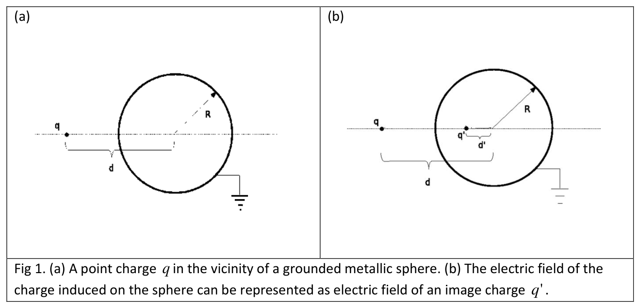
Fig 1. (a) A point charge \(q\) in the vicinity of a grounded metallic sphere. (b) The electric field of the charge induced on the sphere can be represented as electric field of an image charge \(q'\).
Task 1 – The image charge
The symmetry of the problem dictates that the charge \(q'\) should be placed on the line connecting the point charge \(q\) and the center of the sphere [see Fig. 1(b)].
a) What is the value of the potential on the sphere? (0.3 points)
b) Express \(q'\) and the distance \(d'\) of the charge \(q'\) from the center of the sphere, in terms of \(q\), \(d\), and \(R\). (1.9 points)
c) Find the magnitude of force acting on charge \(q\). Is the force repulsive? (0.5 points)
Task 2 – Shielding of an electrostatic field
Consider a point charge \(q\) placed at a distance \(d\) from the center of a grounded metallic sphere of radius \(R\). We are interested in how the grounded metallic sphere affects the electric field at point \(A\) on the opposite side of the sphere (see Fig. 2). Point \(A\) is on the line connecting charge \(q\) and the center of the sphere; its distance from the point charge \(q\) is \(r\).
a) Find the vector of the electric field at point \(A\). (0.6 points)
b) For a very large distance \(r\gg d\), find the expression for the electric field by using the approximation \((1+a)^{-2}\approx 1-2a\), where \(a\ll 1\). (0.6 points)
c) In which limit of \(d\) does the grounded metallic sphere screen the field of the charge \(q\) completely, such that the electric field at point \(A\) is exactly zero? (0.3 points)
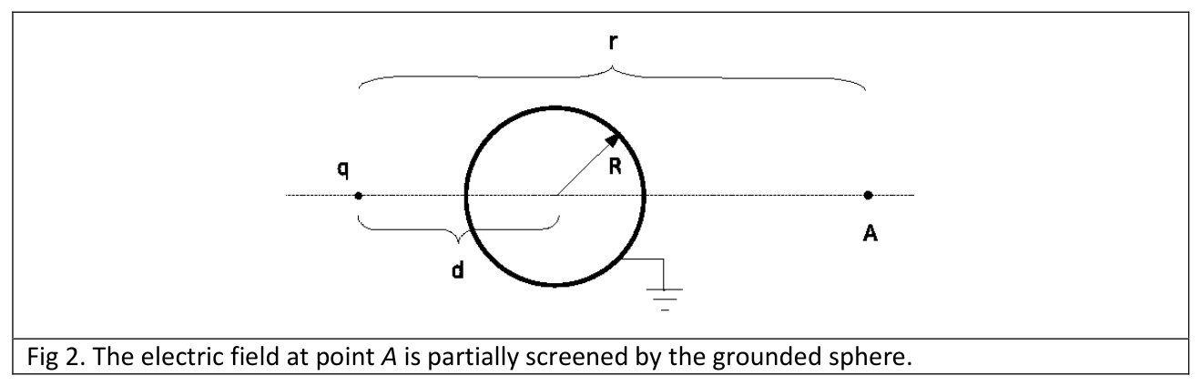
Fig 2. The electric field at point \(A\) is partially screened by the grounded sphere.
Task 3 – Small oscillations in the electric field of the grounded metallic sphere
A point charge \(q\) with mass \(m\) is suspended on a thread of length \(L\) which is attached to a wall, in the vicinity of the grounded metallic sphere. In your considerations, ignore all electrostatic effects of the wall. The point charge makes a mathematical pendulum (see Fig. 3). The point at which the thread is attached to the wall is at a distance \(l\) from the center of the sphere. Assume that the effects of gravity are negligible.
a) Find the magnitude of the electric force acting on the point charge \(q\) for a given angle \(\alpha\) and indicate the direction in a clear diagram (0.8 points)
b) Determine the component of this force acting in the direction perpendicular to the thread in terms of \(l\), \(L\), \(R\), \(q\) and \(\alpha\). (0.8 points)
c) Find the frequency for small oscillations of the pendulum. (1.0 points)
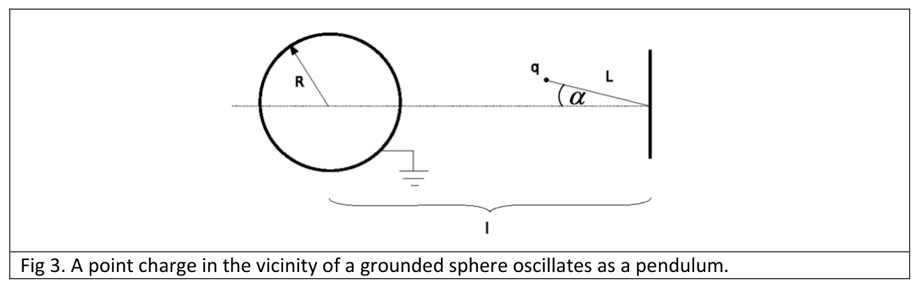
Fig 3. A point charge in the vicinity of a grounded sphere oscillates as a pendulum.
Task 4 – The electrostatic energy of the system
For a distribution of electric charges it is important to know the electrostatic energy of the system. In our problem (see Fig. 1a), there is an electrostatic interaction between the external charge \(q\) and the induced charges on the sphere, and there is an electrostatic interaction among the induced charges on the sphere themselves. In terms of the charge \(q\), radius of the sphere \(R\) and the distance \(d\) determine the following electrostatic energies:
a) the electrostatic energy of the interaction between charge \(q\) and the induced charges on the sphere; (1.0 points)
b) the electrostatic energy of the interaction among the induced charges on the sphere; (1.2 points)
c) the total electrostatic energy of the interaction in the system. (1.0 points)
Hint: There are several ways of solving this problem:
(1) In one of them, you can use the following integral,
\[ \int_d^\infty \frac{x\,dx}{(x^2-R^2)^2} =\frac{1}{2}\frac{1}{d^2-R^2}. \]
(2) In another one, you can use the fact that for a collection of \(N\) charges \(q_i\) located at points \(\vec r_i,i=1,\ldots,N\), the electrostatic energy is a sum over all pairs of charges:
\[ V=\frac{1}{2}\sum_{i=1}^{N} \sum_{\substack{j=1\\i\ne j}}^{N} \frac{1}{4\pi\varepsilon_0} \frac{q_iq_j}{|\vec r_i-\vec r_j|}. \]
Official English text of the problem.
Answers
Write \(k=1/(4\pi\varepsilon_0)\). In Task 2, let \(\hat{\mathbf e}\) point from \(q\) toward \(A\). For Task 3, define \[ d_\alpha=\sqrt{l^2+L^2-2lL\cos\alpha}, \qquad D_0=(l-L)^2-R^2, \] with \(l-L>R\) for the depicted exterior equilibrium. Take the signed perpendicular force as positive toward increasing \(\alpha\).
-
1(a) \[ \boxed{\phi_{\mathrm{sphere}}=0.} \]
-
1(b) \[ \boxed{q'=-\frac{R}{d}q,\qquad d'=\frac{R^2}{d}.} \] The image lies between the center and the surface nearest \(q\).
-
1(c) \[ \boxed{F=\frac{kq^2Rd}{(d^2-R^2)^2}.} \] The force is attractive, toward the sphere’s center.
-
2(a) \[ \boxed{ \mathbf E_A=kq\left[ \frac{1}{r^2} -\frac{R}{d\left(r-d+R^2/d\right)^2} \right]\hat{\mathbf e}. } \]
-
2(b) For \(r\gg d\), through the first correction: \[ \boxed{ \mathbf E_A\simeq \frac{kq}{r^2} \left[ 1-\frac{R}{d} -\frac{2R}{r}\left(1-\frac{R^2}{d^2}\right) \right]\hat{\mathbf e}. } \] The leading term is \(kq(1-R/d)\hat{\mathbf e}/r^2\).
-
2(c) \[ \boxed{d\to R^+\quad\Longrightarrow\quad \mathbf E_A\to\mathbf 0.} \]
-
3(a) \[ \boxed{ F(\alpha)= \frac{kq^2R\sqrt{l^2+L^2-2lL\cos\alpha}} {\left(l^2+L^2-2lL\cos\alpha-R^2\right)^2}. } \] Draw the force arrow from the charge directly toward the sphere’s center.
-
3(b) \[ \boxed{ F_\perp= -\frac{kq^2Rl\sin\alpha} {\left(l^2+L^2-2lL\cos\alpha-R^2\right)^2}. } \]
-
3(c) The ordinary frequency and angular frequency are \[ \boxed{ f=\frac{1}{2\pi}\sqrt{\frac{kq^2Rl}{mL D_0^2}}, \qquad \omega_0=2\pi f. } \]
-
4(a) Charge–surface interaction: \[ \boxed{U_{q\sigma}=-\frac{kq^2R}{d^2-R^2}.} \]
-
4(b) Mutual energy of the induced charges: \[ \boxed{U_{\sigma\sigma}=+\frac{kq^2R}{2(d^2-R^2)}.} \]
-
4(c) Total interaction energy: \[ \boxed{U_{\mathrm{tot}}=-\frac{kq^2R}{2(d^2-R^2)}.} \]
Solution
1(a)
A conductor in electrostatic equilibrium is an equipotential. Grounding fixes its potential to that of Earth, taken as zero: \[ \boxed{\phi_{\mathrm{sphere}}=0.} \]
1(b)
Let \(O\) be the center. Measure axial positions from \(O\) toward the external charge, so that \(q\) is at \(d>R\) and the image is at \(d'\), inside the sphere.
At the surface point nearest \(q\), the zero-potential condition gives \[ k\left(\frac{q}{d-R}+\frac{q'}{R-d'}\right)=0. \] At the opposite surface point, \[ k\left(\frac{q}{d+R}+\frac{q'}{R+d'}\right)=0. \] Consequently, \[ \frac{R-d'}{d-R}=\frac{R+d'}{d+R}. \] Cross-multiplication yields \[ (R-d')(d+R)=(R+d')(d-R), \] hence \[ \boxed{d'=\frac{R^2}{d}}. \] Substituting back, \[ \boxed{q'=-\frac{R}{d}q}. \]
These values also satisfy the boundary condition everywhere on the surface. For a surface point whose radius makes angle \(\theta\) with the direction toward \(q\), let its distances from \(q\) and \(q'\) be \(s\) and \(s'\). Then \[ s^2=d^2+R^2-2dR\cos\theta, \] and \[ s'^2=d'^2+R^2-2d'R\cos\theta =\frac{R^2}{d^2}s^2. \] Thus \(s'=(R/d)s\), and \[ k\left(\frac{q}{s}+\frac{q'}{s'}\right)=0. \]
1(c)
At the external charge, the image reproduces the field of the induced charges. The separation between \(q\) and its image is \[ d-d'=\frac{d^2-R^2}{d}. \] Coulomb’s law therefore gives \[ F=\frac{k|qq'|}{(d-d')^2} =\frac{kq^2(R/d)}{\left[(d^2-R^2)/d\right]^2}. \] Hence \[ \boxed{F=\frac{kq^2Rd}{(d^2-R^2)^2}}. \]
Since \(q'\) has the opposite sign to \(q\), the force is always attractive. It points along the line from \(q\) toward \(O\).
2(a)
Choose the positive axis from \(q\) toward \(A\), with unit vector \(\hat{\mathbf e}\). Put the sphere’s center at \(x=0\). Then \[ x_q=-d,\qquad x_{q'}=-d',\qquad x_A=r-d. \] Because \(A\) is outside the sphere on the opposite side, \(r>d+R\).
The distances from \(A\) to the two charges are \[ r,\qquad r-d+d'=r-d+\frac{R^2}{d}. \] By superposition, \[ \mathbf E_A= k\left[ \frac{q}{r^2} +\frac{q'}{(r-d+d')^2} \right]\hat{\mathbf e}. \] Therefore \[ \boxed{ \mathbf E_A=kq\left[ \frac{1}{r^2} -\frac{R}{d\left(r-d+R^2/d\right)^2} \right]\hat{\mathbf e}. } \] The sign of the scalar coefficient determines the direction along the axis.
2(b)
Define \[ \delta=d-\frac{R^2}{d}. \] Since \(0<\delta<d\), the condition \(r\gg d\) implies \(\delta/r\ll1\). We can write \[ \mathbf E_A= \frac{kq}{r^2} \left[ 1-\frac{R}{d}\left(1-\frac{\delta}{r}\right)^{-2} \right]\hat{\mathbf e}. \]
Using the supplied approximation with \(a=-\delta/r\), \[ \left(1-\frac{\delta}{r}\right)^{-2} \simeq1+\frac{2\delta}{r}. \] It follows that \[ \mathbf E_A\simeq \frac{kq}{r^2} \left[ 1-\frac{R}{d} -\frac{2R\delta}{dr} \right]\hat{\mathbf e}. \] Substituting \(\delta\), \[ \boxed{ \mathbf E_A\simeq \frac{kq}{r^2} \left[ 1-\frac{R}{d} -\frac{2R}{r}\left(1-\frac{R^2}{d^2}\right) \right]\hat{\mathbf e}. } \]
To leading order, the distant field is that of the effective net charge \[ q+q'=q\left(1-\frac{R}{d}\right). \]
2(c)
As the external charge approaches the sphere, \[ d\to R^+,\qquad d'\to R,\qquad q'\to-q. \] Thus the charge and its image approach the same position with equal and opposite charges. Their fields cancel at every fixed exterior observation point away from the contact point.
In particular, the exact expression in 2(a) gives \[ \boxed{\lim_{d\to R^+}\mathbf E_A=\mathbf 0}. \] This is a limit with the charge approaching the surface from outside.
3(a)
Treat the conductor as remaining in electrostatic equilibrium as the charge moves. Let \(P\) be the thread’s attachment point and \(Q\) the charge’s position. Choose \[ O=(0,0),\qquad P=(l,0). \] For the angle shown in Fig. 3, \[ Q=(l-L\cos\alpha,\;L\sin\alpha). \] Therefore the instantaneous center-to-charge distance is \[ d_\alpha=|OQ| =\sqrt{(l-L\cos\alpha)^2+L^2\sin^2\alpha} =\sqrt{l^2+L^2-2lL\cos\alpha}. \]
Applying the result of 1(c), \[ \boxed{ F(\alpha)= \frac{kq^2R\,d_\alpha}{(d_\alpha^2-R^2)^2} = \frac{kq^2R\sqrt{l^2+L^2-2lL\cos\alpha}} {\left(l^2+L^2-2lL\cos\alpha-R^2\right)^2}. } \]
The force points from \(Q\) toward \(O\).
Diagram description: Draw the sphere centered at \(O\), with \(P\) to its right on a horizontal line and \(OP=l\). Place \(Q\) above that line and to the left of \(P\), with \(PQ=L\) and \(\angle OPQ=\alpha\). Draw an arrow starting at \(Q\), along \(QO\), pointing toward \(O\), and label it \(\mathbf F_e\). Label \(OQ=d_\alpha\).
3(b)
A unit vector perpendicular to the thread, in the direction of increasing \(\alpha\), is \[ \hat{\mathbf e}_\alpha=(\sin\alpha,\cos\alpha). \] Since the force points toward \(O\), \[ \mathbf F_e=-\frac{F}{d_\alpha} (l-L\cos\alpha,\;L\sin\alpha). \] Its tangential component is \[ \begin{aligned} F_\perp &=\mathbf F_e\cdot\hat{\mathbf e}_\alpha\\ &=-\frac{F}{d_\alpha} \left[(l-L\cos\alpha)\sin\alpha +L\sin\alpha\cos\alpha\right]\\ &=-\frac{Fl\sin\alpha}{d_\alpha}. \end{aligned} \] Substitution gives \[ \boxed{ F_\perp= -\frac{kq^2Rl\sin\alpha} {\left(l^2+L^2-2lL\cos\alpha-R^2\right)^2}. } \]
For positive \(\alpha\), this component acts toward decreasing \(\alpha\), so it is restoring. Its magnitude is obtained by replacing \(-\sin\alpha\) with \(|\sin\alpha|\).
3(c)
At the equilibrium \(\alpha=0\), \[ d_0=l-L. \] The depicted equilibrium requires \(l-L>R\), so the charge lies outside the sphere.
Tension has no component perpendicular to the thread. Newton’s second law in the tangential direction is therefore \[ mL\ddot\alpha=F_\perp. \] For small \(\alpha\), \[ \sin\alpha\simeq\alpha, \] and \[ d_\alpha^2-R^2 =(l-L)^2-R^2+lL\alpha^2+O(\alpha^4). \] Writing \(D_0=(l-L)^2-R^2\), the linearized equation becomes \[ mL\ddot\alpha =-\frac{kq^2Rl}{D_0^2}\alpha, \] or \[ \ddot\alpha+\omega_0^2\alpha=0, \qquad \omega_0^2=\frac{kq^2Rl}{mL D_0^2}. \]
Thus the ordinary frequency is \[ \boxed{ f=\frac{\omega_0}{2\pi} =\frac{1}{2\pi} \sqrt{ \frac{kq^2Rl} {mL\left[(l-L)^2-R^2\right]^2} }. } \]
The approximation requires sufficiently small amplitude that both \[ |\alpha|\ll1, \qquad lL\alpha^2\ll D_0 \] hold.
4(a)
Omit the external point charge’s self-energy and take the interaction energy to vanish as \(d\to\infty\).
Let \(\phi_\sigma\) denote the potential produced by the induced surface charges. At the position of \(q\), the image gives \[ \phi_\sigma(q)=\frac{kq'}{d-d'} =-\frac{kqR}{d^2-R^2}. \] The interaction energy between \(q\) and the induced charges is \[ U_{q\sigma}=q\phi_\sigma(q). \] There is no factor \(1/2\) here: each pair consisting of \(q\) and an induced charge is counted once. Hence \[ \boxed{ U_{q\sigma}=-\frac{kq^2R}{d^2-R^2}. } \]
4(b)
Let \(\sigma\) be the induced surface charge density, and let \(\phi_q\) be the potential due to the external charge. The mutual energy of the induced charges is \[ U_{\sigma\sigma} =\frac12\int_S \sigma\,\phi_\sigma\,dS. \] The factor \(1/2\) prevents double counting of pairs within the surface distribution.
On the grounded sphere, \[ \phi_q+\phi_\sigma=0. \] Therefore \[ U_{\sigma\sigma} =-\frac12\int_S\sigma\,\phi_q\,dS. \] The remaining integral equals the charge–surface interaction energy: \[ \int_S\sigma\,\phi_q\,dS =kq\int_S\frac{\sigma\,dS}{|\mathbf r-\mathbf r_q|} =q\phi_\sigma(q) =U_{q\sigma}. \] Thus \[ U_{\sigma\sigma}=-\frac12U_{q\sigma}, \] giving \[ \boxed{ U_{\sigma\sigma}=+\frac{kq^2R}{2(d^2-R^2)}. } \]
4(c)
Adding the two physical contributions, \[ U_{\mathrm{tot}}=U_{q\sigma}+U_{\sigma\sigma} =\frac12U_{q\sigma}. \] Consequently, \[ \boxed{ U_{\mathrm{tot}}=-\frac{kq^2R}{2(d^2-R^2)}. } \]
This also follows from the work required to bring \(q\) quasistatically from infinity: \[ U_{\mathrm{tot}}(d) =-\int_d^\infty \frac{kq^2R\,x}{(x^2-R^2)^2}\,dx =-\frac{kq^2R}{2(d^2-R^2)}. \]
As a consistency check, the force in the direction of increasing \(d\) is \[ -\frac{dU_{\mathrm{tot}}}{dd} =-\frac{kq^2Rd}{(d^2-R^2)^2}, \] which reproduces the attractive force found in 1(c).
The solution was checked against the official solution.
IPhO 2010 · Theorieaufgabe 1
Spiegelbild einer Ladung in einem metallischen Körper
Einleitung – Methode der Spiegelladungen
Eine Punktladung \(q\) wird in die Nähe einer geerdeten Metallkugel mit dem Radius \(R\) gebracht [siehe Abb. 1(a)], wodurch auf der Kugel eine Oberflächenladungsverteilung induziert wird. Das elektrische Feld und das Potential dieser Oberflächenladungsverteilung zu berechnen, ist eine anspruchsvolle Aufgabe. Die Berechnung lässt sich jedoch mithilfe der sogenannten Methode der Spiegelladungen erheblich vereinfachen. Bei dieser Methode können das elektrische Feld und das Potential der auf der Kugel verteilten Ladung durch das elektrische Feld und das Potential einer einzelnen Punktladung \(q'\) im Inneren der Kugel dargestellt werden (dies müssen Sie nicht beweisen). Hinweis: Das elektrische Feld dieser Spiegelladung \(q'\) gibt das elektrische Feld und das Potential nur außerhalb der Kugel (einschließlich ihrer Oberfläche) wieder.
Abb. 1. (a) Eine Punktladung \(q\) in der Nähe einer geerdeten Metallkugel. (b) Das elektrische Feld der auf der Kugel induzierten Ladung kann als elektrisches Feld einer Spiegelladung \(q'\) dargestellt werden.
Aufgabe 1 – Die Spiegelladung
Aus der Symmetrie des Problems folgt, dass die Ladung \(q'\) auf der Verbindungslinie zwischen der Punktladung \(q\) und dem Kugelmittelpunkt liegen muss [siehe Abb. 1(b)].
a) Welchen Wert hat das Potential auf der Kugel? (0.3 Punkte)
b) Drücken Sie \(q'\) und den Abstand \(d'\) der Ladung \(q'\) vom Kugelmittelpunkt durch \(q\), \(d\) und \(R\) aus. (1.9 Punkte)
c) Bestimmen Sie den Betrag der auf die Ladung \(q\) wirkenden Kraft. Ist die Kraft abstoßend? (0.5 Punkte)
Aufgabe 2 – Abschirmung eines elektrostatischen Feldes
Betrachten Sie eine Punktladung \(q\), die sich im Abstand \(d\) vom Mittelpunkt einer geerdeten Metallkugel mit dem Radius \(R\) befindet. Uns interessiert, wie die geerdete Metallkugel das elektrische Feld am Punkt \(A\) auf der gegenüberliegenden Seite der Kugel beeinflusst (siehe Abb. 2). Der Punkt \(A\) liegt auf der Verbindungslinie zwischen der Ladung \(q\) und dem Kugelmittelpunkt; sein Abstand von der Punktladung \(q\) beträgt \(r\).
a) Bestimmen Sie den Vektor des elektrischen Feldes am Punkt \(A\). (0.6 Punkte)
b) Bestimmen Sie für einen sehr großen Abstand \(r\gg d\) den Ausdruck für das elektrische Feld mithilfe der Näherung \((1+a)^{-2}\approx 1-2a\), wobei \(a\ll 1\) gilt. (0.6 Punkte)
c) In welchem Grenzfall für \(d\) schirmt die geerdete Metallkugel das Feld der Ladung \(q\) vollständig ab, sodass das elektrische Feld am Punkt \(A\) exakt null ist? (0.3 Punkte)
Abb. 2. Das elektrische Feld am Punkt \(A\) wird durch die geerdete Kugel teilweise abgeschirmt.
Aufgabe 3 – Kleine Schwingungen im elektrischen Feld der geerdeten Metallkugel
Eine Punktladung \(q\) mit der Masse \(m\) hängt in der Nähe der geerdeten Metallkugel an einem Faden der Länge \(L\), der an einer Wand befestigt ist. Vernachlässigen Sie bei Ihren Überlegungen alle elektrostatischen Einflüsse der Wand. Die Punktladung bildet ein mathematisches Pendel (siehe Abb. 3). Der Befestigungspunkt des Fadens an der Wand befindet sich im Abstand \(l\) vom Kugelmittelpunkt. Nehmen Sie an, dass die Schwerkraft vernachlässigbar ist.
a) Bestimmen Sie den Betrag der elektrischen Kraft, die bei einem gegebenen Winkel \(\alpha\) auf die Punktladung \(q\) wirkt, und geben Sie ihre Richtung in einer übersichtlichen Skizze an (0.8 Punkte)
b) Bestimmen Sie die Komponente dieser Kraft senkrecht zum Faden in Abhängigkeit von \(l\), \(L\), \(R\), \(q\) und \(\alpha\). (0.8 Punkte)
c) Bestimmen Sie die Frequenz kleiner Schwingungen des Pendels. (1.0 Punkte)
Abb. 3. Eine Punktladung in der Nähe einer geerdeten Kugel schwingt als Pendel.
Aufgabe 4 – Die elektrostatische Energie des Systems
Für eine Verteilung elektrischer Ladungen ist es wichtig, die elektrostatische Energie des Systems zu kennen. In unserem Problem (siehe Abb. 1a) besteht eine elektrostatische Wechselwirkung zwischen der äußeren Ladung \(q\) und den auf der Kugel induzierten Ladungen sowie eine elektrostatische Wechselwirkung der auf der Kugel induzierten Ladungen untereinander. Bestimmen Sie in Abhängigkeit von der Ladung \(q\), dem Kugelradius \(R\) und dem Abstand \(d\) die folgenden elektrostatischen Energien:
a) die elektrostatische Energie der Wechselwirkung zwischen der Ladung \(q\) und den auf der Kugel induzierten Ladungen; (1.0 Punkte)
b) die elektrostatische Energie der Wechselwirkung der auf der Kugel induzierten Ladungen untereinander; (1.2 Punkte)
c) die gesamte elektrostatische Wechselwirkungsenergie des Systems. (1.0 Punkte)
Hinweis: Es gibt mehrere Möglichkeiten, dieses Problem zu lösen:
(1) Bei einer davon können Sie das folgende Integral verwenden,
\[ \int_d^\infty \frac{x\,dx}{(x^2-R^2)^2} =\frac{1}{2}\frac{1}{d^2-R^2}. \]
(2) Bei einer anderen können Sie nutzen, dass für eine Anordnung von \(N\) Ladungen \(q_i\) an den Punkten \(\vec r_i,i=1,\ldots,N\) die elektrostatische Energie durch eine Summe über alle Ladungspaare gegeben ist:
\[ V=\frac{1}{2}\sum_{i=1}^{N} \sum_{\substack{j=1\\i\ne j}}^{N} \frac{1}{4\pi\varepsilon_0} \frac{q_iq_j}{|\vec r_i-\vec r_j|}. \]
Aufgabentext aus dem offiziellen englischen Text übersetzt.
Antworten
Wir setzen \(k=1/(4\pi\varepsilon_0)\). In Aufgabe 2 zeige \(\hat{\mathbf e}\) von \(q\) nach \(A\). Für Aufgabe 3 definieren wir \[ d_\alpha=\sqrt{l^2+L^2-2lL\cos\alpha}, \qquad D_0=(l-L)^2-R^2, \] wobei für die dargestellte Gleichgewichtslage außerhalb der Kugel \(l-L>R\) gilt. Die vorzeichenbehaftete Kraftkomponente senkrecht zum Faden sei in Richtung zunehmender \(\alpha\) positiv.
-
1(a) \[ \boxed{\phi_{\mathrm{sphere}}=0.} \]
-
1(b) \[ \boxed{q'=-\frac{R}{d}q,\qquad d'=\frac{R^2}{d}.} \] Die Spiegelladung liegt zwischen dem Mittelpunkt und dem \(q\) nächstgelegenen Punkt der Oberfläche.
-
1(c) \[ \boxed{F=\frac{kq^2Rd}{(d^2-R^2)^2}.} \] Die Kraft ist anziehend und zum Kugelmittelpunkt gerichtet.
-
2(a) \[ \boxed{ \mathbf E_A=kq\left[ \frac{1}{r^2} -\frac{R}{d\left(r-d+R^2/d\right)^2} \right]\hat{\mathbf e}. } \]
-
2(b) Für \(r\gg d\) gilt bis einschließlich der ersten Korrektur: \[ \boxed{ \mathbf E_A\simeq \frac{kq}{r^2} \left[ 1-\frac{R}{d} -\frac{2R}{r}\left(1-\frac{R^2}{d^2}\right) \right]\hat{\mathbf e}. } \] Der führende Term ist \(kq(1-R/d)\hat{\mathbf e}/r^2\).
-
2(c) \[ \boxed{d\to R^+\quad\Longrightarrow\quad \mathbf E_A\to\mathbf 0.} \]
-
3(a) \[ \boxed{ F(\alpha)= \frac{kq^2R\sqrt{l^2+L^2-2lL\cos\alpha}} {\left(l^2+L^2-2lL\cos\alpha-R^2\right)^2}. } \] Zeichnen Sie den Kraftpfeil von der Ladung direkt zum Kugelmittelpunkt.
-
3(b) \[ \boxed{ F_\perp= -\frac{kq^2Rl\sin\alpha} {\left(l^2+L^2-2lL\cos\alpha-R^2\right)^2}. } \]
-
3(c) Die Frequenz und die Kreisfrequenz sind \[ \boxed{ f=\frac{1}{2\pi}\sqrt{\frac{kq^2Rl}{mL D_0^2}}, \qquad \omega_0=2\pi f. } \]
-
4(a) Wechselwirkung zwischen Ladung und Oberfläche: \[ \boxed{U_{q\sigma}=-\frac{kq^2R}{d^2-R^2}.} \]
-
4(b) Wechselwirkungsenergie der induzierten Ladungen untereinander: \[ \boxed{U_{\sigma\sigma}=+\frac{kq^2R}{2(d^2-R^2)}.} \]
-
4(c) Gesamte Wechselwirkungsenergie: \[ \boxed{U_{\mathrm{tot}}=-\frac{kq^2R}{2(d^2-R^2)}.} \]
Lösung
1(a)
Ein Leiter im elektrostatischen Gleichgewicht ist ein Äquipotentialkörper. Durch die Erdung wird sein Potential auf das der Erde festgelegt, das als null gewählt wird: \[ \boxed{\phi_{\mathrm{sphere}}=0.} \]
1(b)
Sei \(O\) der Mittelpunkt. Wir messen die Positionen entlang der Achse von \(O\) aus in Richtung der äußeren Ladung, sodass sich \(q\) bei \(d>R\) und die Spiegelladung bei \(d'\) im Inneren der Kugel befindet.
Am \(q\) nächstgelegenen Oberflächenpunkt ergibt die Bedingung verschwindenden Potentials \[ k\left(\frac{q}{d-R}+\frac{q'}{R-d'}\right)=0. \] Am gegenüberliegenden Oberflächenpunkt gilt \[ k\left(\frac{q}{d+R}+\frac{q'}{R+d'}\right)=0. \] Daraus folgt \[ \frac{R-d'}{d-R}=\frac{R+d'}{d+R}. \] Kreuzmultiplikation liefert \[ (R-d')(d+R)=(R+d')(d-R), \] also \[ \boxed{d'=\frac{R^2}{d}}. \] Durch Rückeinsetzen erhalten wir \[ \boxed{q'=-\frac{R}{d}q}. \]
Diese Werte erfüllen die Randbedingung auch überall auf der Oberfläche. Für einen Oberflächenpunkt, dessen Radiusvektor den Winkel \(\theta\) mit der Richtung zu \(q\) bildet, seien die Abstände von \(q\) und \(q'\) mit \(s\) beziehungsweise \(s'\) bezeichnet. Dann gilt \[ s^2=d^2+R^2-2dR\cos\theta, \] und \[ s'^2=d'^2+R^2-2d'R\cos\theta =\frac{R^2}{d^2}s^2. \] Somit ist \(s'=(R/d)s\), und \[ k\left(\frac{q}{s}+\frac{q'}{s'}\right)=0. \]
1(c)
Am Ort der äußeren Ladung gibt die Spiegelladung das Feld der induzierten Ladungen wieder. Der Abstand zwischen \(q\) und ihrer Spiegelladung beträgt \[ d-d'=\frac{d^2-R^2}{d}. \] Das Coulombsche Gesetz liefert daher \[ F=\frac{k|qq'|}{(d-d')^2} =\frac{kq^2(R/d)}{\left[(d^2-R^2)/d\right]^2}. \] Also gilt \[ \boxed{F=\frac{kq^2Rd}{(d^2-R^2)^2}}. \]
Da \(q'\) das entgegengesetzte Vorzeichen zu \(q\) hat, ist die Kraft stets anziehend. Sie zeigt entlang der Verbindungslinie von \(q\) nach \(O\).
2(a)
Wir wählen die positive Achsenrichtung von \(q\) nach \(A\), mit dem Einheitsvektor \(\hat{\mathbf e}\). Der Kugelmittelpunkt liege bei \(x=0\). Dann gilt \[ x_q=-d,\qquad x_{q'}=-d',\qquad x_A=r-d. \] Da \(A\) auf der gegenüberliegenden Seite außerhalb der Kugel liegt, gilt \(r>d+R\).
Die Abstände von \(A\) zu den beiden Ladungen betragen \[ r,\qquad r-d+d'=r-d+\frac{R^2}{d}. \] Nach dem Superpositionsprinzip gilt \[ \mathbf E_A= k\left[ \frac{q}{r^2} +\frac{q'}{(r-d+d')^2} \right]\hat{\mathbf e}. \] Damit folgt \[ \boxed{ \mathbf E_A=kq\left[ \frac{1}{r^2} -\frac{R}{d\left(r-d+R^2/d\right)^2} \right]\hat{\mathbf e}. } \] Das Vorzeichen des skalaren Koeffizienten bestimmt die Richtung entlang der Achse.
2(b)
Wir definieren \[ \delta=d-\frac{R^2}{d}. \] Da \(0<\delta<d\) gilt, folgt aus der Bedingung \(r\gg d\), dass \(\delta/r\ll1\) ist. Wir können schreiben \[ \mathbf E_A= \frac{kq}{r^2} \left[ 1-\frac{R}{d}\left(1-\frac{\delta}{r}\right)^{-2} \right]\hat{\mathbf e}. \]
Mit der angegebenen Näherung für \(a=-\delta/r\) erhalten wir \[ \left(1-\frac{\delta}{r}\right)^{-2} \simeq1+\frac{2\delta}{r}. \] Daraus folgt \[ \mathbf E_A\simeq \frac{kq}{r^2} \left[ 1-\frac{R}{d} -\frac{2R\delta}{dr} \right]\hat{\mathbf e}. \] Durch Einsetzen von \(\delta\) ergibt sich \[ \boxed{ \mathbf E_A\simeq \frac{kq}{r^2} \left[ 1-\frac{R}{d} -\frac{2R}{r}\left(1-\frac{R^2}{d^2}\right) \right]\hat{\mathbf e}. } \]
In führender Ordnung entspricht das Feld in großer Entfernung dem Feld der effektiven Nettoladung \[ q+q'=q\left(1-\frac{R}{d}\right). \]
2(c)
Wenn sich die äußere Ladung der Kugel nähert, gilt \[ d\to R^+,\qquad d'\to R,\qquad q'\to-q. \] Damit nähern sich die Ladung und ihre Spiegelladung derselben Position an, wobei ihre Ladungen betragsgleich und entgegengesetzt sind. Ihre Felder heben sich an jedem festen Beobachtungspunkt außerhalb der Kugel auf, der vom Berührungspunkt verschieden ist.
Insbesondere ergibt der exakte Ausdruck aus 2(a) \[ \boxed{\lim_{d\to R^+}\mathbf E_A=\mathbf 0}. \] Dies ist ein Grenzübergang, bei dem sich die Ladung der Oberfläche von außen nähert.
3(a)
Wir nehmen an, dass der Leiter während der Bewegung der Ladung im elektrostatischen Gleichgewicht bleibt. Sei \(P\) der Befestigungspunkt des Fadens und \(Q\) die Position der Ladung. Wir wählen \[ O=(0,0),\qquad P=(l,0). \] Für den in Abb. 3 dargestellten Winkel gilt \[ Q=(l-L\cos\alpha,\;L\sin\alpha). \] Der momentane Abstand zwischen Mittelpunkt und Ladung beträgt daher \[ d_\alpha=|OQ| =\sqrt{(l-L\cos\alpha)^2+L^2\sin^2\alpha} =\sqrt{l^2+L^2-2lL\cos\alpha}. \]
Mit dem Ergebnis aus 1(c) erhalten wir \[ \boxed{ F(\alpha)= \frac{kq^2R\,d_\alpha}{(d_\alpha^2-R^2)^2} = \frac{kq^2R\sqrt{l^2+L^2-2lL\cos\alpha}} {\left(l^2+L^2-2lL\cos\alpha-R^2\right)^2}. } \]
Die Kraft zeigt von \(Q\) nach \(O\).
Beschreibung der Skizze: Zeichnen Sie die Kugel mit dem Mittelpunkt \(O\) und rechts davon \(P\) auf einer horizontalen Geraden, wobei \(OP=l\) gilt. Platzieren Sie \(Q\) oberhalb dieser Geraden und links von \(P\), sodass \(PQ=L\) und \(\angle OPQ=\alpha\) gelten. Zeichnen Sie einen bei \(Q\) beginnenden Pfeil entlang \(QO\), der nach \(O\) zeigt, und beschriften Sie ihn mit \(\mathbf F_e\). Beschriften Sie \(OQ=d_\alpha\).
3(b)
Ein Einheitsvektor senkrecht zum Faden in Richtung zunehmender \(\alpha\) ist \[ \hat{\mathbf e}_\alpha=(\sin\alpha,\cos\alpha). \] Da die Kraft nach \(O\) zeigt, gilt \[ \mathbf F_e=-\frac{F}{d_\alpha} (l-L\cos\alpha,\;L\sin\alpha). \] Ihre Tangentialkomponente ist \[ \begin{aligned} F_\perp &=\mathbf F_e\cdot\hat{\mathbf e}_\alpha\\ &=-\frac{F}{d_\alpha} \left[(l-L\cos\alpha)\sin\alpha +L\sin\alpha\cos\alpha\right]\\ &=-\frac{Fl\sin\alpha}{d_\alpha}. \end{aligned} \] Durch Einsetzen ergibt sich \[ \boxed{ F_\perp= -\frac{kq^2Rl\sin\alpha} {\left(l^2+L^2-2lL\cos\alpha-R^2\right)^2}. } \]
Für positives \(\alpha\) wirkt diese Komponente in Richtung abnehmender \(\alpha\), sie ist also rücktreibend. Ihren Betrag erhält man, indem man \(-\sin\alpha\) durch \(|\sin\alpha|\) ersetzt.
3(c)
In der Gleichgewichtslage \(\alpha=0\) gilt \[ d_0=l-L. \] Die dargestellte Gleichgewichtslage setzt \(l-L>R\) voraus, sodass die Ladung außerhalb der Kugel liegt.
Die Fadenspannung hat keine Komponente senkrecht zum Faden. Das zweite Newtonsche Gesetz in tangentialer Richtung lautet daher \[ mL\ddot\alpha=F_\perp. \] Für kleine \(\alpha\) gilt \[ \sin\alpha\simeq\alpha, \] und \[ d_\alpha^2-R^2 =(l-L)^2-R^2+lL\alpha^2+O(\alpha^4). \] Mit \(D_0=(l-L)^2-R^2\) lautet die linearisierte Gleichung \[ mL\ddot\alpha =-\frac{kq^2Rl}{D_0^2}\alpha, \] oder \[ \ddot\alpha+\omega_0^2\alpha=0, \qquad \omega_0^2=\frac{kq^2Rl}{mL D_0^2}. \]
Somit beträgt die Frequenz \[ \boxed{ f=\frac{\omega_0}{2\pi} =\frac{1}{2\pi} \sqrt{ \frac{kq^2Rl} {mL\left[(l-L)^2-R^2\right]^2} }. } \]
Die Näherung setzt eine hinreichend kleine Amplitude voraus, sodass beide Bedingungen \[ |\alpha|\ll1, \qquad lL\alpha^2\ll D_0 \] erfüllt sind.
4(a)
Wir lassen die Selbstenergie der äußeren Punktladung außer Betracht und wählen die Wechselwirkungsenergie so, dass sie für \(d\to\infty\) verschwindet.
Sei \(\phi_\sigma\) das von den induzierten Oberflächenladungen erzeugte Potential. Am Ort von \(q\) liefert die Spiegelladung \[ \phi_\sigma(q)=\frac{kq'}{d-d'} =-\frac{kqR}{d^2-R^2}. \] Die Wechselwirkungsenergie zwischen \(q\) und den induzierten Ladungen ist \[ U_{q\sigma}=q\phi_\sigma(q). \] Hier tritt kein Faktor \(1/2\) auf: Jedes Paar aus \(q\) und einer induzierten Ladung wird einmal gezählt. Daher gilt \[ \boxed{ U_{q\sigma}=-\frac{kq^2R}{d^2-R^2}. } \]
4(b)
Sei \(\sigma\) die induzierte Oberflächenladungsdichte und \(\phi_q\) das Potential der äußeren Ladung. Die Wechselwirkungsenergie der induzierten Ladungen untereinander ist \[ U_{\sigma\sigma} =\frac12\int_S \sigma\,\phi_\sigma\,dS. \] Der Faktor \(1/2\) verhindert die doppelte Zählung von Paaren innerhalb der Oberflächenladungsverteilung.
Auf der geerdeten Kugel gilt \[ \phi_q+\phi_\sigma=0. \] Deshalb ist \[ U_{\sigma\sigma} =-\frac12\int_S\sigma\,\phi_q\,dS. \] Das verbleibende Integral ist gleich der Wechselwirkungsenergie zwischen Ladung und Oberfläche: \[ \int_S\sigma\,\phi_q\,dS =kq\int_S\frac{\sigma\,dS}{|\mathbf r-\mathbf r_q|} =q\phi_\sigma(q) =U_{q\sigma}. \] Somit gilt \[ U_{\sigma\sigma}=-\frac12U_{q\sigma}, \] woraus folgt \[ \boxed{ U_{\sigma\sigma}=+\frac{kq^2R}{2(d^2-R^2)}. } \]
4(c)
Durch Addition der beiden physikalischen Beiträge erhalten wir \[ U_{\mathrm{tot}}=U_{q\sigma}+U_{\sigma\sigma} =\frac12U_{q\sigma}. \] Folglich gilt \[ \boxed{ U_{\mathrm{tot}}=-\frac{kq^2R}{2(d^2-R^2)}. } \]
Dies folgt auch aus der Arbeit, die erforderlich ist, um \(q\) quasistatisch aus dem Unendlichen heranzubringen: \[ U_{\mathrm{tot}}(d) =-\int_d^\infty \frac{kq^2R\,x}{(x^2-R^2)^2}\,dx =-\frac{kq^2R}{2(d^2-R^2)}. \]
Zur Konsistenzprüfung ergibt sich für die Kraft in Richtung zunehmender \(d\) \[ -\frac{dU_{\mathrm{tot}}}{dd} =-\frac{kq^2Rd}{(d^2-R^2)^2}, \] was die in 1(c) gefundene anziehende Kraft wiedergibt.
Die Lösung wurde mit der offiziellen Lösung abgeglichen.
IPhO 2010 · Teori sorusu 1
Metal bir cisimdeki yükün görüntüsü
Giriş – Görüntü yük yöntemi
Yarıçapı \(R\) olan topraklanmış metal bir kürenin yakınına bir \(q\) noktasal yükü yerleştirilir [bkz. Şekil 1(a)] ve bunun sonucunda küre üzerinde bir yüzey yük dağılımı indüklenir. Yüzey yük dağılımının oluşturduğu elektrik alanı ve potansiyeli hesaplamak oldukça güçtür. Ancak görüntü yük yöntemi adı verilen yöntem kullanılarak hesaplama önemli ölçüde basitleştirilebilir. Bu yöntemde, küre üzerinde dağılmış yükün oluşturduğu elektrik alan ve potansiyel, kürenin içine yerleştirilmiş tek bir \(q'\) noktasal yükünün elektrik alanı ve potansiyeli ile temsil edilebilir (bunu kanıtlamanız gerekmiyor). Not: Bu \(q'\) görüntü yükünün elektrik alanı, elektrik alanı ve potansiyeli yalnızca kürenin dışında (yüzeyi de dâhil olmak üzere) doğru olarak verir.
Şekil 1. (a) Topraklanmış metal bir kürenin yakınındaki bir \(q\) noktasal yükü. (b) Küre üzerinde indüklenen yükün elektrik alanı, bir \(q'\) görüntü yükünün elektrik alanı ile temsil edilebilir.
Görev 1 – Görüntü yük
Problemin simetrisi, \(q'\) yükünün \(q\) noktasal yükü ile kürenin merkezini birleştiren doğru üzerine yerleştirilmesini gerektirir [bkz. Şekil 1(b)].
a) Kürenin üzerindeki potansiyelin değeri nedir? (0.3 puan)
b) \(q'\) yükünü ve \(q'\) yükünün kürenin merkezine olan \(d'\) uzaklığını \(q\), \(d\) ve \(R\) cinsinden ifade ediniz. (1.9 puan)
c) \(q\) yüküne etki eden kuvvetin büyüklüğünü bulunuz. Kuvvet itici midir? (0.5 puan)
Görev 2 – Elektrostatik alanın perdelenmesi
Yarıçapı \(R\) olan topraklanmış metal bir kürenin merkezinden \(d\) uzaklığa yerleştirilmiş bir \(q\) noktasal yükünü ele alınız. Topraklanmış metal kürenin, kürenin karşı tarafındaki \(A\) noktasında elektrik alanı nasıl etkilediğini incelemek istiyoruz (bkz. Şekil 2). \(A\) noktası, \(q\) yükü ile kürenin merkezini birleştiren doğru üzerindedir; \(q\) noktasal yüküne olan uzaklığı \(r\)'dir.
a) \(A\) noktasındaki elektrik alan vektörünü bulunuz. (0.6 puan)
b) Çok büyük bir \(r\gg d\) uzaklığı için, \(a\ll 1\) olmak üzere \((1+a)^{-2}\approx 1-2a\) yaklaşımını kullanarak elektrik alanın ifadesini bulunuz. (0.6 puan)
c) \(d\)'nin hangi limitinde topraklanmış metal küre, \(q\) yükünün alanını tamamen perdeler ve böylece \(A\) noktasındaki elektrik alan tam olarak sıfır olur? (0.3 puan)
Şekil 2. \(A\) noktasındaki elektrik alan, topraklanmış küre tarafından kısmen perdelenir.
Görev 3 – Topraklanmış metal kürenin elektrik alanında küçük salınımlar
Kütlesi \(m\) olan bir \(q\) noktasal yükü, topraklanmış metal kürenin yakınında, bir duvara tutturulmuş \(L\) uzunluğundaki bir ipe asılmıştır. İncelemenizde duvarın tüm elektrostatik etkilerini ihmal ediniz. Noktasal yük bir basit sarkaç oluşturur (bkz. Şekil 3). İpin duvara tutturulduğu nokta, kürenin merkezinden \(l\) uzaklıktadır. Yerçekimi etkilerinin ihmal edilebilir olduğunu varsayınız.
a) Verilen bir \(\alpha\) açısı için \(q\) noktasal yüküne etki eden elektriksel kuvvetin büyüklüğünü bulunuz ve yönünü açık bir çizimde gösteriniz (0.8 puan)
b) Bu kuvvetin ipe dik doğrultudaki bileşenini \(l\), \(L\), \(R\), \(q\) ve \(\alpha\) cinsinden belirleyiniz. (0.8 puan)
c) Sarkacın küçük salınımlarının frekansını bulunuz. (1.0 puan)
Şekil 3. Topraklanmış bir kürenin yakınındaki noktasal yük, bir sarkaç gibi salınır.
Görev 4 – Sistemin elektrostatik enerjisi
Bir elektrik yük dağılımı için sistemin elektrostatik enerjisini bilmek önemlidir. Problemimizde (bkz. Şekil 1a), dışarıdaki \(q\) yükü ile küre üzerinde indüklenen yükler arasında bir elektrostatik etkileşim ve küre üzerinde indüklenen yüklerin kendi aralarında da bir elektrostatik etkileşim vardır. \(q\) yükü, kürenin \(R\) yarıçapı ve \(d\) uzaklığı cinsinden aşağıdaki elektrostatik enerjileri belirleyiniz:
a) \(q\) yükü ile küre üzerinde indüklenen yükler arasındaki etkileşimin elektrostatik enerjisi; (1.0 puan)
b) küre üzerinde indüklenen yüklerin kendi aralarındaki etkileşimin elektrostatik enerjisi; (1.2 puan)
c) sistemdeki etkileşimin toplam elektrostatik enerjisi. (1.0 puan)
İpucu: Bu problemi çözmenin birkaç yolu vardır:
(1) Bunlardan birinde aşağıdaki integrali kullanabilirsiniz,
\[ \int_d^\infty \frac{x\,dx}{(x^2-R^2)^2} =\frac{1}{2}\frac{1}{d^2-R^2}. \]
(2) Bir diğerinde, \(\vec r_i,i=1,\ldots,N\) noktalarında bulunan \(N\) adet \(q_i\) yükünden oluşan bir topluluğun elektrostatik enerjisinin, tüm yük çiftleri üzerinden alınan bir toplam olduğu gerçeğini kullanabilirsiniz:
\[ V=\frac{1}{2}\sum_{i=1}^{N} \sum_{\substack{j=1\\i\ne j}}^{N} \frac{1}{4\pi\varepsilon_0} \frac{q_iq_j}{|\vec r_i-\vec r_j|}. \]
Soru metni resmi İngilizce metinden çevrilmiştir.
Cevaplar
\(k=1/(4\pi\varepsilon_0)\) yazalım. Görev 2'de \(\hat{\mathbf e}\), \(q\)'dan \(A\)'ya doğru yönelsin. Görev 3 için \[ d_\alpha=\sqrt{l^2+L^2-2lL\cos\alpha}, \qquad D_0=(l-L)^2-R^2, \] olarak tanımlayalım; şekilde gösterilen dış denge konumu için \(l-L>R\) olmalıdır. İşaretli dik kuvvet bileşenini, \(\alpha\)'nın arttığı yönde pozitif alalım.
-
1(a) \[ \boxed{\phi_{\mathrm{sphere}}=0.} \]
-
1(b) \[ \boxed{q'=-\frac{R}{d}q,\qquad d'=\frac{R^2}{d}.} \] Görüntü yük, merkez ile yüzeyin \(q\)'ya en yakın noktası arasında bulunur.
-
1(c) \[ \boxed{F=\frac{kq^2Rd}{(d^2-R^2)^2}.} \] Kuvvet çekicidir ve kürenin merkezine doğrudur.
-
2(a) \[ \boxed{ \mathbf E_A=kq\left[ \frac{1}{r^2} -\frac{R}{d\left(r-d+R^2/d\right)^2} \right]\hat{\mathbf e}. } \]
-
2(b) \(r\gg d\) için, ilk düzeltme terimi dâhil: \[ \boxed{ \mathbf E_A\simeq \frac{kq}{r^2} \left[ 1-\frac{R}{d} -\frac{2R}{r}\left(1-\frac{R^2}{d^2}\right) \right]\hat{\mathbf e}. } \] Başat terim \(kq(1-R/d)\hat{\mathbf e}/r^2\)'dir.
-
2(c) \[ \boxed{d\to R^+\quad\Longrightarrow\quad \mathbf E_A\to\mathbf 0.} \]
-
3(a) \[ \boxed{ F(\alpha)= \frac{kq^2R\sqrt{l^2+L^2-2lL\cos\alpha}} {\left(l^2+L^2-2lL\cos\alpha-R^2\right)^2}. } \] Kuvvet okunu yükten doğrudan kürenin merkezine doğru çiziniz.
-
3(b) \[ \boxed{ F_\perp= -\frac{kq^2Rl\sin\alpha} {\left(l^2+L^2-2lL\cos\alpha-R^2\right)^2}. } \]
-
3(c) Frekans ve açısal frekans şöyledir: \[ \boxed{ f=\frac{1}{2\pi}\sqrt{\frac{kq^2Rl}{mL D_0^2}}, \qquad \omega_0=2\pi f. } \]
-
4(a) Yük–yüzey etkileşimi: \[ \boxed{U_{q\sigma}=-\frac{kq^2R}{d^2-R^2}.} \]
-
4(b) İndüklenen yüklerin karşılıklı etkileşim enerjisi: \[ \boxed{U_{\sigma\sigma}=+\frac{kq^2R}{2(d^2-R^2)}.} \]
-
4(c) Toplam etkileşim enerjisi: \[ \boxed{U_{\mathrm{tot}}=-\frac{kq^2R}{2(d^2-R^2)}.} \]
Çözüm
1(a)
Elektrostatik dengedeki bir iletken eşpotansiyeldir. Topraklama, iletkenin potansiyelini sıfır kabul edilen Yer potansiyeline sabitler: \[ \boxed{\phi_{\mathrm{sphere}}=0.} \]
1(b)
Merkez \(O\) olsun. Eksen üzerindeki konumları \(O\)'dan dış yüke doğru ölçelim; böylece \(q\) yükü \(d>R\) konumunda, görüntü yük ise kürenin içinde, \(d'\) konumundadır.
Yüzeyin \(q\)'ya en yakın noktasında sıfır potansiyel koşulu şu sonucu verir: \[ k\left(\frac{q}{d-R}+\frac{q'}{R-d'}\right)=0. \] Yüzeyin karşı tarafındaki noktada ise \[ k\left(\frac{q}{d+R}+\frac{q'}{R+d'}\right)=0. \] Dolayısıyla, \[ \frac{R-d'}{d-R}=\frac{R+d'}{d+R}. \] İçler dışlar çarpımı yapıldığında \[ (R-d')(d+R)=(R+d')(d-R), \] buradan da \[ \boxed{d'=\frac{R^2}{d}}. \] Bu sonucu yerine koyarsak, \[ \boxed{q'=-\frac{R}{d}q}. \]
Bu değerler, yüzeyin her noktasında sınır koşulunu da sağlar. Yarıçap vektörü \(q\)'ya doğru olan yön ile \(\theta\) açısı yapan bir yüzey noktasının \(q\) ve \(q'\)'ye uzaklıkları sırasıyla \(s\) ve \(s'\) olsun. O hâlde \[ s^2=d^2+R^2-2dR\cos\theta, \] ve \[ s'^2=d'^2+R^2-2d'R\cos\theta =\frac{R^2}{d^2}s^2. \] Böylece \(s'=(R/d)s\) olur ve \[ k\left(\frac{q}{s}+\frac{q'}{s'}\right)=0. \]
1(c)
Dış yükün bulunduğu noktada görüntü yük, indüklenen yüklerin alanını doğru olarak verir. \(q\) ile görüntü yükü arasındaki uzaklık \[ d-d'=\frac{d^2-R^2}{d}. \] Bu nedenle Coulomb yasası şu sonucu verir: \[ F=\frac{k|qq'|}{(d-d')^2} =\frac{kq^2(R/d)}{\left[(d^2-R^2)/d\right]^2}. \] Dolayısıyla \[ \boxed{F=\frac{kq^2Rd}{(d^2-R^2)^2}}. \]
\(q'\), \(q\) ile zıt işaretli olduğundan kuvvet her zaman çekicidir. \(q\)'dan \(O\)'ya uzanan doğru boyunca \(O\)'ya yönelir.
2(a)
Pozitif ekseni \(q\)'dan \(A\)'ya doğru seçelim ve bu yöndeki birim vektör \(\hat{\mathbf e}\) olsun. Kürenin merkezini \(x=0\) noktasına yerleştirelim. O hâlde \[ x_q=-d,\qquad x_{q'}=-d',\qquad x_A=r-d. \] \(A\), kürenin dışında ve karşı tarafta olduğundan \(r>d+R\)'dir.
\(A\)'nın iki yüke olan uzaklıkları \[ r,\qquad r-d+d'=r-d+\frac{R^2}{d}. \] Süperpozisyon ilkesine göre, \[ \mathbf E_A= k\left[ \frac{q}{r^2} +\frac{q'}{(r-d+d')^2} \right]\hat{\mathbf e}. \] Böylece \[ \boxed{ \mathbf E_A=kq\left[ \frac{1}{r^2} -\frac{R}{d\left(r-d+R^2/d\right)^2} \right]\hat{\mathbf e}. } \] Skaler katsayının işareti, eksen üzerindeki yönü belirler.
2(b)
Şu tanımı yapalım: \[ \delta=d-\frac{R^2}{d}. \] \(0<\delta<d\) olduğundan \(r\gg d\) koşulu, \(\delta/r\ll1\) olmasını gerektirir. Şöyle yazabiliriz: \[ \mathbf E_A= \frac{kq}{r^2} \left[ 1-\frac{R}{d}\left(1-\frac{\delta}{r}\right)^{-2} \right]\hat{\mathbf e}. \]
Verilen yaklaşımı \(a=-\delta/r\) ile kullanırsak, \[ \left(1-\frac{\delta}{r}\right)^{-2} \simeq1+\frac{2\delta}{r}. \] Buradan \[ \mathbf E_A\simeq \frac{kq}{r^2} \left[ 1-\frac{R}{d} -\frac{2R\delta}{dr} \right]\hat{\mathbf e}. \] \(\delta\)'nın ifadesini yerine koyarsak, \[ \boxed{ \mathbf E_A\simeq \frac{kq}{r^2} \left[ 1-\frac{R}{d} -\frac{2R}{r}\left(1-\frac{R^2}{d^2}\right) \right]\hat{\mathbf e}. } \]
Başat mertebede, uzaktaki alan şu etkin net yükün alanıdır: \[ q+q'=q\left(1-\frac{R}{d}\right). \]
2(c)
Dış yük küreye yaklaşırken, \[ d\to R^+,\qquad d'\to R,\qquad q'\to-q. \] Böylece yük ve görüntüsü, eşit büyüklükte ve zıt işaretli yüklerle aynı konuma yaklaşır. Alanları, temas noktasından uzaktaki her sabit dış gözlem noktasında birbirini yok eder.
Özellikle, 2(a)'daki tam ifade şu sonucu verir: \[ \boxed{\lim_{d\to R^+}\mathbf E_A=\mathbf 0}. \] Bu, yükün yüzeye dışarıdan yaklaştığı bir limittir.
3(a)
Yük hareket ederken iletkenin elektrostatik dengede kaldığını kabul edelim. İpin tutturulduğu nokta \(P\), yükün konumu ise \(Q\) olsun. Şu seçimi yapalım: \[ O=(0,0),\qquad P=(l,0). \] Şekil 3'te gösterilen açı için, \[ Q=(l-L\cos\alpha,\;L\sin\alpha). \] Dolayısıyla merkez ile yük arasındaki anlık uzaklık \[ d_\alpha=|OQ| =\sqrt{(l-L\cos\alpha)^2+L^2\sin^2\alpha} =\sqrt{l^2+L^2-2lL\cos\alpha}. \]
1(c)'nin sonucunu uygularsak, \[ \boxed{ F(\alpha)= \frac{kq^2R\,d_\alpha}{(d_\alpha^2-R^2)^2} = \frac{kq^2R\sqrt{l^2+L^2-2lL\cos\alpha}} {\left(l^2+L^2-2lL\cos\alpha-R^2\right)^2}. } \]
Kuvvet \(Q\)'dan \(O\)'ya doğru yönelir.
Çizimin açıklaması: Merkezi \(O\) olan küreyi çiziniz; \(P\)'yi, kürenin sağında yatay bir doğru üzerinde ve \(OP=l\) olacak şekilde yerleştiriniz. \(Q\)'yu bu doğrunun üstüne ve \(P\)'nin soluna, \(PQ=L\) ve \(\angle OPQ=\alpha\) olacak şekilde yerleştiriniz. \(Q\)'dan başlayan, \(QO\) boyunca \(O\)'ya yönelen bir ok çiziniz ve bu oku \(\mathbf F_e\) olarak etiketleyiniz. \(OQ=d_\alpha\) etiketini ekleyiniz.
3(b)
İpe dik ve \(\alpha\)'nın arttığı yöndeki birim vektör \[ \hat{\mathbf e}_\alpha=(\sin\alpha,\cos\alpha). \] Kuvvet \(O\)'ya doğru yöneldiğinden, \[ \mathbf F_e=-\frac{F}{d_\alpha} (l-L\cos\alpha,\;L\sin\alpha). \] Teğetsel bileşeni \[ \begin{aligned} F_\perp &=\mathbf F_e\cdot\hat{\mathbf e}_\alpha\\ &=-\frac{F}{d_\alpha} \left[(l-L\cos\alpha)\sin\alpha +L\sin\alpha\cos\alpha\right]\\ &=-\frac{Fl\sin\alpha}{d_\alpha}. \end{aligned} \] Yerine koyma işlemi şu sonucu verir: \[ \boxed{ F_\perp= -\frac{kq^2Rl\sin\alpha} {\left(l^2+L^2-2lL\cos\alpha-R^2\right)^2}. } \]
Pozitif \(\alpha\) için bu bileşen, \(\alpha\)'nın azaldığı yönde etki eder; dolayısıyla geri çağırıcıdır. Büyüklüğü, \(-\sin\alpha\) yerine \(|\sin\alpha|\) konularak elde edilir.
3(c)
\(\alpha=0\) denge konumunda, \[ d_0=l-L. \] Şekilde gösterilen denge konumu \(l-L>R\) koşulunu gerektirir; dolayısıyla yük kürenin dışındadır.
İp gerilmesinin ipe dik bileşeni yoktur. Bu nedenle teğetsel doğrultuda Newton'un ikinci yasası \[ mL\ddot\alpha=F_\perp. \] Küçük \(\alpha\) için, \[ \sin\alpha\simeq\alpha, \] ve \[ d_\alpha^2-R^2 =(l-L)^2-R^2+lL\alpha^2+O(\alpha^4). \] \(D_0=(l-L)^2-R^2\) yazıldığında doğrusallaştırılmış denklem \[ mL\ddot\alpha =-\frac{kq^2Rl}{D_0^2}\alpha, \] veya \[ \ddot\alpha+\omega_0^2\alpha=0, \qquad \omega_0^2=\frac{kq^2Rl}{mL D_0^2}. \]
Böylece frekans \[ \boxed{ f=\frac{\omega_0}{2\pi} =\frac{1}{2\pi} \sqrt{ \frac{kq^2Rl} {mL\left[(l-L)^2-R^2\right]^2} }. } \]
Bu yaklaşım, genliğin hem \[ |\alpha|\ll1, \qquad lL\alpha^2\ll D_0 \] koşullarını sağlayacak kadar küçük olmasını gerektirir.
4(a)
Dış noktasal yükün öz enerjisini hesaba katmayalım ve \(d\to\infty\) iken etkileşim enerjisinin sıfır olduğunu kabul edelim.
İndüklenen yüzey yüklerinin oluşturduğu potansiyeli \(\phi_\sigma\) ile gösterelim. \(q\)'nun bulunduğu konumda görüntü yük şu sonucu verir: \[ \phi_\sigma(q)=\frac{kq'}{d-d'} =-\frac{kqR}{d^2-R^2}. \] \(q\) ile indüklenen yükler arasındaki etkileşim enerjisi \[ U_{q\sigma}=q\phi_\sigma(q). \] Burada \(1/2\) çarpanı yoktur: \(q\) ile indüklenen bir yükten oluşan her çift bir kez sayılır. Dolayısıyla \[ \boxed{ U_{q\sigma}=-\frac{kq^2R}{d^2-R^2}. } \]
4(b)
İndüklenen yüzey yük yoğunluğu \(\sigma\), dış yükün oluşturduğu potansiyel ise \(\phi_q\) olsun. İndüklenen yüklerin karşılıklı etkileşim enerjisi \[ U_{\sigma\sigma} =\frac12\int_S \sigma\,\phi_\sigma\,dS. \] \(1/2\) çarpanı, yüzey dağılımındaki yük çiftlerinin iki kez sayılmasını önler.
Topraklanmış kürenin üzerinde, \[ \phi_q+\phi_\sigma=0. \] Bu nedenle \[ U_{\sigma\sigma} =-\frac12\int_S\sigma\,\phi_q\,dS. \] Geriye kalan integral, yük–yüzey etkileşim enerjisine eşittir: \[ \int_S\sigma\,\phi_q\,dS =kq\int_S\frac{\sigma\,dS}{|\mathbf r-\mathbf r_q|} =q\phi_\sigma(q) =U_{q\sigma}. \] Böylece \[ U_{\sigma\sigma}=-\frac12U_{q\sigma}, \] ve buradan \[ \boxed{ U_{\sigma\sigma}=+\frac{kq^2R}{2(d^2-R^2)}. } \]
4(c)
İki fiziksel katkıyı toplarsak, \[ U_{\mathrm{tot}}=U_{q\sigma}+U_{\sigma\sigma} =\frac12U_{q\sigma}. \] Dolayısıyla, \[ \boxed{ U_{\mathrm{tot}}=-\frac{kq^2R}{2(d^2-R^2)}. } \]
Bu sonuç, \(q\)'yu sonsuzdan kuazistatik olarak getirmek için gereken işten de elde edilir: \[ U_{\mathrm{tot}}(d) =-\int_d^\infty \frac{kq^2R\,x}{(x^2-R^2)^2}\,dx =-\frac{kq^2R}{2(d^2-R^2)}. \]
Bir tutarlılık kontrolü olarak, \(d\)'nin arttığı yöndeki kuvvet \[ -\frac{dU_{\mathrm{tot}}}{dd} =-\frac{kq^2Rd}{(d^2-R^2)^2}, \] olup 1(c)'de bulunan çekici kuvveti yeniden verir.
Çözüm, resmi çözümle karşılaştırılarak kontrol edildi.
IPhO 2010 · Problema teórico 1
Imagen de una carga en un objeto metálico
Introducción – Método de las imágenes
Una carga puntual \(q\) se sitúa en las proximidades de una esfera metálica conectada a tierra de radio \(R\) [véase la Fig. 1(a)] y, como consecuencia, se induce una distribución de carga superficial sobre la esfera. Calcular el campo eléctrico y el potencial debidos a la distribución de carga superficial es una tarea sumamente difícil. Sin embargo, el cálculo puede simplificarse considerablemente utilizando el denominado método de las imágenes. En este método, el campo eléctrico y el potencial producidos por la carga distribuida sobre la esfera pueden representarse como el campo eléctrico y el potencial de una única carga puntual \(q'\) situada en el interior de la esfera (no es necesario demostrarlo). Nota: El campo eléctrico de esta carga imagen \(q'\) reproduce el campo eléctrico y el potencial únicamente en el exterior de la esfera (incluida su superficie).
Fig. 1. (a) Una carga puntual \(q\) en las proximidades de una esfera metálica conectada a tierra. (b) El campo eléctrico de la carga inducida sobre la esfera puede representarse como el campo eléctrico de una carga imagen \(q'\).
Tarea 1 – La carga imagen
La simetría del problema exige que la carga \(q'\) se sitúe sobre la recta que une la carga puntual \(q\) y el centro de la esfera [véase la Fig. 1(b)].
a) ¿Cuál es el valor del potencial en la esfera? (0.3 puntos)
b) Exprese \(q'\) y la distancia \(d'\) de la carga \(q'\) al centro de la esfera en función de \(q\), \(d\) y \(R\). (1.9 puntos)
c) Halle el módulo de la fuerza que actúa sobre la carga \(q\). ¿Es repulsiva la fuerza? (0.5 puntos)
Tarea 2 – Apantallamiento de un campo electrostático
Considere una carga puntual \(q\) situada a una distancia \(d\) del centro de una esfera metálica conectada a tierra de radio \(R\). Nos interesa determinar cómo afecta la esfera metálica conectada a tierra al campo eléctrico en el punto \(A\), situado al otro lado de la esfera (véase la Fig. 2). El punto \(A\) se encuentra sobre la recta que une la carga \(q\) y el centro de la esfera; su distancia a la carga puntual \(q\) es \(r\).
a) Halle el vector campo eléctrico en el punto \(A\). (0.6 puntos)
b) Para una distancia muy grande \(r\gg d\), halle la expresión del campo eléctrico utilizando la aproximación \((1+a)^{-2}\approx 1-2a\), donde \(a\ll 1\). (0.6 puntos)
c) ¿En qué límite de \(d\) apantalla por completo la esfera metálica conectada a tierra el campo de la carga \(q\), de modo que el campo eléctrico en el punto \(A\) sea exactamente cero? (0.3 puntos)
Fig. 2. El campo eléctrico en el punto \(A\) está parcialmente apantallado por la esfera conectada a tierra.
Tarea 3 – Pequeñas oscilaciones en el campo eléctrico de la esfera metálica conectada a tierra
Una carga puntual \(q\) de masa \(m\) está suspendida de un hilo de longitud \(L\) sujeto a una pared, en las proximidades de la esfera metálica conectada a tierra. En su análisis, ignore todos los efectos electrostáticos de la pared. La carga puntual constituye un péndulo simple (véase la Fig. 3). El punto en el que el hilo está sujeto a la pared se encuentra a una distancia \(l\) del centro de la esfera. Suponga que los efectos de la gravedad son despreciables.
a) Halle el módulo de la fuerza eléctrica que actúa sobre la carga puntual \(q\) para un ángulo \(\alpha\) dado e indique su dirección y sentido en un diagrama claro (0.8 puntos)
b) Determine la componente de esta fuerza que actúa en la dirección perpendicular al hilo en función de \(l\), \(L\), \(R\), \(q\) y \(\alpha\). (0.8 puntos)
c) Halle la frecuencia de las pequeñas oscilaciones del péndulo. (1.0 puntos)
Fig. 3. Una carga puntual en las proximidades de una esfera conectada a tierra oscila como un péndulo.
Tarea 4 – La energía electrostática del sistema
Para una distribución de cargas eléctricas es importante conocer la energía electrostática del sistema. En nuestro problema (véase la Fig. 1a), existe una interacción electrostática entre la carga externa \(q\) y las cargas inducidas sobre la esfera, y existe una interacción electrostática entre las propias cargas inducidas sobre la esfera. En función de la carga \(q\), el radio de la esfera \(R\) y la distancia \(d\), determine las siguientes energías electrostáticas:
a) la energía electrostática de interacción entre la carga \(q\) y las cargas inducidas sobre la esfera; (1.0 puntos)
b) la energía electrostática de interacción entre las cargas inducidas sobre la esfera; (1.2 puntos)
c) la energía electrostática total de interacción del sistema. (1.0 puntos)
Indicación: Hay varias formas de resolver este problema:
(1) En una de ellas, puede utilizar la siguiente integral,
\[ \int_d^\infty \frac{x\,dx}{(x^2-R^2)^2} =\frac{1}{2}\frac{1}{d^2-R^2}. \]
(2) En otra, puede utilizar el hecho de que, para un conjunto de \(N\) cargas \(q_i\) situadas en los puntos \(\vec r_i,i=1,\ldots,N\), la energía electrostática es una suma sobre todos los pares de cargas:
\[ V=\frac{1}{2}\sum_{i=1}^{N} \sum_{\substack{j=1\\i\ne j}}^{N} \frac{1}{4\pi\varepsilon_0} \frac{q_iq_j}{|\vec r_i-\vec r_j|}. \]
Enunciado traducido del texto oficial en inglés.
Respuestas
Escribamos \(k=1/(4\pi\varepsilon_0)\). En la Tarea 2, sea \(\hat{\mathbf e}\) el vector unitario dirigido de \(q\) hacia \(A\). Para la Tarea 3, definamos \[ d_\alpha=\sqrt{l^2+L^2-2lL\cos\alpha}, \qquad D_0=(l-L)^2-R^2, \] con \(l-L>R\) para el equilibrio exterior representado. Tomemos la componente perpendicular de la fuerza con signo positivo en el sentido de aumento de \(\alpha\).
-
1(a) \[ \boxed{\phi_{\mathrm{sphere}}=0.} \]
-
1(b) \[ \boxed{q'=-\frac{R}{d}q,\qquad d'=\frac{R^2}{d}.} \] La imagen se encuentra entre el centro y el punto de la superficie más próximo a \(q\).
-
1(c) \[ \boxed{F=\frac{kq^2Rd}{(d^2-R^2)^2}.} \] La fuerza es atractiva y está dirigida hacia el centro de la esfera.
-
2(a) \[ \boxed{ \mathbf E_A=kq\left[ \frac{1}{r^2} -\frac{R}{d\left(r-d+R^2/d\right)^2} \right]\hat{\mathbf e}. } \]
-
2(b) Para \(r\gg d\), incluida la primera corrección: \[ \boxed{ \mathbf E_A\simeq \frac{kq}{r^2} \left[ 1-\frac{R}{d} -\frac{2R}{r}\left(1-\frac{R^2}{d^2}\right) \right]\hat{\mathbf e}. } \] El término dominante es \(kq(1-R/d)\hat{\mathbf e}/r^2\).
-
2(c) \[ \boxed{d\to R^+\quad\Longrightarrow\quad \mathbf E_A\to\mathbf 0.} \]
-
3(a) \[ \boxed{ F(\alpha)= \frac{kq^2R\sqrt{l^2+L^2-2lL\cos\alpha}} {\left(l^2+L^2-2lL\cos\alpha-R^2\right)^2}. } \] Dibuje la flecha de la fuerza desde la carga directamente hacia el centro de la esfera.
-
3(b) \[ \boxed{ F_\perp= -\frac{kq^2Rl\sin\alpha} {\left(l^2+L^2-2lL\cos\alpha-R^2\right)^2}. } \]
-
3(c) La frecuencia ordinaria y la frecuencia angular son \[ \boxed{ f=\frac{1}{2\pi}\sqrt{\frac{kq^2Rl}{mL D_0^2}}, \qquad \omega_0=2\pi f. } \]
-
4(a) Interacción carga–superficie: \[ \boxed{U_{q\sigma}=-\frac{kq^2R}{d^2-R^2}.} \]
-
4(b) Energía de interacción mutua de las cargas inducidas: \[ \boxed{U_{\sigma\sigma}=+\frac{kq^2R}{2(d^2-R^2)}.} \]
-
4(c) Energía total de interacción: \[ \boxed{U_{\mathrm{tot}}=-\frac{kq^2R}{2(d^2-R^2)}.} \]
Solución
1(a)
Un conductor en equilibrio electrostático es equipotencial. La conexión a tierra fija su potencial al de la Tierra, que se toma como cero: \[ \boxed{\phi_{\mathrm{sphere}}=0.} \]
1(b)
Sea \(O\) el centro. Midamos las posiciones axiales desde \(O\) hacia la carga externa, de modo que \(q\) se encuentre en \(d>R\) y la imagen en \(d'\), dentro de la esfera.
En el punto de la superficie más próximo a \(q\), la condición de potencial nulo da \[ k\left(\frac{q}{d-R}+\frac{q'}{R-d'}\right)=0. \] En el punto opuesto de la superficie, \[ k\left(\frac{q}{d+R}+\frac{q'}{R+d'}\right)=0. \] Por consiguiente, \[ \frac{R-d'}{d-R}=\frac{R+d'}{d+R}. \] Multiplicando en cruz se obtiene \[ (R-d')(d+R)=(R+d')(d-R), \] de donde \[ \boxed{d'=\frac{R^2}{d}}. \] Sustituyendo en las expresiones anteriores, \[ \boxed{q'=-\frac{R}{d}q}. \]
Estos valores también satisfacen la condición de contorno en todos los puntos de la superficie. Para un punto de la superficie cuyo radio forma un ángulo \(\theta\) con la dirección hacia \(q\), sean \(s\) y \(s'\) sus distancias a \(q\) y \(q'\). Entonces \[ s^2=d^2+R^2-2dR\cos\theta, \] y \[ s'^2=d'^2+R^2-2d'R\cos\theta =\frac{R^2}{d^2}s^2. \] Así, \(s'=(R/d)s\), y \[ k\left(\frac{q}{s}+\frac{q'}{s'}\right)=0. \]
1(c)
En la posición de la carga externa, la imagen reproduce el campo de las cargas inducidas. La separación entre \(q\) y su imagen es \[ d-d'=\frac{d^2-R^2}{d}. \] Por tanto, la ley de Coulomb da \[ F=\frac{k|qq'|}{(d-d')^2} =\frac{kq^2(R/d)}{\left[(d^2-R^2)/d\right]^2}. \] De ahí, \[ \boxed{F=\frac{kq^2Rd}{(d^2-R^2)^2}}. \]
Como \(q'\) tiene signo opuesto a \(q\), la fuerza es siempre atractiva. Está dirigida a lo largo de la recta que va de \(q\) hacia \(O\).
2(a)
Elijamos el sentido positivo del eje de \(q\) hacia \(A\), con vector unitario \(\hat{\mathbf e}\). Situemos el centro de la esfera en \(x=0\). Entonces \[ x_q=-d,\qquad x_{q'}=-d',\qquad x_A=r-d. \] Como \(A\) está fuera de la esfera, al otro lado de ella, \(r>d+R\).
Las distancias de \(A\) a las dos cargas son \[ r,\qquad r-d+d'=r-d+\frac{R^2}{d}. \] Por superposición, \[ \mathbf E_A= k\left[ \frac{q}{r^2} +\frac{q'}{(r-d+d')^2} \right]\hat{\mathbf e}. \] Por tanto, \[ \boxed{ \mathbf E_A=kq\left[ \frac{1}{r^2} -\frac{R}{d\left(r-d+R^2/d\right)^2} \right]\hat{\mathbf e}. } \] El signo del coeficiente escalar determina el sentido a lo largo del eje.
2(b)
Definamos \[ \delta=d-\frac{R^2}{d}. \] Como \(0<\delta<d\), la condición \(r\gg d\) implica \(\delta/r\ll1\). Podemos escribir \[ \mathbf E_A= \frac{kq}{r^2} \left[ 1-\frac{R}{d}\left(1-\frac{\delta}{r}\right)^{-2} \right]\hat{\mathbf e}. \]
Utilizando la aproximación proporcionada con \(a=-\delta/r\), \[ \left(1-\frac{\delta}{r}\right)^{-2} \simeq1+\frac{2\delta}{r}. \] Se sigue que \[ \mathbf E_A\simeq \frac{kq}{r^2} \left[ 1-\frac{R}{d} -\frac{2R\delta}{dr} \right]\hat{\mathbf e}. \] Sustituyendo \(\delta\), \[ \boxed{ \mathbf E_A\simeq \frac{kq}{r^2} \left[ 1-\frac{R}{d} -\frac{2R}{r}\left(1-\frac{R^2}{d^2}\right) \right]\hat{\mathbf e}. } \]
Al orden dominante, el campo lejano es el de la carga neta efectiva \[ q+q'=q\left(1-\frac{R}{d}\right). \]
2(c)
A medida que la carga externa se aproxima a la esfera, \[ d\to R^+,\qquad d'\to R,\qquad q'\to-q. \] Así, la carga y su imagen se aproximan a la misma posición con cargas iguales en módulo y de signos opuestos. Sus campos se cancelan en todo punto de observación exterior fijo distinto del punto de contacto.
En particular, la expresión exacta de 2(a) da \[ \boxed{\lim_{d\to R^+}\mathbf E_A=\mathbf 0}. \] Este es un límite en el que la carga se aproxima a la superficie desde el exterior.
3(a)
Consideremos que el conductor permanece en equilibrio electrostático mientras se mueve la carga. Sean \(P\) el punto de sujeción del hilo y \(Q\) la posición de la carga. Elijamos \[ O=(0,0),\qquad P=(l,0). \] Para el ángulo mostrado en la Fig. 3, \[ Q=(l-L\cos\alpha,\;L\sin\alpha). \] Por tanto, la distancia instantánea del centro a la carga es \[ d_\alpha=|OQ| =\sqrt{(l-L\cos\alpha)^2+L^2\sin^2\alpha} =\sqrt{l^2+L^2-2lL\cos\alpha}. \]
Aplicando el resultado de 1(c), \[ \boxed{ F(\alpha)= \frac{kq^2R\,d_\alpha}{(d_\alpha^2-R^2)^2} = \frac{kq^2R\sqrt{l^2+L^2-2lL\cos\alpha}} {\left(l^2+L^2-2lL\cos\alpha-R^2\right)^2}. } \]
La fuerza está dirigida de \(Q\) hacia \(O\).
Descripción del diagrama: Dibuje la esfera con centro en \(O\), con \(P\) a su derecha sobre una recta horizontal y \(OP=l\). Sitúe \(Q\) por encima de esa recta y a la izquierda de \(P\), con \(PQ=L\) y \(\angle OPQ=\alpha\). Dibuje una flecha con origen en \(Q\), a lo largo de \(QO\), dirigida hacia \(O\), y rotúlela \(\mathbf F_e\). Indique \(OQ=d_\alpha\).
3(b)
Un vector unitario perpendicular al hilo, en el sentido de aumento de \(\alpha\), es \[ \hat{\mathbf e}_\alpha=(\sin\alpha,\cos\alpha). \] Como la fuerza está dirigida hacia \(O\), \[ \mathbf F_e=-\frac{F}{d_\alpha} (l-L\cos\alpha,\;L\sin\alpha). \] Su componente tangencial es \[ \begin{aligned} F_\perp &=\mathbf F_e\cdot\hat{\mathbf e}_\alpha\\ &=-\frac{F}{d_\alpha} \left[(l-L\cos\alpha)\sin\alpha +L\sin\alpha\cos\alpha\right]\\ &=-\frac{Fl\sin\alpha}{d_\alpha}. \end{aligned} \] Al sustituir se obtiene \[ \boxed{ F_\perp= -\frac{kq^2Rl\sin\alpha} {\left(l^2+L^2-2lL\cos\alpha-R^2\right)^2}. } \]
Para \(\alpha\) positivo, esta componente actúa en el sentido de disminución de \(\alpha\), por lo que es restauradora. Su módulo se obtiene sustituyendo \(-\sin\alpha\) por \(|\sin\alpha|\).
3(c)
En el equilibrio \(\alpha=0\), \[ d_0=l-L. \] El equilibrio representado requiere \(l-L>R\), de modo que la carga se encuentre fuera de la esfera.
La tensión no tiene componente perpendicular al hilo. Por tanto, la segunda ley de Newton en la dirección tangencial es \[ mL\ddot\alpha=F_\perp. \] Para \(\alpha\) pequeño, \[ \sin\alpha\simeq\alpha, \] y \[ d_\alpha^2-R^2 =(l-L)^2-R^2+lL\alpha^2+O(\alpha^4). \] Escribiendo \(D_0=(l-L)^2-R^2\), la ecuación linealizada se convierte en \[ mL\ddot\alpha =-\frac{kq^2Rl}{D_0^2}\alpha, \] o bien \[ \ddot\alpha+\omega_0^2\alpha=0, \qquad \omega_0^2=\frac{kq^2Rl}{mL D_0^2}. \]
Así, la frecuencia ordinaria es \[ \boxed{ f=\frac{\omega_0}{2\pi} =\frac{1}{2\pi} \sqrt{ \frac{kq^2Rl} {mL\left[(l-L)^2-R^2\right]^2} }. } \]
La aproximación requiere una amplitud suficientemente pequeña para que se cumplan ambas condiciones \[ |\alpha|\ll1, \qquad lL\alpha^2\ll D_0 \] simultáneamente.
4(a)
Omitamos la autoenergía de la carga puntual externa y tomemos la energía de interacción como nula cuando \(d\to\infty\).
Sea \(\phi_\sigma\) el potencial producido por las cargas superficiales inducidas. En la posición de \(q\), la imagen da \[ \phi_\sigma(q)=\frac{kq'}{d-d'} =-\frac{kqR}{d^2-R^2}. \] La energía de interacción entre \(q\) y las cargas inducidas es \[ U_{q\sigma}=q\phi_\sigma(q). \] Aquí no hay un factor \(1/2\): cada par formado por \(q\) y una carga inducida se cuenta una sola vez. Por tanto, \[ \boxed{ U_{q\sigma}=-\frac{kq^2R}{d^2-R^2}. } \]
4(b)
Sea \(\sigma\) la densidad de carga superficial inducida y sea \(\phi_q\) el potencial debido a la carga externa. La energía de interacción mutua de las cargas inducidas es \[ U_{\sigma\sigma} =\frac12\int_S \sigma\,\phi_\sigma\,dS. \] El factor \(1/2\) evita contar dos veces los pares dentro de la distribución superficial.
Sobre la esfera conectada a tierra, \[ \phi_q+\phi_\sigma=0. \] Por tanto, \[ U_{\sigma\sigma} =-\frac12\int_S\sigma\,\phi_q\,dS. \] La integral restante es igual a la energía de interacción carga–superficie: \[ \int_S\sigma\,\phi_q\,dS =kq\int_S\frac{\sigma\,dS}{|\mathbf r-\mathbf r_q|} =q\phi_\sigma(q) =U_{q\sigma}. \] Así, \[ U_{\sigma\sigma}=-\frac12U_{q\sigma}, \] lo que da \[ \boxed{ U_{\sigma\sigma}=+\frac{kq^2R}{2(d^2-R^2)}. } \]
4(c)
Sumando las dos contribuciones físicas, \[ U_{\mathrm{tot}}=U_{q\sigma}+U_{\sigma\sigma} =\frac12U_{q\sigma}. \] Por consiguiente, \[ \boxed{ U_{\mathrm{tot}}=-\frac{kq^2R}{2(d^2-R^2)}. } \]
Esto también se deduce del trabajo necesario para traer \(q\) cuasiestáticamente desde el infinito: \[ U_{\mathrm{tot}}(d) =-\int_d^\infty \frac{kq^2R\,x}{(x^2-R^2)^2}\,dx =-\frac{kq^2R}{2(d^2-R^2)}. \]
Como comprobación de coherencia, la fuerza en el sentido de aumento de \(d\) es \[ -\frac{dU_{\mathrm{tot}}}{dd} =-\frac{kq^2Rd}{(d^2-R^2)^2}, \] lo que reproduce la fuerza atractiva hallada en 1(c).
La solución se comprobó con la solución oficial.
IPhO 2010 · 理论题 1
金属物体中的电荷镜像
引言——镜像法
将一个点电荷 \(q\) 放在半径为 \(R\) 的接地金属球附近[见图 1(a)],球面上因而产生感应电荷分布。根据表面电荷分布计算电场和电势是一项十分繁难的任务。然而,采用所谓的镜像法,可以大大简化计算。在这种方法中,球面上分布的电荷所产生的电场和电势,可以用置于球内的单个点电荷 \(q'\) 所产生的电场和电势来表示(你不必证明这一点)。注意:这个镜像电荷 \(q'\) 的电场仅在球外(包括球面)再现感应电荷的电场和电势。
图 1. (a) 接地金属球附近的点电荷 \(q\)。(b) 球面上感应电荷的电场可以用镜像电荷 \(q'\) 的电场来表示。
任务 1——镜像电荷
由问题的对称性可知,电荷 \(q'\) 应置于点电荷 \(q\) 与球心的连线上[见图 1(b)]。
a) 球面上的电势是多少?(0.3 分)
b) 用 \(q\)、\(d\) 和 \(R\) 表示 \(q'\) 以及电荷 \(q'\) 到球心的距离 \(d'\)。(1.9 分)
c) 求电荷 \(q\) 所受力的大小。这个力是斥力吗?(0.5 分)
任务 2——静电场的屏蔽
考虑一个点电荷 \(q\),它与半径为 \(R\) 的接地金属球球心的距离为 \(d\)。我们关心的是,接地金属球如何影响球另一侧的 \(A\) 点处的电场(见图 2)。\(A\) 点位于电荷 \(q\) 与球心的连线上;它与点电荷 \(q\) 的距离为 \(r\)。
a) 求 \(A\) 点处的电场矢量。(0.6 分)
b) 对于很大的距离 \(r\gg d\),利用近似式 \((1+a)^{-2}\approx 1-2a\) 求电场的表达式,其中 \(a\ll 1\)。(0.6 分)
c) 在 \(d\) 趋于什么值的极限下,接地金属球能够完全屏蔽电荷 \(q\) 的电场,使 \(A\) 点处的电场恰好为零?(0.3 分)
图 2. 接地球对 \(A\) 点处的电场起到部分屏蔽作用。
任务 3——接地金属球电场中的小振动
一个质量为 \(m\) 的点电荷 \(q\) 用长为 \(L\) 的细线悬挂在接地金属球附近,细线的另一端固定在墙上。在分析中,忽略墙壁的一切静电效应。该点电荷构成一个单摆(见图 3)。细线在墙上的固定点与球心的距离为 \(l\)。假设重力的影响可以忽略。
a) 对于给定的角度 \(\alpha\),求点电荷 \(q\) 所受电场力的大小,并用清晰的示意图标出其方向(0.8 分)
b) 用 \(l\)、\(L\)、\(R\)、\(q\) 和 \(\alpha\) 表示该力在垂直于细线方向上的分量。(0.8 分)
c) 求单摆作小振动时的频率。(1.0 分)
图 3. 接地球附近的点电荷像单摆一样振动。
任务 4——系统的静电能
对于一个电荷分布,了解系统的静电能很重要。在本题中(见图 1a),外部电荷 \(q\) 与球面上的感应电荷之间存在静电相互作用,球面上的感应电荷彼此之间也存在静电相互作用。用电荷 \(q\)、球的半径 \(R\) 和距离 \(d\) 求出下列静电能:
a) 电荷 \(q\) 与球面上感应电荷之间相互作用的静电能;(1.0 分)
b) 球面上感应电荷彼此之间相互作用的静电能;(1.2 分)
c) 系统中相互作用的总静电能。(1.0 分)
提示:本题有多种解法:
(1) 在其中一种解法中,可以使用下列积分,
\[ \int_d^\infty \frac{x\,dx}{(x^2-R^2)^2} =\frac{1}{2}\frac{1}{d^2-R^2}. \]
(2) 在另一种解法中,可以利用以下事实:对于位于 \(\vec r_i,i=1,\ldots,N\) 各点的 \(N\) 个电荷 \(q_i\),静电能是对所有电荷对求和:
\[ V=\frac{1}{2}\sum_{i=1}^{N} \sum_{\substack{j=1\\i\ne j}}^{N} \frac{1}{4\pi\varepsilon_0} \frac{q_iq_j}{|\vec r_i-\vec r_j|}. \]
题目译自官方英文原文。
答案
记 \(k=1/(4\pi\varepsilon_0)\)。在任务 2 中,令 \(\hat{\mathbf e}\) 从 \(q\) 指向 \(A\)。对于任务 3,定义 \[ d_\alpha=\sqrt{l^2+L^2-2lL\cos\alpha}, \qquad D_0=(l-L)^2-R^2, \] 对于图示的球外平衡位置,有 \(l-L>R\)。规定垂直于细线的力分量以 \(\alpha\) 增大的方向为正。
-
1(a) \[ \boxed{\phi_{\mathrm{sphere}}=0.} \]
-
1(b) \[ \boxed{q'=-\frac{R}{d}q,\qquad d'=\frac{R^2}{d}.} \] 镜像电荷位于球心与最靠近 \(q\) 的球面点之间。
-
1(c) \[ \boxed{F=\frac{kq^2Rd}{(d^2-R^2)^2}.} \] 该力为引力,指向球心。
-
2(a) \[ \boxed{ \mathbf E_A=kq\left[ \frac{1}{r^2} -\frac{R}{d\left(r-d+R^2/d\right)^2} \right]\hat{\mathbf e}. } \]
-
2(b) 对于 \(r\gg d\),保留到第一项修正: \[ \boxed{ \mathbf E_A\simeq \frac{kq}{r^2} \left[ 1-\frac{R}{d} -\frac{2R}{r}\left(1-\frac{R^2}{d^2}\right) \right]\hat{\mathbf e}. } \] 主导项为 \(kq(1-R/d)\hat{\mathbf e}/r^2\)。
-
2(c) \[ \boxed{d\to R^+\quad\Longrightarrow\quad \mathbf E_A\to\mathbf 0.} \]
-
3(a) \[ \boxed{ F(\alpha)= \frac{kq^2R\sqrt{l^2+L^2-2lL\cos\alpha}} {\left(l^2+L^2-2lL\cos\alpha-R^2\right)^2}. } \] 从电荷处画出直接指向球心的力箭头。
-
3(b) \[ \boxed{ F_\perp= -\frac{kq^2Rl\sin\alpha} {\left(l^2+L^2-2lL\cos\alpha-R^2\right)^2}. } \]
-
3(c) 普通频率和角频率为 \[ \boxed{ f=\frac{1}{2\pi}\sqrt{\frac{kq^2Rl}{mL D_0^2}}, \qquad \omega_0=2\pi f. } \]
-
4(a) 电荷与球面电荷之间的相互作用能: \[ \boxed{U_{q\sigma}=-\frac{kq^2R}{d^2-R^2}.} \]
-
4(b) 感应电荷之间的相互作用能: \[ \boxed{U_{\sigma\sigma}=+\frac{kq^2R}{2(d^2-R^2)}.} \]
-
4(c) 总相互作用能: \[ \boxed{U_{\mathrm{tot}}=-\frac{kq^2R}{2(d^2-R^2)}.} \]
解答
1(a)
处于静电平衡的导体是等势体。接地使其电势固定为大地的电势,取为零: \[ \boxed{\phi_{\mathrm{sphere}}=0.} \]
1(b)
设 \(O\) 为球心。从 \(O\) 沿指向外部电荷的方向量取轴向坐标,则 \(q\) 位于 \(d>R\) 处,镜像电荷位于球内的 \(d'\) 处。
在最靠近 \(q\) 的球面点处,零电势条件给出 \[ k\left(\frac{q}{d-R}+\frac{q'}{R-d'}\right)=0. \] 在另一侧的球面点处, \[ k\left(\frac{q}{d+R}+\frac{q'}{R+d'}\right)=0. \] 因此, \[ \frac{R-d'}{d-R}=\frac{R+d'}{d+R}. \] 交叉相乘得到 \[ (R-d')(d+R)=(R+d')(d-R), \] 于是 \[ \boxed{d'=\frac{R^2}{d}}. \] 代回可得, \[ \boxed{q'=-\frac{R}{d}q}. \]
这些取值也满足整个球面上的边界条件。对于一个球面点,其半径方向与指向 \(q\) 的方向成 \(\theta\) 角,设它到 \(q\) 和 \(q'\) 的距离分别为 \(s\) 和 \(s'\)。则 \[ s^2=d^2+R^2-2dR\cos\theta, \] 且 \[ s'^2=d'^2+R^2-2d'R\cos\theta =\frac{R^2}{d^2}s^2. \] 因此 \(s'=(R/d)s\),并且 \[ k\left(\frac{q}{s}+\frac{q'}{s'}\right)=0. \]
1(c)
在外部电荷处,镜像电荷再现了感应电荷的电场。\(q\) 与其镜像电荷之间的距离为 \[ d-d'=\frac{d^2-R^2}{d}. \] 因此由库仑定律可得 \[ F=\frac{k|qq'|}{(d-d')^2} =\frac{kq^2(R/d)}{\left[(d^2-R^2)/d\right]^2}. \] 于是 \[ \boxed{F=\frac{kq^2Rd}{(d^2-R^2)^2}}. \]
由于 \(q'\) 与 \(q\) 异号,该力始终为引力。它沿着从 \(q\) 指向 \(O\) 的直线作用。
2(a)
选取从 \(q\) 指向 \(A\) 的方向为轴的正方向,单位矢量为 \(\hat{\mathbf e}\)。将球心置于 \(x=0\) 处。则 \[ x_q=-d,\qquad x_{q'}=-d',\qquad x_A=r-d. \] 由于 \(A\) 位于球另一侧的球外,有 \(r>d+R\)。
\(A\) 到两个电荷的距离分别为 \[ r,\qquad r-d+d'=r-d+\frac{R^2}{d}. \] 由叠加原理, \[ \mathbf E_A= k\left[ \frac{q}{r^2} +\frac{q'}{(r-d+d')^2} \right]\hat{\mathbf e}. \] 因此 \[ \boxed{ \mathbf E_A=kq\left[ \frac{1}{r^2} -\frac{R}{d\left(r-d+R^2/d\right)^2} \right]\hat{\mathbf e}. } \] 标量系数的正负决定了电场沿轴的方向。
2(b)
定义 \[ \delta=d-\frac{R^2}{d}. \] 由于 \(0<\delta<d\),条件 \(r\gg d\) 意味着 \(\delta/r\ll1\)。可写成 \[ \mathbf E_A= \frac{kq}{r^2} \left[ 1-\frac{R}{d}\left(1-\frac{\delta}{r}\right)^{-2} \right]\hat{\mathbf e}. \]
在给定的近似式中取 \(a=-\delta/r\),得到 \[ \left(1-\frac{\delta}{r}\right)^{-2} \simeq1+\frac{2\delta}{r}. \] 由此可得 \[ \mathbf E_A\simeq \frac{kq}{r^2} \left[ 1-\frac{R}{d} -\frac{2R\delta}{dr} \right]\hat{\mathbf e}. \] 代入 \(\delta\), \[ \boxed{ \mathbf E_A\simeq \frac{kq}{r^2} \left[ 1-\frac{R}{d} -\frac{2R}{r}\left(1-\frac{R^2}{d^2}\right) \right]\hat{\mathbf e}. } \]
在主导阶近似下,远处的电场等效于以下净电荷所产生的电场: \[ q+q'=q\left(1-\frac{R}{d}\right). \]
2(c)
当外部电荷趋近球面时, \[ d\to R^+,\qquad d'\to R,\qquad q'\to-q. \] 因此,电荷及其镜像趋于同一位置,且电荷量大小相等、符号相反。在远离接触点的每一个固定球外观测点处,它们的电场相互抵消。
特别地,2(a) 中的精确表达式给出 \[ \boxed{\lim_{d\to R^+}\mathbf E_A=\mathbf 0}. \] 这是电荷从外侧趋近球面的极限。
3(a)
认为电荷运动时导体始终保持静电平衡。设 \(P\) 为细线的固定点,\(Q\) 为电荷的位置。选取 \[ O=(0,0),\qquad P=(l,0). \] 对于图 3 所示的角度, \[ Q=(l-L\cos\alpha,\;L\sin\alpha). \] 因此,球心到电荷的瞬时距离为 \[ d_\alpha=|OQ| =\sqrt{(l-L\cos\alpha)^2+L^2\sin^2\alpha} =\sqrt{l^2+L^2-2lL\cos\alpha}. \]
应用 1(c) 的结果, \[ \boxed{ F(\alpha)= \frac{kq^2R\,d_\alpha}{(d_\alpha^2-R^2)^2} = \frac{kq^2R\sqrt{l^2+L^2-2lL\cos\alpha}} {\left(l^2+L^2-2lL\cos\alpha-R^2\right)^2}. } \]
力的方向从 \(Q\) 指向 \(O\)。
示意图说明: 画出以 \(O\) 为球心的球,将 \(P\) 置于其右侧的水平线上,且 \(OP=l\)。将 \(Q\) 置于该水平线上方、\(P\) 的左侧,使 \(PQ=L\) 且 \(\angle OPQ=\alpha\)。从 \(Q\) 出发,沿 \(QO\) 画一个指向 \(O\) 的箭头,并标记为 \(\mathbf F_e\)。标出 \(OQ=d_\alpha\)。
3(b)
垂直于细线、沿 \(\alpha\) 增大方向的单位矢量为 \[ \hat{\mathbf e}_\alpha=(\sin\alpha,\cos\alpha). \] 由于力指向 \(O\), \[ \mathbf F_e=-\frac{F}{d_\alpha} (l-L\cos\alpha,\;L\sin\alpha). \] 其切向分量为 \[ \begin{aligned} F_\perp &=\mathbf F_e\cdot\hat{\mathbf e}_\alpha\\ &=-\frac{F}{d_\alpha} \left[(l-L\cos\alpha)\sin\alpha +L\sin\alpha\cos\alpha\right]\\ &=-\frac{Fl\sin\alpha}{d_\alpha}. \end{aligned} \] 代入可得 \[ \boxed{ F_\perp= -\frac{kq^2Rl\sin\alpha} {\left(l^2+L^2-2lL\cos\alpha-R^2\right)^2}. } \]
对于正的 \(\alpha\),该分量沿 \(\alpha\) 减小的方向作用,因此是回复力。将 \(-\sin\alpha\) 换成 \(|\sin\alpha|\),即可得到其大小。
3(c)
在平衡位置 \(\alpha=0\) 处, \[ d_0=l-L. \] 图示的平衡位置要求 \(l-L>R\),从而电荷位于球外。
张力在垂直于细线的方向上没有分量。因此,切向的牛顿第二定律为 \[ mL\ddot\alpha=F_\perp. \] 当 \(\alpha\) 很小时, \[ \sin\alpha\simeq\alpha, \] 且 \[ d_\alpha^2-R^2 =(l-L)^2-R^2+lL\alpha^2+O(\alpha^4). \] 记 \(D_0=(l-L)^2-R^2\),线性化后的方程变为 \[ mL\ddot\alpha =-\frac{kq^2Rl}{D_0^2}\alpha, \] 或 \[ \ddot\alpha+\omega_0^2\alpha=0, \qquad \omega_0^2=\frac{kq^2Rl}{mL D_0^2}. \]
因此,普通频率为 \[ \boxed{ f=\frac{\omega_0}{2\pi} =\frac{1}{2\pi} \sqrt{ \frac{kq^2Rl} {mL\left[(l-L)^2-R^2\right]^2} }. } \]
该近似要求振幅足够小,使下列两个条件 \[ |\alpha|\ll1, \qquad lL\alpha^2\ll D_0 \] 同时成立。
4(a)
忽略外部点电荷的自能,并规定当 \(d\to\infty\) 时相互作用能为零。
用 \(\phi_\sigma\) 表示感应表面电荷产生的电势。在 \(q\) 所在的位置,镜像电荷给出 \[ \phi_\sigma(q)=\frac{kq'}{d-d'} =-\frac{kqR}{d^2-R^2}. \] \(q\) 与感应电荷之间的相互作用能为 \[ U_{q\sigma}=q\phi_\sigma(q). \] 这里没有因子 \(1/2\):由 \(q\) 与一个感应电荷组成的每一对电荷都只被计数一次。因此 \[ \boxed{ U_{q\sigma}=-\frac{kq^2R}{d^2-R^2}. } \]
4(b)
设 \(\sigma\) 为感应表面电荷密度,\(\phi_q\) 为外部电荷产生的电势。感应电荷之间的相互作用能为 \[ U_{\sigma\sigma} =\frac12\int_S \sigma\,\phi_\sigma\,dS. \] 因子 \(1/2\) 用于避免对表面电荷分布中的电荷对重复计数。
在接地球面上, \[ \phi_q+\phi_\sigma=0. \] 因此 \[ U_{\sigma\sigma} =-\frac12\int_S\sigma\,\phi_q\,dS. \] 剩下的积分等于电荷与球面电荷之间的相互作用能: \[ \int_S\sigma\,\phi_q\,dS =kq\int_S\frac{\sigma\,dS}{|\mathbf r-\mathbf r_q|} =q\phi_\sigma(q) =U_{q\sigma}. \] 因此 \[ U_{\sigma\sigma}=-\frac12U_{q\sigma}, \] 得到 \[ \boxed{ U_{\sigma\sigma}=+\frac{kq^2R}{2(d^2-R^2)}. } \]
4(c)
将这两个物理贡献相加, \[ U_{\mathrm{tot}}=U_{q\sigma}+U_{\sigma\sigma} =\frac12U_{q\sigma}. \] 因此, \[ \boxed{ U_{\mathrm{tot}}=-\frac{kq^2R}{2(d^2-R^2)}. } \]
这一结果也可以通过将 \(q\) 从无穷远处准静态地移至该位置所需做的功得到: \[ U_{\mathrm{tot}}(d) =-\int_d^\infty \frac{kq^2R\,x}{(x^2-R^2)^2}\,dx =-\frac{kq^2R}{2(d^2-R^2)}. \]
作为一致性检验,沿 \(d\) 增大方向的力为 \[ -\frac{dU_{\mathrm{tot}}}{dd} =-\frac{kq^2Rd}{(d^2-R^2)^2}, \] 这与 1(c) 中求得的引力一致。
解答已与官方解答核对。
IPhO 2010 · Теоретическая задача 1
Изображение заряда в металлическом теле
Введение – Метод изображений
Точечный заряд \(q\) расположен вблизи заземлённой металлической сферы радиуса \(R\) [см. рис. 1(a)], вследствие чего на сфере индуцируется поверхностный заряд. Вычисление электрического поля и потенциала, создаваемых этим распределением поверхностного заряда, представляет собой весьма сложную задачу. Однако расчёт можно значительно упростить, воспользовавшись так называемым методом изображений. В этом методе электрическое поле и потенциал, создаваемые распределённым по сфере зарядом, можно представить как электрическое поле и потенциал единственного точечного заряда \(q'\), помещённого внутрь сферы (доказывать это не требуется). Примечание: Электрическое поле этого заряда-изображения \(q'\) воспроизводит электрическое поле и потенциал только вне сферы (включая её поверхность).
Рис. 1. (a) Точечный заряд \(q\) вблизи заземлённой металлической сферы. (b) Электрическое поле заряда, индуцированного на сфере, можно представить как электрическое поле заряда-изображения \(q'\).
Задание 1 – Заряд-изображение
Из симметрии задачи следует, что заряд \(q'\) должен находиться на прямой, соединяющей точечный заряд \(q\) и центр сферы [см. рис. 1(b)].
a) Чему равен потенциал сферы? (0.3 балла)
b) Выразите \(q'\) и расстояние \(d'\) от заряда \(q'\) до центра сферы через \(q\), \(d\) и \(R\). (1.9 балла)
c) Найдите модуль силы, действующей на заряд \(q\). Является ли эта сила силой отталкивания? (0.5 балла)
Задание 2 – Экранирование электростатического поля
Рассмотрим точечный заряд \(q\), расположенный на расстоянии \(d\) от центра заземлённой металлической сферы радиуса \(R\). Нас интересует, как заземлённая металлическая сфера влияет на электрическое поле в точке \(A\), находящейся по другую сторону сферы (см. рис. 2). Точка \(A\) лежит на прямой, соединяющей заряд \(q\) и центр сферы; её расстояние от точечного заряда \(q\) равно \(r\).
a) Найдите вектор напряжённости электрического поля в точке \(A\). (0.6 балла)
b) Для очень большого расстояния \(r\gg d\) найдите выражение для напряжённости электрического поля, используя приближение \((1+a)^{-2}\approx 1-2a\), где \(a\ll 1\). (0.6 балла)
c) В каком пределе по \(d\) заземлённая металлическая сфера полностью экранирует поле заряда \(q\), так что напряжённость электрического поля в точке \(A\) становится в точности равной нулю? (0.3 балла)
Рис. 2. Электрическое поле в точке \(A\) частично экранируется заземлённой сферой.
Задание 3 – Малые колебания в электрическом поле заземлённой металлической сферы
Точечный заряд \(q\) массой \(m\) подвешен на нити длиной \(L\), прикреплённой к стене, вблизи заземлённой металлической сферы. При рассмотрении задачи пренебрегайте всеми электростатическими эффектами, связанными со стеной. Точечный заряд образует математический маятник (см. рис. 3). Точка крепления нити к стене находится на расстоянии \(l\) от центра сферы. Считайте, что влиянием силы тяжести можно пренебречь.
a) Найдите модуль электрической силы, действующей на точечный заряд \(q\) при заданном угле \(\alpha\), и укажите её направление на понятном рисунке (0.8 балла)
b) Определите составляющую этой силы в направлении, перпендикулярном нити, через \(l\), \(L\), \(R\), \(q\) и \(\alpha\). (0.8 балла)
c) Найдите частоту малых колебаний маятника. (1.0 балла)
Рис. 3. Точечный заряд вблизи заземлённой сферы совершает колебания как маятник.
Задание 4 – Электростатическая энергия системы
Для распределения электрических зарядов важно знать электростатическую энергию системы. В нашей задаче (см. рис. 1a) существует электростатическое взаимодействие между внешним зарядом \(q\) и индуцированными на сфере зарядами, а также электростатическое взаимодействие индуцированных на сфере зарядов между собой. Выразите через заряд \(q\), радиус сферы \(R\) и расстояние \(d\) следующие электростатические энергии:
a) электростатическую энергию взаимодействия заряда \(q\) с индуцированными на сфере зарядами; (1.0 балла)
b) электростатическую энергию взаимодействия индуцированных на сфере зарядов между собой; (1.2 балла)
c) полную электростатическую энергию взаимодействия в системе. (1.0 балла)
Указание: Существует несколько способов решения этой задачи:
(1) В одном из них можно воспользоваться следующим интегралом,
\[ \int_d^\infty \frac{x\,dx}{(x^2-R^2)^2} =\frac{1}{2}\frac{1}{d^2-R^2}. \]
(2) В другом можно воспользоваться тем, что для совокупности \(N\) зарядов \(q_i\), расположенных в точках \(\vec r_i,i=1,\ldots,N\), электростатическая энергия представляет собой сумму по всем парам зарядов:
\[ V=\frac{1}{2}\sum_{i=1}^{N} \sum_{\substack{j=1\\i\ne j}}^{N} \frac{1}{4\pi\varepsilon_0} \frac{q_iq_j}{|\vec r_i-\vec r_j|}. \]
Условие переведено с официального английского текста.
Ответы
Обозначим \(k=1/(4\pi\varepsilon_0)\). В задании 2 направим \(\hat{\mathbf e}\) от \(q\) к \(A\). Для задания 3 введём обозначения \[ d_\alpha=\sqrt{l^2+L^2-2lL\cos\alpha}, \qquad D_0=(l-L)^2-R^2, \] причём для изображённого положения равновесия вне сферы выполняется \(l-L>R\). Считаем проекцию силы на направление, перпендикулярное нити, положительной в сторону увеличения \(\alpha\).
-
1(a) \[ \boxed{\phi_{\mathrm{sphere}}=0.} \]
-
1(b) \[ \boxed{q'=-\frac{R}{d}q,\qquad d'=\frac{R^2}{d}.} \] Изображение лежит между центром и ближайшей к \(q\) точкой поверхности.
-
1(c) \[ \boxed{F=\frac{kq^2Rd}{(d^2-R^2)^2}.} \] Это сила притяжения, направленная к центру сферы.
-
2(a) \[ \boxed{ \mathbf E_A=kq\left[ \frac{1}{r^2} -\frac{R}{d\left(r-d+R^2/d\right)^2} \right]\hat{\mathbf e}. } \]
-
2(b) При \(r\gg d\), с учётом первой поправки: \[ \boxed{ \mathbf E_A\simeq \frac{kq}{r^2} \left[ 1-\frac{R}{d} -\frac{2R}{r}\left(1-\frac{R^2}{d^2}\right) \right]\hat{\mathbf e}. } \] Главный член равен \(kq(1-R/d)\hat{\mathbf e}/r^2\).
-
2(c) \[ \boxed{d\to R^+\quad\Longrightarrow\quad \mathbf E_A\to\mathbf 0.} \]
-
3(a) \[ \boxed{ F(\alpha)= \frac{kq^2R\sqrt{l^2+L^2-2lL\cos\alpha}} {\left(l^2+L^2-2lL\cos\alpha-R^2\right)^2}. } \] Нарисуйте стрелку силы от заряда прямо к центру сферы.
-
3(b) \[ \boxed{ F_\perp= -\frac{kq^2Rl\sin\alpha} {\left(l^2+L^2-2lL\cos\alpha-R^2\right)^2}. } \]
-
3(c) Обычная и циклическая частоты равны \[ \boxed{ f=\frac{1}{2\pi}\sqrt{\frac{kq^2Rl}{mL D_0^2}}, \qquad \omega_0=2\pi f. } \]
-
4(a) Взаимодействие заряда с поверхностью: \[ \boxed{U_{q\sigma}=-\frac{kq^2R}{d^2-R^2}.} \]
-
4(b) Энергия взаимного взаимодействия индуцированных зарядов: \[ \boxed{U_{\sigma\sigma}=+\frac{kq^2R}{2(d^2-R^2)}.} \]
-
4(c) Полная энергия взаимодействия: \[ \boxed{U_{\mathrm{tot}}=-\frac{kq^2R}{2(d^2-R^2)}.} \]
Решение
1(a)
Проводник в состоянии электростатического равновесия эквипотенциален. Заземление устанавливает его потенциал равным потенциалу Земли, принятому за нуль: \[ \boxed{\phi_{\mathrm{sphere}}=0.} \]
1(b)
Пусть \(O\) — центр сферы. Будем отсчитывать координаты вдоль оси от \(O\) в сторону внешнего заряда, так что \(q\) находится в точке с координатой \(d>R\), а изображение — в точке с координатой \(d'\), внутри сферы.
В ближайшей к \(q\) точке поверхности условие равенства потенциала нулю даёт \[ k\left(\frac{q}{d-R}+\frac{q'}{R-d'}\right)=0. \] В противоположной точке поверхности \[ k\left(\frac{q}{d+R}+\frac{q'}{R+d'}\right)=0. \] Следовательно, \[ \frac{R-d'}{d-R}=\frac{R+d'}{d+R}. \] Перемножая крест-накрест, получаем \[ (R-d')(d+R)=(R+d')(d-R), \] откуда \[ \boxed{d'=\frac{R^2}{d}}. \] Подставляя обратно, получаем \[ \boxed{q'=-\frac{R}{d}q}. \]
Эти значения также удовлетворяют граничному условию во всех точках поверхности. Для точки поверхности, радиус-вектор которой составляет угол \(\theta\) с направлением на \(q\), обозначим расстояния до \(q\) и \(q'\) через \(s\) и \(s'\). Тогда \[ s^2=d^2+R^2-2dR\cos\theta, \] и \[ s'^2=d'^2+R^2-2d'R\cos\theta =\frac{R^2}{d^2}s^2. \] Таким образом, \(s'=(R/d)s\), и \[ k\left(\frac{q}{s}+\frac{q'}{s'}\right)=0. \]
1(c)
В точке расположения внешнего заряда изображение воспроизводит поле индуцированных зарядов. Расстояние между \(q\) и его изображением равно \[ d-d'=\frac{d^2-R^2}{d}. \] Поэтому по закону Кулона \[ F=\frac{k|qq'|}{(d-d')^2} =\frac{kq^2(R/d)}{\left[(d^2-R^2)/d\right]^2}. \] Отсюда \[ \boxed{F=\frac{kq^2Rd}{(d^2-R^2)^2}}. \]
Поскольку знак \(q'\) противоположен знаку \(q\), сила всегда является силой притяжения. Она направлена вдоль прямой от \(q\) к \(O\).
2(a)
Выберем положительное направление оси от \(q\) к \(A\) с единичным вектором \(\hat{\mathbf e}\). Поместим центр сферы в точку \(x=0\). Тогда \[ x_q=-d,\qquad x_{q'}=-d',\qquad x_A=r-d. \] Поскольку \(A\) находится вне сферы с противоположной стороны, \(r>d+R\).
Расстояния от \(A\) до двух зарядов равны \[ r,\qquad r-d+d'=r-d+\frac{R^2}{d}. \] По принципу суперпозиции \[ \mathbf E_A= k\left[ \frac{q}{r^2} +\frac{q'}{(r-d+d')^2} \right]\hat{\mathbf e}. \] Следовательно, \[ \boxed{ \mathbf E_A=kq\left[ \frac{1}{r^2} -\frac{R}{d\left(r-d+R^2/d\right)^2} \right]\hat{\mathbf e}. } \] Знак скалярного коэффициента определяет направление вдоль оси.
2(b)
Введём обозначение \[ \delta=d-\frac{R^2}{d}. \] Поскольку \(0<\delta<d\), из условия \(r\gg d\) следует \(\delta/r\ll1\). Можно записать \[ \mathbf E_A= \frac{kq}{r^2} \left[ 1-\frac{R}{d}\left(1-\frac{\delta}{r}\right)^{-2} \right]\hat{\mathbf e}. \]
Используя приведённое приближение при \(a=-\delta/r\), получаем \[ \left(1-\frac{\delta}{r}\right)^{-2} \simeq1+\frac{2\delta}{r}. \] Отсюда следует \[ \mathbf E_A\simeq \frac{kq}{r^2} \left[ 1-\frac{R}{d} -\frac{2R\delta}{dr} \right]\hat{\mathbf e}. \] Подставляя \(\delta\), получаем \[ \boxed{ \mathbf E_A\simeq \frac{kq}{r^2} \left[ 1-\frac{R}{d} -\frac{2R}{r}\left(1-\frac{R^2}{d^2}\right) \right]\hat{\mathbf e}. } \]
В главном приближении поле на большом расстоянии совпадает с полем эффективного суммарного заряда \[ q+q'=q\left(1-\frac{R}{d}\right). \]
2(c)
При приближении внешнего заряда к сфере \[ d\to R^+,\qquad d'\to R,\qquad q'\to-q. \] Таким образом, заряд и его изображение приближаются к одной и той же точке, имея равные по модулю и противоположные по знаку заряды. Их поля взаимно компенсируются в каждой фиксированной точке наблюдения вне сферы, отличной от точки касания.
В частности, точное выражение из 2(a) даёт \[ \boxed{\lim_{d\to R^+}\mathbf E_A=\mathbf 0}. \] Это предел, в котором заряд приближается к поверхности снаружи.
3(a)
Будем считать, что при движении заряда проводник остаётся в состоянии электростатического равновесия. Обозначим через \(P\) точку крепления нити, а через \(Q\) — положение заряда. Выберем \[ O=(0,0),\qquad P=(l,0). \] Для угла, показанного на рис. 3, \[ Q=(l-L\cos\alpha,\;L\sin\alpha). \] Поэтому мгновенное расстояние от центра до заряда равно \[ d_\alpha=|OQ| =\sqrt{(l-L\cos\alpha)^2+L^2\sin^2\alpha} =\sqrt{l^2+L^2-2lL\cos\alpha}. \]
Применяя результат 1(c), получаем \[ \boxed{ F(\alpha)= \frac{kq^2R\,d_\alpha}{(d_\alpha^2-R^2)^2} = \frac{kq^2R\sqrt{l^2+L^2-2lL\cos\alpha}} {\left(l^2+L^2-2lL\cos\alpha-R^2\right)^2}. } \]
Сила направлена от \(Q\) к \(O\).
Описание рисунка: Нарисуйте сферу с центром в \(O\), расположив \(P\) справа от неё на горизонтальной прямой, причём \(OP=l\). Поместите \(Q\) выше этой прямой и левее \(P\), так чтобы \(PQ=L\) и \(\angle OPQ=\alpha\). Нарисуйте стрелку, начинающуюся в \(Q\), направленную вдоль \(QO\) к \(O\), и обозначьте её \(\mathbf F_e\). Укажите \(OQ=d_\alpha\).
3(b)
Единичный вектор, перпендикулярный нити и направленный в сторону увеличения \(\alpha\), равен \[ \hat{\mathbf e}_\alpha=(\sin\alpha,\cos\alpha). \] Поскольку сила направлена к \(O\), \[ \mathbf F_e=-\frac{F}{d_\alpha} (l-L\cos\alpha,\;L\sin\alpha). \] Её касательная составляющая равна \[ \begin{aligned} F_\perp &=\mathbf F_e\cdot\hat{\mathbf e}_\alpha\\ &=-\frac{F}{d_\alpha} \left[(l-L\cos\alpha)\sin\alpha +L\sin\alpha\cos\alpha\right]\\ &=-\frac{Fl\sin\alpha}{d_\alpha}. \end{aligned} \] После подстановки получаем \[ \boxed{ F_\perp= -\frac{kq^2Rl\sin\alpha} {\left(l^2+L^2-2lL\cos\alpha-R^2\right)^2}. } \]
При положительном \(\alpha\) эта составляющая направлена в сторону уменьшения \(\alpha\), то есть является возвращающей. Её модуль получается заменой \(-\sin\alpha\) на \(|\sin\alpha|\).
3(c)
В положении равновесия \(\alpha=0\) \[ d_0=l-L. \] Для изображённого положения равновесия необходимо \(l-L>R\), так что заряд находится вне сферы.
Сила натяжения не имеет составляющей, перпендикулярной нити. Поэтому второй закон Ньютона в касательном направлении имеет вид \[ mL\ddot\alpha=F_\perp. \] При малых \(\alpha\) \[ \sin\alpha\simeq\alpha, \] и \[ d_\alpha^2-R^2 =(l-L)^2-R^2+lL\alpha^2+O(\alpha^4). \] Обозначая \(D_0=(l-L)^2-R^2\), получаем линеаризованное уравнение \[ mL\ddot\alpha =-\frac{kq^2Rl}{D_0^2}\alpha, \] или \[ \ddot\alpha+\omega_0^2\alpha=0, \qquad \omega_0^2=\frac{kq^2Rl}{mL D_0^2}. \]
Таким образом, обычная частота равна \[ \boxed{ f=\frac{\omega_0}{2\pi} =\frac{1}{2\pi} \sqrt{ \frac{kq^2Rl} {mL\left[(l-L)^2-R^2\right]^2} }. } \]
Для применимости приближения амплитуда должна быть достаточно малой, чтобы оба условия \[ |\alpha|\ll1, \qquad lL\alpha^2\ll D_0 \] выполнялись одновременно.
4(a)
Не будем учитывать собственную энергию внешнего точечного заряда и примем, что энергия взаимодействия стремится к нулю при \(d\to\infty\).
Пусть \(\phi_\sigma\) обозначает потенциал, создаваемый индуцированными поверхностными зарядами. В точке расположения \(q\) изображение даёт \[ \phi_\sigma(q)=\frac{kq'}{d-d'} =-\frac{kqR}{d^2-R^2}. \] Энергия взаимодействия между \(q\) и индуцированными зарядами равна \[ U_{q\sigma}=q\phi_\sigma(q). \] Множителя \(1/2\) здесь нет: каждая пара, состоящая из \(q\) и индуцированного заряда, учитывается один раз. Поэтому \[ \boxed{ U_{q\sigma}=-\frac{kq^2R}{d^2-R^2}. } \]
4(b)
Пусть \(\sigma\) — плотность индуцированного поверхностного заряда, а \(\phi_q\) — потенциал, создаваемый внешним зарядом. Энергия взаимного взаимодействия индуцированных зарядов равна \[ U_{\sigma\sigma} =\frac12\int_S \sigma\,\phi_\sigma\,dS. \] Множитель \(1/2\) предотвращает двойной учёт пар в поверхностном распределении зарядов.
На заземлённой сфере \[ \phi_q+\phi_\sigma=0. \] Следовательно, \[ U_{\sigma\sigma} =-\frac12\int_S\sigma\,\phi_q\,dS. \] Оставшийся интеграл равен энергии взаимодействия заряда с поверхностью: \[ \int_S\sigma\,\phi_q\,dS =kq\int_S\frac{\sigma\,dS}{|\mathbf r-\mathbf r_q|} =q\phi_\sigma(q) =U_{q\sigma}. \] Таким образом, \[ U_{\sigma\sigma}=-\frac12U_{q\sigma}, \] откуда \[ \boxed{ U_{\sigma\sigma}=+\frac{kq^2R}{2(d^2-R^2)}. } \]
4(c)
Складывая два физических вклада, получаем \[ U_{\mathrm{tot}}=U_{q\sigma}+U_{\sigma\sigma} =\frac12U_{q\sigma}. \] Следовательно, \[ \boxed{ U_{\mathrm{tot}}=-\frac{kq^2R}{2(d^2-R^2)}. } \]
Это также следует из работы, необходимой для квазистатического переноса \(q\) из бесконечности: \[ U_{\mathrm{tot}}(d) =-\int_d^\infty \frac{kq^2R\,x}{(x^2-R^2)^2}\,dx =-\frac{kq^2R}{2(d^2-R^2)}. \]
Для проверки согласованности результатов найдём проекцию силы на направление увеличения \(d\): \[ -\frac{dU_{\mathrm{tot}}}{dd} =-\frac{kq^2Rd}{(d^2-R^2)^2}, \] что воспроизводит силу притяжения, найденную в 1(c).
Решение проверено по официальному решению.
IPhO 2010 · مسألة نظرية 1
صورة شحنة في جسم معدني
مقدمة – طريقة الصور
تُوضَع شحنة نقطية \(q\) بالقرب من كرة معدنية مؤرَّضة نصف قطرها \(R\) [انظر الشكل 1(a)]، فيُستحث نتيجة لذلك توزيع للشحنة السطحية على الكرة. ويُعد حساب المجال الكهربائي والجهد الناتجين عن توزيع الشحنة السطحية مهمة شاقة. إلا أنه يمكن تبسيط الحساب بدرجة كبيرة باستخدام ما يُسمّى طريقة الصور. في هذه الطريقة، يمكن تمثيل المجال الكهربائي والجهد الناتجين عن الشحنة الموزعة على الكرة بالمجال الكهربائي والجهد لشحنة نقطية واحدة \(q'\) موضوعة داخل الكرة (لا يُطلب منك إثبات ذلك). ملاحظة: يُعيد المجال الكهربائي لشحنة الصورة هذه \(q'\) إنتاج المجال الكهربائي والجهد خارج الكرة فقط (بما في ذلك سطحها).
الشكل 1. (a) شحنة نقطية \(q\) بالقرب من كرة معدنية مؤرَّضة. (b) يمكن تمثيل المجال الكهربائي للشحنة المستحثة على الكرة بالمجال الكهربائي لشحنة صورة \(q'\).
المهمة 1 – شحنة الصورة
يقتضي تناظر المسألة وضع الشحنة \(q'\) على المستقيم الواصل بين الشحنة النقطية \(q\) ومركز الكرة [انظر الشكل 1(b)].
a) ما قيمة الجهد على الكرة؟ (0.3 نقطة)
b) عبّر عن \(q'\) وعن بُعد الشحنة \(q'\) عن مركز الكرة، \(d'\)، بدلالة \(q\) و\(d\) و\(R\). (1.9 نقطة)
c) أوجد مقدار القوة المؤثرة في الشحنة \(q\). هل القوة تنافرية؟ (0.5 نقطة)
المهمة 2 – حجب مجال كهروستاتيكي
اعتبر شحنة نقطية \(q\) موضوعة على بُعد \(d\) من مركز كرة معدنية مؤرَّضة نصف قطرها \(R\). نريد معرفة كيفية تأثير الكرة المعدنية المؤرَّضة في المجال الكهربائي عند النقطة \(A\) الواقعة على الجانب المقابل من الكرة (انظر الشكل 2). تقع النقطة \(A\) على المستقيم الواصل بين الشحنة \(q\) ومركز الكرة؛ ويبلغ بُعدها عن الشحنة النقطية \(q\) مقدارًا \(r\).
a) أوجد متجه المجال الكهربائي عند النقطة \(A\). (0.6 نقطة)
b) لمسافة كبيرة جدًا \(r\gg d\)، أوجد تعبير المجال الكهربائي باستخدام التقريب \((1+a)^{-2}\approx 1-2a\)، حيث \(a\ll 1\). (0.6 نقطة)
c) في أي نهاية لـ \(d\) تحجب الكرة المعدنية المؤرَّضة مجال الشحنة \(q\) حجبًا تامًا، بحيث يكون المجال الكهربائي عند النقطة \(A\) صفرًا تمامًا؟ (0.3 نقطة)
الشكل 2. تحجب الكرة المؤرَّضة المجال الكهربائي عند النقطة \(A\) حجبًا جزئيًا.
المهمة 3 – اهتزازات صغيرة في المجال الكهربائي للكرة المعدنية المؤرَّضة
تُعلَّق شحنة نقطية \(q\) كتلتها \(m\) بخيط طوله \(L\) مثبت في جدار، بالقرب من الكرة المعدنية المؤرَّضة. أهمل في معالجتك جميع التأثيرات الكهروستاتيكية للجدار. تشكّل الشحنة النقطية بندولًا رياضيًا (انظر الشكل 3). تقع نقطة تثبيت الخيط في الجدار على بُعد \(l\) من مركز الكرة. افترض أن تأثيرات الجاذبية مهملة.
a) أوجد مقدار القوة الكهربائية المؤثرة في الشحنة النقطية \(q\) عند زاوية معطاة \(\alpha\)، وبيّن اتجاهها في رسم واضح (0.8 نقطة)
b) حدّد مركبة هذه القوة في الاتجاه العمودي على الخيط بدلالة \(l\) و\(L\) و\(R\) و\(q\) و\(\alpha\). (0.8 نقطة)
c) أوجد تردد الاهتزازات الصغيرة للبندول. (1.0 نقطة)
الشكل 3. تهتز شحنة نقطية بالقرب من كرة مؤرَّضة كبندول.
المهمة 4 – الطاقة الكهروستاتيكية للنظام
من المهم معرفة الطاقة الكهروستاتيكية لنظام يتألف من توزيع للشحنات الكهربائية. في مسألتنا (انظر الشكل 1a)، يوجد تآثر كهروستاتيكي بين الشحنة الخارجية \(q\) والشحنات المستحثة على الكرة، كما يوجد تآثر كهروستاتيكي بين الشحنات المستحثة على الكرة نفسها. بدلالة الشحنة \(q\) ونصف قطر الكرة \(R\) والمسافة \(d\)، حدّد الطاقات الكهروستاتيكية الآتية:
a) الطاقة الكهروستاتيكية للتآثر بين الشحنة \(q\) والشحنات المستحثة على الكرة؛ (1.0 نقطة)
b) الطاقة الكهروستاتيكية للتآثر بين الشحنات المستحثة على الكرة؛ (1.2 نقطة)
c) الطاقة الكهروستاتيكية الكلية للتآثر في النظام. (1.0 نقطة)
تلميح: توجد عدة طرق لحل هذه المسألة:
(1) في إحدى هذه الطرق، يمكنك استخدام التكامل الآتي،
\[ \int_d^\infty \frac{x\,dx}{(x^2-R^2)^2} =\frac{1}{2}\frac{1}{d^2-R^2}. \]
(2) في طريقة أخرى، يمكنك استخدام حقيقة أنه لمجموعة من \(N\) شحنة \(q_i\) تقع عند النقاط \(\vec r_i,i=1,\ldots,N\)، تكون الطاقة الكهروستاتيكية مجموعًا على جميع أزواج الشحنات:
\[ V=\frac{1}{2}\sum_{i=1}^{N} \sum_{\substack{j=1\\i\ne j}}^{N} \frac{1}{4\pi\varepsilon_0} \frac{q_iq_j}{|\vec r_i-\vec r_j|}. \]
نص المسألة مترجم عن النص الإنجليزي الرسمي.
الإجابات
لنكتب \(k=1/(4\pi\varepsilon_0)\). في المهمة 2، ليكن اتجاه \(\hat{\mathbf e}\) من \(q\) نحو \(A\). وفي المهمة 3، نعرّف \[ d_\alpha=\sqrt{l^2+L^2-2lL\cos\alpha}, \qquad D_0=(l-L)^2-R^2, \] حيث \(l-L>R\) لحالة الاتزان الخارجية المبيّنة في الرسم. نأخذ القوة العمودية ذات الإشارة موجبة في اتجاه تزايد \(\alpha\).
-
1(a) \[ \boxed{\phi_{\mathrm{sphere}}=0.} \]
-
1(b) \[ \boxed{q'=-\frac{R}{d}q,\qquad d'=\frac{R^2}{d}.} \] تقع الصورة بين المركز وأقرب نقطة من السطح إلى \(q\).
-
1(c) \[ \boxed{F=\frac{kq^2Rd}{(d^2-R^2)^2}.} \] القوة تجاذبية، وتتجه نحو مركز الكرة.
-
2(a) \[ \boxed{ \mathbf E_A=kq\left[ \frac{1}{r^2} -\frac{R}{d\left(r-d+R^2/d\right)^2} \right]\hat{\mathbf e}. } \]
-
2(b) عندما \(r\gg d\)، مع تضمين التصحيح الأول: \[ \boxed{ \mathbf E_A\simeq \frac{kq}{r^2} \left[ 1-\frac{R}{d} -\frac{2R}{r}\left(1-\frac{R^2}{d^2}\right) \right]\hat{\mathbf e}. } \] الحد الرئيسي هو \(kq(1-R/d)\hat{\mathbf e}/r^2\).
-
2(c) \[ \boxed{d\to R^+\quad\Longrightarrow\quad \mathbf E_A\to\mathbf 0.} \]
-
3(a) \[ \boxed{ F(\alpha)= \frac{kq^2R\sqrt{l^2+L^2-2lL\cos\alpha}} {\left(l^2+L^2-2lL\cos\alpha-R^2\right)^2}. } \] ارسم سهم القوة من الشحنة مباشرة نحو مركز الكرة.
-
3(b) \[ \boxed{ F_\perp= -\frac{kq^2Rl\sin\alpha} {\left(l^2+L^2-2lL\cos\alpha-R^2\right)^2}. } \]
-
3(c) التردد العادي والتردد الزاوي هما \[ \boxed{ f=\frac{1}{2\pi}\sqrt{\frac{kq^2Rl}{mL D_0^2}}, \qquad \omega_0=2\pi f. } \]
-
4(a) تآثر الشحنة مع السطح: \[ \boxed{U_{q\sigma}=-\frac{kq^2R}{d^2-R^2}.} \]
-
4(b) طاقة التآثر المتبادل بين الشحنات المستحثة: \[ \boxed{U_{\sigma\sigma}=+\frac{kq^2R}{2(d^2-R^2)}.} \]
-
4(c) طاقة التآثر الكلية: \[ \boxed{U_{\mathrm{tot}}=-\frac{kq^2R}{2(d^2-R^2)}.} \]
الحل
1(a)
الموصل في حالة الاتزان الكهروستاتيكي متساوي الجهد. ويثبّت التأريض جهده عند جهد الأرض، الذي يُؤخذ مساويًا للصفر: \[ \boxed{\phi_{\mathrm{sphere}}=0.} \]
1(b)
ليكن \(O\) هو المركز. نقيس المواضع على المحور انطلاقًا من \(O\) نحو الشحنة الخارجية، بحيث تقع \(q\) عند \(d>R\)، وتقع الصورة عند \(d'\)، داخل الكرة.
عند أقرب نقطة من السطح إلى \(q\)، يعطي شرط انعدام الجهد \[ k\left(\frac{q}{d-R}+\frac{q'}{R-d'}\right)=0. \] وعند نقطة السطح المقابلة، \[ k\left(\frac{q}{d+R}+\frac{q'}{R+d'}\right)=0. \] وبالتالي، \[ \frac{R-d'}{d-R}=\frac{R+d'}{d+R}. \] يعطي الضرب التبادلي \[ (R-d')(d+R)=(R+d')(d-R), \] ومن ثم \[ \boxed{d'=\frac{R^2}{d}}. \] وبالتعويض في المعادلات السابقة، \[ \boxed{q'=-\frac{R}{d}q}. \]
تحقق هاتان القيمتان أيضًا الشرط الحدّي في كل نقطة على السطح. لنقطة سطحية يصنع نصف القطر المار بها زاوية \(\theta\) مع الاتجاه نحو \(q\)، ليكن بُعداها عن \(q\) و\(q'\) هما \(s\) و\(s'\). عندئذ \[ s^2=d^2+R^2-2dR\cos\theta, \] و \[ s'^2=d'^2+R^2-2d'R\cos\theta =\frac{R^2}{d^2}s^2. \] إذن \(s'=(R/d)s\)، و \[ k\left(\frac{q}{s}+\frac{q'}{s'}\right)=0. \]
1(c)
عند الشحنة الخارجية، تُعيد الصورة إنتاج مجال الشحنات المستحثة. والمسافة الفاصلة بين \(q\) وصورتها هي \[ d-d'=\frac{d^2-R^2}{d}. \] ولذلك يعطي قانون كولوم \[ F=\frac{k|qq'|}{(d-d')^2} =\frac{kq^2(R/d)}{\left[(d^2-R^2)/d\right]^2}. \] ومن ثم \[ \boxed{F=\frac{kq^2Rd}{(d^2-R^2)^2}}. \]
بما أن إشارة \(q'\) معاكسة لإشارة \(q\)، فإن القوة تجاذبية دائمًا. وتتجه على امتداد المستقيم من \(q\) نحو \(O\).
2(a)
نختار الاتجاه الموجب للمحور من \(q\) نحو \(A\)، بمتجه وحدة \(\hat{\mathbf e}\). نضع مركز الكرة عند \(x=0\). عندئذ \[ x_q=-d,\qquad x_{q'}=-d',\qquad x_A=r-d. \] ولأن \(A\) تقع خارج الكرة على الجانب المقابل، فإن \(r>d+R\).
المسافتان من \(A\) إلى الشحنتين هما \[ r,\qquad r-d+d'=r-d+\frac{R^2}{d}. \] وبمبدأ التراكب، \[ \mathbf E_A= k\left[ \frac{q}{r^2} +\frac{q'}{(r-d+d')^2} \right]\hat{\mathbf e}. \] لذلك \[ \boxed{ \mathbf E_A=kq\left[ \frac{1}{r^2} -\frac{R}{d\left(r-d+R^2/d\right)^2} \right]\hat{\mathbf e}. } \] تحدد إشارة المعامل القياسي الاتجاه على امتداد المحور.
2(b)
نعرّف \[ \delta=d-\frac{R^2}{d}. \] بما أن \(0<\delta<d\)، فإن الشرط \(r\gg d\) يقتضي \(\delta/r\ll1\). يمكننا أن نكتب \[ \mathbf E_A= \frac{kq}{r^2} \left[ 1-\frac{R}{d}\left(1-\frac{\delta}{r}\right)^{-2} \right]\hat{\mathbf e}. \]
باستخدام التقريب المعطى مع \(a=-\delta/r\)، \[ \left(1-\frac{\delta}{r}\right)^{-2} \simeq1+\frac{2\delta}{r}. \] ينتج أن \[ \mathbf E_A\simeq \frac{kq}{r^2} \left[ 1-\frac{R}{d} -\frac{2R\delta}{dr} \right]\hat{\mathbf e}. \] وبالتعويض عن \(\delta\)، \[ \boxed{ \mathbf E_A\simeq \frac{kq}{r^2} \left[ 1-\frac{R}{d} -\frac{2R}{r}\left(1-\frac{R^2}{d^2}\right) \right]\hat{\mathbf e}. } \]
في الرتبة الرئيسية، يكون المجال البعيد هو مجال الشحنة الصافية الفعالة \[ q+q'=q\left(1-\frac{R}{d}\right). \]
2(c)
عندما تقترب الشحنة الخارجية من الكرة، \[ d\to R^+,\qquad d'\to R,\qquad q'\to-q. \] إذن تقترب الشحنة وصورتها من الموضع نفسه، بشحنتين متساويتين مقدارًا ومتعاكستين إشارةً. ويلغي مجال كل منهما مجال الأخرى عند كل نقطة رصد خارجية ثابتة بعيدة عن نقطة التلامس.
وعلى وجه الخصوص، يعطي التعبير الدقيق في 2(a) \[ \boxed{\lim_{d\to R^+}\mathbf E_A=\mathbf 0}. \] هذه نهاية تقترب فيها الشحنة من السطح من الخارج.
3(a)
نتعامل مع الموصل على أنه يظل في حالة اتزان كهروستاتيكي أثناء حركة الشحنة. لتكن \(P\) نقطة تثبيت الخيط، و\(Q\) موضع الشحنة. نختار \[ O=(0,0),\qquad P=(l,0). \] للزاوية المبيّنة في الشكل 3، \[ Q=(l-L\cos\alpha,\;L\sin\alpha). \] لذلك تكون المسافة اللحظية من المركز إلى الشحنة \[ d_\alpha=|OQ| =\sqrt{(l-L\cos\alpha)^2+L^2\sin^2\alpha} =\sqrt{l^2+L^2-2lL\cos\alpha}. \]
بتطبيق نتيجة 1(c)، \[ \boxed{ F(\alpha)= \frac{kq^2R\,d_\alpha}{(d_\alpha^2-R^2)^2} = \frac{kq^2R\sqrt{l^2+L^2-2lL\cos\alpha}} {\left(l^2+L^2-2lL\cos\alpha-R^2\right)^2}. } \]
تتجه القوة من \(Q\) نحو \(O\).
وصف الرسم: ارسم الكرة ومركزها \(O\)، وضع \(P\) إلى يمينها على مستقيم أفقي، بحيث \(OP=l\). ضع \(Q\) فوق ذلك المستقيم وإلى يسار \(P\)، بحيث \(PQ=L\) و\(\angle OPQ=\alpha\). ارسم سهمًا يبدأ عند \(Q\)، على امتداد \(QO\)، ويتجه نحو \(O\)، وسمّه \(\mathbf F_e\). ضع على الرسم \(OQ=d_\alpha\).
3(b)
متجه الوحدة العمودي على الخيط، في اتجاه تزايد \(\alpha\)، هو \[ \hat{\mathbf e}_\alpha=(\sin\alpha,\cos\alpha). \] بما أن القوة تتجه نحو \(O\)، فإن \[ \mathbf F_e=-\frac{F}{d_\alpha} (l-L\cos\alpha,\;L\sin\alpha). \] ومركبتها المماسية هي \[ \begin{aligned} F_\perp &=\mathbf F_e\cdot\hat{\mathbf e}_\alpha\\ &=-\frac{F}{d_\alpha} \left[(l-L\cos\alpha)\sin\alpha +L\sin\alpha\cos\alpha\right]\\ &=-\frac{Fl\sin\alpha}{d_\alpha}. \end{aligned} \] يعطي التعويض \[ \boxed{ F_\perp= -\frac{kq^2Rl\sin\alpha} {\left(l^2+L^2-2lL\cos\alpha-R^2\right)^2}. } \]
عندما تكون \(\alpha\) موجبة، تؤثر هذه المركبة في اتجاه تناقص \(\alpha\)، لذا فهي مركبة إرجاعية. ويُحصَل على مقدارها باستبدال \(-\sin\alpha\) بـ \(|\sin\alpha|\).
3(c)
عند الاتزان \(\alpha=0\)، \[ d_0=l-L. \] تتطلب حالة الاتزان المبيّنة في الرسم أن يكون \(l-L>R\)، بحيث تقع الشحنة خارج الكرة.
ليس لقوة الشد مركبة عمودية على الخيط. ولذلك يكون قانون نيوتن الثاني في الاتجاه المماسي \[ mL\ddot\alpha=F_\perp. \] عندما تكون \(\alpha\) صغيرة، \[ \sin\alpha\simeq\alpha, \] و \[ d_\alpha^2-R^2 =(l-L)^2-R^2+lL\alpha^2+O(\alpha^4). \] بكتابة \(D_0=(l-L)^2-R^2\)، تصبح المعادلة بعد الاكتفاء بالحدود الخطية \[ mL\ddot\alpha =-\frac{kq^2Rl}{D_0^2}\alpha, \] أو \[ \ddot\alpha+\omega_0^2\alpha=0, \qquad \omega_0^2=\frac{kq^2Rl}{mL D_0^2}. \]
إذن التردد العادي هو \[ \boxed{ f=\frac{\omega_0}{2\pi} =\frac{1}{2\pi} \sqrt{ \frac{kq^2Rl} {mL\left[(l-L)^2-R^2\right]^2} }. } \]
يتطلب التقريب سعة صغيرة بما يكفي لتحقق الشرطين \[ |\alpha|\ll1, \qquad lL\alpha^2\ll D_0 \] معًا.
4(a)
نهمل الطاقة الذاتية للشحنة النقطية الخارجية، ونأخذ طاقة التآثر منعدمة عندما \(d\to\infty\).
ليكن \(\phi_\sigma\) هو الجهد الناتج عن الشحنات السطحية المستحثة. عند موضع \(q\)، تعطي الصورة \[ \phi_\sigma(q)=\frac{kq'}{d-d'} =-\frac{kqR}{d^2-R^2}. \] طاقة التآثر بين \(q\) والشحنات المستحثة هي \[ U_{q\sigma}=q\phi_\sigma(q). \] لا يوجد عامل \(1/2\) هنا: إذ يُحتسَب كل زوج يتألف من \(q\) وشحنة مستحثة مرة واحدة. ومن ثم \[ \boxed{ U_{q\sigma}=-\frac{kq^2R}{d^2-R^2}. } \]
4(b)
لتكن \(\sigma\) كثافة الشحنة السطحية المستحثة، وليكن \(\phi_q\) الجهد الناشئ عن الشحنة الخارجية. طاقة التآثر المتبادل بين الشحنات المستحثة هي \[ U_{\sigma\sigma} =\frac12\int_S \sigma\,\phi_\sigma\,dS. \] يمنع العامل \(1/2\) احتساب الأزواج مرتين ضمن التوزيع السطحي.
على الكرة المؤرَّضة، \[ \phi_q+\phi_\sigma=0. \] لذلك \[ U_{\sigma\sigma} =-\frac12\int_S\sigma\,\phi_q\,dS. \] يساوي التكامل المتبقي طاقة التآثر بين الشحنة والسطح: \[ \int_S\sigma\,\phi_q\,dS =kq\int_S\frac{\sigma\,dS}{|\mathbf r-\mathbf r_q|} =q\phi_\sigma(q) =U_{q\sigma}. \] إذن \[ U_{\sigma\sigma}=-\frac12U_{q\sigma}, \] مما يعطي \[ \boxed{ U_{\sigma\sigma}=+\frac{kq^2R}{2(d^2-R^2)}. } \]
4(c)
بجمع المساهمتين الفيزيائيتين، \[ U_{\mathrm{tot}}=U_{q\sigma}+U_{\sigma\sigma} =\frac12U_{q\sigma}. \] وبالتالي، \[ \boxed{ U_{\mathrm{tot}}=-\frac{kq^2R}{2(d^2-R^2)}. } \]
تنتج هذه النتيجة أيضًا من الشغل اللازم لجلب \(q\) من اللانهاية على نحو شبه ساكن: \[ U_{\mathrm{tot}}(d) =-\int_d^\infty \frac{kq^2R\,x}{(x^2-R^2)^2}\,dx =-\frac{kq^2R}{2(d^2-R^2)}. \]
للتحقق من الاتساق، فإن القوة في اتجاه تزايد \(d\) هي \[ -\frac{dU_{\mathrm{tot}}}{dd} =-\frac{kq^2Rd}{(d^2-R^2)^2}, \] وهي تعيد إنتاج القوة التجاذبية التي أُوجدت في 1(c).
تمت مراجعة الحل بمقارنته بالحل الرسمي.