IPhO 2008 · Theory problem 3
Change of Air Temperature with Altitude, Atmospheric Stability and Air Pollution
Vertical motion of air governs many atmospheric processes, such as the formation of clouds and precipitation and the dispersal of air pollutants. If the atmosphere is stable, vertical motion is restricted and air pollutants tend to be accumulated around the emission site rather than dispersed and diluted. Meanwhile, in an unstable atmosphere, vertical motion of air encourages the vertical dispersal of air pollutants. Therefore, the pollutants’ concentrations depend not only on the strength of emission sources but also on the stability of the atmosphere.
We shall determine the atmospheric stability by using the concept of air parcel in meteorology and compare the temperature of the air parcel rising or sinking adiabatically in the atmosphere to that of the surrounding air. We will see that in many cases an air parcel containing air pollutants and rising from the ground will come to rest at a certain altitude, called a mixing height. The greater the mixing height, the lower the air pollutant concentration. We will evaluate the mixing height and the concentration of carbon monoxide emitted by motorbikes in the Hanoi metropolitan area for a morning rush hour scenario, in which the vertical mixing is restricted due to a temperature inversion (air temperature increases with altitude) at elevations above 119 m.
Let us consider the air as an ideal diatomic gas, with molar mass \(\mu=29\ \mathrm{g/mol}\).
Quasi equilibrium adiabatic transformation obey the equation \(pV^\gamma=\mathrm{const}\), where \(\gamma=\dfrac{c_p}{c_V}\) is the ratio between isobaric and isochoric heat capacities of the gas.
The student may use the following data if necessary:
The universal gas constant is \(R=8.31\ \mathrm{J/(mol.K)}\).
The atmospheric pressure on ground is \(p_0=101.3\ \mathrm{kPa}\)
The acceleration due to gravity is constant, \(g=9.81\ \mathrm{m/s^2}\)
The molar isobaric heat capacity is \(c_p=\dfrac72R\) for air.
The molar isochoric heat capacity is \(c_V=\dfrac52R\) for air.
Mathematical hints
a. \[ \int\frac{dx}{A+Bx} =\frac1B\int\frac{d(A+Bx)}{A+Bx} =\frac1B\ln(A+Bx) \]
b. The solution of the differential equation \(\dfrac{dx}{dt}+Ax=B\) (with \(A\) and \(B\) constant) is \[ x(t)=x_1(t)+\frac BA \] where \(x_1(t)\) is the solution of the differential equation \(\dfrac{dx}{dt}+Ax=0\).
c. \[ \lim_{x\to\infty}\left(1+\frac1x\right)^x=e \]
1. Change of pressure with altitude.
1.1. Assume that the temperature of the atmosphere is uniform and equal to \(T_0\). Write down the expression giving the atmospheric pressure \(p\) as a function of the altitude \(z\).
1.2. Assume that the temperature of the atmosphere varies with the altitude according to the relation
\[ T(z)=T(0)-\Lambda z \]
where \(\Lambda\) is a constant, called the temperature lapse rate of the atmosphere (the vertical gradient of temperature is \(-\Lambda\)).
1.2.1. Write down the expression giving the atmospheric pressure \(p\) as a function of the altitude \(z\).
1.2.2. A process called free convection occurs when the air density increases with altitude. At which values of \(\Lambda\) does the free convection occur?
2. Change of the temperature of an air parcel in vertical motion
Consider an air parcel moving upward and downward in the atmosphere. An air parcel is a body of air of sufficient dimension, several meters across, to be treated as an independent thermodynamical entity, yet small enough for its temperature to be considered uniform. The vertical motion of an air parcel can be treated as a quasi adiabatic process, i.e. the exchange of heat with the surrounding air is negligible. If the air parcel rises in the atmosphere, it expands and cools. Conversely, if it moves downward, the increasing outside pressure will compress the air inside the parcel and its temperature will increase.
As the size of the parcel is not large, the atmospheric pressure at different points on the parcel boundary can be considered to have the same value \(p(z)\), with \(z\) - the altitude of the parcel center. The temperature in the parcel is uniform and equals to \(T_{\mathrm{parcel}}(z)\), which is generally different from the temperature of the surrounding air \(T(z)\). In parts 2.1 and 2.2, we do not make any assumption about the form of \(T(z)\).
2.1. The change of the parcel temperature \(T_{\mathrm{parcel}}\) with altitude is defined by \[ \frac{dT_{\mathrm{parcel}}}{dz}=-G. \] Derive the expression of \(G(T,T_{\mathrm{parcel}})\).
2.2. Consider a special atmospheric condition in which at any altitude \(z\) the temperature \(T\) of the atmosphere equals to that of the parcel \(T_{\mathrm{parcel}}\), \(T(z)=T_{\mathrm{parcel}}(z)\). We use \(\Gamma\) to denote the value of \(G\) when \(T=T_{\mathrm{parcel}}\), that is \[ \Gamma=-\frac{dT_{\mathrm{parcel}}}{dz} \] (with \(T=T_{\mathrm{parcel}}\)). \(\Gamma\) is called dry adiabatic lapse rate.
2.2.1. Derive the expression of \(\Gamma\)
2.2.2. Calculate the numerical value of \(\Gamma\).
2.2.3. Derive the expression of the atmospheric temperature \(T(z)\) as a function of the altitude.
2.3. Assume that the atmospheric temperature depends on altitude according to the relation \(T(z)=T(0)-\Lambda z\), where \(\Lambda\) is a constant. Find the dependence of the parcel temperature \(T_{\mathrm{parcel}}(z)\) on altitude \(z\).
2.4. Write down the approximate expression of \(T_{\mathrm{parcel}}(z)\) when \(|\Lambda z|\ll T(0)\) and \(T(0)\approx T_{\mathrm{parcel}}(0)\).
3. The atmospheric stability.
In this part, we assume that \(T\) changes linearly with altitude.
3.1. Consider an air parcel initially in equilibrium with its surrounding air at altitude \(z_0\), i.e. it has the same temperature \(T(z_0)\) as that of the surrounding air. If the parcel is moved slightly up and down (e.g. by atmospheric turbulence), one of the three following cases may occur:
- The air parcel finds its way back to the original altitude \(z_0\), the equilibrium of the parcel is stable. The atmosphere is said to be stable.
- The parcel keeps moving in the original direction, the equilibrium of the parcel is unstable. The atmosphere is unstable.
- The air parcel remains at its new position, the equilibrium of the parcel is indifferent. The atmosphere is said to be neutral.
What is the condition on \(\Lambda\) for the atmosphere to be stable, unstable or neutral?
3.2. A parcel has its temperature on ground \(T_{\mathrm{parcel}}(0)\) higher than the temperature \(T(0)\) of the surrounding air. The buoyancy force will make the parcel rise. Derive the expression for the maximal altitude the parcel can reach in the case of a stable atmosphere in terms of \(\Lambda\) and \(\Gamma\).
4. The mixing height
4.1. Table 1 shows air temperatures recorded by a radio sounding balloon at 7: 00 am on a November day in Hanoi. The change of temperature with altitude can be approximately described by the formula \(T(z)=T(0)-\Lambda z\) with different lapse rates \(\Lambda\) in the three layers \(0<z<96\ \mathrm{m}\), \(96\ \mathrm{m}<z<119\ \mathrm{m}\) and \(119\ \mathrm{m}<z<215\ \mathrm{m}\).
Consider an air parcel with temperature \(T_{\mathrm{parcel}}(0)=22^\circ\mathrm{C}\) ascending from ground. On the basis of the data given in Table 1 and using the above linear approximation, calculate the temperature of the parcel at the altitudes of 96 m and 119 m.
4.2. Determine the maximal elevation \(H\) the parcel can reach, and the temperature \(T_{\mathrm{parcel}}(H)\) of the parcel.
\(H\) is called the mixing height. Air pollutants emitted from ground can mix with the air in the atmosphere (e.g. by wind, turbulence and dispersion) and become diluted within this layer.
Table 1
Data recorded by a radio sounding balloon at 7:00 am on a November day in Hanoi.
| Altitude, m | Temperature, °C |
|---|---|
| 5 | 21.5 |
| 60 | 20.6 |
| 64 | 20.5 |
| 69 | 20.5 |
| 75 | 20.4 |
| 81 | 20.3 |
| 90 | 20.2 |
| 96 | 20.1 |
| 102 | 20.1 |
| 109 | 20.1 |
| 113 | 20.1 |
| 119 | 20.1 |
| 128 | 20.2 |
| 136 | 20.3 |
| 145 | 20.4 |
| 153 | 20.5 |
| 159 | 20.6 |
| 168 | 20.8 |
| 178 | 21.0 |
| 189 | 21.5 |
| 202 | 21.8 |
| 215 | 22.0 |
| 225 | 22.1 |
| 234 | 22.2 |
| 246 | 22.3 |
| 257 | 22.3 |
5. Estimation of carbon monoxide (CO) pollution during a morning motorbike rush hour in Hanoi.
Hanoi metropolitan area can be approximated by a rectangle with base dimensions \(L\) and \(W\) as shown in the figure, with one side taken along the south-west bank of the Red River.
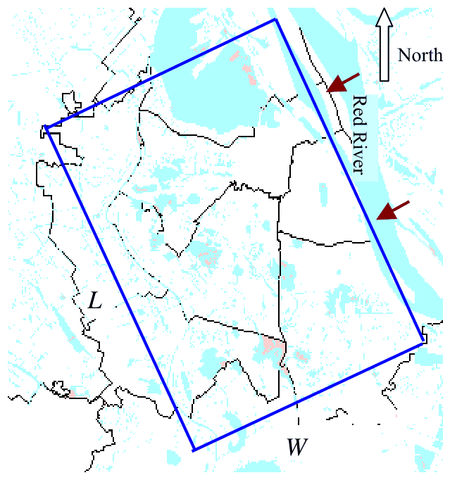
It is estimated that during the morning rush hour, from 7:00 am to 8:00 am, there are \(8\times10^5\) motorbikes on the road, each running on average 5 km and emitting 12 g of CO per kilometer. The amount of CO pollutant is approximately considered as emitted uniformly in time, at a constant rate \(M\) during the rush hour. At the same time, the clean north-east wind blows perpendicularly to the Red River (i.e. perpendicularly to the sides \(L\) of the rectangle) with velocity \(u\), passes the city with the same velocity, and carries a part of the CO-polluted air out of the city atmosphere.
Also, we use the following rough approximate model:
- The CO spreads quickly throughout the entire volume of the mixing layer above the Hanoi metropolitan area, so that the concentration \(C(t)\) of CO at time \(t\) can be assumed to be constant throughout that rectangular box of dimensions \(L\), \(W\) and \(H\).
- The upwind air entering the box is clean and no pollution is assumed to be lost from the box through the sides parallel to the wind.
- Before 7:00 am, the CO concentration in the atmosphere is negligible.
5.1. Derive the differential equation determining the CO pollutant concentration \(C(t)\) as a function of time.
5.2. Write down the solution of that equation for \(C(t)\).
5.3. Calculate the numerical value of the concentration \(C(t)\) at 8:00 a.m.
Given \(L=15\ \mathrm{km}\), \(W=8\ \mathrm{km}\), \(u=1\ \mathrm{m/s}\).
Official English text of the problem.
Answers
Write \(T_0=T(0)\), \(T_p=T_{\mathrm{parcel}}\), and \(T_{p0}=T_p(0)\). Temperature ratios use kelvin. In Part 5, \(t\) is the elapsed time since 7:00 am.
-
1.1. \[ \boxed{p(z)=p_0\exp\!\left(-\frac{\mu gz}{RT_0}\right)} \]
-
1.2.1. For \(\Lambda\ne0\) and \(T_0-\Lambda z>0\), \[ \boxed{p(z)=p_0\left(1-\frac{\Lambda z}{T_0}\right)^{\mu g/(R\Lambda)}} \] The limit \(\Lambda=0\) gives the result of 1.1.
-
1.2.2. Using the density-increase criterion specified in this part, \[ \boxed{\Lambda>\frac{\mu g}{R} =3.42\times10^{-2}\ \mathrm{K\,m^{-1}} =34.2\ \mathrm{K\,km^{-1}}} \]
-
2.1. \[ \boxed{G(T,T_p)=\frac{\mu g}{c_p}\frac{T_p}{T} =\frac{\gamma-1}{\gamma}\frac{\mu g}{R}\frac{T_p}{T}} \]
-
2.2.1. \[ \boxed{\Gamma=\frac{\mu g}{c_p}=\frac{2\mu g}{7R}} \]
-
2.2.2. \[ \boxed{\Gamma=9.78\times10^{-3}\ \mathrm{K\,m^{-1}} =9.78\ \mathrm{K\,km^{-1}}} \]
-
2.2.3. \[ \boxed{T(z)=T_0-\Gamma z} \]
-
2.3. \[ \boxed{ T_p(z)= \begin{cases} T_{p0}\left(1-\dfrac{\Lambda z}{T_0}\right)^{\Gamma/\Lambda}, &\Lambda\ne0,\\[6pt] T_{p0}\exp\!\left(-\dfrac{\Gamma z}{T_0}\right), &\Lambda=0. \end{cases}} \]
-
2.4. To first order in height, \[ \boxed{T_p(z)\simeq T_{p0}-\Gamma\frac{T_{p0}}{T_0}z \simeq T_{p0}-\Gamma z} \]
-
3.1. \[ \boxed{ \begin{aligned} \Lambda<\Gamma &: \text{stable},\\ \Lambda>\Gamma &: \text{unstable},\\ \Lambda=\Gamma &: \text{neutral}. \end{aligned}} \]
-
3.2. In the intended mixing-height approximation, neglecting inertial overshoot, \[ \boxed{z_{\max}\simeq\frac{T_{p0}-T_0}{\Gamma-\Lambda}}, \qquad \Lambda<\Gamma. \] The corresponding expression without linearizing the parcel temperature is given in the solution.
-
4.1. \[ \boxed{T_p(96\ \mathrm m)\simeq21.1^\circ\mathrm C,\qquad T_p(119\ \mathrm m)\simeq20.8^\circ\mathrm C} \]
-
4.2. \[ \boxed{H\simeq144\ \mathrm m,\qquad T_p(H)\simeq20.6^\circ\mathrm C} \]
-
5.1. \[ \boxed{\frac{dC}{dt}+\frac{u}{W}C=\frac{M}{LWH}, \qquad C(0)=0} \]
-
5.2. During the rush hour, \[ \boxed{C(t)=\frac{M}{uLH}\left(1-e^{-ut/W}\right)} \]
-
5.3. \[ \boxed{C(8{:}00\ \mathrm{am})\simeq2.2\ \mathrm{mg\,m^{-3}}} \] Keeping intermediate digits gives \(2.24\ \mathrm{mg\,m^{-3}}\).
Solution
1.1. Isothermal atmosphere
Hydrostatic equilibrium of a horizontal atmospheric layer requires \[ \frac{dp}{dz}=-\rho g. \] For ideal air, the mass density is \[ \rho=\frac{\mu p}{RT}. \] Thus, when \(T=T_0\), \[ \frac{dp}{p}=-\frac{\mu g}{RT_0}\,dz. \] Integrating from the ground, where \(p=p_0\), to altitude \(z\), \[ \ln\frac{p(z)}{p_0}=-\frac{\mu gz}{RT_0}. \] Therefore, \[ \boxed{p(z)=p_0e^{-\mu gz/(RT_0)}}. \]
1.2.1. Atmosphere with a constant temperature lapse rate
With \(T(z)=T_0-\Lambda z\), hydrostatic equilibrium becomes \[ \frac{dp}{p}=-\frac{\mu g}{R}\frac{dz}{T_0-\Lambda z}. \] For \(\Lambda\ne0\), integration gives \[ \ln\frac{p(z)}{p_0} =\frac{\mu g}{R\Lambda} \ln\frac{T_0-\Lambda z}{T_0}. \] Hence \[ \boxed{ p(z)=p_0\left(1-\frac{\Lambda z}{T_0}\right)^{\mu g/(R\Lambda)} }. \] This formula applies where the absolute temperature remains positive.
As \(\Lambda\to0\), \[ \frac{\mu g}{R\Lambda} \ln\left(1-\frac{\Lambda z}{T_0}\right) \longrightarrow-\frac{\mu gz}{RT_0}, \] recovering the isothermal result.
1.2.2. Density increasing with height
Using \(\rho=\mu p/(RT)\), \[ \frac{d\ln\rho}{dz} =\frac{d\ln p}{dz}-\frac{d\ln T}{dz} =-\frac{\mu g}{RT}+\frac{\Lambda}{T}. \] Therefore, \[ \frac{d\rho}{dz} =\frac{\rho}{T}\left(\Lambda-\frac{\mu g}{R}\right). \] Since \(\rho,T>0\), density increases upward precisely when \[ \boxed{\Lambda>\frac{\mu g}{R}}. \] Numerically, \[ \frac{\mu g}{R} =\frac{0.029(9.81)}{8.31} =0.0342347\ \mathrm{K\,m^{-1}}, \] so the requested condition is \[ \boxed{\Lambda>34.2\ \mathrm{K\,km^{-1}}}. \]
This is the density-inversion criterion stated in this question. The adiabatic parcel-instability criterion in Part 3 is less restrictive.
2.1. Temperature change of an adiabatic parcel
The parcel contains a fixed amount of gas, remains in pressure equilibrium with its surroundings, and exchanges negligible heat with them. Its adiabatic and ideal-gas relations are \[ pV^\gamma=\mathrm{const}, \qquad pV=nRT_p. \] Eliminating \(V\), \[ T_p^\gamma p^{1-\gamma}=\mathrm{const}, \] or \[ T_p p^{-(\gamma-1)/\gamma}=\mathrm{const}. \] Taking logarithmic derivatives, \[ \frac{1}{T_p}\frac{dT_p}{dz} =\frac{\gamma-1}{\gamma}\frac1p\frac{dp}{dz}. \]
The pressure gradient is set by the surrounding atmosphere, whose temperature is \(T\): \[ \frac1p\frac{dp}{dz}=-\frac{\mu g}{RT}. \] Consequently, \[ \frac{dT_p}{dz} =-\frac{\gamma-1}{\gamma}\frac{\mu g}{R}\frac{T_p}{T}. \]
Because \(c_p-c_V=R\) and \(\gamma=c_p/c_V\), \[ \frac{\gamma-1}{\gamma}=\frac{R}{c_p}. \] Thus \[ \boxed{G(T,T_p)=\frac{\mu g}{c_p}\frac{T_p}{T}}. \]
The factor \(T_p/T\) matters: the parcel’s cooling rate is not exactly constant when its temperature differs from that of its surroundings.
2.2.1. Dry adiabatic lapse rate
When \(T_p=T\), the temperature ratio in the preceding expression equals one: \[ \boxed{\Gamma=\frac{\mu g}{c_p}}. \] For the specified diatomic gas, \[ c_p=\frac72R, \] so \[ \boxed{\Gamma=\frac{2\mu g}{7R}}. \]
2.2.2. Numerical value
Substitution gives \[ \Gamma =\frac{2(0.029)(9.81)}{7(8.31)} =0.00978133\ \mathrm{K\,m^{-1}}. \] Therefore, \[ \boxed{\Gamma=9.78\ \mathrm{K\,km^{-1}}}. \]
2.2.3. Atmospheric temperature profile
Under the special condition \(T(z)=T_p(z)\), \[ \frac{dT}{dz}=-\Gamma. \] Since \(\Gamma\) is constant, \[ \boxed{T(z)=T(0)-\Gamma z}. \]
2.3. Parcel temperature in an atmosphere with constant \(\Lambda\)
From Part 2.1, \[ \frac{dT_p}{dz} =-\Gamma\frac{T_p}{T_0-\Lambda z}. \] Separating variables, \[ \frac{dT_p}{T_p} =-\Gamma\frac{dz}{T_0-\Lambda z}. \] Integrating, \[ \ln\frac{T_p(z)}{T_{p0}} =\frac{\Gamma}{\Lambda} \ln\left(1-\frac{\Lambda z}{T_0}\right). \] Hence, for \(\Lambda\ne0\), \[ \boxed{ T_p(z)=T_{p0} \left(1-\frac{\Lambda z}{T_0}\right)^{\Gamma/\Lambda} }. \]
If \(\Lambda=0\), the surrounding atmosphere is isothermal. Direct integration instead yields \[ \boxed{T_p(z)=T_{p0}e^{-\Gamma z/T_0}}. \]
For a layer beginning at altitude \(z_i\), the same result can be written \[ T_p(z)=T_p(z_i) \left[\frac{T(z)}{T(z_i)}\right]^{\Gamma/\Lambda}, \] which allows successive layers to be joined continuously.
2.4. Linear approximation
Expanding the result of Part 2.3 about \(z=0\), \[ T_p(z) =T_{p0}\left[ 1-\frac{\Gamma z}{T_0} +\frac{\Gamma(\Gamma-\Lambda)z^2}{2T_0^2} +\cdots \right]. \] To first order, \[ T_p(z)\simeq T_{p0}-\Gamma\frac{T_{p0}}{T_0}z. \] With \(T_{p0}\approx T_0\), \[ \boxed{T_p(z)\simeq T_{p0}-\Gamma z}. \]
Strictly, this is a small-height expansion. If \(\Lambda\) is very small, the stated condition \(|\Lambda z|\ll T_0\) alone does not ensure linearity; one also needs \(\Gamma|z|/T_0\ll1\). Both temperature changes are small compared with the absolute temperature in Part 4.
3.1. Stability of a displaced parcel
Let the parcel initially be at \(z_0\), with \[ T_p(z_0)=T(z_0)=T_*. \] Displace it upward by a small signed distance \(\xi\). At its initial equilibrium, its adiabatic temperature gradient is \(-\Gamma\), so \[ T_p(z_0+\xi)=T_*-\Gamma\xi+O(\xi^2). \] The environmental temperature is \[ T(z_0+\xi)=T_*-\Lambda\xi. \] The parcel’s temperature excess is therefore \[ T_p-T=(\Lambda-\Gamma)\xi+O(\xi^2). \]
At equal pressure, density is inversely proportional to absolute temperature. The parcel’s upward acceleration due to buoyancy and gravity is \[ a_z =g\left(\frac{\rho}{\rho_p}-1\right) =g\left(\frac{T_p}{T}-1\right) \simeq\frac{g}{T_*}(\Lambda-\Gamma)\xi. \]
Thus:
- If \(\Lambda<\Gamma\), acceleration opposes the displacement: the atmosphere is stable.
- If \(\Lambda>\Gamma\), acceleration reinforces the displacement: the atmosphere is unstable.
- If \(\Lambda=\Gamma\), the parcel remains at the same temperature and density as its surroundings: the atmosphere is neutral.
Hence \[ \boxed{ \text{stable: }\Lambda<\Gamma,\qquad \text{unstable: }\Lambda>\Gamma,\qquad \text{neutral: }\Lambda=\Gamma. } \]
3.2. Height reached by an initially warmer parcel
In the linear approximation, \[ T_p(z)\simeq T_{p0}-\Gamma z, \qquad T(z)=T_0-\Lambda z. \] Therefore, \[ T_p(z)-T(z) =(T_{p0}-T_0)-(\Gamma-\Lambda)z. \]
In a stable atmosphere, \(\Gamma-\Lambda>0\), so the parcel’s initial temperature excess decreases with height. The neutral-buoyancy level is obtained by setting this difference to zero: \[ \boxed{ z_{\max}\simeq \frac{T_{p0}-T_0}{\Gamma-\Lambda} }. \] Here the notation \(z_{\max}\) follows the problem’s intended mixing-height model, which neglects inertial overshoot.
For completeness, the neutral-buoyancy height can also be found without the approximation of Part 2.4. Setting the exact parcel temperature equal to the atmospheric temperature gives \[ T_{p0} \left(1-\frac{\Lambda z}{T_0}\right)^{\Gamma/\Lambda} =T_0\left(1-\frac{\Lambda z}{T_0}\right). \] Thus, for \(\Lambda\ne0\), \[ \boxed{ z_{\mathrm n} =\frac{T_0}{\Lambda} \left[ 1-\left(\frac{T_0}{T_{p0}}\right)^{\Lambda/(\Gamma-\Lambda)} \right]. } \] For \(\Lambda=0\), its limit is \[ \boxed{ z_{\mathrm n}=\frac{T_0}{\Gamma} \ln\frac{T_{p0}}{T_0}. } \] Both reduce to the stated linear result when \(T_{p0}-T_0\ll T_0\).
A dynamical qualification is necessary: zero buoyancy means zero acceleration, not necessarily zero velocity. A freely moving parcel can overshoot this level. For example, in the same linear approximation, an undamped parcel released from rest obeys \[ \ddot z\simeq\frac{g}{T_0} \left[(T_{p0}-T_0)-(\Gamma-\Lambda)z\right], \] and its first turning point is \(2z_{\mathrm n}\). The following parts use the intended neutral-buoyancy mixing height.
4.1. Parcel temperatures at 96 m and 119 m
Use straight lines through the measured endpoints of each specified layer. Their lapse rates are
\[ \Lambda_1 =\frac{21.5-20.1}{96-5} =0.0153846\ \mathrm{K\,m^{-1}}, \] \[ \Lambda_2=0, \] and \[ \Lambda_3 =\frac{20.1-22.0}{215-119} =-0.0197917\ \mathrm{K\,m^{-1}}. \]
The first line extrapolates to a ground temperature \[ T(0)\simeq21.5+5\Lambda_1 =21.5769^\circ\mathrm C, \] close to the parcel’s initial \(22^\circ\mathrm C\). All relevant temperature changes are small compared with approximately \(294\ \mathrm K\), so Part 2.4 applies.
Since a kelvin temperature difference equals a Celsius temperature difference, \[ T_p(z)\simeq22^\circ\mathrm C-\Gamma z. \] Consequently, \[ T_p(96) \simeq22-0.00978133(96) =21.06099^\circ\mathrm C, \] and \[ T_p(119) \simeq22-0.00978133(119) =20.83602^\circ\mathrm C. \]
To the precision of the temperature data, \[ \boxed{T_p(96\ \mathrm m)\simeq21.1^\circ\mathrm C}, \qquad \boxed{T_p(119\ \mathrm m)\simeq20.8^\circ\mathrm C}. \]
As a check, applying the exact formula of Part 2.3 separately to the first layer and the isothermal second layer gives \(21.059^\circ\mathrm C\) and \(20.833^\circ\mathrm C\), respectively. These round to the same answers.
4.2. Mixing height
At both 96 m and 119 m, the surrounding temperature is \(20.1^\circ\mathrm C\). The parcel is warmer at both heights, so it continues into the inversion layer above 119 m.
Write the positive temperature gradient there as \[ k=-\Lambda_3 =\frac{22.0-20.1}{215-119} =0.0197917\ \mathrm{K\,m^{-1}}. \] The environmental temperature in that layer is \[ T(z)=20.1^\circ\mathrm C+k(z-119\ \mathrm m). \]
At the mixing height, the parcel and atmosphere have equal temperatures: \[ 22-\Gamma H=20.1+k(H-119), \] with \(H\) in metres and the displayed temperatures in degrees Celsius. Solving, \[ H =\frac{22-20.1+119k}{\Gamma+k} =\frac{4.2552083}{0.029572997} =143.888\ \mathrm m. \] This lies within the assumed inversion layer, as required.
The parcel temperature there is \[ T_p(H) \simeq22-\Gamma H =20.5926^\circ\mathrm C. \] Therefore, \[ \boxed{H\simeq144\ \mathrm m,\qquad T_p(H)\simeq20.6^\circ\mathrm C}. \]
Using the exact parcel-temperature evolution through all three linear atmospheric layers gives \(H=143.78\ \mathrm m\), confirming that the linear parcel approximation is adequate.
5.1. Conservation equation for CO
The uniformly mixed air volume is \[ V=LWH. \] If \(C(t)\) is the CO mass concentration, the total CO mass inside the box is \[ m_{\mathrm{CO}}=LWH\,C. \]
The wind crosses a face of width \(L\) and height \(H\), so its volume flow rate is \[ Q=uLH. \] Because incoming air is clean, the incoming CO flux is zero. The outgoing CO mass rate is \[ QC=uLH\,C. \] Conservation of CO therefore gives \[ \frac{d}{dt}(LWH\,C)=M-uLH\,C. \] The box dimensions are constant, hence \[ \boxed{ \frac{dC}{dt}+\frac{u}{W}C=\frac{M}{LWH} }, \qquad \boxed{C(0)=0}. \]
5.2. Concentration as a function of time
A constant particular solution is \[ C_{\mathrm{ss}}=\frac{M}{uLH}. \] The homogeneous solution is proportional to \(e^{-ut/W}\), so \[ C(t)=\frac{M}{uLH}+A e^{-ut/W}. \] Using \(C(0)=0\), \[ A=-\frac{M}{uLH}. \] Thus \[ \boxed{ C(t)=\frac{M}{uLH}\left(1-e^{-ut/W}\right) }, \qquad 0\le t\le3600\ \mathrm s. \]
The ventilation timescale is \(W/u\). In the limit of no wind, this expression correctly reduces to \(C(t)=Mt/(LWH)\).
5.3. CO concentration at 8:00 am
The total CO emitted during the hour is \[ m_{\mathrm{emitted}} =(8\times10^5)(5\ \mathrm{km}) (12\ \mathrm{g\,km^{-1}}) =4.8\times10^7\ \mathrm g =4.8\times10^4\ \mathrm{kg}. \] Therefore, \[ M=\frac{4.8\times10^4}{3600} =13.3333\ \mathrm{kg\,s^{-1}}. \]
Using \[ L=15000\ \mathrm m,\quad W=8000\ \mathrm m,\quad u=1\ \mathrm{m\,s^{-1}},\quad H\simeq143.888\ \mathrm m, \] the dimensionless elapsed time is \[ \frac{ut}{W} =\frac{1(3600)}{8000} =0.45. \] Hence \[ C(3600) = \frac{13.3333}{(1)(15000)(143.888)} \left(1-e^{-0.45}\right) \ \mathrm{kg\,m^{-3}}, \] giving \[ C(3600) =2.2386\times10^{-6}\ \mathrm{kg\,m^{-3}} =2.2386\ \mathrm{mg\,m^{-3}}. \]
With precision appropriate to the rough input data, \[ \boxed{C(8{:}00\ \mathrm{am})\simeq2.2\ \mathrm{mg\,m^{-3}}}. \]
The solution was checked against the official solution.
IPhO 2008 · Theorieaufgabe 3
Änderung der Lufttemperatur mit der Höhe, atmosphärische Stabilität und Luftverschmutzung
Vertikale Luftbewegungen bestimmen viele atmosphärische Prozesse, beispielsweise die Bildung von Wolken und Niederschlag sowie die Ausbreitung von Luftschadstoffen. Ist die Atmosphäre stabil, sind vertikale Bewegungen eingeschränkt, und Luftschadstoffe sammeln sich eher in der Nähe des Emissionsortes an, als sich auszubreiten und verdünnt zu werden. In einer instabilen Atmosphäre hingegen fördern vertikale Luftbewegungen die vertikale Ausbreitung von Luftschadstoffen. Daher hängen die Schadstoffkonzentrationen nicht nur von der Stärke der Emissionsquellen, sondern auch von der Stabilität der Atmosphäre ab.
Wir werden die atmosphärische Stabilität mithilfe des meteorologischen Konzepts des Luftpakets bestimmen und die Temperatur eines adiabatisch in der Atmosphäre aufsteigenden oder absinkenden Luftpakets mit der Temperatur der Umgebungsluft vergleichen. Wir werden sehen, dass ein Luftpaket, das Luftschadstoffe enthält und vom Boden aufsteigt, in vielen Fällen in einer bestimmten Höhe zur Ruhe kommt, die als Mischungshöhe bezeichnet wird. Je größer die Mischungshöhe ist, desto geringer ist die Luftschadstoffkonzentration. Wir werden die Mischungshöhe und die Konzentration des von Motorrädern im Großraum Hanoi ausgestoßenen Kohlenmonoxids für ein Szenario während des morgendlichen Berufsverkehrs berechnen, bei dem die vertikale Durchmischung durch eine Temperaturinversion (die Lufttemperatur nimmt mit der Höhe zu) oberhalb von 119 m eingeschränkt ist.
Wir betrachten Luft als ideales zweiatomiges Gas mit der molaren Masse \(\mu=29\ \mathrm{g/mol}\).
Quasistatische adiabatische Zustandsänderungen gehorchen der Gleichung \(pV^\gamma=\mathrm{const}\), wobei \(\gamma=\dfrac{c_p}{c_V}\) das Verhältnis der isobaren zur isochoren Wärmekapazität des Gases ist.
Bei Bedarf können die folgenden Daten verwendet werden:
Die universelle Gaskonstante ist \(R=8.31\ \mathrm{J/(mol.K)}\).
Der Luftdruck am Boden ist \(p_0=101.3\ \mathrm{kPa}\)
Die Erdbeschleunigung ist konstant, \(g=9.81\ \mathrm{m/s^2}\)
Die molare isobare Wärmekapazität der Luft ist \(c_p=\dfrac72R\).
Die molare isochore Wärmekapazität der Luft ist \(c_V=\dfrac52R\).
Mathematische Hinweise
a. \[ \int\frac{dx}{A+Bx} =\frac1B\int\frac{d(A+Bx)}{A+Bx} =\frac1B\ln(A+Bx) \]
b. Die Lösung der Differentialgleichung \(\dfrac{dx}{dt}+Ax=B\) (mit konstanten \(A\) und \(B\)) lautet \[ x(t)=x_1(t)+\frac BA \] wobei \(x_1(t)\) die Lösung der Differentialgleichung \(\dfrac{dx}{dt}+Ax=0\) ist.
c. \[ \lim_{x\to\infty}\left(1+\frac1x\right)^x=e \]
1. Änderung des Drucks mit der Höhe.
1.1. Nehmen Sie an, dass die Temperatur der Atmosphäre überall gleich \(T_0\) ist. Geben Sie den Ausdruck für den Luftdruck \(p\) als Funktion der Höhe \(z\) an.
1.2. Nehmen Sie an, dass die Temperatur der Atmosphäre gemäß der Beziehung
\[ T(z)=T(0)-\Lambda z \]
mit der Höhe variiert, wobei \(\Lambda\) eine Konstante ist, die als vertikale Temperaturabnahmerate der Atmosphäre bezeichnet wird (der vertikale Temperaturgradient ist \(-\Lambda\)).
1.2.1. Geben Sie den Ausdruck für den Luftdruck \(p\) als Funktion der Höhe \(z\) an.
1.2.2. Ein als freie Konvektion bezeichneter Prozess tritt auf, wenn die Luftdichte mit der Höhe zunimmt. Für welche Werte von \(\Lambda\) tritt freie Konvektion auf?
2. Änderung der Temperatur eines Luftpakets bei vertikaler Bewegung
Betrachten Sie ein Luftpaket, das sich in der Atmosphäre aufwärts und abwärts bewegt. Ein Luftpaket ist ein Luftvolumen mit einer Ausdehnung von mehreren Metern, das groß genug ist, um als eigenständiges thermodynamisches System behandelt zu werden, zugleich aber klein genug, um seine Temperatur als räumlich einheitlich anzusehen. Die vertikale Bewegung eines Luftpakets kann als näherungsweise adiabatischer Prozess behandelt werden, d. h., der Wärmeaustausch mit der Umgebungsluft ist vernachlässigbar. Steigt das Luftpaket in der Atmosphäre auf, dehnt es sich aus und kühlt ab. Bewegt es sich umgekehrt nach unten, komprimiert der zunehmende Außendruck die Luft im Paket, und ihre Temperatur steigt.
Da das Paket nicht groß ist, kann der Luftdruck an verschiedenen Punkten seiner Oberfläche als gleich angesehen werden und mit \(p(z)\) bezeichnet werden, wobei \(z\) die Höhe des Paketmittelpunkts ist. Die Temperatur im Paket ist räumlich einheitlich und beträgt \(T_{\mathrm{parcel}}(z)\); sie unterscheidet sich im Allgemeinen von der Temperatur der Umgebungsluft \(T(z)\). In den Teilen 2.1 und 2.2 treffen wir keine Annahme über die Form von \(T(z)\).
2.1. Die Änderung der Pakettemperatur \(T_{\mathrm{parcel}}\) mit der Höhe wird definiert durch \[ \frac{dT_{\mathrm{parcel}}}{dz}=-G. \] Leiten Sie den Ausdruck für \(G(T,T_{\mathrm{parcel}})\) her.
2.2. Betrachten Sie einen besonderen Zustand der Atmosphäre, in dem in jeder Höhe \(z\) die Temperatur \(T\) der Atmosphäre gleich der Pakettemperatur \(T_{\mathrm{parcel}}\) ist, \(T(z)=T_{\mathrm{parcel}}(z)\). Wir bezeichnen den Wert von \(G\) für \(T=T_{\mathrm{parcel}}\) mit \(\Gamma\), also \[ \Gamma=-\frac{dT_{\mathrm{parcel}}}{dz} \] (mit \(T=T_{\mathrm{parcel}}\)). \(\Gamma\) wird als trockenadiabatische Temperaturabnahmerate bezeichnet.
2.2.1. Leiten Sie den Ausdruck für \(\Gamma\) her
2.2.2. Berechnen Sie den Zahlenwert von \(\Gamma\).
2.2.3. Leiten Sie den Ausdruck für die Temperatur der Atmosphäre \(T(z)\) als Funktion der Höhe her.
2.3. Nehmen Sie an, dass die Temperatur der Atmosphäre gemäß der Beziehung \(T(z)=T(0)-\Lambda z\) von der Höhe abhängt, wobei \(\Lambda\) eine Konstante ist. Bestimmen Sie die Abhängigkeit der Pakettemperatur \(T_{\mathrm{parcel}}(z)\) von der Höhe \(z\).
2.4. Geben Sie den Näherungsausdruck für \(T_{\mathrm{parcel}}(z)\) an, wenn \(|\Lambda z|\ll T(0)\) und \(T(0)\approx T_{\mathrm{parcel}}(0)\) gelten.
3. Die atmosphärische Stabilität.
In diesem Teil nehmen wir an, dass sich \(T\) linear mit der Höhe ändert.
3.1. Betrachten Sie ein Luftpaket, das sich zunächst in der Höhe \(z_0\) im Gleichgewicht mit der Umgebungsluft befindet, d. h., es hat dieselbe Temperatur \(T(z_0)\) wie die Umgebungsluft. Wird das Paket geringfügig nach oben oder unten ausgelenkt (z. B. durch atmosphärische Turbulenz), kann einer der folgenden drei Fälle eintreten:
- Das Luftpaket kehrt zur ursprünglichen Höhe \(z_0\) zurück; das Gleichgewicht des Pakets ist stabil. Die Atmosphäre wird als stabil bezeichnet.
- Das Paket bewegt sich weiter in der ursprünglichen Richtung; das Gleichgewicht des Pakets ist instabil. Die Atmosphäre ist instabil.
- Das Luftpaket verbleibt an seiner neuen Position; das Gleichgewicht des Pakets ist indifferent. Die Atmosphäre wird als neutral bezeichnet.
Welche Bedingung muss \(\Lambda\) erfüllen, damit die Atmosphäre stabil, instabil oder neutral ist?
3.2. Die Temperatur eines Pakets am Boden \(T_{\mathrm{parcel}}(0)\) ist höher als die Temperatur \(T(0)\) der Umgebungsluft. Die Auftriebskraft lässt das Paket aufsteigen. Leiten Sie für eine stabile Atmosphäre den Ausdruck für die maximale Höhe her, die das Paket erreichen kann, in Abhängigkeit von \(\Lambda\) und \(\Gamma\).
4. Die Mischungshöhe
4.1. Tabelle 1 zeigt Lufttemperaturen, die an einem Novembertag um 7:00 Uhr in Hanoi mit einem Radiosondenballon gemessen wurden. Die Temperaturänderung mit der Höhe lässt sich näherungsweise durch die Formel \(T(z)=T(0)-\Lambda z\) beschreiben, mit unterschiedlichen Temperaturabnahmeraten \(\Lambda\) in den drei Schichten \(0<z<96\ \mathrm{m}\), \(96\ \mathrm{m}<z<119\ \mathrm{m}\) und \(119\ \mathrm{m}<z<215\ \mathrm{m}\).
Betrachten Sie ein Luftpaket mit der Temperatur \(T_{\mathrm{parcel}}(0)=22^\circ\mathrm{C}\), das vom Boden aufsteigt. Berechnen Sie anhand der Daten aus Tabelle 1 und unter Verwendung der obigen linearen Näherung die Temperatur des Pakets in den Höhen 96 m und 119 m.
4.2. Bestimmen Sie die maximale Höhe \(H\), die das Paket erreichen kann, und seine Temperatur \(T_{\mathrm{parcel}}(H)\).
\(H\) wird als Mischungshöhe bezeichnet. Vom Boden emittierte Luftschadstoffe können sich innerhalb dieser Schicht mit der Luft in der Atmosphäre vermischen (z. B. durch Wind, Turbulenz und Dispersion) und dadurch verdünnt werden.
Tabelle 1
Daten, die an einem Novembertag um 7:00 Uhr in Hanoi mit einem Radiosondenballon gemessen wurden.
| Höhe, m | Temperatur, °C |
|---|---|
| 5 | 21.5 |
| 60 | 20.6 |
| 64 | 20.5 |
| 69 | 20.5 |
| 75 | 20.4 |
| 81 | 20.3 |
| 90 | 20.2 |
| 96 | 20.1 |
| 102 | 20.1 |
| 109 | 20.1 |
| 113 | 20.1 |
| 119 | 20.1 |
| 128 | 20.2 |
| 136 | 20.3 |
| 145 | 20.4 |
| 153 | 20.5 |
| 159 | 20.6 |
| 168 | 20.8 |
| 178 | 21.0 |
| 189 | 21.5 |
| 202 | 21.8 |
| 215 | 22.0 |
| 225 | 22.1 |
| 234 | 22.2 |
| 246 | 22.3 |
| 257 | 22.3 |
5. Abschätzung der Kohlenmonoxidbelastung (CO) während des morgendlichen Berufsverkehrs mit Motorrädern in Hanoi.
Der Großraum Hanoi kann näherungsweise als Rechteck mit den Seitenlängen \(L\) und \(W\) beschrieben werden, wie in der Abbildung gezeigt, wobei eine Seite entlang des südwestlichen Ufers des Roten Flusses verläuft.
Schätzungen zufolge sind während des morgendlichen Berufsverkehrs von 7:00 bis 8:00 Uhr \(8\times10^5\) Motorräder unterwegs, die jeweils durchschnittlich 5 km zurücklegen und 12 g CO pro Kilometer ausstoßen. Näherungsweise wird angenommen, dass der Schadstoff CO während des Berufsverkehrs zeitlich gleichmäßig mit einer konstanten Rate \(M\) emittiert wird. Gleichzeitig weht ein sauberer Nordostwind mit der Geschwindigkeit \(u\) senkrecht zum Roten Fluss (d. h. senkrecht zu den Seiten \(L\) des Rechtecks), durchquert die Stadt mit derselben Geschwindigkeit und transportiert einen Teil der CO-belasteten Luft aus der Stadtatmosphäre heraus.
Außerdem verwenden wir das folgende grobe Näherungsmodell:
- Das CO verteilt sich rasch im gesamten Volumen der Mischungsschicht über dem Großraum Hanoi, sodass die CO-Konzentration \(C(t)\) zum Zeitpunkt \(t\) im gesamten Quader mit den Abmessungen \(L\), \(W\) und \(H\) als räumlich konstant angenommen werden kann.
- Die von der Luvseite in den Quader einströmende Luft ist sauber, und es wird angenommen, dass durch die zum Wind parallelen Seiten kein Schadstoff aus dem Quader verloren geht.
- Vor 7:00 Uhr ist die CO-Konzentration in der Atmosphäre vernachlässigbar.
5.1. Leiten Sie die Differentialgleichung her, die die CO-Schadstoffkonzentration \(C(t)\) als Funktion der Zeit bestimmt.
5.2. Geben Sie die Lösung dieser Gleichung für \(C(t)\) an.
5.3. Berechnen Sie den Zahlenwert der Konzentration \(C(t)\) um 8:00 Uhr.
Gegeben sind \(L=15\ \mathrm{km}\), \(W=8\ \mathrm{km}\), \(u=1\ \mathrm{m/s}\).
Aufgabentext aus dem offiziellen englischen Text übersetzt.
Antworten
Wir schreiben \(T_0=T(0)\), \(T_p=T_{\mathrm{parcel}}\) und \(T_{p0}=T_p(0)\). Für Temperaturverhältnisse werden die Temperaturen in Kelvin eingesetzt. In Teil 5 ist \(t\) die seit 7:00 Uhr verstrichene Zeit.
-
1.1. \[ \boxed{p(z)=p_0\exp\!\left(-\frac{\mu gz}{RT_0}\right)} \]
-
1.2.1. Für \(\Lambda\ne0\) und \(T_0-\Lambda z>0\) gilt \[ \boxed{p(z)=p_0\left(1-\frac{\Lambda z}{T_0}\right)^{\mu g/(R\Lambda)}} \] Der Grenzfall \(\Lambda=0\) liefert das Ergebnis aus 1.1.
-
1.2.2. Nach dem in diesem Teil vorgegebenen Kriterium der Dichtezunahme gilt \[ \boxed{\Lambda>\frac{\mu g}{R} =3.42\times10^{-2}\ \mathrm{K\,m^{-1}} =34.2\ \mathrm{K\,km^{-1}}} \]
-
2.1. \[ \boxed{G(T,T_p)=\frac{\mu g}{c_p}\frac{T_p}{T} =\frac{\gamma-1}{\gamma}\frac{\mu g}{R}\frac{T_p}{T}} \]
-
2.2.1. \[ \boxed{\Gamma=\frac{\mu g}{c_p}=\frac{2\mu g}{7R}} \]
-
2.2.2. \[ \boxed{\Gamma=9.78\times10^{-3}\ \mathrm{K\,m^{-1}} =9.78\ \mathrm{K\,km^{-1}}} \]
-
2.2.3. \[ \boxed{T(z)=T_0-\Gamma z} \]
-
2.3. \[ \boxed{ T_p(z)= \begin{cases} T_{p0}\left(1-\dfrac{\Lambda z}{T_0}\right)^{\Gamma/\Lambda}, &\Lambda\ne0,\\[6pt] T_{p0}\exp\!\left(-\dfrac{\Gamma z}{T_0}\right), &\Lambda=0. \end{cases}} \]
-
2.4. Bis zur ersten Ordnung in der Höhe gilt \[ \boxed{T_p(z)\simeq T_{p0}-\Gamma\frac{T_{p0}}{T_0}z \simeq T_{p0}-\Gamma z} \]
-
3.1. \[ \boxed{ \begin{aligned} \Lambda<\Gamma &: \text{stabil},\\ \Lambda>\Gamma &: \text{instabil},\\ \Lambda=\Gamma &: \text{neutral}. \end{aligned}} \]
-
3.2. In der vorgesehenen Näherung für die Mischungshöhe, unter Vernachlässigung des trägheitsbedingten Überschwingens, gilt \[ \boxed{z_{\max}\simeq\frac{T_{p0}-T_0}{\Gamma-\Lambda}}, \qquad \Lambda<\Gamma. \] Der entsprechende Ausdruck ohne Linearisierung der Pakettemperatur wird in der Lösung angegeben.
-
4.1. \[ \boxed{T_p(96\ \mathrm m)\simeq21.1^\circ\mathrm C,\qquad T_p(119\ \mathrm m)\simeq20.8^\circ\mathrm C} \]
-
4.2. \[ \boxed{H\simeq144\ \mathrm m,\qquad T_p(H)\simeq20.6^\circ\mathrm C} \]
-
5.1. \[ \boxed{\frac{dC}{dt}+\frac{u}{W}C=\frac{M}{LWH}, \qquad C(0)=0} \]
-
5.2. Während des Berufsverkehrs gilt \[ \boxed{C(t)=\frac{M}{uLH}\left(1-e^{-ut/W}\right)} \]
-
5.3. \[ \boxed{C(8{:}00\ \mathrm{am})\simeq2.2\ \mathrm{mg\,m^{-3}}} \] Behält man in den Zwischenrechnungen weitere Stellen bei, erhält man \(2.24\ \mathrm{mg\,m^{-3}}\).
Lösung
1.1. Isotherme Atmosphäre
Das hydrostatische Gleichgewicht einer horizontalen Atmosphärenschicht erfordert \[ \frac{dp}{dz}=-\rho g. \] Für Luft als ideales Gas ist die Massendichte \[ \rho=\frac{\mu p}{RT}. \] Für \(T=T_0\) gilt somit \[ \frac{dp}{p}=-\frac{\mu g}{RT_0}\,dz. \] Die Integration vom Boden, wo \(p=p_0\) gilt, bis zur Höhe \(z\) ergibt \[ \ln\frac{p(z)}{p_0}=-\frac{\mu gz}{RT_0}. \] Daher gilt \[ \boxed{p(z)=p_0e^{-\mu gz/(RT_0)}}. \]
1.2.1. Atmosphäre mit konstanter Temperaturabnahmerate
Mit \(T(z)=T_0-\Lambda z\) lautet die Gleichung des hydrostatischen Gleichgewichts \[ \frac{dp}{p}=-\frac{\mu g}{R}\frac{dz}{T_0-\Lambda z}. \] Für \(\Lambda\ne0\) ergibt die Integration \[ \ln\frac{p(z)}{p_0} =\frac{\mu g}{R\Lambda} \ln\frac{T_0-\Lambda z}{T_0}. \] Damit folgt \[ \boxed{ p(z)=p_0\left(1-\frac{\Lambda z}{T_0}\right)^{\mu g/(R\Lambda)} }. \] Diese Formel gilt dort, wo die absolute Temperatur positiv bleibt.
Für \(\Lambda\to0\) gilt \[ \frac{\mu g}{R\Lambda} \ln\left(1-\frac{\Lambda z}{T_0}\right) \longrightarrow-\frac{\mu gz}{RT_0}, \] womit sich wieder das isotherme Ergebnis ergibt.
1.2.2. Mit der Höhe zunehmende Dichte
Mit \(\rho=\mu p/(RT)\) ergibt sich \[ \frac{d\ln\rho}{dz} =\frac{d\ln p}{dz}-\frac{d\ln T}{dz} =-\frac{\mu g}{RT}+\frac{\Lambda}{T}. \] Daher gilt \[ \frac{d\rho}{dz} =\frac{\rho}{T}\left(\Lambda-\frac{\mu g}{R}\right). \] Da \(\rho,T>0\) gilt, nimmt die Dichte genau dann nach oben zu, wenn \[ \boxed{\Lambda>\frac{\mu g}{R}}. \] Numerisch ergibt sich \[ \frac{\mu g}{R} =\frac{0.029(9.81)}{8.31} =0.0342347\ \mathrm{K\,m^{-1}}, \] sodass die gesuchte Bedingung lautet \[ \boxed{\Lambda>34.2\ \mathrm{K\,km^{-1}}}. \]
Dies ist das in dieser Teilaufgabe angegebene Kriterium der Dichteinversion. Das Kriterium für die Instabilität eines adiabatischen Luftpakets in Teil 3 ist weniger einschränkend.
2.1. Temperaturänderung eines adiabatischen Luftpakets
Das Paket enthält eine feste Gasmenge, bleibt im Druckgleichgewicht mit seiner Umgebung und tauscht mit ihr vernachlässigbar wenig Wärme aus. Für das Paket gelten die Adiabatengleichung und die ideale Gasgleichung \[ pV^\gamma=\mathrm{const}, \qquad pV=nRT_p. \] Durch Eliminieren von \(V\) erhält man \[ T_p^\gamma p^{1-\gamma}=\mathrm{const}, \] oder \[ T_p p^{-(\gamma-1)/\gamma}=\mathrm{const}. \] Logarithmisches Differenzieren ergibt \[ \frac{1}{T_p}\frac{dT_p}{dz} =\frac{\gamma-1}{\gamma}\frac1p\frac{dp}{dz}. \]
Der Druckgradient wird durch die umgebende Atmosphäre mit der Temperatur \(T\) bestimmt: \[ \frac1p\frac{dp}{dz}=-\frac{\mu g}{RT}. \] Folglich gilt \[ \frac{dT_p}{dz} =-\frac{\gamma-1}{\gamma}\frac{\mu g}{R}\frac{T_p}{T}. \]
Wegen \(c_p-c_V=R\) und \(\gamma=c_p/c_V\) ist \[ \frac{\gamma-1}{\gamma}=\frac{R}{c_p}. \] Damit folgt \[ \boxed{G(T,T_p)=\frac{\mu g}{c_p}\frac{T_p}{T}}. \]
Der Faktor \(T_p/T\) ist von Bedeutung: Die Abkühlungsrate des Pakets ist nicht exakt konstant, wenn seine Temperatur von der Umgebungstemperatur abweicht.
2.2.1. Trockenadiabatische Temperaturabnahmerate
Für \(T_p=T\) ist das Temperaturverhältnis im vorherigen Ausdruck gleich eins: \[ \boxed{\Gamma=\frac{\mu g}{c_p}}. \] Für das angegebene zweiatomige Gas gilt \[ c_p=\frac72R, \] also \[ \boxed{\Gamma=\frac{2\mu g}{7R}}. \]
2.2.2. Zahlenwert
Einsetzen ergibt \[ \Gamma =\frac{2(0.029)(9.81)}{7(8.31)} =0.00978133\ \mathrm{K\,m^{-1}}. \] Daher gilt \[ \boxed{\Gamma=9.78\ \mathrm{K\,km^{-1}}}. \]
2.2.3. Temperaturprofil der Atmosphäre
Unter der besonderen Bedingung \(T(z)=T_p(z)\) gilt \[ \frac{dT}{dz}=-\Gamma. \] Da \(\Gamma\) konstant ist, folgt \[ \boxed{T(z)=T(0)-\Gamma z}. \]
2.3. Pakettemperatur in einer Atmosphäre mit konstantem \(\Lambda\)
Aus Teil 2.1 folgt \[ \frac{dT_p}{dz} =-\Gamma\frac{T_p}{T_0-\Lambda z}. \] Trennung der Variablen ergibt \[ \frac{dT_p}{T_p} =-\Gamma\frac{dz}{T_0-\Lambda z}. \] Durch Integration erhält man \[ \ln\frac{T_p(z)}{T_{p0}} =\frac{\Gamma}{\Lambda} \ln\left(1-\frac{\Lambda z}{T_0}\right). \] Damit gilt für \(\Lambda\ne0\) \[ \boxed{ T_p(z)=T_{p0} \left(1-\frac{\Lambda z}{T_0}\right)^{\Gamma/\Lambda} }. \]
Für \(\Lambda=0\) ist die umgebende Atmosphäre isotherm. Direkte Integration liefert dann \[ \boxed{T_p(z)=T_{p0}e^{-\Gamma z/T_0}}. \]
Für eine Schicht, die in der Höhe \(z_i\) beginnt, lässt sich dasselbe Ergebnis schreiben als \[ T_p(z)=T_p(z_i) \left[\frac{T(z)}{T(z_i)}\right]^{\Gamma/\Lambda}, \] wodurch aufeinanderfolgende Schichten stetig aneinander angeschlossen werden können.
2.4. Lineare Näherung
Die Entwicklung des Ergebnisses aus Teil 2.3 um \(z=0\) ergibt \[ T_p(z) =T_{p0}\left[ 1-\frac{\Gamma z}{T_0} +\frac{\Gamma(\Gamma-\Lambda)z^2}{2T_0^2} +\cdots \right]. \] Bis zur ersten Ordnung gilt \[ T_p(z)\simeq T_{p0}-\Gamma\frac{T_{p0}}{T_0}z. \] Mit \(T_{p0}\approx T_0\) folgt \[ \boxed{T_p(z)\simeq T_{p0}-\Gamma z}. \]
Streng genommen handelt es sich um eine Entwicklung für kleine Höhen. Ist \(\Lambda\) sehr klein, gewährleistet die angegebene Bedingung \(|\Lambda z|\ll T_0\) allein keine Linearität; zusätzlich muss \(\Gamma|z|/T_0\ll1\) gelten. In Teil 4 sind beide Temperaturänderungen klein gegenüber der absoluten Temperatur.
3.1. Stabilität eines ausgelenkten Luftpakets
Das Paket befinde sich zunächst bei \(z_0\), mit \[ T_p(z_0)=T(z_0)=T_*. \] Es werde um eine kleine vorzeichenbehaftete Strecke \(\xi\) nach oben ausgelenkt. In seiner anfänglichen Gleichgewichtslage beträgt sein adiabatischer Temperaturgradient \(-\Gamma\), also \[ T_p(z_0+\xi)=T_*-\Gamma\xi+O(\xi^2). \] Die Umgebungstemperatur ist \[ T(z_0+\xi)=T_*-\Lambda\xi. \] Der Temperaturüberschuss des Pakets beträgt daher \[ T_p-T=(\Lambda-\Gamma)\xi+O(\xi^2). \]
Bei gleichem Druck ist die Dichte umgekehrt proportional zur absoluten Temperatur. Die nach oben gerichtete Beschleunigung des Pakets infolge von Auftrieb und Schwerkraft ist \[ a_z =g\left(\frac{\rho}{\rho_p}-1\right) =g\left(\frac{T_p}{T}-1\right) \simeq\frac{g}{T_*}(\Lambda-\Gamma)\xi. \]
Somit gilt:
- Für \(\Lambda<\Gamma\) wirkt die Beschleunigung der Auslenkung entgegen: Die Atmosphäre ist stabil.
- Für \(\Lambda>\Gamma\) verstärkt die Beschleunigung die Auslenkung: Die Atmosphäre ist instabil.
- Für \(\Lambda=\Gamma\) behält das Paket dieselbe Temperatur und Dichte wie seine Umgebung: Die Atmosphäre ist neutral.
Damit folgt \[ \boxed{ \text{stabil: }\Lambda<\Gamma,\qquad \text{instabil: }\Lambda>\Gamma,\qquad \text{neutral: }\Lambda=\Gamma. } \]
3.2. Erreichte Höhe eines anfangs wärmeren Luftpakets
In der linearen Näherung gilt \[ T_p(z)\simeq T_{p0}-\Gamma z, \qquad T(z)=T_0-\Lambda z. \] Daher ist \[ T_p(z)-T(z) =(T_{p0}-T_0)-(\Gamma-\Lambda)z. \]
In einer stabilen Atmosphäre ist \(\Gamma-\Lambda>0\), sodass der anfängliche Temperaturüberschuss des Pakets mit der Höhe abnimmt. Die Höhe des neutralen Auftriebs erhält man, indem man diese Differenz gleich null setzt: \[ \boxed{ z_{\max}\simeq \frac{T_{p0}-T_0}{\Gamma-\Lambda} }. \] Hier folgt die Bezeichnung \(z_{\max}\) dem in der Aufgabe vorgesehenen Modell der Mischungshöhe, das trägheitsbedingtes Überschwingen vernachlässigt.
Der Vollständigkeit halber lässt sich die Höhe des neutralen Auftriebs auch ohne die Näherung aus Teil 2.4 bestimmen. Gleichsetzen der exakten Pakettemperatur mit der Temperatur der Atmosphäre ergibt \[ T_{p0} \left(1-\frac{\Lambda z}{T_0}\right)^{\Gamma/\Lambda} =T_0\left(1-\frac{\Lambda z}{T_0}\right). \] Damit gilt für \(\Lambda\ne0\) \[ \boxed{ z_{\mathrm n} =\frac{T_0}{\Lambda} \left[ 1-\left(\frac{T_0}{T_{p0}}\right)^{\Lambda/(\Gamma-\Lambda)} \right]. } \] Für \(\Lambda=0\) ist der Grenzwert \[ \boxed{ z_{\mathrm n}=\frac{T_0}{\Gamma} \ln\frac{T_{p0}}{T_0}. } \] Beide Ausdrücke gehen für \(T_{p0}-T_0\ll T_0\) in das angegebene lineare Ergebnis über.
Eine Einschränkung aus dynamischer Sicht ist erforderlich: Neutraler Auftrieb bedeutet eine Beschleunigung von null, aber nicht notwendigerweise eine Geschwindigkeit von null. Ein frei bewegliches Paket kann über diese Höhe hinausschwingen. Beispielsweise gehorcht ein ungedämpftes, aus der Ruhe freigegebenes Paket in derselben linearen Näherung der Gleichung \[ \ddot z\simeq\frac{g}{T_0} \left[(T_{p0}-T_0)-(\Gamma-\Lambda)z\right], \] und sein erster Umkehrpunkt liegt bei \(2z_{\mathrm n}\). In den folgenden Teilen wird die vorgesehene Mischungshöhe des neutralen Auftriebs verwendet.
4.1. Pakettemperaturen in 96 m und 119 m Höhe
Wir verwenden Geraden durch die gemessenen Endpunkte jeder angegebenen Schicht. Ihre Temperaturabnahmeraten sind
\[ \Lambda_1 =\frac{21.5-20.1}{96-5} =0.0153846\ \mathrm{K\,m^{-1}}, \] \[ \Lambda_2=0, \] und \[ \Lambda_3 =\frac{20.1-22.0}{215-119} =-0.0197917\ \mathrm{K\,m^{-1}}. \]
Die Extrapolation der ersten Geraden ergibt eine Bodentemperatur von \[ T(0)\simeq21.5+5\Lambda_1 =21.5769^\circ\mathrm C, \] die nahe an der Anfangstemperatur des Pakets von \(22^\circ\mathrm C\) liegt. Alle relevanten Temperaturänderungen sind klein gegenüber etwa \(294\ \mathrm K\), sodass Teil 2.4 anwendbar ist.
Da eine Temperaturdifferenz in Kelvin gleich der entsprechenden Temperaturdifferenz in Grad Celsius ist, gilt \[ T_p(z)\simeq22^\circ\mathrm C-\Gamma z. \] Folglich ergibt sich \[ T_p(96) \simeq22-0.00978133(96) =21.06099^\circ\mathrm C, \] und \[ T_p(119) \simeq22-0.00978133(119) =20.83602^\circ\mathrm C. \]
Mit der Genauigkeit der Temperaturdaten erhält man \[ \boxed{T_p(96\ \mathrm m)\simeq21.1^\circ\mathrm C}, \qquad \boxed{T_p(119\ \mathrm m)\simeq20.8^\circ\mathrm C}. \]
Zur Kontrolle liefert die getrennte Anwendung der exakten Formel aus Teil 2.3 auf die erste Schicht und die isotherme zweite Schicht \(21.059^\circ\mathrm C\) beziehungsweise \(20.833^\circ\mathrm C\). Gerundet ergeben sich dieselben Antworten.
4.2. Mischungshöhe
Sowohl in 96 m als auch in 119 m Höhe beträgt die Umgebungstemperatur \(20.1^\circ\mathrm C\). Das Paket ist in beiden Höhen wärmer und steigt daher weiter in die Inversionsschicht oberhalb von 119 m auf.
Den dortigen positiven Temperaturgradienten schreiben wir als \[ k=-\Lambda_3 =\frac{22.0-20.1}{215-119} =0.0197917\ \mathrm{K\,m^{-1}}. \] Die Umgebungstemperatur in dieser Schicht ist \[ T(z)=20.1^\circ\mathrm C+k(z-119\ \mathrm m). \]
In der Mischungshöhe haben Paket und Atmosphäre dieselbe Temperatur: \[ 22-\Gamma H=20.1+k(H-119), \] wobei \(H\) in Metern und die angegebenen Temperaturen in Grad Celsius einzusetzen sind. Auflösen ergibt \[ H =\frac{22-20.1+119k}{\Gamma+k} =\frac{4.2552083}{0.029572997} =143.888\ \mathrm m. \] Diese Höhe liegt wie erforderlich innerhalb der angenommenen Inversionsschicht.
Die Pakettemperatur dort beträgt \[ T_p(H) \simeq22-\Gamma H =20.5926^\circ\mathrm C. \] Daher gilt \[ \boxed{H\simeq144\ \mathrm m,\qquad T_p(H)\simeq20.6^\circ\mathrm C}. \]
Verwendet man die exakte Entwicklung der Pakettemperatur durch alle drei Atmosphärenschichten mit linearem Temperaturverlauf, erhält man \(H=143.78\ \mathrm m\). Dies bestätigt, dass die lineare Näherung für das Paket ausreichend ist.
5.1. Erhaltungsgleichung für CO
Das gleichmäßig durchmischte Luftvolumen ist \[ V=LWH. \] Ist \(C(t)\) die CO-Massenkonzentration, so beträgt die gesamte CO-Masse im Quader \[ m_{\mathrm{CO}}=LWH\,C. \]
Der Wind durchströmt eine Fläche der Breite \(L\) und Höhe \(H\); sein Volumenstrom beträgt daher \[ Q=uLH. \] Da die einströmende Luft sauber ist, ist der einströmende CO-Fluss null. Der ausströmende CO-Massenstrom beträgt \[ QC=uLH\,C. \] Die Erhaltung der CO-Masse ergibt daher \[ \frac{d}{dt}(LWH\,C)=M-uLH\,C. \] Die Abmessungen des Quaders sind konstant, also \[ \boxed{ \frac{dC}{dt}+\frac{u}{W}C=\frac{M}{LWH} }, \qquad \boxed{C(0)=0}. \]
5.2. Konzentration als Funktion der Zeit
Eine konstante partikuläre Lösung ist \[ C_{\mathrm{ss}}=\frac{M}{uLH}. \] Die homogene Lösung ist proportional zu \(e^{-ut/W}\), also \[ C(t)=\frac{M}{uLH}+A e^{-ut/W}. \] Mit \(C(0)=0\) erhält man \[ A=-\frac{M}{uLH}. \] Damit folgt \[ \boxed{ C(t)=\frac{M}{uLH}\left(1-e^{-ut/W}\right) }, \qquad 0\le t\le3600\ \mathrm s. \]
Die Zeitskala der Durchlüftung beträgt \(W/u\). Im Grenzfall ohne Wind geht dieser Ausdruck erwartungsgemäß in \(C(t)=Mt/(LWH)\) über.
5.3. CO-Konzentration um 8:00 Uhr
Die während der Stunde insgesamt emittierte CO-Masse beträgt \[ m_{\mathrm{emitted}} =(8\times10^5)(5\ \mathrm{km}) (12\ \mathrm{g\,km^{-1}}) =4.8\times10^7\ \mathrm g =4.8\times10^4\ \mathrm{kg}. \] Daher gilt \[ M=\frac{4.8\times10^4}{3600} =13.3333\ \mathrm{kg\,s^{-1}}. \]
Mit \[ L=15000\ \mathrm m,\quad W=8000\ \mathrm m,\quad u=1\ \mathrm{m\,s^{-1}},\quad H\simeq143.888\ \mathrm m, \] beträgt die dimensionslose verstrichene Zeit \[ \frac{ut}{W} =\frac{1(3600)}{8000} =0.45. \] Damit folgt \[ C(3600) = \frac{13.3333}{(1)(15000)(143.888)} \left(1-e^{-0.45}\right) \ \mathrm{kg\,m^{-3}}, \] und man erhält \[ C(3600) =2.2386\times10^{-6}\ \mathrm{kg\,m^{-3}} =2.2386\ \mathrm{mg\,m^{-3}}. \]
Mit einer den groben Eingangsdaten angemessenen Genauigkeit gilt \[ \boxed{C(8{:}00\ \mathrm{am})\simeq2.2\ \mathrm{mg\,m^{-3}}}. \]
Die Lösung wurde mit der offiziellen Lösung abgeglichen.
IPhO 2008 · Teori sorusu 3
Hava Sıcaklığının Yükseklikle Değişimi, Atmosferik Kararlılık ve Hava Kirliliği
Havanın düşey hareketi, bulut ve yağış oluşumu ile hava kirleticilerinin dağılması gibi birçok atmosferik süreci belirler. Atmosfer kararlı ise düşey hareket sınırlanır ve hava kirleticileri dağılıp seyrelmek yerine salım noktasının çevresinde birikme eğilimi gösterir. Buna karşılık, kararsız bir atmosferde havanın düşey hareketi, hava kirleticilerinin düşey yönde dağılmasını kolaylaştırır. Dolayısıyla kirleticilerin derişimleri, yalnızca salım kaynaklarının şiddetine değil, atmosferin kararlılığına da bağlıdır.
Meteorolojideki hava parseli kavramını kullanarak atmosferik kararlılığı belirleyecek ve atmosferde adyabatik olarak yükselen ya da alçalan hava parselinin sıcaklığını çevresindeki havanın sıcaklığıyla karşılaştıracağız. Birçok durumda, hava kirleticileri içeren ve yerden yükselen bir hava parselinin, karışım yüksekliği adı verilen belirli bir yükseklikte durduğunu göreceğiz. Karışım yüksekliği ne kadar büyükse hava kirleticilerinin derişimi o kadar düşük olur. Hanoi metropol alanında motosikletlerin saldığı karbonmonoksitin derişimini ve karışım yüksekliğini, 119 m'nin üzerindeki yüksekliklerde görülen sıcaklık terselmesi (hava sıcaklığının yükseklikle artması) nedeniyle düşey karışımın sınırlı olduğu bir sabah yoğun trafik saati senaryosu için değerlendireceğiz.
Havayı, molar kütlesi \(\mu=29\ \mathrm{g/mol}\) olan ideal iki atomlu bir gaz olarak ele alalım.
Yarı dengeli adyabatik dönüşümler \(pV^\gamma=\mathrm{const}\) denklemine uyar; burada \(\gamma=\dfrac{c_p}{c_V}\), gazın sabit basınçtaki ve sabit hacimdeki ısı kapasitelerinin oranıdır.
Öğrenci, gerekirse aşağıdaki verileri kullanabilir:
Evrensel gaz sabiti \(R=8.31\ \mathrm{J/(mol.K)}\)'dir.
Yer seviyesindeki atmosfer basıncı \(p_0=101.3\ \mathrm{kPa}\)'dır.
Yerçekimi ivmesi sabittir ve \(g=9.81\ \mathrm{m/s^2}\)'dir.
Havanın sabit basınçtaki molar ısı kapasitesi \(c_p=\dfrac72R\)'dir.
Havanın sabit hacimdeki molar ısı kapasitesi \(c_V=\dfrac52R\)'dir.
Matematiksel ipuçları
a. \[ \int\frac{dx}{A+Bx} =\frac1B\int\frac{d(A+Bx)}{A+Bx} =\frac1B\ln(A+Bx) \]
b. \(\dfrac{dx}{dt}+Ax=B\) diferansiyel denkleminin (\(A\) ve \(B\) sabit olmak üzere) çözümü \[ x(t)=x_1(t)+\frac BA \] şeklindedir; burada \(x_1(t)\), \(\dfrac{dx}{dt}+Ax=0\) diferansiyel denkleminin çözümüdür.
c. \[ \lim_{x\to\infty}\left(1+\frac1x\right)^x=e \]
1. Basıncın yükseklikle değişimi.
1.1. Atmosferin sıcaklığının her yerde aynı ve \(T_0\)'a eşit olduğunu varsayın. Atmosfer basıncı \(p\)'yi, yükseklik \(z\)'nin fonksiyonu olarak veren ifadeyi yazın.
1.2. Atmosferin sıcaklığının yükseklikle
\[ T(z)=T(0)-\Lambda z \]
bağıntısına göre değiştiğini varsayın; burada \(\Lambda\), atmosferin sıcaklık azalma oranı olarak adlandırılan bir sabittir (sıcaklığın düşey gradyanı \(-\Lambda\)'dır).
1.2.1. Atmosfer basıncı \(p\)'yi, yükseklik \(z\)'nin fonksiyonu olarak veren ifadeyi yazın.
1.2.2. Hava yoğunluğu yükseklikle arttığında serbest konveksiyon adı verilen bir süreç ortaya çıkar. \(\Lambda\)'nın hangi değerlerinde serbest konveksiyon oluşur?
2. Düşey hareket eden bir hava parselinin sıcaklığının değişimi
Atmosferde yukarı ve aşağı hareket eden bir hava parselini ele alın. Hava parseli, bağımsız bir termodinamik sistem olarak ele alınabilecek kadar büyük, birkaç metre genişliğinde, ancak sıcaklığının her yerde aynı kabul edilebileceği kadar küçük bir hava kütlesidir. Bir hava parselinin düşey hareketi yaklaşık olarak adyabatik bir süreç olarak ele alınabilir; yani çevresindeki havayla ısı alışverişi ihmal edilebilir. Hava parseli atmosferde yükselirse genleşir ve soğur. Tersine, aşağı doğru hareket ederse artan dış basınç, parselin içindeki havayı sıkıştırır ve sıcaklığı artar.
Parselin boyutu büyük olmadığından, parsel sınırının farklı noktalarındaki atmosfer basıncının aynı \(p(z)\) değerine sahip olduğu kabul edilebilir; burada \(z\), parsel merkezinin yüksekliğidir. Parselin içindeki sıcaklık her yerde aynıdır ve \(T_{\mathrm{parcel}}(z)\)'ye eşittir; bu sıcaklık genellikle çevredeki havanın \(T(z)\) sıcaklığından farklıdır. 2.1 ve 2.2 kısımlarında \(T(z)\)'nin biçimi hakkında herhangi bir varsayım yapmıyoruz.
2.1. Parsel sıcaklığının \(T_{\mathrm{parcel}}\) yükseklikle değişimi \[ \frac{dT_{\mathrm{parcel}}}{dz}=-G. \] ile tanımlanır. \(G(T,T_{\mathrm{parcel}})\) ifadesini türetin.
2.2. Herhangi bir \(z\) yüksekliğinde atmosferin \(T\) sıcaklığının parselin \(T_{\mathrm{parcel}}\) sıcaklığına eşit olduğu, \(T(z)=T_{\mathrm{parcel}}(z)\), özel bir atmosfer koşulunu ele alın. \(T=T_{\mathrm{parcel}}\) olduğunda \(G\)'nin değerini \(\Gamma\) ile gösteriyoruz; yani \[ \Gamma=-\frac{dT_{\mathrm{parcel}}}{dz} \] (\(T=T_{\mathrm{parcel}}\) olmak üzere). \(\Gamma\), kuru adyabatik sıcaklık azalma oranı olarak adlandırılır.
2.2.1. \(\Gamma\) ifadesini türetin.
2.2.2. \(\Gamma\)'nın sayısal değerini hesaplayın.
2.2.3. Atmosfer sıcaklığı \(T(z)\)'yi yüksekliğin fonksiyonu olarak veren ifadeyi türetin.
2.3. Atmosfer sıcaklığının yüksekliğe \(T(z)=T(0)-\Lambda z\) bağıntısına göre bağlı olduğunu varsayın; burada \(\Lambda\) bir sabittir. Parsel sıcaklığı \(T_{\mathrm{parcel}}(z)\)'nin yükseklik \(z\)'ye bağımlılığını bulun.
2.4. \(|\Lambda z|\ll T(0)\) ve \(T(0)\approx T_{\mathrm{parcel}}(0)\) olduğunda \(T_{\mathrm{parcel}}(z)\)'nin yaklaşık ifadesini yazın.
3. Atmosferik kararlılık.
Bu bölümde \(T\)'nin yükseklikle doğrusal olarak değiştiğini varsayıyoruz.
3.1. Başlangıçta \(z_0\) yüksekliğinde çevresindeki havayla dengede olan, yani çevresindeki havayla aynı \(T(z_0)\) sıcaklığına sahip bir hava parselini ele alın. Parsel biraz yukarı ya da aşağı hareket ettirilirse (örneğin atmosferik türbülans nedeniyle), aşağıdaki üç durumdan biri ortaya çıkabilir:
- Hava parseli başlangıçtaki \(z_0\) yüksekliğine geri döner; parselin dengesi kararlıdır. Atmosferin kararlı olduğu söylenir.
- Parsel başlangıçtaki hareket yönünde ilerlemeye devam eder; parselin dengesi kararsızdır. Atmosfer kararsızdır.
- Hava parseli yeni konumunda kalır; parselin dengesi nötrdür. Atmosferin nötr olduğu söylenir.
Atmosferin kararlı, kararsız veya nötr olması için \(\Lambda\)'nın sağlaması gereken koşul nedir?
3.2. Bir parselin yer seviyesindeki \(T_{\mathrm{parcel}}(0)\) sıcaklığı, çevresindeki havanın \(T(0)\) sıcaklığından yüksektir. Kaldırma kuvveti parselin yükselmesini sağlar. Kararlı bir atmosfer durumunda parselin ulaşabileceği en büyük yüksekliğin ifadesini \(\Lambda\) ve \(\Gamma\) cinsinden türetin.
4. Karışım yüksekliği
4.1. Tablo 1, Hanoi'de bir kasım günü sabah saat 7:00'de bir radyosonda balonuyla kaydedilen hava sıcaklıklarını göstermektedir. Sıcaklığın yükseklikle değişimi, \(0<z<96\ \mathrm{m}\), \(96\ \mathrm{m}<z<119\ \mathrm{m}\) ve \(119\ \mathrm{m}<z<215\ \mathrm{m}\) şeklindeki üç tabakada farklı \(\Lambda\) azalma oranlarıyla, yaklaşık olarak \(T(z)=T(0)-\Lambda z\) formülüyle betimlenebilir.
Yer seviyesinden yükselen, sıcaklığı \(T_{\mathrm{parcel}}(0)=22^\circ\mathrm{C}\) olan bir hava parselini ele alın. Tablo 1'de verilen verilere dayanarak ve yukarıdaki doğrusal yaklaşımı kullanarak parselin 96 m ve 119 m yüksekliklerdeki sıcaklığını hesaplayın.
4.2. Parselin ulaşabileceği en büyük \(H\) yüksekliğini ve parselin \(T_{\mathrm{parcel}}(H)\) sıcaklığını belirleyin.
\(H\), karışım yüksekliği olarak adlandırılır. Yer seviyesinden salınan hava kirleticileri, atmosferdeki havayla karışabilir (örneğin rüzgâr, türbülans ve dağılma yoluyla) ve bu tabaka içinde seyrelebilir.
Tablo 1
Hanoi'de bir kasım günü sabah saat 7:00'de bir radyosonda balonuyla kaydedilen veriler.
| Yükseklik, m | Sıcaklık, °C |
|---|---|
| 5 | 21.5 |
| 60 | 20.6 |
| 64 | 20.5 |
| 69 | 20.5 |
| 75 | 20.4 |
| 81 | 20.3 |
| 90 | 20.2 |
| 96 | 20.1 |
| 102 | 20.1 |
| 109 | 20.1 |
| 113 | 20.1 |
| 119 | 20.1 |
| 128 | 20.2 |
| 136 | 20.3 |
| 145 | 20.4 |
| 153 | 20.5 |
| 159 | 20.6 |
| 168 | 20.8 |
| 178 | 21.0 |
| 189 | 21.5 |
| 202 | 21.8 |
| 215 | 22.0 |
| 225 | 22.1 |
| 234 | 22.2 |
| 246 | 22.3 |
| 257 | 22.3 |
5. Hanoi'de sabah motosiklet trafiğinin yoğun olduğu bir saatte karbonmonoksit (CO) kirliliğinin tahmini.
Hanoi metropol alanı, şekilde gösterildiği gibi taban boyutları \(L\) ve \(W\) olan, bir kenarı Kızıl Nehir'in güneybatı kıyısı boyunca uzanan bir dikdörtgenle yaklaşık olarak temsil edilebilir.
Sabah saat 7:00 ile 8:00 arasındaki yoğun trafik saatinde yollarda \(8\times10^5\) motosiklet bulunduğu, her birinin ortalama 5 km yol katettiği ve kilometre başına 12 g CO saldığı tahmin edilmektedir. CO kirleticisinin, yoğun trafik saati boyunca yaklaşık olarak zamana göre düzgün biçimde, sabit bir \(M\) hızında salındığı kabul edilir. Aynı zamanda temiz kuzeydoğu rüzgârı, Kızıl Nehir'e dik (yani dikdörtgenin \(L\) kenarlarına dik) yönde \(u\) hızıyla eser, şehri aynı hızla geçer ve CO ile kirlenmiş havanın bir bölümünü şehir atmosferinin dışına taşır.
Ayrıca aşağıdaki kaba yaklaşık modeli kullanıyoruz:
- CO, Hanoi metropol alanı üzerindeki karışım tabakasının tüm hacmine hızla yayılır; böylece \(t\) anındaki CO derişimi \(C(t)\)'nin, boyutları \(L\), \(W\) ve \(H\) olan bu dikdörtgenler prizmasının her yerinde aynı olduğu varsayılabilir.
- Rüzgârın geldiği yönden kutuya giren hava temizdir ve rüzgâra paralel yan yüzeylerden kutu dışına kirletici kaybı olmadığı varsayılır.
- Sabah saat 7:00'den önce atmosferdeki CO derişimi ihmal edilebilir düzeydedir.
5.1. CO kirleticisinin derişimi \(C(t)\)'yi zamanın fonksiyonu olarak belirleyen diferansiyel denklemi türetin.
5.2. Bu denklemin \(C(t)\) için çözümünü yazın.
5.3. Sabah saat 8:00'deki \(C(t)\) derişiminin sayısal değerini hesaplayın.
Verilenler: \(L=15\ \mathrm{km}\), \(W=8\ \mathrm{km}\), \(u=1\ \mathrm{m/s}\).
Soru metni resmi İngilizce metinden çevrilmiştir.
Cevaplar
\(T_0=T(0)\), \(T_p=T_{\mathrm{parcel}}\) ve \(T_{p0}=T_p(0)\) olarak yazalım. Sıcaklık oranlarında kelvin kullanılır. Bölüm 5'te \(t\), sabah saat 7:00'den itibaren geçen süredir.
-
1.1. \[ \boxed{p(z)=p_0\exp\!\left(-\frac{\mu gz}{RT_0}\right)} \]
-
1.2.1. \(\Lambda\ne0\) ve \(T_0-\Lambda z>0\) için, \[ \boxed{p(z)=p_0\left(1-\frac{\Lambda z}{T_0}\right)^{\mu g/(R\Lambda)}} \] \(\Lambda=0\) limiti, 1.1'in sonucunu verir.
-
1.2.2. Bu kısımda belirtilen yoğunluk artışı ölçütü kullanıldığında, \[ \boxed{\Lambda>\frac{\mu g}{R} =3.42\times10^{-2}\ \mathrm{K\,m^{-1}} =34.2\ \mathrm{K\,km^{-1}}} \]
-
2.1. \[ \boxed{G(T,T_p)=\frac{\mu g}{c_p}\frac{T_p}{T} =\frac{\gamma-1}{\gamma}\frac{\mu g}{R}\frac{T_p}{T}} \]
-
2.2.1. \[ \boxed{\Gamma=\frac{\mu g}{c_p}=\frac{2\mu g}{7R}} \]
-
2.2.2. \[ \boxed{\Gamma=9.78\times10^{-3}\ \mathrm{K\,m^{-1}} =9.78\ \mathrm{K\,km^{-1}}} \]
-
2.2.3. \[ \boxed{T(z)=T_0-\Gamma z} \]
-
2.3. \[ \boxed{ T_p(z)= \begin{cases} T_{p0}\left(1-\dfrac{\Lambda z}{T_0}\right)^{\Gamma/\Lambda}, &\Lambda\ne0,\\[6pt] T_{p0}\exp\!\left(-\dfrac{\Gamma z}{T_0}\right), &\Lambda=0. \end{cases}} \]
-
2.4. Yüksekliğe göre birinci mertebede, \[ \boxed{T_p(z)\simeq T_{p0}-\Gamma\frac{T_{p0}}{T_0}z \simeq T_{p0}-\Gamma z} \]
-
3.1. \[ \boxed{ \begin{aligned} \Lambda<\Gamma &: \text{kararlı},\\ \Lambda>\Gamma &: \text{kararsız},\\ \Lambda=\Gamma &: \text{nötr}. \end{aligned}} \]
-
3.2. Amaçlanan karışım yüksekliği yaklaşımında, eylemsizlik nedeniyle denge düzeyinin aşılması ihmal edilirse, \[ \boxed{z_{\max}\simeq\frac{T_{p0}-T_0}{\Gamma-\Lambda}}, \qquad \Lambda<\Gamma. \] Parsel sıcaklığı doğrusallaştırılmadan elde edilen karşılık gelen ifade çözümde verilmiştir.
-
4.1. \[ \boxed{T_p(96\ \mathrm m)\simeq21.1^\circ\mathrm C,\qquad T_p(119\ \mathrm m)\simeq20.8^\circ\mathrm C} \]
-
4.2. \[ \boxed{H\simeq144\ \mathrm m,\qquad T_p(H)\simeq20.6^\circ\mathrm C} \]
-
5.1. \[ \boxed{\frac{dC}{dt}+\frac{u}{W}C=\frac{M}{LWH}, \qquad C(0)=0} \]
-
5.2. Yoğun trafik saati boyunca, \[ \boxed{C(t)=\frac{M}{uLH}\left(1-e^{-ut/W}\right)} \]
-
5.3. \[ \boxed{C(8{:}00\ \mathrm{am})\simeq2.2\ \mathrm{mg\,m^{-3}}} \] Ara hesaplamalardaki basamaklar korunduğunda \(2.24\ \mathrm{mg\,m^{-3}}\) elde edilir.
Çözüm
1.1. İzotermal atmosfer
Yatay bir atmosfer tabakasının hidrostatik dengesi \[ \frac{dp}{dz}=-\rho g. \] koşulunu gerektirir. İdeal hava için kütle yoğunluğu \[ \rho=\frac{\mu p}{RT}. \] şeklindedir. Böylece \(T=T_0\) olduğunda, \[ \frac{dp}{p}=-\frac{\mu g}{RT_0}\,dz. \] \(p=p_0\) olan yer seviyesinden \(z\) yüksekliğine kadar integral alınırsa, \[ \ln\frac{p(z)}{p_0}=-\frac{\mu gz}{RT_0}. \] Dolayısıyla, \[ \boxed{p(z)=p_0e^{-\mu gz/(RT_0)}}. \]
1.2.1. Sıcaklık azalma oranı sabit olan atmosfer
\(T(z)=T_0-\Lambda z\) için hidrostatik denge \[ \frac{dp}{p}=-\frac{\mu g}{R}\frac{dz}{T_0-\Lambda z}. \] biçimini alır. \(\Lambda\ne0\) için integral alındığında, \[ \ln\frac{p(z)}{p_0} =\frac{\mu g}{R\Lambda} \ln\frac{T_0-\Lambda z}{T_0}. \] Böylece \[ \boxed{ p(z)=p_0\left(1-\frac{\Lambda z}{T_0}\right)^{\mu g/(R\Lambda)} }. \] Bu formül, mutlak sıcaklığın pozitif kaldığı bölgede geçerlidir.
\(\Lambda\to0\) iken, \[ \frac{\mu g}{R\Lambda} \ln\left(1-\frac{\Lambda z}{T_0}\right) \longrightarrow-\frac{\mu gz}{RT_0}, \] ve izotermal sonuç yeniden elde edilir.
1.2.2. Yoğunluğun yükseklikle artması
\(\rho=\mu p/(RT)\) kullanılarak, \[ \frac{d\ln\rho}{dz} =\frac{d\ln p}{dz}-\frac{d\ln T}{dz} =-\frac{\mu g}{RT}+\frac{\Lambda}{T}. \] Dolayısıyla, \[ \frac{d\rho}{dz} =\frac{\rho}{T}\left(\Lambda-\frac{\mu g}{R}\right). \] \(\rho,T>0\) olduğundan, yoğunluk ancak ve ancak \[ \boxed{\Lambda>\frac{\mu g}{R}}. \] koşulunda yukarı doğru artar. Sayısal olarak, \[ \frac{\mu g}{R} =\frac{0.029(9.81)}{8.31} =0.0342347\ \mathrm{K\,m^{-1}}, \] dolayısıyla istenen koşul \[ \boxed{\Lambda>34.2\ \mathrm{K\,km^{-1}}}. \] şeklindedir.
Bu, sorunun bu kısmında belirtilen yoğunluk terselmesi ölçütüdür. Bölüm 3'teki adyabatik parsel kararsızlığı ölçütü daha az kısıtlayıcıdır.
2.1. Adyabatik bir parselin sıcaklık değişimi
Parsel sabit miktarda gaz içerir, çevresiyle basınç dengesinde kalır ve çevresiyle ısı alışverişi ihmal edilebilir düzeydedir. Adyabatik ve ideal gaz bağıntıları \[ pV^\gamma=\mathrm{const}, \qquad pV=nRT_p. \] şeklindedir. \(V\) elenirse, \[ T_p^\gamma p^{1-\gamma}=\mathrm{const}, \] veya \[ T_p p^{-(\gamma-1)/\gamma}=\mathrm{const}. \] Logaritmik türevler alındığında, \[ \frac{1}{T_p}\frac{dT_p}{dz} =\frac{\gamma-1}{\gamma}\frac1p\frac{dp}{dz}. \]
Basınç gradyanı, sıcaklığı \(T\) olan çevre atmosfer tarafından belirlenir: \[ \frac1p\frac{dp}{dz}=-\frac{\mu g}{RT}. \] Sonuç olarak, \[ \frac{dT_p}{dz} =-\frac{\gamma-1}{\gamma}\frac{\mu g}{R}\frac{T_p}{T}. \]
\(c_p-c_V=R\) ve \(\gamma=c_p/c_V\) olduğundan, \[ \frac{\gamma-1}{\gamma}=\frac{R}{c_p}. \] Böylece \[ \boxed{G(T,T_p)=\frac{\mu g}{c_p}\frac{T_p}{T}}. \]
\(T_p/T\) çarpanı önemlidir: parselin sıcaklığı çevresinin sıcaklığından farklı olduğunda, parselin soğuma oranı tam olarak sabit değildir.
2.2.1. Kuru adyabatik sıcaklık azalma oranı
\(T_p=T\) olduğunda, önceki ifadedeki sıcaklık oranı bire eşittir: \[ \boxed{\Gamma=\frac{\mu g}{c_p}}. \] Belirtilen iki atomlu gaz için, \[ c_p=\frac72R, \] dolayısıyla \[ \boxed{\Gamma=\frac{2\mu g}{7R}}. \]
2.2.2. Sayısal değer
Değerler yerine konulduğunda, \[ \Gamma =\frac{2(0.029)(9.81)}{7(8.31)} =0.00978133\ \mathrm{K\,m^{-1}}. \] Dolayısıyla, \[ \boxed{\Gamma=9.78\ \mathrm{K\,km^{-1}}}. \]
2.2.3. Atmosferin sıcaklık profili
\(T(z)=T_p(z)\) özel koşulu altında, \[ \frac{dT}{dz}=-\Gamma. \] \(\Gamma\) sabit olduğundan, \[ \boxed{T(z)=T(0)-\Gamma z}. \]
2.3. \(\Lambda\)'nın sabit olduğu bir atmosferde parsel sıcaklığı
Bölüm 2.1'den, \[ \frac{dT_p}{dz} =-\Gamma\frac{T_p}{T_0-\Lambda z}. \] Değişkenler ayrılırsa, \[ \frac{dT_p}{T_p} =-\Gamma\frac{dz}{T_0-\Lambda z}. \] İntegral alınırsa, \[ \ln\frac{T_p(z)}{T_{p0}} =\frac{\Gamma}{\Lambda} \ln\left(1-\frac{\Lambda z}{T_0}\right). \] Böylece, \(\Lambda\ne0\) için, \[ \boxed{ T_p(z)=T_{p0} \left(1-\frac{\Lambda z}{T_0}\right)^{\Gamma/\Lambda} }. \]
\(\Lambda=0\) ise çevre atmosfer izotermaldir. Bu durumda doğrudan integral alınması \[ \boxed{T_p(z)=T_{p0}e^{-\Gamma z/T_0}}. \] sonucunu verir.
\(z_i\) yüksekliğinde başlayan bir tabaka için aynı sonuç \[ T_p(z)=T_p(z_i) \left[\frac{T(z)}{T(z_i)}\right]^{\Gamma/\Lambda}, \] biçiminde yazılabilir; bu, ardışık tabakaların sürekli biçimde birleştirilmesini sağlar.
2.4. Doğrusal yaklaşım
Bölüm 2.3'ün sonucu \(z=0\) çevresinde açılırsa, \[ T_p(z) =T_{p0}\left[ 1-\frac{\Gamma z}{T_0} +\frac{\Gamma(\Gamma-\Lambda)z^2}{2T_0^2} +\cdots \right]. \] Birinci mertebede, \[ T_p(z)\simeq T_{p0}-\Gamma\frac{T_{p0}}{T_0}z. \] \(T_{p0}\approx T_0\) için, \[ \boxed{T_p(z)\simeq T_{p0}-\Gamma z}. \]
Kesin olarak ifade etmek gerekirse, bu küçük yükseklikler için bir açılımdır. \(\Lambda\) çok küçükse, belirtilen \(|\Lambda z|\ll T_0\) koşulu tek başına doğrusallığı sağlamaz; ayrıca \(\Gamma|z|/T_0\ll1\) olması gerekir. Bölüm 4'te her iki sıcaklık değişimi de mutlak sıcaklığa göre küçüktür.
3.1. Yer değiştiren bir parselin kararlılığı
Parsel başlangıçta \(z_0\) yüksekliğinde olsun ve \[ T_p(z_0)=T(z_0)=T_*. \] olsun. Parseli yukarı yönde küçük, işaretli bir \(\xi\) uzaklığı kadar yer değiştirelim. Başlangıç dengesinde adyabatik sıcaklık gradyanı \(-\Gamma\) olduğundan, \[ T_p(z_0+\xi)=T_*-\Gamma\xi+O(\xi^2). \] Çevre sıcaklığı \[ T(z_0+\xi)=T_*-\Lambda\xi. \] şeklindedir. Dolayısıyla parselin sıcaklık fazlalığı \[ T_p-T=(\Lambda-\Gamma)\xi+O(\xi^2). \] olur.
Eşit basınçta yoğunluk, mutlak sıcaklıkla ters orantılıdır. Parselin kaldırma kuvveti ve yerçekimi nedeniyle yukarı yöndeki ivmesi \[ a_z =g\left(\frac{\rho}{\rho_p}-1\right) =g\left(\frac{T_p}{T}-1\right) \simeq\frac{g}{T_*}(\Lambda-\Gamma)\xi. \] şeklindedir.
Buna göre:
- \(\Lambda<\Gamma\) ise ivme yer değiştirmeye zıt yöndedir: atmosfer kararlıdır.
- \(\Lambda>\Gamma\) ise ivme yer değiştirmeyi pekiştirir: atmosfer kararsızdır.
- \(\Lambda=\Gamma\) ise parsel, çevresiyle aynı sıcaklık ve yoğunlukta kalır: atmosfer nötrdür.
Böylece \[ \boxed{ \text{kararlı: }\Lambda<\Gamma,\qquad \text{kararsız: }\Lambda>\Gamma,\qquad \text{nötr: }\Lambda=\Gamma. } \]
3.2. Başlangıçta daha sıcak olan bir parselin ulaştığı yükseklik
Doğrusal yaklaşımda, \[ T_p(z)\simeq T_{p0}-\Gamma z, \qquad T(z)=T_0-\Lambda z. \] Dolayısıyla, \[ T_p(z)-T(z) =(T_{p0}-T_0)-(\Gamma-\Lambda)z. \]
Kararlı bir atmosferde \(\Gamma-\Lambda>0\) olduğundan, parselin başlangıçtaki sıcaklık fazlalığı yükseklikle azalır. Nötr yüzebilirlik düzeyi, bu fark sıfıra eşitlenerek bulunur: \[ \boxed{ z_{\max}\simeq \frac{T_{p0}-T_0}{\Gamma-\Lambda} }. \] Buradaki \(z_{\max}\) gösterimi, soruda amaçlanan ve eylemsizlik nedeniyle denge düzeyinin aşılmasını ihmal eden karışım yüksekliği modeline uygundur.
Tamlık açısından, nötr yüzebilirlik yüksekliği Bölüm 2.4'teki yaklaşım kullanılmadan da bulunabilir. Parsel sıcaklığının tam ifadesi atmosfer sıcaklığına eşitlenirse, \[ T_{p0} \left(1-\frac{\Lambda z}{T_0}\right)^{\Gamma/\Lambda} =T_0\left(1-\frac{\Lambda z}{T_0}\right). \] Böylece, \(\Lambda\ne0\) için, \[ \boxed{ z_{\mathrm n} =\frac{T_0}{\Lambda} \left[ 1-\left(\frac{T_0}{T_{p0}}\right)^{\Lambda/(\Gamma-\Lambda)} \right]. } \] \(\Lambda=0\) için bunun limiti \[ \boxed{ z_{\mathrm n}=\frac{T_0}{\Gamma} \ln\frac{T_{p0}}{T_0}. } \] şeklindedir. \(T_{p0}-T_0\ll T_0\) olduğunda her ikisi de belirtilen doğrusal sonuca indirgenir.
Dinamik açıdan bir açıklama gereklidir: nötr yüzebilirlik, ivmenin sıfır olduğu anlamına gelir; hızın da mutlaka sıfır olması gerekmez. Serbestçe hareket eden bir parsel bu düzeyi aşabilir. Örneğin, aynı doğrusal yaklaşımda, durgun hâlden bırakılan ve sönüme uğramayan bir parsel \[ \ddot z\simeq\frac{g}{T_0} \left[(T_{p0}-T_0)-(\Gamma-\Lambda)z\right], \] denklemine uyar ve ilk geri dönüş noktası \(2z_{\mathrm n}\)'dir. Sonraki kısımlarda, amaçlanan nötr yüzebilirlik karışım yüksekliği kullanılır.
4.1. 96 m ve 119 m'deki parsel sıcaklıkları
Belirtilen her tabakanın ölçülmüş uç noktalarından geçen doğruları kullanalım. Bunların sıcaklık azalma oranları
\[ \Lambda_1 =\frac{21.5-20.1}{96-5} =0.0153846\ \mathrm{K\,m^{-1}}, \] \[ \Lambda_2=0, \] ve \[ \Lambda_3 =\frac{20.1-22.0}{215-119} =-0.0197917\ \mathrm{K\,m^{-1}}. \] şeklindedir.
İlk doğru yer seviyesine uzatıldığında, \[ T(0)\simeq21.5+5\Lambda_1 =21.5769^\circ\mathrm C, \] sıcaklığı elde edilir; bu değer parselin başlangıçtaki \(22^\circ\mathrm C\) sıcaklığına yakındır. İlgili tüm sıcaklık değişimleri, yaklaşık \(294\ \mathrm K\) olan mutlak sıcaklığa göre küçüktür; dolayısıyla Bölüm 2.4 uygulanabilir.
Kelvin cinsinden bir sıcaklık farkı, Celsius cinsinden sıcaklık farkına eşit olduğundan, \[ T_p(z)\simeq22^\circ\mathrm C-\Gamma z. \] Sonuç olarak, \[ T_p(96) \simeq22-0.00978133(96) =21.06099^\circ\mathrm C, \] ve \[ T_p(119) \simeq22-0.00978133(119) =20.83602^\circ\mathrm C. \]
Sıcaklık verilerinin hassasiyetine göre, \[ \boxed{T_p(96\ \mathrm m)\simeq21.1^\circ\mathrm C}, \qquad \boxed{T_p(119\ \mathrm m)\simeq20.8^\circ\mathrm C}. \]
Bir kontrol olarak, Bölüm 2.3'teki tam formül birinci tabakaya ve izotermal ikinci tabakaya ayrı ayrı uygulandığında sırasıyla \(21.059^\circ\mathrm C\) ve \(20.833^\circ\mathrm C\) elde edilir. Bunlar yuvarlandığında aynı cevapları verir.
4.2. Karışım yüksekliği
Hem 96 m'de hem de 119 m'de çevre sıcaklığı \(20.1^\circ\mathrm C\)'dir. Parsel her iki yükseklikte de daha sıcaktır; dolayısıyla 119 m'nin üzerindeki terselme tabakasına doğru ilerlemeye devam eder.
Buradaki pozitif sıcaklık gradyanını \[ k=-\Lambda_3 =\frac{22.0-20.1}{215-119} =0.0197917\ \mathrm{K\,m^{-1}}. \] olarak yazalım. Bu tabakadaki çevre sıcaklığı \[ T(z)=20.1^\circ\mathrm C+k(z-119\ \mathrm m). \] şeklindedir.
Karışım yüksekliğinde parsel ve atmosfer aynı sıcaklıktadır: \[ 22-\Gamma H=20.1+k(H-119), \] burada \(H\) metre, gösterilen sıcaklıklar ise Celsius derece cinsindendir. Çözülürse, \[ H =\frac{22-20.1+119k}{\Gamma+k} =\frac{4.2552083}{0.029572997} =143.888\ \mathrm m. \] Bu değer, gerektiği gibi, varsayılan terselme tabakasının içinde yer alır.
Parselin buradaki sıcaklığı \[ T_p(H) \simeq22-\Gamma H =20.5926^\circ\mathrm C. \] olur. Dolayısıyla, \[ \boxed{H\simeq144\ \mathrm m,\qquad T_p(H)\simeq20.6^\circ\mathrm C}. \]
Sıcaklığın doğrusal değiştiği üç atmosfer tabakasının tamamında parsel sıcaklığının tam değişimi kullanıldığında \(H=143.78\ \mathrm m\) elde edilir; bu da parsel için doğrusal yaklaşımın yeterli olduğunu doğrular.
5.1. CO için korunum denklemi
Düzgün biçimde karışmış hava hacmi \[ V=LWH. \] şeklindedir. \(C(t)\), CO'nun kütle derişimi ise kutunun içindeki toplam CO kütlesi \[ m_{\mathrm{CO}}=LWH\,C. \] olur.
Rüzgâr, genişliği \(L\) ve yüksekliği \(H\) olan bir yüzeyden geçtiğinden hacimsel debisi \[ Q=uLH. \] olur. Giren hava temiz olduğundan, içeri giren CO akısı sıfırdır. Dışarı çıkan CO'nun kütlesel debisi \[ QC=uLH\,C. \] şeklindedir. Dolayısıyla CO'nun korunumu \[ \frac{d}{dt}(LWH\,C)=M-uLH\,C. \] denklemini verir. Kutunun boyutları sabittir; böylece \[ \boxed{ \frac{dC}{dt}+\frac{u}{W}C=\frac{M}{LWH} }, \qquad \boxed{C(0)=0}. \]
5.2. Zamanın fonksiyonu olarak derişim
Sabit bir özel çözüm \[ C_{\mathrm{ss}}=\frac{M}{uLH}. \] şeklindedir. Homojen çözüm \(e^{-ut/W}\) ile orantılıdır; dolayısıyla \[ C(t)=\frac{M}{uLH}+A e^{-ut/W}. \] \(C(0)=0\) kullanılırsa, \[ A=-\frac{M}{uLH}. \] Böylece \[ \boxed{ C(t)=\frac{M}{uLH}\left(1-e^{-ut/W}\right) }, \qquad 0\le t\le3600\ \mathrm s. \]
Havalandırmanın karakteristik süresi \(W/u\)'dur. Rüzgârın olmadığı limitte bu ifade, beklendiği gibi \(C(t)=Mt/(LWH)\)'ye indirgenir.
5.3. Sabah saat 8:00'deki CO derişimi
Bir saat boyunca salınan toplam CO miktarı \[ m_{\mathrm{emitted}} =(8\times10^5)(5\ \mathrm{km}) (12\ \mathrm{g\,km^{-1}}) =4.8\times10^7\ \mathrm g =4.8\times10^4\ \mathrm{kg}. \] şeklindedir. Dolayısıyla, \[ M=\frac{4.8\times10^4}{3600} =13.3333\ \mathrm{kg\,s^{-1}}. \]
\[ L=15000\ \mathrm m,\quad W=8000\ \mathrm m,\quad u=1\ \mathrm{m\,s^{-1}},\quad H\simeq143.888\ \mathrm m, \] değerleri kullanıldığında, geçen boyutsuz süre \[ \frac{ut}{W} =\frac{1(3600)}{8000} =0.45. \] olur. Böylece \[ C(3600) = \frac{13.3333}{(1)(15000)(143.888)} \left(1-e^{-0.45}\right) \ \mathrm{kg\,m^{-3}}, \] ve buradan \[ C(3600) =2.2386\times10^{-6}\ \mathrm{kg\,m^{-3}} =2.2386\ \mathrm{mg\,m^{-3}}. \] elde edilir.
Kaba girdi verilerine uygun bir hassasiyetle, \[ \boxed{C(8{:}00\ \mathrm{am})\simeq2.2\ \mathrm{mg\,m^{-3}}}. \]
Çözüm, resmi çözümle karşılaştırılarak kontrol edildi.
IPhO 2008 · Problema teórico 3
Variación de la temperatura del aire con la altitud, estabilidad atmosférica y contaminación del aire
El movimiento vertical del aire determina muchos procesos atmosféricos, como la formación de nubes y precipitaciones y la dispersión de los contaminantes atmosféricos. Si la atmósfera es estable, el movimiento vertical está limitado y los contaminantes atmosféricos tienden a acumularse alrededor del lugar de emisión en vez de dispersarse y diluirse. En cambio, en una atmósfera inestable, el movimiento vertical del aire favorece la dispersión vertical de los contaminantes atmosféricos. Por tanto, las concentraciones de contaminantes no dependen solo de la intensidad de las fuentes de emisión, sino también de la estabilidad de la atmósfera.
Determinaremos la estabilidad atmosférica utilizando el concepto meteorológico de parcela de aire y comparando la temperatura de una parcela de aire que asciende o desciende adiabáticamente en la atmósfera con la del aire circundante. Veremos que, en muchos casos, una parcela de aire que contiene contaminantes atmosféricos y asciende desde el suelo se detiene a cierta altitud, denominada altura de mezcla. Cuanto mayor sea la altura de mezcla, menor será la concentración de contaminantes atmosféricos. Evaluaremos la altura de mezcla y la concentración de monóxido de carbono emitido por las motocicletas en el área metropolitana de Hanoi durante la hora punta de la mañana, en una situación en la que la mezcla vertical está limitada por una inversión térmica (la temperatura del aire aumenta con la altitud) por encima de los 119 m.
Consideremos el aire como un gas ideal diatómico, de masa molar \(\mu=29\ \mathrm{g/mol}\).
Las transformaciones adiabáticas cuasiestáticas obedecen la ecuación \(pV^\gamma=\mathrm{const}\), donde \(\gamma=\dfrac{c_p}{c_V}\) es el cociente entre las capacidades caloríficas isobárica e isocórica del gas.
El estudiante puede utilizar los siguientes datos si es necesario:
La constante universal de los gases es \(R=8.31\ \mathrm{J/(mol.K)}\).
La presión atmosférica a nivel del suelo es \(p_0=101.3\ \mathrm{kPa}\)
La aceleración de la gravedad es constante, \(g=9.81\ \mathrm{m/s^2}\)
La capacidad calorífica molar isobárica del aire es \(c_p=\dfrac72R\).
La capacidad calorífica molar isocórica del aire es \(c_V=\dfrac52R\).
Indicaciones matemáticas
a. \[ \int\frac{dx}{A+Bx} =\frac1B\int\frac{d(A+Bx)}{A+Bx} =\frac1B\ln(A+Bx) \]
b. La solución de la ecuación diferencial \(\dfrac{dx}{dt}+Ax=B\) (con \(A\) y \(B\) constantes) es \[ x(t)=x_1(t)+\frac BA \] donde \(x_1(t)\) es la solución de la ecuación diferencial \(\dfrac{dx}{dt}+Ax=0\).
c. \[ \lim_{x\to\infty}\left(1+\frac1x\right)^x=e \]
1. Variación de la presión con la altitud.
1.1. Suponga que la temperatura de la atmósfera es uniforme e igual a \(T_0\). Escriba la expresión de la presión atmosférica \(p\) en función de la altitud \(z\).
1.2. Suponga que la temperatura de la atmósfera varía con la altitud según la relación
\[ T(z)=T(0)-\Lambda z \]
donde \(\Lambda\) es una constante, denominada tasa de descenso de la temperatura de la atmósfera (el gradiente vertical de temperatura es \(-\Lambda\)).
1.2.1. Escriba la expresión de la presión atmosférica \(p\) en función de la altitud \(z\).
1.2.2. Cuando la densidad del aire aumenta con la altitud, se produce un proceso denominado convección libre. ¿Para qué valores de \(\Lambda\) se produce la convección libre?
2. Variación de la temperatura de una parcela de aire en movimiento vertical
Considere una parcela de aire que asciende y desciende en la atmósfera. Una parcela de aire es una porción de aire de dimensiones suficientes, de varios metros de extensión, para tratarla como una entidad termodinámica independiente, pero lo bastante pequeña como para considerar uniforme su temperatura. El movimiento vertical de una parcela de aire puede tratarse como un proceso cuasiadiabático, es decir, el intercambio de calor con el aire circundante es despreciable. Si la parcela de aire asciende en la atmósfera, se expande y se enfría. Por el contrario, si desciende, el aumento de la presión exterior comprime el aire de la parcela y su temperatura aumenta.
Como el tamaño de la parcela no es grande, puede considerarse que la presión atmosférica en los distintos puntos de su superficie tiene el mismo valor \(p(z)\), donde \(z\) es la altitud del centro de la parcela. La temperatura de la parcela es uniforme e igual a \(T_{\mathrm{parcel}}(z)\), que en general difiere de la temperatura del aire circundante \(T(z)\). En las partes 2.1 y 2.2 no hacemos ninguna suposición sobre la forma de \(T(z)\).
2.1. La variación de la temperatura de la parcela \(T_{\mathrm{parcel}}\) con la altitud se define mediante \[ \frac{dT_{\mathrm{parcel}}}{dz}=-G. \] Deduzca la expresión de \(G(T,T_{\mathrm{parcel}})\).
2.2. Considere una condición atmosférica especial en la que, a cualquier altitud \(z\), la temperatura \(T\) de la atmósfera es igual a la de la parcela \(T_{\mathrm{parcel}}\), \(T(z)=T_{\mathrm{parcel}}(z)\). Utilizamos \(\Gamma\) para denotar el valor de \(G\) cuando \(T=T_{\mathrm{parcel}}\), es decir, \[ \Gamma=-\frac{dT_{\mathrm{parcel}}}{dz} \] (con \(T=T_{\mathrm{parcel}}\)). \(\Gamma\) se denomina gradiente adiabático seco.
2.2.1. Deduzca la expresión de \(\Gamma\)
2.2.2. Calcule el valor numérico de \(\Gamma\).
2.2.3. Deduzca la expresión de la temperatura atmosférica \(T(z)\) en función de la altitud.
2.3. Suponga que la temperatura atmosférica depende de la altitud según la relación \(T(z)=T(0)-\Lambda z\), donde \(\Lambda\) es una constante. Determine la dependencia de la temperatura de la parcela \(T_{\mathrm{parcel}}(z)\) con la altitud \(z\).
2.4. Escriba la expresión aproximada de \(T_{\mathrm{parcel}}(z)\) cuando \(|\Lambda z|\ll T(0)\) y \(T(0)\approx T_{\mathrm{parcel}}(0)\).
3. La estabilidad atmosférica.
En esta parte, suponemos que \(T\) varía linealmente con la altitud.
3.1. Considere una parcela de aire inicialmente en equilibrio con el aire circundante a una altitud \(z_0\), es decir, tiene la misma temperatura \(T(z_0)\) que el aire circundante. Si la parcela se desplaza ligeramente hacia arriba o hacia abajo (por ejemplo, debido a la turbulencia atmosférica), puede darse uno de los tres casos siguientes:
- La parcela de aire regresa a la altitud original \(z_0\); el equilibrio de la parcela es estable. Se dice que la atmósfera es estable.
- La parcela sigue moviéndose en el sentido inicial; el equilibrio de la parcela es inestable. La atmósfera es inestable.
- La parcela de aire permanece en su nueva posición; el equilibrio de la parcela es indiferente. Se dice que la atmósfera es neutra.
¿Qué condición debe cumplir \(\Lambda\) para que la atmósfera sea estable, inestable o neutra?
3.2. Una parcela tiene a nivel del suelo una temperatura \(T_{\mathrm{parcel}}(0)\) superior a la temperatura \(T(0)\) del aire circundante. La fuerza de empuje hará que la parcela ascienda. Deduzca la expresión de la altitud máxima que puede alcanzar la parcela en una atmósfera estable en términos de \(\Lambda\) y \(\Gamma\).
4. La altura de mezcla
4.1. La tabla 1 muestra las temperaturas del aire registradas por un globo de radiosondeo a las 7:00 de la mañana de un día de noviembre en Hanoi. La variación de la temperatura con la altitud puede describirse aproximadamente mediante la fórmula \(T(z)=T(0)-\Lambda z\), con distintas tasas de descenso \(\Lambda\) en las tres capas \(0<z<96\ \mathrm{m}\), \(96\ \mathrm{m}<z<119\ \mathrm{m}\) y \(119\ \mathrm{m}<z<215\ \mathrm{m}\).
Considere una parcela de aire con temperatura \(T_{\mathrm{parcel}}(0)=22^\circ\mathrm{C}\) que asciende desde el suelo. A partir de los datos de la tabla 1 y utilizando la aproximación lineal anterior, calcule la temperatura de la parcela a las altitudes de 96 m y 119 m.
4.2. Determine la altura máxima \(H\) que puede alcanzar la parcela y su temperatura \(T_{\mathrm{parcel}}(H)\).
\(H\) se denomina altura de mezcla. Los contaminantes atmosféricos emitidos desde el suelo pueden mezclarse con el aire de la atmósfera (por ejemplo, mediante el viento, la turbulencia y la dispersión) y diluirse dentro de esta capa.
Tabla 1
Datos registrados por un globo de radiosondeo a las 7:00 de la mañana de un día de noviembre en Hanoi.
| Altitud, m | Temperatura, °C |
|---|---|
| 5 | 21.5 |
| 60 | 20.6 |
| 64 | 20.5 |
| 69 | 20.5 |
| 75 | 20.4 |
| 81 | 20.3 |
| 90 | 20.2 |
| 96 | 20.1 |
| 102 | 20.1 |
| 109 | 20.1 |
| 113 | 20.1 |
| 119 | 20.1 |
| 128 | 20.2 |
| 136 | 20.3 |
| 145 | 20.4 |
| 153 | 20.5 |
| 159 | 20.6 |
| 168 | 20.8 |
| 178 | 21.0 |
| 189 | 21.5 |
| 202 | 21.8 |
| 215 | 22.0 |
| 225 | 22.1 |
| 234 | 22.2 |
| 246 | 22.3 |
| 257 | 22.3 |
5. Estimación de la contaminación por monóxido de carbono (CO) durante una hora punta matutina de tráfico de motocicletas en Hanoi.
El área metropolitana de Hanoi puede aproximarse mediante un rectángulo de dimensiones \(L\) y \(W\), como se muestra en la figura, con uno de sus lados situado a lo largo de la orilla suroeste del río Rojo.
Se estima que durante la hora punta de la mañana, de las 7:00 a las 8:00, circulan \(8\times10^5\) motocicletas, cada una de las cuales recorre una media de 5 km y emite 12 g de CO por kilómetro. Se considera, de forma aproximada, que el CO contaminante se emite uniformemente en el tiempo, a una tasa constante \(M\) durante la hora punta. Al mismo tiempo, un viento limpio del noreste sopla perpendicularmente al río Rojo (es decir, perpendicularmente a los lados \(L\) del rectángulo) con velocidad \(u\), atraviesa la ciudad con la misma velocidad y arrastra parte del aire contaminado con CO fuera de la atmósfera de la ciudad.
Además, utilizamos el siguiente modelo de aproximación:
- El CO se dispersa rápidamente por todo el volumen de la capa de mezcla situada sobre el área metropolitana de Hanoi, de modo que puede suponerse que la concentración \(C(t)\) de CO en el instante \(t\) es constante en todo ese paralelepípedo rectangular de dimensiones \(L\), \(W\) y \(H\).
- El aire que entra en el paralelepípedo por barlovento está limpio y se supone que no se pierde contaminación por las caras paralelas al viento.
- Antes de las 7:00 de la mañana, la concentración de CO en la atmósfera es despreciable.
5.1. Deduzca la ecuación diferencial que determina la concentración \(C(t)\) del contaminante CO en función del tiempo.
5.2. Escriba la solución de esa ecuación para \(C(t)\).
5.3. Calcule el valor numérico de la concentración \(C(t)\) a las 8:00 de la mañana.
Datos: \(L=15\ \mathrm{km}\), \(W=8\ \mathrm{km}\), \(u=1\ \mathrm{m/s}\).
Enunciado traducido del texto oficial en inglés.
Respuestas
Escribamos \(T_0=T(0)\), \(T_p=T_{\mathrm{parcel}}\) y \(T_{p0}=T_p(0)\). En los cocientes de temperaturas se utilizan kelvin. En la Parte 5, \(t\) es el tiempo transcurrido desde las 7:00 de la mañana.
-
1.1. \[ \boxed{p(z)=p_0\exp\!\left(-\frac{\mu gz}{RT_0}\right)} \]
-
1.2.1. Para \(\Lambda\ne0\) y \(T_0-\Lambda z>0\), \[ \boxed{p(z)=p_0\left(1-\frac{\Lambda z}{T_0}\right)^{\mu g/(R\Lambda)}} \] El límite \(\Lambda=0\) da el resultado de 1.1.
-
1.2.2. Utilizando el criterio de aumento de la densidad especificado en esta parte, \[ \boxed{\Lambda>\frac{\mu g}{R} =3.42\times10^{-2}\ \mathrm{K\,m^{-1}} =34.2\ \mathrm{K\,km^{-1}}} \]
-
2.1. \[ \boxed{G(T,T_p)=\frac{\mu g}{c_p}\frac{T_p}{T} =\frac{\gamma-1}{\gamma}\frac{\mu g}{R}\frac{T_p}{T}} \]
-
2.2.1. \[ \boxed{\Gamma=\frac{\mu g}{c_p}=\frac{2\mu g}{7R}} \]
-
2.2.2. \[ \boxed{\Gamma=9.78\times10^{-3}\ \mathrm{K\,m^{-1}} =9.78\ \mathrm{K\,km^{-1}}} \]
-
2.2.3. \[ \boxed{T(z)=T_0-\Gamma z} \]
-
2.3. \[ \boxed{ T_p(z)= \begin{cases} T_{p0}\left(1-\dfrac{\Lambda z}{T_0}\right)^{\Gamma/\Lambda}, &\Lambda\ne0,\\[6pt] T_{p0}\exp\!\left(-\dfrac{\Gamma z}{T_0}\right), &\Lambda=0. \end{cases}} \]
-
2.4. A primer orden en la altura, \[ \boxed{T_p(z)\simeq T_{p0}-\Gamma\frac{T_{p0}}{T_0}z \simeq T_{p0}-\Gamma z} \]
-
3.1. \[ \boxed{ \begin{aligned} \Lambda<\Gamma &: \text{estable},\\ \Lambda>\Gamma &: \text{inestable},\\ \Lambda=\Gamma &: \text{neutra}. \end{aligned}} \]
-
3.2. En la aproximación de altura de mezcla prevista, despreciando el sobrepaso por inercia, \[ \boxed{z_{\max}\simeq\frac{T_{p0}-T_0}{\Gamma-\Lambda}}, \qquad \Lambda<\Gamma. \] La expresión correspondiente sin linealizar la temperatura de la parcela se da en la solución.
-
4.1. \[ \boxed{T_p(96\ \mathrm m)\simeq21.1^\circ\mathrm C,\qquad T_p(119\ \mathrm m)\simeq20.8^\circ\mathrm C} \]
-
4.2. \[ \boxed{H\simeq144\ \mathrm m,\qquad T_p(H)\simeq20.6^\circ\mathrm C} \]
-
5.1. \[ \boxed{\frac{dC}{dt}+\frac{u}{W}C=\frac{M}{LWH}, \qquad C(0)=0} \]
-
5.2. Durante la hora punta, \[ \boxed{C(t)=\frac{M}{uLH}\left(1-e^{-ut/W}\right)} \]
-
5.3. \[ \boxed{C(8{:}00\ \mathrm{am})\simeq2.2\ \mathrm{mg\,m^{-3}}} \] Conservando las cifras intermedias se obtiene \(2.24\ \mathrm{mg\,m^{-3}}\).
Solución
1.1. Atmósfera isotérmica
El equilibrio hidrostático de una capa atmosférica horizontal exige \[ \frac{dp}{dz}=-\rho g. \] Para el aire ideal, la densidad de masa es \[ \rho=\frac{\mu p}{RT}. \] Por tanto, cuando \(T=T_0\), \[ \frac{dp}{p}=-\frac{\mu g}{RT_0}\,dz. \] Integrando desde el suelo, donde \(p=p_0\), hasta la altitud \(z\), \[ \ln\frac{p(z)}{p_0}=-\frac{\mu gz}{RT_0}. \] Por tanto, \[ \boxed{p(z)=p_0e^{-\mu gz/(RT_0)}}. \]
1.2.1. Atmósfera con una tasa de descenso de la temperatura constante
Con \(T(z)=T_0-\Lambda z\), el equilibrio hidrostático se expresa como \[ \frac{dp}{p}=-\frac{\mu g}{R}\frac{dz}{T_0-\Lambda z}. \] Para \(\Lambda\ne0\), la integración da \[ \ln\frac{p(z)}{p_0} =\frac{\mu g}{R\Lambda} \ln\frac{T_0-\Lambda z}{T_0}. \] Por tanto, \[ \boxed{ p(z)=p_0\left(1-\frac{\Lambda z}{T_0}\right)^{\mu g/(R\Lambda)} }. \] Esta fórmula es aplicable donde la temperatura absoluta siga siendo positiva.
Cuando \(\Lambda\to0\), \[ \frac{\mu g}{R\Lambda} \ln\left(1-\frac{\Lambda z}{T_0}\right) \longrightarrow-\frac{\mu gz}{RT_0}, \] con lo que se recupera el resultado isotérmico.
1.2.2. Densidad creciente con la altura
Utilizando \(\rho=\mu p/(RT)\), \[ \frac{d\ln\rho}{dz} =\frac{d\ln p}{dz}-\frac{d\ln T}{dz} =-\frac{\mu g}{RT}+\frac{\Lambda}{T}. \] Por tanto, \[ \frac{d\rho}{dz} =\frac{\rho}{T}\left(\Lambda-\frac{\mu g}{R}\right). \] Como \(\rho,T>0\), la densidad aumenta hacia arriba precisamente cuando \[ \boxed{\Lambda>\frac{\mu g}{R}}. \] Numéricamente, \[ \frac{\mu g}{R} =\frac{0.029(9.81)}{8.31} =0.0342347\ \mathrm{K\,m^{-1}}, \] por lo que la condición solicitada es \[ \boxed{\Lambda>34.2\ \mathrm{K\,km^{-1}}}. \]
Este es el criterio de inversión de densidad establecido en esta pregunta. El criterio de inestabilidad de una parcela adiabática de la Parte 3 es menos restrictivo.
2.1. Variación de temperatura de una parcela adiabática
La parcela contiene una cantidad fija de gas, permanece en equilibrio de presión con su entorno e intercambia una cantidad despreciable de calor con él. Sus relaciones adiabática y de gas ideal son \[ pV^\gamma=\mathrm{const}, \qquad pV=nRT_p. \] Eliminando \(V\), \[ T_p^\gamma p^{1-\gamma}=\mathrm{const}, \] o bien \[ T_p p^{-(\gamma-1)/\gamma}=\mathrm{const}. \] Tomando derivadas logarítmicas, \[ \frac{1}{T_p}\frac{dT_p}{dz} =\frac{\gamma-1}{\gamma}\frac1p\frac{dp}{dz}. \]
El gradiente de presión viene determinado por la atmósfera circundante, cuya temperatura es \(T\): \[ \frac1p\frac{dp}{dz}=-\frac{\mu g}{RT}. \] En consecuencia, \[ \frac{dT_p}{dz} =-\frac{\gamma-1}{\gamma}\frac{\mu g}{R}\frac{T_p}{T}. \]
Como \(c_p-c_V=R\) y \(\gamma=c_p/c_V\), \[ \frac{\gamma-1}{\gamma}=\frac{R}{c_p}. \] Así, \[ \boxed{G(T,T_p)=\frac{\mu g}{c_p}\frac{T_p}{T}}. \]
El factor \(T_p/T\) es relevante: la tasa de enfriamiento de la parcela no es exactamente constante cuando su temperatura difiere de la de su entorno.
2.2.1. Gradiente adiabático seco
Cuando \(T_p=T\), el cociente de temperaturas de la expresión anterior es igual a uno: \[ \boxed{\Gamma=\frac{\mu g}{c_p}}. \] Para el gas diatómico especificado, \[ c_p=\frac72R, \] de modo que \[ \boxed{\Gamma=\frac{2\mu g}{7R}}. \]
2.2.2. Valor numérico
La sustitución da \[ \Gamma =\frac{2(0.029)(9.81)}{7(8.31)} =0.00978133\ \mathrm{K\,m^{-1}}. \] Por tanto, \[ \boxed{\Gamma=9.78\ \mathrm{K\,km^{-1}}}. \]
2.2.3. Perfil de temperatura atmosférica
Bajo la condición especial \(T(z)=T_p(z)\), \[ \frac{dT}{dz}=-\Gamma. \] Como \(\Gamma\) es constante, \[ \boxed{T(z)=T(0)-\Gamma z}. \]
2.3. Temperatura de la parcela en una atmósfera con \(\Lambda\) constante
De la Parte 2.1, \[ \frac{dT_p}{dz} =-\Gamma\frac{T_p}{T_0-\Lambda z}. \] Separando variables, \[ \frac{dT_p}{T_p} =-\Gamma\frac{dz}{T_0-\Lambda z}. \] Integrando, \[ \ln\frac{T_p(z)}{T_{p0}} =\frac{\Gamma}{\Lambda} \ln\left(1-\frac{\Lambda z}{T_0}\right). \] Por tanto, para \(\Lambda\ne0\), \[ \boxed{ T_p(z)=T_{p0} \left(1-\frac{\Lambda z}{T_0}\right)^{\Gamma/\Lambda} }. \]
Si \(\Lambda=0\), la atmósfera circundante es isotérmica. En ese caso, la integración directa da \[ \boxed{T_p(z)=T_{p0}e^{-\Gamma z/T_0}}. \]
Para una capa que comienza a la altitud \(z_i\), el mismo resultado puede escribirse como \[ T_p(z)=T_p(z_i) \left[\frac{T(z)}{T(z_i)}\right]^{\Gamma/\Lambda}, \] lo que permite enlazar de forma continua las capas sucesivas.
2.4. Aproximación lineal
Desarrollando el resultado de la Parte 2.3 en torno a \(z=0\), \[ T_p(z) =T_{p0}\left[ 1-\frac{\Gamma z}{T_0} +\frac{\Gamma(\Gamma-\Lambda)z^2}{2T_0^2} +\cdots \right]. \] A primer orden, \[ T_p(z)\simeq T_{p0}-\Gamma\frac{T_{p0}}{T_0}z. \] Con \(T_{p0}\approx T_0\), \[ \boxed{T_p(z)\simeq T_{p0}-\Gamma z}. \]
Estrictamente, este es un desarrollo para alturas pequeñas. Si \(\Lambda\) es muy pequeño, la condición indicada \(|\Lambda z|\ll T_0\) no garantiza por sí sola la linealidad; también se necesita \(\Gamma|z|/T_0\ll1\). En la Parte 4, ambas variaciones de temperatura son pequeñas en comparación con la temperatura absoluta.
3.1. Estabilidad de una parcela desplazada
Sea una parcela situada inicialmente en \(z_0\), con \[ T_p(z_0)=T(z_0)=T_*. \] Desplacémosla hacia arriba una pequeña distancia con signo \(\xi\). En su equilibrio inicial, su gradiente adiabático de temperatura es \(-\Gamma\), por lo que \[ T_p(z_0+\xi)=T_*-\Gamma\xi+O(\xi^2). \] La temperatura del entorno es \[ T(z_0+\xi)=T_*-\Lambda\xi. \] Por tanto, el exceso de temperatura de la parcela es \[ T_p-T=(\Lambda-\Gamma)\xi+O(\xi^2). \]
A igual presión, la densidad es inversamente proporcional a la temperatura absoluta. La aceleración de la parcela hacia arriba debida al empuje y a la gravedad es \[ a_z =g\left(\frac{\rho}{\rho_p}-1\right) =g\left(\frac{T_p}{T}-1\right) \simeq\frac{g}{T_*}(\Lambda-\Gamma)\xi. \]
Así:
- Si \(\Lambda<\Gamma\), la aceleración se opone al desplazamiento: la atmósfera es estable.
- Si \(\Lambda>\Gamma\), la aceleración refuerza el desplazamiento: la atmósfera es inestable.
- Si \(\Lambda=\Gamma\), la parcela mantiene la misma temperatura y densidad que su entorno: la atmósfera es neutra.
Por tanto, \[ \boxed{ \text{estable: }\Lambda<\Gamma,\qquad \text{inestable: }\Lambda>\Gamma,\qquad \text{neutra: }\Lambda=\Gamma. } \]
3.2. Altura alcanzada por una parcela inicialmente más caliente
En la aproximación lineal, \[ T_p(z)\simeq T_{p0}-\Gamma z, \qquad T(z)=T_0-\Lambda z. \] Por tanto, \[ T_p(z)-T(z) =(T_{p0}-T_0)-(\Gamma-\Lambda)z. \]
En una atmósfera estable, \(\Gamma-\Lambda>0\), por lo que el exceso inicial de temperatura de la parcela disminuye con la altura. El nivel de flotabilidad neutra se obtiene igualando esta diferencia a cero: \[ \boxed{ z_{\max}\simeq \frac{T_{p0}-T_0}{\Gamma-\Lambda} }. \] Aquí, la notación \(z_{\max}\) corresponde al modelo de altura de mezcla previsto en el problema, que desprecia el sobrepaso por inercia.
Para completar el análisis, la altura de flotabilidad neutra también puede hallarse sin la aproximación de la Parte 2.4. Al igualar la temperatura exacta de la parcela a la temperatura atmosférica se obtiene \[ T_{p0} \left(1-\frac{\Lambda z}{T_0}\right)^{\Gamma/\Lambda} =T_0\left(1-\frac{\Lambda z}{T_0}\right). \] Así, para \(\Lambda\ne0\), \[ \boxed{ z_{\mathrm n} =\frac{T_0}{\Lambda} \left[ 1-\left(\frac{T_0}{T_{p0}}\right)^{\Lambda/(\Gamma-\Lambda)} \right]. } \] Para \(\Lambda=0\), su límite es \[ \boxed{ z_{\mathrm n}=\frac{T_0}{\Gamma} \ln\frac{T_{p0}}{T_0}. } \] Ambas expresiones se reducen al resultado lineal indicado cuando \(T_{p0}-T_0\ll T_0\).
Es necesaria una precisión dinámica: una flotabilidad nula implica una aceleración nula, pero no necesariamente una velocidad nula. Una parcela que se mueve libremente puede sobrepasar este nivel. Por ejemplo, en la misma aproximación lineal, una parcela sin amortiguamiento que se libera desde el reposo obedece \[ \ddot z\simeq\frac{g}{T_0} \left[(T_{p0}-T_0)-(\Gamma-\Lambda)z\right], \] y su primer punto de retorno es \(2z_{\mathrm n}\). Las partes siguientes utilizan la altura de mezcla de flotabilidad neutra prevista en el problema.
4.1. Temperaturas de la parcela a 96 m y 119 m
Utilicemos rectas que pasen por los extremos medidos de cada capa especificada. Sus tasas de descenso de la temperatura son
\[ \Lambda_1 =\frac{21.5-20.1}{96-5} =0.0153846\ \mathrm{K\,m^{-1}}, \] \[ \Lambda_2=0, \] y \[ \Lambda_3 =\frac{20.1-22.0}{215-119} =-0.0197917\ \mathrm{K\,m^{-1}}. \]
Al extrapolar la primera recta se obtiene una temperatura a nivel del suelo de \[ T(0)\simeq21.5+5\Lambda_1 =21.5769^\circ\mathrm C, \] cercana a los \(22^\circ\mathrm C\) iniciales de la parcela. Todas las variaciones de temperatura relevantes son pequeñas en comparación con unos \(294\ \mathrm K\), por lo que es aplicable la Parte 2.4.
Como una diferencia de temperatura en kelvin es igual a una diferencia de temperatura en grados Celsius, \[ T_p(z)\simeq22^\circ\mathrm C-\Gamma z. \] En consecuencia, \[ T_p(96) \simeq22-0.00978133(96) =21.06099^\circ\mathrm C, \] y \[ T_p(119) \simeq22-0.00978133(119) =20.83602^\circ\mathrm C. \]
Con la precisión de los datos de temperatura, \[ \boxed{T_p(96\ \mathrm m)\simeq21.1^\circ\mathrm C}, \qquad \boxed{T_p(119\ \mathrm m)\simeq20.8^\circ\mathrm C}. \]
Como comprobación, al aplicar la fórmula exacta de la Parte 2.3 por separado a la primera capa y a la segunda capa isotérmica se obtienen \(21.059^\circ\mathrm C\) y \(20.833^\circ\mathrm C\), respectivamente. Al redondearlos se obtienen las mismas respuestas.
4.2. Altura de mezcla
Tanto a 96 m como a 119 m, la temperatura del entorno es \(20.1^\circ\mathrm C\). La parcela está más caliente a ambas alturas, por lo que continúa ascendiendo hacia la capa de inversión situada por encima de los 119 m.
Escribamos el gradiente positivo de temperatura en esa capa como \[ k=-\Lambda_3 =\frac{22.0-20.1}{215-119} =0.0197917\ \mathrm{K\,m^{-1}}. \] La temperatura del entorno en esa capa es \[ T(z)=20.1^\circ\mathrm C+k(z-119\ \mathrm m). \]
A la altura de mezcla, la parcela y la atmósfera tienen la misma temperatura: \[ 22-\Gamma H=20.1+k(H-119), \] con \(H\) en metros y las temperaturas de la expresión en grados Celsius. Resolviendo, \[ H =\frac{22-20.1+119k}{\Gamma+k} =\frac{4.2552083}{0.029572997} =143.888\ \mathrm m. \] Este valor se encuentra dentro de la capa de inversión supuesta, como debe ser.
La temperatura de la parcela a esa altura es \[ T_p(H) \simeq22-\Gamma H =20.5926^\circ\mathrm C. \] Por tanto, \[ \boxed{H\simeq144\ \mathrm m,\qquad T_p(H)\simeq20.6^\circ\mathrm C}. \]
Utilizando la evolución exacta de la temperatura de la parcela a través de las tres capas atmosféricas de perfil lineal se obtiene \(H=143.78\ \mathrm m\), lo que confirma que la aproximación lineal para la parcela es adecuada.
5.1. Ecuación de conservación del CO
El volumen de aire uniformemente mezclado es \[ V=LWH. \] Si \(C(t)\) es la concentración másica de CO, la masa total de CO dentro del paralelepípedo es \[ m_{\mathrm{CO}}=LWH\,C. \]
El viento atraviesa una cara de anchura \(L\) y altura \(H\), por lo que su caudal volumétrico es \[ Q=uLH. \] Como el aire entrante está limpio, el flujo entrante de CO es cero. El caudal másico saliente de CO es \[ QC=uLH\,C. \] Por tanto, la conservación del CO da \[ \frac{d}{dt}(LWH\,C)=M-uLH\,C. \] Las dimensiones del paralelepípedo son constantes, de modo que \[ \boxed{ \frac{dC}{dt}+\frac{u}{W}C=\frac{M}{LWH} }, \qquad \boxed{C(0)=0}. \]
5.2. Concentración en función del tiempo
Una solución particular constante es \[ C_{\mathrm{ss}}=\frac{M}{uLH}. \] La solución homogénea es proporcional a \(e^{-ut/W}\), por lo que \[ C(t)=\frac{M}{uLH}+A e^{-ut/W}. \] Utilizando \(C(0)=0\), \[ A=-\frac{M}{uLH}. \] Así, \[ \boxed{ C(t)=\frac{M}{uLH}\left(1-e^{-ut/W}\right) }, \qquad 0\le t\le3600\ \mathrm s. \]
La escala temporal de ventilación es \(W/u\). En el límite de ausencia de viento, esta expresión se reduce correctamente a \(C(t)=Mt/(LWH)\).
5.3. Concentración de CO a las 8:00 de la mañana
La cantidad total de CO emitida durante esa hora es \[ m_{\mathrm{emitted}} =(8\times10^5)(5\ \mathrm{km}) (12\ \mathrm{g\,km^{-1}}) =4.8\times10^7\ \mathrm g =4.8\times10^4\ \mathrm{kg}. \] Por tanto, \[ M=\frac{4.8\times10^4}{3600} =13.3333\ \mathrm{kg\,s^{-1}}. \]
Utilizando \[ L=15000\ \mathrm m,\quad W=8000\ \mathrm m,\quad u=1\ \mathrm{m\,s^{-1}},\quad H\simeq143.888\ \mathrm m, \] el tiempo transcurrido adimensional es \[ \frac{ut}{W} =\frac{1(3600)}{8000} =0.45. \] Por tanto, \[ C(3600) = \frac{13.3333}{(1)(15000)(143.888)} \left(1-e^{-0.45}\right) \ \mathrm{kg\,m^{-3}}, \] lo que da \[ C(3600) =2.2386\times10^{-6}\ \mathrm{kg\,m^{-3}} =2.2386\ \mathrm{mg\,m^{-3}}. \]
Con una precisión adecuada a los datos aproximados de partida, \[ \boxed{C(8{:}00\ \mathrm{am})\simeq2.2\ \mathrm{mg\,m^{-3}}}. \]
La solución se comprobó con la solución oficial.
IPhO 2008 · 理论题 3
气温随高度的变化、大气稳定度与空气污染
空气的垂直运动支配着许多大气过程,例如云和降水的形成以及空气污染物的扩散。如果大气是稳定的,垂直运动就会受到限制,空气污染物往往会积聚在排放地点附近,而不是扩散和稀释。相反,在不稳定的大气中,空气的垂直运动会促进空气污染物的垂直扩散。因此,污染物浓度不仅取决于排放源的强度,还取决于大气的稳定度。
我们将利用气象学中的气块概念,通过比较在大气中绝热上升或下沉的气块温度与周围空气温度,来判断大气的稳定度。我们将看到,在许多情况下,含有空气污染物并从地面上升的气块会在某一高度停止上升,这一高度称为混合层高度。混合层高度越大,空气污染物浓度越低。我们将估算河内都市区早高峰情景下的混合层高度以及摩托车排放的一氧化碳浓度。在这一情景中,119 m 以上高度处存在逆温(气温随高度升高而升高),因而垂直混合受到限制。
将空气视为理想双原子气体,其摩尔质量为 \(\mu=29\ \mathrm{g/mol}\)。
准平衡绝热过程遵循方程 \(pV^\gamma=\mathrm{const}\),其中 \(\gamma=\dfrac{c_p}{c_V}\) 是气体的定压热容与定容热容之比。
必要时,考生可以使用以下数据:
普适气体常量为 \(R=8.31\ \mathrm{J/(mol.K)}\)。
地面大气压为 \(p_0=101.3\ \mathrm{kPa}\)
重力加速度为常量,\(g=9.81\ \mathrm{m/s^2}\)
空气的摩尔定压热容为 \(c_p=\dfrac72R\)。
空气的摩尔定容热容为 \(c_V=\dfrac52R\)。
数学提示
a. \[ \int\frac{dx}{A+Bx} =\frac1B\int\frac{d(A+Bx)}{A+Bx} =\frac1B\ln(A+Bx) \]
b. 微分方程 \(\dfrac{dx}{dt}+Ax=B\)(其中 \(A\) 和 \(B\) 为常量)的解为 \[ x(t)=x_1(t)+\frac BA \] 其中 \(x_1(t)\) 是微分方程 \(\dfrac{dx}{dt}+Ax=0\) 的解。
c. \[ \lim_{x\to\infty}\left(1+\frac1x\right)^x=e \]
1. 气压随高度的变化。
1.1. 假设大气温度处处相同,等于 \(T_0\)。写出大气压 \(p\) 随高度 \(z\) 变化的表达式。
1.2. 假设大气温度随高度按以下关系变化
\[ T(z)=T(0)-\Lambda z \]
其中 \(\Lambda\) 为常量,称为大气的温度直减率(温度的垂直梯度为 \(-\Lambda\))。
1.2.1. 写出大气压 \(p\) 随高度 \(z\) 变化的表达式。
1.2.2. 当空气密度随高度升高而增大时,会发生一种称为自由对流的过程。\(\Lambda\) 取何值时会发生自由对流?
2. 气块在垂直运动中的温度变化
考虑一个在大气中上下运动的气块。气块是一团具有足够大尺度的空气,其横向尺度为数米,可以视为独立的热力学系统,同时又足够小,因而可以认为其温度均匀。气块的垂直运动可以视为近似绝热过程,即它与周围空气之间的热交换可以忽略。如果气块在大气中上升,它会膨胀并冷却。反之,如果气块向下运动,增大的外界气压会压缩气块内的空气,使其温度升高。
由于气块的尺度不大,可以认为气块边界上不同位置处的大气压具有相同的值 \(p(z)\),其中 \(z\) 为气块中心的高度。气块内温度均匀,等于 \(T_{\mathrm{parcel}}(z)\),一般不同于周围空气的温度 \(T(z)\)。在 2.1 和 2.2 两部分中,我们不对 \(T(z)\) 的形式作任何假设。
2.1. 气块温度 \(T_{\mathrm{parcel}}\) 随高度的变化由下式定义 \[ \frac{dT_{\mathrm{parcel}}}{dz}=-G. \] 推导 \(G(T,T_{\mathrm{parcel}})\) 的表达式。
2.2. 考虑一种特殊的大气状况:在任意高度 \(z\),大气温度 \(T\) 都等于气块温度 \(T_{\mathrm{parcel}}\),即 \(T(z)=T_{\mathrm{parcel}}(z)\)。我们用 \(\Gamma\) 表示 \(T=T_{\mathrm{parcel}}\) 时 \(G\) 的值,即 \[ \Gamma=-\frac{dT_{\mathrm{parcel}}}{dz} \] (其中 \(T=T_{\mathrm{parcel}}\))。\(\Gamma\) 称为干绝热直减率。
2.2.1. 推导 \(\Gamma\) 的表达式
2.2.2. 计算 \(\Gamma\) 的数值。
2.2.3. 推导大气温度 \(T(z)\) 随高度变化的表达式。
2.3. 假设大气温度随高度按关系 \(T(z)=T(0)-\Lambda z\) 变化,其中 \(\Lambda\) 为常量。求气块温度 \(T_{\mathrm{parcel}}(z)\) 与高度 \(z\) 的关系。
2.4. 当 \(|\Lambda z|\ll T(0)\) 且 \(T(0)\approx T_{\mathrm{parcel}}(0)\) 时,写出 \(T_{\mathrm{parcel}}(z)\) 的近似表达式。
3. 大气稳定度。
在本部分中,假设 \(T\) 随高度线性变化。
3.1. 考虑一个最初在高度 \(z_0\) 处与周围空气处于平衡的气块,即它与周围空气具有相同的温度 \(T(z_0)\)。如果气块受到微小的向上或向下位移(例如由大气湍流引起),则可能出现以下三种情况之一:
- 气块返回原来的高度 \(z_0\),气块的平衡是稳定的。此时称大气是稳定的。
- 气块沿原来的方向继续运动,气块的平衡是不稳定的。此时大气是不稳定的。
- 气块停留在新的位置,气块的平衡是随遇平衡。此时称大气是中性的。
大气分别处于稳定、不稳定或中性状态时,\(\Lambda\) 应满足什么条件?
3.2. 一个气块在地面的温度 \(T_{\mathrm{parcel}}(0)\) 高于周围空气的温度 \(T(0)\)。浮力将使气块上升。对于稳定大气,推导气块所能达到的最大高度的表达式,用 \(\Lambda\) 和 \(\Gamma\) 表示。
4. 混合层高度
4.1. 表 1 给出了河内 11 月某日上午 7:00 无线电探空气球记录的气温。气温随高度的变化可用公式 \(T(z)=T(0)-\Lambda z\) 近似描述,其中在 \(0<z<96\ \mathrm{m}\)、\(96\ \mathrm{m}<z<119\ \mathrm{m}\) 和 \(119\ \mathrm{m}<z<215\ \mathrm{m}\) 这三个气层中,直减率 \(\Lambda\) 各不相同。
考虑一个温度为 \(T_{\mathrm{parcel}}(0)=22^\circ\mathrm{C}\) 的气块从地面上升。根据表 1 所给数据,并使用上述线性近似,计算气块在 96 m 和 119 m 高度处的温度。
4.2. 确定气块所能达到的最大高度 \(H\),以及气块的温度 \(T_{\mathrm{parcel}}(H)\)。
\(H\) 称为混合层高度。从地面排放的空气污染物可以与大气中的空气混合(例如通过风、湍流和扩散),并在这一气层内得到稀释。
表 1
河内 11 月某日上午 7:00 无线电探空气球记录的数据。
| 高度,m | 温度,°C |
|---|---|
| 5 | 21.5 |
| 60 | 20.6 |
| 64 | 20.5 |
| 69 | 20.5 |
| 75 | 20.4 |
| 81 | 20.3 |
| 90 | 20.2 |
| 96 | 20.1 |
| 102 | 20.1 |
| 109 | 20.1 |
| 113 | 20.1 |
| 119 | 20.1 |
| 128 | 20.2 |
| 136 | 20.3 |
| 145 | 20.4 |
| 153 | 20.5 |
| 159 | 20.6 |
| 168 | 20.8 |
| 178 | 21.0 |
| 189 | 21.5 |
| 202 | 21.8 |
| 215 | 22.0 |
| 225 | 22.1 |
| 234 | 22.2 |
| 246 | 22.3 |
| 257 | 22.3 |
5. 估算河内摩托车早高峰期间的一氧化碳(CO)污染。
河内都市区可以近似为如图所示的长方形区域,其底面尺寸为 \(L\) 和 \(W\),其中一边沿红河西南岸。
据估计,在上午 7:00 至 8:00 的早高峰期间,路上共有 \(8\times10^5\) 辆摩托车,每辆车平均行驶 5 km,每千米排放 12 g CO。近似认为,在早高峰期间,CO 污染物以恒定速率 \(M\) 随时间均匀排放。同时,洁净的东北风以速度 \(u\) 垂直于红河吹来(即垂直于长方形的 \(L\) 边),以相同速度穿过城市,并将部分受 CO 污染的空气带出城市上空的大气。
此外,我们采用以下粗略的近似模型:
- CO 迅速扩散至河内都市区上方混合层的整个体积内,因此可以假设在时刻 \(t\),CO 的浓度 \(C(t)\) 在尺寸为 \(L\)、\(W\) 和 \(H\) 的整个长方体内处处相同。
- 从上风向进入长方体的空气是洁净的,并假设污染物不会通过平行于风向的侧面流出长方体。
- 上午 7:00 之前,大气中的 CO 浓度可以忽略。
5.1. 推导决定 CO 污染物浓度 \(C(t)\) 随时间变化的微分方程。
5.2. 写出该方程关于 \(C(t)\) 的解。
5.3. 计算上午 8:00 时浓度 \(C(t)\) 的数值。
已知 \(L=15\ \mathrm{km}\)、\(W=8\ \mathrm{km}\)、\(u=1\ \mathrm{m/s}\)。
题目译自官方英文原文。
答案
记 \(T_0=T(0)\)、\(T_p=T_{\mathrm{parcel}}\)、\(T_{p0}=T_p(0)\)。温度比值中的温度采用开尔文。在第 5 部分中,\(t\) 为自上午 7:00 起经过的时间。
-
1.1. \[ \boxed{p(z)=p_0\exp\!\left(-\frac{\mu gz}{RT_0}\right)} \]
-
1.2.1. 对于 \(\Lambda\ne0\) 且 \(T_0-\Lambda z>0\), \[ \boxed{p(z)=p_0\left(1-\frac{\Lambda z}{T_0}\right)^{\mu g/(R\Lambda)}} \] 取 \(\Lambda=0\) 的极限可得 1.1 的结果。
-
1.2.2. 使用本问指定的密度随高度增大的判据, \[ \boxed{\Lambda>\frac{\mu g}{R} =3.42\times10^{-2}\ \mathrm{K\,m^{-1}} =34.2\ \mathrm{K\,km^{-1}}} \]
-
2.1. \[ \boxed{G(T,T_p)=\frac{\mu g}{c_p}\frac{T_p}{T} =\frac{\gamma-1}{\gamma}\frac{\mu g}{R}\frac{T_p}{T}} \]
-
2.2.1. \[ \boxed{\Gamma=\frac{\mu g}{c_p}=\frac{2\mu g}{7R}} \]
-
2.2.2. \[ \boxed{\Gamma=9.78\times10^{-3}\ \mathrm{K\,m^{-1}} =9.78\ \mathrm{K\,km^{-1}}} \]
-
2.2.3. \[ \boxed{T(z)=T_0-\Gamma z} \]
-
2.3. \[ \boxed{ T_p(z)= \begin{cases} T_{p0}\left(1-\dfrac{\Lambda z}{T_0}\right)^{\Gamma/\Lambda}, &\Lambda\ne0,\\[6pt] T_{p0}\exp\!\left(-\dfrac{\Gamma z}{T_0}\right), &\Lambda=0. \end{cases}} \]
-
2.4. 保留到高度的一阶项, \[ \boxed{T_p(z)\simeq T_{p0}-\Gamma\frac{T_{p0}}{T_0}z \simeq T_{p0}-\Gamma z} \]
-
3.1. \[ \boxed{ \begin{aligned} \Lambda<\Gamma &: \text{稳定},\\ \Lambda>\Gamma &: \text{不稳定},\\ \Lambda=\Gamma &: \text{中性}. \end{aligned}} \]
-
3.2. 在题目所采用的混合层高度近似中,忽略惯性超调, \[ \boxed{z_{\max}\simeq\frac{T_{p0}-T_0}{\Gamma-\Lambda}}, \qquad \Lambda<\Gamma. \] 不对气块温度作线性化时的相应表达式见解答。
-
4.1. \[ \boxed{T_p(96\ \mathrm m)\simeq21.1^\circ\mathrm C,\qquad T_p(119\ \mathrm m)\simeq20.8^\circ\mathrm C} \]
-
4.2. \[ \boxed{H\simeq144\ \mathrm m,\qquad T_p(H)\simeq20.6^\circ\mathrm C} \]
-
5.1. \[ \boxed{\frac{dC}{dt}+\frac{u}{W}C=\frac{M}{LWH}, \qquad C(0)=0} \]
-
5.2. 在早高峰期间, \[ \boxed{C(t)=\frac{M}{uLH}\left(1-e^{-ut/W}\right)} \]
-
5.3. \[ \boxed{C(8{:}00\ \mathrm{am})\simeq2.2\ \mathrm{mg\,m^{-3}}} \] 保留中间计算的位数可得 \(2.24\ \mathrm{mg\,m^{-3}}\)。
解答
1.1. 等温大气
水平大气层的流体静力平衡要求 \[ \frac{dp}{dz}=-\rho g. \] 对于理想气体空气,其质量密度为 \[ \rho=\frac{\mu p}{RT}. \] 因此,当 \(T=T_0\) 时, \[ \frac{dp}{p}=-\frac{\mu g}{RT_0}\,dz. \] 从气压为 \(p=p_0\) 的地面积分到高度 \(z\),得 \[ \ln\frac{p(z)}{p_0}=-\frac{\mu gz}{RT_0}. \] 因此, \[ \boxed{p(z)=p_0e^{-\mu gz/(RT_0)}}. \]
1.2.1. 温度直减率为常量的大气
当 \(T(z)=T_0-\Lambda z\) 时,流体静力平衡方程变为 \[ \frac{dp}{p}=-\frac{\mu g}{R}\frac{dz}{T_0-\Lambda z}. \] 对于 \(\Lambda\ne0\),积分得 \[ \ln\frac{p(z)}{p_0} =\frac{\mu g}{R\Lambda} \ln\frac{T_0-\Lambda z}{T_0}. \] 于是 \[ \boxed{ p(z)=p_0\left(1-\frac{\Lambda z}{T_0}\right)^{\mu g/(R\Lambda)} }. \] 此公式适用于绝对温度保持为正的区域。
当 \(\Lambda\to0\) 时, \[ \frac{\mu g}{R\Lambda} \ln\left(1-\frac{\Lambda z}{T_0}\right) \longrightarrow-\frac{\mu gz}{RT_0}, \] 从而恢复等温大气的结果。
1.2.2. 密度随高度增大
利用 \(\rho=\mu p/(RT)\),得 \[ \frac{d\ln\rho}{dz} =\frac{d\ln p}{dz}-\frac{d\ln T}{dz} =-\frac{\mu g}{RT}+\frac{\Lambda}{T}. \] 因此, \[ \frac{d\rho}{dz} =\frac{\rho}{T}\left(\Lambda-\frac{\mu g}{R}\right). \] 由于 \(\rho,T>0\),密度随高度增大的充要条件为 \[ \boxed{\Lambda>\frac{\mu g}{R}}. \] 代入数值得 \[ \frac{\mu g}{R} =\frac{0.029(9.81)}{8.31} =0.0342347\ \mathrm{K\,m^{-1}}, \] 所以所求条件为 \[ \boxed{\Lambda>34.2\ \mathrm{K\,km^{-1}}}. \]
这是本问所述的密度逆转判据。第 3 部分中的绝热气块不稳定性判据所要求的条件更宽松。
2.1. 绝热气块的温度变化
气块所含气体的物质的量固定,与周围空气保持压强平衡,且与周围空气的热交换可以忽略。其绝热关系和理想气体关系为 \[ pV^\gamma=\mathrm{const}, \qquad pV=nRT_p. \] 消去 \(V\),得 \[ T_p^\gamma p^{1-\gamma}=\mathrm{const}, \] 或 \[ T_p p^{-(\gamma-1)/\gamma}=\mathrm{const}. \] 取对数后求导,得 \[ \frac{1}{T_p}\frac{dT_p}{dz} =\frac{\gamma-1}{\gamma}\frac1p\frac{dp}{dz}. \]
气压梯度由温度为 \(T\) 的周围大气决定: \[ \frac1p\frac{dp}{dz}=-\frac{\mu g}{RT}. \] 因此, \[ \frac{dT_p}{dz} =-\frac{\gamma-1}{\gamma}\frac{\mu g}{R}\frac{T_p}{T}. \]
由于 \(c_p-c_V=R\) 且 \(\gamma=c_p/c_V\), \[ \frac{\gamma-1}{\gamma}=\frac{R}{c_p}. \] 于是 \[ \boxed{G(T,T_p)=\frac{\mu g}{c_p}\frac{T_p}{T}}. \]
因子 \(T_p/T\) 不可忽视:当气块温度与周围空气温度不同时,气块的降温率并非严格恒定。
2.2.1. 干绝热直减率
当 \(T_p=T\) 时,前式中的温度比值等于一: \[ \boxed{\Gamma=\frac{\mu g}{c_p}}. \] 对于题设的双原子气体, \[ c_p=\frac72R, \] 所以 \[ \boxed{\Gamma=\frac{2\mu g}{7R}}. \]
2.2.2. 数值
代入得 \[ \Gamma =\frac{2(0.029)(9.81)}{7(8.31)} =0.00978133\ \mathrm{K\,m^{-1}}. \] 因此, \[ \boxed{\Gamma=9.78\ \mathrm{K\,km^{-1}}}. \]
2.2.3. 大气温度廓线
在特殊条件 \(T(z)=T_p(z)\) 下, \[ \frac{dT}{dz}=-\Gamma. \] 由于 \(\Gamma\) 为常量, \[ \boxed{T(z)=T(0)-\Gamma z}. \]
2.3. 在 \(\Lambda\) 为常量的大气中的气块温度
由第 2.1 部分, \[ \frac{dT_p}{dz} =-\Gamma\frac{T_p}{T_0-\Lambda z}. \] 分离变量,得 \[ \frac{dT_p}{T_p} =-\Gamma\frac{dz}{T_0-\Lambda z}. \] 积分得 \[ \ln\frac{T_p(z)}{T_{p0}} =\frac{\Gamma}{\Lambda} \ln\left(1-\frac{\Lambda z}{T_0}\right). \] 于是,对于 \(\Lambda\ne0\), \[ \boxed{ T_p(z)=T_{p0} \left(1-\frac{\Lambda z}{T_0}\right)^{\Gamma/\Lambda} }. \]
如果 \(\Lambda=0\),周围大气为等温大气。此时直接积分得 \[ \boxed{T_p(z)=T_{p0}e^{-\Gamma z/T_0}}. \]
对于从高度 \(z_i\) 开始的气层,同一结果可写为 \[ T_p(z)=T_p(z_i) \left[\frac{T(z)}{T(z_i)}\right]^{\Gamma/\Lambda}, \] 这样便可将相邻各层连续衔接起来。
2.4. 线性近似
将第 2.3 部分的结果在 \(z=0\) 附近展开,得 \[ T_p(z) =T_{p0}\left[ 1-\frac{\Gamma z}{T_0} +\frac{\Gamma(\Gamma-\Lambda)z^2}{2T_0^2} +\cdots \right]. \] 保留到一阶, \[ T_p(z)\simeq T_{p0}-\Gamma\frac{T_{p0}}{T_0}z. \] 当 \(T_{p0}\approx T_0\) 时, \[ \boxed{T_p(z)\simeq T_{p0}-\Gamma z}. \]
严格来说,这是一个小高度展开。如果 \(\Lambda\) 很小,仅凭题设条件 \(|\Lambda z|\ll T_0\) 并不能保证线性近似成立;还需要 \(\Gamma|z|/T_0\ll1\)。在第 4 部分中,这两种温度变化相对于绝对温度都很小。
3.1. 发生位移的气块的稳定性
设气块最初位于 \(z_0\),且 \[ T_p(z_0)=T(z_0)=T_*. \] 使其沿向上方向发生一个带正负号的微小位移 \(\xi\)。在初始平衡状态,其绝热温度梯度为 \(-\Gamma\),所以 \[ T_p(z_0+\xi)=T_*-\Gamma\xi+O(\xi^2). \] 环境温度为 \[ T(z_0+\xi)=T_*-\Lambda\xi. \] 因此,气块相对于环境的温度超额为 \[ T_p-T=(\Lambda-\Gamma)\xi+O(\xi^2). \]
在相同压强下,密度与绝对温度成反比。气块在浮力和重力作用下的向上加速度为 \[ a_z =g\left(\frac{\rho}{\rho_p}-1\right) =g\left(\frac{T_p}{T}-1\right) \simeq\frac{g}{T_*}(\Lambda-\Gamma)\xi. \]
因此:
- 如果 \(\Lambda<\Gamma\),加速度与位移方向相反:大气是稳定的。
- 如果 \(\Lambda>\Gamma\),加速度使位移进一步增大:大气是不稳定的。
- 如果 \(\Lambda=\Gamma\),气块始终与周围空气具有相同的温度和密度:大气是中性的。
于是 \[ \boxed{ \text{稳定: }\Lambda<\Gamma,\qquad \text{不稳定: }\Lambda>\Gamma,\qquad \text{中性: }\Lambda=\Gamma. } \]
3.2. 初始温度较高的气块所达到的高度
在线性近似下, \[ T_p(z)\simeq T_{p0}-\Gamma z, \qquad T(z)=T_0-\Lambda z. \] 因此, \[ T_p(z)-T(z) =(T_{p0}-T_0)-(\Gamma-\Lambda)z. \]
在稳定大气中,\(\Gamma-\Lambda>0\),所以气块初始的温度超额随高度升高而减小。令这一温差为零,即可求得中性浮力高度: \[ \boxed{ z_{\max}\simeq \frac{T_{p0}-T_0}{\Gamma-\Lambda} }. \] 这里使用的记号 \(z_{\max}\) 沿用题目所采用的混合层高度模型,该模型忽略惯性超调。
为完整起见,也可以不采用第 2.4 部分的近似来求中性浮力高度。令气块温度的精确表达式等于大气温度,得 \[ T_{p0} \left(1-\frac{\Lambda z}{T_0}\right)^{\Gamma/\Lambda} =T_0\left(1-\frac{\Lambda z}{T_0}\right). \] 于是,对于 \(\Lambda\ne0\), \[ \boxed{ z_{\mathrm n} =\frac{T_0}{\Lambda} \left[ 1-\left(\frac{T_0}{T_{p0}}\right)^{\Lambda/(\Gamma-\Lambda)} \right]. } \] 对于 \(\Lambda=0\),其极限为 \[ \boxed{ z_{\mathrm n}=\frac{T_0}{\Gamma} \ln\frac{T_{p0}}{T_0}. } \] 当 \(T_{p0}-T_0\ll T_0\) 时,两式均化为上述线性结果。
这里必须作一点动力学上的说明:净浮力为零意味着加速度为零,但速度不一定为零。自由运动的气块可能越过这一高度。例如,在相同的线性近似下,一个从静止释放且无阻尼的气块满足 \[ \ddot z\simeq\frac{g}{T_0} \left[(T_{p0}-T_0)-(\Gamma-\Lambda)z\right], \] 其第一个转向点位于 \(2z_{\mathrm n}\)。以下各部分使用题目所采用的中性浮力混合层高度。
4.1. 气块在 96 m 和 119 m 处的温度
对每个指定气层,使用通过其实测端点的直线。各层的直减率为
\[ \Lambda_1 =\frac{21.5-20.1}{96-5} =0.0153846\ \mathrm{K\,m^{-1}}, \] \[ \Lambda_2=0, \] 以及 \[ \Lambda_3 =\frac{20.1-22.0}{215-119} =-0.0197917\ \mathrm{K\,m^{-1}}. \]
将第一条直线外推到地面,得到地面温度 \[ T(0)\simeq21.5+5\Lambda_1 =21.5769^\circ\mathrm C, \] 接近气块的初始温度 \(22^\circ\mathrm C\)。所有相关温度变化相对于约 \(294\ \mathrm K\) 的绝对温度都很小,因此第 2.4 部分的近似适用。
由于以开尔文表示的温差与以摄氏度表示的温差数值相同, \[ T_p(z)\simeq22^\circ\mathrm C-\Gamma z. \] 因此, \[ T_p(96) \simeq22-0.00978133(96) =21.06099^\circ\mathrm C, \] 以及 \[ T_p(119) \simeq22-0.00978133(119) =20.83602^\circ\mathrm C. \]
按温度数据的精度取值, \[ \boxed{T_p(96\ \mathrm m)\simeq21.1^\circ\mathrm C}, \qquad \boxed{T_p(119\ \mathrm m)\simeq20.8^\circ\mathrm C}. \]
作为检验,将第 2.3 部分的精确公式分别用于第一层和等温的第二层,得到的温度分别为 \(21.059^\circ\mathrm C\) 和 \(20.833^\circ\mathrm C\)。四舍五入后得到相同的答案。
4.2. 混合层高度
在 96 m 和 119 m 两个高度处,周围空气的温度均为 \(20.1^\circ\mathrm C\)。气块在这两个高度处都更暖,因此会继续上升,进入 119 m 以上的逆温层。
将该层中为正的温度梯度记为 \[ k=-\Lambda_3 =\frac{22.0-20.1}{215-119} =0.0197917\ \mathrm{K\,m^{-1}}. \] 该层中的环境温度为 \[ T(z)=20.1^\circ\mathrm C+k(z-119\ \mathrm m). \]
在混合层高度处,气块与大气的温度相等: \[ 22-\Gamma H=20.1+k(H-119), \] 其中 \(H\) 以米为单位,式中的温度以摄氏度为单位。解得 \[ H =\frac{22-20.1+119k}{\Gamma+k} =\frac{4.2552083}{0.029572997} =143.888\ \mathrm m. \] 这一高度位于所假设的逆温层内,符合要求。
该处的气块温度为 \[ T_p(H) \simeq22-\Gamma H =20.5926^\circ\mathrm C. \] 因此, \[ \boxed{H\simeq144\ \mathrm m,\qquad T_p(H)\simeq20.6^\circ\mathrm C}. \]
采用气块穿过全部三个温度线性变化的大气层时的精确温度演化关系,可得 \(H=143.78\ \mathrm m\),这证实气块温度的线性近似足够准确。
5.1. CO 的守恒方程
均匀混合的空气体积为 \[ V=LWH. \] 若 \(C(t)\) 为 CO 的质量浓度,则长方体内 CO 的总质量为 \[ m_{\mathrm{CO}}=LWH\,C. \]
风穿过宽度为 \(L\)、高度为 \(H\) 的表面,因此其体积流量为 \[ Q=uLH. \] 由于流入的空气是洁净的,流入的 CO 通量为零。CO 流出的质量速率为 \[ QC=uLH\,C. \] 因此,由 CO 守恒得 \[ \frac{d}{dt}(LWH\,C)=M-uLH\,C. \] 长方体的尺寸为常量,故 \[ \boxed{ \frac{dC}{dt}+\frac{u}{W}C=\frac{M}{LWH} }, \qquad \boxed{C(0)=0}. \]
5.2. 浓度随时间的变化
一个常数特解为 \[ C_{\mathrm{ss}}=\frac{M}{uLH}. \] 齐次解正比于 \(e^{-ut/W}\),所以 \[ C(t)=\frac{M}{uLH}+A e^{-ut/W}. \] 利用 \(C(0)=0\),得 \[ A=-\frac{M}{uLH}. \] 于是 \[ \boxed{ C(t)=\frac{M}{uLH}\left(1-e^{-ut/W}\right) }, \qquad 0\le t\le3600\ \mathrm s. \]
通风时间尺度为 \(W/u\)。在无风极限下,此表达式正确地化为 \(C(t)=Mt/(LWH)\)。
5.3. 上午 8:00 的 CO 浓度
这一小时内排放的 CO 总量为 \[ m_{\mathrm{emitted}} =(8\times10^5)(5\ \mathrm{km}) (12\ \mathrm{g\,km^{-1}}) =4.8\times10^7\ \mathrm g =4.8\times10^4\ \mathrm{kg}. \] 因此, \[ M=\frac{4.8\times10^4}{3600} =13.3333\ \mathrm{kg\,s^{-1}}. \]
利用 \[ L=15000\ \mathrm m,\quad W=8000\ \mathrm m,\quad u=1\ \mathrm{m\,s^{-1}},\quad H\simeq143.888\ \mathrm m, \] 得到无量纲经过时间 \[ \frac{ut}{W} =\frac{1(3600)}{8000} =0.45. \] 于是 \[ C(3600) = \frac{13.3333}{(1)(15000)(143.888)} \left(1-e^{-0.45}\right) \ \mathrm{kg\,m^{-3}}, \] 得到 \[ C(3600) =2.2386\times10^{-6}\ \mathrm{kg\,m^{-3}} =2.2386\ \mathrm{mg\,m^{-3}}. \]
按与粗略输入数据相适应的精度取值, \[ \boxed{C(8{:}00\ \mathrm{am})\simeq2.2\ \mathrm{mg\,m^{-3}}}. \]
解答已与官方解答核对。
IPhO 2008 · Теоретическая задача 3
Изменение температуры воздуха с высотой, устойчивость атмосферы и загрязнение воздуха
Вертикальное движение воздуха определяет многие атмосферные процессы, такие как образование облаков и осадков и рассеивание загрязняющих воздух веществ. Если атмосфера устойчива, вертикальное движение ограничено и загрязняющие вещества имеют тенденцию накапливаться вблизи места выброса, а не рассеиваться и разбавляться. В то же время в неустойчивой атмосфере вертикальное движение воздуха способствует рассеиванию загрязняющих веществ по вертикали. Поэтому концентрации загрязняющих веществ зависят не только от интенсивности источников выбросов, но и от устойчивости атмосферы.
Мы будем определять устойчивость атмосферы, используя метеорологическое понятие воздушной частицы и сравнивая температуру воздушной частицы, адиабатически поднимающейся или опускающейся в атмосфере, с температурой окружающего воздуха. Мы увидим, что во многих случаях воздушная частица, содержащая загрязняющие вещества и поднимающаяся от поверхности земли, остановится на некоторой высоте, называемой высотой перемешивания. Чем больше высота перемешивания, тем ниже концентрация загрязняющих воздух веществ. Мы оценим высоту перемешивания и концентрацию монооксида углерода, выбрасываемого мотоциклами в Ханойской агломерации, для утреннего часа пик, когда вертикальное перемешивание ограничено температурной инверсией (температура воздуха растёт с высотой) на высотах более 119 м.
Будем рассматривать воздух как идеальный двухатомный газ с молярной массой \(\mu=29\ \mathrm{g/mol}\).
Квазиравновесное адиабатическое превращение подчиняется уравнению \(pV^\gamma=\mathrm{const}\), где \(\gamma=\dfrac{c_p}{c_V}\) — отношение изобарной и изохорной теплоёмкостей газа.
При необходимости участник может использовать следующие данные:
Универсальная газовая постоянная равна \(R=8.31\ \mathrm{J/(mol.K)}\).
Атмосферное давление у поверхности земли равно \(p_0=101.3\ \mathrm{kPa}\)
Ускорение свободного падения постоянно, \(g=9.81\ \mathrm{m/s^2}\)
Молярная изобарная теплоёмкость воздуха равна \(c_p=\dfrac72R\).
Молярная изохорная теплоёмкость воздуха равна \(c_V=\dfrac52R\).
Математические подсказки
a. \[ \int\frac{dx}{A+Bx} =\frac1B\int\frac{d(A+Bx)}{A+Bx} =\frac1B\ln(A+Bx) \]
b. Решение дифференциального уравнения \(\dfrac{dx}{dt}+Ax=B\) (где \(A\) и \(B\) — постоянные) имеет вид \[ x(t)=x_1(t)+\frac BA \] где \(x_1(t)\) — решение дифференциального уравнения \(\dfrac{dx}{dt}+Ax=0\).
c. \[ \lim_{x\to\infty}\left(1+\frac1x\right)^x=e \]
1. Изменение давления с высотой.
1.1. Предположим, что температура атмосферы всюду одинакова и равна \(T_0\). Запишите выражение для атмосферного давления \(p\) как функции высоты \(z\).
1.2. Предположим, что температура атмосферы изменяется с высотой согласно соотношению
\[ T(z)=T(0)-\Lambda z \]
где \(\Lambda\) — постоянная, называемая вертикальным градиентом убывания температуры атмосферы (вертикальная производная температуры равна \(-\Lambda\)).
1.2.1. Запишите выражение для атмосферного давления \(p\) как функции высоты \(z\).
1.2.2. Процесс, называемый свободной конвекцией, возникает, когда плотность воздуха увеличивается с высотой. При каких значениях \(\Lambda\) возникает свободная конвекция?
2. Изменение температуры воздушной частицы при вертикальном движении
Рассмотрим воздушную частицу, движущуюся вверх и вниз в атмосфере. Воздушная частица — это объём воздуха достаточно большого размера, порядка нескольких метров в поперечнике, чтобы его можно было рассматривать как самостоятельную термодинамическую систему, но при этом достаточно малого, чтобы его температуру можно было считать однородной. Вертикальное движение воздушной частицы можно рассматривать как квазиадиабатический процесс, то есть теплообменом с окружающим воздухом можно пренебречь. Если воздушная частица поднимается в атмосфере, она расширяется и охлаждается. И наоборот, если она движется вниз, возрастающее внешнее давление сжимает воздух внутри частицы и её температура повышается.
Поскольку размер частицы невелик, атмосферное давление в различных точках её границы можно считать одинаковым и равным \(p(z)\), где \(z\) — высота центра частицы. Температура внутри частицы однородна и равна \(T_{\mathrm{parcel}}(z)\), что в общем случае отличается от температуры окружающего воздуха \(T(z)\). В пунктах 2.1 и 2.2 мы не делаем никаких предположений о виде зависимости \(T(z)\).
2.1. Изменение температуры частицы \(T_{\mathrm{parcel}}\) с высотой определяется соотношением \[ \frac{dT_{\mathrm{parcel}}}{dz}=-G. \] Выведите выражение для \(G(T,T_{\mathrm{parcel}})\).
2.2. Рассмотрим особое состояние атмосферы, при котором на любой высоте \(z\) температура \(T\) атмосферы равна температуре частицы \(T_{\mathrm{parcel}}\), \(T(z)=T_{\mathrm{parcel}}(z)\). Обозначим через \(\Gamma\) значение \(G\) при \(T=T_{\mathrm{parcel}}\), то есть \[ \Gamma=-\frac{dT_{\mathrm{parcel}}}{dz} \] (при \(T=T_{\mathrm{parcel}}\)). Величина \(\Gamma\) называется сухоадиабатическим градиентом температуры.
2.2.1. Выведите выражение для \(\Gamma\)
2.2.2. Вычислите численное значение \(\Gamma\).
2.2.3. Выведите выражение для температуры атмосферы \(T(z)\) как функции высоты.
2.3. Предположим, что температура атмосферы зависит от высоты согласно соотношению \(T(z)=T(0)-\Lambda z\), где \(\Lambda\) — постоянная. Найдите зависимость температуры частицы \(T_{\mathrm{parcel}}(z)\) от высоты \(z\).
2.4. Запишите приближённое выражение для \(T_{\mathrm{parcel}}(z)\) при \(|\Lambda z|\ll T(0)\) и \(T(0)\approx T_{\mathrm{parcel}}(0)\).
3. Устойчивость атмосферы.
В этой части мы предполагаем, что \(T\) изменяется линейно с высотой.
3.1. Рассмотрим воздушную частицу, первоначально находящуюся в равновесии с окружающим воздухом на высоте \(z_0\), то есть имеющую ту же температуру \(T(z_0)\), что и окружающий воздух. Если частицу немного сместить вверх или вниз (например, вследствие атмосферной турбулентности), возможен один из следующих трёх случаев:
- Воздушная частица возвращается на исходную высоту \(z_0\); равновесие частицы устойчиво. Атмосферу называют устойчивой.
- Частица продолжает двигаться в первоначальном направлении; равновесие частицы неустойчиво. Атмосфера неустойчива.
- Воздушная частица остаётся в новом положении; равновесие частицы безразлично. Атмосферу называют нейтральной.
Какому условию должна удовлетворять \(\Lambda\), чтобы атмосфера была устойчивой, неустойчивой или нейтральной?
3.2. Температура частицы у поверхности земли \(T_{\mathrm{parcel}}(0)\) выше температуры окружающего воздуха \(T(0)\). Под действием выталкивающей силы частица будет подниматься. Выведите выражение для максимальной высоты, которой может достичь частица в устойчивой атмосфере, через \(\Lambda\) и \(\Gamma\).
4. Высота перемешивания
4.1. В таблице 1 приведены температуры воздуха, зарегистрированные радиозондом в 7:00 утра в один из ноябрьских дней в Ханое. Изменение температуры с высотой можно приближённо описать формулой \(T(z)=T(0)-\Lambda z\) с различными градиентами убывания температуры \(\Lambda\) в трёх слоях \(0<z<96\ \mathrm{m}\), \(96\ \mathrm{m}<z<119\ \mathrm{m}\) и \(119\ \mathrm{m}<z<215\ \mathrm{m}\).
Рассмотрим воздушную частицу с температурой \(T_{\mathrm{parcel}}(0)=22^\circ\mathrm{C}\), поднимающуюся от поверхности земли. На основе данных таблицы 1 и с использованием приведённого выше линейного приближения вычислите температуру частицы на высотах 96 м и 119 м.
4.2. Определите максимальную высоту \(H\), которой может достичь частица, и температуру частицы \(T_{\mathrm{parcel}}(H)\).
Величина \(H\) называется высотой перемешивания. Загрязняющие вещества, выбрасываемые у поверхности земли, могут смешиваться с атмосферным воздухом (например, благодаря ветру, турбулентности и рассеиванию) и разбавляться в пределах этого слоя.
Таблица 1
Данные, зарегистрированные радиозондом в 7:00 утра в один из ноябрьских дней в Ханое.
| Высота, м | Температура, °C |
|---|---|
| 5 | 21.5 |
| 60 | 20.6 |
| 64 | 20.5 |
| 69 | 20.5 |
| 75 | 20.4 |
| 81 | 20.3 |
| 90 | 20.2 |
| 96 | 20.1 |
| 102 | 20.1 |
| 109 | 20.1 |
| 113 | 20.1 |
| 119 | 20.1 |
| 128 | 20.2 |
| 136 | 20.3 |
| 145 | 20.4 |
| 153 | 20.5 |
| 159 | 20.6 |
| 168 | 20.8 |
| 178 | 21.0 |
| 189 | 21.5 |
| 202 | 21.8 |
| 215 | 22.0 |
| 225 | 22.1 |
| 234 | 22.2 |
| 246 | 22.3 |
| 257 | 22.3 |
5. Оценка загрязнения монооксидом углерода (CO) в утренний час пик движения мотоциклов в Ханое.
Ханойскую агломерацию можно приближённо представить прямоугольником с размерами основания \(L\) и \(W\), как показано на рисунке, причём одна из его сторон проходит вдоль юго-западного берега Красной реки.
По оценкам, в утренний час пик, с 7:00 до 8:00, на дорогах находятся \(8\times10^5\) мотоциклов, каждый из которых проезжает в среднем 5 км и выбрасывает 12 г CO на километр пути. Будем приближённо считать, что CO выбрасывается равномерно во времени, с постоянной интенсивностью \(M\) в течение часа пик. Одновременно чистый северо-восточный ветер дует перпендикулярно Красной реке (то есть перпендикулярно сторонам \(L\) прямоугольника) со скоростью \(u\), проходит через город с той же скоростью и выносит часть загрязнённого CO воздуха из атмосферы города.
Кроме того, мы используем следующую грубую приближённую модель:
- CO быстро распространяется по всему объёму слоя перемешивания над Ханойской агломерацией, так что концентрацию \(C(t)\) CO в момент времени \(t\) можно считать одинаковой во всём этом прямоугольном параллелепипеде с размерами \(L\), \(W\) и \(H\).
- Воздух, поступающий в параллелепипед с наветренной стороны, чистый; предполагается, что загрязняющие вещества не выходят из параллелепипеда через грани, параллельные ветру.
- До 7:00 утра концентрацией CO в атмосфере можно пренебречь.
5.1. Выведите дифференциальное уравнение, определяющее концентрацию загрязняющего вещества CO \(C(t)\) как функцию времени.
5.2. Запишите решение этого уравнения для \(C(t)\).
5.3. Вычислите численное значение концентрации \(C(t)\) в 8:00 утра.
Дано: \(L=15\ \mathrm{km}\), \(W=8\ \mathrm{km}\), \(u=1\ \mathrm{m/s}\).
Условие переведено с официального английского текста.
Ответы
Обозначим \(T_0=T(0)\), \(T_p=T_{\mathrm{parcel}}\) и \(T_{p0}=T_p(0)\). В отношениях температур используются значения в кельвинах. В части 5 \(t\) — время, прошедшее с 7:00 утра.
-
1.1. \[ \boxed{p(z)=p_0\exp\!\left(-\frac{\mu gz}{RT_0}\right)} \]
-
1.2.1. При \(\Lambda\ne0\) и \(T_0-\Lambda z>0\), \[ \boxed{p(z)=p_0\left(1-\frac{\Lambda z}{T_0}\right)^{\mu g/(R\Lambda)}} \] Предел при \(\Lambda=0\) даёт результат пункта 1.1.
-
1.2.2. Используя указанный в этом пункте критерий увеличения плотности, получаем \[ \boxed{\Lambda>\frac{\mu g}{R} =3.42\times10^{-2}\ \mathrm{K\,m^{-1}} =34.2\ \mathrm{K\,km^{-1}}} \]
-
2.1. \[ \boxed{G(T,T_p)=\frac{\mu g}{c_p}\frac{T_p}{T} =\frac{\gamma-1}{\gamma}\frac{\mu g}{R}\frac{T_p}{T}} \]
-
2.2.1. \[ \boxed{\Gamma=\frac{\mu g}{c_p}=\frac{2\mu g}{7R}} \]
-
2.2.2. \[ \boxed{\Gamma=9.78\times10^{-3}\ \mathrm{K\,m^{-1}} =9.78\ \mathrm{K\,km^{-1}}} \]
-
2.2.3. \[ \boxed{T(z)=T_0-\Gamma z} \]
-
2.3. \[ \boxed{ T_p(z)= \begin{cases} T_{p0}\left(1-\dfrac{\Lambda z}{T_0}\right)^{\Gamma/\Lambda}, &\Lambda\ne0,\\[6pt] T_{p0}\exp\!\left(-\dfrac{\Gamma z}{T_0}\right), &\Lambda=0. \end{cases}} \]
-
2.4. В первом порядке по высоте, \[ \boxed{T_p(z)\simeq T_{p0}-\Gamma\frac{T_{p0}}{T_0}z \simeq T_{p0}-\Gamma z} \]
-
3.1. \[ \boxed{ \begin{aligned} \Lambda<\Gamma &: \text{устойчивая},\\ \Lambda>\Gamma &: \text{неустойчивая},\\ \Lambda=\Gamma &: \text{нейтральная}. \end{aligned}} \]
-
3.2. В подразумеваемом приближении для высоты перемешивания, пренебрегая подъёмом по инерции выше уровня равновесия, \[ \boxed{z_{\max}\simeq\frac{T_{p0}-T_0}{\Gamma-\Lambda}}, \qquad \Lambda<\Gamma. \] Соответствующее выражение без линеаризации температуры частицы приведено в решении.
-
4.1. \[ \boxed{T_p(96\ \mathrm m)\simeq21.1^\circ\mathrm C,\qquad T_p(119\ \mathrm m)\simeq20.8^\circ\mathrm C} \]
-
4.2. \[ \boxed{H\simeq144\ \mathrm m,\qquad T_p(H)\simeq20.6^\circ\mathrm C} \]
-
5.1. \[ \boxed{\frac{dC}{dt}+\frac{u}{W}C=\frac{M}{LWH}, \qquad C(0)=0} \]
-
5.2. В течение часа пик, \[ \boxed{C(t)=\frac{M}{uLH}\left(1-e^{-ut/W}\right)} \]
-
5.3. \[ \boxed{C(8{:}00\ \mathrm{am})\simeq2.2\ \mathrm{mg\,m^{-3}}} \] При сохранении промежуточных разрядов получается \(2.24\ \mathrm{mg\,m^{-3}}\).
Решение
1.1. Изотермическая атмосфера
Условие гидростатического равновесия горизонтального слоя атмосферы имеет вид \[ \frac{dp}{dz}=-\rho g. \] Для воздуха, рассматриваемого как идеальный газ, массовая плотность равна \[ \rho=\frac{\mu p}{RT}. \] Таким образом, при \(T=T_0\), \[ \frac{dp}{p}=-\frac{\mu g}{RT_0}\,dz. \] Интегрируя от поверхности земли, где \(p=p_0\), до высоты \(z\), получаем \[ \ln\frac{p(z)}{p_0}=-\frac{\mu gz}{RT_0}. \] Следовательно, \[ \boxed{p(z)=p_0e^{-\mu gz/(RT_0)}}. \]
1.2.1. Атмосфера с постоянным градиентом убывания температуры
При \(T(z)=T_0-\Lambda z\) условие гидростатического равновесия принимает вид \[ \frac{dp}{p}=-\frac{\mu g}{R}\frac{dz}{T_0-\Lambda z}. \] При \(\Lambda\ne0\) интегрирование даёт \[ \ln\frac{p(z)}{p_0} =\frac{\mu g}{R\Lambda} \ln\frac{T_0-\Lambda z}{T_0}. \] Отсюда \[ \boxed{ p(z)=p_0\left(1-\frac{\Lambda z}{T_0}\right)^{\mu g/(R\Lambda)} }. \] Эта формула применима там, где абсолютная температура остаётся положительной.
При \(\Lambda\to0\), \[ \frac{\mu g}{R\Lambda} \ln\left(1-\frac{\Lambda z}{T_0}\right) \longrightarrow-\frac{\mu gz}{RT_0}, \] что воспроизводит результат для изотермической атмосферы.
1.2.2. Плотность, возрастающая с высотой
Используя \(\rho=\mu p/(RT)\), получаем \[ \frac{d\ln\rho}{dz} =\frac{d\ln p}{dz}-\frac{d\ln T}{dz} =-\frac{\mu g}{RT}+\frac{\Lambda}{T}. \] Следовательно, \[ \frac{d\rho}{dz} =\frac{\rho}{T}\left(\Lambda-\frac{\mu g}{R}\right). \] Поскольку \(\rho,T>0\), плотность возрастает с высотой тогда и только тогда, когда \[ \boxed{\Lambda>\frac{\mu g}{R}}. \] Численно, \[ \frac{\mu g}{R} =\frac{0.029(9.81)}{8.31} =0.0342347\ \mathrm{K\,m^{-1}}, \] поэтому искомое условие имеет вид \[ \boxed{\Lambda>34.2\ \mathrm{K\,km^{-1}}}. \]
Это критерий инверсии плотности, сформулированный в данном вопросе. Критерий неустойчивости адиабатической частицы в части 3 менее строгий.
2.1. Изменение температуры адиабатической частицы
Частица содержит фиксированное количество газа, остаётся в равновесии по давлению с окружающей средой и обменивается с ней пренебрежимо малым количеством теплоты. Для неё уравнение адиабаты и уравнение состояния идеального газа имеют вид \[ pV^\gamma=\mathrm{const}, \qquad pV=nRT_p. \] Исключая \(V\), получаем \[ T_p^\gamma p^{1-\gamma}=\mathrm{const}, \] или \[ T_p p^{-(\gamma-1)/\gamma}=\mathrm{const}. \] Логарифмическое дифференцирование даёт \[ \frac{1}{T_p}\frac{dT_p}{dz} =\frac{\gamma-1}{\gamma}\frac1p\frac{dp}{dz}. \]
Градиент давления определяется окружающей атмосферой, температура которой равна \(T\): \[ \frac1p\frac{dp}{dz}=-\frac{\mu g}{RT}. \] Следовательно, \[ \frac{dT_p}{dz} =-\frac{\gamma-1}{\gamma}\frac{\mu g}{R}\frac{T_p}{T}. \]
Поскольку \(c_p-c_V=R\) и \(\gamma=c_p/c_V\), \[ \frac{\gamma-1}{\gamma}=\frac{R}{c_p}. \] Таким образом, \[ \boxed{G(T,T_p)=\frac{\mu g}{c_p}\frac{T_p}{T}}. \]
Множитель \(T_p/T\) существенен: темп охлаждения частицы с высотой не является строго постоянным, когда её температура отличается от температуры окружающей среды.
2.2.1. Сухоадиабатический градиент температуры
При \(T_p=T\) отношение температур в предыдущем выражении равно единице: \[ \boxed{\Gamma=\frac{\mu g}{c_p}}. \] Для указанного двухатомного газа \[ c_p=\frac72R, \] поэтому \[ \boxed{\Gamma=\frac{2\mu g}{7R}}. \]
2.2.2. Численное значение
Подстановка даёт \[ \Gamma =\frac{2(0.029)(9.81)}{7(8.31)} =0.00978133\ \mathrm{K\,m^{-1}}. \] Следовательно, \[ \boxed{\Gamma=9.78\ \mathrm{K\,km^{-1}}}. \]
2.2.3. Профиль температуры атмосферы
При особом условии \(T(z)=T_p(z)\), \[ \frac{dT}{dz}=-\Gamma. \] Поскольку \(\Gamma\) постоянна, \[ \boxed{T(z)=T(0)-\Gamma z}. \]
2.3. Температура частицы в атмосфере с постоянной \(\Lambda\)
Из пункта 2.1, \[ \frac{dT_p}{dz} =-\Gamma\frac{T_p}{T_0-\Lambda z}. \] Разделяя переменные, получаем \[ \frac{dT_p}{T_p} =-\Gamma\frac{dz}{T_0-\Lambda z}. \] Интегрируя, получаем \[ \ln\frac{T_p(z)}{T_{p0}} =\frac{\Gamma}{\Lambda} \ln\left(1-\frac{\Lambda z}{T_0}\right). \] Отсюда при \(\Lambda\ne0\), \[ \boxed{ T_p(z)=T_{p0} \left(1-\frac{\Lambda z}{T_0}\right)^{\Gamma/\Lambda} }. \]
Если \(\Lambda=0\), окружающая атмосфера изотермическая. Непосредственное интегрирование в этом случае даёт \[ \boxed{T_p(z)=T_{p0}e^{-\Gamma z/T_0}}. \]
Для слоя, начинающегося на высоте \(z_i\), тот же результат можно записать в виде \[ T_p(z)=T_p(z_i) \left[\frac{T(z)}{T(z_i)}\right]^{\Gamma/\Lambda}, \] что позволяет непрерывно сопрягать последовательные слои.
2.4. Линейное приближение
Разлагая результат пункта 2.3 в окрестности \(z=0\), получаем \[ T_p(z) =T_{p0}\left[ 1-\frac{\Gamma z}{T_0} +\frac{\Gamma(\Gamma-\Lambda)z^2}{2T_0^2} +\cdots \right]. \] В первом порядке, \[ T_p(z)\simeq T_{p0}-\Gamma\frac{T_{p0}}{T_0}z. \] При \(T_{p0}\approx T_0\), \[ \boxed{T_p(z)\simeq T_{p0}-\Gamma z}. \]
Строго говоря, это разложение по малой высоте. Если \(\Lambda\) очень мала, одного указанного условия \(|\Lambda z|\ll T_0\) недостаточно для обеспечения линейности; необходимо также \(\Gamma|z|/T_0\ll1\). В части 4 оба изменения температуры малы по сравнению с абсолютной температурой.
3.1. Устойчивость смещённой частицы
Пусть частица первоначально находится на высоте \(z_0\), причём \[ T_p(z_0)=T(z_0)=T_*. \] Сместим её вверх на малое расстояние \(\xi\), учитываемое со знаком. В исходном равновесном состоянии её адиабатический градиент температуры равен \(-\Gamma\), поэтому \[ T_p(z_0+\xi)=T_*-\Gamma\xi+O(\xi^2). \] Температура окружающей среды равна \[ T(z_0+\xi)=T_*-\Lambda\xi. \] Следовательно, превышение температуры частицы над температурой окружающей среды составляет \[ T_p-T=(\Lambda-\Gamma)\xi+O(\xi^2). \]
При одинаковом давлении плотность обратно пропорциональна абсолютной температуре. Направленное вверх ускорение частицы под действием выталкивающей силы и силы тяжести равно \[ a_z =g\left(\frac{\rho}{\rho_p}-1\right) =g\left(\frac{T_p}{T}-1\right) \simeq\frac{g}{T_*}(\Lambda-\Gamma)\xi. \]
Таким образом:
- Если \(\Lambda<\Gamma\), ускорение направлено против смещения: атмосфера устойчива.
- Если \(\Lambda>\Gamma\), ускорение усиливает смещение: атмосфера неустойчива.
- Если \(\Lambda=\Gamma\), температура и плотность частицы остаются такими же, как у окружающей среды: атмосфера нейтральна.
Отсюда \[ \boxed{ \text{устойчивая: }\Lambda<\Gamma,\qquad \text{неустойчивая: }\Lambda>\Gamma,\qquad \text{нейтральная: }\Lambda=\Gamma. } \]
3.2. Высота, достигаемая первоначально более тёплой частицей
В линейном приближении, \[ T_p(z)\simeq T_{p0}-\Gamma z, \qquad T(z)=T_0-\Lambda z. \] Следовательно, \[ T_p(z)-T(z) =(T_{p0}-T_0)-(\Gamma-\Lambda)z. \]
В устойчивой атмосфере \(\Gamma-\Lambda>0\), поэтому первоначальное превышение температуры частицы уменьшается с высотой. Уровень нейтральной плавучести находится приравниванием этой разности к нулю: \[ \boxed{ z_{\max}\simeq \frac{T_{p0}-T_0}{\Gamma-\Lambda} }. \] Здесь обозначение \(z_{\max}\) соответствует подразумеваемой в задаче модели высоты перемешивания, в которой пренебрегают подъёмом по инерции выше уровня равновесия.
Для полноты высоту нейтральной плавучести можно найти и без приближения пункта 2.4. Приравнивание точного выражения для температуры частицы к температуре атмосферы даёт \[ T_{p0} \left(1-\frac{\Lambda z}{T_0}\right)^{\Gamma/\Lambda} =T_0\left(1-\frac{\Lambda z}{T_0}\right). \] Таким образом, при \(\Lambda\ne0\), \[ \boxed{ z_{\mathrm n} =\frac{T_0}{\Lambda} \left[ 1-\left(\frac{T_0}{T_{p0}}\right)^{\Lambda/(\Gamma-\Lambda)} \right]. } \] При \(\Lambda=0\) предел этого выражения равен \[ \boxed{ z_{\mathrm n}=\frac{T_0}{\Gamma} \ln\frac{T_{p0}}{T_0}. } \] Оба выражения сводятся к указанному линейному результату при \(T_{p0}-T_0\ll T_0\).
Необходимо уточнение с точки зрения динамики: нейтральная плавучесть означает нулевое ускорение, но не обязательно нулевую скорость. Свободно движущаяся частица может по инерции подняться выше этого уровня. Например, в том же линейном приближении движение частицы, отпущенной из состояния покоя при отсутствии затухания, подчиняется уравнению \[ \ddot z\simeq\frac{g}{T_0} \left[(T_{p0}-T_0)-(\Gamma-\Lambda)z\right], \] а её первая точка поворота находится на высоте \(2z_{\mathrm n}\). В следующих частях используется подразумеваемая высота перемешивания, соответствующая нейтральной плавучести.
4.1. Температуры частицы на высотах 96 м и 119 м
Проведём прямые через измеренные значения на границах каждого указанного слоя. Их градиенты убывания температуры равны
\[ \Lambda_1 =\frac{21.5-20.1}{96-5} =0.0153846\ \mathrm{K\,m^{-1}}, \] \[ \Lambda_2=0, \] и \[ \Lambda_3 =\frac{20.1-22.0}{215-119} =-0.0197917\ \mathrm{K\,m^{-1}}. \]
Экстраполяция первой прямой к поверхности земли даёт температуру \[ T(0)\simeq21.5+5\Lambda_1 =21.5769^\circ\mathrm C, \] близкую к начальной температуре частицы \(22^\circ\mathrm C\). Все рассматриваемые изменения температуры малы по сравнению с величиной около \(294\ \mathrm K\), поэтому применим результат пункта 2.4.
Поскольку разность температур в кельвинах равна разности температур в градусах Цельсия, \[ T_p(z)\simeq22^\circ\mathrm C-\Gamma z. \] Следовательно, \[ T_p(96) \simeq22-0.00978133(96) =21.06099^\circ\mathrm C, \] и \[ T_p(119) \simeq22-0.00978133(119) =20.83602^\circ\mathrm C. \]
С точностью исходных температурных данных, \[ \boxed{T_p(96\ \mathrm m)\simeq21.1^\circ\mathrm C}, \qquad \boxed{T_p(119\ \mathrm m)\simeq20.8^\circ\mathrm C}. \]
Для проверки применение точной формулы пункта 2.3 отдельно к первому слою и к изотермическому второму слою даёт соответственно \(21.059^\circ\mathrm C\) и \(20.833^\circ\mathrm C\). После округления получаются те же ответы.
4.2. Высота перемешивания
Как на высоте 96 м, так и на высоте 119 м температура окружающего воздуха равна \(20.1^\circ\mathrm C\). На обеих высотах частица теплее, поэтому она продолжает подниматься в инверсионный слой выше 119 м.
Обозначим положительный градиент температуры в этом слое как \[ k=-\Lambda_3 =\frac{22.0-20.1}{215-119} =0.0197917\ \mathrm{K\,m^{-1}}. \] Температура окружающей среды в этом слое равна \[ T(z)=20.1^\circ\mathrm C+k(z-119\ \mathrm m). \]
На высоте перемешивания температуры частицы и атмосферы равны: \[ 22-\Gamma H=20.1+k(H-119), \] где \(H\) выражена в метрах, а приведённые температуры — в градусах Цельсия. Решая уравнение, получаем \[ H =\frac{22-20.1+119k}{\Gamma+k} =\frac{4.2552083}{0.029572997} =143.888\ \mathrm m. \] Как и требуется, эта высота находится внутри предполагаемого инверсионного слоя.
Температура частицы на этой высоте равна \[ T_p(H) \simeq22-\Gamma H =20.5926^\circ\mathrm C. \] Следовательно, \[ \boxed{H\simeq144\ \mathrm m,\qquad T_p(H)\simeq20.6^\circ\mathrm C}. \]
Использование точной зависимости температуры частицы при прохождении всех трёх атмосферных слоёв с линейным профилем температуры даёт \(H=143.78\ \mathrm m\), подтверждая достаточную точность линейного приближения для частицы.
5.1. Уравнение сохранения CO
Объём воздуха с однородным перемешиванием равен \[ V=LWH. \] Если \(C(t)\) — массовая концентрация CO, то полная масса CO внутри параллелепипеда равна \[ m_{\mathrm{CO}}=LWH\,C. \]
Ветер проходит через грань шириной \(L\) и высотой \(H\), поэтому объёмный расход воздуха равен \[ Q=uLH. \] Поскольку поступающий воздух чистый, входящий поток CO равен нулю. Массовый расход CO на выходе равен \[ QC=uLH\,C. \] Поэтому закон сохранения CO даёт \[ \frac{d}{dt}(LWH\,C)=M-uLH\,C. \] Размеры параллелепипеда постоянны, следовательно, \[ \boxed{ \frac{dC}{dt}+\frac{u}{W}C=\frac{M}{LWH} }, \qquad \boxed{C(0)=0}. \]
5.2. Концентрация как функция времени
Постоянное частное решение имеет вид \[ C_{\mathrm{ss}}=\frac{M}{uLH}. \] Решение однородного уравнения пропорционально \(e^{-ut/W}\), поэтому \[ C(t)=\frac{M}{uLH}+A e^{-ut/W}. \] Используя \(C(0)=0\), получаем \[ A=-\frac{M}{uLH}. \] Таким образом, \[ \boxed{ C(t)=\frac{M}{uLH}\left(1-e^{-ut/W}\right) }, \qquad 0\le t\le3600\ \mathrm s. \]
Характерное время вентиляции равно \(W/u\). В пределе отсутствия ветра это выражение корректно переходит в \(C(t)=Mt/(LWH)\).
5.3. Концентрация CO в 8:00 утра
Полная масса CO, выброшенного за час, равна \[ m_{\mathrm{emitted}} =(8\times10^5)(5\ \mathrm{km}) (12\ \mathrm{g\,km^{-1}}) =4.8\times10^7\ \mathrm g =4.8\times10^4\ \mathrm{kg}. \] Следовательно, \[ M=\frac{4.8\times10^4}{3600} =13.3333\ \mathrm{kg\,s^{-1}}. \]
При значениях \[ L=15000\ \mathrm m,\quad W=8000\ \mathrm m,\quad u=1\ \mathrm{m\,s^{-1}},\quad H\simeq143.888\ \mathrm m, \] безразмерное прошедшее время равно \[ \frac{ut}{W} =\frac{1(3600)}{8000} =0.45. \] Отсюда \[ C(3600) = \frac{13.3333}{(1)(15000)(143.888)} \left(1-e^{-0.45}\right) \ \mathrm{kg\,m^{-3}}, \] что даёт \[ C(3600) =2.2386\times10^{-6}\ \mathrm{kg\,m^{-3}} =2.2386\ \mathrm{mg\,m^{-3}}. \]
С точностью, соответствующей грубым исходным данным, \[ \boxed{C(8{:}00\ \mathrm{am})\simeq2.2\ \mathrm{mg\,m^{-3}}}. \]
Решение проверено по официальному решению.
IPhO 2008 · مسألة نظرية 3
تغير درجة حرارة الهواء مع الارتفاع، واستقرار الغلاف الجوي وتلوث الهواء
تتحكم الحركة الرأسية للهواء في كثير من العمليات الجوية، مثل تكوّن السحب والهطول وانتشار ملوثات الهواء. فإذا كان الغلاف الجوي مستقرًا، كانت الحركة الرأسية محدودة، ومالت ملوثات الهواء إلى التراكم حول موقع انبعاثها بدلًا من الانتشار وانخفاض تركيزها. أما في الغلاف الجوي غير المستقر، فتساعد الحركة الرأسية للهواء على انتشار ملوثات الهواء رأسيًا. لذلك، لا تعتمد تراكيز الملوثات على شدة مصادر الانبعاث وحدها، بل تعتمد أيضًا على استقرار الغلاف الجوي.
سنحدد استقرار الغلاف الجوي باستخدام مفهوم الحزمة الهوائية في علم الأرصاد الجوية، وبمقارنة درجة حرارة الحزمة الهوائية التي ترتفع أو تهبط أديباتيًا في الغلاف الجوي بدرجة حرارة الهواء المحيط بها. وسنرى أن الحزمة الهوائية التي تحتوي على ملوثات الهواء وتصعد من سطح الأرض تستقر، في كثير من الحالات، عند ارتفاع معين يسمى ارتفاع الخلط. وكلما زاد ارتفاع الخلط، انخفض تركيز ملوثات الهواء. وسنحسب ارتفاع الخلط وتركيز أول أكسيد الكربون المنبعث من الدراجات النارية في منطقة هانوي الحضرية في حالة ساعة الذروة الصباحية، حيث يكون الخلط الرأسي محدودًا بسبب انقلاب حراري (تزداد فيه درجة حرارة الهواء مع الارتفاع) عند ارتفاعات تتجاوز 119 m.
لنعتبر الهواء غازًا مثاليًا ثنائي الذرة، كتلته المولية \(\mu=29\ \mathrm{g/mol}\).
تخضع التحولات الأديباتية شبه الاتزانية للمعادلة \(pV^\gamma=\mathrm{const}\)، حيث \(\gamma=\dfrac{c_p}{c_V}\) هي نسبة السعة الحرارية للغاز عند ثبوت الضغط إلى سعته الحرارية عند ثبوت الحجم.
يمكن للطالب استخدام المعطيات الآتية عند الحاجة:
ثابت الغازات العام هو \(R=8.31\ \mathrm{J/(mol.K)}\).
الضغط الجوي عند سطح الأرض هو \(p_0=101.3\ \mathrm{kPa}\)
تسارع الجاذبية ثابت، \(g=9.81\ \mathrm{m/s^2}\)
السعة الحرارية المولية للهواء عند ثبوت الضغط هي \(c_p=\dfrac72R\).
السعة الحرارية المولية للهواء عند ثبوت الحجم هي \(c_V=\dfrac52R\).
تلميحات رياضية
a. \[ \int\frac{dx}{A+Bx} =\frac1B\int\frac{d(A+Bx)}{A+Bx} =\frac1B\ln(A+Bx) \]
b. حل المعادلة التفاضلية \(\dfrac{dx}{dt}+Ax=B\) (حيث \(A\) و\(B\) ثابتان) هو \[ x(t)=x_1(t)+\frac BA \] حيث \(x_1(t)\) هو حل المعادلة التفاضلية \(\dfrac{dx}{dt}+Ax=0\).
c. \[ \lim_{x\to\infty}\left(1+\frac1x\right)^x=e \]
1. تغير الضغط مع الارتفاع.
1.1. افترض أن درجة حرارة الغلاف الجوي منتظمة وتساوي \(T_0\). اكتب التعبير الذي يعطي الضغط الجوي \(p\) بدلالة الارتفاع \(z\).
1.2. افترض أن درجة حرارة الغلاف الجوي تتغير مع الارتفاع وفق العلاقة
\[ T(z)=T(0)-\Lambda z \]
حيث \(\Lambda\) ثابت يسمى معدل تناقص درجة الحرارة مع الارتفاع في الغلاف الجوي (التدرج الرأسي لدرجة الحرارة هو \(-\Lambda\)).
1.2.1. اكتب التعبير الذي يعطي الضغط الجوي \(p\) بدلالة الارتفاع \(z\).
1.2.2. تحدث عملية تسمى الحمل الحراري الحر عندما تزداد كثافة الهواء مع الارتفاع. عند أي قيم لـ\(\Lambda\) يحدث الحمل الحراري الحر؟
2. تغير درجة حرارة حزمة هوائية أثناء حركتها الرأسية
اعتبر حزمة هوائية تتحرك صعودًا وهبوطًا في الغلاف الجوي. والحزمة الهوائية كتلة من الهواء ذات أبعاد كافية، يبلغ امتدادها عدة أمتار، بحيث يمكن التعامل معها بوصفها كيانًا ترموديناميكيًا مستقلًا، لكنها صغيرة بما يكفي لاعتبار درجة حرارتها منتظمة. ويمكن التعامل مع الحركة الرأسية للحزمة الهوائية بوصفها عملية شبه أديباتية، أي إن تبادل الحرارة مع الهواء المحيط مهمل. فإذا ارتفعت الحزمة الهوائية في الغلاف الجوي، تمددت وبردت. وعلى العكس، إذا تحركت إلى أسفل، فإن ازدياد الضغط الخارجي يضغط الهواء داخل الحزمة، فترتفع درجة حرارته.
نظرًا إلى أن حجم الحزمة ليس كبيرًا، يمكن اعتبار الضغط الجوي عند النقاط المختلفة على حدود الحزمة ذا قيمة واحدة \(p(z)\)، حيث \(z\) هو ارتفاع مركز الحزمة. ودرجة الحرارة داخل الحزمة منتظمة وتساوي \(T_{\mathrm{parcel}}(z)\)، وهي تختلف عمومًا عن درجة حرارة الهواء المحيط \(T(z)\). في الجزأين 2.1 و2.2، لا نفترض أي شكل معين للدالة \(T(z)\).
2.1. يُعرَّف تغير درجة حرارة الحزمة \(T_{\mathrm{parcel}}\) مع الارتفاع بالعلاقة \[ \frac{dT_{\mathrm{parcel}}}{dz}=-G. \] اشتق التعبير عن \(G(T,T_{\mathrm{parcel}})\).
2.2. اعتبر حالة جوية خاصة تكون فيها درجة حرارة الغلاف الجوي \(T\) عند أي ارتفاع \(z\) مساوية لدرجة حرارة الحزمة \(T_{\mathrm{parcel}}\)، أي \(T(z)=T_{\mathrm{parcel}}(z)\). نستخدم \(\Gamma\) للدلالة على قيمة \(G\) عندما يكون \(T=T_{\mathrm{parcel}}\)، أي \[ \Gamma=-\frac{dT_{\mathrm{parcel}}}{dz} \] (مع \(T=T_{\mathrm{parcel}}\)). وتسمى \(\Gamma\) معدل التناقص الأديباتي الجاف لدرجة الحرارة مع الارتفاع.
2.2.1. اشتق التعبير عن \(\Gamma\)
2.2.2. احسب القيمة العددية لـ\(\Gamma\).
2.2.3. اشتق التعبير عن درجة حرارة الغلاف الجوي \(T(z)\) بدلالة الارتفاع.
2.3. افترض أن درجة حرارة الغلاف الجوي تعتمد على الارتفاع وفق العلاقة \(T(z)=T(0)-\Lambda z\)، حيث \(\Lambda\) ثابت. أوجد اعتماد درجة حرارة الحزمة \(T_{\mathrm{parcel}}(z)\) على الارتفاع \(z\).
2.4. اكتب التعبير التقريبي عن \(T_{\mathrm{parcel}}(z)\) عندما يكون \(|\Lambda z|\ll T(0)\) و\(T(0)\approx T_{\mathrm{parcel}}(0)\).
3. استقرار الغلاف الجوي.
في هذا الجزء، نفترض أن \(T\) تتغير خطيًا مع الارتفاع.
3.1. اعتبر حزمة هوائية في حالة اتزان ابتدائي مع الهواء المحيط بها عند ارتفاع \(z_0\)، أي إن درجة حرارتها تساوي درجة حرارة الهواء المحيط \(T(z_0)\). إذا أُزيحت الحزمة قليلًا إلى أعلى أو إلى أسفل (بفعل الاضطراب الجوي مثلًا)، فقد تحدث إحدى الحالات الثلاث الآتية:
- تعود الحزمة الهوائية إلى ارتفاعها الأصلي \(z_0\)، ويكون اتزان الحزمة مستقرًا. ويقال إن الغلاف الجوي مستقر.
- تواصل الحزمة حركتها في الاتجاه الأصلي، ويكون اتزان الحزمة غير مستقر. ويكون الغلاف الجوي غير مستقر.
- تبقى الحزمة الهوائية في موضعها الجديد، ويكون اتزان الحزمة محايدًا. ويقال إن الغلاف الجوي متعادل الاستقرار.
ما الشرط على \(\Lambda\) لكي يكون الغلاف الجوي مستقرًا أو غير مستقر أو متعادل الاستقرار؟
3.2. درجة حرارة حزمة عند سطح الأرض \(T_{\mathrm{parcel}}(0)\) أعلى من درجة حرارة الهواء المحيط \(T(0)\). ستجعل قوة الطفو الحزمة ترتفع. اشتق التعبير عن أقصى ارتفاع يمكن أن تبلغه الحزمة في حالة غلاف جوي مستقر بدلالة \(\Lambda\) و\(\Gamma\).
4. ارتفاع الخلط
4.1. يعرض الجدول 1 درجات حرارة الهواء التي سجلها منطاد سبر راديوي في الساعة 7:00 صباحًا في أحد أيام شهر نوفمبر في هانوي. ويمكن وصف تغير درجة الحرارة مع الارتفاع تقريبًا بالصيغة \(T(z)=T(0)-\Lambda z\)، بمعدلات تناقص مختلفة \(\Lambda\) في الطبقات الثلاث \(0<z<96\ \mathrm{m}\)، و\(96\ \mathrm{m}<z<119\ \mathrm{m}\)، و\(119\ \mathrm{m}<z<215\ \mathrm{m}\).
اعتبر حزمة هوائية درجة حرارتها \(T_{\mathrm{parcel}}(0)=22^\circ\mathrm{C}\) تصعد من سطح الأرض. استنادًا إلى المعطيات الواردة في الجدول 1 وباستخدام التقريب الخطي أعلاه، احسب درجة حرارة الحزمة عند الارتفاعين 96 m و119 m.
4.2. حدد أقصى ارتفاع \(H\) يمكن أن تبلغه الحزمة، ودرجة حرارتها \(T_{\mathrm{parcel}}(H)\).
يسمى \(H\) ارتفاع الخلط. ويمكن لملوثات الهواء المنبعثة من سطح الأرض أن تختلط بالهواء في الغلاف الجوي (بفعل الرياح والاضطراب والتشتت مثلًا)، فينخفض تركيزها داخل هذه الطبقة.
الجدول 1
معطيات سجلها منطاد سبر راديوي في الساعة 7:00 صباحًا في أحد أيام شهر نوفمبر في هانوي.
| الارتفاع، m | درجة الحرارة، °C |
|---|---|
| 5 | 21.5 |
| 60 | 20.6 |
| 64 | 20.5 |
| 69 | 20.5 |
| 75 | 20.4 |
| 81 | 20.3 |
| 90 | 20.2 |
| 96 | 20.1 |
| 102 | 20.1 |
| 109 | 20.1 |
| 113 | 20.1 |
| 119 | 20.1 |
| 128 | 20.2 |
| 136 | 20.3 |
| 145 | 20.4 |
| 153 | 20.5 |
| 159 | 20.6 |
| 168 | 20.8 |
| 178 | 21.0 |
| 189 | 21.5 |
| 202 | 21.8 |
| 215 | 22.0 |
| 225 | 22.1 |
| 234 | 22.2 |
| 246 | 22.3 |
| 257 | 22.3 |
5. تقدير التلوث بأول أكسيد الكربون (CO) خلال ساعة الذروة الصباحية لحركة الدراجات النارية في هانوي.
يمكن تقريب منطقة هانوي الحضرية بمستطيل بُعداه \(L\) و\(W\) كما هو مبين في الشكل، ويقع أحد أضلاعه على امتداد الضفة الجنوبية الغربية للنهر الأحمر.
يُقدَّر أنه خلال ساعة الذروة الصباحية، من الساعة 7:00 صباحًا إلى الساعة 8:00 صباحًا، توجد \(8\times10^5\) دراجة نارية على الطرق، تقطع كل منها في المتوسط 5 km وتُصدر 12 g من CO لكل كيلومتر. ويُفترض تقريبًا أن كمية ملوث CO تنبعث بانتظام مع الزمن، بمعدل ثابت \(M\) خلال ساعة الذروة. وفي الوقت نفسه، تهب رياح نظيفة من الشمال الشرقي عموديًا على النهر الأحمر (أي عموديًا على ضلعي المستطيل ذوي الطول \(L\)) بسرعة \(u\)، وتعبر المدينة بالسرعة نفسها، وتحمل جزءًا من الهواء الملوث بـCO إلى خارج الغلاف الجوي للمدينة.
كذلك نستخدم النموذج التقريبي المبسط الآتي:
- ينتشر CO سريعًا في كامل حجم طبقة الخلط فوق منطقة هانوي الحضرية، بحيث يمكن افتراض أن تركيز CO، وهو \(C(t)\) عند الزمن \(t\)، ثابت في جميع أنحاء متوازي المستطيلات ذي الأبعاد \(L\) و\(W\) و\(H\).
- يكون الهواء الداخل إلى متوازي المستطيلات من الجهة المواجهة للرياح نظيفًا، ويُفترض عدم خروج أي ملوثات من متوازي المستطيلات عبر الجوانب الموازية للرياح.
- قبل الساعة 7:00 صباحًا، يكون تركيز CO في الغلاف الجوي مهملًا.
5.1. اشتق المعادلة التفاضلية التي تحدد تركيز ملوث CO، وهو \(C(t)\)، بدلالة الزمن.
5.2. اكتب حل هذه المعادلة لإيجاد \(C(t)\).
5.3. احسب القيمة العددية للتركيز \(C(t)\) عند الساعة 8:00 صباحًا.
المعطيات: \(L=15\ \mathrm{km}\)، و\(W=8\ \mathrm{km}\)، و\(u=1\ \mathrm{m/s}\).
نص المسألة مترجم عن النص الإنجليزي الرسمي.
الإجابات
لنكتب \(T_0=T(0)\)، و\(T_p=T_{\mathrm{parcel}}\)، و\(T_{p0}=T_p(0)\). تُستخدم درجات الحرارة بالكلفن في نسب درجات الحرارة. في الجزء 5، يمثل \(t\) الزمن المنقضي منذ الساعة 7:00 صباحًا.
-
1.1. \[ \boxed{p(z)=p_0\exp\!\left(-\frac{\mu gz}{RT_0}\right)} \]
-
1.2.1. عندما يكون \(\Lambda\ne0\) و\(T_0-\Lambda z>0\)، \[ \boxed{p(z)=p_0\left(1-\frac{\Lambda z}{T_0}\right)^{\mu g/(R\Lambda)}} \] تعطي النهاية عند \(\Lambda=0\) نتيجة 1.1.
-
1.2.2. باستخدام معيار ازدياد الكثافة المحدد في هذا الجزء، \[ \boxed{\Lambda>\frac{\mu g}{R} =3.42\times10^{-2}\ \mathrm{K\,m^{-1}} =34.2\ \mathrm{K\,km^{-1}}} \]
-
2.1. \[ \boxed{G(T,T_p)=\frac{\mu g}{c_p}\frac{T_p}{T} =\frac{\gamma-1}{\gamma}\frac{\mu g}{R}\frac{T_p}{T}} \]
-
2.2.1. \[ \boxed{\Gamma=\frac{\mu g}{c_p}=\frac{2\mu g}{7R}} \]
-
2.2.2. \[ \boxed{\Gamma=9.78\times10^{-3}\ \mathrm{K\,m^{-1}} =9.78\ \mathrm{K\,km^{-1}}} \]
-
2.2.3. \[ \boxed{T(z)=T_0-\Gamma z} \]
-
2.3. \[ \boxed{ T_p(z)= \begin{cases} T_{p0}\left(1-\dfrac{\Lambda z}{T_0}\right)^{\Gamma/\Lambda}, &\Lambda\ne0,\\[6pt] T_{p0}\exp\!\left(-\dfrac{\Gamma z}{T_0}\right), &\Lambda=0. \end{cases}} \]
-
2.4. حتى الرتبة الأولى في الارتفاع، \[ \boxed{T_p(z)\simeq T_{p0}-\Gamma\frac{T_{p0}}{T_0}z \simeq T_{p0}-\Gamma z} \]
-
3.1. \[ \boxed{ \begin{aligned} \Lambda<\Gamma &: \text{مستقر},\\ \Lambda>\Gamma &: \text{غير مستقر},\\ \Lambda=\Gamma &: \text{متعادل الاستقرار}. \end{aligned}} \]
-
3.2. في تقريب ارتفاع الخلط المقصود، مع إهمال تجاوز مستوى الاتزان بفعل القصور الذاتي، \[ \boxed{z_{\max}\simeq\frac{T_{p0}-T_0}{\Gamma-\Lambda}}, \qquad \Lambda<\Gamma. \] يرد في الحل التعبير المقابل دون تقريب درجة حرارة الحزمة بعلاقة خطية.
-
4.1. \[ \boxed{T_p(96\ \mathrm m)\simeq21.1^\circ\mathrm C,\qquad T_p(119\ \mathrm m)\simeq20.8^\circ\mathrm C} \]
-
4.2. \[ \boxed{H\simeq144\ \mathrm m,\qquad T_p(H)\simeq20.6^\circ\mathrm C} \]
-
5.1. \[ \boxed{\frac{dC}{dt}+\frac{u}{W}C=\frac{M}{LWH}, \qquad C(0)=0} \]
-
5.2. خلال ساعة الذروة، \[ \boxed{C(t)=\frac{M}{uLH}\left(1-e^{-ut/W}\right)} \]
-
5.3. \[ \boxed{C(8{:}00\ \mathrm{am})\simeq2.2\ \mathrm{mg\,m^{-3}}} \] يعطي الاحتفاظ بالأرقام في الخطوات الوسيطة \(2.24\ \mathrm{mg\,m^{-3}}\).
الحل
1.1. غلاف جوي متساوي الحرارة
يتطلب الاتزان الهيدروستاتيكي لطبقة أفقية من الغلاف الجوي أن يكون \[ \frac{dp}{dz}=-\rho g. \] للهواء المثالي، تكون الكثافة الكتلية \[ \rho=\frac{\mu p}{RT}. \] ومن ثم، عندما يكون \(T=T_0\)، \[ \frac{dp}{p}=-\frac{\mu g}{RT_0}\,dz. \] بالتكامل من سطح الأرض، حيث \(p=p_0\)، إلى الارتفاع \(z\)، \[ \ln\frac{p(z)}{p_0}=-\frac{\mu gz}{RT_0}. \] إذن، \[ \boxed{p(z)=p_0e^{-\mu gz/(RT_0)}}. \]
1.2.1. غلاف جوي ذو معدل ثابت لتناقص درجة الحرارة مع الارتفاع
عندما يكون \(T(z)=T_0-\Lambda z\)، يصبح شرط الاتزان الهيدروستاتيكي \[ \frac{dp}{p}=-\frac{\mu g}{R}\frac{dz}{T_0-\Lambda z}. \] عندما يكون \(\Lambda\ne0\)، يعطي التكامل \[ \ln\frac{p(z)}{p_0} =\frac{\mu g}{R\Lambda} \ln\frac{T_0-\Lambda z}{T_0}. \] ومن ثم \[ \boxed{ p(z)=p_0\left(1-\frac{\Lambda z}{T_0}\right)^{\mu g/(R\Lambda)} }. \] تنطبق هذه الصيغة حيث تظل درجة الحرارة المطلقة موجبة.
عندما \(\Lambda\to0\)، \[ \frac{\mu g}{R\Lambda} \ln\left(1-\frac{\Lambda z}{T_0}\right) \longrightarrow-\frac{\mu gz}{RT_0}, \] فنستعيد نتيجة الغلاف الجوي متساوي الحرارة.
1.2.2. ازدياد الكثافة مع الارتفاع
باستخدام \(\rho=\mu p/(RT)\)، \[ \frac{d\ln\rho}{dz} =\frac{d\ln p}{dz}-\frac{d\ln T}{dz} =-\frac{\mu g}{RT}+\frac{\Lambda}{T}. \] إذن، \[ \frac{d\rho}{dz} =\frac{\rho}{T}\left(\Lambda-\frac{\mu g}{R}\right). \] بما أن \(\rho,T>0\)، فإن الكثافة تزداد صعودًا إذا وفقط إذا كان \[ \boxed{\Lambda>\frac{\mu g}{R}}. \] عدديًا، \[ \frac{\mu g}{R} =\frac{0.029(9.81)}{8.31} =0.0342347\ \mathrm{K\,m^{-1}}, \] ومن ثم يكون الشرط المطلوب \[ \boxed{\Lambda>34.2\ \mathrm{K\,km^{-1}}}. \]
هذا هو معيار انقلاب الكثافة الوارد في هذا السؤال. أما معيار عدم استقرار الحزمة الأديباتية في الجزء 3 فهو أقل تقييدًا.
2.1. تغير درجة حرارة حزمة أديباتية
تحتوي الحزمة على كمية ثابتة من الغاز، وتظل في اتزان ضغطي مع محيطها، ويكون تبادلها الحراري معه مهملًا. وعلاقتا التحول الأديباتي والغاز المثالي لها هما \[ pV^\gamma=\mathrm{const}, \qquad pV=nRT_p. \] بحذف \(V\)، \[ T_p^\gamma p^{1-\gamma}=\mathrm{const}, \] أو \[ T_p p^{-(\gamma-1)/\gamma}=\mathrm{const}. \] بأخذ المشتقات اللوغاريتمية، \[ \frac{1}{T_p}\frac{dT_p}{dz} =\frac{\gamma-1}{\gamma}\frac1p\frac{dp}{dz}. \]
يتحدد تدرج الضغط بالغلاف الجوي المحيط، الذي تبلغ درجة حرارته \(T\): \[ \frac1p\frac{dp}{dz}=-\frac{\mu g}{RT}. \] وبالتالي، \[ \frac{dT_p}{dz} =-\frac{\gamma-1}{\gamma}\frac{\mu g}{R}\frac{T_p}{T}. \]
لأن \(c_p-c_V=R\) و\(\gamma=c_p/c_V\)، \[ \frac{\gamma-1}{\gamma}=\frac{R}{c_p}. \] إذن \[ \boxed{G(T,T_p)=\frac{\mu g}{c_p}\frac{T_p}{T}}. \]
للعامل \(T_p/T\) أهمية: فمعدل تبريد الحزمة ليس ثابتًا تمامًا عندما تختلف درجة حرارتها عن درجة حرارة محيطها.
2.2.1. معدل التناقص الأديباتي الجاف لدرجة الحرارة مع الارتفاع
عندما يكون \(T_p=T\)، تساوي نسبة درجتي الحرارة في التعبير السابق الواحد: \[ \boxed{\Gamma=\frac{\mu g}{c_p}}. \] للغاز ثنائي الذرة المحدد، \[ c_p=\frac72R, \] ومن ثم \[ \boxed{\Gamma=\frac{2\mu g}{7R}}. \]
2.2.2. القيمة العددية
بالتعويض نحصل على \[ \Gamma =\frac{2(0.029)(9.81)}{7(8.31)} =0.00978133\ \mathrm{K\,m^{-1}}. \] إذن، \[ \boxed{\Gamma=9.78\ \mathrm{K\,km^{-1}}}. \]
2.2.3. التوزيع الرأسي لدرجة حرارة الغلاف الجوي
في ظل الشرط الخاص \(T(z)=T_p(z)\)، \[ \frac{dT}{dz}=-\Gamma. \] بما أن \(\Gamma\) ثابت، \[ \boxed{T(z)=T(0)-\Gamma z}. \]
2.3. درجة حرارة الحزمة في غلاف جوي ذي \(\Lambda\) ثابتة
من الجزء 2.1، \[ \frac{dT_p}{dz} =-\Gamma\frac{T_p}{T_0-\Lambda z}. \] بفصل المتغيرات، \[ \frac{dT_p}{T_p} =-\Gamma\frac{dz}{T_0-\Lambda z}. \] بالتكامل، \[ \ln\frac{T_p(z)}{T_{p0}} =\frac{\Gamma}{\Lambda} \ln\left(1-\frac{\Lambda z}{T_0}\right). \] ومن ثم، عندما يكون \(\Lambda\ne0\)، \[ \boxed{ T_p(z)=T_{p0} \left(1-\frac{\Lambda z}{T_0}\right)^{\Gamma/\Lambda} }. \]
إذا كان \(\Lambda=0\)، يكون الغلاف الجوي المحيط متساوي الحرارة. ويعطي التكامل المباشر في هذه الحالة \[ \boxed{T_p(z)=T_{p0}e^{-\Gamma z/T_0}}. \]
لطبقة تبدأ عند الارتفاع \(z_i\)، يمكن كتابة النتيجة نفسها على الصورة \[ T_p(z)=T_p(z_i) \left[\frac{T(z)}{T(z_i)}\right]^{\Gamma/\Lambda}, \] مما يتيح وصل الطبقات المتتالية بصورة متصلة.
2.4. التقريب الخطي
بنشر نتيجة الجزء 2.3 حول \(z=0\)، \[ T_p(z) =T_{p0}\left[ 1-\frac{\Gamma z}{T_0} +\frac{\Gamma(\Gamma-\Lambda)z^2}{2T_0^2} +\cdots \right]. \] حتى الرتبة الأولى، \[ T_p(z)\simeq T_{p0}-\Gamma\frac{T_{p0}}{T_0}z. \] مع \(T_{p0}\approx T_0\)، \[ \boxed{T_p(z)\simeq T_{p0}-\Gamma z}. \]
على وجه الدقة، هذا نشر عند الارتفاعات الصغيرة. فإذا كانت \(\Lambda\) صغيرة جدًا، فإن الشرط المذكور \(|\Lambda z|\ll T_0\) وحده لا يضمن صلاحية التقريب الخطي؛ إذ يلزم أيضًا أن يكون \(\Gamma|z|/T_0\ll1\). وكلا التغيرين في درجة الحرارة صغير مقارنة بدرجة الحرارة المطلقة في الجزء 4.
3.1. استقرار حزمة مزاحة
لتكن الحزمة في البداية عند \(z_0\)، بحيث \[ T_p(z_0)=T(z_0)=T_*. \] نزيحها إلى أعلى بمسافة صغيرة ذات إشارة \(\xi\). عند اتزانها الابتدائي، يكون تدرج درجة حرارتها الأديباتي \(-\Gamma\)، ولذلك \[ T_p(z_0+\xi)=T_*-\Gamma\xi+O(\xi^2). \] درجة حرارة الوسط المحيط هي \[ T(z_0+\xi)=T_*-\Lambda\xi. \] ومن ثم يكون فائض درجة حرارة الحزمة \[ T_p-T=(\Lambda-\Gamma)\xi+O(\xi^2). \]
عند تساوي الضغط، تتناسب الكثافة عكسيًا مع درجة الحرارة المطلقة. ويكون تسارع الحزمة نحو الأعلى بفعل الطفو والجاذبية \[ a_z =g\left(\frac{\rho}{\rho_p}-1\right) =g\left(\frac{T_p}{T}-1\right) \simeq\frac{g}{T_*}(\Lambda-\Gamma)\xi. \]
إذن:
- إذا كان \(\Lambda<\Gamma\)، يعاكس التسارع الإزاحة: يكون الغلاف الجوي مستقرًا.
- إذا كان \(\Lambda>\Gamma\)، يعزز التسارع الإزاحة: يكون الغلاف الجوي غير مستقر.
- إذا كان \(\Lambda=\Gamma\)، تظل درجة حرارة الحزمة وكثافتها مساويتين لدرجة حرارة محيطها وكثافته: يكون الغلاف الجوي متعادل الاستقرار.
ومن ثم \[ \boxed{ \text{مستقر: }\Lambda<\Gamma,\qquad \text{غير مستقر: }\Lambda>\Gamma,\qquad \text{متعادل الاستقرار: }\Lambda=\Gamma. } \]
3.2. الارتفاع الذي تبلغه حزمة أدفأ من محيطها في البداية
في التقريب الخطي، \[ T_p(z)\simeq T_{p0}-\Gamma z, \qquad T(z)=T_0-\Lambda z. \] إذن، \[ T_p(z)-T(z) =(T_{p0}-T_0)-(\Gamma-\Lambda)z. \]
في الغلاف الجوي المستقر، يكون \(\Gamma-\Lambda>0\)، ولذلك يتناقص فائض درجة حرارة الحزمة الابتدائي مع الارتفاع. ويُحصل على مستوى الطفو المتعادل بجعل هذا الفرق مساويًا للصفر: \[ \boxed{ z_{\max}\simeq \frac{T_{p0}-T_0}{\Gamma-\Lambda} }. \] يتبع الرمز \(z_{\max}\) هنا نموذج ارتفاع الخلط المقصود في المسألة، والذي يهمل تجاوز مستوى الاتزان بفعل القصور الذاتي.
استكمالًا للعرض، يمكن أيضًا إيجاد ارتفاع الطفو المتعادل دون تقريب الجزء 2.4. وبمساواة التعبير الدقيق لدرجة حرارة الحزمة بدرجة حرارة الغلاف الجوي نحصل على \[ T_{p0} \left(1-\frac{\Lambda z}{T_0}\right)^{\Gamma/\Lambda} =T_0\left(1-\frac{\Lambda z}{T_0}\right). \] إذن، عندما يكون \(\Lambda\ne0\)، \[ \boxed{ z_{\mathrm n} =\frac{T_0}{\Lambda} \left[ 1-\left(\frac{T_0}{T_{p0}}\right)^{\Lambda/(\Gamma-\Lambda)} \right]. } \] عندما يكون \(\Lambda=0\)، تكون نهايته \[ \boxed{ z_{\mathrm n}=\frac{T_0}{\Gamma} \ln\frac{T_{p0}}{T_0}. } \] ويختزل كلا التعبيرين إلى النتيجة الخطية المذكورة عندما يكون \(T_{p0}-T_0\ll T_0\).
يلزم توضيح من الناحية الديناميكية: انعدام محصلة الطفو والثقل يعني انعدام التسارع، ولا يعني بالضرورة انعدام السرعة. فقد تتجاوز الحزمة الحرة الحركة هذا المستوى. فعلى سبيل المثال، في التقريب الخطي نفسه، تخضع حزمة أُطلقت من السكون دون تخميد للمعادلة \[ \ddot z\simeq\frac{g}{T_0} \left[(T_{p0}-T_0)-(\Gamma-\Lambda)z\right], \] وتكون نقطة انقلاب اتجاه حركتها الأولى عند \(2z_{\mathrm n}\). وتستخدم الأجزاء التالية ارتفاع الخلط المقصود عند الطفو المتعادل.
4.1. درجتا حرارة الحزمة عند 96 m و119 m
نستخدم خطوطًا مستقيمة تمر بنقطتي القياس الطرفيتين لكل طبقة محددة. ومعدلات تناقص درجة الحرارة مع الارتفاع فيها هي
\[ \Lambda_1 =\frac{21.5-20.1}{96-5} =0.0153846\ \mathrm{K\,m^{-1}}, \] \[ \Lambda_2=0, \] و \[ \Lambda_3 =\frac{20.1-22.0}{215-119} =-0.0197917\ \mathrm{K\,m^{-1}}. \]
يعطي استقراء الخط الأول إلى سطح الأرض درجة حرارة \[ T(0)\simeq21.5+5\Lambda_1 =21.5769^\circ\mathrm C, \] وهي قريبة من درجة حرارة الحزمة الابتدائية \(22^\circ\mathrm C\). وجميع التغيرات المعنية في درجة الحرارة صغيرة مقارنة بدرجة حرارة مقدارها نحو \(294\ \mathrm K\)، لذا ينطبق الجزء 2.4.
بما أن فرق درجات الحرارة بالكلفن يساوي فرق درجات الحرارة بالدرجات المئوية، \[ T_p(z)\simeq22^\circ\mathrm C-\Gamma z. \] وبالتالي، \[ T_p(96) \simeq22-0.00978133(96) =21.06099^\circ\mathrm C, \] و \[ T_p(119) \simeq22-0.00978133(119) =20.83602^\circ\mathrm C. \]
وفق دقة معطيات درجة الحرارة، \[ \boxed{T_p(96\ \mathrm m)\simeq21.1^\circ\mathrm C}, \qquad \boxed{T_p(119\ \mathrm m)\simeq20.8^\circ\mathrm C}. \]
للتحقق، يعطي تطبيق الصيغة الدقيقة من الجزء 2.3 على كل من الطبقة الأولى والطبقة الثانية المتساوية الحرارة على حدة \(21.059^\circ\mathrm C\) و\(20.833^\circ\mathrm C\)، على الترتيب. وبتقريبهما نحصل على الإجابتين نفسيهما.
4.2. ارتفاع الخلط
عند كلا الارتفاعين 96 m و119 m، تبلغ درجة حرارة الوسط المحيط \(20.1^\circ\mathrm C\). وتكون الحزمة أدفأ عند كلا الارتفاعين، لذا تواصل صعودها إلى طبقة الانقلاب الحراري فوق 119 m.
لنكتب تدرج درجة الحرارة الموجب هناك على الصورة \[ k=-\Lambda_3 =\frac{22.0-20.1}{215-119} =0.0197917\ \mathrm{K\,m^{-1}}. \] درجة حرارة الوسط المحيط في تلك الطبقة هي \[ T(z)=20.1^\circ\mathrm C+k(z-119\ \mathrm m). \]
عند ارتفاع الخلط، تتساوى درجة حرارة الحزمة مع درجة حرارة الغلاف الجوي: \[ 22-\Gamma H=20.1+k(H-119), \] حيث \(H\) بالأمتار ودرجات الحرارة المعروضة بالدرجات المئوية. وبالحل، \[ H =\frac{22-20.1+119k}{\Gamma+k} =\frac{4.2552083}{0.029572997} =143.888\ \mathrm m. \] يقع هذا الارتفاع داخل طبقة الانقلاب الحراري المفترضة، كما هو مطلوب.
درجة حرارة الحزمة هناك هي \[ T_p(H) \simeq22-\Gamma H =20.5926^\circ\mathrm C. \] إذن، \[ \boxed{H\simeq144\ \mathrm m,\qquad T_p(H)\simeq20.6^\circ\mathrm C}. \]
يعطي استخدام العلاقة الدقيقة لتغير درجة حرارة الحزمة عبر طبقات الغلاف الجوي الثلاث ذات التغير الخطي في درجة الحرارة \(H=143.78\ \mathrm m\)، مما يؤكد كفاية التقريب الخطي لدرجة حرارة الحزمة.
5.1. معادلة حفظ CO
حجم الهواء المختلط بانتظام هو \[ V=LWH. \] إذا كان \(C(t)\) هو التركيز الكتلي لـCO، فإن كتلة CO الكلية داخل متوازي المستطيلات هي \[ m_{\mathrm{CO}}=LWH\,C. \]
تعبر الرياح وجهًا عرضه \(L\) وارتفاعه \(H\)، ولذلك يكون معدل تدفقها الحجمي \[ Q=uLH. \] بما أن الهواء الداخل نظيف، فإن تدفق CO الداخل يساوي صفرًا. ويكون معدل خروج كتلة CO \[ QC=uLH\,C. \] ومن ثم يعطي حفظ CO \[ \frac{d}{dt}(LWH\,C)=M-uLH\,C. \] أبعاد متوازي المستطيلات ثابتة، لذا \[ \boxed{ \frac{dC}{dt}+\frac{u}{W}C=\frac{M}{LWH} }, \qquad \boxed{C(0)=0}. \]
5.2. التركيز بدلالة الزمن
أحد الحلول الخاصة الثابتة هو \[ C_{\mathrm{ss}}=\frac{M}{uLH}. \] يتناسب حل المعادلة المتجانسة مع \(e^{-ut/W}\)، ولذلك \[ C(t)=\frac{M}{uLH}+A e^{-ut/W}. \] باستخدام \(C(0)=0\)، \[ A=-\frac{M}{uLH}. \] إذن \[ \boxed{ C(t)=\frac{M}{uLH}\left(1-e^{-ut/W}\right) }, \qquad 0\le t\le3600\ \mathrm s. \]
المقياس الزمني للتهوية هو \(W/u\). وفي حد انعدام الرياح، يختزل هذا التعبير على النحو الصحيح إلى \(C(t)=Mt/(LWH)\).
5.3. تركيز CO عند الساعة 8:00 صباحًا
كتلة CO الكلية المنبعثة خلال الساعة هي \[ m_{\mathrm{emitted}} =(8\times10^5)(5\ \mathrm{km}) (12\ \mathrm{g\,km^{-1}}) =4.8\times10^7\ \mathrm g =4.8\times10^4\ \mathrm{kg}. \] إذن، \[ M=\frac{4.8\times10^4}{3600} =13.3333\ \mathrm{kg\,s^{-1}}. \]
باستخدام \[ L=15000\ \mathrm m,\quad W=8000\ \mathrm m,\quad u=1\ \mathrm{m\,s^{-1}},\quad H\simeq143.888\ \mathrm m, \] يكون الزمن المنقضي اللابُعدي \[ \frac{ut}{W} =\frac{1(3600)}{8000} =0.45. \] ومن ثم \[ C(3600) = \frac{13.3333}{(1)(15000)(143.888)} \left(1-e^{-0.45}\right) \ \mathrm{kg\,m^{-3}}, \] مما يعطي \[ C(3600) =2.2386\times10^{-6}\ \mathrm{kg\,m^{-3}} =2.2386\ \mathrm{mg\,m^{-3}}. \]
بدقة مناسبة للمعطيات التقريبية، \[ \boxed{C(8{:}00\ \mathrm{am})\simeq2.2\ \mathrm{mg\,m^{-3}}}. \]
تمت مراجعة الحل بمقارنته بالحل الرسمي.