IPhO 2002 · Theory problem 1
Ground-Penetrating Radar
Ground-penetrating radar (GPR) is used to detect and locate underground objects near the surface by means of transmitting electromagnetic waves into the ground and receiving the waves reflected from those objects. The antenna and the detector are directly on the ground and they are located at the same point.
A linearly polarized electromagnetic plane wave of angular frequency \(\omega\) propagating in the \(z\) direction is represented by the following expression for its field:
\[ E=E_0e^{-\alpha z}\cos(\omega t-\beta z), \tag{1} \]
where \(E_0\) is constant, \(\alpha\) is the attenuation coefficient and \(\beta\) is the wave number expressed respectively as follows
\[ \alpha=\omega\left\{ \frac{\mu\varepsilon}{2} \left[ \left(1+\frac{\sigma^2}{\varepsilon^2\omega^2}\right)^{1/2}-1 \right]\right\}^{1/2}, \qquad \beta=\omega\left\{ \frac{\mu\varepsilon}{2} \left[ \left(1+\frac{\sigma^2}{\varepsilon^2\omega^2}\right)^{1/2}+1 \right]\right\}^{1/2} \tag{2} \]
with \(\mu,\varepsilon,\) and \(\sigma\) denoting the magnetic permeability, the electrical permittivity, and the electrical conductivity respectively.
The signal becomes undetected when the amplitude of the radar signal arriving at the object drops below \(1/e\) (\(\approx 37\%\)) of its initial value. An electromagnetic wave of variable frequency (10 MHz – 1000 MHz) is usually used to allow adjustment of range and resolution of detection.
The performance of GPR depends on its resolution. The resolution is given by the minimum separation between the two adjacent reflectors to be detected. The minimum separation should give rise to a minimum phase difference of \(180^\circ\) between the two reflected waves at the detector.
Questions:
(Given : \(\mu_0=4\pi\times10^{-7}\ \mathrm{H/m}\) and \(\varepsilon_0=8.85\times10^{-12}\ \mathrm{F/m}\))
-
Assume that the ground is non-magnetic (\(\mu=\mu_0\)) satisfying the condition \(\left(\dfrac{\sigma}{\omega\varepsilon}\right)^2\ll1\). Derive the expression of propagation speed \(v\) in terms of \(\mu\) and \(\varepsilon\), using equations (1) and (2) [1.0 pts].
-
Determine the maximum depth of detection of an object in the ground with conductivity of 1.0 mS/m and permittivity of \(9\varepsilon_0\), satisfying the condition \(\left(\dfrac{\sigma}{\omega\varepsilon}\right)^2\ll1\), (\(\mathrm{S}=\mathrm{ohm}^{-1}\) ; use \(\mu=\mu_0\)). [2.0 pts]
-
Consider two parallel conducting rods buried horizontally in the ground. The rods are 4 meter deep. The ground is known to have conductivity of 1.0 mS/m and permittivity of \(9\varepsilon_0\). Suppose the GPR measurement is carried out at a position aproximately above one of the rod. Assume point detector is used. Determine the minimum frequency required to get a lateral resolution of 50 cm [3.5 pts].
-
To determine the depth of a buried rod \(d\) in the same ground, consider the measurements carried out along a line perpendicular to the rod. The result is described by the following figure:
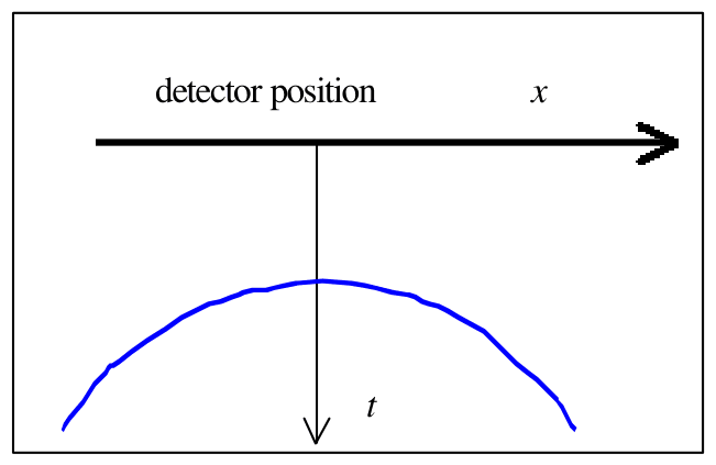
Graph of traveltime \(t\) vs detector position \(x\), \(t_{\min}=100\ \mathrm{ns}\).
Derive \(t\) as a function of \(x\) and determine \(d\) [3.5 pts].
Official English text of the problem.
Answers
-
In the stated low-loss limit, \[ \boxed{v\simeq\frac{1}{\sqrt{\mu\varepsilon}}.} \]
-
The maximum detection depth is \[ \boxed{D_{\max}\simeq\frac{2}{\sigma}\sqrt{\frac{\varepsilon}{\mu_0}} =15.9\ \mathrm{m}\approx16\ \mathrm{m}.} \]
-
With rod depth \(h=4\ \mathrm{m}\) and lateral separation \(s=0.50\ \mathrm{m}\), \[ \boxed{f_{\min}\simeq \frac{v}{4\left(\sqrt{h^2+s^2}-h\right)} \approx8.0\times10^8\ \mathrm{Hz} =800\ \mathrm{MHz}.} \]
-
Taking \(x=0\) directly above the rod, \[ \boxed{t(x)=\frac{2}{v}\sqrt{d^2+x^2} =\sqrt{t_{\min}^2+\frac{4x^2}{v^2}},\qquad d=\frac{vt_{\min}}{2}\approx5.0\ \mathrm{m}.} \]
Solution
1. Propagation speed
A point of constant phase satisfies \[ \omega t-\beta z=\text{constant}. \] Differentiating gives the phase velocity: \[ v=\frac{dz}{dt}=\frac{\omega}{\beta}. \]
Define the small dimensionless parameter \[ q=\frac{\sigma}{\omega\varepsilon},\qquad q^2\ll1. \] Using the binomial expansion, \[ \sqrt{1+q^2}=1+\frac{q^2}{2}+O(q^4). \] Equation (2) therefore gives \[ \beta =\omega\left[ \frac{\mu\varepsilon}{2} \left(2+\frac{q^2}{2}+O(q^4)\right) \right]^{1/2} =\omega\sqrt{\mu\varepsilon} \left(1+\frac{q^2}{8}+O(q^4)\right). \]
Keeping the leading term, \[ \boxed{v\simeq\frac{1}{\sqrt{\mu\varepsilon}}.} \] For non-magnetic ground, \(\mu=\mu_0\). At this order, \(\beta\) is proportional to \(\omega\), so dispersion is negligible and the group velocity also equals this value.
2. Maximum detection depth
For the attenuation coefficient, retain the leading nonzero term of the same expansion: \[ \alpha \simeq \omega\left[ \frac{\mu\varepsilon}{2}\frac{q^2}{2} \right]^{1/2} =\frac{\sigma}{2}\sqrt{\frac{\mu}{\varepsilon}}. \] Thus, to this order, the attenuation coefficient is independent of frequency.
For an object directly below the antenna at depth \(D\), equation (1) gives the incident amplitude ratio \[ \frac{E_{\mathrm{amp}}(D)}{E_0}=e^{-\alpha D}. \] The problem specifies the threshold for the signal arriving at the object, so the propagation distance entering this condition is \(D\). At the limiting depth, \[ e^{-\alpha D_{\max}}=\frac1e, \] and hence \[ D_{\max}=\frac1\alpha \simeq\frac{2}{\sigma}\sqrt{\frac{\varepsilon}{\mu_0}}. \]
Using \[ \sigma=1.0\times10^{-3}\ \mathrm{S/m}, \qquad \varepsilon=9(8.85\times10^{-12}) =7.965\times10^{-11}\ \mathrm{F/m}, \] we obtain \[ \alpha\simeq \frac{1.0\times10^{-3}}{2} \sqrt{\frac{4\pi\times10^{-7}}{7.965\times10^{-11}}} =6.28\times10^{-2}\ \mathrm{m^{-1}}. \] Therefore, \[ \boxed{D_{\max}=15.9\ \mathrm{m}\approx16\ \mathrm{m}.} \]
3. Minimum frequency for a lateral resolution of 50 cm
Work in the vertical plane perpendicular to the rods. Let their common depth be \(h\), their lateral separation be \(s\), and take the antenna–detector position directly above the first rod.
The one-way distances to the two rods are \[ r_1=h,\qquad r_2=\sqrt{h^2+s^2}. \] Since transmitter and detector are at the same point, the reflected signals travel distances \(2r_1\) and \(2r_2\). Their path difference is therefore \[ \Delta L=2\left(\sqrt{h^2+s^2}-h\right). \]
Treating the conducting rods as equivalent reflectors, their common reflection phase cancels. The phase difference at the detector is \[ \Delta\phi=\beta\Delta L =\frac{4\pi f}{v}\left(\sqrt{h^2+s^2}-h\right). \] The specified resolution criterion is \(\Delta\phi\geq\pi\). The minimum frequency occurs at equality: \[ \boxed{ f_{\min}= \frac{v}{4\left(\sqrt{h^2+s^2}-h\right)}. } \]
The wave speed in this ground is \[ v\simeq\frac1{\sqrt{\mu_0(9\varepsilon_0)}} =9.995\times10^7\ \mathrm{m/s}. \] For \(h=4\ \mathrm{m}\) and \(s=0.50\ \mathrm{m}\), \[ \sqrt{h^2+s^2}-h =\sqrt{4^2+0.50^2}-4 =0.0311289\ \mathrm{m}. \] Thus, \[ f_{\min}\simeq \frac{9.995\times10^7}{4(0.0311289)} =8.027\times10^8\ \mathrm{Hz}, \] or, to sensible precision, \[ \boxed{f_{\min}\approx8.0\times10^8\ \mathrm{Hz} =800\ \mathrm{MHz}.} \]
The small-separation approximation gives the same rounded result: \[ \sqrt{h^2+s^2}-h\simeq\frac{s^2}{2h} \quad\Longrightarrow\quad f_{\min}\simeq\frac{vh}{2s^2}. \]
The required frequency lies within the stated \(10\)–\(1000\ \mathrm{MHz}\) range. Moreover, at the calculated frequency, \[ \left(\frac{\sigma}{2\pi f_{\min}\varepsilon}\right)^2 \simeq6.2\times10^{-6}\ll1, \] so the low-loss approximation is consistent. Both rods also lie within the detection range found in part 2.
4. Travel-time curve and rod depth
Choose the horizontal coordinate \(x=0\) directly above the buried rod. In homogeneous ground, the one-way distance from the antenna to the rod is \[ r(x)=\sqrt{d^2+x^2}. \] The measured travel time includes the outward and return journeys: \[ \boxed{t(x)=\frac{2}{v}\sqrt{d^2+x^2}.} \]
The shortest path occurs at \(x=0\), giving \[ t_{\min}=\frac{2d}{v}. \] Consequently, \[ d=\frac{vt_{\min}}{2} =\frac{(9.995\times10^7)(100\times10^{-9})}{2}\ \mathrm{m} =4.998\ \mathrm{m}. \] Thus, \[ \boxed{d\approx5.0\ \mathrm{m}.} \]
Substituting the minimum travel time into the curve gives \[ \boxed{ t(x)=\sqrt{t_{\min}^2+\frac{4x^2}{v^2}} \simeq(100\ \mathrm{ns}) \sqrt{1+\left(\frac{x}{5.0\ \mathrm{m}}\right)^2}. } \]
This is the positive-time branch of the hyperbola \[ \frac{t^2}{t_{\min}^2}-\frac{x^2}{d^2}=1. \] It is symmetric about \(x=0\), has its minimum travel time of \(100\ \mathrm{ns}\) directly above the rod, and increases with \(|x|\). For \(|x|\gg d\), \[ t(x)\sim\frac{2|x|}{v}. \] Because the figure’s time axis points downward, larger travel times appear lower on the page, as shown.
The solution was checked against the official solution.
IPhO 2002 · Theorieaufgabe 1
Bodenradar
Bodenradar (GPR) wird eingesetzt, um oberflächennahe unterirdische Objekte zu erkennen und zu orten, indem elektromagnetische Wellen in den Boden gesendet und die von diesen Objekten reflektierten Wellen empfangen werden. Die Antenne und der Detektor befinden sich unmittelbar auf dem Boden am selben Ort.
Eine linear polarisierte ebene elektromagnetische Welle mit der Kreisfrequenz \(\omega\), die sich in \(z\)-Richtung ausbreitet, wird durch den folgenden Ausdruck für ihr Feld beschrieben:
\[ E=E_0e^{-\alpha z}\cos(\omega t-\beta z), \tag{1} \]
wobei \(E_0\) konstant ist, \(\alpha\) der Dämpfungskoeffizient und \(\beta\) die Wellenzahl sind, die jeweils durch die folgenden Ausdrücke gegeben sind:
\[ \alpha=\omega\left\{ \frac{\mu\varepsilon}{2} \left[ \left(1+\frac{\sigma^2}{\varepsilon^2\omega^2}\right)^{1/2}-1 \right]\right\}^{1/2}, \qquad \beta=\omega\left\{ \frac{\mu\varepsilon}{2} \left[ \left(1+\frac{\sigma^2}{\varepsilon^2\omega^2}\right)^{1/2}+1 \right]\right\}^{1/2} \tag{2} \]
Dabei bezeichnen \(\mu,\varepsilon,\) und \(\sigma\) die magnetische Permeabilität, die elektrische Permittivität bzw. die elektrische Leitfähigkeit.
Das Signal ist nicht mehr nachweisbar, wenn die Amplitude des am Objekt ankommenden Radarsignals unter \(1/e\) (\(\approx 37\%\)) ihres Anfangswerts fällt. Üblicherweise wird eine elektromagnetische Welle mit variabler Frequenz (10 MHz – 1000 MHz) verwendet, um die Reichweite und die Auflösung der Ortung anpassen zu können.
Die Leistungsfähigkeit des Bodenradars hängt von seiner Auflösung ab. Die Auflösung ist durch den Mindestabstand zwischen zwei benachbarten, zu detektierenden Reflektoren gegeben. Dieser Mindestabstand muss am Detektor zu einer Phasendifferenz von mindestens \(180^\circ\) zwischen den beiden reflektierten Wellen führen.
Fragen:
(Gegeben: \(\mu_0=4\pi\times10^{-7}\ \mathrm{H/m}\) und \(\varepsilon_0=8.85\times10^{-12}\ \mathrm{F/m}\))
-
Nehmen Sie an, dass der Boden nichtmagnetisch ist (\(\mu=\mu_0\)) und die Bedingung \(\left(\dfrac{\sigma}{\omega\varepsilon}\right)^2\ll1\) erfüllt. Leiten Sie mithilfe der Gleichungen (1) und (2) den Ausdruck für die Ausbreitungsgeschwindigkeit \(v\) in Abhängigkeit von \(\mu\) und \(\varepsilon\) her [1.0 Punkte].
-
Bestimmen Sie die maximale Tiefe, in der ein Objekt in einem Boden mit einer Leitfähigkeit von 1.0 mS/m und einer Permittivität von \(9\varepsilon_0\) detektiert werden kann, wobei die Bedingung \(\left(\dfrac{\sigma}{\omega\varepsilon}\right)^2\ll1\) erfüllt ist (\(\mathrm{S}=\mathrm{ohm}^{-1}\) ; verwenden Sie \(\mu=\mu_0\)). [2.0 Punkte]
-
Betrachten Sie zwei parallele leitende Stäbe, die horizontal im Boden vergraben sind. Die Stäbe befinden sich in einer Tiefe von 4 Metern. Der Boden hat bekanntermaßen eine Leitfähigkeit von 1.0 mS/m und eine Permittivität von \(9\varepsilon_0\). Die Bodenradarmessung werde an einer Position ungefähr über einem der Stäbe durchgeführt. Nehmen Sie an, dass ein punktförmiger Detektor verwendet wird. Bestimmen Sie die Mindestfrequenz, die erforderlich ist, um eine laterale Auflösung von 50 cm zu erreichen [3.5 Punkte].
-
Um die Tiefe \(d\) eines im selben Boden vergrabenen Stabes zu bestimmen, betrachten Sie Messungen entlang einer Geraden senkrecht zum Stab. Das Ergebnis wird durch die folgende Abbildung beschrieben:
Diagramm der Laufzeit \(t\) in Abhängigkeit von der Detektorposition \(x\), \(t_{\min}=100\ \mathrm{ns}\).
Leiten Sie \(t\) als Funktion von \(x\) her und bestimmen Sie \(d\) [3.5 Punkte].
Aufgabentext aus dem offiziellen englischen Text übersetzt.
Antworten
-
Im angegebenen Grenzfall geringer Verluste gilt \[ \boxed{v\simeq\frac{1}{\sqrt{\mu\varepsilon}}.} \]
-
Die maximale Detektionstiefe beträgt \[ \boxed{D_{\max}\simeq\frac{2}{\sigma}\sqrt{\frac{\varepsilon}{\mu_0}} =15.9\ \mathrm{m}\approx16\ \mathrm{m}.} \]
-
Für eine Tiefe der Stäbe von \(h=4\ \mathrm{m}\) und einen lateralen Abstand von \(s=0.50\ \mathrm{m}\) gilt \[ \boxed{f_{\min}\simeq \frac{v}{4\left(\sqrt{h^2+s^2}-h\right)} \approx8.0\times10^8\ \mathrm{Hz} =800\ \mathrm{MHz}.} \]
-
Wird \(x=0\) direkt über dem Stab gewählt, so gilt \[ \boxed{t(x)=\frac{2}{v}\sqrt{d^2+x^2} =\sqrt{t_{\min}^2+\frac{4x^2}{v^2}},\qquad d=\frac{vt_{\min}}{2}\approx5.0\ \mathrm{m}.} \]
Lösung
1. Ausbreitungsgeschwindigkeit
Ein Punkt konstanter Phase erfüllt \[ \omega t-\beta z=\text{konstant}. \] Durch Differenzieren erhält man die Phasengeschwindigkeit: \[ v=\frac{dz}{dt}=\frac{\omega}{\beta}. \]
Wir definieren den kleinen dimensionslosen Parameter \[ q=\frac{\sigma}{\omega\varepsilon},\qquad q^2\ll1. \] Mit der Binomialentwicklung ergibt sich \[ \sqrt{1+q^2}=1+\frac{q^2}{2}+O(q^4). \] Gleichung (2) liefert daher \[ \beta =\omega\left[ \frac{\mu\varepsilon}{2} \left(2+\frac{q^2}{2}+O(q^4)\right) \right]^{1/2} =\omega\sqrt{\mu\varepsilon} \left(1+\frac{q^2}{8}+O(q^4)\right). \]
Behält man nur den führenden Term bei, so erhält man \[ \boxed{v\simeq\frac{1}{\sqrt{\mu\varepsilon}}.} \] Für nichtmagnetischen Boden gilt \(\mu=\mu_0\). In dieser Ordnung ist \(\beta\) proportional zu \(\omega\), sodass die Dispersion vernachlässigbar ist und auch die Gruppengeschwindigkeit diesem Wert entspricht.
2. Maximale Detektionstiefe
Für den Dämpfungskoeffizienten behalten wir den führenden, von null verschiedenen Term derselben Entwicklung bei: \[ \alpha \simeq \omega\left[ \frac{\mu\varepsilon}{2}\frac{q^2}{2} \right]^{1/2} =\frac{\sigma}{2}\sqrt{\frac{\mu}{\varepsilon}}. \] Somit ist der Dämpfungskoeffizient in dieser Ordnung unabhängig von der Frequenz.
Für ein Objekt direkt unter der Antenne in der Tiefe \(D\) ergibt Gleichung (1) für das Amplitudenverhältnis der einfallenden Welle \[ \frac{E_{\mathrm{amp}}(D)}{E_0}=e^{-\alpha D}. \] Die Aufgabe gibt den Schwellenwert für das am Objekt ankommende Signal vor, daher ist die in diese Bedingung eingehende Ausbreitungsstrecke \(D\). In der Grenztiefe gilt \[ e^{-\alpha D_{\max}}=\frac1e, \] und somit \[ D_{\max}=\frac1\alpha \simeq\frac{2}{\sigma}\sqrt{\frac{\varepsilon}{\mu_0}}. \]
Mit \[ \sigma=1.0\times10^{-3}\ \mathrm{S/m}, \qquad \varepsilon=9(8.85\times10^{-12}) =7.965\times10^{-11}\ \mathrm{F/m}, \] erhalten wir \[ \alpha\simeq \frac{1.0\times10^{-3}}{2} \sqrt{\frac{4\pi\times10^{-7}}{7.965\times10^{-11}}} =6.28\times10^{-2}\ \mathrm{m^{-1}}. \] Daher gilt \[ \boxed{D_{\max}=15.9\ \mathrm{m}\approx16\ \mathrm{m}.} \]
3. Mindestfrequenz für eine laterale Auflösung von 50 cm
Wir betrachten die vertikale Ebene senkrecht zu den Stäben. Ihre gemeinsame Tiefe sei \(h\), ihr lateraler Abstand sei \(s\), und die Position von Antenne und Detektor werde direkt über dem ersten Stab gewählt.
Die einfachen Weglängen zu den beiden Stäben sind \[ r_1=h,\qquad r_2=\sqrt{h^2+s^2}. \] Da sich Sender und Detektor am selben Ort befinden, legen die reflektierten Signale die Strecken \(2r_1\) und \(2r_2\) zurück. Ihr Gangunterschied beträgt daher \[ \Delta L=2\left(\sqrt{h^2+s^2}-h\right). \]
Werden die leitenden Stäbe als gleichwertige Reflektoren behandelt, so hebt sich ihre gemeinsame Phasenverschiebung bei der Reflexion heraus. Die Phasendifferenz am Detektor ist \[ \Delta\phi=\beta\Delta L =\frac{4\pi f}{v}\left(\sqrt{h^2+s^2}-h\right). \] Das vorgegebene Auflösungskriterium lautet \(\Delta\phi\geq\pi\). Die Mindestfrequenz ergibt sich im Fall der Gleichheit: \[ \boxed{ f_{\min}= \frac{v}{4\left(\sqrt{h^2+s^2}-h\right)}. } \]
Die Wellengeschwindigkeit in diesem Boden beträgt \[ v\simeq\frac1{\sqrt{\mu_0(9\varepsilon_0)}} =9.995\times10^7\ \mathrm{m/s}. \] Für \(h=4\ \mathrm{m}\) und \(s=0.50\ \mathrm{m}\) gilt \[ \sqrt{h^2+s^2}-h =\sqrt{4^2+0.50^2}-4 =0.0311289\ \mathrm{m}. \] Somit gilt \[ f_{\min}\simeq \frac{9.995\times10^7}{4(0.0311289)} =8.027\times10^8\ \mathrm{Hz}, \] oder, auf eine sinnvolle Genauigkeit gerundet, \[ \boxed{f_{\min}\approx8.0\times10^8\ \mathrm{Hz} =800\ \mathrm{MHz}.} \]
Die Näherung für kleine Abstände liefert dasselbe gerundete Ergebnis: \[ \sqrt{h^2+s^2}-h\simeq\frac{s^2}{2h} \quad\Longrightarrow\quad f_{\min}\simeq\frac{vh}{2s^2}. \]
Die erforderliche Frequenz liegt innerhalb des angegebenen Bereichs von \(10\)–\(1000\ \mathrm{MHz}\). Außerdem gilt bei der berechneten Frequenz \[ \left(\frac{\sigma}{2\pi f_{\min}\varepsilon}\right)^2 \simeq6.2\times10^{-6}\ll1, \] sodass die Näherung geringer Verluste konsistent ist. Beide Stäbe liegen zudem innerhalb der in Teil 2 bestimmten Detektionsreichweite.
4. Laufzeitkurve und Tiefe des Stabes
Wir wählen die horizontale Koordinate \(x=0\) direkt über dem vergrabenen Stab. In homogenem Boden beträgt die einfache Weglänge von der Antenne zum Stab \[ r(x)=\sqrt{d^2+x^2}. \] Die gemessene Laufzeit umfasst den Hin- und Rückweg: \[ \boxed{t(x)=\frac{2}{v}\sqrt{d^2+x^2}.} \]
Der kürzeste Weg ergibt sich bei \(x=0\), woraus folgt: \[ t_{\min}=\frac{2d}{v}. \] Folglich gilt \[ d=\frac{vt_{\min}}{2} =\frac{(9.995\times10^7)(100\times10^{-9})}{2}\ \mathrm{m} =4.998\ \mathrm{m}. \] Somit gilt \[ \boxed{d\approx5.0\ \mathrm{m}.} \]
Setzt man die minimale Laufzeit in die Kurvengleichung ein, so erhält man \[ \boxed{ t(x)=\sqrt{t_{\min}^2+\frac{4x^2}{v^2}} \simeq(100\ \mathrm{ns}) \sqrt{1+\left(\frac{x}{5.0\ \mathrm{m}}\right)^2}. } \]
Dies ist der Ast für positive Zeiten der Hyperbel \[ \frac{t^2}{t_{\min}^2}-\frac{x^2}{d^2}=1. \] Die Kurve ist symmetrisch bezüglich \(x=0\), hat ihre minimale Laufzeit von \(100\ \mathrm{ns}\) direkt über dem Stab und steigt mit \(|x|\) an. Für \(|x|\gg d\) gilt \[ t(x)\sim\frac{2|x|}{v}. \] Da die Zeitachse der Abbildung nach unten zeigt, erscheinen größere Laufzeiten auf der Seite weiter unten, wie dargestellt.
Die Lösung wurde mit der offiziellen Lösung abgeglichen.
IPhO 2002 · Teori sorusu 1
Yer Radarı
Yer radarı (GPR), zemine elektromanyetik dalgalar gönderip yer altındaki nesnelerden yansıyan dalgaları alarak yüzeye yakın nesneleri tespit etmek ve konumlarını belirlemek için kullanılır. Anten ve dedektör doğrudan zemin üzerinde, aynı noktada bulunur.
\(z\) yönünde yayılan, açısal frekansı \(\omega\) olan doğrusal kutuplanmış bir elektromanyetik düzlem dalganın alanı aşağıdaki ifadeyle gösterilir:
\[ E=E_0e^{-\alpha z}\cos(\omega t-\beta z), \tag{1} \]
Burada \(E_0\) sabittir; \(\alpha\) zayıflama katsayısı, \(\beta\) ise dalga sayısıdır ve sırasıyla aşağıdaki gibi ifade edilirler:
\[ \alpha=\omega\left\{ \frac{\mu\varepsilon}{2} \left[ \left(1+\frac{\sigma^2}{\varepsilon^2\omega^2}\right)^{1/2}-1 \right]\right\}^{1/2}, \qquad \beta=\omega\left\{ \frac{\mu\varepsilon}{2} \left[ \left(1+\frac{\sigma^2}{\varepsilon^2\omega^2}\right)^{1/2}+1 \right]\right\}^{1/2} \tag{2} \]
Burada \(\mu,\varepsilon,\) ve \(\sigma\) sırasıyla manyetik geçirgenliği, elektriksel geçirgenliği ve elektriksel iletkenliği belirtir.
Nesneye ulaşan radar sinyalinin genliği başlangıç değerinin \(1/e\)'sinin (\(\approx 37\%\)) altına düştüğünde sinyal algılanamaz hâle gelir. Algılama menzilinin ve çözünürlüğünün ayarlanabilmesi için genellikle değişken frekanslı (10 MHz – 1000 MHz) bir elektromanyetik dalga kullanılır.
Yer radarının performansı çözünürlüğüne bağlıdır. Çözünürlük, birbirine komşu iki yansıtıcının ayırt edilebilmesi için aralarında bulunması gereken en küçük uzaklıkla verilir. Bu en küçük uzaklık, dedektörde iki yansıyan dalga arasında en az \(180^\circ\) faz farkı oluşturmalıdır.
Sorular:
(Verilenler: \(\mu_0=4\pi\times10^{-7}\ \mathrm{H/m}\) ve \(\varepsilon_0=8.85\times10^{-12}\ \mathrm{F/m}\))
-
Zeminin manyetik olmadığını (\(\mu=\mu_0\)) ve \(\left(\dfrac{\sigma}{\omega\varepsilon}\right)^2\ll1\) koşulunu sağladığını varsayın. (1) ve (2) denklemlerini kullanarak yayılma hızı \(v\)'nin \(\mu\) ve \(\varepsilon\) cinsinden ifadesini türetin [1.0 puan].
-
İletkenliği 1.0 mS/m ve elektriksel geçirgenliği \(9\varepsilon_0\) olan, \(\left(\dfrac{\sigma}{\omega\varepsilon}\right)^2\ll1\) koşulunu sağlayan bir zemindeki bir nesnenin algılanabileceği en büyük derinliği belirleyin (\(\mathrm{S}=\mathrm{ohm}^{-1}\) ; \(\mu=\mu_0\) kullanın). [2.0 puan]
-
Zemine yatay olarak gömülmüş, birbirine paralel iki iletken çubuğu ele alın. Çubuklar 4 metre derinliktedir. Zeminin iletkenliğinin 1.0 mS/m ve elektriksel geçirgenliğinin \(9\varepsilon_0\) olduğu bilinmektedir. Yer radarı ölçümünün, yaklaşık olarak çubuklardan birinin tam üzerinde yapıldığını varsayın. Noktasal bir dedektör kullanıldığını kabul edin. 50 cm yanal çözünürlük elde etmek için gereken en küçük frekansı belirleyin [3.5 puan].
-
Aynı zemine gömülmüş bir çubuğun \(d\) derinliğini belirlemek için çubuğa dik bir doğru boyunca yapılan ölçümleri ele alın. Sonuç aşağıdaki şekilde gösterilmiştir:
Gidiş-dönüş süresi \(t\)'nin dedektör konumu \(x\)'e göre grafiği, \(t_{\min}=100\ \mathrm{ns}\).
\(t\)'yi \(x\)'in bir fonksiyonu olarak türetin ve \(d\)'yi belirleyin [3.5 puan].
Soru metni resmi İngilizce metinden çevrilmiştir.
Cevaplar
-
Belirtilen düşük kayıp sınırında, \[ \boxed{v\simeq\frac{1}{\sqrt{\mu\varepsilon}}.} \]
-
En büyük algılama derinliği \[ \boxed{D_{\max}\simeq\frac{2}{\sigma}\sqrt{\frac{\varepsilon}{\mu_0}} =15.9\ \mathrm{m}\approx16\ \mathrm{m}.} \] olarak bulunur.
-
Çubukların derinliği \(h=4\ \mathrm{m}\) ve aralarındaki yanal uzaklık \(s=0.50\ \mathrm{m}\) için, \[ \boxed{f_{\min}\simeq \frac{v}{4\left(\sqrt{h^2+s^2}-h\right)} \approx8.0\times10^8\ \mathrm{Hz} =800\ \mathrm{MHz}.} \]
-
Çubuğun tam üzerinde \(x=0\) alınırsa, \[ \boxed{t(x)=\frac{2}{v}\sqrt{d^2+x^2} =\sqrt{t_{\min}^2+\frac{4x^2}{v^2}},\qquad d=\frac{vt_{\min}}{2}\approx5.0\ \mathrm{m}.} \]
Çözüm
1. Yayılma hızı
Fazı sabit olan bir nokta \[ \omega t-\beta z=\text{sabit}. \] koşulunu sağlar. Türev alınarak faz hızı elde edilir: \[ v=\frac{dz}{dt}=\frac{\omega}{\beta}. \]
Küçük boyutsuz parametreyi şöyle tanımlayalım: \[ q=\frac{\sigma}{\omega\varepsilon},\qquad q^2\ll1. \] Binom açılımını kullanırsak, \[ \sqrt{1+q^2}=1+\frac{q^2}{2}+O(q^4). \] Böylece (2) denklemi şu sonucu verir: \[ \beta =\omega\left[ \frac{\mu\varepsilon}{2} \left(2+\frac{q^2}{2}+O(q^4)\right) \right]^{1/2} =\omega\sqrt{\mu\varepsilon} \left(1+\frac{q^2}{8}+O(q^4)\right). \]
Yalnızca başat terimi tutarsak, \[ \boxed{v\simeq\frac{1}{\sqrt{\mu\varepsilon}}.} \] Manyetik olmayan bir zemin için \(\mu=\mu_0\)'dır. Bu mertebede \(\beta\), \(\omega\) ile orantılıdır; dolayısıyla dispersiyon ihmal edilebilir ve grup hızı da bu değere eşittir.
2. En büyük algılama derinliği
Zayıflama katsayısı için aynı açılımın sıfırdan farklı başat terimini tutalım: \[ \alpha \simeq \omega\left[ \frac{\mu\varepsilon}{2}\frac{q^2}{2} \right]^{1/2} =\frac{\sigma}{2}\sqrt{\frac{\mu}{\varepsilon}}. \] Dolayısıyla bu mertebede zayıflama katsayısı frekanstan bağımsızdır.
Antenin tam altında, \(D\) derinliğinde bulunan bir nesne için (1) denklemi, gelen dalganın genlik oranını şöyle verir: \[ \frac{E_{\mathrm{amp}}(D)}{E_0}=e^{-\alpha D}. \] Soruda eşik, nesneye ulaşan sinyal için belirtilmiştir; bu nedenle bu koşulda kullanılan yayılma uzaklığı \(D\)'dir. Sınır derinliğinde, \[ e^{-\alpha D_{\max}}=\frac1e, \] ve dolayısıyla \[ D_{\max}=\frac1\alpha \simeq\frac{2}{\sigma}\sqrt{\frac{\varepsilon}{\mu_0}}. \]
Şu değerleri kullanarak \[ \sigma=1.0\times10^{-3}\ \mathrm{S/m}, \qquad \varepsilon=9(8.85\times10^{-12}) =7.965\times10^{-11}\ \mathrm{F/m}, \] şunu elde ederiz: \[ \alpha\simeq \frac{1.0\times10^{-3}}{2} \sqrt{\frac{4\pi\times10^{-7}}{7.965\times10^{-11}}} =6.28\times10^{-2}\ \mathrm{m^{-1}}. \] Dolayısıyla, \[ \boxed{D_{\max}=15.9\ \mathrm{m}\approx16\ \mathrm{m}.} \]
3. 50 cm yanal çözünürlük için en küçük frekans
Çubuklara dik olan düşey düzlemde çalışalım. Çubukların ortak derinliği \(h\), aralarındaki yanal uzaklık \(s\) olsun ve anten–dedektör konumunu birinci çubuğun tam üzerinde alalım.
İki çubuğa olan tek yönlü uzaklıklar \[ r_1=h,\qquad r_2=\sqrt{h^2+s^2}. \] olarak verilir. Verici ve dedektör aynı noktada olduğundan, yansıyan sinyaller \(2r_1\) ve \(2r_2\) uzaklıklarını kateder. Dolayısıyla yol farkları \[ \Delta L=2\left(\sqrt{h^2+s^2}-h\right). \] olur.
İletken çubukları eşdeğer yansıtıcılar olarak ele aldığımızda, ortak yansıma fazları fark alınırken birbirini götürür. Dedektördeki faz farkı şöyledir: \[ \Delta\phi=\beta\Delta L =\frac{4\pi f}{v}\left(\sqrt{h^2+s^2}-h\right). \] Belirtilen çözünürlük ölçütü \(\Delta\phi\geq\pi\)'dir. En küçük frekans eşitlik durumunda elde edilir: \[ \boxed{ f_{\min}= \frac{v}{4\left(\sqrt{h^2+s^2}-h\right)}. } \]
Bu zemindeki dalga hızı şöyledir: \[ v\simeq\frac1{\sqrt{\mu_0(9\varepsilon_0)}} =9.995\times10^7\ \mathrm{m/s}. \] \(h=4\ \mathrm{m}\) ve \(s=0.50\ \mathrm{m}\) için, \[ \sqrt{h^2+s^2}-h =\sqrt{4^2+0.50^2}-4 =0.0311289\ \mathrm{m}. \] Böylece, \[ f_{\min}\simeq \frac{9.995\times10^7}{4(0.0311289)} =8.027\times10^8\ \mathrm{Hz}, \] ya da uygun bir hassasiyete yuvarlandığında, \[ \boxed{f_{\min}\approx8.0\times10^8\ \mathrm{Hz} =800\ \mathrm{MHz}.} \]
Çubuklar arasındaki uzaklığın küçük olduğu yaklaşım da yuvarlama sonrasında aynı sonucu verir: \[ \sqrt{h^2+s^2}-h\simeq\frac{s^2}{2h} \quad\Longrightarrow\quad f_{\min}\simeq\frac{vh}{2s^2}. \]
Gereken frekans, belirtilen \(10\)–\(1000\ \mathrm{MHz}\) aralığındadır. Ayrıca hesaplanan frekansta, \[ \left(\frac{\sigma}{2\pi f_{\min}\varepsilon}\right)^2 \simeq6.2\times10^{-6}\ll1, \] olduğundan düşük kayıp yaklaşımı tutarlıdır. Her iki çubuk da 2. kısımda bulunan algılama menzili içindedir.
4. Gidiş-dönüş süresi eğrisi ve çubuğun derinliği
Yatay koordinatı, gömülü çubuğun tam üzerinde \(x=0\) olacak şekilde seçelim. Homojen zeminde antenden çubuğa olan tek yönlü uzaklık şöyledir: \[ r(x)=\sqrt{d^2+x^2}. \] Ölçülen süre, gidiş ve dönüş yolculuklarını içerir: \[ \boxed{t(x)=\frac{2}{v}\sqrt{d^2+x^2}.} \]
En kısa yol \(x=0\) konumunda elde edilir ve \[ t_{\min}=\frac{2d}{v}. \] sonucunu verir. Buna göre, \[ d=\frac{vt_{\min}}{2} =\frac{(9.995\times10^7)(100\times10^{-9})}{2}\ \mathrm{m} =4.998\ \mathrm{m}. \] Böylece, \[ \boxed{d\approx5.0\ \mathrm{m}.} \]
En küçük gidiş-dönüş süresini eğrinin denkleminde yerine koyarsak, \[ \boxed{ t(x)=\sqrt{t_{\min}^2+\frac{4x^2}{v^2}} \simeq(100\ \mathrm{ns}) \sqrt{1+\left(\frac{x}{5.0\ \mathrm{m}}\right)^2}. } \]
Bu, aşağıdaki hiperbolün zamanın pozitif olduğu koludur: \[ \frac{t^2}{t_{\min}^2}-\frac{x^2}{d^2}=1. \] Eğri \(x=0\)'a göre simetriktir; çubuğun tam üzerinde en küçük gidiş-dönüş süresi olan \(100\ \mathrm{ns}\) değerini alır ve süre \(|x|\) ile artar. \(|x|\gg d\) için, \[ t(x)\sim\frac{2|x|}{v}. \] Şeklin zaman ekseni aşağıya doğru yöneldiğinden, daha büyük gidiş-dönüş süreleri şekilde gösterildiği gibi sayfada daha aşağıda görünür.
Çözüm, resmi çözümle karşılaştırılarak kontrol edildi.
IPhO 2002 · Problema teórico 1
Radar de penetración terrestre
El radar de penetración terrestre (GPR) se utiliza para detectar y localizar objetos subterráneos próximos a la superficie mediante la transmisión de ondas electromagnéticas al interior del terreno y la recepción de las ondas reflejadas por dichos objetos. La antena y el detector se encuentran directamente sobre el terreno y están situados en el mismo punto.
Una onda electromagnética plana, linealmente polarizada, de frecuencia angular \(\omega\), que se propaga en la dirección \(z\), se representa mediante la siguiente expresión de su campo:
\[ E=E_0e^{-\alpha z}\cos(\omega t-\beta z), \tag{1} \]
donde \(E_0\) es constante, \(\alpha\) es el coeficiente de atenuación y \(\beta\) es el número de onda, expresados respectivamente de la siguiente manera:
\[ \alpha=\omega\left\{ \frac{\mu\varepsilon}{2} \left[ \left(1+\frac{\sigma^2}{\varepsilon^2\omega^2}\right)^{1/2}-1 \right]\right\}^{1/2}, \qquad \beta=\omega\left\{ \frac{\mu\varepsilon}{2} \left[ \left(1+\frac{\sigma^2}{\varepsilon^2\omega^2}\right)^{1/2}+1 \right]\right\}^{1/2} \tag{2} \]
donde \(\mu,\varepsilon,\) y \(\sigma\) denotan la permeabilidad magnética, la permitividad eléctrica y la conductividad eléctrica, respectivamente.
La señal deja de detectarse cuando la amplitud de la señal de radar que llega al objeto cae por debajo de \(1/e\) (\(\approx 37\%\)) de su valor inicial. Habitualmente se utiliza una onda electromagnética de frecuencia variable (10 MHz – 1000 MHz) para poder ajustar el alcance y la resolución de la detección.
El rendimiento del GPR depende de su resolución. La resolución viene dada por la separación mínima entre los dos reflectores adyacentes que se desea detectar. Esta separación mínima debe producir una diferencia de fase mínima de \(180^\circ\) entre las dos ondas reflejadas en el detector.
Preguntas:
(Datos: \(\mu_0=4\pi\times10^{-7}\ \mathrm{H/m}\) y \(\varepsilon_0=8.85\times10^{-12}\ \mathrm{F/m}\))
-
Suponga que el terreno es no magnético (\(\mu=\mu_0\)) y satisface la condición \(\left(\dfrac{\sigma}{\omega\varepsilon}\right)^2\ll1\). Deduzca la expresión de la velocidad de propagación \(v\) en función de \(\mu\) y \(\varepsilon\), utilizando las ecuaciones (1) y (2) [1.0 pts].
-
Determine la profundidad máxima de detección de un objeto en un terreno con una conductividad de 1.0 mS/m y una permitividad de \(9\varepsilon_0\), que satisface la condición \(\left(\dfrac{\sigma}{\omega\varepsilon}\right)^2\ll1\), (\(\mathrm{S}=\mathrm{ohm}^{-1}\) ; utilice \(\mu=\mu_0\)). [2.0 pts]
-
Considere dos varillas conductoras paralelas enterradas horizontalmente en el terreno. Las varillas están a 4 metros de profundidad. Se sabe que el terreno tiene una conductividad de 1.0 mS/m y una permitividad de \(9\varepsilon_0\). Suponga que la medición con GPR se realiza en una posición aproximadamente sobre una de las varillas. Suponga que se utiliza un detector puntual. Determine la frecuencia mínima necesaria para obtener una resolución lateral de 50 cm [3.5 pts].
-
Para determinar la profundidad \(d\) de una varilla enterrada en el mismo terreno, considere las mediciones realizadas a lo largo de una línea perpendicular a la varilla. El resultado se describe en la siguiente figura:
Gráfica del tiempo de recorrido \(t\) en función de la posición del detector \(x\), \(t_{\min}=100\ \mathrm{ns}\).
Deduzca \(t\) en función de \(x\) y determine \(d\) [3.5 pts].
Enunciado traducido del texto oficial en inglés.
Respuestas
-
En el límite de bajas pérdidas indicado, \[ \boxed{v\simeq\frac{1}{\sqrt{\mu\varepsilon}}.} \]
-
La profundidad máxima de detección es \[ \boxed{D_{\max}\simeq\frac{2}{\sigma}\sqrt{\frac{\varepsilon}{\mu_0}} =15.9\ \mathrm{m}\approx16\ \mathrm{m}.} \]
-
Con una profundidad de las varillas \(h=4\ \mathrm{m}\) y una separación lateral \(s=0.50\ \mathrm{m}\), \[ \boxed{f_{\min}\simeq \frac{v}{4\left(\sqrt{h^2+s^2}-h\right)} \approx8.0\times10^8\ \mathrm{Hz} =800\ \mathrm{MHz}.} \]
-
Tomando \(x=0\) directamente sobre la varilla, \[ \boxed{t(x)=\frac{2}{v}\sqrt{d^2+x^2} =\sqrt{t_{\min}^2+\frac{4x^2}{v^2}},\qquad d=\frac{vt_{\min}}{2}\approx5.0\ \mathrm{m}.} \]
Solución
1. Velocidad de propagación
Un punto de fase constante satisface \[ \omega t-\beta z=\text{constante}. \] Al derivar se obtiene la velocidad de fase: \[ v=\frac{dz}{dt}=\frac{\omega}{\beta}. \]
Definimos el parámetro adimensional pequeño \[ q=\frac{\sigma}{\omega\varepsilon},\qquad q^2\ll1. \] Utilizando el desarrollo binomial, \[ \sqrt{1+q^2}=1+\frac{q^2}{2}+O(q^4). \] Por tanto, la ecuación (2) da \[ \beta =\omega\left[ \frac{\mu\varepsilon}{2} \left(2+\frac{q^2}{2}+O(q^4)\right) \right]^{1/2} =\omega\sqrt{\mu\varepsilon} \left(1+\frac{q^2}{8}+O(q^4)\right). \]
Conservando el término dominante, \[ \boxed{v\simeq\frac{1}{\sqrt{\mu\varepsilon}}.} \] Para un terreno no magnético, \(\mu=\mu_0\). A este orden, \(\beta\) es proporcional a \(\omega\), por lo que la dispersión es despreciable y la velocidad de grupo también es igual a este valor.
2. Profundidad máxima de detección
Para el coeficiente de atenuación, conservamos el primer término no nulo del mismo desarrollo: \[ \alpha \simeq \omega\left[ \frac{\mu\varepsilon}{2}\frac{q^2}{2} \right]^{1/2} =\frac{\sigma}{2}\sqrt{\frac{\mu}{\varepsilon}}. \] Así pues, a este orden, el coeficiente de atenuación es independiente de la frecuencia.
Para un objeto situado directamente debajo de la antena a una profundidad \(D\), la ecuación (1) da la razón de amplitudes de la onda incidente \[ \frac{E_{\mathrm{amp}}(D)}{E_0}=e^{-\alpha D}. \] El enunciado especifica el umbral para la señal que llega al objeto, por lo que la distancia de propagación que interviene en esta condición es \(D\). A la profundidad límite, \[ e^{-\alpha D_{\max}}=\frac1e, \] y, por tanto, \[ D_{\max}=\frac1\alpha \simeq\frac{2}{\sigma}\sqrt{\frac{\varepsilon}{\mu_0}}. \]
Utilizando \[ \sigma=1.0\times10^{-3}\ \mathrm{S/m}, \qquad \varepsilon=9(8.85\times10^{-12}) =7.965\times10^{-11}\ \mathrm{F/m}, \] obtenemos \[ \alpha\simeq \frac{1.0\times10^{-3}}{2} \sqrt{\frac{4\pi\times10^{-7}}{7.965\times10^{-11}}} =6.28\times10^{-2}\ \mathrm{m^{-1}}. \] Por tanto, \[ \boxed{D_{\max}=15.9\ \mathrm{m}\approx16\ \mathrm{m}.} \]
3. Frecuencia mínima para una resolución lateral de 50 cm
Trabajamos en el plano vertical perpendicular a las varillas. Sean \(h\) su profundidad común y \(s\) su separación lateral, y situemos la antena y el detector directamente sobre la primera varilla.
Las distancias de ida a las dos varillas son \[ r_1=h,\qquad r_2=\sqrt{h^2+s^2}. \] Como el transmisor y el detector están en el mismo punto, las señales reflejadas recorren distancias \(2r_1\) y \(2r_2\). Por tanto, su diferencia de caminos es \[ \Delta L=2\left(\sqrt{h^2+s^2}-h\right). \]
Al tratar las varillas conductoras como reflectores equivalentes, su fase de reflexión común se cancela. La diferencia de fase en el detector es \[ \Delta\phi=\beta\Delta L =\frac{4\pi f}{v}\left(\sqrt{h^2+s^2}-h\right). \] El criterio de resolución especificado es \(\Delta\phi\geq\pi\). La frecuencia mínima se obtiene cuando se cumple la igualdad: \[ \boxed{ f_{\min}= \frac{v}{4\left(\sqrt{h^2+s^2}-h\right)}. } \]
La velocidad de la onda en este terreno es \[ v\simeq\frac1{\sqrt{\mu_0(9\varepsilon_0)}} =9.995\times10^7\ \mathrm{m/s}. \] Para \(h=4\ \mathrm{m}\) y \(s=0.50\ \mathrm{m}\), \[ \sqrt{h^2+s^2}-h =\sqrt{4^2+0.50^2}-4 =0.0311289\ \mathrm{m}. \] Así pues, \[ f_{\min}\simeq \frac{9.995\times10^7}{4(0.0311289)} =8.027\times10^8\ \mathrm{Hz}, \] o, con una precisión razonable, \[ \boxed{f_{\min}\approx8.0\times10^8\ \mathrm{Hz} =800\ \mathrm{MHz}.} \]
La aproximación para separaciones pequeñas da el mismo resultado redondeado: \[ \sqrt{h^2+s^2}-h\simeq\frac{s^2}{2h} \quad\Longrightarrow\quad f_{\min}\simeq\frac{vh}{2s^2}. \]
La frecuencia requerida se encuentra dentro del intervalo indicado de \(10\)–\(1000\ \mathrm{MHz}\). Además, a la frecuencia calculada, \[ \left(\frac{\sigma}{2\pi f_{\min}\varepsilon}\right)^2 \simeq6.2\times10^{-6}\ll1, \] por lo que la aproximación de bajas pérdidas es coherente. Ambas varillas se encuentran también dentro del alcance de detección obtenido en la parte 2.
4. Curva del tiempo de recorrido y profundidad de la varilla
Elegimos la coordenada horizontal \(x=0\) directamente sobre la varilla enterrada. En un terreno homogéneo, la distancia de ida desde la antena hasta la varilla es \[ r(x)=\sqrt{d^2+x^2}. \] El tiempo de recorrido medido incluye los trayectos de ida y vuelta: \[ \boxed{t(x)=\frac{2}{v}\sqrt{d^2+x^2}.} \]
El camino más corto se obtiene en \(x=0\), lo que da \[ t_{\min}=\frac{2d}{v}. \] En consecuencia, \[ d=\frac{vt_{\min}}{2} =\frac{(9.995\times10^7)(100\times10^{-9})}{2}\ \mathrm{m} =4.998\ \mathrm{m}. \] Así pues, \[ \boxed{d\approx5.0\ \mathrm{m}.} \]
Al sustituir el tiempo mínimo de recorrido en la expresión de la curva se obtiene \[ \boxed{ t(x)=\sqrt{t_{\min}^2+\frac{4x^2}{v^2}} \simeq(100\ \mathrm{ns}) \sqrt{1+\left(\frac{x}{5.0\ \mathrm{m}}\right)^2}. } \]
Esta es la rama de tiempos positivos de la hipérbola \[ \frac{t^2}{t_{\min}^2}-\frac{x^2}{d^2}=1. \] Es simétrica respecto a \(x=0\), alcanza su tiempo mínimo de recorrido de \(100\ \mathrm{ns}\) directamente sobre la varilla y crece con \(|x|\). Para \(|x|\gg d\), \[ t(x)\sim\frac{2|x|}{v}. \] Como el eje del tiempo de la figura apunta hacia abajo, los tiempos de recorrido mayores aparecen más abajo en la página, tal como se muestra.
La solución se comprobó con la solución oficial.
IPhO 2002 · 理论题 1
探地雷达
探地雷达(GPR)通过向地下发射电磁波并接收地下物体反射的电磁波,来探测和定位埋藏在地表附近的物体。天线和探测器直接放置在地面上,且位于同一点。
沿 \(z\) 方向传播、角频率为 \(\omega\) 的线偏振电磁平面波,其电场可表示为:
\[ E=E_0e^{-\alpha z}\cos(\omega t-\beta z), \tag{1} \]
其中,\(E_0\) 为常量,\(\alpha\) 为衰减系数,\(\beta\) 为波数,后两者分别表示为
\[ \alpha=\omega\left\{ \frac{\mu\varepsilon}{2} \left[ \left(1+\frac{\sigma^2}{\varepsilon^2\omega^2}\right)^{1/2}-1 \right]\right\}^{1/2}, \qquad \beta=\omega\left\{ \frac{\mu\varepsilon}{2} \left[ \left(1+\frac{\sigma^2}{\varepsilon^2\omega^2}\right)^{1/2}+1 \right]\right\}^{1/2} \tag{2} \]
其中,\(\mu,\varepsilon,\) 和 \(\sigma\) 分别表示磁导率、介电常数和电导率。
当到达物体的雷达信号振幅降至其初始值的 \(1/e\)(\(\approx 37\%\))以下时,信号便无法被探测到。通常使用频率可调的电磁波(10 MHz – 1000 MHz),以便调节探测范围和分辨率。
探地雷达的性能取决于其分辨率。分辨率由能够分辨的两个相邻反射体之间的最小间距给出。此最小间距应使两束反射波到达探测器时产生至少 \(180^\circ\) 的相位差。
问题:
(已知:\(\mu_0=4\pi\times10^{-7}\ \mathrm{H/m}\) 和 \(\varepsilon_0=8.85\times10^{-12}\ \mathrm{F/m}\))
-
假设地下介质为非磁性介质(\(\mu=\mu_0\)),且满足条件 \(\left(\dfrac{\sigma}{\omega\varepsilon}\right)^2\ll1\)。利用式 (1) 和式 (2),推导传播速度 \(v\) 用 \(\mu\) 和 \(\varepsilon\) 表示的表达式 [1.0 分]。
-
地下介质的电导率为 1.0 mS/m,介电常数为 \(9\varepsilon_0\),且满足条件 \(\left(\dfrac{\sigma}{\omega\varepsilon}\right)^2\ll1\)。求埋藏在其中的物体能够被探测到的最大深度(\(\mathrm{S}=\mathrm{ohm}^{-1}\);取 \(\mu=\mu_0\))。[2.0 分]
-
考虑两根平行的导电棒,水平埋藏在地下,埋深为 4 米。已知地下介质的电导率为 1.0 mS/m,介电常数为 \(9\varepsilon_0\)。假设探地雷达在大致位于其中一根导电棒正上方的位置进行测量,并使用点探测器。求获得 50 cm 横向分辨率所需的最低频率 [3.5 分]。
-
为确定埋藏在同一地下介质中的一根导电棒的深度 \(d\),考虑沿垂直于导电棒的直线进行测量。测量结果如下图所示:
传播时间 \(t\) 随探测器位置 \(x\) 变化的曲线,\(t_{\min}=100\ \mathrm{ns}\)。
推导 \(t\) 关于 \(x\) 的函数,并确定 \(d\) [3.5 分]。
题目译自官方英文原文。
答案
-
在题设的低损耗极限下, \[ \boxed{v\simeq\frac{1}{\sqrt{\mu\varepsilon}}.} \]
-
最大探测深度为 \[ \boxed{D_{\max}\simeq\frac{2}{\sigma}\sqrt{\frac{\varepsilon}{\mu_0}} =15.9\ \mathrm{m}\approx16\ \mathrm{m}.} \]
-
当导电棒的埋深为 \(h=4\ \mathrm{m}\)、横向间距为 \(s=0.50\ \mathrm{m}\) 时, \[ \boxed{f_{\min}\simeq \frac{v}{4\left(\sqrt{h^2+s^2}-h\right)} \approx8.0\times10^8\ \mathrm{Hz} =800\ \mathrm{MHz}.} \]
-
取导电棒正上方为 \(x=0\),则 \[ \boxed{t(x)=\frac{2}{v}\sqrt{d^2+x^2} =\sqrt{t_{\min}^2+\frac{4x^2}{v^2}},\qquad d=\frac{vt_{\min}}{2}\approx5.0\ \mathrm{m}.} \]
解答
1. 传播速度
相位恒定的点满足 \[ \omega t-\beta z=\text{常量}. \] 求导可得相速度: \[ v=\frac{dz}{dt}=\frac{\omega}{\beta}. \]
定义无量纲小参数 \[ q=\frac{\sigma}{\omega\varepsilon},\qquad q^2\ll1. \] 利用二项式展开, \[ \sqrt{1+q^2}=1+\frac{q^2}{2}+O(q^4). \] 因此,由式 (2) 得 \[ \beta =\omega\left[ \frac{\mu\varepsilon}{2} \left(2+\frac{q^2}{2}+O(q^4)\right) \right]^{1/2} =\omega\sqrt{\mu\varepsilon} \left(1+\frac{q^2}{8}+O(q^4)\right). \]
保留首项,得 \[ \boxed{v\simeq\frac{1}{\sqrt{\mu\varepsilon}}.} \] 对于非磁性地下介质,\(\mu=\mu_0\)。在这一阶近似下,\(\beta\) 与 \(\omega\) 成正比,因此色散可以忽略,群速度也等于此值。
2. 最大探测深度
对于衰减系数,在同一展开式中保留最低阶非零项: \[ \alpha \simeq \omega\left[ \frac{\mu\varepsilon}{2}\frac{q^2}{2} \right]^{1/2} =\frac{\sigma}{2}\sqrt{\frac{\mu}{\varepsilon}}. \] 因此,在这一阶近似下,衰减系数与频率无关。
对于位于天线正下方、深度为 \(D\) 的物体,由式 (1) 可得入射波的振幅比 \[ \frac{E_{\mathrm{amp}}(D)}{E_0}=e^{-\alpha D}. \] 题目规定的是到达物体的信号的阈值,因此这一条件中所涉及的传播距离为 \(D\)。在极限深度处, \[ e^{-\alpha D_{\max}}=\frac1e, \] 因而 \[ D_{\max}=\frac1\alpha \simeq\frac{2}{\sigma}\sqrt{\frac{\varepsilon}{\mu_0}}. \]
代入 \[ \sigma=1.0\times10^{-3}\ \mathrm{S/m}, \qquad \varepsilon=9(8.85\times10^{-12}) =7.965\times10^{-11}\ \mathrm{F/m}, \] 得到 \[ \alpha\simeq \frac{1.0\times10^{-3}}{2} \sqrt{\frac{4\pi\times10^{-7}}{7.965\times10^{-11}}} =6.28\times10^{-2}\ \mathrm{m^{-1}}. \] 因此, \[ \boxed{D_{\max}=15.9\ \mathrm{m}\approx16\ \mathrm{m}.} \]
3. 获得 50 cm 横向分辨率所需的最低频率
在垂直于导电棒的竖直平面内分析。设两根导电棒的共同埋深为 \(h\),横向间距为 \(s\),并取天线和探测器的位置在第一根导电棒的正上方。
到两根导电棒的单程距离分别为 \[ r_1=h,\qquad r_2=\sqrt{h^2+s^2}. \] 由于发射器和探测器位于同一点,两个反射信号的传播距离分别为 \(2r_1\) 和 \(2r_2\)。因此,它们的波程差为 \[ \Delta L=2\left(\sqrt{h^2+s^2}-h\right). \]
将两根导电棒视为等效的反射体,它们共同的反射相位在求相位差时抵消。探测器处的相位差为 \[ \Delta\phi=\beta\Delta L =\frac{4\pi f}{v}\left(\sqrt{h^2+s^2}-h\right). \] 题目给定的分辨判据为 \(\Delta\phi\geq\pi\)。取等号时得到最低频率: \[ \boxed{ f_{\min}= \frac{v}{4\left(\sqrt{h^2+s^2}-h\right)}. } \]
该地下介质中的波速为 \[ v\simeq\frac1{\sqrt{\mu_0(9\varepsilon_0)}} =9.995\times10^7\ \mathrm{m/s}. \] 对于 \(h=4\ \mathrm{m}\) 和 \(s=0.50\ \mathrm{m}\), \[ \sqrt{h^2+s^2}-h =\sqrt{4^2+0.50^2}-4 =0.0311289\ \mathrm{m}. \] 于是, \[ f_{\min}\simeq \frac{9.995\times10^7}{4(0.0311289)} =8.027\times10^8\ \mathrm{Hz}, \] 取合理的精度,得 \[ \boxed{f_{\min}\approx8.0\times10^8\ \mathrm{Hz} =800\ \mathrm{MHz}.} \]
小间距近似给出相同的舍入结果: \[ \sqrt{h^2+s^2}-h\simeq\frac{s^2}{2h} \quad\Longrightarrow\quad f_{\min}\simeq\frac{vh}{2s^2}. \]
所需频率位于题目给定的 \(10\)–\(1000\ \mathrm{MHz}\) 范围内。此外,在计算得到的频率下, \[ \left(\frac{\sigma}{2\pi f_{\min}\varepsilon}\right)^2 \simeq6.2\times10^{-6}\ll1, \] 因此低损耗近似是自洽的。两根导电棒也都位于第 2 问求得的探测范围之内。
4. 传播时间曲线与导电棒的埋深
选取埋藏的导电棒正上方的水平坐标为 \(x=0\)。在均匀地下介质中,从天线到导电棒的单程距离为 \[ r(x)=\sqrt{d^2+x^2}. \] 测得的传播时间包括去程和回程: \[ \boxed{t(x)=\frac{2}{v}\sqrt{d^2+x^2}.} \]
在 \(x=0\) 处路径最短,因而 \[ t_{\min}=\frac{2d}{v}. \] 所以, \[ d=\frac{vt_{\min}}{2} =\frac{(9.995\times10^7)(100\times10^{-9})}{2}\ \mathrm{m} =4.998\ \mathrm{m}. \] 于是, \[ \boxed{d\approx5.0\ \mathrm{m}.} \]
将最短传播时间代入曲线表达式,得 \[ \boxed{ t(x)=\sqrt{t_{\min}^2+\frac{4x^2}{v^2}} \simeq(100\ \mathrm{ns}) \sqrt{1+\left(\frac{x}{5.0\ \mathrm{m}}\right)^2}. } \]
这是双曲线 \[ \frac{t^2}{t_{\min}^2}-\frac{x^2}{d^2}=1. \] 对应于正时间的一支。它关于 \(x=0\) 对称,在导电棒正上方取得最短传播时间 \(100\ \mathrm{ns}\),并随 \(|x|\) 的增大而增大。当 \(|x|\gg d\) 时, \[ t(x)\sim\frac{2|x|}{v}. \] 由于图中的时间轴指向下方,传播时间越长,图上的位置就越低,如图所示。
解答已与官方解答核对。
IPhO 2002 · Теоретическая задача 1
Георадар
Георадар (GPR) используется для обнаружения и определения положения подземных объектов вблизи поверхности посредством излучения электромагнитных волн в грунт и приёма волн, отражённых от этих объектов. Антенна и приёмник находятся непосредственно на поверхности грунта в одной и той же точке.
Линейно поляризованная плоская электромагнитная волна с угловой частотой \(\omega\), распространяющаяся в направлении \(z\), описывается следующим выражением для её поля:
\[ E=E_0e^{-\alpha z}\cos(\omega t-\beta z), \tag{1} \]
где \(E_0\) — постоянная, \(\alpha\) — коэффициент затухания, а \(\beta\) — волновое число, которые выражаются соответственно следующим образом:
\[ \alpha=\omega\left\{ \frac{\mu\varepsilon}{2} \left[ \left(1+\frac{\sigma^2}{\varepsilon^2\omega^2}\right)^{1/2}-1 \right]\right\}^{1/2}, \qquad \beta=\omega\left\{ \frac{\mu\varepsilon}{2} \left[ \left(1+\frac{\sigma^2}{\varepsilon^2\omega^2}\right)^{1/2}+1 \right]\right\}^{1/2} \tag{2} \]
Здесь \(\mu,\varepsilon,\) и \(\sigma\) обозначают соответственно магнитную проницаемость, диэлектрическую проницаемость и удельную электрическую проводимость.
Сигнал перестаёт обнаруживаться, когда амплитуда сигнала георадара, достигающего объекта, становится меньше \(1/e\) (\(\approx 37\%\)) от её начального значения. Обычно используется электромагнитная волна с изменяемой частотой (10 МГц – 1000 МГц), что позволяет регулировать дальность обнаружения и разрешение.
Эффективность георадара зависит от его разрешения. Разрешение определяется минимальным расстоянием между двумя соседними отражателями, которые можно различить. При этом минимальном расстоянии разность фаз двух отражённых волн на приёмнике должна составлять не менее \(180^\circ\).
Вопросы:
(Дано: \(\mu_0=4\pi\times10^{-7}\ \mathrm{H/m}\) и \(\varepsilon_0=8.85\times10^{-12}\ \mathrm{F/m}\))
-
Предположим, что грунт немагнитный (\(\mu=\mu_0\)) и выполняется условие \(\left(\dfrac{\sigma}{\omega\varepsilon}\right)^2\ll1\). Используя уравнения (1) и (2), выведите выражение для скорости распространения \(v\) через \(\mu\) и \(\varepsilon\) [1.0 балла].
-
Определите максимальную глубину обнаружения объекта в грунте с удельной проводимостью 1.0 мСм/м и диэлектрической проницаемостью \(9\varepsilon_0\), для которого выполняется условие \(\left(\dfrac{\sigma}{\omega\varepsilon}\right)^2\ll1\), (\(\mathrm{S}=\mathrm{ohm}^{-1}\) ; используйте \(\mu=\mu_0\)). [2.0 балла]
-
Рассмотрим два параллельных проводящих стержня, расположенных горизонтально в грунте. Стержни находятся на глубине 4 метра. Известно, что удельная проводимость грунта равна 1.0 мСм/м, а диэлектрическая проницаемость — \(9\varepsilon_0\). Предположим, что измерение георадаром проводится приблизительно над одним из стержней. Считайте, что используется точечный приёмник. Определите минимальную частоту, необходимую для получения поперечного разрешения 50 см [3.5 балла].
-
Чтобы определить глубину залегания стержня \(d\) в том же грунте, рассмотрим измерения, проведённые вдоль линии, перпендикулярной стержню. Результат представлен на следующем рисунке:
График зависимости времени распространения \(t\) от положения приёмника \(x\), \(t_{\min}=100\ \mathrm{ns}\).
Выведите зависимость \(t\) от \(x\) и определите \(d\) [3.5 балла].
Условие переведено с официального английского текста.
Ответы
-
В указанном пределе малых потерь \[ \boxed{v\simeq\frac{1}{\sqrt{\mu\varepsilon}}.} \]
-
Максимальная глубина обнаружения равна \[ \boxed{D_{\max}\simeq\frac{2}{\sigma}\sqrt{\frac{\varepsilon}{\mu_0}} =15.9\ \mathrm{m}\approx16\ \mathrm{m}.} \]
-
При глубине залегания стержней \(h=4\ \mathrm{m}\) и поперечном расстоянии между ними \(s=0.50\ \mathrm{m}\) \[ \boxed{f_{\min}\simeq \frac{v}{4\left(\sqrt{h^2+s^2}-h\right)} \approx8.0\times10^8\ \mathrm{Hz} =800\ \mathrm{MHz}.} \]
-
Выбирая \(x=0\) непосредственно над стержнем, получаем \[ \boxed{t(x)=\frac{2}{v}\sqrt{d^2+x^2} =\sqrt{t_{\min}^2+\frac{4x^2}{v^2}},\qquad d=\frac{vt_{\min}}{2}\approx5.0\ \mathrm{m}.} \]
Решение
1. Скорость распространения
Для точки с постоянной фазой выполняется условие \[ \omega t-\beta z=\text{постоянная}. \] Дифференцируя, получаем фазовую скорость: \[ v=\frac{dz}{dt}=\frac{\omega}{\beta}. \]
Введём малый безразмерный параметр \[ q=\frac{\sigma}{\omega\varepsilon},\qquad q^2\ll1. \] Используя биномиальное разложение, получаем \[ \sqrt{1+q^2}=1+\frac{q^2}{2}+O(q^4). \] Поэтому из уравнения (2) следует \[ \beta =\omega\left[ \frac{\mu\varepsilon}{2} \left(2+\frac{q^2}{2}+O(q^4)\right) \right]^{1/2} =\omega\sqrt{\mu\varepsilon} \left(1+\frac{q^2}{8}+O(q^4)\right). \]
Оставляя главный член, получаем \[ \boxed{v\simeq\frac{1}{\sqrt{\mu\varepsilon}}.} \] Для немагнитного грунта \(\mu=\mu_0\). В этом приближении \(\beta\) пропорционально \(\omega\), поэтому дисперсией можно пренебречь и групповая скорость также равна этому значению.
2. Максимальная глубина обнаружения
Для коэффициента затухания сохраним первый ненулевой член того же разложения: \[ \alpha \simeq \omega\left[ \frac{\mu\varepsilon}{2}\frac{q^2}{2} \right]^{1/2} =\frac{\sigma}{2}\sqrt{\frac{\mu}{\varepsilon}}. \] Таким образом, в этом приближении коэффициент затухания не зависит от частоты.
Для объекта, находящегося непосредственно под антенной на глубине \(D\), уравнение (1) даёт следующее отношение амплитуды падающей волны к начальной амплитуде: \[ \frac{E_{\mathrm{amp}}(D)}{E_0}=e^{-\alpha D}. \] В условии задачи порог задан для сигнала, достигающего объекта, поэтому расстояние распространения, входящее в это условие, равно \(D\). На предельной глубине \[ e^{-\alpha D_{\max}}=\frac1e, \] откуда \[ D_{\max}=\frac1\alpha \simeq\frac{2}{\sigma}\sqrt{\frac{\varepsilon}{\mu_0}}. \]
Используя \[ \sigma=1.0\times10^{-3}\ \mathrm{S/m}, \qquad \varepsilon=9(8.85\times10^{-12}) =7.965\times10^{-11}\ \mathrm{F/m}, \] получаем \[ \alpha\simeq \frac{1.0\times10^{-3}}{2} \sqrt{\frac{4\pi\times10^{-7}}{7.965\times10^{-11}}} =6.28\times10^{-2}\ \mathrm{m^{-1}}. \] Следовательно, \[ \boxed{D_{\max}=15.9\ \mathrm{m}\approx16\ \mathrm{m}.} \]
3. Минимальная частота для поперечного разрешения 50 см
Рассмотрим вертикальную плоскость, перпендикулярную стержням. Обозначим их общую глубину залегания через \(h\), поперечное расстояние между ними — через \(s\) и расположим антенну и приёмник непосредственно над первым стержнем.
Расстояния до двух стержней в одну сторону равны \[ r_1=h,\qquad r_2=\sqrt{h^2+s^2}. \] Поскольку передатчик и приёмник находятся в одной точке, отражённые сигналы проходят расстояния \(2r_1\) и \(2r_2\). Поэтому разность их хода равна \[ \Delta L=2\left(\sqrt{h^2+s^2}-h\right). \]
Если считать проводящие стержни эквивалентными отражателями, одинаковый для них фазовый сдвиг при отражении сокращается. Разность фаз на приёмнике равна \[ \Delta\phi=\beta\Delta L =\frac{4\pi f}{v}\left(\sqrt{h^2+s^2}-h\right). \] Заданный критерий разрешения имеет вид \(\Delta\phi\geq\pi\). Минимальная частота соответствует равенству: \[ \boxed{ f_{\min}= \frac{v}{4\left(\sqrt{h^2+s^2}-h\right)}. } \]
Скорость волны в этом грунте равна \[ v\simeq\frac1{\sqrt{\mu_0(9\varepsilon_0)}} =9.995\times10^7\ \mathrm{m/s}. \] При \(h=4\ \mathrm{m}\) и \(s=0.50\ \mathrm{m}\) \[ \sqrt{h^2+s^2}-h =\sqrt{4^2+0.50^2}-4 =0.0311289\ \mathrm{m}. \] Таким образом, \[ f_{\min}\simeq \frac{9.995\times10^7}{4(0.0311289)} =8.027\times10^8\ \mathrm{Hz}, \] или, с разумной точностью, \[ \boxed{f_{\min}\approx8.0\times10^8\ \mathrm{Hz} =800\ \mathrm{MHz}.} \]
Приближение малого расстояния между стержнями даёт тот же результат после округления: \[ \sqrt{h^2+s^2}-h\simeq\frac{s^2}{2h} \quad\Longrightarrow\quad f_{\min}\simeq\frac{vh}{2s^2}. \]
Требуемая частота лежит в указанном диапазоне \(10\)–\(1000\ \mathrm{MHz}\). Кроме того, при вычисленной частоте \[ \left(\frac{\sigma}{2\pi f_{\min}\varepsilon}\right)^2 \simeq6.2\times10^{-6}\ll1, \] поэтому приближение малых потерь согласуется с полученным результатом. Оба стержня также находятся в пределах дальности обнаружения, найденной в пункте 2.
4. Кривая времени распространения и глубина залегания стержня
Выберем начало горизонтальной координаты \(x=0\) непосредственно над подземным стержнем. В однородном грунте расстояние от антенны до стержня в одну сторону равно \[ r(x)=\sqrt{d^2+x^2}. \] Измеренное время распространения включает путь до стержня и обратно: \[ \boxed{t(x)=\frac{2}{v}\sqrt{d^2+x^2}.} \]
Кратчайший путь соответствует \(x=0\), что даёт \[ t_{\min}=\frac{2d}{v}. \] Следовательно, \[ d=\frac{vt_{\min}}{2} =\frac{(9.995\times10^7)(100\times10^{-9})}{2}\ \mathrm{m} =4.998\ \mathrm{m}. \] Таким образом, \[ \boxed{d\approx5.0\ \mathrm{m}.} \]
Подставляя минимальное время распространения в выражение для кривой, получаем \[ \boxed{ t(x)=\sqrt{t_{\min}^2+\frac{4x^2}{v^2}} \simeq(100\ \mathrm{ns}) \sqrt{1+\left(\frac{x}{5.0\ \mathrm{m}}\right)^2}. } \]
Это ветвь гиперболы, соответствующая положительному времени: \[ \frac{t^2}{t_{\min}^2}-\frac{x^2}{d^2}=1. \] Она симметрична относительно \(x=0\), имеет минимальное время распространения \(100\ \mathrm{ns}\) непосредственно над стержнем и возрастает с увеличением \(|x|\). При \(|x|\gg d\) \[ t(x)\sim\frac{2|x|}{v}. \] Поскольку ось времени на рисунке направлена вниз, большие времена распространения изображаются ниже на странице, как и показано на рисунке.
Решение проверено по официальному решению.
IPhO 2002 · مسألة نظرية 1
الرادار المخترق للأرض
يُستخدم الرادار المخترق للأرض (GPR) لكشف الأجسام المدفونة بالقرب من سطح الأرض وتحديد مواقعها، وذلك بإرسال موجات كهرومغناطيسية إلى داخل الأرض واستقبال الموجات المنعكسة عن تلك الأجسام. يوضع الهوائي والكاشف مباشرة على سطح الأرض، ويقعان عند النقطة نفسها.
تُمثَّل موجة كهرومغناطيسية مستوية مستقطبة خطيًا، ذات تردد زاوي \(\omega\) وتنتشر في اتجاه \(z\)، بالتعبير الآتي لمجالها:
\[ E=E_0e^{-\alpha z}\cos(\omega t-\beta z), \tag{1} \]
حيث \(E_0\) ثابت، و\(\alpha\) معامل التوهين، و\(\beta\) العدد الموجي، ويُعبَّر عن الأخيرين، على الترتيب، كما يأتي:
\[ \alpha=\omega\left\{ \frac{\mu\varepsilon}{2} \left[ \left(1+\frac{\sigma^2}{\varepsilon^2\omega^2}\right)^{1/2}-1 \right]\right\}^{1/2}, \qquad \beta=\omega\left\{ \frac{\mu\varepsilon}{2} \left[ \left(1+\frac{\sigma^2}{\varepsilon^2\omega^2}\right)^{1/2}+1 \right]\right\}^{1/2} \tag{2} \]
حيث ترمز \(\mu,\varepsilon,\) و\(\sigma\) إلى النفاذية المغناطيسية والسماحية الكهربائية والموصلية الكهربائية، على الترتيب.
تصبح الإشارة غير قابلة للكشف عندما تنخفض سعة إشارة الرادار الواصلة إلى الجسم إلى أقل من \(1/e\) (\(\approx 37\%\)) من قيمتها الابتدائية. وعادةً ما تُستخدم موجة كهرومغناطيسية ذات تردد متغير (10 MHz – 1000 MHz) لإتاحة ضبط مدى الكشف وقدرته على التمييز.
يعتمد أداء الرادار المخترق للأرض على قدرته على التمييز. وتُحدَّد هذه القدرة بأصغر مسافة فاصلة بين عاكسين متجاورين يمكن كشفهما. ويجب أن تُنتج هذه المسافة الدنيا فرق طور لا يقل عن \(180^\circ\) بين الموجتين المنعكستين عند الكاشف.
الأسئلة:
(المعطيات: \(\mu_0=4\pi\times10^{-7}\ \mathrm{H/m}\) و\(\varepsilon_0=8.85\times10^{-12}\ \mathrm{F/m}\))
-
افترض أن الأرض غير مغناطيسية (\(\mu=\mu_0\)) وتحقق الشرط \(\left(\dfrac{\sigma}{\omega\varepsilon}\right)^2\ll1\). اشتق تعبير سرعة الانتشار \(v\) بدلالة \(\mu\) و\(\varepsilon\)، باستخدام المعادلتين (1) و(2) [1.0 نقطة].
-
حدِّد أقصى عمق يمكن عنده كشف جسم في أرض موصليتها 1.0 mS/m وسماحيتها \(9\varepsilon_0\)، وتحقق الشرط \(\left(\dfrac{\sigma}{\omega\varepsilon}\right)^2\ll1\)، (\(\mathrm{S}=\mathrm{ohm}^{-1}\)؛ استخدم \(\mu=\mu_0\)). [2.0 نقطة]
-
اعتبر قضيبين موصلين متوازيين مدفونين أفقيًا في الأرض. يقع القضيبان على عمق 4 أمتار. ومن المعلوم أن موصلية الأرض 1.0 mS/m وسماحيتها \(9\varepsilon_0\). افترض أن القياس بالرادار المخترق للأرض يُجرى عند موضع يقع فوق أحد القضيبين تقريبًا. وافترض استخدام كاشف نقطي. حدِّد أدنى تردد مطلوب للحصول على قدرة تمييز جانبية قدرها 50 cm [3.5 نقطة].
-
لتحديد عمق قضيب مدفون \(d\) في الأرض نفسها، اعتبر القياسات التي تُجرى على طول خط عمودي على القضيب. يوضِّح الشكل الآتي النتيجة:
رسم بياني لزمن الانتقال \(t\) بدلالة موضع الكاشف \(x\)، حيث \(t_{\min}=100\ \mathrm{ns}\).
اشتق \(t\) بوصفه دالة في \(x\)، وحدِّد \(d\) [3.5 نقطة].
نص المسألة مترجم عن النص الإنجليزي الرسمي.
الإجابات
-
في حد الفقد المنخفض المذكور، \[ \boxed{v\simeq\frac{1}{\sqrt{\mu\varepsilon}}.} \]
-
أقصى عمق للكشف هو \[ \boxed{D_{\max}\simeq\frac{2}{\sigma}\sqrt{\frac{\varepsilon}{\mu_0}} =15.9\ \mathrm{m}\approx16\ \mathrm{m}.} \]
-
عندما يكون عمق القضيبين \(h=4\ \mathrm{m}\) والمسافة الجانبية الفاصلة بينهما \(s=0.50\ \mathrm{m}\)، \[ \boxed{f_{\min}\simeq \frac{v}{4\left(\sqrt{h^2+s^2}-h\right)} \approx8.0\times10^8\ \mathrm{Hz} =800\ \mathrm{MHz}.} \]
-
باختيار \(x=0\) فوق القضيب مباشرة، \[ \boxed{t(x)=\frac{2}{v}\sqrt{d^2+x^2} =\sqrt{t_{\min}^2+\frac{4x^2}{v^2}},\qquad d=\frac{vt_{\min}}{2}\approx5.0\ \mathrm{m}.} \]
الحل
1. سرعة الانتشار
تحقق نقطة ذات طور ثابت العلاقة \[ \omega t-\beta z=\text{ثابت}. \] بالتفاضل نحصل على سرعة الطور: \[ v=\frac{dz}{dt}=\frac{\omega}{\beta}. \]
نعرِّف المعامل الصغير العديم الأبعاد \[ q=\frac{\sigma}{\omega\varepsilon},\qquad q^2\ll1. \] باستخدام مفكوك ذي الحدين، \[ \sqrt{1+q^2}=1+\frac{q^2}{2}+O(q^4). \] ومن ثم تعطي المعادلة (2) \[ \beta =\omega\left[ \frac{\mu\varepsilon}{2} \left(2+\frac{q^2}{2}+O(q^4)\right) \right]^{1/2} =\omega\sqrt{\mu\varepsilon} \left(1+\frac{q^2}{8}+O(q^4)\right). \]
بالاحتفاظ بالحد الرئيس، \[ \boxed{v\simeq\frac{1}{\sqrt{\mu\varepsilon}}.} \] للأرض غير المغناطيسية، \(\mu=\mu_0\). وعند هذه الرتبة، يتناسب \(\beta\) طرديًا مع \(\omega\)، لذا يمكن إهمال التشتت، وتساوي سرعة المجموعة هذه القيمة أيضًا.
2. أقصى عمق للكشف
لحساب معامل التوهين، نحتفظ بأول حد غير صفري من المفكوك نفسه: \[ \alpha \simeq \omega\left[ \frac{\mu\varepsilon}{2}\frac{q^2}{2} \right]^{1/2} =\frac{\sigma}{2}\sqrt{\frac{\mu}{\varepsilon}}. \] إذن، عند هذه الرتبة، يكون معامل التوهين مستقلًا عن التردد.
لجسم يقع أسفل الهوائي مباشرة على عمق \(D\)، تعطي المعادلة (1) نسبة سعة الموجة الساقطة إلى سعتها الابتدائية: \[ \frac{E_{\mathrm{amp}}(D)}{E_0}=e^{-\alpha D}. \] تحدِّد المسألة عتبة الإشارة الواصلة إلى الجسم، لذا فإن مسافة الانتشار التي تدخل في هذا الشرط هي \(D\). وعند العمق الحدي، \[ e^{-\alpha D_{\max}}=\frac1e, \] ومن ثم \[ D_{\max}=\frac1\alpha \simeq\frac{2}{\sigma}\sqrt{\frac{\varepsilon}{\mu_0}}. \]
باستخدام \[ \sigma=1.0\times10^{-3}\ \mathrm{S/m}, \qquad \varepsilon=9(8.85\times10^{-12}) =7.965\times10^{-11}\ \mathrm{F/m}, \] نحصل على \[ \alpha\simeq \frac{1.0\times10^{-3}}{2} \sqrt{\frac{4\pi\times10^{-7}}{7.965\times10^{-11}}} =6.28\times10^{-2}\ \mathrm{m^{-1}}. \] وعليه، \[ \boxed{D_{\max}=15.9\ \mathrm{m}\approx16\ \mathrm{m}.} \]
3. أدنى تردد للحصول على قدرة تمييز جانبية قدرها 50 cm
نعمل في المستوى الرأسي العمودي على القضيبين. لتكن قيمة عمقهما المشترك \(h\)، والمسافة الجانبية الفاصلة بينهما \(s\)، ولنأخذ موضع الهوائي والكاشف فوق القضيب الأول مباشرة.
المسافتان إلى القضيبين في اتجاه واحد هما \[ r_1=h,\qquad r_2=\sqrt{h^2+s^2}. \] بما أن المرسل والكاشف يقعان عند النقطة نفسها، فإن الإشارتين المنعكستين تقطعان المسافتين \(2r_1\) و\(2r_2\). ومن ثم يكون فرق المسار بينهما \[ \Delta L=2\left(\sqrt{h^2+s^2}-h\right). \]
باعتبار القضيبين الموصلين عاكسين متكافئين، تُلغى إزاحة الطور المشتركة الناجمة عن الانعكاس عند حساب الفرق. ويكون فرق الطور عند الكاشف \[ \Delta\phi=\beta\Delta L =\frac{4\pi f}{v}\left(\sqrt{h^2+s^2}-h\right). \] معيار التمييز المحدد هو \(\Delta\phi\geq\pi\). ويتحقق أدنى تردد عند المساواة: \[ \boxed{ f_{\min}= \frac{v}{4\left(\sqrt{h^2+s^2}-h\right)}. } \]
سرعة الموجة في هذه الأرض هي \[ v\simeq\frac1{\sqrt{\mu_0(9\varepsilon_0)}} =9.995\times10^7\ \mathrm{m/s}. \] عند \(h=4\ \mathrm{m}\) و\(s=0.50\ \mathrm{m}\)، \[ \sqrt{h^2+s^2}-h =\sqrt{4^2+0.50^2}-4 =0.0311289\ \mathrm{m}. \] إذن، \[ f_{\min}\simeq \frac{9.995\times10^7}{4(0.0311289)} =8.027\times10^8\ \mathrm{Hz}, \] أو، بالتقريب إلى دقة مناسبة، \[ \boxed{f_{\min}\approx8.0\times10^8\ \mathrm{Hz} =800\ \mathrm{MHz}.} \]
يعطي تقريب المسافة الفاصلة الصغيرة النتيجة المقربة نفسها: \[ \sqrt{h^2+s^2}-h\simeq\frac{s^2}{2h} \quad\Longrightarrow\quad f_{\min}\simeq\frac{vh}{2s^2}. \]
يقع التردد المطلوب ضمن المجال المذكور \(10\)–\(1000\ \mathrm{MHz}\). علاوة على ذلك، عند التردد المحسوب، \[ \left(\frac{\sigma}{2\pi f_{\min}\varepsilon}\right)^2 \simeq6.2\times10^{-6}\ll1, \] لذا فإن تقريب الفقد المنخفض متسق. ويقع كلا القضيبين أيضًا ضمن مدى الكشف الذي وُجد في الجزء 2.
4. منحنى زمن الانتقال وعمق القضيب
نختار الإحداثي الأفقي \(x=0\) فوق القضيب المدفون مباشرة. في أرض متجانسة، تكون المسافة في اتجاه واحد من الهوائي إلى القضيب \[ r(x)=\sqrt{d^2+x^2}. \] يشمل زمن الانتقال المقيس رحلتي الذهاب والإياب: \[ \boxed{t(x)=\frac{2}{v}\sqrt{d^2+x^2}.} \]
يتحقق أقصر مسار عند \(x=0\)، مما يعطي \[ t_{\min}=\frac{2d}{v}. \] وبالتالي، \[ d=\frac{vt_{\min}}{2} =\frac{(9.995\times10^7)(100\times10^{-9})}{2}\ \mathrm{m} =4.998\ \mathrm{m}. \] إذن، \[ \boxed{d\approx5.0\ \mathrm{m}.} \]
بالتعويض بأدنى زمن انتقال في معادلة المنحنى نحصل على \[ \boxed{ t(x)=\sqrt{t_{\min}^2+\frac{4x^2}{v^2}} \simeq(100\ \mathrm{ns}) \sqrt{1+\left(\frac{x}{5.0\ \mathrm{m}}\right)^2}. } \]
هذا هو فرع الزمن الموجب للقطع الزائد \[ \frac{t^2}{t_{\min}^2}-\frac{x^2}{d^2}=1. \] وهو متناظر حول \(x=0\)، ويبلغ زمن الانتقال قيمته الدنيا، وهي \(100\ \mathrm{ns}\)، فوق القضيب مباشرة، ويزداد مع \(|x|\). وعندما \(|x|\gg d\)، \[ t(x)\sim\frac{2|x|}{v}. \] ولأن محور الزمن في الشكل يتجه إلى الأسفل، تظهر أزمنة الانتقال الأكبر في مواضع أدنى على الصفحة، كما هو موضَّح.
تمت مراجعة الحل بمقارنته بالحل الرسمي.