IPhO 2001 · Theory problem 3
Magnetohydrodynamic (MHD) Generator
A horizontal rectangular plastic pipe of width \(w\) and height \(h\), which closes upon itself, is filled with mercury of resistivity \(\rho\). An overpressure \(P\) is produced by a turbine which drives this fluid with a constant speed \(v_0\). The two opposite vertical walls of a section of the pipe with length \(L\) are made of copper.
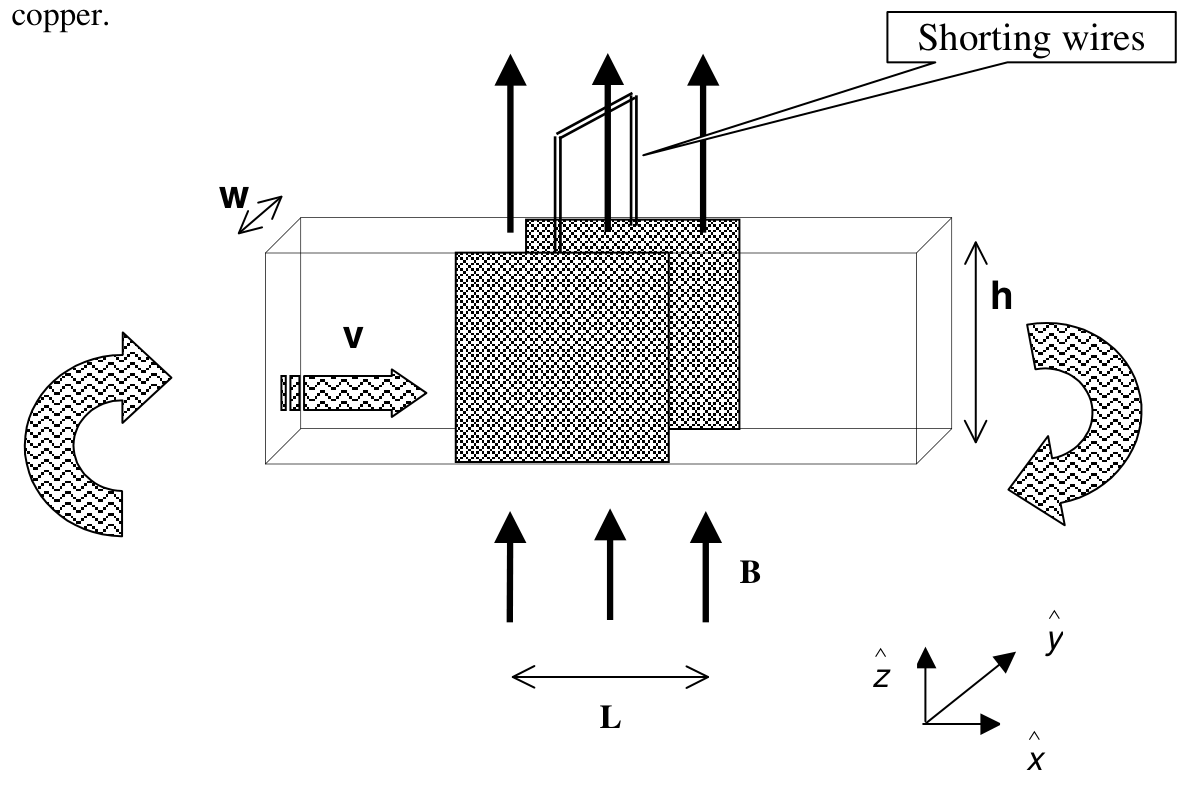
The motion of a real fluid is very complex. To simplify the situation we assume the following:
- Although the fluid is viscous, its speed is uniform over the entire cross section.
- The speed of the fluid is always proportional to the net external force acting upon it.
- The fluid is incompressible.
These walls are electrically shorted externally and a uniform, magnetic field \(\mathbf B\) is applied vertically upward only in this section. The set up is illustrated in the figure above, with the unit vectors \(\hat{x}\), \(\hat{y}\), \(\hat{z}\) to be used in the solution.
a) Find the force acting on the fluid due to the magnetic field (in terms of \(L\), \(B\), \(h\), \(w\), \(\rho\) and the velocity \(v\)) [2.0 pts]
b) Derive an expression for the new speed \(v\) of the fluid (in terms of \(v_0\), \(P\), \(L\), \(B\) and \(\rho\)) after the magnetic field is applied. [3.0 pts]
c) Derive an expression for the additional power that must be supplied by the turbine to increase the speed to its original value \(v_0\). Copy your result onto the answer form. [2.0 pts]
d) Now the magnetic field is turned off and mercury is replaced by water flowing with speed \(v_0\). An electromagnetic wave with a single frequency is sent along the section with length \(L\) in the direction of the flow. The refractive index of water is \(n\), and \(v_0\ll c\). Derive an expression for the contribution of the fluid’s motion to the phase difference between the waves entering and leaving section \(L\). Copy your result onto the answer form. [3.0 pts]
Official English text of the problem.
Answers
-
a) The magnetic force opposes the flow: \[ \boxed{\mathbf F_B=-\frac{LB^2hw}{\rho}\,v\,\hat{x}.} \]
-
b) \[ \boxed{v=\frac{v_0}{1+\dfrac{LB^2v_0}{\rho P}}.} \]
-
c) At the restored speed \(v_0\), the extra power required because of the magnetic field, above the original field-free power, is \[ \boxed{\Delta\mathcal P_{\mathrm{mag}} =\frac{LB^2hw}{\rho}\,v_0^2.} \] If the reference is instead the slowed operating state in (b), the total turbine-power increase is \[ \boxed{\Delta\mathcal P_{(b)\to v_0} =\frac{LB^2hw}{\rho}\,v_0^2+Pwh(v_0-v).} \]
-
d) Let \(\omega=2\pi f\) be the laboratory angular frequency and define the phase lag across the section as \(\Phi=kL\). To first order in \(v_0/c\), \[ \boxed{\delta\Phi \equiv\Phi(v_0)-\Phi(0) =-\frac{\omega L v_0}{c^2}(n^2-1) =-\frac{2\pi f L v_0}{c^2}(n^2-1).} \] Thus the flow reduces the phase lag. The outgoing wave’s corresponding phase advance has the same magnitude and positive sign.
Solution
a) Magnetic force on the fluid
The fluid velocity and applied magnetic field are \[ \mathbf v=v\hat{x}, \qquad \mathbf B=B\hat{z}. \] Consequently, \[ \mathbf v\times\mathbf B=-vB\hat{y}. \] The magnetic force on moving charge carriers therefore drives conventional current through the mercury in the \(-\hat{y}\) direction, between the copper walls.
The walls are separated by \(w\), so the motional electromotive force has magnitude \[ \mathcal E=vBw. \] The current travels a distance \(w\) through mercury with conducting cross-sectional area \(Lh\). Its resistance is therefore \[ R=\rho\frac{w}{Lh}. \] Neglecting the resistance of the copper walls and shorting wires, the current is \[ I=\frac{\mathcal E}{R} =\frac{vBLh}{\rho}. \]
The force on this current in the mercury is \[ \mathbf F_B =I(-w\hat{y})\times(B\hat{z}) =-IwB\hat{x}. \] Hence \[ \boxed{\mathbf F_B=-\frac{LB^2hw}{\rho}\,v\,\hat{x}.} \] Its direction is opposite to the fluid velocity, as expected for magnetic braking.
b) Speed after applying the magnetic field
Let the pipe cross-sectional area be \[ A=wh. \] The turbine’s pressure rise supplies the driving force \[ F_P=PA. \]
The assumed proportionality between speed and applied driving force is equivalent, for steady motion, to a linear viscous resistance \(\kappa v\). Before the magnetic field is applied, \[ PA=\kappa v_0, \] so \[ \kappa=\frac{PA}{v_0}. \]
With the field applied and the same pressure rise \(P\), the steady force balance is \[ PA-\kappa v-\frac{LB^2A}{\rho}v=0. \] Substitution for \(\kappa\) gives \[ PA=\left(\frac{PA}{v_0}+\frac{LB^2A}{\rho}\right)v. \] Canceling \(A\) and solving, \[ \boxed{v=\frac{v_0}{1+\dfrac{LB^2v_0}{\rho P}}.} \]
The result approaches \(v_0\) as \(B\to0\), and the field always reduces the speed.
c) Additional turbine power
At the restored speed \(v_0\), the viscous resistance returns to its original value, \[ F_{\mathrm{visc}}=\kappa v_0=PA. \] The turbine must also overcome the magnetic force \[ |F_B(v_0)|=\frac{LB^2A}{\rho}v_0. \] Thus the required pressure rise is \[ P_{\mathrm{restored}} =P+\frac{LB^2v_0}{\rho}. \]
For incompressible flow, mechanical power supplied by a pressure rise is pressure rise times volume flow rate: \[ \mathcal P=P_{\mathrm{rise}}Av. \] Therefore the total power at the restored speed is \[ \mathcal P_{\mathrm{restored}} =\left(P+\frac{LB^2v_0}{\rho}\right)Av_0 =PAv_0+\frac{LB^2A}{\rho}v_0^2. \]
The original field-free power was \(\mathcal P_0=PAv_0\). The additional power needed at the same speed because of magnetic braking is consequently \[ \boxed{\Delta\mathcal P_{\mathrm{mag}} =\mathcal P_{\mathrm{restored}}-\mathcal P_0 =\frac{LB^2hw}{\rho}v_0^2.} \]
This equals the Joule heating in the mercury: \[ I^2R =\left(\frac{v_0BLh}{\rho}\right)^2 \frac{\rho w}{Lh} =\frac{LB^2hw}{\rho}v_0^2, \] which checks the energy balance.
There is a distinction if “additional power” is measured from the slowed state in (b). In that state, the turbine supplies only \[ \mathcal P_{\mathrm{slowed}}=PAv. \] The increase from that operating state is \[ \boxed{ \begin{aligned} \mathcal P_{\mathrm{restored}}-\mathcal P_{\mathrm{slowed}} &=\frac{LB^2hw}{\rho}v_0^2+Pwh(v_0-v)\\ &=\frac{LB^2hw}{\rho}v_0^2 \left(1+\frac{1}{1+\dfrac{LB^2v_0}{\rho P}}\right). \end{aligned}} \] The second term accounts for restoring the original viscous dissipation as the speed increases.
d) Contribution of the water’s motion to the phase difference
Treat the supplied refractive index \(n\) as constant, neglecting dispersion. In the water’s rest frame, the wave’s phase velocity is \[ u'=\frac{c}{n}. \]
The water moves along the propagation direction at speed \(v_0\). Relativistic velocity addition gives the laboratory phase velocity \[ u=\frac{u'+v_0}{1+\dfrac{u'v_0}{c^2}} =\frac{\dfrac{c}{n}+v_0}{1+\dfrac{v_0}{nc}}. \] Expanding to first order in \(v_0/c\), \[ u\simeq \left(\frac{c}{n}+v_0\right) \left(1-\frac{v_0}{nc}\right) =\frac{c}{n}+v_0\left(1-\frac{1}{n^2}\right). \] The coefficient \(1-1/n^2\) is the Fresnel drag coefficient.
For a laboratory monochromatic wave written as \[ E(x,t)=E_0\cos(\omega t-kx), \] the entrance-to-exit phase lag is \[ \Phi=kL=\frac{\omega L}{u}. \] The source fixes the laboratory frequency \(\omega\).
Expanding the reciprocal velocity, \[ \frac1u\simeq \frac nc-\frac{(n^2-1)v_0}{c^2}. \] Thus \[ \Phi(v_0)\simeq \frac{n\omega L}{c} -\frac{\omega L(n^2-1)v_0}{c^2}. \] For stationary water, \[ \Phi(0)=\frac{n\omega L}{c}. \] Subtracting, \[ \boxed{\delta\Phi =-\frac{\omega L(n^2-1)v_0}{c^2}.} \]
Equivalently, with laboratory vacuum wavelength \(\lambda_0=c/f\), \[ \boxed{\delta\Phi =-\frac{2\pi L v_0}{\lambda_0c}(n^2-1).} \] The negative sign denotes a reduction of the phase lag for propagation along the flow. If phase difference is defined as exit phase minus entrance phase, its change has the opposite sign.
The solution was checked against the official solution.
IPhO 2001 · Theorieaufgabe 3
Magnetohydrodynamischer (MHD) Generator
Ein horizontal verlaufendes, in sich geschlossenes Kunststoffrohr mit rechteckigem Querschnitt der Breite \(w\) und der Höhe \(h\) ist mit Quecksilber mit dem spezifischen elektrischen Widerstand \(\rho\) gefüllt. Eine Turbine erzeugt einen Überdruck \(P\), der diese Flüssigkeit mit einer konstanten Geschwindigkeit \(v_0\) antreibt. Die beiden gegenüberliegenden vertikalen Wände eines Rohrabschnitts der Länge \(L\) bestehen aus Kupfer.
Die Bewegung einer realen Flüssigkeit ist sehr komplex. Zur Vereinfachung nehmen wir Folgendes an:
- Obwohl die Flüssigkeit viskos ist, ist ihre Geschwindigkeit über den gesamten Querschnitt gleichförmig.
- Die Geschwindigkeit der Flüssigkeit ist stets proportional zur resultierenden äußeren Kraft, die auf sie wirkt.
- Die Flüssigkeit ist inkompressibel.
Diese Wände werden außen elektrisch kurzgeschlossen, und nur in diesem Abschnitt wird ein homogenes Magnetfeld \(\mathbf B\) angelegt, das senkrecht nach oben gerichtet ist. Die Anordnung ist in der obigen Abbildung dargestellt, zusammen mit den Einheitsvektoren \(\hat{x}\), \(\hat{y}\), \(\hat{z}\), die in der Lösung zu verwenden sind.
a) Bestimmen Sie die Kraft, die aufgrund des Magnetfelds auf die Flüssigkeit wirkt (in Abhängigkeit von \(L\), \(B\), \(h\), \(w\), \(\rho\) und der Geschwindigkeit \(v\)). [2.0 Punkte]
b) Leiten Sie einen Ausdruck für die neue Geschwindigkeit \(v\) der Flüssigkeit nach dem Anlegen des Magnetfelds her (in Abhängigkeit von \(v_0\), \(P\), \(L\), \(B\) und \(\rho\)). [3.0 Punkte]
c) Leiten Sie einen Ausdruck für die zusätzliche Leistung her, welche die Turbine aufbringen muss, um die Geschwindigkeit auf ihren ursprünglichen Wert \(v_0\) zu erhöhen. Übertragen Sie Ihr Ergebnis auf das Antwortblatt. [2.0 Punkte]
d) Nun wird das Magnetfeld abgeschaltet und das Quecksilber durch Wasser ersetzt, das mit der Geschwindigkeit \(v_0\) strömt. Eine elektromagnetische Welle mit einer einzigen Frequenz wird entlang des Abschnitts der Länge \(L\) in Strömungsrichtung ausgesandt. Der Brechungsindex von Wasser ist \(n\), und es gilt \(v_0\ll c\). Leiten Sie einen Ausdruck für den Beitrag der Flüssigkeitsbewegung zur Phasendifferenz zwischen den in den Abschnitt \(L\) eintretenden und aus ihm austretenden Wellen her. Übertragen Sie Ihr Ergebnis auf das Antwortblatt. [3.0 Punkte]
Aufgabentext aus dem offiziellen englischen Text übersetzt.
Antworten
-
a) Die magnetische Kraft wirkt der Strömung entgegen: \[ \boxed{\mathbf F_B=-\frac{LB^2hw}{\rho}\,v\,\hat{x}.} \]
-
b) \[ \boxed{v=\frac{v_0}{1+\dfrac{LB^2v_0}{\rho P}}.} \]
-
c) Bei der wiederhergestellten Geschwindigkeit \(v_0\) beträgt die aufgrund des Magnetfelds zusätzlich zur ursprünglichen Leistung ohne Magnetfeld benötigte Leistung \[ \boxed{\Delta\mathcal P_{\mathrm{mag}} =\frac{LB^2hw}{\rho}\,v_0^2.} \] Wird stattdessen der verlangsamte Betriebszustand aus (b) als Bezug gewählt, beträgt die gesamte Erhöhung der Turbinenleistung \[ \boxed{\Delta\mathcal P_{(b)\to v_0} =\frac{LB^2hw}{\rho}\,v_0^2+Pwh(v_0-v).} \]
-
d) Es sei \(\omega=2\pi f\) die Kreisfrequenz im Laborsystem, und die Phasenverzögerung über den Abschnitt sei als \(\Phi=kL\) definiert. In erster Ordnung in \(v_0/c\) gilt \[ \boxed{\delta\Phi \equiv\Phi(v_0)-\Phi(0) =-\frac{\omega L v_0}{c^2}(n^2-1) =-\frac{2\pi f L v_0}{c^2}(n^2-1).} \] Die Strömung verringert somit die Phasenverzögerung. Der entsprechende Phasenvorlauf der austretenden Welle hat denselben Betrag und ein positives Vorzeichen.
Lösung
a) Magnetische Kraft auf die Flüssigkeit
Die Geschwindigkeit der Flüssigkeit und das angelegte Magnetfeld sind \[ \mathbf v=v\hat{x}, \qquad \mathbf B=B\hat{z}. \] Daraus folgt \[ \mathbf v\times\mathbf B=-vB\hat{y}. \] Die magnetische Kraft auf die bewegten Ladungsträger treibt daher einen Strom in technischer Stromrichtung durch das Quecksilber zwischen den Kupferwänden in \(-\hat{y}\)-Richtung.
Der Abstand zwischen den Wänden beträgt \(w\), sodass die elektromotorische Kraft der Bewegungsinduktion den Betrag \[ \mathcal E=vBw \] hat. Der Strom durchläuft im Quecksilber eine Strecke \(w\) bei einer leitenden Querschnittsfläche \(Lh\). Der elektrische Widerstand beträgt daher \[ R=\rho\frac{w}{Lh}. \] Vernachlässigt man den Widerstand der Kupferwände und der Kurzschlussdrähte, so beträgt die Stromstärke \[ I=\frac{\mathcal E}{R} =\frac{vBLh}{\rho}. \]
Die Kraft auf diesen Strom im Quecksilber ist \[ \mathbf F_B =I(-w\hat{y})\times(B\hat{z}) =-IwB\hat{x}. \] Damit folgt \[ \boxed{\mathbf F_B=-\frac{LB^2hw}{\rho}\,v\,\hat{x}.} \] Sie ist der Geschwindigkeit der Flüssigkeit entgegengerichtet, wie bei einer magnetischen Bremswirkung zu erwarten ist.
b) Geschwindigkeit nach dem Anlegen des Magnetfelds
Die Querschnittsfläche des Rohrs sei \[ A=wh. \] Die von der Turbine erzeugte Druckerhöhung liefert die antreibende Kraft \[ F_P=PA. \]
Die angenommene Proportionalität zwischen Geschwindigkeit und angelegter Antriebskraft ist bei stationärer Bewegung gleichbedeutend mit einer linearen viskosen Widerstandskraft \(\kappa v\). Vor dem Anlegen des Magnetfelds gilt \[ PA=\kappa v_0, \] also \[ \kappa=\frac{PA}{v_0}. \]
Bei angelegtem Magnetfeld und derselben Druckerhöhung \(P\) lautet das stationäre Kräftegleichgewicht \[ PA-\kappa v-\frac{LB^2A}{\rho}v=0. \] Einsetzen von \(\kappa\) ergibt \[ PA=\left(\frac{PA}{v_0}+\frac{LB^2A}{\rho}\right)v. \] Nach Kürzen von \(A\) und Auflösen folgt \[ \boxed{v=\frac{v_0}{1+\dfrac{LB^2v_0}{\rho P}}.} \]
Für \(B\to0\) nähert sich das Ergebnis \(v_0\), und das Magnetfeld verringert die Geschwindigkeit stets.
c) Zusätzliche Turbinenleistung
Bei der wiederhergestellten Geschwindigkeit \(v_0\) nimmt die viskose Widerstandskraft wieder ihren ursprünglichen Wert an: \[ F_{\mathrm{visc}}=\kappa v_0=PA. \] Die Turbine muss außerdem die magnetische Kraft \[ |F_B(v_0)|=\frac{LB^2A}{\rho}v_0 \] überwinden. Die erforderliche Druckerhöhung beträgt somit \[ P_{\mathrm{restored}} =P+\frac{LB^2v_0}{\rho}. \]
Bei einer inkompressiblen Strömung ist die durch eine Druckerhöhung zugeführte mechanische Leistung gleich dem Produkt aus Druckerhöhung und Volumenstrom: \[ \mathcal P=P_{\mathrm{rise}}Av. \] Daher beträgt die Gesamtleistung bei der wiederhergestellten Geschwindigkeit \[ \mathcal P_{\mathrm{restored}} =\left(P+\frac{LB^2v_0}{\rho}\right)Av_0 =PAv_0+\frac{LB^2A}{\rho}v_0^2. \]
Die ursprüngliche Leistung ohne Magnetfeld war \(\mathcal P_0=PAv_0\). Die bei derselben Geschwindigkeit aufgrund der magnetischen Bremswirkung zusätzlich benötigte Leistung beträgt folglich \[ \boxed{\Delta\mathcal P_{\mathrm{mag}} =\mathcal P_{\mathrm{restored}}-\mathcal P_0 =\frac{LB^2hw}{\rho}v_0^2.} \]
Dies entspricht der jouleschen Wärmeleistung im Quecksilber: \[ I^2R =\left(\frac{v_0BLh}{\rho}\right)^2 \frac{\rho w}{Lh} =\frac{LB^2hw}{\rho}v_0^2, \] womit die Energiebilanz bestätigt wird.
Eine Unterscheidung ist erforderlich, wenn die „zusätzliche Leistung“ vom verlangsamten Zustand aus (b) ausgehend gemessen wird. In diesem Zustand liefert die Turbine lediglich \[ \mathcal P_{\mathrm{slowed}}=PAv. \] Die Erhöhung gegenüber diesem Betriebszustand beträgt \[ \boxed{ \begin{aligned} \mathcal P_{\mathrm{restored}}-\mathcal P_{\mathrm{slowed}} &=\frac{LB^2hw}{\rho}v_0^2+Pwh(v_0-v)\\ &=\frac{LB^2hw}{\rho}v_0^2 \left(1+\frac{1}{1+\dfrac{LB^2v_0}{\rho P}}\right). \end{aligned}} \] Der zweite Term berücksichtigt, dass mit zunehmender Geschwindigkeit die ursprüngliche viskose Dissipationsleistung wiederhergestellt wird.
d) Beitrag der Wasserbewegung zur Phasendifferenz
Der angegebene Brechungsindex \(n\) wird unter Vernachlässigung der Dispersion als konstant betrachtet. Im Ruhesystem des Wassers beträgt die Phasengeschwindigkeit der Welle \[ u'=\frac{c}{n}. \]
Das Wasser bewegt sich mit der Geschwindigkeit \(v_0\) in Ausbreitungsrichtung. Die relativistische Geschwindigkeitsaddition liefert für die Phasengeschwindigkeit im Laborsystem \[ u=\frac{u'+v_0}{1+\dfrac{u'v_0}{c^2}} =\frac{\dfrac{c}{n}+v_0}{1+\dfrac{v_0}{nc}}. \] Eine Entwicklung bis zur ersten Ordnung in \(v_0/c\) ergibt \[ u\simeq \left(\frac{c}{n}+v_0\right) \left(1-\frac{v_0}{nc}\right) =\frac{c}{n}+v_0\left(1-\frac{1}{n^2}\right). \] Der Koeffizient \(1-1/n^2\) ist der Fresnelsche Mitführungskoeffizient.
Für eine im Laborsystem monochromatische Welle, die als \[ E(x,t)=E_0\cos(\omega t-kx), \] geschrieben wird, beträgt die Phasenverzögerung vom Eintritt zum Austritt \[ \Phi=kL=\frac{\omega L}{u}. \] Die Quelle legt die Frequenz \(\omega\) im Laborsystem fest.
Die Entwicklung der reziproken Geschwindigkeit ergibt \[ \frac1u\simeq \frac nc-\frac{(n^2-1)v_0}{c^2}. \] Damit gilt \[ \Phi(v_0)\simeq \frac{n\omega L}{c} -\frac{\omega L(n^2-1)v_0}{c^2}. \] Für ruhendes Wasser gilt \[ \Phi(0)=\frac{n\omega L}{c}. \] Durch Subtraktion folgt \[ \boxed{\delta\Phi =-\frac{\omega L(n^2-1)v_0}{c^2}.} \]
Äquivalent ergibt sich mit der Vakuumwellenlänge im Laborsystem \(\lambda_0=c/f\) \[ \boxed{\delta\Phi =-\frac{2\pi L v_0}{\lambda_0c}(n^2-1).} \] Das negative Vorzeichen bezeichnet eine Verringerung der Phasenverzögerung bei Ausbreitung in Strömungsrichtung. Wird die Phasendifferenz als Austrittsphase minus Eintrittsphase definiert, hat ihre Änderung das entgegengesetzte Vorzeichen.
Die Lösung wurde mit der offiziellen Lösung abgeglichen.
IPhO 2001 · Teori sorusu 3
Manyetohidrodinamik (MHD) Jeneratör
Genişliği \(w\) ve yüksekliği \(h\) olan, kendi üzerine kapanan yatay, dikdörtgen kesitli bir plastik boru, özdirenci \(\rho\) olan cıva ile doldurulmuştur. Bu akışkanı sabit \(v_0\) süratiyle hareket ettiren bir türbin, \(P\) basınç farkı oluşturur. Borunun \(L\) uzunluğundaki bir bölümünün karşılıklı iki düşey duvarı bakırdan yapılmıştır.
Gerçek bir akışkanın hareketi oldukça karmaşıktır. Durumu basitleştirmek için aşağıdaki varsayımları yapıyoruz:
- Akışkan viskoz olmasına rağmen, sürati tüm kesit boyunca aynıdır.
- Akışkanın sürati, üzerine etkiyen net dış kuvvetle her zaman doğru orantılıdır.
- Akışkan sıkıştırılamazdır.
Bu duvarlar dışarıdan elektriksel olarak kısa devre edilmiştir ve yalnızca bu bölümde, düşey olarak yukarı yönelmiş düzgün bir \(\mathbf B\) manyetik alanı uygulanmaktadır. Düzenek, çözümde kullanılacak \(\hat{x}\), \(\hat{y}\), \(\hat{z}\) birim vektörleriyle birlikte yukarıdaki şekilde gösterilmiştir.
a) Manyetik alan nedeniyle akışkana etkiyen kuvveti (\(L\), \(B\), \(h\), \(w\), \(\rho\) ve \(v\) hızı cinsinden) bulunuz. [2.0 puan]
b) Manyetik alan uygulandıktan sonra akışkanın yeni \(v\) sürati için (\(v_0\), \(P\), \(L\), \(B\) ve \(\rho\) cinsinden) bir ifade türetiniz. [3.0 puan]
c) Sürati başlangıçtaki \(v_0\) değerine çıkarmak için türbinin sağlaması gereken ek güç için bir ifade türetiniz. Sonucunuzu cevap formuna yazınız. [2.0 puan]
d) Şimdi manyetik alan kapatılıyor ve cıvanın yerine \(v_0\) süratiyle akan su konuluyor. Tek frekanslı bir elektromanyetik dalga, \(L\) uzunluğundaki bölüm boyunca akış yönünde gönderiliyor. Suyun kırılma indisi \(n\) olup \(v_0\ll c\) koşulu sağlanmaktadır. Akışkanın hareketinin, \(L\) bölümüne giren ve bu bölümden çıkan dalgalar arasındaki faz farkına katkısı için bir ifade türetiniz. Sonucunuzu cevap formuna yazınız. [3.0 puan]
Soru metni resmi İngilizce metinden çevrilmiştir.
Cevaplar
-
a) Manyetik kuvvet akışa karşı koyar: \[ \boxed{\mathbf F_B=-\frac{LB^2hw}{\rho}\,v\,\hat{x}.} \]
-
b) \[ \boxed{v=\frac{v_0}{1+\dfrac{LB^2v_0}{\rho P}}.} \]
-
c) Sürat yeniden \(v_0\) değerine getirildiğinde, manyetik alan nedeniyle gereken ve başlangıçtaki alansız durumda harcanan güce eklenen güç \[ \boxed{\Delta\mathcal P_{\mathrm{mag}} =\frac{LB^2hw}{\rho}\,v_0^2.} \] olur. Bunun yerine (b)'deki yavaşlamış çalışma durumu referans alınırsa, türbin gücündeki toplam artış \[ \boxed{\Delta\mathcal P_{(b)\to v_0} =\frac{LB^2hw}{\rho}\,v_0^2+Pwh(v_0-v).} \] olur.
-
d) \(\omega=2\pi f\) laboratuvar sistemindeki açısal frekans olsun ve bölüm boyunca oluşan faz gecikmesini \(\Phi=kL\) olarak tanımlayalım. \(v_0/c\)'nin birinci mertebesine kadar, \[ \boxed{\delta\Phi \equiv\Phi(v_0)-\Phi(0) =-\frac{\omega L v_0}{c^2}(n^2-1) =-\frac{2\pi f L v_0}{c^2}(n^2-1).} \] Dolayısıyla akış, faz gecikmesini azaltır. Çıkan dalganın buna karşılık gelen faz ilerlemesi aynı büyüklükte ve pozitif işaretlidir.
Çözüm
a) Akışkana etkiyen manyetik kuvvet
Akışkanın hızı ve uygulanan manyetik alan \[ \mathbf v=v\hat{x}, \qquad \mathbf B=B\hat{z}. \] şeklindedir. Dolayısıyla, \[ \mathbf v\times\mathbf B=-vB\hat{y}. \] Bu nedenle, hareketli yük taşıyıcılarına etkiyen manyetik kuvvet, cıva içinde bakır duvarlar arasında \(-\hat{y}\) yönünde bir konvansiyonel akım oluşturur.
Duvarlar arasındaki uzaklık \(w\) olduğundan, hareketten kaynaklanan elektromotor kuvvetin büyüklüğü \[ \mathcal E=vBw. \] olur. Akım, iletken kesit alanı \(Lh\) olan cıva içinde \(w\) uzaklığı boyunca ilerler. Dolayısıyla direnci \[ R=\rho\frac{w}{Lh}. \] olur. Bakır duvarların ve kısa devre tellerinin direnci ihmal edildiğinde akım \[ I=\frac{\mathcal E}{R} =\frac{vBLh}{\rho}. \] olur.
Cıva içindeki bu akıma etkiyen kuvvet \[ \mathbf F_B =I(-w\hat{y})\times(B\hat{z}) =-IwB\hat{x}. \] olur. Buradan \[ \boxed{\mathbf F_B=-\frac{LB^2hw}{\rho}\,v\,\hat{x}.} \] elde edilir. Manyetik frenlemede beklendiği gibi, kuvvetin yönü akışkanın hızına zıttır.
b) Manyetik alan uygulandıktan sonraki sürat
Borunun kesit alanı \[ A=wh. \] olsun. Türbinin oluşturduğu basınç artışı, akışkanı hareket ettiren \[ F_P=PA. \] kuvvetini sağlar.
Sürat ile uygulanan hareket ettirici kuvvet arasında varsayılan doğru orantı, kararlı hareket için doğrusal bir \(\kappa v\) viskoz direnç kuvvetine eşdeğerdir. Manyetik alan uygulanmadan önce, \[ PA=\kappa v_0, \] olduğundan \[ \kappa=\frac{PA}{v_0}. \] elde edilir.
Alan uygulandığında ve aynı \(P\) basınç artışı korunduğunda, kararlı durumdaki kuvvet dengesi \[ PA-\kappa v-\frac{LB^2A}{\rho}v=0. \] şeklindedir. \(\kappa\) yerine ifadesi yazılırsa \[ PA=\left(\frac{PA}{v_0}+\frac{LB^2A}{\rho}\right)v. \] elde edilir. \(A\) sadeleştirilip çözülürse, \[ \boxed{v=\frac{v_0}{1+\dfrac{LB^2v_0}{\rho P}}.} \]
Sonuç, \(B\to0\) iken \(v_0\)'a yaklaşır ve alan sürati her zaman azaltır.
c) Türbinin sağlaması gereken ek güç
Sürat yeniden \(v_0\) değerine getirildiğinde, viskoz direnç kuvveti başlangıçtaki değerine döner: \[ F_{\mathrm{visc}}=\kappa v_0=PA. \] Türbin ayrıca \[ |F_B(v_0)|=\frac{LB^2A}{\rho}v_0. \] manyetik kuvvetini de yenmelidir. Dolayısıyla gerekli basınç artışı \[ P_{\mathrm{restored}} =P+\frac{LB^2v_0}{\rho}. \] olur.
Sıkıştırılamaz akışta, bir basınç artışının sağladığı mekanik güç, basınç artışı ile hacimsel debinin çarpımına eşittir: \[ \mathcal P=P_{\mathrm{rise}}Av. \] Bu nedenle, sürat başlangıçtaki değerine getirildiğinde toplam güç \[ \mathcal P_{\mathrm{restored}} =\left(P+\frac{LB^2v_0}{\rho}\right)Av_0 =PAv_0+\frac{LB^2A}{\rho}v_0^2. \] olur.
Başlangıçtaki alansız durumda güç \(\mathcal P_0=PAv_0\) idi. Dolayısıyla, aynı süratte manyetik frenleme nedeniyle gereken ek güç \[ \boxed{\Delta\mathcal P_{\mathrm{mag}} =\mathcal P_{\mathrm{restored}}-\mathcal P_0 =\frac{LB^2hw}{\rho}v_0^2.} \] olur.
Bu, cıvadaki Joule ısınmasına eşittir: \[ I^2R =\left(\frac{v_0BLh}{\rho}\right)^2 \frac{\rho w}{Lh} =\frac{LB^2hw}{\rho}v_0^2, \] bu da enerji dengesini doğrular.
“Ek güç”, (b)'deki yavaşlamış duruma göre ölçülürse bir farklılık ortaya çıkar. O durumda türbin yalnızca \[ \mathcal P_{\mathrm{slowed}}=PAv. \] gücünü sağlar. Bu çalışma durumuna göre artış \[ \boxed{ \begin{aligned} \mathcal P_{\mathrm{restored}}-\mathcal P_{\mathrm{slowed}} &=\frac{LB^2hw}{\rho}v_0^2+Pwh(v_0-v)\\ &=\frac{LB^2hw}{\rho}v_0^2 \left(1+\frac{1}{1+\dfrac{LB^2v_0}{\rho P}}\right). \end{aligned}} \] olur. İkinci terim, sürat arttıkça viskoz etkiler nedeniyle enerji kayıp hızının başlangıçtaki değerine geri dönmesini hesaba katar.
d) Suyun hareketinin faz farkına katkısı
Dispersiyonu ihmal ederek, verilen \(n\) kırılma indisini sabit kabul edelim. Suyun durgun olduğu referans sisteminde dalganın faz hızı \[ u'=\frac{c}{n}. \] olur.
Su, yayılma doğrultusunda \(v_0\) süratiyle hareket eder. Göreli hız toplama bağıntısı, laboratuvar sistemindeki faz hızını \[ u=\frac{u'+v_0}{1+\dfrac{u'v_0}{c^2}} =\frac{\dfrac{c}{n}+v_0}{1+\dfrac{v_0}{nc}}. \] olarak verir. \(v_0/c\)'nin birinci mertebesine kadar açılım yapılırsa, \[ u\simeq \left(\frac{c}{n}+v_0\right) \left(1-\frac{v_0}{nc}\right) =\frac{c}{n}+v_0\left(1-\frac{1}{n^2}\right). \] \(1-1/n^2\) katsayısı, Fresnel sürüklenme katsayısıdır.
Laboratuvar sisteminde \[ E(x,t)=E_0\cos(\omega t-kx), \] şeklinde yazılan tek renkli bir dalga için, girişten çıkışa faz gecikmesi \[ \Phi=kL=\frac{\omega L}{u}. \] olur. Kaynak, laboratuvar sistemindeki \(\omega\) frekansını sabitler.
Hızın tersinin açılımı yapılırsa, \[ \frac1u\simeq \frac nc-\frac{(n^2-1)v_0}{c^2}. \] Böylece \[ \Phi(v_0)\simeq \frac{n\omega L}{c} -\frac{\omega L(n^2-1)v_0}{c^2}. \] Durgun su için, \[ \Phi(0)=\frac{n\omega L}{c}. \] Çıkarma işlemiyle, \[ \boxed{\delta\Phi =-\frac{\omega L(n^2-1)v_0}{c^2}.} \]
Eşdeğer olarak, laboratuvar sistemindeki boşluk dalga boyu \(\lambda_0=c/f\) kullanıldığında, \[ \boxed{\delta\Phi =-\frac{2\pi L v_0}{\lambda_0c}(n^2-1).} \] Negatif işaret, akış yönündeki yayılmada faz gecikmesinin azaldığını gösterir. Faz farkı, çıkış fazı eksi giriş fazı olarak tanımlanırsa, değişiminin işareti ters olur.
Çözüm, resmi çözümle karşılaştırılarak kontrol edildi.
IPhO 2001 · Problema teórico 3
Generador magnetohidrodinámico (MHD)
Un tubo horizontal de plástico de sección rectangular, de anchura \(w\) y altura \(h\), que forma un circuito cerrado, está lleno de mercurio de resistividad \(\rho\). Una turbina produce una sobrepresión \(P\) que impulsa este fluido con una rapidez constante \(v_0\). Las dos paredes verticales opuestas de un tramo del tubo de longitud \(L\) están hechas de cobre.
El movimiento de un fluido real es muy complejo. Para simplificar la situación, suponemos lo siguiente:
- Aunque el fluido es viscoso, su rapidez es uniforme en toda la sección transversal.
- La rapidez del fluido es siempre proporcional a la fuerza externa neta que actúa sobre él.
- El fluido es incompresible.
Estas paredes se cortocircuitan eléctricamente por el exterior y se aplica un campo magnético uniforme \(\mathbf B\), dirigido verticalmente hacia arriba, solo en este tramo. El montaje se muestra en la figura anterior, junto con los vectores unitarios \(\hat{x}\), \(\hat{y}\), \(\hat{z}\) que se utilizarán en la solución.
a) Determine la fuerza que actúa sobre el fluido debida al campo magnético (en función de \(L\), \(B\), \(h\), \(w\), \(\rho\) y la velocidad \(v\)) [2.0 pts]
b) Deduzca una expresión para la nueva rapidez \(v\) del fluido (en función de \(v_0\), \(P\), \(L\), \(B\) y \(\rho\)) después de aplicar el campo magnético. [3.0 pts]
c) Deduzca una expresión para la potencia adicional que debe suministrar la turbina para aumentar la rapidez hasta su valor original \(v_0\). Copie su resultado en la hoja de respuestas. [2.0 pts]
d) Ahora se desactiva el campo magnético y se sustituye el mercurio por agua que fluye con rapidez \(v_0\). Se envía una onda electromagnética de una sola frecuencia a lo largo del tramo de longitud \(L\), en el sentido del flujo. El índice de refracción del agua es \(n\), y \(v_0\ll c\). Deduzca una expresión para la contribución del movimiento del fluido a la diferencia de fase entre las ondas que entran y salen del tramo \(L\). Copie su resultado en la hoja de respuestas. [3.0 pts]
Enunciado traducido del texto oficial en inglés.
Respuestas
-
a) La fuerza magnética se opone al flujo: \[ \boxed{\mathbf F_B=-\frac{LB^2hw}{\rho}\,v\,\hat{x}.} \]
-
b) \[ \boxed{v=\frac{v_0}{1+\dfrac{LB^2v_0}{\rho P}}.} \]
-
c) Una vez restablecida la rapidez \(v_0\), la potencia adicional necesaria debido al campo magnético, respecto de la potencia original en ausencia de campo, es \[ \boxed{\Delta\mathcal P_{\mathrm{mag}} =\frac{LB^2hw}{\rho}\,v_0^2.} \] Si, en cambio, se toma como referencia el estado de funcionamiento con rapidez reducida de (b), el aumento total de la potencia de la turbina es \[ \boxed{\Delta\mathcal P_{(b)\to v_0} =\frac{LB^2hw}{\rho}\,v_0^2+Pwh(v_0-v).} \]
-
d) Sea \(\omega=2\pi f\) la frecuencia angular en el laboratorio y definamos el retraso de fase a través del tramo como \(\Phi=kL\). A primer orden en \(v_0/c\), \[ \boxed{\delta\Phi \equiv\Phi(v_0)-\Phi(0) =-\frac{\omega L v_0}{c^2}(n^2-1) =-\frac{2\pi f L v_0}{c^2}(n^2-1).} \] Por tanto, el flujo reduce el retraso de fase. El adelanto de fase correspondiente de la onda saliente tiene la misma magnitud y signo positivo.
Solución
a) Fuerza magnética sobre el fluido
La velocidad del fluido y el campo magnético aplicado son \[ \mathbf v=v\hat{x}, \qquad \mathbf B=B\hat{z}. \] Por consiguiente, \[ \mathbf v\times\mathbf B=-vB\hat{y}. \] La fuerza magnética sobre los portadores de carga en movimiento genera, por tanto, una corriente convencional a través del mercurio en la dirección \(-\hat{y}\), entre las paredes de cobre.
Las paredes están separadas por una distancia \(w\), por lo que la fuerza electromotriz inducida por el movimiento tiene una magnitud \[ \mathcal E=vBw. \] La corriente recorre una distancia \(w\) a través del mercurio, cuya sección transversal conductora tiene un área \(Lh\). Por tanto, su resistencia es \[ R=\rho\frac{w}{Lh}. \] Despreciando la resistencia de las paredes de cobre y de los cables que las cortocircuitan, la corriente es \[ I=\frac{\mathcal E}{R} =\frac{vBLh}{\rho}. \]
La fuerza sobre esta corriente en el mercurio es \[ \mathbf F_B =I(-w\hat{y})\times(B\hat{z}) =-IwB\hat{x}. \] Por tanto, \[ \boxed{\mathbf F_B=-\frac{LB^2hw}{\rho}\,v\,\hat{x}.} \] Su sentido es opuesto al de la velocidad del fluido, como cabe esperar del frenado magnético.
b) Rapidez después de aplicar el campo magnético
Sea el área de la sección transversal del tubo \[ A=wh. \] El aumento de presión producido por la turbina proporciona la fuerza impulsora \[ F_P=PA. \]
La proporcionalidad supuesta entre la rapidez y la fuerza impulsora aplicada equivale, para un movimiento estacionario, a una resistencia viscosa lineal \(\kappa v\). Antes de aplicar el campo magnético, \[ PA=\kappa v_0, \] de modo que \[ \kappa=\frac{PA}{v_0}. \]
Con el campo aplicado y el mismo aumento de presión \(P\), el balance de fuerzas en régimen estacionario es \[ PA-\kappa v-\frac{LB^2A}{\rho}v=0. \] Sustituyendo \(\kappa\), se obtiene \[ PA=\left(\frac{PA}{v_0}+\frac{LB^2A}{\rho}\right)v. \] Cancelando \(A\) y despejando, \[ \boxed{v=\frac{v_0}{1+\dfrac{LB^2v_0}{\rho P}}.} \]
El resultado tiende a \(v_0\) cuando \(B\to0\), y el campo siempre reduce la rapidez.
c) Potencia adicional de la turbina
Una vez restablecida la rapidez \(v_0\), la resistencia viscosa vuelve a su valor original, \[ F_{\mathrm{visc}}=\kappa v_0=PA. \] La turbina también debe vencer la fuerza magnética \[ |F_B(v_0)|=\frac{LB^2A}{\rho}v_0. \] Así, el aumento de presión necesario es \[ P_{\mathrm{restored}} =P+\frac{LB^2v_0}{\rho}. \]
Para un flujo incompresible, la potencia mecánica suministrada por un aumento de presión es el producto de dicho aumento por el caudal volumétrico: \[ \mathcal P=P_{\mathrm{rise}}Av. \] Por tanto, la potencia total una vez restablecida la rapidez es \[ \mathcal P_{\mathrm{restored}} =\left(P+\frac{LB^2v_0}{\rho}\right)Av_0 =PAv_0+\frac{LB^2A}{\rho}v_0^2. \]
La potencia original en ausencia de campo era \(\mathcal P_0=PAv_0\). Por consiguiente, la potencia adicional necesaria a la misma rapidez debido al frenado magnético es \[ \boxed{\Delta\mathcal P_{\mathrm{mag}} =\mathcal P_{\mathrm{restored}}-\mathcal P_0 =\frac{LB^2hw}{\rho}v_0^2.} \]
Esta es igual a la potencia disipada por efecto Joule en el mercurio: \[ I^2R =\left(\frac{v_0BLh}{\rho}\right)^2 \frac{\rho w}{Lh} =\frac{LB^2hw}{\rho}v_0^2, \] lo que verifica el balance energético.
Hay una distinción si la «potencia adicional» se mide respecto del estado de rapidez reducida de (b). En ese estado, la turbina suministra únicamente \[ \mathcal P_{\mathrm{slowed}}=PAv. \] El aumento respecto de ese estado de funcionamiento es \[ \boxed{ \begin{aligned} \mathcal P_{\mathrm{restored}}-\mathcal P_{\mathrm{slowed}} &=\frac{LB^2hw}{\rho}v_0^2+Pwh(v_0-v)\\ &=\frac{LB^2hw}{\rho}v_0^2 \left(1+\frac{1}{1+\dfrac{LB^2v_0}{\rho P}}\right). \end{aligned}} \] El segundo término corresponde al restablecimiento de la disipación viscosa original al aumentar la rapidez.
d) Contribución del movimiento del agua a la diferencia de fase
Consideremos constante el índice de refracción dado \(n\), despreciando la dispersión. En el sistema de referencia en reposo con el agua, la velocidad de fase de la onda es \[ u'=\frac{c}{n}. \]
El agua se mueve en el sentido de propagación con rapidez \(v_0\). La composición relativista de velocidades da la velocidad de fase en el laboratorio \[ u=\frac{u'+v_0}{1+\dfrac{u'v_0}{c^2}} =\frac{\dfrac{c}{n}+v_0}{1+\dfrac{v_0}{nc}}. \] Desarrollando a primer orden en \(v_0/c\), \[ u\simeq \left(\frac{c}{n}+v_0\right) \left(1-\frac{v_0}{nc}\right) =\frac{c}{n}+v_0\left(1-\frac{1}{n^2}\right). \] El coeficiente \(1-1/n^2\) es el coeficiente de arrastre de Fresnel.
Para una onda monocromática en el laboratorio escrita como \[ E(x,t)=E_0\cos(\omega t-kx), \] el retraso de fase entre la entrada y la salida es \[ \Phi=kL=\frac{\omega L}{u}. \] La fuente fija la frecuencia en el laboratorio \(\omega\).
Desarrollando el inverso de la velocidad, \[ \frac1u\simeq \frac nc-\frac{(n^2-1)v_0}{c^2}. \] Así, \[ \Phi(v_0)\simeq \frac{n\omega L}{c} -\frac{\omega L(n^2-1)v_0}{c^2}. \] Para el agua en reposo, \[ \Phi(0)=\frac{n\omega L}{c}. \] Restando, \[ \boxed{\delta\Phi =-\frac{\omega L(n^2-1)v_0}{c^2}.} \]
De forma equivalente, con la longitud de onda en el vacío medida en el laboratorio \(\lambda_0=c/f\), \[ \boxed{\delta\Phi =-\frac{2\pi L v_0}{\lambda_0c}(n^2-1).} \] El signo negativo indica una reducción del retraso de fase para la propagación en el sentido del flujo. Si la diferencia de fase se define como la fase de salida menos la fase de entrada, su variación tiene el signo opuesto.
La solución se comprobó con la solución oficial.
IPhO 2001 · 理论题 3
磁流体动力(MHD)发电机
一根水平放置、首尾相接的矩形塑料管,其宽度为 \(w\),高度为 \(h\),管内充满电阻率为 \(\rho\) 的汞。涡轮机产生压强增量 \(P\),驱动该流体以恒定速率 \(v_0\) 流动。管道中一段长度为 \(L\) 的管段,其两个相对的竖直管壁由铜制成。
实际流体的运动十分复杂。为简化问题,作如下假设:
- 尽管流体具有黏性,但其速率在整个横截面上均匀一致。
- 流体的速率始终与作用在流体上的合外力成正比。
- 流体不可压缩。
这两个管壁通过外部导线短接,并且仅在这一管段内施加竖直向上的匀强磁场 \(\mathbf B\)。装置如上图所示,图中的单位矢量 \(\hat{x}\)、\(\hat{y}\)、\(\hat{z}\) 将用于解答。
a) 求磁场对流体施加的力(用 \(L\)、\(B\)、\(h\)、\(w\)、\(\rho\) 和速度 \(v\) 表示)。[2.0 分]
b) 推导施加磁场后流体的新速率 \(v\) 的表达式(用 \(v_0\)、\(P\)、\(L\)、\(B\) 和 \(\rho\) 表示)。[3.0 分]
c) 推导为使速率增大至原来的值 \(v_0\),涡轮机必须额外提供的功率的表达式。将结果抄写到答题纸上。[2.0 分]
d) 现在撤去磁场,并将汞换成以速率 \(v_0\) 流动的水。沿流动方向向长度为 \(L\) 的管段发射一束单一频率的电磁波。水的折射率为 \(n\),且 \(v_0\ll c\)。推导流体运动对进入和离开管段 \(L\) 的波之间的相位差所作贡献的表达式。将结果抄写到答题纸上。[3.0 分]
题目译自官方英文原文。
答案
-
a) 磁力方向与流动方向相反: \[ \boxed{\mathbf F_B=-\frac{LB^2hw}{\rho}\,v\,\hat{x}.} \]
-
b) \[ \boxed{v=\frac{v_0}{1+\dfrac{LB^2v_0}{\rho P}}.} \]
-
c) 当速率恢复为 \(v_0\) 时,由于磁场的存在,相对于原来无磁场时的功率,所需的额外功率为 \[ \boxed{\Delta\mathcal P_{\mathrm{mag}} =\frac{LB^2hw}{\rho}\,v_0^2.} \] 若以 (b) 中减速后的运行状态为基准,则涡轮机功率的总增量为 \[ \boxed{\Delta\mathcal P_{(b)\to v_0} =\frac{LB^2hw}{\rho}\,v_0^2+Pwh(v_0-v).} \]
-
d) 设 \(\omega=2\pi f\) 为实验室参考系中的角频率,并将通过该管段的相位滞后定义为 \(\Phi=kL\)。保留至 \(v_0/c\) 的一阶项, \[ \boxed{\delta\Phi \equiv\Phi(v_0)-\Phi(0) =-\frac{\omega L v_0}{c^2}(n^2-1) =-\frac{2\pi f L v_0}{c^2}(n^2-1).} \] 因此,流动使相位滞后减小。出射波相应的相位超前量具有相同的大小,符号为正。
解答
a) 流体受到的磁力
流体速度和外加磁场分别为 \[ \mathbf v=v\hat{x}, \qquad \mathbf B=B\hat{z}. \] 因此, \[ \mathbf v\times\mathbf B=-vB\hat{y}. \] 运动电荷载流子所受的磁力因而在两个铜壁之间驱动电流沿 \(-\hat{y}\) 方向通过汞,这里的电流方向取正电荷运动的方向。
两个管壁的间距为 \(w\),因此动生电动势的大小为 \[ \mathcal E=vBw. \] 电流在汞中流经的距离为 \(w\),导电横截面积为 \(Lh\)。因此,其电阻为 \[ R=\rho\frac{w}{Lh}. \] 忽略铜壁和短接导线的电阻,电流为 \[ I=\frac{\mathcal E}{R} =\frac{vBLh}{\rho}. \]
汞中这一电流所受的力为 \[ \mathbf F_B =I(-w\hat{y})\times(B\hat{z}) =-IwB\hat{x}. \] 于是 \[ \boxed{\mathbf F_B=-\frac{LB^2hw}{\rho}\,v\,\hat{x}.} \] 其方向与流体速度方向相反,符合磁制动的预期。
b) 施加磁场后的速率
设管道的横截面积为 \[ A=wh. \] 涡轮机产生的压强增量提供驱动力 \[ F_P=PA. \]
对于定常运动,所假设的速率与外加驱动力成正比的关系,等价于存在一个线性黏性阻力 \(\kappa v\)。施加磁场之前, \[ PA=\kappa v_0, \] 所以 \[ \kappa=\frac{PA}{v_0}. \]
施加磁场后,保持相同的压强增量 \(P\),定常状态下的力平衡方程为 \[ PA-\kappa v-\frac{LB^2A}{\rho}v=0. \] 代入 \(\kappa\) 的表达式,得到 \[ PA=\left(\frac{PA}{v_0}+\frac{LB^2A}{\rho}\right)v. \] 约去 \(A\) 并求解,得 \[ \boxed{v=\frac{v_0}{1+\dfrac{LB^2v_0}{\rho P}}.} \]
当 \(B\to0\) 时,该结果趋于 \(v_0\),且磁场始终使速率减小。
c) 涡轮机的额外功率
当速率恢复为 \(v_0\) 时,黏性阻力恢复到原来的值, \[ F_{\mathrm{visc}}=\kappa v_0=PA. \] 涡轮机还必须克服磁力 \[ |F_B(v_0)|=\frac{LB^2A}{\rho}v_0. \] 因此,所需的压强增量为 \[ P_{\mathrm{restored}} =P+\frac{LB^2v_0}{\rho}. \]
对于不可压缩流动,由压强增量提供的机械功率等于压强增量乘以体积流量: \[ \mathcal P=P_{\mathrm{rise}}Av. \] 因此,速率恢复后的总功率为 \[ \mathcal P_{\mathrm{restored}} =\left(P+\frac{LB^2v_0}{\rho}\right)Av_0 =PAv_0+\frac{LB^2A}{\rho}v_0^2. \]
原来无磁场时的功率为 \(\mathcal P_0=PAv_0\)。因此,在相同速率下,因磁制动而需要的额外功率为 \[ \boxed{\Delta\mathcal P_{\mathrm{mag}} =\mathcal P_{\mathrm{restored}}-\mathcal P_0 =\frac{LB^2hw}{\rho}v_0^2.} \]
这等于汞中的焦耳热功率: \[ I^2R =\left(\frac{v_0BLh}{\rho}\right)^2 \frac{\rho w}{Lh} =\frac{LB^2hw}{\rho}v_0^2, \] 这验证了能量平衡。
如果“额外功率”是相对于 (b) 中减速后的状态而言,结果则有所不同。在该状态下,涡轮机仅提供 \[ \mathcal P_{\mathrm{slowed}}=PAv. \] 相对于该运行状态,功率增量为 \[ \boxed{ \begin{aligned} \mathcal P_{\mathrm{restored}}-\mathcal P_{\mathrm{slowed}} &=\frac{LB^2hw}{\rho}v_0^2+Pwh(v_0-v)\\ &=\frac{LB^2hw}{\rho}v_0^2 \left(1+\frac{1}{1+\dfrac{LB^2v_0}{\rho P}}\right). \end{aligned}} \] 第二项对应于速率增大时,黏性耗散恢复至原来水平所需的功率。
d) 水的运动对相位差的贡献
将给定的折射率 \(n\) 视为常数,忽略色散。在水的静止参考系中,波的相速度为 \[ u'=\frac{c}{n}. \]
水以速率 \(v_0\) 沿波的传播方向运动。由相对论速度叠加公式可得实验室参考系中的相速度 \[ u=\frac{u'+v_0}{1+\dfrac{u'v_0}{c^2}} =\frac{\dfrac{c}{n}+v_0}{1+\dfrac{v_0}{nc}}. \] 展开并保留至 \(v_0/c\) 的一阶项, \[ u\simeq \left(\frac{c}{n}+v_0\right) \left(1-\frac{v_0}{nc}\right) =\frac{c}{n}+v_0\left(1-\frac{1}{n^2}\right). \] 系数 \(1-1/n^2\) 称为菲涅耳拖曳系数。
对于实验室参考系中写成如下形式的单色波 \[ E(x,t)=E_0\cos(\omega t-kx), \] 从入口到出口的相位滞后为 \[ \Phi=kL=\frac{\omega L}{u}. \] 波源确定了实验室参考系中的频率 \(\omega\)。
将相速度的倒数展开, \[ \frac1u\simeq \frac nc-\frac{(n^2-1)v_0}{c^2}. \] 因此 \[ \Phi(v_0)\simeq \frac{n\omega L}{c} -\frac{\omega L(n^2-1)v_0}{c^2}. \] 对于静止的水, \[ \Phi(0)=\frac{n\omega L}{c}. \] 相减,得到 \[ \boxed{\delta\Phi =-\frac{\omega L(n^2-1)v_0}{c^2}.} \]
等价地,用实验室参考系中的真空波长 \(\lambda_0=c/f\) 表示, \[ \boxed{\delta\Phi =-\frac{2\pi L v_0}{\lambda_0c}(n^2-1).} \] 负号表示沿流动方向传播时,相位滞后减小。如果将相位差定义为出口相位减去入口相位,则其变化量的符号相反。
解答已与官方解答核对。
IPhO 2001 · Теоретическая задача 3
Магнитогидродинамический (МГД) генератор
Горизонтальная замкнутая пластиковая труба прямоугольного сечения шириной \(w\) и высотой \(h\) заполнена ртутью с удельным сопротивлением \(\rho\). Турбина создаёт избыточное давление \(P\), приводя эту жидкость в движение с постоянной скоростью \(v_0\). Две противоположные вертикальные стенки участка трубы длиной \(L\) изготовлены из меди.
Движение реальной жидкости очень сложно. Для упрощения задачи примем следующие предположения:
- Хотя жидкость вязкая, её скорость одинакова по всему поперечному сечению.
- Скорость жидкости всегда пропорциональна результирующей внешней силе, действующей на неё.
- Жидкость несжимаема.
Эти стенки замкнуты накоротко снаружи, и только на этом участке создаётся однородное магнитное поле \(\mathbf B\), направленное вертикально вверх. Установка показана на рисунке выше вместе с единичными векторами \(\hat{x}\), \(\hat{y}\), \(\hat{z}\), которые следует использовать в решении.
a) Найдите силу, действующую на жидкость со стороны магнитного поля (через \(L\), \(B\), \(h\), \(w\), \(\rho\) и скорость \(v\)) [2.0 балла]
b) Получите выражение для новой скорости \(v\) жидкости (через \(v_0\), \(P\), \(L\), \(B\) и \(\rho\)) после включения магнитного поля. [3.0 балла]
c) Получите выражение для дополнительной мощности, которую должна развивать турбина, чтобы увеличить скорость до её исходного значения \(v_0\). Перенесите результат в бланк ответов. [2.0 балла]
d) Теперь магнитное поле выключают, а ртуть заменяют водой, текущей со скоростью \(v_0\). Вдоль участка длиной \(L\) в направлении течения посылают монохроматическую электромагнитную волну. Показатель преломления воды равен \(n\), причём \(v_0\ll c\). Получите выражение для вклада движения жидкости в разность фаз между волнами на входе и выходе участка \(L\). Перенесите результат в бланк ответов. [3.0 балла]
Условие переведено с официального английского текста.
Ответы
-
a) Магнитная сила направлена против течения: \[ \boxed{\mathbf F_B=-\frac{LB^2hw}{\rho}\,v\,\hat{x}.} \]
-
b) \[ \boxed{v=\frac{v_0}{1+\dfrac{LB^2v_0}{\rho P}}.} \]
-
c) При восстановленной скорости \(v_0\) дополнительная мощность, необходимая из-за наличия магнитного поля сверх исходной мощности в отсутствие поля, равна \[ \boxed{\Delta\mathcal P_{\mathrm{mag}} =\frac{LB^2hw}{\rho}\,v_0^2.} \] Если же отсчёт ведётся от режима с пониженной скоростью из пункта (b), полное увеличение мощности турбины составляет \[ \boxed{\Delta\mathcal P_{(b)\to v_0} =\frac{LB^2hw}{\rho}\,v_0^2+Pwh(v_0-v).} \]
-
d) Пусть \(\omega=2\pi f\) — угловая частота в лабораторной системе отсчёта; определим фазовое запаздывание на участке как \(\Phi=kL\). В первом порядке по \(v_0/c\) \[ \boxed{\delta\Phi \equiv\Phi(v_0)-\Phi(0) =-\frac{\omega L v_0}{c^2}(n^2-1) =-\frac{2\pi f L v_0}{c^2}(n^2-1).} \] Таким образом, течение уменьшает фазовое запаздывание. Соответствующее опережение по фазе выходящей волны имеет ту же величину и положительный знак.
Решение
a) Магнитная сила, действующая на жидкость
Скорость жидкости и приложенное магнитное поле равны \[ \mathbf v=v\hat{x}, \qquad \mathbf B=B\hat{z}. \] Следовательно, \[ \mathbf v\times\mathbf B=-vB\hat{y}. \] Поэтому магнитная сила, действующая на движущиеся носители заряда, вызывает в ртути ток в направлении \(-\hat{y}\), между медными стенками; здесь используется условное направление тока.
Расстояние между стенками равно \(w\), поэтому электродвижущая сила движения по модулю равна \[ \mathcal E=vBw. \] Ток проходит в ртути путь длиной \(w\), а площадь проводящего поперечного сечения равна \(Lh\). Поэтому сопротивление ртути равно \[ R=\rho\frac{w}{Lh}. \] Пренебрегая сопротивлением медных стенок и замыкающих проводов, получаем силу тока \[ I=\frac{\mathcal E}{R} =\frac{vBLh}{\rho}. \]
Сила, действующая на этот ток в ртути, равна \[ \mathbf F_B =I(-w\hat{y})\times(B\hat{z}) =-IwB\hat{x}. \] Отсюда \[ \boxed{\mathbf F_B=-\frac{LB^2hw}{\rho}\,v\,\hat{x}.} \] Она направлена противоположно скорости жидкости, как и следует ожидать при магнитном торможении.
b) Скорость после включения магнитного поля
Обозначим площадь поперечного сечения трубы через \[ A=wh. \] Перепад давления, создаваемый турбиной, обеспечивает движущую силу \[ F_P=PA. \]
Принятая пропорциональность между скоростью и приложенной движущей силой при установившемся движении эквивалентна линейной силе вязкого сопротивления \(\kappa v\). До включения магнитного поля \[ PA=\kappa v_0, \] поэтому \[ \kappa=\frac{PA}{v_0}. \]
При включённом поле и том же перепаде давления \(P\) баланс сил в установившемся режиме имеет вид \[ PA-\kappa v-\frac{LB^2A}{\rho}v=0. \] Подстановка выражения для \(\kappa\) даёт \[ PA=\left(\frac{PA}{v_0}+\frac{LB^2A}{\rho}\right)v. \] Сокращая на \(A\) и решая уравнение, получаем \[ \boxed{v=\frac{v_0}{1+\dfrac{LB^2v_0}{\rho P}}.} \]
Результат стремится к \(v_0\) при \(B\to0\), а поле всегда уменьшает скорость.
c) Дополнительная мощность турбины
При восстановленной скорости \(v_0\) сила вязкого сопротивления возвращается к исходному значению: \[ F_{\mathrm{visc}}=\kappa v_0=PA. \] Турбина должна также преодолевать магнитную силу \[ |F_B(v_0)|=\frac{LB^2A}{\rho}v_0. \] Таким образом, необходимый перепад давления равен \[ P_{\mathrm{restored}} =P+\frac{LB^2v_0}{\rho}. \]
Для несжимаемой жидкости механическая мощность, передаваемая за счёт перепада давления, равна произведению этого перепада на объёмный расход: \[ \mathcal P=P_{\mathrm{rise}}Av. \] Следовательно, полная мощность при восстановленной скорости равна \[ \mathcal P_{\mathrm{restored}} =\left(P+\frac{LB^2v_0}{\rho}\right)Av_0 =PAv_0+\frac{LB^2A}{\rho}v_0^2. \]
Исходная мощность в отсутствие поля составляла \(\mathcal P_0=PAv_0\). Следовательно, дополнительная мощность, необходимая при той же скорости из-за магнитного торможения, равна \[ \boxed{\Delta\mathcal P_{\mathrm{mag}} =\mathcal P_{\mathrm{restored}}-\mathcal P_0 =\frac{LB^2hw}{\rho}v_0^2.} \]
Она равна мощности джоулева тепловыделения в ртути: \[ I^2R =\left(\frac{v_0BLh}{\rho}\right)^2 \frac{\rho w}{Lh} =\frac{LB^2hw}{\rho}v_0^2, \] что подтверждает баланс энергии.
Возникает различие, если «дополнительную мощность» отсчитывать от режима с пониженной скоростью из пункта (b). В этом режиме турбина развивает лишь мощность \[ \mathcal P_{\mathrm{slowed}}=PAv. \] Увеличение мощности относительно этого рабочего режима равно \[ \boxed{ \begin{aligned} \mathcal P_{\mathrm{restored}}-\mathcal P_{\mathrm{slowed}} &=\frac{LB^2hw}{\rho}v_0^2+Pwh(v_0-v)\\ &=\frac{LB^2hw}{\rho}v_0^2 \left(1+\frac{1}{1+\dfrac{LB^2v_0}{\rho P}}\right). \end{aligned}} \] Второе слагаемое учитывает восстановление исходной мощности вязкой диссипации по мере увеличения скорости.
d) Вклад движения воды в разность фаз
Будем считать заданный показатель преломления \(n\) постоянным, пренебрегая дисперсией. В системе отсчёта покоя воды фазовая скорость волны равна \[ u'=\frac{c}{n}. \]
Вода движется в направлении распространения волны со скоростью \(v_0\). Релятивистское сложение скоростей даёт фазовую скорость в лабораторной системе отсчёта \[ u=\frac{u'+v_0}{1+\dfrac{u'v_0}{c^2}} =\frac{\dfrac{c}{n}+v_0}{1+\dfrac{v_0}{nc}}. \] Разлагая до первого порядка по \(v_0/c\), получаем \[ u\simeq \left(\frac{c}{n}+v_0\right) \left(1-\frac{v_0}{nc}\right) =\frac{c}{n}+v_0\left(1-\frac{1}{n^2}\right). \] Коэффициент \(1-1/n^2\) — это коэффициент увлечения Френеля.
Для монохроматической волны, записанной в лабораторной системе отсчёта в виде \[ E(x,t)=E_0\cos(\omega t-kx), \] фазовое запаздывание от входа до выхода равно \[ \Phi=kL=\frac{\omega L}{u}. \] Источник задаёт частоту \(\omega\) в лабораторной системе отсчёта.
Разлагая обратную скорость, получаем \[ \frac1u\simeq \frac nc-\frac{(n^2-1)v_0}{c^2}. \] Таким образом, \[ \Phi(v_0)\simeq \frac{n\omega L}{c} -\frac{\omega L(n^2-1)v_0}{c^2}. \] Для неподвижной воды \[ \Phi(0)=\frac{n\omega L}{c}. \] Вычитая, получаем \[ \boxed{\delta\Phi =-\frac{\omega L(n^2-1)v_0}{c^2}.} \]
Эквивалентная запись через длину волны в вакууме в лабораторной системе отсчёта \(\lambda_0=c/f\) имеет вид \[ \boxed{\delta\Phi =-\frac{2\pi L v_0}{\lambda_0c}(n^2-1).} \] Отрицательный знак означает уменьшение фазового запаздывания при распространении по течению. Если разность фаз определяется как фаза на выходе минус фаза на входе, её изменение имеет противоположный знак.
Решение проверено по официальному решению.
IPhO 2001 · مسألة نظرية 3
مولّد مغناطوهيدروديناميكي (MHD)
أنبوب بلاستيكي أفقي ذو مقطع مستطيل عرضه \(w\) وارتفاعه \(h\)، يشكّل حلقة مغلقة، مملوء بالزئبق ذي المقاومية الكهربائية \(\rho\). يُولِّد توربين زيادة في الضغط مقدارها \(P\)، ويدفع هذا المائع بسرعة ثابتة \(v_0\). والجداران الرأسيان المتقابلان لجزء من الأنبوب طوله \(L\) مصنوعان من النحاس.
حركة المائع الحقيقي معقّدة جدًّا. ولتبسيط الحالة نفترض ما يأتي:
- على الرغم من لزوجة المائع، فإن سرعته منتظمة على كامل المقطع العرضي.
- تتناسب سرعة المائع دائمًا طرديًّا مع محصلة القوى الخارجية المؤثرة فيه.
- المائع غير قابل للانضغاط.
يُوصَل هذان الجداران كهربائيًّا من الخارج بقصر كهربائي، ويُطبَّق في هذا الجزء وحده مجال مغناطيسي منتظم \(\mathbf B\) متجه رأسيًّا إلى أعلى. يوضّح الشكل أعلاه هذا الترتيب، مع متجهات الوحدة \(\hat{x}\)، \(\hat{y}\)، \(\hat{z}\) التي ستُستخدم في الحل.
a) أوجد القوة المؤثرة في المائع بسبب المجال المغناطيسي (بدلالة \(L\)، \(B\)، \(h\)، \(w\)، \(\rho\) والسرعة \(v\)) [2.0 درجة]
b) اشتق تعبيرًا للسرعة الجديدة \(v\) للمائع (بدلالة \(v_0\)، \(P\)، \(L\)، \(B\) و\(\rho\)) بعد تطبيق المجال المغناطيسي. [3.0 درجات]
c) اشتق تعبيرًا للقدرة الإضافية التي يجب أن يوفّرها التوربين لزيادة السرعة إلى قيمتها الأصلية \(v_0\). انقل نتيجتك إلى نموذج الإجابة. [2.0 درجة]
d) يُوقَف الآن المجال المغناطيسي، ويُستبدَل بالزئبق ماء يجري بسرعة \(v_0\). تُرسَل موجة كهرومغناطيسية ذات تردد واحد على امتداد الجزء ذي الطول \(L\) في اتجاه الجريان. معامل انكسار الماء هو \(n\)، و\(v_0\ll c\). اشتق تعبيرًا لمساهمة حركة المائع في فرق الطور بين الموجات الداخلة إلى الجزء \(L\) والخارجة منه. انقل نتيجتك إلى نموذج الإجابة. [3.0 درجات]
نص المسألة مترجم عن النص الإنجليزي الرسمي.
الإجابات
-
a) تعاكس القوة المغناطيسية الجريان: \[ \boxed{\mathbf F_B=-\frac{LB^2hw}{\rho}\,v\,\hat{x}.} \]
-
b) \[ \boxed{v=\frac{v_0}{1+\dfrac{LB^2v_0}{\rho P}}.} \]
-
c) عند استعادة السرعة \(v_0\)، تكون القدرة الإضافية المطلوبة بسبب المجال المغناطيسي، فوق القدرة الأصلية في غياب المجال، هي \[ \boxed{\Delta\mathcal P_{\mathrm{mag}} =\frac{LB^2hw}{\rho}\,v_0^2.} \] وإذا اتُّخذت بدلًا من ذلك حالة التشغيل ذات السرعة المنخفضة في (b) مرجعًا، فإن الزيادة الكلية في قدرة التوربين تكون \[ \boxed{\Delta\mathcal P_{(b)\to v_0} =\frac{LB^2hw}{\rho}\,v_0^2+Pwh(v_0-v).} \]
-
d) لتكن \(\omega=2\pi f\) التردد الزاوي في إطار المختبر، ولنعرّف تأخر الطور عبر الجزء بأنه \(\Phi=kL\). إلى الرتبة الأولى في \(v_0/c\)، \[ \boxed{\delta\Phi \equiv\Phi(v_0)-\Phi(0) =-\frac{\omega L v_0}{c^2}(n^2-1) =-\frac{2\pi f L v_0}{c^2}(n^2-1).} \] وهكذا يقلّل الجريان تأخر الطور. ويكون تقدّم الطور المقابل للموجة الخارجة مساويًا له في المقدار وموجب الإشارة.
الحل
a) القوة المغناطيسية المؤثرة في المائع
سرعة المائع والمجال المغناطيسي المطبَّق هما \[ \mathbf v=v\hat{x}, \qquad \mathbf B=B\hat{z}. \] وبالتالي، \[ \mathbf v\times\mathbf B=-vB\hat{y}. \] لذلك تدفع القوة المغناطيسية المؤثرة في حاملات الشحنة المتحركة تيارًا اصطلاحيًّا عبر الزئبق في الاتجاه \(-\hat{y}\)، بين الجدارين النحاسيين.
تفصل بين الجدارين مسافة \(w\)، لذا فإن مقدار القوة الدافعة الكهربائية الحركية هو \[ \mathcal E=vBw. \] يسري التيار مسافة \(w\) عبر الزئبق، ومساحة المقطع العرضي الموصل هي \(Lh\). ومن ثم تكون مقاومته \[ R=\rho\frac{w}{Lh}. \] بإهمال مقاومة الجدارين النحاسيين وأسلاك القصر، يكون التيار \[ I=\frac{\mathcal E}{R} =\frac{vBLh}{\rho}. \]
القوة المؤثرة في هذا التيار داخل الزئبق هي \[ \mathbf F_B =I(-w\hat{y})\times(B\hat{z}) =-IwB\hat{x}. \] ومن ثم \[ \boxed{\mathbf F_B=-\frac{LB^2hw}{\rho}\,v\,\hat{x}.} \] واتجاهها معاكس لسرعة المائع، كما هو متوقَّع في الكبح المغناطيسي.
b) السرعة بعد تطبيق المجال المغناطيسي
لتكن مساحة المقطع العرضي للأنبوب \[ A=wh. \] توفّر زيادة الضغط التي يولّدها التوربين القوة الدافعة \[ F_P=PA. \]
التناسب المفترض بين السرعة والقوة الدافعة المطبَّقة يكافئ، في الحركة المستقرة، مقاومة لزجة خطية \(\kappa v\). قبل تطبيق المجال المغناطيسي، \[ PA=\kappa v_0, \] ومن ثم \[ \kappa=\frac{PA}{v_0}. \]
مع تطبيق المجال وبقاء زيادة الضغط نفسها \(P\)، يكون اتزان القوى في الحالة المستقرة \[ PA-\kappa v-\frac{LB^2A}{\rho}v=0. \] بالتعويض عن \(\kappa\) نحصل على \[ PA=\left(\frac{PA}{v_0}+\frac{LB^2A}{\rho}\right)v. \] باختزال \(A\) وحل المعادلة، \[ \boxed{v=\frac{v_0}{1+\dfrac{LB^2v_0}{\rho P}}.} \]
تقترب النتيجة من \(v_0\) عندما \(B\to0\)، ويقلّل المجال السرعة دائمًا.
c) القدرة الإضافية للتوربين
عند استعادة السرعة \(v_0\)، تعود المقاومة اللزجة إلى قيمتها الأصلية، \[ F_{\mathrm{visc}}=\kappa v_0=PA. \] ويجب على التوربين أيضًا التغلب على القوة المغناطيسية \[ |F_B(v_0)|=\frac{LB^2A}{\rho}v_0. \] لذا تكون زيادة الضغط المطلوبة \[ P_{\mathrm{restored}} =P+\frac{LB^2v_0}{\rho}. \]
في الجريان غير القابل للانضغاط، تساوي القدرة الميكانيكية الناتجة عن زيادة الضغط حاصل ضرب زيادة الضغط في معدل التدفق الحجمي: \[ \mathcal P=P_{\mathrm{rise}}Av. \] وعليه فإن القدرة الكلية عند استعادة السرعة هي \[ \mathcal P_{\mathrm{restored}} =\left(P+\frac{LB^2v_0}{\rho}\right)Av_0 =PAv_0+\frac{LB^2A}{\rho}v_0^2. \]
كانت القدرة الأصلية في غياب المجال هي \(\mathcal P_0=PAv_0\). وبالتالي فإن القدرة الإضافية اللازمة عند السرعة نفسها بسبب الكبح المغناطيسي هي \[ \boxed{\Delta\mathcal P_{\mathrm{mag}} =\mathcal P_{\mathrm{restored}}-\mathcal P_0 =\frac{LB^2hw}{\rho}v_0^2.} \]
وهذه تساوي قدرة التسخين الجولي في الزئبق: \[ I^2R =\left(\frac{v_0BLh}{\rho}\right)^2 \frac{\rho w}{Lh} =\frac{LB^2hw}{\rho}v_0^2, \] مما يؤكّد اتزان الطاقة.
ثمة فرق إذا قِيست «القدرة الإضافية» انطلاقًا من الحالة ذات السرعة المنخفضة في (b). ففي تلك الحالة، لا يوفّر التوربين سوى \[ \mathcal P_{\mathrm{slowed}}=PAv. \] وتكون الزيادة انطلاقًا من حالة التشغيل تلك \[ \boxed{ \begin{aligned} \mathcal P_{\mathrm{restored}}-\mathcal P_{\mathrm{slowed}} &=\frac{LB^2hw}{\rho}v_0^2+Pwh(v_0-v)\\ &=\frac{LB^2hw}{\rho}v_0^2 \left(1+\frac{1}{1+\dfrac{LB^2v_0}{\rho P}}\right). \end{aligned}} \] يمثّل الحد الثاني استعادة معدل التبديد اللزج الأصلي مع ازدياد السرعة.
d) مساهمة حركة الماء في فرق الطور
نعدّ معامل الانكسار المعطى \(n\) ثابتًا، مع إهمال التشتت. في إطار سكون الماء، تكون سرعة طور الموجة \[ u'=\frac{c}{n}. \]
يتحرك الماء في اتجاه الانتشار بسرعة \(v_0\). ويعطي قانون جمع السرعات النسبي سرعة الطور في إطار المختبر \[ u=\frac{u'+v_0}{1+\dfrac{u'v_0}{c^2}} =\frac{\dfrac{c}{n}+v_0}{1+\dfrac{v_0}{nc}}. \] بالتوسيع إلى الرتبة الأولى في \(v_0/c\)، \[ u\simeq \left(\frac{c}{n}+v_0\right) \left(1-\frac{v_0}{nc}\right) =\frac{c}{n}+v_0\left(1-\frac{1}{n^2}\right). \] المعامل \(1-1/n^2\) هو معامل جرّ فرينل.
لموجة أحادية اللون في إطار المختبر تُكتب على الصورة \[ E(x,t)=E_0\cos(\omega t-kx), \] يكون تأخر الطور من المدخل إلى المخرج \[ \Phi=kL=\frac{\omega L}{u}. \] يثبّت المصدر التردد \(\omega\) في إطار المختبر.
بتوسيع مقلوب السرعة، \[ \frac1u\simeq \frac nc-\frac{(n^2-1)v_0}{c^2}. \] إذن \[ \Phi(v_0)\simeq \frac{n\omega L}{c} -\frac{\omega L(n^2-1)v_0}{c^2}. \] للماء الساكن، \[ \Phi(0)=\frac{n\omega L}{c}. \] بالطرح، \[ \boxed{\delta\Phi =-\frac{\omega L(n^2-1)v_0}{c^2}.} \]
وبصورة مكافئة، باستخدام الطول الموجي في الفراغ المقاس في إطار المختبر \(\lambda_0=c/f\)، \[ \boxed{\delta\Phi =-\frac{2\pi L v_0}{\lambda_0c}(n^2-1).} \] تدل الإشارة السالبة على انخفاض تأخر الطور عند الانتشار في اتجاه الجريان. وإذا عُرّف فرق الطور بأنه طور الخروج ناقص طور الدخول، فإن تغيّره تكون له الإشارة المعاكسة.
تمت مراجعة الحل بمقارنته بالحل الرسمي.