IPhO 2001 · Theory problem 1
Four short problems: 1a Klystron, 1b Intermolecular distance, 1c Simple sawtooth signal generator, 1d Atomic beam
1a) KLYSTRON
Klystrons are devices used for amplifying very high-frequency signals. A klystron basically consists of two identical pairs of parallel plates (cavities) separated by a distance \(b\), as shown in the figure.
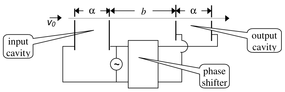
An electron beam with an initial speed \(v_0\) traverses the entire system, passing through small holes in the plates. The high-frequency voltage to be amplified is applied to both pairs of plates with a certain phase difference (where period \(T\) corresponds to \(2\pi\) phase) between them, producing horizontal, alternating electric fields in the cavities. The electrons entering the input cavity when the electric field is to the right are retarded and vice versa, so that the emerging electrons form bunches at a certain distance. If the output cavity is placed at the bunching point, the electric field in this cavity will absorb power from the beam provided that its phase is appropriately chosen. Let the voltage signal be a square wave with period \(T=1.0\times10^{-9}\ \mathrm{s}\), changing between \(V=\pm0.5\) volts. The initial velocity of the electrons is \(v_0=2.0\times10^6\ \mathrm{m/s}\) and the charge to mass ratio is \(e/m=1.76\times10^{11}\ \mathrm{C/kg}\). The distance \(\alpha\) is so small that the transit time in the cavities can be neglected. Keeping 4 significant figures, calculate;
a) the distance \(b\), where the electrons bunch. Copy your result onto the answer form. [1.5 pts]
b) the necessary phase difference to be provided by the phase shifter. Copy your result onto the answer form. [1.0 pts]
1b) INTERMOLECULAR DISTANCE
Let \(d_L\) and \(d_V\) represent the average distances between molecules of water in the liquid phase and in the vapor phase, respectively. Assume that both phases are at \(100\ ^\circ\mathrm{C}\) and atmospheric pressure, and the vapor behaves like an ideal gas. Using the following data, calculate the ratio \(d_V/d_L\) and copy your result onto the answer form. [2.5 pts]
Density of water in liquid phase: \(\rho_L=1.0\times10^3\ \mathrm{kg/m^3}\),
Molar mass of water: \(M=1.8\times10^{-2}\ \mathrm{kg/mol}\)
Atmospheric pressure: \(P_a=1.0\times10^5\ \mathrm{N/m^2}\)
Gas constant: \(R=8.3\) J/mol. K
Avagadro’s number: \(N_A=6.0\times10^{23}\) /mol
1c) SIMPLE SAWTOOTH SIGNAL GENERATOR
A sawtooth voltage waveform \(V_0\) can be obtained across the capacitor \(C\) in Fig. 1. \(R\) is a variable resistor, \(V_i\) is an ideal battery, and \(SG\) is a spark gap consisting of two electrodes with an adjustable distance between them. When the voltage across the electrodes exceeds the firing voltage \(V_f\), the air between the electrodes breaks down, hence the gap becomes a short circuit and remains so until the voltage across the gap becomes very small.
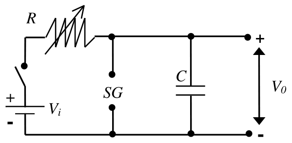
Figure 1
a) Draw the voltage waveform \(V_0\) versus time \(t\), after the switch is closed. [0.5 pts]
b) What condition must be satisfied in order to have an almost linearly varying sawtooth voltage waveform \(V_0\)? Copy your result onto the answer form. [0.2 pts]
c) Provided that this condition is satisfied, derive a simplified expression for the period \(T\) of the waveform. Copy your result onto the answer form. [0.4 pts]
d) What should you vary( \(R\) and/or \(SG\) ) to change the period only? Copy your result onto the answer form. [0.2 pts]
e) What should you vary ( \(R\) and/or \(SG\) ) to change the amplitude only? Copy your result onto the answer form. [0.2 pts]
f) You are given an additional, adjustable DC voltage supply. Design and draw a new circuit indicating the terminals where you would obtain the voltage waveform \(V_0'\) described in Fig. 2. [1.0 pts]
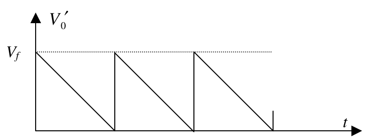
Figure 2
1d) ATOMIC BEAM
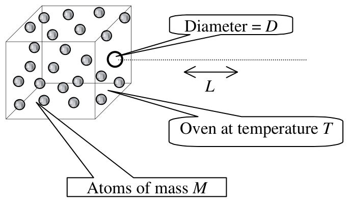
An atomic beam is prepared by heating a collection of atoms to a temperature \(T\) and allowing them to emerge horizontally through a small hole (of atomic dimensions) of diameter \(D\) in one side of the oven. Estimate the diameter of the beam after it has traveled a horizontal length \(L\) along its path. The mass of an atom is \(M\). Copy your result onto the answer form. [2.5 pts]
Official English text of the problem.
Answers
-
1a(a): \[ \boxed{b=2.270\times10^{-2}\ \mathrm{m}=2.270\ \mathrm{cm}}. \]
-
1a(b): The output field must lag the input field by \[ \boxed{\Delta\phi_{\mathrm{lag}}=3.821\ \mathrm{rad}=218.9^\circ} \] modulo \(2\pi\). Equivalently, it may lead by \(2.462\ \mathrm{rad}=141.1^\circ\). The output’s retarding half-cycle must coincide with the arriving bunch.
-
1b: \[ \boxed{\frac{d_V}{d_L} =\left(\frac{\rho_LRT}{P_aM}\right)^{1/3} \simeq 12}. \]
-
1c(a): Repeated, concave-down exponential rises from approximately \(0\) to \(V_f\), followed by nearly vertical drops to \(0\). Each charging segment is \[ V_0=V_i\left(1-e^{-\tau/(RC)}\right), \] where \(\tau\) is the time since the last discharge.
-
1c(b): \[ \boxed{V_f\ll V_i}. \]
-
1c(c): \[ \boxed{T\simeq RC\,\frac{V_f}{V_i}}. \]
-
1c(d): Vary \(R\) only, keeping the spark gap fixed.
-
1c(e): Vary both \(SG\) and \(R\): change the gap to change \(V_f\), and adjust \(R\) so that \[ \boxed{RV_f=\text{constant}} \] in the linear-ramp approximation.
-
1c(f): Set the additional supply to \(V_f\), with its negative terminal connected to the original lower rail. Measure the output with its positive terminal at the additional supply’s positive terminal and its negative terminal at the capacitor’s upper terminal. Then \[ \boxed{V_0'=V_f-V_0}, \] giving a descending ramp from \(V_f\) to \(0\), followed by an abrupt return to \(V_f\).
-
1d: Using a representative thermal speed \(v_{\mathrm{th}}=\sqrt{3k_BT/M}\), the diffraction estimate is \[ \boxed{ d_{\mathrm{beam}}\sim D+\frac{2hL}{D\sqrt{3Mk_BT}} }. \] Thus, when diffraction dominates the initial diameter, \[ \boxed{d_{\mathrm{beam}}\sim\frac{hL}{D\sqrt{Mk_BT}}}, \] up to a numerical factor depending on the beam-width convention.
Solution
1a) Klystron
(a) Bunching distance
Let \(e\) denote the magnitude of the electron charge and let \(U=0.5\ \mathrm{V}\). Neglect space-charge effects and the transit time through either cavity, as intended in the problem.
Nonrelativistic energy conservation gives the two possible speeds after the input cavity:
\[ \frac12mv_s^2=\frac12mv_0^2-eU, \qquad \frac12mv_f^2=\frac12mv_0^2+eU, \]
where \(v_s\) and \(v_f\) are the slow and fast speeds. Hence
\[ v_s=\sqrt{v_0^2-2(e/m)U} =1.955505\ldots\times10^6\ \mathrm{m/s}, \]
\[ v_f=\sqrt{v_0^2+2(e/m)U} =2.043526\ldots\times10^6\ \mathrm{m/s}. \]
Choose the input field to retard electrons during \(0\leq t<T/2\), and to accelerate them during \(T/2\leq t<T\).
A slow electron entering at time \(t_0\) and a fast electron entering at \(t_0+T/2\) reach the output together when
\[ t_0+\frac{b}{v_s} =t_0+\frac{T}{2}+\frac{b}{v_f}. \]
Therefore,
\[ b\left(\frac1{v_s}-\frac1{v_f}\right)=\frac{T}{2}, \]
so that
\[ \boxed{b=\frac{T\,v_sv_f}{2(v_f-v_s)}}. \]
For a square-wave modulation, this condition makes the entire slow half-cycle packet overlap in arrival time with the following fast half-cycle packet. It is the first maximum-bunching distance; the bunch has finite duration rather than being an instantaneous pulse.
Substitution, retaining extra digits until the final step, gives
\[ b=0.022699764\ldots\ \mathrm{m}. \]
Thus, to four significant figures,
\[ \boxed{b=0.02270\ \mathrm{m}=2.270\ \mathrm{cm}}. \]
(b) Phase difference
The slow and fast flight times across the drift region are
\[ \tau_s=\frac{b}{v_s}=11.6081337\ldots\,T, \qquad \tau_f=\frac{b}{v_f}=11.1081337\ldots\,T. \]
The slow packet reaches the output during
\[ [\tau_s,\tau_s+T/2), \]
while the following fast packet reaches it during
\[ [T/2+\tau_f,T+\tau_f). \]
These intervals coincide because \(\tau_s-\tau_f=T/2\).
To extract energy from the beam, the output electric field must point to the right throughout this occupied half-cycle, thereby retarding the electrons. Thus its waveform must reproduce the input waveform delayed by \(\tau_s\):
\[ E_{\mathrm{out}}(t)=E_{\mathrm{in}}(t-\tau_s). \]
Only the fractional part of \(\tau_s/T\) matters:
\[ \frac{\tau_s\bmod T}{T}=0.6081337\ldots. \]
The required output phase lag is therefore
\[ \Delta\phi_{\mathrm{lag}} =2\pi(0.6081337\ldots) =3.8210167\ldots\ \mathrm{rad}. \]
Hence
\[ \boxed{\Delta\phi_{\mathrm{lag}}=3.821\ \mathrm{rad}=218.9^\circ}. \]
If phase is instead written as an additive argument, \(E_{\mathrm{out}}\propto s(\omega t+\phi)\), the same setting is
\[ \boxed{\phi=-3.821\ \mathrm{rad} \equiv 2.462\ \mathrm{rad}\pmod{2\pi}}. \]
1b) Intermolecular distance
For molecular number density \(n\), the characteristic intermolecular spacing is estimated by assigning a volume \(d^3\) to each molecule:
\[ d\sim n^{-1/3}. \]
The liquid’s number density is
\[ n_L=\frac{\rho_LN_A}{M}, \]
so
\[ d_L=\left(\frac{M}{\rho_LN_A}\right)^{1/3}. \]
For the ideal vapor,
\[ P_aV=\frac{N}{N_A}RT, \]
and therefore
\[ n_V=\frac{N}{V}=\frac{P_aN_A}{RT}, \qquad d_V=\left(\frac{RT}{P_aN_A}\right)^{1/3}. \]
Taking the ratio cancels Avogadro’s number:
\[ \frac{d_V}{d_L} =\left(\frac{\rho_LRT}{P_aM}\right)^{1/3}. \]
Using \(T\simeq373\ \mathrm{K}\),
\[ \frac{d_V}{d_L} = \left[ \frac{(1.0\times10^3)(8.3)(373)} {(1.0\times10^5)(1.8\times10^{-2})} \right]^{1/3} =11.9813\ldots. \]
Thus, consistently with the supplied data,
\[ \boxed{\frac{d_V}{d_L}\simeq 12}. \]
The corresponding characteristic distances are approximately
\[ d_L=3.1\times10^{-10}\ \mathrm{m}, \qquad d_V=3.7\times10^{-9}\ \mathrm{m}. \]
1c) Simple sawtooth signal generator
Assume the capacitor is initially uncharged, the residual voltage after a spark is negligible, and discharge takes much less time than charging.
(a) Voltage waveform
While the spark gap is nonconducting, Kirchhoff’s voltage law gives
\[ V_i=IR+V_0, \qquad I=C\frac{dV_0}{dt}. \]
Consequently,
\[ RC\frac{dV_0}{dt}=V_i-V_0. \]
Starting from \(V_0=0\), the charging solution is
\[ \boxed{V_0(\tau)=V_i\left(1-e^{-\tau/(RC)}\right)}. \]
When \(V_0\) reaches \(V_f\), the spark gap conducts and rapidly discharges the capacitor. The gap then becomes nonconducting, and charging begins again.
The requested sketch therefore has:
- An initial point at \((t,V_0)=(0,0)\).
- A rising, concave-down exponential segment ending at \(V_f\).
- A nearly vertical drop from \(V_f\) to \(0\).
- Identical repetitions at regular intervals.
If continued without firing, each charging segment would approach the asymptote \(V_i\). Sustained oscillation requires \(V_i>V_f\); otherwise the capacitor cannot reach the firing threshold in finite time.
(b) Condition for an almost linear ramp
The charging slope is
\[ \frac{dV_0}{dt}=\frac{V_i-V_0}{RC}. \]
It remains nearly constant throughout \(0\leq V_0\leq V_f\) if
\[ \boxed{V_f\ll V_i}. \]
Then
\[ \frac{dV_0}{dt}\simeq\frac{V_i}{RC}, \qquad V_0(\tau)\simeq\frac{V_i}{RC}\tau. \]
(c) Period
Neglecting the discharge duration, the exact charging time to the threshold follows from
\[ V_f=V_i\left(1-e^{-T/(RC)}\right). \]
Thus,
\[ T=RC\ln\left(\frac{V_i}{V_i-V_f}\right). \]
For \(V_f/V_i\ll1\), use \(-\ln(1-x)\simeq x\):
\[ \boxed{T\simeq RC\frac{V_f}{V_i}}. \]
Equivalently, the nearly constant charging current \(V_i/R\) must deliver the charge \(CV_f\), giving the same result.
(d) Changing the period only
The peak voltage is fixed by the spark-gap threshold \(V_f\), while the charging time is proportional to \(R\).
Therefore, vary \(R\) only, keeping \(SG\) fixed. Increasing \(R\) increases the period without changing the peak-to-peak amplitude.
(e) Changing the amplitude only
The peak-to-peak amplitude is approximately \(V_f\). Change the electrode separation of \(SG\) to change this threshold.
Because
\[ T\simeq \frac{C}{V_i}RV_f, \]
keeping the period constant requires
\[ \boxed{R_{\mathrm{new}}V_{f,\mathrm{new}} =R_{\mathrm{old}}V_{f,\mathrm{old}}}. \]
Thus both \(SG\) and \(R\) must be adjusted. For example, increasing the firing voltage requires a compensating decrease in resistance.
Without the linear approximation, the corresponding exact condition is
\[ R\ln\left(\frac{V_i}{V_i-V_f}\right)=\text{constant}. \]
(f) Circuit for the descending sawtooth
Define the original circuit’s lower rail as node \(G\), and the capacitor’s upper terminal as node \(A\). Then
\[ V(A)-V(G)=V_0. \]
Make the following connections:
- Retain the original oscillator circuit.
- Connect the additional DC supply’s negative terminal to \(G\).
- Adjust this supply to \(V_f\), and call its positive terminal \(B\).
- Take the new output between \(B\) and \(A\), with positive at \(B\) and negative at \(A\).
For a high-impedance output measurement,
\[ V_0'=V(B)-V(A)=V_f-V_0. \]
During each nearly linear charging interval,
\[ V_0'\simeq V_f-\frac{V_i}{RC}\tau =V_f\left(1-\frac{\tau}{T}\right). \]
Thus the output starts at \(V_f\), falls almost linearly to \(0\), and jumps back to \(V_f\) when the spark discharges the capacitor. These are precisely the intercepts, slopes, and jumps shown in Fig. 2.
1d) Atomic beam
The atomic-scale opening produces quantum diffraction. Let \(h\) be Planck’s constant and \(k_B\) Boltzmann’s constant.
A representative thermal speed follows from equipartition:
\[ \frac12Mv_{\mathrm{th}}^2=\frac32k_BT, \]
giving
\[ v_{\mathrm{th}}=\sqrt{\frac{3k_BT}{M}}, \qquad p_{\mathrm{th}}=Mv_{\mathrm{th}}=\sqrt{3Mk_BT}. \]
This uses the rms thermal speed as a representative speed; an estimate does not require resolving the full distribution of emerging velocities.
The corresponding de Broglie wavelength is
\[ \lambda=\frac{h}{p_{\mathrm{th}}} =\frac{h}{\sqrt{3Mk_BT}}. \]
For an opening of width \(D\), the characteristic diffraction half-angle satisfies
\[ \theta\sim\frac{\lambda}{D}. \]
This follows because an angular deflection \(\theta\) produces a path difference of order \(D\theta\) across the opening; appreciable diffraction occurs when that difference is comparable with \(\lambda\).
For small angles, propagation over distance \(L\) increases the beam radius by approximately \(L\theta\). A simple diameter estimate is therefore
\[ d_{\mathrm{beam}}\sim D+2L\theta, \]
or
\[ \boxed{ d_{\mathrm{beam}}\sim D+\frac{2hL}{D\sqrt{3Mk_BT}} }. \]
The initial aperture diameter matters when spreading is small. When diffraction dominates,
\[ \boxed{ d_{\mathrm{beam}}\sim\frac{hL}{D\sqrt{Mk_BT}} } \]
up to numerical factors of order unity.
For a more specific convention, the first diffraction minimum of an ideal circular aperture occurs at \(\theta\simeq1.22\lambda/D\). Its far-field central-disk diameter would therefore be
\[ d_{\mathrm{first\ minimum}} \simeq \frac{2.44hL}{D\sqrt{3Mk_BT}}. \]
The small-angle estimates require \(\lambda/D\ll1\). If this ratio is not small, the emerging wave is broadly divergent.
The solution was checked against the official solution.
IPhO 2001 · Theorieaufgabe 1
Vier kurze Aufgaben: 1a Klystron, 1b Intermolekularer Abstand, 1c Einfacher Sägezahnsignalgenerator, 1d Atomstrahl
1a) KLYSTRON
Klystrons sind Geräte zur Verstärkung sehr hochfrequenter Signale. Ein Klystron besteht im Wesentlichen aus zwei identischen Paaren paralleler Platten (Resonatoren), die sich im Abstand \(b\) voneinander befinden, wie in der Abbildung dargestellt.
Ein Elektronenstrahl mit der Anfangsgeschwindigkeit \(v_0\) durchläuft das gesamte System und tritt dabei durch kleine Löcher in den Platten. Die zu verstärkende hochfrequente Spannung wird mit einer bestimmten Phasendifferenz zwischen den beiden Plattenpaaren angelegt (wobei die Periodendauer \(T\) einer Phase von \(2\pi\) entspricht) und erzeugt in den Resonatoren horizontale elektrische Wechselfelder. Elektronen, die in den Eingangsresonator eintreten, während das elektrische Feld nach rechts gerichtet ist, werden abgebremst und umgekehrt, sodass die austretenden Elektronen in einem bestimmten Abstand Pakete bilden. Wird der Ausgangsresonator an der Stelle der Paketbildung angeordnet, so nimmt das elektrische Feld in diesem Resonator Leistung aus dem Strahl auf, sofern seine Phase passend gewählt ist. Das Spannungssignal sei ein Rechtecksignal mit der Periodendauer \(T=1.0\times10^{-9}\ \mathrm{s}\), das zwischen \(V=\pm0.5\) Volt wechselt. Die Anfangsgeschwindigkeit der Elektronen beträgt \(v_0=2.0\times10^6\ \mathrm{m/s}\), und das Verhältnis von Ladung zu Masse ist \(e/m=1.76\times10^{11}\ \mathrm{C/kg}\). Der Abstand \(\alpha\) ist so klein, dass die Durchlaufzeit in den Resonatoren vernachlässigt werden kann. Berechnen Sie mit 4 signifikanten Stellen:
a) den Abstand \(b\), bei dem sich die Elektronen zu Paketen bündeln. Übertragen Sie Ihr Ergebnis auf das Antwortblatt. [1.5 Punkte]
b) die erforderliche Phasendifferenz, die der Phasenschieber erzeugen muss. Übertragen Sie Ihr Ergebnis auf das Antwortblatt. [1.0 Punkte]
1b) INTERMOLEKULARER ABSTAND
\(d_L\) und \(d_V\) bezeichnen die mittleren Abstände zwischen Wassermolekülen in der flüssigen Phase beziehungsweise in der Dampfphase. Nehmen Sie an, dass beide Phasen bei \(100\ ^\circ\mathrm{C}\) und Atmosphärendruck vorliegen und sich der Dampf wie ein ideales Gas verhält. Berechnen Sie anhand der folgenden Daten das Verhältnis \(d_V/d_L\) und übertragen Sie Ihr Ergebnis auf das Antwortblatt. [2.5 Punkte]
Dichte von Wasser in der flüssigen Phase: \(\rho_L=1.0\times10^3\ \mathrm{kg/m^3}\),
Molare Masse von Wasser: \(M=1.8\times10^{-2}\ \mathrm{kg/mol}\)
Atmosphärendruck: \(P_a=1.0\times10^5\ \mathrm{N/m^2}\)
Gaskonstante: \(R=8.3\) J/mol. K
Avogadro-Konstante: \(N_A=6.0\times10^{23}\) /mol
1c) EINFACHER SÄGEZAHNSIGNALGENERATOR
Am Kondensator \(C\) in Abb. 1 lässt sich eine Sägezahnspannung \(V_0\) abgreifen. \(R\) ist ein veränderlicher Widerstand, \(V_i\) eine ideale Batterie und \(SG\) eine Funkenstrecke aus zwei Elektroden mit einstellbarem Abstand. Wenn die Spannung zwischen den Elektroden die Zündspannung \(V_f\) überschreitet, kommt es zu einem elektrischen Durchschlag der Luft zwischen den Elektroden. Die Funkenstrecke wird dadurch zu einem Kurzschluss und bleibt in diesem Zustand, bis die Spannung an ihr sehr klein geworden ist.
Abbildung 1
a) Zeichnen Sie den zeitlichen Verlauf der Spannung \(V_0\) in Abhängigkeit von \(t\) nach dem Schließen des Schalters. [0.5 Punkte]
b) Welche Bedingung muss erfüllt sein, damit die Sägezahnspannung \(V_0\) nahezu linear verläuft? Übertragen Sie Ihr Ergebnis auf das Antwortblatt. [0.2 Punkte]
c) Leiten Sie unter der Voraussetzung, dass diese Bedingung erfüllt ist, einen vereinfachten Ausdruck für die Periodendauer \(T\) des Signals her. Übertragen Sie Ihr Ergebnis auf das Antwortblatt. [0.4 Punkte]
d) Was müssen Sie verändern (\(R\) und/oder \(SG\)), um nur die Periodendauer zu ändern? Übertragen Sie Ihr Ergebnis auf das Antwortblatt. [0.2 Punkte]
e) Was müssen Sie verändern (\(R\) und/oder \(SG\)), um nur die Amplitude zu ändern? Übertragen Sie Ihr Ergebnis auf das Antwortblatt. [0.2 Punkte]
f) Ihnen steht eine zusätzliche einstellbare Gleichspannungsquelle zur Verfügung. Entwerfen und zeichnen Sie eine neue Schaltung und kennzeichnen Sie die Anschlüsse, an denen Sie den in Abb. 2 dargestellten Spannungsverlauf \(V_0'\) erhalten würden. [1.0 Punkte]
Abbildung 2
1d) ATOMSTRAHL
Ein Atomstrahl wird erzeugt, indem eine Ansammlung von Atomen auf die Temperatur \(T\) erhitzt wird und die Atome durch eine kleine Öffnung (mit atomaren Abmessungen) vom Durchmesser \(D\) in einer Seitenwand des Ofens horizontal austreten können. Schätzen Sie den Durchmesser des Strahls ab, nachdem er entlang seiner Bahn eine horizontale Strecke \(L\) zurückgelegt hat. Die Masse eines Atoms beträgt \(M\). Übertragen Sie Ihr Ergebnis auf das Antwortblatt. [2.5 Punkte]
Aufgabentext aus dem offiziellen englischen Text übersetzt.
Antworten
-
1a(a): \[ \boxed{b=2.270\times10^{-2}\ \mathrm{m}=2.270\ \mathrm{cm}}. \]
-
1a(b): Das Ausgangsfeld muss dem Eingangsfeld um \[ \boxed{\Delta\phi_{\mathrm{lag}}=3.821\ \mathrm{rad}=218.9^\circ} \] modulo \(2\pi\) nacheilen. Gleichwertig dazu kann es um \(2.462\ \mathrm{rad}=141.1^\circ\) voreilen. Die abbremsende Halbperiode des Ausgangsfelds muss mit dem eintreffenden Elektronenpaket zusammenfallen.
-
1b: \[ \boxed{\frac{d_V}{d_L} =\left(\frac{\rho_LRT}{P_aM}\right)^{1/3} \simeq 12}. \]
-
1c(a): Wiederholte, nach unten gekrümmte exponentielle Anstiege von ungefähr \(0\) bis \(V_f\), gefolgt von nahezu senkrechten Abfällen auf \(0\). Jeder Ladeabschnitt wird beschrieben durch \[ V_0=V_i\left(1-e^{-\tau/(RC)}\right), \] wobei \(\tau\) die seit der letzten Entladung vergangene Zeit ist.
-
1c(b): \[ \boxed{V_f\ll V_i}. \]
-
1c(c): \[ \boxed{T\simeq RC\,\frac{V_f}{V_i}}. \]
-
1c(d): Verändern Sie nur \(R\) und lassen Sie die Funkenstrecke unverändert.
-
1c(e): Verändern Sie sowohl \(SG\) als auch \(R\): Ändern Sie den Elektrodenabstand, um \(V_f\) zu ändern, und passen Sie \(R\) so an, dass in der Näherung eines linearen Anstiegs \[ \boxed{RV_f=\text{konstant}} \] gilt.
-
1c(f): Stellen Sie die zusätzliche Spannungsquelle auf \(V_f\) ein und verbinden Sie ihren Minuspol mit der ursprünglichen unteren Leitung. Messen Sie die Ausgangsspannung mit dem positiven Messanschluss am Pluspol der zusätzlichen Spannungsquelle und dem negativen Messanschluss am oberen Anschluss des Kondensators. Dann gilt \[ \boxed{V_0'=V_f-V_0}, \] wodurch eine abfallende Rampe von \(V_f\) auf \(0\) entsteht, gefolgt von einem abrupten Rücksprung auf \(V_f\).
-
1d: Mit einer repräsentativen thermischen Geschwindigkeit \(v_{\mathrm{th}}=\sqrt{3k_BT/M}\) ergibt die Abschätzung anhand der Beugung \[ \boxed{ d_{\mathrm{beam}}\sim D+\frac{2hL}{D\sqrt{3Mk_BT}} }. \] Wenn somit die Beugungsaufweitung gegenüber dem Anfangsdurchmesser dominiert, gilt \[ \boxed{d_{\mathrm{beam}}\sim\frac{hL}{D\sqrt{Mk_BT}}}, \] bis auf einen Zahlenfaktor, der von der Definition der Strahlbreite abhängt.
Lösung
1a) Klystron
(a) Abstand der Paketbildung
\(e\) bezeichne den Betrag der Elektronenladung, und es sei \(U=0.5\ \mathrm{V}\). Vernachlässigen Sie Raumladungseffekte und die Durchlaufzeit durch beide Resonatoren, wie in der Aufgabenstellung vorgesehen.
Aus der nichtrelativistischen Energieerhaltung ergeben sich die beiden möglichen Geschwindigkeiten nach dem Eingangsresonator:
\[ \frac12mv_s^2=\frac12mv_0^2-eU, \qquad \frac12mv_f^2=\frac12mv_0^2+eU, \]
wobei \(v_s\) und \(v_f\) die langsame beziehungsweise schnelle Geschwindigkeit sind. Somit gilt
\[ v_s=\sqrt{v_0^2-2(e/m)U} =1.955505\ldots\times10^6\ \mathrm{m/s}, \]
\[ v_f=\sqrt{v_0^2+2(e/m)U} =2.043526\ldots\times10^6\ \mathrm{m/s}. \]
Wählen Sie das Eingangsfeld so, dass es die Elektronen während \(0\leq t<T/2\) abbremst und während \(T/2\leq t<T\) beschleunigt.
Ein langsames Elektron, das zum Zeitpunkt \(t_0\) eintritt, und ein schnelles Elektron, das bei \(t_0+T/2\) eintritt, erreichen den Ausgang gleichzeitig, wenn
\[ t_0+\frac{b}{v_s} =t_0+\frac{T}{2}+\frac{b}{v_f}. \]
Daher gilt
\[ b\left(\frac1{v_s}-\frac1{v_f}\right)=\frac{T}{2}, \]
sodass
\[ \boxed{b=\frac{T\,v_sv_f}{2(v_f-v_s)}}. \]
Bei einer Rechteckmodulation bewirkt diese Bedingung, dass sich das gesamte langsame Halbperiodenpaket hinsichtlich der Ankunftszeit mit dem nachfolgenden schnellen Halbperiodenpaket überlagert. Dies ist der erste Abstand maximaler Bündelung; das Paket hat eine endliche Dauer und ist kein augenblicklicher Impuls.
Durch Einsetzen, wobei zusätzliche Stellen bis zum letzten Rechenschritt beibehalten werden, ergibt sich
\[ b=0.022699764\ldots\ \mathrm{m}. \]
Auf vier signifikante Stellen erhält man somit
\[ \boxed{b=0.02270\ \mathrm{m}=2.270\ \mathrm{cm}}. \]
(b) Phasendifferenz
Die Flugzeiten der langsamen und schnellen Elektronen durch den Driftraum betragen
\[ \tau_s=\frac{b}{v_s}=11.6081337\ldots\,T, \qquad \tau_f=\frac{b}{v_f}=11.1081337\ldots\,T. \]
Das langsame Paket erreicht den Ausgang während des Zeitintervalls
\[ [\tau_s,\tau_s+T/2), \]
während das nachfolgende schnelle Paket ihn in folgendem Zeitintervall erreicht:
\[ [T/2+\tau_f,T+\tau_f). \]
Diese Intervalle stimmen überein, da \(\tau_s-\tau_f=T/2\) gilt.
Um dem Strahl Energie zu entziehen, muss das elektrische Ausgangsfeld während dieser gesamten mit Elektronen besetzten Halbperiode nach rechts gerichtet sein und dadurch die Elektronen abbremsen. Sein zeitlicher Verlauf muss daher den Verlauf des Eingangsfelds um \(\tau_s\) verzögert wiedergeben:
\[ E_{\mathrm{out}}(t)=E_{\mathrm{in}}(t-\tau_s). \]
Nur der Nachkommaanteil von \(\tau_s/T\) ist von Bedeutung:
\[ \frac{\tau_s\bmod T}{T}=0.6081337\ldots. \]
Die erforderliche Phasenverzögerung des Ausgangsfelds beträgt daher
\[ \Delta\phi_{\mathrm{lag}} =2\pi(0.6081337\ldots) =3.8210167\ldots\ \mathrm{rad}. \]
Somit gilt
\[ \boxed{\Delta\phi_{\mathrm{lag}}=3.821\ \mathrm{rad}=218.9^\circ}. \]
Wird die Phase stattdessen als additiver Term im Argument geschrieben, \(E_{\mathrm{out}}\propto s(\omega t+\phi)\), entspricht dieselbe Einstellung
\[ \boxed{\phi=-3.821\ \mathrm{rad} \equiv 2.462\ \mathrm{rad}\pmod{2\pi}}. \]
1b) Intermolekularer Abstand
Bei einer molekularen Anzahldichte \(n\) lässt sich der charakteristische intermolekulare Abstand abschätzen, indem jedem Molekül ein Volumen \(d^3\) zugeordnet wird:
\[ d\sim n^{-1/3}. \]
Die Anzahldichte der Flüssigkeit ist
\[ n_L=\frac{\rho_LN_A}{M}, \]
also gilt
\[ d_L=\left(\frac{M}{\rho_LN_A}\right)^{1/3}. \]
Für den idealen Dampf gilt
\[ P_aV=\frac{N}{N_A}RT, \]
und daher
\[ n_V=\frac{N}{V}=\frac{P_aN_A}{RT}, \qquad d_V=\left(\frac{RT}{P_aN_A}\right)^{1/3}. \]
Bei der Bildung des Verhältnisses kürzt sich die Avogadro-Konstante heraus:
\[ \frac{d_V}{d_L} =\left(\frac{\rho_LRT}{P_aM}\right)^{1/3}. \]
Mit \(T\simeq373\ \mathrm{K}\) folgt
\[ \frac{d_V}{d_L} = \left[ \frac{(1.0\times10^3)(8.3)(373)} {(1.0\times10^5)(1.8\times10^{-2})} \right]^{1/3} =11.9813\ldots. \]
Entsprechend der Genauigkeit der gegebenen Daten ergibt sich somit
\[ \boxed{\frac{d_V}{d_L}\simeq 12}. \]
Die zugehörigen charakteristischen Abstände betragen ungefähr
\[ d_L=3.1\times10^{-10}\ \mathrm{m}, \qquad d_V=3.7\times10^{-9}\ \mathrm{m}. \]
1c) Einfacher Sägezahnsignalgenerator
Es wird angenommen, dass der Kondensator anfangs ungeladen ist, die Restspannung nach einer Funkenentladung vernachlässigbar ist und die Entladung wesentlich weniger Zeit beansprucht als das Aufladen.
(a) Spannungsverlauf
Solange die Funkenstrecke nichtleitend ist, liefert die Kirchhoffsche Maschenregel
\[ V_i=IR+V_0, \qquad I=C\frac{dV_0}{dt}. \]
Folglich gilt
\[ RC\frac{dV_0}{dt}=V_i-V_0. \]
Ausgehend von \(V_0=0\) lautet die Lösung für den Ladevorgang
\[ \boxed{V_0(\tau)=V_i\left(1-e^{-\tau/(RC)}\right)}. \]
Wenn \(V_0\) den Wert \(V_f\) erreicht, wird die Funkenstrecke leitend und entlädt den Kondensator rasch. Anschließend wird die Funkenstrecke wieder nichtleitend, und der Ladevorgang beginnt erneut.
Die verlangte Skizze weist daher Folgendes auf:
- Einen Anfangspunkt bei \((t,V_0)=(0,0)\).
- Einen ansteigenden, nach unten gekrümmten exponentiellen Abschnitt, der bei \(V_f\) endet.
- Einen nahezu senkrechten Abfall von \(V_f\) auf \(0\).
- Identische Wiederholungen in regelmäßigen Abständen.
Würde jeder Ladeabschnitt ohne Zündung fortgesetzt, würde er sich der Asymptote \(V_i\) annähern. Eine anhaltende Schwingung setzt \(V_i>V_f\) voraus; andernfalls kann der Kondensator die Zündschwelle nicht in endlicher Zeit erreichen.
(b) Bedingung für einen nahezu linearen Anstieg
Die Steigung beim Aufladen beträgt
\[ \frac{dV_0}{dt}=\frac{V_i-V_0}{RC}. \]
Sie bleibt im gesamten Bereich \(0\leq V_0\leq V_f\) nahezu konstant, wenn
\[ \boxed{V_f\ll V_i}. \]
Dann gilt
\[ \frac{dV_0}{dt}\simeq\frac{V_i}{RC}, \qquad V_0(\tau)\simeq\frac{V_i}{RC}\tau. \]
(c) Periodendauer
Unter Vernachlässigung der Entladedauer folgt die exakte Ladezeit bis zur Schwelle aus
\[ V_f=V_i\left(1-e^{-T/(RC)}\right). \]
Somit gilt
\[ T=RC\ln\left(\frac{V_i}{V_i-V_f}\right). \]
Für \(V_f/V_i\ll1\) verwendet man \(-\ln(1-x)\simeq x\):
\[ \boxed{T\simeq RC\frac{V_f}{V_i}}. \]
Gleichwertig dazu muss der nahezu konstante Ladestrom \(V_i/R\) die Ladung \(CV_f\) zuführen, was zum selben Ergebnis führt.
(d) Änderung nur der Periodendauer
Die Spitzenspannung wird durch die Zündschwelle \(V_f\) der Funkenstrecke festgelegt, während die Ladezeit proportional zu \(R\) ist.
Verändern Sie daher nur \(R\) und lassen Sie \(SG\) unverändert. Eine Erhöhung von \(R\) verlängert die Periodendauer, ohne die Spitze-Spitze-Amplitude zu verändern.
(e) Änderung nur der Amplitude
Die Spitze-Spitze-Amplitude beträgt ungefähr \(V_f\). Ändern Sie den Elektrodenabstand von \(SG\), um diese Schwelle zu verändern.
Da
\[ T\simeq \frac{C}{V_i}RV_f, \]
muss für eine konstante Periodendauer gelten:
\[ \boxed{R_{\mathrm{new}}V_{f,\mathrm{new}} =R_{\mathrm{old}}V_{f,\mathrm{old}}}. \]
Somit müssen sowohl \(SG\) als auch \(R\) angepasst werden. Eine Erhöhung der Zündspannung erfordert beispielsweise eine entsprechende Verringerung des Widerstands.
Ohne die lineare Näherung lautet die entsprechende exakte Bedingung
\[ R\ln\left(\frac{V_i}{V_i-V_f}\right)=\text{konstant}. \]
(f) Schaltung für die abfallende Sägezahnspannung
Bezeichnen Sie die untere Leitung der ursprünglichen Schaltung als Knoten \(G\) und den oberen Anschluss des Kondensators als Knoten \(A\). Dann gilt
\[ V(A)-V(G)=V_0. \]
Stellen Sie die folgenden Verbindungen her:
- Behalten Sie die ursprüngliche Oszillatorschaltung bei.
- Verbinden Sie den Minuspol der zusätzlichen Gleichspannungsquelle mit \(G\).
- Stellen Sie diese Spannungsquelle auf \(V_f\) ein und bezeichnen Sie ihren Pluspol mit \(B\).
- Greifen Sie die neue Ausgangsspannung zwischen \(B\) und \(A\) ab, mit dem positiven Anschluss an \(B\) und dem negativen Anschluss an \(A\).
Bei einer hochohmigen Messung der Ausgangsspannung gilt
\[ V_0'=V(B)-V(A)=V_f-V_0. \]
Während jedes nahezu linearen Ladeintervalls gilt
\[ V_0'\simeq V_f-\frac{V_i}{RC}\tau =V_f\left(1-\frac{\tau}{T}\right). \]
Die Ausgangsspannung beginnt somit bei \(V_f\), fällt nahezu linear auf \(0\) und springt auf \(V_f\) zurück, wenn der Funke den Kondensator entlädt. Dies sind genau die in Abb. 2 dargestellten Achsenabschnitte, Steigungen und Sprünge.
1d) Atomstrahl
Die Öffnung mit atomaren Abmessungen bewirkt quantenmechanische Beugung. \(h\) sei die Plancksche Konstante und \(k_B\) die Boltzmann-Konstante.
Eine repräsentative thermische Geschwindigkeit folgt aus dem Gleichverteilungssatz:
\[ \frac12Mv_{\mathrm{th}}^2=\frac32k_BT, \]
woraus sich ergibt:
\[ v_{\mathrm{th}}=\sqrt{\frac{3k_BT}{M}}, \qquad p_{\mathrm{th}}=Mv_{\mathrm{th}}=\sqrt{3Mk_BT}. \]
Hier wird die quadratisch gemittelte thermische Geschwindigkeit als repräsentative Geschwindigkeit verwendet; für eine Abschätzung muss die vollständige Geschwindigkeitsverteilung der austretenden Atome nicht bestimmt werden.
Die zugehörige De-Broglie-Wellenlänge ist
\[ \lambda=\frac{h}{p_{\mathrm{th}}} =\frac{h}{\sqrt{3Mk_BT}}. \]
Für eine Öffnung der Breite \(D\) erfüllt der charakteristische Beugungshalbwinkel die Beziehung
\[ \theta\sim\frac{\lambda}{D}. \]
Dies folgt daraus, dass eine Ablenkung um den Winkel \(\theta\) über die Öffnung hinweg einen Gangunterschied der Größenordnung \(D\theta\) erzeugt; merkliche Beugung tritt auf, wenn dieser Unterschied mit \(\lambda\) vergleichbar ist.
Für kleine Winkel vergrößert die Ausbreitung über die Strecke \(L\) den Strahlradius um ungefähr \(L\theta\). Eine einfache Abschätzung des Durchmessers lautet daher
\[ d_{\mathrm{beam}}\sim D+2L\theta, \]
oder
\[ \boxed{ d_{\mathrm{beam}}\sim D+\frac{2hL}{D\sqrt{3Mk_BT}} }. \]
Der anfängliche Öffnungsdurchmesser ist von Bedeutung, wenn die Aufweitung gering ist. Wenn die Beugung dominiert, gilt
\[ \boxed{ d_{\mathrm{beam}}\sim\frac{hL}{D\sqrt{Mk_BT}} } \]
bis auf Zahlenfaktoren der Größenordnung eins.
Für eine konkretere Definition liegt das erste Beugungsminimum einer idealen kreisförmigen Öffnung bei \(\theta\simeq1.22\lambda/D\). Der Durchmesser ihres zentralen Beugungsscheibchens im Fernfeld wäre daher
\[ d_{\mathrm{first\ minimum}} \simeq \frac{2.44hL}{D\sqrt{3Mk_BT}}. \]
Die Kleinwinkelabschätzungen setzen \(\lambda/D\ll1\) voraus. Ist dieses Verhältnis nicht klein, divergiert die austretende Welle stark.
Die Lösung wurde mit der offiziellen Lösung abgeglichen.
IPhO 2001 · Teori sorusu 1
Dört kısa problem: 1a Klistron, 1b Moleküller arası uzaklık, 1c Basit testere dişi sinyal üreteci, 1d Atom demeti
1a) KLİSTRON
Klistronlar, çok yüksek frekanslı sinyalleri yükseltmek için kullanılan aygıtlardır. Bir klistron temel olarak, şekilde gösterildiği gibi aralarında \(b\) uzaklığı bulunan, birbirinin aynı iki paralel levha çiftinden (kavite) oluşur.
Başlangıç sürati \(v_0\) olan bir elektron demeti, levhalardaki küçük deliklerden geçerek tüm sistemi kat eder. Yükseltilecek yüksek frekanslı gerilim, iki levha çiftine aralarında belirli bir faz farkı olacak şekilde uygulanır (burada \(T\) periyodu \(2\pi\) faza karşılık gelir); böylece kavitelerde yatay, yönü dönüşümlü olarak değişen elektrik alanlar oluşur. Elektrik alan sağa doğruyken giriş kavitesine giren elektronlar yavaşlatılır, alan ters yöndeyken ise hızlandırılır; böylece çıkan elektronlar belirli bir uzaklıkta demetçikler oluşturur. Çıkış kavitesi demetçiklerin oluştuğu noktaya yerleştirilirse, bu kavitedeki elektrik alan, fazı uygun seçilmek koşuluyla demetten güç soğurur. Gerilim sinyalinin, \(V=\pm0.5\) volt değerleri arasında değişen, \(T=1.0\times10^{-9}\ \mathrm{s}\) periyotlu bir kare dalga olduğunu kabul edin. Elektronların başlangıç hızı \(v_0=2.0\times10^6\ \mathrm{m/s}\), yüklerinin kütlelerine oranı ise \(e/m=1.76\times10^{11}\ \mathrm{C/kg}\) değerindedir. \(\alpha\) uzaklığı, kavitelerdeki geçiş süresi ihmal edilebilecek kadar küçüktür. 4 anlamlı basamak kullanarak aşağıdakileri hesaplayın:
a) Elektronların demetçikler oluşturduğu \(b\) uzaklığı. Sonucunuzu cevap formuna yazın. [1.5 puan]
b) Faz kaydırıcının sağlaması gereken faz farkı. Sonucunuzu cevap formuna yazın. [1.0 puan]
1b) MOLEKÜLLER ARASI UZAKLIK
\(d_L\) ve \(d_V\), sırasıyla sıvı fazdaki ve buhar fazındaki su molekülleri arasındaki ortalama uzaklıkları göstersin. Her iki fazın da \(100\ ^\circ\mathrm{C}\) sıcaklıkta ve atmosfer basıncında olduğunu, buharın ise ideal gaz gibi davrandığını varsayın. Aşağıdaki verileri kullanarak \(d_V/d_L\) oranını hesaplayın ve sonucunuzu cevap formuna yazın. [2.5 puan]
Sıvı fazdaki suyun yoğunluğu: \(\rho_L=1.0\times10^3\ \mathrm{kg/m^3}\),
Suyun molar kütlesi: \(M=1.8\times10^{-2}\ \mathrm{kg/mol}\)
Atmosfer basıncı: \(P_a=1.0\times10^5\ \mathrm{N/m^2}\)
Gaz sabiti: \(R=8.3\) J/mol. K
Avogadro sayısı: \(N_A=6.0\times10^{23}\) /mol
1c) BASİT TESTERE DİŞİ SİNYAL ÜRETECİ
Şekil 1'deki \(C\) kondansatörünün uçları arasında testere dişi biçiminde bir \(V_0\) gerilimi elde edilebilir. \(R\) değişken bir direnç, \(V_i\) ideal bir pil, \(SG\) ise aralarındaki uzaklık ayarlanabilen iki elektrottan oluşan bir kıvılcım aralığıdır. Elektrotlar arasındaki gerilim ateşleme gerilimi \(V_f\)'yi aştığında, elektrotlar arasındaki hava elektriksel olarak delinir; böylece aralık kısa devre hâline gelir ve uçları arasındaki gerilim çok küçük bir değere inene kadar bu durumda kalır.
Şekil 1
a) Anahtar kapatıldıktan sonra \(V_0\) geriliminin \(t\) zamanına göre dalga biçimini çizin. [0.5 puan]
b) Yaklaşık olarak doğrusal değişen testere dişi biçiminde bir \(V_0\) gerilimi elde etmek için hangi koşul sağlanmalıdır? Sonucunuzu cevap formuna yazın. [0.2 puan]
c) Bu koşulun sağlandığını kabul ederek dalga biçiminin \(T\) periyodu için basitleştirilmiş bir ifade türetin. Sonucunuzu cevap formuna yazın. [0.4 puan]
d) Yalnızca periyodu değiştirmek için neyi (\(R\) ve/veya \(SG\)) değiştirmelisiniz? Sonucunuzu cevap formuna yazın. [0.2 puan]
e) Yalnızca genliği değiştirmek için neyi (\(R\) ve/veya \(SG\)) değiştirmelisiniz? Sonucunuzu cevap formuna yazın. [0.2 puan]
f) Size ek bir ayarlanabilir doğru gerilim kaynağı veriliyor. Şekil 2'de gösterilen \(V_0'\) gerilim dalga biçimini elde edeceğiniz uçları belirterek yeni bir devre tasarlayın ve çizin. [1.0 puan]
Şekil 2
1d) ATOM DEMETİ
Bir atom topluluğu \(T\) sıcaklığına kadar ısıtılıp atomların fırının bir yanındaki \(D\) çaplı küçük (atomik boyutlarda) bir delikten yatay olarak çıkmaları sağlanarak bir atom demeti hazırlanır. Demetin, yolu boyunca yatay doğrultuda \(L\) uzaklığını kat ettikten sonraki çapını tahmin edin. Bir atomun kütlesi \(M\)'dir. Sonucunuzu cevap formuna yazın. [2.5 puan]
Soru metni resmi İngilizce metinden çevrilmiştir.
Cevaplar
-
1a(a): \[ \boxed{b=2.270\times10^{-2}\ \mathrm{m}=2.270\ \mathrm{cm}}. \]
-
1a(b): Çıkış alanının giriş alanına göre faz gecikmesi \[ \boxed{\Delta\phi_{\mathrm{lag}}=3.821\ \mathrm{rad}=218.9^\circ} \] değerinde, \(2\pi\) modunda olmalıdır. Eşdeğer olarak, \(2.462\ \mathrm{rad}=141.1^\circ\) önde olabilir. Çıkışın yavaşlatıcı yarım çevrimi, gelen demetçikle çakışmalıdır.
-
1b: \[ \boxed{\frac{d_V}{d_L} =\left(\frac{\rho_LRT}{P_aM}\right)^{1/3} \simeq 12}. \]
-
1c(a): Yaklaşık \(0\)'dan \(V_f\)'ye kadar tekrarlanan, aşağı doğru içbükey üstel yükselişler ve bunları izleyen, \(0\)'a kadar neredeyse düşey inişler. Her yüklenme parçası \[ V_0=V_i\left(1-e^{-\tau/(RC)}\right), \] biçimindedir; burada \(\tau\), son boşalmadan bu yana geçen süredir.
-
1c(b): \[ \boxed{V_f\ll V_i}. \]
-
1c(c): \[ \boxed{T\simeq RC\,\frac{V_f}{V_i}}. \]
-
1c(d): Kıvılcım aralığını sabit tutarak yalnızca \(R\)'yi değiştirin.
-
1c(e): Hem \(SG\)'yi hem de \(R\)'yi değiştirin: \(V_f\)'yi değiştirmek için aralığı değiştirin ve doğrusal rampa yaklaşımında \[ \boxed{RV_f=\text{sabit}} \] olacak şekilde \(R\)'yi ayarlayın.
-
1c(f): Ek kaynağın negatif ucunu özgün devrenin alt iletken hattına bağlayıp gerilimini \(V_f\)'ye ayarlayın. Çıkışı, pozitif ucu ek kaynağın pozitif ucunda ve negatif ucu kondansatörün üst ucunda olacak şekilde ölçün. Bu durumda \[ \boxed{V_0'=V_f-V_0}, \] olur; böylece \(V_f\)'den \(0\)'a inen bir rampa ve ardından \(V_f\)'ye ani bir dönüş elde edilir.
-
1d: Temsilî bir ısıl sürat olarak \(v_{\mathrm{th}}=\sqrt{3k_BT/M}\) kullanıldığında, kırınıma dayalı tahmin \[ \boxed{ d_{\mathrm{beam}}\sim D+\frac{2hL}{D\sqrt{3Mk_BT}} }. \] olur. Dolayısıyla, kırınımın etkisi başlangıç çapına baskın olduğunda, \[ \boxed{d_{\mathrm{beam}}\sim\frac{hL}{D\sqrt{Mk_BT}}}, \] elde edilir; burada demet genişliği için benimsenen tanıma bağlı sayısal bir çarpan göz ardı edilmiştir.
Çözüm
1a) Klistron
(a) Demetçik oluşma uzaklığı
\(e\), elektron yükünün büyüklüğünü göstersin ve \(U=0.5\ \mathrm{V}\) olsun. Soruda amaçlandığı üzere, uzay yükü etkilerini ve her iki kavitedeki geçiş süresini ihmal edin.
Göreli olmayan enerji korunumu, giriş kavitesinden sonraki iki olası sürati verir:
\[ \frac12mv_s^2=\frac12mv_0^2-eU, \qquad \frac12mv_f^2=\frac12mv_0^2+eU, \]
burada \(v_s\) ve \(v_f\), yavaş ve hızlı elektronların süratleridir. Dolayısıyla
\[ v_s=\sqrt{v_0^2-2(e/m)U} =1.955505\ldots\times10^6\ \mathrm{m/s}, \]
\[ v_f=\sqrt{v_0^2+2(e/m)U} =2.043526\ldots\times10^6\ \mathrm{m/s}. \]
Giriş alanını, \(0\leq t<T/2\) aralığında elektronları yavaşlatacak, \(T/2\leq t<T\) aralığında ise hızlandıracak şekilde seçin.
\(t_0\) anında giren yavaş bir elektron ile \(t_0+T/2\) anında giren hızlı bir elektron, şu koşul sağlandığında çıkışa birlikte ulaşır:
\[ t_0+\frac{b}{v_s} =t_0+\frac{T}{2}+\frac{b}{v_f}. \]
Bu nedenle,
\[ b\left(\frac1{v_s}-\frac1{v_f}\right)=\frac{T}{2}, \]
buradan da
\[ \boxed{b=\frac{T\,v_sv_f}{2(v_f-v_s)}}. \]
Kare dalga modülasyonunda bu koşul, yavaş yarım çevrim paketinin tamamının varış zamanlarının, onu izleyen hızlı yarım çevrim paketinin varış zamanlarıyla örtüşmesini sağlar. Bu, demetçik oluşumunun en yüksek düzeye ulaştığı ilk uzaklıktır; demetçik anlık bir darbe değil, sonlu süreli bir pakettir.
Son adıma kadar ek basamaklar korunarak değerler yerine konulduğunda
\[ b=0.022699764\ldots\ \mathrm{m}. \]
elde edilir. Böylece, dört anlamlı basamakla,
\[ \boxed{b=0.02270\ \mathrm{m}=2.270\ \mathrm{cm}}. \]
(b) Faz farkı
Yavaş ve hızlı elektronların sürüklenme bölgesini geçiş süreleri
\[ \tau_s=\frac{b}{v_s}=11.6081337\ldots\,T, \qquad \tau_f=\frac{b}{v_f}=11.1081337\ldots\,T. \]
şeklindedir. Yavaş paket çıkışa
\[ [\tau_s,\tau_s+T/2), \]
aralığında ulaşırken, onu izleyen hızlı paket
\[ [T/2+\tau_f,T+\tau_f). \]
aralığında ulaşır. \(\tau_s-\tau_f=T/2\) olduğundan bu aralıklar çakışır.
Demetten enerji çekebilmek için, çıkış elektrik alanı elektronların bulunduğu bu yarım çevrim boyunca sağa yönelmiş olmalı ve böylece elektronları yavaşlatmalıdır. Dolayısıyla çıkış alanının dalga biçimi, giriş dalga biçiminin \(\tau_s\) kadar geciktirilmiş hâli olmalıdır:
\[ E_{\mathrm{out}}(t)=E_{\mathrm{in}}(t-\tau_s). \]
Yalnızca \(\tau_s/T\)'nin kesirli kısmı önemlidir:
\[ \frac{\tau_s\bmod T}{T}=0.6081337\ldots. \]
Bu nedenle gerekli çıkış faz gecikmesi
\[ \Delta\phi_{\mathrm{lag}} =2\pi(0.6081337\ldots) =3.8210167\ldots\ \mathrm{rad}. \]
olur. Böylece
\[ \boxed{\Delta\phi_{\mathrm{lag}}=3.821\ \mathrm{rad}=218.9^\circ}. \]
Faz bunun yerine \(E_{\mathrm{out}}\propto s(\omega t+\phi)\) biçiminde, argümana eklenen bir terim olarak yazılırsa, aynı ayar
\[ \boxed{\phi=-3.821\ \mathrm{rad} \equiv 2.462\ \mathrm{rad}\pmod{2\pi}}. \]
şeklindedir.
1b) Moleküller arası uzaklık
Moleküllerin sayı yoğunluğu \(n\) olduğunda, her moleküle \(d^3\) hacmi ayrılarak moleküller arası karakteristik uzaklık tahmin edilir:
\[ d\sim n^{-1/3}. \]
Sıvının sayı yoğunluğu
\[ n_L=\frac{\rho_LN_A}{M}, \]
olduğundan
\[ d_L=\left(\frac{M}{\rho_LN_A}\right)^{1/3}. \]
İdeal buhar için,
\[ P_aV=\frac{N}{N_A}RT, \]
ve dolayısıyla
\[ n_V=\frac{N}{V}=\frac{P_aN_A}{RT}, \qquad d_V=\left(\frac{RT}{P_aN_A}\right)^{1/3}. \]
Oran alındığında Avogadro sayısı sadeleşir:
\[ \frac{d_V}{d_L} =\left(\frac{\rho_LRT}{P_aM}\right)^{1/3}. \]
\(T\simeq373\ \mathrm{K}\) kullanılarak,
\[ \frac{d_V}{d_L} = \left[ \frac{(1.0\times10^3)(8.3)(373)} {(1.0\times10^5)(1.8\times10^{-2})} \right]^{1/3} =11.9813\ldots. \]
Böylece, verilen verilerin hassasiyetiyle tutarlı olarak,
\[ \boxed{\frac{d_V}{d_L}\simeq 12}. \]
Buna karşılık gelen karakteristik uzaklıklar yaklaşık olarak
\[ d_L=3.1\times10^{-10}\ \mathrm{m}, \qquad d_V=3.7\times10^{-9}\ \mathrm{m}. \]
değerindedir.
1c) Basit testere dişi sinyal üreteci
Kondansatörün başlangıçta yüksüz olduğunu, kıvılcımdan sonra kalan gerilimin ihmal edilebilir olduğunu ve boşalmanın yüklenmeden çok daha kısa sürdüğünü varsayın.
(a) Gerilim dalga biçimi
Kıvılcım aralığı iletken değilken Kirchhoff'un gerilim yasası
\[ V_i=IR+V_0, \qquad I=C\frac{dV_0}{dt}. \]
bağıntılarını verir. Dolayısıyla,
\[ RC\frac{dV_0}{dt}=V_i-V_0. \]
\(V_0=0\)'dan başlayan yüklenme çözümü
\[ \boxed{V_0(\tau)=V_i\left(1-e^{-\tau/(RC)}\right)}. \]
şeklindedir. \(V_0\), \(V_f\)'ye ulaştığında kıvılcım aralığı iletken hâle gelir ve kondansatörü hızla boşaltır. Ardından aralık yeniden yalıtkan hâle gelir ve yüklenme tekrar başlar.
Dolayısıyla istenen çizim şu özelliklere sahiptir:
- \((t,V_0)=(0,0)\) noktasında bir başlangıç.
- \(V_f\)'de sonlanan, yükselen ve aşağı doğru içbükey bir üstel parça.
- \(V_f\)'den \(0\)'a neredeyse düşey bir iniş.
- Düzenli aralıklarla aynı biçimin tekrarlanması.
Ateşleme olmadan devam etseydi, her yüklenme parçası \(V_i\) asimptotuna yaklaşırdı. Sürekli salınım için \(V_i>V_f\) gerekir; aksi hâlde kondansatör sonlu bir sürede ateşleme eşiğine ulaşamaz.
(b) Yaklaşık doğrusal bir rampa için koşul
Yüklenme sırasındaki eğim
\[ \frac{dV_0}{dt}=\frac{V_i-V_0}{RC}. \]
şeklindedir. Bu eğimin \(0\leq V_0\leq V_f\) aralığının tamamında yaklaşık sabit kalması için
\[ \boxed{V_f\ll V_i}. \]
olmalıdır. Bu durumda
\[ \frac{dV_0}{dt}\simeq\frac{V_i}{RC}, \qquad V_0(\tau)\simeq\frac{V_i}{RC}\tau. \]
(c) Periyot
Boşalma süresi ihmal edildiğinde, eşiğe kadar yüklenmenin tam süresi
\[ V_f=V_i\left(1-e^{-T/(RC)}\right). \]
bağıntısından bulunur. Böylece,
\[ T=RC\ln\left(\frac{V_i}{V_i-V_f}\right). \]
\(V_f/V_i\ll1\) için \(-\ln(1-x)\simeq x\) yaklaşımı kullanılır:
\[ \boxed{T\simeq RC\frac{V_f}{V_i}}. \]
Eşdeğer olarak, yaklaşık sabit olan \(V_i/R\) yüklenme akımı \(CV_f\) yükünü sağlamalıdır; bu da aynı sonucu verir.
(d) Yalnızca periyodun değiştirilmesi
Tepe gerilimi kıvılcım aralığının \(V_f\) eşiğiyle belirlenirken, yüklenme süresi \(R\) ile orantılıdır.
Bu nedenle, \(SG\)'yi sabit tutarak yalnızca \(R\)'yi değiştirin. \(R\)'yi artırmak, tepeden tepeye genliği değiştirmeden periyodu artırır.
(e) Yalnızca genliğin değiştirilmesi
Tepeden tepeye genlik yaklaşık olarak \(V_f\)'dir. Bu eşiği değiştirmek için \(SG\)'nin elektrotları arasındaki uzaklığı değiştirin.
\[ T\simeq \frac{C}{V_i}RV_f, \]
olduğundan, periyodu sabit tutmak için
\[ \boxed{R_{\mathrm{new}}V_{f,\mathrm{new}} =R_{\mathrm{old}}V_{f,\mathrm{old}}}. \]
koşulu gerekir. Dolayısıyla hem \(SG\) hem de \(R\) ayarlanmalıdır. Örneğin, ateşleme geriliminin artırılması, bunu dengelemek üzere direncin azaltılmasını gerektirir.
Doğrusal yaklaşım kullanılmadığında, buna karşılık gelen tam koşul
\[ R\ln\left(\frac{V_i}{V_i-V_f}\right)=\text{sabit}. \]
şeklindedir.
(f) Azalan testere dişi için devre
Özgün devrenin alt iletken hattını \(G\) düğümü, kondansatörün üst ucunu ise \(A\) düğümü olarak tanımlayın. Bu durumda
\[ V(A)-V(G)=V_0. \]
Aşağıdaki bağlantıları yapın:
- Özgün osilatör devresini koruyun.
- Ek doğru gerilim kaynağının negatif ucunu \(G\)'ye bağlayın.
- Bu kaynağı \(V_f\)'ye ayarlayın ve pozitif ucunu \(B\) olarak adlandırın.
- Yeni çıkışı \(B\) ile \(A\) arasından, pozitif uç \(B\)'de ve negatif uç \(A\)'da olacak şekilde alın.
Yüksek empedanslı bir çıkış ölçümü için,
\[ V_0'=V(B)-V(A)=V_f-V_0. \]
Yaklaşık doğrusal olan her yüklenme aralığında,
\[ V_0'\simeq V_f-\frac{V_i}{RC}\tau =V_f\left(1-\frac{\tau}{T}\right). \]
Dolayısıyla çıkış \(V_f\)'den başlar, yaklaşık doğrusal olarak \(0\)'a iner ve kıvılcım kondansatörü boşalttığında yeniden \(V_f\)'ye sıçrar. Bunlar, Şekil 2'de gösterilen eksen kesişimleri, eğimler ve sıçramalarla tam olarak aynıdır.
1d) Atom demeti
Atomik ölçekteki açıklık kuantum kırınımına yol açar. \(h\) Planck sabiti, \(k_B\) ise Boltzmann sabiti olsun.
Temsilî bir ısıl sürat, enerjinin eşit paylaşımı ilkesinden bulunur:
\[ \frac12Mv_{\mathrm{th}}^2=\frac32k_BT, \]
buradan
\[ v_{\mathrm{th}}=\sqrt{\frac{3k_BT}{M}}, \qquad p_{\mathrm{th}}=Mv_{\mathrm{th}}=\sqrt{3Mk_BT}. \]
elde edilir. Burada temsilî sürat olarak karekök ortalama kare ısıl sürat kullanılır; bir tahmin yapmak için çıkan atomların hız dağılımının tamamını belirlemek gerekmez.
Buna karşılık gelen de Broglie dalga boyu
\[ \lambda=\frac{h}{p_{\mathrm{th}}} =\frac{h}{\sqrt{3Mk_BT}}. \]
şeklindedir. Genişliği \(D\) olan bir açıklık için karakteristik kırınım yarı açısı
\[ \theta\sim\frac{\lambda}{D}. \]
bağıntısını sağlar. Bunun nedeni, \(\theta\) açısal sapmasının açıklık boyunca \(D\theta\) mertebesinde bir yol farkı oluşturmasıdır; bu fark \(\lambda\) ile karşılaştırılabilir olduğunda belirgin kırınım meydana gelir.
Küçük açılar için, \(L\) uzaklığı boyunca ilerleme demetin yarıçapını yaklaşık \(L\theta\) kadar artırır. Dolayısıyla basit bir çap tahmini
\[ d_{\mathrm{beam}}\sim D+2L\theta, \]
veya
\[ \boxed{ d_{\mathrm{beam}}\sim D+\frac{2hL}{D\sqrt{3Mk_BT}} }. \]
şeklindedir. Yayılma küçük olduğunda başlangıçtaki açıklık çapı önem taşır. Kırınım baskın olduğunda,
\[ \boxed{ d_{\mathrm{beam}}\sim\frac{hL}{D\sqrt{Mk_BT}} } \]
elde edilir; burada bir mertebesindeki sayısal çarpanlar göz ardı edilmiştir.
Daha belirli bir tanım kullanılırsa, ideal bir dairesel açıklığın ilk kırınım minimumu \(\theta\simeq1.22\lambda/D\) açısında oluşur. Bu nedenle uzak alandaki merkezî diskin çapı
\[ d_{\mathrm{first\ minimum}} \simeq \frac{2.44hL}{D\sqrt{3Mk_BT}}. \]
olur. Küçük açı tahminleri \(\lambda/D\ll1\) koşulunu gerektirir. Bu oran küçük değilse, çıkan dalga geniş bir açıyla ıraksar.
Çözüm, resmi çözümle karşılaştırılarak kontrol edildi.
IPhO 2001 · Problema teórico 1
Cuatro problemas cortos: 1a Klistrón, 1b Distancia intermolecular, 1c Generador sencillo de señales de diente de sierra, 1d Haz atómico
1a) KLISTRÓN
Los klistrones son dispositivos utilizados para amplificar señales de muy alta frecuencia. Un klistrón consta básicamente de dos pares idénticos de placas paralelas (cavidades) separados por una distancia \(b\), como se muestra en la figura.
Un haz de electrones con una rapidez inicial \(v_0\) atraviesa todo el sistema, pasando por pequeños orificios en las placas. La tensión de alta frecuencia que se desea amplificar se aplica a ambos pares de placas con una cierta diferencia de fase entre ellos (donde el período \(T\) corresponde a una fase de \(2\pi\)), produciendo campos eléctricos alternos horizontales en las cavidades. Los electrones que entran en la cavidad de entrada cuando el campo eléctrico apunta hacia la derecha se frenan, y viceversa, de modo que los electrones que salen forman paquetes a una cierta distancia. Si la cavidad de salida se coloca en el punto de agrupamiento, el campo eléctrico en esta cavidad absorberá potencia del haz siempre que su fase se elija adecuadamente. Sea la señal de tensión una onda cuadrada con período \(T=1.0\times10^{-9}\ \mathrm{s}\), que varía entre \(V=\pm0.5\) voltios. La velocidad inicial de los electrones es \(v_0=2.0\times10^6\ \mathrm{m/s}\) y la relación entre carga y masa es \(e/m=1.76\times10^{11}\ \mathrm{C/kg}\). La distancia \(\alpha\) es tan pequeña que puede despreciarse el tiempo de tránsito por las cavidades. Conservando 4 cifras significativas, calcule:
a) la distancia \(b\) a la que se agrupan los electrones. Copie su resultado en la hoja de respuestas. [1.5 puntos]
b) la diferencia de fase necesaria que debe proporcionar el desfasador. Copie su resultado en la hoja de respuestas. [1.0 puntos]
1b) DISTANCIA INTERMOLECULAR
Sean \(d_L\) y \(d_V\) las distancias medias entre las moléculas de agua en la fase líquida y en la fase de vapor, respectivamente. Suponga que ambas fases se encuentran a \(100\ ^\circ\mathrm{C}\) y a presión atmosférica, y que el vapor se comporta como un gas ideal. Utilizando los siguientes datos, calcule la razón \(d_V/d_L\) y copie su resultado en la hoja de respuestas. [2.5 puntos]
Densidad del agua en fase líquida: \(\rho_L=1.0\times10^3\ \mathrm{kg/m^3}\),
Masa molar del agua: \(M=1.8\times10^{-2}\ \mathrm{kg/mol}\)
Presión atmosférica: \(P_a=1.0\times10^5\ \mathrm{N/m^2}\)
Constante de los gases: \(R=8.3\) J/mol. K
Número de Avogadro: \(N_A=6.0\times10^{23}\) /mol
1c) GENERADOR SENCILLO DE SEÑALES DE DIENTE DE SIERRA
Puede obtenerse una tensión \(V_0\) con forma de onda de diente de sierra entre los bornes del condensador \(C\) de la Fig. 1. \(R\) es una resistencia variable, \(V_i\) es una batería ideal y \(SG\) es un explosor formado por dos electrodos cuya separación puede ajustarse. Cuando la tensión entre los electrodos supera la tensión de cebado \(V_f\), se produce la ruptura dieléctrica del aire entre ellos; por tanto, el explosor se convierte en un cortocircuito y permanece así hasta que la tensión entre sus bornes se hace muy pequeña.
Figura 1
a) Dibuje la forma de onda de la tensión \(V_0\) en función del tiempo \(t\), después de cerrar el interruptor. [0.5 puntos]
b) ¿Qué condición debe cumplirse para obtener una tensión \(V_0\) con forma de onda de diente de sierra que varíe casi linealmente? Copie su resultado en la hoja de respuestas. [0.2 puntos]
c) Suponiendo que se cumple esta condición, deduzca una expresión simplificada para el período \(T\) de la forma de onda. Copie su resultado en la hoja de respuestas. [0.4 puntos]
d) ¿Qué debe variar (\(R\) y/o \(SG\)) para cambiar únicamente el período? Copie su resultado en la hoja de respuestas. [0.2 puntos]
e) ¿Qué debe variar (\(R\) y/o \(SG\)) para cambiar únicamente la amplitud? Copie su resultado en la hoja de respuestas. [0.2 puntos]
f) Se le proporciona una fuente adicional de tensión continua ajustable. Diseñe y dibuje un nuevo circuito indicando los bornes entre los que obtendría la tensión \(V_0'\) con la forma de onda descrita en la Fig. 2. [1.0 puntos]
Figura 2
1d) HAZ ATÓMICO
Se prepara un haz atómico calentando un conjunto de átomos hasta una temperatura \(T\) y permitiendo que salgan horizontalmente a través de un pequeño orificio (de dimensiones atómicas) de diámetro \(D\) situado en un lado del horno. Estime el diámetro del haz después de que haya recorrido una longitud horizontal \(L\) a lo largo de su trayectoria. La masa de un átomo es \(M\). Copie su resultado en la hoja de respuestas. [2.5 puntos]
Enunciado traducido del texto oficial en inglés.
Respuestas
-
1a(a): \[ \boxed{b=2.270\times10^{-2}\ \mathrm{m}=2.270\ \mathrm{cm}}. \]
-
1a(b): El campo de salida debe retrasarse respecto al campo de entrada en \[ \boxed{\Delta\phi_{\mathrm{lag}}=3.821\ \mathrm{rad}=218.9^\circ} \] módulo \(2\pi\). De forma equivalente, puede adelantarse en \(2.462\ \mathrm{rad}=141.1^\circ\). El semiciclo de frenado de la salida debe coincidir con la llegada del paquete.
-
1b: \[ \boxed{\frac{d_V}{d_L} =\left(\frac{\rho_LRT}{P_aM}\right)^{1/3} \simeq 12}. \]
-
1c(a): Subidas exponenciales repetidas, cóncavas hacia abajo, desde aproximadamente \(0\) hasta \(V_f\), seguidas de caídas casi verticales hasta \(0\). Cada tramo de carga viene dado por \[ V_0=V_i\left(1-e^{-\tau/(RC)}\right), \] donde \(\tau\) es el tiempo transcurrido desde la última descarga.
-
1c(b): \[ \boxed{V_f\ll V_i}. \]
-
1c(c): \[ \boxed{T\simeq RC\,\frac{V_f}{V_i}}. \]
-
1c(d): Varíe únicamente \(R\), manteniendo fijo el explosor.
-
1c(e): Varíe tanto \(SG\) como \(R\): cambie la separación entre los electrodos para cambiar \(V_f\) y ajuste \(R\) de modo que \[ \boxed{RV_f=\text{constante}} \] en la aproximación de rampa lineal.
-
1c(f): Ajuste la fuente adicional a \(V_f\), con su borne negativo conectado al conductor inferior del circuito original. Mida la salida con el borne positivo de medida en el borne positivo de la fuente adicional y el borne negativo de medida en el borne superior del condensador. Entonces \[ \boxed{V_0'=V_f-V_0}, \] lo que produce una rampa descendente desde \(V_f\) hasta \(0\), seguida de un retorno brusco a \(V_f\).
-
1d: Utilizando una rapidez térmica representativa \(v_{\mathrm{th}}=\sqrt{3k_BT/M}\), la estimación por difracción es \[ \boxed{ d_{\mathrm{beam}}\sim D+\frac{2hL}{D\sqrt{3Mk_BT}} }. \] Por tanto, cuando la difracción domina sobre el diámetro inicial, \[ \boxed{d_{\mathrm{beam}}\sim\frac{hL}{D\sqrt{Mk_BT}}}, \] salvo un factor numérico que depende de la convención utilizada para la anchura del haz.
Solución
1a) Klistrón
(a) Distancia de agrupamiento
Sea \(e\) el módulo de la carga del electrón y sea \(U=0.5\ \mathrm{V}\). Despreciamos los efectos de carga espacial y el tiempo de tránsito por cada cavidad, tal como se pretende en el problema.
La conservación de la energía no relativista da las dos posibles rapideces después de la cavidad de entrada:
\[ \frac12mv_s^2=\frac12mv_0^2-eU, \qquad \frac12mv_f^2=\frac12mv_0^2+eU, \]
donde \(v_s\) y \(v_f\) son las rapideces de los electrones lentos y rápidos. Por tanto,
\[ v_s=\sqrt{v_0^2-2(e/m)U} =1.955505\ldots\times10^6\ \mathrm{m/s}, \]
\[ v_f=\sqrt{v_0^2+2(e/m)U} =2.043526\ldots\times10^6\ \mathrm{m/s}. \]
Elegimos el campo de entrada de modo que frene los electrones durante \(0\leq t<T/2\) y los acelere durante \(T/2\leq t<T\).
Un electrón lento que entra en el instante \(t_0\) y un electrón rápido que entra en \(t_0+T/2\) llegan juntos a la salida cuando
\[ t_0+\frac{b}{v_s} =t_0+\frac{T}{2}+\frac{b}{v_f}. \]
Por tanto,
\[ b\left(\frac1{v_s}-\frac1{v_f}\right)=\frac{T}{2}, \]
de modo que
\[ \boxed{b=\frac{T\,v_sv_f}{2(v_f-v_s)}}. \]
Para una modulación de onda cuadrada, esta condición hace que todo el paquete del semiciclo lento se solape en tiempo de llegada con el paquete del semiciclo rápido siguiente. Es la primera distancia de agrupamiento máximo; el paquete tiene una duración finita en lugar de ser un pulso instantáneo.
Al sustituir, conservando cifras adicionales hasta el último paso, se obtiene
\[ b=0.022699764\ldots\ \mathrm{m}. \]
Así, con cuatro cifras significativas,
\[ \boxed{b=0.02270\ \mathrm{m}=2.270\ \mathrm{cm}}. \]
(b) Diferencia de fase
Los tiempos de vuelo de los electrones lentos y rápidos a través de la región de deriva son
\[ \tau_s=\frac{b}{v_s}=11.6081337\ldots\,T, \qquad \tau_f=\frac{b}{v_f}=11.1081337\ldots\,T. \]
El paquete lento llega a la salida durante
\[ [\tau_s,\tau_s+T/2), \]
mientras que el paquete rápido siguiente llega durante
\[ [T/2+\tau_f,T+\tau_f). \]
Estos intervalos coinciden porque \(\tau_s-\tau_f=T/2\).
Para extraer energía del haz, el campo eléctrico de salida debe apuntar hacia la derecha durante todo este semiciclo ocupado, frenando así los electrones. Por tanto, su forma de onda debe reproducir la forma de onda de entrada con un retraso de \(\tau_s\):
\[ E_{\mathrm{out}}(t)=E_{\mathrm{in}}(t-\tau_s). \]
Solo importa la parte fraccionaria de \(\tau_s/T\):
\[ \frac{\tau_s\bmod T}{T}=0.6081337\ldots. \]
El retraso de fase necesario de la salida es, por tanto,
\[ \Delta\phi_{\mathrm{lag}} =2\pi(0.6081337\ldots) =3.8210167\ldots\ \mathrm{rad}. \]
Así,
\[ \boxed{\Delta\phi_{\mathrm{lag}}=3.821\ \mathrm{rad}=218.9^\circ}. \]
Si, en cambio, la fase se escribe como un término aditivo en el argumento, \(E_{\mathrm{out}}\propto s(\omega t+\phi)\), el mismo ajuste es
\[ \boxed{\phi=-3.821\ \mathrm{rad} \equiv 2.462\ \mathrm{rad}\pmod{2\pi}}. \]
1b) Distancia intermolecular
Para una densidad numérica de moléculas \(n\), la separación intermolecular característica se estima asignando un volumen \(d^3\) a cada molécula:
\[ d\sim n^{-1/3}. \]
La densidad numérica del líquido es
\[ n_L=\frac{\rho_LN_A}{M}, \]
por lo que
\[ d_L=\left(\frac{M}{\rho_LN_A}\right)^{1/3}. \]
Para el vapor ideal,
\[ P_aV=\frac{N}{N_A}RT, \]
y, por tanto,
\[ n_V=\frac{N}{V}=\frac{P_aN_A}{RT}, \qquad d_V=\left(\frac{RT}{P_aN_A}\right)^{1/3}. \]
Al tomar la razón, se cancela el número de Avogadro:
\[ \frac{d_V}{d_L} =\left(\frac{\rho_LRT}{P_aM}\right)^{1/3}. \]
Utilizando \(T\simeq373\ \mathrm{K}\),
\[ \frac{d_V}{d_L} = \left[ \frac{(1.0\times10^3)(8.3)(373)} {(1.0\times10^5)(1.8\times10^{-2})} \right]^{1/3} =11.9813\ldots. \]
Así, de acuerdo con la precisión de los datos proporcionados,
\[ \boxed{\frac{d_V}{d_L}\simeq 12}. \]
Las distancias características correspondientes son aproximadamente
\[ d_L=3.1\times10^{-10}\ \mathrm{m}, \qquad d_V=3.7\times10^{-9}\ \mathrm{m}. \]
1c) Generador sencillo de señales de diente de sierra
Suponemos que el condensador está inicialmente descargado, que la tensión residual después de una chispa es despreciable y que la descarga dura mucho menos que la carga.
(a) Forma de onda de la tensión
Mientras el explosor no conduce, la ley de tensiones de Kirchhoff da
\[ V_i=IR+V_0, \qquad I=C\frac{dV_0}{dt}. \]
En consecuencia,
\[ RC\frac{dV_0}{dt}=V_i-V_0. \]
Partiendo de \(V_0=0\), la solución para la carga es
\[ \boxed{V_0(\tau)=V_i\left(1-e^{-\tau/(RC)}\right)}. \]
Cuando \(V_0\) alcanza \(V_f\), el explosor conduce y descarga rápidamente el condensador. A continuación, el explosor deja de conducir y la carga comienza de nuevo.
Por tanto, el dibujo solicitado presenta:
- Un punto inicial en \((t,V_0)=(0,0)\).
- Un tramo exponencial creciente, cóncavo hacia abajo, que termina en \(V_f\).
- Una caída casi vertical desde \(V_f\) hasta \(0\).
- Repeticiones idénticas a intervalos regulares.
Si continuara sin que se produjera el cebado, cada tramo de carga se acercaría a la asíntota \(V_i\). Para mantener la oscilación se requiere \(V_i>V_f\); de lo contrario, el condensador no puede alcanzar el umbral de cebado en un tiempo finito.
(b) Condición para una rampa casi lineal
La pendiente durante la carga es
\[ \frac{dV_0}{dt}=\frac{V_i-V_0}{RC}. \]
Se mantiene casi constante en todo el intervalo \(0\leq V_0\leq V_f\) si
\[ \boxed{V_f\ll V_i}. \]
Entonces
\[ \frac{dV_0}{dt}\simeq\frac{V_i}{RC}, \qquad V_0(\tau)\simeq\frac{V_i}{RC}\tau. \]
(c) Período
Despreciando la duración de la descarga, el tiempo exacto de carga hasta el umbral se obtiene de
\[ V_f=V_i\left(1-e^{-T/(RC)}\right). \]
Por tanto,
\[ T=RC\ln\left(\frac{V_i}{V_i-V_f}\right). \]
Para \(V_f/V_i\ll1\), utilizamos \(-\ln(1-x)\simeq x\):
\[ \boxed{T\simeq RC\frac{V_f}{V_i}}. \]
De forma equivalente, la corriente de carga casi constante \(V_i/R\) debe suministrar la carga \(CV_f\), lo que da el mismo resultado.
(d) Cambio únicamente del período
La tensión de pico está fijada por el umbral del explosor \(V_f\), mientras que el tiempo de carga es proporcional a \(R\).
Por tanto, varíe únicamente \(R\), manteniendo fijo \(SG\). Al aumentar \(R\), aumenta el período sin cambiar la amplitud pico a pico.
(e) Cambio únicamente de la amplitud
La amplitud pico a pico es aproximadamente \(V_f\). Cambie la separación entre los electrodos de \(SG\) para cambiar este umbral.
Como
\[ T\simeq \frac{C}{V_i}RV_f, \]
mantener constante el período requiere
\[ \boxed{R_{\mathrm{new}}V_{f,\mathrm{new}} =R_{\mathrm{old}}V_{f,\mathrm{old}}}. \]
Así pues, deben ajustarse tanto \(SG\) como \(R\). Por ejemplo, aumentar la tensión de cebado requiere una disminución compensatoria de la resistencia.
Sin la aproximación lineal, la condición exacta correspondiente es
\[ R\ln\left(\frac{V_i}{V_i-V_f}\right)=\text{constante}. \]
(f) Circuito para el diente de sierra descendente
Definimos el conductor inferior del circuito original como el nodo \(G\) y el borne superior del condensador como el nodo \(A\). Entonces
\[ V(A)-V(G)=V_0. \]
Realice las siguientes conexiones:
- Mantenga el circuito oscilador original.
- Conecte el borne negativo de la fuente adicional de tensión continua a \(G\).
- Ajuste esta fuente a \(V_f\) y denomine \(B\) a su borne positivo.
- Tome la nueva salida entre \(B\) y \(A\), con el positivo en \(B\) y el negativo en \(A\).
Para una medida de la salida con alta impedancia,
\[ V_0'=V(B)-V(A)=V_f-V_0. \]
Durante cada intervalo de carga casi lineal,
\[ V_0'\simeq V_f-\frac{V_i}{RC}\tau =V_f\left(1-\frac{\tau}{T}\right). \]
Así, la salida comienza en \(V_f\), desciende casi linealmente hasta \(0\) y salta de nuevo a \(V_f\) cuando la chispa descarga el condensador. Estos son precisamente los cortes con los ejes, las pendientes y los saltos que se muestran en la Fig. 2.
1d) Haz atómico
La abertura de escala atómica produce difracción cuántica. Sean \(h\) la constante de Planck y \(k_B\) la constante de Boltzmann.
Una rapidez térmica representativa se obtiene a partir de la equipartición:
\[ \frac12Mv_{\mathrm{th}}^2=\frac32k_BT, \]
lo que da
\[ v_{\mathrm{th}}=\sqrt{\frac{3k_BT}{M}}, \qquad p_{\mathrm{th}}=Mv_{\mathrm{th}}=\sqrt{3Mk_BT}. \]
Aquí se utiliza la rapidez térmica cuadrática media como rapidez representativa; una estimación no requiere determinar la distribución completa de las velocidades de salida.
La longitud de onda de de Broglie correspondiente es
\[ \lambda=\frac{h}{p_{\mathrm{th}}} =\frac{h}{\sqrt{3Mk_BT}}. \]
Para una abertura de anchura \(D\), el semiángulo característico de difracción satisface
\[ \theta\sim\frac{\lambda}{D}. \]
Esto se debe a que una desviación angular \(\theta\) produce una diferencia de caminos del orden de \(D\theta\) entre los extremos de la abertura; la difracción es apreciable cuando esa diferencia es comparable con \(\lambda\).
Para ángulos pequeños, la propagación a lo largo de una distancia \(L\) aumenta el radio del haz en aproximadamente \(L\theta\). Por tanto, una estimación sencilla del diámetro es
\[ d_{\mathrm{beam}}\sim D+2L\theta, \]
o bien
\[ \boxed{ d_{\mathrm{beam}}\sim D+\frac{2hL}{D\sqrt{3Mk_BT}} }. \]
El diámetro inicial de la abertura importa cuando el ensanchamiento es pequeño. Cuando domina la difracción,
\[ \boxed{ d_{\mathrm{beam}}\sim\frac{hL}{D\sqrt{Mk_BT}} } \]
salvo factores numéricos del orden de la unidad.
Para una convención más específica, el primer mínimo de difracción de una abertura circular ideal se produce en \(\theta\simeq1.22\lambda/D\). Por tanto, el diámetro de su disco central en el campo lejano sería
\[ d_{\mathrm{first\ minimum}} \simeq \frac{2.44hL}{D\sqrt{3Mk_BT}}. \]
Las estimaciones para ángulos pequeños requieren \(\lambda/D\ll1\). Si esta razón no es pequeña, la onda emergente presenta una gran divergencia.
La solución se comprobó con la solución oficial.
IPhO 2001 · 理论题 1
四道短题:1a 速调管,1b 分子间距,1c 简易锯齿波信号发生器,1d 原子束
1a) 速调管
速调管是一种用于放大甚高频信号的器件。速调管主要由两组相同的平行极板(谐振腔)组成,两组极板之间的距离为 \(b\),如图所示。
一束初速度为 \(v_0\) 的电子束穿过极板上的小孔,贯穿整个系统。将待放大的高频电压施加在两组极板上,并使两者之间具有一定的相位差(其中一个周期 \(T\) 对应于 \(2\pi\) 的相位),从而在谐振腔内产生水平方向的交变电场。当输入腔内的电场向右时,进入该腔的电子会减速;反之则加速,因此离开输入腔的电子会在一定距离处聚成电子群。如果将输出腔放置在聚束位置,只要适当选择其电场的相位,该腔内的电场就会从电子束中吸收功率。设电压信号为周期 \(T=1.0\times10^{-9}\ \mathrm{s}\) 的方波,在 \(V=\pm0.5\) 伏之间变化。电子的初速度为 \(v_0=2.0\times10^6\ \mathrm{m/s}\),荷质比为 \(e/m=1.76\times10^{11}\ \mathrm{C/kg}\)。距离 \(\alpha\) 很小,以至于电子穿越谐振腔所需的时间可以忽略。计算下列各项,结果保留 4 位有效数字:
a) 电子聚束处的距离 \(b\)。将结果填写在答题纸上。[1.5 分]
b) 移相器需要提供的相位差。将结果填写在答题纸上。[1.0 分]
1b) 分子间距
用 \(d_L\) 和 \(d_V\) 分别表示液态水和水蒸气中分子之间的平均距离。假设两相均处于 \(100\ ^\circ\mathrm{C}\) 和大气压下,且水蒸气可视为理想气体。利用以下数据,计算比值 \(d_V/d_L\),并将结果填写在答题纸上。[2.5 分]
液态水的密度:\(\rho_L=1.0\times10^3\ \mathrm{kg/m^3}\),
水的摩尔质量:\(M=1.8\times10^{-2}\ \mathrm{kg/mol}\)
大气压:\(P_a=1.0\times10^5\ \mathrm{N/m^2}\)
气体常量:\(R=8.3\) J/mol. K
阿伏伽德罗常数:\(N_A=6.0\times10^{23}\) /mol
1c) 简易锯齿波信号发生器
在图 1 中的电容器 \(C\) 两端可以得到锯齿波电压 \(V_0\)。\(R\) 为可变电阻,\(V_i\) 为理想电池,\(SG\) 为由两个间距可调的电极构成的火花隙。当电极间电压超过击穿电压 \(V_f\) 时,电极间的空气被击穿,因而火花隙变为短路,并保持这一状态,直到火花隙两端的电压变得很小。
图 1
a) 画出开关闭合后电压 \(V_0\) 随时间 \(t\) 变化的波形。[0.5 分]
b) 要得到几乎线性变化的锯齿波电压 \(V_0\),必须满足什么条件?将结果填写在答题纸上。[0.2 分]
c) 在满足上述条件的情况下,推导波形周期 \(T\) 的简化表达式。将结果填写在答题纸上。[0.4 分]
d) 若只改变周期,应调节什么(\(R\) 和/或 \(SG\))?将结果填写在答题纸上。[0.2 分]
e) 若只改变振幅,应调节什么(\(R\) 和/或 \(SG\))?将结果填写在答题纸上。[0.2 分]
f) 现另提供一个可调直流电源。设计并画出一个新电路,标明可获得图 2 所示电压波形 \(V_0'\) 的端子。[1.0 分]
图 2
1d) 原子束
将一群原子加热到温度 \(T\),使其通过炉子一侧直径为 \(D\) 的小孔(原子尺度)沿水平方向射出,从而制备一束原子束。估算原子束沿其路径水平传播距离 \(L\) 后的直径。一个原子的质量为 \(M\)。将结果填写在答题纸上。[2.5 分]
题目译自官方英文原文。
答案
-
1a(a): \[ \boxed{b=2.270\times10^{-2}\ \mathrm{m}=2.270\ \mathrm{cm}}. \]
-
1a(b): 输出电场的相位必须比输入电场滞后 \[ \boxed{\Delta\phi_{\mathrm{lag}}=3.821\ \mathrm{rad}=218.9^\circ} \] (以 \(2\pi\) 为模)。等价地,也可以超前 \(2.462\ \mathrm{rad}=141.1^\circ\)。输出电场使电子减速的半周期必须与电子群到达的时间重合。
-
1b: \[ \boxed{\frac{d_V}{d_L} =\left(\frac{\rho_LRT}{P_aM}\right)^{1/3} \simeq 12}. \]
-
1c(a): 电压反复从约 \(0\) 按凹向下的指数曲线上升至 \(V_f\),随后几乎竖直下降至 \(0\)。每一段充电过程均满足 \[ V_0=V_i\left(1-e^{-\tau/(RC)}\right), \] 其中 \(\tau\) 为自上一次放电以来经过的时间。
-
1c(b): \[ \boxed{V_f\ll V_i}. \]
-
1c(c): \[ \boxed{T\simeq RC\,\frac{V_f}{V_i}}. \]
-
1c(d): 只调节 \(R\),保持火花隙不变。
-
1c(e): 同时调节 \(SG\) 和 \(R\):改变火花隙以改变 \(V_f\),并调节 \(R\),使得在线性斜坡近似下 \[ \boxed{RV_f=\text{常量}} \] 成立。
-
1c(f): 将附加电源的电压设为 \(V_f\),并将其负极连接到原电路的下方导线。测量输出时,将输出正端接到附加电源的正极,将输出负端接到电容器的上端。于是 \[ \boxed{V_0'=V_f-V_0}, \] 得到从 \(V_f\) 下降至 \(0\) 的斜坡,随后突然返回 \(V_f\)。
-
1d: 取具有代表性的热运动速率 \(v_{\mathrm{th}}=\sqrt{3k_BT/M}\),由衍射得到的估算为 \[ \boxed{ d_{\mathrm{beam}}\sim D+\frac{2hL}{D\sqrt{3Mk_BT}} }. \] 因此,当衍射展宽远大于初始直径时, \[ \boxed{d_{\mathrm{beam}}\sim\frac{hL}{D\sqrt{Mk_BT}}}, \] 其中省略了一个取决于束宽定义方式的数值因子。
解答
1a) 速调管
(a) 聚束距离
用 \(e\) 表示电子电荷量的大小,并令 \(U=0.5\ \mathrm{V}\)。按照题目的设定,忽略空间电荷效应以及电子穿越任一谐振腔所需的时间。
由非相对论能量守恒可得电子通过输入腔后的两种可能速率:
\[ \frac12mv_s^2=\frac12mv_0^2-eU, \qquad \frac12mv_f^2=\frac12mv_0^2+eU, \]
其中 \(v_s\) 和 \(v_f\) 分别为慢电子和快电子的速率。因此
\[ v_s=\sqrt{v_0^2-2(e/m)U} =1.955505\ldots\times10^6\ \mathrm{m/s}, \]
\[ v_f=\sqrt{v_0^2+2(e/m)U} =2.043526\ldots\times10^6\ \mathrm{m/s}. \]
选择输入电场,使其在 \(0\leq t<T/2\) 内使电子减速,在 \(T/2\leq t<T\) 内使电子加速。
在时刻 \(t_0\) 进入的慢电子与在 \(t_0+T/2\) 进入的快电子同时到达输出腔的条件为
\[ t_0+\frac{b}{v_s} =t_0+\frac{T}{2}+\frac{b}{v_f}. \]
因此,
\[ b\left(\frac1{v_s}-\frac1{v_f}\right)=\frac{T}{2}, \]
从而
\[ \boxed{b=\frac{T\,v_sv_f}{2(v_f-v_s)}}. \]
对于方波调制,这一条件使整个慢电子半周期束团与随后到来的快电子半周期束团在到达时间上重合。这是首次达到最大聚束程度的距离;电子群具有有限的持续时间,并非瞬时脉冲。
代入数值,并在最后一步之前保留更多位数,得到
\[ b=0.022699764\ldots\ \mathrm{m}. \]
因此,保留四位有效数字,
\[ \boxed{b=0.02270\ \mathrm{m}=2.270\ \mathrm{cm}}. \]
(b) 相位差
慢电子和快电子穿过漂移区的飞行时间分别为
\[ \tau_s=\frac{b}{v_s}=11.6081337\ldots\,T, \qquad \tau_f=\frac{b}{v_f}=11.1081337\ldots\,T. \]
慢电子束团到达输出腔的时间区间为
\[ [\tau_s,\tau_s+T/2), \]
而随后的快电子束团到达输出腔的时间区间为
\[ [T/2+\tau_f,T+\tau_f). \]
由于 \(\tau_s-\tau_f=T/2\),这两个区间重合。
为了从电子束中提取能量,输出电场必须在电子群占据的整个半周期内指向右方,从而使电子减速。因此,输出电场的波形必须与延迟 \(\tau_s\) 后的输入波形相同:
\[ E_{\mathrm{out}}(t)=E_{\mathrm{in}}(t-\tau_s). \]
只有 \(\tau_s/T\) 的小数部分起作用:
\[ \frac{\tau_s\bmod T}{T}=0.6081337\ldots. \]
因此,输出电场所需的相位滞后为
\[ \Delta\phi_{\mathrm{lag}} =2\pi(0.6081337\ldots) =3.8210167\ldots\ \mathrm{rad}. \]
所以
\[ \boxed{\Delta\phi_{\mathrm{lag}}=3.821\ \mathrm{rad}=218.9^\circ}. \]
若将相位写成自变量中的加性项,即 \(E_{\mathrm{out}}\propto s(\omega t+\phi)\),则同一设置可表示为
\[ \boxed{\phi=-3.821\ \mathrm{rad} \equiv 2.462\ \mathrm{rad}\pmod{2\pi}}. \]
1b) 分子间距
对于分子数密度 \(n\),可通过给每个分子分配体积 \(d^3\) 来估算特征分子间距:
\[ d\sim n^{-1/3}. \]
液体的分子数密度为
\[ n_L=\frac{\rho_LN_A}{M}, \]
所以
\[ d_L=\left(\frac{M}{\rho_LN_A}\right)^{1/3}. \]
对于理想水蒸气,
\[ P_aV=\frac{N}{N_A}RT, \]
因此
\[ n_V=\frac{N}{V}=\frac{P_aN_A}{RT}, \qquad d_V=\left(\frac{RT}{P_aN_A}\right)^{1/3}. \]
取比值后,阿伏伽德罗常数消去:
\[ \frac{d_V}{d_L} =\left(\frac{\rho_LRT}{P_aM}\right)^{1/3}. \]
取 \(T\simeq373\ \mathrm{K}\),
\[ \frac{d_V}{d_L} = \left[ \frac{(1.0\times10^3)(8.3)(373)} {(1.0\times10^5)(1.8\times10^{-2})} \right]^{1/3} =11.9813\ldots. \]
因此,按照所给数据的精度,
\[ \boxed{\frac{d_V}{d_L}\simeq 12}. \]
相应的特征间距约为
\[ d_L=3.1\times10^{-10}\ \mathrm{m}, \qquad d_V=3.7\times10^{-9}\ \mathrm{m}. \]
1c) 简易锯齿波信号发生器
假设电容器初始时不带电,火花放电后的残余电压可以忽略,且放电时间远短于充电时间。
(a) 电压波形
当火花隙不导通时,由基尔霍夫电压定律可得
\[ V_i=IR+V_0, \qquad I=C\frac{dV_0}{dt}. \]
因此,
\[ RC\frac{dV_0}{dt}=V_i-V_0. \]
从 \(V_0=0\) 开始充电,其解为
\[ \boxed{V_0(\tau)=V_i\left(1-e^{-\tau/(RC)}\right)}. \]
当 \(V_0\) 达到 \(V_f\) 时,火花隙导通,电容器迅速放电。随后火花隙恢复不导通状态,充电过程重新开始。
因此,所要求的示意图具有以下特征:
- 起点为 \((t,V_0)=(0,0)\)。
- 一段上升且凹向下的指数曲线,终点电压为 \(V_f\)。
- 从 \(V_f\) 几乎竖直下降至 \(0\)。
- 以固定的时间间隔重复相同的过程。
如果没有发生击穿而继续充电,每一段充电曲线都会趋近渐近线 \(V_i\)。持续振荡要求 \(V_i>V_f\);否则电容器无法在有限时间内达到击穿阈值。
(b) 斜坡近似线性的条件
充电曲线的斜率为
\[ \frac{dV_0}{dt}=\frac{V_i-V_0}{RC}. \]
要使它在整个 \(0\leq V_0\leq V_f\) 范围内几乎保持不变,需要满足
\[ \boxed{V_f\ll V_i}. \]
此时
\[ \frac{dV_0}{dt}\simeq\frac{V_i}{RC}, \qquad V_0(\tau)\simeq\frac{V_i}{RC}\tau. \]
(c) 周期
忽略放电持续时间,充电至阈值所需的精确时间可由下式求得:
\[ V_f=V_i\left(1-e^{-T/(RC)}\right). \]
因此,
\[ T=RC\ln\left(\frac{V_i}{V_i-V_f}\right). \]
对于 \(V_f/V_i\ll1\),利用 \(-\ln(1-x)\simeq x\):
\[ \boxed{T\simeq RC\frac{V_f}{V_i}}. \]
等价地,几乎恒定的充电电流 \(V_i/R\) 必须输送电荷量 \(CV_f\),由此可得到相同结果。
(d) 只改变周期
峰值电压由火花隙的击穿阈值 \(V_f\) 决定,而充电时间与 \(R\) 成正比。
因此,只调节 \(R\),保持 \(SG\) 不变。增大 \(R\) 会增大周期,而不会改变峰峰值。
(e) 只改变振幅
峰峰值约为 \(V_f\)。改变 \(SG\) 的电极间距即可改变这一阈值。
由于
\[ T\simeq \frac{C}{V_i}RV_f, \]
保持周期不变要求
\[ \boxed{R_{\mathrm{new}}V_{f,\mathrm{new}} =R_{\mathrm{old}}V_{f,\mathrm{old}}}. \]
因此,必须同时调节 \(SG\) 和 \(R\)。例如,增大击穿电压时,必须相应减小电阻以作补偿。
不采用线性近似时,相应的精确条件为
\[ R\ln\left(\frac{V_i}{V_i-V_f}\right)=\text{常量}. \]
(f) 产生下降锯齿波的电路
将原电路的下方导线定义为节点 \(G\),电容器的上端定义为节点 \(A\)。则
\[ V(A)-V(G)=V_0. \]
按以下方式连接:
- 保留原振荡电路。
- 将附加直流电源的负极连接到 \(G\)。
- 将该电源的电压调至 \(V_f\),并将其正极记为 \(B\)。
- 在 \(B\) 和 \(A\) 之间取新的输出,\(B\) 为正端,\(A\) 为负端。
采用高输入阻抗测量输出时,
\[ V_0'=V(B)-V(A)=V_f-V_0. \]
在每个近似线性的充电区间内,
\[ V_0'\simeq V_f-\frac{V_i}{RC}\tau =V_f\left(1-\frac{\tau}{T}\right). \]
因此,输出从 \(V_f\) 开始,几乎线性地下降至 \(0\),并在火花使电容器放电时跃变回 \(V_f\)。这与图 2 所示的截距、斜率和跃变完全一致。
1d) 原子束
原子尺度的小孔会产生量子衍射。设 \(h\) 为普朗克常量,\(k_B\) 为玻尔兹曼常量。
由能量均分定理可得一个具有代表性的热运动速率:
\[ \frac12Mv_{\mathrm{th}}^2=\frac32k_BT, \]
从而
\[ v_{\mathrm{th}}=\sqrt{\frac{3k_BT}{M}}, \qquad p_{\mathrm{th}}=Mv_{\mathrm{th}}=\sqrt{3Mk_BT}. \]
这里采用热运动的方均根速率作为代表速率;进行估算不需要求出射出原子速度的完整分布。
相应的德布罗意波长为
\[ \lambda=\frac{h}{p_{\mathrm{th}}} =\frac{h}{\sqrt{3Mk_BT}}. \]
对于宽度为 \(D\) 的孔,特征衍射半角满足
\[ \theta\sim\frac{\lambda}{D}. \]
这是因为偏转角 \(\theta\) 会在孔的两侧之间产生量级为 \(D\theta\) 的程差;当这一程差与 \(\lambda\) 相当时,就会出现显著的衍射。
在小角度情况下,传播距离 \(L\) 后,原子束半径约增加 \(L\theta\)。因此,直径的一个简单估算为
\[ d_{\mathrm{beam}}\sim D+2L\theta, \]
或
\[ \boxed{ d_{\mathrm{beam}}\sim D+\frac{2hL}{D\sqrt{3Mk_BT}} }. \]
当展宽较小时,初始孔径不可忽略。当衍射占主导时,
\[ \boxed{ d_{\mathrm{beam}}\sim\frac{hL}{D\sqrt{Mk_BT}} } \]
其中省略了量级为一的数值因子。
若采用更具体的定义,理想圆孔的第一个衍射极小值出现在 \(\theta\simeq1.22\lambda/D\) 处。因此,其远场中央亮斑的直径为
\[ d_{\mathrm{first\ minimum}} \simeq \frac{2.44hL}{D\sqrt{3Mk_BT}}. \]
小角度估算要求 \(\lambda/D\ll1\)。如果这一比值不小,射出的波就会大幅发散。
解答已与官方解答核对。
IPhO 2001 · Теоретическая задача 1
Четыре короткие задачи: 1a Клистрон, 1b Межмолекулярное расстояние, 1c Простой генератор пилообразного сигнала, 1d Атомный пучок
1a) КЛИСТРОН
Клистроны — это устройства, используемые для усиления сигналов очень высокой частоты. В простейшем случае клистрон состоит из двух одинаковых пар параллельных пластин (резонаторов), расположенных на расстоянии \(b\) друг от друга, как показано на рисунке.
Пучок электронов с начальной скоростью \(v_0\) проходит через всю систему сквозь небольшие отверстия в пластинах. Усиливаемое высокочастотное напряжение подаётся на обе пары пластин с некоторой разностью фаз между ними (при этом периоду \(T\) соответствует фаза \(2\pi\)), создавая в резонаторах горизонтальные переменные электрические поля. Электроны, входящие во входной резонатор в тот момент, когда электрическое поле направлено вправо, замедляются, и наоборот, так что электроны, вышедшие из резонатора, на некотором расстоянии образуют сгустки. Если выходной резонатор поместить в точке образования сгустков, электрическое поле в нём будет отбирать энергию у пучка при соответствующем выборе фазы. Пусть сигнал напряжения представляет собой меандр с периодом \(T=1.0\times10^{-9}\ \mathrm{s}\), принимающий значения \(V=\pm0.5\) вольт. Начальная скорость электронов равна \(v_0=2.0\times10^6\ \mathrm{m/s}\), а отношение заряда к массе равно \(e/m=1.76\times10^{11}\ \mathrm{C/kg}\). Расстояние \(\alpha\) настолько мало, что временем пролёта через резонаторы можно пренебречь. Сохраняя 4 значащие цифры, вычислите:
a) расстояние \(b\), на котором электроны образуют сгустки. Перенесите результат в бланк ответов. [1.5 балла]
b) необходимую разность фаз, которую должен обеспечивать фазовращатель. Перенесите результат в бланк ответов. [1.0 балла]
1b) МЕЖМОЛЕКУЛЯРНОЕ РАССТОЯНИЕ
Пусть \(d_L\) и \(d_V\) обозначают средние расстояния между молекулами воды в жидкой и паровой фазах соответственно. Считайте, что обе фазы находятся при температуре \(100\ ^\circ\mathrm{C}\) и атмосферном давлении, а пар ведёт себя как идеальный газ. Используя приведённые ниже данные, вычислите отношение \(d_V/d_L\) и перенесите результат в бланк ответов. [2.5 балла]
Плотность воды в жидкой фазе: \(\rho_L=1.0\times10^3\ \mathrm{kg/m^3}\),
Молярная масса воды: \(M=1.8\times10^{-2}\ \mathrm{kg/mol}\)
Атмосферное давление: \(P_a=1.0\times10^5\ \mathrm{N/m^2}\)
Газовая постоянная: \(R=8.3\) Дж/(моль·К)
Число Авогадро: \(N_A=6.0\times10^{23}\) моль⁻¹
1c) ПРОСТОЙ ГЕНЕРАТОР ПИЛООБРАЗНОГО СИГНАЛА
Пилообразное напряжение \(V_0\) можно получить на конденсаторе \(C\) на рис. 1. Здесь \(R\) — переменный резистор, \(V_i\) — идеальная батарея, а \(SG\) — искровой разрядник, состоящий из двух электродов с регулируемым расстоянием между ними. Когда напряжение между электродами превышает напряжение пробоя \(V_f\), воздух между ними пробивается, и разрядник замыкает цепь накоротко, оставаясь в этом состоянии до тех пор, пока напряжение на нём не станет очень малым.
Рисунок 1
a) Изобразите график зависимости напряжения \(V_0\) от времени \(t\) после замыкания ключа. [0.5 балла]
b) Какое условие должно выполняться, чтобы получить пилообразное напряжение \(V_0\), изменяющееся почти линейно? Перенесите результат в бланк ответов. [0.2 балла]
c) При выполнении этого условия выведите упрощённое выражение для периода \(T\) сигнала. Перенесите результат в бланк ответов. [0.4 балла]
d) Что следует изменять (\(R\) и/или \(SG\)), чтобы изменять только период? Перенесите результат в бланк ответов. [0.2 балла]
e) Что следует изменять (\(R\) и/или \(SG\)), чтобы изменять только амплитуду? Перенесите результат в бланк ответов. [0.2 балла]
f) Вам дан дополнительный регулируемый источник постоянного напряжения. Разработайте и нарисуйте новую схему, указав выводы, между которыми можно получить напряжение \(V_0'\) с формой сигнала, показанной на рис. 2. [1.0 балла]
Рисунок 2
1d) АТОМНЫЙ ПУЧОК
Атомный пучок получают, нагревая совокупность атомов до температуры \(T\) и позволяя им вылетать горизонтально через небольшое отверстие (атомных размеров) диаметром \(D\) в одной из стенок печи. Оцените диаметр пучка после того, как он пройдёт по горизонтали расстояние \(L\) вдоль своей траектории. Масса атома равна \(M\). Перенесите результат в бланк ответов. [2.5 балла]
Условие переведено с официального английского текста.
Ответы
-
1a(a): \[ \boxed{b=2.270\times10^{-2}\ \mathrm{m}=2.270\ \mathrm{cm}}. \]
-
1a(b): Выходное поле должно отставать по фазе от входного на \[ \boxed{\Delta\phi_{\mathrm{lag}}=3.821\ \mathrm{rad}=218.9^\circ} \] по модулю \(2\pi\). Эквивалентно, оно может опережать его на \(2.462\ \mathrm{rad}=141.1^\circ\). Тормозящий полупериод выходного поля должен совпадать с приходом сгустка.
-
1b: \[ \boxed{\frac{d_V}{d_L} =\left(\frac{\rho_LRT}{P_aM}\right)^{1/3} \simeq 12}. \]
-
1c(a): Повторяющиеся экспоненциальные подъёмы с уменьшающимся наклоном от приблизительно \(0\) до \(V_f\), за которыми следуют почти вертикальные спады до \(0\). Каждый участок зарядки описывается выражением \[ V_0=V_i\left(1-e^{-\tau/(RC)}\right), \] где \(\tau\) — время, прошедшее с последнего разряда.
-
1c(b): \[ \boxed{V_f\ll V_i}. \]
-
1c(c): \[ \boxed{T\simeq RC\,\frac{V_f}{V_i}}. \]
-
1c(d): Изменять только \(R\), оставляя искровой промежуток неизменным.
-
1c(e): Изменять и \(SG\), и \(R\): изменять зазор, чтобы изменить \(V_f\), и подбирать \(R\) так, чтобы \[ \boxed{RV_f=\text{постоянная}} \] в приближении линейного нарастания напряжения.
-
1c(f): Установить напряжение дополнительного источника равным \(V_f\), соединив его отрицательный вывод с нижней шиной исходной схемы. Измерять выходное напряжение, подключив положительный измерительный вывод к положительному выводу дополнительного источника, а отрицательный — к верхнему выводу конденсатора. Тогда \[ \boxed{V_0'=V_f-V_0}, \] что даёт нисходящий участок от \(V_f\) до \(0\), за которым следует резкий возврат к \(V_f\).
-
1d: При использовании характерной тепловой скорости \(v_{\mathrm{th}}=\sqrt{3k_BT/M}\) дифракционная оценка имеет вид \[ \boxed{ d_{\mathrm{beam}}\sim D+\frac{2hL}{D\sqrt{3Mk_BT}} }. \] Поэтому, когда дифракционное уширение значительно превышает начальный диаметр, \[ \boxed{d_{\mathrm{beam}}\sim\frac{hL}{D\sqrt{Mk_BT}}}, \] с точностью до численного множителя, зависящего от принятого определения ширины пучка.
Решение
1a) Клистрон
(a) Расстояние образования сгустков
Обозначим через \(e\) модуль заряда электрона и положим \(U=0.5\ \mathrm{V}\). Пренебрежём эффектами пространственного заряда и временем пролёта через каждый из резонаторов, как предполагается в условии задачи.
Нерелятивистский закон сохранения энергии даёт два возможных значения скорости после входного резонатора:
\[ \frac12mv_s^2=\frac12mv_0^2-eU, \qquad \frac12mv_f^2=\frac12mv_0^2+eU, \]
где \(v_s\) и \(v_f\) — скорости медленных и быстрых электронов. Следовательно,
\[ v_s=\sqrt{v_0^2-2(e/m)U} =1.955505\ldots\times10^6\ \mathrm{m/s}, \]
\[ v_f=\sqrt{v_0^2+2(e/m)U} =2.043526\ldots\times10^6\ \mathrm{m/s}. \]
Выберем входное поле так, чтобы оно тормозило электроны при \(0\leq t<T/2\) и ускоряло их при \(T/2\leq t<T\).
Медленный электрон, входящий в момент \(t_0\), и быстрый электрон, входящий в момент \(t_0+T/2\), достигают выхода одновременно, если
\[ t_0+\frac{b}{v_s} =t_0+\frac{T}{2}+\frac{b}{v_f}. \]
Поэтому
\[ b\left(\frac1{v_s}-\frac1{v_f}\right)=\frac{T}{2}, \]
откуда
\[ \boxed{b=\frac{T\,v_sv_f}{2(v_f-v_s)}}. \]
При модуляции меандром это условие обеспечивает совпадение времён прихода всего пакета медленных электронов, прошедших за один полупериод, с временами прихода следующего за ним пакета быстрых электронов. Это первое расстояние, на котором группировка в сгустки максимальна; сгусток имеет конечную длительность, а не представляет собой мгновенный импульс.
Подстановка с сохранением дополнительных цифр до последнего шага даёт
\[ b=0.022699764\ldots\ \mathrm{m}. \]
Таким образом, с четырьмя значащими цифрами,
\[ \boxed{b=0.02270\ \mathrm{m}=2.270\ \mathrm{cm}}. \]
(b) Разность фаз
Времена пролёта медленных и быстрых электронов через область дрейфа равны
\[ \tau_s=\frac{b}{v_s}=11.6081337\ldots\,T, \qquad \tau_f=\frac{b}{v_f}=11.1081337\ldots\,T. \]
Пакет медленных электронов достигает выхода в интервале
\[ [\tau_s,\tau_s+T/2), \]
а следующий за ним пакет быстрых электронов — в интервале
\[ [T/2+\tau_f,T+\tau_f). \]
Эти интервалы совпадают, поскольку \(\tau_s-\tau_f=T/2\).
Чтобы отбирать энергию у пучка, выходное электрическое поле должно быть направлено вправо в течение всего полупериода, когда через резонатор проходят электроны, тормозя их. Поэтому оно должно воспроизводить входной сигнал с задержкой \(\tau_s\):
\[ E_{\mathrm{out}}(t)=E_{\mathrm{in}}(t-\tau_s). \]
Имеет значение только дробная часть \(\tau_s/T\):
\[ \frac{\tau_s\bmod T}{T}=0.6081337\ldots. \]
Поэтому требуемое отставание выходного поля по фазе равно
\[ \Delta\phi_{\mathrm{lag}} =2\pi(0.6081337\ldots) =3.8210167\ldots\ \mathrm{rad}. \]
Следовательно,
\[ \boxed{\Delta\phi_{\mathrm{lag}}=3.821\ \mathrm{rad}=218.9^\circ}. \]
Если же фазу записать как слагаемое в аргументе, \(E_{\mathrm{out}}\propto s(\omega t+\phi)\), той же настройке соответствует
\[ \boxed{\phi=-3.821\ \mathrm{rad} \equiv 2.462\ \mathrm{rad}\pmod{2\pi}}. \]
1b) Межмолекулярное расстояние
При концентрации молекул \(n\) характерное межмолекулярное расстояние оценивается путём отнесения каждой молекуле объёма \(d^3\):
\[ d\sim n^{-1/3}. \]
Концентрация молекул в жидкости равна
\[ n_L=\frac{\rho_LN_A}{M}, \]
поэтому
\[ d_L=\left(\frac{M}{\rho_LN_A}\right)^{1/3}. \]
Для идеального пара
\[ P_aV=\frac{N}{N_A}RT, \]
и, следовательно,
\[ n_V=\frac{N}{V}=\frac{P_aN_A}{RT}, \qquad d_V=\left(\frac{RT}{P_aN_A}\right)^{1/3}. \]
При вычислении отношения число Авогадро сокращается:
\[ \frac{d_V}{d_L} =\left(\frac{\rho_LRT}{P_aM}\right)^{1/3}. \]
Используя \(T\simeq373\ \mathrm{K}\), получаем
\[ \frac{d_V}{d_L} = \left[ \frac{(1.0\times10^3)(8.3)(373)} {(1.0\times10^5)(1.8\times10^{-2})} \right]^{1/3} =11.9813\ldots. \]
Таким образом, с точностью, соответствующей исходным данным,
\[ \boxed{\frac{d_V}{d_L}\simeq 12}. \]
Соответствующие характерные расстояния приблизительно равны
\[ d_L=3.1\times10^{-10}\ \mathrm{m}, \qquad d_V=3.7\times10^{-9}\ \mathrm{m}. \]
1c) Простой генератор пилообразного сигнала
Будем считать, что конденсатор изначально не заряжен, остаточное напряжение после искрового разряда пренебрежимо мало, а разряд занимает гораздо меньше времени, чем зарядка.
(a) Форма сигнала напряжения
Пока искровой разрядник не проводит ток, второе правило Кирхгофа даёт
\[ V_i=IR+V_0, \qquad I=C\frac{dV_0}{dt}. \]
Следовательно,
\[ RC\frac{dV_0}{dt}=V_i-V_0. \]
При начальном значении \(V_0=0\) решение для зарядки имеет вид
\[ \boxed{V_0(\tau)=V_i\left(1-e^{-\tau/(RC)}\right)}. \]
Когда \(V_0\) достигает \(V_f\), искровой разрядник начинает проводить ток и быстро разряжает конденсатор. Затем разрядник перестаёт проводить ток, и зарядка начинается снова.
Таким образом, требуемый график содержит:
- Начальную точку \((t,V_0)=(0,0)\).
- Возрастающий экспоненциальный участок с уменьшающимся наклоном, заканчивающийся при \(V_f\).
- Почти вертикальный спад от \(V_f\) до \(0\).
- Одинаковые повторения через равные промежутки времени.
Если бы пробой не происходил, каждый участок зарядки приближался бы к асимптоте \(V_i\). Для незатухающих колебаний необходимо \(V_i>V_f\); иначе напряжение на конденсаторе не сможет достичь порога пробоя за конечное время.
(b) Условие почти линейного нарастания
Скорость нарастания напряжения при зарядке равна
\[ \frac{dV_0}{dt}=\frac{V_i-V_0}{RC}. \]
Она остаётся почти постоянной во всём диапазоне \(0\leq V_0\leq V_f\), если
\[ \boxed{V_f\ll V_i}. \]
Тогда
\[ \frac{dV_0}{dt}\simeq\frac{V_i}{RC}, \qquad V_0(\tau)\simeq\frac{V_i}{RC}\tau. \]
(c) Период
Если пренебречь длительностью разряда, точное время зарядки до порога определяется уравнением
\[ V_f=V_i\left(1-e^{-T/(RC)}\right). \]
Таким образом,
\[ T=RC\ln\left(\frac{V_i}{V_i-V_f}\right). \]
При \(V_f/V_i\ll1\) воспользуемся приближением \(-\ln(1-x)\simeq x\):
\[ \boxed{T\simeq RC\frac{V_f}{V_i}}. \]
Тот же результат можно получить, учитывая, что почти постоянный ток зарядки \(V_i/R\) должен перенести заряд \(CV_f\).
(d) Изменение только периода
Максимальное напряжение задаётся порогом пробоя искрового разрядника \(V_f\), тогда как время зарядки пропорционально \(R\).
Поэтому следует изменять только \(R\), оставляя \(SG\) неизменным. Увеличение \(R\) увеличивает период, не изменяя размах напряжения.
(e) Изменение только амплитуды
Размах напряжения приблизительно равен \(V_f\). Чтобы изменить этот порог, следует изменить расстояние между электродами \(SG\).
Поскольку
\[ T\simeq \frac{C}{V_i}RV_f, \]
для сохранения постоянного периода необходимо
\[ \boxed{R_{\mathrm{new}}V_{f,\mathrm{new}} =R_{\mathrm{old}}V_{f,\mathrm{old}}}. \]
Таким образом, необходимо регулировать и \(SG\), и \(R\). Например, увеличение напряжения пробоя требует компенсирующего уменьшения сопротивления.
Без линейного приближения соответствующее точное условие имеет вид
\[ R\ln\left(\frac{V_i}{V_i-V_f}\right)=\text{постоянная}. \]
(f) Схема для получения нисходящего пилообразного сигнала
Обозначим нижнюю шину исходной схемы как узел \(G\), а верхний вывод конденсатора — как узел \(A\). Тогда
\[ V(A)-V(G)=V_0. \]
Выполните следующие соединения:
- Сохраните исходную схему генератора.
- Подключите отрицательный вывод дополнительного источника постоянного напряжения к \(G\).
- Установите напряжение этого источника равным \(V_f\) и обозначьте его положительный вывод как \(B\).
- Снимайте новое выходное напряжение между \(B\) и \(A\), причём положительный вывод находится в \(B\), а отрицательный — в \(A\).
При измерении выходного напряжения прибором с высоким входным сопротивлением
\[ V_0'=V(B)-V(A)=V_f-V_0. \]
В течение каждого почти линейного участка зарядки
\[ V_0'\simeq V_f-\frac{V_i}{RC}\tau =V_f\left(1-\frac{\tau}{T}\right). \]
Таким образом, выходное напряжение начинается со значения \(V_f\), почти линейно падает до \(0\) и скачком возвращается к \(V_f\), когда искровой разряд разряжает конденсатор. Именно такие значения в точках пересечения с осями, наклоны и скачки показаны на рис. 2.
1d) Атомный пучок
Отверстие атомных размеров вызывает квантовую дифракцию. Пусть \(h\) — постоянная Планка, а \(k_B\) — постоянная Больцмана.
Характерная тепловая скорость следует из теоремы о равнораспределении энергии:
\[ \frac12Mv_{\mathrm{th}}^2=\frac32k_BT, \]
откуда
\[ v_{\mathrm{th}}=\sqrt{\frac{3k_BT}{M}}, \qquad p_{\mathrm{th}}=Mv_{\mathrm{th}}=\sqrt{3Mk_BT}. \]
Здесь в качестве характерной скорости используется средняя квадратичная тепловая скорость; для оценки не требуется учитывать полное распределение скоростей вылетающих атомов.
Соответствующая длина волны де Бройля равна
\[ \lambda=\frac{h}{p_{\mathrm{th}}} =\frac{h}{\sqrt{3Mk_BT}}. \]
Для отверстия шириной \(D\) характерный угол дифракционной расходимости относительно оси удовлетворяет соотношению
\[ \theta\sim\frac{\lambda}{D}. \]
Это следует из того, что отклонение на угол \(\theta\) создаёт между краями отверстия разность хода порядка \(D\theta\); заметная дифракция возникает, когда эта разность сравнима с \(\lambda\).
При малых углах распространение на расстояние \(L\) увеличивает радиус пучка приблизительно на \(L\theta\). Поэтому простая оценка диаметра имеет вид
\[ d_{\mathrm{beam}}\sim D+2L\theta, \]
или
\[ \boxed{ d_{\mathrm{beam}}\sim D+\frac{2hL}{D\sqrt{3Mk_BT}} }. \]
Начальный диаметр отверстия существенен, когда уширение мало. Когда преобладает дифракция,
\[ \boxed{ d_{\mathrm{beam}}\sim\frac{hL}{D\sqrt{Mk_BT}} } \]
с точностью до численных множителей порядка единицы.
При более конкретном определении ширины первый дифракционный минимум идеального круглого отверстия наблюдается при \(\theta\simeq1.22\lambda/D\). Поэтому диаметр центрального диска в дальней зоне был бы равен
\[ d_{\mathrm{first\ minimum}} \simeq \frac{2.44hL}{D\sqrt{3Mk_BT}}. \]
Для применимости оценок в приближении малых углов необходимо \(\lambda/D\ll1\). Если это отношение не мало, выходящая волна имеет большую угловую расходимость.
Решение проверено по официальному решению.
IPhO 2001 · مسألة نظرية 1
أربع مسائل قصيرة: 1a الكليسترون، 1b المسافة بين الجزيئات، 1c مولّد بسيط لإشارة سنّ المنشار، 1d حزمة ذرية
1a) الكليسترون
الكليسترونات أجهزة تُستخدم لتضخيم الإشارات ذات التردد العالي جدًا. يتكوّن الكليسترون أساسًا من زوجين متماثلين من الصفائح المتوازية (تجويفين)، تفصل بينهما مسافة \(b\)، كما هو موضح في الشكل.
تعبر حزمة إلكترونات ذات سرعة ابتدائية \(v_0\) المنظومة بأكملها، مارّةً عبر ثقوب صغيرة في الصفائح. يُطبَّق الجهد عالي التردد المراد تضخيمه على كلا زوجي الصفائح، مع فرق طور معيّن بينهما (حيث يقابل الزمن الدوري \(T\) طورًا مقداره \(2\pi\))، فينشأ مجالان كهربائيان أفقيان متناوبان في التجويفين. تتباطأ الإلكترونات التي تدخل تجويف الدخل عندما يكون المجال الكهربائي متجهًا إلى اليمين، والعكس صحيح، فتشكّل الإلكترونات الخارجة حُزَمًا متجمّعة على مسافة معيّنة. إذا وُضع تجويف الخرج عند موضع التجمّع، فإن المجال الكهربائي في هذا التجويف يمتص قدرة من الحزمة، بشرط اختيار طوره على نحو مناسب. لتكن إشارة الجهد موجة مربعة ذات زمن دوري \(T=1.0\times10^{-9}\ \mathrm{s}\)، تتغير بين \(V=\pm0.5\) فولت. السرعة الابتدائية للإلكترونات هي \(v_0=2.0\times10^6\ \mathrm{m/s}\)، ونسبة الشحنة إلى الكتلة هي \(e/m=1.76\times10^{11}\ \mathrm{C/kg}\). المسافة \(\alpha\) صغيرة إلى حدّ يمكن معه إهمال زمن العبور في التجويفين. احسب ما يلي مع الاحتفاظ بأربعة أرقام معنوية:
a) المسافة \(b\) التي تتجمّع عندها الإلكترونات. انقل نتيجتك إلى نموذج الإجابة. [1.5 درجة]
b) فرق الطور اللازم الذي يجب أن يوفّره مُزيح الطور. انقل نتيجتك إلى نموذج الإجابة. [1.0 درجة]
1b) المسافة بين الجزيئات
ليرمز \(d_L\) و\(d_V\) إلى متوسّط المسافة بين جزيئات الماء في الطور السائل وفي الطور البخاري، على الترتيب. افترض أن كلا الطورين عند \(100\ ^\circ\mathrm{C}\) والضغط الجوي، وأن البخار يسلك سلوك الغاز المثالي. باستخدام البيانات التالية، احسب النسبة \(d_V/d_L\)، وانقل نتيجتك إلى نموذج الإجابة. [2.5 درجة]
كثافة الماء في الطور السائل: \(\rho_L=1.0\times10^3\ \mathrm{kg/m^3}\)،
الكتلة المولية للماء: \(M=1.8\times10^{-2}\ \mathrm{kg/mol}\)
الضغط الجوي: \(P_a=1.0\times10^5\ \mathrm{N/m^2}\)
ثابت الغازات: \(R=8.3\ \mathrm{J/(mol\,K)}\)
عدد أفوغادرو: \(N_A=6.0\times10^{23}\) /mol
1c) مولّد بسيط لإشارة سنّ المنشار
يمكن الحصول على موجة جهد ذات شكل سنّ المنشار \(V_0\) بين طرفي المكثّف \(C\) في الشكل 1. يمثّل \(R\) مقاومة متغيّرة، و\(V_i\) بطارية مثالية، و\(SG\) فجوة شرارية تتكوّن من قطبين يمكن ضبط المسافة بينهما. عندما يتجاوز الجهد بين القطبين جهد القدح \(V_f\)، يحدث انهيار كهربائي للهواء بينهما، فتصبح الفجوة دارة قصر، وتبقى كذلك حتى يصبح الجهد بين طرفيها صغيرًا جدًا.
الشكل 1
a) ارسم موجة الجهد \(V_0\) بدلالة الزمن \(t\)، بعد إغلاق المفتاح. [0.5 درجة]
b) ما الشرط الذي يجب أن يتحقّق للحصول على موجة جهد ذات شكل سنّ المنشار \(V_0\) تتغيّر بصورة شبه خطية؟ انقل نتيجتك إلى نموذج الإجابة. [0.2 درجة]
c) بافتراض تحقّق هذا الشرط، اشتق تعبيرًا مبسّطًا للزمن الدوري \(T\) للموجة. انقل نتيجتك إلى نموذج الإجابة. [0.4 درجة]
d) ما الذي ينبغي تغييره (\(R\) و/أو \(SG\)) لتغيير الزمن الدوري فقط؟ انقل نتيجتك إلى نموذج الإجابة. [0.2 درجة]
e) ما الذي ينبغي تغييره (\(R\) و/أو \(SG\)) لتغيير السعة فقط؟ انقل نتيجتك إلى نموذج الإجابة. [0.2 درجة]
f) أُعطيت مصدر جهد مستمر إضافيًا قابلًا للضبط. صمّم دارة جديدة وارسمها، موضّحًا الطرفين اللذين تحصل بينهما على موجة الجهد \(V_0'\) المبيّنة في الشكل 2. [1.0 درجة]
الشكل 2
1d) حزمة ذرية
تُحضَّر حزمة ذرية بتسخين مجموعة من الذرات إلى درجة حرارة \(T\)، والسماح لها بالخروج أفقيًا عبر ثقب صغير (ذي أبعاد ذرية) قطره \(D\) في أحد جوانب الفرن. قدّر قطر الحزمة بعد أن تقطع طولًا أفقيًا \(L\) على امتداد مسارها. كتلة الذرة هي \(M\). انقل نتيجتك إلى نموذج الإجابة. [2.5 درجة]
نص المسألة مترجم عن النص الإنجليزي الرسمي.
الإجابات
-
1a(a): \[ \boxed{b=2.270\times10^{-2}\ \mathrm{m}=2.270\ \mathrm{cm}}. \]
-
1a(b): يجب أن يتأخّر مجال الخرج عن مجال الدخل بمقدار \[ \boxed{\Delta\phi_{\mathrm{lag}}=3.821\ \mathrm{rad}=218.9^\circ} \] بترديد \(2\pi\). وبصورة مكافئة، يمكن أن يتقدّم عليه بمقدار \(2.462\ \mathrm{rad}=141.1^\circ\). يجب أن يتزامن نصف دورة الخرج الذي يبطّئ الإلكترونات مع وصول الحزمة المتجمّعة.
-
1b: \[ \boxed{\frac{d_V}{d_L} =\left(\frac{\rho_LRT}{P_aM}\right)^{1/3} \simeq 12}. \]
-
1c(a): ارتفاعات أسّية متكرّرة مقعّرة إلى الأسفل، من نحو \(0\) إلى \(V_f\)، تعقبها انخفاضات شبه رأسية إلى \(0\). يُعطى كل مقطع شحن بالعلاقة \[ V_0=V_i\left(1-e^{-\tau/(RC)}\right), \] حيث \(\tau\) هو الزمن المنقضي منذ آخر تفريغ.
-
1c(b): \[ \boxed{V_f\ll V_i}. \]
-
1c(c): \[ \boxed{T\simeq RC\,\frac{V_f}{V_i}}. \]
-
1c(d): غيّر \(R\) فقط، مع إبقاء الفجوة الشرارية ثابتة.
-
1c(e): غيّر كلًا من \(SG\) و\(R\): غيّر الفجوة لتغيير \(V_f\)، واضبط \(R\) بحيث \[ \boxed{RV_f=\text{ثابت}} \] في تقريب الارتفاع الخطي.
-
1c(f): اضبط المصدر الإضافي على \(V_f\)، مع توصيل طرفه السالب بالموصل السفلي الأصلي. قِس جهد الخرج بحيث يكون طرف القياس الموجب عند الطرف الموجب للمصدر الإضافي، وطرف القياس السالب عند الطرف العلوي للمكثّف. عندئذٍ \[ \boxed{V_0'=V_f-V_0}, \] وهو ما يعطي انخفاضًا تدريجيًا من \(V_f\) إلى \(0\)، تعقبه عودة مفاجئة إلى \(V_f\).
-
1d: باستخدام سرعة حرارية تمثيلية \(v_{\mathrm{th}}=\sqrt{3k_BT/M}\)، يكون التقدير الناشئ عن الحيود \[ \boxed{ d_{\mathrm{beam}}\sim D+\frac{2hL}{D\sqrt{3Mk_BT}} }. \] ومن ثم، عندما يكون الاتساع الناتج عن الحيود أكبر بكثير من القطر الابتدائي، \[ \boxed{d_{\mathrm{beam}}\sim\frac{hL}{D\sqrt{Mk_BT}}}, \] إلى عامل عددي يتوقف على الاصطلاح المتّبع لتعريف عرض الحزمة.
الحل
1a) الكليسترون
(a) مسافة التجمّع
ليرمز \(e\) إلى مقدار شحنة الإلكترون، ولتكن \(U=0.5\ \mathrm{V}\). نهمل تأثيرات الشحنة الفراغية وزمن العبور عبر أيٍّ من التجويفين، كما هو مقصود في المسألة.
يعطي انحفاظ الطاقة في التقريب غير النسبي السرعتين الممكنتين بعد تجويف الدخل:
\[ \frac12mv_s^2=\frac12mv_0^2-eU, \qquad \frac12mv_f^2=\frac12mv_0^2+eU, \]
حيث \(v_s\) و\(v_f\) هما السرعة البطيئة والسرعة السريعة. ومن ثم
\[ v_s=\sqrt{v_0^2-2(e/m)U} =1.955505\ldots\times10^6\ \mathrm{m/s}, \]
\[ v_f=\sqrt{v_0^2+2(e/m)U} =2.043526\ldots\times10^6\ \mathrm{m/s}. \]
نختار مجال الدخل بحيث يبطّئ الإلكترونات خلال \(0\leq t<T/2\)، ويسرّعها خلال \(T/2\leq t<T\).
يصل إلكترون بطيء يدخل عند الزمن \(t_0\)، وإلكترون سريع يدخل عند \(t_0+T/2\)، إلى الخرج معًا عندما
\[ t_0+\frac{b}{v_s} =t_0+\frac{T}{2}+\frac{b}{v_f}. \]
لذلك،
\[ b\left(\frac1{v_s}-\frac1{v_f}\right)=\frac{T}{2}, \]
ومن ثم
\[ \boxed{b=\frac{T\,v_sv_f}{2(v_f-v_s)}}. \]
عند التعديل بموجة مربعة، يجعل هذا الشرط رزمة الإلكترونات البطيئة الخاصة بنصف دورة كامل تتراكب زمنيًا عند الوصول مع رزمة الإلكترونات السريعة الخاصة بنصف الدورة التالي. وهذه أول مسافة يبلغ عندها التجمّع أقصاه؛ وتكون للحزمة المتجمّعة مدة زمنية محدودة، ولا تكون نبضة لحظية.
بالتعويض، مع الاحتفاظ بأرقام إضافية حتى الخطوة الأخيرة، نحصل على
\[ b=0.022699764\ldots\ \mathrm{m}. \]
إذن، إلى أربعة أرقام معنوية،
\[ \boxed{b=0.02270\ \mathrm{m}=2.270\ \mathrm{cm}}. \]
(b) فرق الطور
زمنا طيران الإلكترونات البطيئة والسريعة عبر منطقة الانجراف هما
\[ \tau_s=\frac{b}{v_s}=11.6081337\ldots\,T, \qquad \tau_f=\frac{b}{v_f}=11.1081337\ldots\,T. \]
تصل الرزمة البطيئة إلى الخرج خلال الفترة
\[ [\tau_s,\tau_s+T/2), \]
بينما تصل إليه الرزمة السريعة التالية خلال الفترة
\[ [T/2+\tau_f,T+\tau_f). \]
تتطابق هاتان الفترتان لأن \(\tau_s-\tau_f=T/2\).
لاستخلاص الطاقة من الحزمة، يجب أن يتجه المجال الكهربائي للخرج إلى اليمين طوال نصف الدورة الذي توجد فيه الإلكترونات، فيبطّئها بذلك. لذا يجب أن يعيد شكله الموجي إنتاج الشكل الموجي للدخل، متأخّرًا عنه بمقدار \(\tau_s\):
\[ E_{\mathrm{out}}(t)=E_{\mathrm{in}}(t-\tau_s). \]
لا يهمّ سوى الجزء الكسري من \(\tau_s/T\):
\[ \frac{\tau_s\bmod T}{T}=0.6081337\ldots. \]
وعليه، فإن تأخّر طور الخرج المطلوب هو
\[ \Delta\phi_{\mathrm{lag}} =2\pi(0.6081337\ldots) =3.8210167\ldots\ \mathrm{rad}. \]
ومن ثم
\[ \boxed{\Delta\phi_{\mathrm{lag}}=3.821\ \mathrm{rad}=218.9^\circ}. \]
إذا كُتب الطور بدلًا من ذلك حدًا مضافًا في حجة الدالة، \(E_{\mathrm{out}}\propto s(\omega t+\phi)\)، فإن الضبط نفسه يُكتب
\[ \boxed{\phi=-3.821\ \mathrm{rad} \equiv 2.462\ \mathrm{rad}\pmod{2\pi}}. \]
1b) المسافة بين الجزيئات
عندما تكون الكثافة العددية للجزيئات \(n\)، تُقدَّر المسافة المميّزة بين الجزيئات بتخصيص حجم \(d^3\) لكل جزيء:
\[ d\sim n^{-1/3}. \]
الكثافة العددية للسائل هي
\[ n_L=\frac{\rho_LN_A}{M}, \]
ومن ثم
\[ d_L=\left(\frac{M}{\rho_LN_A}\right)^{1/3}. \]
للبخار المثالي،
\[ P_aV=\frac{N}{N_A}RT, \]
ولذلك
\[ n_V=\frac{N}{V}=\frac{P_aN_A}{RT}, \qquad d_V=\left(\frac{RT}{P_aN_A}\right)^{1/3}. \]
بأخذ النسبة يُختزل عدد أفوغادرو:
\[ \frac{d_V}{d_L} =\left(\frac{\rho_LRT}{P_aM}\right)^{1/3}. \]
باستخدام \(T\simeq373\ \mathrm{K}\)،
\[ \frac{d_V}{d_L} = \left[ \frac{(1.0\times10^3)(8.3)(373)} {(1.0\times10^5)(1.8\times10^{-2})} \right]^{1/3} =11.9813\ldots. \]
إذن، بما يتّسق مع البيانات المعطاة،
\[ \boxed{\frac{d_V}{d_L}\simeq 12}. \]
والمسافتان المميّزتان المقابلتان تساويان تقريبًا
\[ d_L=3.1\times10^{-10}\ \mathrm{m}, \qquad d_V=3.7\times10^{-9}\ \mathrm{m}. \]
1c) مولّد بسيط لإشارة سنّ المنشار
نفترض أن المكثّف غير مشحون في البداية، وأن الجهد المتبقّي بعد الشرارة مهمل، وأن التفريغ يستغرق زمنًا أقصر بكثير من زمن الشحن.
(a) شكل موجة الجهد
عندما تكون الفجوة الشرارية غير موصلة، يعطي قانون كيرشوف للجهد
\[ V_i=IR+V_0, \qquad I=C\frac{dV_0}{dt}. \]
وبالتالي،
\[ RC\frac{dV_0}{dt}=V_i-V_0. \]
بدءًا من \(V_0=0\)، يكون حلّ معادلة الشحن
\[ \boxed{V_0(\tau)=V_i\left(1-e^{-\tau/(RC)}\right)}. \]
عندما يبلغ \(V_0\) القيمة \(V_f\)، تصبح الفجوة الشرارية موصلة وتفرّغ المكثّف بسرعة. ثم تصبح الفجوة غير موصلة، ويبدأ الشحن من جديد.
لذلك يتضمّن الرسم المطلوب ما يلي:
- نقطة ابتدائية عند \((t,V_0)=(0,0)\).
- مقطعًا أسّيًا صاعدًا مقعّرًا إلى الأسفل، ينتهي عند \(V_f\).
- انخفاضًا شبه رأسي من \(V_f\) إلى \(0\).
- تكرارات متماثلة على فترات منتظمة.
لو استمر كل مقطع شحن دون قدح، لاقترب من خط التقارب \(V_i\). يتطلّب استمرار التذبذب أن يكون \(V_i>V_f\)؛ وإلا فلن يستطيع المكثّف بلوغ عتبة القدح في زمن محدود.
(b) شرط الارتفاع شبه الخطي
ميل منحنى الشحن هو
\[ \frac{dV_0}{dt}=\frac{V_i-V_0}{RC}. \]
ويظل شبه ثابت طوال المجال \(0\leq V_0\leq V_f\) إذا كان
\[ \boxed{V_f\ll V_i}. \]
عندئذٍ
\[ \frac{dV_0}{dt}\simeq\frac{V_i}{RC}, \qquad V_0(\tau)\simeq\frac{V_i}{RC}\tau. \]
(c) الزمن الدوري
بإهمال مدة التفريغ، يُستنتج زمن الشحن الدقيق حتى العتبة من
\[ V_f=V_i\left(1-e^{-T/(RC)}\right). \]
ومن ثم،
\[ T=RC\ln\left(\frac{V_i}{V_i-V_f}\right). \]
عندما يكون \(V_f/V_i\ll1\)، نستخدم \(-\ln(1-x)\simeq x\):
\[ \boxed{T\simeq RC\frac{V_f}{V_i}}. \]
وبصورة مكافئة، يجب أن ينقل تيار الشحن شبه الثابت \(V_i/R\) الشحنة \(CV_f\)، فنحصل على النتيجة نفسها.
(d) تغيير الزمن الدوري فقط
تحدّد عتبة الفجوة الشرارية \(V_f\) جهد القمة، بينما يتناسب زمن الشحن طرديًا مع \(R\).
لذلك، غيّر \(R\) فقط، مع إبقاء \(SG\) ثابتة. تؤدي زيادة \(R\) إلى زيادة الزمن الدوري دون تغيير السعة من قمة إلى قمة.
(e) تغيير السعة فقط
السعة من قمة إلى قمة تساوي تقريبًا \(V_f\). غيّر المسافة بين قطبي \(SG\) لتغيير هذه العتبة.
بما أن
\[ T\simeq \frac{C}{V_i}RV_f, \]
فإن إبقاء الزمن الدوري ثابتًا يتطلّب
\[ \boxed{R_{\mathrm{new}}V_{f,\mathrm{new}} =R_{\mathrm{old}}V_{f,\mathrm{old}}}. \]
إذن يجب ضبط كلٍّ من \(SG\) و\(R\). فعلى سبيل المثال، تتطلّب زيادة جهد القدح خفضًا تعويضيًا في المقاومة.
دون التقريب الخطي، يكون الشرط الدقيق المقابل
\[ R\ln\left(\frac{V_i}{V_i-V_f}\right)=\text{ثابت}. \]
(f) دارة موجة سنّ المنشار الهابطة
نعرّف الموصل السفلي للدارة الأصلية بأنه العقدة \(G\)، والطرف العلوي للمكثّف بأنه العقدة \(A\). عندئذٍ
\[ V(A)-V(G)=V_0. \]
أجرِ التوصيلات التالية:
- أبقِ دارة المذبذب الأصلية.
- صِل الطرف السالب لمصدر الجهد المستمر الإضافي بالعقدة \(G\).
- اضبط هذا المصدر على \(V_f\)، وسمِّ طرفه الموجب \(B\).
- خذ الخرج الجديد بين \(B\) و\(A\)، بحيث يكون الطرف الموجب عند \(B\) والطرف السالب عند \(A\).
عند قياس الخرج باستخدام أداة ذات ممانعة عالية،
\[ V_0'=V(B)-V(A)=V_f-V_0. \]
خلال كل فترة شحن شبه خطية،
\[ V_0'\simeq V_f-\frac{V_i}{RC}\tau =V_f\left(1-\frac{\tau}{T}\right). \]
إذن يبدأ الخرج عند \(V_f\)، وينخفض بصورة شبه خطية إلى \(0\)، ثم يقفز عائدًا إلى \(V_f\) عندما تفرّغ الشرارة المكثّف. وهذه هي بالضبط نقاط التقاطع مع المحورين، والميول، والقفزات المبيّنة في الشكل 2.
1d) حزمة ذرية
تُحدث الفتحة ذات الأبعاد الذرية حيودًا كموميًا. ليكن \(h\) ثابت بلانك، و\(k_B\) ثابت بولتزمان.
تُستنتج سرعة حرارية تمثيلية من مبدأ التوزيع المتساوي للطاقة:
\[ \frac12Mv_{\mathrm{th}}^2=\frac32k_BT, \]
فنحصل على
\[ v_{\mathrm{th}}=\sqrt{\frac{3k_BT}{M}}, \qquad p_{\mathrm{th}}=Mv_{\mathrm{th}}=\sqrt{3Mk_BT}. \]
نستخدم هنا الجذر التربيعي لمتوسّط مربع السرعة الحرارية بوصفه سرعة تمثيلية؛ إذ لا يتطلّب هذا التقدير تحديد التوزيع الكامل للسرعات الخارجة.
الطول الموجي المقابل لدي برولي هو
\[ \lambda=\frac{h}{p_{\mathrm{th}}} =\frac{h}{\sqrt{3Mk_BT}}. \]
لفتحة عرضها \(D\)، يحقّق نصف زاوية الحيود المميّزة العلاقة
\[ \theta\sim\frac{\lambda}{D}. \]
ينتج ذلك لأن انحرافًا زاويًا مقداره \(\theta\) يولّد فرقًا في المسار من رتبة \(D\theta\) عبر الفتحة؛ ويحدث حيود ملحوظ عندما يكون هذا الفرق مقاربًا لـ\(\lambda\).
للزوايا الصغيرة، يزيد الانتشار عبر مسافة \(L\) نصف قطر الحزمة بمقدار يقارب \(L\theta\). لذلك يُعطى تقدير بسيط للقطر بالعلاقة
\[ d_{\mathrm{beam}}\sim D+2L\theta, \]
أو
\[ \boxed{ d_{\mathrm{beam}}\sim D+\frac{2hL}{D\sqrt{3Mk_BT}} }. \]
يكون لقطر الفتحة الابتدائي أثر مهم عندما يكون الاتساع صغيرًا. وعندما يهيمن الحيود،
\[ \boxed{ d_{\mathrm{beam}}\sim\frac{hL}{D\sqrt{Mk_BT}} } \]
إلى عوامل عددية من رتبة الواحد.
إذا اعتُمد اصطلاح أكثر تحديدًا، فإن أول حدّ أدنى للحيود لفتحة دائرية مثالية يقع عند \(\theta\simeq1.22\lambda/D\). لذا يكون قطر قرصها المركزي في المجال البعيد
\[ d_{\mathrm{first\ minimum}} \simeq \frac{2.44hL}{D\sqrt{3Mk_BT}}. \]
تتطلّب تقديرات الزوايا الصغيرة أن تكون \(\lambda/D\ll1\). وإذا لم تكن هذه النسبة صغيرة، فإن الموجة الخارجة تكون شديدة التباعد.
تمت مراجعة الحل بمقارنته بالحل الرسمي.