IPhO 1999 · Theory problem 2
Magnetic field with a V-shaped wire
Among the first successes of the interpretation by Ampère of magnetic phenomena, we have the computation of the magnetic field \(\mathbf B\) generated by wires carrying an electric current, as compared to early assumptions originally made by Biot and Savart.
A particularly interesting case is that of a very long thin wire, carrying a constant current \(i\), made out of two rectilinear sections and bent in the form of a "V", with angular half-span¹ \(\alpha\) (see figure). According to Ampère's computations, the magnitude \(B\) of the magnetic field in a given point P lying on the axis of the "V", outside of it and at a distance \(d\) from its vertex, is proportional to \(\tan\left(\frac{\alpha}{2}\right)\). Ampère's work was later embodied in Maxwell's electromagnetic theory, and is universally accepted.
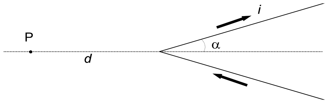
Using our contemporary knowledge of electromagnetism,
-
Find the direction of the field \(\mathbf B\) in P. [1 point]
-
Knowing that the field is proportional to \(\tan\left(\frac{\alpha}{2}\right)\), find the proportionality factor \(k\) in \[ |\mathbf B(\mathrm P)|=k\tan\left(\frac{\alpha}{2}\right). \] [1.5 points]
-
Compute the field \(\mathbf B\) in a point \(\mathrm P^*\) symmetric to P with respect to the vertex, i.e. along the axis and at the same distance \(d\), but inside the "V" (see figure). [2 points]
¹ Throughout this problem \(\alpha\) is expressed in radians
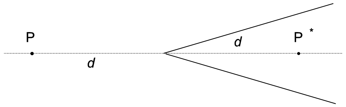
- In order to measure the magnetic field, we place in P a small magnetic needle with moment of inertia \(I\) and magnetic dipole moment \(\boldsymbol\mu\); it oscillates around a fixed point in a plane containing the direction of \(\mathbf B\). Compute the period of small oscillations of this needle as a function of \(B\). [2.5 points]
In the same conditions Biot and Savart had instead assumed that the magnetic field in P might have been (we use here the modern notation) \(B(\mathrm P)=\frac{i\mu_0\alpha}{\pi^2d}\), where \(\mu_0\) is the magnetic permeability of vacuum. In fact they attempted to decide with an experiment between the two interpretations (Ampère's and Biot and Savart's) by measuring the oscillation period of the magnetic needle as a function of the "V" span. For some \(\alpha\) values, however, the differences are too small to be easily measurable.
- If, in order to distinguish experimentally between the two predictions for the magnetic needle oscillation period \(T\) in P, we need a difference by at least 10%, namely \(T_1>1.10\,T_2\) (\(T_1\) being the Ampère prediction and \(T_2\) the Biot-Savart prediction) state in which range, approximately, we must choose the "V" half-span \(\alpha\) for being able to decide between the two interpretations. [3 points]
Hint
Depending on which path you follow in your solution, the following trigonometric equation might be useful: \[ \tan\left(\frac{\alpha}{2}\right)=\frac{\sin\alpha}{1+\cos\alpha} \]
Physical constants and general data
In addition to the numerical data given within the text of the individual problems, the knowledge of some general data and physical constants may be useful, and you may find them among the following ones. These are nearly the most accurate data currently available, and they have thus a large number of digits; you are expected, however, to write your results with a number of digits that must be appropriate for each problem.
Speed of light in vacuum: \(c=299792458\ \mathrm{m\cdot s^{-1}}\)
Magnetic permeability of vacuum: \(\mu_0=4\pi\cdot10^{-7}\ \mathrm{H\cdot m^{-1}}\)
Dielectric constant of vacuum: \(\varepsilon_0=8.8541878\ \mathrm{pF\cdot m^{-1}}\)
Gravitational constant: \(G=6.67259\cdot10^{-11}\ \mathrm{m^3/(kg\cdot s^2)}\)
Gas constant: \(R=8.314510\ \mathrm{J/(mol\cdot K)}\)
Boltzmann's constant: \(k=1.380658\cdot10^{-23}\ \mathrm{J\cdot K^{-1}}\)
Stefan's constant: \(\sigma=56.703\ \mathrm{nW/(m^2\cdot K^4)}\)
Proton charge: \(e=1.60217733\cdot10^{-19}\ \mathrm C\)
Electron mass: \(m_e=9.1093897\cdot10^{-31}\ \mathrm{kg}\)
Planck's constant: \(h=6.6260755\cdot10^{-34}\ \mathrm{J\cdot s}\)
Base of centigrade scale: \(T_K=273.15\ \mathrm K\)
Sun mass: \(M_S=1.991\cdot10^{30}\ \mathrm{kg}\)
Earth mass: \(M_E=5.979\cdot10^{24}\ \mathrm{kg}\)
Mean radius of Earth: \(r_E=6.373\ \mathrm{Mm}\)
Major semiaxis of Earth orbit: \(R_E=1.4957\cdot10^{11}\ \mathrm m\)
Sidereal day: \(d_S=86.16406\ \mathrm{ks}\)
Year: \(y=31.558150\ \mathrm{Ms}\)
Standard value of the gravitational field at the Earth surface: \(g=9.80665\ \mathrm{m\cdot s^{-2}}\)
Standard value of the atmospheric pressure at sea level: \(p_0=101325\ \mathrm{Pa}\)
Refractive index of air for visibile light, at standard pressure and \(15\,^\circ\mathrm C\): \(n_{\mathrm{air}}=1.000277\)
Solar constant: \(S=1355\ \mathrm{W\cdot m^{-2}}\)
Jupiter mass: \(M=1.901\cdot10^{27}\ \mathrm{kg}\)
Equatorial Jupiter radius: \(R_B=69.8\ \mathrm{Mm}\)
Mean radius of Jupiter’s orbit: \(R=7.783\cdot10^{11}\ \mathrm m\)
Jovian day: \(d_J=35.6\ \mathrm{ks}\)
Jovian year: \(y_J=374.32\ \mathrm{Ms}\)
\(\pi\): \(3.14159265\)
Official English text of the problem.
Answers
Let \(\hat{\mathbf z}\) point out of the page, towards the reader, and let \(\mu=|\boldsymbol\mu|\).
-
The field at P is perpendicular to the wire's plane, out of the page.
-
\[ \boxed{k=\frac{\mu_0i}{2\pi d}}, \qquad \boxed{\mathbf B(\mathrm P)= \frac{\mu_0i}{2\pi d}\tan\left(\frac{\alpha}{2}\right)\hat{\mathbf z}}. \]
-
\[ \boxed{\mathbf B(\mathrm P^*)= -\frac{\mu_0i}{2\pi d}\cot\left(\frac{\alpha}{2}\right)\hat{\mathbf z}}, \] directed into the page.
-
\[ \boxed{T=2\pi\sqrt{\frac{I}{\mu B}}}. \]
-
For the stated strict inequality \(T_1>1.10T_2\), \[ \boxed{0<\alpha<\alpha_c,\qquad \alpha_c\simeq0.768\ \mathrm{rad}\simeq44.0^\circ}. \] At \(\alpha=\alpha_c\), the difference is exactly 10%.
Solution
We treat the two long, thin arms as semi-infinite straight wires in vacuum. The current enters the vertex along the lower arm and leaves along the upper arm, as shown. Take the vertex as the origin, with the positive \(x\)-axis pointing into the V and \(\hat{\mathbf z}\) pointing out of the page.
1. Direction of the field at P
The modern Biot–Savart law is \[ d\mathbf B=\frac{\mu_0i}{4\pi} \frac{d\boldsymbol\ell\times\mathbf R}{R^3}, \] where \(d\boldsymbol\ell\) follows the current and \(\mathbf R\) points from the current element to the observation point.
Both vectors lie in the plane of the figure, so every contribution is perpendicular to that plane. At P, the right-hand rule gives an outward contribution from each arm: the lower arm carries current towards the vertex, while the upper arm carries current away from it. Thus their contributions add: \[ \boxed{\mathbf B(\mathrm P)\text{ points out of the page}.} \]
2. Determination of \(k\)
The angular dependence is given: \[ B(\mathrm P)=k\tan\left(\frac{\alpha}{2}\right). \]
Consider the limiting configuration \(\alpha=\pi/2\). The two arms then form one infinite straight wire, and P lies at perpendicular distance \(d\) from it.
For this straight wire, cylindrical symmetry and Ampère's circuital law give \[ \oint\mathbf B\cdot d\boldsymbol\ell =B(2\pi d)=\mu_0i. \] Consequently, \[ B=\frac{\mu_0i}{2\pi d}. \] Since \(\tan(\pi/4)=1\), this determines \[ \boxed{k=\frac{\mu_0i}{2\pi d}}. \]
Using the supplied permeability, \[ k=\left(2\times10^{-7}\ \mathrm{T\,m\,A^{-1}}\right)\frac{i}{d}. \] Therefore, \[ \boxed{\mathbf B(\mathrm P)= \frac{\mu_0i}{2\pi d}\tan\left(\frac{\alpha}{2}\right)\hat{\mathbf z}}. \]
3. Field at \(\mathrm P^*\)
At \(\mathrm P^*\), the right-hand rule gives a field into the page from each original arm.
To find its magnitude, continue both arms through the vertex, preserving their current directions, so that each becomes an infinite straight wire. The perpendicular distance from \(\mathrm P^*\) to either completed wire is \[ \rho=d\sin\alpha. \] Each completed wire produces a field into the page of magnitude \[ \frac{\mu_0i}{2\pi\rho}. \] Their total field therefore has magnitude \[ B_{\mathrm{complete}}=\frac{\mu_0i}{\pi d\sin\alpha}. \]
The two added half-lines form a left-opening V, which is the mirror image of the original wire. Relative to this added V, \(\mathrm P^*\) is an exterior axial point at distance \(d\). Its field consequently has magnitude \(B(\mathrm P)\), and the right-hand rule shows that it also points into the page.
Superposition thus gives \[ B(\mathrm P^*)+B(\mathrm P) =\frac{\mu_0i}{\pi d\sin\alpha}. \] Substituting the result of part 2, \[ B(\mathrm P^*)= \frac{\mu_0i}{2\pi d} \left[\frac{2}{\sin\alpha} -\tan\left(\frac{\alpha}{2}\right)\right]. \] Using \[ \tan\left(\frac{\alpha}{2}\right) =\frac{1-\cos\alpha}{\sin\alpha}, \] the bracket becomes \[ \frac{2-(1-\cos\alpha)}{\sin\alpha} =\frac{1+\cos\alpha}{\sin\alpha} =\cot\left(\frac{\alpha}{2}\right). \] Hence \[ \boxed{\mathbf B(\mathrm P^*)= -\frac{\mu_0i}{2\pi d} \cot\left(\frac{\alpha}{2}\right)\hat{\mathbf z}}. \]
4. Period of small oscillations
Treat the small needle as a magnetic dipole in a field uniform over its length, neglecting damping and other torques. Let \(\theta\) be the angle between its magnetic moment and the field.
The magnetic torque is \[ \boldsymbol\tau=\boldsymbol\mu\times\mathbf B. \] The equilibrium with \(\boldsymbol\mu\) parallel to \(\mathbf B\) is stable. Taking \(\theta\) as displacement from this equilibrium, the rotational equation of motion is \[ I\ddot\theta=-\mu B\sin\theta. \]
For small oscillations, \(|\theta|\ll1\) rad and \(\sin\theta\simeq\theta\), so \[ \ddot\theta+\frac{\mu B}{I}\theta=0. \] This is simple harmonic motion with angular frequency \[ \omega_0=\sqrt{\frac{\mu B}{I}}, \] and therefore \[ \boxed{T=2\pi\sqrt{\frac{I}{\mu B}}}. \] With SI units for \(I\), \(\mu\), and \(B\), the period is in seconds.
5. Angular range giving a period difference greater than 10%
The two field predictions at P are \[ B_1=\frac{\mu_0i}{2\pi d}\tan\left(\frac{\alpha}{2}\right), \qquad B_2=\frac{\mu_0i\alpha}{\pi^2d}, \] where the second expression is the historical assumption quoted in the problem.
Since \(T\propto B^{-1/2}\), \[ \frac{T_1}{T_2} =\sqrt{\frac{B_2}{B_1}} =\sqrt{\frac{2\alpha}{\pi\tan(\alpha/2)}}. \] The experimental requirement becomes \[ \frac{2\alpha}{\pi\tan(\alpha/2)}>1.10^2=1.21. \]
The period ratio decreases as \(\alpha\) increases. To verify this, put \(x=\alpha/2\); its square is proportional to \(x\cot x\), and \[ \frac{d}{dx}(x\cot x) =\frac{\sin x\cos x-x}{\sin^2x}<0, \] because \(\sin(2x)<2x\) for the positive angles considered.
Its limiting values are \[ \lim_{\alpha\to0^+}\frac{T_1}{T_2} =\frac{2}{\sqrt\pi}\simeq1.1284, \qquad \left.\frac{T_1}{T_2}\right|_{\alpha=\pi/2}=1. \] Thus a single threshold separates the distinguishable and indistinguishable ranges.
Solving \[ \frac{2\alpha_c}{\pi\tan(\alpha_c/2)}=1.21 \] numerically gives \[ \alpha_c\simeq0.7682\ \mathrm{rad} \simeq44.01^\circ. \] Therefore the required half-span is approximately \[ \boxed{0<\alpha<0.77\ \mathrm{rad}\quad \text{(approximately below }44^\circ\text{)}.} \]
The exact threshold is included if “at least 10%” is interpreted inclusively; it is excluded by the explicitly printed strict inequality. The degenerate value \(\alpha=0\) is excluded because both fields vanish and there is no finite magnetic oscillation period.
The solution was checked against the official solution.
IPhO 1999 · Theorieaufgabe 2
Magnetfeld eines V-förmigen Drahtes
Zu den ersten Erfolgen von Ampères Deutung magnetischer Erscheinungen gehört die Berechnung des Magnetfeldes \(\mathbf B\), das von stromdurchflossenen Drähten erzeugt wird, im Vergleich zu den frühen, ursprünglich von Biot und Savart aufgestellten Annahmen.
Ein besonders interessanter Fall ist der eines sehr langen, dünnen Drahtes, der einen konstanten Strom \(i\) führt, aus zwei geradlinigen Abschnitten besteht und mit dem halben Öffnungswinkel¹ \(\alpha\) zu einem „V“ gebogen ist (siehe Abbildung). Nach Ampères Berechnungen ist der Betrag \(B\) des Magnetfeldes in einem gegebenen Punkt P, der auf der Symmetrieachse des „V“ außerhalb desselben und im Abstand \(d\) von seinem Scheitelpunkt liegt, proportional zu \(\tan\left(\frac{\alpha}{2}\right)\). Ampères Arbeit ging später in Maxwells elektromagnetische Theorie ein und ist allgemein anerkannt.
Bestimmen Sie mithilfe unserer heutigen Kenntnisse des Elektromagnetismus Folgendes:
-
Bestimmen Sie die Richtung des Feldes \(\mathbf B\) in P. [1 Punkt]
-
Bestimmen Sie unter Verwendung der Tatsache, dass das Feld proportional zu \(\tan\left(\frac{\alpha}{2}\right)\) ist, den Proportionalitätsfaktor \(k\) in \[ |\mathbf B(\mathrm P)|=k\tan\left(\frac{\alpha}{2}\right). \] [1.5 Punkte]
-
Berechnen Sie das Feld \(\mathbf B\) in einem Punkt \(\mathrm P^*\), der bezüglich des Scheitelpunktes symmetrisch zu P liegt, also auf der Symmetrieachse und im gleichen Abstand \(d\), jedoch innerhalb des „V“ (siehe Abbildung). [2 Punkte]
¹ In dieser gesamten Aufgabe wird \(\alpha\) im Bogenmaß angegeben
- Um das Magnetfeld zu messen, bringen wir in P eine kleine Magnetnadel mit dem Trägheitsmoment \(I\) und dem magnetischen Dipolmoment \(\boldsymbol\mu\) an; sie schwingt um einen festen Punkt in einer Ebene, die die Richtung von \(\mathbf B\) enthält. Berechnen Sie die Periodendauer kleiner Schwingungen dieser Nadel als Funktion von \(B\). [2.5 Punkte]
Unter denselben Bedingungen hatten Biot und Savart stattdessen angenommen, dass das Magnetfeld in P durch \(B(\mathrm P)=\frac{i\mu_0\alpha}{\pi^2d}\) gegeben sein könnte (hier verwenden wir die moderne Schreibweise), wobei \(\mu_0\) die magnetische Permeabilität des Vakuums ist. Tatsächlich versuchten sie, durch ein Experiment zwischen den beiden Deutungen (derjenigen von Ampère und derjenigen von Biot und Savart) zu entscheiden, indem sie die Schwingungsdauer der Magnetnadel als Funktion des Öffnungswinkels des „V“ maßen. Für manche Werte von \(\alpha\) sind die Unterschiede jedoch zu gering, um leicht messbar zu sein.
- Um experimentell zwischen den beiden Vorhersagen für die Schwingungsdauer \(T\) der Magnetnadel in P unterscheiden zu können, benötigen wir einen Unterschied von mindestens 10%, nämlich \(T_1>1.10\,T_2\) (wobei \(T_1\) die Vorhersage von Ampère und \(T_2\) diejenige von Biot und Savart ist). Geben Sie an, in welchem Bereich wir den halben Öffnungswinkel \(\alpha\) des „V“ näherungsweise wählen müssen, um zwischen den beiden Deutungen entscheiden zu können. [3 Punkte]
Hinweis
Je nachdem, welchen Lösungsweg Sie wählen, könnte die folgende trigonometrische Gleichung nützlich sein: \[ \tan\left(\frac{\alpha}{2}\right)=\frac{\sin\alpha}{1+\cos\alpha} \]
Physikalische Konstanten und allgemeine Daten
Zusätzlich zu den im Text der einzelnen Aufgaben angegebenen Zahlenwerten kann die Kenntnis einiger allgemeiner Daten und physikalischer Konstanten nützlich sein; diese finden Sie in der folgenden Zusammenstellung. Dies sind nahezu die genauesten derzeit verfügbaren Daten, weshalb sie viele Ziffern aufweisen; von Ihnen wird jedoch erwartet, dass Sie Ihre Ergebnisse mit einer für die jeweilige Aufgabe angemessenen Anzahl von Ziffern angeben.
Lichtgeschwindigkeit im Vakuum: \(c=299792458\ \mathrm{m\cdot s^{-1}}\)
Magnetische Permeabilität des Vakuums: \(\mu_0=4\pi\cdot10^{-7}\ \mathrm{H\cdot m^{-1}}\)
Dielektrizitätskonstante des Vakuums: \(\varepsilon_0=8.8541878\ \mathrm{pF\cdot m^{-1}}\)
Gravitationskonstante: \(G=6.67259\cdot10^{-11}\ \mathrm{m^3/(kg\cdot s^2)}\)
Gaskonstante: \(R=8.314510\ \mathrm{J/(mol\cdot K)}\)
Boltzmann-Konstante: \(k=1.380658\cdot10^{-23}\ \mathrm{J\cdot K^{-1}}\)
Stefan-Boltzmann-Konstante: \(\sigma=56.703\ \mathrm{nW/(m^2\cdot K^4)}\)
Protonenladung: \(e=1.60217733\cdot10^{-19}\ \mathrm C\)
Elektronenmasse: \(m_e=9.1093897\cdot10^{-31}\ \mathrm{kg}\)
Plancksches Wirkungsquantum: \(h=6.6260755\cdot10^{-34}\ \mathrm{J\cdot s}\)
Nullpunkt der Celsius-Skala: \(T_K=273.15\ \mathrm K\)
Sonnenmasse: \(M_S=1.991\cdot10^{30}\ \mathrm{kg}\)
Erdmasse: \(M_E=5.979\cdot10^{24}\ \mathrm{kg}\)
Mittlerer Erdradius: \(r_E=6.373\ \mathrm{Mm}\)
Große Halbachse der Erdbahn: \(R_E=1.4957\cdot10^{11}\ \mathrm m\)
Sterntag: \(d_S=86.16406\ \mathrm{ks}\)
Jahr: \(y=31.558150\ \mathrm{Ms}\)
Normwert der Schwerebeschleunigung an der Erdoberfläche: \(g=9.80665\ \mathrm{m\cdot s^{-2}}\)
Normwert des Luftdrucks auf Meereshöhe: \(p_0=101325\ \mathrm{Pa}\)
Brechungsindex von Luft für sichtbares Licht bei Normaldruck und \(15\,^\circ\mathrm C\): \(n_{\mathrm{air}}=1.000277\)
Solarkonstante: \(S=1355\ \mathrm{W\cdot m^{-2}}\)
Jupitermasse: \(M=1.901\cdot10^{27}\ \mathrm{kg}\)
Äquatorradius des Jupiters: \(R_B=69.8\ \mathrm{Mm}\)
Mittlerer Radius der Jupiterbahn: \(R=7.783\cdot10^{11}\ \mathrm m\)
Jupitertag: \(d_J=35.6\ \mathrm{ks}\)
Jupiterjahr: \(y_J=374.32\ \mathrm{Ms}\)
\(\pi\): \(3.14159265\)
Aufgabentext aus dem offiziellen englischen Text übersetzt.
Antworten
Es sei \(\hat{\mathbf z}\) aus der Zeichenebene heraus zum Leser hin gerichtet, und es sei \(\mu=|\boldsymbol\mu|\).
-
Das Feld in P steht senkrecht auf der Ebene des Drahtes und zeigt aus der Zeichenebene heraus.
-
\[ \boxed{k=\frac{\mu_0i}{2\pi d}}, \qquad \boxed{\mathbf B(\mathrm P)= \frac{\mu_0i}{2\pi d}\tan\left(\frac{\alpha}{2}\right)\hat{\mathbf z}}. \]
-
\[ \boxed{\mathbf B(\mathrm P^*)= -\frac{\mu_0i}{2\pi d}\cot\left(\frac{\alpha}{2}\right)\hat{\mathbf z}}, \] in die Zeichenebene hinein gerichtet.
-
\[ \boxed{T=2\pi\sqrt{\frac{I}{\mu B}}}. \]
-
Für die angegebene strenge Ungleichung \(T_1>1.10T_2\) gilt \[ \boxed{0<\alpha<\alpha_c,\qquad \alpha_c\simeq0.768\ \mathrm{rad}\simeq44.0^\circ}. \] Bei \(\alpha=\alpha_c\) beträgt der Unterschied genau 10%.
Lösung
Wir behandeln die beiden langen, dünnen Schenkel als halbunendliche gerade Drähte im Vakuum. Wie abgebildet, fließt der Strom entlang des unteren Schenkels zum Scheitelpunkt und entlang des oberen Schenkels von ihm weg. Wir wählen den Scheitelpunkt als Ursprung, wobei die positive \(x\)-Achse in das V hinein und \(\hat{\mathbf z}\) aus der Zeichenebene heraus zeigt.
1. Richtung des Feldes in P
Das moderne Biot-Savart-Gesetz lautet \[ d\mathbf B=\frac{\mu_0i}{4\pi} \frac{d\boldsymbol\ell\times\mathbf R}{R^3}, \] wobei \(d\boldsymbol\ell\) in Stromrichtung und \(\mathbf R\) vom Stromelement zum Beobachtungspunkt zeigt.
Beide Vektoren liegen in der Zeichenebene, sodass jeder Beitrag senkrecht auf dieser Ebene steht. In P ergibt die Rechte-Hand-Regel für jeden Schenkel einen nach außen gerichteten Beitrag: Im unteren Schenkel fließt der Strom zum Scheitelpunkt hin, im oberen Schenkel von ihm weg. Daher addieren sich ihre Beiträge: \[ \boxed{\mathbf B(\mathrm P)\text{ zeigt aus der Zeichenebene heraus}.} \]
2. Bestimmung von \(k\)
Die Winkelabhängigkeit ist vorgegeben: \[ B(\mathrm P)=k\tan\left(\frac{\alpha}{2}\right). \]
Betrachten wir den Grenzfall \(\alpha=\pi/2\). Die beiden Schenkel bilden dann einen einzigen unendlich langen geraden Draht, und P liegt im senkrechten Abstand \(d\) von ihm.
Für diesen geraden Draht ergeben die Zylindersymmetrie und das Ampèresche Durchflutungsgesetz \[ \oint\mathbf B\cdot d\boldsymbol\ell =B(2\pi d)=\mu_0i. \] Folglich gilt \[ B=\frac{\mu_0i}{2\pi d}. \] Da \(\tan(\pi/4)=1\), folgt daraus \[ \boxed{k=\frac{\mu_0i}{2\pi d}}. \]
Mit der angegebenen Permeabilität ergibt sich \[ k=\left(2\times10^{-7}\ \mathrm{T\,m\,A^{-1}}\right)\frac{i}{d}. \] Daher gilt \[ \boxed{\mathbf B(\mathrm P)= \frac{\mu_0i}{2\pi d}\tan\left(\frac{\alpha}{2}\right)\hat{\mathbf z}}. \]
3. Feld in \(\mathrm P^*\)
In \(\mathrm P^*\) ergibt die Rechte-Hand-Regel für jeden der ursprünglichen Schenkel ein Feld, das in die Zeichenebene hinein zeigt.
Um seinen Betrag zu bestimmen, verlängern wir beide Schenkel unter Beibehaltung ihrer Stromrichtungen über den Scheitelpunkt hinaus, sodass jeder zu einem unendlich langen geraden Draht wird. Der senkrechte Abstand von \(\mathrm P^*\) zu jedem der vervollständigten Drähte ist \[ \rho=d\sin\alpha. \] Jeder vervollständigte Draht erzeugt ein in die Zeichenebene hinein gerichtetes Feld vom Betrag \[ \frac{\mu_0i}{2\pi\rho}. \] Ihr Gesamtfeld hat daher den Betrag \[ B_{\mathrm{complete}}=\frac{\mu_0i}{\pi d\sin\alpha}. \]
Die beiden hinzugefügten Halbgeraden bilden ein nach links geöffnetes V, das das Spiegelbild des ursprünglichen Drahtes ist. Bezogen auf dieses hinzugefügte V ist \(\mathrm P^*\) ein äußerer Punkt auf der Symmetrieachse im Abstand \(d\). Sein Feld hat folglich den Betrag \(B(\mathrm P)\), und die Rechte-Hand-Regel zeigt, dass es ebenfalls in die Zeichenebene hinein gerichtet ist.
Aus der Superposition folgt somit \[ B(\mathrm P^*)+B(\mathrm P) =\frac{\mu_0i}{\pi d\sin\alpha}. \] Einsetzen des Ergebnisses aus Teil 2 liefert \[ B(\mathrm P^*)= \frac{\mu_0i}{2\pi d} \left[\frac{2}{\sin\alpha} -\tan\left(\frac{\alpha}{2}\right)\right]. \] Mit \[ \tan\left(\frac{\alpha}{2}\right) =\frac{1-\cos\alpha}{\sin\alpha}, \] wird der Ausdruck in der Klammer zu \[ \frac{2-(1-\cos\alpha)}{\sin\alpha} =\frac{1+\cos\alpha}{\sin\alpha} =\cot\left(\frac{\alpha}{2}\right). \] Damit gilt \[ \boxed{\mathbf B(\mathrm P^*)= -\frac{\mu_0i}{2\pi d} \cot\left(\frac{\alpha}{2}\right)\hat{\mathbf z}}. \]
4. Periodendauer kleiner Schwingungen
Wir behandeln die kleine Nadel als magnetischen Dipol in einem über ihre Länge homogenen Feld und vernachlässigen Dämpfung sowie andere Drehmomente. Es sei \(\theta\) der Winkel zwischen ihrem magnetischen Moment und dem Feld.
Das magnetische Drehmoment ist \[ \boldsymbol\tau=\boldsymbol\mu\times\mathbf B. \] Die Gleichgewichtslage, in der \(\boldsymbol\mu\) parallel zu \(\mathbf B\) ist, ist stabil. Wenn \(\theta\) die Auslenkung aus dieser Gleichgewichtslage bezeichnet, lautet die Bewegungsgleichung für die Drehbewegung \[ I\ddot\theta=-\mu B\sin\theta. \]
Für kleine Schwingungen gelten \(|\theta|\ll1\) rad und \(\sin\theta\simeq\theta\), sodass \[ \ddot\theta+\frac{\mu B}{I}\theta=0. \] Dies ist eine harmonische Schwingung mit der Kreisfrequenz \[ \omega_0=\sqrt{\frac{\mu B}{I}}, \] und daher gilt \[ \boxed{T=2\pi\sqrt{\frac{I}{\mu B}}}. \] Werden \(I\), \(\mu\) und \(B\) in SI-Einheiten eingesetzt, ergibt sich die Periodendauer in Sekunden.
5. Winkelbereich für einen Unterschied der Periodendauern von mehr als 10%
Die beiden Vorhersagen für das Feld in P lauten \[ B_1=\frac{\mu_0i}{2\pi d}\tan\left(\frac{\alpha}{2}\right), \qquad B_2=\frac{\mu_0i\alpha}{\pi^2d}, \] wobei der zweite Ausdruck die in der Aufgabenstellung zitierte historische Annahme ist.
Da \(T\propto B^{-1/2}\), gilt \[ \frac{T_1}{T_2} =\sqrt{\frac{B_2}{B_1}} =\sqrt{\frac{2\alpha}{\pi\tan(\alpha/2)}}. \] Die experimentelle Anforderung wird damit zu \[ \frac{2\alpha}{\pi\tan(\alpha/2)}>1.10^2=1.21. \]
Das Verhältnis der Periodendauern nimmt mit zunehmendem \(\alpha\) ab. Um dies nachzuweisen, setzen wir \(x=\alpha/2\); das Quadrat des Verhältnisses ist proportional zu \(x\cot x\), und es gilt \[ \frac{d}{dx}(x\cot x) =\frac{\sin x\cos x-x}{\sin^2x}<0, \] da für die betrachteten positiven Winkel \(\sin(2x)<2x\) gilt.
Seine Grenzwerte sind \[ \lim_{\alpha\to0^+}\frac{T_1}{T_2} =\frac{2}{\sqrt\pi}\simeq1.1284, \qquad \left.\frac{T_1}{T_2}\right|_{\alpha=\pi/2}=1. \] Somit trennt ein einziger Schwellenwert den Bereich, in dem sich die Vorhersagen unterscheiden lassen, von demjenigen, in dem dies nicht möglich ist.
Die numerische Lösung von \[ \frac{2\alpha_c}{\pi\tan(\alpha_c/2)}=1.21 \] ergibt \[ \alpha_c\simeq0.7682\ \mathrm{rad} \simeq44.01^\circ. \] Der erforderliche halbe Öffnungswinkel liegt daher näherungsweise im Bereich \[ \boxed{0<\alpha<0.77\ \mathrm{rad}\quad \text{(ungefähr unter }44^\circ\text{)}.} \]
Der genaue Schwellenwert ist eingeschlossen, wenn „mindestens 10%“ einschließlich des Gleichheitsfalls verstanden wird; durch die ausdrücklich angegebene strenge Ungleichung ist er ausgeschlossen. Der entartete Wert \(\alpha=0\) ist ausgeschlossen, weil beide Felder verschwinden und es keine endliche Periodendauer der magnetischen Schwingung gibt.
Die Lösung wurde mit der offiziellen Lösung abgeglichen.
IPhO 1999 · Teori sorusu 2
V biçiminde bir telin manyetik alanı
Ampère'in manyetik olaylara ilişkin yorumunun ilk başarıları arasında, Biot ve Savart'ın başlangıçta ortaya attığı varsayımlarla karşılaştırılan, elektrik akımı taşıyan tellerin oluşturduğu manyetik alanın \(\mathbf B\) hesaplanması yer alır.
Özellikle ilginç bir durum, sabit bir \(i\) akımı taşıyan, iki doğrusal parçadan oluşan ve yarı açıklık açısı¹ \(\alpha\) olacak şekilde "V" biçiminde bükülmüş çok uzun, ince bir teldir (şekle bakınız). Ampère'in hesaplamalarına göre, "V"nin ekseni üzerinde, dışında ve tepe noktasından \(d\) uzaklıkta bulunan bir P noktasındaki manyetik alanın \(B\) büyüklüğü, \(\tan\left(\frac{\alpha}{2}\right)\) ile orantılıdır. Ampère'in çalışması daha sonra Maxwell'in elektromanyetik kuramının bir parçası olmuş ve evrensel olarak kabul görmüştür.
Günümüzdeki elektromanyetizma bilgilerimizi kullanarak,
-
P noktasındaki \(\mathbf B\) alanının yönünü bulunuz. [1 puan]
-
Alanın \(\tan\left(\frac{\alpha}{2}\right)\) ile orantılı olduğunu bilerek, \[ |\mathbf B(\mathrm P)|=k\tan\left(\frac{\alpha}{2}\right). \] bağıntısındaki \(k\) orantı katsayısını bulunuz. [1.5 puan]
-
P noktasının tepe noktasına göre simetriği olan, yani eksen üzerinde ve aynı \(d\) uzaklığında, ancak "V"nin içinde bulunan bir \(\mathrm P^*\) noktasındaki \(\mathbf B\) alanını hesaplayınız (şekle bakınız). [2 puan]
¹ Bu soru boyunca \(\alpha\) radyan cinsinden ifade edilmektedir
- Manyetik alanı ölçmek için P noktasına, eylemsizlik momenti \(I\) ve manyetik dipol momenti \(\boldsymbol\mu\) olan küçük bir manyetik iğne yerleştiriyoruz; iğne, \(\mathbf B\) yönünü içeren bir düzlemde sabit bir nokta etrafında salınmaktadır. Bu iğnenin küçük salınımlarının periyodunu \(B\)'nin bir fonksiyonu olarak hesaplayınız. [2.5 puan]
Aynı koşullar altında Biot ve Savart ise P noktasındaki manyetik alanın (burada modern gösterimi kullanıyoruz) \(B(\mathrm P)=\frac{i\mu_0\alpha}{\pi^2d}\) olabileceğini varsaymışlardı; burada \(\mu_0\), boşluğun manyetik geçirgenliğidir. Nitekim manyetik iğnenin salınım periyodunu "V"nin açıklık açısının bir fonksiyonu olarak ölçerek, iki yorum (Ampère'in yorumu ile Biot ve Savart'ın yorumu) arasında deneysel bir karar vermeye çalışmışlardı. Ancak bazı \(\alpha\) değerleri için farklar kolayca ölçülemeyecek kadar küçüktür.
- P noktasındaki manyetik iğnenin salınım periyodu \(T\) için verilen iki öngörüyü deneysel olarak ayırt edebilmek amacıyla en az %10'luk bir farka, yani \(T_1>1.10\,T_2\) koşuluna (\(T_1\) Ampère'in, \(T_2\) ise Biot–Savart'ın öngörüsüdür) ihtiyaç duyuyorsak, iki yorum arasında karar verebilmek için "V"nin yarı açıklık açısı \(\alpha\)'yı yaklaşık olarak hangi aralıkta seçmemiz gerektiğini belirtiniz. [3 puan]
İpucu
Çözümünüzde izlediğiniz yola bağlı olarak, aşağıdaki trigonometrik eşitlik yararlı olabilir: \[ \tan\left(\frac{\alpha}{2}\right)=\frac{\sin\alpha}{1+\cos\alpha} \]
Fiziksel sabitler ve genel veriler
Her bir sorunun metninde verilen sayısal verilere ek olarak, bazı genel verilerin ve fiziksel sabitlerin bilinmesi yararlı olabilir; bunları aşağıda bulabilirsiniz. Bunlar, günümüzde mevcut en hassas verilere yakın olduklarından çok sayıda basamak içerir; ancak sizden sonuçlarınızı her soruya uygun sayıda basamakla yazmanız beklenmektedir.
Işığın boşluktaki hızı: \(c=299792458\ \mathrm{m\cdot s^{-1}}\)
Boşluğun manyetik geçirgenliği: \(\mu_0=4\pi\cdot10^{-7}\ \mathrm{H\cdot m^{-1}}\)
Boşluğun dielektrik sabiti: \(\varepsilon_0=8.8541878\ \mathrm{pF\cdot m^{-1}}\)
Evrensel kütleçekim sabiti: \(G=6.67259\cdot10^{-11}\ \mathrm{m^3/(kg\cdot s^2)}\)
Gaz sabiti: \(R=8.314510\ \mathrm{J/(mol\cdot K)}\)
Boltzmann sabiti: \(k=1.380658\cdot10^{-23}\ \mathrm{J\cdot K^{-1}}\)
Stefan sabiti: \(\sigma=56.703\ \mathrm{nW/(m^2\cdot K^4)}\)
Protonun yükü: \(e=1.60217733\cdot10^{-19}\ \mathrm C\)
Elektronun kütlesi: \(m_e=9.1093897\cdot10^{-31}\ \mathrm{kg}\)
Planck sabiti: \(h=6.6260755\cdot10^{-34}\ \mathrm{J\cdot s}\)
Santigrat ölçeğinin sıfır noktası: \(T_K=273.15\ \mathrm K\)
Güneş'in kütlesi: \(M_S=1.991\cdot10^{30}\ \mathrm{kg}\)
Dünya'nın kütlesi: \(M_E=5.979\cdot10^{24}\ \mathrm{kg}\)
Dünya'nın ortalama yarıçapı: \(r_E=6.373\ \mathrm{Mm}\)
Dünya yörüngesinin büyük yarı ekseni: \(R_E=1.4957\cdot10^{11}\ \mathrm m\)
Yıldız günü: \(d_S=86.16406\ \mathrm{ks}\)
Yıl: \(y=31.558150\ \mathrm{Ms}\)
Dünya yüzeyindeki kütleçekim alanının standart değeri: \(g=9.80665\ \mathrm{m\cdot s^{-2}}\)
Deniz seviyesindeki atmosfer basıncının standart değeri: \(p_0=101325\ \mathrm{Pa}\)
Standart basınçta ve \(15\,^\circ\mathrm C\) sıcaklıkta, görünür ışık için havanın kırılma indisi: \(n_{\mathrm{air}}=1.000277\)
Güneş sabiti: \(S=1355\ \mathrm{W\cdot m^{-2}}\)
Jüpiter'in kütlesi: \(M=1.901\cdot10^{27}\ \mathrm{kg}\)
Jüpiter'in ekvator yarıçapı: \(R_B=69.8\ \mathrm{Mm}\)
Jüpiter yörüngesinin ortalama yarıçapı: \(R=7.783\cdot10^{11}\ \mathrm m\)
Jüpiter günü: \(d_J=35.6\ \mathrm{ks}\)
Jüpiter yılı: \(y_J=374.32\ \mathrm{Ms}\)
\(\pi\): \(3.14159265\)
Soru metni resmi İngilizce metinden çevrilmiştir.
Cevaplar
\(\hat{\mathbf z}\) sayfa düzleminden dışarıya, okuyucuya doğru yönelsin ve \(\mu=|\boldsymbol\mu|\) olsun.
-
P noktasındaki alan telin bulunduğu düzleme dik, sayfa düzleminden dışarıya doğrudur.
-
\[ \boxed{k=\frac{\mu_0i}{2\pi d}}, \qquad \boxed{\mathbf B(\mathrm P)= \frac{\mu_0i}{2\pi d}\tan\left(\frac{\alpha}{2}\right)\hat{\mathbf z}}. \]
-
\[ \boxed{\mathbf B(\mathrm P^*)= -\frac{\mu_0i}{2\pi d}\cot\left(\frac{\alpha}{2}\right)\hat{\mathbf z}}, \] sayfa düzleminden içeriye yönelmiştir.
-
\[ \boxed{T=2\pi\sqrt{\frac{I}{\mu B}}}. \]
-
Belirtilen kesin eşitsizlik \(T_1>1.10T_2\) için, \[ \boxed{0<\alpha<\alpha_c,\qquad \alpha_c\simeq0.768\ \mathrm{rad}\simeq44.0^\circ}. \] \(\alpha=\alpha_c\) olduğunda fark tam olarak %10'dur.
Çözüm
İki uzun, ince kolu boşlukta bulunan yarı sonsuz doğrusal teller olarak ele alıyoruz. Şekilde gösterildiği gibi akım, alt kol boyunca tepe noktasına girer ve üst kol boyunca tepe noktasından çıkar. Tepe noktasını başlangıç noktası olarak alalım; pozitif \(x\) ekseni V'nin içine, \(\hat{\mathbf z}\) ise sayfa düzleminden dışarıya yönelsin.
1. P noktasındaki alanın yönü
Modern Biot–Savart yasası \[ d\mathbf B=\frac{\mu_0i}{4\pi} \frac{d\boldsymbol\ell\times\mathbf R}{R^3}, \] şeklindedir; burada \(d\boldsymbol\ell\) akım yönündedir ve \(\mathbf R\), akım elemanından gözlem noktasına yönelir.
Her iki vektör de şeklin düzleminde bulunduğundan her bir katkı bu düzleme diktir. P noktasında sağ el kuralı, her iki koldan da dışarıya doğru bir katkı verir: alt koldaki akım tepe noktasına doğru, üst koldaki akım ise tepe noktasından uzağa doğru akar. Dolayısıyla katkıları toplanır: \[ \boxed{\mathbf B(\mathrm P)\text{ sayfa düzleminden dışarıya yönelir}.} \]
2. \(k\)'nın belirlenmesi
Açıya bağımlılık verilmiştir: \[ B(\mathrm P)=k\tan\left(\frac{\alpha}{2}\right). \]
\(\alpha=\pi/2\) sınır durumunu ele alalım. Bu durumda iki kol, tek bir sonsuz doğrusal tel oluşturur ve P noktasının bu tele dik uzaklığı \(d\)'dir.
Bu doğrusal tel için silindirik simetri ve Ampère'in dolaşım yasası \[ \oint\mathbf B\cdot d\boldsymbol\ell =B(2\pi d)=\mu_0i. \] sonucunu verir. Dolayısıyla, \[ B=\frac{\mu_0i}{2\pi d}. \] \(\tan(\pi/4)=1\) olduğundan buradan \[ \boxed{k=\frac{\mu_0i}{2\pi d}}. \] bulunur.
Verilen manyetik geçirgenlik kullanılırsa, \[ k=\left(2\times10^{-7}\ \mathrm{T\,m\,A^{-1}}\right)\frac{i}{d}. \] Böylece, \[ \boxed{\mathbf B(\mathrm P)= \frac{\mu_0i}{2\pi d}\tan\left(\frac{\alpha}{2}\right)\hat{\mathbf z}}. \]
3. \(\mathrm P^*\) noktasındaki alan
\(\mathrm P^*\) noktasında sağ el kuralı, başlangıçtaki her iki kolun da sayfa düzleminden içeriye doğru bir alan oluşturduğunu gösterir.
Alanın büyüklüğünü bulmak için her iki kolu, akım yönlerini koruyarak tepe noktasının ötesine uzatalım; böylece her biri sonsuz bir doğrusal tel olsun. \(\mathrm P^*\) noktasının tamamlanan tellerin her birine dik uzaklığı \[ \rho=d\sin\alpha. \] olur. Tamamlanan tellerin her biri, sayfa düzleminden içeriye doğru, büyüklüğü \[ \frac{\mu_0i}{2\pi\rho}. \] olan bir alan oluşturur. Dolayısıyla toplam alanlarının büyüklüğü \[ B_{\mathrm{complete}}=\frac{\mu_0i}{\pi d\sin\alpha}. \] olur.
Eklenen iki yarı doğru, başlangıçtaki telin ayna görüntüsü olan, sola açılan bir V oluşturur. Eklenen bu V'ye göre \(\mathrm P^*\), dışarıda, eksen üzerinde ve \(d\) uzaklığında bir noktadır. Bu nedenle oluşturduğu alanın büyüklüğü \(B(\mathrm P)\)'dir ve sağ el kuralı, bu alanın da sayfa düzleminden içeriye yöneldiğini gösterir.
Böylece süperpozisyon ilkesi \[ B(\mathrm P^*)+B(\mathrm P) =\frac{\mu_0i}{\pi d\sin\alpha}. \] bağıntısını verir. 2. kısmın sonucu yerine konursa, \[ B(\mathrm P^*)= \frac{\mu_0i}{2\pi d} \left[\frac{2}{\sin\alpha} -\tan\left(\frac{\alpha}{2}\right)\right]. \] \[ \tan\left(\frac{\alpha}{2}\right) =\frac{1-\cos\alpha}{\sin\alpha}, \] bağıntısı kullanıldığında köşeli parantez içindeki ifade \[ \frac{2-(1-\cos\alpha)}{\sin\alpha} =\frac{1+\cos\alpha}{\sin\alpha} =\cot\left(\frac{\alpha}{2}\right). \] haline gelir. Dolayısıyla \[ \boxed{\mathbf B(\mathrm P^*)= -\frac{\mu_0i}{2\pi d} \cot\left(\frac{\alpha}{2}\right)\hat{\mathbf z}}. \]
4. Küçük salınımların periyodu
Küçük iğneyi, uzunluğu boyunca düzgün olan bir alandaki manyetik dipol olarak ele alalım; sönümü ve diğer torkları ihmal edelim. Manyetik momenti ile alan arasındaki açı \(\theta\) olsun.
Manyetik tork \[ \boldsymbol\tau=\boldsymbol\mu\times\mathbf B. \] şeklindedir. \(\boldsymbol\mu\)'nün \(\mathbf B\)'ye paralel olduğu denge kararlıdır. \(\theta\)'yı bu denge konumundan açısal sapma olarak alırsak dönme hareketinin denklemi \[ I\ddot\theta=-\mu B\sin\theta. \] olur.
Küçük salınımlar için \(|\theta|\ll1\) rad ve \(\sin\theta\simeq\theta\) olduğundan, \[ \ddot\theta+\frac{\mu B}{I}\theta=0. \] Bu, açısal frekansı \[ \omega_0=\sqrt{\frac{\mu B}{I}}, \] olan basit harmonik harekettir ve dolayısıyla \[ \boxed{T=2\pi\sqrt{\frac{I}{\mu B}}}. \] \(I\), \(\mu\) ve \(B\) için SI birimleri kullanıldığında periyot saniye cinsindendir.
5. %10'dan büyük bir periyot farkı veren açı aralığı
P noktasındaki iki alan öngörüsü \[ B_1=\frac{\mu_0i}{2\pi d}\tan\left(\frac{\alpha}{2}\right), \qquad B_2=\frac{\mu_0i\alpha}{\pi^2d}, \] şeklindedir; ikinci ifade, soruda aktarılan tarihsel varsayımdır.
\(T\propto B^{-1/2}\) olduğundan, \[ \frac{T_1}{T_2} =\sqrt{\frac{B_2}{B_1}} =\sqrt{\frac{2\alpha}{\pi\tan(\alpha/2)}}. \] Deneysel koşul \[ \frac{2\alpha}{\pi\tan(\alpha/2)}>1.10^2=1.21. \] haline gelir.
\(\alpha\) arttıkça periyot oranı azalır. Bunu doğrulamak için \(x=\alpha/2\) alalım; bu oranın karesi \(x\cot x\) ile orantılıdır ve \[ \frac{d}{dx}(x\cot x) =\frac{\sin x\cos x-x}{\sin^2x}<0, \] çünkü ele alınan pozitif açılar için \(\sin(2x)<2x\) olur.
Sınır değerleri \[ \lim_{\alpha\to0^+}\frac{T_1}{T_2} =\frac{2}{\sqrt\pi}\simeq1.1284, \qquad \left.\frac{T_1}{T_2}\right|_{\alpha=\pi/2}=1. \] şeklindedir. Dolayısıyla ayırt edilebilen ve ayırt edilemeyen aralıkları tek bir eşik ayırır.
\[ \frac{2\alpha_c}{\pi\tan(\alpha_c/2)}=1.21 \] denkleminin sayısal çözümü \[ \alpha_c\simeq0.7682\ \mathrm{rad} \simeq44.01^\circ. \] sonucunu verir. Bu nedenle gerekli yarı açıklık açısı yaklaşık olarak \[ \boxed{0<\alpha<0.77\ \mathrm{rad}\quad \text{(yaklaşık olarak }44^\circ\text{ altında)}.} \] olmalıdır.
“En az %10” ifadesi eşitliği de kapsayacak şekilde yorumlanırsa tam eşik değeri aralığa dahildir; açıkça yazılmış olan kesin eşitsizlik ise bu değeri dışlar. Her iki alan da sıfır olduğundan ve sonlu bir manyetik salınım periyodu bulunmadığından, dejenere durum olan \(\alpha=0\) değeri dışlanır.
Çözüm, resmi çözümle karşılaştırılarak kontrol edildi.
IPhO 1999 · Problema teórico 2
Campo magnético de un alambre en forma de V
Entre los primeros éxitos de la interpretación de los fenómenos magnéticos por Ampère se encuentra el cálculo del campo magnético \(\mathbf B\) generado por alambres que conducen una corriente eléctrica, en comparación con las primeras hipótesis formuladas originalmente por Biot y Savart.
Un caso particularmente interesante es el de un alambre delgado muy largo, que conduce una corriente constante \(i\), formado por dos tramos rectilíneos y doblado en forma de «V», con un ángulo de semiapertura¹ \(\alpha\) (véase la figura). Según los cálculos de Ampère, el módulo \(B\) del campo magnético en un punto dado P situado sobre el eje de la «V», fuera de ella y a una distancia \(d\) de su vértice, es proporcional a \(\tan\left(\frac{\alpha}{2}\right)\). El trabajo de Ampère se incorporó posteriormente a la teoría electromagnética de Maxwell y goza de aceptación universal.
Utilizando nuestros conocimientos actuales de electromagnetismo,
-
Determine la dirección y el sentido del campo \(\mathbf B\) en P. [1 punto]
-
Sabiendo que el campo es proporcional a \(\tan\left(\frac{\alpha}{2}\right)\), determine el factor de proporcionalidad \(k\) en \[ |\mathbf B(\mathrm P)|=k\tan\left(\frac{\alpha}{2}\right). \] [1.5 puntos]
-
Calcule el campo \(\mathbf B\) en un punto \(\mathrm P^*\) simétrico de P respecto al vértice, es decir, situado sobre el eje y a la misma distancia \(d\), pero dentro de la «V» (véase la figura). [2 puntos]
¹ En todo este problema, \(\alpha\) se expresa en radianes
- Para medir el campo magnético, colocamos en P una pequeña aguja magnética con momento de inercia \(I\) y momento dipolar magnético \(\boldsymbol\mu\); oscila alrededor de un punto fijo en un plano que contiene la dirección de \(\mathbf B\). Calcule el período de las pequeñas oscilaciones de esta aguja en función de \(B\). [2.5 puntos]
En las mismas condiciones, Biot y Savart habían supuesto, en cambio, que el campo magnético en P podría ser (utilizamos aquí la notación moderna) \(B(\mathrm P)=\frac{i\mu_0\alpha}{\pi^2d}\), donde \(\mu_0\) es la permeabilidad magnética del vacío. De hecho, intentaron decidir experimentalmente entre las dos interpretaciones (la de Ampère y la de Biot y Savart) midiendo el período de oscilación de la aguja magnética en función de la apertura de la «V». Sin embargo, para algunos valores de \(\alpha\), las diferencias son demasiado pequeñas para poder medirlas fácilmente.
- Si, para distinguir experimentalmente entre las dos predicciones del período de oscilación \(T\) de la aguja magnética en P, necesitamos una diferencia de al menos el 10%, es decir, \(T_1>1.10\,T_2\) (siendo \(T_1\) la predicción de Ampère y \(T_2\) la de Biot-Savart), indique en qué intervalo, aproximadamente, debemos elegir la semiapertura \(\alpha\) de la «V» para poder decidir entre las dos interpretaciones. [3 puntos]
Sugerencia
Según el procedimiento que siga en su solución, la siguiente ecuación trigonométrica puede resultar útil: \[ \tan\left(\frac{\alpha}{2}\right)=\frac{\sin\alpha}{1+\cos\alpha} \]
Constantes físicas y datos generales
Además de los datos numéricos que se proporcionan en el texto de cada problema, puede ser útil conocer algunos datos generales y constantes físicas, que encontrará a continuación. Estos datos se cuentan entre los más precisos disponibles actualmente y, por ello, tienen un gran número de cifras; no obstante, se espera que exprese sus resultados con un número de cifras adecuado para cada problema.
Velocidad de la luz en el vacío: \(c=299792458\ \mathrm{m\cdot s^{-1}}\)
Permeabilidad magnética del vacío: \(\mu_0=4\pi\cdot10^{-7}\ \mathrm{H\cdot m^{-1}}\)
Constante dieléctrica del vacío: \(\varepsilon_0=8.8541878\ \mathrm{pF\cdot m^{-1}}\)
Constante de gravitación universal: \(G=6.67259\cdot10^{-11}\ \mathrm{m^3/(kg\cdot s^2)}\)
Constante de los gases: \(R=8.314510\ \mathrm{J/(mol\cdot K)}\)
Constante de Boltzmann: \(k=1.380658\cdot10^{-23}\ \mathrm{J\cdot K^{-1}}\)
Constante de Stefan: \(\sigma=56.703\ \mathrm{nW/(m^2\cdot K^4)}\)
Carga del protón: \(e=1.60217733\cdot10^{-19}\ \mathrm C\)
Masa del electrón: \(m_e=9.1093897\cdot10^{-31}\ \mathrm{kg}\)
Constante de Planck: \(h=6.6260755\cdot10^{-34}\ \mathrm{J\cdot s}\)
Origen de la escala centígrada: \(T_K=273.15\ \mathrm K\)
Masa del Sol: \(M_S=1.991\cdot10^{30}\ \mathrm{kg}\)
Masa de la Tierra: \(M_E=5.979\cdot10^{24}\ \mathrm{kg}\)
Radio medio de la Tierra: \(r_E=6.373\ \mathrm{Mm}\)
Semieje mayor de la órbita terrestre: \(R_E=1.4957\cdot10^{11}\ \mathrm m\)
Día sidéreo: \(d_S=86.16406\ \mathrm{ks}\)
Año: \(y=31.558150\ \mathrm{Ms}\)
Valor estándar del campo gravitatorio en la superficie terrestre: \(g=9.80665\ \mathrm{m\cdot s^{-2}}\)
Valor estándar de la presión atmosférica al nivel del mar: \(p_0=101325\ \mathrm{Pa}\)
Índice de refracción del aire para la luz visible, a presión estándar y a \(15\,^\circ\mathrm C\): \(n_{\mathrm{air}}=1.000277\)
Constante solar: \(S=1355\ \mathrm{W\cdot m^{-2}}\)
Masa de Júpiter: \(M=1.901\cdot10^{27}\ \mathrm{kg}\)
Radio ecuatorial de Júpiter: \(R_B=69.8\ \mathrm{Mm}\)
Radio medio de la órbita de Júpiter: \(R=7.783\cdot10^{11}\ \mathrm m\)
Día joviano: \(d_J=35.6\ \mathrm{ks}\)
Año joviano: \(y_J=374.32\ \mathrm{Ms}\)
\(\pi\): \(3.14159265\)
Enunciado traducido del texto oficial en inglés.
Respuestas
Sea \(\hat{\mathbf z}\) un vector que apunta hacia fuera de la página, hacia el lector, y sea \(\mu=|\boldsymbol\mu|\).
-
El campo en P es perpendicular al plano del alambre y apunta hacia fuera de la página.
-
\[ \boxed{k=\frac{\mu_0i}{2\pi d}}, \qquad \boxed{\mathbf B(\mathrm P)= \frac{\mu_0i}{2\pi d}\tan\left(\frac{\alpha}{2}\right)\hat{\mathbf z}}. \]
-
\[ \boxed{\mathbf B(\mathrm P^*)= -\frac{\mu_0i}{2\pi d}\cot\left(\frac{\alpha}{2}\right)\hat{\mathbf z}}, \] dirigido hacia dentro de la página.
-
\[ \boxed{T=2\pi\sqrt{\frac{I}{\mu B}}}. \]
-
Para la desigualdad estricta indicada \(T_1>1.10T_2\), \[ \boxed{0<\alpha<\alpha_c,\qquad \alpha_c\simeq0.768\ \mathrm{rad}\simeq44.0^\circ}. \] En \(\alpha=\alpha_c\), la diferencia es exactamente del 10%.
Solución
Consideramos los dos brazos largos y delgados como alambres rectilíneos semiinfinitos en el vacío. La corriente llega al vértice por el brazo inferior y sale por el brazo superior, como se muestra en la figura. Tomamos el vértice como origen, con el semieje positivo \(x\) dirigido hacia el interior de la V y \(\hat{\mathbf z}\) dirigido hacia fuera de la página.
1. Dirección y sentido del campo en P
La ley de Biot–Savart moderna es \[ d\mathbf B=\frac{\mu_0i}{4\pi} \frac{d\boldsymbol\ell\times\mathbf R}{R^3}, \] donde \(d\boldsymbol\ell\) sigue el sentido de la corriente y \(\mathbf R\) apunta desde el elemento de corriente hasta el punto de observación.
Ambos vectores están en el plano de la figura, de modo que cada contribución es perpendicular a ese plano. En P, la regla de la mano derecha da una contribución hacia fuera de la página para cada brazo: el brazo inferior conduce la corriente hacia el vértice, mientras que el superior la conduce alejándose de él. Por tanto, sus contribuciones se suman: \[ \boxed{\mathbf B(\mathrm P)\text{ apunta hacia fuera de la página}.} \]
2. Determinación de \(k\)
La dependencia angular viene dada: \[ B(\mathrm P)=k\tan\left(\frac{\alpha}{2}\right). \]
Consideremos la configuración límite \(\alpha=\pi/2\). Los dos brazos forman entonces un único alambre rectilíneo infinito, y P se encuentra a una distancia perpendicular \(d\) de él.
Para este alambre rectilíneo, la simetría cilíndrica y la ley de circulación de Ampère dan \[ \oint\mathbf B\cdot d\boldsymbol\ell =B(2\pi d)=\mu_0i. \] Por consiguiente, \[ B=\frac{\mu_0i}{2\pi d}. \] Como \(\tan(\pi/4)=1\), esto determina \[ \boxed{k=\frac{\mu_0i}{2\pi d}}. \]
Utilizando la permeabilidad proporcionada, \[ k=\left(2\times10^{-7}\ \mathrm{T\,m\,A^{-1}}\right)\frac{i}{d}. \] Por tanto, \[ \boxed{\mathbf B(\mathrm P)= \frac{\mu_0i}{2\pi d}\tan\left(\frac{\alpha}{2}\right)\hat{\mathbf z}}. \]
3. Campo en \(\mathrm P^*\)
En \(\mathrm P^*\), la regla de la mano derecha da un campo hacia dentro de la página para cada brazo original.
Para hallar su módulo, prolongamos ambos brazos más allá del vértice, conservando los sentidos de sus corrientes, de modo que cada uno se convierta en un alambre rectilíneo infinito. La distancia perpendicular desde \(\mathrm P^*\) hasta cualquiera de los alambres así completados es \[ \rho=d\sin\alpha. \] Cada alambre completado produce un campo hacia dentro de la página de módulo \[ \frac{\mu_0i}{2\pi\rho}. \] Por tanto, su campo total tiene módulo \[ B_{\mathrm{complete}}=\frac{\mu_0i}{\pi d\sin\alpha}. \]
Las dos semirrectas añadidas forman una V abierta hacia la izquierda, que es la imagen especular del alambre original. Respecto a esta V añadida, \(\mathrm P^*\) es un punto exterior situado sobre el eje a una distancia \(d\). Por consiguiente, su campo tiene módulo \(B(\mathrm P)\), y la regla de la mano derecha muestra que también apunta hacia dentro de la página.
Así, por superposición, \[ B(\mathrm P^*)+B(\mathrm P) =\frac{\mu_0i}{\pi d\sin\alpha}. \] Sustituyendo el resultado de la parte 2, \[ B(\mathrm P^*)= \frac{\mu_0i}{2\pi d} \left[\frac{2}{\sin\alpha} -\tan\left(\frac{\alpha}{2}\right)\right]. \] Utilizando \[ \tan\left(\frac{\alpha}{2}\right) =\frac{1-\cos\alpha}{\sin\alpha}, \] la expresión entre corchetes se convierte en \[ \frac{2-(1-\cos\alpha)}{\sin\alpha} =\frac{1+\cos\alpha}{\sin\alpha} =\cot\left(\frac{\alpha}{2}\right). \] Por lo tanto, \[ \boxed{\mathbf B(\mathrm P^*)= -\frac{\mu_0i}{2\pi d} \cot\left(\frac{\alpha}{2}\right)\hat{\mathbf z}}. \]
4. Período de las pequeñas oscilaciones
Tratamos la pequeña aguja como un dipolo magnético en un campo uniforme a lo largo de toda su longitud, despreciando el amortiguamiento y otros momentos de fuerza. Sea \(\theta\) el ángulo entre su momento magnético y el campo.
El momento de fuerza magnético es \[ \boldsymbol\tau=\boldsymbol\mu\times\mathbf B. \] El equilibrio con \(\boldsymbol\mu\) paralelo a \(\mathbf B\) es estable. Tomando \(\theta\) como el desplazamiento angular respecto a este equilibrio, la ecuación del movimiento de rotación es \[ I\ddot\theta=-\mu B\sin\theta. \]
Para pequeñas oscilaciones, \(|\theta|\ll1\) rad y \(\sin\theta\simeq\theta\), por lo que \[ \ddot\theta+\frac{\mu B}{I}\theta=0. \] Este es un movimiento armónico simple con frecuencia angular \[ \omega_0=\sqrt{\frac{\mu B}{I}}, \] y, por tanto, \[ \boxed{T=2\pi\sqrt{\frac{I}{\mu B}}}. \] Si \(I\), \(\mu\) y \(B\) se expresan en unidades del SI, el período se obtiene en segundos.
5. Intervalo angular que da una diferencia de períodos superior al 10%
Las dos predicciones del campo en P son \[ B_1=\frac{\mu_0i}{2\pi d}\tan\left(\frac{\alpha}{2}\right), \qquad B_2=\frac{\mu_0i\alpha}{\pi^2d}, \] donde la segunda expresión es la hipótesis histórica citada en el enunciado.
Como \(T\propto B^{-1/2}\), \[ \frac{T_1}{T_2} =\sqrt{\frac{B_2}{B_1}} =\sqrt{\frac{2\alpha}{\pi\tan(\alpha/2)}}. \] El requisito experimental se convierte en \[ \frac{2\alpha}{\pi\tan(\alpha/2)}>1.10^2=1.21. \]
El cociente de los períodos disminuye al aumentar \(\alpha\). Para comprobarlo, hacemos \(x=\alpha/2\); su cuadrado es proporcional a \(x\cot x\), y \[ \frac{d}{dx}(x\cot x) =\frac{\sin x\cos x-x}{\sin^2x}<0, \] porque \(\sin(2x)<2x\) para los ángulos positivos considerados.
Sus valores límite son \[ \lim_{\alpha\to0^+}\frac{T_1}{T_2} =\frac{2}{\sqrt\pi}\simeq1.1284, \qquad \left.\frac{T_1}{T_2}\right|_{\alpha=\pi/2}=1. \] Así, un único umbral separa los intervalos en los que las predicciones pueden distinguirse de aquellos en los que no pueden distinguirse.
Resolviendo numéricamente \[ \frac{2\alpha_c}{\pi\tan(\alpha_c/2)}=1.21 \] se obtiene \[ \alpha_c\simeq0.7682\ \mathrm{rad} \simeq44.01^\circ. \] Por tanto, la semiapertura requerida es aproximadamente \[ \boxed{0<\alpha<0.77\ \mathrm{rad}\quad \text{(aproximadamente por debajo de }44^\circ\text{)}.} \]
El umbral exacto se incluye si «al menos el 10%» se interpreta de forma inclusiva; queda excluido por la desigualdad estricta escrita explícitamente. El valor degenerado \(\alpha=0\) se excluye porque ambos campos se anulan y no existe un período finito de oscilación magnética.
La solución se comprobó con la solución oficial.
IPhO 1999 · 理论题 2
V 形导线产生的磁场
安培对磁现象的解释所取得的最早成果之一,是计算载流导线产生的磁场 \(\mathbf B\),并与毕奥和萨伐尔最初提出的早期假设进行比较。
一个特别有趣的情形是:一根很长的细导线由两段直线部分组成,弯成“V”形,夹角的一半¹为 \(\alpha\),其中通有恒定电流 \(i\)(见图)。根据安培的计算,在“V”形外部的对称轴上、距顶点为 \(d\) 的给定点 P 处,磁场的大小 \(B\) 与 \(\tan\left(\frac{\alpha}{2}\right)\) 成正比。安培的工作后来被纳入麦克斯韦电磁理论,并得到普遍认可。
运用我们现今的电磁学知识,
-
求 P 点处磁场 \(\mathbf B\) 的方向。[1 分]
-
已知磁场与 \(\tan\left(\frac{\alpha}{2}\right)\) 成正比,求下式中的比例系数 \(k\): \[ |\mathbf B(\mathrm P)|=k\tan\left(\frac{\alpha}{2}\right). \] [1.5 分]
-
计算与 P 关于顶点对称的 \(\mathrm P^*\) 点处的磁场 \(\mathbf B\),即该点同样位于对称轴上,距顶点的距离也为 \(d\),但位于“V”形内部(见图)。[2 分]
¹ 本题中 \(\alpha\) 均以弧度表示
- 为了测量磁场,我们在 P 点放置一根转动惯量为 \(I\)、磁偶极矩为 \(\boldsymbol\mu\) 的小磁针;它在包含 \(\mathbf B\) 方向的平面内绕一个固定点振动。求该磁针的小振动周期与 \(B\) 的函数关系。[2.5 分]
在相同条件下,毕奥和萨伐尔却曾假设 P 点处的磁场可能为(这里采用现代记号)\(B(\mathrm P)=\frac{i\mu_0\alpha}{\pi^2d}\),其中 \(\mu_0\) 为真空磁导率。事实上,他们曾尝试通过实验测量磁针振动周期随“V”形夹角的变化关系,以判定这两种解释(安培的解释与毕奥和萨伐尔的解释)孰是孰非。然而,对于某些 \(\alpha\) 值,两者的差异太小,难以测量。
- 如果为了在实验上区分 P 点处磁针振动周期 \(T\) 的两种预测,我们需要至少 10% 的差异,即 \(T_1>1.10\,T_2\)(\(T_1\) 为安培的预测,\(T_2\) 为毕奥–萨伐尔的预测),请指出,要能判别这两种解释,“V”形夹角的一半 \(\alpha\) 大致应选在哪个范围内。[3 分]
提示
根据你所采用的解题方法,下列三角恒等式可能有用: \[ \tan\left(\frac{\alpha}{2}\right)=\frac{\sin\alpha}{1+\cos\alpha} \]
物理常量和一般数据
除各题题干中给出的数值数据外,一些一般数据和物理常量也可能有用,可在下列数据中查找。这些数据几乎是目前能获得的最精确数据,因此保留了较多位数;不过,你应根据各题的具体情况,以适当的位数写出结果。
真空中的光速:\(c=299792458\ \mathrm{m\cdot s^{-1}}\)
真空磁导率:\(\mu_0=4\pi\cdot10^{-7}\ \mathrm{H\cdot m^{-1}}\)
真空介电常数:\(\varepsilon_0=8.8541878\ \mathrm{pF\cdot m^{-1}}\)
万有引力常量:\(G=6.67259\cdot10^{-11}\ \mathrm{m^3/(kg\cdot s^2)}\)
气体常量:\(R=8.314510\ \mathrm{J/(mol\cdot K)}\)
玻尔兹曼常量:\(k=1.380658\cdot10^{-23}\ \mathrm{J\cdot K^{-1}}\)
斯特藩常量:\(\sigma=56.703\ \mathrm{nW/(m^2\cdot K^4)}\)
质子电荷:\(e=1.60217733\cdot10^{-19}\ \mathrm C\)
电子质量:\(m_e=9.1093897\cdot10^{-31}\ \mathrm{kg}\)
普朗克常量:\(h=6.6260755\cdot10^{-34}\ \mathrm{J\cdot s}\)
摄氏温标零点对应的热力学温度:\(T_K=273.15\ \mathrm K\)
太阳质量:\(M_S=1.991\cdot10^{30}\ \mathrm{kg}\)
地球质量:\(M_E=5.979\cdot10^{24}\ \mathrm{kg}\)
地球平均半径:\(r_E=6.373\ \mathrm{Mm}\)
地球轨道半长轴:\(R_E=1.4957\cdot10^{11}\ \mathrm m\)
恒星日:\(d_S=86.16406\ \mathrm{ks}\)
年:\(y=31.558150\ \mathrm{Ms}\)
地球表面重力场强的标准值:\(g=9.80665\ \mathrm{m\cdot s^{-2}}\)
海平面大气压的标准值:\(p_0=101325\ \mathrm{Pa}\)
标准气压和 \(15\,^\circ\mathrm C\) 下空气对可见光的折射率:\(n_{\mathrm{air}}=1.000277\)
太阳常量:\(S=1355\ \mathrm{W\cdot m^{-2}}\)
木星质量:\(M=1.901\cdot10^{27}\ \mathrm{kg}\)
木星赤道半径:\(R_B=69.8\ \mathrm{Mm}\)
木星轨道平均半径:\(R=7.783\cdot10^{11}\ \mathrm m\)
木星日:\(d_J=35.6\ \mathrm{ks}\)
木星年:\(y_J=374.32\ \mathrm{Ms}\)
\(\pi\):\(3.14159265\)
题目译自官方英文原文。
答案
令 \(\hat{\mathbf z}\) 指向纸外,即朝向读者,并令 \(\mu=|\boldsymbol\mu|\)。
-
P 点处的磁场垂直于导线所在平面,指向纸外。
-
\[ \boxed{k=\frac{\mu_0i}{2\pi d}}, \qquad \boxed{\mathbf B(\mathrm P)= \frac{\mu_0i}{2\pi d}\tan\left(\frac{\alpha}{2}\right)\hat{\mathbf z}}. \]
-
\[ \boxed{\mathbf B(\mathrm P^*)= -\frac{\mu_0i}{2\pi d}\cot\left(\frac{\alpha}{2}\right)\hat{\mathbf z}}, \] 方向指向纸内。
-
\[ \boxed{T=2\pi\sqrt{\frac{I}{\mu B}}}. \]
-
对于题目给出的严格不等式 \(T_1>1.10T_2\), \[ \boxed{0<\alpha<\alpha_c,\qquad \alpha_c\simeq0.768\ \mathrm{rad}\simeq44.0^\circ}. \] 当 \(\alpha=\alpha_c\) 时,差异恰好为 10%。
解答
将两条细长的臂视为真空中的半无限长直导线。如图所示,电流沿下臂流入顶点,再沿上臂流出。取顶点为原点,\(x\) 轴正方向指向 V 形内部,\(\hat{\mathbf z}\) 指向纸外。
1. P 点处磁场的方向
现代的毕奥–萨伐尔定律为 \[ d\mathbf B=\frac{\mu_0i}{4\pi} \frac{d\boldsymbol\ell\times\mathbf R}{R^3}, \] 其中,\(d\boldsymbol\ell\) 沿电流方向,\(\mathbf R\) 从电流元指向观察点。
这两个矢量都位于图示平面内,因此每个电流元产生的磁场都垂直于该平面。在 P 点,根据右手定则,两臂产生的磁场均指向纸外:下臂中的电流流向顶点,而上臂中的电流背离顶点流动。因此,两者的磁场相加: \[ \boxed{\mathbf B(\mathrm P)\text{ 指向纸外}.} \]
2. 确定 \(k\)
题目已给出磁场对角度的依赖关系: \[ B(\mathrm P)=k\tan\left(\frac{\alpha}{2}\right). \]
考虑 \(\alpha=\pi/2\) 的极限构型。此时两臂构成一根无限长直导线,P 点到导线的垂直距离为 \(d\)。
对于这根直导线,由柱对称性和安培环路定理可得 \[ \oint\mathbf B\cdot d\boldsymbol\ell =B(2\pi d)=\mu_0i. \] 因此, \[ B=\frac{\mu_0i}{2\pi d}. \] 由于 \(\tan(\pi/4)=1\),由此确定 \[ \boxed{k=\frac{\mu_0i}{2\pi d}}. \]
代入给定的磁导率, \[ k=\left(2\times10^{-7}\ \mathrm{T\,m\,A^{-1}}\right)\frac{i}{d}. \] 所以, \[ \boxed{\mathbf B(\mathrm P)= \frac{\mu_0i}{2\pi d}\tan\left(\frac{\alpha}{2}\right)\hat{\mathbf z}}. \]
3. \(\mathrm P^*\) 点处的磁场
在 \(\mathrm P^*\) 点,根据右手定则,原有两臂各自产生的磁场均指向纸内。
为求其大小,将两臂分别穿过顶点延长,并保持各自的电流方向,使每条臂都成为一根无限长直导线。\(\mathrm P^*\) 到任意一根延长后的完整导线的垂直距离为 \[ \rho=d\sin\alpha. \] 每根完整导线产生的磁场都指向纸内,其大小为 \[ \frac{\mu_0i}{2\pi\rho}. \] 因此,它们的总磁场大小为 \[ B_{\mathrm{complete}}=\frac{\mu_0i}{\pi d\sin\alpha}. \]
新增的两条半直线构成一个开口向左的 V 形,它是原导线的镜像。相对于这个新增的 V 形,\(\mathrm P^*\) 是其外部对称轴上距顶点为 \(d\) 的点。因此,新增部分在该点产生的磁场大小为 \(B(\mathrm P)\),根据右手定则,其方向也指向纸内。
由叠加原理可得 \[ B(\mathrm P^*)+B(\mathrm P) =\frac{\mu_0i}{\pi d\sin\alpha}. \] 代入第 2 问的结果, \[ B(\mathrm P^*)= \frac{\mu_0i}{2\pi d} \left[\frac{2}{\sin\alpha} -\tan\left(\frac{\alpha}{2}\right)\right]. \] 利用 \[ \tan\left(\frac{\alpha}{2}\right) =\frac{1-\cos\alpha}{\sin\alpha}, \] 方括号内的表达式变为 \[ \frac{2-(1-\cos\alpha)}{\sin\alpha} =\frac{1+\cos\alpha}{\sin\alpha} =\cot\left(\frac{\alpha}{2}\right). \] 于是 \[ \boxed{\mathbf B(\mathrm P^*)= -\frac{\mu_0i}{2\pi d} \cot\left(\frac{\alpha}{2}\right)\hat{\mathbf z}}. \]
4. 小振动周期
将小磁针视为磁偶极子,认为磁场在其长度范围内均匀,并忽略阻尼及其他力矩。令 \(\theta\) 为磁针的磁矩与磁场之间的夹角。
磁力矩为 \[ \boldsymbol\tau=\boldsymbol\mu\times\mathbf B. \] 当 \(\boldsymbol\mu\) 与 \(\mathbf B\) 同向平行时,平衡是稳定的。以 \(\theta\) 表示相对于这一平衡位置的角位移,转动运动方程为 \[ I\ddot\theta=-\mu B\sin\theta. \]
对于小振动,\(|\theta|\ll1\) rad,且 \(\sin\theta\simeq\theta\),因此 \[ \ddot\theta+\frac{\mu B}{I}\theta=0. \] 这是简谐运动,其角频率为 \[ \omega_0=\sqrt{\frac{\mu B}{I}}, \] 因而 \[ \boxed{T=2\pi\sqrt{\frac{I}{\mu B}}}. \] 当 \(I\)、\(\mu\) 和 \(B\) 均采用国际单位制单位时,周期的单位为秒。
5. 使周期差异大于 10% 的角度范围
对 P 点处磁场的两种预测为 \[ B_1=\frac{\mu_0i}{2\pi d}\tan\left(\frac{\alpha}{2}\right), \qquad B_2=\frac{\mu_0i\alpha}{\pi^2d}, \] 其中,第二个表达式是题目引用的历史假设。
由于 \(T\propto B^{-1/2}\), \[ \frac{T_1}{T_2} =\sqrt{\frac{B_2}{B_1}} =\sqrt{\frac{2\alpha}{\pi\tan(\alpha/2)}}. \] 实验要求化为 \[ \frac{2\alpha}{\pi\tan(\alpha/2)}>1.10^2=1.21. \]
周期之比随 \(\alpha\) 增大而减小。为验证这一点,令 \(x=\alpha/2\);周期之比的平方正比于 \(x\cot x\),且 \[ \frac{d}{dx}(x\cot x) =\frac{\sin x\cos x-x}{\sin^2x}<0, \] 这是因为,对于所考虑的正角度,有 \(\sin(2x)<2x\)。
其极限值为 \[ \lim_{\alpha\to0^+}\frac{T_1}{T_2} =\frac{2}{\sqrt\pi}\simeq1.1284, \qquad \left.\frac{T_1}{T_2}\right|_{\alpha=\pi/2}=1. \] 因此,可区分与不可区分的范围由唯一的临界值分隔。
对方程 \[ \frac{2\alpha_c}{\pi\tan(\alpha_c/2)}=1.21 \] 进行数值求解,得到 \[ \alpha_c\simeq0.7682\ \mathrm{rad} \simeq44.01^\circ. \] 因此,所需的半夹角近似满足 \[ \boxed{0<\alpha<0.77\ \mathrm{rad}\quad \text{(约小于 }44^\circ\text{)}.} \]
如果将“至少 10%”理解为包含等号,则应包含精确的临界值;题目明确写出的严格不等式则不包含该值。退化情形 \(\alpha=0\) 也应排除,因为此时两种磁场均为零,不存在有限的磁针振动周期。
解答已与官方解答核对。
IPhO 1999 · Теоретическая задача 2
Магнитное поле V-образного провода
Одним из первых успехов предложенного Ампером объяснения магнитных явлений стало вычисление магнитного поля \(\mathbf B\), создаваемого проводами с электрическим током, в сравнении с первоначальными предположениями Био и Савара.
Особенно интересен случай очень длинного тонкого провода, по которому течёт постоянный ток \(i\): провод состоит из двух прямолинейных участков и согнут в форме буквы V с половинным углом раствора¹ \(\alpha\) (см. рисунок). Согласно вычислениям Ампера, модуль \(B\) магнитного поля в заданной точке P, лежащей на оси V вне угла на расстоянии \(d\) от его вершины, пропорционален \(\tan\left(\frac{\alpha}{2}\right)\). Позднее работа Ампера вошла в электромагнитную теорию Максвелла и получила всеобщее признание.
Используя современные знания об электромагнетизме,
-
Найдите направление поля \(\mathbf B\) в точке P. [1 балл]
-
Зная, что поле пропорционально \(\tan\left(\frac{\alpha}{2}\right)\), найдите коэффициент пропорциональности \(k\) в выражении \[ |\mathbf B(\mathrm P)|=k\tan\left(\frac{\alpha}{2}\right). \] [1.5 балла]
-
Вычислите поле \(\mathbf B\) в точке \(\mathrm P^*\), симметричной точке P относительно вершины, то есть лежащей на оси на том же расстоянии \(d\), но внутри угла V (см. рисунок). [2 балла]
¹ Во всей задаче \(\alpha\) выражается в радианах
- Для измерения магнитного поля поместим в точку P небольшую магнитную стрелку с моментом инерции \(I\) и магнитным дипольным моментом \(\boldsymbol\mu\); она колеблется вокруг неподвижной точки в плоскости, содержащей направление \(\mathbf B\). Вычислите период малых колебаний этой стрелки как функцию \(B\). [2.5 балла]
Для тех же условий Био и Савар, напротив, предполагали, что магнитное поле в точке P могло бы определяться выражением (здесь мы используем современные обозначения) \(B(\mathrm P)=\frac{i\mu_0\alpha}{\pi^2d}\), где \(\mu_0\) — магнитная проницаемость вакуума. Они действительно пытались экспериментально сделать выбор между двумя объяснениями (Ампера и Био и Савара), измеряя период колебаний магнитной стрелки в зависимости от угла раствора V. Однако при некоторых значениях \(\alpha\) различия слишком малы, чтобы их можно было легко измерить.
- Если для экспериментального различения двух предсказаний периода \(T\) колебаний магнитной стрелки в точке P требуется различие не менее 10%, а именно \(T_1>1.10\,T_2\) (где \(T_1\) — предсказание Ампера, а \(T_2\) — предсказание Био и Савара), укажите, в каком приблизительно диапазоне следует выбирать половинный угол раствора V \(\alpha\), чтобы можно было сделать выбор между двумя объяснениями. [3 балла]
Указание
В зависимости от выбранного способа решения может оказаться полезным следующее тригонометрическое равенство: \[ \tan\left(\frac{\alpha}{2}\right)=\frac{\sin\alpha}{1+\cos\alpha} \]
Физические постоянные и общие данные
Помимо численных данных, приведённых в тексте отдельных задач, могут пригодиться некоторые общие данные и физические постоянные, которые вы найдёте ниже. Эти данные близки к наиболее точным из имеющихся в настоящее время и поэтому содержат большое число цифр; однако в ваших результатах число значащих цифр должно соответствовать каждой конкретной задаче.
Скорость света в вакууме: \(c=299792458\ \mathrm{m\cdot s^{-1}}\)
Магнитная проницаемость вакуума: \(\mu_0=4\pi\cdot10^{-7}\ \mathrm{H\cdot m^{-1}}\)
Диэлектрическая проницаемость вакуума: \(\varepsilon_0=8.8541878\ \mathrm{pF\cdot m^{-1}}\)
Гравитационная постоянная: \(G=6.67259\cdot10^{-11}\ \mathrm{m^3/(kg\cdot s^2)}\)
Универсальная газовая постоянная: \(R=8.314510\ \mathrm{J/(mol\cdot K)}\)
Постоянная Больцмана: \(k=1.380658\cdot10^{-23}\ \mathrm{J\cdot K^{-1}}\)
Постоянная Стефана — Больцмана: \(\sigma=56.703\ \mathrm{nW/(m^2\cdot K^4)}\)
Заряд протона: \(e=1.60217733\cdot10^{-19}\ \mathrm C\)
Масса электрона: \(m_e=9.1093897\cdot10^{-31}\ \mathrm{kg}\)
Постоянная Планка: \(h=6.6260755\cdot10^{-34}\ \mathrm{J\cdot s}\)
Начало шкалы Цельсия: \(T_K=273.15\ \mathrm K\)
Масса Солнца: \(M_S=1.991\cdot10^{30}\ \mathrm{kg}\)
Масса Земли: \(M_E=5.979\cdot10^{24}\ \mathrm{kg}\)
Средний радиус Земли: \(r_E=6.373\ \mathrm{Mm}\)
Большая полуось орбиты Земли: \(R_E=1.4957\cdot10^{11}\ \mathrm m\)
Звёздные сутки: \(d_S=86.16406\ \mathrm{ks}\)
Год: \(y=31.558150\ \mathrm{Ms}\)
Стандартное значение ускорения свободного падения на поверхности Земли: \(g=9.80665\ \mathrm{m\cdot s^{-2}}\)
Стандартное значение атмосферного давления на уровне моря: \(p_0=101325\ \mathrm{Pa}\)
Показатель преломления воздуха для видимого света при стандартном давлении и \(15\,^\circ\mathrm C\): \(n_{\mathrm{air}}=1.000277\)
Солнечная постоянная: \(S=1355\ \mathrm{W\cdot m^{-2}}\)
Масса Юпитера: \(M=1.901\cdot10^{27}\ \mathrm{kg}\)
Экваториальный радиус Юпитера: \(R_B=69.8\ \mathrm{Mm}\)
Средний радиус орбиты Юпитера: \(R=7.783\cdot10^{11}\ \mathrm m\)
Сутки на Юпитере: \(d_J=35.6\ \mathrm{ks}\)
Год на Юпитере: \(y_J=374.32\ \mathrm{Ms}\)
\(\pi\): \(3.14159265\)
Условие переведено с официального английского текста.
Ответы
Пусть \(\hat{\mathbf z}\) направлен из плоскости страницы к читателю, а \(\mu=|\boldsymbol\mu|\).
-
Поле в точке P направлено перпендикулярно плоскости провода, из плоскости страницы к читателю.
-
\[ \boxed{k=\frac{\mu_0i}{2\pi d}}, \qquad \boxed{\mathbf B(\mathrm P)= \frac{\mu_0i}{2\pi d}\tan\left(\frac{\alpha}{2}\right)\hat{\mathbf z}}. \]
-
\[ \boxed{\mathbf B(\mathrm P^*)= -\frac{\mu_0i}{2\pi d}\cot\left(\frac{\alpha}{2}\right)\hat{\mathbf z}}, \] направлено в плоскость страницы от читателя.
-
\[ \boxed{T=2\pi\sqrt{\frac{I}{\mu B}}}. \]
-
Для указанного строгого неравенства \(T_1>1.10T_2\), \[ \boxed{0<\alpha<\alpha_c,\qquad \alpha_c\simeq0.768\ \mathrm{rad}\simeq44.0^\circ}. \] При \(\alpha=\alpha_c\) различие составляет ровно 10%.
Решение
Будем рассматривать два длинных тонких плеча как полубесконечные прямые провода в вакууме. Как показано на рисунке, ток течёт к вершине по нижнему плечу и от вершины по верхнему. Выберем вершину в качестве начала координат, направив положительную ось \(x\) внутрь угла V, а \(\hat{\mathbf z}\) — из плоскости страницы к читателю.
1. Направление поля в точке P
Современный закон Био — Савара — Лапласа имеет вид \[ d\mathbf B=\frac{\mu_0i}{4\pi} \frac{d\boldsymbol\ell\times\mathbf R}{R^3}, \] где \(d\boldsymbol\ell\) направлен по току, а \(\mathbf R\) — от элемента тока к точке наблюдения.
Оба вектора лежат в плоскости рисунка, поэтому каждый вклад перпендикулярен этой плоскости. В точке P по правилу правой руки вклад каждого плеча направлен из плоскости страницы к читателю: по нижнему плечу ток течёт к вершине, а по верхнему — от неё. Таким образом, их вклады складываются: \[ \boxed{\mathbf B(\mathrm P)\text{ направлено из плоскости страницы к читателю}.} \]
2. Определение \(k\)
Угловая зависимость задана: \[ B(\mathrm P)=k\tan\left(\frac{\alpha}{2}\right). \]
Рассмотрим предельную конфигурацию \(\alpha=\pi/2\). Тогда два плеча образуют один бесконечный прямой провод, а расстояние от точки P до него по перпендикуляру равно \(d\).
Для этого прямого провода из цилиндрической симметрии и теоремы о циркуляции магнитного поля следует \[ \oint\mathbf B\cdot d\boldsymbol\ell =B(2\pi d)=\mu_0i. \] Следовательно, \[ B=\frac{\mu_0i}{2\pi d}. \] Поскольку \(\tan(\pi/4)=1\), получаем \[ \boxed{k=\frac{\mu_0i}{2\pi d}}. \]
Используя приведённое значение магнитной проницаемости, \[ k=\left(2\times10^{-7}\ \mathrm{T\,m\,A^{-1}}\right)\frac{i}{d}. \] Поэтому \[ \boxed{\mathbf B(\mathrm P)= \frac{\mu_0i}{2\pi d}\tan\left(\frac{\alpha}{2}\right)\hat{\mathbf z}}. \]
3. Поле в точке \(\mathrm P^*\)
В точке \(\mathrm P^*\) по правилу правой руки поле каждого из исходных плеч направлено в плоскость страницы от читателя.
Чтобы найти его модуль, продолжим оба плеча за вершину, сохраняя направления токов, так чтобы каждое из них стало бесконечным прямым проводом. Расстояние по перпендикуляру от \(\mathrm P^*\) до каждого из полученных проводов равно \[ \rho=d\sin\alpha. \] Каждый полученный провод создаёт поле, направленное в плоскость страницы от читателя, с модулем \[ \frac{\mu_0i}{2\pi\rho}. \] Поэтому модуль их суммарного поля равен \[ B_{\mathrm{complete}}=\frac{\mu_0i}{\pi d\sin\alpha}. \]
Две добавленные полупрямые образуют V, раскрытую влево и являющуюся зеркальным отражением исходного провода. Относительно этой добавленной V точка \(\mathrm P^*\) лежит на оси вне угла на расстоянии \(d\). Следовательно, модуль создаваемого ею поля равен \(B(\mathrm P)\), а по правилу правой руки оно также направлено в плоскость страницы от читателя.
Таким образом, по принципу суперпозиции \[ B(\mathrm P^*)+B(\mathrm P) =\frac{\mu_0i}{\pi d\sin\alpha}. \] Подставляя результат пункта 2, \[ B(\mathrm P^*)= \frac{\mu_0i}{2\pi d} \left[\frac{2}{\sin\alpha} -\tan\left(\frac{\alpha}{2}\right)\right]. \] Используя равенство \[ \tan\left(\frac{\alpha}{2}\right) =\frac{1-\cos\alpha}{\sin\alpha}, \] преобразуем выражение в скобках: \[ \frac{2-(1-\cos\alpha)}{\sin\alpha} =\frac{1+\cos\alpha}{\sin\alpha} =\cot\left(\frac{\alpha}{2}\right). \] Отсюда \[ \boxed{\mathbf B(\mathrm P^*)= -\frac{\mu_0i}{2\pi d} \cot\left(\frac{\alpha}{2}\right)\hat{\mathbf z}}. \]
4. Период малых колебаний
Будем рассматривать небольшую стрелку как магнитный диполь в поле, однородном на протяжении её длины, пренебрегая затуханием и другими моментами сил. Обозначим через \(\theta\) угол между её магнитным моментом и полем.
Момент сил, действующих на магнитный диполь, равен \[ \boldsymbol\tau=\boldsymbol\mu\times\mathbf B. \] Равновесие, при котором \(\boldsymbol\mu\) сонаправлен с \(\mathbf B\), устойчиво. Считая \(\theta\) отклонением от этого положения равновесия, запишем уравнение вращательного движения: \[ I\ddot\theta=-\mu B\sin\theta. \]
Для малых колебаний \(|\theta|\ll1\) рад и \(\sin\theta\simeq\theta\), поэтому \[ \ddot\theta+\frac{\mu B}{I}\theta=0. \] Это простое гармоническое движение с циклической частотой \[ \omega_0=\sqrt{\frac{\mu B}{I}}, \] и, следовательно, \[ \boxed{T=2\pi\sqrt{\frac{I}{\mu B}}}. \] Если \(I\), \(\mu\) и \(B\) выражены в единицах СИ, период получается в секундах.
5. Диапазон углов, при котором различие периодов превышает 10%
Два предсказания поля в точке P имеют вид \[ B_1=\frac{\mu_0i}{2\pi d}\tan\left(\frac{\alpha}{2}\right), \qquad B_2=\frac{\mu_0i\alpha}{\pi^2d}, \] где второе выражение соответствует историческому предположению, приведённому в условии задачи.
Поскольку \(T\propto B^{-1/2}\), \[ \frac{T_1}{T_2} =\sqrt{\frac{B_2}{B_1}} =\sqrt{\frac{2\alpha}{\pi\tan(\alpha/2)}}. \] Экспериментальное требование принимает вид \[ \frac{2\alpha}{\pi\tan(\alpha/2)}>1.10^2=1.21. \]
Отношение периодов уменьшается с увеличением \(\alpha\). Чтобы убедиться в этом, положим \(x=\alpha/2\); квадрат этого отношения пропорционален \(x\cot x\), причём \[ \frac{d}{dx}(x\cot x) =\frac{\sin x\cos x-x}{\sin^2x}<0, \] поскольку для рассматриваемых положительных углов \(\sin(2x)<2x\).
Его предельные значения равны \[ \lim_{\alpha\to0^+}\frac{T_1}{T_2} =\frac{2}{\sqrt\pi}\simeq1.1284, \qquad \left.\frac{T_1}{T_2}\right|_{\alpha=\pi/2}=1. \] Таким образом, существует единственное пороговое значение, разделяющее диапазоны, в которых предсказания различимы и неразличимы.
Численное решение уравнения \[ \frac{2\alpha_c}{\pi\tan(\alpha_c/2)}=1.21 \] даёт \[ \alpha_c\simeq0.7682\ \mathrm{rad} \simeq44.01^\circ. \] Следовательно, требуемый половинный угол раствора приблизительно удовлетворяет условию \[ \boxed{0<\alpha<0.77\ \mathrm{rad}\quad \text{(приблизительно меньше }44^\circ\text{)}.} \]
Точное пороговое значение включается в диапазон, если выражение «не менее 10%» понимать как допускающее равенство; явно записанное строгое неравенство его исключает. Вырожденное значение \(\alpha=0\) исключается, поскольку оба поля обращаются в нуль и конечного периода магнитных колебаний не существует.
Решение проверено по официальному решению.
IPhO 1999 · مسألة نظرية 2
المجال المغناطيسي لسلك على شكل V
من أولى نجاحات تفسير أمبير للظواهر المغناطيسية حساب المجال المغناطيسي \(\mathbf B\) الذي تولّده الأسلاك الحاملة لتيار كهربائي، مقارنةً بالافتراضات المبكرة التي وضعها بيو وسافار في الأصل.
من الحالات المثيرة للاهتمام بوجه خاص حالة سلك رفيع طويل جدًا، يحمل تيارًا ثابتًا \(i\)، ويتكوّن من جزأين مستقيمين مثنيين على شكل الحرف "V"، ونصف زاوية فتحته¹ هو \(\alpha\) (انظر الشكل). وفقًا لحسابات أمبير، فإن مقدار المجال المغناطيسي \(B\) عند نقطة معيّنة P تقع على محور الحرف "V"، خارجه وعلى مسافة \(d\) من رأسه، يتناسب طرديًا مع \(\tan\left(\frac{\alpha}{2}\right)\). وقد أُدرج عمل أمبير لاحقًا في نظرية ماكسويل الكهرومغناطيسية، وهو مقبول على نطاق عالمي.
باستخدام معرفتنا المعاصرة بالكهرومغناطيسية،
-
أوجد اتجاه المجال \(\mathbf B\) عند P. [1 نقطة]
-
علمًا بأن المجال يتناسب طرديًا مع \(\tan\left(\frac{\alpha}{2}\right)\)، أوجد ثابت التناسب \(k\) في \[ |\mathbf B(\mathrm P)|=k\tan\left(\frac{\alpha}{2}\right). \] [1.5 نقطة]
-
احسب المجال \(\mathbf B\) عند نقطة \(\mathrm P^*\) متناظرة مع P بالنسبة إلى الرأس، أي تقع على المحور وعلى المسافة نفسها \(d\)، ولكن داخل الحرف "V" (انظر الشكل). [2 نقطتان]
¹ يُعبَّر عن \(\alpha\) بالراديان في جميع أجزاء هذه المسألة
- لقياس المجال المغناطيسي، نضع عند P إبرة مغناطيسية صغيرة عزم قصورها الذاتي \(I\) وعزمها المغناطيسي ثنائي القطب \(\boldsymbol\mu\)؛ وتتذبذب حول نقطة ثابتة في مستوى يحتوي على اتجاه \(\mathbf B\). احسب زمن دورة التذبذبات الصغيرة لهذه الإبرة بدلالة \(B\). [2.5 نقطة]
في الظروف نفسها، كان بيو وسافار قد افترضا بدلًا من ذلك أن المجال المغناطيسي عند P قد يكون (نستخدم هنا الترميز الحديث) \(B(\mathrm P)=\frac{i\mu_0\alpha}{\pi^2d}\)، حيث \(\mu_0\) هي النفاذية المغناطيسية للفراغ. وقد حاولا بالفعل الحسم تجريبيًا بين التفسيرين (تفسير أمبير وتفسير بيو وسافار) بقياس زمن دورة تذبذب الإبرة المغناطيسية بدلالة زاوية فتحة الحرف "V". غير أن الفروق، لبعض قيم \(\alpha\)، تكون صغيرة جدًا بحيث يصعب قياسها بسهولة.
- إذا كنا، للتمييز تجريبيًا بين التنبؤين بزمن دورة تذبذب الإبرة المغناطيسية \(T\) عند P، نحتاج إلى فرق لا يقل عن 10%، أي \(T_1>1.10\,T_2\) (حيث \(T_1\) هو تنبؤ أمبير و\(T_2\) هو تنبؤ بيو–سافار)، فحدّد المجال التقريبي الذي يجب أن نختار ضمنه نصف زاوية فتحة الحرف "V"، أي \(\alpha\)، لكي نتمكّن من الحسم بين التفسيرين. [3 نقاط]
تلميح
بحسب المسار الذي تتّبعه في الحل، قد تكون المعادلة المثلثية التالية مفيدة: \[ \tan\left(\frac{\alpha}{2}\right)=\frac{\sin\alpha}{1+\cos\alpha} \]
الثوابت الفيزيائية والمعطيات العامة
إضافةً إلى المعطيات العددية الواردة في نص كل مسألة، قد تكون معرفة بعض المعطيات العامة والثوابت الفيزيائية مفيدة، ويمكنك أن تجدها ضمن القائمة التالية. وهذه من أدق المعطيات المتاحة حاليًا تقريبًا، ولذلك تتضمّن عددًا كبيرًا من الأرقام؛ غير أنه يُتوقَّع منك أن تكتب نتائجك بعدد من الأرقام يتناسب مع كل مسألة.
سرعة الضوء في الفراغ: \(c=299792458\ \mathrm{m\cdot s^{-1}}\)
النفاذية المغناطيسية للفراغ: \(\mu_0=4\pi\cdot10^{-7}\ \mathrm{H\cdot m^{-1}}\)
السماحية الكهربائية للفراغ: \(\varepsilon_0=8.8541878\ \mathrm{pF\cdot m^{-1}}\)
ثابت الجاذبية: \(G=6.67259\cdot10^{-11}\ \mathrm{m^3/(kg\cdot s^2)}\)
ثابت الغازات: \(R=8.314510\ \mathrm{J/(mol\cdot K)}\)
ثابت بولتزمان: \(k=1.380658\cdot10^{-23}\ \mathrm{J\cdot K^{-1}}\)
ثابت ستيفان: \(\sigma=56.703\ \mathrm{nW/(m^2\cdot K^4)}\)
شحنة البروتون: \(e=1.60217733\cdot10^{-19}\ \mathrm C\)
كتلة الإلكترون: \(m_e=9.1093897\cdot10^{-31}\ \mathrm{kg}\)
ثابت بلانك: \(h=6.6260755\cdot10^{-34}\ \mathrm{J\cdot s}\)
نقطة الصفر في المقياس المئوي: \(T_K=273.15\ \mathrm K\)
كتلة الشمس: \(M_S=1.991\cdot10^{30}\ \mathrm{kg}\)
كتلة الأرض: \(M_E=5.979\cdot10^{24}\ \mathrm{kg}\)
متوسط نصف قطر الأرض: \(r_E=6.373\ \mathrm{Mm}\)
نصف المحور الأكبر لمدار الأرض: \(R_E=1.4957\cdot10^{11}\ \mathrm m\)
اليوم النجمي: \(d_S=86.16406\ \mathrm{ks}\)
السنة: \(y=31.558150\ \mathrm{Ms}\)
القيمة المعيارية لمجال الجاذبية عند سطح الأرض: \(g=9.80665\ \mathrm{m\cdot s^{-2}}\)
القيمة المعيارية للضغط الجوي عند مستوى سطح البحر: \(p_0=101325\ \mathrm{Pa}\)
معامل انكسار الهواء للضوء المرئي، عند الضغط المعياري ودرجة حرارة \(15\,^\circ\mathrm C\): \(n_{\mathrm{air}}=1.000277\)
الثابت الشمسي: \(S=1355\ \mathrm{W\cdot m^{-2}}\)
كتلة المشتري: \(M=1.901\cdot10^{27}\ \mathrm{kg}\)
نصف قطر المشتري الاستوائي: \(R_B=69.8\ \mathrm{Mm}\)
متوسط نصف قطر مدار المشتري: \(R=7.783\cdot10^{11}\ \mathrm m\)
اليوم على المشتري: \(d_J=35.6\ \mathrm{ks}\)
السنة على المشتري: \(y_J=374.32\ \mathrm{Ms}\)
\(\pi\): \(3.14159265\)
نص المسألة مترجم عن النص الإنجليزي الرسمي.
الإجابات
ليكن اتجاه \(\hat{\mathbf z}\) خارجًا من الصفحة نحو القارئ، ولتكن \(\mu=|\boldsymbol\mu|\).
-
المجال عند P عمودي على مستوى السلك، ومتجه إلى خارج الصفحة.
-
\[ \boxed{k=\frac{\mu_0i}{2\pi d}}, \qquad \boxed{\mathbf B(\mathrm P)= \frac{\mu_0i}{2\pi d}\tan\left(\frac{\alpha}{2}\right)\hat{\mathbf z}}. \]
-
\[ \boxed{\mathbf B(\mathrm P^*)= -\frac{\mu_0i}{2\pi d}\cot\left(\frac{\alpha}{2}\right)\hat{\mathbf z}}, \] واتجاهه إلى داخل الصفحة.
-
\[ \boxed{T=2\pi\sqrt{\frac{I}{\mu B}}}. \]
-
بالنسبة إلى المتباينة الصارمة المذكورة \(T_1>1.10T_2\)، \[ \boxed{0<\alpha<\alpha_c,\qquad \alpha_c\simeq0.768\ \mathrm{rad}\simeq44.0^\circ}. \] عند \(\alpha=\alpha_c\)، يكون الفرق 10% بالضبط.
الحل
نعامل الذراعين الطويلتين الرفيعتين على أنهما سلكان مستقيمان نصف لانهائيين في الفراغ. يدخل التيار إلى الرأس على امتداد الذراع السفلى ويخرج على امتداد الذراع العليا، كما هو موضّح. نتّخذ الرأس مبدأ الإحداثيات، بحيث يتّجه محور \(x\) الموجب إلى داخل الحرف V ويتّجه \(\hat{\mathbf z}\) إلى خارج الصفحة.
1. اتجاه المجال عند P
قانون بيو–سافار الحديث هو \[ d\mathbf B=\frac{\mu_0i}{4\pi} \frac{d\boldsymbol\ell\times\mathbf R}{R^3}, \] حيث يتّجه \(d\boldsymbol\ell\) مع التيار، ويتّجه \(\mathbf R\) من عنصر التيار إلى نقطة الرصد.
يقع كلا المتجهين في مستوى الشكل، ولذلك تكون كل مساهمة عمودية على ذلك المستوى. عند P، تعطي قاعدة اليد اليمنى مساهمة نحو الخارج من كل ذراع: فالذراع السفلى تحمل تيارًا نحو الرأس، بينما تحمل الذراع العليا تيارًا مبتعدًا عنه. ومن ثم تتضافر مساهمتاهما: \[ \boxed{\mathbf B(\mathrm P)\text{ يتجه إلى خارج الصفحة}.} \]
2. تعيين \(k\)
الاعتماد على الزاوية معطى بالعلاقة: \[ B(\mathrm P)=k\tan\left(\frac{\alpha}{2}\right). \]
لننظر في الوضع الحدي \(\alpha=\pi/2\). عندئذ تشكّل الذراعان سلكًا مستقيمًا واحدًا لا نهائيًا، وتقع P على مسافة عمودية \(d\) منه.
لهذا السلك المستقيم، يعطي التناظر الأسطواني وقانون أمبير للدوران \[ \oint\mathbf B\cdot d\boldsymbol\ell =B(2\pi d)=\mu_0i. \] وبالتالي، \[ B=\frac{\mu_0i}{2\pi d}. \] وبما أن \(\tan(\pi/4)=1\)، فإن ذلك يحدّد \[ \boxed{k=\frac{\mu_0i}{2\pi d}}. \]
باستخدام النفاذية المعطاة، \[ k=\left(2\times10^{-7}\ \mathrm{T\,m\,A^{-1}}\right)\frac{i}{d}. \] إذن، \[ \boxed{\mathbf B(\mathrm P)= \frac{\mu_0i}{2\pi d}\tan\left(\frac{\alpha}{2}\right)\hat{\mathbf z}}. \]
3. المجال عند \(\mathrm P^*\)
عند \(\mathrm P^*\)، تعطي قاعدة اليد اليمنى مجالًا متجهًا إلى داخل الصفحة من كل ذراع أصلية.
لإيجاد مقداره، نمدّ كلتا الذراعين عبر الرأس، مع الحفاظ على اتجاهي التيار فيهما، بحيث تصبح كل منهما سلكًا مستقيمًا لا نهائيًا. المسافة العمودية من \(\mathrm P^*\) إلى أيّ من السلكين المكتملين هي \[ \rho=d\sin\alpha. \] يولّد كل سلك مكتمل مجالًا نحو داخل الصفحة مقداره \[ \frac{\mu_0i}{2\pi\rho}. \] ولذلك يكون مقدار مجالهما الكلي \[ B_{\mathrm{complete}}=\frac{\mu_0i}{\pi d\sin\alpha}. \]
يشكّل نصفا المستقيم المضافان حرف V مفتوحًا نحو اليسار، وهو الصورة المرآتية للسلك الأصلي. بالنسبة إلى هذا الحرف V المضاف، تكون \(\mathrm P^*\) نقطة خارجية على المحور تبعد مسافة \(d\). وبالتالي يكون مقدار مجاله عندها \(B(\mathrm P)\)، وتبيّن قاعدة اليد اليمنى أنه يتّجه أيضًا إلى داخل الصفحة.
ومن ثم يعطي مبدأ التراكب \[ B(\mathrm P^*)+B(\mathrm P) =\frac{\mu_0i}{\pi d\sin\alpha}. \] بالتعويض بنتيجة الجزء 2، \[ B(\mathrm P^*)= \frac{\mu_0i}{2\pi d} \left[\frac{2}{\sin\alpha} -\tan\left(\frac{\alpha}{2}\right)\right]. \] وباستخدام \[ \tan\left(\frac{\alpha}{2}\right) =\frac{1-\cos\alpha}{\sin\alpha}, \] يصبح ما بين القوسين \[ \frac{2-(1-\cos\alpha)}{\sin\alpha} =\frac{1+\cos\alpha}{\sin\alpha} =\cot\left(\frac{\alpha}{2}\right). \] ومن ثم \[ \boxed{\mathbf B(\mathrm P^*)= -\frac{\mu_0i}{2\pi d} \cot\left(\frac{\alpha}{2}\right)\hat{\mathbf z}}. \]
4. زمن دورة التذبذبات الصغيرة
نعامل الإبرة الصغيرة على أنها ثنائي قطب مغناطيسي في مجال منتظم على امتداد طولها، مع إهمال التخميد وعزوم القوى الأخرى. لتكن \(\theta\) الزاوية بين عزمها المغناطيسي والمجال.
عزم القوة المغناطيسية هو \[ \boldsymbol\tau=\boldsymbol\mu\times\mathbf B. \] يكون وضع الاتزان الذي فيه \(\boldsymbol\mu\) موازيًا لـ \(\mathbf B\) مستقرًا. وباعتبار \(\theta\) إزاحةً عن وضع الاتزان هذا، تكون معادلة الحركة الدورانية \[ I\ddot\theta=-\mu B\sin\theta. \]
للتذبذبات الصغيرة، تكون \(|\theta|\ll1\) راديان و\(\sin\theta\simeq\theta\)، ولذلك \[ \ddot\theta+\frac{\mu B}{I}\theta=0. \] وهذه حركة توافقية بسيطة تردّدها الزاوي \[ \omega_0=\sqrt{\frac{\mu B}{I}}, \] ولذلك \[ \boxed{T=2\pi\sqrt{\frac{I}{\mu B}}}. \] عند التعبير عن \(I\) و\(\mu\) و\(B\) بوحدات النظام الدولي، يكون زمن الدورة بالثواني.
5. المجال الزاوي الذي يعطي فرقًا في زمن الدورة أكبر من 10%
التنبؤان بالمجال عند P هما \[ B_1=\frac{\mu_0i}{2\pi d}\tan\left(\frac{\alpha}{2}\right), \qquad B_2=\frac{\mu_0i\alpha}{\pi^2d}, \] حيث يمثّل التعبير الثاني الافتراض التاريخي الوارد في المسألة.
بما أن \(T\propto B^{-1/2}\)، \[ \frac{T_1}{T_2} =\sqrt{\frac{B_2}{B_1}} =\sqrt{\frac{2\alpha}{\pi\tan(\alpha/2)}}. \] يصبح الشرط التجريبي \[ \frac{2\alpha}{\pi\tan(\alpha/2)}>1.10^2=1.21. \]
تتناقص نسبة زمني الدورة مع ازدياد \(\alpha\). للتحقّق من ذلك، نضع \(x=\alpha/2\)؛ فيكون مربع هذه النسبة متناسبًا طرديًا مع \(x\cot x\)، ولدينا \[ \frac{d}{dx}(x\cot x) =\frac{\sin x\cos x-x}{\sin^2x}<0, \] لأن \(\sin(2x)<2x\) للزوايا الموجبة التي ننظر فيها.
قيمتاها الحديتان هما \[ \lim_{\alpha\to0^+}\frac{T_1}{T_2} =\frac{2}{\sqrt\pi}\simeq1.1284, \qquad \left.\frac{T_1}{T_2}\right|_{\alpha=\pi/2}=1. \] إذن توجد عتبة واحدة تفصل بين المجال الذي يمكن فيه التمييز والمجال الذي لا يمكن فيه ذلك.
بحل المعادلة \[ \frac{2\alpha_c}{\pi\tan(\alpha_c/2)}=1.21 \] عدديًا نحصل على \[ \alpha_c\simeq0.7682\ \mathrm{rad} \simeq44.01^\circ. \] إذن نصف زاوية الفتحة المطلوب يقع تقريبًا ضمن \[ \boxed{0<\alpha<0.77\ \mathrm{rad}\quad \text{(تقريبًا أقل من }44^\circ\text{)}.} \]
تُدرَج قيمة العتبة الدقيقة إذا فُسِّرت عبارة «لا يقل عن 10%» على أنها تشمل المساواة؛ وتُستبعَد وفقًا للمتباينة الصارمة المذكورة صراحةً. وتُستبعَد القيمة المنحلّة \(\alpha=0\) لأن كلا المجالين ينعدم عندها، ولا يوجد زمن دورة محدود للتذبذب المغناطيسي.
تمت مراجعة الحل بمقارنته بالحل الرسمي.