IPhO 1997 · Theory problem 3
Solar-Powered Aircraft
We wish to design an aircraft which will stay aloft using solar power alone. The most efficient type of layout is one with a wing whose top surface is completely covered in solar cells. The cells supply electrical power with which the motor drives the propeller.
Consider a wing of rectangular plan-form with span \(l\), chord (width) \(c\); the wing area is \(S = cl\), and the wing aspect ratio \(A = l/c\). We can get an approximate idea of the wing’s performance by considering a slice of air of height \(x\) and length \(l\) being deflected downward at a small angle \(\varepsilon\) with only a very small change in speed. Control surfaces can be used to select an optimal value of \(\varepsilon\) for flight. This simple model corresponds closely to reality if \(x = \pi l/4\), and we can assume this to be the case. The total mass of the aircraft is \(M\) and it flies horizontally with velocity \(\vec{v}\) relative to the surrounding air. In the following calculations consider only the air flow around the wing.
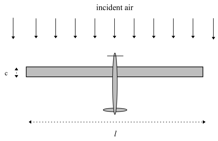
Top view of aircraft (in its own frame of reference):
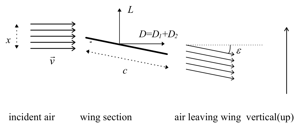
Side view of wing (in a frame of reference moving with the aircraft):
Ignore the modification of the airflow due to the propeller.
(a) Consider the change in momentum of the air moving past the wing, with no change in speed while it does so. Derive expressions for the vertical lift force \(L\) and the horizontal drag force \(D_1\) on the wing in terms of wing dimensions, \(v\), \(\varepsilon\), and the air density \(\rho\). Assume the direction of air flow is always parallel to the plane of the side-view diagram.
(3 marks)
(b) There is an additional horizontal drag force \(D_2\) caused by the friction of air flowing over the surface of the wing. The air slows slightly, with a change of speed \(\Delta v\) (\(\ll 1\%\) of \(v\)) given by:
\[ \frac{\Delta v}{v}=\frac{f}{A} \]
The value of \(f\) is independent of \(\varepsilon\).
Find an expression (in terms of \(M, f, A, S, \rho\) and \(g\)- the acceleration due to gravity) for the flight speed \(v_0\) corresponding to a minimum power being needed to maintain this aircraft in flight at constant altitude and velocity. Neglect terms of order \((\varepsilon^2 f)\) or higher.
(3 marks)
You may find the following small angle approximation useful:
\[ 1-\cos\varepsilon\approx\frac{\sin^2\varepsilon}{2} \]
(c) On the answer sheet, sketch a graph of power \(P\) versus flight speed \(v\). Show the separate contributions to the power needed from the two sources of drag. Find an expression (in terms of \(M, f, A, S, \rho\) and \(g\)) for the minimum power, \(P_{\min}\).
(2 marks)
(d) If the solar cells can supply sufficient energy so that the electric motors and propellers generate mechanical power of \(I = 10\) watts per square metre of wing area, calculate the maximum wing loading \(Mg/S\) (\(\mathrm{N/m^2}\)) for this power and flight speed \(v_0\) (\(\mathrm{m/s}\)). Assume \(\rho = 1.25\ \mathrm{kg/m^3}\), \(f = 0.004\), \(A = 10\).
(2 marks)
Official English text of the problem.
Answers
-
(a) \[ \boxed{L=\frac{\pi}{4}\rho l^2v^2\sin\varepsilon}, \qquad \boxed{D_1=\frac{\pi}{4}\rho l^2v^2(1-\cos\varepsilon)}. \]
-
(b) \[ \boxed{v_0= \left[\frac{8(Mg)^2}{3\pi^2\rho^2 f A S^2}\right]^{1/4}}. \]
-
(c) \[ \boxed{P(v)= \underbrace{\frac{2(Mg)^2}{\pi\rho ASv}}_{P_1} +\underbrace{\frac{\pi}{4}\rho fS v^3}_{P_2}}, \] \[ \boxed{P_{\min}= \left(\frac{512f}{27\pi^2A^3}\right)^{1/4} \frac{(Mg)^{3/2}}{\sqrt{\rho S}}}. \] The induced-power contribution \(P_1\) decreases as \(1/v\), while the friction contribution \(P_2\) increases as \(v^3\). Their sum has one minimum, at \(v_0\), where \(P_1=3P_2\).
-
(d) \[ \boxed{\left(\frac{Mg}{S}\right)_{\max}\approx36\ \mathrm{N/m^2}}, \qquad \boxed{v_0\approx8.6\ \mathrm{m/s}}. \]
Solution
(a)
Work in the aircraft’s reference frame. In a time \(dt\), the volume of air passing through the affected cross-section \(xl\) is \(xlv\,dt\). Thus the mass flow rate is
\[ \dot m=\rho xlv. \]
The air initially has horizontal speed \(v\). After deflection, its horizontal velocity is \(v\cos\varepsilon\) and its downward velocity is \(v\sin\varepsilon\).
By the momentum principle and Newton’s third law, the upward force on the wing equals the rate at which the air gains downward momentum:
\[ L=\dot m\,v\sin\varepsilon =\rho xl v^2\sin\varepsilon. \]
Similarly, the air loses horizontal momentum, producing a drag force on the wing:
\[ D_1=\dot m\,v(1-\cos\varepsilon) =\rho xl v^2(1-\cos\varepsilon). \]
Using \(x=\pi l/4\),
\[ \boxed{L=\frac{\pi}{4}\rho l^2v^2\sin\varepsilon}, \qquad \boxed{D_1=\frac{\pi}{4}\rho l^2v^2(1-\cos\varepsilon)}. \]
For small \(\varepsilon\), these become
\[ L\simeq\frac{\pi}{4}\rho l^2v^2\varepsilon, \qquad D_1\simeq\frac{\pi}{8}\rho l^2v^2\varepsilon^2. \]
(b)
Since \(AS=l^2\), define
\[ K=\rho xl=\frac{\pi}{4}\rho AS, \qquad \dot m=Kv. \]
The additional horizontal momentum loss caused by the reduction in speed gives
\[ D_2=\dot m\,\Delta v\cos\varepsilon. \]
Using \(\Delta v/v=f/A\) and dropping the correction of order \(\varepsilon^2f\),
\[ D_2\simeq Kv^2\frac{f}{A} =\boxed{\frac{\pi}{4}\rho fS v^2}. \]
The slowing also reduces the lift by a relative amount \(f/A\). However, its effect on the induced drag, which is proportional to \(\sin^2\varepsilon\), is of order \(\varepsilon^2f\). Therefore, to the required accuracy, we may impose vertical equilibrium using the lift expression from (a):
\[ Mg=Kv^2\sin\varepsilon, \qquad \sin\varepsilon=\frac{Mg}{Kv^2}. \]
The supplied small-angle approximation then gives
\[ D_1 \simeq\frac{Kv^2}{2}\sin^2\varepsilon =\frac{(Mg)^2}{2Kv^2} =\frac{2(Mg)^2}{\pi\rho ASv^2}. \]
In steady horizontal flight, propeller thrust balances the total drag. The mechanical power required is therefore
\[ P=(D_1+D_2)v =\frac{2(Mg)^2}{\pi\rho ASv} +\frac{\pi}{4}\rho fS v^3. \]
Write this as
\[ P=\frac{\alpha}{v}+\beta v^3, \qquad \alpha=\frac{2(Mg)^2}{\pi\rho AS}, \qquad \beta=\frac{\pi}{4}\rho fS. \]
Differentiating with respect to flight speed,
\[ \frac{dP}{dv}=-\frac{\alpha}{v^2}+3\beta v^2. \]
Hence the optimum speed satisfies
\[ v_0^4=\frac{\alpha}{3\beta} =\frac{8(Mg)^2}{3\pi^2\rho^2fAS^2}, \]
so
\[ \boxed{v_0= \left[\frac{8(Mg)^2}{3\pi^2\rho^2fAS^2}\right]^{1/4}}. \]
This is the unique minimum for \(v>0\), since
\[ \frac{d^2P}{dv^2} =\frac{2\alpha}{v^3}+6\beta v>0. \]
(c)
At the minimum, the condition \(\alpha=3\beta v_0^4\) implies
\[ P_1(v_0)=\frac{\alpha}{v_0} =3\beta v_0^3=3P_2(v_0). \]
Thus
\[ P_{\min}=4\beta v_0^3 =\pi\rho fS v_0^3. \]
Substituting the expression for \(v_0\),
\[ \boxed{ P_{\min} =\left(\frac{512f}{27\pi^2A^3}\right)^{1/4} \frac{(Mg)^{3/2}}{\sqrt{\rho S}} }. \]
The requested graph has the following features:
- \(P_1=\alpha/v\) is a decreasing hyperbola. Formally, it diverges as \(v\to0^+\) and approaches zero as \(v\to\infty\).
- \(P_2=\beta v^3\) starts at the origin with a horizontal tangent and increases monotonically.
- Their sum lies above both curves, decreases to its unique minimum \((v_0,P_{\min})\), and then increases. It diverges at both ends of the positive-speed range and has no axis intercept.
- The two contributions cross at \(v=3^{1/4}v_0\approx1.316v_0\), to the right of the total-power minimum.
A precise dimensionless description is obtained by setting \(u=v/v_0\):
\[ \frac{P_1}{P_{\min}}=\frac{3}{4u}, \qquad \frac{P_2}{P_{\min}}=\frac{u^3}{4}, \qquad \frac{P}{P_{\min}}=\frac{3}{4u}+\frac{u^3}{4}. \]
Useful points for the sketch are:
| \(v/v_0\) | \(P_1/P_{\min}\) | \(P_2/P_{\min}\) | \(P/P_{\min}\) |
|---|---|---|---|
| 0.500 | 1.500 | 0.031 | 1.531 |
| 1.000 | 0.750 | 0.250 | 1.000 |
| 1.316 | 0.570 | 0.570 | 1.140 |
| 2.000 | 0.375 | 2.000 | 2.375 |
The limit \(v\to0^+\) is a formal extrapolation of these equations: sufficiently low speeds would require a deflection angle outside the small-angle approximation.
(d)
Let the wing loading be
\[ w=\frac{Mg}{S}. \]
The available mechanical power is \(IS\). The maximum loading occurs when this just equals the minimum required power:
\[ IS=P_{\min}=\pi\rho fS v_0^3. \]
Consequently,
\[ v_0=\left(\frac{I}{\pi\rho f}\right)^{1/3}. \]
Numerically,
\[ v_0= \left(\frac{10}{\pi(1.25)(0.004)}\right)^{1/3} =8.6025\ldots\ \mathrm{m/s}, \]
giving
\[ \boxed{v_0\approx8.6\ \mathrm{m/s}}. \]
Rearranging the optimum-speed relation from (b),
\[ v_0^4=\frac{8w^2}{3\pi^2\rho^2fA}, \]
we obtain
\[ w_{\max} =\pi\rho v_0^2\sqrt{\frac{3fA}{8}} =\pi\rho\sqrt{\frac{3fA}{8}} \left(\frac{I}{\pi\rho f}\right)^{2/3}. \]
Substitution gives
\[ w_{\max} =\pi(1.25)(8.6025\ldots)^2 \sqrt{\frac{3(0.004)(10)}{8}} =35.5925\ldots\ \mathrm{N/m^2}. \]
Therefore,
\[ \boxed{\left(\frac{Mg}{S}\right)_{\max}\approx36\ \mathrm{N/m^2}}. \]
This is the maximum because \(P_{\min}/S\) increases as \(w^{3/2}\); a larger loading would require more than the available \(10\ \mathrm{W/m^2}\) at every speed.
As a consistency check, at this operating point,
\[ \sin\varepsilon_0=\sqrt{\frac{6f}{A}}, \qquad \varepsilon_0\simeq0.049\ \mathrm{rad}\simeq2.8^\circ, \]
and
\[ \frac{\Delta v}{v}=\frac{f}{A}=0.0004=0.04\%. \]
Both approximations are consistent with the given data.
The solution was checked against the official solution.
IPhO 1997 · Theorieaufgabe 3
Solarbetriebenes Flugzeug
Wir möchten ein Flugzeug entwerfen, das allein mit Solarenergie in der Luft bleibt. Die effizienteste Bauform besitzt einen Tragflügel, dessen Oberseite vollständig mit Solarzellen bedeckt ist. Die Zellen liefern die elektrische Leistung, mit der der Motor den Propeller antreibt.
Betrachten Sie einen Tragflügel mit rechteckigem Grundriss, der Spannweite \(l\) und der Flügeltiefe (Breite) \(c\); die Flügelfläche beträgt \(S = cl\), und die Flügelstreckung ist \(A = l/c\). Eine ungefähre Vorstellung von den aerodynamischen Eigenschaften des Tragflügels erhalten wir, indem wir eine Luftschicht der Höhe \(x\) und der Länge \(l\) betrachten, die unter einem kleinen Winkel \(\varepsilon\) nach unten abgelenkt wird, wobei sich ihr Geschwindigkeitsbetrag nur sehr geringfügig ändert. Mithilfe von Steuerflächen lässt sich ein für den Flug optimaler Wert von \(\varepsilon\) einstellen. Dieses einfache Modell stimmt gut mit der Wirklichkeit überein, wenn \(x = \pi l/4\), und wir können annehmen, dass dies der Fall ist. Die Gesamtmasse des Flugzeugs beträgt \(M\), und es fliegt horizontal mit der Geschwindigkeit \(\vec{v}\) relativ zur umgebenden Luft. Berücksichtigen Sie bei den folgenden Berechnungen nur die Luftströmung um den Tragflügel.
Draufsicht auf das Flugzeug (in seinem eigenen Bezugssystem):
Seitenansicht des Tragflügels (in einem mit dem Flugzeug mitbewegten Bezugssystem):
Vernachlässigen Sie die Veränderung der Luftströmung durch den Propeller.
(a) Betrachten Sie die Impulsänderung der am Tragflügel vorbeiströmenden Luft, wobei sich ihr Geschwindigkeitsbetrag dabei nicht ändert. Leiten Sie Ausdrücke für die vertikale Auftriebskraft \(L\) und die horizontale Widerstandskraft \(D_1\) am Tragflügel in Abhängigkeit von den Flügelabmessungen, \(v\), \(\varepsilon\) und der Luftdichte \(\rho\) her. Nehmen Sie an, dass die Richtung der Luftströmung stets parallel zur Zeichenebene der Seitenansicht ist.
(3 Punkte)
(b) Durch die Reibung der über die Flügeloberfläche strömenden Luft entsteht eine zusätzliche horizontale Widerstandskraft \(D_2\). Die Luft wird geringfügig abgebremst, wobei die Änderung des Geschwindigkeitsbetrags \(\Delta v\) (\(\ll 1\%\) von \(v\)) gegeben ist durch:
\[ \frac{\Delta v}{v}=\frac{f}{A} \]
Der Wert von \(f\) ist unabhängig von \(\varepsilon\).
Bestimmen Sie einen Ausdruck (in Abhängigkeit von \(M, f, A, S, \rho\) und \(g\), der Erdbeschleunigung) für die Fluggeschwindigkeit \(v_0\), bei der die zum Flug mit konstanter Höhe und Geschwindigkeit erforderliche Leistung minimal ist. Vernachlässigen Sie Terme der Ordnung \((\varepsilon^2 f)\) oder höher.
(3 Punkte)
Die folgende Kleinwinkelnäherung kann hilfreich sein:
\[ 1-\cos\varepsilon\approx\frac{\sin^2\varepsilon}{2} \]
(c) Skizzieren Sie auf dem Antwortblatt ein Diagramm der Leistung \(P\) in Abhängigkeit von der Fluggeschwindigkeit \(v\). Zeigen Sie die einzelnen Beiträge zur erforderlichen Leistung aufgrund der beiden Ursachen des Luftwiderstands. Bestimmen Sie einen Ausdruck (in Abhängigkeit von \(M, f, A, S, \rho\) und \(g\)) für die minimale Leistung \(P_{\min}\).
(2 Punkte)
(d) Wenn die Solarzellen genügend Energie liefern können, sodass die Elektromotoren und Propeller eine mechanische Leistung von \(I = 10\) Watt pro Quadratmeter Flügelfläche erzeugen, berechnen Sie für diese Leistung die maximale Flächenbelastung \(Mg/S\) (\(\mathrm{N/m^2}\)) und die Fluggeschwindigkeit \(v_0\) (\(\mathrm{m/s}\)). Nehmen Sie \(\rho = 1.25\ \mathrm{kg/m^3}\), \(f = 0.004\), \(A = 10\) an.
(2 Punkte)
Aufgabentext aus dem offiziellen englischen Text übersetzt.
Antworten
-
(a) \[ \boxed{L=\frac{\pi}{4}\rho l^2v^2\sin\varepsilon}, \qquad \boxed{D_1=\frac{\pi}{4}\rho l^2v^2(1-\cos\varepsilon)}. \]
-
(b) \[ \boxed{v_0= \left[\frac{8(Mg)^2}{3\pi^2\rho^2 f A S^2}\right]^{1/4}}. \]
-
(c) \[ \boxed{P(v)= \underbrace{\frac{2(Mg)^2}{\pi\rho ASv}}_{P_1} +\underbrace{\frac{\pi}{4}\rho fS v^3}_{P_2}}, \] \[ \boxed{P_{\min}= \left(\frac{512f}{27\pi^2A^3}\right)^{1/4} \frac{(Mg)^{3/2}}{\sqrt{\rho S}}}. \] Der durch den induzierten Widerstand verursachte Leistungsanteil \(P_1\) nimmt wie \(1/v\) ab, während der Reibungsanteil \(P_2\) wie \(v^3\) zunimmt. Ihre Summe besitzt ein einziges Minimum bei \(v_0\), wo \(P_1=3P_2\) gilt.
-
(d) \[ \boxed{\left(\frac{Mg}{S}\right)_{\max}\approx36\ \mathrm{N/m^2}}, \qquad \boxed{v_0\approx8.6\ \mathrm{m/s}}. \]
Lösung
(a)
Wir arbeiten im Bezugssystem des Flugzeugs. In einer Zeit \(dt\) beträgt das Luftvolumen, das den betroffenen Querschnitt \(xl\) durchströmt, \(xlv\,dt\). Der Massenstrom ist somit
\[ \dot m=\rho xlv. \]
Die Luft besitzt zunächst die horizontale Geschwindigkeit \(v\). Nach der Ablenkung beträgt ihre horizontale Geschwindigkeitskomponente \(v\cos\varepsilon\) und ihre nach unten gerichtete Geschwindigkeitskomponente \(v\sin\varepsilon\).
Nach dem Impulssatz und dem dritten Newtonschen Gesetz ist die nach oben gerichtete Kraft auf den Tragflügel gleich der zeitlichen Zunahme des nach unten gerichteten Impulses der Luft:
\[ L=\dot m\,v\sin\varepsilon =\rho xl v^2\sin\varepsilon. \]
Ebenso verliert die Luft horizontalen Impuls, wodurch eine Widerstandskraft auf den Tragflügel entsteht:
\[ D_1=\dot m\,v(1-\cos\varepsilon) =\rho xl v^2(1-\cos\varepsilon). \]
Mit \(x=\pi l/4\) folgt
\[ \boxed{L=\frac{\pi}{4}\rho l^2v^2\sin\varepsilon}, \qquad \boxed{D_1=\frac{\pi}{4}\rho l^2v^2(1-\cos\varepsilon)}. \]
Für kleine \(\varepsilon\) werden diese Ausdrücke zu
\[ L\simeq\frac{\pi}{4}\rho l^2v^2\varepsilon, \qquad D_1\simeq\frac{\pi}{8}\rho l^2v^2\varepsilon^2. \]
(b)
Da \(AS=l^2\) gilt, definieren wir
\[ K=\rho xl=\frac{\pi}{4}\rho AS, \qquad \dot m=Kv. \]
Der zusätzliche horizontale Impulsverlust infolge der Verringerung des Geschwindigkeitsbetrags ergibt
\[ D_2=\dot m\,\Delta v\cos\varepsilon. \]
Mit \(\Delta v/v=f/A\) und unter Vernachlässigung der Korrektur der Ordnung \(\varepsilon^2f\) folgt
\[ D_2\simeq Kv^2\frac{f}{A} =\boxed{\frac{\pi}{4}\rho fS v^2}. \]
Die Abbremsung verringert auch den Auftrieb um den relativen Anteil \(f/A\). Ihre Auswirkung auf den induzierten Widerstand, der proportional zu \(\sin^2\varepsilon\) ist, ist jedoch von der Ordnung \(\varepsilon^2f\). Daher dürfen wir mit der geforderten Genauigkeit das vertikale Kräftegleichgewicht mithilfe des Ausdrucks für den Auftrieb aus (a) ansetzen:
\[ Mg=Kv^2\sin\varepsilon, \qquad \sin\varepsilon=\frac{Mg}{Kv^2}. \]
Die angegebene Kleinwinkelnäherung liefert dann
\[ D_1 \simeq\frac{Kv^2}{2}\sin^2\varepsilon =\frac{(Mg)^2}{2Kv^2} =\frac{2(Mg)^2}{\pi\rho ASv^2}. \]
Im stationären Horizontalflug gleicht der Propellerschub den gesamten Widerstand aus. Die erforderliche mechanische Leistung beträgt daher
\[ P=(D_1+D_2)v =\frac{2(Mg)^2}{\pi\rho ASv} +\frac{\pi}{4}\rho fS v^3. \]
Wir schreiben dies in der Form
\[ P=\frac{\alpha}{v}+\beta v^3, \qquad \alpha=\frac{2(Mg)^2}{\pi\rho AS}, \qquad \beta=\frac{\pi}{4}\rho fS. \]
Die Ableitung nach der Fluggeschwindigkeit ergibt
\[ \frac{dP}{dv}=-\frac{\alpha}{v^2}+3\beta v^2. \]
Damit erfüllt die optimale Geschwindigkeit
\[ v_0^4=\frac{\alpha}{3\beta} =\frac{8(Mg)^2}{3\pi^2\rho^2fAS^2}, \]
also
\[ \boxed{v_0= \left[\frac{8(Mg)^2}{3\pi^2\rho^2fAS^2}\right]^{1/4}}. \]
Dies ist das einzige Minimum für \(v>0\), denn
\[ \frac{d^2P}{dv^2} =\frac{2\alpha}{v^3}+6\beta v>0. \]
(c)
Am Minimum folgt aus der Bedingung \(\alpha=3\beta v_0^4\)
\[ P_1(v_0)=\frac{\alpha}{v_0} =3\beta v_0^3=3P_2(v_0). \]
Somit gilt
\[ P_{\min}=4\beta v_0^3 =\pi\rho fS v_0^3. \]
Einsetzen des Ausdrucks für \(v_0\) ergibt
\[ \boxed{ P_{\min} =\left(\frac{512f}{27\pi^2A^3}\right)^{1/4} \frac{(Mg)^{3/2}}{\sqrt{\rho S}} }. \]
Das geforderte Diagramm weist folgende Eigenschaften auf:
- \(P_1=\alpha/v\) ist eine fallende Hyperbel. Formal divergiert sie für \(v\to0^+\) und nähert sich für \(v\to\infty\) null.
- \(P_2=\beta v^3\) beginnt im Ursprung mit einer horizontalen Tangente und nimmt monoton zu.
- Ihre Summe liegt oberhalb beider Kurven, fällt bis zu ihrem einzigen Minimum \((v_0,P_{\min})\) und steigt danach an. Sie divergiert an beiden Enden des Bereichs positiver Geschwindigkeiten und besitzt keinen Achsenschnittpunkt.
- Die beiden Beiträge schneiden sich bei \(v=3^{1/4}v_0\approx1.316v_0\), rechts vom Minimum der Gesamtleistung.
Eine genaue dimensionslose Beschreibung erhält man mit \(u=v/v_0\):
\[ \frac{P_1}{P_{\min}}=\frac{3}{4u}, \qquad \frac{P_2}{P_{\min}}=\frac{u^3}{4}, \qquad \frac{P}{P_{\min}}=\frac{3}{4u}+\frac{u^3}{4}. \]
Nützliche Punkte für die Skizze sind:
| \(v/v_0\) | \(P_1/P_{\min}\) | \(P_2/P_{\min}\) | \(P/P_{\min}\) |
|---|---|---|---|
| 0.500 | 1.500 | 0.031 | 1.531 |
| 1.000 | 0.750 | 0.250 | 1.000 |
| 1.316 | 0.570 | 0.570 | 1.140 |
| 2.000 | 0.375 | 2.000 | 2.375 |
Der Grenzfall \(v\to0^+\) ist eine formale Extrapolation dieser Gleichungen: Bei hinreichend niedrigen Geschwindigkeiten wäre ein Ablenkwinkel außerhalb des Gültigkeitsbereichs der Kleinwinkelnäherung erforderlich.
(d)
Die Flächenbelastung sei
\[ w=\frac{Mg}{S}. \]
Die verfügbare mechanische Leistung beträgt \(IS\). Die maximale Flächenbelastung wird erreicht, wenn diese gerade der minimal erforderlichen Leistung entspricht:
\[ IS=P_{\min}=\pi\rho fS v_0^3. \]
Folglich gilt
\[ v_0=\left(\frac{I}{\pi\rho f}\right)^{1/3}. \]
Numerisch ergibt sich
\[ v_0= \left(\frac{10}{\pi(1.25)(0.004)}\right)^{1/3} =8.6025\ldots\ \mathrm{m/s}, \]
also
\[ \boxed{v_0\approx8.6\ \mathrm{m/s}}. \]
Durch Umstellen der Beziehung für die optimale Geschwindigkeit aus (b),
\[ v_0^4=\frac{8w^2}{3\pi^2\rho^2fA}, \]
erhalten wir
\[ w_{\max} =\pi\rho v_0^2\sqrt{\frac{3fA}{8}} =\pi\rho\sqrt{\frac{3fA}{8}} \left(\frac{I}{\pi\rho f}\right)^{2/3}. \]
Einsetzen ergibt
\[ w_{\max} =\pi(1.25)(8.6025\ldots)^2 \sqrt{\frac{3(0.004)(10)}{8}} =35.5925\ldots\ \mathrm{N/m^2}. \]
Daher ist
\[ \boxed{\left(\frac{Mg}{S}\right)_{\max}\approx36\ \mathrm{N/m^2}}. \]
Dies ist das Maximum, weil \(P_{\min}/S\) wie \(w^{3/2}\) zunimmt; eine größere Flächenbelastung würde bei jeder Geschwindigkeit mehr als die verfügbaren \(10\ \mathrm{W/m^2}\) erfordern.
Zur Konsistenzprüfung gilt an diesem Betriebspunkt
\[ \sin\varepsilon_0=\sqrt{\frac{6f}{A}}, \qquad \varepsilon_0\simeq0.049\ \mathrm{rad}\simeq2.8^\circ, \]
und
\[ \frac{\Delta v}{v}=\frac{f}{A}=0.0004=0.04\%. \]
Beide Näherungen sind mit den gegebenen Daten vereinbar.
Die Lösung wurde mit der offiziellen Lösung abgeglichen.
IPhO 1997 · Teori sorusu 3
Güneş Enerjili Uçak
Yalnızca güneş enerjisini kullanarak havada kalacak bir uçak tasarlamak istiyoruz. En verimli tasarım, üst yüzeyi tamamen güneş hücreleriyle kaplı bir kanada sahip olandır. Hücreler, motorun pervaneyi döndürmek için kullandığı elektrik gücünü sağlar.
Açıklığı \(l\), veter uzunluğu (genişliği) \(c\) olan, üstten görünüşü dikdörtgen biçimindeki bir kanadı ele alın; kanat alanı \(S = cl\), kanat açıklık oranı ise \(A = l/c\)'dir. Yüksekliği \(x\) ve uzunluğu \(l\) olan bir hava diliminin, sürati yalnızca çok az değişerek küçük bir \(\varepsilon\) açısıyla aşağı doğru saptırılmasını ele alarak kanadın performansı hakkında yaklaşık bir fikir edinebiliriz. Uçuş için en uygun \(\varepsilon\) değerini seçmek üzere kumanda yüzeyleri kullanılabilir. Bu basit model, \(x = \pi l/4\) olduğunda gerçeğe oldukça iyi uyar ve bunun geçerli olduğunu varsayabiliriz. Uçağın toplam kütlesi \(M\)'dir ve çevresindeki havaya göre \(\vec{v}\) hızıyla yatay olarak uçmaktadır. Aşağıdaki hesaplamalarda yalnızca kanat çevresindeki hava akışını dikkate alın.
Uçağın üstten görünüşü (kendi referans sisteminde):
Kanadın yandan görünüşü (uçakla birlikte hareket eden bir referans sisteminde):
Pervanenin hava akışında oluşturduğu değişikliği ihmal edin.
(a) Kanadın yanından geçen havanın, bu sırada sürati hiç değişmeden gerçekleşen momentum değişimini ele alın. Kanat boyutları, \(v\), \(\varepsilon\) ve hava yoğunluğu \(\rho\) cinsinden, kanada etki eden düşey kaldırma kuvveti \(L\) ve yatay sürükleme kuvveti \(D_1\) için ifadeler türetin. Hava akışının yönünün her zaman yandan görünüş çiziminin düzlemine paralel olduğunu varsayın.
(3 puan)
(b) Kanat yüzeyi üzerinden akan havanın sürtünmesinden kaynaklanan ek bir yatay sürükleme kuvveti \(D_2\) vardır. Hava hafifçe yavaşlar; süratindeki \(\Delta v\) değişimi (\(v\)'nin \(\ll 1\%\)'i) şu şekilde verilir:
\[ \frac{\Delta v}{v}=\frac{f}{A} \]
\(f\)'nin değeri \(\varepsilon\)'dan bağımsızdır.
Bu uçağı sabit irtifada ve sabit hızla uçuşta tutmak için gereken gücün en küçük olduğu uçuş sürati \(v_0\) için (\(M, f, A, S, \rho\) ve yer çekimi ivmesi \(g\) cinsinden) bir ifade bulun. \((\varepsilon^2 f)\) veya daha yüksek mertebeden terimleri ihmal edin.
(3 puan)
Aşağıdaki küçük açı yaklaşımı yararlı olabilir:
\[ 1-\cos\varepsilon\approx\frac{\sin^2\varepsilon}{2} \]
(c) Cevap kâğıdına, \(P\) gücünün \(v\) uçuş süratine bağlılığını gösteren bir grafik çizin. İki sürükleme kaynağının gereken güce katkılarını ayrı ayrı gösterin. En küçük güç \(P_{\min}\) için (\(M, f, A, S, \rho\) ve \(g\) cinsinden) bir ifade bulun.
(2 puan)
(d) Güneş hücreleri, elektrik motorları ve pervanelerin kanat alanının metrekaresi başına \(I = 10\) watt mekanik güç üretmesine yetecek kadar enerji sağlayabiliyorsa, bu güç için en büyük kanat yüklemesini \(Mg/S\) (\(\mathrm{N/m^2}\)) ve uçuş süratini \(v_0\) (\(\mathrm{m/s}\)) hesaplayın. \(\rho = 1.25\ \mathrm{kg/m^3}\), \(f = 0.004\), \(A = 10\) olduğunu varsayın.
(2 puan)
Soru metni resmi İngilizce metinden çevrilmiştir.
Cevaplar
-
(a) \[ \boxed{L=\frac{\pi}{4}\rho l^2v^2\sin\varepsilon}, \qquad \boxed{D_1=\frac{\pi}{4}\rho l^2v^2(1-\cos\varepsilon)}. \]
-
(b) \[ \boxed{v_0= \left[\frac{8(Mg)^2}{3\pi^2\rho^2 f A S^2}\right]^{1/4}}. \]
-
(c) \[ \boxed{P(v)= \underbrace{\frac{2(Mg)^2}{\pi\rho ASv}}_{P_1} +\underbrace{\frac{\pi}{4}\rho fS v^3}_{P_2}}, \] \[ \boxed{P_{\min}= \left(\frac{512f}{27\pi^2A^3}\right)^{1/4} \frac{(Mg)^{3/2}}{\sqrt{\rho S}}}. \] İndüklenmiş sürüklemeden kaynaklanan güç katkısı \(P_1\), \(1/v\) ile orantılı olarak azalırken sürtünme katkısı \(P_2\), \(v^3\) ile orantılı olarak artar. Toplamlarının, \(P_1=3P_2\) olduğu \(v_0\) süratinde tek bir minimumu vardır.
-
(d) \[ \boxed{\left(\frac{Mg}{S}\right)_{\max}\approx36\ \mathrm{N/m^2}}, \qquad \boxed{v_0\approx8.6\ \mathrm{m/s}}. \]
Çözüm
(a)
Uçağın referans sisteminde çalışalım. \(dt\) süresinde, akışın etkilendiği \(xl\) kesitinden geçen havanın hacmi \(xlv\,dt\)'dir. Dolayısıyla kütlesel debi
\[ \dot m=\rho xlv. \]
Havanın başlangıçtaki yatay sürati \(v\)'dir. Saptırıldıktan sonra yatay hızı \(v\cos\varepsilon\), aşağı yönlü hızı ise \(v\sin\varepsilon\) olur.
Momentum ilkesi ve Newton'un üçüncü yasası gereğince, kanada etki eden yukarı yönlü kuvvet, havanın aşağı yönlü momentum kazanma hızına eşittir:
\[ L=\dot m\,v\sin\varepsilon =\rho xl v^2\sin\varepsilon. \]
Benzer şekilde hava yatay momentum kaybeder ve bu, kanat üzerinde bir sürükleme kuvveti oluşturur:
\[ D_1=\dot m\,v(1-\cos\varepsilon) =\rho xl v^2(1-\cos\varepsilon). \]
\(x=\pi l/4\) kullanılarak,
\[ \boxed{L=\frac{\pi}{4}\rho l^2v^2\sin\varepsilon}, \qquad \boxed{D_1=\frac{\pi}{4}\rho l^2v^2(1-\cos\varepsilon)}. \]
Küçük \(\varepsilon\) için bunlar şu hâli alır:
\[ L\simeq\frac{\pi}{4}\rho l^2v^2\varepsilon, \qquad D_1\simeq\frac{\pi}{8}\rho l^2v^2\varepsilon^2. \]
(b)
\(AS=l^2\) olduğundan şu tanımları yapalım:
\[ K=\rho xl=\frac{\pi}{4}\rho AS, \qquad \dot m=Kv. \]
Süratin azalmasından kaynaklanan ek yatay momentum kaybı şu sonucu verir:
\[ D_2=\dot m\,\Delta v\cos\varepsilon. \]
\(\Delta v/v=f/A\) kullanılarak ve \(\varepsilon^2f\) mertebesindeki düzeltme ihmal edilerek,
\[ D_2\simeq Kv^2\frac{f}{A} =\boxed{\frac{\pi}{4}\rho fS v^2}. \]
Yavaşlama, kaldırma kuvvetini de göreli olarak \(f/A\) oranında azaltır. Ancak bunun, \(\sin^2\varepsilon\) ile orantılı olan indüklenmiş sürükleme üzerindeki etkisi \(\varepsilon^2f\) mertebesindedir. Dolayısıyla, istenen doğruluk düzeyinde, (a)'daki kaldırma kuvveti ifadesini kullanarak düşey denge koşulunu yazabiliriz:
\[ Mg=Kv^2\sin\varepsilon, \qquad \sin\varepsilon=\frac{Mg}{Kv^2}. \]
Verilen küçük açı yaklaşımı daha sonra şu sonucu verir:
\[ D_1 \simeq\frac{Kv^2}{2}\sin^2\varepsilon =\frac{(Mg)^2}{2Kv^2} =\frac{2(Mg)^2}{\pi\rho ASv^2}. \]
Sabit hızlı yatay uçuşta pervanenin itme kuvveti toplam sürükleme kuvvetini dengeler. Dolayısıyla gereken mekanik güç
\[ P=(D_1+D_2)v =\frac{2(Mg)^2}{\pi\rho ASv} +\frac{\pi}{4}\rho fS v^3. \]
Bunu şu şekilde yazalım:
\[ P=\frac{\alpha}{v}+\beta v^3, \qquad \alpha=\frac{2(Mg)^2}{\pi\rho AS}, \qquad \beta=\frac{\pi}{4}\rho fS. \]
Uçuş süratine göre türev alındığında,
\[ \frac{dP}{dv}=-\frac{\alpha}{v^2}+3\beta v^2. \]
Böylece en uygun sürat şu koşulu sağlar:
\[ v_0^4=\frac{\alpha}{3\beta} =\frac{8(Mg)^2}{3\pi^2\rho^2fAS^2}, \]
dolayısıyla
\[ \boxed{v_0= \left[\frac{8(Mg)^2}{3\pi^2\rho^2fAS^2}\right]^{1/4}}. \]
Bu, \(v>0\) için tek minimumdur; çünkü
\[ \frac{d^2P}{dv^2} =\frac{2\alpha}{v^3}+6\beta v>0. \]
(c)
Minimumda, \(\alpha=3\beta v_0^4\) koşulundan
\[ P_1(v_0)=\frac{\alpha}{v_0} =3\beta v_0^3=3P_2(v_0). \]
Böylece
\[ P_{\min}=4\beta v_0^3 =\pi\rho fS v_0^3. \]
\(v_0\) ifadesi yerine konulduğunda,
\[ \boxed{ P_{\min} =\left(\frac{512f}{27\pi^2A^3}\right)^{1/4} \frac{(Mg)^{3/2}}{\sqrt{\rho S}} }. \]
İstenen grafik şu özelliklere sahiptir:
- \(P_1=\alpha/v\) azalan bir hiperboldür. Biçimsel olarak, \(v\to0^+\) iken sonsuza gider ve \(v\to\infty\) iken sıfıra yaklaşır.
- \(P_2=\beta v^3\), yatay bir teğetle orijinden başlar ve monoton olarak artar.
- Toplamları her iki eğrinin de üzerinde yer alır, tek minimumu olan \((v_0,P_{\min})\) noktasına kadar azalır, ardından artar. Pozitif sürat aralığının her iki ucunda da sonsuza gider ve eksenleri kesmez.
- İki katkı, toplam gücün minimumunun sağında, \(v=3^{1/4}v_0\approx1.316v_0\) süratinde kesişir.
\(u=v/v_0\) tanımlanarak kesin bir boyutsuz gösterim elde edilir:
\[ \frac{P_1}{P_{\min}}=\frac{3}{4u}, \qquad \frac{P_2}{P_{\min}}=\frac{u^3}{4}, \qquad \frac{P}{P_{\min}}=\frac{3}{4u}+\frac{u^3}{4}. \]
Grafik çizimi için yararlı noktalar şunlardır:
| \(v/v_0\) | \(P_1/P_{\min}\) | \(P_2/P_{\min}\) | \(P/P_{\min}\) |
|---|---|---|---|
| 0.500 | 1.500 | 0.031 | 1.531 |
| 1.000 | 0.750 | 0.250 | 1.000 |
| 1.316 | 0.570 | 0.570 | 1.140 |
| 2.000 | 0.375 | 2.000 | 2.375 |
\(v\to0^+\) limiti, bu denklemlerin biçimsel bir ekstrapolasyonudur: yeterince düşük süratlerde, küçük açı yaklaşımının dışında kalan bir sapma açısı gerekir.
(d)
Kanat yüklemesi şu olsun:
\[ w=\frac{Mg}{S}. \]
Kullanılabilir mekanik güç \(IS\)'dir. En büyük yükleme, bu güç gereken en küçük güce tam olarak eşit olduğunda elde edilir:
\[ IS=P_{\min}=\pi\rho fS v_0^3. \]
Sonuç olarak,
\[ v_0=\left(\frac{I}{\pi\rho f}\right)^{1/3}. \]
Sayısal olarak,
\[ v_0= \left(\frac{10}{\pi(1.25)(0.004)}\right)^{1/3} =8.6025\ldots\ \mathrm{m/s}, \]
buradan
\[ \boxed{v_0\approx8.6\ \mathrm{m/s}}. \]
(b)'deki en uygun sürat bağıntısını yeniden düzenleyerek,
\[ v_0^4=\frac{8w^2}{3\pi^2\rho^2fA}, \]
şunu elde ederiz:
\[ w_{\max} =\pi\rho v_0^2\sqrt{\frac{3fA}{8}} =\pi\rho\sqrt{\frac{3fA}{8}} \left(\frac{I}{\pi\rho f}\right)^{2/3}. \]
Değerler yerine konulduğunda,
\[ w_{\max} =\pi(1.25)(8.6025\ldots)^2 \sqrt{\frac{3(0.004)(10)}{8}} =35.5925\ldots\ \mathrm{N/m^2}. \]
Dolayısıyla,
\[ \boxed{\left(\frac{Mg}{S}\right)_{\max}\approx36\ \mathrm{N/m^2}}. \]
Bu değer en büyüktür; çünkü \(P_{\min}/S\), \(w^{3/2}\) ile orantılı olarak artar; daha büyük bir yükleme, her süratte kullanılabilir \(10\ \mathrm{W/m^2}\)'den daha fazla güç gerektirir.
Tutarlılık kontrolü olarak, bu çalışma noktasında,
\[ \sin\varepsilon_0=\sqrt{\frac{6f}{A}}, \qquad \varepsilon_0\simeq0.049\ \mathrm{rad}\simeq2.8^\circ, \]
ve
\[ \frac{\Delta v}{v}=\frac{f}{A}=0.0004=0.04\%. \]
Her iki yaklaşım da verilen verilerle tutarlıdır.
Çözüm, resmi çözümle karşılaştırılarak kontrol edildi.
IPhO 1997 · Problema teórico 3
Avión propulsado por energía solar
Deseamos diseñar un avión que se mantenga en vuelo utilizando únicamente energía solar. La configuración más eficiente es aquella en la que la superficie superior del ala está completamente cubierta de células solares. Estas células suministran la energía eléctrica con la que el motor acciona la hélice.
Consideremos un ala de planta rectangular con envergadura \(l\) y cuerda (anchura) \(c\); la superficie alar es \(S = cl\), y el alargamiento del ala es \(A = l/c\). Podemos obtener una idea aproximada del comportamiento del ala considerando una capa de aire de altura \(x\) y longitud \(l\) que se desvía hacia abajo un ángulo pequeño \(\varepsilon\), con una variación muy pequeña de su rapidez. Las superficies de control permiten seleccionar un valor óptimo de \(\varepsilon\) para el vuelo. Este modelo sencillo se ajusta bien a la realidad si \(x = \pi l/4\), y podemos suponer que así ocurre. La masa total del avión es \(M\) y este vuela horizontalmente con velocidad \(\vec{v}\) respecto al aire circundante. En los cálculos siguientes, considere únicamente el flujo de aire alrededor del ala.
Vista superior del avión (en su propio sistema de referencia):
Vista lateral del ala (en un sistema de referencia que se mueve con el avión):
Ignore la modificación del flujo de aire debida a la hélice.
(a) Considere la variación de la cantidad de movimiento del aire que pasa junto al ala, sin que cambie su rapidez durante el proceso. Deduzca expresiones para la fuerza de sustentación vertical \(L\) y la fuerza de resistencia horizontal \(D_1\) que actúan sobre el ala, en función de las dimensiones del ala, \(v\), \(\varepsilon\) y la densidad del aire \(\rho\). Suponga que la dirección del flujo de aire es siempre paralela al plano del diagrama de la vista lateral.
(3 puntos)
(b) Existe una fuerza de resistencia horizontal adicional \(D_2\), causada por el rozamiento del aire que fluye sobre la superficie del ala. El aire se frena ligeramente, con una variación de rapidez \(\Delta v\) (\(\ll 1\%\) de \(v\)) dada por:
\[ \frac{\Delta v}{v}=\frac{f}{A} \]
El valor de \(f\) es independiente de \(\varepsilon\).
Obtenga una expresión (en función de \(M, f, A, S, \rho\) y \(g\), la aceleración de la gravedad) para la rapidez de vuelo \(v_0\) que corresponde a la potencia mínima necesaria para mantener este avión en vuelo a altitud y velocidad constantes. Desprecie los términos de orden \((\varepsilon^2 f)\) o superior.
(3 puntos)
Puede resultar útil la siguiente aproximación para ángulos pequeños:
\[ 1-\cos\varepsilon\approx\frac{\sin^2\varepsilon}{2} \]
(c) En la hoja de respuestas, esboce una gráfica de la potencia \(P\) en función de la rapidez de vuelo \(v\). Muestre por separado las contribuciones a la potencia necesaria debidas a las dos fuentes de resistencia. Obtenga una expresión (en función de \(M, f, A, S, \rho\) y \(g\)) para la potencia mínima, \(P_{\min}\).
(2 puntos)
(d) Si las células solares pueden suministrar suficiente energía para que los motores eléctricos y las hélices generen una potencia mecánica de \(I = 10\) vatios por metro cuadrado de superficie alar, calcule la carga alar máxima \(Mg/S\) (\(\mathrm{N/m^2}\)) para esta potencia y la rapidez de vuelo \(v_0\) (\(\mathrm{m/s}\)). Suponga que \(\rho = 1.25\ \mathrm{kg/m^3}\), \(f = 0.004\), \(A = 10\).
(2 puntos)
Enunciado traducido del texto oficial en inglés.
Respuestas
-
(a) \[ \boxed{L=\frac{\pi}{4}\rho l^2v^2\sin\varepsilon}, \qquad \boxed{D_1=\frac{\pi}{4}\rho l^2v^2(1-\cos\varepsilon)}. \]
-
(b) \[ \boxed{v_0= \left[\frac{8(Mg)^2}{3\pi^2\rho^2 f A S^2}\right]^{1/4}}. \]
-
(c) \[ \boxed{P(v)= \underbrace{\frac{2(Mg)^2}{\pi\rho ASv}}_{P_1} +\underbrace{\frac{\pi}{4}\rho fS v^3}_{P_2}}, \] \[ \boxed{P_{\min}= \left(\frac{512f}{27\pi^2A^3}\right)^{1/4} \frac{(Mg)^{3/2}}{\sqrt{\rho S}}}. \] La contribución de potencia debida a la resistencia inducida \(P_1\) disminuye como \(1/v\), mientras que la contribución del rozamiento \(P_2\) aumenta como \(v^3\). Su suma tiene un único mínimo, en \(v_0\), donde \(P_1=3P_2\).
-
(d) \[ \boxed{\left(\frac{Mg}{S}\right)_{\max}\approx36\ \mathrm{N/m^2}}, \qquad \boxed{v_0\approx8.6\ \mathrm{m/s}}. \]
Solución
(a)
Trabajamos en el sistema de referencia del avión. En un tiempo \(dt\), el volumen de aire que atraviesa la sección transversal afectada \(xl\) es \(xlv\,dt\). Por tanto, el caudal másico es
\[ \dot m=\rho xlv. \]
Inicialmente, el aire tiene una rapidez horizontal \(v\). Tras la desviación, su velocidad horizontal es \(v\cos\varepsilon\) y su velocidad hacia abajo es \(v\sin\varepsilon\).
Por el principio de la cantidad de movimiento y la tercera ley de Newton, la fuerza hacia arriba sobre el ala es igual a la tasa a la que el aire adquiere cantidad de movimiento hacia abajo:
\[ L=\dot m\,v\sin\varepsilon =\rho xl v^2\sin\varepsilon. \]
Análogamente, el aire pierde cantidad de movimiento horizontal, lo que produce una fuerza de resistencia sobre el ala:
\[ D_1=\dot m\,v(1-\cos\varepsilon) =\rho xl v^2(1-\cos\varepsilon). \]
Utilizando \(x=\pi l/4\),
\[ \boxed{L=\frac{\pi}{4}\rho l^2v^2\sin\varepsilon}, \qquad \boxed{D_1=\frac{\pi}{4}\rho l^2v^2(1-\cos\varepsilon)}. \]
Para \(\varepsilon\) pequeño, estas expresiones se convierten en
\[ L\simeq\frac{\pi}{4}\rho l^2v^2\varepsilon, \qquad D_1\simeq\frac{\pi}{8}\rho l^2v^2\varepsilon^2. \]
(b)
Como \(AS=l^2\), definimos
\[ K=\rho xl=\frac{\pi}{4}\rho AS, \qquad \dot m=Kv. \]
La pérdida adicional de cantidad de movimiento horizontal causada por la reducción de la rapidez da
\[ D_2=\dot m\,\Delta v\cos\varepsilon. \]
Utilizando \(\Delta v/v=f/A\) y despreciando la corrección de orden \(\varepsilon^2f\),
\[ D_2\simeq Kv^2\frac{f}{A} =\boxed{\frac{\pi}{4}\rho fS v^2}. \]
La disminución de la rapidez también reduce la sustentación en una fracción \(f/A\). Sin embargo, su efecto sobre la resistencia inducida, que es proporcional a \(\sin^2\varepsilon\), es de orden \(\varepsilon^2f\). Por tanto, con la precisión requerida, podemos imponer el equilibrio vertical utilizando la expresión de la sustentación de (a):
\[ Mg=Kv^2\sin\varepsilon, \qquad \sin\varepsilon=\frac{Mg}{Kv^2}. \]
La aproximación para ángulos pequeños proporcionada da entonces
\[ D_1 \simeq\frac{Kv^2}{2}\sin^2\varepsilon =\frac{(Mg)^2}{2Kv^2} =\frac{2(Mg)^2}{\pi\rho ASv^2}. \]
En vuelo horizontal uniforme, el empuje de la hélice equilibra la resistencia total. Por tanto, la potencia mecánica necesaria es
\[ P=(D_1+D_2)v =\frac{2(Mg)^2}{\pi\rho ASv} +\frac{\pi}{4}\rho fS v^3. \]
Escribimos esta expresión como
\[ P=\frac{\alpha}{v}+\beta v^3, \qquad \alpha=\frac{2(Mg)^2}{\pi\rho AS}, \qquad \beta=\frac{\pi}{4}\rho fS. \]
Derivando respecto a la rapidez de vuelo,
\[ \frac{dP}{dv}=-\frac{\alpha}{v^2}+3\beta v^2. \]
Por consiguiente, la rapidez óptima satisface
\[ v_0^4=\frac{\alpha}{3\beta} =\frac{8(Mg)^2}{3\pi^2\rho^2fAS^2}, \]
de modo que
\[ \boxed{v_0= \left[\frac{8(Mg)^2}{3\pi^2\rho^2fAS^2}\right]^{1/4}}. \]
Este es el único mínimo para \(v>0\), ya que
\[ \frac{d^2P}{dv^2} =\frac{2\alpha}{v^3}+6\beta v>0. \]
(c)
En el mínimo, la condición \(\alpha=3\beta v_0^4\) implica
\[ P_1(v_0)=\frac{\alpha}{v_0} =3\beta v_0^3=3P_2(v_0). \]
Así,
\[ P_{\min}=4\beta v_0^3 =\pi\rho fS v_0^3. \]
Sustituyendo la expresión de \(v_0\),
\[ \boxed{ P_{\min} =\left(\frac{512f}{27\pi^2A^3}\right)^{1/4} \frac{(Mg)^{3/2}}{\sqrt{\rho S}} }. \]
La gráfica solicitada presenta las siguientes características:
- \(P_1=\alpha/v\) es una hipérbola decreciente. Formalmente, diverge cuando \(v\to0^+\) y tiende a cero cuando \(v\to\infty\).
- \(P_2=\beta v^3\) parte del origen con tangente horizontal y aumenta monótonamente.
- Su suma se sitúa por encima de ambas curvas, disminuye hasta su único mínimo \((v_0,P_{\min})\) y después aumenta. Diverge en ambos extremos del intervalo de rapideces positivas y no corta ningún eje.
- Las dos contribuciones se cruzan en \(v=3^{1/4}v_0\approx1.316v_0\), a la derecha del mínimo de la potencia total.
Se obtiene una descripción adimensional precisa definiendo \(u=v/v_0\):
\[ \frac{P_1}{P_{\min}}=\frac{3}{4u}, \qquad \frac{P_2}{P_{\min}}=\frac{u^3}{4}, \qquad \frac{P}{P_{\min}}=\frac{3}{4u}+\frac{u^3}{4}. \]
Algunos puntos útiles para el esbozo son:
| \(v/v_0\) | \(P_1/P_{\min}\) | \(P_2/P_{\min}\) | \(P/P_{\min}\) |
|---|---|---|---|
| 0.500 | 1.500 | 0.031 | 1.531 |
| 1.000 | 0.750 | 0.250 | 1.000 |
| 1.316 | 0.570 | 0.570 | 1.140 |
| 2.000 | 0.375 | 2.000 | 2.375 |
El límite \(v\to0^+\) es una extrapolación formal de estas ecuaciones: unas rapideces suficientemente bajas requerirían un ángulo de desviación fuera del ámbito de validez de la aproximación para ángulos pequeños.
(d)
Sea la carga alar
\[ w=\frac{Mg}{S}. \]
La potencia mecánica disponible es \(IS\). La carga máxima se alcanza cuando esta es exactamente igual a la potencia mínima necesaria:
\[ IS=P_{\min}=\pi\rho fS v_0^3. \]
En consecuencia,
\[ v_0=\left(\frac{I}{\pi\rho f}\right)^{1/3}. \]
Numéricamente,
\[ v_0= \left(\frac{10}{\pi(1.25)(0.004)}\right)^{1/3} =8.6025\ldots\ \mathrm{m/s}, \]
lo que da
\[ \boxed{v_0\approx8.6\ \mathrm{m/s}}. \]
Reordenando la relación para la rapidez óptima de (b),
\[ v_0^4=\frac{8w^2}{3\pi^2\rho^2fA}, \]
obtenemos
\[ w_{\max} =\pi\rho v_0^2\sqrt{\frac{3fA}{8}} =\pi\rho\sqrt{\frac{3fA}{8}} \left(\frac{I}{\pi\rho f}\right)^{2/3}. \]
La sustitución da
\[ w_{\max} =\pi(1.25)(8.6025\ldots)^2 \sqrt{\frac{3(0.004)(10)}{8}} =35.5925\ldots\ \mathrm{N/m^2}. \]
Por tanto,
\[ \boxed{\left(\frac{Mg}{S}\right)_{\max}\approx36\ \mathrm{N/m^2}}. \]
Este es el máximo porque \(P_{\min}/S\) aumenta como \(w^{3/2}\); una carga mayor requeriría más de los \(10\ \mathrm{W/m^2}\) disponibles a cualquier rapidez.
Como comprobación de consistencia, en este punto de funcionamiento,
\[ \sin\varepsilon_0=\sqrt{\frac{6f}{A}}, \qquad \varepsilon_0\simeq0.049\ \mathrm{rad}\simeq2.8^\circ, \]
y
\[ \frac{\Delta v}{v}=\frac{f}{A}=0.0004=0.04\%. \]
Ambas aproximaciones son consistentes con los datos proporcionados.
La solución se comprobó con la solución oficial.
IPhO 1997 · 理论题 3
太阳能飞机
我们希望设计一架仅靠太阳能就能持续飞行的飞机。效率最高的布局是将机翼上表面完全覆盖太阳能电池。太阳能电池提供电能,由电动机驱动螺旋桨。
考虑一个平面形状为矩形的机翼,其翼展为 \(l\),翼弦(宽度)为 \(c\);机翼面积为 \(S = cl\),展弦比为 \(A = l/c\)。设一层高度为 \(x\)、长度为 \(l\) 的空气以小角度 \(\varepsilon\) 向下偏转,而速率仅发生极小的变化,通过考察这一过程,我们可以大致了解机翼的性能。可以利用操纵面选择适合飞行的最佳 \(\varepsilon\) 值。当 \(x = \pi l/4\) 时,这一简单模型与实际情况十分接近,我们可以假定此关系成立。飞机的总质量为 \(M\),相对于周围空气以速度 \(\vec{v}\) 水平飞行。在以下计算中,只考虑机翼周围的气流。
飞机的俯视图(在飞机自身的参考系中):
机翼的侧视图(在随飞机运动的参考系中):
忽略螺旋桨对气流的影响。
(a) 考虑空气流经机翼时的动量变化,假定此过程中空气的速率不变。用机翼尺寸、\(v\)、\(\varepsilon\) 和空气密度 \(\rho\) 推导机翼所受竖直升力 \(L\) 和水平阻力 \(D_1\) 的表达式。假设气流方向始终平行于侧视图所在的平面。
(3 分)
(b) 空气流过机翼表面时的摩擦会产生额外的水平阻力 \(D_2\)。空气略微减速,其速率变化量 \(\Delta v\)(\(\ll 1\%\) 的 \(v\))满足:
\[ \frac{\Delta v}{v}=\frac{f}{A} \]
\(f\) 的值与 \(\varepsilon\) 无关。
求使飞机以恒定高度和速度飞行所需功率最小时的飞行速率 \(v_0\) 的表达式(用 \(M, f, A, S, \rho\) 和重力加速度 \(g\) 表示)。忽略 \((\varepsilon^2 f)\) 阶及更高阶的项。
(3 分)
以下小角近似可能有用:
\[ 1-\cos\varepsilon\approx\frac{\sin^2\varepsilon}{2} \]
(c) 在答题纸上画出功率 \(P\) 随飞行速率 \(v\) 变化的示意图。分别画出两种阻力所对应的所需功率。求最小功率 \(P_{\min}\) 的表达式(用 \(M, f, A, S, \rho\) 和 \(g\) 表示)。
(2 分)
(d) 如果太阳能电池能够提供足够的能量,使电动机和螺旋桨按每平方米机翼面积产生 \(I = 10\) 瓦的机械功率,计算在此功率下的最大翼载荷 \(Mg/S\)(\(\mathrm{N/m^2}\))和飞行速率 \(v_0\)(\(\mathrm{m/s}\))。假设 \(\rho = 1.25\ \mathrm{kg/m^3}\)、\(f = 0.004\)、\(A = 10\)。
(2 分)
题目译自官方英文原文。
答案
-
(a) \[ \boxed{L=\frac{\pi}{4}\rho l^2v^2\sin\varepsilon}, \qquad \boxed{D_1=\frac{\pi}{4}\rho l^2v^2(1-\cos\varepsilon)}. \]
-
(b) \[ \boxed{v_0= \left[\frac{8(Mg)^2}{3\pi^2\rho^2 f A S^2}\right]^{1/4}}. \]
-
(c) \[ \boxed{P(v)= \underbrace{\frac{2(Mg)^2}{\pi\rho ASv}}_{P_1} +\underbrace{\frac{\pi}{4}\rho fS v^3}_{P_2}}, \] \[ \boxed{P_{\min}= \left(\frac{512f}{27\pi^2A^3}\right)^{1/4} \frac{(Mg)^{3/2}}{\sqrt{\rho S}}}. \] 诱导功率项 \(P_1\) 按 \(1/v\) 减小,而摩擦功率项 \(P_2\) 按 \(v^3\) 增大。两者之和在 \(v_0\) 处有唯一的最小值,此时 \(P_1=3P_2\)。
-
(d) \[ \boxed{\left(\frac{Mg}{S}\right)_{\max}\approx36\ \mathrm{N/m^2}}, \qquad \boxed{v_0\approx8.6\ \mathrm{m/s}}. \]
解答
(a)
在飞机的参考系中进行分析。在时间 \(dt\) 内,流过受影响横截面 \(xl\) 的空气体积为 \(xlv\,dt\)。因此,质量流率为
\[ \dot m=\rho xlv. \]
空气最初的水平速率为 \(v\)。偏转后,其水平速度为 \(v\cos\varepsilon\),向下的速度为 \(v\sin\varepsilon\)。
根据动量定理和牛顿第三定律,机翼所受向上的力等于空气向下动量的增加率:
\[ L=\dot m\,v\sin\varepsilon =\rho xl v^2\sin\varepsilon. \]
同样,空气的水平动量减少,从而使机翼受到阻力:
\[ D_1=\dot m\,v(1-\cos\varepsilon) =\rho xl v^2(1-\cos\varepsilon). \]
利用 \(x=\pi l/4\),得
\[ \boxed{L=\frac{\pi}{4}\rho l^2v^2\sin\varepsilon}, \qquad \boxed{D_1=\frac{\pi}{4}\rho l^2v^2(1-\cos\varepsilon)}. \]
当 \(\varepsilon\) 很小时,上式变为
\[ L\simeq\frac{\pi}{4}\rho l^2v^2\varepsilon, \qquad D_1\simeq\frac{\pi}{8}\rho l^2v^2\varepsilon^2. \]
(b)
由于 \(AS=l^2\),定义
\[ K=\rho xl=\frac{\pi}{4}\rho AS, \qquad \dot m=Kv. \]
速率降低引起的额外水平动量损失给出
\[ D_2=\dot m\,\Delta v\cos\varepsilon. \]
利用 \(\Delta v/v=f/A\),并忽略 \(\varepsilon^2f\) 阶的修正,得
\[ D_2\simeq Kv^2\frac{f}{A} =\boxed{\frac{\pi}{4}\rho fS v^2}. \]
减速也使升力相对减小 \(f/A\)。然而,诱导阻力正比于 \(\sin^2\varepsilon\),因此减速对诱导阻力的影响为 \(\varepsilon^2f\) 阶。所以,在所要求的精度下,可以用 (a) 中的升力表达式写出竖直方向的平衡条件:
\[ Mg=Kv^2\sin\varepsilon, \qquad \sin\varepsilon=\frac{Mg}{Kv^2}. \]
利用题目给出的小角近似,得
\[ D_1 \simeq\frac{Kv^2}{2}\sin^2\varepsilon =\frac{(Mg)^2}{2Kv^2} =\frac{2(Mg)^2}{\pi\rho ASv^2}. \]
在匀速水平飞行时,螺旋桨推力与总阻力平衡。因此,所需的机械功率为
\[ P=(D_1+D_2)v =\frac{2(Mg)^2}{\pi\rho ASv} +\frac{\pi}{4}\rho fS v^3. \]
将其写成
\[ P=\frac{\alpha}{v}+\beta v^3, \qquad \alpha=\frac{2(Mg)^2}{\pi\rho AS}, \qquad \beta=\frac{\pi}{4}\rho fS. \]
对飞行速率求导,得
\[ \frac{dP}{dv}=-\frac{\alpha}{v^2}+3\beta v^2. \]
因此,最佳速率满足
\[ v_0^4=\frac{\alpha}{3\beta} =\frac{8(Mg)^2}{3\pi^2\rho^2fAS^2}, \]
所以
\[ \boxed{v_0= \left[\frac{8(Mg)^2}{3\pi^2\rho^2fAS^2}\right]^{1/4}}. \]
这对应于 \(v>0\) 时唯一的最小值,因为
\[ \frac{d^2P}{dv^2} =\frac{2\alpha}{v^3}+6\beta v>0. \]
(c)
在最小值处,由条件 \(\alpha=3\beta v_0^4\) 可得
\[ P_1(v_0)=\frac{\alpha}{v_0} =3\beta v_0^3=3P_2(v_0). \]
因此
\[ P_{\min}=4\beta v_0^3 =\pi\rho fS v_0^3. \]
代入 \(v_0\) 的表达式,得
\[ \boxed{ P_{\min} =\left(\frac{512f}{27\pi^2A^3}\right)^{1/4} \frac{(Mg)^{3/2}}{\sqrt{\rho S}} }. \]
所要求的图像具有以下特征:
- \(P_1=\alpha/v\) 是一条递减的双曲线。从形式上看,它在 \(v\to0^+\) 时发散,在 \(v\to\infty\) 时趋于零。
- \(P_2=\beta v^3\) 从原点出发,在原点处具有水平切线,并且单调递增。
- 两者之和的曲线位于两条曲线之上,先下降至唯一的最小值点 \((v_0,P_{\min})\),随后上升。它在正速率范围的两端均发散,且不与坐标轴相交。
- 两个功率项的曲线在 \(v=3^{1/4}v_0\approx1.316v_0\) 处相交,交点位于总功率最小值点的右侧。
令 \(u=v/v_0\),可得到精确的无量纲描述:
\[ \frac{P_1}{P_{\min}}=\frac{3}{4u}, \qquad \frac{P_2}{P_{\min}}=\frac{u^3}{4}, \qquad \frac{P}{P_{\min}}=\frac{3}{4u}+\frac{u^3}{4}. \]
以下各点有助于绘制示意图:
| \(v/v_0\) | \(P_1/P_{\min}\) | \(P_2/P_{\min}\) | \(P/P_{\min}\) |
|---|---|---|---|
| 0.500 | 1.500 | 0.031 | 1.531 |
| 1.000 | 0.750 | 0.250 | 1.000 |
| 1.316 | 0.570 | 0.570 | 1.140 |
| 2.000 | 0.375 | 2.000 | 2.375 |
极限 \(v\to0^+\) 是这些方程在形式上的外推:当速率足够低时,所需的偏转角将超出小角近似的适用范围。
(d)
设翼载荷为
\[ w=\frac{Mg}{S}. \]
可用的机械功率为 \(IS\)。当它恰好等于所需的最小功率时,翼载荷达到最大:
\[ IS=P_{\min}=\pi\rho fS v_0^3. \]
因此,
\[ v_0=\left(\frac{I}{\pi\rho f}\right)^{1/3}. \]
代入数值,得
\[ v_0= \left(\frac{10}{\pi(1.25)(0.004)}\right)^{1/3} =8.6025\ldots\ \mathrm{m/s}, \]
从而
\[ \boxed{v_0\approx8.6\ \mathrm{m/s}}. \]
将 (b) 中的最佳速率关系改写为
\[ v_0^4=\frac{8w^2}{3\pi^2\rho^2fA}, \]
可得
\[ w_{\max} =\pi\rho v_0^2\sqrt{\frac{3fA}{8}} =\pi\rho\sqrt{\frac{3fA}{8}} \left(\frac{I}{\pi\rho f}\right)^{2/3}. \]
代入数值,得
\[ w_{\max} =\pi(1.25)(8.6025\ldots)^2 \sqrt{\frac{3(0.004)(10)}{8}} =35.5925\ldots\ \mathrm{N/m^2}. \]
因此,
\[ \boxed{\left(\frac{Mg}{S}\right)_{\max}\approx36\ \mathrm{N/m^2}}. \]
这是最大值,因为 \(P_{\min}/S\) 按 \(w^{3/2}\) 增大;若翼载荷更大,则在任何速率下所需的功率都会超过可用的 \(10\ \mathrm{W/m^2}\)。
为检验近似是否自洽,在这一工作点,
\[ \sin\varepsilon_0=\sqrt{\frac{6f}{A}}, \qquad \varepsilon_0\simeq0.049\ \mathrm{rad}\simeq2.8^\circ, \]
并且
\[ \frac{\Delta v}{v}=\frac{f}{A}=0.0004=0.04\%. \]
两项近似均与给定数据相符。
解答已与官方解答核对。
IPhO 1997 · Теоретическая задача 3
Самолёт на солнечной энергии
Мы хотим спроектировать самолёт, который будет держаться в воздухе, используя только солнечную энергию. Наиболее эффективна компоновка с крылом, верхняя поверхность которого полностью покрыта солнечными элементами. Эти элементы вырабатывают электрическую энергию, за счёт которой двигатель приводит во вращение воздушный винт.
Рассмотрим крыло прямоугольной формы в плане с размахом \(l\) и хордой (шириной) \(c\); площадь крыла равна \(S = cl\), а его удлинение — \(A = l/c\). Приближённое представление об аэродинамических характеристиках крыла можно получить, рассматривая слой воздуха высотой \(x\) и длиной \(l\), отклоняемый вниз на малый угол \(\varepsilon\) при очень небольшом изменении скорости. С помощью рулевых поверхностей можно выбрать оптимальное для полёта значение \(\varepsilon\). Эта простая модель хорошо соответствует действительности при \(x = \pi l/4\), и далее будем считать это условие выполненным. Полная масса самолёта равна \(M\), и он летит горизонтально со скоростью \(\vec{v}\) относительно окружающего воздуха. В последующих расчётах рассматривайте только обтекание крыла воздухом.
Вид самолёта сверху (в связанной с ним системе отсчёта):
Вид крыла сбоку (в системе отсчёта, движущейся вместе с самолётом):
Пренебрегите изменением воздушного потока под действием воздушного винта.
(a) Рассмотрите изменение импульса воздуха, проходящего мимо крыла, при неизменном модуле его скорости. Получите выражения для вертикальной подъёмной силы \(L\) и горизонтальной силы сопротивления \(D_1\), действующих на крыло, через размеры крыла, \(v\), \(\varepsilon\) и плотность воздуха \(\rho\). Считайте, что направление воздушного потока всегда параллельно плоскости рисунка с видом сбоку.
(3 балла)
(b) Существует дополнительная горизонтальная сила сопротивления \(D_2\), обусловленная трением воздуха, обтекающего поверхность крыла. Воздух немного замедляется, причём изменение скорости \(\Delta v\) (\(\ll 1\%\) от \(v\)) задаётся выражением:
\[ \frac{\Delta v}{v}=\frac{f}{A} \]
Значение \(f\) не зависит от \(\varepsilon\).
Найдите выражение (через \(M, f, A, S, \rho\) и \(g\) — ускорение свободного падения) для скорости полёта \(v_0\), при которой мощность, необходимая для поддержания полёта этого самолёта на постоянной высоте с постоянной скоростью, минимальна. Пренебрегите членами порядка \((\varepsilon^2 f)\) и выше.
(3 балла)
Вам может пригодиться следующее приближение для малых углов:
\[ 1-\cos\varepsilon\approx\frac{\sin^2\varepsilon}{2} \]
(c) На листе ответов схематически изобразите график зависимости мощности \(P\) от скорости полёта \(v\). Покажите отдельно вклады в требуемую мощность от двух источников сопротивления. Найдите выражение (через \(M, f, A, S, \rho\) и \(g\)) для минимальной мощности \(P_{\min}\).
(2 балла)
(d) Если солнечные элементы могут обеспечить достаточно энергии, чтобы электродвигатели и воздушные винты развивали механическую мощность \(I = 10\) ватт на квадратный метр площади крыла, вычислите максимальную нагрузку на крыло \(Mg/S\) (\(\mathrm{N/m^2}\)) при этой мощности и скорость полёта \(v_0\) (\(\mathrm{m/s}\)). Примите \(\rho = 1.25\ \mathrm{kg/m^3}\), \(f = 0.004\), \(A = 10\).
(2 балла)
Условие переведено с официального английского текста.
Ответы
-
(a) \[ \boxed{L=\frac{\pi}{4}\rho l^2v^2\sin\varepsilon}, \qquad \boxed{D_1=\frac{\pi}{4}\rho l^2v^2(1-\cos\varepsilon)}. \]
-
(b) \[ \boxed{v_0= \left[\frac{8(Mg)^2}{3\pi^2\rho^2 f A S^2}\right]^{1/4}}. \]
-
(c) \[ \boxed{P(v)= \underbrace{\frac{2(Mg)^2}{\pi\rho ASv}}_{P_1} +\underbrace{\frac{\pi}{4}\rho fS v^3}_{P_2}}, \] \[ \boxed{P_{\min}= \left(\frac{512f}{27\pi^2A^3}\right)^{1/4} \frac{(Mg)^{3/2}}{\sqrt{\rho S}}}. \] Мощность \(P_1\), затрачиваемая на преодоление индуктивного сопротивления, убывает как \(1/v\), а мощность \(P_2\), затрачиваемая на преодоление сопротивления трения, возрастает как \(v^3\). Их сумма имеет единственный минимум при \(v_0\), где \(P_1=3P_2\).
-
(d) \[ \boxed{\left(\frac{Mg}{S}\right)_{\max}\approx36\ \mathrm{N/m^2}}, \qquad \boxed{v_0\approx8.6\ \mathrm{m/s}}. \]
Решение
(a)
Будем работать в системе отсчёта самолёта. За время \(dt\) через поперечное сечение \(xl\) потока, отклоняемого крылом, проходит объём воздуха \(xlv\,dt\). Следовательно, массовый расход воздуха равен
\[ \dot m=\rho xlv. \]
Первоначально воздух движется горизонтально со скоростью \(v\). После отклонения горизонтальная составляющая его скорости равна \(v\cos\varepsilon\), а направленная вниз составляющая — \(v\sin\varepsilon\).
Согласно закону изменения импульса и третьему закону Ньютона, направленная вверх сила, действующая на крыло, равна скорости приобретения воздухом импульса, направленного вниз:
\[ L=\dot m\,v\sin\varepsilon =\rho xl v^2\sin\varepsilon. \]
Аналогично, воздух теряет горизонтальный импульс, что приводит к возникновению силы сопротивления, действующей на крыло:
\[ D_1=\dot m\,v(1-\cos\varepsilon) =\rho xl v^2(1-\cos\varepsilon). \]
Подставляя \(x=\pi l/4\), получаем
\[ \boxed{L=\frac{\pi}{4}\rho l^2v^2\sin\varepsilon}, \qquad \boxed{D_1=\frac{\pi}{4}\rho l^2v^2(1-\cos\varepsilon)}. \]
При малых \(\varepsilon\) эти выражения принимают вид
\[ L\simeq\frac{\pi}{4}\rho l^2v^2\varepsilon, \qquad D_1\simeq\frac{\pi}{8}\rho l^2v^2\varepsilon^2. \]
(b)
Поскольку \(AS=l^2\), введём обозначения
\[ K=\rho xl=\frac{\pi}{4}\rho AS, \qquad \dot m=Kv. \]
Дополнительная потеря горизонтального импульса, вызванная уменьшением скорости, даёт
\[ D_2=\dot m\,\Delta v\cos\varepsilon. \]
Используя \(\Delta v/v=f/A\) и отбрасывая поправку порядка \(\varepsilon^2f\), получаем
\[ D_2\simeq Kv^2\frac{f}{A} =\boxed{\frac{\pi}{4}\rho fS v^2}. \]
Замедление также уменьшает подъёмную силу на относительную величину \(f/A\). Однако его влияние на индуктивное сопротивление, пропорциональное \(\sin^2\varepsilon\), имеет порядок \(\varepsilon^2f\). Поэтому с требуемой точностью можно записать условие равновесия по вертикали, используя выражение для подъёмной силы из (a):
\[ Mg=Kv^2\sin\varepsilon, \qquad \sin\varepsilon=\frac{Mg}{Kv^2}. \]
Тогда приведённое в условии приближение для малых углов даёт
\[ D_1 \simeq\frac{Kv^2}{2}\sin^2\varepsilon =\frac{(Mg)^2}{2Kv^2} =\frac{2(Mg)^2}{\pi\rho ASv^2}. \]
В установившемся горизонтальном полёте тяга воздушного винта уравновешивает полную силу сопротивления. Поэтому требуемая механическая мощность равна
\[ P=(D_1+D_2)v =\frac{2(Mg)^2}{\pi\rho ASv} +\frac{\pi}{4}\rho fS v^3. \]
Запишем это в виде
\[ P=\frac{\alpha}{v}+\beta v^3, \qquad \alpha=\frac{2(Mg)^2}{\pi\rho AS}, \qquad \beta=\frac{\pi}{4}\rho fS. \]
Дифференцируя по скорости полёта, получаем
\[ \frac{dP}{dv}=-\frac{\alpha}{v^2}+3\beta v^2. \]
Следовательно, оптимальная скорость удовлетворяет условию
\[ v_0^4=\frac{\alpha}{3\beta} =\frac{8(Mg)^2}{3\pi^2\rho^2fAS^2}, \]
откуда
\[ \boxed{v_0= \left[\frac{8(Mg)^2}{3\pi^2\rho^2fAS^2}\right]^{1/4}}. \]
Это единственный минимум при \(v>0\), поскольку
\[ \frac{d^2P}{dv^2} =\frac{2\alpha}{v^3}+6\beta v>0. \]
(c)
В точке минимума из условия \(\alpha=3\beta v_0^4\) следует
\[ P_1(v_0)=\frac{\alpha}{v_0} =3\beta v_0^3=3P_2(v_0). \]
Таким образом,
\[ P_{\min}=4\beta v_0^3 =\pi\rho fS v_0^3. \]
Подставляя выражение для \(v_0\), получаем
\[ \boxed{ P_{\min} =\left(\frac{512f}{27\pi^2A^3}\right)^{1/4} \frac{(Mg)^{3/2}}{\sqrt{\rho S}} }. \]
Искомый график обладает следующими свойствами:
- \(P_1=\alpha/v\) — убывающая гипербола. Формально эта величина стремится к бесконечности при \(v\to0^+\) и к нулю при \(v\to\infty\).
- График \(P_2=\beta v^3\) начинается в начале координат с горизонтальной касательной и монотонно возрастает.
- График их суммы лежит выше обеих кривых, убывает до своего единственного минимума \((v_0,P_{\min})\), а затем возрастает. Сумма стремится к бесконечности на обоих концах диапазона положительных скоростей, и её график не пересекает оси координат.
- Кривые двух вкладов пересекаются при \(v=3^{1/4}v_0\approx1.316v_0\), справа от минимума полной мощности.
Точное безразмерное описание получается при введении \(u=v/v_0\):
\[ \frac{P_1}{P_{\min}}=\frac{3}{4u}, \qquad \frac{P_2}{P_{\min}}=\frac{u^3}{4}, \qquad \frac{P}{P_{\min}}=\frac{3}{4u}+\frac{u^3}{4}. \]
Для построения эскиза графика полезны следующие точки:
| \(v/v_0\) | \(P_1/P_{\min}\) | \(P_2/P_{\min}\) | \(P/P_{\min}\) |
|---|---|---|---|
| 0.500 | 1.500 | 0.031 | 1.531 |
| 1.000 | 0.750 | 0.250 | 1.000 |
| 1.316 | 0.570 | 0.570 | 1.140 |
| 2.000 | 0.375 | 2.000 | 2.375 |
Предел \(v\to0^+\) представляет собой формальную экстраполяцию этих уравнений: при достаточно низких скоростях потребовался бы угол отклонения, выходящий за пределы применимости приближения малых углов.
(d)
Обозначим нагрузку на крыло через
\[ w=\frac{Mg}{S}. \]
Доступная механическая мощность равна \(IS\). Максимальная нагрузка достигается, когда эта мощность в точности равна минимальной требуемой мощности:
\[ IS=P_{\min}=\pi\rho fS v_0^3. \]
Следовательно,
\[ v_0=\left(\frac{I}{\pi\rho f}\right)^{1/3}. \]
Численно,
\[ v_0= \left(\frac{10}{\pi(1.25)(0.004)}\right)^{1/3} =8.6025\ldots\ \mathrm{m/s}, \]
откуда
\[ \boxed{v_0\approx8.6\ \mathrm{m/s}}. \]
Преобразуя соотношение для оптимальной скорости из (b),
\[ v_0^4=\frac{8w^2}{3\pi^2\rho^2fA}, \]
получаем
\[ w_{\max} =\pi\rho v_0^2\sqrt{\frac{3fA}{8}} =\pi\rho\sqrt{\frac{3fA}{8}} \left(\frac{I}{\pi\rho f}\right)^{2/3}. \]
Подстановка даёт
\[ w_{\max} =\pi(1.25)(8.6025\ldots)^2 \sqrt{\frac{3(0.004)(10)}{8}} =35.5925\ldots\ \mathrm{N/m^2}. \]
Поэтому
\[ \boxed{\left(\frac{Mg}{S}\right)_{\max}\approx36\ \mathrm{N/m^2}}. \]
Это максимальное значение, поскольку \(P_{\min}/S\) возрастает как \(w^{3/2}\); при большей нагрузке на любой скорости потребовалась бы мощность, превышающая доступные \(10\ \mathrm{W/m^2}\).
Для проверки согласованности найдём значения параметров в этом режиме полёта:
\[ \sin\varepsilon_0=\sqrt{\frac{6f}{A}}, \qquad \varepsilon_0\simeq0.049\ \mathrm{rad}\simeq2.8^\circ, \]
и
\[ \frac{\Delta v}{v}=\frac{f}{A}=0.0004=0.04\%. \]
Оба приближения согласуются с заданными данными.
Решение проверено по официальному решению.
IPhO 1997 · مسألة نظرية 3
طائرة تعمل بالطاقة الشمسية
نرغب في تصميم طائرة تبقى محلّقة باستخدام الطاقة الشمسية وحدها. وأكثر التصاميم كفاءة هو تصميم ذو جناح تغطي الخلايا الشمسية سطحه العلوي بالكامل. وتوفّر هذه الخلايا القدرة الكهربائية التي يستخدمها المحرك لتدوير المروحة.
لننظر في جناح مستطيل الشكل عند النظر إليه من أعلى، باعه \(l\) ووتره (عرضه) \(c\)؛ مساحة الجناح هي \(S = cl\)، ونسبة استطالته هي \(A = l/c\). يمكننا تكوين فكرة تقريبية عن أداء الجناح بالنظر في شريحة من الهواء ارتفاعها \(x\) وطولها \(l\)، تنحرف إلى أسفل بزاوية صغيرة \(\varepsilon\)، مع تغير ضئيل جدًا في مقدار سرعتها. ويمكن استخدام أسطح التحكم لاختيار قيمة مثلى للزاوية \(\varepsilon\) أثناء الطيران. يتوافق هذا النموذج البسيط مع الواقع بدرجة كبيرة إذا كان \(x = \pi l/4\)، ويمكننا افتراض تحقق ذلك. الكتلة الكلية للطائرة هي \(M\)، وهي تطير أفقيًا بسرعة متجهة \(\vec{v}\) بالنسبة إلى الهواء المحيط بها. في الحسابات الآتية، اقتصر على النظر في جريان الهواء حول الجناح.
منظر علوي للطائرة (في إطارها المرجعي الخاص):
منظر جانبي للجناح (في إطار مرجعي يتحرك مع الطائرة):
أهمل التغير في جريان الهواء الناتج عن المروحة.
(a) انظر في تغير كمية حركة الهواء المار بالجناح، دون أن يتغير مقدار سرعته أثناء مروره. اشتق تعبيرين لقوة الرفع الرأسية \(L\) وقوة السحب الأفقية \(D_1\) المؤثرتين في الجناح، بدلالة أبعاد الجناح، و\(v\)، و\(\varepsilon\)، وكثافة الهواء \(\rho\). افترض أن اتجاه جريان الهواء يوازي دائمًا مستوى رسم المنظر الجانبي.
(3 درجات)
(b) توجد قوة سحب أفقية إضافية \(D_2\) ناتجة عن احتكاك الهواء المنساب على سطح الجناح. يتباطأ الهواء قليلًا، بمقدار تغير في السرعة \(\Delta v\) (\(\ll 1\%\) من \(v\)) يُعطى بالعلاقة:
\[ \frac{\Delta v}{v}=\frac{f}{A} \]
قيمة \(f\) مستقلة عن \(\varepsilon\).
أوجد تعبيرًا (بدلالة \(M, f, A, S, \rho\) و\(g\)، وهو تسارع الجاذبية) لسرعة الطيران \(v_0\) التي تقابل أقل قدرة لازمة لإبقاء هذه الطائرة محلّقة على ارتفاع ثابت وبسرعة متجهة ثابتة. أهمل الحدود من الرتبة \((\varepsilon^2 f)\) أو أعلى.
(3 درجات)
قد تجد التقريب الآتي للزوايا الصغيرة مفيدًا:
\[ 1-\cos\varepsilon\approx\frac{\sin^2\varepsilon}{2} \]
(c) ارسم على ورقة الإجابة رسمًا بيانيًا تقريبيًا للقدرة \(P\) بدلالة سرعة الطيران \(v\). بيّن المساهمة المنفصلة لكل من مصدري السحب في القدرة المطلوبة. أوجد تعبيرًا (بدلالة \(M, f, A, S, \rho\) و\(g\)) للقدرة الدنيا، \(P_{\min}\).
(درجتان)
(d) إذا كانت الخلايا الشمسية تستطيع توفير طاقة كافية بحيث تولّد المحركات الكهربائية والمراوح قدرة ميكانيكية مقدارها \(I = 10\) واط لكل متر مربع من مساحة الجناح، فاحسب أقصى تحميل للجناح \(Mg/S\) (\(\mathrm{N/m^2}\)) لهذه القدرة، وسرعة الطيران \(v_0\) (\(\mathrm{m/s}\)). افترض أن \(\rho = 1.25\ \mathrm{kg/m^3}\)، و\(f = 0.004\)، و\(A = 10\).
(درجتان)
نص المسألة مترجم عن النص الإنجليزي الرسمي.
الإجابات
-
(a) \[ \boxed{L=\frac{\pi}{4}\rho l^2v^2\sin\varepsilon}, \qquad \boxed{D_1=\frac{\pi}{4}\rho l^2v^2(1-\cos\varepsilon)}. \]
-
(b) \[ \boxed{v_0= \left[\frac{8(Mg)^2}{3\pi^2\rho^2 f A S^2}\right]^{1/4}}. \]
-
(c) \[ \boxed{P(v)= \underbrace{\frac{2(Mg)^2}{\pi\rho ASv}}_{P_1} +\underbrace{\frac{\pi}{4}\rho fS v^3}_{P_2}}, \] \[ \boxed{P_{\min}= \left(\frac{512f}{27\pi^2A^3}\right)^{1/4} \frac{(Mg)^{3/2}}{\sqrt{\rho S}}}. \] تتناقص مساهمة القدرة الناتجة عن السحب المستحث \(P_1\) وفق \(1/v\)، بينما تتزايد مساهمة الاحتكاك \(P_2\) وفق \(v^3\). ولمجموعهما قيمة دنيا واحدة، عند \(v_0\)، حيث \(P_1=3P_2\).
-
(d) \[ \boxed{\left(\frac{Mg}{S}\right)_{\max}\approx36\ \mathrm{N/m^2}}, \qquad \boxed{v_0\approx8.6\ \mathrm{m/s}}. \]
الحل
(a)
نعمل في الإطار المرجعي للطائرة. خلال زمن \(dt\)، يكون حجم الهواء المار عبر مساحة المقطع العرضي المتأثر \(xl\) هو \(xlv\,dt\). ومن ثم يكون معدل تدفق الكتلة
\[ \dot m=\rho xlv. \]
تكون سرعة الهواء في البداية أفقية ومقدارها \(v\). وبعد انحرافه، تكون مركبة سرعته الأفقية \(v\cos\varepsilon\)، ومركبة سرعته نحو الأسفل \(v\sin\varepsilon\).
وفقًا لمبدأ كمية الحركة وقانون نيوتن الثالث، تساوي القوة المؤثرة في الجناح نحو الأعلى معدل اكتساب الهواء لكمية الحركة نحو الأسفل:
\[ L=\dot m\,v\sin\varepsilon =\rho xl v^2\sin\varepsilon. \]
وبالمثل، يفقد الهواء كمية حركة أفقية، مما يولّد قوة سحب تؤثر في الجناح:
\[ D_1=\dot m\,v(1-\cos\varepsilon) =\rho xl v^2(1-\cos\varepsilon). \]
باستخدام \(x=\pi l/4\)،
\[ \boxed{L=\frac{\pi}{4}\rho l^2v^2\sin\varepsilon}, \qquad \boxed{D_1=\frac{\pi}{4}\rho l^2v^2(1-\cos\varepsilon)}. \]
عندما تكون \(\varepsilon\) صغيرة، تصبح هاتان العلاقتان
\[ L\simeq\frac{\pi}{4}\rho l^2v^2\varepsilon, \qquad D_1\simeq\frac{\pi}{8}\rho l^2v^2\varepsilon^2. \]
(b)
بما أن \(AS=l^2\)، نعرّف
\[ K=\rho xl=\frac{\pi}{4}\rho AS, \qquad \dot m=Kv. \]
يعطي الفقد الإضافي في كمية الحركة الأفقية الناتج عن انخفاض السرعة
\[ D_2=\dot m\,\Delta v\cos\varepsilon. \]
باستخدام \(\Delta v/v=f/A\) وإهمال التصحيح من الرتبة \(\varepsilon^2f\)،
\[ D_2\simeq Kv^2\frac{f}{A} =\boxed{\frac{\pi}{4}\rho fS v^2}. \]
يقلّل التباطؤ أيضًا قوة الرفع بمقدار نسبي \(f/A\). إلا أن تأثيره في السحب المستحث، الذي يتناسب مع \(\sin^2\varepsilon\)، هو من الرتبة \(\varepsilon^2f\). ولذلك، ضمن الدقة المطلوبة، يمكننا فرض الاتزان الرأسي باستخدام تعبير قوة الرفع الوارد في (a):
\[ Mg=Kv^2\sin\varepsilon, \qquad \sin\varepsilon=\frac{Mg}{Kv^2}. \]
وعندئذ يعطي تقريب الزوايا الصغيرة المعطى
\[ D_1 \simeq\frac{Kv^2}{2}\sin^2\varepsilon =\frac{(Mg)^2}{2Kv^2} =\frac{2(Mg)^2}{\pi\rho ASv^2}. \]
في الطيران الأفقي المنتظم، تعادل قوة دفع المروحة قوة السحب الكلية. ومن ثم تكون القدرة الميكانيكية المطلوبة
\[ P=(D_1+D_2)v =\frac{2(Mg)^2}{\pi\rho ASv} +\frac{\pi}{4}\rho fS v^3. \]
نكتب هذه العلاقة على الصورة
\[ P=\frac{\alpha}{v}+\beta v^3, \qquad \alpha=\frac{2(Mg)^2}{\pi\rho AS}, \qquad \beta=\frac{\pi}{4}\rho fS. \]
بالتفاضل بالنسبة إلى سرعة الطيران،
\[ \frac{dP}{dv}=-\frac{\alpha}{v^2}+3\beta v^2. \]
إذن تحقق السرعة المثلى
\[ v_0^4=\frac{\alpha}{3\beta} =\frac{8(Mg)^2}{3\pi^2\rho^2fAS^2}, \]
ومن ثم
\[ \boxed{v_0= \left[\frac{8(Mg)^2}{3\pi^2\rho^2fAS^2}\right]^{1/4}}. \]
وهذه هي القيمة الدنيا الوحيدة عندما \(v>0\)، لأن
\[ \frac{d^2P}{dv^2} =\frac{2\alpha}{v^3}+6\beta v>0. \]
(c)
عند القيمة الدنيا، يستلزم الشرط \(\alpha=3\beta v_0^4\) أن
\[ P_1(v_0)=\frac{\alpha}{v_0} =3\beta v_0^3=3P_2(v_0). \]
وبالتالي
\[ P_{\min}=4\beta v_0^3 =\pi\rho fS v_0^3. \]
بالتعويض عن \(v_0\) بتعبيرها،
\[ \boxed{ P_{\min} =\left(\frac{512f}{27\pi^2A^3}\right)^{1/4} \frac{(Mg)^{3/2}}{\sqrt{\rho S}} }. \]
يتصف الرسم البياني المطلوب بالخصائص الآتية:
- منحنى \(P_1=\alpha/v\) قطع زائد متناقص. ومن الناحية الرياضية، يتباعد عندما \(v\to0^+\)، ويقترب من الصفر عندما \(v\to\infty\).
- يبدأ منحنى \(P_2=\beta v^3\) من نقطة الأصل بمماس أفقي، ويتزايد رتيبًا.
- يقع منحنى مجموعهما فوق كلا المنحنيين، ويتناقص حتى يبلغ قيمته الدنيا الوحيدة \((v_0,P_{\min})\)، ثم يتزايد. ويتباعد عند طرفي مجال السرعات الموجبة، ولا يتقاطع مع أي من المحورين.
- يتقاطع منحنيَا المساهمتين عند \(v=3^{1/4}v_0\approx1.316v_0\)، إلى يمين موضع القيمة الدنيا للقدرة الكلية.
نحصل على وصف دقيق لا بُعدي بوضع \(u=v/v_0\):
\[ \frac{P_1}{P_{\min}}=\frac{3}{4u}, \qquad \frac{P_2}{P_{\min}}=\frac{u^3}{4}, \qquad \frac{P}{P_{\min}}=\frac{3}{4u}+\frac{u^3}{4}. \]
فيما يأتي نقاط مفيدة للرسم التقريبي:
| \(v/v_0\) | \(P_1/P_{\min}\) | \(P_2/P_{\min}\) | \(P/P_{\min}\) |
|---|---|---|---|
| 0.500 | 1.500 | 0.031 | 1.531 |
| 1.000 | 0.750 | 0.250 | 1.000 |
| 1.316 | 0.570 | 0.570 | 1.140 |
| 2.000 | 0.375 | 2.000 | 2.375 |
النهاية \(v\to0^+\) هي استقراء رياضي صوري لهذه المعادلات: فالسرعات المنخفضة بما يكفي تتطلب زاوية انحراف تقع خارج نطاق تقريب الزوايا الصغيرة.
(d)
ليكن تحميل الجناح
\[ w=\frac{Mg}{S}. \]
القدرة الميكانيكية المتاحة هي \(IS\). ويتحقق التحميل الأقصى عندما تساوي هذه القدرة تمامًا القدرة الدنيا المطلوبة:
\[ IS=P_{\min}=\pi\rho fS v_0^3. \]
وعليه،
\[ v_0=\left(\frac{I}{\pi\rho f}\right)^{1/3}. \]
عدديًا،
\[ v_0= \left(\frac{10}{\pi(1.25)(0.004)}\right)^{1/3} =8.6025\ldots\ \mathrm{m/s}, \]
مما يعطي
\[ \boxed{v_0\approx8.6\ \mathrm{m/s}}. \]
بإعادة ترتيب علاقة السرعة المثلى الواردة في (b)،
\[ v_0^4=\frac{8w^2}{3\pi^2\rho^2fA}, \]
نحصل على
\[ w_{\max} =\pi\rho v_0^2\sqrt{\frac{3fA}{8}} =\pi\rho\sqrt{\frac{3fA}{8}} \left(\frac{I}{\pi\rho f}\right)^{2/3}. \]
يعطي التعويض
\[ w_{\max} =\pi(1.25)(8.6025\ldots)^2 \sqrt{\frac{3(0.004)(10)}{8}} =35.5925\ldots\ \mathrm{N/m^2}. \]
إذن،
\[ \boxed{\left(\frac{Mg}{S}\right)_{\max}\approx36\ \mathrm{N/m^2}}. \]
هذا هو التحميل الأقصى لأن \(P_{\min}/S\) تتزايد وفق \(w^{3/2}\)؛ فالتحميل الأكبر يتطلب قدرة تتجاوز القدرة المتاحة البالغة \(10\ \mathrm{W/m^2}\) عند كل سرعة.
للتحقق من الاتساق، عند نقطة التشغيل هذه،
\[ \sin\varepsilon_0=\sqrt{\frac{6f}{A}}, \qquad \varepsilon_0\simeq0.049\ \mathrm{rad}\simeq2.8^\circ, \]
وكذلك
\[ \frac{\Delta v}{v}=\frac{f}{A}=0.0004=0.04\%. \]
كلا التقريبين متسق مع المعطيات.
تمت مراجعة الحل بمقارنته بالحل الرسمي.