IPhO 1994 · Theory problem 2
Superconducting Magnet
Super conducting magnets are widely used in laboratories. The most common form of super conducting magnets is a solenoid made of super conducting wire. The wonderful thing about a superconducting magnet is that it produces high magnetic fields without any energy dissipation due to Joule heating, since the electrical resistance of the superconducting wire becomes zero when the magnet is immersed in liquid helium at a temperature of 4.2 K. Usually, the magnet is provided with a specially designed superconducting switch, as shown in Fig. 1. The resistance \(r\) of the switch can be controlled: either \(r=0\) in the superconducting state, or \(r=r_n\) in the normal state. When the persistent mode, with a current circulating through the magnet and superconducting switch indefinitely. The persistent mode allows a steady magnetic field to be maintained for long periods with the external source cut off.
The details of the superconducting switch are not given in Fig. 1. It is usually a small length of superconducting wire wrapped with a heater wire and suitably thermally insulated from the liquid helium bath. On being heated, the temperature of the superconducting wire increases and it reverts to the resistive normal state. The typical value of \(r_n\) is a few ohms. Here we assume it to be \(5\,\Omega\). The inductance of a superconducting magnet depends on its size; assume it be \(10\,\mathrm H\) for the magnet in Fig. 1. The total current \(I\) can be changed by adjusting the resistance \(R\).
This problem will be graded by the plots only!
The arrows denote the positive direction of \(I\), \(I_1\) and \(I_2\).
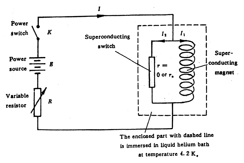
Fig. 1
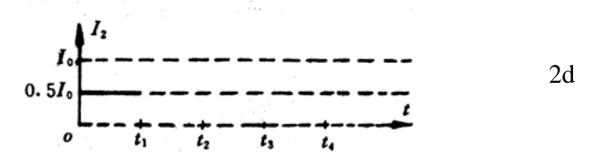
1) If the total current \(I\) and the resistance \(r\) of the superconducting switch are controlled to vary with time in the way shown in Figs, 2a and 2b respectively, and assuming the currents \(I_1\) and \(I_2\) flowing through the magnet and the switch respectively are equal at the beginning (Fig. 2c and Fig. 2d), how do they vary with time from \(t_1\) to \(t_4\)? Plot your answer in Fig. 2c and Fig. 2d
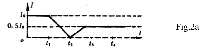
Fig.2a
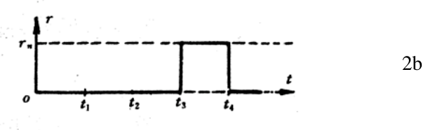
2b
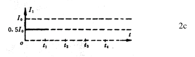
2c
2d
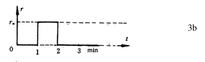
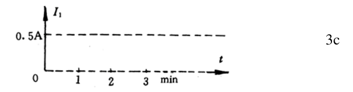
2) Suppose the power switch \(K\) is turned on at time \(t=0\) when \(r=0\), \(I_1=0\) and \(R=7.5\,\Omega\), and the total current \(I\) is \(0.5\,\mathrm A\). With \(K\) kept closed, the resistance \(r\) of the superconducting switch is varied in he way shown in Fig. 3b. Plot the corresponding time dependences of \(I\), \(I_1\) and \(I_2\) in Figs. 3a, 3c and 3d respectively.
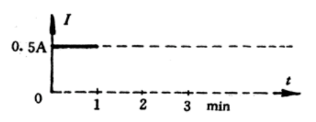
Fig. 3a
3b
3c
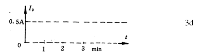
3d
3) Only small currents, less than \(0.5\,\mathrm A\), are allowed to flow through the superconducting switch when it is in the normal state, with larger currents the switch will be burnt out. Suppose the superconducting magnet is operated in a persistent mode, i. e. \(I=0\), and \(I_1=i_1\)(e. g. \(20\,\mathrm A\)), \(I_2=-i_1\), as shown in Fig. 4, from \(t=0\) to \(t=3\mathrm{min}\). If the experiment is to be stopped by reducing the current through the magnet to zero, how would you do it? This has to be done in several operation steps. Plot the corresponding changes of \(I\), \(r\), \(I_1\) and \(I_2\) in Fig. 4
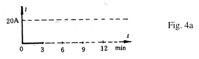
Fig. 4a
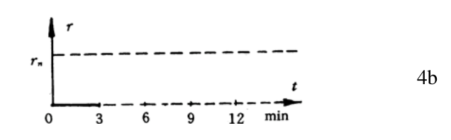
4b
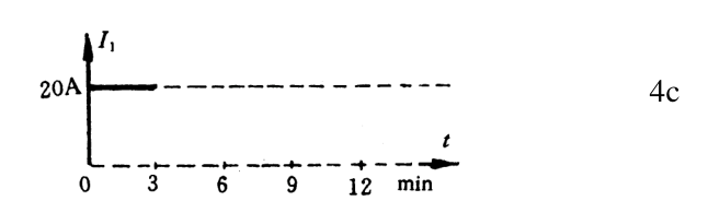
4c
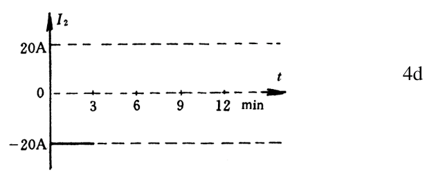
4d
4) Suppose the magnet is operated in a persistent mode with a persistent current of \(20\,\mathrm A\) (\(t=0\) to \(t=3\mathrm{min}\). See Fig. 5). How would you change it to a persistent mode with a current of 30a? plot your answer in Fig. 5.
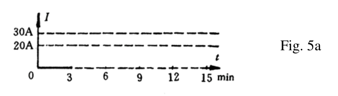
Fig. 5a
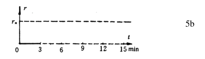
5b
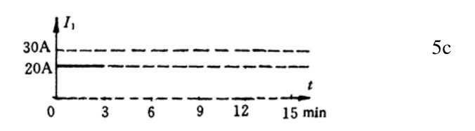
5c
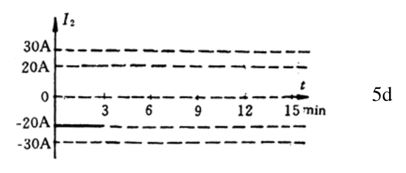
5d
Official English text of the problem.
Answers
-
Throughout the prescribed sequence, \[ \boxed{I_1=\frac{I_0}{2},\qquad I_2=I-\frac{I_0}{2}.} \] Thus \(I_2\) falls linearly from \(+I_0/2\) at \(t_1\) to \(-I_0/2\) at \(t_2\), rises linearly to zero as \(I\) reaches its plateau, and remains zero through \(t_3\) and \(t_4\).
-
The source emf is \(3.75\,\mathrm V\). Initially, \[ (I,I_1,I_2)=(0.50,0,0.50)\,\mathrm A. \] At \(1\,\mathrm{min}\), \(I\) and \(I_2\) jump to \(0.30\,\mathrm A\), while \(I_1\) remains zero. They then approach \((0.50,0.50,0)\,\mathrm A\) exponentially with time constant \[ \boxed{\tau_R=\frac{10}{3}\,\mathrm s\approx3.33\,\mathrm s.} \] After \(2\,\mathrm{min}\), \(I=0.50\,\mathrm A\), \(I_1\) is constant, and \(I_2\approx0\). Exact expressions appear below.
-
With \(r=0\), first raise \(I\) from zero to \(20\,\mathrm A\), leaving \(I_1=20\,\mathrm A\). Then set \(r=5\,\Omega\), reduce \(I\) slowly to zero, and open \(K\). The remaining magnet current decays exponentially with time constant \(2.0\,\mathrm s\). The explicit three-minute ramp below keeps \[ \boxed{|I_2|<0.223\,\mathrm A<0.5\,\mathrm A} \] throughout the normal state.
-
First match \(I=I_1=20\,\mathrm A\) with \(r=0\). Set \(r=5\,\Omega\) and increase \(I_1\) to \(30\,\mathrm A\), using \(I_2=1/9\,\mathrm A\) during a three-minute ramp. Then set \(I=30\,\mathrm A\), cool the switch to \(r=0\), and reduce \(I\) to zero. The final persistent state is \[ \boxed{I=0,\qquad I_1=30\,\mathrm A,\qquad I_2=-30\,\mathrm A,\qquad r=0.} \]
Solution
We treat the magnet as an ideal inductor with constant inductance \(L=10\,\mathrm H\). We neglect lead resistance, stray inductance and switching time, as implicit in the problem.
With the indicated current directions, Kirchhoff’s current law gives \[ I=I_1+I_2. \] The magnet and superconducting switch have the same terminal voltage: \[ V=L\frac{dI_1}{dt}=rI_2. \] Therefore the central equation is \[ \boxed{L\frac{dI_1}{dt}=r(I-I_1).} \]
When \(r=0\), the magnet current is constant. Changes in the source current then pass entirely through the superconducting switch: \[ \frac{dI_1}{dt}=0,\qquad I_2=I-I_1. \]
When \(r=r_n\) and the total current is prescribed, the equation becomes \[ \tau\frac{dI_1}{dt}+I_1=I, \qquad \boxed{\tau=\frac{L}{r_n}=2.0\,\mathrm s.} \] The inductor current remains continuous at switching instants; \(I\) and \(I_2\) may jump.
1) Prescribed total current and switch resistance
Initially the two branch currents are equal, so \[ I_1=I_2=\frac{I_0}{2}. \]
Until \(t_3\), the switch is superconducting. Hence \[ I_1=\frac{I_0}{2}, \qquad I_2=I-\frac{I_0}{2}. \]
By \(t_3\), the imposed current has reached \(I_0/2\). Thus \(I_2=0\) when the switch becomes resistive. During \(t_3<t<t_4\), \[ L\frac{dI_1}{dt}=r_n\left(\frac{I_0}{2}-I_1\right)=0. \] The currents consequently remain unchanged. Returning the switch to \(r=0\) at \(t_4\) also causes no change.
The requested plots are:
- Fig. 2c: a horizontal line at \(I_1=I_0/2\) throughout.
- Fig. 2d: a horizontal line at \(I_0/2\) until \(t_1\), followed by a straight decline to \(-I_0/2\) at \(t_2\). It crosses zero halfway between \(t_1\) and \(t_2\). It then rises linearly to zero when the prescribed \(I\) reaches \(I_0/2\), and stays at zero through \(t_3\), \(t_4\), and afterward.
The negative portion of Fig. 2d must be drawn below the original zero axis.
2) Fixed source resistance
Let the source emf be \(\mathcal E\). Initially \(r=0\), so the parallel combination has zero voltage: \[ \mathcal E=RI=(7.5\,\Omega)(0.50\,\mathrm A) =\boxed{3.75\,\mathrm V}. \]
For \(0\le t<60\,\mathrm s\), the magnet current stays at its initial value zero: \[ \boxed{I=0.50\,\mathrm A,\qquad I_1=0,\qquad I_2=0.50\,\mathrm A.} \]
At \(t=60\,\mathrm s\), the switch becomes resistive. Since \(I_1\) cannot jump, its immediate value remains zero, giving \[ I(60^+)=I_2(60^+) =\frac{\mathcal E}{R+r_n} =\frac{3.75}{12.5} =\boxed{0.30\,\mathrm A}. \]
During the normal-state interval, Kirchhoff’s voltage law gives \[ \mathcal E=R(I_1+I_2)+r_nI_2, \] and therefore \[ I_2=\frac{\mathcal E-RI_1}{R+r_n}. \] Combining this with the inductor equation, \[ L\frac{dI_1}{dt} =\frac{r_nR}{R+r_n}\left(\frac{\mathcal E}{R}-I_1\right). \] Thus \[ \boxed{\tau_R=\frac{L(R+r_n)}{Rr_n} =\frac{10(7.5+5)}{7.5(5)}\,\mathrm s =\frac{10}{3}\,\mathrm s.} \]
For \(60\le t<120\,\mathrm s\), define \[ x=\frac{t-60\,\mathrm s}{\tau_R}. \] The currents are \[ \boxed{ \begin{aligned} I_1(t)&=(0.50\,\mathrm A)(1-e^{-x}),\\ I_2(t)&=(0.30\,\mathrm A)e^{-x},\\ I(t)&=0.50\,\mathrm A-(0.20\,\mathrm A)e^{-x}. \end{aligned}} \]
At \(t=120\,\mathrm s\), \(x=18\), and the switch returns to \(r=0\). The source current becomes \(\mathcal E/R=0.50\,\mathrm A\), while the magnet current freezes at its existing value. Hence, for all \(t\ge120\,\mathrm s\), \[ \boxed{ \begin{aligned} I&=0.50\,\mathrm A,\\ I_1&=(0.50\,\mathrm A)(1-e^{-18}),\\ I_2&=(0.50\,\mathrm A)e^{-18} \approx7.6\,\mathrm{nA}. \end{aligned}} \]
The plot features are:
- Fig. 3a: \(I=0.50\,\mathrm A\) until one minute; a vertical drop to \(0.30\,\mathrm A\); then an exponential, concave-down rise toward \(0.50\,\mathrm A\).
- Fig. 3c: \(I_1=0\) until one minute; then a continuous, concave-down exponential rise toward \(0.50\,\mathrm A\). It becomes exactly constant at two minutes.
- Fig. 3d: \(I_2=0.50\,\mathrm A\) until one minute; a vertical drop to \(0.30\,\mathrm A\); then exponential decay toward zero.
At two minutes, \(I\) and \(I_2\) have upward jumps of only about \(3.0\,\mathrm{nA}\), invisible on the supplied scale. All visible transients occupy only a small fraction of a minute.
3) Reducing the persistent current to zero
The current restriction applies to the magnitude of the normal-state switch current: \[ |I_2|<0.5\,\mathrm A. \] Since \[ I_2=\frac{L}{r_n}\frac{dI_1}{dt}, \] it requires \[ \boxed{\left|\frac{dI_1}{dt}\right| <\frac{r_n}{L}(0.5\,\mathrm A) =0.25\,\mathrm{A\,s^{-1}}.} \]
Heating the switch immediately in the initial persistent state would put \(20\,\mathrm A\) through it. We must first transfer its current to the external source while it is still superconducting.
Here is one definite schedule for the \(20\,\mathrm A\) example.
From 0 to 3 min: retain the given persistent state: \[ I=0,\qquad r=0,\qquad I_1=20\,\mathrm A,\qquad I_2=-20\,\mathrm A. \]
From 3 to 6 min: keep \(r=0\), close \(K\) with sufficiently large \(R\), and raise \(I\) linearly from zero to \(20\,\mathrm A\). Then \[ I_1=20\,\mathrm A,\qquad I_2=I-20\,\mathrm A. \] Thus \(I_2\) rises linearly from \(-20\,\mathrm A\) to zero. At six minutes the source supplies the whole magnet current.
From 6 to 9 min: set \(r=r_n=5\,\Omega\) and reduce the total current linearly from \(20\,\mathrm A\) to zero.
Let \[ u=t-360\,\mathrm s,\qquad T=180\,\mathrm s,\qquad a=\frac{20\,\mathrm A}{T}=\frac19\,\mathrm{A\,s^{-1}}. \] During this interval, \[ I=20\,\mathrm A-au. \] Solving \(\tau\dot I_1+I_1=I\), with \(I_1(0)=20\,\mathrm A\), gives \[ \boxed{ \begin{aligned} I_1&=20\,\mathrm A-au+a\tau(1-e^{-u/\tau}),\\ I_2&=-a\tau(1-e^{-u/\tau}), \end{aligned} \qquad \tau=2.0\,\mathrm s.} \]
Consequently, \[ |I_2|\le a\tau=\frac29\,\mathrm A \approx0.222\,\mathrm A<0.5\,\mathrm A. \] The magnet current follows slightly above the declining source current.
At 9 min and afterward: the source current has reached zero. Open \(K\), leaving the switch normal. The remaining magnet current is \[ D=\frac29(1-e^{-90})\,\mathrm A\approx0.222\,\mathrm A. \] It circulates through the magnet and normal switch and decays as \[ \boxed{ I=0,\qquad I_1=D e^{-(t-540\,\mathrm s)/\tau},\qquad I_2=-D e^{-(t-540\,\mathrm s)/\tau}. } \] After another \(10\,\mathrm s\), \(I_1\approx1.5\,\mathrm{mA}\), and it continues toward zero.
The complete Fig. 4 plots are therefore:
| Plot | Required shape |
|---|---|
| 4a: \(I\) | Zero until 3 min; linear rise to \(20\,\mathrm A\) at 6 min; linear fall to zero at 9 min; zero afterward. |
| 4b: \(r\) | Zero until 6 min; step to \(5\,\Omega\); remain normal during the final discharge. |
| 4c: \(I_1\) | \(20\,\mathrm A\) until 6 min; smoothly enters an almost linear decline, reaching approximately \(0.222\,\mathrm A\) at 9 min; then decays exponentially to zero. |
| 4d: \(I_2\) | \(-20\,\mathrm A\) until 3 min; linear rise to zero at 6 min; becomes slightly negative, approaching \(-0.222\,\mathrm A\); after 9 min returns exponentially toward zero from below. |
As in any passive \(RL\) discharge, exact zero is approached asymptotically. On the minute-scale plot, the final tail is indistinguishable from zero. Returning the switch to \(r=0\) before that tail has decayed would trap the remaining current.
For a different initial \(i_1\), the same procedure applies with a sufficiently slow ramp to respect the \(0.25\,\mathrm{A\,s^{-1}}\) bound.
4) Changing the persistent current from \(20\,\mathrm A\) to \(30\,\mathrm A\)
Again, first match the source current to the existing magnet current before heating the switch.
We can choose an exactly linear magnet-current ramp lasting three minutes: \[ \alpha=\frac{30-20}{180}\,\mathrm{A\,s^{-1}} =\frac1{18}\,\mathrm{A\,s^{-1}}. \] The required switch current during this ramp is \[ \boxed{\delta=\frac{L}{r_n}\alpha =\frac19\,\mathrm A\approx0.111\,\mathrm A,} \] well below the normal-state limit.
To produce this ramp exactly, prescribe \[ I=I_1+\delta. \] For \(u=t-360\,\mathrm s\), \(0<u<180\,\mathrm s\), \[ \boxed{ I_1=20\,\mathrm A+\alpha u,\qquad I_2=\delta,\qquad I=20\,\mathrm A+\alpha u+\delta. } \] Indeed, \(r_nI_2=r_n\delta=L\alpha=L\,dI_1/dt\).
A complete schedule, specifying all four plots, is:
| Time (min) | \(I\) (A), Fig. 5a | \(r\) (\(\Omega\)), Fig. 5b | \(I_1\) (A), Fig. 5c | \(I_2\) (A), Fig. 5d |
|---|---|---|---|---|
| 0–3 | \(0\) | \(0\) | \(20\) | \(-20\) |
| 3–6 | Linear \(0\to20\) | \(0\) | \(20\) | Linear \(-20\to0\) |
| 6–9 | Linear \(20+\delta\to30+\delta\) | \(5\) | Linear \(20\to30\) | \(\delta=1/9\) |
| 9–12 | \(30\) | \(5\) | \(30\) | \(0\) |
| 12–15 | Linear \(30\to0\) | \(0\) | \(30\) | Linear \(0\to-30\) |
| After 15 | \(0\) | \(0\) | \(30\) | \(-30\) |
Here the numerical value of \(\delta\) in the table is in amperes.
The switching details matter:
- At 6 min: \(I=I_1=20\,\mathrm A\), so \(I_2=0\). Make the switch normal, then increase \(I\) by the small amount \(\delta\). This starts the linear magnet-current ramp without any jump in \(I_1\).
- At 9 min: \(I_1\) has reached exactly \(30\,\mathrm A\). Reduce \(I\) from \(30+\delta\) to \(30\,\mathrm A\). Then \(I_2=0\), so the magnet current remains constant.
- At 12 min: return the switch to \(r=0\). Reduce \(I\) to zero over the next three minutes. The magnet current stays fixed at \(30\,\mathrm A\), while \(I_2\) becomes increasingly negative.
- At 15 min: open \(K\). The magnet and superconducting switch carry equal and opposite currents of magnitude \(30\,\mathrm A\).
Thus Fig. 5a includes small \(0.111\,\mathrm A\) steps at 6 and 9 min. Fig. 5d has a small positive rectangular pulse during 6–9 min. The large negative switch currents occur only while \(r=0\), so they do not violate the stated normal-state restriction.
The solution was checked against the official solution. Where this solution differs from the official solution, the official solution contains an error or a misprint.
IPhO 1994 · Theorieaufgabe 2
Supraleitender Magnet
Supraleitende Magnete werden in Laboratorien häufig eingesetzt. Die gebräuchlichste Bauform eines supraleitenden Magneten ist eine Zylinderspule aus supraleitendem Draht. Das Bemerkenswerte an einem supraleitenden Magneten ist, dass er starke Magnetfelder ohne Energieverluste durch Joulesche Wärme erzeugt, da der elektrische Widerstand des supraleitenden Drahtes null wird, wenn der Magnet in flüssiges Helium bei einer Temperatur von 4.2 K eingetaucht wird. Üblicherweise ist der Magnet mit einem speziell konstruierten supraleitenden Schalter ausgestattet, wie in Abb. 1 dargestellt. Der Widerstand \(r\) des Schalters lässt sich steuern: entweder gilt \(r=0\) im supraleitenden Zustand oder \(r=r_n\) im normalleitenden Zustand. Im Dauerstrombetrieb zirkuliert ein Strom unbegrenzt durch den Magneten und den supraleitenden Schalter. Der Dauerstrombetrieb ermöglicht es, bei abgetrennter externer Stromquelle über lange Zeit ein konstantes Magnetfeld aufrechtzuerhalten.
Die Einzelheiten des supraleitenden Schalters sind in Abb. 1 nicht dargestellt. Üblicherweise besteht er aus einem kurzen Stück supraleitenden Drahtes, das mit einem Heizdraht umwickelt und gegenüber dem Bad aus flüssigem Helium ausreichend wärmeisoliert ist. Beim Heizen steigt die Temperatur des supraleitenden Drahtes, und er geht wieder in den normalleitenden Zustand mit endlichem Widerstand über. Der typische Wert von \(r_n\) beträgt einige Ohm. Hier nehmen wir dafür \(5\,\Omega\) an. Die Induktivität eines supraleitenden Magneten hängt von seiner Größe ab; für den Magneten in Abb. 1 sei sie \(10\,\mathrm H\). Der Gesamtstrom \(I\) lässt sich durch Einstellen des Widerstands \(R\) verändern.
Diese Aufgabe wird ausschließlich anhand der Diagramme bewertet!
Die Pfeile kennzeichnen die positiven Richtungen von \(I\), \(I_1\) und \(I_2\).
Abb. 1
1) Der Gesamtstrom \(I\) und der Widerstand \(r\) des supraleitenden Schalters werden so gesteuert, dass sie sich zeitlich wie in Abb. 2a bzw. 2b dargestellt ändern. Unter der Annahme, dass die durch den Magneten bzw. den Schalter fließenden Ströme \(I_1\) und \(I_2\) zu Beginn gleich sind (Abb. 2c und Abb. 2d), wie ändern sie sich mit der Zeit von \(t_1\) bis \(t_4\)? Zeichnen Sie Ihre Antwort in Abb. 2c und Abb. 2d ein.
Abb. 2a
2b
2c
2d
2) Der Schalter \(K\) werde zum Zeitpunkt \(t=0\) geschlossen, wobei \(r=0\), \(I_1=0\) und \(R=7.5\,\Omega\) gelten und der Gesamtstrom \(I\) gleich \(0.5\,\mathrm A\) ist. Während \(K\) geschlossen bleibt, wird der Widerstand \(r\) des supraleitenden Schalters wie in Abb. 3b dargestellt verändert. Zeichnen Sie die entsprechenden zeitlichen Verläufe von \(I\), \(I_1\) und \(I_2\) in Abb. 3a, 3c bzw. 3d ein.
Abb. 3a
3b
3c
3d
3) Durch den supraleitenden Schalter dürfen im normalleitenden Zustand nur kleine Ströme von weniger als \(0.5\,\mathrm A\) fließen; bei größeren Strömen brennt der Schalter durch. Der supraleitende Magnet werde von \(t=0\) bis \(t=3\mathrm{min}\) im Dauerstrombetrieb betrieben, d. h. mit \(I=0\), \(I_1=i_1\) (z. B. \(20\,\mathrm A\)) und \(I_2=-i_1\), wie in Abb. 4 dargestellt. Wie würden Sie vorgehen, wenn das Experiment beendet werden soll, indem der Strom durch den Magneten auf null verringert wird? Dazu sind mehrere Bedienungsschritte erforderlich. Zeichnen Sie die entsprechenden Änderungen von \(I\), \(r\), \(I_1\) und \(I_2\) in Abb. 4 ein.
Abb. 4a
4b
4c
4d
4) Der Magnet werde im Dauerstrombetrieb mit einem Dauerstrom von \(20\,\mathrm A\) betrieben (von \(t=0\) bis \(t=3\mathrm{min}\), siehe Abb. 5). Wie würden Sie ihn in einen Dauerstrombetrieb mit einem Strom von 30 A überführen? Zeichnen Sie Ihre Antwort in Abb. 5 ein.
Abb. 5a
5b
5c
5d
Aufgabentext aus dem offiziellen englischen Text übersetzt.
Antworten
-
Während des gesamten vorgegebenen Ablaufs gilt \[ \boxed{I_1=\frac{I_0}{2},\qquad I_2=I-\frac{I_0}{2}.} \] Somit fällt \(I_2\) linear von \(+I_0/2\) bei \(t_1\) auf \(-I_0/2\) bei \(t_2\), steigt linear auf null, während \(I\) seinen konstanten Wert erreicht, und bleibt über \(t_3\) und \(t_4\) hinweg null.
-
Die elektromotorische Kraft der Quelle beträgt \(3.75\,\mathrm V\). Zu Beginn gilt \[ (I,I_1,I_2)=(0.50,0,0.50)\,\mathrm A. \] Bei \(1\,\mathrm{min}\) springen \(I\) und \(I_2\) auf \(0.30\,\mathrm A\), während \(I_1\) null bleibt. Anschließend nähern sie sich exponentiell \((0.50,0.50,0)\,\mathrm A\) mit der Zeitkonstante \[ \boxed{\tau_R=\frac{10}{3}\,\mathrm s\approx3.33\,\mathrm s.} \] Nach \(2\,\mathrm{min}\) gilt \(I=0.50\,\mathrm A\), \(I_1\) ist konstant und \(I_2\approx0\). Die exakten Ausdrücke stehen weiter unten.
-
Bei \(r=0\) wird zunächst \(I\) von null auf \(20\,\mathrm A\) erhöht, wobei \(I_1=20\,\mathrm A\) bleibt. Anschließend wird \(r=5\,\Omega\) eingestellt, \(I\) langsam auf null verringert und \(K\) geöffnet. Der verbleibende Magnetstrom klingt exponentiell mit der Zeitkonstante \(2.0\,\mathrm s\) ab. Mit der unten angegebenen dreiminütigen Rampe gilt \[ \boxed{|I_2|<0.223\,\mathrm A<0.5\,\mathrm A} \] während des gesamten normalleitenden Zustands.
-
Zunächst wird bei \(r=0\) der Strom auf \(I=I_1=20\,\mathrm A\) eingestellt. Dann wird \(r=5\,\Omega\) eingestellt und \(I_1\) während einer dreiminütigen Rampe mit \(I_2=1/9\,\mathrm A\) auf \(30\,\mathrm A\) erhöht. Anschließend wird \(I=30\,\mathrm A\) eingestellt, der Schalter bis zu \(r=0\) abgekühlt und \(I\) auf null verringert. Der abschließende Dauerstromzustand ist \[ \boxed{I=0,\qquad I_1=30\,\mathrm A,\qquad I_2=-30\,\mathrm A,\qquad r=0.} \]
Lösung
Wir behandeln den Magneten als ideale Spule mit konstanter Induktivität \(L=10\,\mathrm H\). Wir vernachlässigen den Widerstand der Zuleitungen, parasitäre Induktivitäten und die Schaltzeit, wie es in der Aufgabenstellung implizit vorausgesetzt wird.
Mit den angegebenen Stromrichtungen liefert die Kirchhoffsche Knotenregel \[ I=I_1+I_2. \] Am Magneten und am supraleitenden Schalter liegt dieselbe Klemmenspannung an: \[ V=L\frac{dI_1}{dt}=rI_2. \] Damit lautet die zentrale Gleichung \[ \boxed{L\frac{dI_1}{dt}=r(I-I_1).} \]
Bei \(r=0\) ist der Magnetstrom konstant. Änderungen des Quellenstroms fließen dann vollständig durch den supraleitenden Schalter: \[ \frac{dI_1}{dt}=0,\qquad I_2=I-I_1. \]
Wenn \(r=r_n\) gilt und der Gesamtstrom vorgegeben ist, wird die Gleichung zu \[ \tau\frac{dI_1}{dt}+I_1=I, \qquad \boxed{\tau=\frac{L}{r_n}=2.0\,\mathrm s.} \] Der Spulenstrom bleibt an den Schaltzeitpunkten stetig; \(I\) und \(I_2\) können springen.
1) Vorgegebener Gesamtstrom und Schalterwiderstand
Zu Beginn sind die beiden Zweigströme gleich, also gilt \[ I_1=I_2=\frac{I_0}{2}. \]
Bis \(t_3\) ist der Schalter supraleitend. Daher gilt \[ I_1=\frac{I_0}{2}, \qquad I_2=I-\frac{I_0}{2}. \]
Bis \(t_3\) hat der vorgegebene Strom den Wert \(I_0/2\) erreicht. Somit gilt \(I_2=0\), wenn der Schalter normalleitend wird. Während \(t_3<t<t_4\) gilt \[ L\frac{dI_1}{dt}=r_n\left(\frac{I_0}{2}-I_1\right)=0. \] Die Ströme bleiben folglich unverändert. Auch die Rückkehr des Schalters zu \(r=0\) bei \(t_4\) bewirkt keine Änderung.
Die gesuchten Diagramme sind:
- Abb. 2c: durchgehend eine waagerechte Linie bei \(I_1=I_0/2\).
- Abb. 2d: eine waagerechte Linie bei \(I_0/2\) bis \(t_1\), gefolgt von einem geradlinigen Abfall auf \(-I_0/2\) bei \(t_2\). Sie schneidet die Nulllinie in der Mitte zwischen \(t_1\) und \(t_2\). Anschließend steigt sie linear auf null, sobald das vorgegebene \(I\) den Wert \(I_0/2\) erreicht, und bleibt über \(t_3\), \(t_4\) und danach bei null.
Der negative Abschnitt von Abb. 2d muss unterhalb der ursprünglichen Nulllinie eingezeichnet werden.
2) Fester Quellenwiderstand
Die elektromotorische Kraft der Quelle sei \(\mathcal E\). Anfangs gilt \(r=0\), sodass an der Parallelschaltung keine Spannung anliegt: \[ \mathcal E=RI=(7.5\,\Omega)(0.50\,\mathrm A) =\boxed{3.75\,\mathrm V}. \]
Für \(0\le t<60\,\mathrm s\) bleibt der Magnetstrom bei seinem Anfangswert null: \[ \boxed{I=0.50\,\mathrm A,\qquad I_1=0,\qquad I_2=0.50\,\mathrm A.} \]
Bei \(t=60\,\mathrm s\) wird der Schalter normalleitend. Da \(I_1\) nicht springen kann, bleibt sein Wert unmittelbar danach null, woraus folgt \[ I(60^+)=I_2(60^+) =\frac{\mathcal E}{R+r_n} =\frac{3.75}{12.5} =\boxed{0.30\,\mathrm A}. \]
Während des normalleitenden Zeitintervalls liefert die Kirchhoffsche Maschenregel \[ \mathcal E=R(I_1+I_2)+r_nI_2, \] und damit \[ I_2=\frac{\mathcal E-RI_1}{R+r_n}. \] Durch Kombination mit der Spulengleichung ergibt sich \[ L\frac{dI_1}{dt} =\frac{r_nR}{R+r_n}\left(\frac{\mathcal E}{R}-I_1\right). \] Somit gilt \[ \boxed{\tau_R=\frac{L(R+r_n)}{Rr_n} =\frac{10(7.5+5)}{7.5(5)}\,\mathrm s =\frac{10}{3}\,\mathrm s.} \]
Für \(60\le t<120\,\mathrm s\) definieren wir \[ x=\frac{t-60\,\mathrm s}{\tau_R}. \] Die Ströme sind \[ \boxed{ \begin{aligned} I_1(t)&=(0.50\,\mathrm A)(1-e^{-x}),\\ I_2(t)&=(0.30\,\mathrm A)e^{-x},\\ I(t)&=0.50\,\mathrm A-(0.20\,\mathrm A)e^{-x}. \end{aligned}} \]
Bei \(t=120\,\mathrm s\) gilt \(x=18\), und der Schalter kehrt zu \(r=0\) zurück. Der Quellenstrom wird zu \(\mathcal E/R=0.50\,\mathrm A\), während der Magnetstrom seinen zu diesem Zeitpunkt bestehenden Wert beibehält. Daher gilt für alle \(t\ge120\,\mathrm s\) \[ \boxed{ \begin{aligned} I&=0.50\,\mathrm A,\\ I_1&=(0.50\,\mathrm A)(1-e^{-18}),\\ I_2&=(0.50\,\mathrm A)e^{-18} \approx7.6\,\mathrm{nA}. \end{aligned}} \]
Die Merkmale der Diagramme sind:
- Abb. 3a: \(I=0.50\,\mathrm A\) bis zur ersten Minute; ein senkrechter Abfall auf \(0.30\,\mathrm A\); danach ein exponentieller, nach unten gekrümmter Anstieg gegen \(0.50\,\mathrm A\).
- Abb. 3c: \(I_1=0\) bis zur ersten Minute; danach ein stetiger, nach unten gekrümmter exponentieller Anstieg gegen \(0.50\,\mathrm A\). Ab der zweiten Minute ist der Strom exakt konstant.
- Abb. 3d: \(I_2=0.50\,\mathrm A\) bis zur ersten Minute; ein senkrechter Abfall auf \(0.30\,\mathrm A\); danach ein exponentielles Abklingen gegen null.
Bei zwei Minuten weisen \(I\) und \(I_2\) Sprünge nach oben von nur etwa \(3.0\,\mathrm{nA}\) auf, die im vorgegebenen Maßstab nicht sichtbar sind. Alle sichtbaren Übergangsvorgänge nehmen nur einen kleinen Bruchteil einer Minute in Anspruch.
3) Verringern des Dauerstroms auf null
Die Strombegrenzung gilt für den Betrag des Schalterstroms im normalleitenden Zustand: \[ |I_2|<0.5\,\mathrm A. \] Da \[ I_2=\frac{L}{r_n}\frac{dI_1}{dt}, \] erfordert sie \[ \boxed{\left|\frac{dI_1}{dt}\right| <\frac{r_n}{L}(0.5\,\mathrm A) =0.25\,\mathrm{A\,s^{-1}}.} \]
Würde der Schalter im anfänglichen Dauerstromzustand sofort erwärmt, würden \(20\,\mathrm A\) durch ihn fließen. Wir müssen seinen Strom zunächst auf die externe Quelle übertragen, solange er noch supraleitend ist.
Für das Beispiel mit \(20\,\mathrm A\) lässt sich der folgende konkrete Zeitplan angeben.
Von 0 bis 3 min: den vorgegebenen Dauerstromzustand beibehalten: \[ I=0,\qquad r=0,\qquad I_1=20\,\mathrm A,\qquad I_2=-20\,\mathrm A. \]
Von 3 bis 6 min: \(r=0\) beibehalten, \(K\) bei ausreichend großem \(R\) schließen und \(I\) linear von null auf \(20\,\mathrm A\) erhöhen. Dann gilt \[ I_1=20\,\mathrm A,\qquad I_2=I-20\,\mathrm A. \] Somit steigt \(I_2\) linear von \(-20\,\mathrm A\) auf null. Bei sechs Minuten liefert die Quelle den gesamten Magnetstrom.
Von 6 bis 9 min: \(r=r_n=5\,\Omega\) einstellen und den Gesamtstrom linear von \(20\,\mathrm A\) auf null verringern.
Es sei \[ u=t-360\,\mathrm s,\qquad T=180\,\mathrm s,\qquad a=\frac{20\,\mathrm A}{T}=\frac19\,\mathrm{A\,s^{-1}}. \] Während dieses Intervalls gilt \[ I=20\,\mathrm A-au. \] Die Lösung von \(\tau\dot I_1+I_1=I\) mit \(I_1(0)=20\,\mathrm A\) ergibt \[ \boxed{ \begin{aligned} I_1&=20\,\mathrm A-au+a\tau(1-e^{-u/\tau}),\\ I_2&=-a\tau(1-e^{-u/\tau}), \end{aligned} \qquad \tau=2.0\,\mathrm s.} \]
Folglich gilt \[ |I_2|\le a\tau=\frac29\,\mathrm A \approx0.222\,\mathrm A<0.5\,\mathrm A. \] Der Magnetstrom folgt dem abnehmenden Quellenstrom mit einem geringfügig höheren Wert.
Bei 9 min und danach: der Quellenstrom hat null erreicht. \(K\) öffnen und den Schalter normalleitend lassen. Der verbleibende Magnetstrom beträgt \[ D=\frac29(1-e^{-90})\,\mathrm A\approx0.222\,\mathrm A. \] Er zirkuliert durch den Magneten und den normalleitenden Schalter und klingt gemäß \[ \boxed{ I=0,\qquad I_1=D e^{-(t-540\,\mathrm s)/\tau},\qquad I_2=-D e^{-(t-540\,\mathrm s)/\tau}. } \] ab. Nach weiteren \(10\,\mathrm s\) gilt \(I_1\approx1.5\,\mathrm{mA}\), und der Strom nähert sich weiter null.
Die vollständigen Diagramme in Abb. 4 sind daher:
| Diagramm | Erforderlicher Verlauf |
|---|---|
| 4a: \(I\) | Null bis 3 min; linearer Anstieg auf \(20\,\mathrm A\) bei 6 min; linearer Abfall auf null bei 9 min; danach null. |
| 4b: \(r\) | Null bis 6 min; Sprung auf \(5\,\Omega\); während des abschließenden Abklingens normalleitend bleiben. |
| 4c: \(I_1\) | \(20\,\mathrm A\) bis 6 min; glatter Übergang in einen nahezu linearen Abfall, der bei 9 min ungefähr \(0.222\,\mathrm A\) erreicht; danach exponentielles Abklingen auf null. |
| 4d: \(I_2\) | \(-20\,\mathrm A\) bis 3 min; linearer Anstieg auf null bei 6 min; wird leicht negativ und nähert sich \(-0.222\,\mathrm A\); kehrt nach 9 min exponentiell von unten gegen null zurück. |
Wie bei jedem passiven Abklingvorgang in einem \(RL\)-Kreis wird exakt null nur asymptotisch erreicht. Im Diagramm mit einer Zeitskala in Minuten ist die abschließende Abklingphase nicht von null zu unterscheiden. Würde der Schalter vor dem Ende dieser Abklingphase wieder auf \(r=0\) gebracht, bliebe der restliche Strom erhalten.
Für einen anderen Anfangswert \(i_1\) gilt dasselbe Verfahren mit einer ausreichend langsamen Rampe, um die Grenze von \(0.25\,\mathrm{A\,s^{-1}}\) einzuhalten.
4) Ändern des Dauerstroms von \(20\,\mathrm A\) auf \(30\,\mathrm A\)
Auch hier wird zunächst der Quellenstrom an den bestehenden Magnetstrom angepasst, bevor der Schalter erwärmt wird.
Wir können eine exakt lineare Rampe des Magnetstroms mit einer Dauer von drei Minuten wählen: \[ \alpha=\frac{30-20}{180}\,\mathrm{A\,s^{-1}} =\frac1{18}\,\mathrm{A\,s^{-1}}. \] Der während dieser Rampe erforderliche Schalterstrom beträgt \[ \boxed{\delta=\frac{L}{r_n}\alpha =\frac19\,\mathrm A\approx0.111\,\mathrm A,} \] also deutlich weniger als der Grenzwert im normalleitenden Zustand.
Um diese Rampe exakt zu erzeugen, geben wir vor: \[ I=I_1+\delta. \] Für \(u=t-360\,\mathrm s\), \(0<u<180\,\mathrm s\), gilt \[ \boxed{ I_1=20\,\mathrm A+\alpha u,\qquad I_2=\delta,\qquad I=20\,\mathrm A+\alpha u+\delta. } \] Tatsächlich gilt \(r_nI_2=r_n\delta=L\alpha=L\,dI_1/dt\).
Ein vollständiger Zeitplan, der alle vier Diagramme festlegt, lautet:
| Zeit (min) | \(I\) (A), Abb. 5a | \(r\) (\(\Omega\)), Abb. 5b | \(I_1\) (A), Abb. 5c | \(I_2\) (A), Abb. 5d |
|---|---|---|---|---|
| 0–3 | \(0\) | \(0\) | \(20\) | \(-20\) |
| 3–6 | Linear \(0\to20\) | \(0\) | \(20\) | Linear \(-20\to0\) |
| 6–9 | Linear \(20+\delta\to30+\delta\) | \(5\) | Linear \(20\to30\) | \(\delta=1/9\) |
| 9–12 | \(30\) | \(5\) | \(30\) | \(0\) |
| 12–15 | Linear \(30\to0\) | \(0\) | \(30\) | Linear \(0\to-30\) |
| Nach 15 | \(0\) | \(0\) | \(30\) | \(-30\) |
Der Zahlenwert von \(\delta\) in der Tabelle ist dabei in Ampere angegeben.
Die Einzelheiten des Schaltens sind wesentlich:
- Bei 6 min: Es gilt \(I=I_1=20\,\mathrm A\), also \(I_2=0\). Den Schalter normalleitend machen und dann \(I\) um den kleinen Betrag \(\delta\) erhöhen. Dadurch beginnt die lineare Rampe des Magnetstroms ohne einen Sprung in \(I_1\).
- Bei 9 min: \(I_1\) hat exakt \(30\,\mathrm A\) erreicht. \(I\) von \(30+\delta\) auf \(30\,\mathrm A\) verringern. Dann gilt \(I_2=0\), sodass der Magnetstrom konstant bleibt.
- Bei 12 min: Den Schalter wieder auf \(r=0\) bringen. \(I\) während der nächsten drei Minuten auf null verringern. Der Magnetstrom bleibt unverändert bei \(30\,\mathrm A\), während \(I_2\) zunehmend negativ wird.
- Bei 15 min: \(K\) öffnen. Durch den Magneten und den supraleitenden Schalter fließen gleich große, entgegengesetzt gerichtete Ströme mit dem Betrag \(30\,\mathrm A\).
Somit enthält Abb. 5a kleine Sprünge von \(0.111\,\mathrm A\) bei 6 und 9 min. Abb. 5d weist während 6–9 min einen kleinen positiven Rechteckimpuls auf. Die großen negativen Schalterströme treten nur bei \(r=0\) auf und verletzen daher die angegebene Begrenzung für den normalleitenden Zustand nicht.
Die Lösung wurde mit der offiziellen Lösung abgeglichen. Wo diese Lösung von der offiziellen Lösung abweicht, enthält die offizielle Lösung einen Fehler oder Druckfehler.
IPhO 1994 · Teori sorusu 2
Süperiletken Mıknatıs
Süperiletken mıknatıslar laboratuvarlarda yaygın olarak kullanılır. Süperiletken mıknatısların en yaygın biçimi, süperiletken telden yapılmış bir solenoiddir. Süperiletken bir mıknatısın dikkat çekici özelliği, Joule ısınması nedeniyle herhangi bir enerji kaybı olmadan yüksek manyetik alanlar üretmesidir; çünkü mıknatıs 4.2 K sıcaklığındaki sıvı helyuma daldırıldığında süperiletken telin elektriksel direnci sıfır olur. Mıknatıs genellikle Şekil 1'de gösterildiği gibi özel olarak tasarlanmış bir süperiletken anahtarla donatılır. Anahtarın \(r\) direnci kontrol edilebilir: süperiletken durumda \(r=0\), normal durumda ise \(r=r_n\) olur. Kalıcı akım modunda, mıknatıs ve süperiletken anahtar üzerinden süresiz olarak akım dolaşır. Kalıcı akım modu, dış kaynağın bağlantısı kesilmişken uzun süreler boyunca sabit bir manyetik alanın korunmasını sağlar.
Süperiletken anahtarın ayrıntıları Şekil 1'de verilmemiştir. Anahtar genellikle üzerine bir ısıtıcı tel sarılmış ve sıvı helyum banyosundan uygun biçimde ısıl olarak yalıtılmış kısa bir süperiletken tel parçasıdır. Isıtıldığında süperiletken telin sıcaklığı artar ve tel, direnç gösterdiği normal duruma geri döner. \(r_n\)'nin tipik değeri birkaç ohmdur. Burada bu değerin \(5\,\Omega\) olduğunu varsayıyoruz. Süperiletken bir mıknatısın indüktansı boyutlarına bağlıdır; Şekil 1'deki mıknatıs için bunun \(10\,\mathrm H\) olduğunu varsayın. Toplam \(I\) akımı, \(R\) direnci ayarlanarak değiştirilebilir.
Bu soru yalnızca grafiklere göre puanlandırılacaktır!
Oklar, \(I\), \(I_1\) ve \(I_2\)'nin pozitif yönlerini göstermektedir.
Şekil 1
1) Toplam \(I\) akımı ve süperiletken anahtarın \(r\) direnci, zamanla sırasıyla Şekil 2a ve 2b'de gösterilen biçimde değişecek şekilde kontrol edilirse ve sırasıyla mıknatıstan ve anahtardan geçen \(I_1\) ve \(I_2\) akımlarının başlangıçta eşit olduğu varsayılırsa (Şekil 2c ve Şekil 2d), bu akımlar \(t_1\)'den \(t_4\)'e kadar zamanla nasıl değişir? Cevabınızı Şekil 2c ve Şekil 2d'de grafikle gösterin.
Şekil 2a
2b
2c
2d
2) \(r=0\), \(I_1=0\) ve \(R=7.5\,\Omega\) iken güç anahtarı \(K\)'nın \(t=0\) anında kapatıldığını ve toplam \(I\) akımının \(0.5\,\mathrm A\) olduğunu varsayın. \(K\) kapalı tutulurken, süperiletken anahtarın \(r\) direnci Şekil 3b'de gösterilen biçimde değiştiriliyor. \(I\), \(I_1\) ve \(I_2\)'nin buna karşılık gelen zamana bağlı değişimlerini sırasıyla Şekil 3a, 3c ve 3d'de çizin.
Şekil 3a
3b
3c
3d
3) Süperiletken anahtar normal durumdayken üzerinden yalnızca \(0.5\,\mathrm A\)'den küçük akımların geçmesine izin verilir; daha büyük akımlarda anahtar yanar. Süperiletken mıknatısın, Şekil 4'te gösterildiği gibi \(t=0\)'dan \(t=3\mathrm{min}\)'e kadar kalıcı akım modunda, yani \(I=0\), \(I_1=i_1\) (örneğin \(20\,\mathrm A\)) ve \(I_2=-i_1\) olacak şekilde çalıştırıldığını varsayın. Mıknatıstan geçen akım sıfıra indirilerek deney sonlandırılacaksa, bunu nasıl yaparsınız? Bunun birkaç işlem adımında yapılması gerekir. \(I\), \(r\), \(I_1\) ve \(I_2\)'nin buna karşılık gelen değişimlerini Şekil 4'te çizin.
Şekil 4a
4b
4c
4d
4) Mıknatısın \(20\,\mathrm A\)'lik kalıcı akımla kalıcı akım modunda çalıştırıldığını varsayın (\(t=0\)'dan \(t=3\mathrm{min}\)'e kadar. Şekil 5'e bakın). Bunu 30 A akımlı bir kalıcı akım moduna nasıl geçirirsiniz? Cevabınızı Şekil 5'te grafikle gösterin.
Şekil 5a
5b
5c
5d
Soru metni resmi İngilizce metinden çevrilmiştir.
Cevaplar
-
Verilen işlem dizisinin tamamı boyunca, \[ \boxed{I_1=\frac{I_0}{2},\qquad I_2=I-\frac{I_0}{2}.} \] Dolayısıyla \(I_2\), \(t_1\) anındaki \(+I_0/2\) değerinden \(t_2\) anında \(-I_0/2\)'ye doğrusal olarak düşer, \(I\) sabit değerine ulaşırken doğrusal olarak sıfıra yükselir ve \(t_3\) ile \(t_4\) boyunca sıfır kalır.
-
Kaynağın elektromotor kuvveti \(3.75\,\mathrm V\)'tur. Başlangıçta, \[ (I,I_1,I_2)=(0.50,0,0.50)\,\mathrm A. \] \(1\,\mathrm{min}\) anında \(I\) ve \(I_2\) aniden \(0.30\,\mathrm A\)'e düşerken \(I_1\) sıfır kalır. Ardından, zaman sabiti \[ \boxed{\tau_R=\frac{10}{3}\,\mathrm s\approx3.33\,\mathrm s.} \] olacak şekilde üstel olarak \((0.50,0.50,0)\,\mathrm A\) değerlerine yaklaşırlar. \(2\,\mathrm{min}\)'den sonra \(I=0.50\,\mathrm A\), \(I_1\) sabit ve \(I_2\approx0\) olur. Tam ifadeler aşağıda verilmiştir.
-
\(r=0\) iken önce \(I\)'yı sıfırdan \(20\,\mathrm A\)'e yükseltin; bu sırada \(I_1=20\,\mathrm A\) olarak kalır. Ardından \(r=5\,\Omega\) yapın, \(I\)'yı yavaşça sıfıra indirin ve \(K\)'yı açın. Mıknatısta kalan akım, \(2.0\,\mathrm s\) zaman sabitiyle üstel olarak azalır. Aşağıda açıkça verilen üç dakikalık doğrusal değişim, normal durumun tamamı boyunca \[ \boxed{|I_2|<0.223\,\mathrm A<0.5\,\mathrm A} \] koşulunu sağlar.
-
Önce \(r=0\) iken \(I=I_1=20\,\mathrm A\) eşitliğini sağlayın. \(r=5\,\Omega\) yapın ve üç dakikalık doğrusal artış boyunca \(I_2=1/9\,\mathrm A\) kullanarak \(I_1\)'i \(30\,\mathrm A\)'e yükseltin. Ardından \(I=30\,\mathrm A\) yapın, anahtarı soğutarak \(r=0\) durumuna getirin ve \(I\)'yı sıfıra indirin. Son kalıcı akım durumu \[ \boxed{I=0,\qquad I_1=30\,\mathrm A,\qquad I_2=-30\,\mathrm A,\qquad r=0.} \] olur.
Çözüm
Mıknatısı, indüktansı sabit ve \(L=10\,\mathrm H\) olan ideal bir bobin olarak ele alıyoruz. Soruda örtük olarak varsayıldığı üzere bağlantı tellerinin direncini, parazitik indüktansı ve anahtarlama süresini ihmal ediyoruz.
Belirtilen akım yönleriyle Kirchhoff'un akım yasası \[ I=I_1+I_2. \] sonucunu verir. Mıknatıs ile süperiletken anahtarın uçları arasındaki gerilim aynıdır: \[ V=L\frac{dI_1}{dt}=rI_2. \] Dolayısıyla temel denklem \[ \boxed{L\frac{dI_1}{dt}=r(I-I_1).} \] olur.
\(r=0\) olduğunda mıknatıs akımı sabittir. Bu durumda kaynak akımındaki değişimler bütünüyle süperiletken anahtardan geçer: \[ \frac{dI_1}{dt}=0,\qquad I_2=I-I_1. \]
\(r=r_n\) olduğunda ve toplam akımın değişimi verildiğinde denklem şu biçimi alır: \[ \tau\frac{dI_1}{dt}+I_1=I, \qquad \boxed{\tau=\frac{L}{r_n}=2.0\,\mathrm s.} \] Bobin akımı anahtarlama anlarında sürekliliğini korur; \(I\) ve \(I_2\) ani sıçramalar yapabilir.
1) Değişimleri verilen toplam akım ve anahtar direnci
Başlangıçta iki kol akımı eşittir; dolayısıyla \[ I_1=I_2=\frac{I_0}{2}. \]
\(t_3\) anına kadar anahtar süperiletkendir. Bu nedenle \[ I_1=\frac{I_0}{2}, \qquad I_2=I-\frac{I_0}{2}. \]
\(t_3\) anına gelindiğinde uygulanan akım \(I_0/2\)'ye ulaşmıştır. Dolayısıyla anahtar dirençli duruma geçtiğinde \(I_2=0\) olur. \(t_3<t<t_4\) aralığında, \[ L\frac{dI_1}{dt}=r_n\left(\frac{I_0}{2}-I_1\right)=0. \] Bu nedenle akımlar değişmeden kalır. Anahtarın \(t_4\) anında yeniden \(r=0\) durumuna getirilmesi de herhangi bir değişime yol açmaz.
İstenen grafikler şöyledir:
- Şekil 2c: tüm süreç boyunca \(I_1=I_0/2\) düzeyinde yatay bir çizgi.
- Şekil 2d: \(t_1\) anına kadar \(I_0/2\) düzeyinde yatay bir çizgi, ardından \(t_2\) anında \(-I_0/2\)'ye ulaşan doğrusal bir düşüş. \(t_1\) ile \(t_2\)'nin tam ortasında sıfırdan geçer. Daha sonra, verilen \(I\) akımı \(I_0/2\)'ye ulaştığında sıfıra varacak şekilde doğrusal olarak yükselir ve \(t_3\), \(t_4\) anlarında ve sonrasında sıfırda kalır.
Şekil 2d'nin negatif kısmı, verilen sıfır ekseninin altına çizilmelidir.
2) Sabit kaynak direnci
Kaynağın elektromotor kuvveti \(\mathcal E\) olsun. Başlangıçta \(r=0\) olduğundan paralel bağlı kolların uçları arasındaki gerilim sıfırdır: \[ \mathcal E=RI=(7.5\,\Omega)(0.50\,\mathrm A) =\boxed{3.75\,\mathrm V}. \]
\(0\le t<60\,\mathrm s\) aralığında mıknatıs akımı, başlangıç değeri olan sıfırda kalır: \[ \boxed{I=0.50\,\mathrm A,\qquad I_1=0,\qquad I_2=0.50\,\mathrm A.} \]
\(t=60\,\mathrm s\) anında anahtar dirençli duruma geçer. \(I_1\) ani bir sıçrama yapamayacağından bu anın hemen sonrasındaki değeri sıfır kalır ve \[ I(60^+)=I_2(60^+) =\frac{\mathcal E}{R+r_n} =\frac{3.75}{12.5} =\boxed{0.30\,\mathrm A}. \] elde edilir.
Normal durumda geçen süre boyunca Kirchhoff'un gerilim yasası \[ \mathcal E=R(I_1+I_2)+r_nI_2, \] ve dolayısıyla \[ I_2=\frac{\mathcal E-RI_1}{R+r_n}. \] sonucunu verir. Bunu bobin denklemiyle birleştirirsek, \[ L\frac{dI_1}{dt} =\frac{r_nR}{R+r_n}\left(\frac{\mathcal E}{R}-I_1\right). \] Böylece \[ \boxed{\tau_R=\frac{L(R+r_n)}{Rr_n} =\frac{10(7.5+5)}{7.5(5)}\,\mathrm s =\frac{10}{3}\,\mathrm s.} \]
\(60\le t<120\,\mathrm s\) için \[ x=\frac{t-60\,\mathrm s}{\tau_R}. \] tanımını yapalım. Akımlar şöyledir: \[ \boxed{ \begin{aligned} I_1(t)&=(0.50\,\mathrm A)(1-e^{-x}),\\ I_2(t)&=(0.30\,\mathrm A)e^{-x},\\ I(t)&=0.50\,\mathrm A-(0.20\,\mathrm A)e^{-x}. \end{aligned}} \]
\(t=120\,\mathrm s\) anında \(x=18\) olur ve anahtar yeniden \(r=0\) durumuna geçer. Kaynak akımı \(\mathcal E/R=0.50\,\mathrm A\) olurken mıknatıs akımı o andaki değerinde sabitlenir. Dolayısıyla tüm \(t\ge120\,\mathrm s\) için, \[ \boxed{ \begin{aligned} I&=0.50\,\mathrm A,\\ I_1&=(0.50\,\mathrm A)(1-e^{-18}),\\ I_2&=(0.50\,\mathrm A)e^{-18} \approx7.6\,\mathrm{nA}. \end{aligned}} \]
Grafiklerin özellikleri şöyledir:
- Şekil 3a: birinci dakikaya kadar \(I=0.50\,\mathrm A\); \(0.30\,\mathrm A\)'e dikey bir düşüş; ardından \(0.50\,\mathrm A\)'e doğru aşağı konkav, üstel bir yükseliş.
- Şekil 3c: birinci dakikaya kadar \(I_1=0\); ardından \(0.50\,\mathrm A\)'e doğru sürekli, aşağı konkav, üstel bir yükseliş. İkinci dakikada tam olarak sabit hâle gelir.
- Şekil 3d: birinci dakikaya kadar \(I_2=0.50\,\mathrm A\); \(0.30\,\mathrm A\)'e dikey bir düşüş; ardından sıfıra doğru üstel azalma.
İkinci dakikada \(I\) ve \(I_2\), yalnızca yaklaşık \(3.0\,\mathrm{nA}\) büyüklüğünde yukarı yönlü sıçramalar yapar; bunlar verilen ölçekte görünmez. Görünür tüm geçici değişimler, bir dakikanın yalnızca küçük bir kesri kadar sürer.
3) Kalıcı akımın sıfıra indirilmesi
Akım kısıtlaması, normal durumdaki anahtar akımının büyüklüğü için geçerlidir: \[ |I_2|<0.5\,\mathrm A. \] \[ I_2=\frac{L}{r_n}\frac{dI_1}{dt}, \] olduğundan bu kısıtlama \[ \boxed{\left|\frac{dI_1}{dt}\right| <\frac{r_n}{L}(0.5\,\mathrm A) =0.25\,\mathrm{A\,s^{-1}}.} \] koşulunu gerektirir.
Başlangıçtaki kalıcı akım durumunda anahtarın hemen ısıtılması, üzerinden \(20\,\mathrm A\) geçmesine neden olurdu. Önce, anahtar hâlâ süperiletkenken onun taşıdığı akımı dış kaynağa aktarmalıyız.
\(20\,\mathrm A\) örneği için belirli bir işlem programı aşağıda verilmiştir.
0 ile 3 dakika arasında: verilen kalıcı akım durumunu koruyun: \[ I=0,\qquad r=0,\qquad I_1=20\,\mathrm A,\qquad I_2=-20\,\mathrm A. \]
3 ile 6 dakika arasında: \(r=0\) durumunu koruyun, \(R\) yeterince büyükken \(K\)'yı kapatın ve \(I\)'yı sıfırdan \(20\,\mathrm A\)'e doğrusal olarak yükseltin. Bu durumda \[ I_1=20\,\mathrm A,\qquad I_2=I-20\,\mathrm A. \] Dolayısıyla \(I_2\), \(-20\,\mathrm A\)'den sıfıra doğrusal olarak yükselir. Altıncı dakikada kaynak, mıknatıs akımının tamamını sağlar.
6 ile 9 dakika arasında: \(r=r_n=5\,\Omega\) yapın ve toplam akımı \(20\,\mathrm A\)'den sıfıra doğrusal olarak indirin.
Şu tanımları yapalım: \[ u=t-360\,\mathrm s,\qquad T=180\,\mathrm s,\qquad a=\frac{20\,\mathrm A}{T}=\frac19\,\mathrm{A\,s^{-1}}. \] Bu aralıkta, \[ I=20\,\mathrm A-au. \] \(\tau\dot I_1+I_1=I\) denklemi \(I_1(0)=20\,\mathrm A\) başlangıç koşuluyla çözüldüğünde, \[ \boxed{ \begin{aligned} I_1&=20\,\mathrm A-au+a\tau(1-e^{-u/\tau}),\\ I_2&=-a\tau(1-e^{-u/\tau}), \end{aligned} \qquad \tau=2.0\,\mathrm s.} \] elde edilir.
Bunun sonucunda, \[ |I_2|\le a\tau=\frac29\,\mathrm A \approx0.222\,\mathrm A<0.5\,\mathrm A. \] Mıknatıs akımı, azalan kaynak akımını onun biraz üzerinde kalarak izler.
9. dakikada ve sonrasında: kaynak akımı sıfıra ulaşmıştır. Anahtarı normal durumda bırakarak \(K\)'yı açın. Mıknatısta kalan akım \[ D=\frac29(1-e^{-90})\,\mathrm A\approx0.222\,\mathrm A. \] olur. Bu akım, mıknatıs ve normal durumdaki anahtar üzerinden dolaşır ve şu şekilde azalır: \[ \boxed{ I=0,\qquad I_1=D e^{-(t-540\,\mathrm s)/\tau},\qquad I_2=-D e^{-(t-540\,\mathrm s)/\tau}. } \] Bir \(10\,\mathrm s\) daha geçtikten sonra \(I_1\approx1.5\,\mathrm{mA}\) olur ve sıfıra doğru azalmaya devam eder.
Dolayısıyla Şekil 4'teki grafiklerin tamamı şöyledir:
| Grafik | İstenen biçim |
|---|---|
| 4a: \(I\) | 3. dakikaya kadar sıfır; 6. dakikada \(20\,\mathrm A\)'e ulaşan doğrusal yükseliş; 9. dakikada sıfıra ulaşan doğrusal düşüş; sonrasında sıfır. |
| 4b: \(r\) | 6. dakikaya kadar sıfır; \(5\,\Omega\)'a basamak biçiminde geçiş; son boşalma boyunca normal durumda kalış. |
| 4c: \(I_1\) | 6. dakikaya kadar \(20\,\mathrm A\); yumuşak bir geçişle başlayan, hemen hemen doğrusal bir azalma ve 9. dakikada yaklaşık \(0.222\,\mathrm A\)'e ulaşma; ardından sıfıra doğru üstel azalma. |
| 4d: \(I_2\) | 3. dakikaya kadar \(-20\,\mathrm A\); 6. dakikada sıfıra ulaşan doğrusal yükseliş; hafifçe negatif olup \(-0.222\,\mathrm A\)'e yaklaşma; 9. dakikadan sonra negatif taraftan sıfıra doğru üstel dönüş. |
Her pasif \(RL\) boşalmasında olduğu gibi, tam sıfıra asimptotik olarak yaklaşılır. Dakika ölçeğindeki grafikte son kuyruk sıfırdan ayırt edilemez. Bu kuyruk sönümlenmeden önce anahtarın yeniden \(r=0\) durumuna getirilmesi, kalan akımın hapsolmasına yol açar.
Farklı bir başlangıç \(i_1\) değeri için de \(0.25\,\mathrm{A\,s^{-1}}\) sınırına uyacak kadar yavaş bir doğrusal değişimle aynı yöntem uygulanır.
4) Kalıcı akımın \(20\,\mathrm A\)'den \(30\,\mathrm A\)'e değiştirilmesi
Yine, anahtarı ısıtmadan önce kaynak akımını mevcut mıknatıs akımına eşitleyin.
Mıknatıs akımı için üç dakika süren tam doğrusal bir artış seçebiliriz: \[ \alpha=\frac{30-20}{180}\,\mathrm{A\,s^{-1}} =\frac1{18}\,\mathrm{A\,s^{-1}}. \] Bu doğrusal artış sırasında gereken anahtar akımı \[ \boxed{\delta=\frac{L}{r_n}\alpha =\frac19\,\mathrm A\approx0.111\,\mathrm A,} \] olup normal durum sınırının çok altındadır.
Bu doğrusal artışı tam olarak elde etmek için \[ I=I_1+\delta. \] olacak şekilde akımı ayarlayın. \(u=t-360\,\mathrm s\), \(0<u<180\,\mathrm s\) için, \[ \boxed{ I_1=20\,\mathrm A+\alpha u,\qquad I_2=\delta,\qquad I=20\,\mathrm A+\alpha u+\delta. } \] Gerçekten de \(r_nI_2=r_n\delta=L\alpha=L\,dI_1/dt\) olur.
Dört grafiğin tümünü belirleyen eksiksiz bir işlem programı şöyledir:
| Zaman (dakika) | \(I\) (A), Şekil 5a | \(r\) (\(\Omega\)), Şekil 5b | \(I_1\) (A), Şekil 5c | \(I_2\) (A), Şekil 5d |
|---|---|---|---|---|
| 0–3 | \(0\) | \(0\) | \(20\) | \(-20\) |
| 3–6 | Doğrusal \(0\to20\) | \(0\) | \(20\) | Doğrusal \(-20\to0\) |
| 6–9 | Doğrusal \(20+\delta\to30+\delta\) | \(5\) | Doğrusal \(20\to30\) | \(\delta=1/9\) |
| 9–12 | \(30\) | \(5\) | \(30\) | \(0\) |
| 12–15 | Doğrusal \(30\to0\) | \(0\) | \(30\) | Doğrusal \(0\to-30\) |
| 15'ten sonra | \(0\) | \(0\) | \(30\) | \(-30\) |
Burada tabloda verilen \(\delta\)'nın sayısal değeri amper cinsindendir.
Anahtarlama ayrıntıları önemlidir:
- 6. dakikada: \(I=I_1=20\,\mathrm A\), dolayısıyla \(I_2=0\) olur. Anahtarı normal duruma getirin, ardından \(I\)'yı küçük bir \(\delta\) miktarı kadar artırın. Bu, \(I_1\)'de herhangi bir sıçrama olmadan mıknatıs akımının doğrusal artışını başlatır.
- 9. dakikada: \(I_1\) tam olarak \(30\,\mathrm A\)'e ulaşmıştır. \(I\)'yı \(30+\delta\)'dan \(30\,\mathrm A\)'e indirin. Böylece \(I_2=0\) olur ve mıknatıs akımı sabit kalır.
- 12. dakikada: anahtarı yeniden \(r=0\) durumuna getirin. Sonraki üç dakika boyunca \(I\)'yı sıfıra indirin. Mıknatıs akımı \(30\,\mathrm A\)'de sabit kalırken \(I_2\) giderek daha negatif olur.
- 15. dakikada: \(K\)'yı açın. Mıknatıs ve süperiletken anahtar, büyüklükleri \(30\,\mathrm A\) olan eşit ve zıt yönlü akımlar taşır.
Böylece Şekil 5a, 6. ve 9. dakikalarda küçük \(0.111\,\mathrm A\)'lik basamaklar içerir. Şekil 5d'de 6–9. dakikalar arasında küçük, pozitif bir dikdörtgen darbe vardır. Anahtardan geçen büyük negatif akımlar yalnızca \(r=0\) iken oluşur; dolayısıyla belirtilen normal durum kısıtlamasını ihlal etmezler.
Çözüm, resmi çözümle karşılaştırılarak kontrol edildi. Bu çözümün resmi çözümden ayrıldığı yerlerde resmi çözümde bir hata ya da baskı hatası vardır.
IPhO 1994 · Problema teórico 2
Imán superconductor
Los imanes superconductores se utilizan ampliamente en los laboratorios. La forma más común de imán superconductor es un solenoide hecho de hilo superconductor. Lo extraordinario de un imán superconductor es que produce campos magnéticos intensos sin disipación de energía por efecto Joule, ya que la resistencia eléctrica del hilo superconductor se hace nula cuando el imán se sumerge en helio líquido a una temperatura de 4.2 K. Habitualmente, el imán está provisto de un interruptor superconductor especialmente diseñado, como se muestra en la Fig. 1. La resistencia \(r\) del interruptor puede controlarse: puede ser \(r=0\) en el estado superconductor, o \(r=r_n\) en el estado normal. En el modo persistente, una corriente circula indefinidamente por el imán y el interruptor superconductor. El modo persistente permite mantener un campo magnético constante durante largos períodos con la fuente externa desconectada.
Los detalles del interruptor superconductor no se muestran en la Fig. 1. Por lo general, consiste en un pequeño tramo de hilo superconductor rodeado por un hilo calefactor y debidamente aislado térmicamente del baño de helio líquido. Al calentarlo, la temperatura del hilo superconductor aumenta y este vuelve al estado normal resistivo. El valor típico de \(r_n\) es de unos pocos ohmios. Aquí supondremos que es de \(5\,\Omega\). La inductancia de un imán superconductor depende de su tamaño; supóngase que es de \(10\,\mathrm H\) para el imán de la Fig. 1. La corriente total \(I\) puede modificarse ajustando la resistencia \(R\).
¡Este problema se calificará únicamente a partir de las gráficas!
Las flechas indican el sentido positivo de \(I\), \(I_1\) e \(I_2\).
Fig. 1
1) Si la corriente total \(I\) y la resistencia \(r\) del interruptor superconductor se controlan de modo que varíen con el tiempo como se muestra en las Figs. 2a y 2b, respectivamente, y suponiendo que las corrientes \(I_1\) e \(I_2\) que circulan por el imán y el interruptor, respectivamente, son iguales al principio (Fig. 2c y Fig. 2d), ¿cómo varían con el tiempo desde \(t_1\) hasta \(t_4\)? Represente gráficamente su respuesta en la Fig. 2c y la Fig. 2d
Fig. 2a
2b
2c
2d
2) Suponga que el interruptor de alimentación \(K\) se cierra en el instante \(t=0\), cuando \(r=0\), \(I_1=0\) y \(R=7.5\,\Omega\), y la corriente total \(I\) es de \(0.5\,\mathrm A\). Manteniendo \(K\) cerrado, la resistencia \(r\) del interruptor superconductor se hace variar como se muestra en la Fig. 3b. Represente las correspondientes dependencias temporales de \(I\), \(I_1\) e \(I_2\) en las Figs. 3a, 3c y 3d, respectivamente.
Fig. 3a
3b
3c
3d
3) Por el interruptor superconductor solo se permite que circulen corrientes pequeñas, inferiores a \(0.5\,\mathrm A\), cuando se encuentra en el estado normal; con corrientes mayores, el interruptor se quemará. Suponga que el imán superconductor funciona en modo persistente, es decir, \(I=0\), e \(I_1=i_1\) (por ejemplo, \(20\,\mathrm A\)), \(I_2=-i_1\), como se muestra en la Fig. 4, desde \(t=0\) hasta \(t=3\mathrm{min}\). Si se desea detener el experimento reduciendo a cero la corriente que circula por el imán, ¿cómo lo haría? Esto debe hacerse en varias etapas de operación. Represente gráficamente los cambios correspondientes de \(I\), \(r\), \(I_1\) e \(I_2\) en la Fig. 4
Fig. 4a
4b
4c
4d
4) Suponga que el imán funciona en modo persistente con una corriente persistente de \(20\,\mathrm A\) (de \(t=0\) a \(t=3\mathrm{min}\). Véase la Fig. 5). ¿Cómo lo cambiaría a un modo persistente con una corriente de 30 A? Represente gráficamente su respuesta en la Fig. 5.
Fig. 5a
5b
5c
5d
Enunciado traducido del texto oficial en inglés.
Respuestas
-
A lo largo de toda la secuencia prescrita, \[ \boxed{I_1=\frac{I_0}{2},\qquad I_2=I-\frac{I_0}{2}.} \] Por tanto, \(I_2\) disminuye linealmente desde \(+I_0/2\) en \(t_1\) hasta \(-I_0/2\) en \(t_2\), aumenta linealmente hasta cero cuando \(I\) alcanza su meseta y permanece en cero durante \(t_3\) y \(t_4\).
-
La fem de la fuente es de \(3.75\,\mathrm V\). Inicialmente, \[ (I,I_1,I_2)=(0.50,0,0.50)\,\mathrm A. \] En \(1\,\mathrm{min}\), \(I\) e \(I_2\) saltan a \(0.30\,\mathrm A\), mientras que \(I_1\) permanece en cero. A continuación, se aproximan exponencialmente a \((0.50,0.50,0)\,\mathrm A\) con una constante de tiempo \[ \boxed{\tau_R=\frac{10}{3}\,\mathrm s\approx3.33\,\mathrm s.} \] Después de \(2\,\mathrm{min}\), \(I=0.50\,\mathrm A\), \(I_1\) es constante e \(I_2\approx0\). Las expresiones exactas se presentan más adelante.
-
Con \(r=0\), aumente primero \(I\) desde cero hasta \(20\,\mathrm A\), manteniendo \(I_1=20\,\mathrm A\). Después, establezca \(r=5\,\Omega\), reduzca \(I\) lentamente hasta cero y abra \(K\). La corriente restante en el imán decae exponencialmente con una constante de tiempo de \(2.0\,\mathrm s\). La rampa explícita de tres minutos que se presenta más adelante mantiene \[ \boxed{|I_2|<0.223\,\mathrm A<0.5\,\mathrm A} \] durante todo el estado normal.
-
Primero iguale \(I=I_1=20\,\mathrm A\) con \(r=0\). Establezca \(r=5\,\Omega\) y aumente \(I_1\) hasta \(30\,\mathrm A\), utilizando \(I_2=1/9\,\mathrm A\) durante una rampa de tres minutos. Después, establezca \(I=30\,\mathrm A\), enfríe el interruptor hasta que \(r=0\) y reduzca \(I\) a cero. El estado persistente final es \[ \boxed{I=0,\qquad I_1=30\,\mathrm A,\qquad I_2=-30\,\mathrm A,\qquad r=0.} \]
Solución
Tratamos el imán como una bobina ideal con inductancia constante \(L=10\,\mathrm H\). Despreciamos la resistencia de los conductores de conexión, la inductancia parásita y el tiempo de conmutación, como se supone implícitamente en el problema.
Con los sentidos de corriente indicados, la ley de corrientes de Kirchhoff da \[ I=I_1+I_2. \] El imán y el interruptor superconductor tienen la misma tensión entre sus terminales: \[ V=L\frac{dI_1}{dt}=rI_2. \] Por tanto, la ecuación fundamental es \[ \boxed{L\frac{dI_1}{dt}=r(I-I_1).} \]
Cuando \(r=0\), la corriente del imán es constante. Las variaciones de la corriente de la fuente pasan entonces íntegramente por el interruptor superconductor: \[ \frac{dI_1}{dt}=0,\qquad I_2=I-I_1. \]
Cuando \(r=r_n\) y se prescribe la corriente total, la ecuación se convierte en \[ \tau\frac{dI_1}{dt}+I_1=I, \qquad \boxed{\tau=\frac{L}{r_n}=2.0\,\mathrm s.} \] La corriente de la bobina permanece continua en los instantes de conmutación; \(I\) e \(I_2\) pueden presentar saltos.
1) Corriente total y resistencia del interruptor prescritas
Inicialmente, las corrientes de las dos ramas son iguales, de modo que \[ I_1=I_2=\frac{I_0}{2}. \]
Hasta \(t_3\), el interruptor es superconductor. Por ello, \[ I_1=\frac{I_0}{2}, \qquad I_2=I-\frac{I_0}{2}. \]
En \(t_3\), la corriente impuesta ya ha alcanzado \(I_0/2\). Por tanto, \(I_2=0\) cuando el interruptor se vuelve resistivo. Durante \(t_3<t<t_4\), \[ L\frac{dI_1}{dt}=r_n\left(\frac{I_0}{2}-I_1\right)=0. \] En consecuencia, las corrientes permanecen inalteradas. Devolver el interruptor a \(r=0\) en \(t_4\) tampoco produce ningún cambio.
Las gráficas solicitadas son:
- Fig. 2c: una línea horizontal en \(I_1=I_0/2\) durante todo el intervalo.
- Fig. 2d: una línea horizontal en \(I_0/2\) hasta \(t_1\), seguida de un descenso rectilíneo hasta \(-I_0/2\) en \(t_2\). Cruza el cero a mitad de camino entre \(t_1\) y \(t_2\). A continuación, aumenta linealmente hasta cero cuando la corriente prescrita \(I\) alcanza \(I_0/2\), y permanece en cero durante \(t_3\), \(t_4\) y después.
La parte negativa de la Fig. 2d debe dibujarse por debajo del eje original correspondiente a cero.
2) Resistencia de la fuente fija
Sea \(\mathcal E\) la fem de la fuente. Inicialmente, \(r=0\), por lo que la asociación en paralelo tiene tensión nula: \[ \mathcal E=RI=(7.5\,\Omega)(0.50\,\mathrm A) =\boxed{3.75\,\mathrm V}. \]
Para \(0\le t<60\,\mathrm s\), la corriente del imán permanece en su valor inicial nulo: \[ \boxed{I=0.50\,\mathrm A,\qquad I_1=0,\qquad I_2=0.50\,\mathrm A.} \]
En \(t=60\,\mathrm s\), el interruptor se vuelve resistivo. Como \(I_1\) no puede presentar un salto, su valor inmediatamente después sigue siendo cero, lo que da \[ I(60^+)=I_2(60^+) =\frac{\mathcal E}{R+r_n} =\frac{3.75}{12.5} =\boxed{0.30\,\mathrm A}. \]
Durante el intervalo en estado normal, la ley de tensiones de Kirchhoff da \[ \mathcal E=R(I_1+I_2)+r_nI_2, \] y, por tanto, \[ I_2=\frac{\mathcal E-RI_1}{R+r_n}. \] Combinando esto con la ecuación de la bobina, \[ L\frac{dI_1}{dt} =\frac{r_nR}{R+r_n}\left(\frac{\mathcal E}{R}-I_1\right). \] Así, \[ \boxed{\tau_R=\frac{L(R+r_n)}{Rr_n} =\frac{10(7.5+5)}{7.5(5)}\,\mathrm s =\frac{10}{3}\,\mathrm s.} \]
Para \(60\le t<120\,\mathrm s\), definimos \[ x=\frac{t-60\,\mathrm s}{\tau_R}. \] Las corrientes son \[ \boxed{ \begin{aligned} I_1(t)&=(0.50\,\mathrm A)(1-e^{-x}),\\ I_2(t)&=(0.30\,\mathrm A)e^{-x},\\ I(t)&=0.50\,\mathrm A-(0.20\,\mathrm A)e^{-x}. \end{aligned}} \]
En \(t=120\,\mathrm s\), \(x=18\), y el interruptor vuelve a \(r=0\). La corriente de la fuente pasa a ser \(\mathcal E/R=0.50\,\mathrm A\), mientras que la corriente del imán queda fijada en el valor que tenía. Por ello, para todo \(t\ge120\,\mathrm s\), \[ \boxed{ \begin{aligned} I&=0.50\,\mathrm A,\\ I_1&=(0.50\,\mathrm A)(1-e^{-18}),\\ I_2&=(0.50\,\mathrm A)e^{-18} \approx7.6\,\mathrm{nA}. \end{aligned}} \]
Las características de las gráficas son:
- Fig. 3a: \(I=0.50\,\mathrm A\) hasta un minuto; una caída vertical hasta \(0.30\,\mathrm A\); después, un aumento exponencial, cóncavo hacia abajo, hacia \(0.50\,\mathrm A\).
- Fig. 3c: \(I_1=0\) hasta un minuto; después, un aumento exponencial continuo, cóncavo hacia abajo, hacia \(0.50\,\mathrm A\). Se vuelve exactamente constante a los dos minutos.
- Fig. 3d: \(I_2=0.50\,\mathrm A\) hasta un minuto; una caída vertical hasta \(0.30\,\mathrm A\); después, un decaimiento exponencial hacia cero.
A los dos minutos, \(I\) e \(I_2\) presentan saltos ascendentes de solo unos \(3.0\,\mathrm{nA}\), invisibles en la escala proporcionada. Todos los transitorios visibles ocupan solo una pequeña fracción de minuto.
3) Reducción de la corriente persistente a cero
La restricción de corriente se aplica al valor absoluto de la corriente del interruptor en estado normal: \[ |I_2|<0.5\,\mathrm A. \] Como \[ I_2=\frac{L}{r_n}\frac{dI_1}{dt}, \] se requiere \[ \boxed{\left|\frac{dI_1}{dt}\right| <\frac{r_n}{L}(0.5\,\mathrm A) =0.25\,\mathrm{A\,s^{-1}}.} \]
Calentar el interruptor inmediatamente en el estado persistente inicial haría que circularan \(20\,\mathrm A\) por él. Primero debemos transferir su corriente a la fuente externa mientras todavía es superconductor.
A continuación se presenta una secuencia concreta para el ejemplo de \(20\,\mathrm A\).
De 0 a 3 min: mantenga el estado persistente dado: \[ I=0,\qquad r=0,\qquad I_1=20\,\mathrm A,\qquad I_2=-20\,\mathrm A. \]
De 3 a 6 min: mantenga \(r=0\), cierre \(K\) con un valor de \(R\) suficientemente grande y aumente \(I\) linealmente desde cero hasta \(20\,\mathrm A\). Entonces \[ I_1=20\,\mathrm A,\qquad I_2=I-20\,\mathrm A. \] Por tanto, \(I_2\) aumenta linealmente desde \(-20\,\mathrm A\) hasta cero. A los seis minutos, la fuente suministra toda la corriente del imán.
De 6 a 9 min: establezca \(r=r_n=5\,\Omega\) y reduzca la corriente total linealmente desde \(20\,\mathrm A\) hasta cero.
Sean \[ u=t-360\,\mathrm s,\qquad T=180\,\mathrm s,\qquad a=\frac{20\,\mathrm A}{T}=\frac19\,\mathrm{A\,s^{-1}}. \] Durante este intervalo, \[ I=20\,\mathrm A-au. \] Al resolver \(\tau\dot I_1+I_1=I\), con \(I_1(0)=20\,\mathrm A\), se obtiene \[ \boxed{ \begin{aligned} I_1&=20\,\mathrm A-au+a\tau(1-e^{-u/\tau}),\\ I_2&=-a\tau(1-e^{-u/\tau}), \end{aligned} \qquad \tau=2.0\,\mathrm s.} \]
En consecuencia, \[ |I_2|\le a\tau=\frac29\,\mathrm A \approx0.222\,\mathrm A<0.5\,\mathrm A. \] La corriente del imán sigue a la corriente decreciente de la fuente, manteniéndose ligeramente por encima de ella.
A los 9 min y después: la corriente de la fuente ha llegado a cero. Abra \(K\), dejando el interruptor en estado normal. La corriente restante del imán es \[ D=\frac29(1-e^{-90})\,\mathrm A\approx0.222\,\mathrm A. \] Circula por el imán y el interruptor en estado normal y decae según \[ \boxed{ I=0,\qquad I_1=D e^{-(t-540\,\mathrm s)/\tau},\qquad I_2=-D e^{-(t-540\,\mathrm s)/\tau}. } \] Después de otros \(10\,\mathrm s\), \(I_1\approx1.5\,\mathrm{mA}\), y continúa tendiendo a cero.
Por tanto, las gráficas completas de la Fig. 4 son:
| Gráfica | Forma requerida |
|---|---|
| 4a: \(I\) | Cero hasta los 3 min; aumento lineal hasta \(20\,\mathrm A\) a los 6 min; descenso lineal hasta cero a los 9 min; cero después. |
| 4b: \(r\) | Cero hasta los 6 min; escalón hasta \(5\,\Omega\); permanece en estado normal durante la descarga final. |
| 4c: \(I_1\) | \(20\,\mathrm A\) hasta los 6 min; inicia suavemente un descenso casi lineal, alcanzando aproximadamente \(0.222\,\mathrm A\) a los 9 min; después decae exponencialmente hasta cero. |
| 4d: \(I_2\) | \(-20\,\mathrm A\) hasta los 3 min; aumento lineal hasta cero a los 6 min; se vuelve ligeramente negativa, aproximándose a \(-0.222\,\mathrm A\); después de los 9 min vuelve exponencialmente hacia cero desde valores negativos. |
Como en cualquier descarga pasiva \(RL\), el cero exacto se alcanza solo asintóticamente. En la gráfica con escala de minutos, la cola final es indistinguible de cero. Devolver el interruptor a \(r=0\) antes de que esa cola haya decaído dejaría atrapada la corriente restante.
Para un valor inicial distinto de \(i_1\), se aplica el mismo procedimiento con una rampa suficientemente lenta para respetar el límite de \(0.25\,\mathrm{A\,s^{-1}}\).
4) Cambio de la corriente persistente de \(20\,\mathrm A\) a \(30\,\mathrm A\)
De nuevo, primero se iguala la corriente de la fuente a la corriente existente en el imán antes de calentar el interruptor.
Podemos elegir una rampa exactamente lineal de la corriente del imán que dure tres minutos: \[ \alpha=\frac{30-20}{180}\,\mathrm{A\,s^{-1}} =\frac1{18}\,\mathrm{A\,s^{-1}}. \] La corriente necesaria en el interruptor durante esta rampa es \[ \boxed{\delta=\frac{L}{r_n}\alpha =\frac19\,\mathrm A\approx0.111\,\mathrm A,} \] muy inferior al límite del estado normal.
Para producir exactamente esta rampa, se prescribe \[ I=I_1+\delta. \] Para \(u=t-360\,\mathrm s\), \(0<u<180\,\mathrm s\), \[ \boxed{ I_1=20\,\mathrm A+\alpha u,\qquad I_2=\delta,\qquad I=20\,\mathrm A+\alpha u+\delta. } \] En efecto, \(r_nI_2=r_n\delta=L\alpha=L\,dI_1/dt\).
Una secuencia completa, que especifica las cuatro gráficas, es:
| Tiempo (min) | \(I\) (A), Fig. 5a | \(r\) (\(\Omega\)), Fig. 5b | \(I_1\) (A), Fig. 5c | \(I_2\) (A), Fig. 5d |
|---|---|---|---|---|
| 0–3 | \(0\) | \(0\) | \(20\) | \(-20\) |
| 3–6 | Lineal \(0\to20\) | \(0\) | \(20\) | Lineal \(-20\to0\) |
| 6–9 | Lineal \(20+\delta\to30+\delta\) | \(5\) | Lineal \(20\to30\) | \(\delta=1/9\) |
| 9–12 | \(30\) | \(5\) | \(30\) | \(0\) |
| 12–15 | Lineal \(30\to0\) | \(0\) | \(30\) | Lineal \(0\to-30\) |
| Después de 15 | \(0\) | \(0\) | \(30\) | \(-30\) |
Aquí el valor numérico de \(\delta\) en la tabla está expresado en amperios.
Los detalles de la conmutación son importantes:
- A los 6 min: \(I=I_1=20\,\mathrm A\), de modo que \(I_2=0\). Pase el interruptor al estado normal y después aumente \(I\) en la pequeña cantidad \(\delta\). Esto inicia la rampa lineal de corriente del imán sin ningún salto en \(I_1\).
- A los 9 min: \(I_1\) ha alcanzado exactamente \(30\,\mathrm A\). Reduzca \(I\) de \(30+\delta\) a \(30\,\mathrm A\). Entonces \(I_2=0\), por lo que la corriente del imán permanece constante.
- A los 12 min: devuelva el interruptor a \(r=0\). Reduzca \(I\) a cero durante los tres minutos siguientes. La corriente del imán permanece fija en \(30\,\mathrm A\), mientras que \(I_2\) se hace cada vez más negativa.
- A los 15 min: abra \(K\). Por el imán y el interruptor superconductor circulan corrientes iguales y opuestas, de valor absoluto \(30\,\mathrm A\).
Por tanto, la Fig. 5a incluye pequeños escalones de \(0.111\,\mathrm A\) a los 6 y 9 min. La Fig. 5d presenta un pequeño pulso rectangular positivo durante el intervalo de 6 a 9 min. Las grandes corrientes negativas del interruptor solo se producen mientras \(r=0\), por lo que no infringen la restricción indicada para el estado normal.
La solución se comprobó con la solución oficial. Donde esta solución difiere de la solución oficial, la solución oficial contiene un error o una errata.
IPhO 1994 · 理论题 2
超导磁体
超导磁体广泛应用于实验室。最常见的超导磁体是由超导线绕制的螺线管。超导磁体的奇妙之处在于,它能够产生强磁场而不会因焦耳热而耗散能量,这是因为当磁体浸没在温度为 4.2 K 的液氦中时,超导线的电阻变为零。通常,磁体配有一个专门设计的超导开关,如图 1 所示。开关的电阻 \(r\) 可以控制:在超导态下为 \(r=0\),在正常态下为 \(r=r_n\)。在持续电流模式下,电流通过磁体和超导开关无限期地循环流动。持续电流模式允许在切断外部电源后,仍长时间维持稳定的磁场。
图 1 未给出超导开关的具体结构。它通常是一小段超导线,外面缠绕着加热丝,并与液氦浴适当地热绝缘。加热时,超导线的温度升高,恢复到具有电阻的正常态。\(r_n\) 的典型值为几欧姆。这里假设它为 \(5\,\Omega\)。超导磁体的电感取决于其尺寸;假设图 1 中磁体的电感为 \(10\,\mathrm H\)。通过调节电阻 \(R\),可以改变总电流 \(I\)。
本题仅根据所绘图线评分!
箭头表示 \(I\)、\(I_1\) 和 \(I_2\) 的正方向。
图 1
1) 如果控制总电流 \(I\) 和超导开关的电阻 \(r\),使它们分别按照图 2a 和图 2b 所示的方式随时间变化,并假设最初流过磁体和开关的电流 \(I_1\) 和 \(I_2\) 相等(图 2c 和图 2d),那么它们在 \(t_1\) 到 \(t_4\) 之间如何随时间变化?请在图 2c 和图 2d 中画出你的答案。
图 2a
2b
2c
2d
2) 假设在 \(t=0\) 时闭合电源开关 \(K\),此时 \(r=0\)、\(I_1=0\)、\(R=7.5\,\Omega\),总电流 \(I\) 为 \(0.5\,\mathrm A\)。保持 \(K\) 闭合,使超导开关的电阻 \(r\) 按图 3b 所示的方式变化。请分别在图 3a、图 3c 和图 3d 中画出相应的 \(I\)、\(I_1\) 和 \(I_2\) 随时间的变化。
图 3a
3b
3c
3d
3) 超导开关处于正常态时,只允许小于 \(0.5\,\mathrm A\) 的小电流通过;电流较大时,开关会烧毁。假设从 \(t=0\) 到 \(t=3\mathrm{min}\),超导磁体工作在持续电流模式,即 \(I=0\),且 \(I_1=i_1\)(例如 \(20\,\mathrm A\))、\(I_2=-i_1\),如图 4 所示。如果要将通过磁体的电流减小到零以停止实验,你会如何操作?这需要分几个操作步骤完成。请在图 4 中画出 \(I\)、\(r\)、\(I_1\) 和 \(I_2\) 的相应变化。
图 4a
4b
4c
4d
4) 假设磁体工作在持续电流模式,持续电流为 \(20\,\mathrm A\)(\(t=0\) 到 \(t=3\mathrm{min}\),见图 5)。你会如何将其改变为电流为 30a 的持续电流模式?请在图 5 中画出你的答案。
图 5a
5b
5c
5d
题目译自官方英文原文。
答案
-
在整个规定的变化过程中, \[ \boxed{I_1=\frac{I_0}{2},\qquad I_2=I-\frac{I_0}{2}.} \] 因此,\(I_2\) 从 \(t_1\) 时的 \(+I_0/2\) 线性下降到 \(t_2\) 时的 \(-I_0/2\),随后线性上升,在 \(I\) 达到其平台值时变为零,并在经过 \(t_3\) 和 \(t_4\) 的过程中始终保持为零。
-
电源电动势为 \(3.75\,\mathrm V\)。最初, \[ (I,I_1,I_2)=(0.50,0,0.50)\,\mathrm A. \] 在 \(1\,\mathrm{min}\) 时,\(I\) 和 \(I_2\) 跃变为 \(0.30\,\mathrm A\),而 \(I_1\) 仍为零。随后它们以指数规律趋近于 \((0.50,0.50,0)\,\mathrm A\),时间常数为 \[ \boxed{\tau_R=\frac{10}{3}\,\mathrm s\approx3.33\,\mathrm s.} \] 在 \(2\,\mathrm{min}\) 之后,\(I=0.50\,\mathrm A\),\(I_1\) 保持不变,且 \(I_2\approx0\)。精确表达式见下文。
-
在 \(r=0\) 时,先将 \(I\) 从零增大到 \(20\,\mathrm A\),同时 \(I_1=20\,\mathrm A\) 保持不变。然后令 \(r=5\,\Omega\),将 \(I\) 缓慢减小到零,再断开 \(K\)。剩余的磁体电流以指数规律衰减,时间常数为 \(2.0\,\mathrm s\)。下文给出的具体三分钟斜坡变化方案使开关在整个正常态期间始终满足 \[ \boxed{|I_2|<0.223\,\mathrm A<0.5\,\mathrm A} \]
-
先在 \(r=0\) 时使 \(I=I_1=20\,\mathrm A\)。令 \(r=5\,\Omega\),并在三分钟的斜坡变化过程中保持 \(I_2=1/9\,\mathrm A\),将 \(I_1\) 增大到 \(30\,\mathrm A\)。然后令 \(I=30\,\mathrm A\),冷却开关使其达到 \(r=0\),再将 \(I\) 减小到零。最终的持续电流状态为 \[ \boxed{I=0,\qquad I_1=30\,\mathrm A,\qquad I_2=-30\,\mathrm A,\qquad r=0.} \]
解答
将磁体视为电感恒定为 \(L=10\,\mathrm H\) 的理想电感器。按照题目隐含的假设,忽略引线电阻、杂散电感和开关切换时间。
根据所标示的电流方向,由基尔霍夫电流定律可得 \[ I=I_1+I_2. \] 磁体和超导开关两端的电压相同: \[ V=L\frac{dI_1}{dt}=rI_2. \] 因此,核心方程为 \[ \boxed{L\frac{dI_1}{dt}=r(I-I_1).} \]
当 \(r=0\) 时,磁体电流保持不变。此时电源电流的变化全部由通过超导开关的电流承担: \[ \frac{dI_1}{dt}=0,\qquad I_2=I-I_1. \]
当 \(r=r_n\) 且总电流已规定时,方程变为 \[ \tau\frac{dI_1}{dt}+I_1=I, \qquad \boxed{\tau=\frac{L}{r_n}=2.0\,\mathrm s.} \] 电感器中的电流在切换瞬间保持连续;\(I\) 和 \(I_2\) 则可以跃变。
1) 规定总电流和开关电阻的变化
最初,两条支路的电流相等,因此 \[ I_1=I_2=\frac{I_0}{2}. \]
在 \(t_3\) 之前,开关处于超导态。因此 \[ I_1=\frac{I_0}{2}, \qquad I_2=I-\frac{I_0}{2}. \]
到 \(t_3\) 时,外加电流已达到 \(I_0/2\)。因此,当开关变为有电阻的状态时,\(I_2=0\)。在 \(t_3<t<t_4\) 期间, \[ L\frac{dI_1}{dt}=r_n\left(\frac{I_0}{2}-I_1\right)=0. \] 所以各电流保持不变。在 \(t_4\) 时使开关恢复到 \(r=0\),也不会引起变化。
所要求的图线如下:
- 图 2c:整个过程中均为位于 \(I_1=I_0/2\) 的水平线。
- 图 2d:在 \(t_1\) 之前为位于 \(I_0/2\) 的水平线,随后沿直线下降,在 \(t_2\) 时达到 \(-I_0/2\)。它在 \(t_1\) 和 \(t_2\) 的中点时刻过零。然后线性上升,在规定的 \(I\) 达到 \(I_0/2\) 时变为零,并在经过 \(t_3\)、\(t_4\) 及之后始终保持为零。
图 2d 中的负值部分必须画在原有零轴的下方。
2) 电源电阻固定
设电源电动势为 \(\mathcal E\)。最初 \(r=0\),所以并联部分的两端电压为零: \[ \mathcal E=RI=(7.5\,\Omega)(0.50\,\mathrm A) =\boxed{3.75\,\mathrm V}. \]
在 \(0\le t<60\,\mathrm s\) 时,磁体电流保持其初始值零: \[ \boxed{I=0.50\,\mathrm A,\qquad I_1=0,\qquad I_2=0.50\,\mathrm A.} \]
在 \(t=60\,\mathrm s\) 时,开关变为有电阻的状态。由于 \(I_1\) 不能跃变,它在切换后瞬间仍为零,因此 \[ I(60^+)=I_2(60^+) =\frac{\mathcal E}{R+r_n} =\frac{3.75}{12.5} =\boxed{0.30\,\mathrm A}. \]
在正常态期间,由基尔霍夫电压定律可得 \[ \mathcal E=R(I_1+I_2)+r_nI_2, \] 因此 \[ I_2=\frac{\mathcal E-RI_1}{R+r_n}. \] 将其与电感器方程联立,得到 \[ L\frac{dI_1}{dt} =\frac{r_nR}{R+r_n}\left(\frac{\mathcal E}{R}-I_1\right). \] 于是 \[ \boxed{\tau_R=\frac{L(R+r_n)}{Rr_n} =\frac{10(7.5+5)}{7.5(5)}\,\mathrm s =\frac{10}{3}\,\mathrm s.} \]
对于 \(60\le t<120\,\mathrm s\),定义 \[ x=\frac{t-60\,\mathrm s}{\tau_R}. \] 各电流为 \[ \boxed{ \begin{aligned} I_1(t)&=(0.50\,\mathrm A)(1-e^{-x}),\\ I_2(t)&=(0.30\,\mathrm A)e^{-x},\\ I(t)&=0.50\,\mathrm A-(0.20\,\mathrm A)e^{-x}. \end{aligned}} \]
在 \(t=120\,\mathrm s\) 时,\(x=18\),开关恢复到 \(r=0\)。电源电流变为 \(\mathcal E/R=0.50\,\mathrm A\),而磁体电流保持在当时的数值。因此,对于所有 \(t\ge120\,\mathrm s\), \[ \boxed{ \begin{aligned} I&=0.50\,\mathrm A,\\ I_1&=(0.50\,\mathrm A)(1-e^{-18}),\\ I_2&=(0.50\,\mathrm A)e^{-18} \approx7.6\,\mathrm{nA}. \end{aligned}} \]
图线的特征如下:
- 图 3a:一分钟之前 \(I=0.50\,\mathrm A\);随后竖直下降到 \(0.30\,\mathrm A\);然后沿凹向下的指数曲线上升,趋近于 \(0.50\,\mathrm A\)。
- 图 3c:一分钟之前 \(I_1=0\);随后沿连续、凹向下的指数曲线上升,趋近于 \(0.50\,\mathrm A\)。从两分钟时起,它变为严格恒定。
- 图 3d:一分钟之前 \(I_2=0.50\,\mathrm A\);随后竖直下降到 \(0.30\,\mathrm A\);然后以指数规律衰减,趋近于零。
在两分钟时,\(I\) 和 \(I_2\) 均有仅约 \(3.0\,\mathrm{nA}\) 的向上跃变,在给定的图示尺度上无法分辨。所有可见的暂态过程都只占一分钟中的很小一部分。
3) 将持续电流减小到零
电流限制针对的是正常态开关电流的大小: \[ |I_2|<0.5\,\mathrm A. \] 由于 \[ I_2=\frac{L}{r_n}\frac{dI_1}{dt}, \] 因此要求 \[ \boxed{\left|\frac{dI_1}{dt}\right| <\frac{r_n}{L}(0.5\,\mathrm A) =0.25\,\mathrm{A\,s^{-1}}.} \]
如果在初始持续电流状态下立即加热开关,就会有 \(20\,\mathrm A\) 的电流通过它。必须先在开关仍处于超导态时,将其承担的电流转由外部电源提供。
以下给出针对 \(20\,\mathrm A\) 这一例子的一个具体操作时序。
从 0 到 3 min:保持给定的持续电流状态: \[ I=0,\qquad r=0,\qquad I_1=20\,\mathrm A,\qquad I_2=-20\,\mathrm A. \]
从 3 到 6 min:保持 \(r=0\),在 \(R\) 足够大时闭合 \(K\),并将 \(I\) 从零线性增大到 \(20\,\mathrm A\)。此时 \[ I_1=20\,\mathrm A,\qquad I_2=I-20\,\mathrm A. \] 因此,\(I_2\) 从 \(-20\,\mathrm A\) 线性上升到零。在六分钟时,电源提供全部磁体电流。
从 6 到 9 min:令 \(r=r_n=5\,\Omega\),并将总电流从 \(20\,\mathrm A\) 线性减小到零。
令 \[ u=t-360\,\mathrm s,\qquad T=180\,\mathrm s,\qquad a=\frac{20\,\mathrm A}{T}=\frac19\,\mathrm{A\,s^{-1}}. \] 在此期间, \[ I=20\,\mathrm A-au. \] 在初始条件 \(I_1(0)=20\,\mathrm A\) 下求解 \(\tau\dot I_1+I_1=I\),得到 \[ \boxed{ \begin{aligned} I_1&=20\,\mathrm A-au+a\tau(1-e^{-u/\tau}),\\ I_2&=-a\tau(1-e^{-u/\tau}), \end{aligned} \qquad \tau=2.0\,\mathrm s.} \]
因此, \[ |I_2|\le a\tau=\frac29\,\mathrm A \approx0.222\,\mathrm A<0.5\,\mathrm A. \] 磁体电流随电源电流下降,但略高于电源电流。
在 9 min 时及之后:电源电流已达到零。断开 \(K\),使开关保持正常态。剩余的磁体电流为 \[ D=\frac29(1-e^{-90})\,\mathrm A\approx0.222\,\mathrm A. \] 它通过磁体和正常态开关循环流动,并按下式衰减: \[ \boxed{ I=0,\qquad I_1=D e^{-(t-540\,\mathrm s)/\tau},\qquad I_2=-D e^{-(t-540\,\mathrm s)/\tau}. } \] 再经过 \(10\,\mathrm s\) 后,\(I_1\approx1.5\,\mathrm{mA}\),此后继续趋近于零。
因此,图 4 的完整图线如下:
| 图线 | 所需形状 |
|---|---|
| 4a: \(I\) | 3 min 之前为零;线性上升,在 6 min 时达到 \(20\,\mathrm A\);线性下降,在 9 min 时达到零;此后为零。 |
| 4b: \(r\) | 6 min 之前为零;阶跃到 \(5\,\Omega\);在最终放电过程中保持正常态。 |
| 4c: \(I_1\) | 6 min 之前为 \(20\,\mathrm A\);平滑地过渡到近似线性下降,在 9 min 时达到约 \(0.222\,\mathrm A\);随后以指数规律衰减到零。 |
| 4d: \(I_2\) | 3 min 之前为 \(-20\,\mathrm A\);线性上升,在 6 min 时达到零;随后变为略小于零的负值,趋近于 \(-0.222\,\mathrm A\);9 min 之后从负值一侧以指数规律回升,趋近于零。 |
与任何无源 \(RL\) 放电过程一样,电流只能渐近趋于严格的零。在以分钟为尺度的图中,最终的尾部与零无法区分。若在这一尾部衰减完毕之前使开关恢复到 \(r=0\),就会保留剩余电流。
对于不同的初始 \(i_1\),同样的步骤也适用,只需使斜坡变化足够缓慢,以满足 \(0.25\,\mathrm{A\,s^{-1}}\) 的限制。
4) 将持续电流从 \(20\,\mathrm A\) 改变为 \(30\,\mathrm A\)
同样,在加热开关之前,先使电源电流与现有磁体电流相等。
可以选择让磁体电流在三分钟内严格线性增大: \[ \alpha=\frac{30-20}{180}\,\mathrm{A\,s^{-1}} =\frac1{18}\,\mathrm{A\,s^{-1}}. \] 在这一斜坡变化过程中,所需的开关电流为 \[ \boxed{\delta=\frac{L}{r_n}\alpha =\frac19\,\mathrm A\approx0.111\,\mathrm A,} \] 远低于正常态的电流限制。
为了精确实现这一斜坡变化,规定 \[ I=I_1+\delta. \] 对于 \(u=t-360\,\mathrm s\)、\(0<u<180\,\mathrm s\), \[ \boxed{ I_1=20\,\mathrm A+\alpha u,\qquad I_2=\delta,\qquad I=20\,\mathrm A+\alpha u+\delta. } \] 确实,\(r_nI_2=r_n\delta=L\alpha=L\,dI_1/dt\)。
给出全部四条图线的完整操作时序如下:
| 时间 (min) | \(I\) (A),图 5a | \(r\) (\(\Omega\)),图 5b | \(I_1\) (A),图 5c | \(I_2\) (A),图 5d |
|---|---|---|---|---|
| 0–3 | \(0\) | \(0\) | \(20\) | \(-20\) |
| 3–6 | 线性变化 \(0\to20\) | \(0\) | \(20\) | 线性变化 \(-20\to0\) |
| 6–9 | 线性变化 \(20+\delta\to30+\delta\) | \(5\) | 线性变化 \(20\to30\) | \(\delta=1/9\) |
| 9–12 | \(30\) | \(5\) | \(30\) | \(0\) |
| 12–15 | 线性变化 \(30\to0\) | \(0\) | \(30\) | 线性变化 \(0\to-30\) |
| 15 之后 | \(0\) | \(0\) | \(30\) | \(-30\) |
这里,表中 \(\delta\) 的数值以安培为单位。
切换细节很重要:
- 在 6 min 时:\(I=I_1=20\,\mathrm A\),因此 \(I_2=0\)。先使开关进入正常态,再将 \(I\) 增大小量 \(\delta\)。这样就开始了磁体电流的线性斜坡变化,而 \(I_1\) 不会发生任何跃变。
- 在 9 min 时:\(I_1\) 已恰好达到 \(30\,\mathrm A\)。将 \(I\) 从 \(30+\delta\) 减小到 \(30\,\mathrm A\)。此时 \(I_2=0\),所以磁体电流保持不变。
- 在 12 min 时:使开关恢复到 \(r=0\)。在接下来的三分钟内将 \(I\) 减小到零。磁体电流保持为 \(30\,\mathrm A\),而 \(I_2\) 变得越来越负。
- 在 15 min 时:断开 \(K\)。磁体和超导开关中的电流大小均为 \(30\,\mathrm A\),方向相反。
因此,图 5a 在 6 min 和 9 min 时包含大小为 \(0.111\,\mathrm A\) 的小阶跃。图 5d 在 6–9 min 期间有一个小的正矩形脉冲。开关中较大的负电流仅在 \(r=0\) 时出现,因此不违反题目给出的正常态电流限制。
解答已与官方解答核对。本解答与官方解答不同之处,均为官方解答中的错误或印刷错误。
IPhO 1994 · Теоретическая задача 2
Сверхпроводящий магнит
Сверхпроводящие магниты широко используются в лабораториях. Наиболее распространённый тип сверхпроводящего магнита — соленоид из сверхпроводящего провода. Замечательное свойство сверхпроводящего магнита состоит в том, что он создаёт сильные магнитные поля без потерь энергии на джоулево нагревание, поскольку электрическое сопротивление сверхпроводящего провода обращается в нуль при погружении магнита в жидкий гелий с температурой 4.2 K. Обычно магнит снабжён специально сконструированным сверхпроводящим переключателем, как показано на рис. 1. Сопротивлением \(r\) переключателя можно управлять: либо \(r=0\) в сверхпроводящем состоянии, либо \(r=r_n\) в нормальном состоянии. В режиме незатухающего тока ток циркулирует через магнит и сверхпроводящий переключатель неограниченно долго. Режим незатухающего тока позволяет длительное время поддерживать постоянное магнитное поле при отключённом внешнем источнике.
Подробности устройства сверхпроводящего переключателя на рис. 1 не показаны. Обычно он представляет собой небольшой отрезок сверхпроводящего провода, обмотанный нагревательной проволокой и надлежащим образом теплоизолированный от ванны с жидким гелием. При нагревании температура сверхпроводящего провода повышается, и он возвращается в нормальное состояние с ненулевым сопротивлением. Типичное значение \(r_n\) составляет несколько ом. Здесь будем считать его равным \(5\,\Omega\). Индуктивность сверхпроводящего магнита зависит от его размеров; примем её равной \(10\,\mathrm H\) для магнита на рис. 1. Полный ток \(I\) можно изменять, регулируя сопротивление \(R\).
Решение этой задачи будет оцениваться только по графикам!
Стрелки указывают положительные направления токов \(I\), \(I_1\) и \(I_2\).
Рис. 1
1) Если полный ток \(I\) и сопротивление \(r\) сверхпроводящего переключателя изменяются со временем так, как показано соответственно на рис. 2a и 2b, и если вначале токи \(I_1\) и \(I_2\), протекающие соответственно через магнит и переключатель, равны (рис. 2c и рис. 2d), то как они изменяются со временем от \(t_1\) до \(t_4\)? Изобразите ответ графически на рис. 2c и рис. 2d.
Рис. 2a
2b
2c
2d
2) Предположим, что ключ питания \(K\) замыкают в момент \(t=0\), когда \(r=0\), \(I_1=0\) и \(R=7.5\,\Omega\), а полный ток \(I\) равен \(0.5\,\mathrm A\). При замкнутом ключе \(K\) сопротивление \(r\) сверхпроводящего переключателя изменяют так, как показано на рис. 3b. Постройте соответствующие зависимости \(I\), \(I_1\) и \(I_2\) от времени на рис. 3a, 3c и 3d соответственно.
Рис. 3a
3b
3c
3d
3) Через сверхпроводящий переключатель в нормальном состоянии допускается пропускать только малые токи, менее \(0.5\,\mathrm A\); при больших токах переключатель перегорит. Предположим, что сверхпроводящий магнит работает в режиме незатухающего тока, то есть \(I=0\), а \(I_1=i_1\) (например, \(20\,\mathrm A\)), \(I_2=-i_1\), как показано на рис. 4, от \(t=0\) до \(t=3\mathrm{min}\). Если эксперимент нужно завершить, уменьшив ток через магнит до нуля, как вы это сделаете? Это необходимо выполнить в несколько этапов. Постройте соответствующие изменения \(I\), \(r\), \(I_1\) и \(I_2\) на рис. 4.
Рис. 4a
4b
4c
4d
4) Предположим, что магнит работает в режиме незатухающего тока с током \(20\,\mathrm A\) (от \(t=0\) до \(t=3\mathrm{min}\), см. рис. 5). Как перевести его в режим незатухающего тока с током 30 А? Изобразите ответ графически на рис. 5.
Рис. 5a
5b
5c
5d
Условие переведено с официального английского текста.
Ответы
-
На протяжении всей заданной последовательности изменений \[ \boxed{I_1=\frac{I_0}{2},\qquad I_2=I-\frac{I_0}{2}.} \] Таким образом, \(I_2\) линейно убывает от \(+I_0/2\) в момент \(t_1\) до \(-I_0/2\) в момент \(t_2\), линейно возрастает до нуля к моменту выхода \(I\) на постоянный уровень и остаётся равным нулю в моменты \(t_3\) и \(t_4\) и между ними.
-
ЭДС источника равна \(3.75\,\mathrm V\). Вначале \[ (I,I_1,I_2)=(0.50,0,0.50)\,\mathrm A. \] В момент \(1\,\mathrm{min}\) токи \(I\) и \(I_2\) скачком уменьшаются до \(0.30\,\mathrm A\), тогда как \(I_1\) остаётся равным нулю. Затем токи экспоненциально приближаются к значениям \((0.50,0.50,0)\,\mathrm A\) с постоянной времени \[ \boxed{\tau_R=\frac{10}{3}\,\mathrm s\approx3.33\,\mathrm s.} \] После \(2\,\mathrm{min}\) имеем \(I=0.50\,\mathrm A\), ток \(I_1\) постоянен, а \(I_2\approx0\). Точные выражения приведены ниже.
-
При \(r=0\) сначала увеличьте \(I\) от нуля до \(20\,\mathrm A\), сохраняя \(I_1=20\,\mathrm A\). Затем установите \(r=5\,\Omega\), медленно уменьшите \(I\) до нуля и разомкните \(K\). Оставшийся ток магнита экспоненциально затухает с постоянной времени \(2.0\,\mathrm s\). Приведённое ниже конкретное линейное изменение за три минуты обеспечивает \[ \boxed{|I_2|<0.223\,\mathrm A<0.5\,\mathrm A} \] на всём протяжении нормального состояния.
-
Сначала установите \(I=I_1=20\,\mathrm A\) при \(r=0\). Установите \(r=5\,\Omega\) и увеличьте \(I_1\) до \(30\,\mathrm A\), поддерживая \(I_2=1/9\,\mathrm A\) в течение трёхминутного линейного нарастания. Затем установите \(I=30\,\mathrm A\), охладите переключатель до состояния \(r=0\) и уменьшите \(I\) до нуля. Конечное состояние с незатухающим током имеет вид \[ \boxed{I=0,\qquad I_1=30\,\mathrm A,\qquad I_2=-30\,\mathrm A,\qquad r=0.} \]
Решение
Будем рассматривать магнит как идеальную катушку с постоянной индуктивностью \(L=10\,\mathrm H\). Пренебрежём сопротивлением соединительных проводов, паразитной индуктивностью и временем переключения, как это подразумевается в условии.
При указанных направлениях токов первый закон Кирхгофа даёт \[ I=I_1+I_2. \] Напряжения на выводах магнита и сверхпроводящего переключателя одинаковы: \[ V=L\frac{dI_1}{dt}=rI_2. \] Поэтому основное уравнение имеет вид \[ \boxed{L\frac{dI_1}{dt}=r(I-I_1).} \]
При \(r=0\) ток магнита постоянен. Изменения тока источника тогда целиком приходятся на сверхпроводящий переключатель: \[ \frac{dI_1}{dt}=0,\qquad I_2=I-I_1. \]
При \(r=r_n\) и заданном полном токе уравнение принимает вид \[ \tau\frac{dI_1}{dt}+I_1=I, \qquad \boxed{\tau=\frac{L}{r_n}=2.0\,\mathrm s.} \] Ток через катушку остаётся непрерывным в моменты переключения; \(I\) и \(I_2\) могут изменяться скачком.
1) Заданные полный ток и сопротивление переключателя
Вначале токи в двух ветвях равны, поэтому \[ I_1=I_2=\frac{I_0}{2}. \]
До \(t_3\) переключатель находится в сверхпроводящем состоянии. Следовательно, \[ I_1=\frac{I_0}{2}, \qquad I_2=I-\frac{I_0}{2}. \]
К моменту \(t_3\) заданный ток достигает \(I_0/2\). Поэтому \(I_2=0\), когда переключатель приобретает ненулевое сопротивление. При \(t_3<t<t_4\) \[ L\frac{dI_1}{dt}=r_n\left(\frac{I_0}{2}-I_1\right)=0. \] Следовательно, токи остаются неизменными. Возвращение переключателя в состояние \(r=0\) в момент \(t_4\) также не вызывает изменений.
Искомые графики имеют следующий вид:
- Рис. 2c: горизонтальная прямая на уровне \(I_1=I_0/2\) на всём интервале времени.
- Рис. 2d: горизонтальная прямая на уровне \(I_0/2\) до \(t_1\), за которой следует линейное убывание до \(-I_0/2\) в момент \(t_2\). График пересекает нулевую линию посередине между \(t_1\) и \(t_2\). Затем ток линейно возрастает до нуля к моменту достижения заданным током \(I\) значения \(I_0/2\) и остаётся нулевым в моменты \(t_3\), \(t_4\), между ними и далее.
Отрицательную часть графика на рис. 2d необходимо провести ниже исходной нулевой оси.
2) Постоянное сопротивление в цепи источника
Обозначим ЭДС источника через \(\mathcal E\). Вначале \(r=0\), поэтому напряжение на параллельно соединённых элементах равно нулю: \[ \mathcal E=RI=(7.5\,\Omega)(0.50\,\mathrm A) =\boxed{3.75\,\mathrm V}. \]
При \(0\le t<60\,\mathrm s\) ток магнита сохраняет своё начальное нулевое значение: \[ \boxed{I=0.50\,\mathrm A,\qquad I_1=0,\qquad I_2=0.50\,\mathrm A.} \]
В момент \(t=60\,\mathrm s\) переключатель приобретает ненулевое сопротивление. Поскольку \(I_1\) не может измениться скачком, сразу после переключения он остаётся равным нулю, откуда \[ I(60^+)=I_2(60^+) =\frac{\mathcal E}{R+r_n} =\frac{3.75}{12.5} =\boxed{0.30\,\mathrm A}. \]
На интервале нормального состояния второй закон Кирхгофа даёт \[ \mathcal E=R(I_1+I_2)+r_nI_2, \] и поэтому \[ I_2=\frac{\mathcal E-RI_1}{R+r_n}. \] Объединяя это соотношение с уравнением для катушки, получаем \[ L\frac{dI_1}{dt} =\frac{r_nR}{R+r_n}\left(\frac{\mathcal E}{R}-I_1\right). \] Таким образом, \[ \boxed{\tau_R=\frac{L(R+r_n)}{Rr_n} =\frac{10(7.5+5)}{7.5(5)}\,\mathrm s =\frac{10}{3}\,\mathrm s.} \]
При \(60\le t<120\,\mathrm s\) введём \[ x=\frac{t-60\,\mathrm s}{\tau_R}. \] Токи равны \[ \boxed{ \begin{aligned} I_1(t)&=(0.50\,\mathrm A)(1-e^{-x}),\\ I_2(t)&=(0.30\,\mathrm A)e^{-x},\\ I(t)&=0.50\,\mathrm A-(0.20\,\mathrm A)e^{-x}. \end{aligned}} \]
В момент \(t=120\,\mathrm s\) имеем \(x=18\), и переключатель возвращается в состояние \(r=0\). Ток источника становится равным \(\mathcal E/R=0.50\,\mathrm A\), а ток магнита фиксируется на достигнутом значении. Поэтому для всех \(t\ge120\,\mathrm s\) \[ \boxed{ \begin{aligned} I&=0.50\,\mathrm A,\\ I_1&=(0.50\,\mathrm A)(1-e^{-18}),\\ I_2&=(0.50\,\mathrm A)e^{-18} \approx7.6\,\mathrm{nA}. \end{aligned}} \]
Особенности графиков:
- Рис. 3a: \(I=0.50\,\mathrm A\) до первой минуты; вертикальный спад до \(0.30\,\mathrm A\); затем экспоненциальное возрастание к \(0.50\,\mathrm A\) с уменьшающимся наклоном.
- Рис. 3c: \(I_1=0\) до первой минуты; затем непрерывное экспоненциальное возрастание к \(0.50\,\mathrm A\) с уменьшающимся наклоном. В момент двух минут ток становится строго постоянным.
- Рис. 3d: \(I_2=0.50\,\mathrm A\) до первой минуты; вертикальный спад до \(0.30\,\mathrm A\); затем экспоненциальное затухание к нулю.
В момент двух минут токи \(I\) и \(I_2\) испытывают скачки вверх всего примерно на \(3.0\,\mathrm{nA}\), незаметные в предложенном масштабе. Все видимые переходные процессы занимают лишь малую долю минуты.
3) Уменьшение незатухающего тока до нуля
Ограничение на ток относится к модулю тока через переключатель в нормальном состоянии: \[ |I_2|<0.5\,\mathrm A. \] Поскольку \[ I_2=\frac{L}{r_n}\frac{dI_1}{dt}, \] это требует \[ \boxed{\left|\frac{dI_1}{dt}\right| <\frac{r_n}{L}(0.5\,\mathrm A) =0.25\,\mathrm{A\,s^{-1}}.} \]
Если сразу нагреть переключатель в исходном состоянии с незатухающим током, через него будет протекать \(20\,\mathrm A\). Сначала необходимо передать его ток внешнему источнику, пока переключатель ещё находится в сверхпроводящем состоянии.
Приведём один конкретный порядок действий для примера с током \(20\,\mathrm A\).
От 0 до 3 мин: сохраняем заданное состояние с незатухающим током: \[ I=0,\qquad r=0,\qquad I_1=20\,\mathrm A,\qquad I_2=-20\,\mathrm A. \]
От 3 до 6 мин: сохраняем \(r=0\), замыкаем \(K\) при достаточно большом \(R\) и линейно увеличиваем \(I\) от нуля до \(20\,\mathrm A\). Тогда \[ I_1=20\,\mathrm A,\qquad I_2=I-20\,\mathrm A. \] Таким образом, \(I_2\) линейно возрастает от \(-20\,\mathrm A\) до нуля. К шестой минуте источник обеспечивает весь ток магнита.
От 6 до 9 мин: устанавливаем \(r=r_n=5\,\Omega\) и линейно уменьшаем полный ток от \(20\,\mathrm A\) до нуля.
Пусть \[ u=t-360\,\mathrm s,\qquad T=180\,\mathrm s,\qquad a=\frac{20\,\mathrm A}{T}=\frac19\,\mathrm{A\,s^{-1}}. \] На этом интервале \[ I=20\,\mathrm A-au. \] Решая \(\tau\dot I_1+I_1=I\) при \(I_1(0)=20\,\mathrm A\), получаем \[ \boxed{ \begin{aligned} I_1&=20\,\mathrm A-au+a\tau(1-e^{-u/\tau}),\\ I_2&=-a\tau(1-e^{-u/\tau}), \end{aligned} \qquad \tau=2.0\,\mathrm s.} \]
Следовательно, \[ |I_2|\le a\tau=\frac29\,\mathrm A \approx0.222\,\mathrm A<0.5\,\mathrm A. \] Ток магнита следует за убывающим током источника, оставаясь немного выше него.
В момент 9 мин и далее: ток источника достиг нуля. Размыкаем \(K\), оставляя переключатель в нормальном состоянии. Оставшийся ток магнита равен \[ D=\frac29(1-e^{-90})\,\mathrm A\approx0.222\,\mathrm A. \] Он циркулирует через магнит и переключатель в нормальном состоянии и затухает по закону \[ \boxed{ I=0,\qquad I_1=D e^{-(t-540\,\mathrm s)/\tau},\qquad I_2=-D e^{-(t-540\,\mathrm s)/\tau}. } \] Ещё через \(10\,\mathrm s\) имеем \(I_1\approx1.5\,\mathrm{mA}\), и ток продолжает стремиться к нулю.
Таким образом, полные графики на рис. 4 имеют следующий вид:
| График | Требуемая форма |
|---|---|
| 4a: \(I\) | Нуль до 3 мин; линейный рост до \(20\,\mathrm A\) к 6 мин; линейное убывание до нуля к 9 мин; далее нуль. |
| 4b: \(r\) | Нуль до 6 мин; скачок до \(5\,\Omega\); переключатель остаётся в нормальном состоянии в течение заключительного затухания тока. |
| 4c: \(I_1\) | \(20\,\mathrm A\) до 6 мин; плавный переход к почти линейному убыванию с достижением примерно \(0.222\,\mathrm A\) к 9 мин; затем экспоненциальное затухание до нуля. |
| 4d: \(I_2\) | \(-20\,\mathrm A\) до 3 мин; линейный рост до нуля к 6 мин; ток становится слегка отрицательным, приближаясь к \(-0.222\,\mathrm A\); после 9 мин экспоненциально возвращается к нулю со стороны отрицательных значений. |
Как и при любом затухании тока в пассивной \(RL\)-цепи, точное нулевое значение достигается лишь асимптотически. На графике с минутным масштабом заключительный участок затухания неотличим от нуля. Возвращение переключателя в состояние \(r=0\) до затухания этого остаточного тока привело бы к его сохранению.
Для другого начального \(i_1\) применим тот же порядок действий при достаточно медленном изменении тока, чтобы соблюдалось ограничение \(0.25\,\mathrm{A\,s^{-1}}\).
4) Изменение незатухающего тока от \(20\,\mathrm A\) до \(30\,\mathrm A\)
Снова сначала уравниваем ток источника с имеющимся током магнита, прежде чем нагревать переключатель.
Можно выбрать строго линейное нарастание тока магнита в течение трёх минут: \[ \alpha=\frac{30-20}{180}\,\mathrm{A\,s^{-1}} =\frac1{18}\,\mathrm{A\,s^{-1}}. \] Необходимый ток переключателя во время этого нарастания равен \[ \boxed{\delta=\frac{L}{r_n}\alpha =\frac19\,\mathrm A\approx0.111\,\mathrm A,} \] что значительно ниже предельного значения для нормального состояния.
Чтобы в точности получить такое нарастание, зададим \[ I=I_1+\delta. \] При \(u=t-360\,\mathrm s\), \(0<u<180\,\mathrm s\), \[ \boxed{ I_1=20\,\mathrm A+\alpha u,\qquad I_2=\delta,\qquad I=20\,\mathrm A+\alpha u+\delta. } \] Действительно, \(r_nI_2=r_n\delta=L\alpha=L\,dI_1/dt\).
Полная последовательность действий, определяющая все четыре графика:
| Время (мин) | \(I\) (А), рис. 5a | \(r\) (\(\Omega\)), рис. 5b | \(I_1\) (А), рис. 5c | \(I_2\) (А), рис. 5d |
|---|---|---|---|---|
| 0–3 | \(0\) | \(0\) | \(20\) | \(-20\) |
| 3–6 | Линейно \(0\to20\) | \(0\) | \(20\) | Линейно \(-20\to0\) |
| 6–9 | Линейно \(20+\delta\to30+\delta\) | \(5\) | Линейно \(20\to30\) | \(\delta=1/9\) |
| 9–12 | \(30\) | \(5\) | \(30\) | \(0\) |
| 12–15 | Линейно \(30\to0\) | \(0\) | \(30\) | Линейно \(0\to-30\) |
| После 15 | \(0\) | \(0\) | \(30\) | \(-30\) |
Здесь численное значение \(\delta\) в таблице выражено в амперах.
Подробности переключения существенны:
- В момент 6 мин: \(I=I_1=20\,\mathrm A\), поэтому \(I_2=0\). Переводим переключатель в нормальное состояние, затем увеличиваем \(I\) на малую величину \(\delta\). Это запускает линейное нарастание тока магнита без скачка \(I_1\).
- В момент 9 мин: \(I_1\) достиг в точности \(30\,\mathrm A\). Уменьшаем \(I\) от \(30+\delta\) до \(30\,\mathrm A\). Тогда \(I_2=0\), поэтому ток магнита остаётся постоянным.
- В момент 12 мин: возвращаем переключатель в состояние \(r=0\). Уменьшаем \(I\) до нуля за следующие три минуты. Ток магнита остаётся равным \(30\,\mathrm A\), а \(I_2\) принимает всё более отрицательные значения.
- В момент 15 мин: размыкаем \(K\). Через магнит и сверхпроводящий переключатель протекают равные по модулю и противоположно направленные токи величиной \(30\,\mathrm A\).
Таким образом, на рис. 5a имеются небольшие скачки на \(0.111\,\mathrm A\) в моменты 6 и 9 мин. На рис. 5d имеется небольшой положительный прямоугольный импульс в интервале 6–9 мин. Большие отрицательные токи через переключатель возникают только при \(r=0\), поэтому они не нарушают указанного ограничения для нормального состояния.
Решение проверено по официальному решению. Там, где это решение расходится с официальным, в официальном решении есть ошибка или опечатка.
IPhO 1994 · مسألة نظرية 2
مغناطيس فائق التوصيل
تُستخدم المغانط فائقة التوصيل على نطاق واسع في المختبرات. وأكثر أشكالها شيوعًا ملف لولبي مصنوع من سلك فائق التوصيل. وما يميز المغناطيس فائق التوصيل أنه يولّد مجالات مغناطيسية شديدة من دون أي تبديد للطاقة بفعل التسخين الجولي، إذ تصبح المقاومة الكهربائية للسلك فائق التوصيل صفرًا عندما يُغمر المغناطيس في الهيليوم السائل عند درجة حرارة 4.2 K. ويُزوَّد المغناطيس عادةً بمفتاح فائق التوصيل مصمم خصيصًا لهذا الغرض، كما هو موضح في الشكل 1. ويمكن التحكم في مقاومة المفتاح \(r\): فإما أن تكون \(r=0\) في حالة التوصيل الفائق، وإما أن تكون \(r=r_n\) في الحالة العادية. وفي نمط التيار المستديم، يدور تيار عبر المغناطيس والمفتاح فائق التوصيل إلى أجل غير مسمى. ويتيح نمط التيار المستديم الحفاظ على مجال مغناطيسي ثابت لفترات طويلة مع فصل المصدر الخارجي.
لا يوضح الشكل 1 تفاصيل المفتاح فائق التوصيل. وهو عادةً قطعة قصيرة من سلك فائق التوصيل ملفوفة بسلك تسخين ومعزولة حراريًا على نحو مناسب عن حمام الهيليوم السائل. وعند تسخينه، ترتفع درجة حرارة السلك فائق التوصيل ويعود إلى الحالة العادية ذات المقاومة. وتبلغ القيمة النموذجية لـ \(r_n\) بضعة أومات. وسنفترض هنا أنها \(5\,\Omega\). وتعتمد محاثة المغناطيس فائق التوصيل على حجمه؛ افترض أنها \(10\,\mathrm H\) للمغناطيس في الشكل 1. ويمكن تغيير التيار الكلي \(I\) بضبط المقاومة \(R\).
ستُقيَّم هذه المسألة على أساس الرسوم البيانية فقط!
تشير الأسهم إلى الاتجاه الموجب لكل من \(I\) و\(I_1\) و\(I_2\).
الشكل 1
1) إذا جرى التحكم في التيار الكلي \(I\) ومقاومة المفتاح فائق التوصيل \(r\) بحيث يتغيران مع الزمن على النحو الموضح في الشكلين 2a و2b على الترتيب، وبافتراض أن التيارين \(I_1\) و\(I_2\) المارين عبر المغناطيس والمفتاح على الترتيب متساويان في البداية (الشكل 2c والشكل 2d)، فكيف يتغيران مع الزمن من \(t_1\) إلى \(t_4\)؟ مثّل إجابتك بيانيًا في الشكلين 2c و2d.
الشكل 2a
2b
2c
2d
2) افترض أن مفتاح التغذية \(K\) أُغلق عند الزمن \(t=0\)، حين كانت \(r=0\) و\(I_1=0\) و\(R=7.5\,\Omega\)، وكان التيار الكلي \(I\) يساوي \(0.5\,\mathrm A\). مع إبقاء \(K\) مغلقًا، تُغيَّر مقاومة المفتاح فائق التوصيل \(r\) على النحو الموضح في الشكل 3b. ارسم التغيرات الزمنية المقابلة لكل من \(I\) و\(I_1\) و\(I_2\) في الأشكال 3a و3c و3d على الترتيب.
الشكل 3a
3b
3c
3d
3) لا يُسمح بمرور تيارات عبر المفتاح فائق التوصيل حين يكون في الحالة العادية إلا إذا كانت صغيرة، وأقل من \(0.5\,\mathrm A\)؛ إذ تحرق التيارات الأكبر المفتاح. افترض أن المغناطيس فائق التوصيل يعمل في نمط التيار المستديم، أي إن \(I=0\)، و\(I_1=i_1\) (مثلًا \(20\,\mathrm A\))، و\(I_2=-i_1\)، كما هو موضح في الشكل 4، من \(t=0\) إلى \(t=3\mathrm{min}\). إذا أُريد إيقاف التجربة بخفض التيار المار عبر المغناطيس إلى الصفر، فكيف تفعل ذلك؟ يجب تنفيذ ذلك في عدة خطوات تشغيلية. ارسم التغيرات المقابلة في \(I\) و\(r\) و\(I_1\) و\(I_2\) في الشكل 4.
الشكل 4a
4b
4c
4d
4) افترض أن المغناطيس يعمل في نمط التيار المستديم بتيار مستديم مقداره \(20\,\mathrm A\) (من \(t=0\) إلى \(t=3\mathrm{min}\). انظر الشكل 5). كيف تحوّله إلى نمط تيار مستديم بتيار مقداره 30 أمبير؟ مثّل إجابتك بيانيًا في الشكل 5.
الشكل 5a
5b
5c
5d
نص المسألة مترجم عن النص الإنجليزي الرسمي.
الإجابات
-
طوال التسلسل المحدد، \[ \boxed{I_1=\frac{I_0}{2},\qquad I_2=I-\frac{I_0}{2}.} \] ومن ثم ينخفض \(I_2\) خطيًا من \(+I_0/2\) عند \(t_1\) إلى \(-I_0/2\) عند \(t_2\)، ويرتفع خطيًا إلى الصفر عندما يبلغ \(I\) قيمته الثابتة، ويظل صفرًا مرورًا بـ \(t_3\) و\(t_4\).
-
القوة الدافعة الكهربائية للمصدر هي \(3.75\,\mathrm V\). في البداية، \[ (I,I_1,I_2)=(0.50,0,0.50)\,\mathrm A. \] عند \(1\,\mathrm{min}\)، يقفز \(I\) و\(I_2\) إلى \(0.30\,\mathrm A\)، بينما يظل \(I_1\) صفرًا. ثم تقترب التيارات أسيًا من \((0.50,0.50,0)\,\mathrm A\) بثابت زمني \[ \boxed{\tau_R=\frac{10}{3}\,\mathrm s\approx3.33\,\mathrm s.} \] بعد \(2\,\mathrm{min}\)، يكون \(I=0.50\,\mathrm A\)، و\(I_1\) ثابتًا، و\(I_2\approx0\). وترد العبارات الدقيقة أدناه.
-
مع إبقاء \(r=0\)، ارفع أولًا \(I\) من الصفر إلى \(20\,\mathrm A\)، مع بقاء \(I_1=20\,\mathrm A\). ثم اجعل \(r=5\,\Omega\)، وخفّض \(I\) ببطء إلى الصفر، وافتح \(K\). يتناقص تيار المغناطيس المتبقي أسيًا بثابت زمني مقداره \(2.0\,\mathrm s\). ويحافظ التدرج المحدد أدناه، الذي يستغرق ثلاث دقائق، على \[ \boxed{|I_2|<0.223\,\mathrm A<0.5\,\mathrm A} \] طوال الحالة العادية.
-
حقق أولًا التطابق \(I=I_1=20\,\mathrm A\) مع \(r=0\). اجعل \(r=5\,\Omega\) وزد \(I_1\) إلى \(30\,\mathrm A\)، باستخدام \(I_2=1/9\,\mathrm A\) خلال تدرج يستغرق ثلاث دقائق. ثم اجعل \(I=30\,\mathrm A\)، وبرّد المفتاح حتى تصبح \(r=0\)، وخفّض \(I\) إلى الصفر. وتكون حالة التيار المستديم النهائية \[ \boxed{I=0,\qquad I_1=30\,\mathrm A,\qquad I_2=-30\,\mathrm A,\qquad r=0.} \]
الحل
نعامل المغناطيس بوصفه محثًا مثاليًا ذا محاثة ثابتة \(L=10\,\mathrm H\). ونهمل مقاومة أسلاك التوصيل، والمحاثة الطفيلية، وزمن التبديل، كما يُفهم ضمنًا من المسألة.
وفق اتجاهات التيارات المبينة، يعطي قانون كيرشوف للتيارات \[ I=I_1+I_2. \] للمغناطيس والمفتاح فائق التوصيل فرق الجهد نفسه بين طرفيهما: \[ V=L\frac{dI_1}{dt}=rI_2. \] ولذلك فإن المعادلة الأساسية هي \[ \boxed{L\frac{dI_1}{dt}=r(I-I_1).} \]
عندما تكون \(r=0\)، يكون تيار المغناطيس ثابتًا. وعندئذ تمر تغيرات تيار المصدر بأكملها عبر المفتاح فائق التوصيل: \[ \frac{dI_1}{dt}=0,\qquad I_2=I-I_1. \]
عندما تكون \(r=r_n\) ويكون التيار الكلي محددًا، تصبح المعادلة \[ \tau\frac{dI_1}{dt}+I_1=I, \qquad \boxed{\tau=\frac{L}{r_n}=2.0\,\mathrm s.} \] يظل تيار المحث متصلًا عند لحظات التبديل؛ أما \(I\) و\(I_2\) فقد يقفزان.
1) تيار كلي ومقاومة مفتاح محددان
في البداية يتساوى تيارا الفرعين، ومن ثم \[ I_1=I_2=\frac{I_0}{2}. \]
حتى \(t_3\)، يكون المفتاح فائق التوصيل. ولذلك \[ I_1=\frac{I_0}{2}, \qquad I_2=I-\frac{I_0}{2}. \]
بحلول \(t_3\)، يكون التيار المفروض قد بلغ \(I_0/2\). ومن ثم يكون \(I_2=0\) عندما يصبح المفتاح ذا مقاومة. وخلال \(t_3<t<t_4\)، \[ L\frac{dI_1}{dt}=r_n\left(\frac{I_0}{2}-I_1\right)=0. \] وبالتالي تبقى التيارات دون تغيير. كما أن إعادة المفتاح إلى \(r=0\) عند \(t_4\) لا تسبب أي تغيير.
الرسوم البيانية المطلوبة هي:
- الشكل 2c: خط أفقي عند \(I_1=I_0/2\) طوال المدة.
- الشكل 2d: خط أفقي عند \(I_0/2\) حتى \(t_1\)، يليه انخفاض بخط مستقيم إلى \(-I_0/2\) عند \(t_2\). ويعبر الصفر في منتصف الفترة بين \(t_1\) و\(t_2\). ثم يرتفع خطيًا إلى الصفر عندما يبلغ التيار المحدد \(I\) القيمة \(I_0/2\)، ويبقى عند الصفر مرورًا بـ \(t_3\) و\(t_4\) وما بعدهما.
يجب رسم الجزء السالب من الشكل 2d أسفل محور الصفر الأصلي.
2) مقاومة مصدر ثابتة
لتكن القوة الدافعة الكهربائية للمصدر \(\mathcal E\). في البداية تكون \(r=0\)، ولذلك يكون فرق الجهد عبر مجموعة التوازي صفرًا: \[ \mathcal E=RI=(7.5\,\Omega)(0.50\,\mathrm A) =\boxed{3.75\,\mathrm V}. \]
خلال \(0\le t<60\,\mathrm s\)، يبقى تيار المغناطيس عند قيمته الابتدائية، وهي الصفر: \[ \boxed{I=0.50\,\mathrm A,\qquad I_1=0,\qquad I_2=0.50\,\mathrm A.} \]
عند \(t=60\,\mathrm s\)، يصبح المفتاح ذا مقاومة. وبما أن \(I_1\) لا يمكن أن يقفز، فإن قيمته بعد التبديل مباشرة تظل صفرًا، مما يعطي \[ I(60^+)=I_2(60^+) =\frac{\mathcal E}{R+r_n} =\frac{3.75}{12.5} =\boxed{0.30\,\mathrm A}. \]
خلال فترة الحالة العادية، يعطي قانون كيرشوف للجهود \[ \mathcal E=R(I_1+I_2)+r_nI_2, \] ومن ثم \[ I_2=\frac{\mathcal E-RI_1}{R+r_n}. \] بدمج ذلك مع معادلة المحث، \[ L\frac{dI_1}{dt} =\frac{r_nR}{R+r_n}\left(\frac{\mathcal E}{R}-I_1\right). \] إذن \[ \boxed{\tau_R=\frac{L(R+r_n)}{Rr_n} =\frac{10(7.5+5)}{7.5(5)}\,\mathrm s =\frac{10}{3}\,\mathrm s.} \]
خلال \(60\le t<120\,\mathrm s\)، نعرّف \[ x=\frac{t-60\,\mathrm s}{\tau_R}. \] تكون التيارات \[ \boxed{ \begin{aligned} I_1(t)&=(0.50\,\mathrm A)(1-e^{-x}),\\ I_2(t)&=(0.30\,\mathrm A)e^{-x},\\ I(t)&=0.50\,\mathrm A-(0.20\,\mathrm A)e^{-x}. \end{aligned}} \]
عند \(t=120\,\mathrm s\)، تكون \(x=18\)، ويعود المفتاح إلى \(r=0\). ويصبح تيار المصدر \(\mathcal E/R=0.50\,\mathrm A\)، بينما يثبت تيار المغناطيس عند قيمته القائمة. ومن ثم، لكل \(t\ge120\,\mathrm s\)، \[ \boxed{ \begin{aligned} I&=0.50\,\mathrm A,\\ I_1&=(0.50\,\mathrm A)(1-e^{-18}),\\ I_2&=(0.50\,\mathrm A)e^{-18} \approx7.6\,\mathrm{nA}. \end{aligned}} \]
خصائص الرسوم البيانية هي:
- الشكل 3a: \(I=0.50\,\mathrm A\) حتى دقيقة واحدة؛ ثم هبوط رأسي إلى \(0.30\,\mathrm A\)؛ ثم ارتفاع أسي مقعّر إلى أسفل نحو \(0.50\,\mathrm A\).
- الشكل 3c: \(I_1=0\) حتى دقيقة واحدة؛ ثم ارتفاع أسي متصل مقعّر إلى أسفل نحو \(0.50\,\mathrm A\). ويصبح ثابتًا تمامًا عند دقيقتين.
- الشكل 3d: \(I_2=0.50\,\mathrm A\) حتى دقيقة واحدة؛ ثم هبوط رأسي إلى \(0.30\,\mathrm A\)؛ ثم تناقص أسي نحو الصفر.
عند دقيقتين، تحدث لكل من \(I\) و\(I_2\) قفزة صاعدة مقدارها نحو \(3.0\,\mathrm{nA}\) فقط، وهي غير مرئية على المقياس المعطى. ولا تشغل جميع التغيرات العابرة المرئية سوى جزء صغير من الدقيقة.
3) خفض التيار المستديم إلى الصفر
ينطبق قيد التيار على مقدار تيار المفتاح في الحالة العادية: \[ |I_2|<0.5\,\mathrm A. \] وبما أن \[ I_2=\frac{L}{r_n}\frac{dI_1}{dt}, \] فإنه يقتضي \[ \boxed{\left|\frac{dI_1}{dt}\right| <\frac{r_n}{L}(0.5\,\mathrm A) =0.25\,\mathrm{A\,s^{-1}}.} \]
إن تسخين المفتاح مباشرة في حالة التيار المستديم الابتدائية سيجعل تيارًا مقداره \(20\,\mathrm A\) يمر عبره. لذا يجب أولًا نقل تياره إلى المصدر الخارجي بينما لا يزال فائق التوصيل.
فيما يلي جدول زمني محدد لمثال \(20\,\mathrm A\).
من 0 إلى 3 دقائق: أبقِ حالة التيار المستديم المعطاة: \[ I=0,\qquad r=0,\qquad I_1=20\,\mathrm A,\qquad I_2=-20\,\mathrm A. \]
من 3 إلى 6 دقائق: أبقِ \(r=0\)، وأغلق \(K\) مع جعل \(R\) كبيرة بما يكفي، وارفع \(I\) خطيًا من الصفر إلى \(20\,\mathrm A\). عندئذ \[ I_1=20\,\mathrm A,\qquad I_2=I-20\,\mathrm A. \] ومن ثم يرتفع \(I_2\) خطيًا من \(-20\,\mathrm A\) إلى الصفر. وعند ست دقائق، يزوّد المصدر المغناطيس بتياره كاملًا.
من 6 إلى 9 دقائق: اجعل \(r=r_n=5\,\Omega\) وخفّض التيار الكلي خطيًا من \(20\,\mathrm A\) إلى الصفر.
لتكن \[ u=t-360\,\mathrm s,\qquad T=180\,\mathrm s,\qquad a=\frac{20\,\mathrm A}{T}=\frac19\,\mathrm{A\,s^{-1}}. \] خلال هذه الفترة، \[ I=20\,\mathrm A-au. \] بحل \(\tau\dot I_1+I_1=I\)، مع \(I_1(0)=20\,\mathrm A\)، نحصل على \[ \boxed{ \begin{aligned} I_1&=20\,\mathrm A-au+a\tau(1-e^{-u/\tau}),\\ I_2&=-a\tau(1-e^{-u/\tau}), \end{aligned} \qquad \tau=2.0\,\mathrm s.} \]
وبالتالي، \[ |I_2|\le a\tau=\frac29\,\mathrm A \approx0.222\,\mathrm A<0.5\,\mathrm A. \] يتبع تيار المغناطيس تيار المصدر المتناقص بقيمة أعلى منه قليلًا.
عند 9 دقائق وما بعدها: يكون تيار المصدر قد بلغ الصفر. افتح \(K\)، مع إبقاء المفتاح في الحالة العادية. ويكون تيار المغناطيس المتبقي \[ D=\frac29(1-e^{-90})\,\mathrm A\approx0.222\,\mathrm A. \] ويدور عبر المغناطيس والمفتاح في الحالة العادية ويتناقص وفقًا للعلاقة \[ \boxed{ I=0,\qquad I_1=D e^{-(t-540\,\mathrm s)/\tau},\qquad I_2=-D e^{-(t-540\,\mathrm s)/\tau}. } \] بعد \(10\,\mathrm s\) إضافية، يكون \(I_1\approx1.5\,\mathrm{mA}\)، ويستمر في الاقتراب من الصفر.
وعليه، تكون الرسوم البيانية الكاملة للشكل 4 كما يلي:
| الرسم البياني | الشكل المطلوب |
|---|---|
| 4a: \(I\) | صفر حتى 3 دقائق؛ ارتفاع خطي إلى \(20\,\mathrm A\) عند 6 دقائق؛ انخفاض خطي إلى الصفر عند 9 دقائق؛ وصفر بعد ذلك. |
| 4b: \(r\) | صفر حتى 6 دقائق؛ قفزة إلى \(5\,\Omega\)؛ والبقاء في الحالة العادية خلال التفريغ النهائي. |
| 4c: \(I_1\) | \(20\,\mathrm A\) حتى 6 دقائق؛ ثم يبدأ بسلاسة انخفاضًا شبه خطي، ليبلغ نحو \(0.222\,\mathrm A\) عند 9 دقائق؛ ثم يتناقص أسيًا إلى الصفر. |
| 4d: \(I_2\) | \(-20\,\mathrm A\) حتى 3 دقائق؛ ارتفاع خطي إلى الصفر عند 6 دقائق؛ ثم يصبح سالبًا قليلًا، مقتربًا من \(-0.222\,\mathrm A\)؛ وبعد 9 دقائق يعود أسيًا نحو الصفر من الأسفل. |
كما في أي تفريغ سلبي لدائرة \(RL\)، يجري الاقتراب من الصفر التام تقاربيًا. وعلى الرسم ذي المقياس الزمني بالدقائق، لا يمكن تمييز الذيل النهائي عن الصفر. وإعادة المفتاح إلى \(r=0\) قبل اضمحلال هذا الذيل من شأنها أن تحبس التيار المتبقي.
لقيمة ابتدائية مختلفة لـ \(i_1\)، يُطبَّق الإجراء نفسه مع تدرج بطيء بما يكفي للالتزام بحد \(0.25\,\mathrm{A\,s^{-1}}\).
4) تغيير التيار المستديم من \(20\,\mathrm A\) إلى \(30\,\mathrm A\)
مرة أخرى، طابق أولًا تيار المصدر مع تيار المغناطيس القائم قبل تسخين المفتاح.
يمكننا اختيار تدرج خطي تمامًا لتيار المغناطيس يستغرق ثلاث دقائق: \[ \alpha=\frac{30-20}{180}\,\mathrm{A\,s^{-1}} =\frac1{18}\,\mathrm{A\,s^{-1}}. \] تيار المفتاح المطلوب خلال هذا التدرج هو \[ \boxed{\delta=\frac{L}{r_n}\alpha =\frac19\,\mathrm A\approx0.111\,\mathrm A,} \] وهو أقل بكثير من حد الحالة العادية.
لتحقيق هذا التدرج بدقة، افرض \[ I=I_1+\delta. \] عندما يكون \(u=t-360\,\mathrm s\)، و\(0<u<180\,\mathrm s\)، \[ \boxed{ I_1=20\,\mathrm A+\alpha u,\qquad I_2=\delta,\qquad I=20\,\mathrm A+\alpha u+\delta. } \] وبالفعل، \(r_nI_2=r_n\delta=L\alpha=L\,dI_1/dt\).
فيما يلي جدول زمني كامل يحدد الرسوم البيانية الأربعة جميعًا:
| الزمن (دقيقة) | \(I\) (A)، الشكل 5a | \(r\) (\(\Omega\))، الشكل 5b | \(I_1\) (A)، الشكل 5c | \(I_2\) (A)، الشكل 5d |
|---|---|---|---|---|
| 0–3 | \(0\) | \(0\) | \(20\) | \(-20\) |
| 3–6 | خطي \(0\to20\) | \(0\) | \(20\) | خطي \(-20\to0\) |
| 6–9 | خطي \(20+\delta\to30+\delta\) | \(5\) | خطي \(20\to30\) | \(\delta=1/9\) |
| 9–12 | \(30\) | \(5\) | \(30\) | \(0\) |
| 12–15 | خطي \(30\to0\) | \(0\) | \(30\) | خطي \(0\to-30\) |
| بعد 15 | \(0\) | \(0\) | \(30\) | \(-30\) |
القيمة العددية لـ \(\delta\) في الجدول هنا بوحدة الأمبير.
تفاصيل التبديل مهمة:
- عند 6 دقائق: \(I=I_1=20\,\mathrm A\)، ومن ثم \(I_2=0\). حوّل المفتاح إلى الحالة العادية، ثم زد \(I\) بالمقدار الصغير \(\delta\). يبدأ بذلك التدرج الخطي لتيار المغناطيس من دون أي قفزة في \(I_1\).
- عند 9 دقائق: يكون \(I_1\) قد بلغ \(30\,\mathrm A\) تمامًا. خفّض \(I\) من \(30+\delta\) إلى \(30\,\mathrm A\). عندئذ يكون \(I_2=0\)، ولذلك يظل تيار المغناطيس ثابتًا.
- عند 12 دقيقة: أعد المفتاح إلى \(r=0\). خفّض \(I\) إلى الصفر خلال الدقائق الثلاث التالية. يبقى تيار المغناطيس ثابتًا عند \(30\,\mathrm A\)، بينما يصبح \(I_2\) أكثر سلبية تدريجيًا.
- عند 15 دقيقة: افتح \(K\). يحمل المغناطيس والمفتاح فائق التوصيل تيارين متساويين في المقدار ومتعاكسين في الاتجاه، مقدار كل منهما \(30\,\mathrm A\).
وهكذا يتضمن الشكل 5a قفزتين صغيرتين بمقدار \(0.111\,\mathrm A\) عند 6 و9 دقائق. ويحتوي الشكل 5d على نبضة مستطيلة موجبة صغيرة خلال الفترة 6–9 دقائق. ولا تحدث تيارات المفتاح السالبة الكبيرة إلا عندما تكون \(r=0\)، ولذلك فهي لا تخالف القيد المذكور للحالة العادية.
تمت مراجعة الحل بمقارنته بالحل الرسمي. حيثما يختلف هذا الحل عن الحل الرسمي، يحتوي الحل الرسمي على خطأ أو خطأ مطبعي.