IPhO 1993 · Theory problem 3

Electron Beam

Download PDFIPhO 1993

General Tabulated Information

Quantity	Symbol	Value
Earth’s mean radius	\(R_E\)	\(6.4\times10^6\ \mathrm{m}\).
acceleration due to gravity	\(g\)	\(9.8\ \mathrm{m\,s^{-2}}\).
Newtonian gravitational constant	\(G\)	\(6.67\times10^{-11}\ \mathrm{N\,m^2\,kg^{-2}}\).
permittivity of vacuum	\(\varepsilon_0\)	\(8.85\times10^{-12}\ \mathrm{C^2\,N^{-1}\,m^{-2}}\).
permeability of vacuum	\(\mu_0\)	\(8.85\times10^{-7}\ \mathrm{N\,A^{-2}}\) [sic; correct value \(4\pi\times10^{-7}\ \mathrm{N\,A^{-2}}\)].
speed of light in vacuum (or air)	\(c\)	\(3.00\times10^8\ \mathrm{m\,s^{-1}}\).
elementary charge	\(e\)	\(1.60\times10^{-19}\ \mathrm{C}\).
mass of electron	\(m_e\)	\(9.11\times10^{-31}\ \mathrm{kg}\).
mass of proton	\(m_p\)	\(1.67\times10^{-27}\ \mathrm{kg}\)
Planck constant	\(h\)	\(6.63\times10^{-34}\ \mathrm{J\,s}\).
Avogadro constant	\(N_A\)	\(6{,}02\times10^{23}\ \mathrm{mol^{-1}}\).
Boltzmann constant	\(k\)	\(1.38\times10^{-23}\ \mathrm{J\,K^{-1}}\).
molar gas constant	\(R\)	\(8.31\ \mathrm{J\,mol^{-1}\,K^{-1}}\).

Theoretical Problem 3

ELECTRON BEAM

An accelerating voltage \(V_0\) produces a uniform, parallel beam of energetic electrons. The electrons pass a thin, long, positively charged copper wire stretched at right angles to the original direction of the beam, as shown in the figure. The symbol \(b\) denotes the distance at which an electron would pass the wire if the wire were uncharged. The electrons then proceed to a screen (viewing surface) a distance \(L\) (\(\gg b\)) beyond the wire, as shown. The beam initially extends to distances \(\pm b_{\max}\) with respect to the axis of the wire. Both the width of the beam and the length of the wire may be considered infinite in the direction perpendicular to the paper.

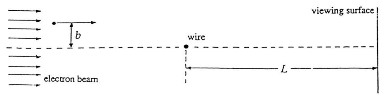
The charged wire extends perpendicularly to the plane of the paper. The sketch is not to scale.

Some numerical data are provided here; you will find other numerical data in the table at the front of the examination:

radius of wire	\(=r_0=\)	\(10^{-6}\ \mathrm{m}\)
maximum value of \(b\)	\(=b_{\max}=\)	\(10^{-4}\ \mathrm{m}\)
electric charge per unit length of wire	\(=q_{\mathrm{linear}}=\)	\(4.4\times10^{-11}\ \mathrm{C\,m^{-1}}\)
accelerating voltage	\(=V_0=\)	\(2\times10^4\ \mathrm{V}\)
length from wire to observing screen	\(=L=\)	\(0.3\ \mathrm{m}\).

Note: For parts 2 - 4, make reasonable approximations that lead to analytical and numerical solutions.

1) Calculate the electric field \(\mathbf E\) produced by the wire. Sketch the magnitude of \(\mathbf E\) as a function of distance from the axis of the wire.

2) Use classical physics to calculate the angular deflection of an electron. Do this for values of the parameter \(b\) such that the electron does not strike the wire. Let \(\theta_{\mathrm{final}}\) denote the (small) angle between the initial velocity of the electron and the velocity when the electron reaches the viewing surface. Hence, calculate \(\theta_{\mathrm{final}}\).

3) Calculate and sketch the pattern of impacts (i.e. the intensity distribution) on the viewing screen that classical physics predicts.

4) Quantum physics predicts a major difference in the intensity distribution (relative to what classical physics predicts). Sketch the pattern for the quantum prediction and provide quantitative detail.

Official English text of the problem.

Answers

Let \(y\) be the signed transverse coordinate on the screen, with \(y=0\) directly opposite the wire, and let \(I_0\) be the incident beam intensity.

The field is radially outward: \[ \boxed{ \mathbf E(r)= \begin{cases} 0,&r<r_0,\\[2pt] \dfrac{q_{\mathrm{linear}}}{2\pi\varepsilon_0r}\,\hat{\mathbf r}, &r>r_0. \end{cases}} \] Its magnitude jumps from zero to \(7.9\times10^5\ \mathrm{V\,m^{-1}}\) at the surface, then decreases as \(1/r\).
Electrons passing on either side are deflected toward the axis by approximately the same angle: \[ \boxed{\theta_{\mathrm{final}}\simeq \frac{q_{\mathrm{linear}}}{4\varepsilon_0V_0} =6.2\times10^{-5}\ \mathrm{rad}.} \]
Including the wire’s finite radius, the classical pattern is \[ \boxed{ I_{\mathrm{cl}}(y)\simeq \begin{cases} 2I_0,&|y|<17.6\ \mu\mathrm m,\\ I_0,&17.6\ \mu\mathrm m<|y|<81.4\ \mu\mathrm m,\\ 0,&|y|>81.4\ \mu\mathrm m. \end{cases}} \] Thus the central doubled-intensity band is about \(35\ \mu\mathrm m\) wide, and the whole illuminated region is about \(163\ \mu\mathrm m\) wide.
For coherent electrons, the central overlap region contains interference fringes: \[ \boxed{\lambda_{\mathrm{dB}}\simeq8.7\times10^{-12}\ \mathrm m,\qquad d\simeq\frac{\lambda_{\mathrm{dB}}}{2\theta_{\mathrm{final}}} =7.0\times10^{-8}\ \mathrm m=70\ \mathrm{nm}.} \] Away from the envelope edges, \[ \boxed{I_{\mathrm q}(y)\simeq4I_0\cos^2\!\left(\frac{\pi y}{d}\right)} \] in the overlap region. The centre is bright; successive maxima reach \(4I_0\), and minima reach zero. There are roughly \(5.1\times10^2\) fringe periods across the overlap region. The wings remain approximately at \(I_0\).

Solution

1) Electric field

Copper is a conductor, so its electrostatic field vanishes inside the wire. Outside an effectively infinite wire, cylindrical symmetry requires a radial field depending only on the distance \(r\) from its axis.

Apply Gauss’s law to a coaxial cylindrical surface of radius \(r>r_0\) and length \(\ell\): \[ E(r)(2\pi r\ell)=\frac{q_{\mathrm{linear}}\ell}{\varepsilon_0}. \] Therefore, \[ \mathbf E(r)=\frac{q_{\mathrm{linear}}}{2\pi\varepsilon_0r}\,\hat{\mathbf r}. \] The direction is outward because the wire is positively charged.

Numerically, \[ \frac{q_{\mathrm{linear}}}{2\pi\varepsilon_0} =\frac{4.4\times10^{-11}}{2\pi(8.85\times10^{-12})} =0.791\ \mathrm V, \] so \[ E(r_0^+)=\frac{0.791}{10^{-6}} \simeq7.9\times10^5\ \mathrm{V\,m^{-1}}. \]

The requested graph lies on the horizontal axis for \(0\le r<r_0\), jumps upward at \(r=r_0\), and follows a decreasing \(1/r\) curve thereafter, approaching zero asymptotically. For example, \[ E(10r_0)=7.9\times10^4\ \mathrm{V\,m^{-1}},\qquad E(100r_0)=7.9\times10^3\ \mathrm{V\,m^{-1}}. \]

2) Angular deflection

Take the \(x\)-axis along the incident beam and the \(y\)-axis perpendicular to it in the plane of the figure. The wire passes through \(x=y=0\).

Use the nonrelativistic energy relation: \[ \frac12m_ev^2=eV_0, \qquad v=\sqrt{\frac{2eV_0}{m_e}} \simeq8.4\times10^7\ \mathrm{m\,s^{-1}}. \] Here \(eV_0/(m_ec^2)\simeq0.039\), so the nonrelativistic treatment is a reasonable approximation for this problem.

We calculate the small transverse impulse along the undeflected path \(y=b\), taking \(v\) as constant. This is consistent with the weak wire potential: the potential difference between \(r_0\) and \(L\) is only \[ \Phi(r_0)-\Phi(L) =\frac{q_{\mathrm{linear}}}{2\pi\varepsilon_0} \ln\!\left(\frac{L}{r_0}\right) \simeq10\ \mathrm V, \] much smaller than \(V_0=2\times10^4\ \mathrm V\).

For an electron passing above the wire, \(b>0\), the transverse force is \[ F_y=-eE_y =-\frac{e q_{\mathrm{linear}}}{2\pi\varepsilon_0} \frac{b}{x^2+b^2}. \] Since \(dt=dx/v\), the transverse momentum change by the time the electron reaches \(x=L\) is approximately \[ \begin{aligned} \Delta p_y &=\frac1v\int_{-\infty}^{L}F_y\,dx\\ &=-\frac{e q_{\mathrm{linear}}}{2\pi\varepsilon_0v} \left[\frac{\pi}{2}+\tan^{-1}\!\left(\frac{L}{b}\right)\right]. \end{aligned} \] The upstream limit assumes that the initial beam is specified sufficiently far from the wire compared with \(b\).

For a small deflection, \[ \theta_{\mathrm{final}}\simeq\frac{|\Delta p_y|}{m_ev}. \] Using \(m_ev^2=2eV_0\), \[ \theta_{\mathrm{final}}(b)\simeq \frac{q_{\mathrm{linear}}}{4\pi\varepsilon_0V_0} \left[\frac{\pi}{2}+\tan^{-1}\!\left(\frac{L}{b}\right)\right]. \] Because \(L\gg b\), the bracket is approximately \(\pi\), giving \[ \boxed{\theta_{\mathrm{final}}\simeq \frac{q_{\mathrm{linear}}}{4\varepsilon_0V_0}.} \]

Thus, to this accuracy, the deflection is independent of the impact parameter: \[ \theta_{\mathrm{final}} =\frac{4.4\times10^{-11}} {4(8.85\times10^{-12})(2\times10^4)} \simeq6.2\times10^{-5}\ \mathrm{rad}. \] Even at \(b=b_{\max}\), the finite-screen correction in the bracket is only about \(10^{-4}\) in relative magnitude.

The upper half of the beam is deflected downward; the lower half is deflected upward. Within the same approximation, transmitted electrons have \(b>r_0\). The small change in the collision cutoff caused by attraction is neglected.

3) Classical intensity distribution

Write \[ \alpha=\theta_{\mathrm{final}},\qquad a=L\alpha\simeq18.6\ \mu\mathrm m. \] Since \(L\gg b_{\max}\), the deflection can be treated as occurring near the wire. An electron incident a distance \(b\) above the axis therefore reaches \[ y=b-a, \] whereas one incident the same distance below reaches \[ y=-b+a. \]

Only \(r_0<b<b_{\max}\) is transmitted. Consequently, the two transmitted portions occupy the following screen intervals: \[ \begin{array}{ll} \text{upper incident portion:}&r_0-a<y<b_{\max}-a,\\[2pt] \text{lower incident portion:}&-b_{\max}+a<y<a-r_0. \end{array} \] Numerically, these are \[ -17.6<y<81.4\ \mu\mathrm m \] and \[ -81.4<y<17.6\ \mu\mathrm m, \] respectively.

For each portion, the mapping has \(|dy/db|=1\). Conservation of electron flux therefore gives an intensity \(I_0\) wherever one portion arrives, and \(2I_0\) wherever both arrive.

Define \[ w=a-r_0\simeq17.6\ \mu\mathrm m,\qquad Y=b_{\max}-a\simeq81.4\ \mu\mathrm m. \] Then \[ \boxed{ I_{\mathrm{cl}}(y)= \begin{cases} 2I_0,&|y|<w,\\ I_0,&w<|y|<Y,\\ 0,&|y|>Y. \end{cases}} \]

The sketch is symmetric about \(y=0\). Starting from the left, the intensity jumps from zero to \(I_0\) at \(-81.4\ \mu\mathrm m\), rises to \(2I_0\) at \(-17.6\ \mu\mathrm m\), drops to \(I_0\) at \(+17.6\ \mu\mathrm m\), and returns to zero at \(+81.4\ \mu\mathrm m\). The bands extend uniformly parallel to the wire.

Their widths are \[ \text{central overlap width}=2(a-r_0)\simeq35.3\ \mu\mathrm m, \] \[ \text{each wing width}=b_{\max}-2a+r_0\simeq63.7\ \mu\mathrm m. \] There is no central geometrical shadow: the two deflected portions overlap.

As a flux check, \[ \int I_{\mathrm{cl}}(y)\,dy =2I_0(b_{\max}-r_0), \] which is exactly the incident flux excluding the electrons intercepted by the wire in this approximation.

4) Quantum intensity distribution

For an ideal monoenergetic, coherent incident beam, the portions passing on opposite sides of the wire interfere where they overlap.

The electron de Broglie wavelength is \[ \lambda_{\mathrm{dB}}=\frac{h}{p} =\frac{h}{\sqrt{2m_eeV_0}}, \] so \[ \lambda_{\mathrm{dB}} =\frac{6.63\times10^{-34}} {\sqrt{2(9.11\times10^{-31})(1.60\times10^{-19})(2\times10^4)}} \simeq8.7\times10^{-12}\ \mathrm m. \]

Within the overlap region, the two approximately plane waves propagate at angles \(+\alpha\) and \(-\alpha\) to the original direction. Their transverse wave-vector components are therefore \(+k\sin\alpha\) and \(-k\sin\alpha\), where \[ k=\frac{2\pi}{\lambda_{\mathrm{dB}}}. \] Reflection symmetry makes their phases equal at \(y=0\). Their phase difference at screen coordinate \(y\) is \[ \Delta\phi(y)=2ky\sin\alpha. \] Each wave separately contributes intensity \(I_0\), so \[ \begin{aligned} I_{\mathrm q}(y) &=I_0+I_0+2I_0\cos\Delta\phi\\ &=4I_0\cos^2(ky\sin\alpha). \end{aligned} \]

The fringe spacing is thus \[ d=\frac{\lambda_{\mathrm{dB}}}{2\sin\alpha} \simeq\frac{\lambda_{\mathrm{dB}}}{2\alpha}, \] giving \[ \boxed{d\simeq6.99\times10^{-8}\ \mathrm m\simeq70\ \mathrm{nm}.} \]

To geometrical-envelope accuracy, \[ \boxed{ I_{\mathrm q}(y)\simeq \begin{cases} 4I_0\cos^2\!\left(\dfrac{\pi y}{d}\right),&|y|<w,\\[4pt] I_0,&w<|y|<Y,\\ 0,&|y|>Y. \end{cases}} \]

The requested sketch has the same broad envelope as the classical pattern, but the central plateau is replaced by closely spaced fringes:

Bright fringes occur at \(y=nd\), with intensity \(4I_0\); \(n\) is an integer.
Dark fringes occur at \(y=(n+\tfrac12)d\), with zero intensity.
The central fringe at \(y=0\) is bright.
The fringes are straight and parallel to the wire.
Their mean intensity is \(2I_0\), equal to the classical central intensity.

The approximate number of fringe periods across the overlap region is \[ N\simeq\frac{2w}{d} =\frac{35.3\times10^{-6}}{6.99\times10^{-8}} \simeq5.1\times10^2. \]

Diffraction rounds the envelope boundaries, so the piecewise expression is intended away from those edges. The relevant transverse diffraction scale is of order \[ \sqrt{\lambda_{\mathrm{dB}}L}\simeq1.6\ \mu\mathrm m. \] A detector that cannot resolve the \(70\ \mathrm{nm}\) fringes measures their average and approximately recovers the classical distribution.

The solution was checked against the official solution.

IPhO 1993 · Theorieaufgabe 3

Elektronenstrahl

PDF herunterladenIPhO 1993

Allgemeine Wertetabelle

Größe	Symbol	Wert
Mittlerer Erdradius	\(R_E\)	\(6.4\times10^6\ \mathrm{m}\).
Erdbeschleunigung	\(g\)	\(9.8\ \mathrm{m\,s^{-2}}\).
Newtonsche Gravitationskonstante	\(G\)	\(6.67\times10^{-11}\ \mathrm{N\,m^2\,kg^{-2}}\).
Elektrische Feldkonstante	\(\varepsilon_0\)	\(8.85\times10^{-12}\ \mathrm{C^2\,N^{-1}\,m^{-2}}\).
Magnetische Feldkonstante	\(\mu_0\)	\(8.85\times10^{-7}\ \mathrm{N\,A^{-2}}\) [sic; korrekter Wert \(4\pi\times10^{-7}\ \mathrm{N\,A^{-2}}\)].
Lichtgeschwindigkeit im Vakuum (oder in Luft)	\(c\)	\(3.00\times10^8\ \mathrm{m\,s^{-1}}\).
Elementarladung	\(e\)	\(1.60\times10^{-19}\ \mathrm{C}\).
Elektronenmasse	\(m_e\)	\(9.11\times10^{-31}\ \mathrm{kg}\).
Protonenmasse	\(m_p\)	\(1.67\times10^{-27}\ \mathrm{kg}\)
Plancksche Konstante	\(h\)	\(6.63\times10^{-34}\ \mathrm{J\,s}\).
Avogadro-Konstante	\(N_A\)	\(6{,}02\times10^{23}\ \mathrm{mol^{-1}}\).
Boltzmann-Konstante	\(k\)	\(1.38\times10^{-23}\ \mathrm{J\,K^{-1}}\).
Universelle Gaskonstante	\(R\)	\(8.31\ \mathrm{J\,mol^{-1}\,K^{-1}}\).

Theoretische Aufgabe 3

ELEKTRONENSTRAHL

Eine Beschleunigungsspannung \(V_0\) erzeugt einen homogenen, parallelen Strahl energiereicher Elektronen. Die Elektronen passieren einen dünnen, langen, positiv geladenen Kupferdraht, der senkrecht zur ursprünglichen Strahlrichtung gespannt ist, wie in der Abbildung gezeigt. Das Symbol \(b\) bezeichnet den Abstand, in dem ein Elektron den Draht passieren würde, wenn dieser ungeladen wäre. Anschließend bewegen sich die Elektronen zu einem Schirm (Beobachtungsfläche), der sich, wie dargestellt, im Abstand \(L\) (\(\gg b\)) hinter dem Draht befindet. Der Strahl erstreckt sich anfangs bis zu den Abständen \(\pm b_{\max}\) relativ zur Drahtachse. Sowohl die Breite des Strahls als auch die Länge des Drahtes können in der Richtung senkrecht zur Papierebene als unendlich angesehen werden.

Der geladene Draht verläuft senkrecht zur Papierebene. Die Skizze ist nicht maßstabsgetreu.

Einige Zahlenwerte sind hier angegeben; weitere Zahlenwerte finden Sie in der Tabelle am Anfang der Prüfungsunterlagen:

Drahtradius	\(=r_0=\)	\(10^{-6}\ \mathrm{m}\)
Maximalwert von \(b\)	\(=b_{\max}=\)	\(10^{-4}\ \mathrm{m}\)
Elektrische Ladung pro Längeneinheit des Drahtes	\(=q_{\mathrm{linear}}=\)	\(4.4\times10^{-11}\ \mathrm{C\,m^{-1}}\)
Beschleunigungsspannung	\(=V_0=\)	\(2\times10^4\ \mathrm{V}\)
Abstand vom Draht zum Beobachtungsschirm	\(=L=\)	\(0.3\ \mathrm{m}\).

Hinweis: Verwenden Sie für die Teile 2 - 4 sinnvolle Näherungen, die zu analytischen und numerischen Lösungen führen.

1) Berechnen Sie das vom Draht erzeugte elektrische Feld \(\mathbf E\). Skizzieren Sie den Betrag von \(\mathbf E\) als Funktion des Abstands von der Drahtachse.

2) Berechnen Sie mithilfe der klassischen Physik den Ablenkwinkel eines Elektrons. Führen Sie dies für Werte des Parameters \(b\) durch, bei denen das Elektron nicht auf den Draht trifft. Mit \(\theta_{\mathrm{final}}\) sei der (kleine) Winkel zwischen der Anfangsgeschwindigkeit des Elektrons und seiner Geschwindigkeit beim Erreichen der Beobachtungsfläche bezeichnet. Berechnen Sie damit \(\theta_{\mathrm{final}}\).

3) Berechnen und skizzieren Sie das von der klassischen Physik vorhergesagte Auftreffmuster (d. h. die Intensitätsverteilung) auf dem Beobachtungsschirm.

4) Die Quantenphysik sagt einen wesentlichen Unterschied in der Intensitätsverteilung gegenüber der Vorhersage der klassischen Physik voraus. Skizzieren Sie das quantenphysikalisch vorhergesagte Muster und machen Sie quantitative Angaben dazu.

Aufgabentext aus dem offiziellen englischen Text übersetzt.

Antworten

Es sei \(y\) die vorzeichenbehaftete Querkoordinate auf dem Schirm, wobei \(y=0\) dem Draht direkt gegenüberliegt, und \(I_0\) die Intensität des einfallenden Strahls.

Das Feld ist radial nach außen gerichtet: \[ \boxed{ \mathbf E(r)= \begin{cases} 0,&r<r_0,\\[2pt] \dfrac{q_{\mathrm{linear}}}{2\pi\varepsilon_0r}\,\hat{\mathbf r}, &r>r_0. \end{cases}} \] Sein Betrag springt an der Oberfläche von null auf \(7.9\times10^5\ \mathrm{V\,m^{-1}}\) und nimmt anschließend wie \(1/r\) ab.
Elektronen, die auf beiden Seiten vorbeifliegen, werden um annähernd denselben Winkel zur Achse hin abgelenkt: \[ \boxed{\theta_{\mathrm{final}}\simeq \frac{q_{\mathrm{linear}}}{4\varepsilon_0V_0} =6.2\times10^{-5}\ \mathrm{rad}.} \]
Unter Berücksichtigung des endlichen Drahtradius ergibt sich das klassische Muster zu \[ \boxed{ I_{\mathrm{cl}}(y)\simeq \begin{cases} 2I_0,&|y|<17.6\ \mu\mathrm m,\\ I_0,&17.6\ \mu\mathrm m<|y|<81.4\ \mu\mathrm m,\\ 0,&|y|>81.4\ \mu\mathrm m. \end{cases}} \] Somit ist das zentrale Band mit doppelter Intensität etwa \(35\ \mu\mathrm m\) breit, und der gesamte beleuchtete Bereich ist etwa \(163\ \mu\mathrm m\) breit.
Bei kohärenten Elektronen enthält der zentrale Überlappungsbereich Interferenzstreifen: \[ \boxed{\lambda_{\mathrm{dB}}\simeq8.7\times10^{-12}\ \mathrm m,\qquad d\simeq\frac{\lambda_{\mathrm{dB}}}{2\theta_{\mathrm{final}}} =7.0\times10^{-8}\ \mathrm m=70\ \mathrm{nm}.} \] Abseits der Ränder der Einhüllenden gilt im Überlappungsbereich \[ \boxed{I_{\mathrm q}(y)\simeq4I_0\cos^2\!\left(\frac{\pi y}{d}\right)} \] Das Zentrum ist hell; aufeinanderfolgende Maxima erreichen \(4I_0\), und die Minima erreichen null. Über den Überlappungsbereich erstrecken sich ungefähr \(5.1\times10^2\) Streifenperioden. Die Intensität in den Seitenbereichen bleibt annähernd bei \(I_0\).

Lösung

1) Elektrisches Feld

Kupfer ist ein Leiter, daher verschwindet das elektrostatische Feld im Inneren des Drahtes. Außerhalb eines praktisch unendlich langen Drahtes erfordert die Zylindersymmetrie ein radiales Feld, das nur vom Abstand \(r\) von seiner Achse abhängt.

Wir wenden das gaußsche Gesetz auf eine koaxiale Zylinderfläche mit dem Radius \(r>r_0\) und der Länge \(\ell\) an: \[ E(r)(2\pi r\ell)=\frac{q_{\mathrm{linear}}\ell}{\varepsilon_0}. \] Daraus folgt \[ \mathbf E(r)=\frac{q_{\mathrm{linear}}}{2\pi\varepsilon_0r}\,\hat{\mathbf r}. \] Das Feld ist nach außen gerichtet, da der Draht positiv geladen ist.

Numerisch ergibt sich \[ \frac{q_{\mathrm{linear}}}{2\pi\varepsilon_0} =\frac{4.4\times10^{-11}}{2\pi(8.85\times10^{-12})} =0.791\ \mathrm V, \] also \[ E(r_0^+)=\frac{0.791}{10^{-6}} \simeq7.9\times10^5\ \mathrm{V\,m^{-1}}. \]

Der gesuchte Graph liegt für \(0\le r<r_0\) auf der horizontalen Achse, springt bei \(r=r_0\) nach oben und folgt danach einer abfallenden \(1/r\)-Kurve, die sich asymptotisch null nähert. Beispielsweise gilt \[ E(10r_0)=7.9\times10^4\ \mathrm{V\,m^{-1}},\qquad E(100r_0)=7.9\times10^3\ \mathrm{V\,m^{-1}}. \]

2) Ablenkwinkel

Wir wählen die \(x\)-Achse entlang des einfallenden Strahls und die \(y\)-Achse senkrecht dazu in der Abbildungsebene. Der Draht verläuft durch \(x=y=0\).

Wir verwenden die nichtrelativistische Energiebeziehung: \[ \frac12m_ev^2=eV_0, \qquad v=\sqrt{\frac{2eV_0}{m_e}} \simeq8.4\times10^7\ \mathrm{m\,s^{-1}}. \] Hier gilt \(eV_0/(m_ec^2)\simeq0.039\), sodass die nichtrelativistische Behandlung für diese Aufgabe eine sinnvolle Näherung ist.

Wir berechnen den kleinen transversalen Kraftstoß entlang der unabgelenkten Bahn \(y=b\) und nehmen dabei \(v\) als konstant an. Dies ist mit dem schwachen Drahtpotential vereinbar: Die Potentialdifferenz zwischen \(r_0\) und \(L\) beträgt nur \[ \Phi(r_0)-\Phi(L) =\frac{q_{\mathrm{linear}}}{2\pi\varepsilon_0} \ln\!\left(\frac{L}{r_0}\right) \simeq10\ \mathrm V, \] und ist damit viel kleiner als \(V_0=2\times10^4\ \mathrm V\).

Für ein Elektron, das oberhalb des Drahtes vorbeifliegt, also mit \(b>0\), lautet die transversale Kraft \[ F_y=-eE_y =-\frac{e q_{\mathrm{linear}}}{2\pi\varepsilon_0} \frac{b}{x^2+b^2}. \] Da \(dt=dx/v\) gilt, beträgt die transversale Impulsänderung bis zum Erreichen von \(x=L\) näherungsweise \[ \begin{aligned} \Delta p_y &=\frac1v\int_{-\infty}^{L}F_y\,dx\\ &=-\frac{e q_{\mathrm{linear}}}{2\pi\varepsilon_0v} \left[\frac{\pi}{2}+\tan^{-1}\!\left(\frac{L}{b}\right)\right]. \end{aligned} \] Die untere Integrationsgrenze setzt voraus, dass der einfallende Strahl in einem im Vergleich zu \(b\) hinreichend großen Abstand vor dem Draht vorgegeben ist.

Für eine kleine Ablenkung gilt \[ \theta_{\mathrm{final}}\simeq\frac{|\Delta p_y|}{m_ev}. \] Mit \(m_ev^2=2eV_0\) folgt \[ \theta_{\mathrm{final}}(b)\simeq \frac{q_{\mathrm{linear}}}{4\pi\varepsilon_0V_0} \left[\frac{\pi}{2}+\tan^{-1}\!\left(\frac{L}{b}\right)\right]. \] Da \(L\gg b\) ist, ist der Ausdruck in eckigen Klammern annähernd gleich \(\pi\), sodass \[ \boxed{\theta_{\mathrm{final}}\simeq \frac{q_{\mathrm{linear}}}{4\varepsilon_0V_0}.} \]

Damit ist die Ablenkung in dieser Näherung unabhängig vom Stoßparameter: \[ \theta_{\mathrm{final}} =\frac{4.4\times10^{-11}} {4(8.85\times10^{-12})(2\times10^4)} \simeq6.2\times10^{-5}\ \mathrm{rad}. \] Selbst bei \(b=b_{\max}\) beträgt die relative Korrektur im Klammerausdruck aufgrund des endlichen Schirmabstands nur etwa \(10^{-4}\).

Die obere Hälfte des Strahls wird nach unten abgelenkt, die untere Hälfte nach oben. In derselben Näherung gilt für vorbeifliegende Elektronen \(b>r_0\). Die kleine, durch die Anziehung verursachte Änderung des Grenzwerts für einen Zusammenstoß mit dem Draht wird vernachlässigt.

3) Klassische Intensitätsverteilung

Wir setzen \[ \alpha=\theta_{\mathrm{final}},\qquad a=L\alpha\simeq18.6\ \mu\mathrm m. \] Da \(L\gg b_{\max}\) ist, kann die Ablenkung als in der Nähe des Drahtes stattfindend behandelt werden. Ein Elektron, das im Abstand \(b\) oberhalb der Achse einfällt, erreicht daher \[ y=b-a, \] während eines, das im gleichen Abstand unterhalb einfällt, folgende Koordinate erreicht: \[ y=-b+a. \]

Nur Elektronen mit \(r_0<b<b_{\max}\) passieren den Draht. Folglich nehmen die beiden durchgelassenen Strahlanteile die folgenden Intervalle auf dem Schirm ein: \[ \begin{array}{ll} \text{oberer einfallender Anteil:}&r_0-a<y<b_{\max}-a,\\[2pt] \text{unterer einfallender Anteil:}&-b_{\max}+a<y<a-r_0. \end{array} \] Numerisch sind dies \[ -17.6<y<81.4\ \mu\mathrm m \] und \[ -81.4<y<17.6\ \mu\mathrm m, \] für den oberen beziehungsweise unteren Anteil.

Für jeden Anteil gilt bei dieser Abbildung \(|dy/db|=1\). Die Erhaltung des Elektronenflusses ergibt daher eine Intensität \(I_0\) überall dort, wo ein Anteil auftrifft, und \(2I_0\) überall dort, wo beide auftreffen.

Wir definieren \[ w=a-r_0\simeq17.6\ \mu\mathrm m,\qquad Y=b_{\max}-a\simeq81.4\ \mu\mathrm m. \] Dann gilt \[ \boxed{ I_{\mathrm{cl}}(y)= \begin{cases} 2I_0,&|y|<w,\\ I_0,&w<|y|<Y,\\ 0,&|y|>Y. \end{cases}} \]

Die Skizze ist symmetrisch bezüglich \(y=0\). Von links beginnend springt die Intensität bei \(-81.4\ \mu\mathrm m\) von null auf \(I_0\), steigt bei \(-17.6\ \mu\mathrm m\) auf \(2I_0\), fällt bei \(+17.6\ \mu\mathrm m\) auf \(I_0\) und kehrt bei \(+81.4\ \mu\mathrm m\) auf null zurück. Die Bänder erstrecken sich gleichförmig parallel zum Draht.

Ihre Breiten betragen \[ \text{Breite des zentralen Überlappungsbereichs}=2(a-r_0)\simeq35.3\ \mu\mathrm m, \] \[ \text{Breite jedes Seitenbereichs}=b_{\max}-2a+r_0\simeq63.7\ \mu\mathrm m. \] Es gibt keinen zentralen geometrischen Schatten: Die beiden abgelenkten Anteile überlappen sich.

Zur Kontrolle des Flusses gilt \[ \int I_{\mathrm{cl}}(y)\,dy =2I_0(b_{\max}-r_0), \] was genau dem einfallenden Fluss abzüglich der in dieser Näherung vom Draht abgefangenen Elektronen entspricht.

4) Quantenphysikalische Intensitätsverteilung

Bei einem idealen monoenergetischen, kohärenten einfallenden Strahl interferieren die auf gegenüberliegenden Seiten des Drahtes vorbeifliegenden Anteile dort, wo sie sich überlappen.

Die De-Broglie-Wellenlänge der Elektronen beträgt \[ \lambda_{\mathrm{dB}}=\frac{h}{p} =\frac{h}{\sqrt{2m_eeV_0}}, \] also \[ \lambda_{\mathrm{dB}} =\frac{6.63\times10^{-34}} {\sqrt{2(9.11\times10^{-31})(1.60\times10^{-19})(2\times10^4)}} \simeq8.7\times10^{-12}\ \mathrm m. \]

Innerhalb des Überlappungsbereichs breiten sich die beiden annähernd ebenen Wellen unter den Winkeln \(+\alpha\) und \(-\alpha\) zur ursprünglichen Richtung aus. Ihre transversalen Wellenvektorkomponenten sind daher \(+k\sin\alpha\) und \(-k\sin\alpha\), wobei \[ k=\frac{2\pi}{\lambda_{\mathrm{dB}}}. \] Aufgrund der Spiegelsymmetrie sind ihre Phasen bei \(y=0\) gleich. Ihre Phasendifferenz an der Schirmkoordinate \(y\) beträgt \[ \Delta\phi(y)=2ky\sin\alpha. \] Jede Welle trägt für sich die Intensität \(I_0\) bei, sodass \[ \begin{aligned} I_{\mathrm q}(y) &=I_0+I_0+2I_0\cos\Delta\phi\\ &=4I_0\cos^2(ky\sin\alpha). \end{aligned} \]

Der Streifenabstand ist somit \[ d=\frac{\lambda_{\mathrm{dB}}}{2\sin\alpha} \simeq\frac{\lambda_{\mathrm{dB}}}{2\alpha}, \] woraus sich ergibt: \[ \boxed{d\simeq6.99\times10^{-8}\ \mathrm m\simeq70\ \mathrm{nm}.} \]

In der Näherung einer geometrisch bestimmten Einhüllenden gilt \[ \boxed{ I_{\mathrm q}(y)\simeq \begin{cases} 4I_0\cos^2\!\left(\dfrac{\pi y}{d}\right),&|y|<w,\\[4pt] I_0,&w<|y|<Y,\\ 0,&|y|>Y. \end{cases}} \]

Die gesuchte Skizze hat dieselbe breite Einhüllende wie das klassische Muster, aber das zentrale Plateau wird durch eng beieinanderliegende Streifen ersetzt:

Helle Streifen treten bei \(y=nd\) mit der Intensität \(4I_0\) auf; \(n\) ist eine ganze Zahl.
Dunkle Streifen treten bei \(y=(n+\tfrac12)d\) mit der Intensität null auf.
Der zentrale Streifen bei \(y=0\) ist hell.
Die Streifen sind gerade und parallel zum Draht.
Ihre mittlere Intensität beträgt \(2I_0\) und ist damit gleich der klassischen Intensität im Zentrum.

Die ungefähre Anzahl der Streifenperioden über den Überlappungsbereich beträgt \[ N\simeq\frac{2w}{d} =\frac{35.3\times10^{-6}}{6.99\times10^{-8}} \simeq5.1\times10^2. \]

Beugung rundet die Ränder der Einhüllenden ab, sodass der stückweise definierte Ausdruck für Bereiche abseits dieser Ränder gedacht ist. Die maßgebliche transversale Beugungsskala liegt in der Größenordnung \[ \sqrt{\lambda_{\mathrm{dB}}L}\simeq1.6\ \mu\mathrm m. \] Ein Detektor, der die Streifen mit einem Abstand von \(70\ \mathrm{nm}\) nicht auflösen kann, misst deren Mittelwert und erhält näherungsweise wieder die klassische Verteilung.

Die Lösung wurde mit der offiziellen Lösung abgeglichen.

IPhO 1993 · Teori sorusu 3

Elektron Demeti

PDF indirIPhO 1993

Genel Bilgi Tablosu

Büyüklük	Sembol	Değer
Dünya'nın ortalama yarıçapı	\(R_E\)	\(6.4\times10^6\ \mathrm{m}\).
yerçekimi ivmesi	\(g\)	\(9.8\ \mathrm{m\,s^{-2}}\).
Newton kütleçekim sabiti	\(G\)	\(6.67\times10^{-11}\ \mathrm{N\,m^2\,kg^{-2}}\).
boşluğun elektriksel geçirgenliği	\(\varepsilon_0\)	\(8.85\times10^{-12}\ \mathrm{C^2\,N^{-1}\,m^{-2}}\).
boşluğun manyetik geçirgenliği	\(\mu_0\)	\(8.85\times10^{-7}\ \mathrm{N\,A^{-2}}\) [sic; doğru değer \(4\pi\times10^{-7}\ \mathrm{N\,A^{-2}}\)].
ışığın boşluktaki (veya havadaki) hızı	\(c\)	\(3.00\times10^8\ \mathrm{m\,s^{-1}}\).
temel yük	\(e\)	\(1.60\times10^{-19}\ \mathrm{C}\).
elektronun kütlesi	\(m_e\)	\(9.11\times10^{-31}\ \mathrm{kg}\).
protonun kütlesi	\(m_p\)	\(1.67\times10^{-27}\ \mathrm{kg}\)
Planck sabiti	\(h\)	\(6.63\times10^{-34}\ \mathrm{J\,s}\).
Avogadro sabiti	\(N_A\)	\(6{,}02\times10^{23}\ \mathrm{mol^{-1}}\).
Boltzmann sabiti	\(k\)	\(1.38\times10^{-23}\ \mathrm{J\,K^{-1}}\).
molar gaz sabiti	\(R\)	\(8.31\ \mathrm{J\,mol^{-1}\,K^{-1}}\).

Teorik Soru 3

ELEKTRON DEMETİ

Bir \(V_0\) hızlandırma gerilimi, enerjik elektronlardan oluşan düzgün, paralel bir demet üretir. Elektronlar, şekilde gösterildiği gibi demetin başlangıç doğrultusuna dik olarak gerilmiş, ince, uzun ve pozitif yüklü bir bakır telin yanından geçer. \(b\) sembolü, tel yüksüz olsaydı bir elektronun tele hangi uzaklıktan geçeceğini belirtir. Elektronlar daha sonra, şekilde gösterildiği gibi telin \(L\) (\(\gg b\)) kadar ötesindeki bir ekrana (gözlem yüzeyine) ilerler. Demet başlangıçta telin eksenine göre \(\pm b_{\max}\) uzaklıklarına kadar uzanır. Kâğıda dik doğrultuda hem demetin genişliği hem de telin uzunluğu sonsuz kabul edilebilir.

Yüklü tel, kâğıt düzlemine dik olarak uzanır. Çizim ölçekli değildir.

Bazı sayısal veriler burada verilmiştir; diğer sayısal verileri sınavın başındaki tabloda bulabilirsiniz:

telin yarıçapı	\(=r_0=\)	\(10^{-6}\ \mathrm{m}\)
\(b\)'nin en büyük değeri	\(=b_{\max}=\)	\(10^{-4}\ \mathrm{m}\)
telin birim uzunluğu başına elektrik yükü	\(=q_{\mathrm{linear}}=\)	\(4.4\times10^{-11}\ \mathrm{C\,m^{-1}}\)
hızlandırma gerilimi	\(=V_0=\)	\(2\times10^4\ \mathrm{V}\)
tel ile gözlem ekranı arasındaki uzaklık	\(=L=\)	\(0.3\ \mathrm{m}\).

Not: 2 - 4. kısımlar için analitik ve sayısal çözümler elde etmeyi sağlayan makul yaklaşımlar yapınız.

1) Telin oluşturduğu \(\mathbf E\) elektrik alanını hesaplayınız. \(\mathbf E\)'nin büyüklüğünü telin ekseninden uzaklığın fonksiyonu olarak çiziniz.

2) Bir elektronun açısal sapmasını klasik fiziği kullanarak hesaplayınız. Bunu, \(b\) parametresinin elektronun tele çarpmadığı değerleri için yapınız. \(\theta_{\mathrm{final}}\), elektronun başlangıç hızı ile gözlem yüzeyine ulaştığındaki hızı arasındaki (küçük) açıyı göstersin. Buradan \(\theta_{\mathrm{final}}\)'i hesaplayınız.

3) Klasik fiziğin gözlem ekranı üzerinde öngördüğü çarpma desenini (yani şiddet dağılımını) hesaplayınız ve çiziniz.

4) Kuantum fiziği, şiddet dağılımında (klasik fiziğin öngördüğüne göre) önemli bir fark öngörür. Kuantum fiziğinin öngördüğü deseni çiziniz ve nicel ayrıntıları veriniz.

Soru metni resmi İngilizce metinden çevrilmiştir.

Cevaplar

\(y\), telin tam karşısında \(y=0\) olacak şekilde ekran üzerindeki işaretli enine koordinat, \(I_0\) ise gelen demetin şiddeti olsun.

Alan, radyal olarak dışa yönelmiştir: \[ \boxed{ \mathbf E(r)= \begin{cases} 0,&r<r_0,\\[2pt] \dfrac{q_{\mathrm{linear}}}{2\pi\varepsilon_0r}\,\hat{\mathbf r}, &r>r_0. \end{cases}} \] Büyüklüğü yüzeyde sıfırdan \(7.9\times10^5\ \mathrm{V\,m^{-1}}\) değerine sıçrar, ardından \(1/r\) ile azalır.
Her iki taraftan geçen elektronlar, yaklaşık olarak aynı açıyla eksene doğru sapar: \[ \boxed{\theta_{\mathrm{final}}\simeq \frac{q_{\mathrm{linear}}}{4\varepsilon_0V_0} =6.2\times10^{-5}\ \mathrm{rad}.} \]
Telin sonlu yarıçapı hesaba katıldığında klasik desen şöyledir: \[ \boxed{ I_{\mathrm{cl}}(y)\simeq \begin{cases} 2I_0,&|y|<17.6\ \mu\mathrm m,\\ I_0,&17.6\ \mu\mathrm m<|y|<81.4\ \mu\mathrm m,\\ 0,&|y|>81.4\ \mu\mathrm m. \end{cases}} \] Dolayısıyla merkezdeki iki kat şiddetli bandın genişliği yaklaşık \(35\ \mu\mathrm m\), aydınlanan bölgenin tamamının genişliği ise yaklaşık \(163\ \mu\mathrm m\)'dir.
Eşevreli elektronlar için merkezdeki örtüşme bölgesinde girişim saçakları oluşur: \[ \boxed{\lambda_{\mathrm{dB}}\simeq8.7\times10^{-12}\ \mathrm m,\qquad d\simeq\frac{\lambda_{\mathrm{dB}}}{2\theta_{\mathrm{final}}} =7.0\times10^{-8}\ \mathrm m=70\ \mathrm{nm}.} \] Zarfın kenarlarından uzakta, örtüşme bölgesinde \[ \boxed{I_{\mathrm q}(y)\simeq4I_0\cos^2\!\left(\frac{\pi y}{d}\right)} \] olur. Merkez aydınlıktır; ardışık maksimumlar \(4I_0\)'a, minimumlar ise sıfıra ulaşır. Örtüşme bölgesi boyunca yaklaşık \(5.1\times10^2\) saçak periyodu vardır. Yan bölgelerin şiddeti yaklaşık \(I_0\) olarak kalır.

Çözüm

1) Elektrik alan

Bakır bir iletkendir; dolayısıyla telin içinde elektrostatik alan sıfırdır. Sonsuz kabul edilebilecek bir telin dışında silindirik simetri, yalnızca eksene olan \(r\) uzaklığına bağlı radyal bir alan gerektirir.

Gauss yasasını, yarıçapı \(r>r_0\) ve uzunluğu \(\ell\) olan eş eksenli bir silindirik yüzeye uygulayalım: \[ E(r)(2\pi r\ell)=\frac{q_{\mathrm{linear}}\ell}{\varepsilon_0}. \] Böylece, \[ \mathbf E(r)=\frac{q_{\mathrm{linear}}}{2\pi\varepsilon_0r}\,\hat{\mathbf r}. \] Tel pozitif yüklü olduğundan alan dışa yönelmiştir.

Sayısal olarak, \[ \frac{q_{\mathrm{linear}}}{2\pi\varepsilon_0} =\frac{4.4\times10^{-11}}{2\pi(8.85\times10^{-12})} =0.791\ \mathrm V, \] dolayısıyla \[ E(r_0^+)=\frac{0.791}{10^{-6}} \simeq7.9\times10^5\ \mathrm{V\,m^{-1}}. \]

İstenen grafik, \(0\le r<r_0\) için yatay eksen üzerinde yer alır, \(r=r_0\)'da yukarı sıçrar ve sonrasında azalan bir \(1/r\) eğrisini izleyerek sıfıra asimptotik olarak yaklaşır. Örneğin, \[ E(10r_0)=7.9\times10^4\ \mathrm{V\,m^{-1}},\qquad E(100r_0)=7.9\times10^3\ \mathrm{V\,m^{-1}}. \]

2) Açısal sapma

\(x\) eksenini gelen demet doğrultusunda, \(y\) eksenini ise şekil düzleminde ona dik alalım. Tel, \(x=y=0\) noktasından geçer.

Göreli olmayan enerji bağıntısını kullanalım: \[ \frac12m_ev^2=eV_0, \qquad v=\sqrt{\frac{2eV_0}{m_e}} \simeq8.4\times10^7\ \mathrm{m\,s^{-1}}. \] Burada \(eV_0/(m_ec^2)\simeq0.039\) olduğundan, göreli olmayan yaklaşım bu soru için makul bir yaklaşımdır.

Küçük enine itmeyi, \(v\)'yi sabit alarak sapmamış \(y=b\) yolu boyunca hesaplayalım. Bu, telin düşük potansiyeliyle tutarlıdır: \(r_0\) ile \(L\) arasındaki potansiyel farkı yalnızca \[ \Phi(r_0)-\Phi(L) =\frac{q_{\mathrm{linear}}}{2\pi\varepsilon_0} \ln\!\left(\frac{L}{r_0}\right) \simeq10\ \mathrm V, \] olup \(V_0=2\times10^4\ \mathrm V\)'tan çok küçüktür.

Telin üstünden geçen bir elektron için \(b>0\) olup enine kuvvet \[ F_y=-eE_y =-\frac{e q_{\mathrm{linear}}}{2\pi\varepsilon_0} \frac{b}{x^2+b^2}. \] şeklindedir. \(dt=dx/v\) olduğundan, elektron \(x=L\)'ye ulaşana kadar enine momentumundaki değişim yaklaşık olarak \[ \begin{aligned} \Delta p_y &=\frac1v\int_{-\infty}^{L}F_y\,dx\\ &=-\frac{e q_{\mathrm{linear}}}{2\pi\varepsilon_0v} \left[\frac{\pi}{2}+\tan^{-1}\!\left(\frac{L}{b}\right)\right]. \end{aligned} \] olur. Geliş tarafındaki integral sınırı, başlangıç demetinin tele uzaklığı \(b\)'ye göre yeterince büyük bir yerde tanımlandığını varsayar.

Küçük bir sapma için, \[ \theta_{\mathrm{final}}\simeq\frac{|\Delta p_y|}{m_ev}. \] \(m_ev^2=2eV_0\) kullanılarak, \[ \theta_{\mathrm{final}}(b)\simeq \frac{q_{\mathrm{linear}}}{4\pi\varepsilon_0V_0} \left[\frac{\pi}{2}+\tan^{-1}\!\left(\frac{L}{b}\right)\right]. \] \(L\gg b\) olduğundan köşeli parantez içindeki ifade yaklaşık \(\pi\)'dir ve \[ \boxed{\theta_{\mathrm{final}}\simeq \frac{q_{\mathrm{linear}}}{4\varepsilon_0V_0}.} \] elde edilir.

Dolayısıyla bu duyarlılıkta sapma, çarpma parametresinden bağımsızdır: \[ \theta_{\mathrm{final}} =\frac{4.4\times10^{-11}} {4(8.85\times10^{-12})(2\times10^4)} \simeq6.2\times10^{-5}\ \mathrm{rad}. \] \(b=b_{\max}\) için bile, ekran uzaklığının sonlu olmasından kaynaklanan köşeli parantez içindeki düzeltmenin bağıl büyüklüğü yalnızca yaklaşık \(10^{-4}\)'tür.

Demetin üst yarısı aşağıya, alt yarısı ise yukarıya sapar. Aynı yaklaşım çerçevesinde, telin yanından geçebilen elektronlar için \(b>r_0\)'dır. Çekimin çarpışma sınırında neden olduğu küçük değişim ihmal edilir.

3) Klasik şiddet dağılımı

Şöyle yazalım: \[ \alpha=\theta_{\mathrm{final}},\qquad a=L\alpha\simeq18.6\ \mu\mathrm m. \] \(L\gg b_{\max}\) olduğundan sapmanın telin yakınında gerçekleştiği kabul edilebilir. Bu nedenle eksenin \(b\) kadar üstünden gelen bir elektron \[ y=b-a, \] koordinatına ulaşırken, aynı uzaklıkta alttan gelen bir elektron \[ y=-b+a. \] koordinatına ulaşır.

Yalnızca \(r_0<b<b_{\max}\) aralığındaki elektronlar geçer. Dolayısıyla geçen iki kısım, ekranda aşağıdaki aralıkları kaplar: \[ \begin{array}{ll} \text{üstten gelen kısım:}&r_0-a<y<b_{\max}-a,\\[2pt] \text{alttan gelen kısım:}&-b_{\max}+a<y<a-r_0. \end{array} \] Sayısal olarak bu aralıklar sırasıyla \[ -17.6<y<81.4\ \mu\mathrm m \] ve \[ -81.4<y<17.6\ \mu\mathrm m, \] şeklindedir.

Her bir kısım için dönüşüm \(|dy/db|=1\) koşulunu sağlar. Bu nedenle elektron akısının korunumu, yalnızca bir kısmın ulaştığı her yerde \(I_0\), her iki kısmın ulaştığı her yerde ise \(2I_0\) şiddetini verir.

Şu tanımları yapalım: \[ w=a-r_0\simeq17.6\ \mu\mathrm m,\qquad Y=b_{\max}-a\simeq81.4\ \mu\mathrm m. \] Böylece \[ \boxed{ I_{\mathrm{cl}}(y)= \begin{cases} 2I_0,&|y|<w,\\ I_0,&w<|y|<Y,\\ 0,&|y|>Y. \end{cases}} \]

Çizim \(y=0\)'a göre simetriktir. Soldan başlanırsa şiddet, \(-81.4\ \mu\mathrm m\)'de sıfırdan \(I_0\)'a sıçrar, \(-17.6\ \mu\mathrm m\)'de \(2I_0\)'a yükselir, \(+17.6\ \mu\mathrm m\)'de \(I_0\)'a düşer ve \(+81.4\ \mu\mathrm m\)'de yeniden sıfır olur. Bantlar, tele paralel doğrultuda düzgün biçimde uzanır.

Genişlikleri şöyledir: \[ \text{merkezdeki örtüşme genişliği}=2(a-r_0)\simeq35.3\ \mu\mathrm m, \] \[ \text{her bir yan bölgenin genişliği}=b_{\max}-2a+r_0\simeq63.7\ \mu\mathrm m. \] Merkezde geometrik gölge yoktur: sapan iki kısım birbiriyle örtüşür.

Akıyı kontrol etmek için, \[ \int I_{\mathrm{cl}}(y)\,dy =2I_0(b_{\max}-r_0), \] yazılır; bu, bu yaklaşımda telin durdurduğu elektronlar dışarıda bırakıldığında gelen akıya tam olarak eşittir.

4) Kuantum şiddet dağılımı

İdeal, tek enerjili ve eşevreli bir gelen demet için telin karşılıklı iki yanından geçen kısımlar, örtüştükleri yerde girişim yapar.

Elektronun de Broglie dalga boyu \[ \lambda_{\mathrm{dB}}=\frac{h}{p} =\frac{h}{\sqrt{2m_eeV_0}}, \] olduğundan, \[ \lambda_{\mathrm{dB}} =\frac{6.63\times10^{-34}} {\sqrt{2(9.11\times10^{-31})(1.60\times10^{-19})(2\times10^4)}} \simeq8.7\times10^{-12}\ \mathrm m. \]

Örtüşme bölgesinde yaklaşık olarak düzlemsel olan iki dalga, başlangıç doğrultusuyla \(+\alpha\) ve \(-\alpha\) açıları yaparak ilerler. Bu nedenle dalga vektörlerinin enine bileşenleri \(+k\sin\alpha\) ve \(-k\sin\alpha\)'dır; burada \[ k=\frac{2\pi}{\lambda_{\mathrm{dB}}}. \] Yansıma simetrisi, \(y=0\)'da fazlarının eşit olmasını sağlar. Ekranın \(y\) koordinatındaki faz farkları \[ \Delta\phi(y)=2ky\sin\alpha. \] şeklindedir. Her dalga ayrı ayrı \(I_0\) şiddeti katkısında bulunduğundan, \[ \begin{aligned} I_{\mathrm q}(y) &=I_0+I_0+2I_0\cos\Delta\phi\\ &=4I_0\cos^2(ky\sin\alpha). \end{aligned} \]

Böylece saçak aralığı \[ d=\frac{\lambda_{\mathrm{dB}}}{2\sin\alpha} \simeq\frac{\lambda_{\mathrm{dB}}}{2\alpha}, \] olup buradan \[ \boxed{d\simeq6.99\times10^{-8}\ \mathrm m\simeq70\ \mathrm{nm}.} \] elde edilir.

Geometrik zarf yaklaşımının duyarlılığı içinde, \[ \boxed{ I_{\mathrm q}(y)\simeq \begin{cases} 4I_0\cos^2\!\left(\dfrac{\pi y}{d}\right),&|y|<w,\\[4pt] I_0,&w<|y|<Y,\\ 0,&|y|>Y. \end{cases}} \]

İstenen çizimin geniş ölçekli zarfı klasik deseninkiyle aynıdır; ancak merkezdeki plato yerini birbirine yakın saçaklara bırakır:

Aydınlık saçaklar \(y=nd\) konumlarında oluşur ve şiddetleri \(4I_0\)'dır; \(n\) bir tam sayıdır.
Karanlık saçaklar \(y=(n+\tfrac12)d\) konumlarında oluşur ve şiddetleri sıfırdır.
\(y=0\)'daki merkez saçağı aydınlıktır.
Saçaklar doğrusaldır ve tele paraleldir.
Ortalama şiddetleri \(2I_0\) olup merkezdeki klasik şiddete eşittir.

Örtüşme bölgesi boyunca yaklaşık saçak periyodu sayısı \[ N\simeq\frac{2w}{d} =\frac{35.3\times10^{-6}}{6.99\times10^{-8}} \simeq5.1\times10^2. \] şeklindedir.

Kırınım, zarf sınırlarını yumuşatır; dolayısıyla parçalı ifade bu kenarlardan uzak bölgeler için geçerlidir. İlgili enine kırınım ölçeği \[ \sqrt{\lambda_{\mathrm{dB}}L}\simeq1.6\ \mu\mathrm m. \] mertebesindedir. \(70\ \mathrm{nm}\) aralıklı saçakları ayırt edemeyen bir dedektör, bunların ortalamasını ölçer ve yaklaşık olarak klasik dağılımı elde eder.

Çözüm, resmi çözümle karşılaştırılarak kontrol edildi.

IPhO 1993 · Problema teórico 3

Haz de electrones

Descargar PDFIPhO 1993

Información general tabulada

Magnitud	Símbolo	Valor
Radio medio de la Tierra	\(R_E\)	\(6.4\times10^6\ \mathrm{m}\).
aceleración de la gravedad	\(g\)	\(9.8\ \mathrm{m\,s^{-2}}\).
constante de gravitación universal de Newton	\(G\)	\(6.67\times10^{-11}\ \mathrm{N\,m^2\,kg^{-2}}\).
permitividad del vacío	\(\varepsilon_0\)	\(8.85\times10^{-12}\ \mathrm{C^2\,N^{-1}\,m^{-2}}\).
permeabilidad del vacío	\(\mu_0\)	\(8.85\times10^{-7}\ \mathrm{N\,A^{-2}}\) [sic; valor correcto \(4\pi\times10^{-7}\ \mathrm{N\,A^{-2}}\)].
velocidad de la luz en el vacío (o en el aire)	\(c\)	\(3.00\times10^8\ \mathrm{m\,s^{-1}}\).
carga elemental	\(e\)	\(1.60\times10^{-19}\ \mathrm{C}\).
masa del electrón	\(m_e\)	\(9.11\times10^{-31}\ \mathrm{kg}\).
masa del protón	\(m_p\)	\(1.67\times10^{-27}\ \mathrm{kg}\)
constante de Planck	\(h\)	\(6.63\times10^{-34}\ \mathrm{J\,s}\).
constante de Avogadro	\(N_A\)	\(6{,}02\times10^{23}\ \mathrm{mol^{-1}}\).
constante de Boltzmann	\(k\)	\(1.38\times10^{-23}\ \mathrm{J\,K^{-1}}\).
constante molar de los gases	\(R\)	\(8.31\ \mathrm{J\,mol^{-1}\,K^{-1}}\).

Problema teórico 3

HAZ DE ELECTRONES

Una tensión de aceleración \(V_0\) produce un haz uniforme y paralelo de electrones de alta energía. Los electrones pasan junto a un alambre de cobre delgado, largo y cargado positivamente, tensado perpendicularmente a la dirección original del haz, como se muestra en la figura. El símbolo \(b\) denota la distancia a la que un electrón pasaría del alambre si este no estuviera cargado. A continuación, los electrones se dirigen hacia una pantalla (superficie de observación) situada a una distancia \(L\) (\(\gg b\)) más allá del alambre, como se muestra. Inicialmente, el haz se extiende hasta distancias \(\pm b_{\max}\) con respecto al eje del alambre. Tanto la anchura del haz como la longitud del alambre pueden considerarse infinitas en la dirección perpendicular al papel.

El alambre cargado se extiende perpendicularmente al plano del papel. El esquema no está a escala.

A continuación se proporcionan algunos datos numéricos; encontrará otros datos numéricos en la tabla al principio del examen:

radio del alambre	\(=r_0=\)	\(10^{-6}\ \mathrm{m}\)
valor máximo de \(b\)	\(=b_{\max}=\)	\(10^{-4}\ \mathrm{m}\)
carga eléctrica por unidad de longitud del alambre	\(=q_{\mathrm{linear}}=\)	\(4.4\times10^{-11}\ \mathrm{C\,m^{-1}}\)
tensión de aceleración	\(=V_0=\)	\(2\times10^4\ \mathrm{V}\)
distancia del alambre a la pantalla de observación	\(=L=\)	\(0.3\ \mathrm{m}\).

Nota: Para los apartados 2 - 4, utilice aproximaciones razonables que permitan obtener soluciones analíticas y numéricas.

1) Calcule el campo eléctrico \(\mathbf E\) producido por el alambre. Represente esquemáticamente el módulo de \(\mathbf E\) en función de la distancia al eje del alambre.

2) Utilice la física clásica para calcular la desviación angular de un electrón. Hágalo para valores del parámetro \(b\) tales que el electrón no choque con el alambre. Sea \(\theta_{\mathrm{final}}\) el ángulo (pequeño) entre la velocidad inicial del electrón y su velocidad cuando alcanza la superficie de observación. Calcule, por tanto, \(\theta_{\mathrm{final}}\).

3) Calcule y represente esquemáticamente el patrón de impactos (es decir, la distribución de intensidad) sobre la pantalla de observación que predice la física clásica.

4) La física cuántica predice una diferencia importante en la distribución de intensidad (con respecto a lo que predice la física clásica). Represente esquemáticamente el patrón de la predicción cuántica y proporcione detalles cuantitativos.

Enunciado traducido del texto oficial en inglés.

Respuestas

Sea \(y\) la coordenada transversal con signo sobre la pantalla, con \(y=0\) directamente frente al alambre, y sea \(I_0\) la intensidad del haz incidente.

El campo es radial y está dirigido hacia fuera: \[ \boxed{ \mathbf E(r)= \begin{cases} 0,&r<r_0,\\[2pt] \dfrac{q_{\mathrm{linear}}}{2\pi\varepsilon_0r}\,\hat{\mathbf r}, &r>r_0. \end{cases}} \] Su módulo salta de cero a \(7.9\times10^5\ \mathrm{V\,m^{-1}}\) en la superficie y después disminuye como \(1/r\).
Los electrones que pasan por ambos lados se desvían hacia el eje aproximadamente el mismo ángulo: \[ \boxed{\theta_{\mathrm{final}}\simeq \frac{q_{\mathrm{linear}}}{4\varepsilon_0V_0} =6.2\times10^{-5}\ \mathrm{rad}.} \]
Teniendo en cuenta el radio finito del alambre, el patrón clásico es \[ \boxed{ I_{\mathrm{cl}}(y)\simeq \begin{cases} 2I_0,&|y|<17.6\ \mu\mathrm m,\\ I_0,&17.6\ \mu\mathrm m<|y|<81.4\ \mu\mathrm m,\\ 0,&|y|>81.4\ \mu\mathrm m. \end{cases}} \] Por tanto, la banda central de intensidad doble tiene una anchura de unos \(35\ \mu\mathrm m\), y toda la región iluminada tiene una anchura de unos \(163\ \mu\mathrm m\).
Para electrones coherentes, la región central de superposición contiene franjas de interferencia: \[ \boxed{\lambda_{\mathrm{dB}}\simeq8.7\times10^{-12}\ \mathrm m,\qquad d\simeq\frac{\lambda_{\mathrm{dB}}}{2\theta_{\mathrm{final}}} =7.0\times10^{-8}\ \mathrm m=70\ \mathrm{nm}.} \] Lejos de los bordes de la envolvente, \[ \boxed{I_{\mathrm q}(y)\simeq4I_0\cos^2\!\left(\frac{\pi y}{d}\right)} \] en la región de superposición. El centro es brillante; los máximos sucesivos alcanzan \(4I_0\), y los mínimos llegan a cero. Hay aproximadamente \(5.1\times10^2\) períodos de las franjas a lo ancho de la región de superposición. Las zonas laterales permanecen aproximadamente a \(I_0\).

Solución

1) Campo eléctrico

El cobre es un conductor, por lo que el campo electrostático en el interior del alambre es nulo. Fuera de un alambre que puede considerarse infinito, la simetría cilíndrica exige un campo radial que dependa únicamente de la distancia \(r\) a su eje.

Aplicamos la ley de Gauss a una superficie cilíndrica coaxial de radio \(r>r_0\) y longitud \(\ell\): \[ E(r)(2\pi r\ell)=\frac{q_{\mathrm{linear}}\ell}{\varepsilon_0}. \] Por tanto, \[ \mathbf E(r)=\frac{q_{\mathrm{linear}}}{2\pi\varepsilon_0r}\,\hat{\mathbf r}. \] El sentido es hacia fuera porque el alambre está cargado positivamente.

Numéricamente, \[ \frac{q_{\mathrm{linear}}}{2\pi\varepsilon_0} =\frac{4.4\times10^{-11}}{2\pi(8.85\times10^{-12})} =0.791\ \mathrm V, \] de modo que \[ E(r_0^+)=\frac{0.791}{10^{-6}} \simeq7.9\times10^5\ \mathrm{V\,m^{-1}}. \]

La gráfica solicitada coincide con el eje horizontal para \(0\le r<r_0\), presenta un salto hacia arriba en \(r=r_0\) y, a partir de ahí, sigue una curva decreciente \(1/r\), acercándose asintóticamente a cero. Por ejemplo, \[ E(10r_0)=7.9\times10^4\ \mathrm{V\,m^{-1}},\qquad E(100r_0)=7.9\times10^3\ \mathrm{V\,m^{-1}}. \]

2) Desviación angular

Tomamos el eje \(x\) en la dirección del haz incidente y el eje \(y\) perpendicular a él en el plano de la figura. El alambre pasa por \(x=y=0\).

Utilizamos la relación no relativista para la energía: \[ \frac12m_ev^2=eV_0, \qquad v=\sqrt{\frac{2eV_0}{m_e}} \simeq8.4\times10^7\ \mathrm{m\,s^{-1}}. \] Aquí \(eV_0/(m_ec^2)\simeq0.039\), de modo que el tratamiento no relativista es una aproximación razonable para este problema.

Calculamos el pequeño impulso transversal a lo largo de la trayectoria sin desviación \(y=b\), tomando \(v\) como constante. Esto es coherente con el pequeño potencial del alambre: la diferencia de potencial entre \(r_0\) y \(L\) es de solo \[ \Phi(r_0)-\Phi(L) =\frac{q_{\mathrm{linear}}}{2\pi\varepsilon_0} \ln\!\left(\frac{L}{r_0}\right) \simeq10\ \mathrm V, \] mucho menor que \(V_0=2\times10^4\ \mathrm V\).

Para un electrón que pasa por encima del alambre, \(b>0\), la fuerza transversal es \[ F_y=-eE_y =-\frac{e q_{\mathrm{linear}}}{2\pi\varepsilon_0} \frac{b}{x^2+b^2}. \] Puesto que \(dt=dx/v\), la variación de la cantidad de movimiento transversal hasta que el electrón alcanza \(x=L\) es aproximadamente \[ \begin{aligned} \Delta p_y &=\frac1v\int_{-\infty}^{L}F_y\,dx\\ &=-\frac{e q_{\mathrm{linear}}}{2\pi\varepsilon_0v} \left[\frac{\pi}{2}+\tan^{-1}\!\left(\frac{L}{b}\right)\right]. \end{aligned} \] El límite inicial supone que el haz inicial se especifica a una distancia del alambre suficientemente grande en comparación con \(b\).

Para una desviación pequeña, \[ \theta_{\mathrm{final}}\simeq\frac{|\Delta p_y|}{m_ev}. \] Utilizando \(m_ev^2=2eV_0\), \[ \theta_{\mathrm{final}}(b)\simeq \frac{q_{\mathrm{linear}}}{4\pi\varepsilon_0V_0} \left[\frac{\pi}{2}+\tan^{-1}\!\left(\frac{L}{b}\right)\right]. \] Como \(L\gg b\), el corchete es aproximadamente \(\pi\), lo que da \[ \boxed{\theta_{\mathrm{final}}\simeq \frac{q_{\mathrm{linear}}}{4\varepsilon_0V_0}.} \]

Así, con esta precisión, la desviación es independiente del parámetro de impacto: \[ \theta_{\mathrm{final}} =\frac{4.4\times10^{-11}} {4(8.85\times10^{-12})(2\times10^4)} \simeq6.2\times10^{-5}\ \mathrm{rad}. \] Incluso para \(b=b_{\max}\), la corrección en el corchete debida a la distancia finita a la pantalla es de solo aproximadamente \(10^{-4}\) en términos relativos.

La mitad superior del haz se desvía hacia abajo; la mitad inferior se desvía hacia arriba. Dentro de la misma aproximación, los electrones transmitidos tienen \(b>r_0\). Se desprecia el pequeño cambio en el valor límite para la colisión causado por la atracción.

3) Distribución clásica de intensidad

Escribimos \[ \alpha=\theta_{\mathrm{final}},\qquad a=L\alpha\simeq18.6\ \mu\mathrm m. \] Como \(L\gg b_{\max}\), puede considerarse que la desviación se produce cerca del alambre. Por tanto, un electrón que incide a una distancia \(b\) por encima del eje llega a \[ y=b-a, \] mientras que uno que incide a la misma distancia por debajo llega a \[ y=-b+a. \]

Solo se transmite la parte con \(r_0<b<b_{\max}\). En consecuencia, las dos porciones transmitidas ocupan los siguientes intervalos de la pantalla: \[ \begin{array}{ll} \text{porción incidente superior:}&r_0-a<y<b_{\max}-a,\\[2pt] \text{porción incidente inferior:}&-b_{\max}+a<y<a-r_0. \end{array} \] Numéricamente, estos son \[ -17.6<y<81.4\ \mu\mathrm m \] y \[ -81.4<y<17.6\ \mu\mathrm m, \] respectivamente.

Para cada porción, la correspondencia cumple \(|dy/db|=1\). Por tanto, la conservación del flujo de electrones da una intensidad \(I_0\) donde llega una sola porción, y \(2I_0\) donde llegan ambas.

Definimos \[ w=a-r_0\simeq17.6\ \mu\mathrm m,\qquad Y=b_{\max}-a\simeq81.4\ \mu\mathrm m. \] Entonces \[ \boxed{ I_{\mathrm{cl}}(y)= \begin{cases} 2I_0,&|y|<w,\\ I_0,&w<|y|<Y,\\ 0,&|y|>Y. \end{cases}} \]

La representación es simétrica respecto a \(y=0\). Partiendo de la izquierda, la intensidad salta de cero a \(I_0\) en \(-81.4\ \mu\mathrm m\), aumenta a \(2I_0\) en \(-17.6\ \mu\mathrm m\), disminuye a \(I_0\) en \(+17.6\ \mu\mathrm m\) y vuelve a cero en \(+81.4\ \mu\mathrm m\). Las bandas se extienden uniformemente en dirección paralela al alambre.

Sus anchuras son \[ \text{anchura de la superposición central}=2(a-r_0)\simeq35.3\ \mu\mathrm m, \] \[ \text{anchura de cada zona lateral}=b_{\max}-2a+r_0\simeq63.7\ \mu\mathrm m. \] No hay una sombra geométrica central: las dos porciones desviadas se superponen.

Como comprobación del flujo, \[ \int I_{\mathrm{cl}}(y)\,dy =2I_0(b_{\max}-r_0), \] que es exactamente el flujo incidente excluyendo los electrones interceptados por el alambre en esta aproximación.

4) Distribución cuántica de intensidad

Para un haz incidente ideal, monoenergético y coherente, las porciones que pasan por lados opuestos del alambre interfieren donde se superponen.

La longitud de onda de de Broglie del electrón es \[ \lambda_{\mathrm{dB}}=\frac{h}{p} =\frac{h}{\sqrt{2m_eeV_0}}, \] de modo que \[ \lambda_{\mathrm{dB}} =\frac{6.63\times10^{-34}} {\sqrt{2(9.11\times10^{-31})(1.60\times10^{-19})(2\times10^4)}} \simeq8.7\times10^{-12}\ \mathrm m. \]

Dentro de la región de superposición, las dos ondas aproximadamente planas se propagan formando ángulos \(+\alpha\) y \(-\alpha\) con la dirección original. Por tanto, las componentes transversales de sus vectores de onda son \(+k\sin\alpha\) y \(-k\sin\alpha\), donde \[ k=\frac{2\pi}{\lambda_{\mathrm{dB}}}. \] La simetría de reflexión hace que sus fases sean iguales en \(y=0\). Su diferencia de fase en la coordenada \(y\) de la pantalla es \[ \Delta\phi(y)=2ky\sin\alpha. \] Cada onda por separado contribuye con una intensidad \(I_0\), de modo que \[ \begin{aligned} I_{\mathrm q}(y) &=I_0+I_0+2I_0\cos\Delta\phi\\ &=4I_0\cos^2(ky\sin\alpha). \end{aligned} \]

La separación entre franjas es, por tanto, \[ d=\frac{\lambda_{\mathrm{dB}}}{2\sin\alpha} \simeq\frac{\lambda_{\mathrm{dB}}}{2\alpha}, \] lo que da \[ \boxed{d\simeq6.99\times10^{-8}\ \mathrm m\simeq70\ \mathrm{nm}.} \]

Con la precisión de la aproximación de envolvente geométrica, \[ \boxed{ I_{\mathrm q}(y)\simeq \begin{cases} 4I_0\cos^2\!\left(\dfrac{\pi y}{d}\right),&|y|<w,\\[4pt] I_0,&w<|y|<Y,\\ 0,&|y|>Y. \end{cases}} \]

La representación solicitada tiene la misma envolvente amplia que el patrón clásico, pero la meseta central se sustituye por franjas muy próximas entre sí:

Las franjas brillantes se encuentran en \(y=nd\), con intensidad \(4I_0\); \(n\) es un número entero.
Las franjas oscuras se encuentran en \(y=(n+\tfrac12)d\), con intensidad nula.
La franja central en \(y=0\) es brillante.
Las franjas son rectas y paralelas al alambre.
Su intensidad media es \(2I_0\), igual a la intensidad central clásica.

El número aproximado de períodos de las franjas a lo ancho de la región de superposición es \[ N\simeq\frac{2w}{d} =\frac{35.3\times10^{-6}}{6.99\times10^{-8}} \simeq5.1\times10^2. \]

La difracción suaviza los límites de la envolvente, por lo que la expresión por tramos se aplica lejos de esos bordes. La escala transversal de difracción pertinente es del orden de \[ \sqrt{\lambda_{\mathrm{dB}}L}\simeq1.6\ \mu\mathrm m. \] Un detector que no pueda resolver las franjas de \(70\ \mathrm{nm}\) mide su promedio y recupera aproximadamente la distribución clásica.

La solución se comprobó con la solución oficial.

IPhO 1993 · 理论题 3

电子束

下载 PDFIPhO 1993

通用数据表

物理量	符号	数值
地球平均半径	\(R_E\)	\(6.4\times10^6\ \mathrm{m}\).
重力加速度	\(g\)	\(9.8\ \mathrm{m\,s^{-2}}\).
牛顿引力常量	\(G\)	\(6.67\times10^{-11}\ \mathrm{N\,m^2\,kg^{-2}}\).
真空介电常数	\(\varepsilon_0\)	\(8.85\times10^{-12}\ \mathrm{C^2\,N^{-1}\,m^{-2}}\).
真空磁导率	\(\mu_0\)	\(8.85\times10^{-7}\ \mathrm{N\,A^{-2}}\)［原文如此；正确值为 \(4\pi\times10^{-7}\ \mathrm{N\,A^{-2}}\)］.
真空（或空气）中的光速	\(c\)	\(3.00\times10^8\ \mathrm{m\,s^{-1}}\).
元电荷	\(e\)	\(1.60\times10^{-19}\ \mathrm{C}\).
电子质量	\(m_e\)	\(9.11\times10^{-31}\ \mathrm{kg}\).
质子质量	\(m_p\)	\(1.67\times10^{-27}\ \mathrm{kg}\)
普朗克常量	\(h\)	\(6.63\times10^{-34}\ \mathrm{J\,s}\).
阿伏伽德罗常量	\(N_A\)	\(6{,}02\times10^{23}\ \mathrm{mol^{-1}}\).
玻尔兹曼常量	\(k\)	\(1.38\times10^{-23}\ \mathrm{J\,K^{-1}}\).
摩尔气体常量	\(R\)	\(8.31\ \mathrm{J\,mol^{-1}\,K^{-1}}\).

理论题 3

电子束

加速电压 \(V_0\) 产生一束均匀、平行的高能电子束。如图所示，电子经过一根细长的带正电铜丝，铜丝沿垂直于电子束初始方向的方向拉直。符号 \(b\) 表示若铜丝不带电，电子经过铜丝时与铜丝的距离。随后，电子继续前进，到达位于铜丝后方距离为 \(L\)（\(\gg b\)）处的屏幕（观察面），如图所示。电子束最初相对于铜丝轴线延伸至 \(\pm b_{\max}\) 处。在垂直于纸面的方向上，电子束的宽度和铜丝的长度均可视为无限大。

带电铜丝沿垂直于纸面的方向延伸。示意图未按比例绘制。

这里给出了一些数值数据；其他数值数据可在试卷前面的表格中找到：

铜丝半径	\(=r_0=\)	\(10^{-6}\ \mathrm{m}\)
\(b\) 的最大值	\(=b_{\max}=\)	\(10^{-4}\ \mathrm{m}\)
铜丝单位长度所带电荷量	\(=q_{\mathrm{linear}}=\)	\(4.4\times10^{-11}\ \mathrm{C\,m^{-1}}\)
加速电压	\(=V_0=\)	\(2\times10^4\ \mathrm{V}\)
铜丝到观察屏的距离	\(=L=\)	\(0.3\ \mathrm{m}\).

注意： 对于第 2 - 4 部分，请作出合理近似，以求得解析解和数值解。

1) 计算铜丝产生的电场 \(\mathbf E\)。画出 \(\mathbf E\) 的大小随到铜丝轴线距离变化的示意图。

2) 运用经典物理计算电子的偏转角。计算时，参数 \(b\) 的取值应使电子不撞上铜丝。用 \(\theta_{\mathrm{final}}\) 表示电子初速度与电子到达观察面时的速度之间的（小）夹角。由此计算 \(\theta_{\mathrm{final}}\)。

3) 计算并画出经典物理预言的观察屏上电子落点图样（即强度分布）。

4) 量子物理预言的强度分布与经典物理预言的分布有重大差异。画出量子物理所预言图样的示意图，并给出定量细节。

题目译自官方英文原文。

答案

设 \(y\) 为屏幕上带正负号的横向坐标，其中 \(y=0\) 位于铜丝正对的位置，并设 \(I_0\) 为入射电子束强度。

电场沿径向向外： \[ \boxed{ \mathbf E(r)= \begin{cases} 0,&r<r_0,\\[2pt] \dfrac{q_{\mathrm{linear}}}{2\pi\varepsilon_0r}\,\hat{\mathbf r}, &r>r_0. \end{cases}} \] 电场大小在表面处从零跃变为 \(7.9\times10^5\ \mathrm{V\,m^{-1}}\)，随后按 \(1/r\) 递减。
从两侧经过的电子均朝轴线偏转，偏转角近似相同： \[ \boxed{\theta_{\mathrm{final}}\simeq \frac{q_{\mathrm{linear}}}{4\varepsilon_0V_0} =6.2\times10^{-5}\ \mathrm{rad}.} \]
考虑铜丝的有限半径，经典图样为 \[ \boxed{ I_{\mathrm{cl}}(y)\simeq \begin{cases} 2I_0,&|y|<17.6\ \mu\mathrm m,\\ I_0,&17.6\ \mu\mathrm m<|y|<81.4\ \mu\mathrm m,\\ 0,&|y|>81.4\ \mu\mathrm m. \end{cases}} \] 因此，中央强度加倍的条带宽约 \(35\ \mu\mathrm m\)，整个照亮区域宽约 \(163\ \mu\mathrm m\)。
对于相干电子，中央重叠区域内存在干涉条纹： \[ \boxed{\lambda_{\mathrm{dB}}\simeq8.7\times10^{-12}\ \mathrm m,\qquad d\simeq\frac{\lambda_{\mathrm{dB}}}{2\theta_{\mathrm{final}}} =7.0\times10^{-8}\ \mathrm m=70\ \mathrm{nm}.} \] 远离包络边缘处， \[ \boxed{I_{\mathrm q}(y)\simeq4I_0\cos^2\!\left(\frac{\pi y}{d}\right)} \] 在重叠区域内成立。中心为亮纹；各极大值均达到 \(4I_0\)，各极小值均为零。整个重叠区域内约有 \(5.1\times10^2\) 个条纹周期。两侧区域的强度仍近似为 \(I_0\)。

解答

1) 电场

铜是导体，因此铜丝内部的静电场为零。在可视为无限长的铜丝外部，由柱对称性可知，电场沿径向，且仅取决于到其轴线的距离 \(r\)。

对半径为 \(r>r_0\)、长度为 \(\ell\) 的同轴圆柱面应用高斯定律： \[ E(r)(2\pi r\ell)=\frac{q_{\mathrm{linear}}\ell}{\varepsilon_0}. \] 因此， \[ \mathbf E(r)=\frac{q_{\mathrm{linear}}}{2\pi\varepsilon_0r}\,\hat{\mathbf r}. \] 由于铜丝带正电，电场方向向外。

代入数值得 \[ \frac{q_{\mathrm{linear}}}{2\pi\varepsilon_0} =\frac{4.4\times10^{-11}}{2\pi(8.85\times10^{-12})} =0.791\ \mathrm V, \] 所以 \[ E(r_0^+)=\frac{0.791}{10^{-6}} \simeq7.9\times10^5\ \mathrm{V\,m^{-1}}. \]

所要求的图线在 \(0\le r<r_0\) 时位于横轴上，在 \(r=r_0\) 处向上跃变，随后沿递减的 \(1/r\) 曲线变化，渐近趋于零。例如， \[ E(10r_0)=7.9\times10^4\ \mathrm{V\,m^{-1}},\qquad E(100r_0)=7.9\times10^3\ \mathrm{V\,m^{-1}}. \]

2) 偏转角

取 \(x\) 轴沿入射电子束方向，\(y\) 轴位于图示平面内并与之垂直。铜丝穿过 \(x=y=0\) 处。

使用非相对论能量关系： \[ \frac12m_ev^2=eV_0, \qquad v=\sqrt{\frac{2eV_0}{m_e}} \simeq8.4\times10^7\ \mathrm{m\,s^{-1}}. \] 这里 \(eV_0/(m_ec^2)\simeq0.039\)，因此对本题采用非相对论处理是合理的近似。

沿未偏转轨迹 \(y=b\) 计算微小的横向冲量，并将 \(v\) 视为常量。这与铜丝电势影响较弱的情况相符：\(r_0\) 与 \(L\) 之间的电势差仅为 \[ \Phi(r_0)-\Phi(L) =\frac{q_{\mathrm{linear}}}{2\pi\varepsilon_0} \ln\!\left(\frac{L}{r_0}\right) \simeq10\ \mathrm V, \] 远小于 \(V_0=2\times10^4\ \mathrm V\)。

对于从铜丝上方经过的电子，\(b>0\)，其所受横向力为 \[ F_y=-eE_y =-\frac{e q_{\mathrm{linear}}}{2\pi\varepsilon_0} \frac{b}{x^2+b^2}. \] 由于 \(dt=dx/v\)，电子到达 \(x=L\) 时的横向动量变化近似为 \[ \begin{aligned} \Delta p_y &=\frac1v\int_{-\infty}^{L}F_y\,dx\\ &=-\frac{e q_{\mathrm{linear}}}{2\pi\varepsilon_0v} \left[\frac{\pi}{2}+\tan^{-1}\!\left(\frac{L}{b}\right)\right]. \end{aligned} \] 上游积分下限的选取假设：给定初始电子束的位置到铜丝的距离与 \(b\) 相比足够大。

对于小角度偏转， \[ \theta_{\mathrm{final}}\simeq\frac{|\Delta p_y|}{m_ev}. \] 利用 \(m_ev^2=2eV_0\)，得 \[ \theta_{\mathrm{final}}(b)\simeq \frac{q_{\mathrm{linear}}}{4\pi\varepsilon_0V_0} \left[\frac{\pi}{2}+\tan^{-1}\!\left(\frac{L}{b}\right)\right]. \] 由于 \(L\gg b\)，方括号内的量近似为 \(\pi\)，得到 \[ \boxed{\theta_{\mathrm{final}}\simeq \frac{q_{\mathrm{linear}}}{4\varepsilon_0V_0}.} \]

因此，在这一精度下，偏转角与瞄准距离无关： \[ \theta_{\mathrm{final}} =\frac{4.4\times10^{-11}} {4(8.85\times10^{-12})(2\times10^4)} \simeq6.2\times10^{-5}\ \mathrm{rad}. \] 即使在 \(b=b_{\max}\) 时，屏幕距离有限所引起的方括号内修正量的相对大小也仅约为 \(10^{-4}\)。

电子束的上半部分向下偏转，下半部分向上偏转。在同一近似下，能够通过的电子满足 \(b>r_0\)。这里忽略吸引力造成的碰撞临界值的微小变化。

3) 经典强度分布

记 \[ \alpha=\theta_{\mathrm{final}},\qquad a=L\alpha\simeq18.6\ \mu\mathrm m. \] 由于 \(L\gg b_{\max}\)，可将偏转视为发生在铜丝附近。因此，在轴线上方距离为 \(b\) 处入射的电子到达 \[ y=b-a, \] 而在轴线下方相同距离处入射的电子到达 \[ y=-b+a. \]

只有 \(r_0<b<b_{\max}\) 的电子能够通过。因此，通过的两部分电子束分别占据屏幕上的以下区间： \[ \begin{array}{ll} \text{上方入射部分：}&r_0-a<y<b_{\max}-a,\\[2pt] \text{下方入射部分：}&-b_{\max}+a<y<a-r_0. \end{array} \] 代入数值，这两个区间分别为 \[ -17.6<y<81.4\ \mu\mathrm m \] 和 \[ -81.4<y<17.6\ \mu\mathrm m, \]

对于每一部分，映射均满足 \(|dy/db|=1\)。因此，由电子通量守恒可知，只有一部分电子束到达的地方强度为 \(I_0\)，两部分均到达的地方强度为 \(2I_0\)。

定义 \[ w=a-r_0\simeq17.6\ \mu\mathrm m,\qquad Y=b_{\max}-a\simeq81.4\ \mu\mathrm m. \] 则 \[ \boxed{ I_{\mathrm{cl}}(y)= \begin{cases} 2I_0,&|y|<w,\\ I_0,&w<|y|<Y,\\ 0,&|y|>Y. \end{cases}} \]

示意图关于 \(y=0\) 对称。从左侧开始，强度在 \(-81.4\ \mu\mathrm m\) 处由零跃变为 \(I_0\)，在 \(-17.6\ \mu\mathrm m\) 处升至 \(2I_0\)，在 \(+17.6\ \mu\mathrm m\) 处降至 \(I_0\)，并在 \(+81.4\ \mu\mathrm m\) 处恢复为零。各条带沿平行于铜丝的方向均匀延伸。

它们的宽度为 \[ \text{中央重叠区域宽度}=2(a-r_0)\simeq35.3\ \mu\mathrm m, \] \[ \text{每侧区域宽度}=b_{\max}-2a+r_0\simeq63.7\ \mu\mathrm m. \] 中央不存在几何阴影：偏转后的两部分电子束相互重叠。

检验通量可得 \[ \int I_{\mathrm{cl}}(y)\,dy =2I_0(b_{\max}-r_0), \] 这恰好等于在此近似下扣除被铜丝截获的电子后的入射通量。

4) 量子强度分布

对于理想的单能相干入射电子束，从铜丝两侧通过的部分在重叠区域内发生干涉。

电子的德布罗意波长为 \[ \lambda_{\mathrm{dB}}=\frac{h}{p} =\frac{h}{\sqrt{2m_eeV_0}}, \] 所以 \[ \lambda_{\mathrm{dB}} =\frac{6.63\times10^{-34}} {\sqrt{2(9.11\times10^{-31})(1.60\times10^{-19})(2\times10^4)}} \simeq8.7\times10^{-12}\ \mathrm m. \]

在重叠区域内，两列近似平面波分别沿与原方向成 \(+\alpha\) 和 \(-\alpha\) 角的方向传播。因此，它们的横向波矢分量分别为 \(+k\sin\alpha\) 和 \(-k\sin\alpha\)，其中 \[ k=\frac{2\pi}{\lambda_{\mathrm{dB}}}. \] 镜像对称性使它们在 \(y=0\) 处的相位相同。在屏幕坐标 \(y\) 处，它们的相位差为 \[ \Delta\phi(y)=2ky\sin\alpha. \] 每列波单独贡献的强度均为 \(I_0\)，所以 \[ \begin{aligned} I_{\mathrm q}(y) &=I_0+I_0+2I_0\cos\Delta\phi\\ &=4I_0\cos^2(ky\sin\alpha). \end{aligned} \]

因此，条纹间距为 \[ d=\frac{\lambda_{\mathrm{dB}}}{2\sin\alpha} \simeq\frac{\lambda_{\mathrm{dB}}}{2\alpha}, \] 得到 \[ \boxed{d\simeq6.99\times10^{-8}\ \mathrm m\simeq70\ \mathrm{nm}.} \]

在几何包络近似的精度下， \[ \boxed{ I_{\mathrm q}(y)\simeq \begin{cases} 4I_0\cos^2\!\left(\dfrac{\pi y}{d}\right),&|y|<w,\\[4pt] I_0,&w<|y|<Y,\\ 0,&|y|>Y. \end{cases}} \]

所要求的示意图与经典图样具有相同的大尺度包络，但中央平台被密集的条纹取代：

亮纹出现在 \(y=nd\) 处，强度为 \(4I_0\)；\(n\) 为整数。
暗纹出现在 \(y=(n+\tfrac12)d\) 处，强度为零。
位于 \(y=0\) 处的中央条纹为亮纹。
条纹为直线，且与铜丝平行。
条纹的平均强度为 \(2I_0\)，等于经典分布的中央强度。

整个重叠区域内的条纹周期数近似为 \[ N\simeq\frac{2w}{d} =\frac{35.3\times10^{-6}}{6.99\times10^{-8}} \simeq5.1\times10^2. \]

衍射使包络边界变得平滑，因此上述分段表达式适用于远离这些边缘的区域。相关的横向衍射尺度的量级为 \[ \sqrt{\lambda_{\mathrm{dB}}L}\simeq1.6\ \mu\mathrm m. \] 无法分辨 \(70\ \mathrm{nm}\) 条纹的探测器测得的是条纹的平均值，因而近似得到经典分布。

解答已与官方解答核对。

IPhO 1993 · Теоретическая задача 3

Электронный пучок

Скачать PDFIPhO 1993

Общие справочные данные

Величина	Обозначение	Значение
Средний радиус Земли	\(R_E\)	\(6.4\times10^6\ \mathrm{m}\).
ускорение свободного падения	\(g\)	\(9.8\ \mathrm{m\,s^{-2}}\).
гравитационная постоянная Ньютона	\(G\)	\(6.67\times10^{-11}\ \mathrm{N\,m^2\,kg^{-2}}\).
электрическая постоянная	\(\varepsilon_0\)	\(8.85\times10^{-12}\ \mathrm{C^2\,N^{-1}\,m^{-2}}\).
магнитная постоянная	\(\mu_0\)	\(8.85\times10^{-7}\ \mathrm{N\,A^{-2}}\) [так в оригинале; правильное значение \(4\pi\times10^{-7}\ \mathrm{N\,A^{-2}}\)].
скорость света в вакууме (или воздухе)	\(c\)	\(3.00\times10^8\ \mathrm{m\,s^{-1}}\).
элементарный заряд	\(e\)	\(1.60\times10^{-19}\ \mathrm{C}\).
масса электрона	\(m_e\)	\(9.11\times10^{-31}\ \mathrm{kg}\).
масса протона	\(m_p\)	\(1.67\times10^{-27}\ \mathrm{kg}\)
постоянная Планка	\(h\)	\(6.63\times10^{-34}\ \mathrm{J\,s}\).
постоянная Авогадро	\(N_A\)	\(6{,}02\times10^{23}\ \mathrm{mol^{-1}}\).
постоянная Больцмана	\(k\)	\(1.38\times10^{-23}\ \mathrm{J\,K^{-1}}\).
универсальная газовая постоянная	\(R\)	\(8.31\ \mathrm{J\,mol^{-1}\,K^{-1}}\).

Теоретическая задача 3

ЭЛЕКТРОННЫЙ ПУЧОК

Ускоряющее напряжение \(V_0\) создаёт однородный параллельный пучок электронов высокой энергии. Электроны пролетают мимо тонкой длинной положительно заряженной медной проволоки, натянутой под прямым углом к первоначальному направлению пучка, как показано на рисунке. Символом \(b\) обозначено расстояние, на котором электрон пролетел бы мимо проволоки, если бы она не была заряжена. Затем электроны попадают на экран (поверхность наблюдения), расположенный на расстоянии \(L\) (\(\gg b\)) за проволокой, как показано на рисунке. Первоначально пучок простирается до расстояний \(\pm b_{\max}\) относительно оси проволоки. Как ширину пучка, так и длину проволоки в направлении, перпендикулярном плоскости рисунка, можно считать бесконечными.

Заряженная проволока расположена перпендикулярно плоскости рисунка. Масштаб на рисунке не соблюдён.

Некоторые численные данные приведены ниже; остальные численные данные вы найдёте в таблице в начале комплекта заданий:

радиус проволоки	\(=r_0=\)	\(10^{-6}\ \mathrm{m}\)
максимальное значение \(b\)	\(=b_{\max}=\)	\(10^{-4}\ \mathrm{m}\)
электрический заряд на единицу длины проволоки	\(=q_{\mathrm{linear}}=\)	\(4.4\times10^{-11}\ \mathrm{C\,m^{-1}}\)
ускоряющее напряжение	\(=V_0=\)	\(2\times10^4\ \mathrm{V}\)
расстояние от проволоки до экрана наблюдения	\(=L=\)	\(0.3\ \mathrm{m}\).

Примечание: В пунктах 2 - 4 используйте разумные приближения, позволяющие получить аналитические и численные решения.

1) Рассчитайте электрическое поле \(\mathbf E\), создаваемое проволокой. Постройте эскиз графика модуля \(\mathbf E\) в зависимости от расстояния до оси проволоки.

2) Используя классическую физику, рассчитайте угол отклонения электрона. Сделайте это для таких значений параметра \(b\), при которых электрон не сталкивается с проволокой. Обозначим через \(\theta_{\mathrm{final}}\) (малый) угол между начальной скоростью электрона и его скоростью в момент достижения поверхности наблюдения. Найдите \(\theta_{\mathrm{final}}\).

3) Рассчитайте и изобразите схематически картину попаданий электронов (то есть распределение интенсивности) на экране наблюдения, предсказываемую классической физикой.

4) Квантовая физика предсказывает существенное отличие в распределении интенсивности (по сравнению с предсказанием классической физики). Схематически изобразите картину, предсказываемую квантовой физикой, и приведите её количественные характеристики.

Условие переведено с официального английского текста.

Ответы

Пусть \(y\) — поперечная координата на экране, принимающая значения обоих знаков, причём \(y=0\) соответствует точке прямо напротив проволоки, а \(I_0\) — интенсивность падающего пучка.

Поле направлено радиально наружу: \[ \boxed{ \mathbf E(r)= \begin{cases} 0,&r<r_0,\\[2pt] \dfrac{q_{\mathrm{linear}}}{2\pi\varepsilon_0r}\,\hat{\mathbf r}, &r>r_0. \end{cases}} \] На поверхности его модуль скачком возрастает от нуля до \(7.9\times10^5\ \mathrm{V\,m^{-1}}\), а затем убывает как \(1/r\).
Электроны, пролетающие с обеих сторон проволоки, отклоняются к оси приблизительно на один и тот же угол: \[ \boxed{\theta_{\mathrm{final}}\simeq \frac{q_{\mathrm{linear}}}{4\varepsilon_0V_0} =6.2\times10^{-5}\ \mathrm{rad}.} \]
С учётом конечного радиуса проволоки классическое распределение имеет вид \[ \boxed{ I_{\mathrm{cl}}(y)\simeq \begin{cases} 2I_0,&|y|<17.6\ \mu\mathrm m,\\ I_0,&17.6\ \mu\mathrm m<|y|<81.4\ \mu\mathrm m,\\ 0,&|y|>81.4\ \mu\mathrm m. \end{cases}} \] Таким образом, ширина центральной полосы с удвоенной интенсивностью составляет около \(35\ \mu\mathrm m\), а ширина всей освещённой области — около \(163\ \mu\mathrm m\).
Для когерентных электронов в центральной области перекрытия возникают интерференционные полосы: \[ \boxed{\lambda_{\mathrm{dB}}\simeq8.7\times10^{-12}\ \mathrm m,\qquad d\simeq\frac{\lambda_{\mathrm{dB}}}{2\theta_{\mathrm{final}}} =7.0\times10^{-8}\ \mathrm m=70\ \mathrm{nm}.} \] Вдали от краёв огибающей \[ \boxed{I_{\mathrm q}(y)\simeq4I_0\cos^2\!\left(\frac{\pi y}{d}\right)} \] в области перекрытия. Центр светлый; в последовательных максимумах интенсивность достигает \(4I_0\), а в минимумах обращается в нуль. На ширине области перекрытия укладывается примерно \(5.1\times10^2\) периодов интерференционной картины. В боковых областях интенсивность остаётся приблизительно равной \(I_0\).

Решение

1) Электрическое поле

Медь — проводник, поэтому внутри проволоки электростатическое поле равно нулю. Снаружи проволоки, которую можно считать бесконечной, цилиндрическая симметрия требует, чтобы поле было радиальным и зависело только от расстояния \(r\) до её оси.

Применим теорему Гаусса к соосной цилиндрической поверхности радиуса \(r>r_0\) и длины \(\ell\): \[ E(r)(2\pi r\ell)=\frac{q_{\mathrm{linear}}\ell}{\varepsilon_0}. \] Следовательно, \[ \mathbf E(r)=\frac{q_{\mathrm{linear}}}{2\pi\varepsilon_0r}\,\hat{\mathbf r}. \] Поле направлено наружу, поскольку проволока заряжена положительно.

Численно, \[ \frac{q_{\mathrm{linear}}}{2\pi\varepsilon_0} =\frac{4.4\times10^{-11}}{2\pi(8.85\times10^{-12})} =0.791\ \mathrm V, \] поэтому \[ E(r_0^+)=\frac{0.791}{10^{-6}} \simeq7.9\times10^5\ \mathrm{V\,m^{-1}}. \]

Искомый график лежит на горизонтальной оси при \(0\le r<r_0\), скачком поднимается при \(r=r_0\), а затем следует убывающей кривой \(1/r\), асимптотически приближаясь к нулю. Например, \[ E(10r_0)=7.9\times10^4\ \mathrm{V\,m^{-1}},\qquad E(100r_0)=7.9\times10^3\ \mathrm{V\,m^{-1}}. \]

2) Угол отклонения

Направим ось \(x\) вдоль падающего пучка, а ось \(y\) — перпендикулярно ей в плоскости рисунка. Проволока проходит через точку \(x=y=0\).

Используем нерелятивистское соотношение для энергии: \[ \frac12m_ev^2=eV_0, \qquad v=\sqrt{\frac{2eV_0}{m_e}} \simeq8.4\times10^7\ \mathrm{m\,s^{-1}}. \] Здесь \(eV_0/(m_ec^2)\simeq0.039\), поэтому нерелятивистское рассмотрение является разумным приближением для этой задачи.

Рассчитаем малое изменение поперечного импульса вдоль неотклонённой траектории \(y=b\), считая \(v\) постоянной. Это согласуется с малостью потенциала проволоки: разность потенциалов между \(r_0\) и \(L\) составляет всего \[ \Phi(r_0)-\Phi(L) =\frac{q_{\mathrm{linear}}}{2\pi\varepsilon_0} \ln\!\left(\frac{L}{r_0}\right) \simeq10\ \mathrm V, \] что значительно меньше \(V_0=2\times10^4\ \mathrm V\).

Для электрона, пролетающего над проволокой, \(b>0\), поперечная сила равна \[ F_y=-eE_y =-\frac{e q_{\mathrm{linear}}}{2\pi\varepsilon_0} \frac{b}{x^2+b^2}. \] Поскольку \(dt=dx/v\), изменение поперечного импульса к моменту достижения электроном \(x=L\) приблизительно равно \[ \begin{aligned} \Delta p_y &=\frac1v\int_{-\infty}^{L}F_y\,dx\\ &=-\frac{e q_{\mathrm{linear}}}{2\pi\varepsilon_0v} \left[\frac{\pi}{2}+\tan^{-1}\!\left(\frac{L}{b}\right)\right]. \end{aligned} \] Нижний предел интегрирования предполагает, что начальные параметры пучка заданы перед проволокой на расстоянии, достаточно большом по сравнению с \(b\).

При малом отклонении \[ \theta_{\mathrm{final}}\simeq\frac{|\Delta p_y|}{m_ev}. \] Используя \(m_ev^2=2eV_0\), получаем \[ \theta_{\mathrm{final}}(b)\simeq \frac{q_{\mathrm{linear}}}{4\pi\varepsilon_0V_0} \left[\frac{\pi}{2}+\tan^{-1}\!\left(\frac{L}{b}\right)\right]. \] Поскольку \(L\gg b\), выражение в скобках приблизительно равно \(\pi\), что даёт \[ \boxed{\theta_{\mathrm{final}}\simeq \frac{q_{\mathrm{linear}}}{4\varepsilon_0V_0}.} \]

Таким образом, с данной точностью угол отклонения не зависит от прицельного параметра: \[ \theta_{\mathrm{final}} =\frac{4.4\times10^{-11}} {4(8.85\times10^{-12})(2\times10^4)} \simeq6.2\times10^{-5}\ \mathrm{rad}. \] Даже при \(b=b_{\max}\) относительная величина поправки в скобках, обусловленной конечным расстоянием до экрана, составляет лишь около \(10^{-4}\).

Верхняя половина пучка отклоняется вниз, а нижняя — вверх. В том же приближении для электронов, пролетающих мимо проволоки, выполняется \(b>r_0\). Малым изменением граничного прицельного параметра столкновения из-за притяжения пренебрегаем.

3) Классическое распределение интенсивности

Обозначим \[ \alpha=\theta_{\mathrm{final}},\qquad a=L\alpha\simeq18.6\ \mu\mathrm m. \] Поскольку \(L\gg b_{\max}\), можно считать, что отклонение происходит вблизи проволоки. Поэтому электрон, падающий на расстоянии \(b\) выше оси, достигает точки \[ y=b-a, \] а электрон, падающий на таком же расстоянии ниже оси, достигает точки \[ y=-b+a. \]

Мимо проволоки пролетают только электроны с \(r_0<b<b_{\max}\). Следовательно, две прошедшие части пучка занимают на экране следующие интервалы: \[ \begin{array}{ll} \text{верхняя часть падающего пучка:}&r_0-a<y<b_{\max}-a,\\[2pt] \text{нижняя часть падающего пучка:}&-b_{\max}+a<y<a-r_0. \end{array} \] Численно эти интервалы имеют вид \[ -17.6<y<81.4\ \mu\mathrm m \] и \[ -81.4<y<17.6\ \mu\mathrm m, \] соответственно.

Для каждой части пучка при таком отображении \(|dy/db|=1\). Поэтому из сохранения потока электронов следует, что интенсивность равна \(I_0\) везде, куда попадает одна часть пучка, и \(2I_0\) везде, куда попадают обе части.

Введём обозначения \[ w=a-r_0\simeq17.6\ \mu\mathrm m,\qquad Y=b_{\max}-a\simeq81.4\ \mu\mathrm m. \] Тогда \[ \boxed{ I_{\mathrm{cl}}(y)= \begin{cases} 2I_0,&|y|<w,\\ I_0,&w<|y|<Y,\\ 0,&|y|>Y. \end{cases}} \]

График симметричен относительно \(y=0\). При движении слева направо интенсивность скачком возрастает от нуля до \(I_0\) при \(-81.4\ \mu\mathrm m\), увеличивается до \(2I_0\) при \(-17.6\ \mu\mathrm m\), падает до \(I_0\) при \(+17.6\ \mu\mathrm m\) и вновь становится равной нулю при \(+81.4\ \mu\mathrm m\). Полосы однородны вдоль направления, параллельного проволоке.

Их ширины равны \[ \text{ширина центральной области перекрытия}=2(a-r_0)\simeq35.3\ \mu\mathrm m, \] \[ \text{ширина каждой боковой области}=b_{\max}-2a+r_0\simeq63.7\ \mu\mathrm m. \] Центральной геометрической тени нет: две отклонённые части пучка перекрываются.

Для проверки сохранения потока вычислим \[ \int I_{\mathrm{cl}}(y)\,dy =2I_0(b_{\max}-r_0), \] что в точности равно падающему потоку за вычетом электронов, перехваченных проволокой в этом приближении.

4) Квантовое распределение интенсивности

Для идеального моноэнергетического когерентного падающего пучка части, проходящие по разные стороны проволоки, интерферируют там, где они перекрываются.

Длина волны де Бройля электрона равна \[ \lambda_{\mathrm{dB}}=\frac{h}{p} =\frac{h}{\sqrt{2m_eeV_0}}, \] поэтому \[ \lambda_{\mathrm{dB}} =\frac{6.63\times10^{-34}} {\sqrt{2(9.11\times10^{-31})(1.60\times10^{-19})(2\times10^4)}} \simeq8.7\times10^{-12}\ \mathrm m. \]

В области перекрытия две приблизительно плоские волны распространяются под углами \(+\alpha\) и \(-\alpha\) к первоначальному направлению. Поэтому поперечные компоненты их волновых векторов равны \(+k\sin\alpha\) и \(-k\sin\alpha\), где \[ k=\frac{2\pi}{\lambda_{\mathrm{dB}}}. \] В силу зеркальной симметрии их фазы при \(y=0\) равны. Разность их фаз в точке экрана с координатой \(y\) составляет \[ \Delta\phi(y)=2ky\sin\alpha. \] Каждая волна по отдельности даёт интенсивность \(I_0\), поэтому \[ \begin{aligned} I_{\mathrm q}(y) &=I_0+I_0+2I_0\cos\Delta\phi\\ &=4I_0\cos^2(ky\sin\alpha). \end{aligned} \]

Таким образом, расстояние между соседними интерференционными полосами равно \[ d=\frac{\lambda_{\mathrm{dB}}}{2\sin\alpha} \simeq\frac{\lambda_{\mathrm{dB}}}{2\alpha}, \] откуда \[ \boxed{d\simeq6.99\times10^{-8}\ \mathrm m\simeq70\ \mathrm{nm}.} \]

В приближении геометрической огибающей \[ \boxed{ I_{\mathrm q}(y)\simeq \begin{cases} 4I_0\cos^2\!\left(\dfrac{\pi y}{d}\right),&|y|<w,\\[4pt] I_0,&w<|y|<Y,\\ 0,&|y|>Y. \end{cases}} \]

Искомый график имеет ту же широкую огибающую, что и классическое распределение, но центральное плато заменяется близко расположенными интерференционными полосами:

Светлые полосы расположены при \(y=nd\), где интенсивность равна \(4I_0\); \(n\) — целое число.
Тёмные полосы расположены при \(y=(n+\tfrac12)d\), где интенсивность равна нулю.
Центральная полоса при \(y=0\) — светлая.
Полосы прямолинейны и параллельны проволоке.
Их средняя интенсивность равна \(2I_0\), то есть классической интенсивности в центре.

Приблизительное число периодов интерференционной картины на ширине области перекрытия равно \[ N\simeq\frac{2w}{d} =\frac{35.3\times10^{-6}}{6.99\times10^{-8}} \simeq5.1\times10^2. \]

Дифракция сглаживает границы огибающей, поэтому кусочно заданное выражение применимо вдали от этих краёв. Характерный поперечный масштаб дифракции имеет порядок \[ \sqrt{\lambda_{\mathrm{dB}}L}\simeq1.6\ \mu\mathrm m. \] Детектор, который не может разрешить полосы с периодом \(70\ \mathrm{nm}\), измеряет их среднюю интенсивность и приблизительно воспроизводит классическое распределение.

Решение проверено по официальному решению.

IPhO 1993 · مسألة نظرية 3

حزمة إلكترونات

تنزيل PDFIPhO 1993

جدول المعلومات العامة

الكمية	الرمز	القيمة
متوسط نصف قطر الأرض	\(R_E\)	\(6.4\times10^6\ \mathrm{m}\).
تسارع الجاذبية	\(g\)	\(9.8\ \mathrm{m\,s^{-2}}\).
ثابت الجذب العام لنيوتن	\(G\)	\(6.67\times10^{-11}\ \mathrm{N\,m^2\,kg^{-2}}\).
سماحية الفراغ	\(\varepsilon_0\)	\(8.85\times10^{-12}\ \mathrm{C^2\,N^{-1}\,m^{-2}}\).
نفاذية الفراغ	\(\mu_0\)	\(8.85\times10^{-7}\ \mathrm{N\,A^{-2}}\) [كذا في الأصل؛ القيمة الصحيحة \(4\pi\times10^{-7}\ \mathrm{N\,A^{-2}}\)].
سرعة الضوء في الفراغ (أو الهواء)	\(c\)	\(3.00\times10^8\ \mathrm{m\,s^{-1}}\).
الشحنة الأولية	\(e\)	\(1.60\times10^{-19}\ \mathrm{C}\).
كتلة الإلكترون	\(m_e\)	\(9.11\times10^{-31}\ \mathrm{kg}\).
كتلة البروتون	\(m_p\)	\(1.67\times10^{-27}\ \mathrm{kg}\)
ثابت بلانك	\(h\)	\(6.63\times10^{-34}\ \mathrm{J\,s}\).
ثابت أفوغادرو	\(N_A\)	\(6{,}02\times10^{23}\ \mathrm{mol^{-1}}\).
ثابت بولتزمان	\(k\)	\(1.38\times10^{-23}\ \mathrm{J\,K^{-1}}\).
ثابت الغازات المولي	\(R\)	\(8.31\ \mathrm{J\,mol^{-1}\,K^{-1}}\).

المسألة النظرية 3

حزمة إلكترونات

يُنتج جهد تسريع \(V_0\) حزمة منتظمة ومتوازية من الإلكترونات عالية الطاقة. تمر الإلكترونات بجوار سلك نحاسي رفيع وطويل وموجب الشحنة، مشدود عموديًا على الاتجاه الأصلي للحزمة، كما هو موضح في الشكل. يرمز \(b\) إلى المسافة التي كان الإلكترون سيمر عندها بجوار السلك لو كان السلك غير مشحون. ثم تواصل الإلكترونات حركتها نحو شاشة (سطح مشاهدة) تقع على مسافة \(L\) (\(\gg b\)) بعد السلك، كما هو موضح. تمتد الحزمة في البداية إلى المسافتين \(\pm b_{\max}\) بالنسبة إلى محور السلك. ويمكن اعتبار كل من عرض الحزمة وطول السلك لا نهائيًا في الاتجاه العمودي على الورقة.

يمتد السلك المشحون عموديًا على مستوى الورقة. الرسم التخطيطي ليس بمقياس رسم.

ترد هنا بعض المعطيات العددية؛ وستجد معطيات عددية أخرى في الجدول في مقدمة ورقة الامتحان:

نصف قطر السلك	\(=r_0=\)	\(10^{-6}\ \mathrm{m}\)
القيمة العظمى لـ \(b\)	\(=b_{\max}=\)	\(10^{-4}\ \mathrm{m}\)
الشحنة الكهربائية لكل وحدة طول من السلك	\(=q_{\mathrm{linear}}=\)	\(4.4\times10^{-11}\ \mathrm{C\,m^{-1}}\)
جهد التسريع	\(=V_0=\)	\(2\times10^4\ \mathrm{V}\)
المسافة من السلك إلى شاشة الرصد	\(=L=\)	\(0.3\ \mathrm{m}\).

ملاحظة: في الأجزاء 2 - 4، استخدم تقريبات معقولة تؤدي إلى حلول تحليلية وعددية.

1) احسب المجال الكهربائي \(\mathbf E\) الذي يولده السلك. ارسم مخططًا لمقدار \(\mathbf E\) بدلالة المسافة من محور السلك.

2) استخدم الفيزياء الكلاسيكية لحساب الانحراف الزاوي لإلكترون. أجرِ ذلك لقيم المعامل \(b\) التي لا يصطدم عندها الإلكترون بالسلك. لتكن \(\theta_{\mathrm{final}}\) الزاوية (الصغيرة) بين السرعة الابتدائية للإلكترون وسرعته عند وصوله إلى سطح المشاهدة. ومن ثم احسب \(\theta_{\mathrm{final}}\).

3) احسب وارسم نمط مواضع اصطدام الإلكترونات (أي توزيع الشدة) على شاشة المشاهدة وفق تنبؤ الفيزياء الكلاسيكية.

4) تتنبأ فيزياء الكم باختلاف كبير في توزيع الشدة (مقارنة بما تتنبأ به الفيزياء الكلاسيكية). ارسم النمط الذي يتنبأ به الوصف الكمي، وقدّم تفاصيل كمية.

نص المسألة مترجم عن النص الإنجليزي الرسمي.

الإجابات

ليكن \(y\) الإحداثي المستعرض ذا الإشارة على الشاشة، بحيث يقع \(y=0\) مقابل السلك مباشرة، ولتكن \(I_0\) شدة الحزمة الساقطة.

يتجه المجال شعاعيًا نحو الخارج: \[ \boxed{ \mathbf E(r)= \begin{cases} 0,&r<r_0,\\[2pt] \dfrac{q_{\mathrm{linear}}}{2\pi\varepsilon_0r}\,\hat{\mathbf r}, &r>r_0. \end{cases}} \] يقفز مقداره من الصفر إلى \(7.9\times10^5\ \mathrm{V\,m^{-1}}\) عند السطح، ثم يتناقص وفق \(1/r\).
تنحرف الإلكترونات المارة على أي من الجانبين نحو المحور بزاوية متساوية تقريبًا: \[ \boxed{\theta_{\mathrm{final}}\simeq \frac{q_{\mathrm{linear}}}{4\varepsilon_0V_0} =6.2\times10^{-5}\ \mathrm{rad}.} \]
مع أخذ نصف قطر السلك المحدود في الحسبان، يكون النمط الكلاسيكي \[ \boxed{ I_{\mathrm{cl}}(y)\simeq \begin{cases} 2I_0,&|y|<17.6\ \mu\mathrm m,\\ I_0,&17.6\ \mu\mathrm m<|y|<81.4\ \mu\mathrm m,\\ 0,&|y|>81.4\ \mu\mathrm m. \end{cases}} \] وهكذا يبلغ عرض الشريط المركزي ذي الشدة المضاعفة نحو \(35\ \mu\mathrm m\)، ويبلغ عرض المنطقة المضاءة بأكملها نحو \(163\ \mu\mathrm m\).
للإلكترونات المترابطة، تحتوي منطقة التراكب المركزية على أهداب تداخل: \[ \boxed{\lambda_{\mathrm{dB}}\simeq8.7\times10^{-12}\ \mathrm m,\qquad d\simeq\frac{\lambda_{\mathrm{dB}}}{2\theta_{\mathrm{final}}} =7.0\times10^{-8}\ \mathrm m=70\ \mathrm{nm}.} \] بعيدًا عن حواف الغلاف، \[ \boxed{I_{\mathrm q}(y)\simeq4I_0\cos^2\!\left(\frac{\pi y}{d}\right)} \] في منطقة التراكب. يكون المركز مضيئًا؛ وتبلغ القيم العظمى المتتالية \(4I_0\)، بينما تبلغ القيم الصغرى الصفر. ويوجد نحو \(5.1\times10^2\) دورة هدبية عبر منطقة التراكب. وتبقى شدة الجناحين عند \(I_0\) تقريبًا.

الحل

1) المجال الكهربائي

النحاس موصل، لذا ينعدم مجاله الكهروستاتيكي داخل السلك. وخارج سلك يمكن اعتباره لا نهائي الطول، يقتضي التناظر الأسطواني أن يكون المجال شعاعيًا وألا يعتمد إلا على المسافة \(r\) من محوره.

نطبق قانون غاوس على سطح أسطواني متحد المحور مع السلك، نصف قطره \(r>r_0\) وطوله \(\ell\): \[ E(r)(2\pi r\ell)=\frac{q_{\mathrm{linear}}\ell}{\varepsilon_0}. \] إذن، \[ \mathbf E(r)=\frac{q_{\mathrm{linear}}}{2\pi\varepsilon_0r}\,\hat{\mathbf r}. \] يتجه المجال نحو الخارج لأن السلك موجب الشحنة.

عدديًا، \[ \frac{q_{\mathrm{linear}}}{2\pi\varepsilon_0} =\frac{4.4\times10^{-11}}{2\pi(8.85\times10^{-12})} =0.791\ \mathrm V, \] ومن ثم \[ E(r_0^+)=\frac{0.791}{10^{-6}} \simeq7.9\times10^5\ \mathrm{V\,m^{-1}}. \]

ينطبق الرسم البياني المطلوب على المحور الأفقي عندما \(0\le r<r_0\)، ويقفز إلى أعلى عند \(r=r_0\)، ثم يتبع منحنى متناقصًا وفق \(1/r\)، مقتربًا من الصفر تقاربيًا. فعلى سبيل المثال، \[ E(10r_0)=7.9\times10^4\ \mathrm{V\,m^{-1}},\qquad E(100r_0)=7.9\times10^3\ \mathrm{V\,m^{-1}}. \]

2) الانحراف الزاوي

نختار المحور \(x\) في اتجاه الحزمة الساقطة والمحور \(y\) عموديًا عليه في مستوى الشكل. يمر السلك بالنقطة \(x=y=0\).

نستخدم علاقة الطاقة غير النسبية: \[ \frac12m_ev^2=eV_0, \qquad v=\sqrt{\frac{2eV_0}{m_e}} \simeq8.4\times10^7\ \mathrm{m\,s^{-1}}. \] هنا \(eV_0/(m_ec^2)\simeq0.039\)، لذا تُعد المعالجة غير النسبية تقريبًا معقولًا لهذه المسألة.

نحسب الدفع المستعرض الصغير على طول المسار غير المنحرف \(y=b\)، مع اعتبار \(v\) ثابتة. ويتفق ذلك مع ضعف جهد السلك: ففرق الجهد بين \(r_0\) و\(L\) لا يتجاوز \[ \Phi(r_0)-\Phi(L) =\frac{q_{\mathrm{linear}}}{2\pi\varepsilon_0} \ln\!\left(\frac{L}{r_0}\right) \simeq10\ \mathrm V, \] وهو أصغر بكثير من \(V_0=2\times10^4\ \mathrm V\).

بالنسبة إلى إلكترون يمر فوق السلك، حيث \(b>0\)، تكون القوة المستعرضة \[ F_y=-eE_y =-\frac{e q_{\mathrm{linear}}}{2\pi\varepsilon_0} \frac{b}{x^2+b^2}. \] بما أن \(dt=dx/v\)، فإن التغير في الزخم المستعرض حتى وصول الإلكترون إلى \(x=L\) يساوي تقريبًا \[ \begin{aligned} \Delta p_y &=\frac1v\int_{-\infty}^{L}F_y\,dx\\ &=-\frac{e q_{\mathrm{linear}}}{2\pi\varepsilon_0v} \left[\frac{\pi}{2}+\tan^{-1}\!\left(\frac{L}{b}\right)\right]. \end{aligned} \] يفترض حد التكامل في جهة قدوم الحزمة أن الحزمة الابتدائية محددة على مسافة من السلك كبيرة بما يكفي مقارنة بـ \(b\).

لانحراف صغير، \[ \theta_{\mathrm{final}}\simeq\frac{|\Delta p_y|}{m_ev}. \] وباستخدام \(m_ev^2=2eV_0\)، \[ \theta_{\mathrm{final}}(b)\simeq \frac{q_{\mathrm{linear}}}{4\pi\varepsilon_0V_0} \left[\frac{\pi}{2}+\tan^{-1}\!\left(\frac{L}{b}\right)\right]. \] ولأن \(L\gg b\)، فإن المقدار بين القوسين يساوي \(\pi\) تقريبًا، فنحصل على \[ \boxed{\theta_{\mathrm{final}}\simeq \frac{q_{\mathrm{linear}}}{4\varepsilon_0V_0}.} \]

إذن، ضمن هذه الدقة، لا يعتمد الانحراف على معامل التصادم: \[ \theta_{\mathrm{final}} =\frac{4.4\times10^{-11}} {4(8.85\times10^{-12})(2\times10^4)} \simeq6.2\times10^{-5}\ \mathrm{rad}. \] حتى عند \(b=b_{\max}\)، لا يتجاوز المقدار النسبي للتصحيح الناتج عن وقوع الشاشة على مسافة محدودة في المقدار بين القوسين نحو \(10^{-4}\).

ينحرف النصف العلوي من الحزمة إلى أسفل، وينحرف نصفها السفلي إلى أعلى. وضمن التقريب نفسه، تحقق الإلكترونات النافذة \(b>r_0\). ويُهمل التغير الصغير في الحد الفاصل للتصادم الناجم عن التجاذب.

3) توزيع الشدة الكلاسيكي

نكتب \[ \alpha=\theta_{\mathrm{final}},\qquad a=L\alpha\simeq18.6\ \mu\mathrm m. \] بما أن \(L\gg b_{\max}\)، يمكن اعتبار الانحراف واقعًا قرب السلك. ولذلك يصل إلكترون ساقط على مسافة \(b\) فوق المحور إلى \[ y=b-a, \] بينما يصل إلكترون ساقط على المسافة نفسها أسفل المحور إلى \[ y=-b+a. \]

لا تنفذ إلا الإلكترونات التي تحقق \(r_0<b<b_{\max}\). ونتيجة لذلك، يشغل الجزءان النافذان المجالين التاليين على الشاشة: \[ \begin{array}{ll} \text{الجزء الساقط العلوي:}&r_0-a<y<b_{\max}-a,\\[2pt] \text{الجزء الساقط السفلي:}&-b_{\max}+a<y<a-r_0. \end{array} \] عدديًا، هذان المجالان هما \[ -17.6<y<81.4\ \mu\mathrm m \] و \[ -81.4<y<17.6\ \mu\mathrm m, \] على الترتيب.

لكل جزء، تحقق علاقة التحويل \(|dy/db|=1\). ولذلك يعطي انحفاظ تدفق الإلكترونات شدة \(I_0\) حيث يصل جزء واحد، وشدة \(2I_0\) حيث يصل كلا الجزأين.

نعرّف \[ w=a-r_0\simeq17.6\ \mu\mathrm m,\qquad Y=b_{\max}-a\simeq81.4\ \mu\mathrm m. \] عندئذ \[ \boxed{ I_{\mathrm{cl}}(y)= \begin{cases} 2I_0,&|y|<w,\\ I_0,&w<|y|<Y,\\ 0,&|y|>Y. \end{cases}} \]

يكون الرسم متناظرًا حول \(y=0\). بدءًا من اليسار، تقفز الشدة من الصفر إلى \(I_0\) عند \(-81.4\ \mu\mathrm m\)، وترتفع إلى \(2I_0\) عند \(-17.6\ \mu\mathrm m\)، وتهبط إلى \(I_0\) عند \(+17.6\ \mu\mathrm m\)، ثم تعود إلى الصفر عند \(+81.4\ \mu\mathrm m\). وتمتد الأشرطة بانتظام موازيةً للسلك.

وتكون عروضها \[ \text{عرض منطقة التراكب المركزية}=2(a-r_0)\simeq35.3\ \mu\mathrm m, \] \[ \text{عرض كل جناح}=b_{\max}-2a+r_0\simeq63.7\ \mu\mathrm m. \] لا يوجد ظل هندسي مركزي: فالجزآن المنحرفان يتراكبان.

للتحقق من التدفق، \[ \int I_{\mathrm{cl}}(y)\,dy =2I_0(b_{\max}-r_0), \] وهو بالضبط التدفق الساقط بعد استبعاد الإلكترونات التي يعترضها السلك في هذا التقريب.

4) توزيع الشدة الكمي

في حالة حزمة ساقطة مثالية أحادية الطاقة ومترابطة، يتداخل الجزءان الماران على جانبي السلك المتقابلين حيث يتراكبان.

طول موجة دي برولي للإلكترون هو \[ \lambda_{\mathrm{dB}}=\frac{h}{p} =\frac{h}{\sqrt{2m_eeV_0}}, \] ومن ثم \[ \lambda_{\mathrm{dB}} =\frac{6.63\times10^{-34}} {\sqrt{2(9.11\times10^{-31})(1.60\times10^{-19})(2\times10^4)}} \simeq8.7\times10^{-12}\ \mathrm m. \]

داخل منطقة التراكب، تنتشر الموجتان المستويتان تقريبًا بزاويتين \(+\alpha\) و\(-\alpha\) بالنسبة إلى الاتجاه الأصلي. ولذلك تكون المركبتان المستعرضتان لمتجهي الموجة هما \(+k\sin\alpha\) و\(-k\sin\alpha\)، حيث \[ k=\frac{2\pi}{\lambda_{\mathrm{dB}}}. \] يجعل التناظر الانعكاسي طوريهما متساويين عند \(y=0\). ويكون فرق الطور بينهما عند الإحداثي \(y\) على الشاشة \[ \Delta\phi(y)=2ky\sin\alpha. \] تسهم كل موجة على حدة بشدة \(I_0\)، لذا \[ \begin{aligned} I_{\mathrm q}(y) &=I_0+I_0+2I_0\cos\Delta\phi\\ &=4I_0\cos^2(ky\sin\alpha). \end{aligned} \]

وعليه، فإن المسافة بين الأهداب هي \[ d=\frac{\lambda_{\mathrm{dB}}}{2\sin\alpha} \simeq\frac{\lambda_{\mathrm{dB}}}{2\alpha}, \] مما يعطي \[ \boxed{d\simeq6.99\times10^{-8}\ \mathrm m\simeq70\ \mathrm{nm}.} \]

ضمن دقة تقريب الغلاف الهندسي، \[ \boxed{ I_{\mathrm q}(y)\simeq \begin{cases} 4I_0\cos^2\!\left(\dfrac{\pi y}{d}\right),&|y|<w,\\[4pt] I_0,&w<|y|<Y,\\ 0,&|y|>Y. \end{cases}} \]

للرسم المطلوب الغلاف العام نفسه للنمط الكلاسيكي، لكن الهضبة المركزية تُستبدل بأهداب متقاربة:

تظهر الأهداب المضيئة عند \(y=nd\)، بشدة \(4I_0\)؛ حيث \(n\) عدد صحيح.
تظهر الأهداب المظلمة عند \(y=(n+\tfrac12)d\)، بشدة تساوي الصفر.
الهدب المركزي عند \(y=0\) مضيء.
الأهداب مستقيمة وموازية للسلك.
متوسط شدتها هو \(2I_0\)، وهو يساوي الشدة المركزية الكلاسيكية.

العدد التقريبي للدورات الهدبية عبر منطقة التراكب هو \[ N\simeq\frac{2w}{d} =\frac{35.3\times10^{-6}}{6.99\times10^{-8}} \simeq5.1\times10^2. \]

يجعل الحيود حدود الغلاف ملساء، لذا يُقصد بالتعبير المعرّف على أجزاء وصف التوزيع بعيدًا عن تلك الحواف. ويكون مقياس الحيود المستعرض ذي الصلة من رتبة \[ \sqrt{\lambda_{\mathrm{dB}}L}\simeq1.6\ \mu\mathrm m. \] يقيس الكاشف الذي لا يستطيع تمييز الأهداب المتباعدة بمقدار \(70\ \mathrm{nm}\) متوسط شدتها، فيستعيد التوزيع الكلاسيكي تقريبًا.

تمت مراجعة الحل بمقارنته بالحل الرسمي.