IPhO 1993 · Theory problem 1
Atmospheric Electricity
General Tabulated Information
| Quantity | Symbol | Value |
|---|---|---|
| Earth’s mean radius | \(R_E\) | \(6.4\times10^6\ \mathrm{m}\). |
| acceleration due to gravity | \(g\) | \(9.8\ \mathrm{m\,s^{-2}}\). |
| Newtonian gravitational constant | \(G\) | \(6.67\times10^{-11}\ \mathrm{N\,m^2\,kg^{-2}}\). |
| permittivity of vacuum | \(\varepsilon_0\) | \(8.85\times10^{-12}\ \mathrm{C^2\,N^{-1}\,m^{-2}}\). |
| permeability of vacuum | \(\mu_0\) | \(8.85\times10^{-7}\ \mathrm{N\,A^{-2}}\) [sic; correct value \(4\pi\times10^{-7}\ \mathrm{N\,A^{-2}}\)]. |
| speed of light in vacuum (or air) | \(c\) | \(3.00\times10^8\ \mathrm{m\,s^{-1}}\). |
| elementary charge | \(e\) | \(1.60\times10^{-19}\ \mathrm{C}\). |
| mass of electron | \(m_e\) | \(9.11\times10^{-31}\ \mathrm{kg}\). |
| mass of proton | \(m_p\) | \(1.67\times10^{-27}\ \mathrm{kg}\) |
| Planck constant | \(h\) | \(6.63\times10^{-34}\ \mathrm{J\,s}\). |
| Avogadro constant | \(N_A\) | \(6{,}02\times10^{23}\ \mathrm{mol^{-1}}\). |
| Boltzmann constant | \(k\) | \(1.38\times10^{-23}\ \mathrm{J\,K^{-1}}\). |
| molar gas constant | \(R\) | \(8.31\ \mathrm{J\,mol^{-1}\,K^{-1}}\). |
Theoretical Problem 1
ATMOSPHERIC ELECTRICITY
From the standpoint of electrostatics, the surface of the Earth can be considered to be a good conductor. It carries a certain total charge \(Q_0\) and an average surface charge density \(\sigma_0\).
1) Under fair-weather conditions, there is a downward electric field, \(E_0\), at the Earth’s surface equal to about \(150\ \mathrm{V/m}\). Deduce the magnitude of the Earth’s surface charge density and the total charge carried on the Earth’s surface.
2) The magnitude of the downward electric field decreases with height, and is about \(100\ \mathrm{V/m}\) at a height of \(100\ \mathrm{m}\). Calculate the average amount of net charge per \(\mathrm{m^3}\) of the atmosphere between the Earth’s surface and \(100\ \mathrm{m}\) altitude.
3) The net charge density you have calculated in (2) is actually the result of having almost equal numbers of positive and negative singly-charged ions per unit volume (\(n_+\) and \(n_-\)). Near the Earth’s surface, under fair-weather conditions, \(n_+\approx n_-\approx6\times10^8\ \mathrm{m^{-3}}\). These ions move under the action of the vertical electric field. Their speed is proportional to the field strength:
\[ v\approx1.5\times10^{-4}\cdot E, \]
where \(v\) is in \(\mathrm{m/s}\) and \(E\) in \(\mathrm{V/m}\). How long would it take for the motion of the atmospheric ions to neutralize half of the Earth’s surface charge, if no other processes (e.g. lightning) occurred to maintain it?
4) One way of measuring the atmospheric electric field, and hence \(\sigma_0\), is with the system shown in the diagram. A pair of metal quadrants, insulated from ground but connected to each other, are mounted just underneath a grounded uniformly rotating disk with two quadrant-shaped holes cut in it. (In the diagram, the spacing has been exaggerated in order to show the arrangement.) Twice in each revolution the insulated quadrants are completely exposed to the field, and then (\(1/4\) of a period later) are completely shielded from it. Let \(T\) be the period of revolution, and let the inner and outer radii of the insulated quadrants be \(r_1\) and \(r_2\) as shown.
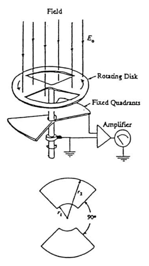
Take \(t=0\) to be an instant when the insulated quadrants are completely shielded.
Obtain expressions that give the total charge \(q(t)\) induced on the upper surface of the insulated quadrants as a function of time between \(t=0\) and \(t=T/2\), and sketch a graph of this variation.
[The effects of the atmospheric ion current can be ignored in this situation.]
(5) The system described in (4) is connected to an amplifier whose input circuit is equivalent to a capacitor \(C\) and a resistor \(R\) in parallel. (You can assume that the capacitance of the quadrant system is negligible compared to \(C\).) Sketch graphs of the form of the voltage difference \(V\) between the points \(M\) and \(N\) as a function of \(t\) during one revolution of the disk, just after it has been set into rotation with period of revolution \(T\), if:
a) \(T=T_a\ll CR\);
b) \(T=T_b\gg CR\).
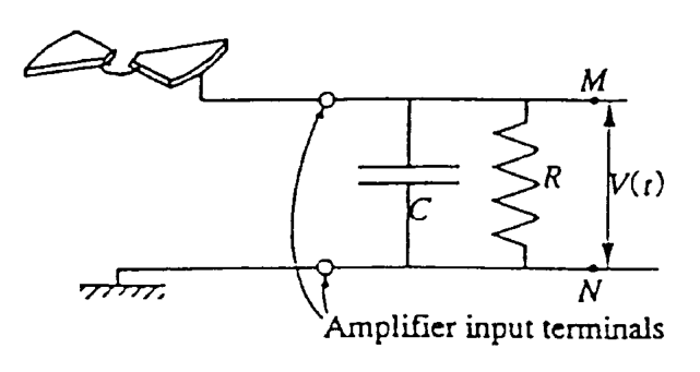
[Assume that \(C\) and \(R\) have fixed values; only \(T\) changes between situations (a) and (b).]
Obtain an expression for the approximate ratio, \(V_a/V_b\), of the largest values of \(V(t)\) in cases (a) and (b).
6) Assume that \(E_0=150\ \mathrm{V/m}\), \(r_1=1\ \mathrm{cm}\), \(r_2=7\ \mathrm{cm}\), \(C=0.01\ \mathrm{\mu F}\), \(R=20\ \mathrm{M\Omega}\), and suppose the disk is set into rotation at \(50\) revolutions per second.
Approximately, what is the largest value of \(V\) during one revolution in this case?
Official English text of the problem.
Answers
Take \(V=V_M-V_N\). For parts 4–6, define the fully exposed area and the magnitude of its induced charge by
\[ A_m=\frac{\pi}{2}(r_2^2-r_1^2), \qquad Q_m=\varepsilon_0E_0A_m>0. \]
-
The Earth’s surface charge is negative: \[ \boxed{\sigma_0\simeq-1.3\times10^{-9}\ \mathrm{C\,m^{-2}}}, \qquad \boxed{Q_0\simeq-6.8\times10^5\ \mathrm C}. \] The requested magnitudes are the absolute values.
-
The average atmospheric charge density is \[ \boxed{\overline{\rho}\simeq+4.4\times10^{-12}\ \mathrm{C\,m^{-3}}}. \]
-
Counting only positive ions arriving at the surface, and taking their concentration as approximately constant, \[ \boxed{t_{1/2}=\frac{\varepsilon_0\ln2}{e n_+(1.5\times10^{-4})} \simeq4.3\times10^2\ \mathrm s\simeq7.1\ \mathrm{min}}. \]
-
The induced upper-surface charge is \[ \boxed{ q(t)= \begin{cases} -Q_m\,\dfrac{4t}{T},&0\le t\le T/4,\\[5pt] -Q_m\left(2-\dfrac{4t}{T}\right),&T/4\le t\le T/2. \end{cases}} \] Its graph joins \((0,0)\), \((T/4,-Q_m)\), and \((T/2,0)\) by straight lines and repeats every \(T/2\).
-
For the first revolution, starting with \(V(0)=0\): - (a) \(V\simeq-q/C\): two positive triangular pulses, each of height \[ \boxed{V_a\simeq\frac{Q_m}{C}}. \] - (b) \(V\) alternates between approximately \(+V_b\) and \(-V_b\), with exponential transitions of time constant \(RC\), where \[ \boxed{V_b\simeq\frac{4RQ_m}{T_b}}. \] Thus \[ \boxed{\frac{V_a}{V_b}\simeq\frac{T_b}{4RC}}. \]
-
The largest voltage during the first revolution is \[ \boxed{V_{\max}\simeq1.0\times10^{-3}\ \mathrm V=1.0\ \mathrm{mV}}. \] Including the finite resistance gives \(0.989\ \mathrm{mV}\), reached at \(t=T/4=5.0\ \mathrm{ms}\).
Solution
1) Earth’s surface charge
The electric field inside a conductor in electrostatic equilibrium is zero. Gauss’s law applied to a small pillbox across its surface gives
\[ E_{\perp,\mathrm{outside}}=\frac{\sigma_0}{\varepsilon_0}, \]
where the normal points outward from the conductor. Since the field points downward into the Earth,
\[ \sigma_0=-\varepsilon_0E_0. \]
Hence
\[ \sigma_0=-(8.85\times10^{-12})(150) =-1.3275\times10^{-9}\ \mathrm{C\,m^{-2}}. \]
Approximating the Earth as a sphere and using this as its average surface charge density,
\[ Q_0=4\pi R_E^2\sigma_0 =-4\pi(6.4\times10^6)^2(1.3275\times10^{-9}) \simeq-6.8\times10^5\ \mathrm C. \]
Thus the surface charge density has magnitude approximately \(1.3\ \mathrm{nC\,m^{-2}}\), and the total charge has magnitude approximately \(6.8\times10^5\ \mathrm C\).
2) Atmospheric space charge
Let \(z\) increase upward. The signed vertical fields at the two heights are
\[ E_z(0)=-150\ \mathrm{V/m}, \qquad E_z(100\ \mathrm m)=-100\ \mathrm{V/m}. \]
Over a height of \(100\ \mathrm m\), the Earth’s curvature is negligible because \(100/R_E\ll1\). Gauss’s law for a vertical column of horizontal cross-sectional area \(A\) therefore gives
\[ \overline{\rho}Ah =\varepsilon_0A\bigl[E_z(h)-E_z(0)\bigr]. \]
Consequently,
\[ \overline{\rho} =\varepsilon_0\frac{-100-(-150)}{100} =(8.85\times10^{-12})(0.50) =4.425\times10^{-12}\ \mathrm{C\,m^{-3}}. \]
The charge is positive, consistent with the downward field becoming weaker as height increases.
3) Time to neutralize half the surface charge
The Earth is negatively charged. Positive ions drift downward and can reach its surface; negative ions drift upward. Thus the surface-neutralization current contains the contribution of the positive ions only.
Write the ion mobility as
\[ \mu=1.5\times10^{-4}\ \mathrm{m^2\,V^{-1}\,s^{-1}}, \qquad v=\mu E. \]
Taking the supplied near-surface concentration \(n_+\) to remain approximately constant in this drift estimate, the positive charge arriving per unit area per unit time is
\[ j_+=e n_+v=e n_+\mu E. \]
Let \(S(t)=|\sigma(t)|\) denote the magnitude of the remaining negative surface charge density. The conductor boundary condition gives
\[ E(t)=\frac{S(t)}{\varepsilon_0}. \]
Since each arriving positive ion reduces \(S\),
\[ \frac{dS}{dt} =-j_+ =-\frac{e n_+\mu}{\varepsilon_0}S. \]
The discharge is therefore exponential:
\[ S(t)=S(0)e^{-t/\tau_+}, \qquad \tau_+=\frac{\varepsilon_0}{e n_+\mu}. \]
Numerically,
\[ e n_+\mu =(1.60\times10^{-19})(6\times10^8)(1.5\times10^{-4}) =1.44\times10^{-14}\ \mathrm{S\,m^{-1}}, \]
and
\[ \tau_+=\frac{8.85\times10^{-12}}{1.44\times10^{-14}} \simeq615\ \mathrm s. \]
Setting \(S(t_{1/2})=S(0)/2\),
\[ \boxed{t_{1/2}=\tau_+\ln2\simeq426\ \mathrm s\simeq7.1\ \mathrm{min}}. \]
Adding the conductivity of the upward-moving negative ions would incorrectly count a current that does not enter the Earth’s surface.
4) Induced charge on the quadrants
Neglect fringing at the edges and treat the shielding as complete wherever the grounded disk covers the quadrants. On an exposed upper surface, the downward field requires surface charge density
\[ \sigma_{\mathrm{upper}}=-\varepsilon_0E_0. \]
The total area of the two annular quadrants is
\[ A_m=2\left[\frac{\pi}{4}(r_2^2-r_1^2)\right] =\frac{\pi}{2}(r_2^2-r_1^2). \]
The disk’s angular speed is
\[ \omega=\frac{2\pi}{T}. \]
During the first quarter-revolution, each opening exposes an angular width \(\theta=\omega t\). The total exposed area is therefore
\[ A(t)=2\left[\frac12(r_2^2-r_1^2)\theta\right] =\frac{2\pi(r_2^2-r_1^2)}{T}t, \qquad 0\le t\le T/4. \]
It reaches \(A_m\) at \(T/4\), then decreases at the same rate to zero at \(T/2\). Thus
\[ A(t)= \begin{cases} A_m\,\dfrac{4t}{T},&0\le t\le T/4,\\[5pt] A_m\left(2-\dfrac{4t}{T}\right),&T/4\le t\le T/2. \end{cases} \]
Since \(q(t)=-\varepsilon_0E_0A(t)\),
\[ \boxed{ q(t)= \begin{cases} -\dfrac{2\pi\varepsilon_0E_0(r_2^2-r_1^2)}{T}\,t, &0\le t\le T/4,\\[7pt] -\dfrac{2\pi\varepsilon_0E_0(r_2^2-r_1^2)}{T} \left(\dfrac T2-t\right), &T/4\le t\le T/2. \end{cases}} \]
The sketch is a downward triangular pulse: it starts at zero, decreases linearly to \(-Q_m\) at \(T/4\), then increases linearly to zero at \(T/2\). There are two identical pulses per revolution.
Here \(q\) is the charge on the upper surface. An isolated quadrant system can acquire this surface charge by redistributing its existing charge.
5) Voltage across the amplifier input
Take \(V=V_M-V_N\), with \(N\) grounded. Before rotation begins, the quadrants are shielded and the resistor has discharged the capacitor, so
\[ q(0)=0,\qquad V(0)=0. \]
Neglecting the quadrant system’s capacitance compared with \(C\), the charge associated with the connected input conductor is \(q+CV\). Positive charge leaves this conductor through the resistor at rate \(V/R\), so charge conservation gives
\[ \frac{d}{dt}(q+CV)=-\frac VR, \]
or
\[ \boxed{C\frac{dV}{dt}+\frac VR=-\frac{dq}{dt}}. \]
As the quadrants become exposed, their upper surfaces acquire negative charge. This leaves positive charge on the capacitor’s upper plate, so the voltage initially rises positive.
From part 4,
\[ -\frac{dq}{dt}= \begin{cases} +I_0,&0<t<T/4,\\ -I_0,&T/4<t<T/2,\\ +I_0,&T/2<t<3T/4,\\ -I_0,&3T/4<t<T, \end{cases} \qquad I_0=\frac{4Q_m}{T}. \]
Thus the circuit is driven by a square-wave current.
For completeness, put \(\tau=RC\), \(B=RI_0\), and \(t_k=kT/4\). On quarter \(k=0,1,2,3\), the voltage is
\[ V(t)=(-1)^kB+ \left[V(t_k)-(-1)^kB\right]e^{-(t-t_k)/\tau}. \]
This expression, together with \(V(0)=0\), specifies the continuous startup waveform.
(a) Fast rotation: \(T_a\ll RC\)
During the first revolution, little charge leaks through \(R\). To leading order,
\[ C\frac{dV}{dt}\simeq-\frac{dq}{dt}. \]
Using the initial conditions,
\[ V(t)\simeq-\frac{q(t)}{C}. \]
The voltage therefore consists of two positive triangular pulses:
| \(t/T_a\) | \(0\) | \(1/4\) | \(1/2\) | \(3/4\) | \(1\) |
|---|---|---|---|---|---|
| \(V/(Q_m/C)\), to leading order | \(0\) | \(1\) | \(0\) | \(1\) | \(0\) |
Join successive entries by straight lines. The largest voltage is approximately
\[ \boxed{V_a\simeq\frac{Q_m}{C}}. \]
For finite \(T_a/RC\), the segments are slightly curved, the minima become slightly negative, and the second positive peak is slightly lower than the first. The positive triangles above are the leading approximation for the requested first revolution.
(b) Slow rotation: \(T_b\gg RC\)
Except during short transitions, the capacitor current is small and
\[ \frac VR\simeq-\frac{dq}{dt}. \]
Hence the voltage approaches alternating levels
\[ \boxed{V\simeq\pm V_b,\qquad V_b=\frac{4RQ_m}{T_b}}. \]
The sketch has the following features:
- It starts at zero and rises exponentially toward \(+V_b\), with time constant \(RC\).
- After \(t=T_b/4\), it falls exponentially toward \(-V_b\).
- After \(t=T_b/2\), it rises toward \(+V_b\).
- After \(t=3T_b/4\), it falls toward \(-V_b\).
Each quarter is long compared with \(RC\), so most of it is an almost horizontal plateau. The voltage remains continuous at the switching times. For example, immediately after the first switch,
\[ V(t)\simeq -V_b+2V_b e^{-(t-T_b/4)/(RC)}, \]
so it crosses zero approximately \(RC\ln2\) after that switch.
The requested ratio is therefore
\[ \boxed{ \frac{V_a}{V_b} \simeq \frac{Q_m/C}{4RQ_m/T_b} =\frac{T_b}{4RC}. } \]
6) Numerical voltage
The fully exposed area is
\[ A_m=\frac{\pi}{2}\left(0.07^2-0.01^2\right) =7.54\times10^{-3}\ \mathrm{m^2}. \]
Thus
\[ Q_m=\varepsilon_0E_0A_m =(8.85\times10^{-12})(150)(7.54\times10^{-3}) \simeq1.00\times10^{-11}\ \mathrm C. \]
The relevant times are
\[ T=\frac1{50}=0.020\ \mathrm s, \]
\[ RC=(20\times10^6)(0.01\times10^{-6}) =0.20\ \mathrm s. \]
In particular, the time to the first peak is only
\[ \frac T4=0.0050\ \mathrm s=0.025\,RC. \]
Consequently, the fast-rotation approximation gives
\[ \boxed{ V_{\max}\simeq\frac{Q_m}{C} =\frac{1.00\times10^{-11}}{1.00\times10^{-8}} =1.0\times10^{-3}\ \mathrm V. } \]
The finite-resistance correction follows from the first-quarter solution:
\[ V_{\max} =\frac{4RQ_m}{T}\left(1-e^{-T/(4RC)}\right) =\frac{Q_m}{C}\frac{1-e^{-0.025}}{0.025} \simeq0.989\ \mathrm{mV}. \]
It occurs at \(t=T/4=5.0\ \mathrm{ms}\); the second positive peak is smaller.
The solution was checked against the official solution.
IPhO 1993 · Theorieaufgabe 1
Atmosphärische Elektrizität
Allgemeine tabellarische Angaben
| Größe | Symbol | Wert |
|---|---|---|
| Mittlerer Erdradius | \(R_E\) | \(6.4\times10^6\ \mathrm{m}\). |
| Erdbeschleunigung | \(g\) | \(9.8\ \mathrm{m\,s^{-2}}\). |
| Newtonsche Gravitationskonstante | \(G\) | \(6.67\times10^{-11}\ \mathrm{N\,m^2\,kg^{-2}}\). |
| Permittivität des Vakuums | \(\varepsilon_0\) | \(8.85\times10^{-12}\ \mathrm{C^2\,N^{-1}\,m^{-2}}\). |
| Permeabilität des Vakuums | \(\mu_0\) | \(8.85\times10^{-7}\ \mathrm{N\,A^{-2}}\) [sic; korrekter Wert \(4\pi\times10^{-7}\ \mathrm{N\,A^{-2}}\)]. |
| Lichtgeschwindigkeit im Vakuum (oder in Luft) | \(c\) | \(3.00\times10^8\ \mathrm{m\,s^{-1}}\). |
| Elementarladung | \(e\) | \(1.60\times10^{-19}\ \mathrm{C}\). |
| Elektronenmasse | \(m_e\) | \(9.11\times10^{-31}\ \mathrm{kg}\). |
| Protonenmasse | \(m_p\) | \(1.67\times10^{-27}\ \mathrm{kg}\) |
| Plancksches Wirkungsquantum | \(h\) | \(6.63\times10^{-34}\ \mathrm{J\,s}\). |
| Avogadro-Konstante | \(N_A\) | \(6{,}02\times10^{23}\ \mathrm{mol^{-1}}\). |
| Boltzmann-Konstante | \(k\) | \(1.38\times10^{-23}\ \mathrm{J\,K^{-1}}\). |
| Molare Gaskonstante | \(R\) | \(8.31\ \mathrm{J\,mol^{-1}\,K^{-1}}\). |
Theoretische Aufgabe 1
ATMOSPHÄRISCHE ELEKTRIZITÄT
Aus elektrostatischer Sicht kann die Erdoberfläche als guter Leiter betrachtet werden. Sie trägt eine bestimmte Gesamtladung \(Q_0\) und besitzt eine mittlere Flächenladungsdichte \(\sigma_0\).
1) Bei schönem Wetter herrscht an der Erdoberfläche ein nach unten gerichtetes elektrisches Feld \(E_0\) mit einer Stärke von etwa \(150\ \mathrm{V/m}\). Bestimmen Sie den Betrag der Flächenladungsdichte der Erde und den Betrag der auf der Erdoberfläche befindlichen Gesamtladung.
2) Der Betrag des nach unten gerichteten elektrischen Feldes nimmt mit der Höhe ab und beträgt in einer Höhe von \(100\ \mathrm{m}\) etwa \(100\ \mathrm{V/m}\). Berechnen Sie die mittlere Nettoladung pro \(\mathrm{m^3}\) der Atmosphäre zwischen der Erdoberfläche und einer Höhe von \(100\ \mathrm{m}\).
3) Die in (2) berechnete Nettoladungsdichte ergibt sich tatsächlich daraus, dass pro Volumeneinheit nahezu gleich viele einfach positiv und einfach negativ geladene Ionen vorhanden sind (\(n_+\) und \(n_-\)). In der Nähe der Erdoberfläche gilt bei schönem Wetter \(n_+\approx n_-\approx6\times10^8\ \mathrm{m^{-3}}\). Diese Ionen bewegen sich unter dem Einfluss des vertikalen elektrischen Feldes. Ihre Geschwindigkeit ist proportional zur Feldstärke:
\[ v\approx1.5\times10^{-4}\cdot E, \]
wobei \(v\) in \(\mathrm{m/s}\) und \(E\) in \(\mathrm{V/m}\) angegeben wird. Wie lange würde es dauern, bis die Bewegung der atmosphärischen Ionen die Hälfte der Ladung auf der Erdoberfläche neutralisiert hätte, wenn keine anderen Prozesse (z. B. Blitze) diese Ladung aufrechterhielten?
4) Eine Möglichkeit, das atmosphärische elektrische Feld und damit \(\sigma_0\) zu messen, bietet die in der Abbildung dargestellte Anordnung. Zwei von der Erde isolierte, aber miteinander verbundene Metallquadranten sind unmittelbar unter einer geerdeten, gleichförmig rotierenden Scheibe angebracht, in die zwei quadrantenförmige Öffnungen geschnitten sind. (In der Abbildung ist der Abstand übertrieben groß dargestellt, um die Anordnung zu verdeutlichen.) Zweimal pro Umdrehung sind die isolierten Quadranten dem Feld vollständig ausgesetzt und anschließend (\(1/4\) einer Umlaufzeit später) vollständig dagegen abgeschirmt. Es sei \(T\) die Umlaufzeit, und \(r_1\) und \(r_2\) seien wie dargestellt der Innen- und der Außenradius der isolierten Quadranten.
Wählen Sie als \(t=0\) einen Zeitpunkt, zu dem die isolierten Quadranten vollständig abgeschirmt sind.
Leiten Sie Ausdrücke her, die die auf der Oberseite der isolierten Quadranten induzierte Gesamtladung \(q(t)\) als Funktion der Zeit zwischen \(t=0\) und \(t=T/2\) angeben, und skizzieren Sie diesen Verlauf.
[Die Auswirkungen des atmosphärischen Ionenstroms können in dieser Situation vernachlässigt werden.]
(5) Die in (4) beschriebene Anordnung wird an einen Verstärker angeschlossen, dessen Eingangsschaltung einer Parallelschaltung aus einem Kondensator \(C\) und einem Widerstand \(R\) entspricht. (Sie können annehmen, dass die Kapazität der Quadrantenanordnung gegenüber \(C\) vernachlässigbar ist.) Skizzieren Sie den Verlauf der Spannungsdifferenz \(V\) zwischen den Punkten \(M\) und \(N\) als Funktion von \(t\) während einer Umdrehung der Scheibe, unmittelbar nachdem diese mit der Umlaufzeit \(T\) in Rotation versetzt wurde, falls:
a) \(T=T_a\ll CR\);
b) \(T=T_b\gg CR\).
[Nehmen Sie an, dass \(C\) und \(R\) feste Werte haben; nur \(T\) ändert sich zwischen den Fällen (a) und (b).]
Leiten Sie einen Ausdruck für das näherungsweise Verhältnis \(V_a/V_b\) der größten Werte von \(V(t)\) in den Fällen (a) und (b) her.
6) Nehmen Sie an, dass \(E_0=150\ \mathrm{V/m}\), \(r_1=1\ \mathrm{cm}\), \(r_2=7\ \mathrm{cm}\), \(C=0.01\ \mathrm{\mu F}\), \(R=20\ \mathrm{M\Omega}\) gilt und die Scheibe mit \(50\) Umdrehungen pro Sekunde in Rotation versetzt wird.
Wie groß ist in diesem Fall näherungsweise der größte Wert von \(V\) während einer Umdrehung?
Aufgabentext aus dem offiziellen englischen Text übersetzt.
Antworten
Es sei \(V=V_M-V_N\). Für die Teile 4–6 definieren wir die vollständig freiliegende Fläche und den Betrag der auf ihr induzierten Ladung durch
\[ A_m=\frac{\pi}{2}(r_2^2-r_1^2), \qquad Q_m=\varepsilon_0E_0A_m>0. \]
-
Die Ladung auf der Erdoberfläche ist negativ: \[ \boxed{\sigma_0\simeq-1.3\times10^{-9}\ \mathrm{C\,m^{-2}}}, \qquad \boxed{Q_0\simeq-6.8\times10^5\ \mathrm C}. \] Die gesuchten Beträge sind die Absolutwerte.
-
Die mittlere atmosphärische Ladungsdichte beträgt \[ \boxed{\overline{\rho}\simeq+4.4\times10^{-12}\ \mathrm{C\,m^{-3}}}. \]
-
Berücksichtigt man nur die an der Oberfläche ankommenden positiven Ionen und nimmt deren Konzentration als näherungsweise konstant an, so gilt \[ \boxed{t_{1/2}=\frac{\varepsilon_0\ln2}{e n_+(1.5\times10^{-4})} \simeq4.3\times10^2\ \mathrm s\simeq7.1\ \mathrm{min}}. \]
-
Die auf der Oberseite induzierte Ladung ist \[ \boxed{ q(t)= \begin{cases} -Q_m\,\dfrac{4t}{T},&0\le t\le T/4,\\[5pt] -Q_m\left(2-\dfrac{4t}{T}\right),&T/4\le t\le T/2. \end{cases}} \] Ihr Graph verbindet \((0,0)\), \((T/4,-Q_m)\) und \((T/2,0)\) durch Geraden und wiederholt sich alle \(T/2\).
-
Für die erste Umdrehung, ausgehend von \(V(0)=0\): - (a) \(V\simeq-q/C\): zwei positive Dreiecksimpulse mit jeweils der Höhe \[ \boxed{V_a\simeq\frac{Q_m}{C}}. \] - (b) \(V\) wechselt zwischen näherungsweise \(+V_b\) und \(-V_b\), mit exponentiellen Übergängen mit der Zeitkonstante \(RC\), wobei \[ \boxed{V_b\simeq\frac{4RQ_m}{T_b}}. \] Somit gilt \[ \boxed{\frac{V_a}{V_b}\simeq\frac{T_b}{4RC}}. \]
-
Die größte Spannung während der ersten Umdrehung beträgt \[ \boxed{V_{\max}\simeq1.0\times10^{-3}\ \mathrm V=1.0\ \mathrm{mV}}. \] Unter Berücksichtigung des endlichen Widerstands ergibt sich \(0.989\ \mathrm{mV}\), erreicht bei \(t=T/4=5.0\ \mathrm{ms}\).
Lösung
1) Ladung auf der Erdoberfläche
Das elektrische Feld im Inneren eines Leiters im elektrostatischen Gleichgewicht ist null. Wendet man das gaußsche Gesetz auf ein kleines flaches zylindrisches Volumen an, das die Oberfläche durchsetzt, erhält man
\[ E_{\perp,\mathrm{outside}}=\frac{\sigma_0}{\varepsilon_0}, \]
wobei die Normale aus dem Leiter heraus zeigt. Da das Feld nach unten in die Erde hinein gerichtet ist, gilt
\[ \sigma_0=-\varepsilon_0E_0. \]
Damit ergibt sich
\[ \sigma_0=-(8.85\times10^{-12})(150) =-1.3275\times10^{-9}\ \mathrm{C\,m^{-2}}. \]
Nähert man die Erde durch eine Kugel an und verwendet diesen Wert als mittlere Flächenladungsdichte, so erhält man
\[ Q_0=4\pi R_E^2\sigma_0 =-4\pi(6.4\times10^6)^2(1.3275\times10^{-9}) \simeq-6.8\times10^5\ \mathrm C. \]
Der Betrag der Flächenladungsdichte beträgt somit näherungsweise \(1.3\ \mathrm{nC\,m^{-2}}\), und der Betrag der Gesamtladung beträgt näherungsweise \(6.8\times10^5\ \mathrm C\).
2) Atmosphärische Raumladung
Die Koordinate \(z\) nehme nach oben zu. Die vorzeichenbehafteten vertikalen Feldkomponenten in den beiden Höhen sind
\[ E_z(0)=-150\ \mathrm{V/m}, \qquad E_z(100\ \mathrm m)=-100\ \mathrm{V/m}. \]
Über eine Höhe von \(100\ \mathrm m\) ist die Erdkrümmung vernachlässigbar, da \(100/R_E\ll1\). Das gaußsche Gesetz liefert daher für eine vertikale Säule mit der horizontalen Querschnittsfläche \(A\)
\[ \overline{\rho}Ah =\varepsilon_0A\bigl[E_z(h)-E_z(0)\bigr]. \]
Folglich gilt
\[ \overline{\rho} =\varepsilon_0\frac{-100-(-150)}{100} =(8.85\times10^{-12})(0.50) =4.425\times10^{-12}\ \mathrm{C\,m^{-3}}. \]
Die Ladung ist positiv, im Einklang damit, dass das nach unten gerichtete Feld mit zunehmender Höhe schwächer wird.
3) Zeit zur Neutralisierung der Hälfte der Oberflächenladung
Die Erde ist negativ geladen. Positive Ionen driften nach unten und können ihre Oberfläche erreichen; negative Ionen driften nach oben. Der Strom, der die Oberflächenladung neutralisiert, enthält daher nur den Beitrag der positiven Ionen.
Wir schreiben die Ionenbeweglichkeit als
\[ \mu=1.5\times10^{-4}\ \mathrm{m^2\,V^{-1}\,s^{-1}}, \qquad v=\mu E. \]
Nimmt man bei dieser Abschätzung der Drift an, dass die angegebene oberflächennahe Konzentration \(n_+\) näherungsweise konstant bleibt, so beträgt die pro Flächeneinheit und Zeiteinheit ankommende positive Ladung
\[ j_+=e n_+v=e n_+\mu E. \]
Es bezeichne \(S(t)=|\sigma(t)|\) den Betrag der verbleibenden negativen Flächenladungsdichte. Die Randbedingung am Leiter liefert
\[ E(t)=\frac{S(t)}{\varepsilon_0}. \]
Da jedes ankommende positive Ion \(S\) verringert, gilt
\[ \frac{dS}{dt} =-j_+ =-\frac{e n_+\mu}{\varepsilon_0}S. \]
Die Entladung verläuft daher exponentiell:
\[ S(t)=S(0)e^{-t/\tau_+}, \qquad \tau_+=\frac{\varepsilon_0}{e n_+\mu}. \]
Numerisch ergibt sich
\[ e n_+\mu =(1.60\times10^{-19})(6\times10^8)(1.5\times10^{-4}) =1.44\times10^{-14}\ \mathrm{S\,m^{-1}}, \]
und
\[ \tau_+=\frac{8.85\times10^{-12}}{1.44\times10^{-14}} \simeq615\ \mathrm s. \]
Setzt man \(S(t_{1/2})=S(0)/2\), so folgt
\[ \boxed{t_{1/2}=\tau_+\ln2\simeq426\ \mathrm s\simeq7.1\ \mathrm{min}}. \]
Würde man die Leitfähigkeit der nach oben driftenden negativen Ionen hinzuzählen, würde man fälschlicherweise einen Strom berücksichtigen, der nicht in die Erdoberfläche eintritt.
4) Induzierte Ladung auf den Quadranten
Wir vernachlässigen Randfelder und nehmen die Abschirmung überall dort als vollständig an, wo die geerdete Scheibe die Quadranten bedeckt. Auf einer freiliegenden Oberseite erfordert das nach unten gerichtete Feld die Flächenladungsdichte
\[ \sigma_{\mathrm{upper}}=-\varepsilon_0E_0. \]
Die Gesamtfläche der beiden Kreisringquadranten beträgt
\[ A_m=2\left[\frac{\pi}{4}(r_2^2-r_1^2)\right] =\frac{\pi}{2}(r_2^2-r_1^2). \]
Die Winkelgeschwindigkeit der Scheibe ist
\[ \omega=\frac{2\pi}{T}. \]
Während der ersten Viertelumdrehung legt jede Öffnung einen Winkelbereich der Breite \(\theta=\omega t\) frei. Die gesamte freiliegende Fläche ist daher
\[ A(t)=2\left[\frac12(r_2^2-r_1^2)\theta\right] =\frac{2\pi(r_2^2-r_1^2)}{T}t, \qquad 0\le t\le T/4. \]
Sie erreicht bei \(T/4\) den Wert \(A_m\) und nimmt anschließend mit derselben Rate bis auf null bei \(T/2\) ab. Somit gilt
\[ A(t)= \begin{cases} A_m\,\dfrac{4t}{T},&0\le t\le T/4,\\[5pt] A_m\left(2-\dfrac{4t}{T}\right),&T/4\le t\le T/2. \end{cases} \]
Wegen \(q(t)=-\varepsilon_0E_0A(t)\) folgt
\[ \boxed{ q(t)= \begin{cases} -\dfrac{2\pi\varepsilon_0E_0(r_2^2-r_1^2)}{T}\,t, &0\le t\le T/4,\\[7pt] -\dfrac{2\pi\varepsilon_0E_0(r_2^2-r_1^2)}{T} \left(\dfrac T2-t\right), &T/4\le t\le T/2. \end{cases}} \]
Die Skizze zeigt einen nach unten gerichteten Dreiecksimpuls: Er beginnt bei null, fällt linear bis auf \(-Q_m\) bei \(T/4\) und steigt dann linear bis auf null bei \(T/2\). Pro Umdrehung treten zwei identische Impulse auf.
Hier ist \(q\) die Ladung auf der Oberseite. Eine isolierte Quadrantenanordnung kann diese Oberflächenladung durch Umverteilung ihrer vorhandenen Ladung annehmen.
5) Spannung am Verstärkereingang
Es sei \(V=V_M-V_N\), wobei \(N\) geerdet ist. Vor Beginn der Rotation sind die Quadranten abgeschirmt, und der Widerstand hat den Kondensator entladen, sodass
\[ q(0)=0,\qquad V(0)=0. \]
Vernachlässigt man die Kapazität der Quadrantenanordnung gegenüber \(C\), so ist die zum angeschlossenen Eingangsleiter gehörende Ladung \(q+CV\). Positive Ladung verlässt diesen Leiter durch den Widerstand mit der Rate \(V/R\), sodass die Ladungserhaltung ergibt:
\[ \frac{d}{dt}(q+CV)=-\frac VR, \]
oder
\[ \boxed{C\frac{dV}{dt}+\frac VR=-\frac{dq}{dt}}. \]
Wenn die Quadranten freigelegt werden, nehmen ihre Oberseiten negative Ladung an. Dadurch bleibt positive Ladung auf der oberen Kondensatorplatte zurück, sodass die Spannung zunächst zu positiven Werten ansteigt.
Aus Teil 4 folgt
\[ -\frac{dq}{dt}= \begin{cases} +I_0,&0<t<T/4,\\ -I_0,&T/4<t<T/2,\\ +I_0,&T/2<t<3T/4,\\ -I_0,&3T/4<t<T, \end{cases} \qquad I_0=\frac{4Q_m}{T}. \]
Die Schaltung wird somit durch einen Rechteckstrom angeregt.
Der Vollständigkeit halber setzen wir \(\tau=RC\), \(B=RI_0\) und \(t_k=kT/4\). Während der Viertelumdrehung \(k=0,1,2,3\) beträgt die Spannung
\[ V(t)=(-1)^kB+ \left[V(t_k)-(-1)^kB\right]e^{-(t-t_k)/\tau}. \]
Dieser Ausdruck legt zusammen mit \(V(0)=0\) den stetigen Spannungsverlauf beim Anlaufen fest.
(a) Schnelle Rotation: \(T_a\ll RC\)
Während der ersten Umdrehung fließt nur wenig Ladung durch \(R\) ab. In führender Ordnung gilt
\[ C\frac{dV}{dt}\simeq-\frac{dq}{dt}. \]
Mit den Anfangsbedingungen ergibt sich
\[ V(t)\simeq-\frac{q(t)}{C}. \]
Die Spannung besteht daher aus zwei positiven Dreiecksimpulsen:
| \(t/T_a\) | \(0\) | \(1/4\) | \(1/2\) | \(3/4\) | \(1\) |
|---|---|---|---|---|---|
| \(V/(Q_m/C)\), in führender Ordnung | \(0\) | \(1\) | \(0\) | \(1\) | \(0\) |
Verbinden Sie aufeinanderfolgende Einträge durch Geraden. Die größte Spannung beträgt näherungsweise
\[ \boxed{V_a\simeq\frac{Q_m}{C}}. \]
Für endliches \(T_a/RC\) sind die Abschnitte leicht gekrümmt, die Minima werden leicht negativ, und der zweite positive Spitzenwert liegt etwas unter dem ersten. Die oben dargestellten positiven Dreiecke sind die führende Näherung für die geforderte erste Umdrehung.
(b) Langsame Rotation: \(T_b\gg RC\)
Abgesehen von kurzen Übergängen ist der Kondensatorstrom klein, und es gilt
\[ \frac VR\simeq-\frac{dq}{dt}. \]
Die Spannung nähert sich daher abwechselnd den Werten
\[ \boxed{V\simeq\pm V_b,\qquad V_b=\frac{4RQ_m}{T_b}}. \]
Die Skizze weist die folgenden Merkmale auf:
- Sie beginnt bei null und steigt mit der Zeitkonstante \(RC\) exponentiell gegen \(+V_b\) an.
- Nach \(t=T_b/4\) fällt sie exponentiell gegen \(-V_b\) ab.
- Nach \(t=T_b/2\) steigt sie gegen \(+V_b\) an.
- Nach \(t=3T_b/4\) fällt sie gegen \(-V_b\) ab.
Jede Viertelumdrehung dauert lange im Vergleich zu \(RC\), sodass der Verlauf während des größten Teils nahezu horizontal ist. Zu den Umschaltzeitpunkten bleibt die Spannung stetig. Beispielsweise gilt unmittelbar nach dem ersten Umschalten
\[ V(t)\simeq -V_b+2V_b e^{-(t-T_b/4)/(RC)}, \]
sodass die Spannung ungefähr \(RC\ln2\) nach diesem Umschalten den Nulldurchgang erreicht.
Das gesuchte Verhältnis ist daher
\[ \boxed{ \frac{V_a}{V_b} \simeq \frac{Q_m/C}{4RQ_m/T_b} =\frac{T_b}{4RC}. } \]
6) Zahlenwert der Spannung
Die vollständig freiliegende Fläche beträgt
\[ A_m=\frac{\pi}{2}\left(0.07^2-0.01^2\right) =7.54\times10^{-3}\ \mathrm{m^2}. \]
Somit gilt
\[ Q_m=\varepsilon_0E_0A_m =(8.85\times10^{-12})(150)(7.54\times10^{-3}) \simeq1.00\times10^{-11}\ \mathrm C. \]
Die maßgeblichen Zeiten sind
\[ T=\frac1{50}=0.020\ \mathrm s, \]
\[ RC=(20\times10^6)(0.01\times10^{-6}) =0.20\ \mathrm s. \]
Insbesondere beträgt die Zeit bis zum ersten Spitzenwert nur
\[ \frac T4=0.0050\ \mathrm s=0.025\,RC. \]
Folglich liefert die Näherung für schnelle Rotation
\[ \boxed{ V_{\max}\simeq\frac{Q_m}{C} =\frac{1.00\times10^{-11}}{1.00\times10^{-8}} =1.0\times10^{-3}\ \mathrm V. } \]
Die Korrektur für den endlichen Widerstand folgt aus der Lösung für die erste Viertelumdrehung:
\[ V_{\max} =\frac{4RQ_m}{T}\left(1-e^{-T/(4RC)}\right) =\frac{Q_m}{C}\frac{1-e^{-0.025}}{0.025} \simeq0.989\ \mathrm{mV}. \]
Dieser Wert wird bei \(t=T/4=5.0\ \mathrm{ms}\) erreicht; der zweite positive Spitzenwert ist kleiner.
Die Lösung wurde mit der offiziellen Lösung abgeglichen.
IPhO 1993 · Teori sorusu 1
Atmosfer Elektriği
Genel Bilgiler Tablosu
| Büyüklük | Sembol | Değer |
|---|---|---|
| Dünya’nın ortalama yarıçapı | \(R_E\) | \(6.4\times10^6\ \mathrm{m}\). |
| yerçekimi ivmesi | \(g\) | \(9.8\ \mathrm{m\,s^{-2}}\). |
| Newton kütleçekim sabiti | \(G\) | \(6.67\times10^{-11}\ \mathrm{N\,m^2\,kg^{-2}}\). |
| boşluğun elektriksel geçirgenliği | \(\varepsilon_0\) | \(8.85\times10^{-12}\ \mathrm{C^2\,N^{-1}\,m^{-2}}\). |
| boşluğun manyetik geçirgenliği | \(\mu_0\) | \(8.85\times10^{-7}\ \mathrm{N\,A^{-2}}\) [sic; doğru değer \(4\pi\times10^{-7}\ \mathrm{N\,A^{-2}}\)]. |
| ışığın boşluktaki (veya havadaki) hızı | \(c\) | \(3.00\times10^8\ \mathrm{m\,s^{-1}}\). |
| temel yük | \(e\) | \(1.60\times10^{-19}\ \mathrm{C}\). |
| elektronun kütlesi | \(m_e\) | \(9.11\times10^{-31}\ \mathrm{kg}\). |
| protonun kütlesi | \(m_p\) | \(1.67\times10^{-27}\ \mathrm{kg}\) |
| Planck sabiti | \(h\) | \(6.63\times10^{-34}\ \mathrm{J\,s}\). |
| Avogadro sabiti | \(N_A\) | \(6{,}02\times10^{23}\ \mathrm{mol^{-1}}\). |
| Boltzmann sabiti | \(k\) | \(1.38\times10^{-23}\ \mathrm{J\,K^{-1}}\). |
| molar gaz sabiti | \(R\) | \(8.31\ \mathrm{J\,mol^{-1}\,K^{-1}}\). |
Teorik Soru 1
ATMOSFER ELEKTRİĞİ
Elektrostatik açısından Dünya’nın yüzeyi iyi bir iletken olarak kabul edilebilir. Bu yüzey, belirli bir toplam \(Q_0\) yükü taşır ve ortalama yüzey yük yoğunluğu \(\sigma_0\)’dır.
1) Açık hava koşullarında, Dünya’nın yüzeyinde aşağı yönlü, yaklaşık \(150\ \mathrm{V/m}\) büyüklüğünde bir \(E_0\) elektrik alanı vardır. Dünya’nın yüzey yük yoğunluğunun ve yüzeyinde taşınan toplam yükün büyüklüklerini bulunuz.
2) Aşağı yönlü elektrik alanın büyüklüğü yükseklikle azalır ve \(100\ \mathrm{m}\) yükseklikte yaklaşık \(100\ \mathrm{V/m}\) olur. Dünya’nın yüzeyi ile \(100\ \mathrm{m}\) yükseklik arasında atmosferin her \(\mathrm{m^3}\)’ündeki ortalama net yük miktarını hesaplayınız.
3) (2)’de hesapladığınız net yük yoğunluğu, aslında birim hacimdeki tek yüklü pozitif ve negatif iyon sayılarının (\(n_+\) ve \(n_-\)) neredeyse eşit olmasının sonucudur. Dünya’nın yüzeyine yakın bölgede, açık hava koşullarında, \(n_+\approx n_-\approx6\times10^8\ \mathrm{m^{-3}}\)’tür. Bu iyonlar düşey elektrik alanın etkisiyle hareket eder. Süratleri alan şiddetiyle orantılıdır:
\[ v\approx1.5\times10^{-4}\cdot E, \]
burada \(v\), \(\mathrm{m/s}\), \(E\) ise \(\mathrm{V/m}\) cinsindendir. Dünya’nın yüzey yükünü koruyan başka hiçbir süreç (örneğin yıldırım) gerçekleşmeseydi, atmosferdeki iyonların hareketiyle bu yükün yarısının nötrlenmesi ne kadar sürerdi?
4) Atmosferdeki elektrik alanı ve dolayısıyla \(\sigma_0\)’ı ölçmenin bir yolu, şekilde gösterilen sistemi kullanmaktır. Topraktan yalıtılmış, ancak birbirine bağlı iki metal çeyrek daire parçası, üzerinde çeyrek daire biçiminde iki delik bulunan, topraklanmış ve sabit hızla dönen bir diskin hemen altına yerleştirilmiştir. (Şekilde, düzeni göstermek amacıyla aralık abartılmıştır.) Her turda iki kez, yalıtılmış çeyrek daire parçaları alana tamamen açık hâle gelir, ardından (bir periyodun \(1/4\)’ü kadar süre sonra) alandan tamamen perdelenir. Dönme periyodu \(T\), yalıtılmış çeyrek daire parçalarının iç ve dış yarıçapları ise şekilde gösterildiği gibi \(r_1\) ve \(r_2\) olsun.
\(t=0\) anını, yalıtılmış çeyrek daire parçalarının tamamen perdelendiği bir an olarak alınız.
Yalıtılmış çeyrek daire parçalarının üst yüzeyinde indüklenen toplam \(q(t)\) yükünü, \(t=0\) ile \(t=T/2\) arasında zamanın fonksiyonu olarak veren ifadeleri elde ediniz ve bu değişimin grafiğini çiziniz.
[Bu durumda atmosferdeki iyon akımının etkileri ihmal edilebilir.]
(5) (4)’te açıklanan sistem, giriş devresi paralel bağlı bir \(C\) kondansatörü ile bir \(R\) direncine eşdeğer olan bir yükseltece bağlanmıştır. (Çeyrek daire sisteminin sığasının \(C\)’ye göre ihmal edilebilir olduğunu varsayabilirsiniz.) Disk, \(T\) dönme periyoduyla dönmeye başlatıldıktan hemen sonra, bir tur boyunca \(M\) ve \(N\) noktaları arasındaki \(V\) gerilim farkının \(t\)’ye bağlı grafiklerinin biçimini aşağıdaki durumlar için çiziniz:
a) \(T=T_a\ll CR\);
b) \(T=T_b\gg CR\).
[\(C\) ve \(R\)’nin sabit değerlere sahip olduğunu; (a) ve (b) durumları arasında yalnızca \(T\)’nin değiştiğini varsayınız.]
(a) ve (b) durumlarında \(V(t)\)’nin en büyük değerlerinin yaklaşık oranı \(V_a/V_b\) için bir ifade elde ediniz.
6) \(E_0=150\ \mathrm{V/m}\), \(r_1=1\ \mathrm{cm}\), \(r_2=7\ \mathrm{cm}\), \(C=0.01\ \mathrm{\mu F}\), \(R=20\ \mathrm{M\Omega}\) olduğunu kabul ediniz ve diskin saniyede \(50\) tur atacak şekilde dönmeye başlatıldığını varsayınız.
Bu durumda bir tur boyunca \(V\)’nin en büyük değeri yaklaşık olarak nedir?
Soru metni resmi İngilizce metinden çevrilmiştir.
Cevaplar
\(V=V_M-V_N\) alınız. 4–6. kısımlar için, tamamen açık durumdaki alanı ve bu alanda indüklenen yükün büyüklüğünü şöyle tanımlayınız:
\[ A_m=\frac{\pi}{2}(r_2^2-r_1^2), \qquad Q_m=\varepsilon_0E_0A_m>0. \]
-
Dünya’nın yüzey yükü negatiftir: \[ \boxed{\sigma_0\simeq-1.3\times10^{-9}\ \mathrm{C\,m^{-2}}}, \qquad \boxed{Q_0\simeq-6.8\times10^5\ \mathrm C}. \] İstenen büyüklükler, bu değerlerin mutlak değerleridir.
-
Atmosferin ortalama yük yoğunluğu \[ \boxed{\overline{\rho}\simeq+4.4\times10^{-12}\ \mathrm{C\,m^{-3}}}. \] olarak bulunur.
-
Yalnızca yüzeye ulaşan pozitif iyonlar hesaba katılıp bunların derişimi yaklaşık olarak sabit alındığında, \[ \boxed{t_{1/2}=\frac{\varepsilon_0\ln2}{e n_+(1.5\times10^{-4})} \simeq4.3\times10^2\ \mathrm s\simeq7.1\ \mathrm{min}}. \]
-
Üst yüzeyde indüklenen yük \[ \boxed{ q(t)= \begin{cases} -Q_m\,\dfrac{4t}{T},&0\le t\le T/4,\\[5pt] -Q_m\left(2-\dfrac{4t}{T}\right),&T/4\le t\le T/2. \end{cases}} \] biçimindedir. Grafiği, \((0,0)\), \((T/4,-Q_m)\) ve \((T/2,0)\) noktalarını doğru parçalarıyla birleştirir ve her \(T/2\) sürede tekrarlanır.
-
\(V(0)=0\) başlangıç koşuluyla ilk tur için: - (a) \(V\simeq-q/C\): her birinin yüksekliği \[ \boxed{V_a\simeq\frac{Q_m}{C}}. \] olan iki pozitif üçgen darbe. - (b) \(V\), \(RC\) zaman sabitli üstel geçişlerle yaklaşık \(+V_b\) ve \(-V_b\) değerleri arasında değişir; burada \[ \boxed{V_b\simeq\frac{4RQ_m}{T_b}}. \] Dolayısıyla \[ \boxed{\frac{V_a}{V_b}\simeq\frac{T_b}{4RC}}. \]
-
İlk tur sırasındaki en büyük gerilim \[ \boxed{V_{\max}\simeq1.0\times10^{-3}\ \mathrm V=1.0\ \mathrm{mV}}. \] olarak bulunur. Sonlu direnç hesaba katıldığında, \(t=T/4=5.0\ \mathrm{ms}\) anında ulaşılan \(0.989\ \mathrm{mV}\) değeri elde edilir.
Çözüm
1) Dünya’nın yüzey yükü
Elektrostatik dengedeki bir iletkenin içindeki elektrik alan sıfırdır. Yüzeyin iki yanına uzanan küçük, yassı bir silindire Gauss yasası uygulandığında
\[ E_{\perp,\mathrm{outside}}=\frac{\sigma_0}{\varepsilon_0}, \]
elde edilir; burada normal, iletkenden dışarı doğru yönelmiştir. Alan aşağıya, Dünya’nın içine doğru yöneldiğinden,
\[ \sigma_0=-\varepsilon_0E_0. \]
Böylece
\[ \sigma_0=-(8.85\times10^{-12})(150) =-1.3275\times10^{-9}\ \mathrm{C\,m^{-2}}. \]
Dünya’yı bir küre olarak yaklaştırıp bu değeri ortalama yüzey yük yoğunluğu olarak kullanırsak,
\[ Q_0=4\pi R_E^2\sigma_0 =-4\pi(6.4\times10^6)^2(1.3275\times10^{-9}) \simeq-6.8\times10^5\ \mathrm C. \]
Dolayısıyla yüzey yük yoğunluğunun büyüklüğü yaklaşık \(1.3\ \mathrm{nC\,m^{-2}}\), toplam yükün büyüklüğü ise yaklaşık \(6.8\times10^5\ \mathrm C\)’dur.
2) Atmosferdeki uzay yükü
\(z\) yukarı doğru artsın. İki yükseklikteki düşey alanların işaretli değerleri
\[ E_z(0)=-150\ \mathrm{V/m}, \qquad E_z(100\ \mathrm m)=-100\ \mathrm{V/m}. \]
şeklindedir. \(100/R_E\ll1\) olduğundan, \(100\ \mathrm m\)’lik yükseklik boyunca Dünya’nın eğriliği ihmal edilebilir. Bu nedenle yatay kesit alanı \(A\) olan düşey bir sütuna Gauss yasası uygulandığında
\[ \overline{\rho}Ah =\varepsilon_0A\bigl[E_z(h)-E_z(0)\bigr]. \]
elde edilir. Sonuç olarak,
\[ \overline{\rho} =\varepsilon_0\frac{-100-(-150)}{100} =(8.85\times10^{-12})(0.50) =4.425\times10^{-12}\ \mathrm{C\,m^{-3}}. \]
Yük pozitiftir; bu, aşağı yönlü alanın yükseklik arttıkça zayıflamasıyla tutarlıdır.
3) Yüzey yükünün yarısını nötrlemek için gereken süre
Dünya negatif yüklüdür. Pozitif iyonlar aşağıya doğru sürüklenir ve yüzeyine ulaşabilir; negatif iyonlar ise yukarıya doğru sürüklenir. Dolayısıyla yüzeyi nötrleyen akıma yalnızca pozitif iyonlar katkıda bulunur.
İyon hareketliliğini şöyle yazalım:
\[ \mu=1.5\times10^{-4}\ \mathrm{m^2\,V^{-1}\,s^{-1}}, \qquad v=\mu E. \]
Bu sürüklenme hesabında, verilen yüzeye yakın \(n_+\) derişiminin yaklaşık olarak sabit kaldığı kabul edilirse, birim alana birim zamanda ulaşan pozitif yük
\[ j_+=e n_+v=e n_+\mu E. \]
olur. \(S(t)=|\sigma(t)|\), kalan negatif yüzey yük yoğunluğunun büyüklüğünü göstersin. İletken sınır koşulu
\[ E(t)=\frac{S(t)}{\varepsilon_0}. \]
bağıntısını verir. Ulaşan her pozitif iyon \(S\)’yi azalttığından,
\[ \frac{dS}{dt} =-j_+ =-\frac{e n_+\mu}{\varepsilon_0}S. \]
Bu nedenle boşalma üsteldir:
\[ S(t)=S(0)e^{-t/\tau_+}, \qquad \tau_+=\frac{\varepsilon_0}{e n_+\mu}. \]
Sayısal olarak,
\[ e n_+\mu =(1.60\times10^{-19})(6\times10^8)(1.5\times10^{-4}) =1.44\times10^{-14}\ \mathrm{S\,m^{-1}}, \]
ve
\[ \tau_+=\frac{8.85\times10^{-12}}{1.44\times10^{-14}} \simeq615\ \mathrm s. \]
\(S(t_{1/2})=S(0)/2\) konulduğunda,
\[ \boxed{t_{1/2}=\tau_+\ln2\simeq426\ \mathrm s\simeq7.1\ \mathrm{min}}. \]
Yukarı hareket eden negatif iyonların iletkenliğini eklemek, Dünya’nın yüzeyine girmeyen bir akımı yanlışlıkla hesaba katmak olurdu.
4) Çeyrek daire parçalarında indüklenen yük
Kenarlardaki saçaklanmayı ihmal edelim ve topraklanmış diskin çeyrek daire parçalarını örttüğü her yerde perdelemenin tam olduğunu kabul edelim. Alana açık bir üst yüzeyde, aşağı yönlü alanın gerektirdiği yüzey yük yoğunluğu
\[ \sigma_{\mathrm{upper}}=-\varepsilon_0E_0. \]
şeklindedir. İki çeyrek halka parçasının toplam alanı
\[ A_m=2\left[\frac{\pi}{4}(r_2^2-r_1^2)\right] =\frac{\pi}{2}(r_2^2-r_1^2). \]
olarak bulunur. Diskin açısal hızı
\[ \omega=\frac{2\pi}{T}. \]
İlk çeyrek tur sırasında, her açıklık \(\theta=\omega t\) açısal genişliğinde bir bölgeyi alana açık bırakır. Bu nedenle toplam açık alan
\[ A(t)=2\left[\frac12(r_2^2-r_1^2)\theta\right] =\frac{2\pi(r_2^2-r_1^2)}{T}t, \qquad 0\le t\le T/4. \]
olur. Bu alan \(T/4\) anında \(A_m\)’ye ulaşır, ardından aynı hızla azalarak \(T/2\) anında sıfır olur. Dolayısıyla
\[ A(t)= \begin{cases} A_m\,\dfrac{4t}{T},&0\le t\le T/4,\\[5pt] A_m\left(2-\dfrac{4t}{T}\right),&T/4\le t\le T/2. \end{cases} \]
\(q(t)=-\varepsilon_0E_0A(t)\) olduğundan,
\[ \boxed{ q(t)= \begin{cases} -\dfrac{2\pi\varepsilon_0E_0(r_2^2-r_1^2)}{T}\,t, &0\le t\le T/4,\\[7pt] -\dfrac{2\pi\varepsilon_0E_0(r_2^2-r_1^2)}{T} \left(\dfrac T2-t\right), &T/4\le t\le T/2. \end{cases}} \]
Grafik aşağı yönlü bir üçgen darbedir: sıfırdan başlar, doğrusal olarak azalarak \(T/4\) anında \(-Q_m\)’ye ulaşır, ardından doğrusal olarak artarak \(T/2\) anında sıfıra döner. Her turda iki özdeş darbe vardır.
Burada \(q\), üst yüzeydeki yüktür. Yalıtılmış bir çeyrek daire sistemi, mevcut yükünü yeniden dağıtarak bu yüzey yükünü edinebilir.
5) Yükselteç girişindeki gerilim
\(N\) topraklanmış olmak üzere \(V=V_M-V_N\) alalım. Dönme başlamadan önce çeyrek daire parçaları perdelenmiştir ve direnç kondansatörü boşaltmıştır; dolayısıyla
\[ q(0)=0,\qquad V(0)=0. \]
Çeyrek daire sisteminin sığası \(C\)’ye göre ihmal edildiğinde, bağlı giriş iletkeniyle ilişkili yük \(q+CV\)’dir. Pozitif yük, bu iletkenden direnç üzerinden \(V/R\) hızıyla ayrılır; dolayısıyla yükün korunumu
\[ \frac{d}{dt}(q+CV)=-\frac VR, \]
veya
\[ \boxed{C\frac{dV}{dt}+\frac VR=-\frac{dq}{dt}}. \]
bağıntısını verir. Çeyrek daire parçaları alana açıldıkça, üst yüzeyleri negatif yük kazanır. Bu, kondansatörün üst levhasında pozitif yük bırakır; dolayısıyla gerilim başlangıçta pozitif yönde artar.
- kısımdan,
\[ -\frac{dq}{dt}= \begin{cases} +I_0,&0<t<T/4,\\ -I_0,&T/4<t<T/2,\\ +I_0,&T/2<t<3T/4,\\ -I_0,&3T/4<t<T, \end{cases} \qquad I_0=\frac{4Q_m}{T}. \]
Dolayısıyla devre, kare dalga biçimindeki bir akımla sürülür.
Eksiksiz bir ifade vermek için \(\tau=RC\), \(B=RI_0\) ve \(t_k=kT/4\) tanımlarını yapalım. \(k=0,1,2,3\) çeyrek turlarında gerilim
\[ V(t)=(-1)^kB+ \left[V(t_k)-(-1)^kB\right]e^{-(t-t_k)/\tau}. \]
şeklindedir. Bu ifade, \(V(0)=0\) ile birlikte başlangıçtaki sürekli dalga biçimini belirler.
(a) Hızlı dönme: \(T_a\ll RC\)
İlk tur sırasında \(R\) üzerinden çok az yük sızar. Baş mertebede,
\[ C\frac{dV}{dt}\simeq-\frac{dq}{dt}. \]
Başlangıç koşulları kullanıldığında,
\[ V(t)\simeq-\frac{q(t)}{C}. \]
Dolayısıyla gerilim, iki pozitif üçgen darbeden oluşur:
| \(t/T_a\) | \(0\) | \(1/4\) | \(1/2\) | \(3/4\) | \(1\) |
|---|---|---|---|---|---|
| \(V/(Q_m/C)\), baş mertebede | \(0\) | \(1\) | \(0\) | \(1\) | \(0\) |
Ardışık değerleri doğru parçalarıyla birleştiriniz. En büyük gerilim yaklaşık olarak
\[ \boxed{V_a\simeq\frac{Q_m}{C}}. \]
olur. Sonlu \(T_a/RC\) için, parçalar hafifçe eğrilir, minimumlar hafifçe negatif olur ve ikinci pozitif tepe birinciden biraz daha alçaktır. Yukarıdaki pozitif üçgenler, soruda istenen ilk tur için baş mertebedeki yaklaşımdır.
(b) Yavaş dönme: \(T_b\gg RC\)
Kısa geçişler dışında kondansatör akımı küçüktür ve
\[ \frac VR\simeq-\frac{dq}{dt}. \]
Böylece gerilim, dönüşümlü olarak şu seviyelere yaklaşır:
\[ \boxed{V\simeq\pm V_b,\qquad V_b=\frac{4RQ_m}{T_b}}. \]
Grafik şu özelliklere sahiptir:
- Sıfırdan başlar ve \(RC\) zaman sabitiyle üstel olarak \(+V_b\)’ye doğru yükselir.
- \(t=T_b/4\) sonrasında üstel olarak \(-V_b\)’ye doğru düşer.
- \(t=T_b/2\) sonrasında \(+V_b\)’ye doğru yükselir.
- \(t=3T_b/4\) sonrasında \(-V_b\)’ye doğru düşer.
Her çeyrek tur \(RC\)’ye göre uzun olduğundan, büyük bölümü neredeyse yatay bir platodur. Gerilim, anahtarlama anlarında sürekli kalır. Örneğin, ilk anahtarlamanın hemen ardından,
\[ V(t)\simeq -V_b+2V_b e^{-(t-T_b/4)/(RC)}, \]
olduğundan, bu anahtarlamadan yaklaşık \(RC\ln2\) süre sonra sıfırdan geçer.
Dolayısıyla istenen oran
\[ \boxed{ \frac{V_a}{V_b} \simeq \frac{Q_m/C}{4RQ_m/T_b} =\frac{T_b}{4RC}. } \]
olarak bulunur.
6) Gerilimin sayısal değeri
Tamamen açık durumdaki alan
\[ A_m=\frac{\pi}{2}\left(0.07^2-0.01^2\right) =7.54\times10^{-3}\ \mathrm{m^2}. \]
olur. Dolayısıyla
\[ Q_m=\varepsilon_0E_0A_m =(8.85\times10^{-12})(150)(7.54\times10^{-3}) \simeq1.00\times10^{-11}\ \mathrm C. \]
İlgili süreler
\[ T=\frac1{50}=0.020\ \mathrm s, \]
\[ RC=(20\times10^6)(0.01\times10^{-6}) =0.20\ \mathrm s. \]
şeklindedir. Özellikle, ilk tepeye kadar geçen süre yalnızca
\[ \frac T4=0.0050\ \mathrm s=0.025\,RC. \]
kadardır. Sonuç olarak, hızlı dönme yaklaşımı
\[ \boxed{ V_{\max}\simeq\frac{Q_m}{C} =\frac{1.00\times10^{-11}}{1.00\times10^{-8}} =1.0\times10^{-3}\ \mathrm V. } \]
değerini verir. Sonlu direnç düzeltmesi, ilk çeyrek turun çözümünden elde edilir:
\[ V_{\max} =\frac{4RQ_m}{T}\left(1-e^{-T/(4RC)}\right) =\frac{Q_m}{C}\frac{1-e^{-0.025}}{0.025} \simeq0.989\ \mathrm{mV}. \]
Bu değere \(t=T/4=5.0\ \mathrm{ms}\) anında ulaşılır; ikinci pozitif tepe daha küçüktür.
Çözüm, resmi çözümle karşılaştırılarak kontrol edildi.
IPhO 1993 · Problema teórico 1
Electricidad atmosférica
Información general tabulada
| Magnitud | Símbolo | Valor |
|---|---|---|
| Radio medio de la Tierra | \(R_E\) | \(6.4\times10^6\ \mathrm{m}\). |
| aceleración de la gravedad | \(g\) | \(9.8\ \mathrm{m\,s^{-2}}\). |
| constante de gravitación universal de Newton | \(G\) | \(6.67\times10^{-11}\ \mathrm{N\,m^2\,kg^{-2}}\). |
| permitividad del vacío | \(\varepsilon_0\) | \(8.85\times10^{-12}\ \mathrm{C^2\,N^{-1}\,m^{-2}}\). |
| permeabilidad del vacío | \(\mu_0\) | \(8.85\times10^{-7}\ \mathrm{N\,A^{-2}}\) [sic; valor correcto \(4\pi\times10^{-7}\ \mathrm{N\,A^{-2}}\)]. |
| velocidad de la luz en el vacío (o en el aire) | \(c\) | \(3.00\times10^8\ \mathrm{m\,s^{-1}}\). |
| carga elemental | \(e\) | \(1.60\times10^{-19}\ \mathrm{C}\). |
| masa del electrón | \(m_e\) | \(9.11\times10^{-31}\ \mathrm{kg}\). |
| masa del protón | \(m_p\) | \(1.67\times10^{-27}\ \mathrm{kg}\) |
| constante de Planck | \(h\) | \(6.63\times10^{-34}\ \mathrm{J\,s}\). |
| constante de Avogadro | \(N_A\) | \(6{,}02\times10^{23}\ \mathrm{mol^{-1}}\). |
| constante de Boltzmann | \(k\) | \(1.38\times10^{-23}\ \mathrm{J\,K^{-1}}\). |
| constante molar de los gases | \(R\) | \(8.31\ \mathrm{J\,mol^{-1}\,K^{-1}}\). |
Problema teórico 1
ELECTRICIDAD ATMOSFÉRICA
Desde el punto de vista de la electrostática, la superficie de la Tierra puede considerarse un buen conductor. Posee una cierta carga total \(Q_0\) y una densidad superficial de carga media \(\sigma_0\).
1) En condiciones de buen tiempo, en la superficie terrestre existe un campo eléctrico dirigido hacia abajo, \(E_0\), de aproximadamente \(150\ \mathrm{V/m}\). Deduzca el módulo de la densidad superficial de carga de la Tierra y de la carga total que posee su superficie.
2) El módulo del campo eléctrico dirigido hacia abajo disminuye con la altura y es de aproximadamente \(100\ \mathrm{V/m}\) a una altura de \(100\ \mathrm{m}\). Calcule la cantidad media de carga neta por \(\mathrm{m^3}\) de atmósfera entre la superficie terrestre y los \(100\ \mathrm{m}\) de altitud.
3) La densidad de carga neta que ha calculado en (2) se debe en realidad a la presencia de cantidades casi iguales de iones positivos y negativos con una sola carga elemental por unidad de volumen (\(n_+\) y \(n_-\)). Cerca de la superficie terrestre, en condiciones de buen tiempo, \(n_+\approx n_-\approx6\times10^8\ \mathrm{m^{-3}}\). Estos iones se mueven bajo la acción del campo eléctrico vertical. Su rapidez es proporcional a la intensidad del campo:
\[ v\approx1.5\times10^{-4}\cdot E, \]
donde \(v\) se expresa en \(\mathrm{m/s}\) y \(E\) en \(\mathrm{V/m}\). ¿Cuánto tiempo tardaría el movimiento de los iones atmosféricos en neutralizar la mitad de la carga de la superficie terrestre, si no se produjeran otros procesos (por ejemplo, rayos) que la mantuvieran?
4) Una forma de medir el campo eléctrico atmosférico y, por tanto, \(\sigma_0\), consiste en utilizar el sistema mostrado en el diagrama. Un par de cuadrantes metálicos, aislados de tierra pero conectados entre sí, están montados justo debajo de un disco conectado a tierra que gira uniformemente y en el que se han recortado dos aberturas en forma de cuadrante. (En el diagrama se ha exagerado la separación para mostrar la disposición.) Dos veces en cada vuelta, los cuadrantes aislados quedan completamente expuestos al campo y, después (\(1/4\) de período más tarde), quedan completamente apantallados frente a él. Sea \(T\) el período de rotación y sean \(r_1\) y \(r_2\) los radios interior y exterior de los cuadrantes aislados, como se muestra.
Tome \(t=0\) en un instante en que los cuadrantes aislados estén completamente apantallados.
Obtenga expresiones para la carga total \(q(t)\) inducida en la superficie superior de los cuadrantes aislados en función del tiempo entre \(t=0\) y \(t=T/2\), y trace una gráfica de esta variación.
[En esta situación pueden despreciarse los efectos de la corriente de iones atmosféricos.]
(5) El sistema descrito en (4) se conecta a un amplificador cuyo circuito de entrada equivale a un condensador \(C\) y una resistencia \(R\) en paralelo. (Puede suponer que la capacidad del sistema de cuadrantes es despreciable frente a \(C\).) Trace gráficas que muestren la forma de la diferencia de potencial \(V\) entre los puntos \(M\) y \(N\) en función de \(t\) durante una vuelta del disco, justo después de ponerlo en rotación con un período \(T\), si:
a) \(T=T_a\ll CR\);
b) \(T=T_b\gg CR\).
[Suponga que \(C\) y \(R\) tienen valores fijos; solo cambia \(T\) entre las situaciones (a) y (b).]
Obtenga una expresión para el cociente aproximado, \(V_a/V_b\), entre los valores máximos de \(V(t)\) en los casos (a) y (b).
6) Suponga que \(E_0=150\ \mathrm{V/m}\), \(r_1=1\ \mathrm{cm}\), \(r_2=7\ \mathrm{cm}\), \(C=0.01\ \mathrm{\mu F}\), \(R=20\ \mathrm{M\Omega}\), y que el disco se pone en rotación a \(50\) vueltas por segundo.
¿Cuál es, aproximadamente, el valor máximo de \(V\) durante una vuelta en este caso?
Enunciado traducido del texto oficial en inglés.
Respuestas
Tómese \(V=V_M-V_N\). Para los apartados 4–6, definamos el área completamente expuesta y el módulo de su carga inducida mediante
\[ A_m=\frac{\pi}{2}(r_2^2-r_1^2), \qquad Q_m=\varepsilon_0E_0A_m>0. \]
-
La carga de la superficie terrestre es negativa: \[ \boxed{\sigma_0\simeq-1.3\times10^{-9}\ \mathrm{C\,m^{-2}}}, \qquad \boxed{Q_0\simeq-6.8\times10^5\ \mathrm C}. \] Los módulos solicitados son los valores absolutos.
-
La densidad media de carga atmosférica es \[ \boxed{\overline{\rho}\simeq+4.4\times10^{-12}\ \mathrm{C\,m^{-3}}}. \]
-
Contando únicamente los iones positivos que llegan a la superficie y considerando que su concentración es aproximadamente constante, \[ \boxed{t_{1/2}=\frac{\varepsilon_0\ln2}{e n_+(1.5\times10^{-4})} \simeq4.3\times10^2\ \mathrm s\simeq7.1\ \mathrm{min}}. \]
-
La carga inducida en la superficie superior es \[ \boxed{ q(t)= \begin{cases} -Q_m\,\dfrac{4t}{T},&0\le t\le T/4,\\[5pt] -Q_m\left(2-\dfrac{4t}{T}\right),&T/4\le t\le T/2. \end{cases}} \] Su gráfica une \((0,0)\), \((T/4,-Q_m)\) y \((T/2,0)\) mediante segmentos rectos y se repite cada \(T/2\).
-
Para la primera vuelta, partiendo de \(V(0)=0\): - (a) \(V\simeq-q/C\): dos pulsos triangulares positivos, cada uno de altura \[ \boxed{V_a\simeq\frac{Q_m}{C}}. \] - (b) \(V\) alterna aproximadamente entre \(+V_b\) y \(-V_b\), con transiciones exponenciales de constante de tiempo \(RC\), donde \[ \boxed{V_b\simeq\frac{4RQ_m}{T_b}}. \] Por tanto, \[ \boxed{\frac{V_a}{V_b}\simeq\frac{T_b}{4RC}}. \]
-
La diferencia de potencial máxima durante la primera vuelta es \[ \boxed{V_{\max}\simeq1.0\times10^{-3}\ \mathrm V=1.0\ \mathrm{mV}}. \] Al incluir la resistencia finita se obtiene \(0.989\ \mathrm{mV}\), que se alcanza en \(t=T/4=5.0\ \mathrm{ms}\).
Solución
1) Carga de la superficie terrestre
El campo eléctrico en el interior de un conductor en equilibrio electrostático es nulo. La ley de Gauss aplicada a una pequeña superficie cilíndrica que atraviesa su superficie da
\[ E_{\perp,\mathrm{outside}}=\frac{\sigma_0}{\varepsilon_0}, \]
donde la normal apunta hacia el exterior del conductor. Puesto que el campo apunta hacia abajo, hacia el interior de la Tierra,
\[ \sigma_0=-\varepsilon_0E_0. \]
Por tanto,
\[ \sigma_0=-(8.85\times10^{-12})(150) =-1.3275\times10^{-9}\ \mathrm{C\,m^{-2}}. \]
Aproximando la Tierra por una esfera y utilizando este valor como su densidad superficial de carga media,
\[ Q_0=4\pi R_E^2\sigma_0 =-4\pi(6.4\times10^6)^2(1.3275\times10^{-9}) \simeq-6.8\times10^5\ \mathrm C. \]
Así, el módulo de la densidad superficial de carga es aproximadamente \(1.3\ \mathrm{nC\,m^{-2}}\), y el de la carga total es aproximadamente \(6.8\times10^5\ \mathrm C\).
2) Carga espacial atmosférica
Tomemos \(z\) creciente hacia arriba. Las componentes verticales del campo, con su signo, a las dos alturas son
\[ E_z(0)=-150\ \mathrm{V/m}, \qquad E_z(100\ \mathrm m)=-100\ \mathrm{V/m}. \]
En un intervalo de altura de \(100\ \mathrm m\), la curvatura terrestre es despreciable porque \(100/R_E\ll1\). Por tanto, la ley de Gauss para una columna vertical de sección transversal horizontal de área \(A\) da
\[ \overline{\rho}Ah =\varepsilon_0A\bigl[E_z(h)-E_z(0)\bigr]. \]
En consecuencia,
\[ \overline{\rho} =\varepsilon_0\frac{-100-(-150)}{100} =(8.85\times10^{-12})(0.50) =4.425\times10^{-12}\ \mathrm{C\,m^{-3}}. \]
La carga es positiva, en consonancia con el debilitamiento del campo dirigido hacia abajo al aumentar la altura.
3) Tiempo necesario para neutralizar la mitad de la carga superficial
La Tierra está cargada negativamente. Los iones positivos se desplazan por deriva hacia abajo y pueden alcanzar su superficie; los iones negativos se desplazan por deriva hacia arriba. Por tanto, la corriente que neutraliza la carga superficial contiene la contribución de los iones positivos únicamente.
Escribamos la movilidad iónica como
\[ \mu=1.5\times10^{-4}\ \mathrm{m^2\,V^{-1}\,s^{-1}}, \qquad v=\mu E. \]
Suponiendo que la concentración \(n_+\) proporcionada para las proximidades de la superficie permanece aproximadamente constante en esta estimación del movimiento de deriva, la carga positiva que llega por unidad de área y por unidad de tiempo es
\[ j_+=e n_+v=e n_+\mu E. \]
Sea \(S(t)=|\sigma(t)|\) el módulo de la densidad superficial de carga negativa restante. La condición de contorno del conductor da
\[ E(t)=\frac{S(t)}{\varepsilon_0}. \]
Como cada ion positivo que llega reduce \(S\),
\[ \frac{dS}{dt} =-j_+ =-\frac{e n_+\mu}{\varepsilon_0}S. \]
La descarga es, por tanto, exponencial:
\[ S(t)=S(0)e^{-t/\tau_+}, \qquad \tau_+=\frac{\varepsilon_0}{e n_+\mu}. \]
Numéricamente,
\[ e n_+\mu =(1.60\times10^{-19})(6\times10^8)(1.5\times10^{-4}) =1.44\times10^{-14}\ \mathrm{S\,m^{-1}}, \]
y
\[ \tau_+=\frac{8.85\times10^{-12}}{1.44\times10^{-14}} \simeq615\ \mathrm s. \]
Imponiendo \(S(t_{1/2})=S(0)/2\),
\[ \boxed{t_{1/2}=\tau_+\ln2\simeq426\ \mathrm s\simeq7.1\ \mathrm{min}}. \]
Añadir la conductividad de los iones negativos que se mueven hacia arriba supondría contar incorrectamente una corriente que no entra en la superficie terrestre.
4) Carga inducida en los cuadrantes
Despreciemos los efectos de borde y consideremos que el apantallamiento es completo allí donde el disco conectado a tierra cubre los cuadrantes. En una superficie superior expuesta, el campo dirigido hacia abajo exige una densidad superficial de carga
\[ \sigma_{\mathrm{upper}}=-\varepsilon_0E_0. \]
El área total de los dos cuadrantes anulares es
\[ A_m=2\left[\frac{\pi}{4}(r_2^2-r_1^2)\right] =\frac{\pi}{2}(r_2^2-r_1^2). \]
La velocidad angular del disco es
\[ \omega=\frac{2\pi}{T}. \]
Durante el primer cuarto de vuelta, cada abertura deja expuesta una anchura angular \(\theta=\omega t\). Por tanto, el área total expuesta es
\[ A(t)=2\left[\frac12(r_2^2-r_1^2)\theta\right] =\frac{2\pi(r_2^2-r_1^2)}{T}t, \qquad 0\le t\le T/4. \]
Alcanza \(A_m\) en \(T/4\) y luego disminuye al mismo ritmo hasta anularse en \(T/2\). Así,
\[ A(t)= \begin{cases} A_m\,\dfrac{4t}{T},&0\le t\le T/4,\\[5pt] A_m\left(2-\dfrac{4t}{T}\right),&T/4\le t\le T/2. \end{cases} \]
Puesto que \(q(t)=-\varepsilon_0E_0A(t)\),
\[ \boxed{ q(t)= \begin{cases} -\dfrac{2\pi\varepsilon_0E_0(r_2^2-r_1^2)}{T}\,t, &0\le t\le T/4,\\[7pt] -\dfrac{2\pi\varepsilon_0E_0(r_2^2-r_1^2)}{T} \left(\dfrac T2-t\right), &T/4\le t\le T/2. \end{cases}} \]
La gráfica es un pulso triangular hacia abajo: parte de cero, disminuye linealmente hasta \(-Q_m\) en \(T/4\) y luego aumenta linealmente hasta cero en \(T/2\). Hay dos pulsos idénticos por vuelta.
Aquí \(q\) es la carga en la superficie superior. Un sistema de cuadrantes aislado puede adquirir esta carga superficial redistribuyendo su carga existente.
5) Diferencia de potencial en la entrada del amplificador
Tómese \(V=V_M-V_N\), con \(N\) conectado a tierra. Antes de que comience la rotación, los cuadrantes están apantallados y la resistencia ha descargado el condensador, por lo que
\[ q(0)=0,\qquad V(0)=0. \]
Despreciando la capacidad del sistema de cuadrantes frente a \(C\), la carga asociada al conductor conectado a la entrada es \(q+CV\). La carga positiva sale de este conductor a través de la resistencia a un ritmo \(V/R\), de modo que la conservación de la carga da
\[ \frac{d}{dt}(q+CV)=-\frac VR, \]
o bien
\[ \boxed{C\frac{dV}{dt}+\frac VR=-\frac{dq}{dt}}. \]
A medida que los cuadrantes quedan expuestos, sus superficies superiores adquieren carga negativa. Esto deja carga positiva en la placa superior del condensador, por lo que la diferencia de potencial aumenta inicialmente hacia valores positivos.
Del apartado 4,
\[ -\frac{dq}{dt}= \begin{cases} +I_0,&0<t<T/4,\\ -I_0,&T/4<t<T/2,\\ +I_0,&T/2<t<3T/4,\\ -I_0,&3T/4<t<T, \end{cases} \qquad I_0=\frac{4Q_m}{T}. \]
Por tanto, el circuito está excitado por una corriente de onda cuadrada.
Para completar la descripción, sean \(\tau=RC\), \(B=RI_0\) y \(t_k=kT/4\). En el cuarto de vuelta \(k=0,1,2,3\), la diferencia de potencial es
\[ V(t)=(-1)^kB+ \left[V(t_k)-(-1)^kB\right]e^{-(t-t_k)/\tau}. \]
Esta expresión, junto con \(V(0)=0\), especifica la forma de onda continua durante el arranque.
(a) Rotación rápida: \(T_a\ll RC\)
Durante la primera vuelta, se fuga poca carga a través de \(R\). En la aproximación dominante,
\[ C\frac{dV}{dt}\simeq-\frac{dq}{dt}. \]
Utilizando las condiciones iniciales,
\[ V(t)\simeq-\frac{q(t)}{C}. \]
Por tanto, la diferencia de potencial consta de dos pulsos triangulares positivos:
| \(t/T_a\) | \(0\) | \(1/4\) | \(1/2\) | \(3/4\) | \(1\) |
|---|---|---|---|---|---|
| \(V/(Q_m/C)\), en la aproximación dominante | \(0\) | \(1\) | \(0\) | \(1\) | \(0\) |
Únanse los valores sucesivos mediante segmentos rectos. La diferencia de potencial máxima es aproximadamente
\[ \boxed{V_a\simeq\frac{Q_m}{C}}. \]
Para un valor finito de \(T_a/RC\), los tramos presentan una ligera curvatura, los mínimos se vuelven ligeramente negativos y el segundo máximo positivo es ligeramente inferior al primero. Los triángulos positivos anteriores constituyen la aproximación dominante para la primera vuelta solicitada.
(b) Rotación lenta: \(T_b\gg RC\)
Salvo durante breves transiciones, la corriente del condensador es pequeña y
\[ \frac VR\simeq-\frac{dq}{dt}. \]
Por tanto, la diferencia de potencial se aproxima a niveles alternos
\[ \boxed{V\simeq\pm V_b,\qquad V_b=\frac{4RQ_m}{T_b}}. \]
La gráfica presenta las siguientes características:
- Parte de cero y aumenta exponencialmente hacia \(+V_b\), con constante de tiempo \(RC\).
- Después de \(t=T_b/4\), disminuye exponencialmente hacia \(-V_b\).
- Después de \(t=T_b/2\), aumenta hacia \(+V_b\).
- Después de \(t=3T_b/4\), disminuye hacia \(-V_b\).
Cada cuarto de vuelta es largo en comparación con \(RC\), por lo que la mayor parte de él corresponde a una meseta casi horizontal. La diferencia de potencial se mantiene continua en los instantes de conmutación. Por ejemplo, inmediatamente después de la primera conmutación,
\[ V(t)\simeq -V_b+2V_b e^{-(t-T_b/4)/(RC)}, \]
por lo que pasa por cero aproximadamente \(RC\ln2\) después de dicha conmutación.
Por tanto, el cociente solicitado es
\[ \boxed{ \frac{V_a}{V_b} \simeq \frac{Q_m/C}{4RQ_m/T_b} =\frac{T_b}{4RC}. } \]
6) Valor numérico de la diferencia de potencial
El área completamente expuesta es
\[ A_m=\frac{\pi}{2}\left(0.07^2-0.01^2\right) =7.54\times10^{-3}\ \mathrm{m^2}. \]
Así,
\[ Q_m=\varepsilon_0E_0A_m =(8.85\times10^{-12})(150)(7.54\times10^{-3}) \simeq1.00\times10^{-11}\ \mathrm C. \]
Los tiempos relevantes son
\[ T=\frac1{50}=0.020\ \mathrm s, \]
\[ RC=(20\times10^6)(0.01\times10^{-6}) =0.20\ \mathrm s. \]
En particular, el tiempo hasta el primer máximo es solo
\[ \frac T4=0.0050\ \mathrm s=0.025\,RC. \]
En consecuencia, la aproximación de rotación rápida da
\[ \boxed{ V_{\max}\simeq\frac{Q_m}{C} =\frac{1.00\times10^{-11}}{1.00\times10^{-8}} =1.0\times10^{-3}\ \mathrm V. } \]
La corrección debida a la resistencia finita se obtiene de la solución para el primer cuarto de vuelta:
\[ V_{\max} =\frac{4RQ_m}{T}\left(1-e^{-T/(4RC)}\right) =\frac{Q_m}{C}\frac{1-e^{-0.025}}{0.025} \simeq0.989\ \mathrm{mV}. \]
Se alcanza en \(t=T/4=5.0\ \mathrm{ms}\); el segundo máximo positivo es menor.
La solución se comprobó con la solución oficial.
IPhO 1993 · 理论题 1
大气电学
常用数据表
| 物理量 | 符号 | 数值 |
|---|---|---|
| 地球平均半径 | \(R_E\) | \(6.4\times10^6\ \mathrm{m}\)。 |
| 重力加速度 | \(g\) | \(9.8\ \mathrm{m\,s^{-2}}\)。 |
| 牛顿引力常量 | \(G\) | \(6.67\times10^{-11}\ \mathrm{N\,m^2\,kg^{-2}}\)。 |
| 真空介电常数 | \(\varepsilon_0\) | \(8.85\times10^{-12}\ \mathrm{C^2\,N^{-1}\,m^{-2}}\)。 |
| 真空磁导率 | \(\mu_0\) | \(8.85\times10^{-7}\ \mathrm{N\,A^{-2}}\)[原文如此;正确值为 \(4\pi\times10^{-7}\ \mathrm{N\,A^{-2}}\)]。 |
| 真空(或空气)中的光速 | \(c\) | \(3.00\times10^8\ \mathrm{m\,s^{-1}}\)。 |
| 元电荷 | \(e\) | \(1.60\times10^{-19}\ \mathrm{C}\)。 |
| 电子质量 | \(m_e\) | \(9.11\times10^{-31}\ \mathrm{kg}\)。 |
| 质子质量 | \(m_p\) | \(1.67\times10^{-27}\ \mathrm{kg}\) |
| 普朗克常量 | \(h\) | \(6.63\times10^{-34}\ \mathrm{J\,s}\)。 |
| 阿伏伽德罗常量 | \(N_A\) | \(6{,}02\times10^{23}\ \mathrm{mol^{-1}}\)。 |
| 玻尔兹曼常量 | \(k\) | \(1.38\times10^{-23}\ \mathrm{J\,K^{-1}}\)。 |
| 摩尔气体常量 | \(R\) | \(8.31\ \mathrm{J\,mol^{-1}\,K^{-1}}\)。 |
理论题 1
大气电学
从静电学的角度来看,地球表面可以视为良导体。它带有一定的总电荷 \(Q_0\),平均面电荷密度为 \(\sigma_0\)。
1) 在晴好天气条件下,地球表面存在竖直向下的电场 \(E_0\),其大小约为 \(150\ \mathrm{V/m}\)。求地球表面的面电荷密度大小及地球表面所带的总电荷量大小。
2) 竖直向下的电场大小随高度增加而减小,在 \(100\ \mathrm{m}\) 高处约为 \(100\ \mathrm{V/m}\)。计算地球表面至 \(100\ \mathrm{m}\) 高度之间的大气中,每 \(\mathrm{m^3}\) 的平均净电荷量。
3) 你在 (2) 中算出的净电荷密度,实际上是单位体积内数量几乎相等的单价正离子和负离子(\(n_+\) 和 \(n_-\))共同作用的结果。在地球表面附近,晴好天气条件下,\(n_+\approx n_-\approx6\times10^8\ \mathrm{m^{-3}}\)。这些离子在竖直电场的作用下运动,其速率与电场强度成正比:
\[ v\approx1.5\times10^{-4}\cdot E, \]
其中,\(v\) 的单位为 \(\mathrm{m/s}\),\(E\) 的单位为 \(\mathrm{V/m}\)。如果没有其他过程(例如闪电)来维持地球表面的电荷,大气离子的运动需要多长时间才能中和地球表面一半的电荷?
4) 测量大气电场并由此确定 \(\sigma_0\) 的一种方法,是使用图示装置。一对与地绝缘但彼此相连的金属象限板,安装在一个接地且匀速旋转的圆盘正下方,圆盘上开有两个象限形孔。(图中为清楚表示装置的结构,夸大了两者之间的间距。)每转一周,绝缘象限板会两次完全暴露于电场中,随后(经过 \(1/4\) 个周期)又被完全屏蔽。设旋转周期为 \(T\),绝缘象限板的内、外半径分别为图示的 \(r_1\) 和 \(r_2\)。
取绝缘象限板被完全屏蔽的某一时刻为 \(t=0\)。
求出从 \(t=0\) 到 \(t=T/2\) 这段时间内,绝缘象限板上表面的感应总电荷 \(q(t)\) 随时间变化的表达式,并画出该变化的示意图。
[在此情形下,可以忽略大气离子电流的影响。]
(5) 将 (4) 中所述装置接到一个放大器上,其输入电路等效于电容 \(C\) 和电阻 \(R\) 的并联电路。(可假设象限板系统的电容与 \(C\) 相比可以忽略。)圆盘刚开始以周期 \(T\) 旋转时,分别在下列情况下,画出一个旋转周期内 \(M\)、\(N\) 两点间电势差 \(V\) 随 \(t\) 变化的示意图:
a) \(T=T_a\ll CR\);
b) \(T=T_b\gg CR\)。
[假设 \(C\) 和 \(R\) 的值固定;情形 (a) 和 (b) 之间只有 \(T\) 发生变化。]
求出情形 (a) 和 (b) 中 \(V(t)\) 最大值的近似比值 \(V_a/V_b\) 的表达式。
6) 假设 \(E_0=150\ \mathrm{V/m}\)、\(r_1=1\ \mathrm{cm}\)、\(r_2=7\ \mathrm{cm}\)、\(C=0.01\ \mathrm{\mu F}\)、\(R=20\ \mathrm{M\Omega}\),并设圆盘开始以每秒 \(50\) 转的转速旋转。
在这种情况下,一个旋转周期内 \(V\) 的最大值约为多少?
题目译自官方英文原文。
答案
取 \(V=V_M-V_N\)。对于第 4–6 问,将完全暴露时的面积及其感应电荷量的大小定义为
\[ A_m=\frac{\pi}{2}(r_2^2-r_1^2), \qquad Q_m=\varepsilon_0E_0A_m>0. \]
-
地球表面带负电: \[ \boxed{\sigma_0\simeq-1.3\times10^{-9}\ \mathrm{C\,m^{-2}}}, \qquad \boxed{Q_0\simeq-6.8\times10^5\ \mathrm C}. \] 题目所求的大小为上述数值的绝对值。
-
大气的平均电荷密度为 \[ \boxed{\overline{\rho}\simeq+4.4\times10^{-12}\ \mathrm{C\,m^{-3}}}. \]
-
只计入到达地表的正离子,并将其浓度视为近似不变,有 \[ \boxed{t_{1/2}=\frac{\varepsilon_0\ln2}{e n_+(1.5\times10^{-4})} \simeq4.3\times10^2\ \mathrm s\simeq7.1\ \mathrm{min}}. \]
-
上表面的感应电荷为 \[ \boxed{ q(t)= \begin{cases} -Q_m\,\dfrac{4t}{T},&0\le t\le T/4,\\[5pt] -Q_m\left(2-\dfrac{4t}{T}\right),&T/4\le t\le T/2. \end{cases}} \] 其图像由连接 \((0,0)\)、\((T/4,-Q_m)\) 和 \((T/2,0)\) 的直线段组成,每隔 \(T/2\) 重复一次。
-
对于从 \(V(0)=0\) 开始的第一转: - (a) \(V\simeq-q/C\):两个正的三角形脉冲,每个脉冲的高度为 \[ \boxed{V_a\simeq\frac{Q_m}{C}}. \] - (b) \(V\) 在约 \(+V_b\) 和 \(-V_b\) 之间交替变化,过渡过程呈指数变化,时间常数为 \(RC\),其中 \[ \boxed{V_b\simeq\frac{4RQ_m}{T_b}}. \] 因此 \[ \boxed{\frac{V_a}{V_b}\simeq\frac{T_b}{4RC}}. \]
-
第一转中的最大电压为 \[ \boxed{V_{\max}\simeq1.0\times10^{-3}\ \mathrm V=1.0\ \mathrm{mV}}. \] 考虑电阻为有限值时,结果为 \(0.989\ \mathrm{mV}\),在 \(t=T/4=5.0\ \mathrm{ms}\) 时达到。
解答
1) 地球表面的电荷
处于静电平衡的导体内部电场为零。对跨越导体表面的一个小扁柱形高斯面应用高斯定律,得到
\[ E_{\perp,\mathrm{outside}}=\frac{\sigma_0}{\varepsilon_0}, \]
其中,法线方向指向导体外部。由于电场向下指向地球内部,
\[ \sigma_0=-\varepsilon_0E_0. \]
因此
\[ \sigma_0=-(8.85\times10^{-12})(150) =-1.3275\times10^{-9}\ \mathrm{C\,m^{-2}}. \]
将地球近似为球体,并以上式作为其平均面电荷密度,有
\[ Q_0=4\pi R_E^2\sigma_0 =-4\pi(6.4\times10^6)^2(1.3275\times10^{-9}) \simeq-6.8\times10^5\ \mathrm C. \]
因此,面电荷密度的大小约为 \(1.3\ \mathrm{nC\,m^{-2}}\),总电荷量的大小约为 \(6.8\times10^5\ \mathrm C\)。
2) 大气空间电荷
取 \(z\) 轴正方向竖直向上。两个高度处带符号的竖直电场分量为
\[ E_z(0)=-150\ \mathrm{V/m}, \qquad E_z(100\ \mathrm m)=-100\ \mathrm{V/m}. \]
在 \(100\ \mathrm m\) 的高度范围内,由于 \(100/R_E\ll1\),地球的曲率可以忽略。因此,对水平横截面积为 \(A\) 的竖直柱体应用高斯定律,得到
\[ \overline{\rho}Ah =\varepsilon_0A\bigl[E_z(h)-E_z(0)\bigr]. \]
于是,
\[ \overline{\rho} =\varepsilon_0\frac{-100-(-150)}{100} =(8.85\times10^{-12})(0.50) =4.425\times10^{-12}\ \mathrm{C\,m^{-3}}. \]
电荷为正电荷,这与向下的电场随高度增加而减弱相一致。
3) 中和一半表面电荷所需的时间
地球带负电。正离子向下漂移并能够到达地表;负离子则向上漂移。因此,中和表面电荷的电流只包含正离子的贡献。
将离子迁移率写为
\[ \mu=1.5\times10^{-4}\ \mathrm{m^2\,V^{-1}\,s^{-1}}, \qquad v=\mu E. \]
在这一漂移估算中,将题给的近地表浓度 \(n_+\) 视为近似不变,则单位时间内到达单位面积的正电荷量为
\[ j_+=e n_+v=e n_+\mu E. \]
用 \(S(t)=|\sigma(t)|\) 表示剩余负面电荷密度的大小。导体的边界条件给出
\[ E(t)=\frac{S(t)}{\varepsilon_0}. \]
由于每个到达的正离子都会使 \(S\) 减小,
\[ \frac{dS}{dt} =-j_+ =-\frac{e n_+\mu}{\varepsilon_0}S. \]
因此,放电过程呈指数衰减:
\[ S(t)=S(0)e^{-t/\tau_+}, \qquad \tau_+=\frac{\varepsilon_0}{e n_+\mu}. \]
代入数值得
\[ e n_+\mu =(1.60\times10^{-19})(6\times10^8)(1.5\times10^{-4}) =1.44\times10^{-14}\ \mathrm{S\,m^{-1}}, \]
以及
\[ \tau_+=\frac{8.85\times10^{-12}}{1.44\times10^{-14}} \simeq615\ \mathrm s. \]
令 \(S(t_{1/2})=S(0)/2\),得到
\[ \boxed{t_{1/2}=\tau_+\ln2\simeq426\ \mathrm s\simeq7.1\ \mathrm{min}}. \]
若再加上向上运动的负离子所贡献的电导率,就会错误地计入一股并未流入地表的电流。
4) 象限板上的感应电荷
忽略边缘效应,并认为凡是被接地圆盘覆盖的象限板部分都受到完全屏蔽。在暴露的上表面,向下的电场要求其面电荷密度为
\[ \sigma_{\mathrm{upper}}=-\varepsilon_0E_0. \]
两块四分之一圆环形象限板的总面积为
\[ A_m=2\left[\frac{\pi}{4}(r_2^2-r_1^2)\right] =\frac{\pi}{2}(r_2^2-r_1^2). \]
圆盘的角速度为
\[ \omega=\frac{2\pi}{T}. \]
在最初的四分之一转内,每个开孔暴露出的角宽为 \(\theta=\omega t\)。因此,总暴露面积为
\[ A(t)=2\left[\frac12(r_2^2-r_1^2)\theta\right] =\frac{2\pi(r_2^2-r_1^2)}{T}t, \qquad 0\le t\le T/4. \]
该面积在 \(T/4\) 时达到 \(A_m\),随后以相同的速率减小,在 \(T/2\) 时降至零。因此
\[ A(t)= \begin{cases} A_m\,\dfrac{4t}{T},&0\le t\le T/4,\\[5pt] A_m\left(2-\dfrac{4t}{T}\right),&T/4\le t\le T/2. \end{cases} \]
由于 \(q(t)=-\varepsilon_0E_0A(t)\),
\[ \boxed{ q(t)= \begin{cases} -\dfrac{2\pi\varepsilon_0E_0(r_2^2-r_1^2)}{T}\,t, &0\le t\le T/4,\\[7pt] -\dfrac{2\pi\varepsilon_0E_0(r_2^2-r_1^2)}{T} \left(\dfrac T2-t\right), &T/4\le t\le T/2. \end{cases}} \]
示意图是一个向下的三角形脉冲:从零开始,线性减小,在 \(T/4\) 时达到 \(-Q_m\),随后线性增大,在 \(T/2\) 时回到零。每转一周出现两个相同的脉冲。
这里的 \(q\) 是上表面的电荷。一个孤立的象限板系统可以通过重新分布其已有电荷,在上表面形成这样的电荷。
5) 放大器输入端的电压
取 \(V=V_M-V_N\),其中 \(N\) 接地。旋转开始之前,象限板被屏蔽,电容器已通过电阻放电,因此
\[ q(0)=0,\qquad V(0)=0. \]
忽略象限板系统相对于 \(C\) 的电容,与输入端相连的导体所带电荷为 \(q+CV\)。正电荷以 \(V/R\) 的速率经电阻流出该导体,因此由电荷守恒可得
\[ \frac{d}{dt}(q+CV)=-\frac VR, \]
即
\[ \boxed{C\frac{dV}{dt}+\frac VR=-\frac{dq}{dt}}. \]
随着象限板逐渐暴露,其上表面积累负电荷。这使电容器的上极板留下正电荷,因此电压起初向正值上升。
由第 4 问可得,
\[ -\frac{dq}{dt}= \begin{cases} +I_0,&0<t<T/4,\\ -I_0,&T/4<t<T/2,\\ +I_0,&T/2<t<3T/4,\\ -I_0,&3T/4<t<T, \end{cases} \qquad I_0=\frac{4Q_m}{T}. \]
因此,该电路由方波电流驱动。
为完整起见,令 \(\tau=RC\)、\(B=RI_0\),并令 \(t_k=kT/4\)。在第 \(k=0,1,2,3\) 个四分之一周期内,电压为
\[ V(t)=(-1)^kB+ \left[V(t_k)-(-1)^kB\right]e^{-(t-t_k)/\tau}. \]
此表达式与 \(V(0)=0\) 一起确定了启动时的连续波形。
(a) 快速旋转:\(T_a\ll RC\)
在第一转内,通过 \(R\) 泄漏的电荷很少。保留主导项,有
\[ C\frac{dV}{dt}\simeq-\frac{dq}{dt}. \]
利用初始条件,得到
\[ V(t)\simeq-\frac{q(t)}{C}. \]
因此,电压由两个正的三角形脉冲组成:
| \(t/T_a\) | \(0\) | \(1/4\) | \(1/2\) | \(3/4\) | \(1\) |
|---|---|---|---|---|---|
| \(V/(Q_m/C)\),保留主导项 | \(0\) | \(1\) | \(0\) | \(1\) | \(0\) |
用直线段依次连接相邻各点。最大电压近似为
\[ \boxed{V_a\simeq\frac{Q_m}{C}}. \]
当 \(T_a/RC\) 为有限值时,各段略有弯曲,极小值略为负值,第二个正峰值略低于第一个。上述正三角形是题目所要求的第一转波形的主导近似。
(b) 缓慢旋转:\(T_b\gg RC\)
除短暂的过渡过程外,电容电流很小,且
\[ \frac VR\simeq-\frac{dq}{dt}. \]
因此,电压交替趋近于以下电平:
\[ \boxed{V\simeq\pm V_b,\qquad V_b=\frac{4RQ_m}{T_b}}. \]
示意图具有以下特征:
- 从零开始,以时间常数 \(RC\) 按指数规律上升,趋近于 \(+V_b\)。
- 在 \(t=T_b/4\) 之后,按指数规律下降,趋近于 \(-V_b\)。
- 在 \(t=T_b/2\) 之后,上升并趋近于 \(+V_b\)。
- 在 \(t=3T_b/4\) 之后,下降并趋近于 \(-V_b\)。
每个四分之一周期都远长于 \(RC\),因此其中的大部分时间对应于几乎水平的平台。电压在切换时刻保持连续。例如,在第一次切换刚发生之后,
\[ V(t)\simeq -V_b+2V_b e^{-(t-T_b/4)/(RC)}, \]
因此,电压在该次切换后约 \(RC\ln2\) 时过零。
所求比值因而为
\[ \boxed{ \frac{V_a}{V_b} \simeq \frac{Q_m/C}{4RQ_m/T_b} =\frac{T_b}{4RC}. } \]
6) 电压的数值
完全暴露时的面积为
\[ A_m=\frac{\pi}{2}\left(0.07^2-0.01^2\right) =7.54\times10^{-3}\ \mathrm{m^2}. \]
因此
\[ Q_m=\varepsilon_0E_0A_m =(8.85\times10^{-12})(150)(7.54\times10^{-3}) \simeq1.00\times10^{-11}\ \mathrm C. \]
相关的时间尺度为
\[ T=\frac1{50}=0.020\ \mathrm s, \]
\[ RC=(20\times10^6)(0.01\times10^{-6}) =0.20\ \mathrm s. \]
特别地,到达第一个峰值所需的时间仅为
\[ \frac T4=0.0050\ \mathrm s=0.025\,RC. \]
因此,快速旋转近似给出
\[ \boxed{ V_{\max}\simeq\frac{Q_m}{C} =\frac{1.00\times10^{-11}}{1.00\times10^{-8}} =1.0\times10^{-3}\ \mathrm V. } \]
由第一个四分之一周期的解可得有限电阻的修正:
\[ V_{\max} =\frac{4RQ_m}{T}\left(1-e^{-T/(4RC)}\right) =\frac{Q_m}{C}\frac{1-e^{-0.025}}{0.025} \simeq0.989\ \mathrm{mV}. \]
该最大值出现在 \(t=T/4=5.0\ \mathrm{ms}\);第二个正峰值较小。
解答已与官方解答核对。
IPhO 1993 · Теоретическая задача 1
Атмосферное электричество
Общие справочные данные
| Величина | Обозначение | Значение |
|---|---|---|
| Средний радиус Земли | \(R_E\) | \(6.4\times10^6\ \mathrm{m}\). |
| ускорение свободного падения | \(g\) | \(9.8\ \mathrm{m\,s^{-2}}\). |
| гравитационная постоянная Ньютона | \(G\) | \(6.67\times10^{-11}\ \mathrm{N\,m^2\,kg^{-2}}\). |
| электрическая постоянная | \(\varepsilon_0\) | \(8.85\times10^{-12}\ \mathrm{C^2\,N^{-1}\,m^{-2}}\). |
| магнитная постоянная | \(\mu_0\) | \(8.85\times10^{-7}\ \mathrm{N\,A^{-2}}\) [так в оригинале; правильное значение \(4\pi\times10^{-7}\ \mathrm{N\,A^{-2}}\)]. |
| скорость света в вакууме (или воздухе) | \(c\) | \(3.00\times10^8\ \mathrm{m\,s^{-1}}\). |
| элементарный заряд | \(e\) | \(1.60\times10^{-19}\ \mathrm{C}\). |
| масса электрона | \(m_e\) | \(9.11\times10^{-31}\ \mathrm{kg}\). |
| масса протона | \(m_p\) | \(1.67\times10^{-27}\ \mathrm{kg}\) |
| постоянная Планка | \(h\) | \(6.63\times10^{-34}\ \mathrm{J\,s}\). |
| постоянная Авогадро | \(N_A\) | \(6{,}02\times10^{23}\ \mathrm{mol^{-1}}\). |
| постоянная Больцмана | \(k\) | \(1.38\times10^{-23}\ \mathrm{J\,K^{-1}}\). |
| универсальная газовая постоянная | \(R\) | \(8.31\ \mathrm{J\,mol^{-1}\,K^{-1}}\). |
Теоретическая задача 1
АТМОСФЕРНОЕ ЭЛЕКТРИЧЕСТВО
С точки зрения электростатики поверхность Земли можно считать хорошим проводником. Она несёт некоторый суммарный заряд \(Q_0\) со средней поверхностной плотностью заряда \(\sigma_0\).
1) В условиях хорошей погоды у поверхности Земли существует направленное вниз электрическое поле \(E_0\), напряжённость которого составляет около \(150\ \mathrm{V/m}\). Определите модуль поверхностной плотности заряда Земли и модуль суммарного заряда на её поверхности.
2) Модуль напряжённости направленного вниз электрического поля уменьшается с высотой и на высоте \(100\ \mathrm{m}\) составляет около \(100\ \mathrm{V/m}\). Вычислите средний нескомпенсированный заряд на \(\mathrm{m^3}\) атмосферы между поверхностью Земли и высотой \(100\ \mathrm{m}\).
3) Найденная вами в (2) плотность нескомпенсированного заряда в действительности обусловлена наличием почти одинакового числа положительных и отрицательных однозарядных ионов в единице объёма (\(n_+\) и \(n_-\)). Вблизи поверхности Земли в условиях хорошей погоды \(n_+\approx n_-\approx6\times10^8\ \mathrm{m^{-3}}\). Эти ионы движутся под действием вертикального электрического поля. Их скорость пропорциональна напряжённости поля:
\[ v\approx1.5\times10^{-4}\cdot E, \]
где \(v\) выражена в \(\mathrm{m/s}\), а \(E\) — в \(\mathrm{V/m}\). За какое время движение атмосферных ионов нейтрализовало бы половину заряда на поверхности Земли, если бы не происходило никаких других процессов (например, разрядов молнии), поддерживающих этот заряд?
4) Один из способов измерения атмосферного электрического поля, а следовательно, и \(\sigma_0\), основан на использовании системы, изображённой на рисунке. Два металлических квадранта, изолированных от земли, но соединённых друг с другом, расположены непосредственно под заземлённым равномерно вращающимся диском, в котором вырезаны два отверстия в форме квадрантов. (На рисунке расстояние между ними увеличено, чтобы показать устройство системы.) Дважды за каждый оборот изолированные квадранты полностью открываются действию поля, а затем (через \(1/4\) периода) полностью экранируются от него. Пусть \(T\) — период вращения, а \(r_1\) и \(r_2\) — внутренний и внешний радиусы изолированных квадрантов, как показано на рисунке.
Примите за \(t=0\) момент, когда изолированные квадранты полностью экранированы.
Получите выражения для суммарного заряда \(q(t)\), индуцированного на верхней поверхности изолированных квадрантов, как функции времени в промежутке от \(t=0\) до \(t=T/2\), и схематически изобразите график этой зависимости.
[В данной ситуации влиянием тока атмосферных ионов можно пренебречь.]
(5) Система, описанная в (4), подключена к усилителю, входная цепь которого эквивалентна параллельно соединённым конденсатору \(C\) и резистору \(R\). (Можно считать, что ёмкость системы квадрантов пренебрежимо мала по сравнению с \(C\).) Схематически изобразите графики зависимости разности потенциалов \(V\) между точками \(M\) и \(N\) от \(t\) в течение одного оборота диска сразу после начала его вращения с периодом \(T\), если:
a) \(T=T_a\ll CR\);
b) \(T=T_b\gg CR\).
[Считайте, что \(C\) и \(R\) имеют фиксированные значения; в ситуациях (a) и (b) различается только \(T\).]
Получите выражение для приближённого отношения \(V_a/V_b\) наибольших значений \(V(t)\) в случаях (a) и (b).
6) Пусть \(E_0=150\ \mathrm{V/m}\), \(r_1=1\ \mathrm{cm}\), \(r_2=7\ \mathrm{cm}\), \(C=0.01\ \mathrm{\mu F}\), \(R=20\ \mathrm{M\Omega}\), и предположим, что диск приводят во вращение с частотой \(50\) оборотов в секунду.
Чему приблизительно равно наибольшее значение \(V\) в течение одного оборота в этом случае?
Условие переведено с официального английского текста.
Ответы
Примем \(V=V_M-V_N\). Для пунктов 4–6 обозначим полностью открытую площадь и модуль индуцированного на ней заряда следующим образом:
\[ A_m=\frac{\pi}{2}(r_2^2-r_1^2), \qquad Q_m=\varepsilon_0E_0A_m>0. \]
-
Заряд поверхности Земли отрицателен: \[ \boxed{\sigma_0\simeq-1.3\times10^{-9}\ \mathrm{C\,m^{-2}}}, \qquad \boxed{Q_0\simeq-6.8\times10^5\ \mathrm C}. \] Искомые модули равны абсолютным значениям этих величин.
-
Средняя объёмная плотность заряда атмосферы равна \[ \boxed{\overline{\rho}\simeq+4.4\times10^{-12}\ \mathrm{C\,m^{-3}}}. \]
-
Учитывая только положительные ионы, достигающие поверхности, и считая их концентрацию приблизительно постоянной, получаем \[ \boxed{t_{1/2}=\frac{\varepsilon_0\ln2}{e n_+(1.5\times10^{-4})} \simeq4.3\times10^2\ \mathrm s\simeq7.1\ \mathrm{min}}. \]
-
Индуцированный заряд верхней поверхности равен \[ \boxed{ q(t)= \begin{cases} -Q_m\,\dfrac{4t}{T},&0\le t\le T/4,\\[5pt] -Q_m\left(2-\dfrac{4t}{T}\right),&T/4\le t\le T/2. \end{cases}} \] Его график соединяет точки \((0,0)\), \((T/4,-Q_m)\) и \((T/2,0)\) отрезками прямых и повторяется с периодом \(T/2\).
-
Для первого оборота при начальном условии \(V(0)=0\): - (a) \(V\simeq-q/C\): два положительных треугольных импульса, каждый высотой \[ \boxed{V_a\simeq\frac{Q_m}{C}}. \] - (b) \(V\) попеременно принимает значения, приблизительно равные \(+V_b\) и \(-V_b\), с экспоненциальными переходами с постоянной времени \(RC\), где \[ \boxed{V_b\simeq\frac{4RQ_m}{T_b}}. \] Таким образом, \[ \boxed{\frac{V_a}{V_b}\simeq\frac{T_b}{4RC}}. \]
-
Наибольшее напряжение в течение первого оборота равно \[ \boxed{V_{\max}\simeq1.0\times10^{-3}\ \mathrm V=1.0\ \mathrm{mV}}. \] Учёт конечного сопротивления даёт \(0.989\ \mathrm{mV}\); это значение достигается при \(t=T/4=5.0\ \mathrm{ms}\).
Решение
1) Заряд поверхности Земли
Электрическое поле внутри проводника в состоянии электростатического равновесия равно нулю. Применяя теорему Гаусса к малому цилиндру, пересекающему его поверхность, получаем
\[ E_{\perp,\mathrm{outside}}=\frac{\sigma_0}{\varepsilon_0}, \]
где нормаль направлена наружу из проводника. Поскольку поле направлено вниз, внутрь Земли,
\[ \sigma_0=-\varepsilon_0E_0. \]
Следовательно,
\[ \sigma_0=-(8.85\times10^{-12})(150) =-1.3275\times10^{-9}\ \mathrm{C\,m^{-2}}. \]
Считая Землю сферой и используя это значение в качестве средней поверхностной плотности её заряда, получаем
\[ Q_0=4\pi R_E^2\sigma_0 =-4\pi(6.4\times10^6)^2(1.3275\times10^{-9}) \simeq-6.8\times10^5\ \mathrm C. \]
Таким образом, модуль поверхностной плотности заряда составляет приблизительно \(1.3\ \mathrm{nC\,m^{-2}}\), а модуль суммарного заряда — приблизительно \(6.8\times10^5\ \mathrm C\).
2) Объёмный заряд атмосферы
Направим ось \(z\) вверх. Вертикальные проекции напряжённости поля на двух высотах с учётом знака равны
\[ E_z(0)=-150\ \mathrm{V/m}, \qquad E_z(100\ \mathrm m)=-100\ \mathrm{V/m}. \]
На высоте \(100\ \mathrm m\) кривизной Земли можно пренебречь, поскольку \(100/R_E\ll1\). Поэтому теорема Гаусса для вертикального столба с площадью горизонтального поперечного сечения \(A\) даёт
\[ \overline{\rho}Ah =\varepsilon_0A\bigl[E_z(h)-E_z(0)\bigr]. \]
Следовательно,
\[ \overline{\rho} =\varepsilon_0\frac{-100-(-150)}{100} =(8.85\times10^{-12})(0.50) =4.425\times10^{-12}\ \mathrm{C\,m^{-3}}. \]
Заряд положителен, что согласуется с ослаблением направленного вниз поля при увеличении высоты.
3) Время нейтрализации половины поверхностного заряда
Земля заряжена отрицательно. Положительные ионы дрейфуют вниз и могут достичь её поверхности; отрицательные ионы дрейфуют вверх. Таким образом, ток, нейтрализующий заряд поверхности, обусловлен только положительными ионами.
Запишем подвижность ионов в виде
\[ \mu=1.5\times10^{-4}\ \mathrm{m^2\,V^{-1}\,s^{-1}}, \qquad v=\mu E. \]
Считая, что при этой оценке дрейфа заданная концентрация \(n_+\) вблизи поверхности остаётся приблизительно постоянной, получаем положительный заряд, поступающий на единицу площади за единицу времени:
\[ j_+=e n_+v=e n_+\mu E. \]
Обозначим через \(S(t)=|\sigma(t)|\) модуль плотности оставшегося отрицательного поверхностного заряда. Граничное условие на поверхности проводника даёт
\[ E(t)=\frac{S(t)}{\varepsilon_0}. \]
Поскольку каждый приходящий положительный ион уменьшает \(S\),
\[ \frac{dS}{dt} =-j_+ =-\frac{e n_+\mu}{\varepsilon_0}S. \]
Поэтому разряд происходит по экспоненциальному закону:
\[ S(t)=S(0)e^{-t/\tau_+}, \qquad \tau_+=\frac{\varepsilon_0}{e n_+\mu}. \]
Численно
\[ e n_+\mu =(1.60\times10^{-19})(6\times10^8)(1.5\times10^{-4}) =1.44\times10^{-14}\ \mathrm{S\,m^{-1}}, \]
и
\[ \tau_+=\frac{8.85\times10^{-12}}{1.44\times10^{-14}} \simeq615\ \mathrm s. \]
Полагая \(S(t_{1/2})=S(0)/2\), получаем
\[ \boxed{t_{1/2}=\tau_+\ln2\simeq426\ \mathrm s\simeq7.1\ \mathrm{min}}. \]
Добавление проводимости, обусловленной движущимися вверх отрицательными ионами, означало бы ошибочный учёт тока, который не поступает на поверхность Земли.
4) Индуцированный заряд на квадрантах
Пренебрежём краевыми эффектами и будем считать экранирование полным везде, где заземлённый диск закрывает квадранты. На открытой верхней поверхности направленному вниз полю соответствует поверхностная плотность заряда
\[ \sigma_{\mathrm{upper}}=-\varepsilon_0E_0. \]
Суммарная площадь двух кольцевых квадрантов равна
\[ A_m=2\left[\frac{\pi}{4}(r_2^2-r_1^2)\right] =\frac{\pi}{2}(r_2^2-r_1^2). \]
Угловая скорость диска равна
\[ \omega=\frac{2\pi}{T}. \]
В течение первой четверти оборота каждое отверстие открывает участок с угловой шириной \(\theta=\omega t\). Поэтому суммарная открытая площадь равна
\[ A(t)=2\left[\frac12(r_2^2-r_1^2)\theta\right] =\frac{2\pi(r_2^2-r_1^2)}{T}t, \qquad 0\le t\le T/4. \]
Она достигает \(A_m\) в момент \(T/4\), затем с той же скоростью уменьшается до нуля к моменту \(T/2\). Таким образом,
\[ A(t)= \begin{cases} A_m\,\dfrac{4t}{T},&0\le t\le T/4,\\[5pt] A_m\left(2-\dfrac{4t}{T}\right),&T/4\le t\le T/2. \end{cases} \]
Поскольку \(q(t)=-\varepsilon_0E_0A(t)\),
\[ \boxed{ q(t)= \begin{cases} -\dfrac{2\pi\varepsilon_0E_0(r_2^2-r_1^2)}{T}\,t, &0\le t\le T/4,\\[7pt] -\dfrac{2\pi\varepsilon_0E_0(r_2^2-r_1^2)}{T} \left(\dfrac T2-t\right), &T/4\le t\le T/2. \end{cases}} \]
График представляет собой направленный вниз треугольный импульс: заряд начинается с нуля, линейно уменьшается до \(-Q_m\) в момент \(T/4\), затем линейно увеличивается до нуля в момент \(T/2\). На каждый оборот приходятся два одинаковых импульса.
Здесь \(q\) — заряд верхней поверхности. Изолированная система квадрантов может приобрести этот поверхностный заряд за счёт перераспределения уже имеющегося в ней заряда.
5) Напряжение на входе усилителя
Примем \(V=V_M-V_N\), причём точка \(N\) заземлена. До начала вращения квадранты экранированы, а конденсатор разряжен через резистор, поэтому
\[ q(0)=0,\qquad V(0)=0. \]
Пренебрегая ёмкостью системы квадрантов по сравнению с \(C\), получаем, что заряд соединённого с ней входного проводника равен \(q+CV\). Положительный заряд уходит с этого проводника через резистор со скоростью \(V/R\), поэтому закон сохранения заряда даёт
\[ \frac{d}{dt}(q+CV)=-\frac VR, \]
или
\[ \boxed{C\frac{dV}{dt}+\frac VR=-\frac{dq}{dt}}. \]
По мере открытия квадрантов их верхние поверхности приобретают отрицательный заряд. При этом на верхней обкладке конденсатора остаётся положительный заряд, поэтому вначале напряжение растёт, принимая положительные значения.
Из пункта 4
\[ -\frac{dq}{dt}= \begin{cases} +I_0,&0<t<T/4,\\ -I_0,&T/4<t<T/2,\\ +I_0,&T/2<t<3T/4,\\ -I_0,&3T/4<t<T, \end{cases} \qquad I_0=\frac{4Q_m}{T}. \]
Таким образом, на цепь воздействует ток прямоугольной формы.
Для полноты положим \(\tau=RC\), \(B=RI_0\) и \(t_k=kT/4\). На четверти оборота \(k=0,1,2,3\) напряжение равно
\[ V(t)=(-1)^kB+ \left[V(t_k)-(-1)^kB\right]e^{-(t-t_k)/\tau}. \]
Это выражение вместе с условием \(V(0)=0\) задаёт непрерывную зависимость напряжения от времени после начала вращения.
(a) Быстрое вращение: \(T_a\ll RC\)
За первый оборот через \(R\) утекает лишь небольшой заряд. В главном приближении
\[ C\frac{dV}{dt}\simeq-\frac{dq}{dt}. \]
Используя начальные условия, получаем
\[ V(t)\simeq-\frac{q(t)}{C}. \]
Поэтому напряжение имеет вид двух положительных треугольных импульсов:
| \(t/T_a\) | \(0\) | \(1/4\) | \(1/2\) | \(3/4\) | \(1\) |
|---|---|---|---|---|---|
| \(V/(Q_m/C)\), в главном приближении | \(0\) | \(1\) | \(0\) | \(1\) | \(0\) |
Соедините последовательные точки отрезками прямых. Наибольшее напряжение приблизительно равно
\[ \boxed{V_a\simeq\frac{Q_m}{C}}. \]
При конечном \(T_a/RC\) участки графика слегка искривлены, минимумы становятся немного отрицательными, а второй положительный максимум оказывается немного ниже первого. Приведённые выше положительные треугольники являются главным приближением для требуемого первого оборота.
(b) Медленное вращение: \(T_b\gg RC\)
За исключением коротких переходных процессов ток через конденсатор мал и
\[ \frac VR\simeq-\frac{dq}{dt}. \]
Следовательно, напряжение приближается к чередующимся уровням
\[ \boxed{V\simeq\pm V_b,\qquad V_b=\frac{4RQ_m}{T_b}}. \]
График имеет следующие особенности:
- Напряжение начинается с нуля и экспоненциально возрастает к \(+V_b\) с постоянной времени \(RC\).
- После \(t=T_b/4\) оно экспоненциально убывает к \(-V_b\).
- После \(t=T_b/2\) оно возрастает к \(+V_b\).
- После \(t=3T_b/4\) оно убывает к \(-V_b\).
Каждая четверть периода велика по сравнению с \(RC\), поэтому большую её часть график представляет собой почти горизонтальное плато. В моменты переключения напряжение остаётся непрерывным. Например, сразу после первого переключения
\[ V(t)\simeq -V_b+2V_b e^{-(t-T_b/4)/(RC)}, \]
так что оно проходит через ноль приблизительно через \(RC\ln2\) после этого переключения.
Таким образом, искомое отношение равно
\[ \boxed{ \frac{V_a}{V_b} \simeq \frac{Q_m/C}{4RQ_m/T_b} =\frac{T_b}{4RC}. } \]
6) Численное значение напряжения
Полностью открытая площадь равна
\[ A_m=\frac{\pi}{2}\left(0.07^2-0.01^2\right) =7.54\times10^{-3}\ \mathrm{m^2}. \]
Следовательно,
\[ Q_m=\varepsilon_0E_0A_m =(8.85\times10^{-12})(150)(7.54\times10^{-3}) \simeq1.00\times10^{-11}\ \mathrm C. \]
Соответствующие времена равны
\[ T=\frac1{50}=0.020\ \mathrm s, \]
\[ RC=(20\times10^6)(0.01\times10^{-6}) =0.20\ \mathrm s. \]
В частности, время до первого максимума составляет всего
\[ \frac T4=0.0050\ \mathrm s=0.025\,RC. \]
Поэтому приближение быстрого вращения даёт
\[ \boxed{ V_{\max}\simeq\frac{Q_m}{C} =\frac{1.00\times10^{-11}}{1.00\times10^{-8}} =1.0\times10^{-3}\ \mathrm V. } \]
Поправка на конечное сопротивление следует из решения для первой четверти оборота:
\[ V_{\max} =\frac{4RQ_m}{T}\left(1-e^{-T/(4RC)}\right) =\frac{Q_m}{C}\frac{1-e^{-0.025}}{0.025} \simeq0.989\ \mathrm{mV}. \]
Этот максимум достигается при \(t=T/4=5.0\ \mathrm{ms}\); второй положительный максимум меньше.
Решение проверено по официальному решению.
IPhO 1993 · مسألة نظرية 1
كهرباء الغلاف الجوي
معلومات عامة مجدولة
| الكمية | الرمز | القيمة |
|---|---|---|
| متوسط نصف قطر الأرض | \(R_E\) | \(6.4\times10^6\ \mathrm{m}\) |
| تسارع الجاذبية | \(g\) | \(9.8\ \mathrm{m\,s^{-2}}\) |
| ثابت الجذب العام لنيوتن | \(G\) | \(6.67\times10^{-11}\ \mathrm{N\,m^2\,kg^{-2}}\) |
| سماحية الفراغ | \(\varepsilon_0\) | \(8.85\times10^{-12}\ \mathrm{C^2\,N^{-1}\,m^{-2}}\) |
| نفاذية الفراغ | \(\mu_0\) | \(8.85\times10^{-7}\ \mathrm{N\,A^{-2}}\) [كذا في الأصل؛ القيمة الصحيحة \(4\pi\times10^{-7}\ \mathrm{N\,A^{-2}}\)] |
| سرعة الضوء في الفراغ (أو الهواء) | \(c\) | \(3.00\times10^8\ \mathrm{m\,s^{-1}}\) |
| الشحنة الأولية | \(e\) | \(1.60\times10^{-19}\ \mathrm{C}\) |
| كتلة الإلكترون | \(m_e\) | \(9.11\times10^{-31}\ \mathrm{kg}\) |
| كتلة البروتون | \(m_p\) | \(1.67\times10^{-27}\ \mathrm{kg}\) |
| ثابت بلانك | \(h\) | \(6.63\times10^{-34}\ \mathrm{J\,s}\) |
| ثابت أفوغادرو | \(N_A\) | \(6{,}02\times10^{23}\ \mathrm{mol^{-1}}\) |
| ثابت بولتزمان | \(k\) | \(1.38\times10^{-23}\ \mathrm{J\,K^{-1}}\) |
| ثابت الغاز المولي | \(R\) | \(8.31\ \mathrm{J\,mol^{-1}\,K^{-1}}\) |
المسألة النظرية 1
كهرباء الغلاف الجوي
من منظور الكهروستاتيكا، يمكن اعتبار سطح الأرض موصلًا جيدًا. وهو يحمل شحنة كلية معينة \(Q_0\)، ومتوسط كثافة شحنته السطحية هو \(\sigma_0\).
1) في ظروف الطقس الصحو، يوجد عند سطح الأرض مجال كهربائي متجه إلى أسفل، \(E_0\)، تساوي شدته نحو \(150\ \mathrm{V/m}\). استنتج مقدار كثافة الشحنة السطحية للأرض ومقدار الشحنة الكلية التي يحملها سطح الأرض.
2) تتناقص شدة المجال الكهربائي المتجه إلى أسفل مع الارتفاع، وتبلغ نحو \(100\ \mathrm{V/m}\) عند ارتفاع \(100\ \mathrm{m}\). احسب متوسط كمية الشحنة الصافية لكل \(\mathrm{m^3}\) من الغلاف الجوي بين سطح الأرض وارتفاع \(100\ \mathrm{m}\).
3) إن كثافة الشحنة الصافية التي حسبتها في (2) تنتج في الواقع عن وجود عددين متساويين تقريبًا من الأيونات الموجبة والسالبة أحادية الشحنة في وحدة الحجم (\(n_+\) و\(n_-\)). بالقرب من سطح الأرض، وفي ظروف الطقس الصحو، \(n_+\approx n_-\approx6\times10^8\ \mathrm{m^{-3}}\). تتحرك هذه الأيونات تحت تأثير المجال الكهربائي الرأسي. وتتناسب سرعتها طرديًا مع شدة المجال:
\[ v\approx1.5\times10^{-4}\cdot E, \]
حيث تُقاس \(v\) بوحدة \(\mathrm{m/s}\)، و\(E\) بوحدة \(\mathrm{V/m}\). ما الزمن الذي تستغرقه حركة أيونات الغلاف الجوي لمعادلة نصف شحنة سطح الأرض، إذا لم تحدث أي عمليات أخرى (مثل البرق) تُبقي هذه الشحنة؟
4) إحدى طرق قياس المجال الكهربائي للغلاف الجوي، ومن ثم \(\sigma_0\)، هي استخدام المنظومة الموضحة في الرسم. يُركَّب زوج من القطاعات المعدنية الربعية، المعزولة عن الأرض ولكن الموصولة بعضها ببعض، مباشرةً أسفل قرص مؤرَّض يدور بانتظام، قُطعت فيه فتحتان على شكل قطاعين ربعيين. (بُولغ في التباعد في الرسم لإظهار ترتيب الأجزاء.) ينكشف القطاعان المعزولان بالكامل للمجال مرتين في كل دورة، ثم يُحجبان عنه بالكامل (بعد مرور \(1/4\) دورة). لتكن \(T\) زمن الدورة، وليكن نصفا القطر الداخلي والخارجي للقطاعين المعزولين \(r_1\) و\(r_2\) كما هو موضح.
اعتبر \(t=0\) لحظة يكون فيها القطاعان المعزولان محجوبين بالكامل.
أوجد تعبيرات تعطي الشحنة الكلية \(q(t)\) المستحثة على السطح العلوي للقطاعين المعزولين بدلالة الزمن بين \(t=0\) و\(t=T/2\)، وارسم مخططًا بيانيًا لهذا التغير.
[يمكن إهمال تأثيرات تيار أيونات الغلاف الجوي في هذه الحالة.]
(5) تُوصَل المنظومة الموصوفة في (4) بمضخِّم تكافئ دائرة دخله مكثفًا سعته \(C\) ومقاومةً قيمتها \(R\) موصولين على التوازي. (يمكنك افتراض أن سعة منظومة القطاعين مهملة بالمقارنة مع \(C\).) ارسم مخططات بيانية لشكل فرق الجهد \(V\) بين النقطتين \(M\) و\(N\) بدلالة \(t\) خلال دورة واحدة للقرص، مباشرةً بعد بدء دورانه بزمن دورة \(T\)، إذا كان:
a) \(T=T_a\ll CR\)؛
b) \(T=T_b\gg CR\).
[افترض أن قيمتي \(C\) و\(R\) ثابتتان؛ وأن \(T\) وحده يتغير بين الحالتين (a) و(b).]
أوجد تعبيرًا للنسبة التقريبية، \(V_a/V_b\)، بين أكبر قيمتي \(V(t)\) في الحالتين (a) و(b).
6) افترض أن \(E_0=150\ \mathrm{V/m}\)، و\(r_1=1\ \mathrm{cm}\)، و\(r_2=7\ \mathrm{cm}\)، و\(C=0.01\ \mathrm{\mu F}\)، و\(R=20\ \mathrm{M\Omega}\)، وافترض أن القرص يبدأ بالدوران بمعدل \(50\) دورة في الثانية.
ما أكبر قيمة تقريبية لـ\(V\) خلال دورة واحدة في هذه الحالة؟
نص المسألة مترجم عن النص الإنجليزي الرسمي.
الإجابات
اعتبر \(V=V_M-V_N\). للأجزاء 4–6، عرِّف المساحة المنكشفة بالكامل ومقدار الشحنة المستحثة عليها بالعلاقتين
\[ A_m=\frac{\pi}{2}(r_2^2-r_1^2), \qquad Q_m=\varepsilon_0E_0A_m>0. \]
-
شحنة سطح الأرض سالبة: \[ \boxed{\sigma_0\simeq-1.3\times10^{-9}\ \mathrm{C\,m^{-2}}}, \qquad \boxed{Q_0\simeq-6.8\times10^5\ \mathrm C}. \] المقداران المطلوبان هما القيمتان المطلقتان.
-
متوسط كثافة الشحنة في الغلاف الجوي هو \[ \boxed{\overline{\rho}\simeq+4.4\times10^{-12}\ \mathrm{C\,m^{-3}}}. \]
-
باحتساب الأيونات الموجبة الواصلة إلى السطح وحدها، واعتبار تركيزها ثابتًا تقريبًا، \[ \boxed{t_{1/2}=\frac{\varepsilon_0\ln2}{e n_+(1.5\times10^{-4})} \simeq4.3\times10^2\ \mathrm s\simeq7.1\ \mathrm{min}}. \]
-
الشحنة المستحثة على السطح العلوي هي \[ \boxed{ q(t)= \begin{cases} -Q_m\,\dfrac{4t}{T},&0\le t\le T/4,\\[5pt] -Q_m\left(2-\dfrac{4t}{T}\right),&T/4\le t\le T/2. \end{cases}} \] يصل منحناها البياني بين \((0,0)\)، و\((T/4,-Q_m)\)، و\((T/2,0)\) بخطوط مستقيمة، ويتكرر كل \(T/2\).
-
خلال الدورة الأولى، بدءًا من \(V(0)=0\): - (a) \(V\simeq-q/C\): نبضتان مثلثيتان موجبتان، ارتفاع كل منهما \[ \boxed{V_a\simeq\frac{Q_m}{C}}. \] - (b) يتناوب \(V\) بين \(+V_b\) و\(-V_b\) تقريبًا، مع انتقالات أسية ثابت زمنها \(RC\)، حيث \[ \boxed{V_b\simeq\frac{4RQ_m}{T_b}}. \] ومن ثم \[ \boxed{\frac{V_a}{V_b}\simeq\frac{T_b}{4RC}}. \]
-
أكبر جهد خلال الدورة الأولى هو \[ \boxed{V_{\max}\simeq1.0\times10^{-3}\ \mathrm V=1.0\ \mathrm{mV}}. \] يؤدي أخذ المقاومة المحدودة في الحسبان إلى القيمة \(0.989\ \mathrm{mV}\)، التي تُبلَغ عند \(t=T/4=5.0\ \mathrm{ms}\).
الحل
1) شحنة سطح الأرض
المجال الكهربائي داخل موصل في حالة اتزان كهروستاتيكي يساوي صفرًا. وبتطبيق قانون غاوس على سطح أسطواني صغير يعبر سطح الموصل، نحصل على
\[ E_{\perp,\mathrm{outside}}=\frac{\sigma_0}{\varepsilon_0}, \]
حيث يتجه العمودي إلى خارج الموصل. وبما أن المجال يتجه إلى أسفل، نحو داخل الأرض، فإن
\[ \sigma_0=-\varepsilon_0E_0. \]
وعليه
\[ \sigma_0=-(8.85\times10^{-12})(150) =-1.3275\times10^{-9}\ \mathrm{C\,m^{-2}}. \]
بتقريب الأرض إلى كرة واستخدام هذه القيمة بوصفها متوسط كثافة شحنتها السطحية،
\[ Q_0=4\pi R_E^2\sigma_0 =-4\pi(6.4\times10^6)^2(1.3275\times10^{-9}) \simeq-6.8\times10^5\ \mathrm C. \]
إذن يبلغ مقدار كثافة الشحنة السطحية نحو \(1.3\ \mathrm{nC\,m^{-2}}\)، ويبلغ مقدار الشحنة الكلية نحو \(6.8\times10^5\ \mathrm C\).
2) الشحنة الفراغية في الغلاف الجوي
ليكن اتجاه تزايد \(z\) إلى أعلى. المركبتان الرأسيتان للمجال، مع مراعاة الإشارة، عند الارتفاعين هما
\[ E_z(0)=-150\ \mathrm{V/m}, \qquad E_z(100\ \mathrm m)=-100\ \mathrm{V/m}. \]
على امتداد ارتفاع قدره \(100\ \mathrm m\)، يمكن إهمال انحناء الأرض لأن \(100/R_E\ll1\). ولذلك يعطي قانون غاوس لعمود رأسي مساحة مقطعه الأفقي \(A\)
\[ \overline{\rho}Ah =\varepsilon_0A\bigl[E_z(h)-E_z(0)\bigr]. \]
وبناءً على ذلك،
\[ \overline{\rho} =\varepsilon_0\frac{-100-(-150)}{100} =(8.85\times10^{-12})(0.50) =4.425\times10^{-12}\ \mathrm{C\,m^{-3}}. \]
الشحنة موجبة، وهو ما يتفق مع تناقص شدة المجال المتجه إلى أسفل كلما ازداد الارتفاع.
3) الزمن اللازم لمعادلة نصف الشحنة السطحية
الأرض مشحونة بشحنة سالبة. تنجرف الأيونات الموجبة إلى أسفل ويمكنها الوصول إلى سطحها؛ أما الأيونات السالبة فتنجرف إلى أعلى. لذا فإن التيار الذي يعادل شحنة السطح يتضمن مساهمة الأيونات الموجبة وحدها.
نكتب حركية الأيونات على الصورة
\[ \mu=1.5\times10^{-4}\ \mathrm{m^2\,V^{-1}\,s^{-1}}, \qquad v=\mu E. \]
باعتبار التركيز المعطى بالقرب من السطح \(n_+\) ثابتًا تقريبًا في هذا التقدير للانجراف، تكون الشحنة الموجبة الواصلة إلى وحدة المساحة في وحدة الزمن
\[ j_+=e n_+v=e n_+\mu E. \]
لتكن \(S(t)=|\sigma(t)|\) مقدار كثافة الشحنة السطحية السالبة المتبقية. يعطي الشرط الحدي للموصل
\[ E(t)=\frac{S(t)}{\varepsilon_0}. \]
وبما أن كل أيون موجب يصل إلى السطح يقلل \(S\)، فإن
\[ \frac{dS}{dt} =-j_+ =-\frac{e n_+\mu}{\varepsilon_0}S. \]
ومن ثم يكون التفريغ أسيًا:
\[ S(t)=S(0)e^{-t/\tau_+}, \qquad \tau_+=\frac{\varepsilon_0}{e n_+\mu}. \]
عدديًا،
\[ e n_+\mu =(1.60\times10^{-19})(6\times10^8)(1.5\times10^{-4}) =1.44\times10^{-14}\ \mathrm{S\,m^{-1}}, \]
و
\[ \tau_+=\frac{8.85\times10^{-12}}{1.44\times10^{-14}} \simeq615\ \mathrm s. \]
بوضع \(S(t_{1/2})=S(0)/2\)،
\[ \boxed{t_{1/2}=\tau_+\ln2\simeq426\ \mathrm s\simeq7.1\ \mathrm{min}}. \]
إن إضافة موصلية الأيونات السالبة المتحركة إلى أعلى ستؤدي، على نحو غير صحيح، إلى احتساب تيار لا يدخل سطح الأرض.
4) الشحنة المستحثة على القطاعين الربعيين
أهمل تأثيرات الحواف، واعتبر الحجب كاملًا حيثما يغطي القرص المؤرَّض القطاعين. على السطح العلوي المنكشف، يقتضي المجال المتجه إلى أسفل كثافة شحنة سطحية مقدارها الجبري
\[ \sigma_{\mathrm{upper}}=-\varepsilon_0E_0. \]
المساحة الكلية للقطاعين الحلقيين الربعيين هي
\[ A_m=2\left[\frac{\pi}{4}(r_2^2-r_1^2)\right] =\frac{\pi}{2}(r_2^2-r_1^2). \]
السرعة الزاوية للقرص هي
\[ \omega=\frac{2\pi}{T}. \]
خلال الربع الأول من الدورة، تكشف كل فتحة عرضًا زاويًا \(\theta=\omega t\). ولذلك تكون المساحة الكلية المنكشفة
\[ A(t)=2\left[\frac12(r_2^2-r_1^2)\theta\right] =\frac{2\pi(r_2^2-r_1^2)}{T}t, \qquad 0\le t\le T/4. \]
تبلغ هذه المساحة \(A_m\) عند \(T/4\)، ثم تتناقص بالمعدل نفسه إلى الصفر عند \(T/2\). ومن ثم
\[ A(t)= \begin{cases} A_m\,\dfrac{4t}{T},&0\le t\le T/4,\\[5pt] A_m\left(2-\dfrac{4t}{T}\right),&T/4\le t\le T/2. \end{cases} \]
بما أن \(q(t)=-\varepsilon_0E_0A(t)\)، فإن
\[ \boxed{ q(t)= \begin{cases} -\dfrac{2\pi\varepsilon_0E_0(r_2^2-r_1^2)}{T}\,t, &0\le t\le T/4,\\[7pt] -\dfrac{2\pi\varepsilon_0E_0(r_2^2-r_1^2)}{T} \left(\dfrac T2-t\right), &T/4\le t\le T/2. \end{cases}} \]
المخطط نبضة مثلثية متجهة إلى أسفل: تبدأ من الصفر، وتتناقص خطيًا إلى \(-Q_m\) عند \(T/4\)، ثم تتزايد خطيًا إلى الصفر عند \(T/2\). وتوجد نبضتان متماثلتان في كل دورة.
هنا تمثل \(q\) الشحنة على السطح العلوي. ويمكن لمنظومة قطاعين معزولة أن تكتسب هذه الشحنة السطحية بإعادة توزيع شحنتها الموجودة أصلًا.
5) الجهد عبر دخل المضخِّم
اعتبر \(V=V_M-V_N\)، مع تأريض \(N\). قبل بدء الدوران، يكون القطاعان محجوبين وتكون المقاومة قد فرَّغت المكثف، ومن ثم
\[ q(0)=0,\qquad V(0)=0. \]
بإهمال سعة منظومة القطاعين بالمقارنة مع \(C\)، تكون الشحنة المرتبطة بموصل الدخل المتصل بها هي \(q+CV\). تغادر الشحنة الموجبة هذا الموصل عبر المقاومة بمعدل \(V/R\)، ولذلك يعطي حفظ الشحنة
\[ \frac{d}{dt}(q+CV)=-\frac VR, \]
أو
\[ \boxed{C\frac{dV}{dt}+\frac VR=-\frac{dq}{dt}}. \]
عندما ينكشف القطاعان، تكتسب سطوحهما العلوية شحنة سالبة. وهذا يترك شحنة موجبة على اللوح العلوي للمكثف، فيرتفع الجهد في البداية إلى قيم موجبة.
من الجزء 4،
\[ -\frac{dq}{dt}= \begin{cases} +I_0,&0<t<T/4,\\ -I_0,&T/4<t<T/2,\\ +I_0,&T/2<t<3T/4,\\ -I_0,&3T/4<t<T, \end{cases} \qquad I_0=\frac{4Q_m}{T}. \]
إذن تُغذَّى الدائرة بتيار ذي موجة مربعة.
لاستكمال العرض، ضع \(\tau=RC\)، و\(B=RI_0\)، و\(t_k=kT/4\). في ربع الدورة ذي الرقم \(k=0,1,2,3\)، يكون الجهد
\[ V(t)=(-1)^kB+ \left[V(t_k)-(-1)^kB\right]e^{-(t-t_k)/\tau}. \]
يحدد هذا التعبير، مع \(V(0)=0\)، الشكل الموجي المستمر عند بدء التشغيل.
(a) الدوران السريع: \(T_a\ll RC\)
خلال الدورة الأولى، تتسرب شحنة قليلة عبر \(R\). وفي التقريب الرائد،
\[ C\frac{dV}{dt}\simeq-\frac{dq}{dt}. \]
باستخدام الشروط الابتدائية،
\[ V(t)\simeq-\frac{q(t)}{C}. \]
لذلك يتكون الجهد من نبضتين مثلثيتين موجبتين:
| \(t/T_a\) | \(0\) | \(1/4\) | \(1/2\) | \(3/4\) | \(1\) |
|---|---|---|---|---|---|
| \(V/(Q_m/C)\)، في التقريب الرائد | \(0\) | \(1\) | \(0\) | \(1\) | \(0\) |
صِل بين القيم المتتالية بخطوط مستقيمة. أكبر جهد يساوي تقريبًا
\[ \boxed{V_a\simeq\frac{Q_m}{C}}. \]
عندما تكون \(T_a/RC\) غير منعدمة، تكون المقاطع منحنية قليلًا، وتصبح القيم الصغرى سالبة قليلًا، وتكون القمة الموجبة الثانية أخفض قليلًا من الأولى. والمثلثان الموجبان أعلاه هما التقريب الرائد للدورة الأولى المطلوبة.
(b) الدوران البطيء: \(T_b\gg RC\)
باستثناء فترات الانتقال القصيرة، يكون تيار المكثف صغيرًا، وتكون
\[ \frac VR\simeq-\frac{dq}{dt}. \]
ومن ثم يقترب الجهد من مستويين متناوبين
\[ \boxed{V\simeq\pm V_b,\qquad V_b=\frac{4RQ_m}{T_b}}. \]
يتسم المخطط بالخصائص الآتية:
- يبدأ من الصفر ويرتفع أسيًا نحو \(+V_b\)، بثابت زمن \(RC\).
- بعد \(t=T_b/4\)، ينخفض أسيًا نحو \(-V_b\).
- بعد \(t=T_b/2\)، يرتفع نحو \(+V_b\).
- بعد \(t=3T_b/4\)، ينخفض نحو \(-V_b\).
كل ربع دورة طويل بالمقارنة مع \(RC\)، لذا يكون معظمه مقطعًا شبه أفقي. ويبقى الجهد مستمرًا عند أزمنة التبديل. فعلى سبيل المثال، مباشرةً بعد التبديل الأول،
\[ V(t)\simeq -V_b+2V_b e^{-(t-T_b/4)/(RC)}, \]
ولذلك يعبر الصفر بعد نحو \(RC\ln2\) من ذلك التبديل.
وعليه تكون النسبة المطلوبة
\[ \boxed{ \frac{V_a}{V_b} \simeq \frac{Q_m/C}{4RQ_m/T_b} =\frac{T_b}{4RC}. } \]
6) القيمة العددية للجهد
المساحة المنكشفة بالكامل هي
\[ A_m=\frac{\pi}{2}\left(0.07^2-0.01^2\right) =7.54\times10^{-3}\ \mathrm{m^2}. \]
ومن ثم
\[ Q_m=\varepsilon_0E_0A_m =(8.85\times10^{-12})(150)(7.54\times10^{-3}) \simeq1.00\times10^{-11}\ \mathrm C. \]
الأزمنة ذات الصلة هي
\[ T=\frac1{50}=0.020\ \mathrm s, \]
\[ RC=(20\times10^6)(0.01\times10^{-6}) =0.20\ \mathrm s. \]
وعلى وجه الخصوص، فإن الزمن اللازم لبلوغ القمة الأولى لا يتجاوز
\[ \frac T4=0.0050\ \mathrm s=0.025\,RC. \]
وبناءً على ذلك، يعطي تقريب الدوران السريع
\[ \boxed{ V_{\max}\simeq\frac{Q_m}{C} =\frac{1.00\times10^{-11}}{1.00\times10^{-8}} =1.0\times10^{-3}\ \mathrm V. } \]
يُستنتج تصحيح المقاومة المحدودة من حل ربع الدورة الأول:
\[ V_{\max} =\frac{4RQ_m}{T}\left(1-e^{-T/(4RC)}\right) =\frac{Q_m}{C}\frac{1-e^{-0.025}}{0.025} \simeq0.989\ \mathrm{mV}. \]
تُبلَغ هذه القيمة عند \(t=T/4=5.0\ \mathrm{ms}\)؛ وتكون القمة الموجبة الثانية أصغر.
تمت مراجعة الحل بمقارنته بالحل الرسمي.