IPhO 1986 · Theory problem 2
Seismic waves and the Earth's liquid core
- Early this century a model of the earth was proposed in which it was assumed to be a sphere of radius \(R\) consisting of a homogeneous isotropic solid mantle down to radius \(R_c\). The core region within radius \(R_c\) contained a liquid.
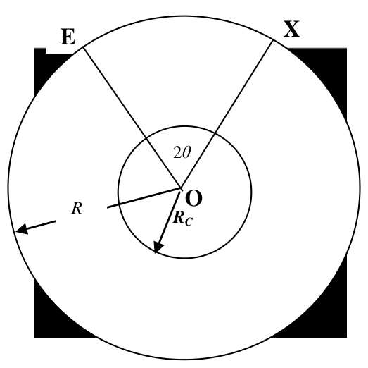
Figure 2.1
The velocities of longitudinal and transverse seismic waves P and S waves respectively, are constant, \(V_P\), and \(V_S\) within the mantle. In the core, longitudinal waves have a constant velocity \(V_{CP}, < V_P\), and transverse waves are not propagated.
An earthquake at E on the surface of the Earth produces seismic waves that travel through the Earth and are observed by a surface observer who can set up his seismometer at any point X on the Earth’s surface. The angular separation between E and X, \(2\theta\) given by
\[ 2\theta=\text{Angle }EOX \]
where O is the centre of the Earth.
(i) Show that the seismic waves that travel through the mantle in a straight line will arrive at X at a time \(t\) (the travel time after the earthquake), is given by
\[ t=\frac{2R\sin\theta}{v}, \qquad \text{for }\theta>\arccos\left[\frac{R_c}{R}\right], \]
where \(v=v_P\) for the P waves and \(v=v_S\) for the S waves.
(ii) For some of the positions of X such that the seismic P waves arrive to the observer after two refractions at the mantle-core interface. Draw the path of such a seismic P wave. Obtain a relation between \(\theta\) and \(i\), the angle of incidence of the seismic P wave at the mantle-core interface, for P waves.
(iii) Using the data
| \(R\) | \(=\) | \(6370\ \mathrm{km}\) |
| \(R_C\) | \(=\) | \(3470\ \mathrm{km}\) |
| \(v_{CP}\) | \(=\) | \(10.85\ \mathrm{km\,s^{-1}}\) |
| \(v_S\) | \(=\) | \(6.31\ \mathrm{km\,s^{-1}}\) |
| \(v_{CP}\) | \(=\) | \(9.02\ \mathrm{km\,s^{-1}}\) |
and the result obtained in (ii),draw a graph of \(\theta\) against \(i\). Comment on the physical consequences of the form of this graph for observers stationed at different points on the Earth's surface. Sketch the variation of the travel time taken by the P and S waves as a function of \(\theta\) for \(0\leq\theta\leq90\) degrees.
(iv) After an earthquake an observer measures the time delay between the arrival of the S wave, following the P wave, as 2 minutes 11 seconds. Deduce the angular separation of the earthquake from the observer using the data given in Section (iii).
(v) The observer in the previous measurement notices that some time after the arrival of the P and S waves there are two further recordings on the seismometer separated by a time interval of 6 minutes 37 seconds. Explain this result and verify that it is indeed associated with the angular separation determined in the previous section.
Official English text of the problem.
Answers
-
(i) The direct-wave travel time is \[ \boxed{t=\frac{2R\sin\theta}{v}}, \qquad \boxed{0\leq\theta\leq\arccos(R_c/R)}. \] Equality describes the limiting tangent ray. The printed inequality is reversed.
-
(ii) Put \(a=R_c/R\), \(b=v_{CP}/v_P\). The ray follows three straight segments, refracting towards the normal on entering the core and away from it on leaving. Its half angular sweep is \[ \boxed{\Phi(i)=\frac{\pi}{2}+i-\arcsin(a\sin i)-\arcsin(b\sin i)}. \] Ordinarily \(\theta=\Phi\); allowing rays that emerge beyond the antipode, the smaller angular separation is given by \[ \boxed{\theta=\min\{\Phi,\pi-\Phi\}}. \]
-
(iii) Direct P and S rays end at \(\theta=56.99^\circ\). Core-transmitted P rays first appear at \[ \boxed{\theta_{\min}=75.58^\circ,\qquad i_{\min}=55.02^\circ}. \] Thus the P-wave shadow is approximately \[ \boxed{113.99^\circ<2\theta<151.15^\circ}, \] while S waves have no direct or core-transmitted arrival for \(2\theta>113.99^\circ\). The refracted P travel-time branches meet at \(20.789\ \mathrm{min}\); their antipodal arrival times are \(21.733\) and \(23.397\ \mathrm{min}\). The complete graph descriptions are given below.
-
(iv) The earthquake–observer angular separation is \[ \boxed{2\theta\approx17.8^\circ}. \]
-
(v) The later signals are P and S waves reflected at the core boundary. Their calculated arrival times are \(551.3\ \mathrm{s}\) and \(947.9\ \mathrm{s}\) after the earthquake, giving \[ \boxed{\Delta t_{\mathrm{ref}}=396.65\ \mathrm{s} \approx6\ \mathrm{min}\ 37\ \mathrm{s}}. \]
Solution
We use the physically consistent reading of the numerical data: \[ v_P=10.85\ \mathrm{km\,s^{-1}},\qquad v_S=6.31\ \mathrm{km\,s^{-1}},\qquad v_{CP}=9.02\ \mathrm{km\,s^{-1}}. \] The data table in (iii) prints the label \(v_{CP}\) twice; the first value so labelled, \(10.85\ \mathrm{km\,s^{-1}}\), is \(v_P\). The inequality printed in (i) is also reversed; see part (i).
We use geometrical ray theory: rays are straight within each homogeneous region, refraction obeys Snell’s law, and reflection obeys equality of incidence and reflection angles. Diffraction, mode conversion and additional reflections at the Earth’s surface are neglected.
(i)
Let \(M\) be the midpoint of the chord \(EX\). The triangle \(OEM\) is right-angled, with \(\angle EOM=\theta\). Hence \[ EM=R\sin\theta,\qquad OM=R\cos\theta. \] The direct path length and travel time are therefore \[ EX=2R\sin\theta, \qquad \boxed{t=\frac{2R\sin\theta}{v}}. \]
The closest point of the chord to the centre is \(M\). Thus the ray avoids the core only if \[ R\cos\theta\geq R_c, \] or \[ \boxed{\theta\leq\arccos(R_c/R)}. \] Strict inequality gives a path entirely within the mantle; equality is the tangent limit. For larger \(\theta\), the chord intersects the core, so the mantle-only formula no longer describes the actual ray.
(ii)
Denote the core entry and exit points by \(A\) and \(B\). Draw the path \[ E\longrightarrow A\longrightarrow B\longrightarrow X, \] with \(EA\) and \(BX\) in the mantle and \(AB\) a chord of the core. Draw the radial normals \(OA\) and \(OB\).
Let \(r\) be the refracted angle inside the core, measured from the normal. Snell’s law gives \[ \frac{\sin i}{v_P}=\frac{\sin r}{v_{CP}}, \] so \[ r=\arcsin\left(\frac{v_{CP}}{v_P}\sin i\right). \] Since \(v_{CP}<v_P\), we have \(r<i\): the ray bends towards the normal on entering the core. By symmetry, its incidence angle at the exit is \(r\), and it emerges into the mantle at angle \(i\).
Let \(\alpha=\angle OEA\). In triangle \(EOA\), the angle at \(A\) is \(\pi-i\). The sine rule gives \[ \frac{\sin\alpha}{R_c}=\frac{\sin i}{R}, \] hence \[ \alpha=\arcsin\left(\frac{R_c}{R}\sin i\right), \qquad \angle EOA=i-\alpha. \]
The isosceles triangle \(AOB\) gives \[ \angle AOB=\pi-2r. \] The total angular sweep of the ray about \(O\) is consequently \[ 2\Phi=2(i-\alpha)+\pi-2r. \] Therefore \[ \boxed{ \Phi(i)=\frac{\pi}{2}+i -\arcsin\left(\frac{R_c}{R}\sin i\right) -\arcsin\left(\frac{v_{CP}}{v_P}\sin i\right) }. \]
For a sweep no greater than \(\pi\), \(\theta=\Phi\). If the ray emerges just beyond the antipode, its smaller source–observer angle is \(2\pi-2\Phi\), giving \[ \boxed{\theta=\min\{\Phi,\pi-\Phi\}}. \]
The requested drawing should therefore show a symmetric broken ray, with equal mantle legs, a straight core chord, and angles \(i\) and \(r<i\) marked at the entry boundary.
(iii)
The dimensionless ratios are \[ a=\frac{R_c}{R}=0.544741,\qquad b=\frac{v_{CP}}{v_P}=0.831336. \] Thus \[ \Phi(i)=\frac{\pi}{2}+i-\arcsin(a\sin i)-\arcsin(b\sin i). \]
Differentiating, with angles in radians, \[ \frac{d\Phi}{di} = 1-\frac{a\cos i}{\sqrt{1-a^2\sin^2 i}} -\frac{b\cos i}{\sqrt{1-b^2\sin^2 i}}. \] At the endpoints, \[ \Phi'(0)=1-a-b=-0.376077,\qquad \Phi'(\pi/2)=1. \] Each subtracted term decreases with \(i\), so \(\Phi'\) increases and has exactly one zero. Numerically, \[ \boxed{i_{\min}=55.017^\circ,\qquad \Phi_{\min}=\theta_{\min}=75.577^\circ}. \]
To obtain the corresponding travel-time graph, the length of either mantle leg is \[ \ell_m =\sqrt{R^2-R_c^2\sin^2 i}-R_c\cos i. \] This follows by projecting the outer and inner radii onto the mantle ray, whose perpendicular distance from \(O\) is \(R_c\sin i\).
The core chord has length \[ \ell_c=2R_c\cos r =2R_c\sqrt{1-b^2\sin^2 i}. \] Consequently, the core-transmitted P travel time is \[ \boxed{ T(i)= \frac{2}{v_P} \left(\sqrt{R^2-R_c^2\sin^2 i}-R_c\cos i\right) +\frac{2R_c}{v_{CP}}\sqrt{1-b^2\sin^2 i} }. \]
The following points specify both requested graphs:
| \(i\) (degrees) | Half sweep \(\Phi\) (degrees) | Physical \(\theta\) (degrees) | Core-transmitted P time (min) |
|---|---|---|---|
| 0 | 90.00 | 90.00 | 21.733 |
| 20 | 82.74 | 82.74 | 21.504 |
| 40 | 77.20 | 77.20 | 21.003 |
| 55.02 | 75.58 | 75.58 | 20.789 |
| 70 | 77.84 | 77.84 | 21.171 |
| 80 | 82.60 | 82.60 | 22.028 |
| 89.23 | 90.00 | 90.00 | 23.397 |
| 90 | 90.76 | 89.24 | 23.538 |
The \(\Phi\)-versus-\(i\) curve begins at \(90^\circ\), falls smoothly to its minimum, then rises to \(90.7568^\circ\). When plotting the physical smaller angle \(\theta\), fold the last portion at \(90^\circ\): \(\theta\) reaches \(90^\circ\) at \(i=89.2322^\circ\), then decreases slightly to \(89.2432^\circ\) at grazing incidence.
The direct-wave cutoff is \[ \theta_d=\arccos(R_c/R)=56.993^\circ. \] The physical consequences are therefore:
- For \(0\leq\theta<56.993^\circ\), direct P and S waves reach the observer.
- For \(56.993^\circ<\theta<75.577^\circ\), neither direct nor core-transmitted P rays reach the observer. This is the P-wave shadow zone.
- For \(\theta>56.993^\circ\), there is no direct S ray, and the liquid core supplies no transmitted S ray.
- At \(\theta=75.577^\circ\), two refracted P paths merge. Since nearby incident rays emerge at nearly the same angular separation, ray energy is concentrated there: this is a caustic.
- For most of \(75.577^\circ<\theta<90^\circ\), two refracted P paths give two distinct arrivals.
Using the given numbers exactly, there is a small additional feature near the antipode. For \[ 89.2432^\circ<\theta<90^\circ, \] a third refracted path reaches the observer by passing beyond the antipodal direction. At the antipode, the two oblique branches have equal travel times.
For the travel-time sketch, draw the direct branches \[ t_{P,\mathrm{dir}}=1174.19\sin\theta\ \mathrm{s}, \qquad t_{S,\mathrm{dir}}=2019.02\sin\theta\ \mathrm{s}, \] only over \(0\leq\theta\leq56.993^\circ\). Both start at the origin and increase with downward curvature; the S curve lies above the P curve. Their endpoints are \[ \begin{aligned} t_{P,\mathrm{dir}}(\theta_d)&=984.68\ \mathrm{s} =16.411\ \mathrm{min},\\ t_{S,\mathrm{dir}}(\theta_d)&=1693.16\ \mathrm{s} =28.219\ \mathrm{min}. \end{aligned} \]
The principal core-transmitted P branches begin together at \[ (\theta,T)=(75.577^\circ,20.789\ \mathrm{min}) \] and rise towards \(90^\circ\). They meet with a common tangent, since differentiation gives \[ \frac{dT}{di} =\frac{2R_c\sin i}{v_P}\frac{d\Phi}{di}, \qquad \frac{dT}{d\Phi}=\frac{2R_c\sin i}{v_P}. \] The smaller-\(i\) branch arrives earlier and flattens at the antipode, where the ray follows a diameter: \[ T(0)=\frac{2(R-R_c)}{v_P}+\frac{2R_c}{v_{CP}} =21.733\ \mathrm{min}. \] The other principal branch reaches \(23.397\ \mathrm{min}\) there. The small third branch decreases from \(23.538\ \mathrm{min}\) at \(\theta=89.243^\circ\) to \(23.397\ \mathrm{min}\) at \(90^\circ\).
For a sketch including the later reflected arrivals discussed in part (v), also draw \[ t_{v,\mathrm{ref}}(\theta) =\frac{2}{v}\sqrt{R^2+R_c^2-2RR_c\cos\theta}, \qquad 0\leq\theta\leq\theta_d. \] These curves increase from \(8.909\ \mathrm{min}\) for P and \(15.320\ \mathrm{min}\) for S at \(\theta=0\), and meet their respective direct curves tangentially at \(\theta_d\).
(iv)
For direct P and S waves the path length is the same, so their arrival-time difference is \[ \Delta t =2R\sin\theta \left(\frac{1}{v_S}-\frac{1}{v_P}\right). \] Here \[ \Delta t=2(60)+11=131\ \mathrm{s}. \] Therefore \[ \sin\theta = \frac{131} {2(6370)\left(\frac1{6.31}-\frac1{10.85}\right)} = \frac{131}{844.8239} =0.1551. \] Thus \[ \theta=8.9204^\circ, \qquad \boxed{2\theta=17.8408^\circ\approx17.8^\circ}. \] Since \(\theta<\theta_d\), the mantle-only path assumption is consistent.
The individual arrival times are \[ t_{P,\mathrm{dir}}=182.07\ \mathrm{s}, \qquad t_{S,\mathrm{dir}}=313.07\ \mathrm{s}. \]
(v)
The core boundary can reflect both P- and S-wave energy. These reflected waves take longer paths through the mantle and therefore produce later arrivals.
Let \(C\) be the reflection point on the core boundary, on the nearer radial bisector of \(\angle EOX\). The path is \[ E\longrightarrow C\longrightarrow X. \] Reflection symmetry about \(OC\) makes the incidence and reflection angles equal, and \(EC=CX\). Since \(\angle EOC=\theta\), the cosine rule gives \[ EC^2=R^2+R_c^2-2RR_c\cos\theta. \] Thus the reflected path length is \[ L_{\mathrm{ref}} =2\sqrt{R^2+R_c^2-2RR_c\cos\theta}. \]
For \(\theta=8.9204^\circ\), \[ L_{\mathrm{ref}}=5981.54\ \mathrm{km}. \] The reflected arrival times are consequently \[ t_{P,\mathrm{ref}} =\frac{5981.54}{10.85} =551.29\ \mathrm{s}, \] \[ t_{S,\mathrm{ref}} =\frac{5981.54}{6.31} =947.95\ \mathrm{s}. \] Both occur after the direct S arrival at \(313.07\ \mathrm{s}\), as required.
Their separation is \[ \begin{aligned} \Delta t_{\mathrm{ref}} &=L_{\mathrm{ref}} \left(\frac1{v_S}-\frac1{v_P}\right)\\ &=396.65\ \mathrm{s}\\ &=6\ \mathrm{min}\ 36.65\ \mathrm{s}. \end{aligned} \] Rounded to the nearest second, \[ \boxed{\Delta t_{\mathrm{ref}}=6\ \mathrm{min}\ 37\ \mathrm{s}}, \] which verifies the interpretation and the angular separation found in part (iv).
The solution was checked against the official solution. Where this solution differs from the official solution, the official solution contains an error or a misprint.
IPhO 1986 · Theorieaufgabe 2
Seismische Wellen und der flüssige Erdkern
- Zu Beginn dieses Jahrhunderts wurde ein Erdmodell vorgeschlagen, in dem die Erde als Kugel mit dem Radius \(R\) angenommen wurde, deren homogener, isotroper, fester Mantel bis zum Radius \(R_c\) reicht. Der Kernbereich innerhalb des Radius \(R_c\) enthielt eine Flüssigkeit.
Abbildung 2.1
Die Geschwindigkeiten der longitudinalen und transversalen seismischen Wellen, der P- bzw. S-Wellen, sind innerhalb des Mantels konstant und betragen \(V_P\) bzw. \(V_S\). Im Kern haben Longitudinalwellen eine konstante Geschwindigkeit \(V_{CP}, < V_P\), und Transversalwellen breiten sich dort nicht aus.
Ein Erdbeben bei E an der Erdoberfläche erzeugt seismische Wellen, die sich durch die Erde ausbreiten und von einem Beobachter an der Oberfläche registriert werden, der sein Seismometer an einem beliebigen Punkt X der Erdoberfläche aufstellen kann. Der Winkelabstand zwischen E und X, \(2\theta\), ist gegeben durch
\[ 2\theta=\text{Winkel }EOX \]
wobei O der Erdmittelpunkt ist.
(i) Zeigen Sie, dass die seismischen Wellen, die sich geradlinig durch den Mantel ausbreiten, bei X zu einer Zeit \(t\) eintreffen (der Laufzeit seit dem Erdbeben), die gegeben ist durch
\[ t=\frac{2R\sin\theta}{v}, \qquad \text{für }\theta>\arccos\left[\frac{R_c}{R}\right], \]
wobei \(v=v_P\) für die P-Wellen und \(v=v_S\) für die S-Wellen gilt.
(ii) Für einige Positionen von X erreichen die seismischen P-Wellen den Beobachter nach zweimaliger Brechung an der Mantel-Kern-Grenze. Zeichnen Sie den Weg einer solchen seismischen P-Welle. Leiten Sie für P-Wellen eine Beziehung zwischen \(\theta\) und \(i\), dem Einfallswinkel der seismischen P-Welle an der Mantel-Kern-Grenze, her.
(iii) Zeichnen Sie mithilfe der Daten
| \(R\) | \(=\) | \(6370\ \mathrm{km}\) |
| \(R_C\) | \(=\) | \(3470\ \mathrm{km}\) |
| \(v_{CP}\) | \(=\) | \(10.85\ \mathrm{km\,s^{-1}}\) |
| \(v_S\) | \(=\) | \(6.31\ \mathrm{km\,s^{-1}}\) |
| \(v_{CP}\) | \(=\) | \(9.02\ \mathrm{km\,s^{-1}}\) |
und des in (ii) erhaltenen Ergebnisses einen Graphen von \(\theta\) in Abhängigkeit von \(i\). Erläutern Sie die physikalischen Folgen der Form dieses Graphen für Beobachter an verschiedenen Punkten der Erdoberfläche. Skizzieren Sie den Verlauf der Laufzeiten der P- und S-Wellen als Funktion von \(\theta\) für \(0\leq\theta\leq90\) Grad.
(iv) Nach einem Erdbeben misst ein Beobachter zwischen der Ankunft der P-Welle und der nachfolgenden S-Welle eine Zeitdifferenz von 2 Minuten 11 Sekunden. Bestimmen Sie mithilfe der in Abschnitt (iii) angegebenen Daten den Winkelabstand zwischen dem Erdbeben und dem Beobachter.
(v) Der Beobachter aus der vorherigen Messung stellt fest, dass einige Zeit nach der Ankunft der P- und S-Wellen zwei weitere Signale auf dem Seismometer registriert werden, zwischen denen ein Zeitintervall von 6 Minuten 37 Sekunden liegt. Erklären Sie dieses Ergebnis und überprüfen Sie, dass es tatsächlich dem im vorherigen Abschnitt bestimmten Winkelabstand entspricht.
Aufgabentext aus dem offiziellen englischen Text übersetzt.
Antworten
-
(i) Die Laufzeit der direkten Welle ist \[ \boxed{t=\frac{2R\sin\theta}{v}}, \qquad \boxed{0\leq\theta\leq\arccos(R_c/R)}. \] Die Gleichheit beschreibt den Grenzfall des tangentialen Strahls. Das gedruckte Ungleichheitszeichen ist umgekehrt.
-
(ii) Setzen wir \(a=R_c/R\), \(b=v_{CP}/v_P\). Der Strahl verläuft entlang dreier gerader Abschnitte und wird beim Eintritt in den Kern zum Lot hin und beim Austritt vom Lot weg gebrochen. Die Hälfte seines insgesamt durchlaufenen Zentriwinkels ist \[ \boxed{\Phi(i)=\frac{\pi}{2}+i-\arcsin(a\sin i)-\arcsin(b\sin i)}. \] Gewöhnlich gilt \(\theta=\Phi\); berücksichtigt man Strahlen, die jenseits des Antipoden austreten, so ist der kleinere Winkelabstand gegeben durch \[ \boxed{\theta=\min\{\Phi,\pi-\Phi\}}. \]
-
(iii) Direkte P- und S-Strahlen enden bei \(\theta=56.99^\circ\). Durch den Kern laufende P-Strahlen treten erstmals bei \[ \boxed{\theta_{\min}=75.58^\circ,\qquad i_{\min}=55.02^\circ} \] auf. Somit liegt der P-Wellen-Schatten ungefähr im Bereich \[ \boxed{113.99^\circ<2\theta<151.15^\circ}, \] während für \(2\theta>113.99^\circ\) weder direkte noch durch den Kern laufende S-Wellen eintreffen. Die Laufzeitäste der gebrochenen P-Wellen treffen sich bei \(20.789\ \mathrm{min}\); ihre Ankunftszeiten am Antipoden betragen \(21.733\) und \(23.397\ \mathrm{min}\). Die vollständigen Beschreibungen der Graphen folgen weiter unten.
-
(iv) Der Winkelabstand zwischen Erdbeben und Beobachter beträgt \[ \boxed{2\theta\approx17.8^\circ}. \]
-
(v) Die späteren Signale sind P- und S-Wellen, die an der Kerngrenze reflektiert wurden. Ihre berechneten Ankunftszeiten betragen \(551.3\ \mathrm{s}\) und \(947.9\ \mathrm{s}\) nach dem Erdbeben, woraus sich \[ \boxed{\Delta t_{\mathrm{ref}}=396.65\ \mathrm{s} \approx6\ \mathrm{min}\ 37\ \mathrm{s}} \] ergibt.
Lösung
Wir verwenden die physikalisch konsistente Lesart der Zahlenangaben: \[ v_P=10.85\ \mathrm{km\,s^{-1}},\qquad v_S=6.31\ \mathrm{km\,s^{-1}},\qquad v_{CP}=9.02\ \mathrm{km\,s^{-1}}. \] Die Datentabelle in Teil (iii) führt die Bezeichnung \(v_{CP}\) zweimal auf; der erste so bezeichnete Wert, \(10.85\ \mathrm{km\,s^{-1}}\), ist \(v_P\). Auch die in (i) gedruckte Ungleichung ist umgekehrt; siehe Teil (i).
Wir verwenden die geometrische Strahlentheorie: Innerhalb jedes homogenen Bereichs verlaufen die Strahlen geradlinig, die Brechung folgt dem Snelliusschen Brechungsgesetz, und bei der Reflexion sind Einfalls- und Reflexionswinkel gleich. Beugung, Modenumwandlung und zusätzliche Reflexionen an der Erdoberfläche werden vernachlässigt.
(i)
Sei \(M\) der Mittelpunkt der Sehne \(EX\). Das Dreieck \(OEM\) ist rechtwinklig, wobei \(\angle EOM=\theta\) gilt. Daher ist \[ EM=R\sin\theta,\qquad OM=R\cos\theta. \] Die direkte Weglänge und die Laufzeit sind somit \[ EX=2R\sin\theta, \qquad \boxed{t=\frac{2R\sin\theta}{v}}. \]
Der dem Mittelpunkt nächstgelegene Punkt der Sehne ist \(M\). Der Strahl verläuft also nur dann außerhalb des Kerns, wenn \[ R\cos\theta\geq R_c, \] oder \[ \boxed{\theta\leq\arccos(R_c/R)}. \] Bei strenger Ungleichheit liegt der Weg vollständig im Mantel; Gleichheit entspricht dem tangentialen Grenzfall. Für größere \(\theta\) schneidet die Sehne den Kern, sodass die nur für den Mantel geltende Formel den tatsächlichen Strahl nicht mehr beschreibt.
(ii)
Bezeichnen wir den Eintritts- und Austrittspunkt am Kern mit \(A\) und \(B\). Zeichnen Sie den Weg \[ E\longrightarrow A\longrightarrow B\longrightarrow X, \] wobei \(EA\) und \(BX\) im Mantel liegen und \(AB\) eine Sehne des Kerns ist. Zeichnen Sie die radialen Lote \(OA\) und \(OB\).
Sei \(r\) der Brechungswinkel innerhalb des Kerns, gemessen zum Lot. Das Snelliussche Brechungsgesetz liefert \[ \frac{\sin i}{v_P}=\frac{\sin r}{v_{CP}}, \] also \[ r=\arcsin\left(\frac{v_{CP}}{v_P}\sin i\right). \] Da \(v_{CP}<v_P\), gilt \(r<i\): Der Strahl wird beim Eintritt in den Kern zum Lot hin gebrochen. Aufgrund der Symmetrie beträgt sein Einfallswinkel beim Austritt \(r\), und er tritt unter dem Winkel \(i\) in den Mantel aus.
Sei \(\alpha=\angle OEA\). Im Dreieck \(EOA\) beträgt der Winkel bei \(A\) gerade \(\pi-i\). Der Sinussatz liefert \[ \frac{\sin\alpha}{R_c}=\frac{\sin i}{R}, \] folglich \[ \alpha=\arcsin\left(\frac{R_c}{R}\sin i\right), \qquad \angle EOA=i-\alpha. \]
Aus dem gleichschenkligen Dreieck \(AOB\) folgt \[ \angle AOB=\pi-2r. \] Der insgesamt vom Strahl um \(O\) durchlaufene Zentriwinkel ist demnach \[ 2\Phi=2(i-\alpha)+\pi-2r. \] Daher gilt \[ \boxed{ \Phi(i)=\frac{\pi}{2}+i -\arcsin\left(\frac{R_c}{R}\sin i\right) -\arcsin\left(\frac{v_{CP}}{v_P}\sin i\right) }. \]
Für einen durchlaufenen Zentriwinkel von höchstens \(\pi\) gilt \(\theta=\Phi\). Tritt der Strahl knapp jenseits des Antipoden aus, so beträgt der kleinere Winkel zwischen Quelle und Beobachter \(2\pi-2\Phi\), woraus \[ \boxed{\theta=\min\{\Phi,\pi-\Phi\}} \] folgt.
Die geforderte Zeichnung sollte daher einen symmetrischen gebrochenen Strahl mit gleich langen Mantelabschnitten und einer geraden Kernsehne zeigen; an der Eintrittsgrenze sind die Winkel \(i\) und \(r<i\) einzuzeichnen.
(iii)
Die dimensionslosen Verhältnisse betragen \[ a=\frac{R_c}{R}=0.544741,\qquad b=\frac{v_{CP}}{v_P}=0.831336. \] Somit ist \[ \Phi(i)=\frac{\pi}{2}+i-\arcsin(a\sin i)-\arcsin(b\sin i). \]
Durch Differenzieren mit Winkeln im Bogenmaß ergibt sich \[ \frac{d\Phi}{di} = 1-\frac{a\cos i}{\sqrt{1-a^2\sin^2 i}} -\frac{b\cos i}{\sqrt{1-b^2\sin^2 i}}. \] An den Endpunkten gilt \[ \Phi'(0)=1-a-b=-0.376077,\qquad \Phi'(\pi/2)=1. \] Jeder der subtrahierten Terme nimmt mit \(i\) ab, sodass \(\Phi'\) zunimmt und genau eine Nullstelle besitzt. Numerisch ergibt sich \[ \boxed{i_{\min}=55.017^\circ,\qquad \Phi_{\min}=\theta_{\min}=75.577^\circ}. \]
Um den zugehörigen Laufzeitgraphen zu erhalten, bestimmen wir die Länge jedes der beiden Mantelabschnitte: \[ \ell_m =\sqrt{R^2-R_c^2\sin^2 i}-R_c\cos i. \] Dies ergibt sich durch Projektion des äußeren und inneren Radius auf den Mantelstrahl, dessen senkrechter Abstand von \(O\) gleich \(R_c\sin i\) ist.
Die Kernsehne hat die Länge \[ \ell_c=2R_c\cos r =2R_c\sqrt{1-b^2\sin^2 i}. \] Folglich beträgt die Laufzeit der durch den Kern laufenden P-Welle \[ \boxed{ T(i)= \frac{2}{v_P} \left(\sqrt{R^2-R_c^2\sin^2 i}-R_c\cos i\right) +\frac{2R_c}{v_{CP}}\sqrt{1-b^2\sin^2 i} }. \]
Die folgenden Punkte legen die beiden geforderten Graphen fest:
| \(i\) (Grad) | Halber durchlaufener Zentriwinkel \(\Phi\) (Grad) | Physikalischer Winkel \(\theta\) (Grad) | Laufzeit der durch den Kern laufenden P-Welle (min) |
|---|---|---|---|
| 0 | 90.00 | 90.00 | 21.733 |
| 20 | 82.74 | 82.74 | 21.504 |
| 40 | 77.20 | 77.20 | 21.003 |
| 55.02 | 75.58 | 75.58 | 20.789 |
| 70 | 77.84 | 77.84 | 21.171 |
| 80 | 82.60 | 82.60 | 22.028 |
| 89.23 | 90.00 | 90.00 | 23.397 |
| 90 | 90.76 | 89.24 | 23.538 |
Die Kurve von \(\Phi\) in Abhängigkeit von \(i\) beginnt bei \(90^\circ\), fällt glatt bis zu ihrem Minimum und steigt dann auf \(90.7568^\circ\) an. Bei der Darstellung des physikalischen kleineren Winkels \(\theta\) ist der letzte Abschnitt an \(90^\circ\) zu spiegeln: \(\theta\) erreicht bei \(i=89.2322^\circ\) den Wert \(90^\circ\) und nimmt dann bis zum streifenden Einfall leicht auf \(89.2432^\circ\) ab.
Der Grenzwinkel für direkte Wellen ist \[ \theta_d=\arccos(R_c/R)=56.993^\circ. \] Daraus ergeben sich die folgenden physikalischen Konsequenzen:
- Für \(0\leq\theta<56.993^\circ\) erreichen direkte P- und S-Wellen den Beobachter.
- Für \(56.993^\circ<\theta<75.577^\circ\) erreichen weder direkte noch durch den Kern laufende P-Strahlen den Beobachter. Dies ist die P-Wellen-Schattenzone.
- Für \(\theta>56.993^\circ\) gibt es keinen direkten S-Strahl, und der flüssige Kern lässt keinen S-Strahl hindurch.
- Bei \(\theta=75.577^\circ\) fallen zwei gebrochene P-Strahlwege zusammen. Da benachbarte einfallende Strahlen bei nahezu demselben Winkelabstand austreten, konzentriert sich dort die Strahlenergie: Es handelt sich um eine Kaustik.
- Im größten Teil des Bereichs \(75.577^\circ<\theta<90^\circ\) führen zwei gebrochene P-Strahlwege zu zwei getrennten Ankünften.
Verwendet man die angegebenen Zahlen exakt, ergibt sich in der Nähe des Antipoden eine kleine zusätzliche Besonderheit. Für \[ 89.2432^\circ<\theta<90^\circ, \] erreicht ein dritter gebrochener Strahl den Beobachter, indem er über die antipodale Richtung hinausläuft. Am Antipoden haben die beiden schräg verlaufenden Äste gleiche Laufzeiten.
Zeichnen Sie für die Laufzeitskizze die direkten Äste \[ t_{P,\mathrm{dir}}=1174.19\sin\theta\ \mathrm{s}, \qquad t_{S,\mathrm{dir}}=2019.02\sin\theta\ \mathrm{s}, \] nur im Bereich \(0\leq\theta\leq56.993^\circ\). Beide beginnen im Ursprung und steigen mit nach unten gerichteter Krümmung an; die S-Kurve liegt oberhalb der P-Kurve. Ihre Endpunkte sind \[ \begin{aligned} t_{P,\mathrm{dir}}(\theta_d)&=984.68\ \mathrm{s} =16.411\ \mathrm{min},\\ t_{S,\mathrm{dir}}(\theta_d)&=1693.16\ \mathrm{s} =28.219\ \mathrm{min}. \end{aligned} \]
Die Hauptäste der durch den Kern laufenden P-Wellen beginnen gemeinsam bei \[ (\theta,T)=(75.577^\circ,20.789\ \mathrm{min}) \] und steigen in Richtung \(90^\circ\) an. Sie treffen sich mit einer gemeinsamen Tangente, denn durch Differenzieren erhält man \[ \frac{dT}{di} =\frac{2R_c\sin i}{v_P}\frac{d\Phi}{di}, \qquad \frac{dT}{d\Phi}=\frac{2R_c\sin i}{v_P}. \] Der Ast mit kleinerem \(i\) trifft früher ein und flacht am Antipoden ab, wo der Strahl entlang eines Durchmessers verläuft: \[ T(0)=\frac{2(R-R_c)}{v_P}+\frac{2R_c}{v_{CP}} =21.733\ \mathrm{min}. \] Der andere Hauptast erreicht dort \(23.397\ \mathrm{min}\). Der kleine dritte Ast fällt von \(23.538\ \mathrm{min}\) bei \(\theta=89.243^\circ\) auf \(23.397\ \mathrm{min}\) bei \(90^\circ\).
Für eine Skizze, die auch die in Teil (v) behandelten späteren reflektierten Ankünfte enthält, zeichnen Sie zusätzlich \[ t_{v,\mathrm{ref}}(\theta) =\frac{2}{v}\sqrt{R^2+R_c^2-2RR_c\cos\theta}, \qquad 0\leq\theta\leq\theta_d. \] Diese Kurven steigen von \(8.909\ \mathrm{min}\) für P und \(15.320\ \mathrm{min}\) für S bei \(\theta=0\) an und treffen bei \(\theta_d\) tangential auf die jeweiligen direkten Kurven.
(iv)
Für direkte P- und S-Wellen ist die Weglänge gleich, sodass die Differenz ihrer Ankunftszeiten \[ \Delta t =2R\sin\theta \left(\frac{1}{v_S}-\frac{1}{v_P}\right) \] beträgt. Hier gilt \[ \Delta t=2(60)+11=131\ \mathrm{s}. \] Somit ergibt sich \[ \sin\theta = \frac{131} {2(6370)\left(\frac1{6.31}-\frac1{10.85}\right)} = \frac{131}{844.8239} =0.1551. \] Also gilt \[ \theta=8.9204^\circ, \qquad \boxed{2\theta=17.8408^\circ\approx17.8^\circ}. \] Da \(\theta<\theta_d\), ist die Annahme eines ausschließlich durch den Mantel verlaufenden Weges konsistent.
Die einzelnen Ankunftszeiten betragen \[ t_{P,\mathrm{dir}}=182.07\ \mathrm{s}, \qquad t_{S,\mathrm{dir}}=313.07\ \mathrm{s}. \]
(v)
Die Kerngrenze kann sowohl P- als auch S-Wellenenergie reflektieren. Diese reflektierten Wellen legen längere Wege durch den Mantel zurück und treffen daher später ein.
Sei \(C\) der Reflexionspunkt an der Kerngrenze auf dem näher gelegenen radialen Strahl der Winkelhalbierenden von \(\angle EOX\). Der Weg ist \[ E\longrightarrow C\longrightarrow X. \] Aufgrund der Spiegelsymmetrie bezüglich \(OC\) sind Einfalls- und Reflexionswinkel gleich, und es gilt \(EC=CX\). Da \(\angle EOC=\theta\), liefert der Kosinussatz \[ EC^2=R^2+R_c^2-2RR_c\cos\theta. \] Somit beträgt die Länge des reflektierten Weges \[ L_{\mathrm{ref}} =2\sqrt{R^2+R_c^2-2RR_c\cos\theta}. \]
Für \(\theta=8.9204^\circ\) gilt \[ L_{\mathrm{ref}}=5981.54\ \mathrm{km}. \] Die Ankunftszeiten der reflektierten Wellen sind folglich \[ t_{P,\mathrm{ref}} =\frac{5981.54}{10.85} =551.29\ \mathrm{s}, \] \[ t_{S,\mathrm{ref}} =\frac{5981.54}{6.31} =947.95\ \mathrm{s}. \] Beide liegen, wie gefordert, nach der Ankunft der direkten S-Welle bei \(313.07\ \mathrm{s}\).
Ihr zeitlicher Abstand beträgt \[ \begin{aligned} \Delta t_{\mathrm{ref}} &=L_{\mathrm{ref}} \left(\frac1{v_S}-\frac1{v_P}\right)\\ &=396.65\ \mathrm{s}\\ &=6\ \mathrm{min}\ 36.65\ \mathrm{s}. \end{aligned} \] Auf die nächste Sekunde gerundet ergibt sich \[ \boxed{\Delta t_{\mathrm{ref}}=6\ \mathrm{min}\ 37\ \mathrm{s}}, \] womit die Deutung und der in Teil (iv) gefundene Winkelabstand bestätigt sind.
Die Lösung wurde mit der offiziellen Lösung abgeglichen. Wo diese Lösung von der offiziellen Lösung abweicht, enthält die offizielle Lösung einen Fehler oder Druckfehler.
IPhO 1986 · Teori sorusu 2
Sismik dalgalar ve Dünya'nın sıvı çekirdeği
- Bu yüzyılın başlarında, Dünya'nın yarıçapı \(R\) olan ve \(R_c\) yarıçapına kadar homojen, izotrop katı bir mantodan oluşan bir küre olarak kabul edildiği bir model önerildi. \(R_c\) yarıçapının içinde kalan çekirdek bölgesi bir sıvı içeriyordu.
Şekil 2.1
Sırasıyla P ve S dalgaları olarak adlandırılan boyuna ve enine sismik dalgaların hızları manto içinde sabittir ve \(V_P\) ile \(V_S\)'dir. Çekirdekte boyuna dalgaların hızı sabit olup \(V_{CP}, < V_P\)'dir ve enine dalgalar yayılmaz.
Dünya yüzeyindeki E noktasında meydana gelen bir deprem, Dünya'nın içinden geçen ve sismometresini Dünya yüzeyindeki herhangi bir X noktasına yerleştirebilen bir yüzey gözlemcisi tarafından gözlenen sismik dalgalar üretir. E ile X arasındaki açısal uzaklık \(2\theta\),
\[ 2\theta=\text{Açı }EOX \]
ile verilir; burada O, Dünya'nın merkezidir.
(i) Manto içinde doğrusal bir yol boyunca ilerleyen sismik dalgaların X'e ulaşma zamanı \(t\)'nin (depremden sonraki yayılma süresinin)
\[ t=\frac{2R\sin\theta}{v}, \qquad \text{koşuluyla }\theta>\arccos\left[\frac{R_c}{R}\right], \]
ile verildiğini gösteriniz; burada P dalgaları için \(v=v_P\), S dalgaları için ise \(v=v_S\)'dir.
(ii) X'in bazı konumlarında sismik P dalgaları, manto–çekirdek ara yüzünde iki kez kırıldıktan sonra gözlemciye ulaşır. Böyle bir sismik P dalgasının izlediği yolu çiziniz. P dalgaları için \(\theta\) ile sismik P dalgasının manto–çekirdek ara yüzüne gelme açısı \(i\) arasında bir bağıntı elde ediniz.
(iii) Aşağıdaki verileri
| \(R\) | \(=\) | \(6370\ \mathrm{km}\) |
| \(R_C\) | \(=\) | \(3470\ \mathrm{km}\) |
| \(v_{CP}\) | \(=\) | \(10.85\ \mathrm{km\,s^{-1}}\) |
| \(v_S\) | \(=\) | \(6.31\ \mathrm{km\,s^{-1}}\) |
| \(v_{CP}\) | \(=\) | \(9.02\ \mathrm{km\,s^{-1}}\) |
ve (ii)'de elde edilen sonucu kullanarak \(\theta\)'nın \(i\)'ye göre grafiğini çiziniz. Bu grafiğin biçiminin, Dünya yüzeyinin farklı noktalarında bulunan gözlemciler açısından fiziksel sonuçlarını yorumlayınız. P ve S dalgalarının yayılma sürelerinin \(\theta\)'ya bağlı değişimini \(0\leq\theta\leq90\) derece aralığında kabaca çiziniz.
(iv) Bir depremden sonra bir gözlemci, P dalgasını izleyen S dalgasının varışı arasındaki zaman farkını 2 dakika 11 saniye olarak ölçer. Bölüm (iii)'te verilen verileri kullanarak depremin gözlemciye olan açısal uzaklığını bulunuz.
(v) Önceki ölçümü yapan gözlemci, P ve S dalgalarının varışından bir süre sonra sismometrede aralarında 6 dakika 37 saniyelik zaman farkı bulunan iki kayıt daha olduğunu fark eder. Bu sonucu açıklayınız ve bunun gerçekten de önceki bölümde belirlenen açısal uzaklıkla ilişkili olduğunu doğrulayınız.
Soru metni resmi İngilizce metinden çevrilmiştir.
Cevaplar
-
(i) Doğrudan gelen dalganın yayılma süresi \[ \boxed{t=\frac{2R\sin\theta}{v}}, \qquad \boxed{0\leq\theta\leq\arccos(R_c/R)}. \] Eşitlik, sınır durumundaki teğet ışını tanımlar. Basılı metindeki eşitsizlik ters yöndedir.
-
(ii) \(a=R_c/R\), \(b=v_{CP}/v_P\) olsun. Işın, çekirdeğe girerken normale yaklaşarak, çıkarken ise normalden uzaklaşarak kırılır ve üç doğru parçasından oluşan bir yol izler. Merkez çevresinde taradığı açının yarısı \[ \boxed{\Phi(i)=\frac{\pi}{2}+i-\arcsin(a\sin i)-\arcsin(b\sin i)}. \] Olağan durumda \(\theta=\Phi\)'dir; karşıt noktanın ötesinden çıkan ışınlar da hesaba katıldığında, küçük açısal uzaklık \[ \boxed{\theta=\min\{\Phi,\pi-\Phi\}}. \] ile verilir.
-
(iii) Doğrudan gelen P ve S ışınları \(\theta=56.99^\circ\)'de sona erer. Çekirdekten geçen P ışınları ilk kez \[ \boxed{\theta_{\min}=75.58^\circ,\qquad i_{\min}=55.02^\circ}. \] değerlerinde ortaya çıkar. Dolayısıyla P dalgasının gölge bölgesi yaklaşık olarak \[ \boxed{113.99^\circ<2\theta<151.15^\circ}, \] aralığıdır; buna karşılık \(2\theta>113.99^\circ\) için doğrudan gelen veya çekirdekten geçen hiçbir S dalgası ulaşmaz. Kırılan P dalgalarının yayılma süresi dalları \(20.789\ \mathrm{min}\)'de birleşir; karşıt noktaya varış süreleri \(21.733\) ve \(23.397\ \mathrm{min}\)'dir. Grafiklerin tam açıklamaları aşağıda verilmiştir.
-
(iv) Deprem ile gözlemci arasındaki açısal uzaklık \[ \boxed{2\theta\approx17.8^\circ}. \]
-
(v) Daha sonra gelen sinyaller, çekirdek sınırında yansıyan P ve S dalgalarıdır. Hesaplanan varış zamanları depremden sonra \(551.3\ \mathrm{s}\) ve \(947.9\ \mathrm{s}\) olup aralarındaki fark \[ \boxed{\Delta t_{\mathrm{ref}}=396.65\ \mathrm{s} \approx6\ \mathrm{min}\ 37\ \mathrm{s}}. \]
Çözüm
Sayısal verilerin fiziksel açıdan tutarlı yorumunu kullanıyoruz: \[ v_P=10.85\ \mathrm{km\,s^{-1}},\qquad v_S=6.31\ \mathrm{km\,s^{-1}},\qquad v_{CP}=9.02\ \mathrm{km\,s^{-1}}. \] (iii) kısmındaki veri tablosunda \(v_{CP}\) etiketi iki kez basılmıştır; bu etiketli ilk satırdaki \(10.85\ \mathrm{km\,s^{-1}}\) değeri \(v_P\) hızıdır. (i) kısmındaki basılı eşitsizlik de ters yöndedir; (i) kısmına bakınız.
Geometrik ışın kuramını kullanıyoruz: ışınlar her homojen bölge içinde doğrusal ilerler, kırılma Snell yasasına uyar ve yansımada gelme açısı ile yansıma açısı eşittir. Kırınım, mod dönüşümü ve Dünya yüzeyindeki ek yansımalar ihmal edilir.
(i)
\(M\), \(EX\) kirişinin orta noktası olsun. \(OEM\) üçgeni dik üçgendir ve \(\angle EOM=\theta\)'dır. Dolayısıyla \[ EM=R\sin\theta,\qquad OM=R\cos\theta. \] Böylece doğrudan yolun uzunluğu ve yayılma süresi \[ EX=2R\sin\theta, \qquad \boxed{t=\frac{2R\sin\theta}{v}}. \]
Kirişin merkeze en yakın noktası \(M\)'dir. Bu nedenle ışın, ancak \[ R\cos\theta\geq R_c, \] yani \[ \boxed{\theta\leq\arccos(R_c/R)}. \] olduğunda çekirdeğe girmez. Kesin eşitsizlik, bütünüyle manto içinde kalan bir yol verir; eşitlik ise teğet sınır durumudur. Daha büyük \(\theta\) değerlerinde kiriş çekirdeği keser; dolayısıyla yalnızca mantoda ilerleme için geçerli olan formül artık gerçek ışını tanımlamaz.
(ii)
Çekirdeğe giriş ve çekirdekten çıkış noktalarını \(A\) ve \(B\) ile gösterelim. \[ E\longrightarrow A\longrightarrow B\longrightarrow X, \] yolunu, \(EA\) ve \(BX\) manto içinde, \(AB\) ise çekirdeğin bir kirişi olacak şekilde çiziniz. Radyal normaller \(OA\) ve \(OB\)'yi çiziniz.
\(r\), çekirdek içindeki, normalden ölçülen kırılma açısı olsun. Snell yasası \[ \frac{\sin i}{v_P}=\frac{\sin r}{v_{CP}}, \] bağıntısını verir; buradan \[ r=\arcsin\left(\frac{v_{CP}}{v_P}\sin i\right). \] \(v_{CP}<v_P\) olduğundan \(r<i\)'dir: ışın çekirdeğe girerken normale doğru bükülür. Simetri gereği, çıkıştaki gelme açısı \(r\)'dir ve mantoya \(i\) açısıyla çıkar.
\(\alpha=\angle OEA\) olsun. \(EOA\) üçgeninde \(A\) köşesindeki açı \(\pi-i\)'dir. Sinüs teoremi \[ \frac{\sin\alpha}{R_c}=\frac{\sin i}{R}, \] bağıntısını verir; dolayısıyla \[ \alpha=\arcsin\left(\frac{R_c}{R}\sin i\right), \qquad \angle EOA=i-\alpha. \]
\(AOB\) ikizkenar üçgeninden \[ \angle AOB=\pi-2r. \] elde edilir. Böylece ışının \(O\) çevresinde taradığı toplam açı \[ 2\Phi=2(i-\alpha)+\pi-2r. \] olur. Dolayısıyla \[ \boxed{ \Phi(i)=\frac{\pi}{2}+i -\arcsin\left(\frac{R_c}{R}\sin i\right) -\arcsin\left(\frac{v_{CP}}{v_P}\sin i\right) }. \]
Taranan açı \(\pi\)'den büyük değilse \(\theta=\Phi\)'dir. Işın karşıt noktanın hemen ötesinden çıkarsa, kaynak ile gözlemci arasındaki küçük açı \(2\pi-2\Phi\) olur ve \[ \boxed{\theta=\min\{\Phi,\pi-\Phi\}}. \] elde edilir.
Bu nedenle istenen çizim, mantodaki kolları eşit, çekirdekteki kirişi düz olan simetrik bir kırık ışın yolunu göstermeli ve giriş sınırında \(i\) ile \(r<i\) açıları işaretlenmelidir.
(iii)
Boyutsuz oranlar \[ a=\frac{R_c}{R}=0.544741,\qquad b=\frac{v_{CP}}{v_P}=0.831336. \] şeklindedir. Böylece \[ \Phi(i)=\frac{\pi}{2}+i-\arcsin(a\sin i)-\arcsin(b\sin i). \]
Açıları radyan cinsinden alarak türev alırsak, \[ \frac{d\Phi}{di} = 1-\frac{a\cos i}{\sqrt{1-a^2\sin^2 i}} -\frac{b\cos i}{\sqrt{1-b^2\sin^2 i}}. \] Uç noktalarda, \[ \Phi'(0)=1-a-b=-0.376077,\qquad \Phi'(\pi/2)=1. \] Çıkarılan terimlerin her biri \(i\) arttıkça azalır; dolayısıyla \(\Phi'\) artar ve tam olarak bir sıfırı vardır. Sayısal olarak, \[ \boxed{i_{\min}=55.017^\circ,\qquad \Phi_{\min}=\theta_{\min}=75.577^\circ}. \]
Buna karşılık gelen yayılma süresi grafiğini elde etmek için, mantodaki kolların her birinin uzunluğu \[ \ell_m =\sqrt{R^2-R_c^2\sin^2 i}-R_c\cos i. \] olarak bulunur. Bu sonuç, dış ve iç yarıçapların, \(O\)'ya dik uzaklığı \(R_c\sin i\) olan manto ışını üzerine izdüşümleri alınarak elde edilir.
Çekirdek kirişinin uzunluğu \[ \ell_c=2R_c\cos r =2R_c\sqrt{1-b^2\sin^2 i}. \] olur. Dolayısıyla çekirdekten geçen P dalgasının yayılma süresi \[ \boxed{ T(i)= \frac{2}{v_P} \left(\sqrt{R^2-R_c^2\sin^2 i}-R_c\cos i\right) +\frac{2R_c}{v_{CP}}\sqrt{1-b^2\sin^2 i} }. \]
Aşağıdaki noktalar, istenen her iki grafiği de belirler:
| \(i\) (derece) | Taranan açının yarısı \(\Phi\) (derece) | Fiziksel \(\theta\) (derece) | Çekirdekten geçen P dalgasının süresi (dakika) |
|---|---|---|---|
| 0 | 90.00 | 90.00 | 21.733 |
| 20 | 82.74 | 82.74 | 21.504 |
| 40 | 77.20 | 77.20 | 21.003 |
| 55.02 | 75.58 | 75.58 | 20.789 |
| 70 | 77.84 | 77.84 | 21.171 |
| 80 | 82.60 | 82.60 | 22.028 |
| 89.23 | 90.00 | 90.00 | 23.397 |
| 90 | 90.76 | 89.24 | 23.538 |
\(\Phi\)'nin \(i\)'ye göre eğrisi \(90^\circ\)'den başlar, düzgün biçimde minimumuna iner, ardından \(90.7568^\circ\)'ye yükselir. Fiziksel küçük açı \(\theta\)'yı çizerken son kısmı \(90^\circ\)'de katlayınız: \(\theta\), \(i=89.2322^\circ\)'de \(90^\circ\)'ye ulaşır, ardından teğet geliş durumunda hafifçe azalarak \(89.2432^\circ\)'ye iner.
Doğrudan gelen dalgaların sınır açısı \[ \theta_d=\arccos(R_c/R)=56.993^\circ. \] olur. Dolayısıyla fiziksel sonuçlar şunlardır:
- \(0\leq\theta<56.993^\circ\) için doğrudan gelen P ve S dalgaları gözlemciye ulaşır.
- \(56.993^\circ<\theta<75.577^\circ\) için ne doğrudan gelen ne de çekirdekten geçen P ışınları gözlemciye ulaşır. Burası P dalgasının gölge bölgesidir.
- \(\theta>56.993^\circ\) için doğrudan gelen bir S ışını yoktur ve sıvı çekirdekten geçen bir S ışını da bulunmaz.
- \(\theta=75.577^\circ\)'de kırılan P dalgalarının iki yolu birleşir. Yakın gelme açılarına sahip ışınlar hemen hemen aynı açısal uzaklıkta çıktığından, ışın enerjisi burada yoğunlaşır: bu bir kostiktir.
- \(75.577^\circ<\theta<90^\circ\) aralığının büyük kısmında, kırılan P dalgalarının iki yolu iki ayrı varışa yol açar.
Verilen sayılar tam olarak kullanıldığında, karşıt nokta yakınında küçük bir ek özellik ortaya çıkar. \[ 89.2432^\circ<\theta<90^\circ, \] için üçüncü bir kırılan ışın yolu, karşıt nokta doğrultusunun ötesinden geçerek gözlemciye ulaşır. Karşıt noktada, iki eğik dalın yayılma süreleri eşittir.
Yayılma süresi grafiğinin taslağı için doğrudan gelen dalgaların \[ t_{P,\mathrm{dir}}=1174.19\sin\theta\ \mathrm{s}, \qquad t_{S,\mathrm{dir}}=2019.02\sin\theta\ \mathrm{s}, \] dallarını yalnızca \(0\leq\theta\leq56.993^\circ\) aralığında çiziniz. Her ikisi de orijinden başlar ve aşağı doğru içbükey biçimde artar; S eğrisi P eğrisinin üzerinde yer alır. Uç noktaları \[ \begin{aligned} t_{P,\mathrm{dir}}(\theta_d)&=984.68\ \mathrm{s} =16.411\ \mathrm{min},\\ t_{S,\mathrm{dir}}(\theta_d)&=1693.16\ \mathrm{s} =28.219\ \mathrm{min}. \end{aligned} \] şeklindedir.
Çekirdekten geçen P dalgalarının ana dalları birlikte \[ (\theta,T)=(75.577^\circ,20.789\ \mathrm{min}) \] noktasında başlar ve \(90^\circ\)'ye doğru yükselir. Ortak bir teğetle birleşirler; çünkü türev alındığında \[ \frac{dT}{di} =\frac{2R_c\sin i}{v_P}\frac{d\Phi}{di}, \qquad \frac{dT}{d\Phi}=\frac{2R_c\sin i}{v_P}. \] elde edilir. Daha küçük \(i\) değerlerine sahip dal daha erken ulaşır ve ışının bir çap boyunca ilerlediği karşıt noktada yataylaşır: \[ T(0)=\frac{2(R-R_c)}{v_P}+\frac{2R_c}{v_{CP}} =21.733\ \mathrm{min}. \] Diğer ana dal burada \(23.397\ \mathrm{min}\)'ye ulaşır. Küçük üçüncü dal, \(\theta=89.243^\circ\)'deki \(23.538\ \mathrm{min}\)'den \(90^\circ\)'de \(23.397\ \mathrm{min}\)'ye iner.
(v) kısmında ele alınan daha geç gelen yansımış dalgaları da içeren bir taslak için ayrıca \[ t_{v,\mathrm{ref}}(\theta) =\frac{2}{v}\sqrt{R^2+R_c^2-2RR_c\cos\theta}, \qquad 0\leq\theta\leq\theta_d. \] eğrilerini çiziniz. Bu eğriler \(\theta=0\)'da P için \(8.909\ \mathrm{min}\), S için \(15.320\ \mathrm{min}\)'den başlayarak artar ve \(\theta_d\)'de kendilerine karşılık gelen doğrudan dalga eğrileriyle teğet olarak birleşir.
(iv)
Doğrudan gelen P ve S dalgaları için yol uzunluğu aynıdır; dolayısıyla varış zamanları arasındaki fark \[ \Delta t =2R\sin\theta \left(\frac{1}{v_S}-\frac{1}{v_P}\right). \] olur. Burada \[ \Delta t=2(60)+11=131\ \mathrm{s}. \] Dolayısıyla \[ \sin\theta = \frac{131} {2(6370)\left(\frac1{6.31}-\frac1{10.85}\right)} = \frac{131}{844.8239} =0.1551. \] Böylece \[ \theta=8.9204^\circ, \qquad \boxed{2\theta=17.8408^\circ\approx17.8^\circ}. \] \(\theta<\theta_d\) olduğundan, yolun yalnızca mantodan geçtiği varsayımı tutarlıdır.
Her bir dalganın varış zamanı \[ t_{P,\mathrm{dir}}=182.07\ \mathrm{s}, \qquad t_{S,\mathrm{dir}}=313.07\ \mathrm{s}. \] şeklindedir.
(v)
Çekirdek sınırı hem P hem de S dalgalarının enerjisini yansıtabilir. Bu yansımış dalgalar manto içinde daha uzun yollar izler ve dolayısıyla daha geç ulaşır.
\(C\), çekirdek sınırı üzerinde, \(\angle EOX\)'in yakın taraftaki radyal açıortayı üzerinde bulunan yansıma noktası olsun. İzlenen yol \[ E\longrightarrow C\longrightarrow X. \] şeklindedir. \(OC\)'ye göre yansıma simetrisi, gelme ve yansıma açılarını eşit kılar ve \(EC=CX\)'tir. \(\angle EOC=\theta\) olduğundan, kosinüs teoremi \[ EC^2=R^2+R_c^2-2RR_c\cos\theta. \] bağıntısını verir. Böylece yansımalı yolun uzunluğu \[ L_{\mathrm{ref}} =2\sqrt{R^2+R_c^2-2RR_c\cos\theta}. \] olur.
\(\theta=8.9204^\circ\) için, \[ L_{\mathrm{ref}}=5981.54\ \mathrm{km}. \] Dolayısıyla yansımış dalgaların varış zamanları \[ t_{P,\mathrm{ref}} =\frac{5981.54}{10.85} =551.29\ \mathrm{s}, \] \[ t_{S,\mathrm{ref}} =\frac{5981.54}{6.31} =947.95\ \mathrm{s}. \] olur. Gerektiği gibi, her ikisi de doğrudan gelen S dalgasının \(313.07\ \mathrm{s}\)'deki varışından sonra gerçekleşir.
Aralarındaki zaman farkı \[ \begin{aligned} \Delta t_{\mathrm{ref}} &=L_{\mathrm{ref}} \left(\frac1{v_S}-\frac1{v_P}\right)\\ &=396.65\ \mathrm{s}\\ &=6\ \mathrm{min}\ 36.65\ \mathrm{s}. \end{aligned} \] olur. En yakın saniyeye yuvarlandığında, \[ \boxed{\Delta t_{\mathrm{ref}}=6\ \mathrm{min}\ 37\ \mathrm{s}}, \] elde edilir; bu da yorumu ve (iv) kısmında bulunan açısal uzaklığı doğrular.
Çözüm, resmi çözümle karşılaştırılarak kontrol edildi. Bu çözümün resmi çözümden ayrıldığı yerlerde resmi çözümde bir hata ya da baskı hatası vardır.
IPhO 1986 · Problema teórico 2
Ondas sísmicas y el núcleo líquido de la Tierra
- A principios de este siglo se propuso un modelo de la Tierra en el que se suponía que esta era una esfera de radio \(R\), constituida por un manto sólido homogéneo e isótropo que se extendía hasta el radio \(R_c\). La región del núcleo, dentro del radio \(R_c\), contenía un líquido.
Figura 2.1
Las velocidades de las ondas sísmicas longitudinales y transversales, ondas P y S respectivamente, son constantes, \(V_P\) y \(V_S\), dentro del manto. En el núcleo, las ondas longitudinales tienen una velocidad constante \(V_{CP}, < V_P\), y las ondas transversales no se propagan.
Un terremoto en E, en la superficie de la Tierra, produce ondas sísmicas que viajan por el interior de la Tierra y son observadas por un observador en la superficie que puede instalar su sismómetro en cualquier punto X de la superficie terrestre. La separación angular entre E y X, \(2\theta\), viene dada por
\[ 2\theta=\text{Ángulo }EOX \]
donde O es el centro de la Tierra.
(i) Demuestre que las ondas sísmicas que viajan por el manto en línea recta llegarán a X en un tiempo \(t\) (el tiempo de propagación desde el terremoto) dado por
\[ t=\frac{2R\sin\theta}{v}, \qquad \text{para }\theta>\arccos\left[\frac{R_c}{R}\right], \]
donde \(v=v_P\) para las ondas P y \(v=v_S\) para las ondas S.
(ii) Para algunas posiciones de X, las ondas sísmicas P llegan al observador tras dos refracciones en la interfaz entre el manto y el núcleo. Dibuje la trayectoria de una de estas ondas sísmicas P. Obtenga una relación entre \(\theta\) e \(i\), el ángulo de incidencia de la onda sísmica P en la interfaz entre el manto y el núcleo, para las ondas P.
(iii) Utilizando los datos
| \(R\) | \(=\) | \(6370\ \mathrm{km}\) |
| \(R_C\) | \(=\) | \(3470\ \mathrm{km}\) |
| \(v_{CP}\) | \(=\) | \(10.85\ \mathrm{km\,s^{-1}}\) |
| \(v_S\) | \(=\) | \(6.31\ \mathrm{km\,s^{-1}}\) |
| \(v_{CP}\) | \(=\) | \(9.02\ \mathrm{km\,s^{-1}}\) |
y el resultado obtenido en (ii), dibuje una gráfica de \(\theta\) en función de \(i\). Comente las consecuencias físicas de la forma de esta gráfica para observadores situados en distintos puntos de la superficie terrestre. Esboce la variación del tiempo de propagación de las ondas P y S en función de \(\theta\) para \(0\leq\theta\leq90\) grados.
(iv) Tras un terremoto, un observador mide un retraso de 2 minutos y 11 segundos entre la llegada de la onda P y la de la onda S, que llega después. Deduzca la separación angular entre el terremoto y el observador utilizando los datos del apartado (iii).
(v) El observador de la medición anterior advierte que, algún tiempo después de la llegada de las ondas P y S, aparecen otros dos registros en el sismómetro separados por un intervalo de tiempo de 6 minutos y 37 segundos. Explique este resultado y verifique que corresponde efectivamente a la separación angular determinada en el apartado anterior.
Enunciado traducido del texto oficial en inglés.
Respuestas
-
(i) El tiempo de propagación de la onda directa es \[ \boxed{t=\frac{2R\sin\theta}{v}}, \qquad \boxed{0\leq\theta\leq\arccos(R_c/R)}. \] La igualdad describe el rayo tangente límite. La desigualdad impresa está invertida.
-
(ii) Sean \(a=R_c/R\), \(b=v_{CP}/v_P\). El rayo sigue tres segmentos rectos y se refracta acercándose a la normal al entrar en el núcleo y alejándose de ella al salir. La mitad de su recorrido angular es \[ \boxed{\Phi(i)=\frac{\pi}{2}+i-\arcsin(a\sin i)-\arcsin(b\sin i)}. \] Normalmente, \(\theta=\Phi\); si se admiten rayos que emergen más allá de la antípoda, la separación angular menor viene dada por \[ \boxed{\theta=\min\{\Phi,\pi-\Phi\}}. \]
-
(iii) Los rayos P y S directos terminan en \(\theta=56.99^\circ\). Los rayos P transmitidos a través del núcleo aparecen por primera vez en \[ \boxed{\theta_{\min}=75.58^\circ,\qquad i_{\min}=55.02^\circ}. \] Por tanto, la zona de sombra de las ondas P es aproximadamente \[ \boxed{113.99^\circ<2\theta<151.15^\circ}, \] mientras que las ondas S no tienen ninguna llegada directa ni transmitida a través del núcleo para \(2\theta>113.99^\circ\). Las ramas del tiempo de propagación de las ondas P refractadas se unen en \(20.789\ \mathrm{min}\); sus tiempos de llegada a la antípoda son \(21.733\) y \(23.397\ \mathrm{min}\). Las descripciones completas de las gráficas se dan a continuación.
-
(iv) La separación angular entre el terremoto y el observador es \[ \boxed{2\theta\approx17.8^\circ}. \]
-
(v) Las señales posteriores son ondas P y S reflejadas en la frontera del núcleo. Sus tiempos de llegada calculados son \(551.3\ \mathrm{s}\) y \(947.9\ \mathrm{s}\) después del terremoto, lo que da \[ \boxed{\Delta t_{\mathrm{ref}}=396.65\ \mathrm{s} \approx6\ \mathrm{min}\ 37\ \mathrm{s}}. \]
Solución
Utilizamos la interpretación físicamente coherente de los datos numéricos: \[ v_P=10.85\ \mathrm{km\,s^{-1}},\qquad v_S=6.31\ \mathrm{km\,s^{-1}},\qquad v_{CP}=9.02\ \mathrm{km\,s^{-1}}. \] En la tabla de datos del apartado (iii), la etiqueta \(v_{CP}\) aparece dos veces; el primer valor así etiquetado, \(10.85\ \mathrm{km\,s^{-1}}\), es \(v_P\). La desigualdad impresa en (i) también está invertida; véase el apartado (i).
Utilizamos la teoría geométrica de rayos: los rayos son rectos dentro de cada región homogénea, la refracción obedece la ley de Snell y la reflexión cumple la igualdad de los ángulos de incidencia y de reflexión. Se desprecian la difracción, la conversión de modos y las reflexiones adicionales en la superficie terrestre.
(i)
Sea \(M\) el punto medio de la cuerda \(EX\). El triángulo \(OEM\) es rectángulo, con \(\angle EOM=\theta\). Por tanto, \[ EM=R\sin\theta,\qquad OM=R\cos\theta. \] La longitud de la trayectoria directa y el tiempo de propagación son, por tanto, \[ EX=2R\sin\theta, \qquad \boxed{t=\frac{2R\sin\theta}{v}}. \]
El punto de la cuerda más cercano al centro es \(M\). Por tanto, el rayo evita el núcleo únicamente si \[ R\cos\theta\geq R_c, \] o bien \[ \boxed{\theta\leq\arccos(R_c/R)}. \] La desigualdad estricta corresponde a una trayectoria completamente contenida en el manto; la igualdad es el límite tangente. Para valores mayores de \(\theta\), la cuerda atraviesa el núcleo, por lo que la fórmula correspondiente a una trayectoria solo por el manto deja de describir el rayo real.
(ii)
Denotemos por \(A\) y \(B\) los puntos de entrada y salida del núcleo. Dibujemos la trayectoria \[ E\longrightarrow A\longrightarrow B\longrightarrow X, \] con \(EA\) y \(BX\) en el manto y \(AB\) como cuerda del núcleo. Dibujemos las normales radiales \(OA\) y \(OB\).
Sea \(r\) el ángulo de refracción dentro del núcleo, medido respecto de la normal. La ley de Snell da \[ \frac{\sin i}{v_P}=\frac{\sin r}{v_{CP}}, \] de modo que \[ r=\arcsin\left(\frac{v_{CP}}{v_P}\sin i\right). \] Como \(v_{CP}<v_P\), tenemos \(r<i\): el rayo se desvía hacia la normal al entrar en el núcleo. Por simetría, su ángulo de incidencia a la salida es \(r\), y emerge al manto con un ángulo \(i\).
Sea \(\alpha=\angle OEA\). En el triángulo \(EOA\), el ángulo en \(A\) es \(\pi-i\). El teorema del seno da \[ \frac{\sin\alpha}{R_c}=\frac{\sin i}{R}, \] por lo que \[ \alpha=\arcsin\left(\frac{R_c}{R}\sin i\right), \qquad \angle EOA=i-\alpha. \]
Del triángulo isósceles \(AOB\) se obtiene \[ \angle AOB=\pi-2r. \] El recorrido angular total del rayo alrededor de \(O\) es, en consecuencia, \[ 2\Phi=2(i-\alpha)+\pi-2r. \] Por tanto, \[ \boxed{ \Phi(i)=\frac{\pi}{2}+i -\arcsin\left(\frac{R_c}{R}\sin i\right) -\arcsin\left(\frac{v_{CP}}{v_P}\sin i\right) }. \]
Para un recorrido angular no mayor que \(\pi\), \(\theta=\Phi\). Si el rayo emerge justo más allá de la antípoda, el ángulo menor entre la fuente y el observador es \(2\pi-2\Phi\), lo que da \[ \boxed{\theta=\min\{\Phi,\pi-\Phi\}}. \]
Por tanto, el dibujo solicitado debe mostrar un rayo quebrado simétrico, con tramos iguales en el manto, una cuerda recta en el núcleo y los ángulos \(i\) y \(r<i\) señalados en la frontera de entrada.
(iii)
Los cocientes adimensionales son \[ a=\frac{R_c}{R}=0.544741,\qquad b=\frac{v_{CP}}{v_P}=0.831336. \] Así, \[ \Phi(i)=\frac{\pi}{2}+i-\arcsin(a\sin i)-\arcsin(b\sin i). \]
Derivando, con los ángulos en radianes, \[ \frac{d\Phi}{di} = 1-\frac{a\cos i}{\sqrt{1-a^2\sin^2 i}} -\frac{b\cos i}{\sqrt{1-b^2\sin^2 i}}. \] En los extremos, \[ \Phi'(0)=1-a-b=-0.376077,\qquad \Phi'(\pi/2)=1. \] Cada término que se resta disminuye con \(i\), por lo que \(\Phi'\) aumenta y tiene exactamente un cero. Numéricamente, \[ \boxed{i_{\min}=55.017^\circ,\qquad \Phi_{\min}=\theta_{\min}=75.577^\circ}. \]
Para obtener la gráfica correspondiente del tiempo de propagación, la longitud de cualquiera de los tramos del manto es \[ \ell_m =\sqrt{R^2-R_c^2\sin^2 i}-R_c\cos i. \] Esto se obtiene proyectando los radios exterior e interior sobre el rayo en el manto, cuya distancia perpendicular a \(O\) es \(R_c\sin i\).
La cuerda del núcleo tiene una longitud \[ \ell_c=2R_c\cos r =2R_c\sqrt{1-b^2\sin^2 i}. \] En consecuencia, el tiempo de propagación de la onda P transmitida a través del núcleo es \[ \boxed{ T(i)= \frac{2}{v_P} \left(\sqrt{R^2-R_c^2\sin^2 i}-R_c\cos i\right) +\frac{2R_c}{v_{CP}}\sqrt{1-b^2\sin^2 i} }. \]
Los siguientes puntos especifican las dos gráficas solicitadas:
| \(i\) (grados) | Mitad del recorrido angular \(\Phi\) (grados) | Ángulo físico \(\theta\) (grados) | Tiempo de la onda P transmitida a través del núcleo (min) |
|---|---|---|---|
| 0 | 90.00 | 90.00 | 21.733 |
| 20 | 82.74 | 82.74 | 21.504 |
| 40 | 77.20 | 77.20 | 21.003 |
| 55.02 | 75.58 | 75.58 | 20.789 |
| 70 | 77.84 | 77.84 | 21.171 |
| 80 | 82.60 | 82.60 | 22.028 |
| 89.23 | 90.00 | 90.00 | 23.397 |
| 90 | 90.76 | 89.24 | 23.538 |
La curva de \(\Phi\) en función de \(i\) comienza en \(90^\circ\), desciende suavemente hasta su mínimo y luego asciende hasta \(90.7568^\circ\). Al representar el ángulo físico menor \(\theta\), pliegue el último tramo en \(90^\circ\): \(\theta\) alcanza \(90^\circ\) en \(i=89.2322^\circ\) y luego disminuye ligeramente hasta \(89.2432^\circ\) para la incidencia rasante.
El límite de las ondas directas es \[ \theta_d=\arccos(R_c/R)=56.993^\circ. \] Por tanto, las consecuencias físicas son:
- Para \(0\leq\theta<56.993^\circ\), las ondas P y S directas llegan al observador.
- Para \(56.993^\circ<\theta<75.577^\circ\), no llega al observador ningún rayo P directo ni transmitido a través del núcleo. Esta es la zona de sombra de las ondas P.
- Para \(\theta>56.993^\circ\), no hay ningún rayo S directo, y el núcleo líquido no transmite ningún rayo S.
- En \(\theta=75.577^\circ\), dos trayectorias P refractadas se unen. Como los rayos incidentes próximos emergen con casi la misma separación angular, la energía de los rayos se concentra allí: se trata de una cáustica.
- En la mayor parte de \(75.577^\circ<\theta<90^\circ\), dos trayectorias P refractadas producen dos llegadas distintas.
Si se utilizan exactamente los números dados, aparece una pequeña característica adicional cerca de la antípoda. Para \[ 89.2432^\circ<\theta<90^\circ, \] una tercera trayectoria refractada llega al observador pasando más allá de la dirección antipodal. En la antípoda, las dos ramas oblicuas tienen tiempos de propagación iguales.
Para el esbozo del tiempo de propagación, dibuje las ramas directas \[ t_{P,\mathrm{dir}}=1174.19\sin\theta\ \mathrm{s}, \qquad t_{S,\mathrm{dir}}=2019.02\sin\theta\ \mathrm{s}, \] únicamente en \(0\leq\theta\leq56.993^\circ\). Ambas parten del origen y crecen con concavidad hacia abajo; la curva S está por encima de la curva P. Sus extremos son \[ \begin{aligned} t_{P,\mathrm{dir}}(\theta_d)&=984.68\ \mathrm{s} =16.411\ \mathrm{min},\\ t_{S,\mathrm{dir}}(\theta_d)&=1693.16\ \mathrm{s} =28.219\ \mathrm{min}. \end{aligned} \]
Las ramas principales de las ondas P transmitidas a través del núcleo comienzan juntas en \[ (\theta,T)=(75.577^\circ,20.789\ \mathrm{min}) \] y ascienden hacia \(90^\circ\). Se unen con una tangente común, ya que al derivar se obtiene \[ \frac{dT}{di} =\frac{2R_c\sin i}{v_P}\frac{d\Phi}{di}, \qquad \frac{dT}{d\Phi}=\frac{2R_c\sin i}{v_P}. \] La rama de menor \(i\) llega antes y se aplana en la antípoda, donde el rayo sigue un diámetro: \[ T(0)=\frac{2(R-R_c)}{v_P}+\frac{2R_c}{v_{CP}} =21.733\ \mathrm{min}. \] La otra rama principal alcanza allí \(23.397\ \mathrm{min}\). La pequeña tercera rama disminuye desde \(23.538\ \mathrm{min}\) en \(\theta=89.243^\circ\) hasta \(23.397\ \mathrm{min}\) en \(90^\circ\).
Para un esbozo que incluya las llegadas reflejadas posteriores tratadas en el apartado (v), dibuje también \[ t_{v,\mathrm{ref}}(\theta) =\frac{2}{v}\sqrt{R^2+R_c^2-2RR_c\cos\theta}, \qquad 0\leq\theta\leq\theta_d. \] Estas curvas crecen desde \(8.909\ \mathrm{min}\) para P y \(15.320\ \mathrm{min}\) para S en \(\theta=0\), y se unen tangencialmente con sus respectivas curvas directas en \(\theta_d\).
(iv)
Para las ondas P y S directas, la longitud de la trayectoria es la misma, por lo que la diferencia entre sus tiempos de llegada es \[ \Delta t =2R\sin\theta \left(\frac{1}{v_S}-\frac{1}{v_P}\right). \] Aquí, \[ \Delta t=2(60)+11=131\ \mathrm{s}. \] Por tanto, \[ \sin\theta = \frac{131} {2(6370)\left(\frac1{6.31}-\frac1{10.85}\right)} = \frac{131}{844.8239} =0.1551. \] Así, \[ \theta=8.9204^\circ, \qquad \boxed{2\theta=17.8408^\circ\approx17.8^\circ}. \] Como \(\theta<\theta_d\), la hipótesis de una trayectoria exclusivamente por el manto es coherente.
Los tiempos de llegada individuales son \[ t_{P,\mathrm{dir}}=182.07\ \mathrm{s}, \qquad t_{S,\mathrm{dir}}=313.07\ \mathrm{s}. \]
(v)
La frontera del núcleo puede reflejar la energía tanto de las ondas P como de las ondas S. Estas ondas reflejadas recorren trayectorias más largas por el manto y, por tanto, producen llegadas posteriores.
Sea \(C\) el punto de reflexión en la frontera del núcleo, sobre la bisectriz radial más cercana de \(\angle EOX\). La trayectoria es \[ E\longrightarrow C\longrightarrow X. \] La simetría de reflexión respecto de \(OC\) hace que los ángulos de incidencia y de reflexión sean iguales, y que \(EC=CX\). Como \(\angle EOC=\theta\), el teorema del coseno da \[ EC^2=R^2+R_c^2-2RR_c\cos\theta. \] Por tanto, la longitud de la trayectoria reflejada es \[ L_{\mathrm{ref}} =2\sqrt{R^2+R_c^2-2RR_c\cos\theta}. \]
Para \(\theta=8.9204^\circ\), \[ L_{\mathrm{ref}}=5981.54\ \mathrm{km}. \] En consecuencia, los tiempos de llegada de las ondas reflejadas son \[ t_{P,\mathrm{ref}} =\frac{5981.54}{10.85} =551.29\ \mathrm{s}, \] \[ t_{S,\mathrm{ref}} =\frac{5981.54}{6.31} =947.95\ \mathrm{s}. \] Ambas llegan después de la onda S directa, que llega a los \(313.07\ \mathrm{s}\), como se requiere.
La separación entre sus tiempos de llegada es \[ \begin{aligned} \Delta t_{\mathrm{ref}} &=L_{\mathrm{ref}} \left(\frac1{v_S}-\frac1{v_P}\right)\\ &=396.65\ \mathrm{s}\\ &=6\ \mathrm{min}\ 36.65\ \mathrm{s}. \end{aligned} \] Redondeando al segundo más cercano, \[ \boxed{\Delta t_{\mathrm{ref}}=6\ \mathrm{min}\ 37\ \mathrm{s}}, \] lo que verifica la interpretación y la separación angular hallada en el apartado (iv).
La solución se comprobó con la solución oficial. Donde esta solución difiere de la solución oficial, la solución oficial contiene un error o una errata.
IPhO 1986 · 理论题 2
地震波与地球的液态地核
- 本世纪初,人们提出了一种地球模型,将地球假定为半径为 \(R\) 的球体,从表面到半径为 \(R_c\) 处为均匀、各向同性的固态地幔。半径 \(R_c\) 以内的地核区域充满液体。
图 2.1
纵向地震波和横向地震波分别称为 P 波和 S 波,它们在地幔中的传播速度分别为常量 \(V_P\) 和 \(V_S\)。在地核中,纵波以恒定速度 \(V_{CP}, < V_P\) 传播,而横波不能传播。
地球表面 E 点发生地震,产生的地震波在地球内部传播,并由地表观测者记录。观测者可将地震仪设置在地球表面的任意点 X。E 与 X 之间的角距离为 \(2\theta\),定义为
\[ 2\theta=\text{角 }EOX \]
其中 O 为地心。
(i) 证明:沿直线穿过地幔的地震波到达 X 的时刻 \(t\)(自地震发生后算起的传播时间)为
\[ t=\frac{2R\sin\theta}{v}, \qquad \text{当 }\theta>\arccos\left[\frac{R_c}{R}\right], \]
其中,对于 P 波,\(v=v_P\);对于 S 波,\(v=v_S\)。
(ii) 对于 X 的某些位置,地震 P 波在地幔与地核的界面处经过两次折射后到达观测者。画出这样的地震 P 波的传播路径。求出 P 波的 \(\theta\) 与 \(i\) 之间的关系,其中 \(i\) 为地震 P 波在地幔与地核界面处的入射角。
(iii) 利用以下数据
| \(R\) | \(=\) | \(6370\ \mathrm{km}\) |
| \(R_C\) | \(=\) | \(3470\ \mathrm{km}\) |
| \(v_{CP}\) | \(=\) | \(10.85\ \mathrm{km\,s^{-1}}\) |
| \(v_S\) | \(=\) | \(6.31\ \mathrm{km\,s^{-1}}\) |
| \(v_{CP}\) | \(=\) | \(9.02\ \mathrm{km\,s^{-1}}\) |
以及 (ii) 中得到的结果,画出 \(\theta\) 随 \(i\) 变化的图像。说明该图像的形状对于位于地球表面不同位置的观测者有何物理意义。画出 P 波和 S 波的传播时间随 \(\theta\) 变化的示意图,范围为 \(0\leq\theta\leq90\) 度。
(iv) 一次地震后,某观测者测得 S 波比 P 波晚到达 2 分 11 秒。利用 (iii) 部分给出的数据,求出震源与观测者之间的角距离。
(v) 上述测量中的观测者注意到,在 P 波和 S 波到达一段时间之后,地震仪又记录到两个信号,两者的时间间隔为 6 分 37 秒。解释这一结果,并验证它确实与上一部分求得的角距离相符。
题目译自官方英文原文。
答案
-
(i) 直达波的传播时间为 \[ \boxed{t=\frac{2R\sin\theta}{v}}, \qquad \boxed{0\leq\theta\leq\arccos(R_c/R)}. \] 等号对应相切射线的极限情形。原题印出的不等号方向相反。
-
(ii) 令 \(a=R_c/R\)、\(b=v_{CP}/v_P\)。射线的路径由三段直线组成,进入地核时向法线偏折,离开地核时背离法线偏折。其绕地心扫过的角度之半为 \[ \boxed{\Phi(i)=\frac{\pi}{2}+i-\arcsin(a\sin i)-\arcsin(b\sin i)}. \] 通常有 \(\theta=\Phi\);若也考虑在对跖点之外出射的射线,则较小的角距离由下式给出 \[ \boxed{\theta=\min\{\Phi,\pi-\Phi\}}. \]
-
(iii) 直达 P 波和 S 波射线的终止位置为 \(\theta=56.99^\circ\)。穿过地核的 P 波射线最早出现在 \[ \boxed{\theta_{\min}=75.58^\circ,\qquad i_{\min}=55.02^\circ}. \] 因此,P 波阴影区约为 \[ \boxed{113.99^\circ<2\theta<151.15^\circ}, \] 而在 \(2\theta>113.99^\circ\) 时,没有直达或穿过地核的 S 波到达。折射 P 波的传播时间分支在 \(20.789\ \mathrm{min}\) 处相交;它们在对跖点的到达时间为 \(21.733\) 和 \(23.397\ \mathrm{min}\)。完整的图像说明见下文。
-
(iv) 震源与观测者之间的角距离为 \[ \boxed{2\theta\approx17.8^\circ}. \]
-
(v) 后到的信号是在地核边界处反射的 P 波和 S 波。计算得到它们在地震发生后的到达时间分别为 \(551.3\ \mathrm{s}\) 和 \(947.9\ \mathrm{s}\),因此 \[ \boxed{\Delta t_{\mathrm{ref}}=396.65\ \mathrm{s} \approx6\ \mathrm{min}\ 37\ \mathrm{s}}. \]
解答
我们采用对数值数据在物理上自洽的解读: \[ v_P=10.85\ \mathrm{km\,s^{-1}},\qquad v_S=6.31\ \mathrm{km\,s^{-1}},\qquad v_{CP}=9.02\ \mathrm{km\,s^{-1}}. \] (iii) 部分的数据表把符号 \(v_{CP}\) 印了两次;其中第一项 \(10.85\ \mathrm{km\,s^{-1}}\) 实为 \(v_P\)。(i) 中印出的不等号方向也相反,见 (i) 部分。
我们采用几何射线理论:射线在每个均匀区域内沿直线传播,折射遵循斯涅尔定律,反射遵循入射角等于反射角的规律。忽略衍射、波型转换以及地球表面处的额外反射。
(i)
设 \(M\) 为弦 \(EX\) 的中点。三角形 \(OEM\) 为直角三角形,且 \(\angle EOM=\theta\)。因此 \[ EM=R\sin\theta,\qquad OM=R\cos\theta. \] 所以,直达路径的长度和传播时间分别为 \[ EX=2R\sin\theta, \qquad \boxed{t=\frac{2R\sin\theta}{v}}. \]
弦上距地心最近的点为 \(M\)。因此,射线不进入地核的条件是 \[ R\cos\theta\geq R_c, \] 即 \[ \boxed{\theta\leq\arccos(R_c/R)}. \] 严格不等号对应完全位于地幔内的路径;等号对应相切的极限情形。对于更大的 \(\theta\),弦穿过地核,因此仅考虑地幔的公式不再描述实际射线。
(ii)
将射线进入和离开地核的点分别记为 \(A\) 和 \(B\)。画出路径 \[ E\longrightarrow A\longrightarrow B\longrightarrow X, \] 其中 \(EA\) 和 \(BX\) 位于地幔内,\(AB\) 为地核的一条弦。画出沿径向的法线 \(OA\) 和 \(OB\)。
设 \(r\) 为地核内相对于法线测量的折射角。由斯涅尔定律得 \[ \frac{\sin i}{v_P}=\frac{\sin r}{v_{CP}}, \] 所以 \[ r=\arcsin\left(\frac{v_{CP}}{v_P}\sin i\right). \] 由于 \(v_{CP}<v_P\),有 \(r<i\):射线进入地核时向法线偏折。根据对称性,射线在出口处的入射角为 \(r\),并以角度 \(i\) 出射进入地幔。
设 \(\alpha=\angle OEA\)。在三角形 \(EOA\) 中,\(A\) 点的内角为 \(\pi-i\)。由正弦定理得 \[ \frac{\sin\alpha}{R_c}=\frac{\sin i}{R}, \] 因此 \[ \alpha=\arcsin\left(\frac{R_c}{R}\sin i\right), \qquad \angle EOA=i-\alpha. \]
由等腰三角形 \(AOB\) 得 \[ \angle AOB=\pi-2r. \] 因此,射线绕 \(O\) 扫过的总角度为 \[ 2\Phi=2(i-\alpha)+\pi-2r. \] 所以 \[ \boxed{ \Phi(i)=\frac{\pi}{2}+i -\arcsin\left(\frac{R_c}{R}\sin i\right) -\arcsin\left(\frac{v_{CP}}{v_P}\sin i\right) }. \]
当扫过的角度不大于 \(\pi\) 时,\(\theta=\Phi\)。若射线在刚越过对跖点的位置出射,震源与观测者之间较小的角距离为 \(2\pi-2\Phi\),从而 \[ \boxed{\theta=\min\{\Phi,\pi-\Phi\}}. \]
因此,所要求的图应画出一条对称的折线射线:两段地幔路径等长,地核内的弦为直线,并在入射边界处标出角度 \(i\) 和 \(r<i\)。
(iii)
无量纲比值为 \[ a=\frac{R_c}{R}=0.544741,\qquad b=\frac{v_{CP}}{v_P}=0.831336. \] 因此 \[ \Phi(i)=\frac{\pi}{2}+i-\arcsin(a\sin i)-\arcsin(b\sin i). \]
以弧度表示角度并求导,得 \[ \frac{d\Phi}{di} = 1-\frac{a\cos i}{\sqrt{1-a^2\sin^2 i}} -\frac{b\cos i}{\sqrt{1-b^2\sin^2 i}}. \] 在端点处, \[ \Phi'(0)=1-a-b=-0.376077,\qquad \Phi'(\pi/2)=1. \] 两个被减去的项均随 \(i\) 增大而减小,因此 \(\Phi'\) 递增且恰有一个零点。数值计算得 \[ \boxed{i_{\min}=55.017^\circ,\qquad \Phi_{\min}=\theta_{\min}=75.577^\circ}. \]
为得到相应的传播时间图像,任一段地幔路径的长度为 \[ \ell_m =\sqrt{R^2-R_c^2\sin^2 i}-R_c\cos i. \] 这一结果可通过将外半径和内半径投影到地幔中的射线上得到,该射线到 \(O\) 的垂直距离为 \(R_c\sin i\)。
地核内弦的长度为 \[ \ell_c=2R_c\cos r =2R_c\sqrt{1-b^2\sin^2 i}. \] 因此,穿过地核的 P 波传播时间为 \[ \boxed{ T(i)= \frac{2}{v_P} \left(\sqrt{R^2-R_c^2\sin^2 i}-R_c\cos i\right) +\frac{2R_c}{v_{CP}}\sqrt{1-b^2\sin^2 i} }. \]
以下各点给出了所要求的两个图像:
| \(i\)(度) | 扫过角度之半 \(\Phi\)(度) | 实际的 \(\theta\)(度) | 穿过地核的 P 波传播时间(min) |
|---|---|---|---|
| 0 | 90.00 | 90.00 | 21.733 |
| 20 | 82.74 | 82.74 | 21.504 |
| 40 | 77.20 | 77.20 | 21.003 |
| 55.02 | 75.58 | 75.58 | 20.789 |
| 70 | 77.84 | 77.84 | 21.171 |
| 80 | 82.60 | 82.60 | 22.028 |
| 89.23 | 90.00 | 90.00 | 23.397 |
| 90 | 90.76 | 89.24 | 23.538 |
\(\Phi\) 随 \(i\) 变化的曲线从 \(90^\circ\) 开始,平滑下降至最小值,然后上升至 \(90.7568^\circ\)。绘制实际的较小角度 \(\theta\) 时,应将最后一段在 \(90^\circ\) 处折回:\(\theta\) 在 \(i=89.2322^\circ\) 时达到 \(90^\circ\),随后略微下降,在掠入射时降至 \(89.2432^\circ\)。
直达波的截止角为 \[ \theta_d=\arccos(R_c/R)=56.993^\circ. \] 因此,其物理意义如下:
- 当 \(0\leq\theta<56.993^\circ\) 时,直达 P 波和 S 波均能到达观测者。
- 当 \(56.993^\circ<\theta<75.577^\circ\) 时,直达 P 波射线和穿过地核的 P 波射线均不能到达观测者。这就是 P 波阴影区。
- 当 \(\theta>56.993^\circ\) 时,没有直达 S 波射线,液态地核也不传输 S 波射线。
- 在 \(\theta=75.577^\circ\) 处,两条折射 P 波路径合并。由于入射方向相近的射线在几乎相同的角距离处出射,射线能量在此集中:这就是焦散。
- 在 \(75.577^\circ<\theta<90^\circ\) 的大部分范围内,两条折射 P 波路径产生两次不同的到达。
严格采用给定数值时,对跖点附近还会出现一个小的附加特征。当 \[ 89.2432^\circ<\theta<90^\circ, \] 第三条折射路径越过对跖点方向后到达观测者。在对跖点处,两个斜射分支的传播时间相等。
对于传播时间示意图,画出直达波分支 \[ t_{P,\mathrm{dir}}=1174.19\sin\theta\ \mathrm{s}, \qquad t_{S,\mathrm{dir}}=2019.02\sin\theta\ \mathrm{s}, \] 但仅限于 \(0\leq\theta\leq56.993^\circ\) 的范围。两条曲线均从原点出发,递增且向下弯曲;S 波曲线位于 P 波曲线上方。它们的端点为 \[ \begin{aligned} t_{P,\mathrm{dir}}(\theta_d)&=984.68\ \mathrm{s} =16.411\ \mathrm{min},\\ t_{S,\mathrm{dir}}(\theta_d)&=1693.16\ \mathrm{s} =28.219\ \mathrm{min}. \end{aligned} \]
穿过地核的 P 波的两个主要分支共同起始于 \[ (\theta,T)=(75.577^\circ,20.789\ \mathrm{min}) \] 并向 \(90^\circ\) 方向上升。它们在相交处具有共同的切线,因为求导得 \[ \frac{dT}{di} =\frac{2R_c\sin i}{v_P}\frac{d\Phi}{di}, \qquad \frac{dT}{d\Phi}=\frac{2R_c\sin i}{v_P}. \] \(i\) 较小的分支到达较早,并在对跖点处变为水平,此时射线沿直径传播: \[ T(0)=\frac{2(R-R_c)}{v_P}+\frac{2R_c}{v_{CP}} =21.733\ \mathrm{min}. \] 另一个主要分支在该处达到 \(23.397\ \mathrm{min}\)。短小的第三个分支从 \(\theta=89.243^\circ\) 处的 \(23.538\ \mathrm{min}\) 下降至 \(90^\circ\) 处的 \(23.397\ \mathrm{min}\)。
若示意图还要包括 (v) 部分讨论的较晚到达的反射波,则还应画出 \[ t_{v,\mathrm{ref}}(\theta) =\frac{2}{v}\sqrt{R^2+R_c^2-2RR_c\cos\theta}, \qquad 0\leq\theta\leq\theta_d. \] 这些曲线从 \(\theta=0\) 处开始上升,P 波的起始值为 \(8.909\ \mathrm{min}\),S 波为 \(15.320\ \mathrm{min}\),并在 \(\theta_d\) 处分别与对应的直达波曲线相切。
(iv)
直达 P 波和 S 波的路径长度相同,因此它们的到达时间差为 \[ \Delta t =2R\sin\theta \left(\frac{1}{v_S}-\frac{1}{v_P}\right). \] 这里 \[ \Delta t=2(60)+11=131\ \mathrm{s}. \] 因此 \[ \sin\theta = \frac{131} {2(6370)\left(\frac1{6.31}-\frac1{10.85}\right)} = \frac{131}{844.8239} =0.1551. \] 于是 \[ \theta=8.9204^\circ, \qquad \boxed{2\theta=17.8408^\circ\approx17.8^\circ}. \] 由于 \(\theta<\theta_d\),路径仅通过地幔的假设是自洽的。
两种波各自的到达时间为 \[ t_{P,\mathrm{dir}}=182.07\ \mathrm{s}, \qquad t_{S,\mathrm{dir}}=313.07\ \mathrm{s}. \]
(v)
地核边界能够反射 P 波和 S 波的能量。这些反射波在地幔中沿更长的路径传播,因此到达较晚。
设 \(C\) 为地核边界上的反射点,位于 \(\angle EOX\) 较近一侧的径向角平分线上。传播路径为 \[ E\longrightarrow C\longrightarrow X. \] 关于 \(OC\) 的反射对称性使入射角与反射角相等,且 \(EC=CX\)。由于 \(\angle EOC=\theta\),由余弦定理得 \[ EC^2=R^2+R_c^2-2RR_c\cos\theta. \] 因此,反射路径的长度为 \[ L_{\mathrm{ref}} =2\sqrt{R^2+R_c^2-2RR_c\cos\theta}. \]
当 \(\theta=8.9204^\circ\) 时, \[ L_{\mathrm{ref}}=5981.54\ \mathrm{km}. \] 因此,反射波的到达时间为 \[ t_{P,\mathrm{ref}} =\frac{5981.54}{10.85} =551.29\ \mathrm{s}, \] \[ t_{S,\mathrm{ref}} =\frac{5981.54}{6.31} =947.95\ \mathrm{s}. \] 两者均晚于直达 S 波在 \(313.07\ \mathrm{s}\) 时的到达,符合要求。
它们的时间间隔为 \[ \begin{aligned} \Delta t_{\mathrm{ref}} &=L_{\mathrm{ref}} \left(\frac1{v_S}-\frac1{v_P}\right)\\ &=396.65\ \mathrm{s}\\ &=6\ \mathrm{min}\ 36.65\ \mathrm{s}. \end{aligned} \] 四舍五入到整秒,得到 \[ \boxed{\Delta t_{\mathrm{ref}}=6\ \mathrm{min}\ 37\ \mathrm{s}}, \] 这验证了上述解释以及 (iv) 部分求得的角距离。
解答已与官方解答核对。本解答与官方解答不同之处,均为官方解答中的错误或印刷错误。
IPhO 1986 · Теоретическая задача 2
Сейсмические волны и жидкое ядро Земли
- В начале этого столетия была предложена модель Земли, в которой она считалась шаром радиуса \(R\), состоящим из однородной изотропной твёрдой мантии, простирающейся вглубь до радиуса \(R_c\). Область ядра внутри радиуса \(R_c\) была заполнена жидкостью.
Рисунок 2.1
Скорости продольных и поперечных сейсмических волн, соответственно P- и S-волн, постоянны в мантии и равны \(V_P\) и \(V_S\). В ядре продольные волны имеют постоянную скорость \(V_{CP}, < V_P\), а поперечные волны не распространяются.
Землетрясение в точке E на поверхности Земли порождает сейсмические волны, которые проходят через Землю и регистрируются наблюдателем на поверхности, способным установить свой сейсмометр в любой точке X земной поверхности. Угловое расстояние между E и X, \(2\theta\), задаётся выражением
\[ 2\theta=\text{Угол }EOX \]
где O — центр Земли.
(i) Покажите, что сейсмические волны, распространяющиеся через мантию по прямой, достигают X за время \(t\) (время распространения после землетрясения), которое определяется выражением
\[ t=\frac{2R\sin\theta}{v}, \qquad \text{при }\theta>\arccos\left[\frac{R_c}{R}\right], \]
где \(v=v_P\) для P-волн и \(v=v_S\) для S-волн.
(ii) При некоторых положениях X сейсмические P-волны достигают наблюдателя после двух преломлений на границе мантии и ядра. Изобразите путь такой сейсмической P-волны. Получите соотношение между \(\theta\) и \(i\), углом падения сейсмической P-волны на границу мантии и ядра, для P-волн.
(iii) Используя данные
| \(R\) | \(=\) | \(6370\ \mathrm{km}\) |
| \(R_C\) | \(=\) | \(3470\ \mathrm{km}\) |
| \(v_{CP}\) | \(=\) | \(10.85\ \mathrm{km\,s^{-1}}\) |
| \(v_S\) | \(=\) | \(6.31\ \mathrm{km\,s^{-1}}\) |
| \(v_{CP}\) | \(=\) | \(9.02\ \mathrm{km\,s^{-1}}\) |
и результат, полученный в (ii), постройте график зависимости \(\theta\) от \(i\). Обсудите физические следствия формы этого графика для наблюдателей, находящихся в разных точках земной поверхности. Схематически изобразите зависимость времени распространения P- и S-волн от \(\theta\) при \(0\leq\theta\leq90\) градусов.
(iv) После землетрясения наблюдатель измерил задержку прихода S-волны относительно P-волны, составившую 2 минуты 11 секунд. Определите угловое расстояние от места землетрясения до наблюдателя, используя данные из пункта (iii).
(v) Наблюдатель, выполнивший предыдущее измерение, замечает, что спустя некоторое время после прихода P- и S-волн сейсмометр регистрирует ещё два сигнала, разделённых интервалом времени 6 минут 37 секунд. Объясните этот результат и проверьте, что он действительно соответствует угловому расстоянию, определённому в предыдущем пункте.
Условие переведено с официального английского текста.
Ответы
-
(i) Время распространения прямой волны равно \[ \boxed{t=\frac{2R\sin\theta}{v}}, \qquad \boxed{0\leq\theta\leq\arccos(R_c/R)}. \] Равенство описывает предельный касательный луч. Знак неравенства в условии обращён.
-
(ii) Положим \(a=R_c/R\), \(b=v_{CP}/v_P\). Луч состоит из трёх прямолинейных отрезков, преломляясь к нормали при входе в ядро и от нормали при выходе из него. Половина угла, охватываемого его траекторией относительно центра Земли, равна \[ \boxed{\Phi(i)=\frac{\pi}{2}+i-\arcsin(a\sin i)-\arcsin(b\sin i)}. \] Обычно \(\theta=\Phi\); с учётом лучей, выходящих за антиподом, меньшее угловое расстояние определяется выражением \[ \boxed{\theta=\min\{\Phi,\pi-\Phi\}}. \]
-
(iii) Прямые P- и S-лучи существуют вплоть до \(\theta=56.99^\circ\). P-лучи, прошедшие через ядро, впервые появляются при \[ \boxed{\theta_{\min}=75.58^\circ,\qquad i_{\min}=55.02^\circ}. \] Таким образом, зона тени P-волн приблизительно соответствует интервалу \[ \boxed{113.99^\circ<2\theta<151.15^\circ}, \] а при \(2\theta>113.99^\circ\) не наблюдается прихода ни прямых S-волн, ни S-волн, прошедших через ядро. Ветви зависимости времени распространения преломлённых P-волн сходятся при \(20.789\ \mathrm{min}\); времена их прихода в антипод составляют \(21.733\) и \(23.397\ \mathrm{min}\). Полные описания графиков приведены ниже.
-
(iv) Угловое расстояние между местом землетрясения и наблюдателем равно \[ \boxed{2\theta\approx17.8^\circ}. \]
-
(v) Более поздние сигналы — это P- и S-волны, отражённые от границы ядра. Расчётные времена их прихода составляют \(551.3\ \mathrm{s}\) и \(947.9\ \mathrm{s}\) после землетрясения, что даёт \[ \boxed{\Delta t_{\mathrm{ref}}=396.65\ \mathrm{s} \approx6\ \mathrm{min}\ 37\ \mathrm{s}}. \]
Решение
Используем физически согласованное прочтение численных данных: \[ v_P=10.85\ \mathrm{km\,s^{-1}},\qquad v_S=6.31\ \mathrm{km\,s^{-1}},\qquad v_{CP}=9.02\ \mathrm{km\,s^{-1}}. \] В таблице данных пункта (iii) обозначение \(v_{CP}\) напечатано дважды; первое из этих значений, \(10.85\ \mathrm{km\,s^{-1}}\), — это \(v_P\). Знак неравенства, напечатанный в пункте (i), также обращён; см. пункт (i).
Используем геометрическую лучевую теорию: в каждой однородной области лучи прямолинейны, преломление подчиняется закону Снеллиуса, а при отражении угол падения равен углу отражения. Дифракцией, преобразованием типов волн и дополнительными отражениями от поверхности Земли пренебрегаем.
(i)
Пусть \(M\) — середина хорды \(EX\). Треугольник \(OEM\) прямоугольный, причём \(\angle EOM=\theta\). Следовательно, \[ EM=R\sin\theta,\qquad OM=R\cos\theta. \] Поэтому длина прямого пути и время распространения равны \[ EX=2R\sin\theta, \qquad \boxed{t=\frac{2R\sin\theta}{v}}. \]
Ближайшая к центру точка хорды — \(M\). Таким образом, луч не пересекает ядро только при условии \[ R\cos\theta\geq R_c, \] или \[ \boxed{\theta\leq\arccos(R_c/R)}. \] Строгое неравенство соответствует пути, целиком лежащему в мантии; равенство — предельному случаю касания. При больших \(\theta\) хорда пересекает ядро, поэтому формула для распространения только в мантии уже не описывает действительный луч.
(ii)
Обозначим точки входа в ядро и выхода из него через \(A\) и \(B\). Изобразим путь \[ E\longrightarrow A\longrightarrow B\longrightarrow X, \] где \(EA\) и \(BX\) лежат в мантии, а \(AB\) является хордой ядра. Проведём радиальные нормали \(OA\) и \(OB\).
Пусть \(r\) — угол преломления внутри ядра, отсчитываемый от нормали. Закон Снеллиуса даёт \[ \frac{\sin i}{v_P}=\frac{\sin r}{v_{CP}}, \] откуда \[ r=\arcsin\left(\frac{v_{CP}}{v_P}\sin i\right). \] Поскольку \(v_{CP}<v_P\), имеем \(r<i\): при входе в ядро луч отклоняется к нормали. В силу симметрии угол его падения при выходе равен \(r\), а в мантию он выходит под углом \(i\).
Пусть \(\alpha=\angle OEA\). В треугольнике \(EOA\) угол при вершине \(A\) равен \(\pi-i\). По теореме синусов \[ \frac{\sin\alpha}{R_c}=\frac{\sin i}{R}, \] следовательно, \[ \alpha=\arcsin\left(\frac{R_c}{R}\sin i\right), \qquad \angle EOA=i-\alpha. \]
Из равнобедренного треугольника \(AOB\) получаем \[ \angle AOB=\pi-2r. \] Следовательно, полный угол, охватываемый траекторией луча относительно \(O\), равен \[ 2\Phi=2(i-\alpha)+\pi-2r. \] Поэтому \[ \boxed{ \Phi(i)=\frac{\pi}{2}+i -\arcsin\left(\frac{R_c}{R}\sin i\right) -\arcsin\left(\frac{v_{CP}}{v_P}\sin i\right) }. \]
Если охватываемый угол не превышает \(\pi\), то \(\theta=\Phi\). Если луч выходит немного за антиподом, меньший угол между источником и наблюдателем равен \(2\pi-2\Phi\), что даёт \[ \boxed{\theta=\min\{\Phi,\pi-\Phi\}}. \]
Таким образом, на требуемом рисунке следует изобразить симметричный ломаный луч с равными отрезками в мантии, прямолинейной хордой в ядре и углами \(i\) и \(r<i\), отмеченными на границе входа.
(iii)
Безразмерные отношения равны \[ a=\frac{R_c}{R}=0.544741,\qquad b=\frac{v_{CP}}{v_P}=0.831336. \] Таким образом, \[ \Phi(i)=\frac{\pi}{2}+i-\arcsin(a\sin i)-\arcsin(b\sin i). \]
Дифференцируя, причём углы выражены в радианах, получаем \[ \frac{d\Phi}{di} = 1-\frac{a\cos i}{\sqrt{1-a^2\sin^2 i}} -\frac{b\cos i}{\sqrt{1-b^2\sin^2 i}}. \] На концах интервала \[ \Phi'(0)=1-a-b=-0.376077,\qquad \Phi'(\pi/2)=1. \] Каждое вычитаемое слагаемое убывает с ростом \(i\), поэтому \(\Phi'\) возрастает и имеет ровно один нуль. Численно получаем \[ \boxed{i_{\min}=55.017^\circ,\qquad \Phi_{\min}=\theta_{\min}=75.577^\circ}. \]
Для построения соответствующего графика времени распространения найдём длину каждого из двух отрезков в мантии: \[ \ell_m =\sqrt{R^2-R_c^2\sin^2 i}-R_c\cos i. \] Это выражение получается при проецировании внешнего и внутреннего радиусов на луч в мантии, перпендикулярное расстояние от которого до \(O\) равно \(R_c\sin i\).
Длина хорды ядра равна \[ \ell_c=2R_c\cos r =2R_c\sqrt{1-b^2\sin^2 i}. \] Следовательно, время распространения P-волны, прошедшей через ядро, равно \[ \boxed{ T(i)= \frac{2}{v_P} \left(\sqrt{R^2-R_c^2\sin^2 i}-R_c\cos i\right) +\frac{2R_c}{v_{CP}}\sqrt{1-b^2\sin^2 i} }. \]
Следующие точки задают оба требуемых графика:
| \(i\) (градусы) | Половина охватываемого угла \(\Phi\) (градусы) | Физический угол \(\theta\) (градусы) | Время распространения P-волны через ядро (мин) |
|---|---|---|---|
| 0 | 90.00 | 90.00 | 21.733 |
| 20 | 82.74 | 82.74 | 21.504 |
| 40 | 77.20 | 77.20 | 21.003 |
| 55.02 | 75.58 | 75.58 | 20.789 |
| 70 | 77.84 | 77.84 | 21.171 |
| 80 | 82.60 | 82.60 | 22.028 |
| 89.23 | 90.00 | 90.00 | 23.397 |
| 90 | 90.76 | 89.24 | 23.538 |
Кривая зависимости \(\Phi\) от \(i\) начинается при \(90^\circ\), плавно убывает до минимума, затем возрастает до \(90.7568^\circ\). При построении графика физического меньшего угла \(\theta\) отразите последнюю часть относительно уровня \(90^\circ\): \(\theta\) достигает \(90^\circ\) при \(i=89.2322^\circ\), затем немного уменьшается до \(89.2432^\circ\) при скользящем падении.
Предельный угол для прямой волны равен \[ \theta_d=\arccos(R_c/R)=56.993^\circ. \] Отсюда следуют физические выводы:
- При \(0\leq\theta<56.993^\circ\) прямые P- и S-волны достигают наблюдателя.
- При \(56.993^\circ<\theta<75.577^\circ\) наблюдателя не достигают ни прямые P-лучи, ни P-лучи, прошедшие через ядро. Это зона тени P-волн.
- При \(\theta>56.993^\circ\) прямого S-луча нет, а через жидкое ядро S-луч не проходит.
- При \(\theta=75.577^\circ\) два пути преломлённых P-волн сливаются. Поскольку близкие падающие лучи выходят почти на одном и том же угловом расстоянии, энергия лучей концентрируется в этой области: это каустика.
- В большей части интервала \(75.577^\circ<\theta<90^\circ\) два пути преломлённых P-волн дают два отдельных прихода.
При использовании приведённых чисел без изменений вблизи антипода возникает небольшая дополнительная особенность. При \[ 89.2432^\circ<\theta<90^\circ, \] наблюдателя достигает третий преломлённый луч, проходящий за направлением на антипод. В антиподе времена распространения по двум наклонным ветвям равны.
На схематическом графике времени распространения изобразите прямые ветви \[ t_{P,\mathrm{dir}}=1174.19\sin\theta\ \mathrm{s}, \qquad t_{S,\mathrm{dir}}=2019.02\sin\theta\ \mathrm{s}, \] только на интервале \(0\leq\theta\leq56.993^\circ\). Обе начинаются в начале координат и возрастают с отрицательной второй производной; кривая S лежит выше кривой P. Их конечные точки: \[ \begin{aligned} t_{P,\mathrm{dir}}(\theta_d)&=984.68\ \mathrm{s} =16.411\ \mathrm{min},\\ t_{S,\mathrm{dir}}(\theta_d)&=1693.16\ \mathrm{s} =28.219\ \mathrm{min}. \end{aligned} \]
Основные ветви P-волн, прошедших через ядро, начинаются вместе в точке \[ (\theta,T)=(75.577^\circ,20.789\ \mathrm{min}) \] и возрастают по направлению к \(90^\circ\). В точке соединения у них общая касательная, поскольку дифференцирование даёт \[ \frac{dT}{di} =\frac{2R_c\sin i}{v_P}\frac{d\Phi}{di}, \qquad \frac{dT}{d\Phi}=\frac{2R_c\sin i}{v_P}. \] Ветвь с меньшим \(i\) соответствует более раннему приходу и имеет горизонтальную касательную в антиподе, где луч проходит по диаметру: \[ T(0)=\frac{2(R-R_c)}{v_P}+\frac{2R_c}{v_{CP}} =21.733\ \mathrm{min}. \] Другая основная ветвь достигает там \(23.397\ \mathrm{min}\). Небольшая третья ветвь убывает от \(23.538\ \mathrm{min}\) при \(\theta=89.243^\circ\) до \(23.397\ \mathrm{min}\) при \(90^\circ\).
Если на схематическом графике нужно также показать более поздние приходы отражённых волн, обсуждаемые в пункте (v), изобразите дополнительно \[ t_{v,\mathrm{ref}}(\theta) =\frac{2}{v}\sqrt{R^2+R_c^2-2RR_c\cos\theta}, \qquad 0\leq\theta\leq\theta_d. \] Эти кривые возрастают от \(8.909\ \mathrm{min}\) для P и \(15.320\ \mathrm{min}\) для S при \(\theta=0\) и касаются соответствующих прямых ветвей при \(\theta_d\).
(iv)
Для прямых P- и S-волн длина пути одинакова, поэтому разность времён их прихода равна \[ \Delta t =2R\sin\theta \left(\frac{1}{v_S}-\frac{1}{v_P}\right). \] Здесь \[ \Delta t=2(60)+11=131\ \mathrm{s}. \] Поэтому \[ \sin\theta = \frac{131} {2(6370)\left(\frac1{6.31}-\frac1{10.85}\right)} = \frac{131}{844.8239} =0.1551. \] Таким образом, \[ \theta=8.9204^\circ, \qquad \boxed{2\theta=17.8408^\circ\approx17.8^\circ}. \] Поскольку \(\theta<\theta_d\), предположение о пути, проходящем только через мантию, согласуется с результатом.
Времена прихода каждой из волн равны \[ t_{P,\mathrm{dir}}=182.07\ \mathrm{s}, \qquad t_{S,\mathrm{dir}}=313.07\ \mathrm{s}. \]
(v)
Граница ядра может отражать энергию как P-, так и S-волн. Эти отражённые волны проходят более длинные пути через мантию и поэтому приходят позже.
Пусть \(C\) — точка отражения на границе ядра, лежащая на ближайшем радиусе, делящем \(\angle EOX\) пополам. Путь имеет вид \[ E\longrightarrow C\longrightarrow X. \] Зеркальная симметрия относительно \(OC\) обеспечивает равенство углов падения и отражения, причём \(EC=CX\). Поскольку \(\angle EOC=\theta\), по теореме косинусов \[ EC^2=R^2+R_c^2-2RR_c\cos\theta. \] Таким образом, длина пути отражённой волны равна \[ L_{\mathrm{ref}} =2\sqrt{R^2+R_c^2-2RR_c\cos\theta}. \]
При \(\theta=8.9204^\circ\) \[ L_{\mathrm{ref}}=5981.54\ \mathrm{km}. \] Следовательно, времена прихода отражённых волн равны \[ t_{P,\mathrm{ref}} =\frac{5981.54}{10.85} =551.29\ \mathrm{s}, \] \[ t_{S,\mathrm{ref}} =\frac{5981.54}{6.31} =947.95\ \mathrm{s}. \] Обе волны приходят после прямой S-волны в момент \(313.07\ \mathrm{s}\), как и требуется.
Интервал между ними равен \[ \begin{aligned} \Delta t_{\mathrm{ref}} &=L_{\mathrm{ref}} \left(\frac1{v_S}-\frac1{v_P}\right)\\ &=396.65\ \mathrm{s}\\ &=6\ \mathrm{min}\ 36.65\ \mathrm{s}. \end{aligned} \] Округляя до ближайшей секунды, получаем \[ \boxed{\Delta t_{\mathrm{ref}}=6\ \mathrm{min}\ 37\ \mathrm{s}}, \] что подтверждает данную интерпретацию и угловое расстояние, найденное в пункте (iv).
Решение проверено по официальному решению. Там, где это решение расходится с официальным, в официальном решении есть ошибка или опечатка.
IPhO 1986 · مسألة نظرية 2
الموجات الزلزالية ولب الأرض السائل
- في أوائل هذا القرن، اقتُرح نموذج للأرض يُفترض فيه أنها كرة نصف قطرها \(R\)، تتكون من وشاح صلب متجانس ومتساوي الخواص يمتد إلى الداخل حتى نصف القطر \(R_c\). وكانت منطقة اللب الواقعة داخل نصف القطر \(R_c\) تحتوي على سائل.
الشكل 2.1
سرعتا الموجات الزلزالية الطولية والمستعرضة، أي الموجات P والموجات S على الترتيب، ثابتتان داخل الوشاح، وتساويان \(V_P\) و\(V_S\). أما في اللب، فللموجات الطولية سرعة ثابتة \(V_{CP}, < V_P\)، ولا تنتشر فيه الموجات المستعرضة.
يُولِّد زلزال عند النقطة E على سطح الأرض موجات زلزالية تنتقل عبر الأرض ويرصدها راصد على السطح يستطيع وضع مقياس الزلازل الخاص به عند أي نقطة X على سطح الأرض. ويُعطى الفصل الزاوي بين E وX، وهو \(2\theta\)، بالعلاقة
\[ 2\theta=\text{الزاوية }EOX \]
حيث O مركز الأرض.
(i) بيّن أن الموجات الزلزالية التي تنتقل عبر الوشاح في خط مستقيم تصل إلى X عند زمن \(t\) (زمن الانتقال بعد وقوع الزلزال)، يُعطى بالعلاقة
\[ t=\frac{2R\sin\theta}{v}, \qquad \text{عندما }\theta>\arccos\left[\frac{R_c}{R}\right], \]
حيث \(v=v_P\) للموجات P و\(v=v_S\) للموجات S.
(ii) عند بعض مواضع X، تصل الموجات الزلزالية P إلى الراصد بعد انكسارين عند السطح الفاصل بين الوشاح واللب. ارسم مسار موجة زلزالية P من هذا النوع. أوجد، للموجات P، علاقة بين \(\theta\) و\(i\)، حيث \(i\) زاوية سقوط الموجة الزلزالية P على السطح الفاصل بين الوشاح واللب.
(iii) باستخدام البيانات
| \(R\) | \(=\) | \(6370\ \mathrm{km}\) |
| \(R_C\) | \(=\) | \(3470\ \mathrm{km}\) |
| \(v_{CP}\) | \(=\) | \(10.85\ \mathrm{km\,s^{-1}}\) |
| \(v_S\) | \(=\) | \(6.31\ \mathrm{km\,s^{-1}}\) |
| \(v_{CP}\) | \(=\) | \(9.02\ \mathrm{km\,s^{-1}}\) |
والنتيجة التي حصلت عليها في (ii)، ارسم منحنى \(\theta\) بدلالة \(i\). علّق على الآثار الفيزيائية المترتبة على شكل هذا المنحنى بالنسبة إلى الراصدين الموجودين عند نقاط مختلفة على سطح الأرض. ارسم رسمًا تخطيطيًا لتغيّر زمن انتقال الموجات P والموجات S بدلالة \(\theta\) في المجال \(0\leq\theta\leq90\) درجة.
(iv) بعد زلزال، قاس راصد التأخر الزمني لوصول الموجة S التي تتبع الموجة P، فوجده دقيقتين و11 ثانية. استنتج الفصل الزاوي بين موقع الزلزال والراصد باستخدام البيانات الواردة في القسم (iii).
(v) لاحظ الراصد في القياس السابق أنه بعد مدة من وصول الموجتين P وS، ظهر تسجيلان آخران على مقياس الزلازل يفصل بينهما فاصل زمني مقداره 6 دقائق و37 ثانية. فسّر هذه النتيجة وتحقّق من أنها ترتبط بالفعل بالفصل الزاوي الذي حُدِّد في القسم السابق.
نص المسألة مترجم عن النص الإنجليزي الرسمي.
الإجابات
-
(i) زمن انتقال الموجة المباشرة هو \[ \boxed{t=\frac{2R\sin\theta}{v}}, \qquad \boxed{0\leq\theta\leq\arccos(R_c/R)}. \] تصف حالة المساواة الشعاع المماس في الحالة الحدية. أما المتباينة المطبوعة فاتجاهها معكوس.
-
(ii) ضع \(a=R_c/R\)، و\(b=v_{CP}/v_P\). يتبع الشعاع ثلاثة مقاطع مستقيمة، وينكسر مقتربًا من العمود المقام عند دخوله اللب ومبتعدًا عنه عند خروجه منه. ويُعطى نصف الزاوية التي يجتازها بالعلاقة \[ \boxed{\Phi(i)=\frac{\pi}{2}+i-\arcsin(a\sin i)-\arcsin(b\sin i)}. \] عادةً تكون \(\theta=\Phi\)؛ وعند السماح بالأشعة التي تخرج بعد تجاوز النقطة المقابلة قطريًا، يُعطى الفصل الزاوي الأصغر بالعلاقة \[ \boxed{\theta=\min\{\Phi,\pi-\Phi\}}. \]
-
(iii) تنتهي الأشعة المباشرة P وS عند \(\theta=56.99^\circ\). وتظهر الأشعة P النافذة عبر اللب لأول مرة عند \[ \boxed{\theta_{\min}=75.58^\circ,\qquad i_{\min}=55.02^\circ}. \] ومن ثم فإن منطقة ظل الموجات P تقع تقريبًا ضمن المجال \[ \boxed{113.99^\circ<2\theta<151.15^\circ}, \] بينما لا تصل الموجات S، سواء مباشرةً أو بالنفاذ عبر اللب، عندما يكون \(2\theta>113.99^\circ\). ويلتقي فرعا زمن انتقال الموجات P المنكسرة عند \(20.789\ \mathrm{min}\)؛ وزمنا وصولها إلى النقطة المقابلة قطريًا هما \(21.733\) و\(23.397\ \mathrm{min}\). وترد الأوصاف الكاملة للمنحنيات أدناه.
-
(iv) الفصل الزاوي بين موقع الزلزال والراصد هو \[ \boxed{2\theta\approx17.8^\circ}. \]
-
(v) الإشارتان اللاحقتان هما موجتان P وS انعكستا عند حد اللب. وزمنا وصولهما المحسوبان هما \(551.3\ \mathrm{s}\) و\(947.9\ \mathrm{s}\) بعد الزلزال، مما يعطي \[ \boxed{\Delta t_{\mathrm{ref}}=396.65\ \mathrm{s} \approx6\ \mathrm{min}\ 37\ \mathrm{s}}. \]
الحل
نعتمد القراءة المتسقة فيزيائيًا للبيانات العددية: \[ v_P=10.85\ \mathrm{km\,s^{-1}},\qquad v_S=6.31\ \mathrm{km\,s^{-1}},\qquad v_{CP}=9.02\ \mathrm{km\,s^{-1}}. \] في جدول البيانات في الجزء (iii) طُبع الرمز \(v_{CP}\) مرتين؛ والقيمة الأولى منهما، \(10.85\ \mathrm{km\,s^{-1}}\)، هي \(v_P\). كما أن المتباينة المطبوعة في الجزء (i) معكوسة الاتجاه؛ انظر الجزء (i).
نستخدم نظرية الأشعة الهندسية: تكون الأشعة مستقيمة داخل كل منطقة متجانسة، ويخضع الانكسار لقانون سنيل، ويخضع الانعكاس لتساوي زاويتي السقوط والانعكاس. ونهمل الحيود، والتحول بين أنماط الموجات، والانعكاسات الإضافية عند سطح الأرض.
(i)
لتكن \(M\) منتصف الوتر \(EX\). المثلث \(OEM\) قائم الزاوية، وفيه \(\angle EOM=\theta\). ومن ثم \[ EM=R\sin\theta,\qquad OM=R\cos\theta. \] وعليه، فإن طول المسار المباشر وزمن الانتقال هما \[ EX=2R\sin\theta, \qquad \boxed{t=\frac{2R\sin\theta}{v}}. \]
أقرب نقطة على الوتر إلى المركز هي \(M\). لذلك لا يتجنب الشعاع اللب إلا إذا كان \[ R\cos\theta\geq R_c, \] أي \[ \boxed{\theta\leq\arccos(R_c/R)}. \] تعطي المتباينة الصارمة مسارًا يقع بأكمله داخل الوشاح؛ أما المساواة فتمثل حالة التماس الحدية. وللقيم الأكبر من \(\theta\)، يقطع الوتر اللب، ومن ثم لا تعود الصيغة الخاصة بالمسار المحصور في الوشاح تصف الشعاع الفعلي.
(ii)
لنرمز إلى نقطتي دخول اللب والخروج منه بـ\(A\) و\(B\). ارسم المسار \[ E\longrightarrow A\longrightarrow B\longrightarrow X, \] بحيث يقع \(EA\) و\(BX\) في الوشاح ويكون \(AB\) وترًا في اللب. ارسم العمودين المقامين الشعاعيين \(OA\) و\(OB\).
لتكن \(r\) زاوية الانكسار داخل اللب، مقيسةً من العمود المقام. يعطي قانون سنيل \[ \frac{\sin i}{v_P}=\frac{\sin r}{v_{CP}}, \] ومن ثم \[ r=\arcsin\left(\frac{v_{CP}}{v_P}\sin i\right). \] بما أن \(v_{CP}<v_P\)، فإن \(r<i\): ينحرف الشعاع نحو العمود المقام عند دخوله اللب. وبفعل التناظر، تكون زاوية سقوطه عند الخروج \(r\)، ويخرج إلى الوشاح بزاوية \(i\).
لتكن \(\alpha=\angle OEA\). في المثلث \(EOA\)، تكون الزاوية عند \(A\) مساويةً لـ\(\pi-i\). ويعطي قانون الجيوب \[ \frac{\sin\alpha}{R_c}=\frac{\sin i}{R}, \] وعليه \[ \alpha=\arcsin\left(\frac{R_c}{R}\sin i\right), \qquad \angle EOA=i-\alpha. \]
ومن المثلث المتساوي الساقين \(AOB\) نحصل على \[ \angle AOB=\pi-2r. \] وبالتالي فإن الزاوية الكلية التي يجتازها الشعاع حول \(O\) هي \[ 2\Phi=2(i-\alpha)+\pi-2r. \] إذن \[ \boxed{ \Phi(i)=\frac{\pi}{2}+i -\arcsin\left(\frac{R_c}{R}\sin i\right) -\arcsin\left(\frac{v_{CP}}{v_P}\sin i\right) }. \]
إذا كانت الزاوية المجتازة لا تتجاوز \(\pi\)، فإن \(\theta=\Phi\). أما إذا خرج الشعاع بعد تجاوز النقطة المقابلة قطريًا بقليل، فإن الزاوية الأصغر بين المصدر والراصد تكون \(2\pi-2\Phi\)، مما يعطي \[ \boxed{\theta=\min\{\Phi,\pi-\Phi\}}. \]
لذلك ينبغي أن يُظهر الرسم المطلوب شعاعًا منكسرًا متناظرًا، ذا مقطعين متساويين في الوشاح ووتر مستقيم في اللب، مع بيان الزاويتين \(i\) و\(r<i\) عند حد الدخول.
(iii)
النسبتان عديمتا الأبعاد هما \[ a=\frac{R_c}{R}=0.544741,\qquad b=\frac{v_{CP}}{v_P}=0.831336. \] ومن ثم \[ \Phi(i)=\frac{\pi}{2}+i-\arcsin(a\sin i)-\arcsin(b\sin i). \]
بالتفاضل، مع قياس الزوايا بالراديان، \[ \frac{d\Phi}{di} = 1-\frac{a\cos i}{\sqrt{1-a^2\sin^2 i}} -\frac{b\cos i}{\sqrt{1-b^2\sin^2 i}}. \] وعند طرفي المجال، \[ \Phi'(0)=1-a-b=-0.376077,\qquad \Phi'(\pi/2)=1. \] يتناقص كل حد من الحدين المطروحين مع \(i\)، ولذلك تزداد \(\Phi'\) وتنعدم مرة واحدة بالضبط. وعدديًا، \[ \boxed{i_{\min}=55.017^\circ,\qquad \Phi_{\min}=\theta_{\min}=75.577^\circ}. \]
للحصول على منحنى زمن الانتقال الموافق، فإن طول كل مقطع من مقطعي المسار في الوشاح هو \[ \ell_m =\sqrt{R^2-R_c^2\sin^2 i}-R_c\cos i. \] تنتج هذه العلاقة من إسقاط نصفي القطر الخارجي والداخلي على الشعاع في الوشاح، الذي يبعد عموديًا عن \(O\) مسافة \(R_c\sin i\).
أما وتر اللب فطوله \[ \ell_c=2R_c\cos r =2R_c\sqrt{1-b^2\sin^2 i}. \] وبالتالي، فإن زمن انتقال الموجة P النافذة عبر اللب هو \[ \boxed{ T(i)= \frac{2}{v_P} \left(\sqrt{R^2-R_c^2\sin^2 i}-R_c\cos i\right) +\frac{2R_c}{v_{CP}}\sqrt{1-b^2\sin^2 i} }. \]
تحدد النقاط التالية كلا المنحنيين المطلوبين:
| \(i\) (بالدرجات) | نصف الزاوية المجتازة \(\Phi\) (بالدرجات) | الزاوية الفيزيائية \(\theta\) (بالدرجات) | زمن انتقال الموجة P النافذة عبر اللب (بالدقائق) |
|---|---|---|---|
| 0 | 90.00 | 90.00 | 21.733 |
| 20 | 82.74 | 82.74 | 21.504 |
| 40 | 77.20 | 77.20 | 21.003 |
| 55.02 | 75.58 | 75.58 | 20.789 |
| 70 | 77.84 | 77.84 | 21.171 |
| 80 | 82.60 | 82.60 | 22.028 |
| 89.23 | 90.00 | 90.00 | 23.397 |
| 90 | 90.76 | 89.24 | 23.538 |
يبدأ منحنى \(\Phi\) بدلالة \(i\) عند \(90^\circ\)، وينخفض بسلاسة إلى قيمته الصغرى، ثم يرتفع إلى \(90.7568^\circ\). وعند رسم الزاوية الفيزيائية الأصغر \(\theta\)، اطوِ الجزء الأخير عند \(90^\circ\): تبلغ \(\theta\) القيمة \(90^\circ\) عند \(i=89.2322^\circ\)، ثم تنخفض قليلًا إلى \(89.2432^\circ\) عند السقوط المماسي.
حد انقطاع الموجات المباشرة هو \[ \theta_d=\arccos(R_c/R)=56.993^\circ. \] ومن ثم فإن النتائج الفيزيائية هي:
- عندما يكون \(0\leq\theta<56.993^\circ\)، تصل الموجات المباشرة P وS إلى الراصد.
- عندما يكون \(56.993^\circ<\theta<75.577^\circ\)، لا تصل إلى الراصد أشعة P مباشرة ولا أشعة P نافذة عبر اللب. وهذه هي منطقة ظل الموجات P.
- عندما يكون \(\theta>56.993^\circ\)، لا يوجد شعاع S مباشر، ولا يتيح اللب السائل نفاذ أي شعاع S.
- عند \(\theta=75.577^\circ\)، يندمج مساران منكسران للموجات P. وبما أن الأشعة الساقطة المتجاورة تخرج عند فصل زاوي يكاد يكون واحدًا، تتركز طاقة الأشعة هناك: وهذا كاوٍ.
- في معظم المجال \(75.577^\circ<\theta<90^\circ\)، يؤدي مساران منكسران للموجات P إلى وصولين متميزين.
عند استخدام الأعداد المعطاة كما هي تمامًا، تظهر سمة إضافية صغيرة قرب النقطة المقابلة قطريًا. ففي المجال \[ 89.2432^\circ<\theta<90^\circ, \] يصل إلى الراصد مسار منكسر ثالث بعد مروره متجاوزًا الاتجاه المقابل قطريًا. وعند النقطة المقابلة قطريًا، يتساوى زمنا الانتقال على الفرعين المائلين.
لإعداد الرسم التخطيطي لزمن الانتقال، ارسم الفرعين المباشرين \[ t_{P,\mathrm{dir}}=1174.19\sin\theta\ \mathrm{s}, \qquad t_{S,\mathrm{dir}}=2019.02\sin\theta\ \mathrm{s}, \] في المجال \(0\leq\theta\leq56.993^\circ\) فقط. يبدأ كلاهما عند نقطة الأصل ويزداد مع تقعر نحو الأسفل؛ ويقع منحنى S فوق منحنى P. ونقطتا نهايتهما هما \[ \begin{aligned} t_{P,\mathrm{dir}}(\theta_d)&=984.68\ \mathrm{s} =16.411\ \mathrm{min},\\ t_{S,\mathrm{dir}}(\theta_d)&=1693.16\ \mathrm{s} =28.219\ \mathrm{min}. \end{aligned} \]
يبدأ الفرعان الرئيسيان للموجات P النافذة عبر اللب معًا عند \[ (\theta,T)=(75.577^\circ,20.789\ \mathrm{min}) \] ويرتفعان باتجاه \(90^\circ\). ويلتقيان بمماس مشترك، إذ يعطي التفاضل \[ \frac{dT}{di} =\frac{2R_c\sin i}{v_P}\frac{d\Phi}{di}, \qquad \frac{dT}{d\Phi}=\frac{2R_c\sin i}{v_P}. \] تصل الموجة على الفرع ذي \(i\) الأصغر أولًا، ويصبح مماس هذا الفرع أفقيًا عند النقطة المقابلة قطريًا، حيث يتبع الشعاع قطرًا: \[ T(0)=\frac{2(R-R_c)}{v_P}+\frac{2R_c}{v_{CP}} =21.733\ \mathrm{min}. \] ويبلغ الفرع الرئيسي الآخر \(23.397\ \mathrm{min}\) هناك. أما الفرع الثالث الصغير فينخفض من \(23.538\ \mathrm{min}\) عند \(\theta=89.243^\circ\) إلى \(23.397\ \mathrm{min}\) عند \(90^\circ\).
ولرسم تخطيطي يشمل أيضًا الوصولات المنعكسة اللاحقة التي يناقشها الجزء (v)، ارسم كذلك \[ t_{v,\mathrm{ref}}(\theta) =\frac{2}{v}\sqrt{R^2+R_c^2-2RR_c\cos\theta}, \qquad 0\leq\theta\leq\theta_d. \] تزداد هذه المنحنيات بدءًا من \(8.909\ \mathrm{min}\) للموجات P و\(15.320\ \mathrm{min}\) للموجات S عند \(\theta=0\)، وتلتقي بالمنحنيات المباشرة الموافقة لها مماسيًا عند \(\theta_d\).
(iv)
للموجتين المباشرتين P وS طول المسار نفسه، لذلك فإن الفرق بين زمني وصولهما هو \[ \Delta t =2R\sin\theta \left(\frac{1}{v_S}-\frac{1}{v_P}\right). \] وهنا \[ \Delta t=2(60)+11=131\ \mathrm{s}. \] ومن ثم \[ \sin\theta = \frac{131} {2(6370)\left(\frac1{6.31}-\frac1{10.85}\right)} = \frac{131}{844.8239} =0.1551. \] إذن \[ \theta=8.9204^\circ, \qquad \boxed{2\theta=17.8408^\circ\approx17.8^\circ}. \] وبما أن \(\theta<\theta_d\)، فإن افتراض انحصار المسار في الوشاح متسق.
وزمنا الوصول المنفردان هما \[ t_{P,\mathrm{dir}}=182.07\ \mathrm{s}, \qquad t_{S,\mathrm{dir}}=313.07\ \mathrm{s}. \]
(v)
يمكن لحد اللب أن يعكس طاقة الموجات P والموجات S على حد سواء. وتسلك هذه الموجات المنعكسة مسارات أطول عبر الوشاح، ولذلك تصل في أوقات لاحقة.
لتكن \(C\) نقطة الانعكاس على حد اللب، الواقعة على المنصف الشعاعي الأقرب للزاوية \(\angle EOX\). ويكون المسار \[ E\longrightarrow C\longrightarrow X. \] يؤدي التناظر الانعكاسي حول \(OC\) إلى تساوي زاويتي السقوط والانعكاس، وإلى \(EC=CX\). وبما أن \(\angle EOC=\theta\)، فإن قانون جيب التمام يعطي \[ EC^2=R^2+R_c^2-2RR_c\cos\theta. \] ومن ثم فإن طول المسار المنعكس هو \[ L_{\mathrm{ref}} =2\sqrt{R^2+R_c^2-2RR_c\cos\theta}. \]
عند \(\theta=8.9204^\circ\)، \[ L_{\mathrm{ref}}=5981.54\ \mathrm{km}. \] وبالتالي فإن زمني وصول الموجتين المنعكستين هما \[ t_{P,\mathrm{ref}} =\frac{5981.54}{10.85} =551.29\ \mathrm{s}, \] \[ t_{S,\mathrm{ref}} =\frac{5981.54}{6.31} =947.95\ \mathrm{s}. \] ويحدث كلاهما بعد وصول الموجة S المباشرة عند \(313.07\ \mathrm{s}\)، كما هو مطلوب.
والفاصل الزمني بينهما هو \[ \begin{aligned} \Delta t_{\mathrm{ref}} &=L_{\mathrm{ref}} \left(\frac1{v_S}-\frac1{v_P}\right)\\ &=396.65\ \mathrm{s}\\ &=6\ \mathrm{min}\ 36.65\ \mathrm{s}. \end{aligned} \] وبالتقريب إلى أقرب ثانية، \[ \boxed{\Delta t_{\mathrm{ref}}=6\ \mathrm{min}\ 37\ \mathrm{s}}, \] مما يؤكد التفسير والفصل الزاوي الذي وُجد في الجزء (iv).
تمت مراجعة الحل بمقارنته بالحل الرسمي. حيثما يختلف هذا الحل عن الحل الرسمي، يحتوي الحل الرسمي على خطأ أو خطأ مطبعي.