IPhO 1975 · Theory problem 3
Ions in a magnetic field
A beam of positive ions (charge \(+e\)) of the same and constant mass \(m\) spread from point Q in different directions in the plane of paper (see figure²). The ions were accelerated by a voltage \(U\). They are deflected in a uniform magnetic field \(B\) that is perpendicular to the plane of paper. The boundaries of the magnetic field are made in a way that the initially diverging ions are focused in point A (\(\overline{QA}=2\cdot a\)). The trajectories of the ions are symmetric to the middle perpendicular on \(\overline{QA}\).
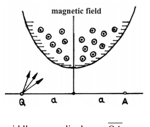
² Remark: This illustrative figure was not part of the original problem formulation.
Among different possible boundaries of magnetic fields a specific type shall be considered in which a contiguous magnetic field acts around the middle perpendicular and in which the points Q and A are in the field free area.
a) Describe the radius curvature \(R\) of the particle path in the magnetic field as a function of the voltage \(U\) and the induction \(B\).
b) Describe the characteristic properties of the particle paths in the setup mentioned above.
c) Obtain the boundaries of the magnetic field boundaries by geometrical constructions for the cases \(R<a\), \(R=a\) and \(R>0\).
d) Describe the general equation for the boundaries of the magnetic field.
Official English text of the problem.
Answers
Take the midpoint of \(QA\) as the origin, with \(Q=(-a,0)\), \(A=(a,0)\), and the illustrated beam above the \(x\)-axis.
-
a)
\[ \boxed{R=\frac{mv}{eB}=\frac{1}{B}\sqrt{\frac{2mU}{e}}.} \] -
b) Each trajectory consists of a straight incoming segment, a circular arc of radius \(R\), and a straight outgoing segment. The circle’s centre lies on the perpendicular bisector of \(QA\). If the initial direction makes an angle \(\theta\) with \(QA\), the magnetic deflection is \(2\theta\), and each straight segment has length \[ \boxed{\ell=\frac{a-R\sin\theta}{\cos\theta}.} \]
-
c) Construct the circle centre by intersecting the perpendicular bisector with a line parallel to the incoming ray, displaced by \(R\) towards the magnetic-force side. Its perpendicular foot on the ray is the entry point; reflection gives the exit point.
For the forward-going rays: \[ \begin{array}{c|c} \text{Case}&\text{Allowed angles with }\ell>0\\ \hline R<a&0<\theta<\pi/2\\ R=a&0<\theta<\pi/2\\ R>a&0<\theta<\arcsin(a/R) \end{array} \] For \(R<a\), the complete boundary branches have vertical asymptotes \(x=\pm R\). For \(R\ge a\), they have limiting endpoints at \(Q,A\); a finite angular aperture keeps those points strictly outside the field.
- d) The portions of the boundary traversed by the beam are \[ \boxed{ x=\pm R\sin\theta,\qquad y=(a-R\sin\theta)\tan\theta } \] or, equivalently, \[ \boxed{ y=\frac{|x|(a-|x|)}{\sqrt{R^2-x^2}}, \qquad 0\le |x|<\min(a,R). } \] Their implicit equation is \[ \boxed{(R^2-x^2)y^2=x^2(a-|x|)^2,} \] with the branch restrictions above.
Solution
a) Radius of curvature
Use the nonrelativistic approximation, neglect the ions’ initial kinetic energy before acceleration, and neglect interactions between ions. Acceleration through the potential difference \(U\) gives
\[ \frac12 mv^2=eU, \qquad v=\sqrt{\frac{2eU}{m}}. \]
The magnetic force is perpendicular to the velocity, so it changes the direction of motion without changing the speed. Inside the uniform field it supplies the centripetal force:
\[ evB=\frac{mv^2}{R}. \]
Consequently,
\[ \boxed{ R=\frac{mv}{eB} =\sqrt{\frac{2mU}{eB^2}}. } \]
Here \(B\) denotes the field magnitude. With SI inputs, \(R\) is in metres.
b) Geometry of the trajectories
Treat the field boundary as sharp, neglecting fringe fields. Let \(O\) be the midpoint of \(QA\), and choose
\[ Q=(-a,0),\qquad A=(a,0). \]
For the outward field direction illustrated, positive ions travelling upwards bend clockwise. Consider an initial direction
\[ \mathbf v=v(\cos\theta,\sin\theta), \qquad 0<\theta<\frac{\pi}{2}. \]
Let \(P\) be the entry point, \(P'\) the exit point, and \(C\) the centre of the circular arc.
Outside the field, the trajectory is straight. At a sharp boundary, the velocity remains continuous, so the straight and circular portions join tangentially. Symmetry about the \(y\)-axis requires \(P'\) to be the reflection of \(P\), and the circle centre must lie on that axis.
Writing \(QP=\ell\),
\[ P=(-a+\ell\cos\theta,\ \ell\sin\theta). \]
The radius from \(P\) towards \(C\) points in the magnetic-force direction:
\[ C-P=R(\sin\theta,-\cos\theta). \]
Since \(C_x=0\),
\[ -a+\ell\cos\theta+R\sin\theta=0, \]
and therefore
\[ \boxed{\ell=\frac{a-R\sin\theta}{\cos\theta}.} \]
It follows that
\[ P=\left(-R\sin\theta,\ (a-R\sin\theta)\tan\theta\right), \]
\[ P'=\left(R\sin\theta,\ (a-R\sin\theta)\tan\theta\right). \]
The centre is
\[ \boxed{ C=\left(0,\frac{a\sin\theta-R}{\cos\theta}\right). } \]
The outgoing velocity has direction \((\cos\theta,-\sin\theta)\). A straight segment of length \(\ell\) then carries the ion from \(P'\) to \(A\), because
\[ P'+\ell(\cos\theta,-\sin\theta)=(a,0). \]
The velocity thus turns through \(2\theta\) inside the field. The circular arc subtends the same angle at \(C\), and its chord has length
\[ PP'=2R\sin\theta. \]
c) Geometrical construction and the three regimes
For a chosen incoming direction, the construction is:
- Draw the ray from \(Q\).
- Draw a parallel line a perpendicular distance \(R\) away, on the side towards which the magnetic force bends the ion.
- Its intersection with the perpendicular bisector of \(QA\) is \(C\).
- Drop the perpendicular from \(C\) to the incoming ray. Its foot is \(P\).
- Reflect \(P\) in the perpendicular bisector to obtain \(P'\), and draw the clockwise circular arc of radius \(R\) joining them.
Varying the incoming direction traces the entrance boundary. Reflection traces the exit boundary. The perpendicular foot must lie ahead of \(Q\), so
\[ \ell>0 \quad\Longleftrightarrow\quad R\sin\theta<a. \]
For describing the shapes, put \(s=|x|\).
- \(R<a\).
Every acute incoming angle is admissible. As \(\theta\) increases from \(0\) towards \(\pi/2\), the boundary runs from \(O\) towards infinite height, approaching \[ \boxed{x=-R\quad\text{and}\quad x=R} \] on the two sides. Since \(a>R\), \(Q\) and \(A\) lie outside this strip.
Near \(O\), \[ y\sim\frac{a}{R}|x|, \] so the complete limiting locus has a pointed bottom.
The branches need not rise monotonically throughout. If \[ \frac{R}{a}>\sqrt{\frac{27}{32}}, \] each branch has a local maximum followed by a local minimum before rising towards its asymptote. Otherwise it rises monotonically. These features follow from the derivative given in part (d).
- \(R=a\).
The construction works for every acute angle, and \[ y=s\sqrt{\frac{a-s}{a+s}}, \qquad 0\le s<a. \] Each branch starts at \(O\), rises to a maximum, and returns towards the corresponding source or image point as \(\theta\to\pi/2\).
The maximum occurs at \[ s=\frac{\sqrt5-1}{2}\,a, \] with height \[ y_{\max} =a\left(\frac{\sqrt5-1}{2}\right)^{5/2} \approx0.3003a. \]
The limiting circular trajectory is the upper semicircle of radius \(a\) centred at \(O\), with endpoints \(Q,A\).
- \(R>a\) — the likely intended third case.
The construction requires \[ 0<\theta<\alpha,\qquad \boxed{\alpha=\arcsin(a/R)}. \] Geometrically, \(\alpha\) is obtained from a right triangle with hypotenuse \(R\) and opposite side \(a\).
Each boundary branch starts at \(O\), rises to one maximum, and returns towards \(Q\) or \(A\) as \(\theta\to\alpha\). At that limit, \(\ell\to0\), and the circular trajectory has centre \[ C=\left(0,-\sqrt{R^2-a^2}\right). \] Its highest point is \[ y=R-\sqrt{R^2-a^2}. \]
For \(R\ge a\), using the complete limiting locus would put \(Q,A\) on the field boundary. To keep them strictly within field-free areas, choose a beam whose maximum angle is strictly below the limiting value. Continue the unused boundary around its trajectories; for example, close the field above them with a circular arc constructed for a slightly larger admissible angle. The resulting field is connected and remains separated from \(Q,A\).
Only boundary portions actually crossed by the beam are fixed by the focusing condition.
d) General boundary equation
From part (b),
\[ s=R\sin\theta, \qquad y=(a-s)\tan\theta. \]
For the acute-angle branch,
\[ \tan\theta=\frac{s}{\sqrt{R^2-s^2}}. \]
Eliminating \(\theta\) gives
\[ \boxed{ y=f(s)=\frac{s(a-s)}{\sqrt{R^2-s^2}}, \qquad s=|x|,\quad 0\le s<\min(a,R). } \]
Hence
\[ \boxed{(R^2-x^2)y^2=x^2(a-|x|)^2.} \]
The unsquared expression and domain select the physical upper boundary. Squaring alone also admits other branches.
For completeness, differentiating gives
\[ f'(s)= \frac{s^3-2R^2s+aR^2}{(R^2-s^2)^{3/2}}. \]
Thus all stationary heights mentioned in part (c) satisfy
\[ \boxed{s^3-2R^2s+aR^2=0.} \]
For \(R>a\), this equation has exactly one root in \(0<s<a\), giving the maximum of each branch.
We can also verify that the constructed boundary keeps each trajectory in the appropriate region. Write the centre height for entry coordinate \(s\) as
\[ c(s)=f(s)-\sqrt{R^2-s^2} =\frac{as-R^2}{\sqrt{R^2-s^2}}. \]
Then
\[ c'(s)= \frac{R^2(a-s)}{(R^2-s^2)^{3/2}}>0. \]
An ion entering at \(s=s_0\) follows the upper circular arc
\[ y_{\rm arc}(s)=c(s_0)+\sqrt{R^2-s^2}, \qquad 0\le s\le s_0. \]
For \(s<s_0\), monotonicity of \(c(s)\) gives
\[ y_{\rm arc}(s)>c(s)+\sqrt{R^2-s^2}=f(s). \]
Thus the circular portion lies above the entrance and exit boundaries, inside the field. Before entry, the incoming line lies below the boundary because
\[ y_{\rm line}(s)=(a-s)\tan\theta < (a-s)\frac{s}{\sqrt{R^2-s^2}} =f(s) \]
for \(s>s_0\) in the boundary’s domain. Reflection establishes the same result after exit. The boundary therefore produces the required focusing.
The solution was checked against the official solution.
IPhO 1975 · Theorieaufgabe 3
Ionen in einem Magnetfeld
Ein Strahl positiver Ionen (Ladung \(+e\)) gleicher und konstanter Masse \(m\) breitet sich vom Punkt Q aus in verschiedenen Richtungen in der Papierebene aus (siehe Abbildung²). Die Ionen wurden durch eine Spannung \(U\) beschleunigt. Sie werden in einem homogenen Magnetfeld \(B\) abgelenkt, das senkrecht zur Papierebene steht. Die Grenzen des Magnetfeldes sind so gestaltet, dass die zunächst auseinanderlaufenden Ionen im Punkt A fokussiert werden (\(\overline{QA}=2\cdot a\)). Die Bahnen der Ionen sind symmetrisch bezüglich der Mittelsenkrechten auf \(\overline{QA}\).
² Anmerkung: Diese veranschaulichende Abbildung war nicht Bestandteil der ursprünglichen Aufgabenstellung.
Unter den verschiedenen möglichen Begrenzungen von Magnetfeldern soll ein bestimmter Typ betrachtet werden, bei dem ein zusammenhängendes Magnetfeld um die Mittelsenkrechte herum wirkt und die Punkte Q und A im feldfreien Bereich liegen.
a) Geben Sie den Krümmungsradius \(R\) der Teilchenbahn im Magnetfeld als Funktion der Spannung \(U\) und der magnetischen Flussdichte \(B\) an.
b) Beschreiben Sie die charakteristischen Eigenschaften der Teilchenbahnen in der oben genannten Anordnung.
c) Bestimmen Sie die Grenzen des Magnetfeldes durch geometrische Konstruktionen für die Fälle \(R<a\), \(R=a\) und \(R>0\).
d) Geben Sie die allgemeine Gleichung für die Grenzen des Magnetfeldes an.
Aufgabentext aus dem offiziellen englischen Text übersetzt.
Antworten
Wählen wir den Mittelpunkt von \(QA\) als Ursprung, mit \(Q=(-a,0)\), \(A=(a,0)\) und dem dargestellten Strahl oberhalb der \(x\)-Achse.
-
a)
\[ \boxed{R=\frac{mv}{eB}=\frac{1}{B}\sqrt{\frac{2mU}{e}}.} \] -
b) Jede Bahn besteht aus einem geraden einlaufenden Abschnitt, einem Kreisbogen mit Radius \(R\) und einem geraden auslaufenden Abschnitt. Der Kreismittelpunkt liegt auf der Mittelsenkrechten von \(QA\). Schließt die Anfangsrichtung mit \(QA\) einen Winkel \(\theta\) ein, so beträgt die magnetische Ablenkung \(2\theta\), und jeder gerade Abschnitt hat die Länge \[ \boxed{\ell=\frac{a-R\sin\theta}{\cos\theta}.} \]
-
c) Konstruieren Sie den Kreismittelpunkt als Schnittpunkt der Mittelsenkrechten mit einer Parallelen zum einlaufenden Strahl, die um \(R\) in Richtung der magnetischen Kraft versetzt ist. Der Lotfußpunkt auf dem Strahl ist der Eintrittspunkt; durch Spiegelung erhält man den Austrittspunkt.
Für die vorwärts gerichteten Strahlen: \[ \begin{array}{c|c} \text{Fall}&\text{Zulässige Winkel mit }\ell>0\\ \hline R<a&0<\theta<\pi/2\\ R=a&0<\theta<\pi/2\\ R>a&0<\theta<\arcsin(a/R) \end{array} \] Für \(R<a\) haben die vollständigen Grenzkurvenäste die senkrechten Asymptoten \(x=\pm R\). Für \(R\ge a\) haben sie Grenzendpunkte bei \(Q,A\); eine endliche Winkelöffnung hält diese Punkte strikt außerhalb des Feldes.
- d) Die vom Strahl durchquerten Abschnitte der Grenze sind \[ \boxed{ x=\pm R\sin\theta,\qquad y=(a-R\sin\theta)\tan\theta } \] oder gleichwertig \[ \boxed{ y=\frac{|x|(a-|x|)}{\sqrt{R^2-x^2}}, \qquad 0\le |x|<\min(a,R). } \] Ihre implizite Gleichung lautet \[ \boxed{(R^2-x^2)y^2=x^2(a-|x|)^2,} \] mit den oben angegebenen Einschränkungen für die Äste.
Lösung
a) Krümmungsradius
Wir verwenden die nichtrelativistische Näherung, vernachlässigen die anfängliche kinetische Energie der Ionen vor der Beschleunigung und vernachlässigen Wechselwirkungen zwischen den Ionen. Die Beschleunigung durch die Potentialdifferenz \(U\) ergibt
\[ \frac12 mv^2=eU, \qquad v=\sqrt{\frac{2eU}{m}}. \]
Die magnetische Kraft steht senkrecht zur Geschwindigkeit und ändert daher die Bewegungsrichtung, ohne den Geschwindigkeitsbetrag zu ändern. Innerhalb des homogenen Feldes liefert sie die Zentripetalkraft:
\[ evB=\frac{mv^2}{R}. \]
Folglich gilt
\[ \boxed{ R=\frac{mv}{eB} =\sqrt{\frac{2mU}{eB^2}}. } \]
Hier bezeichnet \(B\) den Betrag der magnetischen Flussdichte. Werden die Größen in SI-Einheiten eingesetzt, ergibt sich \(R\) in Metern.
b) Geometrie der Bahnen
Wir behandeln die Feldgrenze als scharf und vernachlässigen Randfelder. Sei \(O\) der Mittelpunkt von \(QA\), und wir wählen
\[ Q=(-a,0),\qquad A=(a,0). \]
Bei der dargestellten, aus der Papierebene heraus gerichteten Feldrichtung werden positive Ionen, die sich nach oben bewegen, im Uhrzeigersinn abgelenkt. Wir betrachten die Anfangsrichtung
\[ \mathbf v=v(\cos\theta,\sin\theta), \qquad 0<\theta<\frac{\pi}{2}. \]
Seien \(P\) der Eintrittspunkt, \(P'\) der Austrittspunkt und \(C\) der Mittelpunkt des Kreisbogens.
Außerhalb des Feldes verläuft die Bahn geradlinig. An einer scharfen Grenze bleibt die Geschwindigkeit stetig, sodass die geraden und kreisförmigen Abschnitte tangential ineinander übergehen. Die Symmetrie bezüglich der \(y\)-Achse erfordert, dass \(P'\) das Spiegelbild von \(P\) ist, und der Kreismittelpunkt muss auf dieser Achse liegen.
Mit \(QP=\ell\) gilt
\[ P=(-a+\ell\cos\theta,\ \ell\sin\theta). \]
Der Radiusvektor von \(P\) nach \(C\) zeigt in Richtung der magnetischen Kraft:
\[ C-P=R(\sin\theta,-\cos\theta). \]
Da \(C_x=0\), gilt
\[ -a+\ell\cos\theta+R\sin\theta=0, \]
und somit
\[ \boxed{\ell=\frac{a-R\sin\theta}{\cos\theta}.} \]
Daraus folgt
\[ P=\left(-R\sin\theta,\ (a-R\sin\theta)\tan\theta\right), \]
\[ P'=\left(R\sin\theta,\ (a-R\sin\theta)\tan\theta\right). \]
Der Mittelpunkt ist
\[ \boxed{ C=\left(0,\frac{a\sin\theta-R}{\cos\theta}\right). } \]
Die austretende Geschwindigkeit hat die Richtung \((\cos\theta,-\sin\theta)\). Ein gerader Abschnitt der Länge \(\ell\) führt das Ion dann von \(P'\) nach \(A\), denn
\[ P'+\ell(\cos\theta,-\sin\theta)=(a,0). \]
Die Geschwindigkeit dreht sich innerhalb des Feldes somit um \(2\theta\). Der Kreisbogen überstreicht bei \(C\) denselben Mittelpunktswinkel, und seine Sehne hat die Länge
\[ PP'=2R\sin\theta. \]
c) Geometrische Konstruktion und die drei Fälle
Für eine gewählte Einfallsrichtung erfolgt die Konstruktion so:
- Zeichnen Sie den von \(Q\) ausgehenden Strahl.
- Zeichnen Sie eine parallele Gerade im senkrechten Abstand \(R\) auf der Seite, zu der die magnetische Kraft das Ion ablenkt.
- Ihr Schnittpunkt mit der Mittelsenkrechten von \(QA\) ist \(C\).
- Fällen Sie das Lot von \(C\) auf den einlaufenden Strahl. Sein Fußpunkt ist \(P\).
- Spiegeln Sie \(P\) an der Mittelsenkrechten, um \(P'\) zu erhalten, und zeichnen Sie den im Uhrzeigersinn durchlaufenen Kreisbogen mit Radius \(R\), der beide Punkte verbindet.
Durch Variation der Einfallsrichtung erhält man die Eintrittsgrenze. Durch Spiegelung erhält man die Austrittsgrenze. Der Lotfußpunkt muss in Strahlrichtung vor \(Q\) liegen, also gilt
\[ \ell>0 \quad\Longleftrightarrow\quad R\sin\theta<a. \]
Zur Beschreibung der Formen setzen wir \(s=|x|\).
- \(R<a\).
Jeder spitze Einfallswinkel ist zulässig. Wenn \(\theta\) von \(0\) aus gegen \(\pi/2\) wächst, verläuft die Grenze von \(O\) aus zu unendlicher Höhe und nähert sich auf den beiden Seiten \[ \boxed{x=-R\quad\text{und}\quad x=R} \] an. Da \(a>R\), liegen \(Q\) und \(A\) außerhalb dieses Streifens.
In der Nähe von \(O\) gilt \[ y\sim\frac{a}{R}|x|, \] sodass die vollständige Grenzkurve unten eine Spitze besitzt.
Die Äste müssen nicht durchgehend monoton ansteigen. Falls \[ \frac{R}{a}>\sqrt{\frac{27}{32}}, \] besitzt jeder Ast zunächst ein lokales Maximum und anschließend ein lokales Minimum, bevor er zu seiner Asymptote hin ansteigt. Andernfalls steigt er monoton an. Diese Eigenschaften folgen aus der in Teil (d) angegebenen Ableitung.
- \(R=a\).
Die Konstruktion funktioniert für jeden spitzen Winkel, und es gilt \[ y=s\sqrt{\frac{a-s}{a+s}}, \qquad 0\le s<a. \] Jeder Ast beginnt bei \(O\), steigt bis zu einem Maximum an und kehrt für \(\theta\to\pi/2\) zum jeweiligen Quell- oder Bildpunkt zurück.
Das Maximum liegt bei \[ s=\frac{\sqrt5-1}{2}\,a, \] mit der Höhe \[ y_{\max} =a\left(\frac{\sqrt5-1}{2}\right)^{5/2} \approx0.3003a. \]
Die kreisförmige Grenzbahn ist der obere Halbkreis mit Radius \(a\) und Mittelpunkt \(O\), dessen Endpunkte \(Q,A\) sind.
- \(R>a\) — der vermutlich beabsichtigte dritte Fall.
Die Konstruktion erfordert \[ 0<\theta<\alpha,\qquad \boxed{\alpha=\arcsin(a/R)}. \] Geometrisch erhält man \(\alpha\) aus einem rechtwinkligen Dreieck mit Hypotenuse \(R\) und Gegenkathete \(a\).
Jeder Grenzkurvenast beginnt bei \(O\), steigt bis zu einem einzigen Maximum an und kehrt für \(\theta\to\alpha\) zu \(Q\) oder \(A\) zurück. In diesem Grenzfall gilt \(\ell\to0\), und die Kreisbahn hat den Mittelpunkt \[ C=\left(0,-\sqrt{R^2-a^2}\right). \] Ihr höchster Punkt liegt bei \[ y=R-\sqrt{R^2-a^2}. \]
Für \(R\ge a\) würden \(Q,A\) bei Verwendung der vollständigen Grenzkurve auf der Feldgrenze liegen. Damit sie strikt innerhalb feldfreier Bereiche bleiben, wählen wir einen Strahl, dessen maximaler Winkel strikt unter dem Grenzwert liegt. Wir führen den nicht genutzten Teil der Grenze um seine Bahnen herum weiter; beispielsweise schließen wir das Feld oberhalb dieser Bahnen mit einem Kreisbogen ab, der für einen etwas größeren zulässigen Winkel konstruiert wird. Das resultierende Feld ist zusammenhängend und bleibt von \(Q,A\) getrennt.
Nur diejenigen Grenzabschnitte, die der Strahl tatsächlich durchquert, sind durch die Fokussierungsbedingung festgelegt.
d) Allgemeine Gleichung der Grenze
Aus Teil (b) folgt
\[ s=R\sin\theta, \qquad y=(a-s)\tan\theta. \]
Für den Ast mit spitzen Winkeln gilt
\[ \tan\theta=\frac{s}{\sqrt{R^2-s^2}}. \]
Eliminieren von \(\theta\) ergibt
\[ \boxed{ y=f(s)=\frac{s(a-s)}{\sqrt{R^2-s^2}}, \qquad s=|x|,\quad 0\le s<\min(a,R). } \]
Somit gilt
\[ \boxed{(R^2-x^2)y^2=x^2(a-|x|)^2.} \]
Der nicht quadrierte Ausdruck und der Definitionsbereich wählen die physikalisch relevante obere Grenzkurve aus. Durch das Quadrieren allein werden auch andere Äste zugelassen.
Der Vollständigkeit halber ergibt die Ableitung
\[ f'(s)= \frac{s^3-2R^2s+aR^2}{(R^2-s^2)^{3/2}}. \]
Somit erfüllen alle in Teil (c) erwähnten stationären Höhen die Gleichung
\[ \boxed{s^3-2R^2s+aR^2=0.} \]
Für \(R>a\) hat diese Gleichung genau eine Nullstelle in \(0<s<a\), die das Maximum jedes Astes liefert.
Wir können auch überprüfen, dass die konstruierte Grenze jede Bahn im jeweils richtigen Bereich hält. Wir schreiben die Höhe des Kreismittelpunkts für die Eintrittskoordinate \(s\) als
\[ c(s)=f(s)-\sqrt{R^2-s^2} =\frac{as-R^2}{\sqrt{R^2-s^2}}. \]
Dann gilt
\[ c'(s)= \frac{R^2(a-s)}{(R^2-s^2)^{3/2}}>0. \]
Ein bei \(s=s_0\) eintretendes Ion folgt dem oberen Kreisbogen
\[ y_{\rm arc}(s)=c(s_0)+\sqrt{R^2-s^2}, \qquad 0\le s\le s_0. \]
Für \(s<s_0\) ergibt die Monotonie von \(c(s)\)
\[ y_{\rm arc}(s)>c(s)+\sqrt{R^2-s^2}=f(s). \]
Somit liegt der kreisförmige Abschnitt oberhalb der Eintritts- und Austrittsgrenzen, also innerhalb des Feldes. Vor dem Eintritt liegt die einlaufende Gerade unterhalb der Grenze, denn
\[ y_{\rm line}(s)=(a-s)\tan\theta < (a-s)\frac{s}{\sqrt{R^2-s^2}} =f(s) \]
gilt für \(s>s_0\) im Definitionsbereich der Grenze. Durch Spiegelung erhält man dasselbe Ergebnis nach dem Austritt. Die Grenze bewirkt somit die geforderte Fokussierung.
Die Lösung wurde mit der offiziellen Lösung abgeglichen.
IPhO 1975 · Teori sorusu 3
Manyetik alandaki iyonlar
Aynı ve sabit \(m\) kütlesine sahip pozitif iyonlardan (yükleri \(+e\)) oluşan bir demet, Q noktasından kâğıt düzleminde farklı yönlere yayılmaktadır (şekle² bakınız). İyonlar \(U\) gerilimiyle hızlandırılmıştır. Kâğıt düzlemine dik olan düzgün bir \(B\) manyetik alanında saptırılırlar. Manyetik alanın sınırları, başlangıçta birbirinden uzaklaşan iyonlar A noktasında odaklanacak şekilde düzenlenmiştir (\(\overline{QA}=2\cdot a\)). İyonların yörüngeleri, \(\overline{QA}\) doğru parçasının orta dikmesine göre simetriktir.
² Not: Açıklama amacıyla verilen bu şekil, özgün soru metninde yer almamaktadır.
Manyetik alan sınırlarının mümkün olan farklı biçimleri arasından, orta dikmenin çevresinde kesintisiz bir manyetik alanın bulunduğu ve Q ile A noktalarının alanın bulunmadığı bölgede kaldığı belirli bir tür ele alınacaktır.
a) Parçacığın manyetik alandaki yörüngesinin eğrilik yarıçapı \(R\)'yi, \(U\) geriliminin ve \(B\) manyetik indüksiyonunun fonksiyonu olarak ifade ediniz.
b) Yukarıda belirtilen düzenekte parçacık yörüngelerinin karakteristik özelliklerini açıklayınız.
c) \(R<a\), \(R=a\) ve \(R>0\) durumları için manyetik alanın sınırlarını geometrik çizimlerle elde ediniz.
d) Manyetik alanın sınırlarının genel denklemini ifade ediniz.
Soru metni resmi İngilizce metinden çevrilmiştir.
Cevaplar
\(QA\)'nın orta noktasını başlangıç noktası alınız; \(Q=(-a,0)\), \(A=(a,0)\) olsun ve şekilde gösterilen demet \(x\) ekseninin üstünde bulunsun.
-
a)
\[ \boxed{R=\frac{mv}{eB}=\frac{1}{B}\sqrt{\frac{2mU}{e}}.} \] -
b) Her yörünge, doğrusal bir giriş parçasından, \(R\) yarıçaplı bir çember yayından ve doğrusal bir çıkış parçasından oluşur. Çemberin merkezi \(QA\)'nın orta dikmesi üzerinde bulunur. Başlangıç doğrultusu \(QA\) ile \(\theta\) açısı yapıyorsa manyetik sapma \(2\theta\) olur ve her bir doğrusal parçanın uzunluğu \[ \boxed{\ell=\frac{a-R\sin\theta}{\cos\theta}.} \] ile verilir.
-
c) Gelen ışına paralel ve manyetik kuvvet yönündeki tarafa doğru \(R\) kadar ötelenmiş bir doğruyu orta dikmeyle kesiştirerek çember merkezini bulunuz. Bu merkezden ışına indirilen dikmenin ayağı giriş noktasıdır; simetriği ise çıkış noktasını verir.
İleri yönde giden ışınlar için: \[ \begin{array}{c|c} \text{Durum}&\text{İzin verilen açılar, }\ell>0\\ \hline R<a&0<\theta<\pi/2\\ R=a&0<\theta<\pi/2\\ R>a&0<\theta<\arcsin(a/R) \end{array} \] \(R<a\) için sınır dallarının tamamının düşey asimptotları \(x=\pm R\)'dir. \(R\ge a\) için bu dalların limit uç noktaları \(Q,A\)'dır; sonlu bir açısal açıklık bu noktaları kesin olarak alanın dışında tutar.
- d) Sınırın demet tarafından geçilen kısımları \[ \boxed{ x=\pm R\sin\theta,\qquad y=(a-R\sin\theta)\tan\theta } \] veya eşdeğer olarak \[ \boxed{ y=\frac{|x|(a-|x|)}{\sqrt{R^2-x^2}}, \qquad 0\le |x|<\min(a,R). } \] ile verilir. Yukarıdaki dal kısıtlamaları altında bunların kapalı denklemi \[ \boxed{(R^2-x^2)y^2=x^2(a-|x|)^2,} \] biçimindedir.
Çözüm
a) Eğrilik yarıçapı
Göreli olmayan yaklaşımı kullanıp iyonların hızlandırılmadan önceki başlangıç kinetik enerjilerini ve iyonlar arasındaki etkileşimleri ihmal edelim. \(U\) potansiyel farkı altında hızlandırma sonucunda
\[ \frac12 mv^2=eU, \qquad v=\sqrt{\frac{2eU}{m}}. \]
elde edilir. Manyetik kuvvet hıza diktir; dolayısıyla sürati değiştirmeden hareketin yönünü değiştirir. Düzgün alanın içinde merkezcil kuvveti sağlar:
\[ evB=\frac{mv^2}{R}. \]
Böylece,
\[ \boxed{ R=\frac{mv}{eB} =\sqrt{\frac{2mU}{eB^2}}. } \]
Burada \(B\), alanın büyüklüğünü gösterir. Girdi değerleri SI birimleriyle verildiğinde \(R\) metre cinsindendir.
b) Yörüngelerin geometrisi
Saçak alanlarını ihmal ederek alan sınırını keskin kabul edelim. \(O\), \(QA\)'nın orta noktası olsun ve
\[ Q=(-a,0),\qquad A=(a,0). \]
seçelim. Şekilde gösterilen, kâğıt düzleminden dışarıya doğru alan yönü için yukarı doğru hareket eden pozitif iyonlar saat yönünde kıvrılır. Şu başlangıç doğrultusunu ele alalım:
\[ \mathbf v=v(\cos\theta,\sin\theta), \qquad 0<\theta<\frac{\pi}{2}. \]
Giriş noktası \(P\), çıkış noktası \(P'\) ve çember yayının merkezi \(C\) olsun.
Alanın dışında yörünge doğrusaldır. Keskin bir sınırda hız sürekliliğini korur; bu nedenle doğrusal ve çembersel kısımlar teğet olarak birleşir. \(y\) eksenine göre simetri, \(P'\)'nün \(P\)'nin simetriği olmasını gerektirir ve çember merkezi bu eksen üzerinde bulunmalıdır.
\(QP=\ell\) yazarsak,
\[ P=(-a+\ell\cos\theta,\ \ell\sin\theta). \]
\(P\)'den \(C\)'ye doğru yönelen yarıçap, manyetik kuvvet yönündedir:
\[ C-P=R(\sin\theta,-\cos\theta). \]
\(C_x=0\) olduğundan,
\[ -a+\ell\cos\theta+R\sin\theta=0, \]
ve dolayısıyla
\[ \boxed{\ell=\frac{a-R\sin\theta}{\cos\theta}.} \]
Buradan
\[ P=\left(-R\sin\theta,\ (a-R\sin\theta)\tan\theta\right), \]
\[ P'=\left(R\sin\theta,\ (a-R\sin\theta)\tan\theta\right). \]
elde edilir. Merkez ise
\[ \boxed{ C=\left(0,\frac{a\sin\theta-R}{\cos\theta}\right). } \]
ile verilir. Çıkış hızının yönü \((\cos\theta,-\sin\theta)\)'dır. Ardından \(\ell\) uzunluğundaki doğrusal bir parça iyonu \(P'\)'den \(A\)'ya götürür; çünkü
\[ P'+\ell(\cos\theta,-\sin\theta)=(a,0). \]
Böylece hız vektörü alanın içinde \(2\theta\) kadar döner. Çember yayı \(C\) merkezinde aynı açıyı görür ve kirişinin uzunluğu
\[ PP'=2R\sin\theta. \]
olur.
c) Geometrik çizim ve üç rejim
Seçilen bir geliş doğrultusu için çizim şu şekilde yapılır:
- \(Q\)'dan çıkan ışını çiziniz.
- Manyetik kuvvetin iyonu büktüğü tarafta, dik uzaklığı \(R\) olan paralel bir doğru çiziniz.
- Bu doğrunun \(QA\)'nın orta dikmesiyle kesişimi \(C\)'dir.
- \(C\)'den gelen ışına dikme indiriniz. Dikmenin ayağı \(P\)'dir.
- \(P\)'nin orta dikmeye göre simetriğini alarak \(P'\)'nü elde ediniz ve bu noktaları birleştiren, saat yönündeki \(R\) yarıçaplı çember yayını çiziniz.
Geliş doğrultusu değiştirildiğinde giriş sınırı çizilir. Simetri alınarak çıkış sınırı çizilir. Dikmenin ayağı \(Q\)'nun ilerisinde olmalıdır; dolayısıyla
\[ \ell>0 \quad\Longleftrightarrow\quad R\sin\theta<a. \]
Şekilleri betimlemek için \(s=|x|\) alalım.
- \(R<a\).
Her dar geliş açısına izin verilir. \(\theta\), \(0\)'dan \(\pi/2\)'ye doğru arttıkça sınır \(O\)'dan sonsuz yüksekliğe doğru uzanır ve iki tarafta \[ \boxed{x=-R\quad\text{ve}\quad x=R} \] doğrularına yaklaşır. \(a>R\) olduğundan \(Q\) ve \(A\) bu şeridin dışında kalır.
\(O\) yakınında, \[ y\sim\frac{a}{R}|x|, \] olduğundan limitteki geometrik yerin tamamının alt kısmı sivridir.
Dalların tümü boyunca monoton olarak yükselmesi gerekmez. Eğer \[ \frac{R}{a}>\sqrt{\frac{27}{32}}, \] ise her dal, asimptotuna doğru yükselmeden önce bir yerel maksimuma, ardından bir yerel minimuma sahiptir. Aksi hâlde monoton olarak yükselir. Bu özellikler (d) kısmında verilen türevden çıkar.
- \(R=a\).
Çizim her dar açı için geçerlidir ve \[ y=s\sqrt{\frac{a-s}{a+s}}, \qquad 0\le s<a. \] olur. Her dal \(O\)'dan başlar, bir maksimuma kadar yükselir ve \(\theta\to\pi/2\) iken karşılık gelen kaynak veya görüntü noktasına doğru geri döner.
Maksimum, \[ s=\frac{\sqrt5-1}{2}\,a, \] konumunda oluşur ve yüksekliği \[ y_{\max} =a\left(\frac{\sqrt5-1}{2}\right)^{5/2} \approx0.3003a. \] olur.
Limitteki çembersel yörünge, merkezi \(O\), yarıçapı \(a\) ve uç noktaları \(Q,A\) olan üst yarım çemberdir.
- \(R>a\) — muhtemelen kastedilen üçüncü durum.
Çizim için \[ 0<\theta<\alpha,\qquad \boxed{\alpha=\arcsin(a/R)}. \] koşulu gerekir. Geometrik olarak \(\alpha\), hipotenüsü \(R\), karşı kenarı \(a\) olan bir dik üçgenden elde edilir.
Her sınır dalı \(O\)'dan başlar, tek bir maksimuma kadar yükselir ve \(\theta\to\alpha\) iken \(Q\) veya \(A\)'ya doğru geri döner. Bu limitte \(\ell\to0\) olur ve çembersel yörüngenin merkezi \[ C=\left(0,-\sqrt{R^2-a^2}\right). \] ile verilir. En yüksek noktası \[ y=R-\sqrt{R^2-a^2}. \] yüksekliğindedir.
\(R\ge a\) için limitteki geometrik yerin tamamını kullanmak, \(Q,A\)'yı alan sınırı üzerine yerleştirir. Bu noktaları kesin olarak alanın bulunmadığı bölgelerin içinde tutmak için maksimum açısı limit değerden kesin olarak küçük olan bir demet seçiniz. Sınırın kullanılmayan kısmını demetin yörüngelerinin çevresinde devam ettiriniz; örneğin, izin verilen biraz daha büyük bir açı için çizilen bir çember yayıyla alanı yörüngelerin üstünden kapatınız. Ortaya çıkan alan bağlantılıdır ve \(Q,A\)'dan ayrı kalır.
Odaklama koşulu yalnızca sınırın demet tarafından gerçekten geçilen kısımlarını belirler.
d) Genel sınır denklemi
(b) kısmından,
\[ s=R\sin\theta, \qquad y=(a-s)\tan\theta. \]
Dar açılara karşılık gelen dal için,
\[ \tan\theta=\frac{s}{\sqrt{R^2-s^2}}. \]
\(\theta\) yok edilirse
\[ \boxed{ y=f(s)=\frac{s(a-s)}{\sqrt{R^2-s^2}}, \qquad s=|x|,\quad 0\le s<\min(a,R). } \]
elde edilir. Dolayısıyla
\[ \boxed{(R^2-x^2)y^2=x^2(a-|x|)^2.} \]
Karesi alınmamış ifade ve tanım aralığı, fiziksel üst sınırı seçer. Yalnızca kare alma işlemi başka dallara da izin verir.
Tamamlayıcı olarak, türev alındığında
\[ f'(s)= \frac{s^3-2R^2s+aR^2}{(R^2-s^2)^{3/2}}. \]
elde edilir. Böylece (c) kısmında sözü edilen tüm durağan yükseklikler
\[ \boxed{s^3-2R^2s+aR^2=0.} \]
koşulunu sağlar.
\(R>a\) için bu denklemin \(0<s<a\) aralığında tam olarak bir kökü vardır ve bu kök her dalın maksimumunu verir.
Çizilen sınırın her yörüngeyi uygun bölgede tuttuğunu da doğrulayabiliriz. Giriş koordinatı \(s\) için merkez yüksekliğini
\[ c(s)=f(s)-\sqrt{R^2-s^2} =\frac{as-R^2}{\sqrt{R^2-s^2}}. \]
olarak yazalım. O hâlde
\[ c'(s)= \frac{R^2(a-s)}{(R^2-s^2)^{3/2}}>0. \]
\(s=s_0\) konumunda giren bir iyon, üst çember yayını izler:
\[ y_{\rm arc}(s)=c(s_0)+\sqrt{R^2-s^2}, \qquad 0\le s\le s_0. \]
\(s<s_0\) için \(c(s)\)'nin monotonluğundan
\[ y_{\rm arc}(s)>c(s)+\sqrt{R^2-s^2}=f(s). \]
elde edilir. Böylece çembersel kısım, giriş ve çıkış sınırlarının üstünde, alanın içinde kalır. Girişten önce gelen doğru sınırın altında kalır; çünkü sınırın tanım aralığında \(s>s_0\) için
\[ y_{\rm line}(s)=(a-s)\tan\theta < (a-s)\frac{s}{\sqrt{R^2-s^2}} =f(s) \]
olur. Simetri, çıkıştan sonra da aynı sonucun geçerli olduğunu gösterir. Dolayısıyla sınır, gerekli odaklamayı sağlar.
Çözüm, resmi çözümle karşılaştırılarak kontrol edildi.
IPhO 1975 · Problema teórico 3
Iones en un campo magnético
Un haz de iones positivos (carga \(+e\)) de la misma masa constante \(m\) se propaga desde el punto Q en distintas direcciones en el plano del papel (véase la figura²). Los iones han sido acelerados mediante una tensión \(U\). Se desvían en un campo magnético uniforme \(B\) perpendicular al plano del papel. Los límites del campo magnético están dispuestos de manera que los iones, inicialmente divergentes, se enfocan en el punto A (\(\overline{QA}=2\cdot a\)). Las trayectorias de los iones son simétricas respecto de la mediatriz de \(\overline{QA}\).
² Observación: Esta figura ilustrativa no formaba parte del enunciado original del problema.
Entre los distintos límites posibles del campo magnético, se considerará un tipo específico en el que un campo magnético contiguo actúa en torno a la mediatriz y los puntos Q y A se encuentran en la región libre de campo.
a) Exprese el radio de curvatura \(R\) de la trayectoria de la partícula en el campo magnético en función de la tensión \(U\) y de la inducción magnética \(B\).
b) Describa las propiedades características de las trayectorias de las partículas en la configuración mencionada anteriormente.
c) Obtenga los límites del campo magnético mediante construcciones geométricas para los casos \(R<a\), \(R=a\) y \(R>0\).
d) Describa la ecuación general de los límites del campo magnético.
Enunciado traducido del texto oficial en inglés.
Respuestas
Tómese el punto medio de \(QA\) como origen, con \(Q=(-a,0)\), \(A=(a,0)\) y el haz representado por encima del eje \(x\).
-
a)
\[ \boxed{R=\frac{mv}{eB}=\frac{1}{B}\sqrt{\frac{2mU}{e}}.} \] -
b) Cada trayectoria consta de un tramo rectilíneo de entrada, un arco de circunferencia de radio \(R\) y un tramo rectilíneo de salida. El centro de la circunferencia se encuentra en la mediatriz de \(QA\). Si la dirección inicial forma un ángulo \(\theta\) con \(QA\), la desviación magnética es \(2\theta\), y cada tramo rectilíneo tiene una longitud \[ \boxed{\ell=\frac{a-R\sin\theta}{\cos\theta}.} \]
-
c) Construya el centro de la circunferencia como la intersección de la mediatriz con una recta paralela al rayo incidente, desplazada una distancia \(R\) hacia el lado de la fuerza magnética. El pie de la perpendicular trazada desde el centro al rayo es el punto de entrada; la reflexión proporciona el punto de salida.
Para los rayos que avanzan hacia delante: \[ \begin{array}{c|c} \text{Caso}&\text{Ángulos permitidos con }\ell>0\\ \hline R<a&0<\theta<\pi/2\\ R=a&0<\theta<\pi/2\\ R>a&0<\theta<\arcsin(a/R) \end{array} \] Para \(R<a\), las ramas completas del límite tienen asíntotas verticales \(x=\pm R\). Para \(R\ge a\), tienen extremos límite en \(Q,A\); una apertura angular finita mantiene esos puntos estrictamente fuera del campo.
- d) Las porciones del límite atravesadas por el haz son \[ \boxed{ x=\pm R\sin\theta,\qquad y=(a-R\sin\theta)\tan\theta } \] o, de forma equivalente, \[ \boxed{ y=\frac{|x|(a-|x|)}{\sqrt{R^2-x^2}}, \qquad 0\le |x|<\min(a,R). } \] Su ecuación implícita es \[ \boxed{(R^2-x^2)y^2=x^2(a-|x|)^2,} \] con las restricciones de rama anteriores.
Solución
a) Radio de curvatura
Se utiliza la aproximación no relativista, se desprecia la energía cinética inicial de los iones antes de la aceleración y se desprecian las interacciones entre iones. La aceleración mediante la diferencia de potencial \(U\) da
\[ \frac12 mv^2=eU, \qquad v=\sqrt{\frac{2eU}{m}}. \]
La fuerza magnética es perpendicular a la velocidad, por lo que cambia la dirección del movimiento sin modificar la rapidez. Dentro del campo uniforme, proporciona la fuerza centrípeta:
\[ evB=\frac{mv^2}{R}. \]
Por consiguiente,
\[ \boxed{ R=\frac{mv}{eB} =\sqrt{\frac{2mU}{eB^2}}. } \]
Aquí \(B\) representa el módulo del campo. Si los datos se expresan en unidades del SI, \(R\) se obtiene en metros.
b) Geometría de las trayectorias
Se considera que el límite del campo es abrupto y se desprecian los campos de borde. Sea \(O\) el punto medio de \(QA\), y elijamos
\[ Q=(-a,0),\qquad A=(a,0). \]
Para el sentido del campo saliente del papel que se muestra en la figura, los iones positivos que se desplazan hacia arriba se desvían en sentido horario. Consideremos una dirección inicial
\[ \mathbf v=v(\cos\theta,\sin\theta), \qquad 0<\theta<\frac{\pi}{2}. \]
Sean \(P\) el punto de entrada, \(P'\) el punto de salida y \(C\) el centro del arco de circunferencia.
Fuera del campo, la trayectoria es rectilínea. En un límite abrupto, la velocidad permanece continua, por lo que las porciones rectilíneas y circulares se unen tangencialmente. La simetría respecto del eje \(y\) exige que \(P'\) sea el reflejo de \(P\), y el centro de la circunferencia debe estar en ese eje.
Escribiendo \(QP=\ell\),
\[ P=(-a+\ell\cos\theta,\ \ell\sin\theta). \]
El radio desde \(P\) hacia \(C\) apunta en la dirección de la fuerza magnética:
\[ C-P=R(\sin\theta,-\cos\theta). \]
Como \(C_x=0\),
\[ -a+\ell\cos\theta+R\sin\theta=0, \]
y, por tanto,
\[ \boxed{\ell=\frac{a-R\sin\theta}{\cos\theta}.} \]
Se deduce que
\[ P=\left(-R\sin\theta,\ (a-R\sin\theta)\tan\theta\right), \]
\[ P'=\left(R\sin\theta,\ (a-R\sin\theta)\tan\theta\right). \]
El centro es
\[ \boxed{ C=\left(0,\frac{a\sin\theta-R}{\cos\theta}\right). } \]
La velocidad de salida tiene la dirección \((\cos\theta,-\sin\theta)\). Un tramo rectilíneo de longitud \(\ell\) lleva entonces al ion desde \(P'\) hasta \(A\), puesto que
\[ P'+\ell(\cos\theta,-\sin\theta)=(a,0). \]
Así pues, la velocidad gira un ángulo \(2\theta\) dentro del campo. El arco de circunferencia subtiende el mismo ángulo en \(C\), y su cuerda tiene una longitud
\[ PP'=2R\sin\theta. \]
c) Construcción geométrica y los tres regímenes
Para una dirección de incidencia elegida, la construcción es la siguiente:
- Trace el rayo desde \(Q\).
- Trace una recta paralela a una distancia perpendicular \(R\), en el lado hacia el que la fuerza magnética desvía al ion.
- Su intersección con la mediatriz de \(QA\) es \(C\).
- Trace la perpendicular desde \(C\) hasta el rayo incidente. Su pie es \(P\).
- Refleje \(P\) respecto de la mediatriz para obtener \(P'\), y trace el arco de circunferencia de radio \(R\) que los une en sentido horario.
Al variar la dirección de incidencia se traza el límite de entrada. La reflexión traza el límite de salida. El pie de la perpendicular debe quedar por delante de \(Q\), de modo que
\[ \ell>0 \quad\Longleftrightarrow\quad R\sin\theta<a. \]
Para describir las formas, tomemos \(s=|x|\).
- \(R<a\).
Todo ángulo agudo de incidencia es admisible. Cuando \(\theta\) aumenta desde \(0\) hacia \(\pi/2\), el límite va desde \(O\) hacia una altura infinita, aproximándose a \[ \boxed{x=-R\quad\text{y}\quad x=R} \] a ambos lados. Como \(a>R\), \(Q\) y \(A\) se encuentran fuera de esta franja.
Cerca de \(O\), \[ y\sim\frac{a}{R}|x|, \] por lo que el lugar geométrico límite completo tiene una parte inferior puntiaguda.
Las ramas no tienen por qué ascender monótonamente en todo su recorrido. Si \[ \frac{R}{a}>\sqrt{\frac{27}{32}}, \] cada rama tiene un máximo local seguido de un mínimo local antes de ascender hacia su asíntota. En caso contrario, asciende monótonamente. Estas características se deducen de la derivada dada en el apartado (d).
- \(R=a\).
La construcción es válida para todo ángulo agudo, y \[ y=s\sqrt{\frac{a-s}{a+s}}, \qquad 0\le s<a. \] Cada rama comienza en \(O\), asciende hasta un máximo y regresa hacia el punto fuente o imagen correspondiente cuando \(\theta\to\pi/2\).
El máximo se alcanza en \[ s=\frac{\sqrt5-1}{2}\,a, \] con una altura \[ y_{\max} =a\left(\frac{\sqrt5-1}{2}\right)^{5/2} \approx0.3003a. \]
La trayectoria circular límite es la semicircunferencia superior de radio \(a\) centrada en \(O\), con extremos \(Q,A\).
- \(R>a\) — probablemente el tercer caso que se pretendía plantear.
La construcción requiere \[ 0<\theta<\alpha,\qquad \boxed{\alpha=\arcsin(a/R)}. \] Geométricamente, \(\alpha\) se obtiene a partir de un triángulo rectángulo con hipotenusa \(R\) y cateto opuesto \(a\).
Cada rama del límite comienza en \(O\), asciende hasta un único máximo y regresa hacia \(Q\) o \(A\) cuando \(\theta\to\alpha\). En ese límite, \(\ell\to0\), y la trayectoria circular tiene centro \[ C=\left(0,-\sqrt{R^2-a^2}\right). \] Su punto más alto es \[ y=R-\sqrt{R^2-a^2}. \]
Para \(R\ge a\), utilizar el lugar geométrico límite completo situaría \(Q,A\) en el límite del campo. Para mantenerlos estrictamente dentro de regiones libres de campo, se elige un haz cuyo ángulo máximo sea estrictamente inferior al valor límite. Se prolonga la parte no utilizada del límite alrededor de sus trayectorias; por ejemplo, se cierra el campo por encima de ellas mediante un arco de circunferencia construido para un ángulo admisible ligeramente mayor. El campo resultante es conexo y permanece separado de \(Q,A\).
Solo las porciones del límite que el haz atraviesa realmente quedan fijadas por la condición de enfoque.
d) Ecuación general del límite
Del apartado (b),
\[ s=R\sin\theta, \qquad y=(a-s)\tan\theta. \]
Para la rama de ángulos agudos,
\[ \tan\theta=\frac{s}{\sqrt{R^2-s^2}}. \]
Al eliminar \(\theta\) se obtiene
\[ \boxed{ y=f(s)=\frac{s(a-s)}{\sqrt{R^2-s^2}}, \qquad s=|x|,\quad 0\le s<\min(a,R). } \]
Por tanto,
\[ \boxed{(R^2-x^2)y^2=x^2(a-|x|)^2.} \]
La expresión sin elevar al cuadrado y el dominio seleccionan el límite superior físico. La elevación al cuadrado por sí sola también admite otras ramas.
Para completar el análisis, al derivar se obtiene
\[ f'(s)= \frac{s^3-2R^2s+aR^2}{(R^2-s^2)^{3/2}}. \]
Así, todas las alturas estacionarias mencionadas en el apartado (c) satisfacen
\[ \boxed{s^3-2R^2s+aR^2=0.} \]
Para \(R>a\), esta ecuación tiene exactamente una raíz en \(0<s<a\), que da el máximo de cada rama.
También podemos verificar que el límite construido mantiene cada trayectoria en la región apropiada. Escribamos la altura del centro para la coordenada de entrada \(s\) como
\[ c(s)=f(s)-\sqrt{R^2-s^2} =\frac{as-R^2}{\sqrt{R^2-s^2}}. \]
Entonces
\[ c'(s)= \frac{R^2(a-s)}{(R^2-s^2)^{3/2}}>0. \]
Un ion que entra en \(s=s_0\) sigue el arco de circunferencia superior
\[ y_{\rm arc}(s)=c(s_0)+\sqrt{R^2-s^2}, \qquad 0\le s\le s_0. \]
Para \(s<s_0\), la monotonía de \(c(s)\) da
\[ y_{\rm arc}(s)>c(s)+\sqrt{R^2-s^2}=f(s). \]
Por tanto, la porción circular se encuentra por encima de los límites de entrada y salida, dentro del campo. Antes de la entrada, la recta incidente se encuentra por debajo del límite porque
\[ y_{\rm line}(s)=(a-s)\tan\theta < (a-s)\frac{s}{\sqrt{R^2-s^2}} =f(s) \]
para \(s>s_0\) en el dominio del límite. La reflexión establece el mismo resultado después de la salida. Por consiguiente, el límite produce el enfoque requerido.
La solución se comprobó con la solución oficial.
IPhO 1975 · 理论题 3
磁场中的离子
一束质量相同且恒为 \(m\) 的正离子(电荷为 \(+e\))从 Q 点出发,在纸面内沿不同方向发散(见图²)。这些离子经过电压 \(U\) 加速。它们在垂直于纸面的匀强磁场 \(B\) 中发生偏转。磁场边界的形状使最初发散的离子会聚于 A 点(\(\overline{QA}=2\cdot a\))。离子的轨迹关于 \(\overline{QA}\) 的垂直平分线对称。
² 注:此示意图不属于原始题目的一部分。
磁场边界可以有多种形状,这里考虑其中一种特定类型:磁场区域连通,分布在垂直平分线周围,而 Q 点和 A 点位于无磁场区域。
a) 求粒子在磁场中运动轨迹的曲率半径 \(R\) 与电压 \(U\) 和磁感应强度 \(B\) 的关系。
b) 描述上述装置中粒子轨迹的特征。
c) 对于 \(R<a\)、\(R=a\) 和 \(R>0\) 三种情况,用几何作图法求出磁场边界。
d) 写出磁场边界的一般方程。
题目译自官方英文原文。
答案
取 \(QA\) 的中点为原点,令 \(Q=(-a,0)\)、\(A=(a,0)\),图示离子束位于 \(x\) 轴上方。
-
a)
\[ \boxed{R=\frac{mv}{eB}=\frac{1}{B}\sqrt{\frac{2mU}{e}}.} \] -
b) 每条轨迹由入射直线段、半径为 \(R\) 的圆弧和出射直线段组成。圆心位于 \(QA\) 的垂直平分线上。若初始方向与 \(QA\) 的夹角为 \(\theta\),则磁场引起的偏转角为 \(2\theta\),每条直线段的长度均为 \[ \boxed{\ell=\frac{a-R\sin\theta}{\cos\theta}.} \]
-
c) 将与入射射线平行的直线向磁力作用的一侧平移距离 \(R\),它与垂直平分线的交点就是圆心。从圆心向入射射线作垂线,垂足就是入射点;通过对称作图可得出射点。
对于向前传播的射线: \[ \begin{array}{c|c} \text{情况}&\text{允许角度,满足 }\ell>0\\ \hline R<a&0<\theta<\pi/2\\ R=a&0<\theta<\pi/2\\ R>a&0<\theta<\arcsin(a/R) \end{array} \] 当 \(R<a\) 时,完整边界的两支具有竖直渐近线 \(x=\pm R\)。当 \(R\ge a\) 时,两支的极限端点为 \(Q,A\);采用有限的角孔径可使这两点严格位于磁场之外。
- d) 离子束穿过的边界部分为 \[ \boxed{ x=\pm R\sin\theta,\qquad y=(a-R\sin\theta)\tan\theta } \] 或等价地写为 \[ \boxed{ y=\frac{|x|(a-|x|)}{\sqrt{R^2-x^2}}, \qquad 0\le |x|<\min(a,R). } \] 它们的隐式方程为 \[ \boxed{(R^2-x^2)y^2=x^2(a-|x|)^2,} \] 并须满足上述分支限制。
解答
a) 曲率半径
采用非相对论近似,忽略离子在加速前的初始动能,并忽略离子之间的相互作用。离子经过电势差 \(U\) 加速后,有
\[ \frac12 mv^2=eU, \qquad v=\sqrt{\frac{2eU}{m}}. \]
磁力垂直于速度,因此只改变运动方向,不改变速率。在匀强磁场内,磁力提供向心力:
\[ evB=\frac{mv^2}{R}. \]
因此,
\[ \boxed{ R=\frac{mv}{eB} =\sqrt{\frac{2mU}{eB^2}}. } \]
这里 \(B\) 表示磁感应强度的大小。若各输入量采用国际单位制单位,则 \(R\) 的单位为米。
b) 轨迹的几何性质
将磁场边界视为突变边界,忽略边缘场。设 \(O\) 为 \(QA\) 的中点,并取
\[ Q=(-a,0),\qquad A=(a,0). \]
对于图示垂直纸面向外的磁场方向,向上运动的正离子沿顺时针方向偏转。考虑初始方向为
\[ \mathbf v=v(\cos\theta,\sin\theta), \qquad 0<\theta<\frac{\pi}{2}. \]
设 \(P\) 为入射点,\(P'\) 为出射点,\(C\) 为圆弧的圆心。
在磁场之外,轨迹为直线。在突变边界处,速度保持连续,因此直线段与圆弧段相切连接。关于 \(y\) 轴的对称性要求 \(P'\) 为 \(P\) 的对称点,且圆心必须位于该轴上。
记 \(QP=\ell\),则
\[ P=(-a+\ell\cos\theta,\ \ell\sin\theta). \]
从 \(P\) 指向 \(C\) 的半径方向就是磁力的方向:
\[ C-P=R(\sin\theta,-\cos\theta). \]
由于 \(C_x=0\),有
\[ -a+\ell\cos\theta+R\sin\theta=0, \]
因此
\[ \boxed{\ell=\frac{a-R\sin\theta}{\cos\theta}.} \]
由此可得
\[ P=\left(-R\sin\theta,\ (a-R\sin\theta)\tan\theta\right), \]
\[ P'=\left(R\sin\theta,\ (a-R\sin\theta)\tan\theta\right). \]
圆心为
\[ \boxed{ C=\left(0,\frac{a\sin\theta-R}{\cos\theta}\right). } \]
出射速度的方向为 \((\cos\theta,-\sin\theta)\)。随后,离子沿长度为 \(\ell\) 的直线段从 \(P'\) 到达 \(A\),因为
\[ P'+\ell(\cos\theta,-\sin\theta)=(a,0). \]
因此,速度在磁场内转过的角度为 \(2\theta\)。圆弧在 \(C\) 点所对的圆心角也等于该角度,其弦长为
\[ PP'=2R\sin\theta. \]
c) 几何作图与三种情形
对于选定的入射方向,作图步骤如下:
- 从 \(Q\) 作出射线。
- 在磁力使离子偏转的一侧,作一条与该射线平行、垂直距离为 \(R\) 的直线。
- 该直线与 \(QA\) 的垂直平分线的交点为 \(C\)。
- 从 \(C\) 向入射射线作垂线,垂足为 \(P\)。
- 作出 \(P\) 关于垂直平分线的对称点 \(P'\),并画出连接这两点、半径为 \(R\) 的顺时针圆弧。
改变入射方向,就能描出入射边界。通过对称作图可描出出射边界。垂足必须位于 \(Q\) 的前方,因此
\[ \ell>0 \quad\Longleftrightarrow\quad R\sin\theta<a. \]
为描述边界形状,令 \(s=|x|\)。
- \(R<a\)。
任意锐角入射角均允许。当 \(\theta\) 从 \(0\) 增大并趋于 \(\pi/2\) 时,边界从 \(O\) 延伸至无限高处,在两侧分别趋近于 \[ \boxed{x=-R\quad\text{和}\quad x=R} \] 由于 \(a>R\),\(Q\) 和 \(A\) 位于该条带之外。
在 \(O\) 附近, \[ y\sim\frac{a}{R}|x|, \] 因此,完整的极限轨迹在底部有一个尖点。
各分支不一定始终单调上升。若 \[ \frac{R}{a}>\sqrt{\frac{27}{32}}, \] 则每一支先出现一个局部极大值,再出现一个局部极小值,随后上升并趋近其渐近线。否则,该分支单调上升。这些特征可由第 (d) 问给出的导数得出。
- \(R=a\)。
该作图方法适用于任意锐角,且 \[ y=s\sqrt{\frac{a-s}{a+s}}, \qquad 0\le s<a. \] 每一支均从 \(O\) 出发,上升至最大值,然后在 \(\theta\to\pi/2\) 时回落并趋向相应的源点或像点。
最大值出现在 \[ s=\frac{\sqrt5-1}{2}\,a, \] 其高度为 \[ y_{\max} =a\left(\frac{\sqrt5-1}{2}\right)^{5/2} \approx0.3003a. \]
极限圆轨迹是以 \(O\) 为圆心、半径为 \(a\)、端点为 \(Q,A\) 的上半圆。
- \(R>a\)——这很可能是题目原本想表达的第三种情况。
作图要求 \[ 0<\theta<\alpha,\qquad \boxed{\alpha=\arcsin(a/R)}. \] 从几何上看,\(\alpha\) 可由斜边为 \(R\)、对边为 \(a\) 的直角三角形作出。
每一条边界分支均从 \(O\) 出发,上升至唯一的最大值,然后在 \(\theta\to\alpha\) 时回落并趋向 \(Q\) 或 \(A\)。在此极限下,\(\ell\to0\),圆轨迹的圆心为 \[ C=\left(0,-\sqrt{R^2-a^2}\right). \] 其最高点为 \[ y=R-\sqrt{R^2-a^2}. \]
对于 \(R\ge a\),若采用完整的极限轨迹作为边界,\(Q,A\) 就会位于磁场边界上。为了使这两点严格处于无磁场区域内,应选择最大入射角严格小于极限值的离子束。在这些轨迹外围延伸未被离子束穿过的边界;例如,可用一个稍大的允许角度作出圆弧,在这些轨迹上方封闭磁场区域。所得磁场区域是连通的,并且与 \(Q,A\) 保持分离。
会聚条件只确定离子束实际穿过的边界部分。
d) 边界的一般方程
由第 (b) 问,
\[ s=R\sin\theta, \qquad y=(a-s)\tan\theta. \]
对于锐角分支,
\[ \tan\theta=\frac{s}{\sqrt{R^2-s^2}}. \]
消去 \(\theta\),得到
\[ \boxed{ y=f(s)=\frac{s(a-s)}{\sqrt{R^2-s^2}}, \qquad s=|x|,\quad 0\le s<\min(a,R). } \]
因此
\[ \boxed{(R^2-x^2)y^2=x^2(a-|x|)^2.} \]
未平方的表达式及其定义域选出了具有物理意义的上方边界。仅用平方后的方程还会包含其他分支。
为使讨论完整,求导得
\[ f'(s)= \frac{s^3-2R^2s+aR^2}{(R^2-s^2)^{3/2}}. \]
因此,第 (c) 问中提到的所有高度驻点均满足
\[ \boxed{s^3-2R^2s+aR^2=0.} \]
当 \(R>a\) 时,该方程在 \(0<s<a\) 内恰有一个根,对应于每条分支的最大值。
还可以验证,所构造的边界使每条轨迹均处于恰当的区域内。将入射坐标为 \(s\) 时的圆心高度写为
\[ c(s)=f(s)-\sqrt{R^2-s^2} =\frac{as-R^2}{\sqrt{R^2-s^2}}. \]
则
\[ c'(s)= \frac{R^2(a-s)}{(R^2-s^2)^{3/2}}>0. \]
在 \(s=s_0\) 处进入磁场的离子沿上方圆弧运动:
\[ y_{\rm arc}(s)=c(s_0)+\sqrt{R^2-s^2}, \qquad 0\le s\le s_0. \]
对于 \(s<s_0\),由 \(c(s)\) 的单调性可得
\[ y_{\rm arc}(s)>c(s)+\sqrt{R^2-s^2}=f(s). \]
因此,圆弧段位于入射边界和出射边界上方,即处于磁场内部。进入磁场前,入射直线位于边界下方,因为
\[ y_{\rm line}(s)=(a-s)\tan\theta < (a-s)\frac{s}{\sqrt{R^2-s^2}} =f(s) \]
对于边界定义域内的 \(s>s_0\) 成立。由对称性可知,离子离开磁场后也满足相同的结论。因此,该边界能够实现所要求的会聚。
解答已与官方解答核对。
IPhO 1975 · Теоретическая задача 3
Ионы в магнитном поле
Пучок положительных ионов (заряд \(+e\)) одинаковой и постоянной массы \(m\) расходится из точки Q в различных направлениях в плоскости рисунка (см. рисунок²). Ионы были ускорены напряжением \(U\). Они отклоняются в однородном магнитном поле \(B\), перпендикулярном плоскости рисунка. Границы магнитного поля выбраны так, что первоначально расходящиеся ионы фокусируются в точке A (\(\overline{QA}=2\cdot a\)). Траектории ионов симметричны относительно серединного перпендикуляра к \(\overline{QA}\).
² Примечание: Этот поясняющий рисунок не входил в исходную формулировку задачи.
Среди различных возможных границ магнитного поля следует рассмотреть особый тип, при котором связная область магнитного поля располагается вокруг серединного перпендикуляра, а точки Q и A находятся в области, свободной от поля.
a) Выразите радиус кривизны \(R\) траектории частицы в магнитном поле как функцию напряжения \(U\) и индукции \(B\).
b) Опишите характерные свойства траекторий частиц в описанной выше системе.
c) Найдите границы магнитного поля с помощью геометрических построений для случаев \(R<a\), \(R=a\) и \(R>0\).
d) Запишите общее уравнение границ магнитного поля.
Условие переведено с официального английского текста.
Ответы
Примем середину \(QA\) за начало координат, положив \(Q=(-a,0)\), \(A=(a,0)\); изображённый пучок находится над осью \(x\).
-
a)
\[ \boxed{R=\frac{mv}{eB}=\frac{1}{B}\sqrt{\frac{2mU}{e}}.} \] -
b) Каждая траектория состоит из прямолинейного входящего участка, дуги окружности радиуса \(R\) и прямолинейного выходящего участка. Центр окружности лежит на серединном перпендикуляре к \(QA\). Если начальное направление составляет угол \(\theta\) с \(QA\), то угол отклонения в магнитном поле равен \(2\theta\), а длина каждого прямолинейного участка равна \[ \boxed{\ell=\frac{a-R\sin\theta}{\cos\theta}.} \]
-
c) Постройте центр окружности как точку пересечения серединного перпендикуляра с прямой, параллельной входящему лучу и смещённой на \(R\) в сторону действия магнитной силы. Основание перпендикуляра, опущенного из центра на луч, является точкой входа; отражение даёт точку выхода.
Для лучей, направленных вперёд: \[ \begin{array}{c|c} \text{Случай}&\text{Допустимые углы при }\ell>0\\ \hline R<a&0<\theta<\pi/2\\ R=a&0<\theta<\pi/2\\ R>a&0<\theta<\arcsin(a/R) \end{array} \] При \(R<a\) полные ветви границы имеют вертикальные асимптоты \(x=\pm R\). При \(R\ge a\) их предельными конечными точками являются \(Q,A\); ограничение угловой апертуры позволяет оставить эти точки строго вне поля.
- d) Участки границы, пересекаемые пучком, задаются уравнениями \[ \boxed{ x=\pm R\sin\theta,\qquad y=(a-R\sin\theta)\tan\theta } \] или, что эквивалентно, \[ \boxed{ y=\frac{|x|(a-|x|)}{\sqrt{R^2-x^2}}, \qquad 0\le |x|<\min(a,R). } \] Их неявное уравнение имеет вид \[ \boxed{(R^2-x^2)y^2=x^2(a-|x|)^2,} \] с указанными выше ограничениями на ветви.
Решение
a) Радиус кривизны
Используем нерелятивистское приближение, пренебрежём начальной кинетической энергией ионов до ускорения и взаимодействием между ионами. Ускорение разностью потенциалов \(U\) даёт
\[ \frac12 mv^2=eU, \qquad v=\sqrt{\frac{2eU}{m}}. \]
Магнитная сила перпендикулярна скорости, поэтому она изменяет направление движения, не изменяя модуля скорости. Внутри однородного поля она играет роль центростремительной силы:
\[ evB=\frac{mv^2}{R}. \]
Следовательно,
\[ \boxed{ R=\frac{mv}{eB} =\sqrt{\frac{2mU}{eB^2}}. } \]
Здесь \(B\) обозначает модуль магнитной индукции. Если исходные величины выражены в единицах СИ, то \(R\) получается в метрах.
b) Геометрия траекторий
Будем считать границу поля резкой, пренебрегая краевыми полями. Пусть \(O\) — середина \(QA\), и выберем
\[ Q=(-a,0),\qquad A=(a,0). \]
При показанном на рисунке направлении поля из плоскости рисунка положительные ионы, движущиеся вверх, отклоняются по часовой стрелке. Рассмотрим начальное направление
\[ \mathbf v=v(\cos\theta,\sin\theta), \qquad 0<\theta<\frac{\pi}{2}. \]
Пусть \(P\) — точка входа, \(P'\) — точка выхода, а \(C\) — центр дуги окружности.
Вне поля траектория прямолинейна. На резкой границе скорость остаётся непрерывной, поэтому прямолинейный и круговой участки сопрягаются по касательной. Из симметрии относительно оси \(y\) следует, что \(P'\) должна быть отражением \(P\), а центр окружности должен лежать на этой оси.
Обозначив \(QP=\ell\), получим
\[ P=(-a+\ell\cos\theta,\ \ell\sin\theta). \]
Радиус, направленный от \(P\) к \(C\), совпадает по направлению с магнитной силой:
\[ C-P=R(\sin\theta,-\cos\theta). \]
Поскольку \(C_x=0\),
\[ -a+\ell\cos\theta+R\sin\theta=0, \]
и поэтому
\[ \boxed{\ell=\frac{a-R\sin\theta}{\cos\theta}.} \]
Отсюда следует, что
\[ P=\left(-R\sin\theta,\ (a-R\sin\theta)\tan\theta\right), \]
\[ P'=\left(R\sin\theta,\ (a-R\sin\theta)\tan\theta\right). \]
Центр имеет координаты
\[ \boxed{ C=\left(0,\frac{a\sin\theta-R}{\cos\theta}\right). } \]
Скорость на выходе имеет направление \((\cos\theta,-\sin\theta)\). Затем по прямолинейному участку длины \(\ell\) ион попадает из \(P'\) в \(A\), поскольку
\[ P'+\ell(\cos\theta,-\sin\theta)=(a,0). \]
Таким образом, внутри поля вектор скорости поворачивается на угол \(2\theta\). Дуге окружности соответствует такой же центральный угол с вершиной в \(C\), а длина её хорды равна
\[ PP'=2R\sin\theta. \]
c) Геометрическое построение и три режима
Для выбранного направления входящего луча построение выполняется следующим образом:
- Проведите луч из \(Q\).
- Проведите параллельную ему прямую на перпендикулярном расстоянии \(R\) с той стороны, в которую магнитная сила отклоняет ион.
- Точка её пересечения с серединным перпендикуляром к \(QA\) есть \(C\).
- Опустите перпендикуляр из \(C\) на входящий луч. Его основание есть \(P\).
- Отразите \(P\) относительно серединного перпендикуляра, чтобы получить \(P'\), и проведите соединяющую их дугу окружности радиуса \(R\), проходимую по часовой стрелке.
Изменяя направление входящего луча, получаем входную границу. Отражение даёт выходную границу. Основание перпендикуляра должно лежать впереди \(Q\), поэтому
\[ \ell>0 \quad\Longleftrightarrow\quad R\sin\theta<a. \]
Для описания формы границ положим \(s=|x|\).
- \(R<a\).
Допустим любой острый угол входа. При увеличении \(\theta\) от \(0\) к \(\pi/2\) граница идёт от \(O\) к бесконечной высоте, приближаясь к \[ \boxed{x=-R\quad\text{и}\quad x=R} \] с двух сторон. Поскольку \(a>R\), точки \(Q\) и \(A\) лежат вне этой полосы.
Вблизи \(O\) \[ y\sim\frac{a}{R}|x|, \] поэтому полное предельное геометрическое место точек имеет заострённую нижнюю часть.
Ветви не обязательно возрастают монотонно на всём протяжении. Если \[ \frac{R}{a}>\sqrt{\frac{27}{32}}, \] то каждая ветвь имеет локальный максимум, за которым следует локальный минимум, после чего она поднимается к своей асимптоте. В противном случае она возрастает монотонно. Эти свойства следуют из производной, приведённой в пункте (d).
- \(R=a\).
Построение применимо для любого острого угла, причём \[ y=s\sqrt{\frac{a-s}{a+s}}, \qquad 0\le s<a. \] Каждая ветвь начинается в \(O\), поднимается до максимума и возвращается к соответствующей точке источника или изображения при \(\theta\to\pi/2\).
Максимум достигается при \[ s=\frac{\sqrt5-1}{2}\,a, \] на высоте \[ y_{\max} =a\left(\frac{\sqrt5-1}{2}\right)^{5/2} \approx0.3003a. \]
Предельная круговая траектория представляет собой верхнюю полуокружность радиуса \(a\) с центром в \(O\) и концами \(Q,A\).
- \(R>a\) — вероятно, именно этот третий случай имелся в виду.
Для построения требуется \[ 0<\theta<\alpha,\qquad \boxed{\alpha=\arcsin(a/R)}. \] Геометрически угол \(\alpha\) определяется из прямоугольного треугольника с гипотенузой \(R\) и противолежащим катетом \(a\).
Каждая ветвь границы начинается в \(O\), поднимается до единственного максимума и возвращается к \(Q\) или \(A\) при \(\theta\to\alpha\). В этом пределе \(\ell\to0\), а центр круговой траектории имеет координаты \[ C=\left(0,-\sqrt{R^2-a^2}\right). \] Её наивысшая точка находится на высоте \[ y=R-\sqrt{R^2-a^2}. \]
При \(R\ge a\) использование полного предельного геометрического места точек поместило бы \(Q,A\) на границу поля. Чтобы оставить их строго внутри свободных от поля областей, следует выбрать пучок, максимальный угол которого строго меньше предельного значения. Продолжите неиспользуемую часть границы вокруг его траекторий; например, замкните область поля над ними дугой окружности, построенной для немного большего допустимого угла. Полученная область поля связна и остаётся отделённой от \(Q,A\).
Условие фокусировки определяет только те участки границы, которые действительно пересекаются пучком.
d) Общее уравнение границы
Из пункта (b) имеем
\[ s=R\sin\theta, \qquad y=(a-s)\tan\theta. \]
Для ветви, соответствующей острым углам,
\[ \tan\theta=\frac{s}{\sqrt{R^2-s^2}}. \]
Исключая \(\theta\), получаем
\[ \boxed{ y=f(s)=\frac{s(a-s)}{\sqrt{R^2-s^2}}, \qquad s=|x|,\quad 0\le s<\min(a,R). } \]
Следовательно,
\[ \boxed{(R^2-x^2)y^2=x^2(a-|x|)^2.} \]
Выражение до возведения в квадрат и область определения выделяют физическую верхнюю границу. Одно лишь уравнение, полученное возведением в квадрат, допускает также другие ветви.
Для полноты, дифференцирование даёт
\[ f'(s)= \frac{s^3-2R^2s+aR^2}{(R^2-s^2)^{3/2}}. \]
Таким образом, все стационарные значения высоты, упомянутые в пункте (c), достигаются при условии
\[ \boxed{s^3-2R^2s+aR^2=0.} \]
При \(R>a\) это уравнение имеет ровно один корень в интервале \(0<s<a\), определяющий максимум каждой ветви.
Можно также проверить, что построенная граница удерживает каждую траекторию в соответствующей области. Запишем высоту центра для координаты входа \(s\) в виде
\[ c(s)=f(s)-\sqrt{R^2-s^2} =\frac{as-R^2}{\sqrt{R^2-s^2}}. \]
Тогда
\[ c'(s)= \frac{R^2(a-s)}{(R^2-s^2)^{3/2}}>0. \]
Ион, входящий при \(s=s_0\), движется по верхней дуге окружности
\[ y_{\rm arc}(s)=c(s_0)+\sqrt{R^2-s^2}, \qquad 0\le s\le s_0. \]
При \(s<s_0\) из монотонности \(c(s)\) следует
\[ y_{\rm arc}(s)>c(s)+\sqrt{R^2-s^2}=f(s). \]
Таким образом, круговой участок лежит выше входной и выходной границ, внутри поля. До входа входящая прямая лежит ниже границы, поскольку
\[ y_{\rm line}(s)=(a-s)\tan\theta < (a-s)\frac{s}{\sqrt{R^2-s^2}} =f(s) \]
при \(s>s_0\) в области определения границы. Отражение устанавливает тот же результат после выхода. Следовательно, граница обеспечивает требуемую фокусировку.
Решение проверено по официальному решению.
IPhO 1975 · مسألة نظرية 3
أيونات في مجال مغناطيسي
تنتشر حزمة من الأيونات الموجبة (شحنتها \(+e\))، ذات كتلة واحدة ثابتة \(m\)، من النقطة Q في اتجاهات مختلفة في مستوى الورقة (انظر الشكل²). سُرّعت الأيونات بجهد \(U\). وتنحرف في مجال مغناطيسي منتظم \(B\) عمودي على مستوى الورقة. شُكّلت حدود المجال المغناطيسي بحيث تتجمع الأيونات المتباعدة في البداية عند النقطة A (\(\overline{QA}=2\cdot a\)). وتتناظر مسارات الأيونات بالنسبة إلى العمود المنصف للقطعة \(\overline{QA}\).
² ملاحظة: لم يكن هذا الشكل التوضيحي جزءًا من الصياغة الأصلية للمسألة.
من بين الأشكال المختلفة الممكنة لحدود المجالات المغناطيسية، سندرس نوعًا محددًا يشغل فيه المجال المغناطيسي منطقة متصلة حول العمود المنصف، وتقع فيه النقطتان Q وA في المنطقة الخالية من المجال.
a) عبّر عن نصف قطر انحناء \(R\) مسار الجسيم في المجال المغناطيسي بدلالة الجهد \(U\) والحث المغناطيسي \(B\).
b) صِف الخصائص المميزة لمسارات الجسيمات في الترتيب المذكور أعلاه.
c) أوجد حدود المجال المغناطيسي بإنشاءات هندسية للحالات \(R<a\) و\(R=a\) و\(R>0\).
d) بيّن المعادلة العامة لحدود المجال المغناطيسي.
نص المسألة مترجم عن النص الإنجليزي الرسمي.
الإجابات
اتخذ منتصف \(QA\) مبدأً للإحداثيات، بحيث تكون \(Q=(-a,0)\) و\(A=(a,0)\)، وتكون الحزمة المرسومة فوق محور \(x\).
-
a)
\[ \boxed{R=\frac{mv}{eB}=\frac{1}{B}\sqrt{\frac{2mU}{e}}.} \] -
b) يتكون كل مسار من قطعة مستقيمة واردة، وقوس دائري نصف قطره \(R\)، وقطعة مستقيمة خارجة. يقع مركز الدائرة على العمود المنصف للقطعة \(QA\). إذا كان الاتجاه الابتدائي يصنع زاوية \(\theta\) مع \(QA\)، فإن زاوية الانحراف المغناطيسي هي \(2\theta\)، وطول كل قطعة مستقيمة هو \[ \boxed{\ell=\frac{a-R\sin\theta}{\cos\theta}.} \]
-
c) أنشئ مركز الدائرة بتقاطع العمود المنصف مع مستقيم موازٍ للشعاع الوارد، مزاح عنه بمقدار \(R\) نحو جهة القوة المغناطيسية. ومسقط المركز العمودي على الشعاع هو نقطة الدخول؛ ويعطي انعكاسها نقطة الخروج.
للأشعة المتجهة إلى الأمام: \[ \begin{array}{c|c} \text{الحالة}&\text{الزوايا المسموح بها مع }\ell>0\\ \hline R<a&0<\theta<\pi/2\\ R=a&0<\theta<\pi/2\\ R>a&0<\theta<\arcsin(a/R) \end{array} \] عندما يكون \(R<a\)، يكون لفرعي الحدود الكاملين خطا تقارب رأسيان \(x=\pm R\). وعندما يكون \(R\ge a\)، تكون لهما نهايتان حدّيتان عند \(Q,A\)؛ وتُبقي فتحة زاوية محدودة هاتين النقطتين خارج المجال تمامًا.
- d) أجزاء الحدود التي تعبرها الحزمة هي \[ \boxed{ x=\pm R\sin\theta,\qquad y=(a-R\sin\theta)\tan\theta } \] أو، على نحو مكافئ، \[ \boxed{ y=\frac{|x|(a-|x|)}{\sqrt{R^2-x^2}}, \qquad 0\le |x|<\min(a,R). } \] ومعادلتها الضمنية هي \[ \boxed{(R^2-x^2)y^2=x^2(a-|x|)^2,} \] مع القيود السابقة على الفروع.
الحل
a) نصف قطر الانحناء
نستخدم التقريب غير النسبي، ونهمل الطاقة الحركية الابتدائية للأيونات قبل التسريع، كما نهمل التآثرات بين الأيونات. يعطي التسريع عبر فرق الجهد \(U\)
\[ \frac12 mv^2=eU, \qquad v=\sqrt{\frac{2eU}{m}}. \]
القوة المغناطيسية عمودية على السرعة، ولذلك تغيّر اتجاه الحركة دون أن تغيّر مقدار السرعة. وداخل المجال المنتظم، تؤمّن القوة الجاذبة المركزية:
\[ evB=\frac{mv^2}{R}. \]
ومن ثم،
\[ \boxed{ R=\frac{mv}{eB} =\sqrt{\frac{2mU}{eB^2}}. } \]
يرمز \(B\) هنا إلى مقدار المجال. وعند استخدام وحدات النظام الدولي للمدخلات، يكون \(R\) بالأمتار.
b) هندسة المسارات
نفترض أن حدّ المجال حاد، مع إهمال مجالات الحواف. لتكن \(O\) منتصف \(QA\)، ولنختر
\[ Q=(-a,0),\qquad A=(a,0). \]
بالنسبة إلى اتجاه المجال المرسوم، الخارج من مستوى الورقة، تنحني الأيونات الموجبة المتحركة إلى الأعلى في اتجاه عقارب الساعة. لننظر في اتجاه ابتدائي
\[ \mathbf v=v(\cos\theta,\sin\theta), \qquad 0<\theta<\frac{\pi}{2}. \]
لتكن \(P\) نقطة الدخول، و\(P'\) نقطة الخروج، و\(C\) مركز القوس الدائري.
خارج المجال، يكون المسار مستقيمًا. وعند الحدّ الحاد، تظل السرعة المتجهة متصلة، ولذلك يلتقي الجزآن المستقيم والدائري مماسيًا. يقتضي التناظر حول محور \(y\) أن تكون \(P'\) صورة \(P\) بالانعكاس، وأن يقع مركز الدائرة على ذلك المحور.
بكتابة \(QP=\ell\)،
\[ P=(-a+\ell\cos\theta,\ \ell\sin\theta). \]
يتجه نصف القطر من \(P\) نحو \(C\) في اتجاه القوة المغناطيسية:
\[ C-P=R(\sin\theta,-\cos\theta). \]
وبما أن \(C_x=0\)،
\[ -a+\ell\cos\theta+R\sin\theta=0, \]
وبالتالي
\[ \boxed{\ell=\frac{a-R\sin\theta}{\cos\theta}.} \]
ينتج عن ذلك أن
\[ P=\left(-R\sin\theta,\ (a-R\sin\theta)\tan\theta\right), \]
\[ P'=\left(R\sin\theta,\ (a-R\sin\theta)\tan\theta\right). \]
والمركز هو
\[ \boxed{ C=\left(0,\frac{a\sin\theta-R}{\cos\theta}\right). } \]
اتجاه السرعة الخارجة هو \((\cos\theta,-\sin\theta)\). ثم تنقل قطعة مستقيمة طولها \(\ell\) الأيون من \(P'\) إلى \(A\)، لأن
\[ P'+\ell(\cos\theta,-\sin\theta)=(a,0). \]
إذن تدور السرعة المتجهة بزاوية \(2\theta\) داخل المجال. ويقابل القوس الدائري الزاوية نفسها عند \(C\)، وطول وتره هو
\[ PP'=2R\sin\theta. \]
c) الإنشاء الهندسي والحالات الثلاث
لاتجاه وارد مختار، يكون الإنشاء كما يلي:
- ارسم الشعاع المنطلق من \(Q\).
- ارسم مستقيمًا موازيًا له على مسافة عمودية \(R\)، في الجهة التي تحني القوة المغناطيسية الأيون نحوها.
- نقطة تقاطعه مع العمود المنصف للقطعة \(QA\) هي \(C\).
- أسقط عمودًا من \(C\) على الشعاع الوارد. قدم هذا العمود هي \(P\).
- اعكس \(P\) بالنسبة إلى العمود المنصف للحصول على \(P'\)، وارسم القوس الدائري الذي يصل بينهما في اتجاه عقارب الساعة ونصف قطره \(R\).
بتغيير الاتجاه الوارد، نرسم حدّ الدخول. وبالانعكاس، نرسم حدّ الخروج. يجب أن تقع قدم العمود أمام \(Q\)، ولذلك
\[ \ell>0 \quad\Longleftrightarrow\quad R\sin\theta<a. \]
لوصف الأشكال، نضع \(s=|x|\).
- \(R<a\).
كل زاوية ورود حادة مسموح بها. ومع ازدياد \(\theta\) من \(0\) نحو \(\pi/2\)، يمتد الحدّ من \(O\) نحو ارتفاع لا نهائي، مقتربًا من \[ \boxed{x=-R\quad\text{و}\quad x=R} \] على الجانبين. وبما أن \(a>R\)، تقع \(Q\) و\(A\) خارج هذا الشريط.
بالقرب من \(O\)، \[ y\sim\frac{a}{R}|x|, \] ولذلك يكون للمحل الهندسي الحدّي الكامل رأس مدبب في أسفله.
ليس من الضروري أن يرتفع الفرعان رتيبًا على امتدادهما كله. إذا كان \[ \frac{R}{a}>\sqrt{\frac{27}{32}}, \] فإن لكل فرع قيمة عظمى محلية تليها قيمة صغرى محلية قبل أن يرتفع نحو خط تقاربه. وفيما عدا ذلك، يرتفع رتيبًا. وتنتج هذه الخصائص من المشتقة الواردة في الجزء (d).
- \(R=a\).
يصح الإنشاء لكل زاوية حادة، ويكون \[ y=s\sqrt{\frac{a-s}{a+s}}, \qquad 0\le s<a. \] يبدأ كل فرع عند \(O\)، ويرتفع إلى قيمة عظمى، ثم يعود نحو نقطة المصدر أو الصورة المقابلة عندما \(\theta\to\pi/2\).
تتحقق القيمة العظمى عند \[ s=\frac{\sqrt5-1}{2}\,a, \] بارتفاع \[ y_{\max} =a\left(\frac{\sqrt5-1}{2}\right)^{5/2} \approx0.3003a. \]
المسار الدائري الحدّي هو نصف الدائرة العلوي الذي نصف قطره \(a\) ومركزه \(O\)، ونقطتا نهايته \(Q,A\).
- \(R>a\) — وهي على الأرجح الحالة الثالثة المقصودة.
يتطلب الإنشاء \[ 0<\theta<\alpha,\qquad \boxed{\alpha=\arcsin(a/R)}. \] هندسيًا، تُستخرج \(\alpha\) من مثلث قائم الزاوية وتره \(R\) وضلعه المقابل \(a\).
يبدأ كل فرع من الحدود عند \(O\)، ويرتفع إلى قيمة عظمى واحدة، ثم يعود نحو \(Q\) أو \(A\) عندما \(\theta\to\alpha\). وعند هذه النهاية، يكون \(\ell\to0\)، ويكون مركز المسار الدائري \[ C=\left(0,-\sqrt{R^2-a^2}\right). \] وأعلى نقطة فيه هي \[ y=R-\sqrt{R^2-a^2}. \]
عندما يكون \(R\ge a\)، فإن استخدام المحل الهندسي الحدّي الكامل يضع \(Q,A\) على حدّ المجال. ولإبقائهما داخل منطقتين خاليتين من المجال تمامًا، نختار حزمة تكون زاويتها العظمى أقل تمامًا من القيمة الحدّية. ونُكمل الجزء غير المستخدم من الحدود حول مساراتها؛ فمثلًا، نغلق المجال من أعلاها بقوس دائري مُنشأ لزاوية مسموح بها أكبر قليلًا. يكون المجال الناتج متصلًا ويظل منفصلًا عن \(Q,A\).
لا يحدد شرط التجميع إلا أجزاء الحدود التي تعبرها الحزمة فعلًا.
d) المعادلة العامة للحدود
من الجزء (b)،
\[ s=R\sin\theta, \qquad y=(a-s)\tan\theta. \]
بالنسبة إلى فرع الزوايا الحادة،
\[ \tan\theta=\frac{s}{\sqrt{R^2-s^2}}. \]
بحذف \(\theta\) نحصل على
\[ \boxed{ y=f(s)=\frac{s(a-s)}{\sqrt{R^2-s^2}}, \qquad s=|x|,\quad 0\le s<\min(a,R). } \]
ومن ثم
\[ \boxed{(R^2-x^2)y^2=x^2(a-|x|)^2.} \]
يحدد التعبير غير المربّع ومجال التعريف الحدّ العلوي الفيزيائي. أما التربيع وحده فيسمح بفروع أخرى أيضًا.
واستكمالًا للعرض، يعطي الاشتقاق
\[ f'(s)= \frac{s^3-2R^2s+aR^2}{(R^2-s^2)^{3/2}}. \]
إذن تحقق جميع الارتفاعات التي تنعدم عندها المشتقة، والمذكورة في الجزء (c)، المعادلة
\[ \boxed{s^3-2R^2s+aR^2=0.} \]
عندما يكون \(R>a\)، يكون لهذه المعادلة جذر واحد بالضبط في \(0<s<a\)، وهو الذي يعطي القيمة العظمى لكل فرع.
يمكننا أيضًا التحقق من أن الحدّ المُنشأ يُبقي كل مسار في المنطقة المناسبة. نكتب ارتفاع المركز لإحداثي الدخول \(s\) على الصورة
\[ c(s)=f(s)-\sqrt{R^2-s^2} =\frac{as-R^2}{\sqrt{R^2-s^2}}. \]
عندئذ
\[ c'(s)= \frac{R^2(a-s)}{(R^2-s^2)^{3/2}}>0. \]
يتبع الأيون الذي يدخل عند \(s=s_0\) القوس الدائري العلوي
\[ y_{\rm arc}(s)=c(s_0)+\sqrt{R^2-s^2}, \qquad 0\le s\le s_0. \]
عندما يكون \(s<s_0\)، تعطينا رتابة \(c(s)\)
\[ y_{\rm arc}(s)>c(s)+\sqrt{R^2-s^2}=f(s). \]
إذن يقع الجزء الدائري فوق حدّي الدخول والخروج، داخل المجال. وقبل الدخول، يقع المستقيم الوارد تحت الحدّ لأن
\[ y_{\rm line}(s)=(a-s)\tan\theta < (a-s)\frac{s}{\sqrt{R^2-s^2}} =f(s) \]
عندما يكون \(s>s_0\) ضمن مجال تعريف الحدّ. ويثبت الانعكاس النتيجة نفسها بعد الخروج. ومن ثم تحقق الحدود التجميع المطلوب.
تمت مراجعة الحل بمقارنته بالحل الرسمي.