IChO 2016 · Theory problem 3
Determination of iodine in iodized salt
Iodine deficiency is of special concern in Georgia because it occupies a region where iodine is scarce in soil and water. Iodine deficiency can be effectively and inexpensively prevented if salt for human consumption is fortified with small amounts of iodine. Methods for analyzing salt for iodine content are thus important. Current regulations in Georgia are that iodized salt must contain between 25 - 55 ppm iodine (1 ppm = 1 mg iodine/kg salt).
Most salt is iodized by fortification with potassium iodate (\(\ce{KIO3}\)). Iodate content can be determined in salt samples using iodometric titration. In a typical procedure, 10.000 g of an iodized salt sample is dissolved in 100 \(\mathrm{cm^3}\) aqueous \(\ce{HCl}\) (\(c=1.0\ \mathrm{mol\,dm^{-3}}\)) to which 1.0 g \(\ce{KI}\) has been added. The solution is then titrated with aqueous sodium thiosulfate solution (\(c=0.00235\ \mathrm{mol\,dm^{-3}}\)) to a starch endpoint; this requires 7.50 \(\mathrm{cm^3}\) of titrant.
3.1.1 Write a balanced net ionic equation for the reaction when iodate reacts with excess iodide in acidic solution.
3.1.2 Write a balanced net ionic equation for the reaction taking place during the titration with thiosulfate.
3.1.3 Calculate the iodization level, in ppm, of this salt sample.
A less common agent for iodizing salt is potassium iodide, which cannot be easily measured by iodometric titration.
One possible method for analyzing iodide in the presence of chloride is potentiometric titration. However, this method is not very precise in the presence of large amounts of chloride. In this method, a silver wire is immersed in the solution (containing iodide and chloride) to be analyzed and silver ion is gradually added to the solution. The potential of the silver wire is measured relative to a reference electrode consisting of a silver wire in a solution of \(\ce{AgNO3}\) (\(c=1.000\ \mathrm{mol\,dm^{-3}}\)). The measured potentials are negative and the absolute values of these potentials are reported. The solution to be analysed has a volume of 1.000 \(\mathrm{dm^3}\) (which you may assume does not change as silver ion is added) and \(t=25.0\ ^\circ\mathrm{C}\).
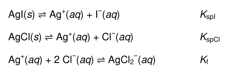
The results of this experiment are governed by three equilibria: the solubility of \(\ce{AgI(s)}\) [\(K_{\mathrm{spI}}\)] and \(\ce{AgCl(s)}\) [\(K_{\mathrm{spCl}}\)] and the formation of \(\ce{AgCl2^-(aq)}\) [\(K_{\mathrm f}\)]. (Iodide also forms complex ions with silver but this may be neglected at the very low concentrations of iodide present in this experiment).
Below are shown the results of two experiments measuring the observed potential as a function of added number of moles of silver ion. Experiment A (solid circles) was carried out with 1.000 \(\mathrm{dm^3}\) of iodide solution with concentration \(1.00\times10^{-5}\ \mathrm{mol\,dm^{-3}}\) and containing no chloride ion. Experiment B (open circles) was done using 1.000 \(\mathrm{dm^3}\) of solution with a concentration of iodide \(1.00\times10^{-5}\ \mathrm{mol\,dm^{-3}}\) and that of chloride equal to \(1.00\times10^{-1}\ \mathrm{mol\,dm^{-3}}\).
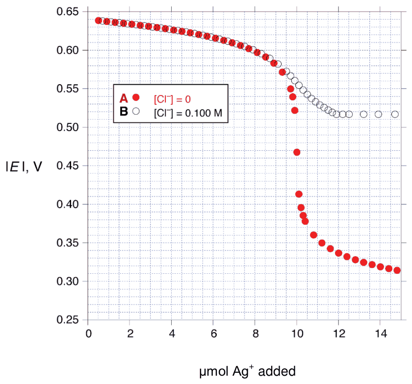
| \(\mu\mathrm{mol}\ \ce{Ag+}\) added | \(\lvert E\rvert,\ \mathrm{V}\), exp. A | \(\lvert E\rvert,\ \mathrm{V}\), exp. B |
|---|---|---|
| 1.00 | 0.637 | 0.637 |
| 3.00 | 0.631 | 0.631 |
| 5.00 | 0.622 | 0.622 |
| 7.00 | 0.609 | 0.610 |
| 9.00 | 0.581 | 0.584 |
| 10.0 | 0.468 | 0.558 |
| 11.0 | 0.355 | 0.531 |
| 12.0 | 0.337 | 0.517 |
| 13.0 | 0.327 | 0.517 |
| 15.0 | 0.313 | 0.517 |
3.2.1 Select an appropriate data from the experiments and use it to calculate the solubility product of \(\ce{AgI}\), (\(K_{\mathrm{spI}}\).).
3.2.2 Select an appropriate data from the experiments and use it to calculate the solubility product of \(\ce{AgCl}\), (\(K_{\mathrm{spCl}}\).).
3.2.3 Select an appropriate data from the experiments and use it to calculate \(K_{\mathrm f}\). You may need to use values of \(K_{\mathrm{spI}}\) or \(K_{\mathrm{spCl}}\) to do this calculation. If you were unable to carry out the calculations in 3.2.1 or 3.2.2 you may use the arbitrary values of \(K_{\mathrm{spI}}=1.00\times10^{-15}\) and \(K_{\mathrm{spCl}}=1.00\times10^{-9}\) without penalty.
An analytical method that is more practical, because it is not sensitive to the presence of chloride, uses the Sandell-Kolthoff reaction. This is the reaction of \(\ce{H3AsO3}\) with \(\ce{Ce(IV)}\) to give \(\ce{Ce(III)}\) in acidic solution, which is strongly catalyzed by iodide ion.
3.3.1 Write balanced net ionic equations for the reaction of cerium(IV) with \(\ce{H3AsO3}\) in acidic solution, as well as reactions of cerium(IV) with a species containing the element iodine and \(\ce{H3AsO3}\) with a species containing the element iodine, that could reasonably account for the catalysis of the net reaction by iodide.
The reaction of \(\ce{Ce(IV)}\) with \(\ce{H3AsO3}\) can be monitored by measuring the absorbance at 405 nm, as \(\ce{Ce(IV)}\) is orange and absorbs significantly at 405 nm, while the other reactants and products are colorless and do not absorb appreciably. Three runs were carried out, all in \(0.50\ \mathrm{mol\,dm^{-3}}\) \(\ce{H2SO4}\) at 25.0°C using the following initial concentrations:
| Run | \([\ce{H3AsO3}]_0\), \((\mathrm{mol\,dm^{-3}})\) | \([\ce{Ce(IV)}]_0\), \((\mathrm{mol\,dm^{-3}})\) | \([\ce{I^-}]_0\), \((\mathrm{mol\,dm^{-3}})\) |
|---|---|---|---|
| 1 | 0.01250 | 0.00120 | \(1.43\cdot10^{-6}\) |
| 2 | 0.00625 | 0.00060 | \(1.43\cdot10^{-6}\) |
| 3 | 0.01250 | 0.00120 | \(7.16\cdot10^{-7}\) |
An analyst initiated the reactions by mixing the reagents in a cuvette. After a short variable delay absorbance measurements were started, with the first measurement recorded at \(t=0\ \mathrm{s}\). The data obtained are shown below:
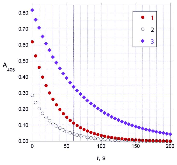
| \(t,\ \mathrm{s}\) | \(A_{405}\), Run 1 | \(A_{405}\), Run 2 | \(A_{405}\), Run 3 |
|---|---|---|---|
| 0 | 0.621 | 0.287 | 0.818 |
| 20 | 0.348 | 0.149 | 0.608 |
| 40 | 0.198 | 0.083 | 0.455 |
| 60 | 0.113 | 0.046 | 0.340 |
| 80 | 0.064 | 0.025 | 0.254 |
| 100 | 0.037 | 0.014 | 0.191 |
Under these conditions (\(0.5\ \mathrm{mol\,dm^{-3}}\) \(\ce{H2SO4}\), 25.0°C), the rate law for the reaction can be written as
\[ \text{Rate}=k[\ce{H3AsO3}]^m[\ce{Ce(IV)}]^n[\ce{I^-}]^p \]
where \(m\), \(n\) and \(p\) are integers.
3.3.2. Determine the values of \(m\), \(n\), and \(p\) and calculate the value of \(k\) (be sure to specify its units).
A 1.000 g sample of iodized salt is dissolved in water to give 10.00 \(\mathrm{cm^3}\) of solution. A 0.0500 \(\mathrm{cm^3}\) aliquot of this solution is added to a mixture of 1.000 \(\mathrm{cm^3}\) \(0.025\ \mathrm{mol\,dm^{-3}}\) \(\ce{H3AsO3}\) in \(0.5\ \mathrm{mol\,dm^{-3}}\) \(\ce{H2SO4}\) and 0.800 \(\mathrm{cm^3}\) \(0.5\ \mathrm{mol\,dm^{-3}}\) \(\ce{H2SO4}\). To this mixture is added 0.200 \(\mathrm{cm^3}\) \(0.0120\ \mathrm{mol\,dm^{-3}}\) \(\ce{Ce(NH4)2(NO3)6}\) in \(0.5\ \mathrm{mol\,dm^{-3}}\) \(\ce{H2SO4}\) and the absorbance at 405 nm is measured as a function of time at 25.0°C:
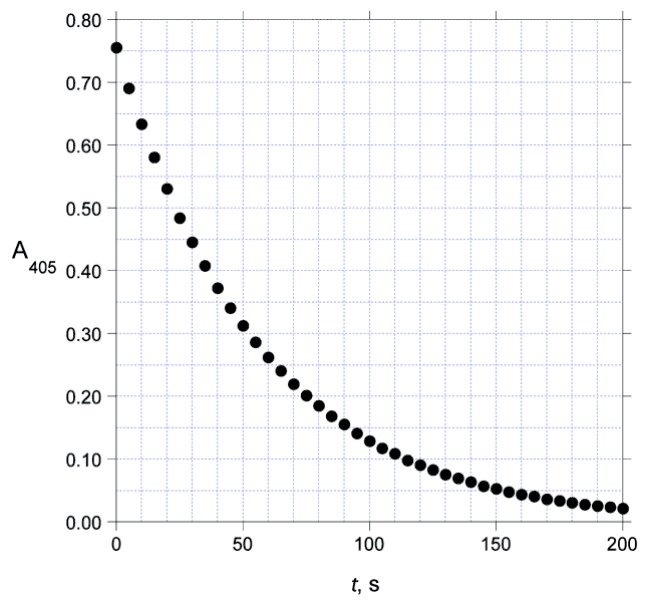
| \(t,\ \mathrm{s}\) | \(A_{405}\) |
|---|---|
| 0 | 0.756 |
| 20 | 0.531 |
| 40 | 0.373 |
| 60 | 0.262 |
| 80 | 0.185 |
| 100 | 0.129 |
3.3.3. Calculate the iodization level, in ppm, of this salt sample.
Official English text of the problem.
Answers
Species names and SMILES are supplied in the corresponding solution parts. Equilibrium constants below use the concentration convention.
-
3.1.1 \[ \boxed{\ce{IO3^- + 5I^- + 6H+ -> 3I2 + 3H2O}} \]
-
3.1.2 \[ \boxed{\ce{I2 + 2S2O3^2- -> 2I^- + S4O6^2-}} \]
-
3.1.3 \(\boxed{37.3\ \mathrm{ppm}}\) iodine.
-
3.2.1 \[ \boxed{K_{\mathrm{spI}}\approx1.5\times10^{-16}\ \mathrm{mol^2\,dm^{-6}}} \]
-
3.2.2 \[ \boxed{K_{\mathrm{spCl}}\approx1.8\times10^{-10}\ \mathrm{mol^2\,dm^{-6}}} \]
-
3.2.3 \[ \boxed{K_{\mathrm f}\approx1.1\times10^5\ \mathrm{dm^6\,mol^{-2}}} \]
-
3.3.1 Overall reaction: \[ \boxed{\ce{2Ce^4+ + H3AsO3 + H2O -> 2Ce^3+ + H3AsO4 + 2H+}} \] A plausible catalytic cycle is: \[ \boxed{\ce{2Ce^4+ + 2I^- -> 2Ce^3+ + I2}} \] \[ \boxed{\ce{H3AsO3 + I2 + H2O -> H3AsO4 + 2I^- + 2H+}} \]
-
3.3.2 \[ \boxed{m=0,\qquad n=1,\qquad p=1} \] \[ \boxed{k\approx2.0\times10^4\ \mathrm{dm^3\,mol^{-1}\,s^{-1}}} \] Here the rate is defined as the disappearance rate of cerium(IV), \(-d[\ce{Ce^4+}]/dt\).
-
3.3.3 \(\boxed{\text{Approximately }46\ \mathrm{ppm}}\) iodine.
Solution
The numerical calculations use \(M(\ce{I})=126.90\ \mathrm{g\,mol^{-1}}\). At \(25.0^\circ\mathrm C\), \(2.303RT/F=0.05916\ \mathrm V\).
The SMILES below specify connectivity or ionic composition. They do not encode aqueous solvation, crystal lattices, or the electron transfers described in words.
3.1.1
Iodate contains iodine in oxidation state \(+5\), whereas iodide contains iodine in oxidation state \(-1\). Both form molecular iodine, whose oxidation state is zero. Thus, one iodate ion accepts the five electrons supplied by five iodide ions. Balancing oxygen and hydrogen in acidic solution gives
\[ \boxed{\ce{IO3^- + 5I^- + 6H+ -> 3I2 + 3H2O}}. \]
The species are iodate, \(\ce{IO3^-}\), [O-]I(=O)=O; iodide, \(\ce{I^-}\), [I-]; proton, \(\ce{H+}\), [H+]; molecular iodine, \(\ce{I2}\), II; and water, \(\ce{H2O}\), O.
3.1.2
Iodine is reduced to iodide, while two thiosulfate ions are oxidized to one tetrathionate ion:
\[ \ce{I2 + 2e^- -> 2I^-}, \]
\[ \ce{2S2O3^2- -> S4O6^2- + 2e^-}. \]
Adding these half-reactions gives
\[ \boxed{\ce{I2 + 2S2O3^2- -> 2I^- + S4O6^2-}}. \]
Thiosulfate, \(\ce{S2O3^2-}\), has SMILES [O-]S(=O)(=O)[S-]. Tetrathionate, \(\ce{S4O6^2-}\), has SMILES [O-]S(=O)(=O)SSS(=O)(=O)[O-].
3.1.3
One mole of iodate generates three moles of iodine, each consuming two moles of thiosulfate. Therefore,
\[ n(\ce{IO3^-})=\frac{n(\ce{S2O3^2-})}{6}. \]
The amount of thiosulfate used is
\[ n(\ce{S2O3^2-}) =(0.00235\ \mathrm{mol\,dm^{-3}}) (7.50\times10^{-3}\ \mathrm{dm^3}) =1.7625\times10^{-5}\ \mathrm{mol}. \]
Thus,
\[ n(\ce{IO3^-})=2.9375\times10^{-6}\ \mathrm{mol}. \]
Each iodate ion contains one iodine atom. The iodine originally present in the salt therefore has mass
\[ m_{\mathrm I} =(2.9375\times10^{-6})(126.90) =3.7277\times10^{-4}\ \mathrm g =0.37277\ \mathrm{mg}. \]
The iodide added as a reagent is not counted as iodine originally present in the sample. Hence,
\[ \text{iodization level} =\frac{0.37277\ \mathrm{mg}}{0.010000\ \mathrm{kg}} =\boxed{37.3\ \mathrm{ppm}}. \]
This is within the stated range of 25–55 ppm.
3.2.1
For the silver electrode,
\[ \ce{Ag+ + e^- <=> Ag(s)}. \]
Silver(I) ion has SMILES [Ag+]; elemental silver is represented as [Ag].
The two electrodes have the same standard electrode potential, which cancels when their potentials are subtracted. With the reference concentration equal to \(1.000\ \mathrm{mol\,dm^{-3}}\),
\[ E=0.05916\log_{10} \left(\frac{[\ce{Ag+}]}{1.000\ \mathrm{mol\,dm^{-3}}}\right). \]
Since the reported number is \(\lvert E\rvert=-E\),
\[ \boxed{ [\ce{Ag+}] =10^{-\lvert E\rvert/0.05916}\ \mathrm{mol\,dm^{-3}} }. \]
Choose experiment A at \(10.0\ \mu\mathrm{mol}\) of added silver. The initial amount of iodide is also
\[ (1.000\ \mathrm{dm^3})(1.00\times10^{-5}\ \mathrm{mol\,dm^{-3}}) =10.0\ \mu\mathrm{mol}. \]
Thus, this is the equivalence point. There are no chloride complexes, and the equal analytical amounts of silver and iodide require
\[ [\ce{Ag+}]=[\ce{I^-}]. \]
Using \(\lvert E\rvert=0.468\ \mathrm V\),
\[ [\ce{Ag+}] =10^{-0.468/0.05916} =1.23\times10^{-8}\ \mathrm{mol\,dm^{-3}}. \]
For the dissolution equilibrium
\[ \ce{AgI(s) <=> Ag+ + I^-}, \]
we obtain
\[ K_{\mathrm{spI}} =[\ce{Ag+}][\ce{I^-}] =(1.23\times10^{-8})^2 =\boxed{1.5\times10^{-16}\ \mathrm{mol^2\,dm^{-6}}}. \]
Silver(I) iodide, \(\ce{AgI}\), has the ionic-composition SMILES [Ag+].[I-]; this does not represent its crystal lattice.
3.2.2
In experiment B, the potential becomes constant at \(\lvert E\rvert=0.517\ \mathrm V\). This plateau indicates precipitation of silver chloride:
\[ \ce{AgCl(s) <=> Ag+ + Cl^-}. \]
The large chloride concentration remains approximately \(0.100\ \mathrm{mol\,dm^{-3}}\), so coexistence with solid silver chloride fixes the free silver concentration.
From the plateau potential,
\[ [\ce{Ag+}] =10^{-0.517/0.05916} =1.82\times10^{-9}\ \mathrm{mol\,dm^{-3}}. \]
Consequently,
\[ K_{\mathrm{spCl}} =[\ce{Ag+}][\ce{Cl^-}] =(1.82\times10^{-9})(0.100) =\boxed{1.8\times10^{-10}\ \mathrm{mol^2\,dm^{-6}}}. \]
Chloride has SMILES [Cl-]. Silver(I) chloride, \(\ce{AgCl}\), has the ionic-composition SMILES [Ag+].[Cl-].
3.2.3
Choose experiment B at \(10.0\ \mu\mathrm{mol}\) of added silver, where \(\lvert E\rvert=0.558\ \mathrm V\). The free silver concentration is
\[ [\ce{Ag+}] =10^{-0.558/0.05916} =3.70\times10^{-10}\ \mathrm{mol\,dm^{-3}}. \]
At this point, silver chloride has not yet precipitated, because
\[ [\ce{Ag+}][\ce{Cl^-}] \approx3.70\times10^{-11} <K_{\mathrm{spCl}}. \]
Solid silver iodide is present, giving
\[ [\ce{I^-}] =\frac{K_{\mathrm{spI}}}{[\ce{Ag+}]} =\frac{1.51\times10^{-16}}{3.70\times10^{-10}} =4.08\times10^{-7}\ \mathrm{mol\,dm^{-3}}. \]
The total amounts of silver and iodide are equal. Subtracting their mass balances cancels the silver iodide precipitate, leaving
\[ [\ce{I^-}] =[\ce{Ag+}]+[\ce{AgCl2^-}]. \]
Therefore,
\[ [\ce{AgCl2^-}] =4.08\times10^{-7}-3.70\times10^{-10} \approx4.07\times10^{-7}\ \mathrm{mol\,dm^{-3}}. \]
For
\[ \ce{Ag+ + 2Cl^- <=> AgCl2^-}, \]
the formation constant is
\[ K_{\mathrm f} =\frac{[\ce{AgCl2^-}]} {[\ce{Ag+}][\ce{Cl^-}]^2}. \]
The chloride bound in the complex is negligible compared with \(0.100\ \mathrm{mol\,dm^{-3}}\), so
\[ K_{\mathrm f} =\frac{4.07\times10^{-7}} {(3.70\times10^{-10})(0.100)^2} =\boxed{1.1\times10^5\ \mathrm{dm^6\,mol^{-2}}}. \]
The complex is dichloridoargentate(I), \(\ce{AgCl2^-}\), with dative-bond SMILES [Cl-]->[Ag+]<-[Cl-]. Its coordination geometry is linear; that geometry is not specified by the SMILES.
3.3.1
Arsenic is oxidized from \(+3\) to \(+5\), releasing two electrons. Each cerium(IV) ion accepts one electron:
\[ \ce{H3AsO3 + H2O -> H3AsO4 + 2H+ + 2e^-}, \]
\[ \ce{2Ce^4+ + 2e^- -> 2Ce^3+}. \]
The overall reaction is therefore
\[ \boxed{\ce{2Ce^4+ + H3AsO3 + H2O -> 2Ce^3+ + H3AsO4 + 2H+}}. \]
The species introduced here are:
| Species | Name | SMILES |
|---|---|---|
| \(\ce{H3AsO3}\) | Arsenous acid | O[As](O)O |
| \(\ce{H3AsO4}\) | Arsenic acid | O=[As](O)(O)O |
| \(\ce{Ce^4+}\) | Cerium(IV) ion | [Ce+4] |
| \(\ce{Ce^3+}\) | Cerium(III) ion | [Ce+3] |
The oxygen atoms around arsenic have a trigonal pyramidal arrangement in arsenous acid and an approximately tetrahedral arrangement in arsenic acid.
A plausible catalytic cycle consists of oxidation of iodide by cerium(IV),
\[ \boxed{\ce{2Ce^4+ + 2I^- -> 2Ce^3+ + I2}}, \]
followed by reduction of iodine by arsenous acid,
\[ \boxed{\ce{H3AsO3 + I2 + H2O -> H3AsO4 + 2I^- + 2H+}}. \]
Adding these reactions cancels both iodine and iodide and reproduces the overall reaction. Iodide is regenerated, allowing it to act as a catalyst. These balanced steps describe a plausible redox cycle; they need not be elementary reactions.
3.3.2
By the Beer–Lambert law,
\[ A_{405}=\varepsilon l[\ce{Ce^4+}], \]
so the absorbance is directly proportional to the cerium(IV) concentration.
Arsenous acid is in substantial excess. Even complete consumption of cerium(IV) would consume only
\[ \frac{[\ce{Ce^4+}]_0}{2[\ce{H3AsO3}]_0} =\frac{0.00120}{2(0.01250)} =0.0480 \]
of the arsenous acid in run 1, or 4.80%. The same fraction applies to the other runs. Its concentration can therefore be treated as approximately constant while identifying the kinetic orders.
The plots of \(\ln A_{405}\) against time are approximately straight lines. Thus, cerium(IV) follows first-order decay:
\[ -\frac{d[\ce{Ce^4+}]}{dt} =k_{\mathrm{obs}}[\ce{Ce^4+}], \qquad \ln A_{405}(t)=\ln A_{405}(0)-k_{\mathrm{obs}}t. \]
Hence,
\[ \boxed{n=1}. \]
The variable delay before the first measurement affects the intercept, not the slope. Therefore, the measured \(A_{405}(0)\) must not be identified with the absorbance immediately after mixing.
Linear fits using all six points give:
| Run | \(k_{\mathrm{obs}}\), \(\mathrm{s^{-1}}\) |
|---|---|
| 1 | \(2.820\times10^{-2}\) |
| 2 | \(3.007\times10^{-2}\) |
| 3 | \(1.455\times10^{-2}\) |
For example, the endpoints of run 1 give essentially the same result:
\[ k_{\mathrm{obs},1} =\frac{\ln(0.621/0.037)}{100\ \mathrm s} =2.820\times10^{-2}\ \mathrm{s^{-1}}. \]
With \(n=1\),
\[ k_{\mathrm{obs}} =k[\ce{H3AsO3}]^m[\ce{I^-}]^p. \]
Runs 1 and 2 have the same iodide concentration. Halving the arsenous acid concentration leaves \(k_{\mathrm{obs}}\) approximately unchanged. Since the orders are integers,
\[ \boxed{m=0}. \]
Runs 1 and 3 have the same initial arsenous acid and cerium(IV) concentrations. Halving the iodide concentration approximately halves \(k_{\mathrm{obs}}\):
\[ \frac{k_{\mathrm{obs},1}}{k_{\mathrm{obs},3}} \approx1.94, \qquad \frac{[\ce{I^-}]_{0,1}}{[\ce{I^-}]_{0,3}} \approx2.00. \]
Therefore,
\[ \boxed{p=1}. \]
The rate law, using the cerium(IV) disappearance rate, is
\[ \boxed{ -\frac{d[\ce{Ce^4+}]}{dt} =k[\ce{Ce^4+}][\ce{I^-}] }. \]
The individual estimates of \(k\) are
\[ k_1=\frac{0.02820}{1.43\times10^{-6}} =1.97\times10^4\ \mathrm{dm^3\,mol^{-1}\,s^{-1}}, \]
\[ k_2=\frac{0.03007}{1.43\times10^{-6}} =2.10\times10^4\ \mathrm{dm^3\,mol^{-1}\,s^{-1}}, \]
\[ k_3=\frac{0.01455}{7.16\times10^{-7}} =2.03\times10^4\ \mathrm{dm^3\,mol^{-1}\,s^{-1}}. \]
These support the representative value
\[ \boxed{k\approx2.0\times10^4\ \mathrm{dm^3\,mol^{-1}\,s^{-1}}}. \]
3.3.3
For the unknown sample, the absorbance again decreases exponentially. From the endpoints,
\[ k_{\mathrm{obs,sample}} =\frac{\ln(0.756/0.129)}{100\ \mathrm s} =1.768\times10^{-2}\ \mathrm{s^{-1}}. \]
Since \(k_{\mathrm{obs}}=k[\ce{I^-}]\),
\[ [\ce{I^-}]_{\mathrm{mixture}} =\frac{1.768\times10^{-2}}{2.0\times10^4} \approx8.84\times10^{-7}\ \mathrm{mol\,dm^{-3}}. \]
The total reaction volume includes the salt aliquot:
\[ V_{\mathrm{mixture}} =0.0500+1.000+0.800+0.200 =2.050\ \mathrm{cm^3}. \]
Thus, the amount of iodide in the aliquot is
\[ n_{\mathrm{aliquot}} =(8.84\times10^{-7})(2.050\times10^{-3}) \approx1.81\times10^{-9}\ \mathrm{mol}. \]
The aliquot represents the fraction \(0.0500/10.00\) of the stock solution, so the original 1.000 g salt sample contains
\[ n_{\mathrm I} =n_{\mathrm{aliquot}}\frac{10.00}{0.0500} \approx3.62\times10^{-7}\ \mathrm{mol}. \]
Its iodine mass is therefore
\[ m_{\mathrm I} =(3.62\times10^{-7})(126.90) \approx4.60\times10^{-5}\ \mathrm g =0.0460\ \mathrm{mg}. \]
Finally,
\[ \text{iodization level} =\frac{0.0460\ \mathrm{mg}}{0.001000\ \mathrm{kg}} \approx\boxed{46\ \mathrm{ppm}}. \]
This sample also lies within the specified range of 25–55 ppm.
The solution was checked against the official solution. Where this solution differs from the official solution, the official solution contains an error or a misprint.
IChO 2016 · Theorieaufgabe 3
Bestimmung von Iod in iodiertem Speisesalz
Iodmangel ist in Georgien ein besonderes Problem, da das Land in einer Region liegt, deren Böden und Gewässer iodarm sind. Iodmangel lässt sich wirksam und kostengünstig verhindern, indem Speisesalz mit kleinen Mengen Iod angereichert wird. Daher sind Methoden zur Bestimmung des Iodgehalts von Salz wichtig. Nach den geltenden Vorschriften in Georgien muss iodiertes Speisesalz zwischen 25 - 55 ppm Iod enthalten (1 ppm = 1 mg Iod/kg Salz).
Das meiste Salz wird durch Zusatz von Kaliumiodat (\(\ce{KIO3}\)) iodiert. Der Iodatgehalt von Salzproben lässt sich durch iodometrische Titration bestimmen. Bei einem typischen Verfahren werden 10.000 g einer Probe iodierten Speisesalzes in 100 \(\mathrm{cm^3}\) wässriger \(\ce{HCl}\) (\(c=1.0\ \mathrm{mol\,dm^{-3}}\)) gelöst, der 1.0 g \(\ce{KI}\) zugesetzt wurde. Anschließend wird die Lösung mit wässriger Natriumthiosulfatlösung (\(c=0.00235\ \mathrm{mol\,dm^{-3}}\)) unter Verwendung von Stärke als Endpunktindikator titriert; hierfür werden 7.50 \(\mathrm{cm^3}\) der Maßlösung benötigt.
3.1.1 Stellen Sie eine ausgeglichene Nettoionengleichung für die Reaktion von Iodat mit überschüssigem Iodid in saurer Lösung auf.
3.1.2 Stellen Sie eine ausgeglichene Nettoionengleichung für die Reaktion auf, die bei der Titration mit Thiosulfat stattfindet.
3.1.3 Berechnen Sie den Iodierungsgrad dieser Salzprobe in ppm.
Ein weniger häufig verwendeter Zusatz zur Iodierung von Salz ist Kaliumiodid, das sich nicht ohne Weiteres durch iodometrische Titration bestimmen lässt.
Eine mögliche Methode zur Bestimmung von Iodid in Gegenwart von Chlorid ist die potentiometrische Titration. In Gegenwart großer Mengen Chlorid ist diese Methode jedoch nicht sehr präzise. Bei diesem Verfahren wird ein Silberdraht in die zu untersuchende Lösung (die Iodid und Chlorid enthält) eingetaucht, und der Lösung werden nach und nach Silberionen zugesetzt. Das Potential des Silberdrahts wird gegen eine Referenzelektrode gemessen, die aus einem Silberdraht in einer Lösung von \(\ce{AgNO3}\) (\(c=1.000\ \mathrm{mol\,dm^{-3}}\)) besteht. Die gemessenen Potentiale sind negativ; angegeben werden ihre Absolutbeträge. Die zu untersuchende Lösung hat ein Volumen von 1.000 \(\mathrm{dm^3}\) (Sie dürfen annehmen, dass sich dieses bei der Zugabe von Silberionen nicht ändert), und es gilt \(t=25.0\ ^\circ\mathrm{C}\).
Die Ergebnisse dieses Experiments werden durch drei Gleichgewichte bestimmt: die Löslichkeit von \(\ce{AgI(s)}\) [\(K_{\mathrm{spI}}\)] und \(\ce{AgCl(s)}\) [\(K_{\mathrm{spCl}}\)] sowie die Bildung von \(\ce{AgCl2^-(aq)}\) [\(K_{\mathrm f}\)]. (Auch Iodid bildet mit Silber Komplexionen; dies kann jedoch bei den sehr niedrigen Iodidkonzentrationen in diesem Experiment vernachlässigt werden.)
Nachfolgend sind die Ergebnisse zweier Experimente dargestellt, in denen das beobachtete Potential in Abhängigkeit von der zugesetzten Stoffmenge an Silberionen gemessen wurde. Experiment A (ausgefüllte Kreise) wurde mit 1.000 \(\mathrm{dm^3}\) einer Iodidlösung der Konzentration \(1.00\times10^{-5}\ \mathrm{mol\,dm^{-3}}\) durchgeführt, die keine Chloridionen enthielt. Experiment B (offene Kreise) wurde mit 1.000 \(\mathrm{dm^3}\) einer Lösung durchgeführt, deren Iodidkonzentration \(1.00\times10^{-5}\ \mathrm{mol\,dm^{-3}}\) und deren Chloridkonzentration \(1.00\times10^{-1}\ \mathrm{mol\,dm^{-3}}\) betrug.
| zugesetzte \(\mu\mathrm{mol}\ \ce{Ag+}\) | \(\lvert E\rvert,\ \mathrm{V}\), Exp. A | \(\lvert E\rvert,\ \mathrm{V}\), Exp. B |
|---|---|---|
| 1.00 | 0.637 | 0.637 |
| 3.00 | 0.631 | 0.631 |
| 5.00 | 0.622 | 0.622 |
| 7.00 | 0.609 | 0.610 |
| 9.00 | 0.581 | 0.584 |
| 10.0 | 0.468 | 0.558 |
| 11.0 | 0.355 | 0.531 |
| 12.0 | 0.337 | 0.517 |
| 13.0 | 0.327 | 0.517 |
| 15.0 | 0.313 | 0.517 |
3.2.1 Wählen Sie geeignete Messdaten aus den Experimenten aus und berechnen Sie damit das Löslichkeitsprodukt von \(\ce{AgI}\), (\(K_{\mathrm{spI}}\).).
3.2.2 Wählen Sie geeignete Messdaten aus den Experimenten aus und berechnen Sie damit das Löslichkeitsprodukt von \(\ce{AgCl}\), (\(K_{\mathrm{spCl}}\).).
3.2.3 Wählen Sie geeignete Messdaten aus den Experimenten aus und berechnen Sie damit \(K_{\mathrm f}\). Für diese Berechnung benötigen Sie möglicherweise die Werte von \(K_{\mathrm{spI}}\) oder \(K_{\mathrm{spCl}}\). Falls Sie die Berechnungen in 3.2.1 oder 3.2.2 nicht durchführen konnten, dürfen Sie ohne Punktabzug die willkürlich gewählten Werte \(K_{\mathrm{spI}}=1.00\times10^{-15}\) und \(K_{\mathrm{spCl}}=1.00\times10^{-9}\) verwenden.
Eine für die Praxis besser geeignete analytische Methode, die durch die Anwesenheit von Chlorid nicht beeinträchtigt wird, nutzt die Sandell-Kolthoff-Reaktion. Dabei reagiert \(\ce{H3AsO3}\) mit \(\ce{Ce(IV)}\) in saurer Lösung unter Bildung von \(\ce{Ce(III)}\); diese Reaktion wird durch Iodidionen stark katalysiert.
3.3.1 Stellen Sie ausgeglichene Nettoionengleichungen für die Reaktion von Cer(IV) mit \(\ce{H3AsO3}\) in saurer Lösung sowie für Reaktionen von Cer(IV) mit einer iodhaltigen Spezies und von \(\ce{H3AsO3}\) mit einer iodhaltigen Spezies auf, die die Katalyse der Gesamtreaktion durch Iodid plausibel erklären könnten.
Die Reaktion von \(\ce{Ce(IV)}\) mit \(\ce{H3AsO3}\) lässt sich durch Messung der Extinktion bei 405 nm verfolgen, da \(\ce{Ce(IV)}\) orange ist und bei 405 nm deutlich absorbiert, während die anderen Edukte und Produkte farblos sind und nicht nennenswert absorbieren. Es wurden drei Versuche durchgeführt, alle in \(0.50\ \mathrm{mol\,dm^{-3}}\) \(\ce{H2SO4}\) bei 25.0°C mit den folgenden Anfangskonzentrationen:
| Versuch | \([\ce{H3AsO3}]_0\), \((\mathrm{mol\,dm^{-3}})\) | \([\ce{Ce(IV)}]_0\), \((\mathrm{mol\,dm^{-3}})\) | \([\ce{I^-}]_0\), \((\mathrm{mol\,dm^{-3}})\) |
|---|---|---|---|
| 1 | 0.01250 | 0.00120 | \(1.43\cdot10^{-6}\) |
| 2 | 0.00625 | 0.00060 | \(1.43\cdot10^{-6}\) |
| 3 | 0.01250 | 0.00120 | \(7.16\cdot10^{-7}\) |
Ein Analytiker startete die Reaktionen durch Mischen der Reagenzien in einer Küvette. Nach einer kurzen, unterschiedlich langen Verzögerung wurden die Extinktionsmessungen begonnen, wobei die erste Messung bei \(t=0\ \mathrm{s}\) aufgezeichnet wurde. Die erhaltenen Daten sind nachfolgend dargestellt:
| \(t,\ \mathrm{s}\) | \(A_{405}\), Versuch 1 | \(A_{405}\), Versuch 2 | \(A_{405}\), Versuch 3 |
|---|---|---|---|
| 0 | 0.621 | 0.287 | 0.818 |
| 20 | 0.348 | 0.149 | 0.608 |
| 40 | 0.198 | 0.083 | 0.455 |
| 60 | 0.113 | 0.046 | 0.340 |
| 80 | 0.064 | 0.025 | 0.254 |
| 100 | 0.037 | 0.014 | 0.191 |
Unter diesen Bedingungen (\(0.5\ \mathrm{mol\,dm^{-3}}\) \(\ce{H2SO4}\), 25.0°C) lässt sich das Geschwindigkeitsgesetz der Reaktion schreiben als
\[ \text{Reaktionsgeschwindigkeit}=k[\ce{H3AsO3}]^m[\ce{Ce(IV)}]^n[\ce{I^-}]^p \]
wobei \(m\), \(n\) und \(p\) ganze Zahlen sind.
3.3.2. Bestimmen Sie die Werte von \(m\), \(n\) und \(p\) und berechnen Sie den Wert von \(k\) (geben Sie unbedingt die Einheiten an).
Eine 1.000 g schwere Probe iodierten Speisesalzes wird in Wasser gelöst, sodass 10.00 \(\mathrm{cm^3}\) Lösung entstehen. Ein Aliquot von 0.0500 \(\mathrm{cm^3}\) dieser Lösung wird zu einer Mischung aus 1.000 \(\mathrm{cm^3}\) \(0.025\ \mathrm{mol\,dm^{-3}}\) \(\ce{H3AsO3}\) in \(0.5\ \mathrm{mol\,dm^{-3}}\) \(\ce{H2SO4}\) und 0.800 \(\mathrm{cm^3}\) \(0.5\ \mathrm{mol\,dm^{-3}}\) \(\ce{H2SO4}\) gegeben. Dieser Mischung werden 0.200 \(\mathrm{cm^3}\) \(0.0120\ \mathrm{mol\,dm^{-3}}\) \(\ce{Ce(NH4)2(NO3)6}\) in \(0.5\ \mathrm{mol\,dm^{-3}}\) \(\ce{H2SO4}\) zugesetzt, und die Extinktion bei 405 nm wird bei 25.0°C in Abhängigkeit von der Zeit gemessen:
| \(t,\ \mathrm{s}\) | \(A_{405}\) |
|---|---|
| 0 | 0.756 |
| 20 | 0.531 |
| 40 | 0.373 |
| 60 | 0.262 |
| 80 | 0.185 |
| 100 | 0.129 |
3.3.3. Berechnen Sie den Iodierungsgrad dieser Salzprobe in ppm.
Aufgabentext aus dem offiziellen englischen Text übersetzt.
Antworten
Die Namen der Spezies und ihre SMILES sind in den entsprechenden Lösungsteilen angegeben. Für die nachfolgenden Gleichgewichtskonstanten wird die Konzentrationskonvention verwendet.
-
3.1.1 \[ \boxed{\ce{IO3^- + 5I^- + 6H+ -> 3I2 + 3H2O}} \]
-
3.1.2 \[ \boxed{\ce{I2 + 2S2O3^2- -> 2I^- + S4O6^2-}} \]
-
3.1.3 \(\boxed{37.3\ \mathrm{ppm}}\) Iod.
-
3.2.1 \[ \boxed{K_{\mathrm{spI}}\approx1.5\times10^{-16}\ \mathrm{mol^2\,dm^{-6}}} \]
-
3.2.2 \[ \boxed{K_{\mathrm{spCl}}\approx1.8\times10^{-10}\ \mathrm{mol^2\,dm^{-6}}} \]
-
3.2.3 \[ \boxed{K_{\mathrm f}\approx1.1\times10^5\ \mathrm{dm^6\,mol^{-2}}} \]
-
3.3.1 Gesamtreaktion: \[ \boxed{\ce{2Ce^4+ + H3AsO3 + H2O -> 2Ce^3+ + H3AsO4 + 2H+}} \] Ein plausibler Katalysezyklus lautet: \[ \boxed{\ce{2Ce^4+ + 2I^- -> 2Ce^3+ + I2}} \] \[ \boxed{\ce{H3AsO3 + I2 + H2O -> H3AsO4 + 2I^- + 2H+}} \]
-
3.3.2 \[ \boxed{m=0,\qquad n=1,\qquad p=1} \] \[ \boxed{k\approx2.0\times10^4\ \mathrm{dm^3\,mol^{-1}\,s^{-1}}} \] Hier ist die Reaktionsgeschwindigkeit als Verbrauchsgeschwindigkeit von Cer(IV), \(-d[\ce{Ce^4+}]/dt\), definiert.
-
3.3.3 \(\boxed{\text{Ungefähr }46\ \mathrm{ppm}}\) Iod.
Lösung
Für die numerischen Berechnungen wird \(M(\ce{I})=126.90\ \mathrm{g\,mol^{-1}}\) verwendet. Bei \(25.0^\circ\mathrm C\) gilt \(2.303RT/F=0.05916\ \mathrm V\).
Die nachfolgenden SMILES geben die Konnektivität oder die ionische Zusammensetzung an. Sie bilden weder die Solvatation in Wasser noch Kristallgitter oder die in Worten beschriebenen Elektronenübertragungen ab.
3.1.1
Iodat enthält Iod in der Oxidationsstufe \(+5\), während Iodid Iod in der Oxidationsstufe \(-1\) enthält. Beide bilden molekulares Iod, dessen Oxidationsstufe null ist. Somit nimmt ein Iodation die fünf Elektronen auf, die von fünf Iodidionen abgegeben werden. Der Ausgleich von Sauerstoff und Wasserstoff in saurer Lösung ergibt
\[ \boxed{\ce{IO3^- + 5I^- + 6H+ -> 3I2 + 3H2O}}. \]
Die Spezies sind Iodat, \(\ce{IO3^-}\), [O-]I(=O)=O; Iodid, \(\ce{I^-}\), [I-]; Proton, \(\ce{H+}\), [H+]; molekulares Iod, \(\ce{I2}\), II; und Wasser, \(\ce{H2O}\), O.
3.1.2
Iod wird zu Iodid reduziert, während zwei Thiosulfationen zu einem Tetrathionation oxidiert werden:
\[ \ce{I2 + 2e^- -> 2I^-}, \]
\[ \ce{2S2O3^2- -> S4O6^2- + 2e^-}. \]
Die Addition dieser Teilreaktionen ergibt
\[ \boxed{\ce{I2 + 2S2O3^2- -> 2I^- + S4O6^2-}}. \]
Thiosulfat, \(\ce{S2O3^2-}\), hat die SMILES [O-]S(=O)(=O)[S-]. Tetrathionat, \(\ce{S4O6^2-}\), hat die SMILES [O-]S(=O)(=O)SSS(=O)(=O)[O-].
3.1.3
Ein Mol Iodat erzeugt drei Mol Iod, von denen jedes zwei Mol Thiosulfat verbraucht. Daher gilt
\[ n(\ce{IO3^-})=\frac{n(\ce{S2O3^2-})}{6}. \]
Die verbrauchte Stoffmenge an Thiosulfat beträgt
\[ n(\ce{S2O3^2-}) =(0.00235\ \mathrm{mol\,dm^{-3}}) (7.50\times10^{-3}\ \mathrm{dm^3}) =1.7625\times10^{-5}\ \mathrm{mol}. \]
Somit gilt
\[ n(\ce{IO3^-})=2.9375\times10^{-6}\ \mathrm{mol}. \]
Jedes Iodation enthält ein Iodatom. Das ursprünglich im Salz enthaltene Iod hat daher die Masse
\[ m_{\mathrm I} =(2.9375\times10^{-6})(126.90) =3.7277\times10^{-4}\ \mathrm g =0.37277\ \mathrm{mg}. \]
Das als Reagenz zugesetzte Iodid wird nicht zum ursprünglich in der Probe enthaltenen Iod gezählt. Daher gilt
\[ \text{Iodierungsgrad} =\frac{0.37277\ \mathrm{mg}}{0.010000\ \mathrm{kg}} =\boxed{37.3\ \mathrm{ppm}}. \]
Dieser Wert liegt innerhalb des angegebenen Bereichs von 25–55 ppm.
3.2.1
Für die Silberelektrode gilt
\[ \ce{Ag+ + e^- <=> Ag(s)}. \]
Das Silber(I)-Ion hat die SMILES [Ag+]; elementares Silber wird als [Ag] dargestellt.
Die beiden Elektroden haben dasselbe Standardelektrodenpotential, das bei der Subtraktion ihrer Potentiale wegfällt. Bei einer Referenzkonzentration von \(1.000\ \mathrm{mol\,dm^{-3}}\) gilt
\[ E=0.05916\log_{10} \left(\frac{[\ce{Ag+}]}{1.000\ \mathrm{mol\,dm^{-3}}}\right). \]
Da der angegebene Wert \(\lvert E\rvert=-E\) ist, gilt
\[ \boxed{ [\ce{Ag+}] =10^{-\lvert E\rvert/0.05916}\ \mathrm{mol\,dm^{-3}} }. \]
Wir wählen Experiment A bei einer zugesetzten Silberstoffmenge von \(10.0\ \mu\mathrm{mol}\). Die anfängliche Iodidstoffmenge beträgt ebenfalls
\[ (1.000\ \mathrm{dm^3})(1.00\times10^{-5}\ \mathrm{mol\,dm^{-3}}) =10.0\ \mu\mathrm{mol}. \]
Dies ist somit der Äquivalenzpunkt. Es liegen keine Chloridkomplexe vor, und aus den gleichen analytischen Stoffmengen von Silber und Iodid folgt
\[ [\ce{Ag+}]=[\ce{I^-}]. \]
Mit \(\lvert E\rvert=0.468\ \mathrm V\) erhält man
\[ [\ce{Ag+}] =10^{-0.468/0.05916} =1.23\times10^{-8}\ \mathrm{mol\,dm^{-3}}. \]
Für das Lösungsgleichgewicht
\[ \ce{AgI(s) <=> Ag+ + I^-}, \]
erhalten wir
\[ K_{\mathrm{spI}} =[\ce{Ag+}][\ce{I^-}] =(1.23\times10^{-8})^2 =\boxed{1.5\times10^{-16}\ \mathrm{mol^2\,dm^{-6}}}. \]
Silber(I)-iodid, \(\ce{AgI}\), hat die SMILES [Ag+].[I-] zur Angabe der ionischen Zusammensetzung; diese stellen sein Kristallgitter nicht dar.
3.2.2
In Experiment B wird das Potential bei \(\lvert E\rvert=0.517\ \mathrm V\) konstant. Dieses Plateau zeigt die Fällung von Silberchlorid an:
\[ \ce{AgCl(s) <=> Ag+ + Cl^-}. \]
Die hohe Chloridkonzentration bleibt annähernd bei \(0.100\ \mathrm{mol\,dm^{-3}}\), sodass die Koexistenz mit festem Silberchlorid die Konzentration der freien Silberionen festlegt.
Aus dem Plateaupotential folgt
\[ [\ce{Ag+}] =10^{-0.517/0.05916} =1.82\times10^{-9}\ \mathrm{mol\,dm^{-3}}. \]
Folglich gilt
\[ K_{\mathrm{spCl}} =[\ce{Ag+}][\ce{Cl^-}] =(1.82\times10^{-9})(0.100) =\boxed{1.8\times10^{-10}\ \mathrm{mol^2\,dm^{-6}}}. \]
Chlorid hat die SMILES [Cl-]. Silber(I)-chlorid, \(\ce{AgCl}\), hat die SMILES [Ag+].[Cl-] zur Angabe der ionischen Zusammensetzung.
3.2.3
Wir wählen Experiment B bei einer zugesetzten Silberstoffmenge von \(10.0\ \mu\mathrm{mol}\), bei der \(\lvert E\rvert=0.558\ \mathrm V\) gilt. Die Konzentration der freien Silberionen beträgt
\[ [\ce{Ag+}] =10^{-0.558/0.05916} =3.70\times10^{-10}\ \mathrm{mol\,dm^{-3}}. \]
Zu diesem Zeitpunkt ist noch kein Silberchlorid ausgefallen, denn
\[ [\ce{Ag+}][\ce{Cl^-}] \approx3.70\times10^{-11} <K_{\mathrm{spCl}}. \]
Festes Silberiodid liegt vor, sodass gilt
\[ [\ce{I^-}] =\frac{K_{\mathrm{spI}}}{[\ce{Ag+}]} =\frac{1.51\times10^{-16}}{3.70\times10^{-10}} =4.08\times10^{-7}\ \mathrm{mol\,dm^{-3}}. \]
Die Gesamtstoffmengen von Silber und Iodid sind gleich. Bei der Subtraktion ihrer Stoffbilanzen fällt der Silberiodidniederschlag weg, und es bleibt
\[ [\ce{I^-}] =[\ce{Ag+}]+[\ce{AgCl2^-}]. \]
Daher gilt
\[ [\ce{AgCl2^-}] =4.08\times10^{-7}-3.70\times10^{-10} \approx4.07\times10^{-7}\ \mathrm{mol\,dm^{-3}}. \]
Für
\[ \ce{Ag+ + 2Cl^- <=> AgCl2^-}, \]
lautet die Bildungskonstante
\[ K_{\mathrm f} =\frac{[\ce{AgCl2^-}]} {[\ce{Ag+}][\ce{Cl^-}]^2}. \]
Das im Komplex gebundene Chlorid ist gegenüber \(0.100\ \mathrm{mol\,dm^{-3}}\) vernachlässigbar, sodass gilt
\[ K_{\mathrm f} =\frac{4.07\times10^{-7}} {(3.70\times10^{-10})(0.100)^2} =\boxed{1.1\times10^5\ \mathrm{dm^6\,mol^{-2}}}. \]
Der Komplex ist Dichloridoargentat(I), \(\ce{AgCl2^-}\), mit den SMILES [Cl-]->[Ag+]<-[Cl-], die koordinative Bindungen darstellen. Seine Koordinationsgeometrie ist linear; diese Geometrie wird durch die SMILES nicht angegeben.
3.3.1
Arsen wird von \(+3\) zu \(+5\) oxidiert und gibt dabei zwei Elektronen ab. Jedes Cer(IV)-Ion nimmt ein Elektron auf:
\[ \ce{H3AsO3 + H2O -> H3AsO4 + 2H+ + 2e^-}, \]
\[ \ce{2Ce^4+ + 2e^- -> 2Ce^3+}. \]
Die Gesamtreaktion lautet daher
\[ \boxed{\ce{2Ce^4+ + H3AsO3 + H2O -> 2Ce^3+ + H3AsO4 + 2H+}}. \]
Die hier eingeführten Spezies sind:
| Spezies | Name | SMILES |
|---|---|---|
| \(\ce{H3AsO3}\) | Arsenige Säure | O[As](O)O |
| \(\ce{H3AsO4}\) | Arsensäure | O=[As](O)(O)O |
| \(\ce{Ce^4+}\) | Cer(IV)-Ion | [Ce+4] |
| \(\ce{Ce^3+}\) | Cer(III)-Ion | [Ce+3] |
Die Sauerstoffatome um das Arsen sind in arseniger Säure trigonal-pyramidal und in Arsensäure annähernd tetraedrisch angeordnet.
Ein plausibler Katalysezyklus besteht aus der Oxidation von Iodid durch Cer(IV),
\[ \boxed{\ce{2Ce^4+ + 2I^- -> 2Ce^3+ + I2}}, \]
gefolgt von der Reduktion von Iod durch arsenige Säure,
\[ \boxed{\ce{H3AsO3 + I2 + H2O -> H3AsO4 + 2I^- + 2H+}}. \]
Bei der Addition dieser Reaktionen fallen sowohl Iod als auch Iodid weg, und man erhält wieder die Gesamtreaktion. Iodid wird regeneriert und kann daher als Katalysator wirken. Diese ausgeglichenen Schritte beschreiben einen plausiblen Redoxzyklus; sie müssen keine Elementarreaktionen sein.
3.3.2
Nach dem Lambert-Beerschen Gesetz gilt
\[ A_{405}=\varepsilon l[\ce{Ce^4+}], \]
sodass die Extinktion direkt proportional zur Cer(IV)-Konzentration ist.
Arsenige Säure liegt in erheblichem Überschuss vor. Selbst bei vollständigem Verbrauch von Cer(IV) würde in Versuch 1 nur der Anteil
\[ \frac{[\ce{Ce^4+}]_0}{2[\ce{H3AsO3}]_0} =\frac{0.00120}{2(0.01250)} =0.0480 \]
der arsenigen Säure verbraucht, also 4.80%. Derselbe Anteil gilt für die anderen Versuche. Ihre Konzentration kann daher bei der Bestimmung der Reaktionsordnungen als annähernd konstant behandelt werden.
Die Auftragungen von \(\ln A_{405}\) gegen die Zeit ergeben annähernd Geraden. Somit nimmt die Cer(IV)-Konzentration nach einem Zeitgesetz erster Ordnung ab:
\[ -\frac{d[\ce{Ce^4+}]}{dt} =k_{\mathrm{obs}}[\ce{Ce^4+}], \qquad \ln A_{405}(t)=\ln A_{405}(0)-k_{\mathrm{obs}}t. \]
Daraus folgt
\[ \boxed{n=1}. \]
Die unterschiedlich lange Verzögerung vor der ersten Messung beeinflusst den Achsenabschnitt, nicht die Steigung. Daher darf der gemessene Wert \(A_{405}(0)\) nicht mit der Extinktion unmittelbar nach dem Mischen gleichgesetzt werden.
Lineare Ausgleichsrechnungen unter Verwendung aller sechs Punkte ergeben:
| Versuch | \(k_{\mathrm{obs}}\), \(\mathrm{s^{-1}}\) |
|---|---|
| 1 | \(2.820\times10^{-2}\) |
| 2 | \(3.007\times10^{-2}\) |
| 3 | \(1.455\times10^{-2}\) |
Beispielsweise ergeben die Endpunkte von Versuch 1 im Wesentlichen dasselbe Ergebnis:
\[ k_{\mathrm{obs},1} =\frac{\ln(0.621/0.037)}{100\ \mathrm s} =2.820\times10^{-2}\ \mathrm{s^{-1}}. \]
Mit \(n=1\) gilt
\[ k_{\mathrm{obs}} =k[\ce{H3AsO3}]^m[\ce{I^-}]^p. \]
Die Versuche 1 und 2 haben dieselbe Iodidkonzentration. Bei Halbierung der Konzentration der arsenigen Säure bleibt \(k_{\mathrm{obs}}\) annähernd unverändert. Da die Reaktionsordnungen ganzzahlig sind, gilt
\[ \boxed{m=0}. \]
Die Versuche 1 und 3 haben dieselben Anfangskonzentrationen an arseniger Säure und Cer(IV). Bei Halbierung der Iodidkonzentration halbiert sich \(k_{\mathrm{obs}}\) annähernd:
\[ \frac{k_{\mathrm{obs},1}}{k_{\mathrm{obs},3}} \approx1.94, \qquad \frac{[\ce{I^-}]_{0,1}}{[\ce{I^-}]_{0,3}} \approx2.00. \]
Daher gilt
\[ \boxed{p=1}. \]
Das Geschwindigkeitsgesetz, bezogen auf die Verbrauchsgeschwindigkeit von Cer(IV), lautet
\[ \boxed{ -\frac{d[\ce{Ce^4+}]}{dt} =k[\ce{Ce^4+}][\ce{I^-}] }. \]
Die einzelnen Schätzwerte für \(k\) sind
\[ k_1=\frac{0.02820}{1.43\times10^{-6}} =1.97\times10^4\ \mathrm{dm^3\,mol^{-1}\,s^{-1}}, \]
\[ k_2=\frac{0.03007}{1.43\times10^{-6}} =2.10\times10^4\ \mathrm{dm^3\,mol^{-1}\,s^{-1}}, \]
\[ k_3=\frac{0.01455}{7.16\times10^{-7}} =2.03\times10^4\ \mathrm{dm^3\,mol^{-1}\,s^{-1}}. \]
Diese stützen den repräsentativen Wert
\[ \boxed{k\approx2.0\times10^4\ \mathrm{dm^3\,mol^{-1}\,s^{-1}}}. \]
3.3.3
Bei der unbekannten Probe nimmt die Extinktion ebenfalls exponentiell ab. Aus den Endpunkten ergibt sich
\[ k_{\mathrm{obs,sample}} =\frac{\ln(0.756/0.129)}{100\ \mathrm s} =1.768\times10^{-2}\ \mathrm{s^{-1}}. \]
Da \(k_{\mathrm{obs}}=k[\ce{I^-}]\) gilt, folgt
\[ [\ce{I^-}]_{\mathrm{mixture}} =\frac{1.768\times10^{-2}}{2.0\times10^4} \approx8.84\times10^{-7}\ \mathrm{mol\,dm^{-3}}. \]
Das gesamte Reaktionsvolumen schließt das Aliquot der Salzlösung ein:
\[ V_{\mathrm{mixture}} =0.0500+1.000+0.800+0.200 =2.050\ \mathrm{cm^3}. \]
Somit beträgt die Iodidstoffmenge im Aliquot
\[ n_{\mathrm{aliquot}} =(8.84\times10^{-7})(2.050\times10^{-3}) \approx1.81\times10^{-9}\ \mathrm{mol}. \]
Das Aliquot entspricht dem Anteil \(0.0500/10.00\) der Stammlösung, sodass die ursprüngliche 1.000 g schwere Salzprobe folgende Stoffmenge enthält:
\[ n_{\mathrm I} =n_{\mathrm{aliquot}}\frac{10.00}{0.0500} \approx3.62\times10^{-7}\ \mathrm{mol}. \]
Ihre Iodmasse beträgt daher
\[ m_{\mathrm I} =(3.62\times10^{-7})(126.90) \approx4.60\times10^{-5}\ \mathrm g =0.0460\ \mathrm{mg}. \]
Schließlich gilt
\[ \text{Iodierungsgrad} =\frac{0.0460\ \mathrm{mg}}{0.001000\ \mathrm{kg}} \approx\boxed{46\ \mathrm{ppm}}. \]
Auch diese Probe liegt innerhalb des vorgeschriebenen Bereichs von 25–55 ppm.
Die Lösung wurde mit der offiziellen Lösung abgeglichen. Wo diese Lösung von der offiziellen Lösung abweicht, enthält die offizielle Lösung einen Fehler oder Druckfehler.
IChO 2016 · Teori sorusu 3
İyotlu tuzda iyot tayini
Gürcistan, toprakta ve suda iyodun az bulunduğu bir bölgede yer aldığından, iyot eksikliği burada özellikle önem taşıyan bir sorundur. İnsan tüketimine yönelik tuz küçük miktarlarda iyotla zenginleştirilirse iyot eksikliği etkili ve düşük maliyetli bir şekilde önlenebilir. Bu nedenle tuzun iyot içeriğini belirlemeye yönelik analiz yöntemleri önemlidir. Gürcistan'daki mevcut düzenlemeler, iyotlu tuzun 25 - 55 ppm iyot içermesini gerektirmektedir (1 ppm = 1 mg iyot/kg tuz).
Tuzların çoğu potasyum iyodat (\(\ce{KIO3}\)) ile zenginleştirilerek iyotlanır. Tuz örneklerindeki iyodat içeriği iyodometrik titrasyonla belirlenebilir. Tipik bir işlemde, 10.000 g iyotlu tuz örneği, içine 1.0 g \(\ce{KI}\) eklenmiş 100 \(\mathrm{cm^3}\) sulu \(\ce{HCl}\) (\(c=1.0\ \mathrm{mol\,dm^{-3}}\)) çözeltisinde çözülür. Çözelti daha sonra sulu sodyum tiyosülfat çözeltisi (\(c=0.00235\ \mathrm{mol\,dm^{-3}}\)) ile nişasta indikatörünün gösterdiği dönüm noktasına kadar titre edilir; bunun için 7.50 \(\mathrm{cm^3}\) titrant gerekir.
3.1.1 İyodatın asidik çözeltide aşırı miktarda iyodürle tepkimeye girmesi için denkleştirilmiş bir net iyon denklemi yazınız.
3.1.2 Tiyosülfatla titrasyon sırasında gerçekleşen tepkime için denkleştirilmiş bir net iyon denklemi yazınız.
3.1.3 Bu tuz örneğinin iyotlanma düzeyini ppm cinsinden hesaplayınız.
Tuzun iyotlanmasında daha az kullanılan bir madde, iyodometrik titrasyonla kolayca tayin edilemeyen potasyum iyodürdür.
Klorür varlığında iyodür analizi için kullanılabilecek yöntemlerden biri potansiyometrik titrasyondur. Ancak bu yöntemin kesinliği, yüksek miktarda klorür varlığında pek iyi değildir. Bu yöntemde, analiz edilecek (iyodür ve klorür içeren) çözeltiye bir gümüş tel daldırılır ve çözeltiye yavaş yavaş gümüş iyonu eklenir. Gümüş telin potansiyeli, \(\ce{AgNO3}\) (\(c=1.000\ \mathrm{mol\,dm^{-3}}\)) çözeltisi içindeki bir gümüş telden oluşan referans elektroda göre ölçülür. Ölçülen potansiyeller negatiftir ve bu potansiyellerin mutlak değerleri rapor edilir. Analiz edilecek çözeltinin hacmi 1.000 \(\mathrm{dm^3}\) (gümüş iyonu eklendikçe bu hacmin değişmediğini varsayabilirsiniz) ve sıcaklığı \(t=25.0\ ^\circ\mathrm{C}\)'dir.
Bu deneyin sonuçlarını üç denge belirler: \(\ce{AgI(s)}\)'ın [\(K_{\mathrm{spI}}\)] ve \(\ce{AgCl(s)}\)'ın [\(K_{\mathrm{spCl}}\)] çözünürlüğü ve \(\ce{AgCl2^-(aq)}\)'ın [\(K_{\mathrm f}\)] oluşumu. (İyodür de gümüşle kompleks iyonlar oluşturur; ancak bu deneydeki çok düşük iyodür derişimlerinde bu durum ihmal edilebilir).
Aşağıda, gözlenen potansiyelin eklenen gümüş iyonunun mol sayısına bağlı olarak ölçüldüğü iki deneyin sonuçları gösterilmektedir. A deneyi (dolu daireler), derişimi \(1.00\times10^{-5}\ \mathrm{mol\,dm^{-3}}\) olan ve klorür iyonu içermeyen 1.000 \(\mathrm{dm^3}\) iyodür çözeltisiyle gerçekleştirilmiştir. B deneyi (boş daireler), iyodür derişimi \(1.00\times10^{-5}\ \mathrm{mol\,dm^{-3}}\) ve klorür derişimi \(1.00\times10^{-1}\ \mathrm{mol\,dm^{-3}}\) olan 1.000 \(\mathrm{dm^3}\) çözelti kullanılarak gerçekleştirilmiştir.
| Eklenen \(\mu\mathrm{mol}\ \ce{Ag+}\) | \(\lvert E\rvert,\ \mathrm{V}\), deney A | \(\lvert E\rvert,\ \mathrm{V}\), deney B |
|---|---|---|
| 1.00 | 0.637 | 0.637 |
| 3.00 | 0.631 | 0.631 |
| 5.00 | 0.622 | 0.622 |
| 7.00 | 0.609 | 0.610 |
| 9.00 | 0.581 | 0.584 |
| 10.0 | 0.468 | 0.558 |
| 11.0 | 0.355 | 0.531 |
| 12.0 | 0.337 | 0.517 |
| 13.0 | 0.327 | 0.517 |
| 15.0 | 0.313 | 0.517 |
3.2.1 Deneylerden uygun bir veri seçiniz ve bunu kullanarak \(\ce{AgI}\)'ın çözünürlük çarpımını (\(K_{\mathrm{spI}}\).) hesaplayınız.
3.2.2 Deneylerden uygun bir veri seçiniz ve bunu kullanarak \(\ce{AgCl}\)'ın çözünürlük çarpımını (\(K_{\mathrm{spCl}}\).) hesaplayınız.
3.2.3 Deneylerden uygun bir veri seçiniz ve bunu kullanarak \(K_{\mathrm f}\)'yi hesaplayınız. Bu hesaplamayı yapmak için \(K_{\mathrm{spI}}\) veya \(K_{\mathrm{spCl}}\) değerlerini kullanmanız gerekebilir. 3.2.1 veya 3.2.2'deki hesaplamaları yapamadıysanız, puan kaybı olmadan keyfî olarak verilen \(K_{\mathrm{spI}}=1.00\times10^{-15}\) ve \(K_{\mathrm{spCl}}=1.00\times10^{-9}\) değerlerini kullanabilirsiniz.
Klorür varlığına duyarlı olmadığından daha pratik olan bir analiz yöntemi, Sandell-Kolthoff tepkimesini kullanır. Bu, \(\ce{H3AsO3}\)'ün asidik çözeltide \(\ce{Ce(IV)}\) ile tepkimeye girerek \(\ce{Ce(III)}\) oluşturduğu ve iyodür iyonunun güçlü biçimde katalizlediği tepkimedir.
3.3.1 Seryum(IV)'ün asidik çözeltide \(\ce{H3AsO3}\) ile tepkimesinin yanı sıra, net tepkimenin iyodür tarafından katalizlenmesini makul biçimde açıklayabilecek şekilde, seryum(IV)'ün iyot elementi içeren bir türle ve \(\ce{H3AsO3}\)'ün iyot elementi içeren bir türle tepkimeleri için denkleştirilmiş net iyon denklemlerini yazınız.
\(\ce{Ce(IV)}\)'ün \(\ce{H3AsO3}\) ile tepkimesi 405 nm'deki absorbans ölçülerek izlenebilir; çünkü \(\ce{Ce(IV)}\) turuncudur ve 405 nm'de belirgin ölçüde soğurma yapar, diğer reaktanlar ve ürünler ise renksizdir ve kayda değer ölçüde soğurma yapmaz. Aşağıdaki başlangıç derişimleri kullanılarak, tümü 25.0°C'de \(0.50\ \mathrm{mol\,dm^{-3}}\) \(\ce{H2SO4}\) içinde olmak üzere üç deney gerçekleştirilmiştir:
| Deney | \([\ce{H3AsO3}]_0\), \((\mathrm{mol\,dm^{-3}})\) | \([\ce{Ce(IV)}]_0\), \((\mathrm{mol\,dm^{-3}})\) | \([\ce{I^-}]_0\), \((\mathrm{mol\,dm^{-3}})\) |
|---|---|---|---|
| 1 | 0.01250 | 0.00120 | \(1.43\cdot10^{-6}\) |
| 2 | 0.00625 | 0.00060 | \(1.43\cdot10^{-6}\) |
| 3 | 0.01250 | 0.00120 | \(7.16\cdot10^{-7}\) |
Bir analist, reaktifleri bir küvette karıştırarak tepkimeleri başlatmıştır. Süresi değişken olan kısa bir gecikmenin ardından absorbans ölçümlerine başlanmış ve ilk ölçüm \(t=0\ \mathrm{s}\) anında kaydedilmiştir. Elde edilen veriler aşağıda gösterilmektedir:
| \(t,\ \mathrm{s}\) | \(A_{405}\), Deney 1 | \(A_{405}\), Deney 2 | \(A_{405}\), Deney 3 |
|---|---|---|---|
| 0 | 0.621 | 0.287 | 0.818 |
| 20 | 0.348 | 0.149 | 0.608 |
| 40 | 0.198 | 0.083 | 0.455 |
| 60 | 0.113 | 0.046 | 0.340 |
| 80 | 0.064 | 0.025 | 0.254 |
| 100 | 0.037 | 0.014 | 0.191 |
Bu koşullarda (\(0.5\ \mathrm{mol\,dm^{-3}}\) \(\ce{H2SO4}\), 25.0°C), tepkimenin hız bağıntısı şöyle yazılabilir:
\[ \text{Hız}=k[\ce{H3AsO3}]^m[\ce{Ce(IV)}]^n[\ce{I^-}]^p \]
Burada \(m\), \(n\) ve \(p\) tam sayılardır.
3.3.2. \(m\), \(n\) ve \(p\) değerlerini belirleyiniz ve \(k\)'nın değerini hesaplayınız (birimlerini belirtmeyi unutmayınız).
1.000 g iyotlu tuz örneği, 10.00 \(\mathrm{cm^3}\) çözelti elde edilecek şekilde suda çözülür. Bu çözeltiden alınan 0.0500 \(\mathrm{cm^3}\)'lük bir kısım, \(0.5\ \mathrm{mol\,dm^{-3}}\) \(\ce{H2SO4}\) içindeki 1.000 \(\mathrm{cm^3}\) \(0.025\ \mathrm{mol\,dm^{-3}}\) \(\ce{H3AsO3}\) çözeltisi ile 0.800 \(\mathrm{cm^3}\) \(0.5\ \mathrm{mol\,dm^{-3}}\) \(\ce{H2SO4}\) çözeltisinin karışımına eklenir. Bu karışıma, \(0.5\ \mathrm{mol\,dm^{-3}}\) \(\ce{H2SO4}\) içindeki 0.200 \(\mathrm{cm^3}\) \(0.0120\ \mathrm{mol\,dm^{-3}}\) \(\ce{Ce(NH4)2(NO3)6}\) çözeltisi eklenir ve 405 nm'deki absorbans 25.0°C'de zamanın fonksiyonu olarak ölçülür:
| \(t,\ \mathrm{s}\) | \(A_{405}\) |
|---|---|
| 0 | 0.756 |
| 20 | 0.531 |
| 40 | 0.373 |
| 60 | 0.262 |
| 80 | 0.185 |
| 100 | 0.129 |
3.3.3. Bu tuz örneğinin iyotlanma düzeyini ppm cinsinden hesaplayınız.
Soru metni resmi İngilizce metinden çevrilmiştir.
Cevaplar
Türlerin adları ve SMILES gösterimleri çözümün ilgili kısımlarında verilmiştir. Aşağıdaki denge sabitlerinde derişim esas alınmıştır.
-
3.1.1 \[ \boxed{\ce{IO3^- + 5I^- + 6H+ -> 3I2 + 3H2O}} \]
-
3.1.2 \[ \boxed{\ce{I2 + 2S2O3^2- -> 2I^- + S4O6^2-}} \]
-
3.1.3 \(\boxed{37.3\ \mathrm{ppm}}\) iyot.
-
3.2.1 \[ \boxed{K_{\mathrm{spI}}\approx1.5\times10^{-16}\ \mathrm{mol^2\,dm^{-6}}} \]
-
3.2.2 \[ \boxed{K_{\mathrm{spCl}}\approx1.8\times10^{-10}\ \mathrm{mol^2\,dm^{-6}}} \]
-
3.2.3 \[ \boxed{K_{\mathrm f}\approx1.1\times10^5\ \mathrm{dm^6\,mol^{-2}}} \]
-
3.3.1 Toplam tepkime: \[ \boxed{\ce{2Ce^4+ + H3AsO3 + H2O -> 2Ce^3+ + H3AsO4 + 2H+}} \] Olası bir katalitik çevrim şöyledir: \[ \boxed{\ce{2Ce^4+ + 2I^- -> 2Ce^3+ + I2}} \] \[ \boxed{\ce{H3AsO3 + I2 + H2O -> H3AsO4 + 2I^- + 2H+}} \]
-
3.3.2 \[ \boxed{m=0,\qquad n=1,\qquad p=1} \] \[ \boxed{k\approx2.0\times10^4\ \mathrm{dm^3\,mol^{-1}\,s^{-1}}} \] Burada hız, seryum(IV)'ün tükenme hızı, \(-d[\ce{Ce^4+}]/dt\), olarak tanımlanmıştır.
-
3.3.3 \(\boxed{\text{Yaklaşık }46\ \mathrm{ppm}}\) iyot.
Çözüm
Sayısal hesaplamalarda \(M(\ce{I})=126.90\ \mathrm{g\,mol^{-1}}\) kullanılmıştır. \(25.0^\circ\mathrm C\)'de \(2.303RT/F=0.05916\ \mathrm V\)'tur.
Aşağıdaki SMILES gösterimleri atomların bağlanma biçimini veya iyonik bileşimi belirtir. Sulu ortamda solvatasyonu, kristal örgüleri veya metinde açıklanan elektron aktarımlarını kodlamazlar.
3.1.1
İyodatta iyodun yükseltgenme basamağı \(+5\), iyodürde ise \(-1\)'dir. Her ikisi de yükseltgenme basamağı sıfır olan moleküler iyodu oluşturur. Dolayısıyla bir iyodat iyonu, beş iyodür iyonunun verdiği beş elektronu alır. Asidik çözeltide oksijen ve hidrojen denkleştirildiğinde şu denklem elde edilir:
\[ \boxed{\ce{IO3^- + 5I^- + 6H+ -> 3I2 + 3H2O}}. \]
Bu türler iyodat, \(\ce{IO3^-}\), [O-]I(=O)=O; iyodür, \(\ce{I^-}\), [I-]; proton, \(\ce{H+}\), [H+]; moleküler iyot, \(\ce{I2}\), II; ve su, \(\ce{H2O}\), O'dur.
3.1.2
İyot iyodüre indirgenirken iki tiyosülfat iyonu bir tetratiyonat iyonuna yükseltgenir:
\[ \ce{I2 + 2e^- -> 2I^-}, \]
\[ \ce{2S2O3^2- -> S4O6^2- + 2e^-}. \]
Bu yarı tepkimeler toplandığında şu denklem elde edilir:
\[ \boxed{\ce{I2 + 2S2O3^2- -> 2I^- + S4O6^2-}}. \]
Tiyosülfatın, \(\ce{S2O3^2-}\), SMILES gösterimi [O-]S(=O)(=O)[S-]'dir. Tetratiyonatın, \(\ce{S4O6^2-}\), SMILES gösterimi [O-]S(=O)(=O)SSS(=O)(=O)[O-]'dir.
3.1.3
Bir mol iyodat, her biri iki mol tiyosülfat tüketen üç mol iyot oluşturur. Bu nedenle,
\[ n(\ce{IO3^-})=\frac{n(\ce{S2O3^2-})}{6}. \]
Kullanılan tiyosülfat miktarı şöyledir:
\[ n(\ce{S2O3^2-}) =(0.00235\ \mathrm{mol\,dm^{-3}}) (7.50\times10^{-3}\ \mathrm{dm^3}) =1.7625\times10^{-5}\ \mathrm{mol}. \]
Dolayısıyla,
\[ n(\ce{IO3^-})=2.9375\times10^{-6}\ \mathrm{mol}. \]
Her iyodat iyonu bir iyot atomu içerir. Bu nedenle tuzda başlangıçta bulunan iyodun kütlesi şöyledir:
\[ m_{\mathrm I} =(2.9375\times10^{-6})(126.90) =3.7277\times10^{-4}\ \mathrm g =0.37277\ \mathrm{mg}. \]
Reaktif olarak eklenen iyodür, örnekte başlangıçta bulunan iyoda dahil edilmez. Buna göre,
\[ \text{iyotlanma düzeyi} =\frac{0.37277\ \mathrm{mg}}{0.010000\ \mathrm{kg}} =\boxed{37.3\ \mathrm{ppm}}. \]
Bu değer, belirtilen 25–55 ppm aralığındadır.
3.2.1
Gümüş elektrot için,
\[ \ce{Ag+ + e^- <=> Ag(s)}. \]
Gümüş(I) iyonunun SMILES gösterimi [Ag+]'dır; elementel gümüş [Ag] olarak gösterilir.
İki elektrodun standart elektrot potansiyelleri aynıdır ve potansiyelleri birbirinden çıkarıldığında bu terimler birbirini götürür. Referans derişim \(1.000\ \mathrm{mol\,dm^{-3}}\) olduğunda,
\[ E=0.05916\log_{10} \left(\frac{[\ce{Ag+}]}{1.000\ \mathrm{mol\,dm^{-3}}}\right). \]
Rapor edilen değer \(\lvert E\rvert=-E\) olduğundan,
\[ \boxed{ [\ce{Ag+}] =10^{-\lvert E\rvert/0.05916}\ \mathrm{mol\,dm^{-3}} }. \]
A deneyinde \(10.0\ \mu\mathrm{mol}\) gümüş eklenen noktayı seçelim. Başlangıçtaki iyodür miktarı da şöyledir:
\[ (1.000\ \mathrm{dm^3})(1.00\times10^{-5}\ \mathrm{mol\,dm^{-3}}) =10.0\ \mu\mathrm{mol}. \]
Dolayısıyla bu nokta eşdeğerlik noktasıdır. Klorür kompleksleri yoktur ve gümüş ile iyodürün analitik miktarlarının eşit olması şu koşulu gerektirir:
\[ [\ce{Ag+}]=[\ce{I^-}]. \]
\(\lvert E\rvert=0.468\ \mathrm V\) kullanıldığında,
\[ [\ce{Ag+}] =10^{-0.468/0.05916} =1.23\times10^{-8}\ \mathrm{mol\,dm^{-3}}. \]
Şu çözünme dengesi için,
\[ \ce{AgI(s) <=> Ag+ + I^-}, \]
şunu elde ederiz:
\[ K_{\mathrm{spI}} =[\ce{Ag+}][\ce{I^-}] =(1.23\times10^{-8})^2 =\boxed{1.5\times10^{-16}\ \mathrm{mol^2\,dm^{-6}}}. \]
Gümüş(I) iyodürün, \(\ce{AgI}\), iyonik bileşimini gösteren SMILES ifadesi [Ag+].[I-]'dir; bu ifade kristal örgüsünü temsil etmez.
3.2.2
B deneyinde potansiyel \(\lvert E\rvert=0.517\ \mathrm V\) değerinde sabitlenir. Bu plato, gümüş klorürün çöktüğünü gösterir:
\[ \ce{AgCl(s) <=> Ag+ + Cl^-}. \]
Yüksek olan klorür derişimi yaklaşık \(0.100\ \mathrm{mol\,dm^{-3}}\) olarak kalır; dolayısıyla katı gümüş klorürle bir arada bulunması, serbest gümüş derişimini sabitler.
Plato potansiyelinden,
\[ [\ce{Ag+}] =10^{-0.517/0.05916} =1.82\times10^{-9}\ \mathrm{mol\,dm^{-3}}. \]
Bunun sonucunda,
\[ K_{\mathrm{spCl}} =[\ce{Ag+}][\ce{Cl^-}] =(1.82\times10^{-9})(0.100) =\boxed{1.8\times10^{-10}\ \mathrm{mol^2\,dm^{-6}}}. \]
Klorürün SMILES gösterimi [Cl-]'dir. Gümüş(I) klorürün, \(\ce{AgCl}\), iyonik bileşimini gösteren SMILES ifadesi [Ag+].[Cl-]'dir.
3.2.3
B deneyinde \(10.0\ \mu\mathrm{mol}\) gümüş eklenen ve \(\lvert E\rvert=0.558\ \mathrm V\) olan noktayı seçelim. Serbest gümüş derişimi şöyledir:
\[ [\ce{Ag+}] =10^{-0.558/0.05916} =3.70\times10^{-10}\ \mathrm{mol\,dm^{-3}}. \]
Bu noktada gümüş klorür henüz çökmemiştir; çünkü
\[ [\ce{Ag+}][\ce{Cl^-}] \approx3.70\times10^{-11} <K_{\mathrm{spCl}}. \]
Katı gümüş iyodür mevcuttur ve buradan şu sonuç elde edilir:
\[ [\ce{I^-}] =\frac{K_{\mathrm{spI}}}{[\ce{Ag+}]} =\frac{1.51\times10^{-16}}{3.70\times10^{-10}} =4.08\times10^{-7}\ \mathrm{mol\,dm^{-3}}. \]
Gümüş ve iyodürün toplam miktarları eşittir. Kütle denklikleri birbirinden çıkarıldığında gümüş iyodür çökeleğine ait terimler birbirini götürür ve geriye şu kalır:
\[ [\ce{I^-}] =[\ce{Ag+}]+[\ce{AgCl2^-}]. \]
Bu nedenle,
\[ [\ce{AgCl2^-}] =4.08\times10^{-7}-3.70\times10^{-10} \approx4.07\times10^{-7}\ \mathrm{mol\,dm^{-3}}. \]
Şu denge için,
\[ \ce{Ag+ + 2Cl^- <=> AgCl2^-}, \]
oluşum sabiti şöyledir:
\[ K_{\mathrm f} =\frac{[\ce{AgCl2^-}]} {[\ce{Ag+}][\ce{Cl^-}]^2}. \]
Komplekse bağlanan klorür, \(0.100\ \mathrm{mol\,dm^{-3}}\) ile karşılaştırıldığında ihmal edilebilir; dolayısıyla
\[ K_{\mathrm f} =\frac{4.07\times10^{-7}} {(3.70\times10^{-10})(0.100)^2} =\boxed{1.1\times10^5\ \mathrm{dm^6\,mol^{-2}}}. \]
Kompleks, koordinatif bağları gösteren SMILES ifadesi [Cl-]->[Ag+]<-[Cl-] olan dikloridoarjantat(I), \(\ce{AgCl2^-}\), iyonudur. Koordinasyon geometrisi doğrusaldır; bu geometri SMILES gösteriminde belirtilmez.
3.3.1
Arsenik, iki elektron vererek \(+3\)'ten \(+5\)'e yükseltgenir. Her seryum(IV) iyonu bir elektron alır:
\[ \ce{H3AsO3 + H2O -> H3AsO4 + 2H+ + 2e^-}, \]
\[ \ce{2Ce^4+ + 2e^- -> 2Ce^3+}. \]
Dolayısıyla toplam tepkime şöyledir:
\[ \boxed{\ce{2Ce^4+ + H3AsO3 + H2O -> 2Ce^3+ + H3AsO4 + 2H+}}. \]
Burada ilk kez karşılaşılan türler şunlardır:
| Tür | Adı | SMILES |
|---|---|---|
| \(\ce{H3AsO3}\) | Arsenöz asit | O[As](O)O |
| \(\ce{H3AsO4}\) | Arsenik asit | O=[As](O)(O)O |
| \(\ce{Ce^4+}\) | Seryum(IV) iyonu | [Ce+4] |
| \(\ce{Ce^3+}\) | Seryum(III) iyonu | [Ce+3] |
Arseniğin çevresindeki oksijen atomları, arsenöz asitte üçgen piramit, arsenik asitte ise yaklaşık tetrahedral bir düzenlenmeye sahiptir.
Olası bir katalitik çevrim, iyodürün seryum(IV) tarafından yükseltgenmesinden,
\[ \boxed{\ce{2Ce^4+ + 2I^- -> 2Ce^3+ + I2}}, \]
ve ardından iyodun arsenöz asit tarafından indirgenmesinden oluşur:
\[ \boxed{\ce{H3AsO3 + I2 + H2O -> H3AsO4 + 2I^- + 2H+}}. \]
Bu tepkimeler toplandığında hem iyot hem de iyodür birbirini götürür ve toplam tepkime yeniden elde edilir. İyodür yeniden oluşur ve böylece katalizör olarak işlev görebilir. Bu denkleştirilmiş basamaklar, olası bir redoks çevrimini betimler; bunların elementer tepkimeler olması gerekmez.
3.3.2
Beer–Lambert yasasına göre,
\[ A_{405}=\varepsilon l[\ce{Ce^4+}], \]
dolayısıyla absorbans seryum(IV) derişimiyle doğru orantılıdır.
Arsenöz asit önemli ölçüde aşırı miktardadır. Seryum(IV)'ün tamamen tükenmesi bile 1. deneydeki arsenöz asidin yalnızca
\[ \frac{[\ce{Ce^4+}]_0}{2[\ce{H3AsO3}]_0} =\frac{0.00120}{2(0.01250)} =0.0480 \]
oranında, yani %4.80'inin tüketilmesine yol açar. Diğer deneylerde de aynı oran geçerlidir. Bu nedenle kinetik dereceler belirlenirken derişimi yaklaşık olarak sabit kabul edilebilir.
\(\ln A_{405}\)'in zamana karşı grafikleri yaklaşık olarak doğrusaldır. Dolayısıyla seryum(IV), birinci dereceden azalma gösterir:
\[ -\frac{d[\ce{Ce^4+}]}{dt} =k_{\mathrm{obs}}[\ce{Ce^4+}], \qquad \ln A_{405}(t)=\ln A_{405}(0)-k_{\mathrm{obs}}t. \]
Buna göre,
\[ \boxed{n=1}. \]
İlk ölçümden önceki değişken gecikme, eğimi değil, doğrunun düşey ekseni kestiği değeri etkiler. Bu nedenle ölçülen \(A_{405}(0)\), karıştırmanın hemen sonrasındaki absorbansla özdeş kabul edilmemelidir.
Altı noktanın tümü kullanılarak yapılan doğrusal uyumlar şu sonuçları verir:
| Deney | \(k_{\mathrm{obs}}\), \(\mathrm{s^{-1}}\) |
|---|---|
| 1 | \(2.820\times10^{-2}\) |
| 2 | \(3.007\times10^{-2}\) |
| 3 | \(1.455\times10^{-2}\) |
Örneğin, 1. deneyin başlangıç ve son noktaları esasen aynı sonucu verir:
\[ k_{\mathrm{obs},1} =\frac{\ln(0.621/0.037)}{100\ \mathrm s} =2.820\times10^{-2}\ \mathrm{s^{-1}}. \]
\(n=1\) olduğunda,
\[ k_{\mathrm{obs}} =k[\ce{H3AsO3}]^m[\ce{I^-}]^p. \]
- ve 2. deneylerde iyodür derişimi aynıdır. Arsenöz asit derişiminin yarıya indirilmesi, \(k_{\mathrm{obs}}\)'u yaklaşık olarak değiştirmemektedir. Dereceler tam sayı olduğundan,
\[ \boxed{m=0}. \]
- ve 3. deneylerde başlangıçtaki arsenöz asit ve seryum(IV) derişimleri aynıdır. İyodür derişiminin yarıya indirilmesi, \(k_{\mathrm{obs}}\)'u yaklaşık olarak yarıya indirir:
\[ \frac{k_{\mathrm{obs},1}}{k_{\mathrm{obs},3}} \approx1.94, \qquad \frac{[\ce{I^-}]_{0,1}}{[\ce{I^-}]_{0,3}} \approx2.00. \]
Bu nedenle,
\[ \boxed{p=1}. \]
Seryum(IV)'ün tükenme hızı kullanıldığında hız bağıntısı şöyledir:
\[ \boxed{ -\frac{d[\ce{Ce^4+}]}{dt} =k[\ce{Ce^4+}][\ce{I^-}] }. \]
Her bir deneyden elde edilen \(k\) tahminleri şöyledir:
\[ k_1=\frac{0.02820}{1.43\times10^{-6}} =1.97\times10^4\ \mathrm{dm^3\,mol^{-1}\,s^{-1}}, \]
\[ k_2=\frac{0.03007}{1.43\times10^{-6}} =2.10\times10^4\ \mathrm{dm^3\,mol^{-1}\,s^{-1}}, \]
\[ k_3=\frac{0.01455}{7.16\times10^{-7}} =2.03\times10^4\ \mathrm{dm^3\,mol^{-1}\,s^{-1}}. \]
Bu sonuçlar şu temsilî değeri destekler:
\[ \boxed{k\approx2.0\times10^4\ \mathrm{dm^3\,mol^{-1}\,s^{-1}}}. \]
3.3.3
Bilinmeyen örnekte de absorbans üstel olarak azalır. Başlangıç ve son noktalardan,
\[ k_{\mathrm{obs,sample}} =\frac{\ln(0.756/0.129)}{100\ \mathrm s} =1.768\times10^{-2}\ \mathrm{s^{-1}}. \]
\(k_{\mathrm{obs}}=k[\ce{I^-}]\) olduğundan,
\[ [\ce{I^-}]_{\mathrm{mixture}} =\frac{1.768\times10^{-2}}{2.0\times10^4} \approx8.84\times10^{-7}\ \mathrm{mol\,dm^{-3}}. \]
Toplam tepkime hacmi, tuz çözeltisinden alınan kısmı da içerir:
\[ V_{\mathrm{mixture}} =0.0500+1.000+0.800+0.200 =2.050\ \mathrm{cm^3}. \]
Dolayısıyla alınan kısımdaki iyodür miktarı şöyledir:
\[ n_{\mathrm{aliquot}} =(8.84\times10^{-7})(2.050\times10^{-3}) \approx1.81\times10^{-9}\ \mathrm{mol}. \]
Alınan kısım, stok çözeltinin \(0.0500/10.00\) oranındaki bölümünü temsil eder; dolayısıyla başlangıçtaki 1.000 g tuz örneği şu miktarı içerir:
\[ n_{\mathrm I} =n_{\mathrm{aliquot}}\frac{10.00}{0.0500} \approx3.62\times10^{-7}\ \mathrm{mol}. \]
Buna göre iyot kütlesi şöyledir:
\[ m_{\mathrm I} =(3.62\times10^{-7})(126.90) \approx4.60\times10^{-5}\ \mathrm g =0.0460\ \mathrm{mg}. \]
Son olarak,
\[ \text{iyotlanma düzeyi} =\frac{0.0460\ \mathrm{mg}}{0.001000\ \mathrm{kg}} \approx\boxed{46\ \mathrm{ppm}}. \]
Bu örnek de belirtilen 25–55 ppm aralığındadır.
Çözüm, resmi çözümle karşılaştırılarak kontrol edildi. Bu çözümün resmi çözümden ayrıldığı yerlerde resmi çözümde bir hata ya da baskı hatası vardır.
IChO 2016 · Problema teórico 3
Determinación de yodo en la sal yodada
La deficiencia de yodo es especialmente preocupante en Georgia, ya que se encuentra en una región donde el yodo es escaso en el suelo y el agua. La deficiencia de yodo puede prevenirse de forma eficaz y económica si la sal destinada al consumo humano se enriquece con pequeñas cantidades de yodo. Por tanto, los métodos para analizar el contenido de yodo de la sal son importantes. La normativa vigente en Georgia establece que la sal yodada debe contener entre 25 - 55 ppm de yodo (1 ppm = 1 mg de yodo/kg de sal).
La mayor parte de la sal se yoda mediante la adición de yodato de potasio (\(\ce{KIO3}\)). El contenido de yodato en muestras de sal puede determinarse mediante una valoración yodométrica. En un procedimiento típico, se disuelven 10.000 g de una muestra de sal yodada en 100 \(\mathrm{cm^3}\) de una disolución acuosa de \(\ce{HCl}\) (\(c=1.0\ \mathrm{mol\,dm^{-3}}\)) a la que se ha añadido 1.0 g de \(\ce{KI}\). A continuación, se valora la disolución con una disolución acuosa de tiosulfato de sodio (\(c=0.00235\ \mathrm{mol\,dm^{-3}}\)), utilizando almidón para detectar el punto final; se requieren 7.50 \(\mathrm{cm^3}\) de valorante.
3.1.1 Escriba una ecuación iónica neta ajustada para la reacción del yodato con un exceso de yoduro en disolución ácida.
3.1.2 Escriba una ecuación iónica neta ajustada para la reacción que tiene lugar durante la valoración con tiosulfato.
3.1.3 Calcule el grado de yodación, en ppm, de esta muestra de sal.
Un agente menos habitual para yodar la sal es el yoduro de potasio, que no puede determinarse fácilmente mediante una valoración yodométrica.
Un posible método para analizar el yoduro en presencia de cloruro es la valoración potenciométrica. Sin embargo, este método no es muy preciso en presencia de grandes cantidades de cloruro. En este método, se sumerge un alambre de plata en la disolución que se va a analizar (que contiene yoduro y cloruro) y se añade gradualmente ion plata a la disolución. El potencial del alambre de plata se mide con respecto a un electrodo de referencia constituido por un alambre de plata en una disolución de \(\ce{AgNO3}\) (\(c=1.000\ \mathrm{mol\,dm^{-3}}\)). Los potenciales medidos son negativos y se indican sus valores absolutos. La disolución que se va a analizar tiene un volumen de 1.000 \(\mathrm{dm^3}\) (que puede suponerse constante a medida que se añade ion plata) y \(t=25.0\ ^\circ\mathrm{C}\).
Los resultados de este experimento están regidos por tres equilibrios: la solubilidad del \(\ce{AgI(s)}\) [\(K_{\mathrm{spI}}\)] y del \(\ce{AgCl(s)}\) [\(K_{\mathrm{spCl}}\)] y la formación de \(\ce{AgCl2^-(aq)}\) [\(K_{\mathrm f}\)]. (El yoduro también forma iones complejos con la plata, pero esto puede despreciarse a las concentraciones de yoduro tan bajas presentes en este experimento).
A continuación se muestran los resultados de dos experimentos en los que se mide el potencial observado en función del número de moles de ion plata añadidos. El experimento A (círculos rellenos) se realizó con 1.000 \(\mathrm{dm^3}\) de una disolución de yoduro de concentración \(1.00\times10^{-5}\ \mathrm{mol\,dm^{-3}}\) que no contenía ion cloruro. El experimento B (círculos vacíos) se realizó con 1.000 \(\mathrm{dm^3}\) de una disolución con una concentración de yoduro de \(1.00\times10^{-5}\ \mathrm{mol\,dm^{-3}}\) y una concentración de cloruro igual a \(1.00\times10^{-1}\ \mathrm{mol\,dm^{-3}}\).
| \(\mu\mathrm{mol}\ \ce{Ag+}\) añadidos | \(\lvert E\rvert,\ \mathrm{V}\), exp. A | \(\lvert E\rvert,\ \mathrm{V}\), exp. B |
|---|---|---|
| 1.00 | 0.637 | 0.637 |
| 3.00 | 0.631 | 0.631 |
| 5.00 | 0.622 | 0.622 |
| 7.00 | 0.609 | 0.610 |
| 9.00 | 0.581 | 0.584 |
| 10.0 | 0.468 | 0.558 |
| 11.0 | 0.355 | 0.531 |
| 12.0 | 0.337 | 0.517 |
| 13.0 | 0.327 | 0.517 |
| 15.0 | 0.313 | 0.517 |
3.2.1 Seleccione un dato adecuado de los experimentos y utilícelo para calcular el producto de solubilidad del \(\ce{AgI}\), (\(K_{\mathrm{spI}}\).).
3.2.2 Seleccione un dato adecuado de los experimentos y utilícelo para calcular el producto de solubilidad del \(\ce{AgCl}\), (\(K_{\mathrm{spCl}}\).).
3.2.3 Seleccione un dato adecuado de los experimentos y utilícelo para calcular \(K_{\mathrm f}\). Puede que necesite utilizar los valores de \(K_{\mathrm{spI}}\) o \(K_{\mathrm{spCl}}\) para realizar este cálculo. Si no ha podido realizar los cálculos de 3.2.1 o 3.2.2, puede utilizar los valores arbitrarios de \(K_{\mathrm{spI}}=1.00\times10^{-15}\) y \(K_{\mathrm{spCl}}=1.00\times10^{-9}\) sin penalización.
Un método analítico más práctico, por no ser sensible a la presencia de cloruro, utiliza la reacción de Sandell-Kolthoff. Se trata de la reacción del \(\ce{H3AsO3}\) con el \(\ce{Ce(IV)}\) para dar \(\ce{Ce(III)}\) en disolución ácida, que está fuertemente catalizada por el ion yoduro.
3.3.1 Escriba ecuaciones iónicas netas ajustadas para la reacción del cerio(IV) con el \(\ce{H3AsO3}\) en disolución ácida, así como para las reacciones del cerio(IV) con una especie que contenga el elemento yodo y del \(\ce{H3AsO3}\) con una especie que contenga el elemento yodo, que puedan explicar razonablemente la catálisis de la reacción neta por el yoduro.
La reacción del \(\ce{Ce(IV)}\) con el \(\ce{H3AsO3}\) puede seguirse midiendo la absorbancia a 405 nm, ya que el \(\ce{Ce(IV)}\) es de color naranja y absorbe significativamente a 405 nm, mientras que los demás reactivos y productos son incoloros y no absorben de forma apreciable. Se realizaron tres ensayos, todos en \(0.50\ \mathrm{mol\,dm^{-3}}\) de \(\ce{H2SO4}\) a 25.0°C, utilizando las siguientes concentraciones iniciales:
| Ensayo | \([\ce{H3AsO3}]_0\), \((\mathrm{mol\,dm^{-3}})\) | \([\ce{Ce(IV)}]_0\), \((\mathrm{mol\,dm^{-3}})\) | \([\ce{I^-}]_0\), \((\mathrm{mol\,dm^{-3}})\) |
|---|---|---|---|
| 1 | 0.01250 | 0.00120 | \(1.43\cdot10^{-6}\) |
| 2 | 0.00625 | 0.00060 | \(1.43\cdot10^{-6}\) |
| 3 | 0.01250 | 0.00120 | \(7.16\cdot10^{-7}\) |
Un analista inició las reacciones mezclando los reactivos en una cubeta. Tras un breve intervalo de duración variable, se comenzaron las medidas de absorbancia, registrándose la primera medida en \(t=0\ \mathrm{s}\). Los datos obtenidos se muestran a continuación:
| \(t,\ \mathrm{s}\) | \(A_{405}\), Ensayo 1 | \(A_{405}\), Ensayo 2 | \(A_{405}\), Ensayo 3 |
|---|---|---|---|
| 0 | 0.621 | 0.287 | 0.818 |
| 20 | 0.348 | 0.149 | 0.608 |
| 40 | 0.198 | 0.083 | 0.455 |
| 60 | 0.113 | 0.046 | 0.340 |
| 80 | 0.064 | 0.025 | 0.254 |
| 100 | 0.037 | 0.014 | 0.191 |
En estas condiciones (\(0.5\ \mathrm{mol\,dm^{-3}}\) de \(\ce{H2SO4}\), 25.0°C), la ley de velocidad de la reacción puede escribirse como
\[ \text{Velocidad}=k[\ce{H3AsO3}]^m[\ce{Ce(IV)}]^n[\ce{I^-}]^p \]
donde \(m\), \(n\) y \(p\) son números enteros.
3.3.2. Determine los valores de \(m\), \(n\) y \(p\) y calcule el valor de \(k\) (asegúrese de especificar sus unidades).
Se disuelve una muestra de 1.000 g de sal yodada en agua para obtener 10.00 \(\mathrm{cm^3}\) de disolución. Se añade una alícuota de 0.0500 \(\mathrm{cm^3}\) de esta disolución a una mezcla de 1.000 \(\mathrm{cm^3}\) de una disolución \(0.025\ \mathrm{mol\,dm^{-3}}\) de \(\ce{H3AsO3}\) en \(0.5\ \mathrm{mol\,dm^{-3}}\) de \(\ce{H2SO4}\) y 0.800 \(\mathrm{cm^3}\) de una disolución \(0.5\ \mathrm{mol\,dm^{-3}}\) de \(\ce{H2SO4}\). A esta mezcla se añaden 0.200 \(\mathrm{cm^3}\) de una disolución \(0.0120\ \mathrm{mol\,dm^{-3}}\) de \(\ce{Ce(NH4)2(NO3)6}\) en \(0.5\ \mathrm{mol\,dm^{-3}}\) de \(\ce{H2SO4}\) y se mide la absorbancia a 405 nm en función del tiempo a 25.0°C:
| \(t,\ \mathrm{s}\) | \(A_{405}\) |
|---|---|
| 0 | 0.756 |
| 20 | 0.531 |
| 40 | 0.373 |
| 60 | 0.262 |
| 80 | 0.185 |
| 100 | 0.129 |
3.3.3. Calcule el grado de yodación, en ppm, de esta muestra de sal.
Enunciado traducido del texto oficial en inglés.
Respuestas
Los nombres de las especies y sus SMILES se proporcionan en los apartados correspondientes de la solución. Las constantes de equilibrio que se indican a continuación utilizan la convención de concentraciones.
-
3.1.1 \[ \boxed{\ce{IO3^- + 5I^- + 6H+ -> 3I2 + 3H2O}} \]
-
3.1.2 \[ \boxed{\ce{I2 + 2S2O3^2- -> 2I^- + S4O6^2-}} \]
-
3.1.3 \(\boxed{37.3\ \mathrm{ppm}}\) de yodo.
-
3.2.1 \[ \boxed{K_{\mathrm{spI}}\approx1.5\times10^{-16}\ \mathrm{mol^2\,dm^{-6}}} \]
-
3.2.2 \[ \boxed{K_{\mathrm{spCl}}\approx1.8\times10^{-10}\ \mathrm{mol^2\,dm^{-6}}} \]
-
3.2.3 \[ \boxed{K_{\mathrm f}\approx1.1\times10^5\ \mathrm{dm^6\,mol^{-2}}} \]
-
3.3.1 Reacción global: \[ \boxed{\ce{2Ce^4+ + H3AsO3 + H2O -> 2Ce^3+ + H3AsO4 + 2H+}} \] Un ciclo catalítico plausible es: \[ \boxed{\ce{2Ce^4+ + 2I^- -> 2Ce^3+ + I2}} \] \[ \boxed{\ce{H3AsO3 + I2 + H2O -> H3AsO4 + 2I^- + 2H+}} \]
-
3.3.2 \[ \boxed{m=0,\qquad n=1,\qquad p=1} \] \[ \boxed{k\approx2.0\times10^4\ \mathrm{dm^3\,mol^{-1}\,s^{-1}}} \] Aquí, la velocidad se define como la velocidad de desaparición del cerio(IV), \(-d[\ce{Ce^4+}]/dt\).
-
3.3.3 \(\boxed{\text{Aproximadamente }46\ \mathrm{ppm}}\) de yodo.
Solución
Los cálculos numéricos utilizan \(M(\ce{I})=126.90\ \mathrm{g\,mol^{-1}}\). A \(25.0^\circ\mathrm C\), \(2.303RT/F=0.05916\ \mathrm V\).
Los SMILES que figuran a continuación especifican la conectividad o la composición iónica. No codifican la solvatación acuosa, las redes cristalinas ni las transferencias de electrones descritas con palabras.
3.1.1
El yodato contiene yodo en el estado de oxidación \(+5\), mientras que el yoduro contiene yodo en el estado de oxidación \(-1\). Ambos forman yodo molecular, cuyo estado de oxidación es cero. Por tanto, un ion yodato acepta los cinco electrones aportados por cinco iones yoduro. Al ajustar el oxígeno y el hidrógeno en disolución ácida se obtiene
\[ \boxed{\ce{IO3^- + 5I^- + 6H+ -> 3I2 + 3H2O}}. \]
Las especies son el yodato, \(\ce{IO3^-}\), [O-]I(=O)=O; el yoduro, \(\ce{I^-}\), [I-]; el protón, \(\ce{H+}\), [H+]; el yodo molecular, \(\ce{I2}\), II; y el agua, \(\ce{H2O}\), O.
3.1.2
El yodo se reduce a yoduro, mientras que dos iones tiosulfato se oxidan para formar un ion tetrationato:
\[ \ce{I2 + 2e^- -> 2I^-}, \]
\[ \ce{2S2O3^2- -> S4O6^2- + 2e^-}. \]
Al sumar estas semirreacciones se obtiene
\[ \boxed{\ce{I2 + 2S2O3^2- -> 2I^- + S4O6^2-}}. \]
El tiosulfato, \(\ce{S2O3^2-}\), tiene el SMILES [O-]S(=O)(=O)[S-]. El tetrationato, \(\ce{S4O6^2-}\), tiene el SMILES [O-]S(=O)(=O)SSS(=O)(=O)[O-].
3.1.3
Un mol de yodato genera tres moles de yodo, cada uno de los cuales consume dos moles de tiosulfato. Por tanto,
\[ n(\ce{IO3^-})=\frac{n(\ce{S2O3^2-})}{6}. \]
La cantidad de tiosulfato utilizada es
\[ n(\ce{S2O3^2-}) =(0.00235\ \mathrm{mol\,dm^{-3}}) (7.50\times10^{-3}\ \mathrm{dm^3}) =1.7625\times10^{-5}\ \mathrm{mol}. \]
Así,
\[ n(\ce{IO3^-})=2.9375\times10^{-6}\ \mathrm{mol}. \]
Cada ion yodato contiene un átomo de yodo. Por tanto, el yodo presente originalmente en la sal tiene una masa de
\[ m_{\mathrm I} =(2.9375\times10^{-6})(126.90) =3.7277\times10^{-4}\ \mathrm g =0.37277\ \mathrm{mg}. \]
El yoduro añadido como reactivo no se contabiliza como yodo presente originalmente en la muestra. Por consiguiente,
\[ \text{grado de yodación} =\frac{0.37277\ \mathrm{mg}}{0.010000\ \mathrm{kg}} =\boxed{37.3\ \mathrm{ppm}}. \]
Este valor está dentro del intervalo indicado de 25–55 ppm.
3.2.1
Para el electrodo de plata,
\[ \ce{Ag+ + e^- <=> Ag(s)}. \]
El ion plata(I) tiene el SMILES [Ag+]; la plata elemental se representa como [Ag].
Los dos electrodos tienen el mismo potencial estándar de electrodo, que se cancela al restar sus potenciales. Con la concentración de referencia igual a \(1.000\ \mathrm{mol\,dm^{-3}}\),
\[ E=0.05916\log_{10} \left(\frac{[\ce{Ag+}]}{1.000\ \mathrm{mol\,dm^{-3}}}\right). \]
Dado que el valor indicado es \(\lvert E\rvert=-E\),
\[ \boxed{ [\ce{Ag+}] =10^{-\lvert E\rvert/0.05916}\ \mathrm{mol\,dm^{-3}} }. \]
Se elige el experimento A con \(10.0\ \mu\mathrm{mol}\) de plata añadida. La cantidad inicial de yoduro también es
\[ (1.000\ \mathrm{dm^3})(1.00\times10^{-5}\ \mathrm{mol\,dm^{-3}}) =10.0\ \mu\mathrm{mol}. \]
Por tanto, este es el punto de equivalencia. No hay complejos de cloruro, y la igualdad de las cantidades analíticas de plata y yoduro exige que
\[ [\ce{Ag+}]=[\ce{I^-}]. \]
Utilizando \(\lvert E\rvert=0.468\ \mathrm V\),
\[ [\ce{Ag+}] =10^{-0.468/0.05916} =1.23\times10^{-8}\ \mathrm{mol\,dm^{-3}}. \]
Para el equilibrio de disolución
\[ \ce{AgI(s) <=> Ag+ + I^-}, \]
se obtiene
\[ K_{\mathrm{spI}} =[\ce{Ag+}][\ce{I^-}] =(1.23\times10^{-8})^2 =\boxed{1.5\times10^{-16}\ \mathrm{mol^2\,dm^{-6}}}. \]
El yoduro de plata(I), \(\ce{AgI}\), tiene el SMILES de composición iónica [Ag+].[I-]; este no representa su red cristalina.
3.2.2
En el experimento B, el potencial se hace constante en \(\lvert E\rvert=0.517\ \mathrm V\). Esta meseta indica la precipitación del cloruro de plata:
\[ \ce{AgCl(s) <=> Ag+ + Cl^-}. \]
La elevada concentración de cloruro se mantiene aproximadamente en \(0.100\ \mathrm{mol\,dm^{-3}}\), por lo que la coexistencia con cloruro de plata sólido fija la concentración de plata libre.
A partir del potencial de la meseta,
\[ [\ce{Ag+}] =10^{-0.517/0.05916} =1.82\times10^{-9}\ \mathrm{mol\,dm^{-3}}. \]
En consecuencia,
\[ K_{\mathrm{spCl}} =[\ce{Ag+}][\ce{Cl^-}] =(1.82\times10^{-9})(0.100) =\boxed{1.8\times10^{-10}\ \mathrm{mol^2\,dm^{-6}}}. \]
El cloruro tiene el SMILES [Cl-]. El cloruro de plata(I), \(\ce{AgCl}\), tiene el SMILES de composición iónica [Ag+].[Cl-].
3.2.3
Se elige el experimento B con \(10.0\ \mu\mathrm{mol}\) de plata añadida, donde \(\lvert E\rvert=0.558\ \mathrm V\). La concentración de plata libre es
\[ [\ce{Ag+}] =10^{-0.558/0.05916} =3.70\times10^{-10}\ \mathrm{mol\,dm^{-3}}. \]
En este punto, el cloruro de plata aún no ha precipitado, porque
\[ [\ce{Ag+}][\ce{Cl^-}] \approx3.70\times10^{-11} <K_{\mathrm{spCl}}. \]
Hay yoduro de plata sólido, lo que da
\[ [\ce{I^-}] =\frac{K_{\mathrm{spI}}}{[\ce{Ag+}]} =\frac{1.51\times10^{-16}}{3.70\times10^{-10}} =4.08\times10^{-7}\ \mathrm{mol\,dm^{-3}}. \]
Las cantidades totales de plata y yoduro son iguales. Al restar sus balances de materia se cancela el precipitado de yoduro de plata, y queda
\[ [\ce{I^-}] =[\ce{Ag+}]+[\ce{AgCl2^-}]. \]
Por tanto,
\[ [\ce{AgCl2^-}] =4.08\times10^{-7}-3.70\times10^{-10} \approx4.07\times10^{-7}\ \mathrm{mol\,dm^{-3}}. \]
Para
\[ \ce{Ag+ + 2Cl^- <=> AgCl2^-}, \]
la constante de formación es
\[ K_{\mathrm f} =\frac{[\ce{AgCl2^-}]} {[\ce{Ag+}][\ce{Cl^-}]^2}. \]
El cloruro unido en el complejo es despreciable en comparación con \(0.100\ \mathrm{mol\,dm^{-3}}\), por lo que
\[ K_{\mathrm f} =\frac{4.07\times10^{-7}} {(3.70\times10^{-10})(0.100)^2} =\boxed{1.1\times10^5\ \mathrm{dm^6\,mol^{-2}}}. \]
El complejo es el dicloridoargentato(I), \(\ce{AgCl2^-}\), con el SMILES de enlaces dativos [Cl-]->[Ag+]<-[Cl-]. Su geometría de coordinación es lineal; el SMILES no especifica esa geometría.
3.3.1
El arsénico se oxida de \(+3\) a \(+5\), liberando dos electrones. Cada ion cerio(IV) acepta un electrón:
\[ \ce{H3AsO3 + H2O -> H3AsO4 + 2H+ + 2e^-}, \]
\[ \ce{2Ce^4+ + 2e^- -> 2Ce^3+}. \]
Por tanto, la reacción global es
\[ \boxed{\ce{2Ce^4+ + H3AsO3 + H2O -> 2Ce^3+ + H3AsO4 + 2H+}}. \]
Las especies introducidas aquí son:
| Especie | Nombre | SMILES |
|---|---|---|
| \(\ce{H3AsO3}\) | Ácido arsenioso | O[As](O)O |
| \(\ce{H3AsO4}\) | Ácido arsénico | O=[As](O)(O)O |
| \(\ce{Ce^4+}\) | Ion cerio(IV) | [Ce+4] |
| \(\ce{Ce^3+}\) | Ion cerio(III) | [Ce+3] |
Los átomos de oxígeno alrededor del arsénico presentan una disposición piramidal trigonal en el ácido arsenioso y una disposición aproximadamente tetraédrica en el ácido arsénico.
Un ciclo catalítico plausible consiste en la oxidación del yoduro por el cerio(IV),
\[ \boxed{\ce{2Ce^4+ + 2I^- -> 2Ce^3+ + I2}}, \]
seguida de la reducción del yodo por el ácido arsenioso,
\[ \boxed{\ce{H3AsO3 + I2 + H2O -> H3AsO4 + 2I^- + 2H+}}. \]
Al sumar estas reacciones se cancelan tanto el yodo como el yoduro y se reproduce la reacción global. El yoduro se regenera, lo que le permite actuar como catalizador. Estas etapas ajustadas describen un ciclo redox plausible; no tienen por qué ser reacciones elementales.
3.3.2
Según la ley de Beer–Lambert,
\[ A_{405}=\varepsilon l[\ce{Ce^4+}], \]
por lo que la absorbancia es directamente proporcional a la concentración de cerio(IV).
El ácido arsenioso se encuentra en un exceso considerable. Incluso el consumo completo del cerio(IV) consumiría tan solo
\[ \frac{[\ce{Ce^4+}]_0}{2[\ce{H3AsO3}]_0} =\frac{0.00120}{2(0.01250)} =0.0480 \]
del ácido arsenioso del ensayo 1, es decir, un 4.80%. La misma fracción se aplica a los demás ensayos. Por tanto, su concentración puede considerarse aproximadamente constante al identificar los órdenes cinéticos.
Las gráficas de \(\ln A_{405}\) frente al tiempo son aproximadamente rectas. Por tanto, la concentración de cerio(IV) disminuye según una cinética de primer orden:
\[ -\frac{d[\ce{Ce^4+}]}{dt} =k_{\mathrm{obs}}[\ce{Ce^4+}], \qquad \ln A_{405}(t)=\ln A_{405}(0)-k_{\mathrm{obs}}t. \]
Por consiguiente,
\[ \boxed{n=1}. \]
El intervalo variable anterior a la primera medida afecta a la ordenada en el origen, no a la pendiente. Por tanto, el valor medido de \(A_{405}(0)\) no debe identificarse con la absorbancia inmediatamente después de la mezcla.
Los ajustes lineales utilizando los seis puntos dan:
| Ensayo | \(k_{\mathrm{obs}}\), \(\mathrm{s^{-1}}\) |
|---|---|
| 1 | \(2.820\times10^{-2}\) |
| 2 | \(3.007\times10^{-2}\) |
| 3 | \(1.455\times10^{-2}\) |
Por ejemplo, los puntos extremos del ensayo 1 dan esencialmente el mismo resultado:
\[ k_{\mathrm{obs},1} =\frac{\ln(0.621/0.037)}{100\ \mathrm s} =2.820\times10^{-2}\ \mathrm{s^{-1}}. \]
Con \(n=1\),
\[ k_{\mathrm{obs}} =k[\ce{H3AsO3}]^m[\ce{I^-}]^p. \]
Los ensayos 1 y 2 tienen la misma concentración de yoduro. Al reducir a la mitad la concentración de ácido arsenioso, \(k_{\mathrm{obs}}\) permanece aproximadamente constante. Como los órdenes son números enteros,
\[ \boxed{m=0}. \]
Los ensayos 1 y 3 tienen las mismas concentraciones iniciales de ácido arsenioso y cerio(IV). Al reducir a la mitad la concentración de yoduro, \(k_{\mathrm{obs}}\) se reduce aproximadamente a la mitad:
\[ \frac{k_{\mathrm{obs},1}}{k_{\mathrm{obs},3}} \approx1.94, \qquad \frac{[\ce{I^-}]_{0,1}}{[\ce{I^-}]_{0,3}} \approx2.00. \]
Por tanto,
\[ \boxed{p=1}. \]
La ley de velocidad, utilizando la velocidad de desaparición del cerio(IV), es
\[ \boxed{ -\frac{d[\ce{Ce^4+}]}{dt} =k[\ce{Ce^4+}][\ce{I^-}] }. \]
Las estimaciones individuales de \(k\) son
\[ k_1=\frac{0.02820}{1.43\times10^{-6}} =1.97\times10^4\ \mathrm{dm^3\,mol^{-1}\,s^{-1}}, \]
\[ k_2=\frac{0.03007}{1.43\times10^{-6}} =2.10\times10^4\ \mathrm{dm^3\,mol^{-1}\,s^{-1}}, \]
\[ k_3=\frac{0.01455}{7.16\times10^{-7}} =2.03\times10^4\ \mathrm{dm^3\,mol^{-1}\,s^{-1}}. \]
Estos resultados respaldan el valor representativo
\[ \boxed{k\approx2.0\times10^4\ \mathrm{dm^3\,mol^{-1}\,s^{-1}}}. \]
3.3.3
Para la muestra desconocida, la absorbancia vuelve a disminuir exponencialmente. A partir de los puntos extremos,
\[ k_{\mathrm{obs,sample}} =\frac{\ln(0.756/0.129)}{100\ \mathrm s} =1.768\times10^{-2}\ \mathrm{s^{-1}}. \]
Dado que \(k_{\mathrm{obs}}=k[\ce{I^-}]\),
\[ [\ce{I^-}]_{\mathrm{mixture}} =\frac{1.768\times10^{-2}}{2.0\times10^4} \approx8.84\times10^{-7}\ \mathrm{mol\,dm^{-3}}. \]
El volumen total de reacción incluye la alícuota de la disolución de sal:
\[ V_{\mathrm{mixture}} =0.0500+1.000+0.800+0.200 =2.050\ \mathrm{cm^3}. \]
Así, la cantidad de yoduro en la alícuota es
\[ n_{\mathrm{aliquot}} =(8.84\times10^{-7})(2.050\times10^{-3}) \approx1.81\times10^{-9}\ \mathrm{mol}. \]
La alícuota representa la fracción \(0.0500/10.00\) de la disolución madre, por lo que la muestra original de 1.000 g de sal contiene
\[ n_{\mathrm I} =n_{\mathrm{aliquot}}\frac{10.00}{0.0500} \approx3.62\times10^{-7}\ \mathrm{mol}. \]
Por tanto, su masa de yodo es
\[ m_{\mathrm I} =(3.62\times10^{-7})(126.90) \approx4.60\times10^{-5}\ \mathrm g =0.0460\ \mathrm{mg}. \]
Finalmente,
\[ \text{grado de yodación} =\frac{0.0460\ \mathrm{mg}}{0.001000\ \mathrm{kg}} \approx\boxed{46\ \mathrm{ppm}}. \]
Esta muestra también se encuentra dentro del intervalo especificado de 25–55 ppm.
La solución se comprobó con la solución oficial. Donde esta solución difiere de la solución oficial, la solución oficial contiene un error o una errata.
IChO 2016 · 理论题 3
加碘盐中碘的测定
碘缺乏问题在格鲁吉亚尤为值得关注,因为该国所在地区的土壤和水中碘含量很低。在食用盐中添加少量碘,可以有效且经济地预防碘缺乏。因此,测定食盐中碘含量的方法十分重要。格鲁吉亚现行法规规定,加碘盐的碘含量必须在 25 - 55 ppm 之间(1 ppm = 1 mg 碘/kg 食盐)。
大多数食盐通过添加碘酸钾(\(\ce{KIO3}\))进行加碘。盐样中的碘酸根含量可用碘量法滴定测定。在一种典型操作中,将 10.000 g 加碘盐样品溶解于已加入 1.0 g \(\ce{KI}\) 的 100 \(\mathrm{cm^3}\) \(\ce{HCl}\) 水溶液(\(c=1.0\ \mathrm{mol\,dm^{-3}}\))中。随后用硫代硫酸钠水溶液(\(c=0.00235\ \mathrm{mol\,dm^{-3}}\))滴定,以淀粉为指示剂判断终点;消耗滴定剂 7.50 \(\mathrm{cm^3}\)。
3.1.1 写出碘酸根在酸性溶液中与过量碘离子反应的配平净离子方程式。
3.1.2 写出用硫代硫酸盐滴定时所发生反应的配平净离子方程式。
3.1.3 计算该盐样的加碘量,以 ppm 表示。
另一种较少使用的食盐加碘剂是碘化钾,它不易用碘量法滴定测定。
在氯离子存在时,测定碘离子的一种可行方法是电位滴定法。然而,当存在大量氯离子时,这种方法的精密度不高。在该方法中,将一根银丝浸入待分析的溶液(含碘离子和氯离子)中,并逐渐向溶液中加入银离子。测量银丝相对于参比电极的电势,该参比电极由浸在 \(\ce{AgNO3}\) 溶液(\(c=1.000\ \mathrm{mol\,dm^{-3}}\))中的银丝构成。测得的电势为负值,所报告的是这些电势的绝对值。待分析溶液的体积为 1.000 \(\mathrm{dm^3}\)(可假定该体积不随银离子的加入而改变),温度为 \(t=25.0\ ^\circ\mathrm{C}\)。
该实验的结果由三个平衡决定:\(\ce{AgI(s)}\) 的溶解平衡 [\(K_{\mathrm{spI}}\)]、\(\ce{AgCl(s)}\) 的溶解平衡 [\(K_{\mathrm{spCl}}\)] 以及 \(\ce{AgCl2^-(aq)}\) 的生成平衡 [\(K_{\mathrm f}\)]。(碘离子也能与银形成配离子,但在本实验中碘离子浓度极低,可以忽略这一作用。)
下图给出了两组实验的结果,表示测得的电势随所加入银离子物质的量的变化。实验 A(实心圆)使用 1.000 \(\mathrm{dm^3}\) 碘离子溶液,浓度为 \(1.00\times10^{-5}\ \mathrm{mol\,dm^{-3}}\),且不含氯离子。实验 B(空心圆)使用 1.000 \(\mathrm{dm^3}\) 溶液,其中碘离子的浓度为 \(1.00\times10^{-5}\ \mathrm{mol\,dm^{-3}}\),氯离子的浓度为 \(1.00\times10^{-1}\ \mathrm{mol\,dm^{-3}}\)。
| 加入的 \(\mu\mathrm{mol}\ \ce{Ag+}\) | \(\lvert E\rvert,\ \mathrm{V}\),实验 A | \(\lvert E\rvert,\ \mathrm{V}\),实验 B |
|---|---|---|
| 1.00 | 0.637 | 0.637 |
| 3.00 | 0.631 | 0.631 |
| 5.00 | 0.622 | 0.622 |
| 7.00 | 0.609 | 0.610 |
| 9.00 | 0.581 | 0.584 |
| 10.0 | 0.468 | 0.558 |
| 11.0 | 0.355 | 0.531 |
| 12.0 | 0.337 | 0.517 |
| 13.0 | 0.327 | 0.517 |
| 15.0 | 0.313 | 0.517 |
3.2.1 从实验中选取适当的数据,用其计算 \(\ce{AgI}\) 的溶度积(\(K_{\mathrm{spI}}\).)。
3.2.2 从实验中选取适当的数据,用其计算 \(\ce{AgCl}\) 的溶度积(\(K_{\mathrm{spCl}}\).)。
3.2.3 从实验中选取适当的数据,用其计算 \(K_{\mathrm f}\)。计算时可能需要使用 \(K_{\mathrm{spI}}\) 或 \(K_{\mathrm{spCl}}\) 的数值。如果你未能完成 3.2.1 或 3.2.2 中的计算,可以使用任意给定值 \(K_{\mathrm{spI}}=1.00\times10^{-15}\) 和 \(K_{\mathrm{spCl}}=1.00\times10^{-9}\),不予扣分。
一种更实用的分析方法利用 Sandell-Kolthoff 反应,因为该方法不受氯离子存在的影响。这是在酸性溶液中 \(\ce{H3AsO3}\) 与 \(\ce{Ce(IV)}\) 反应生成 \(\ce{Ce(III)}\) 的反应,碘离子对该反应具有很强的催化作用。
3.3.1 写出酸性溶液中铈(IV)与 \(\ce{H3AsO3}\) 反应的配平净离子方程式,并写出铈(IV)与一种含碘元素的物种反应以及 \(\ce{H3AsO3}\) 与一种含碘元素的物种反应的配平净离子方程式,使这些反应能够合理解释碘离子对总反应的催化作用。
可以通过测量 405 nm 处的吸光度来监测 \(\ce{Ce(IV)}\) 与 \(\ce{H3AsO3}\) 的反应,因为 \(\ce{Ce(IV)}\) 呈橙色,在 405 nm 处有显著吸收,而其他反应物和产物均无色,在该波长处无明显吸收。进行了三组实验,均在 25.0°C、\(0.50\ \mathrm{mol\,dm^{-3}}\) \(\ce{H2SO4}\) 中进行,初始浓度如下:
| 实验组 | \([\ce{H3AsO3}]_0\),\((\mathrm{mol\,dm^{-3}})\) | \([\ce{Ce(IV)}]_0\),\((\mathrm{mol\,dm^{-3}})\) | \([\ce{I^-}]_0\),\((\mathrm{mol\,dm^{-3}})\) |
|---|---|---|---|
| 1 | 0.01250 | 0.00120 | \(1.43\cdot10^{-6}\) |
| 2 | 0.00625 | 0.00060 | \(1.43\cdot10^{-6}\) |
| 3 | 0.01250 | 0.00120 | \(7.16\cdot10^{-7}\) |
一位分析人员在比色皿中混合试剂以启动反应。经过一段长短不一的短暂延迟后,开始测量吸光度,并将第一次测量记为 \(t=0\ \mathrm{s}\)。所得数据如下:
| \(t,\ \mathrm{s}\) | \(A_{405}\),第 1 组 | \(A_{405}\),第 2 组 | \(A_{405}\),第 3 组 |
|---|---|---|---|
| 0 | 0.621 | 0.287 | 0.818 |
| 20 | 0.348 | 0.149 | 0.608 |
| 40 | 0.198 | 0.083 | 0.455 |
| 60 | 0.113 | 0.046 | 0.340 |
| 80 | 0.064 | 0.025 | 0.254 |
| 100 | 0.037 | 0.014 | 0.191 |
在这些条件下(\(0.5\ \mathrm{mol\,dm^{-3}}\) \(\ce{H2SO4}\),25.0°C),反应的速率方程可写为
\[ \text{速率}=k[\ce{H3AsO3}]^m[\ce{Ce(IV)}]^n[\ce{I^-}]^p \]
其中 \(m\)、\(n\) 和 \(p\) 均为整数。
3.3.2. 确定 \(m\)、\(n\) 和 \(p\) 的值,并计算 \(k\) 的值(务必注明单位)。
将 1.000 g 加碘盐样品溶于水,配成 10.00 \(\mathrm{cm^3}\) 溶液。移取该溶液 0.0500 \(\mathrm{cm^3}\),加入由 1.000 \(\mathrm{cm^3}\) 以 \(0.5\ \mathrm{mol\,dm^{-3}}\) \(\ce{H2SO4}\) 配制的 \(0.025\ \mathrm{mol\,dm^{-3}}\) \(\ce{H3AsO3}\) 溶液与 0.800 \(\mathrm{cm^3}\) \(0.5\ \mathrm{mol\,dm^{-3}}\) \(\ce{H2SO4}\) 组成的混合液中。向该混合液中加入 0.200 \(\mathrm{cm^3}\) 以 \(0.5\ \mathrm{mol\,dm^{-3}}\) \(\ce{H2SO4}\) 配制的 \(0.0120\ \mathrm{mol\,dm^{-3}}\) \(\ce{Ce(NH4)2(NO3)6}\) 溶液,并在 25.0°C 下测量 405 nm 处的吸光度随时间的变化:
| \(t,\ \mathrm{s}\) | \(A_{405}\) |
|---|---|
| 0 | 0.756 |
| 20 | 0.531 |
| 40 | 0.373 |
| 60 | 0.262 |
| 80 | 0.185 |
| 100 | 0.129 |
3.3.3. 计算该盐样的加碘量,以 ppm 表示。
题目译自官方英文原文。
答案
各物种的名称和 SMILES 在相应的解答部分给出。下列平衡常数采用浓度形式。
-
3.1.1 \[ \boxed{\ce{IO3^- + 5I^- + 6H+ -> 3I2 + 3H2O}} \]
-
3.1.2 \[ \boxed{\ce{I2 + 2S2O3^2- -> 2I^- + S4O6^2-}} \]
-
3.1.3 碘含量为 \(\boxed{37.3\ \mathrm{ppm}}\)。
-
3.2.1 \[ \boxed{K_{\mathrm{spI}}\approx1.5\times10^{-16}\ \mathrm{mol^2\,dm^{-6}}} \]
-
3.2.2 \[ \boxed{K_{\mathrm{spCl}}\approx1.8\times10^{-10}\ \mathrm{mol^2\,dm^{-6}}} \]
-
3.2.3 \[ \boxed{K_{\mathrm f}\approx1.1\times10^5\ \mathrm{dm^6\,mol^{-2}}} \]
-
3.3.1 总反应: \[ \boxed{\ce{2Ce^4+ + H3AsO3 + H2O -> 2Ce^3+ + H3AsO4 + 2H+}} \] 一个合理的催化循环为: \[ \boxed{\ce{2Ce^4+ + 2I^- -> 2Ce^3+ + I2}} \] \[ \boxed{\ce{H3AsO3 + I2 + H2O -> H3AsO4 + 2I^- + 2H+}} \]
-
3.3.2 \[ \boxed{m=0,\qquad n=1,\qquad p=1} \] \[ \boxed{k\approx2.0\times10^4\ \mathrm{dm^3\,mol^{-1}\,s^{-1}}} \] 此处将速率定义为铈(IV)的消耗速率,即 \(-d[\ce{Ce^4+}]/dt\)。
-
3.3.3 碘含量为 \(\boxed{\text{约 }46\ \mathrm{ppm}}\)。
解答
数值计算采用 \(M(\ce{I})=126.90\ \mathrm{g\,mol^{-1}}\)。在 \(25.0^\circ\mathrm C\) 时,\(2.303RT/F=0.05916\ \mathrm V\)。
下列 SMILES 表示原子的连接关系或离子组成。它们不表示水溶液中的溶剂化、晶格或文字描述中的电子转移。
3.1.1
碘酸根中碘的氧化态为 \(+5\),而碘离子中碘的氧化态为 \(-1\)。二者均生成氧化态为零的碘分子。因此,一个碘酸根离子接受五个碘离子提供的五个电子。在酸性溶液中配平氧和氢,得到
\[ \boxed{\ce{IO3^- + 5I^- + 6H+ -> 3I2 + 3H2O}}. \]
这些物种分别为:碘酸根离子,\(\ce{IO3^-}\),[O-]I(=O)=O;碘离子,\(\ce{I^-}\),[I-];质子,\(\ce{H+}\),[H+];碘分子,\(\ce{I2}\),II;以及水,\(\ce{H2O}\),O。
3.1.2
碘被还原为碘离子,同时两个硫代硫酸根离子被氧化为一个连四硫酸根离子:
\[ \ce{I2 + 2e^- -> 2I^-}, \]
\[ \ce{2S2O3^2- -> S4O6^2- + 2e^-}. \]
将这两个半反应相加,得到
\[ \boxed{\ce{I2 + 2S2O3^2- -> 2I^- + S4O6^2-}}. \]
硫代硫酸根离子 \(\ce{S2O3^2-}\) 的 SMILES 为 [O-]S(=O)(=O)[S-]。连四硫酸根离子 \(\ce{S4O6^2-}\) 的 SMILES 为 [O-]S(=O)(=O)SSS(=O)(=O)[O-]。
3.1.3
一摩尔碘酸根生成三摩尔碘,每摩尔碘消耗两摩尔硫代硫酸根。因此,
\[ n(\ce{IO3^-})=\frac{n(\ce{S2O3^2-})}{6}. \]
消耗的硫代硫酸根的物质的量为
\[ n(\ce{S2O3^2-}) =(0.00235\ \mathrm{mol\,dm^{-3}}) (7.50\times10^{-3}\ \mathrm{dm^3}) =1.7625\times10^{-5}\ \mathrm{mol}. \]
因此,
\[ n(\ce{IO3^-})=2.9375\times10^{-6}\ \mathrm{mol}. \]
每个碘酸根离子含有一个碘原子。因此,食盐中原有碘的质量为
\[ m_{\mathrm I} =(2.9375\times10^{-6})(126.90) =3.7277\times10^{-4}\ \mathrm g =0.37277\ \mathrm{mg}. \]
作为试剂加入的碘离子不计入样品原有的碘。因此,
\[ \text{加碘量} =\frac{0.37277\ \mathrm{mg}}{0.010000\ \mathrm{kg}} =\boxed{37.3\ \mathrm{ppm}}. \]
该值在规定的 25–55 ppm 范围内。
3.2.1
对于银电极,
\[ \ce{Ag+ + e^- <=> Ag(s)}. \]
银(I)离子的 SMILES 为 [Ag+];单质银表示为 [Ag]。
两个电极具有相同的标准电极电势,在两者电势相减时该项抵消。参比电极溶液的浓度为 \(1.000\ \mathrm{mol\,dm^{-3}}\),因此
\[ E=0.05916\log_{10} \left(\frac{[\ce{Ag+}]}{1.000\ \mathrm{mol\,dm^{-3}}}\right). \]
由于所报告的数值为 \(\lvert E\rvert=-E\),
\[ \boxed{ [\ce{Ag+}] =10^{-\lvert E\rvert/0.05916}\ \mathrm{mol\,dm^{-3}} }. \]
选取实验 A 中加入 \(10.0\ \mu\mathrm{mol}\) 银时的数据。碘离子的初始物质的量也为
\[ (1.000\ \mathrm{dm^3})(1.00\times10^{-5}\ \mathrm{mol\,dm^{-3}}) =10.0\ \mu\mathrm{mol}. \]
因此,此时为化学计量点。体系中没有氯配合物,银与碘离子的分析总量相等,要求
\[ [\ce{Ag+}]=[\ce{I^-}]. \]
代入 \(\lvert E\rvert=0.468\ \mathrm V\),
\[ [\ce{Ag+}] =10^{-0.468/0.05916} =1.23\times10^{-8}\ \mathrm{mol\,dm^{-3}}. \]
对于溶解平衡
\[ \ce{AgI(s) <=> Ag+ + I^-}, \]
可得
\[ K_{\mathrm{spI}} =[\ce{Ag+}][\ce{I^-}] =(1.23\times10^{-8})^2 =\boxed{1.5\times10^{-16}\ \mathrm{mol^2\,dm^{-6}}}. \]
碘化银(I) \(\ce{AgI}\) 的离子组成 SMILES 为 [Ag+].[I-];这不表示其晶格。
3.2.2
在实验 B 中,电势在 \(\lvert E\rvert=0.517\ \mathrm V\) 处变为恒定值。该平台表明氯化银开始沉淀:
\[ \ce{AgCl(s) <=> Ag+ + Cl^-}. \]
氯离子的浓度较大,仍近似为 \(0.100\ \mathrm{mol\,dm^{-3}}\),因此与固体氯化银共存时,游离银离子浓度保持恒定。
由平台电势可得,
\[ [\ce{Ag+}] =10^{-0.517/0.05916} =1.82\times10^{-9}\ \mathrm{mol\,dm^{-3}}. \]
因此,
\[ K_{\mathrm{spCl}} =[\ce{Ag+}][\ce{Cl^-}] =(1.82\times10^{-9})(0.100) =\boxed{1.8\times10^{-10}\ \mathrm{mol^2\,dm^{-6}}}. \]
氯离子的 SMILES 为 [Cl-]。氯化银(I) \(\ce{AgCl}\) 的离子组成 SMILES 为 [Ag+].[Cl-]。
3.2.3
选取实验 B 中加入 \(10.0\ \mu\mathrm{mol}\) 银时的数据,此时 \(\lvert E\rvert=0.558\ \mathrm V\)。游离银离子的浓度为
\[ [\ce{Ag+}] =10^{-0.558/0.05916} =3.70\times10^{-10}\ \mathrm{mol\,dm^{-3}}. \]
此时氯化银尚未沉淀,因为
\[ [\ce{Ag+}][\ce{Cl^-}] \approx3.70\times10^{-11} <K_{\mathrm{spCl}}. \]
体系中存在固体碘化银,因此
\[ [\ce{I^-}] =\frac{K_{\mathrm{spI}}}{[\ce{Ag+}]} =\frac{1.51\times10^{-16}}{3.70\times10^{-10}} =4.08\times10^{-7}\ \mathrm{mol\,dm^{-3}}. \]
银和碘离子的总物质的量相等。将两者的物料衡算式相减,碘化银沉淀项抵消,得到
\[ [\ce{I^-}] =[\ce{Ag+}]+[\ce{AgCl2^-}]. \]
因此,
\[ [\ce{AgCl2^-}] =4.08\times10^{-7}-3.70\times10^{-10} \approx4.07\times10^{-7}\ \mathrm{mol\,dm^{-3}}. \]
对于
\[ \ce{Ag+ + 2Cl^- <=> AgCl2^-}, \]
生成常数为
\[ K_{\mathrm f} =\frac{[\ce{AgCl2^-}]} {[\ce{Ag+}][\ce{Cl^-}]^2}. \]
与 \(0.100\ \mathrm{mol\,dm^{-3}}\) 相比,配合物中结合的氯离子可以忽略,因此
\[ K_{\mathrm f} =\frac{4.07\times10^{-7}} {(3.70\times10^{-10})(0.100)^2} =\boxed{1.1\times10^5\ \mathrm{dm^6\,mol^{-2}}}. \]
该配合物为二氯合银(I)酸根离子 \(\ce{AgCl2^-}\),其含配位键的 SMILES 为 [Cl-]->[Ag+]<-[Cl-]。其配位构型为直线形;SMILES 并未指明这一几何构型。
3.3.1
砷从 \(+3\) 价被氧化至 \(+5\) 价,释放两个电子。每个铈(IV)离子接受一个电子:
\[ \ce{H3AsO3 + H2O -> H3AsO4 + 2H+ + 2e^-}, \]
\[ \ce{2Ce^4+ + 2e^- -> 2Ce^3+}. \]
因此,总反应为
\[ \boxed{\ce{2Ce^4+ + H3AsO3 + H2O -> 2Ce^3+ + H3AsO4 + 2H+}}. \]
此处引入的物种为:
| 物种 | 名称 | SMILES |
|---|---|---|
| \(\ce{H3AsO3}\) | 亚砷酸 | O[As](O)O |
| \(\ce{H3AsO4}\) | 砷酸 | O=[As](O)(O)O |
| \(\ce{Ce^4+}\) | 铈(IV)离子 | [Ce+4] |
| \(\ce{Ce^3+}\) | 铈(III)离子 | [Ce+3] |
亚砷酸中砷周围的氧原子呈三角锥形排列,而砷酸中则呈近似四面体排列。
一个合理的催化循环包括铈(IV)氧化碘离子,
\[ \boxed{\ce{2Ce^4+ + 2I^- -> 2Ce^3+ + I2}}, \]
随后亚砷酸还原碘,
\[ \boxed{\ce{H3AsO3 + I2 + H2O -> H3AsO4 + 2I^- + 2H+}}. \]
将这两个反应相加,碘和碘离子均被抵消,得到总反应。碘离子得到再生,因此能够充当催化剂。这些配平的反应步骤描述了一个合理的氧化还原循环;它们不一定是基元反应。
3.3.2
根据比尔–朗伯定律,
\[ A_{405}=\varepsilon l[\ce{Ce^4+}], \]
因此,吸光度与铈(IV)浓度成正比。
亚砷酸大大过量。即使铈(IV)完全消耗,第 1 组实验中消耗的亚砷酸也仅占其初始量的
\[ \frac{[\ce{Ce^4+}]_0}{2[\ce{H3AsO3}]_0} =\frac{0.00120}{2(0.01250)} =0.0480 \]
即 4.80%。其他各组实验的这一比例也相同。因此,在确定反应级数时,可以将其浓度视为近似恒定。
\(\ln A_{405}\) 对时间的图线近似为直线。因此,铈(IV)按一级反应规律衰减:
\[ -\frac{d[\ce{Ce^4+}]}{dt} =k_{\mathrm{obs}}[\ce{Ce^4+}], \qquad \ln A_{405}(t)=\ln A_{405}(0)-k_{\mathrm{obs}}t. \]
因此,
\[ \boxed{n=1}. \]
首次测量前长短不一的延迟影响的是截距,而不是斜率。因此,不能将测得的 \(A_{405}(0)\) 视为混合后瞬间的吸光度。
使用全部六个数据点进行线性拟合,得到:
| 实验组 | \(k_{\mathrm{obs}}\),\(\mathrm{s^{-1}}\) |
|---|---|
| 1 | \(2.820\times10^{-2}\) |
| 2 | \(3.007\times10^{-2}\) |
| 3 | \(1.455\times10^{-2}\) |
例如,使用第 1 组实验的首末两个数据点可得到基本相同的结果:
\[ k_{\mathrm{obs},1} =\frac{\ln(0.621/0.037)}{100\ \mathrm s} =2.820\times10^{-2}\ \mathrm{s^{-1}}. \]
当 \(n=1\) 时,
\[ k_{\mathrm{obs}} =k[\ce{H3AsO3}]^m[\ce{I^-}]^p. \]
第 1 组和第 2 组实验的碘离子浓度相同。亚砷酸浓度减半时,\(k_{\mathrm{obs}}\) 近似不变。由于反应级数为整数,
\[ \boxed{m=0}. \]
第 1 组和第 3 组实验的亚砷酸及铈(IV)初始浓度相同。碘离子浓度减半时,\(k_{\mathrm{obs}}\) 近似减半:
\[ \frac{k_{\mathrm{obs},1}}{k_{\mathrm{obs},3}} \approx1.94, \qquad \frac{[\ce{I^-}]_{0,1}}{[\ce{I^-}]_{0,3}} \approx2.00. \]
因此,
\[ \boxed{p=1}. \]
以铈(IV)的消耗速率表示的速率方程为
\[ \boxed{ -\frac{d[\ce{Ce^4+}]}{dt} =k[\ce{Ce^4+}][\ce{I^-}] }. \]
各组实验估算的 \(k\) 值为
\[ k_1=\frac{0.02820}{1.43\times10^{-6}} =1.97\times10^4\ \mathrm{dm^3\,mol^{-1}\,s^{-1}}, \]
\[ k_2=\frac{0.03007}{1.43\times10^{-6}} =2.10\times10^4\ \mathrm{dm^3\,mol^{-1}\,s^{-1}}, \]
\[ k_3=\frac{0.01455}{7.16\times10^{-7}} =2.03\times10^4\ \mathrm{dm^3\,mol^{-1}\,s^{-1}}. \]
这些结果支持采用以下代表值
\[ \boxed{k\approx2.0\times10^4\ \mathrm{dm^3\,mol^{-1}\,s^{-1}}}. \]
3.3.3
对于未知样品,吸光度同样按指数规律下降。由首末两个数据点可得,
\[ k_{\mathrm{obs,sample}} =\frac{\ln(0.756/0.129)}{100\ \mathrm s} =1.768\times10^{-2}\ \mathrm{s^{-1}}. \]
由于 \(k_{\mathrm{obs}}=k[\ce{I^-}]\),
\[ [\ce{I^-}]_{\mathrm{mixture}} =\frac{1.768\times10^{-2}}{2.0\times10^4} \approx8.84\times10^{-7}\ \mathrm{mol\,dm^{-3}}. \]
反应总体积包括移取的盐溶液:
\[ V_{\mathrm{mixture}} =0.0500+1.000+0.800+0.200 =2.050\ \mathrm{cm^3}. \]
因此,移取部分中碘离子的物质的量为
\[ n_{\mathrm{aliquot}} =(8.84\times10^{-7})(2.050\times10^{-3}) \approx1.81\times10^{-9}\ \mathrm{mol}. \]
移取部分占原液的比例为 \(0.0500/10.00\),因此最初的 1.000 g 盐样中含有
\[ n_{\mathrm I} =n_{\mathrm{aliquot}}\frac{10.00}{0.0500} \approx3.62\times10^{-7}\ \mathrm{mol}. \]
因此,其碘的质量为
\[ m_{\mathrm I} =(3.62\times10^{-7})(126.90) \approx4.60\times10^{-5}\ \mathrm g =0.0460\ \mathrm{mg}. \]
最后,
\[ \text{加碘量} =\frac{0.0460\ \mathrm{mg}}{0.001000\ \mathrm{kg}} \approx\boxed{46\ \mathrm{ppm}}. \]
该样品也在规定的 25–55 ppm 范围内。
解答已与官方解答核对。本解答与官方解答不同之处,均为官方解答中的错误或印刷错误。
IChO 2016 · Теоретическая задача 3
Определение йода в йодированной соли
Йододефицит представляет особую проблему для Грузии, поскольку она расположена в регионе с низким содержанием йода в почве и воде. Йододефицит можно эффективно и с небольшими затратами предотвратить, обогащая пищевую соль небольшими количествами йода. Поэтому важное значение имеют методы анализа соли на содержание йода. Согласно действующим в Грузии нормативам, йодированная соль должна содержать от 25 до 55 ppm йода (1 ppm = 1 мг йода/кг соли).
В большинстве случаев соль йодируют добавлением йодата калия (\(\ce{KIO3}\)). Содержание йодата в образцах соли можно определить методом йодометрического титрования. В типичной методике 10.000 г образца йодированной соли растворяют в 100 \(\mathrm{cm^3}\) водного раствора \(\ce{HCl}\) (\(c=1.0\ \mathrm{mol\,dm^{-3}}\)), к которому добавлено 1.0 г \(\ce{KI}\). Затем раствор титруют водным раствором тиосульфата натрия (\(c=0.00235\ \mathrm{mol\,dm^{-3}}\)), определяя конечную точку титрования с помощью крахмала; на это расходуется 7.50 \(\mathrm{cm^3}\) титранта.
3.1.1 Напишите уравнение реакции йодата с избытком йодида в кислом растворе в сокращённой ионной форме, расставив коэффициенты.
3.1.2 Напишите уравнение реакции, протекающей при титровании тиосульфатом, в сокращённой ионной форме, расставив коэффициенты.
3.1.3 Рассчитайте содержание йода в данном образце соли в ppm.
Менее распространённым реагентом для йодирования соли является йодид калия, содержание которого трудно определить йодометрическим титрованием.
Один из возможных методов определения йодида в присутствии хлорида — потенциометрическое титрование. Однако в присутствии больших количеств хлорида этот метод не отличается высокой точностью. При использовании этого метода серебряную проволоку погружают в анализируемый раствор, содержащий йодид и хлорид, и постепенно добавляют в раствор ионы серебра. Потенциал серебряной проволоки измеряют относительно электрода сравнения, представляющего собой серебряную проволоку в растворе \(\ce{AgNO3}\) (\(c=1.000\ \mathrm{mol\,dm^{-3}}\)). Измеренные потенциалы отрицательны; приводятся их абсолютные значения. Объём анализируемого раствора составляет 1.000 \(\mathrm{dm^3}\) (можно считать, что он не изменяется при добавлении ионов серебра), а \(t=25.0\ ^\circ\mathrm{C}\).
Результаты этого эксперимента определяются тремя равновесиями: растворением \(\ce{AgI(s)}\) [\(K_{\mathrm{spI}}\)] и \(\ce{AgCl(s)}\) [\(K_{\mathrm{spCl}}\)] и образованием \(\ce{AgCl2^-(aq)}\) [\(K_{\mathrm f}\)]. (Йодид также образует комплексные ионы с серебром, но при очень низких концентрациях йодида в данном эксперименте этим можно пренебречь).
Ниже приведены результаты двух экспериментов, в которых измеряли наблюдаемый потенциал в зависимости от количества добавленных ионов серебра в молях. Эксперимент A (закрашенные кружки) проводили с 1.000 \(\mathrm{dm^3}\) раствора йодида с концентрацией \(1.00\times10^{-5}\ \mathrm{mol\,dm^{-3}}\), не содержащего хлорид-ионов. Эксперимент B (незакрашенные кружки) проводили с 1.000 \(\mathrm{dm^3}\) раствора с концентрацией йодида \(1.00\times10^{-5}\ \mathrm{mol\,dm^{-3}}\) и концентрацией хлорида \(1.00\times10^{-1}\ \mathrm{mol\,dm^{-3}}\).
| Добавлено \(\mu\mathrm{mol}\ \ce{Ag+}\) | \(\lvert E\rvert,\ \mathrm{V}\), эксп. A | \(\lvert E\rvert,\ \mathrm{V}\), эксп. B |
|---|---|---|
| 1.00 | 0.637 | 0.637 |
| 3.00 | 0.631 | 0.631 |
| 5.00 | 0.622 | 0.622 |
| 7.00 | 0.609 | 0.610 |
| 9.00 | 0.581 | 0.584 |
| 10.0 | 0.468 | 0.558 |
| 11.0 | 0.355 | 0.531 |
| 12.0 | 0.337 | 0.517 |
| 13.0 | 0.327 | 0.517 |
| 15.0 | 0.313 | 0.517 |
3.2.1 Выберите подходящие экспериментальные данные и используйте их для расчёта произведения растворимости \(\ce{AgI}\), (\(K_{\mathrm{spI}}\).).
3.2.2 Выберите подходящие экспериментальные данные и используйте их для расчёта произведения растворимости \(\ce{AgCl}\), (\(K_{\mathrm{spCl}}\).).
3.2.3 Выберите подходящие экспериментальные данные и используйте их для расчёта \(K_{\mathrm f}\). Для этого расчёта вам могут потребоваться значения \(K_{\mathrm{spI}}\) или \(K_{\mathrm{spCl}}\). Если вы не смогли выполнить расчёты в 3.2.1 или 3.2.2, вы можете без потери баллов использовать произвольные значения \(K_{\mathrm{spI}}=1.00\times10^{-15}\) и \(K_{\mathrm{spCl}}=1.00\times10^{-9}\).
Более практичный аналитический метод, нечувствительный к присутствию хлорида, основан на реакции Санделла—Кольтгофа. Это реакция \(\ce{H3AsO3}\) с \(\ce{Ce(IV)}\) с образованием \(\ce{Ce(III)}\) в кислом растворе, которую сильно катализирует йодид-ион.
3.3.1 Напишите в сокращённой ионной форме, расставив коэффициенты, уравнения реакции церия(IV) с \(\ce{H3AsO3}\) в кислом растворе, а также реакций церия(IV) с частицей, содержащей элемент йод, и \(\ce{H3AsO3}\) с частицей, содержащей элемент йод, которые могли бы правдоподобно объяснить каталитическое действие йодида в суммарной реакции.
За реакцией \(\ce{Ce(IV)}\) с \(\ce{H3AsO3}\) можно следить, измеряя оптическую плотность при 405 нм, поскольку \(\ce{Ce(IV)}\) имеет оранжевую окраску и значительно поглощает свет при 405 нм, тогда как остальные реагенты и продукты бесцветны и практически не поглощают свет. Было проведено три опыта, каждый в \(0.50\ \mathrm{mol\,dm^{-3}}\) \(\ce{H2SO4}\) при 25.0°C, со следующими начальными концентрациями:
| Опыт | \([\ce{H3AsO3}]_0\), \((\mathrm{mol\,dm^{-3}})\) | \([\ce{Ce(IV)}]_0\), \((\mathrm{mol\,dm^{-3}})\) | \([\ce{I^-}]_0\), \((\mathrm{mol\,dm^{-3}})\) |
|---|---|---|---|
| 1 | 0.01250 | 0.00120 | \(1.43\cdot10^{-6}\) |
| 2 | 0.00625 | 0.00060 | \(1.43\cdot10^{-6}\) |
| 3 | 0.01250 | 0.00120 | \(7.16\cdot10^{-7}\) |
Аналитик запускал реакции, смешивая реагенты в кювете. После небольшой задержки, различавшейся от опыта к опыту, начинали измерять оптическую плотность; момент первого измерения принимали за \(t=0\ \mathrm{s}\). Полученные данные приведены ниже:
| \(t,\ \mathrm{s}\) | \(A_{405}\), опыт 1 | \(A_{405}\), опыт 2 | \(A_{405}\), опыт 3 |
|---|---|---|---|
| 0 | 0.621 | 0.287 | 0.818 |
| 20 | 0.348 | 0.149 | 0.608 |
| 40 | 0.198 | 0.083 | 0.455 |
| 60 | 0.113 | 0.046 | 0.340 |
| 80 | 0.064 | 0.025 | 0.254 |
| 100 | 0.037 | 0.014 | 0.191 |
В этих условиях (\(0.5\ \mathrm{mol\,dm^{-3}}\) \(\ce{H2SO4}\), 25.0°C) кинетическое уравнение реакции можно записать в виде
\[ \text{Скорость}=k[\ce{H3AsO3}]^m[\ce{Ce(IV)}]^n[\ce{I^-}]^p \]
где \(m\), \(n\) и \(p\) — целые числа.
3.3.2. Определите значения \(m\), \(n\) и \(p\) и рассчитайте значение \(k\) (обязательно укажите единицы измерения).
Образец йодированной соли массой 1.000 г растворяют в воде, получая 10.00 \(\mathrm{cm^3}\) раствора. Аликвоту этого раствора объёмом 0.0500 \(\mathrm{cm^3}\) добавляют к смеси 1.000 \(\mathrm{cm^3}\) раствора \(0.025\ \mathrm{mol\,dm^{-3}}\) \(\ce{H3AsO3}\) в \(0.5\ \mathrm{mol\,dm^{-3}}\) \(\ce{H2SO4}\) и 0.800 \(\mathrm{cm^3}\) \(0.5\ \mathrm{mol\,dm^{-3}}\) \(\ce{H2SO4}\). К этой смеси добавляют 0.200 \(\mathrm{cm^3}\) раствора \(0.0120\ \mathrm{mol\,dm^{-3}}\) \(\ce{Ce(NH4)2(NO3)6}\) в \(0.5\ \mathrm{mol\,dm^{-3}}\) \(\ce{H2SO4}\) и измеряют оптическую плотность при 405 нм в зависимости от времени при 25.0°C:
| \(t,\ \mathrm{s}\) | \(A_{405}\) |
|---|---|
| 0 | 0.756 |
| 20 | 0.531 |
| 40 | 0.373 |
| 60 | 0.262 |
| 80 | 0.185 |
| 100 | 0.129 |
3.3.3. Рассчитайте содержание йода в данном образце соли в ppm.
Условие переведено с официального английского текста.
Ответы
Названия частиц и SMILES приведены в соответствующих частях решения. Приведённые ниже константы равновесия выражены через концентрации.
-
3.1.1 \[ \boxed{\ce{IO3^- + 5I^- + 6H+ -> 3I2 + 3H2O}} \]
-
3.1.2 \[ \boxed{\ce{I2 + 2S2O3^2- -> 2I^- + S4O6^2-}} \]
-
3.1.3 \(\boxed{37.3\ \mathrm{ppm}}\) йода.
-
3.2.1 \[ \boxed{K_{\mathrm{spI}}\approx1.5\times10^{-16}\ \mathrm{mol^2\,dm^{-6}}} \]
-
3.2.2 \[ \boxed{K_{\mathrm{spCl}}\approx1.8\times10^{-10}\ \mathrm{mol^2\,dm^{-6}}} \]
-
3.2.3 \[ \boxed{K_{\mathrm f}\approx1.1\times10^5\ \mathrm{dm^6\,mol^{-2}}} \]
-
3.3.1 Суммарная реакция: \[ \boxed{\ce{2Ce^4+ + H3AsO3 + H2O -> 2Ce^3+ + H3AsO4 + 2H+}} \] Возможный каталитический цикл: \[ \boxed{\ce{2Ce^4+ + 2I^- -> 2Ce^3+ + I2}} \] \[ \boxed{\ce{H3AsO3 + I2 + H2O -> H3AsO4 + 2I^- + 2H+}} \]
-
3.3.2 \[ \boxed{m=0,\qquad n=1,\qquad p=1} \] \[ \boxed{k\approx2.0\times10^4\ \mathrm{dm^3\,mol^{-1}\,s^{-1}}} \] Здесь скорость определяется как скорость расходования церия(IV), \(-d[\ce{Ce^4+}]/dt\).
-
3.3.3 \(\boxed{\text{Приблизительно }46\ \mathrm{ppm}}\) йода.
Решение
В численных расчётах используется \(M(\ce{I})=126.90\ \mathrm{g\,mol^{-1}}\). При \(25.0^\circ\mathrm C\) \(2.303RT/F=0.05916\ \mathrm V\).
Приведённые ниже SMILES задают порядок соединения атомов или ионный состав. Они не описывают сольватацию в воде, кристаллические решётки или перенос электронов, описанный словами.
3.1.1
В йодате йод имеет степень окисления \(+5\), а в йодиде — \(-1\). Оба образуют молекулярный йод, степень окисления которого равна нулю. Таким образом, один йодат-ион принимает пять электронов, отдаваемых пятью йодид-ионами. Уравнивая число атомов кислорода и водорода в кислом растворе, получаем
\[ \boxed{\ce{IO3^- + 5I^- + 6H+ -> 3I2 + 3H2O}}. \]
Участвующие частицы: йодат-ион, \(\ce{IO3^-}\), [O-]I(=O)=O; йодид-ион, \(\ce{I^-}\), [I-]; протон, \(\ce{H+}\), [H+]; молекулярный йод, \(\ce{I2}\), II; и вода, \(\ce{H2O}\), O.
3.1.2
Йод восстанавливается до йодида, а два тиосульфат-иона окисляются с образованием одного тетратионат-иона:
\[ \ce{I2 + 2e^- -> 2I^-}, \]
\[ \ce{2S2O3^2- -> S4O6^2- + 2e^-}. \]
Складывая эти полуреакции, получаем
\[ \boxed{\ce{I2 + 2S2O3^2- -> 2I^- + S4O6^2-}}. \]
Тиосульфат-иону, \(\ce{S2O3^2-}\), соответствует SMILES [O-]S(=O)(=O)[S-]. Тетратионат-иону, \(\ce{S4O6^2-}\), соответствует SMILES [O-]S(=O)(=O)SSS(=O)(=O)[O-].
3.1.3
Один моль йодата образует три моля йода, на каждый из которых расходуется два моля тиосульфата. Следовательно,
\[ n(\ce{IO3^-})=\frac{n(\ce{S2O3^2-})}{6}. \]
Количество израсходованного тиосульфата равно
\[ n(\ce{S2O3^2-}) =(0.00235\ \mathrm{mol\,dm^{-3}}) (7.50\times10^{-3}\ \mathrm{dm^3}) =1.7625\times10^{-5}\ \mathrm{mol}. \]
Таким образом,
\[ n(\ce{IO3^-})=2.9375\times10^{-6}\ \mathrm{mol}. \]
Каждый йодат-ион содержит один атом йода. Поэтому масса йода, изначально присутствовавшего в соли, равна
\[ m_{\mathrm I} =(2.9375\times10^{-6})(126.90) =3.7277\times10^{-4}\ \mathrm g =0.37277\ \mathrm{mg}. \]
Йодид, добавленный в качестве реагента, не учитывается при определении йода, изначально присутствовавшего в образце. Следовательно,
\[ \text{содержание йода} =\frac{0.37277\ \mathrm{mg}}{0.010000\ \mathrm{kg}} =\boxed{37.3\ \mathrm{ppm}}. \]
Это значение находится в указанном диапазоне 25–55 ppm.
3.2.1
Для серебряного электрода
\[ \ce{Ag+ + e^- <=> Ag(s)}. \]
Иону серебра(I) соответствует SMILES [Ag+]; простое вещество серебро представлено как [Ag].
Оба электрода имеют одинаковый стандартный электродный потенциал, который сокращается при вычитании их потенциалов. При концентрации в электроде сравнения, равной \(1.000\ \mathrm{mol\,dm^{-3}}\),
\[ E=0.05916\log_{10} \left(\frac{[\ce{Ag+}]}{1.000\ \mathrm{mol\,dm^{-3}}}\right). \]
Поскольку приведённое значение равно \(\lvert E\rvert=-E\),
\[ \boxed{ [\ce{Ag+}] =10^{-\lvert E\rvert/0.05916}\ \mathrm{mol\,dm^{-3}} }. \]
Выберем эксперимент A при добавлении \(10.0\ \mu\mathrm{mol}\) серебра. Исходное количество йодида также равно
\[ (1.000\ \mathrm{dm^3})(1.00\times10^{-5}\ \mathrm{mol\,dm^{-3}}) =10.0\ \mu\mathrm{mol}. \]
Таким образом, это точка эквивалентности. Хлоридные комплексы отсутствуют, а равенство общих аналитических количеств серебра и йодида требует, чтобы
\[ [\ce{Ag+}]=[\ce{I^-}]. \]
Используя \(\lvert E\rvert=0.468\ \mathrm V\), получаем
\[ [\ce{Ag+}] =10^{-0.468/0.05916} =1.23\times10^{-8}\ \mathrm{mol\,dm^{-3}}. \]
Для равновесия растворения
\[ \ce{AgI(s) <=> Ag+ + I^-}, \]
получаем
\[ K_{\mathrm{spI}} =[\ce{Ag+}][\ce{I^-}] =(1.23\times10^{-8})^2 =\boxed{1.5\times10^{-16}\ \mathrm{mol^2\,dm^{-6}}}. \]
Йодиду серебра(I), \(\ce{AgI}\), соответствует SMILES ионного состава [Ag+].[I-]; эта запись не описывает его кристаллическую решётку.
3.2.2
В эксперименте B потенциал становится постоянным при \(\lvert E\rvert=0.517\ \mathrm V\). Это плато указывает на выпадение хлорида серебра в осадок:
\[ \ce{AgCl(s) <=> Ag+ + Cl^-}. \]
Высокая концентрация хлорида остаётся приблизительно равной \(0.100\ \mathrm{mol\,dm^{-3}}\), поэтому сосуществование с твёрдым хлоридом серебра фиксирует концентрацию свободных ионов серебра.
Из потенциала на плато получаем
\[ [\ce{Ag+}] =10^{-0.517/0.05916} =1.82\times10^{-9}\ \mathrm{mol\,dm^{-3}}. \]
Следовательно,
\[ K_{\mathrm{spCl}} =[\ce{Ag+}][\ce{Cl^-}] =(1.82\times10^{-9})(0.100) =\boxed{1.8\times10^{-10}\ \mathrm{mol^2\,dm^{-6}}}. \]
Хлорид-иону соответствует SMILES [Cl-]. Хлориду серебра(I), \(\ce{AgCl}\), соответствует SMILES ионного состава [Ag+].[Cl-].
3.2.3
Выберем эксперимент B при добавлении \(10.0\ \mu\mathrm{mol}\) серебра, когда \(\lvert E\rvert=0.558\ \mathrm V\). Концентрация свободных ионов серебра равна
\[ [\ce{Ag+}] =10^{-0.558/0.05916} =3.70\times10^{-10}\ \mathrm{mol\,dm^{-3}}. \]
В этот момент хлорид серебра ещё не выпал в осадок, поскольку
\[ [\ce{Ag+}][\ce{Cl^-}] \approx3.70\times10^{-11} <K_{\mathrm{spCl}}. \]
Твёрдый йодид серебра присутствует, поэтому
\[ [\ce{I^-}] =\frac{K_{\mathrm{spI}}}{[\ce{Ag+}]} =\frac{1.51\times10^{-16}}{3.70\times10^{-10}} =4.08\times10^{-7}\ \mathrm{mol\,dm^{-3}}. \]
Общие количества серебра и йодида равны. При вычитании уравнений их материального баланса слагаемые, отвечающие осадку йодида серебра, сокращаются, и остаётся
\[ [\ce{I^-}] =[\ce{Ag+}]+[\ce{AgCl2^-}]. \]
Следовательно,
\[ [\ce{AgCl2^-}] =4.08\times10^{-7}-3.70\times10^{-10} \approx4.07\times10^{-7}\ \mathrm{mol\,dm^{-3}}. \]
Для равновесия
\[ \ce{Ag+ + 2Cl^- <=> AgCl2^-}, \]
константа образования равна
\[ K_{\mathrm f} =\frac{[\ce{AgCl2^-}]} {[\ce{Ag+}][\ce{Cl^-}]^2}. \]
Количество хлорида, связанного в комплекс, пренебрежимо мало по сравнению с \(0.100\ \mathrm{mol\,dm^{-3}}\), поэтому
\[ K_{\mathrm f} =\frac{4.07\times10^{-7}} {(3.70\times10^{-10})(0.100)^2} =\boxed{1.1\times10^5\ \mathrm{dm^6\,mol^{-2}}}. \]
Этот комплекс — дихлоридоаргентат(I), \(\ce{AgCl2^-}\), со SMILES, содержащим донорно-акцепторные связи, [Cl-]->[Ag+]<-[Cl-]. Его координационная геометрия линейная; эта геометрия не задаётся записью SMILES.
3.3.1
Мышьяк окисляется из степени окисления \(+3\) до \(+5\), отдавая два электрона. Каждый ион церия(IV) принимает один электрон:
\[ \ce{H3AsO3 + H2O -> H3AsO4 + 2H+ + 2e^-}, \]
\[ \ce{2Ce^4+ + 2e^- -> 2Ce^3+}. \]
Поэтому суммарная реакция имеет вид
\[ \boxed{\ce{2Ce^4+ + H3AsO3 + H2O -> 2Ce^3+ + H3AsO4 + 2H+}}. \]
Введённые здесь частицы:
| Частица | Название | SMILES |
|---|---|---|
| \(\ce{H3AsO3}\) | Мышьяковистая кислота | O[As](O)O |
| \(\ce{H3AsO4}\) | Мышьяковая кислота | O=[As](O)(O)O |
| \(\ce{Ce^4+}\) | Ион церия(IV) | [Ce+4] |
| \(\ce{Ce^3+}\) | Ион церия(III) | [Ce+3] |
Атомы кислорода вокруг мышьяка в мышьяковистой кислоте образуют тригонально-пирамидальное окружение, а в мышьяковой кислоте — приблизительно тетраэдрическое.
Возможный каталитический цикл состоит из окисления йодида церием(IV),
\[ \boxed{\ce{2Ce^4+ + 2I^- -> 2Ce^3+ + I2}}, \]
за которым следует восстановление йода мышьяковистой кислотой,
\[ \boxed{\ce{H3AsO3 + I2 + H2O -> H3AsO4 + 2I^- + 2H+}}. \]
При сложении этих реакций и йод, и йодид сокращаются, и получается суммарная реакция. Йодид регенерируется, что позволяет ему действовать как катализатор. Эти уравнения с расставленными коэффициентами описывают возможный окислительно-восстановительный цикл; соответствующие реакции не обязательно являются элементарными.
3.3.2
Согласно закону Бугера—Ламберта—Бера,
\[ A_{405}=\varepsilon l[\ce{Ce^4+}], \]
поэтому оптическая плотность прямо пропорциональна концентрации церия(IV).
Мышьяковистая кислота находится в значительном избытке. Даже при полном расходовании церия(IV) в опыте 1 была бы израсходована лишь доля мышьяковистой кислоты, равная
\[ \frac{[\ce{Ce^4+}]_0}{2[\ce{H3AsO3}]_0} =\frac{0.00120}{2(0.01250)} =0.0480 \]
то есть 4.80%. Та же доля относится и к остальным опытам. Поэтому при определении порядков реакции её концентрацию можно считать приблизительно постоянной.
Графики зависимости \(\ln A_{405}\) от времени приблизительно линейны. Таким образом, концентрация церия(IV) убывает по закону первого порядка:
\[ -\frac{d[\ce{Ce^4+}]}{dt} =k_{\mathrm{obs}}[\ce{Ce^4+}], \qquad \ln A_{405}(t)=\ln A_{405}(0)-k_{\mathrm{obs}}t. \]
Следовательно,
\[ \boxed{n=1}. \]
Различная задержка перед первым измерением влияет на свободный член, но не на наклон прямой. Поэтому измеренное значение \(A_{405}(0)\) нельзя отождествлять с оптической плотностью непосредственно после смешивания.
Линейная аппроксимация по всем шести точкам даёт:
| Опыт | \(k_{\mathrm{obs}}\), \(\mathrm{s^{-1}}\) |
|---|---|
| 1 | \(2.820\times10^{-2}\) |
| 2 | \(3.007\times10^{-2}\) |
| 3 | \(1.455\times10^{-2}\) |
Например, крайние точки опыта 1 дают практически тот же результат:
\[ k_{\mathrm{obs},1} =\frac{\ln(0.621/0.037)}{100\ \mathrm s} =2.820\times10^{-2}\ \mathrm{s^{-1}}. \]
При \(n=1\)
\[ k_{\mathrm{obs}} =k[\ce{H3AsO3}]^m[\ce{I^-}]^p. \]
В опытах 1 и 2 концентрация йодида одинакова. При уменьшении концентрации мышьяковистой кислоты вдвое значение \(k_{\mathrm{obs}}\) остаётся приблизительно неизменным. Поскольку порядки реакции — целые числа,
\[ \boxed{m=0}. \]
В опытах 1 и 3 начальные концентрации мышьяковистой кислоты и церия(IV) одинаковы. Уменьшение концентрации йодида вдвое приводит к приблизительно двукратному уменьшению \(k_{\mathrm{obs}}\):
\[ \frac{k_{\mathrm{obs},1}}{k_{\mathrm{obs},3}} \approx1.94, \qquad \frac{[\ce{I^-}]_{0,1}}{[\ce{I^-}]_{0,3}} \approx2.00. \]
Следовательно,
\[ \boxed{p=1}. \]
Кинетическое уравнение, в котором используется скорость расходования церия(IV), имеет вид
\[ \boxed{ -\frac{d[\ce{Ce^4+}]}{dt} =k[\ce{Ce^4+}][\ce{I^-}] }. \]
Отдельные оценки \(k\) равны
\[ k_1=\frac{0.02820}{1.43\times10^{-6}} =1.97\times10^4\ \mathrm{dm^3\,mol^{-1}\,s^{-1}}, \]
\[ k_2=\frac{0.03007}{1.43\times10^{-6}} =2.10\times10^4\ \mathrm{dm^3\,mol^{-1}\,s^{-1}}, \]
\[ k_3=\frac{0.01455}{7.16\times10^{-7}} =2.03\times10^4\ \mathrm{dm^3\,mol^{-1}\,s^{-1}}. \]
Эти результаты позволяют принять характерное значение
\[ \boxed{k\approx2.0\times10^4\ \mathrm{dm^3\,mol^{-1}\,s^{-1}}}. \]
3.3.3
Для неизвестного образца оптическая плотность также убывает экспоненциально. По крайним точкам получаем
\[ k_{\mathrm{obs,sample}} =\frac{\ln(0.756/0.129)}{100\ \mathrm s} =1.768\times10^{-2}\ \mathrm{s^{-1}}. \]
Поскольку \(k_{\mathrm{obs}}=k[\ce{I^-}]\),
\[ [\ce{I^-}]_{\mathrm{mixture}} =\frac{1.768\times10^{-2}}{2.0\times10^4} \approx8.84\times10^{-7}\ \mathrm{mol\,dm^{-3}}. \]
Общий объём реакционной смеси включает аликвоту раствора соли:
\[ V_{\mathrm{mixture}} =0.0500+1.000+0.800+0.200 =2.050\ \mathrm{cm^3}. \]
Таким образом, количество йодида в аликвоте равно
\[ n_{\mathrm{aliquot}} =(8.84\times10^{-7})(2.050\times10^{-3}) \approx1.81\times10^{-9}\ \mathrm{mol}. \]
Аликвота составляет долю \(0.0500/10.00\) исходного раствора, поэтому первоначальный образец соли массой 1.000 г содержит
\[ n_{\mathrm I} =n_{\mathrm{aliquot}}\frac{10.00}{0.0500} \approx3.62\times10^{-7}\ \mathrm{mol}. \]
Следовательно, масса йода в нём равна
\[ m_{\mathrm I} =(3.62\times10^{-7})(126.90) \approx4.60\times10^{-5}\ \mathrm g =0.0460\ \mathrm{mg}. \]
Наконец,
\[ \text{содержание йода} =\frac{0.0460\ \mathrm{mg}}{0.001000\ \mathrm{kg}} \approx\boxed{46\ \mathrm{ppm}}. \]
Содержание йода в этом образце также находится в установленном диапазоне 25–55 ppm.
Решение проверено по официальному решению. Там, где это решение расходится с официальным, в официальном решении есть ошибка или опечатка.
IChO 2016 · مسألة نظرية 3
تعيين اليود في الملح الميودن
يمثل نقص اليود مصدر قلق خاص في جورجيا، إذ تقع في منطقة يندر فيها اليود في التربة والماء. ويمكن الوقاية من نقص اليود بفعالية وبتكلفة منخفضة إذا دُعِّم الملح المخصص للاستهلاك البشري بكميات صغيرة من اليود. ولذلك تكتسب طرائق تحليل محتوى الملح من اليود أهمية كبيرة. وتنص اللوائح الحالية في جورجيا على أن يحتوي الملح الميودن على ما بين 25 - 55 ppm من اليود (1 ppm = 1 mg يود/kg ملح).
تُجرى يودنة معظم الملح بتدعيمه بيودات البوتاسيوم (\(\ce{KIO3}\)). ويمكن تعيين محتوى عينات الملح من اليودات باستخدام المعايرة اليودومترية. وفي إجراء نموذجي، تُذاب 10.000 g من عينة ملح ميودن في 100 \(\mathrm{cm^3}\) من محلول مائي من \(\ce{HCl}\) (\(c=1.0\ \mathrm{mol\,dm^{-3}}\)) أُضيفت إليه 1.0 g من \(\ce{KI}\). ثم يُعايَر المحلول بمحلول مائي من ثيوكبريتات الصوديوم (\(c=0.00235\ \mathrm{mol\,dm^{-3}}\)) حتى نقطة النهاية باستخدام النشا؛ ويتطلب ذلك 7.50 \(\mathrm{cm^3}\) من محلول المعايِر.
3.1.1 اكتب معادلة أيونية صافية موزونة للتفاعل الذي يحدث عندما تتفاعل اليودات مع فائض من اليوديد في محلول حمضي.
3.1.2 اكتب معادلة أيونية صافية موزونة للتفاعل الذي يحدث أثناء المعايرة بالثيوكبريتات.
3.1.3 احسب مستوى اليودنة، بوحدة ppm، لعينة الملح هذه.
من المواد الأقل شيوعًا في يودنة الملح يوديد البوتاسيوم، الذي لا يمكن قياسه بسهولة بالمعايرة اليودومترية.
إحدى الطرائق الممكنة لتحليل اليوديد بوجود الكلوريد هي المعايرة الجهدية. إلا أن هذه الطريقة لا تتسم بدقة عالية بوجود كميات كبيرة من الكلوريد. وفي هذه الطريقة، يُغمر سلك فضي في المحلول المراد تحليله (المحتوي على اليوديد والكلوريد)، وتُضاف أيونات الفضة تدريجيًا إلى المحلول. ويُقاس جهد السلك الفضي بالنسبة إلى قطب مرجعي يتكون من سلك فضي في محلول من \(\ce{AgNO3}\) (\(c=1.000\ \mathrm{mol\,dm^{-3}}\)). وتكون الجهود المقاسة سالبة، وتُورَد القيم المطلقة لهذه الجهود. يبلغ حجم المحلول المراد تحليله 1.000 \(\mathrm{dm^3}\) (ويمكنك افتراض أنه لا يتغير عند إضافة أيونات الفضة)، وتكون \(t=25.0\ ^\circ\mathrm{C}\).
تتحكم في نتائج هذه التجربة ثلاثة اتزانات: ذوبانية \(\ce{AgI(s)}\) [\(K_{\mathrm{spI}}\)] و\(\ce{AgCl(s)}\) [\(K_{\mathrm{spCl}}\)] وتكوُّن \(\ce{AgCl2^-(aq)}\) [\(K_{\mathrm f}\)]. (يُكوِّن اليوديد أيضًا أيونات معقدة مع الفضة، ولكن يمكن إهمال ذلك عند تراكيز اليوديد المنخفضة جدًا الموجودة في هذه التجربة).
تُعرض أدناه نتائج تجربتين لقياس الجهد المرصود بدلالة عدد مولات أيونات الفضة المضافة. أُجريت التجربة A (دوائر مصمتة) باستخدام 1.000 \(\mathrm{dm^3}\) من محلول يوديد تركيزه \(1.00\times10^{-5}\ \mathrm{mol\,dm^{-3}}\) ولا يحتوي على أيونات الكلوريد. وأُجريت التجربة B (دوائر مفرغة) باستخدام 1.000 \(\mathrm{dm^3}\) من محلول تركيز اليوديد فيه \(1.00\times10^{-5}\ \mathrm{mol\,dm^{-3}}\) وتركيز الكلوريد فيه يساوي \(1.00\times10^{-1}\ \mathrm{mol\,dm^{-3}}\).
| \(\mu\mathrm{mol}\ \ce{Ag+}\) المضافة | \(\lvert E\rvert,\ \mathrm{V}\)، التجربة A | \(\lvert E\rvert,\ \mathrm{V}\)، التجربة B |
|---|---|---|
| 1.00 | 0.637 | 0.637 |
| 3.00 | 0.631 | 0.631 |
| 5.00 | 0.622 | 0.622 |
| 7.00 | 0.609 | 0.610 |
| 9.00 | 0.581 | 0.584 |
| 10.0 | 0.468 | 0.558 |
| 11.0 | 0.355 | 0.531 |
| 12.0 | 0.337 | 0.517 |
| 13.0 | 0.327 | 0.517 |
| 15.0 | 0.313 | 0.517 |
3.2.1 اختر بيانات مناسبة من التجربتين واستخدمها لحساب حاصل الإذابة لـ \(\ce{AgI}\)، (\(K_{\mathrm{spI}}\).).
3.2.2 اختر بيانات مناسبة من التجربتين واستخدمها لحساب حاصل الإذابة لـ \(\ce{AgCl}\)، (\(K_{\mathrm{spCl}}\).).
3.2.3 اختر بيانات مناسبة من التجربتين واستخدمها لحساب \(K_{\mathrm f}\). قد تحتاج إلى استخدام قيم \(K_{\mathrm{spI}}\) أو \(K_{\mathrm{spCl}}\) لإجراء هذا الحساب. وإذا لم تتمكن من إجراء الحسابات في 3.2.1 أو 3.2.2، فيمكنك استخدام القيمتين الافتراضيتين \(K_{\mathrm{spI}}=1.00\times10^{-15}\) و\(K_{\mathrm{spCl}}=1.00\times10^{-9}\) دون خصم درجات.
تستخدم طريقة تحليلية أكثر ملاءمة من الناحية العملية، لعدم تأثرها بوجود الكلوريد، تفاعل ساندل–كولثوف. وهو تفاعل \(\ce{H3AsO3}\) مع \(\ce{Ce(IV)}\) لإنتاج \(\ce{Ce(III)}\) في محلول حمضي، ويحفزه أيون اليوديد بقوة.
3.3.1 اكتب معادلات أيونية صافية موزونة لتفاعل السيريوم(IV) مع \(\ce{H3AsO3}\) في محلول حمضي، وكذلك لتفاعل السيريوم(IV) مع نوع كيميائي يحتوي على عنصر اليود، وتفاعل \(\ce{H3AsO3}\) مع نوع كيميائي يحتوي على عنصر اليود، بحيث يمكن أن تفسر بصورة معقولة تحفيز اليوديد للتفاعل الصافي.
يمكن تتبع تفاعل \(\ce{Ce(IV)}\) مع \(\ce{H3AsO3}\) بقياس الامتصاصية عند 405 nm، إذ إن \(\ce{Ce(IV)}\) برتقالي اللون ويمتص بدرجة كبيرة عند 405 nm، بينما تكون المتفاعلات والنواتج الأخرى عديمة اللون ولا تمتص بدرجة ملحوظة. أُجريت ثلاث تجارب، جميعها في \(0.50\ \mathrm{mol\,dm^{-3}}\) من \(\ce{H2SO4}\) عند 25.0°C، باستخدام التراكيز الابتدائية الآتية:
| التجربة | \([\ce{H3AsO3}]_0\)، \((\mathrm{mol\,dm^{-3}})\) | \([\ce{Ce(IV)}]_0\)، \((\mathrm{mol\,dm^{-3}})\) | \([\ce{I^-}]_0\)، \((\mathrm{mol\,dm^{-3}})\) |
|---|---|---|---|
| 1 | 0.01250 | 0.00120 | \(1.43\cdot10^{-6}\) |
| 2 | 0.00625 | 0.00060 | \(1.43\cdot10^{-6}\) |
| 3 | 0.01250 | 0.00120 | \(7.16\cdot10^{-7}\) |
بدأ محلل التفاعلات بمزج الكواشف في خلية قياس ضوئية. وبعد تأخير قصير متفاوت المدة، بدأت قياسات الامتصاصية، وسُجِّل القياس الأول عند \(t=0\ \mathrm{s}\). وتُعرض البيانات المتحصل عليها أدناه:
| \(t,\ \mathrm{s}\) | \(A_{405}\)، التجربة 1 | \(A_{405}\)، التجربة 2 | \(A_{405}\)، التجربة 3 |
|---|---|---|---|
| 0 | 0.621 | 0.287 | 0.818 |
| 20 | 0.348 | 0.149 | 0.608 |
| 40 | 0.198 | 0.083 | 0.455 |
| 60 | 0.113 | 0.046 | 0.340 |
| 80 | 0.064 | 0.025 | 0.254 |
| 100 | 0.037 | 0.014 | 0.191 |
في هذه الظروف (\(0.5\ \mathrm{mol\,dm^{-3}}\) من \(\ce{H2SO4}\)، 25.0°C)، يمكن كتابة قانون سرعة التفاعل على الصورة
\[ \text{السرعة}=k[\ce{H3AsO3}]^m[\ce{Ce(IV)}]^n[\ce{I^-}]^p \]
حيث \(m\) و\(n\) و\(p\) أعداد صحيحة.
3.3.2. عيّن قيم \(m\) و\(n\) و\(p\)، واحسب قيمة \(k\) (مع الحرص على تحديد وحداته).
تُذاب عينة من الملح الميودن كتلتها 1.000 g في الماء للحصول على 10.00 \(\mathrm{cm^3}\) من المحلول. ويُضاف جزء حجمي مقداره 0.0500 \(\mathrm{cm^3}\) من هذا المحلول إلى مزيج من 1.000 \(\mathrm{cm^3}\) من محلول بتركيز \(0.025\ \mathrm{mol\,dm^{-3}}\) من \(\ce{H3AsO3}\) في محلول بتركيز \(0.5\ \mathrm{mol\,dm^{-3}}\) من \(\ce{H2SO4}\)، و0.800 \(\mathrm{cm^3}\) من محلول بتركيز \(0.5\ \mathrm{mol\,dm^{-3}}\) من \(\ce{H2SO4}\). ويُضاف إلى هذا المزيج 0.200 \(\mathrm{cm^3}\) من محلول بتركيز \(0.0120\ \mathrm{mol\,dm^{-3}}\) من \(\ce{Ce(NH4)2(NO3)6}\) في محلول بتركيز \(0.5\ \mathrm{mol\,dm^{-3}}\) من \(\ce{H2SO4}\)، وتُقاس الامتصاصية عند 405 nm بدلالة الزمن عند 25.0°C:
| \(t,\ \mathrm{s}\) | \(A_{405}\) |
|---|---|
| 0 | 0.756 |
| 20 | 0.531 |
| 40 | 0.373 |
| 60 | 0.262 |
| 80 | 0.185 |
| 100 | 0.129 |
3.3.3. احسب مستوى اليودنة، بوحدة ppm، لعينة الملح هذه.
نص المسألة مترجم عن النص الإنجليزي الرسمي.
الإجابات
تُورَد أسماء الأنواع الكيميائية وصيغ SMILES في الأجزاء المقابلة من الحل. وتستخدم ثوابت الاتزان أدناه اصطلاح التراكيز.
-
3.1.1 \[ \boxed{\ce{IO3^- + 5I^- + 6H+ -> 3I2 + 3H2O}} \]
-
3.1.2 \[ \boxed{\ce{I2 + 2S2O3^2- -> 2I^- + S4O6^2-}} \]
-
3.1.3 \(\boxed{37.3\ \mathrm{ppm}}\) من اليود.
-
3.2.1 \[ \boxed{K_{\mathrm{spI}}\approx1.5\times10^{-16}\ \mathrm{mol^2\,dm^{-6}}} \]
-
3.2.2 \[ \boxed{K_{\mathrm{spCl}}\approx1.8\times10^{-10}\ \mathrm{mol^2\,dm^{-6}}} \]
-
3.2.3 \[ \boxed{K_{\mathrm f}\approx1.1\times10^5\ \mathrm{dm^6\,mol^{-2}}} \]
-
3.3.1 التفاعل الكلي: \[ \boxed{\ce{2Ce^4+ + H3AsO3 + H2O -> 2Ce^3+ + H3AsO4 + 2H+}} \] دورة تحفيزية معقولة هي: \[ \boxed{\ce{2Ce^4+ + 2I^- -> 2Ce^3+ + I2}} \] \[ \boxed{\ce{H3AsO3 + I2 + H2O -> H3AsO4 + 2I^- + 2H+}} \]
-
3.3.2 \[ \boxed{m=0,\qquad n=1,\qquad p=1} \] \[ \boxed{k\approx2.0\times10^4\ \mathrm{dm^3\,mol^{-1}\,s^{-1}}} \] تُعرَّف السرعة هنا بأنها سرعة اختفاء السيريوم(IV)، \(-d[\ce{Ce^4+}]/dt\).
-
3.3.3 \(\boxed{\text{نحو }46\ \mathrm{ppm}}\) من اليود.
الحل
تستخدم الحسابات العددية \(M(\ce{I})=126.90\ \mathrm{g\,mol^{-1}}\). وعند \(25.0^\circ\mathrm C\)، تكون \(2.303RT/F=0.05916\ \mathrm V\).
تحدد صيغ SMILES أدناه كيفية ترابط الذرات أو التركيب الأيوني. وهي لا تُمثِّل الإذابة في الماء، أو الشبكات البلورية، أو انتقالات الإلكترونات الموصوفة بالكلمات.
3.1.1
تحتوي اليودات على اليود بحالة أكسدة \(+5\)، بينما يحتوي اليوديد على اليود بحالة أكسدة \(-1\). ويكوِّن كلاهما اليود الجزيئي، الذي تكون حالة أكسدته صفرًا. وبذلك يستقبل أيون يودات واحد الإلكترونات الخمسة التي تمنحها خمسة أيونات يوديد. وتؤدي موازنة الأكسجين والهيدروجين في المحلول الحمضي إلى
\[ \boxed{\ce{IO3^- + 5I^- + 6H+ -> 3I2 + 3H2O}}. \]
الأنواع الكيميائية هي اليودات، \(\ce{IO3^-}\)، [O-]I(=O)=O؛ واليوديد، \(\ce{I^-}\)، [I-]؛ والبروتون، \(\ce{H+}\)، [H+]؛ واليود الجزيئي، \(\ce{I2}\)، II؛ والماء، \(\ce{H2O}\)، O.
3.1.2
يُختزَل اليود إلى يوديد، بينما يتأكسد أيونا ثيوكبريتات إلى أيون رباعي الثيونات واحد:
\[ \ce{I2 + 2e^- -> 2I^-}, \]
\[ \ce{2S2O3^2- -> S4O6^2- + 2e^-}. \]
بجمع نصفي التفاعل هذين نحصل على
\[ \boxed{\ce{I2 + 2S2O3^2- -> 2I^- + S4O6^2-}}. \]
صيغة SMILES للثيوكبريتات، \(\ce{S2O3^2-}\)، هي [O-]S(=O)(=O)[S-]. وصيغة SMILES لرباعي الثيونات، \(\ce{S4O6^2-}\)، هي [O-]S(=O)(=O)SSS(=O)(=O)[O-].
3.1.3
يُنتِج مول واحد من اليودات ثلاثة مولات من اليود، يستهلك كل منها مولين من الثيوكبريتات. ولذلك،
\[ n(\ce{IO3^-})=\frac{n(\ce{S2O3^2-})}{6}. \]
كمية مادة الثيوكبريتات المستخدمة هي
\[ n(\ce{S2O3^2-}) =(0.00235\ \mathrm{mol\,dm^{-3}}) (7.50\times10^{-3}\ \mathrm{dm^3}) =1.7625\times10^{-5}\ \mathrm{mol}. \]
ومن ثم،
\[ n(\ce{IO3^-})=2.9375\times10^{-6}\ \mathrm{mol}. \]
يحتوي كل أيون يودات على ذرة يود واحدة. ولذلك تكون كتلة اليود الموجود أصلًا في الملح
\[ m_{\mathrm I} =(2.9375\times10^{-6})(126.90) =3.7277\times10^{-4}\ \mathrm g =0.37277\ \mathrm{mg}. \]
لا يُحتسَب اليوديد المضاف بوصفه كاشفًا ضمن اليود الموجود أصلًا في العينة. وعليه،
\[ \text{مستوى اليودنة} =\frac{0.37277\ \mathrm{mg}}{0.010000\ \mathrm{kg}} =\boxed{37.3\ \mathrm{ppm}}. \]
تقع هذه القيمة ضمن المجال المذكور، وهو 25–55 ppm.
3.2.1
بالنسبة إلى قطب الفضة،
\[ \ce{Ag+ + e^- <=> Ag(s)}. \]
صيغة SMILES لأيون الفضة(I) هي [Ag+]؛ وتُمثَّل الفضة العنصرية بالصيغة [Ag].
للقطبين جهد القطب القياسي نفسه، الذي يُلغى عند طرح جهديهما. وبما أن التركيز المرجعي يساوي \(1.000\ \mathrm{mol\,dm^{-3}}\)، فإن
\[ E=0.05916\log_{10} \left(\frac{[\ce{Ag+}]}{1.000\ \mathrm{mol\,dm^{-3}}}\right). \]
ولأن القيمة الموردة هي \(\lvert E\rvert=-E\)، فإن
\[ \boxed{ [\ce{Ag+}] =10^{-\lvert E\rvert/0.05916}\ \mathrm{mol\,dm^{-3}} }. \]
نختار التجربة A عند إضافة \(10.0\ \mu\mathrm{mol}\) من الفضة. وكمية مادة اليوديد الابتدائية هي أيضًا
\[ (1.000\ \mathrm{dm^3})(1.00\times10^{-5}\ \mathrm{mol\,dm^{-3}}) =10.0\ \mu\mathrm{mol}. \]
إذن، هذه هي نقطة التكافؤ. ولا توجد معقدات كلوريد، ويقتضي تساوي الكميتين التحليليتين للفضة واليوديد أن يكون
\[ [\ce{Ag+}]=[\ce{I^-}]. \]
وباستخدام \(\lvert E\rvert=0.468\ \mathrm V\)،
\[ [\ce{Ag+}] =10^{-0.468/0.05916} =1.23\times10^{-8}\ \mathrm{mol\,dm^{-3}}. \]
لاتزان الذوبان
\[ \ce{AgI(s) <=> Ag+ + I^-}, \]
نحصل على
\[ K_{\mathrm{spI}} =[\ce{Ag+}][\ce{I^-}] =(1.23\times10^{-8})^2 =\boxed{1.5\times10^{-16}\ \mathrm{mol^2\,dm^{-6}}}. \]
صيغة SMILES التي تصف التركيب الأيوني ليوديد الفضة(I)، \(\ce{AgI}\)، هي [Ag+].[I-]؛ وهي لا تُمثِّل شبكته البلورية.
3.2.2
في التجربة B، يصبح الجهد ثابتًا عند \(\lvert E\rvert=0.517\ \mathrm V\). ويشير هذا الجزء الأفقي إلى ترسُّب كلوريد الفضة:
\[ \ce{AgCl(s) <=> Ag+ + Cl^-}. \]
يبقى تركيز الكلوريد المرتفع مساويًا تقريبًا لـ \(0.100\ \mathrm{mol\,dm^{-3}}\)، ولذلك فإن وجود المحلول مع كلوريد الفضة الصلب يثبت تركيز الفضة الحرة.
من جهد الجزء الأفقي،
\[ [\ce{Ag+}] =10^{-0.517/0.05916} =1.82\times10^{-9}\ \mathrm{mol\,dm^{-3}}. \]
وبناءً على ذلك،
\[ K_{\mathrm{spCl}} =[\ce{Ag+}][\ce{Cl^-}] =(1.82\times10^{-9})(0.100) =\boxed{1.8\times10^{-10}\ \mathrm{mol^2\,dm^{-6}}}. \]
صيغة SMILES للكلوريد هي [Cl-]. وصيغة SMILES التي تصف التركيب الأيوني لكلوريد الفضة(I)، \(\ce{AgCl}\)، هي [Ag+].[Cl-].
3.2.3
نختار التجربة B عند إضافة \(10.0\ \mu\mathrm{mol}\) من الفضة، حيث \(\lvert E\rvert=0.558\ \mathrm V\). ويكون تركيز الفضة الحرة
\[ [\ce{Ag+}] =10^{-0.558/0.05916} =3.70\times10^{-10}\ \mathrm{mol\,dm^{-3}}. \]
عند هذه النقطة، لم يترسب كلوريد الفضة بعد، لأن
\[ [\ce{Ag+}][\ce{Cl^-}] \approx3.70\times10^{-11} <K_{\mathrm{spCl}}. \]
يوجد يوديد الفضة الصلب، مما يعطي
\[ [\ce{I^-}] =\frac{K_{\mathrm{spI}}}{[\ce{Ag+}]} =\frac{1.51\times10^{-16}}{3.70\times10^{-10}} =4.08\times10^{-7}\ \mathrm{mol\,dm^{-3}}. \]
الكميتان الكليتان للفضة واليوديد متساويتان. وبطرح معادلتي موازنة المادة لهما، يُلغى راسب يوديد الفضة، ويتبقى
\[ [\ce{I^-}] =[\ce{Ag+}]+[\ce{AgCl2^-}]. \]
ولذلك،
\[ [\ce{AgCl2^-}] =4.08\times10^{-7}-3.70\times10^{-10} \approx4.07\times10^{-7}\ \mathrm{mol\,dm^{-3}}. \]
بالنسبة إلى
\[ \ce{Ag+ + 2Cl^- <=> AgCl2^-}, \]
يكون ثابت التكوُّن
\[ K_{\mathrm f} =\frac{[\ce{AgCl2^-}]} {[\ce{Ag+}][\ce{Cl^-}]^2}. \]
كمية الكلوريد المرتبط في المعقد مهملة مقارنةً بـ \(0.100\ \mathrm{mol\,dm^{-3}}\)، ولذلك
\[ K_{\mathrm f} =\frac{4.07\times10^{-7}} {(3.70\times10^{-10})(0.100)^2} =\boxed{1.1\times10^5\ \mathrm{dm^6\,mol^{-2}}}. \]
المعقد هو ثنائي كلوريدوأرجنتات(I)، \(\ce{AgCl2^-}\)، وصيغة SMILES ذات الروابط التناسقية له هي [Cl-]->[Ag+]<-[Cl-]. وهندسته التناسقية خطية؛ ولا تحدد صيغة SMILES هذه الهندسة.
3.3.1
يتأكسد الزرنيخ من \(+3\) إلى \(+5\)، مطلقًا إلكترونين. ويستقبل كل أيون سيريوم(IV) إلكترونًا واحدًا:
\[ \ce{H3AsO3 + H2O -> H3AsO4 + 2H+ + 2e^-}, \]
\[ \ce{2Ce^4+ + 2e^- -> 2Ce^3+}. \]
ومن ثم يكون التفاعل الكلي
\[ \boxed{\ce{2Ce^4+ + H3AsO3 + H2O -> 2Ce^3+ + H3AsO4 + 2H+}}. \]
الأنواع الكيميائية التي أُدخلت هنا هي:
| النوع الكيميائي | الاسم | SMILES |
|---|---|---|
| \(\ce{H3AsO3}\) | حمض الزرنيخوز | O[As](O)O |
| \(\ce{H3AsO4}\) | حمض الزرنيخيك | O=[As](O)(O)O |
| \(\ce{Ce^4+}\) | أيون السيريوم(IV) | [Ce+4] |
| \(\ce{Ce^3+}\) | أيون السيريوم(III) | [Ce+3] |
تنتظم ذرات الأكسجين حول الزرنيخ في ترتيب هرمي ثلاثي في حمض الزرنيخوز، وفي ترتيب رباعي السطوح تقريبًا في حمض الزرنيخيك.
تتكون دورة تحفيزية معقولة من أكسدة اليوديد بالسيريوم(IV)،
\[ \boxed{\ce{2Ce^4+ + 2I^- -> 2Ce^3+ + I2}}, \]
يتبعها اختزال اليود بحمض الزرنيخوز،
\[ \boxed{\ce{H3AsO3 + I2 + H2O -> H3AsO4 + 2I^- + 2H+}}. \]
يؤدي جمع هذين التفاعلين إلى إلغاء كلٍّ من اليود واليوديد، ويعيد إنتاج التفاعل الكلي. ويتجدد اليوديد، مما يتيح له العمل بوصفه حفازًا. تصف هذه الخطوات الموزونة دورة أكسدة واختزال معقولة؛ وليس من الضروري أن تكون تفاعلات أولية.
3.3.2
وفقًا لقانون بير–لامبرت،
\[ A_{405}=\varepsilon l[\ce{Ce^4+}], \]
ولذلك تتناسب الامتصاصية طرديًا مع تركيز السيريوم(IV).
يوجد حمض الزرنيخوز بفائض كبير. وحتى الاستهلاك الكامل للسيريوم(IV) لن يستهلك إلا نسبة
\[ \frac{[\ce{Ce^4+}]_0}{2[\ce{H3AsO3}]_0} =\frac{0.00120}{2(0.01250)} =0.0480 \]
من حمض الزرنيخوز في التجربة 1، أي 4.80%. وتنطبق النسبة نفسها على التجارب الأخرى. ولذلك يمكن التعامل مع تركيزه على أنه ثابت تقريبًا عند تعيين رتب التفاعل.
تكون الرسوم البيانية لـ \(\ln A_{405}\) مقابل الزمن خطوطًا مستقيمة تقريبًا. ولذلك يتناقص تركيز السيريوم(IV) وفق حركية من الرتبة الأولى:
\[ -\frac{d[\ce{Ce^4+}]}{dt} =k_{\mathrm{obs}}[\ce{Ce^4+}], \qquad \ln A_{405}(t)=\ln A_{405}(0)-k_{\mathrm{obs}}t. \]
وعليه،
\[ \boxed{n=1}. \]
يؤثر التأخير المتفاوت قبل القياس الأول في الجزء المقطوع من المحور، لا في الميل. ولذلك يجب ألا تُعَدّ القيمة المقاسة \(A_{405}(0)\) مساوية للامتصاصية مباشرةً بعد المزج.
تعطي الملاءمات الخطية باستخدام النقاط الست جميعها:
| التجربة | \(k_{\mathrm{obs}}\)، \(\mathrm{s^{-1}}\) |
|---|---|
| 1 | \(2.820\times10^{-2}\) |
| 2 | \(3.007\times10^{-2}\) |
| 3 | \(1.455\times10^{-2}\) |
فعلى سبيل المثال، تعطي النقطتان الطرفيتان للتجربة 1 النتيجة نفسها تقريبًا:
\[ k_{\mathrm{obs},1} =\frac{\ln(0.621/0.037)}{100\ \mathrm s} =2.820\times10^{-2}\ \mathrm{s^{-1}}. \]
عندما تكون \(n=1\)،
\[ k_{\mathrm{obs}} =k[\ce{H3AsO3}]^m[\ce{I^-}]^p. \]
للتجربتين 1 و2 تركيز اليوديد نفسه. ويُبقي خفض تركيز حمض الزرنيخوز إلى النصف قيمة \(k_{\mathrm{obs}}\) دون تغير تقريبًا. وبما أن الرتب أعداد صحيحة، فإن
\[ \boxed{m=0}. \]
للتجربتين 1 و3 التركيزان الابتدائيان نفسيهما لحمض الزرنيخوز والسيريوم(IV). ويؤدي خفض تركيز اليوديد إلى النصف إلى خفض \(k_{\mathrm{obs}}\) إلى النصف تقريبًا:
\[ \frac{k_{\mathrm{obs},1}}{k_{\mathrm{obs},3}} \approx1.94, \qquad \frac{[\ce{I^-}]_{0,1}}{[\ce{I^-}]_{0,3}} \approx2.00. \]
ولذلك،
\[ \boxed{p=1}. \]
قانون السرعة، باستخدام سرعة اختفاء السيريوم(IV)، هو
\[ \boxed{ -\frac{d[\ce{Ce^4+}]}{dt} =k[\ce{Ce^4+}][\ce{I^-}] }. \]
التقديرات الفردية لـ \(k\) هي
\[ k_1=\frac{0.02820}{1.43\times10^{-6}} =1.97\times10^4\ \mathrm{dm^3\,mol^{-1}\,s^{-1}}, \]
\[ k_2=\frac{0.03007}{1.43\times10^{-6}} =2.10\times10^4\ \mathrm{dm^3\,mol^{-1}\,s^{-1}}, \]
\[ k_3=\frac{0.01455}{7.16\times10^{-7}} =2.03\times10^4\ \mathrm{dm^3\,mol^{-1}\,s^{-1}}. \]
وتؤيد هذه التقديرات القيمة التمثيلية
\[ \boxed{k\approx2.0\times10^4\ \mathrm{dm^3\,mol^{-1}\,s^{-1}}}. \]
3.3.3
بالنسبة إلى العينة المجهولة، تتناقص الامتصاصية مرة أخرى تناقصًا أسيًا. ومن النقطتين الطرفيتين،
\[ k_{\mathrm{obs,sample}} =\frac{\ln(0.756/0.129)}{100\ \mathrm s} =1.768\times10^{-2}\ \mathrm{s^{-1}}. \]
بما أن \(k_{\mathrm{obs}}=k[\ce{I^-}]\)، فإن
\[ [\ce{I^-}]_{\mathrm{mixture}} =\frac{1.768\times10^{-2}}{2.0\times10^4} \approx8.84\times10^{-7}\ \mathrm{mol\,dm^{-3}}. \]
يشمل الحجم الكلي للتفاعل الجزء الحجمي المأخوذ من محلول الملح:
\[ V_{\mathrm{mixture}} =0.0500+1.000+0.800+0.200 =2.050\ \mathrm{cm^3}. \]
ومن ثم تكون كمية مادة اليوديد في الجزء الحجمي
\[ n_{\mathrm{aliquot}} =(8.84\times10^{-7})(2.050\times10^{-3}) \approx1.81\times10^{-9}\ \mathrm{mol}. \]
يمثل الجزء الحجمي الكسر \(0.0500/10.00\) من المحلول الأصلي، ولذلك تحتوي عينة الملح الأصلية التي كتلتها 1.000 g على
\[ n_{\mathrm I} =n_{\mathrm{aliquot}}\frac{10.00}{0.0500} \approx3.62\times10^{-7}\ \mathrm{mol}. \]
وتكون كتلة اليود فيها، تبعًا لذلك،
\[ m_{\mathrm I} =(3.62\times10^{-7})(126.90) \approx4.60\times10^{-5}\ \mathrm g =0.0460\ \mathrm{mg}. \]
وأخيرًا،
\[ \text{مستوى اليودنة} =\frac{0.0460\ \mathrm{mg}}{0.001000\ \mathrm{kg}} \approx\boxed{46\ \mathrm{ppm}}. \]
تقع هذه العينة أيضًا ضمن المجال المحدد، وهو 25–55 ppm.
تمت مراجعة الحل بمقارنته بالحل الرسمي. حيثما يختلف هذا الحل عن الحل الرسمي، يحتوي الحل الرسمي على خطأ أو خطأ مطبعي.