IChO 2007 · Theory problem 3
Unstable chemical reactions
Many chemical reactions display unstable kinetic behavior. At different conditions (concentrations and temperature) such reactions can proceed in various modes: stable, oscillatory or chaotic. Most of these reactions include autocatalytic elementary steps.
Consider a simple reaction mechanism involving autocatalytic step:
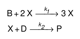
(\(\ce{B}\) and \(\ce{D}\) are reagents, \(\ce{X}\) is an intermediate and \(\ce{P}\) is a product).
3.1 Write down the overall reaction equation for this two-step mechanism. Write the rate equation for \(\ce{X}\).
3.2 Deduce a rate equation using steady-state approximation. Find the orders:
(i) a partial reaction order with respect to \(\ce{B}\);
(ii) a partial reaction order with respect to \(\ce{D}\);
(iii) the overall order of a reaction.
Let the reaction occur in an open system where reagents \(\ce{B}\) and \(\ce{D}\) are being continuously added to the mixture so that their concentrations are maintained constant and equal: \([\ce{B}]=[\ce{D}]=\mathrm{const}\).
3.3 Without solving the kinetic equation draw the kinetic curve \([\ce{X}](t)\) for the cases:
\[ 1)\quad [\ce{X}]_0>\frac{k_2}{k_1}; \qquad 2)\quad [\ce{X}]_0<\frac{k_2}{k_1}. \]
3.4 Without solving the kinetic equation draw the kinetic curve \([\ce{X}](t)\) for the case when the reaction proceeds in a closed vessel with the initial concentrations: \([\ce{B}]_0=[\ce{D}]_0\), \([\ce{X}]_0>\dfrac{k_2}{k_1}\).
Much more complex kinetic behavior is possible for the reactions with several intermediates. Consider a simplified reaction mechanism for cold burning of ethane in oxygen:
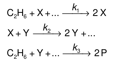
Under specific conditions this reaction displays oscillatory behavior:
Intermediates are peroxide \(\ce{C2H6O2}\) and aldehyde \(\ce{C2H4O}\), \(\ce{P}\) is a stable product.
3.5 Identify \(\ce{X}\), \(\ce{Y}\), and \(\ce{P}\). Fill the blanks in the reaction mechanism.
Behavior of unstable reactions is often controlled by temperature which affects the rate constants. In the above oxidation mechanism oscillations of concentrations are possible only if \(k_1\geq k_2\). Parameters of the Arrhenius equations were determined experimentally:
| Step | \(A,\ \mathrm{cm^3\,mol^{-1}\,s^{-1}}\) | \(E_{\mathrm A},\ \mathrm{kJ\,mol^{-1}}\) |
|---|---|---|
| 1 | \(1.0\times10^{11}\) | 90 |
| 2 | \(3.0\times10^{12}\) | 100 |
3.6 What is the highest temperature at which oscillatory regime is possible? Show your calculations.
Official English text of the problem.
Answers
-
3.1 \[ \boxed{\ce{B + D -> P}} \] \[ \boxed{\frac{d[\ce{X}]}{dt} =k_1[\ce{B}][\ce{X}]^2-k_2[\ce{D}][\ce{X}].} \]
-
3.2 On the nonzero steady-state branch, \[ [\ce{X}]_{\mathrm{ss}}=\frac{k_2[\ce{D}]}{k_1[\ce{B}]}, \qquad \boxed{v=\frac{k_2^2}{k_1}\frac{[\ce{D}]^2}{[\ce{B}]}.} \] The orders are \(-1\) with respect to \(\ce{B}\), \(2\) with respect to \(\ce{D}\), and \(1\) overall.
-
3.3 Write \(K=k_2/k_1\). 1. For \([\ce{X}]_0>K\), the curve increases continuously, is concave upward, and becomes unbounded at a finite time in the idealized model. 2. For \(0<[\ce{X}]_0<K\), the curve decreases continuously toward zero. If initially above \(K/2\), it first curves downward, passes through an inflection at \(K/2\), and then curves upward; if initially at or below \(K/2\), it curves upward thereafter.
-
3.4 The curve rises from \([\ce{X}]_0\), reaches one maximum, and then decreases toward the horizontal asymptote \[ \boxed{[\ce{X}]_{\infty}=[\ce{X}]_0.} \]
-
3.5 Using the carbon-skeleton-preserving structural assignments:
| Species | Identity | Formula | SMILES |
|---|---|---|---|
| \(\ce{X}\) | Ethyl hydroperoxide | \(\ce{C2H5OOH}\) | CCOO |
| \(\ce{Y}\) | Ethanal (acetaldehyde) | \(\ce{CH3CHO}\) | CC=O |
| \(\ce{P}\) | Ethanol | \(\ce{C2H5OH}\) | CCO |
The blanks, in order, are oxygen \(\ce{O2}\), O=O; water \(\ce{H2O}\), O; and water \(\ce{H2O}\), O. The completed balanced mechanism is given below.
- 3.6 \[ \boxed{T_{\max}=\frac{10\,000}{R\ln30} \approx354\ \mathrm K\quad(\text{about }81\,^\circ\mathrm C).} \]
Solution
3.1
In this first mechanism, \(\ce{B}\), \(\ce{D}\), \(\ce{X}\), and \(\ce{P}\) are unspecified species, so molecular names and SMILES cannot be assigned.
The steps are \[ \ce{B + 2X ->[k_1] 3X}, \qquad \ce{X + D ->[k_2] P}. \]
Adding them and cancelling the intermediate gives \[ \boxed{\ce{B + D -> P}.} \]
Because the steps are elementary, their rates are \[ v_1=k_1[\ce{B}][\ce{X}]^2, \qquad v_2=k_2[\ce{X}][\ce{D}]. \]
Each occurrence of the first step produces one net \(\ce{X}\), whereas the second consumes one. Therefore, \[ \boxed{\frac{d[\ce{X}]}{dt} =(3-2)v_1-v_2 =k_1[\ce{B}][\ce{X}]^2-k_2[\ce{D}][\ce{X}].} \]
3.2
The steady-state approximation sets the net production rate of the intermediate approximately equal to zero: \[ 0\simeq[\ce{X}] \left(k_1[\ce{B}][\ce{X}]-k_2[\ce{D}]\right). \]
Besides the zero-concentration solution, the nonzero stationary concentration is \[ [\ce{X}]_{\mathrm{ss}} =\frac{k_2[\ce{D}]}{k_1[\ce{B}]}. \]
Substitution into the product-formation rate gives \[ v=\frac{d[\ce{P}]}{dt} =k_2[\ce{D}][\ce{X}]_{\mathrm{ss}} =\boxed{\frac{k_2^2}{k_1}\frac{[\ce{D}]^2}{[\ce{B}]}}. \]
Thus:
\[ \boxed{n_{\ce B}=-1,\qquad n_{\ce D}=2,\qquad n_{\mathrm{overall}}=-1+2=1.} \]
The other stationary branch, \([\ce{X}]=0\), gives zero reaction rate. The nonzero branch yields the requested formal rate law, although it is unstable when the reagent concentrations are held fixed, as the next part shows.
3.3
Define \[ x=[\ce{X}],\qquad x_0=[\ce{X}]_0,\qquad C=[\ce{B}]=[\ce{D}]>0,\qquad K=\frac{k_2}{k_1}. \] Here \(K\) has concentration units. The kinetic equation becomes \[ \dot x=Ck_1x(x-K). \]
The stationary concentrations are \(x=0\) and \(x=K\). The sign of \(\dot x\) determines the direction of motion without solving the equation.
For each sketch, put time on the horizontal axis and \(x\) on the vertical axis.
Case 1: \(x_0>K\).
Both factors \(x\) and \(x-K\) are positive, so \(x\) increases. Moreover, \[ \ddot x=Ck_1(2x-K)\dot x>0. \]
The curve therefore starts above \(K\), rises continuously, and becomes progressively steeper. Its unbounded growth occurs at a finite time: since \(x\geq x_0\), \[ \dot x\geq Ck_1\left(1-\frac{K}{x_0}\right)x^2, \] so \(1/x\) decreases at least at a fixed positive rate until it reaches zero. Thus the idealized sketch has a finite-time vertical asymptote.
Case 2: \(0<x_0<K\).
Now \(\dot x<0\), so the concentration decreases. It approaches zero asymptotically, flattening toward the time axis.
The curvature follows from \[ \ddot x=Ck_1(2x-K)\dot x. \]
Because \(\dot x<0\):
- For \(K/2<x<K\), the curve is concave downward.
- At \(x=K/2\), it has an inflection.
- For \(0<x<K/2\), it is concave upward.
Consequently, an initial concentration above \(K/2\) gives a decreasing curve with one inflection; an initial concentration at or below \(K/2\) gives a curve that is concave upward thereafter.
For completeness, \(x_0=0\) remains zero, and \(x_0=K\) remains exactly \(K\). The latter stationary state is unstable: a small upward displacement grows, while a small downward displacement leads toward zero.
3.4
In a closed vessel, let \[ b=[\ce{B}],\qquad d=[\ce{D}],\qquad x=[\ce{X}], \qquad b_0=d_0=C_0. \]
The equations are \[ \dot b=-v_1,\qquad \dot d=-v_2,\qquad \dot x=v_1-v_2. \]
Hence \[ \frac{d}{dt}(x+b-d)=0. \] Using the equal initial reagent concentrations, \[ \boxed{x+b-d=x_0,\qquad x=x_0+d-b.} \]
Initially, \[ \dot x_0=C_0x_0(k_1x_0-k_2)>0, \] so the concentration rises.
It cannot subsequently cross below \(x_0\): at any point where \(x=x_0\), conservation requires \(b=d\), and therefore \[ \dot x=bx_0(k_1x_0-k_2)>0 \] while reagents remain.
Since \(x\geq x_0>0\), both reagents are continuously consumed and tend to zero. For example, \[ \dot b\leq-k_1x_0^2b,\qquad \dot d\leq-k_2x_0d. \] The conservation relation then gives \[ \boxed{x_\infty=x_0.} \]
There is exactly one maximum. At a stationary point, \(v_1=v_2=v>0\), and \[ \ddot x =-k_1vx^2+k_2vx =vx(k_2-k_1x)<0, \] because \(x\geq x_0>K\). Every stationary point is therefore a strict maximum; no intervening minimum is possible.
The requested sketch starts at \(x_0\), rises to a single peak with a horizontal tangent, then decreases and flattens toward \(x_0\) from above. Its initial concavity is not fixed by the supplied conditions.
3.5
Ethane is \(\ce{C2H6}\), SMILES CC.
In the first step, one molecule of ethane is converted into one additional molecule of \(\ce{X}\). Addition of oxygen gives
\[
\ce{C2H6 + O2 -> C2H6O2}.
\]
Thus \(\ce{X}\) is the peroxide. Retaining the ethane carbon skeleton gives ethyl hydroperoxide, \(\ce{C2H5OOH}\), CCOO.
The second step consumes one net peroxide molecule and produces one net molecule of the other intermediate. The balance is
\[
\ce{C2H6O2 -> C2H4O + H2O}.
\]
Therefore \(\ce{Y}\) is the aldehyde ethanal, \(\ce{CH3CHO}\), CC=O, and the missing product is water.
In the third step, adding water to ethane and ethanal gives the combined composition
\[
\ce{C2H6 + C2H4O + H2O},
\]
containing four carbon, twelve hydrogen, and two oxygen atoms. Two molecules of \(\ce{P}\) consequently each have formula \(\ce{C2H6O}\). The carbon-skeleton-preserving product is ethanol, \(\ce{C2H5OH}\), CCO.
The completed mechanism is therefore \[ \boxed{\ce{C2H6 + C2H5OOH + O2 ->[k_1] 2C2H5OOH}} \] \[ \boxed{\ce{C2H5OOH + CH3CHO ->[k_2] 2CH3CHO + H2O}} \] \[ \boxed{\ce{C2H6 + CH3CHO + H2O ->[k_3] 2C2H5OH}}. \]
All three equations conserve carbon, hydrogen, and oxygen. Adding them cancels both intermediates and water, giving the overall partial oxidation: \[ \ce{2C2H6 + O2 -> 2C2H5OH}. \]
3.6
The Arrhenius equation is \[ k_i=A_i\exp\left(-\frac{E_{\mathrm A,i}}{RT}\right). \]
Thus \[ \frac{k_1}{k_2} =\frac{A_1}{A_2} \exp\left(\frac{E_{\mathrm A,2}-E_{\mathrm A,1}}{RT}\right) =\frac1{30}\exp\left(\frac{10\,000\ \mathrm{J\,mol^{-1}}}{RT}\right). \]
The stated condition \(k_1\geq k_2\) requires \[ \frac{10\,000\ \mathrm{J\,mol^{-1}}}{RT}\geq\ln30. \] Therefore, \[ T\leq\frac{10\,000\ \mathrm{J\,mol^{-1}}}{R\ln30}. \]
Using \(R=8.314\ \mathrm{J\,mol^{-1}\,K^{-1}}\), \[ T_{\max} =\frac{10\,000}{8.314\ln30}\ \mathrm K =353.6\ \mathrm K. \]
Hence \[ \boxed{T_{\max}\approx354\ \mathrm K \approx81\,^\circ\mathrm C.} \]
This is the upper temperature allowed by the stated necessary condition; that condition alone does not guarantee oscillations at every lower temperature.
The solution was checked against the official solution.
IChO 2007 · Theorieaufgabe 3
Instabile chemische Reaktionen
Viele chemische Reaktionen zeigen ein instabiles kinetisches Verhalten. Unter unterschiedlichen Bedingungen (Konzentrationen und Temperatur) können solche Reaktionen in verschiedenen Zuständen ablaufen: stabil, oszillierend oder chaotisch. Die meisten dieser Reaktionen enthalten autokatalytische Elementarschritte.
Betrachten Sie einen einfachen Reaktionsmechanismus mit einem autokatalytischen Schritt:
(\(\ce{B}\) und \(\ce{D}\) sind Edukte, \(\ce{X}\) ist ein Zwischenprodukt und \(\ce{P}\) ist ein Produkt).
3.1 Geben Sie die Gesamtreaktionsgleichung für diesen zweistufigen Mechanismus an. Stellen Sie die Geschwindigkeitsgleichung für \(\ce{X}\) auf.
3.2 Leiten Sie mithilfe der Quasistationaritätsnäherung ein Geschwindigkeitsgesetz her. Bestimmen Sie die Ordnungen:
(i) die Teilreaktionsordnung bezüglich \(\ce{B}\);
(ii) die Teilreaktionsordnung bezüglich \(\ce{D}\);
(iii) die Gesamtreaktionsordnung.
Die Reaktion soll in einem offenen System ablaufen, in dem die Edukte \(\ce{B}\) und \(\ce{D}\) dem Gemisch kontinuierlich zugeführt werden, sodass ihre Konzentrationen konstant und gleich gehalten werden: \([\ce{B}]=[\ce{D}]=\mathrm{const}\).
3.3 Zeichnen Sie, ohne die kinetische Gleichung zu lösen, die Konzentrations-Zeit-Kurve \([\ce{X}](t)\) für die Fälle:
\[ 1)\quad [\ce{X}]_0>\frac{k_2}{k_1}; \qquad 2)\quad [\ce{X}]_0<\frac{k_2}{k_1}. \]
3.4 Zeichnen Sie, ohne die kinetische Gleichung zu lösen, die Konzentrations-Zeit-Kurve \([\ce{X}](t)\) für den Fall, dass die Reaktion in einem geschlossenen Gefäß mit den Anfangskonzentrationen \([\ce{B}]_0=[\ce{D}]_0\), \([\ce{X}]_0>\dfrac{k_2}{k_1}\) abläuft.
Bei Reaktionen mit mehreren Zwischenprodukten ist ein wesentlich komplexeres kinetisches Verhalten möglich. Betrachten Sie einen vereinfachten Reaktionsmechanismus für die kalte Verbrennung von Ethan in Sauerstoff:
Unter bestimmten Bedingungen zeigt diese Reaktion ein oszillierendes Verhalten:
Die Zwischenprodukte sind das Peroxid \(\ce{C2H6O2}\) und der Aldehyd \(\ce{C2H4O}\), \(\ce{P}\) ist ein stabiles Produkt.
3.5 Identifizieren Sie \(\ce{X}\), \(\ce{Y}\) und \(\ce{P}\). Ergänzen Sie die Lücken im Reaktionsmechanismus.
Das Verhalten instabiler Reaktionen wird häufig durch die Temperatur gesteuert, die die Geschwindigkeitskonstanten beeinflusst. Im obigen Oxidationsmechanismus sind Konzentrationsoszillationen nur möglich, wenn \(k_1\geq k_2\). Die Parameter der Arrhenius-Gleichungen wurden experimentell bestimmt:
| Schritt | \(A,\ \mathrm{cm^3\,mol^{-1}\,s^{-1}}\) | \(E_{\mathrm A},\ \mathrm{kJ\,mol^{-1}}\) |
|---|---|---|
| 1 | \(1.0\times10^{11}\) | 90 |
| 2 | \(3.0\times10^{12}\) | 100 |
3.6 Wie hoch ist die höchste Temperatur, bei der ein oszillierender Reaktionsverlauf möglich ist? Zeigen Sie Ihre Berechnungen.
Aufgabentext aus dem offiziellen englischen Text übersetzt.
Antworten
-
3.1 \[ \boxed{\ce{B + D -> P}} \] \[ \boxed{\frac{d[\ce{X}]}{dt} =k_1[\ce{B}][\ce{X}]^2-k_2[\ce{D}][\ce{X}].} \]
-
3.2 Auf dem stationären Lösungszweig mit einer von null verschiedenen Konzentration gilt \[ [\ce{X}]_{\mathrm{ss}}=\frac{k_2[\ce{D}]}{k_1[\ce{B}]}, \qquad \boxed{v=\frac{k_2^2}{k_1}\frac{[\ce{D}]^2}{[\ce{B}]}.} \] Die Ordnungen sind \(-1\) bezüglich \(\ce{B}\), \(2\) bezüglich \(\ce{D}\) und insgesamt \(1\).
-
3.3 Setzen wir \(K=k_2/k_1\). 1. Für \([\ce{X}]_0>K\) steigt die Kurve stetig an, ist nach oben gekrümmt und wächst im idealisierten Modell innerhalb endlicher Zeit über alle Grenzen. 2. Für \(0<[\ce{X}]_0<K\) fällt die Kurve stetig gegen null. Liegt die Anfangskonzentration oberhalb von \(K/2\), ist sie zunächst nach unten gekrümmt, durchläuft bei \(K/2\) einen Wendepunkt und ist danach nach oben gekrümmt; liegt die Anfangskonzentration bei oder unterhalb von \(K/2\), ist sie im weiteren Verlauf nach oben gekrümmt.
-
3.4 Die Kurve steigt ausgehend von \([\ce{X}]_0\) an, erreicht ein einziges Maximum und fällt anschließend gegen die horizontale Asymptote \[ \boxed{[\ce{X}]_{\infty}=[\ce{X}]_0.} \]
-
3.5 Bei Strukturzuordnungen unter Erhaltung des Kohlenstoffgerüsts ergibt sich:
| Spezies | Identität | Formel | SMILES |
|---|---|---|---|
| \(\ce{X}\) | Ethylhydroperoxid | \(\ce{C2H5OOH}\) | CCOO |
| \(\ce{Y}\) | Ethanal (Acetaldehyd) | \(\ce{CH3CHO}\) | CC=O |
| \(\ce{P}\) | Ethanol | \(\ce{C2H5OH}\) | CCO |
Die Lücken sind der Reihe nach mit Sauerstoff \(\ce{O2}\), O=O; Wasser \(\ce{H2O}\), O; und Wasser \(\ce{H2O}\), O zu füllen. Der vervollständigte, ausgeglichene Mechanismus ist unten angegeben.
- 3.6 \[ \boxed{T_{\max}=\frac{10\,000}{R\ln30} \approx354\ \mathrm K\quad(\text{etwa }81\,^\circ\mathrm C).} \]
Lösung
3.1
In diesem ersten Mechanismus sind \(\ce{B}\), \(\ce{D}\), \(\ce{X}\) und \(\ce{P}\) nicht näher spezifizierte Spezies, sodass ihnen keine Molekülnamen und SMILES zugeordnet werden können.
Die Schritte lauten \[ \ce{B + 2X ->[k_1] 3X}, \qquad \ce{X + D ->[k_2] P}. \]
Durch Addition und Kürzen des Zwischenprodukts erhält man \[ \boxed{\ce{B + D -> P}.} \]
Da es sich um Elementarschritte handelt, sind ihre Geschwindigkeiten \[ v_1=k_1[\ce{B}][\ce{X}]^2, \qquad v_2=k_2[\ce{X}][\ce{D}]. \]
Bei jedem Ablauf des ersten Schritts entsteht netto ein \(\ce{X}\), während beim zweiten eines verbraucht wird. Daher gilt \[ \boxed{\frac{d[\ce{X}]}{dt} =(3-2)v_1-v_2 =k_1[\ce{B}][\ce{X}]^2-k_2[\ce{D}][\ce{X}].} \]
3.2
Die Quasistationaritätsnäherung setzt die Nettobildungsgeschwindigkeit des Zwischenprodukts näherungsweise gleich null: \[ 0\simeq[\ce{X}] \left(k_1[\ce{B}][\ce{X}]-k_2[\ce{D}]\right). \]
Neben der Lösung mit der Konzentration null ergibt sich die von null verschiedene stationäre Konzentration \[ [\ce{X}]_{\mathrm{ss}} =\frac{k_2[\ce{D}]}{k_1[\ce{B}]}. \]
Einsetzen in die Produktbildungsgeschwindigkeit liefert \[ v=\frac{d[\ce{P}]}{dt} =k_2[\ce{D}][\ce{X}]_{\mathrm{ss}} =\boxed{\frac{k_2^2}{k_1}\frac{[\ce{D}]^2}{[\ce{B}]}}. \]
Somit gilt:
\[ \boxed{n_{\ce B}=-1,\qquad n_{\ce D}=2,\qquad n_{\mathrm{overall}}=-1+2=1.} \]
Der andere stationäre Lösungszweig, \([\ce{X}]=0\), ergibt eine Reaktionsgeschwindigkeit von null. Der Zweig mit einer von null verschiedenen Konzentration liefert das gesuchte formale Geschwindigkeitsgesetz, obwohl er bei konstant gehaltenen Eduktkonzentrationen instabil ist, wie der nächste Teil zeigt.
3.3
Wir definieren \[ x=[\ce{X}],\qquad x_0=[\ce{X}]_0,\qquad C=[\ce{B}]=[\ce{D}]>0,\qquad K=\frac{k_2}{k_1}. \] Hier hat \(K\) die Einheit einer Konzentration. Die kinetische Gleichung lautet damit \[ \dot x=Ck_1x(x-K). \]
Die stationären Konzentrationen sind \(x=0\) und \(x=K\). Das Vorzeichen von \(\dot x\) bestimmt die Änderungsrichtung, ohne dass die Gleichung gelöst werden muss.
Tragen Sie in jeder Skizze die Zeit auf der horizontalen Achse und \(x\) auf der vertikalen Achse auf.
Fall 1: \(x_0>K\).
Beide Faktoren \(x\) und \(x-K\) sind positiv, also nimmt \(x\) zu. Außerdem gilt \[ \ddot x=Ck_1(2x-K)\dot x>0. \]
Die Kurve beginnt daher oberhalb von \(K\), steigt stetig an und wird zunehmend steiler. Ihr unbeschränktes Wachstum erfolgt innerhalb endlicher Zeit: Wegen \(x\geq x_0\) gilt \[ \dot x\geq Ck_1\left(1-\frac{K}{x_0}\right)x^2, \] also nimmt \(1/x\) mindestens mit einer festen positiven Rate ab, bis es null erreicht. Die idealisierte Skizze besitzt somit eine vertikale Asymptote bei einer endlichen Zeit.
Fall 2: \(0<x_0<K\).
Nun gilt \(\dot x<0\), sodass die Konzentration abnimmt. Sie nähert sich asymptotisch null, wobei die Kurve zur Zeitachse hin abflacht.
Die Krümmung ergibt sich aus \[ \ddot x=Ck_1(2x-K)\dot x. \]
Da \(\dot x<0\) gilt:
- Für \(K/2<x<K\) ist die Kurve nach unten gekrümmt.
- Bei \(x=K/2\) besitzt sie einen Wendepunkt.
- Für \(0<x<K/2\) ist sie nach oben gekrümmt.
Folglich ergibt eine Anfangskonzentration oberhalb von \(K/2\) eine fallende Kurve mit einem Wendepunkt; bei einer Anfangskonzentration bei oder unterhalb von \(K/2\) ist die Kurve im weiteren Verlauf nach oben gekrümmt.
Der Vollständigkeit halber: Bei \(x_0=0\) bleibt die Konzentration null, und bei \(x_0=K\) bleibt sie genau \(K\). Der letztere stationäre Zustand ist instabil: Eine kleine Abweichung nach oben wächst an, während eine kleine Abweichung nach unten zu einer Annäherung an null führt.
3.4
Für ein geschlossenes Gefäß setzen wir \[ b=[\ce{B}],\qquad d=[\ce{D}],\qquad x=[\ce{X}], \qquad b_0=d_0=C_0. \]
Die Gleichungen lauten \[ \dot b=-v_1,\qquad \dot d=-v_2,\qquad \dot x=v_1-v_2. \]
Daraus folgt \[ \frac{d}{dt}(x+b-d)=0. \] Mit den gleichen Anfangskonzentrationen der Edukte ergibt sich \[ \boxed{x+b-d=x_0,\qquad x=x_0+d-b.} \]
Zu Beginn gilt \[ \dot x_0=C_0x_0(k_1x_0-k_2)>0, \] also steigt die Konzentration an.
Sie kann anschließend nicht unter \(x_0\) fallen: An jedem Punkt, an dem \(x=x_0\) gilt, erfordert die Erhaltungsbeziehung \(b=d\), und daher gilt \[ \dot x=bx_0(k_1x_0-k_2)>0 \] solange noch Edukte vorhanden sind.
Da \(x\geq x_0>0\), werden beide Edukte kontinuierlich verbraucht, und ihre Konzentrationen streben gegen null. Beispielsweise gilt \[ \dot b\leq-k_1x_0^2b,\qquad \dot d\leq-k_2x_0d. \] Die Erhaltungsbeziehung ergibt dann \[ \boxed{x_\infty=x_0.} \]
Es gibt genau ein Maximum. An einem stationären Punkt gilt \(v_1=v_2=v>0\), und \[ \ddot x =-k_1vx^2+k_2vx =vx(k_2-k_1x)<0, \] weil \(x\geq x_0>K\). Jeder stationäre Punkt ist daher ein striktes Maximum; ein dazwischenliegendes Minimum ist nicht möglich.
Die gesuchte Skizze beginnt bei \(x_0\), steigt zu einem einzigen Maximum mit horizontaler Tangente an, fällt danach ab und nähert sich unter Abflachung von oben an \(x_0\) an. Ihre anfängliche Krümmung ist durch die angegebenen Bedingungen nicht festgelegt.
3.5
Ethan ist \(\ce{C2H6}\), SMILES CC.
Im ersten Schritt wird ein Molekül Ethan in ein zusätzliches Molekül \(\ce{X}\) umgewandelt. Durch Addition von Sauerstoff ergibt sich
\[
\ce{C2H6 + O2 -> C2H6O2}.
\]
Somit ist \(\ce{X}\) das Peroxid. Unter Erhaltung des Kohlenstoffgerüsts von Ethan ergibt sich Ethylhydroperoxid, \(\ce{C2H5OOH}\), CCOO.
Im zweiten Schritt wird netto ein Peroxidmolekül verbraucht und netto ein Molekül des anderen Zwischenprodukts gebildet. Die Bilanz lautet
\[
\ce{C2H6O2 -> C2H4O + H2O}.
\]
Daher ist \(\ce{Y}\) der Aldehyd Ethanal, \(\ce{CH3CHO}\), CC=O, und das fehlende Produkt ist Wasser.
Im dritten Schritt ergibt die Zugabe von Wasser zu Ethan und Ethanal die Gesamtzusammensetzung
\[
\ce{C2H6 + C2H4O + H2O},
\]
die vier Kohlenstoff-, zwölf Wasserstoff- und zwei Sauerstoffatome enthält. Zwei Moleküle \(\ce{P}\) haben folglich jeweils die Formel \(\ce{C2H6O}\). Das Produkt unter Erhaltung des Kohlenstoffgerüsts ist Ethanol, \(\ce{C2H5OH}\), CCO.
Der vervollständigte Mechanismus lautet daher \[ \boxed{\ce{C2H6 + C2H5OOH + O2 ->[k_1] 2C2H5OOH}} \] \[ \boxed{\ce{C2H5OOH + CH3CHO ->[k_2] 2CH3CHO + H2O}} \] \[ \boxed{\ce{C2H6 + CH3CHO + H2O ->[k_3] 2C2H5OH}}. \]
In allen drei Gleichungen bleiben die Anzahlen der Kohlenstoff-, Wasserstoff- und Sauerstoffatome erhalten. Bei der Addition kürzen sich beide Zwischenprodukte und Wasser heraus, sodass sich insgesamt die partielle Oxidation ergibt: \[ \ce{2C2H6 + O2 -> 2C2H5OH}. \]
3.6
Die Arrhenius-Gleichung lautet \[ k_i=A_i\exp\left(-\frac{E_{\mathrm A,i}}{RT}\right). \]
Somit gilt \[ \frac{k_1}{k_2} =\frac{A_1}{A_2} \exp\left(\frac{E_{\mathrm A,2}-E_{\mathrm A,1}}{RT}\right) =\frac1{30}\exp\left(\frac{10\,000\ \mathrm{J\,mol^{-1}}}{RT}\right). \]
Die angegebene Bedingung \(k_1\geq k_2\) erfordert \[ \frac{10\,000\ \mathrm{J\,mol^{-1}}}{RT}\geq\ln30. \] Daher gilt \[ T\leq\frac{10\,000\ \mathrm{J\,mol^{-1}}}{R\ln30}. \]
Mit \(R=8.314\ \mathrm{J\,mol^{-1}\,K^{-1}}\) erhält man \[ T_{\max} =\frac{10\,000}{8.314\ln30}\ \mathrm K =353.6\ \mathrm K. \]
Damit ergibt sich \[ \boxed{T_{\max}\approx354\ \mathrm K \approx81\,^\circ\mathrm C.} \]
Dies ist die obere Temperaturgrenze, die durch die angegebene notwendige Bedingung zulässig ist; diese Bedingung allein garantiert keine Oszillationen bei jeder niedrigeren Temperatur.
Die Lösung wurde mit der offiziellen Lösung abgeglichen.
IChO 2007 · Teori sorusu 3
Kararsız kimyasal tepkimeler
Birçok kimyasal tepkime kararsız kinetik davranış gösterir. Farklı koşullarda (derişimler ve sıcaklık) bu tür tepkimeler çeşitli biçimlerde ilerleyebilir: kararlı, salınımlı veya kaotik. Bu tepkimelerin çoğu otokatalitik elementer basamaklar içerir.
Otokatalitik bir basamak içeren basit bir tepkime mekanizmasını ele alalım:
(\(\ce{B}\) ve \(\ce{D}\) reaktifler, \(\ce{X}\) bir ara ürün ve \(\ce{P}\) bir üründür).
3.1 Bu iki basamaklı mekanizmanın toplam tepkime denklemini yazınız. \(\ce{X}\) için hız denklemini yazınız.
3.2 Kararlı hâl yaklaşımını kullanarak bir hız denklemi türetiniz. Aşağıdaki dereceleri bulunuz:
(i) \(\ce{B}\)'ye göre kısmi tepkime derecesi;
(ii) \(\ce{D}\)'ye göre kısmi tepkime derecesi;
(iii) tepkimenin toplam derecesi.
Tepkimenin, \(\ce{B}\) ve \(\ce{D}\) reaktiflerinin derişimleri sabit ve birbirine eşit tutulacak şekilde karışıma sürekli eklendiği açık bir sistemde gerçekleştiğini varsayalım: \([\ce{B}]=[\ce{D}]=\mathrm{const}\).
3.3 Kinetik denklemi çözmeden, aşağıdaki durumlar için \([\ce{X}](t)\) kinetik eğrisini çiziniz:
\[ 1)\quad [\ce{X}]_0>\frac{k_2}{k_1}; \qquad 2)\quad [\ce{X}]_0<\frac{k_2}{k_1}. \]
3.4 Tepkimenin kapalı bir kapta şu başlangıç derişimleriyle gerçekleştiği durum için, kinetik denklemi çözmeden \([\ce{X}](t)\) kinetik eğrisini çiziniz: \([\ce{B}]_0=[\ce{D}]_0\), \([\ce{X}]_0>\dfrac{k_2}{k_1}\).
Birden fazla ara ürün içeren tepkimelerde çok daha karmaşık kinetik davranışlar mümkündür. Etanın oksijen içinde soğuk yanmasına ilişkin basitleştirilmiş bir tepkime mekanizmasını ele alalım:
Belirli koşullar altında bu tepkime salınımlı davranış gösterir:
Ara ürünler peroksit \(\ce{C2H6O2}\) ve aldehit \(\ce{C2H4O}\)'dur; \(\ce{P}\) ise kararlı bir üründür.
3.5 \(\ce{X}\), \(\ce{Y}\) ve \(\ce{P}\)'yi belirleyiniz. Tepkime mekanizmasındaki boşlukları doldurunuz.
Kararsız tepkimelerin davranışı çoğu zaman hız sabitlerini etkileyen sıcaklık tarafından kontrol edilir. Yukarıdaki yükseltgenme mekanizmasında derişim salınımları yalnızca \(k_1\geq k_2\) ise mümkündür. Arrhenius denklemlerinin parametreleri deneysel olarak belirlenmiştir:
| Basamak | \(A,\ \mathrm{cm^3\,mol^{-1}\,s^{-1}}\) | \(E_{\mathrm A},\ \mathrm{kJ\,mol^{-1}}\) |
|---|---|---|
| 1 | \(1.0\times10^{11}\) | 90 |
| 2 | \(3.0\times10^{12}\) | 100 |
3.6 Salınımlı rejimin mümkün olduğu en yüksek sıcaklık nedir? Hesaplamalarınızı gösteriniz.
Soru metni resmi İngilizce metinden çevrilmiştir.
Cevaplar
-
3.1 \[ \boxed{\ce{B + D -> P}} \] \[ \boxed{\frac{d[\ce{X}]}{dt} =k_1[\ce{B}][\ce{X}]^2-k_2[\ce{D}][\ce{X}].} \]
-
3.2 Sıfırdan farklı kararlı hâl dalında, \[ [\ce{X}]_{\mathrm{ss}}=\frac{k_2[\ce{D}]}{k_1[\ce{B}]}, \qquad \boxed{v=\frac{k_2^2}{k_1}\frac{[\ce{D}]^2}{[\ce{B}]}.} \] Dereceler \(\ce{B}\)'ye göre \(-1\), \(\ce{D}\)'ye göre \(2\) ve toplamda \(1\)'dir.
-
3.3 \(K=k_2/k_1\) olarak yazalım. 1. \([\ce{X}]_0>K\) için eğri sürekli artar, yukarı doğru içbükeydir ve idealleştirilmiş modelde sonlu bir zamanda sınırsız hâle gelir. 2. \(0<[\ce{X}]_0<K\) için eğri sürekli azalarak sıfıra yaklaşır. Başlangıçta \(K/2\)'nin üzerindeyse önce aşağı doğru bükülür, \(K/2\)'de bir büküm noktasından geçer ve ardından yukarı doğru bükülür; başlangıçta \(K/2\)'de veya bunun altındaysa bundan sonra yukarı doğru bükülür.
-
3.4 Eğri \([\ce{X}]_0\)'dan başlayarak yükselir, bir maksimuma ulaşır ve ardından azalarak şu yatay asimptota yaklaşır: \[ \boxed{[\ce{X}]_{\infty}=[\ce{X}]_0.} \]
-
3.5 Karbon iskeletini koruyan yapısal atamalar kullanıldığında:
| Tür | Kimliği | Formül | SMILES |
|---|---|---|---|
| \(\ce{X}\) | Etil hidroperoksit | \(\ce{C2H5OOH}\) | CCOO |
| \(\ce{Y}\) | Etanal (asetaldehit) | \(\ce{CH3CHO}\) | CC=O |
| \(\ce{P}\) | Etanol | \(\ce{C2H5OH}\) | CCO |
Boşluklar sırasıyla oksijen \(\ce{O2}\), O=O; su \(\ce{H2O}\), O; ve su \(\ce{H2O}\), O şeklindedir. Tamamlanmış ve denkleştirilmiş mekanizma aşağıda verilmiştir.
- 3.6 \[ \boxed{T_{\max}=\frac{10\,000}{R\ln30} \approx354\ \mathrm K\quad(\text{yaklaşık }81\,^\circ\mathrm C).} \]
Çözüm
3.1
Bu ilk mekanizmada \(\ce{B}\), \(\ce{D}\), \(\ce{X}\) ve \(\ce{P}\) kimlikleri belirtilmemiş türlerdir; dolayısıyla bunlara molekül adları ve SMILES gösterimleri atanamaz.
Basamaklar şöyledir: \[ \ce{B + 2X ->[k_1] 3X}, \qquad \ce{X + D ->[k_2] P}. \]
Bunlar toplanıp ara ürün sadeleştirildiğinde şu denklem elde edilir: \[ \boxed{\ce{B + D -> P}.} \]
Basamaklar elementer olduğundan hızları şöyledir: \[ v_1=k_1[\ce{B}][\ce{X}]^2, \qquad v_2=k_2[\ce{X}][\ce{D}]. \]
Birinci basamağın her gerçekleşmesinde net bir \(\ce{X}\) üretilirken ikinci basamakta bir tane tüketilir. Dolayısıyla, \[ \boxed{\frac{d[\ce{X}]}{dt} =(3-2)v_1-v_2 =k_1[\ce{B}][\ce{X}]^2-k_2[\ce{D}][\ce{X}].} \]
3.2
Kararlı hâl yaklaşımında ara ürünün net oluşum hızı yaklaşık olarak sıfıra eşit alınır: \[ 0\simeq[\ce{X}] \left(k_1[\ce{B}][\ce{X}]-k_2[\ce{D}]\right). \]
Sıfır derişimli çözümün yanı sıra, sıfırdan farklı durağan derişim şöyledir: \[ [\ce{X}]_{\mathrm{ss}} =\frac{k_2[\ce{D}]}{k_1[\ce{B}]}. \]
Bu ifade ürün oluşum hızında yerine konulduğunda şu sonuç elde edilir: \[ v=\frac{d[\ce{P}]}{dt} =k_2[\ce{D}][\ce{X}]_{\mathrm{ss}} =\boxed{\frac{k_2^2}{k_1}\frac{[\ce{D}]^2}{[\ce{B}]}}. \]
Böylece:
\[ \boxed{n_{\ce B}=-1,\qquad n_{\ce D}=2,\qquad n_{\mathrm{overall}}=-1+2=1.} \]
Diğer durağan dal olan \([\ce{X}]=0\), sıfır tepkime hızı verir. Sıfırdan farklı dal, istenen biçimsel hız yasasını verir; ancak bir sonraki kısımda gösterildiği gibi reaktif derişimleri sabit tutulduğunda bu dal kararsızdır.
3.3
Şu tanımları yapalım: \[ x=[\ce{X}],\qquad x_0=[\ce{X}]_0,\qquad C=[\ce{B}]=[\ce{D}]>0,\qquad K=\frac{k_2}{k_1}. \] Burada \(K\) derişim birimine sahiptir. Kinetik denklem şu hâle gelir: \[ \dot x=Ck_1x(x-K). \]
Durağan derişimler \(x=0\) ve \(x=K\)'dır. \(\dot x\)'in işareti, denklemi çözmeden değişimin yönünü belirler.
Her çizimde yatay eksene zamanı, düşey eksene ise \(x\)'i yerleştiriniz.
Durum 1: \(x_0>K\).
Hem \(x\) hem de \(x-K\) çarpanı pozitiftir; dolayısıyla \(x\) artar. Ayrıca, \[ \ddot x=Ck_1(2x-K)\dot x>0. \]
Bu nedenle eğri \(K\)'nın üzerinden başlar, sürekli yükselir ve giderek dikleşir. Sınırsız büyümesi sonlu bir zamanda gerçekleşir: \(x\geq x_0\) olduğundan, \[ \dot x\geq Ck_1\left(1-\frac{K}{x_0}\right)x^2, \] dolayısıyla \(1/x\), sıfıra ulaşıncaya kadar en az sabit bir pozitif hızla azalır. Böylece idealleştirilmiş çizimde sonlu bir zamanda düşey bir asimptot bulunur.
Durum 2: \(0<x_0<K\).
Bu durumda \(\dot x<0\) olduğundan derişim azalır. Zaman eksenine doğru yataylaşarak asimptotik biçimde sıfıra yaklaşır.
Eğrilik şu ifadeden belirlenir: \[ \ddot x=Ck_1(2x-K)\dot x. \]
\(\dot x<0\) olduğundan:
- \(K/2<x<K\) için eğri aşağı doğru içbükeydir.
- \(x=K/2\)'de bir büküm noktası vardır.
- \(0<x<K/2\) için eğri yukarı doğru içbükeydir.
Sonuç olarak, \(K/2\)'nin üzerindeki bir başlangıç derişimi tek bir büküm noktası olan azalan bir eğri verir; \(K/2\)'deki veya bunun altındaki bir başlangıç derişimi ise bundan sonra yukarı doğru içbükey olan bir eğri verir.
Eksiksiz olması açısından, \(x_0=0\) durumunda derişim sıfırda, \(x_0=K\) durumunda ise tam olarak \(K\)'da kalır. İkinci durağan durum kararsızdır: yukarı yöndeki küçük bir sapma büyürken aşağı yöndeki küçük bir sapma sıfıra doğru ilerlemeye yol açar.
3.4
Kapalı bir kapta şu tanımları yapalım: \[ b=[\ce{B}],\qquad d=[\ce{D}],\qquad x=[\ce{X}], \qquad b_0=d_0=C_0. \]
Denklemler şöyledir: \[ \dot b=-v_1,\qquad \dot d=-v_2,\qquad \dot x=v_1-v_2. \]
Buradan, \[ \frac{d}{dt}(x+b-d)=0. \] Başlangıç reaktif derişimlerinin eşitliği kullanıldığında, \[ \boxed{x+b-d=x_0,\qquad x=x_0+d-b.} \]
Başlangıçta, \[ \dot x_0=C_0x_0(k_1x_0-k_2)>0, \] dolayısıyla derişim yükselir.
Derişim daha sonra \(x_0\)'ın altına geçemez: \(x=x_0\) olan herhangi bir noktada korunum bağıntısı \(b=d\) olmasını gerektirir ve dolayısıyla reaktifler tükenmediği sürece \[ \dot x=bx_0(k_1x_0-k_2)>0 \] olur.
\(x\geq x_0>0\) olduğundan her iki reaktif de sürekli tüketilir ve derişimleri sıfıra yaklaşır. Örneğin, \[ \dot b\leq-k_1x_0^2b,\qquad \dot d\leq-k_2x_0d. \] Korunum bağıntısı bu durumda şu sonucu verir: \[ \boxed{x_\infty=x_0.} \]
Tam olarak bir maksimum vardır. Bir durağan noktada \(v_1=v_2=v>0\) olur ve \[ \ddot x =-k_1vx^2+k_2vx =vx(k_2-k_1x)<0, \] çünkü \(x\geq x_0>K\)'dır. Dolayısıyla her durağan nokta kesin bir maksimumdur; arada bir minimum bulunması mümkün değildir.
İstenen çizim \(x_0\)'dan başlar, yatay teğete sahip tek bir tepeye yükselir, ardından azalır ve yukarıdan \(x_0\)'a yaklaşırken yataylaşır. Başlangıçtaki içbükeylik yönü verilen koşullarla belirlenmez.
3.5
Etan \(\ce{C2H6}\)'dır; SMILES gösterimi CC'dir.
Birinci basamakta bir etan molekülü, ilave bir \(\ce{X}\) molekülüne dönüşür. Oksijen katılmasıyla şu denklem elde edilir:
\[
\ce{C2H6 + O2 -> C2H6O2}.
\]
Buna göre \(\ce{X}\) peroksittir. Etanın karbon iskeleti korunduğunda etil hidroperoksit, \(\ce{C2H5OOH}\), CCOO elde edilir.
İkinci basamakta net bir peroksit molekülü tüketilir ve diğer ara üründen net bir molekül üretilir. Denkleştirilmiş ifade şöyledir:
\[
\ce{C2H6O2 -> C2H4O + H2O}.
\]
Dolayısıyla \(\ce{Y}\), etanal aldehididir: \(\ce{CH3CHO}\), CC=O; eksik ürün ise sudur.
Üçüncü basamakta etan ve etanale su eklenmesi, toplamda
\[
\ce{C2H6 + C2H4O + H2O},
\]
bileşimini verir; bu bileşim dört karbon, on iki hidrojen ve iki oksijen atomu içerir. Bu nedenle iki \(\ce{P}\) molekülünün her birinin formülü \(\ce{C2H6O}\)'dur. Karbon iskeletini koruyan ürün etanol, \(\ce{C2H5OH}\), CCO'dur.
Böylece tamamlanmış mekanizma şöyledir: \[ \boxed{\ce{C2H6 + C2H5OOH + O2 ->[k_1] 2C2H5OOH}} \] \[ \boxed{\ce{C2H5OOH + CH3CHO ->[k_2] 2CH3CHO + H2O}} \] \[ \boxed{\ce{C2H6 + CH3CHO + H2O ->[k_3] 2C2H5OH}}. \]
Üç denklemde de karbon, hidrojen ve oksijen korunur. Denklemler toplandığında her iki ara ürün ve su sadeleşir; toplam kısmi yükseltgenme tepkimesi elde edilir: \[ \ce{2C2H6 + O2 -> 2C2H5OH}. \]
3.6
Arrhenius denklemi şöyledir: \[ k_i=A_i\exp\left(-\frac{E_{\mathrm A,i}}{RT}\right). \]
Buna göre, \[ \frac{k_1}{k_2} =\frac{A_1}{A_2} \exp\left(\frac{E_{\mathrm A,2}-E_{\mathrm A,1}}{RT}\right) =\frac1{30}\exp\left(\frac{10\,000\ \mathrm{J\,mol^{-1}}}{RT}\right). \]
Verilen \(k_1\geq k_2\) koşulu şu eşitsizliği gerektirir: \[ \frac{10\,000\ \mathrm{J\,mol^{-1}}}{RT}\geq\ln30. \] Dolayısıyla, \[ T\leq\frac{10\,000\ \mathrm{J\,mol^{-1}}}{R\ln30}. \]
\(R=8.314\ \mathrm{J\,mol^{-1}\,K^{-1}}\) kullanıldığında, \[ T_{\max} =\frac{10\,000}{8.314\ln30}\ \mathrm K =353.6\ \mathrm K. \]
Böylece, \[ \boxed{T_{\max}\approx354\ \mathrm K \approx81\,^\circ\mathrm C.} \]
Bu, belirtilen gerekli koşulun izin verdiği üst sıcaklık sınırıdır; bu koşul tek başına daha düşük her sıcaklıkta salınımların gerçekleşeceğini garanti etmez.
Çözüm, resmi çözümle karşılaştırılarak kontrol edildi.
IChO 2007 · Problema teórico 3
Reacciones químicas inestables
Muchas reacciones químicas presentan un comportamiento cinético inestable. En distintas condiciones (concentraciones y temperatura), estas reacciones pueden transcurrir en diversos regímenes: estable, oscilatorio o caótico. La mayoría de estas reacciones incluyen etapas elementales autocatalíticas.
Considere un mecanismo de reacción sencillo que incluye una etapa autocatalítica:
(\(\ce{B}\) y \(\ce{D}\) son reactivos, \(\ce{X}\) es un intermedio y \(\ce{P}\) es un producto).
3.1 Escriba la ecuación global de la reacción correspondiente a este mecanismo de dos etapas. Escriba la ecuación de velocidad para \(\ce{X}\).
3.2 Deduzca una ecuación de velocidad utilizando la aproximación del estado estacionario. Determine los órdenes:
(i) el orden parcial de reacción respecto a \(\ce{B}\);
(ii) el orden parcial de reacción respecto a \(\ce{D}\);
(iii) el orden global de la reacción.
Suponga que la reacción tiene lugar en un sistema abierto en el que los reactivos \(\ce{B}\) y \(\ce{D}\) se añaden continuamente a la mezcla, de modo que sus concentraciones se mantienen constantes e iguales: \([\ce{B}]=[\ce{D}]=\mathrm{const}\).
3.3 Sin resolver la ecuación cinética, dibuje la curva cinética \([\ce{X}](t)\) para los casos:
\[ 1)\quad [\ce{X}]_0>\frac{k_2}{k_1}; \qquad 2)\quad [\ce{X}]_0<\frac{k_2}{k_1}. \]
3.4 Sin resolver la ecuación cinética, dibuje la curva cinética \([\ce{X}](t)\) para el caso en que la reacción transcurre en un recipiente cerrado con las concentraciones iniciales: \([\ce{B}]_0=[\ce{D}]_0\), \([\ce{X}]_0>\dfrac{k_2}{k_1}\).
Las reacciones con varios intermedios pueden presentar un comportamiento cinético mucho más complejo. Considere un mecanismo de reacción simplificado para la combustión fría del etano en oxígeno:
En determinadas condiciones, esta reacción presenta un comportamiento oscilatorio:
Los intermedios son el peróxido \(\ce{C2H6O2}\) y el aldehído \(\ce{C2H4O}\), y \(\ce{P}\) es un producto estable.
3.5 Identifique \(\ce{X}\), \(\ce{Y}\) y \(\ce{P}\). Complete los espacios en blanco del mecanismo de reacción.
El comportamiento de las reacciones inestables suele estar controlado por la temperatura, que afecta a las constantes de velocidad. En el mecanismo de oxidación anterior, las oscilaciones de las concentraciones solo son posibles si \(k_1\geq k_2\). Los parámetros de las ecuaciones de Arrhenius se determinaron experimentalmente:
| Etapa | \(A,\ \mathrm{cm^3\,mol^{-1}\,s^{-1}}\) | \(E_{\mathrm A},\ \mathrm{kJ\,mol^{-1}}\) |
|---|---|---|
| 1 | \(1.0\times10^{11}\) | 90 |
| 2 | \(3.0\times10^{12}\) | 100 |
3.6 ¿Cuál es la temperatura máxima a la que es posible un régimen oscilatorio? Muestre sus cálculos.
Enunciado traducido del texto oficial en inglés.
Respuestas
-
3.1 \[ \boxed{\ce{B + D -> P}} \] \[ \boxed{\frac{d[\ce{X}]}{dt} =k_1[\ce{B}][\ce{X}]^2-k_2[\ce{D}][\ce{X}].} \]
-
3.2 En la rama no nula del estado estacionario, \[ [\ce{X}]_{\mathrm{ss}}=\frac{k_2[\ce{D}]}{k_1[\ce{B}]}, \qquad \boxed{v=\frac{k_2^2}{k_1}\frac{[\ce{D}]^2}{[\ce{B}]}.} \] Los órdenes son \(-1\) respecto a \(\ce{B}\), \(2\) respecto a \(\ce{D}\) y \(1\) globalmente.
-
3.3 Escribamos \(K=k_2/k_1\). 1. Para \([\ce{X}]_0>K\), la curva crece continuamente, es cóncava hacia arriba y se hace ilimitada en un tiempo finito en el modelo idealizado. 2. Para \(0<[\ce{X}]_0<K\), la curva decrece continuamente hacia cero. Si inicialmente está por encima de \(K/2\), primero es cóncava hacia abajo, pasa por un punto de inflexión en \(K/2\) y después es cóncava hacia arriba; si inicialmente está en \(K/2\) o por debajo, es cóncava hacia arriba a partir de entonces.
-
3.4 La curva asciende desde \([\ce{X}]_0\), alcanza un único máximo y después desciende hacia la asíntota horizontal \[ \boxed{[\ce{X}]_{\infty}=[\ce{X}]_0.} \]
-
3.5 Utilizando las asignaciones estructurales que conservan el esqueleto carbonado:
| Especie | Identidad | Fórmula | SMILES |
|---|---|---|---|
| \(\ce{X}\) | Hidroperóxido de etilo | \(\ce{C2H5OOH}\) | CCOO |
| \(\ce{Y}\) | Etanal (acetaldehído) | \(\ce{CH3CHO}\) | CC=O |
| \(\ce{P}\) | Etanol | \(\ce{C2H5OH}\) | CCO |
Los espacios en blanco corresponden, por orden, a oxígeno \(\ce{O2}\), O=O; agua \(\ce{H2O}\), O; y agua \(\ce{H2O}\), O. El mecanismo completo y ajustado se presenta a continuación.
- 3.6 \[ \boxed{T_{\max}=\frac{10\,000}{R\ln30} \approx354\ \mathrm K\quad(\text{aproximadamente }81\,^\circ\mathrm C).} \]
Solución
3.1
En este primer mecanismo, \(\ce{B}\), \(\ce{D}\), \(\ce{X}\) y \(\ce{P}\) son especies sin especificar, por lo que no se les pueden asignar nombres moleculares ni SMILES.
Las etapas son \[ \ce{B + 2X ->[k_1] 3X}, \qquad \ce{X + D ->[k_2] P}. \]
Al sumarlas y cancelar el intermedio se obtiene \[ \boxed{\ce{B + D -> P}.} \]
Como las etapas son elementales, sus velocidades son \[ v_1=k_1[\ce{B}][\ce{X}]^2, \qquad v_2=k_2[\ce{X}][\ce{D}]. \]
Cada vez que ocurre la primera etapa se produce una unidad neta de \(\ce{X}\), mientras que la segunda consume una. Por tanto, \[ \boxed{\frac{d[\ce{X}]}{dt} =(3-2)v_1-v_2 =k_1[\ce{B}][\ce{X}]^2-k_2[\ce{D}][\ce{X}].} \]
3.2
La aproximación del estado estacionario establece que la velocidad neta de producción del intermedio es aproximadamente igual a cero: \[ 0\simeq[\ce{X}] \left(k_1[\ce{B}][\ce{X}]-k_2[\ce{D}]\right). \]
Además de la solución de concentración nula, la concentración estacionaria no nula es \[ [\ce{X}]_{\mathrm{ss}} =\frac{k_2[\ce{D}]}{k_1[\ce{B}]}. \]
Al sustituirla en la velocidad de formación del producto se obtiene \[ v=\frac{d[\ce{P}]}{dt} =k_2[\ce{D}][\ce{X}]_{\mathrm{ss}} =\boxed{\frac{k_2^2}{k_1}\frac{[\ce{D}]^2}{[\ce{B}]}}. \]
Así:
\[ \boxed{n_{\ce B}=-1,\qquad n_{\ce D}=2,\qquad n_{\mathrm{overall}}=-1+2=1.} \]
La otra rama estacionaria, \([\ce{X}]=0\), da una velocidad de reacción nula. La rama no nula proporciona la ley de velocidad formal solicitada, aunque es inestable cuando las concentraciones de los reactivos se mantienen fijas, como muestra el apartado siguiente.
3.3
Definamos \[ x=[\ce{X}],\qquad x_0=[\ce{X}]_0,\qquad C=[\ce{B}]=[\ce{D}]>0,\qquad K=\frac{k_2}{k_1}. \] Aquí \(K\) tiene unidades de concentración. La ecuación cinética se convierte en \[ \dot x=Ck_1x(x-K). \]
Las concentraciones estacionarias son \(x=0\) y \(x=K\). El signo de \(\dot x\) determina el sentido de la evolución sin necesidad de resolver la ecuación.
En cada esbozo, sitúe el tiempo en el eje horizontal y \(x\) en el eje vertical.
Caso 1: \(x_0>K\).
Ambos factores, \(x\) y \(x-K\), son positivos, por lo que \(x\) aumenta. Además, \[ \ddot x=Ck_1(2x-K)\dot x>0. \]
Por tanto, la curva comienza por encima de \(K\), asciende continuamente y su pendiente aumenta progresivamente. Su crecimiento ilimitado se produce en un tiempo finito: puesto que \(x\geq x_0\), \[ \dot x\geq Ck_1\left(1-\frac{K}{x_0}\right)x^2, \] de modo que \(1/x\) disminuye a una tasa al menos igual a una constante positiva hasta llegar a cero. Así, el esbozo idealizado presenta una asíntota vertical en un tiempo finito.
Caso 2: \(0<x_0<K\).
Ahora \(\dot x<0\), por lo que la concentración disminuye. Se aproxima asintóticamente a cero, aplanándose hacia el eje del tiempo.
La curvatura se deduce de \[ \ddot x=Ck_1(2x-K)\dot x. \]
Como \(\dot x<0\):
- Para \(K/2<x<K\), la curva es cóncava hacia abajo.
- En \(x=K/2\), tiene un punto de inflexión.
- Para \(0<x<K/2\), es cóncava hacia arriba.
En consecuencia, una concentración inicial superior a \(K/2\) da lugar a una curva decreciente con un punto de inflexión; una concentración inicial igual o inferior a \(K/2\) da lugar a una curva que es cóncava hacia arriba a partir de entonces.
Para completar el análisis, \(x_0=0\) permanece en cero y \(x_0=K\) permanece exactamente en \(K\). Este último estado estacionario es inestable: una pequeña desviación hacia arriba aumenta, mientras que una pequeña desviación hacia abajo conduce hacia cero.
3.4
En un recipiente cerrado, sean \[ b=[\ce{B}],\qquad d=[\ce{D}],\qquad x=[\ce{X}], \qquad b_0=d_0=C_0. \]
Las ecuaciones son \[ \dot b=-v_1,\qquad \dot d=-v_2,\qquad \dot x=v_1-v_2. \]
Por tanto, \[ \frac{d}{dt}(x+b-d)=0. \] Utilizando la igualdad de las concentraciones iniciales de los reactivos, \[ \boxed{x+b-d=x_0,\qquad x=x_0+d-b.} \]
Inicialmente, \[ \dot x_0=C_0x_0(k_1x_0-k_2)>0, \] por lo que la concentración aumenta.
Posteriormente no puede pasar por debajo de \(x_0\): en cualquier punto donde \(x=x_0\), la conservación exige que \(b=d\), y por tanto \[ \dot x=bx_0(k_1x_0-k_2)>0 \] mientras queden reactivos.
Como \(x\geq x_0>0\), ambos reactivos se consumen continuamente y sus concentraciones tienden a cero. Por ejemplo, \[ \dot b\leq-k_1x_0^2b,\qquad \dot d\leq-k_2x_0d. \] La relación de conservación da entonces \[ \boxed{x_\infty=x_0.} \]
Existe exactamente un máximo. En un punto estacionario, \(v_1=v_2=v>0\), y \[ \ddot x =-k_1vx^2+k_2vx =vx(k_2-k_1x)<0, \] porque \(x\geq x_0>K\). Por tanto, todo punto estacionario es un máximo estricto; no puede haber ningún mínimo intermedio.
El esbozo solicitado comienza en \(x_0\), asciende hasta un único máximo con tangente horizontal y después desciende y se aplana al aproximarse a \(x_0\) desde arriba. Su concavidad inicial no queda determinada por las condiciones dadas.
3.5
El etano es \(\ce{C2H6}\), SMILES CC.
En la primera etapa, una molécula de etano se convierte en una molécula adicional de \(\ce{X}\). La adición de oxígeno da
\[
\ce{C2H6 + O2 -> C2H6O2}.
\]
Por tanto, \(\ce{X}\) es el peróxido. Al conservar el esqueleto carbonado del etano se obtiene hidroperóxido de etilo, \(\ce{C2H5OOH}\), CCOO.
La segunda etapa consume, en términos netos, una molécula de peróxido y produce una molécula del otro intermedio. El balance es
\[
\ce{C2H6O2 -> C2H4O + H2O}.
\]
Por tanto, \(\ce{Y}\) es el aldehído etanal, \(\ce{CH3CHO}\), CC=O, y el producto que falta es agua.
En la tercera etapa, al añadir agua al etano y al etanal se obtiene la composición conjunta
\[
\ce{C2H6 + C2H4O + H2O},
\]
que contiene cuatro átomos de carbono, doce de hidrógeno y dos de oxígeno. En consecuencia, cada una de las dos moléculas de \(\ce{P}\) tiene la fórmula \(\ce{C2H6O}\). El producto que conserva el esqueleto carbonado es etanol, \(\ce{C2H5OH}\), CCO.
Por tanto, el mecanismo completo es \[ \boxed{\ce{C2H6 + C2H5OOH + O2 ->[k_1] 2C2H5OOH}} \] \[ \boxed{\ce{C2H5OOH + CH3CHO ->[k_2] 2CH3CHO + H2O}} \] \[ \boxed{\ce{C2H6 + CH3CHO + H2O ->[k_3] 2C2H5OH}}. \]
Las tres ecuaciones conservan el carbono, el hidrógeno y el oxígeno. Al sumarlas se cancelan ambos intermedios y el agua, y se obtiene la reacción global de oxidación parcial: \[ \ce{2C2H6 + O2 -> 2C2H5OH}. \]
3.6
La ecuación de Arrhenius es \[ k_i=A_i\exp\left(-\frac{E_{\mathrm A,i}}{RT}\right). \]
Así, \[ \frac{k_1}{k_2} =\frac{A_1}{A_2} \exp\left(\frac{E_{\mathrm A,2}-E_{\mathrm A,1}}{RT}\right) =\frac1{30}\exp\left(\frac{10\,000\ \mathrm{J\,mol^{-1}}}{RT}\right). \]
La condición indicada \(k_1\geq k_2\) exige \[ \frac{10\,000\ \mathrm{J\,mol^{-1}}}{RT}\geq\ln30. \] Por tanto, \[ T\leq\frac{10\,000\ \mathrm{J\,mol^{-1}}}{R\ln30}. \]
Utilizando \(R=8.314\ \mathrm{J\,mol^{-1}\,K^{-1}}\), \[ T_{\max} =\frac{10\,000}{8.314\ln30}\ \mathrm K =353.6\ \mathrm K. \]
Por consiguiente, \[ \boxed{T_{\max}\approx354\ \mathrm K \approx81\,^\circ\mathrm C.} \]
Esta es la temperatura máxima permitida por la condición necesaria indicada; esa condición por sí sola no garantiza que haya oscilaciones a todas las temperaturas inferiores.
La solución se comprobó con la solución oficial.
IChO 2007 · 理论题 3
不稳定的化学反应
许多化学反应表现出不稳定的动力学行为。在不同条件(浓度和温度)下,这类反应可以按不同模式进行:稳定、振荡或混沌。这些反应大多包含自催化基元步骤。
考虑一个包含自催化步骤的简单反应机理:
(\(\ce{B}\) 和 \(\ce{D}\) 是反应物,\(\ce{X}\) 是中间体,\(\ce{P}\) 是产物)。
3.1 写出这一两步机理的总反应方程式。写出 \(\ce{X}\) 的速率方程。
3.2 利用稳态近似推导反应速率方程。求出以下反应级数:
(i) 对 \(\ce{B}\) 的分反应级数;
(ii) 对 \(\ce{D}\) 的分反应级数;
(iii) 反应的总级数。
设反应在开放体系中进行,不断向混合物中加入反应物 \(\ce{B}\) 和 \(\ce{D}\),使其浓度保持恒定且相等:\([\ce{B}]=[\ce{D}]=\mathrm{const}\)。
3.3 不求解动力学方程,画出下列情况下的动力学曲线 \([\ce{X}](t)\):
\[ 1)\quad [\ce{X}]_0>\frac{k_2}{k_1}; \qquad 2)\quad [\ce{X}]_0<\frac{k_2}{k_1}. \]
3.4 不求解动力学方程,画出反应在密闭容器中进行时的动力学曲线 \([\ce{X}](t)\),初始浓度为:\([\ce{B}]_0=[\ce{D}]_0\),\([\ce{X}]_0>\dfrac{k_2}{k_1}\)。
具有多种中间体的反应可能表现出复杂得多的动力学行为。考虑乙烷在氧气中冷焰燃烧的一个简化反应机理:
在特定条件下,该反应表现出振荡行为:
中间体为过氧化物 \(\ce{C2H6O2}\) 和醛 \(\ce{C2H4O}\),\(\ce{P}\) 为稳定产物。
3.5 确定 \(\ce{X}\)、\(\ce{Y}\) 和 \(\ce{P}\)。填补反应机理中的空白。
不稳定反应的行为通常受温度控制,因为温度会影响速率常数。在上述氧化机理中,只有当 \(k_1\geq k_2\) 时才可能发生浓度振荡。实验测得的阿伦尼乌斯方程参数如下:
| 步骤 | \(A,\ \mathrm{cm^3\,mol^{-1}\,s^{-1}}\) | \(E_{\mathrm A},\ \mathrm{kJ\,mol^{-1}}\) |
|---|---|---|
| 1 | \(1.0\times10^{11}\) | 90 |
| 2 | \(3.0\times10^{12}\) | 100 |
3.6 可能出现振荡状态的最高温度是多少?写出计算过程。
题目译自官方英文原文。
答案
-
3.1 \[ \boxed{\ce{B + D -> P}} \] \[ \boxed{\frac{d[\ce{X}]}{dt} =k_1[\ce{B}][\ce{X}]^2-k_2[\ce{D}][\ce{X}].} \]
-
3.2 在非零稳态分支上, \[ [\ce{X}]_{\mathrm{ss}}=\frac{k_2[\ce{D}]}{k_1[\ce{B}]}, \qquad \boxed{v=\frac{k_2^2}{k_1}\frac{[\ce{D}]^2}{[\ce{B}]}.} \] 对 \(\ce{B}\) 的反应级数为 \(-1\),对 \(\ce{D}\) 的反应级数为 \(2\),总反应级数为 \(1\)。
-
3.3 记 \(K=k_2/k_1\)。 1. 当 \([\ce{X}]_0>K\) 时,曲线持续上升,凹向上,并在理想化模型中于有限时间内趋于无穷大。 2. 当 \(0<[\ce{X}]_0<K\) 时,曲线持续下降并趋于零。如果初始浓度高于 \(K/2\),曲线先凹向下,在 \(K/2\) 处经过拐点,随后凹向上;如果初始浓度等于或低于 \(K/2\),则此后曲线凹向上。
-
3.4 曲线从 \([\ce{X}]_0\) 开始上升,达到唯一的极大值后下降,并趋近水平渐近线 \[ \boxed{[\ce{X}]_{\infty}=[\ce{X}]_0.} \]
-
3.5 采用保持碳骨架不变的结构归属:
| 物种 | 名称 | 化学式 | SMILES |
|---|---|---|---|
| \(\ce{X}\) | 乙基过氧化氢 | \(\ce{C2H5OOH}\) | CCOO |
| \(\ce{Y}\) | 乙醛(醋醛) | \(\ce{CH3CHO}\) | CC=O |
| \(\ce{P}\) | 乙醇 | \(\ce{C2H5OH}\) | CCO |
各空白依次为氧气 \(\ce{O2}\),O=O;水 \(\ce{H2O}\),O;以及水 \(\ce{H2O}\),O。完整配平的反应机理见下文。
- 3.6 \[ \boxed{T_{\max}=\frac{10\,000}{R\ln30} \approx354\ \mathrm K\quad(\text{约 }81\,^\circ\mathrm C).} \]
解答
3.1
在第一个反应机理中,\(\ce{B}\)、\(\ce{D}\)、\(\ce{X}\) 和 \(\ce{P}\) 都是未指明具体身份的物种,因此无法给出其分子名称和 SMILES。
各步骤为 \[ \ce{B + 2X ->[k_1] 3X}, \qquad \ce{X + D ->[k_2] P}. \]
将它们相加并消去中间体,得到 \[ \boxed{\ce{B + D -> P}.} \]
由于这些步骤是基元步骤,其速率为 \[ v_1=k_1[\ce{B}][\ce{X}]^2, \qquad v_2=k_2[\ce{X}][\ce{D}]. \]
第一步每发生一次,净生成一个 \(\ce{X}\),而第二步消耗一个。因此, \[ \boxed{\frac{d[\ce{X}]}{dt} =(3-2)v_1-v_2 =k_1[\ce{B}][\ce{X}]^2-k_2[\ce{D}][\ce{X}].} \]
3.2
稳态近似令中间体的净生成速率近似等于零: \[ 0\simeq[\ce{X}] \left(k_1[\ce{B}][\ce{X}]-k_2[\ce{D}]\right). \]
除零浓度解外,非零定态浓度为 \[ [\ce{X}]_{\mathrm{ss}} =\frac{k_2[\ce{D}]}{k_1[\ce{B}]}. \]
代入产物生成速率,得到 \[ v=\frac{d[\ce{P}]}{dt} =k_2[\ce{D}][\ce{X}]_{\mathrm{ss}} =\boxed{\frac{k_2^2}{k_1}\frac{[\ce{D}]^2}{[\ce{B}]}}. \]
因此:
\[ \boxed{n_{\ce B}=-1,\qquad n_{\ce D}=2,\qquad n_{\mathrm{overall}}=-1+2=1.} \]
另一个定态分支 \([\ce{X}]=0\) 对应的反应速率为零。非零分支给出了题目所要求的形式上的速率定律,不过当反应物浓度保持不变时,该分支是不稳定的,如下一小题所示。
3.3
定义 \[ x=[\ce{X}],\qquad x_0=[\ce{X}]_0,\qquad C=[\ce{B}]=[\ce{D}]>0,\qquad K=\frac{k_2}{k_1}. \] 这里 \(K\) 具有浓度单位。动力学方程变为 \[ \dot x=Ck_1x(x-K). \]
定态浓度为 \(x=0\) 和 \(x=K\)。无需求解方程,即可根据 \(\dot x\) 的正负确定变化方向。
每幅示意图均以时间为横轴,以 \(x\) 为纵轴。
情况 1:\(x_0>K\)。
因子 \(x\) 和 \(x-K\) 均为正,因此 \(x\) 增大。此外, \[ \ddot x=Ck_1(2x-K)\dot x>0. \]
因此,曲线从高于 \(K\) 的位置出发,持续上升,且越来越陡。其无界增长发生在有限时间内:由于 \(x\geq x_0\), \[ \dot x\geq Ck_1\left(1-\frac{K}{x_0}\right)x^2, \] 所以 \(1/x\) 的下降速率至少为某个固定的正值,直至降为零。因此,理想化示意曲线在有限时刻具有一条竖直渐近线。
情况 2:\(0<x_0<K\)。
此时 \(\dot x<0\),因此浓度下降。它渐近地趋于零,曲线逐渐变平并趋近时间轴。
曲线的凹向可由下式确定: \[ \ddot x=Ck_1(2x-K)\dot x. \]
由于 \(\dot x<0\):
- 当 \(K/2<x<K\) 时,曲线凹向下。
- 在 \(x=K/2\) 处,曲线有一个拐点。
- 当 \(0<x<K/2\) 时,曲线凹向上。
因此,初始浓度高于 \(K/2\) 时,得到的是具有一个拐点的下降曲线;初始浓度等于或低于 \(K/2\) 时,此后的曲线凹向上。
为完整起见,\(x_0=0\) 时浓度始终为零,\(x_0=K\) 时浓度始终恰好为 \(K\)。后一个定态是不稳定的:向上的微小偏离会不断增大,而向下的微小偏离则会使浓度趋于零。
3.4
在密闭容器中,令 \[ b=[\ce{B}],\qquad d=[\ce{D}],\qquad x=[\ce{X}], \qquad b_0=d_0=C_0. \]
各方程为 \[ \dot b=-v_1,\qquad \dot d=-v_2,\qquad \dot x=v_1-v_2. \]
所以 \[ \frac{d}{dt}(x+b-d)=0. \] 利用反应物初始浓度相等这一条件, \[ \boxed{x+b-d=x_0,\qquad x=x_0+d-b.} \]
初始时, \[ \dot x_0=C_0x_0(k_1x_0-k_2)>0, \] 因此浓度上升。
此后浓度不可能越过 \(x_0\) 而降到其下方:在任何满足 \(x=x_0\) 的时刻,守恒关系要求 \(b=d\),因此,只要还有反应物剩余,就有 \[ \dot x=bx_0(k_1x_0-k_2)>0 \] 成立。
由于 \(x\geq x_0>0\),两种反应物都不断被消耗,浓度趋于零。例如, \[ \dot b\leq-k_1x_0^2b,\qquad \dot d\leq-k_2x_0d. \] 由守恒关系于是得到 \[ \boxed{x_\infty=x_0.} \]
曲线恰有一个极大值。在驻点处,\(v_1=v_2=v>0\),并且 \[ \ddot x =-k_1vx^2+k_2vx =vx(k_2-k_1x)<0, \] 因为 \(x\geq x_0>K\)。因此,每个驻点都是严格极大值点;其间不可能出现极小值。
所要求的示意曲线从 \(x_0\) 出发,上升至唯一一个切线水平的峰值,然后下降并逐渐变平,从上方趋近 \(x_0\)。所给条件不能确定曲线初始的凹向。
3.5
乙烷的化学式为 \(\ce{C2H6}\),SMILES 为 CC。
在第一步中,一个乙烷分子转化为一个额外生成的 \(\ce{X}\) 分子。加入氧气,得到
\[
\ce{C2H6 + O2 -> C2H6O2}.
\]
因此,\(\ce{X}\) 是过氧化物。保留乙烷的碳骨架,得到乙基过氧化氢,\(\ce{C2H5OOH}\),CCOO。
第二步净消耗一个过氧化物分子,并净生成一个另一种中间体的分子。配平后的关系为
\[
\ce{C2H6O2 -> C2H4O + H2O}.
\]
因此,\(\ce{Y}\) 是醛类中的乙醛,\(\ce{CH3CHO}\),CC=O,缺失的产物是水。
在第三步中,乙烷、乙醛与加入的水合计具有如下组成:
\[
\ce{C2H6 + C2H4O + H2O},
\]
其中含有四个碳原子、十二个氢原子和两个氧原子。因此,两个 \(\ce{P}\) 分子中,每个分子的分子式均为 \(\ce{C2H6O}\)。保持碳骨架不变的产物为乙醇,\(\ce{C2H5OH}\),CCO。
因此,完整的反应机理为 \[ \boxed{\ce{C2H6 + C2H5OOH + O2 ->[k_1] 2C2H5OOH}} \] \[ \boxed{\ce{C2H5OOH + CH3CHO ->[k_2] 2CH3CHO + H2O}} \] \[ \boxed{\ce{C2H6 + CH3CHO + H2O ->[k_3] 2C2H5OH}}. \]
这三个方程式中的碳、氢、氧原子数均守恒。将它们相加后,两种中间体和水均被消去,得到总的部分氧化反应: \[ \ce{2C2H6 + O2 -> 2C2H5OH}. \]
3.6
阿伦尼乌斯方程为 \[ k_i=A_i\exp\left(-\frac{E_{\mathrm A,i}}{RT}\right). \]
因此 \[ \frac{k_1}{k_2} =\frac{A_1}{A_2} \exp\left(\frac{E_{\mathrm A,2}-E_{\mathrm A,1}}{RT}\right) =\frac1{30}\exp\left(\frac{10\,000\ \mathrm{J\,mol^{-1}}}{RT}\right). \]
所给条件 \(k_1\geq k_2\) 要求 \[ \frac{10\,000\ \mathrm{J\,mol^{-1}}}{RT}\geq\ln30. \] 所以, \[ T\leq\frac{10\,000\ \mathrm{J\,mol^{-1}}}{R\ln30}. \]
取 \(R=8.314\ \mathrm{J\,mol^{-1}\,K^{-1}}\), \[ T_{\max} =\frac{10\,000}{8.314\ln30}\ \mathrm K =353.6\ \mathrm K. \]
由此得 \[ \boxed{T_{\max}\approx354\ \mathrm K \approx81\,^\circ\mathrm C.} \]
这是所给必要条件允许的温度上限;仅凭这一条件,并不能保证在每个更低的温度下都会出现振荡。
解答已与官方解答核对。
IChO 2007 · Теоретическая задача 3
Неустойчивые химические реакции
Многие химические реакции проявляют неустойчивое кинетическое поведение. При различных условиях (концентрациях и температуре) такие реакции могут протекать в различных режимах: устойчивом, колебательном или хаотическом. Большинство этих реакций включает автокаталитические элементарные стадии.
Рассмотрим простой механизм реакции, включающий автокаталитическую стадию:
(\(\ce{B}\) и \(\ce{D}\) — реагенты, \(\ce{X}\) — промежуточное вещество, а \(\ce{P}\) — продукт).
3.1 Запишите суммарное уравнение реакции для этого двухстадийного механизма. Запишите уравнение скорости изменения концентрации \(\ce{X}\).
3.2 Выведите кинетическое уравнение, используя квазистационарное приближение. Найдите порядки реакции:
(i) частный порядок реакции по \(\ce{B}\);
(ii) частный порядок реакции по \(\ce{D}\);
(iii) общий порядок реакции.
Пусть реакция протекает в открытой системе, в которой реагенты \(\ce{B}\) и \(\ce{D}\) непрерывно добавляют в смесь так, чтобы их концентрации оставались постоянными и равными: \([\ce{B}]=[\ce{D}]=\mathrm{const}\).
3.3 Не решая кинетического уравнения, изобразите кинетическую кривую \([\ce{X}](t)\) для следующих случаев:
\[ 1)\quad [\ce{X}]_0>\frac{k_2}{k_1}; \qquad 2)\quad [\ce{X}]_0<\frac{k_2}{k_1}. \]
3.4 Не решая кинетического уравнения, изобразите кинетическую кривую \([\ce{X}](t)\) для случая, когда реакция протекает в закрытом сосуде при начальных концентрациях: \([\ce{B}]_0=[\ce{D}]_0\), \([\ce{X}]_0>\dfrac{k_2}{k_1}\).
Для реакций с несколькими промежуточными веществами возможно гораздо более сложное кинетическое поведение. Рассмотрим упрощённый механизм реакции холодного горения этана в кислороде:
При определённых условиях эта реакция проявляет колебательное поведение:
Промежуточными веществами являются пероксид \(\ce{C2H6O2}\) и альдегид \(\ce{C2H4O}\), а \(\ce{P}\) — устойчивый продукт.
3.5 Определите \(\ce{X}\), \(\ce{Y}\) и \(\ce{P}\). Заполните пропуски в механизме реакции.
Поведение неустойчивых реакций часто определяется температурой, которая влияет на константы скорости. В приведённом выше механизме окисления колебания концентраций возможны только при \(k_1\geq k_2\). Параметры уравнений Аррениуса были определены экспериментально:
| Стадия | \(A,\ \mathrm{cm^3\,mol^{-1}\,s^{-1}}\) | \(E_{\mathrm A},\ \mathrm{kJ\,mol^{-1}}\) |
|---|---|---|
| 1 | \(1.0\times10^{11}\) | 90 |
| 2 | \(3.0\times10^{12}\) | 100 |
3.6 Какова наибольшая температура, при которой возможен колебательный режим? Приведите расчёты.
Условие переведено с официального английского текста.
Ответы
-
3.1 \[ \boxed{\ce{B + D -> P}} \] \[ \boxed{\frac{d[\ce{X}]}{dt} =k_1[\ce{B}][\ce{X}]^2-k_2[\ce{D}][\ce{X}].} \]
-
3.2 На ненулевой стационарной ветви \[ [\ce{X}]_{\mathrm{ss}}=\frac{k_2[\ce{D}]}{k_1[\ce{B}]}, \qquad \boxed{v=\frac{k_2^2}{k_1}\frac{[\ce{D}]^2}{[\ce{B}]}.} \] Порядки реакции равны \(-1\) по \(\ce{B}\), \(2\) по \(\ce{D}\) и \(1\) в целом.
-
3.3 Обозначим \(K=k_2/k_1\). 1. При \([\ce{X}]_0>K\) кривая непрерывно возрастает, имеет положительную кривизну и в идеализированной модели неограниченно возрастает за конечное время. 2. При \(0<[\ce{X}]_0<K\) кривая непрерывно убывает, стремясь к нулю. Если начальное значение выше \(K/2\), сначала кривизна отрицательна, затем при \(K/2\) кривая проходит через точку перегиба, после чего кривизна становится положительной; если начальное значение равно \(K/2\) или ниже, в дальнейшем кривизна положительна.
-
3.4 Кривая возрастает от \([\ce{X}]_0\), достигает единственного максимума, а затем убывает, приближаясь к горизонтальной асимптоте \[ \boxed{[\ce{X}]_{\infty}=[\ce{X}]_0.} \]
-
3.5 При определении структур с сохранением углеродного скелета:
| Вещество | Название | Формула | SMILES |
|---|---|---|---|
| \(\ce{X}\) | Гидропероксид этила | \(\ce{C2H5OOH}\) | CCOO |
| \(\ce{Y}\) | Этаналь (ацетальдегид) | \(\ce{CH3CHO}\) | CC=O |
| \(\ce{P}\) | Этанол | \(\ce{C2H5OH}\) | CCO |
В пропуски по порядку следует вписать кислород \(\ce{O2}\), O=O; воду \(\ce{H2O}\), O; и воду \(\ce{H2O}\), O. Полностью заполненный механизм с уравненными реакциями приведён ниже.
- 3.6 \[ \boxed{T_{\max}=\frac{10\,000}{R\ln30} \approx354\ \mathrm K\quad(\text{около }81\,^\circ\mathrm C).} \]
Решение
3.1
В этом первом механизме \(\ce{B}\), \(\ce{D}\), \(\ce{X}\) и \(\ce{P}\) — неуказанные вещества, поэтому им нельзя сопоставить названия молекул и записи SMILES.
Стадии имеют вид \[ \ce{B + 2X ->[k_1] 3X}, \qquad \ce{X + D ->[k_2] P}. \]
Складывая их и сокращая промежуточное вещество, получаем \[ \boxed{\ce{B + D -> P}.} \]
Поскольку стадии элементарные, их скорости равны \[ v_1=k_1[\ce{B}][\ce{X}]^2, \qquad v_2=k_2[\ce{X}][\ce{D}]. \]
В каждом акте первой стадии в сумме образуется одна частица \(\ce{X}\), тогда как во второй стадии одна частица расходуется. Поэтому \[ \boxed{\frac{d[\ce{X}]}{dt} =(3-2)v_1-v_2 =k_1[\ce{B}][\ce{X}]^2-k_2[\ce{D}][\ce{X}].} \]
3.2
В квазистационарном приближении суммарную скорость образования промежуточного вещества полагают приблизительно равной нулю: \[ 0\simeq[\ce{X}] \left(k_1[\ce{B}][\ce{X}]-k_2[\ce{D}]\right). \]
Помимо решения с нулевой концентрацией, существует ненулевая стационарная концентрация \[ [\ce{X}]_{\mathrm{ss}} =\frac{k_2[\ce{D}]}{k_1[\ce{B}]}. \]
Подстановка в выражение для скорости образования продукта даёт \[ v=\frac{d[\ce{P}]}{dt} =k_2[\ce{D}][\ce{X}]_{\mathrm{ss}} =\boxed{\frac{k_2^2}{k_1}\frac{[\ce{D}]^2}{[\ce{B}]}}. \]
Таким образом:
\[ \boxed{n_{\ce B}=-1,\qquad n_{\ce D}=2,\qquad n_{\mathrm{overall}}=-1+2=1.} \]
Другая стационарная ветвь, \([\ce{X}]=0\), соответствует нулевой скорости реакции. Ненулевая ветвь даёт искомое формальное кинетическое уравнение, хотя при постоянных концентрациях реагентов она неустойчива, как показано в следующем пункте.
3.3
Введём обозначения \[ x=[\ce{X}],\qquad x_0=[\ce{X}]_0,\qquad C=[\ce{B}]=[\ce{D}]>0,\qquad K=\frac{k_2}{k_1}. \] Здесь \(K\) имеет размерность концентрации. Кинетическое уравнение принимает вид \[ \dot x=Ck_1x(x-K). \]
Стационарные концентрации равны \(x=0\) и \(x=K\). Знак \(\dot x\) определяет направление изменения концентрации без решения уравнения.
На каждом схематическом графике отложите время по горизонтальной оси, а \(x\) — по вертикальной.
Случай 1: \(x_0>K\).
Оба множителя, \(x\) и \(x-K\), положительны, поэтому \(x\) возрастает. Кроме того, \[ \ddot x=Ck_1(2x-K)\dot x>0. \]
Следовательно, кривая начинается выше \(K\), непрерывно возрастает и становится всё круче. Неограниченный рост происходит за конечное время: поскольку \(x\geq x_0\), \[ \dot x\geq Ck_1\left(1-\frac{K}{x_0}\right)x^2, \] поэтому \(1/x\) убывает со скоростью, величина которой не меньше некоторой положительной постоянной, пока не достигнет нуля. Таким образом, на идеализированном графике имеется вертикальная асимптота при конечном значении времени.
Случай 2: \(0<x_0<K\).
Теперь \(\dot x<0\), поэтому концентрация убывает. Она асимптотически приближается к нулю, а кривая становится всё более пологой по мере приближения к оси времени.
Кривизна определяется выражением \[ \ddot x=Ck_1(2x-K)\dot x. \]
Поскольку \(\dot x<0\):
- При \(K/2<x<K\) кривизна отрицательна.
- При \(x=K/2\) кривая имеет точку перегиба.
- При \(0<x<K/2\) кривизна положительна.
Следовательно, при начальной концентрации выше \(K/2\) получается убывающая кривая с одной точкой перегиба; при начальной концентрации, равной \(K/2\) или ниже, кривизна в дальнейшем положительна.
Для полноты отметим, что при \(x_0=0\) концентрация остаётся нулевой, а при \(x_0=K\) — в точности равной \(K\). Последнее стационарное состояние неустойчиво: малое отклонение вверх нарастает, тогда как малое отклонение вниз приводит к стремлению концентрации к нулю.
3.4
Для закрытого сосуда положим \[ b=[\ce{B}],\qquad d=[\ce{D}],\qquad x=[\ce{X}], \qquad b_0=d_0=C_0. \]
Уравнения имеют вид \[ \dot b=-v_1,\qquad \dot d=-v_2,\qquad \dot x=v_1-v_2. \]
Отсюда \[ \frac{d}{dt}(x+b-d)=0. \] Учитывая равенство начальных концентраций реагентов, получаем \[ \boxed{x+b-d=x_0,\qquad x=x_0+d-b.} \]
В начальный момент \[ \dot x_0=C_0x_0(k_1x_0-k_2)>0, \] поэтому концентрация возрастает.
Впоследствии она не может опуститься ниже \(x_0\): в любой точке, где \(x=x_0\), соотношение сохранения требует \(b=d\), и поэтому \[ \dot x=bx_0(k_1x_0-k_2)>0 \] до тех пор, пока остаются реагенты.
Поскольку \(x\geq x_0>0\), оба реагента непрерывно расходуются, и их концентрации стремятся к нулю. Например, \[ \dot b\leq-k_1x_0^2b,\qquad \dot d\leq-k_2x_0d. \] Тогда из соотношения сохранения получаем \[ \boxed{x_\infty=x_0.} \]
Имеется ровно один максимум. В стационарной точке \(v_1=v_2=v>0\), и \[ \ddot x =-k_1vx^2+k_2vx =vx(k_2-k_1x)<0, \] поскольку \(x\geq x_0>K\). Следовательно, каждая стационарная точка является строгим максимумом; промежуточный минимум невозможен.
Искомая кривая начинается в точке \(x_0\), возрастает до единственного максимума с горизонтальной касательной, затем убывает и становится всё более пологой, приближаясь к \(x_0\) сверху. Заданные условия не определяют знак её начальной кривизны.
3.5
Этан имеет формулу \(\ce{C2H6}\), SMILES CC.
На первой стадии одна молекула этана превращается в одну дополнительную молекулу \(\ce{X}\). Присоединение кислорода даёт
\[
\ce{C2H6 + O2 -> C2H6O2}.
\]
Таким образом, \(\ce{X}\) — пероксид. При сохранении углеродного скелета этана получается гидропероксид этила, \(\ce{C2H5OOH}\), CCOO.
На второй стадии в сумме расходуется одна молекула пероксида и образуется одна молекула другого промежуточного вещества. Материальный баланс имеет вид
\[
\ce{C2H6O2 -> C2H4O + H2O}.
\]
Следовательно, \(\ce{Y}\) — альдегид этаналь, \(\ce{CH3CHO}\), CC=O, а недостающий продукт — вода.
На третьей стадии добавление воды к этану и этаналю даёт суммарный состав
\[
\ce{C2H6 + C2H4O + H2O},
\]
содержащий четыре атома углерода, двенадцать атомов водорода и два атома кислорода. Следовательно, каждая из двух молекул \(\ce{P}\) имеет формулу \(\ce{C2H6O}\). Продукт с сохранением углеродного скелета — этанол, \(\ce{C2H5OH}\), CCO.
Таким образом, полностью заполненный механизм имеет вид \[ \boxed{\ce{C2H6 + C2H5OOH + O2 ->[k_1] 2C2H5OOH}} \] \[ \boxed{\ce{C2H5OOH + CH3CHO ->[k_2] 2CH3CHO + H2O}} \] \[ \boxed{\ce{C2H6 + CH3CHO + H2O ->[k_3] 2C2H5OH}}. \]
Во всех трёх уравнениях сохраняется число атомов углерода, водорода и кислорода. При их сложении оба промежуточных вещества и вода сокращаются, что даёт суммарное уравнение частичного окисления: \[ \ce{2C2H6 + O2 -> 2C2H5OH}. \]
3.6
Уравнение Аррениуса имеет вид \[ k_i=A_i\exp\left(-\frac{E_{\mathrm A,i}}{RT}\right). \]
Следовательно, \[ \frac{k_1}{k_2} =\frac{A_1}{A_2} \exp\left(\frac{E_{\mathrm A,2}-E_{\mathrm A,1}}{RT}\right) =\frac1{30}\exp\left(\frac{10\,000\ \mathrm{J\,mol^{-1}}}{RT}\right). \]
Указанное условие \(k_1\geq k_2\) требует \[ \frac{10\,000\ \mathrm{J\,mol^{-1}}}{RT}\geq\ln30. \] Поэтому \[ T\leq\frac{10\,000\ \mathrm{J\,mol^{-1}}}{R\ln30}. \]
Используя \(R=8.314\ \mathrm{J\,mol^{-1}\,K^{-1}}\), получаем \[ T_{\max} =\frac{10\,000}{8.314\ln30}\ \mathrm K =353.6\ \mathrm K. \]
Отсюда \[ \boxed{T_{\max}\approx354\ \mathrm K \approx81\,^\circ\mathrm C.} \]
Это верхняя граница температуры, допускаемая указанным необходимым условием; само по себе это условие не гарантирует колебаний при любой более низкой температуре.
Решение проверено по официальному решению.
IChO 2007 · مسألة نظرية 3
التفاعلات الكيميائية غير المستقرة
تُظهر تفاعلات كيميائية عديدة سلوكًا حركيًا غير مستقر. ففي ظروف مختلفة من التركيز ودرجة الحرارة، يمكن أن تجري هذه التفاعلات بأنماط متنوعة: مستقرة أو تذبذبية أو فوضوية. وتتضمن معظم هذه التفاعلات خطوات أولية ذات حفز ذاتي.
تأمل آلية تفاعل بسيطة تتضمن خطوة ذات حفز ذاتي:
(حيث إن \(\ce{B}\) و\(\ce{D}\) متفاعلان، و\(\ce{X}\) وسيط، و\(\ce{P}\) ناتج).
3.1 اكتب معادلة التفاعل الكلية لهذه الآلية المكوّنة من خطوتين. واكتب معادلة السرعة الخاصة بـ\(\ce{X}\).
3.2 استنتج معادلة للسرعة باستخدام تقريب الحالة المستقرة. وأوجد الرتب الآتية:
(i) رتبة التفاعل الجزئية بالنسبة إلى \(\ce{B}\)؛
(ii) رتبة التفاعل الجزئية بالنسبة إلى \(\ce{D}\)؛
(iii) الرتبة الكلية للتفاعل.
لنفترض أن التفاعل يجري في نظام مفتوح يُضاف فيه المتفاعلان \(\ce{B}\) و\(\ce{D}\) باستمرار إلى المزيج، بحيث يظل تركيزاهما ثابتين ومتساويين: \([\ce{B}]=[\ce{D}]=\mathrm{const}\).
3.3 من دون حل المعادلة الحركية، ارسم المنحنى الحركي \([\ce{X}](t)\) للحالتين:
\[ 1)\quad [\ce{X}]_0>\frac{k_2}{k_1}; \qquad 2)\quad [\ce{X}]_0<\frac{k_2}{k_1}. \]
3.4 من دون حل المعادلة الحركية، ارسم المنحنى الحركي \([\ce{X}](t)\) في الحالة التي يجري فيها التفاعل في وعاء مغلق، مع التراكيز الابتدائية: \([\ce{B}]_0=[\ce{D}]_0\)، \([\ce{X}]_0>\dfrac{k_2}{k_1}\).
يمكن أن يكون السلوك الحركي أكثر تعقيدًا بكثير في التفاعلات التي تتضمن عدة وسائط. تأمل آلية تفاعل مبسطة للاحتراق البارد للإيثان في الأكسجين:
في ظروف محددة، يُظهر هذا التفاعل سلوكًا تذبذبيًا:
الوسيطان هما البيروكسيد \(\ce{C2H6O2}\) والألدهيد \(\ce{C2H4O}\)، أما \(\ce{P}\) فهو ناتج مستقر.
3.5 حدّد \(\ce{X}\) و\(\ce{Y}\) و\(\ce{P}\). واملأ الفراغات في آلية التفاعل.
غالبًا ما تتحكم درجة الحرارة في سلوك التفاعلات غير المستقرة، إذ تؤثر في ثوابت السرعة. وفي آلية الأكسدة السابقة، لا تكون تذبذبات التراكيز ممكنة إلا إذا كان \(k_1\geq k_2\). وقد حُدّدت معاملات معادلات أرهينيوس تجريبيًا:
| الخطوة | \(A,\ \mathrm{cm^3\,mol^{-1}\,s^{-1}}\) | \(E_{\mathrm A},\ \mathrm{kJ\,mol^{-1}}\) |
|---|---|---|
| 1 | \(1.0\times10^{11}\) | 90 |
| 2 | \(3.0\times10^{12}\) | 100 |
3.6 ما أعلى درجة حرارة يمكن عندها حدوث النمط التذبذبي؟ بيّن حساباتك.
نص المسألة مترجم عن النص الإنجليزي الرسمي.
الإجابات
-
3.1 \[ \boxed{\ce{B + D -> P}} \] \[ \boxed{\frac{d[\ce{X}]}{dt} =k_1[\ce{B}][\ce{X}]^2-k_2[\ce{D}][\ce{X}].} \]
-
3.2 على فرع الحالة المستقرة غير الصفري، \[ [\ce{X}]_{\mathrm{ss}}=\frac{k_2[\ce{D}]}{k_1[\ce{B}]}, \qquad \boxed{v=\frac{k_2^2}{k_1}\frac{[\ce{D}]^2}{[\ce{B}]}.} \] الرتب هي \(-1\) بالنسبة إلى \(\ce{B}\)، و\(2\) بالنسبة إلى \(\ce{D}\)، و\(1\) للتفاعل ككل.
-
3.3 لنكتب \(K=k_2/k_1\). 1. عندما يكون \([\ce{X}]_0>K\)، يتزايد المنحنى باستمرار، ويكون مقعّرًا إلى أعلى، ويصبح غير محدود عند زمن منتهٍ في النموذج المثالي. 2. عندما يكون \(0<[\ce{X}]_0<K\)، يتناقص المنحنى باستمرار نحو الصفر. وإذا كان التركيز الابتدائي أعلى من \(K/2\)، فإنه يتقعّر أولًا إلى أسفل، ويمر بنقطة انعطاف عند \(K/2\)، ثم يتقعّر إلى أعلى؛ أما إذا كان التركيز الابتدائي مساويًا لـ\(K/2\) أو أقل منه، فإنه يتقعّر إلى أعلى بعد ذلك.
-
3.4 يرتفع المنحنى انطلاقًا من \([\ce{X}]_0\)، ويبلغ قيمة عظمى واحدة، ثم يتناقص مقتربًا من المقارب الأفقي \[ \boxed{[\ce{X}]_{\infty}=[\ce{X}]_0.} \]
-
3.5 باستخدام التعيينات البنيوية التي تحافظ على الهيكل الكربوني:
| النوع الكيميائي | الهوية | الصيغة | SMILES |
|---|---|---|---|
| \(\ce{X}\) | هيدروبيروكسيد الإيثيل | \(\ce{C2H5OOH}\) | CCOO |
| \(\ce{Y}\) | الإيثانال (الأسيتالدهيد) | \(\ce{CH3CHO}\) | CC=O |
| \(\ce{P}\) | الإيثانول | \(\ce{C2H5OH}\) | CCO |
الفراغات، بالترتيب، هي الأكسجين \(\ce{O2}\)، O=O؛ والماء \(\ce{H2O}\)، O؛ والماء \(\ce{H2O}\)، O. وترد الآلية المكتملة والموزونة أدناه.
- 3.6 \[ \boxed{T_{\max}=\frac{10\,000}{R\ln30} \approx354\ \mathrm K\quad(\text{نحو }81\,^\circ\mathrm C).} \]
الحل
3.1
في هذه الآلية الأولى، تمثل \(\ce{B}\) و\(\ce{D}\) و\(\ce{X}\) و\(\ce{P}\) أنواعًا كيميائية غير محددة، ولذلك لا يمكن تعيين أسماء جزيئية أو تمثيلات SMILES لها.
الخطوتان هما \[ \ce{B + 2X ->[k_1] 3X}, \qquad \ce{X + D ->[k_2] P}. \]
بجمعهما واختزال الوسيط نحصل على \[ \boxed{\ce{B + D -> P}.} \]
بما أن الخطوتين أوليتان، فإن سرعتيهما هما \[ v_1=k_1[\ce{B}][\ce{X}]^2, \qquad v_2=k_2[\ce{X}][\ce{D}]. \]
ينتج عن كل حدوث للخطوة الأولى جزيء واحد صافٍ من \(\ce{X}\)، بينما تستهلك الخطوة الثانية جزيئًا واحدًا. لذلك، \[ \boxed{\frac{d[\ce{X}]}{dt} =(3-2)v_1-v_2 =k_1[\ce{B}][\ce{X}]^2-k_2[\ce{D}][\ce{X}].} \]
3.2
يفترض تقريب الحالة المستقرة أن معدل الإنتاج الصافي للوسيط يساوي الصفر تقريبًا: \[ 0\simeq[\ce{X}] \left(k_1[\ce{B}][\ce{X}]-k_2[\ce{D}]\right). \]
إلى جانب الحل ذي التركيز الصفري، يكون التركيز الثابت غير الصفري \[ [\ce{X}]_{\mathrm{ss}} =\frac{k_2[\ce{D}]}{k_1[\ce{B}]}. \]
بالتعويض في معدل تكوّن الناتج نحصل على \[ v=\frac{d[\ce{P}]}{dt} =k_2[\ce{D}][\ce{X}]_{\mathrm{ss}} =\boxed{\frac{k_2^2}{k_1}\frac{[\ce{D}]^2}{[\ce{B}]}}. \]
إذن:
\[ \boxed{n_{\ce B}=-1,\qquad n_{\ce D}=2,\qquad n_{\mathrm{overall}}=-1+2=1.} \]
يعطي الفرع الثابت الآخر، \([\ce{X}]=0\)، سرعة تفاعل صفرية. ويعطي الفرع غير الصفري قانون السرعة الشكلي المطلوب، مع أنه غير مستقر عندما تُثبَّت تراكيز المتفاعلات، كما يبيّن الجزء التالي.
3.3
نعرّف \[ x=[\ce{X}],\qquad x_0=[\ce{X}]_0,\qquad C=[\ce{B}]=[\ce{D}]>0,\qquad K=\frac{k_2}{k_1}. \] هنا، لـ\(K\) وحدات التركيز. وتصبح المعادلة الحركية \[ \dot x=Ck_1x(x-K). \]
التركيزان الثابتان هما \(x=0\) و\(x=K\). وتحدد إشارة \(\dot x\) اتجاه التغير من دون حل المعادلة.
في كل رسم تخطيطي، ضع الزمن على المحور الأفقي و\(x\) على المحور الرأسي.
الحالة 1: \(x_0>K\).
كلا العاملين \(x\) و\(x-K\) موجب، ولذلك تتزايد \(x\). وعلاوة على ذلك، \[ \ddot x=Ck_1(2x-K)\dot x>0. \]
لذلك يبدأ المنحنى فوق \(K\)، ويرتفع باستمرار، ويزداد انحداره تدريجيًا. ويحدث نموه غير المحدود عند زمن منتهٍ: إذ بما أن \(x\geq x_0\)، \[ \dot x\geq Ck_1\left(1-\frac{K}{x_0}\right)x^2, \] فإن \(1/x\) يتناقص بمعدل موجب ثابت على الأقل حتى يصل إلى الصفر. وهكذا يكون للرسم التخطيطي المثالي مقارب رأسي عند زمن منتهٍ.
الحالة 2: \(0<x_0<K\).
الآن، \(\dot x<0\)، ولذلك يتناقص التركيز. ويقترب من الصفر تقاربيًا، مع تسطّح المنحنى باتجاه محور الزمن.
يتحدد التقعّر من العلاقة \[ \ddot x=Ck_1(2x-K)\dot x. \]
بما أن \(\dot x<0\):
- عندما يكون \(K/2<x<K\)، يكون المنحنى مقعّرًا إلى أسفل.
- عند \(x=K/2\)، تكون له نقطة انعطاف.
- عندما يكون \(0<x<K/2\)، يكون مقعّرًا إلى أعلى.
وبالتالي، يعطي التركيز الابتدائي الأعلى من \(K/2\) منحنى متناقصًا له نقطة انعطاف واحدة؛ أما التركيز الابتدائي المساوي لـ\(K/2\) أو الأقل منه فيعطي منحنى مقعّرًا إلى أعلى بعد ذلك.
واستكمالًا للعرض، إذا كان \(x_0=0\) فإنه يبقى صفرًا، وإذا كان \(x_0=K\) فإنه يبقى مساويًا تمامًا لـ\(K\). وهذه الحالة الثابتة الأخيرة غير مستقرة: فالانحراف الصغير إلى أعلى يتنامى، بينما يؤدي الانحراف الصغير إلى أسفل إلى الاقتراب من الصفر.
3.4
في وعاء مغلق، لنضع \[ b=[\ce{B}],\qquad d=[\ce{D}],\qquad x=[\ce{X}], \qquad b_0=d_0=C_0. \]
المعادلات هي \[ \dot b=-v_1,\qquad \dot d=-v_2,\qquad \dot x=v_1-v_2. \]
ومن ثم \[ \frac{d}{dt}(x+b-d)=0. \] وباستخدام تساوي تركيزي المتفاعلين الابتدائيين، \[ \boxed{x+b-d=x_0,\qquad x=x_0+d-b.} \]
في البداية، \[ \dot x_0=C_0x_0(k_1x_0-k_2)>0, \] ولذلك يرتفع التركيز.
ولا يمكنه لاحقًا أن يتجاوز \(x_0\) نزولًا إلى ما دونه: فعند أي نقطة يكون فيها \(x=x_0\)، يقتضي قانون الحفظ أن يكون \(b=d\)، ولذلك \[ \dot x=bx_0(k_1x_0-k_2)>0 \] ما دامت المتفاعلات باقية.
بما أن \(x\geq x_0>0\)، يُستهلك كلا المتفاعلين باستمرار ويؤول تركيزاهما إلى الصفر. فعلى سبيل المثال، \[ \dot b\leq-k_1x_0^2b,\qquad \dot d\leq-k_2x_0d. \] وعندئذ تعطي علاقة الحفظ \[ \boxed{x_\infty=x_0.} \]
توجد قيمة عظمى واحدة بالضبط. فعند نقطة سكون، يكون \(v_1=v_2=v>0\)، و \[ \ddot x =-k_1vx^2+k_2vx =vx(k_2-k_1x)<0, \] لأن \(x\geq x_0>K\). ولذلك تمثل كل نقطة سكون قيمة عظمى صارمة؛ ولا يمكن وجود قيمة صغرى فاصلة بينها.
يبدأ الرسم التخطيطي المطلوب عند \(x_0\)، ويرتفع إلى قمة واحدة ذات مماس أفقي، ثم يتناقص ويتسطّح مقتربًا من \(x_0\) من أعلى. ولا تحدد الشروط المعطاة تقعّره الابتدائي.
3.5
الإيثان هو \(\ce{C2H6}\)، وتمثيله بصيغة SMILES هو CC.
في الخطوة الأولى، يتحول جزيء واحد من الإيثان إلى جزيء إضافي واحد من \(\ce{X}\). وتعطي إضافة الأكسجين
\[
\ce{C2H6 + O2 -> C2H6O2}.
\]
إذن \(\ce{X}\) هو البيروكسيد. ويعطي الحفاظ على الهيكل الكربوني للإيثان هيدروبيروكسيد الإيثيل، \(\ce{C2H5OOH}\)، CCOO.
تستهلك الخطوة الثانية، بصورة صافية، جزيئًا واحدًا من البيروكسيد، وتنتج، بصورة صافية، جزيئًا واحدًا من الوسيط الآخر. وتكون المعادلة الموزونة
\[
\ce{C2H6O2 -> C2H4O + H2O}.
\]
لذلك فإن \(\ce{Y}\) هو الألدهيد الإيثانال، \(\ce{CH3CHO}\)، CC=O، والناتج الناقص هو الماء.
في الخطوة الثالثة، تعطي إضافة الماء إلى الإيثان والإيثانال التركيب الإجمالي
\[
\ce{C2H6 + C2H4O + H2O},
\]
الذي يحتوي على أربع ذرات كربون واثنتي عشرة ذرة هيدروجين وذرتي أكسجين. وبناءً على ذلك، تكون صيغة كل جزيء من جزيئي \(\ce{P}\) هي \(\ce{C2H6O}\). والناتج الذي يحافظ على الهيكل الكربوني هو الإيثانول، \(\ce{C2H5OH}\)، CCO.
إذن الآلية المكتملة هي \[ \boxed{\ce{C2H6 + C2H5OOH + O2 ->[k_1] 2C2H5OOH}} \] \[ \boxed{\ce{C2H5OOH + CH3CHO ->[k_2] 2CH3CHO + H2O}} \] \[ \boxed{\ce{C2H6 + CH3CHO + H2O ->[k_3] 2C2H5OH}}. \]
تحافظ المعادلات الثلاث جميعها على أعداد ذرات الكربون والهيدروجين والأكسجين. وبجمعها يُختزل الوسيطان والماء، فنحصل على تفاعل الأكسدة الجزئية الكلي: \[ \ce{2C2H6 + O2 -> 2C2H5OH}. \]
3.6
معادلة أرهينيوس هي \[ k_i=A_i\exp\left(-\frac{E_{\mathrm A,i}}{RT}\right). \]
إذن \[ \frac{k_1}{k_2} =\frac{A_1}{A_2} \exp\left(\frac{E_{\mathrm A,2}-E_{\mathrm A,1}}{RT}\right) =\frac1{30}\exp\left(\frac{10\,000\ \mathrm{J\,mol^{-1}}}{RT}\right). \]
يقتضي الشرط المذكور \(k_1\geq k_2\) أن يكون \[ \frac{10\,000\ \mathrm{J\,mol^{-1}}}{RT}\geq\ln30. \] لذلك، \[ T\leq\frac{10\,000\ \mathrm{J\,mol^{-1}}}{R\ln30}. \]
وباستخدام \(R=8.314\ \mathrm{J\,mol^{-1}\,K^{-1}}\)، \[ T_{\max} =\frac{10\,000}{8.314\ln30}\ \mathrm K =353.6\ \mathrm K. \]
ومن ثم \[ \boxed{T_{\max}\approx354\ \mathrm K \approx81\,^\circ\mathrm C.} \]
هذه هي درجة الحرارة القصوى التي يسمح بها الشرط اللازم المذكور؛ وهذا الشرط وحده لا يضمن حدوث تذبذبات عند كل درجة حرارة أدنى منها.
تمت مراجعة الحل بمقارنته بالحل الرسمي.