IChO 2002 · Theory problem 2
Nitrogen Cycle in Nature
Ammonia is a toxic substance to marine animals at levels exceeding 1 ppm. Nitrifying bacteria play an important role in the conversion of \(\ce{NH3}\) first to nitrite and then to nitrate, the storage form of nitrogen in the soil.

\(\ce{NADH}\) is the biochemical reducing agent of the coenzyme nicotinamide dinucleotide (NAD), \(\ce{NAD+}\) is the oxidized form of the coenzyme NAD.

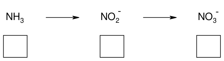
2.1 Give the oxidation states of N in the following series: (Use the boxes below the compounds)
The spectrophotometric analysis of nitrite is based on a reaction with an indicator. The coloured product then obtained has an absorbance maximum at \(\lambda = 543\ \mathrm{nm}\). For quantitative analyses a calibration curve has to be made, in which absorbance at the maximum absorbance wavelength \(\lambda = 543\ \mathrm{nm}\) is plotted against nitrite concentration in a series of standards.
2.2 The measurements are performed at the wavelength with the maximum absorbance because:
- ☐ There is no interference of impurities.
- ☐ There is no contribution of stray light.
- ☐ There is optimal accuracy of the measurement.
- ☐ None of these statements.
Mark the correct answer.
The absorption is measured with a single beam spectrophotometer. However 5 % of the light, the so-called stray light \(I_s\), strikes the detector directly (see Figure 2).
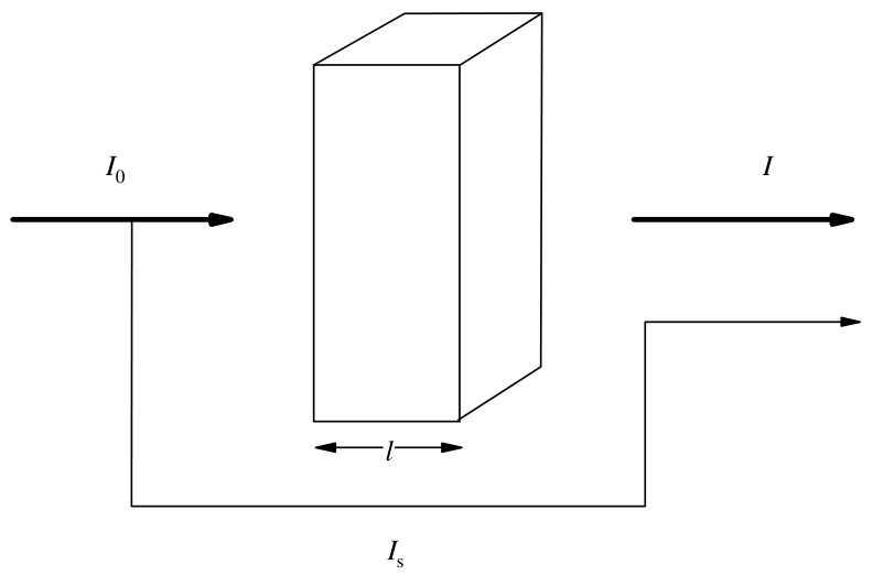
Figure 2
2.3 Calculate the value of the absorbance \(A\) shown by the spectrophotometer if \(\varepsilon = 6\,000\ \mathrm{M^{-1}\,cm^{-1}}\), \(l = 1\ \mathrm{cm}\) and \(c = 1\times10^{-4}\ \mathrm{M}\)
For a nitrite determination in water the following data have been measured.
Table 1
| concentration of nitrite nitrogen (ppm) | absorbance at 543 nm (1.000 cm cell) |
|---|---|
| blank | 0.003 (due to impurities in the solvent) |
| 0.915 | 0.167 |
| 1.830 | 0.328 |
2.4 Determine (show calculation) from the data given above, using the values corrected for the solvent impurities, the slope \(m\) and the intercept \(b\) of the calibration curve \(A = mc + b\).
The duplicate analyses of a water sample are given below. The measurements have been performed at a wavelength of 543 nm and in a 2.000 cm cell.
Table 2
| water sample | absorbance |
|---|---|
| analysis 1 | 0.562 |
| analysis 2 | 0.554 |
For the calculation of the concentration of the nitrite nitrogen (\(c\) in ppm) the equation obtained by the method of least squares
\[ \text{corrected absorbance}=0.1769\,c+0.0015 \tag{a} \]
may be applied, using the measurements in a 1.000 cm cell.
2.5 Calculate the average nitrite nitrogen concentration in ppm and \(\mathrm{\mu g\,cm^{-3}}\).
Hint: Take the blank from problem 2.4.
Official English text of the problem.
Answers
- 2.1: Ammonia, \(\ce{NH3}\), SMILES
N: −3; nitrite ion, \(\ce{NO2-}\), SMILESO=N[O-]: +3; nitrate ion, \(\ce{NO3-}\), SMILES[O-][N+](=O)[O-]: +5. - 2.2: Select the third statement: “There is optimal accuracy of the measurement.”
- 2.3: \(\boxed{A=0.540}\).
- 2.4: \(\boxed{m=0.176\ \mathrm{ppm^{-1}},\quad b=0.003}\).
- 2.5: \(\boxed{\overline c=1.55\ \mathrm{ppm}=1.55\ \mathrm{\mu g\,cm^{-3}}}\), expressed as nitrogen and scaling the solvent blank with path length. The alternative blank interpretation, subtracting \(0.003\) unchanged from each \(2.000\ \mathrm{cm}\) reading, gives 1.56 in both units.
Solution
2.1
The sum of oxidation states equals the overall charge. Hydrogen has oxidation state \(+1\) and oxygen has oxidation state \(-2\) in these species. Writing \(x\) for the oxidation state of nitrogen:
\[ \begin{aligned} \ce{NH3}:&\quad x+3(+1)=0 &&\Longrightarrow x=-3,\\ \ce{NO2-}:&\quad x+2(-2)=-1 &&\Longrightarrow x=+3,\\ \ce{NO3-}:&\quad x+3(-2)=-1 &&\Longrightarrow x=+5. \end{aligned} \]
Fill the left, middle and right boxes with −3, +3 and +5, respectively.
The ionic SMILES given above represent individual resonance contributors; the actual nitrogen–oxygen bonding is delocalized.
2.2
The Beer–Lambert law is
\[ A=\varepsilon lc. \]
At the absorption maximum, \(\varepsilon\) is greatest, so the concentration sensitivity,
\[ \frac{\partial A}{\partial c}=\varepsilon l, \]
is greatest. For a given small absorbance uncertainty, this reduces the uncertainty in the inferred concentration.
Also, at a smooth absorption maximum,
\[ \frac{d\varepsilon}{d\lambda}=0, \]
so small wavelength-setting errors have a smaller effect on absorbance. These considerations support the third statement. Measuring at the maximum does not eliminate impurity absorption or stray light.
2.3
The absorbance of the light passing through the solution is
\[ A_{\mathrm{true}} =\varepsilon lc =(6000\ \mathrm{M^{-1}\,cm^{-1}}) (1\ \mathrm{cm}) (1\times10^{-4}\ \mathrm{M}) =0.600. \]
Its transmittance is therefore
\[ T_{\mathrm{true}}=10^{-0.600}=0.2511886. \]
As shown by the branching diagram, \(5\%\) of the incident light bypasses the cell, while \(95\%\) passes through it. The total fraction reaching the detector is
\[ T_{\mathrm{measured}} =0.05+0.95T_{\mathrm{true}} =0.05+0.95(0.2511886) =0.2886292. \]
Thus,
\[ \boxed{ A_{\mathrm{measured}} =-\log_{10}(0.2886292) =0.5396597 \approx0.540 }. \]
The stray light increases the detected intensity and consequently lowers the displayed absorbance.
2.4
Subtract the solvent blank from each standard:
\[ A_1=0.167-0.003=0.164, \qquad A_2=0.328-0.003=0.325. \]
The slope of the line through the two corrected standards is
\[ m=\frac{A_2-A_1}{c_2-c_1} =\frac{0.325-0.164}{(1.830-0.915)\ \mathrm{ppm}} =0.175956\ \mathrm{ppm^{-1}}. \]
Its intercept is
\[ b=A_1-mc_1 =0.164-(0.175956\ \mathrm{ppm^{-1}})(0.915\ \mathrm{ppm}) =0.003. \]
Hence,
\[ \boxed{m=0.176\ \mathrm{ppm^{-1}},\qquad b=0.003} \]
and the calibration line is
\[ \boxed{A=(0.175956\ \mathrm{ppm^{-1}})\,c+0.003}. \]
Absorbance and \(b\) are dimensionless. Subtracting the solvent blank does not force the line through the two measured standards to have zero intercept.
2.5
Use the supplied least-squares calibration,
\[ A_{\mathrm{corrected,\;1\,cm}} =(0.1769\ \mathrm{ppm^{-1}})\,c+0.0015. \]
The sample readings were obtained in a \(2.000\ \mathrm{cm}\) cell, whereas both this calibration and the tabulated solvent blank refer to \(1.000\ \mathrm{cm}\).
Under the Beer–Lambert law, the solvent-impurity absorbance scales with path length. Thus the blank in the \(2.000\ \mathrm{cm}\) cell is
\[ A_{\mathrm{blank,\;2\,cm}} =0.003\frac{2.000}{1.000}=0.006. \]
Subtracting this blank and then halving is equivalent to halving the readings first and subtracting \(0.003\):
\[ A_{1,\mathrm{corrected,\;1\,cm}} =\frac{0.562}{2}-0.003=0.278, \]
\[ A_{2,\mathrm{corrected,\;1\,cm}} =\frac{0.554}{2}-0.003=0.274. \]
Therefore,
\[ c_1=\frac{0.278-0.0015}{0.1769\ \mathrm{ppm^{-1}}} =1.56303\ \mathrm{ppm}, \]
\[ c_2=\frac{0.274-0.0015}{0.1769\ \mathrm{ppm^{-1}}} =1.54042\ \mathrm{ppm}. \]
The average is
\[ \boxed{ \overline c=\frac{1.56303+1.54042}{2} =1.55172\ \mathrm{ppm} \approx1.55\ \mathrm{ppm} }. \]
For dilute water, taking \(\rho\approx1.00\ \mathrm{g\,cm^{-3}}\),
\[ 1\ \mathrm{ppm} =1\ \mathrm{mg\,kg^{-1}} \approx1\ \mathrm{mg\,L^{-1}} =1\ \mathrm{\mu g\,cm^{-3}}. \]
Consequently,
\[ \boxed{\overline c=1.55\ \mathrm{\mu g\,cm^{-3}}}. \]
Both results are nitrite nitrogen concentrations, so no conversion to the total mass of the nitrite ion is required.
The solution was checked against the official solution.
IChO 2002 · Theorieaufgabe 2
Stickstoffkreislauf in der Natur
Ammoniak ist für Meerestiere bei Konzentrationen über 1 ppm giftig. Nitrifizierende Bakterien spielen eine wichtige Rolle bei der Umwandlung von \(\ce{NH3}\) zunächst in Nitrit und anschließend in Nitrat, die Speicherform des Stickstoffs im Boden.
\(\ce{NADH}\) ist das biochemische Reduktionsmittel des Coenzyms Nicotinamiddinukleotid (NAD), \(\ce{NAD+}\) ist die oxidierte Form des Coenzyms NAD.
2.1 Geben Sie die Oxidationszahlen von N in der folgenden Reihe an: (Verwenden Sie die Kästchen unter den Verbindungen)
Die spektrophotometrische Bestimmung von Nitrit beruht auf einer Reaktion mit einem Indikator. Das dabei erhaltene gefärbte Produkt hat ein Absorbanzmaximum bei \(\lambda = 543\ \mathrm{nm}\). Für quantitative Analysen muss eine Kalibrierkurve erstellt werden, in der die Absorbanz bei der Wellenlänge des Absorbanzmaximums \(\lambda = 543\ \mathrm{nm}\) gegen die Nitritkonzentration einer Reihe von Standardlösungen aufgetragen wird.
2.2 Die Messungen werden bei der Wellenlänge des Absorbanzmaximums durchgeführt, weil:
- ☐ Keine Störung durch Verunreinigungen auftritt.
- ☐ Kein Beitrag von Streulicht auftritt.
- ☐ Die Messgenauigkeit optimal ist.
- ☐ Keine dieser Aussagen zutrifft.
Markieren Sie die richtige Antwort.
Die Absorption wird mit einem Einstrahlspektrophotometer gemessen. Allerdings treffen 5 % des Lichts, das sogenannte Streulicht \(I_s\), direkt auf den Detektor (siehe Abbildung 2).
Abbildung 2
2.3 Berechnen Sie den vom Spektrophotometer angezeigten Wert der Absorbanz \(A\), wenn \(\varepsilon = 6\,000\ \mathrm{M^{-1}\,cm^{-1}}\), \(l = 1\ \mathrm{cm}\) und \(c = 1\times10^{-4}\ \mathrm{M}\)
Für eine Nitritbestimmung in Wasser wurden die folgenden Daten gemessen.
Tabelle 1
| Konzentration des Nitritstickstoffs (ppm) | Absorbanz bei 543 nm (1.000-cm-Küvette) |
|---|---|
| Blindwert | 0.003 (aufgrund von Verunreinigungen im Lösungsmittel) |
| 0.915 | 0.167 |
| 1.830 | 0.328 |
2.4 Bestimmen Sie aus den oben angegebenen Daten unter Verwendung der um die Lösungsmittelverunreinigungen korrigierten Werte die Steigung \(m\) und den Achsenabschnitt \(b\) der Kalibrierkurve \(A = mc + b\). Geben Sie den Rechenweg an.
Die Ergebnisse der Doppelbestimmung einer Wasserprobe sind nachstehend angegeben. Die Messungen wurden bei einer Wellenlänge von 543 nm in einer 2.000-cm-Küvette durchgeführt.
Tabelle 2
| Wasserprobe | Absorbanz |
|---|---|
| Analyse 1 | 0.562 |
| Analyse 2 | 0.554 |
Zur Berechnung der Konzentration des Nitritstickstoffs (\(c\) in ppm) kann die mit der Methode der kleinsten Quadrate erhaltene Gleichung
\[ \text{korrigierte Absorbanz}=0.1769\,c+0.0015 \tag{a} \]
unter Verwendung der Messwerte in einer 1.000-cm-Küvette angewendet werden.
2.5 Berechnen Sie die mittlere Nitritstickstoffkonzentration in ppm und \(\mathrm{\mu g\,cm^{-3}}\).
Hinweis: Verwenden Sie den Blindwert aus Aufgabe 2.4.
Aufgabentext aus dem offiziellen englischen Text übersetzt.
Antworten
- 2.1: Ammoniak, \(\ce{NH3}\), SMILES
N: −3; Nitrit-Ion, \(\ce{NO2-}\), SMILESO=N[O-]: +3; Nitrat-Ion, \(\ce{NO3-}\), SMILES[O-][N+](=O)[O-]: +5. - 2.2: Wählen Sie die dritte Aussage: „Die Messgenauigkeit ist optimal.“
- 2.3: \(\boxed{A=0.540}\).
- 2.4: \(\boxed{m=0.176\ \mathrm{ppm^{-1}},\quad b=0.003}\).
- 2.5: \(\boxed{\overline c=1.55\ \mathrm{ppm}=1.55\ \mathrm{\mu g\,cm^{-3}}}\), bezogen auf Stickstoff und unter Skalierung des Lösungsmittelblindwerts mit der Schichtdicke. Die alternative Interpretation des Blindwerts, bei der \(0.003\) unverändert von jedem Messwert bei \(2.000\ \mathrm{cm}\) abgezogen wird, ergibt 1.56 in beiden Einheiten.
Lösung
2.1
Die Summe der Oxidationszahlen ist gleich der Gesamtladung. Wasserstoff hat in diesen Spezies die Oxidationszahl \(+1\) und Sauerstoff die Oxidationszahl \(-2\). Mit \(x\) als Oxidationszahl des Stickstoffs gilt:
\[ \begin{aligned} \ce{NH3}:&\quad x+3(+1)=0 &&\Longrightarrow x=-3,\\ \ce{NO2-}:&\quad x+2(-2)=-1 &&\Longrightarrow x=+3,\\ \ce{NO3-}:&\quad x+3(-2)=-1 &&\Longrightarrow x=+5. \end{aligned} \]
Tragen Sie in das linke, mittlere und rechte Kästchen jeweils −3, +3 und +5 ein.
Die oben angegebenen SMILES der Ionen stellen einzelne mesomere Grenzstrukturen dar; die tatsächlichen Stickstoff–Sauerstoff-Bindungen sind delokalisiert.
2.2
Das Lambert-Beer-Gesetz lautet
\[ A=\varepsilon lc. \]
Am Absorptionsmaximum ist \(\varepsilon\) am größten, sodass die Konzentrationsempfindlichkeit
\[ \frac{\partial A}{\partial c}=\varepsilon l, \]
am größten ist. Bei einer gegebenen kleinen Unsicherheit der Absorbanz verringert dies die Unsicherheit der daraus ermittelten Konzentration.
Außerdem gilt an einem glatten Absorptionsmaximum
\[ \frac{d\varepsilon}{d\lambda}=0, \]
sodass kleine Fehler bei der Wellenlängeneinstellung einen geringeren Einfluss auf die Absorbanz haben. Diese Überlegungen stützen die dritte Aussage. Die Messung am Maximum beseitigt weder die Absorption durch Verunreinigungen noch das Streulicht.
2.3
Die Absorbanz des durch die Lösung tretenden Lichts beträgt
\[ A_{\mathrm{true}} =\varepsilon lc =(6000\ \mathrm{M^{-1}\,cm^{-1}}) (1\ \mathrm{cm}) (1\times10^{-4}\ \mathrm{M}) =0.600. \]
Der zugehörige Transmissionsgrad beträgt daher
\[ T_{\mathrm{true}}=10^{-0.600}=0.2511886. \]
Wie im Verzweigungsschema dargestellt, umgehen \(5\%\) des einfallenden Lichts die Küvette, während \(95\%\) sie durchlaufen. Der gesamte Anteil, der den Detektor erreicht, beträgt
\[ T_{\mathrm{measured}} =0.05+0.95T_{\mathrm{true}} =0.05+0.95(0.2511886) =0.2886292. \]
Somit gilt
\[ \boxed{ A_{\mathrm{measured}} =-\log_{10}(0.2886292) =0.5396597 \approx0.540 }. \]
Das Streulicht erhöht die detektierte Intensität und senkt dadurch die angezeigte Absorbanz.
2.4
Subtrahieren Sie den Lösungsmittelblindwert von jedem Messwert der Standardlösungen:
\[ A_1=0.167-0.003=0.164, \qquad A_2=0.328-0.003=0.325. \]
Die Steigung der Geraden durch die beiden korrigierten Standardmesspunkte beträgt
\[ m=\frac{A_2-A_1}{c_2-c_1} =\frac{0.325-0.164}{(1.830-0.915)\ \mathrm{ppm}} =0.175956\ \mathrm{ppm^{-1}}. \]
Ihr Achsenabschnitt beträgt
\[ b=A_1-mc_1 =0.164-(0.175956\ \mathrm{ppm^{-1}})(0.915\ \mathrm{ppm}) =0.003. \]
Damit gilt
\[ \boxed{m=0.176\ \mathrm{ppm^{-1}},\qquad b=0.003} \]
und die Kalibriergerade lautet
\[ \boxed{A=(0.175956\ \mathrm{ppm^{-1}})\,c+0.003}. \]
Die Absorbanz und \(b\) sind dimensionslos. Die Subtraktion des Lösungsmittelblindwerts erzwingt keinen Achsenabschnitt von null für die Gerade durch die beiden gemessenen Standardmesspunkte.
2.5
Verwenden Sie die angegebene Kalibriergleichung nach der Methode der kleinsten Quadrate:
\[ A_{\mathrm{corrected,\;1\,cm}} =(0.1769\ \mathrm{ppm^{-1}})\,c+0.0015. \]
Die Probenmesswerte wurden in einer \(2.000\ \mathrm{cm}\)-Küvette erhalten, während sich sowohl diese Kalibrierung als auch der tabellierte Lösungsmittelblindwert auf \(1.000\ \mathrm{cm}\) beziehen.
Nach dem Lambert-Beer-Gesetz ist die Absorbanz der Lösungsmittelverunreinigungen proportional zur Schichtdicke. Daher beträgt der Blindwert in der \(2.000\ \mathrm{cm}\)-Küvette
\[ A_{\mathrm{blank,\;2\,cm}} =0.003\frac{2.000}{1.000}=0.006. \]
Diesen Blindwert zu subtrahieren und anschließend zu halbieren ist gleichbedeutend damit, zuerst die Messwerte zu halbieren und dann \(0.003\) zu subtrahieren:
\[ A_{1,\mathrm{corrected,\;1\,cm}} =\frac{0.562}{2}-0.003=0.278, \]
\[ A_{2,\mathrm{corrected,\;1\,cm}} =\frac{0.554}{2}-0.003=0.274. \]
Daher gilt
\[ c_1=\frac{0.278-0.0015}{0.1769\ \mathrm{ppm^{-1}}} =1.56303\ \mathrm{ppm}, \]
\[ c_2=\frac{0.274-0.0015}{0.1769\ \mathrm{ppm^{-1}}} =1.54042\ \mathrm{ppm}. \]
Der Mittelwert beträgt
\[ \boxed{ \overline c=\frac{1.56303+1.54042}{2} =1.55172\ \mathrm{ppm} \approx1.55\ \mathrm{ppm} }. \]
Für verdünnte wässrige Lösungen gilt unter der Annahme \(\rho\approx1.00\ \mathrm{g\,cm^{-3}}\):
\[ 1\ \mathrm{ppm} =1\ \mathrm{mg\,kg^{-1}} \approx1\ \mathrm{mg\,L^{-1}} =1\ \mathrm{\mu g\,cm^{-3}}. \]
Folglich gilt
\[ \boxed{\overline c=1.55\ \mathrm{\mu g\,cm^{-3}}}. \]
Beide Ergebnisse sind Nitritstickstoffkonzentrationen, sodass keine Umrechnung auf die Gesamtmasse des Nitrit-Ions erforderlich ist.
Die Lösung wurde mit der offiziellen Lösung abgeglichen.
IChO 2002 · Teori sorusu 2
Doğada Azot Döngüsü
Amonyak, 1 ppm'i aşan düzeylerde deniz hayvanları için toksik bir maddedir. Nitrifikasyon bakterileri, \(\ce{NH3}\)'ün önce nitrite, ardından azotun topraktaki depolanma biçimi olan nitrata dönüştürülmesinde önemli bir rol oynar.
\(\ce{NADH}\), nikotinamid dinükleotit (NAD) koenziminin biyokimyasal indirgen maddesidir; \(\ce{NAD+}\) ise NAD koenziminin yükseltgenmiş biçimidir.
2.1 Aşağıdaki dizide N'nin yükseltgenme basamaklarını belirtiniz: (Bileşiklerin altındaki kutuları kullanınız)
Nitritin spektrofotometrik analizi, bir indikatörle verdiği tepkimeye dayanır. Bu tepkimede elde edilen renkli ürünün absorbansı \(\lambda = 543\ \mathrm{nm}\) dalga boyunda maksimumdur. Nicel analizler için, bir dizi standart çözeltinin maksimum absorbans dalga boyu olan \(\lambda = 543\ \mathrm{nm}\)'deki absorbanslarının nitrit derişimine karşı grafiğe geçirildiği bir kalibrasyon eğrisi oluşturulmalıdır.
2.2 Ölçümler maksimum absorbansın görüldüğü dalga boyunda yapılır, çünkü:
- ☐ Safsızlıkların girişimi yoktur.
- ☐ Kaçak ışığın katkısı yoktur.
- ☐ Ölçüm doğruluğu en uygun düzeydedir.
- ☐ Bu ifadelerin hiçbiri doğru değildir.
Doğru cevabı işaretleyiniz.
Soğurma, tek ışınlı bir spektrofotometreyle ölçülür. Ancak ışığın % 5'i, kaçak ışık olarak adlandırılan \(I_s\), doğrudan dedektöre ulaşır (bkz. Şekil 2).
Şekil 2
2.3 \(\varepsilon = 6\,000\ \mathrm{M^{-1}\,cm^{-1}}\), \(l = 1\ \mathrm{cm}\) ve \(c = 1\times10^{-4}\ \mathrm{M}\) olduğunda spektrofotometrenin gösterdiği absorbans \(A\) değerini hesaplayınız.
Suda nitrit tayini için aşağıdaki veriler ölçülmüştür.
Tablo 1
| nitrit azotu derişimi (ppm) | 543 nm'deki absorbans (1.000 cm'lik küvet) |
|---|---|
| kör | 0.003 (çözücüdeki safsızlıklardan kaynaklanır) |
| 0.915 | 0.167 |
| 1.830 | 0.328 |
2.4 Yukarıda verilen verilerden, çözücü safsızlıkları için düzeltilmiş değerleri kullanarak \(A = mc + b\) kalibrasyon eğrisinin eğimini \(m\) ve düşey ekseni kesim noktasını \(b\) belirleyiniz (hesaplamayı gösteriniz).
Bir su numunesinin iki tekrarlı analizinin sonuçları aşağıda verilmiştir. Ölçümler 543 nm dalga boyunda ve 2.000 cm'lik bir küvette yapılmıştır.
Tablo 2
| su numunesi | absorbans |
|---|---|
| analiz 1 | 0.562 |
| analiz 2 | 0.554 |
Nitrit azotu derişiminin (ppm cinsinden \(c\)) hesaplanması için, 1.000 cm'lik bir küvette yapılan ölçümler kullanılarak en küçük kareler yöntemiyle elde edilen
\[ \text{düzeltilmiş absorbans}=0.1769\,c+0.0015 \tag{a} \]
denklemi uygulanabilir.
2.5 Ortalama nitrit azotu derişimini ppm ve \(\mathrm{\mu g\,cm^{-3}}\) cinsinden hesaplayınız.
İpucu: Kör değerini 2.4 numaralı sorudan alınız.
Soru metni resmi İngilizce metinden çevrilmiştir.
Cevaplar
- 2.1: Amonyak, \(\ce{NH3}\), SMILES
N: −3; nitrit iyonu, \(\ce{NO2-}\), SMILESO=N[O-]: +3; nitrat iyonu, \(\ce{NO3-}\), SMILES[O-][N+](=O)[O-]: +5. - 2.2: Üçüncü ifadeyi seçiniz: “Ölçüm doğruluğu en uygun düzeydedir.”
- 2.3: \(\boxed{A=0.540}\).
- 2.4: \(\boxed{m=0.176\ \mathrm{ppm^{-1}},\quad b=0.003}\).
- 2.5: Azot cinsinden ifade edildiğinde ve çözücü körü optik yol uzunluğuyla ölçeklendirildiğinde \(\boxed{\overline c=1.55\ \mathrm{ppm}=1.55\ \mathrm{\mu g\,cm^{-3}}}\). Kör değerine ilişkin alternatif yorum, \(2.000\ \mathrm{cm}\) optik yol uzunluğundaki her okumadan \(0.003\) değerinin değiştirilmeden çıkarılmasıyla, her iki birimde de 1.56 sonucunu verir.
Çözüm
2.1
Yükseltgenme basamaklarının toplamı, toplam yüke eşittir. Bu türlerde hidrojenin yükseltgenme basamağı \(+1\), oksijeninki ise \(-2\)'dir. Azotun yükseltgenme basamağını \(x\) ile gösterirsek:
\[ \begin{aligned} \ce{NH3}:&\quad x+3(+1)=0 &&\Longrightarrow x=-3,\\ \ce{NO2-}:&\quad x+2(-2)=-1 &&\Longrightarrow x=+3,\\ \ce{NO3-}:&\quad x+3(-2)=-1 &&\Longrightarrow x=+5. \end{aligned} \]
Sol, orta ve sağ kutulara sırasıyla −3, +3 ve +5 yazınız.
Yukarıda verilen iyonik SMILES gösterimleri, ayrı ayrı rezonans yapılarını temsil eder; gerçek azot–oksijen bağlanması delokalizedir.
2.2
Beer–Lambert yasası şöyledir:
\[ A=\varepsilon lc. \]
Soğurma maksimumunda \(\varepsilon\) en büyük değerini alır; dolayısıyla derişime duyarlılık da,
\[ \frac{\partial A}{\partial c}=\varepsilon l, \]
en büyük değerindedir. Belirli bir küçük absorbans belirsizliği için bu durum, hesaplanan derişimdeki belirsizliği azaltır.
Ayrıca, düzgün bir soğurma maksimumunda,
\[ \frac{d\varepsilon}{d\lambda}=0, \]
olduğundan, dalga boyu ayarındaki küçük hataların absorbans üzerindeki etkisi daha azdır. Bu gerekçeler üçüncü ifadeyi destekler. Maksimumda ölçüm yapmak, safsızlıkların soğurmasını veya kaçak ışığı ortadan kaldırmaz.
2.3
Çözeltiden geçen ışığın absorbansı şöyledir:
\[ A_{\mathrm{true}} =\varepsilon lc =(6000\ \mathrm{M^{-1}\,cm^{-1}}) (1\ \mathrm{cm}) (1\times10^{-4}\ \mathrm{M}) =0.600. \]
Dolayısıyla geçirgenliği şöyledir:
\[ T_{\mathrm{true}}=10^{-0.600}=0.2511886. \]
Dallanma şemasında gösterildiği gibi, gelen ışığın \(5\%\)'i küvetten geçmeden ilerlerken \(95\%\)'i küvetten geçer. Dedektöre ulaşan toplam ışık kesri şöyledir:
\[ T_{\mathrm{measured}} =0.05+0.95T_{\mathrm{true}} =0.05+0.95(0.2511886) =0.2886292. \]
Böylece,
\[ \boxed{ A_{\mathrm{measured}} =-\log_{10}(0.2886292) =0.5396597 \approx0.540 }. \]
Kaçak ışık, dedektörün algıladığı ışık şiddetini artırır ve bunun sonucunda gösterilen absorbansı düşürür.
2.4
Her bir standarttan çözücü körünü çıkarınız:
\[ A_1=0.167-0.003=0.164, \qquad A_2=0.328-0.003=0.325. \]
Düzeltilmiş iki standart noktasından geçen doğrunun eğimi şöyledir:
\[ m=\frac{A_2-A_1}{c_2-c_1} =\frac{0.325-0.164}{(1.830-0.915)\ \mathrm{ppm}} =0.175956\ \mathrm{ppm^{-1}}. \]
Düşey ekseni kesim noktası şöyledir:
\[ b=A_1-mc_1 =0.164-(0.175956\ \mathrm{ppm^{-1}})(0.915\ \mathrm{ppm}) =0.003. \]
Dolayısıyla,
\[ \boxed{m=0.176\ \mathrm{ppm^{-1}},\qquad b=0.003} \]
ve kalibrasyon doğrusu şöyledir:
\[ \boxed{A=(0.175956\ \mathrm{ppm^{-1}})\,c+0.003}. \]
Absorbans ve \(b\) boyutsuzdur. Çözücü körünün çıkarılması, ölçülen iki standart noktasından geçen doğrunun düşey ekseni kesim noktasının sıfır olmasını zorunlu kılmaz.
2.5
Verilen en küçük kareler kalibrasyonunu kullanınız:
\[ A_{\mathrm{corrected,\;1\,cm}} =(0.1769\ \mathrm{ppm^{-1}})\,c+0.0015. \]
Numune okumaları \(2.000\ \mathrm{cm}\)'lik bir küvette elde edilmiştir; oysa hem bu kalibrasyon hem de tabloda verilen çözücü körü \(1.000\ \mathrm{cm}\)'lik küvete aittir.
Beer–Lambert yasasına göre, çözücü safsızlıklarının absorbansı optik yol uzunluğuyla orantılıdır. Dolayısıyla \(2.000\ \mathrm{cm}\)'lik küvetteki kör değeri şöyledir:
\[ A_{\mathrm{blank,\;2\,cm}} =0.003\frac{2.000}{1.000}=0.006. \]
Bu kör değerini çıkarıp ardından ikiye bölmek, okumaları önce ikiye bölüp sonra \(0.003\) çıkarmaya eşdeğerdir:
\[ A_{1,\mathrm{corrected,\;1\,cm}} =\frac{0.562}{2}-0.003=0.278, \]
\[ A_{2,\mathrm{corrected,\;1\,cm}} =\frac{0.554}{2}-0.003=0.274. \]
Dolayısıyla,
\[ c_1=\frac{0.278-0.0015}{0.1769\ \mathrm{ppm^{-1}}} =1.56303\ \mathrm{ppm}, \]
\[ c_2=\frac{0.274-0.0015}{0.1769\ \mathrm{ppm^{-1}}} =1.54042\ \mathrm{ppm}. \]
Ortalama şöyledir:
\[ \boxed{ \overline c=\frac{1.56303+1.54042}{2} =1.55172\ \mathrm{ppm} \approx1.55\ \mathrm{ppm} }. \]
Seyreltik sulu çözelti için \(\rho\approx1.00\ \mathrm{g\,cm^{-3}}\) alınırsa,
\[ 1\ \mathrm{ppm} =1\ \mathrm{mg\,kg^{-1}} \approx1\ \mathrm{mg\,L^{-1}} =1\ \mathrm{\mu g\,cm^{-3}}. \]
Sonuç olarak,
\[ \boxed{\overline c=1.55\ \mathrm{\mu g\,cm^{-3}}}. \]
Her iki sonuç da nitrit azotu derişimidir; bu nedenle nitrit iyonunun toplam kütlesine dönüştürme yapılması gerekmez.
Çözüm, resmi çözümle karşılaştırılarak kontrol edildi.
IChO 2002 · Problema teórico 2
Ciclo del nitrógeno en la naturaleza
El amoníaco es una sustancia tóxica para los animales marinos a concentraciones superiores a 1 ppm. Las bacterias nitrificantes desempeñan un papel importante en la conversión del \(\ce{NH3}\) primero en nitrito y después en nitrato, la forma en que se almacena el nitrógeno en el suelo.
El \(\ce{NADH}\) es el agente reductor bioquímico de la coenzima nicotinamida dinucleótido (NAD), y el \(\ce{NAD+}\) es la forma oxidada de la coenzima NAD.
2.1 Indique los estados de oxidación del N en la siguiente serie: (Utilice las casillas situadas debajo de los compuestos)
El análisis espectrofotométrico del nitrito se basa en una reacción con un indicador. El producto coloreado obtenido presenta un máximo de absorbancia a \(\lambda = 543\ \mathrm{nm}\). Para los análisis cuantitativos se debe construir una curva de calibración, en la que se representa la absorbancia a la longitud de onda de máxima absorbancia \(\lambda = 543\ \mathrm{nm}\) frente a la concentración de nitrito en una serie de patrones.
2.2 Las mediciones se realizan a la longitud de onda de máxima absorbancia porque:
- ☐ No hay interferencias de las impurezas.
- ☐ No hay contribución de la luz parásita.
- ☐ La exactitud de la medición es óptima.
- ☐ Ninguna de estas afirmaciones.
Marque la respuesta correcta.
La absorción se mide con un espectrofotómetro de haz único. Sin embargo, el 5 % de la luz, la denominada luz parásita \(I_s\), incide directamente sobre el detector (véase la Figura 2).
Figura 2
2.3 Calcule el valor de la absorbancia \(A\) que muestra el espectrofotómetro si \(\varepsilon = 6\,000\ \mathrm{M^{-1}\,cm^{-1}}\), \(l = 1\ \mathrm{cm}\) y \(c = 1\times10^{-4}\ \mathrm{M}\)
En una determinación de nitrito en agua se han obtenido los siguientes datos experimentales.
Tabla 1
| concentración de nitrógeno en forma de nitrito (ppm) | absorbancia a 543 nm (cubeta de 1.000 cm) |
|---|---|
| blanco | 0.003 (debida a impurezas en el disolvente) |
| 0.915 | 0.167 |
| 1.830 | 0.328 |
2.4 Determine (mostrando los cálculos), a partir de los datos anteriores y utilizando los valores corregidos por las impurezas del disolvente, la pendiente \(m\) y la ordenada en el origen \(b\) de la curva de calibración \(A = mc + b\).
A continuación se presentan los análisis por duplicado de una muestra de agua. Las mediciones se han realizado a una longitud de onda de 543 nm y en una cubeta de 2.000 cm.
Tabla 2
| muestra de agua | absorbancia |
|---|---|
| análisis 1 | 0.562 |
| análisis 2 | 0.554 |
Para calcular la concentración de nitrógeno en forma de nitrito (\(c\) en ppm), puede aplicarse la ecuación obtenida mediante el método de mínimos cuadrados
\[ \text{absorbancia corregida}=0.1769\,c+0.0015 \tag{a} \]
utilizando las mediciones en una cubeta de 1.000 cm.
2.5 Calcule la concentración media de nitrógeno en forma de nitrito en ppm y \(\mathrm{\mu g\,cm^{-3}}\).
Indicación: Tome el blanco del apartado 2.4.
Enunciado traducido del texto oficial en inglés.
Respuestas
- 2.1: Amoníaco, \(\ce{NH3}\), SMILES
N: −3; ion nitrito, \(\ce{NO2-}\), SMILESO=N[O-]: +3; ion nitrato, \(\ce{NO3-}\), SMILES[O-][N+](=O)[O-]: +5. - 2.2: Seleccione la tercera afirmación: «La exactitud de la medición es óptima».
- 2.3: \(\boxed{A=0.540}\).
- 2.4: \(\boxed{m=0.176\ \mathrm{ppm^{-1}},\quad b=0.003}\).
- 2.5: \(\boxed{\overline c=1.55\ \mathrm{ppm}=1.55\ \mathrm{\mu g\,cm^{-3}}}\), expresada como nitrógeno y ajustando el blanco del disolvente proporcionalmente a la longitud del trayecto óptico. La interpretación alternativa del blanco, restando \(0.003\) sin modificar de cada lectura a \(2.000\ \mathrm{cm}\), da 1.56 en ambas unidades.
Solución
2.1
La suma de los estados de oxidación es igual a la carga total. El hidrógeno tiene un estado de oxidación de \(+1\) y el oxígeno de \(-2\) en estas especies. Si se representa por \(x\) el estado de oxidación del nitrógeno:
\[ \begin{aligned} \ce{NH3}:&\quad x+3(+1)=0 &&\Longrightarrow x=-3,\\ \ce{NO2-}:&\quad x+2(-2)=-1 &&\Longrightarrow x=+3,\\ \ce{NO3-}:&\quad x+3(-2)=-1 &&\Longrightarrow x=+5. \end{aligned} \]
Rellene las casillas izquierda, central y derecha con −3, +3 y +5, respectivamente.
Los SMILES de los iones indicados anteriormente representan estructuras resonantes individuales; los enlaces reales entre nitrógeno y oxígeno están deslocalizados.
2.2
La ley de Beer–Lambert es
\[ A=\varepsilon lc. \]
En el máximo de absorción, \(\varepsilon\) alcanza su valor máximo, por lo que la sensibilidad respecto a la concentración,
\[ \frac{\partial A}{\partial c}=\varepsilon l, \]
es máxima. Para una incertidumbre pequeña dada en la absorbancia, esto reduce la incertidumbre en la concentración deducida.
Además, en un máximo de absorción suave,
\[ \frac{d\varepsilon}{d\lambda}=0, \]
por lo que los pequeños errores en el ajuste de la longitud de onda tienen un efecto menor sobre la absorbancia. Estas consideraciones respaldan la tercera afirmación. Medir en el máximo no elimina la absorción de las impurezas ni la luz parásita.
2.3
La absorbancia de la luz que atraviesa la disolución es
\[ A_{\mathrm{true}} =\varepsilon lc =(6000\ \mathrm{M^{-1}\,cm^{-1}}) (1\ \mathrm{cm}) (1\times10^{-4}\ \mathrm{M}) =0.600. \]
Por tanto, su transmitancia es
\[ T_{\mathrm{true}}=10^{-0.600}=0.2511886. \]
Como muestra el diagrama de bifurcación, el \(5\%\) de la luz incidente no atraviesa la cubeta, mientras que el \(95\%\) la atraviesa. La fracción total que llega al detector es
\[ T_{\mathrm{measured}} =0.05+0.95T_{\mathrm{true}} =0.05+0.95(0.2511886) =0.2886292. \]
Así,
\[ \boxed{ A_{\mathrm{measured}} =-\log_{10}(0.2886292) =0.5396597 \approx0.540 }. \]
La luz parásita aumenta la intensidad detectada y, en consecuencia, reduce la absorbancia indicada.
2.4
Reste el blanco del disolvente de cada patrón:
\[ A_1=0.167-0.003=0.164, \qquad A_2=0.328-0.003=0.325. \]
La pendiente de la recta que pasa por los dos patrones corregidos es
\[ m=\frac{A_2-A_1}{c_2-c_1} =\frac{0.325-0.164}{(1.830-0.915)\ \mathrm{ppm}} =0.175956\ \mathrm{ppm^{-1}}. \]
Su ordenada en el origen es
\[ b=A_1-mc_1 =0.164-(0.175956\ \mathrm{ppm^{-1}})(0.915\ \mathrm{ppm}) =0.003. \]
Por tanto,
\[ \boxed{m=0.176\ \mathrm{ppm^{-1}},\qquad b=0.003} \]
y la recta de calibración es
\[ \boxed{A=(0.175956\ \mathrm{ppm^{-1}})\,c+0.003}. \]
La absorbancia y \(b\) son adimensionales. Restar el blanco del disolvente no obliga a que la recta que pasa por los dos patrones medidos tenga una ordenada en el origen nula.
2.5
Utilice la calibración por mínimos cuadrados proporcionada,
\[ A_{\mathrm{corrected,\;1\,cm}} =(0.1769\ \mathrm{ppm^{-1}})\,c+0.0015. \]
Las lecturas de la muestra se obtuvieron en una cubeta de \(2.000\ \mathrm{cm}\), mientras que tanto esta calibración como el blanco del disolvente tabulado corresponden a \(1.000\ \mathrm{cm}\).
Según la ley de Beer–Lambert, la absorbancia debida a las impurezas del disolvente es proporcional a la longitud del trayecto óptico. Por tanto, el blanco en la cubeta de \(2.000\ \mathrm{cm}\) es
\[ A_{\mathrm{blank,\;2\,cm}} =0.003\frac{2.000}{1.000}=0.006. \]
Restar este blanco y dividir después entre dos equivale a dividir primero las lecturas entre dos y restar \(0.003\):
\[ A_{1,\mathrm{corrected,\;1\,cm}} =\frac{0.562}{2}-0.003=0.278, \]
\[ A_{2,\mathrm{corrected,\;1\,cm}} =\frac{0.554}{2}-0.003=0.274. \]
Por tanto,
\[ c_1=\frac{0.278-0.0015}{0.1769\ \mathrm{ppm^{-1}}} =1.56303\ \mathrm{ppm}, \]
\[ c_2=\frac{0.274-0.0015}{0.1769\ \mathrm{ppm^{-1}}} =1.54042\ \mathrm{ppm}. \]
La media es
\[ \boxed{ \overline c=\frac{1.56303+1.54042}{2} =1.55172\ \mathrm{ppm} \approx1.55\ \mathrm{ppm} }. \]
Para una disolución acuosa diluida, tomando \(\rho\approx1.00\ \mathrm{g\,cm^{-3}}\),
\[ 1\ \mathrm{ppm} =1\ \mathrm{mg\,kg^{-1}} \approx1\ \mathrm{mg\,L^{-1}} =1\ \mathrm{\mu g\,cm^{-3}}. \]
En consecuencia,
\[ \boxed{\overline c=1.55\ \mathrm{\mu g\,cm^{-3}}}. \]
Ambos resultados son concentraciones de nitrógeno en forma de nitrito, por lo que no es necesario convertirlos a la masa total del ion nitrito.
La solución se comprobó con la solución oficial.
IChO 2002 · 理论题 2
自然界中的氮循环
当浓度超过 1 ppm 时,氨对海洋动物具有毒性。硝化细菌在将 \(\ce{NH3}\) 先转化为亚硝酸盐、再转化为硝酸盐的过程中起着重要作用,硝酸盐是氮在土壤中的储存形式。
\(\ce{NADH}\) 是辅酶烟酰胺二核苷酸(NAD)的生物化学还原剂形式,\(\ce{NAD+}\) 是辅酶 NAD 的氧化态形式。
2.1 给出下列一系列物质中 N 的氧化数:(填写在化合物下方的方框中)
亚硝酸盐的分光光度分析基于其与指示剂的反应。反应得到的有色产物在 \(\lambda = 543\ \mathrm{nm}\) 处具有最大吸光度。进行定量分析时,必须绘制校准曲线,即以一系列标准溶液中亚硝酸盐的浓度为横坐标,以最大吸收波长 \(\lambda = 543\ \mathrm{nm}\) 处的吸光度为纵坐标作图。
2.2 在最大吸收波长处进行测量,是因为:
- ☐ 不存在杂质的干扰。
- ☐ 不存在杂散光的影响。
- ☐ 测量的准确度最佳。
- ☐ 以上说法均不正确。
标出正确答案。
使用单光束分光光度计测量吸收。然而,有 5 % 的光,即所谓的杂散光 \(I_s\),直接照射到检测器上(见图 2)。
图 2
2.3 若 \(\varepsilon = 6\,000\ \mathrm{M^{-1}\,cm^{-1}}\)、\(l = 1\ \mathrm{cm}\) 且 \(c = 1\times10^{-4}\ \mathrm{M}\),计算分光光度计显示的吸光度 \(A\) 的值。
在测定水中亚硝酸盐时,测得以下数据。
表 1
| 亚硝酸盐氮的浓度(ppm) | 543 nm 处的吸光度(1.000 cm 比色皿) |
|---|---|
| 空白 | 0.003(由溶剂中的杂质引起) |
| 0.915 | 0.167 |
| 1.830 | 0.328 |
2.4 根据上述数据,使用扣除溶剂杂质影响后的数值,确定校准曲线 \(A = mc + b\) 的斜率 \(m\) 和截距 \(b\)(写出计算过程)。
下表给出某水样的两次平行分析结果。测量在 543 nm 波长处进行,使用 2.000 cm 比色皿。
表 2
| 水样 | 吸光度 |
|---|---|
| 分析 1 | 0.562 |
| 分析 2 | 0.554 |
计算亚硝酸盐氮的浓度(\(c\),单位为 ppm)时,可使用根据 1.000 cm 比色皿中的测量结果,通过最小二乘法得到的方程
\[ \text{校正后的吸光度}=0.1769\,c+0.0015 \tag{a} \]
进行计算。
2.5 计算亚硝酸盐氮的平均浓度,分别以 ppm 和 \(\mathrm{\mu g\,cm^{-3}}\) 表示。
提示:使用第 2.4 题中的空白值。
题目译自官方英文原文。
答案
- 2.1: 氨,\(\ce{NH3}\),SMILES
N:−3;亚硝酸根离子,\(\ce{NO2-}\),SMILESO=N[O-]:+3;硝酸根离子,\(\ce{NO3-}\),SMILES[O-][N+](=O)[O-]:+5。 - 2.2: 选择第三项:“测量的准确度最佳。”
- 2.3: \(\boxed{A=0.540}\)。
- 2.4: \(\boxed{m=0.176\ \mathrm{ppm^{-1}},\quad b=0.003}\)。
- 2.5: \(\boxed{\overline c=1.55\ \mathrm{ppm}=1.55\ \mathrm{\mu g\,cm^{-3}}}\),以氮计,并按光程对溶剂空白值进行换算。对空白值采用另一种解释时,即从光程为 \(2.000\ \mathrm{cm}\) 的每个读数中减去未经换算的 \(0.003\),以这两种单位表示的结果均为 1.56。
解答
2.1
各原子的氧化数之和等于总电荷。在这些物种中,氢的氧化数为 \(+1\),氧的氧化数为 \(-2\)。以 \(x\) 表示氮的氧化数:
\[ \begin{aligned} \ce{NH3}:&\quad x+3(+1)=0 &&\Longrightarrow x=-3,\\ \ce{NO2-}:&\quad x+2(-2)=-1 &&\Longrightarrow x=+3,\\ \ce{NO3-}:&\quad x+3(-2)=-1 &&\Longrightarrow x=+5. \end{aligned} \]
在左、中、右三个方框中分别填入 −3、+3 和 +5。
上面给出的离子 SMILES 各自表示一个共振贡献式;实际的氮–氧成键具有离域性。
2.2
比尔–朗伯定律为
\[ A=\varepsilon lc. \]
在吸收峰处,\(\varepsilon\) 最大,因此浓度灵敏度
\[ \frac{\partial A}{\partial c}=\varepsilon l, \]
也最大。对于给定的较小吸光度不确定度,这会减小由吸光度推算出的浓度的不确定度。
此外,在平滑的吸收峰处,
\[ \frac{d\varepsilon}{d\lambda}=0, \]
因此,波长设置的微小误差对吸光度的影响较小。这些考虑支持第三项说法。在吸收峰处测量并不能消除杂质吸收或杂散光。
2.3
穿过溶液的光所对应的吸光度为
\[ A_{\mathrm{true}} =\varepsilon lc =(6000\ \mathrm{M^{-1}\,cm^{-1}}) (1\ \mathrm{cm}) (1\times10^{-4}\ \mathrm{M}) =0.600. \]
因此,其透射比为
\[ T_{\mathrm{true}}=10^{-0.600}=0.2511886. \]
如分支光路图所示,\(5\%\) 的入射光绕过比色皿,而 \(95\%\) 的入射光穿过比色皿。到达检测器的光占入射光的总比例为
\[ T_{\mathrm{measured}} =0.05+0.95T_{\mathrm{true}} =0.05+0.95(0.2511886) =0.2886292. \]
因此,
\[ \boxed{ A_{\mathrm{measured}} =-\log_{10}(0.2886292) =0.5396597 \approx0.540 }. \]
杂散光使检测到的光强增大,从而使显示的吸光度降低。
2.4
从每个标准溶液的吸光度中减去溶剂空白值:
\[ A_1=0.167-0.003=0.164, \qquad A_2=0.328-0.003=0.325. \]
通过两个校正后的标准点的直线,其斜率为
\[ m=\frac{A_2-A_1}{c_2-c_1} =\frac{0.325-0.164}{(1.830-0.915)\ \mathrm{ppm}} =0.175956\ \mathrm{ppm^{-1}}. \]
其截距为
\[ b=A_1-mc_1 =0.164-(0.175956\ \mathrm{ppm^{-1}})(0.915\ \mathrm{ppm}) =0.003. \]
所以,
\[ \boxed{m=0.176\ \mathrm{ppm^{-1}},\qquad b=0.003} \]
校准直线为
\[ \boxed{A=(0.175956\ \mathrm{ppm^{-1}})\,c+0.003}. \]
吸光度和 \(b\) 均为无量纲量。减去溶剂空白值并不意味着通过两个实测标准点的直线必须具有零截距。
2.5
使用题目给出的最小二乘校准方程,
\[ A_{\mathrm{corrected,\;1\,cm}} =(0.1769\ \mathrm{ppm^{-1}})\,c+0.0015. \]
样品读数是在 \(2.000\ \mathrm{cm}\) 比色皿中测得的,而该校准方程和表中列出的溶剂空白值均对应于 \(1.000\ \mathrm{cm}\) 比色皿。
根据比尔–朗伯定律,溶剂杂质产生的吸光度与光程成正比。因此,\(2.000\ \mathrm{cm}\) 比色皿中的空白值为
\[ A_{\mathrm{blank,\;2\,cm}} =0.003\frac{2.000}{1.000}=0.006. \]
先减去这一空白值再除以二,等效于先将读数除以二,再减去 \(0.003\):
\[ A_{1,\mathrm{corrected,\;1\,cm}} =\frac{0.562}{2}-0.003=0.278, \]
\[ A_{2,\mathrm{corrected,\;1\,cm}} =\frac{0.554}{2}-0.003=0.274. \]
因此,
\[ c_1=\frac{0.278-0.0015}{0.1769\ \mathrm{ppm^{-1}}} =1.56303\ \mathrm{ppm}, \]
\[ c_2=\frac{0.274-0.0015}{0.1769\ \mathrm{ppm^{-1}}} =1.54042\ \mathrm{ppm}. \]
平均值为
\[ \boxed{ \overline c=\frac{1.56303+1.54042}{2} =1.55172\ \mathrm{ppm} \approx1.55\ \mathrm{ppm} }. \]
对于稀水溶液,取 \(\rho\approx1.00\ \mathrm{g\,cm^{-3}}\),
\[ 1\ \mathrm{ppm} =1\ \mathrm{mg\,kg^{-1}} \approx1\ \mathrm{mg\,L^{-1}} =1\ \mathrm{\mu g\,cm^{-3}}. \]
因此,
\[ \boxed{\overline c=1.55\ \mathrm{\mu g\,cm^{-3}}}. \]
这两个结果均为亚硝酸盐氮的浓度,因此无需换算为亚硝酸根离子的总质量。
解答已与官方解答核对。
IChO 2002 · Теоретическая задача 2
Круговорот азота в природе
Аммиак токсичен для морских животных при концентрациях, превышающих 1 ppm. Нитрифицирующие бактерии играют важную роль в превращении \(\ce{NH3}\) сначала в нитрит, а затем в нитрат — форму, в которой азот накапливается в почве.
\(\ce{NADH}\) — биохимический восстановитель, восстановленная форма кофермента никотинамиддинуклеотида (NAD), \(\ce{NAD+}\) — окисленная форма кофермента NAD.
2.1 Укажите степени окисления N в следующем ряду: (Используйте поля под соединениями)
Спектрофотометрическое определение нитрита основано на реакции с индикатором. Образующийся окрашенный продукт имеет максимум поглощения при \(\lambda = 543\ \mathrm{nm}\). Для количественного анализа необходимо построить градуировочный график зависимости оптической плотности при длине волны максимального поглощения \(\lambda = 543\ \mathrm{nm}\) от концентрации нитрита в серии стандартных растворов.
2.2 Измерения проводят при длине волны максимального поглощения, потому что:
- ☐ Отсутствует мешающее влияние примесей.
- ☐ Отсутствует вклад рассеянного света.
- ☐ Обеспечивается оптимальная точность измерения.
- ☐ Ни одно из этих утверждений не верно.
Отметьте правильный ответ.
Оптическую плотность измеряют с помощью однолучевого спектрофотометра. Однако 5 % света, так называемый рассеянный свет \(I_s\), попадает непосредственно на детектор (см. рисунок 2).
Рисунок 2
2.3 Рассчитайте значение оптической плотности \(A\), показываемое спектрофотометром, если \(\varepsilon = 6\,000\ \mathrm{M^{-1}\,cm^{-1}}\), \(l = 1\ \mathrm{cm}\) и \(c = 1\times10^{-4}\ \mathrm{M}\)
При определении нитрита в воде были получены следующие данные измерений.
Таблица 1
| концентрация нитритного азота (ppm) | оптическая плотность при 543 нм (кювета 1.000 см) |
|---|---|
| холостой опыт | 0.003 (обусловлена примесями в растворителе) |
| 0.915 | 0.167 |
| 1.830 | 0.328 |
2.4 По приведённым выше данным определите (покажите расчёт) угловой коэффициент \(m\) и свободный член \(b\) градуировочной прямой \(A = mc + b\), используя значения с поправкой на примеси в растворителе.
Ниже приведены результаты двух параллельных определений для пробы воды. Измерения проводили при длине волны 543 нм в кювете 2.000 см.
Таблица 2
| проба воды | оптическая плотность |
|---|---|
| определение 1 | 0.562 |
| определение 2 | 0.554 |
Для расчёта концентрации нитритного азота (\(c\) в ppm) можно использовать уравнение, полученное методом наименьших квадратов
\[ \text{оптическая плотность с поправкой}=0.1769\,c+0.0015 \tag{a} \]
по результатам измерений в кювете 1.000 см.
2.5 Рассчитайте среднюю концентрацию нитритного азота в ppm и \(\mathrm{\mu g\,cm^{-3}}\).
Указание: Используйте значение холостого опыта из задания 2.4.
Условие переведено с официального английского текста.
Ответы
- 2.1: Аммиак, \(\ce{NH3}\), SMILES
N: −3; нитрит-ион, \(\ce{NO2-}\), SMILESO=N[O-]: +3; нитрат-ион, \(\ce{NO3-}\), SMILES[O-][N+](=O)[O-]: +5. - 2.2: Выберите третье утверждение: «Обеспечивается оптимальная точность измерения».
- 2.3: \(\boxed{A=0.540}\).
- 2.4: \(\boxed{m=0.176\ \mathrm{ppm^{-1}},\quad b=0.003}\).
- 2.5: \(\boxed{\overline c=1.55\ \mathrm{ppm}=1.55\ \mathrm{\mu g\,cm^{-3}}}\), в пересчёте на азот и с учётом изменения оптической плотности холостого опыта с растворителем пропорционально длине оптического пути. Альтернативная трактовка холостого опыта, при которой из каждого показания при длине оптического пути \(2.000\ \mathrm{cm}\) вычитают \(0.003\) без изменения, даёт 1.56 в обеих единицах.
Решение
2.1
Сумма степеней окисления равна общему заряду частицы. В этих частицах водород имеет степень окисления \(+1\), а кислород — \(-2\). Обозначим степень окисления азота через \(x\):
\[ \begin{aligned} \ce{NH3}:&\quad x+3(+1)=0 &&\Longrightarrow x=-3,\\ \ce{NO2-}:&\quad x+2(-2)=-1 &&\Longrightarrow x=+3,\\ \ce{NO3-}:&\quad x+3(-2)=-1 &&\Longrightarrow x=+5. \end{aligned} \]
Впишите в левое, среднее и правое поля −3, +3 и +5 соответственно.
Приведённые выше SMILES ионов представляют отдельные резонансные структуры; в действительности связи азот–кислород делокализованы.
2.2
Закон Бугера–Ламберта–Бера имеет вид
\[ A=\varepsilon lc. \]
В максимуме поглощения \(\varepsilon\) имеет наибольшее значение, поэтому чувствительность к изменению концентрации,
\[ \frac{\partial A}{\partial c}=\varepsilon l, \]
также максимальна. При заданной малой неопределённости оптической плотности это уменьшает неопределённость определяемой концентрации.
Кроме того, в точке гладкого максимума поглощения
\[ \frac{d\varepsilon}{d\lambda}=0, \]
поэтому небольшие погрешности установки длины волны слабее влияют на оптическую плотность. Эти соображения подтверждают третье утверждение. Измерение в максимуме не устраняет поглощение примесями или рассеянный свет.
2.3
Оптическая плотность для света, проходящего через раствор, равна
\[ A_{\mathrm{true}} =\varepsilon lc =(6000\ \mathrm{M^{-1}\,cm^{-1}}) (1\ \mathrm{cm}) (1\times10^{-4}\ \mathrm{M}) =0.600. \]
Следовательно, коэффициент пропускания равен
\[ T_{\mathrm{true}}=10^{-0.600}=0.2511886. \]
Как показано на схеме разделения светового потока, \(5\%\) падающего света обходит кювету, а \(95\%\) проходит через неё. Общая доля света, достигающего детектора, равна
\[ T_{\mathrm{measured}} =0.05+0.95T_{\mathrm{true}} =0.05+0.95(0.2511886) =0.2886292. \]
Таким образом,
\[ \boxed{ A_{\mathrm{measured}} =-\log_{10}(0.2886292) =0.5396597 \approx0.540 }. \]
Рассеянный свет увеличивает регистрируемую интенсивность и, следовательно, уменьшает показываемую оптическую плотность.
2.4
Вычтем значение холостого опыта с растворителем из значения для каждого стандартного раствора:
\[ A_1=0.167-0.003=0.164, \qquad A_2=0.328-0.003=0.325. \]
Угловой коэффициент прямой, проходящей через две точки для стандартных растворов после внесения поправки, равен
\[ m=\frac{A_2-A_1}{c_2-c_1} =\frac{0.325-0.164}{(1.830-0.915)\ \mathrm{ppm}} =0.175956\ \mathrm{ppm^{-1}}. \]
Её свободный член равен
\[ b=A_1-mc_1 =0.164-(0.175956\ \mathrm{ppm^{-1}})(0.915\ \mathrm{ppm}) =0.003. \]
Следовательно,
\[ \boxed{m=0.176\ \mathrm{ppm^{-1}},\qquad b=0.003} \]
а уравнение градуировочной прямой имеет вид
\[ \boxed{A=(0.175956\ \mathrm{ppm^{-1}})\,c+0.003}. \]
Оптическая плотность и \(b\) — безразмерные величины. Вычитание значения холостого опыта с растворителем не означает, что прямая, проведённая через две измеренные точки для стандартных растворов, обязательно имеет нулевой свободный член.
2.5
Используем приведённое градуировочное уравнение, полученное методом наименьших квадратов,
\[ A_{\mathrm{corrected,\;1\,cm}} =(0.1769\ \mathrm{ppm^{-1}})\,c+0.0015. \]
Показания для пробы были получены в кювете \(2.000\ \mathrm{cm}\), тогда как и это градуировочное уравнение, и приведённое в таблице значение холостого опыта с растворителем относятся к кювете \(1.000\ \mathrm{cm}\).
Согласно закону Бугера–Ламберта–Бера, оптическая плотность, обусловленная примесями в растворителе, пропорциональна длине оптического пути. Поэтому значение холостого опыта в кювете \(2.000\ \mathrm{cm}\) равно
\[ A_{\mathrm{blank,\;2\,cm}} =0.003\frac{2.000}{1.000}=0.006. \]
Вычитание этого значения холостого опыта с последующим делением пополам эквивалентно делению показаний пополам с последующим вычитанием \(0.003\):
\[ A_{1,\mathrm{corrected,\;1\,cm}} =\frac{0.562}{2}-0.003=0.278, \]
\[ A_{2,\mathrm{corrected,\;1\,cm}} =\frac{0.554}{2}-0.003=0.274. \]
Следовательно,
\[ c_1=\frac{0.278-0.0015}{0.1769\ \mathrm{ppm^{-1}}} =1.56303\ \mathrm{ppm}, \]
\[ c_2=\frac{0.274-0.0015}{0.1769\ \mathrm{ppm^{-1}}} =1.54042\ \mathrm{ppm}. \]
Среднее значение равно
\[ \boxed{ \overline c=\frac{1.56303+1.54042}{2} =1.55172\ \mathrm{ppm} \approx1.55\ \mathrm{ppm} }. \]
Для разбавленного водного раствора, принимая \(\rho\approx1.00\ \mathrm{g\,cm^{-3}}\),
\[ 1\ \mathrm{ppm} =1\ \mathrm{mg\,kg^{-1}} \approx1\ \mathrm{mg\,L^{-1}} =1\ \mathrm{\mu g\,cm^{-3}}. \]
Следовательно,
\[ \boxed{\overline c=1.55\ \mathrm{\mu g\,cm^{-3}}}. \]
Оба результата представляют собой концентрации нитритного азота, поэтому пересчёт на полную массу нитрит-иона не требуется.
Решение проверено по официальному решению.
IChO 2002 · مسألة نظرية 2
دورة النيتروجين في الطبيعة
الأمونيا مادة سامة للحيوانات البحرية عند تراكيز تتجاوز 1 ppm. وتؤدي بكتيريا النترجة دورًا مهمًا في تحويل \(\ce{NH3}\) أولًا إلى نتريت ثم إلى نترات، وهي الصورة التي يُخزَّن بها النيتروجين في التربة.
\(\ce{NADH}\) هو العامل المختزل الكيميائي الحيوي للمرافق الإنزيمي نيكوتيناميد ثنائي النوكليوتيد (NAD)، و\(\ce{NAD+}\) هو الصورة المؤكسدة للمرافق الإنزيمي NAD.
2.1 أعطِ أعداد تأكسد N في السلسلة الآتية: (استخدم المربعات أسفل المركبات)
يعتمد التحليل الطيفي الضوئي للنتريت على تفاعله مع كاشف لوني. ويكون للناتج الملون المتكوّن أقصى امتصاصية عند \(\lambda = 543\ \mathrm{nm}\). ولإجراء التحاليل الكمية، يجب إنشاء منحنى معايرة تُمثَّل فيه الامتصاصية عند الطول الموجي لأقصى امتصاصية \(\lambda = 543\ \mathrm{nm}\) بدلالة تركيز النتريت في سلسلة من المحاليل القياسية.
2.2 تُجرى القياسات عند الطول الموجي لأقصى امتصاصية لأن:
- ☐ لا يوجد تداخل من الشوائب.
- ☐ لا توجد مساهمة للضوء الشارد.
- ☐ تكون دقة القياس مثلى.
- ☐ لا تنطبق أيٌّ من هذه العبارات.
ضع علامة على الإجابة الصحيحة.
يُقاس الامتصاص باستخدام مقياس طيف ضوئي أحادي الحزمة. إلا أن 5 % من الضوء، وهو ما يُسمَّى الضوء الشارد \(I_s\)، يسقط على الكاشف مباشرةً (انظر الشكل 2).
الشكل 2
2.3 احسب قيمة الامتصاصية \(A\) التي يُظهرها مقياس الطيف الضوئي إذا كانت \(\varepsilon = 6\,000\ \mathrm{M^{-1}\,cm^{-1}}\)، و\(l = 1\ \mathrm{cm}\)، و\(c = 1\times10^{-4}\ \mathrm{M}\)
قِيست البيانات الآتية لتعيين النتريت في الماء.
الجدول 1
| تركيز نيتروجين النتريت (ppm) | الامتصاصية عند 543 nm (خلية بطول 1.000 cm) |
|---|---|
| العينة الشاهدة | 0.003 (بسبب الشوائب الموجودة في المذيب) |
| 0.915 | 0.167 |
| 1.830 | 0.328 |
2.4 حدِّد (مع إظهار الحسابات)، من البيانات الواردة أعلاه وباستخدام القيم المصححة لأثر شوائب المذيب، الميل \(m\) والمقطع \(b\) لمنحنى المعايرة \(A = mc + b\).
فيما يلي نتائج تحليلين مكررين لعينة ماء. أُجريت القياسات عند طول موجي قدره 543 nm وفي خلية بطول 2.000 cm.
الجدول 2
| عينة الماء | الامتصاصية |
|---|---|
| التحليل 1 | 0.562 |
| التحليل 2 | 0.554 |
لحساب تركيز نيتروجين النتريت (\(c\) بوحدة ppm)، يمكن تطبيق المعادلة المستنتجة بطريقة المربعات الصغرى
\[ \text{الامتصاصية المصححة}=0.1769\,c+0.0015 \tag{a} \]
باستخدام القياسات في خلية بطول 1.000 cm.
2.5 احسب متوسط تركيز نيتروجين النتريت بوحدتَي ppm و\(\mathrm{\mu g\,cm^{-3}}\).
تلميح: خذ قيمة العينة الشاهدة من المسألة 2.4.
نص المسألة مترجم عن النص الإنجليزي الرسمي.
الإجابات
- 2.1: الأمونيا، \(\ce{NH3}\)، وصيغة SMILES هي
N: −3؛ أيون النتريت، \(\ce{NO2-}\)، وصيغة SMILES هيO=N[O-]: +3؛ أيون النترات، \(\ce{NO3-}\)، وصيغة SMILES هي[O-][N+](=O)[O-]: +5. - 2.2: اختر العبارة الثالثة: «تكون دقة القياس مثلى».
- 2.3: \(\boxed{A=0.540}\).
- 2.4: \(\boxed{m=0.176\ \mathrm{ppm^{-1}},\quad b=0.003}\).
- 2.5: \(\boxed{\overline c=1.55\ \mathrm{ppm}=1.55\ \mathrm{\mu g\,cm^{-3}}}\)، مع التعبير عن التركيز على أساس النيتروجين وتعديل قيمة شاهد المذيب بما يتناسب مع طول المسار. ويعطي التفسير البديل لقيمة العينة الشاهدة، بطرح \(0.003\) دون تغيير من كل قراءة عند طول مسار \(2.000\ \mathrm{cm}\)، 1.56 بكلتا الوحدتين.
الحل
2.1
يساوي مجموع أعداد التأكسد الشحنة الكلية. وللهيدروجين عدد تأكسد \(+1\)، وللأكسجين عدد تأكسد \(-2\) في هذه الأنواع الكيميائية. وبالرمز \(x\) لعدد تأكسد النيتروجين:
\[ \begin{aligned} \ce{NH3}:&\quad x+3(+1)=0 &&\Longrightarrow x=-3,\\ \ce{NO2-}:&\quad x+2(-2)=-1 &&\Longrightarrow x=+3,\\ \ce{NO3-}:&\quad x+3(-2)=-1 &&\Longrightarrow x=+5. \end{aligned} \]
املأ المربعات الأيسر والأوسط والأيمن بالقيم −3 و+3 و+5، على الترتيب.
تمثل صيغ SMILES الأيونية الواردة أعلاه صيغًا رنينية مساهمة منفردة؛ أما الترابط الفعلي بين النيتروجين والأكسجين فغير متمركز.
2.2
ينص قانون بير–لامبرت على أن
\[ A=\varepsilon lc. \]
عند ذروة الامتصاص، تبلغ \(\varepsilon\) أكبر قيمة لها، ومن ثم تكون حساسية القياس للتركيز،
\[ \frac{\partial A}{\partial c}=\varepsilon l, \]
أكبر ما يمكن. وعند مقدار صغير ومحدد من عدم اليقين في الامتصاصية، يقلِّل ذلك عدم اليقين في التركيز المستنتج.
كذلك، عند ذروة امتصاص ملساء،
\[ \frac{d\varepsilon}{d\lambda}=0, \]
لذا يكون لأخطاء ضبط الطول الموجي الصغيرة أثر أقل في الامتصاصية. وتؤيد هذه الاعتبارات العبارة الثالثة. ولا يؤدي القياس عند الذروة إلى إزالة امتصاص الشوائب أو الضوء الشارد.
2.3
الامتصاصية الخاصة بالضوء المار عبر المحلول هي
\[ A_{\mathrm{true}} =\varepsilon lc =(6000\ \mathrm{M^{-1}\,cm^{-1}}) (1\ \mathrm{cm}) (1\times10^{-4}\ \mathrm{M}) =0.600. \]
ومن ثم تكون نفاذيته
\[ T_{\mathrm{true}}=10^{-0.600}=0.2511886. \]
كما يوضح مخطط التفرع، تتجاوز نسبة \(5\%\) من الضوء الساقط الخلية دون المرور بها، بينما تمر نسبة \(95\%\) عبرها. والكسر الكلي الذي يصل إلى الكاشف هو
\[ T_{\mathrm{measured}} =0.05+0.95T_{\mathrm{true}} =0.05+0.95(0.2511886) =0.2886292. \]
وعليه،
\[ \boxed{ A_{\mathrm{measured}} =-\log_{10}(0.2886292) =0.5396597 \approx0.540 }. \]
يزيد الضوء الشارد الشدة التي يرصدها الكاشف، ومن ثم يخفض الامتصاصية المعروضة.
2.4
اطرح امتصاصية شاهد المذيب من امتصاصية كل محلول قياسي:
\[ A_1=0.167-0.003=0.164, \qquad A_2=0.328-0.003=0.325. \]
ميل المستقيم المار بنقطتَي المحلولين القياسيين بعد التصحيح هو
\[ m=\frac{A_2-A_1}{c_2-c_1} =\frac{0.325-0.164}{(1.830-0.915)\ \mathrm{ppm}} =0.175956\ \mathrm{ppm^{-1}}. \]
ومقطعه هو
\[ b=A_1-mc_1 =0.164-(0.175956\ \mathrm{ppm^{-1}})(0.915\ \mathrm{ppm}) =0.003. \]
إذن،
\[ \boxed{m=0.176\ \mathrm{ppm^{-1}},\qquad b=0.003} \]
ومستقيم المعايرة هو
\[ \boxed{A=(0.175956\ \mathrm{ppm^{-1}})\,c+0.003}. \]
الامتصاصية و\(b\) كميتان بلا أبعاد. ولا يفرض طرح امتصاصية شاهد المذيب أن يكون مقطع المستقيم المار بنقطتَي المحلولين القياسيين المقاسين مساويًا للصفر.
2.5
استخدم معادلة المعايرة المعطاة بطريقة المربعات الصغرى،
\[ A_{\mathrm{corrected,\;1\,cm}} =(0.1769\ \mathrm{ppm^{-1}})\,c+0.0015. \]
أُخذت قراءات العينة في خلية بطول \(2.000\ \mathrm{cm}\)، بينما تشير كلٌّ من هذه المعايرة وقيمة شاهد المذيب المدرجة في الجدول إلى طول \(1.000\ \mathrm{cm}\).
وفقًا لقانون بير–لامبرت، تتناسب امتصاصية شوائب المذيب مع طول المسار. لذا فإن امتصاصية العينة الشاهدة في الخلية التي طولها \(2.000\ \mathrm{cm}\) هي
\[ A_{\mathrm{blank,\;2\,cm}} =0.003\frac{2.000}{1.000}=0.006. \]
يكافئ طرح هذه القيمة ثم القسمة على اثنين قسمة القراءات على اثنين أولًا ثم طرح \(0.003\):
\[ A_{1,\mathrm{corrected,\;1\,cm}} =\frac{0.562}{2}-0.003=0.278, \]
\[ A_{2,\mathrm{corrected,\;1\,cm}} =\frac{0.554}{2}-0.003=0.274. \]
وعليه،
\[ c_1=\frac{0.278-0.0015}{0.1769\ \mathrm{ppm^{-1}}} =1.56303\ \mathrm{ppm}, \]
\[ c_2=\frac{0.274-0.0015}{0.1769\ \mathrm{ppm^{-1}}} =1.54042\ \mathrm{ppm}. \]
المتوسط هو
\[ \boxed{ \overline c=\frac{1.56303+1.54042}{2} =1.55172\ \mathrm{ppm} \approx1.55\ \mathrm{ppm} }. \]
للمحاليل المائية المخففة، باعتماد \(\rho\approx1.00\ \mathrm{g\,cm^{-3}}\)،
\[ 1\ \mathrm{ppm} =1\ \mathrm{mg\,kg^{-1}} \approx1\ \mathrm{mg\,L^{-1}} =1\ \mathrm{\mu g\,cm^{-3}}. \]
وبالتالي،
\[ \boxed{\overline c=1.55\ \mathrm{\mu g\,cm^{-3}}}. \]
كلتا النتيجتين تمثلان تراكيز نيتروجين النتريت، لذا لا يلزم التحويل إلى الكتلة الكلية لأيون النتريت.
تمت مراجعة الحل بمقارنته بالحل الرسمي.