IChO 1996 · Theory problem 3
Avogadro's number from the decay of radium
In 1908 Rutherford together with H.Geiger measured the rate of emission of \(\alpha\)-particles (\(x\)) by radium (in the nature this element is represented by a single nuclide \(\ce{^{226}_{88}Ra}\)) and found that 1.00 g of radium emits \(x = 3.42\times10^{10}\) \(\alpha\) - particles per second.
In 1911 Rutherford and American physical chemist B.Boltwood measured the rate of formation of helium from radium. This experiment permits to obtain the most accurate value of Avogadro’s number available at that time, given that the value of molar volume of ideal gas was well established. To achieve this goal a sample of radium salt purified from decay products and containing \(m = 192\) mg of \(\ce{Ra}\) was put into a device and the volume of the evolved helium was measured. After 83 days (\(t = 83.0\) days) of the experiment 6.58 \(\mathrm{mm^3}\) of \(\ce{He}\) was collected (\(V_{\mathrm{He}} = 6.58\ \mathrm{mm^3}\) corrected to \(0^\circ\mathrm{C}\) and 1 atm).
To understand the results of this experiment we shall need the kinetic scheme of radioactive decay of \(\ce{Ra}\) which is given below (half-lives are over the arrows, the type of decay is below the arrows).

(RaA - RaE are intermediate products of radon decay).
3.1 Write the first six radioactive decays using a modern notation showing atomic and mass numbers of all nuclei involved.
As a rough first approximation half-lives of all radium decay products, except those of RaD and \(\ce{Po}\), may be assumed to be negligible compared to the time of measurement \(t\). Using this approximation perform the following calculations.
3.2 a) How many helium atoms were formed from each decayed radium atom after 83 days?
b) How many helium atoms were formed in total during the experiment?
3.3 Calculate an approximate value of Avogadro’s number from the above data.
For a more accurate computation of Avogadro’s number the half-life of radon \(T_{1/2}(\ce{Rn}) = 3.83\) days cannot be neglected as it is comparable with the duration of experiment \(t\) and not all of radon atoms decayed to the end of experiment.
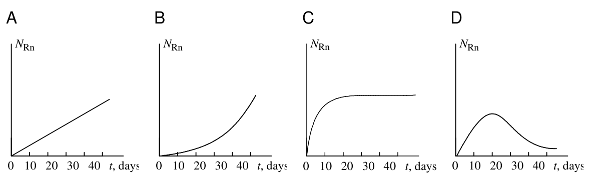
3.4 Choose which of the plots given below displays the time dependence of the number \(N_{\mathrm{Rn}}\) of radon atoms in the course of the experiment.
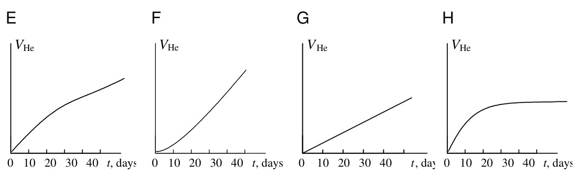
3.5 Choose which of the plots given below shows the time dependence of the volume of helium in the course of the experiment.
3.6 Choose the relation between the decay rate \(k\) of any given nuclide and its half-life \(T_{1/2}\).
3.7 a) Using a short kinetic scheme

(where \(k_1\) and \(k_2\) are the rate constants of the corresponding reactions) and the plot which you have selected in question 4, write a relation between the number of radon atoms at the end of experiment \(N'_{\mathrm{Rn}}\) and the number of radium atoms \(N_{\mathrm{Ra}}\).
b) Calculate \(N'_{\mathrm{Rn}}\) using the rate of radium decay given above (\(x = 3.42\times10^{10}\) \(\alpha\)-particles per gram of radium per second).
3.8 How many helium atoms could be formed from radon atoms remaining at the end of experiment \(N'_{\mathrm{Rn}}\), if all these atoms had decayed to RaD?
3.9 Using the solutions of the above questions calculate a better approximation to:
a) the number of helium atoms formed;
b) the Avogadro’s number.
Official English text of the problem.
Answers
- 3.1: The first six decays are \(\alpha,\alpha,\alpha,\beta^-,\beta^-,\alpha\), producing successively \(\ce{^{222}_{86}Rn}\), \(\ce{^{218}_{84}Po}\), \(\ce{^{214}_{82}Pb}\), \(\ce{^{214}_{83}Bi}\), \(\ce{^{214}_{84}Po}\), and \(\ce{^{210}_{82}Pb}\). The balanced equations are given below.
- 3.2(a): \(4\) helium atoms per decayed radium atom.
- 3.2(b): \(1.88\times10^{17}\) helium atoms.
- 3.3: \(N_{\mathrm A}\approx6.41\times10^{23}\ \mathrm{mol^{-1}}\).
- 3.4: Plot C.
- 3.5: Plot F.
- 3.6: \(k=\ln 2/T_{1/2}\).
- 3.7(a): \(k_1N_{\mathrm{Ra}}\approx k_2N'_{\mathrm{Rn}}\), hence \(N'_{\mathrm{Rn}}\approx(k_1/k_2)N_{\mathrm{Ra}}\).
- 3.7(b): \(N'_{\mathrm{Rn}}=3.13\times10^{15}\) radon atoms.
- 3.8: \(3N'_{\mathrm{Rn}}=9.40\times10^{15}\) additional helium atoms.
- 3.9(a): \(1.79\times10^{17}\) helium atoms.
- 3.9(b): \(N_{\mathrm A}\approx6.09\times10^{23}\ \mathrm{mol^{-1}}\).
The numerical Avogadro constants use \(V_m=22.4\ \mathrm{L\,mol^{-1}}\) at \(0^\circ\mathrm C\) and 1 atm.
Solution
3.1 — The first six radioactive decays
In an \(\alpha\)-decay, the mass number decreases by four and the atomic number decreases by two. In a \(\beta^-\)-decay, the mass number remains unchanged and the atomic number increases by one. Applying these rules successively gives:
| Historical designation | Modern nuclide | Name |
|---|---|---|
| Ra | \(\ce{^{226}_{88}Ra}\) | Radium-226 |
| Rn | \(\ce{^{222}_{86}Rn}\) | Radon-222 |
| RaA | \(\ce{^{218}_{84}Po}\) | Polonium-218 |
| RaB | \(\ce{^{214}_{82}Pb}\) | Lead-214 |
| RaC | \(\ce{^{214}_{83}Bi}\) | Bismuth-214 |
| RaC′ | \(\ce{^{214}_{84}Po}\) | Polonium-214 |
| RaD | \(\ce{^{210}_{82}Pb}\) | Lead-210 |
The balanced nuclear equations are
\[ \ce{^{226}_{88}Ra -> ^{222}_{86}Rn + ^{4}_{2}He}, \]
\[ \ce{^{222}_{86}Rn -> ^{218}_{84}Po + ^{4}_{2}He}, \]
\[ \ce{^{218}_{84}Po -> ^{214}_{82}Pb + ^{4}_{2}He}, \]
\[ \ce{^{214}_{82}Pb -> ^{214}_{83}Bi + ^{0}_{-1}e} +\bar{\nu}_e, \]
\[ \ce{^{214}_{83}Bi -> ^{214}_{84}Po + ^{0}_{-1}e} +\bar{\nu}_e, \]
\[ \ce{^{214}_{84}Po -> ^{210}_{82}Pb + ^{4}_{2}He}. \]
Here \(\bar{\nu}_e\) is an electron antineutrino. Each equation conserves mass number and electric charge.
An \(\alpha\)-particle is a helium-4 nucleus, \(\ce{^{4}He^{2+}}\), SMILES [4He+2]. After acquiring two electrons, it becomes a neutral helium-4 atom, \(\ce{^{4}He}\), SMILES [4He]. Thus each emitted \(\alpha\)-particle contributes one collected helium atom.
3.2(a) — Helium atoms per decayed radium atom
Under the first approximation, the transformations from radium to RaD occur effectively immediately. There are four \(\alpha\)-decays along this part of the chain:
- Radium-226 to radon-222.
- Radon-222 to polonium-218.
- Polonium-218 to lead-214.
- Polonium-214 to lead-210.
RaD has a half-life of 27.1 years, much longer than 83 days, so further decay is neglected at this accuracy. Consequently,
\[ \boxed{4\text{ helium atoms per decayed radium atom}.} \]
3.2(b) — Total helium atoms in the first approximation
The radium half-life exceeds 1500 years, so its activity is effectively constant during 83 days. The sample’s radium decay rate is
\[ R=mx =(0.192\ \mathrm g) (3.42\times10^{10}\ \mathrm{g^{-1}s^{-1}}) =6.5664\times10^9\ \mathrm{s^{-1}}. \]
The duration is
\[ t=83.0\times24\times3600 =7.1712\times10^6\ \mathrm s. \]
The number of radium atoms that decay is therefore
\[ D=Rt =(6.5664\times10^9)(7.1712\times10^6) =4.708896768\times10^{16}. \]
Multiplying by four,
\[ N_{\mathrm{He}}^{(0)}=4D =1.8835587072\times10^{17}, \]
or, to three significant figures,
\[ \boxed{N_{\mathrm{He}}^{(0)}=1.88\times10^{17}\text{ atoms}.} \]
3.3 — First approximation to Avogadro’s number
Using the standard ideal-gas molar volume at the stated conditions,
\[ V_m=22.4\ \mathrm{L\,mol^{-1}}, \qquad V_{\mathrm{He}}=6.58\ \mathrm{mm^3} =6.58\times10^{-6}\ \mathrm L. \]
The collected amount of helium is
\[ n_{\mathrm{He}} =\frac{V_{\mathrm{He}}}{V_m} =\frac{6.58\times10^{-6}}{22.4} =2.9375\times10^{-7}\ \mathrm{mol}. \]
Hence
\[ N_{\mathrm A}^{(0)} =\frac{N_{\mathrm{He}}^{(0)}}{n_{\mathrm{He}}} =\frac{1.8835587072\times10^{17}} {2.9375\times10^{-7}} =\boxed{6.41\times10^{23}\ \mathrm{mol^{-1}}}. \]
3.4 — Time dependence of the radon inventory
Initially, the purified sample contains no radon. Radium supplies radon at the approximately constant rate \(R\), while radon decays at rate \(k_2N_{\mathrm{Rn}}\). Therefore,
\[ \frac{dN_{\mathrm{Rn}}}{dt}=R-k_2N_{\mathrm{Rn}}, \qquad N_{\mathrm{Rn}}(0)=0. \]
The solution is
\[ N_{\mathrm{Rn}}(t) =\frac{R}{k_2}\left(1-e^{-k_2t}\right). \]
The radon inventory starts at zero, increases with a progressively decreasing slope, and approaches the plateau \(R/k_2\). Thus the correct plot is
\[ \boxed{\mathrm C}. \]
3.5 — Time dependence of the helium volume
Each radium decay immediately supplies one helium atom. Each radon decay, followed by the short-lived intermediates down to RaD, supplies three more. Thus
\[ \frac{dN_{\mathrm{He}}}{dt} =R+3k_2N_{\mathrm{Rn}} =R\left(4-3e^{-k_2t}\right). \]
The helium production rate increases from \(R\) initially to \(4R\) once the radon inventory reaches equilibrium. In particular,
\[ \frac{d^2N_{\mathrm{He}}}{dt^2} =3Rk_2e^{-k_2t}>0. \]
The helium volume is proportional to \(N_{\mathrm{He}}\), so it increases with upward curvature and eventually becomes nearly linear. The matching plot is
\[ \boxed{\mathrm F}. \]
The idealized curve has a nonzero initial slope because radium itself emits \(\alpha\)-particles from the start.
3.6 — Decay constant and half-life
Radioactive decay follows
\[ N(t)=N(0)e^{-kt}. \]
At one half-life,
\[ \frac{N(T_{1/2})}{N(0)} =\frac12=e^{-kT_{1/2}}. \]
Taking logarithms gives
\[ \boxed{k=\frac{\ln2}{T_{1/2}}}. \]
3.7(a) — Relation between radon and radium inventories
The radon production rate is
\[ R=k_1N_{\mathrm{Ra}}. \]
Under the constant-parent approximation, the finite-time relation is
\[ N'_{\mathrm{Rn}} =\frac{k_1N_{\mathrm{Ra}}}{k_2} \left(1-e^{-k_2t}\right). \]
At 83.0 days,
\[ e^{-k_2t} =2^{-83.0/3.83} =2.99\times10^{-7}, \]
so radon is effectively at its equilibrium plateau. Production and decay rates are consequently equal:
\[ \boxed{k_1N_{\mathrm{Ra}}\approx k_2N'_{\mathrm{Rn}}}, \]
or
\[ \boxed{N'_{\mathrm{Rn}}\approx \frac{k_1}{k_2}N_{\mathrm{Ra}}}. \]
3.7(b) — Number of radon atoms remaining
The radon decay constant is
\[ k_2 =\frac{\ln2}{3.83\times86400\ \mathrm s} =2.09466\times10^{-6}\ \mathrm{s^{-1}}. \]
Therefore,
\[ N'_{\mathrm{Rn}} \approx\frac{R}{k_2} =\frac{6.5664\times10^9\ \mathrm{s^{-1}}} {2.09466\times10^{-6}\ \mathrm{s^{-1}}} =\boxed{3.13\times10^{15}\text{ atoms}}. \]
Including the finite-time factor leaves this rounded result unchanged.
3.8 — Helium still obtainable from the remaining radon
Between radon-222 and RaD, three \(\alpha\)-decays occur. Therefore each remaining radon atom would produce three additional helium atoms upon reaching RaD.
Using the unrounded radon inventory,
\[ N_{\mathrm{He,additional}} =3N'_{\mathrm{Rn}} =3(3.13483\times10^{15}) =\boxed{9.40\times10^{15}\text{ atoms}}. \]
The initial radium-to-radon \(\alpha\)-particle has already been emitted, so it is not included in this additional yield.
3.9(a) — Improved number of helium atoms formed
The first approximation counted four helium atoms for every radium decay. It therefore included three helium atoms not yet produced for every radon atom still present at the end.
Subtracting this missing production,
\[ N_{\mathrm{He}} =4Rt-3N'_{\mathrm{Rn}}. \]
Numerically,
\[ N_{\mathrm{He}} =1.8835587072\times10^{17} -9.4044986\times10^{15} =1.7895137\times10^{17}. \]
Thus
\[ \boxed{N_{\mathrm{He}}=1.79\times10^{17}\text{ atoms}.} \]
3.9(b) — Improved Avogadro constant
The measured amount of helium remains \(2.9375\times10^{-7}\ \mathrm{mol}\). Hence
\[ N_{\mathrm A} =\frac{N_{\mathrm{He}}}{n_{\mathrm{He}}} =\frac{1.7895137\times10^{17}} {2.9375\times10^{-7}} =\boxed{6.09\times10^{23}\ \mathrm{mol^{-1}}}. \]
This incorporates the finite radon lifetime while retaining the problem’s approximations for the other decay products.
The solution was checked against the official solution.
IChO 1996 · Theorieaufgabe 3
Die Avogadro-Zahl aus dem Zerfall von Radium
Im Jahr 1908 maßen Rutherford und H.Geiger gemeinsam die Emissionsrate von \(\alpha\)-Teilchen (\(x\)) durch Radium (in der Natur ist dieses Element durch ein einziges Nuklid, \(\ce{^{226}_{88}Ra}\), vertreten) und stellten fest, dass 1.00 g Radium pro Sekunde \(x = 3.42\times10^{10}\) \(\alpha\)-Teilchen emittiert.
Im Jahr 1911 maßen Rutherford und der amerikanische Physikochemiker B.Boltwood die Bildungsrate von Helium aus Radium. Dieses Experiment ermöglichte die Bestimmung des genauesten damals verfügbaren Wertes der Avogadro-Zahl, da das molare Volumen eines idealen Gases bereits gut bekannt war. Hierzu wurde eine von Zerfallsprodukten gereinigte Radiumsalzprobe, die \(m = 192\) mg \(\ce{Ra}\) enthielt, in eine Apparatur eingebracht und das Volumen des entstandenen Heliums gemessen. Nach 83 Versuchstagen (\(t = 83.0\) Tage) waren 6.58 \(\mathrm{mm^3}\) \(\ce{He}\) aufgefangen worden (\(V_{\mathrm{He}} = 6.58\ \mathrm{mm^3}\), umgerechnet auf \(0^\circ\mathrm{C}\) und 1 atm).
Zum Verständnis der Ergebnisse dieses Experiments benötigen wir das unten dargestellte kinetische Schema des radioaktiven Zerfalls von \(\ce{Ra}\) (die Halbwertszeiten stehen über den Pfeilen, die Zerfallsart unter den Pfeilen).
(RaA - RaE sind Zwischenprodukte des Radonzerfalls).
3.1 Schreiben Sie die ersten sechs radioaktiven Zerfälle in moderner Schreibweise unter Angabe der Ordnungs- und Massenzahlen aller beteiligten Kerne auf.
In einer groben ersten Näherung können die Halbwertszeiten aller Zerfallsprodukte des Radiums mit Ausnahme von RaD und \(\ce{Po}\) gegenüber der Messdauer \(t\) als vernachlässigbar angenommen werden. Führen Sie mit dieser Näherung die folgenden Berechnungen durch.
3.2 a) Wie viele Heliumatome waren nach 83 Tagen aus jedem zerfallenen Radiumatom entstanden?
b) Wie viele Heliumatome entstanden insgesamt während des Experiments?
3.3 Berechnen Sie aus den obigen Daten einen Näherungswert für die Avogadro-Zahl.
Für eine genauere Berechnung der Avogadro-Zahl darf die Halbwertszeit von Radon, \(T_{1/2}(\ce{Rn}) = 3.83\) Tage, nicht vernachlässigt werden, da sie mit der Versuchsdauer \(t\) vergleichbar ist und bis zum Ende des Experiments nicht alle Radonatome zerfallen waren.
3.4 Wählen Sie aus den unten angegebenen Diagrammen dasjenige aus, das die Zeitabhängigkeit der Anzahl \(N_{\mathrm{Rn}}\) der Radonatome während des Experiments darstellt.
3.5 Wählen Sie aus den unten angegebenen Diagrammen dasjenige aus, das die Zeitabhängigkeit des Heliumvolumens während des Experiments zeigt.
3.6 Wählen Sie die Beziehung zwischen der Zerfallskonstante \(k\) eines beliebigen Nuklids und seiner Halbwertszeit \(T_{1/2}\) aus.
3.7 a) Verwenden Sie das verkürzte kinetische Schema
(wobei \(k_1\) und \(k_2\) die Geschwindigkeitskonstanten der entsprechenden Reaktionen sind) und das in Frage 4 ausgewählte Diagramm, um eine Beziehung zwischen der Anzahl der Radonatome am Ende des Experiments \(N'_{\mathrm{Rn}}\) und der Anzahl der Radiumatome \(N_{\mathrm{Ra}}\) aufzustellen.
b) Berechnen Sie \(N'_{\mathrm{Rn}}\) mithilfe der oben angegebenen Zerfallsrate von Radium (\(x = 3.42\times10^{10}\) \(\alpha\)-Teilchen pro Gramm Radium und Sekunde).
3.8 Wie viele Heliumatome könnten aus den am Ende des Experiments verbliebenen Radonatomen \(N'_{\mathrm{Rn}}\) entstehen, wenn alle diese Atome zu RaD zerfallen wären?
3.9 Berechnen Sie mithilfe der Lösungen der obigen Fragen eine bessere Näherung für:
a) die Anzahl der entstandenen Heliumatome;
b) die Avogadro-Zahl.
Aufgabentext aus dem offiziellen englischen Text übersetzt.
Antworten
- 3.1: Die ersten sechs Zerfälle sind \(\alpha,\alpha,\alpha,\beta^-,\beta^-,\alpha\); dabei entstehen nacheinander \(\ce{^{222}_{86}Rn}\), \(\ce{^{218}_{84}Po}\), \(\ce{^{214}_{82}Pb}\), \(\ce{^{214}_{83}Bi}\), \(\ce{^{214}_{84}Po}\) und \(\ce{^{210}_{82}Pb}\). Die ausgeglichenen Gleichungen sind unten angegeben.
- 3.2(a): \(4\) Heliumatome pro zerfallenem Radiumatom.
- 3.2(b): \(1.88\times10^{17}\) Heliumatome.
- 3.3: \(N_{\mathrm A}\approx6.41\times10^{23}\ \mathrm{mol^{-1}}\).
- 3.4: Diagramm C.
- 3.5: Diagramm F.
- 3.6: \(k=\ln 2/T_{1/2}\).
- 3.7(a): \(k_1N_{\mathrm{Ra}}\approx k_2N'_{\mathrm{Rn}}\), also \(N'_{\mathrm{Rn}}\approx(k_1/k_2)N_{\mathrm{Ra}}\).
- 3.7(b): \(N'_{\mathrm{Rn}}=3.13\times10^{15}\) Radonatome.
- 3.8: \(3N'_{\mathrm{Rn}}=9.40\times10^{15}\) zusätzliche Heliumatome.
- 3.9(a): \(1.79\times10^{17}\) Heliumatome.
- 3.9(b): \(N_{\mathrm A}\approx6.09\times10^{23}\ \mathrm{mol^{-1}}\).
Die Zahlenwerte der Avogadro-Konstante wurden mit \(V_m=22.4\ \mathrm{L\,mol^{-1}}\) bei \(0^\circ\mathrm C\) und 1 atm berechnet.
Lösung
3.1 — Die ersten sechs radioaktiven Zerfälle
Bei einem \(\alpha\)-Zerfall nimmt die Massenzahl um vier und die Ordnungszahl um zwei ab. Bei einem \(\beta^-\)-Zerfall bleibt die Massenzahl unverändert und die Ordnungszahl nimmt um eins zu. Die schrittweise Anwendung dieser Regeln ergibt:
| Historische Bezeichnung | Modernes Nuklid | Name |
|---|---|---|
| Ra | \(\ce{^{226}_{88}Ra}\) | Radium-226 |
| Rn | \(\ce{^{222}_{86}Rn}\) | Radon-222 |
| RaA | \(\ce{^{218}_{84}Po}\) | Polonium-218 |
| RaB | \(\ce{^{214}_{82}Pb}\) | Blei-214 |
| RaC | \(\ce{^{214}_{83}Bi}\) | Bismut-214 |
| RaC′ | \(\ce{^{214}_{84}Po}\) | Polonium-214 |
| RaD | \(\ce{^{210}_{82}Pb}\) | Blei-210 |
Die ausgeglichenen Kernreaktionsgleichungen lauten
\[ \ce{^{226}_{88}Ra -> ^{222}_{86}Rn + ^{4}_{2}He}, \]
\[ \ce{^{222}_{86}Rn -> ^{218}_{84}Po + ^{4}_{2}He}, \]
\[ \ce{^{218}_{84}Po -> ^{214}_{82}Pb + ^{4}_{2}He}, \]
\[ \ce{^{214}_{82}Pb -> ^{214}_{83}Bi + ^{0}_{-1}e} +\bar{\nu}_e, \]
\[ \ce{^{214}_{83}Bi -> ^{214}_{84}Po + ^{0}_{-1}e} +\bar{\nu}_e, \]
\[ \ce{^{214}_{84}Po -> ^{210}_{82}Pb + ^{4}_{2}He}. \]
Hier ist \(\bar{\nu}_e\) ein Elektron-Antineutrino. In jeder Gleichung bleiben die Massenzahl und die elektrische Ladung erhalten.
Ein \(\alpha\)-Teilchen ist ein Helium-4-Kern, \(\ce{^{4}He^{2+}}\), SMILES [4He+2]. Nach Aufnahme zweier Elektronen wird daraus ein neutrales Helium-4-Atom, \(\ce{^{4}He}\), SMILES [4He]. Somit trägt jedes emittierte \(\alpha\)-Teilchen ein Atom zum aufgefangenen Helium bei.
3.2(a) — Heliumatome pro zerfallenem Radiumatom
In der ersten Näherung erfolgen die Umwandlungen von Radium zu RaD praktisch augenblicklich. In diesem Abschnitt der Zerfallsreihe treten vier \(\alpha\)-Zerfälle auf:
- Radium-226 zu Radon-222.
- Radon-222 zu Polonium-218.
- Polonium-218 zu Blei-214.
- Polonium-214 zu Blei-210.
RaD hat eine Halbwertszeit von 27.1 Jahren, die wesentlich länger als 83 Tage ist, sodass sein weiterer Zerfall bei dieser Genauigkeit vernachlässigt wird. Folglich gilt:
\[ \boxed{4\text{ Heliumatome pro zerfallenem Radiumatom}.} \]
3.2(b) — Gesamtzahl der Heliumatome in der ersten Näherung
Die Halbwertszeit von Radium beträgt mehr als 1500 Jahre, sodass seine Aktivität während der 83 Tage praktisch konstant bleibt. Die Zerfallsrate des Radiums in der Probe ist
\[ R=mx =(0.192\ \mathrm g) (3.42\times10^{10}\ \mathrm{g^{-1}s^{-1}}) =6.5664\times10^9\ \mathrm{s^{-1}}. \]
Die Versuchsdauer beträgt
\[ t=83.0\times24\times3600 =7.1712\times10^6\ \mathrm s. \]
Die Anzahl der zerfallenden Radiumatome ist daher
\[ D=Rt =(6.5664\times10^9)(7.1712\times10^6) =4.708896768\times10^{16}. \]
Multiplikation mit vier ergibt
\[ N_{\mathrm{He}}^{(0)}=4D =1.8835587072\times10^{17}, \]
oder auf drei signifikante Stellen gerundet
\[ \boxed{N_{\mathrm{He}}^{(0)}=1.88\times10^{17}\text{ Atome}.} \]
3.3 — Erste Näherung für die Avogadro-Zahl
Mit dem üblichen molaren Volumen eines idealen Gases unter den angegebenen Bedingungen gilt
\[ V_m=22.4\ \mathrm{L\,mol^{-1}}, \qquad V_{\mathrm{He}}=6.58\ \mathrm{mm^3} =6.58\times10^{-6}\ \mathrm L. \]
Die Stoffmenge des aufgefangenen Heliums beträgt
\[ n_{\mathrm{He}} =\frac{V_{\mathrm{He}}}{V_m} =\frac{6.58\times10^{-6}}{22.4} =2.9375\times10^{-7}\ \mathrm{mol}. \]
Somit ergibt sich
\[ N_{\mathrm A}^{(0)} =\frac{N_{\mathrm{He}}^{(0)}}{n_{\mathrm{He}}} =\frac{1.8835587072\times10^{17}} {2.9375\times10^{-7}} =\boxed{6.41\times10^{23}\ \mathrm{mol^{-1}}}. \]
3.4 — Zeitabhängigkeit des Radonbestands
Zu Beginn enthält die gereinigte Probe kein Radon. Radium liefert Radon mit der annähernd konstanten Rate \(R\), während Radon mit der Rate \(k_2N_{\mathrm{Rn}}\) zerfällt. Daher gilt
\[ \frac{dN_{\mathrm{Rn}}}{dt}=R-k_2N_{\mathrm{Rn}}, \qquad N_{\mathrm{Rn}}(0)=0. \]
Die Lösung lautet
\[ N_{\mathrm{Rn}}(t) =\frac{R}{k_2}\left(1-e^{-k_2t}\right). \]
Der Radonbestand beginnt bei null, nimmt mit stetig abnehmender Steigung zu und nähert sich dem Plateau \(R/k_2\). Das richtige Diagramm ist somit
\[ \boxed{\mathrm C}. \]
3.5 — Zeitabhängigkeit des Heliumvolumens
Jeder Radiumzerfall liefert sofort ein Heliumatom. Jeder Radonzerfall liefert zusammen mit den nachfolgenden Zerfällen der kurzlebigen Zwischenprodukte bis zu RaD drei weitere. Somit gilt
\[ \frac{dN_{\mathrm{He}}}{dt} =R+3k_2N_{\mathrm{Rn}} =R\left(4-3e^{-k_2t}\right). \]
Die Heliumbildungsrate steigt vom Anfangswert \(R\) auf \(4R\), sobald der Radonbestand sein Gleichgewicht erreicht. Insbesondere gilt
\[ \frac{d^2N_{\mathrm{He}}}{dt^2} =3Rk_2e^{-k_2t}>0. \]
Das Heliumvolumen ist proportional zu \(N_{\mathrm{He}}\); seine Kurve steigt daher mit einer Krümmung nach oben an und verläuft schließlich nahezu linear. Das passende Diagramm ist
\[ \boxed{\mathrm F}. \]
Die idealisierte Kurve hat eine von null verschiedene Anfangssteigung, weil Radium selbst von Beginn an \(\alpha\)-Teilchen emittiert.
3.6 — Zerfallskonstante und Halbwertszeit
Der radioaktive Zerfall folgt dem Gesetz
\[ N(t)=N(0)e^{-kt}. \]
Nach einer Halbwertszeit gilt
\[ \frac{N(T_{1/2})}{N(0)} =\frac12=e^{-kT_{1/2}}. \]
Durch Logarithmieren erhält man
\[ \boxed{k=\frac{\ln2}{T_{1/2}}}. \]
3.7(a) — Beziehung zwischen Radon- und Radiumbestand
Die Radonbildungsrate ist
\[ R=k_1N_{\mathrm{Ra}}. \]
Unter der Annahme eines konstanten Bestands des Mutternuklids lautet die Beziehung für eine endliche Zeit
\[ N'_{\mathrm{Rn}} =\frac{k_1N_{\mathrm{Ra}}}{k_2} \left(1-e^{-k_2t}\right). \]
Nach 83.0 Tagen gilt
\[ e^{-k_2t} =2^{-83.0/3.83} =2.99\times10^{-7}, \]
sodass Radon praktisch sein Gleichgewichtsplateau erreicht hat. Bildungs- und Zerfallsrate sind folglich gleich:
\[ \boxed{k_1N_{\mathrm{Ra}}\approx k_2N'_{\mathrm{Rn}}}, \]
oder
\[ \boxed{N'_{\mathrm{Rn}}\approx \frac{k_1}{k_2}N_{\mathrm{Ra}}}. \]
3.7(b) — Anzahl der verbliebenen Radonatome
Die Zerfallskonstante von Radon beträgt
\[ k_2 =\frac{\ln2}{3.83\times86400\ \mathrm s} =2.09466\times10^{-6}\ \mathrm{s^{-1}}. \]
Daher gilt
\[ N'_{\mathrm{Rn}} \approx\frac{R}{k_2} =\frac{6.5664\times10^9\ \mathrm{s^{-1}}} {2.09466\times10^{-6}\ \mathrm{s^{-1}}} =\boxed{3.13\times10^{15}\text{ Atome}}. \]
Die Berücksichtigung des Faktors für die endliche Versuchsdauer lässt dieses gerundete Ergebnis unverändert.
3.8 — Noch aus dem verbliebenen Radon gewinnbares Helium
Zwischen Radon-222 und RaD treten drei \(\alpha\)-Zerfälle auf. Daher würde jedes verbliebene Radonatom bei seinem Zerfall bis zu RaD drei zusätzliche Heliumatome liefern.
Mit dem ungerundeten Radonbestand ergibt sich
\[ N_{\mathrm{He,additional}} =3N'_{\mathrm{Rn}} =3(3.13483\times10^{15}) =\boxed{9.40\times10^{15}\text{ Atome}}. \]
Das anfängliche \(\alpha\)-Teilchen aus dem Zerfall von Radium zu Radon wurde bereits emittiert und wird daher in dieser zusätzlichen Ausbeute nicht mitgezählt.
3.9(a) — Verbesserte Anzahl der entstandenen Heliumatome
In der ersten Näherung wurden für jeden Radiumzerfall vier Heliumatome gezählt. Damit wurden für jedes am Ende noch vorhandene Radonatom drei noch nicht entstandene Heliumatome mitgezählt.
Durch Abziehen dieser noch ausstehenden Heliumbildung erhält man
\[ N_{\mathrm{He}} =4Rt-3N'_{\mathrm{Rn}}. \]
Zahlenmäßig ergibt sich
\[ N_{\mathrm{He}} =1.8835587072\times10^{17} -9.4044986\times10^{15} =1.7895137\times10^{17}. \]
Somit gilt
\[ \boxed{N_{\mathrm{He}}=1.79\times10^{17}\text{ Atome}.} \]
3.9(b) — Verbesserte Avogadro-Konstante
Die gemessene Stoffmenge des Heliums bleibt \(2.9375\times10^{-7}\ \mathrm{mol}\). Daher gilt
\[ N_{\mathrm A} =\frac{N_{\mathrm{He}}}{n_{\mathrm{He}}} =\frac{1.7895137\times10^{17}} {2.9375\times10^{-7}} =\boxed{6.09\times10^{23}\ \mathrm{mol^{-1}}}. \]
Damit wird die endliche Lebensdauer von Radon berücksichtigt, während die Näherungen der Aufgabe für die übrigen Zerfallsprodukte beibehalten werden.
Die Lösung wurde mit der offiziellen Lösung abgeglichen.
IChO 1996 · Teori sorusu 3
Radyumun bozunmasından Avogadro sayısının belirlenmesi
1908 yılında Rutherford, H.Geiger ile birlikte radyumun (bu element doğada tek bir nüklitle, \(\ce{^{226}_{88}Ra}\), temsil edilir) \(\alpha\)-parçacığı yayma hızını (\(x\)) ölçmüş ve 1.00 g radyumun saniyede \(x = 3.42\times10^{10}\) \(\alpha\)-parçacığı yaydığını bulmuştur.
1911 yılında Rutherford ve Amerikalı fizikokimyacı B.Boltwood, radyumdan helyum oluşma hızını ölçmüştür. İdeal gazın molar hacmi o dönemde güvenilir biçimde bilindiğinden, bu deney Avogadro sayısının o zamana kadar elde edilebilen en doğru değerinin bulunmasını sağlamıştır. Bu amaçla, bozunma ürünlerinden arındırılmış ve \(m = 192\) mg \(\ce{Ra}\) içeren bir radyum tuzu örneği bir düzeneğe yerleştirilmiş ve açığa çıkan helyumun hacmi ölçülmüştür. Deneyin 83 günü (\(t = 83.0\) gün) sonunda 6.58 \(\mathrm{mm^3}\) \(\ce{He}\) toplanmıştır (\(0^\circ\mathrm{C}\) ve 1 atm koşullarına düzeltilmiş hacim \(V_{\mathrm{He}} = 6.58\ \mathrm{mm^3}\)).
Bu deneyin sonuçlarını anlamak için aşağıda verilen \(\ce{Ra}\)'nın radyoaktif bozunmasına ait kinetik şemaya ihtiyacımız olacaktır (yarı ömürler okların üzerinde, bozunma türleri ise okların altında verilmiştir).
(RaA - RaE, radonun bozunmasının ara ürünleridir).
3.1 İlk altı radyoaktif bozunmayı, katılan tüm çekirdeklerin atom ve kütle numaralarını gösteren modern gösterimle yazınız.
Kaba bir ilk yaklaşım olarak, RaD ve \(\ce{Po}\) dışındaki tüm radyum bozunma ürünlerinin yarı ömürlerinin ölçüm süresi \(t\)'ye kıyasla ihmal edilebilir olduğu varsayılabilir. Bu yaklaşımı kullanarak aşağıdaki hesaplamaları yapınız.
3.2 a) 83 gün sonunda, bozunan her radyum atomundan kaç helyum atomu oluşmuştur?
b) Deney boyunca toplam kaç helyum atomu oluşmuştur?
3.3 Yukarıdaki verilerden Avogadro sayısının yaklaşık bir değerini hesaplayınız.
Avogadro sayısının daha doğru hesaplanması için radonun yarı ömrü \(T_{1/2}(\ce{Rn}) = 3.83\) gün ihmal edilemez; çünkü bu süre deney süresi \(t\) ile karşılaştırılabilir büyüklüktedir ve deneyin sonunda radon atomlarının tamamı bozunmuş değildir.
3.4 Aşağıdaki grafiklerden hangisinin deney süresince radon atomlarının sayısı \(N_{\mathrm{Rn}}\)'nin zamana bağlı değişimini gösterdiğini seçiniz.
3.5 Aşağıdaki grafiklerden hangisinin deney süresince helyum hacminin zamana bağlı değişimini gösterdiğini seçiniz.
3.6 Herhangi bir nüklidin bozunma hızı \(k\) ile yarı ömrü \(T_{1/2}\) arasındaki bağıntıyı seçiniz.
3.7 a) Kısa kinetik şemayı
(burada \(k_1\) ve \(k_2\), ilgili tepkimelerin hız sabitleridir) ve 4. soruda seçtiğiniz grafiği kullanarak deneyin sonundaki radon atomlarının sayısı \(N'_{\mathrm{Rn}}\) ile radyum atomlarının sayısı \(N_{\mathrm{Ra}}\) arasında bir bağıntı yazınız.
b) Yukarıda verilen radyum bozunma hızını (gram radyum başına saniyede \(x = 3.42\times10^{10}\) \(\alpha\)-parçacığı) kullanarak \(N'_{\mathrm{Rn}}\)'yi hesaplayınız.
3.8 Deneyin sonunda kalan \(N'_{\mathrm{Rn}}\) radon atomunun tümü RaD'ye kadar bozunsaydı, bu atomlardan kaç helyum atomu oluşabilirdi?
3.9 Yukarıdaki soruların çözümlerini kullanarak aşağıdakiler için daha iyi bir yaklaşık değer hesaplayınız:
a) oluşan helyum atomlarının sayısı;
b) Avogadro sayısı.
Soru metni resmi İngilizce metinden çevrilmiştir.
Cevaplar
- 3.1: İlk altı bozunma \(\alpha,\alpha,\alpha,\beta^-,\beta^-,\alpha\) olup sırasıyla \(\ce{^{222}_{86}Rn}\), \(\ce{^{218}_{84}Po}\), \(\ce{^{214}_{82}Pb}\), \(\ce{^{214}_{83}Bi}\), \(\ce{^{214}_{84}Po}\) ve \(\ce{^{210}_{82}Pb}\) oluşturur. Denkleştirilmiş denklemler aşağıda verilmiştir.
- 3.2(a): Bozunan radyum atomu başına \(4\) helyum atomu.
- 3.2(b): \(1.88\times10^{17}\) helyum atomu.
- 3.3: \(N_{\mathrm A}\approx6.41\times10^{23}\ \mathrm{mol^{-1}}\).
- 3.4: C grafiği.
- 3.5: F grafiği.
- 3.6: \(k=\ln 2/T_{1/2}\).
- 3.7(a): \(k_1N_{\mathrm{Ra}}\approx k_2N'_{\mathrm{Rn}}\), dolayısıyla \(N'_{\mathrm{Rn}}\approx(k_1/k_2)N_{\mathrm{Ra}}\).
- 3.7(b): \(N'_{\mathrm{Rn}}=3.13\times10^{15}\) radon atomu.
- 3.8: İlave \(3N'_{\mathrm{Rn}}=9.40\times10^{15}\) helyum atomu.
- 3.9(a): \(1.79\times10^{17}\) helyum atomu.
- 3.9(b): \(N_{\mathrm A}\approx6.09\times10^{23}\ \mathrm{mol^{-1}}\).
Avogadro sabitinin sayısal değerleri için \(0^\circ\mathrm C\) ve 1 atm koşullarında \(V_m=22.4\ \mathrm{L\,mol^{-1}}\) kullanılmıştır.
Çözüm
3.1 — İlk altı radyoaktif bozunma
Bir \(\alpha\)-bozunmasında kütle numarası dört, atom numarası ise iki azalır. Bir \(\beta^-\)-bozunmasında kütle numarası değişmez, atom numarası ise bir artar. Bu kurallar art arda uygulandığında şu sonuçlar elde edilir:
| Tarihsel gösterim | Modern nüklit gösterimi | Adı |
|---|---|---|
| Ra | \(\ce{^{226}_{88}Ra}\) | Radyum-226 |
| Rn | \(\ce{^{222}_{86}Rn}\) | Radon-222 |
| RaA | \(\ce{^{218}_{84}Po}\) | Polonyum-218 |
| RaB | \(\ce{^{214}_{82}Pb}\) | Kurşun-214 |
| RaC | \(\ce{^{214}_{83}Bi}\) | Bizmut-214 |
| RaC′ | \(\ce{^{214}_{84}Po}\) | Polonyum-214 |
| RaD | \(\ce{^{210}_{82}Pb}\) | Kurşun-210 |
Denkleştirilmiş çekirdek tepkimesi denklemleri şöyledir:
\[ \ce{^{226}_{88}Ra -> ^{222}_{86}Rn + ^{4}_{2}He}, \]
\[ \ce{^{222}_{86}Rn -> ^{218}_{84}Po + ^{4}_{2}He}, \]
\[ \ce{^{218}_{84}Po -> ^{214}_{82}Pb + ^{4}_{2}He}, \]
\[ \ce{^{214}_{82}Pb -> ^{214}_{83}Bi + ^{0}_{-1}e} +\bar{\nu}_e, \]
\[ \ce{^{214}_{83}Bi -> ^{214}_{84}Po + ^{0}_{-1}e} +\bar{\nu}_e, \]
\[ \ce{^{214}_{84}Po -> ^{210}_{82}Pb + ^{4}_{2}He}. \]
Burada \(\bar{\nu}_e\) bir elektron antinötrinosudur. Her denklemde kütle numarası ve elektrik yükü korunur.
Bir \(\alpha\)-parçacığı, \(\ce{^{4}He^{2+}}\) biçiminde gösterilen bir helyum-4 çekirdeğidir; SMILES gösterimi [4He+2] şeklindedir. İki elektron aldıktan sonra nötr bir helyum-4 atomuna, \(\ce{^{4}He}\), dönüşür; SMILES gösterimi [4He] şeklindedir. Dolayısıyla yayılan her \(\alpha\)-parçacığı, toplanan helyuma bir atom katkıda bulunur.
3.2(a) — Bozunan radyum atomu başına helyum atomları
İlk yaklaşımda, radyumdan RaD'ye kadar olan dönüşümler pratik olarak anında gerçekleşir. Zincirin bu bölümünde dört \(\alpha\)-bozunması vardır:
- Radyum-226'dan radon-222'ye.
- Radon-222'den polonyum-218'e.
- Polonyum-218'den kurşun-214'e.
- Polonyum-214'ten kurşun-210'a.
RaD'nin yarı ömrü 27.1 yıldır ve 83 günden çok daha uzundur; bu nedenle bu doğruluk düzeyinde sonraki bozunmalar ihmal edilir. Sonuç olarak,
\[ \boxed{4\text{ helyum atomu, bozunan radyum atomu başına}.} \]
3.2(b) — İlk yaklaşımda toplam helyum atomu sayısı
Radyumun yarı ömrü 1500 yılı aştığından, aktivitesi 83 gün boyunca pratik olarak sabittir. Örnekteki radyumun bozunma hızı
\[ R=mx =(0.192\ \mathrm g) (3.42\times10^{10}\ \mathrm{g^{-1}s^{-1}}) =6.5664\times10^9\ \mathrm{s^{-1}}. \]
Süre
\[ t=83.0\times24\times3600 =7.1712\times10^6\ \mathrm s. \]
Dolayısıyla bozunan radyum atomlarının sayısı
\[ D=Rt =(6.5664\times10^9)(7.1712\times10^6) =4.708896768\times10^{16}. \]
Dört ile çarpıldığında,
\[ N_{\mathrm{He}}^{(0)}=4D =1.8835587072\times10^{17}, \]
ya da üç anlamlı basamakla,
\[ \boxed{N_{\mathrm{He}}^{(0)}=1.88\times10^{17}\text{ atom}.} \]
3.3 — Avogadro sayısına ilk yaklaşım
Belirtilen koşullardaki standart ideal gaz molar hacmi kullanıldığında,
\[ V_m=22.4\ \mathrm{L\,mol^{-1}}, \qquad V_{\mathrm{He}}=6.58\ \mathrm{mm^3} =6.58\times10^{-6}\ \mathrm L. \]
Toplanan helyumun madde miktarı
\[ n_{\mathrm{He}} =\frac{V_{\mathrm{He}}}{V_m} =\frac{6.58\times10^{-6}}{22.4} =2.9375\times10^{-7}\ \mathrm{mol}. \]
Böylece
\[ N_{\mathrm A}^{(0)} =\frac{N_{\mathrm{He}}^{(0)}}{n_{\mathrm{He}}} =\frac{1.8835587072\times10^{17}} {2.9375\times10^{-7}} =\boxed{6.41\times10^{23}\ \mathrm{mol^{-1}}}. \]
3.4 — Mevcut radon atomu sayısının zamana bağlı değişimi
Başlangıçta arındırılmış örnek radon içermez. Radyum, yaklaşık olarak sabit \(R\) hızıyla radon üretirken radon \(k_2N_{\mathrm{Rn}}\) hızıyla bozunur. Bu nedenle,
\[ \frac{dN_{\mathrm{Rn}}}{dt}=R-k_2N_{\mathrm{Rn}}, \qquad N_{\mathrm{Rn}}(0)=0. \]
Çözüm şöyledir:
\[ N_{\mathrm{Rn}}(t) =\frac{R}{k_2}\left(1-e^{-k_2t}\right). \]
Mevcut radon atomu sayısı sıfırdan başlar, giderek azalan bir eğimle artar ve \(R/k_2\) plato değerine yaklaşır. Dolayısıyla doğru grafik
\[ \boxed{\mathrm C}. \]
3.5 — Helyum hacminin zamana bağlı değişimi
Her radyum bozunması anında bir helyum atomu sağlar. Her radon bozunması ise ardından RaD'ye kadar gerçekleşen kısa ömürlü ara ürünlerin bozunmalarıyla birlikte üç helyum atomu daha sağlar. Böylece
\[ \frac{dN_{\mathrm{He}}}{dt} =R+3k_2N_{\mathrm{Rn}} =R\left(4-3e^{-k_2t}\right). \]
Helyum oluşma hızı başlangıçta \(R\) iken, mevcut radon atomu sayısı dengeye ulaştığında \(4R\)'ye yükselir. Özellikle,
\[ \frac{d^2N_{\mathrm{He}}}{dt^2} =3Rk_2e^{-k_2t}>0. \]
Helyum hacmi \(N_{\mathrm{He}}\) ile orantılı olduğundan, yukarı doğru kavis yaparak artar ve sonunda yaklaşık olarak doğrusal hâle gelir. Buna karşılık gelen grafik
\[ \boxed{\mathrm F}. \]
İdealleştirilmiş eğrinin başlangıç eğimi sıfırdan farklıdır; çünkü radyumun kendisi başlangıçtan itibaren \(\alpha\)-parçacıkları yayar.
3.6 — Bozunma sabiti ve yarı ömür
Radyoaktif bozunma şu bağıntıya uyar:
\[ N(t)=N(0)e^{-kt}. \]
Bir yarı ömür sonunda,
\[ \frac{N(T_{1/2})}{N(0)} =\frac12=e^{-kT_{1/2}}. \]
Logaritma alınırsa
\[ \boxed{k=\frac{\ln2}{T_{1/2}}}. \]
3.7(a) — Mevcut radon ve radyum atomu sayıları arasındaki bağıntı
Radon oluşma hızı
\[ R=k_1N_{\mathrm{Ra}}. \]
Ana nüklidin miktarının sabit olduğu yaklaşımında, sonlu süre için bağıntı şöyledir:
\[ N'_{\mathrm{Rn}} =\frac{k_1N_{\mathrm{Ra}}}{k_2} \left(1-e^{-k_2t}\right). \]
83.0 gün sonunda,
\[ e^{-k_2t} =2^{-83.0/3.83} =2.99\times10^{-7}, \]
dolayısıyla radon pratik olarak denge platosundadır. Bu nedenle oluşma ve bozunma hızları eşittir:
\[ \boxed{k_1N_{\mathrm{Ra}}\approx k_2N'_{\mathrm{Rn}}}, \]
ya da
\[ \boxed{N'_{\mathrm{Rn}}\approx \frac{k_1}{k_2}N_{\mathrm{Ra}}}. \]
3.7(b) — Kalan radon atomlarının sayısı
Radonun bozunma sabiti
\[ k_2 =\frac{\ln2}{3.83\times86400\ \mathrm s} =2.09466\times10^{-6}\ \mathrm{s^{-1}}. \]
Dolayısıyla,
\[ N'_{\mathrm{Rn}} \approx\frac{R}{k_2} =\frac{6.5664\times10^9\ \mathrm{s^{-1}}} {2.09466\times10^{-6}\ \mathrm{s^{-1}}} =\boxed{3.13\times10^{15}\text{ atom}}. \]
Sonlu süre çarpanının hesaba katılması, bu yuvarlatılmış sonucu değiştirmez.
3.8 — Kalan radondan hâlâ elde edilebilecek helyum
Radon-222 ile RaD arasında üç \(\alpha\)-bozunması gerçekleşir. Dolayısıyla kalan her radon atomu, RaD'ye ulaştığında ilave üç helyum atomu oluşturacaktır.
Yuvarlatılmamış radon atomu sayısı kullanıldığında,
\[ N_{\mathrm{He,additional}} =3N'_{\mathrm{Rn}} =3(3.13483\times10^{15}) =\boxed{9.40\times10^{15}\text{ atom}}. \]
Başlangıçtaki radyumdan radona dönüşümde açığa çıkan \(\alpha\)-parçacığı zaten yayıldığından, bu ilave miktara dâhil edilmez.
3.9(a) — Oluşan helyum atomu sayısının iyileştirilmiş değeri
İlk yaklaşımda her radyum bozunması için dört helyum atomu sayılmıştır. Dolayısıyla deneyin sonunda hâlâ mevcut olan her radon atomu için henüz oluşmamış üç helyum atomu da bu sayıya dâhil edilmiştir.
Henüz gerçekleşmemiş bu üretim çıkarıldığında,
\[ N_{\mathrm{He}} =4Rt-3N'_{\mathrm{Rn}}. \]
Sayısal olarak,
\[ N_{\mathrm{He}} =1.8835587072\times10^{17} -9.4044986\times10^{15} =1.7895137\times10^{17}. \]
Böylece
\[ \boxed{N_{\mathrm{He}}=1.79\times10^{17}\text{ atom}.} \]
3.9(b) — İyileştirilmiş Avogadro sabiti
Ölçülen helyumun madde miktarı \(2.9375\times10^{-7}\ \mathrm{mol}\) olarak kalır. Dolayısıyla
\[ N_{\mathrm A} =\frac{N_{\mathrm{He}}}{n_{\mathrm{He}}} =\frac{1.7895137\times10^{17}} {2.9375\times10^{-7}} =\boxed{6.09\times10^{23}\ \mathrm{mol^{-1}}}. \]
Bu hesaplama, diğer bozunma ürünleri için soruda yapılan yaklaşımları korurken radonun sonlu ömrünü hesaba katar.
Çözüm, resmi çözümle karşılaştırılarak kontrol edildi.
IChO 1996 · Problema teórico 3
El número de Avogadro a partir de la desintegración del radio
En 1908, Rutherford, junto con H.Geiger, midió la tasa de emisión de partículas \(\alpha\) (\(x\)) del radio (en la naturaleza, este elemento está representado por un único nucleido, \(\ce{^{226}_{88}Ra}\)) y encontró que 1.00 g de radio emite \(x = 3.42\times10^{10}\) partículas \(\alpha\) por segundo.
En 1911, Rutherford y el fisicoquímico estadounidense B.Boltwood midieron la tasa de formación de helio a partir del radio. Este experimento permite obtener el valor más preciso del número de Avogadro disponible en aquella época, dado que el valor del volumen molar de un gas ideal estaba bien establecido. Para lograr este objetivo, se introdujo en un dispositivo una muestra de una sal de radio, purificada para eliminar los productos de desintegración y que contenía \(m = 192\) mg de \(\ce{Ra}\), y se midió el volumen de helio desprendido. Tras 83 días (\(t = 83.0\) días) de experimento, se recogieron 6.58 \(\mathrm{mm^3}\) de \(\ce{He}\) (\(V_{\mathrm{He}} = 6.58\ \mathrm{mm^3}\), corregido a \(0^\circ\mathrm{C}\) y 1 atm).
Para comprender los resultados de este experimento, necesitaremos el esquema cinético de la desintegración radiactiva del \(\ce{Ra}\), que se presenta a continuación (los períodos de semidesintegración figuran sobre las flechas y el tipo de desintegración, debajo de ellas).
(RaA - RaE son productos intermedios de la desintegración del radón).
3.1 Escriba las seis primeras desintegraciones radiactivas utilizando la notación moderna e indicando los números atómicos y másicos de todos los núcleos implicados.
Como primera aproximación, de carácter preliminar, puede suponerse que los períodos de semidesintegración de todos los productos de desintegración del radio, excepto los de RaD y \(\ce{Po}\), son despreciables en comparación con el tiempo de medida \(t\). Utilizando esta aproximación, realice los siguientes cálculos.
3.2 a) ¿Cuántos átomos de helio se habían formado por cada átomo de radio desintegrado al cabo de 83 días?
b) ¿Cuántos átomos de helio se formaron en total durante el experimento?
3.3 Calcule un valor aproximado del número de Avogadro a partir de los datos anteriores.
Para calcular el número de Avogadro con mayor precisión, no puede despreciarse el período de semidesintegración del radón, \(T_{1/2}(\ce{Rn}) = 3.83\) días, ya que es comparable con la duración del experimento \(t\) y no todos los átomos de radón se habían desintegrado al finalizar el experimento.
3.4 Elija cuál de las gráficas siguientes representa la dependencia temporal del número \(N_{\mathrm{Rn}}\) de átomos de radón durante el experimento.
3.5 Elija cuál de las gráficas siguientes muestra la dependencia temporal del volumen de helio durante el experimento.
3.6 Elija la relación entre la constante de desintegración \(k\) de un nucleido cualquiera y su período de semidesintegración \(T_{1/2}\).
3.7 a) Utilizando el esquema cinético simplificado
(donde \(k_1\) y \(k_2\) son las constantes de velocidad de las reacciones correspondientes) y la gráfica que ha seleccionado en la pregunta 4, escriba una relación entre el número de átomos de radón al finalizar el experimento, \(N'_{\mathrm{Rn}}\), y el número de átomos de radio, \(N_{\mathrm{Ra}}\).
b) Calcule \(N'_{\mathrm{Rn}}\) utilizando la tasa de desintegración del radio indicada anteriormente (\(x = 3.42\times10^{10}\) partículas \(\alpha\) por gramo de radio y por segundo).
3.8 ¿Cuántos átomos de helio podrían formarse a partir de los átomos de radón restantes al finalizar el experimento, \(N'_{\mathrm{Rn}}\), si todos estos átomos se hubieran desintegrado hasta RaD?
3.9 Utilizando las soluciones de las preguntas anteriores, calcule una mejor aproximación de:
a) el número de átomos de helio formados;
b) el número de Avogadro.
Enunciado traducido del texto oficial en inglés.
Respuestas
- 3.1: Las seis primeras desintegraciones son \(\alpha,\alpha,\alpha,\beta^-,\beta^-,\alpha\), y producen sucesivamente \(\ce{^{222}_{86}Rn}\), \(\ce{^{218}_{84}Po}\), \(\ce{^{214}_{82}Pb}\), \(\ce{^{214}_{83}Bi}\), \(\ce{^{214}_{84}Po}\) y \(\ce{^{210}_{82}Pb}\). Las ecuaciones ajustadas se presentan a continuación.
- 3.2(a): \(4\) átomos de helio por átomo de radio desintegrado.
- 3.2(b): \(1.88\times10^{17}\) átomos de helio.
- 3.3: \(N_{\mathrm A}\approx6.41\times10^{23}\ \mathrm{mol^{-1}}\).
- 3.4: Gráfica C.
- 3.5: Gráfica F.
- 3.6: \(k=\ln 2/T_{1/2}\).
- 3.7(a): \(k_1N_{\mathrm{Ra}}\approx k_2N'_{\mathrm{Rn}}\), por lo que \(N'_{\mathrm{Rn}}\approx(k_1/k_2)N_{\mathrm{Ra}}\).
- 3.7(b): \(N'_{\mathrm{Rn}}=3.13\times10^{15}\) átomos de radón.
- 3.8: \(3N'_{\mathrm{Rn}}=9.40\times10^{15}\) átomos de helio adicionales.
- 3.9(a): \(1.79\times10^{17}\) átomos de helio.
- 3.9(b): \(N_{\mathrm A}\approx6.09\times10^{23}\ \mathrm{mol^{-1}}\).
Los valores numéricos de la constante de Avogadro se calculan utilizando \(V_m=22.4\ \mathrm{L\,mol^{-1}}\) a \(0^\circ\mathrm C\) y 1 atm.
Solución
3.1 — Las seis primeras desintegraciones radiactivas
En una desintegración \(\alpha\), el número másico disminuye en cuatro y el número atómico disminuye en dos. En una desintegración \(\beta^-\), el número másico permanece invariable y el número atómico aumenta en uno. La aplicación sucesiva de estas reglas da:
| Designación histórica | Nucleido en notación moderna | Nombre |
|---|---|---|
| Ra | \(\ce{^{226}_{88}Ra}\) | Radio-226 |
| Rn | \(\ce{^{222}_{86}Rn}\) | Radón-222 |
| RaA | \(\ce{^{218}_{84}Po}\) | Polonio-218 |
| RaB | \(\ce{^{214}_{82}Pb}\) | Plomo-214 |
| RaC | \(\ce{^{214}_{83}Bi}\) | Bismuto-214 |
| RaC′ | \(\ce{^{214}_{84}Po}\) | Polonio-214 |
| RaD | \(\ce{^{210}_{82}Pb}\) | Plomo-210 |
Las ecuaciones nucleares ajustadas son
\[ \ce{^{226}_{88}Ra -> ^{222}_{86}Rn + ^{4}_{2}He}, \]
\[ \ce{^{222}_{86}Rn -> ^{218}_{84}Po + ^{4}_{2}He}, \]
\[ \ce{^{218}_{84}Po -> ^{214}_{82}Pb + ^{4}_{2}He}, \]
\[ \ce{^{214}_{82}Pb -> ^{214}_{83}Bi + ^{0}_{-1}e} +\bar{\nu}_e, \]
\[ \ce{^{214}_{83}Bi -> ^{214}_{84}Po + ^{0}_{-1}e} +\bar{\nu}_e, \]
\[ \ce{^{214}_{84}Po -> ^{210}_{82}Pb + ^{4}_{2}He}. \]
Aquí, \(\bar{\nu}_e\) es un antineutrino electrónico. Cada ecuación conserva el número másico y la carga eléctrica.
Una partícula \(\alpha\) es un núcleo de helio-4, \(\ce{^{4}He^{2+}}\), SMILES [4He+2]. Tras adquirir dos electrones, se convierte en un átomo neutro de helio-4, \(\ce{^{4}He}\), SMILES [4He]. Por tanto, cada partícula \(\alpha\) emitida aporta un átomo de helio recogido.
3.2(a) — Átomos de helio por átomo de radio desintegrado
En la primera aproximación, las transformaciones del radio hasta RaD se producen de forma prácticamente inmediata. En esta parte de la cadena tienen lugar cuatro desintegraciones \(\alpha\):
- De radio-226 a radón-222.
- De radón-222 a polonio-218.
- De polonio-218 a plomo-214.
- De polonio-214 a plomo-210.
RaD tiene un período de semidesintegración de 27.1 años, mucho mayor que 83 días, por lo que, con este grado de precisión, se desprecia su desintegración posterior. En consecuencia,
\[ \boxed{4\text{ átomos de helio por átomo de radio desintegrado}.} \]
3.2(b) — Número total de átomos de helio en la primera aproximación
El período de semidesintegración del radio supera los 1500 años, por lo que su actividad es prácticamente constante durante 83 días. La tasa de desintegración del radio de la muestra es
\[ R=mx =(0.192\ \mathrm g) (3.42\times10^{10}\ \mathrm{g^{-1}s^{-1}}) =6.5664\times10^9\ \mathrm{s^{-1}}. \]
La duración es
\[ t=83.0\times24\times3600 =7.1712\times10^6\ \mathrm s. \]
Por tanto, el número de átomos de radio que se desintegran es
\[ D=Rt =(6.5664\times10^9)(7.1712\times10^6) =4.708896768\times10^{16}. \]
Multiplicando por cuatro,
\[ N_{\mathrm{He}}^{(0)}=4D =1.8835587072\times10^{17}, \]
o, con tres cifras significativas,
\[ \boxed{N_{\mathrm{He}}^{(0)}=1.88\times10^{17}\text{ átomos}.} \]
3.3 — Primera aproximación del número de Avogadro
Utilizando el volumen molar estándar de un gas ideal en las condiciones indicadas,
\[ V_m=22.4\ \mathrm{L\,mol^{-1}}, \qquad V_{\mathrm{He}}=6.58\ \mathrm{mm^3} =6.58\times10^{-6}\ \mathrm L. \]
La cantidad de sustancia de helio recogido es
\[ n_{\mathrm{He}} =\frac{V_{\mathrm{He}}}{V_m} =\frac{6.58\times10^{-6}}{22.4} =2.9375\times10^{-7}\ \mathrm{mol}. \]
Por tanto,
\[ N_{\mathrm A}^{(0)} =\frac{N_{\mathrm{He}}^{(0)}}{n_{\mathrm{He}}} =\frac{1.8835587072\times10^{17}} {2.9375\times10^{-7}} =\boxed{6.41\times10^{23}\ \mathrm{mol^{-1}}}. \]
3.4 — Dependencia temporal del número de átomos de radón
Inicialmente, la muestra purificada no contiene radón. El radio produce radón a una tasa aproximadamente constante \(R\), mientras que el radón se desintegra a una tasa \(k_2N_{\mathrm{Rn}}\). Por tanto,
\[ \frac{dN_{\mathrm{Rn}}}{dt}=R-k_2N_{\mathrm{Rn}}, \qquad N_{\mathrm{Rn}}(0)=0. \]
La solución es
\[ N_{\mathrm{Rn}}(t) =\frac{R}{k_2}\left(1-e^{-k_2t}\right). \]
El número de átomos de radón parte de cero, aumenta con una pendiente que disminuye progresivamente y se aproxima a una meseta de valor \(R/k_2\). Así, la gráfica correcta es
\[ \boxed{\mathrm C}. \]
3.5 — Dependencia temporal del volumen de helio
Cada desintegración del radio aporta inmediatamente un átomo de helio. Cada desintegración del radón, seguida de las de los productos intermedios de vida corta hasta RaD, aporta tres más. Así,
\[ \frac{dN_{\mathrm{He}}}{dt} =R+3k_2N_{\mathrm{Rn}} =R\left(4-3e^{-k_2t}\right). \]
La tasa de producción de helio aumenta desde \(R\) inicialmente hasta \(4R\) una vez que el número de átomos de radón alcanza el equilibrio. En particular,
\[ \frac{d^2N_{\mathrm{He}}}{dt^2} =3Rk_2e^{-k_2t}>0. \]
El volumen de helio es proporcional a \(N_{\mathrm{He}}\), por lo que aumenta con una curvatura hacia arriba y finalmente su evolución se vuelve casi lineal. La gráfica correspondiente es
\[ \boxed{\mathrm F}. \]
La curva idealizada tiene una pendiente inicial distinta de cero porque el propio radio emite partículas \(\alpha\) desde el principio.
3.6 — Constante de desintegración y período de semidesintegración
La desintegración radiactiva sigue la ley
\[ N(t)=N(0)e^{-kt}. \]
Al cabo de un período de semidesintegración,
\[ \frac{N(T_{1/2})}{N(0)} =\frac12=e^{-kT_{1/2}}. \]
Tomando logaritmos se obtiene
\[ \boxed{k=\frac{\ln2}{T_{1/2}}}. \]
3.7(a) — Relación entre los números de átomos de radón y de radio
La tasa de producción de radón es
\[ R=k_1N_{\mathrm{Ra}}. \]
Bajo la aproximación de que el número de átomos del nucleido progenitor es constante, la relación para un tiempo finito es
\[ N'_{\mathrm{Rn}} =\frac{k_1N_{\mathrm{Ra}}}{k_2} \left(1-e^{-k_2t}\right). \]
Al cabo de 83.0 días,
\[ e^{-k_2t} =2^{-83.0/3.83} =2.99\times10^{-7}, \]
por lo que el radón se encuentra prácticamente en su meseta de equilibrio. En consecuencia, las tasas de producción y desintegración son iguales:
\[ \boxed{k_1N_{\mathrm{Ra}}\approx k_2N'_{\mathrm{Rn}}}, \]
o bien
\[ \boxed{N'_{\mathrm{Rn}}\approx \frac{k_1}{k_2}N_{\mathrm{Ra}}}. \]
3.7(b) — Número de átomos de radón restantes
La constante de desintegración del radón es
\[ k_2 =\frac{\ln2}{3.83\times86400\ \mathrm s} =2.09466\times10^{-6}\ \mathrm{s^{-1}}. \]
Por tanto,
\[ N'_{\mathrm{Rn}} \approx\frac{R}{k_2} =\frac{6.5664\times10^9\ \mathrm{s^{-1}}} {2.09466\times10^{-6}\ \mathrm{s^{-1}}} =\boxed{3.13\times10^{15}\text{ átomos}}. \]
La inclusión del factor correspondiente al tiempo finito no modifica este resultado redondeado.
3.8 — Helio que aún puede obtenerse del radón restante
Entre el radón-222 y RaD se producen tres desintegraciones \(\alpha\). Por tanto, cada átomo de radón restante produciría tres átomos de helio adicionales al transformarse en RaD.
Utilizando el número de átomos de radón sin redondear,
\[ N_{\mathrm{He,additional}} =3N'_{\mathrm{Rn}} =3(3.13483\times10^{15}) =\boxed{9.40\times10^{15}\text{ átomos}}. \]
La partícula \(\alpha\) inicial de la transformación del radio en radón ya se ha emitido, por lo que no se incluye en esta producción adicional.
3.9(a) — Valor mejorado del número de átomos de helio formados
La primera aproximación contabilizaba cuatro átomos de helio por cada desintegración del radio. Por tanto, incluía tres átomos de helio aún no producidos por cada átomo de radón que seguía presente al finalizar el experimento.
Restando esta producción pendiente,
\[ N_{\mathrm{He}} =4Rt-3N'_{\mathrm{Rn}}. \]
Numéricamente,
\[ N_{\mathrm{He}} =1.8835587072\times10^{17} -9.4044986\times10^{15} =1.7895137\times10^{17}. \]
Así,
\[ \boxed{N_{\mathrm{He}}=1.79\times10^{17}\text{ átomos}.} \]
3.9(b) — Valor mejorado de la constante de Avogadro
La cantidad de sustancia de helio medida sigue siendo \(2.9375\times10^{-7}\ \mathrm{mol}\). Por tanto,
\[ N_{\mathrm A} =\frac{N_{\mathrm{He}}}{n_{\mathrm{He}}} =\frac{1.7895137\times10^{17}} {2.9375\times10^{-7}} =\boxed{6.09\times10^{23}\ \mathrm{mol^{-1}}}. \]
Este resultado incorpora el tiempo de vida finito del radón y mantiene las aproximaciones del problema para los demás productos de desintegración.
La solución se comprobó con la solución oficial.
IChO 1996 · 理论题 3
由镭的衰变测定阿伏伽德罗常数
1908 年,卢瑟福与 H.盖革测量了镭发射 \(\alpha\) 粒子的速率(\(x\))(在自然界中,该元素仅以一种核素 \(\ce{^{226}_{88}Ra}\) 的形式存在),发现 1.00 g 镭每秒发射 \(x = 3.42\times10^{10}\) 个 \(\alpha\) 粒子。
1911 年,卢瑟福与美国物理化学家 B.博尔特伍德测量了镭生成氦的速率。由于当时理想气体的摩尔体积已得到准确测定,这一实验能够给出当时最精确的阿伏伽德罗常数值。为此,将一份已除去衰变产物、含有 \(m = 192\) mg \(\ce{Ra}\) 的镭盐样品放入装置中,并测量释放出的氦的体积。实验进行 83 天(\(t = 83.0\) 天)后,收集到 6.58 \(\mathrm{mm^3}\) 的 \(\ce{He}\)(\(V_{\mathrm{He}} = 6.58\ \mathrm{mm^3}\),已校正至 \(0^\circ\mathrm{C}\) 和 1 atm)。
为理解这一实验的结果,我们需要用到下列 \(\ce{Ra}\) 放射性衰变的动力学示意图(箭头上方为半衰期,箭头下方为衰变类型)。
(RaA - RaE 为氡衰变的中间产物)。
3.1 用现代符号写出前六步放射性衰变,标明所有参与反应的原子核的原子序数和质量数。
作为粗略的初步近似,可以认为除 RaD 和 \(\ce{Po}\) 之外,镭的所有衰变产物的半衰期与测量时间 \(t\) 相比均可忽略不计。利用这一近似进行以下计算。
3.2 a) 83 天后,每个已衰变的镭原子生成了多少个氦原子?
b) 实验期间总共生成了多少个氦原子?
3.3 根据上述数据计算阿伏伽德罗常数的近似值。
为了更准确地计算阿伏伽德罗常数,不能忽略氡的半衰期 \(T_{1/2}(\ce{Rn}) = 3.83\) 天,因为它与实验持续时间 \(t\) 相比并非微不足道,而且到实验结束时,并非所有氡原子都已衰变。
3.4 从下列图中选出表示实验期间氡原子数 \(N_{\mathrm{Rn}}\) 随时间变化的图。
3.5 从下列图中选出表示实验期间氦的体积随时间变化的图。
3.6 选择任意给定核素的衰变速率常数 \(k\) 与其半衰期 \(T_{1/2}\) 之间的关系式。
3.7 a) 利用简化的动力学示意图
(其中 \(k_1\) 和 \(k_2\) 为相应反应的速率常数)以及你在第 4 问中选择的图,写出实验结束时氡原子数 \(N'_{\mathrm{Rn}}\) 与镭原子数 \(N_{\mathrm{Ra}}\) 之间的关系式。
b) 利用上述镭的衰变速率(每克镭每秒发射 \(x = 3.42\times10^{10}\) 个 \(\alpha\) 粒子),计算 \(N'_{\mathrm{Rn}}\)。
3.8 如果实验结束时剩余的 \(N'_{\mathrm{Rn}}\) 个氡原子全部衰变为 RaD,它们还能生成多少个氦原子?
3.9 利用以上各问的结果,计算下列各量更准确的近似值:
a) 已生成的氦原子数;
b) 阿伏伽德罗常数。
题目译自官方英文原文。
答案
- 3.1: 前六步衰变依次为 \(\alpha,\alpha,\alpha,\beta^-,\beta^-,\alpha\),依次生成 \(\ce{^{222}_{86}Rn}\)、\(\ce{^{218}_{84}Po}\)、\(\ce{^{214}_{82}Pb}\)、\(\ce{^{214}_{83}Bi}\)、\(\ce{^{214}_{84}Po}\) 和 \(\ce{^{210}_{82}Pb}\)。配平的方程式见下文。
- 3.2(a): 每个已衰变的镭原子生成 \(4\) 个氦原子。
- 3.2(b): \(1.88\times10^{17}\) 个氦原子。
- 3.3: \(N_{\mathrm A}\approx6.41\times10^{23}\ \mathrm{mol^{-1}}\)。
- 3.4: 图 C。
- 3.5: 图 F。
- 3.6: \(k=\ln 2/T_{1/2}\)。
- 3.7(a): \(k_1N_{\mathrm{Ra}}\approx k_2N'_{\mathrm{Rn}}\),因此 \(N'_{\mathrm{Rn}}\approx(k_1/k_2)N_{\mathrm{Ra}}\)。
- 3.7(b): \(N'_{\mathrm{Rn}}=3.13\times10^{15}\) 个氡原子。
- 3.8: 还可生成 \(3N'_{\mathrm{Rn}}=9.40\times10^{15}\) 个氦原子。
- 3.9(a): \(1.79\times10^{17}\) 个氦原子。
- 3.9(b): \(N_{\mathrm A}\approx6.09\times10^{23}\ \mathrm{mol^{-1}}\)。
上述阿伏伽德罗常数的数值采用 \(0^\circ\mathrm C\) 和 1 atm 下的 \(V_m=22.4\ \mathrm{L\,mol^{-1}}\) 计算。
解答
3.1 — 前六步放射性衰变
在 \(\alpha\) 衰变中,质量数减少四,原子序数减少二。在 \(\beta^-\) 衰变中,质量数不变,原子序数增加一。依次应用这些规律可得:
| 历史名称 | 现代核素符号 | 名称 |
|---|---|---|
| Ra | \(\ce{^{226}_{88}Ra}\) | 镭-226 |
| Rn | \(\ce{^{222}_{86}Rn}\) | 氡-222 |
| RaA | \(\ce{^{218}_{84}Po}\) | 钋-218 |
| RaB | \(\ce{^{214}_{82}Pb}\) | 铅-214 |
| RaC | \(\ce{^{214}_{83}Bi}\) | 铋-214 |
| RaC′ | \(\ce{^{214}_{84}Po}\) | 钋-214 |
| RaD | \(\ce{^{210}_{82}Pb}\) | 铅-210 |
配平的核反应方程式为
\[ \ce{^{226}_{88}Ra -> ^{222}_{86}Rn + ^{4}_{2}He}, \]
\[ \ce{^{222}_{86}Rn -> ^{218}_{84}Po + ^{4}_{2}He}, \]
\[ \ce{^{218}_{84}Po -> ^{214}_{82}Pb + ^{4}_{2}He}, \]
\[ \ce{^{214}_{82}Pb -> ^{214}_{83}Bi + ^{0}_{-1}e} +\bar{\nu}_e, \]
\[ \ce{^{214}_{83}Bi -> ^{214}_{84}Po + ^{0}_{-1}e} +\bar{\nu}_e, \]
\[ \ce{^{214}_{84}Po -> ^{210}_{82}Pb + ^{4}_{2}He}. \]
其中 \(\bar{\nu}_e\) 为电子反中微子。每个方程式都满足质量数守恒和电荷守恒。
\(\alpha\) 粒子是氦-4 原子核,\(\ce{^{4}He^{2+}}\),其 SMILES 为 [4He+2]。获得两个电子后,它变为中性的氦-4 原子,\(\ce{^{4}He}\),其 SMILES 为 [4He]。因此,每发射一个 \(\alpha\) 粒子,就对应收集到一个氦原子。
3.2(a) — 每个已衰变的镭原子生成的氦原子数
在初步近似下,从镭到 RaD 的转变实际上可视为瞬间完成。这一段衰变链中共有四次 \(\alpha\) 衰变:
- 镭-226 变为氡-222。
- 氡-222 变为钋-218。
- 钋-218 变为铅-214。
- 钋-214 变为铅-210。
RaD 的半衰期为 27.1 年,远长于 83 天,因此在这一精度下忽略其进一步衰变。于是,
\[ \boxed{4\text{ 个氦原子,由每个已衰变的镭原子生成}.} \]
3.2(b) — 初步近似下的氦原子总数
镭的半衰期超过 1500 年,因此其放射性活度在 83 天内基本保持不变。样品中镭的衰变速率为
\[ R=mx =(0.192\ \mathrm g) (3.42\times10^{10}\ \mathrm{g^{-1}s^{-1}}) =6.5664\times10^9\ \mathrm{s^{-1}}. \]
实验持续时间为
\[ t=83.0\times24\times3600 =7.1712\times10^6\ \mathrm s. \]
因此,发生衰变的镭原子数为
\[ D=Rt =(6.5664\times10^9)(7.1712\times10^6) =4.708896768\times10^{16}. \]
乘以四,得
\[ N_{\mathrm{He}}^{(0)}=4D =1.8835587072\times10^{17}, \]
即保留三位有效数字为
\[ \boxed{N_{\mathrm{He}}^{(0)}=1.88\times10^{17}\text{ 个原子}.} \]
3.3 — 阿伏伽德罗常数的初步近似值
采用所给条件下的标准理想气体摩尔体积,
\[ V_m=22.4\ \mathrm{L\,mol^{-1}}, \qquad V_{\mathrm{He}}=6.58\ \mathrm{mm^3} =6.58\times10^{-6}\ \mathrm L. \]
收集到的氦的物质的量为
\[ n_{\mathrm{He}} =\frac{V_{\mathrm{He}}}{V_m} =\frac{6.58\times10^{-6}}{22.4} =2.9375\times10^{-7}\ \mathrm{mol}. \]
因此
\[ N_{\mathrm A}^{(0)} =\frac{N_{\mathrm{He}}^{(0)}}{n_{\mathrm{He}}} =\frac{1.8835587072\times10^{17}} {2.9375\times10^{-7}} =\boxed{6.41\times10^{23}\ \mathrm{mol^{-1}}}. \]
3.4 — 氡原子存量随时间的变化
最初,纯化后的样品不含氡。镭以近似恒定的速率 \(R\) 生成氡,而氡以速率 \(k_2N_{\mathrm{Rn}}\) 衰变。因此,
\[ \frac{dN_{\mathrm{Rn}}}{dt}=R-k_2N_{\mathrm{Rn}}, \qquad N_{\mathrm{Rn}}(0)=0. \]
其解为
\[ N_{\mathrm{Rn}}(t) =\frac{R}{k_2}\left(1-e^{-k_2t}\right). \]
氡原子存量从零开始增加,曲线的斜率逐渐减小,并趋近于平台值 \(R/k_2\)。因此,正确的图为
\[ \boxed{\mathrm C}. \]
3.5 — 氦的体积随时间的变化
每次镭衰变立即生成一个氦原子。每次氡衰变及其后续短寿命中间产物直至 RaD 的衰变,又生成三个氦原子。因此
\[ \frac{dN_{\mathrm{He}}}{dt} =R+3k_2N_{\mathrm{Rn}} =R\left(4-3e^{-k_2t}\right). \]
氦的生成速率从初始的 \(R\) 增大到氡原子存量达到平衡时的 \(4R\)。具体而言,
\[ \frac{d^2N_{\mathrm{He}}}{dt^2} =3Rk_2e^{-k_2t}>0. \]
氦的体积与 \(N_{\mathrm{He}}\) 成正比,因此其增长曲线向上弯曲,最终变得近似线性。与之相符的图为
\[ \boxed{\mathrm F}. \]
理想化曲线的初始斜率不为零,因为镭本身从一开始就发射 \(\alpha\) 粒子。
3.6 — 衰变常数与半衰期
放射性衰变遵循
\[ N(t)=N(0)e^{-kt}. \]
经过一个半衰期时,
\[ \frac{N(T_{1/2})}{N(0)} =\frac12=e^{-kT_{1/2}}. \]
取对数得
\[ \boxed{k=\frac{\ln2}{T_{1/2}}}. \]
3.7(a) — 氡与镭原子存量之间的关系
氡的生成速率为
\[ R=k_1N_{\mathrm{Ra}}. \]
在母体核素数量保持恒定的近似下,有限时间内的关系式为
\[ N'_{\mathrm{Rn}} =\frac{k_1N_{\mathrm{Ra}}}{k_2} \left(1-e^{-k_2t}\right). \]
在 83.0 天时,
\[ e^{-k_2t} =2^{-83.0/3.83} =2.99\times10^{-7}, \]
因此氡实际上已达到平衡平台值。于是,生成速率与衰变速率相等:
\[ \boxed{k_1N_{\mathrm{Ra}}\approx k_2N'_{\mathrm{Rn}}}, \]
或
\[ \boxed{N'_{\mathrm{Rn}}\approx \frac{k_1}{k_2}N_{\mathrm{Ra}}}. \]
3.7(b) — 剩余的氡原子数
氡的衰变常数为
\[ k_2 =\frac{\ln2}{3.83\times86400\ \mathrm s} =2.09466\times10^{-6}\ \mathrm{s^{-1}}. \]
因此,
\[ N'_{\mathrm{Rn}} \approx\frac{R}{k_2} =\frac{6.5664\times10^9\ \mathrm{s^{-1}}} {2.09466\times10^{-6}\ \mathrm{s^{-1}}} =\boxed{3.13\times10^{15}\text{ 个原子}}. \]
计入有限时间因子后,这一舍入结果不变。
3.8 — 剩余氡仍可生成的氦
从氡-222 到 RaD 之间发生三次 \(\alpha\) 衰变。因此,每个剩余的氡原子在衰变至 RaD 时,还会生成三个氦原子。
采用未舍入的氡原子存量,
\[ N_{\mathrm{He,additional}} =3N'_{\mathrm{Rn}} =3(3.13483\times10^{15}) =\boxed{9.40\times10^{15}\text{ 个原子}}. \]
最初镭衰变为氡时的 \(\alpha\) 粒子已经发射,因此不计入这一额外产量。
3.9(a) — 改进后的已生成氦原子数
初步近似将每次镭衰变均计为生成四个氦原子。因此,对于实验结束时仍然存在的每个氡原子,该近似都计入了三个尚未生成的氦原子。
减去这部分尚未生成的量,
\[ N_{\mathrm{He}} =4Rt-3N'_{\mathrm{Rn}}. \]
代入数值得
\[ N_{\mathrm{He}} =1.8835587072\times10^{17} -9.4044986\times10^{15} =1.7895137\times10^{17}. \]
因此
\[ \boxed{N_{\mathrm{He}}=1.79\times10^{17}\text{ 个原子}.} \]
3.9(b) — 改进后的阿伏伽德罗常数
测得的氦的物质的量仍为 \(2.9375\times10^{-7}\ \mathrm{mol}\)。因此
\[ N_{\mathrm A} =\frac{N_{\mathrm{He}}}{n_{\mathrm{He}}} =\frac{1.7895137\times10^{17}} {2.9375\times10^{-7}} =\boxed{6.09\times10^{23}\ \mathrm{mol^{-1}}}. \]
这一结果计入了氡的有限寿命,同时保留了题目对其他衰变产物所作的近似。
解答已与官方解答核对。
IChO 1996 · Теоретическая задача 3
Число Авогадро по данным о распаде радия
В 1908 году Резерфорд совместно с Г. Гейгером измерил скорость испускания \(\alpha\)-частиц (\(x\)) радием (в природе этот элемент представлен единственным нуклидом \(\ce{^{226}_{88}Ra}\)) и установил, что 1.00 г радия испускает \(x = 3.42\times10^{10}\) \(\alpha\)-частиц в секунду.
В 1911 году Резерфорд и американский физикохимик Б. Болтвуд измерили скорость образования гелия из радия. Этот эксперимент позволил получить наиболее точное на тот момент значение числа Авогадро, поскольку значение молярного объёма идеального газа было хорошо известно. Для этого образец соли радия, очищенный от продуктов распада и содержащий \(m = 192\) мг \(\ce{Ra}\), поместили в прибор и измеряли объём выделявшегося гелия. За 83 дня (\(t = 83.0\) суток) эксперимента было собрано 6.58 \(\mathrm{mm^3}\) \(\ce{He}\) (\(V_{\mathrm{He}} = 6.58\ \mathrm{mm^3}\), приведённый к \(0^\circ\mathrm{C}\) и 1 атм).
Для понимания результатов этого эксперимента нам понадобится кинетическая схема радиоактивного распада \(\ce{Ra}\), приведённая ниже (периоды полураспада указаны над стрелками, тип распада — под стрелками).
(RaA - RaE — промежуточные продукты распада радона).
3.1 Запишите первые шесть радиоактивных распадов в современных обозначениях, указав атомные и массовые числа всех участвующих ядер.
В грубом первом приближении периоды полураспада всех продуктов распада радия, кроме RaD и \(\ce{Po}\), можно считать пренебрежимо малыми по сравнению со временем измерения \(t\). Используя это приближение, выполните следующие расчёты.
3.2 a) Сколько атомов гелия образовалось из каждого распавшегося атома радия за 83 дня?
b) Сколько всего атомов гелия образовалось за время эксперимента?
3.3 Рассчитайте приближённое значение числа Авогадро по приведённым выше данным.
Для более точного вычисления числа Авогадро нельзя пренебрегать периодом полураспада радона \(T_{1/2}(\ce{Rn}) = 3.83\) суток, поскольку он сопоставим с продолжительностью эксперимента \(t\) и не все атомы радона распались к концу эксперимента.
3.4 Выберите, какой из приведённых ниже графиков показывает зависимость числа атомов радона \(N_{\mathrm{Rn}}\) от времени в ходе эксперимента.
3.5 Выберите, какой из приведённых ниже графиков показывает зависимость объёма гелия от времени в ходе эксперимента.
3.6 Выберите соотношение между константой скорости распада \(k\) любого данного нуклида и его периодом полураспада \(T_{1/2}\).
3.7 a) Используя сокращённую кинетическую схему
(где \(k_1\) и \(k_2\) — константы скорости соответствующих реакций) и график, выбранный вами в вопросе 4, запишите соотношение между числом атомов радона в конце эксперимента \(N'_{\mathrm{Rn}}\) и числом атомов радия \(N_{\mathrm{Ra}}\).
b) Рассчитайте \(N'_{\mathrm{Rn}}\), используя приведённую выше скорость распада радия (\(x = 3.42\times10^{10}\) \(\alpha\)-частиц на грамм радия в секунду).
3.8 Сколько атомов гелия могло бы образоваться из атомов радона, оставшихся в конце эксперимента, \(N'_{\mathrm{Rn}}\), если бы все эти атомы распались до RaD?
3.9 Используя решения предыдущих вопросов, рассчитайте более точные приближённые значения:
a) числа образовавшихся атомов гелия;
b) числа Авогадро.
Условие переведено с официального английского текста.
Ответы
- 3.1: Первые шесть распадов — \(\alpha,\alpha,\alpha,\beta^-,\beta^-,\alpha\), при этом последовательно образуются \(\ce{^{222}_{86}Rn}\), \(\ce{^{218}_{84}Po}\), \(\ce{^{214}_{82}Pb}\), \(\ce{^{214}_{83}Bi}\), \(\ce{^{214}_{84}Po}\) и \(\ce{^{210}_{82}Pb}\). Сбалансированные уравнения приведены ниже.
- 3.2(a): \(4\) атома гелия на каждый распавшийся атом радия.
- 3.2(b): \(1.88\times10^{17}\) атомов гелия.
- 3.3: \(N_{\mathrm A}\approx6.41\times10^{23}\ \mathrm{mol^{-1}}\).
- 3.4: График C.
- 3.5: График F.
- 3.6: \(k=\ln 2/T_{1/2}\).
- 3.7(a): \(k_1N_{\mathrm{Ra}}\approx k_2N'_{\mathrm{Rn}}\), следовательно, \(N'_{\mathrm{Rn}}\approx(k_1/k_2)N_{\mathrm{Ra}}\).
- 3.7(b): \(N'_{\mathrm{Rn}}=3.13\times10^{15}\) атомов радона.
- 3.8: \(3N'_{\mathrm{Rn}}=9.40\times10^{15}\) дополнительных атомов гелия.
- 3.9(a): \(1.79\times10^{17}\) атомов гелия.
- 3.9(b): \(N_{\mathrm A}\approx6.09\times10^{23}\ \mathrm{mol^{-1}}\).
Численные значения постоянной Авогадро получены с использованием \(V_m=22.4\ \mathrm{L\,mol^{-1}}\) при \(0^\circ\mathrm C\) и 1 атм.
Решение
3.1 — Первые шесть радиоактивных распадов
При \(\alpha\)-распаде массовое число уменьшается на четыре, а атомное число — на два. При \(\beta^-\)-распаде массовое число остаётся неизменным, а атомное число увеличивается на единицу. Последовательное применение этих правил даёт:
| Историческое обозначение | Современное обозначение нуклида | Название |
|---|---|---|
| Ra | \(\ce{^{226}_{88}Ra}\) | Радий-226 |
| Rn | \(\ce{^{222}_{86}Rn}\) | Радон-222 |
| RaA | \(\ce{^{218}_{84}Po}\) | Полоний-218 |
| RaB | \(\ce{^{214}_{82}Pb}\) | Свинец-214 |
| RaC | \(\ce{^{214}_{83}Bi}\) | Висмут-214 |
| RaC′ | \(\ce{^{214}_{84}Po}\) | Полоний-214 |
| RaD | \(\ce{^{210}_{82}Pb}\) | Свинец-210 |
Сбалансированные уравнения ядерных реакций имеют вид
\[ \ce{^{226}_{88}Ra -> ^{222}_{86}Rn + ^{4}_{2}He}, \]
\[ \ce{^{222}_{86}Rn -> ^{218}_{84}Po + ^{4}_{2}He}, \]
\[ \ce{^{218}_{84}Po -> ^{214}_{82}Pb + ^{4}_{2}He}, \]
\[ \ce{^{214}_{82}Pb -> ^{214}_{83}Bi + ^{0}_{-1}e} +\bar{\nu}_e, \]
\[ \ce{^{214}_{83}Bi -> ^{214}_{84}Po + ^{0}_{-1}e} +\bar{\nu}_e, \]
\[ \ce{^{214}_{84}Po -> ^{210}_{82}Pb + ^{4}_{2}He}. \]
Здесь \(\bar{\nu}_e\) — электронное антинейтрино. В каждом уравнении сохраняются массовое число и электрический заряд.
\(\alpha\)-Частица представляет собой ядро гелия-4, \(\ce{^{4}He^{2+}}\), SMILES [4He+2]. Присоединив два электрона, оно превращается в нейтральный атом гелия-4, \(\ce{^{4}He}\), SMILES [4He]. Таким образом, каждой испущенной \(\alpha\)-частице соответствует один собранный атом гелия.
3.2(a) — Число атомов гелия на каждый распавшийся атом радия
В первом приближении превращения от радия до RaD происходят практически мгновенно. На этом участке цепочки происходят четыре \(\alpha\)-распада:
- Радий-226 превращается в радон-222.
- Радон-222 превращается в полоний-218.
- Полоний-218 превращается в свинец-214.
- Полоний-214 превращается в свинец-210.
Период полураспада RaD составляет 27.1 года, что намного больше 83 дней, поэтому при такой точности дальнейшим распадом пренебрегают. Следовательно,
\[ \boxed{4\text{ атома гелия на каждый распавшийся атом радия}.} \]
3.2(b) — Общее число атомов гелия в первом приближении
Период полураспада радия превышает 1500 лет, поэтому его активность в течение 83 дней практически постоянна. Скорость распада радия в образце равна
\[ R=mx =(0.192\ \mathrm g) (3.42\times10^{10}\ \mathrm{g^{-1}s^{-1}}) =6.5664\times10^9\ \mathrm{s^{-1}}. \]
Продолжительность составляет
\[ t=83.0\times24\times3600 =7.1712\times10^6\ \mathrm s. \]
Таким образом, число распавшихся атомов радия равно
\[ D=Rt =(6.5664\times10^9)(7.1712\times10^6) =4.708896768\times10^{16}. \]
Умножая на четыре, получаем
\[ N_{\mathrm{He}}^{(0)}=4D =1.8835587072\times10^{17}, \]
или, с точностью до трёх значащих цифр,
\[ \boxed{N_{\mathrm{He}}^{(0)}=1.88\times10^{17}\text{ атомов}.} \]
3.3 — Первое приближение для числа Авогадро
Используем стандартный молярный объём идеального газа при указанных условиях:
\[ V_m=22.4\ \mathrm{L\,mol^{-1}}, \qquad V_{\mathrm{He}}=6.58\ \mathrm{mm^3} =6.58\times10^{-6}\ \mathrm L. \]
Количество вещества собранного гелия равно
\[ n_{\mathrm{He}} =\frac{V_{\mathrm{He}}}{V_m} =\frac{6.58\times10^{-6}}{22.4} =2.9375\times10^{-7}\ \mathrm{mol}. \]
Следовательно,
\[ N_{\mathrm A}^{(0)} =\frac{N_{\mathrm{He}}^{(0)}}{n_{\mathrm{He}}} =\frac{1.8835587072\times10^{17}} {2.9375\times10^{-7}} =\boxed{6.41\times10^{23}\ \mathrm{mol^{-1}}}. \]
3.4 — Зависимость числа атомов радона от времени
Изначально очищенный образец не содержит радона. Радий образует радон с приблизительно постоянной скоростью \(R\), а радон распадается со скоростью \(k_2N_{\mathrm{Rn}}\). Поэтому
\[ \frac{dN_{\mathrm{Rn}}}{dt}=R-k_2N_{\mathrm{Rn}}, \qquad N_{\mathrm{Rn}}(0)=0. \]
Решение имеет вид
\[ N_{\mathrm{Rn}}(t) =\frac{R}{k_2}\left(1-e^{-k_2t}\right). \]
Число атомов радона первоначально равно нулю, затем возрастает со всё меньшей скоростью и приближается к постоянному значению \(R/k_2\). Таким образом, правильный график —
\[ \boxed{\mathrm C}. \]
3.5 — Зависимость объёма гелия от времени
Каждый распад радия сразу даёт один атом гелия. Каждый распад радона с последующими превращениями короткоживущих промежуточных продуктов вплоть до RaD даёт ещё три. Таким образом,
\[ \frac{dN_{\mathrm{He}}}{dt} =R+3k_2N_{\mathrm{Rn}} =R\left(4-3e^{-k_2t}\right). \]
Скорость образования гелия возрастает от начального значения \(R\) до \(4R\), когда число атомов радона достигает равновесного значения. В частности,
\[ \frac{d^2N_{\mathrm{He}}}{dt^2} =3Rk_2e^{-k_2t}>0. \]
Объём гелия пропорционален \(N_{\mathrm{He}}\), поэтому он возрастает по кривой с положительной второй производной, которая со временем становится почти прямой. Этому соответствует график
\[ \boxed{\mathrm F}. \]
Идеализированная кривая имеет ненулевой начальный наклон, поскольку сам радий испускает \(\alpha\)-частицы с самого начала.
3.6 — Константа распада и период полураспада
Радиоактивный распад подчиняется закону
\[ N(t)=N(0)e^{-kt}. \]
Через один период полураспада
\[ \frac{N(T_{1/2})}{N(0)} =\frac12=e^{-kT_{1/2}}. \]
Логарифмируя, получаем
\[ \boxed{k=\frac{\ln2}{T_{1/2}}}. \]
3.7(a) — Соотношение между числами атомов радона и радия
Скорость образования радона равна
\[ R=k_1N_{\mathrm{Ra}}. \]
В приближении постоянного числа атомов материнского нуклида соотношение для конечного времени имеет вид
\[ N'_{\mathrm{Rn}} =\frac{k_1N_{\mathrm{Ra}}}{k_2} \left(1-e^{-k_2t}\right). \]
Через 83.0 суток
\[ e^{-k_2t} =2^{-83.0/3.83} =2.99\times10^{-7}, \]
поэтому число атомов радона практически достигает равновесного постоянного значения. Следовательно, скорости образования и распада равны:
\[ \boxed{k_1N_{\mathrm{Ra}}\approx k_2N'_{\mathrm{Rn}}}, \]
или
\[ \boxed{N'_{\mathrm{Rn}}\approx \frac{k_1}{k_2}N_{\mathrm{Ra}}}. \]
3.7(b) — Число оставшихся атомов радона
Константа распада радона равна
\[ k_2 =\frac{\ln2}{3.83\times86400\ \mathrm s} =2.09466\times10^{-6}\ \mathrm{s^{-1}}. \]
Следовательно,
\[ N'_{\mathrm{Rn}} \approx\frac{R}{k_2} =\frac{6.5664\times10^9\ \mathrm{s^{-1}}} {2.09466\times10^{-6}\ \mathrm{s^{-1}}} =\boxed{3.13\times10^{15}\text{ атомов}}. \]
Учёт множителя, связанного с конечной продолжительностью эксперимента, не изменяет этот округлённый результат.
3.8 — Гелий, который ещё можно получить из оставшегося радона
При превращении радона-222 в RaD происходят три \(\alpha\)-распада. Поэтому каждый оставшийся атом радона при превращении в RaD дал бы три дополнительных атома гелия.
Используя неокруглённое число атомов радона, получаем
\[ N_{\mathrm{He,additional}} =3N'_{\mathrm{Rn}} =3(3.13483\times10^{15}) =\boxed{9.40\times10^{15}\text{ атомов}}. \]
Исходная \(\alpha\)-частица, образующаяся при превращении радия в радон, уже испущена, поэтому она не включается в этот дополнительный выход.
3.9(a) — Уточнённое число образовавшихся атомов гелия
В первом приближении на каждый распад радия учитывались четыре атома гелия. Поэтому в него входили три ещё не образовавшихся атома гелия на каждый атом радона, оставшийся к концу эксперимента.
Вычитая это число ещё не образовавшихся атомов, получаем
\[ N_{\mathrm{He}} =4Rt-3N'_{\mathrm{Rn}}. \]
Численно
\[ N_{\mathrm{He}} =1.8835587072\times10^{17} -9.4044986\times10^{15} =1.7895137\times10^{17}. \]
Таким образом,
\[ \boxed{N_{\mathrm{He}}=1.79\times10^{17}\text{ атомов}.} \]
3.9(b) — Уточнённое значение постоянной Авогадро
Измеренное количество вещества гелия остаётся равным \(2.9375\times10^{-7}\ \mathrm{mol}\). Следовательно,
\[ N_{\mathrm A} =\frac{N_{\mathrm{He}}}{n_{\mathrm{He}}} =\frac{1.7895137\times10^{17}} {2.9375\times10^{-7}} =\boxed{6.09\times10^{23}\ \mathrm{mol^{-1}}}. \]
Здесь учтено конечное время жизни радона при сохранении принятых в задаче приближений для остальных продуктов распада.
Решение проверено по официальному решению.
IChO 1996 · مسألة نظرية 3
عدد أفوجادرو من اضمحلال الراديوم
في عام 1908، قاس رذرفورد بالاشتراك مع H.Geiger معدل انبعاث جسيمات \(\alpha\) (\(x\)) من الراديوم (يتمثل هذا العنصر في الطبيعة بنويدة واحدة هي \(\ce{^{226}_{88}Ra}\))، ووجدا أن 1.00 g من الراديوم تُصدر \(x = 3.42\times10^{10}\) من جسيمات \(\alpha\) في الثانية.
في عام 1911، قاس رذرفورد والكيميائي الفيزيائي الأمريكي B.Boltwood معدل تكوّن الهيليوم من الراديوم. تتيح هذه التجربة الحصول على أدق قيمة لعدد أفوجادرو كانت متاحة آنذاك، نظرًا إلى أن قيمة الحجم المولي للغاز المثالي كانت معروفة بدقة. ولتحقيق هذا الهدف، وُضعت في جهاز عينة من ملح الراديوم، نُقّيت من نواتج الاضمحلال وتحتوي على \(m = 192\) mg من \(\ce{Ra}\)، وقيس حجم الهيليوم المتصاعد. وبعد 83 يومًا (\(t = 83.0\) يومًا) من بدء التجربة، جُمع 6.58 \(\mathrm{mm^3}\) من \(\ce{He}\) (\(V_{\mathrm{He}} = 6.58\ \mathrm{mm^3}\) بعد تصحيحه إلى \(0^\circ\mathrm{C}\) و1 atm).
لفهم نتائج هذه التجربة، سنحتاج إلى المخطط الحركي للاضمحلال الإشعاعي لـ \(\ce{Ra}\) المبين أدناه (أعمار النصف فوق الأسهم، ونوع الاضمحلال تحت الأسهم).
(RaA - RaE نواتج وسيطة لاضمحلال الرادون).
3.1 اكتب الاضمحلالات الإشعاعية الستة الأولى باستخدام الترميز الحديث، مع إظهار العددين الذري والكتلي لجميع النوى المشاركة.
كتقريب أولي خشن، يمكن افتراض أن أعمار النصف لجميع نواتج اضمحلال الراديوم، باستثناء RaD و\(\ce{Po}\)، مهملة مقارنة بزمن القياس \(t\). باستخدام هذا التقريب، أجرِ الحسابات التالية.
3.2 a) كم ذرة هيليوم تكوّنت من كل ذرة راديوم اضمحلّت بعد 83 يومًا؟
b) كم ذرة هيليوم تكوّنت إجمالًا خلال التجربة؟
3.3 احسب قيمة تقريبية لعدد أفوجادرو من البيانات أعلاه.
لإجراء حساب أدق لعدد أفوجادرو، لا يمكن إهمال عمر النصف للرادون \(T_{1/2}(\ce{Rn}) = 3.83\) يومًا، لأنه من رتبة مدة التجربة \(t\)، ولأن ذرات الرادون لم تضمحلّ جميعها بحلول نهاية التجربة.
3.4 اختر أيًّا من الرسوم البيانية الواردة أدناه يمثّل اعتماد عدد ذرات الرادون \(N_{\mathrm{Rn}}\) على الزمن خلال التجربة.
3.5 اختر أيًّا من الرسوم البيانية الواردة أدناه يبيّن اعتماد حجم الهيليوم على الزمن خلال التجربة.
3.6 اختر العلاقة بين معدل الاضمحلال \(k\) لأي نويدة معينة وعمر نصفها \(T_{1/2}\).
3.7 a) باستخدام المخطط الحركي المختصر
(حيث \(k_1\) و\(k_2\) ثابتا سرعة التفاعلين المقابلين) والرسم البياني الذي اخترته في السؤال 4، اكتب علاقة بين عدد ذرات الرادون في نهاية التجربة \(N'_{\mathrm{Rn}}\) وعدد ذرات الراديوم \(N_{\mathrm{Ra}}\).
b) احسب \(N'_{\mathrm{Rn}}\) باستخدام معدل اضمحلال الراديوم المعطى أعلاه (\(x = 3.42\times10^{10}\) من جسيمات \(\alpha\) لكل غرام من الراديوم في الثانية).
3.8 كم ذرة هيليوم كان يمكن أن تتكوّن من ذرات الرادون المتبقية في نهاية التجربة \(N'_{\mathrm{Rn}}\)، لو اضمحلّت جميع هذه الذرات إلى RaD؟
3.9 باستخدام حلول الأسئلة السابقة، احسب تقريبًا أفضل لكل مما يلي:
a) عدد ذرات الهيليوم المتكوّنة؛
b) عدد أفوجادرو.
نص المسألة مترجم عن النص الإنجليزي الرسمي.
الإجابات
- 3.1: الاضمحلالات الستة الأولى هي \(\alpha,\alpha,\alpha,\beta^-,\beta^-,\alpha\)، وتنتج على التوالي \(\ce{^{222}_{86}Rn}\)، و\(\ce{^{218}_{84}Po}\)، و\(\ce{^{214}_{82}Pb}\)، و\(\ce{^{214}_{83}Bi}\)، و\(\ce{^{214}_{84}Po}\)، و\(\ce{^{210}_{82}Pb}\). ترد المعادلات الموزونة أدناه.
- 3.2(a): \(4\) ذرات هيليوم لكل ذرة راديوم اضمحلّت.
- 3.2(b): \(1.88\times10^{17}\) ذرة هيليوم.
- 3.3: \(N_{\mathrm A}\approx6.41\times10^{23}\ \mathrm{mol^{-1}}\).
- 3.4: الرسم البياني C.
- 3.5: الرسم البياني F.
- 3.6: \(k=\ln 2/T_{1/2}\).
- 3.7(a): \(k_1N_{\mathrm{Ra}}\approx k_2N'_{\mathrm{Rn}}\)، ومن ثم \(N'_{\mathrm{Rn}}\approx(k_1/k_2)N_{\mathrm{Ra}}\).
- 3.7(b): \(N'_{\mathrm{Rn}}=3.13\times10^{15}\) ذرة رادون.
- 3.8: \(3N'_{\mathrm{Rn}}=9.40\times10^{15}\) ذرة هيليوم إضافية.
- 3.9(a): \(1.79\times10^{17}\) ذرة هيليوم.
- 3.9(b): \(N_{\mathrm A}\approx6.09\times10^{23}\ \mathrm{mol^{-1}}\).
تُحسب القيم العددية لثابت أفوجادرو باستخدام \(V_m=22.4\ \mathrm{L\,mol^{-1}}\) عند \(0^\circ\mathrm C\) و1 atm.
الحل
3.1 — الاضمحلالات الإشعاعية الستة الأولى
في اضمحلال \(\alpha\)، ينقص العدد الكتلي بمقدار أربعة والعدد الذري بمقدار اثنين. وفي اضمحلال \(\beta^-\)، يبقى العدد الكتلي دون تغيير ويزداد العدد الذري بمقدار واحد. وبتطبيق هذه القواعد تباعًا نحصل على:
| التسمية التاريخية | النويدة بالترميز الحديث | الاسم |
|---|---|---|
| Ra | \(\ce{^{226}_{88}Ra}\) | الراديوم-226 |
| Rn | \(\ce{^{222}_{86}Rn}\) | الرادون-222 |
| RaA | \(\ce{^{218}_{84}Po}\) | البولونيوم-218 |
| RaB | \(\ce{^{214}_{82}Pb}\) | الرصاص-214 |
| RaC | \(\ce{^{214}_{83}Bi}\) | البزموت-214 |
| RaC′ | \(\ce{^{214}_{84}Po}\) | البولونيوم-214 |
| RaD | \(\ce{^{210}_{82}Pb}\) | الرصاص-210 |
المعادلات النووية الموزونة هي
\[ \ce{^{226}_{88}Ra -> ^{222}_{86}Rn + ^{4}_{2}He}, \]
\[ \ce{^{222}_{86}Rn -> ^{218}_{84}Po + ^{4}_{2}He}, \]
\[ \ce{^{218}_{84}Po -> ^{214}_{82}Pb + ^{4}_{2}He}, \]
\[ \ce{^{214}_{82}Pb -> ^{214}_{83}Bi + ^{0}_{-1}e} +\bar{\nu}_e, \]
\[ \ce{^{214}_{83}Bi -> ^{214}_{84}Po + ^{0}_{-1}e} +\bar{\nu}_e, \]
\[ \ce{^{214}_{84}Po -> ^{210}_{82}Pb + ^{4}_{2}He}. \]
هنا يمثّل \(\bar{\nu}_e\) ضديد النيوترينو الإلكتروني. وتحفظ كل معادلة العدد الكتلي والشحنة الكهربائية.
جسيم \(\alpha\) هو نواة هيليوم-4، \(\ce{^{4}He^{2+}}\)، وتمثيلها بصيغة SMILES هو [4He+2]. وبعد اكتساب إلكترونين، تصبح ذرة هيليوم-4 متعادلة، \(\ce{^{4}He}\)، وتمثيلها بصيغة SMILES هو [4He]. ومن ثم يسهم كل جسيم \(\alpha\) منبعث بذرة هيليوم واحدة تُجمع.
3.2(a) — ذرات الهيليوم لكل ذرة راديوم اضمحلّت
وفق التقريب الأول، تحدث التحولات من الراديوم إلى RaD بصورة فورية عمليًا. وتقع أربعة اضمحلالات من نوع \(\alpha\) على امتداد هذا الجزء من السلسلة:
- من الراديوم-226 إلى الرادون-222.
- من الرادون-222 إلى البولونيوم-218.
- من البولونيوم-218 إلى الرصاص-214.
- من البولونيوم-214 إلى الرصاص-210.
يبلغ عمر النصف لـ RaD مقدار 27.1 سنة، وهو أطول بكثير من 83 يومًا، لذا يُهمل الاضمحلال اللاحق عند هذا المستوى من الدقة. وبالتالي،
\[ \boxed{4\text{ ذرات هيليوم لكل ذرة راديوم اضمحلّت}.} \]
3.2(b) — العدد الكلي لذرات الهيليوم في التقريب الأول
يتجاوز عمر النصف للراديوم 1500 سنة، لذا يبقى نشاطه الإشعاعي ثابتًا عمليًا خلال 83 يومًا. ويكون معدل اضمحلال الراديوم في العينة
\[ R=mx =(0.192\ \mathrm g) (3.42\times10^{10}\ \mathrm{g^{-1}s^{-1}}) =6.5664\times10^9\ \mathrm{s^{-1}}. \]
المدة هي
\[ t=83.0\times24\times3600 =7.1712\times10^6\ \mathrm s. \]
وعليه، فإن عدد ذرات الراديوم التي تضمحلّ هو
\[ D=Rt =(6.5664\times10^9)(7.1712\times10^6) =4.708896768\times10^{16}. \]
بالضرب في أربعة،
\[ N_{\mathrm{He}}^{(0)}=4D =1.8835587072\times10^{17}, \]
أو، إلى ثلاثة أرقام معنوية،
\[ \boxed{N_{\mathrm{He}}^{(0)}=1.88\times10^{17}\text{ ذرة}.} \]
3.3 — التقريب الأول لعدد أفوجادرو
باستخدام الحجم المولي القياسي للغاز المثالي عند الشروط المحددة،
\[ V_m=22.4\ \mathrm{L\,mol^{-1}}, \qquad V_{\mathrm{He}}=6.58\ \mathrm{mm^3} =6.58\times10^{-6}\ \mathrm L. \]
كمية مادة الهيليوم المجمّع هي
\[ n_{\mathrm{He}} =\frac{V_{\mathrm{He}}}{V_m} =\frac{6.58\times10^{-6}}{22.4} =2.9375\times10^{-7}\ \mathrm{mol}. \]
ومن ثم
\[ N_{\mathrm A}^{(0)} =\frac{N_{\mathrm{He}}^{(0)}}{n_{\mathrm{He}}} =\frac{1.8835587072\times10^{17}} {2.9375\times10^{-7}} =\boxed{6.41\times10^{23}\ \mathrm{mol^{-1}}}. \]
3.4 — اعتماد عدد ذرات الرادون الموجودة على الزمن
في البداية، لا تحتوي العينة المنقّاة على أي رادون. ويُنتج الراديوم الرادون بمعدل ثابت تقريبًا \(R\)، بينما يضمحلّ الرادون بمعدل \(k_2N_{\mathrm{Rn}}\). لذلك،
\[ \frac{dN_{\mathrm{Rn}}}{dt}=R-k_2N_{\mathrm{Rn}}, \qquad N_{\mathrm{Rn}}(0)=0. \]
الحل هو
\[ N_{\mathrm{Rn}}(t) =\frac{R}{k_2}\left(1-e^{-k_2t}\right). \]
يبدأ عدد ذرات الرادون الموجودة من الصفر، ويزداد بميل يتناقص تدريجيًا، ويقترب من المستوى الثابت \(R/k_2\). ومن ثم فإن الرسم البياني الصحيح هو
\[ \boxed{\mathrm C}. \]
3.5 — اعتماد حجم الهيليوم على الزمن
ينتج كل اضمحلال لذرة راديوم ذرة هيليوم واحدة فورًا. وينتج كل اضمحلال لذرة رادون، تتبعه النواتج الوسيطة قصيرة العمر وصولًا إلى RaD، ثلاث ذرات أخرى. ومن ثم
\[ \frac{dN_{\mathrm{He}}}{dt} =R+3k_2N_{\mathrm{Rn}} =R\left(4-3e^{-k_2t}\right). \]
يزداد معدل إنتاج الهيليوم من \(R\) في البداية إلى \(4R\) بمجرد أن يبلغ عدد ذرات الرادون الموجودة حالة الاتزان. وعلى وجه الخصوص،
\[ \frac{d^2N_{\mathrm{He}}}{dt^2} =3Rk_2e^{-k_2t}>0. \]
يتناسب حجم الهيليوم طرديًا مع \(N_{\mathrm{He}}\)، لذا يزداد وفق منحنى مقعّر إلى الأعلى ويصبح في النهاية شبه خطي. والرسم البياني المطابق هو
\[ \boxed{\mathrm F}. \]
للمنحنى المثالي ميل ابتدائي غير صفري، لأن الراديوم نفسه يُصدر جسيمات \(\alpha\) منذ البداية.
3.6 — ثابت الاضمحلال وعمر النصف
يتبع الاضمحلال الإشعاعي العلاقة
\[ N(t)=N(0)e^{-kt}. \]
عند انقضاء عمر نصف واحد،
\[ \frac{N(T_{1/2})}{N(0)} =\frac12=e^{-kT_{1/2}}. \]
بأخذ اللوغاريتمات نحصل على
\[ \boxed{k=\frac{\ln2}{T_{1/2}}}. \]
3.7(a) — العلاقة بين عددي ذرات الرادون والراديوم الموجودة
معدل إنتاج الرادون هو
\[ R=k_1N_{\mathrm{Ra}}. \]
وفق تقريب ثبات عدد ذرات النويدة الأم، تكون العلاقة عند زمن محدود
\[ N'_{\mathrm{Rn}} =\frac{k_1N_{\mathrm{Ra}}}{k_2} \left(1-e^{-k_2t}\right). \]
عند 83.0 يومًا،
\[ e^{-k_2t} =2^{-83.0/3.83} =2.99\times10^{-7}, \]
لذا يكون الرادون عمليًا عند مستواه الثابت الموافق للاتزان. وبالتالي يتساوى معدلا الإنتاج والاضمحلال:
\[ \boxed{k_1N_{\mathrm{Ra}}\approx k_2N'_{\mathrm{Rn}}}, \]
أو
\[ \boxed{N'_{\mathrm{Rn}}\approx \frac{k_1}{k_2}N_{\mathrm{Ra}}}. \]
3.7(b) — عدد ذرات الرادون المتبقية
ثابت اضمحلال الرادون هو
\[ k_2 =\frac{\ln2}{3.83\times86400\ \mathrm s} =2.09466\times10^{-6}\ \mathrm{s^{-1}}. \]
لذلك،
\[ N'_{\mathrm{Rn}} \approx\frac{R}{k_2} =\frac{6.5664\times10^9\ \mathrm{s^{-1}}} {2.09466\times10^{-6}\ \mathrm{s^{-1}}} =\boxed{3.13\times10^{15}\text{ ذرة}}. \]
لا يؤدي إدراج العامل الخاص بالزمن المحدود إلى تغيير هذه النتيجة المقرّبة.
3.8 — الهيليوم الذي لا يزال من الممكن الحصول عليه من الرادون المتبقي
تحدث ثلاثة اضمحلالات من نوع \(\alpha\) بين الرادون-222 وRaD. لذلك، ستنتج كل ذرة رادون متبقية ثلاث ذرات هيليوم إضافية عند وصولها إلى RaD.
باستخدام القيمة غير المقرّبة لعدد ذرات الرادون الموجودة،
\[ N_{\mathrm{He,additional}} =3N'_{\mathrm{Rn}} =3(3.13483\times10^{15}) =\boxed{9.40\times10^{15}\text{ ذرة}}. \]
لقد انبعث بالفعل جسيم \(\alpha\) الأول الناتج عن تحوّل الراديوم إلى الرادون، لذا لا يُدرج في هذا الناتج الإضافي.
3.9(a) — قيمة محسّنة لعدد ذرات الهيليوم المتكوّنة
احتسب التقريب الأول أربع ذرات هيليوم لكل اضمحلال لذرة راديوم. ولذلك شمل ثلاث ذرات هيليوم لم تتكوّن بعد مقابل كل ذرة رادون ما زالت موجودة في النهاية.
بطرح هذا الإنتاج الذي لم يتحقق بعد،
\[ N_{\mathrm{He}} =4Rt-3N'_{\mathrm{Rn}}. \]
عدديًا،
\[ N_{\mathrm{He}} =1.8835587072\times10^{17} -9.4044986\times10^{15} =1.7895137\times10^{17}. \]
ومن ثم
\[ \boxed{N_{\mathrm{He}}=1.79\times10^{17}\text{ ذرة}.} \]
3.9(b) — قيمة محسّنة لثابت أفوجادرو
تبقى كمية مادة الهيليوم المقيسة \(2.9375\times10^{-7}\ \mathrm{mol}\). ومن ثم
\[ N_{\mathrm A} =\frac{N_{\mathrm{He}}}{n_{\mathrm{He}}} =\frac{1.7895137\times10^{17}} {2.9375\times10^{-7}} =\boxed{6.09\times10^{23}\ \mathrm{mol^{-1}}}. \]
يأخذ هذا الحساب عمر الرادون المحدود في الحسبان، مع الإبقاء على تقريبات المسألة الخاصة بنواتج الاضمحلال الأخرى.
تمت مراجعة الحل بمقارنته بالحل الرسمي.