IChO 1982 · Theory problem 5
Solubility of iodine in potassium iodide solutions
Iodine is soluble to a certain extent in pure water. It is, however, more soluble in solutions containing iodide ions. By studying the total solubility of iodine as a function of iodide concentration, the equilibrium constants of the following reactions can be determined:
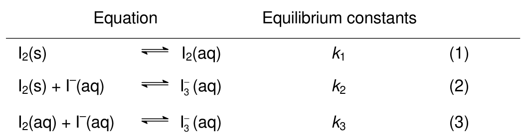
5.1 Give the equilibrium equations for (1) – (3).
Solutions of known potassium iodide concentration \([\ce{I^-}]_{\mathrm{tot}}\) were equilibrated with solid iodine. Subsequent titration with sodium thiosulphate solution served to determine the total solubility of iodine \([\ce{I2}]_{\mathrm{tot}}\).
The experiments yielded the following results:
| \([\ce{I^-}]_{\mathrm{tot}}\,/\,\mathrm{mmol\,dm^{-3}}\) | 10.00 | 20.00 | 30.00 | 40.00 | 50.00 |
|---|---|---|---|---|---|
| \([\ce{I^-}]_{\mathrm{tot}}\,/\,\mathrm{mmol\,dm^{-3}}\) | 5.85 | 10.53 | 15.11 | 19.96 | 24.82 |
5.2 Plot \([\ce{I2}]_{\mathrm{tot}}\) versus \([\ce{I^-}]_{\mathrm{tot}}\) in a diagram.
5.3 Derive a suitable algebraic expression relating \([\ce{I2}]_{\mathrm{tot}}\) and \([\ce{I^-}]_{\mathrm{tot}}\).
5.4 Use the graph to determine values of the equilibrium constants \(k_1\), \(k_2\), and \(k_3\).
Official English text of the problem.
Answers
-
5.1 Using concentration equilibrium constants, \[ \boxed{ k_1=[\ce{I2}],\qquad k_2=\frac{[\ce{I3^-}]}{[\ce{I^-}]},\qquad k_3=\frac{[\ce{I3^-}]}{[\ce{I2}][\ce{I^-}]} } \] and \(k_2=k_1k_3\).
-
5.2 The points lie approximately on a straight line, with \([\ce{I^-}]_{\mathrm{tot}}\) on the horizontal axis and \([\ce{I2}]_{\mathrm{tot}}\) on the vertical axis: \[ \boxed{ [\ce{I2}]_{\mathrm{tot}} \simeq 1.043\ \mathrm{mmol\,dm^{-3}} +0.4737[\ce{I^-}]_{\mathrm{tot}} }. \]
-
5.3 \[ \boxed{ [\ce{I2}]_{\mathrm{tot}} =k_1+\frac{k_2}{1+k_2}[\ce{I^-}]_{\mathrm{tot}} =k_1+\frac{k_1k_3}{1+k_1k_3}[\ce{I^-}]_{\mathrm{tot}} }. \]
-
5.4 From the fitted line, \[ \boxed{ k_1\approx1.04\times10^{-3}\ \mathrm{mol\,dm^{-3}},\qquad k_2\approx0.900,\qquad k_3\approx8.63\times10^2\ \mathrm{dm^3\,mol^{-1}} }. \] These are approximate graphical determinations.
Solution
The molecular and ionic species used below are:
| Species | Formula | SMILES |
|---|---|---|
| Iodine | \(\ce{I2}\) | II |
| Iodide ion | \(\ce{I^-}\) | [I-] |
| Triiodide ion | \(\ce{I3^-}\) | I[I-]I |
| Thiosulphate ion | \(\ce{S2O3^2-}\) | [O-]S(=O)(=O)[S-] |
| Tetrathionate ion | \(\ce{S4O6^2-}\) | [O-]S(=O)(=O)SSS(=O)(=O)[O-] |
Triiodide is linear. Its SMILES gives formal connectivity; it does not convey the three-centre, four-electron bonding or the distribution of charge.
5.1 — Equilibrium expressions
Use the concentration convention implied by the problem, treating the solutions as ideal. The activity of pure solid iodine is unity, so the solid does not appear in the equilibrium expressions. Unsubscripted concentrations below denote free aqueous species.
For reaction (1), \[ \ce{I2(s) <=> I2(aq)}, \] hence \[ \boxed{k_1=[\ce{I2}]}. \]
Thus the concentration of free molecular iodine remains constant while the solution is equilibrated with solid iodine.
For reaction (2), \[ \ce{I2(s) + I^-(aq) <=> I3^-(aq)}, \] hence \[ \boxed{k_2=\frac{[\ce{I3^-}]}{[\ce{I^-}]}}. \]
For reaction (3), \[ \ce{I2(aq) + I^-(aq) <=> I3^-(aq)}, \] hence \[ \boxed{k_3=\frac{[\ce{I3^-}]}{[\ce{I2}][\ce{I^-}]}}. \]
Adding reactions (1) and (3) gives reaction (2), so their constants satisfy \[ \boxed{k_2=k_1k_3}. \]
With concentrations in \(\mathrm{mol\,dm^{-3}}\), these concentration constants have units \(\mathrm{mol\,dm^{-3}}\), no units, and \(\mathrm{dm^3\,mol^{-1}}\), respectively.
5.2 — Description of the graph
Interpret the second row of numerical data as \([\ce{I2}]_{\mathrm{tot}}\), consistently with the experimental description.
Draw the horizontal axis as \([\ce{I^-}]_{\mathrm{tot}}\), from \(0\) to \(50\ \mathrm{mmol\,dm^{-3}}\), and the vertical axis as \([\ce{I2}]_{\mathrm{tot}}\), from \(0\) to about \(26\ \mathrm{mmol\,dm^{-3}}\). Plot the five points, with both coordinates in \(\mathrm{mmol\,dm^{-3}}\): \[ (10.00,5.85),\quad (20.00,10.53),\quad (30.00,15.11),\quad (40.00,19.96),\quad (50.00,24.82). \]
Draw a straight best-fit line through the group of points and extend it to the vertical axis.
For a numerical check, let \(x\) and \(y\) be the numerical concentrations in \(\mathrm{mmol\,dm^{-3}}\). Then \[ \bar{x}=30.00,\qquad \bar{y}=15.254, \] and the least-squares slope is \[ m=\frac{\sum_i(x_i-\bar{x})(y_i-\bar{y})} {\sum_i(x_i-\bar{x})^2} =\frac{473.7}{1000}=0.4737. \] The intercept is \[ b=\bar{y}-m\bar{x} =15.254-0.4737(30.00)=1.043. \]
Thus the line crosses the vertical axis at \(1.043\ \mathrm{mmol\,dm^{-3}}\) and passes through approximately \((50.00,24.73)\).
5.3 — Relation between the total concentrations
Each triiodide ion forms from one iodine molecule and one iodide ion. The analytical iodide balance is therefore \[ \boxed{ [\ce{I^-}]_{\mathrm{tot}} =[\ce{I^-}]+[\ce{I3^-}] }. \]
The iodine titration measures iodine equivalents. The balanced titration reactions are \[ \ce{I2 + 2S2O3^2- -> 2I^- + S4O6^2-} \] and \[ \ce{I3^- + 2S2O3^2- -> 3I^- + S4O6^2-}. \]
One mole of either iodine or triiodide consumes two moles of thiosulphate. Consequently, each mole of triiodide contributes one mole to the measured total iodine solubility: \[ \boxed{ [\ce{I2}]_{\mathrm{tot}} =[\ce{I2}]+[\ce{I3^-}] }. \]
From reaction (2), \[ [\ce{I3^-}]=k_2[\ce{I^-}]. \] Substitution into the iodide balance gives \[ [\ce{I^-}]_{\mathrm{tot}} =(1+k_2)[\ce{I^-}], \] so \[ [\ce{I3^-}] =\frac{k_2}{1+k_2}[\ce{I^-}]_{\mathrm{tot}}. \]
Since \([\ce{I2}]=k_1\), \[ \boxed{ [\ce{I2}]_{\mathrm{tot}} =k_1+\frac{k_2}{1+k_2}[\ce{I^-}]_{\mathrm{tot}} }. \]
Using \(k_2=k_1k_3\), the equivalent expression is \[ \boxed{ [\ce{I2}]_{\mathrm{tot}} =k_1+\frac{k_1k_3}{1+k_1k_3}[\ce{I^-}]_{\mathrm{tot}} }. \]
This explains the observed straight line: its intercept is \(k_1\), and its slope is \(k_2/(1+k_2)\).
5.4 — Determination of the equilibrium constants
The intercept gives \[ k_1=1.043\ \mathrm{mmol\,dm^{-3}} =1.043\times10^{-3}\ \mathrm{mol\,dm^{-3}}, \] or approximately \[ \boxed{k_1\approx1.04\times10^{-3}\ \mathrm{mol\,dm^{-3}}}. \]
From the slope, \[ m=\frac{k_2}{1+k_2} \quad\Longrightarrow\quad k_2=\frac{m}{1-m}. \] Therefore, \[ k_2=\frac{0.4737}{1-0.4737} =\frac{0.4737}{0.5263} =0.900057\ldots, \] giving \[ \boxed{k_2\approx0.900}. \]
Finally, \[ k_3=\frac{k_2}{k_1} =\frac{0.900057\ldots} {1.043\times10^{-3}\ \mathrm{mol\,dm^{-3}}}, \] so \[ \boxed{k_3\approx8.63\times10^2\ \mathrm{dm^3\,mol^{-1}}}. \]
The solution was checked against the official solution.
IChO 1982 · Theorieaufgabe 5
Löslichkeit von Iod in Kaliumiodidlösungen
Iod ist in reinem Wasser in gewissem Umfang löslich. In Lösungen, die Iodidionen enthalten, ist es jedoch besser löslich. Durch Untersuchung der Gesamtlöslichkeit von Iod in Abhängigkeit von der Iodidkonzentration lassen sich die Gleichgewichtskonstanten der folgenden Reaktionen bestimmen:
5.1 Geben Sie die Gleichgewichtsausdrücke für (1) – (3) an.
Lösungen bekannter Kaliumiodidkonzentration \([\ce{I^-}]_{\mathrm{tot}}\) wurden mit festem Iod ins Gleichgewicht gebracht. Eine anschließende Titration mit Natriumthiosulfatlösung diente zur Bestimmung der Gesamtlöslichkeit von Iod \([\ce{I2}]_{\mathrm{tot}}\).
Die Versuche ergaben die folgenden Ergebnisse:
| \([\ce{I^-}]_{\mathrm{tot}}\,/\,\mathrm{mmol\,dm^{-3}}\) | 10.00 | 20.00 | 30.00 | 40.00 | 50.00 |
|---|---|---|---|---|---|
| \([\ce{I^-}]_{\mathrm{tot}}\,/\,\mathrm{mmol\,dm^{-3}}\) | 5.85 | 10.53 | 15.11 | 19.96 | 24.82 |
5.2 Tragen Sie \([\ce{I2}]_{\mathrm{tot}}\) gegen \([\ce{I^-}]_{\mathrm{tot}}\) in einem Diagramm auf.
5.3 Leiten Sie einen geeigneten algebraischen Ausdruck her, der \([\ce{I2}]_{\mathrm{tot}}\) und \([\ce{I^-}]_{\mathrm{tot}}\) miteinander verknüpft.
5.4 Bestimmen Sie mithilfe des Diagramms die Werte der Gleichgewichtskonstanten \(k_1\), \(k_2\) und \(k_3\).
Aufgabentext aus dem offiziellen englischen Text übersetzt.
Antworten
-
5.1 Bei Verwendung konzentrationsbezogener Gleichgewichtskonstanten gilt \[ \boxed{ k_1=[\ce{I2}],\qquad k_2=\frac{[\ce{I3^-}]}{[\ce{I^-}]},\qquad k_3=\frac{[\ce{I3^-}]}{[\ce{I2}][\ce{I^-}]} } \] und \(k_2=k_1k_3\).
-
5.2 Die Punkte liegen näherungsweise auf einer Geraden, wobei \([\ce{I^-}]_{\mathrm{tot}}\) auf der horizontalen Achse und \([\ce{I2}]_{\mathrm{tot}}\) auf der vertikalen Achse aufgetragen wird: \[ \boxed{ [\ce{I2}]_{\mathrm{tot}} \simeq 1.043\ \mathrm{mmol\,dm^{-3}} +0.4737[\ce{I^-}]_{\mathrm{tot}} }. \]
-
5.3 \[ \boxed{ [\ce{I2}]_{\mathrm{tot}} =k_1+\frac{k_2}{1+k_2}[\ce{I^-}]_{\mathrm{tot}} =k_1+\frac{k_1k_3}{1+k_1k_3}[\ce{I^-}]_{\mathrm{tot}} }. \]
-
5.4 Aus der Ausgleichsgeraden erhält man \[ \boxed{ k_1\approx1.04\times10^{-3}\ \mathrm{mol\,dm^{-3}},\qquad k_2\approx0.900,\qquad k_3\approx8.63\times10^2\ \mathrm{dm^3\,mol^{-1}} }. \] Dies sind näherungsweise grafisch bestimmte Werte.
Lösung
Die im Folgenden verwendeten molekularen und ionischen Spezies sind:
| Spezies | Formel | SMILES |
|---|---|---|
| Iod | \(\ce{I2}\) | II |
| Iodidion | \(\ce{I^-}\) | [I-] |
| Triiodidion | \(\ce{I3^-}\) | I[I-]I |
| Thiosulfation | \(\ce{S2O3^2-}\) | [O-]S(=O)(=O)[S-] |
| Tetrathionation | \(\ce{S4O6^2-}\) | [O-]S(=O)(=O)SSS(=O)(=O)[O-] |
Triiodid ist linear. Seine SMILES-Schreibweise gibt die formale Verknüpfung der Atome wieder; sie beschreibt weder die Dreizentren-Vierelektronen-Bindung noch die Ladungsverteilung.
5.1 — Gleichgewichtsausdrücke
Es wird die in der Aufgabe vorausgesetzte Konzentrationskonvention verwendet, wobei die Lösungen als ideal betrachtet werden. Die Aktivität von reinem festem Iod ist eins, sodass der Feststoff in den Gleichgewichtsausdrücken nicht erscheint. Konzentrationen ohne Index bezeichnen im Folgenden freie Spezies in wässriger Lösung.
Für Reaktion (1) gilt \[ \ce{I2(s) <=> I2(aq)}, \] also \[ \boxed{k_1=[\ce{I2}]}. \]
Somit bleibt die Konzentration des freien molekularen Iods konstant, solange sich die Lösung mit festem Iod im Gleichgewicht befindet.
Für Reaktion (2) gilt \[ \ce{I2(s) + I^-(aq) <=> I3^-(aq)}, \] also \[ \boxed{k_2=\frac{[\ce{I3^-}]}{[\ce{I^-}]}}. \]
Für Reaktion (3) gilt \[ \ce{I2(aq) + I^-(aq) <=> I3^-(aq)}, \] also \[ \boxed{k_3=\frac{[\ce{I3^-}]}{[\ce{I2}][\ce{I^-}]}}. \]
Durch Addition der Reaktionen (1) und (3) erhält man Reaktion (2), sodass für ihre Konstanten gilt: \[ \boxed{k_2=k_1k_3}. \]
Werden die Konzentrationen in \(\mathrm{mol\,dm^{-3}}\) angegeben, so haben diese Konzentrationskonstanten der Reihe nach die Einheit \(\mathrm{mol\,dm^{-3}}\), keine Einheit beziehungsweise die Einheit \(\mathrm{dm^3\,mol^{-1}}\).
5.2 — Beschreibung des Diagramms
Die zweite Zeile der Zahlenwerte ist entsprechend der Versuchsbeschreibung als \([\ce{I2}]_{\mathrm{tot}}\) zu interpretieren.
Zeichnen Sie die horizontale Achse für \([\ce{I^-}]_{\mathrm{tot}}\) von \(0\) bis \(50\ \mathrm{mmol\,dm^{-3}}\) und die vertikale Achse für \([\ce{I2}]_{\mathrm{tot}}\) von \(0\) bis etwa \(26\ \mathrm{mmol\,dm^{-3}}\). Tragen Sie die fünf Punkte ein, wobei beide Koordinaten in \(\mathrm{mmol\,dm^{-3}}\) angegeben sind: \[ (10.00,5.85),\quad (20.00,10.53),\quad (30.00,15.11),\quad (40.00,19.96),\quad (50.00,24.82). \]
Zeichnen Sie eine Ausgleichsgerade durch die Punktgruppe und verlängern Sie sie bis zur vertikalen Achse.
Zur numerischen Überprüfung seien \(x\) und \(y\) die Zahlenwerte der Konzentrationen in \(\mathrm{mmol\,dm^{-3}}\). Dann gilt \[ \bar{x}=30.00,\qquad \bar{y}=15.254, \] und die nach der Methode der kleinsten Quadrate bestimmte Steigung beträgt \[ m=\frac{\sum_i(x_i-\bar{x})(y_i-\bar{y})} {\sum_i(x_i-\bar{x})^2} =\frac{473.7}{1000}=0.4737. \] Der Achsenabschnitt beträgt \[ b=\bar{y}-m\bar{x} =15.254-0.4737(30.00)=1.043. \]
Die Gerade schneidet die vertikale Achse somit bei \(1.043\ \mathrm{mmol\,dm^{-3}}\) und verläuft näherungsweise durch \((50.00,24.73)\).
5.3 — Zusammenhang zwischen den Gesamtkonzentrationen
Jedes Triiodidion entsteht aus einem Iodmolekül und einem Iodidion. Die analytische Iodidbilanz lautet daher \[ \boxed{ [\ce{I^-}]_{\mathrm{tot}} =[\ce{I^-}]+[\ce{I3^-}] }. \]
Die Iodtitration erfasst Iodäquivalente. Die ausgeglichenen Titrationsreaktionen lauten \[ \ce{I2 + 2S2O3^2- -> 2I^- + S4O6^2-} \] und \[ \ce{I3^- + 2S2O3^2- -> 3I^- + S4O6^2-}. \]
Ein Mol Iod oder Triiodid verbraucht jeweils zwei Mol Thiosulfat. Folglich trägt jedes Mol Triiodid ein Mol zur gemessenen Gesamtlöslichkeit von Iod bei: \[ \boxed{ [\ce{I2}]_{\mathrm{tot}} =[\ce{I2}]+[\ce{I3^-}] }. \]
Aus Reaktion (2) folgt \[ [\ce{I3^-}]=k_2[\ce{I^-}]. \] Einsetzen in die Iodidbilanz ergibt \[ [\ce{I^-}]_{\mathrm{tot}} =(1+k_2)[\ce{I^-}], \] also \[ [\ce{I3^-}] =\frac{k_2}{1+k_2}[\ce{I^-}]_{\mathrm{tot}}. \]
Da \([\ce{I2}]=k_1\), gilt \[ \boxed{ [\ce{I2}]_{\mathrm{tot}} =k_1+\frac{k_2}{1+k_2}[\ce{I^-}]_{\mathrm{tot}} }. \]
Mit \(k_2=k_1k_3\) erhält man den äquivalenten Ausdruck \[ \boxed{ [\ce{I2}]_{\mathrm{tot}} =k_1+\frac{k_1k_3}{1+k_1k_3}[\ce{I^-}]_{\mathrm{tot}} }. \]
Dies erklärt den beobachteten geradlinigen Verlauf: Der Achsenabschnitt ist \(k_1\), und die Steigung ist \(k_2/(1+k_2)\).
5.4 — Bestimmung der Gleichgewichtskonstanten
Aus dem Achsenabschnitt ergibt sich \[ k_1=1.043\ \mathrm{mmol\,dm^{-3}} =1.043\times10^{-3}\ \mathrm{mol\,dm^{-3}}, \] oder näherungsweise \[ \boxed{k_1\approx1.04\times10^{-3}\ \mathrm{mol\,dm^{-3}}}. \]
Aus der Steigung folgt \[ m=\frac{k_2}{1+k_2} \quad\Longrightarrow\quad k_2=\frac{m}{1-m}. \] Daher gilt \[ k_2=\frac{0.4737}{1-0.4737} =\frac{0.4737}{0.5263} =0.900057\ldots, \] woraus sich ergibt: \[ \boxed{k_2\approx0.900}. \]
Schließlich gilt \[ k_3=\frac{k_2}{k_1} =\frac{0.900057\ldots} {1.043\times10^{-3}\ \mathrm{mol\,dm^{-3}}}, \] also \[ \boxed{k_3\approx8.63\times10^2\ \mathrm{dm^3\,mol^{-1}}}. \]
Die Lösung wurde mit der offiziellen Lösung abgeglichen.
IChO 1982 · Teori sorusu 5
İyodun potasyum iyodür çözeltilerindeki çözünürlüğü
İyot, saf suda belirli bir ölçüde çözünür. Ancak iyodür iyonları içeren çözeltilerde daha fazla çözünür. İyodun toplam çözünürlüğünün iyodür derişimine bağlı olarak incelenmesiyle aşağıdaki tepkimelerin denge sabitleri belirlenebilir:
5.1 (1) – (3) için denge bağıntılarını yazınız.
Potasyum iyodür derişimi \([\ce{I^-}]_{\mathrm{tot}}\) bilinen çözeltiler, katı iyot ile dengeye getirildi. Ardından sodyum tiyosülfat çözeltisiyle yapılan titrasyonla iyodun toplam çözünürlüğü \([\ce{I2}]_{\mathrm{tot}}\) belirlendi.
Deneylerde aşağıdaki sonuçlar elde edildi:
| \([\ce{I^-}]_{\mathrm{tot}}\,/\,\mathrm{mmol\,dm^{-3}}\) | 10.00 | 20.00 | 30.00 | 40.00 | 50.00 |
|---|---|---|---|---|---|
| \([\ce{I^-}]_{\mathrm{tot}}\,/\,\mathrm{mmol\,dm^{-3}}\) | 5.85 | 10.53 | 15.11 | 19.96 | 24.82 |
5.2 \([\ce{I2}]_{\mathrm{tot}}\)'un \([\ce{I^-}]_{\mathrm{tot}}\)'a karşı grafiğini çiziniz.
5.3 \([\ce{I2}]_{\mathrm{tot}}\) ile \([\ce{I^-}]_{\mathrm{tot}}\) arasındaki ilişkiyi veren uygun bir cebirsel ifade türetiniz.
5.4 Grafiği kullanarak \(k_1\), \(k_2\) ve \(k_3\) denge sabitlerinin değerlerini belirleyiniz.
Soru metni resmi İngilizce metinden çevrilmiştir.
Cevaplar
-
5.1 Derişim cinsinden denge sabitleri kullanıldığında, \[ \boxed{ k_1=[\ce{I2}],\qquad k_2=\frac{[\ce{I3^-}]}{[\ce{I^-}]},\qquad k_3=\frac{[\ce{I3^-}]}{[\ce{I2}][\ce{I^-}]} } \] ve \(k_2=k_1k_3\) olur.
-
5.2 Yatay eksende \([\ce{I^-}]_{\mathrm{tot}}\), düşey eksende \([\ce{I2}]_{\mathrm{tot}}\) olmak üzere noktalar yaklaşık olarak bir doğru üzerinde yer alır: \[ \boxed{ [\ce{I2}]_{\mathrm{tot}} \simeq 1.043\ \mathrm{mmol\,dm^{-3}} +0.4737[\ce{I^-}]_{\mathrm{tot}} }. \]
-
5.3 \[ \boxed{ [\ce{I2}]_{\mathrm{tot}} =k_1+\frac{k_2}{1+k_2}[\ce{I^-}]_{\mathrm{tot}} =k_1+\frac{k_1k_3}{1+k_1k_3}[\ce{I^-}]_{\mathrm{tot}} }. \]
-
5.4 Verilere uydurulan doğrudan, \[ \boxed{ k_1\approx1.04\times10^{-3}\ \mathrm{mol\,dm^{-3}},\qquad k_2\approx0.900,\qquad k_3\approx8.63\times10^2\ \mathrm{dm^3\,mol^{-1}} }. \] Bunlar grafik yoluyla belirlenen yaklaşık değerlerdir.
Çözüm
Aşağıda kullanılan moleküler ve iyonik türler şunlardır:
| Tür | Formül | SMILES |
|---|---|---|
| İyot | \(\ce{I2}\) | II |
| İyodür iyonu | \(\ce{I^-}\) | [I-] |
| Triiyodür iyonu | \(\ce{I3^-}\) | I[I-]I |
| Tiyosülfat iyonu | \(\ce{S2O3^2-}\) | [O-]S(=O)(=O)[S-] |
| Tetratiyonat iyonu | \(\ce{S4O6^2-}\) | [O-]S(=O)(=O)SSS(=O)(=O)[O-] |
Triiyodür doğrusaldır. SMILES gösterimi biçimsel bağlanma düzenini verir; üç merkezli, dört elektronlu bağlanmayı veya yük dağılımını yansıtmaz.
5.1 — Denge bağıntıları
Çözeltileri ideal kabul ederek soruda esas alınan derişim yaklaşımını kullanınız. Saf katı iyodun aktivitesi birdir; bu nedenle katı, denge bağıntılarında yer almaz. Aşağıda alt indis taşımayan derişimler, sulu çözeltideki serbest türleri belirtir.
(1) tepkimesi için, \[ \ce{I2(s) <=> I2(aq)}, \] dolayısıyla \[ \boxed{k_1=[\ce{I2}]}. \]
Böylece çözelti katı iyot ile dengede olduğu sürece serbest moleküler iyodun derişimi sabit kalır.
(2) tepkimesi için, \[ \ce{I2(s) + I^-(aq) <=> I3^-(aq)}, \] dolayısıyla \[ \boxed{k_2=\frac{[\ce{I3^-}]}{[\ce{I^-}]}}. \]
(3) tepkimesi için, \[ \ce{I2(aq) + I^-(aq) <=> I3^-(aq)}, \] dolayısıyla \[ \boxed{k_3=\frac{[\ce{I3^-}]}{[\ce{I2}][\ce{I^-}]}}. \]
(1) ve (3) tepkimeleri toplandığında (2) tepkimesi elde edilir; dolayısıyla denge sabitleri şu bağıntıyı sağlar: \[ \boxed{k_2=k_1k_3}. \]
Derişimler \(\mathrm{mol\,dm^{-3}}\) cinsinden verildiğinde, derişim cinsinden tanımlanan bu sabitlerin birimleri sırasıyla \(\mathrm{mol\,dm^{-3}}\), birimsiz ve \(\mathrm{dm^3\,mol^{-1}}\) olur.
5.2 — Grafiğin açıklaması
Sayısal verilerin ikinci satırını, deneyin açıklamasıyla tutarlı olacak şekilde \([\ce{I2}]_{\mathrm{tot}}\) olarak yorumlayınız.
Yatay ekseni \([\ce{I^-}]_{\mathrm{tot}}\) olarak \(0\) ile \(50\ \mathrm{mmol\,dm^{-3}}\) arasında, düşey ekseni ise \([\ce{I2}]_{\mathrm{tot}}\) olarak \(0\) ile yaklaşık \(26\ \mathrm{mmol\,dm^{-3}}\) arasında çiziniz. Her iki koordinat da \(\mathrm{mmol\,dm^{-3}}\) cinsinden olmak üzere beş noktayı işaretleyiniz: \[ (10.00,5.85),\quad (20.00,10.53),\quad (30.00,15.11),\quad (40.00,19.96),\quad (50.00,24.82). \]
Nokta grubundan geçen en iyi uyum doğrusunu çiziniz ve düşey eksene kadar uzatınız.
Sayısal bir kontrol için \(x\) ve \(y\), derişimlerin \(\mathrm{mmol\,dm^{-3}}\) cinsinden sayısal değerleri olsun. Bu durumda \[ \bar{x}=30.00,\qquad \bar{y}=15.254, \] ve en küçük kareler yöntemiyle bulunan eğim \[ m=\frac{\sum_i(x_i-\bar{x})(y_i-\bar{y})} {\sum_i(x_i-\bar{x})^2} =\frac{473.7}{1000}=0.4737. \] Doğrunun düşey ekseni kestiği değer \[ b=\bar{y}-m\bar{x} =15.254-0.4737(30.00)=1.043. \]
Böylece doğru, düşey ekseni \(1.043\ \mathrm{mmol\,dm^{-3}}\) değerinde keser ve yaklaşık olarak \((50.00,24.73)\) noktasından geçer.
5.3 — Toplam derişimler arasındaki ilişki
Her triiyodür iyonu, bir iyot molekülü ile bir iyodür iyonundan oluşur. Bu nedenle analitik iyodür madde denkliği şöyledir: \[ \boxed{ [\ce{I^-}]_{\mathrm{tot}} =[\ce{I^-}]+[\ce{I3^-}] }. \]
İyot titrasyonu, iyot eşdeğerlerini ölçer. Denkleştirilmiş titrasyon tepkimeleri şunlardır: \[ \ce{I2 + 2S2O3^2- -> 2I^- + S4O6^2-} \] ve \[ \ce{I3^- + 2S2O3^2- -> 3I^- + S4O6^2-}. \]
Bir mol iyot da bir mol triiyodür de iki mol tiyosülfat tüketir. Dolayısıyla her bir mol triiyodür, ölçülen toplam iyot çözünürlüğüne bir mol katkıda bulunur: \[ \boxed{ [\ce{I2}]_{\mathrm{tot}} =[\ce{I2}]+[\ce{I3^-}] }. \]
(2) tepkimesinden, \[ [\ce{I3^-}]=k_2[\ce{I^-}]. \] Bu ifade iyodür madde denkliğinde yerine konulduğunda \[ [\ce{I^-}]_{\mathrm{tot}} =(1+k_2)[\ce{I^-}], \] dolayısıyla \[ [\ce{I3^-}] =\frac{k_2}{1+k_2}[\ce{I^-}]_{\mathrm{tot}}. \]
\([\ce{I2}]=k_1\) olduğundan, \[ \boxed{ [\ce{I2}]_{\mathrm{tot}} =k_1+\frac{k_2}{1+k_2}[\ce{I^-}]_{\mathrm{tot}} }. \]
\(k_2=k_1k_3\) kullanıldığında eşdeğer ifade şöyledir: \[ \boxed{ [\ce{I2}]_{\mathrm{tot}} =k_1+\frac{k_1k_3}{1+k_1k_3}[\ce{I^-}]_{\mathrm{tot}} }. \]
Bu, gözlenen doğrusal ilişkiyi açıklar: doğrunun düşey ekseni kestiği değer \(k_1\), eğimi ise \(k_2/(1+k_2)\)'dir.
5.4 — Denge sabitlerinin belirlenmesi
Doğrunun düşey ekseni kestiği değerden \[ k_1=1.043\ \mathrm{mmol\,dm^{-3}} =1.043\times10^{-3}\ \mathrm{mol\,dm^{-3}}, \] veya yaklaşık olarak \[ \boxed{k_1\approx1.04\times10^{-3}\ \mathrm{mol\,dm^{-3}}}. \]
Eğimden, \[ m=\frac{k_2}{1+k_2} \quad\Longrightarrow\quad k_2=\frac{m}{1-m}. \] Dolayısıyla, \[ k_2=\frac{0.4737}{1-0.4737} =\frac{0.4737}{0.5263} =0.900057\ldots, \] buradan \[ \boxed{k_2\approx0.900}. \]
Son olarak, \[ k_3=\frac{k_2}{k_1} =\frac{0.900057\ldots} {1.043\times10^{-3}\ \mathrm{mol\,dm^{-3}}}, \] dolayısıyla \[ \boxed{k_3\approx8.63\times10^2\ \mathrm{dm^3\,mol^{-1}}}. \]
Çözüm, resmi çözümle karşılaştırılarak kontrol edildi.
IChO 1982 · Problema teórico 5
Solubilidad del yodo en disoluciones de yoduro de potasio
El yodo es soluble hasta cierto punto en agua pura. Sin embargo, es más soluble en disoluciones que contienen iones yoduro. Al estudiar la solubilidad total del yodo en función de la concentración de yoduro, pueden determinarse las constantes de equilibrio de las siguientes reacciones:
5.1 Escriba las expresiones de equilibrio de (1) – (3).
Se equilibraron disoluciones de concentración conocida de yoduro de potasio \([\ce{I^-}]_{\mathrm{tot}}\) con yodo sólido. La posterior valoración con una disolución de tiosulfato de sodio permitió determinar la solubilidad total del yodo \([\ce{I2}]_{\mathrm{tot}}\).
Los experimentos dieron los siguientes resultados:
| \([\ce{I^-}]_{\mathrm{tot}}\,/\,\mathrm{mmol\,dm^{-3}}\) | 10.00 | 20.00 | 30.00 | 40.00 | 50.00 |
|---|---|---|---|---|---|
| \([\ce{I^-}]_{\mathrm{tot}}\,/\,\mathrm{mmol\,dm^{-3}}\) | 5.85 | 10.53 | 15.11 | 19.96 | 24.82 |
5.2 Represente gráficamente \([\ce{I2}]_{\mathrm{tot}}\) frente a \([\ce{I^-}]_{\mathrm{tot}}\).
5.3 Deduzca una expresión algebraica adecuada que relacione \([\ce{I2}]_{\mathrm{tot}}\) y \([\ce{I^-}]_{\mathrm{tot}}\).
5.4 Utilice la gráfica para determinar los valores de las constantes de equilibrio \(k_1\), \(k_2\) y \(k_3\).
Enunciado traducido del texto oficial en inglés.
Respuestas
-
5.1 Utilizando constantes de equilibrio expresadas en concentraciones, \[ \boxed{ k_1=[\ce{I2}],\qquad k_2=\frac{[\ce{I3^-}]}{[\ce{I^-}]},\qquad k_3=\frac{[\ce{I3^-}]}{[\ce{I2}][\ce{I^-}]} } \] y \(k_2=k_1k_3\).
-
5.2 Los puntos se sitúan aproximadamente sobre una recta, con \([\ce{I^-}]_{\mathrm{tot}}\) en el eje horizontal y \([\ce{I2}]_{\mathrm{tot}}\) en el eje vertical: \[ \boxed{ [\ce{I2}]_{\mathrm{tot}} \simeq 1.043\ \mathrm{mmol\,dm^{-3}} +0.4737[\ce{I^-}]_{\mathrm{tot}} }. \]
-
5.3 \[ \boxed{ [\ce{I2}]_{\mathrm{tot}} =k_1+\frac{k_2}{1+k_2}[\ce{I^-}]_{\mathrm{tot}} =k_1+\frac{k_1k_3}{1+k_1k_3}[\ce{I^-}]_{\mathrm{tot}} }. \]
-
5.4 A partir de la recta ajustada, \[ \boxed{ k_1\approx1.04\times10^{-3}\ \mathrm{mol\,dm^{-3}},\qquad k_2\approx0.900,\qquad k_3\approx8.63\times10^2\ \mathrm{dm^3\,mol^{-1}} }. \] Estas son determinaciones gráficas aproximadas.
Solución
Las especies moleculares e iónicas utilizadas a continuación son:
| Especie | Fórmula | SMILES |
|---|---|---|
| Yodo | \(\ce{I2}\) | II |
| Ion yoduro | \(\ce{I^-}\) | [I-] |
| Ion triyoduro | \(\ce{I3^-}\) | I[I-]I |
| Ion tiosulfato | \(\ce{S2O3^2-}\) | [O-]S(=O)(=O)[S-] |
| Ion tetrationato | \(\ce{S4O6^2-}\) | [O-]S(=O)(=O)SSS(=O)(=O)[O-] |
El triyoduro es lineal. Su SMILES indica la conectividad formal; no representa el enlace de tres centros y cuatro electrones ni la distribución de la carga.
5.1 — Expresiones de equilibrio
Utilice la convención de concentraciones implícita en el problema, considerando ideales las disoluciones. La actividad del yodo sólido puro es la unidad, por lo que el sólido no aparece en las expresiones de equilibrio. Las concentraciones sin subíndice que aparecen a continuación corresponden a las especies acuosas libres.
Para la reacción (1), \[ \ce{I2(s) <=> I2(aq)}, \] por tanto, \[ \boxed{k_1=[\ce{I2}]}. \]
Así, la concentración de yodo molecular libre permanece constante mientras la disolución está en equilibrio con yodo sólido.
Para la reacción (2), \[ \ce{I2(s) + I^-(aq) <=> I3^-(aq)}, \] por tanto, \[ \boxed{k_2=\frac{[\ce{I3^-}]}{[\ce{I^-}]}}. \]
Para la reacción (3), \[ \ce{I2(aq) + I^-(aq) <=> I3^-(aq)}, \] por tanto, \[ \boxed{k_3=\frac{[\ce{I3^-}]}{[\ce{I2}][\ce{I^-}]}}. \]
Al sumar las reacciones (1) y (3) se obtiene la reacción (2), por lo que sus constantes satisfacen \[ \boxed{k_2=k_1k_3}. \]
Con las concentraciones en \(\mathrm{mol\,dm^{-3}}\), estas constantes expresadas en concentraciones tienen unidades de \(\mathrm{mol\,dm^{-3}}\), carecen de unidades y tienen unidades de \(\mathrm{dm^3\,mol^{-1}}\), respectivamente.
5.2 — Descripción de la gráfica
Interprete la segunda fila de datos numéricos como \([\ce{I2}]_{\mathrm{tot}}\), de acuerdo con la descripción experimental.
Trace el eje horizontal para \([\ce{I^-}]_{\mathrm{tot}}\), desde \(0\) hasta \(50\ \mathrm{mmol\,dm^{-3}}\), y el eje vertical para \([\ce{I2}]_{\mathrm{tot}}\), desde \(0\) hasta aproximadamente \(26\ \mathrm{mmol\,dm^{-3}}\). Represente los cinco puntos, con ambas coordenadas en \(\mathrm{mmol\,dm^{-3}}\): \[ (10.00,5.85),\quad (20.00,10.53),\quad (30.00,15.11),\quad (40.00,19.96),\quad (50.00,24.82). \]
Trace la recta que mejor se ajuste al conjunto de puntos y prolónguela hasta el eje vertical.
Para realizar una comprobación numérica, sean \(x\) e \(y\) los valores numéricos de las concentraciones en \(\mathrm{mmol\,dm^{-3}}\). Entonces, \[ \bar{x}=30.00,\qquad \bar{y}=15.254, \] y la pendiente obtenida por mínimos cuadrados es \[ m=\frac{\sum_i(x_i-\bar{x})(y_i-\bar{y})} {\sum_i(x_i-\bar{x})^2} =\frac{473.7}{1000}=0.4737. \] La ordenada en el origen es \[ b=\bar{y}-m\bar{x} =15.254-0.4737(30.00)=1.043. \]
Por tanto, la recta corta el eje vertical en \(1.043\ \mathrm{mmol\,dm^{-3}}\) y pasa aproximadamente por \((50.00,24.73)\).
5.3 — Relación entre las concentraciones totales
Cada ion triyoduro se forma a partir de una molécula de yodo y un ion yoduro. Por tanto, el balance analítico de yoduro es \[ \boxed{ [\ce{I^-}]_{\mathrm{tot}} =[\ce{I^-}]+[\ce{I3^-}] }. \]
La valoración del yodo mide equivalentes de yodo. Las reacciones ajustadas de valoración son \[ \ce{I2 + 2S2O3^2- -> 2I^- + S4O6^2-} \] y \[ \ce{I3^- + 2S2O3^2- -> 3I^- + S4O6^2-}. \]
Un mol de yodo o de triyoduro consume dos moles de tiosulfato. En consecuencia, cada mol de triyoduro aporta un mol a la solubilidad total del yodo medida: \[ \boxed{ [\ce{I2}]_{\mathrm{tot}} =[\ce{I2}]+[\ce{I3^-}] }. \]
A partir de la reacción (2), \[ [\ce{I3^-}]=k_2[\ce{I^-}]. \] Al sustituir en el balance de yoduro se obtiene \[ [\ce{I^-}]_{\mathrm{tot}} =(1+k_2)[\ce{I^-}], \] por lo que \[ [\ce{I3^-}] =\frac{k_2}{1+k_2}[\ce{I^-}]_{\mathrm{tot}}. \]
Dado que \([\ce{I2}]=k_1\), \[ \boxed{ [\ce{I2}]_{\mathrm{tot}} =k_1+\frac{k_2}{1+k_2}[\ce{I^-}]_{\mathrm{tot}} }. \]
Utilizando \(k_2=k_1k_3\), la expresión equivalente es \[ \boxed{ [\ce{I2}]_{\mathrm{tot}} =k_1+\frac{k_1k_3}{1+k_1k_3}[\ce{I^-}]_{\mathrm{tot}} }. \]
Esto explica la recta observada: su ordenada en el origen es \(k_1\) y su pendiente es \(k_2/(1+k_2)\).
5.4 — Determinación de las constantes de equilibrio
La ordenada en el origen da \[ k_1=1.043\ \mathrm{mmol\,dm^{-3}} =1.043\times10^{-3}\ \mathrm{mol\,dm^{-3}}, \] o, aproximadamente, \[ \boxed{k_1\approx1.04\times10^{-3}\ \mathrm{mol\,dm^{-3}}}. \]
A partir de la pendiente, \[ m=\frac{k_2}{1+k_2} \quad\Longrightarrow\quad k_2=\frac{m}{1-m}. \] Por tanto, \[ k_2=\frac{0.4737}{1-0.4737} =\frac{0.4737}{0.5263} =0.900057\ldots, \] lo que da \[ \boxed{k_2\approx0.900}. \]
Finalmente, \[ k_3=\frac{k_2}{k_1} =\frac{0.900057\ldots} {1.043\times10^{-3}\ \mathrm{mol\,dm^{-3}}}, \] por lo que \[ \boxed{k_3\approx8.63\times10^2\ \mathrm{dm^3\,mol^{-1}}}. \]
La solución se comprobó con la solución oficial.
IChO 1982 · 理论题 5
碘在碘化钾溶液中的溶解度
碘在纯水中有一定的溶解度。然而,在含有碘离子的溶液中,碘的溶解度更大。通过研究碘的总溶解度随碘离子浓度的变化关系,可以确定下列反应的平衡常数:
5.1 写出反应 (1) – (3) 的平衡关系式。
将已知碘化钾浓度 \([\ce{I^-}]_{\mathrm{tot}}\) 的溶液与固体碘达到平衡。随后用硫代硫酸钠溶液滴定,以测定碘的总溶解度 \([\ce{I2}]_{\mathrm{tot}}\)。
实验得到以下结果:
| \([\ce{I^-}]_{\mathrm{tot}}\,/\,\mathrm{mmol\,dm^{-3}}\) | 10.00 | 20.00 | 30.00 | 40.00 | 50.00 |
|---|---|---|---|---|---|
| \([\ce{I^-}]_{\mathrm{tot}}\,/\,\mathrm{mmol\,dm^{-3}}\) | 5.85 | 10.53 | 15.11 | 19.96 | 24.82 |
5.2 绘制 \([\ce{I2}]_{\mathrm{tot}}\) 随 \([\ce{I^-}]_{\mathrm{tot}}\) 变化的图像。
5.3 推导一个适当的代数表达式,将 \([\ce{I2}]_{\mathrm{tot}}\) 与 \([\ce{I^-}]_{\mathrm{tot}}\) 联系起来。
5.4 利用图像确定平衡常数 \(k_1\)、\(k_2\) 和 \(k_3\) 的值。
题目译自官方英文原文。
答案
-
5.1 采用浓度平衡常数, \[ \boxed{ k_1=[\ce{I2}],\qquad k_2=\frac{[\ce{I3^-}]}{[\ce{I^-}]},\qquad k_3=\frac{[\ce{I3^-}]}{[\ce{I2}][\ce{I^-}]} } \] 且 \(k_2=k_1k_3\)。
-
5.2 各点近似位于一条直线上,横轴为 \([\ce{I^-}]_{\mathrm{tot}}\),纵轴为 \([\ce{I2}]_{\mathrm{tot}}\): \[ \boxed{ [\ce{I2}]_{\mathrm{tot}} \simeq 1.043\ \mathrm{mmol\,dm^{-3}} +0.4737[\ce{I^-}]_{\mathrm{tot}} }. \]
-
5.3 \[ \boxed{ [\ce{I2}]_{\mathrm{tot}} =k_1+\frac{k_2}{1+k_2}[\ce{I^-}]_{\mathrm{tot}} =k_1+\frac{k_1k_3}{1+k_1k_3}[\ce{I^-}]_{\mathrm{tot}} }. \]
-
5.4 由拟合直线得, \[ \boxed{ k_1\approx1.04\times10^{-3}\ \mathrm{mol\,dm^{-3}},\qquad k_2\approx0.900,\qquad k_3\approx8.63\times10^2\ \mathrm{dm^3\,mol^{-1}} }. \] 这些数值是通过作图法确定的近似值。
解答
下文使用的分子和离子如下:
| 物种 | 化学式 | SMILES |
|---|---|---|
| 碘 | \(\ce{I2}\) | II |
| 碘离子 | \(\ce{I^-}\) | [I-] |
| 三碘离子 | \(\ce{I3^-}\) | I[I-]I |
| 硫代硫酸根离子 | \(\ce{S2O3^2-}\) | [O-]S(=O)(=O)[S-] |
| 连四硫酸根离子 | \(\ce{S4O6^2-}\) | [O-]S(=O)(=O)SSS(=O)(=O)[O-] |
三碘离子呈直线形。其 SMILES 表示形式上的连接关系,并不体现三中心四电子键或电荷分布。
5.1 — 平衡常数表达式
采用题目隐含的浓度约定,将溶液视为理想溶液。纯固体碘的活度为一,因此固体不出现在平衡常数表达式中。下文未加下标的浓度表示水溶液中游离物种的浓度。
对于反应 (1), \[ \ce{I2(s) <=> I2(aq)}, \] 因此 \[ \boxed{k_1=[\ce{I2}]}. \]
因此,当溶液与固体碘处于平衡时,游离碘分子的浓度保持恒定。
对于反应 (2), \[ \ce{I2(s) + I^-(aq) <=> I3^-(aq)}, \] 因此 \[ \boxed{k_2=\frac{[\ce{I3^-}]}{[\ce{I^-}]}}. \]
对于反应 (3), \[ \ce{I2(aq) + I^-(aq) <=> I3^-(aq)}, \] 因此 \[ \boxed{k_3=\frac{[\ce{I3^-}]}{[\ce{I2}][\ce{I^-}]}}. \]
将反应 (1) 与反应 (3) 相加得到反应 (2),因此它们的平衡常数满足 \[ \boxed{k_2=k_1k_3}. \]
当浓度以 \(\mathrm{mol\,dm^{-3}}\) 为单位时,这些浓度平衡常数的单位依次为 \(\mathrm{mol\,dm^{-3}}\)、无单位和 \(\mathrm{dm^3\,mol^{-1}}\)。
5.2 — 图像说明
根据实验描述,将第二行数值数据理解为 \([\ce{I2}]_{\mathrm{tot}}\)。
以 \([\ce{I^-}]_{\mathrm{tot}}\) 为横轴,范围从 \(0\) 到 \(50\ \mathrm{mmol\,dm^{-3}}\);以 \([\ce{I2}]_{\mathrm{tot}}\) 为纵轴,范围从 \(0\) 到约 \(26\ \mathrm{mmol\,dm^{-3}}\)。描出以下五个点,横、纵坐标的单位均为 \(\mathrm{mmol\,dm^{-3}}\): \[ (10.00,5.85),\quad (20.00,10.53),\quad (30.00,15.11),\quad (40.00,19.96),\quad (50.00,24.82). \]
画出穿过这组点的最佳拟合直线,并将其延长至纵轴。
为进行数值核验,令 \(x\) 和 \(y\) 表示以 \(\mathrm{mmol\,dm^{-3}}\) 为单位的浓度数值。则 \[ \bar{x}=30.00,\qquad \bar{y}=15.254, \] 最小二乘拟合的斜率为 \[ m=\frac{\sum_i(x_i-\bar{x})(y_i-\bar{y})} {\sum_i(x_i-\bar{x})^2} =\frac{473.7}{1000}=0.4737. \] 截距为 \[ b=\bar{y}-m\bar{x} =15.254-0.4737(30.00)=1.043. \]
因此,该直线在 \(1.043\ \mathrm{mmol\,dm^{-3}}\) 处与纵轴相交,并近似通过点 \((50.00,24.73)\)。
5.3 — 总浓度之间的关系
每个三碘离子由一个碘分子和一个碘离子形成。因此,碘离子的分析浓度满足以下物料衡算关系: \[ \boxed{ [\ce{I^-}]_{\mathrm{tot}} =[\ce{I^-}]+[\ce{I3^-}] }. \]
碘的滴定测定的是折合为碘分子的量。配平后的滴定反应为 \[ \ce{I2 + 2S2O3^2- -> 2I^- + S4O6^2-} \] 以及 \[ \ce{I3^- + 2S2O3^2- -> 3I^- + S4O6^2-}. \]
一摩尔碘分子或三碘离子均消耗两摩尔硫代硫酸根离子。因此,在测得的碘总溶解度中,每摩尔三碘离子计作一摩尔碘: \[ \boxed{ [\ce{I2}]_{\mathrm{tot}} =[\ce{I2}]+[\ce{I3^-}] }. \]
由反应 (2), \[ [\ce{I3^-}]=k_2[\ce{I^-}]. \] 代入碘离子的物料衡算式得 \[ [\ce{I^-}]_{\mathrm{tot}} =(1+k_2)[\ce{I^-}], \] 因此 \[ [\ce{I3^-}] =\frac{k_2}{1+k_2}[\ce{I^-}]_{\mathrm{tot}}. \]
由于 \([\ce{I2}]=k_1\), \[ \boxed{ [\ce{I2}]_{\mathrm{tot}} =k_1+\frac{k_2}{1+k_2}[\ce{I^-}]_{\mathrm{tot}} }. \]
利用 \(k_2=k_1k_3\),可得等价表达式 \[ \boxed{ [\ce{I2}]_{\mathrm{tot}} =k_1+\frac{k_1k_3}{1+k_1k_3}[\ce{I^-}]_{\mathrm{tot}} }. \]
这解释了实验观察到的直线关系:其截距为 \(k_1\),斜率为 \(k_2/(1+k_2)\)。
5.4 — 平衡常数的确定
由截距得 \[ k_1=1.043\ \mathrm{mmol\,dm^{-3}} =1.043\times10^{-3}\ \mathrm{mol\,dm^{-3}}, \] 其近似值为 \[ \boxed{k_1\approx1.04\times10^{-3}\ \mathrm{mol\,dm^{-3}}}. \]
由斜率得, \[ m=\frac{k_2}{1+k_2} \quad\Longrightarrow\quad k_2=\frac{m}{1-m}. \] 因此, \[ k_2=\frac{0.4737}{1-0.4737} =\frac{0.4737}{0.5263} =0.900057\ldots, \] 得到 \[ \boxed{k_2\approx0.900}. \]
最后, \[ k_3=\frac{k_2}{k_1} =\frac{0.900057\ldots} {1.043\times10^{-3}\ \mathrm{mol\,dm^{-3}}}, \] 因此 \[ \boxed{k_3\approx8.63\times10^2\ \mathrm{dm^3\,mol^{-1}}}. \]
解答已与官方解答核对。
IChO 1982 · Теоретическая задача 5
Растворимость йода в растворах йодида калия
Йод в некоторой степени растворим в чистой воде. Однако в растворах, содержащих йодид-ионы, его растворимость выше. Изучая зависимость общей растворимости йода от концентрации йодид-ионов, можно определить константы равновесия следующих реакций:
5.1 Запишите выражения для констант равновесия реакций (1) – (3).
Растворы с известной концентрацией йодида калия \([\ce{I^-}]_{\mathrm{tot}}\) приводили в равновесие с твёрдым йодом. Последующим титрованием раствором тиосульфата натрия определяли общую растворимость йода \([\ce{I2}]_{\mathrm{tot}}\).
В экспериментах были получены следующие результаты:
| \([\ce{I^-}]_{\mathrm{tot}}\,/\,\mathrm{mmol\,dm^{-3}}\) | 10.00 | 20.00 | 30.00 | 40.00 | 50.00 |
|---|---|---|---|---|---|
| \([\ce{I^-}]_{\mathrm{tot}}\,/\,\mathrm{mmol\,dm^{-3}}\) | 5.85 | 10.53 | 15.11 | 19.96 | 24.82 |
5.2 Постройте график зависимости \([\ce{I2}]_{\mathrm{tot}}\) от \([\ce{I^-}]_{\mathrm{tot}}\).
5.3 Выведите подходящее алгебраическое выражение, связывающее \([\ce{I2}]_{\mathrm{tot}}\) и \([\ce{I^-}]_{\mathrm{tot}}\).
5.4 Используя график, определите значения констант равновесия \(k_1\), \(k_2\) и \(k_3\).
Условие переведено с официального английского текста.
Ответы
-
5.1 При использовании концентрационных констант равновесия \[ \boxed{ k_1=[\ce{I2}],\qquad k_2=\frac{[\ce{I3^-}]}{[\ce{I^-}]},\qquad k_3=\frac{[\ce{I3^-}]}{[\ce{I2}][\ce{I^-}]} } \] и \(k_2=k_1k_3\).
-
5.2 Точки лежат приблизительно на прямой; по горизонтальной оси отложена \([\ce{I^-}]_{\mathrm{tot}}\), а по вертикальной — \([\ce{I2}]_{\mathrm{tot}}\): \[ \boxed{ [\ce{I2}]_{\mathrm{tot}} \simeq 1.043\ \mathrm{mmol\,dm^{-3}} +0.4737[\ce{I^-}]_{\mathrm{tot}} }. \]
-
5.3 \[ \boxed{ [\ce{I2}]_{\mathrm{tot}} =k_1+\frac{k_2}{1+k_2}[\ce{I^-}]_{\mathrm{tot}} =k_1+\frac{k_1k_3}{1+k_1k_3}[\ce{I^-}]_{\mathrm{tot}} }. \]
-
5.4 Из аппроксимирующей прямой получаем \[ \boxed{ k_1\approx1.04\times10^{-3}\ \mathrm{mol\,dm^{-3}},\qquad k_2\approx0.900,\qquad k_3\approx8.63\times10^2\ \mathrm{dm^3\,mol^{-1}} }. \] Эти значения определены графически и являются приближёнными.
Решение
Ниже используются следующие молекулы и ионы:
| Частица | Формула | SMILES |
|---|---|---|
| Йод | \(\ce{I2}\) | II |
| Йодид-ион | \(\ce{I^-}\) | [I-] |
| Трийодид-ион | \(\ce{I3^-}\) | I[I-]I |
| Тиосульфат-ион | \(\ce{S2O3^2-}\) | [O-]S(=O)(=O)[S-] |
| Тетратионат-ион | \(\ce{S4O6^2-}\) | [O-]S(=O)(=O)SSS(=O)(=O)[O-] |
Трийодид-ион имеет линейное строение. Его запись SMILES отражает формальный порядок соединения атомов; она не передаёт ни трёхцентровую четырёхэлектронную связь, ни распределение заряда.
5.1 — Выражения для констант равновесия
Используем концентрационную форму записи констант, подразумеваемую в условии задачи, считая растворы идеальными. Активность чистого твёрдого йода равна единице, поэтому твёрдая фаза не входит в выражения для констант равновесия. Концентрации без нижнего индекса ниже обозначают концентрации свободных частиц в водном растворе.
Для реакции (1) \[ \ce{I2(s) <=> I2(aq)}, \] следовательно, \[ \boxed{k_1=[\ce{I2}]}. \]
Таким образом, концентрация свободного молекулярного йода остаётся постоянной, пока раствор находится в равновесии с твёрдым йодом.
Для реакции (2) \[ \ce{I2(s) + I^-(aq) <=> I3^-(aq)}, \] следовательно, \[ \boxed{k_2=\frac{[\ce{I3^-}]}{[\ce{I^-}]}}. \]
Для реакции (3) \[ \ce{I2(aq) + I^-(aq) <=> I3^-(aq)}, \] следовательно, \[ \boxed{k_3=\frac{[\ce{I3^-}]}{[\ce{I2}][\ce{I^-}]}}. \]
Сложение реакций (1) и (3) даёт реакцию (2), поэтому их константы связаны соотношением \[ \boxed{k_2=k_1k_3}. \]
При выражении концентраций в \(\mathrm{mol\,dm^{-3}}\) эти концентрационные константы имеют единицы измерения \(\mathrm{mol\,dm^{-3}}\), являются безразмерными и имеют единицы измерения \(\mathrm{dm^3\,mol^{-1}}\) соответственно.
5.2 — Описание графика
В соответствии с описанием эксперимента будем считать, что во второй строке числовых данных приведены значения \([\ce{I2}]_{\mathrm{tot}}\).
По горизонтальной оси отложим \([\ce{I^-}]_{\mathrm{tot}}\) от \(0\) до \(50\ \mathrm{mmol\,dm^{-3}}\), а по вертикальной оси — \([\ce{I2}]_{\mathrm{tot}}\) от \(0\) до приблизительно \(26\ \mathrm{mmol\,dm^{-3}}\). Нанесём пять точек, обе координаты которых выражены в \(\mathrm{mmol\,dm^{-3}}\): \[ (10.00,5.85),\quad (20.00,10.53),\quad (30.00,15.11),\quad (40.00,19.96),\quad (50.00,24.82). \]
Проведём через совокупность точек прямую, наилучшим образом их аппроксимирующую, и продолжим её до вертикальной оси.
Для численной проверки обозначим через \(x\) и \(y\) численные значения концентраций в \(\mathrm{mmol\,dm^{-3}}\). Тогда \[ \bar{x}=30.00,\qquad \bar{y}=15.254, \] а угловой коэффициент, определённый методом наименьших квадратов, равен \[ m=\frac{\sum_i(x_i-\bar{x})(y_i-\bar{y})} {\sum_i(x_i-\bar{x})^2} =\frac{473.7}{1000}=0.4737. \] Свободный член равен \[ b=\bar{y}-m\bar{x} =15.254-0.4737(30.00)=1.043. \]
Таким образом, прямая пересекает вертикальную ось при \(1.043\ \mathrm{mmol\,dm^{-3}}\) и проходит приблизительно через точку \((50.00,24.73)\).
5.3 — Связь между общими концентрациями
Каждый трийодид-ион образуется из одной молекулы йода и одного йодид-иона. Поэтому материальный баланс по аналитической концентрации йодида имеет вид \[ \boxed{ [\ce{I^-}]_{\mathrm{tot}} =[\ce{I^-}]+[\ce{I3^-}] }. \]
При титровании йода определяется количество йода в пересчёте на молекулярный йод. Уравнения реакций титрования с расставленными коэффициентами имеют вид \[ \ce{I2 + 2S2O3^2- -> 2I^- + S4O6^2-} \] и \[ \ce{I3^- + 2S2O3^2- -> 3I^- + S4O6^2-}. \]
Один моль как молекулярного йода, так и трийодид-ионов расходует два моля тиосульфата. Следовательно, каждый моль трийодид-ионов даёт вклад в один моль в измеряемую общую растворимость йода: \[ \boxed{ [\ce{I2}]_{\mathrm{tot}} =[\ce{I2}]+[\ce{I3^-}] }. \]
Из реакции (2) следует \[ [\ce{I3^-}]=k_2[\ce{I^-}]. \] Подстановка в уравнение материального баланса по йодиду даёт \[ [\ce{I^-}]_{\mathrm{tot}} =(1+k_2)[\ce{I^-}], \] откуда \[ [\ce{I3^-}] =\frac{k_2}{1+k_2}[\ce{I^-}]_{\mathrm{tot}}. \]
Поскольку \([\ce{I2}]=k_1\), \[ \boxed{ [\ce{I2}]_{\mathrm{tot}} =k_1+\frac{k_2}{1+k_2}[\ce{I^-}]_{\mathrm{tot}} }. \]
Используя \(k_2=k_1k_3\), получаем эквивалентное выражение \[ \boxed{ [\ce{I2}]_{\mathrm{tot}} =k_1+\frac{k_1k_3}{1+k_1k_3}[\ce{I^-}]_{\mathrm{tot}} }. \]
Это объясняет наблюдаемую линейную зависимость: свободный член равен \(k_1\), а угловой коэффициент — \(k_2/(1+k_2)\).
5.4 — Определение констант равновесия
Из свободного члена получаем \[ k_1=1.043\ \mathrm{mmol\,dm^{-3}} =1.043\times10^{-3}\ \mathrm{mol\,dm^{-3}}, \] или приближённо \[ \boxed{k_1\approx1.04\times10^{-3}\ \mathrm{mol\,dm^{-3}}}. \]
Из углового коэффициента \[ m=\frac{k_2}{1+k_2} \quad\Longrightarrow\quad k_2=\frac{m}{1-m}. \] Следовательно, \[ k_2=\frac{0.4737}{1-0.4737} =\frac{0.4737}{0.5263} =0.900057\ldots, \] что даёт \[ \boxed{k_2\approx0.900}. \]
Наконец, \[ k_3=\frac{k_2}{k_1} =\frac{0.900057\ldots} {1.043\times10^{-3}\ \mathrm{mol\,dm^{-3}}}, \] откуда \[ \boxed{k_3\approx8.63\times10^2\ \mathrm{dm^3\,mol^{-1}}}. \]
Решение проверено по официальному решению.
IChO 1982 · مسألة نظرية 5
ذوبانية اليود في محاليل يوديد البوتاسيوم
يذوب اليود إلى حد معين في الماء النقي. لكنه أكثر ذوبانًا في المحاليل المحتوية على أيونات اليوديد. ومن خلال دراسة الذوبانية الكلية لليود بدلالة تركيز اليوديد، يمكن تحديد ثوابت الاتزان للتفاعلات الآتية:
5.1 اكتب معادلات الاتزان للتفاعلات (1) – (3).
تُركت محاليل ذات تركيز معلوم من يوديد البوتاسيوم \([\ce{I^-}]_{\mathrm{tot}}\) حتى وصلت إلى الاتزان مع اليود الصلب. ثم استُخدمت معايرتها بمحلول ثيوكبريتات الصوديوم لتحديد الذوبانية الكلية لليود \([\ce{I2}]_{\mathrm{tot}}\).
أسفرت التجارب عن النتائج الآتية:
| \([\ce{I^-}]_{\mathrm{tot}}\,/\,\mathrm{mmol\,dm^{-3}}\) | 10.00 | 20.00 | 30.00 | 40.00 | 50.00 |
|---|---|---|---|---|---|
| \([\ce{I^-}]_{\mathrm{tot}}\,/\,\mathrm{mmol\,dm^{-3}}\) | 5.85 | 10.53 | 15.11 | 19.96 | 24.82 |
5.2 ارسم \([\ce{I2}]_{\mathrm{tot}}\) بدلالة \([\ce{I^-}]_{\mathrm{tot}}\) في مخطط بياني.
5.3 اشتق تعبيرًا جبريًا مناسبًا يربط بين \([\ce{I2}]_{\mathrm{tot}}\) و\([\ce{I^-}]_{\mathrm{tot}}\).
5.4 استخدم الرسم البياني لتحديد قيم ثوابت الاتزان \(k_1\) و\(k_2\) و\(k_3\).
نص المسألة مترجم عن النص الإنجليزي الرسمي.
الإجابات
-
5.1 باستخدام ثوابت الاتزان المعبر عنها بالتراكيز، \[ \boxed{ k_1=[\ce{I2}],\qquad k_2=\frac{[\ce{I3^-}]}{[\ce{I^-}]},\qquad k_3=\frac{[\ce{I3^-}]}{[\ce{I2}][\ce{I^-}]} } \] و\(k_2=k_1k_3\).
-
5.2 تقع النقاط تقريبًا على خط مستقيم، حيث يُمثَّل \([\ce{I^-}]_{\mathrm{tot}}\) على المحور الأفقي و\([\ce{I2}]_{\mathrm{tot}}\) على المحور الرأسي: \[ \boxed{ [\ce{I2}]_{\mathrm{tot}} \simeq 1.043\ \mathrm{mmol\,dm^{-3}} +0.4737[\ce{I^-}]_{\mathrm{tot}} }. \]
-
5.3 \[ \boxed{ [\ce{I2}]_{\mathrm{tot}} =k_1+\frac{k_2}{1+k_2}[\ce{I^-}]_{\mathrm{tot}} =k_1+\frac{k_1k_3}{1+k_1k_3}[\ce{I^-}]_{\mathrm{tot}} }. \]
-
5.4 من المستقيم الملائم للبيانات، \[ \boxed{ k_1\approx1.04\times10^{-3}\ \mathrm{mol\,dm^{-3}},\qquad k_2\approx0.900,\qquad k_3\approx8.63\times10^2\ \mathrm{dm^3\,mol^{-1}} }. \] هذه قيم تقريبية محددة بيانيًا.
الحل
الأنواع الجزيئية والأيونية المستخدمة أدناه هي:
| النوع الكيميائي | الصيغة | SMILES |
|---|---|---|
| اليود | \(\ce{I2}\) | II |
| أيون اليوديد | \(\ce{I^-}\) | [I-] |
| أيون ثلاثي اليوديد | \(\ce{I3^-}\) | I[I-]I |
| أيون الثيوكبريتات | \(\ce{S2O3^2-}\) | [O-]S(=O)(=O)[S-] |
| أيون رباعي الثيونات | \(\ce{S4O6^2-}\) | [O-]S(=O)(=O)SSS(=O)(=O)[O-] |
أيون ثلاثي اليوديد خطي. ويعطي تمثيله بصيغة SMILES اتصال الذرات الصوري؛ ولا يعبّر عن الترابط ذي المراكز الثلاثة والإلكترونات الأربعة أو عن توزيع الشحنة.
5.1 — تعبيرات الاتزان
استخدم اصطلاح التعبير بالتراكيز الذي تنطوي عليه المسألة، مع اعتبار المحاليل مثالية. ففعالية اليود الصلب النقي تساوي الواحد، ولذلك لا يظهر الصلب في تعبيرات الاتزان. وتشير التراكيز غير المزودة برموز سفلية أدناه إلى الأنواع الحرة في المحلول المائي.
للتفاعل (1)، \[ \ce{I2(s) <=> I2(aq)}, \] ومن ثم \[ \boxed{k_1=[\ce{I2}]}. \]
إذن يبقى تركيز اليود الجزيئي الحر ثابتًا ما دام المحلول في حالة اتزان مع اليود الصلب.
للتفاعل (2)، \[ \ce{I2(s) + I^-(aq) <=> I3^-(aq)}, \] ومن ثم \[ \boxed{k_2=\frac{[\ce{I3^-}]}{[\ce{I^-}]}}. \]
للتفاعل (3)، \[ \ce{I2(aq) + I^-(aq) <=> I3^-(aq)}, \] ومن ثم \[ \boxed{k_3=\frac{[\ce{I3^-}]}{[\ce{I2}][\ce{I^-}]}}. \]
ينتج التفاعل (2) من جمع التفاعلين (1) و(3)، ولذلك تحقق ثوابتها العلاقة \[ \boxed{k_2=k_1k_3}. \]
عند التعبير عن التراكيز بوحدة \(\mathrm{mol\,dm^{-3}}\)، تكون وحدات ثوابت الاتزان التركيزية هذه هي \(\mathrm{mol\,dm^{-3}}\)، وبلا وحدة، و\(\mathrm{dm^3\,mol^{-1}}\)، على الترتيب.
5.2 — وصف الرسم البياني
اعتبر أن الصف الثاني من البيانات العددية يمثل \([\ce{I2}]_{\mathrm{tot}}\)، بما يتفق مع وصف التجربة.
ارسم المحور الأفقي ليمثل \([\ce{I^-}]_{\mathrm{tot}}\)، من \(0\) إلى \(50\ \mathrm{mmol\,dm^{-3}}\)، والمحور الرأسي ليمثل \([\ce{I2}]_{\mathrm{tot}}\)، من \(0\) إلى نحو \(26\ \mathrm{mmol\,dm^{-3}}\). مثّل النقاط الخمس، مع التعبير عن كلا الإحداثيين بوحدة \(\mathrm{mmol\,dm^{-3}}\): \[ (10.00,5.85),\quad (20.00,10.53),\quad (30.00,15.11),\quad (40.00,19.96),\quad (50.00,24.82). \]
ارسم خط أفضل ملاءمة مستقيمًا عبر مجموعة النقاط، ومدّه حتى المحور الرأسي.
للتحقق عدديًا، لتكن \(x\) و\(y\) القيم العددية للتراكيز بوحدة \(\mathrm{mmol\,dm^{-3}}\). عندئذ \[ \bar{x}=30.00,\qquad \bar{y}=15.254, \] ويكون الميل بطريقة المربعات الصغرى \[ m=\frac{\sum_i(x_i-\bar{x})(y_i-\bar{y})} {\sum_i(x_i-\bar{x})^2} =\frac{473.7}{1000}=0.4737. \] ويكون المقطع الرأسي \[ b=\bar{y}-m\bar{x} =15.254-0.4737(30.00)=1.043. \]
إذن يقطع المستقيم المحور الرأسي عند \(1.043\ \mathrm{mmol\,dm^{-3}}\)، ويمر تقريبًا بالنقطة \((50.00,24.73)\).
5.3 — العلاقة بين التراكيز الكلية
يتكون كل أيون ثلاثي اليوديد من جزيء يود واحد وأيون يوديد واحد. ولذلك تكون موازنة اليوديد التحليلية \[ \boxed{ [\ce{I^-}]_{\mathrm{tot}} =[\ce{I^-}]+[\ce{I3^-}] }. \]
تقيس معايرة اليود مكافئات اليود. وتفاعلا المعايرة الموزونان هما \[ \ce{I2 + 2S2O3^2- -> 2I^- + S4O6^2-} \] و \[ \ce{I3^- + 2S2O3^2- -> 3I^- + S4O6^2-}. \]
يستهلك مول واحد من اليود أو من ثلاثي اليوديد مولين من الثيوكبريتات. وبناءً على ذلك، يسهم كل مول من ثلاثي اليوديد بمول واحد في الذوبانية الكلية المقيسة لليود: \[ \boxed{ [\ce{I2}]_{\mathrm{tot}} =[\ce{I2}]+[\ce{I3^-}] }. \]
من التفاعل (2)، \[ [\ce{I3^-}]=k_2[\ce{I^-}]. \] بالتعويض في موازنة اليوديد نحصل على \[ [\ce{I^-}]_{\mathrm{tot}} =(1+k_2)[\ce{I^-}], \] ومن ثم \[ [\ce{I3^-}] =\frac{k_2}{1+k_2}[\ce{I^-}]_{\mathrm{tot}}. \]
بما أن \([\ce{I2}]=k_1\)، \[ \boxed{ [\ce{I2}]_{\mathrm{tot}} =k_1+\frac{k_2}{1+k_2}[\ce{I^-}]_{\mathrm{tot}} }. \]
باستخدام \(k_2=k_1k_3\)، يكون التعبير المكافئ \[ \boxed{ [\ce{I2}]_{\mathrm{tot}} =k_1+\frac{k_1k_3}{1+k_1k_3}[\ce{I^-}]_{\mathrm{tot}} }. \]
وهذا يفسر الخط المستقيم المرصود: مقطعه الرأسي هو \(k_1\)، وميله هو \(k_2/(1+k_2)\).
5.4 — تحديد ثوابت الاتزان
يعطي المقطع الرأسي \[ k_1=1.043\ \mathrm{mmol\,dm^{-3}} =1.043\times10^{-3}\ \mathrm{mol\,dm^{-3}}, \] أو تقريبًا \[ \boxed{k_1\approx1.04\times10^{-3}\ \mathrm{mol\,dm^{-3}}}. \]
من الميل، \[ m=\frac{k_2}{1+k_2} \quad\Longrightarrow\quad k_2=\frac{m}{1-m}. \] وعليه، \[ k_2=\frac{0.4737}{1-0.4737} =\frac{0.4737}{0.5263} =0.900057\ldots, \] مما يعطي \[ \boxed{k_2\approx0.900}. \]
أخيرًا، \[ k_3=\frac{k_2}{k_1} =\frac{0.900057\ldots} {1.043\times10^{-3}\ \mathrm{mol\,dm^{-3}}}, \] ومن ثم \[ \boxed{k_3\approx8.63\times10^2\ \mathrm{dm^3\,mol^{-1}}}. \]
تمت مراجعة الحل بمقارنته بالحل الرسمي.